Open Research OnlineThe Open University’s repository of research publicationsand other research outputs

On-Demand Electricity from Future Fission EnergySystemsThesisHow to cite:

Wilson, Andy Robert (2021). On-Demand Electricity from Future Fission Energy Systems. PhD thesis TheOpen University.

For guidance on citations see FAQs.

c© 2020 Andrew Robert Wilson

https://creativecommons.org/licenses/by-nc-nd/4.0/

Version: Version of Record

Link(s) to article on publisher’s website:http://dx.doi.org/doi:10.21954/ou.ro.0001250e

Copyright and Moral Rights for the articles on this site are retained by the individual authors and/or other copyrightowners. For more information on Open Research Online’s data policy on reuse of materials please consult the policiespage.

oro.open.ac.uk

On-Demand Electricity from Future

Fission Energy Systems

Thesis submitted for the degree of Doctor of Philosophy (PhD)

in Engineering and Innovation

Andy Robert Wilson

Original submission of thesis: 28th May 2020

Resubmission following post-examination corrections: 7th December 2020

2

Acknowledgements

I would like to give my heartfelt thanks to my supervision team of William J. Nuttall, Bartek A.

Glowacki, John Bouchard and Satheesh Krishnamurthy for their support throughout the course of my

studies. A special thanks to Bill and John who advocated for my interests in November 2019.

To Bill, who pushed me to do things of which I had not previously considered myself capable, I owe

an extraordinary debt of gratitude. Thank you for all those times I needed support, discussion, or

steering. I could not have made it to this point without you.

My wife Hannah deserves a special thanks. Without her support, I could not have finished this thesis.

Thank you for being a light in the darkness. For being everything. Your name might not be on the front

of this document, but it is as much yours as it is mine.

Thank you to my mother and father, without whom nothing would be possible. Thanks to my brother

Dave who has always been my hero.

I would like to thank Charles W. Forsberg and Nikolaos K. Kazantzis who both inspired the ideas in

this thesis.

Thank you to my examination team whose insights and advisory comments have helped to improve the

content of this thesis.

For my friend Minnie. Always missed, never forgotten. To my friend Timmy. Always my support.

This work was supported by the Engineering and Physical Sciences Research Council (EPSRC) and the

Imperial College, Open University and Cambridge University Centre for Doctoral Training (ICO CDT)

in Nuclear Energy under award 1653547.

3

Table of contents

- INTRODUCTION 8

1.1. OVERVIEW 8

1.2. STUDY SPECIFICS 8

1.3. METHODOLOGICAL APPLICABILITY 9

1.4. OBJECTIVES AND METHODOLOGY 10

- LITERATURE REVIEW 11

2.1. INTRODUCTION 11

2.2. NUCLEAR POWER AND RENEWABLES 11

2.3. LOAD-FOLLOWING WITH NUCLEAR 20

2.4. ENERGY STORAGE OPTIONS 23

2.4.1. PUMPED HYDROELECTRIC ENERGY STORAGE 24

2.4.2. BATTERIES 24

2.4.3. HYDROGEN 25

2.4.4. THERMAL ENERGY STORAGE 30

2.4.5. AIR STORAGE 32

2.4.6. DISCUSSION OF REVENUE GENERATION 33

2.5. LIQUID AIR ENERGY STORAGE 35

2.5.1. SYSTEM BASIS 35

2.5.2. ENGINEERING STUDIES 38

2.5.3. FINANCIAL STUDIES 50

2.6. ENGINEERING MODELLING 53

2.7. FINANCIAL MODELLING 56

2.8. INTERIM REMARKS 66

- ENGINEERING MODELLING 69

3.1. INTRODUCTION 69

3.1.1. OBJECTIVES 69

3.1.2. BACKGROUND 70

3.1.3. TERMINOLOGY 71

3.2. COMPONENT MODELLING 72

3.2.1. ONE-DIMENSIONAL FINITE VOLUME FLOW MODEL 73

3.2.2. COUNTER-CURRENT FLOW REGIME 82

4

3.2.3. METAL TUBES 83

3.2.4. HEAT EXCHANGERS 85

3.2.5. INTERCOOLERS 87

3.2.6. COMPRESSORS 90

3.2.7. TURBINES 92

3.2.8. GRAVEL BED 94

3.2.9. COLD STORAGE 95

3.2.10. VAPOUR-LIQUID SEPARATOR 98

3.2.11. STORAGE TANK 100

3.2.12. MASS FLOW SOURCE 101

3.2.13. MASS FLOW SINK 103

3.2.14. PUMP (SIMPLE) 104

3.2.15. PUMP (CONTROLLER) 106

3.2.16. A NOTE ON FLOW CONTROLLERS 107

3.2.17. FLOW JOINER 107

3.2.18. FLOW SPLITTER 109

3.3. MODEL VALIDATION 110

- FINANCIAL MODELLING 112

4.1. INTRODUCTION 112

4.1.1. OBJECTIVES 113

4.1.2. BACKGROUND 113

4.2. MONTE CARLO MODELLING – INITIAL PARAMETERS 115

4.2.1. NUCLEAR POWER PLANT SPENDING FACTOR 115

4.2.2. NUCLEAR POWER PLANT CONSTRUCTION TIME 118

4.2.3. LAES PLANT CONSTRUCTION TIME 120

4.3. DETAILED COST ESTIMATION – LAES PLANT 121

4.3.1. EQUIPMENT CAPITAL COST ESTIMATION 121

4.3.2. PLANT CAPITAL INVESTMENT ESTIMATION 123

4.4. TIME SERIES PARAMETERS 125

4.4.1. ELECTRICITY PRICE MODELLING 125

4.4.2. DAILY AVERAGE PRICE 126

4.4.3. DAILY PROFILE 132

4.4.4. HALF-HOURLY ERROR VALUE 145

4.4.5. CONSUMER PRICE INDEX 160

5

4.5. MODEL CONSTRUCTION 162

4.5.1. ELECTRICITY PRICE MODEL SHEETS 164

4.5.2. ANNUAL ACCOUNTS SHEET 166

4.5.3. YEARLY CALCULATION SHEETS 168

- CONFIGURATIONAL MODELLING 172

5.1. INTRODUCTION 172

5.2. INITIAL ENGINEERING MODELLING 172

5.2.1. SUPPLY OF NUCLEAR STEAM 173

5.2.2. COLD STORE MODELLING 180

5.2.3. DISCHARGE CYCLE MODELLING 183

5.2.4. COLD STORE DUTY CYCLING 188

5.2.5. CHARGE CYCLE MODELLING 200

5.2.6. CONFIGURATIONAL PLANT DESIGN OPTIONS 207

- FINANCIALLY MOTIVATED PLANT DESIGN 209

6.1.1. INTRODUCTION 209

6.1.2. PRELIMINARY WORK 209

6.1.3. PLANT COMPRESSION AND EXPANSION STAGING 214

6.1.4. MARKET CONDITIONS 220

6.2. SUMMARY AND DISCUSSION 223

- PROJECT DISCUSSION 226

7.1. INTRODUCTION 226

7.2. PROJECT SUCCESSES 226

7.3. PROJECT LIMITATIONS 228

7.3.1. MODELLING ASSUMPTIONS 229

7.3.2. COLD RECYCLE SIZE MISMATCH 236

7.3.3. OTHER LIMITATIONS 238

7.4. FURTHER WORK 240

- CONCLUSIONS 242

8.1. FURTHER DISCUSSION 245

8.2. CLOSING REMARKS 246

6

Table of Abbreviations

Abbreviation Meaning

1DFV One-dimensional finite volume

ABWR Advanced boiling water reactor

AGR Advanced gas-cooled reactor

AIC Akaike information criterion

AR Auto-regressive

ARCH Autoregressive conditional heteroskedasticity

ARMA Auto-regressive moving average

BMMR Brownian motion mean reversion

BWR Boiling water reactor

CAES Compressed air energy storage

CCGT Combined cycle gas turbine

CfD Contract for difference

CPI Consumer prices index

Cu-Cl Copper-chlorine

DCF Discounted cash flow

EES Engineering equation solver

EPR European pressurised (water) reactor

ESDU (formerly) Engineering Sciences Data Unit

ESS Energy storage system

FIRES Firebrick resistance-heated energy storage

FOAK First of a kind

FV Finite volume

GARCH Generalised autoregressive conditional heteroskedasticity

HX Heat exchanger

IFR Integral fast reactor

J-T Joule-Thomson

LAES Liquid air energy storage

LAES Liquid air energy storage

LCOE Levelized cost of electricity

LCOS Levelized cost of storage

LNG Liquefied natural gas

LTE Low-temperature electrolysis

LWR Light water reactor

MA Moving average

MIT Massachusetts Institute of Technology

MSR Methane steam reformation

NOAK nth of a kind

NPP Nuclear power plant

NPV Net present value

O&M Operation and maintenance

ORC Organic Rankine cycle

PERT Performance evaluation and review technique

PHES Pumped hydroelectric energy storage

PWR Pressurised water reactor

RNG Random number generator

S-I Sulphur-iodine

SMR Small modular reactor

S-PRISM Super power reactor innovative small module

STOR Short-term operating reserve

HTE High-temperature electrolysis

UTES Underground thermal energy storage

VBA Visual basic for applications

VHTR Very high temperature reactor

7

Abstract

This thesis details a novel methodological approach to assessing the relative economic viability of a

combined power generation and energy storage plant. The approach optimises the given system from

both a process engineering and a financial perspective and this is the key novel contribution that this

work provides to the field.

The thesis utilises two key pieces of software. The first is Modelica code used within the Dymola

simulation environment for engineering process modelling of the energy storage plant. The second is

the Palisade @RISK plugin used within Excel for economic evaluation of the plant performance in a

simulated UK electricity spot market, using a Monte Carlo approach for evaluating plant designs in the

face of uncertainty.

The first two technical sections of the thesis following the literature review comprise a detailed

description of the engineering model and the financial model, respectively. The former describes the

equations that are used in each component of the engineering process model. The latter describes not

only the equations that make up the financial model, but also the approach taken to estimating energy

storage plant capital costs.

This thesis builds on previous work on liquid air energy storage, particularly the substantial body of

engineering studies and the smaller but increasing body of economic studies. The market-led approach

to engineering design remains, at the time of writing, the only example of a detailed study of how plant

design parameters impact the economic viability of the plant in question.

Results are presented in two sections. The first discusses the initial engineering-focused modelling in

which the bulk of the plant engineering design work was performed. This begins with a deep dive into

the effect of design parameters on plant performance and goes on to compare different plant

configurations with a focus on the number of compression and expansion stages. The second result

section discusses the initial results of the financial modelling using the plant performance results from

both the engineering and financial models.

The closing sections discuss the successes and limitations of the project and speculate on other fields in

which this novel approach might prove enlightening. Whilst a nuclear power plant coupled with energy

storage was the chosen example for demonstration of this work, the methodology could be equally well

applied to other energy storage plants and is particularly well-suited to asymmetrical energy storage

systems.

8

- Introduction

1.1. Overview

This thesis details a novel methodological approach to assessing the relative economic viability

of different configurations of a combined power generation and energy storage plant. The

approach optimises the given system from both a process engineering and a financial

perspective and this is the key novel contribution that this work provides to the field.

In this study, the methodology is applied to a hypothetical combined NPP (nuclear power plant)

and LAES (liquid air energy storage) plant. The study is performed in two stages using the

engineering model discussed in Chapter 3 and the financial model discussed in 0. The different

options for plant configuration are assessed via the engineering model in Chapter 5 and the

early part of Chapter 6 is devoted to assessing the relative risk of different plant configurations

and deciding upon an optimal configuration given this information. The second stage involves

investigating the effect of spot market conditions on the relative risk of the chosen configuration

and is detailed in the latter part of Chapter 6.

The intention of this particular thesis is to demonstrate the methodological approach by

determining whether the inclusion of LAES in the plant detailed herein can be used to provide

a load-following output from an NPP to the UK electricity grid. The plant is considered to sell

power to two markets; the non-variable output is sold on the basis of a strike price under a CfD

(contract for difference) agreement and the variable output is sold on the spot market. The study

quantifies how high a strike price and how volatile the spot market must become to make a

given proposition financially viable. With this information, it then assesses the relative financial

risk of different system sizes to optimise the system from a financial perspective for the different

market scenarios.

1.2. Study specifics

The engineering model is a plant process model written in the Modelica language and simulated

within the Dassault Systèmes Dymola simulation environment. The model is built in a modular

sense from a range of components. Broadly, these comprise two types of component;

thermodynamic models of turbomachinery and finite volume flow models that are used in heat

exchangers and thermal store components. The detailed approach to heat exchangers allows

them to be sized and costed while the modular approach to modelling facilitates the rapid

modelling of multiple competing configurations. Both of these features are essential to the

9

overall approach of this study, which is reliant on the simulation and sizing of a variety of plant

design configurations.

The financial model was developed in Excel using the Palisade @RISK plugin. @RISK is a

Monte Carlo simulation plugin that allows modelling to be performed in the face of uncertain

input parameters. There are two sets of input parameters; initial parameters such as plant capital

cost and construction time are defined using probability distributions and provide a single

starting value for each iteration of the simulation. Time series are used to model electricity

prices and cost indices as these values vary over time. The model is run for several thousand

iterations and provides a probability distribution of the NPV (net present value) and the payback

period of a given proposition. Using these distributions, the relative investment risk of different

plant sizes and configurations may be assessed.

1.3. Methodological applicability

As discussed above, the key contribution of this work to the field is the methodology used,

which combines engineering and financial modelling in a much more detailed way than

previous work in the field. The application of this methodology is detailed in the specific

example of a combined NPP and LAES plant system (hereafter referred to as a hybrid plant),

however the methodology and the models themselves can be extended to other systems. This

applicability and a number of ways in which the work could be extended are discussed in more

detail in Chapter 7.

Work on such a hybrid plant represents a significant gap in the available literature, with only a

single paper performing a detailed engineering assessment of such a system, as far as this author

is aware. Financial modelling work on energy storage systems has become an emergent topic

in the years the work in this thesis has been developed and the development of an important

metric for this, in LCOS (levelized cost of storage), is at the forefront of this work. In contrast

to LCOS, which defines the average electricity sale price required for a given energy storage

proposition to become profitable, this thesis presents an alternative methodology by which the

required market conditions for plant profitability might be explored. In addition, it provides a

means by which the performance of alternative system designs might be compared within the

context of a hypothetical electricity market.

The crux of this thesis is the question of whether engineering and financial modelling can be

combined in such a way that an engineering system for energy storage can be optimised from a

market-led perspective. This thesis will discuss the development of a novel methodological

10

approach that attempts to achieve precisely that, and of the modelling framework that supports

it. This is demonstrated and applied within the context of a coupled LAES and NPP design but

has potentially far broader reaching applications within the context of energy storage systems

as a whole.

1.4. Objectives and methodology

This thesis is intended to explore the economic viability of a combined LAES and NPP design

through completion of the following objectives:

• Develop an engineering model and library of components in the Modelica language for

plant process modelling of the combined NPP and LAES system.

• Use the engineering model to determine operating parameters for a range of proposed

plant configurations.

• Size components for the given plant configurations and use these to evaluate asset costs

for the LAES plant.

• Develop a financial model for determining relative economic performance of the plant

designs in the face of uncertain market conditions using Excel and the Palisade @RISK

plugin.

• Use the financial model to determine the relative economic performance and

investment risk of the plant design outputs from the engineering model.

In achieving these objectives, this work would provide a novel scientific contribution to the

field of economic assessment of energy storage systems in the form of a methodology for

assessing the economic performance of engineering storage systems within uncertain market

conditions. At the time that this study was conceived, no such methodology had been applied

to the described system, or indeed to any energy storage system, in this level of detail. During

the development of the methodology supporting this thesis, the LCOS approach emerged for

the analysis of ESSs (energy storage systems). As discussed in section 1.3, in Chapter 7 and in

0, this thesis provides an alternative to the LCOS approach, providing additional insights into

plant performance.

11

- Literature Review

2.1. Introduction

In recent decades, investment costs of nuclear power plants have risen, however pricing

incentives for baseload clean energy have been elusive, largely due to the favouring of

renewables for direct subsidy (Newbery, 2016). This has left nuclear power in a difficult

situation in the UK; with investment costs on the rise and public and political support wavering,

there is a very real possibility of not only nuclear losing its relevance to the future of UK

electricity generation, but a loss of the associated skills. This project aims to explore whether

nuclear can vary its power output to act as a backup for intermittent renewable sources by

incorporating some form of energy storage. This chapter attempts to discuss the role of nuclear

in a future energy grid.

Section 2.2 aims to contextualise the role of nuclear within a power grid with increasing

penetration of renewable generators and section 2.3 discusses the difficulties associated with

using nuclear energy in a load-following role. Section 2.4 examines a few of the available

technologies for energy storage and discusses any potential synergies they might have with

nuclear power. Section 2.5 discusses LAES (liquid air energy storage) in detail and examines

the expanding base of literature available on the subject in detail. Sections 2.6 and 2.7 discuss

the various options and software packages available for the two forms of modelling that have

been performed in this project and discusses the reasoning for the approach taken to modelling

seen in later chapters.

2.2. Nuclear power and renewables

A fundamental assumption in this work is that the world, and more specifically the UK, will

work towards large-scale decarbonisation of not only electricity generation, but all forms of

energy use. This would mean, broadly, either large-scale transition to sources of low carbon

intensity, such as renewables and nuclear, significant development and application of carbon

capture and storage technologies and continued use of fossil fuels, or a combination of the two.

This section studies the literature available on the role of nuclear in the future of energy supply.

It aims to study the question of whether or not nuclear energy has a place in a power grid with

significant quantities of renewable generators.

12

A key feature of modern electricity grids is that demand for electricity varies significantly

throughout the day. Figure 2-1 (data from (Smith and Halliday, 2016)) shows the daily

electricity profile for a Wednesday in January, April, July, and October for 2014. As might be

expected, electricity use is at its lowest overnight, between the hours of 23:00 and 06:00, when

most of the population is asleep. There is a rise in the morning which typically plateaus around

09:00 by which time most people are at work. There is a peak in consumption in evenings

during the winter months. This is presumably a result of the fact that people are beginning to

arrive at home, but industry, offices and schools are still occupied and consuming power. With

the exception of unplanned plant outages, it seems that it is demand that drives the electricity

price.

The discussions in the previous paragraph are highly generalised, superficial, and only consider

a tiny portion of the dataset (Smith and Halliday, 2016). In actuality, the dataset exhibits

complex daily, weekly, and seasonal variation and is highly unpredictable. A significant part of

this project was dedicated to the detailed analysis of this dataset and its use in constructing a

model to predict electricity prices. This process is discussed in far greater detail in section 4.4.

As renewables become more integrated into electricity grids, the need for provision of energy

storage, demand-side management, or dispatchable (load-following) plants will come to the

fore, and indeed has already begun to do so. Nascent energy storage has a number of drawbacks;

in the case of batteries it remains expensive for grid-scale capacity (Strbac et al., 2012); in the

case of flywheels capacity is limited and the storage is itself more suitable for frequency

stability (Strbac et al., 2012); and in the case of PHES (pumped hydroelectric energy storage),

it requires specific terrain. Large scale deployment of electric vehicles may provide significant

additional storage within the grid however study of this suggests that significant subsidy will

Figure 2-1: Day electricity price profiles in 2014

13

likely be required (Richardson, 2013) and that such schemes are likely better suited to frequency

regulation than actual load following (White and Zhang, 2011). In addition, some form of

centralised control will likely be required to ensure that the vehicles are charged at the right

time (Khayyam et al., 2012).

Demand-side management has the potential to make a significant contribution to power grid

balancing and some policies have been proposed for the UK (Warren, 2014). Ultimately,

however, the use of electricity is liable to increase dramatically in the near future as a result of

the electrification of systems that are typically powered by fossil fuels. Transportation and

heating (both domestic and industrial) are the two most significant examples of primary energy

consumers that are likely to see conversion to electrification (Waters, 2019). As a result, the

disparity between the peaks and the average shown in Figure 2-1 is likely to increase. Demand-

side management is unlikely to be sufficient to fully manage this without either changing public

behaviour, externally controlling the population’s power consumption or, most likely, offering

some kind of financial incentive, as (Warren, 2014) notes.

Dispatchable power generation is a key contributor to grid balancing, and currently by far the

most important (Alexander et al., 2015). The term ‘dispatchable power plant’ has a somewhat

nebulous definition and in this text will be used to describe a power plant that can be ramped

from zero to full power in a matter of minutes. The only plants that can currently do this without

ancillary energy storage are PHES and natural gas power plants. It should be noted that this is

a definition similar to the National Grid’s requirement for provision of fast reserve (National

Grid, 2020a), which specifies a ramping rate of 25 MW per minute for a given participating

plant and whose most recent report (National Grid, 2019a) exclusively contains PHES,

hydroelectric and natural gas plants. Such plants are primarily used for load following and peak

matching, that is ensuring that the supply of electricity into the grid matches the demand on an

instantaneous basis. A second type of balancing service in the UK is STOR (short-term

operating reserve), whose plants, in contrast to fast reserve, are required to supply small changes

in output for periods of a few hours (National Grid, 2020b). There are myriad providers to the

UK STOR service ranging from small diesel generation units to distributed provisions supplied

by multiple plants (National Grid, 2019b)

The economics of dispatchable power generation is important to discuss briefly at this stage.

Natural gas power plants require a relatively small capital investment but have high fuel costs

(Ponciroli et al., 2017). Due to these characteristics, it is preferable to an operator that these

plants are run only at times when the electricity price is high in order to maximise profit. This

14

contrasts with nuclear plants which, as discussed in section 2.3, require high capital investments

and have small fuel costs necessitating that they operate in a baseload capacity.

The economics of running a power grid with increasing renewable capacity has been explored

in countless studies. The role of nuclear in such a grid is a subject of no small debate. Some

studies argue that correctly designed and managed renewable grids require no nuclear power

and no backup from fossil fuels, arguably the most extreme approach to decarbonisation.

Perhaps the most vocal proponent of this idea is Mark Z Jacobson, whose two-part 2010 paper

makes an argument for such a grid (Jacobson and Delucchi, 2011, Delucchi and Jacobson,

2011). These papers have some significant shortcomings, not least their qualitative treatment

of both renewable intermittency and seasonal storage, their ignorance of the investment

required for energy storage, and their limited discussion of the socio-economic impacts of the

chosen approach to grid management.

A paper published a few years later by the same lead author (Jacobson et al., 2015) provided a

more quantitative analysis. This comprises a combination of weather modelling to determine

energy supply and stochastic modelling to determine demand during 30s intervals over a six-

year period. The key conclusions state a total energy requirement of over 92,000 TWh over a

six-year period. Of this, 7% is lost to transmission, distribution and maintenance and a mere

4% is lost in storage media. A shift away from thermal fuels and energy generation is indeed

likely to reduce the amount of energy rejected from transport, electricity generation and heating,

however a reduction from around 70% energy rejection today (Lawrence Livermore National

Laboratory, 2019) to a mere 11% is incredibly ambitious.

The paper’s appendices detail the modelling assumptions as regards storage round-trip

efficiencies and go some way to explaining how this conclusion was reached. Thermal storage

round-trip efficiencies are all in excess of 70%, with some approaching 100% - these

assumptions are very high, as will be discussed in more detail in section 2.4. The conversion of

concentrated solar heat to electricity is also very high, exceeding 70% - well in excess of current

highly efficient combined cycle gas turbine capabilities. As a result of the deficiencies in the

paper, a rebuttal paper was published a few years later (Clack et al., 2017), refuting many of

the conclusions drawn. Despite this, Jacobson remains confident and continues to publish

papers on a transition to a 100% wind, water and solar grid.

Despite their shortcomings, these papers do make some important points relevant to this study,

and to the topic of power grid decarbonisation as a whole. All of these Jacobson-authored papers

(Jacobson et al., 2015, Jacobson and Delucchi, 2011, Delucchi and Jacobson, 2011) emphasise

15

the importance of hydrogen in energy production. Whilst clean hydrogen production remains

difficult, hydrogen is likely to be an important fuel in the future, as discussed in section 2.4.

Published work (Jacobson et al., 2015) highlights lithium ion battery degradation over repeated

charge/discharge cycles and the resulting difficulties associated with using them as grid-scale

storage or using electric vehicles as a storage medium, in contrast to the suggestions in the early

work (Jacobson and Delucchi, 2011). The related paper (Delucchi and Jacobson, 2011)

mentions the potential grid reliability issues associated with unplanned outages in large,

centralised plants, and the fact that their size means such outages will have a greater impact on

the grid. Whilst this is not a particularly novel point, it remains an important point for

consideration in future grid planning. These papers also provide a cautionary tale; this study is

a large-scale model of global energy generation and demand. The fallacy of a one-size-fits-all

solution aside, such a far-reaching study will inevitably require a vast number of assumptions

and these must always be treated with vigilance.

Less common is the view that nuclear could dominate a future decarbonised energy mix.

Published work (Barry et al., 2018) promotes such a view, arguing that next-generation nuclear

technologies combined with fuel synthesis technologies, with a little niche support from

renewables, could support a decarbonised future. These are two major flaws with this paper that

stem from the same fundamental issue; their reliance on technologies without proven

commercial applicability. A central focus of the paper is the IFR (Integral Fast Reactor) system

and its associated waste reprocessing techniques, along with some mention of MSR (Molten

Salt Reactor) technologies. The IFR was a sodium-cooled fast reactor technology developed in

the United States in the 80s and the genesis of the S-PRISM (Super power reactor innovative

small module) which GE Hitachi have attempted to commercialise (GE Power & Water, 2015).

Despite interest from both the US and UK governments, the reactor design remains without a

prototype. The vision in (Barry et al., 2018) also relies on the use of synthetic fuels, another

technology without any commercial demonstration to date.

Ultimately, the assertion that a baseload generator should dominate the energy mix presents

issues with grid balancing and requirements for substantial provision of electricity storage that

mirror those of renewables. It is worth noting however, that energy storage profitability is

broadly reliant on having multiple charge-discharge cycles, something which a mix with a lot

of baseload generation might be better suited to than a mix with a lot of intermittent generation

by providing more opportunities to charge the system. This point is expanded on further in

section 2.4.6. As is the case with the authors of the paper disputing the Jacobson work (Clack

et al., 2017), the prevailing view in the field of grid management and planning is that a grid

16

with a diverse portfolio of generators provides the most inexpensive and secure route to

decarbonisation.

An old paper (Roques et al., 2008) studies the ways liberalised electricity markets dictate the

constituent parts of the energy mix. Unfortunately, this study is somewhat dated and completely

omits renewables. Despite this, it still makes some interesting points. Its primary argument is

that the UK’s liberalised market exhibits a strong correlation between electricity, gas and carbon

prices. This in turn incentivises construction of CCGT (combined cycle gas turbine) plants

because the margin between revenues (in the form of electricity sales) and costs (in the form of

gas and carbon credits) is largely fixed due to the correlation between their prices. The high

capital costs and lack of fixed revenue increases the perceived risk of nuclear and coal plants,

resulting in a lack of diversity in generators. It highlights access to low-cost capital and long-

term energy purchase contracts as means to incentivise investment in a more diverse mix of

generators. The rise of CfD pricing in the UK for nuclear goes some way to address this latter

point, however capital investment remains, for the most part, private and hence higher-cost than

public funding.

An interesting report from MIT (Massachusetts Institute of Technology) (Buongiorno et al.,

2018) studies the cost of decarbonisation to different target emissions levels for a number of

scenarios; one for a world without nuclear power, and four for nuclear power at various cost

levels relative to the projected 2050 cost from the US Department of Energy (high, nominal,

low and extremely low). This is achieved via modelling in MIT’s GenX model. With inputs of

generator costs and characteristics, this model optimises the generator mix by minimising the

system cost for a given scenario, whilst still matching supply with demand on an hourly basis

and meeting the emissions criteria set.

In the six geographical cases considered, the model shows that generation cost, even in the no

nuclear scenario, increases only modestly as decarbonisation approaches 90%; the most

dramatic increases are seen beyond this point. In all but the high cost scenario for nuclear, the

inclusion of nuclear in the energy mix represents a substantial system cost saving. Indeed, for

the low and extremely low cases, full decarbonisation can be achieved with only modest system

cost increases.

There is however one important caveat to these results. In all cases where nuclear contributes

to significant system cost savings, nuclear contributes the lion’s share of the system’s

generation capacity. The model itself does not appear to take into account market effects, in

particular the increase in cost of nuclear fuel as a result of the significant expansion of nuclear

17

generation. Whilst this is not necessarily an issue for the nominal cost scenarios, as fuel does

not contribute a large amount to nuclear power’s overall cost, as the cost of nuclear falls fuel

costs will become a larger fraction of the whole and changes in the market will have an

increasing effect on overall system cost. This is not to discount the results of the study as a

whole, which appears to be a well thought out and thorough study of energy markets, but rather

to say that the results for the most optimistic scenarios for nuclear cost should be treated with

caution.

Broadly, the report emphasises that large-scale decarbonisation of electricity generation cannot

be achieved without either significant cost increases (by factors of 3-6 depending on location),

or increased construction of NPPs. Despite this conclusion, the report does concede that a key

problem with the construction of NPPs is cost. The authors propose six ways to address these

cost concerns:

• improving project/construction management techniques,

• serial plant manufacture,

• using NPP designs that incorporate passive safety,

• enacting decarbonisation policies that favour CO2 reduction rather than specific

technologies,

• establishment of sites for prototype reactor testing, and

• increased funding of prototype plants.

Whilst the latter three are important points in their own right, this study will not directly

consider policy issues. The first three points are important considerations for this study and

each will be discussed in turn.

The report highlights a key issue with both current and historical nuclear power plants; the

breakdown of the construction management process. Many of these failures, particularly the

lack of an experienced supply chain and construction workforce, and the mismanagement of

projects, can be best seen very recently in the issues experienced with the construction of the

new EPR (European Pressurised Water Reactor) plants (World Nuclear News, 2018) and there

is little question that these failings have contributed to budget and schedule overruns. Others,

such as the tendency to redesign plants either during construction, or between plant iterations,

can be seen as far back as the UK’s AGR (Advanced Gas-cooled Reactor) plants, which saw

repeated redesigns as more iterations were built (Rush et al., 1977, Chesshire, 1992).

18

The use of standardised manufactured units for NPPs presents considerable opportunities for

cost reduction by learning, something which the nuclear industry has historically not achieved.

On the contrary, nuclear costs have risen over time. A recent book (Lévêque, 2015) cites an

array of contributing factors, stemming from a lack of both the learning effect and economies

of scale. The latter is exemplified by the very same iterative redesign with each generation of

plant that plagued the AGRs, where larger plants are not simply larger in capacity; they are

more complex and take significantly longer to build per kW. The learning effect has

traditionally been elusive to nuclear new build, but there is some evidence of it in the French

construction programme.

The French programme was largely seen as the most successful worldwide in terms of iterative

learning, however (Grubler, 2010) disputes this using publicised financial records from EDF to

analyse the cost escalation, and finding a negative learning effect. Dissenting work (Rangel and

Lévêque, 2015) argues that this negative learning arose due to errors in the extrapolation of the

EDF financial reports and that cost escalation can largely be attributed to attempts to scale up,

rather than a negative learning effect in iterations of identical plant designs. There remains

contention as two which of these two papers has the right of it (Berthélemy and Rangel, 2015,

Perrier, 2018) and the original paper (Grubler, 2010) continues to be cited regularly.

Whilst standardised manufacturing is a characteristic most commonly associated with SMRs

(Small Modular Reactors), (Buongiorno et al., 2018) asserts the opportunities are also present

in larger current-generation LWRs (Light Water Reactors). This assertion is largely dependent

on deference to the successes of the French programme. This opportunity for cost reduction

remains a key hallmark and selling point of SMRs (Roulstone, 2015), but whether such savings

will actually materialise remains unproven and a somewhat contentious issue (Kidd, 2010,

Wearing, 2017, Boldon et al., 2014).

The aforementioned book (Lévêque, 2015) asserts that the key driving factor for escalating

nuclear costs is the effect of safety regulation. This is not simply the effect of regulation

increasing the complexity and hence cost of plants, but also due to the difficulty in assessing

plant designs for adherence to regulation prior to their approval. Many plant in the US were

simply not up to regulation at the time of their construction and had to be retrofitted for

compliance (Cooper, 2010). One way to reduce the additional costs is the introduction of

passive safety, that is designing reactors that can tolerate accident conditions with no emergency

power and minimal operator intervention. This reduces the cost of regulatory compliance by

relying on physics and plant designs rather than costly engineering safety systems. Whilst

passive safety is again a hallmark of SMRs (Boldon et al., 2014), some passive safety features

19

have already been incorporated into newer current-generation LWRs, such as the AP-1000

(Cummins, 2013). Even the AGRs had passive safety systems of which modern plants might

be envious (Wilson, 2015), however the nascent regulatory environment in the UK at the time

was likely not a major contributing factor to cost.

All of the papers mentioned so far have a common discussion point to a greater or lesser degree:

cost. It is easy to understand why; large-scale decarbonisation of global electricity generation

is a gargantuan task in itself, even before considering the wholesale electrification of end uses

that would typically be fulfilled by fossil fuels, such as transportation and heating. A pair of

studies (McCombie and Jefferson, 2016, Kis et al., 2018) provide a comparison of nuclear and

renewable generation (and in the latter, fossil generation) that stand out because of their focus

on characteristics aside from cost. (McCombie and Jefferson, 2016) compares energy return,

resource requirements, emissions, health effects, accidents, waste and public perception for

nuclear and a variety of renewable generators by way of a qualitative literature review. (Kis et

al., 2018) provides a more quantitative analysis of material use, energy return, job creation and

carbon dioxide emissions by way of numerical modelling.

A pertinent point is that the energy returned for nuclear as a factor of the energy invested in

construction is significantly greater than that for renewables. The data for renewables in

(McCombie and Jefferson, 2016) is particularly damning, however the supporting data is

sourced from an article that is not peer-reviewed, dated and somewhat disputed by (Kis et al.,

2018). Nevertheless, this is a vital consideration as the world decarbonises; the energy input

into construction today is carbon intensive and the smaller the ratio of energy yield to energy

investment, the less tangible an energy source’s contribution to that decarbonisation.

The papers take different approaches to material requirements. (Kis et al., 2018) provides a

numerical analysis of material used per unit electricity output with a focus on cement and steel.

Surprisingly, nuclear’s cement and steel usage is comparable to that of many renewables and is

ultimately less in many cases. This is presumably a result of the quantity of material being

calculated as a factor of the energy produced, which due to nuclear’s capacity factor and

lifespan is inevitably higher than that of renewables. (McCombie and Jefferson, 2016) chooses

to focus more on the rare elements associated with renewable generation, which whilst a tiny

fraction of the whole, are still an important consideration. The paper cites reliance on China,

which controls a significant proportion of the currently available materials, and the toxicity of

these materials and their processing wastes as potential pitfalls. The paper does however

concede that nuclear wastes are likely more expensive and more difficult to manage

appropriately in the long run.

20

Social considerations are a feature of both papers. (McCombie and Jefferson, 2016) places

emphasis on the fatalities per unit energy produced by the various sources considered. In this

paper, three figures are used to make this comparison. The first two place nuclear and

renewables on a similar footing and greatly below that of fossil fuelled generators. The third

compares fatalities resulting from accidents with Chernobyl painting an unflattering picture for

nuclear. Whilst focusing on accidents is perhaps not the most considered approach to social

impacts – these events are rare in the extreme for both nuclear and renewables – the paper

makes an important point in stating that these are events that capture the public imagination and

likely have a greater impact on public sentiment than any statistical analysis. (Kis et al., 2018)

focuses on the jobs created per unit electricity output per year, with far more jobs created in

renewables than in nuclear. Once again, the figures are likely skewed somewhat by the energy

density of nuclear, this time in the favour of renewables.

In summation, the discussions above highlight important considerations for any work that

studies the performance of an engineered system in a real-world market. (Delucchi and

Jacobson, 2011, Jacobson and Delucchi, 2011, Jacobson et al., 2015) highlight the potential

pitfalls of making assumptions too broad and how difficult this is to avoid where a study

attempts to be too generally applied. (Buongiorno et al., 2018) highlights the importance of

construction costs to nuclear power and the risks associated with considering only the effect of

a market on a proposition, not said proposition’s effect on the market. It also provides a strong

argument for potential cost reductions in future nuclear projects.

One point that most of these studies consider, to a greater or lesser degree, is the intermittency

of renewable generators and the requirement for balancing technologies in the form of either

load-following generators, or energy storage. The former will be discussed in the context of

nuclear in section 2.3, whilst the latter will be discussed in section 2.4. In answering the

fundamental question of this section, there is an argument that baseload nuclear power can

provide backup for renewable intermittency up to a point, however as the penetration of

renewables increases, power plants capable of flexibly adjusting their electricity output will

become more and more valuable.

2.3. Load-following with nuclear

Broadly, NPPs are typically seen as baseload generators; plants with a fixed power output that

does not vary over time. Whilst this is indeed a role these plants have historically filled in the

UK, some nuclear plants have provided variable output power to the grid, particularly those in

France, Canada and, historically Germany (Ingersoll et al., 2016a, Ingersoll et al., 2016b,

21

Ponciroli et al., 2017, Kidd, 2009, Lokhov, 2011b). In the former two cases this is largely a

result of the high percentage of nuclear generated capacity, while in the latter it was a result of

the high penetration of intermittent wind power.

Load-following in nuclear is often seen as having an adverse effect on the lifetime of NPP

components, however this can be refuted to some degree (Lokhov, 2011b). Whilst cycling will

surely affect the lifetime of some components, particularly valves and high temperature

pipework, and increase O&M (operation and maintenance) costs, larger components are, for

the most part, unaffected by this accelerated ageing – provided that the ramping rate and

operational power ranges remain within specified limits (Lokhov, 2011b), as discussed below.

Previous study (Ponciroli et al., 2017) highlights several key operational considerations for

varying the output power of a nuclear reactor; chiefly xenon poisoning. Xenon-135 is a decay

product and acts as a strong neutron absorber, essentially slowing the nuclear reaction. After

power reductions, the concentration of xenon rises over the following 7-8 hours due to the decay

of Iodine-135, leading to a reduction in the reactivity of the core if the power is ramped back

up too soon afterwards (Lokhov, 2011b). The former work (Ponciroli et al., 2017) also cites

axial power variations over the height of the core, and fuel integrity and reliability as factors

discouraging the operation of NPPs in anything other than baseload, whilst the latter (Lokhov,

2011b) notes the limitations on reactor manoeuvrability late in the fuel cycle due to the reduced

core reactivity and increased fuel damage resulting from core temperature cycling.

The effect of load-following on profitability is modelled in detail in one study (Ponciroli et al.,

2017). The factors mentioned above are found to be of minimal consequence compared to the

potential revenue loss. Given the correct market conditions, the flexible operation proposed can

actually increase plant profits. It is important to note that by the authors’ own admission, the

market study is too limited to prove this conclusively. It should also be noted that this study

assumes that the NPP is operated within a market that already has regulatory acceptance of

load-following with NPPs and makes no consideration of operation in markets where this is not

the case. The previously mentioned paper (Lokhov, 2011b) compares the LCOE (Levelized

Cost of Electricity) for various generators depending on load factor. At lower load factors of

around 60%, gas performs best, followed by coal, with nuclear performing poorest. At 85%,

the LCOE of these generators is similar. Above 85%, nuclear performs best and gas performs

poorest.

Whilst not a viability consideration, the ramping rate of an NPP speaks to its usefulness in a

load following capacity. Gas turbines are a key component of backup and load following power

22

supply and are capable of ramping at a rate of up to 15% of their nominal power each minute

(Hentschel et al., 2016, Kumar et al., 2012). They also have the advantage of being able to cold

start in minutes. Adding a steam power cycle to this, as with CCGT (Combined Cycle Gas

Turbine) plants, reduces the ramping rate to a maximum of 8% of nominal power per minute

with cold start time increasing into the range of hours rather than minutes. Steam-only cycles

reduce the potential ramping rate to a maximum of 5% of nominal power each minute.

The paper discussing ramping rates (Kumar et al., 2012) also goes into great detail on the costs

of cycling non-nuclear thermal power plants, which are primarily due to the early failure of

components and the associated increase in O&M costs. An important point this report makes is

the substantial difference in ramping rates between steam and gas turbines. Broadly, it would

seem that gas turbines can start up and ramp more quickly than steam turbines. On the other

hand, the power range of 40-90% of nominal power in which ramping is viable is similar for

gas and steam turbines. In most cases of load following NPPs, the regulator sets the maximum

power ranges and limitations on the ramping rates. In France, for example, NPPs are typically

allowed to vary power by 5% of rated power per minute in the range of 50-100% of rated power

(Lokhov, 2011b).

Reasons for operating NPPs in a baseload capacity are arguably driven by economic factors to

a much greater extent than technical ones. As touched on in section 2.2, NPPs contrast with,

say, natural gas plants because NPPs have high capital costs and low fuel costs. In such a

scenario, it is preferable to an operator to maximise profits by running the plant at its maximum

capacity throughout its working lifetime. Where fuel costs are negligible, this provides the

greatest possible revenue to the operators. This is especially true in the UK where electricity

prices are set years in advance of operation by CfD arrangements.

Recent work (Loisel et al., 2018) provides an interesting study into market effects of load-

following with nuclear. Perhaps its most interesting conclusion is that the economic

performance of such a proposition is, for the most part, market dependent. Like many other

studies, it asserts that NPP components perform best in a load following role when power output

is between 50 and 100% of the rated output, largely in line with the steam-driven turbines as

mentioned above. As a result, such a system performs better in markets with modest intermittent

renewable penetrations. (Lokhov, 2011a) places the minimum operational level even lower,

with French plants occasionally operating at levels below 30% of nominal power.

This paper’s (Loisel et al., 2018) market treatment is also interesting; the paper models market

energy prices under the expectation that whilst prices will continue to increase up to 2030 as a

23

result of decarbonisation efforts, that prices will decrease approaching 2050 as a result of

maturation of renewable technology and diversification of generation technologies. It is worth

pointing out, however, that the paper does not appear to consider that renewables have a shorter

lifespan than conventional plants. The effect of reliable load-following technology on market

conditions is an important consideration; it is not unreasonable to assume that as more load-

following capacity is made available (either through generators or commission of energy

storage systems), that overall spot market volatility and price swings will fall.

The considerations in this section can be broadly placed into two categories; operational and

economic. Operational considerations are those associated with reactor reactivity and control,

increased fuel damage, and the reduction of efficiency in optimised systems, such as the

turbomachinery and generators. One way of mitigating these issues is to use an energy storage

system. This allows the NPP to run in a baseload capacity whilst the coupled energy storage

system can absorb or output additional power to vary to output power of the hybrid plant. Such

energy storage systems are discussed in section 2.4.

The key economic consideration is that running an NPP in anything other than a baseload

capacity can have an adverse effect on revenues, especially in a market such as the UK’s, where

electricity prices for new NPPs are fixed prior to construction. Despite this, some in this field

see this as a potential opportunity (Stack et al., 2016, Stack and Forsberg, 2015), especially if

future spot markets provide sufficient volatility for a combination of variable plant power

output and energy arbitrage to capitalise on energy prices. This last point is discussed in more

detail in section 2.4.

2.4. Energy storage options

This section will detail and discuss a number of the energy storage options available today.

There is a plethora of ESSs available today, at various stages of technological development and

application within the electricity grid. It will discuss a number of potential ESSs:

• PHES, where electricity is converted to potential energy.

• Batteries and chemical stores, where electricity is converted to chemical energy.

• Thermal stores, where electricity is converted to heat.

• Air storage, where electricity is used to compress or liquefy air.

The objective of this study is to determine whether nuclear power can provide variable

electricity to the grid. The discussions of ESSs herein thus focus on whether these systems

might contribute to achieving this objective.

24

2.4.1. Pumped hydroelectric energy storage

The most prevalent and important ESS to date is PHES. The basic principle is simple; when

electricity is in abundance (and prices are low), power is used to pump water uphill from a

lower to an elevated reservoir. When electricity is in demand (and prices are high), the water is

allowed to run downhill through turbines, generating electricity which is in turn sold back to

the grid. It is important to note, however, that arbitrage is not sufficient to turn a profit from

PHES and that current systems are reliant on ancillary service payments to maintain economic

viability (Ela et al., 2013). The potential capacity of PHES plant is sizeable; Dinorwig, the UK’s

largest PHES plant, can store up to 9 GWh and has an output capacity of 1.7 GW. The overall

PHES capacity in the UK is around 26 GWh (Barbour et al., 2012). The ramping rate for PHES

is extremely fast, allowing them to ramp from zero to full power in a matter of seconds and the

round-trip efficiency is in excess of 75%.

The economic viability of PHES is partially reliant on maximisation of the number of charge-

discharge cycles (Forsberg, 2015, Barbour et al., 2012); the greater the number of cycles, the

greater the opportunity for generating revenue through arbitrage. This arguably makes PHES

more compatible with grids with large installed capacity of baseload generators, as this provides

more guaranteed opportunities to charge the system than a grid with a large installed capacity

of intermittent renewable sources. Detailed financial modelling (Connolly et al., 2011, Barbour

et al., 2016, Barbour et al., 2012) has shown that PHES is unlikely to make sufficient profit

from arbitrage, with payback periods exceeding 40 years (Barbour et al., 2016), a period

prohibitive to potential investors. Installation costs of PHES are highly variable (Lazard, 2015,

Dames and Moore, 1981, Karl Zach, 2012), primarily due to their dependence on large

structures and suitability of terrain. Whilst the UK’s capacity for pumped storage remains

considerable, it is insufficient for large penetrations of renewables and other ESSs need to be

considered (Guittet et al., 2016).

2.4.2. Batteries

Perhaps the next most developed ESS is batteries, of which there are a variety of types, as

summarised in Table 2-1. A review paper (Aneke and Wang, 2016), whilst not exhaustive,

provides a thorough summary of the different types of battery in use and in development today.

Conventional chemical storage batteries such as sodium-sulphur, lead-acid or lithium-ion

batteries, whilst by far the most well-understood, have the disadvantage of degradation of the

electrodes over time (Wang et al., 2016). Flow batteries have an advantage over conventional

batteries in that electron exchange takes place in the electrolyte rather than the electrodes,

25

preventing physical and chemical degradation (Aneke and Wang, 2016). Flow batteries are

however more complex and much larger than conventional batteries and are thus best suited to

grid-scale energy storage. They have the potential to be cheaper than conventional batteries,

but most designs remain in the development stage (Koohi-Kamali et al., 2013). Air batteries

utilise an anode made of an easily oxidised metal, such as zinc, which is oxidised by the air in

the presence of a catalyst to generate electricity (Koohi-Kamali et al., 2013). Air batteries can

be highly compact but suffer from a difficulty recharging and a low number of operating cycles

before electrode degradation. These issues must be solved before these batteries become viable

for grid-scale energy storage.

Technology Efficiency Primary use Notes

Sodium sulphur ~85% Grid energy storage

Sodium nickel chloride Electric vehicles

Vanadium redox flow battery ~85% Grid energy storage

Iron chromium flow battery - Currently in development

Zinc bromine flow battery - Currently in development

Zinc air battery 50% Currently in development Short lifespan

Lead acid 85-90% Household

Nickel cadmium Household Toxicity issues Table 2-1: Comparison of battery energy storage systems (Aneke and Wang, 2016, Koohi-Kamali et al., 2013)

2.4.3. Hydrogen

Hydrogen is such an important commodity that it deserves to be discussed in its own context,

separately from batteries. It is widely used today in the production of fertiliser and in the

refinement of petroleum (Sharma and Ghoshal, 2015, Ramachandran and Menon, 1998). It is

also viewed by many as a cornerstone of a future low carbon economy by merit of its potential

use as an energy storage medium (Gorensek and Forsberg, 2009, Hanley et al., 2015), and as a

chemical reducer to replace carbon in processes such as steel making (Forsberg, 2009, Forsberg,

2004). It could furthermore be used as a feedstock for the production of synthetic fuels

(Takeshita and Yamaji, 2008), or the upgrading of conventional hydrocarbon fuels or biofuels

(Brown et al., 2015).

The current industry standard for hydrogen production is the MSR (methane-steam

reformation) process. This is a multi-stage chemical process that first combines natural gas with

steam in the presence of a nickel catalyst at temperature in excess of 700°C:

CH4 + H2O ↔ CO + 3H2 ( 2-1 )

Additional hydrogen is produced in the shift reaction, where steam is added to the reactants:

26

CO + H2O ↔ CO2 + H2 ( 2-2 )

The reaction in equation ( 2-1 ) is highly endothermic. The reaction heat is typically provided

by combusting natural gas, adding to both the quantity of feedstock consumed and the overall

carbon dioxide produced by the system (Hori, 2008). The process itself releases significant

quantities of unreacted methane, nitrogen oxides and sulphur oxides (Spath and Mann, 2001).

These are all important greenhouse gases.

If methane-steam reformation is to contribute to low-carbon hydrogen production, significant

reductions in emissions will have to be made, potentially by providing the heat for reaction (2-

1) from a clean heat source, such as a nuclear reactor (Hori et al., 2005), or by reducing the

temperature of this reaction by using alternative catalysts (Zeppieri et al., 2010, Matsumura and

Nakamori, 2004, Nieva et al., 2014). In 2014, the Gen IV International Forum reduced the target

temperature of the VHTR (Very High Temperature Reactor) from 1000°C to 750°C (Gen IV

International Forum, 2014), reducing its potential process heat applications and making the

former unlikely. The catalysts mentioned are some way from commercial application, making

the later unlikely for the time being.

There are alternative hydrogen production processes to methane-steam reformation. The most

developed of these is arguably electrolysis, but thermochemical cycles are potentially an

important future technology. LTE (Low-temperature Electrolysis) involves the electrolysis of

liquid water to split it into hydrogen and oxygen and is a technology that has some small-scale

use today. Its main drawbacks are its low efficiency and difficulties with scaling up to

production of industrial quantities. It is seen by some as ideal for coupling with wind energy as

it can assist with intermittency by acting as an energy sink during times of high supply and low

demand (Lee, 2012, Orhan et al., 2012). It is important to consider that the value of

intermittently producing hydrogen in this way is potentially somewhat limited, since the uses

for hydrogen mentioned above require continuous supply of industrial quantities.

HTE (High-temperature electrolysis) is a development of LTE in which the water is heated to

produce steam before it is electrolysed. As (Fujiwara et al., 2008) shows, increasing the

temperature of the steam reduces the required electrical energy input. Provided an efficient

source of heat is available, less energy will be lost in heating water than in the conversion of

that heat to electricity (Fujiwara et al., 2008). Once again, however, the 750°C temperature of

the VHTR is at the lower end of economic viability for HTE.

The final important method of hydrogen production that will be discussed here is

thermochemical. These are series of chemical reactions that are used to split water into

hydrogen and oxygen. They are characterised by the reuse of all the chemical reactants except

27

water. These involve endothermic reactions and an efficient source of heat. Some are hybrid

cycles and also require a supply of electricity. There are many such processes; here, the S-I

(sulphur-iodine) cycle will be given as an example of a pure thermochemical cycle and the Cu-

Cl (copper-chlorine) cycle will serve as an example of a hybrid cycle.

The S-I cycle has seen plenty of small-scale testing in Japan (Zhu et al., 2012, Zhang et al.,

2010). This is a purely thermochemical cycle and only requires heat supplied to each of its three

steps.

Step 1 (at 120°C):

SO2 + I2 + 2H2O → H2SO4 + 2HI ( 2-3 )

Step 2 (at 830°C):

H2SO4 → SO2 + H2O +

1

2O2 ( 2-4 )

Step 3 (at 450°C):

2HI → H2 + I2 ( 2-5 )

28

This process is summarised diagrammatically in Figure 2-2 (diagram taken from (Wilson,

2015)).

The Cu-Cl cycle has also seen a great deal of development, this time primarily in Canada

(Naterer et al., 2010, Naterer et al., 2013, Naterer et al., 2009). This has the advantage of a lower

temperature requirement than the S-I cycle, however it requires an electrical input into one of

its reactions.

Step 1 (at <100°C with electrolysis):

2CuCl(aq) + 2HCl(aq) → H2(g) + 2CuCl2(aq) ( 2-6 )

Step 2 (at <100°C):

2CuCl2(aq) → 2CuCl2(s) ( 2-7 )

Step 3 (at 400°C):

2CuCl2(s) + H2O(g) → Cu2OCl2(s) + 2HCl(g) ( 2-8 )

Step 3 (at 500°C):

Figure 2-2: S-I cycle process diagram

29

Cu2OCl2(s) → 2CuCl(l) +12⁄ O2(g) ( 2-9 )

This process is summarised diagrammatically in Figure 2-3 (diagram taken from (Wilson,

2015)).

As mentioned above, there are many other water-splitting chemical cycles available, as well as

variants of both the Cu-Cl and S-I cycles, but these two have seen the most development. There

has been significant interest in these cycles as a means to produce hydrogen with nuclear heat

(Barbooti and Al-Ani, 1984, Wang et al., 2009, Wang et al., 2010, Norman et al., 1982). Clearly,

however, the S-I cycle has a major disadvantage in its extremely high temperature requirement,

especially with the aforementioned limitations of the VHTR. The Cu-Cl cycle goes some way

to reduce this requirement, however the requirement for electrical input will reduce its overall

efficiency for thermal power plants. In terms of energy input to energy output, both of these

cycles have a round-trip efficiency of approximately 55%. This does not take into account the

losses in generation of electricity, so the effective thermal round-trip efficiency will be lower

for the Cu-Cl cycle. The reactants used in these cycles include highly corrosive materials and

would add to the considerable thermal strain on the equipment used.

It is important to consider whether hydrogen generation could contribute to the development of

a output-flexible NPP. For this, there are two options; either producing hydrogen for sale to

industry and reducing NPP output at time of low electricity demand, or as an internal energy

Figure 2-3: Cu-Cl cycle process diagram

30

store, absorbing power at times of low demand and releasing it at times of high demand, either

using a gas turbine or a hydrogen fuel cell. As discussed, industrial hydrogen users require

continuous production of pipeline quantities of hydrogen. It is thus not unreasonable to think

that the best use for these systems in the context of an NPP would be as an internal energy store

for time-shifting power output.

Nuclear-assisted MSR, HTE and the thermochemical cycles require too high temperatures for

currently available LWR designs. Ultimately, all of these applications will require significant

development of next generation designs and are unlikely to be commercially viable for decades.

Of the hydrogen production options discussed, only LTE is compatible with current-generation

reactor designs and a candidate for this study. Given its high cost and difficulties scaling, it is

better suited to generators of low-cost electricity, such as wind power, than nuclear.

2.4.4. Thermal energy storage

Storing energy from thermal power plants as heat would arguably seem to make a lot of sense

from an efficiency perspective. This is because it negates the energy losses associated with the

conversion of one form of energy to another. The basic concept of any thermal store is to use

power plant heat to increase the temperature of a medium, typically a fluid with a high heat

capacity, and store this is an insulated container for later use.

Steam accumulators are one of the oldest forms of heat storage and consist of an insulated

pressure vessel containing a mixture of hot water and steam. To charge the system, steam is

blown into the tank and raises the temperature of the water inside as well as the overall pressure.

During discharge, steam is drawn off for power generation or, more commonly, process heat

purposes. This reduces the pressure in the tank, allowing more water to boil and producing

additional steam. This would, on the face of it, seem highly suited to an LWR, which uses steam

as a working fluid.

Heat-to-heat round-trip efficiencies for steam accumulators are in excess of 90% (O’Brien and

Pye, 2010). Steam accumulators have a key drawback in that they are a high-pressure store and,

as such, require a strong pressure vessel. This has been a major cost in nuclear power plants,

especially PWRs, and could make steam accumulators prohibitively expensive when compared

to other ESSs (Kuravi et al., 2013). Their energy density is also relatively low compared to

chemical options. At this stage, however, it is important to point out that one of the main reasons

nuclear reactor pressure vessels have been so expensive is their size; steam accumulators as an

energy store could benefit from having multiple small vessels rather than a single large one as

31

in a PWR. Steam accumulators are still used and actively marketed, however studies in coupling

them to thermal power plants are either quite old (Fritz and Gilli, 1970, Gilli and Beckman,

1973), or in need of further development (Ryu et al., 2012).

Molten salts have been put forward as a potential thermal storage medium. A molten salt ESS

would be charged by heating the salt using a thermal power source and storing it in an insulated

tank. On discharge, it would then be pumped through a heat exchanger to supply heat to a

working fluid which would then be used to generate electricity.

This is a promising energy storage technology which is capable of achieving high heat-to-heat

round-trip efficiencies in excess of 80%. It is important to note, however that the requirement

for heat exchange with their coupled thermal plant’s working fluid will result in additional

losses in the conversion of heat to electricity. This is because the temperature gradients required

by heat exchangers will require that the working fluid produced during discharge be of a lower

temperature than that used during charge, reducing the efficiency of the power cycle. For this

reason, it has primarily been associated with high-temperature thermal power plants such as

concentrated solar-thermal (Slocum et al., 2011), or high temperature nuclear reactors (Green

et al., 2013). There has been significant research into the molten salts themselves, but the

materials required for resistance to these corrosive materials are still in development (Forsberg,

2011).

UTES (underground thermal energy storage) involves storing hot water in geological features

such as aquifers or underground caverns (Eames et al., 2014, Forsberg, 2015). Because the

energy density of UTES is very low, finding the right geological conditions are highly important

to limit costs. Because rock is a particularly poor conductor of heat, UTES could provide highly

efficient energy storage over seasonal timescales (Pavlov and Olesen, 2012). Whilst there has

been some success with UTES in Europe, experience in the UK is limited (Sanner et al., 2003).

The slow response of UTES limits its value as a means of providing variable electricity to the

grid and it is better suited as a grid-scale seasonal ESS.

Heat can be stored in solid media, such as ceramics. Perhaps the most common example is that

of storage heaters which allow homes with potentially expensive electrical heating to take

advantage of low electricity prices by storing the resultant heat for when it is needed. More

recently, the same idea has been developed into a potential ESS in the form of FIRES (firebrick

resistance-heated energy storage) (Stack et al., 2016, Stack and Forsberg, 2015).

32

FIRES consists of a high heat capacity solid energy storage medium and some form of

resistance heating. When charging, the medium would be heated using a thermal power source,

electricity via the resistance heaters, or by a combination of the two. The system would be

discharged by blowing air through the medium and using the resulting hot air to either supply

process heat or to drive an air power cycle.

The system is highly flexible in that it allows designers to vary capacity, charge rate and

discharge rate simply by altering the volume, heating element resistance and the air throughput

of the system respectively (Stack et al., 2016). Its development has been associated with the

FHR (fluoride-salt-cooled high-temperature reactor) design (Forsberg et al., 2015) and the

intention of the developers to increase nuclear power’s economic viability by increasing

revenues rather than decreasing costs has been a major inspiration for this project.

FIRES shares the same drawbacks as molten salt storage in that the overall efficiency of the

system is associated with the efficiency of the output power cycle. As a result, FIRES is

specifically designed to be coupled with high temperature reactor systems. One particularly

interesting feature of the design is the designers’ suggestion that natural gas could be used to

increase power cycle temperatures (Forsberg et al., 2015). This not only improves the efficiency

of the coupled power cycle, but also allows it to provide peaking power when the FIRES storage

has been completely exhausted. Whilst using natural gas as part of a topping cycle does reduce

the associate carbon dioxide emissions over a purely natural gas power cycle, it does lessen the

green credentials of what would otherwise be a highly environmentally friendly system.

2.4.5. Air storage

Thermal storage systems need not necessarily be high temperature; cold systems can also

effectively and efficiently store energy. CAES (compressed air energy storage) and LAES

(liquid air energy storage) have seen significant development and have both been demonstrated

in pilot-scale plants (Institution of Mechanical Engineers, 2012). Both systems operate in a

similar way. When charging, energy is used to compress air, which is then stored in a tank.

LAES takes this one step further and liquefies the air using a process similar to commercial

liquefaction plants, as discussed in section 2.5. Discharge involves heating the air (following

vaporisation in LAES) and expanding it through turbines.

Two CAES plants have been built; the first in Germany and the second in the United States

(Luo and Wang, 2013, Nakhamkin et al., 2010, Rouindej et al., 2020). Both are gas turbine

plants that store the compressed air in underground salt domes. Air is compressed using

33

electrically driven compressors at times of low electricity demand and is heated by natural gas

combustion and expanded during times of high demand. These plants achieve round-trip

efficiencies of around 50% and significantly reduce the carbon dioxide emissions associated

with the natural gas that they consume (Energy Storage Association, 2016). Improvements can

be made on overall system efficiency by storing the heat of compression and using this to heat

the discharge air, eliminating the need for natural gas. Work is underway to commercialise such

systems (Rouindej et al., 2020, RWE Power, 2010) and they are expected to achieve efficiencies

of 70% or higher.

A great deal of experience in LAES systems has been gained from the pilot plant demonstrated

by Highview Power Storage (Highview Power Storage, 2016). Whilst round-trip efficiency at

the pilot plant was less than 10%, two important features of a commercial plant were highlighted

(Morgan et al., 2015b). Firstly, cooling a storage medium with the air during discharge and

using it to cool the incoming compressed air during the subsequent charge phase is paramount

to improving round-trip efficiency. This is most commonly known as cold recycle (Li, 2011).

Secondly, reserve service trials were favourable with the plant showing excellent ramping

ability and rapid start up.

Coupling LAES with a nuclear plant has been suggested (Li et al., 2014). Highview suggest an

expected round-trip efficiency of 50% might be improved to in excess of 55% with the use of

a source of waste heat or potentially even higher by storing the heat of compression during the

charging phase (Peng et al., 2018). It is in this area that LAES truly shines as an ESS; the low

temperatures of its working fluid allow it to utilise heat that would otherwise be considered

waste. Furthermore, this makes LAES uniquely suited to coupling with an LWR NPP, which

has low- and medium-grade heat in abundance. LAES is discussed in significantly greater detail

in section 2.5.

2.4.6. Discussion of revenue generation

Revenue generation and profits for ESSs are a vital consideration. Section 2.3 discusses a study,

(Loisel et al., 2018), whose market treatment assumes that spot market prices will fall as more

energy storage technologies are integrated into the grid. (Roques et al., 2008) would seem to

support this assumption. As discussed in section 2.2, this paper (Roques et al., 2008) posits that

electricity and gas prices are strongly correlated. This makes intuitive sense; CCGT plants

provide the bulk of variable electricity sold into the spot market and will presumably bid to

ensure their margins are sufficiently high. The necessity to fulfil power demand and the bidding

34

nature of the UK spot market will drive electricity prices sufficiently high to allow CCGT

operators to make a profit. In this way the generators, and their costs, are driving the market.

The case of energy storage, however, is more complicated. The revenues from energy storage

are likely to be based on a combination of arbitrage and ancillary service payments (Mauricio

et al., 2017, Dunbar et al., 2016, Ela et al., 2013) and the cost to charge the store is much more

difficult to predict. The minimum spot market price is likely to be driven by an excess of

electricity supply. Currently, this takes place overnight (Smith and Halliday, 2016) and is driven

by a combination of reduced demand at night and the fact that baseload generators are still

running. A grid with significant quantities of renewables could increase supply (at least from

wind generation) and if demand were to remain the same, this could reasonably be expected to

drive down the electricity price. Like a CCGT plant’s gas price, the cost to charge energy

storage is driven by factors external to the plant itself.

The revenue from energy storage is generated in the same way as that for CCGT peaking plants;

by bidding into the spot market. Here however, a new bidder is being introduced into a market

already dominated by another generator. As discussed in the previous paragraph, cost drivers

for CCGT and energy storage systems are entirely independent from one another. It is not hard

to envisage a situation where a saturation of energy storage systems results in a decreased

reliance on natural gas, reducing gas demand and prices. This, in turn, could allow CCGT to

bid lower into the spot market, essentially undercutting energy storage systems. This thinking

would seem to support the market treatment in the aforementioned paper (Loisel et al., 2018).

Predicting the effect of an increasing share of renewables in the grid is thus important in

attempting to model electricity price and revenue for energy storage. One hypothesis is that

increasing intermittent generation in the energy mix will result in greater price volatility.

Considering the lowest electricity prices first, some expect that high concentrations of

renewables could result in negative electricity prices (Grünewald et al., 2011, Barbour et al.,

2014). Broadly, the reasoning behind this is that renewables are typically subsidised, and it is

preferable to an operator that they bid into the day-ahead market with a negative price of

magnitude on par with their subsidy. This minimises their risk of curtailment, which would

result in zero revenue for energy generated. Others (Dunbar et al., 2016) suggest that negative

prices will not transpire as renewables expand and subsidies shrink.

The possibility of negative electricity prices has major implications for energy storage. As

(Barbour et al., 2014) notes, the presence of negative prices means that an energy store

generates revenue on both the charging and discharging phases, meaning that even systems of

35

low efficiency can become viable. When electricity prices are always positive, the ratio of the

electricity prices during charging to those during discharge must be greater than the storage

system’s round-trip efficiency if that system is to turn a profit. As far as analysing arbitrage

revenue goes, this latter scenario would be the more conservative.

2.5. Liquid air energy storage

2.5.1. System basis

The basis of LAES lies in the liquefaction of air. Gas liquefaction has seen significant

development over the past century. The first liquefaction technique was cascade liquefaction

and relied on the ability to liquefy gases by compression (Kerry, 2007). This is possible where

the gas has a sufficiently high critical temperature that the temperature of the compressed gas

does not exceed. This first liquid can then be used to cool a second gas (one with a lower critical

temperature), allowing this second fluid to be liquefied by compression.

The critical temperature and critical pressure define the critical point of a fluid; the point above

which the boundaries between the liquid and gaseous states of the fluid are no longer clearly

Figure 2-4: p-T diagram showing saturation points for air

36

defined. This critical point is shown by the end point of the saturation line (the line connecting

all points at which a phase transition between liquid and gas occur) on the p-T diagram for air

in Figure 2-4 (data taken from (Lemmon et al., 2000)) and shows that the critical temperature

for air is 132.6 K. Above the critical temperature, it is impossible to liquefy a fluid no matter

how much it is compressed. It is this quality that makes the critical temperature so important

for cascade liquefaction; the temperature of the fluid prior to compression must be sufficiently

low that the temperature rise of compression does not exceed the critical temperature, otherwise

liquefaction will be impossible.

Cascade liquefaction is poorly suited to continuous production. The majority of processes that

have been developed since then rely on the J-T (Joule-Thomson) effect. This effect occurs when

a fluid that is below its inversion temperature is expanded through an insulated valve

(subsequently known as a J-T valve) in an adiabatic process (Kerry, 2007). An adiabatic process

is one in which there is no transfer of heat to or from the process (i.e. a process that occurs at a

constant enthalpy). The inversion temperature for a fluid is the temperature below which that

fluid will fall in temperature during expansion and above which it will increase in temperature

when expanded.

Expansion at a constant enthalpy below the inversion temperature results in the cooling of the

gas. If the starting temperature is sufficiently low and the pressure drop sufficiently large, the

fluid in question will reach its saturation line and experience a phase transition from the gaseous

to liquid state. This process was first exploited for gas liquefaction in the Linde-Hampson

system, as shown in Figure 2-5 (Kerry, 2007).

Compression

piston

Heat exchange

Expansion valve

Vapour-liquid

separator

Makeup gas

Liquid producedVapour stream

Figure 2-5: Linde-Hampson air liquefaction

37

In the L-H system, the gaseous fluid is compressed (and cooled) in a piston. It is then cooled

via heat exchange with the return vapour stream before being expanded in a J-T valve to be

partially liquefied. The liquid is separated as a product while the vapour is returned via the heat

exchanger to be mixed with makeup gas and restart the cycle. This process was used for some

50 years (Kerry, 2007) and was improved by adding some cooling via a separate refrigeration

process immediately following the compression stage. Incidentally, this process was the basis

for the original proposal for the original LAES system design (Smith, 1977).

The expansion valve is the key disadvantage of the L-H system. Adiabatic processes are

irreversible and are by definition less efficient than reversible processes. Improvements can be

made to the process by expanding some of the working fluid in a work-producing expander, a

device that approximates a reversible isentropic process. Unlike a J-T valve where the enthalpy

of the working fluid is kept constant, in an ideal expander, entropy is kept constant and enthalpy

falls as energy is extracted from the system. This not only provides an additional cooling effect

but also produces some useful mechanical work, improving the efficiency of the overall

process. A reciprocating expansion engine was included in a liquefier in the Claude system, as

shown in Figure 2-6 (Kerry, 2007).

In the Claude process, a portion of the compressed fluid (typically around 75%) is diverted to

a reciprocating expander following the first heat exchanger. Once expanded, the cooled exhaust

is mixed with the return fluid stream and used to cool the incoming stream. The development

of large amounts of liquids in reciprocating expanders would damage them, so this expansion

Compression

Expansion valve

Vapour-liquid

separator

Makeup gas

Liquid produced

Vapour stream

Expander

Figure 2-6: Claude liquefaction process

38

must take place at an early stage. The ultimate liquefying expansion still takes place in a J-T

valve following cooling by heat exchange with the return fluid stream.

Multiple alternatives to the Claude process have been used commercially in the intervening

years. The Kapitza and Heylandt cycles both replaced the reciprocating expander with a

centrifugal turbine and used one fewer heat exchanger. The former replaced the first heat

exchanger with a regenerator for initial cooling of the compressed fluid (Kerry, 2007), allowing

operation of the cycle at far lower pressures than previously used, at less than 1 MPa. The latter

diverted gas flow to the turbine immediately following compression but did not use regenerative

heat exchange, requiring significantly higher pressures of 20 MPa. Another alternative, the

Collins cycle, used additional heat exchangers and multiple expanders with similar pressures

and is capable of helium liquefaction (Thomas et al., 2012).

LAES further complicates the issue by including both liquefaction and power cycles. The fact

that stored air is discharged, vaporised and used to drive turbines provides a unique opportunity;

the discharged air can be used to cool a thermal medium, thereby offering a free and passive

source of cooling during subsequent liquefaction. Whilst ‘cold’ is not technically an energy so

much as the absence of one, the term ‘cold store’ will be used herein to discuss the medium that

the discharge air cools and ‘cold recycle’ will be used to discuss the process of cooling this

medium and the subsequent cooling of the charge air stream. This both facilitates ease of

discussion and brings the terminology in line with that used in literature on the subject. There

have been several modelling studies into LAES, but almost all of the literature that will be

discussed below uses some form of cold recycle.

2.5.2. Engineering studies

The literature available on LAES is substantial, but the majority of published papers are

engineering studies. Highview Power has a patented LAES design and built the first pilot plant

in Slough in the UK. The company has co-authored several papers (Morgan et al., 2015b,

Morgan, 2016) discussing the pilot plant. (Morgan et al., 2015b) discusses the lessons learned

from this plant and compares its performance to theoretical performance of a grid-scale plant.

A Highview study (Morgan et al., 2015b) discusses two models; a basic model studying the

maximum theoretical efficiency of the plant and a more detailed cycle performance model that

uses Aspen HYSYS. The former calculates theoretical round-trip efficiencies in excess of 75%

that increases with charging pressure. The latter incorporates second-law losses associated with

heat transfer processes and yields some interesting results that inform process design. Firstly,

while increasing the peak pressure of the discharge cycle improves the energy yield, so too does

39

it reduce the available cold recycle. This results in diminishing returns on round-trip efficiencies

for peak discharge pressures in excess of 15 MPa. Secondly, the specific energy of production

has a minima at a pressure of around 5.4 MPa at the expansion valve above which the increased

work of compression offsets improvements in liquid yield. Finally, the model demonstrates that

increased turbine inlet pressures and temperatures improve energy yield during discharge and

the paper notes the importance of using waste heat from nearby industry to improve power, as

well as the particular suitability of LAES to capturing low-grade waste heat. Whilst the

modelling assumptions of compressor and turbine efficiencies of 90% is potentially a little high,

this is a sensible and thorough engineering study with some results that usefully inform process

design. Furthermore, the authors have access to data from the pilot plant and state that their

model predictions provide a good match with experimental data.

In addition to its engineering study, (Morgan et al., 2015b) discusses the commercialisation of

the technology. It cites being able to vary the discharge rate of the cold store as allowing the

system to respond to electricity prices. When prices are low, the paper suggests limiting cold

store use during charging, retaining some of the cold stored and subsequently allowing the

system to produce air a high efficiency when electricity prices rise again. Whilst this is an

interesting idea, it is of dubious value in today’s market, where there are long periods at night

during which the behaviourally-driven prices are low as discussed in section 2.4.6.

Nevertheless, this point highlights an aspect of design flexibility that could be advantageous in

changing markets.

The paper (Morgan et al., 2015b) also discusses additional means of revenue generation in the

UK; reserve and response services. Reserve service requires plant to be able to bring its

generators on-load within 15 minutes of a call from the grid operator. The pilot plant achieved

reliability sufficient to provide this service but the paper notes that the higher rotational inertia

of turbomachinery in a larger-scale plant would increase ramping times. Conversely, it notes

that the operational temperature range is significantly lower than for a natural gas turbine,

limiting the effect of fast ramping on thermal fatigue damage. Response service requires plant

to able to load-follow in response to an instruction from the operator. The pilot plant excelled

in this trial.

This paper (Morgan et al., 2015b) also discusses practical lessons learned from operating the

pilot plant. It discusses potential oxygen enrichment in the air storage tank by preferential

evaporation of nitrogen, whose boiling point is lower than that of oxygen and the potential

hazard of this coming into contact with hydrocarbons, such as turbine lubrication oil. The paper

emphasises the importance of a cold store in improving efficiency whist noting that the cold

40

store is the sole system component that was not available off the shelf and highlighting the

importance of minimising its cost.

Another paper co-authored by Highview Power (Morgan, 2016) provides discussion of the

modelling work performed in their preceding work (Morgan et al., 2015b) but provides a less

detailed study of the engineering system results. However, (Morgan, 2016) does discuss some

potentially useful design options for the cold store. It discusses an early system proposal (Smith,

1977) that used an inline cold storage system that is cooled directly by the discharge air stream

and directly cools the charge air stream. The paper notes that whilst this design reduces heat

transfer losses, a high-pressure storage vessel is required that will increase cost. A further paper

by the same group (Morgan et al., 2015a) goes into greater detail of the results of the Aspen

HYSYS model from (Morgan et al., 2015b). Perhaps the most important part of this paper is

the discussion of a ‘warm recycle’ system; a corollary of cold recycle that stores the heat of

compression when charging and uses it to heat the air prior to expansion during discharge. The

paper highlights a trade-off between the number of compression stages and the temperature of

the recycled heat. Despite the reductions in the energy cost of production for more compression

stages, the reduced warm recycle temperature resulted in a lower overall round-trip efficiency.

This paper also provides a basic cost analysis that is discussed in section 2.5.3.

Highview’s pilot plant was relocated from Slough to the University of Birmingham 2014, and

the team involved in its study published a number of papers. (Sciacovelli et al., 2017a,

Sciacovelli et al., 2017b) detail the engineering modelling work they performed. With sufficient

levels of cold and warm storage, the group asserts that round-trip efficiencies in excess of 60%

are achievable. (Sciacovelli et al., 2017a) provides an overview of the group’s engineering

model and provides a thorough account of their attempts to validate their process model against

experimental data from the Highview pilot plant. Their results show a strong match to the

thermodynamic states seen in the actual system. This paper also predicts the theoretical round-

trip efficiency limit for the pilot plant at around 35%. This is about half the theoretical limit of

a commercial system as a result of the low pressure of the liquefaction system and the limited

cold recycle in the pilot plant.

(Sciacovelli et al., 2017b) provides a more rigorous discussion of the dynamic process model

developed using EES (engineering equation solver) software (F-Chart Software) by the

University of Birmingham group. The bulk of this paper, however, is dedicated to the modelling

of a commercial plant design. This is the intended mature design for LAES and features two-

stage compression, both warm and cold recycle systems, and a liquefier design most similar to

the Heylandt cycle discussed in section 2.5.1. The account of their modelling is detailed and

41

depicts a credible system design with feasible modelling assumptions of isentropic turbine and

compressor efficiencies of 85%.

One of the triumphs of (Sciacovelli et al., 2017b) is its detailed treatment of the cold store. The

model uses empirical relationships to estimate both heat transfer coefficients and axial pressure

drops to dynamically calculate temperatures along the axis of the gravel bed during the charge

and discharge of the system. These provide an excellent match to experimental data and

highlight an important consideration; the temperature of the air from the cold store rises towards

the end of the charge cycle as the cold box temperature rises. As a consequence of this, the

specific energy of liquefaction rises towards the end of the charging cycle as the temperature of

the air prior to expansion rises. This is a similarly important consideration for this work and is

one that is discussed in detail in sections 5.2.2 and 5.2.6.

This feature of cold recycle also represents an important consideration in the applicability of

LAES to grid-scale storage. Despite the effectiveness of modern insulation techniques, the cold

store will inevitably be warmed by the environment over time. Since the specific energy of

liquefaction is highly dependent on the quantity of cold recycled, the longer the system is

allowed to idle, the greater the energy cost of liquefaction. As a result, even if sufficient storage

were available for the liquefied air, the system would be wholly unsuitable for seasonal storage,

given the large time delay between the discharge and subsequent charge cycles that would

result.

Members of the same group went on to publish papers focused on further improvements of the

round-trip efficiency of the LAES design. The first of these was a detailed assessment of the

effect of cold and warm recycle on the performance of LAES (Peng et al., 2018). Using the

same model as (Sciacovelli et al., 2017b), the authors study the improvements available by

utilising cold and warm recycle systems, as well as considering the opportunities of capturing

additional waste heat using an ORC (organic Rankine cycle). This paper highlights the

importance of the cold store in an LAES plant’s round-trip efficiency, noting that even small

reductions in the efficiency of the cold store can have significant ramifications for the efficiency

of the overall plant. The effect of inefficiencies in the warm store, although non-negligible, is

significantly less. The inclusion of ORCs is discussed in more detail below.

Other papers focused on the coupling of LAES with LNG (liquefied natural gas) regasification

(Peng et al., 2019, Kim et al., 2018). This is a particularly interesting idea. Cooling of the

compressed air is done by heat exchanging the incoming air stream with the return air stream

(the vapour fraction separated from the post-expansion air) and a second cold stream (air or

42

hydrocarbon) from the cold store in most of the papers already discussed. (Peng et al., 2019,

Kim et al., 2018) augment this cooling by using the cold stream form an LNG store prior to

vaporisation. (Peng et al., 2019) considers a system that supplies the resulting natural gas to the

grid, generating some additional power during its expansion, whereas (Kim et al., 2018)

combusts the gas onsite. Both studies yield expected round-trip efficiencies in excess of 70%,

with (Peng et al., 2019) claiming an efficiency of 88%. The latter paper does not burn the gas

onsite so the associated inefficiencies have been discounted and neither paper considers the

energy losses associated with the natural gas liquefaction process, however, it may well be that

this cold would otherwise be waste. It should be noted that (Kim et al., 2018) also mixes the

natural gas with the discharged air stream from the LAES plant.

Burning natural gas in the discharge cycle is an interesting concept that is studied in other papers

(Antonelli et al., 2017, Kim et al., 2018). Doing so provides benefits to both the LAES discharge

cycle, in the form of an increased turbine inlet temperature, and to the gas turbine cycle, as the

discharge air is compressed by a pump in its liquid state and the requirement for a gas

compressor is negated entirely. Predicted round-trip efficiencies are typically in excess of 70%.

Natural gas combustion allows the LAES plant greater flexibility in its power output during

discharge. Burning natural gas is an interesting proposition as discharge air from an LAES plant

will likely be higher in oxygen than atmospheric air due to preferential boil-off of nitrogen in

the liquid air tank, improving combustion efficiency. Such a proposal must be treated with

caution, however due to the safety concerns associated with oxygen-enriched combustion. The

implications for the low-carbon credibility of the plant are obvious. However, as the natural gas

is mixed with the discharge air following vaporisation in most cases, removing the natural gas

supply at a later date is not out of the question. It is furthermore arguable that if natural gas is

to be burnt somewhere in the world, it is best to do so as efficiently as possible.

A unique paper (Wu et al., 2020) discusses a thermochemical energy storage system coupled

with an LAES plant. The paper asserts that the requirement for warm recycle significantly

reduces the energy density of LAES. It explores synergies between thermochemical energy

storage and LAES as a means to eliminate this. Thermochemical ESSs rely on two reversible

chemical reactions; one endothermic:

Me𝑥O𝑦 → Me𝑥O𝑦−1 +

1

2O2 ( 2-10 )

43

and one exothermic:

Me𝑥O𝑦−1 +

1

2O2 → Me𝑥O𝑦 ( 2-11 )

Here, Me is taken to be a metal used in the oxidation reaction. The endothermic reaction allows

the system to store heat for later release by the exothermic reaction. This energy is released in

the form of heat and requires a power cycle, typically an air cycle, in order to generate

electricity. The study notes that the energy required for compressing air is one a detriment to

the round-trip efficiency of the system and posits that coupling such a system with an

LAES/CAES presents opportunities to reduce the losses associated with compression. The

paper performs process simulation of the overall plant. Overall, the engineering approach is

detailed and rigorous, although it should be noted that its assumption that pressure drops are

negligible is perhaps overly optimistic. The real bulk of the paper, however is in its financial

modelling, which is discussed in section 2.5.3.

One paper highly relevant to this thesis (Li et al., 2014) provides a study into the use of LAES

for load-shifting with NPPs. This models an LAES system that uses a simplified Claude cycle

for liquefaction during charge and uses steam from an NPP to heat the air during discharge. The

diversion of steam from the NPP is obviously detrimental to the NPP’s power output and

efficiency and is a core consideration of sections 5.2.1 and 5.2.3. This paper is a thorough and

detailed engineering study, but some assumptions are arguably overly optimistic. Perhaps the

most glaring of these is the use of air compressors approximated to an isothermal process with

an isothermal efficiency of 90%. The isentropic efficiencies of turbines are also a little high.

Finally, the steam is provided at 7 MPa by the NPP, approximately double the pressure of a

standard PWR. The implications of these assumptions will now be discussed in turn.

A gas is compressed by reducing its volume, increasing both its pressure and its temperature.

The best thermodynamic approximation of this process is that it is isentropic – both adiabatic

and reversible. This means that no heat is transferred to or from the system, which is broadly

accurate for an industrial compression process; when gases are compressed quickly, the heat is

not able to diffuse quickly enough, and the temperature rises. In isothermal compression, the

reduction of volume is performed sufficiently slowly to allow heat to dissipate, significantly

reducing the required energy input. The implication of this is shown in Figure 2-7.

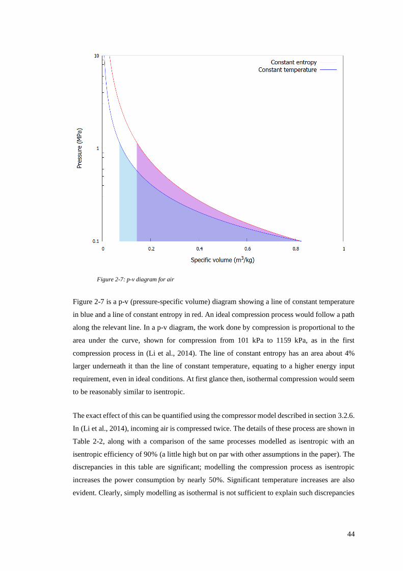
44

Figure 2-7 is a p-v (pressure-specific volume) diagram showing a line of constant temperature

in blue and a line of constant entropy in red. An ideal compression process would follow a path

along the relevant line. In a p-v diagram, the work done by compression is proportional to the

area under the curve, shown for compression from 101 kPa to 1159 kPa, as in the first

compression process in (Li et al., 2014). The line of constant entropy has an area about 4%

larger underneath it than the line of constant temperature, equating to a higher energy input

requirement, even in ideal conditions. At first glance then, isothermal compression would seem

to be reasonably similar to isentropic.

The exact effect of this can be quantified using the compressor model described in section 3.2.6.

In (Li et al., 2014), incoming air is compressed twice. The details of these process are shown in

Table 2-2, along with a comparison of the same processes modelled as isentropic with an

isentropic efficiency of 90% (a little high but on par with other assumptions in the paper). The

discrepancies in this table are significant; modelling the compression process as isentropic

increases the power consumption by nearly 50%. Significant temperature increases are also

evident. Clearly, simply modelling as isothermal is not sufficient to explain such discrepancies

Figure 2-7: p-v diagram for air

45

in the modelling results. The exact modelling equations used in (Li et al., 2014) are not given,

but assuming isothermal compression, the work done per unit mole could be calculated using:

𝑊 = 𝑅𝑇 ln (

𝑝2𝑝1) ( 2-12 )

where 𝑝1 and 𝑝2 are the inlet and outlet pressures, 𝑇 is the operating temperature and 𝑅 is the

molar gas constant. This provides results that are very close to the paper under discussion and

is presumably the equation that has been used to model compression. The compressor model

detailed in section 3.2.6 disagrees with the compression powers in (Li et al., 2014) but produces

results consistent with other literature reviewed.

Variable Stage 1 90%

isothermal

Stage 2 90%

isothermal

Stage 1 90%

isentropic

Stage 2 90%

isentropic

Mass flow rate (kg/s) 150 150

Inlet pressure (kPa) 101.3 1159.0 101.3 1159.0

Inlet temperature (K) 282 282

Outlet pressure (kPa) 1159.0 13409.0 1159.0 13409.0

Outlet temperature (K) 288 288 592 596

Power consumption (MW) 40.03 39.83 57.93 57.91

Table 2-2: Comparison of compression processes from literature and this thesis

Some work has been done on the approximation of an isothermal compression process in a real-

world compressor. (Teng et al., 2019) discusses a piston compressor whose compression

chamber is partially filled with a liquid that is cooled via a heat exchanger loop and against

which the gas is compressed. As the paper notes, this setup results in dissolution of the gas in

the liquid in question, which is significant, even at the low pressures demonstrated and does

reduce the efficiency gains. Despite the gas lost in this way, the work demonstrates an reduction

of compression work of nearly 20% over a standard piston compressor. (Jia et al., 2018)

describes an alternative piston compressor where water is injected during compression via a

water spray to cool the air during compression. This again results in a significant reduction in

the work done.

It should be noted that (Teng et al., 2019, Jia et al., 2018) rely on piston compression; these

techniques are inappropriate for centrifugal compressors which must operate using dry air to

prevent damage. Both piston compression techniques would humidify the resulting compressed

air which would require drying prior to expansion in order to prevent damage to equipment (in

the case of cryoturbine expansion) and the presence of ice in the expanded air. Both studies

model and demonstrate peak pressures in the sub-megapascal range, an order of magnitude

lower than that required for air liquefaction, and neither implies that the technology can be

46

scaled to higher pressures and industrial throughputs. Finally, the isothermal efficiency of the

process is significantly less than 90% in both cases. The conclusion here must be that the

assumption of being able to compress air at an isothermal efficiency of 90% made in (Li et al.,

2014) is invalid.

As discussed above, (Li et al., 2014) uses isentropic efficiencies of 92% for turbines, slightly

higher than the value of 85% used in the bulk of similar work. Whilst only a small difference,

this still makes a non-negligible difference to the work output by the turbines. The paper also

makes the assumption that steam is supplied by the NPP at approximately 7 MPa, rather than

the 3.5 MPa peak pressure more typical of PWRs. The supply pressure of steam is important,

as it affects the saturation temperature of water, which in turn affects the pinch point

temperature in a heat exchanger. Using steam of a higher pressure means that it stays at a higher

temperature during its phase change from vapour to liquid. This in turn increases the air

temperature that it is possible to achieve following heat exchange and the inlet temperature of

the turbines. Higher inlet temperatures result in improved power generation by the turbines for

the same pressure ratio and hence the assumption of high steam pressures has the potential to

result in overcalculation of the discharge power of the system.

The steam pressure delivered by the NPP is thus an important point. As mentioned, most PWR

designs output steam at a pressure of around 3.5 MPa (NuScale Power LLC, 2018b, AREVA,

2013). This is not exclusively true, however; the AP-1000 outputs steam at a pressure of 5.7

MPa (Westinghouse Electric Company, 2011). BWRs (boiling water reactors) are capable of

higher still steam outputs, with the ABWR (advanced boiling water reactor) operating at a

pressure of 6.8 MPa (GE Nuclear Energy, 1997). The paper under discussion (Li et al., 2014)

is explicit in stating that a PWR is used.

An LAES study from Italy (Antonelli et al., 2017) is an unusual one; it studies different

configurations of the discharge side from an LAES using an Aspen HYSYS model but does not

model the liquefaction cycle at all. Instead, it simply takes the specific energy of liquefaction

to be 0.35 kWh/kg, significantly higher than other papers (Sciacovelli et al., 2017a). This is,

however, a reasonable assumption, since the power cycles used do not appear to include a

facility for cold recycle. The discharge cycles modelled include a baseline case where the

discharge air is simply vaporised and expanded through turbines and additional cases all of

which combust natural gas in the discharge air stream. Some of the cycles modelled also couple

ORCs or cold Brayton cycles to capture and utilise additional waste heat from the process. This

is an attractive proposition; the modelling, whilst somewhat superficial, uses reasonable

turbomachinery efficiencies and achieves round-trip efficiencies in excess of 75%. The lack of

47

detailed engineering modelling, and the reliance on either natural gas combustion or on power

cycles that have yet to be commercially proven means that this paper has little to contribute to

this thesis.

One particular issue with many of the LAES papers is the use of cryoturbines for the final

expansion before storage in the tank. Such a design is present in (Li et al., 2014, Guizzi et al.,

2015, Sciacovelli et al., 2017b). The purpose of the final expansion is to partially liquefy the

compressed and cooled air prior to separation of the liquid and vapour phases. In all of these

papers, the air is over 80% liquid at the turbine outlet; such low vapour quality would certainly

cause damage to the turbine. The Claude process shown in Figure 2-6 shows how turbines are

typically used; air is drawn from the main stream and sent to the turbine before it is cooled

sufficiently to cause liquefaction. This technique is similar to that used by Highview Power

(Morgan et al., 2015b). The implications of using final stage cryoturbine expansion are non-

trivial. Expansion is typically performed in a J-T valve, an insulated valve which approximates

an adiabatic expansion process, keeping gas enthalpy constant. When expansion is performed

in a cryoturbine, the process is closer to an isentropic process.

48

The difference is best visualised using a p-h (pressure-enthalpy) diagram, as shown in Figure

2-8. This shows the process of expanding air from 105 K and 15 MPa to atmospheric pressure.

The red line shows air expanded in a J-T; the vertical line shows that enthalpy is fixed. The blue

line shows cryoturbine expansion, showing a significant reduction in enthalpy. The reduction

in enthalpy is due to the air’s internal energy being removed by the turbine. The results of this

are two-fold; the fluid leaves at a lower vapour quality than it would from a J-T valve (0.17 for

the cryoturbine compared to 0.29 for a J-T valve), and the cryoturbine performs useful work.

The use of a cryoturbine then represents an increased yield and a power saving, potentially

producing misleading results.

Another potential issue with many studies is the use of liquid hydrocarbon cold stores. The cold

store is a vital piece of equipment for LAES. As (Morgan et al., 2015b) states, limited cold

recycle is part of the reason Highview Power’s pilot plant’s round-trip efficiency was so low.

It is however, treated differently by the studies discussed herein. Whilst some studies

(Sciacovelli et al., 2017b, Morgan et al., 2015b) model a cold store that uses a solid medium

like a gravel bed, others (Guizzi et al., 2015, Li et al., 2014) use a liquid hydrocarbon cold store.

These use heat exchangers to cool hydrocarbons with the discharged air, storing the cooled

liquid in tanks ready to be used to cool the incoming air during the following charge cycle. In

Figure 2-8: p-h diagram for two different expansion processes

49

(Guizzi et al., 2015, Li et al., 2014), two such loops are used; a low temperature loop containing

propane and a high temperature loop containing methanol. The use of two liquids prevents

phase changes and ensures that both fluids remain liquid throughout the cycle temperature

ranges.

A hydrocarbon cold store has its advantages; where a solid media store’s temperature will

change over the course of a charge or discharge cycle, a hydrocarbon store’s tank temperature

will be continuous, mitigating a production rate drop-off towards the end of the charge cycle.

On the other hand, there is a potentially serious safety issue. At atmospheric pressure, nitrogen

liquefies at 77.4 K while oxygen liquefies at a higher temperature 90.2 K. This potentially leads

to oxygen preferentially condensing on the outside of system pipework. If the hydrocarbons

used in the cold store were to leak, this could create an extremely hazardous situation with a

fire in an oxygen-rich environment. Whether or not this would be too much of a risk for

regulators remains to be seen but hydrocarbon cold stores are a nascent technology, whereas

solid media cold stores have been successfully demonstrated by Highview Power (Morgan et

al., 2015b, Sciacovelli et al., 2017b, Sciacovelli et al., 2017a, Morgan, 2016). Pertinent to this

discussion, one of these papers (Sciacovelli et al., 2017b) discusses a warm recycle where the

heat of compression is stored when charging the system and utilised to heat the discharge air

stream. The proposed system that uses a hot oil loop, however such a loop would be separate

from exchange with fluids in the cryogenic temperature range and is perhaps of less concern.

(Tafone et al., 2019) provides an interesting study. Noting the complexity of the plant and of

thermodynamic modelling, this paper uses existing gas turbine data to develop performance

maps for different system configurations. These maps allow designers to determine the effect

of modifying plant operating parameters, such as charging pressure or the quantity of cold or

warm recycle, on overall plant performance. These maps, validated against actual data from the

Highview power pilot plant, provide designers a shorthand means of evaluating the

performance of an LAES system depending on their design choices.

Other papers (Antonelli et al., 2017, Tafone et al., 2018, She et al., 2017, Peng et al., 2018)

suggest making use of ORCs (organic Rankine cycle) to capture additional energy from the

discharge air stream. An ORC uses an organic working fluid with a saturation point lower than

that of water, which allows it to make use of low-grade heat that would otherwise be wasted.

LAES has a potentially useful synergy with such systems; many of the proposed working fluids

have a boiling point below 0°C and thus the low temperature air of an LAES discharge cycle

provides an effective heat sink for the ORC condenser. As (Tafone et al., 2018) notes, ORCs

50

remain in early stages of development and it remains to be proven whether they can be

commercially competitive.

These papers provide a variety of potential system configurations, some more realistic than

others. This study is intended to explore what can be done with operable processes and current

technology. Highview Power and their literature (particularly (Morgan et al., 2015b, Morgan,

2016)), as well as the University of Birmingham group and theirs (Sciacovelli et al., 2017b,

Sciacovelli et al., 2017a) provide the best basis with which to develop a realistic model of the

liquefaction side of the plant. The plant configurations taken forward for further modelling are

largely based on the pilot plant and grid scale plant designs discussed in (Morgan et al., 2015b,

Sciacovelli et al., 2017b, Sciacovelli et al., 2017a) and are detailed in section 5.2. The

availability of steam from the nuclear power plant provides opportunities to improve the power

yield during discharge but requires significant modification of the Highview design, as

discussed in section 5.2.6.

2.5.3. Financial studies

Cost analysis of LAES systems is not as readily available as that for engineering analyses, but

there are still some papers available on the subject, particularly in recent years. (Morgan et al.,

2015a) provides the earliest example of a cost analysis of a standalone system. It calculates

equipment costs scaled from pieces of equipment of a known cost. This is an approach discussed

in section 2.7 and one that would ultimately become part of the methodology of this thesis. The

study concludes that the levelized cost of a mature LAES plant is comparable to that of PHES.

It should be noted, however, that this study appears somewhat superficial when compared to

more recent work, due to the fact that it does not simulate in-market plant performance and does

not consider the influence of uncertainty on its cost analysis.

A paper co-authored by members of the University of Birmingham group (Xie et al., 2018) is

associated with many of the engineering studies discussed in section 2.5.2. It provides a detailed

assessment of the market viability of an LAES plant in the UK electricity market, focusing on

revenues from two sources: electricity arbitrage and ancillary service payments from STOR

services. The capital cost of the CES plant is estimated using Highview Power’s cost estimator

(Highview Power), which assesses cost based on three parameters; the storage and discharge

rates, and the storage capacity. The use of this estimator is surprising; given the group’s access

to detailed engineering modelling, not performing a more detailed capital cost analysis seems

like a missed opportunity.

51

The study (Xie et al., 2018) itself consists of a financial optimisation model with minimisation

of system NPV as the objective of the optimisation algorithm. It uses a variety of metrics of

economic performance including NPV, internal rate of return and payback period. Perhaps

unusually, payback period is not based on discounted values, meaning it is unaffected by

discount rate and may result in some misleading results. Electricity prices are simulated by

resampling of the 2015 UK spot market prices. As sections 4.4.2 and 4.4.3 will show, this is

not an overly optimistic approach; of the dataset used, represents a year of fairly low volatility

in daily average electricity prices and an average year in terms of the price swing seen in daily

profiles. Whilst the engineering analysis is not detailed, its assumptions are reasonable and

presumably derived from the group’s previous engineering-focused studies. The study does,

however, assume that external heat is used as a by-product of another process and that it is

obtained free of charge. This assumption is important and will be discussed again below.

The model assumes two revenue streams; one from electricity price arbitrage and one from the

provision of STOR services to the UK grid. It speculates that additional revenue might be

possible from frequency response services, but concedes that the very short response time

required would necessitate additional equipment and increase plant capital cost. With regard to

STOR, the paper notes that LAES can both absorb and supply energy to such a service and that

whilst this requires a larger tank storage capacity, this does not greatly affect the capital cost of

the plant.

The model itself assumes that the plant receives both standby payments for provision of STOR

services and payments for whenever this service is utilised by the grid. The utilisation from day

to day is triggered by a probability distribution. Only a portion of the plant’s capacity is

contracted for STOR services and the model ensures that there is always sufficient air stored to

meet this demand by charging the system, where required, whenever there is an impending

contracted period. The study’s conclusions are arguably unfavourable of provision of this

service. Whilst prices for this service are well in excess of electricity prices for the resampled

dataset, only 12.5% of the contracted STOR volume is actually utilised. The study also notes

that STOR services windows typically coincide with periods where the electricity price peaks.

This limits opportunities for arbitrage where the system receives a call for STOR services at

inopportune moments. Despite these issues, however, the study asserts that NPV results for

plants that provide the STOR service are always preferable to plants which operate on an

arbitrage-only means of revenue generation. Aside from this, the study shows that plant

discharge capacities of 100 MW or greater are required for positive NPVs.

52

There is, however, one potential issue with this study. That is the assumption that waste heat is

provided free of charge. The temperature of this waste heat is an input parameter for the model

and ranges from 50 to 250°C. At the upper end, these temperatures are well above the boiling

point of water and are arguably in the range where revenue-generating services, such as district

heating, are possible. These temperatures are not out of the realms of possibility for free waste

heat (PWR secondary loops operate at temperatures of around 300°C, these being on the low

end of steam power cycle peak temperatures) but at the higher end could arguably be revenue-

generating. The study predicts a threshold temperature 150°C for waste heat as being sufficient

for positive system NPV. In short, whether a plant would be able to attain heat at the required

temperature and at the required rate is an assertion that requires more justification than that

given in the study.

The Birmingham University group (Kim et al., 2018) also performed a financial study, this time

based on the results of their engineering study of both CAES and LAES systems discussed in

section 2.5.2. This study features one of the more detailed analyses discussed in this section,

where plant capital investment is directly calculated by sizing system components. Their

financial modelling is a LCOE analysis which is essentially a life-cycle cost calculation of the

per MWh cost of producing electricity based primarily on the plant capital cost, the system

energy performance, and the cost of electricity used to charge the system. Overall, this is a

detailed and valuable study and one that has somewhat damning conclusions for both

technologies with high LCOE values of $125/MWh or greater. Combined with the assumption

that the electricity to charge the system is purchased for $30/MWh, the study demonstrates that

either a significant price swing is required of the system or that some form of external subsidy

would be required to ensure profitability. (Wu et al., 2020) presents a similar LCOE analysis of

an LAES system, this time coupled with a thermochemical ESS. Once again, this is a techno-

economic analysis whose engineering study is discussed in section 2.5.2.

(Tafone et al., 2020) uses the parametric performance maps developed in (Tafone et al., 2019)

in a financial model to determine the LCOS (levelized cost of storage) of a LAES plant. This is

a relatively new metric that is, broadly, calculated by the discounted system cost divided by the

discounted quantity of electricity generated over the lifetime of the plant. This is a valuable

piece of information to have; it essentially represents the average price that electricity must be

sold at for the plant to break even. The study determines a LCOS of €385/MWh; an extremely

high electricity price compared to the UK’s electricity spot market prices over the period from

2008 to 2015 (Smith and Halliday, 2016). The authors argue that this is within the realms of

economic viability whilst conceding that it is reliant on opportune pricing. Despite this perhaps

optimistic conclusion, the paper does represent a novel study of a nascent metric for examining

53

energy storage systems, although it does not attempt to model the day-to-day operation of the

plant.

By contrast, (Lin et al., 2019) seeks to directly model the day-to-day operation of an LAES

plant. Using Highview Power’s cost estimation, and the UK electricity prices for 2015, the

study aims to simulate how a plant would operate in the real world, depending on plant capacity.

The model keeps a track of the amount of air stored and uses electricity prices (either past or

future from the model’s perspective) to set thresholds for when to charge or discharge the LAES

system. Three different operating scenarios were tested: two where both past and future prices

were used to set thresholds, and one where thresholds were set only by past prices. The study

concludes that larger discharge power output plants perform better selling into the spot market,

but that some sort of external waste heat is required for the plant to be profitable. This paper

presents an ambitious modelling strategy that uses resampled electricity price data to determine

the economic viability of an LAES plant and its conclusions are significantly less damning than

those in (Tafone et al., 2020).

2.6. Engineering modelling

The core of the project that this thesis discusses is an engineering process simulation model.

Given the time constraints of a PhD project and the availability of engineering software

packages, the chosen path for the construction of this model is to use modelling software, rather

than to code the model from scratch. At its most fundamental level, this software comprises a

means to define sets of known parameters, unknown variables, and the sets of simultaneous

equations that govern them, along with a means to solve those equations and calculate the

unknowns. There are several options for process modelling software, some of which are

detailed below.

MATLAB (MathWorks) is a multipurpose environment that facilitates data analysis and model

creation. It is ubiquitous in both academia and industry for good reason; it offers a highly

flexible numerical computing environment with the ability to call on functions written in other

programming languages. It allows the development of proprietary simulations run within the

MATLAB solver, as used in (Li et al., 2014). Additional packages, such as Simulink

(MathWorks) assist with modelling engineering systems by allowing the construction of models

in a modular sense and provide some pre-built models of process system components.

Aspen HYSYS (aspentech) is a process simulator geared primarily towards chemical

engineering and focuses on the optimisation of engineering processes. It has been used in a

54

number of the papers discussed in section 2.5.2 (Antonelli et al., 2017, Morgan et al., 2015b).

The broader family of Aspen software products (aspentech) offers packages for the optimisation

of everything from top-level process design to detailed analysis of individual chemical

processes or heat exchanger design. These software packages allow construction of models

from a diverse set of prebuilt components. Whilst this software is expensive, the availability of

prebuilt components is advantageous in that it dramatically reduces the work required for

systems modelling. There are, however, two major drawbacks. Firstly, these components are

something of a black box; there is little user control over the equations that govern the

relationship between input parameters and outputs. Secondly, the software is proprietary, and

any independent verification of results requires access to the Aspen software.

EES (F-Chart Software) is an equation-solving program that shares some similarities with

MATLAB’s solver. As discussed in section 2.5.2, the University of Birmingham group used

this as their process modelling environment (Sciacovelli et al., 2017b, Sciacovelli et al., 2017a).

It allows the definition and soloution of large arrays of equations and is entirely user-

programmable, offering a distinct advantage over the Aspen family of programs. EES’s solver

allows the input of equations in any order and unlike MATLAB does not rely on user-defined

algorithmic solving of complex systems.

Dymola (Dassault Systemes) is a simulation environment software package that is based on the

open-source Modelica language (Mattsson and Elmqvist, 1997). Its use of Modelica makes it

extremely versatile; Dymola is able to use the diverse open-source libraries of Modelica whilst

allowing commercial entities to develop proprietary code that can be run within the simulation

program. Dymola allows proprietary code to be protected and in this way straddles the gap

between the transparency of MATLAB and the black box nature of Aspen.

Modelica itself is a modelling language. Unlike programming languages such as C++, Modelica

code must be translated and executed within an external simulation environment. Like EES,

Modelica code need not be algorithmic; the equations can be supplied to the environment in

any order and supported simulation environments are required to be able to parse, rearrange

and solve equations written in Modelica to produce results. There are many programs that

implement Modelica; some, such as Dymola, are commercial whereas others, such as

OpenModelica (Open Source Modelica Consortium), are entirely open-source. Modelica has a

large userbase and an online community that continues to actively develop and publish a diverse

set of open-source libraries.

55

The list of software packages summarised in this section is by no means exhaustive but does

represent a good cross section of the options available. The programs discussed cover a

spectrum from the work-intensive, but highly flexible MATLAB, to the prebuilt models Aspen.

Software like Dymola and EES operate somewhere between these extremes, offering the

powerful preprogramed solving abilities of Aspen but retaining the coding flexibility and

transparency of MATLAB.

The requirements for the engineering model discussed in this project are reasonably simple.

The model needs to be capable of both steady-state and dynamic process modelling. The latter

is important; the cold store part of LAES in particular is a dynamic system whose properties

change over the course of a simulation. The model also needs to be able to treat heat exchange

in sufficient detail to allow phase changes to be modelled. This is particularly important for the

NPP secondary loop and the liquefaction cycle modelling, both of which feature fluid phase

changes. For its ability to facilitate the modelling of these aspects, as well as its open-source

and transparent nature, Dymola was selected as the software package to be used in this project.

Not only does this allow independent verification and follow-up of this work by others, it also

allows development of a niche library of components for modelling liquefaction systems that

may be of use to the wider Modelica community.

At the time this project was being developed, Modelica had not been used directly to simulate

air liquefaction processes. That being said, many of the tools required had already been coded.

The ThermoPower library (Casella and Leva, 2009, Casella and Leva, 2003) is a library that

was developed for the modelling of thermodynamic systems within Modelica. It includes a

variety of component models including fluid flows, heat exchangers and turbomachinery. The

ExternalMedia library (Casella and Richter, Casella and Richter, 2008) provides a means of

incorporating external code for calculation of thermophysical properties into a model.

The calculation of thermophysical fluid properties is an important part of any process model.

In Modelica, thermophysical properties can be defined in two ways; either using a medium

package within a Modelica library or looking up properties externally via the ExternalMedia

library. The Modelica standard library contains two dry air models, however the lowest

operating temperature of these is 200 K; not low enough to calculate properties in the liquid

phase. The ExternalMedia library allows integration of a multitude of external thermophysical

property codes. In the spirit of the transparent nature of this work, the open-source library

CoolProp (Bell et al., 2014) was selected for integration. Its implementation is discussed in

section 3.1.3.

56

One major limitation of the use of ExternalMedia is its treatment of multi-component fluid

mixtures. At the time of writing, the library is incapable of implementing fluid models that

constitute more than one component. Fortunately, CoolProp includes a pseudo-pure fluid model

of air that treats air as a single fluid. For this reason, the return flow from the air liquefier must

be treated with some caution. Many of the liquefaction cycles discussed in section 2.5 blend the

return vapour stream with make-up air from the atmosphere following the expansion and

separation process in the liquefier. This stream will be nitrogen-rich and will change the

properties of the resulting air mixture at cryogenic temperatures by reducing its saturation

temperature; essentially making it more difficult to liquefy. It is important that, in this model,

this stream not be mixed with make-up air before being returned the liquefaction cycle and

instead be exhausted to the atmosphere.

Definition of parameters is a central part of the engineering modelling process. NPP fluid flow

and thermodynamic properties can be sourced directly from the system designers; regulatory

application documents are particularly useful for this purpose. Heat exchange parameters,

particularly heat transfer coefficients are more difficult, especially with the relatively diverse

set of fluids and operating pressures that will be used in the engineering model. The standard

approach to heat exchanger design is the use of so-called U-values as heat transfer coefficients.

ESDU (formerly Engineering Sciences Data Unit) (IHS Markit, 2019) provides standards

documents containing U-values for heat exchanger design, however access to this data was not

available to this project. (Couper, 2012, Kuppan, 2013, Smith, 2005) provide a detailed list of

heat transfer coefficient ranges for a variety of heat exchanger designs and working fluids.

Given the resolution required by the model, and the lack of access to EDSU datasets, the

decision was made to use these ranges in the final engineering model. The ensure the model

would be conservative, the low end of the heat transfer ranges would be used resulting in a

tendency for the model to overestimate heat exchanger size and thus cost.

2.7. Financial modelling

An early decision in this project was made to perform any financial modelling with some

consideration of uncertainty. The fundamental requirements of such an analysis are an ability

to define probability distributions, use these to predict model input parameters for successive

iterations of the simulation, and to capture and collate the output variables. As with engineering

modelling discussed in section 2.6, there are a variety of software packages and programming

languages that are available for this purpose.

57

R (The R Foundation) is an open-source programming language that includes data analysis and

modelling tools that would be ideal for financial modelling in the face of uncertainty. It offers

tools for both probability distribution and time series fitting, both of which would prove vital

to the model described in 0. The fact that it is a second programming language which was

entirely unknown to this author prior to this project presents a significant issue, however. It was

felt that learning a second language in addition to Modelica would be impossible within the

time constraints of this project.

Microsoft Excel (Microsoft) is a spreadsheet program that is used within multiple industries for

a variety of purposes. Its vast array of formulae and powerful macro automation means it is

potentially a powerful financial modelling tool in its own right. Whilst Excel’s RNG (random

number generator) function would allow a means of predicting values from probability

distributions, and is formulae would allow a means of defining the distributions themselves,

Excel has no in-built means to capture results from multiple iterations of the same simulation

and would require significant automation with VBA (Visual Basic for Applications) in order to

facilitate this. This presents the same issue as R in that learning a second programming language

in addition to Modelica would simply be too time consuming for this project.

Several plug-ins for Excel are designed specifically to perform financial modelling in the face

of uncertainty. Of these, XLSim (Analycorp) and @RISK (Palisade) were considered for this

project. The two are broadly similar in terms of their functionality; both offer an array of

probability distributions, time series, data fitting algorithms and both automatically capture and

collate simulation data and results. Both are implementations of VBA within Excel. An

important difference lies in the probability distributions offered. @RISK offers some additional

distributions, most notably PERT (project evaluation and review technique), which is used

extensively in this project for the reasons discussed in 0. Another difference is @RISK’s

implementation of copulas, powerful tools that allow the definition of correlations between

input probability distributions, something that would also prove to be important to the financial

model in this project. As a result, @RISK was the software chosen for this project.

Financial modelling in the face of uncertainty requires a means of defining model probability

distribution or time series parameters. Some parameters can be defined by distribution fitting.

Given a sufficiently large dataset, distributions or time series can be defined according to the

fitting algorithms offered in @RISK. This thesis had the benefit of access to a detailed historical

dataset of UK electricity prices for the years 2008 to 2015 (Smith and Halliday, 2016), which

facilitated the definition of the electricity price model parameters as discussed in detail in

section 4.4. Other parameters, such as NPP cost or construction time, are much harder to

58

accurately define given the lack of a large historical dataset, the largely opaque nature of

commercial costs of recently constructed plants and considerable contention over the actual

cost of new nuclear plants (Kessides, 2010). In defining these parameters, then, a degree of user

judgment is required. The approach to defining such parameters is discussed in section 4.2. The

risk of error associated with such an approach can be reduced by a combination of testing

different scenarios and sensitivity testing of the final result.

Some parameters can be defined based on detailed engineering analyses. An engineering

process model can be used to estimate sizes of system components, allowing estimation of

capital cost for those components and in turn an estimation of capital cost for the plant as a

whole. A team at WPI (Worcester Polytechnic Institute) used such an approach to publish a

number of papers on the economic performance of IGCC (integrated gasification combined

cycle) plants in the US electricity market (Koc et al., 2012, Koc et al., 2013). The first of these

papers (Koc et al., 2012) discusses a performance assessment of an IGCC plant and its use in

estimating the asset cost of key components. The paper details the estimation of these

components from differently-sized but similar components of known cost using the six-tenths

rule (Peters et al., 1968):

𝐶(𝐴) = 𝐶(𝐵) (

𝑆(𝐴)

𝑆(𝐵))

0.6

( 2-13 )

where 𝐶(𝐴) is the unknown cost of piece of equipment A, 𝐶(𝐵) is the known cost of piece of

equipment B, and 𝑆(𝐴) and 𝑆(𝐵) are the sizes of pieces of equipment A and B respectively. A

slightly more detailed estimation can be obtained using the alternative formula (Peters et al.,

1968):

𝐶(𝐴) = 𝐶(𝐵) (

𝑆(𝐴)

𝑆(𝐵))

𝑋

( 2-14 )

This is very similar to equation ( 2-13 ) but includes the term 𝑋, a cost exponent specific to the

given type of equipment, and in a plant with a variety of system components can provide a more

accurate assessment of system components.

Given the investment costs of the key pieces of equipment, the WPI team (Koc et al., 2012)

used the process described in (Peters et al., 1968) to estimate the overall plant capital

investment. An Excel model with XLSim was then used to determine the NPV of the plant in

question via a DCF (discounted cash flow) analysis in the presence of uncertainty. Uncertain

59

model inputs were defined using a combination of triangular probability distributions (defined

using minimum, most likely, and maximum values) and resampling of historical data, where

sufficient data was available. Revenue is assessed based on electricity price sales given the

values of electricity price and plant capacity factor calculated via the defined probability

distributions for each simulation iteration. Whilst not explicitly stated in the paper, the model

seems to assume an equal capacity factor for each year of the simulation. This is not necessarily

the case, particularly as the plant in question contains a reactor whose catalyst bed must be

periodically replaced, potentially leading to significant variability in plant capacity factor from

one year to the next. Such variation has an impact on NPV, given the importance of time-

dependent value of revenue in DCF analyses. Despite this, however, the analysis in the paper

provides a detailed and insightful account of the relative risk of plant investment given a

detailed engineering analysis with which to estimate cost.

An interesting part of (Koc et al., 2012) is its consideration of the effect an accident at the plant

on system NPV. The chance of an accident occurring in any given model year is defined by

probability distribution and the cost of an accident incorporated into the NPV calculation. The

relative risk of investment, or reduction thereof, in preventative safety measures is assessed as

part of the study. A follow-up paper (Koc et al., 2013) provides a more detailed study of

investment in preventative safety measures by assessing competing options for safety systems.

Ultimately, the cost and likelihood of accidents, especially in nuclear plants, has historically

been very difficult to quantify and the decision was made to omit consideration of accidents

from the modelling in this project.

A cornerstone of the financial modelling process will be the estimation of plant cost. (Peters et

al., 1968) describes a methodology for doing so by first estimating the costs of key pieces of

equipment using equation ( 2-13 ), then by using a series of factors to estimate the overall plant

cost. The factors are detailed in section 4.3.2. In addition to estimating equipment costs from

equipment, it is also important to be able to adjust historical costs to present-day equivalents.

This is done using the CEPCI (Chemical Engineering Plant Cost Index) in the following

formula:

𝐶(𝑌1) = 𝐶(𝑌2) (

𝐼(𝑌1)

𝐼(𝑌2))

( 2-15 )

60

where 𝐶(𝑌1) and 𝐶(𝑌2) are the costs of a given piece of equipment in years 𝑌1 and 𝑌2

respectively and 𝐼(𝑌1) and 𝐼(𝑌2) are the indexes for those years. The values of CEPCI are

published by the magazine Chemical Engineering and indices from the years 1990 to 2018 were

used in this study (Jenkins, 2018, 2015, 2010, 2008). These are shown in Figure 2-9.

The use of equation ( 2-13 ) is reliant on scaling costs for pieces of equipment of known size

but unknown cost from pieces of equipment of a known size and cost. It is then paramount that

these base costs be as accurate as possible. Whilst (Peters et al., 1968) provides base costs for

many of the required pieces of equipment, the original text is some six decades old at the time

of writing and even the most recent edition contains costs that are nearly 30 years old.

Alternative base costs to use for estimation were thus sought from literature and used where

they were available.

Compressors and turbines are vital components for the charge and discharge cycles of LAES

plants. (Couper, 2012) provides formulae for estimating the cost of both in 2009 US$ prices.

Here, compressor costs are estimated using:

𝐶COMP = 7,022 (

�̇�

0.746)

0.62

( 2-16 )

where �̇� is the rated power of the compressor in kW and the formula from the literature has

been converted to 2018 GB£. Similarly, turbine costs are estimated using:

Figure 2-9: Values of CEPCI for 1990-2018

61

𝐶TURB = 978 (

�̇�

0.746)

0.81

( 2-17 )

where �̇� is the rated power of the turbine in kW and the formula has once again been converted

to GB£. Cryoturbines are as having the same cost, in line with (Wu et al., 2020).

(Wu et al., 2020) provides an equation for estimating the cost of cryogenic pumps:

𝐶PUMP = 0.483 �̇� ( 2-18 )

where �̇� is the rated power of the pump in kW.

The industry standard method for estimating heat exchanger cost is the use of C-values (Hewitt

and Pugh, 2007), which calculate heat exchanger cost as a function of its type and surface area

(or volume in the case of multi-stream exchangers). As with heat transfer coefficients, ESDU

(IHS Markit, 2019) provides lists of C-values for this purpose, however this data was not

available to this project. Other literature (Smith, 2005, Couper, 2012) provides means of

estimating heat exchanger costs that are more detailed than the aforementioned textbook

estimates (Peters et al., 1968), and provides examples that are more up to date. This literature

(Couper, 2012, Smith, 2005) highlights the importance of consideration of operating pressure,

material selection and heat exchanger type on capital cost. One (Smith, 2005), however, is

reliant on cost law coefficients which are specific to heat exchanger design but not provided in

the text. An alternative study (Wu et al., 2020) provides an equation for calculating heat

exchanger capital costs , derived from the aforementioned (Smith, 2005). Converted to 2018

GB£ prices, this is:

𝐶HX = 32,500 (

𝐴

80)0.68

( 2-19 )

where 𝐴 is the heat exchanger area in m2. This equation does not account for differences in cost

associated with increasing pressure ratings of heat exchangers and assumes a parity in cost

between heat exchangers of the same size regardless of their pressure rating. Since the LAES

system in particular has multiple pressure stages each with separate heat exchange, the decision

was made to use the data provided by (Peters et al., 1968) to calculate heat exchanger costs.

This yielded five equations for different pressure ratings between 2 and 20 MPa in 2018 GB£

prices:

62

𝐶HX, 2 MPa = 151,879 (

𝐴

140)0.44

( 2-20 )

𝐶HX, 3 MPa = 190,203 (

𝐴

140)0.44

( 2-21 )

𝐶HX, 7 MPa = 227,109 (

𝐴

140)0.44

( 2-22 )

𝐶HX, 10 MPa = 287,434 (

𝐴

140)0.44

( 2-23 )

𝐶HX, 20 MPa = 359,399 (

𝐴

140)0.44

( 2-24 )

As Figure 2-10 shows, despite their smaller exponent, equations ( 2-20 ) to ( 2-24 ) provide

significantly higher cost estimates than equation ( 2-19 ). Despite the discrepancy, it was

deemed sufficiently important that cost differences between heat exchange units of different

pressure ratings be properly captured to allow the model to err on the side of caution in this

way. This also ensures that the model estimates cost conservatively.

63

Storage vessels are also an important piece of equipment for this study. The storage tank for

cryogenic air is ubiquitous to all LAES designs. It is, however, a complicated piece of

equipment to assess the cost of, because there is limited cost data against which to assess the

various cost models available in the literature.

(Peters et al., 1968) provides a starting point with which to assess storage tank costs. Assuming,

for the moment, a stainless-steel tank, the cost can be obtained in 2018 GB£ prices using:

𝐶TANK = 118,500 (

𝑉

450)0.57

( 2-25 )

where 𝑉 is the volume of the tank in m3.

It is important to note, however that storage of cryogens requires more than simply a tank. Due

to environmental heating, it is important that the tank be properly insulated. For industrial

cryogenic gas plants, this means using a vacuum walled storage tank (Kerry, 2007), so the actual

cost can reasonably be expected to be significantly higher than that given by equation ( 2-25 ).

Figure 2-10: Heat exchanger cost model comparison

64

(Hu et al., 2013) provides a base cost of US$ 800,000 for a 2,500 m3 liquid oxygen storage tank

in 2013 US$. With this base cost as a reference, and using the same cost exponent as equation

( 2-25 ), the cost can be obtained in 2018 GB£ using:

𝐶TANK = 654,210 (

𝑉

2,500)0.57

( 2-26 )

where 𝑉 is the volume of the tank in m3.

An alternative relation is proposed by (Wu et al., 2020). This linear relationship is based on the

same base cost given in (Hu et al., 2013) and is given by:

𝐶TANK = 262𝑉 ( 2-27 )

where 𝑉 is the volume of the tank in m3.

Clearly, these two relationships are bound to differ significantly in their prediction of cost. It

would be useful to compare these to actual cost data from real-world pieces of equipment to

assess the relative merits of the two relationships. Whilst costs for different sizes of cryogenic

tank were sparse in the literature reviewed, (Shi, 2012) provides actual cost data for LNG

storage tanks against which these relationships might be compared. It is important to first assess

the merits of such a comparison. Liquefied air and natural gas are both stored at or around

atmospheric pressure. Their storage temperatures differ significantly though; LNG’s saturation

temperature at 101 kPa is 111.15 K whilst nitrogen’s is 77.3 K at the same pressure. This means

that the difference between the temperatures of the tank’s contents and the environment, and

hence the amount of insulation required, will be greater for storing air than for storing LNG. It

is reasonable, then to expect that the costs for an air storage tank will be higher than for an LNG

storage tank.

At this stage, it is also important to point out that an upper limit for storage tank size will be

required. This project chooses to focus on systems that can be delivered with off-the-shelf

system components. Searches for LNG storage tank manufacturers, for example (Chart

Industries, 2018, Corban Energy Group, 2018) , suggest an upper limit of around 1,500 m3 for

manufactured tanks. Whilst larger tanks ranging into the hundreds of thousands of m3 are

possible (Corban Energy Group, 2018, Osaka Gas, 2017), these are specialist products built on-

site. Furthermore, assuming a storage temperature of 77 K at 101 kPa, and a specific energy of

liquefaction of 0.3 kWh/kg (towards the upper limit for the papers discussed in section 2.5.2),

a tank size of 1,500 m3 is sufficient to store approximately 400 MWh of electricity. A few such

65

tanks could thus provide storage in the gigawatt range and are thus sufficient for an LAES plant

of those envisaged by the literature.

Figure 2-11 shows the comparison between the two cost estimation models equations ( 2-26 )

and ( 2-27 ) and the real-world data from (Shi, 2012). Clearly, the exponential cost model in

equation ( 2-26 ) provides the highest cost estimation up to a tank volume of 2,500 m3, where

the exponential and linear equations intersect (as a result of both being based on the same base

cost). From the real-world data, it would appear that both cost estimation models provide a

higher liquid air tank cost than for an equivalent size of LNG tank, however the exponential

model estimates costs well over double, whereas the linear model estimates costs at around 20%

over the real-world data at tank sizes of 100 m3 or above. Ultimately, the decision was taken to

use the exponential model to once again ensure the model errs on the side of caution. The

maximum tank size will be taken as 1,500 m3, in line with the concept of taking all equipment

off-the-shelf.

Figure 2-11: Storage tank cost estimation comparison with real-world data for LNG storage tanks

66

The values used for equation ( 2-14 ), the associated exponents, the CEPCI indices used and

the equations used for the estimation of plant costs are listed in section 4.3.

2.8. Interim remarks

The discussions of section 2.5 of the literature review highlight that there is a significant body

of work on LAES, both from an engineering perspective, and to a lesser extent, from an

economic perspective. Nevertheless, there are some niches which have not been studied in the

available literature, and the question of whether LAES plants can be successfully coupled with

nuclear plants to allow them to fulfil a load following capacity remains almost entirely absent

from the body of study on the subject. This is an interesting question in and of itself and

represents a significant part of the focus of this thesis.

The core of this thesis, however, aims to answer a far broader, and potentially more practically

valuable question. That is, whether engineering and financial modelling can be combined in

such a way that an engineering system for energy storage can be optimised from a market-led

perspective. This thesis will discuss the development of a modelling and methodological

approach that will attempt to achieve exactly that. This, whilst applied specifically to the

problem of a couple LAES and NPP design, has potentially far broader reaching applications.

The nature of many of the ESSs described in the literature means that they are asymmetrical, in

that their charge and discharge power ratings are largely independent of one another. This is

especially true of LAES. This presents a significant opportunity in that the power ratings of

such systems might be tailored for the given market in which they are to operate. However, the

effect of such engineering design is not trivial and, as 0 will discuss, has a significant impact

on a system’s cost. It is then not difficult to imagine a trade-off between optimising a system

from an engineering design perspective for its chosen market and maximising its economic

performance. This is an important consideration and one that is not explored in studies that

perform either economic or engineering analyses in isolation. Indeed, there remain significant

gaps in literature that attempts to combine the two approaches that are discussed in the following

paragraphs.

Detailed cost and financial performance analyses are a feature lacking from the studies

discussed in section 2.5.3. Despite many of those authors having an association with detailed

engineering studies, many use Highview Power’s cost estimator rather than directly estimating

plant costs from engineering model data. Of the studies cited, there are only two exceptions to

this (Kim et al., 2018, Wu et al., 2020), and not one of the works cited seek to directly simulate

67

the electricity spot market and its effect on the profitability, or otherwise, of the systems

presented.

The detailed simulation of the electricity market is also a potentially important feature absent

from the literature discussed. Studies that consider electricity prices tend to use a method known

as resampling (Koc et al., 2012, Koc et al., 2013, Xie et al., 2018). This involves the use of

historical electricity price data as a means of simulating the electricity price market. One major

disadvantage of such a method is that it assumes that the past will accurately represent the

future. As the discussions in section 4.4 will show, this is very rarely the case with electricity

prices, which tend to exhibit significant variation in their patterns from one year to the next.

An alternative approach is the use of time series which are used to simulate stochastic data such

a stock prices and have even been used in the simulation of electricity prices (Weron, 2014).

Time series significant advantages over data resampling. Their parameters can be user-defined.

This means that different hypothetical electricity markets can be simulated and the economic

performance of system designs within them considered. Their parameters can also set by fitting

them to existing data, which provides significant insight into how different market

characteristics should be simulated. Such an approach is a middle ground between the fixed

series provided by resampling and the more subjective simulated series provided by user-

defined time series. Electricity market simulation by time series is an approach entirely absent

from the literature on ESSs economic performance discussed in this thesis.

It is worth restating the thesis objectives from section 1.4 at this point and discussing which

gaps in the literature they fill. As discussed in the previous paragraphs, detailed cost analyses

of a variety of engineering configurations for LAES plants are absent from the majority of the

literature with many authors preferring to utilise Highview Power’s cost estimator for LAES

designs. The sole study on a coupled LAES and NPP design (Li et al., 2014) is also mentioned

as having significant shortcomings and a more detailed engineering analysis would provide a

valuable contribution to the field. The completion of the following objectives will seek to fill

these knowledge gaps:

• Develop an engineering model and library of components in the Modelica language for

plant process modelling of the combined NPP and LAES system.

• Use the engineering model to determine operating parameters for a range of proposed

plant configurations.

• Size components for the given plant configurations and use these to evaluate asset costs

for the LAES plant.

68

Financial modelling of ESSs and of LAES plants in particular has often relied on deterministic

modelling and resampling of electricity price data. In doing so, the conclusions regarding

relative risk of differing plant configurations in uncertain conditions are impossible to make.

The following objectives contribute to developing a methodology for economic analyses of

such systems in the face of uncertainty, and applying it to the proposed hybrid plant:

• Develop a financial model for determining relative economic performance of the plant

designs in the face of uncertain market conditions using Excel and the Palisade @RISK

plugin.

• Use the financial model to determine the relative economic performance and

investment risk of the plant design outputs from the engineering model.

The engineering and financial modelling approaches are discussed in Chapter 3 and 0

respectively. The simulation of a combined LAES and NPP system is discussed in Chapter 5

and the market-led design of said system is the subject of Chapter 6.

69

- Engineering Modelling

3.1. Introduction

This chapter details the engineering model. Section 3.1.1 discusses the intended objectives of

the model and 3.1.2 summarises the way Modelica code is implemented. This serves as a primer

to section 3.2, which discusses the component models in depth. Chapter 5 details how the

components were used to model the LAES system and the results obtained. Several of the

component models have been written specifically for this study but are compatible with other

user libraries based on the Modelica language and may be of use to the wider community. The

model library is available via Open Research Data Online (Wilson, 2020b).

3.1.1. Objectives

As discussed in sections 2.5, 2.6 and 2.7, LAES is a promising candidate for coupling to an

NPP for the purposes of load following. The reasons for this are discussed in these sections.

Primarily, it is argued that this is a highly mature energy storage technology that could be built

and indeed is being built, today. A secondary argument, but one that is more relevant to the

engineering modelling that is to be described in this chapter is its low operating temperatures

and opportunities for capturing and utilising low-grade waste heat. This latter point is worth

discussing further here in as much as it relates to the core objectives of the modelling approach.

One of the core reasons for selecting LAES as the ESS for this thesis is its ability to capture

very low-grade heat that might otherwise be considered waste. As is discussed in greater detail

in section 5.2.1, the steam for an NPP’s is heated in a steam generator before being expanded

to a pressure well below atmospheric. At this point, it is condensed via heat exchange with a

coolant water stream (hereafter denoted the tertiary coolant) that is itself cooled by air in a

cooling tower before being discharged from the plant. The temperature profiles in the condenser

mean that this tertiary coolant does not exceed 300 K (NuScale Power LLC, 2018b). The flow

rates of tertiary coolant, however, are very high – in excess of 10,000 kg/s, as section 5.2.1

shows. This means that a significant amount of heat is ultimately rejected from the NPP.

This rejected heat is in a very low temperature form and is thus not particularly useful for

industrial or domestic heating purposes. The LAES system presents an opportunity in this

regard. During system discharge, the air remains at a low temperature following the

vaporisation stage. The exact temperature varies in the literature but it typically in the region of

250 K. This presents an opportunity for coupling the system to an NPP. The temperature

difference between the LAES plant’s discharge air stream and the NPP’s primary coolant is

70

sufficient for heat exchange to take place between the two, allowing the NPP’s waste heat to be

captured, utilised, and ultimately sold in the form of electricity. Quantifying the exact value of

this opportunity is a significant gap in the literature and thus a key objective of modelling.

One final point discussed in section 2.5.2 relates to the cold recycle part of LAES plants. As is

emphasised in those discussions, the capture of cold during system discharge and its utilisation

when charging the system is paramount to the overall round-trip efficiency of the system. Two

options are discussed in the literature: the use of hydrocarbon fluid media and the use of packed

gravel bed thermal stores. Of these options, the latter was deemed most appropriate for study

in this thesis, due to its demonstrable use in pilot plants and safety concerns associated with

hydrocarbon fluids. Both points are discussed in detail in section 2.5.2.

The engineering model is intended to determine how a coupled NPP and LAES system could

be built and to enable the sizing of components to facilitate plant cost estimation. In order to do

this, it is required to fulfil the following objectives:

• Determine the rate and temperature at which the NPP side can supply steam to the

LAES plant,

• determine the optimal LAES configuration given the constraints on the supply of power

by the NPP side,

• develop flowsheets for the chosen plant designs and determine required component

sizes.

3.1.2. Background

Modelica is an object-orientated modelling language. It is loosely based on C but has a number

of additional commands to facilitate engineering systems modelling. Whilst it would be onerous

and unnecessary to define the Modelica syntax in detail within this thesis, it is sensible to define

the key terms and the way models are constructed in order for readers to fully understand the

discussions that follow.

Dymola is the simulation environment used in this study for running Modelica code. It checks

and compiles the code and operates the solvers required for integrating the models. Dymola

will always check that a model has the same number of variables and equations prior to

simulation. This is the reason that unused equations are required to balance some of the models

discussed below.

71

3.1.3. Terminology

Packages are collections of models. For most purposes, these can be thought of simply as

folders containing related models. There is, however, one important special case; the use of

packages in fluid medium models. The set of models that define the relationships between fluid

properties is defined within a package for that fluid. Defining these as packages allows

component models to quickly replace one fluid with another. In this study, the ExternalMedia

library (Casella and Richter, 2008) is used to define packages that reference the third party

software CoolProp (Bell et al., 2014) for fluid thermophysical properties. The key fluid

properties used are those for air and water, which are taken from (Lemmon et al., 2000) and

(Wagner and Pruß, 2002) respectively.

Individual models interact via flanges, connected by connectors. Flanges and their associated

connectors allow properties to be carried from on model to another. There are three types of

variable associated with flanges and connectors available in Modelica:

• ‘across’ variables which equate to the same value on both sides of the connector,

• ‘flow’ variables which sum to zero on both sides of the connector,

• ‘stream’ variables which are associated with material properties and are taken to be

carried by the flange’s flow variable.

Due to the relationship between flow and stream variables, each flange may only have a single

flow variable, but may have any number of stream variables. In thermodynamic modelling, the

change in a stream variable, such as enthalpy, through a component may be different depending

on the direction of the flow. For this reason, Modelica requires that equations are used to define

stream variable changes for both directions through a component. The inStream command

facilitates this; where it is used, the stream variable in question is taken to be that entering a

component and where it is absent, the variable is taken to be that leaving a component. Across

variables are entirely independent and there is again no limit on the number that can be present

in a single flange.

Related to flanges are interfaces. In this model, interfaces are used to transfer single variables

via connectors. These are dimensionless real numbers and can be considered analogous to

across variables, being equal on both sides of the connector.

Models are the sections of Modelica code that actually do calculations. Models open with the

definitions section which defines parameters, initial values that are user-defined within the user

interface and do not change over time, constants, fixed values that are user-defined within the

72

Modelica code itself, variables that the model uses to calculate values that change over time,

and outputs which are variables that are made easier to access during post-processing. In

addition, this section defines fluid states, which are essentially variables defining the

thermodynamic state of a fluid. Variable and parameter definitions are associated with a either

a base unit, a real number or an integer definition which is defined in the same line of code. All

of these definitions may take the form of matrix vectors, which are represented by 𝑉𝑎𝑟[𝑛] for

a matrix variable 𝑉𝑎𝑟 of size 𝑛.

Fluid states are important for any models that used defined thermodynamic properties of fluids.

To define a fluid state, two unique properties must be provided, for example enthalpy and

pressure, or entropy and pressure. A combination of temperature and pressure is also acceptable

under certain conditions. However, if the temperature and pressure provided specifies a

thermodynamic state where the fluid is under a phase transition, the model will return an error.

This is because a temperature and pressure can define a thermodynamic state at any point along

that phase boundary, meaning that a unique state point cannot be defined.

The definitions section also defines other models, flanges or connectors that are used as sub-

components of the model being defined. Such models would be expected to have the values of

their parameters defined, either explicitly, or in terms of the parameters of is overarching model.

The equation section follows the definitions section and consists of the equations that calculate

the change in variables over time. The modelling environment, which compiles and runs the

Modelica code will typically decide in which order equations are calculated. This can be

overridden by using an optional algorithm section which forces the environment to run

equations in the order that they appear in the code and can appear either in conjunction or in

place of the equation section. Finally, another optional section, the initialisation section allows

the inclusion of equations that the model must satisfy at the start of each simulation run.

3.2. Component modelling

The following subsections detail the component models used in the engineering model. As

discussed, Modelica and Dymola facilitate the construction of models in a modular fashion.

The foundation of these models is the individual models of components. Many of the models

used are based on the models available in the ThermoPower library for Modelica (Casella and

Leva, 2009), but have been modified for use in this system. Wherever this is the case, the

ThermoPower library is credited and the changes summarised.

73

Two types of flange are used in this study, both taken from ThermoPower. The first is a 2PF

(two-phase fluid flow) flange, which transmits the following fluid properties from one

component to another:

• A flow variable, �̇�, defining the mass flow rate of the fluid stream. Flow into a

component is taken as positive and out of a component is taken as negative.

• An across variable, 𝑝, defining the absolute pressure of the fluid stream.

• A stream variable, ℎ, defining the specific enthalpy of the fluid stream.

• A matrix stream variable, 𝑋𝑖[𝑚], defining the mass fraction of each component in the

fluid flow, where 𝑚 is the number of components. It should be noted that only single-

component medium models are used for fluids in this study, such that this variable is

redundant.

The second flange is a DHT (distributed heat transfer) flange for finite volumes, which

transmits a matrix of material properties, where 𝑛 is the number of volumes. This transmits the

following material properties:

• A matrix across variable, 𝑇[𝑛], defining the absolute temperature of the materials.

• A matrix flow variable, �̇�[𝑛], defining the heat flow rate at the volumes. Flow into a

component is taken as positive and out of a component is taken as negative.

The component models used in the engineering model will now be discussed in detail.

Following an opening paragraph for each model, a table will outline the details of each

parameter, variable and fluid states used in the model. This table will include the symbol used

for the item in this text, the name used in the Modelica code, the units for the item and a brief

description. Following the table, the text will detail and discuss each equation used in the model.

3.2.1. One-dimensional finite volume flow model

The 1DFV (one-dimensional finite volume) flow model is the fundamental component for fluid

flows in the engineering model and is primarily used as a sub-component in heat exchangers.

An FV (finite volume) model approximates a system, such as a fluid flow, by dividing it into a

set of volumes and dividing the relationships between these volumes and at the interfaces,

regions hereafter referred to as nodes. This concept is shown in Figure 3-1.

74

Figure 3-1: One-dimensional finite volume flow model diagram showing the role of the distributed heat transfer

flange

ThermoPower (Casella, 2014) provides a basis for this model with a model that provides

simulation of both thermodynamic and fluid dynamic properties in a flow. Whilst the

thermodynamic considerations are vital for this engineering model, the fluid dynamic properties

are less so. Indeed, detailed geometric design of heat exchangers is not considered within the

scope of this study and the 1DFV flow model was simplified accordingly. The equations

associated with friction factors were replaced with a single equation relating flow pressure drop

to the inlet pressure. An additional initialisation equation was added to ensure steady-state mass

in each volume during model initialisation.

Item Code Units Description

Parameters

Medium Replaceable medium package for fluid flow

𝑁 N Number of wall nodes for thermal variables

𝑁𝑉 Nw Number of volumes for thermal variables

(defaults to 𝑁 − 1)

𝐿 L m Length of fluid flow

𝐻 H m Elevation of outlet over inlet

𝐴 A m2 Flow cross-sectional area

𝜔 omega m Perimeter of heat-transfer surface

�̇�nom wnom kg/s Nominal mass flow rate

𝑝drop PressureDrop Pressure drop as a fraction of inlet pressure

𝛾 gamma W/m2kg Heat transfer coefficient

Initial parameters

𝑝start pstart Pa Expected pressure start value

ℎstart,inlet hstartin J/kg Expected starting fluid specific enthalpy at inlet

ℎstart,outlet hstartout J/kg Expected starting fluid specific enthalpy at

outlet

ℎstart[𝑁] hstart J/kg Expected starting fluid enthalpy vector

SSinit Boolean parameter for steady-state initialisation

Variables

∆𝑝friction Dpfric Pa Pressure drop due to friction

∆𝑝static Dpstat Pa Pressure drop due to static head

𝑝 p Pa Pressure for initial state calculations

∆𝑝fric[𝑁𝑉] dpf[N-1] Pa Pressure drop due to friction between nodes

�̇� w kg/s Mass flow rate

�̅̇�[𝑁𝑉 wbar[N-1] kg/s Average mass flow rate for a volume

�̇�[𝑁𝑉] Q[N-1] W Heat flow rate into a volume

𝑢[𝑁] u[N] m/s Fluid velocity at a node

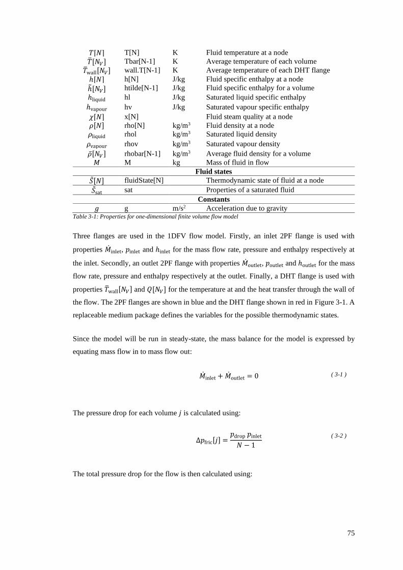
75

𝑇[𝑁] T[N] K Fluid temperature at a node

�̅�[𝑁𝑉] Tbar[N-1] K Average temperature of each volume

�̅�wall[𝑁𝑉] wall.T[N-1] K Average temperature of each DHT flange

ℎ[𝑁] h[N] J/kg Fluid specific enthalpy at a node

ℎ̃[𝑁𝑉] htilde[N-1] J/kg Fluid specific enthalpy for a volume

ℎliquid hl J/kg Saturated liquid specific enthalpy

ℎvapour hv J/kg Saturated vapour specific enthalpy

𝜒[𝑁] x[N] Fluid steam quality at a node

𝜌[𝑁] rho[N] kg/m3 Fluid density at a node

𝜌liquid rhol kg/m3 Saturated liquid density

𝜌vapour rhov kg/m3 Saturated vapour density

�̅�[𝑁𝑉] rhobar[N-1] kg/m3 Average fluid density for a volume

𝑀 M kg Mass of fluid in flow

Fluid states

�̃�[𝑁] fluidState[N] Thermodynamic state of fluid at a node

�̃�sat sat Properties of a saturated fluid

Constants

𝑔 g m/s2 Acceleration due to gravity Table 3-1: Properties for one-dimensional finite volume flow model

Three flanges are used in the 1DFV flow model. Firstly, an inlet 2PF flange is used with

properties �̇�inlet, 𝑝inlet and ℎinlet for the mass flow rate, pressure and enthalpy respectively at

the inlet. Secondly, an outlet 2PF flange with properties �̇�outlet, 𝑝outlet and ℎoutlet for the mass

flow rate, pressure and enthalpy respectively at the outlet. Finally, a DHT flange is used with

properties �̅�wall[𝑁𝑉] and 𝑄[𝑁𝑉] for the temperature at and the heat transfer through the wall of

the flow. The 2PF flanges are shown in blue and the DHT flange shown in red in Figure 3-1. A

replaceable medium package defines the variables for the possible thermodynamic states.

Since the model will be run in steady-state, the mass balance for the model is expressed by

equating mass flow in to mass flow out:

�̇�inlet + �̇�outlet = 0 ( 3-1 )

The pressure drop for each volume 𝑗 is calculated using:

∆𝑝fric[𝑗] =𝑝drop 𝑝inlet

𝑁 − 1

( 3-2 )

The total pressure drop for the flow is then calculated using:

76

∆𝑝friction = ∑ ∆𝑝fric[𝑗]

𝑁−1

𝑗=1

( 3-3 )

The total static pressure drop is calculated using:

∆𝑝static =𝑔𝐻

(𝑁 − 1)∑ �̅�[𝑗]

𝑁−1

𝑗=1

( 3-4 )

Momentum balance for the system thus allows calculation of the outlet pressure:

𝑝outlet = 𝑝inlet − ∆𝑝friction − ∆𝑝static ( 3-5 )

Energy balance for each volume 𝑗 is expressed:

�̇�[𝑗] =

𝐴𝐿

(𝑁 − 1)�̅�[𝑗]ℎ̃[𝑗]̇ + �̅̇�[𝑗](ℎ[𝑗 + 1] − ℎ[𝑗]) −

𝐴𝐿

(𝑁 − 1)�̇�

( 3-6 )

where �̇� and ℎ̃[𝑗]̇ are the respective derivatives of pressure and volume specific enthalpy with

respect to time, 𝑡. In words, this equates the flow of heat into a volume to the energy stored in

the fluid within the volume (first term), the net energy flowing into the volume (second term,

noting that flow out of a volume is negative) and the energy stored when pressurising the fluid

(third term).

The saturation state for the fluid, �̃�sat, is defined within the medium model as the saturation

state at pressure 𝑝, taken to be the pressure at the flow inlet:

𝑝 = 𝑝inlet ( 3-7 )

From this definition, values for the saturated liquid and vapour specific enthalpies, ℎliquid and

ℎvapour respectively, and the saturated liquid and vapour densities, 𝜌liquid and 𝜌vapour

respectively, are set by reference to the medium model at �̃�sat.

The average density for each volume 𝑗 is calculated depending on the state of the fluid within

that volume, using if statements comparing the enthalpy entering the volume, ℎ[𝑗], and the

enthalpy leaving the volume, ℎ[𝑗 + 1], hereafter referred to as the nodal enthalpies, to the

77

saturated liquid and vapour specific enthalpies, ℎliquid and ℎvapour respectively. Where both

nodal enthalpies are smaller than the liquid enthalpy or both are greater than the vapour

enthalpy, the fluid in the volume is taken to be single-phase and:

�̅�[𝑗] =

𝜌[𝑗] + 𝜌[𝑗 + 1]

2

( 3-8 )

If both nodal enthalpies are between the liquid enthalpy and the vapour enthalpy, the fluid in

the volume is taken to be entirely two-phase and:

�̅�[𝑗] =ℎvapour − ℎliquid

(1

𝜌vapour−

1𝜌liquid

)(ln (𝜌[𝑗]

𝜌[𝑗 + 1]⁄ )

ℎ[𝑗 + 1] − ℎ[𝑗])

( 3-9 )

If the enthalpy entering the volume is smaller than the liquid enthalpy and the enthalpy leaving

the volume is between the liquid and vapour enthalpies, the fluid in the volume is taken to be

transitioning from liquid to two-phase and:

�̅�[𝑗] =

12(𝜌[𝑗] + 𝜌liquid)(ℎliquid − ℎ[𝑗]) +

ℎvapour − ℎliquid

(1

𝜌vapour−

1𝜌liquid

)ln (

𝜌liquid𝜌[𝑗 + 1]

)

ℎ[𝑗 + 1] − ℎ[𝑗]

( 3-10 )

If the enthalpy entering the volume is between the liquid and vapour enthalpies and the enthalpy

leaving the volume is greater than the vapour enthalpy, the fluid in the volume is taken to be

transitioning from two-phase to vapour and:

�̅�[𝑗] =

ℎvapour − ℎliquid

(1

𝜌vapour−

1𝜌liquid

)ln (

𝜌[𝑗]𝜌vapour

) +12(𝜌vapour + 𝜌[𝑗 + 1])(ℎ[𝑗 + 1] − ℎvapour)

ℎ[𝑗 + 1] − ℎ[𝑗]

( 3-11 )

If the enthalpy entering the volume is less than the liquid enthalpy and the enthalpy leaving the

volume is greater than the vapour enthalpy, the fluid in the volume is taken to be transitioning

from liquid to two-phase to vapour and:

78

�̅�[𝑗] =1

(ℎ[𝑗 + 1] − ℎ[𝑗])

(

1

2(𝜌[𝑗] + 𝜌liquid)(ℎliquid − ℎ[𝑗])

+ℎvapour − ℎliquid

(1

𝜌vapour−

1𝜌liquid

)ln (

𝜌liquid

𝜌vapour)

+1

2(𝜌vapour + 𝜌[𝑗 + 1])(ℎ[𝑗 + 1] − ℎvapour)

)

( 3-12 )

If the enthalpy entering the volume is between the liquid and vapour enthalpies and the enthalpy

leaving the volume is less than the liquid enthalpy, the fluid in the volume is taken to be

transitioning from two-phase to liquid and:

�̅�[𝑗] =

ℎvapour − ℎliquid

(1

𝜌vapour−

1𝜌liquid

)ln (

𝜌[𝑗]𝜌liquid

) +12(𝜌liquid + 𝜌[𝑗 + 1])(ℎ[𝑗 + 1] − ℎliquid)

ℎ[𝑗 + 1] − ℎ[𝑗]

( 3-13 )

If the enthalpy entering the volume is greater than the vapour enthalpy and the enthalpy leaving

the volume is less than the liquid enthalpy, the fluid in the volume is taken to be transitioning

from vapour to two-phase to liquid and:

�̅�[𝑗] =1

(ℎ[𝑗 + 1] − ℎ[𝑗])

(

1

2(𝜌[𝑗] + 𝜌vapour)(ℎvapour − ℎ[𝑗])

+ℎvapour − ℎliquid

(1

𝜌vapour−

1𝜌liquid

)ln (

𝜌vapour

𝜌liquid)

+1

2(𝜌liquid + 𝜌[𝑗 + 1])(ℎ[𝑗 + 1] − ℎliquid)

)

( 3-14 )

Where none of the criteria for equations ( 3-8 ) to ( 3-14 ) hold true, the fluid in the volume is

taken to be transitioning from vapour to two-phase and:

79

�̅�[𝑗] =

12(𝜌[𝑗] + 𝜌vapour)(ℎvapour + ℎ[𝑗]) +

ℎvapour − ℎliquid

(1

𝜌vapour−

1𝜌liquid

)ln (

𝜌vapour𝜌[𝑗 + 1]

)

ℎ[𝑗 + 1] − ℎ[𝑗]

( 3-15 )

For each volume 𝑗, the average flow rate is equated to the inlet flow rate:

�̅̇�[𝑗] = �̇�inlet ( 3-16 )

The fluid state at each node 𝑖, �̃�[𝑖], is defined in the medium model using the pressure, 𝑝, and

the specific enthalpy at that volume, ℎ[𝑖]. From this definition, values for the temperature, 𝑇[𝑖]

and the density, 𝜌[𝑖], are set via lookup in the medium model.

The fluid velocity at each node 𝑖 is calculated:

𝑢[𝑖] =

�̇�

𝐴𝜌[𝑖]

( 3-17 )

The steam quality for each node 𝑖 is calculated depending on the state of the fluid at node ℎ[𝑖]

to ℎliquid and ℎvapour. Where ℎ[𝑖] > ℎvapour, the fluid is entirely vapour and 𝜒[𝑖] = 1. Where

ℎ[𝑖] < ℎliquid, the fluid is entirely liquid and 𝜒[𝑖] = 0. Otherwise, the steam quality is

calculated:

𝜒[𝑖] =

ℎ[𝑖] − ℎliquid

ℎvapour − ℎliquid

( 3-18 )

As mentioned previously, the enthalpy flow at a flange is considered to be carried by the mass

flow rate. The 1DFV flow model does not specify a direction of flow, so specific enthalpy

within a volume must be approximated to the specific enthalpy at a node bounding that volume.

Since models are expected to be built such that flow will be from inlet to outlet flange, the

enthalpy for a node 𝑖 is equated to the fluid specific enthalpy leaving the previous volume:

ℎ[𝑖] = ℎ̃[𝑖 − 1] ( 3-19 )

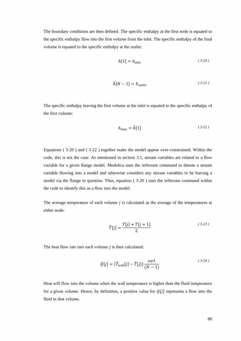
80

The boundary conditions are then defined. The specific enthalpy at the first node is equated to

the specific enthalpy flow into the first volume from the inlet. The specific enthalpy of the final

volume is equated to the specific enthalpy at the outlet:

ℎ[1] = ℎinlet ( 3-20 )

ℎ̃[𝑁 − 1] = ℎoutlet ( 3-21 )

The specific enthalpy leaving the first volume at the inlet is equated to the specific enthalpy of

the first volume:

ℎinlet = ℎ̃[1] ( 3-22 )

Equations ( 3-20 ) and ( 3-22 ) together make the model appear over-constrained. Within the

code, this is not the case. As mentioned in section 3.1, stream variables are related to a flow

variable for a given flange model. Modelica uses the inStream command to denote a stream

variable flowing into a model and otherwise considers any stream variables to be leaving a

model via the flange in question. Thus, equation ( 3-20 ) uses the inStream command within

the code to identify this as a flow into the model.

The average temperature of each volume 𝑗 is calculated as the average of the temperatures at

either node:

�̅�[𝑗] =

𝑇[𝑗] + 𝑇[𝑗 + 1]

2

( 3-23 )

The heat flow rate into each volume 𝑗 is then calculated:

�̇�[𝑗] = (�̅�wall[𝑗] − �̅�[𝑗])

𝜔𝛾𝐿

(𝑁 − 1)

( 3-24 )

Heat will flow into the volume when the wall temperature is higher than the fluid temperature

for a given volume. Hence, by definition, a positive value for 𝑄[𝑗] represents a flow into the

fluid in that volume.

81

�̅�wall[𝑗] represents the value of the temperature at the DHT flange. The DHT is the means by

which the model transfers heat between adjacent flow models. The way multiple flows are

connected into larger models like heat exchangers is discussed in section 3.2.4.

At the start of modelling, the initial parameters are used for the starting points of the model

variables. The vector ℎstart[𝑁] is defined with 𝑁 values linearly spaced between ℎinlet, start and

ℎoutlet, start. Then, the initial nodal enthalpies and the initial pressure are defined:

ℎ[𝑁] = ℎstart[𝑁] ( 3-25 )

𝑝 = 𝑝start ( 3-26 )

Should the steady-state initialisation Boolean parameter be set to true, the initial parameters are

varied until the following equations are satisfied:

𝑑ℎ̃[𝑁 − 1]

𝑑𝑡= 𝟎

( 3-27 )

𝑑𝑝

𝑑𝑡= 0

( 3-28 )

𝑑𝜌[𝑗]

𝑑𝑡= 𝟎 ( 3-29 )

i.e. initial pressure and the initial volume enthalpies and densities must be fixed with respect to

time. Once these conditions are satisfied, the model run commences.

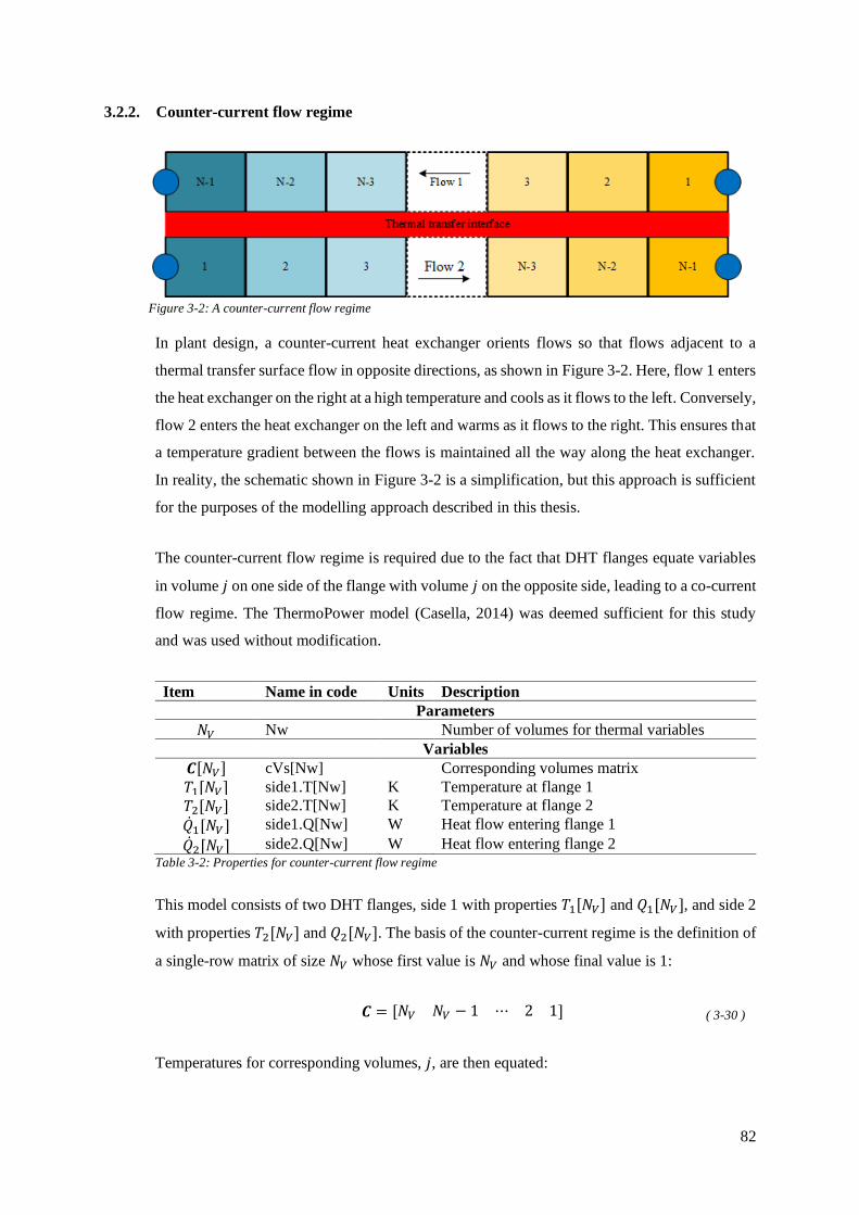
82

3.2.2. Counter-current flow regime

In plant design, a counter-current heat exchanger orients flows so that flows adjacent to a

thermal transfer surface flow in opposite directions, as shown in Figure 3-2. Here, flow 1 enters

the heat exchanger on the right at a high temperature and cools as it flows to the left. Conversely,

flow 2 enters the heat exchanger on the left and warms as it flows to the right. This ensures that

a temperature gradient between the flows is maintained all the way along the heat exchanger.

In reality, the schematic shown in Figure 3-2 is a simplification, but this approach is sufficient

for the purposes of the modelling approach described in this thesis.

The counter-current flow regime is required due to the fact that DHT flanges equate variables

in volume 𝑗 on one side of the flange with volume 𝑗 on the opposite side, leading to a co-current

flow regime. The ThermoPower model (Casella, 2014) was deemed sufficient for this study

and was used without modification.

Item Name in code Units Description

Parameters

𝑁𝑉 Nw Number of volumes for thermal variables

Variables

𝑪[𝑁𝑉] cVs[Nw] Corresponding volumes matrix

𝑇1[𝑁𝑉] side1.T[Nw] K Temperature at flange 1

𝑇2[𝑁𝑉] side2.T[Nw] K Temperature at flange 2

�̇�1[𝑁𝑉] side1.Q[Nw] W Heat flow entering flange 1

�̇�2[𝑁𝑉] side2.Q[Nw] W Heat flow entering flange 2 Table 3-2: Properties for counter-current flow regime

This model consists of two DHT flanges, side 1 with properties 𝑇1[𝑁𝑉] and 𝑄1[𝑁𝑉], and side 2

with properties 𝑇2[𝑁𝑉] and 𝑄2[𝑁𝑉]. The basis of the counter-current regime is the definition of

a single-row matrix of size 𝑁𝑉 whose first value is 𝑁𝑉 and whose final value is 1:

𝑪 = [𝑁𝑉 𝑁𝑉 − 1 ⋯ 2 1] ( 3-30 )

Temperatures for corresponding volumes, 𝑗, are then equated:

Figure 3-2: A counter-current flow regime

83

𝑇1[𝑗] = 𝑇2[𝑪[𝑗]] ( 3-31 )

Similarly, energy conservation is maintained across the regime:

�̇�1[𝑗] = �̇�2[𝑪[𝑗]] ( 3-32 )

This model achieves counter-current flow by the definition of matrix 𝑪. For example, when 𝑗 =

1, the value of 𝑪[1] returns 𝑁𝑉.

3.2.3. Metal tubes

The metal tubes model forms the final important part of heat exchanger models and simulates

the flow of heat through and the accumulation of heat within metal tubes. The ThermoPower

model (Casella, 2014) was again deemed sufficient for this study and was used without

modification.

Item Name in code Units Description

Parameters

𝑁𝑉 Nw Number of volumes for tube

𝐿 L m Length of tube

𝑟internal rint m Internal radius of tube

𝑟external rext m External radius of tube

𝐶vol rhomcm J/m3K Volumetric heat capacity of tube metal

𝜆 lambda W/mK Thermal conductivity of tube metal

WallRes Boolean parameter for wall resistance

Initial parameters

𝑇start,1 Tstart1 K Expected starting temperature of first volume

𝑇start,N TstartN K Expected starting temperature of final volume

𝑇start[𝑁𝑉] Tstart[Nw] K Expected starting temperature of volumes

SSinit kg Boolean parameter for steady-state initialisation

Variables

𝑇[𝑁𝑉] Tvol[Nw] K Volume temperatures

𝐴 Am m2 Area of metal tube cross-section

Constants

𝜋 pi Pi Table 3-3: Properties for metal tube model

Two DHT flanges are used in the metal tube model. One for the internal surface with properties

𝑇internal[𝑁𝑉] and �̇�internal[𝑁𝑉], and one for the external surface with properties 𝑇external[𝑁𝑉] and

�̇�external[𝑁𝑉].

The metal tube begins by asserting that the external radius of the metal tube is larger than the

internal radius:

84

𝑟external > 𝑟internal ( 3-33 )

If this is not true, the simulation is halted, and an error message returned.

The cross-sectional area of the tube is calculated:

𝐴 = 𝜋(𝑟external2 − 𝑟internal

2) ( 3-34 )

Should the wall resistance Boolean parameter be set to true, the thermal resistance of the tube

walls is accounted for. Heat conduction through the internal half-thickness of the tube is

calculated for each volume 𝑗 using:

�̇�internal[𝑗] =2𝜆𝜋 𝐿 𝑁𝑉

⁄ (𝑇internal[𝑗] − 𝑇[𝑗])

log (𝑟internal + 𝑟external

2𝑟internal)

( 3-35 )

Similarly, heat conduction through the external half-thickness of the tube is calculated for each

volume 𝑗 using:

�̇�external[𝑗] =2𝜆𝜋 𝐿 𝑁𝑉

⁄ (𝑇external[𝑗] − 𝑇[𝑗])

log (2𝑟external

𝑟internal + 𝑟external)

( 3-36 )

Where the wall resistance parameter is set to false, the simplification that there is no temperature

gradient across the tube thickness is assumed and the temperatures for the internal and external

surfaces are equated to the temperatures for the volumes 𝑗:

𝑇internal[𝑗] = 𝑇[𝑗] ( 3-37 )

𝑇external[𝑗] = 𝑇[𝑗] ( 3-38 )

Energy balance is defined for each volume 𝑗:

𝐿𝑁𝑉⁄ 𝐶vol𝐴

𝑑𝑇[𝑗]

𝑑𝑡= �̇�internal[𝑗] + �̇�external[𝑗] ( 3-39 )

At the start of modelling, initial temperatures vector 𝑇start[𝑁𝑉] is defined with 𝑁𝑉 values

linearly spaced between 𝑇start,1 and 𝑇start, N. The volume temperatures are then defined on these

values:

85

𝑇[𝑁𝑉] = 𝑇start[𝑁𝑉] ( 3-40 )

Should the steady-state initialisation parameter be set to true, the starting variables are varied

until the following equation is satisfied:

𝑑𝑇[𝑁𝑉]

𝑑𝑡= 𝟎 ( 3-41 )

3.2.4. Heat exchangers

Heat exchangers are models built from the 1DFV flow, counter current regime and metal tube

models in sections 3.2.1, 3.2.2 and 3.2.3 respectively. They are built in much the same way as

in the ThermoPower library (Casella, 2014) however these have been built differently to reduce

the number of parameters required for the model.

Figure 3-3 is a schematic diagram of a generic heat exchanger model. A heat exchanger consists

of two 1DFV models, denoted flow 1 and flow 2, a counter-current flow regime and a metal

tube model. Adjacent DHT nodes are connected, meaning that the across variable temperature

is equal on both sides and the flow variable heat flows on connected sides sum to zero.

For brevity, only newly introduced parameters are discussed below. These parameters have

been defined in order to limit the number of user-input parameters required where there is

overlap in the components that constitute the heat exchanger model. Where sub-component

parameters are omitted, these should be assumed as being defined in the top-level heat

exchanger model and propagating through to the relevant components. For clarity, any

component parameters are shown with a subscript in angle brackets, ⟨1⟩ for flow 1, ⟨2⟩ for flow

Figure 3-3: Heat exchanger schematic (red bars represent DHT flanges)

86

2, ⟨m⟩ for metal tube and ⟨c⟩ for counter-current flow regime. For example 𝐿⟨1⟩ references the

length parameter for the flow 1 sub-component.

Item Name in code Units Description

Parameters

Flow1Medium Medium package for flow 1 fluid

Flow2Medium Medium package for flow 2 fluid

𝑁 Nodes Number of wall nodes

𝐴1 Flow1ExchSurf m2 Exchange surface area for flow 1

𝑉1 Flow1Vol m3 Volume for flow 1

RoundFlow2 Boolean parameter for perimeter of flow 2; true

for circular, false for rectangular

𝑎2 Flow2SectLength m Length or diameter for flow 2 perimeter

𝑏2 Flow2SectWidth m Width for flow 2 perimeter (0 if circular)

𝑑tube TubeThickness m Thickness of metal tube

𝛾 Gamma W/m2K Minimum heat transfer coefficient Table 3-4: Parameters for heat exchanger model

Parameters for the number of nodes and volumes are defined:

𝑁⟨1⟩ = 𝑁⟨2⟩ = 𝑁 ( 3-42 )

𝑁𝑉,⟨1⟩ = 𝑁𝑉,⟨2⟩ = 𝑁𝑉,⟨m⟩ = 𝑁𝑉,⟨c⟩ = 𝑁 − 1 ( 3-43 )

The length parameters for the flows and the metal tube are calculated as a function of the flow

1 surface area and volume:

𝐿⟨1⟩ = 𝐿⟨2⟩ = 𝐿⟨m⟩ =

𝐴12

4𝜋𝑉1 ( 3-44 )

The cross-sectional area of flow 1 is calculated as a function of its heat exchange surface area

and volume:

𝐴⟨1⟩ =

𝜋

4(4𝑉1𝐴1)2

( 3-45 )

The cross-sectional area of flow 2 is calculated depending on the perimeter shape Boolean

parameter of flow 2. If this is true, then the flow is annular, and its cross-sectional area is

calculated:

𝐴⟨2⟩ =

𝜋

4𝑎12 −

𝜋

4(4𝑉1𝐴1)2

( 3-46 )

87

Otherwise, if the perimeter of flow 2 is taken to be rectangular and its cross-sectional area is

calculated:

𝐴⟨2⟩ = 𝑎1𝑎2 −

𝜋

4(4𝑉1𝐴1)2

( 3-47 )

The perimeter of the heat transfer surface for both flows is taken as the perimeter of the internal

flows, since this is the smaller heat exchange surface and the limit on the overall power of the

heat exchanger:

𝜔⟨1⟩ = 𝜔⟨2⟩ =

4𝜋𝑉1𝐴1

( 3-48 )

The heat transfer coefficient for both flows is defined as the minimum heat transfer coefficient

between the flows, since this will again be the limiting factor on heat exchanger power:

𝛾⟨1⟩ = 𝛾⟨2⟩ = 𝛾 ( 3-49 )

The internal and external radii of the metal tubes are defined:

𝑟internal,⟨m⟩ =

2𝑉1𝐴1

( 3-50 )

𝑟external,⟨m⟩ =

2𝑉1𝐴1+ 𝑑tube ( 3-51 )

3.2.5. Intercoolers

The use of finite volume methods in the heat exchangers described in section 3.2.4 is a

computationally intensive process, particularly during the initialisation stage of simulation.

This is compounded when multiple heat exchangers are used in concert. It is, however,

necessary when the minimum approach temperature in the heat exchanger is expected to occur

along its length, rather than at the inlet or outlet. This is likely where fluid on one side of the

heat exchanger is expected to undergo a phase change while the fluid on the other side is not.

There are instances in this plant design this is not necessary. One such instance occurs during

the charge process of the LAES plant. Air heats up when it is compressed, which reduces the

efficiency of the compression process. This effect can be mitigated by intercooling, that is

88

splitting the compression into stages and cooling the air in between these stages. This is done

by intercooling.

Because there is little change in temperature on one side of an intercooler, compared to a large

change in temperature on the other, finite volume modelling is unnecessary and computational

load can be reduced by using a simpler approach to process modelling, discussed in this section.

Component sizing can be performed using the LMTD (log mean temperature difference)

method discussed in section 6.1.3.

The intercooler component is purpose-built for this model.

Item Name in code Units Description

Parameters

AirMedium Medium package for air

WaterMedium Medium package for water

𝑇outlet,air AirTargetTemp K Target temperature of air flow at outlet

𝑝drop,air AirPressureDrop Air pressure drop as a fraction of inlet

pressure

𝑇supply,water WaterTempIn K Temperature of water supply

𝑇discharge,water WaterTempOut K Temperature of discharge water

𝑝water WaterPressure Pa Pressure of water supply

𝑝drop,water WaterPresssureDrop Water pressure drop as a fraction of inlet

pressure

𝜂pump EtaPump Efficiency of the pump as a decimal

Variables

�̇� Qdot W Heat removal rate

𝜌 Rho kg/m3 Water density

ℎin,air hin J/kg Specific enthalpy of air at inlet

ℎout,air hout J/kg Specific enthalpy of air at outlet

ℎsupply,water hsupply J/kg Specific enthalpy of water at supply

ℎdischarge,water hdischarge J/kg Specific enthalpy of water at discharge

�̇� Power W Pumping power required

�̇�water mdot kg/s Water mass flow flow rate Table 3-5: Properties for intercooler model

Two flanges are used in the intercooler model. Firstly, an inlet 2PF flange is used with

properties �̇�inlet,air, 𝑝inlet,air and ℎinlet,air for the air mass flow rate, pressure and enthalpy

respectively at the inlet. Secondly, an outlet 2PF flange with properties �̇�outlet,air, 𝑝outlet,air and

ℎoutlet,air for the air mass flow rate, pressure and enthalpy respectively at the outlet.

Since flow reversal cannot be allowed in the intercooler for the modelling assumptions to hold,

the model asserts that the inlet mass flow rate is positive:

89

�̇�inlet,air > 0 ( 3-52 )

Where this is not the case, the model is halted, and an error message posted.

Mass balance is defined:

�̇�inlet,air + �̇�outlet,air = 0 ( 3-53 )

The pressure drop in the air flow is calculated:

𝑝outlet,air = (1 − 𝑝drop,air)𝑝inlet,air ( 3-54 )

The boundary conditions for the flow are defined:

ℎin,air = ℎinlet,air ( 3-55 )

ℎout,air = ℎoutlet,air ( 3-56 )

Equation ( 3-55 ) uses the inStream command (see section 3.1.3) for ℎinlet,air to signify enthalpy

entering the model. The outlet enthalpy, ℎout,air, is defined based on 𝑇outlet,air and 𝑝outlet,air using

the air medium model. A final unused balancing equation (see section 3.1.2) is supplied:

ℎoutlet,air = ℎinlet,air ( 3-57 )

This uses the inStream command for ℎoutlet,air to calculate enthalpy at the inlet for reverse flows.

The total required rate of heat extraction is calculated:

�̇� = �̇�inlet,air(ℎin,air − ℎout,air) ( 3-58 )

The water supply enthalpy, ℎsupply,water, is defined based on 𝑇supply,water and 𝑝water using the

water medium model. The water discharge enthalpy is defined using the water medium model

based on 𝑇discharge,water and the calculated discharge pressure:

𝑝discharge,water = (1 − 𝑝drop,water)𝑝supply,water ( 3-59 )

The required water mass flow rate is defined:

90

�̇� = �̇�water(ℎdischarge,water − ℎsupply,water) ( 3-60 )

The pumping power required for the intercooler is calculated:

�̇� =

�̇�water𝜌𝜂pump

(𝑝drop,water𝑝supply,water) ( 3-61 )

3.2.6. Compressors

Compressors are used to increase the pressure of gaseous flows. These are vital components for

the air liquefier model. The compressor model is purpose-built for this study.

Item Name in code Units Description

Parameters

Medium Medium package for fluid

�̇�design m_flow_des kg/s Design mass flow rate

𝑃𝑅 PR Pressure ratio of compressor

𝜂[𝑥, 2] tableEta Table with 𝑥 rows defining the

compressor isentropic efficiency at

different mass flow rates

Initial parameters

𝑝start,inlet pstart_in Pa Start pressure at compressor inlet

𝑝start,outlet pstart_out Pa Start pressure at compressor outlet

𝑇start,inlet Tstart_in K Start temperature at compressor inlet

𝑇start,outlet Tstart_out K Start temperature at compressor

outlet

�̇�start m_flow_start kg/s Start mass flow rate through

compressor

Variables

𝑠inlet sin J/kgK Inlet specific entropy

ℎout,iso hout_iso J/kg Outlet specific enthalpy, assuming

isentropic compression

ℎout hout J/kg Actual outlet specific enthalpy

𝑝out pout Pa Outlet pressure

�̇� w kg/s Mass flow rate through compressor

�̇� Power W Compressor power consumption

𝜂 eta Compressor isentropic efficiency

�̇�factor m_flow_factor Instantaneous mass flow rate as a

fraction of design flow rate

Fluid states

�̃�inlet state_in Fluid state at inlet

�̃�iso state_iso Fluid state at outlet, assuming

isentropic compression Table 3-6: Properties for compressor model

Two flanges are used in the compressor model. Firstly, an inlet 2PF flange is used with

properties �̇�inlet, 𝑝inlet and ℎinlet for the air mass flow rate, pressure and enthalpy respectively

91

at the inlet. Secondly, an outlet 2PF flange with properties �̇�outlet, 𝑝outlet and ℎoutlet for the air

mass flow rate, pressure and enthalpy respectively at the outlet.

Since flow reversal cannot be allowed in the intercooler for the modelling assumptions to hold,

the model asserts that the inlet mass flow rate is positive:

�̇�inlet > 0 ( 3-62 )

Where this is not the case, the model is halted, and an error message posted.

Mass balance is defined:

�̇�inlet + �̇�outlet = 0 ( 3-63 )

The instantaneous mass flow rate is defined:

�̇� = �̇�inlet ( 3-64 )

The mass flow rate factor is calculated:

�̇�factor =

�̇�

�̇�design ( 3-65 )

From this, a value for 𝜂 is determined from the matrix 𝜂[𝑥, 2]. The first column of this matrix

contains the lookup values for �̇�factor while the second column contains the resulting efficiency

for the compressor. The model interpolates values, resulting in a continuous relationship

between �̇�factor and 𝜂. This is to capture the fact that compressor efficiency will fall when the

compressor runs at less than its design capacity.

The inlet state, �̃�inlet, is defined using the medium model and the inlet properties 𝑝inlet and ℎinlet,

with the inStream command used for the latter. The outlet pressure is defined:

𝑃𝑅 =𝑝out𝑝inlet

( 3-66 )

The isentropic transformation is then applied. The specific entropy at the inlet, 𝑠inlet, is

determined from the state �̃�inlet. Assuming isentropic expansion, this entropy is the same at the

92

outlet and the isentropic outlet state, �̃�iso, is defined using the medium model and 𝑠inlet and 𝑝out.

The isentropic outlet specific enthalpy,ℎout,iso, is then determined from �̃�iso.

The actual outlet specific enthalpy can then be calculated using the definition of isentropic

efficiency:

ℎout =

ℎout,iso − ℎinlet𝜂

+ ℎinlet ( 3-67 )

Finally, energy balance is used to calculate the compressor power consumption:

�̇� = �̇�(ℎout − ℎinlet) ( 3-68 )

3.2.7. Turbines

Turbines are used to extract energy from expanding fluid flows. These are vital components for

the air power model. The turbine model is purpose-built for this study and is very similar to the

compressor model.

Item Name in code Units Description

Parameters

Medium Medium package for fluid

�̇�design m_flow_des kg/s Design mass flow rate

𝑃𝑅 PR Pressure ratio of turbine

𝜂[𝑥, 2] tableEta Table with 𝑥 rows defining the

turbine isentropic efficiency at

different mass flow rates

Initial parameters

𝑝start,inlet pstart_in Pa Start pressure at turbine inlet

𝑝start,outlet pstart_out Pa Start pressure at turbine outlet

𝑇start,inlet Tstart_in K Start temperature at turbine inlet

𝑇start,outlet Tstart_out K Start temperature at turbine outlet

�̇�start m_flow_start kg/s Start mass flow rate through turbine

Variables

𝑠inlet sin J/kgK Inlet specific entropy

ℎout,iso hout_iso J/kg Outlet specific enthalpy, assuming

isentropic compression

ℎout hout J/kg Actual outlet specific enthalpy

𝑝out pout Pa Outlet pressure

�̇� w kg/s Mass flow rate through turbine

�̇� Power W Turbine power consumption

𝜂 eta Turbine isentropic efficiency

93

�̇�factor m_flow_factor Instantaneous mass flow rate as a

fraction of design flow rate

Fluid states

�̃�inlet state_in Fluid state at inlet

�̃�iso state_iso Fluid state at outlet, assuming

isentropic compression Table 3-7: Properties for turbine model

Two flanges are used in the turbine model. Firstly, an inlet 2PF flange is used with properties

�̇�inlet, 𝑝inlet and ℎinlet for the air mass flow rate, pressure and enthalpy respectively at the inlet.

Secondly, an outlet 2PF flange with properties �̇�outlet, 𝑝outlet and ℎoutlet for the air mass flow

rate, pressure and enthalpy respectively at the outlet.

Since flow reversal cannot be allowed in the turbine for the modelling assumptions to hold, the

model asserts that the inlet mass flow rate is positive:

�̇�inlet > 0 ( 3-69 )

Where this is not the case, the model is halted, and an error message posted.

Mass balance is defined:

�̇�inlet + �̇�outlet = 0 ( 3-70 )

The instantaneous mass flow rate is defined:

�̇� = �̇�inlet ( 3-71 )

The mass flow rate factor is calculated:

�̇�factor =

�̇�

�̇�design ( 3-72 )

From this, a value for 𝜂 is determined from the matrix 𝜂[𝑥, 2]. The first column of this matrix

contains the lookup values for �̇�factor while the second column contains the resulting efficiency

for the turbine. The model interpolates values, resulting in a continuous relationship between

�̇�factor and 𝜂. As before, this is to capture the fact that turbine efficiency will fall when the

turbine runs at less than its design capacity (Karakurt and Gunes, 2017).

94

The inlet state, �̃�inlet, is defined using the medium model and the inlet properties 𝑝inlet and ℎinlet,

with the inStream command used for the latter. The outlet pressure is defined:

𝑃𝑅 =𝑝out𝑝inlet

( 3-73 )

The isentropic transformation is then applied. The specific entropy at the inlet, 𝑠inlet, is

determined from the state �̃�inlet. Assuming isentropic expansion, this entropy is the same at the

outlet and the isentropic outlet state, �̃�iso, is defined using the medium model and 𝑠inlet and 𝑝out.

The isentropic outlet specific enthalpy,ℎout,iso, is then determined from �̃�iso.

The actual outlet specific enthalpy can then be calculated using the definition of isentropic

efficiency:

ℎout = 𝜂(ℎout,iso − ℎinlet) + ℎinlet ( 3-74 )

Finally, energy balance is used to calculate the turbine power output:

�̇� = �̇�(ℎinlet − ℎout) ( 3-75 )

It should be noted that equations ( 3-74 ) and ( 3-75 ) are the only differences from the

compressor model.

3.2.8. Gravel bed

A gravel bed is an important part of the LAES system and provides a means of passively cooling

air being liquefied using gravel that has been cooled by air that has previously been vaporised.

This model has been purpose-built.

Item Name in code Units Description

Parameters

𝑁V Nw Number of model volumes

𝑀 M kg Total mass of gravel material

𝐶m cm J/kgK Heat capacity of the gravel

𝜅 k W/mK Thermal conductivity of the gravel

𝐴eff A_eff m2 Effective area for conduction

𝑥vol VolDist m Distance between volume centres

Initial parameters

𝑇start[𝑁𝑉] Tvolstart[Nw] K Start temperature of all volumes

Variables

𝑇[𝑁𝑉] Tvol[Nw] K Instantaneous volume temperature

�̇�cond[𝑁𝑉 − 1] Q_Cond[Nw-1] W Volume heat transfer rates by conduction Table 3-8: Properties for gravel bed model

95

A DHT flange is used in the gravel bed model for heat exchange with an associated fluid flow.

This has properties 𝑇surf[𝑁𝑉] and �̇�surf[𝑁𝑉] for the gravel bed surface temperature and the

surface heat flow respectively.

Equations are defined for the heat flow between volumes for each volume 𝑗:

�̇�cond[𝑗] =

𝜅𝐴eff𝑥vol

(𝑇[𝑗 + 1] − 𝑇[𝑗]) ( 3-76 )

By definition, a positive value for �̇�cond[𝑗] represents a heat flow into that volume. The number

of equations here is one less than the number of volumes, since they are concerned with the

flow of heat between volumes.

With the inclusion of conduction, three energy balance equations are required. Firstly, two for

the first volume, 1, and for the final volume, 𝑁𝑉:

𝑀𝐶m𝑁𝑉

𝑑𝑇[1]

𝑑𝑡= �̇�surf[1] + �̇�cond[1] ( 3-77 )

𝑀𝐶m𝑁𝑉

𝑑𝑇[𝑁𝑉]

𝑑𝑡= �̇�surf[𝑁𝑉] − �̇�cond[𝑁𝑉 − 1] ( 3-78 )

Finally, an equation for each other volume 𝑗 where 𝑗 = 2,… ,𝑁𝑉 − 1:

𝑀𝐶m𝑁𝑉

𝑑𝑇[𝑗]

𝑑𝑡= �̇�surf[𝑗] + �̇�cond[𝑗] − �̇�cond[𝑗 − 1] ( 3-79 )

The surface temperature is equated to the temperature of that volume for each volume 𝑗:

𝑇surf[𝑗] = 𝑇[𝑗] ( 3-80 )

3.2.9. Cold storage

The gravel bed model discussed in section 3.2.8 needs to be combined with a fluid flow model,

described in section 3.2.1, to be useful. As discussed in section 3.2.4, this allows parameters

that are shared by both models to be defined at the top level, thus limiting the number of user-

input parameters required.

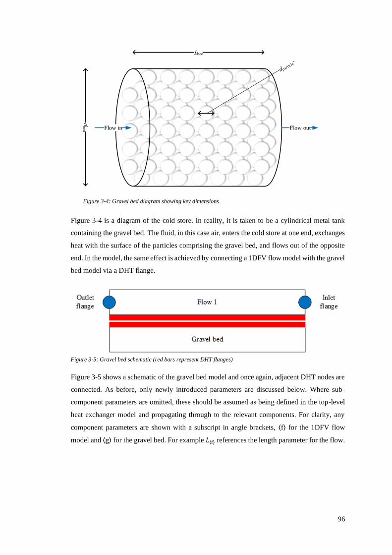
96

Figure 3-4 is a diagram of the cold store. In reality, it is taken to be a cylindrical metal tank

containing the gravel bed. The fluid, in this case air, enters the cold store at one end, exchanges

heat with the surface of the particles comprising the gravel bed, and flows out of the opposite

end. In the model, the same effect is achieved by connecting a 1DFV flow model with the gravel

bed model via a DHT flange.

Figure 3-5 shows a schematic of the gravel bed model and once again, adjacent DHT nodes are

connected. As before, only newly introduced parameters are discussed below. Where sub-

component parameters are omitted, these should be assumed as being defined in the top-level

heat exchanger model and propagating through to the relevant components. For clarity, any

component parameters are shown with a subscript in angle brackets, ⟨f⟩ for the 1DFV flow

model and ⟨g⟩ for the gravel bed. For example 𝐿⟨f⟩ references the length parameter for the flow.

Figure 3-5: Gravel bed schematic (red bars represent DHT flanges)

Lbed

Flow outFlow in

db

ed

Figure 3-4: Gravel bed diagram showing key dimensions

97

Item Name in code Units Description

Parameters

Medium Medium package for flow fluid

𝑁 Nodes Number of wall nodes

𝑑bed FlowDiameter m Internal diameter of the gravel bed

𝐿bed FlowLength m Length of the gravel bed

𝜌particle ParticleDensity m Density of the gravel bed particles

𝑑particle ParticleDiameter m Diameter of the gravel bed particles

�̇� NomMassFlowRate kg/s Nominal mass flow rate Table 3-9: Parameters for cold storage model

Parameters for the number of nodes and volumes are defined:

𝑁⟨f⟩ = 𝑁 ( 3-81 )

𝑁𝑉,⟨f⟩ = 𝑁𝑉,⟨g⟩ = 𝑁 − 1 ( 3-82 )

The flow length and area are defined:

𝐿⟨f⟩ = 𝐿bed ( 3-83 )

𝐴⟨f⟩ =𝜋

4𝑑bed

2 ( 3-84 )

The void fraction (the amount of empty space) of a gravel bed is an important factor to a number

of other parameters. To simplify the following equations, it is hereafter denoted 휀 and is

estimated using the empirical relationship (Sciacovelli et al., 2017b):

휀 = 0.375 + 0.17

𝑑particle

𝑑bed+ 0.39 (

𝑑particle

𝑑bed)

2

( 3-85 )

As discussed in section 2.6, the perimeter of the heat transfer surface is defined:

𝜔⟨f⟩ =

3𝜋

2(1 − 휀)𝑑bed ( 3-86 )

As discussed in the same section, the heat transfer coefficient is defined using the empirical

relationship:

𝛾⟨f⟩ =

700

6(1 − 휀)(4�̇�

𝜋𝑑bed2)

0.76

𝑑particle0.24 ( 3-87 )

98

The total mass of storage media is defined by multiplying the occupied volume fraction by the

particle density:

𝑀⟨g⟩ =

(1 − 휀)𝜋

4𝑑bed𝐿bed𝜌particle ( 3-88 )

3.2.10. Vapour-liquid separator

Another important part of the liquefaction plant is the vapour-liquid separator. Following the

expansion stage, the air will be in a two-phase state. The separator calculates the fluid properties

and flow rates of the separated liquid and vapour fractions.

Item Name in code Units Description

Parameters

Medium Medium package for flow fluid

Variables

𝜒mix x Vapour quality of mix

�̇�mix HMixIn W Enthalpy flow rate of mix into separator

�̇�liquid HLiquidOut W Enthalpy flow rate of liquid out of separator

�̇�vapour HVapourOut W Enthalpy flow rate of vapour out of separator

𝑝 p Pa System pressure

Fluid states

�̃�mix InletState Fluid state at the inlet

�̃�mix,sat InletSat Fluid saturation state at the inlet pressure

Table 3-10: Parameters for vapour-liquid separator model

Three 2PF flanges are used in the vapour-liquid separator model. An inlet flange is used with

properties �̇�mix, 𝑝mix and ℎmix for the mass flow rate, pressure and enthalpy respectively at the

inlet. Two outlet 2PF flanges are used. The first with properties �̇�liquid, 𝑝liquid and ℎliquid for

the mass flow rate, pressure and enthalpy respectively at the liquid outlet. The second with

properties �̇�vapour, 𝑝vapour and ℎvapour for the mass flow rate, pressure and enthalpy respectively

at the vapour outlet.

Since flow reversal cannot be allowed in the separator for the modelling assumptions to hold,

the model asserts that the inlet mass flow rate is positive:

�̇�mix > 0 ( 3-89 )

Where this is not the case, the model is halted, and an error message posted.

The inlet fluid state, �̃�mix, is defined on the inlet pressure 𝑝mix and enthalpy ℎmix. The vapour

quality at the inlet, 𝜒mix, is defined by reference to this state. Mass balance can then be defined:

99

�̇�liquid = (1 − 𝜒)�̇�mix ( 3-90 )

�̇�vapour = 𝜒�̇�mix ( 3-91 )

The separator pressure is defined on the inlet pressure:

𝑝 = 𝑝mix ( 3-92 )

Pressure is taken to be equal throughout the separator:

𝑝liquid = 𝑝vapour ( 3-93 )

The inlet saturation state, �̃�mix,sat, is defined on the pressure 𝑝. The liquid enthalpy, ℎliquid, is

defined as the enthalpy at the bubble point with reference to �̃�mix,sat.

The enthalpy flow rates are defined:

�̇�mix = �̇�mixℎmix ( 3-94 )

�̇�liquid = −�̇�liquidℎliquid ( 3-95 )

�̇�vapour = −�̇�vapourℎvapour ( 3-96 )

Once again, the inStream command is for equation ( 3-94 ) to specify enthalpy flowing into the

separator. Energy balance is thus defined:

�̇�mix = �̇�liquid + �̇�vapour ( 3-97 )

A single unused balancing equation is defined:

�̇�mixℎmix + �̇�liquidℎliquid + �̇�vapourℎvapour = 0 ( 3-98 )

In contrast to equations ( 3-94 ) to ( 3-96 ), the inStream command is used for ℎliquid and ℎvapour

for reverse flow. This equation remains unused due to the assertion of equation ( 3-89 ) but its

presence is required to balance the model.

100

3.2.11. Storage tank

Some means of fluid storage is required for the LAES plant. In this case, it is a fixed pressure

tank. This model has been purpose-built.

Item Name in code Units Description

Parameters

Medium Medium package for fluid

𝑝 p Pa Tank design pressure

Initial parameters

𝑀start Mstart kg Initial stored fluid mass

ℎstart hstart J/kg Initial fluid specific enthalpy

SSinit Boolean parameter for steady-state initialisation

Variables

𝑉 V m3 Volume of fluid stored

𝑀 M kg Mass of fluid stored

𝐻 H J Total enthalpy of fluid in tank

ℎ h J/kg Specific enthalpy of fluid in tank

𝜌 rho kg/m3 Density of fluid in tank

ℎin hin J/kg Specific enthalpy at inlet

ℎout hout J/kg Specific enthalpy at outlet

Fluid states

�̃� state Fluid state inside tank Table 3-11: Parameters for storage tank model

Two flanges are used in the tank model. Firstly, an inlet 2PF flange is used with properties

�̇�inlet, 𝑝inlet and ℎinlet for the mass flow rate, pressure and enthalpy respectively at the inlet.

Secondly, an outlet 2PF flange with properties �̇�outlet, 𝑝outlet and ℎoutlet for the mass flow rate,

pressure and enthalpy respectively at the outlet.

An assertion is made that flow at the inlet let must be into the tank and flow at the outlet must

be out of the tank:

�̇�inlet > 0 ( 3-99 )

�̇�outlet < 0 ( 3-100 )

The inlet and outlet specific enthalpies are then equated to the flange specific enthalpies:

ℎinlet = ℎin ( 3-101 )

ℎoutlet = ℎout ( 3-102 )

101

The inStream command is used for equation ( 3-101 ) to denote enthalpy entering the tank. The

flange specific enthalpies are equated to the specific enthalpy of the fluid in the tank:

ℎinlet = ℎoutlet ( 3-103 )

The flange pressure are equated to the tank pressures:

𝑝inlet = 𝑝outlet ( 3-104 )

Energy balance for the tank is defined:

𝑑𝐻

𝑑𝑡= �̇�inletℎin + �̇�outletℎout ( 3-105 )

Mass balance is defined:

𝑑𝑀

𝑑𝑡= �̇�inlet + �̇�outlet ( 3-106 )

The fluid specific enthalpy is defined:

𝐻 = 𝑀ℎ ( 3-107 )

The fluid state within the tank, �̃�, is defined using the pressure 𝑝 and the specific enthalpy ℎ.

The fluid density, 𝜌 is defined by reference to the fluid state. The volume of fluid within the

tank is then calculated:

𝑉 =𝑀

𝜌 ( 3-108 )

3.2.12. Mass flow source

The mass flow source provides a supply of a fluid at a given flow rate. This flow rate can be set

either by a parameter or by using an external real number source. The latter allows the user to

vary the flow rate, rather than having it fixed throughout the simulation. This component

determines the mass flow rate for all components connected to it. The ThermoPower model

(Casella, 2014) was deemed sufficient for this study and was used with some small

modifications.

102

Item Name in code Units Description

Parameters

Medium Medium package for fluid

�̇�nom w0 kg/s Nominal mass flow rate

ℎ h0 J/kg Nominal specific enthalpy

use_in_w0 Boolean operator activating mass flow rate input

use_in_h Boolean operator activating specific enthalpy input

Variables

�̇� w kg/s Instantaneous mass flow rate

Table 3-12: Parameters for storage tank model

A single outlet 2PF flange with properties �̇�outlet, 𝑝outlet and ℎoutlet for the mass flow rate,

pressure and enthalpy respectively at the outlet. Where the mass flow input Boolean is set to

true, an interface is used to provide a mass flow input �̇�input. Where the enthalpy input Boolean

is set to true, an interface is used to provide a specific enthalpy input ℎinput.

The mass flow rate at the flange is defined:

�̇�outlet = −�̇� ( 3-109 )

The instantaneous mass flow rate is defined:

�̇� = �̇�input ( 3-110 )

Where the mass flow input Boolean is set to false, the input mass flow rate is defined using the

fixed parameter:

�̇�input = �̇�nom ( 3-111 )

The specific enthalpy is defined:

ℎoutlet = ℎinput ( 3-112 )

Where the specific enthalpy input Boolean is set to false, the specific enthalpy is defined using

the fixed parameter:

ℎinput = ℎnom ( 3-113 )

103

3.2.13. Mass flow sink

The mass flow sink provides a sink for a fluid at a given flow rate. This flow rate can be set

either by a parameter or by using an external real number source. The latter allows the user to

vary the flow rate, rather than having it fixed throughout the simulation. This component

determines the mass flow rate for all components connected to it. The ThermoPower model

(Casella, 2014) was again deemed sufficient for this study and was used with some small

modifications.

Item Name in code Units Description

Parameters

Medium Medium package for fluid

�̇�nom w0 kg/s Nominal mass flow rate

ℎ h0 J/kg Nominal specific enthalpy

use_in_w0 Boolean operator activating mass flow rate input

use_in_h Boolean operator activating specific enthalpy input

Variables

�̇� w kg/s Instantaneous mass flow rate

Table 3-13: Parameters for storage tank model

A single inlet 2PF flange with properties �̇�inlet, 𝑝inlet and ℎinlet for the mass flow rate, pressure

and enthalpy respectively at the inlet. Where the mass flow input Boolean is set to true, an

interface is used to provide a mass flow input �̇�input. Where the enthalpy input Boolean is set

to true, an interface is used to provide a specific enthalpy input ℎinput.

The mass flow rate at the flange is defined:

�̇�inlet = −�̇� ( 3-114 )

The instantaneous mass flow rate is defined:

�̇� = �̇�input ( 3-115 )

Where the mass flow input Boolean is set to false, the input mass flow rate is defined using the

fixed parameter:

�̇�input = �̇�nom ( 3-116 )

The specific enthalpy is defined:

104

ℎinlet = ℎinput ( 3-117 )

Where the specific enthalpy input Boolean is set to false, the specific enthalpy is defined using

the fixed parameter:

ℎinput = ℎnom ( 3-118 )

3.2.14. Pump (simple)

Two pump models were developed. This one is designed for use in conjunction with the flow

controllers discussed in sections 3.2.12 and 3.2.13 in open power cycles and simply calculates

the power required for a defined pressure increase based mass flow provided by a mass flow

source or sink. A second pump model will be described in section 3.2.15 and acts as a flow

controller. Both pump models were purpose-build for this model.

Item Name in code Units Description

Parameters

Medium Medium package for fluid

∆𝑝 dp Pa Pressure increase in pump

𝜂 Eta Pump efficiency

Variables

�̇� w kg/s Mass flow rate

�̇� q m3/s Volumetric flow rate

ℎ h J/kg Fluid specific enthalpy

ℎin hin J/kg Specific enthalpy of fluid at inlet

ℎout hout J/kg Specific enthalpy of fluid at outlet

𝜌 rho kg/m3 Fluid density

�̇� Power W Power consumption

Fluid states

�̃�inlet state_in Fluid state at inlet

Table 3-14: Properties for pump (simple) model

Two flanges are used in the pump (simple) model. Firstly, an inlet 2PF flange is used with

properties �̇�inlet, 𝑝inlet and ℎinlet for the air mass flow rate, pressure and enthalpy respectively

at the inlet. Secondly, an outlet 2PF flange with properties �̇�outlet, 𝑝outlet and ℎoutlet for the air

mass flow rate, pressure and enthalpy respectively at the outlet.

Flow reversal is not allowed in the pump, so the model asserts that the inlet mass flow rate is

positive:

�̇�inlet > 0 ( 3-119 )

105

Where this is not the case, the model is halted, and an error message posted.

The mass flow rate is defined:

�̇� = �̇�inlet ( 3-120 )

The fluid state at the inlet, �̃�inlet, is defined based on the inlet specific enthalpy, ℎinlet, and the

inlet pressure, 𝑝inlet. The fluid density, 𝜌, is defined by reference to this state. The volumetric

flow rate is calculated:

�̇� =�̇�

𝜌 ( 3-121 )

The power consumed by the pump is defined:

�̇� =∆𝑝�̇�

𝜂 ( 3-122 )

The outlet pressure is calculated:

∆𝑝 = 𝑝outlet − 𝑝inlet ( 3-123 )

The inlet and outlet pressures are equated to the model variables:

ℎin = ℎinlet ( 3-124 )

ℎout = ℎoutlet ( 3-125 )

Here, equation ( 3-124 ) uses the inStream command to specify specific enthalpy entering the

pump. An additional balancing equation for reverse flow is defined but remains unused due to

the assertion in equation ( 3-119 ).

ℎout = ℎinlet ( 3-126 )

Mass balance is defined:

�̇�inlet + �̇�outlet = 0 ( 3-127 )

Energy balance is defined:

106

�̇�inletℎin + �̇�outletℎout + �̇� = 0 ( 3-128 )

3.2.15. Pump (controller)

This second pump model defines mass flow as a parameter and is used itself as a flow controller

for closed cycles where there is no source or terminus for the flow. To facilitate this role, this

pump also defines initialisation fluid properties at either the inlet or the outlet, allowing it to

replace the role of a source in a closed power cycle. As with the pump (simple) model, this was

purpose-built for this model.

Item Name in code Units Description

Parameters

Medium Medium package for fluid

𝑝outlet poutlet Pa Fluid pressure at outlet

𝜂 Eta Pump efficiency

Initial parameters

�̇�start wstart kg/s Initial mass flow rate

𝑇outlet,start Toutlet K Initial fluid temperature

Variables

∆𝑝 dp Pa Pressure increase in pump

�̇� w kg/s Mass flow rate

�̇� q m3/s Volumetric flow rate

ℎin hin J/kg Specific enthalpy of fluid at inlet

ℎout hout J/kg Specific enthalpy of fluid at outlet

𝜌 rho kg/m3 Fluid density

�̇� Power W Power consumption

Fluid states

�̃�inlet state_in Fluid state at inlet

�̃�outlet,start state_out Initial fluid state at outlet

Table 3-15: Properties for pump (controller) model

As before, two flanges are used in the pump (controller) model. Firstly, an inlet 2PF flange is

used with properties �̇�inlet, 𝑝inlet and ℎinlet for the air mass flow rate, pressure and enthalpy

respectively at the inlet. Secondly, an outlet 2PF flange with properties �̇�outlet, 𝑝outlet and ℎoutlet

for the air mass flow rate, pressure and enthalpy respectively at the outlet.

Again, flow reversal is not allowed in the pump, so the model asserts that the inlet mass flow

rate is non-negative:

�̇�inlet ≥ 0 ( 3-129 )

In this model, the starting mass flow rate is defined during initialisation:

107

�̇� = �̇�start ( 3-130 )

The initial fluid state, �̃�start, is defined according to 𝑇start and 𝑝start. The initial specific enthalpy

is defined based on this initial fluid state. Where the startInlet Boolean is set to true, this specific

enthalpy is used to define the start value for ℎin. Otherwise, it is used to define the starting value

for ℎout.

Finally, the starting pressures are defined:

𝑝inlet = 𝑝start ( 3-131 )

𝑝outlet = 𝑝start ( 3-132 )

Equation ( 3-131 ) is used where the startInlet Boolean is set to true and equation ( 3-132 ) is

used where the Boolean is set to false.

3.2.16. A note on flow controllers

The storage tank in section 3.2.11, the mass flow controller in sections 3.2.12 and 3.2.13, and

the pump (controller) in section 3.2.15 provide all of the means of control required for the open

cycle models. The storage tank and the pressure sink allow pressure to be defined at either the

origin or the terminus of the flow, with the pressures throughout the remainder of the model

calculated either via flow pressure drops or by turbomachinery pressure ratios. The latter allows

mass flow rate to be defined at either a source or sink (containing an infinite amount of the fluid

in question) and the mass flow rates throughout the remainder of the model being calculated by

the respective components’ mass balance equations. It is important to note that only one

pressure definition and one mass flow rate definition should be used for each model to prevent

the model from becoming over constrained.

3.2.17. Flow joiner

ThermoPower (Casella, 2014) provides a basis for this model, however the original model

allows flow reversal through the component. Due to the construction of the flow splitter

discussed in section 3.2.18 , reverse flow is not necessary and the ThermoPower model was

simplified to prevent reverse flow through the joiner.

Three 2PF flanges are used in the joiner model. Two inlet flanges are used with properties

�̇�inlet,1, 𝑝inlet,1 and ℎinlet,1, and �̇�inlet,2, 𝑝inlet,2 and ℎinlet,2 for the mass flow rate, pressure and

108

enthalpy at the inlets 1 and 2 respectively. One outlet 2PF flange is used with properties �̇�outlet,

𝑝outlet and ℎoutlet for the mass flow rate, pressure and enthalpy respectively at the outlet. No

user-defined parameters are required.

Assertions are made concerning the inlet mass flow rates:

�̇�inlet,1 > 0 ( 3-133 )

�̇�inlet,2 > 0 ( 3-134 )

Where these are not true, the model is halted, and an error message posted.

Mass balance is defined:

�̇�inlet,1 + �̇�inlet,2 + �̇�outlet = 0 ( 3-135 )

Pressure is defined on the outlet flow:

𝑝inlet,1 = 𝑝outlet ( 3-136 )

𝑝inlet,2 = 𝑝outlet ( 3-137 )

Energy balance is defined:

�̇�inlet,1ℎinlet,1 + �̇�inlet,2ℎinlet,2 + �̇�outletℎoutlet = 0 ( 3-138 )

Once again, the inStream command is used for the inlet specific enthalpy terms to specify these

properties entering the joiner. Additional balancing equations are defined but remain unused

due to the assertions made by equations ( 3-133 ) and ( 3-134 ):

ℎinlet,1 = ℎoutlet ( 3-139 )

ℎinlet,2 = ℎoutlet ( 3-140 )

Here, the inStream command is used for the outlet specific enthalpies to specify reverse flow

properties.

109

3.2.18. Flow splitter

ThermoPower (Casella, 2014) provides a basis for this model, however the original model was

modified to prevent reverse flow through the joiner.

Item Name in code Units Description

Parameters

𝑆𝑅 SplitRatio Proportion of inlet flow sent to outlet 1

Table 3-16: Properties for flow splitter model

Three 2PF flanges are used in the splitter model. One inlet 2PF flange is used with properties

�̇�inlet, 𝑝inlet and ℎinlet for the mass flow rate, pressure and enthalpy respectively at the inlet.

Two outlet flanges are used with properties �̇�outlet,1, 𝑝outlet,1 and ℎoutlet,1, and �̇�outlet,2, 𝑝outlet,2

and ℎoutlet,2 for the mass flow rate, pressure and enthalpy at the outlets 1 and 2 respectively.

Assertions are made on the inlet mass flow rate:

�̇�inlet > 0 ( 3-141 )

Where this is not true, the model is halted, and an error message posted.

Outlet mass flow rates are defined:

�̇�outlet,1 = −�̇�inlet𝑆𝑅 ( 3-142 )

�̇�outlet,2 = −�̇�inlet(1 − 𝑆𝑅) ( 3-143 )

Pressure is defined on the inlet flow:

𝑝inlet = 𝑝outlet,1 ( 3-144 )

𝑝inlet = 𝑝outlet,2 ( 3-145 )

Outlet specific enthalpies are defined:

ℎinlet = ℎoutlet,1 ( 3-146 )

ℎinlet = ℎoutlet,2 ( 3-147 )

110

Once again, the inStream command is used for the inlet specific enthalpy terms to specify these

properties entering the splitter. An additional balancing equation is defined but remains unused

due to the assertions made by equation ( 3-141 ).

ℎinlet = ℎoutlet,1 ( 3-148 )

Here, the inStream command is used for the outlet specific enthalpy to specify reverse flow

properties.

3.3. Model validation

Validation is an important part of any modelling regimen, especially when a combination of

existing and novel code is being used to simulate a complex engineering system, as is the case

in this thesis. A major hurdle to validation of the model is that there is only one instance in the

literature of a coupled NPP and LAES plant design (Li et al., 2014). The shortcomings of this

work are discussed in detail in section 2.5.2 and their implications are explored in the results of

Chapter 5. The lack of a comparable plant thus makes holistic model validation impossible.

That said, the modular nature of the model described in this chapter and the way in which

components can be tested in isolation allows validation of individual components to be

performed against available data, which provides assurances that the novel code is fit for

purpose and performing as intended. For this purpose, the Birmingham University and

Highview Power literature discussed in section 2.5.2 was used primarily due to the rigour and

transparency in its engineering approach, and those groups’ access to the pilot plant and their

resulting ability to compare their modelling results with experimental data. For some parts of

the NPP, NuScale regulatory applications were used.

The basic machinery components (turbines, compressors, and pumps) were compared against

the work of the Birmingham University group using their modelling parameters and flow

thermophysical properties. All provided identical results the given conditions. This is perhaps

unsurprising given the relatively straightforward nature of the modelling of such components

and the highly mature state of modelling in this area.

Heat exchangers present something of a greater issue to validation. There are a variety of

approaches to heat exchanger modelling, of which the finite volume approach described herein

is one of the more complex. The simplifying assumption has been made of a continuous heat

transfer coefficient throughout each flow of a given heat exchanger further complicates

comparison. The approach taken to ensuring that heat exchanger results would be as accurate

111

as possible was to set heat transfer coefficients such that thermal power loads on a given heat

exchanger of a given size would match those from the literature. For water-water heat

exchangers, the NuScale regulatory application (NuScale Power LLC, 2018a) provides the flow

stream, heat exchanger area and thermal load data required to make these comparisons. For air-

air and air-water heat exchangers, an article from Highview Power (Morgan et al., 2015a)

provides the necessary data.

The gravel bed model is perhaps the most difficult component to compare to available data.

Whilst the Birmingham University group provide a thorough and detailed treatment of the

gravel bed (Sciacovelli et al., 2017b), the assumption of a linear pressure drop along the cold

store, as described in section 3.2.9, represents a significant departure from this work.

Nevertheless, comparisons can still be made; not least in the quantity of heat transferred

between the working fluid and the gravel bed during comparable charge and discharge cycles

for a given mass of thermal storage medium. These comparisons show that the quantity of heat

transfer was within 1% for a comparable charge or discharge cycle. Whilst this was deemed

sufficient for the modelling work discussed in this thesis, the simplifying assumption of a linear

pressure drop is an important one that is discussed in greater detail in section 7.3.1.

Ultimately, the comparisons made provide considerable assurance that the engineering

modelling approach will provide results sufficiently accurate for the purposes of this thesis: the

evaluation of LAES plant output power ratings and the sizing of the components required to

achieve these. Whenever a plant design model was built from components, of the kind described

in Chapter 5, all flow variables into and out of components were compared to ensure that flanges

and connectors were operating as expected.

In light of this, this author would assert that the results of the engineering modelling approach

are as accurate as possible in light of the simplifying assumptions that have been made. In a

more philosophical sense, the simplifying nature of any modelling approach is non-trivial, and

it is important that the developer of any engineering model be aware of the limitations of such

assumptions and be as transparent as possible of their implications. This is the purpose of

section 7.3.1.

112

- Financial modelling

4.1. Introduction

This chapter details the financial model. Section 4.1.1 summarises the objectives of the financial

model while section 4.1.2 goes into greater detail of the minutiae of financial modelling under

uncertain conditions. Section 4.2 details the basis for, and definition of, the probability

distributions for the initial model parameters. Section 4.3 details the way that plant capital costs

have been estimated from equipment costs. Section 4.4 details the basis for, and definition of

the time series functions used to simulate SPOT market prices. Section 0 details the way the

model has been built from its components and summarises the key parameters and their values.

The model library is available via Open Research Data Online (Wilson, 2020a)

Model parameters and calculated variables are defined using symbols; either Latin-script

alphabet letters or Greek letters. The symbols used, their definitions, and the sections in which

parameters or variables are introduced are summarised in Table 4-1. Where variable values vary

depending on the values of other variables, the time period symbol is given in brackets, e.g.

𝐴(𝐷) defines the daily average price, 𝐴, for a given day, 𝐷. Where the same parameter is

defined independently for different models, the differentiation is made using a subscript, e.g.

𝜇𝐴(𝐷) described the mean parameter for the daily average price model, whereas 𝜇𝜀(𝑃) denotes

the mean parameters for the half-hourly period error value.

Symbol Description

Parameters and variables

�̇� Mass flow rate

�̇� Power

𝐴 Daily average price

𝐶 Cost

𝐼 Chemical engineering plant cost index

𝑁 Random number

𝑅 Revenue (cash flow)

𝑆 Electricity sale price

𝑎 Autoregressive coefficient

𝑏 Moving average coefficient

𝑖 Percentage rate

𝑠 Equipment size

𝑦 Time series value for descriptions

𝛼 Amplitude

𝛽 BetaGeneral distribution parameters

𝛿 Price difference

휀 Error value (for electricity price model)

𝜖 Error value (for time series model definitions)

𝜃 Clayton copula parameter

𝜇 Mean

113

𝜎 Volatility (standard deviation)

𝜑 Ratio

Time periods

𝑌 Year

𝑄 Quarter

𝐷 Day

𝑃 Period (half-hour)

𝑡 Arbitrary time period for descriptions

Identifying subscripts

CHG Charge

CONST Construction

CPI Consumer prices index

CfD Contract for difference

DIS Discharge

DISC Discount rate

FUEL Fuel

NPP Nuclear power plant

O&M Operation and maintenance

REFUEL Refuel

Table 4-1: Parameter, variable and other subscript symbol definitions

4.1.1. Objectives

The financial model is intended to determine hybrid plant economics when selling into real-

world markets. In order to do this, it is required to fulfil the following objectives:

• determine uncertain initial parameters such as plant capital cost and construction times

using probability distributions,

• simulate spot market electricity prices over an extended period using time series,

• estimate NPV distributions under first-of-a-kind (FOAK) and nth-of-a-kind (NOAK)

scenarios for different plant outputs.

4.1.2. Background

Financial modelling of power plants is fraught with uncertainty. This is especially true of

nuclear power given the complexities of construction, the high capital cost and the frequent

overruns in construction time. This study adds further complexity by including energy storage

and sale of power into multiple markets; some power is sold on a CfD basis while the variable

power output is sold into the SPOT market, where prices are most volatile.

Monte Carlo modelling offers a means of incorporating uncertainty into financial modelling. In

an entirely deterministic model, input parameters such as plant cost and construction time are

given discrete values and yield a single output, often an NPV value from a DCF analysis. DCF

is a means of considering the time-dependent value of money. This is done by estimating future

114

cash flows and then discounting them based on the cost of capital. This is captured in the

following equation:

𝑁𝑃𝑉 = ∑𝑅(𝑌)

(1 + 𝑖𝐷𝐼𝑆𝐶)𝑌

𝑁

𝑌=0

( 4-1 )

where N is the total number of periods, in this case years, 𝑅(𝑌) is the cash flow for a given

year, 𝑌 is that year and 𝑖𝐷𝐼𝑆𝐶 is the discount rate, dependent on the cost of the capital used to

fund the project. Discount rates are determined by the potential appreciation in the value of

capital were it not used in a project, typically the interest or growth garnered from more

conventional and predictable investments.

In Monte Carlo modelling, each initial parameter is given defined by a probability distribution

rather than a static value. The model is then run for a large number of iterations and with each

iteration, parameter values are using an RNG and the corresponding probability distribution.

Running the model tens of thousands or even hundreds of thousands of times yields a

probability distribution for the NPV, rather than a single static value, which provides the relative

likelihood of different NPV values.

The model described below also requires the prediction of stochastic variables, chiefly the

electricity price and the CPI. In reality, these variables are not simply random. Their values

form series where one value is dependent on previous values in the series to a greater or lesser

degree. This is in contrast to probability distributions where a value selected for a given iteration

has no dependence on the previous values selected and imposes no preference on any future

values selected. Time series have long been used in financial modelling, for example in the

prediction of share prices.

Obviously, a key consideration in the construction of a model is the definition of the probability

distributions used for initial parameters and the definition of time series models used to predict

stochastic variables. This chapter describes the decision-making process used in defining these

distributions and time series. Section 4.2 describes the definition of distributions for initial

parameters, section 4.3 those for the LAES plant capital cost, and section 4.4 describes the

definition of time series models.

115

4.2. Monte Carlo modelling – Initial parameters

This section details the decision-making process in the definition of probability distributions

for the Monte Carlo financial model. These definitions are based on historical data as much as

possible. It should be noted, however, that their definition remains a largely subjective process

and, as a result, not everyone will agree with the justifications to follow. This highlights the

importance of sensitivity analysis in the final decision as to whether a plant will be built. As

similar plants are built, the distributions should move closer to certainty, allowing a more

informed decision to be made by prospective plant operators. Sensitivity analysis will highlight

the most important considerations for this process. The parameters used in the final model are

summarised in Table 4-5 in section 0.

4.2.1. Nuclear power plant spending factor

The determination of NPP capital cost is a complex problem beyond the scope of this project.

The manufacturer’s system price will be used for the model, but it is important to consider that

overspend is likely on a large NPP construction project. This will be incorporated into the model

by a capital cost factor by which the base plant price will be multiplied, with a factor of 1

representing a project that is delivered on-budget. The shape of the probability distribution that

defines this factor is an important consideration as the capital investment for the project is an

early-stage cost and, as a consequence of DCF likely to be a major driver in the overall NPV of

the project. Given that this study considers a novel SMR-based power plant, there is no

historical data that this can be directly based on. As a result, the decision was made to use PERT

(project evaluation and review technique) distributions. This has the benefit of using a small

number of easily defined parameters (minimum, most likely and maximum).

Detailed accountings of costs for recently built nuclear plants are elusive at best, and at worst

entirely hidden from the public (Kessides, 2010). As a result, much of the discussion in this

section is based upon news articles and the scant financial details that have been made publicly

available. Complex engineering projects in the UK and overseas commonly come in over

budget, often significantly (MacLeod, 2014, Staff Writer, 2014). The examples shown are all

large-scale construction projects, so clearly the capital dedicated to plant construction can be

overspent substantially – some of these projects overspend by 100% or more.

Within the nuclear industry, there are also significant overspends. The EPR (European

Pressurised Reactor) is the most recent and high-profile example of this. Finland’s Olkiluoto

EPR was estimated to cost EUR 3.7bn for a 1.6 GWe plant when its construction was first

116

agreed. Costs were estimated in 2012 to have risen to EUR 8bn (Landauro, 2012) – an

overspend of well over 100%. It’s important to note that EDF have not updated their cost

estimates since the 2012 estimate (Rosendahl and Forsell, 2017), so this is almost certainly out-

of-date information. France’s Flamanville EPR is even worse – the most recent cost estimate is

EUR 10.9bn (World Nuclear News, 2018), up from the starting estimate of EUR 3.3bn – an

increase of 230% in 6 years.

The cost rise described in the preceding discussion would seem extreme, and indeed it is. The

fact that these significant rises have occurred so soon after the commitment to build has been

agreed is further questionable. Whilst it is not the place of this thesis to speculate the reactor

designer’s potential foreknowledge of overspend, this does raise an important point in the

context of financial modelling undertaken herein. Clearly, this kind of overspend is a likely

consequence of being the first to build a particular plant, that is, building a FOAK plant. Whilst

subsequent NOAK plants are not guaranteed to provide more accurate cost assessments, the

assumption that they will is one that is made in this thesis.

That being said, the proposed system considered in this study utilises an SMR, of significantly

smaller capacity than the EPR. SMRs are intended to avoid many of the potential pitfalls of

conventional nuclear power due to their small, modular nature. The benefits of SMRs are in

economies of volume as opposed to economies of scale (Roulstone, 2015). Simply put, being

able to build more SMRs could reduce costs as components can be mass produced. We can

consider this in a qualitative sense as follows:

The EPRs mentioned are 1.65 GW (electric) plants, which, assuming each has a final

commissioned cost of EUR 11bn, or say £10bn (an approximately similar cost of each of the

UK’s two intended EPRs at the Hinckley Point site (Farrell and Macalister, 2015). This provides

a commissioned cost of £6,061 per kW. The original estimate for the Finnish and French plants

was £2,037 per kW. The current estimate for the NuScale SMR is $4,200 or £3,500 per kW.

Comparing the EPR and SMR initial plant estimates first, this is perhaps what could be expected

- the cost per unit power of the NuScale SMR is around 1.5 times the cost of the EPR - which

could represent the increase of per unit costs associated with economies of scale. This is perhaps

to be expected; nuclear plants have long suffered from higher costs due to a lack of learning

and there is every reason to think that the same would be the case for SMRs until they begin to

be built in large numbers (Roulstone, 2015). Even the French nuclear programme, arguably one

of the most successful worldwide, saw considerable cost increases, although as (Lévêque, 2015)

117

notes, this was largely due to redesigns associated with increases in plant size. Similarly, the

early SMRs will not benefit from the promised economies of volume.

Whether SMRs can indeed benefit from serialised construction at all is a matter of no small

debate. Detailed design and costing of the NPP part of the proposed plant is beyond the scope

of this thesis, however the benefits of smaller and serialised construction can be contextualised

by considering the pressure vessel of a PWR, a part making up a significant portion of

equipment costs (Mizia, 2008). The EPR features the largest pressure vessel, with the fewest

separate parts of any reactor build to date, and a range of problems related to both supply chain

and material defects have plagued the early EPRs and contributed considerably to delays and

cost rises. It is not unreasonable to argue that smaller pressure vessels for SMRs will reduce

both equipment costs and supply chain issues, potentially helping to deliver on the promised

cost savings associated with SMRs (Power Technology, 2013, Boldon et al., 2014).

This historical insight can be used to define the minimum and maximum ends of the probability

distribution for the spending factor. The minimum factor should be the expected production

cost for the plant, a factor of 1. The maximum factor should be the maximum historical

overspend in the UK – double the budget, or a factor of 2. This is, of course, less than the

comparative Flamanville overspend of 3, but it is a core assumption of this thesis that SMR cost

savings are achieved. A further benefit of a statistical modelling approach is that conclusions

are not static and can be re-evaluated as new data becomes available. The main point of

contention is the location of the most likely value between these points.

Since this study intends to explore both FOAK and NOAK scenarios for the nuclear plant, two

distributions are required. For a FOAK plant, the most likely value can reasonably be expected

to be at the upper end of the probability distribution. In an alternative NOAK scenario, where

several such plants have been constructed, the actual project spend can be reasonably expected

to be much closer to the expected value, with a reduced maximum spend. The defined

distributions for this factor are shown in Figure 4-1.

Figure 4-1: Spending factor probability distributions - FOAK on left, NOAK on right

118

4.2.2. Nuclear power plant construction time

The construction time for the plant is of major practical significance. Whilst nuclear plants run

for in excess of sixty years, the fact that plant profitability is considered on an NPV (net present

value) basis in this model means that discounted cash flows for years far into the future become

almost negligible. Consider the NPV formula:

𝑁𝑃𝑉 = ∑𝑅(𝑌)

(1 + 𝑖𝐷𝐼𝑆𝐶)𝑌

𝑁

Y=0

( 4-1 )

where N is the total number of periods, in this case years, 𝑅(𝑌) is the revenue for a given year,

t is the current year and 𝑖𝐷𝐼𝑆𝐶 is the discount rate.

In the case of a nuclear power plant that takes 5 years to build and runs for 60, even at modest

discount rates of say 8%, the denominator of this formula increases by a factor of 10 over a 30-

year period. After the 5 years of construction, the nature of the NPV formula means that the

cash flow is discounted by a factor of 1.47 and after 30 years of operation it is discounted by

14.8. Indeed, at 60 years, cash flow is discounted by a factor of nearly 150. This massively

outweighs the effect of inflation, which is historically between 2 and 3%. This illustrates the

importance of build time. Longevity of nuclear power plants cannot make up for the revenue

lost during construction when project value is assessed in this way.

NuScale state a period of 5 years construction time including mobilisation, with a critical path

of 3 years (NuScale). The model assumes that costs may be spread over the initial construction

period but that funds must be reserved and allocated to the project prior to committing to the 3

year critical path, meaning that these final years of construction can be considered to contribute

to loss of revenue. How this is done in model is discussed in section 0.

The way this is expressed within the financial model depends on the limitations of the model.

Construction time is analysed by year, and part years cannot be considered due to the use of an

annual discount rate. As a result, construction time is not defined by a factor but by a whole

number of years. This means that the continuous PERT distribution cannot be used and a

binomial distribution is used instead, providing only integer values to the model. This

distribution uses 3 parameters; n describing the number of possible values to be taken, p

defining how the probabilities of each is weighted and a shift value providing the first of the

possible values.

119

In the model, construction is split into two phases; mobilisation where initial costs are spread

over the years and critical path where all capital is considered to be invested in the project and

is applied to costs in the first year of critical path construction. Construction projects in the UK

have typically seen delays of between 10 and 30% of the expected construction time for the

project. This contrasts with the EPR, which has seen construction times double at its Finnish

and French plants.

With this information in mind, two potential routes are considered for the construction time

values. Firstly, an early scenario where the considered plant is one of the first of its kind and

secondly an experienced scenario where several of these plants have been built. Again, the

FOAK scenario will weight probabilities towards the higher end, while the NOAK scenario will

weight probabilities towards the time expected by the plant designer. The construction times

for mobilisation are shown in Figure 4-2 and those for the critical path are shown in Figure 4-3.

Figure 4-2: Mobilisation construction time probability distributions - FOAK on left, NOAK on right

Figure 4-3: Critical path construction time probability distributions - FOAK on left, NOAK on right

120

Of course, in reality, the construction time and the overspend are closely linked – delays in

construction mean workers are on site and paid for longer. As a result, the capital cost and

construction time are linked using a copula. A copula correlates two probability distributions

and in this model ensures that a high construction cost is correlated to a longer construction

time. A three-dimensional Clayton copula is used to correlate the modelled values of NPP

spending factor, mobilisation and critical path construction times possible in @RISK. The

degree of correlation is defined using a parameter, 𝜃.

The effect of a copula on the modelled values of critical path construction times is shown in

Figure 4-4. There are 100,000 points for each value of 𝜃. The effect is clear; the larger the value

of 𝜃, the greater the correlation between spending factor and construction time. With 𝜃 = 0,

there is no forced correlation and the values of NPP spending factor for the different

construction times overlap entirely. As 𝜃 increases in value, correlation increases and the

overlap in NPP spending factor values lessens. For modelling purposes, it was assumed that

correlation was high but that there would be some degree of overlap, so a value of 𝜃 = 25 was

used.

4.2.3. LAES plant construction time

As with the nuclear power plant, the construction time for the LAES plant is also defined by a

binomial distribution. The key difference here is that LAES uses existing technology with an

established supply chain and fewer safety-critical components (Highview Power, 2015). Plants

Figure 4-4: Copula parameter comparison using FOAK parameters

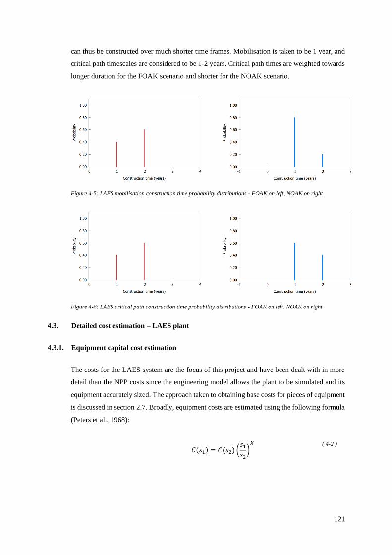
121

can thus be constructed over much shorter time frames. Mobilisation is taken to be 1 year, and

critical path timescales are considered to be 1-2 years. Critical path times are weighted towards

longer duration for the FOAK scenario and shorter for the NOAK scenario.

Figure 4-5: LAES mobilisation construction time probability distributions - FOAK on left, NOAK on right

Figure 4-6: LAES critical path construction time probability distributions - FOAK on left, NOAK on right

4.3. Detailed cost estimation – LAES plant

4.3.1. Equipment capital cost estimation

The costs for the LAES system are the focus of this project and have been dealt with in more

detail than the NPP costs since the engineering model allows the plant to be simulated and its

equipment accurately sized. The approach taken to obtaining base costs for pieces of equipment

is discussed in section 2.7. Broadly, equipment costs are estimated using the following formula

(Peters et al., 1968):

𝐶(𝑠1) = 𝐶(𝑠2) (

𝑠1𝑠2)𝑋

( 4-2 )

122

where 𝐶(𝑠1) is the unknown cost of piece of equipment of size 𝑠1, 𝐶(𝑠2) is the known cost of

piece of equipment of size 𝑠2, and 𝑋 is a cost exponent for the type of equipment. This is detailed

further in section 2.6.

The price data obtained has been retrieved from several sources spanning the previous 3

decades. As a result, the price for each piece of equipment must be adjusted for a 2018

equivalent price. This is done using the CEPCI (Chemical Engineering Plant Cost Index) in the

following formula:

𝐶(𝑌1) = 𝐶(𝑌2) (

𝐼(𝑌1)

𝐼(𝑌2))

( 4-3 )

where 𝐶(𝑌1) and 𝐶(𝑌2) are the costs of a given piece of equipment in years 𝑌1 and 𝑌2

respectively and 𝐼(𝑌1) and 𝐼(𝑌2) are the indexes for those years. The CPI data has been collated

from (Vatavuk, 2015, 2010, 2008) and is shown in Figure 4-7.

The origin of the base costs used, along with their adjusted 2018 GB£ values and their exponents

are detailed in section 2.7 and summarised in Table 4-2.

Figure 4-7: Values of CEPCI for 1990-2018

123

Equipment 𝐶(𝑠2) 𝑠2 𝑋 Size units

Compressor 7,022 0.746 0.62 kW

Turbine 978 0.746 0.81 kW

Pump 0.483 1 1 kW

Heat exchanger (rated to 2 MPa) 151,879 140 0.44 m2

Heat exchanger (rated to 3 MPa) 190,203 140 0.44 m2

Heat exchanger (rated to 7 MPa) 227,109 140 0.44 m2

Heat exchanger (rated to 10 MPa) 287,434 140 0.44 m2

Heat exchanger (rated to 20 MPa) 359,399 140 0.44 m2

Storage tank 654,210 2,500 0.57 m3

Cold store 834,211 2,500 0.57 m3

Table 4-2: Equipment 2018 cost data, sizes and exponents for cost estimation

These costs form the basis of an Excel spreadsheet that acts as a cost estimator for the total

capital cost of these key pieces of equipment and produces a probability distribution for the

LAES plant capital investment. The weighting factors for the cost estimator are shown in

section 4.3.2 and the plant capital costs produced discussed in Chapter 6.

4.3.2. Plant capital investment estimation

A capital cost investment amount was then estimated using the estimation of the major pieces

of equipment according to the method in (Peters et al., 1968). An alternative would have been

to use the Lang factors, which provide a more rudimentary means to estimate total plant cost

using a single factor. Despite these factors being over 70 years old, they remain accurate today

for order-of-magnitude capital estimates for process plants (Wolf, 2015). However, given the

detailed engineering analysis that has been used to size the major pieces of equipment, it makes

sense to perform a more detailed cost estimation based on the factors available in the literature.

Given that these factors are provided in terms of a minimum, maximum and typical value, this

approach lends itself to the use of PERT distributions, using these factors for the minimum,

maximum and most likely value respectively. The parameters used are shown in Table 4-3.

124

Item Minimum Most likely Maximum

Yard Improvement

Site clearing 0.4% 0.8% 1.2%

Roads and walks 0.2% 0.6% 1.2%

Rail 0.3% 0.6% 0.9%

Fencing 0.1% 0.2% 0.3%

Yard and fence lighting 0.1% 0.2% 0.3%

Parking areas 0.1% 0.2% 0.3%

Landscaping 0.1% 0.1% 0.2%

Other improvements 0.2% 0.3% 0.6%

Service facilities

Steam distribution 0.2% 1.0% 2.0%

Water supply, cooling, pumping 0.4% 1.8% 3.7%

Water treatment 0.5% 1.3% 2.1%

Water distribution 0.1% 0.8% 2.0%

Electric substation 0.9% 1.3% 2.6%

Electric distribution 0.4% 1.0% 2.1%

Sanitary waste disposal 0.2% 0.4% 0.6%

Communications 0.1% 0.2% 0.3%

Fire protection 0.3% 0.5% 1.0%

Safety installations 0.2% 0.4% 0.6%

Engineering and services

Engineering 1.5% 2.2% 6.0%

Drafting 2.0% 4.8% 12.0%

Purchasing 0.2% 0.3% 0.5%

Accounting 0.2% 0.3% 1.0%

Travel and living 0.1% 0.3% 1.0%

Reproductions and communication 0.2% 0.2% 0.5%

Construction

Temporary construction and operations 1.0% 1.7% 3.0%

Construction tools and rental 1.0% 1.5% 3.0%

Home office personnel 0.2% 0.4% 2.0%

Field payroll 0.4% 1.0% 4.0%

Travel and living 0.1% 0.3% 0.8%

Taxes and insurance 1.0% 1.2% 2.0%

Startup materials and labour 0.2% 0.4% 1.0% Table 4-3: PERT distribution parameters for LAES plant cost estimation (Peters et al., 1968)

The probability distributions based on these factors have been used in an @RISK model to

estimate the probability distribution for the overall capital investment for the plant in question.

Of course, whilst detailed study of the equipment and estimation of its cost has been performed,

this remains only an estimate and potential inaccuracy must be considered. It was however

decided that the conservative selection of possible cost comparisons in section 2.7 meant that

addition hedging of costs was neither necessary nor appropriate.

125

Once the model has been run for the capital investment distribution, these results are fit to the

library of available distributions in @RISK, which are then rated using the AIC (Akaike

Information Criterion). The most accurate fit was shown to be the BetaGeneral function for all

plant configurations. This is a Beta distribution that has been scaled to fit to maximum and

minimum values, rather than general values between 0 and 1. This is the distribution upon which

the PERT distribution is based. It requires two shape parameters, 𝛽1 and 𝛽2 as well as a

maximum and minimum for the distribution.

4.4. Time series parameters

Time series are used in the model to predict two key factors: the electricity price for each half-

hourly period and the evolution of the CPI over years. Definition of these series is made easier

by the availability of large datasets to which the models can be fitted. A dataset of the SSP over

the years 2008-2015 (Smith and Halliday, 2016) was used to parametrise the electricity price

model. The analysis of this data is discussed in detail in this section. A dataset of CPI over the

years 2002-2018 (Gooding, 2018) was used to parametrise the CPI model.

4.4.1. Electricity price modelling

As will be discussed in this section, the electricity price data is extremely complex and exhibits

patterns in its hourly, daily and seasonal variation. Early attempts were made to fit a single time

series model to the electricity price data to predict the evolution of the electricity price over

time. This presented two problems.

Firstly, predicting electricity prices for half-hour periods over a period of 30 years results in

over a half million discrete values. Time series models use a combination of the overall trend

and the most recent values to predict each subsequent value. Because of this, using a single time

series tended to allow the values to increase or decrease to ridiculous values towards the later

stages of the model.

Secondly, time series models are very much stochastic models based on an RNG. As such, there

is no way to define repeating patterns within these time series. This means that daily peaks and

troughs are not properly captured by a time series model. Given that daily price profiles are

societally driven (e.g. an evening peak occurs between 17:00 and 18:00 as people return home

but schools and offices remain lit), it was felt important to properly capture these features.

In order to properly capture these patterns, the data was split into components prior to time

series fitting. First, the mean average system sell price, 𝐴(𝐷), for each day, 𝐷, was calculated.

126

Then, ratio, 𝜑(𝑃) of the system sell price, 𝑆(𝑃), for each period, 𝑃, to that day’s average price

was calculated. The average of these prices was then found for each month of the year and used

to define a daily price profile curve. Finally, the absolute difference, 휀(𝑃), between the price

predicted by the profile curve and the daily average and the actual price was calculated.

This process provided two series to which time series models were then fitted: a daily average

price series and an error value series, described in sections 4.4.2, and 4.4.4 respectively. In

addition, the study yielded daily price profile curves, described in section 4.4.3. The model

could then calculate a system sell price, 𝑆(𝑃), for a given half-hour period using:

𝑆(𝑃) = [휀(𝑃) + 𝜑(𝑃)] × 𝐴(𝐷) ( 4-4 )

An important feature for the dataset used was that it included years where the daily average was

highly volatile and years where it was more stable. Similarly, some years exhibited substantial

daily variance with large differences between periods of high price and low price, while others

had much less variation in the half-hourly prices, with prices remaining fairly stable over the

course of a day. This provided an understanding of what different markets look like and allowed

the testing of a variety of scenarios for electricity prices.

4.4.2. Daily average price

As discussed in section 4.4, the first analysis performed on (Smith and Halliday, 2016) was to

calculate the daily mean for the system sell price, with the intention of determining whether

there was any evidence of seasonal or annual cyclic variation. The evolution of this average

price over the years of the dataset is shown over the following pages, along with a 30-day

Figure 4-8: A(D) data for 2008/2009

127

running mean average. Charts are limited to displaying two years in order to maintain visual

clarity, and to allow particularly interesting years to be isolated.

The data for 2008 and 2009 is shown in Figure 4-8. For 2008, the data appears to show some

seasonal variation, specifically in the significantly higher volatility in daily average price in the

middle of the year. Whilst 2009 exhibits a similar pattern, the effect is lessened. The running

mean for the data is also shown for the 30th day of each year onwards. From this, it can be seen

that average prices in 2008 increase in the middle of the year and fall again towards the end of

the year. Perhaps most importantly, there is a marked increase in running average following

price shocks, indicating that the effect of price shocks lasts for some time. In 2009, prices fall

steadily during the first quarter and exhibit a modest rise towards the end of the year. The

ongoing effect of price shocks is still visible but lessened compared to 2008.

The data for 2010 and 2011 is shown in Figure 4-9. Other than high volatility at the beginning

and end of 2010, the prices typically show low volatility throughout both years. Interestingly,

this high volatility at the end of 2010 does not continue into the beginning of 2011. The running

means show that other than the periods of high volatility in 2010, prices are largely consistent

throughout both years. The ongoing effect of shocks remains present in 2010 but is largely

absent in 2011.

Figure 4-9: A(D) data for 2010/2011

128

The data for 2012 and 2013 is shown in Figure 4-10. Once again, other than short-lived periods

of high volatility, volatility is low, and the running mean shows that prices are largely consistent

throughout the year. Both years show some ongoing effect of price shocks.

The data for 2014 and 2015 is shown in Figure 4-11. 2014 exhibits some short-lived price

shocks and shows some seasonally cyclic behaviour. 2015 is broadly similar to 2012 and 2013

in its behaviour. In both years, the ongoing effect of price shocks is almost entirely absent.

As the discussion in this section shows, there is some evidence of seasonal variation in the daily

average electricity prices for some years and evidence of stability throughout the year for others.

Figure 4-10: A(D) data for 2012/2013

Figure 4-11: A(D) data for 2014/2015

129

As discussed in section 2.5.2, however, the importance of cold recycle to LAES means that it

is unsuitable for seasonal-duration storage. Thus, as long as the diurnally cyclic behaviour of

electricity price and its seasonal dependence is properly captured, as is discussed in section

4.4.3, and as long as the daily average price model accurately captures volatility, it is reasonable

to assume that the seasonally cyclic behaviour will not affect the performance of LAES within

the modelled market. The effect of shocks is more contentious, but there is considerable

evidence that price shocks can have a medium-term effect on pricing that can last for up to two

months. It is important that the model be capable of capturing this behaviour and the user have

adequate control over this phenomenon in order to explore different scenarios.

Given the assumption that seasonally cyclic behaviour need not be captured, but that the effect

of shocks is important, the decision was made to use a time series model to predict values of

𝐴(𝐷). There are several time series models available to the @RISK software. These are:

• AR (autoregressive) first and second order

• MA (moving average) first and second order

• ARMA (autoregressive moving average) first order

• ARCH (autoregressive conditional heteroskedasticity) first order

• GARCH (generalised ARCH) first order

• BMMR (Brownian motion mean reversion) first order

These all have some history of use in electricity price modelling (Weron, 2014). With a

substantial dataset available, it made the most sense to use the fitting algorithms built into the

software to define the time series models. As discussed in section 2.7, the software provides a

variety of time series models. As a starting point, the daily average data was used to fit all time

series models available.

130

Figure 4-12 shows a comparison of the time series models for the years of data available; a

lower value represents a better fit. Since the AIC values are generally quite close together, and

the values from one year to another can vary significantly, the values have been normalised for

the sake of comparison. This was done by dividing each AIC value by the average AIC value

for that year. The comparison shows that the first-order ARMA time series provides the best fit

in the majority of cases, and close to in the remainder. Thus, this series was chosen as the basis

of the daily average price model.

An ARMA model is a combination of AR and MA models. Its parameters are average, 𝜇,

volatility, 𝜎, autoregressive coefficient, 𝑎 with magnitude less than 1, moving average

coefficient, 𝑏, initial value 𝑦(0), and initial error 𝜖(0). Whilst @RISK’s series fitting

algorithms will assist with parameter definition, it’s worth considering how values are

calculated and in order to understand which of these parameters should be user-defined. Each

consecutive value is based on an RN, 𝑁(𝑡), taken from a normal distribution with mean 0 and

standard deviation 1. For the tth series value, an error term is calculated:

Figure 4-12: Time series model fit comparison (lower AIC value represents a better fit)

131

𝜖(𝑡) = 𝜎𝑁(𝑡) ( 4-5 )

Then, the time series value, 𝑦(𝑡), is calculated using:

(𝑦(𝑡) − 𝜇) = 𝑎(𝑦(𝑡 − 1) − 𝜇) + 𝑏𝜖(𝑡 − 1) + 𝜖(𝑡) ( 4-6 )

Examining equation ( 4-6 ) shows the importance of the values of 𝑎 and 𝑏. Considering the

equation without the 𝑏 term yields the equation for a first-order AR model:

𝑦(𝑡) = 𝜇 + 𝑎(𝑦(𝑡 − 1) − 𝜇) + 𝜖(𝑡) ( 4-7 )

Considering the first term following on the right of the equation, if the previous value 𝑦(𝑡 − 1)

is far from the mean, this term will be large in magnitude. Since the mean of 𝜖(𝑡) is zero and

its standard deviation is small, the average result of this will be that the term before the equals

will be large and of the same sign. Hence, if one value of the time series is far from the mean,

the next will, on average, tend to get further from the mean – in the same direction, hence the

description of this model as autoregressive. The larger the value of 𝑎, the greater this effect.

Now, considering equation ( 4-6 ) without the 𝑎 term yields the equation for a first-order MA

model. Rearranging:

𝑦(𝑡) = 𝜇 + 𝑏𝜖(𝑡 − 1) + 𝜖(𝑡) ( 4-8 )

In contrast to the AR model, the previous error value, 𝜖(𝑡 − 1), has a direct effect on the current

term but the actual previous value, 𝑌(𝑡 − 1), has no effect. Consideration of equations ( 4-7 )

and ( 4-8 ) has thus showed the key difference between these two models; shocks (i.e. large

values of 𝜖(𝑡)) have a significant effect on an MA model but only for a finite number of values.

The immediate effect of shocks is lessened in an AR model, but the because each value 𝑦(𝑡) is

strongly dependent on its previous value, and ultimately on all previous values, shocks affect

series values until the end of the series.

With this understanding of model behaviour, the fitting shown in Figure 4-12 can be put into

the context of the qualitative discussion of the analysis of dataset (Smith and Halliday, 2016).

ARMA models represent a middle ground between AR and MA models where shocks have a

modest medium-term effect, less significant than MA models and for a shorter time than AR

models. It is for this reason that MA and AR models fit similarly well to one another, and to the

ARMA model, in years where the effect of shocks is almost entirely absent, such as 2011 and

2015. In 2008, where the effect of shocks is most obvious in the data, but remains short-term,

the difference between the ARMA and AR model fits is greatest.

132

The values 𝑎 and 𝑏 act together to have a complex effect on the values taken by an ARMA time

series. As a result, the decision was taken to define these by applying @RISK’s fitting

algorithms to the available data.

By definition, the time series models will ultimately take a mean of value 𝜇, with the cumulative

mean moving closer to 𝜇 as the value of 𝑡 increases. The decision was taken to allow the model

user to define 𝜇 since this would allow the examination of different electricity price scenarios.

The volatility, 𝜎, controls the size each error value, 𝜖(𝑡), amplifying the effect of the normal

distribution that is used to define these values. Once again, the decision was taken to allow the

user to define these values for the sake of testing different scenarios. Direction was taken from

the values resulting from @RISK’s fitting algorithms for different years from the data set for

direction on what value this should take for more or less volatile years.

The initial value 𝑦(0), and initial error 𝜖(0) simply represent the start of the series. Since the

daily average price time series will be extended for the 30 years over which modelling is

performed, initial values will have a negligible effect. Thus, the decision was taken to define

the value 𝑦(0) = 𝜇 and 𝜖(0) = 0 in year 0 for simplicity.

The time series was used to model an average price, 𝐴(𝐷) for a given day, 𝐷.

4.4.3. Daily profile

The daily profile data was analysed by calculating the ratio, 𝜑(𝑃), of the price, 𝑆(𝑃) for a given

period, 𝑃, to the average price for that day, 𝐴(𝐷):

𝜑(𝑃) =

𝑆(𝑃)

𝐴(𝐷)

( 4-9 )

With the values of 𝜑(𝑃) calculated for each period of the dataset (Smith and Halliday, 2016),

mean averages of the resulting data for 𝜑(𝑃) were calculated with the data split in the following

ways:

• data split by quarter,

• data split by month,

• data split into weekend and weekday datasets by month.

This section will first discuss analysis of the data split by quarter, followed by analysis of the

data split into weekends and weekdays by month. The focus will be on qualitative data analysis,

identifying patterns and speculating on the reasons behind them.

133

A quantitative analysis of how well the ratio 𝜑(𝑃) predicts prices for the given splits, and how

best to model the errors in this prediction will be the focus of section 4.4.4.

The first quarter daily price profiles for each year are shown in Figure 4-13. For this winter

period, the daily price profile is largely consistent for each year of the dataset. Each year shows

a trough overnight from around midnight to around 06:00. Peaks also occur around similar

times of 18:00 each day, presumably due to the fact that people are returning home and

workplaces remain lit and heated. For the most part, years with shallow troughs have

correspondingly short peaks; 2011 is a good example of this with a relatively flat daily profile

compared to the other years.

Figure 4-13: 𝜑(𝑃) day profile for first quarters

134

The second quarter daily price profiles for each year are shown in Figure 4-14. For this spring

period, trough times occur at a similar time of day to the first quarter data. The peak is far less

pronounced and occurs at midday, most likely due to workplace air conditioning. Once again,

shallow troughs correspond to short peaks.

The third quarter daily price profiles for each year are shown in Figure 4-15. This summer data

exhibits a pattern broadly similar to the spring data. The afternoon profile is slightly flatter.

Figure 4-14: 𝜑(𝑃) day profile for second quarters

Figure 4-15: 𝜑(𝑃) day profile for third quarters

135

The fourth quarter daily profiles for each year are shown in Figure 4-16. This autumn data

exhibits a pattern broadly similar to the winter data.

The daily profiles for January weekdays for each year are shown in Figure 4-17. The patterns

are similar to the first quarter data shown in Figure 4-13, however the peaks are more

pronounced and narrower, with a single-period peak around 17:30 for most years. Perhaps most

interestingly, the shallowest troughs no longer occur in the same years as the shortest peaks.

Figure 4-16: 𝜑(𝑃) day profile for fourth quarters

Figure 4-17: 𝜑(𝑃) day profile for January weekdays

136

The daily profiles for January weekends for each year are shown in Figure 4-18. Whilst similar

to the weekday data, this data exhibits a broader trough at night, beginning slightly later around

01:00 and ending at around 10:00. Surprisingly, the 17:30 afternoon peak remains and would

seem to indicate that this phenomenon is not confined to the working week. Indeed, the peak is

more evident in later years at weekends than it is for weekdays.

The daily profiles for April weekdays for each year are shown in Figure 4-19. This time, the

patterns differ a little more from the second quarter patterns seen in Figure 4-14. The midday

peak is now far broader and less pronounced. A more pronounced peak occurs around 21:00,

presumably when lights start being switched on in homes. The trough is less broad than for

Figure 4-18: 𝜑(𝑃) day profile for January weekends

Figure 4-19: 𝜑(𝑃) day profile for April weekdays

137

January weekdays, most likely because it is becoming lighter in the mornings and home lighting

is not required. The characteristic deep troughs coinciding with high peaks is once again

apparent in this data.

The daily profiles for April weekends for each year are shown in Figure 4-20. As for January,

the night-time trough starts later and lasts longer. This time, the midday peak is a little more

pronounced and the 21:00 is much the same as for weekdays. There is an anomalous trough at

15:00 in 2015, most likely due to increasing installation of solar panels around that time.

The daily profiles for July weekdays for each year are shown in Figure 4-21. Much like the

third quarter data in Figure 4-15, the profile for the whole day is very flat for the later years of

the dataset.

Figure 4-20: 𝜑(𝑃) day profile for April weekends

Figure 4-21: 𝜑(𝑃) day profile for July weekdays

138

The daily profiles for July weekends for each year are shown in Figure 4-22. These profiles are

much the same as those for July weekdays. Once again, the profile is very flat throughout the

day and peaks are almost entirely absent. Much as for the April data, 2015 shows a high degree

of variability throughout the day.

The daily profiles for October weekdays for each year are shown in Figure 4-23. As Autumn

approaches, the evening peaks become more pronounced, although later than in January, as the

days are longer.

Figure 4-22: 𝜑(𝑃) day profile for July weekends

Figure 4-23: 𝜑(𝑃) day profile for October weekdays

139

The daily profiles for October weekends for each year are shown in Figure 4-24. Much as for

January, the evening peak remains present at weekends and is more apparent at weekends than

it is during the week.

The analysis of the electricity price daily profile data reveals some interesting patterns. Firstly,

it would appear lighting is a key driver of electricity price throughout the day. The evening

peaks are largest in the evenings in the autumn and winter months. As the UK moves out of

winter, peaks become less pronounced and occur later into the evening as days get longer.

Moving into autumn, peaks become more pronounced and start to occur earlier as days get

shorter.

The troughs exhibit behaviour that differs more from weekdays to weekends than seasonally.

Typically, prices begin to rise around 06:00 on weekdays as people awaken for work. At

weekends, this rise is less steep and occurs later in the day, presumably as a result of more

people sleeping late at weekends.

Importantly for this model, the overall shape of the profile appears broadly consistent. Aside

from the anomalous profile of the April 2015 weekends, monthly profiles follow similar shapes

year-on-year and for the most part, deeper troughs coincide with higher peaks. This adds

credence to the assumption that daily profiles are behaviourally driven by electricity consumers.

It is important to note, however that the April 2015 weekend result coincided with an increased

presence of solar generators; capacity increased 70% on the previous year. As a result, there

does seem to be some evidence of supplier-driven pricing. It is unfortunate that the dataset

available (Smith and Halliday, 2016) did not continue beyond 2015.

Figure 4-24: 𝜑(𝑃) day profile for October weekends

140

In taking the assumption of consumer-driven pricing, it was decided that the financial model

would use the available data to create curves that would define the daily evolution of electricity

prices. Given the demonstrable differences between months and between weekdays and

weekends in the latter part of this section, the decision was made to define curves on this basis.

Each month has two daily profile curves defined within the model: one for weekdays and one

for weekends. The curves were defined for half-hourly periods on the average of those periods

for the relevant days over all 8 years of the dataset.

With the shapes of the profile curves defined, a method for user control of the amplitudes of

the curves had to be devised. This was done by calculating the difference, 𝛿(𝑃), between the

value of 𝜑(𝑃) and 1, by definition the average value of the curve:

𝛿(𝑃) = 𝜑(𝑃) − 1 ( 4-10 )

The controls for the model allow the user to define a multiplier for the value of 𝛿(𝑃) for

specified periods. To limit the number of parameters under user control, one amplitude

parameter is user-defined for each quarter of each year. This is defined as the amplitude, 𝛼(𝑄),

for a given quarter 𝑄. The model then applies this amplitude to the six profiles that fall within

that quarter (two for each month representing weekdays and weekends) by multiplying it by the

relevant values of 𝛿(𝑃). Thus, an amplitude of less than one would represent below-average

daily volatility and an amplitude of greater than one would represent above-average daily

volatility.

141

The values for 𝛿(𝑃) for weekdays in the first quarter of the model are shown in Figure 4-25.

The effect of days getting longer and the peak becoming later is clearly evident here.

The values for 𝛿(𝑃) for weekends in the first quarter of the model are shown in Figure 4-26.

Weekends exhibit more pronounced peaks and an overnight trough that begins and ends later.

Figure 4-25: 𝛿(𝑃) model curve for first quarter weekdays

Figure 4-26: 𝛿(𝑃) model curve for first quarter weekends

142

The values for 𝛿(𝑃) for weekdays in the second quarter of the model are shown in Figure 4-27.

The effect of longer days is shown in the reduced evening peaks. A small midday peak is also

becoming apparent moving into late spring.

The values for 𝛿(𝑃) for weekends in the second quarter of the model are shown in Figure 4-28.

Once again weekends exhibit slightly more pronounced peaks and an overnight trough that

begins and ends later. The effect of lengthening days on the evening peak is more apparent here,

as is the effect of hotter days on the midday peak.

Figure 4-27: 𝛿(𝑃) model curve for second quarter weekdays

Figure 4-28: 𝛿(𝑃) model curve for second quarter weekends

143

The values for 𝛿(𝑃) for weekdays in the third quarter of the model are shown in Figure 4-29.

The evening peak is beginning to return and become more apparent as summer ends. The small

midday peak also falls away later into the year.

The values of 𝛿(𝑃) for weekends is shown in Figure 4-30. The effect of the changing season is

once again more apparent for the weekend curves.

Figure 4-29: 𝛿(𝑃) model curve for third quarter weekdays

Figure 4-30: 𝛿(𝑃) model curve for third quarter weekends

144

The values for 𝛿(𝑃) for weekdays in the fourth quarter of the model are shown in Figure 4-31.

As days get shorter, the peaks occur earlier in the day. The midday peak is less apparent.

The values for 𝛿(𝑃) for weekends in the fourth quarter of the model are shown in Figure 4-32.

As with other times of year, the peaks are more apparent at weekends.

The values of 𝛿(𝑃) shown in Figure 4-25 to Figure 4-32 evidence the cyclic diurnal nature of

the electricity prices. These values form an integral part of how the financial model in this study

captures this behaviour. As mentioned above, the user can control the amplitude of this diurnal

Figure 4-31: 𝛿(𝑃) model curve for fourth quarter weekdays

Figure 4-32: 𝛿(𝑃) model curve for fourth quarter weekends

145

cycle using an amplitude parameter, 𝛼(𝑄). The final values of 𝜑(𝑃) are then calculated for

each period using:

𝜑(𝑃) = 𝛼(𝑄)𝛿(𝑃) + 1 ( 4-11 )

By calculating 𝜑(𝑃) using the values of 𝛿(𝑃), the model ensures that the average value of

𝜑(𝑃) is always 1, ensuring that the daily average, 𝐴(𝐷), always remains such, no matter how

large the amplitude. It is important to note that the prediction of an electricity price, 𝑆(𝑃), for

a half-hour period in this way will result in identical ratio 𝜑(𝑃) for every day in a given quarter.

Clearly, this is not representative of the actual behaviour of the electricity price relative to the

day average. In order to properly capture this, a final stochastic variable, the error value 휀(𝑃),

for each period was introduced into the model to reintroduce unpredictability into the diurnal

cycle. The modelling of this variable is discussed in section 4.4.4.

4.4.4. Half-hourly error value

Calculation of the half-hourly error value provides a measure of how well the values of 𝜑(𝑃)

predict the dataset (Smith and Halliday, 2016) values of 𝑆(𝑃). Section 4.4.3 discussed how the

values of 𝜑(𝑃) calculated for each period of the dataset split in the following ways:

• data split by quarter,

• data split by month,

• data split into weekend and weekday datasets by month.

As discussed, daily profile curves were calculated for each of these data subsets. The difference

between the model predicted values of 𝜑(𝑃) and the values calculated for the data were then

calculated as an error value, 휀(𝑃), for each period 𝑃:

휀(𝑃) = 𝜑actual(𝑃) − 𝜑model(𝑃) ( 4-12 )

where the actual and model subscripts denote values taken from the dataset calculations and the

model respectively. These calculations provided three sets of error values showing how well

each type of profile curve predicted its relevant data subset. In this section, the quality of the

predicted values will be compared by studying the statistical spread of 휀(𝑃) values. Where

specific data splits result in particularly large or small improvements in prediction of 𝜑(𝑃), the

data will be studied and discussed in more detail.

146

Figure 4-33 compares the maximum and minimum values, as well as the standard deviation for

휀(𝑃), depending on the method of splitting the dataset. From considering only the standard

deviation, it would appear that defining models for 𝜑(𝑃) based on monthly splits provides

better prediction accuracy than additionally splitting the data by weekend and weekday. This

is, however, not the whole story, as despite modest reductions in standard deviation, the

maximum and minimum values for 휀(𝑃) that result are significantly higher in all cases.

For the sake of brevity, only years of significant interest will be examined in more detail in this

section. 2008 and 2014 show the most dramatic reduction in spread for 휀(𝑃) when further

splitting the dataset, whereas 2015 shows the most modest improvement. 2012 shows the largest

difference between standard deviation values for the two approaches to monthly split, so this

will also be looked at in greater detail.

Figure 4-33: Prediction quality comparison for 𝑅(𝑃) models ‘Q’ shows quarterly split data, ‘M’ shows monthly

split data and ‘Md’ shows data split monthly and into weekends and weekdays

147

The values of 휀(𝑃) for the 2008 quarterly split are shown in Figure 4-34, along with the standard

deviation and mean. The figure reveals some important information: primarily that the model

for 𝜑(𝑃) is a relatively poor predictor in the first quarter compared to the rest of the year.

Additionally, the majority of values for the second and third quarters of the year that lie outside

the standard deviation are positive. This means that when the model is predicting 𝜑(𝑃)

Figure 4-34: ε(P) values for 2008 for data split by quarter

Figure 4-35: ε(P) values for 2008 for data split by month

148

comparatively poorly, it is underestimating its value. This is further exemplified by the higher

density of points below the mean but within the standard deviation for this period.

The values of 휀(𝑃) for the 2008 monthly split are shown in Figure 4-35. The improvement in

prediction accuracy in the first quarter is readily apparent comparing this with Figure 4-34.

There is more symmetry around the mean over the whole year, meaning that the model is not

tending to favour underestimation as much compared to the quarterly split, however there is

still some evidence of this.

The values of 휀(𝑃) for the 2008 monthly split with weekday/weekend separation are shown in

Figure 4-36. The datapoints show a similar distribution to those in Figure 4-35, but with greater

error values in the first and at the beginning of the fourth quarter. Overall prediction quality is

largely similar to the monthly split, if not a little worse.

Figure 4-36: ε(P) values for 2008 for data split by month and weekend/weekday

149

The values for 휀(𝑃) for the 2012 quarterly split are shown in Figure 4-37. As with the 2008

data, there is clear evidence of poor prediction in the first and last quarters compared with the

rest of the year. The underestimation of 𝜑(𝑃) values remains present in the final quarter but is

far less noticeable during the rest of the year.

The values for 휀(𝑃) for the 2012 monthly split are shown in Figure 4-38. As with 2008, there

is a significant improvement in prediction accuracy over the monthly split.

Figure 4-37: ε(P) values for 2012 for data split by quarter

Figure 4-38: ε(P) values for 2012 for data split by month

150

The values of 휀(𝑃) for the 2012 monthly split with weekday/weekend separation are shown in

Figure 4-39. As might be expected from Figure 4-33, the prediction accuracy has worsened

compared to the monthly split without day separation, especially in the first five months of the

year. The effect is, however, only slight.

The values for 휀(𝑃) for the 2014 quarterly split are shown in Figure 4-40. Of all the quarterly

splits so far, this is by far the best predictor of error values. As the caption notes, there is an

Figure 4-39: ε(P) values for 2012 for data split by month and weekend/weekday

Figure 4-40: ε(P) values for 2014 for data split by quarter showing an anomalous day in August

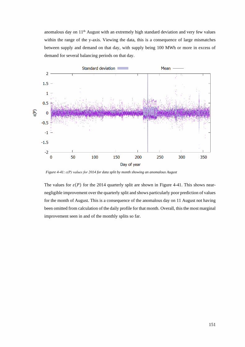
151

anomalous day on 11th August with an extremely high standard deviation and very few values

within the range of the y-axis. Viewing the data, this is a consequence of large mismatches

between supply and demand on that day, with supply being 100 MWh or more in excess of

demand for several balancing periods on that day.

The values for 휀(𝑃) for the 2014 quarterly split are shown in Figure 4-41. This shows near-

negligible improvement over the quarterly split and shows particularly poor prediction of values

for the month of August. This is a consequence of the anomalous day on 11 August not having

been omitted from calculation of the daily profile for that month. Overall, this the most marginal

improvement seen in and of the monthly splits so far.

Figure 4-41: ε(P) values for 2014 for data split by month showing an anomalous August

152

The values of 휀(𝑃) for the 2014 monthly split with weekday/weekend separation are shown in

Figure 4-42. The majority of the year is very similar to the basic monthly split with a slightly

narrower spread of values, however August prediction accuracy has again worsened

significantly. The poor prediction in August is perhaps the reason for the modest improvement

in 휀(𝑃) standard deviation seen in Figure 4-33. This particularly volatile August might also be

the key contributing factor to the significantly higher standard deviations for 2014 compared to

the other years of the dataset.

Figure 4-42: ε(P) values for 2014 for data split by month and weekend/weekday showing an anomalous August

153

The values of 휀(𝑃) for the 2015 quarterly split are shown in Figure 4-43. Prediction accuracy

is very good overall; by far the best of all the detailed examples in this section. Fourth quarter

prediction accuracy is lower than the rest of the year but not particularly bad. Once again, there

is an anomalous day on 16th May. Unlike 11th August 2014, there is no clear reason for this.

Electricity prices seem particularly volatile on 16th May, but the mismatch between demand and

supply is neither greater nor more sporadic than other days in May.

Figure 4-43: ε(P) values for 2015 for data split by quarter showing an anomalous day in May

154

The values of 휀(𝑃) for the 2015 monthly split are shown in Figure 4-44. As might be expected

from Figure 4-33, there is only a very modest improvement in prediction accuracy.

The values of 휀(𝑃) for the 2015 monthly split with weekday/weekend separation are shown in

Figure 4-45. Once again, improvements are barely noticeable.

Figure 4-44: ε(P) values for 2015 for data split by month

Figure 4-45: ε(P) values for 2014 for data split by month and weekend/weekday

155

One of the most important pieces of information that can be gleaned from Figure 4-34 to Figure

4-45 is that there are several occasions where particularly large magnitude values of 휀(𝑃) occur

on the same day, as can be seen by the clustering of datapoints in vertical columns. This is

perhaps explainable in terms of volatility; when a given day’s 𝑆(𝑃) progression is unusually

volatile, the modelled values of 𝜑(𝑃) are likely to predict 𝑆(𝑃) poorly for the whole day. This

has an important influence on the modelling approach to the 휀(𝑃) values. Simple probability

distributions could be fit to the data and used to predict 휀(𝑃), however if the hypothesis that

poor predictions are often caused by particularly volatile days holds true, time series models,

particularly those that have an immediate and short-term response to shocks, might provide a

better means of prediction.

It is also worth noting that the clustering of datapoints in this way has a tendency to occur on

only one side of the mean; i.e. when the model underestimates the value of 𝜑(𝑃), it tends to do

so for the whole day, and so too when it overestimates. As discussed in section 4.4.2 this has

an important effect on time series selection. MA time series tend to generate values that oscillate

on either side of the mean, whereas AR time series tend to generate values that stay on one side

of the mean for extended periods. In terms of shocks, in MA series, one shock is typically

followed by another whereas in AR series, shocks tend to be followed by periods of relative

calm. It is reasonable to expect, then, that AR series should model the behaviour discussed in

the previous paragraph better than MA series. Alas, time series models are stochastic in nature

and there is no way to directly define the length of calm periods in AR series in a way that

would effectively capture the periodic nature of the prediction accuracy of 𝜑(𝑃). Indirectly, it

is conceivable that one could use a combination of probability distributions and time series to

achieve this effect, with a distinct AR series being used for each day modelled and the

parameters of these series defined individually via probability distribution. However, for the

model described in this work, defining time series in this way would be onerous in the extreme

requiring some 10,000 individually defined time series models to cover the 30-year period of

the model.

Using time series has an unfortunate consequence; values produced by probability distributions

are independent of one another whereas values produced by time series must be computed

sequentially and thus place a far greater computational load on the model. This has a significant

impact on model runtimes, especially in Monte Carlo modelling where simulations are run for

thousands of iterations at a time. However, conversely to the discussions in section 4.4.2

regarding seasonal patterns, it is important that the model be capable of capturing this

behaviour. With an LAES system being capable of charging and discharging in a single day,

sudden short-lived periods of volatility in 휀(𝑃) are likely to have a significant effect on spot

156

market pricing and thus on plant revenue. Given the considerations in this paragraph and the

previous two, the decision was made to test data fits for both probability distributions and time

series.

Initial testing showed that Laplace and logistic probability distributions offered the best fit in

the majority of cases. Loglogistic offered a good fit for several years, but there were other years

where @RISK was unable to determine a suitable fit. GARCH, ARMA, first order AR and first

order MA time series offered the best fit in most cases. ARCH and GARCH series are

particularly suited to capturing datasets that exhibit volatility clustering and may potentially

offer a good means of capturing the short periods of high volatility seen in the 휀(𝑃) data

(signified by the short periods of high standard deviation).

ARCH and GARCH processes are used when the data’s standard deviation varies over time,

exactly as seen in the 휀(𝑃) data. ARCH models assume that the standard deviation follows an

AR model, whereas GARCH models assume that the standard deviation follows and ARMA

model. ARCH parameters are average, 𝜇, positive volatility, 𝜔, positive autoregressive

coefficient, 𝑎, initial value 𝑦(0), and initial standard deviation 𝜎(0). Each consecutive value is

based on an RN, 𝑁(𝑡), taken from a normal distribution with mean 0 and standard deviation 1.

The tth series value is calculated:

𝑦(𝑡) = 𝜇 + 𝜎(𝑡)𝑁(𝑡) ( 4-13 )

where the value of 𝜎(𝑡) is modelled using:

(𝜎(𝑡))2= 𝜔 + 𝑎(𝑦(𝑡 − 1) − 𝜇)2 ( 4-14 )

As with the discussion in section 4.4.2, it is worth considering these equations in detail to

determine exactly how consecutive values are calculated. As shown in equation ( 4-14 ), the

standard deviation for a given value of the series is driven by the volatility parameter, 𝜔 and a

second term with the autoregressive coefficient, 𝑎. When the previous value of 𝑦 is far from the

mean, this second term will be large, meaning that the value of 𝜎(𝑡) will also be large meaning

that the value of 𝑦 is more likely to be far from the mean. This behaviour is very much like that

seen in the AR model. The value of 𝑎 relative to 𝜔 defines how strong this autoregressive effect

is.

As shown in equation ( 4-13 ), the value of 𝜎(𝑡) drives the value of 𝑦. When, 𝜎(𝑡) is large,

more extreme values of 𝑁(𝑡) will drive 𝑦 further from the mean. Because 𝑁(𝑡) is a standard

157

deviation, its mean value, and hence the mean value of the second term will be zero, meaning

that the mean of 𝑦 will be equal to 𝜇 for series with many values.

GARCH parameters are average, 𝜇, positive volatility, 𝜔, positive autoregressive coefficient,

𝑎, positive moving average coefficient, 𝑏, initial value 𝑦(0), and initial standard deviation 𝜎(0).

As with an ARCH model, the tth series value is calculated:

𝑦(𝑡) = 𝜇 + 𝜎(𝑡)𝑁(𝑡) ( 4-15 )

where the value of 𝜎(𝑡) is modelled using:

(𝜎(𝑡))2= 𝜔 + 𝑎(𝑦(𝑡 − 1) − 𝜇)2 + 𝑏(𝜎(𝑡 − 1))

2 ( 4-16 )

If 𝑏 is taken to be zero, this yields equation ( 4-14 ) for an ARCH model. If 𝑎 is taken to be

zero, then equation ( 4-16 ) becomes:

(𝜎(𝑡))2= 𝜔 + 𝑏(𝜎(𝑡 − 1))

2 ( 4-17 )

As the equation shows, the standard deviation for a given value of the series is driven by the

volatility parameter, 𝜔 and a second term with the moving average coefficient, 𝑏. This second

term shows that a large value of standard deviation is expected when the value of the previous

standard deviation is large. This behaviour is very similar that that seen in the moving average

model discussed in section 4.4.2. The effect of this moving average behaviour on 𝜎(𝑡) is

governed by the size of 𝑏 relative to 𝜔.

158

The model fit comparison for the quarterly split data is shown in Figure 4-46. This shows that

in almost all cases, the probability distributions and GARCH time series provide a better fit

than the ARMA, AR and MA time series.

The model fit comparison for the monthly split is shown in Figure 4-47. As with the quarterly

split, the GARCH and probability distributions exhibit a better fit in almost all cases and this

preference is somewhat more apparent.

Figure 4-46: Model fit comparison for quarterly split data (lower AIC value represents a better fit, no fit was

possible where bars are missing)

Figure 4-47: Model fit comparison for monthly split data (no fit was possible where bars are missing)

159

The model fit comparison for the monthly split with weekday/weekend separation is shown in

Figure 4-48. There is little difference between this and Figure 4-47, except for 2012 and 2015

where the superiority of the GARCH fit to the other time series is less apparent.

From examination of Figure 4-46 to Figure 4-48, it would appear that probability distributions

and GARCH models all offer better fits to the 휀(𝑃) data than the ARMA, MA and AR models.

It is however important to note that for all probability distributions tested, as well as the

GARCH and MA time series, a given value being above or below the mean has no bearing on

the likelihood of the following value being above or below the mean. As the discussion

regarding Figure 4-34 to Figure 4-45 notes above, the data for 휀(𝑃) generally exhibits strong

directionality relative to the mean over the course of a day. AR time series, and to a lesser extent

ARMA time series, are better suited to capturing this characteristic of the 휀(𝑃) data and likely

to be better suited to this aspect of the model.

Given that there is little difference in fit quality between these models, and that in all years

except 2009, 2014 and 2015, there is little difference in fit quality between the GARCH and the

other time series, the final decision was taken to use an AR time series to ensure that the

directionality of the 휀(𝑃) data was properly captured by the model.

Figure 4-48: Model fit comparison for monthly and weekend/weekday split data (no fit was possible where bars

are missing)

160

4.4.5. Consumer Price Index

Plant costs, such as operation and maintenance and fuelling costs are subject to inflation. In

addition, strike prices are adjusted each year according to CPI (Department of Energy and

Climate Change, 2013). The decision was made to use this index in order to adjust plant costs

and the strike price throughout the duration of the model. As a result, the model requires a

means of simulating CPI rates for its duration. A time series was fit to the CPI annual rate data

(King, 2020), as shown in Figure 4-49.

The time series fit was performed with the available time series in @RISK and yielded a first-

order MA process as the best fit. This series is introduced in section 4.4.2. It has four

parameters; mean, 𝜇, volatility, 𝜎, moving average coefficient 𝑏 and initial error term 𝜖(0). As

with AR and ARMA series, for the tth series value, an error term is calculated based on a random

number generated by a normal distribution 𝑁(𝑡) with mean 0 and standard deviation 1:

𝜖(𝑡) = 𝜎𝑁(𝑡) ( 4-18 )

Then, the time series value, 𝑦(𝑡), is calculated using:

𝑦(𝑡) = 𝜇 + 𝑏𝜖(𝑡 − 1) + 𝜖(𝑡) ( 4-19 )

As discussed in section 4.4.2, shocks have a substantial effect on subsequent values of 𝑦(𝑡),

but only for a short period. Values are expected to oscillate on both sides of the mean and not

to show preference for one side or another following shocks. Whilst the data in Figure 4-49 is

Figure 4-49: CPI annual rate data 1989-2019

161

for a relatively limited period of 20 years, this is broadly what can be seen; the data appears to

oscillate above and below the mean.

162

4.5. Model construction

The financial model is built in an Excel spreadsheet with a single front page for the entry of

model parameters. The user-defined parameters and their nominal values are listed in Table

4-4. Parameters of interest whose effect will be explicitly explored during modelling are

indicated, as are the LAES plant characteristics which are defined via the engineering model

and the parameters either defined by or calculated from a probability distribution for each

iteration. The symbol 𝐼 in parentheses is used to indicate a parameter that changes each iteration.

Input parameters

Symbol Value Description

𝐶NPP,BASE £1.05bn Base asset cost of NPP

𝑆CfD *1 Starting NPP CfD price

𝜑COST,NPP(𝐼) *3 NPP spending factor

𝐶NPP(𝐼) *3 Iteration cost of NPP

𝐶LAES(𝐼) *3 Iteration cost of LAES

𝑡MOB,NPP(𝐼) *3 Iteration mobilisation construction time for the NPP (years)

𝑡CRIT,NPP(𝐼) *3 Iteration critical path construction time for the NPP (years)

𝑡MOB,LAES(𝐼) *3 Iteration mobilisation construction time for the LAES (years)

𝑡CRIT,LAES(𝐼) *3 Iteration critical path construction time for the LAES (years)

𝐶NPP,MOB(𝐼) *3 Iteration NPP mobilisation construction costs

𝐶NPP,CRIT(𝐼) *3 Iteration NPP critical path construction costs

𝐶LAES,MOB(𝐼) *3 Iteration LAES mobilisation construction costs

𝐶LAES,CRIT(𝐼) *3 Iteration LAES critical path construction costs

𝜑CONST 0.30 Proportion of cost spent during construction mobilisation

𝐶O&M,NPP £30m Fixed O&M costs for the NPP

𝐶REFUEL £10m Refuelling costs for the NPP

𝜑O&M,LAES 1.5% O&M costs for the LAES as a percentage of LAES plant cost

𝐶O&M,LAES(𝐼) *3 Iteration LAES O&M costs

�̇�NPP 300 MW Electrical power of the NPP

�̇�CHG *2 Electrical power consumption of LAES during charge

�̇�DIS *2 Electrical power yield of LAES during discharge

�̇�CHG *2 Air mass flow rate during charge

�̇�DIS *2 Air mass flow rate during discharge

𝑀TANK,MAX *2 Maximum storage capacity of the liquid air tank

𝑡START,CHG *1 Start time for charging period

𝑡START,CHG *1 End time for charging period

𝑡START,DIS *1 Start time for discharging period

𝑡END,DIS *1 End time for discharging period

𝑡FUEL 500 d Reactor uptime for a single fuel load

𝑡REFUEL 10 d Reactor downtime for refuelling

𝑌START 2020 Year in which plant construction begins

𝑇CORP 20% Corporation tax on profits

𝑖CPI *3 CPI rate

𝑖DISC *1 Discount rate Table 4-4: Financial model fixed parameters (*1 represents a user-defined parameter of interest, *2 represents a

parameter defined by the chosen plant configuration, *3 represents an initial parameter defined by, or calculated

from, a probability distribution for each iteration)

163

The front page also defines the probability distribution parameters and the time series

parameters for the uncertain model inputs. The chosen parameters for the uncertain initial

probability distributions are shown in Table 4-5.

PERT distribution parameters FOAK scenario NOAK scenario

Min

imu

m

Mo

st likely

Max

imu

m

Min

imu

m

Mo

st likely

Max

imu

m

NPP spending factor 𝜑COST,NPP 1 1.7 2 1 1.1 1.3

Binomial distribution parameters FOAK scenario NOAK scenario

𝒏 𝒑 shift 𝒏 𝒑 shift

NPP construction time –

mobilisation 1 0.6 2 0 0.4 2

NPP construction time –

critical path 2 0.6 3 1 0.4 3

LAES construction time –

mobilisation 1 0.6 1 1 0.2 1

LAES construction time –

critical path 1 0.6 1 1 0.4 1

Table 4-5: Financial model initial uncertain probability distribution parameters

The chosen parameters for the time series are shown in Table 4-6. The parameters for mean and

volatility for the 𝐴(𝐷) time series, as well as volatility for the 휀(𝑃) time series, remain user-

defined to allow exploration of different market price scenarios. Whilst not displayed in the

table, amplitude factors are similarly defined for each quarter in the front page. All time series

parameters are user-defined once every five years (for year 0, 5, 10, etc.) and are interpolated

between these values for the 30 modelled years. The option remains to directly adjust the

interpolated parameters if necessary, however this is not done in this study. Mean daily average

electricity prices are defined in 2019 (year 0) prices and are adjusted by CPI for each subsequent

year, as discussed in section 4.5.1.

ARMA time series

parameters Mean Volatility

Autoregressive

coefficient

Moving average

coefficient

Daily average electricity

price 𝐴(𝐷) *1 *1 0.8 -0.2

First-order AR

parameters Mean Volatility

Autoregressive

coefficient Initial value

Half-hourly error value

휀(𝑃) 0 0.12 0.6 0

First-order MA

parameters Mean Volatility

Moving average

coefficient

Initial error

term

Consumer price index, 𝑖CPI 0.225 0.002 0.823 0

Table 4-6: Financial model time series parameters (*1 represents a user-defined parameter of interest)

164

The front page defines the initial parameters from probability distributions for each iteration

run of the model. The iteration value for the spending factor of the NPP, 𝜑COST,NPP(𝐼), is used

to calculate the iteration cost of the NPP from the NPP base cost, 𝐶NPP,BASE:

𝐶NPP(𝐼) = 𝐶NPP,BASE × 𝜑COST,NPP(𝐼) ( 4-20 )

The construction time iteration parameters for the mobilisation and critical path construction

times for both the NPP and the LAES plant, 𝑡MOB,NPP(𝐼), 𝑡CRIT,NPP(𝐼), 𝑡MOB,LAES(𝐼) and

𝑡CRIT,LAES(𝐼) are determined from their respective probability distributions. The iteration cost

for LAES, 𝐶LAES(𝐼), is determined from its probability distribution and the annual O&M cost

is calculated using the ratio 𝜑O&M,LAES:

𝐶O&M,LAES(𝐼) = 𝐶LAES(𝐼) × 𝜑O&M,LAES ( 4-21 )

The NPP mobilisation and critical path construction costs, 𝐶NPP,MOB(𝐼) and 𝐶NPP,CRIT(𝐼)

respectively are calculated using the construction cost ratio 𝜑CONST:

𝐶NPP,MOB(𝐼) = 𝐶NPP(𝐼) × 𝜑CONST ( 4-22 )

𝐶NPP,CRIT(𝐼) = 𝐶NPP(𝐼) × (1 − 𝜑CONST) ( 4-23 )

The LAES mobilisation and critical path construction costs are similarly calculated:

𝐶LAES,MOB(𝐼) = 𝐶LAES(𝐼) × 𝜑CONST ( 4-24 )

𝐶LAES,CRIT(𝐼) = 𝐶LAES(𝐼) × (1 − 𝜑CONST) ( 4-25 )

These calculated iteration values are then used to populate the columns of the annual accounts

sheet that represent the project years during which the plant is under construction, as described

in section 4.5.2.

4.5.1. Electricity price model sheets

The electricity price model consists of four sheets. The first three calculate the values of 𝐴(𝐷)

for each day, the values of 휀(𝑃) for each period and the values of 𝜑(𝑃) for each period. The

final sheet calculates the system sell price 𝑆(𝑃) based on the values in the other three sheets.

The four sheets will now be discussed in turn, starting with the 𝐴(𝐷) sheet. As discussed in

section 0, the mean parameter, 𝜇𝐴(𝐷)(𝑌), for year 𝑌 for each time series is taken from the user-

165

defined front page parameters and the resulting interpolations. Since all 31 values of 𝜇𝐴(𝐷)(𝑌)

are defined in year 𝑌 = 0 prices, its values are adjusted according to CPI for all subsequent

years according to the formula:

𝜇𝐴(𝐷)(𝑌) = 𝜇𝐴(𝐷)(𝑌)((𝑖𝐶𝑃𝐼(𝑌) + 1)(𝑖𝐶𝑃𝐼(𝑌 − 1) + 1)⋯(𝑖𝐶𝑃𝐼(2) + 1)(𝑖𝐶𝑃𝐼(1) + 1)) ( 4-26 )

Parameter values for 𝜎𝐴(𝐷) over the modelled years are similarly taken from the front sheet but

since these represent volatility, they do not need to be adjusted for CPI. The parameters for the

autoregressive coefficient 𝑎𝐴(𝐷) and the moving average coefficient 𝑏𝐴(𝐷) are taken from the

front sheet but remain fixed throughout the course of the model. One time series is then

calculated for each year using the ARMA formula from section 4.4.2. This yields a value of

𝐴(𝐷) for each day, 𝐷, according to the series parameters and the following equation:

(𝐴(𝐷) − 𝜇𝐴(𝐷)(𝑌)) = 𝑎𝐴(𝐷)(𝐴(𝐷 − 1) − 𝜇𝐴(𝐷)(𝑌)) + 𝑏𝐴(𝐷)𝜖(𝐷 − 1) + 𝜖(𝐷) ( 4-27 )

where 𝜖(𝐷) is an error term calculated with standard deviation defined by 𝜎𝐴(𝐷) and a random

number 𝑁(𝐷) from a normal distribution with mean 0 and standard deviation 1:

𝜖(𝐷) = 𝜎𝐴(𝐷)𝑁(𝐷) ( 4-28 )

For simplicity, the initial value for a given year is taken to be equal to the average value for that

year, i.e. 𝐴(0) = 𝜇𝐴(𝐷)(𝑌), and the initial error term is taken to be zero, i.e. 𝜖(0) = 0. This

process yields 31 separate series for the duration of the model each with 366 values. These time

series are recalculated for each iteration of the simulation.

The second sheet calculates the day curves based on the values of 𝛿(𝑃) shown in Figure 4-25

to Figure 4-32 of section 4.4.3. The user-defined amplitude values, 𝛼(𝑄), are then used to

calculate the final values of 𝜑(𝑃) for each period using:

𝜑(𝑃) = 𝛼(𝑄)𝛿(𝑃) + 1 ( 4-29 )

This process yields 31 separate series for the duration of the model each with 17,568 values.

Since these series are adjusted by the half-hourly error values, they are fixed for each iteration

of the simulation.

The third sheet simulates the half-hourly error values, 휀(𝑃), using an AR time series as

discussed in section 4.4.4. This series uses a mean value 𝜇𝜀(𝑃)(𝑌) and volatility 𝜎𝜀(𝑃) for each

year, taken from the user-defined front sheet parameters and the resulting interpolations. The

166

autoregressive coefficient 𝑎𝜀(𝑃) and the initial error term 𝜖𝜀(𝑃)(0) remain fixed for each year of

the model.

휀(𝑃) = 𝜇𝜀(𝑃)(𝑌) + 𝑎𝜀(𝑃)(𝜖(𝑃 − 1) − 𝜇𝜀(𝑃)(𝑌)) + 𝜖(𝑃) ( 4-30 )

where 𝜖(𝐷) is an error term calculated with standard deviation defined by 𝜎𝐴(𝐷) and a random

number 𝑁(𝐷) from a normal distribution with mean 0 and standard deviation 1:

𝜖(𝐷) = 𝜎𝜀(𝑃)𝑁(𝐷) ( 4-31 )

This process yields 31 separate series for the duration of the model each with 17,568 values.

These time series are recalculated for each iteration of the simulation.

The fourth sheet calculates the system sell price 𝑆(𝑃) for each period, based on the values in

the other three sheets, according to:

𝑆(𝑃) = [휀(𝑃) + 𝜑(𝑃)] × 𝐴(𝐷) ( 4-32 )

This sheet provides the final absolute values of electricity price, already adjusted for CPI, that

are then used to populate the yearly calculation sheets described in section 4.5.3.

4.5.2. Annual accounts sheet

This sheet represents the annual balance sheets for the plant. Each column represents one year.

A single column contains one row for each of the variables shown in Table 4-7.

Annual accounts sheet variables

Symbol Description

𝑆CfD(𝑌) Strike price for a given year

𝑖CPI(𝑌) CPI rate for a given year

𝐶CONST(𝑌) Construction costs for a given year

𝐶O&M,NPP(𝑌) NPP O&M costs for a given year

𝐶O&M,LAES(𝑌) LAES O&M costs for a given year

𝐶REFUEL(𝑌) Refuelling costs for a given year

𝐶TOTAL(𝑌) Total costs for a given year

𝑅SALES(𝑌) Sales revenue for a given year

𝑃GROSS(𝑌) Gross profit for a given year

𝑇CORP(𝑌) Corporation tax for a given year

𝑃NET(𝑌) Net profit for a given year

𝑁𝑃𝑉(𝑌) NPV to date for a given year Table 4-7: Annual accounts sheet variables

The first year of plant operation is denoted 𝑌 = 1. Construction years are filled backwards from

this column, with the final year of construction being year 𝑌 = 0. NPP mobilisation

167

construction costs, 𝐶NPP,MOB(𝐼), are divided evenly between the years 𝑌 = 0 − [𝑡CRIT,NPP(𝐼) +

𝑡MOB,NPP(𝐼)] and 𝑌 = 0 − [𝑡CRIT,NPP(𝐼) + 1]. The critical path construction costs, 𝐶NPP,CRIT(𝐼)

and assigned entirely to year 𝑌 = 0 − 𝑡CRIT,NPP(𝐼). LAES construction costs are similarly

assigned to the relevant years.

All user-defined cost parameters are defined in 2020 prices, with this being the first year of

construction in the model, i.e. year 𝑌 = 0 − [𝑡CRIT,NPP(𝐼) + 𝑡MOB,NPP(𝐼)]. The year 𝑌 = 1

values for 𝑆CfD(𝑌), 𝐶CONST(𝑌), 𝐶O&M,NPP(𝑌), 𝐶O&M,LAES(𝑌) and 𝐶REFUEL(𝑌) are all adjusted

according to 𝑖CPI(𝑌) for the intervening years in exactly the same fashion as the values of

𝜇𝐴(𝐷)(𝑌) in equation ( 4-26 ) and populated into the column for year 𝑌 = 1. The same method is used

to populate their values for the remaining 29 years of the model. Values of 𝐶REFUEL(𝑌) are set to zero

unless the given year’s calculation sheet shows that refuelling has taken place that year. Total

costs, 𝐶TOTAL(𝑌), are then calculated from the sum of all cost variables.

Values of 𝑅SALES(𝑌) from each year are taken from the values of 𝑅TOTAL from the given year’s

calculation sheet as discussed in section 4.5.3. Gross profit is the calculated using:

𝑃GROSS(𝑌) = 𝑅SALES(𝑌) − 𝐶TOTAL(𝑌) ( 4-33 )

Corporation tax is calculated based on gross profit (or taken to be zero where 𝑃GROSS(𝑌) is

negative), and the value of 𝑃NET(𝑌) is thus calculated:

𝑃NET(𝑌) = 𝑃GROSS(𝑌) × [1 − 𝑇CORP] ( 4-34 )

The NPV to date for the given year is calculated using:

𝑁𝑃𝑉(𝑌) = ∑𝑅(𝑌)

(1 + 𝑖𝐷𝐼𝑆𝐶)𝑌

𝑌

𝑌=0−[𝑡CRIT,NPP(𝐼)+𝑡MOB,NPP(𝐼)]

( 4-35 )

This calculation is important because it allows the discounted payback period to be calculated

by counting the total number of years for which 𝑁𝑃𝑉(𝑌) < 0. Finally, the overall project NPV

over the 30-year lifespan of the plant, plus its construction years, 𝑁𝑃𝑉(𝐼), for the given

iteration, is calculated as:

168

𝑁𝑃𝑉 = ∑𝑅(𝑌)

(1 + 𝑖𝐷𝐼𝑆𝐶)𝑌

30

𝑌=0−[𝑡CRIT,NPP(𝐼)+𝑡MOB,NPP(𝐼)]

( 4-36 )

The discounted payback period and the overall project NPV are taken as model iteration

outputs and are recorded and collated for each iteration of the simulation by @RISK

4.5.3. Yearly calculation sheets

The 30 yearly calculation sheets are the workhorse of the financial model. These are arranged

with each row representing a half-hour period of the model. Each column calculates a different

variable or defines the operating state of the plant. The plant has five operating conditions:

• Baseload: the plant is operating as a baseload NPP.

• Charge: the plant is charging the LAES system.

• Discharge: the plant is discharging the LAES system.

• Offline: the plant is refuelling; neither the NPP nor the LAES system are operating.

• Restart: the plant is refuelled and ready to restart.

System variables

Symbol Description

𝑆CfD(𝑌) Strike price for a given year

𝑡(𝑃) Time of day for a given period

𝑆(𝑃) Spot market price for a given period

�̇�FIX(𝑃) Fixed power output for a given half-hour period

�̇�VAR(𝑃) Variable power output for a given half-hour period

𝑅TOTAL(𝑃) Total revenue for a given half-hour period

𝑅NPP(𝑃) NPP revenue for a given half-hour period

𝑅LAES(𝑃) LAES revenue for a given half-hour period

𝑡UP(𝑃) Length of time the plant has been up for during a given period

𝑡DOWN(𝑃) Length of time the plant has been down for during a given period

𝑀TANK(𝑃) Mass currently stored in the tank

∆𝑀TANK Change in mass in the tank

𝜇(𝑃) Mean average cost to charge Table 4-8: Yearly calculation sheet variables

The calculations used in each column will now be described in this section. The first column

defines the current time of day, 𝑡(𝑃) for the given period. This simply cycles through 24 hours

for every 48 rows of the spreadsheet.

The second set of columns define the plant’s output power for the period in question. The first

column calculated the plant’s fixed power output for the period, �̇�FIX(𝑃). For any time the plant

is online, this is simply taken from the parameter sheet value for �̇�NPP. When the period’s

169

operating decision is ‘Offline’, this is taken to be zero. The second column calculates the

variable power output of the plant, �̇�VAR(𝑃). When the periods operating decision is ‘charge’,

this is taken to be equal to −�̇�CHG and when the period’s operating decision is ‘discharge’, this

is taken to be equal to �̇�DIS. At all other times, this is taken to be zero.

The next set of columns define the plant’s stored air capacity, 𝑀TANK. The second of these, the

stored air change, ∆𝑀TANK, takes a value of �̇�CHG when the period’s operating decision is

‘Charge’ and a value of −�̇�DIS when the period’s operating decision is ‘Discharge’. The first

column calculates the current period’s value of 𝑀TANK as the sum of the previous period’s value

of 𝑀TANK and the previous period’s value of ∆𝑀TANK.

The next set of columns define the period’s spot market electricity price and the resulting

revenue from the plant. The first takes the value of 𝑆(𝑃) for the relevant period, as defined in

section 4.4.3. The second column calculates the NPP revenue for the period, 𝑅NPP(𝑃), as the

product of �̇�FIX(𝑃) and the strike price for the given year, 𝑆CfD(𝑌). The third column calculates

the LAES revenue for the period, 𝑅LAES(𝑃), as the product of �̇�VAR(𝑃) and 𝑆(𝑃). The fourth

column calculates the total revenue for the period, 𝑅TOTAL(𝑃), as the sum of the previous two

columns.

The next two columns keep a running tally of the length of time the plate has been running and

the plant has been down for refuelling. The first, 𝑡UP(𝑃), is the running total of days the plant

has been running. If the previous period’s operating decision is ‘Restart’, this is reset to zero,

otherwise, 1 48⁄ is simply added to the previous period’s value. The second column, 𝑡DOWN(𝑃),

is the running total of days the plant has been refuelling. If the previous period’s operating

decision is ‘Offline’, then 1 48⁄ is added to the previous period’s value, otherwise this is reset

to zero.

The penultimate column keeps a rolling average of the cost to charge the system, 𝜇(𝑃).

Whenever the operating decision is ‘Charge’, this takes the value of the current period’s spot

market price, 𝑆(𝑃). If the current operating decision is ‘Baseload’ and the previous periods was

‘Charge’, 𝜇(𝑃) takes the mean average of all of the non-zero values in this column in the

previous 12 hours. If the current operating decision is ‘Baseload’, this takes the value of the

same variable in the previous period. Finally if the previous period’s decision is ‘Discharge’,

this is reset to zero.

170

The final column defines the operating decision for each period of the model. This is done using

IF formulae in accordance to the flowchart presented in Figure 4-50. The first two steps of the

decision making determine whether the NPP requires refuelling or whether it is ready to restart.

If the plant downtime, 𝑡DOWN(𝑃), is equal to the required time to refuel the NPP, 𝑡REFUEL, the

decision is set to ‘Restart’. If the plant’s uptime, 𝑡UP(𝑃), is equal to the lifetime of the fuel

load, 𝑡FUEL, the decision is set to ‘Offline’.

The next steps determine whether the plant should charge or discharge. If the air storage tank

is empty and the current time of day is within the charge window set by 𝑡START,CHG and 𝑡END,CHG,

the operating decision is set to ‘Charge’. If the tank is neither empty nor full, that decision is

similarly set to ‘Charge’. Then, if the plant was discharging the previous period and the tank

in not yet empty, the operating decision is set to ‘Discharge’. If the storage tank is full and the

current spot market price, 𝑆(𝑃), is greater than the rolling average charge price, 𝜇(𝑃), the

decision is similarly set to ‘Discharge’. If none of these criteria apply, the decision is set to

‘Baseload’.

Total values of 𝑅TOTAL are calculated at the bottom of each yearly calculation sheet.

171

Operating decision:

Refuel

Move to next period

of model

YES

NO

Operating decision:

Restart YES

Operating decision:

Charge

Operating decision:

Charge

Discharge

previous

period?

Operating decision:

Discharge

Operating decision:

Discharge

NO

NO

YES

NO

YES

YES

NO

YESYES

NO

YES YES

Operating decision:

Baseload

NONO

NO

Figure 4-50: Plant operating decision

172

- Configurational modelling

5.1. Introduction

There are multiple process configurations possible for the steam, air liquefier and air power

cycles of the LAES plant. Sections 2.7 details how costs of key pieces of equipment are to be

calculated and section 4.3 details how these drive the overall cost of the LAES plant. The

differences in potential configurations are significant in terms of not only the size, but also the

numbers of heat exchangers and power train components; components that make up the lion’s

share of the LAES system capital investment.

This thesis is less concerned with optimisation from a thermodynamic perspective than from a

economic perspective. Ultimately, as this chapter and Chapter 6 will show, thermodynamic

efficiency improvements come at a real financial cost. The initial investigative modelling in

these chapters aims to answer the question of whether the additional revenue resulting from

these improvements are worth their cost. It will compare system configurations and assess their

relative NPVs to allow an optimal system configuration to be defined.

5.2. Initial engineering modelling

Following basic model testing and component model validation, engineering modelling was

begun. The initial engineering model was built up from a basic system with a small number of

isolated components eventually to a full system with all components. One of the advantages of

the modular construction of the engineering model is the ability to test components or cycles in

isolation. This reduces computing load and allows parameter sweeps to be performed much

more quickly. It also facilitated diagnosing issues with the model as it was developed. The

LAES system being explored has two cycles; the liquefier cycle and the power cycle. As a

starting point, a symmetrical system was designed with a discharge mass flow rate of 100 kg/s,

and a charge mass flow rate of 101 kg/s. This additional 1% is charge mass flow rate is to

account for boil-off losses from the stored air tank since this is not explicitly considered by the

model.

As a starting point, the availability of heat from the secondary loop of the NPP was determined

using an isolated model of the steam cycle, as discussed in section 5.2.1. The LAES system was

then studied. Starting in section 5.2.2, the cold store was investigated to determine the effect of

charging and discharging on the temperatures and heat storage of the system. Following this, in

section 5.2.3, the discharge system was studied to determine the effect of applying NPP heat to

the LAES system. Then, in section 5.2.4 the power consumed by the charge cycle was studied.

173

Finally, in section 5.2.6, the different plant configurations were modelled. At this point, the cold

store and other components were sized for the different system configurations.

5.2.1. Supply of nuclear steam

The starting point of engineering modelling was to determine how much heat could be made

available from the NPP for supply to the air power cycle during discharge. Steam turbines are

expanded to a vacuum and this provides the best possible efficiency for the steam cycle, as it

allows a much larger amount of heat to be extracted from the steam than expanding to

atmospheric pressure. This is because decreasing the turbine outlet pressure lowers the

saturation temperature of water, allowing more energy to be extracted from the water before it

condenses. Since steam turbines can tolerate a steam quality of no less than around 85%, this

results in a lower outlet temperature and a greater energy yield from the turbine. It has a

disadvantage when coupling to a LAES plant in that the lower saturation temperature of water

reduces the peak temperature of the air in the discharge cycle as highlighted in section 2.6 in

the context of (Li et al., 2014) and demonstrated via modelling in section 5.2.1. For brevity, the

different configurational options in this section have been denoted S-y where y is the number

designation of that configuration.

Several steam cycles were studied. The first two assumed providing heat to the discharge cycle

air using only the condenser coolant from the NPP. In the first (configuration S1), steam was

expanded to a vacuum and in the second (configuration S2, steam was expanded to atmospheric

pressure. These have the advantage of ensuring that the NPP’s power output does not change

between times when the discharge cycle is running and times when the NPP is simply running

in baseload. In the latter, however, this would increase condenser coolant temperature but

reduce plant output power by 25%. Considering this is a design choice and that this would affect

the NPP’s power output even during baseload operation, this is a significant cost to power

output to benefit a system that will only operate for a part of the day. Ultimately, the low-grade

heat provided by both cycles, at less than 373 K, meant that the discharge cycle performed very

Figure 5-1: Steam cycle configuration S1/S2

174

poorly, limiting the round-trip efficiency of the LAES plant to less than 25%. With only

marginal savings in equipment cost, these options were quickly discarded, however the steam

cycle results remain recorded here for posterity.

Configurations S1 and S2 are shown in Figure 5-1. It is important to note at this stage that this

is a simplified schematic. The NPP considered herein is the NuScale iSMR. A 300 MWe plant

would consist of a total of 6 nuclear reactors each with its own secondary loop consisting of

steam generator, turbine, condenser and pump.

The third steam cycle explored (configuration S3) considered diverting a portion of the

secondary loop steam away from the steam turbines and directly to the air power cycle. This

has some potential disadvantages in that running turbines at a flow rate lower than that of their

design lowers their efficiency. This configuration is shown in Figure 5-2. As before, this

diagram and the model have been simplified to treat the system of multiple SMR steam

generators and multiple turbines as a single cycle. Table 5-1 shows the parameters used in the

S3 model, but an additional parameter has been introduced to define the quantity of steam

diverted away from the secondary loop.

In light of the discussions in section 2.3, it is important to note that the secondary loop should

not be shut down completely. In this study it is assumed that the steam turbines operate between

50 and 100% of their rated power. It is furthermore important to consider that running the

turbines at anything other than their design flow rate results in a loss of efficiency. As discussed

in section 3.2.7, the model defines this using a matrix parameter 𝜂[𝑥, 2] that defines 𝑥 values

of �̇�factor (the ratio of the actual mass flow rate to the design mass flow rate) against their

resulting isentropic efficiencies, 𝜂. The values for 𝜂[𝑥, 2] are taken from (Karakurt and Gunes,

2017) and interpolated to provide the continuous relationship shown in Figure 5-3.

Figure 5-2: Steam cycle configuration S3

175

All steam cycle configurations are optimised by performing a parameter sweep. The objective

is to determine the required mass flow rate for the secondary loop to operate in a steady state.

Additional equations are defined at the top level of the steam cycle model to assist with

optimisation. The first of these calculates the rate of change of specific enthalpy, 𝑑ℎpump

𝑑𝑡, in the

flow stream following the pump. For this optimisation, the size of the condenser is set to very

large to prevent it from being a limiting factor in the extraction of heat from the post-turbine

water stream. The model is then run repeatedly over a range of mass flow rates. The mass flow

rate for which 𝑑ℎpump

𝑑𝑡= 0, is considered sufficient for the system. The size of the condenser is

then reduced as much as possible without reducing the heat transfer rate.

The modelling parameters are shown in Table 5-1.

Parameter Value Units

Primary loop thermal power 960 MWth

Steam generator heat exchange surface area 1666 m2

Steam generator heat transfer coefficient 875 W/m2 K

Secondary loop peak temperature 580.0 K

Secondary loop minimum temperature 314.8 K

Secondary loop peak pressure 3,450 kPa

Secondary loop expansion pressure, configuration S1/S3 21.5 kPa

Secondary loop expansion pressure, configuration S2 101.3 kPa

Secondary loop mass flow rate 402 kg/s

Figure 5-3: Values of steam turbine isentropic efficiency for the parameter 𝜂[𝑥, 2]

176

Water pressure drops 0.01

Tertiary coolant supply temperature 298.15 K

Tertiary coolant peak temperature 310 K

Tertiary coolant supply pressure 102.5 kPa

Condenser heat transfer surface area Optimisation parameter

Condenser heat transfer coefficient 1610 W/m2 K

Steam turbine peak efficiency 90 %

Steam turbine off-design efficiency Figure 5-3

Pump efficiency 80 %

Table 5-1: Key parameters for steam cycle models – all configurations

The results for configuration S1 are shown in Figure 5-4. As might be expected, increasing the

condenser outlet temperature reduces the required mass flow rate but increases the required

exchanger surface area. The NPP power output is the design 300 MWe.

Figure 5-4: Configuration S1 results

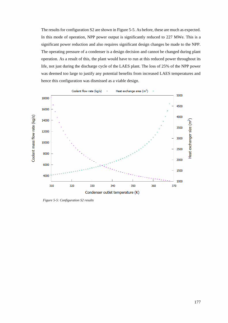
177

The results for configuration S2 are shown in Figure 5-5. As before, these are much as expected.

In this mode of operation, NPP power output is significantly reduced to 227 MWe. This is a

significant power reduction and also requires significant design changes be made to the NPP.

The operating pressure of a condenser is a design decision and cannot be changed during plant

operation. As a result of this, the plant would have to run at this reduced power throughout its

life, not just during the discharge cycle of the LAES plant. The loss of 25% of the NPP power

was deemed too large to justify any potential benefits from increased LAES temperatures and

hence this configuration was dismissed as a viable design.

Figure 5-5: Configuration S2 results

178

Finally, the results for configuration S3 are shown in Figure 5-6 to Figure 5-8. Note that the x-

axis now shows the ratio of secondary loop flow sent to the air power cycle.

Figure 5-6 shows the power output of the NPP as a function of the amount of steam that

bypasses the secondary loop. Whilst this figure only shows the power outputs for 310 K

condenser outlet temperature, increasing the coolant-side condenser outlet temperature

provides only small power improvements in the range of tens of kilowatts. These improvements

are related to the savings in pumping power due to the reduced coolant flow rates. The ‘ideal’

line shows the power output that the plant would yield if the steam turbine’s isentropic

efficiency were continuous throughout the operating mass flow rate range. The ‘actual’ line

shows the power output given the flow rate dependency of isentropic efficiency shown in Figure

5-3. The power lost line shows the percentage difference between the ideal and actual lines.

As might be expected, the most power is lost at the highest bypass ratios where the isentropic

efficiency of the turbine is at its lowest. The percentage of power lost increases most steeply at

low bypass ratios and almost linearly at higher bypass ratios. Figure 5-6 has important

implications for the use of nuclear steam during discharge of the LAES plant. Using the higher-

grade heat from the NPP comes at a significant power cost and could potentially outweigh the

gains from improvement in LAES power output. The implications are discussed in more detail

in section 5.2.3.

Figure 5-6: Configuration S3 NPP power output results

179

Figure 5-7: Configuration S3 coolant mass flow rate results

Figure 5-8: Configuration S3 condenser surface area results

180

Figure 5-7 shows the condenser coolant mass flow rate results, whilst Figure 5-8 shows the

resulting required condenser sizes for configuration S3. The flow rate results are much as

expected. Increasing the bypass ratio and thus decreasing the NPP secondary loop mass flow

rate reduces the required coolant flow rate and the resulting heat exchanger size. Increasing the

condenser coolant-side outlet temperature results in a reduced coolant flow rate but increases

the condenser size requirement due to the smaller temperature difference between the secondary

loop and coolant flows at the hot end of the condenser.

5.2.2. Cold store modelling

As discussed above, the charge and discharge thermodynamic cycles are almost entirely

independent with the exception of one key component; the cold store.

The sizing of this component is of critical importance; the cold store will be heated by the

incoming air during each charging phase and cooled by the liquefied air during each discharge

phase. During charging, only the liquefied fraction is sent to the storage tank, and thus only this

fraction is available to cool the bed again during discharge.

Testing was performed on isolated models to determine the effect of key model parameters and

duty cycling on the performance of the cold store. In order to do this, the cold recycle system

components were modelled in isolation using mass flow sources and sinks. Simulations were

run for 1800 s to the evolution of temperatures in the gravel bed and in the air at the outlet of

the cold store. Testing was first performed to understand the effect of cold store heating during

a hypothetical charge cycle on the heat extraction rate, average bed temperatures and outlet

temperatures using a range of supply pressures using the parameters in Table 5-2.

Parameter Value

Inlet air temperature 298.15 K

Inlet air mass flow rate 150 kg/s

Inlet air pressure 101.325 kPa

Bed particle diameter 0.02 m

Bed particle density 2320 kg/m3

Bed particle specific heat capacity 810 J/kg K

Initial bed temperature 88 K

Bed pressure drop 0.05

Bed diameter 3 m

Bed length 15.5 m Table 5-2: Parameters used for testing the effect of charging on cold store temperatures

181

The implications of the importance of gravel bed size are most apparent when referring to

Figure 5-9. The outlet air temperature begins to rise at a time of 500 s, shown by the vertical

red line. At the same time, the bed heating rate begins to fall. This is an important point; once

the outlet temperature begins to rise, less heat will be extracted from the charge air stream and

the resulting mixture will have a lower liquid fraction once it has been expanded. Since the

power consumption of the compression cycle will not change for a given configuration at a set

flow rate and peak pressure, the energy input per unit mass of liquid air produced (i.e. the

specific energy of liquefaction) will increase and the overall efficiency of the system will fall.

The same model was run for a cold store during a hypothetical discharge cycle to understand

the effect of cold store cooling. The parameters used for the model are shown in Table 5-3.

Figure 5-9: Heating rate, average bed temperature and air outlet temperature during a single charge cycle

182

Parameter Value

Inlet air temperature 88 K

Inlet air mass flow rate 150 kg/s

Inlet air pressure 101.325 kPa

Bed particle diameter 0.02 m

Bed particle density 2320 kg/m3

Bed particle specific heat capacity 810 J/kg K

Initial bed temperature 298.15 K

Bed pressure drop 0.05

Bed diameter 3 m

Bed length 15.5 m Table 5-3: Parameters used for testing the effect of discharging on cold store temperatures

The results for discharging are shown in Figure 5-10. These mirror those for charging. Note

that here, the heating rate is still shown. That is, the rate of heat transfer into the gravel bed.

Because the bed is being cooled during discharge, this is negative. In a corollary of what occurs

during system charging, the outlet temperature of the bed begins to fall at around 500 s and the

rate of heat extraction from the bed begins to fall. This implies equally important considerations

for the cold store during system discharge. The cold store air stream exchanges heat with the

discharge air via a heat exchanger. As the cold store temperature, and hence the air temperature

Figure 5-10: Cooling rate, average bed temperature and air outlet temperature during a single discharge cycle

183

at the outlet, falls, the temperature difference across this heat exchanger will also fall. This

reduces the amount of heat that can be imparted to the discharge air stream during discharge

which in turn reduces the quantity of specific cold recycle that can be achieved. As noted in

section 2.5.2, maximising cold recycle is paramount to achieving optimal liquefaction

efficiency when charging the system.

5.2.3. Discharge cycle modelling

The third step in exploratory engineering modelling was demonstration of the air power cycle.

This system is far simpler system to model than the air liquefier cycle and, as such, was

modelled in its entirety for all configurations considered. For brevity, cycles considered in this

section are denoted D-y where y is the number of turbine stages used.

The air power cycle first pumps the liquid air from the tank to the peak discharge temperature.

The pressurised but still liquid air is then vaporised in a heat exchanger where it cools the air

used in the cold recycle loop. It then travels through additional heat exchangers; the first a

preheater which uses the condenser water from the NPP’s tertiary loop to further heat the air

stream and the second a recuperator used to recover residual heat from the exhaust air. The air

then passes through the expansion sequence, each stage of which involves superheating the air

using NPP secondary loop steam before expanding it in a turbine.

It was expected that the power train efficiency would improve with staged expansion. In the air

power cycle, air is heated by steam or water from the NPP in the quantities and at the

temperatures shown in section 5.2.1. Ultimately, the inlet temperature from a single turbine is

limited by the saturation temperature of the NPP secondary loop, as this represents the pinch

point in the air superheaters. As the temperature through the turbine falls, so too does the power

it produces. By adding multiple turbine stages and reheating the air following each turbine

stage, the power output can be increased. There are, of course, capital cost implications

Figure 5-11: Air power cycle configuration D-4

184

associated with the additional turbines and heat exchangers required to achieve these

improvements, as is discussed in Chapter 6.

One discharge configuration was considered; only the number of expansion stages was varied.

Figure 5-11 shows the discharge configuration with 4 turbine stages. Initial modelling showed

that the key parameter for system optimisation is the peak discharge pressure. The water stream

flow rates were varied according to the results of section 5.2.1. Because all design options utilise

multiple turbines, the proportion of the stream diverted to each turbine is also an important

optimisation parameter. Optimising these parameters ensure that each expansion stage has the

highest possible turbine inlet temperature whilst also ensuring that the quantity of steam

diverted from the NPP secondary loop was kept to a minimum.

Parameter Value Units

Secondary loop peak temperature 580.0 K

Secondary loop minimum temperature 314.8 K

Secondary loop peak pressure 3,450 kPa

Secondary loop mass flow rate 402 kg/s

Water pressure drops 0.01

Tertiary coolant peak temperature 310 K

Tertiary coolant return temperature 298.15 K

Air mass flow rate Swept parameter

Condenser heat transfer surface area Optimisation parameter

Superheater heat transfer coefficient 300 W/m2 K

Air turbine peak efficiency 85 %

Pump efficiency 80 %

Table 5-4: Key parameters for discharge cycle models – all configurations

Parameter sweeps were performed on the total ratio of NPP steam sent to the discharge cycle,

the ratios of steam sent to each turbine, the peak discharge pressure, and the discharge mass

flow rate of the cycle. Top level model expressions calculate the specific energy yield:

𝛽discharge =

�̇�discharge

�̇�discharge ( 5-1 )

where 𝛽discharge is the discharge specific energy, �̇�discharge is the discharge power (net of both

the power reduction in the NPP and the power consumed by the pump) and �̇�discharge is the

discharge mass flow rate. This yields the amount of energy generated for each kilogram of

discharged air. The result has been converted to kWh/kg rather than J/kg to achieve parity with

the literature and ease comparison.

185

Figure 5-12 shows the effect of increasing the discharge mass flow rate of the system for a 2-

turbine discharge cycle. For this, and indeed all discharge configurations, increasing mass flow

rate increases the specific energy yield of the system (the net energy yielded at the turbines for

each kg of liquid air sent through the cycle). This is due to the fact that that increasing mass

flow rate requires drawing additional heat from the NPP secondary loop. As can be seen in

Figure 5-3 and Figure 5-6, the NPP’s steam turbine efficiency and hence NPP output power

falls most steeply at small bypass ratios (and, by corollary, so too does the percentage of power

lost to increasing inefficiency). As a result, each incremental increase in bypass ratio results in

a smaller increment of NPP power lost to reduced steam turbine efficiency.

There is, of course, a limit to this improvement, set by the limit on steam diversion discussed

in section 5.2.1. Once the ratio of steam diverted from the NPP secondary loop reaches 50%,

increases to discharge mass flow rate cannot draw extra steam from the NPP secondary loop.

This results in a fall in turbine inlet temperatures and a decline in specific energy, as seen by

the downturn above mass flow rates of 1,400 kg/s. The effect occurs earlier at higher pressure

due to air having a higher specific heat capacity and thus fully utilising available NPP heat at

Figure 5-12: D-2 discharge specific energy yields

186

lower mass flow rates. Despite this, increasing discharge pressure improves specific energy

yield throughout the mass flow rate range.

Figure 5-13 shows the effect of increasing the discharge mass flow rate of the system for a 3-

turbine discharge cycle. These are largely similar to those for the D-2 discharge cycle, with

specific energy yield increasing as mass flow rate rises and with improvements exhibited by

increasing the peak cycle pressure. As expected, increasing the number of turbines has

improved the specific energy yield. There is, however, one important feature of the results that

warrants further discussion. Above the peak, the specific energy yield does not drop off linearly

as seen in Figure 5-12. Instead, it shows an initially steep decline. The result of this is that there

are points above the optimal flow rate where lower pressures actually achieve greater specific

energy yields.

This is a result of the effectiveness of the recuperator. Recuperators are designed to capture

exhaust heat from a power cycle by using it to heat the working fluid at an earlier stage of the

cycle. In the recuperator, the exhaust air leaving the cycle (on the hot side of the recuperator) is

at atmospheric pressure, whilst the air on the cold side is at just below the peak discharge

pressure of the cycle. Increasing the peak discharge pressure increases the heat capacity of the

air on the cold side whilst simultaneously lowering the outlet temperature of the turbine. These

effects conspire to reduce recuperator heat loads for higher pressures, resulting in a lower inlet

Figure 5-13: D-3 discharge specific energy yields

187

temperature for the first stage turbine. This results in a reduced power output and the regions

where specific energy yield is higher for lower pressures.

Incidentally, this phenomenon is not seen in configuration D-2. This is because the larger

pressure ratios required for a 2-turbine system to achieve the same peak pressure extract more

heat from each stage of the expansion cycle and result in a similarly lower turbine outlet

temperature from each stage. Above discharge flow rates of around 300 kg/s, this turbine outlet

temperature means that the exhaust is actually cooler than the incoming air, and the recuperator

is undesirable. The recuperator was removed from the model for any simulations where this

occurred to ensure that the system was not wasting energy by heating the exhaust air.

Figure 5-14 shows the effect of increasing the discharge mass flow rate of the system for a 4-

turbine discharge cycle. The results are much the same as those in Figure 5-13 and exhibit the

same phenomenon at high flow rates with lower pressures achieving higher specific energy

yields in certain circumstances. Once again, the effect of increasing the number of turbines is

pronounced; significantly more so than increasing from 2 to 3 turbines.

Figure 5-14: D-4 discharge specific energy yields

188

The ratios of secondary loop steam sent to each turbine stage are also important to discharge

cycle efficiency. Whilst increasing discharge mass flow rate increases the required diversion

ratio of steam from the NPP to each stage of the expansion process, the optimal ratios remain

fixed independent of discharge mass flow rate. The ratios do, however, vary somewhat with the

peak pressure of the discharge cycle, typically increasing slightly as pressure is increased (more

heat is required as the air has a higher specific heat capacity), although this variance is very

small. Figure 5-15 shows that for all optimal ratios, the most significant fraction of the NPP

steam is diverted to the first turbine stage. This can be understood in terms of the turbine inlet

temperatures. The discharge air stream leaves the recuperator at a temperature somewhat lower

than it leaves each turbine stage, so the temperature increase between the superheater inlet and

outlet is greater for this first stage and the required mass flow rate of NPP steam is greater.

5.2.4. Cold store duty cycling

The next step was to determine the performance of the cold store in a coupled liquefier and

power system over a number of duty cycles. The cold store is heated during the charging cycle

and cooled during the discharging cycle, as discussed in section 5.2.2. Because of this

temperature cycling, the cold store can be expected to eventually reach cyclic equilibrium, a

point at which the amount of energy stored in, and the temperature profiles along the cold store

do not vary from one cycle to the next. This section explores this effect and attempts to

determine an optimal size for the cold store.

Figure 5-15: stage diversion ratios for 15 MPa discharge pressure

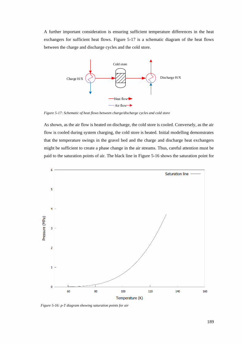
189

A further important consideration is ensuring sufficient temperature differences in the heat

exchangers for sufficient heat flows. Figure 5-17 is a schematic diagram of the heat flows

between the charge and discharge cycles and the cold store.

As shown, as the air flow is heated on discharge, the cold store is cooled. Conversely, as the air

flow is cooled during system charging, the cold store is heated. Initial modelling demonstrates

that the temperature swings in the gravel bed and the charge and discharge heat exchangers

might be sufficient to create a phase change in the air streams. Thus, careful attention must be

paid to the saturation points of air. The black line in Figure 5-16 shows the saturation point for

Cold store

Discharge H/XCharge H/X

Heat flow

Air flow

Figure 5-17: Schematic of heat flows between charge/discharge cycles and cold store

Figure 5-16: p-T diagram showing saturation points for air

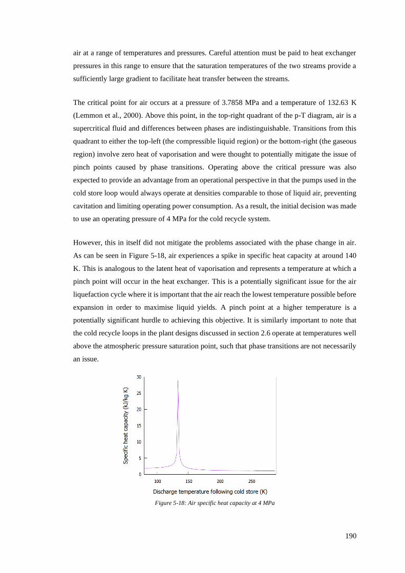
190

air at a range of temperatures and pressures. Careful attention must be paid to heat exchanger

pressures in this range to ensure that the saturation temperatures of the two streams provide a

sufficiently large gradient to facilitate heat transfer between the streams.

The critical point for air occurs at a pressure of 3.7858 MPa and a temperature of 132.63 K

(Lemmon et al., 2000). Above this point, in the top-right quadrant of the p-T diagram, air is a

supercritical fluid and differences between phases are indistinguishable. Transitions from this

quadrant to either the top-left (the compressible liquid region) or the bottom-right (the gaseous

region) involve zero heat of vaporisation and were thought to potentially mitigate the issue of

pinch points caused by phase transitions. Operating above the critical pressure was also

expected to provide an advantage from an operational perspective in that the pumps used in the

cold store loop would always operate at densities comparable to those of liquid air, preventing

cavitation and limiting operating power consumption. As a result, the initial decision was made

to use an operating pressure of 4 MPa for the cold recycle system.

However, this in itself did not mitigate the problems associated with the phase change in air.

As can be seen in Figure 5-18, air experiences a spike in specific heat capacity at around 140

K. This is analogous to the latent heat of vaporisation and represents a temperature at which a

pinch point will occur in the heat exchanger. This is a potentially significant issue for the air

liquefaction cycle where it is important that the air reach the lowest temperature possible before

expansion in order to maximise liquid yields. A pinch point at a higher temperature is a

potentially significant hurdle to achieving this objective. It is similarly important to note that

the cold recycle loops in the plant designs discussed in section 2.6 operate at temperatures well

above the atmospheric pressure saturation point, such that phase transitions are not necessarily

an issue.

Figure 5-18: Air specific heat capacity at 4 MPa

191

Operating outside in the supercritical rather than the gaseous region will increase the power

consumed by pumping air within the cold recycle loop. It is worth considering by exactly how

much this will affect plant energy balance. In order to do so, it is important to understand how

air density changes with pressure and temperature. This is shown in Figure 5-19. The sharp

drops in density occur at phase transitions.

As can be seen, as air temperature increases, its density falls. As discussed in section 3.2.14,

the power required to pump a fluid through a given pressure increase, ∆𝑝, is given by:

�̇� =∆𝑝�̇�

𝜂𝜌 ( 5-2 )

where �̇� is the fluid’s mass flow rate, 𝜌 is its density and 𝜂 is the pump’s efficiency. As a result,

a decrease in density results in a increase in pumping power. From equation Figure 5-19, it can

be seen that liquid density falls by a factor of around 200, resulting in a likewise increase in

pumping power. It is important to note, however, that for the modest mass flow rates and

Figure 5-19: Density of air for different temperatures and pressures

192

pressure drops seen in the literature, the pumping power remains in the sub-megawatt and the

decision was made to use a low-pressure cold store operating at atmospheric pressure, in line

with the literature. This eases both engineering modelling, from the perspective of the

aforementioned minimum approach temperatures, and financial modelling in maintaining

operating pressure parity between air storage tanks and cold store tanks as discussed in section

2.7.

Considering the points discussed so far in this section points to how to build the model itself.

At this stage in the project, the known parameters were limited. The temperature of liquefied

air for a given storage pressure is known and can be used as a starting point for an air stream

mass flow source. As discussed in section 2.5, and shown in section 5.2.3, the peak discharge

pressure is an important parameter determining turbine performance. It will also affect the

temperature of the air following pumping, and likewise the temperature difference in the cold

store air streams, and thus the amount of cold that can actually be recycled to the charging cycle.

This information provides a means to estimate the size of the cold store prior to full modelling.

This is important given the multi-parameter nature of the system and the parameter sweep

approach to engineering modelling. Estimating component sizes serves to narrow the design

space for the system and limit the required system modelling. Since air pumping is performed

before the cold store inlet, and the model assumes a pressure drop proportional to the inlet

pressure, the temperature delta across heat exchangers on the charge and discharge sides of the

cold store loop will be equal. This delta will be approximately equal to the difference between

the cold store temperatures following charge and following discharge, subject to the discussions

at the beginning of this section.

193

Simple models were built to determine the likely cold store loop parameters. As a starting point,

the theoretical maximum specific cold recycle available depending on the temperature

difference across the heat exchanger between the discharge cycle and the cold recycle loop. The

specific cold recycle, that is the amount of heat transferred to the discharge stream per kilogram

of air discharged, is shown in Figure 5-20. As shown, the higher the peak discharge pressure

(the further along the x-axis), the smaller the specific cold recycle. Conversely, the higher the

intermediate discharge temperature, the greater the specific cold recycle, as a greater

temperature difference is achievable across the discharge-side cold store heat exchanger and

between the hot and cold states of the cold store.

These results have important implications for the system’s overall round-trip efficiency. Higher

peak discharge pressures will result in higher turbine power but will lessen the amount of cold

recycle possible for a given temperature delta, increasing the temperature of the charge air

stream prior to expansion, as discussed in section 5.2.5. Thus, a higher peak discharge pressure

may ultimately reduce the round-trip efficiency by reducing the efficiency of the liquefier.

The results in this section have important implications for the cold store. As Figure 5-9, Figure

5-10 and the subsequent discussions show, the cold store heat transfer rate, the air temperature

at the outlet and the temperature of the cold store itself all vary as the cold store is cooled. The

amount of storage capacity can be controlled by varying the length of the cold store, but in turn

will affect its heat transfer rates during both the charge and discharge cycles.

Figure 5-20: Theoretical specific cold available for isolated cold store modelling

194

With this information in mind, duty cycle modelling of the cold store was begun. This was

performed using the same model shown in Figure 5-21.

The cold store was modelled in cycles to a point of cyclic equilibrium. That is, the point at

which the heat transferred to the cold store during the charging phase was equal to the heat lost

by the gravel bed during the discharging phase. Typically, this occurred after around 20 cycles.

This modelling was performed using the parameters shown in Table 5-5. It was assumed that

the charge cycle would operate at a significantly larger mass flow rate than the discharge cycle,

since only some of the total air flow compressed will be liquefied. A high mass flow rate was

used to ensure that the maximise heat transfer between the cold store and the charge air stream.

Parameter Value Units

Discharge mass flow rate 100 kg/s

Discharge source temperature 78.9 K

Discharge source pressure 101.325 kPa

Discharge peak pressure 12,500 kPa

Cold store loop mass flow rate 185 kg/s

Cold store loop peak pressure 101.325 kPa

Cold store starting temperature 150 K

Cold store diameter 3 m

Cold store length Swept parameter

Bed particle diameter 0.02 m

Bed particle density 2320 kg/m3

Bed particle specific heat capacity 810 J/kg K

Charge mass flow rate 150 kg/s

Charge source temperature 293.15 K

Charge source pressure 18,000 kPa

Heat exchanger pressure drops 0.01

Pump efficiency 90 %

Table 5-5: Cold store duty cycle model parameters

Cold store

Discharge Pump

Discharge HX

Charge HX

Air source

Air sink

Figure 5-21: Isolated model for testing cold store parameters

195

The cold store model discussed in sections 3.2.8 and 3.2.9 is capable of modelling axial

conduction along the length of the cold store. At this stage, however, the length of the periods

during which the system might be idle and the cold store temperatures would approach

equilibrium was not known. As a result of this, the assumption was made that there would be

no conduction through the cold store and the parameter for the thermal conductivity of the

gravel bed, 𝜅, was set to zero. The implications of this assumption are discussed in section 7.3.1.

As will be discussed below, the efficiency of the cold recycle system is dependent on

maximising temperature differences across the cold store loop heat exchangers. In order to

maximise efficiency of the cold recycle system, (Sciacovelli et al., 2017b) envisages an

arrangement of parallel cold stores which are operated sequentially during a single duty cycle,

allowing temperature differences to remain at nominal levels for as large a part of the duty cycle

as possible. Essentially, this reduces the amount of time that they operate at points beyond the

red line in Figure 5-9 and Figure 5-10. A similar system was assumed to operate for this project,

and it was assumed that four cold store cells would serve a single half-hour duty cycle for the

100 kg/s symmetrical system being designed. Much like (Sciacovelli et al., 2017b), a single-

Figure 5-23: Axial temperature profile of the cold store following discharge for a 16m cold store

Figure 5-22: Axial temperature profile of the cold store following charge for a 16m cold store

196

cell system was used to model the behaviour of a transient system, and as a result, the

simulations were run for 450 s.

Figure 5-23 shows the temperature profile of the cold store following discharge cycles 1, 5, 10,

15 and 20 for the example of a 16 m cold store. The x-axis shows the axial co-ordinate;

essentially the length along the cold store normalised to the length of the whole cold store. As

the figure shows, the temperature profile has converged to a state of cyclic equilibrium by

around cycle 10. Figure 5-22 shows temperature profiles following charge cycles, exhibiting

the same convergence behaviour.

Figure 5-24 shows how the energy capacity of the cold store varies with its length. This is

shown as both an amount in kWh, and a percentage of the theoretical energy available based on

the enthalpy difference across the discharge heat exchanger at the start of the simulation, the

discharge flow rate and the length of time for which the simulation was run (in this case, just

below 4000 kWh).

Figure 5-24: Cold store energy capacity dependency on cold store size

197

The percentage of available energy that is stored is an important metric. The cold store is a

dynamic system and its temperature rises during the discharge cycle. As this occurs, the

temperature difference of the air across the cold store loop side of the discharge heat exchanger

will reduce, and the heat load of that heat exchanger will similarly fall. This can be seen in

Figure 5-25. The line at the top is the temperature of the air in the cold store loops at the store’s

outlet. The falling line below this represents the average temperature of the gravel; as this falls,

so too does the air temperature at the outlet. Two lines are shown increasing from bottom-left

to top-right. The yellow line is the ideal cold that could be stored; essentially the initial storage

rate extrapolated linearly. The blue line shows the actual cold stored and this falls as the outlet

temperature falls due to the aforementioned reduction in heat load of the discharge-side heat

exchanger.

This is an interesting consequence of the of the finite volume approach to modelling the cold

store. Because the gravel bed part of the cold store is modelled as an array of finite volumes,

the volumes will essentially cool down (or heat up) sequentially/ from the inlet to the outlet end

as air enters the bed and equilibrates with the cold store volumes. Because of the fact that

Figure 5-25: Cold store energy stored and temperature profiles over a single discharge cycle with a 16m cold

store

198

conduction between the volumes is assumed to be zero for the purposes of this simulation, the

finite volumes act almost as individual cold store cells, in the context discussed above. As a

result, the volumes at the inlet end of the cold store are always fully heated or cooled during the

charge or discharge phases, respectively. A consequence of this is that shown in Figure 5-24.

Essentially it means that the cold stored will approach 100% of that theoretically available as

the size of the cold store approaches infinity. Whilst this is an interesting quirk of the modelling

approach, it does not necessarily mean that the model is poorly representative of real-life

conditions; the same behaviour discussed in the previous paragraph as regards flow temperature

transients and the resulting cold capture will manifest in a real system.

As a result of this, this system can never extract 100% of the theoretically available energy from

the discharge air stream. This can be seen in Figure 5-24; whilst the graph has begun to level

off and its behaviour at lengths larger than around 20 m is somewhat linear, it is still continuing

to level off beyond this point. This presented a difficult design decision at this stage as there is

no obvious choice for a cut off point for an optimal cold store size. Ultimately, a larger cold

store will always be preferable from an efficiency perspective, but this must be offset against

cost considerations. A capture of 95% of the available cold was deemed sufficient for this

design and thus, a cold store size of 16m was taken as the size of the store for this quantity of

cold stored.

Due to the complexity of optimising the cold store length, this process was only performed

once. The amount of energy the cold store is capable of storing is defined by:

𝑄 = 𝑀𝐶m∆𝑇 ( 5-3 )

where 𝑀 is the mass of gravel in the cold store, 𝐶m is its specific heat capacity and ∆𝑇 is the

temperature difference between the charged state and the discharged state. This is, of course, a

simplification, as the cold store does not have a uniform temperature along its axis at the end

of either phase. It is, however, sufficient for these purposes. In order to limit the additional

modelling required, it was assumed that the overall temperature swing between the hot and cold

states for the cold store would be the same for any given discharge pressure. Thus, the heat

storage capacity of the cold store varies linearly with its mass.

With this in mind, the cold store was sized for the different quantities of specific cold recycle

shown in Figure 5-20 according to the equation:

199

𝐿 = 16

𝐶𝑅𝑚320,000

( 5-4 )

where 𝐶𝑅𝑚 is the theoretical maximum specific cold recycle available for the discharge air

stream, in Joules, and 𝐿 is the length of the cold store. In the case of the example discussed in

this section, 16 m is the length of the store and 320 kJ/kg is the theoretical maximum cold

recycle based on the initial enthalpy difference across the discharge-side heat exchanger.

Altering the theoretical available specific cold recycle similarly increases the required flow rate

through the cold store loop. As before, heat exchanger temperature differences were assumed

to be equal through the cold store loop side of the discharge heat exchanger, and given that the

loop’s pressure was also taken to be fixed, it was assumed that the required mass flow rate

would also scale linearly with the specific cold recycle using the equation:

�̇� = 185

𝐶𝑅𝑚320,000

( 5-5 )

where �̇� is the required cold store loop mass flow rate. Here, 185 kg/s is the operating flow rate

in the case of the example discussed in this section.

Using these scaling equations, cold store cycling was performed for discharge pressures of

between 7.5 and 15 MPa at 0.5 MPa intervals, mirroring the pressures used in section 5.2.3. To

determine the theoretical maximum specific cold recycle, the same temperature differences

Figure 5-26: Cold store size and loop parameters for different pressures

200

across the discharge side heat exchanger were assumed as those used in the example in this

section, that is the discharge air stream leaving the heat exchanger at 258.5 K.

Cold stores were cycled in the same way as in the example above for the input parameters

shown in Figure 5-26. This yielded a set of initial temperature profiles for the cold store which

could then be used for modelling the charge an discharge cycles from a point of cyclic

equilibrium.

5.2.5. Charge cycle modelling

With potential cold store dynamics understood, and an understanding of operating ranges for

the discharge system, the final step was to study the options for liquefaction. Once again,

modelling was built up in a modular sense. Because the liquefier cycle bears minimal bearing

on the compression and the compressed air is water cooled to a known temperature, a mass flow

source was used to define the flow from the compression cycle, allowing optimisation the

liquefaction cycles beyond the compression train. Following this, compression trains were

modelled to determine the specific energy of liquefaction for each potential configuration. For

brevity, cycles considered in this section are denoted C-y where y is the number of compression

stages used. In order to link the system to the discharge cycle, the temperature profiles for the

cold store from section 5.2.5 were used as an initial parameter for these simulations.

As discussed in section 2.5, Highview Power and the associated study group at the University

of Birmingham provide the most comprehensive, realistic and experimentally verified body of

modelling work on the LAES system (Morgan et al., 2015b, Morgan, 2016, Sciacovelli et al.,

2017a, Sciacovelli et al., 2017b). Their system is Highview’s vision for their commercial

design, and is the design on which this study is based. This bears most similarity to the Collins

cycle. In its first stage, compressed air is first cooled and then some is diverted away to a warm

turbine, which, after being expanded, is combined with the return air stream. A second stage

involves the same process, cooling first, then diverting a fraction to a cold turbine and joining

it with the return air stream. The incoming air stream is then further cooled by both the return

air stream and the cold store loop before being expanded in a J-T valve. Finally, the air is

separated into its vapour and liquid fractions. The vapour fraction begins its return journey back

through the cycle and the liquid fraction is sent to the tank.

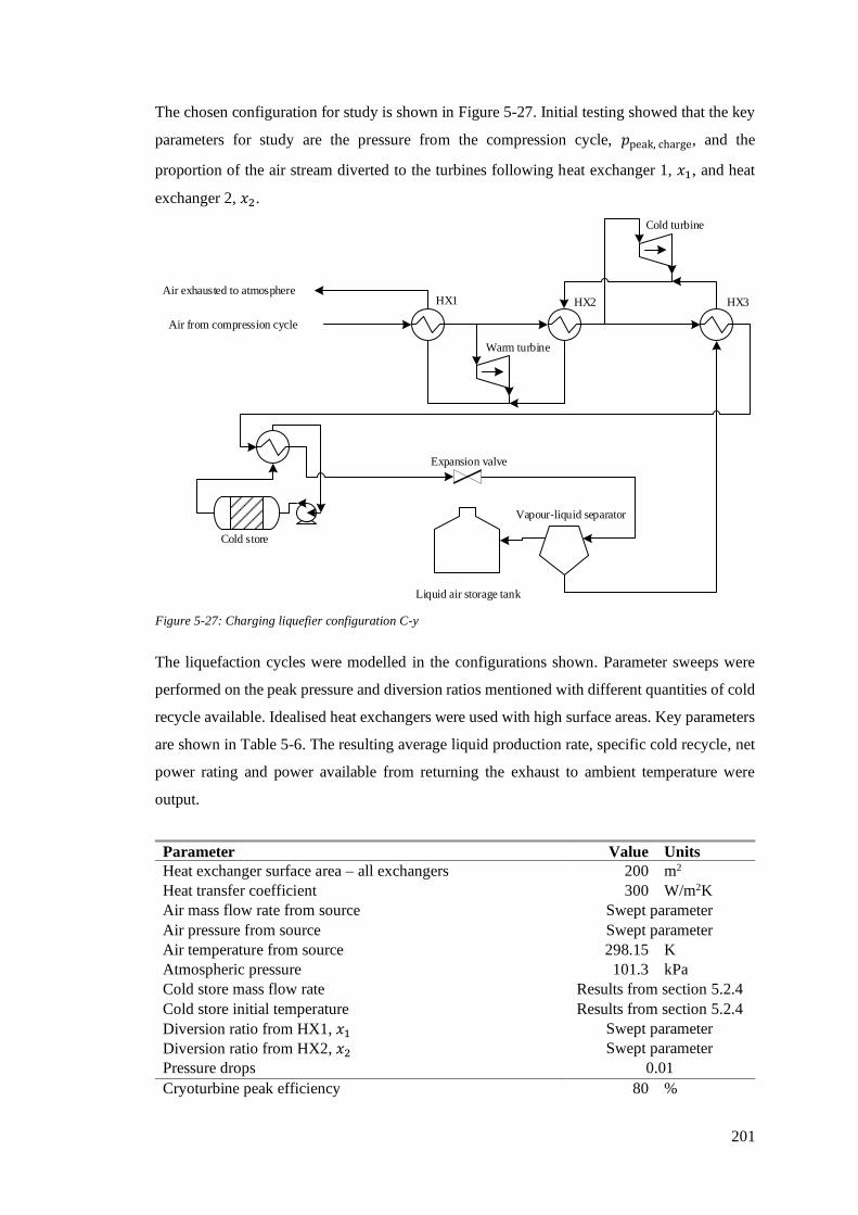
201

The chosen configuration for study is shown in Figure 5-27. Initial testing showed that the key

parameters for study are the pressure from the compression cycle, 𝑝peak, charge, and the

proportion of the air stream diverted to the turbines following heat exchanger 1, 𝑥1, and heat

exchanger 2, 𝑥2.

The liquefaction cycles were modelled in the configurations shown. Parameter sweeps were

performed on the peak pressure and diversion ratios mentioned with different quantities of cold

recycle available. Idealised heat exchangers were used with high surface areas. Key parameters

are shown in Table 5-6. The resulting average liquid production rate, specific cold recycle, net

power rating and power available from returning the exhaust to ambient temperature were

output.

Parameter Value Units

Heat exchanger surface area – all exchangers 200 m2

Heat transfer coefficient 300 W/m2K

Air mass flow rate from source Swept parameter

Air pressure from source Swept parameter

Air temperature from source 298.15 K

Atmospheric pressure 101.3 kPa

Cold store mass flow rate Results from section 5.2.4

Cold store initial temperature Results from section 5.2.4

Diversion ratio from HX1, 𝑥1 Swept parameter

Diversion ratio from HX2, 𝑥2 Swept parameter

Pressure drops 0.01

Cryoturbine peak efficiency 80 %

Liquid air storage tank

Vapour-liquid separator

Cold store

HX1Air exhausted to atmosphere

Air from compression cycle

HX3

Expansion valve

HX2

Warm turbine

Cold turbine

Figure 5-27: Charging liquefier configuration C-y

202

Pump efficiency 80 %

Table 5-6: Key parameters for liquefaction cycle models

As discussed above, the compression train was initially modelled separately. It consists of a

series of compressor stages with intercooling between each stage. Intercooling is important

because as the temperature of air in a compressor increases, so does the energy required to

compress it. The availability of exhaust air from the liquefaction cycle complicates the

compression train. This air can be used to pre-cool the air prior to each compression stage and

reducing power consumption further.

The decision was made to model the compression train with between 2 and 8 compression

stages, as shown in Table 5-7. Figure 5-28 shows the largest system modelled, with 8

compression stages. Precooling was treated as an input parameter with units of power to enable

compression results to be matched with results from the liquefaction cycle modelling. This

power was assumed to be equally divided between the precoolers. Initial testing showed that

the key parameters for modelling the compression train for a given pressure are the number of

turbines and the amount of precooling available.

Configuration Cx-2 Cx-6 Cx-7 Cx-8

Compression stages 2 4 6 8

Table 5-7: Air liquefier cycle configurations tested

The compression system was modelled with the parameters in Table 5-8. The power

consumption, and precooler outlet temperatures for given cooling rate were output.

Compressor 1

Air taken from atmosphere

Intercooler 1

Compressor 2

Intercooler 2

Compressor 3

Intercooler 3

Compressor 4

Intercooler 4

Compressor 5

Intercooler 5

Compressor 6

Intercooler 6

Compressor 7

Intercooler 7

Compressor 8

Intercooler 8

Air to liquefaction cycle

Precooler 1

Precooler 2

Precooler 3

Precooler 4

Precooler 5 Precooler 7

Precooler 6 Precooler 8

Figure 5-28: Compression train configuration Cx-8 (water flow and air exhaust streams omitted)

203

Parameter Value Units

Air mass flow rate from source Swept parameter

Air pressure from source (atmospheric pressure) 101.3 kPa

Air temperature from source 293.15 K

Temperature at intercooler outlets 298.15 K

Peak pressure following compression Swept parameter

Cooling power at precoolers Swept parameter

Pressure drops 0.01

Compressor peak efficiency 85 %

Pump efficiency 80 %

Table 5-8: Key parameters for compression train models

Following isolated system modelling, model results were collated and impossible results (those

with cold recycle exceeding the energy available for a given temperature change, or those with

incompatible heat exchange temperatures) were discarded. Of the remaining results, those with

the lowest specific energy of production for each configuration were taken forward for final

modelling discussed in section 5.2.6, where components were sized and energy balance within

the cold store for the combined system was considered.

204

These initial investigations revealed some important information. As discussed in section 2.5.2,

isothermal compression can theoretically significantly reduce the power requirement over

isentropic compression (Li et al., 2014). In reality, the only way to approach isothermal

compression with axial compressors is to compress in multiple stages and cool the air in

intercoolers between each stage. For the sake of discussion, additional compression stages were

modelled up to a total of 16. As shown in Figure 5-29, each successive addition of compression

stages achieves a diminishing reduction in the compression power required. This is indicative

of the futility in trying to approach isothermal compression with industrial-capacity equipment;

8 compression stages with intercooling is already a large and unwieldy system and the

diminishing returns gained by further staging are clearly demonstrable. Ultimately, the decision

was made to focus on a maximum of eight-stage compression.

The next consideration was the amount of recycled cold that could be utilised by the liquefier.

Obviously, this is an important consideration for the efficiency of the liquefier. The amount of

cold that can be utilised is dependent on the pressure, temperature, and mass flow rate of air

following heat exchanger 3, and the amount of cold recycle available based on the relevant

Figure 5-29: Power of compression for 150 kg/s flow rate

205

discharge pressure. These variables can all be controlled, with varying effectiveness, by the

diversion ratios to the hot and cold turbines, 𝑥1 and 𝑥2.

The cold store size and loop mass flow rate for each candidate discharge pressure using the

relevant value of specific cold recycle was set via equations ( 5-4 ) and ( 5-5 ) respectively.

Recapped from section 5.2.4:

𝐿 = 16

𝐶𝑅𝑚320,000

( 5-4 )

�̇� = 185

𝐶𝑅𝑚320,000

( 5-5 )

The relevant temperature profile from the results of section 5.2.4 was also used as an initial

parameter for the initial condition of the gravel bed and cold recycle loop mass flow rates, which

were both set via table data based on the length of the cold store using the same tables that set

the compressor and turbine efficiencies in sections 3.2.6 and 3.2.7 respectively. Parameter

sweeps were performed on mass flow rate initially, using a 0.1 bypass ratio for both 𝑥1 and 𝑥2.

Of the yielded results, those for which the temperature of the air returning to the cold store in

the cold recycle loop was outside 5% of the expected temperature were discarded. Similarly,

results for which the liquid yield mass flow rate was less than 100 kg/s were discarded. Withing

the remaining results, fine adjustments were made to both the supply mass flow rate and the

bypass ratios, via further parameter sweeps, to determine parameters for which the desired cold

recycle loop return temperature and the liquid yield target of 101 kg/s were achieved.

206

The results of this process are shown in Figure 5-30. The lower set of lines show the specific

energy of liquefaction at the given peak charge pressure. Each line is for a given peak discharge

pressure shown in the key. Note that, for brevity, discharge pressures are shown at intervals of

2.5 MPa, along with the optimal peak pressure of 12 MPa. The specific energy cost of

liquefaction increases with the discharge pressure, due to the lower specific cold recycle

available at these higher discharge pressures as shown in Figure 5-20.

The discontinuity in the results data is important. The lines cover only a small portion of the

pressure range used for modelling. This is due to the criteria set on modelling results and the

requirement for both mass balance in terms of the liquid yield flow rate, and energy balance in

terms of the return temperature of the cold store loop. To the left of each line, the temperature

of the air returning to the cold store was too low, meaning that the cold store would not be at a

sufficiently high temperature during the following discharge cycle to effectively capture the

available cold from the air being discharged. To the right of each line, the air stream was able

to effectively capture the available cold from the cold store loop, but the system could not

achieve sufficiently high liquid yields to ensure mass balance from charge to discharge.

From the lower set of lines in Figure 5-30, it appears that lower discharge pressures are

preferable from the perspective of the charge cycle, due to the greater availability of cold

Figure 5-30: specific energy of liquefaction and round-trip efficiency depending on charge and discharge peak

pressures (all results net of pumping energy costs)

207

recycle lowering the specific energy of liquefaction for the system. In the context of LAES

however, this is only half of the story. The upper set of lines in the figure show the round-trip

efficiency of the system when the increased specific energy yield of the discharge system

available at higher pressures is considered. These lines show that the optimal peak discharge

pressure occurs at 12 MPa, with the optimal peak charge pressure occurring at 18.5 MPa. It is

important to note that these results are all based on discharge mass flow rates of 100 kg/s, which

section 5.2.3 shows is very much sub-optimal.

5.2.6. Configurational plant design options

The final step of engineering modelling was to model different plant configurations to be taken

forward for economic performance comparison, the subject of Chapter 6. The decision was

made to simulate a total of four charge cycles (with 2, 4, 6 and 8-stage compression trains) and

three discharge cycles (with 2, 3 and 4-stage expansion trains). These models were simulated

in steady-state conditions to reduce the computational time, and to provide sufficient stream

data to properly size the required components. The charge cycle is most affected by transient

behaviour and, as such, the specific energy cost of liquefaction results were taken from section

5.2.5 to ensure that this behaviour was properly captured rather than using the steady-state data

from this round of modelling.

Preliminary work (Wilson et al., 2020) showed that market conditions suitable for a positive

NPV for a combined NPP and LAES plant favoured plants with a high discharge rate. This

work is discussed in detail in section 6.1.2.With the conclusions of this work in mind, and the

fact that there is an optimal discharge rate for a given peak discharge pressure, as shown in

section 5.2.3, discharge cycles were modelled at their optimal mass flow rates.

Figure 5-31 shows the round-trip efficiencies of the 12 systems resulting from this round of

modelling.

208

Figure 5-31: round-trip efficiencies of LAES storage systems depending on compression and expansion staging

209

- Financially motivated plant design

6.1.1. Introduction

This section discusses the results of the financial modelling and how they influence the overall

plant design. Section 6.1.2 discusses the preliminary work performed using an early version of

both the engineering and the financial models. Despite some simplifications, there are some

important results that were used as a basis of the detailed modelling discussed in the later

sections. Section 6.1.3 details the comparison of the economic performance of the different

system configurations within the financial model. From these results, a final configuration was

taken forward for further modelling. Section 6.1.4 studies the market conditions required for

the plant to become profitable.

All results in this chapter are expressed in the form of box-and-whisker plots. These plots are

useful for displaying statistical measures of large sets of values that have been output by a

model. They consist of two parts: the box and the whisker. The box’s upper and lower limits

are located at the respective upper and lower quartiles of the dataset. The central bar of the box

is located at the mean of the dataset. In this study, the whiskers have been used to show the 10 th

and 90th percentiles of the data. This is important to note, as the whiskers would typically show

the minimum and maximum of the dataset, however in this case, this caused difficulty in scaling

plots sufficiently well to present the results clearly.

6.1.2. Preliminary work

Work as part of this project that has been previously published as a peer-reviewed working

paper (Wilson et al., 2020) by the Energy Policy Research Group at Cambridge University

provides important insights that serve as a starting point for the work in this thesis. This early

work was based on early versions of both the engineering and the financial model, both of which

had some important differences to the final versions. These are discussed in the following

paragraphs.

The early engineering model results assumed a continuous isentropic efficiency for the NPP’s

steam turbine, meaning that power dropped off linearly, in contrast to the most recent modelling

discussed in section 5.2.1. For this reason, the power yield from the discharge system increased

linearly with mass flow rate and resulted in a higher overall power output for a given staging

configuration and peak pressure. This meant that the resulting specific energy yield and round-

trip efficiency of the system was significantly higher than the results discussed in Chapter 5.

210

Unlike the model described in section 0, the early financial model made no provisions for

arbitrage. Any electricity used by the LAES plant while charging the system was assumed to

be purchased from the NPP (or to simply reduce the NPP’s overall power output), meaning that

its cost was always defined by whatever the strike price happened to be for the year in question.

Whilst a minor simplification, this meant that varying the charge-side mass flow rate had no

effect on the profitability, or otherwise, of the proposed plant design.

The calculation of plant equipment costs used the scaling equation shown in section 2.7.

𝐶(𝐴) = 𝐶(𝐵) (

𝑆(𝐴)

𝑆(𝐵))

𝑋

( 6-1 )

The base equipment costs used were the somewhat dated costs taken from the literature (Peters

et al., 1968) and adjusted to 2018 prices using CEPCI data. This CEPCI data was collected from

the same set of sources (Vatavuk, 2015, 2010, 2008) as that discussed in section 2.7. Using

these prices, shown in Table 6-1, resulted in a tendency to underestimate plant capital

investment, making the proposed plant appear more attractive than it actually was.

Eq

uip

men

t

Size fo

r

com

pa

rison

Un

it for

com

pa

rison

Co

st for

com

pa

rison

Yea

r for

com

pa

rison

CE

PC

I Price

ind

ex

20

18

Eq

uiv

alen

t

Co

mp

ariso

n

exp

on

ent (𝑿

)

Turbine 10 MW £2,000,000 2017 535.3 £2,079,955 0.60

Cryoturbine 745 kW £113,250 1990 392.2 £160,750 0.69

Water pump 50 kW £8,500 1990 392.2 £12,065 0.33

Cryo pump 50 kW £15,000 2014 576.1 £14,495 0.60

H/X - 2 MPa 140 m2 £107,000 1990 392.2 £151,879 0.44

H/X - 3 MPa 140 m2 £134,000 1990 392.2 £190,203 0.44

H/X - 7 MPa 140 m2 £160,000 1990 392.2 £227,109 0.44

H/X - 10 MPa 140 m2 £202,500 1990 392.2 £287,434 0.44

H/X - 20 MPa 140 m2 £253,200 1990 392.2 £359,399 0.44

Air tank 400 tonnes £83,500 1990 392.2 £118,522 0.57

Table 6-1: Equipment cost data for comparison, 2018 equivalent prices and exponents for comparison

Despite these simplifications, the early work provides some important results that are a valuable

starting point for the financial modelling discussed herein and will be recapped in this section.

The initial uncertain parameters used for the financial model are shown in Table 6-2. As shown

in the table, two pricing scenarios were considered: ‘high spot market pricing’ and ‘extreme

spot market pricing’.

211

PERT distribution

parameters

FOAK scenario NOAK scenario

Min

imu

m

Mo

st likely

Ma

xim

um

Min

imu

m

Mo

st likely

Ma

xim

um

NPP spending factor 1 1.7 2 1 1.1 1.3

Binomial distribution

parameters

FOAK scenario NOAK scenario

𝒏 𝒑 shift 𝒏 𝒑 shift

NPP construction time –

mobilisation 1 0.6 2 0 0.4 2

NPP construction time –

critical path 2 0.6 3 1 0.4 3

LAES construction time –

mobilisation 1 0.6 1 1 0.2 1

LAES construction time –

critical path 1 0.6 1 1 0.4 1

BetaGeneral distribution parameters α1 α2 Minimum

/£m

Maximum

/£m

CES configuration 1 (slow discharge) 9.8763 16.457 20.9 23.3

CES configuration 2 (moderate

discharge) 7.7810 13.202 44.5 51.9

CES configuration 3 (rapid discharge) 10.949 21.242 66.3 80.0

Electricity price amplitudes (NOAK scenario) Q1 Q2 Q3 Q4

Amplitude factor 𝛼(𝑄) 2 2 2 2

ARMA time series parameters Mean Volatility

Auto-

regressive

coefficient

Moving

average

coefficient

𝐴(𝐷) high spot market pricing 115 8 0.8 -0.2

𝐴(𝐷) extreme spot market pricing 150 8 0.8 -0.2

First order MA parameters Mean Volatility

Moving

average

coefficient

Initial

error term

Half-hourly error value (휀(𝑃)) 0 0.12 0.6 0

Consumer Price Index (CPI) 0.225 0.002 0.823 0

Table 6-2: Financial model initial uncertain probability distribution parameters and time series parameters

The plant model used an 8-compressor 4-turbine design and the plant charge/discharge

configuration is shown in Table 6-3. The study tested four configurations, the first of which,

configuration 0, was a baseload NPP without LAES. The remaining configurations all included

LAES systems that discharged and charged over a single half-hour period. The systems in the

preliminary work had a round-trip efficiency of 53%, significantly higher than those detailed in

Chapter 5, due to the reasons discussed above.

212

Configuration 0 P1 P2 P3

Charge power (MW) 0 50 50 50

Charge flow rate (tonnes/h) 0 222 222 222

Discharge power (MW) 0 30 150 300

Discharge flow rate (tonnes/h) 0 241.2 1,206 2,412

Storage capacity (tonnes) 0 120.6 603 1,206

Table 6-3: Plant design charge/discharge parameters

The starting point for modelling in both the FOAK and NOAK scenarios was to determine the

minimum CfD price that would ensure that the NPP-only plant has a positive NPV in every

model iteration. This was considered central to the viability of the project, since NPP financial

security is likely to be a major barrier to new build construction. FOAK scenarios required an

initial CfD price of £75/MWh or higher for this to be the case. NOAK scenarios required

significantly smaller CfD prices of £55/MWh to ensure a positive return on project investment.

The hybrid NPP-LAES plant was then tested for the FOAK scenario. These configurations only

became more profitable than NPP-only configurations for extremely high values of mean daily

average 𝐴(𝐷), in excess of £230/MWh, and with amplitude values of 𝛼(𝑄) = 3 for all quarters.

The idea of spot market prices reaching this level and a new build NPP plant being able to

attract a CfD price of only a third this value seemed unlikely and, as a result, the FOAK scenario

was abandoned for the time being.

The FOAK results, whilst not particularly interesting in themselves, go a long way to

highlighting the crux of the problem with the preliminary financial model. As discussed above,

the power used to charge the LAES plant was always considered to come from the NPP, and as

such, always came at whatever CfD price the NPP was being paid. This, given the round-trip

efficiency of the plant being just in excess of 50%, meant that the spot market price had to be

double the CfD price before the model would allow the system to discharge.

This threshold price for discharging likely had another important effect given the nature of the

model construction. Since both the CfD price and the value of 𝜇𝐴(𝐷) are indexed to the same

value of CPI, they will rise in concert. As a result, the threshold price for discharging, being

double the CfD price, will rise at a faster rate than the value of 𝜇𝐴(𝐷). As a result, the likelihood

of the plant being able to discharge will lessen over the course of the model. Unfortunately, the

preliminary financial model did not track this information.

213

The results of the preliminary financial modelling for the NOAK scenario are shown in Figure

6-1. Considering the ‘high spot market pricing’ first (the purple and yellow bars), these results

demonstrate that the construction of a hybrid NPP-LAES plant is an extremely unattractive

proposition. In fact, as can be seen from the lower set of bars, moving from right to left, NPV

improves as the plant size tends to zero, but always remains lower than that of the NPP-only

configuration 0. Similarly, the upper set of bars shows that payback period increases as the plant

size increases, and that payback period is always longer for the plants where LAES is included.

A smaller discount rate improves plant profitability in all cases, but the overall conclusion

remains the same; including LAES in the plant design is detrimental to plant profitability in all

cases.

In the ‘extreme spot market pricing’ (the cyan and green bars), the spot market pricing is

sufficient for the LAES to become profitable and start paying for itself. Once spot market prices

reach this threshold, the LAES becomes increasingly profitable as plant size rises, shown by

the bars appearing higher moving from left to right. It should be noted that the plant

configurations in Table 6-3 provide storage such that the plant is fully discharged in a single

half-hour period. This was a key system parameter for testing in the early stages of financial

modelling, and this demonstrated that, in all cases, this was preferable to having larger storage

capacity and allowed the plant to capitalise on the highest electricity prices. This is potentially

Figure 6-1: Preliminary financial modelling results (NOAK scenario)

214

due to the constraint the model places that the plant must be charged or discharged continuously,

as shown in section 4.5.3; the plant would be unable to stop discharging if the instantaneous

price fell below the discharge threshold price if the tank was not already empty.

6.1.3. Plant compression and expansion staging

As seen in section 5.2, charge compression staging and discharge expansion staging have

significant effects on the overall efficiency of the plant. Given this information, determining

the effect of these design choices on project NPV was the starting point for this round of

financial modelling.

As discussed in section 6.1.2, the combined NPP-LAES performed best when the discharge rate

was large and discharged the entirety of its store air in a single half-hour period. As a result,

this was the starting point for this second round of modelling. Plant discharge rates were chosen

such that they coincided with the peak discharge rates discussed in section 5.2.3. The plant

designs modelled 2, 4, 6 and 8-stage compression and 2, 3 and 4-stage expansion, resulting in

a total of 12 possible staging options for each of the two liquefier configurations considered.

The full-plant cycles were modelled for each of these configurations and the components sized

in a cost estimation spreadsheet using the equations summarised in section 4.3.1. The same

spreadsheet includes the PERT distributions described in section 4.3.2 and uses these in a

100,000-iteration @RISK simulation that results in a distribution of overall plant cost. A

BetaGeneral function was then fit to the resultant distribution and used for the LAES cost input

into the financial model simulation.

Power ratings for pumps, turbines and compressors were taken directly from the engineering

model simulation results. Tanks and cold stores were sized according to the requirements of the

given configuration. Single-phase heat exchangers were sized according to the relationship:

𝐴 =

�̇�

𝛾 ∆𝑇𝐿𝑀

( 6-2 )

where �̇� is the heat load in W, 𝛾 is the heat transfer coefficient in W/m2K and ∆𝑇𝐿𝑀 is the

logarithmic mean temperature difference across the heat exchanger calculated by:

∆𝑇𝐿𝑀 =

∆𝑇hot − ∆𝑇coldln ∆𝑇hot − ln∆𝑇cold

( 6-3 )

215

where ∆𝑇hot is the temperature difference between the two streams at the hot end of the heat

exchanger and ∆𝑇cold is the temperature difference between the two streams at the cold end of

the heat exchanger.

Heat exchangers in which one or both of the fluids exhibited a phase change cannot be sized

using equation ( 6-3 ) due to the phase change and were hence modelled in isolated models

using mass flow sources, pressure sinks and heat exchanger models. The relevant stream data

parameters were set using the data from the plant model and the heat exchanger size was

reduced progressively until it was at the smallest size for which it could maintain its required

heat transfer rate.

Model inputs for the market conditions and other top-level parameters are shown in Table 6-4.

The remaining parameters for spending factors, construction times, and time series controls are

identical to those shown in Table 6-2. As can be seen in Table 6-4, for the sake of comparing

plant configurations, the model assumes a sustained high daily average electricity price and a

high amplitude of price fluctuations for the duration of the model. The table also shows the key

difference between the A and B simulation sets; a low daily average price is assumed for the A

simulations whilst a high price is assumed for the B.

Parameter Value

NPP plant base capital cost (£m) 1,050

Starting CfD price (£/MWh) 55

Plant costs spent during mobilisation 30%

Annual fixed NPP O&M costs (£m) 30

NPP refuel costs (£m) 10

Annual fixed LAES O&M costs as a fraction of plant cost 1.5%

NPP fuel load duration (days) 500

NPP time to refuel (days) 10

Charge window start time 00:30:00

Charge window end time 06:00:00

Discharge window start time 17:30:00

Discharge window end time 23:30:00

Day average 𝜇𝐴(𝐷), all years, A simulations (£/MWh) 100

Day average 𝜇𝐴(𝐷), all years, B simulations (£/MWh) 220

Amplitude factor 𝛼(𝑄), all quarters, all years 2 Table 6-4: Model market parameters for A/B simulations investigating the effect of compression/expansion staging

Model parameter inputs for the LAES plant are shown in Table 6-5. The leftmost section of the

table shows the simulation designation. Each round of simulations is given an identical letter

designation and the simulations in that round are numbered separately in order of increasing

number of compression stages, then in order of increasing number of turbine stages. The next

section to the right shows the LAES plant characteristics for that simulation including charge

216

and discharge power ratings. It is important to note that the discharge power is shown as the net

power, that is the losses resulting from ramping down the NPP secondary loop are factored in.

The next section shows the overall contribution of each subsystem to the overall plant cost:

• charge considers all of the heat exchangers and compressors used in the charge cycle

but not the heat exchange with the cold recycle system,

• discharge considers all of the heat exchangers, pumps and turbines used in the discharge

cycle but not the heat exchange with the cold recycle system,

• cold recycle cost includes the cold store itself, the pumps and the associated heat

exchangers,

• storage cost considers only the air storage tank.

The rightmost section defines the model parameters for the BetaGeneral probability distribution

used to model plant cost for each iteration.

217

Sim

#

Co

mp

ression

stag

es

Ex

pa

nsio

n

stag

es

Ch

arg

e

po

wer

(kW

)

Disch

arg

e

po

wer

(kW

)

Ro

un

d trip

efficiency

Ch

arg

e

cost

Disch

arg

e

cost

Co

ld recy

cle

cost

Sto

rag

e

cost

𝜶𝟏

𝜶𝟐

Min

imu

m

(£m

)

Ma

xim

um

(£m

)

1 2 2 145,179 405,270 27.9% 25.8% 59.3% 9.3% 5.6% 10.398 19.143 101.3 124.5

2 2 3 127,350 391,500 30.7% 23.8% 61.6% 9.2% 5.5% 9.3579 16.216 103.1 125.1

3 2 4 122,256 397,440 32.5% 22.4% 63.5% 8.8% 5.3% 9.4947 17.165 107.3 130.6

4 4 2 118,503 405,270 34.2% 28.5% 57.1% 9.0% 5.4% 9.2377 16.207 105.5 127.9

5 4 3 103,950 391,500 37.7% 26.4% 59.5% 8.8% 5.3% 9.7422 17.77 106.7 130.5

6 4 4 99,792 397,440 39.8% 24.9% 61.5% 8.5% 5.1% 9.01 16.015 111.0 134.4

7 6 2 110,808 405,270 36.6% 30.9% 55.3% 8.7% 5.2% 10.507 19.31 108.6 133.8

8 6 3 97,200 391,500 40.3% 29% 58% 9% 5% 9.5496 17.249 110.1 134.2

9 6 4 93,312 397,440 42.6% 27% 60% 8% 5% 10.851 21.03 113.6 141.0

10 8 2 107,217 405,270 37.8% 33% 54% 8% 5% 10.377 19.066 112.1 137.8

11 8 3 94,050 391,500 41.6% 31% 56% 8% 5% 9.9871 17.527 113.0 137.9

12 8 4 90,288 397,440 44.0% 29% 58% 8% 5% 10.566 20.266 116.8 144.5

Table 6-5: Model LAES parameters for A and B simulations investigating the effect of compression/expansion staging

Table 6-5 shows the financial model input parameters for the ‘A’ and ‘B’ simulations of the financial model. These simulations consider the varying the number of

compression and expansion stages. It is important to note here that overall efficiency does not necessarily increase according to the number of stages; the charge

compression staging appears to have a greater overall contribution to the plant’s efficiency than the discharge expansion staging. All simulations were performed

according to the parameters in Table 6-4.

218

Figure 6-2: A/B simulation results for NOAK scenario

219

Figure 6-2 shows the results for the A and B simulations for the combined NPP-LAES plant.

The A results are, without question, unfavourable to the proposition of the hybrid plant. They

show that, under any configuration, the hybrid plant performs extremely poorly. All NPV

results are lower than those for an NPV-only configuration, and all payback period results are

longer. Interestingly, the difference between results is almost imperceptible, with a very small

improvement in more efficient plants. This is an interesting effect of the hybrid plant; the

profitability of the NPP is essentially driving the NPV and reducing the losses made by the

LAES plant. It is important to note that this is in contrast to the preliminary results in section

6.1.2, whose economic performance worsened with increasing plant cost due to the fact that

round-trip efficiency was fixed for all configurations in that work. Here, the round-trip

efficiency is not fixed and the difference in results, whilst small, is apparent.

The B results are more favourable. All configurations with LAES perform better than the NPV-

only configuration. It is apparent that increasing efficiency, via increasing the number of turbine

and expansion stages, improves the economic performance of the plant in all cases. It is

important to note that the results also show that improving performance is not solely related to

plant output power, as was the conclusion from the preliminary work discussed in section 6.1.2.

It is important to bear in mind, however, that this work did not consider designs whose

efficiency differed. The effect of efficiency can be most clearly seen when comparing the 2-

turbine discharge results with those of the 3- and 4-turbine systems. Despite the fact that the 2-

turbine systems power output is significantly higher (by virtue of its peak performance

discussed in section 5.2.3), their performance is notably worse due to the decline in round-trip

efficiency.

The B results also show an effect of diminishing returns when increasing system efficiency.

Increasing the number of compression stages from 2 to 4 offers significant improvement in

economic performance but increasing further offers only small benefits. This is a result of the

scaling equations used in the plant cost estimation; the nature of these equations favours the

cost of large equipment compared to small equipment, so increasing the number of stages also

significantly increases the cost of equipment of an equal power rating. Surprisingly, this effect

is not apparent when comparing the 2-, 3- and 4-turbine results, despite the fact that not only

do the equipment scaling equations favour larger pieces of equipment, but also the fact that the

discharge system comprises a much larger part of the overall plant cost, as seen in Table 6-5.

This lends credence to the hypothesis that hybrid plant efficiency and overall output power are

both important drivers of plant economic performance.

220

The overarching conclusion of this section is then that the most efficient 4-turbine, 8-

compressor LAES plant design offers the best chance of hybrid plant profitability, but that,

much as the preliminary results have shown, very high spot market pricing is required for

profitability. With this in mind, configuration 12 from table Table 6-5 was taken forward for

additional modelling, with the intention of studying exactly how high market pricing had to be,

and for how long it needed to be sustained.

6.1.4. Market conditions

The final set of simulations all used LAES configuration 12 from section 6.1.3 and were aimed

at determining the threshold market conditions for LAES plant profitability. The plant design

model input parameters are recapped in Table 6-6. The market parameters are shown in Table

6-7. Much as was the case for the A simulations, these market conditions are assumed to run

throughout the 30-year course of the model for these simulations. Table 6-7 shows that the

value of 𝜇𝐴(𝐷) was varied and that for each value taken, the effect of the changing the value of

𝛼(𝑄) was investigated for three separate cases. From this point onward, all modelling is

performed with the assumption of an NOAK scenario.

Parameter Value

Charge power (kW) 90,288

Discharge power (kW) 397,440

Storage capacity (kWh) 198,720

𝛼1 10.566

𝛼2 20.266

Minimum (£m) 116.8

Maximum (£m) 144.5 Table 6-6: LAES parameters for C/D simulations investigating the effect of market conditions

Simulation Day average 𝜇𝐴(𝐷) Amplitude factor 𝛼(𝑄)

C1 190 2

C2 190 2.5

C3 190 3

C4 180 2

C5 180 2.5

C6 180 3

C7 170 2

C8 170 2.5

C9 170 3

C10 160 2

C11 160 2.5

C12 160 3

C13 150 2

C14 150 2.5

C15 150 3 Table 6-7: Market parameters for C simulations investigating the effect of market conditions

221

Figure 6-3 shows the simulation results for the C set of simulations. The groups of coloured

bars are sets of results for the same day average price. Each new set from left to right represents

a decline of £10/MWh in this price. The effect of this is clearly visible: with less revenue

available when discharging the system, the NPV falls and the payback period rises.

Within each set the effect of varying the amplitude of the day profile curves can be seen. A

larger amplitude results in a greater difference between the high and low electricity prices and

thus an improved opportunity for arbitrage. This is shown by the rise in NPV and the fall in

payback period from left to right within each set. This is particular shows the importance of

considering arbitrage within the financial model. The increase in day profile shows a marked

improvement in NPV by increasing the amplitude of the day curves by 50%.

It should be noted, however, that the value of 𝜇𝐴(𝐷) remains the more powerful driver of the

output results. This can be seen when comparing C3 with C15, for example. This increase of

around 25% in the value of 𝜇𝐴(𝐷) from C15 to C3 results in an improvement in mean NPV from

£400m to £450m; around 12.5%. Comparing C13 with C15, for example shows that increasing

the value of 𝛼(𝑄) by 50% improves the NPV by a similar amount. Clearly then, despite the

additional opportunity greater arbitrage margins present, 𝜇𝐴(𝐷) remains a more important driver

of NPV than 𝛼(𝑄).

Figure 6-3: C simulation results for NOAK scenario

222

DCF analysis is one that favours revenues early in a project’s lifecycle to revenues generated

later. The next set of simulations explore this effect by varying how long the high spot market

prices are sustained. Figure 6-5 shows the input parameters for 𝜇𝐴(𝐷), whilst Figure 6-4 shows

the input parameters for 𝛼(𝑄) for the D set of simulations.

As the figures show, simulations D1-D4 begin with the same parameters as simulation C15 and

simulations D5-D8 begin with the same parameters as simulation C3. For each of the sets of

four, the first simulation is the same as the relevant C simulation, with prices remaining high

throughout the duration of the simulation. For the remaining three in each set, the market

parameters are curbed after a period of either 20, 15, and 10 years. The parameters are otherwise

the same as the C set of simulations as shown in Table 6-6.

Figure 6-5: 𝜇𝐴(𝐷) values by year for D simulations

Figure 6-4: 𝛼(𝑄) values by year for D simulations

223

Figure 6-6 shows the simulation results for the D set of simulations. Neither set of results is

particularly surprising; in both cases, NPV falls and payback period lengthens as the period for

which high prices are sustained is shortened. Looking at the £150/MWh average price data first,

the D1 simulation shows and NPV distribution that is slightly higher than the NPP-only result.

This is consistent with the C set of simulation results, where £150/MWh was the threshold price

above which the combined NPP and LAES plant would be profitable. As the duration for which

this price is sustained is reduced below 20 years, the resultant NPV distribution falls below the

NPP-only results and the payback period increases to longer than the NPP-only results.

The £190/MWh results are a little less damning to the prospect of a combined NPP and LAES

plant. Simulation D7 shows that prices that are sustained for a period of at least 15 years are

sufficient to bring NPV and PBP distributions to parity with the NPP-only scenario. This,

however remains a long period for which extreme spot market pricing must prevail.

6.2. Summary and discussion

This chapter has discussed the published preliminary work (Wilson et al., 2020) as part of

section 6.1.2. This work comprised the foundation of the bulk of the work in this thesis and

helped to define the approximate parameter ranges of interest for further financial modelling.

This preliminary work has two fundamental conclusions. Firstly, large capacity LAES plants

Figure 6-6: D simulation results for NOAK scenario

224

that discharge their entire inventory of liquid air in a single period perform better economically

than any other scale of combined LAES and NPP plants. Secondly, spot market parameters

must be pushed into ranges that are without doubt extreme in order for such plants to become

preferable to NPP-only scenarios.

The remaining data analysis in this chapter can be split into two parts; plant configurational

analyses in section 6.1.3 and market condition analyses in section 6.1.4. The plant

configurational discussion is one of the cornerstones of this work and arguably its largest

contribution to the field of techno-economic analyses. This is the only example, as far as this

author is aware, where detailed engineering modelling has been performed in tandem with

financial modelling allowing plant design decisions to be driven by market factors. The

implications and applicability of this are important and are the subject of Chapter 7 and 0.

The results of the B simulations showed that the most complex (and most efficient) plant

configuration boasted the most attractive NPV distribution, provided that spot market prices

were sufficiently high for the hybrid plant to be preferable to the NPP-only plant. It is important

not to read this as a direct endorsement of this technology, however; situations where 𝜇𝐴(𝐷) is

£220/MWh are unheard of in the dataset to which the financial model was fit and would seem

to be highly unlikely at best. The results of the A simulations were perhaps a little more

surprising. With results less attractive than those of an NPP-only plant, the hybrid plant designs

all perform equally poorly for the most part. This is a consequence of the guaranteed income

from the NPP’s CfD price providing something of an offset to the financial losses from the

LAES part of the plant.

Finally, the C and D simulations sought to determine threshold market prices above which the

hybrid plant would be profitable. The C simulations showed that a 𝜇𝐴(𝐷) value of £190/MWh

was sufficient to ensure profitability at 𝛼(𝑄) amplitudes of 2 or greater, comparable to at least

some of the historical dataset. Where 𝜇𝐴(𝐷) was reduced to £150/MWh, more extreme 𝛼(𝑄)

amplitudes of at least 3 are required to ensure profitability, these being well in excess of any

seen in the historical dataset. The D simulations showed that, at the lower prices of £150/MWh,

prices had to be maintained for the full 30-year duration of the model to prevent the hybrid plant

results falling below those of the NPP-only plant. For the £190/MWh results, periods of 15

years or more were sufficient to bring NPV distributions into line with those for the NPP-only

configuration.

In summation, the results of financial modelling would appear particularly critical of the

proposed hybrid plant. Without pushing financial modelling parameters to the extreme and

225

having these extreme prices sustained for long periods, the case for the hybrid plant is always

weaker than the NPP-only proposition. The fundamental conclusion of this chapter must then

be that without significant subsidy to guarantee favourable storage prices, and without having

these prices guaranteed for a long period, the proposed plant would be impossible to justify to

potential investors.

226

- Project discussion

7.1. Introduction

This chapter discusses the successes and limitations of this work, as well as suggesting some

additional work that might be useful as a follow-up to this project. It should, however, be noted

at this stage that the results of Chapter 6 are particularly damning of the proposed system. The

only results in which the system is profitable involve spot market prices well over double the

market average price, and swings between high and low price more significant than any of those

seen in the historical electricity price dataset used. The inescapable conclusion of this work is

that coupling an LAES system to an NPP in the way proposed is, at best, an extremely weak

proposition. It would be extremely difficult to persuade any investor to buy into this concept.

This is not to say that this application of the methodology is without value. As section 7.2

discusses, there are a number of practically useful conclusions that can be drawn from this

study. Furthermore, the financial model itself, as well as the methodology in which it is used,

could be applied to other asymmetrical ESSs, as well as to alternative design options for the

LAES system. Section 7.3 discusses the limitations of the project, especially with regard to the

design choices for the LAES plant and the approach to engineering modelling. It notes that

whilst there is some room for potential improvements in the liquefier design in particular, these

are unlikely to make the overall conclusions of this work any less problematic for proponents

of the proposed system. In closing, section 7.4 proposes potential follow-up work for this

project.

7.2. Project successes

This project has demonstrated difficulties associated with coupling an NPP to and LAES

system. As section 5.2.3 concludes, the optimal LAES system discharge rate is set by the

maximum diversion ratio of steam from the NPP. This is an inherent limitation on the system

and presents something of a hurdle to the practical applicability of such a system. LAES is a

highly flexible system, especially with regard to the decoupling of the charge and discharge

rates. Coupling it to an NPP either locks the system into a given discharge rate or means running

the system at sub-optimal conditions. This is an important result for design engineers and one

not considered in either the existing literature on the subject (Li et al., 2014) or the preliminary

work for this study (Wilson et al., 2020). These novel conclusions have arisen as a consequence

of a more detailed engineering modelling approach with fewer simplifying assumptions. The

227

consideration of reduced efficiency for off-design steam turbine operation as discussed in

section 5.2.1 was a key contributor to these conclusions.

Perhaps the most attractive reason for coupling LAES to an NPP is the ability to use low-grade

heat from the condenser. As section 5.2.3 notes, only some of the available heat is used by the

LAES plant. Only using condenser heat is arguably a more sensible option than using a

combination of condenser heat and NPP secondary loop steam. If the LAES concept of warm

recycle can be proven, the use of condenser heat might provide a means of bridging the

temperature gap between the vaporised air leaving the cold store heat exchange system and it

being superheated by the recycled heat of compression. Such a system might, however, turn the

conclusions of this project on their head. As (Morgan et al., 2015a) notes, increasing the number

of compression stages reduces the temperature of compressed air leaving each compressor. This

in turn results in a lower peak warm recycle temperature and a lower temperature inlet

temperature during the discharge cycle. Thus, the results of section 6.1.3 might well no longer

be valid in this context, and the preference might be for a system with fewer compression stages.

There are additional drawbacks to coupled LAES and NPP systems associated with the ramping

rates possible with steam turbines. Several of the studies discussed in section 2.5.3 assumes the

plant operators are able to garner additional revenue from ancillary service payments associated

with the provision for STOR services to the UK grid. Doing so, however, requires the systems

to be able to ramp quickly; something not possible with steam turbines as section 2.3 notes. It

may transpire that this is a key characteristic of ESSs in the future and that this presents an

additional barrier to coupling LAES and NPP plants.

The financial model itself, and the methodology used for market-led system design are arguably

the crowning achievement of this thesis and the ones with the greatest applicability to other

systems. With some minor modification, the financial model could be used to simulate any

asymmetric ESS within spot markets. It contains many features that such modelling would

require; a means of tracking current stored energy, a means of making decisions as to whether

to charge, discharge or hold the system, and a means to analyse different market scenarios.

LCOS (Tafone et al., 2020) is a useful metric that was introduced at around the same time that

this work was started. This author was not aware of it until late in the project and as such, the

modelling approach does not include calculation of LCOS. With some additional capture of

data in the financial model, this is potentially a metric that could be calculated, however. The

period-by-period approach this model takes to electricity sales potentially offers a number of

advantages over the LCOS approach, as is discussed in the following paragraphs.

228

Firstly, the model tracks the ongoing mass of liquid air stored over the duration of the model

and simulates a real-world plant bidding into the spot market. With LCOS, the number of

charge/discharge cycles the plant achieves is a model assumption and input parameter; here it

is one of the model outputs. This gives designers the opportunity to understand expected cycling

requirements of the system under different market conditions at the design stage.

Secondly, the model in this study allows designers to test a variety of market scenarios, as

section 6.1.4 attempts to do. Again, this is in contrast to LCOS, which outputs a required

average electricity price necessary for a storage plant to break even; here the market conditions

are a model parameter. Whether one is more useful over the other is contentious, however there

is arguably significant value in designers being able to determine not only what kind of market

conditions would be conducive to plant profitability, but how long these need to last for a system

to remain viable. Whilst the model does not consider a subsidy incentive for operating the LAES

plant, this modelling could potentially be used to determine how long such a subsidy would

need to be guaranteed for; something which LCOS cannot.

One of the biggest successes of the financial model is that, unlike the studies discussed in

section 2.5.3, it is not reliant on perfect prediction of electricity prices. By contrast, the decision-

making framework within the financial model only requires known information. That is, that

plant operators would know what price was paid to charge the system and would be able to bid

into the spot market in such a way that they could ensure system profitability. In reality,

operators would have more recent electricity price data and would arguably have a significantly

better understanding of potential market prices than the hypothetical operators in this study,

allowing them to make better-informed decisions on how to operate the plant.

7.3. Project limitations

This thesis, like any that attempts to model real-world problems, is reliant on assumptions to

simplify models and achieve objectives within the limited time available. Section 7.3.1

discusses the key assumptions in the approach to modelling and discusses them in turn. Section

7.3.2 discusses a potential size mismatch in the cold recycle system between the charge and

discharge cycles and its implications for the results of the engineering model. Section 7.3.3

discusses additional systemic limitations in the thesis that are not the direct result of

assumptions.

229

7.3.1. Modelling assumptions

The major assumptions made by both the engineering and by the financial model will be

discussed here in detail and, where possible, attempts made to quantify their implications and

highlight the ways the approach to modelling might be improved. This is by no means an

exhaustive list but highlights the key assumptions made by the modelling approach.

Assumption: there is no conduction along the axis of the cold store.

During the early stages of the engineering modelling, the assumption was made that the

conduction along the cold store was zero. The reasoning behind this was simple. The thermal

cycling of the cold store is a complex thermodynamic system and, at the time, it was not known

how long the LAES system would be standing by (the periods where the NPP operates at

baseload). In fact, the financial modelling would later show that the plant would have to operate

daily charge-discharge cycling in order to remain profitable. That is, the NPV becomes negative

before the capacity factor for the LAES drops below 100%.

A more realistic duty cycle for the cold store is shown in Figure 7-1. The temperature states of

the cold store are shown in ellipses at the corners of the diagram and the processes by which

the cold store is heated or cooled are shown by the arrows. As seen in the figure, the cold store

is heated during charge and cooled during discharge. Also important are the processes labelled

hold. Between periods of charge and discharge, the cold store temperatures will approach

Store is cold

Temperatures have begun to

equilibrate

Store is warm

Temperatures are stratified

Store is at its coldest

Temperatures are stratified

Store is at its hottest

Temperatures have begun to

equilibrate

HOLD - RECOVERY

Store approaches equilibrium for a short period

CHARGE

Store is heated by incoming air

HOLD - BASELOAD

Store approaches equilibrium for a long period

DISCHARGE

Store is cooled by the discharged air

Figure 7-1: Expected duty cycle from the perspective of the cold store

230

equilibrium as conduction between volumes takes place. As discussed in section 5.2.6, the

specific energy of liquefaction increases as the temperature of the cold store increases.

With the knowledge of the periods during which the system would be charged and discharged,

attempts could be made to determine the effect of temperature equilibration over the holding

periods between the charge and discharge cycles. This would likely have a more significant

effect on the charging cycle, since the lowest temperature point in the cold store would not be

as low as was assumed in section 5.2.2, meaning that the energy cost of liquefaction would be

higher. The effect on the discharge cycle would also be non-negligible, with a lower peak

temperature in the cold store meaning that cold capture from the discharge stream and the

resulting specific cold recycle would be lower.

The model of the cold store itself, discussed in sections 3.2.8 and 3.2.9, is in fact capable of

modelling axial conduction in the cold store. To reduce the complexity of modelling, the

thermal conductivity coefficient of the gravel, 𝜅, was set to zero when cycling the cold store.

Armed with a greater understanding of the demands of plant profitability on system cycling,

attempts could be made to investigate the effect of temperature equilibration in the cold store

during the holding periods between charge and discharge.

Assumption: pressure drops in heat exchangers are proportional to inlet pressure.

This assumption is at the heart of the engineering model, and is one that is not without

precedent; almost all of the engineering modelling studies discussed in section 2.5.2 make the

same assumption, with the exception of those that omit pressure losses entirely. As with any

model of a real-world system, there is a trade-off between prediction accuracy and modelling

complexity. The system design in this study did not consider the detailed design of heat

exchangers. Once the plant reached a detailed design stage, this would become a far more

significant concern. The bulk of the liquefaction plant would comprise plate-and-fin heat

exchangers, in which subtle changes in plate size, shape and orientation can have implications

for heat transfer rates, flow regimes, and ultimately cost (Guo et al., 2018). Such detailed design

work is beyond the scope of this study to allow for a more top-level study of system

configurations. Furthermore, given the results of financial modelling, significant improvements

in plant efficiency would be required to substantially improve profitability rather than the

incremental improvements that would likely result from detailed heat exchanger design.

Assumption: the subsystems of the LAES plant can be safely modelled in isolation.

231

This is perhaps the most contentious assumption of the engineering model, not least because it

contributed to the error in the cold recycle system discussed in more detail in section 7.3.2. This

assumption was a product of necessity. The basis of the engineering model is discussed in

Chapter 3 and its implementation in Chapter 5. In section 3.2.1, the finite volume flow models

are discussed and the way these are built into heat exchanger models is discussed in section

3.2.4. Finite volume approaches to process modelling are inherently computationally intensive,

and this is compounded when multiple heat exchangers are used in a single model. The

approach taken to reduce computational load was to divide the overall plant model into separate

components in order to simulate the distinct parts of the cycle in isolation.

The fundamental issue with this is the interconnection between the charge and discharge

systems; the cold store. In order to accurately predict axial temperature profiles of the cold store

at the beginning of the charge and discharge cycles, the cold store had to be simulated to a point

of cyclic equilibrium. This process is discussed in section 5.2.4 and resulted in a series of

temperature profiles for the cold store, as well as store sizes and loop mass flow rates, for a

range of peak discharge pressures. These were then used as initial parameters when modelling

the charge and discharge cycles of the final symmetrical plant design discussed in section 5.2.6.

The implications of doing this on the modelling of the discharge are not too severe. As section

5.2.6 shows, the air temperature following heat exchange with the cold store does fall during

the discharge cycle, however there is sufficient low-grade heat available from the NPP

condenser coolant to maintain a steady air stream temperature as it enters the expansion train.

As a result, errors introduced here should not have an effect on discharge power ratings; these

are primarily a function of the system flow rate and the utilisation of the NPP’s steam.

Errors introduced in the charge cycle will, however, have a far more significant effect. The

effectiveness of the liquefier is ultimately dependent on the thermodynamic state of the air as it

enters the J-T valve. The lower the enthalpy at this point, the greater the liquid yield, and the

lower the energy cost of liquefaction for a given pressure and mass flow rate. Since the cold

store is the key source of refrigeration for the incoming airstream prior to the J-T valve, any

errors introduced will have a significant effect on the energy cost of liquefaction, and hence the

round-trip efficiency of the system as a whole. The implications of such errors are discussed in

more detail in section 7.3.2.

As discussed, the decision to divide the LAES plant into subsystems for engineering modelling

was born of necessity; a system this complex would require more computing power and a more

sophisticated code to model in its entirety than this project had available. Ultimately, the

232

approach to modelling allowed some important insights into coupling LAES and NPP plants

that would not otherwise have been possible. These include the steam diversion ratio optimising

during discharge discussed in section 5.2.3, the results of the cold store cycling in section 5.2.4

and the results of the charge cycle modelling in section 5.2.5. All required detailed modelling

that would have been too time consuming to perform without being able to model the respective

systems in isolation.

Assumption: the number of finite volumes was sufficient for an accurate assessment of plant

performance.

This is another contentious assumption made by the engineering modelling approach. Beyond

200 nodes, heat exchanger temperatures approached convergence, but cannot be said to have

fully converged, even to the point of 500+ nodes being used. Once again, there is a trade-off

here between computing time and accuracy that cannot be avoided without access to greater

computing power. This can be seen in convergence testing performed on the cold store average

Figure 7-2: Convergence testing for the number of FV nodes

233

temperature and outlet temperature performed on the plant charge model results shown in

section 5.2.2, Figure 5-9.

Figure 7-2 shows the convergence testing results based on increasing the number of FV nodes.

The rising line shows the integration time for the simulation. Note that this does not include the

initialisation time for the model. The falling lines show the incremental change in outlet

temperature achieved by increasing the number of nodes. As the shows, incremental

improvements to outlet temperature accuracy fall to less than a tenth of a Kelvin with 250 nodes

or more used in the cold store’s gravel bed. By contrast, the integration time for a single

simulation increases exponentially as the number of nodes is increased. Interestingly, this

increase is not continuous; presumably, a result of different computer operating conditions

between model runs. Any time increases are compounded during both the initialisation and the

results phases of the simulation as additional components that rely on FV modelling are

introduced.

One of the major pitfalls of an insufficient number of nodes manifested in heat exchangers

during early engineering modelling. When the number of nodes in a heat exchanger is

sufficiently small, and temperature differences are sufficiently large, heat flow rates between

the two sides of the heat exchanger can be so large that the direction of heat flow changes from

one volume to the next as a result of temperature changes being too great. This is obviously

indicative of a fundamental error being introduced and was one of the key considerations when

checking engineering model results. A similar pitfall occurs with insufficient numbers of nodes

in the cold store, where it can make the cold store appear more effective than it actually was.

The decision was made to use 250 nodes for simulation models. Whilst this does not result in

convergence of results, it does ensure that the results are at least approaching convergence. The

0.1 K improvement shown in Figure 7-2 beyond this point amounts to a tenth of a percent

change in temperature and this was deemed sufficient for the purposes of what is a very early

stage assessment of plant profitability. It remains an important assumption to be aware of given

that the calculation of plant costs, especially of its heat exchangers, is dependent on the system

temperatures resulting from the engineering model.

Assumption: the cold store size and the flow rate required in its loops can be accurately scaled

using the theoretical maximum specific cold recycle of the discharge air stream.

As discussed at the end of section 5.2.4, the cold store size and mass flow rate were scaled using

linear equations from the detailed cold store modelling performed on the 4000 kWh simulated

234

in detail in that section. The reasons for this are discussed in that section but, in brief, it is

assumed that the amount of energy the cold store is capable of storing is defined by:

𝑄 = 𝑀𝐶m∆𝑇 ( 7-1 )

where 𝑀 is the mass of gravel in the cold store, 𝐶m is its specific heat capacity and ∆𝑇 is the

temperature difference between the charged state and the discharged state.

On the face of it, this is a reasonable assumption, however it does not consider the fact that the

enthalpy, and hence temperature, of the air following the pump in the discharge cycle will

change depending on the peak pressure of that cycle. This will affect the minimum temperature

of the cold store following a discharge cycle. As a result, equation ( 7-1 ) is not entirely valid.

It is, however, the case that the temperature of the air following pumping varies only by a small

amount with increasing peak pressure, as shown in Figure 7-3.

Once again this is a trade-off, this time between being able to model the dynamics of the

charging cycle for as many discharge peak pressure (and hence cold store states) as possible

and being able to obtain the initial temperature profiles of those cold store states. This is no

doubt a flawed assumption but has made possible a greater search of the possible design space

for the system.

Figure 7-3: Temperature of discharge air following pumping

235

Assumption: steady-state simulation of the charge cycle is sufficient for parametric

comparison.

Section 5.2.5 discusses how the charge cycle was modelled first in a steady-state simulation

before the transient behaviour was modelled, as discussed in section 5.2.6. The steady-state

modelling was deemed sufficient to compare the effects of parameters on the performance of

the liquefaction system. As the results of the transient modelling in section 5.2.6 show, the

transient behaviour occurs for only a small part of the half-hour period of system charging and

has only a small effect on the overall energy cost of liquefaction. It would seem, then, that

assuming steady-state behaviour is an acceptable means of parametric comparison.

Assumption: the charge cycle can be scaled according to the specific cost of liquefaction from

the symmetrical plant modelling.

As discussed in section 6.1.3, the larger power consumption (above 100 kg/s flow rate) charge

systems were exclusively modelled in steady-state simulations in order to determine the sizes

of components for the cost estimations. The actual specific cost of liquefaction was taken from

the results of section 5.2.6, where transient behaviour was modelled. When determining system

costs, it was assumed that as long as the modules of the cold store were of smaller size than the

asymmetric system, that the performance of the liquefier would be the same or better than that

of the symmetric plant. Whilst this is, again, a simplifying assumption, it is one that allowed

for a greater exploration of the design space than would otherwise have been possible. By

ensuring that the modules of the cold store were always smaller than those used for the

symmetric system modelling in section 5.2.6, this approach ensured that both the energy cost

of liquefying air, and the cost estimation of the plant would always err on the side of pessimism.

Assumption: the plant will always fully charge or discharge continuously.

The assumption that the plant would always fully charge or discharge in a single continuous

process is one that underpins the workings of the financial model. For selling into the spot

market, this is a perfectly acceptable assumption for the discharge cycle given the results of the

financial modelling. As section 6.1.2 discusses, plant designs that discharge fully in a single

half-hour period had greater profitability than those that discharged over two or more periods,

and given the half-hour granularity of the financial model, and indeed of the UK stock market,

this assumption would seem acceptable.

The same is not necessarily true for the charge cycle. Where the plant operators can take

advantage of arbitrage opportunities, it is not necessarily the case that the cheapest electricity

236

prices will occur during consecutive spot market balancing periods. Taking advantage of these

periods by stopping and starting the plant would require perfect forecasting of electricity prices,

something which the model assumes is not possible. In the context of the model, then, this

assumption would seem to be acceptable for both the charge and the discharge cycles.

Assumption: prices for buying and selling on the spot market are equal.

In the market data that was available to this project, the buying and selling prices for electricity

in the wholesale market were the same, except for a very small number of days. As renewable

penetration increases, however, this may not be the case. It may become just as important to

grid operators that excess power is disincentivised just as much as energy shortfalls are. This

could present additional challenges, or additional opportunities, to ESS plant operators and is

something that could be considered in further work based on this thesis.

There would be two approaches to such an amendment to the model. The simpler of these would

be to set a ratio of the price for buying electricity from the spot market to the price of selling

electricity to the spot market. This would require some amendment to the individual sheets of

the model but would entail little additional computing power. The more complicated, but

arguably better approach would be to introduce a second set of time series to the model

dedicated to modelling the price for buying electricity from the spot market. The benefit of this

latter approach would be that the buy and sell price time series parameters could be set

independently of one another based on market data. A major hurdle to this, however, would be

that it would entail significant additional computation load in both the modelling of prices, and

the decision-making process within the model. The model developed as part of this thesis is

already pushing towards the limits of both the capacity of a single Excel workbook, and the

capabilities of the @RISK software. Given these considerations, if such a model was desired,

a preferable approach might be to develop a new model in either MATLAB or R.

7.3.2. Cold recycle size mismatch

Section 5.2.5 discusses how duty cycling of the gravel bed was modelled. This is a particularly

lengthy process, requiring charge and discharge simulations to be run sequentially with the end-

state values of the temperature profile of the cold store being used as the input parameters for

the following simulation. After several iterations of this process, the cold store converges on a

state of cyclic equilibrium where the end state of the cold store’s temperature profile is the same

at the end of each consecutive charge cycle, and each consecutive discharge cycle.

237

In order to avoid having to perform this process of iterating the model to a state of cyclic

equilibrium when it came to modelling the charge cycle and the full plant, as discussed in

section 5.2.6, the known end-state temperature profiles were used as initial parameters for the

cold store’s temperature profile for the charge and discharge simulation. This is a valid

assumption only if the gravel bed is of identical size as it was in the isolated models from which

the temperature profiles were taken. Unfortunately, this was not the case. In an error made when

writing the simulation code, the cold store length for the charge loop was set at 1.2 times that

of the isolated model from which the temperature profiles were generated. The amount of cold

stored by the cold store is a function of the mass of its storage medium, which for a given

particle size and density, is determined by the length of the gravel bed. In short, increasing the

length of the gravel bed has the effect of increasing its volume by the same amount, ultimately

increasing the quantity of cooling available at the heat exchanger with the cold store loop.

This is a not insignificant effect. Because the simulation was optimised by increasing the mass

flow rate of the cold store loop until the required rate of heat transfer was reached, and because

this heating rate was divided by the mass of the cold store to arrive at a quantity in terms of

specific energy, this error was not picked up on until the late stages of this project, by which

time it was too late to make significant changes to the model. On a further note, this error allows

a greater rate of cooling for a smaller temperature difference across the two ends of the cold

store heat exchanger on the side of the cold recycle loop. This in turn allows for a smaller

temperature difference on the liquefier side of this heat exchanger. Since this is the key

bottleneck for heat exchange in the simulation (the lower the temperature of the air following

heat exchanger 2, the less efficient the heat exchanger becomes at cooling the air stream), this

improves both the available cold recycle and hence the specific energy cost of liquefaction. This

is likely the reason the simulated plant was able to achieve modest air liquefaction energy

requirements without multi-stream heat exchange. This latter point is discussed further in

section 7.3.3.

This has additional effects for the financial model. Clearly, the most fundamental issue is that

the assumed charge power consumption is too low meaning the revenue losses during discharge

are less than they should be. In addition to this, because the size of heat exchanger has been

calculated using the log mean temperature difference method, the larger temperature difference

at the two ends of the heat exchanger means that a smaller heat exchanger cost would have been

calculated.

Further review of the engineering modelling showed that this error amounted to less than 1%

in terms of plant performance and translated to a cost change of less than 0.1% in overall system

238

cost. Ultimately, this error is lost in the uncertainty introduced by the financial modelling,

especially with respect to the cost estimation process discussed in section 4.3, where the cost

estimation factors used have a maximum mean value of 2%. It is safe, then, to assume that these

errors are negligible when considered relative to the uncertainty inherent to the financial

modelling approach.

7.3.3. Other limitations

A key limitation of the engineering model is its treatment of the air liquefier as using two-

stream heat exchangers. The majority of the work discussed in section 2.5.2 uses multi-stream

heat exchangers where three air streams exchange heat with one another. This allows the

incoming compressed air to be cooled by both the return air (from the turbine outlet and the

vapour fraction from the vapour-liquid separator) and by the air stream from the cold store

simultaneously. This allows a significantly large temperature difference across the two ends of

the cold store when charging the system, in turn allowing a larger temperature difference when

discharging and a corresponding increase in the specific cold recycle for the system. As seen in

section 5.2.6, improving specific cold recycle improves the specific energy of liquefaction. In

addition a greater temperature difference across the cold store also allows for the same specific

cold recycle even as peak discharge pressure is increased.

This omission was primarily a result of the time constraints of the project. Once the model

components had been coded, engineering modelling had to begin in earnest in order to meet

deadlines. The time necessary for developing a model for a multi-stream heat exchanger was

simply unavailable. The approach to heat exchanger modelling does, however, lend itself to the

development of a multi-stream heat exchanger. Much like a heat exchanger involving a phase

transition in one of its streams, a multi-stream heat exchanger can have a point of minimum

approach temperature along its length rather than at one end. Thus, it is important that any

model of such a heat exchanger be analysed in axial sections. The FV flows and metal tubes

discussed in sections 3.2.1 and 3.2.3 respectively should lend themselves well to such a model.

With some minor modifications, the metal tube model could be used as the metal matrix of the

heat exchanger and the FV flow model should work as is.

As discussed in sections 2.6 and 2.7, access to the ESDU heat exchanger data (IHS Markit,

2019) could have provided more detailed heat transfer coefficients and cost data to inform both

the engineering and the financial model. It is worth bearing in mind, however, that the system

in question ultimately performed poorly in all but the most extreme spot market conditions.

There is little sense in increasing the accuracy of modelling and plant costing when this project

239

has demonstrated that the plant would be an unattractive investment in any likely market

scenario. Any reductions in cost resulting from higher accuracy are unlikely to be significant

enough to change this fact. Indeed, the scope of the design work for any project must have its

limits, and the minutiae of engineering design that is possible is almost limitless. Without being

able to demonstrate additional gains by an engineering redesign, or without some sort of

incentive for such a plant (such as a subsidy or capacity payment), there is little point in further

refining the modelling regimen.

The version of Dymola used also contributed to some of the limitations of the engineering

model. The full industrial version features multi-parameter optimisation algorithms that could

have potentially been used to provide further optimisation than has been possible with this

project. Whilst the optimisation methodology used (performing wide parameter sweeps to

define the search space, followed by fine parameter sweeps for the optimal regions) was sound,

such an approach is ultimately limited to the resolution of the parameter sweep. Ultimately,

some 12 configurations were modelled in the early stages of this project, and whether or not

algorithmic optimisation could have covered as much ground in the same time is unclear, but

potentially warrants further study.

Initialisation of Dymola models was also problematic at times. This is most apparent in the

sizing of the cold store discussed in section 5.2.6. The air flow through the cold store needs to

be initialised at a steady state to prevent failures in simulating the engineering model. As such,

when modelling whole-plant systems, the engineering model was run for a full discharge cycle,

stopped, had its parameters reset for a charging cycle and then restarted, allowing initialisation

to be performed again prior to simulation. This made this stage of the work particularly labour-

intensive with pulling end variables from the simulation results and re-entering them as

parameters for the next stage of the simulation. It is however possible that some additional

scripting within Dymola could have reduced the level of user interaction required.

Perhaps the most important omission in the engineering modelling is the lack of exploration of

a warm recycle system for the plant. As many of the papers discussed in section 2.5.2 note,

warm recycle is an important way to improve system efficiency. It was omitted from this project

in this case because it was expected that the combination of waste and medium-grade heat from

the NPP would be sufficient to develop a competitively efficient system. This was partially due

to early investigations not considering the efficiency lost when ramping down the NPP’s

secondary loop, as discussed in sections 5.2.1 and 6.1.1, and partially due to the over-optimistic

preceding work (Li et al., 2014) implying a greater improvement in energy yield using NPP

heat than is actually possible.

240

It is worth noting that warm recycle is the most nebulous part of the LAES plant modelling

performed so far. As several of the papers in section 2.5.2 note, cold recycle is a far more

important part of improving plant round-trip efficiency than warm recycle. Indeed, the many of

these studies have not even selected the medium for warm recycle, typically referring to it as

simply ‘hot oil’. The reasons for this are relatively easy to understand; the studies in question

generally rely on either RefProp, CoolProp, or Aspen’s inbuilt thermophysical property

database for calculation of fluid properties. Neither of the first two property databases features

fluids that are liquid throughout the 300-600 K range that would be required of a warm recycle

medium, generally focusing on refrigerants and power cycle fluids. Aspen’s property database

was not available to this project. As a result, all of the papers that study warm recycle typically

define nominal values of density and specific heat capacity to the warm recycle fluid media in

their models.

As section 6.1.2 notes, the construction of the financial model places the constraint that

whenever the plant charges or discharges, it must do so fully within the limits of the storage

tank size. This could potentially favour single-period discharge designs as the preliminary

financial modelling investigations demonstrated and is a key limitation of the model. The effect

of only partially discharging the system has potentially significant implications for the cold

store temperatures at the end of the discharge cycle and its potential effectiveness during

subsequent charge cycles. As a result, these effects would require extensive additional

engineering modelling to allow part charging and discharging to be incorporated into the

financial model.

7.4. Further work

Following on from the discussion in section 7.3, arguably the most important and immediate

improvements that could be made to the engineering work are the development of a multi-

stream heat exchanger model and the modelling of warm recycle. For the former, this work

provides a solid foundation on which to build a multi-stream heat exchanger, as discussed in

section 7.3.3. As that section notes, this omission is not a major hurdle to the design of an LAES

plant but is representative of an area in which plant performance is likely sub-optimal. Multi-

stream heat exchange would allow the utilisation of additional cold from the discharge system

and could have a significant effect on plant round-trip efficiency by reducing the energy cost of

liquefaction.

There are also opportunities to develop a model for a warm recycle system within the

engineering model. There is a major obstacle to this discussed in section 7.3.3. That is that the

241

thermophysical property databases available for integration into the engineering model do not

provide data for fluids that are liquid in the required temperature ranges. A fluid model would

not need to be overly complex to come in line with the available literature (whose fluids are

assumed to be of continuous phase and specific heat capacity) but its development is a

significant undertaking and one which was beyond the scope of this particular project.

There are also opportunities to improve the financial modelling. The model itself operates with

no preference for a given purchase price for electricity. The reasoning behind this is simple.

The electricity price dataset shows a period of reconciliation of weeks to months, where the

final system price is subject to change. Whilst the price rarely changes during this period, it was

assumed that the plant operators would not have perfect knowledge of the instantaneous

electricity price. Their best option would then be to charge the system over a long period

overnight, when the electricity prices are generally at their cheapest. In doing so, the electricity

price would be subject to variation during the period of charging, but the cost of charging the

system would be governed not by a single period but by the average price over the whole period

during which the system was charged. In charging this way, the operators would essentially be

hedging their cost of charging by spreading the time spent charging over several half-hour

periods when prices are expected to be at their lowest.

The operators of a real plant would have access to more recent electricity price data than the

hypothetical operators of the plant in this model, however. This information, and the

improvements it could make to electricity price forecasting, might provide an opportunity for

the operators to strategically charge the system at specific periods when the electricity price

was expected to be at its lowest. The way the financial model operates during discharge points

to a way this could be simulated. Much as the model sets a threshold price for discharging the

system based on the cost to charge and the round-trip efficiency, a threshold charging price

could be set, based perhaps on a rolling average. The model would then only charge the system

during periods when the instantaneous electricity price was below this threshold price. This

would require significant changes to be made to the financial model to allow for discontinuous

charging. It would also likely require a faster charge rate (higher power consumption) in order

to ensure that the system was always fully charged given its reduced opportunity to do so.

242

- Conclusions

Section 1.4 summarised the objectives of this thesis. Each of these objectives is discussed in

turn in this section and the successes of the project in achieving them.

• Develop an engineering model and library of components in the Modelica language for

plant process modelling of the combined NPP and LAES system.

The development of a Modelica library of components for the simulation of an LAES system

was successfully achieved as part of this project, as detailed in section 3.2. This library has been

made available to the wider community via Open Research Data Online (Wilson, 2020b). This

is a significant contribution to the wider Modelica community.

• Use the engineering model to determine operating parameters for a range of proposed

plant configurations.

The engineering model was used to determine the performance of a variety of system

configurations for a hybrid NPP and LAES plant. This is a key novel contribution of this thesis

to the field. This furthermore represents a significant improvement on the previous work on this

plant design (Li et al., 2014). Interim results have been presented as a peer-reviewed working

paper (Wilson et al., 2020) and efforts are underway to have a second paper published on the

broader conclusions of the work.

There are several major novel conclusions of the engineering modelling approach. The first of

these is a consequence of the treatment of the steam turbine of the NPP as having a variable

isentropic efficiency when operating away from its design power rating. As section 5.2.3 shows,

this has a major effect on the discharge power rating of the LAES plant, with an peak discharge

power rating coinciding with the point at which the NPP is operating at 50% capacity. This

essentially forces system designers to trade-off between operating the LAES plant at a set

discharge power rating or allowing more flexible operation at the cost of plant efficiency.

The second major novel conclusion is that waste heat from the condenser is sufficiently

abundant that none of the plant designs described in this thesis are unable to fully utilise it.

Indeed, the aforementioned NPP operating range is the most important limiting factor on LAES

plant operating conditions and place a prohibitive energy cost on discharge flow rates well

before the heat available at the condenser can be fully utilised by the discharge air stream. This

is an important conclusion in itself that points the way to a better coupling regime for LAES

and NPPs; that of simply using the NPP’s condenser as a waste heat source and making no

243

changes to the NPP’s secondary loop operating conditions. Whether such an approach would

be preferable to other potential waste heat sources would need to be the subject of further study.

A third novel conclusion can be garnered as to the importance of compression and expansion

train staging to the efficiency of the LAES plant. That being said, these conclusions are

unsurprising from a thermodynamic perspective alone, and are much more interesting when

considered in the context of financial modelling, as discussed below.

A fourth important conclusion is the importance of warm recycle to such a system. Previous

work on a comparable system (Li et al., 2014) implied that this was not the case, and that the

supplemental heat available when coupling to a nuclear plant was sufficient for round-trip

efficiencies approaching 70%. This thesis unequivocally refutes this conclusion and section

2.5.2 attributes these erroneous conclusions to a number of inappropriate assumptions made by

the aforementioned study’s thermodynamic model. Conversely, this thesis asserts that a warm

recycle system is an integral part of any LAES plant, whether or not supplemental heat is

available. This conclusion is in line with the bulk of the work discussed in section 2.5.2, and is

reinforced by the compatibility issues associated with the proposed plant coupling. Specifically,

these are the NPP secondary loop pressures and the resultant inefficiencies encountered during

heat exchange with the LAES discharge cycle, as discussed in section 7.2. Any further work on

this plant design should consider this point.

• Size components for the given plant configurations and use these to evaluate asset costs

for the LAES plant.

The approach taken to sizing components, evaluating key asset costs, and using these to

estimate the total cost of the LAES plant is not a novel one and one that has been demonstrated

in several studies referenced in section 2.7. Nevertheless, the success of the approach in this

thesis, not least the closeness of the resulting estimates to Highview Power’s own (Highview

Power) lends credence to this approach. The results of this approach themselves are

representative of new knowledge due to the additional plant equipment that the proposed design

necessitates.

• Develop a financial model for determining relative economic performance of the plant

designs in the face of uncertain market conditions using Excel and the Palisade @RISK

plugin.

The financial model was successfully developed. This model represents, to this author’s

knowledge, the only financial model of its type to simulate plant performance within the UK

244

electricity spot market to the resolution of half hour periods. Other comparable work is reliant

on data resampling to achieve a similar level of resolution. As section 7.2 discusses, time series

modelling allows far greater flexibility in the exploration of hypothetical markets than simple

data resampling. Furthermore, such an approach allows models to be updated as new data

becomes available and the effect of the changing face of UK generating assets on the market

becomes better understood. This financial model is, in itself, a major novel contribution to the

field and one that has been made publicly available via Open Research Data Online (Wilson,

2020a).

• Use the financial model to determine the relative economic performance and

investment risk of the plant design outputs from the engineering model.

The financial model was successfully demonstrated. The conclusions drawn from the results of

this demonstration once again represent a major novel contribution to the field. As with the

engineering work, interim results have been presented as a peer-reviewed working paper

(Wilson et al., 2020) and efforts are underway to have a second paper published on the broader

conclusions of the work.

There are many conclusions that can be drawn from the financial model results and are unique

to this work. The very real effect that chasing plant efficiency has on the LAES plant asset cost,

and thus its economic risk can be demonstrably seen in the content of section 6.1.3. This section

shows that as the number of compression and expansion stages are increased, the diminishing

returns of plant efficiency are also manifested in diminishing improvements of economic

performance and the corollary reduction of risk.

The suitability of this system for the market is also an important consideration. Only by pushing

market parameters to extremes, and only by assuming the most modest of overspends in plant

cost does the proposed system become viable. It is important to concede that by virtue of its

design, this plant is less efficient than others proposed in literature. That being said, the

conclusion of this thesis must be that not only is this plant not economically viable in current

market conditions, nor in the most extreme of hypothesised conditions. This is not to say that

improvements in efficiency are not worth chasing, but it would support the conclusion that more

detailed engineering modelling of the proposed system is unwise. The incremental

improvements more detailed optimisation would provide will not be sufficient to make this

plant viable; only a ground-up configurational redesign with a warm recycle system could

render the improvements necessary. These points are discussed in detail in section 7.3.

245

In summation, this thesis asserts that there are several novel contributions to the fields of both

engineering and financial modelling in this work. Furthermore, the open nature and public

availability of the models it has yielded should speak to the transparency and replicability that

should be required of academic work at this level. Furthermore, their availability presents

opportunities for those who might want to build on this work. Some suggestions of further work

relevant to this thesis are discussed in section 7.4.

8.1. Further discussion

Perhaps the most significant contribution of this work relates not directly to the objectives

themselves, but in an understanding of how this project fits into a broader whole. As discussed

during the introductory remarks of this thesis, it is a core assumption that the world will, as a

whole, move towards the decarbonisation of energy. In this sense, the combined approach taken

might seem like something of a coarse tool. Indeed, there are broader societal benefits to both

power grid balancing and displacement of carbon in generation to be gained by the construction

of the plant described herein. Viewed through this lens, it could be argued that the economics

of a proposal should matter less if it helps us with the issues associated with decarbonisation.

This is an argument that this author is not unsympathetic to and would indeed agree that a more

holistic approach exploring routes to decarbonisation is required than simply considering

economics. With that being said, the wholesale decarbonisation of energy (even if only the

electricity generating network is considered) will be one of the largest and most resource-

hungry endeavours mankind has ever undertaken and will most likely require the mass

deployment of ESSs. In light of this, the real financial cost to society must be part of this holistic

approach. It might be argued that energy and its consumption are a major hallmark of developed

society. With this in mind, decarbonisation should not come at such a cost that the poor are

priced out of access to clean energy. In this sense, financial analyses like those described in this

thesis are indeed just a piece of a larger puzzle but are nevertheless an important one.

It is in this area that the methodology developed in this thesis is perhaps of its greatest value.

The LCOS approach to assessing the financial cost of energy storage is a metric that has come

to the fore over the years that this project was developed. In its simplest form, it represents the

sale price of electricity required for an ESS to become economically viable. This is very useful

if one wants to subsidise the construction of an ESS that will sell electricity into the spot market.

It is possible that such a subsidy might work in a similar way to CfD pricing, wherein the

operator is guaranteed a sale price and any shortfall is ultimately made up by the ratepayer. It

is here where energy storage might become extremely expensive.

246

LCOS provides an understanding of how high a subsidy might need to be for a given

proposition. Conversely, it does little to assess the ultimate cost of providing such a subsidy.

Such insights are only available by testing the proposition in a simulated electricity market in

order to determine the shortfall. This thesis has yielded a first of its kind tool to do just that.

Used in concert with LCOS, the approach can yield insights into the real financial cost of

subsidising a given ESS. Whilst the probabilistic nature of the model means that only

speculative conclusions can be drawn for a given ESS in a hypothetical market, the comparison

of the relative risk of several competing systems in multiple proposed markets will provide real

and practical insights into which might be better suited for the majority of proposed markets.

A further ancillary benefit is a novel understanding of the interplay of engineering and

economic factors. The conclusions regarding the effect that coupling an NPP has on locking the

LAES plant into a specific discharge rate is an unexpected one and one which has important

consequences. The previous paragraphs discuss the likely significant need for grid-scale energy

storage, the necessity for this storage to be suitable for the market, and the ways in which this

suitability will define its cost. Related to this point is the question of flexibility and

consideration of whether a given system is able to adjust its charge/discharge profile to respond

to changing market conditions. In light of this consideration, the hurdles to flexibility

encountered when coupling systems, and their real economic consequences, are an important

consideration.

8.2. Closing remarks

This thesis set out to explore a coupled engineering and financial modelling approach that

would allow a combined NPP and LAES plant to be optimised from a market-led perspective.

Unlike the previous work discussed in section 2.5, which are either solely engineering-focused

optimisation studies, or seek to determine the economic viability of an already-designed

engineering system, this thesis has proposed a novel methodology in which exploration of

hypothetical markets has directly influenced the engineering design of the LAES plant.

This methodology is the core novel contribution of this thesis to the field of study and one that

has important features that set it apart from comparable work. In contrast to previous studies

discussed in section 2.5.3, the financial model is not reliant on perfect forecasting of electricity

prices. The approach to financial modelling simulates a practical method by which operators

could conceivably run the plant. With the knowledge of the price they had paid to charge the

system, and a knowledge of the round-trip efficiency of the plant, the operators can bid into the

spot market at a level that ensures profits are made via arbitrage of the electricity price. The

247

nature of the UK spot market, where all successful bidders are paid at the highest successful

bid price facilitates this.

The financial model also allows exploration of hypothetical markets and their effect on plant

profitability. In doing so, it provides a means for investors to assess the type of market in which

a plant will become profitable, allowing them a greater understanding with which to make

decisions. It could, with some additional development, also provide governments a means to

assess what subsidisation might be required to incentivise such a plant. It would similarly allow

an understanding of how such a subsidy would need to respond to market conditions and enable

simulation of the probable costs of such a subsidy given market conditions.

In summation, this thesis has been successful in developing and demonstrating a novel approach

to techno-economic analysis in the context of a combined LAES and NPP system. The financial

model especially, however, could be applied to different ESS systems in different markets and

contexts with little modification. As part of the demonstration of this approach, a library of

components has been developed for the Modelica language that facilitates the engineering

modelling of liquefaction systems and could be of use to other researchers in the field. This

thesis has revealed the importance of, and demonstrated the practicality of, engineering design

co-optimised with market performance. Advanced software modelling and further development

of the techniques demonstrated in this thesis could reveal additional insights and opportunities

that might otherwise be neglected.

248

References

2008. Chemical Engineering Plant Cost Index (CEPCI). Chemical Engineering.

2010. Chemical Engineering Plant Cost Index (CEPCI). Chemical Engineering, 117, 80.

2015. Chemical Engineering Plant Cost Index (CEPCI). Chemical Engineering.

ALEXANDER, M. J., RICHARDSON, N. & JAMES, P. 2015. Energy storage against interconnection

as a balancing mechanism for a 100% renewable UK electricity grid. IET Renewable Power

Generation, 9, 131-141.

ANALYCORP. XLSim [Online]. Available: https://xlsim.software.informer.com/download/

[Accessed].

ANEKE, M. & WANG, M. 2016. Energy storage technologies and real life applications – A state of

the art review. Applied Energy, 179, 350-377.

ANTONELLI, M., BARSALI, S., DESIDERI, U., GIGLIOLI, R., PAGANUCCI, F. & PASINI, G.

2017. Liquid air energy storage: Potential and challenges of hybrid power plants. Applied

Energy, 194, 522-529.

AREVA 2013. Chapter Ten: Steam and Power Conversion System. U.S. EPR FINAL SAFETY

ANALYSIS REPORT.

ASPENTECH. Aspen HYSYS [Online]. Available:

https://www.aspentech.com/products/engineering/aspen-hysys [Accessed].

ASPENTECH. aspenONE Product Portfolio [Online]. Available:

https://www.aspentech.com/en/products/full-product-listing [Accessed 14 January 2020].

BARBOOTI, M. M. & AL-ANI, R. R. 1984. The copper—chlorine thermochemical cycle of water

splitting for hydrogen production. Thermochimica Acta, 78, 275-284.

BARBOUR, E., WILSON, G., HALL, P. & RADCLIFFE, J. 2014. Can negative electricity prices

encourage inefficient electrical energy storage devices? International Journal of Environmental

Studies, 71, 862-876.

BARBOUR, E., WILSON, I. A. G., BRYDEN, I. G., MCGREGOR, P. G., MULHERAN, P. A. &

HALL, P. J. 2012. Towards an objective method to compare energy storage technologies:

development and validation of a model to determine the upper boundary of revenue available

from electrical price arbitrage. Energy Environ. Sci., 5, 5425-5436.

BARBOUR, E., WILSON, I. A. G., RADCLIFFE, J., DING, Y. & LI, Y. 2016. A review of pumped

hydro energy storage development in significant international electricity markets.(Report).

Renewable and Sustainable Energy Reviews, 61, 421.

BARRY, W. B., TOM, B., TOM, M. L. W. & SANGHYUN, H. 2018. Silver Buckshot or Bullet: Is a

Future “Energy Mix” Necessary? Sustainability, 10, 302.

BELL, I. H., WRONSKI, J., QUOILIN, S. & LEMORT, V. 2014. Pure and Pseudo-pure Fluid

Thermophysical Property Evaluation and the Open-Source Thermophysical Property Library

CoolProp. Industrial & Engineering Chemistry Research, 53, 2498-2508.

BERTHÉLEMY, M. & RANGEL, L. 2015. Nuclear reactors' construction costs: The role of lead-time,

standardization and technological progress. Energy Policy, 82, 118.

BOLDON, L., SABHARWALL, P., PAINTER, C. & LIU, L. 2014. An overview of small modular

reactors: status of global development, potential design advantages, and methods for economic

assessment. International Journal of Energy, Environment and Economics, 22, 437-459.

BROWN, R. C., BROWN, T., DALE, B., EDWARDS, D., ESTES, V., GRANDA, C., HOLTZAPPLE,

M., LONKAR, S. & WYMAN, C. 2015. Lignocellulosic Biofuels. In: ENGINEERING, S. F.

B. (ed.). American Institute of Chemical Engineers.

BUONGIORNO, J., CORRADINI, M., PARSONS, J. & PETTI, D. 2018. The Future of Nuclear

Energy in a Carbon-Constrained World. Massachusetts Institute of Technology.

CASELLA, F. 2014. ThermoPower [Online]. Politecnico di Milano. Available:

http://thermopower.sourceforge.net/ [Accessed 2 September 2016].

CASELLA, F. & LEVA, A. 2003. Modelling of Distributed Thermo-Hydraulic Processes Using

Modelica.

CASELLA, F. & LEVA, A. 2009. ThermoPower library [Online]. Available:

https://github.com/casella/ThermoPower [Accessed].

249

CASELLA, F. & RICHTER, C. ExternalMedia [Online]. Available: https://github.com/modelica-

3rdparty/ExternalMedia [Accessed].

CASELLA, F. & RICHTER, C. ExternalMedia: a library for easy re-use of external fluid property code

in Modelica. Proceedings 6th International Modelica Conference, Bielefeld, Germany, March,

2008. 3-4.

CHART INDUSTRIES. 2018. Cryogenic Storage Tanks and Regasification [Online]. Available:

http://www.chartindustries.com/Energy/LNG-Solutions-Equipment/Storage [Accessed 16th

October 2018].

CHESSHIRE, J. 1992. Why nuclear power failed the market test in the UK. Energy Policy, 20, 744-

754.

CLACK, C. T. M., QVIST, S. A., APT, J., BAZILIAN, M., BRANDT, A. R., CALDEIRA, K., DAVIS,

S. J., DIAKOV, V., HANDSCHY, M. A., HINES, P. D. H., JARAMILLO, P., KAMMEN, D.

M., LONG, J. C. S., MORGAN, M. G., REED, A., SIVARAM, V., SWEENEY, J., TYNAN,

G. R., VICTOR, D. G., WEYANT, J. P. & WHITACRE, J. F. 2017. Evaluation of a proposal

for reliable low-cost grid power with 100% wind, water, and solar. Proceedings of the National

Academy of Sciences, 114, 6722-6727.

CONNOLLY, D., LUND, H., FINN, P., MATHIESEN, B. V. & LEAHY, M. 2011. Practical operation

strategies for pumped hydroelectric energy storage (PHES) utilising electricity price arbitrage.

Energy Policy, 39, 4189-4196.

COOPER, M. 2010. Policy challenges of nuclear reactor construction: cost escalation and crowding out

alternatives. Institute for Energy and the Environment, Vermont Law School, September.

CORBAN ENERGY GROUP. 2018. LNG Tanks [Online]. Available:

https://www.corbanenergygroup.com/lng-storage-tanks/ [Accessed 16 October 2018].

COUPER, J. R. 2012. Chemical process equipment : selection and design, Waltham, Mass., Waltham,

Mass. : Butterworth-Heinemann.

CUMMINS, W. 2013. Passively Safe Plant. Nuclear Plant Journal, 31, 28-29.

DAMES AND MOORE 1981. An Assessment of Hydroelectric Pumped Storage. In: NATIONAL

HYDROELECTRIC POWER RESOURCES STUDY (ed.).

DASSAULT SYSTEMES. Dymola (Dynamic Modelling Laboratory) [Online]. Available:

http://www.3ds.com/products-services/catia/products/dymola/ [Accessed].

DELUCCHI, M. A. & JACOBSON, M. Z. 2011. Providing all global energy with wind, water, and

solar power, Part II: Reliability, system and transmission costs, and policies. Energy Policy, 39,

1170-1190.

DEPARTMENT OF ENERGY AND CLIMATE CHANGE 2013. Annex B: Strike price methodology.

London.

DUNBAR, A., WALLACE, A. R. & HARRISON, G. P. 2016. Energy storage and wind power:

sensitivity of revenue to future market uncertainties. IET Renewable Power Generation, 10,

1535-1542.

EAMES, P., LOVEDAY, D., HAINES, V. & ROMANOS, P. 2014. The Future Role of Thermal Energy

Storage in the UK Energy System: An Assessment of the Technical Feasibility and Factors

Influencing Adoption. London: UK Energy Research Centre.

ELA, E., KIRBY, B., BOTTERUD, A., MILOSTAN, C., KRAD, I. & KORITAROV, V. 2013. The

role of pumped storage hydro resources in electricity markets and system operation.

Proceedings of the Hydro Vision International, Denver, CO, USA, 2326, 110.

ENERGY STORAGE ASSOCIATION. 2016. Compressed Air Energy Storage (CAES) [Online].

Available: http://energystorage.org/compressed-air-energy-storage-caes [Accessed 27 June

2016].

F-CHART SOFTWARE. Engineering Equation Solver [Online]. Available:

http://fchartsoftware.com/ees/index.php/ [Accessed].

FARRELL, S. & MACALISTER, T. 2015. Work to begin on Hinkley Point reactor within weeks after

China deal signed [Online]. The Guardian. Available:

https://www.theguardian.com/environment/2015/oct/21/hinkley-point-reactor-costs-rise-by-

2bn-as-deal-confirmed?CMP=twt_gu [Accessed 15 October 2018].

FORSBERG, C. 2011. Thermal Energy Storage Systems for Peak Electricity from Nuclear Energy.

250

FORSBERG, C., RICHARD, J., POUNDERS, J., KOCHENDARFER, R., STEIN, K.,

SHWAGERAUS, E. & PARKS, G. 2015. Development of a Fluoride-Salt-Cooled High-

Temperature Reactor (FHR) Using Advanced Gas-Cooled Reactor (AGR) Technology.

Transactions of the American Nuclear Society Annual Meeting. San Antonio.

FORSBERG, C. W. 2004. Hydrogen, nuclear energy, and the advanced high-temperature reactor.

International Journal of Hydrogen Energy, 28, 1073-1081.

FORSBERG, C. W. 2009. Sustainability by combining nuclear, fossil, and renewable energy sources.

Progress in Nuclear Energy, 51, 192-200.

FORSBERG, C. W. 2015. Strategies for a Low-Carbon Electricity Grid with Full Use of Nuclear, Wind,

and Solar Capacity to Minimize Total Costs. MIT.

FRITZ, K. & GILLI, P. V. Nuclear Power Plants with Integrated Steam Accumulators for Load Peaking.

IAEA Symposium on Economic Integration of Nuclear Power Stations in Electric Power

Systems, 1970 Vienna.

FUJIWARA, S., KASAI, S., YAMAUCHI, H., YAMADA, K., MAKINO, S., MATSUNAGA, K.,

YOSHINO, M., KAMEDA, T., OGAWA, T., MOMMA, S. & HOASHI, E. 2008. Hydrogen

production by high temperature electrolysis with nuclear reactor. Progress in Nuclear Energy,

50, 422-426.

GE NUCLEAR ENERGY 1997. ABWR Design Control Document.

GE POWER & WATER, G. H. N. E. 2015. GE Hitachi PRISM [Online]. Available:

http://gehitachiprism.com/ [Accessed May 2015].

GEN IV INTERNATIONAL FORUM 2014. Technology Roadmap Update for Generation IV Nuclear

Energy Systems. OECD Nuclear Energy Agency.

GILLI, P. V. & BECKMAN, G. 1973. Steam Storage Adds Peaking Capacity to Nuclear Plants. Energy

International, 10, 16-18.

GOODING, P. 2018. Consumer price inflation tables. In: OFFICE FOR NATIONAL STATISTICS

(ed.).

GORENSEK, M. B. & FORSBERG, C. W. 2009. Relative economic incentives for hydrogen from

nuclear, renewable, and fossil energy sources. International Journal of Hydrogen Energy, 34,

4237-4242.

GREEN, M., SABHARWALL, P., YOON, S., BRAGG-SITTON, S. & STOOTS, C. 2013. Nuclear

Hybrid Energy Systems: Molten Salt Energy Storage. INL/EXT-13-31768, November.

GRUBLER, A. 2010. The costs of the French nuclear scale-up: A case of negative learning by doing.

Energy Policy, 38, 5174-5188.

GRÜNEWALD, P., COCKERILL, T., CONTESTABILE, M. & PEARSON, P. 2011. The role of large

scale storage in a GB low carbon energy future: Issues and policy challenges. Energy Policy,

39, 4807-4815.

GUITTET, M., CAPEZZALI, M., GAUDARD, L., ROMERIO, F., VUILLE, F. & AVELLAN, F.

2016. Study of the drivers and asset management of pumped-storage power plants historical

and geographical perspective. Energy, 111, 560-579.

GUIZZI, G. L., MANNO, M., TOLOMEI, L. M. & VITALI, R. M. 2015. Thermodynamic analysis of

a liquid air energy storage system. Energy, 93, 1639-1647.

GUO, K., ZHANG, N. & SMITH, R. 2018. Design optimisation of multi-stream plate fin heat

exchangers with multiple fin types. Applied Thermal Engineering, 131, 30-40.

HANLEY, E. S., GLOWACKI, B. A., NUTTALL, W. J. & KAZANTZIS, N. 2015. Natural gas -

Synergies with hydrogen. Proceedings of Institution of Civil Engineers: Energy, 168, 47-60.

HENTSCHEL, J., BABIĆ, U. A. & SPLIETHOFF, H. 2016. A parametric approach for the valuation

of power plant flexibility options. Energy Reports, 2, 40-47.

HEWITT, G. F. & PUGH, S. J. 2007. Approximate Design and Costing Methods for Heat Exchangers.

Heat Transfer Engineering, 28, 76-86.

HIGHVIEW POWER. Cost Estimator [Online]. Available: https://www.highviewpower.com/#calc-

jumper [Accessed 17 March 2018].

HIGHVIEW POWER 2015. Liquid Air Energy Storage (LAES).

HIGHVIEW POWER STORAGE. 2016. Pilot Demonstrator [Online]. Available:

http://www.highview-power.com/pilot-demonstrator-january-2010-february-2011/ [Accessed

25 June 2016].

251

HORI, M. 2008. Nuclear energy for transportation: Paths through electricity, hydrogen and liquid fuels.

Progress in Nuclear Energy, 50, 411-416.

HORI, M., MATSUI, K., TASHIMO, M. & YASUDA, I. 2005. Synergistic hydrogen production by

nuclear-heated steam reforming of fossil fuels. Progress in Nuclear Energy, 47, 519-526.

HU, Y., LI, X., LI, H. & YAN, J. 2013. Peak and off-peak operations of the air separation unit in oxy-

coal combustion power generation systems. Applied Energy, 112, 747-754.

IHS MARKIT. 2019. ESDU [Online]. Available: https://www.esdu.com/ [Accessed 18 December

2019].

INGERSOLL, D. T., COLBERT, C., HOUGHTON, Z., SNUGGERUD, R., GASTON, J. W. &

EMPEY, M. 2016a. Integrating nuclear and renewables. Nuclear Engineering International.

INGERSOLL, D. T., COLBERT, C., HOUGHTON, Z., SNUGGERUD, R., GASTON, J. W. &

EMPEY, M. 2016b. Integrating nuclear and renewables (Operation & safety: Load following).

Nuclear Engineering International.

INSTITUTION OF MECHANICAL ENGINEERS 2012. Electricity Storage. London: Institution of

Mechanical Engineers.

JACOBSON, M. Z. & DELUCCHI, M. A. 2011. Providing all global energy with wind, water, and

solar power, Part I: Technologies, energy resources, quantities and areas of infrastructure, and

materials. Energy Policy, 39, 1154-1169.

JACOBSON, M. Z., DELUCCHI, M. A., CAMERON, M. A. & FREW, B. A. 2015. Low-cost solution

to the grid reliability problem with 100% penetration of intermittent wind, water, and solar for

all purposes. Proceedings of the National Academy of Sciences, 112, 15060-15065.

JENKINS, S. 2018. The CE Plant Cost Index: An Update. Chemical Engineering, 125, 76-77.

JIA, G., CAI, M., XU, W. & SHI, Y. 2018. Energy conversion characteristics of reciprocating piston

quasi-isothermal compression systems using water sprays. Science China Technological

Sciences, 61, 285-298.

KARAKURT, A. S. & GUNES, U. 2017. Performance Analysis of a Steam Turbine Power Plant at Part

Load Conditions. Journal of Thermal Engineering, 3, 1121-1128.

KARL ZACH, H. A., GEORG LETTNER 2012. Facilitating energy storage to allow high penetration

of intermittent renewable energy. In: STORE (ed.).

KERRY, F. G. 2007. Industrial Gas Handbook: Gas Separation and Purification, CRC Press.

KESSIDES, I. N. 2010. Nuclear power: Understanding the economic risks and uncertainties. Energy

Policy, 38, 3849-3864.

KHAYYAM, H., RANJBARZADEH, H. & MARANO, V. 2012. Intelligent control of vehicle to grid

power.(Report). Journal of Power Sources, 201, 1.

KIDD, S. 2009. Nuclear in France--what did they get right? With its fleet of standardised, load-

following nuclear reactors and range of domestic fuel cycle facilities, the French nuclear

programme is certainly unique. But it is not without critics.(COMMENT). Nuclear Engineering

International, 54, 14.

KIDD, S. 2010. SMRs--what are their prospects? Although small reactors overcome one of the biggest

hurdles of nuclear power--its great up-front cost--the designs' cost claims should be viewed

with caution, since they have not yet been tested by regulatory design review.(Comment).

Nuclear Engineering International, 55, 12.

KIM, J., NOH, Y. & CHANG, D. 2018. Storage system for distributed-energy generation using liquid

air combined with liquefied natural gas. Applied Energy, 212, 1417-1432.

KING, A. 2020. CPI Annual Rate 00: All Items. In: OFFICE OF NATIONAL STATISTICS (ed.).

KIS, Z., PANDYA, N. & KOPPELAAR, R. H. E. M. 2018. Electricity generation technologies:

Comparison of materials use, energy return on investment, jobs creation and CO2 emissions

reduction. Energy Policy, 120, 144-157.

KOC, R., KAZANTZIS, N. K., NUTTALL, W. J. & MA, Y. H. 2012. Economic assessment of

inherently safe membrane reactor technology options integrated into IGCC power plants.

Process Safety and Environmental Protection, 90, 436-450.

KOC, R., KAZANTZIS, N. K., NUTTALL, W. J. & MA, Y. H. 2013. An economic evaluation

framework for inherently safe membrane reactor modules in the presence of uncertainty: the

case for process safety investment and risk reduction. Journal of Loss Prevention in the Process

Industries, 26, 468-477.

252

KOOHI-KAMALI, S., TYAGI, V. V., RAHIM, N. A., PANWAR, N. L. & MOKHLIS, H. 2013.

Emergence of energy storage technologies as the solution for reliable operation of smart power

systems: A review. Renewable and Sustainable Energy Reviews, 25, 135-165.

KUMAR, N., BESUNER, P., LEFTON, S., AGAN, D. & HILLEMAN, D. 2012. Power plant cycling

costs. National Renewable Energy Lab.(NREL), Golden, CO (United States).

KUPPAN, T. 2013. Heat exchanger design handbook, Boca Raton, Fla., Boca Raton, Fla. : CRC Press.

KURAVI, S., TRAHAN, J., GOSWAMI, D. Y., RAHMAN, M. M. & STEFANAKOS, E. K. 2013.

Thermal energy storage technologies and systems for concentrating solar power plants.

Progress in Energy and Combustion Science, 39, 285-319.

LANDAURO, I. 2012. Costs of Finland’s Olkiluoto nuclear reactor go up yet again [Online]. nuclear-

news. Available: https://nuclear-news.net/2012/12/14/costs-of-finlands-olkiluoto-nuclear-

reactor-go-up-yet-again/ [Accessed 15 October 2018].

LAWRENCE LIVERMORE NATIONAL LABORATORY. 2019. Energy Flow Charts [Online].

Available: https://flowcharts.llnl.gov/ [Accessed 16 August 2019].

LAZARD 2015. Lazard's Levelized Cost of Storage Analysis - Version 1.0. Lazard.

LEE, D.-H. 2012. Toward the clean production of hydrogen: Competition among renewable energy

sources and nuclear power. International Journal of Hydrogen Energy, 37, 15726-15735.

LEMMON, E. W., JACOBSEN, R. T., PENONCELLO, S. G. & FRIEND, D. G. 2000. Thermodynamic

properties of air and mixtures of nitrogen, argon, and oxygen from 60 to 2000 K at pressures to

2000 MPa. Journal of physical and chemical reference data, 29, 331-385.

LÉVÊQUE, F. 2015. The Economics and Uncertainties of Nuclear Power, Cambridge, Cambridge

University Press.

LI, Y. 2011. Cryogen based energy storage: process modelling and optimisation. The University of

Leeds.

LI, Y., CAO, H., WANG, S., JIN, Y., LI, D., WANG, X. & DING, Y. 2014. Load shifting of nuclear

power plants using cryogenic energy storage technology. Applied Energy, 113, 1710-1716.

LIN, B., WU, W., BAI, M., XIE, C. & RADCLIFFE, J. 2019. Liquid air energy storage: Price arbitrage

operations and sizing optimization in the GB real-time electricity market. Energy Economics,

78, 647-655.

LOISEL, R., ALEXEEVA, V., ZUCKER, A. & SHROPSHIRE, D. 2018. Load-following with nuclear

power: Market effects and welfare implications. Progress in Nuclear Energy, 109, 280-292.

LOKHOV, A. 2011a. Load-following with nuclear power plants. NEA News, 29, 18.

LOKHOV, A. 2011b. Technical and economic aspects of load following with nuclear power plants.

NEA, OECD, Paris, France, 2.

LUO, X. & WANG, J. 2013. Overview of current development on compressed air energy storage.

School of Engineering, University of Warwick,, Coventry, UK.

MACLEOD, F. 2014. See The Most Over Budget Projects of All Time Ranked in this Infographic

[Online]. archdaily. Available: https://www.archdaily.com/555907/see-the-most-over-budget-

projects-of-all-time-ranked-in-this-infographic [Accessed 15 October 2018].

MATHWORKS. MATLAB [Online]. Available: https://uk.mathworks.com/products/matlab.html

[Accessed].

MATHWORKS. Simulink [Online]. Available: https://uk.mathworks.com/products/simulink.html

[Accessed].

MATSUMURA, Y. & NAKAMORI, T. 2004. Steam reforming of methane over nickel catalysts at low

reaction temperature. Applied Catalysis A: General, 258, 107-114.

MATTSSON, S. E. & ELMQVIST, H. Modelica–An international effort to design the next generation

modeling language. 7th IFAC Symposium on Computer Aided Control Systems Design, Gent,

Belgium, 1997. 1-5.

MAURICIO, B. C. S., JUNLING, H., MICHAEL, J. A. & WILLIAM, W. H. 2017. Potential Arbitrage

Revenue of Energy Storage Systems in PJM. Energies, 10, 1100.

MCCOMBIE, C. & JEFFERSON, M. 2016. Renewable and nuclear electricity: Comparison of

environmental impacts. Energy Policy, 96, 758-769.

MICROSOFT. Excel [Online]. Available: https://products.office.com/en-us/excel [Accessed].

MIZIA, R. E. 2008. Next Generation Nuclear Plant Reactor Pressure Vessel Acquisition Strategy.

Idaho.

253

MORGAN, R., NELMES, S., GIBSON, E. & BRETT, G. 2015a. An analysis of a large-scale liquid air

energy storage system. Proceedings of the Institution of Civil Engineers - Energy, 168, 135-

144.

MORGAN, R., NELMES, S., GIBSON, E. & BRETT, G. 2015b. Liquid air energy storage – Analysis

and first results from a pilot scale demonstration plant. Applied Energy, 137, 845-853.

MORGAN, R. E. 2016. Liquid air energy storage – from theory to demonstration. International Journal

of Environmental Studies, 73, 469-480.

NAKHAMKIN, M., CHIRUVOLU, M. & DANIEL, C. 2010. Available compressed air energy storage

(CAES) plant concepts. Energy, 4100, 0.81.

NATERER, G., SUPPIAH, S., LEWIS, M., GABRIEL, K., DINCER, I., ROSEN, M. A., FOWLER,

M., RIZVI, G., EASTON, E. B., IKEDA, B. M., KAYE, M. H., LU, L., PIORO, I.,

SPEKKENS, P., TREMAINE, P., MOSTAGHIMI, J., AVSEC, J. & JIANG, J. 2009. Recent

Canadian advances in nuclear-based hydrogen production and the thermochemical Cu–Cl

cycle. International Journal of Hydrogen Energy, 34, 2901-2917.

NATERER, G. F., SUPPIAH, S., STOLBERG, L., LEWIS, M., WANG, Z., DAGGUPATI, V.,

GABRIEL, K., DINCER, I., ROSEN, M. A., SPEKKENS, P., LVOV, S. N., FOWLER, M.,

TREMAINE, P., MOSTAGHIMI, J., EASTON, E. B., TREVANI, L., RIZVI, G., IKEDA, B.

M., KAYE, M. H., LU, L., PIORO, I., SMITH, W. R., SECNIK, E., JIANG, J. & AVSEC, J.

2010. Canada’s program on nuclear hydrogen production and the thermochemical Cu–Cl cycle.

International Journal of Hydrogen Energy, 35, 10905-10926.

NATERER, G. F., SUPPIAH, S., STOLBERG, L., LEWIS, M., WANG, Z., DINCER, I., ROSEN, M.

A., GABRIEL, K., SECNIK, E., EASTON, E. B., PIORO, I., LVOV, S., JIANG, J.,

MOSTAGHIMI, J., IKEDA, B. M., RIZVI, G., LU, L., ODUKOYA, A., SPEKKENS, P.,

FOWLER, M. & AVSEC, J. 2013. Progress of international hydrogen production network for

the thermochemical Cu–Cl cycle. International Journal of Hydrogen Energy, 38, 740-759.

NATIONAL GRID 2019a. Fast Reserve Market Information Delivery from February 2020. Warwick:

National Grid,.

NATIONAL GRID 2019b. TR39 Results Appendix.

NATIONAL GRID. 2020a. Fast reserve [Online]. Available:

https://www.nationalgrideso.com/balancing-services/reserve-services/fast-reserve?overview

[Accessed 14 January 2020].

NATIONAL GRID. 2020b. Short-term operating reserve [Online]. Available:

https://www.nationalgrideso.com/industry-information/balancing-services/reserve-

services/short-term-operating-reserve-stor?overview [Accessed 14 January 2020].

NEWBERY, D. M. 2016. Towards a green energy economy? The EU Energy Union’s transition to a

low-carbon zero subsidy electricity system – Lessons from the UK’s Electricity Market

Reform. Applied Energy, 179, 1321-1330.

NIEVA, M. A., VILLAVERDE, M. M., MONZÓN, A., GARETTO, T. F. & MARCHI, A. J. 2014.

Steam-methane reforming at low temperature on nickel-based catalysts. Chemical Engineering

Journal, 235, 158-166.

NORMAN, J. H., BESENBRUCH, G. E., BROWN, L. C., O'KEEFE, D. R. & ALLEN, C. L. 1982.

Thermochemical water-splitting cycle, bench-scale investigations, and process engineering.

Final report, February 1977-December 31, 1981. Other Information: Portions of this document

are illegible in microfiche products.

NUSCALE. A cost competitive nuclear option for multiple applications [Online]. Available:

https://www.nuscalepower.com/benefits/cost-competitive [Accessed 6 July 2018].

NUSCALE POWER LLC 2018a. Chapter Five: Reactor Coolant System and Connecting Systems.

NuScale Standard Plant Design Certification Application.

NUSCALE POWER LLC 2018b. Chapter Ten: Steam and Power Conversion System. NuScale

Standard Plant Design Certification Application.

O’BRIEN, P. T. & PYE, J. Exergetic analysis of a steam-flashing thermal storage system. Proceedings

of Solar2010, 48th AuSES conference. Canberra, Australia, 2010. Citeseer.

OPEN SOURCE MODELICA CONSORTIUM. OpenModelica [Online]. Available:

https://www.openmodelica.org/ [Accessed].

254

ORHAN, M. F., DINCER, I., ROSEN, M. A. & KANOGLU, M. 2012. Integrated hydrogen production

options based on renewable and nuclear energy sources. Renewable and Sustainable Energy

Reviews, 16, 6059-6082.

OSAKA GAS. 2017. Project to construct one of the world's largest LNG storage tank [Online].

Available: https://www.osakagas.co.jp/en/company/enterprise_future/article2/ [Accessed 16th

October 2018].

PALISADE. @RISK [Online]. Available: https://www.palisade.com/risk/ [Accessed].

PAVLOV, G. K. & OLESEN, B. W. 2012. Thermal energy storage—A review of concepts and systems

for heating and cooling applications in buildings: Part 1—Seasonal storage in the ground.

HVAC&R Research, 18, 515-538.

PENG, X., SHE, X., CONG, L., ZHANG, T., LI, C., LI, Y., WANG, L., TONG, L. & DING, Y. 2018.

Thermodynamic study on the effect of cold and heat recovery on performance of liquid air

energy storage. Applied Energy, 221, 86-99.

PENG, X., SHE, X., LI, C., LUO, Y., ZHANG, T., LI, Y. & DING, Y. 2019. Liquid air energy storage

flexibly coupled with LNG regasification for improving air liquefaction. Applied Energy, 250,

1190-1201.

PERRIER, Q. 2018. The second French nuclear bet. Energy Economics, 74, 858-877.

PETERS, M. S., TIMMERHAUS, K. D., WEST, R. E., TIMMERHAUS, K. & WEST, R. 1968. Plant

design and economics for chemical engineers, McGraw-Hill New York.

PONCIROLI, R., WANG, Y., ZHOU, Z., BOTTERUD, A., JENKINS, J., VILIM, R. B. & GANDA,

F. 2017. Profitability Evaluation of Load-Following Nuclear Units with Physics-Induced

Operational Constraints. Nuclear Technology, 200, 189-207.

POWER TECHNOLOGY. 2013. Pocket rocket - a new generation of small modular reactors.

Progressive Digital Media Oil & Gas, Mining, Power, CleanTech and Renewable Energy

News, 08/14/2013.

RAMACHANDRAN, R. & MENON, R. K. 1998. An overview of industrial uses of hydrogen.

International Journal of Hydrogen Energy, 23, 593-598.

RANGEL, L. & LÉVÊQUE, F. 2015. Revisiting the Cost Escalation Curse of Nuclear Power: New

Lessons from the French Experience. Economics of Energy & Environmental Policy, 4.

RICHARDSON, D. B. 2013. Encouraging vehicle-to-grid (V2G) participation through premium tariff

rates. Journal of Power Sources, 243, 219.

ROQUES, F., NEWBERY, D. M. & NUTTALL, W. J. 2008. Fuel mix diversification incentives in

liberalized electricity markets: a Mean–Variance Portfolio theory approach.

ROSENDAHL, J. & FORSELL, T. 2017. Areva's Finland reactor to start in 2019 after another delay

[Online]. Reuters. Available: https://www.reuters.com/article/us-finland-nuclear-

olkiluoto/arevas-finland-reactor-to-start-in-2019-after-another-delay-idUSKBN1CE1ND

[Accessed 15 October 2018].

ROUINDEJ, K., SAMADANI, E. & FRASER, R. A. 2020. A comprehensive data-driven study of

electrical power grid and its implications for the design, performance, and operational

requirements of adiabatic compressed air energy storage systems. Applied Energy, 257.

ROULSTONE, T. 2015. Economies of scale vs. economies of volume: Tony Roulstone looks at the

economics of small modular reactors and the conditions needed for them to become competitive

with today's larger reactor designs. Nuclear Engineering International.

RUSH, H. J., MACKERRON, G. & SURREY, J. 1977. The advanced gas-cooled reactor: A case study

in reactor choice. Energy Policy, 5, 95-105.

RWE POWER 2010. ADELE - Adiabatic Compressed Air Energy Storage for Electricity Supply. Köln.

RYU, K. H., KIMA, B. D., KIMA, J. H., SOHN, S. H., KO, J. W. & CHO, J. H. Simulation of a Steam

Accumulator for the Development of Nuclear Equipment Performance Evaluation System.

Korean Nuclear Society Spring Meeting, 2012 Jeju.

SANNER, B., KARYTSAS, C., MENDRINOS, D. & RYBACH, L. 2003. Current status of ground

source heat pumps and underground thermal energy storage in Europe. Geothermics, 32, 579-

588.

SCIACOVELLI, A., SMITH, D., NAVARRO, M. E., VECCHI, A., PENG, X., LI, Y., RADCLIFFE,

J. & DING, Y. 2017a. Performance Analysis and Detailed Experimental Results of the First

Liquid Air Energy Storage Plant in the World. Journal of Energy Resources Technology, 140.

255

SCIACOVELLI, A., VECCHI, A. & DING, Y. 2017b. Liquid air energy storage (LAES) with packed

bed cold thermal storage – From component to system level performance through dynamic

modelling. Applied Energy, 190, 84-98.

SHARMA, S. & GHOSHAL, S. K. 2015. Hydrogen the future transportation fuel: From production to

applications. Renewable and Sustainable Energy Reviews, 43, 1151-1158.

SHE, X., PENG, X., NIE, B., LENG, G., ZHANG, X., WENG, L., TONG, L., ZHENG, L., WANG, L.

& DING, Y. 2017. Enhancement of round trip efficiency of liquid air energy storage through

effective utilization of heat of compression. Applied Energy, 206, 1632-1642.

SHI, G. 2012. Cost Optimal Selection of Storage Tanks in LPG Vaporization Station. Natural

Resources, 03, 164-169.

SLOCUM, A. H., CODD, D. S., BUONGIORNO, J., FORSBERG, C., MCKRELL, T., NAVE, J.-C.,

PAPANICOLAS, C. N., GHOBEITY, A., NOONE, C. J., PASSERINI, S., ROJAS, F. &

MITSOS, A. 2011. Concentrated solar power on demand. Solar Energy, 85, 1519-1529.

SMITH, A. Z. P. & HALLIDAY, J. A. 2016. The P114 data set: disaggregate half-hourly demand and

supply data on the GB electricity grid. In: UK ENERGY RESEARCH CENTRE (ed.).

SMITH, E. 1977. Storage of electrical energy using supercritical liquid air. Proceedings of the

Institution of Mechanical Engineers, 191, 289-298.

SMITH, R. 2005. Chemical Process Design and Integration, Chichester, John Wiley & Sons Ltd,.

SPATH, P. & MANN, M. 2001. Life Cycle Assessment of Hydrogen Production via Natural Gas Steam

Reforming. National Renewable Energy Laboratory.

STACK, D. & FORSBERG, C. Improving Nuclear System Economics using Firebrick Resistance-

Heated Energy Storage (FIRES). American Nuclear Society Annual Meeting, 2015 San

Antonio, TX.

STACK, D. C., CURTIS, D., IBEKWE, R. & FORSBERG, C. 2016. Conceptual Design and Market

Assessment of Firebrick Resistance Heated Energy Storage (FIRES) – Avoiding Wind and

Solar Electricity Price Collapse to Improve Nuclear, Wind, and Solar Economics. International

Congress on Advanced Nuclear Power Plants. San Francisco, California.

STAFF WRITER. 2014. Major construction projects that went billions over budget [Online].

Construction Global. Available: https://www.constructionglobal.com/major-

projects/infographic-major-construction-projects-went-billions-over-budget [Accessed 15

October 2018].

STRBAC, G., AUNEDI, M., PUDJIANTO, D., DJAPIC, P., TENG, F., STURT, A., JACKRAVUT,

D., SANSOM, R., YUFIT, V. & BRANDON, N. 2012. Strategic assessment of the role and

value of energy storage systems in the UK low carbon energy future. Carbon Trust.

TAFONE, A., BORRI, E., COMODI, G., VAN DEN BROEK, M. & ROMAGNOLI, A. 2018. Liquid

Air Energy Storage performance enhancement by means of Organic Rankine Cycle and

Absorption Chiller. Applied Energy, 228, 1810-1821.

TAFONE, A., DING, Y., LI, Y., XIE, C. & ROMAGNOLI, A. 2020. Levelised Cost of Storage (LCOS)

analysis of liquid air energy storage system integrated with Organic Rankine Cycle. Energy,

198.

TAFONE, A., ROMAGNOLI, A., BORRI, E. & COMODI, G. 2019. New parametric performance

maps for a novel sizing and selection methodology of a Liquid Air Energy Storage system.

Applied Energy, 250, 1641-1656.

TAKESHITA, T. & YAMAJI, K. 2008. Important roles of Fischer–Tropsch synfuels in the global

energy future. Energy Policy, 36, 2773-2784.

TENG, R., WEIQING, X., MAOLIN, C., XIAOSHUANG, W. & MINGHAN, L. 2019. Experiments

on Air Compression with an Isothermal Piston for Energy Storage. Energies, 12, 3730.

THE R FOUNDATION. R [Online]. Available: https://www.r-project.org/ [Accessed].

THOMAS, R. J., GHOSH, P. & CHOWDHURY, K. 2012. Role of heat exchangers in helium

liquefaction cycles: Simulation studies using Collins cycle. Fusion Engineering and Design,

87, 39-46.

VATAVUK, W. M. Updating the CE plant cost index.

WAGNER, W. & PRUß, A. 2002. The IAPWS Formulation 1995 for the Thermodynamic Properties

of Ordinary Water Substance for General and Scientific Use. Journal of Physical and Chemical

Reference Data, 31, 387-535.

256

WANG, Y., ZHOU, Z., BOTTERUD, A., ZHANG, K. & DING, Q. 2016. Stochastic coordinated

operation of wind and battery energy storage system considering battery degradation. Journal

of Modern Power Systems and Clean Energy, 4, 581-592.

WANG, Z. L., NATERER, G. F., GABRIEL, K. S., GRAVELSINS, R. & DAGGUPATI, V. N. 2009.

Comparison of different copper–chlorine thermochemical cycles for hydrogen production.

International Journal of Hydrogen Energy, 34, 3267-3276.

WANG, Z. L., NATERER, G. F., GABRIEL, K. S., GRAVELSINS, R. & DAGGUPATI, V. N. 2010.

Comparison of sulfur–iodine and copper–chlorine thermochemical hydrogen production

cycles. International Journal of Hydrogen Energy, 35, 4820-4830.

WARREN, P. 2014. A review of demand-side management policy in the UK. Renewable and

Sustainable Energy Reviews, 29, 941.

WATERS, L. 2019. Energy Consumption in the UK (ECUK) 1970 to 2018. Department for Business,

Energy & Industrial Strategy;.

WEARING, L. 2017. SMRs--a plausible reality for the UK: Lisa Wearing gives an update on the

opportunities for small modular reactors (SMRs) in the UK.(SMRs: Power market

developments)(Small modular nuclear reactors). Nuclear Engineering International, 62, 20.

WERON, R. 2014. Electricity price forecasting: A review of the state-of-the-art with a look into the

future. International Journal of Forecasting, 30, 1030-1081.

WESTINGHOUSE ELECTRIC COMPANY 2011. Bellefonte Nuclear Plant, Units 3 & 4

WHITE, C. D. & ZHANG, K. M. 2011. Using vehicle-to-grid technology for frequency regulation and

peak-load reduction. Journal of Power Sources, 196, 3972-3980.

WILSON, A. 2015. Advanced Gas-cooled Reactors as Precursors to the Very High Temperature

Reactor (MSc Thesis). MSc Nuclear Engineering, Imperial College London.

WILSON, A. 2020a. Energy Storage System @RISK financial model [Online]. Available:

https://ordo.open.ac.uk/articles/software/Energy_Storage_System_RISK_financial_model/13

110011 [Accessed].

WILSON, A. 2020b. Liquid air energy storage system Modelica components [Online]. Available:

https://figshare.com/s/bb31ed1855362199ebba [Accessed].

WILSON, A., NUTTALL, W. J. & GLOWACKI, B. A. 2020. Techno-economic study of output-

flexible light water nuclear reactor systems with cryogenic energy storage. EPRG Working

Papers, 2020.

WOLF, T. E. 2015. An update on lang factors. Hydrocarbon Processing, 2015-.

WORLD NUCLEAR NEWS. 2018. EDF revises schedule, costs of Flamanville EPR [Online]. World

Nuclear News. Available: http://world-nuclear-news.org/Articles/EDF-revises-schedule,-

costs-of-Flamanville-EPR [Accessed].

WU, S., ZHOU, C., DOROODCHI, E. & MOGHTADERI, B. 2020. Techno-economic analysis of an

integrated liquid air and thermochemical energy storage system. Energy Conversion and

Management, 205.

XIE, C., HONG, Y., DING, Y., LI, Y. & RADCLIFFE, J. 2018. An economic feasibility assessment of

decoupled energy storage in the UK: With liquid air energy storage as a case study. Applied

Energy, 225, 244-257.

ZEPPIERI, M., VILLA, P. L., VERDONE, N., SCARSELLA, M. & DE FILIPPIS, P. 2010. Kinetic of

methane steam reforming reaction over nickel- and rhodium-based catalysts. Applied Catalysis

A: General, 387, 147-154.

ZHANG, P., CHEN, S. Z., WANG, L. J. & XU, J. M. 2010. Overview of nuclear hydrogen production

research through iodine sulfur process at INET. International Journal of Hydrogen Energy, 35,

2883-2887.

ZHU, Q., ZHANG, Y., ZHOU, C., WANG, Z., ZHOU, J. & CEN, K. 2012. Optimization of liquid–

liquid phase separation characteristics in the Bunsen section of the sulfur–iodine hydrogen

production process. International Journal of Hydrogen Energy, 37, 6407-6414.