OULU BUSINESS SCHOOL

Mohammadreza Ahang

DEMAND RESPONSE IN THE ELECTRICITY MARKET

Master’s Thesis

Department of Economics

August 2017

OULU BUSINESS SCHOOL

ABSTRACT OF THE MASTER THESIS

Unite

Department of Economics

Author

Mohammadreza Ahang

Supervisor

Professor Rauli Svento

Title

Demand response in the electricity market

Major subject

Economics

Type of thesis

Master’s Thesis

Year

August 2017

Number of pages

65

Abstract The flexibility of the system depends on the price elasticities. Demand response

programs use the price elasticities in order to smooth the load curve and also

increases the flexibility as well as the reliability of the system.

Nordic regions have international energy exchange market (Nord pool). This

market determines the clearing price after receiving the information from supply

and demand sides. This study uses system price from Nord pool market and the

electricity consumption from Finland to estimate the hourly price elasticities from

2013 to 2016.

The project uses the system of simultaneous equations includes demand and

supply sides. Two different models have been applied to estimate the price

elasticities consist of TSLS and SUR procedures. On the one hand, there is some

evidence support that the electricity price can be exogenous variable in the demand

equation; on the other hand, the reaction of industries to the price volatilities

indicates the endogenous prices.

The hourly price elasticities during peak load time differ from off-peak load time.

The range of the price elasticities in TSLS model is from - 0.001 to – 0.027. The

size of price elasticities during working hours is larger than the other periods of

time, therefore demand response programs would be more successful throughout

the peak load time. This result can help policy makers to shift the electricity

consumption from peak load time to off-peak load time. Keywords

Demand response, Hourly price elasticities, The systems of simultaneous

equations

3

Acknowledgement

Foremost, I would like to thank my supervisor Professor Rauli Svento. The patient

guidance, as well as encouragement throughout these two years, has been the main

reason that I will forever be beholden to him.

I would also like to thank the M.A. Santtu Karhinen most warmly. I have used the

advice he has provided to finalize this project.

Finally, I wish to find a suitable word to thank my dear mother but words are

powerless to express my gratitude.

4

Contents 1 INTRODUCTION............................................................................................... 9

1.1 The goals of the project .............................................................................. 9

1.2 Introduction to the topics ........................................................................ 10

1.2.1 The importance of price elasticity (from Prosumer to market)....... 10

1.2.2 Prosumer-Consumer ....................................................................... 11

1.2.3 Build environment .......................................................................... 12

1.2.4 Storage System and Distributed Energy Resources (DERs)........... 12

1.2.5 Demand Flexibility ......................................................................... 13

1.2.6 Electricity Market ........................................................................... 14

1.3 The Nordic Energy Exchange Market (Nord Pool) .............................. 16

1.3.1 The Electricity Production .............................................................. 17

1.3.2 The Electricity Demand .................................................................. 17

1.3.3 Peak load time ................................................................................. 18

1.3.4 Price area ......................................................................................... 18

1.3.5 Retail price (Finland) ...................................................................... 19

1.3.6 Symptoms ....................................................................................... 20

2 LITERATURE REVIEW ................................................................................ 23

2.1 The effects of price lags ............................................................................ 24

2.2 Supply-Demand Model ............................................................................ 25

2.3 Hourly estimation ..................................................................................... 25

2.4 Weather condition as an independent variable ..................................... 25

2.5 2SLS model ............................................................................................... 26

2.6 Dummy variables ..................................................................................... 26

3 DATA ................................................................................................................. 28

3.1 Consumption and Price ........................................................................... 28

3.2 Temperature ............................................................................................. 31

5

3.3 Light .......................................................................................................... 31

3.4 Hydro reservoir and Power exchange .................................................... 32

3.5 Dummy variables ..................................................................................... 32

4 ECONOMETRIC SPECIFICATION ............................................................. 33

4.1 Panel data .................................................................................................. 33

4.2 Seemingly unrelated estimation (SUR) procedure ................................ 36

4.2.1 GENERALIZED LEAST SQUARES (GLS) ................................. 37

4.3 Two-Stage least squares (TSLS) procedure ........................................... 40

5 RESULTS .......................................................................................................... 43

5.1 Robustness ................................................................................................ 44

5.2 SUR Procedure ......................................................................................... 46

5.3 TSLS Procedure ....................................................................................... 48

6 CONCLUSION ................................................................................................. 51

7 REFERENCES .................................................................................................. 53

8 APPENDIX ........................................................................................................ 57

8.1 The statistical analysis ............................................................................. 57

8.2 The results of the panel data estimation ................................................ 63

8.3 The results of Dickey-Fuller Test from 9 am to 10 am ......................... 64

6

Figures:

Figure 1. The specification of clearing point before increasing the amount of intermittent

production (Source: Wang, 2016) .............................................................................................. 15

Figure 2. Minimum generation capacity (Source: Wang 2016) .............................................. 16

Figure 3. Power sources in Nordic regions 2013 (Source: NordREG, 2014) .......................... 17

Figure 4. Power consumption in Nordic regions 2013 (Source: NordREG, 2014) ................ 18

Figure 5. Consumer price structure 2013 (Source: NordREG, 2014) .................................... 19

Figure 6. Wholesale and retail price in Finland (Source: Fortum, 2016) ............................... 21

Figure 7. Withdrawal capacity in Nordic regions (Source: Fortum, 2016) ............................ 21

Figure 8.The average electricity consumption (MW) between 2 am and 3 am in the course of

a year. ........................................................................................................................................... 29

Figure 9.The average electricity consumption (MW) between 4 pm and 5 pm in the course

of a year. ....................................................................................................................................... 29

Figure 10.The average electricity price (MW) between 4 pm and 5 pm in the course of a

year. .............................................................................................................................................. 30

Figure 11.The average electricity price (MW) between 2 am and 3 am in the course of a

year. .............................................................................................................................................. 30

Figure 12.The average weighted temperature throughout a year. ......................................... 31

Figure 13. Comparing electricity consumption between hour 0:00 and hour 18:00 ............. 43

Figure 14. Electricity consumption by sector 2016 (Source: Statistics Finland) ................... 44

Figure 15. The electricity consumption pattern ....................................................................... 45

7

Tables:

Table 1. The size of price elasticities in different studies ......................................................... 23

Table 2. The elasticities of four categories by applying the averaged data. ........................... 36

Table 3. The price elasticities (SUR model) .............................................................................. 46

Table 4. The price elasticities (TSLS model) ............................................................................ 49

Table 5. The electricity consumption and price on Mondays. ................................................. 57

Table 6.The electricity consumption and price on Tuesdays. .................................................. 57

Table 7.The electricity consumption and price on Wednesdays. ............................................ 57

Table 8.The electricity consumption and price on Thursdays. ............................................... 58

Table 9.The electricity consumption and price on Fridays. .................................................... 58

Table 10.The electricity consumption and price on Saturdays. .............................................. 58

Table 11.The electricity consumption and price on Sundays. ................................................. 59

Table 12.The electricity consumption, price, and production between 11:59 pm and 2 am. 59

Table 13.The electricity consumption, price, and production between 2 am and 4 am. ....... 59

Table 14.The electricity consumption, price, and production between 4 am and 6 am. ....... 60

Table 15.The electricity consumption, price, and production between 6 am and 8 am. ....... 60

Table 16.The electricity consumption, price, and production between 8 am and 10 am. ..... 60

Table 17.The electricity consumption, price, and production between 10 am and 12 am. ... 61

Table 18.The electricity consumption, price, and production between 12 am and 2 pm. ..... 61

Table 19.The electricity consumption, price, and production between 2 pm and 4 pm. ....... 61

Table 20.The electricity consumption, price, and production between 4 pm and 6 pm. ....... 62

Table 21.The electricity consumption, price, and production between 6 pm and 8 pm. ....... 62

Table 22.The electricity consumption, price, and production between 8 pm and 10 pm. ..... 62

Table 23.The electricity consumption, price, and production between 10 pm and 00:00. .... 63

Table 24. The panel data estimation by applying the averaged data from 6:00 to 8:59 ....... 63

Table 25.The panel data estimation by applying the averaged data from 9:00 to 16:59. ..... 63

Table 26.The panel data estimation by applying the averaged data from 17:00 to 20:59. ... 64

Table 27.The panel data estimation by applying the averaged data from 21:00 to 5:59. ..... 64

8

Table 28. Test regression drift. .................................................................................................. 64

Table 29.Test regression trend ................................................................................................... 65

9

1 INTRODUCTION

1.1 The goals of the project

The goal of this project is to estimate the hourly price elasticity of electricity demand

in Finland throughout the period of time from 2013 to 2016. This project has

different aspects that should be taken into consideration for acquiring unbiased

coefficients in the model. The first important factor that affects the size of price

elasticity in Finland is the international energy exchange market’s structure (Nord

Pool). In addition, the structure of electricity consumption and production are crucial

factors to estimate the price elasticities. Hence, these variables would be surveyed

before studying related literature.

Literature review is the next stage to illustrate previous studies related to price

elasticities which can provide good knowledge in this context for conducting

research with the least obstacles. Choosing the details of the model is an important

part of this project for achieving reliable coefficients. In addition, selecting suitable

econometrics approach by regarding our model specifications can guarantee unbiased

estimations.

The hypothesis of this study includes two groups of customers. The first group has

fixed contract or do not have enough time to shift their consumption, therefore the

price elasticities of electricity demand in short-term should be near zero but in mid-

term or long-term the absolute amount of price elasticities should increase. The

second group has real time contract, hence price volatility is a convenient incentive

to persuade customers to shift or decrease their consumption.

This project wants to find out:

1. The value of hourly price elasticities in Finland,

2. The best period of time for implementing demand response programs in

Finland,

3. The effect of different exogenous and endogenous variables on the electricity

consumption and price in Finland.

10

1.2 Introduction to the topics

1.2.1 The importance of price elasticity (from Prosumer to market)

Anyone reading energy magazines has seen words such as “Smart Grid”, “Virtual

Power Plant” and “Micro Grid”. The key part of all these concepts is smartness so

that the system is seeking for smart devices and also smart consumers as well as

smart prosumers. This study has the aim to survey the price elasticity of the

electricity consumption in Finland which can be one of the smartness indicators from

economics point of view. Each electricity system has different sectors that may be

influenced by price elasticity, for simplification it is assumed that an electricity

system consists of demand side (includes final customers and Build environments),

Storage systems, Supply side (includes Distributed Energy Resources (DER)), and

Demand Flexibility that is connected with electricity market. The willingness of

Nordic countries toward renewable energies may jeopardize the balance between

supply and demand in the electricity system, therefore using demand response

programs along with the usage of DERs can increase the reliability of system

(Asmus, 2010). All these duties depend on the smartness of customers. The price

elasticity specifies customers’ behavior in return for the system’s policies. For

instance, the amount of electricity consumption at the certain time and customers’

willingness to shift electricity consumption are parameters that help demand

response to smooth the load curve for achieving high reliability in the system.

The market-clearing price is determined by two sides; aggregate demand and price-

response. Significant price-response could decline the fluctuation of prices in the

course of a day because consumers would respond to high and low price through a

shift in consumption from peak load time to off-peak load time.

The price elasticity shows how the electricity consumption responses to one percent

changes of electricity price. There are two types of elasticity: On the one hand,

substitution elasticity which normally is positive and provides information about

substituting different sources of energy after price changes, on the other hand, own-

price elasticity that can show the willingness of consumers to adjust their

11

consumption by changing the price which typically has a negative sign. (Fan &

Hyndman, 2011)

Generally, the price elasticity in the electricity market is not so strong. From

economics’ point of view, the electricity cost constitutes a small proportion of

households’ budget, and also industries do not incline to decrease their electricity

consumption in short-run just for acquiring some cents, thus at least in short-run the

amount of response to price volatility is not considerable. It has been argued that

social factors are other parameters that result in weak elasticity, for example,

households in industrialized societies have specific preferences that may prefer to

maintain their comfort instead of saving a small amount of money. (Kirschen, 2003)

In this chapter, we aim to sketch the role of price elasticity in electricity system

because in my opinion at present and also in the future all decision making in

electricity sectors are based on price elasticities.

1.2.2 Prosumer-Consumer

The smartness of consumers is an important parameter for making girds profitable.

The most of the people have specific definition from smartness that directs the

amount of intelligence, but here the smartness is interpreted as a measure that shows

the willingness of users to react to the changes in the system (e.g. price volatility).

The electricity customers are the source of price elasticities’ existence; they will

change their consumptions by regarding electricity price volatility and also their

comfort. The amount of these changes depends on customers’ willingness and

elasticities. Consumers have specific budget constraints that should be observed

when they want to maximize their utilities; therefore price fluctuations can change

the structure of their good bundles. Prosumers are consumers who produce whole or

a part of electricity that they need by themselves, hence their reaction to price

volatility is not the same as consumers because the amount of this good in their

bundles is not as much as consumers.

12

1.2.3 Build environment

Nowadays, the concept of “Energy Efficiency Gap” is one of the controversial issues

among scientists. Imperfect information is the main reason of investment inefficiency

that may lead to energy efficiency gap. Buyers are aware of different houses that may

have various energy efficiency levels, but it would be expensive to observe these

differences. Therefore, the willingness for purchasing building based on energy

efficiency is low. It is clear that elasticity plays a pivotal function in this situation

because the costs can be covered by increasing the elasticities. It has been argued that

information disclosure (e.g. labeling requirements) may increase elasticity and

decrease energy efficiency gap (Allcott, 2008). Also, Real time Pricing (RTP) is

another strong instrument for reaching information symmetry stage and

consequently, enlarging the absolute amount of elasticity (Allcott, 2011). On the

other hand, Anna Sahari 2017, has indicated that technology choices in buildings

influence the electricity expenses and this fact would affect the willingness of

customers for buying building in Finland.

1.2.4 Storage System and Distributed Energy Resources (DERs)

The difficulties and flaws in the electricity systems such as congestion problems,

high investment in transmission systems, the inefficiency of peak load power plants,

the stresses of environmental engineers on the “Global Warming”, and the

application of intermittent productions were factors that pave the path for emerging

new concepts like Smart Grids (SG). Utilizing wind power and solar energy are

inseparable parts of SGs, but by increasing the usage of these intermittent

productions the probability of market imbalance would increase severely.

Unexpected nature changes would result in stochastic production, hence electricity

system needs an instrument to prevent an imbalance between supply and demand.

Three ways are suggested to decrease negative effect of intermittent production;

increasing electricity elasticity, decoupling generation and consumption by using

storage systems (Römer, Reichhart, Kranz, & Picot, 2012), and also a capacity

market in order to provide enough load in case of emergency in future. The

improvement of Storage systems needs sheer volume of investments, but the absolute

13

amount of elasticity can increase by policy making. Price elasticity is a convenient

supplement for decreasing unreliability in the electricity system.

1.2.5 Demand Flexibility

Demand flexibility by using price elasticity helps to save system against large

fluctuations in supply and demand sides because electricity systems are going to

utilize a considerable number of intermittent productions which may decrease the

correlation among different parts of the market including demand and supply sides.

Demand side management (DSM) by using DR and energy efficiency issues tries to

increase flexibility(Ruokamo & Kopsakangas-Savolainen, 2016). Demand response

could change end-use consumers’ behavior successfully if the absolute amount of

price elasticity satisfies the determined goals of policy makers.

The U.S Department of Energy (DOE) has used the specific definition of “Demand

Response” (DR)(Hobbs, Hu, Iñón, Stoft, & Bhavaraju, 2007): “The electricity price

volatilities over time will persuade consumers to change their electricity

consumption patterns, in addition, DR includes some incentive payments that are

taken into consideration for enticing people to decrease electricity usage during peak

load time or when the reliability of system is at stake”.

Demand response has two major categories consisting of time-based programs and

incentive based programs. Time-based programs include Time-Of-Use (TOU),

Critical-Peak Pricing (CPP), and Real-Time-Pricing (RTP). Incentive based

programs include direct load control, Interruptible/curtailable rates, Demand

bidding/buyback programs, Emergency demand response programs, Capacity market

programs, and Ancillary-services market programs:

- Direct load control (DLC): Utility will provide incentives like bill credit to

tackle reliability problems by controlling consumers’ electricity appliances

such as air conditioner remotely.

- Interruptible/curtailable rates: Customers will be asked to decrease their

consumption during peak load time in return for a rate discount or any other

kind of financial incentives. In the case that consumers do not curtail their

consumption, they would be penalized.

14

- Emergency demand response programs: Is a kind of voluntary curtailment

during peak load time which provides financial incentives to increase the

reliability of the system.

- Capacity market programs: Utility determines the specific amount of

electricity curtailment to confront system contingencies in return for financial

incentives, also penalties are considered for customers who do not follow the

orders.

- Demand bidding/buyback programs: The aim of this program is large

customers who are willing to bid specific price for the specific load

curtailment or the amount of load that they are willing to curtail at given

price.

- Ancillary-services: This program paves the way for customers to bid

consumption decline in the market which can be considered as operating

reserves.

- Time-Of-Use: Different periods of time with various peak and off-peak load

have different rates of the price.

- Critical-Peak Pricing: This program at peak load time that jeopardizes the

reliability of systems will use real time pricing.

These definitions are provided by Federal Energy regulatory Commission (FERC).

The commission is committed to increase the role of demand response programs in

the U.S electricity market.

1.2.6 Electricity Market

By increasing the willingness for using renewable energies, minimum generation

levels are factors that may cause an imbalance in the market. If we assume that

power plants are divided into two groups including peak load generators and base

load generators, minimum load production that could cover the operating cost in

these power plants would be different.(Wang & Lemmon, 2016)

15

Figure 1. The specification of clearing point before increasing the amount of intermittent production

(Source: Wang, 2016)

It means that in the peak load power plants (e.g. gas turbines) the minimum level of

electricity production for covering the fixed costs is negligible; therefore these kinds

of generators are ready to turn on/off after each requisition. On the other hand, base

load power plants should generate at least 10% of their capacity in order to cover

their expenses(Wang & Lemmon, 2016). In Figure 2 and 1, the minimum capacity is

depicted by dashed section parts.

Increasing the proportion of stochastic production with low operation cost can affect

day-ahead market (DA) negatively. After increasing the application of solar energy

and wind energy among prosumers, demand curve would shift to the left. At this

situation supply curve might be intersected by demand curve at dashed sections,

hence base load generators prefer to shut down. Indeed, 10% of base load power

plants’ capacity is considerable units of electricity that lead to an imbalance in the

market. (Wang & Lemmon, 2016)

16

Figure 2. Minimum generation capacity (Source: Wang 2016)

Increasing the share of intermittent production (e.g. wind power), will decrease the

cost of electricity production. Therefore, the structure of electricity generation will

change but increase the stochastic source of energy in the system would not observe

the commitments of Transmission System Operator (TSO) in order to guarantee the

reliability of system if the supply side is dominated by RES. Therefore, the

composition of supply side that includes hydro and nuclear power plants is an

important factor that should be taken into consideration. China and The U.S have

experienced “wind curtailment” so that they decrease the amount of electricity

production by wind farms in order to maintain the operation of base load power

plants. This situation ends up a waste of renewable energy resources. It is clear that

DA should use strong policies to confront unreliability at the system. As mentioned

before, demand flexibility is one of the appropriate approaches in order to provide

ancillary services and decreases the risk of imbalance in the system, and also the

most important part of demand flexibility is price elasticity. (Wang & Lemmon,

2016)

1.3 The Nordic Energy Exchange Market (Nord Pool)

The Nordic energy exchange market includes seven countries: Norway, Sweden,

Finland, Denmark, Estonia, Lithuania, and Estonia. The deregulation in the Nordic

countries has started from the 1990s when they decided to have a common Nordic

17

market, although this unification is gradual. Deregulation means that the structure of

the electricity market has changed, and finally results in privatization in supply side

so that the new structure should increase competition in this market. Consequently,

efficiency and productivity will increase dramatically. (NordPool, 2017)

1.3.1 The Electricity Production

In 2013, Nordic countries produced electricity about 380TWh. The share of power

sources in these countries shows that hydro power has the largest share among

others, and also countries are increasing the share of wind power about 4 TWh per

year.(NordREG, 2014)

Figure 3. Power sources in Nordic regions 2013 (Source: NordREG, 2014)

1.3.2 The Electricity Demand

Nuclear power, hydro power, and wind power are reasons that the electricity prices

in Nordic countries are low. The electricity consumption in industries (energy

intensive industries) is high, and also the most of the houses for heating systems are

Biomass(23TWH)

Wind(24TWH)

Fossil(47TWH)

Nuclear(86TWH)

Hydropwer(203TWH)

6%

6%

12%

23%

53%

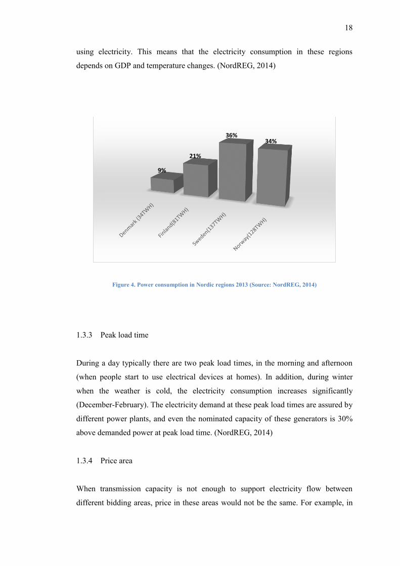
18

using electricity. This means that the electricity consumption in these regions

depends on GDP and temperature changes. (NordREG, 2014)

Figure 4. Power consumption in Nordic regions 2013 (Source: NordREG, 2014)

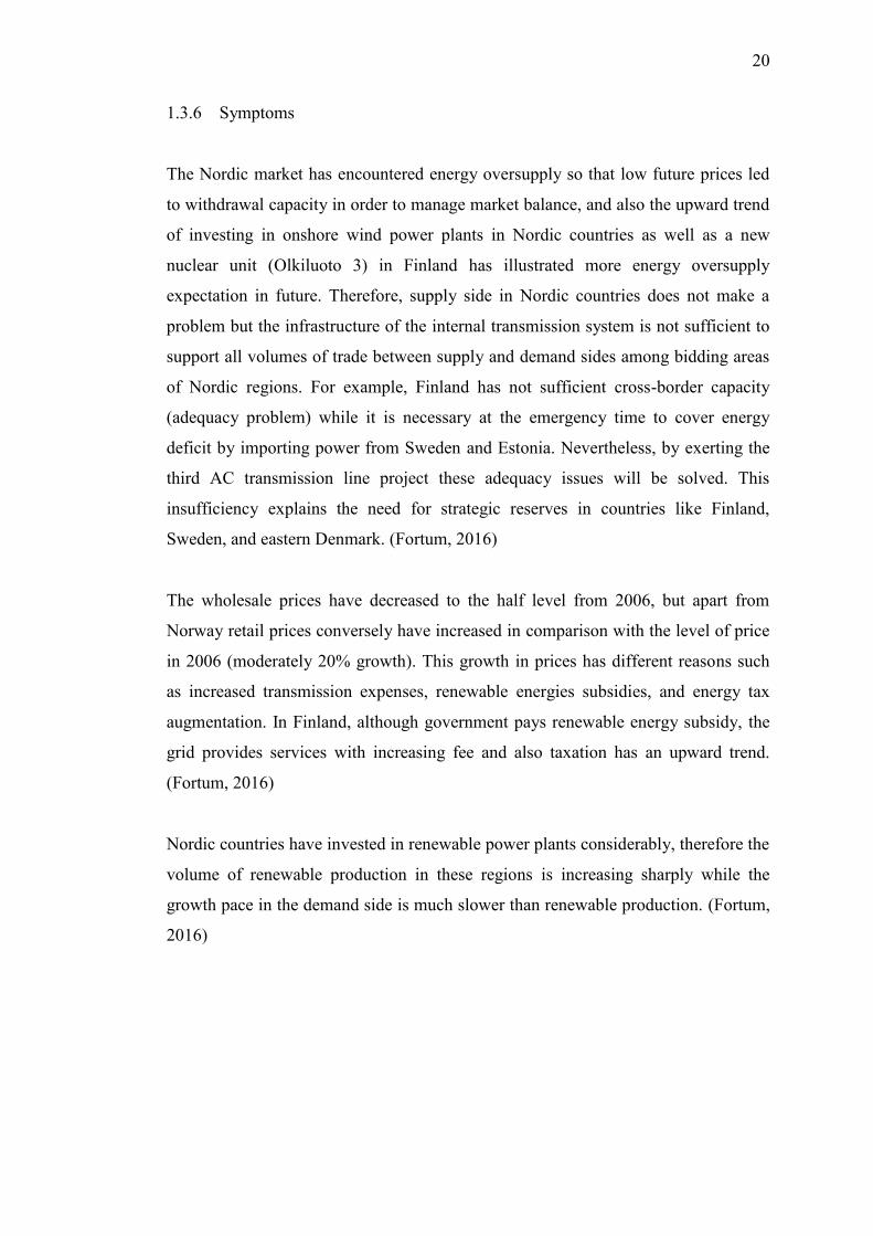
1.3.3 Peak load time

During a day typically there are two peak load times, in the morning and afternoon

(when people start to use electrical devices at homes). In addition, during winter

when the weather is cold, the electricity consumption increases significantly

(December-February). The electricity demand at these peak load times are assured by

different power plants, and even the nominated capacity of these generators is 30%

above demanded power at peak load time. (NordREG, 2014)

1.3.4 Price area

When transmission capacity is not enough to support electricity flow between

different bidding areas, price in these areas would not be the same. For example, in

9%

21%

36% 34%

19

2013 the average amount of difference between prices was about 3.82 euro/MWh.

(NordREG, 2014)

1.3.5 Retail price (Finland)

There are three different types of contracts in Finland consisting of fixed term

contracts (16% of total), permanent contracts or variable price (80% of total), and

permanent spot contracts (4% of total). Therefore, price volatility at the wholesale

market will not affect consumer prices considerably, and consumer price would

change at mid-term or long term. Moreover, in Figure 5, wholesale price is one of the

components of retail price but the proportion of wholesale price to other parts such as

taxes and grid’s cost is not considerable. It means that the correlation between price

volatility in wholesale market and price volatility in the retail market is not very

significant. (NordREG, 2014)

Figure 5. Consumer price structure 2013 (Source: NordREG, 2014)

2.0%

7.4%

12.2%

19.4%

27.4%

31.6%

0.0% 5.0% 10.0% 15.0% 20.0% 25.0% 30.0% 35.0%

TSO FEE

SALES

TAX

VAT

GRID COSTS

ELECTRICITY PRICE

20

1.3.6 Symptoms

The Nordic market has encountered energy oversupply so that low future prices led

to withdrawal capacity in order to manage market balance, and also the upward trend

of investing in onshore wind power plants in Nordic countries as well as a new

nuclear unit (Olkiluoto 3) in Finland has illustrated more energy oversupply

expectation in future. Therefore, supply side in Nordic countries does not make a

problem but the infrastructure of the internal transmission system is not sufficient to

support all volumes of trade between supply and demand sides among bidding areas

of Nordic regions. For example, Finland has not sufficient cross-border capacity

(adequacy problem) while it is necessary at the emergency time to cover energy

deficit by importing power from Sweden and Estonia. Nevertheless, by exerting the

third AC transmission line project these adequacy issues will be solved. This

insufficiency explains the need for strategic reserves in countries like Finland,

Sweden, and eastern Denmark. (Fortum, 2016)

The wholesale prices have decreased to the half level from 2006, but apart from

Norway retail prices conversely have increased in comparison with the level of price

in 2006 (moderately 20% growth). This growth in prices has different reasons such

as increased transmission expenses, renewable energies subsidies, and energy tax

augmentation. In Finland, although government pays renewable energy subsidy, the

grid provides services with increasing fee and also taxation has an upward trend.

(Fortum, 2016)

Nordic countries have invested in renewable power plants considerably, therefore the

volume of renewable production in these regions is increasing sharply while the

growth pace in the demand side is much slower than renewable production. (Fortum,

2016)

21

Figure 6. Wholesale and retail price in Finland (Source: Fortum, 2016)

Consequently, the profitability of generators in the market is at the stake, for

instance, recently in Sweden the wholesale price was less than the operational cost of

nuclear energy while a third of power in Sweden is generated by nuclear power

plants. This incident has led to the withdrawal capacity in different countries.

(Fortum, 2016)

Figure 7. Withdrawal capacity in Nordic regions (Source: Fortum, 2016)

0

20

40

60

80

100

120

140

160

180

2000

2001

2002

2003

2004

2005

2006

2007

2008

2009

2010

2011

2012

2013

2014

2015

2016

2017

2018

2019

2020

2021

2022

2023

2024

2025

2026

Nord Pool System Price Retail Price in Finland

0200400600800

10001200

Hana

saar

i Coa

l CHP

Krist

iina

Tahk

oluo

to

Haap

aves

i Pea

t

Nai

sten

laht

i Gas

-CHP

Ring

hals2

Ring

hals1

Osk

arsh

amn

2

Osk

arsh

amn

1

Fors

mak

3

Stud

stru

pave

rket

Asna

esva

erke

t Coa

l

Nat

urkr

aft's

kår

sto

Finland Sweden DenmarkNorway

Power Plants would be dismantled in Nordic countries ( in the near future)

22

By increasing the application of renewable generators, peak power plants, as well as

CHP power plants, are not profitable anymore and the flexibility of the system is one

of the new issues of the energy system. Hence, scarcity pricing may not be a

successful model for increasing the flexibility of the market because oversupply in

this market prevents any scarcity events and many generators would not able to

finance their operations. This situation brings about negotiations for expanding

capacity remuneration mechanism. (Fortum, 2016)

It has been argued that policy intervention for backing renewable energy in the

market has led to oversupply. Therefore, market incentives do not work appropriately

and a capacity mechanism such as increasing the price caps may decrease this

inefficiency in the market. (Fortum, 2016)

23

2 LITERATURE REVIEW

This study focuses on hourly price elasticity in the day-ahead market. There are not

many papers that have conducted research in hourly price elasticity, but many studies

have surveyed the price elasticity yearly, seasonally or monthly. In addition, some

papers have tried to estimate elasticities for real time pricing (or Time Of Use)

customers but the size of data related to RTP customers is not enough or just

industrial sector has RTP contracts (Kopsakangas Savolainen & Svento, 2012).

Table 2 depicts price elasticities annually, quarterly or monthly in different studies.

Then, the details of studies that have focused on hourly price elasticities would be

explained.

Table 1. The size of price elasticities in different studies

Researcher Country Period Elasticity Comment

Al-Faris, 2002 GCC1

1970-1997

(Annually)

– 0.04, -0.18

(short-term)

– 0.82, -3.39

(long-term)

ECM2 model has

been used in this

study.

Bjorner & Jensen,

2002

Denmark

(Industrial

companies)

1983-1997

(Panel data)

– 0.04, -0.13

(Own-price)

– 0.44, -0.50

(District heating)

Translog Model

and Linear Logit

Model with fixed

effect approach

have been applied.

Filippini &

Pachauri, 2004

India

(Households)

1993-1994

(Monthly)

Winter: -0.42

Monsoon: -0.51

Summer: -0.29

This study has

used single

equation approach

for three different

seasons.

Boonekamp, 2007 Netherlands 1990-2000 – 0.12 This study has

1 The Gulf Cooperation Council countries

2 Error-correction model

24

(Households) (Annually) (Own-price )

used bottom-up

model.

Zachariadis &

Pashourtidou,

2007

Cyprus

(Residential and

services sectors)

1960-2004

(Annually)

– 0.3, -0.4

(Long-term)

This study has

used Vector Error

Correction model.

King &

Chatterjee, 2003

California (U.S.)

(Residential

sector)

Review of

Different study

– 0.0, -0.64

(Houses with

different

segments)

This study has

surveyed various

papers with the

case of study from

California.

Reiss & White,

2002

California (U.S.)

(Residential

sector)

1,307 Households

from 1993 and

1997

– 0,39

(Own-price)

This study has

used a generalized

method of

moments (GMM).

Faruqui &

George, 2005

California (U.S.)

(Residential and

industrial sectors)

2,500 customers

during 2003-2004

0.09

(Substitution

elasticity)

Different sectors

response price

volatility and

shave the peak

load.

2.1 The effects of price lags

Bushnell (2005), has collected data from San Diego during 1998-2000. After

deregulation nonlinear tariffs have affected consumption and this paper attempted to

show the responsiveness to the electricity price volatilities. Lagging price changes in

this study show long-run responses to the changes of prices which have a significant

effect on the electricity consumption. The responsiveness is measured by two

methods. Initially, price response is estimated by utilizing a demand model. Then,

DID3 estimation has been used to find the effect of average monthly because prices

mixed with uncertainty. The results show that consumers’ response more to lagged

prices than real time prices. The elasticity of demand by regarding lagged prices is

about -0.10, but the elasticity of current prices is not significant. This study has

3 Difference-in-difference

25

modeled demand during each day as a function of GDP, weather condition (daylight

and temperature), retail price and dummy variables. Instrumental variables used for

estimating this equation. (Bushnell & Mansur, 2005)

2.2 Supply-Demand Model

Johnsen (2001), has modeled supply-demand in the electricity market in Norway.

Weekly data has been used in this study which covers the period of time from 1994

to 1995. In Norway there are different natural aspects that affect electricity

generation such as snow, changing temperature and inflow. Demand and price

equations have been estimated simultaneously. Therefore, FIML4 procedure is

considered to capture common coefficients. The range of price elasticities is from -

0.05 to -0.35. (Johnsen, 2001)

2.3 Hourly estimation

Patrick (2001), has estimated the half-hour electricity demand in industrial and

commercial sectors in England from 1991 to 1995. Different industries have various

price elasticities as well as within-day substitution elasticity. For instance, the price

elasticity in the water supply industry is significant. It has been reported between -

0.142 to -0.27. (Patrick & Wolak, 2001)

2.4 Weather condition as an independent variable

Taylor (2005), has determined hourly price elasticities in industrial sectors in the

U.S. different factors like weather condition and customer characteristics have been

taken into consideration for estimating equations. By increasing the experience of

customers after facing real time pricing, they have shown that RTP makes enough

incentive for decreasing consumption. Global curvature restriction is one of the terms

that this paper has been observed by using GM5 procedure. The results show that

response has a positive correlation with experience. Hourly own-price and cross-

4 full-information maximum likelihood

5 The Generalized McFadden

26

price elasticities in different industries have been reported by this paper. For

example, at 1 am the average of own-price elasticity for all customers was -0.05 and

at 2 pm it changed to -0.25. The sign of cross-price elasticities was positive and

negative and also among diverse industries, positive own-price elasticities have been

reported. (Taylor, Schwarz, & Cochell, 2005)

Lijesen (2007), uses hourly data related to peak load periods in 2003 from the

Netherlands. Weather condition is an important factor that is considered as an

independent variable in the model. Price elasticity is about -0.0014 from linear model

and it changes to -0.0043 from the log-linear model. (Lijesen, 2007)

2.5 2SLS model

Bönte (2015), has tried to estimate price elasticities by using data from EPEX day-

ahead market. Instrument variable in this study is wind speed because after 2010 the

usage of wind power has increased and today intermittent production is the main part

of electricity supply. This study uses 2SLS model for estimating price elasticities and

it shows that the average price elasticity of demand between 2010, 2014 was about -

0.43. (Bönte, Nielen, Valitov, & Engelmeyer, 2015)

Knaut (2017), surveys the price elasticity of demand in Germany. It shows that the

short-run price volatilities in the day-ahead market can affect consumption. Demand

and supply sides have been considered simultaneously. TSLS procedure has been

applied so that electricity price is estimated by using a renewable source of energy

and then the result sets in the demand equation. The price elasticity at the peak load

is about -0.13. (Knaut & Paulus, 2017)

2.6 Dummy variables

Bye (2008), has used the hourly price of electricity from Nord pool energy exchange

market to estimate hourly price elasticities in two countries including Norway and

Sweden from 2000 to 2004. Demand and supply sides have been estimated

simultaneously by using FIML procedure for achieving reliable coefficients. The

effects of stochastic variables are assumed in the model and different dummy

27

variables have been applied to consider the periodical movements of parameters. The

lagged prices in this study play a pivotal role because their coefficients show long-

term elasticities. It has been shown that in short-run some price elasticities have a

positive sign, and also the size of hourly price elasticities are smaller than other

similar studies from near zero to -0.04.(Bye & Hansen, 2008)

28

3 DATA

This study has used different databases in order to estimate the hourly price elasticity

of demand from 1st hour of 8 January 2013 to the 24

th hour of 31 December 2016 in

Finland.

The Nordpool exchange server provides different electricity data that some of them

have been utilized in the project consisting of hourly electricity consumption in

Finland, hourly system price6, a weekly hydro reservoir in Finland, and hourly net

electricity import (NordPool, 2017). “The Finnish Meteorological Institute’s (FMI)

open data” is used to calculate hourly weighted-temperature in Finland (FMI, 2017),

and hourly data for weighted-daylight is applied from “Timeanddate”. In addition,

monthly coal price is provided by “Statics Finland”. Finally, the weekly gas price is

utilized from “Federal Reserve Economic Data”.

3.1 Consumption and Price

Hourly real time consumption and different lagged consumptions have been applied

in the model, and because consumption data for 2012 is not accessible from

Nordpool server, therefore the period of the survey has started from 8 January 2013.

Consumption data from 1 January 2013 to 7 January 2013 are used to build lagged

consumption variables. Hourly system price and different lagged prices have been

used in both demand and price equations.

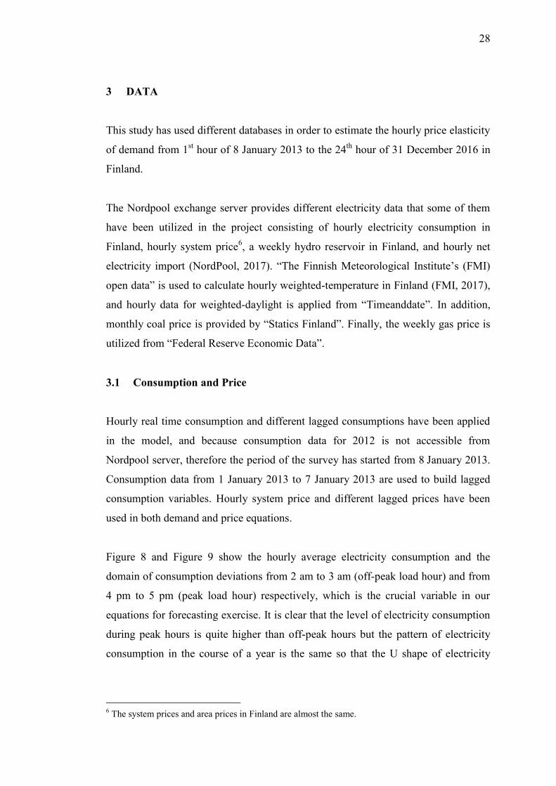
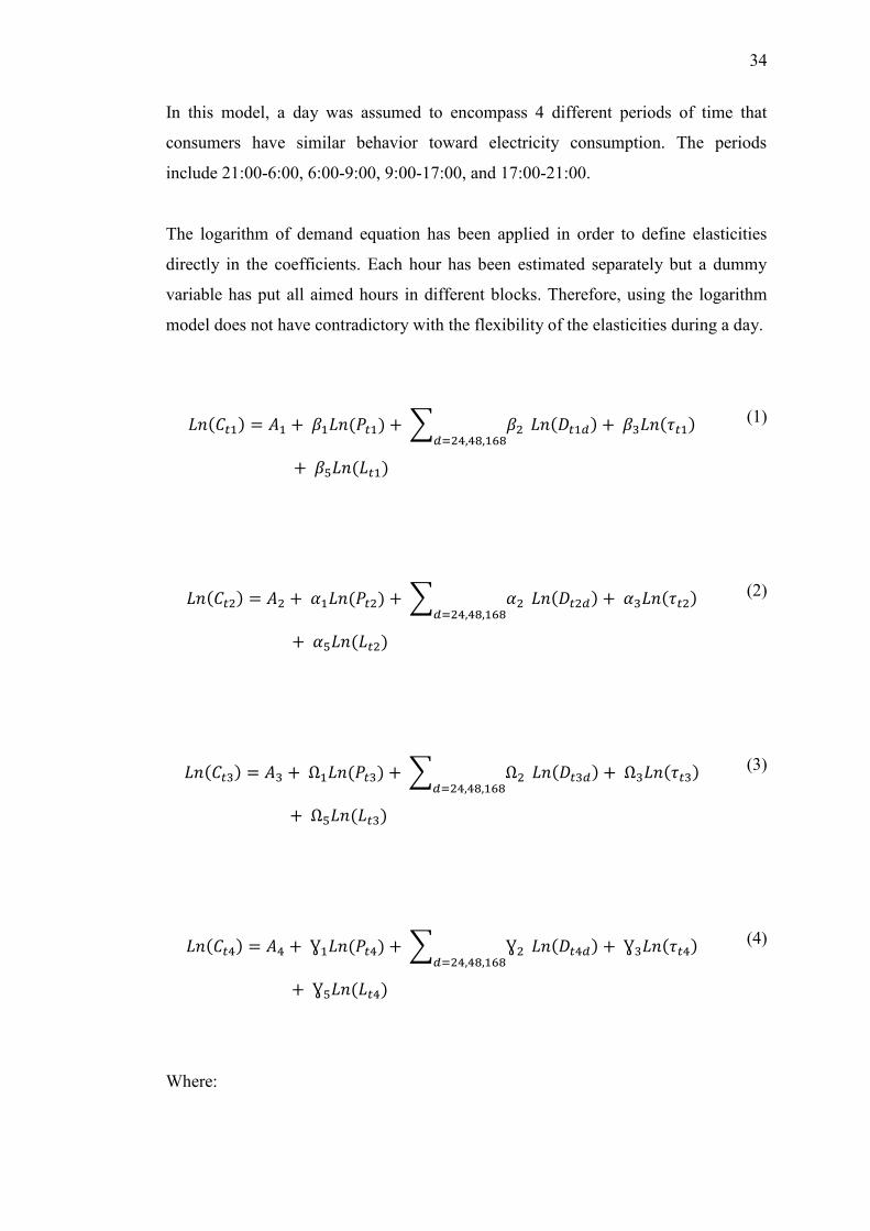
Figure 8 and Figure 9 show the hourly average electricity consumption and the

domain of consumption deviations from 2 am to 3 am (off-peak load hour) and from

4 pm to 5 pm (peak load hour) respectively, which is the crucial variable in our

equations for forecasting exercise. It is clear that the level of electricity consumption

during peak hours is quite higher than off-peak hours but the pattern of electricity

consumption in the course of a year is the same so that the U shape of electricity

6 The system prices and area prices in Finland are almost the same.

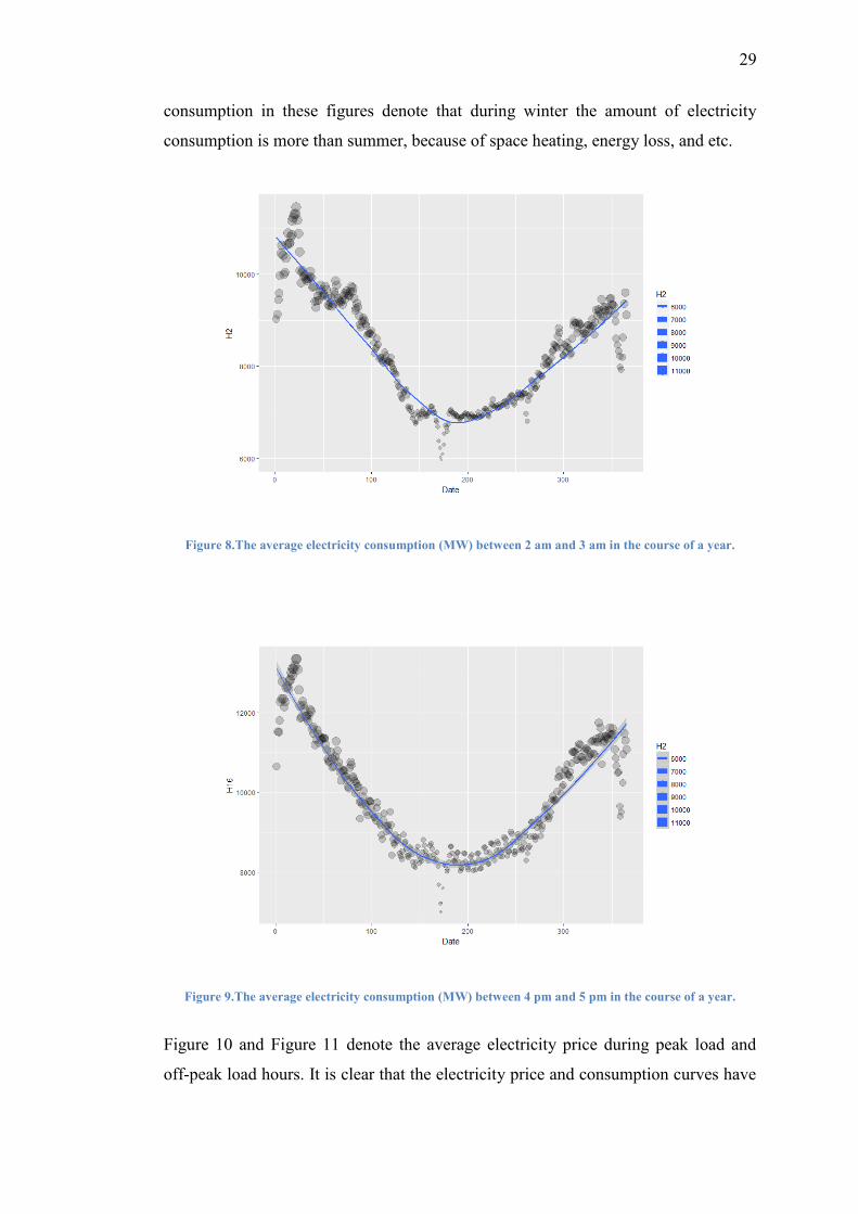
29

consumption in these figures denote that during winter the amount of electricity

consumption is more than summer, because of space heating, energy loss, and etc.

Figure 8.The average electricity consumption (MW) between 2 am and 3 am in the course of a year.

Figure 9.The average electricity consumption (MW) between 4 pm and 5 pm in the course of a year.

Figure 10 and Figure 11 denote the average electricity price during peak load and

off-peak load hours. It is clear that the electricity price and consumption curves have

30

not the same pattern because the consumption has experienced the lowest amount

around the day 200 but the electricity price in peak load time has dropped to the

lowest level around the day 100. Moreover, the electricity price at 2 am has followed

a kind of sine pattern. It seems that the electricity consumption is not able to

illustrate all electricity price changes lonely.

Figure 10.The average electricity price (MW) between 4 pm and 5 pm in the course of a year.

Figure 11.The average electricity price (MW) between 2 am and 3 am in the course of a year.

31

3.2 Temperature

About 18 cities have been used to find the average temperature in Finland and these

include Lappeenranta, Seinäjoki, Savonlinna, Kajaani, Hämeenlinna, Kokkola,

Jämsä, Kouvola, Rovaniemi, Tampere, Vaasa, Joensuu, Oulu, Kuopio, Lahti, Pori,

Helsinki, and Turku. The temperatures of these cities are weighted by their

population. Figure 12 depicts the average weighted temperature and the trend in

comparison with electricity consumption has a reverse slope. It may indicate that by

increasing the level of temperature, electricity consumption would experience a

downward trend and vice versa.

Figure 12.The average weighted temperature throughout a year.

3.3 Light

Daylight among different cities is variable, so that the differences between sun rise

and sun set in two cities from north and south of Finland may exceed one hour. This

study has applied these differences between cities by regarding their populations for

achieving a dummy variable of daylight. Apart from two periods of time from 0:00 to

2:00 and from 10:00 to 14:00 throughout a year that all cities have the same

condition, thus daylight variable is not included in these equations. Other periods of

time, all cities together do not have bright days or dark nights. This variable is

weighted by population the same as temperature and about seven cities have been

32

used for calculating the weighted data consisting of Helsinki, Tampere, Oulu, Turku,

Jyvaskyla, Lahti, and Kuopio.

3.4 Hydro reservoir and Power exchange

Weekly data from Finland is applied for capturing the effect of cheap hydro power in

the system. It has been claimed that the level of water storage has a negative

correlation with the price level.

The power exchange variable has utilized hourly net electricity imported data from

Finland. This variable helps to capture the effect of other countries’ production on

the electricity price in Finland.

3.5 Dummy variables

A week has been separated into four parts including Monday (industry and

commercial sectors start to work at this day), Tuesday-Wednesday-Thursday (normal

working days), Friday (the last day of work), Saturday-Sunday (weekend), and also a

year has been divided to winter and summer. In addition, another dummy variable is

considered to show holidays throughout a year.

33

4 ECONOMETRIC SPECIFICATION

At the first attempt, the hourly price elasticities have been estimated by demand

equation and the electricity demand per day has divided to four categories consist of

hours between 21:00-06:00, 06:00-09:00, 09:00-17:00, and 17:00-21:00. Each week

has 7 days and 28 categories. Therefore, statistical analysis for each category can

provide a convenient intuition about the electricity consumption as well as price in

Finland.

The results show that mean value of price (Euro/MWh) and consumption (MWh)

from Monday to Thursday as well as Sunday experiences the highest amount

between 6 am and 9 am. Friday and Saturday have different patterns so that the

highest mean value of consumption and price is located in the forth category.

In SUR and TSLS procedures, each day has been divided to 24 hours and each hour

has been surveyed in the course of 4 years. These models apply a system of

simultaneous equations and there are three core variables include price, consumption,

and production.

These tables depict that the most consumption has occurred between 6 pm and 7 pm

but the market has experienced the highest price and production between 9 am to 10

am.

This study uses R-studio program to estimate price elasticities. There are different

packages in this environment that make estimations easier than other similar

programs. Three packages that have been used in this project consist of “plm”,

“systemfit”, and “urca”. The statistical analyses are reported in the appendix section.

4.1 Panel data

The first attempt for estimating the price elasticity of electricity demand was based

on demand equation while the supply side was ignored.

34

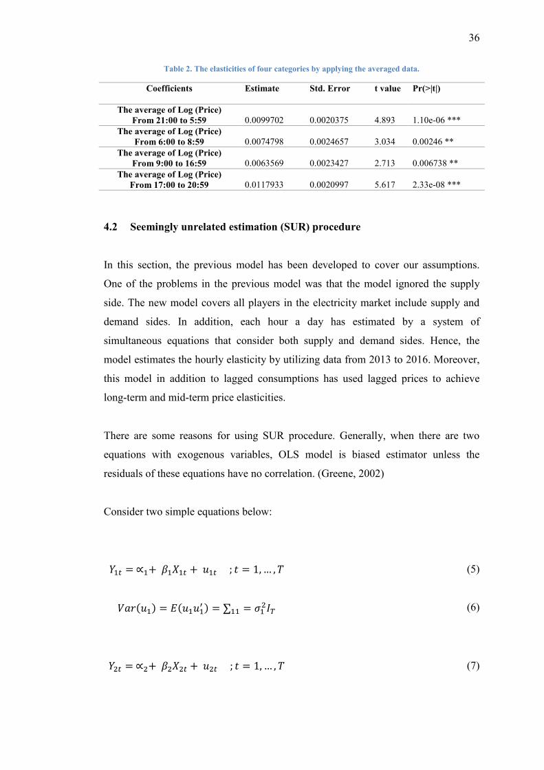
In this model, a day was assumed to encompass 4 different periods of time that

consumers have similar behavior toward electricity consumption. The periods

include 21:00-6:00, 6:00-9:00, 9:00-17:00, and 17:00-21:00.

The logarithm of demand equation has been applied in order to define elasticities

directly in the coefficients. Each hour has been estimated separately but a dummy

variable has put all aimed hours in different blocks. Therefore, using the logarithm

model does not have contradictory with the flexibility of the elasticities during a day.

𝐿𝑛(𝐶𝑡1) = 𝐴1 + 𝛽1𝐿𝑛(𝑃𝑡1) + ∑ 𝛽2 𝑑=24,48,168

𝐿𝑛(𝐷𝑡1𝑑) + 𝛽3𝐿𝑛(𝜏𝑡1)

+ 𝛽5𝐿𝑛(𝐿𝑡1)

(1)

𝐿𝑛(𝐶𝑡2) = 𝐴2 + 𝛼1𝐿𝑛(𝑃𝑡2) + ∑ 𝛼2 𝑑=24,48,168

𝐿𝑛(𝐷𝑡2𝑑) + 𝛼3𝐿𝑛(𝜏𝑡2)

+ 𝛼5𝐿𝑛(𝐿𝑡2)

(2)

𝐿𝑛(𝐶𝑡3) = 𝐴3 + Ω1𝐿𝑛(𝑃𝑡3) + ∑ Ω2 𝑑=24,48,168

𝐿𝑛(𝐷𝑡3𝑑) + Ω3𝐿𝑛(𝜏𝑡3)

+ Ω5𝐿𝑛(𝐿𝑡3)

(3)

𝐿𝑛(𝐶𝑡4) = 𝐴4 + Ɣ1𝐿𝑛(𝑃𝑡4) + ∑ Ɣ2 𝑑=24,48,168

𝐿𝑛(𝐷𝑡4𝑑) + Ɣ3𝐿𝑛(𝜏𝑡4)

+ Ɣ5𝐿𝑛(𝐿𝑡4)

(4)

Where:

35

𝐴 : Intercept

𝛽: Coefficients for first block (include price elasticities)

𝛼: Coefficients for second block (include price elasticities)

Ω: Coefficients for third block (include price elasticities)

Ɣ: Coefficients for fourth block (include price elasticities)

𝑃: The average of system price in each block

𝐷: Dynamic adjustment by a lagged consumption (24 hours, 48 hours, and

168 hours)

𝜏: Temperature

𝐿: Day light

𝐶: The average of electricity consumption in each block.

𝑆𝑢𝑏𝑠𝑐𝑟𝑖𝑝𝑡𝑠: Blocks one, two, three, and four have been shown by 1, 2, 3, and

4, respectively.

Data related to all four equations has been combined and used in a panel data model

to estimate the price elasticities. These equations are presented separately to deliver

the logic behind the assumptions.

The results of this estimation were not promising because the most of the blocks had

positive and insignificant elasticity. These results couldn’t support our literature

review because of positive price elasticities. The reasons behind these unexpected

results could be an unsuitable econometric model, the absence of supply side in our

equation, the absence of lagged prices, or real time inflexibility in the demand side.

The averaged data from four different categories have been applied and the results

are provided in Table 2.7

7 The results of the panel data procedure are available at the appendix part

36

Table 2. The elasticities of four categories by applying the averaged data.

Coefficients Estimate

Std. Error t value Pr(>|t|)

The average of Log (Price)

From 21:00 to 5:59

0.0099702

0.0020375

4.893

1.10e-06 ***

The average of Log (Price)

From 6:00 to 8:59

0.0074798

0.0024657

3.034

0.00246 **

The average of Log (Price)

From 9:00 to 16:59

0.0063569

0.0023427

2.713

0.006738 **

The average of Log (Price)

From 17:00 to 20:59

0.0117933

0.0020997

5.617

2.33e-08 ***

4.2 Seemingly unrelated estimation (SUR) procedure

In this section, the previous model has been developed to cover our assumptions.

One of the problems in the previous model was that the model ignored the supply

side. The new model covers all players in the electricity market include supply and

demand sides. In addition, each hour a day has estimated by a system of

simultaneous equations that consider both supply and demand sides. Hence, the

model estimates the hourly elasticity by utilizing data from 2013 to 2016. Moreover,

this model in addition to lagged consumptions has used lagged prices to achieve

long-term and mid-term price elasticities.

There are some reasons for using SUR procedure. Generally, when there are two

equations with exogenous variables, OLS model is biased estimator unless the

residuals of these equations have no correlation. (Greene, 2002)

Consider two simple equations below:

𝑌1𝑡 = ∝1+ 𝛽1𝑋1𝑡 + 𝑢1𝑡 ; 𝑡 = 1,… , 𝑇

𝑉𝑎𝑟(𝑢1) = 𝐸(𝑢1𝑢1′ ) = ∑11 = 𝜎1

2𝐼𝑇

(5)

(6)

𝑌2𝑡 = ∝2+ 𝛽2𝑋2𝑡 + 𝑢2𝑡 ; 𝑡 = 1, … , 𝑇 (7)

37

𝑉𝑎𝑟(𝑢2) = 𝐸(𝑢2𝑢2′ ) = ∑22 = 𝜎2

2𝐼𝑇 (8)

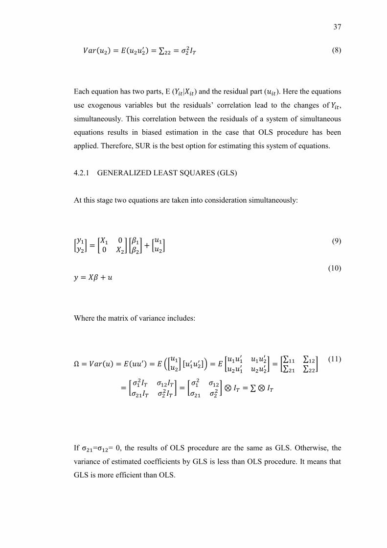
Each equation has two parts, E (𝑌𝑖𝑡|𝑋𝑖𝑡) and the residual part (𝑢𝑖𝑡). Here the equations

use exogenous variables but the residuals’ correlation lead to the changes of 𝑌𝑖𝑡,

simultaneously. This correlation between the residuals of a system of simultaneous

equations results in biased estimation in the case that OLS procedure has been

applied. Therefore, SUR is the best option for estimating this system of equations.

4.2.1 GENERALIZED LEAST SQUARES (GLS)

At this stage two equations are taken into consideration simultaneously:

[𝑦1𝑦2] = [

𝑋1 00 𝑋2

] [𝛽1𝛽2] + [

𝑢1𝑢2]

𝑦 = 𝑋𝛽 + 𝑢

(9)

(10)

Where the matrix of variance includes:

Ω = 𝑉𝑎𝑟(𝑢) = 𝐸(𝑢𝑢′) = 𝐸 ([𝑢1𝑢2] [𝑢1

′𝑢2′ ]) = 𝐸 [

𝑢1𝑢1′ 𝑢1𝑢2

′

𝑢2𝑢1′ 𝑢2𝑢2

′ ] = [∑11 ∑12∑21 ∑22

]

= [𝜎12𝐼𝑇 𝜎12𝐼𝑇

𝜎21𝐼𝑇 𝜎22𝐼𝑇] = [

𝜎12 𝜎12𝜎21 𝜎2

2 ] ⊗ 𝐼𝑇 = ∑⊗ 𝐼𝑇

(11)

If σ21=σ12= 0, the results of OLS procedure are the same as GLS. Otherwise, the

variance of estimated coefficients by GLS is less than OLS procedure. It means that

GLS is more efficient than OLS.

38

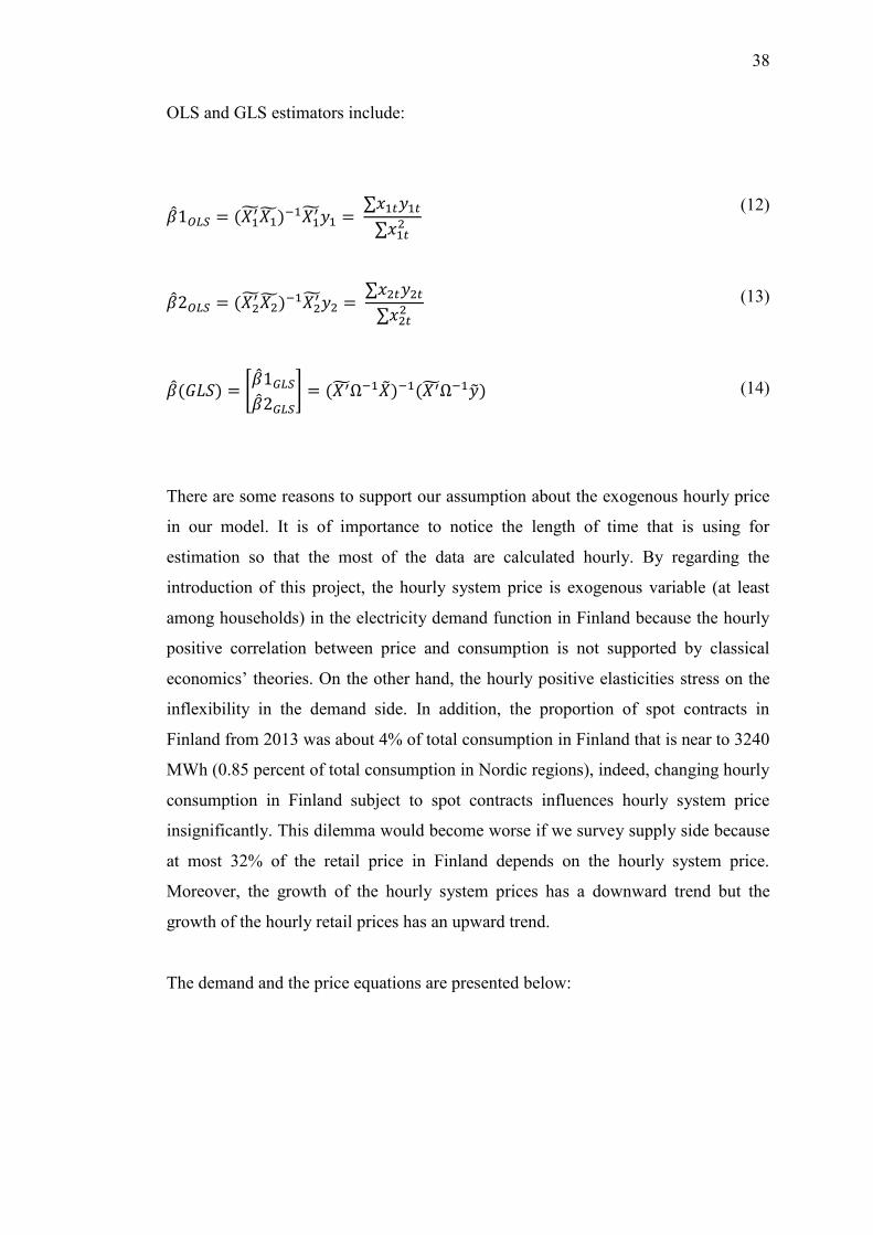
OLS and GLS estimators include:

1𝑂𝐿𝑆 = (𝑋1′𝑋1)

−1𝑋1′𝑦1 =

∑𝑥1𝑡𝑦1𝑡

∑𝑥1𝑡2

2𝑂𝐿𝑆 = (𝑋2′𝑋2)

−1𝑋2′𝑦2 =

∑𝑥2𝑡𝑦2𝑡

∑𝑥2𝑡2

(𝐺𝐿𝑆) = [1𝐺𝐿𝑆2𝐺𝐿𝑆

] = (𝑋 ′Ω−1)−1(𝑋 ′Ω−1)

(12)

(13)

(14)

There are some reasons to support our assumption about the exogenous hourly price

in our model. It is of importance to notice the length of time that is using for

estimation so that the most of the data are calculated hourly. By regarding the

introduction of this project, the hourly system price is exogenous variable (at least

among households) in the electricity demand function in Finland because the hourly

positive correlation between price and consumption is not supported by classical

economics’ theories. On the other hand, the hourly positive elasticities stress on the

inflexibility in the demand side. In addition, the proportion of spot contracts in

Finland from 2013 was about 4% of total consumption in Finland that is near to 3240

MWh (0.85 percent of total consumption in Nordic regions), indeed, changing hourly

consumption in Finland subject to spot contracts influences hourly system price

insignificantly. This dilemma would become worse if we survey supply side because

at most 32% of the retail price in Finland depends on the hourly system price.

Moreover, the growth of the hourly system prices has a downward trend but the

growth of the hourly retail prices has an upward trend.

The demand and the price equations are presented below:

39

𝐿𝑛(𝐶𝑡) =

𝐴 + ∑ 𝛽1𝑏=0,24,72,168,30,13,26 𝐿𝑛(𝑃𝑡−𝑏) + ∑ 𝛽2𝑑=24,48,168 𝐿𝑛(𝐶𝑡−𝑑) +

𝛽3𝐿𝑛(𝜏𝑡) + 𝛽5𝐿𝑛(𝐿𝑡) + 𝛽6𝑀 + 𝛽7𝑇𝑊𝑇 + 𝛽8𝐹 + 𝛽9𝑆𝑆 + 𝛽10Ho + 𝛽11𝑊𝑆

(15)

𝐿𝑛(𝑃𝑡) = 𝐴 + ∑ ∝1𝑏=24,72,168,30,13,26 𝐿𝑛(𝑃𝑡−𝑏) +∝4 𝐿𝑛(𝜏𝑡) + ∝5 𝐿𝑛(𝐻𝑡)

+ ∝6 𝐿𝑛(𝐶𝑜𝑡) + ∝7 𝐿𝑛(𝐺𝑎𝑡)

(16)

Where:

𝐶: Consumption

𝑃: Wholesale price of electricity

𝑀: Monday (Dummy variable)

𝑇𝑊𝑇: Tuesday, Wednesday, and Thursday (Dummy variable)

𝐹: Friday (Dummy variable)

𝑆𝑆: Saturday, and Sunday (Dummy variable)

𝐻𝑜: Holidays (Dummy variable)

𝑊𝑆: Winter-Summer (Dummy variable)

𝐻: Hydro reservoir

𝐶𝑜: Coal price

𝐺𝑎: Gas price

𝛼: Coefficient

Different dummy variables have been applied in order to capture the structural

movements in the equations. Different days of a week, different seasons, and

different holidays might influence the patterns of electricity consumption, thus

utilizing these dummy variables can increase the reliability of estimations.

40

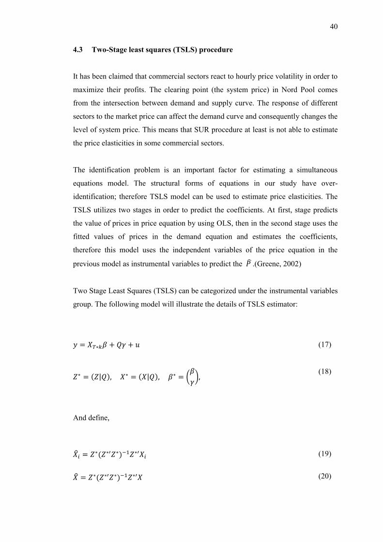
4.3 Two-Stage least squares (TSLS) procedure

It has been claimed that commercial sectors react to hourly price volatility in order to

maximize their profits. The clearing point (the system price) in Nord Pool comes

from the intersection between demand and supply curve. The response of different

sectors to the market price can affect the demand curve and consequently changes the

level of system price. This means that SUR procedure at least is not able to estimate

the price elasticities in some commercial sectors.

The identification problem is an important factor for estimating a simultaneous

equations model. The structural forms of equations in our study have over-

identification; therefore TSLS model can be used to estimate price elasticities. The

TSLS utilizes two stages in order to predict the coefficients. At first, stage predicts

the value of prices in price equation by using OLS, then in the second stage uses the

fitted values of prices in the demand equation and estimates the coefficients,

therefore this model uses the independent variables of the price equation in the

previous model as instrumental variables to predict the 𝑃 .(Greene, 2002)

Two Stage Least Squares (TSLS) can be categorized under the instrumental variables

group. The following model will illustrate the details of TSLS estimator:

𝑦 = 𝑋𝑇∗𝑘𝛽 + 𝑄𝛾 + 𝑢

𝑍∗ = (𝑍|𝑄), 𝑋∗ = (𝑋|𝑄), 𝛽∗ = (𝛽

𝛾),

(17)

(18)

And define,

𝑖 = 𝑍∗(𝑍∗′𝑍∗)−1𝑍∗′𝑋𝑖

= 𝑍∗(𝑍∗′𝑍∗)−1𝑍∗′𝑋

(19)

(20)

41

∗ = 𝑍∗(𝑍∗′𝑍∗)−1𝑍∗′𝑋∗ (21)

Where:

𝑋: Endogenous variables

𝑍: Set of instruments

: Secure the instruments for 𝑋

∗: Secure the instruments for 𝑋∗

The TSLS estimator would be considered as follows,

∗ = (∗′𝑋∗)−1∗′𝑦

and we have the regression of below,

𝑦 = ∗𝛽∗ + 𝑢

therefore, by regarding the instrumental variables,

∗ = (∗′𝑋∗)

−1∗

′(∗𝛽 + 𝑢) = 𝛽 + (∗

′𝑋∗)

−1∗

′𝑢

𝑝𝑙𝑖𝑚 ∗ = 𝛽 + 𝑝𝑙𝑖𝑚(∗′𝑋∗)

−1∗

′𝑢 = 𝛽 + (𝑝𝑙𝑖𝑚

∗′𝑋∗

𝑇)

−1

𝑝𝑙𝑖𝑚∗

′𝑢

𝑇

√𝑇(∗ − 𝛽∗) = (∗

′𝑋∗

𝑇)

−1∗

′𝑢

𝑇

𝑝𝑙𝑖𝑚𝑇(∗ − 𝛽∗)(∗ − 𝛽∗)′= 𝑝𝑙𝑖𝑚(

∗′𝑋∗

𝑇)

−1∗

′𝑢

√𝑇.𝑢′∗

√𝑇 (𝑋∗

′∗

𝑇)

−1

= 𝛿2 (𝑝𝑙𝑖𝑚∗

′𝑋∗

𝑇)

−1

𝑝𝑙𝑖𝑚∗

′∗

𝑇 (𝑝𝑙𝑖𝑚

𝑋∗′∗

𝑇)

−1

(22)

(23)

(24)

(25)

(26)

(27)

42

𝑦𝑖𝑒𝑙𝑑𝑠→ √𝑇(∗ − 𝛽∗) ~ 𝑁(0, 𝑉)

𝑉 = 𝛿2 (𝑝𝑙𝑖𝑚∗

′𝑋∗

𝑇)

−1

𝑝𝑙𝑖𝑚∗

′∗

𝑇 (𝑝𝑙𝑖𝑚

𝑋∗′∗

𝑇)

−1

(28)

The price and demand equations that have been used in this part is the same as

previous model but it is clear that each hour has unique specification, therefore in

hourly estimations all variables are not fitted in the model and different combinations

have been applied in order to increase the efficiency of the models and decrease the

multicollinearity and autocorrelation problems (these equations are general forms of

24 hourly equations).

43

5 RESULTS

The results of estimations that have been procured by applying different models are

not the same because of endogeneity issues. Each hour a day has a unique

specification, therefore it is necessary to survey one by one. It would be helpful to

take a look at electricity consumption pattern before engaging in the interpretation of

the results.

Figure 13 depicts the electricity consumption of two different hours (0:00-1:00,

18:00-19:00) from 2013 to 2016.

Figure 13. Comparing electricity consumption between hour 0:00 and hour 18:00

It is clear that the consumption during off-peak load time (0:00-1:00) is less than

peak load time (18:00-19:00) but this figure does not show the effective sectors

during each period of time.

Figure 14 depicts the electricity consumption by different sectors in Finland during

2016. The share of industry and construction is almost a half of total consumption.

The coincidence that the peak load time and industry consumption happen during a

specific period of time, support the claim that during peak load time a huge

proportion of the electricity consumption depends on industries activities. On the

44

other hand, during off-peak load time, the share of residential sectors from total

consumption can be considerable because the level of industry activities during this

period of time decreases.

Figure 14. Electricity consumption by sector 2016 (Source: Statistics Finland)

Therefore, it seems that from 0:00 to 1:00 the residential sector is more responsive in

comparison to working hours, but the responsiveness of industrial sector during

working hours is relatively higher than other hours a day.

In the following sections, the results of different models that have been applied for

each hour a day will be explained.

5.1 Robustness

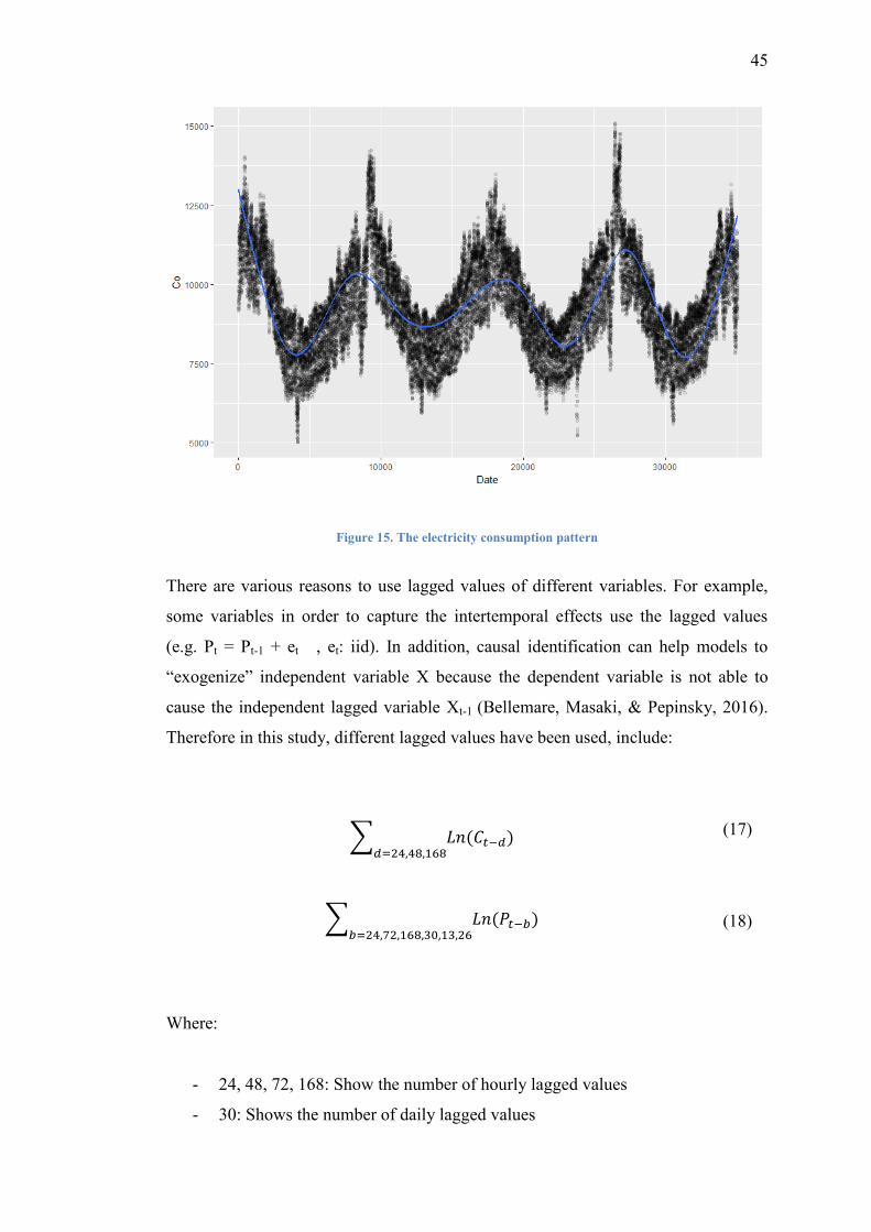
The electricity consumption follows a periodical pattern. Figure 15 shows the sine

movement; therefore lagged consumptions, as well as logarithmic model, can

decrease the effect of autocorrelation problem. Different lags have been utilized in

order to find the best-fitted variables. Throughout a day, each hour has specific

structure so that all lagged consumptions are not significant to be considered in all 24

equations.

45

Figure 15. The electricity consumption pattern

There are various reasons to use lagged values of different variables. For example,

some variables in order to capture the intertemporal effects use the lagged values

(e.g. Pt = Pt-1 + et , et: iid). In addition, causal identification can help models to

“exogenize” independent variable X because the dependent variable is not able to

cause the independent lagged variable Xt-1 (Bellemare, Masaki, & Pepinsky, 2016).

Therefore in this study, different lagged values have been used, include:

∑ 𝐿𝑛(𝐶𝑡−𝑑)𝑑=24,48,168

∑ 𝐿𝑛(𝑃𝑡−𝑏)𝑏=24,72,168,30,13,26

(17)

(18)

Where:

- 24, 48, 72, 168: Show the number of hourly lagged values

- 30: Shows the number of daily lagged values

46

- 13, 26: Show the number of weekly lagged values

The unit root test also has been applied in order to determine the stationary of

electricity price and electricity consumption. Dickey-Fuller test approves that the

logarithm of these variables is stationary or trend-stationary (The sample result is

provided in the appendix part).

Different periods of time have unique structures so that the significant variables

during the specific hour a day may be insignificant throughout the rest of the day.

Therefore, all mentioned variables in the general equations have not been applied in

hourly estimations. For example, dummy variables are not significant throughout

some hours a day and daylight has not been used in estimations from 10 am to 2 pm.

It is clear that general equations include all variables that might be used in 24-hour

estimations.

5.2 SUR Procedure8

The most of the hours between 10:00 and 22:00 have short-run positive elasticities

(Table 3). It shows that customers are not able to shift or decrease their consumption

in short-run during this specific period of time.

Table 3. The price elasticities (SUR model)

Hour RT 24 Lag 72 Lag 168 Lag 30 Lag 13 Lag 26 Lag

0:00 0.0000 – 0.0079

1:00 – 0.0045 – 0.0067

2:00 – 0.0043 – 0.0029

3:00 – 0.0043 – 0.0030

4:00 – 0.0041 – 0.0051

5:00 – 0.0055 – 0.0074

6:00 – 0.0048 – 0.0074

7:00 – 0.0039 – 0.0041

8:00 0.0000 – 0.0042

9:00 0.0000 – 0.0112

10:00 0.0123 – 0.0110 – 0.0140

11:00 0.0178 – 0.0155 – 0.0196

8 The tables of results are available at the appendix part.

47

12:00 0.0148 – 0.0123 – 0.0094

13:00 0.0177 – 0.0096 – 0.0099 – 0.0153

14:00 0.0226 – 0.0102 – 0.0110

15:00 0.0179 – 0.0179

16:00 0.0110 – 0.0164 – 0.0093

17:00 0.0123 – 0.0164

18:00 0.0088 – 0.0122

19:00 0.0000 – 0.0071

20:00 – 0.0037 0.0000

21:00 0.0270 – 0.0206 – 0.0099

22:00 0.0242 – 0.0199 – 0.0085

23:00 – 0.0026 – 0.0018

Where:

- RT: The real time elasticities

- 24 Lag: The mid-term elasticity after 24 hours

- 72 Lag: The mid-term elasticity after 72 hours

- 168 Lag: The mid-term elasticity after 168 hours

- 30 Lag: The long-term elasticity after 30 days

- 13 Lag: The long-term elasticity after 13 weeks

- 26 Lag: The long-term elasticity after 26 weeks

The logic behind the positive elasticities could encompass behavioral reasons or/and

some difficulties to identify appropriate variables in our model. A part of consumers

that have a considerable share of consumption at this period of time, might is not

able to observe real time pricing or has fixed contracts.

On the other hand, all long-term and mid-term price elasticities are negative. The

customers would have enough time to change their consumption in mid-term and

long-term. These responses depend on factors like fixed electricity contracts or the

lack of real time information.

The results show that temperature has a negative effect on the electricity

consumption during a day. The electricity consumption would increase if the

temperature decreases.

Official holidays except Saturday and Sunday have negative effects on the electricity

consumption, but the effect of this dummy variable was not significant between

48

10:00 and 21:00 o’clock. It seems that people during these days do not spend a lot of

time at their homes.

Winter is a season that the electricity consumption increases dramatically. Hence, the

results prove the positive effect of this dummy variable on the amount of electricity

that has been used by customers.

Gas and coal are important fuels that peak power plants use for generating electricity,

therefore an upward trend of the gas price can increase the electricity price. The

results show that the coal and gas prices have significant positive effects on the

electricity price.

The hydro reservoir is an important factor that affects the output of hydro power

plants. The opportunity cost of water depends on the water storage; therefore the

electricity price would decrease if the level of water storage increases. The results

establish the case and it has a negative effect on the electricity price.

The daylight is a dummy variable that shows two different types of electricity

consumption. This variable divides a day into two parts; night includes the electricity

consumption for the sake of electric light, the day includes the electricity

consumption dominated by economic activities. The estimation proves the positive

effect of daylight on the electricity consumption.

Economic activities at the outset of weekdays impose a shock to the system. Monday

as a dummy variable has positive coefficient between 4:00 and 17:00 in the

estimation.

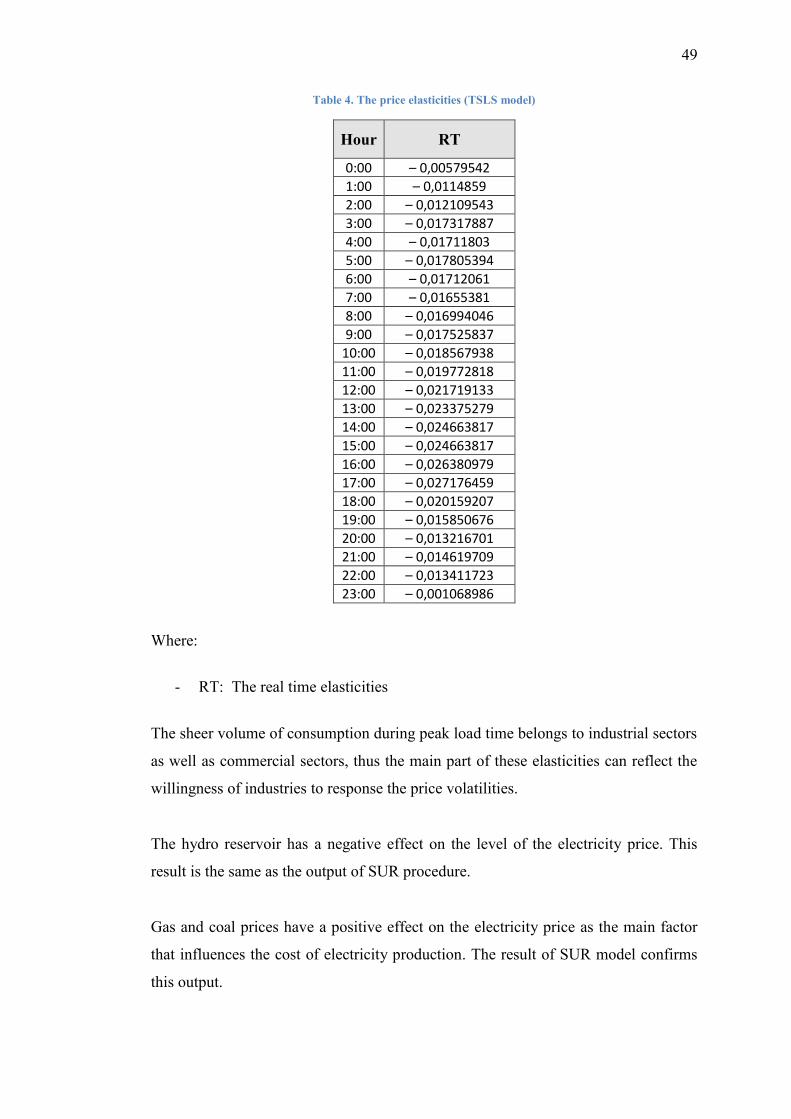
5.3 TSLS Procedure

The results of TSLS model are completely different from SUR model. In Error!

eference source not found. all hourly elasticities are negative but the absolute

values of elasticities during off-peak load times differ from peak load times.

Therefore, there is a tendency for shifting or decreasing the electricity consumption

during peak load time in the short-run.

49

Table 4. The price elasticities (TSLS model)

Hour RT

0:00 – 0,00579542

1:00 – 0,0114859

2:00 – 0,012109543

3:00 – 0,017317887

4:00 – 0,01711803

5:00 – 0,017805394

6:00 – 0,01712061

7:00 – 0,01655381

8:00 – 0,016994046

9:00 – 0,017525837

10:00 – 0,018567938

11:00 – 0,019772818

12:00 – 0,021719133

13:00 – 0,023375279

14:00 – 0,024663817

15:00 – 0,024663817

16:00 – 0,026380979

17:00 – 0,027176459

18:00 – 0,020159207

19:00 – 0,015850676

20:00 – 0,013216701

21:00 – 0,014619709

22:00 – 0,013411723

23:00 – 0,001068986

Where:

- RT: The real time elasticities

The sheer volume of consumption during peak load time belongs to industrial sectors

as well as commercial sectors, thus the main part of these elasticities can reflect the

willingness of industries to response the price volatilities.

The hydro reservoir has a negative effect on the level of the electricity price. This

result is the same as the output of SUR procedure.

Gas and coal prices have a positive effect on the electricity price as the main factor

that influences the cost of electricity production. The result of SUR model confirms

this output.

50

Temperature is one of the main reasons that customers change their electricity

consumption. The coefficient of this variable in both models shows negative effects

on the electricity consumption.

The variable of holidays is another dummy variable that has a negative effect on the

consumption in the both models.

Daylight has positive and negative effects on the electricity consumption subjects to

the period of time. There are some individual hours during peak load time that light

has a positive effect on the consumption but during off-peak load time, some results

show the negative effect of light on the consumption.

Winter and Monday are dummy variables that have positive effects on the

consumption. These results are the same as the results of SUR model.

51

6 CONCLUSION

Nowadays, different countries have a tendency for applying distributed energy

resources (DER) because of environmental and financial issues. Virtual power plants

(VPP) and Smart Grids (SG) use intermittent production and DERs in order to

decentralize the electricity production and increase the reliability of the system. One

of the consequences of intermittent production is the imbalance problem in the

system because these productions have stochastic nature.

There are two ways to increase the reliability of the system and decrease the negative

side effects of intermittent productions. The first solution encompasses the storage

systems that can decline the imbalances in the system, but this solution just focuses

on the supply side to solve the problem. The second solution is increasing the

flexibility of the system by using demand response (DR). Demand response

programs use different incentives and penalties in order to persuade consumers to

shift or decrease their consumption during peak load time. These programs help

smart systems to decline the Co2 emission and increase the reliability of the system

because DR programs try to smooth load curve, thus peak load power plants will shut

down and consequently, Co2 emissions will decrease.

Demand response programs are based on the price elasticities. The willingness of

customers to respond to incentives and penalties determines the prosperousness of

programs. One of the DR programs is called “Real Time Pricing”, customers

monitor the real time price and response to the price volatilities. Therefore, procuring

the proper hourly elasticities can help policy makers to exert these programs at

convenient periods of time, and also they will obtain unbiased prediction about the

results of the DR programs.

This project uses two different methods by regarding the endogeneity of the price in

order to estimate the price elasticities. The reason of applying two different

procedure is that the connection between wholesale price and retail price in Finland

is weak and demand response programs are not able to increase the demand

flexibility due to the exogeneity of price. The range of the price elasticities in SUR

model is from – 0.0023 to 0.0263 in short-term and from 0 to – 0.0198 in long-term.

52

On the other hand, the absolute value of the price elasticities from TSLS model is

quite larger than the estimated coefficients from SUR procedure, therefore by

increasing the connection between wholesale price and retail price it is possible to

achieve significant hourly price elasticities. The range of the price elasticities is from

– 0.0272 to 0. The price elasticities that have been calculated by the majority of

previous studies are larger than the results of this project but it is of importance to

consider the differences between these studies, for example, the most of the previous

studies have used yearly or seasonal data, and also these studies have utilized retail

prices.

There are not many studies that focus on Nord pool market and hourly price

elasticities. Bye (2008), conducted a research on the hourly price elasticities in

Norway and Sweden. The range of their results was from 0 to – 0.04.

In the course of this research and after surveying different data, some structural

problems emerged. For instance, the correlation between system price and

consumption is positive but it is expected that this correlation between retail price

and consumption becomes negative. Therefore, utilizing retail price is more

convenient for calculating the price elasticities. On the other hand, demand response

programs try to smooth the load curve and achieving this aim depends on system

prices.

The pricing system in Finland cannot provide a convenient connection between retail

price and system price. In near future, the cost of electricity production will decrease

dramatically because of the new nuclear sites and intermittent productions.

Customers will suffer from the load imbalance in the system more than before. While

the price elasticities play pivotal function in this situation, but the size of price

elasticities will not be enough to mitigate the negative effects of load imbalance.

Demand response in future should target income and price in order to smooth the

load curve. There are some experiences about bills that based on individuals’ income

but it is necessary to conduct research on the new pricing system in Nord pool

market and the electricity market of Finland to increase the responses of consumers.

53

7 REFERENCES

Al-Faris, A. R. F. (2002). The demand for electricity in the GCC countries. Energy

Policy, 30(2), 117–124. http://doi.org/10.1016/S0301-4215(01)00064-7

Allcott. (2008). Is there an “energy gap”? Allcott, Hunt Greenstone, Michael, 161(4),

145–157. http://doi.org/10.1680/ener.2008.161.4.145

Allcott, H. (2011). Rethinking real-time electricity pricing. Resource and Energy

Economics, 33(4), 820–842. http://doi.org/10.1016/j.reseneeco.2011.06.003

Asmus, P. (2010). Microgrids, Virtual Power Plants and Our Distributed Energy

Future. The Electricity Journal, 23(10), 72–82.

http://doi.org/10.1016/j.tej.2010.11.001

Bellemare, M. F., Masaki, T., & Pepinsky, T. (2016). Lagged Explanatory Variables

and the Estimation of Causal Effects. Journal of Politics, 1–40.

http://doi.org/http://dx.doi.org/10.2139/ssrn.2568724

Bjorner, T. B., & Jensen, H. H. (2002). Interfuel substitution within industrial

companies : An analysis based on pan ...

Bönte, W., Nielen, S., Valitov, N., & Engelmeyer, T. (2015). Price elasticity of

demand in the EPEX spot market for electricity—New empirical evidence.

Economics Letters, 135, 5–8.

http://doi.org/http://dx.doi.org/10.1016/j.econlet.2015.07.007

Boonekamp, P. G. M. (2007). Price elasticities, policy measures and actual

developments in household energy consumption - A bottom up analysis for the

Netherlands. Energy Economics, 29(2), 133–157.

http://doi.org/10.1016/j.eneco.2005.09.010

Bushnell, J. B., & Mansur, E. T. (2005). Consumption under noisy price signals: A

study of electricity retail rate deregulation in San Diego. Journal of Industrial

54

Economics, 53(4), 493–513. http://doi.org/10.1111/j.1467-6451.2005.00267.x

Bye, T., & Hansen, P. V. (2008). How do spot prices affect aggregate electricity

demand? Statistics Norway (SSB), Discussion Papers, 527(527). Retrieved from

www.ssb.no/publikasjoner/pdf/dp527.pdf

Fan, S., & Hyndman, R. J. (2011). The price elasticity of electricity demand in South

Australia. Energy Policy, 39(6), 3709–3719.

http://doi.org/10.1016/j.enpol.2011.03.080

Faruqui, A., & George, S. (2005). Quantifying customer response to dynamic

pricing. Electricity Journal, 18(4), 53–63.

http://doi.org/10.1016/j.tej.2005.04.005

Filippini, M., & Pachauri, S. (2004). Elasticities of electricity demand in urban

Indian households. Energy Policy, 32(3), 429–436.

http://doi.org/10.1016/S0301-4215(02)00314-2

Fortum. (2016). Nordic power market. Fortum Energy Review.

Greene, W. (2002). Econometric Analysis. Pearson Education, Inc. (Vol. 5).

http://doi.org/10.1198/jasa.2002.s458

Hobbs, B. F., Hu, M. C., Iñón, J. G., Stoft, S. E., & Bhavaraju, M. P. (2007). A

dynamic analysis of a demand curve-based capacity market proposal: The PJM

reliability pricing model. IEEE Transactions on Power Systems, 22(1), 3–14.

http://doi.org/10.1109/TPWRS.2006.887954

Johnsen, T. A. (2001). Demand, generation and price in the Norwegian market for

electric power. Energy Economics. http://doi.org/10.1016/S0140-

9883(00)00052-9

King, C. S., & Chatterjee, S. (2003). California Demand Response. Public Utilities

Fortnightly, 27–32.

55

Kirschen, D. S. (2003). Demand-side view of electricity markets. IEEE Transactions

on Power Systems, 18(2), 520–527.

http://doi.org/10.1109/TPWRS.2003.810692

Knaut, A., & Paulus, S. (2017). When Are Consumers Responding to Electricity

Prices ? An Hourly Pattern of Demand Elasticity When are consumers

responding to electricity prices ? An hourly pattern of demand elasticity.

Institute of Energy Economics at the University of Cologne (EWI), (August

2016).

Kopsakangas Savolainen, M., & Svento, R. (2012). Real-Time Pricing in the Nordic

Power markets. Energy Economics, 34(4), 1131–1142.

http://doi.org/10.1016/j.eneco.2011.10.006

Lijesen, M. G. (2007). The real-time price elasticity of electricity. Energy

Economics, 29(2), 249–258. http://doi.org/10.1016/j.eneco.2006.08.008

NordREG. (2014). Development in the Nordic Electricity Market Nordic Market

Report, 60.

Patrick, R. H., & Wolak, F. a. (2001). Estimating the Customer-Level Demand for

Electricity Under Real-Time Market Prices. National Bureau of Economic

Research Working Paper Series, No. 8213. http://doi.org/10.3386/w8213

Reiss, P. C., & White, M. W. (2002). Household Electricity Demand , Revisited

Household Electricity Demand , Revisited, (1830).

Römer, B., Reichhart, P., Kranz, J., & Picot, A. (2012). The role of smart metering

and decentralized electricity storage for smart grids: The importance of positive

externalities. Energy Policy, 50, 486–495.

http://doi.org/10.1016/j.enpol.2012.07.047

Ruokamo, E., & Kopsakangas-Savolainen, M. (2016). Key elements and attributes

affecting prosumers’ behavior, (3.2-6).

56

Sahari, A. (2017). Essays on Households' Technology Choices and Long-Term

Energy Use.Aalto University poblication series, Doctoral Dissertations, 38/2017

Taylor, T. N., Schwarz, P. M., & Cochell, J. E. (2005). 24/7 Hourly response to

electricity real-time pricing with up to eight summers of experience. Journal of

Regulatory Economics, 27(3), 235–262. http://doi.org/10.1007/s11149-005-

6623-6

Wang, Z., & Lemmon, M. (2016). Utility-Scale Microgrids and Day-Ahead

Markets : A New Curtailment ?

Zachariadis, T., & Pashourtidou, N. (2007). An empirical analysis of electricity

consumption in Cyprus. Energy Economics, 29(2), 183–198.

http://doi.org/10.1016/j.eneco.2006.05.002

57

8 APPENDIX

8.1 The statistical analysis

Table 5. The electricity consumption and price on Mondays.

P1 P2 P3 P4 C1 C2 C3 C4

Min. 3.59 12.43 19.38 13.90 6075 7917 7850 7296

1st Qu. 23.87 36.17 35.52 34.33 7832 9010 8997 8670

Median 29.44 43.02 40.98 39.91 8772 9986 9817 9868

Mean 28.92 45.05 43.39 41.50 8946 10134 10031 9993

3rd

Qu. 34.41 51.33 48.96 45.92 9995 11079 10908 11130

Max. 60.02 150.02 167.88 183.52 13994 14155 14087 14064

Table 6.The electricity consumption and price on Tuesdays.

P5 P6 P7 P8 C5 C6 C7 C8

Min. 3.38 9.26 14.08 12.86 5862 7584 7479 7071

1st Qu. 23.93 36.18 35.74 34.94 7825 9017 8988 8700

Median 29.30 42.77 41.39 39.90 8812 10018 9823 9946

Mean 28.95 45.02 42.88 41.98 8931 10091 9990 10019

3rd

Qu. 34.38 48.32 47.03 46.05 9913 11004 10860 11190

Max. 100.08 199.93 198.02 210.01 14113 14406 14335 14409

Table 7.The electricity consumption and price on Wednesdays.

P9 P10 P11 P12 C9 C10 C11 C12

Min. 3.25 7.79 11.96 11.29 5686 7568 7253 6711

1st Qu. 23.66 35.84 35.20 34.49 7824 8995 8986 8682

Median 29.25 43.01 40.33 39.17 8830 10099 9883 9819

Mean 28.94 45.43 42.60 42.54 8971 10117 10032 10009

3rd

Qu. 34.09 50.78 47.06 46.41 9959 11029 10952 11142

Max. 84.75 214.25 200.00 200.09 14523 14888 15105 15043

58

Table 8.The electricity consumption and price on Thursdays.

P13 P14 P15 P16 C13 C14 C15 C16

Min. 0.32 4.01 9.59 6.83 5365 6192 6262 5796

1st Qu. 23.91 36.88 34.89 33.25 7828 9088 9010 8636

Median 28.89 43.47 40.03 37.84 8912 10042 9854 9846

Mean 28.64 46.00 41.64 39.29 8998 10205 10072 9992

3rd

Qu. 33.90 52.87 46.68 43.95 10002 11152 11032 11236

Max. 77.10 134.43 150.01 149.95 14631 14802 14756 14399

Table 9.The electricity consumption and price on Fridays.

P17 P18 P19 P20 C17 C18 C19 C20

Min. 3.72 4.48 6.26 6.99 5035 5370 5736 5819

1st Qu. 22.76 24.11 25.54 27.34 7484 7878 8084 8185

Median 27.91 29.95 31.47 34.02 8592 8845 8965 9455

Mean 27.35 29.46 30.90 33.61 8656 8939 9193 9596

3rd

Qu. 32.95 35.09 36.57 38.74 9661 9820 10134 10853

Max. 53.19 60.85 62.24 82.70 12982 12971 13643 13808

Table 10.The electricity consumption and price on Saturdays.

P21 P22 P23 P24 C21 C22 C23 C24

Min. 1.03 1.15 6.78 6.79 5020 5402 5932 6051

1st Qu. 20.94 20.38 24.07 26.45 7352 7452 7812 7964

Median 26.89 26.66 30.03 32.12 8416 8366 8702 9137

Mean 26.43 26.22 29.24 31.55 8515 8504 8901 9283

3rd

Qu. 32.44 32.76 35.01 36.95 9480 9438 9898 10490

Max. 58.04 47.43 55.11 60.71 13121 12453 13367 13465

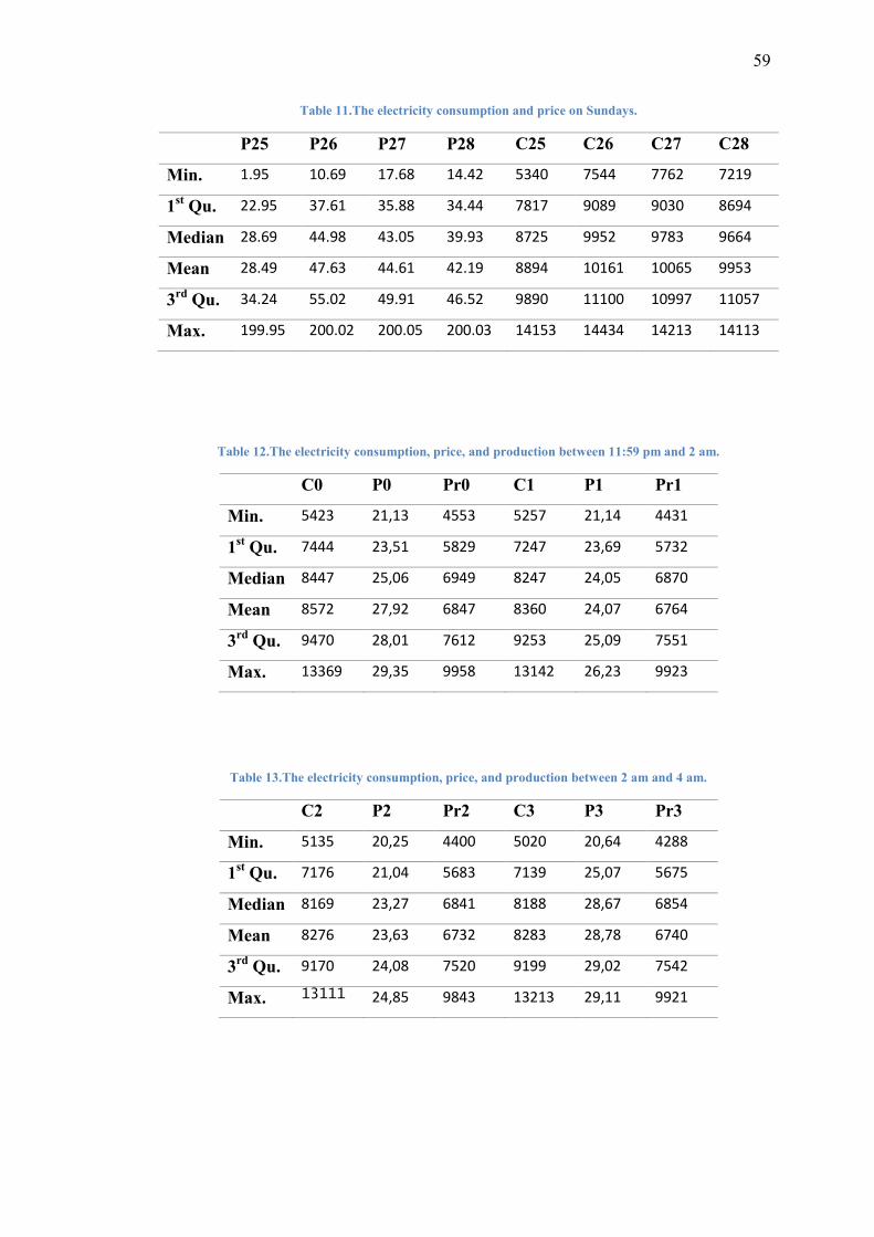
59

Table 11.The electricity consumption and price on Sundays.

P25 P26 P27 P28 C25 C26 C27 C28

Min. 1.95 10.69 17.68 14.42 5340 7544 7762 7219

1st Qu. 22.95 37.61 35.88 34.44 7817 9089 9030 8694

Median 28.69 44.98 43.05 39.93 8725 9952 9783 9664

Mean 28.49 47.63 44.61 42.19 8894 10161 10065 9953

3rd

Qu. 34.24 55.02 49.91 46.52 9890 11100 10997 11057

Max. 199.95 200.02 200.05 200.03 14153 14434 14213 14113

Table 12.The electricity consumption, price, and production between 11:59 pm and 2 am.

C0 P0 Pr0 C1 P1 Pr1

Min. 5423 21,13 4553 5257 21,14 4431

1st Qu. 7444 23,51 5829 7247 23,69 5732

Median 8447 25,06 6949 8247 24,05 6870

Mean 8572 27,92 6847 8360 24,07 6764

3rd

Qu. 9470 28,01 7612 9253 25,09 7551

Max. 13369 29,35 9958 13142 26,23 9923

Table 13.The electricity consumption, price, and production between 2 am and 4 am.

C2 P2 Pr2 C3 P3 Pr3

Min. 5135 20,25 4400 5020 20,64 4288

1st Qu. 7176 21,04 5683 7139 25,07 5675

Median 8169 23,27 6841 8188 28,67 6854

Mean 8276 23,63 6732 8283 28,78 6740

3rd

Qu. 9170 24,08 7520 9199 29,02 7542

Max. 13111 24,85 9843 13213 29,11 9921

60

Table 14.The electricity consumption, price, and production between 4 am and 6 am.

C4 P4 Pr4 C5 P5 Pr5

Min. 5022 19,87 4247 5125 24,08 4224

1st Qu. 7260 19,96 5709 7849 24,52 6003

Median 8422 21,07 6956 9001 25,08 7178

Mean 8492 23,18 6837 9100 25,17 7125

3rd

Qu. 9478 24,84 7674 10206 29,94 8028

Max. 13602 26,86 10095 14414 30,07 10942

Table 15.The electricity consumption, price, and production between 6 am and 8 am.

C6 P6 Pr6 C7 P7 Pr7

Min. 5241 25,43 4376 5370 20,43 4483

1st Qu. 8373 32,14 6376 8651 30 6662

Median 9333 33,27 7480 9556 34,07 7670

Mean 9494 34,95 7504 9719 41,89 7763

3rd

Qu. 10651 36,53 8522 10874 42,02 8805

Max. 14631 38,33 11543 14888 43,06 11632

Table 16.The electricity consumption, price, and production between 8 am and 10 am.

C8 P8 Pr8 C9 P9 Pr9

Min. 5552 34,01 4601 5673 24,44 4892

1st Qu. 8823 34,92 6813 8903 30,31 6857

Median 9661 35,38 7766 9676 34,42 7787

Mean 9811 36,91 7864 9837 42,44 7874

3rd

Qu. 10884 39,08 8869 10812 44,81 8833

Max. 14808 41,94 11843 14797 45,04 11754

61

Table 17.The electricity consumption, price, and production between 10 am and 12 am.

C10 P10 Pr10 C11 P11 Pr11

Min. 5736 30,52 5058 5779 30,17 5111

1st Qu. 8953 30,96 6891 8948 37,95 6861

Median 9676 34,97 7793 9627 40,03 7767

Mean 9849 35,76 7850 9833 41,5 7810

3rd

Qu. 10797 44,97 8740 10754 43,58 8664

Max. 14791 45,02 11616 14747 45 11444

Table 18.The electricity consumption, price, and production between 12 am and 2 pm.

C12 P12 Pr12 C13 P13 Pr13

Min. 5789 25 4956 5776 28,53 4840

1st Qu. 8884 35,2 6831 8812 29,42 6753

Median 9539 36,02 7697 9465 30,12 7617

Mean 9755 39,94 7753 9689 34,48 7710

3rd

Qu. 10663 42,54 8599 10632 36,07 8579

Max. 14670 48,03 11394 14647 44,03 11396

Table 19.The electricity consumption, price, and production between 2 pm and 4 pm.

C14 P14 Pr14 C15 P15 Pr15

Min. 5823 29,76 4893 5859 33,32 4976

1st Qu. 8754 29,94 6658 8678 34,45 6601

Median 9445 34,47 7572 9431 34,49 7571

Mean 9700 34,49 7704 9741 35,02 7730

3rd

Qu. 10689 35,84 8675 10825 36,41 8809

Max. 14716 36,09 11556 15075 39,99 11617

62

Table 20.The electricity consumption, price, and production between 4 pm and 6 pm.

C16 P16 Pr16 C17 P17 Pr17

Min. 5897 33,59 4938 5933 30,89 4945

1st Qu. 8634 34,15 6540 8562 34,44 6548

Median 9489 34,43 7658 9607 34,47 7767

Mean 9808 34,44 7767 9848 36,99 7820

3rd

Qu. 10991 36,94 8874 11091 37,93 8948

Max. 15105 39,95 11666 15043 42 11722

Table 21.The electricity consumption, price, and production between 6 pm and 8 pm.

C18 P18 Pr18 C19 P19 Pr19

Min. 5963 28,18 4966 5928 29,94 4993

1st Qu. 8592 34,07 6584 8584 31,92 6580

Median 9792 36,59 7860 9780 31,96 7785

Mean 9926 40,99 7831 9846 33,13 7730

3rd

Qu. 11128 41,91 8901 10940 36,07 8669

Max. 14982 41,94 11624 14829 37,23 11540

Table 22.The electricity consumption, price, and production between 8 pm and 10 pm.

C20 P20 Pr20 C21 P21 Pr21

Min. 5796 33,51 4842 5904 24,08 4814

1st Qu. 8353 34,02 6501 8415 24,75 6383

Median 9444 34,42 7572 9450 30,33 7402

Mean 9509 34,48 7522 9543 30,78 7371

3rd

Qu. 10467 34,99 8329 10507 32,42 8127

Max. 14342 37,56 11127 14303 34,04 10795

63

Table 23.The electricity consumption, price, and production between 10 pm and 00:00.

C22 P22 Pr22 C23 P23 Pr23

Min. 5999 24,77 4802 5788 19,03 4697

1st Qu. 8239 27,82 6225 7804 24,08 6009

Median 9272 29,76 7220 8824 24,72 7054

Mean 9372 30,02 7205 8929 28,07 6989

3rd

Qu. 10288 34,04 7945 9834 28,1 7737

Max. 14074 34,99 10545 13643 34,59 10317

8.2 The results of the panel data estimation

Table 24. The panel data estimation by applying the averaged data from 6:00 to 8:59

Coefficients Estimate

Std. Error t value Pr(>|t|)

(Intercept) 5.0491451 0.1088866 46.371 < 2e-16 ***

The average of Log (Price) 0.0074798 0.0024657 3.034 0.00246 **

The average of Log (Price) with

seven day lag

-0.0205426

0.0024946 -8.235 3.98e-16 ***

Dummy variable Holyday -0.0216109

0.0052949 -4.081 4.72e-05 ***

The average of Log (Consumption)

with 24 hour lag

0.4436429

0.0120567 36.796 < 2e-16 ***

The average of Temperature -0.0077472 0.0002075 -37.336 < 2e-16 ***

Dummy variable winter-summer 0.0308069 0.0027878 11.051 < 2e-16 ***

Dummy variable Monday 0.0626938 0.0032846 19.087 < 2e-16 *** Adjusted R-squared: 0.95 F-statistic: 3946 on 7 and 1446 DF

p-value: < 2.2e-16

Signif. codes: 0 ‘***’ 0.001 ‘**’ 0.01 ‘*’ 0.05 ‘.’ 0.1 ‘ ’ 1

Table 25.The panel data estimation by applying the averaged data from 9:00 to 16:59.

Coefficients Estimate

Std. Error t value Pr(>|t|)

(Intercept) 3.5067657 0.1237464 28.338 < 2e-16 ***

The average of Log (Price) 0.0063569 0.0023427 2.713 0.006738 **

The average of Log (Price) with

one day lag

-0.0126412 0.0034343 -3.681 0.000241 ***

The average of Log (Consumption)

with 24 hour lag

0.4830422 0.0160039 30.183 < 2e-16 ***

The average of Log (Consumption)

with 48 hour lag

0.1257085 0.0124640 10.086 < 2e-16 ***

The average of Temperature -0.0067547 0.0001922 -35.153 < 2e-16 ***

Dummy variable winter-summer 0.0178464 0.0026195 6.813 1.4e-11 ***

Dummy variable Holydays -0.0160374 0.0046997 -3.412 0.000662 ***

Dummy variable Monday 0.0424562 0.0025487 16.658 < 2e-16 ***

Adjusted R-squared: 0.9609 F-statistic: 4459 on 8 and 1445 DF

p-value: < 2.2e-16

Signif. codes: 0 ‘***’ 0.001 ‘**’ 0.01 ‘*’ 0.05 ‘.’ 0.1 ‘ ’ 1

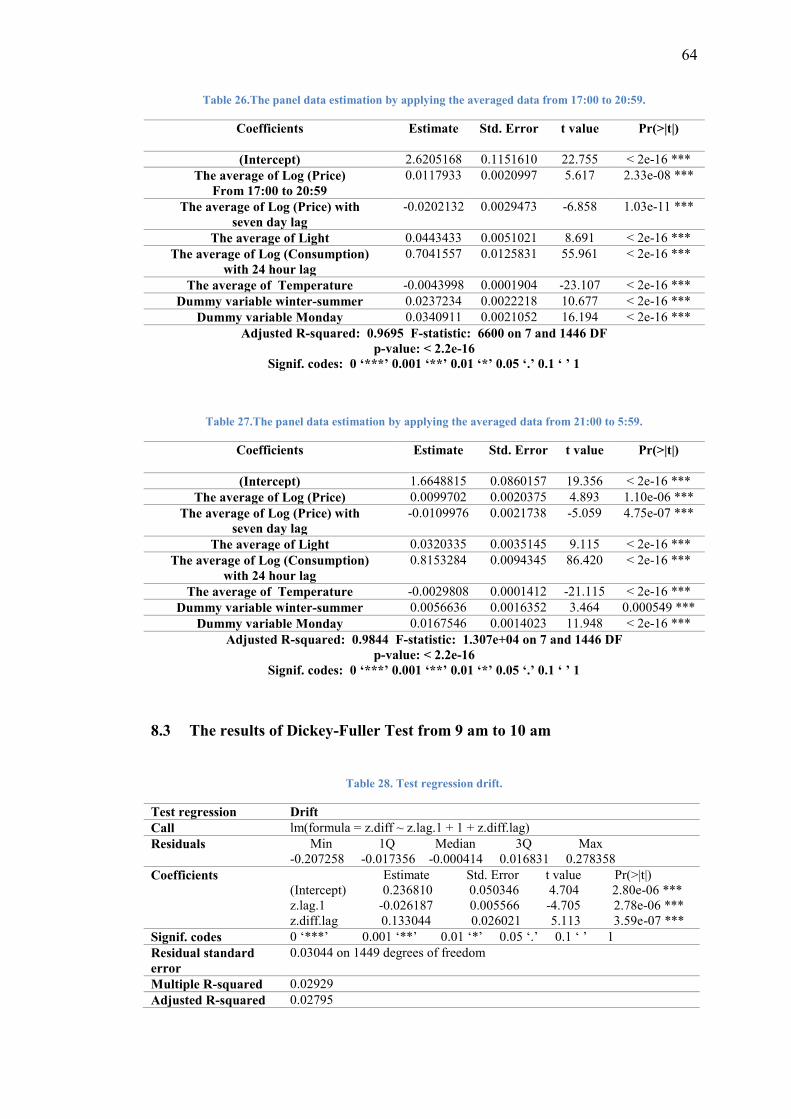
64

Table 26.The panel data estimation by applying the averaged data from 17:00 to 20:59.

Coefficients Estimate

Std. Error t value Pr(>|t|)

(Intercept) 2.6205168 0.1151610 22.755 < 2e-16 ***

The average of Log (Price)

From 17:00 to 20:59

0.0117933 0.0020997 5.617 2.33e-08 ***

The average of Log (Price) with

seven day lag

-0.0202132 0.0029473 -6.858 1.03e-11 ***

The average of Light 0.0443433 0.0051021 8.691 < 2e-16 ***

The average of Log (Consumption)

with 24 hour lag

0.7041557 0.0125831 55.961 < 2e-16 ***

The average of Temperature -0.0043998 0.0001904 -23.107 < 2e-16 ***

Dummy variable winter-summer 0.0237234 0.0022218 10.677 < 2e-16 ***

Dummy variable Monday 0.0340911 0.0021052 16.194 < 2e-16 ***

Adjusted R-squared: 0.9695 F-statistic: 6600 on 7 and 1446 DF

p-value: < 2.2e-16

Signif. codes: 0 ‘***’ 0.001 ‘**’ 0.01 ‘*’ 0.05 ‘.’ 0.1 ‘ ’ 1

Table 27.The panel data estimation by applying the averaged data from 21:00 to 5:59.

Coefficients Estimate

Std. Error t value Pr(>|t|)

(Intercept) 1.6648815 0.0860157 19.356 < 2e-16 ***

The average of Log (Price) 0.0099702 0.0020375 4.893 1.10e-06 ***

The average of Log (Price) with

seven day lag

-0.0109976 0.0021738 -5.059 4.75e-07 ***

The average of Light 0.0320335 0.0035145 9.115 < 2e-16 ***

The average of Log (Consumption)

with 24 hour lag

0.8153284 0.0094345 86.420 < 2e-16 ***

The average of Temperature -0.0029808 0.0001412 -21.115 < 2e-16 ***

Dummy variable winter-summer 0.0056636 0.0016352 3.464 0.000549 ***

Dummy variable Monday 0.0167546 0.0014023 11.948 < 2e-16 ***

Adjusted R-squared: 0.9844 F-statistic: 1.307e+04 on 7 and 1446 DF

p-value: < 2.2e-16

Signif. codes: 0 ‘***’ 0.001 ‘**’ 0.01 ‘*’ 0.05 ‘.’ 0.1 ‘ ’ 1

8.3 The results of Dickey-Fuller Test from 9 am to 10 am

Table 28. Test regression drift.

Test regression Drift

Call lm(formula = z.diff ~ z.lag.1 + 1 + z.diff.lag)

Residuals Min 1Q Median 3Q Max

-0.207258 -0.017356 -0.000414 0.016831 0.278358

Coefficients Estimate Std. Error t value Pr(>|t|)

(Intercept) 0.236810 0.050346 4.704 2.80e-06 ***

z.lag.1 -0.026187 0.005566 -4.705 2.78e-06 ***

z.diff.lag 0.133044 0.026021 5.113 3.59e-07 ***

Signif. codes 0 ‘***’ 0.001 ‘**’ 0.01 ‘*’ 0.05 ‘.’ 0.1 ‘ ’ 1

Residual standard

error

0.03044 on 1449 degrees of freedom

Multiple R-squared 0.02929

Adjusted R-squared 0.02795

65

F-statistic 21.86 on 2 and 1449 DF

p-value 4.433e-10

Value of test-statistic -4.7052 11.0709

Critical values for

test statistics

1pct 5pct 10pct

tau2 -3.43 -2.86 -2.57

phi1 6.43 4.59 3.78

Table 29.Test regression trend

Test regression Trend

Call lm(formula = z.diff ~ z.lag.1 + 1 + tt + z.diff.lag)

Residuals Min 1Q Median 3Q Max

-0.207380 -0.017437 -0.000462 0.016846 0.278234

Coefficients Estimate Std. Error t value Pr(>|t|)

(Intercept) 2.362e-01 5.042e-02 4.685 3.06e-06 ***

z.lag.1 -2.616e-02 5.569e-03 -4.698 2.88e-06 ***

tt 4.526e-07 1.907e-06 0.237 0.812

z.diff.lag 1.330e-01 2.603e-02 5.107 3.70e-07 ***

Signif. codes 0 ‘***’ 0.001 ‘**’ 0.01 ‘*’ 0.05 ‘.’ 0.1 ‘ ’ 1

Residual standard

error

0.03045 on 1448 degrees of freedom

Multiple R-squared 0.02933

Adjusted R-squared 0.02732

F-statistic 14.58 on 3 and 1448 DF

p-value 2.327e-09

Value of test-statistic -4.6975 7.3946 11.0902

Critical values for

test statistics

1pct 5pct 10pct

tau3 -3.96 -3.41 -3.12

phi2 6.09 4.68 4.03

phi3 8.27 6.25 5.34