Nanoimaging Cells Using Soft X-Ray Tomography

457

Alioscka A. Sousa and Michael J. Kruhlak (eds.), Nanoimaging: Methods and Protocols, Methods in Molecular Biology, vol. 950,DOI 10.1007/978-1-62703-137-0_25, © Springer Science+Business Media, LLC 2013

Chapter 25

Nanoimaging Cells Using Soft X-Ray Tomography

Dilworth Y. Parkinson , Lindsay R. Epperly , Gerry McDermott , Mark A. Le Gros , Rosanne M. Boudreau , and Carolyn A. Larabell

Abstract

Soft X-ray microscopy is ideally suited to visualizing and quantifying biological cells. Specimens, including eukaryotic cells, are imaged intact, unstained and fully hydrated, and therefore visualized in a near-native state. The contrast in soft X-ray microscopy is generated by the differential attenuation of X-rays by the molecules in the specimen—water is relatively transmissive to this type of illumination compared to carbon and nitrogen. The attenuation of X-rays by the specimen follows the Beer–Lambert law, and therefore both linear and a quantitative measure of thickness and chemical species present at each point in the cell. In this chapter, we will describe the procedures and computational methods that lead to 50 nm (or better) tomographic reconstructions of cells using soft X-ray microscope data, and the subsequent segmentation and analysis of these volumetric reconstructions. In addition to being a high- fi delity imaging modality, soft X-ray tomography is relatively high-throughput; a complete tomographic data set can be collected in a matter of minutes. This new modality is being applied to imaging cells that range from small prokaryotes to stem cells obtained from mammalian tissues.

Key words: Cell structure , Microscopy , Nanoimaging , Reconstruction , Soft X-ray tomography , Segmentation , Visualization

Soft X-ray tomography (SXT) is a relatively recent addition to the spectacular array of imaging techniques available to biologists ( 1 ) . As with all modalities, SXT fi lls a niche as being the optimal imag-ing technique for answering a particular set of questions ( 2 ) . Speci fi cally, SXT is uniquely suited to high-resolution, quantitative imaging of cells that are intact, unstained and fully hydrated—in other words, SXT excels at visualizing cells, including eukaryotic cells, that are held in a near-native state, and are, therefore, highly representative of the in vivo fully functional cell ( 1, 2 ) .

The interior of a cell is highly organized and fi nely structured ( 1 ) . This is especially true in the case of eukaryotic cells that are

1. Introduction

458 D.Y. Parkinson et al.

partitioned into functionally discrete subcellular spaces termed organelles ( 3– 5 ) . In a 2-dimensional projection image of a cell these structural features are superimposed, making interpretation dif fi cult, if not impossible. As a consequence, the subcellular archi-tecture must be imaged in 3-dimensions. Since microscopes can only produce 2-dimensional images this may appear at fi rst sight to be a major hurdle. However, in practice it is a relatively straightfor-ward process to calculate 3-dimensional views from 2-dimensional data by the application of methods such as deconvolution or tomography ( 6 ) . In the case of tomography, this simply means taking 2-dimensional images of the specimen from a number of different perspectives, usually at angular intervals around a rotation axis. Provided a suf fi cient number of images are taken, a fully isotropic, 3-dimensional representation of the specimen can be calculated from 2-dimensional imaging data ( 7 ) . For SXT, a series (or “stack”) of images of the specimen are taken in this manner using a soft X-ray microscope ( 8 ) . This contains all of the information necessary to calculate a volumetric reconstruction of the entire fi eld of view over which imaging data was collected ( 9 ) . In the case of small prokaryotic cells, the fi eld of view may contain many tens or even hundreds of cells. For larger cells, such as eukaryotic cells, this number is obviously lower. For yeast, each fi eld of view typically contains a maximum of six cells, and for higher order cells this will typically be a single cell. However, since SXT data collection is relatively rapid—standard exposure times for each image are on the order of 100 ms; a data set contains 90 or 180 images—the specimen throughput is still exceptionally high compared to other high-resolution cellular imaging modalities, even for large eukaryotic cells ( 9 ) . Consequently, a large number of cells can be character-ized in a relatively short space of time. For example, in two recently published studies quantifying yeast morphology, data from hundreds of high-resolution tomographic reconstructions were used in the analyses ( 5, 10 ) . Neither of these types of nanoimaging studies could have been carried out using alternative techniques, such as electron tomography.

The specimen in SXT is illuminated using photons with ener-gies that lie in the so-called water window region of the electro-magnetic spectrum ( 11 ) . The attenuation of these photons follows the Beer–Lambert Law, and is therefore linear, quantitative and dependent on chemical species and thickness. Carbon and nitro-gen—major constituents of most biomolecules—attenuate the transmission of X-rays an order of magnitude more strongly than water ( 12 ) . This characteristic produces exquisite contrast in SXT images of cells ( 5, 8, 13, 14 ) . As a result, subcellular structures in an SXT reconstruction can be readily identi fi ed and “segmented” (i.e., isolated from the other contents in the reconstruction) based on their shape and the measured linear absorption coef fi cient (LAC) at each point in the cell ( 8, 12, 13, 15, 16 ) ). Each organelle type

45925 Nanoimaging Cells Using Soft X-Ray Tomography

has a characteristic LAC. This re fl ects the organelle’s biochemical composition. For example, yeast vacuoles have a low concentration of biomolecules and relatively high water content. Their LAC is, therefore, small compared with organelles that have low water content and are densely packed with biomolecules, for example the nucleus. The LAC values allow individual organelles to be identi fi ed and isolated, and provide key information on the internal structure of the organelle. Segmentation of the subcellular contents allows valuable quantitative analyses to be carried out. For example, it is easy to determine key parameters such as the volume and density of the organelles at key stages in the cell cycle, or how these param-eters are affected by exposure to external in fl uences, such as the presence or absence of speci fi c molecules, temperature, con fl uence, and so on. This information is enormously valuable in studies rang-ing from basic cell biology to applied research aimed at generating new pharmaceuticals or in optimizing the economics of biofuel production.

We will now describe the methods and steps needed to image a sample of cells using SXT, beginning with specimen preparation.

Currently, soft X-ray microscopes are primarily located at synchrotron light sources. However, “table top” soft X-ray sources with suitable characteristics are being actively developed ( 17– 19 ) . We fully expect that in the near future soft X-ray microscopes using illumination from these types of small-scale sources will become commonplace in most research institutions.

Cell types suitable for SXT imaging span the entire spectrum of cell biology; from small bacteria cultured in the laboratory to large eukaryotic cells puri fi ed directly from primary mammalian tissue ( 1 ) . The materials needed for the preparation of cells for soft X-ray microscopy are wide-ranging and highly speci fi c to each cell type, and will, therefore, not be listed here. However, the follow-ing materials and instruments are in common use on the soft X-ray microscope XM-2 at the Advanced Light Source, Berkeley, CA (the optical layout of this microscope is shown in Fig. 1 ), and are generally useful for carrying out the technique irrespective of the photon source, or soft X-ray microscope design.

1. Bright fi eld Light Microscope: Zeiss Axiovert 40 CFL with Condenser 4.0 ( a = 53 mm) and Zeiss Objective A-Plan 10×/0.25 Ph 1.

2. Glass capillaries (Hilgenberg GmbH 1409190). 3. Quartz capillaries (Hilgenberg GmbH 1406785).

2. Materials


4. Capillary tube puller (Sutter Instrument Co. Models P-97 & P-2000).

5. 100 nm colloidal gold nanoparticles (BB International, UK). 6. Filters: glue (Dow Corning 732 multipurpose sealant) and 20

and 15 μ m sieves (BioDesign Cellmicrosieve). 7. Microloader tips (Eppendorf 930001007). 8. A multi-processor computer: Apple cluster with 20 nodes, each

with two dual-core processors (see Note 1 for more details). 9. Image processing software: Matlab (Mathworks), ImageJ

(National Institutes of Health, USA), XMIPP (Centro Nacional de Biotecnología, Madrid, Spain), ASPIRE (U. Michigan), and SPARX (Baylor College of Medicine) (see Note 2).

10. 3-D visualization and analysis software: Amira™ (Visage Imaging, Germany) and Avizo (VSG, France) (see Note 3).

When collecting imaging data for tomographic reconstruction the ideal specimen holder allows arbitrary access to a minimum of 180° of rotation (360° is even better). Use of grids and other mounting systems developed for electron microscopy hinders full rotation over angular ranges as large as these. Therefore, when possible it is preferable to use a mounting system such as thin-walled glass capil-lary tubes. In this chapter, we will only describe methods for imag-ing cells in glass or quartz capillary tubes. This approach allows full-rotation tomography, and gives optimum results. Capillary geometry allows data to be collected around a complete circle, and hence eliminates the issue of having to deal with the “missing wedge” of data inherent in other types of specimen holders.

3. Methods

3.1. Data Collection

3.1.1. Specimen Holders

Bend magnet

Mirror

Condenser zone plate

SpecimenObjective zone plate

CCD

X-ray source

Fig. 1. Schematic representation of XM-2, a soft X-ray microscope for nanoimaging biological cells (located at the Advanced Light Source, Lawrence Berkeley National Laboratory, Berkeley, California). This is the fi rst such microscope in the world to be built speci fi cally for biological and biomedical research (for more information visit http://ncxt.lbl.gov ).

http://ncxt.lbl.gov


The “missing wedge” is at best a frustration that causes an unavoid-able artifact in the tomographic reconstruction. At worst, this incompleteness in data makes segmentation dif fi cult and interpre-tations ambiguous. Capillary specimen holders are made from glass or quartz tubes that have had one end pulled to a diameter of 2–10 μ m, and have a length of more than 300 μ m suitable for being imaged in the soft X-ray microscope, see Fig. 2 .

In order to align the images to a common frame of reference (see section below), it is bene fi cial to coat the capillary specimen hold-ers with 100 nm gold fi ducial markers, prior to loading them with cells. This can be done easily using commercially available gold nanoparticles.

1. To coat the capillary specimen holder, simply dip it in the solu-tion of 100 nm gold nanoparticles and slowly withdraw.

2. While the outside of tube is being coated, gently blow air through the capillary to prevent the solution from getting inside.

Prior to being imaged using SXT, lower order cells do not require any special preparation. Indeed, cells such as prokaryotes or yeast can simply be taken from their growth chamber and pipetted directly into a specimen holder and then mounted in the soft X-ray micro-scope. In some cases the growth media is very high in carbon and nitrogen, and it may be advantageous to transfer the cells into phos-phate-buffered saline solution; however, this is not a prerequisite.

For higher order mammalian cells, particularly adherent cells, more care must be taken to ensure the good health of the cells

3.1.2. Adding Fiducial Markers to Capillary Specimen Holders

3.1.3. Specimen Preparation

Fig. 2. Dimensions and geometry of a capillary specimen holder.


when they are imaged. In general, we have found the following protocol to produce the best results when imaging adherent cells.

1. Remove a mammalian cell stock vial from liquid nitrogen temperature storage. If the vial has been submerged in nitro-gen, assume nitrogen has seeped into the vial and do not allow it to warm in your hands. Touch the vial as little as possible and always point the cap away from you and others. Place the vial in a preheated 37°C water bath and allow it to thaw for 2–2.5 min. Do not allow the cells to stay at 37°C once the vial is thawed.

2. The outside of the thawed vial is sterilized by dunking, spraying, or dripping with 70% ethanol. Open the vial under sterile con-ditions and transfer the contents to preheated 37°C media. Freshly frozen cells can be fragile so transfer cells slowly into and out of serological pipette and use care to avoid introduc-ing bubbles.

3. Cell number/cm 2 differs depending on the size of the cell and the particular requirement of cell line but, generally, plate cells at ~15% density in a plastic cell culture plate, dish or fl ask. Some cell lines may require a surface coating such as fi bronectin, laminin, etc.; however, the actual plating density and surface of growth is cell line speci fi c, and must be determined on a case-by-case basis.

Prior to being imaged, adherent mammalian cells are suspended in solution. Once suspended, adherent mammalian cells are treated identically to prokaryotes or lower order eukaryotes, such as yeasts.

1. Filter trypsin, media, and soybean trypsin inhibitor using a 0.2 μ m fi lter to remove debris or other particulate matter.

2. Use trypsin to detach adherent cells for loading into a sample holder (see Note 4). In our hands, we see the best results when cells are detached from plates that are 75–80% con fl uent.

3. Generally, for a 75 cm 2 fl ask, aspirate media, then quickly wash serum from the cell layer with 3 mL of 0.25% trypsin and aspirate wash. Add back 1 mL 0.25% trypsin, distribute, and incubate at 37°C for 2 min or until cells move when the plate is tilted.

4. Stop trypsin by adding 10 mL of media containing 10% serum. 5. Pellet cells by centrifugation (0.3 rcf for 4–10 min) and resus-

pend the pellet in 400 μ L to 1 mL of media.

Cells must be loaded into the narrow, drawn region of the specimen holder and debris must be kept to a minimum. To help achieve selection of single cells and to minimize debris, size selection via fl uorescence-activated cell sorting (FACS) or fi ltration

3.1.4. Thawing Adherent Cells to Plating

3.1.5. Suspending Adherent Mammalian Cells

3.1.6. Specimen Loading in Capillary Sample Holders


is recommended. Filtration by size is described below; discussing FACS of cells is out of the scope of this chapter and may be a protocol that needs to be carried out at a specialist resource, depending on availability.

1. Using a clean air source, blow air into fi lters and Eppendorf tubes to remove debris, and fi lter all liquids using a 0.2 μ m fi lter.

2. Construct fi lter set-ups by gluing (Dow Corning RTV Sealant 732) 1.5 cm 2 squares of BioDesign Cellmicrosieve (20 and 15 μ m) onto halved p1000 pipetman tips that have been cut in half to remove the pointed tips. Fit the fi lter set-ups into 1.5 mL Eppendorf tubes and transfer suspended cells onto fi lters. Selection for size is done by centrifugation (0.2 rcf for 10 s) using fi rst 20 μ m, then 15 μ m fi lters.

3. After fi nal fi ltration, remove fi lter set-ups from Eppendorf tubes and pellet cells (0.3 rcf for 4 min). For ef fi cient loading, a high cell titer is recommended. Resuspend the pellet into a volume of loading media (usually growth media) that is 1× to 2× volume of the pellet.

4. To load cells into a glass capillary tube, add 0.98 μ L of high titer cell solution into a microloader tip. Thread the micro-loader tip into the back end of a capillary tube, place the tip of the microloader in the region of the capillary tube where the glass begins to taper into the portion that has been pulled to a diameter of between 2 and 10 μ m and dispense fl uid. About 0.1 μ L of fl uid will fi ll the pulled tip.

5. Under a bright fi eld light microscope (10× or higher magni fi cation air lens), check that cells are in the region of the glass capillary tube where the sample holder has narrowed to 15 μ m or less in diameter. Remove any moveable fl uid from the sample holder.

6. Capillary sample holders with cells spanning a 2–10 mm region along its length are ready to be rapidly frozen at the beamline or plunge frozen for later imaging.

There is a signi fi cant amount of literature from the electron micros-copy community on cryo fi xation ( 20– 23 ) . Because SXT imaging is carried out with lower spatial resolution than electron tomography (i.e., 50 nm rather than a few nm), and with X-rays rather than electrons, not all of the commonly accepted “rules” for cryo fi xation developed by electron microscopists apply (see Note 5). In prac-tice, for soft X-ray tomography success has been achieved with each of two different approaches to cryo fi xation: cryogenic gas streams and plunge freezing.

1. First, set up a cryostage in the soft X-ray tomography instru-ment to maintain the sample at near liquid nitrogen temperature

3.1.7. Cryo fi xation


with a stream of cryogenic helium gas at atmospheric pressure (this is the set up of the XM-2 instrument at the ALS in Berkeley).

2. First approach to freezing: Cryogenic gas stream . Mount the sample on the sample stage so that it is outside of the cryogeni-cally cooled region, and then quickly plunge the sample into the cryogenically cooled stream of cold helium gas. The sample is then maintained in the stream of helium gas for the duration of the experiment.

3. Second approach to freezing: Plunge freezing . Quickly plunge the sample into cryogenic liquid such as liquid propane, liquid ethane, or any other suitable media. In principle, this approach can be straightforward, to the extent that the capillary can be simply plunged manually into the cryogenic liquid. However, to maintain consistency, and allow the speed of plunging to be controlled, it is better if this process is carried out using instru-mentation that can vary the speed with which the capillary enters the liquid. Moreover, the plunging time is specimen dependent. For some specimens the time taken to plunge into cryogen is unimportant, for others it is essential that the speci-men is plunged as quickly as possible. One dif fi culty with this technique is maintaining the specimen at cryogenic tempera-ture whilst it is being transferred from the cryogenic liquid onto the sample cryostage of the X-ray microscope; this requires the use of a cryotransfer device. In practice, this can be challenging, and is an additional potential cause of damage to the specimen, if the transfer device is inadvertently allowed to warm up during use. The development of new plunge meth-ods and instruments is very much a work in progress.

In either of these approaches, the fi nal result of the procedure is that the specimen has been loaded into a cryogenically cooled helium gas stream, and is held in place by a spring-loaded clip attached to a motion control stage. At this point, data collection can begin.

In the following sections we will describe data collection using the soft X-ray microscope XM-2 located at the Advanced Light Source (ALS), Berkeley. However, the basic principles and concepts will apply to data collection using any soft X-ray microscope.

The previous section described the process of mounting the speci-men in a capillary holder, and cryocooling the sample, typically in situ in the XM-2 cryorotation stage. When the sample is being cooled using the gas method (most common for cells less than 5 μ m in diameter), an alignment step is performed after the sample is mounted but before it is cooled. Using the plunge freezing method, the capillary is aligned off-line prior to mounting.

3.2. Soft X- Ray Microscopic Data Collection

3.2.1. Aligning the Specimen in the Microscope


Alignment places the tip of the capillary such that the region to be imaged is centered on the axis of rotation. This is an important step. During tomographic data collection the specimen is rotated by 180°; during which the specimen should not leave the fi eld of view. The specimen will stay in the fi eld of view during this rotation only if it is centered on the axis of rotation.

1. To perform this alignment, the sample is positioned at 0 and 180°, and the position of the tube is recorded. A tip-tilt stage controlled by a joystick is used to adjust the capillary such that it splits the difference between its positions at the two angles. This procedure is repeated for the tube when positioned at 90 and 270°. Typically, two rounds of alignment are performed to con fi rm that the tube is exactly centered, especially in the case of large tubes (greater than 8 μ m) that nearly fi ll the fi eld of view.

2. The capillary is then lowered quickly into the cryogenic gas stream.

3. Once the tube is aligned and lowered into position for X-ray imaging, the tip-tilt alignment procedure is repeated a fi nal time at fi ner resolution using X-ray imaging, usually using a region above or below the sample of interest to reduce the X-ray dose on the sample to be imaged.

1. Look for fi elds of view that contain cells of interest for the given experiment. Projection images are taken along the length of the capillary. This allows the position of the optimal fi elds of view to be identi fi ed.

2. Set up a tomography scan. In the XM-2 control GUI, sample description is saved in a header fi le along with the image data; this information is also transferred into the image database. The parameters for the scan are also selected: exposure time, angular increment and total angular range. Exposure time is chosen such that the CCD receives the maximum number of counts without saturating (also known as clipping) any pixels, generally around 100 ms on this microscope. The angular increment is generally between 1 and 2°, for a total number of images between 90 and 180, spread over 180°.

3. After the scan is started, continue observing the sample. In rare cases, drift leads the specimen to leave the fi eld of view during the scan. In this case, slightly adjust the horizontal or vertical position between images to re-center the sample in the fi eld of view. Obviously, this adjustment should be timed so that it is not carried out during acquisition of an image.

4. Collect a set of “ fl at fi eld” images before and after tomographic image data are recorded. To do this, move the capillary out of the fi eld of view, and collect a series of 10–20 images. By combin-ing these images with the sample images from the tomogram,

3.2.2. Tomographic Data Collection


the percent transmission can be calculated, yielding quantitative X-ray absorption data.

5. Data for a completed tomographic set is saved as 16 bit unsigned tiff stacks. There are a total of three fi les: one with the initial fl at fi elds, one tomography image series, and one with the fi nal fl at fi elds.

1. As the fi rst step in processing the images, subtract the detector dark counts from both the sample images and the fl at fi eld images. The dark counts can be measured by collecting an image with the X-ray shutter closed. The dark fi eld image only needs to be measured every few months; our experience is that it does not change on this time scale.

2. After subtracting the dark counts, average each of the two sets of fl at fi eld images to produce a single initial fl at fi eld image and a single fi nal fl at fi eld image. Average multiple fl at fi elds to reduce the noise level.

3. Divide the fi rst half of the images in the tilt series by the initial averaged fl at fi eld image, and divide the second half of the images in the tilt series by the fi nal averaged fl at fi eld image. In other words, the value of each pixel in the sample image is divided by the value in the corresponding pixel of the fl at fi eld image, and the resulting value is placed in the corresponding pixel of the output image. This results in a stack of images cor-responding to the percent X-ray transmission through the sam-ple over the series of angles recorded.

4. Before going to the next step (image alignment), correct for dead pixels on the CCD. These are pixels that read out very low counts regardless of the X-ray fl ux on them. To carry out this correction requires a pixel-by-pixel map identifying each bad CCD pixel. For each image in the series, the bad pixels are replaced by a value interpolated from the surrounding pixels. We use a program from the IMOD package called CCDERASER to perform this step.

5. Finally, down-sample the images from 2,048 × 2,048 to 1,024 × 1,024 using a simple binning strategy. This is done to reduce the extent of unnecessary oversampling: the resolution of the experiment is approximately 50 nm (based on the zone plate outer ring radius), but the pixel size at 2,048 × 2,048 is approximately 8 nm. By reducing the image size to 1,024 × 1,024, the pixel size is increased to 16 nm, which is still suf fi ciently small enough to capture all relevant detail in the images.

In practice, these calculations have been implemented both as a MATLAB script and an ImageJ plugin. Either of these implementa-tions can be used to carry out this step, yielding identical output in

3.3. Data Processing

3.3.1. Image Correction and Normalization


a similar amount of time (the bottleneck is mainly reading from and writing to disk). In both cases, versions of the script or plugin can be run in which an entire directory of images can automatically be processed. In Fig. 3 we show the software packages in common use by users of XM-2, together with their relative sequence of use and the functions performed. Naturally, this list of software is organic, and liable to change as new, improved algorithms become available, or when experimental need dictates use of other software.

Fig. 3. A fl owchart showing the steps and software packages required to process raw imaging data from XM-2, and to calculate, visualize and segment 3-dimensional reconstructions.


Because of imperfections in the specimen rotation stage, the sample appears to “jump” in position (x and y translation as well as rota-tion in the plane of the image) from one frame to another. The images in the projection image series must, therefore, be aligned to bring them into agreement within a single frame of reference. From the perspective of a user of the soft X-ray tomography instru-ment, the two approaches to this are to rely on the automated methods that have already been implemented, or to manually align the images by tracking the fi ducial markers (the gold nanoparticles which were added to the outside of the capillary tubes). These methods will be described below. While automated alignment can give results quickly and with no human interaction, as of this writ-ing, the quality of the alignment given by automated methods does not always match that given by manually tracking fi ducial markers. Thus, in practice the automated approach is often used to guide decisions during an experiment and give initial results. However, when a higher quality alignment is required, manual fi ducial align-ment is typically required.

A number of automated alignment approaches have been pub-lished. At XM-2, a robust approach has been implemented and recently submitted for publication (Parkinson et al. J. Struct. Biology, submitted). First, each image in the projection stack is aligned to the projection images from adjacent angles by cross cor-relations. In the words of the IMOD software package, this allows the construction of a coarsely aligned projection image stack by applying transforms to the original images. Second, the position of the center of rotation with respect to the images is determined. Third, an initial tomographic reconstruction is generated. Fourth, at each angle at which a projection image was collected in the orig-inal data set, a re-projection is generated from the reconstructed 3D model volume. Fifth, these re-projections are compared with the original projection images, and the transform needed to align each original projection to the re-projection from the model at that angle is re fi ned. Finally, steps three through fi ve are repeated iteratively. On each iteration the reconstructed volume should improve as the alignment errors decrease. This process is generally termed “model-based alignment”.

In practice at XM-2, a user types a single command in MATLAB, with the fi le name of the normalized image stack as the input parameter (alternatively, an entire directory of fi les can be auto-matically aligned). The MATLAB distributed computing toolbox is used, running on a 20-node Mac cluster, which increases the speed of the process. Typically, it only takes seconds to minutes to carry out this stage.

For manual alignment of fi ducial markers we recommend the IMOD software package. Their Web site has extensive documentation

3.3.2. Image Alignment

3.3.3. Automated Alignment

3.3.4. Fiducial Alignment


and tutorials on this software. We note a few important details speci fi c to soft X-ray tomography using capillary tubes, and which are not extensively covered in the IMOD tutorials.

1. In the coarse alignment phase (which is similar to the cross-correlation stage of automatic alignment, described above), check the box for “cumulative correlation” along with the box for “no cosine stretch”.

2. When creating the seed model, avoid attempting to mark gold fi ducial markers when they are at the edges of the tube—it is too dif fi cult to accurately mark them in these regions. We have found that in soft X-ray microscopy the gold fi ducial markers are of much lower relative contrast with respect to the surrounding sample than in electron microscopy. This is due in large part to the thickness of the samples in SXT compared to those imaged with EM. This is especially true at the extreme left and right edges of the tube, where the X-rays pass nearly tangent to the tube edge and thus transmit through more glass or quartz material.

3. In a similar vein to step 2, during fi ducial model generation, avoid tracking the seed model or fi lling model gaps. Automatic tracking generally fails in these regions, and leads to worse overall alignment.

4. The more fi ducial markers, the better the alignment. We pick a minimum of six markers, if available, which is much less than recommended by IMOD, but which we have found, neverthe-less, gives a good alignment.

In the reconstruction step, a three-dimensional volume is produced based on the stack of aligned projections. There are a number of algorithms used to carry out this step, and this is very much an active area of research. In terms of the differences apparent to the eye, the methods mainly differ in the amount and type of noise and/or artifacts present in the fi nal reconstruction, and in the smoothness or sharpness of object boundaries in the image. The goal of all of these methods is to give the minimum amount of noise, while still preserving all relevant image detail, including sharp edges (sometimes referred to as resolution). The challenge is that, in general, methods that reduce noise in the image also reduce resolution. The compromise that is reached between noise and resolution generally depends on what subsequent processing will be applied to the reconstructed volume. If digital slices through the volume are going to be directly visualized, different settings have been found to be optimal as compared to the case when volumes are going to be automatically segmented. The two main classes of reconstruction algorithms can be classi fi ed as Fourier methods and real-space methods, and will be brie fl y described below, followed by a description of their practical implementation and the comparisons between them.

3.4. Tomographic Reconstruction


The most common method in this class is known as fi ltered backprojection. It relies on the central slice theorem, and is imple-mented by Fourier transforming each image in the original stack, fi ltering it, performing an inverse Fourier transform, and “backprojecting” this fi ltered image across the volume to be recon-structed, interpolating appropriate values for all the voxels. By combining the backprojections from all of the various orientations, a fi nal volume is reconstructed. Two strengths of this algorithm are that it is computationally fast, and it gives a unique result for a given type and level of fi ltering.

In real-space methods, individual images are iteratively compared directly with the reconstructed volume, and the volume voxels are updated to bring them into better agreement with the values expected. There are a large number of strategies for how to per-form this update and carry out the iterations. There are also a number of constraints that can be added during the iterations, including a requirement that all voxels must have values greater than or equal to zero (corresponding to no voxels having a physi-cally impossible “negative transmission”). In addition, there are a number of ways to add smoothing, or regularization, to the result–for example, when updating the voxels, a penalty term can be added which encourages adjacent voxels to have similar, rather than different values. This penalty term can be made nonlinear, in an attempt to both encourage sharp edges (high resolution) while reducing noise.

A particular strength of iterative methods is that they have been shown in the literature to give the optimal tradeoff between noise and resolution. This is especially true for the relatively low number of projections used in soft X-ray tomography. In addition, iterative methods have the advantage of being able to include addi-tional constraints, which can improve the accuracy of results. One drawback of iterative methods is that they are computationally intensive, and thus can be very time consuming in the absence of signi fi cant computational resources.

A number of iterative and Fourier reconstruction methods are available to users of XM-2 through MATLAB scripts which take advantage of the 20-node cluster and the MATLAB distributed computing toolbox. The reconstructions are run by typing a single command, with inputs to indicate the selected reconstruction method, and the type and level of fi ltering (or regularization). Reconstructions by Fourier methods are complete in 1 min or less; reconstructions by iterative methods generally take 10–20 min to complete. Thus, for data that will be analyzed in depth in subse-quent steps, users sometimes perform reconstructions with a series of methods and fi ltering levels to determine which best meets their needs. A challenge in comparing Fourier and real-space methods is

3.4.1. Fourier Methods

3.4.2. Real-Space Methods

3.4.3. Reconstruction in Practice


that each method has a different approach to achieving the optimal tradeoff between noise and resolution. In addition, the original images can be fi ltered prior to carrying out the reconstruction, which also affects the fi nal result. Thus, rather than to try to give a detailed comparison, we will make a few general observations:

1. Iterative methods give a clear advantage in terms of reducing “streaking” artifacts due to the presence of gold fi ducial markers. Using fi ltered backprojection, we often fi nd streaks coming off of these markers in one or more directions; these streaks are signi fi cantly reduced using iterative methods.

2. Iterative algorithms which use nonlinear regularization to implement edge-preserving smoothing during the reconstruc-tion process can give volumes which are more readily segmented using automated methods, whereas volumes from fi ltered backprojection must be fi ltered by other methods before per-forming automated segmentation. Distinguishing which of these methods provides more accurate results for real data is dif fi cult, and must be assessed on a case to base basis .

A number of commercial, academic, and open source software packages are available for visualizing tomographic reconstructions (see Subheading 2 ). Amira is our preferred tool; we note that Avizo uses much of the same code base as Amira, and has similar capabili-ties. In this section, we will describe our work fl ow in Amira, but similar results can be achieved with other tools.

1. First load reconstructions into Amira. Correctly set the voxel size to the appropriate units; for example, in many cases we use volumes where the voxel size is 32.7 nm on each side. The vol-ume is then visualized in the form of one-voxel-thick digital slices through the volume (known as “orthoslices” or “oblique slices” in Amira; Fig. 4a, b ). These allow for viewing of exterior and interior portions of a volume from any arbitrary axis.

2. Adjust the contrast of the orthoslices in order to discern subtle subcellular features, for example, to help delineate the bound-aries between organelles and the cytosol, or between structures inside a particular cellular space. An examination of the orthoslices is a relatively quick way to determine the cellular characteristics of the reconstructed cells, for example, to deter-mine the condition of the cells or their stage in the cell cycle. Inspection of the orthoslices also allows for a quick compari-son between control cells and variable cells. This facilitates ef fi cient screening of the reconstructions, allowing good recon-structions with useful information to be chosen for segmenta-tion. Since manual segmentation can be very time consuming, being able to select only the optimal reconstructions increases the ef fi ciency of data analysis.

3.5. Visualization


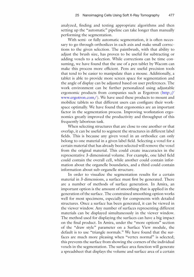
Fig. 4. Screen captures showing commonly used tools in the visualization software package Amira. ( a ) The viewer panel on the right hand side is being used to view a single orthoslice through the reconstructed fi eld of view (in this case, this is a reconstruction of a capillary tube fi lled with a suspension of bacterial cells). The vertical thick black lines are from the capil-lary tube. Darker regions represent areas with a relatively high LAC compared to lighter regions. ( b ) When carrying out the process of segmentation it is usually bene fi cial to view the reconstruction from orthogonal angles. Top half and bottom-left quadrant of the viewing panel shows three slices through the reconstruction. Bottom right quadrant shows 3D representa-tion of segmented cells. ( c ) View of the “magic wand” tool being used to select regions inside the cells with similar LAC values. ( d ) Using the “paintbrush” tool to edit the region selected with the “magic wand” shown in ( c, e ) The “lasso” tool is an ef fi cient means of isolating regions of interest in the reconstruction. For example, you could use it to isolate one cell from other cells reconstructed in the same fi eld of view. ( f ) One example of visualizing the segmented data set. Purple represents the transparent outer surface of the cells. Orange represents the internal structures of interest.

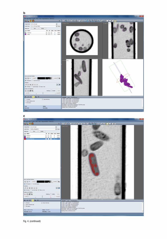
Fig. 4. (continued)


The purpose of segmentation is to delineate the boundaries of structures of interest. Segmentation serves as a way to isolate a speci fi c cellular component from the data set, allowing 3-dimensional visualization of that component either alone or with other compo-nents. This segmented region can serve as the basis for a represen-tation of a whole cell, organelle, or some other speci fi c structure that has been selected for analysis.

Two factors serve as the basis for segmentation of cellular struc-tures. First, different structures differentially attenuate X-rays, and thus boundaries between structures can often be found on the basis of changes in voxel values (corresponding to different X-ray attenuation). Sometimes, cells or organelles to be segmented have uniform X-ray attenuation, and thus regions of interest are separated from each other based on attenuation alone. In other cases, a second

3.6. Segmentation and Analysis

Fig. 4. (continued)


factor must be used: knowledge of the expected structure of the items to be segmented. For example, some organelles often have complex shapes, and are composed of subregions with different X-ray attenuations. Thus, these organelles must be segmented not only based on attenuation, but also based on prior information about expected shapes.

Segmentation of areas of interest within the cell can be per-formed manually using image manipulation with tools such as a “magic wand” (Fig. 4c ), “paintbrush” (Fig. 4d ) and “lasso” (Fig. 4e ). The magic wand function is used as a region-growing tool, where the user picks a seed point as well as an upper and lower threshold; all voxels connected to the seed point that fall within the threshold are added to the region. The magic wand can function either in 2D or 3D. With the paintbrush tool, a user paints regions of interest on a slice-by-slice basis. In order to create a 3-dimensional representation of a cellular component, each por-tion of the component must be selected on each orthoslice. After performing initial paintbrush segmentation by selecting through slices along one axis, it is important to view the selected compo-nents in an orthogonal axis to con fi rm the continuity and accuracy of the selected region in 3 dimensions. Efforts must be taken to reconcile the regions that can be viewed in each axis. Amira can also show a 3-dimensional view of the currently selected voxels, which can aid in determining the accuracy of segmentation; for example, many organelles should have relatively spherical shapes, and the 3D view of the segmentation should conform to this. Segmentation must be recorded in some way; in Amira this is done by means of a “label fi eld”. Label fi elds are used to assign a unique identity to each voxel in a volume. Label fi elds can then be used as a mask for the original volume or can be used as the basis for a 3D surface representation (Fig. 4f ).

Although segmentation of complex biological samples often needs to be done manually, it is possible to automate the process in some cases. In fact, the magic wand tool could be viewed as a semi-automatic segmentation method. If the difference in X-ray attenu-ation between a given structure and its neighbors is relatively large, the magic wand can be fast and accurate. In other cases, or in cases of samples with high levels of noise, selecting appropriate thresh-olds is more dif fi cult; often a smaller threshold range must be used to prevent bleed-through of the selected region to the surround-ing structures. This adjustment of the threshold in turn changes the overall selected volume. Thus, the ability to arbitrarily adjust the thresholds is very useful but can lead to highly subjective results if segmentation is being used as the basis for volume analysis.

A number of more automatic segmentation methods are pos-sible, however, we have found that automated image processing “pipelines” must have a number of parameters very speci fi c to a given problem. Unless a number of cells or organelles are being


analyzed, fi nding and testing appropriate algorithms and then setting up the “automatic” pipeline can take longer than manually performing the segmentation.

With semi- or fully automatic segmentation, it is often neces-sary to go through orthoslices in each axis and make small correc-tions to the given selection. The paintbrush, with that ability to adjust the brush size, has proven to be useful for subtracting or adding voxels to a selection. While corrections can be time con-suming, we have found that the use of a pen tablet by Wacom can make this process more ef fi cient. Pens are useful precision tools that tend to be easier to manipulate than a mouse. Additionally, a tablet is able to provide more screen space for segmentation and the angle of display can be adjusted based on user preferences. The work environment can be further personalized using adjustable ergonomic products from companies such as Ergotron ( http://www.ergotron.com/ ). We have used these products to mount and mobilize tablets so that different users can con fi gure their work-space optimally. We have found that ergonomics are an important factor in the segmentation process. Improving workstation ergo-nomics greatly improved the productivity and throughput of this frequently laborious task.

When selecting structures that are close to one another or that overlap, it can be useful to segment the structures in different label fi elds. This is because any given voxel in an orthoslice can only belong to one material in a given label fi eld. Selecting a voxel for a certain material that has already been selected will remove the voxel from the original material. This could create inaccuracies in the representative 3-dimensional volume. For example, one label fi eld could contain the overall cell, while another could contain infor-mation about the organelle boundaries, and a third could contain information about sub-organelle structure.

In order to visualize the segmentation results for a certain material in 3-dimensions, a surface must fi rst be generated. There are a number of methods of surface generation. In Amira, an important option is the amount of smoothing that is applied in the generation of the surface. The constrained smoothing option works well for most specimens, especially for components with detailed structures. Once a surface has been generated, it can be viewed in the viewer window. Any number of surfaces representing different materials can be displayed simultaneously in the viewer window. The method used for displaying the surfaces can have a big impact on the fi nal product. In Amira, under the “more options” section of the “draw style” parameter on a Surface View module, the default is to use “triangle normals.” We have found that the sur-faces are much more pleasing when “vertex normal” is selected; this prevents the surface from showing the corners of the individual voxels in the segmentation. The surface area function will generate a spreadsheet that displays the volume and surface area of a certain

http://www.ergotron.com/

http://www.ergotron.com/


material in voxel units. The material statistics function can also be used to directly calculate the volumes from the label fi eld. If the voxel size was appropriately set when a data set was loaded, the volume and surface area values will be in the appropriate units (in our case, we use cubic or squared microns).

We note that because data is measured in terms of percent transmission, if appropriate reconstruction algorithms are used, the voxel values in the fi nal volume correspond to the average value of the linear absorption coef fi cient (LAC) for the material in that voxel. In some cases, it may be necessary to scale the values in the volume by some conversion factor so that they correspond to appropriate units—in X-ray microscopy; absorption per inverse micrometer is a common measure.

1. A wide range of computing hardware can be used to run tomo-graphic reconstruction and analysis software packages. However, as with most computationally intensive operations, access to more/faster CPUs will result in a reduction in the time it takes to process and analyze data. At XM-2, data are currently pro-cessed and analyzed using an Apple cluster with 20 nodes, each with two 2-core processors. In the near future, it appears these types of calculations will be best carried out using GPU clusters (Graphical Processing Units) as these typically produce a signi fi cant decrease in processing time (a factor of 20 or more is generally expected for this type of calculation). However, at a push tomographic reconstruction using the fi ltered backprojec-tion algorithm can even be carried out on a modest laptop. Therefore, computational hardware is mostly determined by availability of funding, and required throughput.

2. Much of the pre- and post-processing can be done using com-monly available commercial software packages such as MATLAB (Mathworks) or with the freeware package ImageJ (National Institutes of Health, USA; http://rsbweb.nih.gov/ij ). Tomographic reconstructions can also be carried out in MATLAB or in ImageJ using readily available plugins. There are also a number of dedicated tomography software packages, and in our hands we have found these to offer some distinct advantages, such as utilities for the correction for bad CCD pixels (CCDERASER in IMOD). Many of the required computational operations can be combined into one automated “pipeline” using either a MATLAB script or an ImageJ plugin; this saves time and makes it relatively easy for a neophyte to process their own SXT data. For the calculation of iterative reconstructions we use a number of different packages, including XMIPP

4. Notes

http://rsbweb.nih.gov/ij


( http://xmipp.cnb.csic.es/ ), ASPIRE ( http://www.eecs.umich.edu/~fessler/aspire/ ), and SPARX ( http://macro-em.org/sparxwiki/SparxWiki ). We recommend fl exibility in terms of software packages. Some packages deal with particular data sets better than others (based on how the algorithm handles noise, aberrations, and other inherent features in the data). For best results, it is usually worthwhile to carryout data processing and analysis in parallel using different software packages, and com-pare the fi nal products to determine which performed best with that particular specimen/data set.

3. Amira™ (Visage Imaging, Germany) and Avizo (VSG, France) are two examples with similar functionality. Additional soft-ware packages include ImageJ, Chimera (University of California in San Francisco, USA), IMOD (University of Colorado, USA), VisIt (Department of Energy: Advanced Simulation and Computation Initiative, https://wci.llnl.gov/codes/visit/ ), Paraview (Kitware, Inc., http://www.paraview.org/ ), and VG Studio Max (Volume Graphics). The choice of package (between these, and many others available either com-mercially or freely) depends on funding and preference. For the most part, any of the modern software packages are suf fi ciently advanced and can meet most needs; choice comes down to one of individual preference, perceived ease of use, and other similar considerations.

4. The actual strength of trypsin used is cell line dependent as is the method of stopping action of trypsin. Some cell lines require lower strength of trypsin, for example 0.10%, and may require non-serum stops such as soybean trypsin inhibitor (Sigma Aldrich). To achieve cells in suspension, balance expo-sure to trypsin with the morphology of cells. Longer trypsin exposure detaches more cells but also negatively effects cell viability and morphology. Also, do not use forceful pipetting, knocking, or scraping to detach cells. Fast liquid movement, knocking and scraping can shear cells, producing debris that may be dif fi cult to separate from desired samples.

5. SXT is a relatively straightforward imaging technique, and comparatively free of issues once the cells are mounted in a suitable holder and cryo fi xed. The primary concern is always the authenticity of the specimen—is the reconstructed cell a true and accurate representation of the in vivo state. Therefore, we encourage the use of correlated imaging methods, both as a source of additional information and as a “reality check.” Towards this end we have developed high-numerical aperture cryogenic light microscopy, and installed this instrumentation into XM-2 ( 9, 24 ) . As a result, fl uorescent tagged-molecules or structures in the cells can be imaged using fl uorescence microscopy prior to the cells being imaged using SXT. By fl uorescently tagging subcellular structures with well-established

http://xmipp.cnb.csic.es/

http://www.eecs.umich.edu/~fessler/aspire/

http://www.eecs.umich.edu/~fessler/aspire/

http://macro-em.org/sparxwiki/SparxWiki

http://macro-em.org/sparxwiki/SparxWiki

https://wci.llnl.gov/codes/visit/

https://wci.llnl.gov/codes/visit/

http://www.paraview.org/

http://www.paraview.org/


architecture—such as the mitochondria in yeast—and compar-ing room temperature fl uorescence imaging data with the pat-terns seen in cryogenic light and X-ray microscopy it is possible to validate the integrity of the cell after cryo fi xation, and after SXT data collection. We feel this is enormously important and this correlated approach should be a routine part of imaging cells by any high-resolution modality. We have observed a number of dramatic structural changes that we determined were simply due to poor freezing, or other specimen handling protocols. In the absence of correlated imaging data these changes could easily have been attributed as being biologically signi fi cant.

Acknowledgments

XM-2 and associated research is funded by the Department of Energy Of fi ce of Biological and Environmental Research Grant DE-AC02-05CH11231, the NIH National Center for Research Resources (5P41 RR019664-08) and the National Institute of General Medical Sciences (8P41 GM103445-08) from the National Institutes of Health.

References

1. Larabell CA, Nugent KA (2010) Imaging cel-lular architecture with X-rays. Curr Opin Struct Biol 20:623–631

2. Leis A, Rockel B, Andrees L, Baumeister W (2009) Visualizing cells at the nanoscale. Trends Biochem Sci 34:60–70

3. Fagarasanu A, Fagarasanu M, Rachubinski RA (2007) Maintaining peroxisome populations: a story of division and inheritance. Annu Rev Cell Dev Biol 23:321–344

4. Warren G, Wickner W (1996) Organelle inher-itance. Cell 84:395–400

5. Uchida M, Sun Y, McDermott G et al (2011) Quantitative analysis of yeast internal architecture using soft X-ray tomography. Yeast 28:227–236

6. Baumeister W (2002) Electron tomography: towards visualizing the molecular organization of the cytoplasm. Curr Opin Struct Biol 12:679–684

7. Natterer F (1986) The mathematics of com-puterized tomography. Wiley, New York

8. Larabell CA, McDermott G, Le Gros MA (2005) X-ray tomography of whole cells. Curr Opin Struct Biol 15:593–600

9. McDermott G, Le Gros MA, Knoechel CG, Uchida M, Larabell CA (2009) Soft X-ray tomography and cryogenic light microscopy: the cool combination in cellular imaging. Trends Cell Biol 19:587–595

10. Uchida M, McDermott G, Wetzler M et al (2009) Soft X-ray tomography of phenotypic switching and the cellular response to antifun-gal peptoids in Candida albicans. Proc Natl Acad Sci USA 106:19375–19380

11. Attwood DT (1999) Soft X-rays and extreme ultraviolet radioation: principles and applica-tions. Cambridge University Press, New York

12. Weiss D (2000) Computed tomography based on cryo X-ray microscopic images of unsec-tioned biological specimens. Georg-August University of Göttingen, Göttingen

13. Le Gros MA, McDermott G, Larabell CA (2005) X-ray tomography of whole cells. Curr Opin Struct Biol 15:593–600

14. Parkinson DY, McDermott G, Etkin LD, Le Gros MA, Larabell CA (2008) Quantitative 3-D imaging of eukaryotic cells using soft X-ray tomography. J Struc Biol 162:380–386


15. Larabell C, McDermott G, Uchida M, Knoechel C, Le Gros MA (2009) Imaging whole cells at better than 50 nm isotropic resolution with X-rays. Abst, Papers Am Chem Soc, 238

16. Larabell CA, Le Gros MA (2004) X-ray tomog-raphy generates 3-D reconstructions of the yeast, saccharomyces cerevisiae, at 60-nm reso-lution. Mol Biol Cell 15:957–962

17. Bertilson M, Von Hofsten O, Lindblom M, Wilhein T, Hertz H, Vogt U (2008) Compact high-resolution differential interference con-trast soft X-ray microscopy. App Phys Lett 92:064104

18. Bertilson MC, Takman PAC, Holmberg A, Vogt U, Hertz HM (2007) Laboratory arrangement for soft X-ray zone plate ef fi ciency measurements. Rev Sci Instrum 78:026103–026101

19. Takman PAC, Stollberg H, Johansson GA, Holmberg A, Lindblom M, Hertz HM (2007) High-resolution compact X-ray microscopy. J Microsc 226:175–181

20. Bell PB, Sa fi ejkoMroczka B (1997) Preparing whole mounts of biological specimens for imaging macromolecular structures by light and electron microscopy. Int J Imaging Syst Tech 8:225–239

21. Quintana C (1994) Cryo fi xation, Cryosubstitution, Cryoembedding for Ultrastructural, Immunocytochemical and Microanalytical Studies. Micron 25:63–99

22. Ryan KP (1992) Cryo fi xation of tissues for electron-microscopy—a review of plunge cool-ing methods. Scanning Microsc 6:715–743

23. Studer D, Humbel BM, Chiquet M (2008) Electron microscopy of high pressure frozen samples: bridging the gap between cellular ultrastructure and atomic resolution. Histochem Cell Biol 130:877–889

24. Le Gros MA, McDermott G, Uchida M, Knoechel CG, Larabell CA (2009) High-aperture cryogenic light microscopy. J Microsc 235:1–8

Nanoimaging Cells Using Soft X-Ray Tomography

Documents

Transcript of Nanoimaging Cells Using Soft X-Ray Tomography