1

Abstract

Soil sample physical properties can greatly be affected during soil sampling procedures. Improper

procedures can impose modifications on soil sample structure and consequently lead to wrong

measurements of soil properties. The objective of this work was to evaluate the damage caused by

soil samplers to soil structure through the analysis of computed tomography (CT) images. A first

generation tomograph was used, having a 241

Am source and a 7.62 x 7.62 cm NaI(Tl) scintillation

crystal detector coupled to a photomultiplier tube. Results confirm the effect of soil sampler devices

on the structure of soil samples, and that the compaction caused during sampling causes significant

alterations of soil bulk density. Through the use of CT it was possible to determine the level of

compaction and to make a detailed analysis of the soil bulk density distribution within the soil

sample.

Additional Keywords: Soil sampler device, soil compaction, computed tomography, gamma

radiation.

Introduction

Many soil scientists have investigated the influence of sampling volume on the evaluation of

soil physical properties such as, soil bulk density, air volume, water volume, and porosity (Rogasik

2

et al. 1999). VandenBygaart and Protz (1999) tried to define a representative elementary area

(REA) in the study of pedofeatures for quantitative analysis. They showed that there is a minimum

area to represent pedofeatures and that it is not possible to make quantitative analyses for smaller

areas. Baveye et al. (2002) showed the importance of the soil sampling volume in the determination

of macroscopic parameters, and that small sampling volumes exhibit significant and seemingly

erratic fluctuations.

Instruments used for soil sampling may also affect measurements. Camponez do Brasil

(2000) showed that for 4 different soil sampling devices, certain soil physical properties could be

strongly affected by soil sampling process. The equipment could cause compaction of the samples,

causing modifications of the porous system and consequently in soil structure.

Soil compaction and changes in soil structure can cause serious alterations of soil physical

properties such as bulk density. Soil bulk density, represented by the ratio between soil mass and

soil volume, is meant to give an idea of the percentage of voids that define soil structure. Low

porosity represents a more compact region of the soil sample. These compacted regions can cause

modifications in soil water storage capacity and matric soil water potential, which are parameters

used in irrigation and drainage management, and therefore have economic significance in

agriculture.

Computed tomography (CT) is a noninvasive imaging technique that allows good resolution

images of materials and permits quantitative analyses of physical properties. CT has been used to

obtain non-destructive images of different objects in several areas of knowledge (Hounsfield 1973;

Borgia et al. 2001; Stampanoni et al. 2003; Treimer et al. 2003; Jenneson et al. 2003). Petrovic et

al. (1982) introduced CT into soil science through studies of soil bulk density. Hainsworth and

Aylmore (1983) and Crestana et al. (1985) performed measurements of soil water content and soil

water movement through X-ray and gamma ray CT. Crestana et al. (1986) developed a CT scanner

dedicated to soil science analysis and showed that this equipment has advantages over the

3

commercial medical scanner. Vaz et al. (1989) used miniscanner CT to study soil compaction

caused during plowing operations with heavy equipments. Perret et al. (1999) made a 3-D

quantification of soil macropores in undisturbed soil columns. Wildenschild et al. (2002) used X-

ray CT for hydrological purposes and compared results obtained for 3 different CT systems, and

Balogun and Cruvinel (2003) investigated soil density distributions for agricultural purposes

utilizing Compton scattering tomography.

We propose to use gamma ray CT to observe the effect of soil sampler devices on the

measurement of soil bulk density distribution inside collected samples.

Theory

When a gamma ray beam passes through a soil sample of thickness x (cm) different

electromagnetic processes can occur, and the transmitted photon intensity I follows the Beer-

Lambert law:

)](xexp[.II *

ws

*

s0 (1)

where I0 is the incident photon intensity, *s and *

w (cm2/g) are the soil and water mass attenuation

coefficients, s (g/cm3) is the soil bulk density, respectively, and (cm

3/cm

3) is the volumetric soil

water content. The CT often uses the linear attenuation (cm-1

) converted into numbers called

tomographic units (TU) that are numerical values assigned to gray levels (Herman 1980). For a soil

sample the relation between TU and of the sample is given by:

)...(.TU *

ws

*

s (2)

4

where represents the correlation coefficient between and TU.

Differences in TU values represent differences in soil physical density at each point or pixel.

Consequently, it is possible to obtain density distributions along the length of the soil sample, and

in the case of a moist soil sample, this density distribution includes the water content distribution.

On the other hand, if the soil sample is dry or its water content is uniformly distributed, the TU

distribution permits the calculation of soil bulk density values:

.

TU*

w

*

s

s (3)

where (g/g) represents the gravimetric soil water content.

Material and Methods

Soils

Soil core samples were taken from a soil profile of an Eutrustox from an experimental field

of the Department of Plant Production of ESALQ/USP, in Piracicaba, SP, Brazil (22°4´S; 47°38´W;

580 m above sea level). Four different soil sampling devices were used and correspond to inox

cylinders of different sizes: (1) Sampler A (4.2 cm high, 2.7 cm i.d., 25 cm3 volume), (2) Sampler B

(3.0 cm high, 4.8 cm i.d., 55 cm3 volume), (3) Sampler C (2.65 cm high, 4.9 cm i.d., 50 cm

3

volume), and (4) Sampler D (5.3 cm high, 4.9 cm i.d., 100 cm3 volume). All samplers permit the

introduction of the steel cylinders in their inner space and soil samples are collected in these

cylinders by a procedure that starts with a rubber mass falling from different heights to introduce

the sampler containing the steel cylinder into the soil, down to the desired depth. After complete

5

introduction of the set into the soil, the surrounding soil is removed with a spade. The excavation is

made carefully allowing the extraction of the cylinder containing the sample for density evaluation.

Caution is needed during this process to minimise vibration, scissoring and compaction effects on

the structure of the soil sample.

CT analysis was performed on 20 soil samples (5 from each soil sampler) carefully collected

close to the soil surface using the steel cylinders described above.

Scanning system

The CT scanner was a first generation system with a fixed source-detector arrangement, with

translation/rotational movements of the sample. The radioactive gamma ray source was 241

Am with

an activity of 3.7 GBq emitting monoenergetic photons of 59.54 keV. The detector was a 7.62 x

7.62 cm NaI(Tl) scintillation crystal coupled to a photomultiplier tube. Circular lead collimators of

2mm were adjusted and aligned between source and detector. Angular sample rotation steps

were 2.25° until completing a scan of 180°, with linear steps r of 0.14 cm. The pixel size was 1.0 x

1.0 mm for sampler A; 1.14 x 1.14 mm for samplers B and C; and 1.40 x 1.40 mm for sampler D.

The pixel size was calculated by the ratio between the inner diameter of the soil sample and number

of pixels of the reconstruction matrix. Acquired data were stored in a PC and a reconstruction

algorithm called Microvis (2000) developed by Embrapa Agricultural Instrumentation (CNPDIA –

São Carlos, Brazil) was used to obtain CT images. The calibration of the CT system was obtained

through linear correlation between linear attenuation coefficients and tomographic units of different

materials (Pires et al. 2002; Pires et al. 2003). The tomographic images of the soil samples were

taken on vertical planes crossing the center of the cylindrical sample.

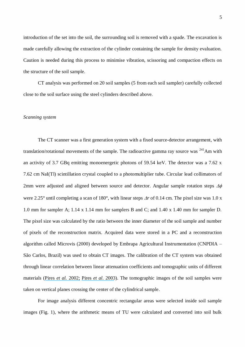
For image analysis different concentric rectangular areas were selected inside soil sample

images (Fig. 1), where the arithmetic means of TU were calculated and converted into soil bulk

6

density, giving a general idea of the spatial variability of this parameter, in depth as well as

laterally, within the sample.

Fig. 1. Concentric rectangular areas utilized for soil sample image analysis. Each area represents arithmetic

means of the pixels inside the area. H represents the height and D the diameter of sample.

Results and discussion

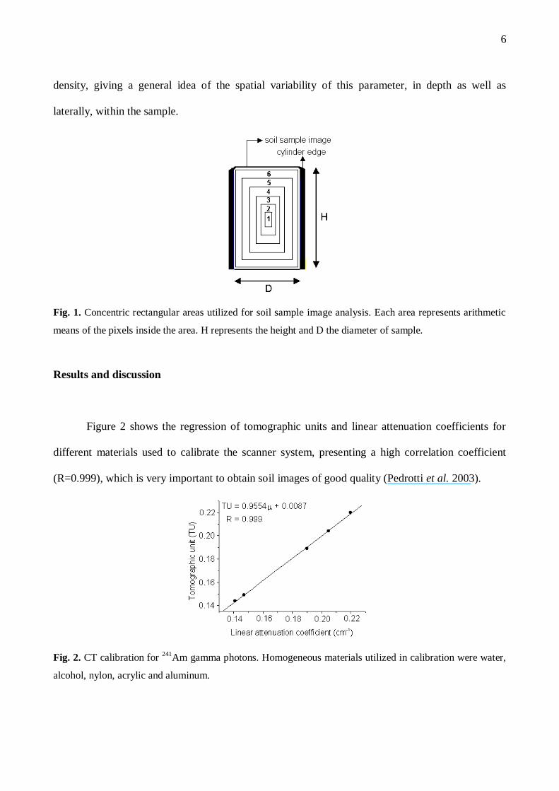
Figure 2 shows the regression of tomographic units and linear attenuation coefficients for

different materials used to calibrate the scanner system, presenting a high correlation coefficient

(R=0.999), which is very important to obtain soil images of good quality (Pedrotti et al. 2003).

Fig. 2. CT calibration for 241

Am gamma photons. Homogeneous materials utilized in calibration were water,

alcohol, nylon, acrylic and aluminum.

7

The mass attenuation coefficients for soil and water were 0.244290.00250 and

0.198900.00018 cm2/g, respectively, for the 59.54 keV photons, which agree with values found in

the literature for 241

Am source (Ferraz and Mansell 1979).

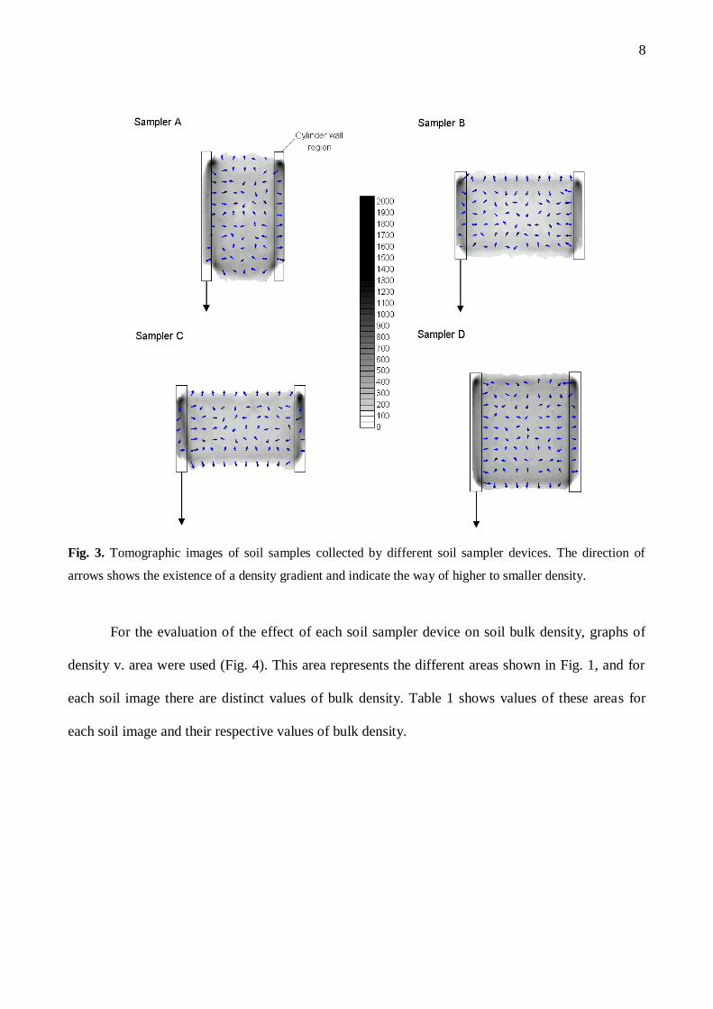
Four images of soil samples obtained for each soil sampler device are shown in Fig. 3. The

planes of image acquisition were vertical and the available data permitted a continuous 2-D analysis

of the density distribution along the soil sample. These images show a clear heterogeneity of soil

bulk density and the occurrence of larger values near the edges of the soil samples. There was a

density gradient for samples obtained by all soil sampler devices and this gradient is represented in

Fig. 3 through arrows. Each arrow indicates the direction of higher to smaller densities, and

therefore, the direction of the arrows for all soil samples indicates an increase in soil density near

the edges and the lowest bulk density is found in the center region. For the sampler A it is possible

to observe a compaction at the bottom and at the top of the sample, probably due to the lower

internal diameter of the cylinder. Pires et al. (2004) shown through of the analyses of transects of

CT images that small soil-sampling volumes may induce compaction at the top and at the bottom of

the soil sample.

8

Fig. 3. Tomographic images of soil samples collected by different soil sampler devices. The direction of

arrows shows the existence of a density gradient and indicate the way of higher to smaller density.

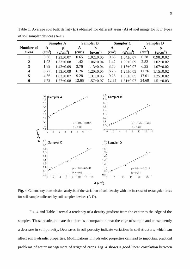
For the evaluation of the effect of each soil sampler device on soil bulk density, graphs of

density v. area were used (Fig. 4). This area represents the different areas shown in Fig. 1, and for

each soil image there are distinct values of bulk density. Table 1 shows values of these areas for

each soil image and their respective values of bulk density.

9

Table 1. Average soil bulk density () obtained for different areas (A) of soil image for four types

of soil sampler devices (A-D).

Sampler A Sampler B Sampler C Sampler D

Number of

areas

A

(cm2)

(g/cm3)

A

(cm2)

(g/cm3)

A

(cm2)

(g/cm3)

A

(cm2)

(g/cm3)

1 0.38 1.230.07 0.65 1.020.05 0.65 1.040.07 0.78 0.980.02

2 1.03 1.330.08 1.42 1.060.04 1.42 1.090.09 2.82 1.020.02

3 1.89 1.420.09 3.76 1.130.04 3.76 1.160.07 6.35 1.070.02

4 3.22 1.530.09 6.26 1.200.05 6.26 1.250.05 11.76 1.150.02

5 4.56 1.620.07 9.28 1.310.06 9.28 1.350.05 17.01 1.250.02

6 6.73 1.770.08 12.65 1.570.07 12.65 1.610.07 24.69 1.510.03

Fig. 4. Gamma ray transmission analysis of the variation of soil density with the increase of rectangular areas

for soil sample collected by soil sampler devices (A-D).

Fig. 4 and Table 1 reveal a tendency of a density gradient from the center to the edge of the

samples. These results indicate that there is a compaction near the edge of sample and consequently

a decrease in soil porosity. Decreases in soil porosity indicate variations in soil structure, which can

affect soil hydraulic properties. Modifications in hydraulic properties can lead to important practical

problems of water management of irrigated crops. Fig. 4 shows a good linear correlation between

10

bulk density and area, and the angular coefficients obtained represent the density gradient for each

soil sample. Soil samples collected by sampler A presented the largest slope value and samples

collected by sampler D the smallest. Soil samples collected by samplers B and C presented

practically equal values. The larger value of the slope for sampler A indicates the great impact of

this soil sampler in soil sample structure and the smaller value obtained for sampler D indicates that

this instrument causes the lowest impact. Similar results for sampler B and C indicate that these

instruments cause the same effect on soil samples. Fig. 5 presents a comparison of all soil samplers

and their impacts in soil sample structure.

Fig. 5. Comparison of all soil samplers and their respective impacts in the soil sample. , Sampler A; ,

Sampler B; , Sampler C; , Sampler D.

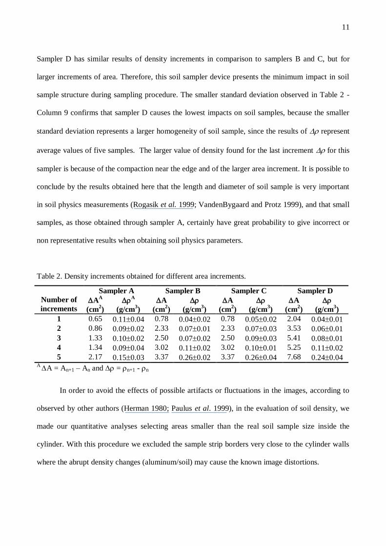
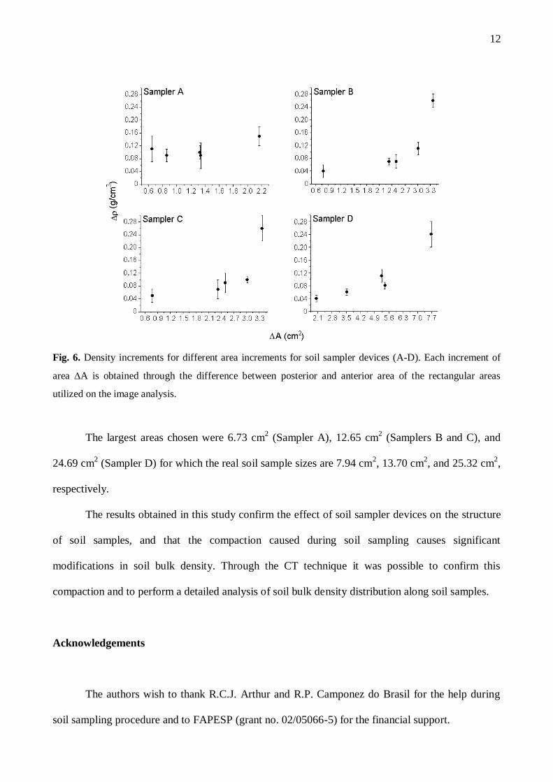
Fig. 6 and Table 2 show density increments () for different area increments (A). Each

increment of area is obtained through the difference between posterior and anterior area represented

in Fig. 1. By the analysis of these density increments it is possible to notice that the largest

variations of density occur for sampler A. Sampler A presents a practically homogeneous variation

of density for small increments of area, and as consequence, more significant modifications in soil

structure. Analyzing Table 2 - Column 2 and 3 it is possible to observe that for small increments of

area the density increment for sampler A is very similar to the results obtained for the other

samplers. Samplers B and C present similar variations of densities and the larger value of density

increment found for the last value of d, represents a direct result of the compaction near the edge.

11

Sampler D has similar results of density increments in comparison to samplers B and C, but for

larger increments of area. Therefore, this soil sampler device presents the minimum impact in soil

sample structure during sampling procedure. The smaller standard deviation observed in Table 2 -

Column 9 confirms that sampler D causes the lowest impacts on soil samples, because the smaller

standard deviation represents a larger homogeneity of soil sample, since the results of represent

average values of five samples. The larger value of density found for the last increment for this

sampler is because of the compaction near the edge and of the larger area increment. It is possible to

conclude by the results obtained here that the length and diameter of soil sample is very important

in soil physics measurements (Rogasik et al. 1999; VandenBygaard and Protz 1999), and that small

samples, as those obtained through sampler A, certainly have great probability to give incorrect or

non representative results when obtaining soil physics parameters.

Table 2. Density increments obtained for different area increments.

Sampler A Sampler B Sampler C Sampler D

Number of

increments A

A

(cm2)

A

(g/cm3)

A

(cm2)

(g/cm3)

A

(cm2)

(g/cm3)

A

(cm2)

(g/cm3)

1 0.65 0.110.04 0.78 0.040.02 0.78 0.050.02 2.04 0.040.01

2 0.86 0.090.02 2.33 0.070.01 2.33 0.070.03 3.53 0.060.01

3 1.33 0.100.02 2.50 0.070.02 2.50 0.090.03 5.41 0.080.01

4 1.34 0.090.04 3.02 0.110.02 3.02 0.100.01 5.25 0.110.02

5 2.17 0.150.03 3.37 0.260.02 3.37 0.260.04 7.68 0.240.04 A A = An+1 – An and = n+1 - n

In order to avoid the effects of possible artifacts or fluctuations in the images, according to

observed by other authors (Herman 1980; Paulus et al. 1999), in the evaluation of soil density, we

made our quantitative analyses selecting areas smaller than the real soil sample size inside the

cylinder. With this procedure we excluded the sample strip borders very close to the cylinder walls

where the abrupt density changes (aluminum/soil) may cause the known image distortions.

12

Fig. 6. Density increments for different area increments for soil sampler devices (A-D). Each increment of

area A is obtained through the difference between posterior and anterior area of the rectangular areas

utilized on the image analysis.

The largest areas chosen were 6.73 cm2 (Sampler A), 12.65 cm

2 (Samplers B and C), and

24.69 cm2 (Sampler D) for which the real soil sample sizes are 7.94 cm

2, 13.70 cm

2, and 25.32 cm

2,

respectively.

The results obtained in this study confirm the effect of soil sampler devices on the structure

of soil samples, and that the compaction caused during soil sampling causes significant

modifications in soil bulk density. Through the CT technique it was possible to confirm this

compaction and to perform a detailed analysis of soil bulk density distribution along soil samples.

Acknowledgements

The authors wish to thank R.C.J. Arthur and R.P. Camponez do Brasil for the help during

soil sampling procedure and to FAPESP (grant no. 02/05066-5) for the financial support.

13

References

Balogun FA, Cruvinel PE (2003) Compton scattering tomography in soil compaction study.

Nuclear Instruments and Methods in Physics Research – Section A 505, 502-507.

Baveye P, Rogasik H, Wendroth O, Onasch I, Crawford JW (2002) Effect of sampling volume on

the measurement of soil physical properties: simulation with X-ray tomography data.

Measurement Science Technology 13, 775-784.

Borgia GC, Bortolotti V, Fantazzini P (2001) Changes of the local pore scale structure quantified in

heterogeneous porous media by 1H magnetic resonance relaxation tomography. Journal of

Applied Physics 90, 1155-1163.

Camponez do Brasil RP (2000) ’Influência das técnicas de coleta de amostras na determinação das

propriedades físicas do solo.’ (MSc. Thesis, ESALQ/USP-Brazil)

Crestana S, Mascarenhas S, Pozzi-Mucelli RS (1985) Static and dynamic 3-dimensional studies of

water in soil using computed tomographic scanning. Soil Science 140, 326-332.

Crestana S, Cesareo R, Mascarenhas S (1986) Using a computed tomography miniscanner in soil

science. Soil Science 142, 56-61.

Ferraz ESB, Mansell RS (1979) Determining water content and bulk density of soil by gamma ray

attenuation methods. Technical Bulletin, No. 807, IFAS, USA.

Hainsworth JM, Aylmore LAG (1983) The use of computer-assisted tomography to determine

spatial distribution of soil water content. Australian Journal of Soil Research 21, 435-443.

Herman GT (1980) ‘Image Reconstruction from Projections.’ (Academic Press: London)

Hounsfield GN (1973) Computerized transverse axial scanning (tomography). 1. Description of

system. British Journal of Radiology 46, 1016-1022.

14

Jenneson PM, Gilboy WB, Morton EJ, Gregory PJ (2003) An X-ray micro-tomography system

optimized for the low-dose study of living organisms. Applied Radiation and Isotopes 58, 177-

181.

MICROVIS (2000) ’Microvis – Programa de Reconstrução e Visualização de Imagens

Tomográficas, Guia do Usuário.’ (EMBRAPA/CNPDIA: São Carlos, Brasil)

Paulus MJ, Sari-Sarraf H, Gleason SS, Bobrek M, Hicks JS, Johnson DK, Behel JK, Thompson LH,

Allen WC (1999) A new X-ray computed tomography system for laboratory mouse imaging.

IEEE Transactions on Nuclear Science 46, 558-564.

Pedrotti A, Pauletto EA, Crestana S, Cruvinel PE, Vaz CMP, Naime JM, da Silva AM (2003)

Planossol soil sample size for computerized tomography measurement of physical parameters.

Scientia Agrícola 60, 735-740.

Perret J, Prasher SO, Kantzas A, Langford C (1999) Three-Dimensional quantification of

macropore networks in undisturbed soil cores. Soil Science Society American Journal 63, 1530-

1543.

Petrovic AM, Siebert JE, Rieke PE (1982) Soil bulk density analysis in three dimensions by

computed tomographic scanning. Soil Science Society American Journal 46, 445-450.

Pires LF, Macedo JR, Souza MD, Bacchi OOS, Reichardt K (2002) Gamma-ray computed

tomography to characterize soil surface sealing. Applied Radiation and Isotopes 57, 375-380.

Pires LF, Macedo JR, Souza MD, Bacchi OOS, Reichardt K (2003) Gamma-ray computed

tomography to investigate compaction on sewage-sludge-treated soil. Applied Radiation and

Isotopes 59, 17-25.

Pires LF, Arthur RC, Camponez do Brasil RP, Correchel V, Bacchi OOS, Reichardt K (2004) The

use of gamma ray computed tomography to investigate soil compaction due to core sampling

devices. Brazilian Journal of Physics (in press)

15

Rogasik H, Crawford JW, Wendroth O, Young IM, Joschko M, Ritz K (1999) Discrimination of

Soil Phases by Dual Energy X-ray Tomography. Soil Science Society of American Journal 63,

741-751.

Stampanoni M, Borchert G, Abela R, Ruegsegger P (2003) Nanotomography based on double

asymmetrical Bragg diffraction. Applied Physics Letters 82, 2922-2924.

Treimer W, Strobl M, Hilger A, Seifert C, Feye-Treimer U (2003) Refraction as imaging signal for

computerized (neutron) tomography. Applied Physics Letters 83, 398-400.

VandenBygaart AJ, Protz R (1999) The representative elementary area (REA) in studies of

quantitative soil micromorphology. Geoderma 89, 333-346.

Vaz CMP, Crestana S, Mascarenhas S, Cruvinel PE, Reichardt K, Stolf R (1989) Computed

tomography miniscanner for studying tillage induced soil compaction. Soil Technology 2, 313-

321.

Wildenschild D, Hopmans JW, Vaz CMP, Rivers ML, Rikard D, Christensen BSB (2002) Using X-

ray computed tomography in hydrology: systems, resolutions, and limitations. Journal of

Hydrology 267, 285-297.