
MODELLING AND VALIDATION OF BEHAVIOUR ... - NITK Surathkal
338
MODELLING AND VALIDATION OF BEHAVIOUR OF MUSHY STATE ROLLED Al-4.5Cu-5TiB 2 COMPOSITE USING NEURAL NETWORK TECHNIQUES Thesis Submitted in partial fulfilment of the requirements for the degree of DOCTOR OF PHILOSOPHY By NIGALYE AKSHAY VITHAL DEPARTMENT OF MECHANICAL ENGINEERING NATIONAL INSTITUTE OF TECHNOLOGY KARNATAKA, SURATHKAL, MANGALORE -575025 October, 2013
-
Upload
khangminh22 -
Category
Documents
-
view
3 -
download
0
Transcript of MODELLING AND VALIDATION OF BEHAVIOUR ... - NITK Surathkal
MODELLING AND VALIDATION OF
BEHAVIOUR OF MUSHY STATE
ROLLED Al-4.5Cu-5TiB2
COMPOSITE USING NEURAL
NETWORK TECHNIQUES
Thesis
Submitted in partial fulfilment of the requirements for the
degree of
DOCTOR OF PHILOSOPHY
By
NIGALYE AKSHAY VITHAL
DEPARTMENT OF MECHANICAL ENGINEERING
NATIONAL INSTITUTE OF TECHNOLOGY
KARNATAKA,
SURATHKAL, MANGALORE -575025
October, 2013

Dedicated to
My Parents, Wife and Children
D EC L A R A T I O N by the Ph. D. Research Scholar
I hereby declare that the Research Thesis entitled “MODELLING AND
VALIDATION OF BEHAVIOUR OF MUSHY STATE ROLLED Al-4.5Cu-
5TiB2 COMPOSITE USING NEURAL NETWORK TECHNIQUES” which
is being submitted to National Institute of Technology Karnataka,
Surathkal in partial fulfilment of the requirements of award of the degree
Doctor of Philosophy in Department of Mechanical Engineering is a
bonafide report of the research work carried out by me. The material
contained in this Research Thesis has not been submitted to any University or
Institution for the award of any degree.
Register Number: ME08P03
Name of the Research Scholar: Nigalye Akshay Vithal
Signature of the Research Scholar:
Department of Mechanical Engineering
Place: NITK- Surathkal
Date: 19-10-2013
CERTIFICATE
This is to certify that the Research Thesis entitled “MODELLING
AND VALIDATION OF BEHAVIOUR OF MUSHY STATE
ROLLED Al-4.5Cu-5TiB2 COMPOSITE USING NEURAL
NETWORK TECHNIQUES” submitted by Mr. Nigalye Akshay
Vithal (Reg. No. ME08P03) as the record the of research work
carried out by him, is accepted as the Research Thesis submission
in partial fulfillment of the requirements for the award of the
degree of Doctor of Philosophy.
Dr. M. A. Herbert Dr. S. S. Rao
Date: Research Guides Date:
Chairman DRPC:
Date:

Acknowledgement
It has been indeed a great honour for me to work under the guidance of my advisors Dr.
Mervin A. Herbert and Dr. Shrikantha S. Rao, Department of Mechanical
Engineering, NITK Surathkal. With deep sense of gratitude and humility, I express my
sincere thanks to them for their valuable guidance, untiring perseverance and unending
patience which made the research not merely educational but also enjoyable. I also take
this opportunity to thank Director, NITK Surathkal and Head of Mechanical Engineering
Department NITK Surathkal for allowing me to take carry out my doctoral studies.
I sincerely thank the Research Progress Assessment Committee consisting of Dr.
Sitharam Nayak (Civil Engineering Department), Dr. Krishna Prasad (Head of
Mechanical Engineering Department), Dr. Mervin Herbert and Dr. Shrikantha Rao for
their valuable comments and constructive criticism which has helped the enrichment of
this doctoral work. My heartfelt thanks to Dr. Naveen Karanth for his valuable
suggestions and constant support during the course of my research work. I am indeed
extremely indebted to all of them.
My sincere thanks to Dr. N. S. Reddy and my co research colleague Mr. Conel
Rodrigues for rendering their support in coding for the ANN and RNN. I am immensely
indebted to the unending help and support I received from my co-research colleagues Mr.
Arunkumar Shettigar and Mr. Nagraj Shetty during the course of my research work. I
also thank Mr. Vitlapur, Manager Guest House who made my stays at the International
Hostel at NITK Surathkal possible.
Mushy state rolling experiments conducted in the Department of Metallurgical and
Material Sciences at IIT Kharagpur would not have been possible without the help and
guidance of Prof. R. Mitra (Dept. of Metallurgical and Material Sciences, IIT
Kharagpur). I express heartfelt gratitude to Prof. R. Mitra for his invaluable guidance and
support. I also thank the Head of Department (Metallurgical and material Sciences), IIT
Kharagpur for allowing me to use the facilities. My gratitude and thanks also go to Mr.
Kamal Kumar Saw fondly referred as Kamalda for helping me in conduct of melting and

casting experiments, as well as for his help in the conduct of mushy state rolling
experiments. The stay at the Hostel at IIT Khatragpur would not have been comfortable
without the help rendered by Mr. Anirudh Jana. I would like to express my sincere thanks
to Dr. R. Maiti for providing help in SEM analysis of mushy state rolled samples.
I am indeed grateful to my colleague Prof. Siddesh Salelkar from Computer Engineering
department of Goa Engineering College for rendering support in designing a GUI using
Microsoft Silverlight (API) educational package. I am indebted to the constant help
provided by my colleague Mr. Pushpashil Satardekar and Mr. Akash Kapdi of Computer
Centre in sorting out the problems related to computer hardware.
Late Prof. Uday Amonkar, former Head of Mechanical Engineering Department at our
Goa Engineering College was my close friend and colleague. Through my student days
he has been my friend, philosopher and guide. I thank him for the nurturing environment
he created and maintained around me that helped me to complete my research work.
I would fail in my duties if I do not remember the role my friends and close colleagues
Dr. V. Mariappan. Dr. R. Prabhu Gaonkar, Dr. P. Savoicar, Prof. M. J. Sakhardande,
Prof. M. N. Dhawalikar, Prof. M. Caisukar, Prof. Chetan Desai, Prof. S. Borkar, Prof.
A.K.S. Bahadauria, Mr. V. B. Kamat Director of Tech Education, Goa & Ex- Principal
and Dr. R. B. Lohani, Principal GEC, and my friend Mr. Rajiv Dhawalikar for their
constant support. I would like to specially mention the help provided by Prof. Anant Naik
during my visits to NITK Surathkal.
I am indebted to my parents for inculcating in me the right values and virtues. I am
extremely grateful to my beloved wife Medha and lovely children Anukool and Akhilesh
for enduring a lot of hardships caused on the domestic front due to my research priorities.
I wish to express my special thanks to all my siblings, my brothers Arunkumar and
Ashok, my sisters Mrs. Usha, Mrs. Shashikala and Mrs. Sudha who were a constant
source of motivation and encouragement during the entire course of my doctoral work.
Nigalye Akshay Vithal
Abstract
Aluminium alloy matrix composites reinforced with in situ formed TiB2 particles are
found to possess excellent mechanical properties as well as high stability at elevated
temperatures. Forming of these composites by conventional methods is difficult due
to their tendency of cracking. The problem is overcome by subjecting these
composites to mushy state forming. Studies on mushy state rolling of Al-4.5Cu-5TiB2
composite have witnessed formation of bimodal equiaxed grains having spheroidal
morphology from one that is essentially dendritic in as cast condition. Resulting
mechanical and wear properties of mushy state rolled Al-4.5Cu-5TiB2 composite are
also observed to be superior to that of as cast composite. The data on the grain sizes,
hardness, wear and tensile properties of mushy state rolled composite has been
expanded by using neural network techniques. This is done to have better
understanding of the relationship between mushy state rolling process parameters and
the resulting mechanical and wear properties.
Artificial Neural Networks with feed forward architecture, and trained using
backpropagation algorithm have been used to predict bimodal grain sizes, hardness,
tensile and wear properties of Al-4.5Cu-5TiB2 composite rolled from mushy state in
as cast and in pre hot rolled condition. The models have been validated by conducting
mushy state rolling experiments. The composite samples in as cast and in pre hot
rolled condition are mushy state rolled at pre set points within and outside the bounds
of data used for training the ANN models. The validity of the models is established by
way of comparison of the validation experiment results with the values predicted by
models. The ANN models formulated for grain size, hardness, wear and tensile
properties prediction are found to predict the corresponding outputs quite accurately,
within the acceptable limits of prediction errors.
Artificial Neural Networks though known for non linear mapping of complex
systems, are static mapping tools in the sense that the knowledge update is based on
static data provided for training the network. Simple recurrent neural networks (SRN)
such as the one proposed by Elman have the capacity of dynamic learning. The

computational power of Elman networks has been thought to be comparable to that of
finite state machines. However, such extended simple recurrent neural networks when
adopted, are found to possess severely hampered learning capabilities due to
convergence problems. A novel way of overcoming the problem of convergence is
proposed through this work by using a Hybrid Recurrent Neural Network (HRNN)
modelled from an ANN. The HRNN is modelled by borrowing weights into an Elman
Simple Recurrent Neural Network having similar architecture (devoid of context
layers). Such an HRNN formulated is found to converge excellently in a significantly
less time as compared to an ANN for the same value of preset MSE. The prediction
errors of HRNN and prediction errors resulting from ANN predictions when subjected
to statistical testing are found to be equivalent.
The predictions resulting from HRNNs modelled for prediction of duplex grain sizes,
hardness, tensile and wear properties are seen to be in close agreement with the
predictions made by the ANN models. However, it is seen that the overall time
required for training HRNNs which includes the time required for training of partially
trained ANNs, is significantly reduced. Thus it is observed that an HRNN modelled
from a partially trained ANN has equivalent prediction capability and is superior to
ANN in terms of computational time.
Graphical user interface (GUI) has been designed using available API libraries which
include two main modules, namely, ANN and RNN. Each model has the sub
components for prediction of grain size, hardness, wear rate and tensile properties.
There is provision to obtain outputs by manually feeding the input values as well for
plotting line graphs by varying one parameter at a time, keeping other parameters
constant. The GUI is also designed to generate bar plots by varying each mushy state
processing input parameter at a time. Use of GUI is made in optimising the mushy
state processing parameters for obtaining the best possible hardness values and
minimum wear rate for mushy state rolled Al-4.5Cu-5TiB2 composite.
Key words: Aluminium alloy matrix composites, Mushy state forming, Artificial
Neural Networks (ANN), Elman Simple Recurrent Neural Network (SRN), Hybrid
Recurrent Neural Networks (HRNN).

i
Contents
Page
No.
Declaration
Certificate
Acknowledgements
Abstract
Content (i)
List of Figures (ix)
List of Tables (xvii)
Nomenclature (xxi)
1 INTRODUCTION 1
1.1 GENERAL BACKGROUND 1
1.2 PROPOSED WORK SUMMARY 3
1.3 ORGANISATION OF THE THESIS 4
2 LITERATURE REVIEW 9
2.1 INTRODUCTION 9
2.2 SEMISOLID PROCESSING 10
2.3 FUNDAMENTALS OF SEMISOLID PROCESSING 11
2.4 EVOLUTION OF THIXOTROPY 14
2.5 MICROSTRUCTURAL EVOLUTION DURING PARTIAL
REMELTING AND ISOTHERMAL HOLDING
15
2.6 MECHANISM OF NON DENDRITIC MICROSTRUCTURE
FORMATION
17
2.7 METHODS TO FORM SPHEROIDAL GRAIN STRUCTURE 20
2.7.1 Magnetohydrodynamic (MHD) Stirring 20
2.7.2 Spray Forming (Osprey) 21
2.7.3 Strain Induced Melt Activated/ recrystallization and
partial melting
21
ii
2.7.4 Liquidus/ near liquidus casting 22
2.7.5 Semi-solid rheocasting 23
2.7.6 Grain refinement 23
2.7.7 Semisolid thermal transformation 23
2.8 FLOW BEHAVIOUR OF MUSHY METAL 24
2.9 VOLUME FRACTION EVALUATION 25
2.10 SEMISOLID PROCESSING METHODS 25
2.10.1 Rheocasting 25
2.10.2 Rheomoulding 26
2.10.3 Thixomoulding 26
2.10.4 Thixoforming 27
2.10.5 Mushy state extrusion 28
2.10.6 Mushy state rolling 28
2.11 APPLICATIONS 30
2.11.1 Semisolid processing of alloys 30
2.11.2 Semisolid processing of composites 31
2.12 MECHANICAL PROPERTIES 33
2.12.1 Alloys 33
2.12.2 Composites 37
2.13 WEAR PROPERTIES 39
2.14 COMPUTATIONAL INTELLIGENCE 42
2.14.1 Artificial Neural Networks 43
2.14.2 Neuron: The Fundamental Unit of the Network 44
2.14.3 Developments in the Field of Neural Networks 46
2.14.4 Function Approximation and ANN 50
2.14.5 Neural Networks Vs. Statistical Techniques 51
2.15 NEURAL NETWORKS IN MATERIAL SCIENCE 53
2.16 NEURAL NETWORKS IN SEMISOLID PROCESSING OF
COMPOSITES
55
2.16.1 Procedure Involved in ANN Model Development 55

iii
2.16.2 Data Preparation 56
2.16.2.1 Data Collection and Generation 56
2.16.2.2 Range and Distribution of Samples 56
2.16.2.3 Pre-Processing and Post-Processing of Data 57
2.17 STRUCTURE OF AN ANN MODEL 59
2.17.1 Summing function 59
2.17.2 Activation Function 60
2.17.3 Initial Weights 61
2.17.4 Learning Rate 61
2.17.5 Momentum Factor 61
2.17.6 Number of Hidden layers 62
2.17.7 Number of Hidden Neurons per Layer 63
2.18 GRAPHICAL USER INTERFACE DESIGN 64
2.18.1 Objectives of Graphical User Interface Design 66
2.19 SUMMARY AND GAP IN KNOWLEDGE 67
2.19.1 Conclusions 67
2.19.2 Statement of Problem 72
2.19.3 Statement of objectives 74
2.19.4 Scope 75
2.19.5 Plan of work 76
3 EXPERIMENTAL DETAILS 77
3.1 INTRODUCTION 77
3.2 SELECTION OF RAW MATERIALS 79
3.3 SYNTHESIS OF AL BASED ALLOY AND Al-4.5(Wt. %)Cu-
5(Wt. %)TiB2 COMPOSITE
80
3.3.1 Preparation of Al-4.5 (wt %) Cu Master alloy 80
3.3.2 Preparation of Al-4.5(wt %)Cu-5(wt %)TiB2 composite
by mixed salt route
80
3.4 EVALUATION OF VOLUME FRACTION OF in situ Al-4.5Cu-
5TiB2 COMPOSITE IN MUSHY STATE
83
3.5 MUSHY STATE ROLLING OF Al-4.5Cu-5TiB2 COMPOSITE 84

iv
3.6 SECTIONING OF AS CAST AND ROLLED SPECIMENS 89
3.7 METALLOGRAPHIC SAMPLE PREPARATION 89
3.8 CHARACTERIZATION OF MUSHY STATE ROLLED in situ
Al-4.5Cu-5TiB2 COMPOSITE
89
3.8.1 Optical microscopy and image analysis 89
3.8.2 Scanning electron microscopy 91
3.9 EVALUATION OF HARDNESS OF MUSHY STATE ROLLED
Al-4.5Cu-5TiB2 COMPOSITE
91
3.10 EVALUATION OF DRY SLIDING WEAR PROPERTIES 92
4 RESULTS AND DISCUSSION (PART I)
ANN MODELLING FOR GRAIN SIZE PREDICTION
95
4.1 INTRODUCTION 95
4.2 SCOPE 95
4.3 DATA COLLECTION AND ANN MODELLING FOR GRAIN
SIZE PREDICTION
97
4.3.1 Data collection 97
4.3.2 Model development for Grain Size predictions 98
4.3.2.1 Brief description of neural networks training 99
4.4 EXPERIMENTS FOR VALIDATION OF NN MODEL 102
4.4.1 Optical microscopy and SEM imaging 103
4.4.1.1 Mushy state rolled Al-4.5Cu-5TiB2
composite from as cast state
103
4.4.1.2 Hot rolled Al-4.5Cu-5TiB2 composite 106
4.4.1.3 Mushy state rolled Al-4.5Cu-5TiB2
composite from pre hot rolled condition
107
4.5 GRAIN SIZE ANALYSIS OF MUSHY STATE ROLLED Al-
4.5Cu-5TiB2 COMPOSITE
110
4.5.1 Grain size analysis of mushy state rolled as cast and pre
hot rolled Al-4.5Cu-5TiB2 composite
110
4.6 GRAIN SIZE PREDICTION USING ARTIFICIAL NEURAL
NETWORKS (ANN)
112
4.6.1 Comparison of Grain sizes obtained by experimentation
and ANN prediction
112

v
4.6.1.1 Rolling of as cast Al-4.5Cu-5TiB2
composite from mushy state
112
4.6.1.2 Pre-hot rolled composite rolled from mushy
state
119
4.7 PARAMETRIC STUDY 125
4.7.1 Variation of grain sizes of mushy state rolled
composite with respect to thickness reduction at
given liquid fraction.
125
4.8 CONCLUSIONS 126
5 RESULTS AND DISCUSSION (PART II)
ANN MODELLING FOR HARDNESS PREDICTION
129
5.1 INTRODUCTION 129
5.2 SCOPE 130
5.3 HARDNESS 131
5.4 DATA COLLECTION 131
5.5 HARDNESS EXPERIMENTS FOR MODEL VALIDATION 132
5.5.1 Hardness measurement of in situ Al-4.5Cu-5TiB2
composite mushy state rolled from as cast condition
133
5.5.2 Hardness measurement of in situ Al-4.5Cu-5TiB2
composite mushy state rolled in pre hot rolled condition
133
5.6 ANN MODEL DEVELOPMENT FOR HARDNESS
PREDICTION
134
5.6.1 Neural Network training 134
5.7 HARDNESS PREDICTION THROUGH ANN
MODEL
135
5.7.1 Comparison of hardness obtained by experimentation
and prediction by ANN model
136
5.7.1.1 Rolling of as cast Al-4.5(wt.%)Cu-5(wt.%)TiB2
composite in mushy state
136
5.7.1.2 Rolling of pre hot rolled Al-4.5(wt. %)Cu-5(wt. %)TiB2
composite in mushy state
145
5.8 PARAMETRIC STUDY 150
5.8.1 Variation of hardness of mushy state rolled composite
with respect to thickness reduction at given liquid
fraction.
150

vi
5.9 SUMMARY 151
6 RESULTS AND DISCUSSION (PART III)
ANN MODELLING FOR PREDICTION OF TENSILE
PROPERTIES
153
6.1 INTRODUCTION 153
6.2 SCOPE 154
6.3 TENSILE PROPERTIES 155
6.3.1 Strength 155
6.3.1.1 Yield strength (YS) 155
6.3.1.2 Ultimate tensile strength (UTS) 155
6.3.1.3 Percentage (pct.) elongation 155
6.4 DATA COLLECTION 155
6.5 NEURAL NETWORK TRAINING DESCRIPTION 157
6.6 DISCUSSION 159
6.6.1 Comparison of ANN predictions and experimental
values of Yield strength and UTS
161
6.6.1.1 Rolling of as cast Al-4.5Cu alloy in mushy
state
161
6.6.1.2 Rolling of as cast Al-4.5Cu-5TiB2
composite from mushy state
162
6.6.1.3 Rolling of pre-hot rolled Al-4.5Cu-5TiB2
composite from mushy state
163
6.6.2 Comparison of Percentage Elongation obtained by
experimentation and ANN prediction
165
6.6.2.1 Al-4.5Cu alloy 165
6.6.2.2 Mushy state rolling of as cast Al-4.5Cu-5TiB2
composite
166
6.6.2.3 Mushy state rolling of pre-hot rolled Al-4.5Cu-5TiB2
composite
167
6.7 PARAMETRIC STUDY 168
6.7.1 Variation of Tensile Properties with respect to liquid
fraction for pre hot rolled Al-4.5Cu-5TiB2 composite
rolled in mushy state to 5 pct. thickness reduction.
168
6.8 SUMMARY 169

vii
7 RESULTS AND DISCUSSION (PART IV)
ANN MODELLING FOR PREDICTION OF WEAR
PROPERTIES
171
7.1 INTRODUCTION 171
7.2 WEAR PARAMETERS 172
7.2.1 Wear rate 173
7.2.2 Wear resistance 173
7.2.3 Specific wear rate 174
7.2.4 Wear coefficient 174
7.2.5 Coefficient of friction 175
7.3 SCOPE 175
7.4 DATA COLLECTION 176
7.5 WEAR TEST EXPERIMENTS FOR MODEL VALIDATION 178
7.6 ANN MODELLING FOR PREDICTION OF WEAR RATE 181
7.7 WEAR RESISTANCE 189
7.8 SPECIFIC WEAR RATE 193
7.9 PARAMETRIC STUDIES 198
7.9.1 Variation of wear rate with normal load at different
thickness reductions. 198
7.10 SUMMARY 199
8 RESULTS AND DISCUSSION (PART V)
RECURRENT NEURAL NETWORK MODELLING
201
8.1 INTRODUCTION 201
8.2 SCOPE 202
8.3 ELMAN SIMPLE NEURAL NETWORK 203
8.4 RNN MODELLING 205
8.4.1 Modelling of HRNN with 4-7-4-2 architecture 210
8.4.2 HRNN with 4-9-9-2 architecture 211
8.4.3 Statistical testing of RNN model predictions 214
8.4.3.1 Testing of equality of means 215
8.4.3.2 Testing errors for standard normal
distribution
216
viii
8.4.3.3 Testing of equality of continuous
distributions using two samples Kolmogorov
– Smirnov test
217
8.5 MODELLING OF HRNN FOR PREDICTION OF GRAIN SIZES 218
8.5.1 Comparison of prediction of grain sizes by ANN and
HRNN for mushy state rolled as cast Al-4.5Cu-5TiB2
composite
218
8.5.2 Comparison of prediction of grain sizes by ANN and
HRNN for mushy state rolled Al-4.5Cu-5TiB2
composite in pre hot rolled condition
221
8.6 MODELLING OF HRNN FOR PREDICTION OF HARDNESS 221
8.6.1 Comparison of hardness predictions made by HRNN with ANN
predicted values of hardness for Al-4.5Cu-5TiB2 composite rolled
from mushy state in as cast condition
222
8.6.2 Comparison of hardness predictions made by HRNN with the
ANN predicted values for Al-4.5Cu-5TiB2 composite rolled from
mushy state in pre hot rolled condition
227
8.7 MODELLING OF HRNN FOR PREDICTION OF TENSILE
PROPERTIES
231
8.7.1 Comparison of prediction of tensile properties by
HRNN with ANN predictions
231
8.8 MODELLING OF HRNN FOR PREDICTION OF
WEAR PROPERTIES
233
8.8.1 Comparison of predictions of wear rate by HRNN and
ANN
234
8.9 SUMMARY 238
9 CONCLUSIONS AND SCOPE FOR FUTURE WORK 241
9.1 CONCLUSIONS 241
9.2 SCOPE FOR FUTURE WORK 243
APPENDIX - I 245
APPENDIX - II 265
APPENDIX - III 281
APPENDIX - IV 283
REFERENCES 287
ix
List of Figures
Figure
No. Figure Caption
Page
No.
2.1 Paths for growth and coarsening of a “grain nucleus” (a) initial
dendritic fragment (b) growth of dendrite (c) Ripened rosette (d)
spheroid (Flemings 2006).
18
2.2 The process map of thixoforming variants (Kopp 2003) 27
2.3 Schematic illustration of flow and solidification of a mushy workpiece
inside the roll gap (Kiuchi 1991)
29
2.4 Structure of a neuron 46
2.5 Flowchart giving the sequence of a neural network model development 65
2.6 Al-Cu binary phase diagram. 71
2.7 TTT diagram for Al-4.5 Cu alloy. 72
3.1 Schematic representation of experimental work 79
3.2 Schematic representation of Al-4.5Cu-5TiB2 composite processing 82
3.3 Map for proposed validation experiments 84
3.4 Schematic view of mushy state rolling set up 85
3.5 A two high roll mill used for mushy state rolling of Al-4.5Cu-5TiB2
composite
85
3.6 Schematic Representation of Portable Furnace 86
3.7 Fracture due to Alligatoring (Dieter 1986) 88
3.8 Photograph of (a) as cast Al-4.5Cu-5TiB2 composite; (b) defect free
mushy state rolled specimen and (c) fractured surface generated by
alligatoring.
88
3.9 Schematic representation of sections selected for characterization 90
3.10 Schematic diagram of the rolled product: L-rolling direction, T-
Thickness direction and W-width direction, L-T = Longitudinal rolling
plane, T-W = Tranverse rolling plane, L-W = Rolling surface
91

x
3.11 Schematic view of the Pin-on-Disc type wear testing machine 93
4.1 ANN Architecture 102
4.2 Optical micrograph showing rosette like dendritic grain structure (the
dendritic arms are shown with arrow) in as cast Al-4.5Cu-5TiB2
composite. (Herbert 2007)
103
4.3 Optical micrographs showing the microstructure of Al-4.5Cu-5TiB2
composite subjected to mushy state rolling to thickness reduction of;
(a) 2% at 619ºC (17% liquid), (b) 6% at 598
ºC (7% liquid), (c) 6% at
619ºC (17% liquid), (d) 6% at 633
ºC (33% liquid) and (e) 11.5% at
619ºC.
104
4.4 SEM images of showing the microstructure of Al-4.5Cu-5TiB2
composite subjected to mushy state rolling to thickness reduction of:
(a) 6% at 598ºC (7% liquid), (b) 6% at 619
ºC (17% liquid), (c) 6% at
633ºC (33% liquid) and (d) 11.5% at 619
ºC (17% liquid).
105
4.5 Typical microstructure of Al-4.5Cu-5TiB2 composite subjected to hot
rolling at 370ºC with a thickness reduction of 2.5%: (a) optical
micrograph (b) SEM image.
107
4.6 Optical micrographs showing the microstructure of Al-4.5Cu-5TiB2
composite subjected to mushy state rolling to thickness reduction of;
(a) 2% at 619ºC (17% liquid), (b) 6% at 598
ºC (7% liquid), (c) 6% at
619ºC (17% liquid), (d) 6% at 633
ºC (33% liquid) and (e) 11.5% at
619ºC.
108
4.7 SEM images showing the microstructure of Al-4.5Cu-5TiB2 composite
subjected to mushy state rolling to thickness reduction of: (a) 2% at
619ºC (17% liquid), (b) 6% at 598
ºC (7% liquid), (c) 6% at 619
ºC (17%
liquid), (d) 6% at 633ºC (33% liquid) and (e) 11.5% at 619
ºC.
109
4.8(a) Bar diagram showing the grain sizes (along longitudinal rolling plane
for as cast Al-4.5Cu-5TiB2 composite samples subjected to mushy
state rolling
111
4.8(b) Bar diagram showing the grain sizes (along longitudinal rolling plane
for pre hot rolled Al-4.5Cu-5TiB2 composite samples subjected to
mushy state rolling
112
4.9 Plots showing variation of ANN predicted values of large grain and
small grain size with % thickness reduction at 5% liquid volume
fraction when as cast Al-4.5Cu-5TiB2 composite is rolled in mushy
state.
116

xi
4.10 Plots showing variation of ANN predicted values of large grain and
small grain size with % thickness reduction at 35% liquid volume
fraction when as cast Al-4.5Cu-5TiB2 composite is rolled in mushy
state.
116
4.11 Plot showing comparison of variation of large grain and small grain
size with % thickness reduction at 10% liquid volume fraction when as
cast Al-4.5Cu-5TiB2 composite is rolled in mushy state, with that
predicted by ANN.
118
4.12 Plots showing comparison of variation of large grain and small grain
size with % thickness reduction at 20% liquid volume fraction when as
cast Al-4.5Cu-5TiB2 composite is rolled in mushy state, with that
predicted by ANN.
118
4.13 Plots showing comparison of variation of large grain and small grain
size with % thickness reduction at 30% liquid volume fraction when as
cast Al-4.5Cu-5TiB2 composite is rolled in mushy state, with that
predicted by ANN.
119
4.14 Plots showing variation of ANN predicted values of large grain and
small grain size with % thickness reduction at 5% liquid volume
fraction when pre hot rolled Al-4.5Cu-5TiB2 composite is rolled from
mushy state.
121
4.15 Plots showing variation of ANN predicted values of large grain and
small grain size with % thickness reduction at 35% liquid volume
fraction when pre hot rolled Al-4.5Cu-5TiB2 composite is rolled from
mushy state.
122
4.16 Plots showing comparison of variation of large grain and small grain
size with % thickness reduction at 10% liquid volume fraction when
pre hot rolled Al-4.5Cu-5TiB2 composite is rolled from mushy state,
with that predicted by ANN.
122
4.17 Plots showing comparison of variation of large grain and small grain
size with % thickness reduction at 20% liquid volume fraction when
pre hot rolled Al-4.5Cu-5TiB2 composite is rolled from mushy state,
with that predicted by ANN.
123
4.18 Plots showing comparison of variation of large grain and small grain
size with % thickness reduction at 30% liquid volume fraction when
pre hot rolled Al-4.5Cu-5TiB2 composite is rolled from mushy state,
with that predicted by ANN.
123
4.19 Contour maps showing (a) large grain size and (b) small grain size
spectrum when as cast Al-4.5Cu- 5TiB2 composite is rolled in mushy
state to different thickness reductions and with different Percentage
Liquid fractions.
124
xii
4.20 Contour maps showing (a) Large grain size and (b) Small grain size
spectrum when pre Hot Rolled Al-4.5Cu- 5TiB2 composite is rolled in
mushy state to various thickness reductions and with different liquid
volume fractions.
124
4.21 Plot showing variation of large and small grain sizes with % thickness
reduction at 30% liquid volume fraction, as predicted by ANN, when
Al-4.5Cu-5TiB2 composite is rolled in mushy state.
125
5.1 ANN architecture 135
5.2 Screen capture of GUI designed for ANN model. 140
5.3 Plot showing comparison of variation of experimental values of
hardness with ANN predictions at varied % thickness reduction when
as cast Al-4.5Cu-5TiB2 containing 20% liquid volume fraction
composite is rolled in mushy state.
141
5.4 Plot showing comparison of variation of experimental values of
hardness with ANN predictions at varied % thickness reduction when
as cast Al-4.5Cu-5TiB2 composite containing 30% liquid volume
fraction is rolled in mushy state.
143
5.5 Plot showing the variation of hardness with thickness reduction at
different volumes of liquid fraction for Al-4.5Cu-5TiB2 composite,
mushy state rolled in as cast state.
144
5.6 Graph showing the variation of hardness for as cast Al-4.5Cu-5TiB2
composite rolled in mushy state to various thickness reductions (TR)
with different volume fractions of liquid.
144
5.7 Contour maps showing Hardness Spectrum when as cast Al-4.5Cu-
5TiB2 composite is rolled from mushy state to different thickness
reductions with various liquid fractions.
145
5.8 Plots showing comparison of variation of experimental values of
hardness with change in % thickness reduction when pre-hot rolled Al-
4.5Cu-5TiB2 composite containing 20% liquid volume fraction is
rolled from mushy state, with that predicted by ANN.
146
5.9 Plots showing comparison of variation of experimental values of
hardness with change in % thickness reduction when pre-hot rolled Al-
4.5Cu-5TiB2 composite containing 30% liquid volume fraction is
rolled from mushy state, with that predicted by ANN.
147
5.10 Plot showing the variation of hardness with thickness reduction at
different % volume fractions of liquid (LVF) for pre hot rolled Al-
4.5Cu-5TiB2 composite rolled in mushy state.
148

xiii
5.11 Graph showing the variation of ANN predicted values of hardness for
pre hot rolled Al-4.5Cu-5TiB2 composite rolled from mushy state to
various Thickness Reductions (TR) with different percent volume of
liquid in the composite.
149
5.12 Contour maps showing hardness spectrum when pre hot rolled Al-
4.5Cu-5TiB2 composite is rolled from mushy state to different
thickness reductions with different liquid volume fractions.
149
5.13 Plot showing variation of hardness predicted by ANN at varied %
thickness reduction when as cast Al-4.5Cu-5TiB2 composite is rolled
in mushy state with 20% liquid volume fraction.
150
6.1 Plot showing comparison of variation of experimental and ANN
predicted values of yield strength and UTS of as cast Al-4.5-Cu alloy
containing 30% liquid volume fraction, rolled from mushy state to
various thickness reductions.
161
6.2 Plot showing comparison of experimental and ANN predicted values
of yield and ultimate strength in tension for as cast composite
containing 30% liquid volume fraction, rolled in mushy state to various
thickness reductions.
163
6.3 Plot showing comparison of experimental and ANN predicted values
of yield and ultimate strength for pre hot rolled composite rolled in
mushy state to 5% thickness reduction at different liquid volume
fractions.
164
6.4 Plot showing comparison of experimental and ANN predicted values
of pct elongation for Al-4.5Cu alloy containing 30% liquid volume
fraction, rolled from mushy state to various thickness reductions.
165
6.5 Plot showing comparison of experimental and ANN predicted values
of pct elongation for Al-4.5Cu-5TiB2 composite having 30% liquid
volume fraction, rolled from mushy state to various thickness
reductions.
166
6.6 Plots showing comparison of experimental and ANN predicted values
of pct elongation for pre hot rolled composite rolled in mushy state to
5% thickness reduction at different liquid volume fractions.
167
6.7 Plot showing variation of tensile properties as predicted by ANN. 168
7.1 Schematic plot of wear volume loss against sliding distance showing
transient and steady state wear regime
172
7.2 Screen capture showing optimal value of wear rate. 184

xiv
7.3 Plots showing comparison of experimental and ANN predicted
variation of wear rates as a function of normal load for the Al-4.5Cu-
5TiB2 composite mushy state rolled in as cast condition subjected to
different thickness reduction at 30 % liquid content.
187
7.4 Plots showing comparison of experimental and ANN predicted
variation of wear rates as a function of normal load for the Al-4.5Cu-
5TiB2 composite mushy state rolled in pre-hot rolled condition
subjected to different thickness reductions at 30 % liquid content.
188
7.5 Plots showing comparison of experimental and ANN predicted
variation of wear rates as a function of normal load for the Al-4.5Cu-
5TiB2 composite mushy state rolled in pre-hot rolled condition to 7.5%
thickness reduction with different liquid volume fractions.
189
7.6 Plots showing comparison of experimental and ANN predicted
variation of wear resistance as a function of normal load, for the Al-
4.5Cu-5TiB2 composite mushy state rolled in as cast condition to
different thickness reductions with 30 % liquid content.
191
7.7 Plots showing comparison of experimental and ANN predicted
variation of wear resistance as a function of normal load, for the Al-
4.5Cu-5TiB2 composite mushy state rolled in pre hot rolled condition
to different thickness reduction with 30% liquid content.
192
7.8 Plots showing comparison of experimental and ANN predicted
variation of wear resistance as a function of normal load, for the Al-
4.5Cu-5TiB2 composite mushy state rolled in pre hot rolled condition
to 7.5% thickness reduction with different liquid content in composite.
193
7.9 Plots showing comparison of variation of experimental and ANN
predicted values of specific wear rate for the Al-4.5Cu-5TiB2
composite rolled from mushy state in as cast condition to different
thickness reductions from 632C (30 vol.% liquid).
195
7.10 Plots showing comparison of experimental and ANN predicted
variation of specific wear rate as a function of normal load, for the Al-
4.5Cu-5TiB2 composite rolled from mushy state to different thickness
reductions from 632C (30 vol.% liquid) in pre hot rolled condition.
196
7.11 Plots showing comparison of experimental and ANN predicted
variation of specific wear rate as a function of normal load, for the Al-
4.5Cu-5TiB2 composite rolled from mushy state rolled in pre hot rolled
condition to 7.5% thickness reduction, with various liquid contents.
197
7.12 Plot showing the variation of wear rate as a function of normal load
for mushy state rolled Al-4.5Cu-5TiB2 composite rolled to 5%
thickness reduction with 30% liquid volume fraction.
198
xv
8.1 A simple RNN proposed by Elman (1990) 204
8.2 An extended simple RNN 205
8.3 Formulation of HRNN model 208
8.4 Plot showing comparison of predictions of hardness made by ANN and
RNN when as cast Al-4.5Cu-5TiB2 composite is rolled to varying
thickness reductions in mushy state with 10% liquid volume fraction.
224
8.5 Plot showing comparison of predictions of hardness made by ANN and
RNN when as cast Al-4.5Cu-5TiB2 composite is rolled to varying
thickness reductions in mushy state with 17% liquid volume fraction.
225
8.6 Plot showing comparison of predictions of hardness made by ANN and
RNN when as cast Al-4.5Cu-5TiB2 composite is rolled to varying
thickness reductions in mushy state with 20% liquid volume fraction.
225
8.7 Plot showing comparison of predictions of hardness made by ANN and
RNN when as cast Al-4.5Cu-5TiB2 composite is rolled to varying
thickness reductions in mushy state with 30% liquid volume fraction.
226
8.8 Plot showing comparison of predictions of hardness made by ANN and
RNN when pre hot rolled Al-4.5Cu-5TiB2 composite is rolled to
varying thickness reductions in mushy state with 10% liquid volume
fraction.
229
8.9 Plot showing comparison of predictions of hardness made by ANN and
RNN when pre hot rolled Al-4.5Cu-5TiB2 composite is rolled to
varying thickness reductions in mushy state with 17% liquid volume
fraction.
229
8.10 Plot showing comparison of predictions of hardness made by ANN and
RNN when pre hot rolled Al-4.5Cu-5TiB2 composite is rolled to
varying thickness reductions in mushy state with 20 % liquid volume
fraction.
230
8.11 Plot showing comparison of predictions of hardness made by ANN and
RNN when pre hot rolled Al-4.5Cu-5TiB2 composite is rolled to
varying thickness reductions in mushy state with 30% liquid volume
fraction.
230
8.12 Plot showing comparison of predictions of wear rate by HRNN and
ANN with respect to normal load when as cast Al-4.5Cu-5TiB2
composite containing 30 % volume fractions of liquid is mushy state
rolled to 2.5 and 5 % thickness reduction per pass.
236
8.13 Plot showing comparison of predictions of wear rate by HRNN and
ANN with respect to normal load when pre hot rolled Al-4.5Cu-5TiB2
composite containing 30% volume fractions of liquid is mushy state
rolled to 2.5 and 5 % thickness reduction per pass.
237

xvi
8.14 Plot showing comparison of predictions of wear rate by HRNN and
ANN with respect to normal load when pre hot rolled Al-4.5Cu-5TiB2
composite containing 10, 20 and 30% volume fractions of liquid is
mushy state rolled to 7.5% thickness reduction per pass.
237

xvii
List of Tables
Table
No.
Table Caption Page
No.
2.1 Mechanical properties of some thixoformed Cast and wrought alloys 34
2.2 Mechanical properties of some thixoformed Al based MMCs 38
2.3 Table showing grain size of mushy state rolled Al-4.5Cu alloy and
Al-4.5Cu-5TiB2 Composite
41
2.4 Table showing hardness of mushy state rolled Al-4.5Cu-5TiB2
Composite.
42
2.5 Table showing the summary of the Literature review. 68
3.1 Chemical composition of the Al and its alloy used in the present
study
80
3.2 Temperature corresponding to 7, 17 and 33 volume fraction of
liquid in Al-4.5Cu alloy and Al-4.5Cu-5TiB2 composite, determined
from phase diagram
84
3.3 Rolling Schedule 87
3.4 Dry sliding wear studies of mushy state rolled Al-4.5Cu-5TiB2
composite
94
4.1 Experimental data on Al-4.5Cu-5TiB2 composite mushy state rolled
in as cast and pre-hot rolled conditions (Herbert 2007)
98
4.2 Grain sizes of Al-4.5Cu-5TiB2 composite samples subjected to
mushy state rolling in as cast state (along longitudinal rolling plane).
111
4.3 Grain sizes of Al-4.5Cu-5TiB2 composite samples subjected to
mushy state rolling in pre hot rolled condition. (along longitudinal
rolling plane).
111
4.4 Comparison of Experimental values of grain sizes of as cast Al-
4.5Cu- 5TiB2 composite samples subjected to mushy state rolling
with ANN predicted values.
115
4.5 Comparison of Experimental values of grain size and hardness for
pre hot rolled Al-4.5Cu-5TiB2 composite samples subjected to
mushy state rolling with ANN predicted values.
120
5.1 Vickers hardness (HV) of in situ Al-4.5Cu-5TiB2 composite rolled in
mushy state in as cast as well as pre hot rolled condition (Herbert
2007).
132

xviii
5.2 Vickers hardness (HV) of in situ Al-4.5Cu-5TiB2 composite rolled in
mushy state in as cast condition.
133
5.3 Vickers hardness (HV) of in situ Al-4.5Cu-5TiB2 composite rolled in
mushy state in pre hot rolled condition.
133
5.4 Comparison of Experimental values of Hardness of as cast Al-
4.5Cu-5TiB2 composite samples subjected to mushy state rolling
with ANN predicted values.
137
5.5 Comparison of Experimental values hardness for pre hot rolled Al-
4.5Cu-5TiB2 composite samples subjected to mushy state rolling
with ANN predicted values.
138
5.6 Optimal values of Grain size and Hardness as predicted by ANN for
as cast Al-4.5Cu-5TiB2 composite samples subjected to mushy state
rolling with ANN predicted values.
140
5.7 Optimal values of Grain size and Hardness as predicted by ANN for
pre hot rolled Al-4.5Cu-5TiB2 composite samples subjected to
mushy state rolling.
148
6.1 Tensile testing details of mushy state rolled alloy and composite
(Herbert2007).
156
6.2 Table showing the Tensile properties of as cast Al-4.5Cu alloy and
Al-4.5Cu-5TiB2 composite rolled in mushy state in as cast and pre
hot rolled condition (Herbert2007).
157
6.3 Table showing the comparison of Tensile properties of as cast
Al-4.5Cu alloy and Al-4.5Cu-5TiB2 composite rolled in mushy state
in as cast and pre hot rolled condition.
160
7.1 Dry sliding wear studies of mushy state rolled Al-4.5Cu-5TiB2
composite
177
7.2 Wear rate, wear resistance and specific wear rate of mushy state
rolled Al-4.5Cu-5TiB2 composite in as cast and pre hot rolled
condition.
179
7.3 Dry sliding wear studies of mushy state rolled Al-4.5Cu-5TiB2
composite planned for model validation.
179
7.4 Validation experiment results for wear rate, wear resistance and
specific wear rate of mushy state rolled Al-4.5Cu-5TiB2 composite.
180
7.5 Comparison of Wear rate predicted by ANN with the
experimentally obtained values of wear rate for mushy state rolled
Al-4.5Cu-5TiB2 composite in as cast condition.
184
7.6 Comparison of Wear rate predicted by ANN with the
experimentally obtained values of wear rate for mushy state rolled
Al-4.5Cu-5TiB2 composite in pre hot rolled condition.
185

xix
7.7 Optimal values of wear rate predicted by the ANN model 186
7.8 Values of wear resistance predicted by ANN with the
experimentally obtained values of wear resistance for mushy state
rolled Al-4.5Cu-5TiB2 composite rolled in as cast and pre hot rolled
condition.
190
7.9 Table showing values of specific wear rate predicted by ANN with
the experimentally obtained values for mushy state rolled Al-4.5Cu-
5TiB2 composite rolled in as cast and pre hot rolled condition.
194
8.1 Experimental data on Al-4.5Cu-5TiB2 composite mushy state rolled
in as cast and pre-hot rolled conditions (Herbert 2007)
209
8.2 Variation of MSE with number of epochs 210
8.3 Comparison of grain sizes by ANN and Hybrid RNN after 2.24 lakh
epochs of HRNN and 15 lakh epochs of ANN
212
8.4 Comparison of grain size predicted by ANN & hybrid RNN after
MSE = 0.0001762
213
8.5 Results of two sample student_t test 216
8.6 Results of one sample Kolmogorov – Smirnov test 216
8.7 Results of two samples Kolmogorov – Smirnov test 217
8.8 ANN & HRNN comparison of grain sizes for Al-4.5Cu-5TiB2
composite rolled in mushy state in as cast condition.
218
8.9 Comparison of grain sizes predictions by ANN and HRNN for Al-
4.5Cu-5TiB2 composite rolled in mushy state in Pre Hot Rolled
condition.
220
8.10 RNN predicted values of hardness of as cast Al-4.5Cu-5TiB2
composite samples subjected to mushy state rolling with ANN
predicted values
222
8.11 RNN predicted values of hardness of pre hot rolled Al-4.5Cu-5TiB2
composite samples subjected to mushy state rolling with ANN
predicted values.
226
8.12 Predicted values of tensile properties with HRNN and ANN for as
cast Al-4.5Cu alloy and Al-4.5Cu-5TiB2 composite rolled in mushy
state in as cast and pre hot rolled condition.
232
8.13 Predicted values of pct. elongation with HRNN and ANN for as cast
Al-4.5Cu alloy and Al-4.5Cu-5TiB2 composite rolled in mushy state
in as cast and pre hot rolled condition.
233
8.14 Wear rate predicted by HRNN &ANN for mushy state rolled Al-
4.5Cu-5TiB2 composite in as cast and pre hot rolled condition.
234

xx
A.1 Comparison of values of grain sizes of as cast Al-4.5Cu- 5TiC
composite samples subjected to mushy state rolling with ANN
predicted values. (Herbert 2007).
284
A.2 Comparison of values hardness from literature for pre hot rolled Al-
4.5Cu-TiC composite samples subjected to mushy state rolling with
ANN predicted values.
285
xxi
Nomenclature
DRA Discontinuously reinforced aluminium alloys
MMC Metal matrix composites
FEA Finite Element Analysis
ANN Artificial neural networks
FFNN Feed forward neural network
RNN Recurrent neural network
HRNN Hybrid recurrent neural network
GUI Graphical user interface
API Application programming interface
MLP Multi layer perceptron
CI Computational intelligence
NN Neural networks
SSM Semi solid metal
MHD Magnetohydrodynamic
SIMA Strain induced melt activation
RPA Recrystallization and partial melting
NRC New RheoCasting
SSRTM
Semisolid rheocasting
SSTT Semisolid thermal transformation
PM Permanent mould casting
SLC Sub liquidus casting
EM/ES Electromagnetically stirred
W Wrought
CS Cooling slope casting
TR Thickness reduction per roll pass
LVF Liquid volume fraction in composite
AI Artificial intelligence
xxii
ART Adaptive resonance theory
RBN Radial basis function networks
BP Back propagation
MSE Mean squared error
RBF Radial basis function
SRN Simple recurrent network
EBP Elman back propagation
BPTT Back propagation through time
eEBP Extended Elman back propagation
ARMA Autoregressive moving average
CP-Al Commercially pure aluminium
OES Optical Emission Spectrometer
SEM Scanning electron microscope
EDX Energy dispersive X-ray
HV Vicker’s hardness number
Exptl Experimental values
FSM Finite state machines
LGS Large grain size
SGS Small grain size
YS Yield strength in tension
UTS Ultimate tensile strength
Pct Percent
Ws Weight fraction of the solid phase constituent
Q(T) Heat absorbed from initiation of melting (J)
T Temperature of the alloy (K)
∆H Heat of melting (J)
fs Volume fraction of solid
ρs Density of the solid
ρl Density of the liquid
C0 Composition
xxiii
k Partition coefficient of alloy
mL Slope of the liquidus line
TM Melting point of the pure solvent
f1 Liquid volume fraction in composite
Xi Input to the ith
node
w0 Squashing function
wi Weight to the ith neuron
y Output of a ARMA model
η Learning rate parameter
α Momentum term, significance level for one and two sample Kolmogorov
– Smirnov test
xmin Minimum value in data range
xmax Maximum value in data range
xn Normalised value of input data
x De-normalised value of input data
ok+1
Output from a neuron
k Discrete time instant
∆w(t) Increase or decrease in weight at time instant t
∇𝐸 𝑡 Gradient of error function at time instant t
∆w(t-1) Increase or decrease in weight at time instant (t-1)
J Number of hidden layers
M Number of training input patterns
d Diameter of indentation
bkp Targetoutput
skp0 Network output for the k
th output neuron for the p
th pattern
Etr(x) Mean error in prediction of training data set for output parameter x
bk(x) Target output for kth neuron
Pk(x) Predicted output of kth neuron for output parameter x
Tip Target output of ith
neuron
Oip Predicted output for the ith neuron and the p
th pattern

xxiv
Ti(x) Target output for ith
neuron
Pi(x) Predicted output of ith
neuron
V Wear volume in mm3
L Sliding distance in m
W Wear rate
WR Wear resistance
WS Specific wear rate
k Wear coefficient
μ Coefficient of friction
FT Tangential force in Newton
N Normal load in Newton
H0 Acceptance for one and two sample Kolmogorov – Smirnov test
H1 Rejection for one and two sample Kolmogorov – Smirnov test
1
Chapter 1
INTRODUCTION
1.1 GENERAL BACKGROUND
The potential of metal matrix composites (MMC) as a new material for engineering
use has recently been established. Commercial viability of metal matrix composites,
are vigorously investigated, for use in automotives and aircrafts for structural and
engine components (Viala and Bouix 1984, Huda et al. 1995, Hunt 2000). The recent
focus though has been on discontinuously reinforced aluminium alloys (DRA) based
MMCs, due to their better strength to weight ratio, high stiffness, high modulus, better
thermal stability and their isotropic nature. Recent developments in the in situ
fabrication of MMCs through chemical reactions have led to better distribution of
ceramic reinforcement particles in the aluminium alloy (Herbert 2007,
Siddhaligeshwar 2011).
The Al alloys based MMCs are known to encounter difficulties in conventional
forming (Lasa et al. 2003, Herbert et al. 2006, Herbert 2007, Siddhaligeshwar 2011).
Mushy state forming as an alternative route to material processing has provided
improvement in the forming capabilities of in situ MMCs. The studies on mushy state
rolling of Al-4.5Cu-5TiB2 composite (Kiuchi 1989, Herbert et al. 2006,
Siddhalingeshwar 2011) have shown improvement in the grain morphology, which is
essentially dendritic in case of cast MMCs fabricated by in situ route. The grains,
upon rolling in mushy state, revealed globular morphology and resulted in
improvement in the mechanical and wear properties of the composite. Therefore,
formability of MMCs in mushy state not only overcomes the difficulty in forming
through conventional forming methods, but also improves the mechanical and wear
properties of the alloy. In addition, requirement of lower forces in mushy state
forming due to lower deformation resistances results in low energy requirements. This
proposes mushy state forming as a strong contender for commercial acceptance.
2
The studies on Al-4.5Cu-5TiB2 composite were carried out at preselected parameters
of mushy state rolling process. Experimental studies were carried out at these
conditions to determine duplex grain sizes, hardness, wear and tensile properties of
the composite (Herbert 2007). However, commercial viability of manufacturing of
mushy state rolled Al-4.5Cu-5TiB2 composite and the feasibility of mushy state
rolling as a manufacturing process for composites needs larger data bank of results
corresponding to larger combinations of mushy state rolling conditions, than those
obtained by experiments carried out in these studies. Moreover the user industry
would like to optimise the process of mushy state rolling to achieve various objectives
driven by market demands and select the best possible conditions for achieving the
desired output, be it hardness, tensile or wear properties of the composite. Further, it
would be in fact worthwhile considering in general, the in process monitoring and
control (smart manufacturing) of such processes leading to optimisation of process
and product properties.
The engineering approach to solve such issues is to construct a mathematical model.
A mathematical model for the process of mushy state rolling of Al-4.5Cu-5TiB2
composite will involve a number of inputs such as initial state of material, thickness
reduction and the volume fraction of liquid in composite when rolling is initiated and
so on. The outputs from the model would be grain size, hardness, wear and tensile
properties. This results in a complex and non linear input - output relationship. It is
difficult to develop such accurate complex and non linear models in the form of
mathematical equations (Reddy 2004). Statistical techniques such as linear regression
are not suitable for accurate modelling of data, as it exhibits a lot of noise. The
method of regression analysis to model non linear data necessitates the use of an
equation to transform the data to linear form. This leads to approximation which
eventually results in significant error levels in predictions by model. Another method
of modelling such systems has been finite element analysis (FEA), which is
mathematically quite involved and therefore not user friendly.
Artificial neural networks (ANN) are a mathematical model that mimics the human
way of learning the subtle relationships between the outputs and inputs and when
3
made to learn (trained), generalises the input - output relationship. The model can
then be used to map the input - output relationship for any given input. The
formulation and use of the model is quite simple but more effective as compared to
more involved techniques such as developing a generic mathematical equation or
developing other statistical or finite element method models.
1.2 PROPOSED WORK SUMMARY
This thesis is an effort to develop ANN models using Feed Forward Neural Network
(FFNN) which can predict mechanical and wear properties of mushy state rolled Al-
4.5Cu-5TiB2 composite, for a given thickness reduction and volume fraction of liquid
in the composite during mushy state rolling and to establish the relationship between
these properties and input variables. Further, the predictions made by the ANN
models are validated by conducting validation experiments within and outside the
range of data used for training the ANN models. The predictions made by the models
are then analysed with respect to the training as well as validation data to assess the
suitability of the ANNs to model the mushy state rolling of Al-4.5Cu-5TiB2
composite.
Recurrent neural networks (RNN) are known for better convergence characteristics
(Elman 1990). However, the use of Elman Simple recurrent network as well as
extended Elman network (Kremer 1995, Song et al. 2008, Gruning 2006) using back
propagation training algorithm led to network getting stuck in local minima. The
problem of convergence has also been noticed while modelling the process of mushy
state rolling using Elman and extended Elman recurrent neural networks, to predict
the grain sizes, hardness, wear and tensile properties. Various strategies were tried out
to overcome the problem of Elman extended recurrent neural network which led to
the formulation of a Hybrid Recurrent Neural Network (HRNN). The predictions of
the HRNNs formulated are shown to be statistically equivalent to the predictions done
by using FFNN model. Further, the predictions made by HRNNs modelled for mushy
state rolling of Al-4.5Cu-5TiB2 composite are analysed with those obtained using
ANN models. The assessment of the performance of HRNN models with the ANN
models provides the decision to accept the HRNN model as an alternative tool for
4
predictions and input - output mappings, with the added advantage of faster
convergence.
1.3 ORGANISATION OF THE THESIS
The entire thesis has been divided into nine chapters, with each chapter devoted to a
specific area of the work done while carrying out the entire study on the modelling
and validation of mushy state rolled Al-4.5Cu-5TiB2 composite using neural network
techniques. The summary of discussions carried out chapter wise is detailed below.
Chapter 1 presents the historical background as well as the challenges faced and
motivation to take up the present work. An overview of the proposed work with
specific objectives is also enunciated in this chapter.
Chapter 2 deals with a detailed and critical review of literature in the area of semisolid
processing or thixoforming of Al based alloys and composites highlighting the
documented knowledge. The experimental studies carried out in mushy state rolling
of Al alloy based composites which has led to establishing mushy state rolling as a
process that supplements the conventional forming methods is also discussed in this
chapter. The chapter also makes a critical review of the current knowledge in the area
of neural network techniques as a tool for mapping input – output relationships right
from the historical inventions of artificial neuron till the current literature regarding
convergence in recurrent neural networks. The thorough and critical analysis of the
current knowledge in semisolid or mushy state processing and neural network
techniques as a modelling tool has given the direction to the current work. The
inspiration obtained from the existing work in these areas has been used to model the
mushy state rolling process of Al-4.5Cu-5TiB2 composite using neural network
techniques. The chapter also addresses the need for creating a Graphical User
Interface using available GUI/API packages.
Chapter 3 elucidates the selection and characterisation of raw materials for conducting
the experiments for validation of the model. The chapter also provides detailed
description of the experimental and measurement procedures used for obtaining the

5
results of validation experiments on mushy state rolling of Al-4.5Cu-5TiB2
composite. The steps involved in the casting of the alloy and its in situ composite,
evaluation of volume fraction of liquid in composite at the initiation of rolling,
specimen preparation for different experiments, mechanical testing for measurement
of hardness and wear rate have also been discussed at length.
Chapter 4 deals with the prediction of bimodal grain sizes of mushy state rolled Al-
4.5Cu-5TiB2 composite, using an ANN. The chapter discusses the formulation of a
multi layer perceptron (MLP) or an FFNN with two hidden layers, the outputs of the
model being small and large grain sizes of the mushy state rolled composite rolled in
as cast, as well as, in pre hot rolled condition. The comparison of outputs from the
model with the target outputs has been carried out. The discussions on variation of the
grain sizes with respect to composite condition (as cast or pre hot rolled) during
initiation of rolling, thickness reduction per roll pass and volume fraction of liquid in
the composite are also presented in this chapter. The chapter also discusses the
validation of the ANN model by way of comparison of grain sizes obtained from
validation experiments with those predicted by the model from the inputs
corresponding to validation experiments.
Chapter 5 deals with the formulation and validation of ANN model with FFNN
architecture for prediction of hardness of mushy state rolled Al-4.5Cu-5TiB2
composite. The chapter addresses the performance of this neural network model being
modelled for as cast, as well as, pre hot rolled composite mushy state rolled to various
thickness reductions and with various liquid volume fractions. The chapter analyses
the hardness predictions made by the model with respect to the target values. With the
help of curvilinear plots and contour plots, variation of hardness with thickness
reduction per roll pass and the volume fraction of liquid, has also been presented in
this chapter. The chapter also presents the optimum values of hardness predicted by
the model using Microsoft Silverlight (API) application. The chapter also
demonstrates the capability of the model to interpolate and extrapolate the values of
hardness within and outside the range of data used for training the model.

6
Chapter 6 illustrates the formulation of ANN model for prediction of tensile
properties of mushy state rolled Al-4.5Cu-5TiB2 composite, rolled in as cast and pre
hot rolled condition. The chapter presents the analysis of variation of strength and
elongation of mushy state rolled Al-4.5Cu-5TiB2 composite with different thickness
reductions per roll pass and volume fraction of liquid in the composite. The
comparisons of model predictions with the target values are presented in the chapter
to establish the suitability of the model for prediction of tensile properties of mushy
state rolled Al-4.5Cu-5TiB2 composite.
Chapter 7 is dedicated to formulation and validation of the ANN model with feed
forward architecture to predict the wear properties of as cast and pre hot rolled Al-
4.5Cu-5TiB2 composite, rolled from mushy state to various thickness reductions per
pass and from different temperatures (corresponding to volume fraction of liquid in
composite). The variation of wear rate, wear resistance and specific wear rate of
mushy state rolled composite with respect to normal load at various thickness
reductions and liquid content in the composite has also been discussed at length in this
chapter. The chapter also presents the optimal values of wear rate predicted by the
model along with the corresponding values of mushy state rolling process parameters.
Chapter 8 deals with the formulation of an RNN model as a tool that could be used as
an improvement over the ANN model. The chapter highlights the problems
encountered in formulation of an RNN model to map the input – output data and the
strategies to overcome this problem are discussed. The development of HRNN model
is discussed at length in this chapter and the statistical analysis of the prediction errors
resulting from ANN and HRNN model predictions, leading to statistical equivalence
of these models has been presented. The formulation of HRNN models for prediction
of grain sizes, hardness, wear and tensile parameters of mushy state rolled Al-4.5Cu-
5TiB2 composite have also been included here. The performance of HRNN models
with the corresponding ANN models has also been discussed, establishing the use of
HRNN models as prediction tools having capabilities equivalent to ANN models in
terms of predictions but being better than ANN models in terms of convergence
characteristics.

7
Chapter 9 presents the overall summary and the major conclusions derived from the
present work.
9
Chapter 2
LITERATURE REVIEW
2.1 INTRODUCTION
A growing demand is being witnessed in recent years for light weight Al based alloys
and composites for a large variety of automotive and aerospace applications (Hirt et
al. 1997). However, these composites pose a challenging task in obtaining complex
shapes by conventional forming and machining processes, due to the presence of hard
ceramic particles in them. Semisolid processing provides an alternative route to
conventional forming methods, and also results in improved mechanical properties
through microstructural refinement. Researchers across the globe are doing extensive
work in the semisolid processing technology, as it is found to be an excellent way to
manufacture intricate shaped parts from composites to near net shapes coupled with
improved mechanical properties. Generally, the research findings in the works carried
out in any field, result in breakthrough technologies. However, these works mostly
emphasize on the viability of a process and for this technological achievement to be
commercially acceptable, a large bank of data is required. It is difficult to carry out
the quantum of experiments to generate this data, as it may be too time consuming
and may not be prudent economically.
Artificial Neural Network (ANN) is a mathematical model used for mapping
complex, non linear input output relationships. A tool like ANN can help the research
community in expanding the data of experimentations. ANN when properly trained
understands the subtle relationships that exist between comparatively small volumes
of experimental data available from the research work. The nicely generalized model
so developed can then predict the results from unknown inputs and generate the data
required for commercial harnessing.
One of the main objectives of this thesis is to present Artificial Neural Network
(ANN) as a tool for modelling behaviour of complex metallurgical systems. This
10
involves the ANN modelling for prediction of microstructural evolution and
mechanical properties of mushy state processed aluminium metal matrix composites
(MMCs). The model is designed to predict the behaviour of Al-4.5% (wt. %) Cu-5%
(wt. %) TiB2 composite containing varying liquid volume fraction as it is rolled in
the mushy state with varying thickness reductions. In view of this the pertinent
literature reviewed has been presented in the forthcoming sections of this chapter.
The literature reviewed has been categorised broadly under two heads. Firstly, history
of evolution of metal matrix composites as a viable alternative to conventional metals
and alloys followed by discussions on the recent trends in secondary processing of
these composites. Review of mushy state processing of MMCs with in the
forthcoming sections presents a strong case for its acceptance for the MMC to be
commercially viable as materials for manufacturing and engineering industry. The
literature related to Al-4.5Cu alloy and Al-4.5% (wt. %) Cu-5% (wt. %) TiB2
composite has also been reviewed to underline its importance as an important
emerging material. Secondly, the literature pertaining to an important component of
Computational Intelligence (CI), the neural networks (NN), has been presented in
respect of its invention, development, computational capability and application to
engineering fields with greater emphasis on engineering metallurgy.
2.2 SEMISOLID PROCESSING
The relevance and the importance of ANN modelling for metallurgical systems are
discussed in this section. In the present study the ANN is being modelled to
understand the behaviour of in situ manufactured Al-4.5Cu-5TiB2 composite rolled to
different thickness reductions in mushy state with various volume fractions of liquid
content in the composite. Therefore, this section deals with the critical review of the
current literature in the field of thixoforming or mushy state forming of Al based
alloys composites. The review is presented under the following detailed heads.
Fundamentals of semisolid processing
Evolution of thixotropy
Microstructural evolution during partial holding and isothermal holding
Mechanism of non dendritic microstructure formation
11
Methods to form spheroidal microstructure
Flow behaviour of mushy metal
Volume fraction evaluation
Semisolid processing methods
Applications of semisolid processing
Mechanical properties
Wear properties
2.3 FUNDAMENTALS OF SEMISOLID PROCESSING
Processing of metals in semisolid state is a recent breakthrough in technology which
involves forming of metals in semisolid state to near net shape components. The
starting material in the conventional methods is either in solid state (e.g. powder
metallurgy, sheet metal forming) or in liquid state (casting process). As against this,
slurry of metal which contains a fraction of the metal in liquid state is used as the
starting material in semisolid metal (SSM) processing as reported in the work by Fan
(2002). The semisolid slurry is formed due to the dispersion of solid particles in
viscous liquid matrix as reviewed in the work by Z. Fan and M. Flemings (Flemings
1991, Fan 2002).
Previously, it was believed that solidification is a natural process in metals and alloys
of given composition, by rapid solidification process brought about by accelerated
cooling. Discovery of semisolid processing technique has made it possible to
manipulate the solidification process by using external means, so that desired
microstructure can be obtained yielding improved mechanical properties (Fan 2002).
The discovery of the semisolid processing route was rather more of an accident than
an actual research attempt (Flemings 1991). In the year 1971 (Spencer 1972, Flemings
1991), Spencer carried out hot tearing tests on Sn – 15% Pb alloy. During the course
of the experiment related to viscosity measurement of the semisolid alloy, it was
observed that the shearing started above the liquidus, and continued on slow cooling
in the semisolid (mushy) region, till the solidification was nearly complete as
reviewed in (Flemings 1991). Due to shear thinning, the viscosity of the alloy
reduced, making it behave more like a fluid, resulting in the prevention of formation

12
of dendrites and prevention of accompanying solute segregation (Spencer 1972,
Flemings 1991). This led to the discovery of a semisolid alloy having a liquid fraction
of 0.4, devoid of dendritic structure, behaving like a fluid (Spencer 1972), and having
viscosity less than that of olive oil (Flemings 1991). The viscosity of the resulting
semisolid was found to be significantly lower if the semisolid alloy is subjected to
continuous agitation while cooling as against if the cooling was carried out without
agitation (Flemings 1991, Fan 2002 and Atkinson 2005). Moreover, it has been
reported (Cho and Kang 2000) that semisolid forming brings about significant
refinement of microstructure, which in turn leads to better mechanical properties.
Semisolid processing is broadly classified into two routes namely „rheocasting‟ and
„thixocasting‟. Rheocasting was for the first time discovered by Fleming (1992) and
his co-workers and was proposed as a process involving the control of rheological
properties of the semisolid alloy. Rheocasting involves the agitation of the semisolid
alloy which causes the breaking up of dendrites. The structure formed upon agitation
consists of spheroids of solid surrounded by liquid. Further, when this alloy without
dendrites is allowed to rest, the spheroids agglomerate and cause increase in viscosity
of the semisolid alloy with time. Thus, a non dendritic alloy with 30-50% liquid
content, containing solid phase in form of agglomerated spheroids, can support its
own weight, maintain its shape and act like a solid. If on the other hand the
agglomerated solid is sheared, agglomerations break up and viscosity is decreased as
reviewed by Atkinson (Atkinson 2005). This continues till a steady state condition is
reached for given solid fraction (Joly and Mehrabian 1976). „Thixotropy‟ can be
defined as the property of time dependence of viscosity at constant shear rate. The
thixotropic properties are (achieved) due to the non dendritic microstructure of the
alloy, once the alloy is heated in the semisolid range. The thixotropic property is made
use of in semisolid processing (Kirkwood 1994, Atkinson 2005), especially for the
thixocasting process. The word „thixo‟ means reheating while the word casting
indicates that the liquid content in the alloy is relatively high, i.e. above 50%
(Moschini 1996). In „thixocasting‟ the alloy with a processing prehistory of non
dendritic microstructure is heated to semisolid range and is then cast in dies as
reviewed in (Atkinson2005). In the first step during the thixocasting process, the feed

13
stock material of non dendritic microstructure is prepared. In the next step, this
material which exhibits thixotropic behaviour is reheated to mushy state to produce
SSM slurry. This slurry is then used for component forming. Thixoforming is the term
used for the process which involves the near net shape forming from a non-dendritic
alloy feed stock, which is reheated to mushy state within a metal die.
In the initial period of research, the focus was on semisolid processing of steels as
steel was the major material used in engineering industries and the casting
temperatures for steel could be reduced by semisolid processing. But due to oil crisis
in 80‟s followed by environmental concerns taking centre stage in 90‟s and the first
decade of 21st century, the need was felt for lighter materials. Therefore, the
processing of Al alloys has acquired a lot of focus and attention in semisolid
processing. It has taken about 40 years of extensive research and development to
establish the feasibility of SSM processing. After 40 years of extensive research, the
semisolid processing technology has today established itself as a commercially viable
technology having strong technological background for producing metallic
components, having intricate and complex shapes with high integrity, improved
mechanical properties and with tight tolerances (Fan 2002). As a matter of fact, the
SSM has opened the doors towards further research in technological refinement in
SSM processing to be adapted commercially on a large scale.
In case of thixotropic fluids, the shear stress is not proportional to shear rate.
Therefore they are termed as non-Newtonian fluids. In general, the rheological
behaviour of slurries in semisolid state is a function of shear rate, solid fraction in the
alloy, soaking time at high temperatures and the rate of cooling (Spencer 1972, Joly
1976, Suery et al.1996). The viscosity of the slurry at a given solid fraction was found
to decrease with the decrease in the rate of cooling and increase in the shear rate (Joly
1976). Turng and Wang (1991) have shown that the steady state viscosity of semi-
solid slurry having fixed solid fraction decreases with increase in shear rate and the
variation becomes asymptotic, as the shear rate approaches infinity. This finding of
the pseudo-plastic behaviour of slurries with fixed solid fraction has also been
confirmed by other researchers as well (Lehuy, et al. 1985, Taha et al. 1988,

14
Kattamis, and Piccone 1991, Ito et al. 1992, Flemings et al. 1992). Lately, Quaak et
al. (1996) have shown that at a given shear rate, the steady state viscosity depends on
the quantum of agglomeration between solid particles. The degree of agglomeration
depends on the dynamic equilibrium achieved between the agglomeration and de-
agglomeration process. Now it is broadly accepted that alloys which have
recrystallized prior to semisolid processing show lower viscosities than those with
dendritic structures (Ferrante and DeFreitas 1999). The rate of increase of apparent
viscosity with increase in solid fraction in slurry is observed to be high at high solid
fraction and found to be low at low solid fraction.
Another important criterion in understanding the steady state pseudo-plastic
behaviour of the semisolid alloy is “yield”, which has not been understood quite
clearly so far ( Barnes et al. 1989, Harnett et al. 1989, Bartels et al. 1997). A limited
data on yield strength (Sigworth 1996, Peng and Wang1996) of mushy state Mg
(Sannes et al. 1994) and Sn-15Pb alloys (Modigell 2000) is available. There have
been question marks on the ability of thixotropic material exhibiting yield stress
(Mclelland et al. 1997). Koke and Modigell (2003) have measured the static and
dynamic yield stress of Sn-15% alloy. A predominance of agglomeration has been
witnessed after shear rate drop and de-agglomeration is observed after a shear rate
jump (Martin et al. 1994, Mar, Mada, and Ajersch 1996a, 1996b, Modigell et al.
1999).
2.4 EVOLUTION OF THIXOTROPY
Flocculated suspensions and semi-solid systems have many things in common. In a
semisolid system, the colliding particles agglomerate together. The particles with low
energy boundary orientation preference will prefer agglomeration as compared to
particles oriented to form high energy boundary. If a three dimensional network is
formed throughout the structure, the semisolid will support its own weight and act like
a solid. When shear rate is increased, the bond between the agglomerated particles
breaks causing a decrease in the size of the agglomerate. The agglomerated particles
sinter once the bonds are formed. Although thixotropic materials exhibit reversibility,
15
the evolution of particle shape and size with time of stirring is not reversible in the
semisolid alloy slurry (Atkinson2005).
2.5 MICROSTRUCTURAL EVOLUTION DURING PARTIAL
REMELTING AND ISOTHERMAL HOLDING
In the recent years, microstructural evolution of semisolid state during isothermal
holding has received significant attention (Loue et al. 1992, Sannes et al. 1994b, Loue
and Suery 1995, Braccini et al. 1998, Geblin et al. 1999, Zoqui and Robert 2001). The
rate at which grain coarsening takes place increases with decreasing solid fraction
with the major contribution at high solid fraction being from coalescence ripening
while the major contributor at low solid fraction being Ostwald ripening (Sannes et al.
1994). From the studies on the effect of thermomechanical treatment of A357 alloy, it
is revealed (Loue and Suery 1995) that grain density increases with increased holding
time during partial remelting, provided that the initial structure is globular and that the
grain density does not change in the case in which initial structure is dendritic. It is
also reported that grain coarsening mechanism is accelerated with larger solidification
time as well as smaller initial grain size. Blais et al. (1996) have reported that
spheroidal grains evolve from solid phase, irrespective of the initial grain
morphology. Further to this, Hong et al. (2000), based on their research work on Mg
alloy based composites, have reported that globular grain morphology evolves from
solid phase in the presence of SiC particles. Moreover, with the increase in the
volume fraction of SiC particles, size of the globular grains decreases. The formation
of globular grain structure during isothermal holding is dealt with further in section
2.6.
Another phenomenon observed during partial remelting and simultaneous isothermal
holding is that of the entrapped liquid emerging as fine globules and dendrites in the
solidified structure. Geblin et al. (1999) reported the evolution of globular
morphology with liquid entrapment during partial remelting and isothermal soaking of
grain refined AZ91 alloy. On their studies on rheocast A356 alloy, Zoqui et al. (2002)
reported that higher holding time and inadequate stirring leads to coarser grain size
and globule size. The literature on evolution of entrapped liquid during isothermal

16
soaking in semisolid state is not large (Seconde and Suery 1984, Braccini et al. 1998).
From literature it seems that Ostwald ripening and dendritic arm coalescence
(Seconde and Suery 1984, Annavarapu and Doherty 1995) are the factors that lead to
liquid entrapment. Coalescence of complex shaped particles leads to liquid
entrapment (Seconde and Suery 1984, Annavarapu and Doherty 1995, Braccini et al.
1998).
Lou and Surey (1995) witnessed rapid globularization in A356 alloy subjected to cold
working before partial remelting. Lapkowski (1998) has reported evolution of fine
grains in the microstructure in Al based alloys subjected to cold working prior to
remelting. A study on the comparison of microstructures obtained by semisolid
processing with Magnetohydrodynamic (MHD) stirring, Strain Induced Melt
Activation (SIMA) and spray casting was carried out by Tzimas and Zavaliangos
(2000a), with a conclusion that the spray cast and the SIMA processed alloys exhibit
uniformly distributed equiaxed grain structures in the alloy matrix, while the same
alloy when manufactured via MHD route leads to irregular spheroidal grains. Chen et
al. (2002) reported in their work on the evolution of spheroidal grains upon partial
remelting of ZA27 alloy that become coarser in size and irregular in shape due to
coalescence and growth. Of late, studies on morphological analysis of Al-4.5 wt% Cu
by Zoqui (2003) have revealed that grain refinement is more predominant when the
alloy is subjected to deformation prior to partial remelting as compared to that in case
of cast structure. The increase in strain amount not only results in grain refinement but
also leads to a more uniform globular structure which is further confirmed by the
work of DeFreitas et al. (2004) and Herbert et al. (2006).
The review of literature brings out that comparatively, less attention has been paid to
microstructural evolution during partial remelting and isothermal holding before
thixoforming than solidification from liquid state. The study leads to the
understanding that microstructural reheating followed by isothermal soaking is
represented by partial remelting starting at the grain boundaries, then by rapid
coalescence of dendritic arms, resulting in liquid entrapment. The grain
spheroidization takes place by mass transfer. Further isothermal holding leads to grain

17
coarsening by grain boundary migration at the cost of finer grains, which either
coalesce or dissolve, with liquid entrapment. It is obvious that the holding time must
be sufficiently long to cause complete transformation from dendritic to spheroidal
structure but also should not be too long to cause excessive grain growth. Excessive
grain growth will result in deterioration of mechanical properties of the thixoformed
components.
2.6 MECHANISM OF NON DENDRITIC MICROSTRUCTURE
FORMATION
There have been many mechanisms reported in literature to obtain non dendritic
morphologies and fine grained structure by forced convection techniques like
agitation caused by stirring. Fleming (1991) has suggested a number of mechanisms
to bring about dendritic fragmentation which can be divided under three groups; (1)
dendritic arm root remelting, (2) growth control mechanism, and (3) dendrite arm
fragmentation. In semisolid processing, a prolonged isothermal soaking causes the
particle with any morphology to attain spheroidal microstructure in order to achieve
minimum interfacial free energy state, even under full diffusion control (Fan 2002).
Recently, Flemings and Martinez (2006) and Martinez et al. (2006) have reported that
the essential step in semisolid forming is to obtain a high grain density during the
initial stages of solidification of an alloy melt. If the grain density is higher in the
initial stages, then the grains grow to spheroidal shape in a short time. The paper
claims that there are two distinct paths to achieve the desired structure, (1) coarsening
of fine dendrites and (2) direct spheroidal growth. The high grain density promotes
the growth of fine dendrites leading to formation of fully spheroidal grains. If there is
sufficiently large number of grains, they will be of small size and isothermal holding
or slow cooling will lead to fully developed structure with little or no entrapped
liquid. This has been presented schematically in Figure 2.1 by the paths a-b-c-d. The
intermediate structure shown at c is sometimes termed as rosette structure
At too low a grain density, even with long ripening time, the dendritic structure does
not disappear as shown by b-b2. Contrary to this, if grain density is sufficiently high,
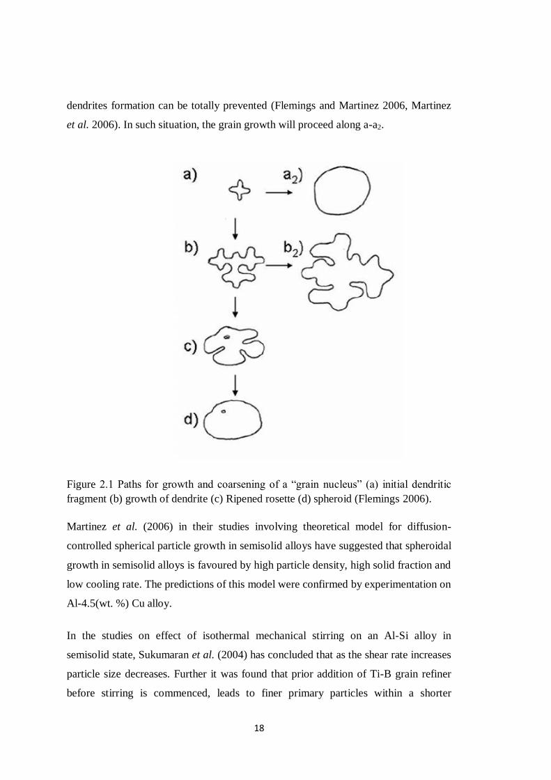
18
dendrites formation can be totally prevented (Flemings and Martinez 2006, Martinez
et al. 2006). In such situation, the grain growth will proceed along a-a2.
Figure 2.1 Paths for growth and coarsening of a “grain nucleus” (a) initial dendritic
fragment (b) growth of dendrite (c) Ripened rosette (d) spheroid (Flemings 2006).
Martinez et al. (2006) in their studies involving theoretical model for diffusion-
controlled spherical particle growth in semisolid alloys have suggested that spheroidal
growth in semisolid alloys is favoured by high particle density, high solid fraction and
low cooling rate. The predictions of this model were confirmed by experimentation on
Al-4.5(wt. %) Cu alloy.
In the studies on effect of isothermal mechanical stirring on an Al-Si alloy in
semisolid state, Sukumaran et al. (2004) has concluded that as the shear rate increases
particle size decreases. Further it was found that prior addition of Ti-B grain refiner
before stirring is commenced, leads to finer primary particles within a shorter

19
isothermal stirring duration. The boundary level model developed by Vogel and
Canter (1977a) to study the effect of stirring on the growth of spherical particles from
the melt has shown that stirring causes destabilization of solid/liquid interface for both
low and high mobility surfaces. Further, Vogel (1977b) suggested that the non-
dendritic microstructure observed in rheocasting might be the result of overlapping
diffusion fields of a large number of growing particles. Another study by Hellawell
(1996) shows that formation of stable diffusion field for continued evolution of
dendrites is negated by vigorous stirring. The work further points out that the solute
enrichment and thermosolutal convection due to remelting can detach the dendrites
from their roots.
From the literature surveyed it is revealed that , in the stirred slurries, fragmentation
of dendrites results in evolution of spheroidal morphology, the direct evidence for
which is the work done by Spencer et al. (1972). It is learnt that shearing breaks up
dendrites on partial solidification. Although after a lot of research is being done in this
area (Spencer et al. 1972, Vogel and Canter 1977a, Vogel 1977b, Vogel et al. 1979,
Apaydin et al. 1980, Doherty et al. 1984 and Hellawell 1996), the question still
remains to be answered is as to how shearing can exert such a large bending moment
to cause the fracture of dendritic arms, the dendritic arms being small. Vogel et al.
(1979) have proposed a completely different theory suggesting that the dendritic arms
break under the shear stress created by the stirring of melt and the plastic strain is
accommodated by dislocation generation.
At low shear stress, neither the mechanism of remelting nor that of fragmentation
offers perfect explanation for evolution of rosette type morphology. Mullis (1999) has
proposed a theoretical model explaining how the bending of dendritic arms gives rise
to rosette shaped structure, although the predicted model has not been experimentally
verified so far. The Monte Carlo technique invented by Das et al. (2001, 2004) has
shown that growth of dendrites is enhanced at low shear rates and is in agreement to
the works carried out by Vogel and Canter (1977a). It is reported that turbulent type
flow that penetrates into the interdendritic region appears to prevent the dendritic
growth.

20
The literature reviewed in this section indicates that enhanced mass transfer during
forced convection gives rise to rosette and spheroidal morphology. Laminar flow
causes the evolution of rosette morphology from dendritic structures, while turbulent
flow modifies grain morphology from rosette shaped to spheroid. A nucleation
mechanism aided by uniform temperature and well distributed heterogeneous
nucleation agents may be the most likely cause for structural refinement under intense
stirring. Dendritic arm remelting (Flemings 1991) and fragmentation mechanisms
may be significant at low shear rates.
2.7 METHODS TO FORM SPHEROIDAL GRAIN STRUCTURE
The following subsections provide a brief summary of the important routes towards
obtaining non dendritic (spheroidal) structures.
2.7.1 Magnetohydrodynamic (MHD) Stirring
MHD stirring process was developed and patented by Young et al. (1983, 1984), to
overcome the problems related to mechanical stirring (Nafisi and Ghomashchi 2005).
In the MHD stirring process, electromagnetic stirring is used to break the dendrites in
semisolid state (Kenney et al. 1988). The solidifying metal acts as the rotor and the
stirring action caused shears the dendrites formed in the mushy zone to form globules.
Since the invention of the MHD stirring process for production of thixotropic starting
material, several citations of its use have been reported in literature (Ilegbusi and
Szekely 1988, Kenney et al. 1988, Naidermaier et al. 1988, Gabathuler et al. 1992,
Vives 1992, Vives et al. 1993, Blazek et al. 1995, Kahn Mann et al. 1996, Zillgen and
Hirt 1996 and Nafisi and Ghomashchi 2005). Kenney et al. (1988) have reported that
MHD could provide the desired microstructure with a grain size of 30μm as compared
to 100 μm obtained from mechanical stirring. Kirkwood (1994), Fan (2002), Atkinson
(2005) and Nafisi and Ghomashchi (2005) have reviewed the existing work in this
area. The review points out that the microstructures produced by MHD process are
strongly affected by the design of inductive coils. Further the electromagnetic force
fields in the mushy state are not uniform and can result in different degrees of

21
structural modification in the radial direction, incomplete spheroidization and
presence of „rosette‟ type grains.
2.7.2 Spray Forming (Osprey)
Spray casting (Osprey process) is a process for preparation of feedstock and involves
no agitation. In this process, the molten metal is directed through a nozzle into a gas
(Nitrogen or Argon gas) atomizer causing the liquid stream to be atomised in the form
of different size droplets as they experience high cooling rate during the course of
their flight. During atomisation, the large size droplets remain in liquid state, the
intermediate size in semisolid state, while small droplets solidify (Mathur et al. 1989).
These droplets are collected on a moving substrate and solidified to form shaped
castings (Nafisi and Ghomashchi 2005). The resulting structure from Osprey process
gives equiaxed microstructure with fine grains. It is reported that this material is ideal
for thixoforming, if heated into semi-solid state (Elias et al. 1988). Spray forming
method has been investigated in detail (Sukimoto et al. 1986, Amhold and Muller-
Schwelling 1991, Sano et al. 1992, Annavarapu and Doherty 1995), and several
methods have been proposed to describe the method in detail. This process finds wide
applications which include, processing of aluminium alloys and its composites, high
speed steel and copper alloys (Leatham et al. 1989, Mathur et al. 1989, Nafisi and
Ghomashchi 2005). Ward et al. (1996) have reported that spray casting method is
ideal for fabrication of Al-Si alloys containing more than 20 wt. % Silicon. The spray
forming process has aroused lot of interest amongst research fraternity as witnessed in
various review articles (Kirkwood 1994, Fan 2002, Atkinson 2005, Nafisi and
Ghomashchi 2005).
2.7.3 Strain Induced Melt Activated/ recrystallization and partial melting
Strain Induced Melt Activation (SIMA) developed by Young et al. (1983) involves
cold deformation or quenching of hot extruded or rolled bar into a billet, inducing
sufficient residual plastic strain. Once this billet is reheated to semi-solid state, partial
remelting occurs resulting in fine, uniform and non-dendritic microstructure, which
can then be thixoformed in its semi-solid state (Nafisi and Ghomashchi 2005).

22
Kirkwood et al. (1989) have suggested a modification in SIMA process in which the
initial heating is done below the recrystallization temperature (warm working) to
ensure maximum strain hardening as reviewed in (Nafisi and Ghomashchi 2005). A
thorough investigation on SIMA process by researchers (Loue and Suery 1995,
Turkeli and Akbas 1996, Cho et al. 1996, Choi and Park 1998a, 1998b, Lapkowski
1998, Valer et al. 1999, Tzimas and Zavaliangos 2000a) has resulted in more insight
and understanding on the effect of process parameters on the resulting microstructure.
Turkeli et al. (1996b) have reported the possibility of obtaining non-dendritic
structure with 7075 wrought aluminium alloy. Choi et al. (1998) have cited the
conditions for obtaining globular structure using SIMA process for Al 2024 and other
aluminium alloys.
Although SIMA process is a little similar to recrystallization and partial melting
(RAP) route, yet there are basic differences between the two (Atkinson 2005).
Recrystallization takes place when heating to semi-solid state and the recrystallized
boundaries are penetrated by the liquid resulting in formation of spheroids surrounded
by liquid. SIMA route (Young 1982) involves cold working while the RAP route
involves warm working (Kirkwood 1992). The main advantage of SIMA and RAP
route is that the extruded feedstock can directly be used and the grains are globular
than those obtained by MHD route. The main disadvantage is that the variation of
work stored across the section cause inhomogeneities in the grain sizes.
2.7.4 Liquidus/ near liquidus casting
Liquidus or near liquidus casting method is a recent method for developing
thixotropic source material (Xia and Tausig 1998, Wang et al. 2000a). The technique
so far has been reported for both cast (Wang et al. 2000a, 2000b, 2000c) as well as
wrought (Xia and Tausig 1998, Yurko et al. 1999, Cui et al. 2000) aluminium alloys.
The process consists of pouring the molten metal at or near the liquidus temperature
in a tilted crucible and the nucleation occurs on the side of the crucible. The low
pouring temperature results in fine non-dendritic microstructure. This is the principle
on which the UBE New Rheo Casting (NRC) process (also known as UBE process)
has been developed by UBE Industries Ltd, Japan.

23
2.7.5 Semi-solid rheocasting
The semisolid rheocasting (SSRTM
) process, developed recently is a hybrid of
mechanical stirring and near liquidus casting. A team of researchers (Martinez 2001,
Martinez et al. 2001, Flemings et al. 2003, Yurko et al. 2003) have invented this
process, which produce SSM structures without liquid entrapment. The alloy is held
slightly above the liquidus temperature and a stirrer, which also provides the cooling
action, is inserted into it. After a few seconds of stirring, the melt temperature reaches
a value corresponding to a solid fraction of few percent, and the stirrer is withdrawn.
2.7.6 Grain refinement
Grain refinement is one of the methods to obtain equiaxed grain structure (Wang et al.
1993) in an alloy. However, the method does not ensure uniform spheroidal and fine
grain structure. The pioneering work has been carried out by Cibula (1949, 1951) on
the effect of a number of elements like Ti, B, Zr, Nb, V, W, Ta, Ce on the grain
refinement Aluminium. Jones and Pearson (1976) have reported that the grain refiner
can be considered as effective only if the size of Al reaches below an acceptance level
of 220μm. The various aspects related to grain refinement and the proposed
mechanisms thereto have been reviewed in (McCullagh and Nelder 1989, Easton and
St. John 1999a, 1999b and Murty et al. 2002).
2.7.7 Semisolid thermal transformation
It is found that if the dendritic structure is heated in the semi-solid range for a certain
amount of time, spheroidal structure is obtained. The process is known as semisolid
thermal transformation (SSTT) (Berry and Linoff 1997). The mechanism for
formation of non-dendritic structures has already been discussed in sections 2.5 and
2.6.
A number of other techniques to obtain thixotropic feedstock have been reviewed in
articles by Kirkwood (1994), Fan (2002), Atkinson (2005) and Nafisi and
Ghomashchi (2005).

24
2.8 FLOW BEHAVIOUR OF MUSHY METAL
Tzimas and Zavaliangos (2000a) have reported that during mushy state forming, the
externally induced strain is accommodated by (i) plastic deformation of the unmelted
grains in contact (ii) deformation or fragmentation of bulk grains and, (iii)
rearrangement of grains through sliding. Tzimas and Zavaaliangos (2000b) and
Kiuchi (1989) conducted compression tests with constant strain rate and showed that
the flow stress reduces with increase in liquid content. Kiuchi and co workers
(Fukuoka and Kiuchi 1974, Kiuchi 1979b) have worked on determining the flow
stress of Al, Cu, and Pb based alloys in mushy state, and proposed that there is
substantial decrease in flow stress with decrease in solid fraction starting from 100%.
Through the studies on Al-5.5% Cu and A2017 alloys, Lapkowski et al. have shown
that plastic deformation of semisolid alloys require low forces as compared to that
with traditional hot working. It is found that the flow stress is a function of liquid
content, immaterial of the type of alloy (Kiuchi 1989), and that the chemical
composition and the structure of the alloy have minimal effect on the flow stress.
Since the deformation is fully accommodated by the viscous flow of liquid near the
grain boundary, the dependence of flow stress solely on the liquid content seems
justified. Hence the strain accommodation by the liquid at the grain boundaries is
dependent only on the viscosity of the liquid, which of course is a function of
temperature. Kiuchi (1989) has shown that the data representing the flow stress of a
given alloy in the mushy state normalized by its flow stress at the solidus line
temperature, if plotted against its solid fraction for different alloys, fall on the same
straight line or curve. Due to the presence of liquid at the grain boundaries, the grains
are free to rotate and/or slide against each other. On the other hand, the liquid flows as
lubricant through intergranular gaps. As a result, the constraints in polycrystalline
materials to deformation due to presence of grain boundaries are partially or
completely removed. When the solid fraction in the mushy alloy is high, the liquid is
trapped in the unmelted grain junctions and exerts an internal hydrostatic pressure in
response to the applied load.

25
2.9 VOLUME FRACTION EVALUATION
The evaluation of volume fraction plays a significant role in determining the
deformation process conditions (Lapkowski 1997), mainly because the flow stress is
significantly dependent on the liquid fraction content. An accurate determination of
liquid volume content is necessary as it determines the rheological behaviour (Joly
and Mehrabian 1976, Flemings 1991, Kirkwood 1994, Lapkowski 1997, Tzimas and
zavaliangos 1999 and Fan 2002) and microstructural evolution (Hardy and Voorhes
1988, Martinez 1994, Salvo et al.1995, Loue and Suery 1995, Tzimas and
Zavaliangos 2000a). Literature review suggests three methods which are used to
evaluate the volume fraction of solid (Tzimas and Zavaliangos 2000a). These methods
are (a) Thermal analysis technique, (b) Quenching experiment method and (c) Use of
lever rule in equilibrium phase diagram. Tzimas and Zavaliangos (2000b) have
inferred that all the above methods are approximate evaluations of volume fraction
and each has its own merits and limitations.
2.10 SEMISOLID PROCESSING METHODS
Semisolid processing encompasses a whole family of processes. The broad
categorisation of these processes follows in the upcoming subsections.
2.10.1 Rheocasting
The process in which the alloy is cooled from the liquid state into semisolid state and
injected into die without any intermediate solidification step is known as rheocasting.
The non dendritic structure can be obtained by various means such as, mechanical
stirring, MHD stirring, simulated nucleation of solid particles as in the new
rheocasting (NRC) process patented by UBE, Japan as reviewed in (Nafisi and
Ghomashchi 2005), or by electromagnetic stirring in the sleeve as in the new semi-
solid metal casting process from Hitachi Ltd, Japan as reviewed in (Nafisi and
Ghomashchi 2005). In the NRC process, the alloy is heated slightly above the liquidus
temperature and is poured in a crucible, followed by controlled cooling resulting in
spheroidal microstructure, before being taken up for forming. There is no need for a

26
specially treated thixo-formable feed stock for this process. The NRC method has
been used for processing cast Al alloys (Kaufmann et al. 2000a, Wabbuseg et al.
2000), wrought Al alloys (Kaufmann et al. 2000b) and magnesium alloys (Potts
2000).
2.10.2 Rheomoulding
The first rheomoulding prototype was patented by Cornell University (Peng et al.
1994) which uses a vertical injection moulding and clamping single screw machine,
more or less similar to that used for polymer injection moulding. The liquid alloy is
fed into a barrel. The cooling s carried out while the liquid is stirred by the rotating
screw. Either single (Peng et al. 1994, Peng and Hsu 2000) or twin stirrer (Fan et al.
1999a, Fan et al. 2001a) can be used. The semisolid alloy is then forced into the die
cavity. The process is suitable for mass production of components and does not
require specially prepared feedstock. The process has been described in a number of
publications (Peng et al. 1994, Wang et al. 1996) and can be applied to mould Sn-Pb
and Zn-Al-Cu alloys. In the recent past, Fan and co workers (Fan et al. 1999a,
Fan et al. 2001) have extended twin screw rheomoulding process to a
rheomixing process for processing usually immiscible liquid alloys.
2.10.3 Thixomoulding
Thixomoulding is the process developed to fabricate the near net shaped components
(Pasternak et al. 1992) and licensed to „Thixomat‟ (Pasternak et al. 1992, Walukas et
al. 2000). The raw material for the process are solid chips of 2 to 5 mm in size
obtained during machining or other metal working of magnesium alloys as reviewed
in (Nafisi and Ghomashchi 2005). The chips are fed into a heated injection system
using a continuous rotating screw and are partially melted to thixotropic slurry under
continuous shear force generated by rotating Archimedean screw (Pasternak et al.
1992). Spheroidal microstructure is produced during the process and the material is
fed into the die. The major advantage of this process over the majority of the other
SSM processing techniques is that slurry making and component forming is reduced
to a single step, leading to process economy.

27
2.10.4 Thixoforming
Thixoforming is the name given to the process which involves heating the material to
the semisolid state with liquid content in the region between 30 to 50 vol. % and
subsequently forcing into a die (Kopp et al. 2001). Component forming in a closed die
is named as „Thixocasting‟ while that done in an open die is called „Thixoforging‟
(Fan 2002).
Figure 2.2 shows the process map of thixoforming process in terms of the starting
material routes as well as process variants. Components are manufactured using
thixocasting, thixoforging and thixotransverse extrusion. Long products are
manufactured using thixoextrusion and thixorolling. As a variant of thixoforming,
forming could be done with an arbitrary liquid volume content which could be either
more than or less than 30 volume percent. Such semisolid deformation processes are
categorised as mushy state forming and a brief discussion on these is presented in the
sections to follow.
Figure 2.2 The process map of thixoforming variants (Kopp 2003)
28
2.10.5 Mushy state extrusion
Mushy state extrusion has been used to obtain wires, tubes and bars from billets
reheated in an electric furnace (Kiuchi 1989) with the liquid weight content between
20-30%, so that the billet is able to retain its original shape and size. The extrusion
pressure required in this case is only about one fourth that would be required at
solidus temperature. The extrusion pressure decreases sharply when the solid content
reduces from 100% to 80% and practically seen to remain constant at and below 60%.
The extrusion pressure at a given solid content is a function of extrusion ratio. Higher
the extrusion ratio, greater will be the extrusion pressure at a given solid content. Due
to lower extrusion pressures involved with mushy state extrusion, high extrusion
ratios of the order of 40:1 have been reported in case of Al-5.7 wt. % Cu alloy. As the
liquid content in the billet acts as a lubricant in the container, and die and the pressure
required is low, it has been possible to extrude complicated cross-sections in a single
pass.
2.10.6 Mushy state rolling
Mushy state rolling is a recently developed metal forming process, which requires a
stable, steady flow and homogeneous deformation of the semisolid plate or sheet, as
well as rapid cooling inside the roll gap (Kiuchi 1989). Figure 2.3 depicts the
schematic diagram showing the mushy state rolling of a workpiece. As the semisolid
plate is in contact with the rolls during deformation of plate, the deformation zone is
narrow with a wide free surface existing around it. The liquid from the deformation
zone flows freely from the narrow deformation zone to the other parts of the plate or
sheet. This means that a steady state condition between co-ordinated flow of solid and
liquid component is difficult to be attained. Often, it is observed, that the solid and the
liquid component flow independently. It has been shown that the thickness reduction
is reduced at high liquid content, as the alloy flows in the gap as slurry. At the
entrance to the roll gap, the liquid is likely to flow to the top and bottom surfaces
under pressure created in the deformation zone. The liquid component however, does
not separate out, but solidifies in contact with the comparatively cold roll surfaces and
forced into the roll gap. The solid skeleton containing the unmelted grains is

29
compressed and is drawn into the roll gap. The grains in the solid skeleton tend to
elongate at low liquid content, when the grains touch one another combined with high
thickness reduction. The entire liquid solidifies in the roll gap.
Figure 2.3 Schematic illustration of flow and solidification of a mushy workpiece
inside the roll gap (Kiuchi 1991)
Mushy state rolling was first attempted by Kiuchi on AA5052 and AA7075 alloys
(Kiuchi (1989). He showed that the mushy state rolled sheet provides a heterogeneous
grain structure. The process yields a fine grained structure at the surfaces as compared
to that at the central portion due to rapid solidification of liquid component at the
surface with the rolls. Such inhomogenity is responsible for providing a gradient in
hardness and yield strength across the plate and sheet thickness.
Mushy state rolling has been used to process laminated composite sheets in the form
of metal ceramic composite bonded to the base alloy. Composite sheets of stainless
steel diffusion bonded to composite of cast iron, deoxidised iron and Al2O3 particles
have been processed by mushy state rolling (Kiuchi 1989). A review conducted by
Fan (2002) discusses the various aspects of thixoforming process.
Recently it has been reported (Herbert 2007) that mushy state rolling of Al-4.5Cu-
5TiB2 composite at temperatures corresponding to 10-30% liquid volume, leads to
refinement of rosette–shaped structure in α-Al matrix of the as-cast composite to give
globular or equiaxed grains. Grain refinement is achieved in the as-cast composite due
30
to Zener pinning by TiB2 particles (Zu and Luo 2001, Herbert et al. 2006). Rolling
under similar condition resulted in grain coarsening in case of Al-4.5Cu alloy due to
extensive diffusive mass transfer in presence of liquid at grain boundaries.
Furthermore, in case of mushy state rolled Al-4.5Cu-5TiB2 composite, the bimodal
grain size distribution observed in the microstructure is found to have larger volume
fractions of finer grains at near surface locations of the plate as compared to those at
the centre. A larger volume of fine grains in the near surface locations has been
attributed to the formation of fine grains due to rapid solidification of liquid being
squeezed out to the surface upon being compressed within the roll gap, which is in
confirmation with the results of Kiuchi (1989) and Herbert (2007). The mechanical
and wear properties are found to improve dramatically on mushy state rolling of this
composite due to chemical homogenisation, grain refinement and limited work
hardening of the unmelted grains (Herbert et al. 2008, 2010).
2.11 APPLICATIONS
2.11.1 Semisolid processing of alloys
Semisolid processing of alloys have been investigated (Kiuchi and Sugiyama 1991,
Hirt et al. 1997, Rovira et al. 1999, Cho and Kang 2000, Kapranos et al. 2000,
Kaufmann et al. 2000a, Rachmat et al. 2000, Siegert et al. 2000, Rice and Mendez
2001, Jung and Kang 2002, Kapranos et al. 2003 and Liu et al. 2003) with an
objective towards its practical investigations over the last two decades. Kaufmann et
al. (2000) showed that the “New RheoCasting” (NRC) process can be applied to
aluminium wrought alloys (6082) to obtain better mechanical properties as against the
standard casting alloys. Rice and Mendez (2001) have proposed new slurry based die
casting process and have successfully used it in fabricating fuel rail, compressor
heads, pistons and clutch covers for automotive applications.
Kiuchi and Sugiyama (1991) have investigated the mushy state rolling of aluminium
alloys and cast iron with emphasis on the effect of thickness reduction, solid volume
fraction and roll speed on the microstructure and properties of the resultant roll
product. They concluded that the mushy state rolling has the potential to develop and

31
manufacture new functional metallic or composite sheets. Rovira et al. (1999) have
reported the evolution of globular microstructure in the thixo-forged or thixo-extruded
Al-4.5 wt. % Cu alloys. Cho and Kang (2000) have studied the effect of pressure and
die temperature on microstructure and mechanical properties of thixo-forged AA2024.
Rachmet et al. (2000) and Liu et al. (2003) have reported the successful filling of the
die cavity with their investigations on thixoforging of high performance Al alloys
suggesting the viability of near net shaping using this process. Kapranos et al. (2003)
have successfully thixoforged a brake drum of A390 alloy for automotive application,
as an alternative to cast iron, with lower weight and good wear resistance.
Investigations have been carried out by Xie et al. (2006)) on application of Al-6Si-
2Mg alloy by fabricating water pump lid and connecting rod for automotive
application using thixoforming process. Wang and Xu (2006) also successfully
manufactured the water pump lid for automotive application using semisolid casting
of A357 alloy. The possibility of forming light weight components using
thixoforming has been explored by Hirt et al. (1997). A steering knuckle for a
passenger car fabricated by thixoforming A356 alloy resulted in 50% saving in
weight. Kapranos et al. (2000) proved that „near net shaped‟ structures could be
produced by fabricating thixoformed end plates of an electric motor from Al alloy.
2.11.2 Semisolid processing of composites
Particulate reinforced metal matrix composites (MMC) have generated a lot of
interest amongst the researchers due to their high specific strength, high specific
modulus, high wear resistance and stability at elevated temperatures. However, poor
formability has become a hindrance to a wider use of most MMCs. A lot of research
has been carried out on thixoforming of MMCs (Kiuchi and Sugiyama 1982, Lee et
al. 1994, Ward et al. 1996, Youn et al. 2002, Zu and Luo 2001, Hamilton et al. 2003).
Flemings and co workers were the pioneers in noting that metal slurries possessed
ideal environments to incorporate ceramic particles to form composites. Moon et al.
(1991) and Quaak et al. (1994b) have carried out research on castability
(compocasting) and forgeability of ceramic reinforced MMCs. McLelland et al.
(1992) have reported successful fabrication of Al-Si composites with uniform particle

32
distribution using thixoforming technique. Kiuchi and Sugiyama (1992) and Miwa et
al. (1992) have proposed techniques to incorporate SiC fibres as well as whiskers into
semisolid alloy. The amount of the ceramic phase that can be incorporated in the
MMC depends on the liquid fraction corresponding to the SSM temperature (Hong et
al. 2000).
Kiuchi (1987) has investigated the application of mushy state processing to
manufacture various kinds of metal-ceramic composites with successful manufacture
of particle reinforced cladding metal and composite sheets. Mushy state rolling has
also been used to manufacture laminated composites or cladding sheets with alternate
layers of base metal or alloy and composite sheets (Kiuchi 1989). Thixo-extrusion of
SiC/2024Al composite was successfully carried out by Lijun Zu and Shoujing Luo
(2001) with the microstructure characterised by well-densified matrix and uniform
distribution of reinforcements. Minghetti et al. (2001) investigated the back extrusion
of Al2O3 particle reinforced Al alloy/AA6061 matrix composite in semisolid state and
observed a gradient distribution of ceramic reinforcements based on the semisolid
forming parameters. Zhang and Wang (2001) carried out investigations on spray
formed 6066Al/SiC composites and have shown that thixoformed composites have
fine grained structure and that the process has the capability of near net shaping.
Hamilton et al. (2003), based on their study on AA2124/SiC composites, have
demonstrated the viability of the semisolid processing to achieve near net shaping of
metal matrix composites.
The research activities in the semisolid processing of composites have also focussed
on the manufacturing of MMC prototypes for a range of practical applications. One
such remarkable achievement has been the successful fabrication of cylinder liners
made with SiC reinforced MMCs using thixoforging demonstrated by Youn et al.
(2002). Ward et al. (1996) have carried out investigations on thixoforming of Al-Si
MMCs, wherein they have successfully manufactured oil pump housing and
demonstrator components. Applications of thixoforming are continuously gaining
popularity, since it is safe, clean and practical method for near net shaping.

33
2.12 MECHANICAL PROPERTIES
2.12.1 Alloys
Some of the data available from the literature about the mechanical properties of the
thixoformed Al alloys are listed in Table 2.1. Kenney et al. (1988), Gabathuler et al.
(1993) and Tietmann et al. (1992) have investigated the mechanical properties of the
A356 and A357 cast and Al alloys. Examination of data in Table 2.1 reveals that the
heat treated (T6 temper) thixocasting A356 Al cast alloy (Al-7 Si-0.5 Mg) shows
better mechanical properties as against those specimens produced by permanent
mould casting route. The effect of the temperature of the die and variation of applied
pressure on mechanical properties during thixoforming of complex shapes using A356
alloy has been investigated by Cho and Kang (2000). It has been found that the yield
strength, ultimate strength and the elongation of the alloy increase with increasing
applied pressure while they are found to decrease with a little increase in temperature
due to grain coarsening accompanying increase in temperature.
The thixoformed A357 alloy exhibits mechanical properties similar to that shown by
permanent mould route, albeit with greater ductility (Kenney et al. 1988, Gabathuler
et al. 1993). Bergsma et al. (1997) have compared the mechanical properties of
semisolid thermal transformed (SSTT) A357 alloy with electromagnetically stirred
A357 alloy, and found both exhibiting close similarity. It is observed that thermal
treatment of A357 alloy provides a god alternative to EMS method in obtaining
spheroidal microstructure.
The tension tests carried out by Zoqui and Robert (1998) on Al-4.5 (wt. %) Cu alloy
in both as rheocast and T6 condition show that the increase in grain size results in
decrease in the tensile and yield strength. It is observed that the initially an increase in
grain diameter results in a slight increase in elongation but elongation decreases on
higher increase in grain diameter. The increase in grain diameter is responsible for
poorer tensile properties of the as rheocast Al-4.5(wt. %) Cu alloy as compared to
those of it‟s as cast samples.
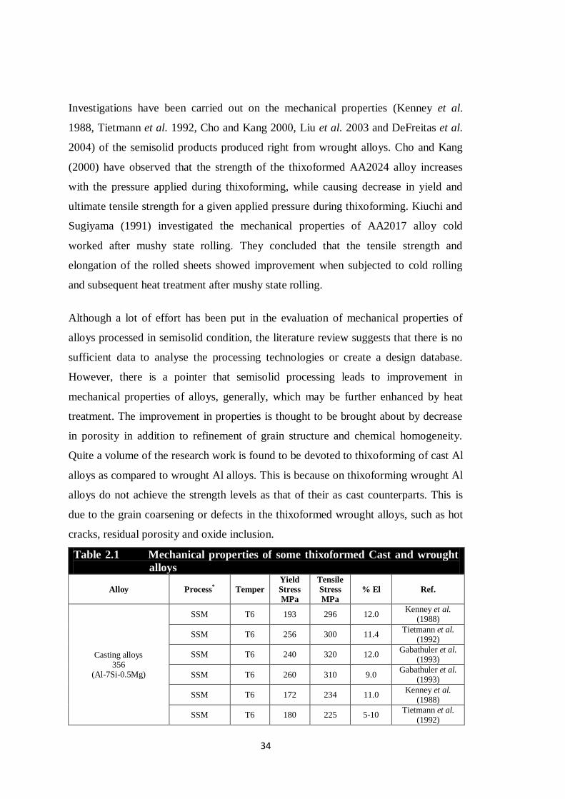
34
Investigations have been carried out on the mechanical properties (Kenney et al.
1988, Tietmann et al. 1992, Cho and Kang 2000, Liu et al. 2003 and DeFreitas et al.
2004) of the semisolid products produced right from wrought alloys. Cho and Kang
(2000) have observed that the strength of the thixoformed AA2024 alloy increases
with the pressure applied during thixoforming, while causing decrease in yield and
ultimate tensile strength for a given applied pressure during thixoforming. Kiuchi and
Sugiyama (1991) investigated the mechanical properties of AA2017 alloy cold
worked after mushy state rolling. They concluded that the tensile strength and
elongation of the rolled sheets showed improvement when subjected to cold rolling
and subsequent heat treatment after mushy state rolling.
Although a lot of effort has been put in the evaluation of mechanical properties of
alloys processed in semisolid condition, the literature review suggests that there is no
sufficient data to analyse the processing technologies or create a design database.
However, there is a pointer that semisolid processing leads to improvement in
mechanical properties of alloys, generally, which may be further enhanced by heat
treatment. The improvement in properties is thought to be brought about by decrease
in porosity in addition to refinement of grain structure and chemical homogeneity.
Quite a volume of the research work is found to be devoted to thixoforming of cast Al
alloys as compared to wrought Al alloys. This is because on thixoforming wrought Al
alloys do not achieve the strength levels as that of their as cast counterparts. This is
due to the grain coarsening or defects in the thixoformed wrought alloys, such as hot
cracks, residual porosity and oxide inclusion.
Table 2.1 Mechanical properties of some thixoformed Cast and wrought
alloys
Alloy Process* Temper
Yield
Stress
MPa
Tensile
Stress
MPa
% El Ref.
Casting alloys 356
(Al-7Si-0.5Mg)
SSM T6 193 296 12.0 Kenney et al.
(1988)
SSM T6 256 300 11.4 Tietmann et al.
(1992)
SSM T6 240 320 12.0 Gabathuler et al.
(1993)
SSM T6 260 310 9.0 Gabathuler et al.
(1993)
SSM T6 172 234 11.0 Kenney et al.
(1988)
SSM T6 180 225 5-10 Tietmann et al.
(1992)

35
PM T6 186 262 5.0 Metal Hand.
(1990)
PM T51 138 186 2.0 Metal Hand.
(1990)
A356 (ALTHIX)
Thixoformed (@ 100MPA)
T6 256 298 5.7
Cho and Kang
(2000)
Thixoformed (@ 150MPA)
T6 262 313 7.8
A356 (ALTHIX)
Applied pressure 100MPa
Thixoformed
(@ Td=3000C T6 256 298 5.7
Thixoformed (@ Td=3500C
T6 253 295 5.4
Thixoformed (@ Td=4000C
T6 247 285 3.5
A356(0.4% Mg)
Thixocast T5 160 250 14
Jorstad et al.
(2005)
T6 240 310 13
NRC T5 165 265 10
T6 190 295 12
SLC
F 130 220 12
T5 160 265 12
T6 180 295 12
A356 (0.3%Mg) SLC
F 115 185 10
T5 115 190 10
T6 215 310 12
B319 (0.35Mg/4% Cu)
SLC
F 140 240 9
Jorstad et al. (2005)
T5 165 265 9
T6 225 305 9
357, A357 (Al-7Si-0.3Mg)
SSM T6 290 358 10.0 Kenney et al.
(1988)
SSM T6 260 330 9.0 Gabathuler et al.
(1993) SSM T7 290 330 7.0
SSM T5 207 296 11.0 Kenney et al.
(1988)
SSM T5 200 285 5-10 Gabathuler et al.
(1993)
PM T6 296 359 5.0 Metal Hand.
(1990)
PM T51 145 200 4.0 Metal Hand.
(1990)
A357 (Pechiney, RD0430)
SSTT T6(1) 266 304 13.8
Bergsma et al. (1997)
SSTT T6(1) 260 312 11.3
SSTT T6(1) 239 279 4.5
A357 (NWA, G001-3)
ES T6(1) 296 341 5.8
ES T6(2) 330 361 9.4
ES T6(3) 323 367 10.3
ES T6(2) 270 314 12.2
357
SSTT T5a 219 289 5.5
Bergsma et al. (2001)
Sand Cast T5 117 179 3.0
SSTT T6b 288 339 6.3
EM T6[1] 300 341 10.8
Sand Cast T6[6] 296 345 2.0
DF53 SSTT T5c 224 327 5.2
319 EM T5d[8] 237 292 2.8
Sand Cast T5[6] 179 207 1.5
Modified 319 (DF53)
SSTT T6e 316 387 4.8
SSTT T6f 351 409 5.9
SSTT T6g 299 398 10.2
Modified 319
EM T6h[8] 334 379 1.6
EM T6i[10] 320 405 5.0
Sand Cast T6[6] 164 250 2.0
B319 SLC F 140 240 9

36
(0.35Mg/4% Cu) T5 165 265 9 Jorstad et al. (2005) T6 225 305 9
357, A357 (Al-7Si-0.3Mg)
SSM T6 290 358 10.0 Kenney et al.
(1988)
SSM T6 260 330 9.0 Gabathuler et al. (1993) SSM T7 290 330 7.0
SSM T5 207 296 11.0 Kenney et al.
(1988)
SSM T5 200 285 5-10 Gabathuler et al.
(1993)
PM T6 296 359 5.0 Metal Hand.
(1990)
PM T51 145 200 4.0 Metal Hand.
(1990)
A357 (Pechiney, RD0430)
SSTT T6(1) 266 304 13.8
Bergsma et al. (1997)
SSTT T6(1) 260 312 11.3
SSTT T6(1) 239 279 4.5
A357 (NWA, G001-3)
ES T6(1) 296 341 5.8
ES T6(2) 330 361 9.4
ES T6(3) 323 367 10.3
ES T6(2) 270 314 12.2
357
SSTT T5a 219 289 5.5
Bergsma et al. (2001)
Sand Cast T5 117 179 3.0
SSTT T6b 288 339 6.3
EM T6[1] 300 341 10.8
Sand Cast T6[6] 296 345 2.0
DF53 SSTT T5c 224 327 5.2
319 EM T5d[8] 237 292 2.8
Sand Cast T5[6] 179 207 1.5
Modified 319 (DF53)
SSTT T6e 316 387 4.8
SSTT T6f 351 409 5.9
SSTT T6g 299 398 10.2
Modified 319
EM T6h[8] 334 379 1.6
EM T6i[10] 320 405 5.0
Sand Cast T6[6] 164 250 2.0
2024
Thixocast T6 37.4kgf/
mm2 46.4kgf/
mm2 11.2
Chen et al. (1979) Squeezecast T6 36.2kgf/
mm2 48.3kgf/
mm2 13.4
T6 T6 40kgf/
mm2 48.5kgf/
mm2 10
2024 (Al-4Cu-1Mg) SSM T6 277 366 9.2 Tietmann et al.
(1992)
2024 W T6 393 476 10 Metal Hand.
(1990)
2024 W T4 324 469 19 Metal Hand.
(1990)
Al2024
Thixoformed (@100MPa)
T6 233 377 20.3
Cho and Kang (2000)
Thixoformed (@150MPa)
T6 236 387 21
Al2024 Apllied pressure 100MPa
Thixoformed
(@Td=3500C) T6 233 377 20.3
Thixoformed (@Td=4000C)
T6 210 371 19.9
AA2024
Thixoextruded - - 243 9
DeFreitas et al. (2004)
Thixoextruded T6 - 402 11
Forged T6 420 8
W T6 - 475 10
2219 (Al-6Cu) SSM T8 310 352 5.0 Kenney et al.
(1988)
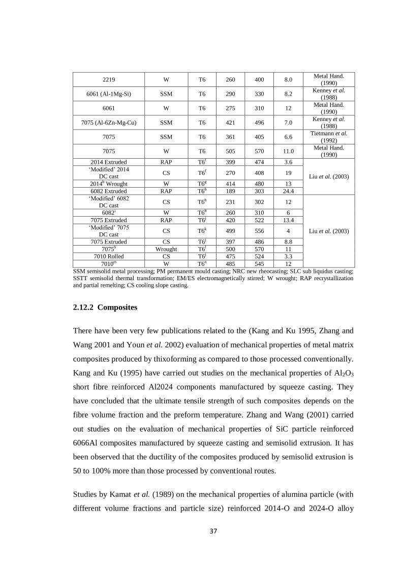
37
2219 W T6 260 400 8.0 Metal Hand.
(1990)
6061 (Al-1Mg-Si) SSM T6 290 330 8.2 Kenney et al.
(1988)
6061 W T6 275 310 12 Metal Hand.
(1990)
7075 (Al-6Zn-Mg-Cu) SSM T6 421 496 7.0 Kenney et al.
(1988)
7075 SSM T6 361 405 6.6 Tietmann et al.
(1992)
7075 W T6 505 570 11.0 Metal Hand.
(1990)
2014 Extruded RAP T6f 399 474 3.6
Liu et al. (2003)
„Modified‟ 2014 DC cast
CS T6f 270 408 19
2014b Wrought W T6g 414 480 13
6082 Extruded RAP T6h 189 303 24.4
„Modified‟ 6082 DC cast
CS T6h 231 302 12
Liu et al. (2003)
6082i W T6h 260 310 6
7075 Extruded RAP T6j 420 522 13.4
„Modified‟ 7075 DC cast
CS T6k 499 556 4
7075 Extruded CS T6j 397 486 8.8
7075b Wrought T6l 500 570 11
7010 Rolled CS T6j 475 524 3.3
7010m W T6n 485 545 12
SSM semisolid metal processing; PM permanent mould casting; NRC new rheocasting; SLC sub liquidus casting; SSTT semisolid thermal transformation; EM/ES electromagnetically stirred; W wrought; RAP recrystallization and partial remelting; CS cooling slope casting.
2.12.2 Composites
There have been very few publications related to the (Kang and Ku 1995, Zhang and
Wang 2001 and Youn et al. 2002) evaluation of mechanical properties of metal matrix
composites produced by thixoforming as compared to those processed conventionally.
Kang and Ku (1995) have carried out studies on the mechanical properties of Al2O3
short fibre reinforced Al2024 components manufactured by squeeze casting. They
have concluded that the ultimate tensile strength of such composites depends on the
fibre volume fraction and the preform temperature. Zhang and Wang (2001) carried
out studies on the evaluation of mechanical properties of SiC particle reinforced
6066Al composites manufactured by squeeze casting and semisolid extrusion. It has
been observed that the ductility of the composites produced by semisolid extrusion is
50 to 100% more than those processed by conventional routes.
Studies by Kamat et al. (1989) on the mechanical properties of alumina particle (with
different volume fractions and particle size) reinforced 2014-O and 2024-O alloy
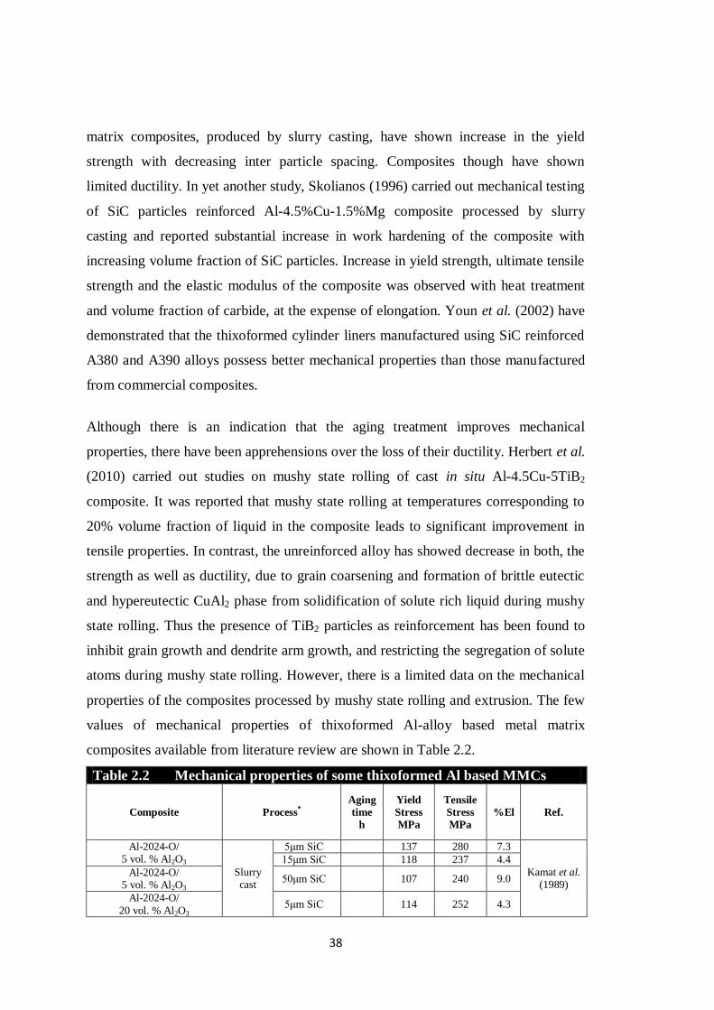
38
matrix composites, produced by slurry casting, have shown increase in the yield
strength with decreasing inter particle spacing. Composites though have shown
limited ductility. In yet another study, Skolianos (1996) carried out mechanical testing
of SiC particles reinforced Al-4.5%Cu-1.5%Mg composite processed by slurry
casting and reported substantial increase in work hardening of the composite with
increasing volume fraction of SiC particles. Increase in yield strength, ultimate tensile
strength and the elastic modulus of the composite was observed with heat treatment
and volume fraction of carbide, at the expense of elongation. Youn et al. (2002) have
demonstrated that the thixoformed cylinder liners manufactured using SiC reinforced
A380 and A390 alloys possess better mechanical properties than those manufactured
from commercial composites.
Although there is an indication that the aging treatment improves mechanical
properties, there have been apprehensions over the loss of their ductility. Herbert et al.
(2010) carried out studies on mushy state rolling of cast in situ Al-4.5Cu-5TiB2
composite. It was reported that mushy state rolling at temperatures corresponding to
20% volume fraction of liquid in the composite leads to significant improvement in
tensile properties. In contrast, the unreinforced alloy has showed decrease in both, the
strength as well as ductility, due to grain coarsening and formation of brittle eutectic
and hypereutectic CuAl2 phase from solidification of solute rich liquid during mushy
state rolling. Thus the presence of TiB2 particles as reinforcement has been found to
inhibit grain growth and dendrite arm growth, and restricting the segregation of solute
atoms during mushy state rolling. However, there is a limited data on the mechanical
properties of the composites processed by mushy state rolling and extrusion. The few
values of mechanical properties of thixoformed Al-alloy based metal matrix
composites available from literature review are shown in Table 2.2.
Table 2.2 Mechanical properties of some thixoformed Al based MMCs
Composite Process*
Aging
time
h
Yield
Stress
MPa
Tensile
Stress
MPa
%El Ref.
Al-2024-O/ 5 vol. % Al2O3
Slurry cast
5μm SiC 137 280 7.3
Kamat et al. (1989)
15μm SiC 118 237 4.4
Al-2024-O/ 5 vol. % Al2O3
50μm SiC 107 240 9.0
Al-2024-O/
20 vol. % Al2O3 5μm SiC 114 252 4.3

39
Al-2024-O/ 20 vol. % Al2O3
50μm SiC 92 194 2.5
Al-2024/
Al2O3
673K
Squeeze cast
488 Kang and Ku (1995)
773K 470
1073K 428
Al-4.5%Cu-1.5%Mg
Slurry cast
10.7μm SiC
- 85.1 103 5.2
Skolianos (1996)
3.5 108.2 126.1 4.8
Al-4.5%Cu-1.5%Mg/ 4
vol.% SiC
- 101.2 114.2 5.0
3.5 113.3 132.2 4.3
Al-4.5%Cu-1.5%Mg/ 12 vol.% SiC
- 118.0 123.0 5.0
3.5 133.1 141.1 3.1
Al-4.5%Cu-1.5%Mg/ 25 vol.% SiC
- 143.2 161.0 2.1
3.5 169.0 200.3 1.5
Spray formed 6066Al/SiC
883K
Squeeze cast
0 316 274 8.2
Zhang and Wang (2001)
2 314 275 10.9
8 369 322 9.2
16 329 290 8.8
893K
0 262 220 6.8
2 280 250 3.6
8 305 265 3.9
16 296 262 2.6
903K
0 272 210 10
2 298 242 6.4
8 366 328 5.9
16 339 302 5.2
6066Al Matrix Casting + Forging
8 345 310 8
Spray formed 6066Al/SiC
Spray formed 6066Al/SiC
883K Semisolid Extrusion
Semisolid Extrusion
0 225 175 11.4
8 352 282 15.2
893K 0 210 170 21.1
8 314 240 16.2
903K 0 233 171 15.1
8 362 313 13.3
6066Al Matrix Casting + Forging
8 345 310 8
A380/A390
Thixo-forging
14μm SiC
- 138-159 -
Youn et al.
(2002)
A380/10 vol. %SiC - 290-310 -
A380/20 vol. %SiC - 300-325 -
A380/A390
Thixo-forging
5.5μm SiC
- 138-159 -
A380/10 vol. %SiC - 300-320 -
A380/20 vol. %SiC - 310-330 -
2.13 WEAR PROPERTIES
Tribological properties are one of the important factors to be considered in
applications of metal matrix composites. Investigations in wear properties of
composites have revealed the influence of reinforcements on the wear properties of
composites. Roy et al. (1992) have reported that strongly bonded particle-reinforced

40
interface is the most significant factor causing the improvement in wear resistance of
conventional composites.
Skolianos and Kattamis (1993) have evaluated the tribological properties of SiCp
reinforced Al-4.5%Cu-1.5%Mg matrix composite specimens processed by slurry
casting, in both as cast and heat treated condition, using pin on disc wear testing
machine. It has been observed that specific wear rate and coefficient of friction
decrease with increasing volume fraction of carbide, decreasing carbide particle size,
and reduction in inter-particle spacing. Kamat et al. (1989) in their investigation of
tensile properties on composites have reported increase in yield strength with decrease
in the particle spacing. Thus in other words, specific wear rate and coefficient of
friction have been found to increase with increase in yield strength and therefore
hardness. The solutionising and aging treatment will lead to further increase in wear
resistance, and reduction in coefficient of friction.
Ward et al. (1996) have carried out the pin on disc and pin on plate wear testing of
thixoformed Al-25Si-5Cu, Al-30Si-5Cu and Al-40Si-5Cu alloys against a nitriding
steel counterface material in unlubricated condition. It has been observed that only a
small difference in wear rate exists in thixoformed alloys and Al-40Si-5Cu alloy in T6
condition. Furthermore, it has been observed that wear rate increases with Si content.
Investigations by Youn et al. (2002) on the wear properties of thixoformed cylinder
liners produced using SiC reinforced A380 and A390 alloy matrix composites were
carried out using pin on disc wear testing machine. Examination of the effect of
forging pressure on the wear properties has revealed that wear rate decreases with
increase in the forging pressure. The wear rate of cylinder liner made by semisolid
processing of A380-10 vol. % SiCp composite has been found to be 37.5% less than
that shown by commercially fabricated composite cylinder liner.
From the investigations carried out on the wear properties of semisolid processing of
composites, it appears that there is a definite improvement observed in the wear
properties of thixoformed products. Skolianos and Kattamis (1993) have reported that
aging helps in improving the wear resistance. The reviews conducted by Kirkwood
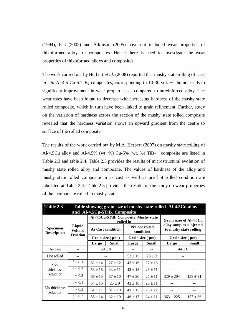
41
(1994), Fan (2002) and Atkinson (2005) have not included wear properties of
thixoformed alloys or composites. Hence there is need to investigate the wear
properties of thixoformed alloys and composites.
The work carried out by Herbert et al. (2008) reported that mushy state rolling of cast
in situ Al-4.5 Cu-5 TiB2 composites, corresponding to 10-30 vol. % liquid, leads to
significant improvement in wear properties, as compared to unreinforced alloy. The
wear rates have been found to decrease with increasing hardness of the mushy state
rolled composite, which in turn have been linked to grain refinement. Further, study
on the variation of hardness across the section of the mushy state rolled composite
revealed that the hardness variation shows an upward gradient from the centre to
surface of the rolled composite.
The results of the work carried out by M.A. Herbert (2007) on mushy state rolling of
Al-4.5Cu alloy and Al-4.5% (wt. %) Cu-5% (wt. %) TiB2 composite are listed in
Table 2.3 and table 2.4. Table 2.3 provides the results of microstructural evolution of
mushy state rolled alloy and composite. The values of hardness of the alloy and
mushy state rolled composite in as cast as well as pre hot rolled condition are
tabulated at Table 2.4. Table 2.5 provides the results of the study on wear properties
of the composite rolled in mushy state.
Table 2.3 Table showing grain size of mushy state rolled Al-4.5Cu alloy
and Al-4.5Cu-5TiB2 Composite
Specimen
Description
Liquid
Volume
Fraction
Al-4.5Cu-5TiB2 Composite Mushy state
rolled in Grain sizes of Al-4.5Cu
alloy samples subjected
to mushy state rolling As Cast condition Pre hot rolled
condition
Grain size ( μm ) Grain size ( μm) Grain size ( μm)
Large Small Large Small Large Small
As cast -- 50 ± 8 -- -- 44 ± 6
Hot rolled -- -- 52 ± 15 28 ± 9 --
2.5%
thickness
reduction
fl ~ 0.1 62 ± 14 27 ± 12 43 ± 16 27 ± 13 -- --
fl ~ 0.2 58 ± 18 33 ± 11 42 ± 18 26 ± 11 -- --
fl ~ 0.3 66 ± 15 37 ± 10 47 ± 20 25 ± 11 329 ± 204 158 ± 91
5% thickness
reduction
fl ~ 0.1 54 ± 16 25 ± 9 42 ± 16 26 ± 11 -- --
fl ~ 0.2 51 ± 11 31 ± 10 41 ± 15 25 ± 12 -- --
fl ~ 0.3 55 ± 14 32 ± 10 46 ± 17 24 ± 11 363 ± 225 157 ± 86
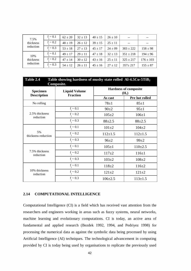
42
2.14 COMPUTATIONAL INTELLIGENCE
Computational Intelligence (CI) is a field which has received vast attention from the
researchers and engineers working in areas such as fuzzy systems, neural networks,
machine learning and evolutionary computations. CI is today, an active area of
fundamental and applied research (Bezdek 1992, 1994, and Pedriyez 1998) for
processing the numerical data as against the symbolic data being processed by using
Artificial Intelligence (AI) techniques. The technological advancement in computing
provided by CI is today being used by organisations to replicate the previously used
7.5%
thickness reduction
fl ~ 0.1 62 ± 20 32 ± 13 40 ± 15 26 ± 10 -- --
fl ~ 0.2 48 ± 19 26 ± 12 39 ± 15 25 ± 11 -- --
fl ~ 0.3 53 ± 18 27 ± 13 45 ± 17 24 ± 09 383 ± 222 158 ± 98
10% thickness
reduction
fl ~ 0.1 49 ± 17 29 ± 11 47 ± 18 32 ± 13 351 ± 218 194 ± 96
fl ~ 0.2 47 ± 14 30 ± 12 43 ± 16 25 ± 11 325 ± 217 176 ± 103
fl ~ 0.3 54 ± 12 26 ± 11 45 ± 16 27 ± 12 357± 217 155 ± 87
Table 2.4 Table showing hardness of mushy state rolled Al-4.5Cu-5TiB2
Composite.
Specimen
Description
Liquid Volume
Fraction
Hardness of composite
(Hv)
As cast Pre hot rolled
No rolling 78±1 85±1
2.5% thickness
reduction
fl ~ 0.1 90±2 95±1
fl ~ 0.2 105±2 106±1
fl ~ 0.3 88±2.5 88±2.5
5%
thickness reduction
fl ~ 0.1 101±2 104±2
fl ~ 0.2 112±1.5 112±1.5
fl ~ 0.3 96±2 99±2
7.5% thickness
reduction
fl ~ 0.1 105±1 110±2.5
fl ~ 0.2 117±2 116±1
fl ~ 0.3 103±2 108±2
10% thickness
reduction
fl ~ 0.1 118±2 116±2
fl ~ 0.2 121±2 121±2
fl ~ 0.3 106±2.5 113±1.5
43
models as well as to solve new problems in engineering industry. Of late, there have
been successful attempts in using hybrid models made from different components of
CI as building blocks, to build what can be called as hybrid intelligent systems.
Intelligence is a set of specific mind capabilities which allow the individual to use the
acquired knowledge efficiently to behave appropriately in the presence of
continuously evolving tasks and living conditions (Szezepaniak 1999). The definition
of CI (Szezepaniak 1999) states that it is a set of machine capabilities which allows it
to solve evolving tasks in the presence of evolving conditions. Bezdek (1994) stated
that “a system is computationally intelligent when it: deals only with numerical (low-
level) data, has a pattern recognition component and does not use the knowledge in
the AI sense; and additionally when it exhibits (a) computational adaptivity, (b)
computational fault tolerance, (c) speed of human mind, and (d) error rates that are
close to human performance.
The present work deals with the use of Artificial Neural Network i.e. the Feed
Forward Neural Networks (FFNN) and Recurrent Neural Networks (RNN) for
modelling the behaviour of mushy state rolling of Al matrix composites as a function
of a number of process parameters, involving multiple inputs and single or multiple
output(s) and hence can be termed as a complex system.
2.14.1 Artificial Neural Networks
Modern methods of computing to perform pattern recognition tasks are inspired by
the structure of biological neural network in the human brain. The human brain is a
complex carbon based computer which can do complex, non linear and parallel
computing/processing in a matter of few milliseconds. Today‟s computer
architectures are extremely powerful in the sense, that their speed of processing is
often million times faster than that of the brain (Yegnanarayana 2008). However,
since the human brain can perform massively parallel operations, each one having
comparatively lesser steps, a human brain can perform certain tasks like pattern
recognition, classification etc. much faster than the modern computers
(Yegnanarayana 2008).

44
The neural networks store the information in the interconnections between the
neurons. As against the computer wherein the information is stored in the memory
and addressed by its location, gets overwritten in case there is new information
addressed to the same location, the interconnection strengths are adjusted in case of
neural networks in the event of new information received, without losing the old
information (Yegnanarayana 2008, Zurada 1994).
Another important feature of neural network is fault tolerance due to parallel and
distributed processing. The information is distributed in interconnections which are
distributed parallely. Hence, even if some of the neurons are not functional, in course
of time, the information is preserved due to its distributed nature. The distributed
information storage in connections can be utilized to make the network to function as
memory and therefore neural networks can perform associative memory tasks. All in
all, neural networks are much more reliable and fault tolerant. An ANN is a parallel
and distributed processing network, which takes the inspiration from the functioning
of a human brain. ANN resembles the human brain (Zurada 1994) in following
aspects:
1. A neuron in an ANN replaces the biological neuron.
2. The ANN acquires knowledge through learning.
3. Knowledge is stored in weighted connections between neurons.
The important terms in artificial neural networks are discussed in the following sub-
sections.
2.14.2 Neuron: The Fundamental Unit of the Network
Muller and Reinhardt (1991) described the biological neural network in which the
fundamental unit is the neuron which is the basic building block of central nervous
system. Figure 2.4 shows the schematic structure of a neuron (Yegnanarayana 2008).
It consists of a cell body or soma where the cell nucleus is located. Dendrites are tree
like nerve fibres which originate from the soma. These dendrites receive signals from
other neurons. A single and long fibre known as axon originates from the cell body or

45
axon and branches out into further strands and sub-strands connecting many other
neurons at the synaptic junctions or synapses. The receiving ends of the junctions on
the other cells may be on the cell body or on their dendrites. Typically, an axon of one
cell can connect to a few thousand cells through their synapses. The synapse provides
memory of the past knowledge or experience. The size of the cell is of the range of 10
to 80μm. The length of the axon ranges from 50μm to several meters and has a tubular
shape having diameters of the order of few μm.
In the normal state the neuron is in the inhibited stage. The neuron is said to have
fired when an electric signal traverses across the cell. The interior of the cell or
protoplasm is negatively charged and is surrounded by liquid containing Na+ ions. In
the inhibited stage, protoplasm is at a potential of -70mV and is impermeable to Na+
ions. This causes deficiency of positive ions in the protoplasm. When the potential
increases above -60mV in the protoplasm, the surrounding membrane suddenly loses
its impermeability against Na+ ions which enter the protoplasm and reduce the
potential difference. This sudden change in the membrane potential causes the neuron
to discharge and is said to have fired. Whenever the neuron fires the ions reach the
axon and from there they reach the adjacent neuron through synaptic junctions. This
adjacent neuron, as mentioned in paragraph above, may be receiving connection from
a number of neurons. Thus the output of a neuron is the weighted function of the
inputs it receives from the connected neurons. Some of the inputs may be more
decisive in deciding the outcome of the connected neuron, if its synaptic connection
with the receiving neuron is stronger (Yegnanarayana 2008).
Quite similar to the biological neuron, a neuron can be created in a computer‟s
memory (McCulloh and Pitts 1993) which can be connected to a number of other
neurons to form a network of neurons. The strength of the various connections can be
represented by a numeric value known as synaptic weights or just as weights. The
learning is said to have occurred when the set of weights causes the network to recall
or behave in a particular expected way. ANNs are much easier to design and more
economical to operate as compared to their solid state hard wired neural networks
(Stern 1996, Fraser 2000). A host of applications using ANNs are being witnessed in

46
recent times in tasks comprising pattern classification, pattern recognition and pattern
mapping.
2.14.3 Developments in the Field of Neural Networks
In the year 1943 McCulloch and Pitts proposed a model of a computing element
called as neuron, which marked the beginning of the technique of machine learning.
The McCulloch Pitts model, basically, performed the weighted sum of the inputs to
the neuron followed by logic operation. The logic operation gave an output of either 1
or 0. A combination of these elements made it possible to realise a lot of logic
operations. The model had the drawback that it could not learn from examples as the
weights were fixed. Hebb (1949) then proposed a model in which learning was based
on pre and post synaptic values and was the first and fundamental learning rule
witnessed in literature relating to neural networks. Minsky (1954) further developed a
machine that could learn automatically through adaption of connection weights
followed by a very important invention by Rosenblatt. Rosenblatt (1958), in 1958 put
forth the Perceptron model with weight adjustments being done by using Perceptron
law. The Rosenblatt Perceptron model was able to solve pattern classification
problems with linearly separable data. In 1960 Widrow and Hoff (1960) invented the
From other
Neurons
Synapse
Dendrites Cell body
Nucleus
To other neurons
Figure 2.4 Structure of a Neuron (Yegnanarayana 2008)
47
Adaline model. The weight adjustment was done using LMS learning algorithm. The
convergence of LMS learning algorithm was proved by them and the algorithm was
successfully used for adaptive signal processing applications. However, Minsky and
Papert (1969) demonstrated through a number of examples, the limitations of a single
layer perceptrons in solving hard problems.
Feedback neural networks by Hopfield (1982, 1984) showed that stable equilibrium
states could be achieved, when the network possessed symmetric weights and the
state update is done asynchronously. During the same time, their contemporaries
Rumelhart and MeClelland (1986) proved that it is possible to adjust the weights of a
multilayered feed forward neural network in a symmetric manner to understand the
subtle and implicit relationship between input-output patterns (1986a). The
multilayered network proposed by Rumelhart could solve the hard problems, i.e.
problems wherein the pattern classes were not linearly separable. The convergence of
Perceptron model proved by Rosenblatt ensured that the final set of weights could be
reached in a finite number of steps for linearly separable data. However, Cameron
(1960) and Muroga (1971) showed that the number of linearly separable functions
decreased rapidly for two class problems, as the dimension of the input space is
increased. In the model proposed by Rumelhart, the weight adjustments were carried
out by using generalised delta rule or error backpropagation learning algorithm.
During the same time period, Ackley et al. (1985) proposed the Boltzmann machine, a
feedback neural network with a combination of the characteristics of the Hopfield
model and simulated annealing. The output function of the neurons in the Hopfield
networks, which was based on deterministic update rule, was based in Boltzmann
machines based on probabilistic update. In addition, in the recent few years, there
have been notable developments such as, self organisation and simulated annealing.
Self organisation has been useful in feature mapping while simulated annealing was
effectively used in Boltzmann machine. Learning laws like competitive learning,
reinforcement learning has been developed. Various architectures such as, Adaptive
Resonance Theory (ART), Recurrent Neural Networks (RNN), Radial Basis Function
(RBN) Networks and Counter propagation networks are being used to solve a variety
48
of problems related to pattern recognition, classification and pattern mapping. The
ANNs are being used today in applications ranging from image processing, speech
recognition, bomb detection, and robotics applications to forecasting applications. The
field of neural networks has steadily yet surely made its presence and importance felt
in various engineering disciplines. The field of mechanical engineering and
metallurgical and material science also has not been an exception and has seen a lot of
use of neural networks in various applications.
One of the most popular ways of training a Multi-Layered Perceptron (MLP) has been
Back Propagation algorithm (BP). This algorithm trains the network through recursive
technique and used the negative gradient descent method to decrease the error on the
Mean Squared Error (MSE) v/s weights plane and adjust the weights accordingly. A
completely different approach in which the curve fitting is done in a multidimensional
space has emerged as another method of function approximation. This method is
known as Radial Basis Function. The viewpoint here is to determine a surface in
multidimensional space that best fits the training data. Thus the generalisation is
brought about by a curve that interpolates the training data in a multidimensional
space. RBF was first proposed by Powell (1985), while recent work by Light (1992)
has generated more interest in this research area for application in numerical methods.
Recurrent networks distinguish from feed forward neural networks in that they
possess one or more feedback loops. The feedback loops may be local or global. The
recurrent network may contain three or more layers. The feedback from the neurons
may be to all other neurons in the current layer and/or to itself. The feedback
connections may start from the hidden neurons as well as from the output neurons.
The presence of feedback elements is reported to have a strong influence on learning
capability of the network. The feedback loops with unit time delay are known to
provide non linear dynamic behaviour in case of neural networks with hidden layers
(Haykin 2004).
Elman (1990, 1991) proposed the Simple Recurrent Network (SRN) which was used
to discover the word boundaries in a stream of phonemes without any built-in
constraints. The network contained a context layer or a temporal layer which stored
49
the output of hidden neurons for one time step and fed them back to the input layer.
The unit time step delay in the fed back signals was reported to provide the network
with ability to provide learning tasks that extend over time. As against a Jordan
network (Jordan 1986, 1992), which has feedback from the output layer, the recurrent
feedback in Elman network takes place in the hidden layer. Kremer (1995) showed
that the computational power of the Elman simple neural network was as good as that
of finite state machines.
The training of the recurrent network proposed by Elman used backpropagation
algorithm with gradient descent for weight adjustment i.e. learning (Elman 1990,
Jordan 1986, 1992, Li et al. 2002, Gruning 2006, Kremer 1995). However the
problem of the network getting stuck indefinitely in a local minimum was observed
(Gruning 2007). Thus there was problem of convergence while training with back
propagation algorithm (Gormann and Sejnowski 1988, Bengioy et al.1994, Plett 2003,
Yoon et al. 1993, Gruning 2007, Mandic and Chambers 2001, Kolen 2001, Koike
2002, Song et al. 2008, 2008a). Kremer (1995) stated that the power of Elman
network is only partly explored. Researches in this area (Sevan-Schreiber 1988) cited
that it firstly, could be because, that under the network constraints posed by Elman
architecture solution may not be available. Secondly, the fault could lie with the
technique of training itself, so that it does not give the solution. Mozer (1993)
suggests that the Elman training technique is powerful to handle any arbitrary
recurrent network. But practically it has been found that EBP training has been unable
to discover the subtle relationship that exists in temporal sequences. Weight
convergence in recurrent network using BP algorithm was critically analysed by Kuan
et al. (1994). It was considered that the estimated weights were bounded and since
weight estimation being a stochastic process, had considerable dependence. Some
simulations, though provided weight convergence, could not be guaranteed for any
arbitrary recurrent network. The implausibility of the back propagation learning was
attributed to two things. Firstly, the synapses are bidirectional and secondly to the
need for providing the fully specified target answer by the teacher to learner (Gruning
2007). However, not always such a fully specified target answer may be available. In
this context Gruning (2007) showed that the Elman network can be reused as

50
reinforcement learning model (wherein signals are fed back about success or failure).
The back propagation through time (BPTT) algorithm, which has given way to EBP
for on line (real time) applications (Song 2010), showed convergence with low values
of learning rate parameter while with high learning rates showed weight divergence.
Low learning rate results in slow convergence which though is not guaranteed. Song
(2009, 2010) developed an Extended EBP (eEPB) for training Elman networks using
an adaptive learning rate and an adaptive dead zone, resulting in optimisation of
training speed and weight convergence as well as improvement in generalisation
performance. Elman recurrent network training is therefore, still a subject of active
research in the area of neural computations.
The interest developed by McCulloh and Pitt‟s model (McCulloh and Pitts 1993)
followed by resurgence in interest brought about by Rosenblatt‟s work continues till
date. The major areas of intense research are in the fields of feed forward neural
networks or multilayered perceptrons and symmetric recurrent networks.
2.14.4 Function Approximation and ANN
Function approximation from a given bunch of input-output pairs has innumerable
applications in engineering and science as also in finance, medical diagnostics,
weather prediction etc. In a function approximation, using statistical techniques such
as regression, the specific function to which the data is to be fitted is first chosen. The
data is then fitted to this function by using some methods of error minimisation such
as method of least squares or by using some goodness of fit methods. An ANN when
used as a function approximation model has the ability to predict the system
performance which it represents and/or control it. The properties of an ANN model
such as its adaptivity and non linearity are ideally suited for real world applications.
The technique is mathematically less rigorous as compared to statistical and the finite
element method. The mapping network does approximation in a manner similar to the
generalisation that occurs with the regression technique. Any type of functional
relationship between input-output pairs can be aptly represented by a three layered
network (Chen and Jain 1994). In fact, function representation by a FFNN network is

51
more generic in nature as it encompasses many representation schemes of classical
approximation method.
2.14.5 Neural Networks vs. Statistical Techniques
As a forecasting tool, ANN can be compared to Autoregressive moving Average
(ARMA) class of models. ARMA methods, since ages have been used to model time
series. In general, similarities do exist between the ANN and statistical techniques. An
FFNN can be termed as a form of non liner regression (Ripley 1994, Potzinger et al.
2000). A multiple linear regression scheme, a standard statistical tool, can be thought
of as a simple ANN node. For example, for a linear equation of the type, y = w0 +
w1x1 + w2x2 + . . . . . . . . + wnxn, the xi can be taken to represent the inputs to the node,
wi can be taken as the corresponding weights and w0 can be the threshold function.
While fitting the ARMA type of model to a time series, the data has to be stationary
and must exhibit normal distribution. If indeed, that is not the case, then techniques
have to be used to induce stationary data and normally distribute the data. In case of
ANN, the statistical variation of data is immaterial, as the hidden neurons account for
non stationarities in the data (Reddy 2004). An ANN also possesses another
advantage over ARMA type models as it is a non linear model, though some non
linear ARMA type models are witnessed in literature in statistics. ANNs are most
ideally suited for mapping complex relationships between input-output and where the
relationships are not clearly understood, either due to no proper relationship being
there or inadequate data. Furthermore, ANN can make an n-step ahead forecast
directly without any recursive procedure. Due to its inherent robustness in design
which can be attributed to massive parallel processing, the ANNs are good modelling
tools for real life problems, in which data may be inadequate, may be available with a
lot of noise, and there could be distortions in data.
The ANNs have been rigorously compared with statistical methods for applications
pertaining to classification and prediction (Ripley 1994). Effectiveness of ANN in
time series forecasting have been examined. Lapedes and Farber (1988) have shown
that in two time series prediction problems, neural networks are clearly superior to

52
statistical methods. Sharada and Patil (1994) analysed 75 different time series
problems and inferred that the ANN and Box-Jekins forecasting system performed
equally. Interestingly, it has been observed that the memory of a time series has some
bearing on the performance. ANN performs slightly better than Box_Jekins model for
time series with short memory while reverse is true for time series with long memory.
One of the major demerits of the artificial neural network is that unlike the statistical
methods wherein the entire functioning of the model is transparent, the working of an
ANN is opaque. What exactly happens inside the hidden layers is not visible although
the output of the model is obviously useful. In artificial neural nets the functioning of
the hidden neurons once they are trained is not clearly understood (Fraser 2000).
Which of the neuron fires or why it fires is as mysterious as it was in the early days of
research in neural computations. Moreover, a trained ANN serves a model for a
particular problem, while there are set procedures or frameworks for selection of a
fitment model in statistical techniques. Some disadvantages of ANN have been
highlighted by Maier and Dandy (1999). First of all, the architecture, learning rate
parameter (η) and momentum factor (α), which are functional parameters of an ANN
are dependent on the problem at hand. There are no guidelines as to what architecture
or what learning rate and momentum factor should be used for a particular problem.
Each problem attempted by ANN is unique and all the function parameters are likely
to be unique for that problem. The entire training process is a trial and error process
with different combinations of number of hidden layers, number of neurons in each
hidden layer, learning rate parameter and momentum factor. Another problem with
ANN is that many a times, the data available to train the network isn‟t sufficient
enough to be able to bring the generalisation of the model. Also in a system which is
quite responsive to changes in the environment, ANN modelling may not be
appropriate as the network may not be able to cope up to the changes taking place.
For example, the networks when trained on static (past data) data may not be able to
lend results for future, unless the weight matrices are updated or adjusted with
suitable learning, to understand the new changes in the system.

53
A lot of study has been done on artificial neural networks and the regression methods
to determine the suitability of these models for pattern mappings (Kim et al. 1993,
Patuwo et al. 1993, Subramanian et al. 1993, Yoon et al. 1993 and Potts 2000).
Thus it can be summarised that
1. ANN can learn the relationship between input-output patterns and can
generalise the relationship
2. They can handle a wide variety of data
3. They are universal approximators
4. No assumptions are required to be made in understanding relationships
5. The type or in general, the details of the process need not be known to frame
an ANN model
6. Rigorous mathematical treatment is not required
All things put together, in actual practical situations, a trained ANN model has proved
to be a success, complementing human brain decision making.
2.15 NEURAL NETWORKS IN MATERIAL SCIENCE
An artificial neural network is thus a parallel processing system which mimics the
human style of learning through biological systems and understands the unknown
process or behaviour, through prior experience. The basic unit of the network is the
neuron, which passes or inhibits the signal to other neurons through connections. The
knowledge is stored in the trained network by the strength of these connections, which
are called as synaptic weights or simply as weights. This knowledge stored in the
connections is used in predicting the behaviour of process under changed process
parameters conditions. Artificial neural networks have been successfully used in the
manufacturing sector as well as service sector. In the non physical sector, ANNs have
been used in speech and image processing, fault detection, economy forecasting,
weather forecasting, stock markets. In the manufacturing sector, use of ANN is found
in steel plants, cold mill prediction, plate rolling, manufacturing of aluminium,
copper, magnesium alloys and composites. The list runs quite long as far as, the use of
54
ANN in material science and metallurgy is concerned. The iron, steel and non ferrous
metal industry is showing great interest in use of ANN in their process set up. This is
to a great extent, because the system is reliable when dealing with complex and non
linear relationships and does not involve rigorous mathematics. The field has also
invoked a strong interest from researchers across universities and regions as it
provides a good model to deal with complexities of data, non requirement of the
process details, and that the model provides scope for process monitoring, control and
optimization (Gormann and Sejnowski 1988, Widrow 1994, Hartley and Pillinger
2006, Su et al. 2007, Mousavi Anjidan 2007, Mandal et al. 2009).
In the recent past, a lot of applications of neural computational science are witnessed
in engineering to deal with problems related to complex and non linear relationships
of data. In the steel industry rolling is one of the most important forming processes.
The use of ANN in rolling dates back to 1990 decade (Wang et al. 1995, Sun et al.
1995, Rao et al. 1995, Larkiola et al. 1996, 1998). Larkiola (1998) used the neural
networks to optimise the mill settings to produce a product of given cross sectional
dimensions and strength, and also to predict the mechanical properties of the roll
strips along with the prediction of the temper force. Welding is a metal joining
process used to join mostly ferrous metals and is mostly used in steel structural
applications. Rao (2002) successfully used ANN for online eddy current testing of
austenitic steel welds. The ANN formulated was able to evaluate the depth of the
surface breaking notches within acceptable deviation. Kusiak and Kuziak (2002)
proposed a new approach based on ANN to predict the volume fraction and mean size
of the phase constituents after the material undergoes thermo-mechanical treatment
followed by cooling. Artificial neural networks have been successfully used in
predicting microstructure of 60Si2MnA rod (Jiahe et al. 2003), prediction of creep
behaviour of 316L (N) stainless steel (Srinivasan et al. 2003), for simulating the
forging process (Hartley and Pillinger 2006), modelling of mechanical properties of
Al-Si-Cu cast alloys (Dobrazanski et al. 2007), optimization of flow stress in 304
stainless steels during cold and warm compression (Anijdah et al. 2007), and
optimization of aging process for Cu-Cr-Zr-Mg alloy for aging treatment, hardness
and conductivity (Su et al. 2007).
55
The deformation behaviour of AISI 304L type stainless steel was studied by Mandal
et al. (2009) using ANN trained with standard BP algorithm. Recently, Wen et al.
(2009) used ANN model to predict microstructural change in conventional rolling and
thermo-mechanical processing of C-Mn and high strength alloy steels and were found
to be capable of supplementing their counterparts using conventional classical and
empirical methods. Poppe et al. (1995) looks at neural network as that can lead to an
intelligent steel production plant, which shall include automation of processes,
scheduling and management decisions being influenced by Neural Networks.
2.16 NEURAL NETWORKS IN SEMISOLID PROCESSING OF
COMPOSITES
2.16.1 Procedure Involved in ANN Model Development
The development of an ANN model involves various processes and functions. To
develop an ANN model one needs to know the best representative input parameters
for the given output(s). The preparation of the model would require sufficient amount
of training data so that network can learn. The selection of the type and amount of
data is often a matter of in depth knowledge and experience about the process
considered for modelling. The model developer should be in a position to determine
the data which is most representative of the input-output population. Thus data
generation becomes an important task in model development. Next, the input as well
as output data needs to be scaled so that data is grouped in a pre-decided range. Also,
the methods for weight initialisation to be used, determination of biases, deciding on
the architecture etc. are not readily available and require good amount of attention
during model development. The model developer should be aware that a neural
network does not have any information about the metallurgical process that is being
modelled. In order that the network understands the underlying relationships for the
process, the network needs to be trained. Hence, neural network training is the heart
of the entire ANN model development. The model developer should be sure that the
data that is being used for training is authentic, devoid of any significant measurement
errors. Any erroneous data used for training can lead to a situation similar to teaching

56
wrong things thereby, resulting in wrong learning. Wrong learning will automatically
lead to erroneous outputs from the model.
2.16.2 Data Preparation
Generally the data for an NN model arrives from a variety of sources. The NN is able
to process the data in a certain structured form. The network learning is affected by
the form in which the data is presented to the network. Hence the right coding scheme
for the data needs to be decided before hand, so that the network can learn and can
perform the given task. Therefore, the coding scheme for the data has to be in place
before the data collection task is taken up. Design of data coding system should be
decided before data collection as one should be aware as to what he is going to do
with that data. The process of data preparation involves the following steps.
2.16.2.1 Data Collection and Generation
The primary step in the ANN model development is deciding on the input and output
data required. After these have been identified, the metallurgical system/process data
needs to be generated. There are usually, two sources available for data
generation/collection. One can get data from the hand books or data books in
metallurgy and secondly from experiments. Actually, data generation means use of a
data generator which will give an output for each chosen sample. The total numbers
of samples are so chosen that the final model represents the actual metallurgical
problem on hand accurately. The type of data generator selected, generally depends
upon the type of problem being modelled. In the present work, the data is collected
from the experimental work done by Herbert (2007).
2.16.2.2 Range and Distribution of Samples
In general for modelling, a neural network needs three types of data sets. They are
named as training data, test data and validation data. Training data is used for training
the network, that is, to update the weights as the network learns from the test samples
being presented to it during training. The validation data performs the function of
monitoring the quality of training and helps in decision making as regards to
57
terminating the training process. The test data is used to check the final performance
of the trained model.
If the data being collected to develop the model lies in the range [xmin, xmax], the
validation and the test data also needs to be generated in the range [xmin, xmax]. The
training data can also be generated in the same range. In the region near the extremes
i.e. at the boundaries, it is advisable that training data may be sampled slightly beyond
the bounded values of data. The reason for this is to improve the performance of the
model at the boundaries of input sample space.
After deciding upon the range of the input parameters, the next step is to determine
the distribution of the input samples within the range. Generally, one can adopt three
methods, namely, uniform grid or equal spacing method, non uniform grid or unequal
spacing method or random distribution. By default, if there is no other compulsive
reason, one goes by the uniform grid method. Non uniform grid method is mostly
chosen when the process requires the sampling to be dense in some regions in the
input parameter space, where there is a likelihood of highly non linear process
behaviour. In such cases, it is better the neural network designer has a prior
knowledge of the process behaviour. In a randomised data distribution, each sample in
the range [xmin, xmax] is a random variable and the method is used when dimension of
the input parameter space is high.
2.16.2.3 Pre-Processing and Post-Processing of Data
In most of the cases, the input space consists of more than one variable. Each of the
input for the data collected may have different range. Similarly the number of outputs
may be more than one and each may have a different range. Hence each of the inputs
and the outputs needs to be normalised by its own normalising factors. Hence there is
a need for pre-processing of the raw input and output data or else the network will not
perform satisfactorily. This is a critical phase in the overall model design and
development.
58
There are two methods of data pre-processing. These are transformation method and
the normalisation method. In the transformation method, the raw input data is
manipulated to create a single input to a network, while normalisation transforms a
single input data to be distributed evenly and scales it into a workable range that for
the network (Swingler 1996, Berry and Linoff 1997, Reddy et al. 2005). As stated
earlier, it is desirable that the knowledge of the processes and systems for which the
model is developed be known, as it will help to understand the underlying features of
the process. All this will help the network to be trained in a better fashion resulting in
better performance of the network.
Normalisation of data is the last step in data pre-processing. The goal is to distribute
the data in such a way that it is spread uniformly across the data range. This applies to
both the input as well as the output data and the values should be scaled in such a way
that the range of the input and output data matches the range of the summing and
squashing device, the neuron. Thus, it can be seen that one may perform any other
transformation, normalisation as a final pre-processing step is indispensable.
It is possible to scale the raw input data within any range. However, for our work the
data is scaled between 0.1 and 0.9 using the following normalising function.
𝑥𝑛 = 𝑥−𝑥𝑚𝑖𝑛 ∗0.8
(𝑥𝑚𝑎𝑥 −𝑥𝑚𝑖𝑛 )+ 0.1 (2.1)
In the above equation xn refers to the normalised value, xmin is the minimum and xmax
is the maximum value in the range.
Upon training the network to a required degree of performance, it is expected that the
network will provide the output values that are well understood by the end user. In
order to achieve this, the post- processing of data becomes necessary. In this step, the
outputs of the network in the normalised form are de-normalised using the below
mentioned equation.
𝑥 = 𝑥𝑚𝑎𝑥 −𝑥𝑚𝑖𝑛 ∗(𝑥𝑛−0.1)
0.8+ 𝑥𝑚𝑖𝑛 (2.2)

59
2.17 STRUCTURE OF AN ANN MODEL
As of present, there is no way by which a structure of a network can be determined
using some analytical formulae or any empirical methods based on the network
parameters (Swingler 1996, Kang and Song 1998, Attoh-Okine 1999, Reddy 2004).
Thus, the structure must be manually selected using trial and error approach. While
deciding upon the network structure, several factors need to be taken into account.
These can be listed as follows.
Number of hidden layers
Number of neurons in each hidden layer
The network is trained using standard BP algorithm. The convergence of the network
depends, in addition to the above parameters, upon the following.
Summing function
Activation function
Initial weights
Learning rate
Momentum term
2.17.1 Summing function
The non input neurons in the network receive the inputs through the weighted
connections from other neurons, producing a single input known as the net input. This
is known as a combination or summing function and converts a column vector into a
scalar quantity (Zurada 1994, Reddy et al. 2005). Most neural networks such as
FNNN, use linear combination functions while the argument(s) of the activation
function in Radial-basis function (RBF) networks are Euclidean norm (distance)
based combination functions.
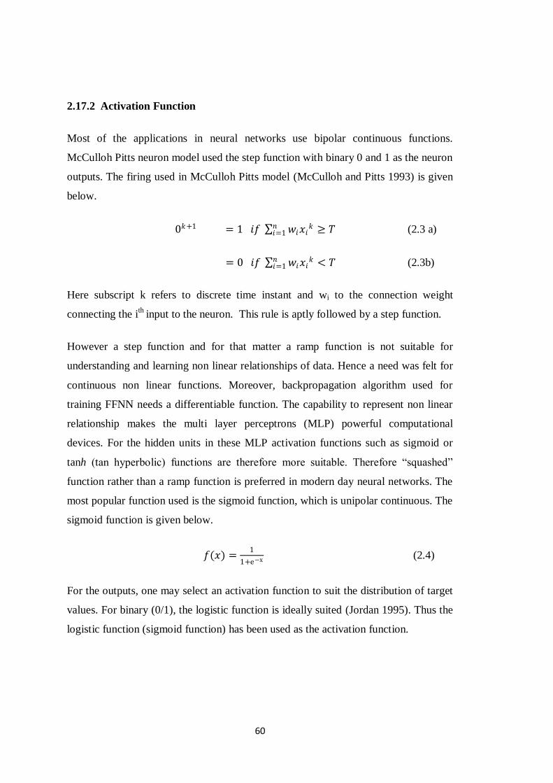
60
2.17.2 Activation Function
Most of the applications in neural networks use bipolar continuous functions.
McCulloh Pitts neuron model used the step function with binary 0 and 1 as the neuron
outputs. The firing used in McCulloh Pitts model (McCulloh and Pitts 1993) is given
below.
0𝑘+1 = 1 𝑖𝑓 𝑤𝑖𝑥𝑖𝑘 ≥ 𝑇𝑛
𝑖=1 (2.3 a)
= 0 𝑖𝑓 𝑤𝑖𝑥𝑖𝑘 < 𝑇𝑛
𝑖=1 (2.3b)
Here subscript k refers to discrete time instant and wi to the connection weight
connecting the ith
input to the neuron. This rule is aptly followed by a step function.
However a step function and for that matter a ramp function is not suitable for
understanding and learning non linear relationships of data. Hence a need was felt for
continuous non linear functions. Moreover, backpropagation algorithm used for
training FFNN needs a differentiable function. The capability to represent non linear
relationship makes the multi layer perceptrons (MLP) powerful computational
devices. For the hidden units in these MLP activation functions such as sigmoid or
tanh (tan hyperbolic) functions are therefore more suitable. Therefore “squashed”
function rather than a ramp function is preferred in modern day neural networks. The
most popular function used is the sigmoid function, which is unipolar continuous. The
sigmoid function is given below.
𝑓(𝑥) =1
1+e−x (2.4)
For the outputs, one may select an activation function to suit the distribution of target
values. For binary (0/1), the logistic function is ideally suited (Jordan 1995). Thus the
logistic function (sigmoid function) has been used as the activation function.
61
2.17.3 Initial Weights
Typically the weights of the network are initialised at small random values. The
weight initialisation has a strong bearing on the way the network learns. If one starts
out with equal weights and the network solution requires that the weights be unequal,
then learning will not proceed in proper direction. The network may fail to learn from
the training data due to either the error stabilising or due to increase in error as
training continues. If one continues training the network even when the region of low
plateau has reached, it may result in drifting of weights, which is not desirable. The
error then increases and the mapping quality of network suffer. To counter this, it is
desirable to start with a fresh set of random weights.
2.17.4 Learning Rate
Learning rate parameter (η) determines the quantum of weight adjustment done at
each step and is responsible for the rate at which the convergence of the network takes
place. A poor choice of this parameter can lead to convergence problems. The
selection of proper value of learning rate coefficient determines the effectiveness of
the use of backpropagation algorithm. There is no information available on selection
of learning rate parameter and it depends upon the type of relationship that exists in
the data sets (Reddy et al. 2005). Thus learning rate coefficient is unique for each
problem being modelled and has to be arrived at by trial and error. Use of too low a
learning rate parameter will lead to very slow convergence. A too high value of η may
cause the network to oscillate or diverge thereby leading to non convergence. Under
this situation, no learning will take place. Rumelhart and McClelland (1986) reported
that a value of η = 0.25 and α = 0.9 gives good results for most computations. Usually
η being the quantum of weight adjustment for each iteration, its value lies between 0.1
and 0.9.
2.17.5 Momentum Factor
The crux of backpropagation algorithm is the evaluation of the contribution of each
weight to the error output. This is a credit assignment problem. The objective function
62
in NN training is a continuously differentiable function of the weights. Therefore
evaluation of the credit assignment is easily possible. It therefore may appear that the
use of BP training scheme is a guarantee for network convergence. But this is not the
case though. This is because the error surface on the error v/s weight plane may have
a number of local minimums, besides possessing a global minimum. There is quite a
possibility that the training may get stuck in the local minimum and may not move on
this plane. Secondly, there may be some stationary points on the error profile. The
stationary points too, inhibit the learning process in the BP algorithm. The purpose of
introducing the momentum term in the training scheme of an FFNN is to accelerate
the convergence of the network by overcoming these issues. The method involves
supplementing the current weight adjustments with a fraction of the weight
adjustment in the previous time step. The current weight adjustment then takes the
form shown below.
∆𝑤 𝑡 = −𝜇∇𝐸 𝑡 + 𝛼∆𝑤(𝑡 − 1) (2.5)
The arguments t and (t-1) in the above equation indicate the current and the most
recent previous training step. The term α is called as the momentum term or the
momentum factor. The advantage of using the momentum term is that it gives an
added momentum to the downward descent movement. This process can help the
network to climb out of the local minima and travel further down the slope of error
profile. The larger the momentum term, as can be seen from above equation, the
larger will be its impact on convergence. Typically α is chosen between 0.1 and 0.9.
2.17.6 Number of Hidden layers
There are many linear classification applications, which do not need any hidden
layers. They are basically two layer perceptrons (McCullagh and Nelder 1989). In an
FFNN model design, one of the most important aspects is to choose the number of
hidden layers. The universal approximation theorem states that a single hidden layer
or a three layered perceptron is sufficient to compute a uniform approximation to a
given training set represented by the set of multidimensional inputs and desired target.
The theorem does not though throw any light, whether the single hidden layer is an
63
optimum solution in terms of learning, implementation and most of all generalization.
In feed forward networks with any of the wide variety of the continuous and non
linear activation functions in the hidden layer neurons, one hidden layer with a large
number of neurons gives the network a “universal approximation” property (German
and Bienenstock 1992, Hornik 1993, Reddy 2004). Currently, there is no theoretical
evidence on the number of hidden layers required to approximate any given function.
If there is only one input, then one hidden layer is good enough to approximate and
generalize the function. However, the things get more complex, when the number of
inputs is two or more. Literature (Lippman 1987, Reddy 2005) suggests that a
multilayer perceptron using the sigmoid function and having two hidden layers can
virtually solve any problem of function approximation. The actual architecture
involving the number of hidden layers and arriving at the total number of units
required is problem specific and is done by trial and error method (Stern 1996,
Swingler 1996).
2.17.7 Number of Hidden Neurons per Layer
The size of the number of neurons in the hidden layer(s) is one of the important
considerations from the convergence viewpoint. There have been no conclusive
answers thus far on the size of the hidden layers, for many tasks. The reasons for this
could be the complexity of the mappings and the non deterministic nature of the many
successfully completed training tasks. Thus selection of the size of the hidden layers
is a challenging problem. The optimal number of hidden units depends on a number
of factors, like the number of inputs, outputs, the type of activation function used, the
number of training patterns available, the noise in these patterns, the net architecture
and the type of training algorithm used.
Hecht-Nielsen (1991) used the network interpretation of Kolmogorov‟s theorem to
arrive at the upper limit of the number of hidden layer units as 2(Ni+1), where Ni
indicates the number of input units. Zurada (1994) as well as Mirchandani and Cao
(1989) suggested that the relationship between number of hidden layers J and the
number of training input patterns M as “J=log2M”. This relationship was based on the
observations of Lippmaan (1987) and Gorman and Sejnowski (1988). Another
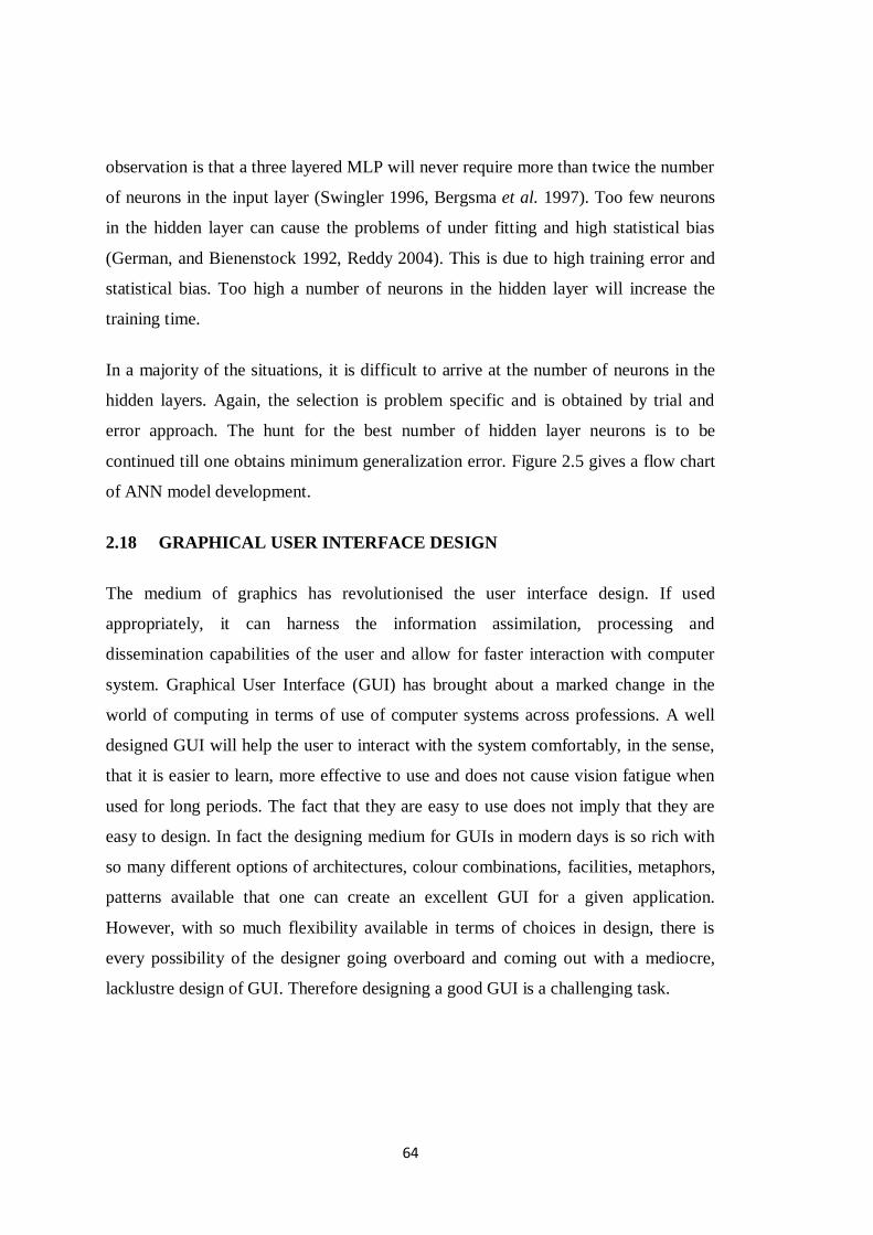
64
observation is that a three layered MLP will never require more than twice the number
of neurons in the input layer (Swingler 1996, Bergsma et al. 1997). Too few neurons
in the hidden layer can cause the problems of under fitting and high statistical bias
(German, and Bienenstock 1992, Reddy 2004). This is due to high training error and
statistical bias. Too high a number of neurons in the hidden layer will increase the
training time.
In a majority of the situations, it is difficult to arrive at the number of neurons in the
hidden layers. Again, the selection is problem specific and is obtained by trial and
error approach. The hunt for the best number of hidden layer neurons is to be
continued till one obtains minimum generalization error. Figure 2.5 gives a flow chart
of ANN model development.
2.18 GRAPHICAL USER INTERFACE DESIGN
The medium of graphics has revolutionised the user interface design. If used
appropriately, it can harness the information assimilation, processing and
dissemination capabilities of the user and allow for faster interaction with computer
system. Graphical User Interface (GUI) has brought about a marked change in the
world of computing in terms of use of computer systems across professions. A well
designed GUI will help the user to interact with the system comfortably, in the sense,
that it is easier to learn, more effective to use and does not cause vision fatigue when
used for long periods. The fact that they are easy to use does not imply that they are
easy to design. In fact the designing medium for GUIs in modern days is so rich with
so many different options of architectures, colour combinations, facilities, metaphors,
patterns available that one can create an excellent GUI for a given application.
However, with so much flexibility available in terms of choices in design, there is
every possibility of the designer going overboard and coming out with a mediocre,
lacklustre design of GUI. Therefore designing a good GUI is a challenging task.
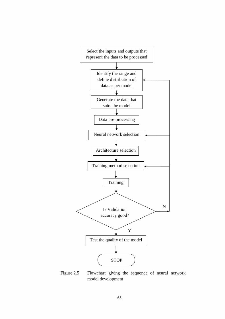
65
Select the inputs and outputs that
represent the data to be processed
Identify the range and
define distribution of
data as per model
requirement
Generate the data that
suits the model
requirement
Data pre-processing
Neural network selection
Architecture selection
Training method selection
Training
Is Validation
accuracy good?
STOP
Test the quality of the model
N
Y
Figure 2.5 Flowchart giving the sequence of neural network
model development

66
2.18.1 Objectives of Graphical User Interface Design
The user interface is a part of the computer system which connects the user with the
internal system of the computer. In a typical information system or the systems used
in offices, the user interface may include following.
The components of the computer hardware with which the user can interact
with the system such as, screen, mouse, keyboard, toggle switch, on/off switch
etc.
The images within the computer application software such as windows, task
bars, pull down menus, pop ups, messages, help screens, etc.
User documentations such as manuals, catalogues, reference cards
While the user operates on a GUI, he/she has no access to what is happening inside
the computer system. The system will work in the background based on the
information provided by the user in the input section and provide him/her with the
processed outputs. Therefore the user is more concerned with the interface, rather than
what is happening in the background. Hence the objective of the GUI design is to
make it as user friendly as possible, by increasing its usability. Usability here means,
making the computer system adaptable to human beings who are going to use it, and
has a lot of bearing on the psychological issues relating to human memory,
perception, comprehension and conceptualization.
A good interface design is important as it is the only medium that allows the user to
interact with the computer internals. A lacklustre design may not be attractive to the
user and he may not use it. Further a wrongly designed GUI may confuse the user and
there is every possibility that one may use it wrongly or stop using it. Actually, the
interface is the front end of the computer system by which the designer represents the
system to the user. A good user interface can result in increase of productivity while a
poorly designed one may cause stress followed by fatigue and discomfort to the user.

67
2.19 SUMMARY AND GAP IN KNOWLEDGE
2.19.1 Conclusions
The near net shaping of parts by thixoforming and low weight to strength
ratio, high specific modulus, high thermal stability and high wear resistance of
the composites is set to bring about revolution in the engineering industry,
especially the automotive and aerospace industry.
Literature survey indicates that the data available on semisolid processing
through research carried out on various composites as on date is inadequate to
be viable commercially. This is because the experiments that are carried out
successfully at specific predetermined points only indicate the success of the
process.
For the process to be commercially viable, a lot of other factors relating to
output optimization based on the process parameters and variation of inputs is
needed. This requires expansion of data available in the research literature.
The mushy state rolling experiments are done at high temperatures. It involves
a tight control of mushy state parameters, mainly the temperature which
determines the mushy state i.e. the liquid content in the composite.
Maintaining precise temperature (±2ºC) during the conduct of these
experiments is a challenging task. Moreover, the specimen needs to be held at
that temperature corresponding to liquid volume fraction for certain period of
time for homogenization. Therefore the conduct of a large number of
experiments to meet the commercial requirements is not prudent, as it would
be tedious, time consuming and costly.
The survey of literature on neural networks reveals the use of artificial neural
networks in various applications ranging from speech recognition and image
processing to robotics and material science.
The use of feed forward neural networks in metallurgy has been surprisingly
limited in composite processing. Moreover, the author has not come across
any application of recurrent neural networks in metallurgy and material
science. Hence, the possibility of use of recurrent neural networks in
processing of composites needs to be explored.

68
The FFNN presents a powerful tool for generalisation of relationships between
inputs and outputs of a metallurgical process without a need to understand the
intricacies of the process, which can be used to improve the research databank.
This will also help in improving the usefulness of the research work carried
out in semisolid processing of composites.
Therefore, in the present study, neural network approach, inclusive of FFNN
modelling and RNN modelling, towards process/system generalisation has
been demonstrated, the data for which has been taken from the results of the
study carried out by Herbert (2007).
Table 2.5 Table showing the summary of the Literature review
Year Author(s) Findings Remarks
1972 Spencer et al.
Led to the discovery of a
semisolid alloy having a liquid
fraction of 0.4, devoid of
dendritic structure, behaving
like a fluid.
Established semisolid
processing as a new
manufacturing process,
whose commercial viability
can be enhanced.
1974 Fukuoka and
Kiuchi
Demonstrated that there is
substantial decrease in flow
stress with decrease in solid
fraction in the semisolid
material.
Saving in Energy
requirements, which can be
justified by process
modelling.
1989 Kiuchi
Mushy state extrusion has
been used to obtain wires,
tubes and bars from billets
with the liquid weight content
between 20-30%.
Alternative to conventional
extrusion process.
1989 Kiuchi
Demonstrated mushy state
rolling on AA5052 and
AA7075 alloys by stable,
steady flow and homogeneous
deformation of the semisolid
plate or sheet, as well as rapid
cooling inside the roll gap.
Alternative to conventional
rolling process.
1992 Fleming et al.
Found a process involving the
control of rheological
properties of the semisolid
alloy that led to a process
called Rheocasting.
Better process control and
prediction of flow in die
cavity during forming
process.
1994 Kirkwood The property of Thixotropy
can be used for Thixocasting.
Led to component
manufacture by
Thixoforming.
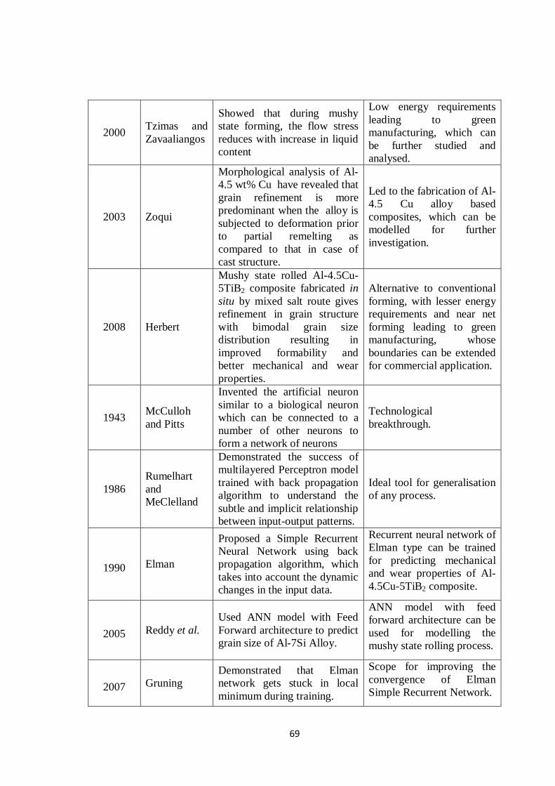
69
2000 Tzimas and
Zavaaliangos
Showed that during mushy
state forming, the flow stress
reduces with increase in liquid
content
Low energy requirements
leading to green
manufacturing, which can
be further studied and
analysed.
2003 Zoqui
Morphological analysis of Al-
4.5 wt% Cu have revealed that
grain refinement is more
predominant when the alloy is
subjected to deformation prior
to partial remelting as
compared to that in case of
cast structure.
Led to the fabrication of Al-
4.5 Cu alloy based
composites, which can be
modelled for further
investigation.
2008 Herbert
Mushy state rolled Al-4.5Cu-
5TiB2 composite fabricated in
situ by mixed salt route gives
refinement in grain structure
with bimodal grain size
distribution resulting in
improved formability and
better mechanical and wear
properties.
Alternative to conventional
forming, with lesser energy
requirements and near net
forming leading to green
manufacturing, whose
boundaries can be extended
for commercial application.
1943 McCulloh
and Pitts
Invented the artificial neuron
similar to a biological neuron
which can be connected to a
number of other neurons to
form a network of neurons
Technological
breakthrough.
1986
Rumelhart
and
MeClelland
Demonstrated the success of
multilayered Perceptron model
trained with back propagation
algorithm to understand the
subtle and implicit relationship
between input-output patterns.
Ideal tool for generalisation
of any process.
1990 Elman
Proposed a Simple Recurrent
Neural Network using back
propagation algorithm, which
takes into account the dynamic
changes in the input data.
Recurrent neural network of
Elman type can be trained
for predicting mechanical
and wear properties of Al-
4.5Cu-5TiB2 composite.
2005 Reddy et al.
Used ANN model with Feed
Forward architecture to predict
grain size of Al-7Si Alloy.
ANN model with feed
forward architecture can be
used for modelling the
mushy state rolling process.
2007 Gruning
Demonstrated that Elman
network gets stuck in local
minimum during training.
Scope for improving the
convergence of Elman
Simple Recurrent Network.
70
2008 Reddy et al.
Used Artificial Neural
networks model for Prediction
of flow stress in Ti-6Al- 4V
alloy.
ANN model with feed
forward architecture can be
used to predict the
mechanical and wear
properties of Al-4.5Cu-
5TiB2 composite.
Thus it is seen that the FFNN presents a powerful tool for generalisation of relationships
between inputs and outputs of a metallurgical process without a need to understand the
intricacies of the process. A dedicated approach therefore needs to be undertaken to
improve the usefulness of the research work carried out in semisolid processing of
composites. Further, the possibility of use of recurrent neural networks in processing of
composites needs to be explored. In the present study, neural network approach, inclusive
of FFNN modelling and RNN modelling, towards process/system generalisation has been
demonstrated and the data for study has been taken from the work carried out by Herbert
(2007).
Aluminium alloy based Metal Matrix Composites are reinforced with ceramic particles
such as TiB2, TiC, SiC etc. which are very hard. When such composites containing hard
ceramic particles are subjected to conventional forming processes, cracking is observed.
This difficulty is overcome by forming of Al based alloy composites in mushy state.
Further, forming of aluminium alloy based composite components in mushy state has
gained importance because it requires lower flow stress compared to the working by
conventional forming methods. This leads to saving in energy requirements. Moreover,
mushy state forming of Aluminium based composites gives near net shaping of
components leading to green manufacturing (Herbert 2007). Therefore, mushy state
forming, in addition to overcoming the difficulties rendered by conventional forming of
composites also leads to reduction in cost of manufacture. In this study, the concentration
of Cu in the Al-Cu alloy is chosen as 4.5 wt% because of the formation of single phase α-
Al at the solidus, strong age hardenability, as well as the sufficient gap between the
liquidus and solidus temperatures (Herbert et al. 2006). Figure 2.6 and Figure 2.7 show the
Al-Cu binary phase diagram and the TTT curve for Al-4.5 Cu alloy respectively. The gap
between liquidus and solidus temperatures is extremely important in semisolid processing.
The study of mushy state rolled Al-4.5 Cu alloy reinforced with 5 wt.% TiB2 particles was

71
carried out by Herbert(2007) to explore the microstructural evolution, mechanical and wear
properties. The conduct of these studies involved:
i. Casting of Al-4.5Cu-5TiB2 composite.
ii. Preparation of specimens (as cast specimens and pre-hot rolled specimens) for
rolling.
iii. Mushy state rolling experiments being carried out at temperatures in excess of
700ᴏC, with a precise control over temperature (±2
ᴏC).
iv. Conducting SEM, XRD studies for microstructural evolution followed by Vickers
hardness tests, wear tests and tensile tests.
Figure 2.6 Al-Cu binary phase diagram.
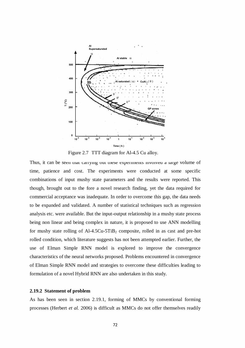
72
Thus, it can be seen that carrying out these experiments involved a large volume of
time, patience and cost. The experiments were conducted at some specific
combinations of input mushy state parameters and the results were reported. This
though, brought out to the fore a novel research finding, yet the data required for
commercial acceptance was inadequate. In order to overcome this gap, the data needs
to be expanded and validated. A number of statistical techniques such as regression
analysis etc. were available. But the input-output relationship in a mushy state process
being non linear and being complex in nature, it is proposed to use ANN modelling
for mushy state rolling of Al-4.5Cu-5TiB2 composite, rolled in as cast and pre-hot
rolled condition, which literature suggests has not been attempted earlier. Further, the
use of Elman Simple RNN model is explored to improve the convergence
characteristics of the neural networks proposed. Problems encountered in convergence
of Elman Simple RNN model and strategies to overcome these difficulties leading to
formulation of a novel Hybrid RNN are also undertaken in this study.
2.19.2 Statement of problem
As has been seen in section 2.19.1, forming of MMCs by conventional forming
processes (Herbert et al. 2006) is difficult as MMCs do not offer themselves readily
Figure 2.7 TTT diagram for Al-4.5 Cu alloy.
73
for conventional forming. As seen earlier, this is due to the presence of hard ceramic
particles, uniformly distributed in the matrix of the composite. Processing of MMCs
in semisolid state offers a convenient route in overcoming this difficulty. When the
MMC in semisolid state is subjected to forming upon application of an external load,
the induced strain is fully accommodated by the viscous flow of the liquid entrapped
at the grain boundaries and therefore the possibility of cracks originating during the
forming process is prevented.
The properties exhibited by the MMCs depend upon the extent of distribution of the
hard ceramic particles in the matrix of the composite. It is seen that the in situ
fabrication of Al-4.5Cu-5TiB2 composite via the mixed salt route(Herbert 2007) gives
a uniform distribution of fine TiB2 particles in the matrix of Al-4.5Cu alloy. The
wettability of the particles due to very fine particles is known to be better. Further, the
fabrication of the composite via mixed salt route offers a cleaner method of obtaining
castings as the possibility of unwanted impurities entering the system is drastically
reduced.
It is seen that mushy state rolling of Al-4.5Cu-5TiB2 composite leads to nearly
equiaxed grains having bimodal grain size distribution. Rolling at low liquid content
with high thickness reduction leads to deformation of unmelted grains which work
harden significantly, thereby causing increase in hardness of the composite. This in
turn leads to higher strength and wear properties. Thus it is seen that the resulting
properties of the Al-4.5Cu-5TiB2 composite subjected to mushy state rolling depend
upon the mushy state rolling parameters viz. thickness reduction and liquid volume
fraction. The mushy state rolling experiments carried out by Herbert (2007) on as cast
and pre-hot rolled Al-4.5Cu-5TiB2 composite samples provided the resulting
microstructural properties, mechanical and wear properties only at some
predetermined combinations of input parameters viz. initial state of the composite (i.e.
as cast or pre hot rolled condition), % thickness reduction and % liquid volume
fraction in the composite. The excellent findings of the study provided a great
potential for the mushy state rolling as a near net shaping process, resulting in
decreased power requirements and saving in energy. But for commercial viability, a
larger volume of input-output data of the mushy state rolling of the composite is
required.
74
Artificial Neural Networks provide an excellent technique to generalise the
relationship between inputs and outputs of process, provided that the network has
been trained on such known relationships. The ANN models are especially suitable
where the relationship is non linear and quite complex. Large and small grain sizes,
hardness, wear and tensile properties as functions of the mushy state rolling
parameters, (viz. initial state of the composite, thickness reduction and liquid volume
fraction in the composite) define a non linear complex system. Thus ANN model with
feed forward architecture and trained with error backpropagation algorithm provides
an excellent option to predict the microstructural, mechanical and wear properties of
the composite.
Elman simple Recurrent Network was proposed by Elman which exhibited faster
convergence than feed forward neural networks. But generally, Elman networks were
found to get stuck in local minima, resulting in convergence problems. Therefore,
there is a need to explore the possibility of identifying a modification to existing
Elman Simple Recurrent Network which will combine the faster convergence
capability of Elman network and overcome the limitation of getting stuck in local
minima.
This thesis proposes to use ANN models with feed forward architecture to predict
grain sizes, hardness, tensile and wear properties of mushy state rolled Al-4.5Cu-
5TiB2 composite rolled in as cast and pre hot rolled condition with different
combinations of thickness reduction (2 to 12.5%) and liquid volume fraction (5 to
35%). The work also deals with the formulation of Hybrid Recurrent Neural Network
that can predict the output comparable to a feed forward neural network with better
convergence characteristics, due to its inherent self looping properties.
2.19.3 Statement of objectives
Studies on mushy state rolling of cast Al- 4.5 (wt.%) - 5(wt.%)TiB2 composite by
Herbert (2007) have provided mushy state forming as an alternative route to
conventional hot rolling as a forming method, yielding better mechanical and wear
properties. For commercial applications, the data now needs to be made available in
the entire range of parameters in which experiments were carried out and also at close

75
points outside the bounds of experimentation. With this in mind, the proposed work
envisages the accomplishment of following specific objectives:
1. Development of ANN model to simulate the relationship of mushy state
rolling process parameters and their influence on grain size and mechanical
properties like hardness, wear and strength.
2. Experimental work for validation of the above ANN models for prediction of
grain sizes, hardness and wear properties and analysing the results for
checking the authenticity of ANN model in prediction.
3. Optimization of the process of mushy state rolling in terms of the mushy state
rolling parameters to obtain the best output, by using Graphical User Interface/
Application Programmer Interface libraries.
4. Development of Hybrid Recurrent Neural Network from an Extended Elman
RNN (SRN) model for mimicking the process of mushy state rolling of Al-
4.5Cu-5TiB2 composite to predict grain sizes, hardness, wear and tensile
properties.
5. Comparing the performance of HRNN model with reference to ANN model
for its effectiveness.
2.19.4 Scope
The scope of the work in the proposed study shall include;
a. The modelling of ANN with feed forward architecture to correlate the mushy
state rolling parameters with grain sizes, hardness, tensile and wear properties
of Al-4.5Cu-5TiB2 composite.
b. The modelling of Hybrid Recurrent Neural network to correlate the mushy
state rolling parameters with grain sizes, hardness, tensile and wear properties
of Al-4.5Cu-5TiB2 composite.
c. Comparing the performance of ANN with feed forward architecture and
HRNN in terms of:
i. The prediction capability and

76
ii. Convergence characteristics.
d. Developing a GUI based tool for studying parametric influence on the mushy
state rolling of Al-4.5Cu-5TiB2 composite.
e. Validation of the models by conducting mushy state rolling of Al-4.5Cu-5TiB2
composite at some input parameter combinations which lie within and outside
the data used for training the networks cited at (a) and (b) above.
2.19.5 Plan of work
The overall plan of work for carrying out the study is listed out hereunder:
a. To gather data from literature survey.
b. To analyse the data and apply suitable modelling technique for prediction of
desired outputs, based on ANN principles.
c. Try out neural network models by error back propagation network, recurrent
neural network and a hybrid option of ANN with RNN to simulate the mushy
state rolling process for Al-4.5Cu-5TiB2 composite.
d. To develop a graphics interface for observing the relationship between inputs
and outputs as desired by the user instantaneously and graphically.
e. Validate the predictions by conducting suitable mushy state rolling
experiments on Al-4.5Cu-5TiB2 composite.

77
Chapter 3
EXPERIMENTAL DETAILS
3.1 INTRODUCTION
As reviewed in chapter 2, a large number of research is going on the in the field of
mushy state forming of metals and metal matrix composites. As seen in the literature
review, a fair amount of work is going on in the field of rolling of discontinuously
reinforced Al alloy based composites in mushy state, with rolling initiated when the
composite is in as cast condition and in pre hot rolled condition (Herbert 2007). The
study (Herbert 2007, Siddalingeshwar 2011), deals with the evolution of
microstructure in the mushy state rolled Al-4.5Cu-5TiB2 composite and its effect on
the mechanical properties, wear properties and creep properties. The work done by
Herbert (2007) and Siddalingeshwar (2010) establishes the fact that it is possible to
nearly net shape discontinuously reinforced Al alloy based in situ composites by
subjecting the composite to mushy state rolling. In the experimentations carried out
by Herbert (2007), the Al-4.5Cu-5TiB2 composite is rolled in mushy state to thickness
reductions ranging from 2.5 to 10%, with a step size of 2.5%, and with rolling being
initiated when the composite has a volume fraction of liquid as 10%, 20% and 30%.
The work done by them (Herbert 2007, Siddalingeshwar 2010, 2011) does establish
that mushy state rolling results in improvement of grain structure, resulting in
improvement in properties. The study also reveals the influence of rolling parameters
such as, thickness reduction and liquid content on the resulting mechanical and wear
properties. However, the investigation of microstructural details and properties with
combination of inputs (thickness reduction and liquid volume content) is done at
specific points of experimentation only, and therefore gives only a glimpse of the
potential of mushy state rolling of the said composite. The user industry however
needs more data, so that the process can be optimised based on either the input
parameters control or controlling the output parameters. The commercial acceptance
of the technological breakthrough is therefore the problem at hand. The data,
however, if expanded to include more combinations of the input parameters providing
78
the corresponding microstructure and mechanical properties as outputs, will become
more useful to the ultimate user, the industries. The ANN model proposed, as
discussed in Chapter 1 will provide the solution for improving the database for
correlation of mushy state parameters with microstructure and the resulting
mechanical and wear properties. Indeed the model has to be checked to verify its
authenticity as well as its correctness in prediction of outputs from an unknown set of
inputs. In order to validate the ANN model, it is endeavoured to perform the
investigations detailed out as under:
Preparation of Al-4.5(wt %) Cu alloy and in situ Al-4.5(wt. %) Cu-5(wt. %)
TiB2 composite followed by characterization of the Al-4.5(wt. %) Cu-5(wt. %)
TiB2 composite by using Scanning Electron Microscope (SEM).
Determining the temperature corresponding to the volume fraction of liquid
selected for carrying out the mushy state rolling of the said composite, by
applying the lever rule to Al-Cu equilibrium phase diagram.
Mushy state rolling of the composite to x (x=2, 6, 11.5) percent thickness
reduction containing y (y=7, 17 and 33) volume fraction of liquid followed by
microstructural characterization using SEM. The mushy state rolling
experiments with these values of x and y are carried out to validate the ANN
model performance with values of x and y other than those used for training
the model. A comparative study is then carried out between the model
predictions and the experimental results at values corresponding to the values
of x and y used for training of the model as well as those used for model
validation.
Study of wear behaviour of mushy state rolled Al-4.5(wt. %) Cu-5(wt. %)
TiB2 composite is carried out at x (x=2, 6 and 11.5) percent thickness
reduction containing y (y=7, 17 and 33) volume percent liquid.
The work is started with the selection of raw materials followed by planning of
experiments for different segments mentioned above. A schematic presentation of the
overview is shown in Figure 3.1. The details of the experiments to be carried out are
given in the subsequent sections.

79
3.2 SELECTION OF RAW MATERIALS
The raw materials used for the present work consist of commercially pure metals like
aluminium (CP-Al) and copper in addition to chemicals such as potassium fluoborate
(KBF4) and potassium titanium fluoride (K2TiF6). Al was used for the preparation of
Al-33Cu master alloy, which was subsequently used to prepare Al-4.5(wt. %) Cu-
5(wt. %) TiB2 composite plates for mushy state rolling. The composition of Al and its
alloy was analysed by an Optical Emission Spectrometer (OES) (Model ARL 3460 of
Thermo Electron Corporation, Switzerland). The composition of Al and Al-4.5(wt. %)
Cu alloy is presented in the Table 3.1. The salts used in the present work were
commercial grade K2TiF6 and KBF4 in the powder form (~200 mesh i.e.74μm).
Casting of composite
Mushy state rolling with
varying parameters
Microstructural analysis
SEM
SEM mapping
Mechanical properties
Hardness
Wear
Analysis
Results
Figure 3.1 Schematic representation of experimental work
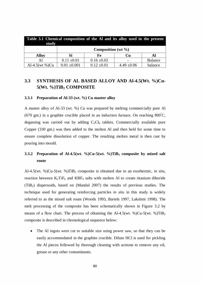
80
Table 3.1 Chemical composition of the Al and its alloy used in the present
study
Composition (wt %)
Alloy Si Fe Cu Al
Al 0.11 ±0.01 0.16 ±0.02 - Balance
Al-4.5(wt %)Cu 0.01 ±0.001 0.12 ±0.01 4.49 ±0.06 balance
3.3 SYNTHESIS OF AL BASED ALLOY AND Al-4.5(Wt. %)Cu-
5(Wt. %)TiB2 COMPOSITE
3.3.1 Preparation of Al-33 (wt. %) Cu master alloy
A master alloy of Al-33 (wt. %) Cu was prepared by melting commercially pure Al
(670 gm.) in a graphite crucible placed in an induction furnace. On reaching 800ºC,
degassing was carried out by adding C2Cl6 tablets. Commercially available pure
Copper (330 gm.) was then added to the molten Al and then held for some time to
ensure complete dissolution of copper. The resulting molten metal is then cast by
pouring into mould.
3.3.2 Preparation of Al-4.5(wt. %)Cu-5(wt. %)TiB2 composite by mixed salt
route
Al-4.5(wt. %)Cu-5(wt. %)TiB2 composite is obtained due to an exothermic, in situ,
reaction between K2TiF6 and KBF4 salts with molten Al to create titanium diboride
(TiB2) dispersoids, based on (Mandal 2007) the results of previous studies. The
technique used for generating reinforcing particles in situ in this study is widely
referred to as the mixed salt route (Woods 1993, Bartels 1997, Lakshmi 1998). The
melt processing of the composite has been schematically shown in Figure 3.2 by
means of a flow chart. The process of obtaining the Al-4.5(wt. %)Cu-5(wt. %)TiB2
composite is described in chronological sequence below:
The Al ingots were cut to suitable size using power saw, so that they can be
easily accommodated in the graphite crucible. Dilute HCl is used for pickling
the Al pieces followed by thorough cleaning with acetone to remove any oil,
grease or any other contaminants.
81
The requisite amount of K2TiF6 (109 gm.) and KBF4 (114 gm.) to achieve the
required wt. % (5) of TiB2 was weighed and subsequently dried in an oven at
150ºC for around 2 hours to remove any physisorbed moisture present, as
aluminium is known to be very sensitive to moisture. Simultaneously, the
moulds in which the melt would be ultimately poured were also kept in a
separate oven for 2 hours at around 200ºC.
The salts were removed from the oven after the requisite time and mixed
thoroughly, so that a homogeneous mixture of salts was obtained.
The mixed salts were then wrapped in aluminium foils (capsule form) in
suitable quantities to form a number of batches of sizes convenient for adding
to the liquid alloy.
The master alloy (68.2 gm.) was remelted with suitable amount (431.8 gm.) of
commercially pure Al in a pit type resistance furnace using a graphite crucible,
to obtain 500 gm alloy of the desired composition. Once the melt attains a
temperature of 8000C, degassing of the melt with hexachloroethane (C2Cl6)
tablets is carried out. The temperature decreases slightly upon addition of
tablets.
Once the temperature reaches 800ºC again, the packets were added to the
liquid alloy in batches. The melt is stirred with Zirconia coated graphite stirrer
every ten minutes.
When all the packets are added, the melt was held for duration of one hour at
reaction temperature in the furnace. Intermittent stirring of the melt is carried
out at every 10 minutes interval to achieve uniform distribution of salt in
molten Al ensuring uniform reaction throughout the melt.
The TiB2 particles were formed in situ inside the molten Al due to the exothermic
reaction of K2TiF6 and KBF4 salts following equation (3.1) (Mandal et al. 2004,
Herbert 2007).
K2TiF6 + KBF4 + Al alloy Al alloy + TiB2 + KAlF4 (3.1)
(composite) (dross)

82
KAlF4 floats on the melt as dross and is subsequently removed. The melt is then
poured in the cast iron plate shaped moulds preheated to a temperature of 200ºC.
Figure 3.2 Schematic representation of Al-4.5Cu-5TiB2 composite processing.
Melting of Al-4.5 Cu inside
graphite crucible in pit furnace Thorough mixing of
K2TiF6 (109 gm.)+ KBF4 (104 gm)
Pouring of mixed salts to molten aluminium at
800ºC
Thorough mixing and holding at 800ºC
Stirring at every 10 min (For 1 hour)
Casting
Al-4.5Cu-5TiB2
Addition of C2Cl6 tablets for degassing
Removal of dross
Melting of Al - 4.5 Cu alloy
inside graphite crucible in pit
furnace
Thorough mixing of
K2TiF6 (109 gm.)+ KBF4 (114 gm)
salts
83
3.4 EVALUATION OF VOLUME FRACTION OF in situ Al-
4.5Cu-5TiB2 COMPOSITE IN MUSHY STATE
The volume fraction of the liquid present in Al-4.5Cu-5TiB2 composite work piece
during rolling in mushy state were chosen as 10, 20 and 30 percent for investigations
carried out by Herbert (Herbert 2007) on mushy state rolling of Al-4.5Cu alloy based
composites reinforced with TiB2 particles. The ANN model proposed in this study has
been trained on the investigations carried out in the above work on the Al-4.5Cu-
5TiB2 composite, rolled in mushy state, when in as cast and in pre hot rolled form.
Therefore, the volume fractions of the Al-4.5Cu-5TiB2 composite were chosen as 7,
17 and 33 percent for validation experiments proposed to be carried out. Figure 3.3
shows the chart map at locations where validation experiments are proposed. The
bullet entries indicate the points at which validation experiments are proposed. The
temperatures corresponding to the nominal liquid volume fractions of 7, 17 and 33
percent were obtained by applying the lever rule to the Al-Cu thermal equilibrium
diagram (ASM Handbook 1997). In case of the binary Al-4.5Cu alloy, the
temperature corresponding to 7, 17 and 33 volume fractions has been found to be
597ºC, 618
ºC and 632
ºC respectively. For the composite, the amount of TiB2 has to be
considered as part of the solid fraction, in addition to the unmelted alloy grains
(Herbert 2007). Hence the temperatures for the composites are taken to be 1ºC higher
than that of the binary alloy for the same volume fraction of liquid (Herbert 2007).
While determining the temperatures corresponding to the volume fractions of liquid in
the composite using lever rule, the densities of solid and liquid Al were assumed to be
same (Herbert 2007). The temperatures corresponding to the different volume
fractions of the liquid in the composite (for validation experiments to be carried out)
obtained from phase diagram are shown in Table 3.2.

84
Table 3.2 Temperature corresponding to 7, 17 and 33 volume fraction of liquid
in Al-4.5Cu alloy and Al-4.5Cu-5TiB2 composite, determined from
phase diagram
Liquid volume fraction Al-4.5Cu alloy Al-4.5Cu-5TiB2
composite
7 597 598
17 618 619
33 632 633
3.5 MUSHY STATE ROLLING OF Al-4.5Cu-5TiB2 COMPOSITE
A schematic representation of the experimental set up used for mushy state rolling of
Al-4.5Cu-5TiB2 composite is shown in Figure 3.4. Figure 3.5 shows the photograph
of the experimental set up used for mushy state rolling of composite. The
experimental setup has been specially designed to facilitate partial remelting of the
composite workpiece. A two high rolling mill, having rolls of 120 mm diameter, and
12 mm barrel width was used for conducting the experiments. The mill surfaces were
maintained at ambient temperature to facilitate instantaneous solidification during
mushy state rolling.
10 20 30
% Liq. Vol. Fraction
%
Th
. R
edu
ctio
n
10
2.5
5
7.5
Figure 3.3 Map for proposed validation experiments
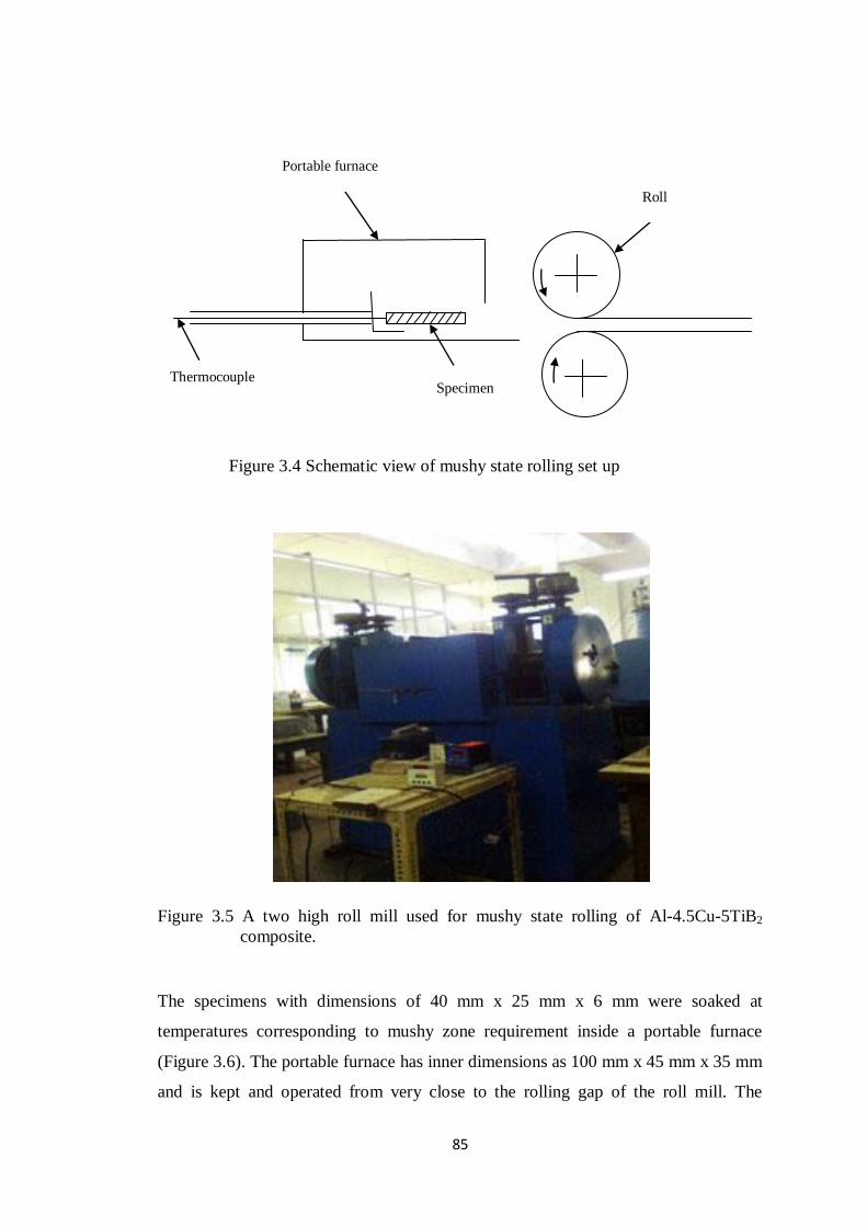
85
Figure 3.5 A two high roll mill used for mushy state rolling of Al-4.5Cu-5TiB2
composite.
The specimens with dimensions of 40 mm x 25 mm x 6 mm were soaked at
temperatures corresponding to mushy zone requirement inside a portable furnace
(Figure 3.6). The portable furnace has inner dimensions as 100 mm x 45 mm x 35 mm
and is kept and operated from very close to the rolling gap of the roll mill. The
Roll
Thermocouple Specimen
Portable furnace
Figure 3.4 Schematic view of mushy state rolling set up
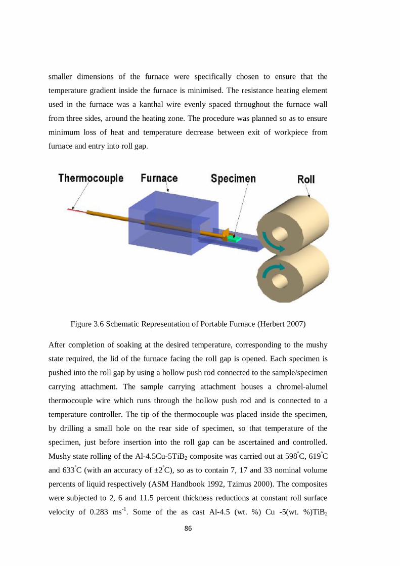
86
smaller dimensions of the furnace were specifically chosen to ensure that the
temperature gradient inside the furnace is minimised. The resistance heating element
used in the furnace was a kanthal wire evenly spaced throughout the furnace wall
from three sides, around the heating zone. The procedure was planned so as to ensure
minimum loss of heat and temperature decrease between exit of workpiece from
furnace and entry into roll gap.
Figure 3.6 Schematic Representation of Portable Furnace (Herbert 2007)
After completion of soaking at the desired temperature, corresponding to the mushy
state required, the lid of the furnace facing the roll gap is opened. Each specimen is
pushed into the roll gap by using a hollow push rod connected to the sample/specimen
carrying attachment. The sample carrying attachment houses a chromel-alumel
thermocouple wire which runs through the hollow push rod and is connected to a
temperature controller. The tip of the thermocouple was placed inside the specimen,
by drilling a small hole on the rear side of specimen, so that temperature of the
specimen, just before insertion into the roll gap can be ascertained and controlled.
Mushy state rolling of the Al-4.5Cu-5TiB2 composite was carried out at 598ºC, 619
ºC
and 633ºC (with an accuracy of ±2
ºC), so as to contain 7, 17 and 33 nominal volume
percents of liquid respectively (ASM Handbook 1992, Tzimus 2000). The composites
were subjected to 2, 6 and 11.5 percent thickness reductions at constant roll surface
velocity of 0.283 ms-1
. Some of the as cast Al-4.5 (wt. %) Cu -5(wt. %)TiB2
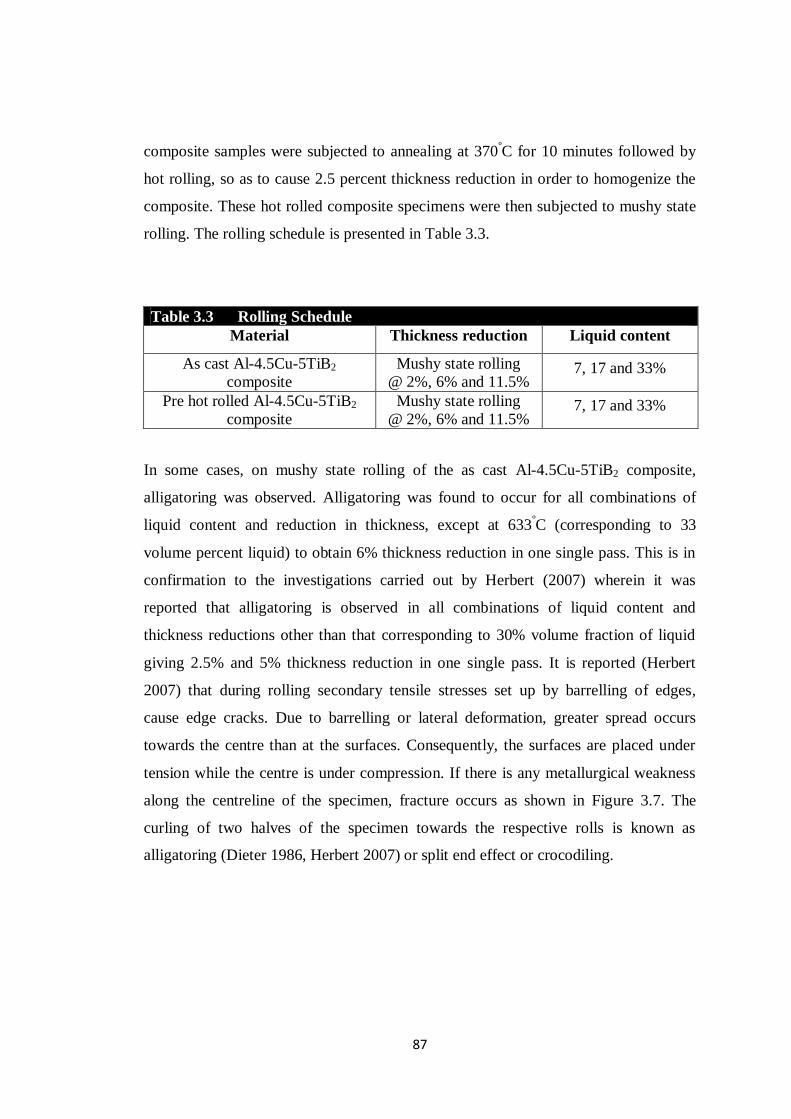
87
composite samples were subjected to annealing at 370ºC for 10 minutes followed by
hot rolling, so as to cause 2.5 percent thickness reduction in order to homogenize the
composite. These hot rolled composite specimens were then subjected to mushy state
rolling. The rolling schedule is presented in Table 3.3.
Table 3.3 Rolling Schedule
Material Thickness reduction Liquid content
As cast Al-4.5Cu-5TiB2
composite
Mushy state rolling
@ 2%, 6% and 11.5% 7, 17 and 33%
Pre hot rolled Al-4.5Cu-5TiB2
composite
Mushy state rolling
@ 2%, 6% and 11.5% 7, 17 and 33%
In some cases, on mushy state rolling of the as cast Al-4.5Cu-5TiB2 composite,
alligatoring was observed. Alligatoring was found to occur for all combinations of
liquid content and reduction in thickness, except at 633ºC (corresponding to 33
volume percent liquid) to obtain 6% thickness reduction in one single pass. This is in
confirmation to the investigations carried out by Herbert (2007) wherein it was
reported that alligatoring is observed in all combinations of liquid content and
thickness reductions other than that corresponding to 30% volume fraction of liquid
giving 2.5% and 5% thickness reduction in one single pass. It is reported (Herbert
2007) that during rolling secondary tensile stresses set up by barrelling of edges,
cause edge cracks. Due to barrelling or lateral deformation, greater spread occurs
towards the centre than at the surfaces. Consequently, the surfaces are placed under
tension while the centre is under compression. If there is any metallurgical weakness
along the centreline of the specimen, fracture occurs as shown in Figure 3.7. The
curling of two halves of the specimen towards the respective rolls is known as
alligatoring (Dieter 1986, Herbert 2007) or split end effect or crocodiling.

88
Figure 3.8 shows the photographs of (a) as cast composite specimen (b) specimen
rolled to 6% thickness reduction with 17% liquid volume fraction and (c) specimen
which has undergone alligatoring, when subjected to mushy state rolling at 598ºC
(corresponding to 7% volume fraction of liquid) to a thickness reduction of 6% in one
pass.
Figure 3.8 Photograph of (a) as cast Al-4.5Cu-5TiB2 composite; (b)defect free mushy
state rolled specimen and (c) fractured surface generated by alligatoring.
Figure 3.7 Fracture due to Alligatoring (Dieter 1986)

89
3.6 SECTIONING OF AS CAST AND ROLLED SPECIMENS
Figure 3.9 illustrates the way in which the plate shaped Al-4.5Cu-5TiB2 composite
was sectioned to obtain the specimens for microstructural characterization and wear
studies. The surfaces selected were in the direction of rolling for both microstructural
as well as wear studies. The samples were cut using Isomet 4000 Linear precision saw
(Buehler Inc., IL, USA) equipped with diamond coated blades.
3.7 METALLOGRAPHIC SAMPLE PREPARATION
Sample preparations were required for studies of optical and scanning electron
microscopes. Samples of size 10mm x 5mm x 5mm were cut. Both as cast as well as
mushy state rolled composite samples of Al-4.5Cu-5TiB2 composite were prepared
for microstructural study by polishing using different grades of SiC papers of grades
200,320 and 600 grit until the sketches of previous grade polishing vanished
completely. Subsequently, the samples were polished on a disc polishing machine
(ECOMET 3000 variable speed grinder-polisher, Buehler, Germany) having polishing
cloth, using water suspension of alumina powder (400 mesh size) as grinding
medium. This is followed by meticulous polishing on lapping cloth fixed on a rotating
disc and smeared with 1μm, 0.25μm followed ultimately with 0.05μm diamond pastes
till a very fine mirror surface finish is achieved. After every stage of polishing, the
samples were carefully cleaned with soap solution and alcohol after which drying
followed. This was followed by etching the specimens with Keller’s reagent
(2.5%HNO3, 1.5% HCl, 1% HF, and 95% H2O) for a period of approximately 10
seconds, so that grain boundaries are delineated. Etched samples were carefully
cleaned in acetone bath using ultrasonic cleaner (VS120, Vibronics Pvt. Ltd., India,
120W).
3.8 CHARACTERIZATION OF MUSHY STATE ROLLED in situ
Al-4.5Cu-5TiB2 COMPOSITE
3.8.1 Optical microscopy and image analysis
Optical microscopy and grain size analysis were carried out using Leica DFC320
image analyzer (Model: Q5501W) interfaced with Leica Q-win V3 Image analysis
software. Optical photomicrographs of metallographically polished specimens of the
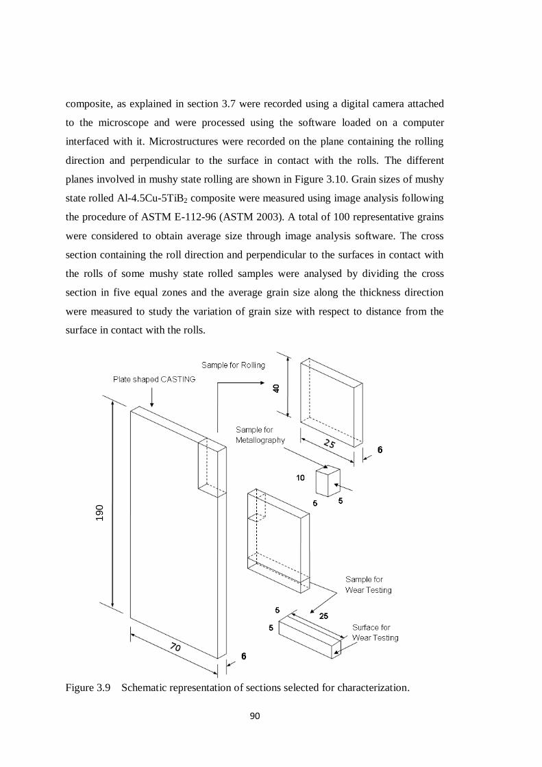
90
composite, as explained in section 3.7 were recorded using a digital camera attached
to the microscope and were processed using the software loaded on a computer
interfaced with it. Microstructures were recorded on the plane containing the rolling
direction and perpendicular to the surface in contact with the rolls. The different
planes involved in mushy state rolling are shown in Figure 3.10. Grain sizes of mushy
state rolled Al-4.5Cu-5TiB2 composite were measured using image analysis following
the procedure of ASTM E-112-96 (ASTM 2003). A total of 100 representative grains
were considered to obtain average size through image analysis software. The cross
section containing the roll direction and perpendicular to the surfaces in contact with
the rolls of some mushy state rolled samples were analysed by dividing the cross
section in five equal zones and the average grain size along the thickness direction
were measured to study the variation of grain size with respect to distance from the
surface in contact with the rolls.
190
Figure 3.9 Schematic representation of sections selected for characterization.
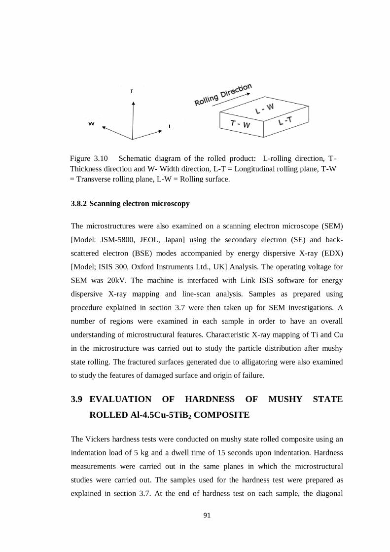
91
3.8.2 Scanning electron microscopy
The microstructures were also examined on a scanning electron microscope (SEM)
[Model: JSM-5800, JEOL, Japan] using the secondary electron (SE) and back-
scattered electron (BSE) modes accompanied by energy dispersive X-ray (EDX)
[Model; ISIS 300, Oxford Instruments Ltd., UK] Analysis. The operating voltage for
SEM was 20kV. The machine is interfaced with Link ISIS software for energy
dispersive X-ray mapping and line-scan analysis. Samples as prepared using
procedure explained in section 3.7 were then taken up for SEM investigations. A
number of regions were examined in each sample in order to have an overall
understanding of microstructural features. Characteristic X-ray mapping of Ti and Cu
in the microstructure was carried out to study the particle distribution after mushy
state rolling. The fractured surfaces generated due to alligatoring were also examined
to study the features of damaged surface and origin of failure.
3.9 EVALUATION OF HARDNESS OF MUSHY STATE
ROLLED Al-4.5Cu-5TiB2 COMPOSITE
The Vickers hardness tests were conducted on mushy state rolled composite using an
indentation load of 5 kg and a dwell time of 15 seconds upon indentation. Hardness
measurements were carried out in the same planes in which the microstructural
studies were carried out. The samples used for the hardness test were prepared as
explained in section 3.7. At the end of hardness test on each sample, the diagonal
Figure 3.10 Schematic diagram of the rolled product: L-rolling direction, T-
Thickness direction and W- Width direction, L-T = Longitudinal rolling plane, T-W
= Transverse rolling plane, L-W = Rolling surface.

92
length of indentation was carefully measured. The Vickers Hardness Number is
calculated using the following relation:
Hv = 1.854P
𝑑2 (3.2)
where P is the indentation load (kg) and d is the mean diagonal length (mm). While
taking hardness readings on a specimen, care is taken to see to it that the indentation
marks are separated by at least a distance of three times the diagonal length. This is
done to ensure that the accuracy of the hardness readings is not affected due to elastic
deformations and to minimize the errors in measurement of diagonal length.
3.10 EVALUATION OF DRY SLIDING WEAR PROPERTIES
Dry sliding wear tests were carried out on Al-4.5Cu-5TiB2 composite samples after
the composite was subjected to mushy state rolling. The mushy state rolling of Al-
4.5Cu-5TiB2 composite was carried out as per the rolling schedule given in Table 3.3.
After rolling the specimens having cross section of 5mm x 5mm and 25mm height
were prepared as shown in sectioning chart in Figure 3.9. These square specimens
were tested using pin-on-disc wear-testing machine (Model TR-20, DUCOM,
Bangalore, India) following the ASTM G99-04 standard (ASM 1992). A schematic
view of the wear testing machine is shown in Figure 3.11. The surface of the cross
section in the longitudinal rolling direction was considered for wear testing. Wear
specimens were cut to required size by using Isomet 4000 linear precision cutting saw
(Buehler). For each case, two samples were considered and the average height loss
was found out. From the average height loss, volume loss was determined and from
volume loss, the wear rates were calculated. The wear tests were carried out in dry
condition to obviate the effects of lubricating medium contamination. Hardened
chromium steel (Rc64) was used as the counterface material. The tests were carried
out with loads as 19.6N, 39.2N, 58.8N and 78.4N. For all the tests, sliding distance
was maintained as 1800m, while the sliding speed was kept as 1ms-1
(corresponding
to a constant disc speed of 240 rpm). The track radius was fixed at 40mm. The dry
wear tests were carried out at ambient temperature. A computerised data acquisition
system was used in this study to simultaneously monitor height loss as well as
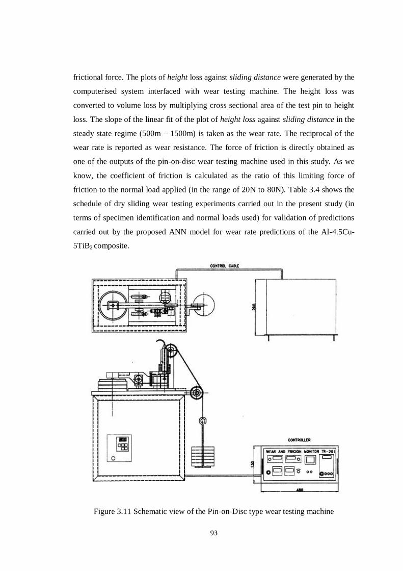
93
frictional force. The plots of height loss against sliding distance were generated by the
computerised system interfaced with wear testing machine. The height loss was
converted to volume loss by multiplying cross sectional area of the test pin to height
loss. The slope of the linear fit of the plot of height loss against sliding distance in the
steady state regime (500m – 1500m) is taken as the wear rate. The reciprocal of the
wear rate is reported as wear resistance. The force of friction is directly obtained as
one of the outputs of the pin-on-disc wear testing machine used in this study. As we
know, the coefficient of friction is calculated as the ratio of this limiting force of
friction to the normal load applied (in the range of 20N to 80N). Table 3.4 shows the
schedule of dry sliding wear testing experiments carried out in the present study (in
terms of specimen identification and normal loads used) for validation of predictions
carried out by the proposed ANN model for wear rate predictions of the Al-4.5Cu-
5TiB2 composite.
Figure 3.11 Schematic view of the Pin-on-Disc type wear testing machine

94
Table 3.4 Dry sliding wear studies of mushy state rolled Al-4.5Cu-5TiB2
composite
Material*
Mushy state rolling parameters
Normal load (N) Thickness
reduction
(%)
Liquid fraction
(%)
As cast
Al-4.5Cu-5TiB2
2 17
19.6, 39.2, 58.8 and
78.4
6 33
Pre-hot rolled
Al-4.5Cu-5TiB2
2 17
6 07, 17, 33 *All figures are in wt. %
95
Chapter 4
RESULTS AND DISCUSSION (PART I)
ANN MODELLING FOR GRAIN SIZE PREDICTION
4.1 INTRODUCTION
The development of ANN model for prediction of bimodal grain sizes for as cast and
pre hot rolled Al-4.5Cu-5TiB2 composite when rolled in mushy state is discussed in
the present chapter. Rolling is initiated from different mushy state temperatures
(corresponding to the required liquid volume fraction in the composite) and to
different thickness reductions during rolling in single pass. The model has been
trained with data collected from the work carried out by Herbert (2007). The mushy
state rolling data ranging from 2.5 to 10% thickness reduction per pass with 10 to
30% liquid volume content in the composite at the initiation of mushy state rolling,
has been considered for training the model. The validation of the model to predict
bimodal grain size in mushy state rolled Al-4.5Cu-5TiB2 composite has been
established by conducting experiments on mushy state rolling of Al-4.5Cu-5TiB2
composite in as cast and pre hot rolled condition at pre determined input parameters.
The chapter further deals with the characterization of this mushy state rolled
composite using optical microscopy and SEM/EDX microanalysis. Discussion on the
variation of grain sizes with different combinations of thickness reductions per roll
pass and liquid volume content (mushy state parameter) during rolling initiation has
also been presented. The summary of the discussions has been presented in the
concluding part of the chapter.
4.2 SCOPE
In this section, it is proposed to develop a Feed Forward Neural Network model to
predict the grain size as a function of input parameters namely, % thickness reduction
and % volume fraction of liquid in the composite. The input parameters for the mushy
96
state rolling process of Al-4.5Cu-5TiB2 composite are initial state of composite (i.e.
as cast or pre hot rolled condition), % thickness reduction and % liquid volume
fraction in the composite. The outputs of the process are small and large grain sizes. It
is obvious that the relationship between output and input is non linear and complex.
Statistical techniques like regression analysis use the technique of fitting the non
linear data on a goodness of fit line. This obviously leads to errors creeping in
predictions due to fitment errors. Finite element methods are mathematically too
involved. The use of Feed Forward Neural Networks with one or two hidden layers is
an attractive option as these networks are known to correlate complex and non linear
input-output relationships without requirement of in depth mathematical knowledge to
the user. The FFNN generalises the input-output relationship with a fair degree of
accuracy by understanding the subtle relationships between them. This justifies the
use of FFNN for prediction of grain sizes of mushy state rolled Al-4.5Cu-5TiB2
composite.
The present work attempts to develop a FFNN model keeping in mind the following:
(a) The analysis of the effect of initial state composite material (as cast or pre hot
rolled) on grain size of Al-45Cu-5TiB2 composite.
(b) The analysis of effect of the thickness reduction and liquid volume fraction
during mushy state rolling and mushy state condition when rolling is
initiated.
(c) Extrapolate and interpolate the average grain sizes for unknown thickness
reductions and liquid volume fractions in the mushy state composite.
(d) Determining optimum condition of thickness reduction and liquid volume
content to obtain desired grain sizes.
(e) Validation of the model predictions through experiments.
97
4.3 DATA COLLECTION AND ANN MODELLING FOR GRAIN
SIZE PREDICTION
4.3.1 Data collection
The experimental data are taken from the work of Herbert (2007). The work dealt
with the study of microstructural evolution of the Al-4.5(wt. %) Cu alloy and in situ
Al-4.5(wt. %)Cu -5(wt. %) TiB2 composite, both subjected to mushy state rolling.
The condition is either as cast or pre hot rolled for single or multiple roll passes with
different combinations of thickness reductions and volume fractions of liquid.
Microstructural evolution in as cast and pre hot rolled Al-4.5Cu-5TiB2 composite, led
to more or less equiaxed grain structure, and a modest refinement of the grain size.
The matrix in the hot-rolled composite showed a bimodal or duplex grain size
distribution. The finer equiaxed grains emerged through dynamic recrystallization,
with finer grains appeared randomly mixed with coarser grains (Herbert et al. 2006).
The grain size in the α-Al matrix of the cast Al-4.5Cu-5TiB2 was found to be 50±8μm
(Herbert et al. 2006, Herbert 2007). The comparative study of the grain sizes in in situ
as cast Al-4.5Cu-5TiB2 composite and the pre hot rolled composite subjected to
mushy state rolling was carried out to examine its effect on the mechanical properties.
The mean size and standard deviation of the un-melted α-Al grains in the as-cast and
pre hot rolled composite subjected to mushy state rolling to various thickness
reductions are listed in Table. 4.1. The average grain size was seen to be higher, for
both small and large grains, in case as cast composite subjected to mushy state rolling.
It is seen that that this is the least in case of the pre hot rolled composite subjected to
mushy state rolling. The mean values of the large grain size vary from 47μm to 62μm
in the case of as cast composite subjected to mushy state rolling and from 39μm to
47μm in the case of the pre-hot rolled composite subjected to mushy state rolling.
Similarly, the mean values of the small grain size vary from 25μm to 37μm for as cast
composite subjected to mushy state rolling and from 24μm to 32μm in the case of pre
hot rolled composite.
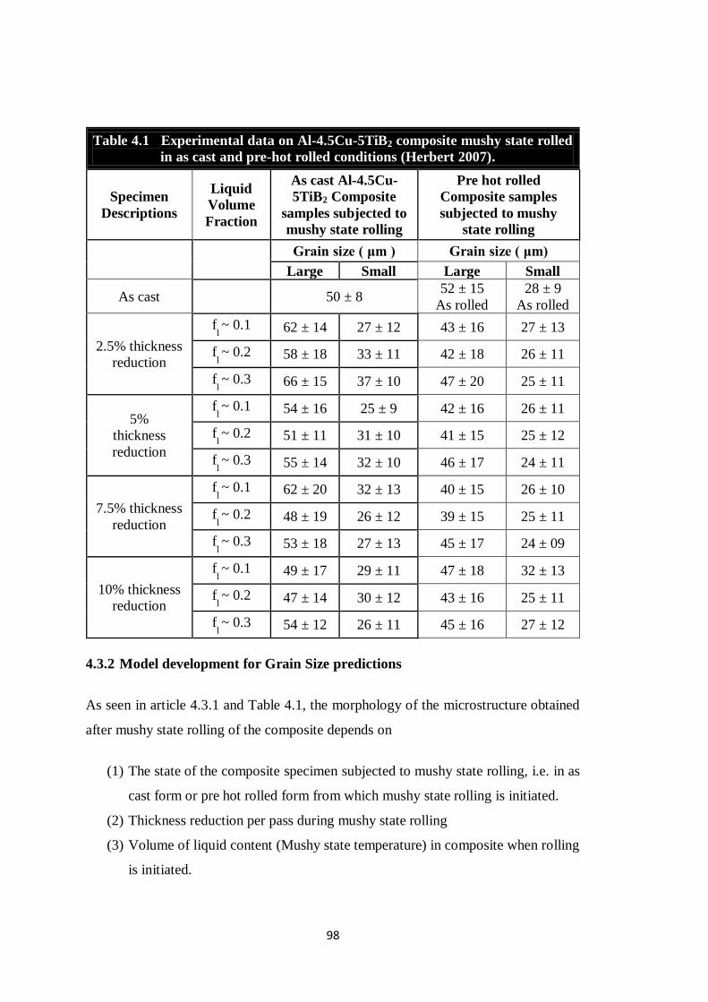
98
Table 4.1 Experimental data on Al-4.5Cu-5TiB2 composite mushy state rolled
in as cast and pre-hot rolled conditions (Herbert 2007).
Specimen
Descriptions
Liquid
Volume
Fraction
As cast Al-4.5Cu-
5TiB2 Composite
samples subjected to
mushy state rolling
Pre hot rolled
Composite samples
subjected to mushy
state rolling
Grain size ( μm ) Grain size ( μm)
Large Small Large Small
As cast 50 ± 8 52 ± 15
As rolled
28 ± 9
As rolled
2.5% thickness
reduction
fl ~ 0.1 62 ± 14 27 ± 12 43 ± 16 27 ± 13
fl ~ 0.2 58 ± 18 33 ± 11 42 ± 18 26 ± 11
fl ~ 0.3 66 ± 15 37 ± 10 47 ± 20 25 ± 11
5%
thickness
reduction
fl ~ 0.1 54 ± 16 25 ± 9 42 ± 16 26 ± 11
fl ~ 0.2 51 ± 11 31 ± 10 41 ± 15 25 ± 12
fl ~ 0.3 55 ± 14 32 ± 10 46 ± 17 24 ± 11
7.5% thickness
reduction
fl ~ 0.1 62 ± 20 32 ± 13 40 ± 15 26 ± 10
fl ~ 0.2 48 ± 19 26 ± 12 39 ± 15 25 ± 11
fl ~ 0.3 53 ± 18 27 ± 13 45 ± 17 24 ± 09
10% thickness
reduction
fl ~ 0.1 49 ± 17 29 ± 11 47 ± 18 32 ± 13
fl ~ 0.2 47 ± 14 30 ± 12 43 ± 16 25 ± 11
fl ~ 0.3 54 ± 12 26 ± 11 45 ± 16 27 ± 12
4.3.2 Model development for Grain Size predictions
As seen in article 4.3.1 and Table 4.1, the morphology of the microstructure obtained
after mushy state rolling of the composite depends on
(1) The state of the composite specimen subjected to mushy state rolling, i.e. in as
cast form or pre hot rolled form from which mushy state rolling is initiated.
(2) Thickness reduction per pass during mushy state rolling
(3) Volume of liquid content (Mushy state temperature) in composite when rolling
is initiated.

99
Hence, the grain sizes are found to be greatly influenced by the initial state of
composite material, thickness reduction per rolling pass and the liquid volume
fraction of the composite at the instant of initiation of mushy state rolling. Thus, the
input variables for the FFNN model for grain size predictions have been identified as
initial state of composite (i.e. as cast or pre hot rolled condition), % thickness
reduction and % liquid volume fraction in the composite. Obviously the output
variables are small grain size and large grain size.
4.3.2.1 Brief description of neural networks training
The aim of the present work is to estimate the grain sizes (small and large) of mushy
state rolled Al-4.5Cu-5TiB2 composite as a function of starting material type,
thickness reduction and liquid volume fraction in the composite. Both the input and
output variables have been normalized using the normalizing function (Reddy et al.
2005)
xn = [(x – xmin) * 0.8 / (xmax – xmin)] + 0.1 (4.1)
where xn is the normalized value of x, that has the maximum and minimum value
given by xmax and xmin, respectively. Once the network is trained, all the values of x
acquire their original value given by (Reddy et al. 2005)
x = [(xn -0.1) (xmax – xmin) / 0.8] + 0.1 (4.2)
The main reason for standardizing the data is that it is received in terms of variables
that have different units. Normalizing converts the data into non dimensional
quantities and removes the arbitrary effect of similarities between the objects
(Srinivasan et al. 2003, Reddy et al. 2005, 2008, Mandal et al. 2009). The output
layer had two nodes for bimodal grain sizes. The percentage thickness reduction was
varied from 2.5% to 10%, while the % volume of liquid fraction was varied from 10%
to 30%.
The mushy state rolling process is a high temperature forming process. It involves a
tight control of mushy state parameters, mainly the temperature which determines the
100
mushy state i.e. the liquid content in the composite. Secondly, this temperature is to
be maintained with ±2ºC accuracy (Herbert et al. 2006, Herbert 2007). During the
conduct of experiments, each specimen is heated to above 600ºC and held at that
temperature corresponding to liquid volume fraction for 10 minutes for
homogenization and then pushed into the roll gaps. Hence these experiments are time
consuming and tedious. In addition, Herbert et al. (2006) have also reported the
problem of alligatoring at higher thickness reductions, beyond 10%. Hence above
10% thickness reduction, experiments were not conducted and also conducting a large
number of experiments at high temperatures is practically not feasible. For each
starting condition of the composite (i.e. as cast and pre hot rolled condition) 12
experiments were conducted, as reported by Herbert et al. (2006). Thus in all 24 data
sets (as cast and pre hot rolled) were available for training the neural network.
However commercial application would require more data and hence prediction using
neural network is an effective alternate to the time consuming and tedious nature of
the experiments. The resultant grain sizes predicted by the ANN are discussed in
Section 4.6.
In any FFNN application even today, the exact architecture to be used needs to be
found (Reddy et al. 2005). More often than not, this is a trial and error exercise, as
regards to the selection of a number of hidden layers and neurons in each of these
layers. In this application, training was started with two hidden layers from 2 to 12
neurons in each hidden layer. The minimum mean squared error (MSE) was set as
0.00001 and the number of iterations to be executed as 1500000. Initially during
training, the learning rate parameter and momentum factor were preferred as 0.5 each.
The number of hidden neurons was fixed based on MSE and the mean error in
prediction of training data (Etr).
Single and two hidden layers were tried out to obtain the minimum MSE. It was
observed that the network fails to converge with single hidden layer, when tried with
different number of nodes varying from 2 to 12 in the hidden layer. This probably
happens due to the fact that the input-output relationship is quite complex and non
linear. Therefore, training with single hidden layer was terminated and training was
101
started with two hidden layers. Here the training was started with varying learning
rates from 0.1 to 0.9 in steps of 0.05. The learning rate and the momentum
parameters were initially taken as 0.3 and 0.9 respectively for training. For all
patterns, p, the global error function is expressed in terms of MSE (Yagnanarayana
2008) and is given by
E= ΣEp = (1/p) ΣΣ (bkp – skp0)
2 (4.3)
where, bkp is the actual output and skp0 is the network output for the k
th output neuron
for the pth pattern.
The mean error in the output prediction is (Reddy et al. 2005)
Etr(x) = 1/N Σ |(bk(x) – Pk(x))| (4.4)
where Etr(x) is the mean error in prediction of training data set for output parameter x,
N is the number of the data sets, bk(x) is the actual output and Pk(x) is the predicted
output.
The following sigmoid function was used as the activation function (Reddy et al.
2008, Mandal et al. 2009, Reddy et al. 2005, Li, Liu and Xiong 2002, Mousavi et al.
2007, Haque and Sudhakar 2002).
F(x) = 1/ (1+exp (-x)) (4.5)
Back propagation algorithm was used for training the network. It was found after a lot
of trial and error that convergence of the network was obtained with 2 hidden layers
with 7 neurons in the first and 4 neurons in the second hidden layer. Figure 4.1 shows
the schematic diagram of the FFNN used for grain size predictions. The learning rate
parameter was increased from 0.1 to 0.9 in steps of 0.05 and the momentum term was
decreased from 0.9 in steps of 0.05 to observe the network behaviour with respect to
MSE and number of epochs. Finally, the optimized architecture obtained with
learning parameter η = 0.85 and momentum factor α =0.65 was found to converge

102
excellently after 15 lakh epochs giving a MSE of 0.00023, to predict the grain sizes in
microns (μm).
.
Figure 4. 1 ANN Architecture
4.4 EXPERIMENTS FOR VALIDATION OF NN MODEL
As discussed in chapter 3, mushy state rolling experiments were conducted with Al-
4.5Cu-5TiB2 composite with the composite in as cast and pre hot rolled condition.
The process described for synthesis of Al-4.5Cu-5TiB2 composite as discussed in
section 3.3.3 of chapter 3 was followed. The microstructural evolution of Al-4.5Cu-
5TiB2 composite has been characterized using optical microscopy and SEM and EDX
microanalysis.

103
4.4.1 Optical microscopy and SEM imaging
4.4.1.1 Mushy state rolled Al-4.5Cu-5TiB2 composite from as cast state
Figure 4.2 (Herbert 2007) is the micrograph showing the characteristic microstructure
of the as cast Al-4.5Cu-5TiB2 composite. The microstructure reveals rosette like
irregular grain structure with dendritic character.
Figure 4.2 Optical micrograph showing rosette like dendritic grain structure (the
dendritic arms are shown with arrow) in as cast Al-4.5Cu-5TiB2
composite. (Herbert2007)
Figure 4.3(a) shows the optical micrographs of Al-4.5Cu-5TiB2 rolled in mushy state
with 17% volume percent liquid to a thickness reduction of 2%. The dendritic
structure witnessed in Figure 4.2 in case of as cast composite has tended to modify
modestly to globular shape due to tendency of α-Al grains having natural tendency to
become globular with small deformation at a higher liquid content (Herbert et al.
2006, Herbert 2007). Figure 4.3(b) to (d) show the optical micrographs for the
composite rolled to 6% thickness reduction at mushy zone temperatures
corresponding to 598ºC, 619
ºC and 633
ºC, while Figure 4.3(e) is the optical
micrograph for the composite rolled to 11.5% thickness reduction from a temperature
of 619ºC. The globular shape of grains can also be witnessed in Figure 4.3(d), with
6% thickness reduction with rolling initiated at 33% liquid content in the composite.
From the micrographs in Figure 4.3(c) and Figure 4.3(e), it can be observed that the
grain elongation is more with higher deformation. This is because at higher
deformation sufficient liquid is not available for strain accommodation, causing

104
elongation of the unmelted grains in the direction of rolling (Herbert et al. 2006,
Herbert 2007). The change in the pattern of grains from globular to elongated can be
seen in Figure 4.3(e). Evidence of grain fragmentation and transgranular cracks can
also be seen in Figure 4.3(e).
Figure 4.3 Optical micrographs showing the microstructure of Al-4.5Cu-5TiB2
composite subjected to mushy state rolling to thickness reduction of; (a)
2% at 619ºC (17% liquid), (b) 6% at 598
ºC (7% liquid), (c) 6% at 619
ºC
(17% liquid), (d) 6% at 633ºC (33% liquid) and (e) 11.5% at 619
ºC.

105
The SEM (BSE) images of the composite subjected to mushy state rolling in as cast
condition with 6% thickness reduction and with 7, 17 and 33% liquid volume content
are shown in Figure 4.4 (a) to (c). Figure 4.4(d) shows the SEM image for the mushy
state rolled composite subjected to 11.5% thickness reduction with 17% liquid volume
content. The grain boundaries as can be seen from the images appear dotted due to
bright TiB2 particles accumulated at grain boundaries. It can be observed that TiB2
particles appear to be aligned along rolling direction.
Upon mushy state rolling of the composite in as cast form, alligatoring was observed
in all cases except only when the composite was rolled to 6% thickness reduction and
with 33% liquid volume fractions in composite.
Figure 4.4 SEM images of showing the microstructure of Al-4.5Cu-5TiB2 composite
subjected to mushy state rolling to thickness reduction of: (a) 6% at 598ºC
(7% liquid), (b) 6% at 619ºC (17% liquid), (c) 6% at 633
ºC (33% liquid)
and (d) 11.5% at 619ºC (17% liquid).

106
4.4.1.2 Hot rolled Al-4.5Cu-5TiB2 composite
On subjecting the composite plates to hot rolling, the dendritic structure breaks down
to a more or less equiaxed grain structure and a modest grain refinement is witnessed
in the microstructure. Figure 4.5(a) is the optical micrograph and Figure 4.5(b) is the
SEM image which shows the typical microstructure of the hot rolled composite when
subjected to hot rolling at 370ºC with a thickness reduction of 2.5%. It indicates that
the cast microstructure in Figure. 4.3 is modified. The bimodal grain size distribution
reported by Herbert et al. (2006) and Herbert (2007) is confirmed as seen in Figure
4.5(a). The finer equiaxed grains originate due to dynamic recrystallization and
appear to be randomly mixed amongst the coarser grains. Dynamic recrystallization
has also been confirmed in Al-4.5Cu alloy based composite when subjected to high
temperature compression tests in previous studies ((Bhat et al. 1992, Herbert et al.
2006, Herbert 2007).
Upon hot rolling of the composite, prior to mushy state rolling, alligatoring was
observed only when the composite was rolled to 11.5% thickness reduction with
mushy state temperatures corresponding to 33% liquid volume fractions in composite.
The prior hot rolling of the composite before mushy state rolling is known to inhibit
alligatoring, except with very large thickness reductions (Herbert et al. 2006, Herbert
2007). This is due to reduction in stress concentration at grain boundaries owing to
equiaxed grain morphology evolved after hot rolling. Such a phenomenon makes
grain sliding easier as observed (Raj & Ashby 1971, Sherby & Wadsworth 1989) in
super plastic deformation involving much finer grains. In addition, large amounts of
diffusion during annealing in hot rolling leads to redistribution of the solute, Cu in the
composite matrix (Herbert 2007). This in turn leads to more uniform accumulation of
liquid near grain boundaries. It is reported (Herbert et al. 2006, Herbert 2007) to
result in more uniform distribution of strain and strain accommodation by inter-grain
sliding, in line with the observations made in this study. Tzimas and Zavalnigos
(1999) have reported much lower flow stress during the compression tests on
previously deformed (strain induced melt activated) 2014 alloy specimens, compared
to that seen with as cast specimens having dendritic microstructure.

107
Figure 4.5 Typical microstructure of Al-4.5Cu-5TiB2 composite subjected to hot
rolling at 370ºC with a thickness reduction of 2.5%: (a) optical micrograph
(b) SEM image.
4.4.1.3 Mushy state rolled Al-4.5Cu-5TiB2 composite from pre hot rolled
condition
Figure 4.6 (a) to (e) show the optical micrographs of pre hot rolled composite rolled in
mushy state to various thickness reductions and at various mushy zone temperatures.
Figure 4.6(a) is the optical micrograph for specimen rolled in mushy state with 17%
liquid volume content to 2% thickness reduction. Figure 4.6(b) to (d) show the optical
micrographs of mushy state rolled composite to 6% thickness reduction with 7, 17 and
33% liquid volume content, respectively. Optical micrograph depicted in Figure
4.6(e) is for the specimen mushy state rolled to 11.5% thickness reduction with 17%
liquid volume content. The grains are found to be globular with low reduction and
high liquid content as observed in Figure 4.6(a). Grains appear to be elongated with
higher thickness reduction and low liquid content as seen in Figure 4.6(e), as was the
case observed in mushy state rolled composite in as cast form in Figure 4.3(e). It can
also be seen from Figure 4.6(a) through (e) that the overall morphology of the
microstructure in mushy state rolled specimens rolled in pre hot rolled condition gets
more refined, with the bimodal grain size morphology being maintained.
Figure 4.7 (a) to (e) show the SEM (BSE) images of the composite rolled in mushy
state when in pre hot rolled condition with various liquid volume contents and at
various thickness reductions. Figure 4.7(a) shows image for 2% thickness reduction
with 17% liquid volume content of the composite. Figure 4.7(b) to (d) are the images
for 6% thickness reduction of composite with 7, 17 and 33% liquid volume content
while Figure 4.7(e) shows the SEM image for the pre hot rolled composite, mushy
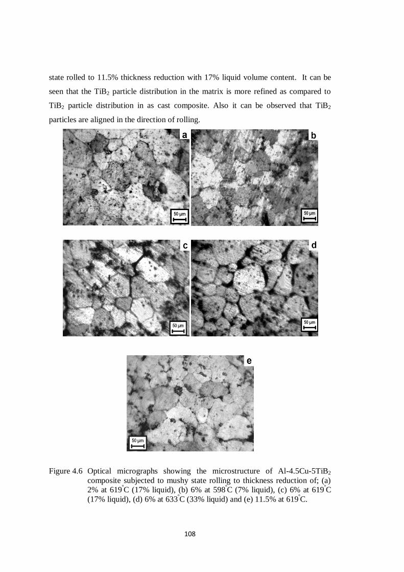
108
state rolled to 11.5% thickness reduction with 17% liquid volume content. It can be
seen that the TiB2 particle distribution in the matrix is more refined as compared to
TiB2 particle distribution in as cast composite. Also it can be observed that TiB2
particles are aligned in the direction of rolling.
Figure 4.6 Optical micrographs showing the microstructure of Al-4.5Cu-5TiB2
composite subjected to mushy state rolling to thickness reduction of; (a)
2% at 619ºC (17% liquid), (b) 6% at 598
ºC (7% liquid), (c) 6% at 619
ºC
(17% liquid), (d) 6% at 633ºC (33% liquid) and (e) 11.5% at 619
ºC.

109
Figure 4.7 SEM images showing the microstructure of Al-4.5Cu-5TiB2 composite
subjected to mushy state rolling to thickness reduction of: (a) 2% at 619ºC
(17% liquid), (b) 6% at 598ºC (7% liquid), (c) 6% at 619
ºC (17% liquid),
(d) 6% at 633ºC (33% liquid) and (e) 11.5% at 619
ºC.
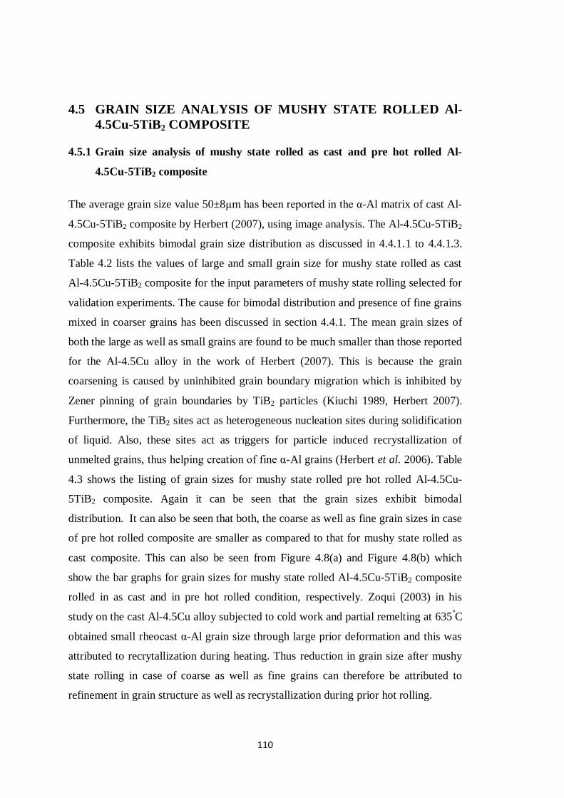
110
4.5 GRAIN SIZE ANALYSIS OF MUSHY STATE ROLLED Al-
4.5Cu-5TiB2 COMPOSITE
4.5.1 Grain size analysis of mushy state rolled as cast and pre hot rolled Al-
4.5Cu-5TiB2 composite
The average grain size value 50±8μm has been reported in the α-Al matrix of cast Al-
4.5Cu-5TiB2 composite by Herbert (2007), using image analysis. The Al-4.5Cu-5TiB2
composite exhibits bimodal grain size distribution as discussed in 4.4.1.1 to 4.4.1.3.
Table 4.2 lists the values of large and small grain size for mushy state rolled as cast
Al-4.5Cu-5TiB2 composite for the input parameters of mushy state rolling selected for
validation experiments. The cause for bimodal distribution and presence of fine grains
mixed in coarser grains has been discussed in section 4.4.1. The mean grain sizes of
both the large as well as small grains are found to be much smaller than those reported
for the Al-4.5Cu alloy in the work of Herbert (2007). This is because the grain
coarsening is caused by uninhibited grain boundary migration which is inhibited by
Zener pinning of grain boundaries by TiB2 particles (Kiuchi 1989, Herbert 2007).
Furthermore, the TiB2 sites act as heterogeneous nucleation sites during solidification
of liquid. Also, these sites act as triggers for particle induced recrystallization of
unmelted grains, thus helping creation of fine α-Al grains (Herbert et al. 2006). Table
4.3 shows the listing of grain sizes for mushy state rolled pre hot rolled Al-4.5Cu-
5TiB2 composite. Again it can be seen that the grain sizes exhibit bimodal
distribution. It can also be seen that both, the coarse as well as fine grain sizes in case
of pre hot rolled composite are smaller as compared to that for mushy state rolled as
cast composite. This can also be seen from Figure 4.8(a) and Figure 4.8(b) which
show the bar graphs for grain sizes for mushy state rolled Al-4.5Cu-5TiB2 composite
rolled in as cast and in pre hot rolled condition, respectively. Zoqui (2003) in his
study on the cast Al-4.5Cu alloy subjected to cold work and partial remelting at 635ºC
obtained small rheocast α-Al grain size through large prior deformation and this was
attributed to recrytallization during heating. Thus reduction in grain size after mushy
state rolling in case of coarse as well as fine grains can therefore be attributed to
refinement in grain structure as well as recrystallization during prior hot rolling.

111
Table 4.2 Grain sizes of Al-4.5Cu-5TiB2 composite samples subjected to
mushy state rolling in as cast state. (along longitudinal rolling
plane).
Sr. No.
Thickness
Reduction
(%)
Liquid
Volume
Fraction
(%)
Large Grain size
(μm)
Small Grain size
(μm)
1 2 17 63 30
2 6 7 66 29
3 6 17 49 26
4 6 33 55 28
5 11.5 17 46 30
Table 4.3 Grain sizes of Al-4.5Cu-5TiB2 composite samples subjected to
mushy state rolling in pre hot rolled condition. (along
longitudinal rolling plane).
Sr. No.
Thickness
Reduction
(%)
Liquid
Volume
Fraction
(%)
Large Grain size
(μm)
Small Grain size
(μm)
1 2 17 43 25
2 6 7 41 26
3 6 17 40 26
4 6 33 46 24
5 11.5 17 46 30
0.000 2.875 5.750 8.625 11.500 14.375
0
20
40
60
80
100
120
Gra
in S
ize
(
Thickness reduction (%)
Large Grain size(17% liquid)
Small Grain size (17% liquid)
Large Grain size(7% liquid)
Small Grain size (7% liquid)
Large Grain size(33% liquid)
Small Grain size (33% liquid)
Figure 4.8(a) Bar diagram showing the grain sizes (along longitudinal rolling
plane for as cast Al-4.5Cu-5TiB2 composite samples subjected to
mushy state rolling.

112
0 1 2 3 4 5 6 7 8 9 10 11 12 13
0
10
20
30
40
50
60
70
80
90
100
Gra
in s
ize
(
m))
Thickness Reduction
Large Grain size 7% Liquid
Small Grain size 7% Liquid
large Grain size 17% Liquid
small Grain Size 17% Liquid
Large Grain size 33% Liquid
Small Grain size 33% Liquid
4.6 GRAIN SIZE PREDICTION USING ARTIFICIAL NEURAL
NETWORKS (ANN)
The values of grain size predicted by ANN are compared in the next sub-section with
the corresponding experimentally obtained values listed at Table 4.1, to check the
suitability of the model within the purview of experimentation. Further, the model is
checked for its capability to extrapolate and interpolate the values of grain size with
the outcome of validation experiments. A detailed analysis of the variation of the
values of grain sizes with respect to amount of thickness reduction during rolling and
with liquid volume fraction at the beginning of rolling is also presented in this section.
4.6.1 Comparison of Grain sizes obtained by experimentation and ANN
prediction
4.6.1.1 Rolling of as cast Al-4.5Cu-5TiB2 composite in mushy state
Table 4.4 shows the values of experimentally obtained large and small grain sizes as
well as those predicted by ANN for as cast Al-4.5Cu-5TiB2 composite in mushy state
containing varying liquid volume fractions (10% corresponding to 610ºC, 20%
corresponding to 626ºC and 30% corresponding to 631
ºC) and rolled to 2.5%, 5%,
Figure 4.8(b) Bar diagram showing the grain sizes (along longitudinal rolling
plane for pre hot rolled Al-4.5Cu-5TiB2 composite samples
subjected to mushy state rolling.

113
7.5% and 10% thickness reductions per pass. The experimental values used for
training the network are taken from the PhD work of Herbert (2007), for experiments
carried out at 10%, 20% and 30% liquid volume fractions to 2.5%, 5%, 7.5% and 10%
thickness reductions while the ANN predictions have been extended beyond the upper
and lower limits of experimentation. Table 4.4 lists the values of large and small grain
sizes predicted by the trained ANN for the data used for training the network as well
as the data corresponding to validation experiments.
From Table 4.4, it can be seen that the percentage error between the experimental
values used for training the network and corresponding ANN predicted values ranges
from -3.0987% to +1.99% for large grain size, with the maximum errors
corresponding to 10% liquid volume fraction at 5% thickness reduction and 20%
liquid volume fraction at 5% thickness reduction, respectively. Similarly, for small
grain size, the maximum % error is between -5.3307% corresponding to 10% liquid
volume fraction at 10% thickness reduction and 4.8529% corresponding to 20% liquid
volume fraction at 5% thickness reduction.
The percentage error between experimental values and values predicted by ANN at
various percent liquid volume fractions for entire range of percentage thickness
reduction are within |5.4%|. This suggests that the model has learnt the relationship
between the mushy state parameters and the grain sizes quite adequately and has
generalized it to predict the large and small grain sizes for any values of input
parameters viz. the material type, % thickness reduction and % liquid volume
fractions supplied to it, within an error of 5.4%. Kusiak and Kuziak (2002) have
reported a maximum error of 8% in ANN predictions, while Jiahe et al. (2003)
reported a maximum error of 5.7% in the prediction of average ferrite grain size of
60Si2MnA stainless steel rod based on controlled rolling and cooling process
parameters.
Figure 4.9 and 4.10 show the variation of grain sizes (coarse and small) with change
in % thickness reduction as predicted by ANN at 5% and 35% liquid volume
fractions, respectively. It can be seen from Figure 4.9 that size of coarse grain size
increases gradually till 7% thickness reduction but subsequently falls drastically
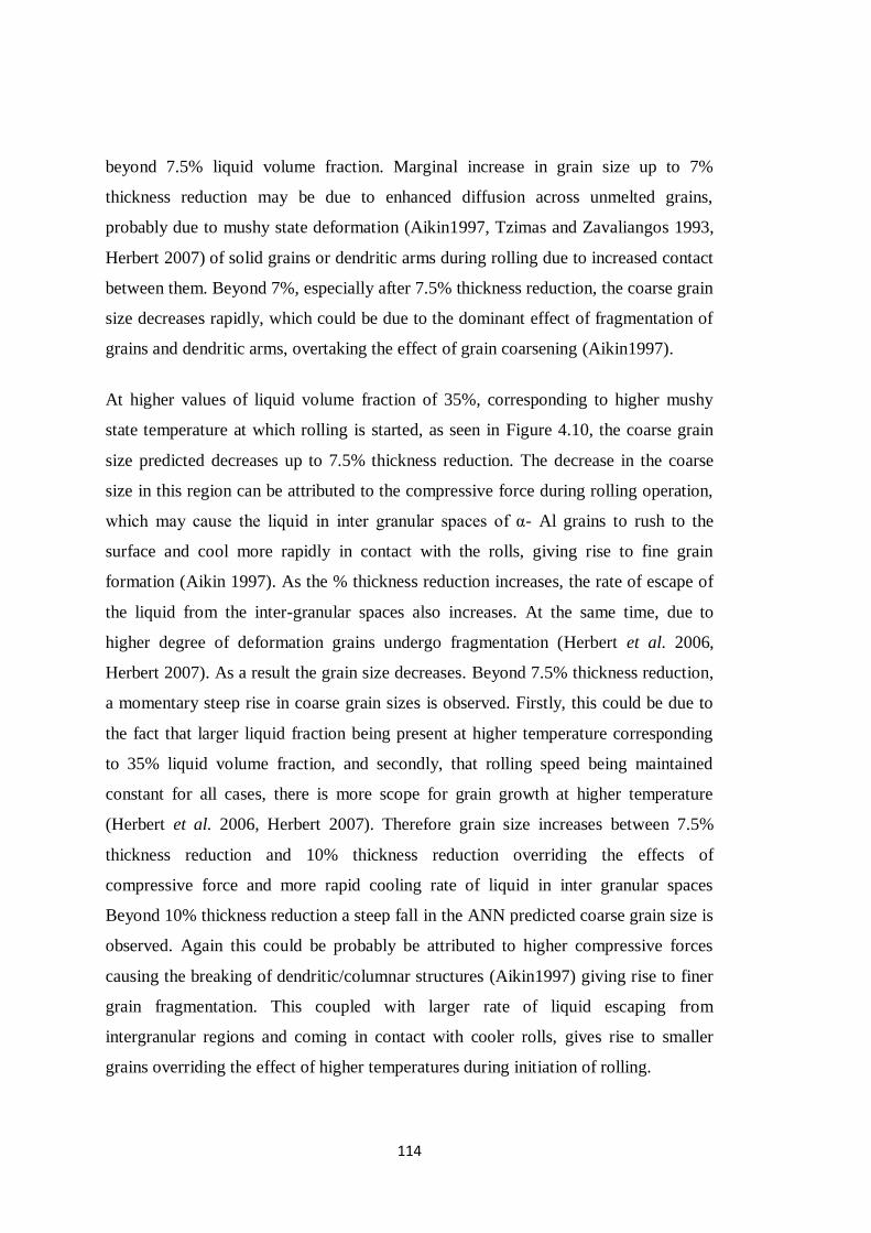
114
beyond 7.5% liquid volume fraction. Marginal increase in grain size up to 7%
thickness reduction may be due to enhanced diffusion across unmelted grains,
probably due to mushy state deformation (Aikin1997, Tzimas and Zavaliangos 1993,
Herbert 2007) of solid grains or dendritic arms during rolling due to increased contact
between them. Beyond 7%, especially after 7.5% thickness reduction, the coarse grain
size decreases rapidly, which could be due to the dominant effect of fragmentation of
grains and dendritic arms, overtaking the effect of grain coarsening (Aikin1997).
At higher values of liquid volume fraction of 35%, corresponding to higher mushy
state temperature at which rolling is started, as seen in Figure 4.10, the coarse grain
size predicted decreases up to 7.5% thickness reduction. The decrease in the coarse
size in this region can be attributed to the compressive force during rolling operation,
which may cause the liquid in inter granular spaces of α- Al grains to rush to the
surface and cool more rapidly in contact with the rolls, giving rise to fine grain
formation (Aikin 1997). As the % thickness reduction increases, the rate of escape of
the liquid from the inter-granular spaces also increases. At the same time, due to
higher degree of deformation grains undergo fragmentation (Herbert et al. 2006,
Herbert 2007). As a result the grain size decreases. Beyond 7.5% thickness reduction,
a momentary steep rise in coarse grain sizes is observed. Firstly, this could be due to
the fact that larger liquid fraction being present at higher temperature corresponding
to 35% liquid volume fraction, and secondly, that rolling speed being maintained
constant for all cases, there is more scope for grain growth at higher temperature
(Herbert et al. 2006, Herbert 2007). Therefore grain size increases between 7.5%
thickness reduction and 10% thickness reduction overriding the effects of
compressive force and more rapid cooling rate of liquid in inter granular spaces
Beyond 10% thickness reduction a steep fall in the ANN predicted coarse grain size is
observed. Again this could be probably be attributed to higher compressive forces
causing the breaking of dendritic/columnar structures (Aikin1997) giving rise to finer
grain fragmentation. This coupled with larger rate of liquid escaping from
intergranular regions and coming in contact with cooler rolls, gives rise to smaller
grains overriding the effect of higher temperatures during initiation of rolling.

115
* Validation experiments carried out in the present study within range of training data.
** Validation experiments carried out in the present study outside training data range.
a Experimental data.
TABLE 4.4 Comparison of Experimental values of grain sizes of as cast Al-
4.5Cu- 5TiB2 composite samples subjected to mushy state rolling
with ANN predicted values.
Specimen
descriptions
Experimental ANN %Error
Grain size(μm) Grain size (μm) Grain size
Large Small Large Small Large Small
As cast 50 49.9944 49.9944 0.0112 0.2106
** 2%
thickness.
Reduction
**f1~ 0.17
63 30 61.5498 30.2633 2.3019 -0.8777
2.5%
thickness
reduction
fl ~ 0.05 66.7204 27.2855 afl ~ 0.1 62 27 60.7838 27.4532 1.9616
1
-1.6785 afl ~ 0.2 58 33 59.338 33.8438 -2.3069 -2.557
afl ~ 0.3 66 37 64.776 35.8221 1.8545
5
3.1835
1 fl ~ 0.35 66.6396 30.0602
5%
thickness
reduction
fl ~ 0.05 69.5573 27.2271 afl ~ 0.1 54 25 55.6733 25.8852 -3.0987 -3.5408
afl ~ 0.2 51 31 49.9853 29.4956 1.9896
1
4.8529 afl ~ 0.3 55 32 55.5784 33.4465 -1.0516 -4.5203
fl ~ 0.35 61.1633 28.4914
*6%
thickness
reduction
**f1~ 0.07 66 29 66.9744 28.032 -1.476 3.3379
*f1~0.17 49 26 48.496 25.793 1.0286 0.7962
**f1~0.33 55 28 56.3759 28.2583 -2.5016 -0.9255
7.5%
thickness
reduction
fl ~ 0.05 71.394 32.4656 afl ~ 0.1 62 32 61.5025 30.92 0.8024
2
3.375 afl ~ 0.2 48 26 47.299 27.3059 1.4604
2
-5.0227 afl ~ 0.3 53 27 52.922 26.4012 0.1471
7
2.2177
8 fl ~ 0.35 56.2987 24.2107
10%
thickness
reduction
fl ~ 0.05 48.5162 30.514 afl ~ 0.1 49 29 49.2457 30.5459 -0.5014 -5.3307
afl ~ 0.2 47 30 48.0792 30.494 -2.2962 -1.6467
afl ~ 0.3 54 26 54.1504 26.2361 -0.2785 -0.9081
fl ~ 0.35 59.3253 21.9236
** 11.5%
thickness
reduction
**f1 ~ 0.17 46 30 47.0124 30.4498 -2.2008 -1.4993
12.5%
thickness
reduction
fl ~ 0.05 46.7048 30.4369
fl ~ 0.1 46.7111 30.3472
fl ~ 0.2 46.7789 30.44
fl ~ 0.3 46.8364 30.391
fl ~ 0.35 48.8614 29.249

116
0.0 2.5 5.0 7.5 10.0 12.5
25
30
35
40
45
50
55
60
65
70
75
G
rain
siz
e (
m)
Thickness Reduction (%)
Small Grain size
Large Grain size
0.0 2.5 5.0 7.5 10.0 12.5
20
25
30
35
40
45
50
55
60
65
70
Gra
in S
ize
(m
)
Thickness Reduction (%)
LargeGrain Size
Small Grain Size
Figure 4.9 Plots showing variation of ANN predicted values of large grain and
small grain size with % thickness reduction at 5% liquid volume
fraction when as cast Al-4.5Cu-5TiB2 composite is rolled in mushy
state.
Figure 4.10 Plots showing variation of ANN predicted values of large grain and
small grain size with % thickness reduction at 35% liquid volume
fraction when as cast Al-4.5Cu-5TiB2 composite is rolled in mushy
state.
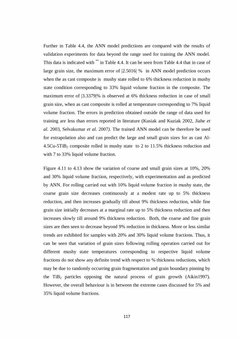
117
Further in Table 4.4, the ANN model predictions are compared with the results of
validation experiments for data beyond the range used for training the ANN model.
This data is indicated with **
in Table 4.4. It can be seen from Table 4.4 that in case of
large grain size, the maximum error of |2.5016| % in ANN model prediction occurs
when the as cast composite is mushy state rolled to 6% thickness reduction in mushy
state condition corresponding to 33% liquid volume fraction in the composite. The
maximum error of |3.3379|% is observed at 6% thickness reduction in case of small
grain size, when as cast composite is rolled at temperature corresponding to 7% liquid
volume fraction. The errors in prediction obtained outside the range of data used for
training are less than errors reported in literature (Kusiak and Kuziak 2002, Jiahe et
al. 2003, Selvakumar et al. 2007). The trained ANN model can be therefore be used
for extrapolation also and can predict the large and small grain sizes for as cast Al-
4.5Cu-5TiB2 composite rolled in mushy state to 2 to 11.5% thickness reduction and
with 7 to 33% liquid volume fraction.
Figure 4.11 to 4.13 show the variation of coarse and small grain sizes at 10%, 20%
and 30% liquid volume fraction, respectively, with experimentation and as predicted
by ANN. For rolling carried out with 10% liquid volume fraction in mushy state, the
coarse grain size decreases continuously at a modest rate up to 5% thickness
reduction, and then increases gradually till about 9% thickness reduction, while fine
grain size initially decreases at a marginal rate up to 5% thickness reduction and then
increases slowly till around 9% thickness reduction. Both, the coarse and fine grain
sizes are then seen to decrease beyond 9% reduction in thickness. More or less similar
trends are exhibited for samples with 20% and 30% liquid volume fractions. Thus, it
can be seen that variation of grain sizes following rolling operation carried out for
different mushy state temperatures corresponding to respective liquid volume
fractions do not show any definite trend with respect to % thickness reductions, which
may be due to randomly occurring grain fragmentation and grain boundary pinning by
the TiB2 particles opposing the natural process of grain growth (Aikin1997).
However, the overall behaviour is in between the extreme cases discussed for 5% and
35% liquid volume fractions.
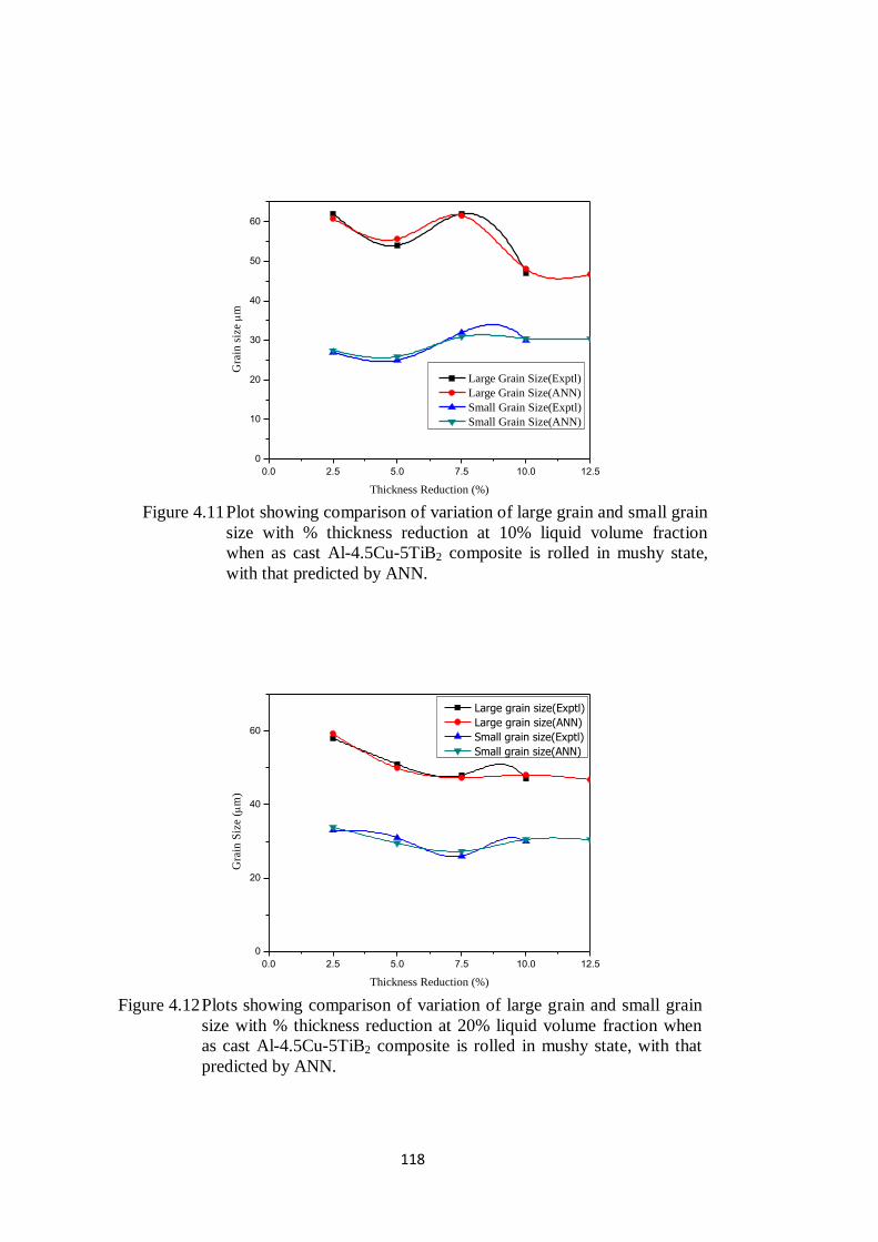
118
0.0 2.5 5.0 7.5 10.0 12.5
0
10
20
30
40
50
60
Gra
in s
ize
m
Thickness Reduction (%)
Large Grain Size(Exptl)
Large Grain Size(ANN)
Small Grain Size(Exptl)
Small Grain Size(ANN)
0.0 2.5 5.0 7.5 10.0 12.5
0
20
40
60
Gra
in S
ize
(m
)
Thickness Reduction (%)
Large grain size(Exptl)
Large grain size(ANN)
Small grain size(Exptl)
Small grain size(ANN)
Figure 4.11 Plot showing comparison of variation of large grain and small grain
size with % thickness reduction at 10% liquid volume fraction
when as cast Al-4.5Cu-5TiB2 composite is rolled in mushy state,
with that predicted by ANN.
Figure 4.12 Plots showing comparison of variation of large grain and small grain
size with % thickness reduction at 20% liquid volume fraction when
as cast Al-4.5Cu-5TiB2 composite is rolled in mushy state, with that
predicted by ANN.

119
0.0 2.5 5.0 7.5 10.0 12.5
0
20
40
60
80
Gra
in S
ize
( m
)
Thickness Reduction (%)
Large grain size(Exptl)
Large grain size(ANN)
Small grain size(Exptl)
Small grain size(ANN)
4.6.1.2 Pre-hot rolled composite rolled in mushy state
Table 4.5 lists the values of grain sizes predicted by ANN for mushy state rolled Al-
4.5Cu-5TiB2 composite rolled in pre hot rolled condition. Here the model, predicts
the grain sizes for the entire range of mushy state rolling from 2.5% to 10% thickness
reduction and the composite containing liquid volume fractions from 10% to 30%
within an error of |6.1|%. Figure 4.14 and 4.15 show the variation of grain sizes
predicted by ANN, while those in Figure 4.16, 4.17 and 4.18 show comparison of
grain sizes obtained experimentally and those predicted by ANN model, when pre hot
rolled Al-4.5 Cu- 5TiB2 composite is rolled to different % thickness reductions, (i.e.
2.5%, 5%, 7.5%, 10% and 12.5%) with varying % liquid volume fractions ( i.e. 5%,
10%, 20%, 30% and 35%).
The comparison of experimental and ANN predicted graphs in Figure 4.16, 4.17 and
4.18 shows that there is a very small variation between these values. The values
predicted by ANN are plotted in Figure 4.14 and 4.15, and show the expected values
of coarse and small grain size for the Al-4.5Cu-5TiB2 composite in pre hot rolled
condition, rolled in mushy state containing 5% liquid volume fractions and 35%
liquid volume fractions, respectively.
Figure 4.13 Plots showing comparison of variation of large grain and small grain
size with % thickness reduction at 30% liquid volume fraction when as
cast Al-4.5Cu-5TiB2 composite is rolled in mushy state, with that
predicted by ANN.
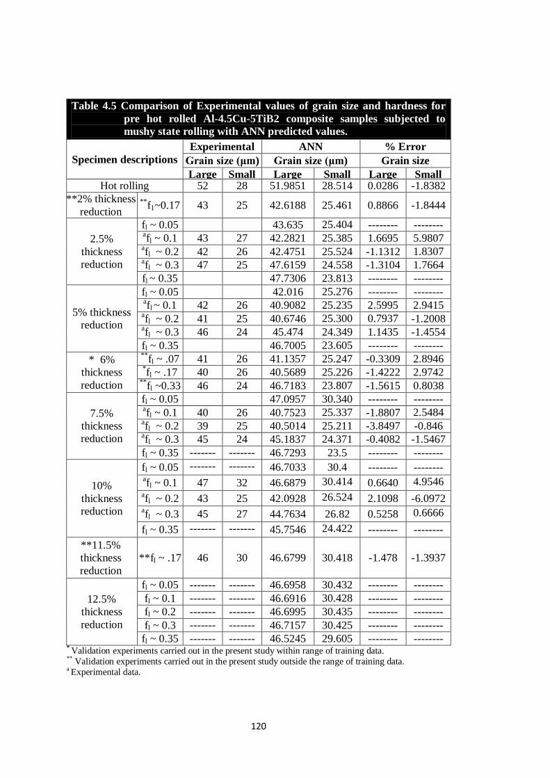
120
Table 4.5 Comparison of Experimental values of grain size and hardness for
pre hot rolled Al-4.5Cu-5TiB2 composite samples subjected to
mushy state rolling with ANN predicted values.
Specimen descriptions
Experimental ANN % Error
Grain size (μm) Grain size (μm) Grain size
Large Small Large Small Large Small Hot rolling 52 28 51.9851 28.514
7
0.0286
5
-1.8382
**2% thickness
reduction **
f1~0.17 43 25 42.6188 25.461 0.8866 -1.8444
2.5%
thickness
reduction
fl ~ 0.05 43.635 25.404
7
-------- -------- afl ~ 0.1 43 27 42.2821 25.385
2
1.6695 5.9807
4 afl ~ 0.2 42 26 42.4751 25.524 -1.1312 1.8307
7 afl ~ 0.3 47 25 47.6159 24.558
4
-1.3104 1.7664
fl ~ 0.35 47.7306 23.813
5
-------- --------
5% thickness
reduction
fl ~ 0.05 42.016 25.276
4
-------- -------- afl ~ 0.1 42 26 40.9082 25.235
2
2.5995 2.9415
4 afl ~ 0.2 41 25 40.6746 25.300
2
0.7937
9
-1.2008 afl ~ 0.3 46 24 45.474 24.349
3
1.1435 -1.4554
fl ~ 0.35 46.7005 23.605
9
-------- --------
* 6%
thickness
reduction
**fl ~ .07 41 26 41.1357 25.247
4
-0.3309 2.8946 *fl ~ .17 40 26 40.5689 25.226
7
-1.4222 2.9742 **
fl ~0.33 46 24 46.7183 23.807
1
-1.5615 0.8038
7.5%
thickness
reduction
fl ~ 0.05 47.0957 30.340
6
-------- -------- afl ~ 0.1 40 26 40.7523 25.337
4
-1.8807 2.5484
6 afl ~ 0.2 39 25 40.5014 25.211
5
-3.8497 -0.846 afl ~ 0.3 45 24 45.1837 24.371
2
-0.4082 -1.5467
fl ~ 0.35 -------
-
-------
-
46.7293 23.5 -------- --------
10%
thickness
reduction
fl ~ 0.05 -------
-
-------
- 46.7033 30.4 -------- --------
afl ~ 0.1 47 32 46.6879 30.414
5 0.6640 4.9546
9 afl ~ 0.2 43 25 42.0928 26.524
3 2.1098 -6.0972
afl ~ 0.3 45 27 44.7634 26.82 0.5258 0.6666
7 fl ~ 0.35 -------
-
-------
- 45.7546 24.422
7 -------- --------
**11.5%
thickness
reduction
**fl ~ .17 46 30 46.6799 30.418 -1.478 -1.3937
12.5%
thickness
reduction
fl ~ 0.05 -------
-
-------
-
46.6958 30.432
5
-------- --------
fl ~ 0.1 -------
-
-------
-
46.6916 30.428
8
-------- --------
fl ~ 0.2 -------
-
-------
-
46.6995 30.435
9
-------- --------
fl ~ 0.3 -------
-
-------
-
46.7157 30.425 -------- --------
fl ~ 0.35 -------
-
-------
-
46.5245 29.605 -------- -------- * Validation experiments carried out in the present study within range of training data. ** Validation experiments carried out in the present study outside the range of training data. a Experimental data.

121
From all the Figure 4.16, 4.17 and 4.18, it can be seen that the variation does not show
any definite continuous increase or decrease with increase in % thickness reduction.
As we have seen earlier, this may be again due to randomly occurring fragmentation
of grains and grain boundary pinning by TiB2 particles which restrict grain growth
(Aikin1997). However, it can be seen that, coarse grain sizes have higher values in the
composite with 30% liquid volume fractions rolled to 10% thickness reduction.
0.0 2.5 5.0 7.5 10.0 12.5
0
10
20
30
40
50
Gra
in S
ize
(m
)
Thickness Reduction (%))
Large Grain Size
Small Grain Size
It can be seen from Table 4.5 that the trained ANN model for grain size prediction
predicts the large grain sizes within an error of |1.5615|% outside the bounds of data
range used for training the model. The maximum error of |1.5615|% is observed at 6%
thickness reduction when pre hot rolled composite is mushy state rolled with 33%
liquid volume fraction. Similarly, the model predicts the small grain size within an
error of |2.8946|% with this maximum error observed at 6% thickness reduction and
7% liquid volume fraction. Thus the model extrapolates the large and small grain
sizes within an error of |2.9|% for mushy state rolled composite rolled to 2 to 12%
thickness reduction and with 7 to 33% liquid volume fraction. These observed errors
Figure 4.14 Plots showing variation of ANN predicted values of large grain and
small grain size with % thickness reduction at 5% liquid volume
fraction when pre hot rolled Al-4.5Cu-5TiB2 composite is rolled from
mushy state.
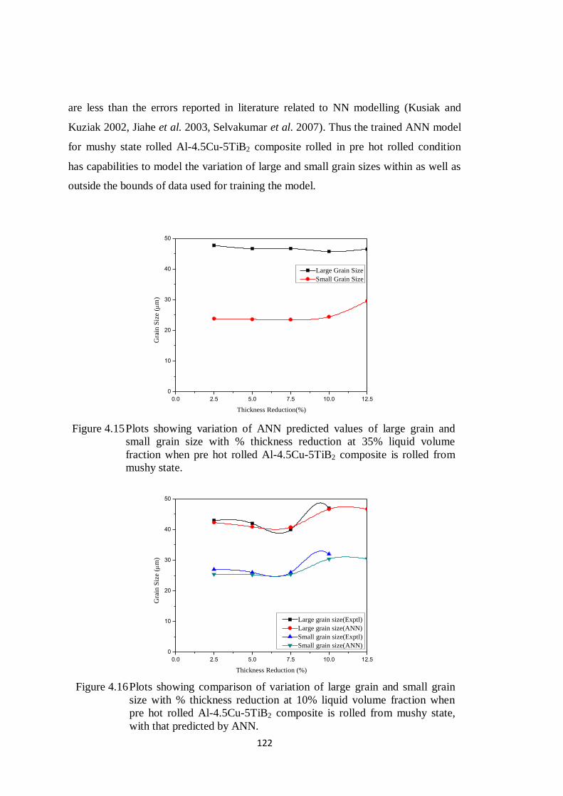
122
are less than the errors reported in literature related to NN modelling (Kusiak and
Kuziak 2002, Jiahe et al. 2003, Selvakumar et al. 2007). Thus the trained ANN model
for mushy state rolled Al-4.5Cu-5TiB2 composite rolled in pre hot rolled condition
has capabilities to model the variation of large and small grain sizes within as well as
outside the bounds of data used for training the model.
0.0 2.5 5.0 7.5 10.0 12.5
0
10
20
30
40
50
Gra
in S
ize (
m)
Thickness Reduction(%)
Large Grain Size
Small Grain Size
0.0 2.5 5.0 7.5 10.0 12.5
0
10
20
30
40
50
Gra
in S
ize (
m)
Thickness Reduction (%)
Large grain size(Exptl)
Large grain size(ANN)
Small grain size(Exptl)
Small grain size(ANN)
Figure 4.15 Plots showing variation of ANN predicted values of large grain and
small grain size with % thickness reduction at 35% liquid volume
fraction when pre hot rolled Al-4.5Cu-5TiB2 composite is rolled from
mushy state.
Figure 4.16 Plots showing comparison of variation of large grain and small grain
size with % thickness reduction at 10% liquid volume fraction when
pre hot rolled Al-4.5Cu-5TiB2 composite is rolled from mushy state,
with that predicted by ANN.

123
0.0 2.5 5.0 7.5 10.0 12.5
0
20
40
60
Gra
in S
ize
(m
)
Thickness Reduction (%)
Large grain size(Exptl)
Large grain size(ANN)
Small grain size(Exptl)
Small grain size(ANN)
0.0 2.5 5.0 7.5 10.0 12.5
0
20
40
60
Gra
in S
ize
(m
)
Thickness Reduction (%)
Large grain size(Exptl)
Large grain size(ANN)
Small grain size(Exptl)
Small grain size(ANN)
Figure 4.19(a) and (b) show the contour graphs of the distribution of large grain sizes
and small grain sizes for as cast composite with variations in % thickness reduction
and % liquid volume fractions. In the contour plot shown in Figure 4.19(b) it is seen
that low values of small grain size are concentrated in the region between 2.5% and
Figure 4.17 Plots showing comparison of variation of large grain and small grain
size with % thickness reduction at 20% liquid volume fraction when
pre hot rolled Al-4.5Cu-5TiB2 composite is rolled from mushy state,
with that predicted by ANN.
Figure 4.18 Plots showing comparison of variation of large grain and small grain
size with % thickness reduction at 30% liquid volume fraction when
pre hot rolled Al-4.5Cu-5TiB2 composite is rolled from mushy state,
with that predicted by ANN.
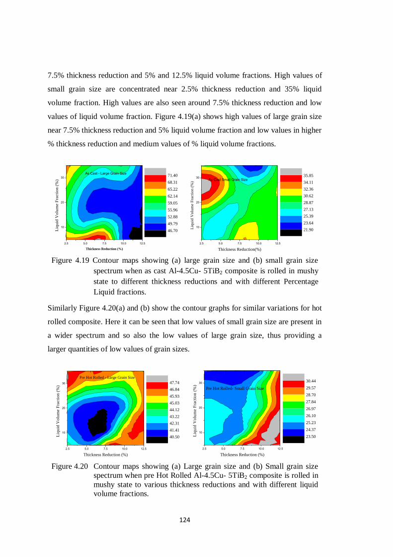
124
7.5% thickness reduction and 5% and 12.5% liquid volume fractions. High values of
small grain size are concentrated near 2.5% thickness reduction and 35% liquid
volume fraction. High values are also seen around 7.5% thickness reduction and low
values of liquid volume fraction. Figure 4.19(a) shows high values of large grain size
near 7.5% thickness reduction and 5% liquid volume fraction and low values in higher
% thickness reduction and medium values of % liquid volume fractions.
2.5 5.0 7.5 10.0 12.5
10
20
30
As Cast - Large Grain Size
Liq
uid
Vo
lum
e F
racti
on
(%
)
Thickness Reduction (%)
46.70
49.79
52.88
55.96
59.05
62.14
65.22
68.31
71.40
2.5 5.0 7.5 10.0 12.5
10
20
30As Cast Small Grain Size
Liq
uid
Vo
lum
e F
racti
on
(%
)
Thickness Reduction(%)
21.90
23.64
25.39
27.13
28.87
30.62
32.36
34.11
35.85
Similarly Figure 4.20(a) and (b) show the contour graphs for similar variations for hot
rolled composite. Here it can be seen that low values of small grain size are present in
a wider spectrum and so also the low values of large grain size, thus providing a
larger quantities of low values of grain sizes.
2.5 5.0 7.5 10.0 12.5
10
20
30
Pre Hot Rolled - Large Grain Size
Liq
uid
Vo
lum
e F
racti
on
(%
)
Thickness Reduction (%)
40.50
41.41
42.31
43.22
44.12
45.03
45.93
46.84
47.74
2.5 5.0 7.5 10.0 12.5
10
20
30
Pre Hot Rolled- Small Grain Size
Liq
uid
Vo
lum
e F
racti
on
(%
)
Thickness Reduction (%)
23.50
24.37
25.23
26.10
26.97
27.84
28.70
29.57
30.44
Figure 4.19 Contour maps showing (a) large grain size and (b) small grain size
spectrum when as cast Al-4.5Cu- 5TiB2 composite is rolled in mushy
state to different thickness reductions and with different Percentage
Liquid fractions.
Figure 4.20 Contour maps showing (a) Large grain size and (b) Small grain size
spectrum when pre Hot Rolled Al-4.5Cu- 5TiB2 composite is rolled in
mushy state to various thickness reductions and with different liquid
volume fractions.

125
4.7 PARAMETRIC STUDY
4.7.1 Variation of grain sizes of mushy state rolled composite with respect to
thickness reduction at given liquid fraction.
Figure 4.21 shows the variation of grain sizes with thickness reduction when Al-
4.5Cu-5TiB2 composite is rolled in mushy state from temperature corresponding to 30
% liquid volume fraction. It is seen that, the predicted coarse grain size decreases up
to 7.5% thickness reduction.
0.0 2.5 5.0 7.5 10.0 12.5
20
30
40
50
60
70
Gra
in s
ize
(m
)
Thickness Reduction (%)
Large Grain Size
Small Grain size
Figure 4.21 Plot showing variation of large and small grain sizes with % thickness
reduction at 30% liquid volume fraction, as predicted by ANN, when
Al-4.5Cu-5TiB2 composite is rolled in mushy state.
The decrease in the coarse size in this region can be attributed to the compressive
force during rolling operation, which may cause the liquid in intergranular spaces of
α-Al grains to flow to the surface and cool more rapidly in contact with the rolls,
giving rise to fine grain formation (Herbert et al. 2006). As the % thickness reduction
increases, the amount of liquid shifted to the surface by the squeezing action of the
rolls also increases. Rapid solidification of this liquid, together with greater degree of
fragmentation decreases the grain size. Beyond 7.5% thickness reduction, a
momentary steep rise in coarse grain sizes is observed. Probably, grain growth could
have been promoted by coalescence of unmelted grains on application of higher roll

126
pressure for 7.5 thickness reduction. Again, beyond 10% thickness reduction, a steep
fall in the ANN predicted coarse grain size is observed. This is attributed to higher
compressive forces causing the fragmentation of dendritic/columnar structures
(Herbert 2007) giving rise to finer grains, along with dynamic recrystallization of the
unmelted deformed grains.
Besides this mechanism, larger amount of liquid escaping to the surface and coming
in contact with cooler rolls could also be responsible for the formation of smaller
grains. In case of small grain sizes, grain growth is observed beyond 10% thickness
reduction. This is probably because at high temperature (632ºC) corresponding to
30% liquid volume fraction, grain growth could have been promoted by coalescence
of unmelted grains (on application of higher roll pressure) overriding the effects of
higher compressive force due to 12.5% thickness reduction.
4.8 CONCLUSIONS
1. Artificial neural network with feed forward architecture is successfully
modelled to predict large and small grain sizes in mushy state rolled Al-4.5Cu-
5TiB2 composite.
2. The values of grain sizes (small and coarse) predicted by the ANN model
proposed give an error less than |5.53%| and |6.1%| for as cast and pre hot
rolled Al–4.5Cu-5TiB2 composite respectively rolled in mushy state, with
thickness reduction in the range from 2.5% to 10% per pass and % liquid
volume fraction in the mushy state ranging from 10% to 30%. Therefore, the
model characterizes the process of mushy state rolling very much within the
reasonable limits in this range and therefore can be used as an alternative to
costly and time consuming experimentation.
3. The ANN model has been validated by conducting experiments on mushy
state rolling of Al-4.5Cu-5TiB2 composite with predefined starting parameters
i.e. (a) with thickness reduction of 2% at 619ºC, (b) with 6% thickness
reduction at 598ºC, 619
ºC and 633
ºC respectively and (c) 11.5% thickness
reduction at 619ºC. In case of mushy state rolled as cast composite, the relative
error between validation experiment values of grain sizes and ANN predicted
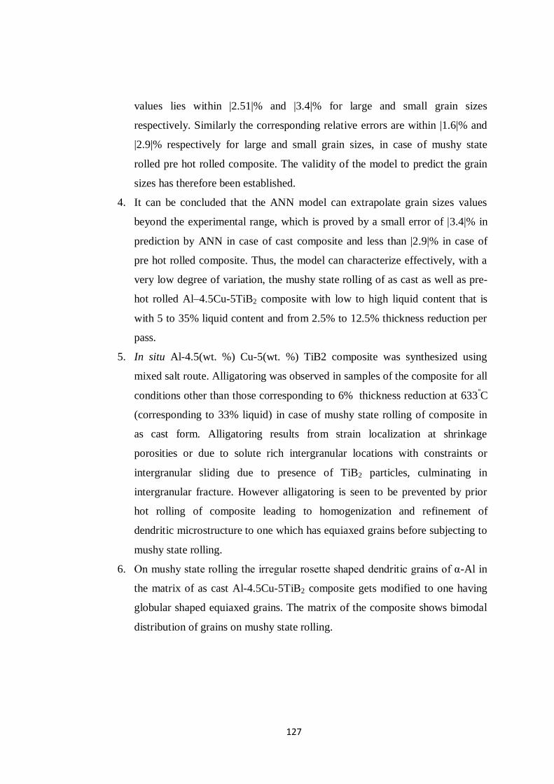
127
values lies within |2.51|% and |3.4|% for large and small grain sizes
respectively. Similarly the corresponding relative errors are within |1.6|% and
|2.9|% respectively for large and small grain sizes, in case of mushy state
rolled pre hot rolled composite. The validity of the model to predict the grain
sizes has therefore been established.
4. It can be concluded that the ANN model can extrapolate grain sizes values
beyond the experimental range, which is proved by a small error of |3.4|% in
prediction by ANN in case of cast composite and less than |2.9|% in case of
pre hot rolled composite. Thus, the model can characterize effectively, with a
very low degree of variation, the mushy state rolling of as cast as well as pre-
hot rolled Al–4.5Cu-5TiB2 composite with low to high liquid content that is
with 5 to 35% liquid content and from 2.5% to 12.5% thickness reduction per
pass.
5. In situ Al-4.5(wt. %) Cu-5(wt. %) TiB2 composite was synthesized using
mixed salt route. Alligatoring was observed in samples of the composite for all
conditions other than those corresponding to 6% thickness reduction at 633ºC
(corresponding to 33% liquid) in case of mushy state rolling of composite in
as cast form. Alligatoring results from strain localization at shrinkage
porosities or due to solute rich intergranular locations with constraints or
intergranular sliding due to presence of TiB2 particles, culminating in
intergranular fracture. However alligatoring is seen to be prevented by prior
hot rolling of composite leading to homogenization and refinement of
dendritic microstructure to one which has equiaxed grains before subjecting to
mushy state rolling.
6. On mushy state rolling the irregular rosette shaped dendritic grains of α-Al in
the matrix of as cast Al-4.5Cu-5TiB2 composite gets modified to one having
globular shaped equiaxed grains. The matrix of the composite shows bimodal
distribution of grains on mushy state rolling.
129
Chapter 5
RESULTS AND DISCUSSION (PART II)
ANN MODELLING FOR HARDNESS PREDICTION
5.1 INTRODUCTION
The formulation of ANN model for prediction of hardness of in situ fabricated Al-
4.5Cu-5TiB2 composite has been discussed in this chapter. The microstructural
evolution was discussed in the previous chapter. It is seen that the original dendritic
morphology present in the cast composite gets modified to one which has globular
grains on being subjected to hot working and mushy state rolling. It was also seen in
chapter 4 that mushy state rolling led to bimodal grain size distribution along with a
refinement in grain structure. It is well known that the hardness is vastly influenced
by grain morphology and size distribution. In general, the surface of the mushy state
rolled composite contains higher volume of fine grains (and therefore hard grain
boundary volume) as compared to that at the interior of the composite (Herbert et al.
2006, Herbert 2007). This therefore, leads to higher surface hardness in the
composite. The present study involves the formulation of the ANN model for
hardness prediction, which is treated as a function of grain sizes in addition to the
initial state of material, thickness reduction per pass and liquid volume fraction in
composite during mushy state rolling. The study also presents the results of the
experiments on Al-4.5Cu-5TiB2 composite performed to validate the ANN model for
hardness and compares them with the hardness values predicted by the model. It
involves, as was the case with the work (Herbert 2007) from which data is collected,
measurement of Vickers hardness of in situ Al-4.5Cu-5TiB2 composite samples rolled
in mushy state in as cast and pre hot rolled condition. The data for training the
network has been taken from previous work related to studies on mushy state
processing of Al-4.5Cu-5TiB2 composite (Herbert 2007).
130
5.2 SCOPE
In this section, it is proposed to formulate an Artificial Neural Network model with
Feed Forward architecture to predict the hardness of Al-4.5Cu-5TiB2 composite rolled
in mushy state in as cast as well as pre hot rolled condition with the input parameters
being, % thickness reduction, % volume fraction of liquid, large and small grain sizes.
The present work attempts to develop the ANN model with following:
(a) The analysis of the effect of initial state of composite material (as cast or pre
hot rolled) on hardness of Al-4.5Cu-5TiB2 composite.
(b) The analysis of effect of thickness reduction during mushy state rolling and
mushy state condition from where rolling is initiated.
(c) Extrapolation and interpolation of hardness for unknown thickness reductions
and liquid volume fractions in the mushy state composite.
(d) Optimisation of the input parameters for achieving best possible hardness
within the range of permissible thickness reduction per pass and permissible
mushy state from where rolling is initiated.
(e) Validation of the model predictions by hardness measurements on Al-4.5Cu-
5TiB2 composite samples subjected to mushy state rolling.
The input parameters for predicting the hardness of mushy state rolled Al-4.5Cu-
5TiB2 composite are initial material state, % thickness reduction, % liquid volume
fraction, large and small grain sizes. The relationship being complex and non linear
necessitates the use of neural network techniques. ANN with feed forward
architecture and trained with error back propagation technique offers a powerful
method to predict the outputs from a given input parameter combinations and hence is
proposed to be used in prediction of hardness of mushy state rolled Al-4.5Cu-5TiB2
composite.

131
5.3 HARDNESS
Hardness is defined as resistance to plastic deformation by indentation. It is therefore
related to yield strength of its material (Sahoo and Koczak 1991). The hardness of the
material provides an approximate assessment of tensile strength of the material. Thus,
hardness provides a means for comparative assessment of strength of materials in the
absence of data on strength properties of material.
5.4 DATA COLLECTION
The data for training the ANN network proposed for hardness prediction of mushy
state rolled Al-4.5Cu-5TiB2 composite is collected from previous studies done on
mushy state rolling of as cast as well as pre hot rolled Al-4.5Cu-5TiB2 composite
(Herbert 2007). This data is listed in Table 5.1. The hardness of the material also
depends upon the grain size distribution, in addition to the parameters of mushy state
rolling. Table 5.1 also includes the grain sizes corresponding to the inputs of mushy
state rolling (viz. Initial state of the material, % thickness reduction and % liquid
content) which shall be used for training the network.
From Table 5.1, it can be seen that the hardness increases with increase in thickness
reduction during rolling per pass. Also, it is observed that for a given thickness
reduction during mushy state rolling, the hardness values increase with increase in
liquid volume fraction above 10% and up to 20% and then found to decrease at 30%
liquid volume. This phenomenon is observed both in case of as cast as well as pre hot
rolled mushy state rolled composite. It is of interest to know the initial state of the
composite which will give the maximum value of hardness, as hardness is not only an
indicator of strength, but also a determinant of the wear properties of the material. The
determination of optimised parameters of mushy state rolling for maximum hardness
is therefore the prime objective of ANN formulation, in addition to understanding the
variation of hardness with different conditions of mushy state rolling.
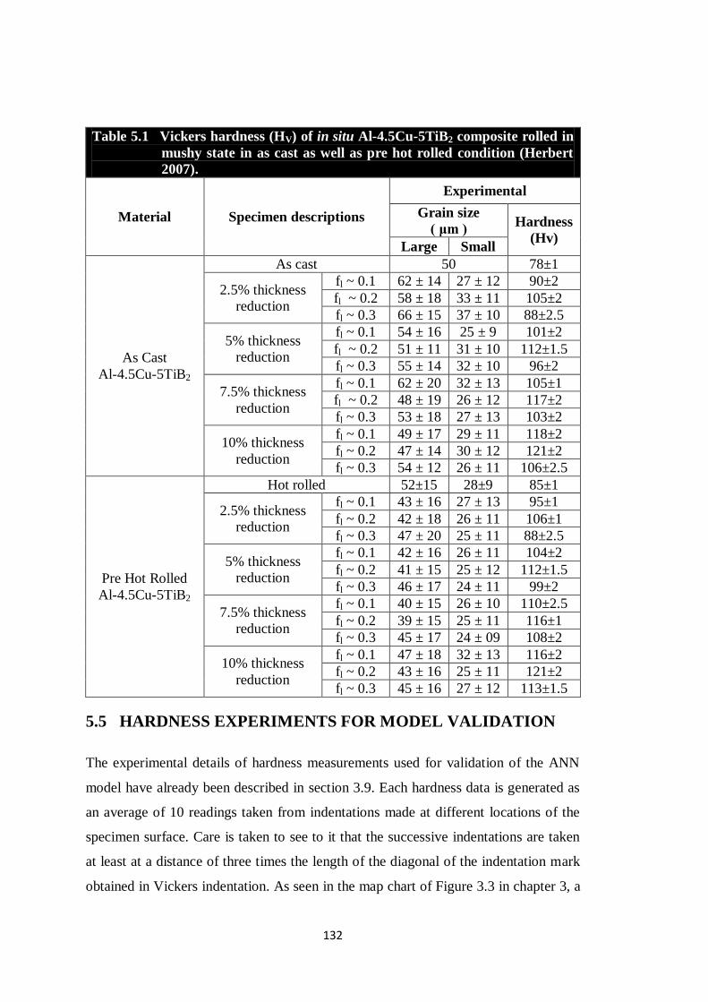
132
Table 5.1 Vickers hardness (HV) of in situ Al-4.5Cu-5TiB2 composite rolled in
mushy state in as cast as well as pre hot rolled condition (Herbert
2007).
Material Specimen descriptions
Experimental
Grain size
( μm ) Hardness
(Hv) Large Small
As Cast
Al-4.5Cu-5TiB2
As cast 50 78±1
2.5% thickness
reduction
fl ~ 0.1 62 ± 14 27 ± 12 90±2
fl ~ 0.2 58 ± 18 33 ± 11 105±2
fl ~ 0.3 66 ± 15 37 ± 10 88±2.5
5% thickness
reduction
fl ~ 0.1 54 ± 16 25 ± 9 101±2
fl ~ 0.2 51 ± 11 31 ± 10 112±1.5
fl ~ 0.3 55 ± 14 32 ± 10 96±2
7.5% thickness
reduction
fl ~ 0.1 62 ± 20 32 ± 13 105±1
fl ~ 0.2 48 ± 19 26 ± 12 117±2
fl ~ 0.3 53 ± 18 27 ± 13 103±2
10% thickness
reduction
fl ~ 0.1 49 ± 17 29 ± 11 118±2
fl ~ 0.2 47 ± 14 30 ± 12 121±2
fl ~ 0.3 54 ± 12 26 ± 11 106±2.5
Pre Hot Rolled
Al-4.5Cu-5TiB2
Hot rolled 52±15 28±9 85±1
2.5% thickness
reduction
fl ~ 0.1 43 ± 16 27 ± 13 95±1
fl ~ 0.2 42 ± 18 26 ± 11 106±1
fl ~ 0.3 47 ± 20 25 ± 11 88±2.5
5% thickness
reduction
fl ~ 0.1 42 ± 16 26 ± 11 104±2
fl ~ 0.2 41 ± 15 25 ± 12 112±1.5
fl ~ 0.3 46 ± 17 24 ± 11 99±2
7.5% thickness
reduction
fl ~ 0.1 40 ± 15 26 ± 10 110±2.5
fl ~ 0.2 39 ± 15 25 ± 11 116±1
fl ~ 0.3 45 ± 17 24 ± 09 108±2
10% thickness
reduction
fl ~ 0.1 47 ± 18 32 ± 13 116±2
fl ~ 0.2 43 ± 16 25 ± 11 121±2
fl ~ 0.3 45 ± 16 27 ± 12 113±1.5
5.5 HARDNESS EXPERIMENTS FOR MODEL VALIDATION
The experimental details of hardness measurements used for validation of the ANN
model have already been described in section 3.9. Each hardness data is generated as
an average of 10 readings taken from indentations made at different locations of the
specimen surface. Care is taken to see to it that the successive indentations are taken
at least at a distance of three times the length of the diagonal of the indentation mark
obtained in Vickers indentation. As seen in the map chart of Figure 3.3 in chapter 3, a
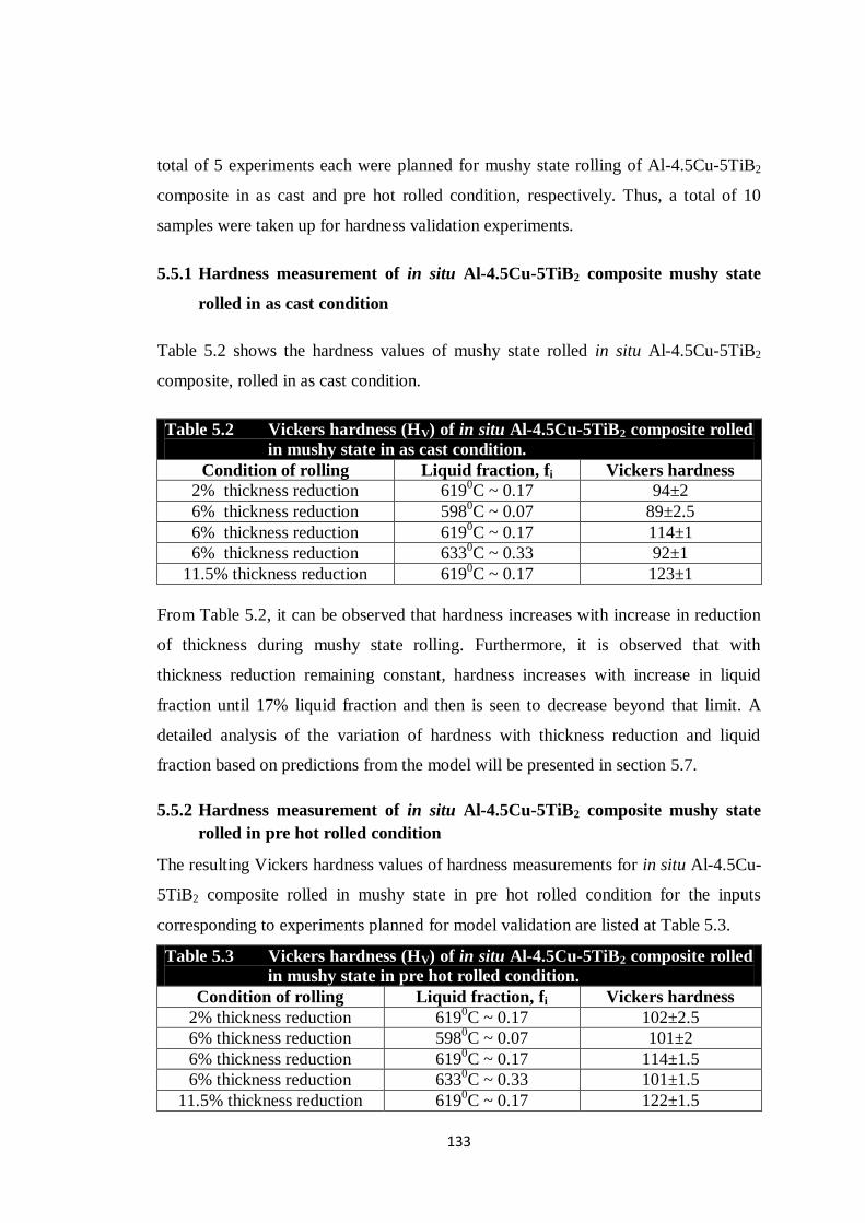
133
total of 5 experiments each were planned for mushy state rolling of Al-4.5Cu-5TiB2
composite in as cast and pre hot rolled condition, respectively. Thus, a total of 10
samples were taken up for hardness validation experiments.
5.5.1 Hardness measurement of in situ Al-4.5Cu-5TiB2 composite mushy state
rolled in as cast condition
Table 5.2 shows the hardness values of mushy state rolled in situ Al-4.5Cu-5TiB2
composite, rolled in as cast condition.
Table 5.2 Vickers hardness (HV) of in situ Al-4.5Cu-5TiB2 composite rolled
in mushy state in as cast condition.
Condition of rolling Liquid fraction, fi Vickers hardness
2% thickness reduction 6190C ~ 0.17 94±2
6% thickness reduction 5980C ~ 0.07 89±2.5
6% thickness reduction 6190C ~ 0.17 114±1
6% thickness reduction 6330C ~ 0.33 92±1
11.5% thickness reduction 6190C ~ 0.17 123±1
From Table 5.2, it can be observed that hardness increases with increase in reduction
of thickness during mushy state rolling. Furthermore, it is observed that with
thickness reduction remaining constant, hardness increases with increase in liquid
fraction until 17% liquid fraction and then is seen to decrease beyond that limit. A
detailed analysis of the variation of hardness with thickness reduction and liquid
fraction based on predictions from the model will be presented in section 5.7.
5.5.2 Hardness measurement of in situ Al-4.5Cu-5TiB2 composite mushy state
rolled in pre hot rolled condition
The resulting Vickers hardness values of hardness measurements for in situ Al-4.5Cu-
5TiB2 composite rolled in mushy state in pre hot rolled condition for the inputs
corresponding to experiments planned for model validation are listed at Table 5.3.
Table 5.3 Vickers hardness (HV) of in situ Al-4.5Cu-5TiB2 composite rolled
in mushy state in pre hot rolled condition.
Condition of rolling Liquid fraction, fi Vickers hardness
2% thickness reduction 6190C ~ 0.17 102±2.5
6% thickness reduction 5980C ~ 0.07 101±2
6% thickness reduction 6190C ~ 0.17 114±1.5
6% thickness reduction 6330C ~ 0.33 101±1.5
11.5% thickness reduction 6190C ~ 0.17 122±1.5

134
The variation of hardness with respect to thickness reduction and volume fraction of
liquid in the composite during mushy state rolling of composite in pre hot rolled
condition presents a scenario similar to that seen in case of mushy state rolling of as
cast composite as can be observed by comparing values of hardness from Table 5.2
and Table 5.3.
5.6 ANN MODEL DEVELOPMENT FOR HARDNESS
PREDICTION
In this section, the development of ANN model using FFNN for prediction of
hardness for mushy state rolled Al-4.5Cu-5TiB2 composite rolled in as cast as well as
pre hot rolled condition is discussed. As discussed in section 5.1 and also
subsequently in section 5.4, the input variables/nodes for the model are taken as initial
material state, % thickness reduction, % liquid volume fraction, large and small grain
sizes, while the output node of the network is dedicated to hardness.
5.6.1 Neural Network training
As discussed in chapter 4 for grain size description, the ANN was modelled with
FFNN architecture. Both single as well as two hidden layers were tried out. Before
training the network, both the input as well as the output variables were normalised
between values 0.1 to 0.9 using the normalising function given in equation (4.1) of
chapter 4. Once the network is trained, all the values acquire their original values
provided by the de-normalising function stated at equation (4.2) in chapter 4. Back
propagation algorithm was used for training the network. With single hidden layered
network (i.e. three layered perceptron network), the network was trained with
different values of learning rate parameter (η) and momentum factor (α). The learning
was started with 5 hidden nodes, with an initial value of η as 0.1 and with α=0.9. The
value of η was increased while that of α was decreased in steps of 0.05 in each
subsequent iteration. The MSE which is an indicator of network convergence,
discussed earlier in chapter 4 and given by equation (4.3) was set at 0.0001 while the
number of epochs (iterations) was fixed at 5 lakhs. With repeated trials involving
different values of hidden nodes ranging from 2 to 9, different values of η and α as

135
well as by changing the order of the input vector presentation to the network, the
network failed to converge towards the set MSE. This probably is due to the non
linear correlation between the input output relationships of data (Reddy et al. 2005).
The network was then tried with two hidden layers following the same procedure used
for three layered perceptron. The network converged satisfactorily with 5 nodes in the
first hidden layer and 3 nodes in the second hidden layer with η=0.5 and α=0.5, with a
MSE of 9.76 x 10⁻⁵
after 3.25 lakh iterations. The sigmoid function in equation (4.4)
of chapter 4 used to train the ANN model for grain size predictions is reproduced
below as the activation function for training the network:
xe
xF
1
1)(
(5.1)
Figure 5. 1 ANN Architecture
5.7 HARDNESS PREDICTION THROUGH ANN MODEL
Table 5.4 and Table 5.5 respectively provide the values of hardness predicted by the
trained ANN model for mushy state rolled Al-4.5Cu-5TiB2 composite, rolled in as

136
cast and pre hot rolled state, respectively, to a thickness reduction ranging from 2 to
12.5% and liquid volume fraction ranging from 5 to 35%. The table lists the values
predicted by the model for the training data represented by superscript a, while the
validation data within training data range is represented by the superscript * while that
outside the range is represented by superscript **
.
5.7.1 Comparison of hardness obtained by experimentation and prediction by
ANN model
5.7.1.1 Rolling of as cast Al-4.5(wt.%)Cu-5(wt.%)TiB2 composite in mushy state
The values of hardness obtained by experimentation (Herbert 2007) and those
predicted by the trained ANN model are presented in Table 5.4. The percentage error
in prediction by the ANN model, as can be seen from the Table 5.4, is between
-2.436% and +2.6323%, which is very much within the acceptable limits of accuracy
for any prediction system. Further, the hardness of cast composite obtained
experimentally is 78HV. While using the ANN model, the hardness value for the as
cast composite is obtained by using zeros as inputs for % thickness reduction and %
liquid volume fractions in the model. The value so predicted by ANN model is 77.66
HV resulting in an error of 0.4359% over experimental result.
Kusiak & Kuziak (2002) have reported a maximum percentage error of 8% in
prediction of ultimate tensile and yield strength of steel, while Mandal et al. (2009)
have reported a Gaussian distribution of percentage error of prediction within ±10%
in prediction of flow stress using Resilient Propagation algorithm which has been
reported to perform better than Back Propagation algorithm. Selvakumar et al. (2007)
have reported a maximum error of 5% in the prediction of axial stress, hoop stress ,
hydrostatic stress and the axial strain in their work on modelling the effect of particle
size and iron content on forming of Al-Fe preforms using ANN. Considering that the
network has been trained with experimental values between 10% to 30% liquid
volume fraction and rolling with 2.5% to 10% thickness reduction, a percentage error
of 2.6323% within and 1.4234% outside the range of training data values is quite
reasonable.
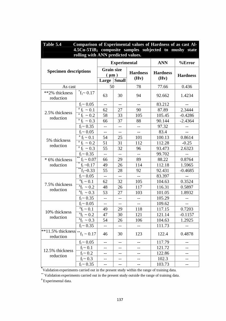
137
Table 5.4 Comparison of Experimental values of Hardness of as cast Al-
4.5Cu-5TiB2 composite samples subjected to mushy state
rolling with ANN predicted values.
Specimen descriptions
Experimental ANN %Error
Grain size
( μm ) Hardness
(Hv)
Hardness
(Hv) Hardness
Large Small
As cast 50 78 77.66 0.436
**2% thickness
reduction
*f1~ 0.17
63 30 94 92.662 1.4234
2.5% thickness
reduction
fl ~ 0.05 -- -- -- 83.212 -- a fl ~ 0.1 62 27 90 87.89 2.3444
a fl ~ 0.2 58 33 105 105.45 -0.4286
a fl ~ 0.3 66 37 88 90.144 -2.4364
fl ~ 0.35 -- -- -- 97.32 --
5% thickness
reduction
fl ~ 0.05 -- -- -- 83.4 -- a fl ~ 0.1 54 25 101 100.13 0.8614
a fl ~ 0.2 51 31 112 112.28 -0.25
a fl ~ 0.3 55 32 96 93.473 2.6323
fl ~ 0.35 -- -- -- 99.702 --
* 6% thickness
reduction
** fl ~ 0.07 66 29 89 88.22 0.8764
* fl ~0.17 49 26 114 112.18 1.5965
**f1~0.33 55 28 92 92.431 -0.4685
7.5% thickness
reduction
fl ~ 0.05 -- -- -- 83.397 -- afl ~ 0.1 62 32 105 104.63 0.3524
afl ~ 0.2 48 26 117 116.31 0.5897
afl ~ 0.3 53 27 103 101.05 1.8932
fl ~ 0.35 -- -- -- 105.29 --
10% thickness
reduction
fl ~ 0.05 -- -- -- 109.62 -- afl ~ 0.1 49 29 118 117.15 0.7203
afl ~ 0.2 47 30 121 121.14 -0.1157
afl ~ 0.3 54 26 106 104.63 1.2925
fl ~ 0.35 -- -- -- 111.73 --
**11.5% thickness
reduction **
f1 ~ 0.17 46 30 123 122.4 0.4878
12.5% thickness
reduction
fl ~ 0.05 -- -- -- 117.79 --
fl ~ 0.1 -- -- -- 121.72 --
fl ~ 0.2 -- -- -- 122.86 --
fl ~ 0.3 -- -- -- 102.3 --
fl ~ 0.35 -- -- -- 103.73 -- *Validation experiments carried out in the present study within the range of training data.
** Validation experiments carried out in the present study outside the range of training data. a Experimental data.
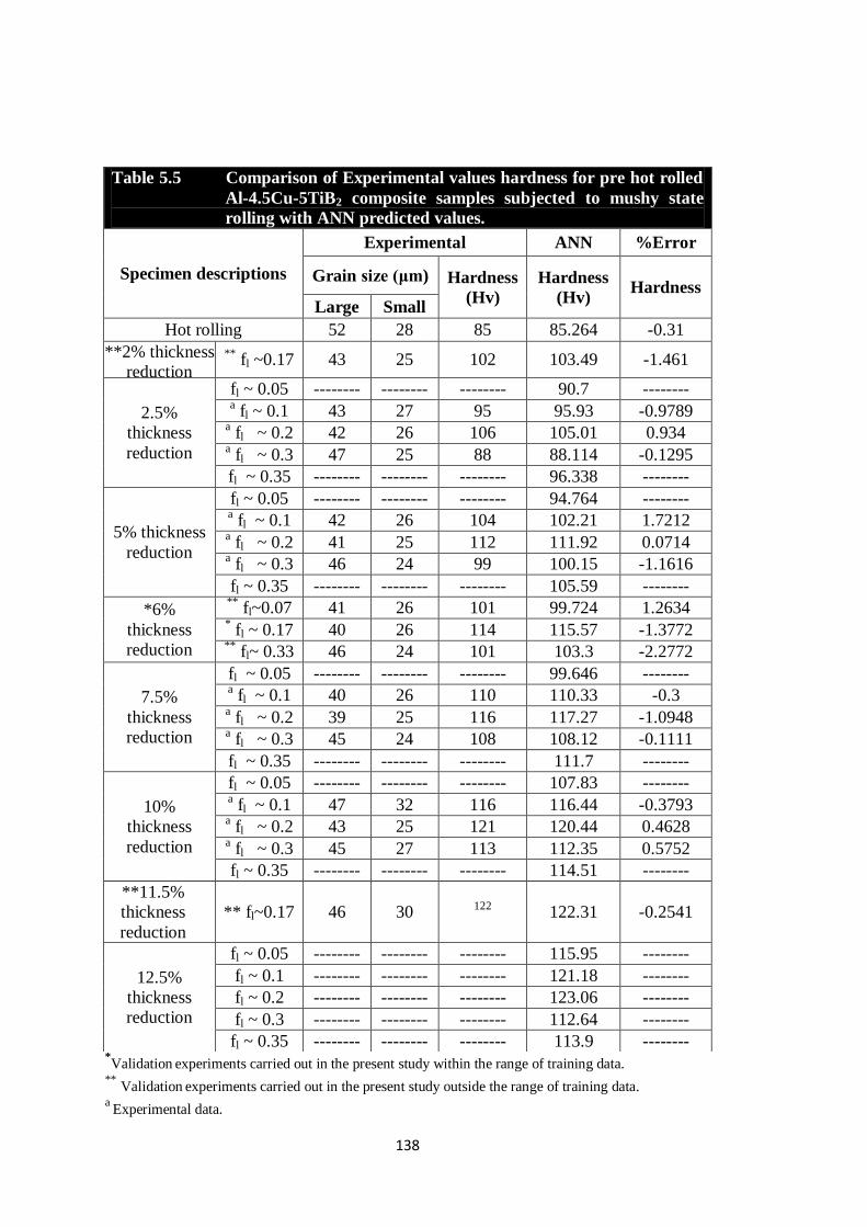
138
*Validation experiments carried out in the present study within the range of training data.
** Validation experiments carried out in the present study outside the range of training data.
a Experimental data.
Table 5.5 Comparison of Experimental values hardness for pre hot rolled
Al-4.5Cu-5TiB2 composite samples subjected to mushy state
rolling with ANN predicted values.
Specimen descriptions
Experimental ANN %Error
Grain size (μm) Hardness
(Hv)
Hardness
(Hv) Hardness
Large Small
Hot rolling 52 28 85 85.264 -0.31
**2% thickness
reduction
** fl ~0.17 43 25 102 103.49 -1.461
2.5%
thickness
reduction
fl ~ 0.05 -------- -------- -------- 90.7 -------- a fl ~ 0.1 43 27 95 95.93 -0.9789
a fl ~ 0.2 42 26 106 105.01 0.934
a fl ~ 0.3 47 25 88 88.114 -0.1295
fl ~ 0.35 -------- -------- -------- 96.338 --------
5% thickness
reduction
fl ~ 0.05 -------- -------- -------- 94.764 -------- a fl ~ 0.1 42 26 104 102.21 1.7212
a fl ~ 0.2 41 25 112 111.92 0.0714
a fl ~ 0.3 46 24 99 100.15 -1.1616
fl ~ 0.35 -------- -------- -------- 105.59 --------
*6%
thickness
reduction
** fl~0.07 41 26 101 99.724 1.2634
* fl ~ 0.17 40 26 114 115.57 -1.3772
** fl~ 0.33 46 24 101 103.3 -2.2772
7.5%
thickness
reduction
fl ~ 0.05 -------- -------- -------- 99.646 -------- a fl ~ 0.1 40 26 110 110.33 -0.3
a fl ~ 0.2 39 25 116 117.27 -1.0948
a fl ~ 0.3 45 24 108 108.12 -0.1111
fl ~ 0.35 -------- -------- -------- 111.7 --------
10%
thickness
reduction
fl ~ 0.05 -------- -------- -------- 107.83 -------- a fl ~ 0.1 47 32 116 116.44 -0.3793
a fl ~ 0.2 43 25 121 120.44 0.4628
a fl ~ 0.3 45 27 113 112.35 0.5752
fl ~ 0.35 -------- -------- -------- 114.51 --------
**11.5%
thickness
reduction
** fl~0.17 46 30 122
122.31 -0.2541
12.5%
thickness
reduction
fl ~ 0.05 -------- -------- -------- 115.95 --------
fl ~ 0.1 -------- -------- -------- 121.18 --------
fl ~ 0.2 -------- -------- -------- 123.06 --------
fl ~ 0.3 -------- -------- -------- 112.64 --------
fl ~ 0.35 -------- -------- -------- 113.9 --------

139
This suggests that the ANN model is quite capable of extrapolating the grain sizes and
hardness of the composite beyond 10% & below 2.5% thickness reduction and
beyond 30% liquid volume fraction and below 10% liquid volume fraction
respectively, when as cast Al-4.5Cu-5TiB2 composite is rolled in mushy state. One of
the prime objectives of the present study is to obtain the optimised values of thickness
reduction per roll pass and volume fraction of liquid in the composite that provides a
maximum value of hardness. It is desirable to know the conditions leading to
maximum hardness since hardness is a measure not only of strength but also of wear
properties of the composite. To achieve the optimised mushy state rolling parameters
for maximum hardness, a small optimisation code was written in the front end
designed for ANN and RNN model in the present study. The code written in C++
(included at APPENDIX II) is interfaced with Microsoft Silver light software, which
is a web based application, to provide hardness by continuous variation of one input
parameter selected at a time, with the help of slider button provided on the screen. By
alternately varying the % thickness reduction from 2 to 12.5% and liquid volume
fraction from 5 to 35%, the maximum hardness was recorded for data within and
outside the training range of the model. Table 5.6 shows the maximum value of
hardness predicted by the ANN model within the training range as 121.324 HV
corresponding to 19% liquid volume fraction at 10% thickness reduction. The
maximum value of hardness predicted by the model is 123.1 HV corresponding to
17.4% liquid volume fraction at 12.5% thickness reduction for the entire range of
study carried out i.e. rolling at mushy state temperatures corresponding to 5% liquid
volume fraction to 35% liquid volume fraction at various thickness reductions ranging
from 2 % thickness reduction to 12.5% thickness reduction. Figure 5.2 shows a screen
capture at an instance when the hardness of the as cast composite is 121.3 HV.
The comparison of ANN predicted values of hardness with the values obtained from
validation experiments reveals errors in prediction within |1.43%|, as seen from Table
5.4. This vindicates the generalisation of hardness relationship of the composite,
mushy state rolled in as cast state, to 2 to 12.5% thickness reduction and with 5 to
35% volume fraction of liquid in composite.
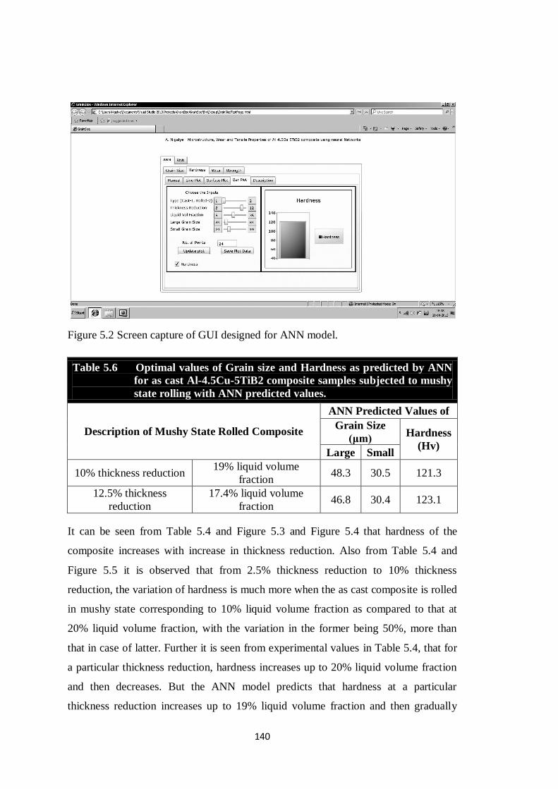
140
Figure 5.2 Screen capture of GUI designed for ANN model.
Table 5.6 Optimal values of Grain size and Hardness as predicted by ANN
for as cast Al-4.5Cu-5TiB2 composite samples subjected to mushy
state rolling with ANN predicted values.
Description of Mushy State Rolled Composite
ANN Predicted Values of
Grain Size
(μm) Hardness
(Hv) Large Small
10% thickness reduction 19% liquid volume
fraction 48.3 30.5 121.3
12.5% thickness
reduction
17.4% liquid volume
fraction 46.8 30.4 123.1
It can be seen from Table 5.4 and Figure 5.3 and Figure 5.4 that hardness of the
composite increases with increase in thickness reduction. Also from Table 5.4 and
Figure 5.5 it is observed that from 2.5% thickness reduction to 10% thickness
reduction, the variation of hardness is much more when the as cast composite is rolled
in mushy state corresponding to 10% liquid volume fraction as compared to that at
20% liquid volume fraction, with the variation in the former being 50%, more than
that in case of latter. Further it is seen from experimental values in Table 5.4, that for
a particular thickness reduction, hardness increases up to 20% liquid volume fraction
and then decreases. But the ANN model predicts that hardness at a particular
thickness reduction increases up to 19% liquid volume fraction and then gradually
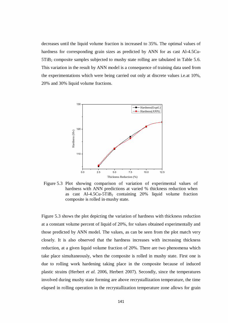
141
decreases until the liquid volume fraction is increased to 35%. The optimal values of
hardness for corresponding grain sizes as predicted by ANN for as cast Al-4.5Cu-
5TiB2 composite samples subjected to mushy state rolling are tabulated in Table 5.6.
This variation in the result by ANN model is a consequence of training data used from
the experimentations which were being carried out only at discrete values i.e.at 10%,
20% and 30% liquid volume fractions.
0.0 2.5 5.0 7.5 10.0 12.5
110
120
130
Hard
ness
(H
v)
Thickness Reduction (%)
Hardness(Exptl.)
Hardness(ANN)
Figure 5.3 shows the plot depicting the variation of hardness with thickness reduction
at a constant volume percent of liquid of 20%, for values obtained experimentally and
those predicted by ANN model. The values, as can be seen from the plot match very
closely. It is also observed that the hardness increases with increasing thickness
reduction, at a given liquid volume fraction of 20%. There are two phenomena which
take place simultaneously, when the composite is rolled in mushy state. First one is
due to rolling work hardening taking place in the composite because of induced
plastic strains (Herbert et al. 2006, Herbert 2007). Secondly, since the temperatures
involved during mushy state forming are above recrystallization temperature, the time
elapsed in rolling operation in the recrystallization temperature zone allows for grain
Figure 5.3 Plot showing comparison of variation of experimental values of
hardness with ANN predictions at varied % thickness reduction when
as cast Al-4.5Cu-5TiB2 containing 20% liquid volume fraction
composite is rolled in mushy state.
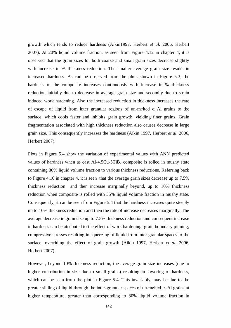
142
growth which tends to reduce hardness (Aikin1997, Herbert et al. 2006, Herbert
2007). At 20% liquid volume fraction, as seen from Figure 4.12 in chapter 4, it is
observed that the grain sizes for both coarse and small grain sizes decrease slightly
with increase in % thickness reduction. The smaller average grain size results in
increased hardness. As can be observed from the plots shown in Figure 5.3, the
hardness of the composite increases continuously with increase in % thickness
reduction initially due to decrease in average grain size and secondly due to strain
induced work hardening. Also the increased reduction in thickness increases the rate
of escape of liquid from inter granular regions of un-melted α–Al grains to the
surface, which cools faster and inhibits grain growth, yielding finer grains. Grain
fragmentation associated with high thickness reduction also causes decrease in large
grain size. This consequently increases the hardness (Aikin 1997, Herbert et al. 2006,
Herbert 2007).
Plots in Figure 5.4 show the variation of experimental values with ANN predicted
values of hardness when as cast Al-4.5Cu-5TiB2 composite is rolled in mushy state
containing 30% liquid volume fraction to various thickness reductions. Referring back
to Figure 4.10 in chapter 4, it is seen that the average grain sizes decrease up to 7.5%
thickness reduction and then increase marginally beyond, up to 10% thickness
reduction when composite is rolled with 35% liquid volume fraction in mushy state.
Consequently, it can be seen from Figure 5.4 that the hardness increases quite steeply
up to 10% thickness reduction and then the rate of increase decreases marginally. The
average decrease in grain size up to 7.5% thickness reduction and consequent increase
in hardness can be attributed to the effect of work hardening, grain boundary pinning,
compressive stresses resulting in squeezing of liquid from inter granular spaces to the
surface, overriding the effect of grain growth (Aikin 1997, Herbert et al. 2006,
Herbert 2007).
However, beyond 10% thickness reduction, the average grain size increases (due to
higher contribution in size due to small grains) resulting in lowering of hardness,
which can be seen from the plot in Figure 5.4. This invariably, may be due to the
greater sliding of liquid through the inter-granular spaces of un-melted α–Al grains at
higher temperature, greater than corresponding to 30% liquid volume fraction in
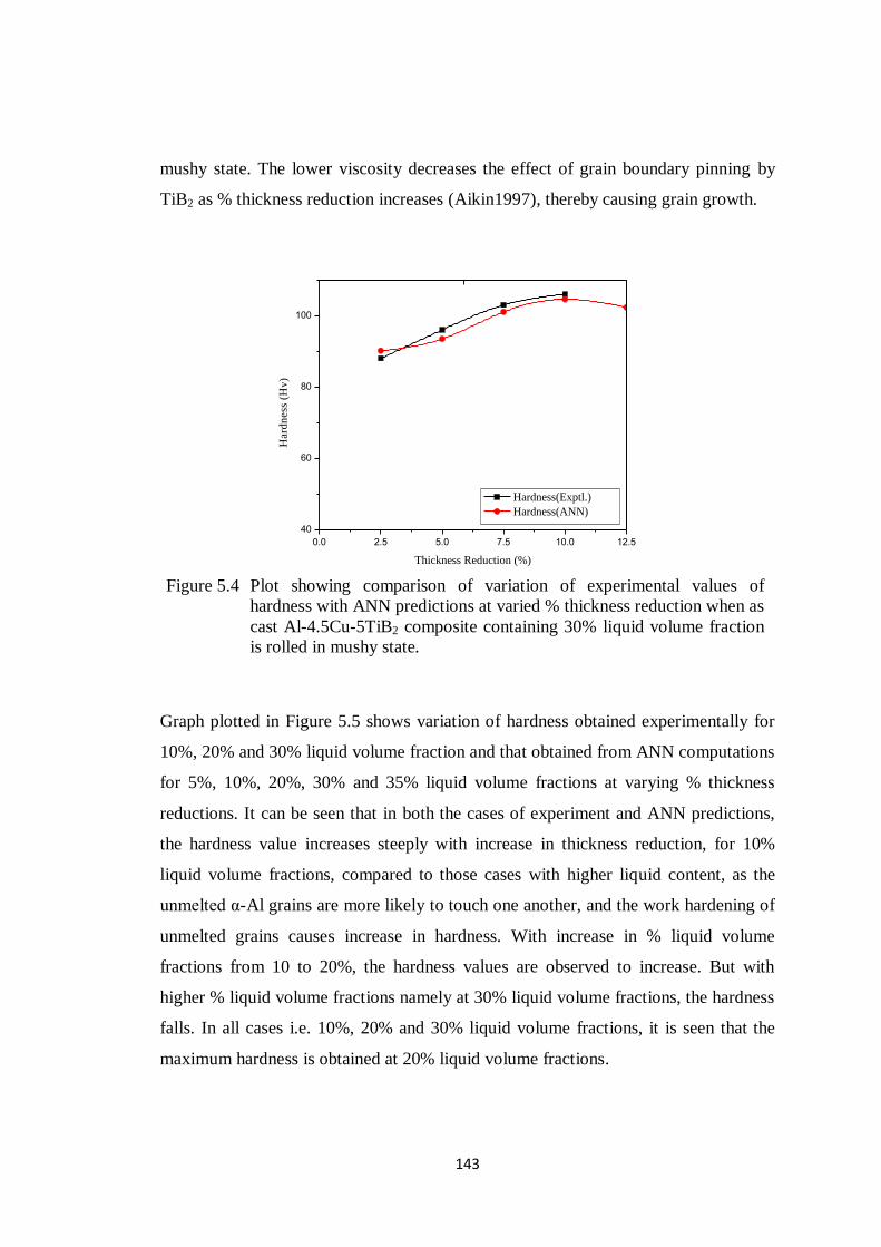
143
mushy state. The lower viscosity decreases the effect of grain boundary pinning by
TiB2 as % thickness reduction increases (Aikin1997), thereby causing grain growth.
0.0 2.5 5.0 7.5 10.0 12.5
40
60
80
100
Hard
ness
(H
v)
Thickness Reduction (%)
Hardness(Exptl.)
Hardness(ANN)
Graph plotted in Figure 5.5 shows variation of hardness obtained experimentally for
10%, 20% and 30% liquid volume fraction and that obtained from ANN computations
for 5%, 10%, 20%, 30% and 35% liquid volume fractions at varying % thickness
reductions. It can be seen that in both the cases of experiment and ANN predictions,
the hardness value increases steeply with increase in thickness reduction, for 10%
liquid volume fractions, compared to those cases with higher liquid content, as the
unmelted α-Al grains are more likely to touch one another, and the work hardening of
unmelted grains causes increase in hardness. With increase in % liquid volume
fractions from 10 to 20%, the hardness values are observed to increase. But with
higher % liquid volume fractions namely at 30% liquid volume fractions, the hardness
falls. In all cases i.e. 10%, 20% and 30% liquid volume fractions, it is seen that the
maximum hardness is obtained at 20% liquid volume fractions.
Figure 5.4 Plot showing comparison of variation of experimental values of
hardness with ANN predictions at varied % thickness reduction when as
cast Al-4.5Cu-5TiB2 composite containing 30% liquid volume fraction
is rolled in mushy state.
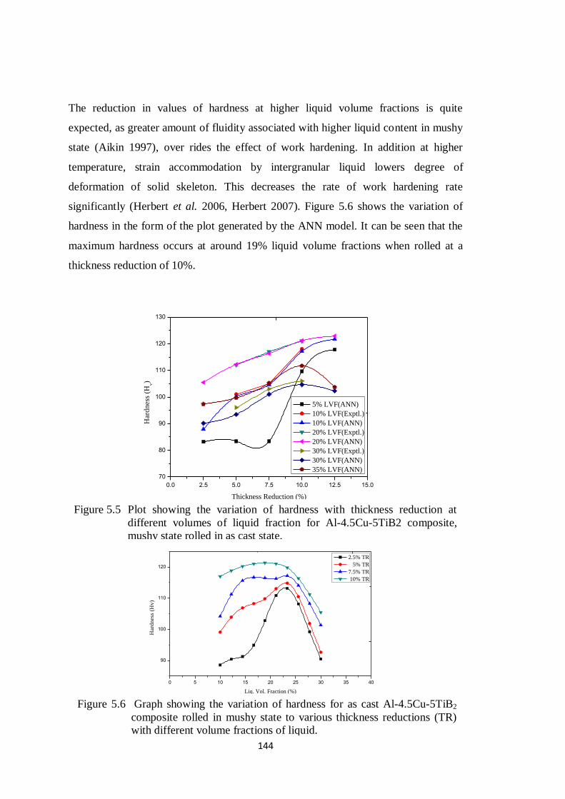
144
The reduction in values of hardness at higher liquid volume fractions is quite
expected, as greater amount of fluidity associated with higher liquid content in mushy
state (Aikin 1997), over rides the effect of work hardening. In addition at higher
temperature, strain accommodation by intergranular liquid lowers degree of
deformation of solid skeleton. This decreases the rate of work hardening rate
significantly (Herbert et al. 2006, Herbert 2007). Figure 5.6 shows the variation of
hardness in the form of the plot generated by the ANN model. It can be seen that the
maximum hardness occurs at around 19% liquid volume fractions when rolled at a
thickness reduction of 10%.
0.0 2.5 5.0 7.5 10.0 12.5 15.0
70
80
90
100
110
120
130
Hard
ness
(H
v)
Thickness Reduction (%)
5% LVF(ANN)
10% LVF(Exptl.)
10% LVF(ANN)
20% LVF(Exptl.)
20% LVF(ANN)
30% LVF(Exptl.)
30% LVF(ANN)
35% LVF(ANN)
0 5 10 15 20 25 30 35 40
90
100
110
120
Hard
ness
(H
v)
Liq. Vol. Fraction (%)
2.5% TR
5% TR
7.5% TR
10% TR
Figure 5.5 Plot showing the variation of hardness with thickness reduction at
different volumes of liquid fraction for Al-4.5Cu-5TiB2 composite,
mushy state rolled in as cast state.
Figure 5.6 Graph showing the variation of hardness for as cast Al-4.5Cu-5TiB2
composite rolled in mushy state to various thickness reductions (TR)
with different volume fractions of liquid.
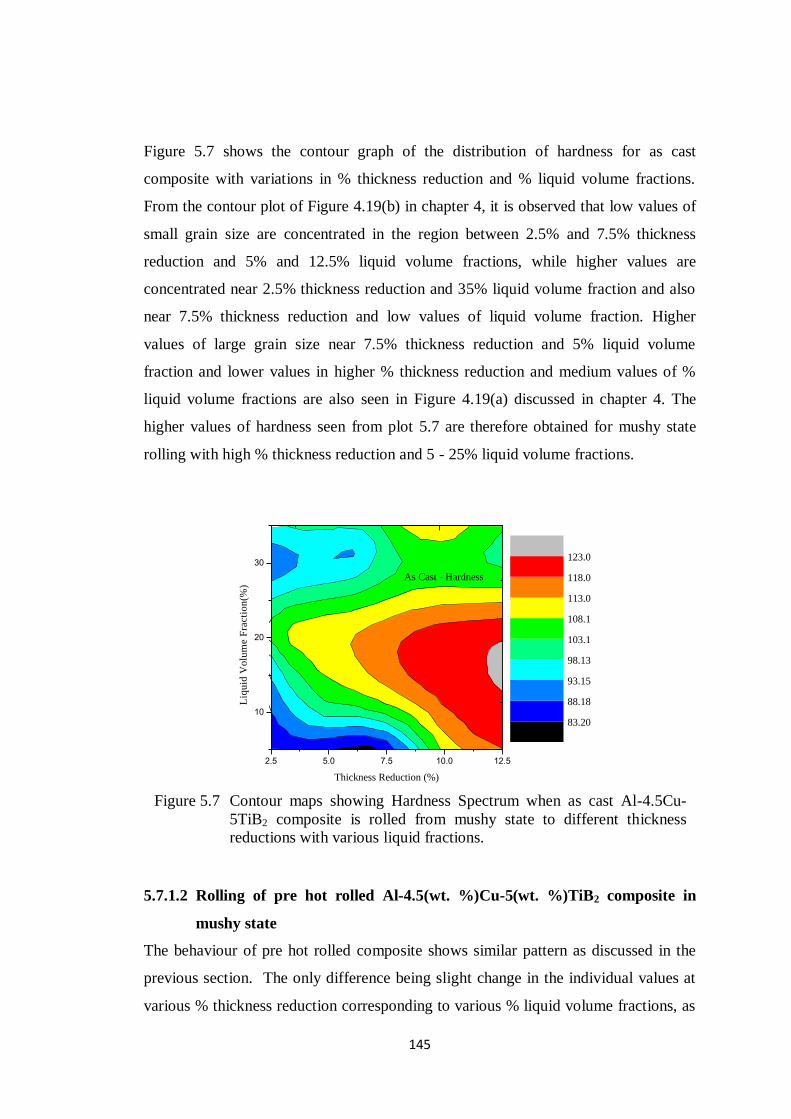
145
Figure 5.7 shows the contour graph of the distribution of hardness for as cast
composite with variations in % thickness reduction and % liquid volume fractions.
From the contour plot of Figure 4.19(b) in chapter 4, it is observed that low values of
small grain size are concentrated in the region between 2.5% and 7.5% thickness
reduction and 5% and 12.5% liquid volume fractions, while higher values are
concentrated near 2.5% thickness reduction and 35% liquid volume fraction and also
near 7.5% thickness reduction and low values of liquid volume fraction. Higher
values of large grain size near 7.5% thickness reduction and 5% liquid volume
fraction and lower values in higher % thickness reduction and medium values of %
liquid volume fractions are also seen in Figure 4.19(a) discussed in chapter 4. The
higher values of hardness seen from plot 5.7 are therefore obtained for mushy state
rolling with high % thickness reduction and 5 - 25% liquid volume fractions.
2.5 5.0 7.5 10.0 12.5
10
20
30
As Cast - Hardness
Liq
uid
Vo
lum
e F
racti
on
(%)
Thickness Reduction (%)
83.20
88.18
93.15
98.13
103.1
108.1
113.0
118.0
123.0
5.7.1.2 Rolling of pre hot rolled Al-4.5(wt. %)Cu-5(wt. %)TiB2 composite in
mushy state
The behaviour of pre hot rolled composite shows similar pattern as discussed in the
previous section. The only difference being slight change in the individual values at
various % thickness reduction corresponding to various % liquid volume fractions, as
Figure 5.7 Contour maps showing Hardness Spectrum when as cast Al-4.5Cu-
5TiB2 composite is rolled from mushy state to different thickness
reductions with various liquid fractions.
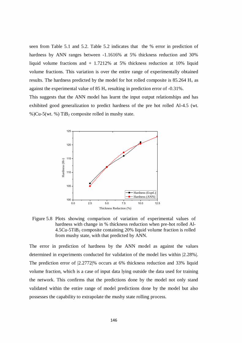
146
seen from Table 5.1 and 5.2. Table 5.2 indicates that the % error in prediction of
hardness by ANN ranges between -1.1616% at 5% thickness reduction and 30%
liquid volume fractions and + 1.7212% at 5% thickness reduction at 10% liquid
volume fractions. This variation is over the entire range of experimentally obtained
results. The hardness predicted by the model for hot rolled composite is 85.264 Hv as
against the experimental value of 85 Hv resulting in prediction error of -0.31%.
This suggests that the ANN model has learnt the input output relationships and has
exhibited good generalization to predict hardness of the pre hot rolled Al-4.5 (wt.
%)Cu-5(wt. %) TiB2 composite rolled in mushy state.
0.0 2.5 5.0 7.5 10.0 12.5
100
105
110
115
120
125
Hard
ness
(H
v)
Thickness Reduction (%)
Hardness (Exptl.)
Hardness (ANN)
The error in prediction of hardness by the ANN model as against the values
determined in experiments conducted for validation of the model lies within |2.28%|.
The prediction error of |2.2772|% occurs at 6% thickness reduction and 33% liquid
volume fraction, which is a case of input data lying outside the data used for training
the network. This confirms that the predictions done by the model not only stand
validated within the entire range of model predictions done by the model but also
possesses the capability to extrapolate the mushy state rolling process.
Figure 5.8 Plots showing comparison of variation of experimental values of
hardness with change in % thickness reduction when pre-hot rolled Al-
4.5Cu-5TiB2 composite containing 20% liquid volume fraction is rolled
from mushy state, with that predicted by ANN.
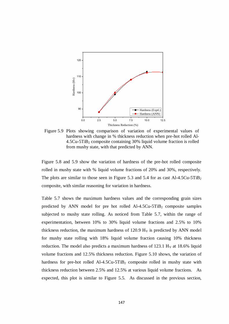
147
0.0 2.5 5.0 7.5 10.0 12.5
90
100
110
120
Hard
ness
(H
v)
Thickness Reduction (%)
Hardness (Exptl.)
Hardness (ANN)
Figure 5.8 and 5.9 show the variation of hardness of the pre-hot rolled composite
rolled in mushy state with % liquid volume fractions of 20% and 30%, respectively.
The plots are similar to those seen in Figure 5.3 and 5.4 for as cast Al-4.5Cu-5TiB2
composite, with similar reasoning for variation in hardness.
Table 5.7 shows the maximum hardness values and the corresponding grain sizes
predicted by ANN model for pre hot rolled Al-4.5Cu-5TiB2 composite samples
subjected to mushy state rolling. As noticed from Table 5.7, within the range of
experimentation, between 10% to 30% liquid volume fractions and 2.5% to 10%
thickness reduction, the maximum hardness of 120.9 HV is predicted by ANN model
for mushy state rolling with 18% liquid volume fraction causing 10% thickness
reduction. The model also predicts a maximum hardness of 123.1 HV at 18.6% liquid
volume fractions and 12.5% thickness reduction. Figure 5.10 shows, the variation of
hardness for pre-hot rolled Al-4.5Cu-5TiB2 composite rolled in mushy state with
thickness reduction between 2.5% and 12.5% at various liquid volume fractions. As
expected, this plot is similar to Figure 5.5. As discussed in the previous section,
Figure 5.9 Plots showing comparison of variation of experimental values of
hardness with change in % thickness reduction when pre-hot rolled Al-
4.5Cu-5TiB2 composite containing 30% liquid volume fraction is rolled
from mushy state, with that predicted by ANN.

148
reduction in hardness is expected for mushy state rolling at higher values of % liquid
volume fractions.
TABLE 5.7 Optimal values of Grain size and Hardness as predicted by ANN
for pre hot rolled Al-4.5Cu-5TiB2 composite samples subjected
to mushy state rolling.
Description of Mushy State Rolled Composite
ANN Predicted Values of
Grain size ( μm ) Hardness
(Hv) Large Small
10% thickness
reduction 18% Liquid volume fraction 43.261 27.4832 120.9
12.5% thickness
reduction 18.6% liquid volume fraction 46.6982 30.4346 123.1
0 5 10 15
90
100
110
120
Hard
ness
(H
v)
Thickness Reduction (%)
5% LVF(ANN)
10% LVF(Exptl.)
10% LVF(ANN)
20% LVF(Exptl.)
20% LVF(ANN)
30% LVF(Exptl.)
30% LVF(ANN)
35% LVF(ANN)
Figure 5.11 plots the variation of hardness based on the ANN model within the range
of experimentation, with maximum value of hardness of 120.9 HV occurring at 18%
liquid volume fractions and 10% thickness reduction. Figure 5.12 shows the contour
plot generated for hardness variation, with respect to thickness reduction per pass
during mushy state rolling of pre hot rolled composite and volume fraction of liquid in
the composite at the initiation of rolling. It can be seen that as compared to the
contour plot in Figure 5.7 for as cast composite, this plot provides a larger region
depicting higher values of hardness.
Figure 5.10 Plot showing the variation of hardness with thickness reduction at
different % volume fractions of liquid (LVF) for pre hot rolled Al-
4.5Cu-5TiB2 composite rolled in mushy state.

149
5 10 15 20 25 30 35
90
100
110
120
Hard
ness
(H
v)
Liq. Vol. Fraction (%)
2.5% TR
5.0% TR
7.5% TR
10.5% TR
2.5 5.0 7.5 10.0 12.5
10
20
30
Pre Hot Rolled- Hardness
Liq
uid
Vo
lum
e F
racti
on
(%
)
Thickness Reduction (%)
88.10
92.48
96.85
101.2
105.6
110.0
114.4
118.7
123.1
Figure 5.11 Graph showing the variation of ANN predicted values of hardness for
pre hot rolled Al-4.5Cu-5TiB2 composite rolled from mushy state to
various Thickness Reductions (TR) with different percent volume of
liquid in the composite.
Figure 5.12 Contour maps showing hardness spectrum when pre hot rolled Al-
4.5Cu-5TiB2 composite is rolled from mushy state to different
thickness reductions with different liquid volume fractions.
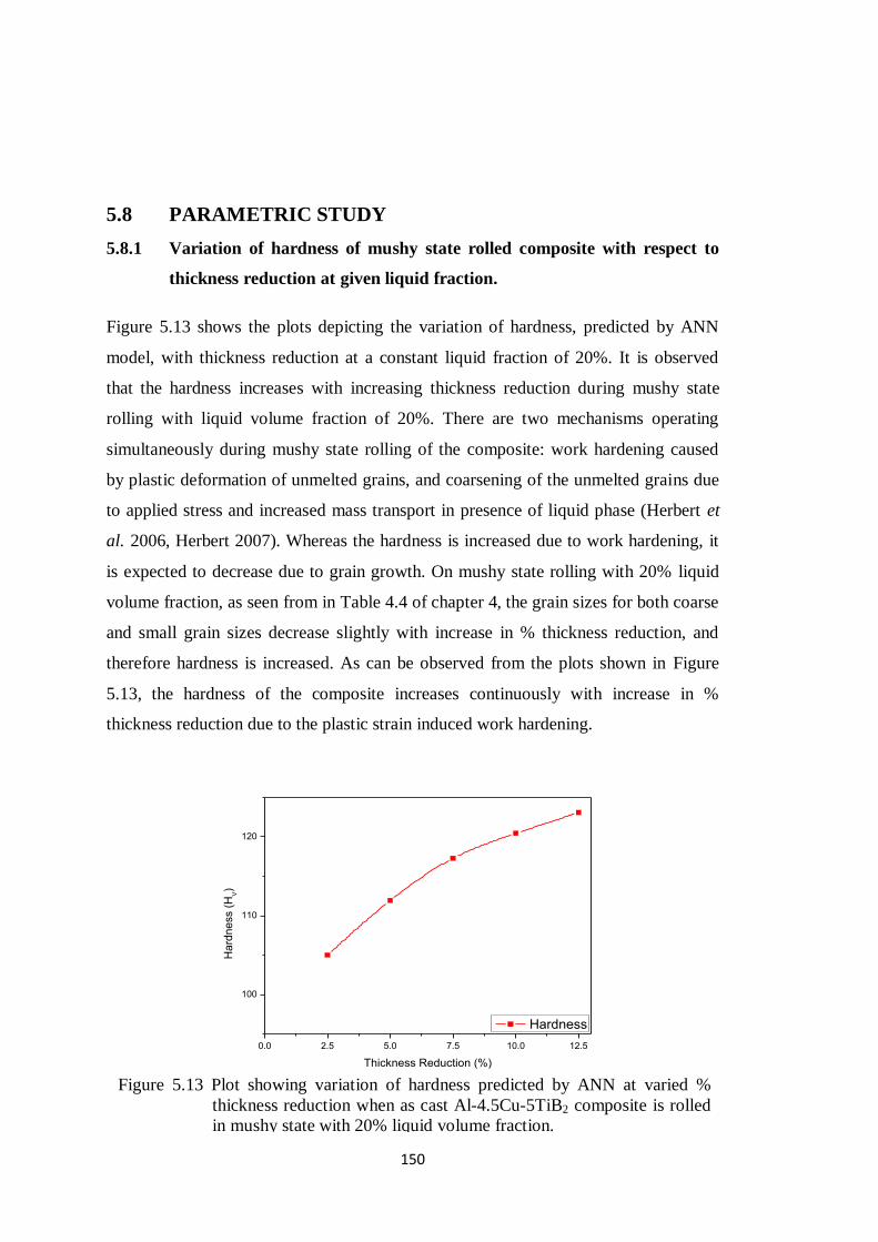
150
5.8 PARAMETRIC STUDY
5.8.1 Variation of hardness of mushy state rolled composite with respect to
thickness reduction at given liquid fraction.
Figure 5.13 shows the plots depicting the variation of hardness, predicted by ANN
model, with thickness reduction at a constant liquid fraction of 20%. It is observed
that the hardness increases with increasing thickness reduction during mushy state
rolling with liquid volume fraction of 20%. There are two mechanisms operating
simultaneously during mushy state rolling of the composite: work hardening caused
by plastic deformation of unmelted grains, and coarsening of the unmelted grains due
to applied stress and increased mass transport in presence of liquid phase (Herbert et
al. 2006, Herbert 2007). Whereas the hardness is increased due to work hardening, it
is expected to decrease due to grain growth. On mushy state rolling with 20% liquid
volume fraction, as seen from in Table 4.4 of chapter 4, the grain sizes for both coarse
and small grain sizes decrease slightly with increase in % thickness reduction, and
therefore hardness is increased. As can be observed from the plots shown in Figure
5.13, the hardness of the composite increases continuously with increase in %
thickness reduction due to the plastic strain induced work hardening.
0.0 2.5 5.0 7.5 10.0 12.5
100
110
120
Ha
rdn
ess (
HV)
Thickness Reduction (%)
Hardness
Figure 5.13 Plot showing variation of hardness predicted by ANN at varied %
thickness reduction when as cast Al-4.5Cu-5TiB2 composite is rolled
in mushy state with 20% liquid volume fraction.

151
5.9 SUMMARY
1. The ANN model for prediction of hardness of Al-4.5Cu-5TiB2 composite
rolled in mushy state in as cast and Prehot rolled condition was successfully
formulated. Within the data used for training the model, the values of hardness
predicted by the ANN model proposed give an error less than |2.65%| and
|1.8%| for as cast and pre hot rolled Al – 4.5Cu- 5TiB2 composite respectively
rolled in mushy state, with thickness reduction in the range from 2.5% to 10%
per pass and % liquid volume fraction in the mushy state varying from 10% to
30%. Therefore, the model characterizes the process of mushy state rolling
very well within the reasonable limits in this range and therefore can be used
as an alternative to tedious, costly and time consuming experimentation.
Further, within the range of data used to train the model, the ANN model
reveals that the hardness of the mushy state rolled composite containing any
liquid volume fraction shows highest value for a thickness reduction of 10%
per roll pass, both in case of as cast as well as pre hot rolled composite.
2. It can be concluded that the ANN model proposed for predicting hardness can
extrapolate hardness values beyond the experimental range, which is proved
by a small error of |1.43|% in prediction by ANN in case of cast composite and
less than |2.3|% in case of pre hot rolled composite. Thus, the model can
characterize effectively, with a very low degree of variation, the mushy state
rolling of as cast as well as pre-hot rolled Al – 4.5 Cu -5TiB2 composite with
liquid content varying from 5 to 35% and thickness reduction per pass varying
from 2% to 12.5%.
3. The study of variation of hardness of mushy state composite predicted by
ANN model within the range of data used to train the model (i.e. experimental
range), with reduction in thickness per roll pass at a given liquid volume
fraction indicates that the highest hardness values for any thickness reduction
are obtained for a liquid volume fraction of 20%. This information along with
the conclusion at point 1 above indicates that the highest value of hardness of
the composite lies somewhere in the range of 10% thickness reduction and

152
20% liquid volume fraction, for both as cast as well as pre hot rolled
composite rolled in mushy state. This conclusion can also be arrived by the
study of contour plots shown in Figure 5.7 and Figure 5.12.
4. The experimental values show the maximum hardness for mushy state rolling
causing all thickness reductions with 20% liquid volume fraction, while the
maximum hardness depicted by the ANN model in experimental range is
121.3 HV at 19% liquid volume fraction and 10% thickness reduction for as
cast composite and 120.9 HV at 18 % liquid volume fraction and 10%
thickness reduction for pre hot rolled composite.
5. The maximum hardness predicted for the mushy state rolled composite by the
ANN model for entire range with 2 to 12.5% thickness reduction and with 5 to
35% liquid volume fractions is 123.1 HV at 17.4% liquid volume fraction and
12.5% thickness reduction for as cast composite. For pre hot rolled composite,
for the corresponding range, the maximum value of hardness predicted is
123.116 HV when composite containing 18.6% liquid volume fraction is
mushy state rolled to 12.5% thickness reduction per pass.
6. The errors in prediction of hardness by ANN model compared with the
hardness values obtained from experiments carried out for validation of model
are within |2.28%|. This ensures that the generalisation of relationship of
hardness variation with respect to thickness reduction, mushy state of the
composite and initial material state of composite rolled in mushy is validated
within an error of |2.28%|.
153
Chapter 6
RESULTS AND DISCUSSION (PART III)
ANN MODELLING FOR PREDICTION OF TENSILE
PROPERTIES
6.1 INTRODUCTION
In the previous chapter, the details of ANN modelling and prediction of hardness of
Al-4.5Cu-5TiB2 composite were presented. The predictions from the validated model
were used to analyse the variation of hardness with the mushy state rolling
parameters. Along with hardness, which is a very important property in any
engineering application, strength and ductility too are equally important. The
determinants of the strength of the material obviously have its roots related to grain
morphology. Grain morphology, in turn can be affected to ones requirement by
subjecting the material to pre treatment, including conventional hot working in case of
conventional materials. However, as we have seen in chapter 2, literature survey
indicates that MMCs do not offer themselves conveniently to traditional methods of
forming. Mushy state rolling of Al-4.5Cu-5TiB2 composite led to bimodal grain
distribution (Herbert et al. 2006, Herbert 2007). Investigation of tensile properties of
Al-4.5Cu-5TiB2 composite was carried out by Herbert (2007). Since the mushy state
rolled composite led to duplex grain size distribution, it would be of interest to
possess knowledge about the variation of tensile properties with respect to mushy
state rolling parameters. It is seen from previous work (Herbert et al. 2010, Herbert
2007), that the tensile properties of the composite are a function of mushy state rolling
parameters as well as grain sizes and hardness, leading to a complex and non linear
relationship between input and output parameters. The use of ANNs is known to map
complex and non linear input output relationships. ANN can therefore be used as a
system to predict these properties of the composites. Once it has been trained, it
understands the subtle and underlying relationships of tensile properties with mushy
154
state rolling parameters, hardness and the grain morphology of the mushy state rolled
composite. The data on the tensile properties of Al-4.5Cu-5TiB2 composite being
inadequate, the present work has also considered the published data (Herbert 2007) on
tensile properties of Al-4.5Cu alloy. The present chapter deals with the ANN
modelling for prediction of tensile properties viz. yield strength, ultimate tensile
strength and percentage elongation of mushy state rolled Al-4.5Cu-5TiB2 composite
as well as Al-4.5Cu alloy.
6.2 SCOPE
The tensile properties (Ultimate Tensile Strength, Yield Strength and percentage
elongation) of mushy state rolled Al-4.5Cu-5TiB2 composite depend on the initial
material state, % thickness reduction, % liquid volume fraction, large and small grain
sizes, %TiB2 and hardness of the composite. Therefore the relationship between
inputs and outputs is quite complex apart from being non linear. Hence, it is proposed
to formulate the Artificial Neural Network model with Feed Forward architecture to
predict the tensile properties which include, yield strength, ultimate strength and
elongation of Al-4.5Cu-5TiB2 composite rolled in mushy state in as cast as well as pre
hot rolled condition with the input parameters being, % thickness reduction, %
volume fraction of liquid, large and small grain sizes, hardness and the % wt. content
of TiB2 (which is fixed as 5%) in the composite. The present work describes the
development of the ANN model with following:
(a) The analysis of the effect Initial state of composite material during mushy
state rolling (as cast or pre hot rolled) on yield strength, ultimate tensile
strength and elongation of Al-4.5Cu-5TiB2 composite mushy state rolled in
as cast as well as pre hot rolled state.
(b) The analysis of effect of thickness reduction during mushy state rolling and
mushy state condition when rolling is initiated.
(c) Interpolate and thereby expand the data on tensile properties of mushy state
rolled composite for a wider range of thickness reductions and liquid volume
fractions in the composite.

155
6.3 TENSILE PROPERTIES
The yield strength, ultimate tensile strength and elongation until failure are important
properties of the material from the view of applications in structural engineering. The
tensile properties are a function of the microstructure as well as flaws present in the
material. The following tensile properties of interest are considered in this section:
6.3.1 Strength
6.3.1.1 Yield strength (YS)
It is defined as the stress at which the material starts deviating from the straight line
relationship on the stress strain curve. In case of structural steel, the yield point is
obvious. However in case of non ferrous materials, since the yielding is not obvious,
0.2% proof stress is considered as yield stress and is denoted as 0.2% yield stress.
(Dieter 1986). The data taken in the present development of model refers to the 0.2%
yield strength of Al-Cu alloy and Al-4.5Cu-5TiB2 composite.
6.3.1.2 Ultimate tensile strength (UTS)
This refers to the maximum strength resisted by the material before undergoing failure
by breaking and as in case of yield strength, is expressed in MPa (Dieter 1986).
6.3.1.3 Percentage (pct) elongation
Percentage elongation is the elongation to failure expressed as a fraction of the
original length of the specimen tested in tension test. It is a measure of the ductile
properties of the material and therefore is an important property from material
formability point of view (Dieter 1986).
6.4 DATA COLLECTION
The data for developing ANN model for prediction of tensile properties has been
taken from previous work done on studies of mushy state rolling of Al-Cu alloy and
Al-4.5Cu-5TiB2 composite (Herbert 2007). The tensile properties being dependent on
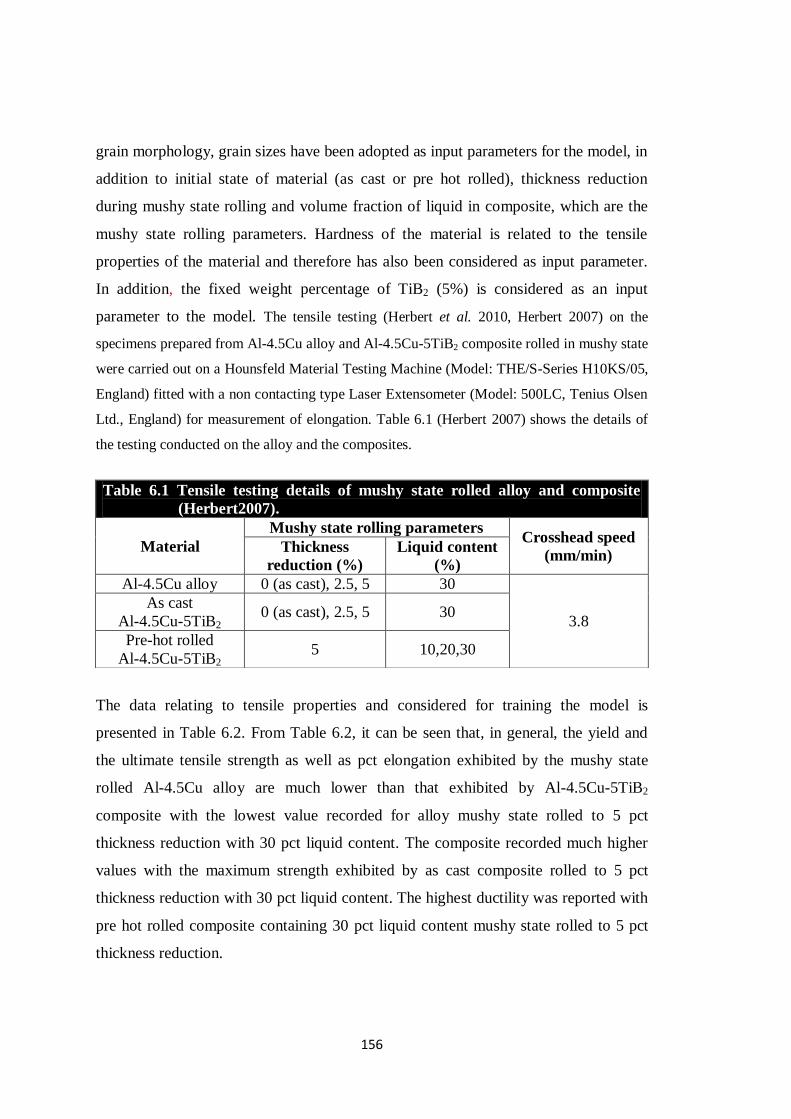
156
grain morphology, grain sizes have been adopted as input parameters for the model, in
addition to initial state of material (as cast or pre hot rolled), thickness reduction
during mushy state rolling and volume fraction of liquid in composite, which are the
mushy state rolling parameters. Hardness of the material is related to the tensile
properties of the material and therefore has also been considered as input parameter.
In addition, the fixed weight percentage of TiB2 (5%) is considered as an input
parameter to the model. The tensile testing (Herbert et al. 2010, Herbert 2007) on the
specimens prepared from Al-4.5Cu alloy and Al-4.5Cu-5TiB2 composite rolled in mushy state
were carried out on a Hounsfeld Material Testing Machine (Model: THE/S-Series H10KS/05,
England) fitted with a non contacting type Laser Extensometer (Model: 500LC, Tenius Olsen
Ltd., England) for measurement of elongation. Table 6.1 (Herbert 2007) shows the details of
the testing conducted on the alloy and the composites.
The data relating to tensile properties and considered for training the model is
presented in Table 6.2. From Table 6.2, it can be seen that, in general, the yield and
the ultimate tensile strength as well as pct elongation exhibited by the mushy state
rolled Al-4.5Cu alloy are much lower than that exhibited by Al-4.5Cu-5TiB2
composite with the lowest value recorded for alloy mushy state rolled to 5 pct
thickness reduction with 30 pct liquid content. The composite recorded much higher
values with the maximum strength exhibited by as cast composite rolled to 5 pct
thickness reduction with 30 pct liquid content. The highest ductility was reported with
pre hot rolled composite containing 30 pct liquid content mushy state rolled to 5 pct
thickness reduction.
Table 6.1 Tensile testing details of mushy state rolled alloy and composite
(Herbert2007).
Material
Mushy state rolling parameters Crosshead speed
(mm/min) Thickness
reduction (%)
Liquid content
(%)
Al-4.5Cu alloy 0 (as cast), 2.5, 5 30
3.8
As cast
Al-4.5Cu-5TiB2 0 (as cast), 2.5, 5 30
Pre-hot rolled
Al-4.5Cu-5TiB2 5 10,20,30
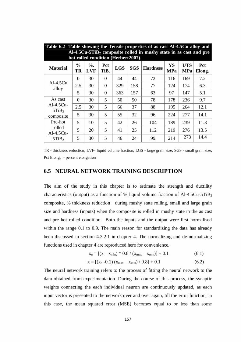
157
Table 6.2 Table showing the Tensile properties of as cast Al-4.5Cu alloy and
Al-4.5Cu-5TiB2 composite rolled in mushy state in as cast and pre
hot rolled condition (Herbert2007).
Material %
TR
%.
LVF
Pct
TiB2 LGS SGS Hardness
YS
MPa
UTS
MPa
Pct
Elong.
Al-4.5Cu
alloy
0 30 0 44 44 72 116 169 7.2
2.5 30 0 329 158 77 124 174 6.3
5 30 0 363 157 63 97 147 5.1
As cast
Al-4.5Cu-
5TiB2
composite
0 30 5 50 50 78 178 236 9.7
2.5 30 5 66 37 88 195 264 12.1
5 30 5 55 32 96 224 277 14.1
Pre-hot
rolled
Al-4.5Cu-
5TiB2
composite
5 10 5 42 26 104 189 239 11.3
5 20 5 41 25 112 219 276 13.5
5 30 5 46 24 99 214 273
14.4
TR - thickness reduction; LVF- liquid volume fraction; LGS - large grain size; SGS - small grain size;
Pct Elong. – percent elongation
6.5 NEURAL NETWORK TRAINING DESCRIPTION
The aim of the study in this chapter is to estimate the strength and ductility
characteristics (output) as a function of % liquid volume fraction of Al-4.5Cu-5TiB2
composite, % thickness reduction during mushy state rolling, small and large grain
size and hardness (inputs) when the composite is rolled in mushy state in the as cast
and pre hot rolled condition. Both the inputs and the output were first normalised
within the range 0.1 to 0.9. The main reason for standardizing the data has already
been discussed in section 4.3.2.1 in chapter 4. The normalizing and de-normalizing
functions used in chapter 4 are reproduced here for convenience.
xn = [(x – xmin) * 0.8 / (xmax – xmin)] + 0.1 (6.1)
x = [(xn -0.1) (xmax – xmin) / 0.8] + 0.1 (6.2)
The neural network training refers to the process of fitting the neural network to the
data obtained from experimentation. During the course of this process, the synaptic
weights connecting the each individual neuron are continuously updated, as each
input vector is presented to the network over and over again, till the error function, in
this case, the mean squared error (MSE) becomes equal to or less than some
158
predefined value or the training is stopped at some specified number of iterations. In
the present model development, FFNN model with an input layer and an output layer
with a single hidden layer was tried with different values of η and α and with number
of nodes ranging from 2 to 15 in the hidden layer (Reddy et al. 2005), with a MSE of
0.00001 and number of iterations as 5 lakhs. But the network failed to converge. This
was expected since the relationship between input and output parameters is obviously
quite complex and probably non linear. The FFNN was then tried with two hidden
layers. The training of the model was started with 2 to 15 neurons in each hidden
layer (Reddy et al. 2005). The minimum MSE was set at 0.0001 and the number of
iterations was limited to 500000. At the beginning, the starting values of the learning
rate parameter (η) and the momentum factor (α) were taken as 0.1 and 0.9
respectively. For all patterns ps the global error function MSE is given by Reddy et al.
(2005),
𝑀𝑆𝐸 = 𝐸𝑝 =1
𝑝𝑝 𝑇𝑖𝑝 − 𝑂𝑖𝑝 2
𝑖𝑝 (6.3)
where, Tip is the target output and Oip is the predicted output, for the ith
neuron and the
pth pattern presented to the network. The mean error in the output prediction is given
by Reddy et al. (2005),
𝐸𝑡𝑟 (𝑥) =1
𝑁 |(𝑇𝑖 𝑥 − 𝑝𝑖 𝑥 )|𝑁
1 (6.4)
where 𝐸𝑡𝑟 𝑥 is the mean error in prediction of data set for the output parameter 𝑥, N
is the number of data sets, Ti(x) is the target output and pi(x) is the predicted output.
The learning rate η was then varied from 0.1 to 0.9 in steps of 0.05 to start with the
training. The learning rate was selected for the model based on the MSE and 𝐸𝑡𝑟 of
the training. Now, the learning rate was fixed for the model and the momentum factor
was varied from 0.9 to 0.1 in steps of 0.05. Again based on the MSE and 𝐸𝑡𝑟 the
momentum was selected and the FFNN architecture was finalised for predicting the
yield strength, ultimate tensile strength and pct elongation for the Al-4.5Cu alloy
rolled in the as cast form and Al-4.5Cu-5TiB2 composite in the as cast and pre hot
rolled condition when rolled in mushy state to various % thickness reductions and
with various % liquid volume fractions. Sigmoid function stated at equation (4.5)
(Reddy et al. 2005, Yagnanarayana 2007, Zurada 1994, 2003) and reproduced here at

159
equation (6.5) was used for activating the neurons and back propagation algorithm
was used for training the network.
𝐹 𝑥 =1
[1+exp −𝑥 ] (6.5)
An extensive analysis of different combinations of the learning rate parameter,
momentum factor and the number of neurons in each hidden layer was done. The
number of neurons in each hidden layer was varied from 2 to 15. Learning rate was
varied from 0.1 to 0.9 and momentum term varied from 0.9 to 01 in steps of 0.05 in
each of these cases. The network was found to excellently converge with 9 and 6
neurons in the first and second hidden layer respectively with η=0.85 and α=0.7. The
MSE was reset at 0.0001692 and 𝐸𝑡𝑟 = 8 x 10⁻⁶
and the epochs were restricted to
500000. Training was decided to be stopped either when MSE reached 0.00017 or
when the number of iterations reached 500000, whichever occurred earlier. Here the
targeted MSE was achieved after 490000 iterations. The inputs to the model were
material type (as cast alloy, as cast or pre hot rolled composite), pct thickness
reduction, pct liquid content, large grain size, small grain size and hardness. The
outputs predicted were the yield strength, ultimate tensile strength and pct elongation
of the alloy in cast and mushy state rolled form and of the composite in the as cast as
well as pre hot rolled form when it is rolled in mushy state. The prediction of the
strength and ductility parameters carried out for the range of experimental values
tabulated in Table 6.2 for the cases listed in Table 6.1 are shown in Table 6.3.
6.6 DISCUSSION
The resulting values of strength parameters, namely, yield strength and ultimate
tensile strength and the ductility characteristic represented by pct elongation predicted
by Artificial Neural Network are compared with the corresponding experimentally
obtained values to check the suitability of the ANN model within the perview of
experimentation. A detailed analysis of the variation of the values of strength and pct
elongation with respect to percentage thickness reduction during rolling and with
percent liquid volume fraction at which the rolling is initiated is also presented in this
section.

160
Table 6.3 Table showing the comparison of Tensile properties of as cast Al-
4.5Cu alloy and Al-4.5Cu-5TiB2 composite rolled in mushy state in as
cast and pre hot rolled condition.
Material
%
TR
%
LVF
%
TiB2
LGS
(μm)
SGS
(μm)
Hardness
(Hv)
Yield
strength
MPa
Pct
Error
UTS MPa Pct
Error
Pct
elongation Pct
Error
Exptl ANN Exptl ANN Exptl ANN
Al-4.5Cu
alloy
0 30 0 44 44 72 116 118.9 -2.55 169 167 1.20 7.2 6.95 3.44
2.5 30 0 329 158 77 124 120.4 2.86 174 176.6 -1.48 6.3 6.39 -1.40
5 30 0 363 157 63 97 99.4 -2.46 147 145.5 1.03 5.1 5.12 -0.45
As cast
Al-4.5Cu-5TiB2
0 30 5 50 50 78 178 175.8 1.23 236 238.3 -0.96 9.7 10.4 -7.65
2.5 30 5 66 37 88 195 197.9 -1.52 264 260.3 1.39 12.1 11.8 2.22
5 30 5 55 32 96 224 223.4 0.27 277 278.2 -0.44 14.1 14.1 0.01
Pre-hot
rolled
Al-
4.5Cu-
5TiB2
5 10 5 42 26 104 189 185.1 2.06 239 242.9 -1.64 11.3 11.5 -1.94
5 20 5 41 25 112 219 220.6 -0.71 276 273.3 0.97 13.5 14.3 -6.24
5 30 5 46 24 99 214 215.2 -0.58 273 271.2 0.65 14.4 13.6 5.57
TR - thickness reduction; LVF- liquid volume fraction; LGS - large grain size; SGS - small grain size.
It can be seen from Table 6.3 that the maximum error in prediction by the ANN
model is 7.65%, while the majority of the predictions are within 3.5% error in
predictions. Jiahe et al. (2003) have reported prediction of microstructure of
60Si2MnA rod within a prediction of 3.2% error. Selvakumar et al. (2007) have
modelled the effect of particle size and iron content on forming of Al-Fe composite
preforms within an error of 5%. Peng et al. (2002) in their work on semisolid
processing of steel-Al-7 graphite binding plate have formulated an ANN model for
relationship of the bonding parameters and interfacial shear strength of bonding plate
within a prediction error of 3.9%. Microstructural evolution model of TA15 titanium
alloy based on BP algorithm trained ANN model has been reported by Zhicago et al.
(2010), with an estimation error of 5%. Kusiak & Kuziak (2002) have reported a
maximum percentage error of 8% in prediction of ultimate tensile and yield strength
of steel, while Mandal et al. (2009) in their paper reported a Gaussian distribution of
% error of prediction within ±10% in prediction of flow stress using Resilient
Propagation algorithm which has been reported to perform better than Back
Propagation algorithm. In light of these findings in similar contemporary works, the
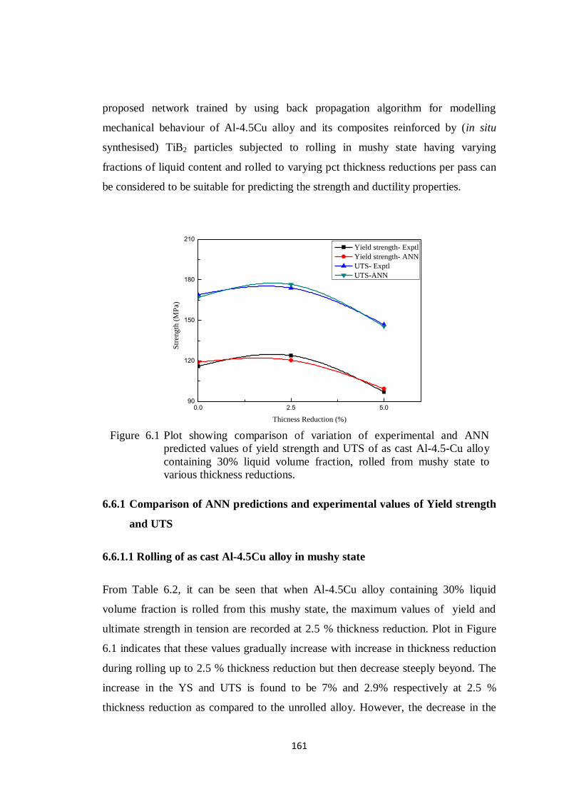
161
proposed network trained by using back propagation algorithm for modelling
mechanical behaviour of Al-4.5Cu alloy and its composites reinforced by (in situ
synthesised) TiB2 particles subjected to rolling in mushy state having varying
fractions of liquid content and rolled to varying pct thickness reductions per pass can
be considered to be suitable for predicting the strength and ductility properties.
0.0 2.5 5.090
120
150
180
210
Str
eng
th (
MP
a)
Thicness Reduction (%)
Yield strength- Exptl
Yield strength- ANN
UTS- Exptl
UTS-ANN
6.6.1 Comparison of ANN predictions and experimental values of Yield strength
and UTS
6.6.1.1 Rolling of as cast Al-4.5Cu alloy in mushy state
From Table 6.2, it can be seen that when Al-4.5Cu alloy containing 30% liquid
volume fraction is rolled from this mushy state, the maximum values of yield and
ultimate strength in tension are recorded at 2.5 % thickness reduction. Plot in Figure
6.1 indicates that these values gradually increase with increase in thickness reduction
during rolling up to 2.5 % thickness reduction but then decrease steeply beyond. The
increase in the YS and UTS is found to be 7% and 2.9% respectively at 2.5 %
thickness reduction as compared to the unrolled alloy. However, the decrease in the
Figure 6.1 Plot showing comparison of variation of experimental and ANN
predicted values of yield strength and UTS of as cast Al-4.5-Cu alloy
containing 30% liquid volume fraction, rolled from mushy state to
various thickness reductions.

162
YS and UTS is found to be 21.77% and 17.24% respectively at 5 % thickness
reduction as compared to that at 2.5 %. This steep decrease in strength with increase
in thickness reduction beyond 2.5 % thickness reduction, which can also be seen from
Table 6.2, is attributed to grain growth (Herbert et al. 2010, Herbert 2007).
6.6.1.2 Rolling of as cast Al-4.5Cu-5TiB2 composite in mushy state
Table 6.3 shows the experimentally obtained values of YS and UTS as well as those
predicted by Neural Network for cast Al-4.5Cu-5TiB2 composite rolled in mushy state
containing 30 % liquid volume fraction corresponding to 632ºC temperature and
rolled to 2.5% and 5% thickness reductions per pass.
It can be seen that the percentage error between the experimental values for yield
strength in tension and ANN predicted values ranges from -1.5221% to +1.2348%,
with these maximum errors occurring at 2.5 % thickness reduction. Similarly, for
ultimate tensile strength, the % error is between -0.4458% and +1.3943% under same
conditions of rolling. The percentage error between experimental values and values
predicted by ANN at various percent liquid volume fractions for entire range of
percentage thickness reduction are within |1.6%|. The errors in prediction by
proposed ANN model are comparable with those reported in literature (Peng et al.
2002, Kusiak and Kuziak 2002, Zhicago et al. 2010).
Plot in Figure 6.2 shows the variation of YS and UTS of as cast composite when
rolled in mushy state with temperature corresponding to 30 % liquid volume fraction
at various thickness reductions. The values predicted by ANN are observed to closely
match with the corresponding experimental values. It can be seen from the plots that
both, the YS as well as the UTS increase with increase in thickness reduction. From
Table 6.3, it is seen that the grain size decrease is modest at 2.5 % thickness reduction
while it is quite significant when the thickness reduction is 5 %. This is manifested in
modest increase of yield strength at 2.5 % thickness reduction followed by a steeper
increase beyond. However, in case of UTS the increase is more in the beginning and
modest beyond. The increase in the strength properties are in good agreement with
the hardness values as can be seen from Table 6.2 and 6.3.

163
0.0 2.5 5.0
160
180
200
220
240
260
280
300
320
340
Str
eng
th (
MP
a)
Thickness Reduction (%)
Yield Strength(Exptl.)
Yield Strength(ANN)
UTS(Exptl.)
UTS(ANN)
6.6.1.3 Rolling of pre-hot rolled Al-4.5Cu-5TiB2 composite in mushy state
Table 6.3 shows the experimentally obtained values of YS and UTS as well as those
predicted by Neural Network for pre-hot rolled Al-4.5Cu-5TiB2 composite rolled in
mushy state containing 10, 20 or 30 % liquid volume fraction (corresponding to
610ºC, 626
ºC or 632
ºC temperatures respectively) and rolled to 5% thickness
reductions per pass. The percentage error in prediction in case of UTS is found to vary
from -1.6448% to 0.9783% while that for YS varied from -0.7128% to 2.0571% with
maximum error in prediction exhibited at 10% liquid volume fraction, in both the
cases. The errors in prediction by the model are in agreement with predictions done
by ANN models in various applications in material science (Kusiak and Kuziak 2002,
Jiahe et al. 2003, Selvakumar et al. 2007). Therefore it can be concluded that the
ANN model proposed has generalised the relationship between the inputs to the
network and is able to predict the YS and UTS for the composite rolled in mushy state
in pre hot rolled condition within acceptable levels of accuracy.
Figure 6.2 Plot showing comparison of experimental and ANN predicted values of
yield and ultimate strength in tension for as cast composite containing
30% liquid volume fraction, rolled in mushy state to various thickness
reductions.
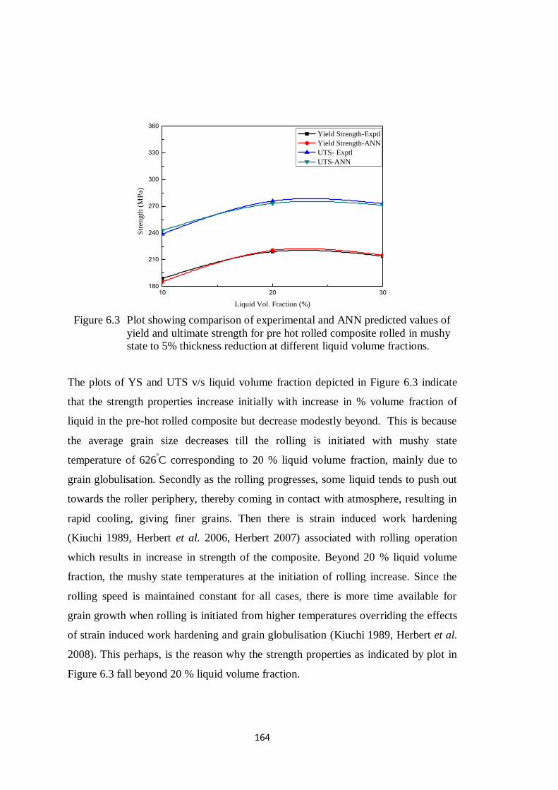
164
10 20 30180
210
240
270
300
330
360
Str
eng
th (
MP
a)
Liquid Vol. Fraction (%)
Yield Strength-Exptl
Yield Strength-ANN
UTS- Exptl
UTS-ANN
The plots of YS and UTS v/s liquid volume fraction depicted in Figure 6.3 indicate
that the strength properties increase initially with increase in % volume fraction of
liquid in the pre-hot rolled composite but decrease modestly beyond. This is because
the average grain size decreases till the rolling is initiated with mushy state
temperature of 626ºC corresponding to 20 % liquid volume fraction, mainly due to
grain globulisation. Secondly as the rolling progresses, some liquid tends to push out
towards the roller periphery, thereby coming in contact with atmosphere, resulting in
rapid cooling, giving finer grains. Then there is strain induced work hardening
(Kiuchi 1989, Herbert et al. 2006, Herbert 2007) associated with rolling operation
which results in increase in strength of the composite. Beyond 20 % liquid volume
fraction, the mushy state temperatures at the initiation of rolling increase. Since the
rolling speed is maintained constant for all cases, there is more time available for
grain growth when rolling is initiated from higher temperatures overriding the effects
of strain induced work hardening and grain globulisation (Kiuchi 1989, Herbert et al.
2008). This perhaps, is the reason why the strength properties as indicated by plot in
Figure 6.3 fall beyond 20 % liquid volume fraction.
Figure 6.3 Plot showing comparison of experimental and ANN predicted values of
yield and ultimate strength for pre hot rolled composite rolled in mushy
state to 5% thickness reduction at different liquid volume fractions.
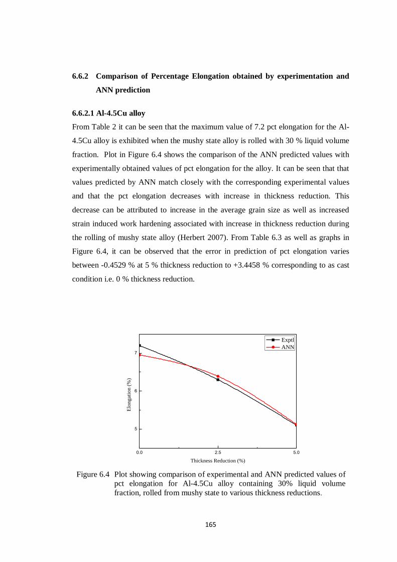
165
6.6.2 Comparison of Percentage Elongation obtained by experimentation and
ANN prediction
6.6.2.1 Al-4.5Cu alloy
From Table 2 it can be seen that the maximum value of 7.2 pct elongation for the Al-
4.5Cu alloy is exhibited when the mushy state alloy is rolled with 30 % liquid volume
fraction. Plot in Figure 6.4 shows the comparison of the ANN predicted values with
experimentally obtained values of pct elongation for the alloy. It can be seen that that
values predicted by ANN match closely with the corresponding experimental values
and that the pct elongation decreases with increase in thickness reduction. This
decrease can be attributed to increase in the average grain size as well as increased
strain induced work hardening associated with increase in thickness reduction during
the rolling of mushy state alloy (Herbert 2007). From Table 6.3 as well as graphs in
Figure 6.4, it can be observed that the error in prediction of pct elongation varies
between -0.4529 % at 5 % thickness reduction to +3.4458 % corresponding to as cast
condition i.e. 0 % thickness reduction.
0.0 2.5 5.0
5
6
7
Elo
ng
atio
n (
%)
Thickness Reduction (%)
Exptl
ANN
Figure 6.4 Plot showing comparison of experimental and ANN predicted values of
pct elongation for Al-4.5Cu alloy containing 30% liquid volume
fraction, rolled from mushy state to various thickness reductions.
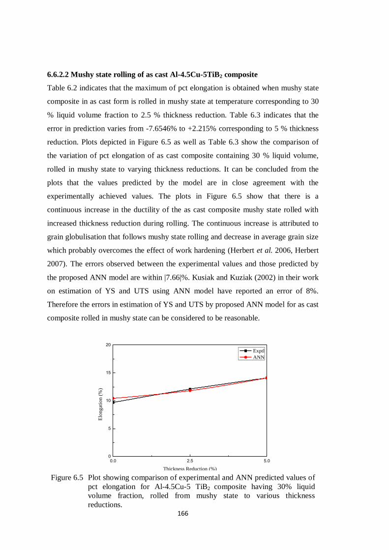
166
6.6.2.2 Mushy state rolling of as cast Al-4.5Cu-5TiB2 composite
Table 6.2 indicates that the maximum of pct elongation is obtained when mushy state
composite in as cast form is rolled in mushy state at temperature corresponding to 30
% liquid volume fraction to 2.5 % thickness reduction. Table 6.3 indicates that the
error in prediction varies from -7.6546% to +2.215% corresponding to 5 % thickness
reduction. Plots depicted in Figure 6.5 as well as Table 6.3 show the comparison of
the variation of pct elongation of as cast composite containing 30 % liquid volume,
rolled in mushy state to varying thickness reductions. It can be concluded from the
plots that the values predicted by the model are in close agreement with the
experimentally achieved values. The plots in Figure 6.5 show that there is a
continuous increase in the ductility of the as cast composite mushy state rolled with
increased thickness reduction during rolling. The continuous increase is attributed to
grain globulisation that follows mushy state rolling and decrease in average grain size
which probably overcomes the effect of work hardening (Herbert et al. 2006, Herbert
2007). The errors observed between the experimental values and those predicted by
the proposed ANN model are within |7.66|%. Kusiak and Kuziak (2002) in their work
on estimation of YS and UTS using ANN model have reported an error of 8%.
Therefore the errors in estimation of YS and UTS by proposed ANN model for as cast
composite rolled in mushy state can be considered to be reasonable.
0.0 2.5 5.00
5
10
15
20
Elo
ng
atio
n (
%)
Thickness Reduction (%)
Exptl
ANN
Figure 6.5 Plot showing comparison of experimental and ANN predicted values of
pct elongation for Al-4.5Cu-5 TiB2 composite having 30% liquid
volume fraction, rolled from mushy state to various thickness
reductions.
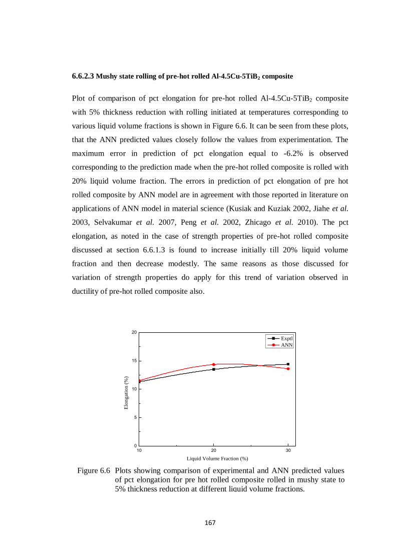
167
6.6.2.3 Mushy state rolling of pre-hot rolled Al-4.5Cu-5TiB2 composite
Plot of comparison of pct elongation for pre-hot rolled Al-4.5Cu-5TiB2 composite
with 5% thickness reduction with rolling initiated at temperatures corresponding to
various liquid volume fractions is shown in Figure 6.6. It can be seen from these plots,
that the ANN predicted values closely follow the values from experimentation. The
maximum error in prediction of pct elongation equal to -6.2% is observed
corresponding to the prediction made when the pre-hot rolled composite is rolled with
20% liquid volume fraction. The errors in prediction of pct elongation of pre hot
rolled composite by ANN model are in agreement with those reported in literature on
applications of ANN model in material science (Kusiak and Kuziak 2002, Jiahe et al.
2003, Selvakumar et al. 2007, Peng et al. 2002, Zhicago et al. 2010). The pct
elongation, as noted in the case of strength properties of pre-hot rolled composite
discussed at section 6.6.1.3 is found to increase initially till 20% liquid volume
fraction and then decrease modestly. The same reasons as those discussed for
variation of strength properties do apply for this trend of variation observed in
ductility of pre-hot rolled composite also.
10 20 300
5
10
15
20
Elo
ng
atio
n (
%)
Liquid Volume Fraction (%)
Exptl
ANN
Figure 6.6 Plots showing comparison of experimental and ANN predicted values
of pct elongation for pre hot rolled composite rolled in mushy state to
5% thickness reduction at different liquid volume fractions.
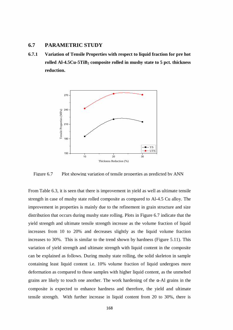
168
6.7 PARAMETRIC STUDY
6.7.1 Variation of Tensile Properties with respect to liquid fraction for pre hot
rolled Al-4.5Cu-5TiB2 composite rolled in mushy state to 5 pct. thickness
reduction.
10 20 30
150
180
210
240
270
Ten
sile
Pro
per
ties
(M
Pa)
Thickness Reduction (%)
YS
UTS
From Table 6.3, it is seen that there is improvement in yield as well as ultimate tensile
strength in case of mushy state rolled composite as compared to Al-4.5 Cu alloy. The
improvement in properties is mainly due to the refinement in grain structure and size
distribution that occurs during mushy state rolling. Plots in Figure 6.7 indicate that the
yield strength and ultimate tensile strength increase as the volume fraction of liquid
increases from 10 to 20% and decreases slightly as the liquid volume fraction
increases to 30%. This is similar to the trend shown by hardness (Figure 5.11). This
variation of yield strength and ultimate strength with liquid content in the composite
can be explained as follows. During mushy state rolling, the solid skeleton in sample
containing least liquid content i.e. 10% volume fraction of liquid undergoes more
deformation as compared to those samples with higher liquid content, as the unmelted
grains are likely to touch one another. The work hardening of the α-Al grains in the
composite is expected to enhance hardness and therefore, the yield and ultimate
tensile strength. With further increase in liquid content from 20 to 30%, there is
Figure 6.7 Plot showing variation of tensile properties as predicted by ANN
.model

169
decline in the strength properties, due to the grain coarsening phenomena occurring at
higher temperature (632ºC) corresponding to 30% liquid volume fraction. For a given
thickness reduction, the composite mushy state rolled with 20% liquid volume
fraction (Figure 5.11) exhibits the maximum value of hardness and therefore shall
exhibit high values of strength in the same region. The maximum value of hardness
and therefore the strength properties at 20% liquid volume fraction is due to the
optimum combination of the effects of work hardening of solid skeleton and the fine
grains formed by rapid solidification of the liquid.
6.8 SUMMARY
1. The ANN model proposed for prediction of tensile properties of Al-4.5Cu
alloy and its composite reinforced with 5 wt. % TiB2 has very well generalised
the relationship with the mushy state rolling parameters. The values of yield
strength in tension predicted by the ANN model proposed give an error less than
|2.1%| while the prediction of tensile strength is within an error of |1.5%|, for the
entire range of data within which the ANN has been trained
2. The predictions done by the trained ANN model for pct elongation at various
thickness reductions and starting state of Al-4.5Cu alloy and its composite
reinforced with 5 wt.% TiB2 during mushy state rolling, are within an error of
|7.65%|, with the majority of the predictions being within |2.3%| error as
compared to experimental results.
3. The ANN model proposed, therefore characterizes the process of mushy state rolling
very much within the reasonable limits in the range of experimentation carried out
and therefore can be used as an alternative to costly and time consuming
experimentation.
4. The model can be used to make predictions of tensile properties at any point within 0
to 5% thickness reduction with mushy state rolling initiated at 632ºC (corresponding
to 30% liquid volume fraction) in case of as cast Al-4.5Cu-5TiB2 composite.
5. For mushy state rolling of pre hot rolled composite, the model can make predictions
at any intermediate point between 10 and 30% volume fractions of liquid (i.e. from
610º C until 632
º C).
171
Chapter 7
RESULTS AND DISCUSSION (PART IV)
ANN MODELLING FOR PREDICTION OF WEAR PROPERTIES
7.1 INTRODUCTION
This chapter reports the modelling of ANN for prediction of dry sliding wear
properties of Al-4.5Cu-5TiB2 composite rolled from mushy state conditions.
Literature (Caracostas et al. 1992, Roy et al. 1992) reports that the metal matrix
composites have superior wear properties in comparison to monolithic alloys. Studies
have revealed that Al based MMCs undergo adhesive wear (Deuis et al. 1997, Herbert
2007, Herbert et al. 2008), strongly influenced by hardness. Hardness in a particulate
reinforced MMC is a function of grain morphology, hardness of particles and their
distribution. The hardness of mushy state rolled Al-4.5Cu-5TiB2 composite, as was
seen in chapter 5, varies with the matrix grain size, volume content of liquid in the
composite and thickness reduction per roll pass. Herbert (2007) and Herbert et al.
(2008) carried out study on dry sliding wear properties of Al-4.5Cu-5TiB2 composite
as a function of mushy state rolling parameters and analyzed the tribological
properties using adhesive wear model. The outcome of this study has been used as the
data for training the ANN model to predict the wear rates of mushy state rolled Al-
4.5Cu-5TiB2 composite with respect to various combinations of thickness reductions
and volume content of liquid in the composite. The proposed ANN model is validated
by conducting validation experiments within and outside the bounds of data used for
training the network. Thus the trained ANN model will be able to predict the wear
properties of the mushy state rolled Al-4.5Cu-5TiB2 composite within and outside the
bounds of training data set. The proposed ANN model along with the user friendly
GUI designed for the purpose will serve as a useful tool for optimization of wear
properties based on the parameters specified by the user.

172
7.2 WEAR PARAMETERS
Figure 7.1 is the plot of wear volume loss with respect to sliding distance, which
shows the regions of transient and steady state sliding wear. As seen from Figure 7.1,
initially, the volume loss is seen to vary in curvilinear fashion and the rate of volume
loss with sliding distance is observed to decrease at point B, beyond which it is found
to vary in linear trend along line BC. Yang (2003) has reported that the wear in the
region given by portion AB is known as unsteady state or transient wear, while the
wear in the portion provided by BC regime is termed as steady state wear. In the
steady state wear condition, the wear volume loss occurs at a constant rate over an
extended duration of time. For this reason, the wear rate in the first 600 m was
ignored in his work by Herbert (2007). Generally, the steady state wear behaviour of
materials is expressed in terms of some key parameters, namely, wear rate, wear
resistance, wear coefficient, specific wear rate and coefficient of friction. In the
subsections to follow, these parameters are further discussed in more detail.
Figure 7.1 Schematic plot of wear volume loss against sliding distance showing
transient and steady state wear regime
B C
A
Sliding Distance
Wear
Volu
me
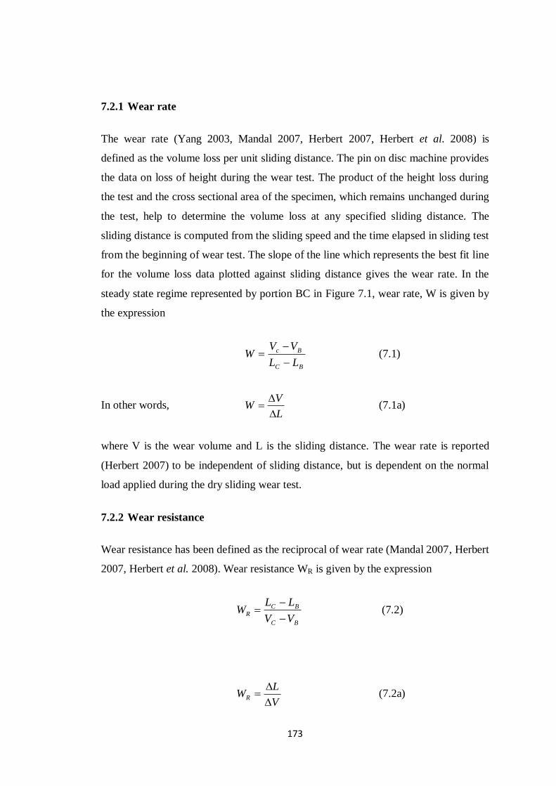
173
7.2.1 Wear rate
The wear rate (Yang 2003, Mandal 2007, Herbert 2007, Herbert et al. 2008) is
defined as the volume loss per unit sliding distance. The pin on disc machine provides
the data on loss of height during the wear test. The product of the height loss during
the test and the cross sectional area of the specimen, which remains unchanged during
the test, help to determine the volume loss at any specified sliding distance. The
sliding distance is computed from the sliding speed and the time elapsed in sliding test
from the beginning of wear test. The slope of the line which represents the best fit line
for the volume loss data plotted against sliding distance gives the wear rate. In the
steady state regime represented by portion BC in Figure 7.1, wear rate, W is given by
the expression
BC
Bc
LL
VVW
(7.1)
In other words, L
VW
(7.1a)
where V is the wear volume and L is the sliding distance. The wear rate is reported
(Herbert 2007) to be independent of sliding distance, but is dependent on the normal
load applied during the dry sliding wear test.
7.2.2 Wear resistance
Wear resistance has been defined as the reciprocal of wear rate (Mandal 2007, Herbert
2007, Herbert et al. 2008). Wear resistance WR is given by the expression
BC
BC
RVV
LLW
(7.2)
V
LWR
(7.2a)
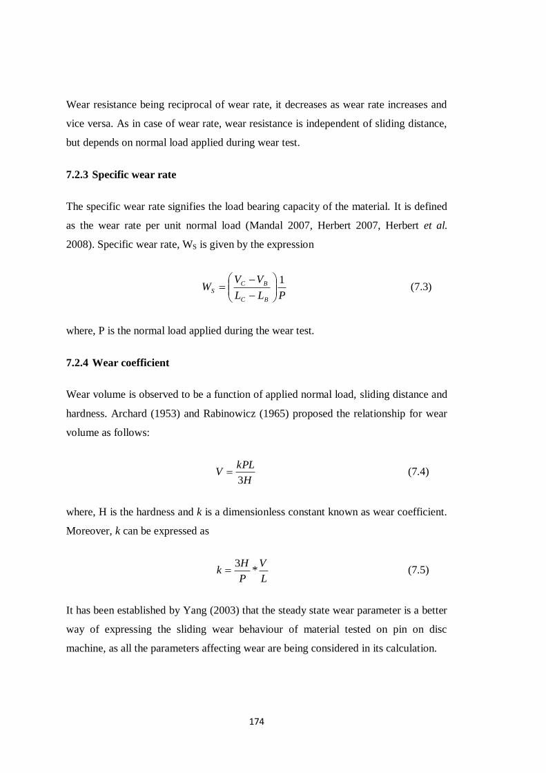
174
Wear resistance being reciprocal of wear rate, it decreases as wear rate increases and
vice versa. As in case of wear rate, wear resistance is independent of sliding distance,
but depends on normal load applied during wear test.
7.2.3 Specific wear rate
The specific wear rate signifies the load bearing capacity of the material. It is defined
as the wear rate per unit normal load (Mandal 2007, Herbert 2007, Herbert et al.
2008). Specific wear rate, WS is given by the expression
PLL
VVW
BC
BC
S
1
(7.3)
where, P is the normal load applied during the wear test.
7.2.4 Wear coefficient
Wear volume is observed to be a function of applied normal load, sliding distance and
hardness. Archard (1953) and Rabinowicz (1965) proposed the relationship for wear
volume as follows:
H
kPLV
3 (7.4)
where, H is the hardness and k is a dimensionless constant known as wear coefficient.
Moreover, k can be expressed as
L
V
P
Hk *
3 (7.5)
It has been established by Yang (2003) that the steady state wear parameter is a better
way of expressing the sliding wear behaviour of material tested on pin on disc
machine, as all the parameters affecting wear are being considered in its calculation.

175
7.2.5 Coefficient of friction
It is defined as the ratio of the limiting tangential force needed to produce sliding to
the normal load between the mating surfaces (Rabinowicz 1965). Coefficient of
friction, μ is given by the relation
N
FT (7.6)
where, FT is the tangential force reported in the steady state regime and N is the
normal load.
7.3 SCOPE
We have seen that ANN is a mathematical model for solving complex relationships
between inputs and outputs, wherein the model mimics the human brain in solving the
relationships (Reddy et al. 2005, 2008). The Neural Network has the ability to
compute these complex relationships by virtue of their similarity to the activities
carried out by biological neurons in the human brain by way of parallel and
distributed processing. This parallel and distributed processing adapts to the subtle
relationships between the inputs and outputs and generalizes the functional
relationship between them, even from a limited number of samples provided to it for
training. The experiments carried out leading to any formidable conclusion always
rely on a specific and limited number of readings at which the results are obtained or
proved. Although this brings to the fore a very important research outcome, the
information can be more useful for commercial applications when this experimental
data is available over a wider range, within and outside the range of experimentation.
ANN is an efficient tool to predict the output for any input within and in close
locations outside the range of experimentation. Wear properties of mushy state rolled
Al-4.5Cu-5TiB2 composite depend on a number of parameters such as initial material
state, % thickness reduction, % liquid volume fraction, large and small grain sizes,
hardness and % TiB2 in of the composite. The relationship as discussed earlier in
section 6.2 is very complex and exhibits non linearity. Various ANN architectures and

176
training algorithms are available, but the most widely used architectures use FFNN
with Back Propagation learning algorithm. FFNN is trained using supervised learning
through the use of generalised delta rule in which the mean squared error is minimised
step by step over the error surface by adjustment of weights, as each sample pattern is
offered to the network (Zurada 2003, Reddy et al. 2005, 2008, Yagnanarayana 2008).
In this chapter it is proposed to model ANN with FFNN architecture and trained using
BP algorithm to predict the wear properties of Al-4.5(wt. %)Cu-5(wt. %)TiB2
composite rolled from mushy state with various volume content of liquid in the
composite and to various thickness reductions during rolling. The scope of the work
to be achieved through this chapter is outlined as follows:
a) To model ANN with FFNN architecture using BP algorithm to predict
wear properties of Al-4.5Cu-5TiB2 composite rolled in mushy state at
various volume content of liquid in the composite and to various thickness
reductions per pass during rolling.
b) To compare the predictions of the model with the target values used for
training the network.
c) To validate the model through experimentations planned at specific points
within and outside the bounds of data used for proposed training the ANN
model.
d) To analyse the variation of wear properties of mushy state rolled Al-
4.5Cu-5TiB2 composite with respect to mushy state parameters.
e) To optimise the mushy state rolling process for wear parameters (wear
rate) using proposed ANN model.
7.4 DATA COLLECTION
The data collected for training the ANN model proposed for prediction of wear
properties of Al-4.5Cu-5TiB2 composite is taken from previous study carried out by
Herbert (2007) on wear properties of mushy state rolled Al-4.5Cu alloy and its
composite reinforced with TiB2 particles. The work involved the study of the
behaviour of Al-4.5Cu alloy and Al-4.5Cu-5TiB2 composite when rolled from mushy

177
state with various thickness reductions and temperatures corresponding to portion of
the volume of liquid content in the semisolid composite. The behaviour of the
composite was analysed for microstructural evolution, hardness and wear properties
in addition to strength. The behaviour of the composite rolled in mushy state, at
temperatures corresponding to 10%, 20% and 30% liquid volume fraction
(corresponding to mushy state temperatures of 610ºC, 626
ºC and 632
ºC respectively)
with thickness reduction of 2.5, 5, 7.5 and 10% has been studied. The composite is
rolled in mushy sate with initial state being in as cast and prior hot-rolled form. The
parameters which represent the wear of the composite such as wear rate, wear
resistance i.e. reciprocal of wear rate (Mandal et al. 2004), specific wear rate which is
defined as wear rate per unit normal load (Mandal et al. 2004, Mandal 2007) have
been determined. The dry sliding test was conducted on the composite in cast, pre hot
rolled and mushy condition. Square specimens of 5mm x 5mm x 25mm height were
tested using pin on disc wear testing machine (Model: TR-20, DUCOM, Bangalore,
India). ASTM G99-04 standard was followed for conducting the test (ASM 1992).
From the height loss, volume loss was calculated as product of cross sectional area
and height loss. From these, the wear rates were calculated. Dry tests were conducted
at normal loads of 19.6N, 39.2N, 58.4N and 78.4N at an ambient temperature to avoid
the effects of lubricating medium. Hardened chromium steel (Rc64) was used as the
counter face material. For all the tests, the sliding distance was kept as 1800m and the
sliding speed was maintained at 1ms-1
. The track radius was fixed as 40mm. Plots of
volume loss v/s sliding distance were constructed. The slope of this graph in the
steady state wear regime (sliding distance of 500m to 1500m) (Herbert 2007, Herbert
et al. 2008) is taken as the wear rate.
Table 7. 1. Dry sliding wear studies of mushy state rolled Al-4.5Cu-5TiB2
composite
Material#
Mushy state rolling parameters
Normal Load (N) Thickness
reduction (%)
Liquid content
(%)
As cast
Al-4.5Cu-5TiB2 As cast 2.5, 5 30
19.6, 39.2, 58.8 and
78.4 Pre hot rolled
Al-4.5Cu-5TiB2
2.5, 5 30
7.5 10, 20 and 30 # All figures are in weight %.

178
Table 7.1 provides the details related to the specimen identification and the normal
loads used to carry out experiments on the wear studies of Al-4.5Cu-5TiB2 composite
when rolled in mushy state to various thickness reductions and at various
temperatures corresponding to the volume of liquid content in the semisolid
composite in as cast and pre hot rolled condition (Herbert 2007). The wear rates
obtained from the plot of volume loss v/s sliding distance obtained for the composite
for the cases listed in Table 7.1 (by fitting the best fit line using regression analysis)
are tabulated in Table 7.2 (Herbert 2007). Listed further, in Table 7.2, are the
calculated values of wear resistance and specific wear rate.
From Table 7.2, it can be seen that the wear rate is maximum in case of as cast Al-
4.5Cu-5TiB2 composite when rolled in mushy state to 2.5% thickness reduction
corresponding to 30% liquid volume fraction with 19.6 N normal load, while it is
minimum in case when rolled to 5% thickness reduction from mushy state with 30%
liquid volume fraction with 78.4 N normal load. Similarly, it can be seen that the
maximum and minimum wear rates occur for pre hot rolled composite when it is
mushy state rolled from 10% and 20% liquid volume fractions, with 7.5% thickness
reduction and with 78.4N and 19.6N normal load respectively.
7.5 WEAR TEST EXPERIMENTS FOR MODEL VALIDATION
Experiments were planned to validate the proposed ANN model for prediction of
wear properties of mushy state rolled Al-4.5Cu-5TiB2 composite, as per the schedule
shown in Table 7.3. As can be seen from Table 7.3, the experiments are planned
within, as well as outside the bounds of experimental data given at Table 7.2, which is
used for training the model. Validation experiments were carried out for the cases
listed in Figure 3.4 of chapter 3. Wear testing experiments have not been conducted
with 6% thickness reduction at 7 and 17% volume fractions of liquid and with 11.5 %
thickness reduction during mushy state rolling in as cast composite. Similarly, in case
of pre hot rolled composite, experiments are not planned with 11.5% thickness
reduction. This is because, in all the cases mentioned, alligatoring was observed
(Herbert 2007, Herbert et al. 2006).
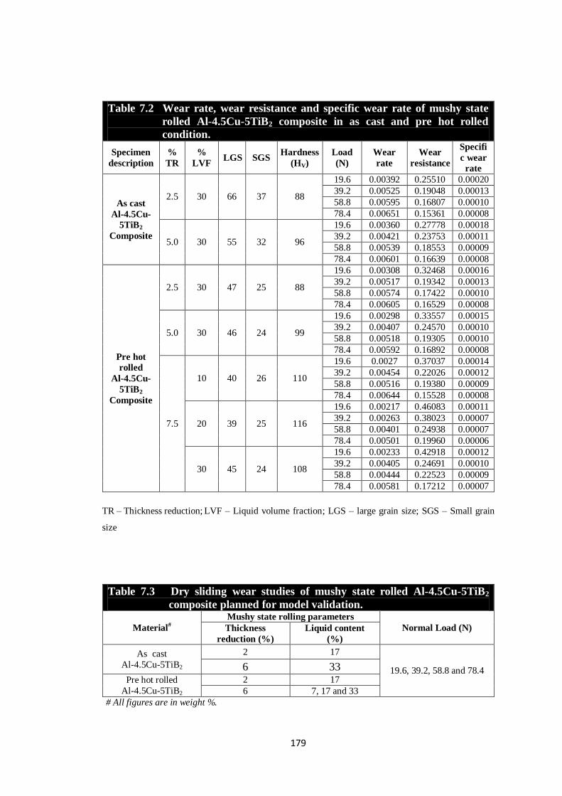
179
Table 7.2 Wear rate, wear resistance and specific wear rate of mushy state
rolled Al-4.5Cu-5TiB2 composite in as cast and pre hot rolled
condition.
Specimen
description
%
TR
%
LVF LGS SGS
Hardness
(HV)
Load
(N)
Wear
rate
Wear
resistance
Specifi
c wear
rate
As cast
Al-4.5Cu-
5TiB2
Composite
2.5 30 66 37 88
19.6 0.00392 0.25510 0.00020
39.2 0.00525 0.19048 0.00013
58.8 0.00595 0.16807 0.00010
78.4 0.00651 0.15361 0.00008
5.0 30 55 32 96
19.6 0.00360 0.27778 0.00018
39.2 0.00421 0.23753 0.00011
58.8 0.00539 0.18553 0.00009
78.4 0.00601 0.16639 0.00008
Pre hot
rolled
Al-4.5Cu-
5TiB2
Composite
2.5 30 47 25 88
19.6 0.00308 0.32468 0.00016
39.2 0.00517 0.19342 0.00013
58.8 0.00574 0.17422 0.00010
78.4 0.00605 0.16529 0.00008
5.0 30 46 24 99
19.6 0.00298 0.33557 0.00015
39.2 0.00407 0.24570 0.00010
58.8 0.00518 0.19305 0.00010
78.4 0.00592 0.16892 0.00008
7.5
10 40 26 110
19.6 0.0027 0.37037 0.00014
39.2 0.00454 0.22026 0.00012
58.8 0.00516 0.19380 0.00009
78.4 0.00644 0.15528 0.00008
20 39 25 116
19.6 0.00217 0.46083 0.00011
39.2 0.00263 0.38023 0.00007
58.8 0.00401 0.24938 0.00007
78.4 0.00501 0.19960 0.00006
30 45 24 108
19.6 0.00233 0.42918 0.00012
39.2 0.00405 0.24691 0.00010
58.8 0.00444 0.22523 0.00009
78.4 0.00581 0.17212 0.00007
TR – Thickness reduction; LVF – Liquid volume fraction; LGS – large grain size; SGS – Small grain
size
Table 7.3 Dry sliding wear studies of mushy state rolled Al-4.5Cu-5TiB2
composite planned for model validation.
Material#
Mushy state rolling parameters
Normal Load (N) Thickness
reduction (%)
Liquid content
(%)
As cast
Al-4.5Cu-5TiB2
2 17
19.6, 39.2, 58.8 and 78.4 6 33 Pre hot rolled
Al-4.5Cu-5TiB2
2 17
6 7, 17 and 33
# All figures are in weight %.
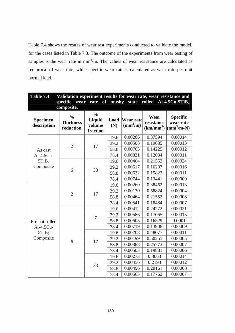
180
Table 7.4 shows the results of wear test experiments conducted to validate the model,
for the cases listed in Table 7.3. The outcome of the experiments from wear testing of
samples is the wear rate in mm3/m. The values of wear resistance are calculated as
reciprocal of wear rate, while specific wear rate is calculated as wear rate per unit
normal load.
Table 7.4 Validation experiment results for wear rate, wear resistance and
specific wear rate of mushy state rolled Al-4.5Cu-5TiB2
composite.
Specimen
description
%
Thickness
reduction
%
Liquid
volume
fraction
Load
(N)
Wear rate
(mm3/m)
Wear
resistance
(km/mm3)
Specific
wear rate
(mm3/m-N)
As cast
Al-4.5Cu-
5TiB2
Composite
2 17
19.6 0.00266 0.37594 0.00014
39.2 0.00508 0.19685 0.00013
58.8 0.00703 0.14225 0.00012
78.4 0.00831 0.12034 0.00011
6 33
19.6 0.00464 0.21552 0.00024
39.2 0.00617 0.16207 0.00016
58.8 0.00632 0.15823 0.00011
78.4 0.00744 0.13441 0.00009
Pre hot rolled
Al-4.5Cu-
5TiB2
Composite
2 17
19.6 0.00260 0.38462 0.00013
39.2 0.00170 0.58824 0.00004
58.8 0.00464 0.21552 0.00008
78.4 0.00541 0.18484 0.00007
6
7
19.6 0.00412 0.24272 0.00021
39.2 0.00586 0.17065 0.00015
58.8 0.00605 0.16529 0.0001
78.4 0.00719 0.13908 0.00009
17
19.6 0.00208 0.48077 0.00011
39.2 0.00199 0.50251 0.00005
58.8 0.00388 0.25773 0.00007
78.4 0.00503 0.19881 0.00006
33
19.6 0.00273 0.3663 0.00014
39.2 0.00456 0.2193 0.00012
58.8 0.00496 0.20161 0.00008
78.4 0.00563 0.17762 0.00007

181
7.6 ANN MODELLING FOR PREDICTION OF WEAR RATE
The aim of the proposed ANN model is to estimate the wear rate(output) as a function
of liquid volume fraction in mushy state Al-4.5Cu-5TiB2 composite, thickness
reduction during mushy state rolling, small and large grain size and hardness (inputs)
when the composite is rolled in mushy state in the as cast and pre hot rolled condition.
Both the inputs and the output were as usual, first normalised within the range 0.1 to
0.9. Neural network training is the process of fitting the NN to the experimental data.
In this process, the synaptic weights connecting each neuron are continuously updated
as each input vector is being presented to the network. The adjustment of these
weights is continued till the mean squared error (MSE) is minimised to a predefined
value or the number of iterations are predefined. The model developed for the present
application is FFNN model with input, output and hidden layer(s). The training of the
model was started with, a single hidden layer with 2 to 15 neurons in hidden layer
(Reddy et al. 2005, 2008). The minimum MSE was set at 0.000001 and the number of
iterations was limited to 300000. The initial values of the learning rate (η) and the
momentum factor (α) were taken as 0.1 and 0.9 respectively for training.
Subsequently, two hidden layers with 2 to 15 neurons in each hidden layer had to be
attempted, as the network failed to converge with single hidden layer prescription for
all combinations attempted with η and α.
As discussed in previous paragraph, single and two hidden layers were attempted to
obtain the least MSE. The learning rate η was varied from 0.1 to 0.9 in steps of 0.05
to start with the training. The learning rate was selected for the model based on the
MSE and 𝐸𝑡𝑟 of the training. Now, the learning rate and the number of hidden layers
were fixed for the model and the momentum factor was varied from 0.1 to 0.9 in steps
of 0.05. Again based on the MSE and 𝐸𝑡𝑟 the momentum was selected and the FFNN
architecture was finalised for analysis of wear rate for the Al-4.5Cu-5TiB2 composite
when rolled from mushy state in the as cast or pre hot rolled condition at various %
thickness reductions and % liquid volume fractions. Sigmoid function was used for
activating the neurons, while back propagation algorithm was used for training the
network.
182
Extensive analysis of various combinations of learning rate parameter and momentum
factor was done to understand the criterion of convergence. It is found to exhibit
convergence with 7 neurons in first and 4 neurons in second hidden layer, with
η=0.25 and α=0.9 after 300000 iterations. Back propagation learning was carried out
starting with these fixed values of η and α. For our model, the best combination was
found to be η=0.5 and α=0.5. Training was stopped when MSE reaches 29 x 10-5
with
Etr = 3.44 x 10⁻⁶
or when the number of iterations reached 2000000, whichever
occurred earlier. Here the targeted MSE was achieved after 18 lakh iterations.
The prediction of wear rate is carried out for the range of experimentation tabulated in
Table 7.2 and 7.4, respectively, for as cast composite and pre hot rolled composite for
the cases listed in Table 7.1 and 7.3. Alligatoring has been reported to be absent
(Herbert 2007, Herbert et al. 2006) for combinations of thickness reductions and
liquid content, while mushy state rolling of Al-4.5Cu-5TiB2 composite in as cast as
well as pre hot rolled condition, at temperature of 632ºC (30% liquid volume fraction)
with thickness reduction of 2.5 and 5 percent in one single pass. Again, in case of pre
hot rolled composite at 7.5% thickness reduction with temperatures corresponding to
10, 20 and 30% liquid volume fraction, alligatoring is not observed. Therefore, the
model is used to predict the values within the range of experimentation where the
phenomenon of alligatoring is absent and to determine the optimal values of wear rate
and the corresponding parameters of the composite yielding optimal wear rate. The
predicted values of wear rate for as cast composite and pre hot rolled composite are
compared with the experimentally obtained values and the same are presented in
Table 7.5 and 7.6 respectively. The relative error in Table 7.5 and 7.6 is calculated
using the following relation:
Relative Error 100*
Exptl
ANNExptl
Value
valueValue (7.7)
It can be seen from Table 7.5 that within the data range used for training the model, a
maximum error of 3.06 % occurs with 2.5 % thickness reduction when composite is
rolled with 30 % liquid volume fraction, for19.6 N normal load. A minimum (i.e.
zero) error occurs when composite is rolled to 5 % thickness reduction from same
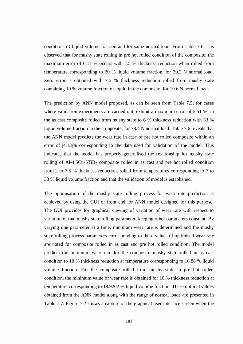
183
conditions of liquid volume fraction and for same normal load. From Table 7.6, it is
observed that for mushy state rolling in pre hot rolled condition of the composite, the
maximum error of 6.17 % occurs with 7.5 % thickness reduction when rolled from
temperature corresponding to 30 % liquid volume fraction, for 39.2 N normal load.
Zero error is obtained with 7.5 % thickness reduction rolled from mushy state
containing 10 % volume fraction of liquid in the composite, for 19.6 N normal load.
The prediction by ANN model proposed, as can be seen from Table 7.5, for cases
where validation experiments are carried out, exhibit a maximum error of 5.51 %, in
the as cast composite rolled from mushy state to 6 % thickness reduction with 33 %
liquid volume fraction in the composite, for 78.4 N normal load. Table 7.6 reveals that
the ANN model predicts the wear rate in case of pre hot rolled composite within an
error of |4.13|% corresponding to the data used for validation of the model. This
indicates that the model has properly generalised the relationship for mushy state
rolling of Al-4.5Cu-5TiB2 composite rolled in as cast and pre hot rolled condition
from 2 to 7.5 % thickness reduction, rolled from temperatures corresponding to 7 to
33 % liquid volume fraction and that the validation of model is established.
The optimisation of the mushy state rolling process for wear rate prediction is
achieved by using the GUI or front end for ANN model designed for this purpose.
The GUI provides for graphical viewing of variation of wear rate with respect to
variation of one mushy state rolling parameter, keeping other parameters constant. By
varying one parameter at a time, minimum wear rate is determined and the mushy
state rolling process parameters corresponding to these values of optimised wear rate
are noted for composite rolled in as cast and pre hot rolled condition. The model
predicts the minimum wear rate for the composite mushy state rolled in as cast
condition to 10 % thickness reduction at temperature corresponding to 16.88 % liquid
volume fraction. For the composite rolled from mushy state in pre hot rolled
condition, the minimum value of wear rate is obtained for 10 % thickness reduction at
temperature corresponding to 18.9202 % liquid volume fraction. These optimal values
obtained from the ANN model along with the range of normal loads are presented in
Table 7.7. Figure 7.2 shows a capture of the graphical user interface screen when the

184
optimum value of wear rate is achieved using the GUI designed with Microsoft
SilverLight API package, in case of as cast Al-4.5Cu-5TiB2 composite rolled in
mushy state.
Table 7.5 Comparison of Wear rate predicted by ANN with the
experimentally obtained values of wear rate for mushy state
rolled Al-4.5Cu-5TiB2 composite in as cast condition.
Specimen
description
%
Thickness
reduction
%
Liquid
volume
fraction
Load
(N)
Wear rate (mm3/m) Relative
Error
(%) Experimental ANN
As cast
Al-4.5Cu-
5TiB2
Composite
2* 17
*
19.6 0.00266 0.00258 3.01
39.2 0.00508 0.00499 1.77
58.8 0.00703 0.00676 3.84
78.4 0.00831 0.00797 4.09
2.5 30
19.6 0.00392 0.0038 3.06
39.2 0.00525 0.0052 0.95
58.8 0.00595 0.0058 2.52
78.4 0.00651 0.0064 1.69
5.0 30
19.6 0.00360 0.0036 0.00
39.2 0.00421 0.0042 0.24
58.8 0.00539 0.0053 1.67
78.4 0.00601 0.006 0.17
6+ 33
*
19.6 0.00464 0.00457 1.51
39.2 0.00617 0.00612 0.81
58.8 0.00632 0.00621 1.74
78.4 0.00744 0.00703 5.51 *validation experiments
Figure 7.2 Screen capture showing optimal value of wear rate

185
Table 7.6 Comparison of Wear rate predicted by ANN with the
experimentally obtained values of wear rate for mushy state
rolled Al-4.5Cu-5TiB2 composite in pre hot rolled condition.
Specimen
description
%
Thickness
reduction
%
Liquid
volume
fraction
Load Wear rate (mm3/m)
Relative
Error
(N) Experimental ANN (%)
Pre hot
rolled
Al-4.5Cu-
5TiB2
Composite
2*
17*
19.6 0.00260 0.00255 1.92
39.2 0.00170 0.00168 1.18
58.8 0.00464 0.00452 2.59
78.4 0.00541 0.00536 0.92
2.5 30
19.6 0.00308 0.00300 2.60
39.2 0.00517 0.00500 3.29
58.8 0.00574 0.00580 -1.10
78.4 0.00605 0.00590 2.48
5 30
19.6 0.00298 0.00300 -0.70
39.2 0.00407 0.00400 1.72
58.8 0.00518 0.00520 -0.40
78.4 0.00592 0.00590 0.34
6*
7*
19.6 0.00412 0.00407 1.21
39.2 0.00586 0.00582 0.68
58.8 0.00605 0.00597 1.32
78.4 0.00719 0.00703 2.23
17*
19.6 0.00208 0.00217 -4.33
39.2 0.00199 0.00195 2.01
58.8 0.00388 0.00395 -1.80
78.4 0.00503 0.00500 0.60
33*
19.6 0.00273 0.00271 0.73
39.2 0.00456 0.00450 1.32
58.8 0.00496 0.00484 2.42
78.4 0.00563 0.00575 -2.13
7.5
10
19.6 0.0027 0.00270 0.00
39.2 0.00454 0.00450 0.88
58.8 0.00516 0.00510 1.16
78.4 0.00644 0.00640 0.62
20
19.6 0.00217 0.00210 3.23
39.2 0.00263 0.00280 -6.5
58.8 0.00401 0.00390 2.74
78.4 0.00501 0.00500 0.2
30
19.6 0.00233 0.00220 5.58
39.2 0.00405 0.00380 6.17
58.8 0.00444 0.00440 1.67
78.4 0.00581 0.00560 3.61 *validation experiments
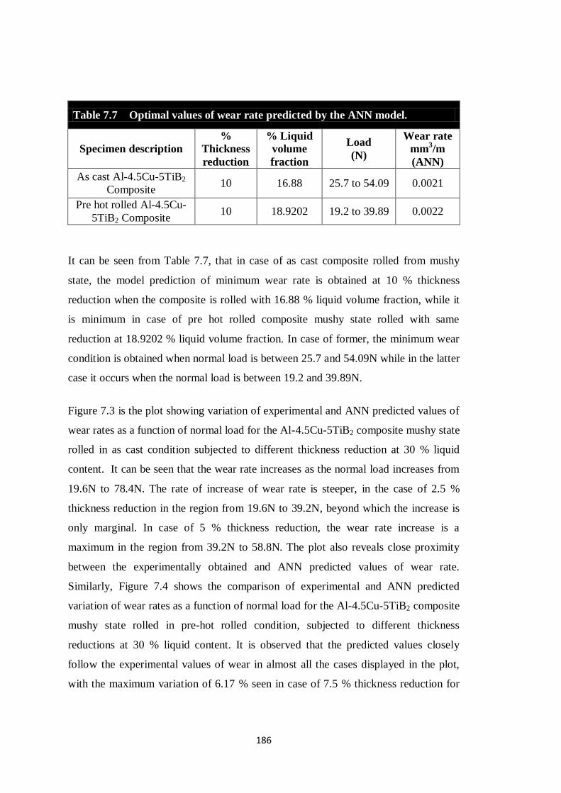
186
Table 7.7 Optimal values of wear rate predicted by the ANN model.
Specimen description
%
Thickness
reduction
% Liquid
volume
fraction
Load
(N)
Wear rate
mm3/m
(ANN)
As cast Al-4.5Cu-5TiB2
Composite 10 16.88 25.7 to 54.09 0.0021
Pre hot rolled Al-4.5Cu-
5TiB2 Composite 10 18.9202 19.2 to 39.89 0.0022
It can be seen from Table 7.7, that in case of as cast composite rolled from mushy
state, the model prediction of minimum wear rate is obtained at 10 % thickness
reduction when the composite is rolled with 16.88 % liquid volume fraction, while it
is minimum in case of pre hot rolled composite mushy state rolled with same
reduction at 18.9202 % liquid volume fraction. In case of former, the minimum wear
condition is obtained when normal load is between 25.7 and 54.09N while in the latter
case it occurs when the normal load is between 19.2 and 39.89N.
Figure 7.3 is the plot showing variation of experimental and ANN predicted values of
wear rates as a function of normal load for the Al-4.5Cu-5TiB2 composite mushy state
rolled in as cast condition subjected to different thickness reduction at 30 % liquid
content. It can be seen that the wear rate increases as the normal load increases from
19.6N to 78.4N. The rate of increase of wear rate is steeper, in the case of 2.5 %
thickness reduction in the region from 19.6N to 39.2N, beyond which the increase is
only marginal. In case of 5 % thickness reduction, the wear rate increase is a
maximum in the region from 39.2N to 58.8N. The plot also reveals close proximity
between the experimentally obtained and ANN predicted values of wear rate.
Similarly, Figure 7.4 shows the comparison of experimental and ANN predicted
variation of wear rates as a function of normal load for the Al-4.5Cu-5TiB2 composite
mushy state rolled in pre-hot rolled condition, subjected to different thickness
reductions at 30 % liquid content. It is observed that the predicted values closely
follow the experimental values of wear in almost all the cases displayed in the plot,
with the maximum variation of 6.17 % seen in case of 7.5 % thickness reduction for

187
the composite pre hot rolled from 30 % liquid volume fraction with 39.2N normal
load.
19.6 39.2 58.8 78.43
4
5
6
7
8
Wea
r ra
te m
m3/k
m
Normal Load (N)
2.5% Reduction (Exptl)
2.5% Reduction (ANN))
5% Reduction (Exptl)
5% Reduction (ANN)
The variation between the experimental values and those predicted by ANN are found
to be the least i.e. 0.34 % in case of composite mushy state rolled with 5 % thickness
reduction, while the maximum variation of 6.17 % is observed in case of pre hot
rolled composite mushy state rolled with 7.5 % thickness reduction from 30 % liquid
volume fraction. Although there appears to be only a minor variation in the wear rates
based on whether mushy state rolling was performed after casting or prior hot rolling,
it is obvious that the wear rates tend to decrease with increase in thickness reduction.
The decrease in wear rate with increase in thickness reduction is more pronounced for
wear tests at lower normal loads, and is less obvious for tests under the normal load of
78.4N. It can be seen from Figure 7.3 and 7.4 that the wear rates of the mushy state
pre hot rolled composites are lower than those rolled as cast, when tested under the
same load.
Figure 7.3 Plots showing comparison of experimental and ANN predicted
variation of wear rates as a function of normal load for the Al-4.5Cu-
5TiB2 composite mushy state rolled in as cast condition subjected to
different thickness reduction at 30 % liquid content.

188
19.6 39.2 58.8 78.42
4
6
8
Wea
r ra
te m
m3/k
m
Normal Load (N)
2.5% Reduction ( Exptl)
2.5% Reduction ( ANN)
5% Reduction ( Exptl)
5% Reduction (ANN)
7.5% Reduction (Exptl)
7.5% Reduction (ANN)
Figure 7.5 shows the comparison of experimental and ANN predicted variation of
wear rates as a function of normal load for the Al-4.5Cu-5TiB2 composite mushy state
rolled in pre-hot rolled condition to 7.5 % thickness reduction with different liquid
volume fractions. For composite rolled from 10 and 30 % volume fractions of liquid,
it can be seen that the wear rate increase is quite steep in the region between 19.6N to
39.2N and between 58.8N and 78.4N normal loads, while it is marginal between
39.2N and 58.8N normal loads. In case of 20% liquid volume content, the increase is
maximum between 39.2N and 58.8N normal loads, while is minimum between 19.6N
to 39.2N normal loads. The path of ANN predicted values of wear rate and that
obtained by experimentation closely follow one another, in case of 2.5 % reduction,
while it differs maximum with 7.5 % reduction. At 39.2N normal load, for mushy
state rolled composite containing 30 % liquid volume fraction, a maximum error of
6.17% is observed from Fig. 7.5. It is obvious from Fig. 7.5, that the wear rate is
minimum in the composite mushy state rolled with 20% volume liquid, followed by
those with samples rolled at temperatures corresponding to 30 and 10 volume percent
liquid in pre hot rolled composite.
Figure 7.4 Plots showing comparison of experimental and ANN predicted
variation of wear rates as a function of normal load for the Al-4.5Cu-
5TiB2 composite mushy state rolled in pre-hot rolled condition
subjected to different thickness reductions at 30 % liquid content.
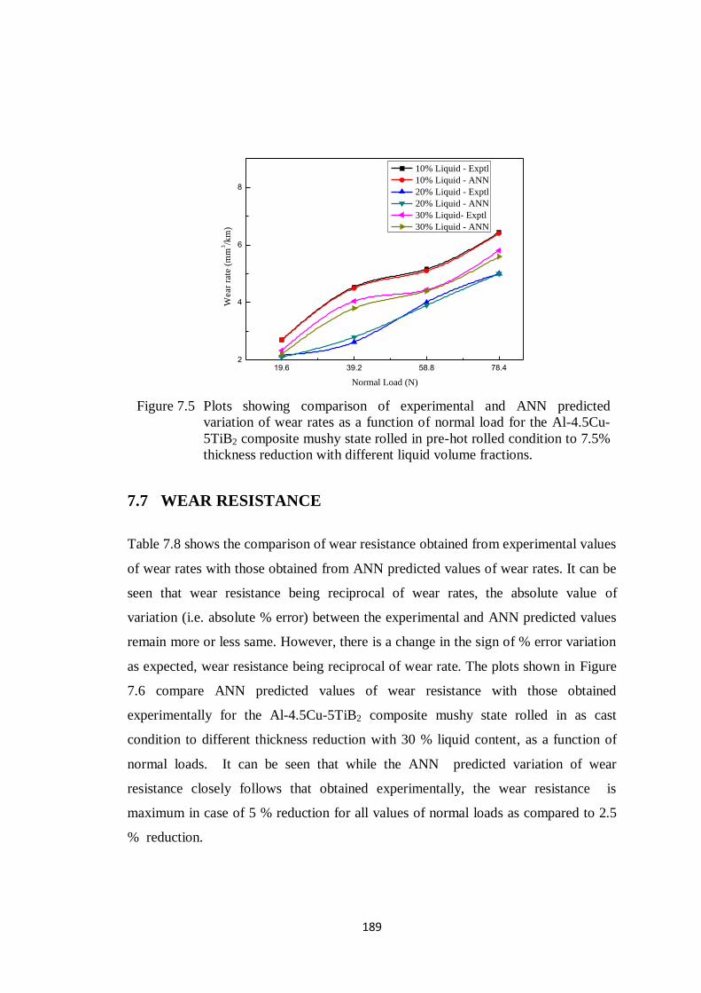
189
19.6 39.2 58.8 78.42
4
6
8
Wea
r ra
te (
mm
3/k
m)
Normal Load (N)
10% Liquid - Exptl
10% Liquid - ANN
20% Liquid - Exptl
20% Liquid - ANN
30% Liquid- Exptl
30% Liquid - ANN
7.7 WEAR RESISTANCE
Table 7.8 shows the comparison of wear resistance obtained from experimental values
of wear rates with those obtained from ANN predicted values of wear rates. It can be
seen that wear resistance being reciprocal of wear rates, the absolute value of
variation (i.e. absolute % error) between the experimental and ANN predicted values
remain more or less same. However, there is a change in the sign of % error variation
as expected, wear resistance being reciprocal of wear rate. The plots shown in Figure
7.6 compare ANN predicted values of wear resistance with those obtained
experimentally for the Al-4.5Cu-5TiB2 composite mushy state rolled in as cast
condition to different thickness reduction with 30 % liquid content, as a function of
normal loads. It can be seen that while the ANN predicted variation of wear
resistance closely follows that obtained experimentally, the wear resistance is
maximum in case of 5 % reduction for all values of normal loads as compared to 2.5
% reduction.
Figure 7.5 Plots showing comparison of experimental and ANN predicted
variation of wear rates as a function of normal load for the Al-4.5Cu-
5TiB2 composite mushy state rolled in pre-hot rolled condition to 7.5%
thickness reduction with different liquid volume fractions.
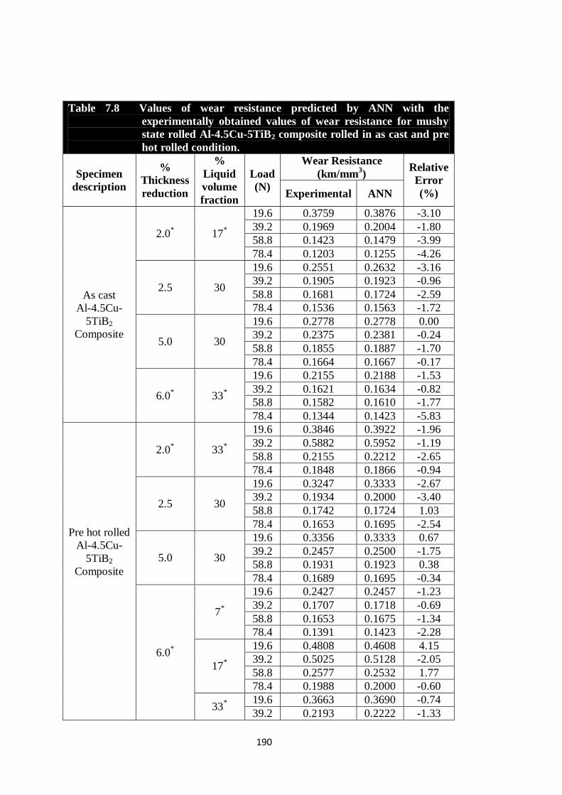
190
Table 7.8 Values of wear resistance predicted by ANN with the
experimentally obtained values of wear resistance for mushy
state rolled Al-4.5Cu-5TiB2 composite rolled in as cast and pre
hot rolled condition.
Specimen
description
%
Thickness
reduction
%
Liquid
volume
fraction
Load
(N)
Wear Resistance
(km/mm3)
Relative
Error
(%) Experimental ANN
As cast
Al-4.5Cu-
5TiB2
Composite
2.0* 17
*
19.6 0.3759 0.3876 -3.10
39.2 0.1969 0.2004 -1.80
58.8 0.1423 0.1479 -3.99
78.4 0.1203 0.1255 -4.26
2.5 30
19.6 0.2551 0.2632 -3.16
39.2 0.1905 0.1923 -0.96
58.8 0.1681 0.1724 -2.59
78.4 0.1536 0.1563 -1.72
5.0 30
19.6 0.2778 0.2778 0.00
39.2 0.2375 0.2381 -0.24
58.8 0.1855 0.1887 -1.70
78.4 0.1664 0.1667 -0.17
6.0* 33
*
19.6 0.2155 0.2188 -1.53
39.2 0.1621 0.1634 -0.82
58.8 0.1582 0.1610 -1.77
78.4 0.1344 0.1423 -5.83
Pre hot rolled
Al-4.5Cu-
5TiB2
Composite
2.0* 33
*
19.6 0.3846 0.3922 -1.96
39.2 0.5882 0.5952 -1.19
58.8 0.2155 0.2212 -2.65
78.4 0.1848 0.1866 -0.94
2.5 30
19.6 0.3247 0.3333 -2.67
39.2 0.1934 0.2000 -3.40
58.8 0.1742 0.1724 1.03
78.4 0.1653 0.1695 -2.54
5.0 30
19.6 0.3356 0.3333 0.67
39.2 0.2457 0.2500 -1.75
58.8 0.1931 0.1923 0.38
78.4 0.1689 0.1695 -0.34
6.0*
7*
19.6 0.2427 0.2457 -1.23
39.2 0.1707 0.1718 -0.69
58.8 0.1653 0.1675 -1.34
78.4 0.1391 0.1423 -2.28
17*
19.6 0.4808 0.4608 4.15
39.2 0.5025 0.5128 -2.05
58.8 0.2577 0.2532 1.77
78.4 0.1988 0.2000 -0.60
33*
19.6 0.3663 0.3690 -0.74
39.2 0.2193 0.2222 -1.33

191
58.8 0.2016 0.2066 -2.48
78.4 0.1776 0.1739 2.09
7.5
10
19.6 0.3704 0.3704 0.00
39.2 0.2203 0.2222 -0.89
58.8 0.1938 0.1961 -1.18
78.4 0.1553 0.1563 -0.63
20 19.6 0.4608 0.4762 -3.33
39.2 0.3802 0.3571 6.07
Pre hot rolled
Al-4.5Cu-
5TiB2
Composite
7.5
20 58.8 0.2494 0.2564 -2.82
78.4 0.1996 0.2000 -0.20
30
19.6 0.4292 0.4545 -5.91
39.2 0.2469 0.2632 -6.58
58.8 0.2252 0.2273 -0.91
78.4 0.1721 0.1786 -3.75 *validation experiments
19.6 39.2 58.8 78.4
0.14
0.21
0.28
Wea
r re
sist
ance
km
/mm
3
Normal Load (N)
2.5% Reduction (as cast - Exptl)
2.5% Reduction (As cast - ANN)
5% Reduction (as cast - Exptl)
5% Reduction (As cast - ANN)
The reduction in wear resistance with increase in normal load is more in case of 2.5 %
reduction as compared to 5 % reduction, quite evident in portion between 19.6N to
39.2N range. Figure 7.7 shows comparison of experimental and ANN predicted
variation of wear resistance as a function of normal load, for the Al-4.5Cu-5TiB2
composite mushy state rolled in pre hot rolled condition to different thickness
reduction at 30 % liquid content. The ANN predicted values and experimentally
obtained values follow each other quite closely. A steep decrease in wear resistance is
Figure 7.6 Plots showing comparison of experimental and ANN predicted
variation of wear resistance as a function of normal load, for the Al-
4.5Cu-5TiB2 composite mushy state rolled in as cast condition to
different thickness reductions with 30 % liquid content.
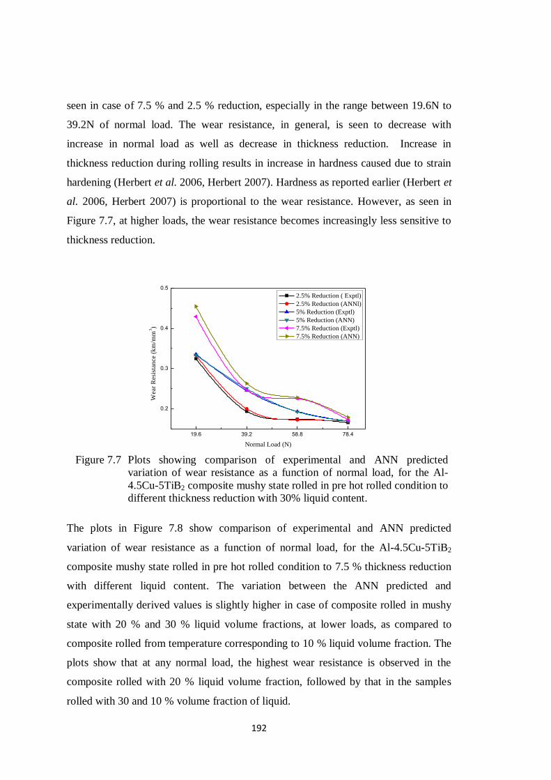
192
seen in case of 7.5 % and 2.5 % reduction, especially in the range between 19.6N to
39.2N of normal load. The wear resistance, in general, is seen to decrease with
increase in normal load as well as decrease in thickness reduction. Increase in
thickness reduction during rolling results in increase in hardness caused due to strain
hardening (Herbert et al. 2006, Herbert 2007). Hardness as reported earlier (Herbert et
al. 2006, Herbert 2007) is proportional to the wear resistance. However, as seen in
Figure 7.7, at higher loads, the wear resistance becomes increasingly less sensitive to
thickness reduction.
19.6 39.2 58.8 78.4
0.2
0.3
0.4
0.5
Wea
r R
esis
tan
ce (
km
/mm
3)
Normal Load (N)
2.5% Reduction ( Exptl)
2.5% Reduction (ANNl)
5% Reduction (Exptl)
5% Reduction (ANN)
7.5% Reduction (Exptl)
7.5% Reduction (ANN)
The plots in Figure 7.8 show comparison of experimental and ANN predicted
variation of wear resistance as a function of normal load, for the Al-4.5Cu-5TiB2
composite mushy state rolled in pre hot rolled condition to 7.5 % thickness reduction
with different liquid content. The variation between the ANN predicted and
experimentally derived values is slightly higher in case of composite rolled in mushy
state with 20 % and 30 % liquid volume fractions, at lower loads, as compared to
composite rolled from temperature corresponding to 10 % liquid volume fraction. The
plots show that at any normal load, the highest wear resistance is observed in the
composite rolled with 20 % liquid volume fraction, followed by that in the samples
rolled with 30 and 10 % volume fraction of liquid.
Figure 7.7 Plots showing comparison of experimental and ANN predicted
variation of wear resistance as a function of normal load, for the Al-
4.5Cu-5TiB2 composite mushy state rolled in pre hot rolled condition to
different thickness reduction with 30% liquid content.
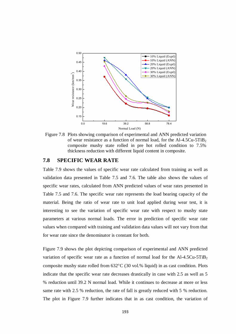
193
0.0 19.6 39.2 58.8 78.4
0.15
0.20
0.25
0.30
0.35
0.40
0.45
0.50
Wea
r re
sist
ance
(k
m/m
m3)
Normal Load (N)
10% Liquid (Exptl)
10% Liquid (ANN)
20% Liquid (Exptl)
20% Liquid (ANN)
30% Liquid (Exptl)
30% Liquid (ANN)
7.8 SPECIFIC WEAR RATE
Table 7.9 shows the values of specific wear rate calculated from training as well as
validation data presented in Table 7.5 and 7.6. The table also shows the values of
specific wear rates, calculated from ANN predicted values of wear rates presented in
Table 7.5 and 7.6. The specific wear rate represents the load bearing capacity of the
material. Being the ratio of wear rate to unit load applied during wear test, it is
interesting to see the variation of specific wear rate with respect to mushy state
parameters at various normal loads. The error in prediction of specific wear rate
values when compared with training and validation data values will not vary from that
for wear rate since the denominator is constant for both.
Figure 7.9 shows the plot depicting comparison of experimental and ANN predicted
variation of specific wear rate as a function of normal load for the Al-4.5Cu-5TiB2
composite mushy state rolled from 632C (30 vol.% liquid) in as cast condition. Plots
indicate that the specific wear rate decreases drastically in case with 2.5 as well as 5
% reduction until 39.2 N normal load. While it continues to decrease at more or less
same rate with 2.5 % reduction, the rate of fall is greatly reduced with 5 % reduction.
The plot in Figure 7.9 further indicates that in as cast condition, the variation of
Figure 7.8 Plots showing comparison of experimental and ANN predicted variation
of wear resistance as a function of normal load, for the Al-4.5Cu-5TiB2
composite mushy state rolled in pre hot rolled condition to 7.5%
thickness reduction with different liquid content in composite.
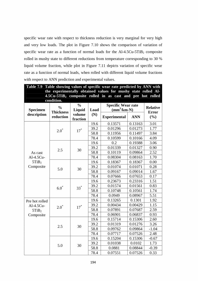
194
specific wear rate with respect to thickness reduction is very marginal for very high
and very low loads. The plot in Figure 7.10 shows the comparison of variation of
specific wear rate as a function of normal loads for the Al-4.5Cu-5TiB2 composite
rolled in mushy state to different reductions from temperature corresponding to 30 %
liquid volume fraction, while plot in Figure 7.11 depicts variation of specific wear
rate as a function of normal loads, when rolled with different liquid volume fractions
with respect to ANN prediction and experimental values.
Table 7.9 Table showing values of specific wear rate predicted by ANN with
the experimentally obtained values for mushy state rolled Al-
4.5Cu-5TiB2 composite rolled in as cast and pre hot rolled
condition.
Specimen
description
%
Thickness
reduction
%
Liquid
volume
fraction
Load
(N)
Specific Wear rate
(mm3/km-N)
Relative
Error
(%) Experimental ANN
As cast
Al-4.5Cu-
5TiB2
Composite
2.0* 17
*
19.6 0.13571 0.13163 3.01
39.2 0.01296 0.01273 1.77
58.8 0.11956 0.11497 3.84
78.4 0.10599 0.10166 4.09
2.5 30
19.6 0.2 0.19388 3.06
39.2 0.01339 0.01327 0.90
58.8 0.10119 0.09864 2.52
78.4 0.08304 0.08163 1.70
5.0 30
19.6 0.18367 0.18367 0.00
39.2 0.01074 0.01071 0.28
58.8 0.09167 0.09014 1.67
78.4 0.07666 0.07653 0.17
6.0* 33
*
19.6 0.23673 0.23316 1.51
39.2 0.01574 0.01561 0.83
58.8 0.10748 0.10561 1.74
78.4 0.0949 0.08967 5.51
Pre hot rolled
Al-4.5Cu-
5TiB2
Composite
2.0* 17
*
19.6 0.13265 0.1301 1.92
39.2 0.00434 0.00429 1.15
58.8 0.07891 0.07687 2.59
78.4 0.06901 0.06837 0.93
2.5 30
19.6 0.15714 0.15306 2.60
39.2 0.01319 0.01276 3.26
58.8 0.09762 0.09864 -1.04
78.4 0.07717 0.07526 2.48
5.0 30
19.6 0.15204 0.15306 -0.67
39.2 0.01038 0.0102 1.73
58.8 0.0881 0.08844 -0.39
78.4 0.07551 0.07526 0.33

195
Pre hot rolled
Al-4.5Cu-
5TiB2
Composite
6.0*
7*
19.6 0.2102 0.20765 1.21
39.2 0.01495 0.01485 0.67
58.8 0.10289 0.10153 1.32
78.4 0.09171 0.08967 2.22
17
19.6 0.10612 0.11071 -4.33
39.2 0.00508 0.00497 2.17
58.8 0.06599 0.06718 -1.80
78.4 0.06416 0.06378 0.59
33
19.6 0.13929 0.13827 0.73
39.2 0.01163 0.01148 1.29
58.8 0.08435 0.08231 2.42
78.4 0.07181 0.07334 -2.13
7.5
10
19.6 0.13776 0.13776 0.00
39.2 0.01158 0.01148 0.86
58.8 0.08776 0.08673 1.17
78.4 0.08214 0.08163 0.62
20
19.6 0.11071 0.10714 3.22
39.2 0.00671 0.00714 -6.41
58.8 0.0682 0.06633 2.74
78.4 0.0639 0.06378 0.19
30
19.6 0.11888 0.11224 5.59
39.2 0.01033 0.00969 6.20
58.8 0.07551 0.07483 0.90
78.4 0.07411 0.07143 3.62 *validation experiments
19.6 39.2 58.8 78.4
0.06
0.12
0.18
Sp
ecif
ic W
ear
Rat
e (m
m3/k
m-N
)
Normal Load (N)
(2.5% Reduction - Exptl)
(2.5% Reduction - ANN)
(5% Reduction - Exptl)
(5% Reduction - ANN)
Figure 7.9 Plots showing comparison of variation of experimental and ANN
predicted values of specific wear rate for the Al-4.5Cu-5TiB2 composite
rolled from mushy state in as cast condition to different thickness
reductions from 632C (30 vol.% liquid).

196
The difference between the ANN predicted and experimental (training data) values of
specific wear rates at different normal loads with various thickness reductions as seen
through Figure 7.10 and from liquid volume fraction in Figure 7.11 is high at low
loads. The variation of specific wear rate is a maximum with 39.2N normal load. The
variation of specific wear rate as seen from Figure 7.10 for the pre hot rolled
composite mushy state rolled with 30 % liquid volume fraction is more at lower loads,
with specific wear rate being minimum at 7.5 % reduction. The specific wear rate is
insensitive to reduction at very high loads, since much of the higher load is utilised in
plastic deformation rather than wear (Herbert 2007, Herbert et al. 2008).
From Figure 7.11, it is seen that, when the pre hot rolled composite is mushy state
rolled with 20 % liquid volume content in composite, the specific wear rate initially
decreases at a rapid rate till 39.2N load. Then it is seen to rise till 58.8N load and then
gradually decreases. In the case of 10 % liquid volume fraction, the decrease is, more
or less, at constant rate till 58.8N and then remains constant.
19.6 39.2 58.8 78.4
0.08
0.12
0.16
Sp
ecif
ic W
ear
Rat
e (m
m3/k
m-N
)
Normal Load (N)
(2.5% Reduction - Exptl)
(2.5% Reduction - ANN)
(5% Reduction - Exptl)
(5% Reduction - ANN)
(7.5% Reduction - Exptl)
(7.5% Reduction - ANN)
Figure 7.10 Plots showing comparison of experimental and ANN predicted
variation of specific wear rate as a function of normal load, for the Al-
4.5Cu-5TiB2 composite rolled from mushy state to different thickness
reductions from 632C (30 vol.% liquid) in pre hot rolled condition.

197
19.6 39.2 58.8 78.40.06
0.09
0.12
0.15
Sp
ecif
ic W
ear
Rat
e (m
m3/k
m-N
)
Normal Load (N)
(10% Liquid - Exptl)
(10% Liquid - ANN)
(20% Liquid - Exptl)
(20% Liquid - ANN)
(30% Liquid - Exptl)
(30% Liquid - ANN)
With 30 % liquid fraction in composite, a steep decrease in specific wear rate is
observed from 39.2N to 58.8N load and thereon it remains practically constant.
From Table 7.7, the minimum (optimal) specific wear rate based on the wear rate
predicted by the model works out to 0.039 mm3/km-N for as cast composite and 0.055
mm3/km-N for pre hot rolled composite rolled from mushy state with 10 % thickness
reduction from temperatures corresponding to 16.88 and 18.92 % volume fraction of
liquid in composite, respectively.
Obvious from the plots in Figure 7.11 also is the fact that specific wear rate is
minimum for composite mushy state rolled from 20 % liquid volume fraction at any
given normal load. This indicates that the load bearing capacity of composite rolled in
mushy state from around 20 % liquid volume fraction is going to yield highest values
for any given normal load situation, which is in agreement with the studies on
hardness in chapter 5.
Figure 7.11 Plots showing comparison of experimental and ANN predicted
variation of specific wear rate as a function of normal load, for the Al-
4.5Cu-5TiB2 composite rolled from mushy state rolled in pre hot rolled
condition to 7.5% thickness reduction, with various liquid contents.

198
7.9 PARAMETRIC STUDIES
7.9.1 Variation of wear rate with normal load at different thickness
reductions.
From plots in Figure 7.4 we can see the variation of wear rates as a function of normal
load for the Al-4.5Cu-5TiB2 composite mushy state rolled in pre-hot rolled condition
subjected to different thickness reductions at 30 % liquid content. It is obvious that
the wear rates decrease with increase in thickness reduction at a given normal load.
The decrease in the wear rate is more pronounced at lower normal loads and is less
obvious at the normal load of 78.4N. It is also seen that for a given thickness
reduction, the wear rate increases as normal load increases.
0.0 19.6 39.2 58.8 78.4
3
4
5
6
Wea
r R
ate
(mm
3/k
m)
Normal Load (N)
Wear Rate
Figure 7.12 shows the variation of wear rate as a function of normal load for mushy
state rolled Al-4.5Cu-5TiB2 composite rolled to 5% thickness reduction with 30%
liquid volume fraction in the composite. It is seen from the figure that the wear rate
increases with the normal load up to 78.4 N. During the wear process, the TiB2
particles in the composite tend to align themselves in the sliding direction. At higher
normal loads, plastic deformation and material removal occurs exposing the TiB2
Figure 7.12 Plot showing the variation of wear rate as a function of normal load
for mushy state rolled Al-4.5Cu-5TiB2 composite rolled to 5%
thickness reduction with 30% liquid volume fraction.
199
particles (Herbert 2007). The material displaced due to cutting or deformation gets
embedded on either side of the cut grooves. As the wear process continues, further
sliding causes both the reinforcement and the matrix to be ironed flat, forming
deformation tongues (Herbert et al. 2008). These deformation tongues then gets
detached as debris resulting in material loss. This explains the reason as to why wear
rate increases as normal load increases, even though it may appear that high normal
loads cause strain induced work hardening and therefore should result in low wear
rates.
7.10 SUMMARY
1. ANN model has been successfully designed and validated to predict the wear
rate, with the experimental data adopted from the studies already carried out on
mushy state rolling of Al-4.5Cu-5TiB2 composite being used for training.
2. The ANN model successfully predicts the values within an overall error of |6.5|
percent for wear rate. However for majority of the predictions, the error is
between ±3.6 percent. The proposed model is validated within a prediction error
of |5.51 |percent within and outside the bounds of data used for training the
model.
3. The wear rate and the specific wear rate are seen to decrease with increase in
thickness reduction as the composite is rolled from mushy state in as cast as
well as in pre hot rolled condition. The variation is more pronounced at lower
values of normal loads. The wear resistance being reciprocal of wear rate, it
increases with thickness reduction during mushy state rolling and again the
maximum variation is observed at lower loads, i.e. at 19.6N and 39.2N.
4. At higher loads, the wear rate, specific wear rate and the wear resistance
variations are insensitive to normal load as compared to that at lower loads.
5. Considering the region of mushy state rolling in which the phenomenon of
alligatoring is absent, the load bearing capacity of composite rolled in pre hot
rolled condition from mushy state containing 20 % liquid volume fraction is
found to be maximum for any given normal load situation. The specific wear
rate for Al-4.5Cu-5TiB2 composite at all normal loads is found to be least when

200
mushy state rolling with 7.5 % thickness reduction is carried out from
temperature corresponding to 20 % liquid volume fraction.

201
Chapter 8
RESULTS AND DISCUSSION (PART V)
RECURRENT NEURAL NETWORK MODELLING
8.1 INTRODUCTION
ANN as a prediction tool has been vastly discussed in chapters 4 through 7 in terms of
formulation, training as well as predictions done by these trained networks to provide
outputs like grain sizes, hardness, strength and wear rate respectively. An attempt has
been made here to develop an improvised neural network solution over the feed
forward neural networks (FFNN). The objective here may mean either better
predictions with equal training time for the model or at least comparable predictions
with a decrease in the time required for training the model.
It is well known (Reddy et al. 2005, Selvakumar et al. 2007) that a major issue in use
of multilayered perceptron or FFNN to be used as a mapping tool is the problem of
the model getting stuck while training, on the gradient descent curve of MSE v/s
weight planes, in areas of local minima. The momentum factor (α) helps the model to
jump over the local cliffs and the training proceeds further, and disturbances are
encountered and overcome, till the training has reached a stage where the neural
network reaches the bottom of the bowl. At this point, the training is stopped and the
MSE of the network is checked with the set error. If the set error is significantly
smaller as compared to the FFNN mean squared error (MSE), the parameters of the
network (η and α) are changed and the training is started all over again. The FFNN
model is trained with various combinations of η and α and also with different
architectures (i.e. number of hidden layers and number of nodes per hidden layer), till
the near about of the set MSE is achieved. As seen in the case of FFNN training for
grain size predictions, the number of epochs required to obtain the set MSE were
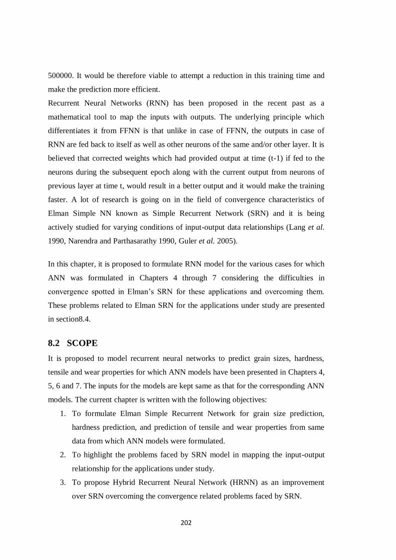
202
500000. It would be therefore viable to attempt a reduction in this training time and
make the prediction more efficient.
Recurrent Neural Networks (RNN) has been proposed in the recent past as a
mathematical tool to map the inputs with outputs. The underlying principle which
differentiates it from FFNN is that unlike in case of FFNN, the outputs in case of
RNN are fed back to itself as well as other neurons of the same and/or other layer. It is
believed that corrected weights which had provided output at time (t-1) if fed to the
neurons during the subsequent epoch along with the current output from neurons of
previous layer at time t, would result in a better output and it would make the training
faster. A lot of research is going on in the field of convergence characteristics of
Elman Simple NN known as Simple Recurrent Network (SRN) and it is being
actively studied for varying conditions of input-output data relationships (Lang et al.
1990, Narendra and Parthasarathy 1990, Guler et al. 2005).
In this chapter, it is proposed to formulate RNN model for the various cases for which
ANN was formulated in Chapters 4 through 7 considering the difficulties in
convergence spotted in Elman’s SRN for these applications and overcoming them.
These problems related to Elman SRN for the applications under study are presented
in section8.4.
8.2 SCOPE
It is proposed to model recurrent neural networks to predict grain sizes, hardness,
tensile and wear properties for which ANN models have been presented in Chapters 4,
5, 6 and 7. The inputs for the models are kept same as that for the corresponding ANN
models. The current chapter is written with the following objectives:
1. To formulate Elman Simple Recurrent Network for grain size prediction,
hardness prediction, and prediction of tensile and wear properties from same
data from which ANN models were formulated.
2. To highlight the problems faced by SRN model in mapping the input-output
relationship for the applications under study.
3. To propose Hybrid Recurrent Neural Network (HRNN) as an improvement
over SRN overcoming the convergence related problems faced by SRN.

203
4. Application of HRNN models to predict grain sizes, hardness, tensile and wear
properties.
5. Analysis of predictions done by HRNN and its comparison with FFNN and
establishing the usefulness of HRNN as a prediction system.
8.3 ELMAN SIMPLE NEURAL NETWORK
In the recent past quite a few Recurrent Neural Network (RNN) architectures have
been studied (Elman 1990, Lang et al. 1990, Frasconi et al. 1992, Giles et al. 1992,
Tesauro et al. 1995). Recurrent networks are neural networks with one or more
feedback loops, in which the loops may be local or global. RNN can be divided into
two broad categories depending on whether the states of the network are guaranteed
and observable or not. Observable state is one in which the state of the network can be
derived by observing only the inputs and outputs (Giles et al. 1992). A model which
falls into this class was proposed by Narendra and Parthasarathy (1990) and had time
delayed outputs as well as inputs fed to a Multi Layer Perceptron (MLP) which
computed the output using the recent state dynamics. However, network having
hidden dynamic states are not observable (Giles et al. 1992). Single layered and multi
layered recurrent networks are being extensively studied in recent times. A typical
single layered RNN was the one proposed by Elman in 1990 (Elman 1990). In this
network, the hidden layer is copied in a virtual or context layer and the feedback is
given back to the same layer along with the next set of inputs in the next time step as
seen in Figure 8.1.
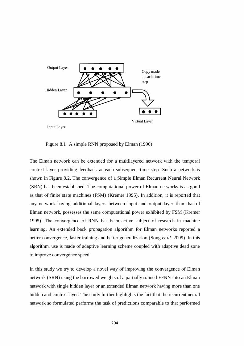
204
The Elman network can be extended for a multilayered network with the temporal
context layer providing feedback at each subsequent time step. Such a network is
shown in Figure 8.2. The convergence of a Simple Elman Recurrent Neural Network
(SRN) has been established. The computational power of Elman networks is as good
as that of finite state machines (FSM) (Kremer 1995). In addition, it is reported that
any network having additional layers between input and output layer than that of
Elman network, possesses the same computational power exhibited by FSM (Kremer
1995). The convergence of RNN has been active subject of research in machine
learning. An extended back propagation algorithm for Elman networks reported a
better convergence, faster training and better generalization (Song et al. 2009). In this
algorithm, use is made of adaptive learning scheme coupled with adaptive dead zone
to improve convergence speed.
In this study we try to develop a novel way of improving the convergence of Elman
network (SRN) using the borrowed weights of a partially trained FFNN into an Elman
network with single hidden layer or an extended Elman network having more than one
hidden and context layer. The study further highlights the fact that the recurrent neural
network so formulated performs the task of predictions comparable to that performed
Input Layer
Output Layer
Virtual Layer
Copy made
at each time
step
Hidden Layer
Figure 8.1 A simple RNN proposed by Elman (1990)
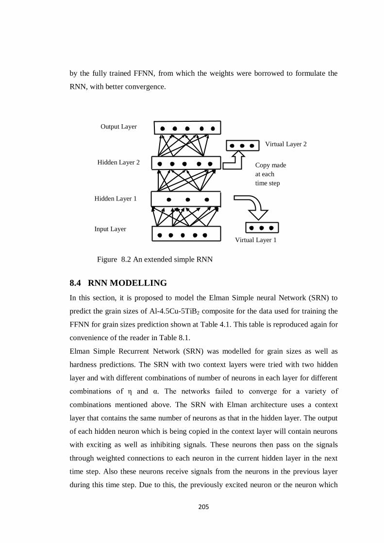
205
by the fully trained FFNN, from which the weights were borrowed to formulate the
RNN, with better convergence.
8.4 RNN MODELLING
In this section, it is proposed to model the Elman Simple neural Network (SRN) to
predict the grain sizes of Al-4.5Cu-5TiB2 composite for the data used for training the
FFNN for grain sizes prediction shown at Table 4.1. This table is reproduced again for
convenience of the reader in Table 8.1.
Elman Simple Recurrent Network (SRN) was modelled for grain sizes as well as
hardness predictions. The SRN with two context layers were tried with two hidden
layer and with different combinations of number of neurons in each layer for different
combinations of η and α. The networks failed to converge for a variety of
combinations mentioned above. The SRN with Elman architecture uses a context
layer that contains the same number of neurons as that in the hidden layer. The output
of each hidden neuron which is being copied in the context layer will contain neurons
with exciting as well as inhibiting signals. These neurons then pass on the signals
through weighted connections to each neuron in the current hidden layer in the next
time step. Also these neurons receive signals from the neurons in the previous layer
during this time step. Due to this, the previously excited neuron or the neuron which
Input Layer
Output Layer
Virtual Layer 1
Copy made
at each
time step
Hidden Layer 2
Hidden Layer 1
Figure 8.2 An extended simple RNN
Virtual Layer 2

206
otherwise would have received a consistent excited signal from previous layer
neurons may get inhibiting signals from the context layer neurons or vice versa. This
probably, does not allow the network to move progressively along the path of
negative gradient on the MSE weight plane. Such a phenomenon is likely to cause an
oscillatory profile on the MSE synaptic weight plane, as witnessed while training the
simple Elman recurrent network.
In order to overcome this shortcoming, various strategies discussed hereunder were
tried:
a. The networks with single hidden layer were trained for the same architectures
mentioned earlier with different combinations of η and α. During training, it
was observed that the network does not converge. The system learns smoothly
during initial phase. But as the training progresses, the network starts
oscillating randomly. Further it is observed that the oscillations decrease and
the network stops learning and MSE reaches a value much higher than the pre
set value which in our case is selected as 0.0001, thus indicating that the
network has not been able to map the input output pattern.
b. In the next instance, the neural network model was modified with each neuron
in the hidden layer giving feedback only to itself. The networks were modelled
for each of the case with similar architectures discussed at (a) above with
different combinations of η and α. It was observed that the networks still
oscillate during training and fail to converge to the pre-set value, but a better
convergence is seen as indicated by slightly lower MSE indicating that
learning capability of the network has slightly improved. But the convergence
obtained is nowhere near the pre-set value of MSE. Hence, this strategy,
though could not be discarded totally, was found to be ineffective.
c. In the modified model stated at (b) above, the weight vectors of a partially
trained ANN with similar architecture were borrowed. The ANN network is
partially trained till a steep negative gradient is identified on the MSE weights
plane indicating the downward movement of MSE. The SNN with single
context layer for second hidden layer, with each neuron giving feedback to
itself in layer 2 is modeled with similar architecture as that of partially trained
ANN. The weight vectors of the SNN from input layer to hidden layer 1,

207
hidden layer1 to hidden layer 2 and from hidden layer 2 to output layer are
replaced by the corresponding weight vectors of partially trained ANN. The
biases for different layers except the context layers of the SNN are also
replaced by the corresponding biases from the partially trained ANN. The
weight vector from the context layer neurons to hidden layer neurons (each
neuron to itself) is taken as a zero vector (unbiased). Once the architecture is
finalized this way, the network is trained. Upon training with the same values
of η and α as that used for partially trained ANN, the SNN so formulated is
found to converge excellently. The convergence of SNNs so modeled is found
to be better as compared to the parent ANNs from which these have been
modelled. The performance of the SNNs modelled from the parent ANNs is
demonstrated using the following cases. The SNN so developed has been
named as Hybrid RNN (HRNN), since the RNN incorporates the weights from
the partially trained FFNN for its processing. Figure 8.3 shows the block
diagram for such an HRNN model formulation.

208
ANN MODEL
(PARTIALLY
TRAINED WITH η
AND α)
HRNN MODEL
TWO LAYERED
ELMAN SNN
Copy weight vectors and biases from
partially trained ANN
Delete context layer connecting HL-1
Add zero weight vector from CL-2 to HL-2 (self
feedback)
Add zero biases to neurons in CL-2
TRAINED
HRNN MODEL
Train with
same η and α
Figure 8.3 Formulation of HRNN model
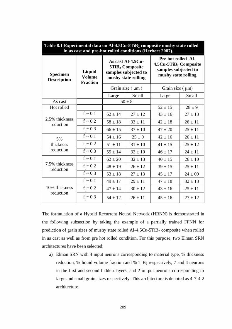
209
The formulation of a Hybrid Recurrent Neural Network (HRNN) is demonstrated in
the following subsection by taking the example of a partially trained FFNN for
prediction of grain sizes of mushy state rolled Al-4.5Cu-5TiB2 composite when rolled
in as cast as well as from pre hot rolled condition. For this purpose, two Elman SRN
architectures have been selected:
a) Elman SRN with 4 input neurons corresponding to material type, % thickness
reduction, % liquid volume fraction and % TiB2 respectively, 7 and 4 neurons
in the first and second hidden layers, and 2 output neurons corresponding to
large and small grain sizes respectively. This architecture is denoted as 4-7-4-2
architecture.
Table 8.1 Experimental data on Al-4.5Cu-5TiB2 composite mushy state rolled
in as cast and pre-hot rolled conditions (Herbert 2007).
Specimen
Description
Liquid
Volume
Fraction
As cast Al-4.5Cu-
5TiB2 Composite
samples subjected to
mushy state rolling
Pre hot rolled Al-
4.5Cu-5TiB2 Composite
samples subjected to
mushy state rolling
Grain size ( μm ) Grain size ( μm)
Large Small Large Small
As cast 50 ± 8
Hot rolled 52 ± 15 28 ± 9
2.5% thickness
reduction
fl ~ 0.1 62 ± 14 27 ± 12 43 ± 16 27 ± 13
fl ~ 0.2 58 ± 18 33 ± 11 42 ± 18 26 ± 11
fl ~ 0.3 66 ± 15 37 ± 10 47 ± 20 25 ± 11
5%
thickness
reduction
fl ~ 0.1 54 ± 16 25 ± 9 42 ± 16 26 ± 11
fl ~ 0.2 51 ± 11 31 ± 10 41 ± 15 25 ± 12
fl ~ 0.3 55 ± 14 32 ± 10 46 ± 17 24 ± 11
7.5% thickness
reduction
fl ~ 0.1 62 ± 20 32 ± 13 40 ± 15 26 ± 10
fl ~ 0.2 48 ± 19 26 ± 12 39 ± 15 25 ± 11
fl ~ 0.3 53 ± 18 27 ± 13 45 ± 17 24 ± 09
10% thickness
reduction
fl ~ 0.1 49 ± 17 29 ± 11 47 ± 18 32 ± 13
fl ~ 0.2 47 ± 14 30 ± 12 43 ± 16 25 ± 11
fl ~ 0.3 54 ± 12 26 ± 11 45 ± 16 27 ± 12

210
b) The second architecture considered for demonstration of HRNN is the one
containing 4 neurons in the input layer, 9 neurons each in the first and second
hidden layer and 2 neurons in the output layer. This architecture is denoted as
4-9-9-2 architecture.
8.4.1 Modelling of HRNN with 4-7-4-2 architecture
The network was trained with learning rate parameter as 0.85 and momentum factor
0.65. Initially the network is trained as an ANN network. Table 8.2 gives the details
of the error in prediction in terms of MSE existing at various stages of network
training. The ANN network converges to a MSE of 0.000362612 after 15 lakh epochs.
To obtain the HRNN, the ANN is now trained till 50000 epochs. The weights of this
ANN are then borrowed in the input weights file for RNN training. The network is
found to oscillate after it reaches a MSE of 0.00205. This happens, probably due to
the fact that the ANN training up to 50000 epochs has not provided sufficient gradient
descent on the MSE weights plane for the Hybrid RNN to further travel in the
direction of negative gradient.
Table 8.2 Variation of MSE with number of epochs Sr. No. Number of epochs MSE
1 1 0.329771
2 100000 0.00467185
3 200000 0.002215
4 300000 0.00153321
5 400000 0.0014147
6 500000 0.00129209
7 600000 0.00105979
8 700000 0.000684544
9 800000 0.00056784
10 1500000 0.000362612
Further to this, the ANN was trained up to 100000 epochs and the weights were
borrowed in the input weights file for RNN training. The results were better than the
first case, but the convergence was found to be slow. After training for 150000
epochs, the MSE is found to be 0.0013. Hence in the next step the ANN is trained for
500000 epochs and subsequently, the weights are borrowed in the input file for RNN

211
training. It was found that after further training of HRNN for around 227000 epochs,
the network converged satisfactorily.
The results of the HRNN predictions of grain sizes after being trained from partially
trained ANN of 4-7-4-2 architecture are compared with the parent ANN having same
architecture after being trained for 1500000 epochs and are listed in Table 8.3. In the
material type column, numeral 1 denotes as cast condition of Al-4.5Cu-5TiB2
composite, while numeral 2 indicates its pre hot rolled condition.
It is seen that the maximum error is |0.58|% at 5 % thickness reduction with 10 %
liquid volume fraction in the as cast composite for small grain size, while for large
grain size it is also at the same location. However in the majority of the cases, the
error with hybrid RNN is within |0.5|%. The HRNN is modelled after borrowing the
weights from partially trained ANN after 5 lakh epochs. Further, the HRNN
converged nicely to a MSE of 0.000362612. Thus to achieve the same degree of
convergence HRNN has consumed 776000 lesser epochs as compared to that of
parent ANN, thus giving a saving of 51.7 % of computational time, which is quite
substantial. Furthermore, the error in predictions too is quite insignificant in
comparison with the parent ANN predictions for the same data.
8.4.2 HRNN with 4-9-9-2 architecture
Here, the network is formulated with 4 input neurons, 9 neurons each in second and
third layer and 2 output neurons. The number of input vectors is taken as 240, just to
emphasize that the number of input vectors has no great bearing on the convergence
of Hybrid RNN. The ANN network is first trained until 50000 epochs and then hybrid
RNN is constructed by borrowing weights of trained ANN. The network is further
trained for 85000 epochs as it gave the same MSE as that of parent ANN when trained
to 277356 epochs.

212
Table 8.3 Comparison of grain sizes by ANN and Hybrid RNN after 2.24 lakh
epochs of HRNN and 15 lakh epochs of ANN
Sr.
No.
Input Output
Mat/
Pro.
%
TR*
%LVF**
Grain Sizes
Large Small
ANN RNN
% Error
over
ANN
ANN RNN
% Error
over
ANN
1 1 2.5 10 61.21 61.10 0.190139 28.12 28.03 0.307209
2 1 2.5 20 58.33 58.32 0.026569 33.37 33.36 0.018879
3 1 2.5 30 66.01 65.97 0.054232 36.22 36.2 0.064047
4 1 5 10 54.53 54.23 0.54335 23.87 23.73 0.578546
5 1 5 20 50.53 50.52 0.023745 28.84 28.84 0.004854
6 1 5 30 55.64 56.66 -1.83923 29.86 29.86 0.024776
7 1 7.5 10 61.72 61.62 0.168968 31.65 31.58 0.21482
8 1 7.5 20 47.58 47.58 0.007986 26.49 26.49 -0.01057
9 1 7.5 30 53.17 53.13
0.060559 27.75 27.75 0.022696
10 1 10 10 48.36 48.36 0.004135 31.30 31.30 0.002236
11 1 10 20 48.28 48.27 0.010149 28.31 28.31 -0.00671
12 1 10 30 52.63 52.60 0.057751 27.88 27.87 0.020085
13 2 2.5 10 43.25 43.21 0.085769 27.89 27.88 0.047323
14 2 2.5 20 43.18 43.19 -0.01343 27.26 27.27 -0.0154
15 2 2.5 30 47.31 47.30 0.018177 26.77 26.77 -0.00486
16 2 5 10 41.21 41.20 0.032511 26.38 26.37 0.013267
17 2 5 20 41.05 41.05 -0.02168 25.33 25.34 -0.02566
18 2 5 30 44.99 44.99 0.021111 25.37 25.38 -0.01025
19 2 7.5 10 41.79 41.79 -0.00885 26.30 26.30 -0.01369
20 2 7.5 20 39.70 39.71 -0.0267 24.06 24.07 -0.03282
21 2 7.5 30 44.71 44.70 0.022366 24.92 24.92 -0.01163
22 2 10 10 46.25 46.25 -0.00757 30.49 30.49 -0.00394
23 2 10 20 42.35 42.35 -0.01983 26.46 26.46 -0.02381
24 2 10 30 45.59 45.58 0.025658 25.61 25.61 -0.00781
% TR* - % ThicknessReduction % LVF** - %Liquid Volume Fraction
1 – as cast 2 – Pre hot rolled Mat – Material Pro. - Process
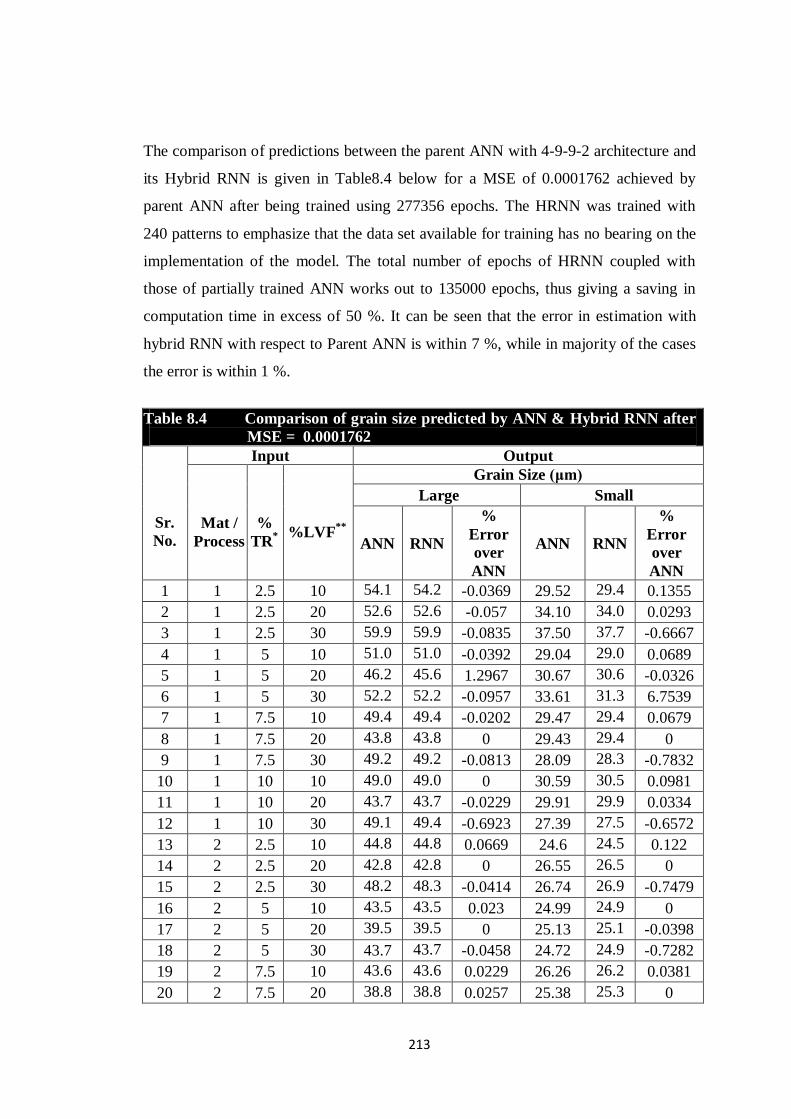
213
The comparison of predictions between the parent ANN with 4-9-9-2 architecture and
its Hybrid RNN is given in Table8.4 below for a MSE of 0.0001762 achieved by
parent ANN after being trained using 277356 epochs. The HRNN was trained with
240 patterns to emphasize that the data set available for training has no bearing on the
implementation of the model. The total number of epochs of HRNN coupled with
those of partially trained ANN works out to 135000 epochs, thus giving a saving in
computation time in excess of 50 %. It can be seen that the error in estimation with
hybrid RNN with respect to Parent ANN is within 7 %, while in majority of the cases
the error is within 1 %.
Table 8.4 Comparison of grain size predicted by ANN & Hybrid RNN after
MSE = 0.0001762
Sr.
No.
Input Output
Mat /
Process
%
TR*
%LVF**
Grain Size (μm)
Large Small
ANN RNN
%
Error
over
ANN
ANN RNN
%
Error
over
ANN
1 1 2.5 10 54.1
9
54.2
1 -0.0369 29.52 29.4
8 0.1355
2 1 2.5 20 52.6
6
52.6
9 -0.057 34.10 34.0
9 0.0293
3 1 2.5 30 59.9
0
59.9
5 -0.0835 37.50 37.7
5 -0.6667
4 1 5 10 51.0
5
51.0
7 -0.0392 29.04 29.0
2 0.0689
5 1 5 20 46.2
7
45.6
7 1.2967 30.67 30.6
8 -0.0326
6 1 5 30 52.2
4
52.2
9 -0.0957 33.61 31.3
4 6.7539
7 1 7.5 10 49.4
0
49.4
1 -0.0202 29.47 29.4
5 0.0679
8 1 7.5 20 43.8
1
43.8
1 0 29.43 29.4
3 0
9 1 7.5 30 49.2
3
49.2
7 -0.0813 28.09 28.3
1 -0.7832
10 1 10 10 49.0
1
49.0
1 0 30.59 30.5
6 0.0981
11 1 10 20 43.7
2
43.7
3 -0.0229 29.91 29.9
0 0.0334
12 1 10 30 49.1
1
49.4
5 -0.6923 27.39 27.5
7 -0.6572
13 2 2.5 10 44.8
5
44.8
2 0.0669 24.6 24.5
7 0.122
14 2 2.5 20 42.8
5
42.8
5 0 26.55 26.5
5 0
15 2 2.5 30 48.2
8
48.3
0 -0.0414 26.74 26.9
4 -0.7479
16 2 5 10 43.5
4
43.5
3 0.023 24.99 24.9
9 0
17 2 5 20 39.5
4
39.5
4 0 25.13 25.1
4 -0.0398
18 2 5 30 43.7 43.7
2 -0.0458 24.72 24.9
0 -0.7282
19 2 7.5 10 43.6
7
43.6
6 0.0229 26.26 26.2
5 0.0381
20 2 7.5 20 38.8
6
38.8
5 0.0257 25.38 25.3
8 0

214
21 2 7.5 30 42.8
7
42.8
6
0.0233 25.04 25.0
4 0
22 2 10 10 44.9
3
44.9
1 0.0445 28.19 28.1
7 0.0709
23 2 10 20 40.3
2
40.3
1 0.0248 26.95 26.9
4 0.0371
24 2 10 30 44.3
0
44.3
2 -0.0451 26.661
2
26.7
7 -0.4081
% TR* - % Thickness Reduction Mat - Material % LVF** - % Liquid Volume Fraction
8.4.3 Statistical testing of RNN model predictions
In this section it is proposed to assess statistically the predictions of RNN. To be able
to perform the statistical testing, the predictions of parent ANN and HRNN are
compared with the actual values of grain sizes as well as amongst themselves. The
resulting errors are then statistically checked using the following statistical tools.
In the statistical analysis carried out (refer APENDIX III), the following three tests
were being used:
1. Testing the quality of two means using the two sample student_t test.
2. Testing whether the population has standard mean normal distribution using
one sample Kolmogorov – Smirnov test.
3. Testing if the two populations belong to the same continuous distribution
using two samples Kolmogorov – Smirnov test.
K-S test for single sample and two samples were used to test the normality of the
distribution of errors in prediction of large and small grain sizes as predicted by ANN
and HRNN with different architectures mentioned at 8.4.1 and 8.4.2 above. The errors
were calculated between the predicted values obtained from ANN and actual values
and also between the predicted values obtained from HRNN and actual values. A third
type of error was calculated between the values predicted by HRNN and ANN.
Further to this, two sample student t_test was performed for testing the equality of
means of populations representing the errors between ANN and HRNN predictions
for large grain size and small grain size. To be able to analyze the data more
meaningfully, the population of errors was divided into errors in predictions for as
cast Al-4.5Cu-5TiB2 composite and pre hot rolled Al-4.5Cu-5TiB2 composite. For the
215
purpose of statistical analysis of the performance of HRNN with the fully trained
parent ANN, the following terminology of errors is defined.
a. Error (a): Error in prediction of large grain size and small grain size by ANN
with 4-7-4-2 architecture over the target values.
b. Error (b); Error in prediction of large grain size and small grain size by HRNN
with 4-7-4-2 architecture over the target values.
c. Error(c); Error in prediction of large grain size and small grain size by ANN
with 4-9-9-2 architecture over the target values.
d. Error (d); Error in prediction of large grain size and small grain size by HRNN
with 4-9-9-2 architecture over the target values.
8.4.3.1 Testing of equality of means
Table 8.5 gives the results of the two sample student t test performed on the error
population deduced from the predictions of HRNN and ANN with different
architectures. It can be seen that the means of the errors from HRNN prediction
populations are comparable to the mean values of populations obtained from ANN
predictions for similar architectures. Furthermore, the standard deviation values also
are comparable for similar architectures of ANN and HRNN.
In testing of hypothesis, the strength of the conclusion is decided by level of
significance α. The popular value of α is 0.05. The decision about the test is based on
the value of the test statistics obtained from the sample and the benchmark value of
appropriate test statistics obtained from the tables, using α and degrees of freedom
(which can always be obtained from the size of sample).
However, while reporting the conclusion, the value of test statistic obtained is never
reported. As a result, closeness of this test value obtained from the sample and the
bench mark value of appropriate test statistic also does not get reported.
This difficulty is overcome when p value of test is indicated. The p value indicates the
probability of obtaining a test statistic as extreme as the one actually observed,
assuming that the null hypothesis is true.

216
Table 8.5 Results of two sample student t test.
Architecture
Large grain size (HRNN)
Error Population 1
Small grain size (ANN)
Error Population 2
As cast Pre hot rolled As cast Pre hot rolled
4-7-4-2 Mean: -0.0334 0.0034 -0.0136 0.0047
St.dev: 0.0401 0.0068 0.0244 0.0026
4-9-9-2 Mean: -0.0201 -0.0134 -0.0053 0.0052
St.dev: 0.0099 0.0073 0.0022 0.0015
St. dev = standard deviation
8.4.3.2 Testing errors for standard normal distribution
Testing of the error distribution of ANN and HRNN predictions over target values of
large grain sizes and small grain sizes was carried out using one sample Kolmogorov –
Smirnov test. For this purpose, the various errors as defined in section 8.4.3 were
considered. The results of the test are tabulated in Table 8.6. It can be seen that with a
significance level of 5% (α = 0.05), used for the test, all the error distributions i.e.
Error (a) to Error (d) are accepted as standard normal distributions. Table 8.6 gives
the p values for all the error distributions. H0 indicates that the error population has
normal distribution, while H1 indicates that the error population does not have normal
distribution.
Table 8.6 Results of one sample Kolmogorov – Smirnov test.
Test No. α Errors p value
Conclusion Large grain size Small grain size
A 0.05 Error(a) 0.7366 0.8174 H0:
Accepted
B 0.05 Error(b) 0.8174 0.0940 H0:
Accepted
C 0.05 Error(c) 0.1879 0.1860 H0:
Accepted
D 0.05 Error(d) 0.1983 0.1901 H0:
Accepted

217
8.4.3.3 Testing of equality of continuous distributions using two samples
Kolmogorov – Smirnov test
Here the distribution of errors between ANN predicted values for grain sizes using 4-
7-4-2 and 4-9-9-2 architectures over target values of grain sizes were checked with
their counterparts predicted by HRNN with similar architectures, for equality. The
results of this test are presented in Table 8.7. H0 indicates that the two error
distributions under test are equal, while H1 indicates that they are not equal.
Table 8.7 Results of two samples Kolmogorov – Smirnov test.
Test No. Population of
errors tested α
p value
Conclusion Large grain
size
Small grain
size
A Error(a) v/s Error(b) 0.05 0.9999 0.1094 H0:
Accepted
B Error(c) v/s Error(d) 0.05 0.9999 0.9999 H0:
Accepted
From the discussions carried out in this and the previous two sections, namely 8.4.3.1
and 8.4.3.2, it is seen that the predictions done by the trained parent ANN and the
HRNN formulated from the partially trained parent ANN are statistically equivalent.
This lends us with an important decision making criterion to select HRNN as a
possible mathematical model to compliment ANN modelling using FFNN
architectures, especially when the training of FFNN becomes a cumbersome process
in terms of problems related to its convergence. Thus the equivalence of HRNN
model with ANN model is well established, in addition to lesser training time for
HRNNs.
Discussion on HRNN models for prediction of different parameters of mushy state
rolling of Al-4.5Cu-5TiB2 composite and their comparison with the corresponding
ANN models are presented below.

218
8.5 MODELLING OF HRNN FOR PREDICTION OF GRAIN
SIZES
The hybrid RNN will now be modelled afresh for prediction of grain sizes using
architecture similar to that which was used for ANN model for grain size predictions.
In other words, the HRNN now proposed to be modelled is formulated by borrowing
the weights from a partially trained parent ANN used in chapter 4 for prediction of
grain sizes. The architecture used for the parent ANN of chapter 4 had the designation
3-7-4-2. This ANN was trained with η = 0.85 and α = 0.65 till steep downward
gradient is witnessed on the MSE weights plane, which can be witnessed from the
programme execution on the computer screen. Such steep decrease was observed at
500000 lakh epochs where the MSE was found to be 0.00128. At this point HRNN
with same architecture was formulated by borrowing the weights from parent ANN.
The weights in the context layers were kept as zero (i.e. unbiased). The network was
then trained with same values of η and α. After training for a further 2 lakh iterations,
the network converged very well with a MSE of 0.000236682.
8.5.1 Comparison of prediction of grain sizes by ANN and HRNN for mushy
state rolled as cast Al-4.5Cu-5TiB2 composite
Table 8.8 lists down the values of large grain sizes and small grain sizes (μm)
predicted by ANN and HRNN respectively along with the error in prediction of grain
sizes by HRNN over ANN.
Table 8.8 ANN & HRNN comparison of grain sizes for Al-4.5Cu-5TiB2
composite rolled in mushy state in as cast condition.
Sr.
No.
Input Output
%
Th.
Red
%Liq.
Vol.
Fraction
Grain Sizes (μm)
Large Small
ANN RNN %
Error ANN RNN % Error
1 0 0 49.9944 49.99 0.0088 49.8947 49.89 0.0094
2 2 17 61.5498 61.48 0.1134 30.2633 30.26 0.0109
3 2.5 5 66.7204 66.64 0.1205 27.2855 27.31 -0.0898
4 2.5 10 60.7838 60.7 0.1379 27.4532 27.46 -0.0248
5 2.5 20 59.338 59.28 0.0977 33.8438 33.82 0.0703
6 2.5 30 64.776 64.72 0.0865 35.8221 35.84 -0.05

219
7 2.5 35 66.6396 66.64 -0.0006 30.0602 30.06 0.0007
8 5 5 69.5573 69.49 0.0968 27.2271 27.25 -0.0841
9 5 10 55.6733 55.59 0.1496 25.8852 25.9 -0.0572
10 5 20 49.9853 49.95 0.0706 29.4956 29.48 0.0529
11 5 30 55.5784 55.53 0.0871 33.4465 33.45 -0.0105
12 5 35 61.1633 61.17 -0.011 28.4914 28.48 0.04
13 6 7 66.9744 66.89 0.126 28.032 28.01 0.0785
14 6 17 48.496 48.47 0.0536 25.793 25.8 -0.0271
15 6 33 56.3759 56.38 -0.0073 28.2583 28.25 0.0294
16 7.5 5 71.394 71.39 0.0056 32.4656 32.49 -0.0752
17 7.5 10 61.5025 61.45 0.0854 30.92 30.91 0.0323
18 7.5 20 47.299 47.23 0.1459 27.3059 27.26 0.1681
19 7.5 30 52.922 52.91 0.0227 26.4012 26.4 0.0045
20 7.5 35 56.2987 56.32 -0.0378 24.2107 24.19 0.0855
21 10 5 48.5162 48.52 -0.0078 30.514 30.52 -0.0197
22 10 10 49.2457 49.26 -0.029 30.5459 30.54 0.0193
23 10 20 48.0792 48.07 0.0191 30.494 30.49 0.0131
24 10 30 54.1504 54.17 -0.0362 26.2361 26.22 0.0614
25 10 35 59.3253 59.36 -0.0585 21.9236 21.88 0.1989
26 11.5 17 47.0124 47 0.0264 30.4498 30.44 0.0322
27 12.5 5 46.7048 46.69 0.0317 30.4369 30.43 0.0227
28 12.5 10 46.7111 46.69 0.0452 30.4372 30.44 -0.0092
29 12.5 20 46.7789 46.76 0.0404 30.44 30.43 0.0329
30 12.5 30 46.8364 46.83 0.0137 30.391 30.38 0.0362
31 12.5 35 48.8614 48.87 -0.0176 29.249 29.23 0.065
It can be seen from Table 8.8 that the maximum error of 0.1496 % in prediction is
observed in the as cast composite. This maximum error is observed when composite is
mushy state rolled with 5 % thickness reduction from temperature corresponding to
10 % liquid volume fraction. The lowest error in large grain size prediction is
observed as -0.0585 % with 10 % thickness reduction when rolled at temperature
corresponding to 35 % volume fraction of liquid. A maximum error of 0.1989 % is
witnessed in case of small grain size prediction when the composite is mushy state
rolled with 35 % liquid volume fraction to 10% thickness reduction. A minimum error
of -0.0898 % occurs in small grain size predictions at 2.5 % thickness reduction rolled
from temperature corresponding to 5 % volume fraction of liquid.

220
Table 8.9 Comparison of grain sizes predictions by ANN and HRNN for
Al-4.5Cu-5TiB2 composite rolled in mushy state in Pre Hot
Rolled condition.
Sr.
No.
Input Output
%
Th.
Red
%Liq.
Vol.
Fraction
Grain Sizes (μm)
Large Small
ANN RNN %
Error ANN RNN
%
Error
1 0 0 51.985 51.97 0.0289 28.51
47 28.53 -0.0537
2 2 17 42.619 42.62 -0.0023 25.46
11 25.47 -0.035
3 2.5 5 43.635 43.63 0.0115 25.40
47 25.41 -0.0209
4 2.5 10 42.282 42.28 0.0047 25.38
52 25.39 -0.0189
5 2.5 20 42.475 42.48 -0.0118 25.52
4 25.53 -0.0235
6 2.5 30 47.616 47.64 -0.0504 24.55
84 24.57 -0.0472
7 2.5 35 47.731 47.78 -0.1027 23.81
35 23.82 -0.0273
8 5 5 42.016 42.02 -0.0095 25.27
64 25.28 -0.0142
9 5 10 40.908 40.91 -0.0049 25.23
52 25.24 -0.019
10 5 20 40.675 40.68 -0.0123 25.30
02 25.31 -0.0387
11 5 30 45.474 45.51 -0.0792 24.34
93 24.37 -0.085
12 5 35 46.701 46.76 -0.1263 23.60
59 23.62 -0.0597
13 6 7 41.136 41.14 -0.0097 25.24
74 25.26 -0.0499
14 6 17 40.569 40.58 -0.0271 25.22
67 25.23 -0.0131
15 6 33 46.718 46.77 -0.1113 23.80
71 23.82 -0.0542
16 7.5 5 47.096 47.08 0.034 30.34
06 30.33 0.0349
17 7.5 10 40.752 40.76 -0.0196 25.33
74 25.34 -0.0103
18 7.5 20 40.501 40.51 -0.0222 25.21
15 25.22 -0.0337
19 7.5 30 45.184 45.21 -0.0575 24.37
12 24.39 -0.0771
20 7.5 35 46.729 46.79 -0.1305 23.51 23.53 -0.0851
21 10 5 46.703 46.69 0.0278 30.43 30.42 0.0329
22 10 10 46.687 46.66 0.0578 30.41
45 30.40 0.0477
23 10 20 42.093 42.05 0.1022 26.52
43 26.49 0.1293
24 10 30 44.7634 44.78 -0.0371 26.82 26.83 -0.0373
25 10 35 45.7546 45.81 -0.1211 24.42
27 24.44 -0.0708
26 11.5 17 46.6799 46.66 0.0426 30.41
81 30.41 0.0266
27 12.5 5 46.699 46.68 0.0407 30.43
25 30.42 0.0411
28 12.5 10 46.692 46.67 0.0471 30.42
88 30.42 0.0289
29 12.5 20 46.7 46.67 0.0642 30.43
59 30.41 0.0851
30 12.5 30 46.716 46.70 0.0342 30.42
5 30.42 0.0164
31 12.5 35 46.526 46.53 -0.0086 29.60
5 29.6 0.0169

221
8.5.2 Comparison of prediction of grain sizes by ANN and HRNN for mushy
state rolled Al-4.5Cu-5TiB2 composite in pre hot rolled condition
Table 8.9 shows the values of large and small grain sizes predicted by ANN and
HRNN for pre hot rolled composite rolled in mushy state to different thickness
reductions ranging from 2 to 12.5 % and from mushy state temperatures
corresponding to 5 to 35 % volume fractions of liquid in the composite. From Table
8.9, it can be seen that maximum error of 0.1022 % occurs in prediction of large grain
size when pre hot rolled composite is rolled to 10 % thickness reduction in mushy
state with 20 % volume fraction of liquid in the pre hot rolled composite. Minimum
error in prediction of -0.1305 % is witnessed with 7.5 % thickness reduction when
mushy state rolled from 35 % liquid volume content in the composite. In case of small
grain size prediction by HRNN, maximum and minimum errors of prediction of
HRNN over ANN are 0.1293 and -0.0851 % at 10 and 7.5 % thickness reduction and
corresponding to 20 and 35 % liquid volume fractions respectively.
From Table 8.8 it is seen that the HRNN model predicts grain sizes for as cast
composite rolled from mushy state within an error of |0.2|% over ANN model
predictions. Also Table 8.9 shows that the HRNN model predicts large and small
grain sizes within an error of |0.1305|% over corresponding ANN model predictions.
Moreover, the time required for training is significantly lower than that for ANN
model. Thus the ANN model can be replaced by a HRNN model, especially in cases
where there is dynamic feedback of changing process parameters usually associated
with smart manufacturing systems.
8.6 MODELLING OF HRNN FOR PREDICTION OF HARDNESS
In chapter 5, modelling of ANN for prediction of hardness of mushy state rolled Al-
4.5Cu-5TiB2 composite was discussed. The architecture of the four layer perceptron
used for prediction of hardness was 5-5-3-1. It was found to converge satisfactorily
after 325000 iterations with an MSE of 0.0000975. The formulation of HRNN was
done from a parent ANN containing 5 input nodes (corresponding to material type, %
thickness reduction, % liquid volume fraction, large grain size and small grain size of
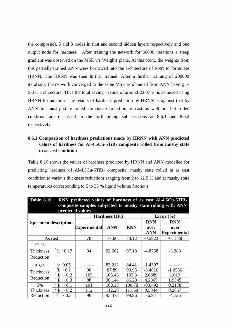
222
the composite), 5 and 3 nodes in first and second hidden layers respectively and one
output node for hardness. After training the network for 50000 iterations a steep
gradient was observed on the MSE v/s Weights plane. At this point, the weights from
this partially trained ANN were borrowed into the architecture of RNN to formulate
HRNN. The HRNN was then further trained. After a further training of 200000
iterations, the network converged to the same MSE as obtained from ANN having 5-
5-3-1 architecture. Thus the total saving in time of around 23.07 % is achieved using
HRNN formulation. The results of hardness prediction by HRNN as against that by
ANN for mushy state rolled composite rolled in as cast as well pre hot rolled
condition are discussed in the forthcoming sub sections at 8.6.1 and 8.6.2
respectively.
8.6.1 Comparison of hardness predictions made by HRNN with ANN predicted
values of hardness for Al-4.5Cu-5TiB2 composite rolled from mushy state
in as cast condition
Table 8.10 shows the values of hardness predicted by HRNN and ANN modelled for
predicting hardness of Al-4.5Cu-5TiB2 composite, mushy state rolled in as cast
condition to various thickness reductions ranging from 2 to 12.5 % and at mushy state
temperatures corresponding to 5 to 35 % liquid volume fractions.
Table 8.10 RNN predicted values of hardness of as cast Al-4.5Cu-5TiB2
composite samples subjected to mushy state rolling with ANN
predicted values
Specimen description
Hardness (Hv) Error (%)
Experimental ANN RNN
RNN
over
ANN
RNN
over
Experimental
As cast 78 77.66 78.12 -0.5923 -0.1538
*2 %
Thickness
Reduction
*f1~ 0.17 94 92.662 97.18 -4.8758 -3.383
2.5%
Thickness
Reduction
fl~ 0.05 ------- 83.212 84.41 -1.4397 ------- afl ~ 0.1 90 87.89 90.95 -3.4816 -1.0556
a fl ~ 0.2 105 105.45 103.3 2.0389 1.619
a fl ~ 0.3 88 90.144 86.28 4.2865 1.9545
5%
thickness
reduction
a fl ~ 0.1 101 100.13 100.78 -0.6492 0.2178
Thickness
reduction
a fl ~ 0.2 112 112.28 111.68 0.5344 0.2857
Reduction afl ~ 0.3 96 93.473 99.96 -6.94 -4.125

223
*6%
Thickness
reduction
*f1~ 0.07 89 88.22 92.18 -4.4888 -3.573
*f1~0.17 114 112.18 112.06 0.107 1.7018
*f1~0.33 92 92.431 84.11 9.0024 8.5761
7.5%
Thickness
Reduction
afl ~ 0.1 105 104.63 107.13 -2.3894 -2.0286
afl ~ 0.2 117 116.31 117.10 -0.6792 -0.0855
afl ~ 0.3 103 101.05 102.17 -1.1084 0.8058
10%
Thickness
Reduction
afl ~ 0.1 118 117.15 115.6 1.3231 2.0339
afl ~ 0.2 121 121.14 121.59 -0.3715 -0.4876
afl ~ 0.3 106 104.63 106.99 -2.2556 -0.934
* 11.5%
Thickness
Reduction
*f1 ~ 0.17 123 122.4 123.05 -0.531 -0.0407
12.5%
Thickness
Reduction
fl ~ 0.05 ------- 117.79 116.37 1.2055 ------- fl ~ 0.1 ------- 121.72 120.37 1.1091 ------- f l~ 0.2 ------- 122.86 124.71 -1.5058 ------- fl ~ 0.3 ------- 102.3 118.54 -
15.8749
------- fl ~ 0.35 ------- 103.73 102.44 1.2436 -------
It can be seen from Table 8.10 that the error in prediction of hardness by RNN
compared to that by ANN within the range of experimentation is within |6.95|% while
that of RNN over target values is within |8.58|%. However, the maximum error in
prediction by the model is -15.8749 % corresponding to rolling with 12.5 % and with
composite mushy state rolled from temperature corresponding to 30 % volume
fraction of liquid. Thus it appears that the model is ideally suited for making
predictions within the data set for which the HRNN is trained with certain constraints
for extrapolation. Moreover, while extracting the results of the HRNN for values
outside the range of training data, error in excess of 40 % was observed corresponding
to 2.5 % thickness reduction with 35 % liquid volume fraction, as compared to the
ANN predictions. Thus the HRNN model proposed for hardness predictions for
mushy state rolled Al-4.5Cu-5TiB2 composite is definitely suitable for interpolating
the data for hardness within the range for which the HRNN is trained. Furthermore, it
can be observed from Table 8.10, that the error observed between validation
experiment results of hardness and HRNN predicted results is within |8.6|%. Kusiak
and Kuziak (2002) have reported a maximum error of 8 % in ANN predictions, while
Jiahe et al. (2003) reported a maximum error of 5.7 % in grain size predictions using
ANN. Hence it can be concluded that the model, in addition to prediction of hardness

224
within the training data range can also extrapolate results within the range of
experiments conducted to validate the ANN model i.e. from 2 to 11.5 % thickness
reduction and 7 to 33 % liquid volume fraction.
Figure 8.4 through 8.7 show the plots of variation of hardness of Al-4.5Cu-5TiB2
composite mushy state rolled in as cast condition, predicted by HRNN and by ANN
with different thickness reductions, with rolling initiated from mushy state
temperatures corresponding to 10, 17, 20 and 30 % volume fractions of liquid in the
as cast composite. It can be seen from the plots of Figure 8.4 to Figure 8.6 that the
prediction curves of HRNN closely follow the curves of predictions by ANN.
However, as can be seen from Figure 8.7, when as cast Al-4.5Cu-5TiB2 composite
containing 30 % volume fraction of liquid is rolled in mushy state, the predictions of
hardness by HRNN seem to diverge from predictions made by ANN beyond 11.5 %
thickness reduction, clearly indicating that, beyond 11.5 % thickness reduction, the
model loses its capability to predict hardness within an acceptable level of accuracy as
discussed earlier in this section.
0.0 2.5 5.0 7.5 10.0 12.560
70
80
90
100
110
120
130
140
Har
dn
ess
(HV)
Thickness Reduction (%)
ANN
RNN
Figure 8.4 Plot showing comparison of predictions of hardness made by ANN and
RNN when as cast Al-4.5Cu-5TiB2 composite is rolled to varying
thickness reductions in mushy state with 10% liquid volume fraction.

225
0 2 4 6 8 10 1260
80
100
120
140
Har
dn
ess
(HV)
Thickness Reduction (%)
ANN
RNN
0.0 2.5 5.0 7.5 10.0 12.580
90
100
110
120
130
140
Har
dn
ess
(HV)
Thickness Reduction (%)
ANN
RNN
Figure 8.5 Plot showing comparison of predictions of hardness made by ANN and
RNN when as cast Al-4.5Cu-5TiB2 composite is rolled to varying
thickness reductions in mushy state with 17% liquid volume fraction.
Figure 8.6 Plot showing comparison of predictions of hardness made by ANN
and RNN when as cast Al-4.5Cu-5TiB2 composite is rolled to varying
thickness reductions in mushy state with 20% liquid volume fraction.
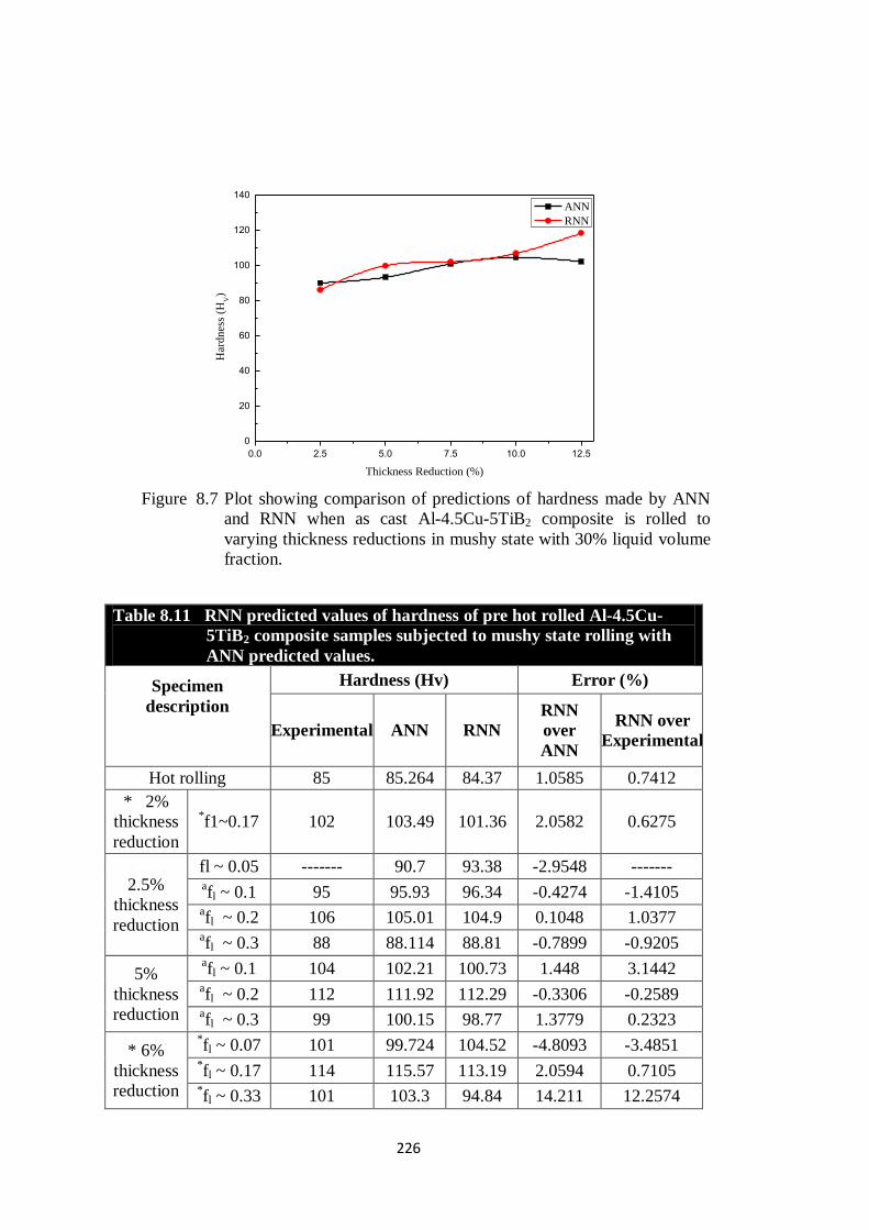
226
0.0 2.5 5.0 7.5 10.0 12.5
0
20
40
60
80
100
120
140
Har
dn
ess
(HV)
Thickness Reduction (%)
ANN
RNN
Table 8.11 RNN predicted values of hardness of pre hot rolled Al-4.5Cu-
5TiB2 composite samples subjected to mushy state rolling with
ANN predicted values.
Specimen
description
Hardness (Hv) Error (%)
Experimental ANN RNN
RNN
over
ANN
RNN over
Experimental
Hot rolling 85 85.264 84.37 1.0585 0.7412
* 2%
thickness
reduction
*f1~0.17 102 103.49 101.36 2.0582 0.6275
2.5%
thickness
reduction
fl ~ 0.05 ------- 90.7 93.38 -2.9548 ------- afl ~ 0.1 95 95.93 96.34 -0.4274 -1.4105
afl ~ 0.2 106 105.01 104.9 0.1048 1.0377
afl ~ 0.3 88 88.114 88.81 -0.7899 -0.9205
5%
thickness
reduction
afl ~ 0.1 104 102.21 100.73 1.448 3.1442
afl ~ 0.2 112 111.92 112.29 -0.3306 -0.2589
afl ~ 0.3 99 100.15 98.77 1.3779 0.2323
* 6%
thickness
reduction
*fl ~ 0.07 101 99.724 104.52 -4.8093 -3.4851
*fl ~ 0.17 114 115.57 113.19 2.0594 0.7105
*fl ~ 0.33 101 103.3 94.84 14.211 12.2574
Figure 8.7 Plot showing comparison of predictions of hardness made by ANN
and RNN when as cast Al-4.5Cu-5TiB2 composite is rolled to
varying thickness reductions in mushy state with 30% liquid volume
fraction.
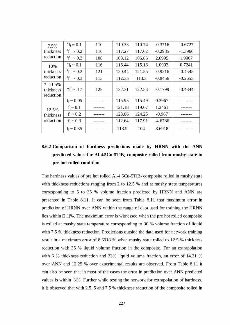
227
7.5%
thickness
reduction
afl ~ 0.1 110 110.33 110.74 -0.3716 -0.6727
afl ~ 0.2 116 117.27 117.62 -0.2985 -1.3966
afl ~ 0.3 108 108.12 105.85 2.0995 1.9907
10%
thickness
reduction
afl ~ 0.1 116 116.44 115.16 1.0993 0.7241
afl ~ 0.2 121 120.44 121.55 -0.9216 -0.4545
afl ~ 0.3 113 112.35 113.3 -0.8456 -0.2655
* 11.5%
thickness
reduction
*fl ~ .17 122 122.31 122.53 -0.1799 -0.4344
12.5%
thickness
reduction
fl ~ 0.05 ------- 115.95 115.49 0.3967 -------
fl ~ 0.1 ------- 121.18 119.67 1.2461 -------
fl ~ 0.2 ------- 123.06 124.25 -0.967 -------
fl ~ 0.3 ------- 112.64 117.91 -4.6786 -------
fl ~ 0.35 ------- 113.9 104 8.6918 -------
8.6.2 Comparison of hardness predictions made by HRNN with the ANN
predicted values for Al-4.5Cu-5TiB2 composite rolled from mushy state in
pre hot rolled condition
The hardness values of pre hot rolled Al-4.5Cu-5TiB2 composite rolled in mushy state
with thickness reductions ranging from 2 to 12.5 % and at mushy state temperatures
corresponding to 5 to 35 % volume fraction predicted by HRNN and ANN are
presented in Table 8.11. It can be seen from Table 8.11 that maximum error in
prediction of HRNN over ANN within the range of data used for training the HRNN
lies within |2.1|%. The maximum error is witnessed when the pre hot rolled composite
is rolled at mushy state temperature corresponding to 30 % volume fraction of liquid
with 7.5 % thickness reduction. Predictions outside the data used for network training
result in a maximum error of 8.6918 % when mushy state rolled to 12.5 % thickness
reduction with 35 % liquid volume fraction in the composite. For an extrapolation
with 6 % thickness reduction and 33% liquid volume fraction, an error of 14.21 %
over ANN and 12.25 % over experimental results are observed. From Table 8.11 it
can also be seen that in most of the cases the error in prediction over ANN predicted
values is within |3|%. Further while testing the network for extrapolation of hardness,
it is observed that with 2.5, 5 and 7.5 % thickness reduction of the composite rolled in

228
mushy state with 35 % liquid volume fraction in the composite, the error in prediction
is of the order of 30 %. Therefore, it can be inferred that the HRNN model proposed
can supplement the ANN in predictions of hardness of mushy state rolled Al-4.5Cu-
5TiB2 composite rolled to 2 % to 12.5 % thickness reductions and at mushy state
temperatures corresponding to 5 to 33 % liquid volume fraction.
Figure 8.8 to Figure 8.11 show the plots of variation of hardness with respect to
thickness reduction during mushy state rolling of pre hot rolled Al-4.5Cu-5TiB2
composite rolled from constant mushy state temperatures corresponding to 10, 17, 20
and 30 % volume fractions of liquid in the composite. It can be seen from plots of
Figure 8.8 to Figure 8.10, that the hardness prediction plot of HRNN closely follows
that of ANN. In Figure 8.11, it is seen that plot of hardness prediction by HRNN tends
to deviate from ANN predictions beyond 12.5 % thickness reduction when the
composite is mushy state rolled from temperature corresponding to 30 % volume
fraction of liquid. Thus it is clear that prediction beyond 30 % liquid volume fraction
the accuracy in prediction deteriorates. However from Table 8.11 it is seen that error
of 8.57 % at 33 % liquid volume fraction is reasonable. Kusiak and Kuziak (2002)
reported an error of 8 % in the prediction of ultimate stress in steel using neural
networks. Plot in Figure 8.9 relates to the predictions made by HRNN with ANN
predictions for the data used for validation of NN model. This plot is for variation of
hardness with respect to thickness reduction per roll pass when the pre hot rolled
composite containing 17 % liquid fraction is rolled in mushy state. The plots of
hardness predictions by HRNN are seen to closely match the predictions by ANN.
Thus the plots from Figure 8.8 to Figure 8.11 communicate the usefulness of HRNN
model in prediction of hardness of pre hot rolled Al-4.5Cu-5TiB2 composite rolled at
mushy state temperatures corresponding to 5 to 33 % liquid volume fractions and
rolled to 2 to 11.5 % thickness reductions per pass.

229
0.0 2.5 5.0 7.5 10.0 12.580
90
100
110
120
130
Har
dn
ess
(HV)
Thickness Reduction (%)
ANN
RNN
0 2 4 6 8 10 1260
70
80
90
100
110
120
130
140
Har
dn
ess
(HV)
Thickness Reduction (%)
ANN
RNN
Figure 8.8 Plot showing comparison of predictions of hardness made by ANN and
RNN when pre hot rolled Al-4.5Cu-5TiB2 composite is rolled to
varying thickness reductions in mushy state with 10% liquid volume
fraction.
Figure 8.9 Plot showing comparison of predictions of hardness made by ANN and
RNN when pre hot rolled Al-4.5Cu-5TiB2 composite is rolled to
varying thickness reductions in mushy state with 17% liquid volume
fraction.
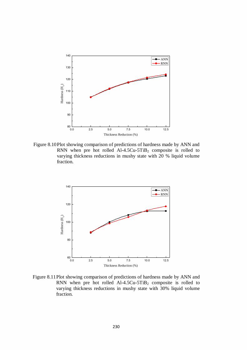
230
0.0 2.5 5.0 7.5 10.0 12.580
90
100
110
120
130
140
Har
dn
ess
(HV)
Thickness Reduction (%)
ANN
RNN
0.0 2.5 5.0 7.5 10.0 12.560
80
100
120
140
Har
dn
ess
(HV)
Thickness Reduction (%)
ANN
RNN
Figure 8.10 Plot showing comparison of predictions of hardness made by ANN and
RNN when pre hot rolled Al-4.5Cu-5TiB2 composite is rolled to
varying thickness reductions in mushy state with 20 % liquid volume
fraction.
Figure 8.11 Plot showing comparison of predictions of hardness made by ANN and
RNN when pre hot rolled Al-4.5Cu-5TiB2 composite is rolled to
varying thickness reductions in mushy state with 30% liquid volume
fraction.

231
8.7 MODELLING OF HRNN FOR PREDICTION OF TENSILE
PROPERTIES
The FFNN modelled for prediction of tensile properties had 7-9-6-3 architecture. The
HRNN proposed for prediction of tensile properties is constructed from the same
basic architecture. Initially, the ANN with 7 input nodes (corresponding to material
type, % thickness reduction, % liquid volume fraction, % TiB2, large and small grain
sizes and hardness), 9 and 6 nodes in first and second hidden layers respectively and 3
output nodes (corresponding to yield strength, UTS and pct. elongation) is considered
for partial training, till a steep downward gradient in MSE is observed. The fully
trained ANN of the same architecture converged clearly after 4,90,000 iterations with
an MSE of 0.00017 using the values of η and α as 0.85 and 0.7, respectively. Now, for
formulating the HRNN, the ANN network was trained partially and weights of this
partially trained parent ANN were borrowed in the HRNN network of similar
architecture as that of parent ANN. The HRNN then was further trained till the MSE
was comparable to that obtained with fully trained ANN. The training of HRNN with
η=0.85 and α=0.7 was stopped when MSE reached a value of 0.000137. In the
forthcoming subsections the performance of HRNN is compared with ANN model in
terms of values of yield strength, ultimate tensile strength and pct. elongation
predicted by them.
8.7.1 Comparison of prediction of tensile properties by HRNN with ANN
predictions
The predictions of yield and ultimate tensile strength for Al-4.5Cu alloy and Al-
4.5Cu-5TiB2 composite obtained by using trained HRNN and those obtained using
ANN model of Chapter 6 are presented in Table 8.12.
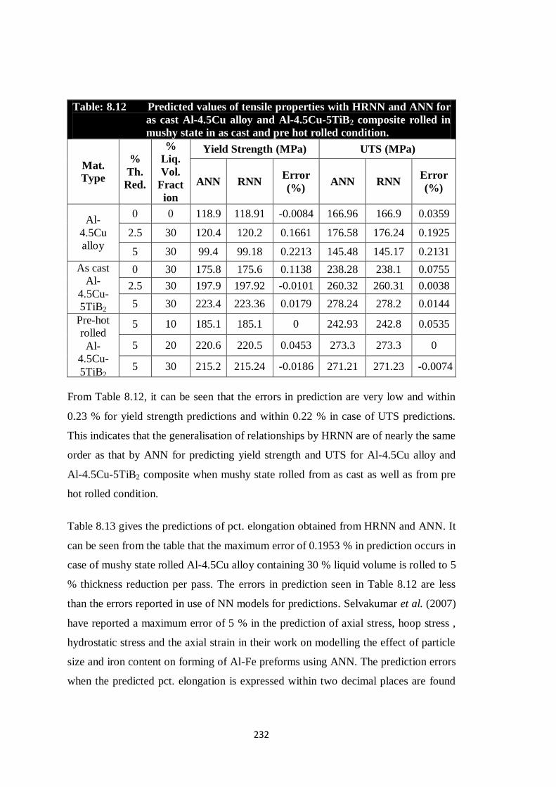
232
Table: 8.12 Predicted values of tensile properties with HRNN and ANN for
as cast Al-4.5Cu alloy and Al-4.5Cu-5TiB2 composite rolled in
mushy state in as cast and pre hot rolled condition.
Mat.
Type
%
Th.
Red.
%
Liq.
Vol.
Fract
ion
Yield Strength (MPa) UTS (MPa)
ANN RNN Error
(%) ANN RNN
Error
(%)
Al-
4.5Cu
alloy
0 0 118.9 118.91 -0.0084 166.96 166.9 0.0359
2.5 30 120.4 120.2 0.1661 176.58 176.24 0.1925
5 30 99.4 99.18 0.2213 145.48 145.17 0.2131
As cast
Al-
4.5Cu-
5TiB2
0 30 175.8 175.6 0.1138 238.28 238.1 0.0755
2.5 30 197.9 197.92 -0.0101 260.32 260.31 0.0038
5 30 223.4 223.36 0.0179 278.24 278.2 0.0144
Pre-hot
rolled
Al-
4.5Cu-
5TiB2
5 10 185.1 185.1 0 242.93 242.8 0.0535
5 20 220.6 220.5 0.0453 273.3 273.3 0
5 30 215.2 215.24 -0.0186 271.21 271.23 -0.0074
From Table 8.12, it can be seen that the errors in prediction are very low and within
0.23 % for yield strength predictions and within 0.22 % in case of UTS predictions.
This indicates that the generalisation of relationships by HRNN are of nearly the same
order as that by ANN for predicting yield strength and UTS for Al-4.5Cu alloy and
Al-4.5Cu-5TiB2 composite when mushy state rolled from as cast as well as from pre
hot rolled condition.
Table 8.13 gives the predictions of pct. elongation obtained from HRNN and ANN. It
can be seen from the table that the maximum error of 0.1953 % in prediction occurs in
case of mushy state rolled Al-4.5Cu alloy containing 30 % liquid volume is rolled to 5
% thickness reduction per pass. The errors in prediction seen in Table 8.12 are less
than the errors reported in use of NN models for predictions. Selvakumar et al. (2007)
have reported a maximum error of 5 % in the prediction of axial stress, hoop stress ,
hydrostatic stress and the axial strain in their work on modelling the effect of particle
size and iron content on forming of Al-Fe preforms using ANN. The prediction errors
when the predicted pct. elongation is expressed within two decimal places are found

233
to be very small (infinitesimal in most cases), indicating that the HRNN has
generalised the relationship of inputs and output to the same order as that of ANN.
Table: 8.13 Predicted values of pct. elongation with HRNN and ANN for as
cast Al-4.5Cu alloy and Al-4.5Cu-5TiB2 composite rolled in
mushy state in as cast and pre hot rolled condition.
Mat.
Type
% Th.
Red.
% Liq.
Vol.
Fraction
Pct
elongation Error (%)
ANN RNN
Al-4.5Cu alloy
0 30 6.95 6.947 0.0432
2.5 30 6.39 6.39 0
5 30 5.12 5.11 0.1953
As cast
Al-4.5Cu-
5TiB2
0 30 10.44 10.43 0.0958
2.5 30 11.83 11.83 0
5 30 14.1 14.1 0
Pre-hot rolled
Al-4.5Cu-
5TiB2
5 10 11.52 11.52 0
5 20 14.34 14.34 0
5 30 13.6 13.59 0.0735
Thus from Table 8.12 and 8.13 it can be concluded that the performance of HRNN
and ANN model are identical in terms of predictions of strength and elongation of Al-
4.5Cu alloy and Al-4.5Cu-5TiB2 composite rolled in mushy state within the range of
data for which these models have been trained.
8.8 MODELLING OF HRNN FOR PREDICTION OF WEAR
PROPERTIES
Hybrid recurrent neural network is constructed from a parent ANN having the same
architecture as that was modelled for prediction of wear rate. The FFNN modelled for
predicting wear rate of Al-4.5Cu-5TiB2 composite rolled from mushy state had
architecture of 7 neurons in input layer (corresponding to material type, % thickness
reduction, % liquid volume fraction, large and small grain sizes, hardness and normal
load), 7 and 4 neurons in first and second hidden layer respectively and one output
node representing wear rate. The HRNN for wear rate predictions was trained and
modelled in a manner similar to that obtained for grain size, hardness and tensile
properties predictions. The training of the HRNN for wear rate predictions was
stopped when an MSE of 2.92 x 10⁻⁵
was achieved using η = 0.5 and α = 0.5. In the

234
subsection to follow, the prediction of wear rate by HRNN is compared with that by
the fully trained ANN modelled for wear rate predictions in chapter 7.
8.8.1 Comparison of predictions of wear rate by HRNN and ANN
The wear rate predictions by HRNN and ANN when Al-4.5Cu-5TiB2 composite is
rolled in mushy state with different thickness reductions per pass, and at different
mushy state temperatures are listed in Table 8.14. The last column of the table shows
the error in prediction of HRNN over the values predicted by ANN. It can be
observed from Table 8.14 that the maximum prediction error equaling -10% occurs in
prediction of wear rate by HRNN with 7.5% thickness reduction when pre hot rolled
Al-4.5Cu-5TiB2 composite is mushy state rolled at temperature corresponding to 30
% volume fraction of liquid with a normal load of 19.6N. In the case of as cast
composite, the maximum error in prediction is -2.931 % with 2.5 % thickness
reduction, 30 % liquid volume fraction and a normal load 58.8N. It can also be
observed from Table 8.14 that majority of errors are within |5|%.The prediction errors
of HRNN model are comparable with the errors reported in literature. Mandal et al.
(2007) in their paper reported a Gaussian distribution of % error of prediction within
±10 % in prediction of flow stress using Resilient Propagation algorithm which is
reported to perform better than Back Propagation algorithm.
Table 8.14 Wear rate predicted by HRNN &ANN for mushy state rolled Al-
4.5Cu-5TiB2 composite in as cast and pre hot rolled condition.
Material
Thickness
reduction
(%)
Liquid
volume
fraction
(%)
Load
(N)
Wear rate Error
of RNN
over
ANN
(%)
Experimental ANN RNN
As cast Al-
4.5Cu-
5TiB2
Composite
2.5 30
19.6 0.00392 0.0038 0.00391 -2.8947
39.2 0.00525 0.0052 0.00524 -0.7692
58.8 0.00595 0.0058 0.00597 -2.931
78.4 0.00651 0.0064 0.00655 -2.3438
5.0 30
19.6 0.00360 0.0036 0.00360 0
39.2 0.00421 0.0042 0.00424 -0.9524
58.8 0.00539 0.0053 0.00536 -1.1321
78.4 0.00601 0.006 0.00595 0.8333

235
Pre hot
rolled Al-
4.5Cu-
5TiB2
Composite
2.5 30
19.6 0.00308 0.003 0.00315 -5
39.2 0.00517 0.005 0.00514 -2.8
58.8 0.00574 0.0058 0.00577 0.5172
78.4 0.00605 0.0059 0.00619 -4.9153
5.0 30
19.6 0.00298 0.003 0.0028 6.6667
39.2 0.00407 0.004 0.00413 -3.25
58.8 0.00518 0.0052 0.00502 3.4615
78.4 0.00592 0.0059 0.006 -1.6949
7.5
10
19.6 0.0027 0.0027 0.0026 3.7037
39.2 0.00454 0.0045 0.00456 -1.3333
58.8 0.00516 0.0051 0.00518 -1.5686
78.4 0.00644 0.0064 0.00654 -2.1875
20
19.6 0.00217 0.0021 0.00215 -2.381
39.2 0.00263 0.0028 0.00262 6.4286
58.8 0.00401 0.0039 0.00391 -0.2564
78.4 0.00501 0.005 0.00515 -3
30
19.6 0.00233 0.0022 0.00242 -10
39.2 0.00405 0.0038 0.00405 -6.5789
58.8 0.00444 0.0044 0.00461 -4.7727
78.4 0.00581 0.0056 0.00591 -5.5357
Figure 8.12 shows the plots of variation of wear rate (mm3/km) predicted by HRNN
and ANN when Al-4.5Cu-5TiB2 composite in as cast state is rolled in mushy state at
632ºC with respect to normal load (N) with 2.5 and 5 % thickness reductions. It can be
seen that the curves with both thickness reductions follow each other quite closely.

236
19.6 39.2 58.8 78.40
1
2
3
4
5
6
7
8
9
10
Wea
r R
ate
(mm
3/k
m)
Normal Load (N)
ANN-2.5 % Th. Red.
RNN-2.5 % Th. Red
ANN-5 % Th. Red.
RNN-5 % Th. Red
Similarly plots in Figure 8.13 show variations in wear rate predicted by HRNN and
ANN for pre hot rolled composite under same conditions as in Figure 8.12. Here too,
it can be seen that the predictions match closely with the curves being almost similar.
However, the curve for HRNN predictions with 2.5 % thickness reduction seems to
diverge beyond normal load of 78.4N. Plots in Figure 8.14 show the variation of wear
rate predictions by HRNN in comparison to that by ANN when pre hot rolled Al-
4.5Cu-5TiB2 composite is rolled in mushy state at temperatures 610ºC, 626
ºC and
632ºC (corresponding to 10, 20 and 30 % liquid volume fraction) to 7.5 % thickness
reduction. It is observed that the predictions made by both the models are quite
similar with the curves closely following each other in all the three cases. From the
foregoing discussion on the performance of the HRNN modelled for prediction of
wear rate of mushy state rolled Al-4.5Cu-5TiB2 composite, it can be concluded that
HRNN model predictions are comparable to that of ANN within an overall error of
prediction of |10|% over ANN model predictions.
Figure 8.12 Plot showing comparison of predictions of wear rate by HRNN and
ANN with respect to normal load when as cast Al-4.5Cu-5TiB2
composite containing 30 % volume fractions of liquid is mushy state
rolled to 2.5 and 5 % thickness reduction per pass.

237
19.6 39.2 58.8 78.42
3
4
5
6
7
8
Wea
r R
ate
(mm
3/k
m)
Normal Load (N)
ANN-2.5 % Th. Red.
RNN-2.5 % Th. Red
ANN-5 % Th. Red.
RNN-5 % Th. Red
19.6 39.2 58.8 78.4
2
4
6
8
10
Wea
r R
ate
(mm
3 /km
)
Normal Load (N)
ANN-10 % LVF
RNN- 10 % LVF
ANN-20 % LVF
RNN-20 % LVF
ANN-30 % LVF
RNN-30 % LVF
Figure 8.13 Plot showing comparison of predictions of wear rate by HRNN and
ANN with respect to normal load when pre hot rolled Al-4.5Cu-5TiB2
composite containing 30% volume fractions of liquid is mushy state
rolled to 2.5 and 5 % thickness reduction per pass.
Figure 8.14 Plot showing comparison of predictions of wear rate by HRNN and
ANN with respect to normal load when pre hot rolled Al-4.5Cu-5TiB2
composite containing 10, 20 and 30% volume fractions of liquid is
mushy state rolled to 7.5% thickness reduction per pass.

238
8.9 SUMMARY
1. Elman simple neural network (SRN) was found to have issues relating to
convergence when trained for prediction of grain size (large and small) for
application relating to mushy state rolling of Al-4.5Cu-5TiB2 composite. Three
layered as well as four layered extended Elman recurrent networks were tried
out with different combinations of neurons per hidden layer and learning rate
parameter (η) and momentum term (α). The network was found to oscillate in
local minimums and subsequently stopped learning with three layered SRN. The
four layered extended Elman recurrent neural network fared slightly better, but
was unable to map the input output relationships as there was no learning
possible beyond a certain stage of training.
2. The problem of convergence of extended Elman recurrent neural network was
overcome by constructing a hybrid recurrent neural network (HRNN) by
borrowing weights from a partially trained FFNN having same architecture as
that of extended Elman recurrent neural network (minus context or temporal
layers), when steep downward gradient is observed on the MSE v/s. Weights
plane. Further training of such HRNN resulted in fast learning. The overall
training time was found to reduce significantly.
3. The statistical study of errors done using two sample student t test and one
sample and two sampled Kolmogorov – Smirnov test indicated that the means
of the errors in prediction of both the HRNN and ANN models calculated over
target values are comparable and the statistical distribution of the two errors is
equivalent. Thus the statistical analysis inferred that the error distributions of
both the models are statistically equivalent.
4. The HRNN model for grain size prediction predicted large and small grain sizes
of Al-4.5Cu-5TiB2 composite rolled in mushy state in as cast and pre hot rolled
condition, containing 5 to 35 % liquid volume fraction with 2 to 12.5 %
thickness reduction per pass within an error of |0.2|% of the corresponding
values predicted by ANN model.
5. The HRNN model for hardness predictions of the mushy state rolled composite
rolled in as cast as well as pre hot rolled form predicted the hardness within an
239
error of |6.58|% within the range of data used for training the network and
within |14.2|% within the data used for validating the ANN. However, the
predictions were observed to diverge beyond 33 % liquid volume fractions with
all cases of thickness reductions considered. Therefore, the HRNN model for
hardness predictions are valid from 5 to 33 % volume fractions of liquid in the
composite rolled to 2 to 12.5 % thickness reductions only. Thus HRNN model
can be used for interpolating the data as well as for extrapolation with small
constraints.
6. The predictions of HRNN modelled for prediction of tensile properties of
mushy state rolled Al_4.5Cu alloy and Al-4.5Cu-5TiB2 composite matched the
predictions done by ANN model.
7. The wear rates of as cast as well as pre hot rolled Al-4.5Cu-5TiB2 composite
rolled from mushy state that were predicted by HRNN were within an error of
10 % of the values predicted by the ANN model for wear rate predictions.
8. This leads to an inference that HRNN models, being similar in performance to
the ANN (FFNN) models in terms of prediction capabilities and the time
required for training of HRNN being significantly reduced, they are superior to
ANN models.
241
Chapter 9
CONCLUSIONS AND SCOPE FOR FUTURE WORKS
9.1 CONCLUSIONS
1. Artificial neural network models were successfully formulated to predict the
grain sizes, hardness, wear properties and tensile properties of Al-4.5Cu-
5TiB2 composite rolled in mushy state in as cast and pre hot rolled condition,
with varying thickness reductions ranging from 2 to 12.5 % and at various
temperatures corresponding to 5 % to 35 % volume fraction of liquid in the
composite with a fair degree of accuracy.
2. The large and small grain sizes predicted by the ANN model for grain size
predictions were found to be within ±6.1 pct. over the target values of large
and small grain sizes. The ANN models for hardness, tensile properties and
wear rate are found to predict within an error of ±2.65 pct, ±7.65 pct and
±6.5 pct respectively. Majority of the predictions done by the ANN model
for tensile properties are within ±2.3 pct, while those by ANN model for
wear properties are within ±3.6 pct. Thus, the ANN models successfully
represent the relationships between the mushy state rolling parameters and
the properties for which they have been modelled. The ANN models have
been validated by conducting experiments on mushy state rolling of Al-
4.5Cu-5TiB2 composite with predefined mushy state conditions i.e. (a) with
thickness reduction of 2% at 619ºC, (b) with 6% thickness reduction at
598ºC, 619
ºC and 633
ºC, respectively and (c) 11.5% thickness reduction at
619ºC. The grain size model predicts the large and small grain sizes within an
error of ± 3.4 pct. for the composite rolled in as cast as well as pre hot rolled
conditions. The hardness model exhibits an error of ±2.8 pct. over the
validation target values of hardness. The wear properties model is validated
within an error of ±5.51 pct. The ANN models for grain size, hardness and
wear properties predictions extrapolate beyond the range of data used for

242
training within a small error of ±2.5 pct. The validity of the model to predict
the grain sizes, hardness, wear and tensile properties of mushy state rolled
Al-4.5Cu-5TiB2 composite has therefore been established.
3. The grain size model reveals that the variation of grain sizes following
rolling carried out at different mushy state temperatures corresponding to
required liquid volume fractions in the composite does not show any definite
trend with respect to % thickness reductions. The study of variation of
hardness of mushy state composite predicted by hardness model (within the
range of data used to train the model), with respect to reduction in thickness
at any given liquid volume fraction indicates that the highest value of
hardness of the composite lies in the range of 10 % thickness reduction and
20 % liquid volume fraction. Outside the training data range, higher values of
hardness are found with 12.5 % thickness reduction when the composite is
mushy state rolled at around 18 % liquid volume fraction. The variation of
wear rate analysed using the ANN model for wear properties indicates that
the wear rate and specific wear rate decrease with increase in thickness
reduction for any given volume fraction of liquid in composite, with
variation more pronounced at lower values of normal loads. The variation of
wear rate and specific wear rate is found to be insignificant at higher values
of normal loads. The variation of specific wear rate with normal loads
indicates lower values of specific wear rate when the composite is mushy
state rolled from range of temperatures corresponding to around 20 % liquid
volume fraction in the composite. The ANN model for tensile properties
indicates that maximum strength and elongation of the composite rolled from
mushy state in as cast and pre hot rolled condition to 5 % thickness reduction
lies in the region containing 20 to 30 % liquid volume fraction.
4. The optimization of the hardness and wear properties has been obtained by
interfacing the ANN models for hardness and wear property predictions with
available GUI / API libraries. The model predicts the maximum hardness and
wear rate of mushy state rolled Al-4.5Cu-5TiB2 composite and also provide
mushy state rolling parameters to achieve these optimum values.

243
5. Elman simple recurrent neural network (SRN) was found to have issues
relating to convergence when trained as evidenced by different
configurations discussed earlier. The problem of convergence of extended
Elman recurrent neural network was overcome by constructing a novel
hybrid recurrent neural network (HRNN) by borrowing weights from a
partially trained FFNN having same architecture as that of extended Elman
recurrent neural network (devoid of context or temporal layers), when steep
downward gradient is observed on the MSE vs. Weights plane. Further
training of such HRNN resulted in fast learning.
6. The statistical study of errors indicates that the means of the errors in
prediction of both the HRNN and ANN models calculated over target values
are comparable and the statistical distribution of the two errors is equivalent.
Thus the ANN and HRNN models are equivalent in terms of prediction
capability, provided that the HRNN model is constructed from the parent
ANN model having similar architecture as that of HRNN (devoid of the
temporal layers). The overall training time for an HRNN constructed by
borrowing weights from a partially trained ANN is found to reduce
significantly as compared to a fully trained ANN having the same prediction
capability
The unique feature of the current research is the development of an HRNN model
which performs faster predictions than corresponding FFNNs with same levels of
accuracy. This HRNN model has been developed through a novel approach of
borrowing weights from a partially trained FFNN model, to be fed into an extended
Elman Simple Recurrent Neural Network.
9.2 SCOPE FOR FUTURE WORK
The HRNN model due to its faster learning ability scores over ANN. The present day
industrial processes involve a lot of in process monitoring and control. Any subtle
changes in the output(s) of the process are fed back into the process control
mechanism. The mechanism then takes appropriate corrective action, resets the
process parameters and brings back the process output(s) to the desired state. The

244
developed HRNN model, due to its faster processing could be embedded as part of
such controller strategy in mushy state rolling process in future.
The HRNN model developed could be customised to suit many other processes
because of its generality in coding and flexibility. The generality of coding allows the
user to select the any area ranging from finance to engineering and meteorological
applications. The flexibility of the code written allows the user to select any number
of input parameters and desired number of output parameters. The code also provides
flexibility and generality in selection of learning rate parameter, momentum term and
number of neurons in each hidden layer.

245
Appendix I
Extract of code used for training the Feed Forward Neural Network and
computation of the outputs from the Network.
main()
{
cout << " Prediction of Grainsize, Hardness and Wear Properties of " <<
endl;
cout << " Mushy State rolled Al-4.5Cu-TiB2 Composite" << endl;
cout << " using Feed Forward and Recuurent Neural Networks" << endl;
cout << " by" << endl;
cout << " Akshay V. Nigalye, (ME08p03) " << endl;
cout << " National Institute of Technology Karnataka, Surathkal" <<
endl;
cout << endl;
cout << endl << "Enter your Network preference" << endl;
cout << "1. Feed Forward Neural Network" << endl;
cout << "2. Recurrent Neural Network" << endl;
fchoise = getch();
if (fchoise != '1' && fchoise != '2' ) { return 0; }
else for(;;) {
char choice;
cout << endl << "Enter the Training or Prediction preference" << endl;
cout << "1. load data" << endl;
cout << "2. learn from data" << endl;
cout << "3. compute output pattern" << endl;

246
cout << "4. make new data file" << endl;
cout << "5. save data" << endl;
cout << "6. print data" << endl;
cout << "7. change learning rate and momentum factor" << endl;
cout << "8. exit" << endl << endl;
cout << "Enter your choice (1-8)";
do { choice = getch(); }
while (choice != '1' && choice != '2' && choice != '3' && choice != '4'
&& choice != '5' && choice != '6' && choice != '7' && choice !=
'8');
switch(choice) {
case '1':{ if (file_loaded == 1) clear_memory();
get_file_name();
file_loaded = 1;
if (fchoise=='2')
{recurrent_load_data(filename); }
else {load_data(filename); }
}
break;
case '2': learn();
break;
case '3': compute_output_pattern();
break;
case '4': make();
break ;
case '5':{ if (file_loaded == 0)
{

247
cout << endl << "there is no data loaded into
memory" << endl;
break;
}
cout << endl << "enter a filename to save data to: ";
cin >> filename;
save_data(filename); }
break;
case '6': print_data();
break;
case '7': change_learning_rate_and_momentum();
break;
case '8': return 0;
};
}
}
void initialize_net()
{
int x;
input = new double * [number_of_input_patterns];
if(!input) { cout << endl << "memory problem!"; exit(1); }
for(x=0; x<number_of_input_patterns; x++)
{
input[x] = new double [input_array_size];
if(!input[x]) { cout << endl << "memory problem!"; exit(1); }
}
hidden1 = new double [hidden_array_1_size];

248
if(!hidden1) { cout << endl << "memory problem!"; exit(1); }
if (fchoise==2) { rhidden1 = new double [rhidden_array_1_size];
if(!rhidden1) { cout << endl << "memory problem!"; exit(1);
}}
hidden2 = new double [hidden_array_2_size];
if(!hidden2) { cout << endl << "memory problem!"; exit(1); }
if (fchoise==2) { rhidden2 = new double [rhidden_array_2_size];
if(!rhidden2) { cout << endl << "memory problem!"; exit(1);
}}
output = new double * [number_of_input_patterns];
if(!output) { cout << endl << "memory problem!"; exit(1); }
for(x=0; x<number_of_input_patterns; x++)
{
output[x] = new double [output_array_size];
if(!output[x]) { cout << endl << "memory problem!"; exit(1); }
}
target = new double * [number_of_input_patterns];
if(!target) { cout << endl << "memory problem!"; exit(1); }
for(x=0; x<number_of_input_patterns; x++)
{
target[x] = new double [output_array_size];
if(!target[x]) { cout << endl << "memory problem!"; exit(1); }
}
bias = new double [bias_array_size];

249
if(!bias) { cout << endl << "memory problem!"; exit(1); }
weight_i_h = new double * [input_array_size];
if(!weight_i_h) { cout << endl << "memory problem!"; exit(1); }
for(x=0; x<input_array_size; x++)
{
weight_i_h[x] = new double [hidden_array_1_size];
if(!weight_i_h[x]) { cout << endl << "memory problem!"; exit(1); }
}
oldweight_i_h = new double * [input_array_size];
if(!oldweight_i_h) { cout << endl << "memory problem!"; exit(1); }
for(x=0; x<input_array_size; x++)
{
oldweight_i_h[x] = new double [hidden_array_1_size];
if(!oldweight_i_h[x]) { cout << endl << "memory problem!"; exit(1); }
}
if (fchoise==2) { rweight_h1 = new double * [rhidden_array_1_size];
if(!rweight_h1) { cout << endl << "memory problem!"; exit(1); }
for(x=0; x<rhidden_array_1_size; x++)
{
rweight_h1[x] = new double [hidden_array_1_size];
if(!rweight_h1[x]) { cout << endl << "memory problem!"; exit(1); }
}}
weight_h_h = new double * [hidden_array_1_size];
if(!weight_h_h) { cout << endl << "memory problem!"; exit(1); }
for(x=0; x<hidden_array_1_size; x++)
{

250
weight_h_h[x] = new double [hidden_array_2_size];
if(!weight_h_h[x]) { cout << endl << "memory problem!"; exit(1); }
}
oldweight_h_h = new double * [hidden_array_1_size];
if(!oldweight_h_h) { cout << endl << "memory problem!"; exit(1); }
for(x=0; x<hidden_array_1_size; x++)
{
oldweight_h_h[x] = new double [hidden_array_2_size];
if(!oldweight_h_h[x]) { cout << endl << "memory problem!"; exit(1);
}
}
if (fchoise==2) { rweight_h2 = new double * [rhidden_array_2_size];
if(!rweight_h2) { cout << endl << "memory problem!"; exit(1); }
for(x=0; x<rhidden_array_2_size; x++)
{
rweight_h2[x] = new double [hidden_array_2_size];
if(!rweight_h2[x]) { cout << endl << "memory problem!"; exit(1); }
}}
weight_h_o = new double * [hidden_array_2_size];
if(!weight_h_o) { cout << endl << "memory problem!"; exit(1); }
for(x=0; x<hidden_array_2_size; x++)
{
weight_h_o[x] = new double [output_array_size];
if(!weight_h_o[x]) { cout << endl << "memory problem!"; exit(1); }
251
}
oldweight_h_o = new double * [hidden_array_2_size];
if(!oldweight_h_o) { cout << endl << "memory problem!"; exit(1); }
for(x=0; x<hidden_array_2_size; x++)
{
oldweight_h_o[x] = new double [output_array_size];
if(!oldweight_h_o[x]) { cout << endl << "memory problem!"; exit(1);
}
}
errorsignal_hidden1 = new double [hidden_array_1_size];
if(!errorsignal_hidden1) { cout << endl << "memory problem!"; exit(1); }
errorsignal_hidden2 = new double [hidden_array_2_size];
if(!errorsignal_hidden2) { cout << endl << "memory problem!"; exit(1); }
errorsignal_output = new double [output_array_size];
if(!errorsignal_output) { cout << endl << "memory problem!"; exit(1); }
return;
}
void learn()
{
if (epochstat==0) epoch=0;
if (file_loaded == 0)
{
cout << endl << "there is no data loaded into memory" << endl;

252
return;
}
cout << endl << "learning..." << endl << "press a key to return to menu" <<
endl;
register int y;
if (fchoise==1)
{
while(!kbhit()) {
cout << "FFNN learning ";
for(y=0; y<number_of_input_patterns; y++) {
forward_pass(y);
backward_pass(y);
}
if(compare_output_to_target()) {
cout << endl << "Feed forward learning successful" << endl;
return;
}
epoch++;
epochstat=1;
}
}
else
{
while(!kbhit()) {
cout << "RNN learning " ;
for(y=0; y<number_of_input_patterns; y++) {

253
recurrent_forward_pass(y);
recurrent_backward_pass(y);
}
if(compare_output_to_target()) {
cout << endl << "Recurrent learning successful" << endl;
return;
}
epoch++;
epochstat=1;
}
}
cout << endl << "learning not successful yet" << endl;
return;
}
void forward_pass(int pattern)
{
register double temp=0;
register int x,y;
// INPUT -> HIDDEN1
for(y=0; y<hidden_array_1_size; y++) {
for(x=0; x<input_array_size; x++)
{
temp += (input[pattern][x] * weight_i_h[x][y]);
}
hidden1[y] = (1.0 / (1.0 + exp(-1.0 * (temp + bias[y]))));
temp = 0;
}

254
// HIDDEN1 -> HIDDEN2
for(y=0; y<hidden_array_2_size; y++) {
for(x=0; x<hidden_array_1_size; x++)
{
temp += (hidden1[x] * weight_h_h[x][y]);
}
hidden2[y] = (1.0 / (1.0 + exp(-1.0 * (temp + bias[y +
hidden_array_1_size]))));
temp = 0;
}
// HIDDEN2 -> OUTPUT
for(y=0; y<output_array_size; y++) {
for(x=0; x<hidden_array_2_size; x++)
{
temp += (hidden2[x] * weight_h_o[x][y]);
}
output[pattern][y] = (1.0 / (1.0 + exp(-1.0 * (temp + bias[y +
hidden_array_1_size + hidden_array_2_size]))));
temp = 0;
}
return;
}
void backward_pass(int pattern)
{
register int x, y;
register double dweight_h_o = 0.0 , dweight_h_h = 0.0, dweight_i_h = 0.0,
temp = 0.0;
// COMPUTE ERRORSIGNAL FOR OUTPUT UNITS

255
for(x=0; x<output_array_size; x++)
{
errorsignal_output[x] = ((target[pattern][x] - output[pattern][x]) *
output[pattern][x] * (1- output[pattern][x])) ;
}
// ADJUST WEIGHTS OF CONNECTIONS FROM HIDDEN LAYER 2 TO
OUTPUT UNITS
for(x=0; x<hidden_array_2_size; x++) {
for(y=0; y<output_array_size; y++) {
dweight_h_o = weight_h_o[x][y] - oldweight_h_o[x][y];
weight_h_o[x][y] += ((learning_rate * errorsignal_output[y] *
hidden2[x]) + (momentum * dweight_h_o));
}
}
for(x=0; x<hidden_array_2_size; x++)
for(y=0; y<output_array_size; y++)
oldweight_h_o[x][y] = weight_h_o[x][y];
// ADJUST BIASES FOR OUTPUT UNITS
for(x=(hidden_array_1_size+hidden_array_2_size); x<bias_array_size; x++) {
bias[x] += (learning_rate * errorsignal_output[x]);
}
// COMPUTE ERRORSIGNAL FOR HIDDEN LAYER 2 UNITS
for(x=0; x<hidden_array_2_size; x++) {
for(y=0; y<output_array_size; y++) {
temp += (errorsignal_output[y] * weight_h_o[x][y]);
}
errorsignal_hidden2[x] = hidden2[x] * (1-hidden2[x]) * temp;
temp = 0.0;
256
}
// ADJUST WEIGHTS OF CONNECTIONS FROM HIDDEN LAYER 2 TO
HIDDEN LAYER 1
for(x=0; x<hidden_array_1_size; x++) {
for(y=0; y<hidden_array_2_size; y++) {
dweight_h_h = weight_h_h[x][y] - oldweight_h_h[x][y];
weight_h_h[x][y] += ((learning_rate * errorsignal_hidden2[y] *
hidden1[x]) + (momentum * dweight_h_h));
}
}
for(x=0; x<hidden_array_1_size; x++)
for(y=0; y<hidden_array_2_size; y++)
oldweight_h_h[x][y] = weight_h_h[x][y];
// ADJUST BIASES OF HIDDEN LAYER 2 UNITS
for(x=hidden_array_1_size; x<(bias_array_size-hidden_array_2_size); x++) {
bias[x] += (learning_rate * errorsignal_hidden2[x]);
}
// COMPUTE ERRORSIGNAL FOR HIDDEN LAYER 1 UNITS
for(x=0; x<hidden_array_1_size; x++) {
for(y=0; y<hidden_array_2_size; y++) {
temp += (errorsignal_hidden2[y] * weight_h_h[x][y]);
}
errorsignal_hidden1[x] = hidden1[x] * (1-hidden1[x]) * temp;
temp = 0.0;
}
// ADJUST WEIGHTS OF CONNECTIONS FROM INPUT TO HIDDEN LAYER 1
UNITS
for(x=0; x<input_array_size; x++) {

257
for(y=0; y<hidden_array_1_size; y++) {
dweight_i_h = weight_i_h[x][y] - oldweight_i_h[x][y];
weight_i_h[x][y] +=((learning_rate *
errorsignal_hidden1[y]*input[pattern][x]) + (momentum*dweight_i_h));
}
}
for(x=0; x<input_array_size; x++)
for(y=0; y<hidden_array_1_size; y++)
oldweight_i_h[x][y] = weight_i_h[x][y];
// ADJUST BIASES OF HIDDEN LAYER 1 UNITS
for(x=0; x<hidden_array_1_size; x++) {
bias[x] += (learning_rate * errorsignal_hidden1[x]);
}
return;
}
void compute_output_pattern()
{
if (file_loaded == 0)
{
cout << endl << "there is no data loaded into memory" << endl;
return;
}
char choice;
cout << endl << endl << "1. load trained input pattern into network" << endl;
cout << "2. load custom input pattern into network" << endl;
cout << "3. go back to main menu" << endl << endl;
cout << "Enter your choice (1-3)" << endl;

258
do { choice = getch(); } while (choice != '1' && choice != '2' && choice !=
'3');
switch(choice) {
case '1': test();
break;
case '2': if (fchoise==2) rcustom();
else custom();
break;
case '3': return;
};
}
void test()
{
int x;
double y;
pattern = 0;
while(pattern == 0) {
cout << endl << endl << "There are " << number_of_input_patterns <<
" input patterns in the file," << endl << "enter a number within this range: ";
cin >> pattern;
}
if(pattern > number_of_input_patterns) {
cout << "Pattern number entered exceeded the limit" <<
number_of_input_patterns << endl;
return;
}
pattern--;

259
if (fchoise==2)
recurrent_forward_pass(pattern);
else
forward_pass(pattern);
output_to_screen();
return;
}
void output_to_screen()
{
int x;
double y, z ;
double diff= maxnum - minnum;
cout << endl << "Output pattern:" << endl;
for(x=0; x<output_array_size; x++) {
y= ((( output[pattern][x] - 0.1 ) * diff ) / 0.8 ) + minnum;
cout << endl << (x+1) << " Tested Output: " << y ;
}
cout << endl;
return;
}
void custom()
{
double temp=0;
int x,y,z,fload=0;
int num_patterns;
double **custom_input;

260
char cusfile[128],
outfile[128];
cout << endl << "enter the number of patterns in the file" << endl;
cin >> num_patterns;
custom_input = new double *[num_patterns];
if(!custom_input) { cout << endl << "memory problem!"; return; }
for(x=0; x<num_patterns; x++)
{
custom_input[x] = new double [input_array_size];
if(!custom_input[x]) { cout << endl << "memory problem!"; exit(1); }
}
double *custom_output = new double [output_array_size];
if(!custom_output) { delete [] custom_input; cout << endl << "memory
problem!"; return; }
double *custom = new double [input_array_size];
if(!custom_output) { delete [] custom_input; cout << endl << "memory
problem!"; return; }
char cchoice;
cout << endl << endl << "1. load custom input pattern individually" << endl;
cout << "2. load custom inputs patterns file" << endl;
cout << "3. go back to main menu" << endl << endl;
cout << "Enter your choice (1-3)" << endl;
261
do { cchoice = getch(); } while (cchoice != '1' && cchoice != '2' && cchoice !=
'3');
switch(cchoice) {
case '1': {
cout << " load the custom input"<< endl;
for(x = 0; x < input_array_size; x++) cin >> custom_input[0][x];
}
break;
case '2': {
cout << endl << endl << "enter file that contains test input pattern: ";
cin >> cusfile;
ifstream in(cusfile);
if(!in) { cout << endl << "failed to load data file" << endl; return; }
for(z=0; z<num_patterns; z++)
for(x = 0; x < input_array_size; x++) in >>
custom_input[z][x];
in.close();
}
break;
case '3': return;
};
for(z=0; z<num_patterns; z++) {
double diff= maxnum-minnum;
for (x = 0; x < input_array_size; x++)
{

262
custom[x]= (((custom_input[z][x]- minnum)*0.8)/diff)+0.1;
}
for(y=0; y<hidden_array_1_size; y++) {
for(x=0; x<input_array_size; x++) {
temp += (custom[x] * weight_i_h[x][y]);
}
hidden1[y] = (1.0 / (1.0 + exp(-1.0 * (temp + bias[y]))));
temp = 0;
}
for(y=0; y<hidden_array_2_size; y++) {
for(x=0; x<hidden_array_1_size; x++) {
temp += (hidden1[x] * weight_h_h[x][y]);
}
hidden2[y] = (1.0 / (1.0 + exp(-1.0 * (temp + bias[y +
hidden_array_1_size]))));
temp = 0;
}
for(y=0; y<output_array_size; y++) {
for(x=0; x<hidden_array_2_size; x++) {
temp += (hidden2[x] * weight_h_o[x][y]);
}
custom_output[y] = (1.0 / (1.0 + exp(-1.0 * (temp + bias[y +
hidden_array_1_size + hidden_array_2_size]))));
temp = 0;
}

263
if(cchoice=='2'){ if(fload!=1){
cout << " enter the name of the file to save the predicted outputs from input file
" << cusfile << endl;
cin >> outfile;
fload=1;}
}
cout << endl << "Input pattern:" << "[" << (z+1) << "]" << endl;
for(x = 0; x < input_array_size; x++) {
cout << (x+1) << ": " << (((( custom[x] - 0.1 ) * diff ) / 0.8 ) +
minnum) <<endl;
}
cout << endl << endl << "Output pattern:";
for(x=0; x<output_array_size; x++) {
cout << endl << (x+1) << ": " << (((( custom_output[x] - 0.1 )
* diff ) / 0.8 ) + minnum)<< endl ;
}
ofstream out;
out.open(outfile, ofstream::app);
if(!out) {cout << endl << " failed to save custom output file" << endl;
return;}
for(x=0; x<output_array_size; x++) {
out << "[" << (z+1) << "]" << "[" << (x+1) << "] " << ((((
custom_output[x] - 0.1 ) * diff ) / 0.8 ) + minnum) << ' ' ;
out <<endl;
}
out.close();

264
delete [] custom_output;
delete [] custom;
cout << endl;
}
for(x=0; x<num_patterns; x++)
{
delete [] custom_input[x];
}
delete [] custom_input;
fload=0;
return;
}
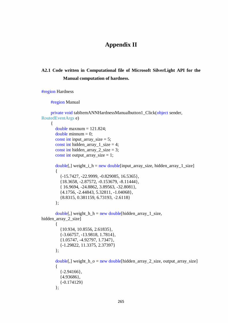
265
Appendix II
A2.1 Code written in Computational file of Microsoft SilverLight API for the
Manual computation of hardness.
#region Hardness
#region Manual
private void tabItemANNHardnessManualbutton1_Click(object sender,
RoutedEventArgs e)
{
double maxnum = 121.824;
double minnum = 0;
const int input_array_size = 5;
const int hidden_array_1_size = 4;
const int hidden_array_2_size = 3;
const int output_array_size = 1;
double[,] weight_i_h = new double[input_array_size, hidden_array_1_size]
{
{-15.7427, -22.9999, -0.829085, 16.5365},
{18.3658, -2.87572, -0.153679, -8.11444},
{ 16.9694, -24.8862, 3.89563, -32.8081},
{4.1756, -2.44843, 5.32811, -1.04068},
{8.8315, 0.381159, 6.73193, -2.6118}
};
double[,] weight_h_h = new double[hidden_array_1_size,
hidden_array_2_size]
{
{10.934, 10.8556, 2.61835},
{-3.66757, -13.9818, 1.7814},
{1.05747, -4.92797, 1.7347},
{-1.29822, 11.3375, 2.37397}
};
double[,] weight_h_o = new double[hidden_array_2_size, output_array_size]
{
{-2.94166},
{4.93686},
{-0.174129}
};

266
double[] bias = new double[]
{
-8.83525, 12.7545, -5.1725, 10.2617,
0.33406, 0.69, 0.65,
0.68
};
// generate the input patterns
double[] inputPattern = new double[input_array_size];
inputPattern[0] =
float.Parse(tabItemANNHardnessManualInputtextBox5.Text);
inputPattern[1] =
float.Parse(tabItemANNHardnessManualInputtextBox1.Text);
inputPattern[2] =
float.Parse(tabItemANNHardnessManualInputtextBox2.Text);
inputPattern[3] =
float.Parse(tabItemANNHardnessManualInputtextBox4.Text);
inputPattern[4] =
float.Parse(tabItemANNHardnessManualInputtextBox3.Text);
// create normalized input and output arrays
double[] normInputPattern = new double[input_array_size];
double[] normOutputPattern = new double[output_array_size];
// create hidden arrays
double[] hidden1 = new double[hidden_array_1_size];
double[] hidden2 = new double[hidden_array_2_size];
double temp = 0;
double diff = maxnum - minnum;
// normalize inputs
for (int x = 0; x < input_array_size; x++)
{
normInputPattern[x] = (((inputPattern[x] - minnum) * 0.8) / diff) + 0.1;
}
// inputs -> hidden1
for (int y = 0; y < hidden_array_1_size; y++)
{
for (int x = 0; x < input_array_size; x++)
{
temp += (normInputPattern[x] * weight_i_h[x, y]);
}
hidden1[y] = (1.0 / (1.0 + Math.Exp(-1.0 * (temp + bias[y]))));
temp = 0;

267
}
// hidden1 -> hidden2
for (int y = 0; y < hidden_array_2_size; y++)
{
for (int x = 0; x < hidden_array_1_size; x++)
{
temp += (hidden1[x] * weight_h_h[x, y]);
}
hidden2[y] = (1.0 / (1.0 + Math.Exp(-1.0 * (temp + bias[y +
hidden_array_1_size]))));
temp = 0;
}
// hidden2 -> output
for (int y = 0; y < output_array_size; y++)
{
for (int x = 0; x < hidden_array_2_size; x++)
{
temp += (hidden2[x] * weight_h_o[x, y]);
}
normOutputPattern[y] = (1.0 / (1.0 + Math.Exp(-1.0 * (temp + bias[y +
hidden_array_1_size + hidden_array_2_size]))));
temp = 0;
}
tabItemANNHardnessManualOutputtextBox2.Text =
((((normOutputPattern[0] - 0.1) * diff) / 0.8) + minnum).ToString();
}
#endregion
A2.2 Code is written in Computational file of Microsoft SilverLight API
for obtaining the Line plot of hardness at varying small grain size.
#region Line Plot
private void ANNHardnessLineplotInputradbut3_Click(object sender,
RoutedEventArgs e)
{
if ((bool)ANNHardnessLineplotInputradbut1.IsChecked)
{
ANNHardnessLineplotInputtextBox1.Visibility =
System.Windows.Visibility.Visible;
ANNHardnesseLineplotTB1.Visibility =
System.Windows.Visibility.Visible;
ANNHardnessLineplotInputtextBox2.Visibility =
System.Windows.Visibility.Visible;
268
ANNHardnessLineplotInputtextBox3.Visibility =
System.Windows.Visibility.Visible;
ANNHardnesseLineplotTB2.Visibility =
System.Windows.Visibility.Collapsed;
ANNHardnessLineplotInputtextBox4.Visibility =
System.Windows.Visibility.Collapsed;
ANNHardnessLineplotInputtextBox5.Visibility =
System.Windows.Visibility.Visible;
ANNHardnesseLineplotTB3.Visibility =
System.Windows.Visibility.Collapsed;
ANNHardnessLineplotInputtextBox6.Visibility =
System.Windows.Visibility.Collapsed;
ANNHardnessLineplotInputtextBox7.Visibility =
System.Windows.Visibility.Visible;
ANNHardnesseLineplotTB4.Visibility =
System.Windows.Visibility.Collapsed;
ANNHardnessLineplotInputtextBox8.Visibility =
System.Windows.Visibility.Collapsed;
ANNHardnessLineplotInputtextBox9.Visibility =
System.Windows.Visibility.Visible;
ANNHardnesseLineplotTB5.Visibility =
System.Windows.Visibility.Collapsed;
ANNHardnessLineplotInputtextBox10.Visibility =
System.Windows.Visibility.Collapsed;
}
else if ((bool)ANNHardnessLineplotInputradbut2.IsChecked)
{
ANNHardnessLineplotInputtextBox1.Visibility =
System.Windows.Visibility.Visible;
ANNHardnesseLineplotTB1.Visibility =
System.Windows.Visibility.Collapsed;
ANNHardnessLineplotInputtextBox2.Visibility =
System.Windows.Visibility.Collapsed;
ANNHardnessLineplotInputtextBox3.Visibility =
System.Windows.Visibility.Visible;
ANNHardnesseLineplotTB2.Visibility =
System.Windows.Visibility.Visible;
ANNHardnessLineplotInputtextBox4.Visibility =
System.Windows.Visibility.Visible;
ANNHardnessLineplotInputtextBox5.Visibility =
System.Windows.Visibility.Visible;
ANNHardnesseLineplotTB3.Visibility =
System.Windows.Visibility.Collapsed;
ANNHardnessLineplotInputtextBox6.Visibility =
System.Windows.Visibility.Collapsed;
ANNHardnessLineplotInputtextBox7.Visibility =
System.Windows.Visibility.Visible;

269
ANNHardnesseLineplotTB4.Visibility =
System.Windows.Visibility.Collapsed;
ANNHardnessLineplotInputtextBox8.Visibility =
System.Windows.Visibility.Collapsed;
ANNHardnessLineplotInputtextBox9.Visibility =
System.Windows.Visibility.Visible;
ANNHardnesseLineplotTB5.Visibility =
System.Windows.Visibility.Collapsed;
ANNHardnessLineplotInputtextBox10.Visibility =
System.Windows.Visibility.Collapsed;
}
else if ((bool)ANNHardnessLineplotInputradbut4.IsChecked)
{
ANNHardnessLineplotInputtextBox1.Visibility =
System.Windows.Visibility.Visible;
ANNHardnesseLineplotTB1.Visibility =
System.Windows.Visibility.Collapsed;
ANNHardnessLineplotInputtextBox2.Visibility =
System.Windows.Visibility.Collapsed;
ANNHardnessLineplotInputtextBox3.Visibility =
System.Windows.Visibility.Visible;
ANNHardnesseLineplotTB2.Visibility =
System.Windows.Visibility.Collapsed;
ANNHardnessLineplotInputtextBox4.Visibility =
System.Windows.Visibility.Collapsed;
ANNHardnessLineplotInputtextBox5.Visibility =
System.Windows.Visibility.Visible;
ANNHardnesseLineplotTB3.Visibility =
System.Windows.Visibility.Collapsed;
ANNHardnessLineplotInputtextBox6.Visibility =
System.Windows.Visibility.Collapsed;
ANNHardnessLineplotInputtextBox7.Visibility =
System.Windows.Visibility.Visible;
ANNHardnesseLineplotTB4.Visibility =
System.Windows.Visibility.Visible;
ANNHardnessLineplotInputtextBox8.Visibility =
System.Windows.Visibility.Visible;
ANNHardnessLineplotInputtextBox9.Visibility =
System.Windows.Visibility.Visible;
ANNHardnesseLineplotTB5.Visibility =
System.Windows.Visibility.Collapsed;
ANNHardnessLineplotInputtextBox10.Visibility =
System.Windows.Visibility.Collapsed;
}
else if ((bool)ANNHardnessLineplotInputradbut3.IsChecked)
{
270
ANNHardnessLineplotInputtextBox1.Visibility =
System.Windows.Visibility.Visible;
ANNHardnesseLineplotTB1.Visibility =
System.Windows.Visibility.Collapsed;
ANNHardnessLineplotInputtextBox2.Visibility =
System.Windows.Visibility.Collapsed;
ANNHardnessLineplotInputtextBox3.Visibility =
System.Windows.Visibility.Visible;
ANNHardnesseLineplotTB2.Visibility =
System.Windows.Visibility.Collapsed;
ANNHardnessLineplotInputtextBox4.Visibility =
System.Windows.Visibility.Collapsed;
ANNHardnessLineplotInputtextBox5.Visibility =
System.Windows.Visibility.Visible;
ANNHardnesseLineplotTB3.Visibility =
System.Windows.Visibility.Visible;
ANNHardnessLineplotInputtextBox6.Visibility =
System.Windows.Visibility.Visible;
ANNHardnessLineplotInputtextBox7.Visibility =
System.Windows.Visibility.Visible;
ANNHardnesseLineplotTB4.Visibility =
System.Windows.Visibility.Collapsed;
ANNHardnessLineplotInputtextBox8.Visibility =
System.Windows.Visibility.Collapsed;
ANNHardnessLineplotInputtextBox9.Visibility =
System.Windows.Visibility.Visible;
ANNHardnesseLineplotTB5.Visibility =
System.Windows.Visibility.Collapsed;
ANNHardnessLineplotInputtextBox10.Visibility =
System.Windows.Visibility.Collapsed;
}
else if ((bool)ANNHardnessLineplotInputradbut5.IsChecked)
{
ANNHardnessLineplotInputtextBox1.Visibility =
System.Windows.Visibility.Visible;
ANNHardnesseLineplotTB1.Visibility =
System.Windows.Visibility.Collapsed;
ANNHardnessLineplotInputtextBox2.Visibility =
System.Windows.Visibility.Collapsed;
ANNHardnessLineplotInputtextBox3.Visibility =
System.Windows.Visibility.Visible;
ANNHardnesseLineplotTB2.Visibility =
System.Windows.Visibility.Collapsed;
ANNHardnessLineplotInputtextBox4.Visibility =
System.Windows.Visibility.Collapsed;
ANNHardnessLineplotInputtextBox5.Visibility =
System.Windows.Visibility.Visible;
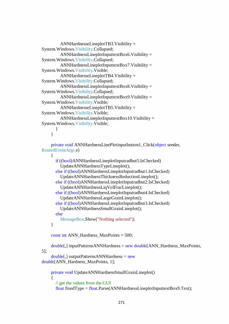
271
ANNHardnesseLineplotTB3.Visibility =
System.Windows.Visibility.Collapsed;
ANNHardnessLineplotInputtextBox6.Visibility =
System.Windows.Visibility.Collapsed;
ANNHardnessLineplotInputtextBox7.Visibility =
System.Windows.Visibility.Visible;
ANNHardnesseLineplotTB4.Visibility =
System.Windows.Visibility.Collapsed;
ANNHardnessLineplotInputtextBox8.Visibility =
System.Windows.Visibility.Collapsed;
ANNHardnessLineplotInputtextBox9.Visibility =
System.Windows.Visibility.Visible;
ANNHardnesseLineplotTB5.Visibility =
System.Windows.Visibility.Visible;
ANNHardnessLineplotInputtextBox10.Visibility =
System.Windows.Visibility.Visible;
}
}
private void ANNHardnessLinePlotinputbutton1_Click(object sender,
RoutedEventArgs e)
{
if ((bool)ANNHardnessLineplotInputradbut5.IsChecked)
UpdateANNHardnessTypeLineplot();
else if ((bool)ANNHardnessLineplotInputradbut1.IsChecked)
UpdateANNHardnessThicknessReductionLineplot();
else if ((bool)ANNHardnessLineplotInputradbut2.IsChecked)
UpdateANNHardnessLiqVolFracLineplot();
else if ((bool)ANNHardnessLineplotInputradbut4.IsChecked)
UpdateANNHardnessLargeGrainLineplot();
else if ((bool)ANNHardnessLineplotInputradbut3.IsChecked)
UpdateANNHardnessSmallGrainLineplot();
else
MessageBox.Show("Nothing selected");
}
const int ANN_Hardness_MaxPoints = 500;
double[,] inputPatternsANNHardness = new double[ANN_Hardness_MaxPoints,
5];
double[,] outputPatternsANNHardness = new
double[ANN_Hardness_MaxPoints, 1];
private void UpdateANNHardnessSmallGrainLineplot()
{
// get the values from the GUI
float fixedType = float.Parse(ANNHardnessLineplotInputtextBox9.Text);

272
float fixedthickness = float.Parse(ANNHardnessLineplotInputtextBox1.Text);
float fixedLiqVolFrac =
float.Parse(ANNHardnessLineplotInputtextBox3.Text);
float fixedLargeGrain =
float.Parse(ANNHardnessLineplotInputtextBox7.Text);
float SmallGrainLow =
float.Parse(ANNHardnessLineplotInputtextBox5.Text);
float SmallGrainHigh =
float.Parse(ANNHardnessLineplotInputtextBox6.Text);
int numPoints = int.Parse(ANNHardnessLineplotInputtextBox11.Text);
// calculate the independent and dependent values
List<Item> series1 = new List<Item>();
LineSeries plottable1 = new LineSeries();
Style noPointstyle = new System.Windows.Style(typeof(Control));
noPointstyle.Setters.Add(new Setter() { Property = TemplateProperty, Value =
null });
// calculate the step size for the points
float stepSize = (SmallGrainHigh - SmallGrainLow) / (numPoints - 1);
// generate the input patterns
for (int i = 0; i < numPoints; i++)
{
inputPatternsANNHardness[i, 0] = fixedType;
inputPatternsANNHardness[i, 1] = fixedthickness;
inputPatternsANNHardness[i, 2] = fixedLiqVolFrac;
inputPatternsANNHardness[i, 3] = fixedLargeGrain;
inputPatternsANNHardness[i, 4] = SmallGrainLow + i * stepSize;
}
// create array for output patterns
//double[] outputPatterns = new double[numPoints];
double maxnum = 121.824;
double minnum = 0;
const int input_array_size = 5;
const int hidden_array_1_size = 4;
const int hidden_array_2_size = 3;
const int output_array_size = 1;
// create normalized input and output arrays
double[] normInputPattern = new double[input_array_size];
double[] normOutputPattern = new double[output_array_size];
// create hidden arrays

273
double[] hidden1 = new double[hidden_array_1_size];
double[] hidden2 = new double[hidden_array_2_size];
double temp = 0;
double[,] weight_i_h = new double[input_array_size, hidden_array_1_size]
{
{-15.7427, -22.9999, -0.829085, 16.5365},
{18.3658, -2.87572, -0.153679, -8.11444},
{ 16.9694, -24.8862, 3.89563, -32.8081},
{4.1756, -2.44843, 5.32811, -1.04068},
{8.8315, 0.381159, 6.73193, -2.6118}
};
double[,] weight_h_h = new double[hidden_array_1_size,
hidden_array_2_size]
{
{10.934, 10.8556, 2.61835},
{-3.66757, -13.9818, 1.7814},
{1.05747, -4.92797, 1.7347},
{-1.29822, 11.3375, 2.37397}
};
double[,] weight_h_o = new double[hidden_array_2_size, output_array_size]
{
{-2.94166},
{4.93686},
{-0.174129}
};
double[] bias = new double[]
{
-8.83525, 12.7545, -5.1725, 10.2617,
0.33406, 0.69, 0.65,
0.68
};
for (int z = 0; z < numPoints; z++)
{
double diff = maxnum - minnum;
// normalize inputs
for (int x = 0; x < input_array_size; x++)
{
normInputPattern[x] = (((inputPatternsANNHardness[z, x] - minnum) *
0.8) / diff) + 0.1;
}
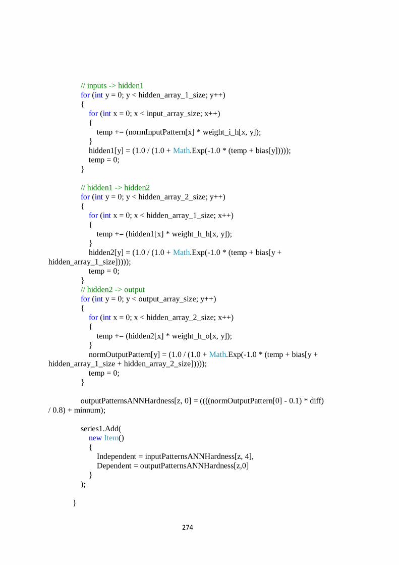
274
// inputs -> hidden1
for (int y = 0; y < hidden_array_1_size; y++)
{
for (int x = 0; x < input_array_size; x++)
{
temp += (normInputPattern[x] * weight_i_h[x, y]);
}
hidden1[y] = (1.0 / (1.0 + Math.Exp(-1.0 * (temp + bias[y]))));
temp = 0;
}
// hidden1 -> hidden2
for (int y = 0; y < hidden_array_2_size; y++)
{
for (int x = 0; x < hidden_array_1_size; x++)
{
temp += (hidden1[x] * weight_h_h[x, y]);
}
hidden2[y] = (1.0 / (1.0 + Math.Exp(-1.0 * (temp + bias[y +
hidden_array_1_size]))));
temp = 0;
}
// hidden2 -> output
for (int y = 0; y < output_array_size; y++)
{
for (int x = 0; x < hidden_array_2_size; x++)
{
temp += (hidden2[x] * weight_h_o[x, y]);
}
normOutputPattern[y] = (1.0 / (1.0 + Math.Exp(-1.0 * (temp + bias[y +
hidden_array_1_size + hidden_array_2_size]))));
temp = 0;
}
outputPatternsANNHardness[z, 0] = ((((normOutputPattern[0] - 0.1) * diff)
/ 0.8) + minnum);
series1.Add(
new Item()
{
Independent = inputPatternsANNHardness[z, 4],
Dependent = outputPatternsANNHardness[z,0]
}
);
}

275
ANNHardnessLineplot.Series.Clear();
if ((bool)ANNHardnessLinePlotinputCkbox1.IsChecked)
{
// update the plot
plottable1.ItemsSource = series1;
plottable1.IndependentValueBinding = new
System.Windows.Data.Binding("Independent");
plottable1.DependentValueBinding = new
System.Windows.Data.Binding("Dependent");
plottable1.DataPointStyle = noPointstyle;
ANNHardnessLineplot.Series.Add(plottable1);
}
}

276
A2.3 Code written in Computational file of Microsoft SilverLight API for
the Bar plot of hardness (used to optimise hardness of mushy state
rolled composite) by varying each input parameter.
#region Bar Plot
// paste here and change names accordingly
List<Item1> Hardness;
ColumnSeries plotHardness;
bool HardnessBarPlotLoaded = false;
private void ANNHardnessBarplot_Loaded(object sender,RoutedEventArgs e)
{
if (HardnessBarPlotLoaded)
return;
Hardness = new List<Item1>();
Hardness.Add(new Item1() { Independent = String.Empty, Dependent = 20 });
ANNHardnessBarplot.Axes.Clear();
ANNHardnessBarplot.Axes.Add(new CategoryAxis()
{
Orientation = AxisOrientation.X
});
ANNHardnessBarplot.Axes.Add(new LinearAxis()
{
Orientation = AxisOrientation.Y,
Minimum = 40,
Maximum = 140,
Interval = 20
});
plotHardness = new ColumnSeries()
{
Title = "Hardness",
ItemsSource = Hardness,
IndependentValueBinding = new
System.Windows.Data.Binding("Independent"),
DependentValueBinding = new
System.Windows.Data.Binding("Dependent"),
Visibility = System.Windows.Visibility.Collapsed
};
ANNHardnessBarplot.Series.Clear();
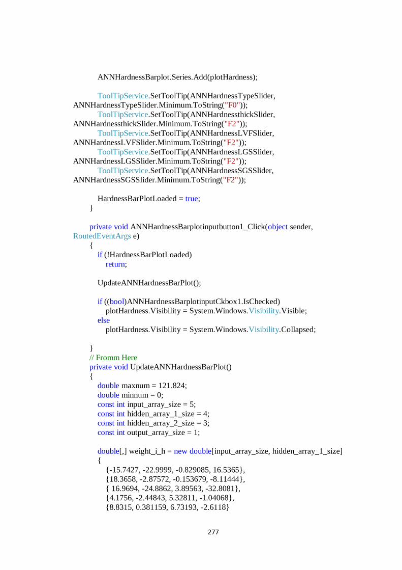
277
ANNHardnessBarplot.Series.Add(plotHardness);
ToolTipService.SetToolTip(ANNHardnessTypeSlider,
ANNHardnessTypeSlider.Minimum.ToString("F0"));
ToolTipService.SetToolTip(ANNHardnessthickSlider,
ANNHardnessthickSlider.Minimum.ToString("F2"));
ToolTipService.SetToolTip(ANNHardnessLVFSlider,
ANNHardnessLVFSlider.Minimum.ToString("F2"));
ToolTipService.SetToolTip(ANNHardnessLGSSlider,
ANNHardnessLGSSlider.Minimum.ToString("F2"));
ToolTipService.SetToolTip(ANNHardnessSGSSlider,
ANNHardnessSGSSlider.Minimum.ToString("F2"));
HardnessBarPlotLoaded = true;
}
private void ANNHardnessBarplotinputbutton1_Click(object sender,
RoutedEventArgs e)
{
if (!HardnessBarPlotLoaded)
return;
UpdateANNHardnessBarPlot();
if ((bool)ANNHardnessBarplotinputCkbox1.IsChecked)
plotHardness.Visibility = System.Windows.Visibility.Visible;
else
plotHardness.Visibility = System.Windows.Visibility.Collapsed;
}
// Fromm Here
private void UpdateANNHardnessBarPlot()
{
double maxnum = 121.824;
double minnum = 0;
const int input_array_size = 5;
const int hidden_array_1_size = 4;
const int hidden_array_2_size = 3;
const int output_array_size = 1;
double[,] weight_i_h = new double[input_array_size, hidden_array_1_size]
{
{-15.7427, -22.9999, -0.829085, 16.5365},
{18.3658, -2.87572, -0.153679, -8.11444},
{ 16.9694, -24.8862, 3.89563, -32.8081},
{4.1756, -2.44843, 5.32811, -1.04068},
{8.8315, 0.381159, 6.73193, -2.6118}

278
};
double[,] weight_h_h = new double[hidden_array_1_size,
hidden_array_2_size]
{
{10.934, 10.8556, 2.61835},
{-3.66757, -13.9818, 1.7814},
{1.05747, -4.92797, 1.7347},
{-1.29822, 11.3375, 2.37397}
};
double[,] weight_h_o = new double[hidden_array_2_size, output_array_size]
{
{-2.94166},
{4.93686},
{-0.174129}
};
double[] bias = new double[]
{
-8.83525, 12.7545, -5.1725, 10.2617,
0.33406, 0.69, 0.65,
0.68
};
// generate the input patterns
double[] inputPattern = new double[input_array_size];
inputPattern[0] = (ANNHardnessTypeSlider.Value >= 1.5) ? 2 : 1;
inputPattern[1] = (ANNHardnessthickSlider.Value);
inputPattern[2] = (ANNHardnessLVFSlider.Value);
inputPattern[3] = (ANNHardnessLGSSlider.Value);
inputPattern[4] = (ANNHardnessSGSSlider.Value);
// create normalized input and output arrays
double[] normInputPattern = new double[input_array_size];
double[] normOutputPattern = new double[output_array_size];
// create hidden arrays
double[] hidden1 = new double[hidden_array_1_size];
double[] hidden2 = new double[hidden_array_2_size];
double temp = 0;
double diff = maxnum - minnum;
// normalize inputs
for (int x = 0; x < input_array_size; x++)
{

279
normInputPattern[x] = (((inputPattern[x] - minnum) * 0.8) / diff) + 0.1;
}
// inputs -> hidden1
for (int y = 0; y < hidden_array_1_size; y++)
{
for (int x = 0; x < input_array_size; x++)
{
temp += (normInputPattern[x] * weight_i_h[x, y]);
}
hidden1[y] = (1.0 / (1.0 + Math.Exp(-1.0 * (temp + bias[y]))));
temp = 0;
}
// hidden1 -> hidden2
for (int y = 0; y < hidden_array_2_size; y++)
{
for (int x = 0; x < hidden_array_1_size; x++)
{
temp += (hidden1[x] * weight_h_h[x, y]);
}
hidden2[y] = (1.0 / (1.0 + Math.Exp(-1.0 * (temp + bias[y +
hidden_array_1_size]))));
temp = 0;
}
// hidden2 -> output
for (int y = 0; y < output_array_size; y++)
{
for (int x = 0; x < hidden_array_2_size; x++)
{
temp += (hidden2[x] * weight_h_o[x, y]);
}
normOutputPattern[y] = (1.0 / (1.0 + Math.Exp(-1.0 * (temp + bias[y +
hidden_array_1_size + hidden_array_2_size]))));
temp = 0;
}
Hardness.ElementAt(0).Dependent = ((((normOutputPattern[0] - 0.1) * diff) /
0.8) + minnum);
plotHardness.Refresh();
}
private void ANNhardnessSlider_ValueChanged(object sender,
RoutedPropertyChangedEventArgs<double> e)
{
if (sender.Equals(ANNHardnessTypeSlider))

280
ToolTipService.SetToolTip(ANNHardnessTypeSlider,
(ANNHardnessTypeSlider.Value >= 1.5) ? "2" : "1");
else if (sender.Equals(ANNHardnessthickSlider))
ToolTipService.SetToolTip(ANNHardnessthickSlider,
ANNHardnessthickSlider.Value.ToString("F2"));
else if (sender.Equals(ANNHardnessLVFSlider))
ToolTipService.SetToolTip(ANNHardnessLVFSlider,
ANNHardnessLVFSlider.Value.ToString("F2"));
else if (sender.Equals(ANNHardnessLGSSlider))
ToolTipService.SetToolTip(ANNHardnessLGSSlider,
ANNHardnessLGSSlider.Value.ToString("F2"));
else if (sender.Equals(ANNHardnessSGSSlider))
ToolTipService.SetToolTip(ANNHardnessSGSSlider,
ANNHardnessSGSSlider.Value.ToString("F2"));
else
return;
UpdateANNHardnessBarPlot();
}
#endregion
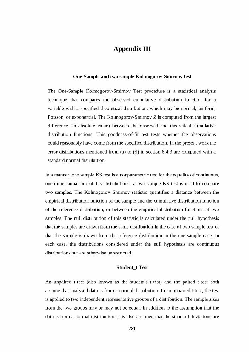
281
Appendix III
One-Sample and two sample Kolmogorov-Smirnov test
The One-Sample Kolmogorov-Smirnov Test procedure is a statistical analysis
technique that compares the observed cumulative distribution function for a
variable with a specified theoretical distribution, which may be normal, uniform,
Poisson, or exponential. The Kolmogorov-Smirnov Z is computed from the largest
difference (in absolute value) between the observed and theoretical cumulative
distribution functions. This goodness-of-fit test tests whether the observations
could reasonably have come from the specified distribution. In the present work the
error distributions mentioned from (a) to (d) in section 8.4.3 are compared with a
standard normal distribution.
In a manner, one sample KS test is a nonparametric test for the equality of continuous,
one-dimensional probability distributions a two sample KS test is used to compare
two samples. The Kolmogorov–Smirnov statistic quantifies a distance between the
empirical distribution function of the sample and the cumulative distribution function
of the reference distribution, or between the empirical distribution functions of two
samples. The null distribution of this statistic is calculated under the null hypothesis
that the samples are drawn from the same distribution in the case of two sample test or
that the sample is drawn from the reference distribution in the one-sample case. In
each case, the distributions considered under the null hypothesis are continuous
distributions but are otherwise unrestricted.
Student_t Test
An unpaired t-test (also known as the student's t-test) and the paired t-test both
assume that analysed data is from a normal distribution. In an unpaired t-test, the test
is applied to two independent representative groups of a distribution. The sample sizes
from the two groups may or may not be equal. In addition to the assumption that the
data is from a normal distribution, it is also assumed that the standard deviations are

282
approximately same in both the groups. Then the t-test compares the means of the two
groups of data. The test determines whether the data has come from the same
population or not. The mean difference is then calculated which could be positive or
negative. The mean difference is calculated with a 95% confidence interval or 5%
significance. A p-value is calculated where p is the probability of a false-positive
event.
In a paired t-test, the data is derived from study subjects who have been measured at
two time points (each individual has two measurements). The two measurements
generally are before and after a cause and effect relationship. Then a 95% confidence
interval is derived from the difference between the two sets of paired observations.

283
Appendix IV
The data used for validation of the ANN with feed forward architectures are actually
the unseen data, as the network modelling was done prior to conduct of validation
experiments. Therefore, the generalisation of the ANN models proposed is implied by
the small errors in prediction that have been cited in the thesis (Table 4.4, 4.5, 5.4,
5.5, 6.3 and 7.2). However, the generalisation capability of the ANN model (i. e. The
architecture used for prediction of grain sizes, hardness etc.) can be demonstrated by
picking up a similar data and training the network for this data and checking:
i. Convergence characteristics
ii. Error in prediction
Generalisation capability of the ANN model for grain size prediction
The generalisation capability of the ANN model for prediction of grain sizes is
presented by considering the case of mushy state rolling of as cast Al-4.5Cu-5TiC
composite which is different from the material tried out in our study. The data has
been taken from the work of Herbert (2007). The input parameters for the network are
initial material of the Al-4.5Cu-5TiC composite (which is kept constant = 1), %
Thickness reduction and % Liquid volume fraction in the composite. The outputs of
the network are large and small grain sizes. The network is trained with the available
12 input-output patterns. Same architecture as that was used for the prediction of grain
sizes for Al-4.5Cu-5TiB2 composite is used for training this network. Similarly the
learning rate and momentum term was also not changed. The network converged
nicely to a MSE of 0.00016 after around 18.8 lakh epochs. Table 4.6 gives the
comparison of literature data with the ANN predictions in terms of percentage error in
prediction over the literature data.

284
It can be seen from Table 4.6 that the ANN model predicts the large grain sizes within
± 1.93%. Similarly, the small grain sizes are predicted by the network within an error
of ± 3.45%. Thus it is seen that for a given kind of model processing, be it mushy
state rolling, mushy state forging or any other mushy state forming process, same
ANN model can be used to predict the grain sizes.
Generalisation capability of the ANN model for hardness prediction
The data for demonstrating the generalisation capability of the ANN model for
hardness prediction is taken from the work of Herbert (2007). The part of the work of
Herbert (2007) used here involved the study on the hardness characteristics of mushy
state rolled as cast Al-4.5Cu-5TiC composite. ANN model with 12 available patterns
is trained with the same architecture, learning rate parameter and momentum factor as
used for training the model for predicting hardness of Al-4.5Cu-5TiB2 composite. The
inputs to the network are initial material of the Al-4.5Cu-5TiC composite (which is
kept constant = 1), % Thickness reduction and % Liquid volume fraction in the
composite, large and small grain size. The output of the network is hardness. The
network was found to excellently converge to a MSE of 2.4 x 10⁻⁵
after 6.3 lakh
TABLE A.1 Comparison of values of grain sizes of as cast Al-4.5Cu- 5TiC
composite samples subjected to mushy state rolling with ANN
predicted values. (Herbert 2007)
Specimen
descriptions
Literature ANN %Error
Grain size(μm) Grain size (μm) Grain size
Large Small Large Small Large Small
2.5%
Thickness
Reduction
fl ~ 0.1 78 40 77.93 40.21 0.09 -0.53
fl ~ 0.2 75 38 73.70 39.05 1.73 -2.76
fl ~ 0.3 84 47 83.88 46.92 0.14 0.17
5%
Thickness
Reduction
fl ~ 0.1 71 39 70.99 38.04 0.01 2.46
fl ~ 0.2 70 41 69.62 40.35 0.54 1.59
fl ~ 0.3 76 42 77.47 40.55 -1.93 3.45
7.5%
Thickness
Reduction
fl ~ 0.1 70 44 70.49 44.61 -0.7 -1.39
fl ~ 0.2 69 48 71.69 48.05 -3.9 -0.1
fl ~ 0.3 82 49 81.24 49.37 0.93 -0.76
10.5%
Thickness
Reduction
fl ~ 0.1 68 48 68.34 47.87 -0.5 0.27
fl ~ 0.2 67 44 66.14 44.84 1.28 -1.91
fl ~ 0.3 79 44 78.75 44.66 0.32 -1.5

285
epochs. Table A.2 shows the comparison of the literature values of hardness with the
ANN predicted values of hardness.
It can be seen from Table A.2 that the error in prediction for hardness over the entire
range of data used for training the network is within ± 1.47 %. This demonstrates that
the ANN model with a particular architecture can be used to model similar processes.
This is because ANN models having similar architectures possess capabilities to
generalise the subtle relationships that exist between the input-output data for similar
processes. Moreover, the code that has been developed is generic in nature having
flexibility in the selection of architectures, in terms of number of layers and number
of neurons in each layer as well as associated coefficients. Due to this, the Hybrid
RNN model developed may be easily adopted to any of the process prediction,
following proper training.
Table A.2 Comparison of values hardness from literature for pre hot rolled
Al-4.5Cu-TiC composite samples subjected to mushy state
rolling with ANN predicted values.
Specimen descriptions
Experimental ANN %Error
Grain size
(μm) Hardness
(Hv)
Hardness
(Hv) Hardness
Large Small
2.5%
Thickness
Reduction
fl ~ 0.1 78 40 89 89.32 -0.36
fl ~ 0.2 75 38 92 91.14 0.93
fl ~ 0.3 84 47 85 84.55 0.53
5%
Thickness
Reduction
fl ~ 0.1 71 39 92 92.16 -0.17
fl ~ 0.2 70 41 95 94.3 0.74
fl ~ 0.3 76 42 88 89.29 -1.47
7.5%
Thickness
Reduction
fl ~ 0.1 70 44 93 93.5 -0.54
fl ~ 0.2 69 48 96 96.2 -0.21
fl ~ 0.3 82 49 91 91.12 -0.13
10.5%
Thickness
Reduction
fl ~ 0.1 68 48 95 94.79 0.22
fl ~ 0.2 67 44 98 97.83 0.17
fl ~ 0.3 79 44 94 93.55 0.48

287
REFERENCES
Ackley, D.H., Hinton, G.E., and Sejnowski, T.J. (1985). “A learning algorithm for
Boltzman machines.” Cognitive Science, 9, 147-169.
Aikin, R. (1997). "The mechanical properties of in-situ composites." JOM, Journal
of the Minerals, Metals and Materials Society 49(8), 35-39.
Amhold, V. and Muller-Schwelling, D. (1991). SAE Technical Paper Series 910156.
SAE International, Warrendale, PA
Annavarapu, S. and Doherty, R.D. (1995). "Inhibited coarsening of solid-liquid
microstructures in spray casting at high-volume fractions of solid." Acta Metall.
Mater., 43, 3207-3230.
Apaydin, N. Prabhakar, K.V. and Doherty, R.D. (1980). "Special grain boundaries
in rheocast Al-Mg." Mater. Sci. Eng. A., 46, 145-150.
Archard, J.F. (1953). “Contact and rubbing of flat surfaces”. J. Appl. Phys., 24, 981-
988.
Atkinson, H.V. (2005). "Modelling the semisolid processing of metallic alloys."
Prog. in Mater. Sci., 50, 341-412.
Attoh-Okine, N.O. (1999). “Analysis of learning rate and momentum term in
backpropagation neural network algorithm trained to predict pavement
performance.” Adances in Engineering Software, 30, 291-302.
Barnes, H.A., and Walters, K. (1985). "The Yield Stress Myth." Rheol. Acta, 24,
323-326.
Barnes, H.A., Hutton, J.F., and Walters, K. (1989). "An introduction to rheology."
Amsterdam, The Netherlands: Elsevier, 27-31.
Bartels, C., Raabe, D Gottstein, G., Huber, U. (1997). "Investigation of the
precipitation kinetics in an Al6061/TiB2 metal matrix composite." Mater Sci. Eng. A,
237, 12-23.
Bengioy, Y., Simrad, P., and Frasconi, P. (1994). „Learning long time dependencies
with gradient descent is difficult.” IEEE Trans. Neural Netw., 5(2), 157-166.
Bergsma, S.C., Tolle, M.C., Kassner, M.E., Li, X., and E. Evangelista, (1997).
"Semi-solid thermal transformations of Al-Si alloys and the resulting mechanical
properties." Mater. Sci. Eng. A, 237, 24–34.

288
Bergsma, S.C. Li, X. Kassner, M.E. (2001). "Semi-solid thermal transformations in
Al–Si alloys: II. The optimized tensile and fatigue properties of semi-solid 357 and
modified 319 aluminum alloys." Mater. Sci. Eng. A, 297, 69-77.
Bezdek, J.C. (1992). “On the relationship between neural networks, pattern
recognition and intelligence.” Int. J. Approx. Reasoning, 6, 85-107.
Bhat Radhakrishna, B.V., Mahajan, Y.R., Roshan, H.M., Prasad, Y.U.R.K. (1992).
“Processing map for hot working of powder metallurgy 2124 Al-20 vol. pct. SiCp
metal matrix composite”. Metall. Trans. A., 23, 2223-2230.
Blazek, K.E., Kelly, J.E., and Pottore, N.S. (1995). "The development of a
continuous rheocaster for ferrous and high-melting point alloys.” ISIJ Int., 35, 813-
818.
Blais, S., Loue, W., and Pluchon, C. (1996). "Structure Control by Electromagnetic
Stirring and Reheating at Semi-solid State." Proc. 4th Int. Conf. on Semi-Solid
Processing of Alloys and Composites, Kirkwood DH, Kapranos P, eds., Sheffield,
UK, June 1996, University of Sheffield, 187-192.
Braccini, M., Salvo, L., Suery, M., Brechet, Y. (1998). Proc. 5th Int. Conf. on Semi-
Solid Processing of Alloys and Composites, Bhasin AK, Moore JJ, Young KP,
Midson S, eds., Golden, Colorado, USA, June 1998. Golden, CO: Colorado School
of Mines, USA, 371-378.
Cameron, S. H. (1960). “An estimate of the complexity requisite in a universal
decision network.‟ Wright Air Development Division, report, 60-600.
Caracostas, C.A., Chiou, w.A., Fine, M.E. and Chung, H.S. (1992). “Wear
mechanisms during lubricated sliding of XDTM
2024 – Al-TiB2 metal matrix
composites against steel”. Scripta Metall. Mater., 27, 167-172.
Chen, C.Y., Sekhar, J.A., Backman, D.G. and Mehrabian, R. (1979). “Thixoforging
of aluminium alloys.” Mater. Sci. Eng, 40, 265-272.
Chen, D.S., and Jain, R.C. (1994). “A robust backpropagation algorithm for function
approximation.” IEEE Trans. Neural Networks, 5, 467-479.
Chen, T.J., Hao, Y., and Sun, J. (2002). "Microstructural evolution of previously
deformed ZA27 alloy during partial remelting." Mater. Sci. Eng. A, 337, 73-81.
Cho, J.C., Cho, H.Y., Min, G.S., Park, H.J., and Choi, J.U. (1996). “A fundamental
study on semi-solid forging with light and hardly formable materials.” J. Korean
Soc. Prec. Eng., 13(7), 29-35.
Cho W.G., and Kang, C.G. (2000). "Mechanical properties and their microstructural
evaluation in the thixoforming process of semisolid aluminium alloy." J. Mater.
Process. Tech., 105, 269-277.
289
Choi, J.C., and Park, H.J. (1998a). Proc. 5th Int. Conf. on Semi-Solid Processing of
Alloys and Composites, Bhasin AK, Moore JJ, Young KP, Midson S, eds. Golden,
Colorado, USA, June 1998. Golden, CO: Colorado School of Mines, USA, 457-464.
Choi, J.C., and Park, H.J. (1998b). "Microstructural characteristics of Aluminium
2024 by cold workingin the SIMA process." J. Mater. Process. Tech., 82, 107-116.
Cibula, A. (1949). "The mechanism of grain refinement of sand castings in Al
alloys." J. Inst. Metals, 76, 321-360.
Cibula, A. (1951). "The grain refinement of Al alloy castings by additions of Ti and
B." J. Inst. Metals, 80, 1-16.
Cui, J. Lu, G. Dong, J. Xia, K. (2000). "Microstructures after casting and reheating
in a continuously cast aluminium alloy 7075." Proc. 6th Int. Conf. on Semi-Solid
Processing of Alloys and Composites, Chiarmetta GL, Rosso M, eds., Turin, Italy,
Sept 2000, Brescia. Italy: Edimet Spa: (2000), 701-704.
Cumming, S. (1993). “Neural networks for monitoring of engine condition data.”
Neural Computing and applications, 1, 96-102.
Das, A., Ji, S., and Fan, Z. (2002). "Morphological development of solidification
structures under forced fluid flow: a Monte-Carlo simulation." Acta Mater., 50(18),
4571-4585.
Das, A., and Fan, Z. (2004). "A Monte Carlo simulation of solidification structure
formation under melt shearing.” Mater. Sci. Eng. A., 365(1-2), 330-335.
DeFreitas, E.R., Ferracini Jr., E., and Ferrante, M. (2004). "Microstructure and
rheology of an AA2024 aluminium alloy in the semisolid state, and mechanical
properties of a back extruded part." J. Mater. Process. Tech., 146, 241–249.
Deuis, R.L., Subramanian, C. and Yellup, J.M. (1997). “Dry sliding wear of
aluminium composites – A review”. Compos. Sci. Tech., 57, 415-435.
Dobrazanski, L.A.,Maniara, R., Sokolowski, J.H., and Krupinski, M. (2007).
“Modelling of mechanical properties of Al-Si-Cu cast alloys using the neural
network.” J. Achievements in Materials and Manufacturing Engineering, 20(1-2),
347-350.
Doherty, R.D., Lee, H.I., and Feest, E.A. (1984). "Microstructure of stir-cast
metals." Mater. Sci. Eng. A., 65, 181-189.
Easton, M., and St. John, D. (1999a). "Grain refinement of Aluminum Alloys: Part I:
the Nucleant and Solute paradigms- A review of the Literature." Metall. Trans. A,
30, 1613-1623.
290
Easton, M. St. John, D. (1999b). "Grain refinement of Aluminum Alloys: Part II:
Confirmation of, and a Mechanism for, the Solute Paradigm." Metall. Trans. A, 30,
1625-1633.
Elias L., Kirkwood, D.H., and Sellars, C.M. (1988). Proc 2nd World Basque
Congress, Conference on New Structural Materials, Bilbao, Spain (Servicio Central
de Publicaciones del Gobeierno Vasco), 285–295.
Elman, J.L. (1990). “Finding structure in time.” Cognitive Science, 14, 179-211.
Elman, J.L. (1991). “Distributed representations, simple neural networks and
grammatical structures.” Machine Learning, 7, 195-225.
Fan, Z., Bevis, M.J., and Ji, S. (1999a). "Method and apparatus for producing
semisolid metal slurries and shaped components." Patent PCT/WO/O1/21343A1,
1999.
Fan, Z., Bevis, M.J., and Ji, S. (1999b). "Process and apparatus for manufacturing
castings from immiscible metallic liquids." PCT/WO 01/23124 Al (1999).
Fan, Z., Ji, S., and Bevis, M.J. (2001a). "Semi-solid processing of engineering alloys
by a twin-screw rheomoulding process." Mater. Sci. Eng. A, 299, 210–217.
Fan, Z., Ji, S., and Zhang, J., (2001b). "Processing of immiscible metallic alloys by
rheomixing process." Mater. Sci. Technol., 17, 837-842.
Fan, Z. (2002). “Semisolid metal processing.” Int. Mat. Rev., 47(2), 49-85.
Ferrante, M., and DeFreitas, E. (1999). "Rheology and microstructural development
of Al-4%Cu alloy in the semisolid state." Mater. Sci. Engg, A, 271, 172-180.
Flemings, M. C. (1991). “Behaviour of Metal alloys in semisolid state.” Metall.
Trans. A, 22, 957-981.
Flemings, M.C. (1991). “Behaviour of metals in semisolid state.” Metall. Trans. A,
22, 957-981.
Flemings, M.C., Chen, S.F., Diewwanit, I., and Cornie, J. A. (1992). "Rheology and
structure of some Aluminium base composites." Proc. 2nd Int. Conf. on Semi-Solid
Processing of Alloys and Composites, Brown SB, Flemings MC, eds.,Cambridge,
MA, USA. Warrendale, TMS (1992), 202-210.
Flemings, M C., Martinez, R.A., Figuredo, A., and Yurko, J.A. (2003). "Metal alloy
compositions and Process." United States Patent No. 6645323, November 11, 2003.
Flemings M.C., and Martinez, R.A. (2006). "Principles of Microstructural Formation
in Semi-Solid Metal Processing." Solid state Phenomena, 116-117, 1-8.

291
Frasconi, P., Gori, M. and Soda, G. (1992). “Local feedback multilayered networks”.
Neural Computation, 120-130.
Fraser, M.C. (2000). “Neural networks literature review from a statistical
perspective.” California State University, Hayward.
Fukuoka, S., and Kiuchi, M. (1974). "A study on plastic working of alloys in their
mushy state.” Proc. 15th
Int. Conf. on Machine Tool Design and Research. Tobias,
S.A., Koenigsberger, F. eds., Birmingham, 18-20 September (1974), 423.
Gabathuler, J.P., Barras, D., Krahenbuhl, Y., and Weber, J.C. (June 1992).
"Evaluation of various processes for the production of billets with Thixotropic
properties." Proc. 2nd Int. Conf. on Semi-Solid Processing of Alloys and Composites,
Brown SB, Flemings MC, eds., Cambridge, MA, USA. Warrendale, TMS (1992),
33-46.
Gabathuler, J.P., Huber, H.J., and Erling, J. (1993). "Specific properties of produced
parts using the thixocasting process." Proceedings of the International Conference
on Aluminium Alloys: new process technologies. Associazonne Italiana Metallurgia.
Italy: Ravenna, 169-180.
Gebelin,J.C., Suery, M., and Favier, D. (1999). "Characteriztion of the rheological
behavior in the semisolid solid state of grain refined AZ91 magnesium alloys."
Mater. Sci. Eng. A, 272, 134-144.
Giles, C., Miller C., Chen, D., Chen, H., Sun, G. And lee, Y. (1992). “Learning and
extracting Finite state automats with second order recurrent neural networks.”,
Neural Computations, 4, 393-405.
German, S., and Bienenstock, E. (1992). “Neural networks and the bias/variance
dilemma.” Networks and Neural Computation, 4 (1), 1-54.
Gormann, R.P., and Sejnowski, T.J. (1988). “Analysis of hidden units in a layered
network trained to classify sonar targets.” Neural Networks, 1(1), 75-89.
Gruning, A. (2006). “Stack-like and que-like dynamics in recurrent neural
networks.” Connection Sci., 18(1), 23-42.
Gruning, A. (2007) “Elman backpropagation as reinforcement of simple recurrent
neural networks.” Neural computation, 19(11), 3108-3131.
Guler, N.F., Ubeyli E.D. and Guler I. (2005). “Recurrent neural networks employing
Lyapunov exponents for EEG signals classification”. Expert systems with
applications, 29, 506-514.
Hamilton, R. W., Zhu, Z., Dashwood, R. J., and Lee, P. D. (2003). "Direct semi-solid
forming of a powder SiC-Al PMMC: flow analysis, Compos." Part A Appl. Sci.
Manuf., 34(4), 333-339.
292
Haque, M.E. and Sudhakar (2002). “ANN Back Propagation Model for fracture
toughness in microalloy steel”. Int. Jour. of Fatigue, 24, 1003-1010.
Hardy, S.C., and Voorhes, P.W. (1988). "Ostwald ripening in a system with a high
volume fraction of coarsening phase.' Metall. Trans. A, 19, 2713-2721.
Hartnett, J.P., and Hu, R.Y.Z. (1989). "Technical Note: The Yield Stress - An
Engineering Reality." J. Rheol., 33, 671-679.
Hartley, P., and Pillinger, I. (2006). “Numerical simulation of the forging process.”
Comp. Methods Appl. Mech. Engrg., 195, 6676-6790.
Hellawell, A. (1996). "Grain Evolution in Conventional and Rheocastings, Proc. 4th
Int Conf on Semi-solid Processing of Alloy and Composites.” Proc. 4th Int. Conf. on
Semi-Solid Processing of Alloys and Composites, Kirkwood DH, Kapranos P, eds.,
Sheffield, UK, June 1996, University of Sheffield, 60-65.
Herbert, M.A., Sarkar, C., Mitra, R., and Chakraborty, M. (2006). “Microstructural
evolution, hardness and alligatoring in the mushy state rolled cast Al-4.5Cu Alloy
and in-situ Al-4.5Cu-5tiB2 composite.” Metall. Mater. Trans. A, 38, 2110-2143.
Herbert, M.A. (2007) “Some studies on the mushy state rolling of Al-4.5Cu alloy
base in situ composites reinforced with TiB2 or TiC particles.” Ph.D. thesis, Indian
Institute of Technology, Kharagpur, India.
Herbert, M.A., Maiti, R., Mitra, R., and Chakraborty, M. (2008). “Wear behaviour of
cast and mushy state rolled Al-4.Cu alloy and in-situ al-4.5Cu-5TiB2 composite.”
Wear, 265, 1306-1618.
Herbert, M.A., Das, A.G., Maiti, R., Chakraborty, M., and Mitra, R., (2010).
“Tensile properties of cast and mushy state rolled Al-4.Cu alloy and in-situ al-4.5Cu-
5TiB2 composite.” Inter. J. Cast Metal, Res, 23(4), 216-224.
Hirt, G., Cremer, T., Witulski, R., and Tinius, H.C. (1997). "Lightweight near net
shape components produced by thixofroming." Materials and Design, 18(4/6), 315-
321.
Hong, T.W., Kim, S.K., Ha, H.S., Kim, M.G., Lee, D.B., Kim, Y.J. (2000).
"Microstructural evolution and semisolid forming of SiC particulate reinforced
AZ91HP magnesium composites." Mater. Sci. Technol., 16, 887-892.
Hopfield, J.J. (1982). “Neural networks and physical systems with emergent
collective computational capabilities.” Proc. National Academy of Sciences, USA,
79, 2554-2558.
Hopfield J.J. (1984). “Neurons with graded responses have collective computational
properties like those of two-state neurons.” Proc. National Academy of Sciences,
USA, 81, 3088-3092.
293
Hornik, K. (1993). “Some new results on neural network approximation.”Neural
Networks, 6(8), 1069-1072.
Ilegbusi, O.J., and Szekely, J. (1988). "Mathematical Modelling of the
Electromagnetic Stirring of Molten Metal Solid Suspensions." Trans. Iron Steel Inst.
Jpn., 28, 97-103.
Ito, Y., Flemings, M.C., and Corne, J.A. (1992). “Rheological behaviour and
microstructure of. Al-6wtpcSi”, Nature and properties of semi-solid materials,
Sekhar J. A., and Dantzig, J. A. eds., Warrcndale, PA, TMS (1992), 3–17.
Jiahe, A., Jiang, X., Huiju, G., Yaohe, H., and Xishan, X. (2003). “Artificial neural
network for prediction of the microstructure of 60Si2MnA rod based on its
controlled rolling and cooling process parameters.” Mater. Sci. and Engg. A, 344,
318-322.
Joly, P. A. and Mehrabian, R. (1976). "The rheology of a partially solid alloy." J. of
Materials Science, 11, 1393-1418.
Jones, G. P., and Pearson, J. (1976). "Factors affecting the grain refinement of Al
using Ti and B additives." Metall. Trans. B, 7, 223-234.
Jordan, M. (1992). “Constrained supervised learning.” J. Math. Psychol., 36, 396-
425.
Jordan, M. I. (1995). “The organization of action sequences: evidence from a
relearning task.” J. Motor behaviour, 27, 179-192.
Jorstad, J.L., Pan, Q. Y., and Apelian, D. (2005). "Solidification microstructure
affecting ductility in semisolid cast products." Mater. Sci. Engg. A, 413-414, 186-
191.
Jung, H.K., and Kang, C. G. (2002). "Induction heating process of an Al-Si
aluminum alloy for semi-solid die casting and its resulting microstructure.” J. Mater.
Process. Tech., 120, 355-364.
Kahermann, W., Sachragner, R., Young, K.P. (1996). “Free standing raw material
production system for SSM recycling.” Proc. 4th Int. Conf. on Semi-Solid
Processing of Alloys and Composites, Kirkwood, D.H., Kapranos P., eds., Sheffield,
UK, June 1996, University of Sheffield, 154-158.
Kamat, S.V., Hirth, J.P., and Mehrabian, R. (1989). "Mechanical properties of
particulate reinforced Aluminium matrix composites." Acta Metall., 37(9), 2395-
2402.
Kang, C.G., and Ku, G.S. (1995). "An experimental investigation on infiltration limit
and mechanical properties of Al2O3 short fiber reinforced metal matrix composites
fabricated by squeeze casting." J. Comp. Mater., 29(4), 444-462.

294
Kang, J.Y. and Song, J.H. (1998). “Neural network applications in determining the
fatigue crack opening load.” Int. J. Fatigue, 20(1), 57-69.
Kapranos, P., Ward, P.J., Atkinson, H.V., and Kirkwood, D.H. (2000). “Near net
shaping by semi-solid metal processing." Materials and Design, 21, 387-394.
Kapranos, P., Kirkwood, D.H., Atkinson, H.V., Rheinlander, J.T., Bentzen, J.J.,
Toft, P.T., Debel, C.P., Laslaz, G., Maenner, L., Blais, S., Rodriguez-Ibabe, J.M.,
Lasa. L., Giordano, P., Chiarmetta, G., and Giese, A. (2003). "Thixoforming of an
automotive part in A390 hypereutectic Al–Si alloy." J. Mater. Process. Tech., 135,
271–277.
Kattamis, T.Z., and Piccone, T.J. (1991). "Rheology of semisolid Al–4.5%Cu–
1.5%Mg alloy." Mater. Sci. Eng. A, 131, 265–272.
Kaufmann, H., Wabusseg, H., Uggowitzer, P.J. Wabusseg, H., and Uggowitzer, P.J.
(2000a). “Metallurgical and processing aspects of the NRC semi-solid casting
technology.” Aluminium, 76, 70-75.
Kaufmann, H., Wabusseg, H., and Uggowitzer, P.J (2000b). “Casting of light metal
wrought alloys by New Rheocasting.” Proc. 6th Int. Conf. on Semi-Solid Processing
of Alloys and Composites, Chiarmetta GL, Rosso M, eds., Turin, Italy, Sept 2000,
Brescia. Italy: Edimet Spa: 457-462.
Kenney, M.P., Courtois, J.A., Evans, R.D., Farrior, G.M., Kyonka, C.P., Koch,
A.A., and Young, K.P. (1988). Metals handbook, 9th ed., ASM International, Metals
Park, OH, USA, 15, 327–338.
Kim, J.W., Weistroffer, H.R., and Redmond, R.T. (1993). “Expert systems for bond
rating: a comparative analysis of statistical, rule-based and neural network systems”,
Expert Systems, 10, 167-172.
Kirkwood, D.H., and Kapranos, P. (1989). "Semisolid Processing of Alloys." Met.
Mater., 5(1), 16-19.
Kirkwood, D.H. (1994). "Semi-solid metal processing." Int. Mat. Rev., 39(5), 173-
189.
Kiuchi, M., and Fukuoka, S. (1979). "Study on flow stress of alloys in mashy state."
Journal of Japan Society for Technology of Plasticity, 20, 826-833.
Kiuchi, M., Sugiyama S. (1982). "Investigation into mashy state processing and
working of particle reinforced composite metals." J. Jap. Soc. for Technol. of Plast.,
23, 915-923.
Kiuchi, M. (1987). "Application of mashy state working processes to production of
metal ceramic composites." Annals of CIRP, 36(1), 173-176.
295
Kiuchi, M. (1989). "Metal forming in mushy state in Plasticity and Modern metal
forming technology." Blazynski, T.Z. ed., Elsivier Applied Science., London & New
York, 289-313.
Kiuchi, M., and Sugiyama, S. (1991). "Mushy state rolling of Aluminium alloys and
Cast irons." Annals of the CIRP, 40, 259-261.
Kiuchi, M., and Sugiyama, S. (June 1992). "Application of mashy metal processing
and forging technologies to manufacturing fiber reinforced metals." Proc. 2nd Int.
Conf. on Semi-Solid Processing of Alloys and Composites, Brown SB, Flemings
MC, eds., Cambridge, MA, USA. Warrendale, TMS (1992), 382-389.
Koike, S. (2002). “A class of adaptive size control algorithms for adaptive filters.”
IEEE Trans. Signal Processes, 50(6), 1315-1326.
Koke, J., and Modigell, M. (2003). "Flow behaviour of semisolid metal alloys." Jour.
Non-Newtonian Fluid Mech., 112, 141–160.
Kopp, R. (1996). “Some current developments in metal forming technology.” J.
Mater. Process. Tech., 60, 1-9.
Kopp, R., Neudenberger, D., and Winning, G. (2001). "Different concepts of
thixoforging and experiments for rheological data.” J. Mater. Process. Tech., 111,
48–52.
Kremer, S.C. (1995). “On the computational power of Elman style neural networks.”
IEEE Trans. Neural Netw., 6, 1000-1004.
Kuan, C.M., Hornik,K., and White, H. (1994). “A convergence result for learning in
recurrent neural networks.” Neural Computation, 420-444.
Kusiak, J., and Kuziak, S. (2002). “Modelling of microstructure and mechanical
properties of steel using artificial neural networks.” J. Mater. Process. Tech., 127,
115-121.
Lakshmi,S., Lu, L. and Gupta, M. (1998) “In situ preparation of TiB2 reinforced Al
based composites”. J. Mater. Process. Tech., 73, 160-166.
Lang, K.J., Waibet, A.H. and Hinton, G.E. (1990). “A time-delay neural network
architecture for isolated word recognition”. Neural Networks, 3, 23-44.
Lapedes, A., and Farber, R. (1988). “How neural network works.” Neural Network
Processing Systems, Anderson, and D. Z. eds., (Denver), American Institute of
Physics, New York, 442-456.
Lapkowski, W. Sinczak, J. Rusz, S. (1997). "Feasibility of metal forming in
semisolid state." J. Mater. Process. Tech., 63, 260-264.

296
Lapkowski, W. (1998). "Some studies regarding thixoforming of metal alloys." Jour.
Mater. Process. Technol., 80-81, 463-468.
Larkiola, J., Myllykeski, P., Nylander, J., and Korhonen, A.S. (1996). “Prediction of
rolling force in cold rolling by using physical models and neural computing.” J.
Mater. Process. Tech., 60(1-4), 381-386.
Larkiola, J., Myllykeski, P., Korhonen, A.S., and Cser, L. (1998). “The role of neural
networks in optimisation of rolling processes.” J. Mater. Process. Tech., 80-81, 16-
23.
Leatham, A., Ogilvy, A., Chesney, P., and Wood, P. (1989). "Osprey process-
production flexibility in material manufacture." Metals and Materials, 5, 140-143.
Lee, H.I., Doherty, R.D. E.A. Feest, and Titchmarsh, J.M. (1983). "Structure and
segregation of stir-cast aluminum alloys." Proc. Int. Conf. on Solidification
Technology in the Foundry and Cast house, Warwick, Coventry, 1980 (The Metals
Society, London (1983)), 119-125.
Lee,D.K., Jung, H.K., and Kang, C.G. (1994). "Filling Limitation in Intelligent
Thixoforging Processing of Metal Matrix Composites and their Mechanical
Properties." Proc. 3rd Int. Conf. on Semi-Solid Processing of Alloys and Composites,
Kiuchi M, editor., Tokyo, Japan, June 1994. Tokyo Institute of Industrial Science
(1994), 731-738.
Lehuy, H., Masounave, J. and Blain, J. (1985). “Rheological behaviour and
microstructure of stir-casting zinc-aluminium alloys.” Mater. Sci., 20, 105–113.
Li, X., Chen, G, Chen, Z. And Yuan, Z. (2002). “Chaotifying linear Elman
networks.” IEEE Trans. Neural Netw., 13(5), 11193-1199.
Li, M., Liu, X., Xiong, A. (2002). “Prediction of Mechanical properties of forged
TC11 titanium alloy by ANN”. J. Mater. Process. Tech., 121, 1-4
Light, W.A. (1992). “Some aspects of radial basis function approximation.”
Proc.,approximation Theory, Spline Functions and Applications, Singh, S.P eds.,
NATO, ASI, Baston: Kluwer Academic Publishers, 256, 163-190.
Lippman, R.P. (1987). “An introduction to computing with neural nets.” IEEE ASSP
Magazine, 4, 4-22.
Liu, D., Atkinson, H.V., Kapranos, P., Jirattiticharoean, W., and Jones, H. (2003).
"Microstructural evolution and tensile mechanical properties of thixoformed high
performance aluminium alloys." Mat. Sc. and Engg A., 361, 213-224.
297
Loue, W.R., Suery, M., Lquerbes, J. (June 1992). "Microstructure and rheology of
partially remelted Al-Si alloys." Proc. 2nd Int. Conf. on Semi-Solid Processing of
Alloys and Composites, Brown SB, Flemings MC, eds., Cambridge, MA, USA.
Warrendale, TMS (1992), 266-275.
Loue, W.R., and Suery, M. (1995). "Microstructural evolution during partial
remelting of Al-Si7Mg alloys.” Mater. Sci. Eng. A., 203, 1-13.
Mada, M., and Ajersch, F., (1996). "Rheological model of semisolid A356-SiC
composite alloys. Part I. Dissociation of agglomerate Structures during shear."
Mater. Sci. Eng. A, 212, 157–170.
Mada,M., and Ajersch, F. (1996). "Rheological model of semisolid A356-SiC
composite alloys. Part II. Reconstitution of agglomerate structures at rest." Mater.
Sci. Eng. A, 212, 171–177.
Maier, H.E., and Dandy, G.C. (1999). “Empirical comparison of various methods for
training feed-Forward neural networks for salinity forecasting.” Water Resources
Research, 35, 2591-2596.
Mandal, A., Maiti, R., Chakraborty, M. and Murty, B.S. (2004). “Effect of TiB2
particles on aging response of Al-Cu alloy”. Mater. Sci. and Eng. A., 386, 296-300.
Mandal A., (2007). “Studies on synthesis and characterisation of Al based in situ
composites reinforced with TiB2 particles”. Ph.D. Thesis, Indian Institute of
Technology, Kharagpur, India.
Mandal, S., Sivaprasad, P.V., Venugopal, S., and Murthy, K.P.N. (2009). “Artificial
neural network modelling to evaluate and predict the deformation behaviour of
stainless steel type AISI 304L during hot torsion.” Applied Soft Computing, 9, 237-
244.
Martinez, R.A., Figuredo, A., Yurko, J.A., and Flemings, M C. (2001). "Efficient
formation of structures suitable for semi-solid forming." Transactions of the 21st
Intl.
Die casting Congress (2001), 47-54.
Martin, C.L., Kumar, P., and Brown, S.B. (1994). "Constitutive modeling and
characterization of the flow behaviour of semisolid metal alloy slurries - 2. Structural
evolution under shear deformation." Acta. Metall. Mater., 42, 3603-3614.
Martinez, R.A. (2001) "A new technique for the formation of semi-solid structures."
MS Thesis. Massachusetts Institute of Technology, Cambridge, MA.
Martinez, R.A., Karma, A., and Flemimgs, M C. (2006). "Spheroidal particle
stability in semisolid processing." Metall. Mater. Trans. A., 17, 2807 –2815.
Mathur, P., Apelian, D., and Lawley, A. (1989). "Analysis of spray deposition
process." Acta Metall., 37(2), 429-443.

298
McCartney, D. G. (1989). "Grain refining of Aluminum and its alloys using
inoculants." Int. Mater. Rev., 34, 247-260
McLelland, A.R.A., Atkinson, H.V., Kapranos, P., and Kirkwood, D.H. (1991).
"Thixoforming spray-formed aluminum silicon-carbide metal matrix composites."
Mater. Lett., 11(1-2), 26-30.
McCulloh, W.S., Pitts, W. (1943). “A logical calculus of the ideas immanent in
nervous activity.” Bulletin of Mathematical biophysics, 5, 115-133.
Mclelland, A.R.A., Henderson, N.G., Atkinson, H.V., Kirkwood, D.H. (1997).
"Anomalous rheological behaviour of semi-solid alloy slurries at low shear rates."
Mater. Sci. Eng. A, 232, 110–118.
Minsky, M.L. (1954). “Theory of neural analog reinforcement systems and its
application to the brain model problem.” Ph.D. thesis, Princeton University,
Princeton, NJ, USA.
Minsky, M.L. (1961). “Steps towards artificial intelligence.” Proc. IRE, 49, 5-30.
Minsky, M.L., Papert S.A. (1969). “Perceptrons.” Cambridge: MA, MIT Press, 68-
81.
Minghetti, T., Stone-hope, K., Nastran, M., Kuzman, K., Gullo, G.C., and
Uggowitzer, P.J. (2001). "Advanced forming techniques for aluminum based metal
matrix of composites." Proc. Proc. 4th Int. Conf. ESAFORM Conference on material
Forming, Liege (B), 23-25.
Mirchandani, G., and Cao, W. (1989). “On hidden nodes for neural nets.” IEEE
Trans. Circuits and systems, 36(5), 661-664.
Miwa, K., Takashi, I., and Ohashi, T. (June 1992). "Fabrication of SiC whisker
reinforced aluminium alloy matrix composites by compocasting process." Proc. 2nd
Int. Conf. on Semi-Solid Processing of Alloys and Composites, Brown SB, Flemings
MC, eds., Cambridge, MA, USA, J Warrendale, TMS (1992), 398-405.
Modigell, M., Koke, J., and Petera, J. (1999). "Time-dependent rheological
properties of semisolid metal alloy." Mech. Time-Depend. Mater., 3, 15–30.
Modigell, M., Koke, J., Kopp,R., Nuedenburger, D., Sahm, P.R., and Klaassen, O.
(2000). "Comparison of rheological measurement methods for semi-solid alloys."
Proc. 6th Int. Conf. on Semi-Solid Processing of Alloys and Composites, Chiarmetta
GL, Rosso M, eds., Turin, Italy, Sept 2000, Brescia. Italy: Edimet Spa; (2000), 605-
609.
299
Moon, H.K., Cornie, J.A., and Flemings, M.C. (1991). "Rheological behavior of SiC
particulate (Al-6.5wt-percent-Si) composite slurries at temperatures above the
liquidus and within the liquid + solid region of the matrix." Mater. Sci. Engg, A, 144,
253-265.
Moschini, R. (1996). "Mass production of Fuel Rails by pressure die casting in the
semi liquid state.” In: Proc. 4th Int. Conf. on Semi-Solid Processing of Alloys and
Composites, Kirkwood DH, Kapranos P, eds., Sheffield, UK, June 1996, University
of Sheffield, 248–250.
Mousavi Anijdah, S.M., Madaah-Hosseini, H., and Baharami, A. (2007). “Flow
stress optimisation for 304 stainless steel under cold and warm compression by
Artificial neural networks and genetic algorithm.” Materials and Design, 28, 609-
615.
Mullis, A.M. (1999). "Growth induced dendritic bending and rosette formation
during solidification in a shearing flow." Acta Mater., 47, 1783-1789.
Murty, B.S. Kori, S.A. Chakraborty, M. (2002). "Grain refinement of Al and its
alloys by heterogeneous nucleation and alloying." Int. Mater, Rev., 47(1), 3-29.
Nafisi, S., and Ghomashchi, R. (2005). "Semi-solid metal processing routes: An
overview." Can. Metall. Q., 44(3), 289-304.
Naidermaier, F., Langgarther, J., Hirt, G. And Niedic I. (1998). “Horizontal
continuous casting of SSM Billets.” Proc. 5th
Int. Conf. on Semi-solid Processing of
Alloys and Composites, Bhasin, AK, Moore, J.J., young K.P., Midson, S. eds.,
Golden Colrado, USA, June 1998, Golden CO; Colrado, Scool of Mines,
USA(1998), 407-414.
Narendra, K. and Parthasarathy, K. (1990)”Identification and control of dynamical
systems using neural networks”. IEEE Trans. Neural Netw., 1 (1), 4-27.
Nozer, M. (1993). “Neural net architectures for temporal sequence processing.”
Predicting the failure and understanding the part, Weigend, A., Gershenfeld, N.
eds., Redwood city, CA: Addison-Wesley.
Pasternak, L., Carnahan, R., Decker, R., and Kilbert, R. (1992a). “Semi-solid
production processing of magnesium alloy by Thixomoulding.” Proc. 2nd
Int. Conf.
on Semi-Solid Processing of Alloys and Composites, Brown, S.B., Flemings, M.C.,
eds., Cambridge, MA, USA, June 1992, Warrendale, TMS, 398-405.
Pasternak, L., Carnahan, R., Decker, R., and Kilbert, R. (1992b). “Semisolid
production processing of magnesium alloys by Thixomoulding.” Proc. 2nd
Int. Conf.
on semisolid processing of alloys and Composites, Brown, S.B., Flemings, M.C.,
eds. Cambridge, MA. USA, June 1992, Warrendale, TMS, 159-169.
300
Patuwo, E., Hu, M.Y., and Hung, M.S. (1993). “Two-group classification using
neural networks.” Decision Sciences, 24(4), 825-845.
Peng, H., Wang, S.P., Wang, N., and Wang, K.K. (1994). "Rheomolding – Injection
Molding of Semi-Solid Metals." Proc. 3rd Int. Conf. on Semi-Solid Processing of
Alloys and Composites, Kiuchi M, editor., Tokyo, Japan, June 1994. Tokyo Institute
of Industrial Science (1994) 191–200.
Peng, H., and Wang, K.K. (1996). “Steady-state and transient rheological behavior of
a semi-solid tin–lead alloy in simple shear flow." Proc. 4th Int. Conf. on Semi-Solid
Processing of Alloys and Composites, Kirkwood D.H., Kapranos P, eds., Sheffield,
UK, June 1996, University of Sheffield, 2-9.
Peng, H. Hsu, W.M. (September 2000). "Development on rheomolding of
magnesium parts." In: Proc. 6th Int. Conf. Semi Solid Processing of Alloys and
Composites, Chiarmetta GL, Rosso M, eds. Turin, Italy, Edimet Spa, 313–317.
Peng, Z., Yun-hui, D., Xing, S., Zhang, L., Zeng, D. and Li-min, B. (2002). “Semi-
solid Processing of Steel-Al-7 Graphite Binding plate”. J. of Wuhan Univ. of Tech.-
Mater. Sci. Ed., 17(3), 46-49.
Plett, G.L. (2003). “Adaptive inverse control of linear and non linear systems using
dynamic neural networks.” IEEE Trans. Neural Netw., 14(2), 360-376.
Poppe, T., Obradevic, D., and Schlang, M. (1995). “Neural networks: reducing
energy and raw materials requirements.” Siemens review – R&D Special, Fall
(1995), 24-27.
Potzinger,R., Kaufmann, H., and Uggowitzer, P.J., (2000). "Magnesium New
Rheocasting - A Novel Approach To High Quality Magnesium Castings." Proc. 6th
Int. Conf. on Semi-Solid Processing of Alloys and Composites, Chiarmetta GL,
Rosso M, eds., Turin, Italy, Sept 2000, Brescia. Italy: Edimet Spa: (2000), 85-90.
Powell, B.J.D. (1985). “Radial basis functions for multivariable interpolation: A
review.‟ Proc. IMA Conference on algorithms for the approximation of Functions
and Data RMCS, Shrevenhem, England, 143-167.
Quaak, C. J., Horsten, M. G., and Kool, W. H. (1994). "Rheological behaviour of
partially solidified aluminium matrix composites." Mater. Sci. Engg, A, 183, 247-
256.
Quaak, C. J., Katgerman,, L., and Kool, W.H. (1996). "Viscosity evolution of
partially solidified aluminium slurries after a shear rate jump.” Proc. 4th Int. Conf.
on Semi-Solid Processing of Alloys and Composites, Kirkwood DH, Kapranos P,
eds., Sheffield, UK, June 1996, University of Sheffield, 35–39.
301
Rachmat, R.S., Takano, H., Ikeya, N., Kamado, S., and Kojima,Y. (2000).
"Application of semi-solid forming to 2024 and 7075 wrought aluminum billets
fabricated by the EMC process." Mater. Sci. Forum, 329(3), 487-492.
Raj, R., Ashby, M.F. (1971). “On grain boundary sliding and diffusional creep”.
Metall. Trans., 2, 1113-1127.
Rao, K.P., and Prasad, Y.K.D.V. (1995). “Neural network approach to flow stress
evaluation in hot deformation.” J. Mater. Process. Tech., 53(3-4), 552-566.
Rao, B.P.C., Raj, B., Jayakumar, T., and Kalyanasundaram, P. (2002). “An artificial
neural network for eddy current testing of austenitic stainless steel welds.‟ NDT & E
International, 35, 393-398.
Reddy, N.S. (2004). “Study of some complex metallurgical systems by
Computational Intelligence techniques.” Ph.D. thesis, Indian Institute of
Technology, Kharagpur, India.
Reddy, N.S., Prasad Rao, A.K., Chakraborty, M., and Murty, B.S. (2005).
“Prediction of grain size of Al_7Si alloy by neural networks.” Mater. Sci. and Eng.
A, 391, 131-140.
Reddy N.S., Lee Y. H., Park C. H., Lee S. C. (2008). “Prediction of flow stress in Ti-
6Al- 4V alloy with an equiaxed α + β microstructure by artificial neural networks.”
Mater. Sci. and Engg. A, 492(1-2), 276-282.
Rice, C. S., and Mendez, P.F. (2001). "Slurry based semisolid die casting." Adv.
Mater. Proc., 159(10), 49-52.
Ripley, B.D. (1994). “Neural networks and related methods for classification.”
Journal of the Royal Statistical society, series B, Methodological, 56(3), 409-456.
Rosenblatt, F. (1958). “The Perceptron: A probabilistic model for information
storage and organisation in the brain.” Psychological Review, 3, 461-483.
Rovira,M.M., Lancini,B.C., and Robert, M.H. (1999). "Thixo-forming of Al-Cu
alloys." J. Mater. Process. Tech., 92-93, 42-49.
Roy, B.M. Venkataraman, V.V. Bhanuprasad, Y.R. Mahajan, G., Sundararajan.
(1992). "The effect of particulate reinforcement on the sliding wear behaviour of
aluminium matrix composites." Metall. Mater. Trans. A, 23, 2833–2847.
Rumelhart, D.E., MeClelland J.C. (1986). In: Parallel distributed processing:
Explorations in the Microstructure of Cognition, vol. 1, Cambridge, MA: MIT Press.

302
Rumelhart, D.E., Hinton, G.E., and Williams R.J. (1986a). “Learning internal
representations by error propagation.” In Parallel distributed processing:
Explorations in the Microstructure of Cognition, vol. 1, Rumelhart, D.E.,
MeClelland J.C. and the PDP Reasearch group, eds., Cambridge, MA: MIT Press,
318-362.
Sahoo, P. and Koczak, J. (1991). “Microstructure Property – Relationships of in situ
reacted TiC/Al-Cu metal Matrix composites”. Mate. Sci. and Eng. A, 131, 69-76
Salvo, L., Loue, W.R., and Suery, M. (1995). "Influence of prior solidification
conditions on the structure and rheological behaviour of partially remelted Al-Si
alloys." ISIJ Intl., 35, 798-804.
Sano, H., Tosiane, N., Chikubo, Y. et al. (1992). “Spray formed aluminium alloy
components for automotive applications.‟ Proc. 2nd
Int. Conf. Spray Forming,
Osprey Metals, Neath, UK, 363-375.
Sannes, S., Gjestland, H., Arnberg, L., and Solberg, J.K. (1994a). "Microstructure
Coarsening of Semi-Solid Mg Alloys." Proc. 3rd Int. Conf. on Semi-Solid
Processing of Alloys and Composites, Kiuchi M, ed., Tokyo, Japan, June 1994.
Tokyo Institute of Industrial Science, 75-84.
Sannes,S., Gjestland ,H., Arnberg, L., and Solberg, J.K. (1994b). "Yield Point
Behaviour of Semi-Solid Mg. Alloys." Proc. 3rd Int. Conf. on Semi-Solid Processing
of Alloys and Composites, Kiuchi M, ed., Tokyo, Japan, June 1994. Tokyo Institute
of Industrial Science, 271-280.
Seconde, J.F., and Suery, M. (1984). "Effect of solidification conditions on
deformation-behaviour of semi-solid Sn-Pb alloys." J. Mater. Sci., 19, 3995-4006.
Selvakumar, N., Ganesan P., Radha, P., Narayanasamy, P. and Pandey, K. (2007).
“Modelling the effect of particle size and iron content on forming of Al–Fe
composite preforms using neural network”.Materials and Design, 28, 119-130.
Sevan-Schreiber, D., Cleeremans, A., and MeClelland, J. (1988). Carnegie, Mellon
Univ. Tech. Rep. CMV-CS-88-193.
Sharda, R. and Patil (1994). "Neural Networks for the OR/MS Analyst: An
Application Bibliography." Interfaces, 24, 116-130.
Sherby, O.D., Wadsworth, J.D. (1989). “Superplasticity – recent advances and future
directions.” Prog. Mater. Sci., 33, 169-221
Siddhalingeshwar, I.G. (2011). “Microstructure-Property relationship in mushy state
rolled in-situ Al-4.5Cu-5TiB2 composite.” Ph.D. thesis, Indian Institute of
Technology, Kharagpur, India.

303
Siegert, K., Wolf, A., and Baur, J. (2000). "Thixoforging of Aluminium and Brass."
Production Engineering (Annals of the German Academic Society for Production
Engineering, VII/1, 21 – 24.
Sigworth, G.K. (1996). "Rheological properties of metal alloys in the semi-
solidstate." Can. Metall. Q., 35, 101-122.
Skolianos, S. and Kattamis, T.Z. (1993) "Tribological properties of cast SiCp
reinforced Al-4.5%Cu-1.5% Mg alloy." Mater. Sci. Eng. A., 163, 107-114.
Skolianos, S. (1996) "M.echanical behavior of cast SiCp reinforced Al-4.5%Cu-1.5%
Mg alloy." Mater. Sci. Eng. A., 369, 76-82.
Song, Q., Spall, J., Soh, Y.C., and Ni, J. (2008). “Robust neural network tracking
controller using simultaneous perturbation stochastic approximation.” IEEE Trans.
Neural Netw., 19(5), 817-835.
Song, Q., Wu, Y.L., and Soh, Y.C. (2008a). “Robust adaptive gradient descent
training algorithm for recurrent neural networks in discrete time domain.” IEEE
Trans. Neural Netw., 19(11), 1841-1853.
Song, Q., Soh, Y.C., and Zhao, L. (2009). “A robust extended Elman
backpropagation algorithm” In: Proc., Int. Joint Conf. Neural Netw., Atlanta,
Georgia, USA, 2971-2977.
Song, Q. (2010). “On the weight convergence of Elman networks.” IEEE Trans.
Neural Netw., 21(3), 463-480.
Spencer, D. Mehrabian, B. R., and Fleming, M. C. (1972). "The rheological
behaviour of Sn-15Pb in the crystallization range." Metall. Trans. A, 3, 1925-1932.
Srinivasan, V., Valsan, M., Rao, K.B.S., Mannan, S.L., and Raj, B. (2003). “Low
cycle and creep interaction behaviour of 316L(N) stainless steel and life prediction
by artificial neural network approach.” Int. J. Fatigue, 25, 1327-1338.
Stern, H.S. (1996). “Neural networks in applied statistics.” Techno Metrics, 38, 205-
214.
Su, J., Li, H., Liu, P., Dong, Q., and Li, A. (2007). “Aging process for a copper alloy
considering hardness and electrical conductivity.” Comp. Mater. Sci., 38, 697-701.
Subramanian, V., Hung, M.S., and Hu, M.Y. (1993). “An experimental evaluation of
neural networks for classification.” Computers and Operations research, 20(7), 769-
782.

304
Suery, M., Martin,C.L., and Salvo, L. (1996). "Overview of the rheological
behaviour of globular and dendritic slurries." Proc. 4th Int. Conf. on Semi-Solid
Processing of Alloys and Composites, Kirkwood DH, Kapranos P, eds., Sheffield,
UK, June 1996, University of Sheffield, 21-29.
Sukimoto, M., Iwai, I. and I. Murase. (1986). In Aluminium Technology „86:
Proceedings of the International Conference, Institute of Metals, London (1986)
557-564.
Sukumaran, K. Pai, B.C. Chakraborty, M. (2004). "The effect of isothermal stirring
on an Al-Si alloy in the semisolid condition." Mater. Sci. Eng. A, 369, 275-283.
Sun, X., Chang, C., Liu, X., Wang, G., and Yu, B. (1995). Iron and Steel (China),
30(11), 26-29.
Taha, M.A., Elmahallawy, N.A., and Assar, A.M. (1988). "Control of the continuous
rheocasting process. 1. Heat flow model 2. Rheological behaviour analysis." J.
Mater. Sci., 23, 1379–1390.
Tan, W., Liu, Z., Wu, D., and Wang, G. (2009). “Artificial neural network modelling
of microstructure during C-Mn and HSLA plate rolling.” J. Iron and Steel, 16(2), 80-
83.
Teasauro, G.,Touretzky, G. and Leen, T. (1995). “An experimental comparison of
Recurrent Neural Networks”. MIT Press, 697-704.
Tietmann, A., Bremer, T., Hirt, G., and Kopp, R. (1992). "Preliminary results in
thixoforging aluminum wrought alloys." Proc. 2nd Int. Conf. on Semi-Solid
Processing of Alloys and Composites, Brown SB, Flemings MC, eds., Cambridge,
MA, USA, June 1992. Warrendale, TMS, 170-179.
Turng, L.S., and Wang,K.K. (1991). "Rheological behaviour and modelling of semi-
solid Sn-15 Pb alloy." J. Mater. Sci., 26, 2173–2183.
Turczyn, S., and Malinowski, Z. (1996a). “Split ends and central burst defects in
rolling materials processing defects.” Elsevier, Ghosh, S.K., and Predeleance, M.,
eds., 401-416.
Turkeli,A., and Akbas,, N. (1996). "Formation of non-dendritic structure in 7075
wrought aluminum alloy by SIMA process and effect of heat treatment." Proc. 4th
Int. Conf. on Semi-Solid Processing of Alloys and Composites, Kirkwood DH,
Kapranos P, eds., Sheffield, UK, June 1996, University of Sheffield, 1–74.
Tzimas, E., and Zavaliangos, A. (1999). "Mechanical behaviour of alloys with
equiaxed microstructure in the semisolid state at high solid content." Acta Mater.,
47(2), 517-528.
305
Tzimas, E., and Zavaliangos, A., (2000a). "Evaluation of volume fraction of solid in
alloys formed by semisolid processing." J. Mater. Sci., 35, 5319-5329.
Tzimas, E., and Zavaliangos, A. (2000b). "Evolution of near-equiaxed microstructure
in the semisolid state." Mater. Sci. Eng. A., 289, 228-240.
Valer, J., Meneses, J.P., Antonin, F.S., and Suery, M. (1999). "Microstructural and
mechanical characterization of an Al-21.8 wt.% Ge brazing alloy with a globular
morphology of the primary Al-rich phase." Mater. Sci. Eng. A., 272, 342-350.
Vives,C. (1992). "Elaboration of semisolid alloy by means of new electro magnetic
rheocasting processes." Metall. Trans. B, 23(2), 189-205.
Vives, C., Bas,J., Beltran, G., and Fontaine, G. (1993). "Fabrication of metal-matrix
composites using a helical induction stirrer." Mater. Sci. Eng. A., 173, 239-242.
Vogel, A., and Cantor, B. (1977). "Stability of a spherical particle growing from a
stirred melt." J. Cryst. Growth, 37, 309-316.
Vogel, A. (1977). PhD Thesis, University of Sussex, U.K.
Vogel, A., Doherty, R.D., and Cantor, B. (1979). "Stircast microstructure and slow
crack growth." In: Proc. Int. Conf. on Solidification and casting of Metals, The
Metals Society, London (1979), 518-525.
Wabbuseg, H., Kaufmann, H., and Uggowitzer, P.J. (2000). "Struktur und
Eigenschaften von New Rheocasting-Bauteilen." Giesserei 87, 39-43.
Waluka, D., LeBeau, S., Prewitt, N., and Decker, R. (2000). “Thixomoulding
technology opportunities and practical uses.” Proc. 6th
Int. conf. Seemi Solid
processing of Alloys and Composites, Chiarmetta Gl, Rosso M, eds., Turin, Italy,
September 2000: Edimet Spa, 109-114.
Wan, G., Witulski, T., and Hirt, G. (1993). “Thixoforming of Al alloys using
modified chemical grain refinement for billet production.” Proc. Int. Conf. on
aluminium alloys, New Process Technologies, Marine di Ravenna, Italy, Assiciazona
di Metallurgia, 3-4 June, 129-141.
Wang, D.H., Liu, Z.Y., Wank, G.D., Zhang, Q., Jiang, H.S., and Wang, H.S. (1995).
“Predicting mechanical properties of hot rolled strip using neural network.” Iron and
Steel (China), 30(1), 28-31.
Wang, N. Peng, H., and Wang,K.K. (1996). "Assessment of porosity level in
rheomolded parts.” In: Proc. 4th Int. Conf. on Semi-Solid Processing of Alloys and
Composites. Kirkwood DH, Kapranos P, eds., Sheffield, UK, June 1996, University
of Sheffield, 342-346.

306
Wang, H., and Xu, J. (2006). "Semisolid casting of automotive component, Water
pump lid.” Solid state phenomena, 116-117, 88-91.
Wang, H. Davidson, C.J. St. John, D. H. (2000a). "The semisolid shear properties
and casting behaviour of Al7Si0.3Mg alloys produced by low temperature pouring."
Proc. 6th Int. Conf. on Semi-Solid Processing of Alloys and Composites, Chiarmetta
GL, Rosso M, eds., Turin, Italy, Sept 2000, Brescia. Italy: Edimet Spa: 149-154.
Wang, H., St. John, D. H., Davidson, C.J., and Couper, M.J. (2000b).
“Characterization and shear behaviour of semi solid Al-7Si-0.35Mg alloy
microstructures.” Aluminium Trans., 2, 57-66.
Wang, H. St. John, D. H. Davidson, C.J. Couper, M.J. (2000c). "Comparison of the
semisolid shear behaviour of Al-7Si-0.35Mg alloys produced by two casting
method." Mater. Sci. Forum., 329-330, 449-454.
Ward, P.J., Atkinson, H.V., Anderson, P.R.G., Elias, L.G., Garcia, B., Kahlen, L.,
and Rodriguez-Ibabe, J.M. (1996). "Semi-solid processing of novel MMCs based on
hypereutectic aluminium-silicon alloys." Acta Metall. et Mater., 44, 1717–1727.
Widrow, B., Hoff, M.E. (1960). “Adaptive switching circuits.” Proc. IRE Wescon
Convention Record, 4, 96-104.
Widrow, B., Rumelhart D.E., and Lehr, M.A. (1994). “Neural Networks:
Applications in industry, business and science.” Communication of the ACM, 37, 93-
105.
Wood, J.V., Davies, P. and Kellie, J.L.F. (1993) “Properties of reactively cast
Aluminium-TiB2 alloys”. Mater. Sci. Tech., 9, 833-840.
Worgotter, F., and Porr, B. (2005). “Temporal sequence learning, prediction and
control – A review of different models and their relation to biological mechanisms.”
Neural Computation, 17(2), 245-319.
Xia, K., and Tausig, G., (1998). "Liquidus casting of a wrought aluminum alloy 2618
for thixoforming.” Mater. Sci. Eng. A., 246, 1-10.
Xie, L., Xu, J., Yang, B., Zhang, Z., and Shi, L. (2006). "Thixoforming and
Industrial applications of semisolid alloy Al-6Si-2Mg." Solid state phenomena, 116-
117, 72-75.
Yang, L.J. (2003). “Wear coefficient equation for aluminium based matrix
composites against steel disc‟. Wear, 255, 579-592.
Yoon, Y., Swales, G., and Margario, T.M. (1993). “A comparison of discriminant
analysis versus artificial neural networks.” Journal of Operational Research Society,
44, 51-60.

307
Youn, S. W., Kang, C. G. and Seo, P. K. (2002). “Mechanical characteristics
evaluation of hollow shape part with metal matrix composites fabricated by
thixoforging process.” J. Mater. Process. Tech., 130-131, 574-580.
Young, K.P., Kyonka,C., and Courtois, F. (1983). "Fine grained metal composition."
United States Patent No. 4415374, November 15 (1983).
Young, K.P., Tyler, D.E., Cheskis, H.P., and Watson, W.G. (1984). "Process and
apparatus for continuous slurry casting." United States Patent No. 4482012,
November 13 (1984).
Yurko, J.A., Niu, X.P., and Pinwill, I. (1999). "Thixocasting of a near-liquidus cast
Al-Mg based alloy." J. Mater. Sci. Lett., 18, 1869-1870.
Yurko, J.A., Martinez, R.A., and Flemings, M C. (2003). “Commercial development
of the Semi-Solid Rheocasting (SSR)." Transactions of the 21st
Intl. Die casting
Congress, 379-384.
Zhang, H., and Wang, J.N. (2001). "Thixoforming of spray-formed 6066Al/SiCp
composites." Compos. Sci. and Technol., 61, 1233–1238.
Zhicago, S., He, Y. and Ze, T. (2010). “Microstructural evolution model of TA15
titanium alloy based on BP neural network method and application in isothermal
deformation”. Computational Material Science, 50, 308-318.
Zillgen, M., and Hirt, G. (1996). "Microstructural Effects of Electro-magnetic
Stirring in Continuous Casting of Various Aluminum Alloys." Proc. 4th Int. Conf. on
Semi-Solid Processing of Alloys and Composites, Kirkwood DH, Kapranos P, eds.,
Sheffield, UK, June 1996, University of Sheffield, 180-186.
Zoqui, E. J., and Robert, M. H. (1998). "Structural modification in rheocast Al-Cu
alloys by heat treatment and implications on mechanical properties." J. Mater.
Process. Tech., 78, 198-203.
Zoqui, E., and J. Robert, M. H. (2001). "Contribution to the study of mechanisms
involved in the formation of rheocast structure." J. Mater. Process. Tech., 109, 215-
219.
Zoqui, E.J., Shehata, M.T., Paes, M., Kao, V., Es-Sadiqi, E. (2002). “Morphological
evolution of A356 during partial remelting.” Mater. Sci. Eng. A., 325, 38-53.
Zoqui, E. J. (2003). "Morphological analysis of SSM Al-4.5wt % Cu measured by
the rheocast quality index." J. Mater. Process. Tech., 135-144, 195-201.
Zu Lijjun and Luo Shoujing (2001). "Study on the powder mixing and semi-solid
extrusion forming process of SiCp/2024Al composites." J. Mater. Process. Tech.,
114(3), 189-193.
308
ASM Handbook. (1992), “Friction, lubrication and wear”. 18, 785-794 & 801-811.
ASM Handbook, (1992). Vol. 3, ASM International, Materials Park, OH, USA, 4,
1.23 & 1.24.
ASM Handbook, (1997). Heat treating, ASM International, Materials Park, OH,
USA, 4, 841-887.
Annual Book of ASTM standards. (2003). ASTM standard E 112-96e2
, Philadelphia,
PA, United States.
Berry, M.J.A., and Linoff, G. (1997). “Data mining techniques for marketing sales
and customer support.” John Wiley and Sons, New York.
Bezdek, J.C. (1994). “Computational Intelligence: Imitating Life.” Zurada, J.M.,
Marks II, R.J., Robinson, IEEE Press.
Dieter, G.E. (1986). “Mechanical Metallurgy”. Third Edition, McGraw Hill Book
Co., New York, NY, 586.
Haykin, S. (2004). “Neural Networks: A comprehensive Foundation.” Pearson
Education (Singapore) Pte. Ltd., 482, F.I.E., Patparganj, Delhi.
Hebb, D.O. (1949). “The organisation of behaviour: A neuropsychological Theory.”
Wiley, New York.
Hecht-Nielsen, R. (1991). “Neurocomputing.” Addison Wesley Publishing
Company, Inc., USA.
Jordan, M. (1986). “Serial order: A parallel distributed processing approach.”
Advances in Connectionist Theory: Speech, Elman, J.L., Rumelhart, D.E., eds., New
Jersey, Erlbaum, Hillsdale.
Kolen, G.F. (2001). “A Field Guide to Dynamical Recurrent Networks.” New York,
IEEE Press.
Mandic, D.P., and Chambers, A. (2001). “Recurrent neural networks for prediction:
Learning, Algorithms, Architecture and Stability.” Chichester UK: Wiley.
McCullagh, P.C., and Nelder, J.A. (1989). “Generalised Linear Models.” Chapman
& Hall, London.
Metals handbook, 10th
ed., ASM International, Metals Park, OH, USA, 2 (1990).
Muller, B. and Reinhardt, J. (1991). “Neural Network: An Introduction.” Physics of
Neural Networks, Springer-Verlag, New York.
Muroga, S. (1971). “Threshold Logic and its Application.” Wiley Interscience, New
York.

309
Pedriyez, W. (1998). “Computational Intelligence An Introduction.” CRS Press,
Boca Raton, New York.
Rabinowicz, E. (1965). “Friction and wear of materials”. John Wiley and sons, New
York, USA, 168-169.
Sutton, R.S., and Barto, A.G. (2002). “Reinforcement learning: An Introduction.”
Bradford Books, MIT Press, Cambridge.
Swingler, K. (1996). “Applying Neural Networks: A Practical Guide.” Academic
Press, Harcourt, Brace and Company, Publishers, London.
Szezepaniak, P.S. (1999). “Computational Intelligence and applications.” Physica-
Verlag, Springer-Verlag, Heidelberg, New York.
Yegnanarayana, B. (2008). “Artificial Neural Networks.” PHI Pvt. Ltd., New Delhi,
India.
Zurada, J.M., Marks II, R.J., and Robinson, C.J. (1994). eds. "Computational
Intelligence Imitating Life". IEEE Press.
Zurada, J. (2003). "Introduction to Artificial Neural Systems”. Jaico Publishing
House, Mumbai, India.
Potts, W.J.E. (2000) Neural Network modelling course notes, Cary, NC, SAS institute.

LIST OF PUBLICATIONS
International Journal Papers:
1. “Convergence of Recurrent Neural Networks Using Partially Trained ANN.”
International Journal of Engineering Research and Technology (IJERT), Vol.
1, No. 5, 1-14.
2. “Prediction of Bimodal Grain Size in Mushy State Rolled Al - 4.5Cu - 5 TiB2
Composite Using Artificial Neural Networks.” Materials and Design”, Under
review.
International Conferences:
1. “Correlation of Grain Size with process parameters and Wt. % TiB2 in Al -
4.5(wt. %) Cu - 5 (wt. %) TiB2 Composite Using Artificial Neural Networks.”
4th International Conference on Advances in Mechanical Engineering, S.V.
National Institute of Technology, Surat, Gujrat, Sept, 2010.
2. “Prediction of grain size and hardness in pre hot rolled Al-4.5(wt. %) Cu-
5(wt. %) TiB2 composite using artificial neural networks." International
Conference on Reliability, Infocom Technology and Optimization 2010,
Lingaya’s University, Nov, 2010.
3. “Correlation of hardness, microstructural properties and phase parameters
with wear properties during the mushy state rolling of Al-4.5Cu-5TiB2
composite, using Artificial Neural Networks.” International Conference on
Mathematical Modelling and Applications to Industrial Problems, NIT
Calicut, March, 2011.
RESUME
The author Akshay V. Nigalye was born on 22nd
October 1964 at Vasco – Da - Gama,
Goa. He obtained his primary education in Government Primary School, Vaddem,
Vasco – Da -Gama, Goa. He completed his secondary and higher secondary education
in St. Joseph’s Institute and M.E.S. Higher Secondary school, Vasco – Da - Gama,
Goa respectively. He secured his Bachelors degree in Mechanical Engineering from
Bombay University in the year 1988 with First Class (Honours). He worked with M/s
Goa Auto Accessories Ltd., Goa for a brief period of one year as Graduate Engineer
Trainee and then worked as Assistant Production Engineer with M/s United Lead
Oxide Products (Pvt.) Ltd., for 3 years. He later joined Institute of Shipbuilding
Technology, Goa as lecturer in Mechanical Engineering. He obtained his Masters
degree in Machine Design from Bombay University in the year 1998 securing First
Class with Distinction. He became Head of Department (Mechanical Engineering) at
Institute of shipbuilding Technology, Goa in the year 1999 and then took over as
Principal in the year 2005. Presently he is working as a teaching faculty in
Department of Mechanical Engineering of Goa College of Engineering.
The author is a member of Society of Automobile Engineers India. He is also the
advisor for the Students’ Chapter SAEINDIA at Goa College of Engineering,
Farmagudi, Ponda, Goa.
The author has published a part of his research work in the form of papers in three
International Conferences and one paper in an International Journal. The papers in
International Conferences have been presented at SVNIT Surat, NIT Calicut and
Lingaya’s University, Faridabad, Harayana. The author also has submitted a paper to
an International Journal which is presently under review.
The author has been associated with testing of materials. He has expertise in the use
of Universal Testing Machines, Brinell and Rockwell Hardness Testing Machine and
universal Impact Testing machine. His research interests include Neural Network
modelling of mushy state forming processes and conventional high temperature
forming processes.