Modelling and Validation ofthe Impact Response inCompliant MechanismsUsing Pseudo-Rigid-Body Modelling andRigid Body Dynamics

S. Boersma

Tech

nisc

heUn

iversi

teit

Delft

MODELLING AND VALIDATION OF THE

IMPACT RESPONSE INCOMPLIANT MECHANISMS

USING PSEUDO-RIGID-BODY MODELLING AND RIGID BODYDYNAMICS

by

S. Boersma

in partial fulfillment of the requirements for the degree of

Master of Sciencein Mechanical Engineering

at the Delft University of Technology,to be defended publicly on Thursday May 7, 2015 at 13:30 AM.

Supervisor: Prof. dr. ir. J.L. Herder, TU DelftDaily Supervisor: dr. N. Tolou, TU Delft & Flexous B.V.Thesis committee: ..........., TU Delft

..........., TU Delft

An electronic version of this thesis is available at http://repository.tudelft.nl/.

PREFACE

This thesis has been divided into three parts, a literature review, a paper and an extended report. The liter-ature review comprehends different dynamic modelling techniques for the use in flexible mechanisms. Thepaper is the proposal and validation of a modelling technique which describes the impact response of flexiblemechanisms. Finally the extended report consists of all performed work during my thesis project.

Many have contributed to the realization of this master thesis and I would like to take the opportunityto thank them. First of all I would like to express my appreciation to Nima Tolou and Oleg Guziy for theopportunity to perform my research at Flexous. I also want to thank the employees of Flexous for all the helpin setting up and performing my experiments. Finally I want to thank Just Herder and Nima Tolou for all themeetings, guidance and the assessment of my work.

S. BoersmaDelft, April 2015

iii

CONTENTS

I Literature Review 1

II Thesis Paper 11

III Report 21

v

ILITERATURE REVIEW

1

3

Review: Modelling techniques for Dynamics of CompliantMechanisms

S. Boersma, N. Tolou, J.L. HerderFaculty of Mechanical Maritime and Materials Engineering, Department of Precision and Microsystems Engineering, Delft University of

Technology, Delft, The Netherlands

Abstract—An overview of the available dynamic modelling techniques which can be applied for compliant mechanisms has been made.After a literature search the found methods have been categorized by their working principle. Criteria were presented and evaluatedfor the modelling techniques, supported by numerical data when available in literature. Further categorization was done after briefexplanations of the found methods. A discussion on when certain methods should be taken into consideration shows that choosing amodelling technique is highly dependent on the situation and its requirements.

Index Terms—compliant mechanisms, modelling, dynamics, FEM, analytical, lumped parameter

F

1 INTRODUCTION

COMPLIANT mechanisms are a subset of mechanisms whichgain at least some of their mobility from the deflection

of flexible members as opposed to using joints. This type ofmechanisms has become a popular alternative to rigid bodymechanisms due to their advantages such as a reduced numberof parts, reduced wear and weight and increased precision.Within the field of compliant mechanisms one of the largestchallenges is the relative difficulty in analysing and designingthe mechanisms for a certain behaviour. Due to the non linear-ities which are introduced by the large deflections of compliantmechanisms the assumptions made for linear beam theory areno longer valid [1].

Numerous methods have been developed to study thekinematics of these mechanisms and comparisons have beenperformed [2]. Besides the kinematics, accurate dynamic mod-elling is essential in obtaining the sought behaviour of acompliant mechanism. A literature review of dynamic analysisof flexible manipulators was performed by Dwivedy et al.containing methods used for flexible robotic manipulatorsdynamics and control. Papers up to 2005 are included byDwivedy, et al. [3]. A number of the methods presented forsingle-link manipulators could be applied to compliant mech-anisms. However this review does not discuss the performanceof the found methods.

In this review a search will be done for different dynamicmodelling methods which are currently available in literature.The methods are categorized and criteria are set up to discussthe performance of the methods.

The paper is set up starting with the method. The methodexplains the search method used, the criteria created and thecategorization. Followed by the method, the results of thesearch method are shown with a brief description for the foundmethods. These are in order of the categorization, which issubsequently explained. Following the results, a qualitativediscussion evaluates the methods for the criteria. Numericalsupport will be given when available. Following this advan-tages and disadvantages for the methods are discussed. Arecommendation in what methods can be used is made andfinally conclusions are drawn.

2 METHOD

In this section the method is explained, starting with the searchmethod. Followed by this, the criteria will be discussed whichare used to evaluate the different methods. Finally, an initialcategorization is described in which the found methods areseparated. Further categorization is done after brief explana-tions of the methods in the results section.

2.1 Search method

To find the literature necessary for this review a literaturesearch was performed for dynamic modelling techniques incompliant mechanisms. Search terms were chosen to finddynamic modelling techniques in multiple search engines. Themain search terms and synonyms for these terms are listedbelow:• Dynamic modelling

– Dynamic response– Transient response– Simulation

• Compliant mechanisms– Flexible– Elastic

• Large deflection– Non linear deflection

2.2 Criteria

After categorizing the different techniques, these will be eval-uated with three criteria. These criteria are clarified and listedbelow:

Accuracy -The accuracy is the most important benchmark of modellingtechniques, although for certain circumstances it is not a ne-cessity to have a high accuracy. The accuracy of the dynamicresponse is described in different ways in literature. Mostcommon is a percentage error from a verified method, suchas finite element modelling or an analytical method.

Computation time -Computing the dynamics of a system is often necessary nu-merous times, especially when performing an optimization ofdynamic behaviour. Therefore to be able to efficiently optimize

4

a mechanisms behaviour the computation time of the chosenmethod is an important criteria.

Ease of use -Besides these two criteria a third also plays a role in all of thesemethods; the ease of use. Is it time consuming to set up theproblem for the method or is there a commercially availablesoftware package which makes it easy to implement. This isa subjective criteria and will therefore differ from person toperson. Certain methods will have a varying ease of use fordifferent model complexities, this will be taken into account.• Accuracy• Computation time• Ease of useThis gives us our three main criteria, as listed above. Besides

these main criteria the methods should also be evaluated fora number of other things. First, how compatible the methodsare with additional dynamic effects such as impact or friction.Adding to this a distinction will be made if the literatureconcerning a method provides a means of modelling the dy-namics of either one cantilever beam or a complete mechanism.When the compliant mechanism can be modelled as a wholethis will greatly simplify the implementation for an arbitrarymechanism.

2.3 Categorization

To get a better overview the available methods found inliterature are categorized into different working principles. Theworking principles have been chosen to provide an effectiveway of grouping methods together. The categories chosen arethe following:• Analytical• Numerical

– Finite Element Method– Meshfree Methods– Lumped Parameter Methods

Within these categories further categorization will be donewhere possible after the search has been performed and themethods elaborated upon. The realisation of a categorizationwill ease the discussion of the different methods and providean insight into where research is being done and where futurepotential lies.

3 RESULTS

In this section the methods found in the search are brieflydescribed in order of the main categorization shown in section2.3.

3.1 Different Modelling Techniques

3.1.1 Analytical methodsThere are numerous analytical methods found that describe thedynamic response of beams subject to a variety of loads. Theanalytical methods result in deriving the equations of motion,or governing equations, of the system. It is often not possibleto solve these equations directly and therefore they require anapproximation by a numerical method. This numerical methodis just as important as the analytical method in terms of thethree posed criteria.

Research on large amplitude oscillations of thin beams wasalready performed in 1966 by Woodall. Woodall used the

finite difference and Galerkin methods to solve the governingequations he acquired for free oscillations [4].

Lan et al. (2009) found the dynamic equations using Hamil-ton’s principle of least action resulting in the following partialdifferential equations which govern the dynamics of a large-deflected link. Here, a dot is a derivative with respect to timeand a prime indicates the derivative with respect to the arclength.

EI

L2ψ′′ − Iρρ+ v(

e′

L+ 1) cosψ − h(

e′

L+ 1) sinψ = 0

L(Aρx+ σ1x)− h′ = 0; L(Aρy + σ2y)− v′ = 0

x′ − (L+ e′) cosψ = 0; y′ − (L+ e′) sinψ = 0

EAe′′ − L(h cosψ + v sinψ)′ = 0 (1)

These equations are numerically approximated using a gen-eralized multiple shooting method (GMSM) developed by Lanet al. In this method the acquired boundary value problemis treated as an initial value problem. In addition to this byusing joint boundary conditions multiple beams can be linked,making it possible to model the dynamics of a monolithicstructure [5].

Another way of approaching the dynamic response problemhas been shown based on Lagrange’s principle and the har-monic balance method. This theory reduces the problem to aset of non-linear algebraic equations, similar to using Hamil-ton’s principle. Since it is known that the non-linear couplingis weak a response is gotten by neglecting the coupling termsand considering each mode individually. This reduces thegoverning equations of motion to the modal equation. Azrar etal. studied the 1-D analysis for free and forced vibration cases.Using a technique based on Pade approximants is proposedin order to increase the range of amplitudes for which powerexpansion can be used to increase the accuracy of the results[6].

Kong et al, developed a method for static and dynamic anal-ysis of micro beams based on strain gradient elasticity theory[7]. The major difference with conventional elastic theory isthat the strain energy density depends not only on the firstorder deformation gradient, the strain, but also on the secondorder deformation gradient [8].

3.1.2 Finite Element MethodThe most well known and widely used methods to find the(dynamic) behaviour of compliant mechanisms are based onthe Finite Element Method (FEM). This method is like statedbefore, a way to approximate the solution of the govern-ing equations. Commercial software packages for structuralanalysis rely on finite element modelling. The majority ofthese packages however are predominantly designed for staticbehaviour and not for modelling the dynamic behaviour ofmechanisms. In this review not all of the software packageswill be discussed, a choice has been made to discuss COMSOL[9] and ANSYS [10] since these are available through theuniversity.

Besides the commercial packages research is also being doneinto FEM specifically for compliant mechanisms Li et al. hasdeveloped a dynamic analysis tool especially for use withcompliant mechanisms [11]. Honke et al. created a two-nodeelement which includes large displacements [12] . Weifang etal. used FEM to model a flexible crank slider mechanism inMATLAB [13].

5

3.1.3 Meshfree methods

Meshfree methods have been developed to tackle problemswhich are not well suited for conventional computationalapproaches, such as finite element [14]. These methods donot require the traditional mesh on the elements. Numerousmethods were developed for a variety of different applications.One of these applications being the static deflection and dy-namic behaviour of thin beams [15]. Since the discretizationis independent of a mesh over the element and uses a locallysupported shape function, these methods are well suited forproblems with large strains and complex geometries [16]. Ad-vantages of the meshfree methods are that they easily handlelarge deformations. Linking with CAD programs is easier anddamage of components can be incorporated. Besides this theaccuracy can be increased by adding nodes, therefore thereis always an accurate representation of the geometric object[17]. Two meshfree methods have been incorporated in thecommercially available software LS-DYNA, the smooth particlehydrodynamics and element-free Galerkin methods [18].

Liu, et al. have created a meshfree adaptive stress analysissoftware [19]. This software is in the development stage butoffers an insight into how a future commercial package mightlook.

Research is being done into an extended finite elementmethod, XFEM. This was developed by Fries and Belytschko in2000 and enriches the polynomial approximation space of theclassical finite element method [20]. This technique strives tocombine the advantages of meshfree methods into FEM whileavoiding their negative sides. Using the new technique makesit possible to model the propagation of discontinuities, such ascracks, during static or dynamic simulations.

3.1.4 Lumped parameter methods

Numerous methods have been based on simplifying the dy-namics of a system by using lumped parameter models. Sim-plifying the model will make it easier to set up the equationsof motion. The Ding-Holzer method divides the beams ofa system into ’fields’ and ’stations’. The fields are masslessbut contain elasticity while the stations have only mass. Thismethod is based on three basic principles, elasticity conserva-tion, inertia conservation and mass conservation. Ding et al.further created a dynamic model of their simplified compliantarm using screw theory [21].

Another method which uses lumped masses and torsionalsprings is the pseudo-rigid-body model (PRBM), which is usedto analyse the kinematics of compliant mechanisms. Opposedto the PRBM the pseudo-rigid-body dynamic model (PRBDM)masses of the beams are also considered. Using the principleof dynamic equivalence, the kinetic and potential energy ofthe compliant mechanism are equal to the energies of thePRBDM. For the acquired model equations of motion can beset up using the Lagrange method [22]. Alternatively dynamicresponse of the model can be simulated by using the tor-sional springs and the beam lengths from the PRBDM in amultibody dynamics software package. Wang, et al. have alsodeveloped a method to create dynamic equations based on thepseudo-rigid-body model and numerical methods. [23]. Thistechnique has been applied to perform the dynamic modellingof compliant constant-force compression mechanisms [24] anda compliant slider mechanism [25].

3.2 Categorization

The figure below gives a graphical representation of the cate-gorization of the found methods.

The finite element method has been split into commercialand non-commercial methods. The main reason for this is theabundant availability of FEM software packages. The meshfreemethods have been grouped together, with a separate extendedfinite element group. XFEM is essentially a combination ofmeshfree methods and FEM. The analytical methods have beensplit into three methods of deriving the equations of motion.Hamilton’s equation, strain gradient elasticity and multiplescales methods have been found. The lumped parametermethod has been split up into two different ways of simplifyingthe system, the Ding-Holzer method and the pseudo-rigid-body method. A full categorization of found methods is givenin the appendix.

4 DISCUSSION

4.1 Criteria

4.1.1 Accuracy

Analytical -Lan, et al. provide a comparison of their general multipleshooting method, GMSM, with finite element method using aranging number of elements. The first comparison done is forthe deflection of a Timoshenko beam, a static situation. Theresults here show that at least 50 elements are needed in thefinite element method to acquire the same accuracy as withGMSM. A second experiment involves a high-speed rotatinglink, the results of which have been compared to a publishedsolution which utilizes FEM. The error of GMSM with respectto the published solution is approximately 0.03% [5].

Azrar et al. provided a comparison of forced vibrationfrequency ratio ω/ωL between their Pad’e approximant methodand the elliptic integral solution. This shows us that theirsolution for the forced vibration has errors under 1% [6].

The strain gradient elasticity theory has been created toincrease the accuracy of modelling deflection and dynamics ofmicro beams by including a material length scaling parameter.Numerical results presented show that the scaling effects be-come significant when the length and thickness of the beamapproach each other. This shows that as the dimensions ofbeams in a mechanism approach this, the scaling effects have

6

to be taken into consideration in order to get the most accurateresult.

Finite element -The accuracy of the finite element method is largely dependenton the refinement of the element mesh. Although the solutionwill always be an approximation of the exact solution, a finermesh will result in a more accurate solution. Due to theavailability of tuning the number of elements the requiredaccuracy can be obtained.

Meshfree -An insight into the accuracy of meshfree methods is shown inthe paper by Gu et al. on the static and dynamic analysis ofbeams [15]. Gu et al. use the local point interpolation method,which is one of the (truly) meshless methods. Comparisonsof the acquired solutions for free and forced vibrations withproven analytical solutions are shown. These tables indicatethat the error with respect to the analytical exact solution staysunder 0.2%.

Lumped parameter -Lumped parameter methods rely on a simplification of thesystem. Regardless of how the system is simplified this willalways result in a loss of accuracy. Wang et al. have usedtheir method and finite element analysis software (ANSYS) tocalculate the natural frequency of a compliant parallel-guidingmechanism. The results showed that the relative error of thePRBDM is approximately 0.66% [23].

4.1.2 Computation timeAnalytical -The computation time of GMSM has been compared withthe co-rotational finite element method, used in ANSYS. Thecomparison is done for a slider crank mechanism in twodifferent materials, aluminium and rubber. Both show that thecomputation of the GMSM is more than four times as fast [5].

Finite Element -The computation time of the finite element model is dependenton a number of things. First of all the mesh size, using a coarsermesh will result in a faster computation. Therefore fine meshshould only be used in the areas where it is necessary. Besidesthe amount of elements the element type has an influence onthe computation time. An element with the least amount ofdegrees of freedom that can describe the system should bechosen. A difference between the software packages ANSYSand COMSOL is the availability of non-linear behaviour whileusing beam elements. Using beam elements can drasticallyincrease the computation time for structures with high lengthto width ratios. This feature is not yet available in COMSOLbut is on the list for future developments, in ANSYS this isavailable.

Meshfree -Meshfree methods are useful in situations where constantremeshing is necessary, since the mesh is not element basedthis is easier and faster than in conventional FEM. Accordingto Fries et al. the computational effort to require a reasonableaccuracy is considerably more time-consuming than the con-ventional finite element methods. This is due to the complexshape functions which are used in meshfree methods, oftenmore integration points are necessary to evaluate the integralsand multiple steps are needed at these points [26]. Dynamore,the developer of LS-DYNA, also reveals in a slide show thatthe computation time for their meshfree methods is 2 to 3 timeshigher than their finite element counterparts [27].

Lumped Parameter-By simplifying the system we are essentially trading in someaccuracy for quicker computation time and an easier set up ofthe problem. Using the PRBDM changes our problem of flexiblemembers to a rigid multi-body dynamics problem. Since withthe simplified problem no mesh is required the computationtime will be much quicker.

4.1.3 Ease of use

Analytical -The ease of use of analytical methods is mainly based onthe numerical method chosen to solve the acquired equations.These methods can be solved by using a numerical computingsoftware, like MATLAB [28]. The GMSM method shows someexplanation into how example systems have been solved.Overall it will take time to learn how a method should beapplied.

Finite Element -A wide variety of software packages is commercially available,which makes applying the finite element method relativelyeasy. These software packages have a steep learning curve anddocumentation is abundantly available making it quite easyfor (new) users to perform the necessary calculations.

Meshfree -Meshfree methods are complex, however the choice can bemade to use the software package LS-DYNA. Using a softwarepackage will make the method relatively easy to use. A bigdifference with finite element methods is that up till now,LS-DYNA is the only commercial software which offers themeshfree functionality. An advantage of meshfree methods isthe compatibility with CAD programs. Since the mesh is noton the mechanism itself the geometry can be taken directly outof a CAD program.

Lumped Parameter -The pseudo-rigid-body model is a well known technique fordesigners of compliant mechanisms. Applying a variation ofthis familiar technique to model the dynamic behaviour of amechanism is therefore a relatively easy task. Using rigid bodydynamics will also makes implementation of contact or impactequations into the system easier.

4.2 Advantages and Disadvantages

The different methods of dynamic modelling all have advan-tages and disadvantages. An overview of these advantages anddisadvantages is given per working principle category.

4.2.1 Analytical

The analytical methods can achieve a high accuracy with aquick computation time. The disadvantages of these methodshowever lie in the ease of use, especially when dealing withcomplex geometries. For simple systems these methods can beapplied effectively.

4.2.2 Finite Element

Finite element is the most widely used method to modeldynamics. These commercial packages create user friendlyenvironments in which complex geometries can be modelledwith relative ease. However transient responses can becomevery time consuming.

7

4.2.3 MeshfreeMeshfree methods have the advantage of being easily imple-mented in a CAD environment and can be used to modelcomplex geometries. These methods focus on highly non-linear behaviour such as crack propagation. This exceeds ournecessities for modelling a dynamic response. The computationtime of meshfree methods is higher than for other methods.

4.2.4 Lumped ParameterWithin the field of compliant mechanisms lumped parametermethods, mainly the PRBM, are well known. They are easyto use and computation times are low. Similar to the analyt-ical methods the effort increases with increasing mechanismcomplexity.

4.3 Qualitative DiscussionAnalytical methods show good accuracies and computationtimes. However, the implementation of these methods is diffi-cult. These methods can be used when the model is relativelysimple and computation time is an issue, for example for anoptimization.

Finite element methods are the first choice for many engi-neers modelling complex geometries. The software packageshave good accuracies and are easy to use. The software pack-ages provide a lot of documentation and help is generally avail-able either from the software company, or fellow engineers.Within the finite element software packages a choice is madeto use ANSYS for the dynamics of compliant mechanisms.This choice has been made since COMSOL does not (yet)incorporate non-linear behaviour in beam elements.

Meshfree methods have a bunch of applications in variousfields. However in the field of compliant mechanisms themeshfree methods do not seem to have significant advantagesover the finite element method. The accuracy can be achievedin either method, with the meshfree having a higher compu-tation time.

The PRBM is a widely used method in the field of com-pliant mechanisms to give an insight into the kinematics of amechanism. Applying a variation of this, PRBDM, to model thedynamics of a system provides an easy technique to model thebehaviour. The accuracy of the model will not be at the samelevel as finite element methods, however computation timeswill be much lower.

The PRBM is a well understood technique for researchers inthe field of compliant mechanisms. Although this might notbe the most accurate technique, it will provide quick insightsinto how a mechanism performs. Since the computation timeis relatively low the PRBDM could also be a good option fora coarse optimization.

4.4 Choosing a MethodDepending on the project a choice should be made for themost appropriate method. To make an educated choice intowhich method should be used, the criteria should be takeninto account. The following things should be considered whenchoosing a modelling method:• Requirements on accuracy• Requirements on computation time• Complexity of the model• Available expertise and documentation

As can be seen, besides the criteria the available expertiseand documentation is added since this can make the processmuch easier. Starting out with a simplified model could givean idea in which direction a possible optimal solution mightbe. By increasing the complexity and accuracy of the modeland/or modelling technique in steps, the computationallyheavy techniques only have to be applied a limited numberof times.

Choosing a model can be brought back to a simple schemeas shown above. Note that this is only an example, the choiceshould be made according to the list above.

5 CONCLUSION

An overview of existing dynamic modelling techniques hasbeen presented. A general classification of found techniqueshas been made using the working principle of the methods.Criteria were set up and a qualitative analysis of the methodsis performed. Advantages and disadvantages are discussedfor the techniques. Depending on the users requirements atechnique can be chosen.

In the case of simple geometries analytical methods can bechosen, mainly the general multiple shooting method (GMSM)stands out. This method has a good accuracy and computationtime and shows how multiple flexible links can be modelled.For complex geometries however, this method is not as ap-plicable. Two options remain for more complex geometries,finite element method and lumped parameter methods. Mesh-free methods have similarities with FEM but no significantadvantages for application in dynamic modelling of compliantmechanisms. FEM should be chosen when the accuracy ofmodelling is essential. Lumped parameter methods work witha simplification and provide a quick insight into the workingsof a mechanism. This method is a good choice when workingwith new designs where the accuracy of modelling is lesscritical.

8

REFERENCES

[1] L. L. Howell, Compliant Mechanisms. John Wiley n Sons Inc., 2001.[2] F. M. Morsch, N. Tolou, and J. L. Herder, “Comparison of methods

for large deflection analysis of a cantilever beam under free endpoint load cases,” in ASME 2009 International Design EngineeringTechnical Conferences and Computers and Information in EngineeringConference. American Society of Mechanical Engineers, 2009, pp.183–191.

[3] S. K. Dwivedy and P. Eberhard, “Dynamic analysis of flexiblemanipulators, a literature review,” Mechanism and machine theory,vol. 41, no. 7, pp. 749–777, 2006.

[4] S. R. Woodall, “On the large amplitude oscillations of a thin elasticbeam,” International Journal of Non-linear Mechanics, vol. 1, no. 4,pp. 217–238, 1966.

[5] C.-C. Lan, K.-M. Lee, and J.-H. Liou, “Dynamics of highly elasticmechanisms using the generalized multiple shooting method:Simulations and experiments,” Mechanism and Machine Theory,vol. 44, no. 12, pp. 2164–2178, 2009. [Online]. Available: http://www.sciencedirect.com/science/article/pii/S0094114X09001207

[6] L. Azrar, R. Benamar, and R. White, “Semi-analytical approach tothe non-linear dynamic response problem of s–s and c–c beams atlarge vibration amplitudes part i: General theory and applicationto the single mode approach to free and forced vibration analysis,”Journal of Sound and Vibration, vol. 224, no. 2, pp. 183–207, 1999.

[7] S. Kong, S. Zhou, Z. Nie, and K. Wang, “Static and dynamicanalysis of micro beams based on strain gradient elasticitytheory,” International Journal of Engineering Science, vol. 47,no. 4, pp. 487 – 498, 2009. [Online]. Available: http://www.sciencedirect.com/science/article/pii/S002072250800133X

[8] D. Lam, F. Yang, A. Chong, J. Wang, and P. Tong, “Experimentsand theory in strain gradient elasticity,” Journal of the Mechanicsand Physics of Solids, vol. 51, no. 8, pp. 1477–1508, 2003.

[9] “Comsol - multiphysics.” [Online]. Available: http://www.comsol.com

[10] “Ansys - mechanical apdl.” [Online]. Available: http://www.ansys.com

[11] Z. Li and S. Kota, “Dynamic analysis of compliant mechanisms,”in ASME 2002 International Design Engineering Technical Conferencesand Computers and Information in Engineering Conference. AmericanSociety of Mechanical Engineers, 2002, pp. 43–50.

[12] K. Honke, Y. Inoue, E. Hirooka, and N. Sugano, “A study on thesimulation of flexible link mechanics: Development of a reductionmethod and two-node element including large displacement,”JSME international journal. Series C, Mechanical systems, machineelements and manufacturing, vol. 42, no. 1, pp. 180–187, 1999.

[13] S. Weijfang, Z. Xiangzhou, and L. Jingrui, “Dynamics of flexibleslider-crank mechanism based on the floating frame referenceformulation,” Applied Mechanics and Materials, vol. 456, pp. 330–333, 2013.

[14] T. Belytschko, Y. Krongauz, D. Organ, M. Fleming, and P. Krysl,“Meshless methods: An overview and recent developments,”Computer Methods in Applied Mechanics and Engineering, vol. 139,no. 14, pp. 3 – 47, 1996. [Online]. Available: http://www.sciencedirect.com/science/article/pii/S004578259601078X

[15] Y. Gu and G. Liu, “A local point interpolation method forstatic and dynamic analysis of thin beams,” Computer Methods inApplied Mechanics and Engineering, vol. 190, no. 42, pp. 5515 –5528, 2001. [Online]. Available: http://www.sciencedirect.com/science/article/pii/S0045782501001803

[16] D. Iglesias and J. C. Garcia Orden, “A meshfree application to thenonlinear dynamics of flexible multibody systems,” UniversidadPolitecnica de Madrid, Madrid Spain, 2007.

[17] S. Li and W. K. Liu, “Meshfree and particle methods andtheir applications,” Applied Mechanics Reviews, vol. 55, no. 1, pp.1–34, Jan. 2002. [Online]. Available: http://dx.doi.org/10.1115/1.1431547

[18] “Ls-dyna.” [Online]. Available: http://www.ls-dyna.com[19] G. Liu, “Mfree2d.” [Online]. Available: http://mfree2d.

sharewarejunction.com[20] T.-P. Fries and T. Belytschko, “The extended/generalized finite el-

ement method: An overview of the method and its applications,”International Journal For Numerical Methods In Engineering, Int. J.Numer. Meth. Engng, pp. 1–6, 2000.

[21] X. Ding and J. M. Selig, “Dynamic modelling of a compliantarm with 6-dimensional tip forces using screw theory,” Robotica,

vol. 21, pp. 193–197, 3 2003. [Online]. Available: http://journals.cambridge.org/article S0263574702004630

[22] Y.-Q. Yu, L. L. Howell, C. Lusk, Y. Yue, and M.-G. He,“Dynamic Modeling of Compliant Mechanisms Based onthe Pseudo-Rigid-Body Model,” Journal of Mechanical Design,vol. 127, no. 4, pp. 760–765, Feb. 2005. [Online]. Available:http://dx.doi.org/10.1115/1.1900750

[23] Y. Wang, Wenjing; Yu, “New approach to the dynamic modeling ofcompliant mechanisms,” Journal of Mechanisms and Robotics, vol. 2,2010. [Online]. Available: http://dx.doi.org/10.1115/1.4001091

[24] C. Boyle, L. L. Howell, S. P. Magleby, and M. S. Evans, “Dynamicmodeling of compliant constant-force compression mechanisms,”Mechanism and Machine Theory, vol. 38, no. 12, pp. 1469 –1487, 2003. [Online]. Available: http://www.sciencedirect.com/science/article/pii/S0094114X03000983

[25] C. I. Ugwuoke, S. M. Abolarin, and V. O. Ogwuagwu, “Dynamicbehavior of compliant slider mechanism using the pseudo-rigid-body modeling technique,” AU Journal of Technology, vol. 12, pp.227–234, 2009.

[26] T. Fries and H. Matthies, “Classification and overview of mesh-free methods,” Technische Universitt Braunschweig, Brunswick,Germany, 2003.

[27] Y. Guo, “Meshless methods in ls-dyna: An overview of efgand sph,” LS-DYNA Seminar, Livermore Software TechnologyCorporation, 2010.

[28] “Matlab.” [Online]. Available: http://www.mathworks.nl/products/matlab/

[29] C.-C. Lan and K.-M. Lee, “Generalized shooting method foranalyzing compliant mechanisms with curved members,” Journalof Mechanical Design, vol. 128, no. 4, pp. 765–775, 2006.

[30] ——, “Dynamic model of a compliant link with large deflectionand shear deformation,” in Advanced Intelligent Mechatronics. Pro-ceedings, 2005 IEEE/ASME International Conference on, July 2005,pp. 729–734.

[31] J. O. Song and E. J. Haug, “Dynamic analysis of planar flexiblemechanisms,” Computer Methods in Applied Mechanics and Engi-neering, vol. 24, no. 3, pp. 359–381, 1980.

[32] D. Xilun and J. Selig, “Lumped parameter dynamic modeling forthe flexible manipulator,” in Intelligent Control and Automation,2004. WCICA 2004. Fifth World Congress on, vol. 1. IEEE, 2004,pp. 280–284.

9

APPENDIX: CLASSIFICATION

IITHESIS PAPER

11

13

Modelling and Validation of Impact Response in CompliantMechanisms

S. Boersma, N. Tolou, J.L. HerderFaculty of Mechanical Maritime and Materials Engineering, Department of Precision and Microsystems Engineering, Delft University of

Technology, Delft, The Netherlands

Abstract—Modelling of the behaviour of compliant mechanisms leads to a better understanding and synthesis of designedmechanisms. Static and dynamic responses for compliant mechanisms have been researched extensively. While impact modellingis a well known field in rigid body dynamics, impact modelling in compliant mechanisms research is lacking. By combining the fieldsof dynamic modelling of compliant mechanisms using the pseudo-rigid-body model and rigid body impact modelling a technique isproposed. The efficiency of the impact is considered as the amount of energy fed back into the first mode shape, for which the compliantmechanism was designed. Energy is expected to be lost higher frequency vibrations of the system. Modelling and experiments weredone for a case study to show the effects of impacting in line with and outside of the centre of mass with varying impact angles.Results for an increasing impact angle show less energy returned to the fundamental mode shape. Impacting outside of the centre ofmass shows asymmetric results and impacting closer to the base from the centre of mass results in less energy loss than further fromthe base. Using rigid body impact modelling on the pseudo-rigid-body dynamic model (PRBDM) provides quick simulations includingimpact. The single degree of freedom of the PRBDM does not capture the effects of higher mode shapes outside of extra energylosses from the first mode. Therefore a two rotation pseudo-rigid-body model (2R-PRBM) is converted into a dynamic model and isapplied to the case study including impact equations. This model has multiple degrees of freedom and can therefore contain the higherfrequencies in which energy is lost. The dynamic 2R-PRBM provides the same response for an impact in line with the centre of massand straight path and shows energy moves to higher frequencies at a shifted impact position or angle. The amount of energy losscurrently does not match the experiments. Expected cause are assumptions made by the impact modelling.

Index Terms—Compliant, Dynamic, Impact, Pseudo Rigid Body, Restitution

F

1 INTRODUCTION

COMPLIANT mechanisms are mechanisms that gain func-tion through the deflection of flexible members. This

subset of mechanisms has numerous advantages over classicalrigid body systems. These include, but are not limited to, areduced number of parts, lower assembly effort, less hysteresis,wear and friction. These advantages are making compliantmechanisms more popular for use in various fields and there-fore increase the value of simple, yet effective, modellingtechniques.

Modelling the behaviour of compliant mechanisms is morecomplex due to the non-linear force deflection of flexible struc-tures. Currently for static deflections finite-element softwarepackages are most widely used and provide a user friendly andaccurate analysis. Besides the use of finite element packagesthe static deflection can be approached by using analyticalmethods or other lumped parameter methods. An importanttool in the design of planar compliant mechanisms is thepseudo-rigid-body model (PRBM) which provides a quick in-sight into the behaviour of a system [1]. This has also been donewith increasing complexity in multiple rotation models. Thesemethods increase the accuracy at the cost of computationalefficiency [4], [5].

The dynamics of compliant mechanisms can also be mod-elled using finite element software packages. Due to the oftennon-linear force deflection characteristics of compliant mecha-nisms modal superposition methods are not applicable. A fulltransient method is therefore required to achieve a high accu-racy. However, this is much more time consuming. Yu, et al.(2001) created the pseudo-rigid-body dynamic model (PRBDM)which simplifies the structure and makes the computationof a transient response possible with rigid body modelling

techniques [2], [3]. A large advantage that has been providedhere is that the response of the compliant mechanisms ismodelled with a constant stiffness matrix. This results in acomputationally efficient method of approaching the dynamicresponse of a compliant mechanism.

The majority of research into contact in compliant mecha-nisms is done for contact-aided compliant mechanisms. How-ever, influences of impact have not been studied as muchfor the field of compliant mechanisms. Rigid body dynamicsresearch into impact was started by Sir Isaac Newton and anextensive amount of research has been done since then [6]. Thefield of flexible multibody dynamics is of interest for the manysimilarities with compliant mechanisms and also here impactmodelling research is performed [7].

This paper investigates the effect of modelling impact incompliant mechanisms using the pseudo-rigid-body dynamicmodel and rigid body collisions. As a start simple impactequations are used based on Newton’s law of restitution.Impact locations and angles are varied to see the effects onthe response of the compliant mechanism. First this is doneby adding the impact equations to the PRBDM [2]. Secondlya 2R-PRBM is converted into a dynamic model by includingmass, and impact equations are added to this model. Anexperimental model is fabricated to evaluate the performanceof the proposed methods.

By modelling the flexibility of compliant mechanisms asrigid bodies and torsional springs, the dynamic equations aregreatly simplified. This opens up the possibilities of applyingrigid body techniques. The collision is modelled using New-ton’s impact laws in which the relative velocity and coefficientof restitution are used to model the impact response. The ap-plicability of using rigid body collision laws in a pseudo-rigid-

14

body approach is tested and discussed using experimentalresults.

The remainder of this paper is set up as follows. Themethod consists of a section briefly explaining the theory ofthe PRBDM, the dynamic 2R-PRBM and the impact equations.Followed by this the case study is proposed. Applying themethods to this case study is elaborated upon, along with theexperiments performed. Following the method the results ofthe experiments and the modelling are presented. Followedby this the experimental results and the performance of themodelling techniques are discussed. Finally, conclusions aredrawn and recommendations made.

2 METHOD

In this section the method of the research is presented. Firstthe theory of the proposed methods is explained, followed bya choice of a case study and the application of the methods onthis case study.

2.1 Applied Theory2.1.1 Pseudo-Rigid-Body Dynamic ModelThe pseudo-rigid-body dynamic model of a compliant mech-anism is a pseudo-rigid-body model that includes mass andinertia effects. The pseudo-rigid-body dynamic model can becreated as described by Yu, et al. (2001) [2]. The model thatcan be drawn to represent its compliant counterpart consistsof rigid links, point masses and torsional springs. Using the ac-quired model the equations of motion of the mechanism can beset up. This can be done manually by using the Lagrangian orTMT-method or be modelled in multibody dynamics softwarepackages such as ADAMS c© or COMSOL c©. In this researchthe equations of motion were derived using the TMT-method (acombination of Newton-Euler and Lagrange) and MATLAB c©[8]. The positions of the masses are described using generalizedcoordinates. Constraints are then used to bring the system backto the correct number of degrees of freedom. The equations ofmotion take the following form, in matrix vector notation withM as the mass matrix, f as the force vector and q containsthe accelerations of the state vector. The forces exerted by thetorsional springs and damping forces are added to the forcevector by use of their virtual power.

Mq = f (1)

The stiffness’s of the torsional springs are dependent on thematerial properties and the dimensions of the flexible beams,along with a constant Kθ . The value of Kθ is dependenton the load on the beam, whether this is an end force loadan end moment load or a combination. The optimal valueof this dimensionless parameter can be found by matchingthe fundamental frequency of the system with a measuredfrequency or the frequency found from a modal analysis.

To find the dynamic response of the model the equations ofmotion are integrated over time using a numerical integrationscheme. The Runge-Kutta fourth order method is used. Toensure that the model does not fly apart at the constrainedpoints an error-projection is performed at each time step.

2.1.2 2R-PRBMThe 2R, two rotation, pseudo-rigid-body model proposed byYu, et al (2012) splits flexures up into three rigid links andtwo joints as shown in Fig. 1. To use this model to describe

Fig. 1. 2R-PRBM of a cantilever beam

the dynamic response of a mechanism requires the addition ofmass and inertia effects.

Assumptions - The path followed by the tip of a cantileverbeam depends on the values of γ0, γ1 and γ2. Yu, et al. (2012)have shown that the γ values for a combined end force andmoment are optimal at γ0 = 0.1, γ1 = 0.44 and γ2 = 0.46. Ina dynamic response the path travelled by the end of a beammust remain the same as in a static deflection. Therefore thesevalues are used in subsequent modelling.

Mass and mass moment of inertia - The mass of the flexureis divided over the moving links, γ1l and γ2l. The mass isdescribed as a pointmass with a mass moment of inertia. Apointmass is placed halfway γ1l and halfway γ2l, the size beingproportionate to the length of the beam. The mass moment ofinertia is calculated for the two links.

Torsional spring stiffness - The stiffness of the torsionalsprings, K1 and K2 in Fig. 1, are given by the followingequations and are added by means of their virtual power. Thevalue Kθ1 = 3.4710 and Kθ2 = 2.0682 are given by Yu, et al(2012) for combined end force and moment.

K1 = γ1Kθ1

EI

l(2)

K2 = γ2Kθ2

EI

l(3)

Deriving equations of motion - The equations of motion ofthe mechanism being modelled are derived in the same manneras is done for the PRBDM, as described in section 2.1.1.

2.1.3 ImpactLike the derivation of the equations of motion this is doneidentically for the PRBDM and the dynamic 2R-PRBM. Animpact can be added to the equations of motion by using eventdetection. An equation is set up called the contact condition,Dc(q). This equation equals zero when contact is made. Thecontact condition is checked every time step. When the condi-tion is met the impact equations are run, which calculate newspeeds that correspond with the situation just after impact hasoccurred.

During the impact energy is lost. The amount of energy lostis described by the coefficient of restitution from Newton’s lawof restitution. This is given by the relative speed (∆Vafter) aftercollision over the relative speed before (∆Vbefore) collision. Thecoefficient of restitution is dependent on the two impacting

15

materials, at (Cr = 0) all impact energy is lost and at (Cr = 1)all impact energy is preserved.

Cr =∆Vafter∆Vbefore

(4)

The relative speed of the impact can be found by taking thederivative of the same contact condition that is set up to checkwhen an impact occurs (Dci q = dDc(q)

dq). With the speeds before

impact being known the speeds after impact can be calculatedwith a known coefficient of restitution. This makes Newton’simpact law the following, with before and after indicating justbefore and just after impact.

Dci qbefore = −CrDci qafter (5)

Together with the equations of motion and the law of theconservation of momentum the new velocities, qafter , can becalculated.

Assumptions - This method of modelling the impact oftwo bodies relies on a number of assumptions. The responseto the impact is now just dependent on the relative velocities,masses and mass moments of inertia. Numerous effects thataffect the response, such as friction or contact shapes, areneglected for the time being. This is done since this researchperforms an initial investigation in the possibilities of using thepseudo-rigid-body model with impact to describe a compliantmechanism with impact.

2.1.4 Efficiency

Compliant mechanisms are designed for deflection. This de-flection is most commonly also the first mode shape of thestructure. Therefore the efficiency of an impact in a compliantmechanism can be described as the amount of energy that is fedback into the principle mode shape. This is also the only motionthat can be described by the PRBDM. Fitting a coefficient ofrestitution in the PRBDM on experimental data will thereforegive us insight into the efficiency of a compliant mechanism.

2.2 Case Study

A case study is done for which the responses will be modelled.A compliant parallel guiding mechanism has been chosen withan impacting point on the right side of the mechanism. A fourbar mechanism was chosen since a large number of compliantmechanisms are based on similar structures. The special formof a four bar mechanism, the parallel guiding mechanism ischosen to simplify measurements of the movement. The toprigid bar of the mechanism will be called the shuttle from hereon.

2.2.1 Pseudo Rigid Body Dynamic Model

The pseudo rigid body dynamic model of the compliant mech-anism is created as shown in Fig. 2.

The system is modelled as a triple pendulum with a con-straint putting the end of the third pendulum on the ground.The constraints on x- and y-position bring the total system backfrom three degrees of freedom to one degree of freedom. Thecentre of mass of the shuttle has an offset from the beam (y-direction in Fig 2). The four torsional springs are added to theequations of motion using virtual power.

Fig. 2. Compliant mechanism with flexible beams and its Pseudo-Rigid-Body model. The function of the flexible beams (light grey)is replaced by rigid beams (dark grey) and torsional springs. Animpacting point is added in the form of a wall on the right side of theshuttle.

2.2.2 Dynamic 2R-PRBMThe 2R-PRBM model of the parallel guiding mechanism iscreated as shown in Fig. 3. The fixed guided beams of thefour-bar mechanism are modelled as two fixed free beams withlength l

2. The values for the dimensionless parameters γ and θ

are used for combined end force and moment loading as foundby Yu, et al (2012) and are given in the table below.

TABLE 1PRBM parameters

0 1 2γ 0.1 0.44 0.46Kθ - 3.4710 2.0682

The resulting model can be modelled as explained before asa 7 link pendulum with 8 torsional springs. Using Gruebler’sequation the amount of degrees of freedom of the model canbe determined, with N being the number of links and j thenumber of joints in the mechanism. This gives us a total of 5degrees of freedom for the 2R-PRBM of the parallel guidingmechanism, which make it possible to see higher frequencyvibrations of the system.

DOF = 3(N − 1) − 2 · j (6)

The seven link pendulum is given a constraint for the x- andy- positions of the end of the last link. This brings the equationsof motion of the system back from 7 to 5 degrees of freedom.

Fig. 3. 2R-PRBM of the parallel guiding mechanism

Matching fundamental frequency - To be able to use thismodel dynamically the fundamental frequency should matchthe frequency of the compliant mechanism and the PRBDM.This is achieved by optimizing the values of Kθ1 and Kθ2

with an objective function to minimize the error between theresponse and the validated PRBDM response. The values γ arekept as given for static deflection with combined end force andmoment loads.

16

Prestressing - To compare the results of the 2R-PRBM modelthe system must be prestressed to a deflected position, fromwhich it can be released. The prestressed configuration is foundby adding a force on the shuttle to the equations of motion andfinding the stable position of the mechanism. This gives us avalue for the seven angles that describe the rotation of eachrigid link in the system in prestressed configuration.

2.2.3 ImpactA wall is added to the system and as explained a contactcondition is set up. An expression is made for the x-location ofthe right side of the shuttle. When this equals the x-coordinateof the wall an impact occurs. The derivative of this equationto the three generalized coordinates that describe the systemprovide the relative velocity of the impact.

Dc = Xshuttle −Xwall (7)

Impact equations were derived using this contact condition asdescribed in section 2.1. During the numerical integration eventdetection is done until Dc > 0. At this moment the impactequations are run and the numerical integration continues withthe newly calculated velocities.

The pseudo-rigid-body model that is being used has a singledegree of freedom. Due to this, the influence of higher modeshapes cannot be observed in the response. The coefficient ofrestitution that is used in this model is better described as the”coefficient of restitution in fundamental mode shape (Cfmr )”.

2.2.4 EfficiencyAs stated before the efficiency of the mechanism can be de-scribed as the amount of energy that remains in the principlemode shape after impact. For the case study the impact isagainst a wall at a certain distance. By varying this distancethe impact could take place at either one of the positions inFig. 4.

Fig. 4. Compliant mechanism case study in straight (zero position)and deflected configuration

Undeflected position - In the case of an impact and straightflexures of the mechanism the shuttle is moving in the x-direction. Since the impact is a flat surface the normal force itexerts is now in line with the velocity of the shuttle. An impactin this position in line with the centre of mass is theoreticallygoing to return the maximum amount of energy back into thefundamental mode of the mechanism. If the impact does notoccur in line with the centre of mass the impact force will createa moment on the shuttle, which will result in energy loss asthe mechanism will inherently try to keep the shuttle parallel.

Deflected position - When the mechanism experiencescontact in a deflected position the shuttle’s velocity will be at anangle since the shuttle path follows an arc. The shuttle velocityis therefore not normal to the contact surface and not in linewith the impact force. The shuttle has a velocity in the verticaldirection along with the horizontal direction. The impact force

will only affect the horizontal speed and the shuttle will wantto deflect, keeping its vertical speed. This will result in energyloss as the system is pushed in an undesirable motion, namely,outside of the principle mode shape.

The impact position with respect to the centre of mass shiftsthe location of the impact force. This causes the impact energyto be divided over a force and a moment on the shuttle, causingan overall decrease in efficiency.

2.3 Experimental Validation

2.3.1 Introduction

To be able to verify the modelling performance a model ischosen which will be evaluated experimentally as well as usingthe proposed method of modelling. In this chapter the choicesfor materials and dimensions will be explained. The orientationof the model will be shifted by 90 degrees from Fig. 2 toensure that gravity forces will be working in the direction of themotion and no buckling forces are present. This does have theconsequence that the system is at rest in a deflected position.

2.3.2 Material Choice

To see the effects of an impact on the compliant mechanismthe damping is desired to be kept as low as possible. Forthis reason the flexible beams have been chosen to be madeof spring steel, since metals contain much lower materialdamping than plastics. The Young’s modulus of this materialdoes however vary per batch, so an additional experimentto test the Young’s modulus is performed. This material isavailable in various thickness’s, here 100µm is used. To besure that the shuttle will not deflect it is also chosen to notbe a plastic. Aluminium provides a higher Young’s moduluswhile keeping the mass low. The flexures are attached to theshuttle by clamping.

2.3.3 Dimensioning

The dimensions of the experimental model are shown in Fig.5. To keep the frequency low the flexures should be long.However longer flexures will result in the mass being furtherfrom the base and this results in the rest position being afurther deflected shuttle. The 40mm length of the flexuresis chosen to keep the deflection by gravity at a minimum.A modal analysis of the deflected system was performedusing ANSYS c©. This showed the fundamental frequency isat approximately 4.81 Hz. Using the 3D drawing the centre ofmass and the mass of the shuttle were determined for futuremodelling. The centre of mass is located in the middle of theflexures and 17.77mm further from the base. The mass of theshuttle was verified after fabrication.

2.3.4 Experimental Setup

For the experiment the model was attached to linear stages tomake positioning of the impact possible. A laser displacementsensor was placed above the shuttle to measure the displace-ment of the shuttle in y-direction. The sensor used is theoptoNCDT 1302, which has a sampling rate of 750 Hz and amaximum resolution of 4µm. Data was extracted via Labviewand analyzed in MATLAB.

17

Fig. 5. Experimental model with chosen dimensions in mm. Theright side is the shuttle and the left side is attached to the ground

2.3.5 Impacting BlockThe shuttle of the experimental mechanism will have an impactduring oscillation which takes place on the bottom of theshuttle. In order to see the effects of shifting the alignmentof the impact point and the centre of mass of the shuttle theimpact block was manufactured as a thin strip of 1 millimetrewidth. By using the thin strip the location of the impact isknown. The impact block is manufactured out of two materials,aluminium and a 3D-printed PLA-like (Polylactic acid) plastic.

Fig. 6. Impact block for experimental evaluation

2.3.6 Performed ExperimentsA number of experiments were performed to evaluate theperformance of the created model. The experiments are listedbelow. The experiments were all performed multiple times toensure that the result are repeatable.

Young’s modulus test - The test for the Young’s modulus ofthe flexures was performed with a linear precision stage and aload cell that was calibrated for a 0-0.5N range. The flexure wasdeflected slightly and using linear beam theory the Young’smodulus is extracted from the force deflection characteristic.This experiment was repeated five times.

Free oscillation - The free oscillation experiment wasperformed to check if the fundamental frequency is as expectedafter modelling with the acquired Young’s modulus. Besidesthis a generalized damping coefficient ζ was extracted for usein subsequent models. The damping can be calculated withthe following formula C = 2ζωf with ωf as the fundamentalfrequency.

Varying height (angle) - The mechanism shuttle does notfollow a straight path, but rather an arc. Therefore by varyingthe height the angle of impact is studied. The impact willoccur when the path is straight (straight flexures) and withdeflected beams where relative velocity is at an angle due tothe path of the shuttle. Experiments were done at 5 and 10

millimetres below the straight configuration and at 5 and 10millimetres above the straight configuration, resulting in a totalof 5 different heights.

Varying location - By varying the location of the impactthe influence of an impact outside of the centre of mass onthe efficiency of a mechanism can be investigated. Experimentswere performed in line with the centre of mass and 2 and 4millimetres from the centre of mass, on both sides. Thereforefor each height, five impact locations were tested.

2.4 Data Analysis

In this section the data analysis is discussed for each of theperformed experiments. For the experiments with impact thedata analysis was the same.

Young’s modulus test - For the Young’s modulus test thedata is averaged to remove noise. By performing a linear fiton the averaged force deflection data a stiffness for the beamis obtained. The stiffness data of the flexure can be used tocalculate the Young’s modulus (E) using the dimensions withthe following equations. Here F

dis the stiffness, with F as the

force and d as the displacement. The dimensions are given bythe principle moment of inertia I and length l.

d =Fl3

3EI(8)

E =F

d· l

3

3I(9)

Free oscillation - The data of the free oscillation is a dampedsine wave. From this data the frequency will be extracted byperforming Fourier analysis. From this data the damping of thesystem is also extracted, which will be used in the modelling.

Varying height (angle) and position - Using the modelling acoefficient of restitution in fundamental mode (Cfmr ) is used tofit to the PRBDM to experimental data at each different heightand position.

3 RESULTS

In this section the results of the experiments are listed in theorder that has been shown in section 2.3.6. Followed by theseresults the modelling results of the dynamic 2R-PRBM areshown.

3.1 Flexure Young’s Modulus Test

The extracted Young’s modulus of the flexure is at 181.5GPa. This value is used in the subsequent modelling. Thefree vibration result of the experiment show the fundamentalfrequency at 4.82Hz. The frequency of the pseudo-rigid-bodydynamic modelling is found within 0.1% of this value.

3.2 Free Vibration

Fundamental frequency - The results of the free vibrationexperiment and the modelling result are shown in Fig. 7. TheFourier analysis of the experiment shows the fundamental fre-quency at 4.82Hz with an accuracy of ±0.06Hz. The frequencyof the system using pseudo-rigid-body dynamic modelling isfound to be 4.8Hz by averaging over 8 periods of the signal.

General damping - By measuring the decline of the am-plitudes over multiple periods a damping coefficient ζ is fit tothe data. The fit data corresponds with ζ = 6.88e−9.

18

Fig. 7. Free vibration results - Y-displacement of the shuttle plottedfor experimental data (solid line) and pseudo-rigid-body dynamicmodel simulation (dashed line)

3.3 Impact in Line with Centre of Mass with Straight Flex-uresThe results of the experiment with the impact in the centre ofmass with straight flexures and the fit modelling results areshown in Fig. 8. The coefficient of restitution which has beenfit has a value of 0.6.

Fig. 8. Y-displacement of the shuttle in experiment, and modellingwith impact results. Impact with straight flexures and in line with thecentre of mass

3.4 Varying the Position and Height (Angle) of the ImpactFig. 9 (a) and (b) show the fit coefficient of restitution at the25 combinations of position and height. These show the samedata from a different perspective to make trends more clear.

3.5 Dynamic 2R-PRBMIn this section the results of the proposed dynamic two rotationpseudo rigid body model with multiple degrees of freedom areshown. The Kθ values obtained by matching the fundamentalfrequency of the system are Kθ1 = 8.7614 and Kθ2 = 4.0104.

The response of the mechanism released from a deflectedposition and experiencing an impact with straight flexures andin line with the centre of mass is shown in Fig. 10.

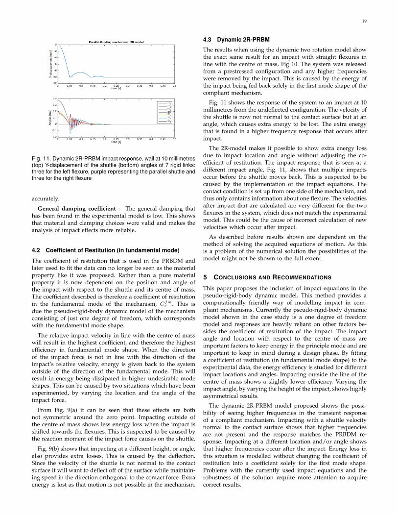
The results for an impact location 10 millimetres from thestraight flexure configuration is shown in Fig. 11.

4 DISCUSSION

4.1 Free VibrationFundamental frequency - The free vibration results of theexperiment show the fundamental frequency at 4.8218Hz. The

Fig. 9. Y-displacement of the shuttle in experiment and modelling.(a) Impact location and height varied with respect to the centre ofmass and straight flexures. (b) Same data viewed from different side

Fig. 10. Dynamic 2R-PRBM impact response wall at straight flexureconfiguration (top) Y-displacement of the shuttle (bottom) angles of7 rigid links: three for the left flexure, purple representing the parallelshuttle and three for the right flexure

frequency of the pseudo-rigid-body dynamic modelling is at4.8224Hz. These frequencies closely match the expected valuesobtained from the finite element modal analysis of the system.This shows that the dynamics without contact are modelled

19

Fig. 11. Dynamic 2R-PRBM impact response, wall at 10 millimetres(top) Y-displacement of the shuttle (bottom) angles of 7 rigid links:three for the left flexure, purple representing the parallel shuttle andthree for the right flexure

accurately.

General damping coefficient - The general damping thathas been found in the experimental model is low. This showsthat material and clamping choices were valid and makes theanalysis of impact effects more reliable.

4.2 Coefficient of Restitution (in fundamental mode)

The coefficient of restitution that is used in the PRBDM andlater used to fit the data can no longer be seen as the materialproperty like it was proposed. Rather than a pure materialproperty it is now dependent on the position and angle ofthe impact with respect to the shuttle and its centre of mass.The coefficient described is therefore a coefficient of restitutionin the fundamental mode of the mechanism, Cfmr . This isdue the pseudo-rigid-body dynamic model of the mechanismconsisting of just one degree of freedom, which correspondswith the fundamental mode shape.

The relative impact velocity in line with the centre of masswill result in the highest coefficient, and therefore the highestefficiency in fundamental mode shape. When the directionof the impact force is not in line with the direction of theimpact’s relative velocity, energy is given back to the systemoutside of the direction of the fundamental mode. This willresult in energy being dissipated in higher undesirable modeshapes. This can be caused by two situations which have beenexperimented, by varying the location and the angle of theimpact force.

From Fig. 9(a) it can be seen that these effects are bothnot symmetric around the zero point. Impacting outside ofthe centre of mass shows less energy loss when the impact isshifted towards the flexures. This is suspected to be caused bythe reaction moment of the impact force causes on the shuttle.

Fig. 9(b) shows that impacting at a different height, or angle,also provides extra losses. This is caused by the deflection.Since the velocity of the shuttle is not normal to the contactsurface it will want to deflect off of the surface while maintain-ing speed in the direction orthogonal to the contact force. Extraenergy is lost as that motion is not possible in the mechanism.

4.3 Dynamic 2R-PRBM

The results when using the dynamic two rotation model showthe exact same result for an impact with straight flexures inline with the centre of mass, Fig 10. The system was releasedfrom a prestressed configuration and any higher frequencieswere removed by the impact. This is caused by the energy ofthe impact being fed back solely in the first mode shape of thecompliant mechanism.

Fig. 11 shows the response of the system to an impact at 10millimetres from the undeflected configuration. The velocity ofthe shuttle is now not normal to the contact surface but at anangle, which causes extra energy to be lost. The extra energythat is found in a higher frequency response that occurs afterimpact.

The 2R-model makes it possible to show extra energy lossdue to impact location and angle without adjusting the co-efficient of restitution. The impact response that is seen at adifferent impact angle, Fig. 11, shows that multiple impactsoccur before the shuttle moves back. This is suspected to becaused by the implementation of the impact equations. Thecontact condition is set up from one side of the mechanism, andthus only contains information about one flexure. The velocitiesafter impact that are calculated are very different for the twoflexures in the system, which does not match the experimentalmodel. This could be the cause of incorrect calculation of newvelocities which occur after impact.

As described before results shown are dependent on themethod of solving the acquired equations of motion. As thisis a problem of the numerical solution the possibilities of themodel might not be shown to the full extent.

5 CONCLUSIONS AND RECOMMENDATIONS

This paper proposes the inclusion of impact equations in thepseudo-rigid-body dynamic model. This method provides acomputationally friendly way of modelling impact in com-pliant mechanisms. Currently the pseudo-rigid-body dynamicmodel shown in the case study is a one degree of freedommodel and responses are heavily reliant on other factors be-sides the coefficient of restitution of the impact. The impactangle and location with respect to the centre of mass areimportant factors to keep energy in the principle mode and areimportant to keep in mind during a design phase. By fittinga coefficient of restitution (in fundamental mode shape) to theexperimental data, the energy efficiency is studied for differentimpact locations and angles. Impacting outside the line of thecentre of mass shows a slightly lower efficiency. Varying theimpact angle, by varying the height of the impact, shows highlyasymmetrical results.

The dynamic 2R-PRBM model proposed shows the possi-bility of seeing higher frequencies in the transient responseof a compliant mechanism. Impacting with a shuttle velocitynormal to the contact surface shows that higher frequenciesare not present and the response matches the PRBDM re-sponse. Impacting at a different location and/or angle showsthat higher frequencies occur after the impact. Energy loss inthis situation is modelled without changing the coefficient ofrestitution into a coefficient solely for the first mode shape.Problems with the currently used impact equations and therobustness of the solution require more attention to acquirecorrect results.

20

REFERENCES

[1] Larry L. Howell, Compliant Mechanisms, John Wiley n Sons Inc.,2001.

[2] YU, Yue-Qing, et al. Dynamic modeling of compliant mechanismsbased on the pseudo-rigid-body model. Journal of MechanicalDesign, 2005, 127.4: 760-765.

[3] WANG, Wenjing; YU, Yueqing. New approach to the dynamicmodeling of compliant mechanisms. Journal of Mechanisms andRobotics, 2010, 2.2: 021003.

[4] YU, Yue-Qing; FENG, Zhong-Lei; XU, Qi-Ping. A pseudo-rigid-body 2R model of flexural beam in compliant mechanisms. Mech-anism and Machine Theory, 2012, 55: 18-33.

[5] SU, Hai-Jun. A pseudorigid-body 3R model for determining largedeflection of cantilever beams subject to tip loads. Journal ofMechanisms and Robotics, 2009, 1.2: 021008.

[6] GILARDI, G.; SHARF, I. Literature survey of contact dynamicsmodelling. Mechanism and machine theory, 2002, 37.10: 1213-1239.

[7] MAYO, J. Impacts with friction in planar flexible multibody sys-tems: Application of the momentum-balance approach. In: 12thIFToMM World Congress, Besanon (France), June. 2007. p. 18-21.

[8] R.Q. van der Linde and A.L. Schwab ”Lecture Notes: MultibodyDynamics B”, 2002,

IIIREPORT

21

CONTENTS

1 Introduction 25

2 Problem Analysis 272.1 Transient Response . . . . . . . . . . . . . . . . . . . . . . . . . . . . . . . . . . . . . . . . 272.2 Contact in ANSYS . . . . . . . . . . . . . . . . . . . . . . . . . . . . . . . . . . . . . . . . . 272.3 Problem Description . . . . . . . . . . . . . . . . . . . . . . . . . . . . . . . . . . . . . . . 28

2.3.1 Requirements . . . . . . . . . . . . . . . . . . . . . . . . . . . . . . . . . . . . . . . 28

3 Method 293.1 Literature Review . . . . . . . . . . . . . . . . . . . . . . . . . . . . . . . . . . . . . . . . . 293.2 Approach . . . . . . . . . . . . . . . . . . . . . . . . . . . . . . . . . . . . . . . . . . . . . 293.3 Choosing a test model . . . . . . . . . . . . . . . . . . . . . . . . . . . . . . . . . . . . . . 30

3.3.1 Considered geometries/mechanisms . . . . . . . . . . . . . . . . . . . . . . . . . . . 303.3.2 Chosen Testing Model . . . . . . . . . . . . . . . . . . . . . . . . . . . . . . . . . . . 30

3.4 Proposing the method . . . . . . . . . . . . . . . . . . . . . . . . . . . . . . . . . . . . . . 313.4.1 PRBDM . . . . . . . . . . . . . . . . . . . . . . . . . . . . . . . . . . . . . . . . . . 313.4.2 Deriving Equations of Motion . . . . . . . . . . . . . . . . . . . . . . . . . . . . . . . 333.4.3 Parallel Guiding Mechanism: applied . . . . . . . . . . . . . . . . . . . . . . . . . . . 353.4.4 Animate . . . . . . . . . . . . . . . . . . . . . . . . . . . . . . . . . . . . . . . . . . 363.4.5 Multibody Dynamics software . . . . . . . . . . . . . . . . . . . . . . . . . . . . . . . 363.4.6 Finite Element Analysis . . . . . . . . . . . . . . . . . . . . . . . . . . . . . . . . . . 37

4 Simulation Results - Comparison with ANSYS 394.1 Comparing results of Dynamics. . . . . . . . . . . . . . . . . . . . . . . . . . . . . . . . . . 394.2 Comparing results including Impact . . . . . . . . . . . . . . . . . . . . . . . . . . . . . . . 404.3 Results of simulating including friction . . . . . . . . . . . . . . . . . . . . . . . . . . . . . . 404.4 Discussion . . . . . . . . . . . . . . . . . . . . . . . . . . . . . . . . . . . . . . . . . . . . 41

5 Experimental Validation 435.1 Variables . . . . . . . . . . . . . . . . . . . . . . . . . . . . . . . . . . . . . . . . . . . . . 43

5.1.1 Coefficient of Restitution. . . . . . . . . . . . . . . . . . . . . . . . . . . . . . . . . . 435.2 Choices . . . . . . . . . . . . . . . . . . . . . . . . . . . . . . . . . . . . . . . . . . . . . . 43

5.2.1 Material . . . . . . . . . . . . . . . . . . . . . . . . . . . . . . . . . . . . . . . . . . 435.2.2 Dimensioning . . . . . . . . . . . . . . . . . . . . . . . . . . . . . . . . . . . . . . . 445.2.3 Fixation . . . . . . . . . . . . . . . . . . . . . . . . . . . . . . . . . . . . . . . . . . 44

5.3 Test structure . . . . . . . . . . . . . . . . . . . . . . . . . . . . . . . . . . . . . . . . . . . 445.3.1 Modal Analysis . . . . . . . . . . . . . . . . . . . . . . . . . . . . . . . . . . . . . . . 445.3.2 Solidworks . . . . . . . . . . . . . . . . . . . . . . . . . . . . . . . . . . . . . . . . . 44

5.4 Experiments . . . . . . . . . . . . . . . . . . . . . . . . . . . . . . . . . . . . . . . . . . . 455.5 Results . . . . . . . . . . . . . . . . . . . . . . . . . . . . . . . . . . . . . . . . . . . . . . 46

5.5.1 Impact on center of mass . . . . . . . . . . . . . . . . . . . . . . . . . . . . . . . . . 475.5.2 Varying impact location and angle . . . . . . . . . . . . . . . . . . . . . . . . . . . . . 47

5.6 Discussion . . . . . . . . . . . . . . . . . . . . . . . . . . . . . . . . . . . . . . . . . . . . 475.6.1 Influence of location with respect to centre of mass . . . . . . . . . . . . . . . . . . . . 475.6.2 Influence of impact angle (varying height) . . . . . . . . . . . . . . . . . . . . . . . . . 47

6 MultiDOF 496.1 Introduction . . . . . . . . . . . . . . . . . . . . . . . . . . . . . . . . . . . . . . . . . . . 496.2 Creating the 2R model . . . . . . . . . . . . . . . . . . . . . . . . . . . . . . . . . . . . . . 496.3 Optimize to match frequency . . . . . . . . . . . . . . . . . . . . . . . . . . . . . . . . . . . 50

6.3.1 Optimization. . . . . . . . . . . . . . . . . . . . . . . . . . . . . . . . . . . . . . . . 51

iii

iv CONTENTS

6.3.2 Adding contact. . . . . . . . . . . . . . . . . . . . . . . . . . . . . . . . . . . . . . . 516.3.3 Animate . . . . . . . . . . . . . . . . . . . . . . . . . . . . . . . . . . . . . . . . . . 51

6.4 Simulation Results . . . . . . . . . . . . . . . . . . . . . . . . . . . . . . . . . . . . . . . . 526.4.1 Free Vibration . . . . . . . . . . . . . . . . . . . . . . . . . . . . . . . . . . . . . . . 526.4.2 Impact . . . . . . . . . . . . . . . . . . . . . . . . . . . . . . . . . . . . . . . . . . . 526.4.3 Different impact location . . . . . . . . . . . . . . . . . . . . . . . . . . . . . . . . . 52

6.5 Discussion . . . . . . . . . . . . . . . . . . . . . . . . . . . . . . . . . . . . . . . . . . . . 53

7 Material testing - CarbonNanoTubes 557.1 Introduction . . . . . . . . . . . . . . . . . . . . . . . . . . . . . . . . . . . . . . . . . . . 557.2 Material . . . . . . . . . . . . . . . . . . . . . . . . . . . . . . . . . . . . . . . . . . . . . . 557.3 Test structures . . . . . . . . . . . . . . . . . . . . . . . . . . . . . . . . . . . . . . . . . . 56

7.3.1 Experimental setup . . . . . . . . . . . . . . . . . . . . . . . . . . . . . . . . . . . . 567.4 Test results . . . . . . . . . . . . . . . . . . . . . . . . . . . . . . . . . . . . . . . . . . . . 57

7.4.1 100 µm beam testing. . . . . . . . . . . . . . . . . . . . . . . . . . . . . . . . . . . . 577.4.2 Discussion . . . . . . . . . . . . . . . . . . . . . . . . . . . . . . . . . . . . . . . . . 58

8 Discussion 618.1 Approach . . . . . . . . . . . . . . . . . . . . . . . . . . . . . . . . . . . . . . . . . . . . . 618.2 Energy Efficiency . . . . . . . . . . . . . . . . . . . . . . . . . . . . . . . . . . . . . . . . . 61

8.2.1 Impact angle . . . . . . . . . . . . . . . . . . . . . . . . . . . . . . . . . . . . . . . . 618.2.2 Impact position . . . . . . . . . . . . . . . . . . . . . . . . . . . . . . . . . . . . . . 61

8.3 Multi Degree of Freedom Model . . . . . . . . . . . . . . . . . . . . . . . . . . . . . . . . . 61

9 Conclusion and Recommendations 639.1 Conclusions. . . . . . . . . . . . . . . . . . . . . . . . . . . . . . . . . . . . . . . . . . . . 63

9.1.1 Multi DoF . . . . . . . . . . . . . . . . . . . . . . . . . . . . . . . . . . . . . . . . . 639.1.2 CNT . . . . . . . . . . . . . . . . . . . . . . . . . . . . . . . . . . . . . . . . . . . . 63

9.2 Recommendations . . . . . . . . . . . . . . . . . . . . . . . . . . . . . . . . . . . . . . . . 639.2.1 CNT . . . . . . . . . . . . . . . . . . . . . . . . . . . . . . . . . . . . . . . . . . . . 64

A MATLAB code 65A.1 Equations of Motion - PRBDM . . . . . . . . . . . . . . . . . . . . . . . . . . . . . . . . . . 65A.2 Impact equations . . . . . . . . . . . . . . . . . . . . . . . . . . . . . . . . . . . . . . . . . 66A.3 Numerical Integration . . . . . . . . . . . . . . . . . . . . . . . . . . . . . . . . . . . . . . 66

A.3.1 Runge-Kutta 4th order function . . . . . . . . . . . . . . . . . . . . . . . . . . . . . . 68A.3.2 Error Projection function . . . . . . . . . . . . . . . . . . . . . . . . . . . . . . . . . 68

A.4 Example writefunction . . . . . . . . . . . . . . . . . . . . . . . . . . . . . . . . . . . . . . 68A.5 2R model . . . . . . . . . . . . . . . . . . . . . . . . . . . . . . . . . . . . . . . . . . . . . 68

A.5.1 Equations of Motion . . . . . . . . . . . . . . . . . . . . . . . . . . . . . . . . . . . . 68A.5.2 Optimization of Kθ . . . . . . . . . . . . . . . . . . . . . . . . . . . . . . . . . . . . . 72

A.6 CNT Example data analysis . . . . . . . . . . . . . . . . . . . . . . . . . . . . . . . . . . . . 73

B APDL code 75B.1 Initial tests . . . . . . . . . . . . . . . . . . . . . . . . . . . . . . . . . . . . . . . . . . . . 75

B.1.1 Static Analysis . . . . . . . . . . . . . . . . . . . . . . . . . . . . . . . . . . . . . . . 75B.1.2 Modal . . . . . . . . . . . . . . . . . . . . . . . . . . . . . . . . . . . . . . . . . . . 76B.1.3 Transient Analysis . . . . . . . . . . . . . . . . . . . . . . . . . . . . . . . . . . . . . 76B.1.4 Transient Analysis with Impact. . . . . . . . . . . . . . . . . . . . . . . . . . . . . . . 77

B.2 Test structure . . . . . . . . . . . . . . . . . . . . . . . . . . . . . . . . . . . . . . . . . . . 78B.2.1 Shuttle modelled as beam . . . . . . . . . . . . . . . . . . . . . . . . . . . . . . . . . 78B.2.2 Shuttle modelled as point mass . . . . . . . . . . . . . . . . . . . . . . . . . . . . . . 79

Bibliography 81

1INTRODUCTION

Compliant mechanisms gain at least some of their mobility and function from the deflection of their flexibleparts. This special type of mechanism has numerous advantages over rigid body mechanisms. These include,but are not limited to, a reduced number of parts, less assembly, hysteresis, wear and friction. Due to theseadvantages compliant mechanisms are becoming more and more popular. These mechanisms are overallmore difficult to model due to the non-linearities of the deflections which give the mechanisms their func-tion. Extensive research has been done in how these mechanisms can be modelled statically, but the dynamicand especially transient modelling comprises a smaller field.

A literature review was done to create an overview of currently available dynamic modelling techniques.The current standard of modelling dynamics of compliant mechanisms is using finite element software pack-ages. Due to the often non-linear force deflection characteristics of compliant mechanisms modal superpo-sition methods are not applicable. A full transient method is therefore required to achieve a high accuracy,however is much more time consuming. Yu, et al. (2001) created the Pseudo-Rigid-Body dynamic model(PRBDM) which simplifies the structure and makes the computation of a transient response possible withrigid body modelling techniques [1][2]. A large advantage that has been provided here is that the responseof the compliant mechanisms is modelled with a constant stiffness matrix. This results in a computation-ally efficient method of approaching the dynamic response of a compliant mechanism. Therefore dynamicmodelling based on the Pseudo-Rigid-Body model is a good alternative to the commonly used finite elementapproaches.

Incorporation of contact effects in the transient response of compliant mechanisms introduces high com-putation times and converging issues. Finite element software packages are considered to be the golden stan-dard in static, modal and transient analyses. The introduction of contact to these analyses however show thatthe performance of the software packages is not as reliable.

Research has been done into dynamic modelling using the PRBM, however the effects of impact and fric-tion have not been included yet in this research. This thesis will investigate the possibilities of incorporationthese effects into the pseudo rigid body model by using rigid body dynamics. Experiments were done to mea-sure the response of a physical model. The results will be compared with results obtained by a commercialfinite element software package. The acquired method will be applied to test cases where the roles of impactand friction play an important role in the performance of the mechanism.

The method which is proposed is intended to stay general so it can be applied to any type of planar com-pliant mechanism. The pseudo-rigid-body dynamic model will be used to show the behaviour of the com-pliant mechanism. By treating the model as rigid, contact can be added in a classical rigid body dynamicsway. To demonstrate the proposed method and validate the results the simplest geometry is looked for whichrepresents a large portion of compliant mechanisms. The equations of motion of the pseudo-rigid-body dy-namic model are derived using the TMT-method and impact equations are formed [3]. Using the experimen-tal model the performance and restrictions of the method are discussed. From these restrictions a slightlymore complex method is proposed, of which the performance is discussed subsequently.

In the modelling of compliant mechanisms using any method the material properties of the mechanismplay an important part. The Young’s modulus, also known as elastic modulus, of a material is a measure of

25

26 1. INTRODUCTION

the stiffness of a material. The Young’s modulus of carbon infiltrated carbon nano tube (CNT) structures isinvestigated to see if this could be a useful material for compliant micro mechanisms.

This thesis is built up as follows. To start a problem analysis is done. This is followed by the method,where the literature review and the approach are discussed followed by the proposed method and case study.After the method the first simulation results are found, where the proposed method is compared with finiteelement analysis. Then the experimental validation and the experimental results are discussed. Then a modelwith multiple degree of freedom model is proposed and the results are evaluated as well. This is followed bythe CNT material testing and a general discussion and conclusion.

2PROBLEM ANALYSIS

Compliant mechanisms gain their motion and function from the flexibility of their elastic members. Thestatic and dynamic analyses of the mechanisms play an essential part in the design of novel mechanisms foruse in one of various fields where compliant mechanisms are preferred. The analysis of compliant mecha-nisms comes paired with large deflections and is therefore more complex due to the non-linear behaviourthat is introduced. The current standard in static and dynamic analyses is FEA-software (Finite ElementAnalysis software). A variety of commercial software is available which can accurately predicts the static anddynamic behaviour of a compliant mechanism. Modelling the dynamic response of a compliant mechanismin FEA-software is accurate, but a time consuming analysis. In this section the current methods of perform-ing a transient response and the addition of contact is discussed. Followed by this the problem definition isstated and goals for the thesis are set up.

2.1. TRANSIENT RESPONSEFor the remainder of this thesis ANSYS will be used as the commercial FEA software package. The dynamicanalysis of a compliant mechanism in ANSYS is a non-linear structural dynamics problem. The differen-tial equations that are solved for each step are the following; semi-discrete and finite element equations ofmotion.

M · u(t )+C · u(t )+F i (t ) = F a(t ) (2.1)

where:

M = structural mass matrix (2.2)

C = structural damping matrix (2.3)

F i = internal load vector (2.4)

F a = applied load vector (2.5)

For non-linear structural dynamics problems the Newmark method is default, and for this method the initialvalues of u, u and u must be known. For non-linear equations the Newton-Raphson method is used. TheNewton-Raphson method is an iterative process of solving the non-linear equations which is performed eachtime step and balances the internal and applied load vectors. Contrary to a linear problem the stiffness matrixchanges as the beams deform. Therefore the stiffness matrix needs to be updated each time step to be usedin the Newton-Raphson iteration.

2.2. CONTACT IN ANSYSIntroducing contact can be done by using various elements. Since a lot of compliant mechanisms analysesuse beam elements, the 2D/3D node to surface contact element (CONTA175) is used, in combination witha target element (TARGE169). A number of different contact algorithms are available in ANSYS of which theaugmented Lagrangian method is default. The penalty method uses a spring stiffness during the contact,called the contact stiffness. In the augmented Lagrangian method an iterative series of penalty methods isused. The contact forces (from pressure and friction) are augmented during equilibrium iterations so that

27

28 2. PROBLEM ANALYSIS

the final penetration is smaller than the set allowable tolerance. Another method is the Lagrange multipliermethod which assumes zero penetration. Therefore stiffness values are not required however penetrationtolerances and allowable tensile contact pressures must be provided.

Choosing and implementing the correct contact algorithm in ANSYS is difficult and often solutions do notconverge. When a solution does converge the results are not necessarily correct and must be validated. Finiteelement software in the case of contact is no longer the golden standard which it is in static and dynamicanalyses.

2.3. PROBLEM DESCRIPTIONFrom the current situation the following problem definition is formulated: Current methods for dynamicanalysis of flexible mechanisms have high computation times and contact often causes converging issues.

During this graduation assignment two goals are set up in the search for a solution to the problem.

• Proposal of a computationally efficient modelling technique for the dynamic analysis of compliantmechanisms which incorporates contact effects

• Experimental validation of the proposed methods

2.3.1. REQUIREMENTSThe modelling method which will be proposed needs to meet the following requirements:

• Usable for any planar compliant mechanism

• Provide a transient response

• Includes contact effects

• Includes damping effects

To be able to accurately describe the transient response is the main requirement of the proposed method.This requirement is expanded by requiring the method to include contact and damping effects. A focus hasbeen put on finding a method to describe the motion of planar compliant mechanisms. This is done be-cause the majority of compliant mechanisms are planar. The method proposed should be applicable to anymechanism within this subset.

3METHOD

3.1. LITERATURE REVIEWTo tackle the problem described, a literature review has been done of currently developed dynamic mod-elling techniques. In this literature review more promising techniques for modelling the dynamics of compli-ant mechanisms are based on either lumped parameter methods or analytical methods. Although analyticalmethods show good potential these grow in complexity faster than lumped parameter methods. Due to thisthe methods are hard to apply to larger compliant mechanisms with a lot of flexures. The methods basedon lumped parameters are therefore the most promising. In this thesis an alternative to FEA is desired andthe methods based on the pseudo-rigid-body model (PRBM) simplification have promising results. Contactmodels often use the assumption of rigid bodies during the contact. Since the compliant mechanism is mod-elled as a system of rigid bodies, the PRBM is an ideal candidate for implementation of these contact models.

3.2. APPROACHPseudo-Rigid-Body techniques are based on the PRBM which is a widely used method for modelling the staticdeflection of compliant mechanisms. This method models the flexible beams of a compliant mechanism asa combination of rigid (undeformable) bodies, joints and torsional springs. Equations of motion can be setup for the PRBM of the compliant mechanism using rigid body dynamics.

The PRBM approach makes use of two dimensionless parameters for each replaced link, γ and Kθ . Forstatic deflection, experiments have been done to determine the values of these parameters for different load-ing conditions. γ defines the location of the joint, and thus the path described by the end of the rigid beam.Therefore γ should be the same in dynamic modelling as static modelling and is kept at the value that hasbeen extracted from previous research. The Kθ value on the other hand is dependent on the loading condi-tions. To find the optimal value the results of the modelling are compared with the "cheap" finite elementmodal analysis. An optimization is run to find the Kθ value to match the fundamental frequency of the mech-anism and the PRBM. Once a correct response for the dynamics can be modelled contact is added to thesystem. This is done using methods which treat the mechanism as a system of rigid bodies, as the PRBM doesalso.

After developing a method to model the dynamic response including impact and damping, a validationhas to be performed. This validation will be done using a simple model which incorporates contact, thechoice of a suitable model is explained in the following chapter. The chosen model will be used as an exampleto propose the method. The dynamic response of the model will also be simulated using a finite elementsoftware package, ANSYS, to provide a comparison. The mechanism will then be fabricated and experimentswill be done to validate the response. An improvement on the proposed method is considered to improveperformance.

When fabricating the mechanism and choosing materials the material properties are important to takeinto account. Testing material properties can be done in a number of ways. During this thesis the Young’smodulus of carbon infiltrated carbon-nanotube (CNT) structures is tested. With the acquired data a conclu-sion will be drawn if the material and fabrication techniques are suitable for application in compliant micro

29

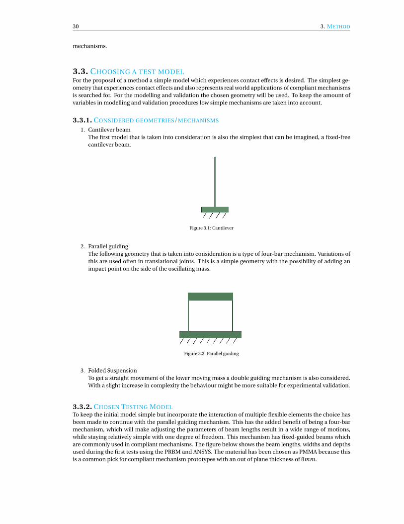
30 3. METHOD

mechanisms.

3.3. CHOOSING A TEST MODELFor the proposal of a method a simple model which experiences contact effects is desired. The simplest ge-ometry that experiences contact effects and also represents real world applications of compliant mechanismsis searched for. For the modelling and validation the chosen geometry will be used. To keep the amount ofvariables in modelling and validation procedures low simple mechanisms are taken into account.

3.3.1. CONSIDERED GEOMETRIES/MECHANISMS

1. Cantilever beamThe first model that is taken into consideration is also the simplest that can be imagined, a fixed-freecantilever beam.

Figure 3.1: Cantilever

2. Parallel guidingThe following geometry that is taken into consideration is a type of four-bar mechanism. Variations ofthis are used often in translational joints. This is a simple geometry with the possibility of adding animpact point on the side of the oscillating mass.

Figure 3.2: Parallel guiding

3. Folded SuspensionTo get a straight movement of the lower moving mass a double guiding mechanism is also considered.With a slight increase in complexity the behaviour might be more suitable for experimental validation.

3.3.2. CHOSEN TESTING MODELTo keep the initial model simple but incorporate the interaction of multiple flexible elements the choice hasbeen made to continue with the parallel guiding mechanism. This has the added benefit of being a four-barmechanism, which will make adjusting the parameters of beam lengths result in a wide range of motions,while staying relatively simple with one degree of freedom. This mechanism has fixed-guided beams whichare commonly used in compliant mechanisms. The figure below shows the beam lengths, widths and depthsused during the first tests using the PRBM and ANSYS. The material has been chosen as PMMA because thisis a common pick for compliant mechanism prototypes with an out of plane thickness of 8mm.

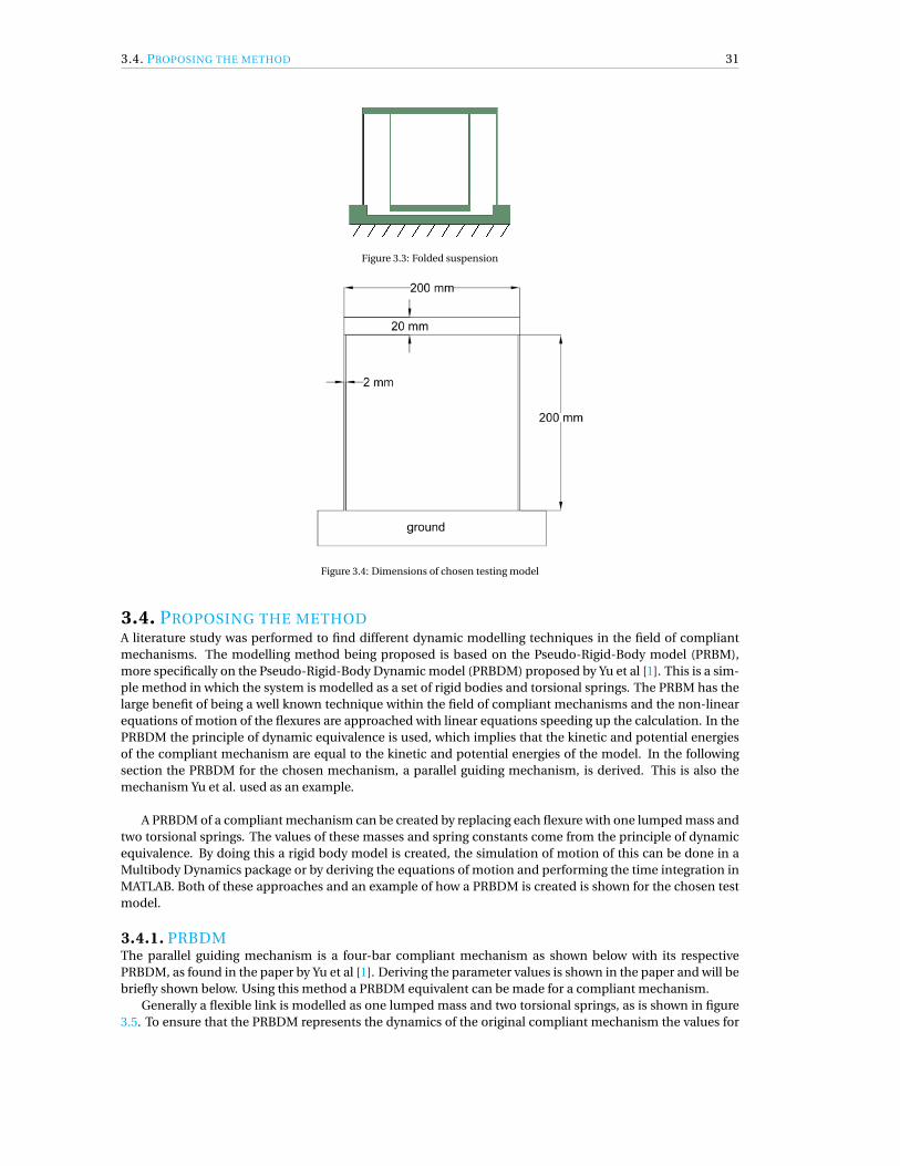
3.4. PROPOSING THE METHOD 31

Figure 3.3: Folded suspension

Figure 3.4: Dimensions of chosen testing model

3.4. PROPOSING THE METHODA literature study was performed to find different dynamic modelling techniques in the field of compliantmechanisms. The modelling method being proposed is based on the Pseudo-Rigid-Body model (PRBM),more specifically on the Pseudo-Rigid-Body Dynamic model (PRBDM) proposed by Yu et al [1]. This is a sim-ple method in which the system is modelled as a set of rigid bodies and torsional springs. The PRBM has thelarge benefit of being a well known technique within the field of compliant mechanisms and the non-linearequations of motion of the flexures are approached with linear equations speeding up the calculation. In thePRBDM the principle of dynamic equivalence is used, which implies that the kinetic and potential energiesof the compliant mechanism are equal to the kinetic and potential energies of the model. In the followingsection the PRBDM for the chosen mechanism, a parallel guiding mechanism, is derived. This is also themechanism Yu et al. used as an example.

A PRBDM of a compliant mechanism can be created by replacing each flexure with one lumped mass andtwo torsional springs. The values of these masses and spring constants come from the principle of dynamicequivalence. By doing this a rigid body model is created, the simulation of motion of this can be done in aMultibody Dynamics package or by deriving the equations of motion and performing the time integration inMATLAB. Both of these approaches and an example of how a PRBDM is created is shown for the chosen testmodel.

3.4.1. PRBDMThe parallel guiding mechanism is a four-bar compliant mechanism as shown below with its respectivePRBDM, as found in the paper by Yu et al [1]. Deriving the parameter values is shown in the paper and will bebriefly shown below. Using this method a PRBDM equivalent can be made for a compliant mechanism.

Generally a flexible link is modelled as one lumped mass and two torsional springs, as is shown in figure3.5. To ensure that the PRBDM represents the dynamics of the original compliant mechanism the values for

32 3. METHOD

Figure 3.5: Compliant four-bar mechanism and its PRBDM

the lumped masses at C and D and the position and stiffness of the four torsional springs constants must bechosen. This is done by applying the method of dynamic equivalence. The position of the torsional springsis chosen as it is in the static PRBM, to ensure that the path followed is correct. For this system making surethat the PRBDM is dynamically equivalent is done in two steps, first for the kinetic energy in the system andsubsequently for the potential energy.

EQUIVALENCE OF KINETIC ENERGY

The system consists of one rigid body and two compliant members. Since the top bar is considered to berigid it will not deform and therefore remain the same in the PRBDM. For both of the links the kinetic energymust remain the same as its compliant counterpart, this is done by setting up the energy equation for bothsituations. The equations below show these energies for the left link of the mechanism, here m3

2 representsthe lumped mass at point C.

KCompli ant = 1

2m2V 2

m2 +1

2J2ω

22 (3.1)

KPRBDM = 1

2m3

2V 2C (3.2)

Using the values we know and rewriting the velocities in terms of the angular velocityω, we can derive therequired value of the lumped mass.

m32 =

1

m2+ J2

r 22

(3.3)

EQUIVALENCE OF POTENTIAL ENERGY

For the potential energy of the system we look at the stored energy in the bending of the beams of the com-pliant mechanism versus the stored energy in the four torsional springs. The potential energy stored is notdependent on velocities. Therefore it can be assumed to be the same as in a conventional PRBM. These haveshown to be accurate till up to 0.5% and therefore this expression for the torsional stiffness can be used forthe calculation of the potential energy in the torsional springs. Since there two springs are used to replace theflexible beam, only half of the length is used in this calculation.

Kd1 = γKθ2

E2I212 l2

(3.4)

P = 1

2kθ2

2 (3.5)

3.4. PROPOSING THE METHOD 33

With this simplification the dynamics of the mechanism can be simulated in different ways. Either byusing a commercial Multibody Dynamics software package or by using MATLAB to derive the equations ofmotion by hand. In the following section it is shown how the equations can be derived by using Multibodydynamics in MATLAB. Followed by this a look will be done into using COMSOL to implement the PRBDM.

3.4.2. DERIVING EQUATIONS OF MOTION

Using Multibody Dynamics and MATLAB the equations of motion of the system can be set up for the PRBDMin figure 3.5. This is done by using the TMT-method as it is proposed in the lecture notes of the course Multi-body Dynamics B by R.Q. van der Linde and A.L. Schwab [3]. A short explanation of how these equations arederived is provided below.

The equations of motion are derived for a triple pendulum as it is shown below, with angles θ,φ and α.Two constraints are used to constrain the position of the end of the third pendulum at (l1,0). The system ismodelled as a 3 DoF system with 2 constraints instead of finding the single degree of freedom of the system.For a four-bar mechanism this degree of freedom can be found. However, for systems with more links findingthe exact degrees of freedom becomes very difficult. For this reason the method uses a degree of freedom foreach link and a set of constraints to accurately describe the system being modelled. This results in modellingthe PRBDM as a multibody system with n-beams and n-degrees of freedom. The degrees of freedom arechosen as the angles of the beams. By using a number of (m) constraints the number of degrees of freedomare brought back to the amount of degrees of freedom in the original compliant mechanism. This results in asystem with (n-m) total degrees of freedom.

Figure 3.6: Triple pendulum used to model the four-bar mechanism

The coordinates of the masses in the PRBDM are described in terms of the three angles, which are thegeneralized coordinates. With constraints which position end of the third pendulum at specific x- and y-coordinates the system is brought back to one degree of freedom. Using the coordinates of the (lumped)masses the TMT-method is applied to find the equations of motion. The four torsional springs are added tothese equations by means of their virtual power.

NUMERICAL INTEGRATION

Numerical integration is used to simulate the behaviour of the system for various initial configurations. Thisis done with the Runge-Kutta fourth order method. This method approximates the solution of the differentialequations by guessing the next state. For the state y , yn+1 (after a timestep h) is approximated in the fol-lowing way. Writing the Runge-Kutta method instead of using an available ODE-solver in Matlab is done tomake implementation of error projection and event detection easier. Below the function f computes the newaccelerations using the equations of motion.

34 3. METHOD

yn+1 = yn + h

6(k1 +2k2 +2k3 +k4) (3.6)

tn+1 = tn +h (3.7)

wi th

k1 = f (tn , yn) (3.8)

k2 = f (tn + h

2, yn + 1

2k1h) (3.9)

k3 = f (tn + h

2, yn + 1

2k2h) (3.10)

k4 = f (tn +h, yn +k3h) (3.11)

(3.12)

A function was written which performs the Runge-Kutta fourth order integration method, the file can befound Appendix A. To make sure the beams of the mechanism do not fly away from the constraints, angles areprojected onto the constraints each time step. By doing this every time step the new state is ensured to satisfythe constraints that have been put in. This has been done by using error projection. The new solution is givenas the new state vector which is projected on the constraint surface (a surface with possible state values thatsatisfy the constraints). This is done until the calculated error is below a threshold value [4].

IMPACT

After simulating the dynamic response of the system, an impact is introduced. This is done in the form ofa wall on the right side of the mechanism, which is hit by the joint D in figure 3.5. Inside the numericalintegration, each time step an event check is done to see if joint D hits the wall.

When the impact occurs energy is lost from the system and Newton’s impact law is used to calculate newvelocities for the mechanism. This method uses a material dependent property known as the coefficient ofrestitution. The coefficient of restitution, e, is a factor which represents the energy lost during the impact.The coefficient varies between 0 and 1, zero corresponding to a fully inelastic contact in which all impactenergy is lost, and 1 corresponding to a fully elastic contact in which all impact energy is retained.

Cr =∆Va f ter

∆Vbe f or e(3.13)

The following equation is set up for the impact. Where q is the state vector that contains the positions andvelocities of the generalized coordinates, Dci is the derivative of the contact condition and qbe f or e and qa f ter

represent the state just before and just after impact.

Dci qbe f or e =−Cr Dci qa f ter (3.14)

The solution for the new state must satisfy the equations of motion, therefore the impact equation shownabove is solved.

FRICTION AND DAMPING

Friction can be modelled using various friction models. Overall these require a normal force and a frictioncoefficient. As a first step a simplification will be done, since the friction coefficient should be found ex-perimentally and is not readily available. This will provide an insight into how this phenomenon affects theoverall dynamics of the mechanism. A friction point is introduced on the top bar, which results in a force inthe opposite direction of the motion. This force is chosen to be dependent on the y-component of the topbar, since a higher normal force will be present when the four-bar mechanism passes its neutral position.

Damping is added in a similar manner by introducing a force dependent on the velocities of the differentcomponents. Using the Eigenfrequency the damping can be added as a percentual loss per oscillation. Thismakes it easy to measure a general damping, from different sources, and implement this into the model.This general damping, c, is dependent on the natural frequency and is added to the system of equations ofmotion as described in the equations below. In these equationsωn is the natural frequency and ζ is the criticaldamping coefficient.

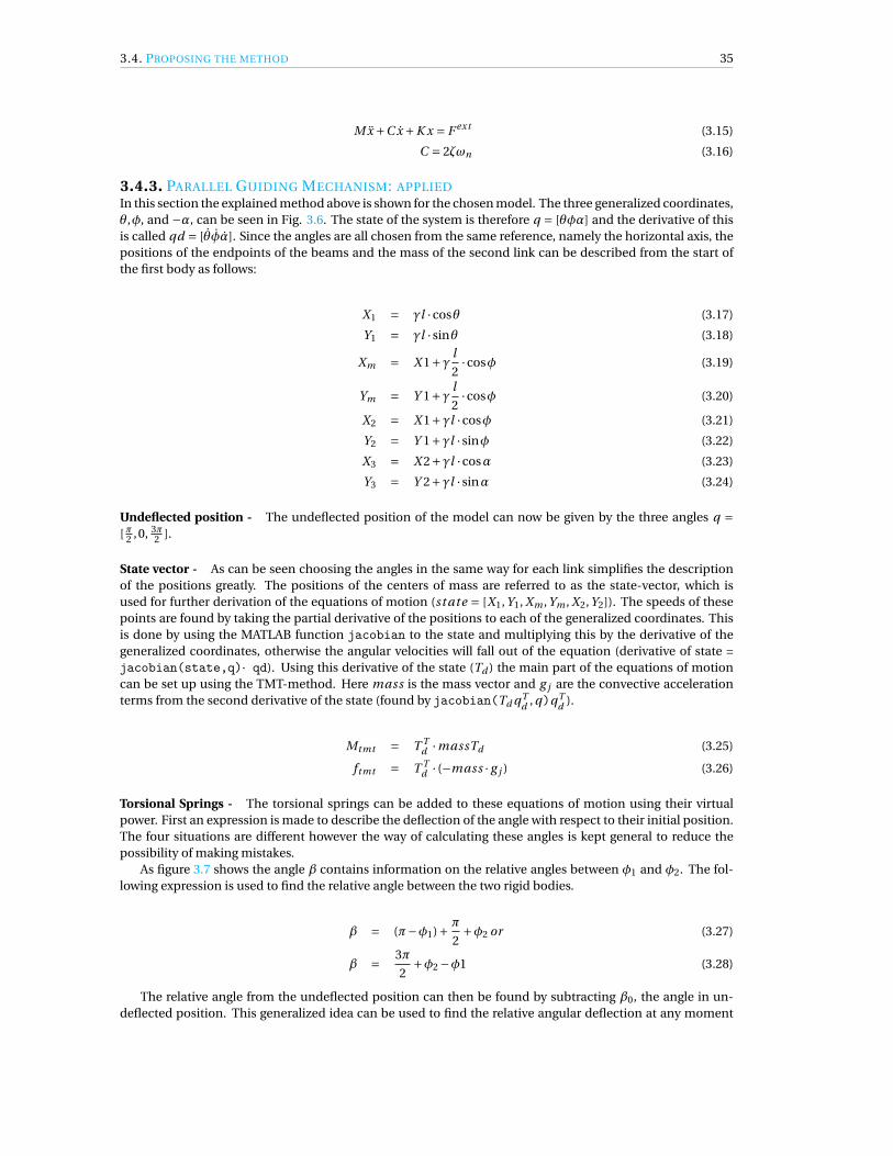
3.4. PROPOSING THE METHOD 35

M x +C x +K x = F ext (3.15)

C = 2ζωn (3.16)

3.4.3. PARALLEL GUIDING MECHANISM: APPLIEDIn this section the explained method above is shown for the chosen model. The three generalized coordinates,θ,φ, and −α, can be seen in Fig. 3.6. The state of the system is therefore q = [θφα] and the derivative of thisis called qd = [θφα]. Since the angles are all chosen from the same reference, namely the horizontal axis, thepositions of the endpoints of the beams and the mass of the second link can be described from the start ofthe first body as follows:

X1 = γl ·cosθ (3.17)

Y1 = γl · sinθ (3.18)

Xm = X 1+γ l

2·cosφ (3.19)

Ym = Y 1+γ l

2·cosφ (3.20)

X2 = X 1+γl ·cosφ (3.21)

Y2 = Y 1+γl · sinφ (3.22)

X3 = X 2+γl ·cosα (3.23)

Y3 = Y 2+γl · sinα (3.24)

Undeflected position - The undeflected position of the model can now be given by the three angles q =[π2 ,0, 3π

2 ].

State vector - As can be seen choosing the angles in the same way for each link simplifies the descriptionof the positions greatly. The positions of the centers of mass are referred to as the state-vector, which isused for further derivation of the equations of motion (st ate = [X1,Y1, Xm ,Ym , X2,Y2]). The speeds of thesepoints are found by taking the partial derivative of the positions to each of the generalized coordinates. Thisis done by using the MATLAB function jacobian to the state and multiplying this by the derivative of thegeneralized coordinates, otherwise the angular velocities will fall out of the equation (derivative of state =jacobian(state,q)· qd). Using this derivative of the state (Td ) the main part of the equations of motioncan be set up using the TMT-method. Here mass is the mass vector and g j are the convective accelerationterms from the second derivative of the state (found by jacobian(Td qT

d , q)qTd ).

Mtmt = T Td ·massTd (3.25)

ftmt = T Td · (−mass · g j ) (3.26)

Torsional Springs - The torsional springs can be added to these equations of motion using their virtualpower. First an expression is made to describe the deflection of the angle with respect to their initial position.The four situations are different however the way of calculating these angles is kept general to reduce thepossibility of making mistakes.

As figure 3.7 shows the angle β contains information on the relative angles between φ1 and φ2. The fol-lowing expression is used to find the relative angle between the two rigid bodies.

β = (π−φ1)+ π

2+φ2 or (3.27)

β = 3π

2+φ2 −φ1 (3.28)

The relative angle from the undeflected position can then be found by subtracting β0, the angle in un-deflected position. This generalized idea can be used to find the relative angular deflection at any moment

36 3. METHOD

Figure 3.7: Angles of the torsional spring

between two beams. The first and last torsional springs can also be described this way, however here the firstand second angles are 3π

2 and 0 respectively.

β1 = θ− pi

2(3.29)

β2 = 3π

2+φ−θ (3.30)

β3 = 3π

2+α−φ (3.31)

β4 = 3π

2+φ−0 (3.32)

A check is performed to see if the undeflected position results in undeformed springs.

Constraints - Since the 1 DoF model is described by three generalized coordinates, two constraints areneeded to get back to the single degree of freedom. These are put in the form of a constraint for the X and Ylocation of the end of the third rigid body. This tip should always be in the same location, fixed on the ground.The following equations should always be fulfilled:

Dc =[

X3 − lY3

]= 0 (3.33)

These constraints are rewritten to velocity terms to be able to add them to the equations of motion. Thisis done by taking the jacobian to the state vector q (Dck = jacobian(Dc,q)). By including the constraintequations we find the full set of equations of motion for the system as shown below:

[Mtmt DckDck ′ zer os(2,2)

]q =

[ftmt

zer os(2,1)

](3.34)

3.4.4. ANIMATETo be able to analyse the movement quickly the acquired angular response is translated into an animation.This is done in MATLAB by using the endpoints of beams at each time step. Lines are drawn for every timestep to represent the beams with the MATLAB function line. Using the function getframe a video animationof the motion can be created and saved.

3.4.5. MULTIBODY DYNAMICS SOFTWAREA different way of approaching the problem is taking the acquired PRBDM and putting this in a multibody dy-namics software package. Using this method the impact and friction effects can be performed by the softwarepackage. The software package chosen for use is COMSOL, since it allows strictly 2D multibody dynamics.

3.4. PROPOSING THE METHOD 37

This is a nice feature since the focus of this research is on planar compliant mechanisms.

COMSOL consists of a nice graphical user interface, in which the beams of the PRBDM can be created.These are all set up as rigid domains. Between these rigid domains spring and damper systems can be added,these are used to represent the torsional springs in the PRBDM. A snapshot of a deflected position of theparallel guiding mechanism below shows the graphical interface which is used to represent the simulatedbehaviour. Note that the different colours in the figure below only represent deflection.

Figure 3.8: PRBDM of parallel guiding mechanism in COMSOL (colour shows magnitude of displacement)

3.4.6. FINITE ELEMENT ANALYSISAs a reference the mechanism is also modelled using finite element analysis. All FEA-modelling was per-formed in ANSYS using an APDL-script. Below a brief description of the APDL-scripts is given. Examples ofused APDL-scripts can be found in the Appendix.

Keypoints and lines are used to create the model. These lines have been meshed with beam elements(BEAM188). With the acquired model containing three beams, two thin flexures and one acting rigidly ontop, static modal and transient analyses can be performed. Adding contact is done by introducing contactelements and creating a contact pair. The contact pair is a combination of two elements, a contact elementand a target element. Both of these elements are placed on existing elements, in this case the beam elements.The contact element (CONTA175) is placed on the elements in the top right corner which will impact thewall. Reducing the number of contact and target elements will speed up the simulation. For the target ele-ments a line is drawn at the position of the wall and beam elements are meshed over this. The target elementTARGE169 is then meshed over the new beam elements. The contact and target elements now form a contactpair. To excite the system it is prestressed by pulling one of the nodes to the side. The beams and prestressingcan be seen in the figure below.

38 3. METHOD

Figure 3.9: Parallel guiding mechanism perturbed in ANSYS. Left and right beams show the deflection, top two beams are rigid.

4SIMULATION RESULTS - COMPARISON WITH

ANSYS

4.1. COMPARING RESULTS OF DYNAMICSIn the following section the first set of results from the PRBDM simulated by deriving equations of motionin MATLAB and simulating the behaviour using COMSOL are compared with the transient analysis acquiredfrom ANSYS. The transient response of the model is shown in the graph below. The initial configuration ofthe model was the non-deflected configuration, an initial velocity was set on the top bar of 1m/s.

Figure 4.1: Comparison of the dynamic response of the PRBDM with ANSYS

Besides comparing the different models, a test was also done using a PRBM without a lumped mass at thejoints. The center of mass of the flexible beams was in this case also located in the centre of the beam. Thefrequency of the acquired responses is given in table 4.1.

The acquired results for the PRBDM have been taken from a simulation in which the characteristic lengthand spring constants were the following; γ = 0.8517 and Kθ = 2.65. These dimensionless parameters havebeen taken from the original PRBM [5].

Kθ has been determined to be this value for end force loads on the flexible beams, for the case of endmoment loads this value is lower. In our case the flexible beams will always be loaded by a combination

39

40 4. SIMULATION RESULTS - COMPARISON WITH ANSYS

Table 4.1: Responses and their errors

Method Frequency [Hz] Error w/rt FEA [%] max. deviation [mm] Error w/rt FEA [%]ANSYS - FEA 5.6348 - 25.4474 -

MATLAB - PRBDM 5.6348 2.5296 25.4474 8.2516COMSOL - PRBDM 5.7940 3.3650 26.0180 2.2424

COMSOL - Distributed mass 5.8244 2.8260 25.8831 1.7121

of force and moment loads, therefore the optimum value for Kθ is sought to ensure a correct response. Ascan be seen in figure 4.1 and in table 4.1. Especially the frequency error provides a large problem in thetransient response of the system, since the phases of the vibrations shift. The shifting of the phases causes apropagation of the error as shown in the figure below.

Figure 4.2: Propagation of error between PRBDM and ANSYS - wrong frequency

To ensure that the path remains the same as in the original PRBMγ is kept at 0.8517. However, to minimizethe error between the PRBDM and ANSYS an optimization was done on the value of Kθ. This resulted in aKθ of 2.5449 instead of 2.65 and the response shown in figure 4.3. As expected in minimizing the error thefrequency is the most important aspect.

The optimization performed to find this new value of Kθ was done with one objective, which was to min-imize the root-mean-square error between the PRBDM response with respect to the ANSYS response.

4.2. COMPARING RESULTS INCLUDING IMPACT

In modelling an impact with the PRBDM as well as using FEA in ANSYS a coefficient of restitution of 0.7was used in both cases. This value is dependent on the two colliding materials and has been chosen as acommon value for both simulations. The result shown in figure 4.4 shows that the PRBDM response matchesthe FEA response nicely. In both simulations no penetration of the colliding objects was allowed, to keep thecomparison fair.

4.3. RESULTS OF SIMULATING INCLUDING FRICTION

To ensure that the incorporation of friction effects into the model is possible, a simplified version of frictionis added. Figure 4.5 shows the response of the model with a simplified friction force.

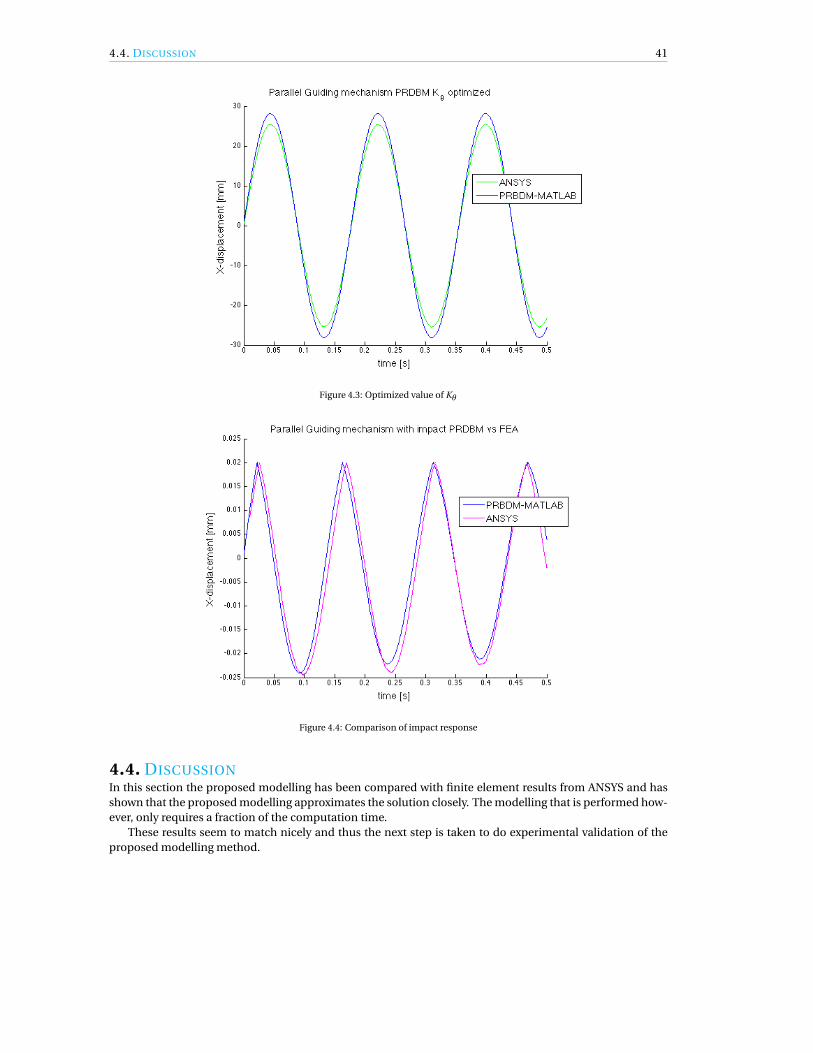
4.4. DISCUSSION 41

Figure 4.3: Optimized value of Kθ

Figure 4.4: Comparison of impact response

4.4. DISCUSSIONIn this section the proposed modelling has been compared with finite element results from ANSYS and hasshown that the proposed modelling approximates the solution closely. The modelling that is performed how-ever, only requires a fraction of the computation time.

These results seem to match nicely and thus the next step is taken to do experimental validation of theproposed modelling method.

42 4. SIMULATION RESULTS - COMPARISON WITH ANSYS

Figure 4.5: Results with simplified friction model

5EXPERIMENTAL VALIDATION

5.1. VARIABLESTo be able to validate the proposed model the test structure has to be fabricated and the responses to variousinputs have to be measured. The measurements will be dependent on a multitude of parameters. Theseinclude the material choice, the choice of dimensions and fabrication. While designing the test set-up anumber of choices were made to minimize the number of acting variables in the experiment. A choice hasbeen made in how to tackle the problem for each of the variables and the steps towards the choices will beexplained. The acting variables in this experiment are listed below.

• Material– Young’s modulus– Material damping– Coefficient of restitution– Density/mass

• Dimensions– Beam dimensions

¦ Length¦ Cross section

– Viscous damping– Center of mass

• Orientation in gravity

5.1.1. COEFFICIENT OF RESTITUTIONThe coefficient of restitution that is used in the pseudo-rigid-body model cannot be described as a coefficientof restitution of the mechanism. Since the model only contains a single degree of freedom, the coefficientrepresents the amount of energy that is fed back into this motion. Therefore the coefficient of restitution is

referred to as the coefficient of restitution in fundamental mode, C f mr .

5.2. CHOICES

5.2.1. MATERIALWhen choosing a material or combination of materials the obvious choice in making a quick prototype is aplastic. PMMA (Polymethylmethacrylate), also known as plexiglas can be used and is easily cut into a desiredshape using a laser cutter. However for the use in this experiment brittleness of the material is not desiredwhen working with an impact. Another downside of using a plastic is the amount of material damping that ispresent. For these two reasons the option of using springsteel seems like a good choice as a material for theflexures. Springsteel is often used in the field of compliant mechanisms since it is available in small widthsand has a high yield stress. The small widths are required when working with metal because low frequenciesare preferred, since measurements of the response will be done using a displacement sensor. The materialof the parallel bar is also not made of plastic to ensure that this part acts as a rigid body. For this reasonaluminium is chosen which has a higher Young’s modulus and a low density.

43

44 5. EXPERIMENTAL VALIDATION

5.2.2. DIMENSIONINGTo remove out of plane forces the orientation of the test model is chosen to be upright with gravity prestress-ing the structure. The neutral position will therefore be a deflected position. The dimensions of the modelare chosen so the deflection in rest is low and are further determined by the range of the displacement sensorwhich is available.

5.2.3. FIXATIONTo attach the flexures to the base and the shuttle they can be glued or be clamped. Using glue will add damp-ing so the flexures are preferably clamped to the base and shuttle. The clamping is done by using clampingblocks and a screw to attach to the shuttle or the base.

5.3. TEST STRUCTURE

5.3.1. MODAL ANALYSISThe thickness of the flexures is chosen to be 100µm and their length is chosen to be 40mm. Using thesedimensions and the materials that have been chosen a modal analysis is performed in ANSYS to check theinfluence of the Eigenmodes. The APDL-code for the modal analysis can be found in Appendix B.

The modal analysis has been performed in undeflected position as well as a 10mm deflected position.The results show that the out of plane modes have much lower Eigenfrequencies in deflected position. Thesystem is tested in the direction of gravity, thus the focus is put on the planar Eigenmodes. The first five inplane modes are listed below for the undeflected and deflected case.

Figure 5.1: ANSYS modal analysis - in undeflected and deflected positions (10mm)

5.3.2. SOLIDWORKSOnce the choices for the test structure variables are made a CAD-drawing is made. Using the drawing inSolidworks the mass of the shuttle and the position of its center of mass can be determined. From the solid-

Figure 5.2: Solidworks drawing of test structure

works drawing the mass including bolts can be estimated for the modelling. Solidworks shows a mass ofapproximately 53 grams. More importantly the center of mass can also be found for the shuttle, this will havea significant influence on the modelling. The center of mass is found to be at 17.77mm from the base of thestructure. The mechanism will be mounted as seen in the figure below, with gravity working in plane, this willcause the system to have a deflected stable position. Using the mass and center of mass the modal analysis

5.4. EXPERIMENTS 45

can also be improved. The mass of the shuttle is introduced into the model as a point mass which gives us amore accurate idea of the Eigenfrequencies. The fundamental frequency of the system is found to be 4.8 Hzand the second in plane frequency is 136 Hz.

Figure 5.3: Solidworks render of test structure mounted on stages on bread board

5.4. EXPERIMENTSMaterial ordered was machined to size using the facilities at 3mE and using the drawings from Solidworks as aguide. In the experiments the mass of the shuttle and the Young’s modulus of the springsteel flexures are crit-ical. The shuttle including clamping blocks and bolts has therefore been weighed and a test was performed todetermine the Young’s modulus of the flexures. The flexure test was performed using a linear precision stage(PI M-406) and a load cell which was calibrated for loads from 0−0.5N .

The experiments will be done by deflecting the shuttle of the test structure and then releasing. The re-sponse of the system is measured by measuring the x-displacement of the shuttle. This is done with a laserdisplacement sensor (optoNCDT 1302), which has a maximum range of 50mm and a sampling frequency of750 Hz. After weighing the shuttle to get an exact mass the measurements will be performed. The first mea-surements will be on a free oscillation, from this data a general damping coefficient will be extracted. Thisis done by averaging the percentual energy loss per oscillation. The data from this oscillation is also used tocheck if the natural frequency of the experiment is as expected. After this the impact will be tested at multiplepositions. The distance of the structure to the impact block will be varied, giving the following experiments:

• Free oscillation• Impact below undeflected flexure position (5 and 10 mm)• Impact on undeflected flexure position• Impact above undeflected flexure position (5 and 10 mm)The position of the impact will also be shifted in the other in plane direction. This will shift the point of

impact away from the center of mass. These tests will therefore be done in three positions:• Impact left of CoM (2 and 4 mm)• Impact on CoM• Impact right of CoM (2 and 4 mm)Five different heights of the impact and five different x-positions give a total of 9 tests including impact.

These will all be done three times to see if the result is reproducible.

Data is acquired using Labview and further analysed in MATLAB. Using the PRBDM a coefficient of resti-tution in fundamental mode shape is fit to the data. This gives an overview of the energy efficiency of impactin compliant mechanisms.

46 5. EXPERIMENTAL VALIDATION

5.5. RESULTSThe testing of the Young’s modulus of the flexure was done with the linear precision stage and a force sensor.The result of a test in which the force displacement is measured is shown in Fig. 5.4. The mass was checkedusing an accurate scale. This showed that Solidworks was close to the actual mass, which is 53.187g .

Figure 5.4: Spring steel flexure - Young’s modulus test

The Young’s modulus test of the springsteel flexures is shown in Fig. 5.4. Using the force deflection of theflexure and linear beam theory the Young’s modulus can be extracted as shown in the equations below.

d = F l 3

3E I(5.1)

E = F

d· l 3

3E I(5.2)

After measuring two essential model properties (flexure Young’s modulus and shuttle mass) a test is per-formed to calibrate the voltage output of the displacement sensor to mm. This has been done by tracking thetest structure while it is moved 2.5mm with a linear stage. This data is used to find a calibration factor whichis used to transform the output signal into millimetres. After calibration the free oscillation experiment isperformed. The response of the system and the model fit are shown in the Fig. 5.5:

Figure 5.5: Test structure - Free vibration

The generalized damping in the structure can be expressed C = 2ζωn . The free oscillation data is usedto fit a damping parameter which describes the general damping, including material and viscous damping.The extracted ζ value is 6.88e −9. The fit ζ value is used in all subsequent modelling which is used to fit thecoefficient of restitution (in fundamental mode shape) to the experimental data.

5.6. DISCUSSION 47

5.5.1. IMPACT ON CENTER OF MASSFor the first test done will be an impact in line with the centre of mass and with straight flexures. This con-figuration will theoretically return the maximum amount of energy back into the mechanisms, and showssimilarities with a bouncing ball. Fig. 5.6 shows a single response with the fit Cr . The other responses weregathered in the same way, for sake of space these are not all included in the report.

Figure 5.6: Experiment response and model fit of an impact in line with center of mass and straight flexures

5.5.2. VARYING IMPACT LOCATION AND ANGLEThe following 3D plot shows the fit coefficient of restitution (in fundamental mode) at different impact loca-tions and angles (heights).

Figure 5.7: 3D plot of fit coefficients of restitution at different heights and locations

5.6. DISCUSSION

5.6.1. INFLUENCE OF LOCATION WITH RESPECT TO CENTRE OF MASSThe influence of the location of impact with respect to the centre of mass can be seen in the 3D plot, but ismade more clear in Fig. 5.8. Two things are striking about the data. First the central point does not showthe highest coefficient of restitution in fundamental mode, and secondly the results are asymmetric around

the centre of mass. Although the highest C f me is not found in the centre with straight flexures this could be a

measurement error, and trends show higher values nearer the centre.

5.6.2. INFLUENCE OF IMPACT ANGLE ( VARYING HEIGHT )The influence of a varying impact angle is shown in the figure below. Note that this is the same data as shownbefore in the 3D plot. Surprising is that this is also not symmetrical. The impact at -10mm lost a lot more

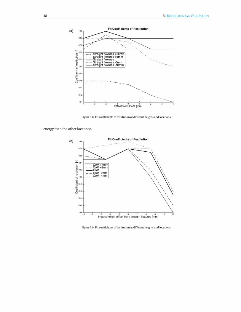
48 5. EXPERIMENTAL VALIDATION

Figure 5.8: Fit coefficients of restitution at different heights and locations

energy than the other locations.

Figure 5.9: Fit coefficients of restitution at different heights and locations

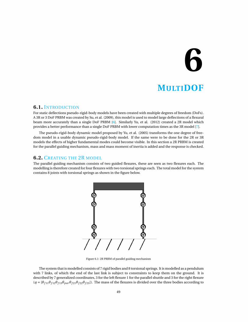
6MULTIDOF

6.1. INTRODUCTIONFor static deflections pseudo-rigid-body models have been created with multiple degrees of freedom (DoFs).A 3R or 3 DoF PRBM was created by Su, et al. (2009), this model is used to model large deflections of a flexuralbeam more accurately than a single DoF PRBM [6]. Similarly Yu, et al. (2012) created a 2R model whichprovides a better performance than a single DoF PRBM with lower computation times as the 3R model [7].

The pseudo-rigid-body dynamic model proposed by Yu, et al. (2005) transforms the one degree of free-dom model in a usable dynamic pseudo-rigid-body model. If the same were to be done for the 2R or 3Rmodels the effects of higher fundamental modes could become visible. In this section a 2R PRBM is createdfor the parallel guiding mechanism, mass and mass moment of inertia is added and the response is checked.

6.2. CREATING THE 2R MODELThe parallel guiding mechanism consists of two guided flexures, these are seen as two flexures each. Themodelling is therefore created for four flexures with two torsional springs each. The total model for the systemcontains 8 joints with torsional springs as shown in the figure below.

Figure 6.1: 2R PRBM of parallel guiding mechanism

The system that is modelled consists of 7 rigid bodies and 8 torsional springs. It is modelled as a pendulumwith 7 links, of which the end of the last link is subject to constraints to keep them on the ground. It isdescribed by 7 generalized coordinates, 3 for the left flexure 1 for the parallel shuttle and 3 for the right flexure(q = [θ f 11θ f 12θ f 13θparθ f 21θ f 22θ f 23]). The mass of the flexures is divided over the three bodies according to

49

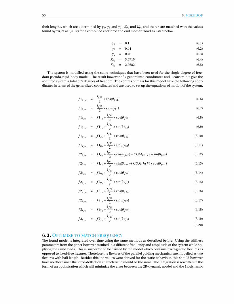
50 6. MULTIDOF

their lengths, which are determined by γ0, γ1 and γ2. Kθ1 and Kθ2 and the γ’s are matched with the valuesfound by Yu, et al. (2012) for a combined end force and end moment load as listed below.

γ0 = 0.1 (6.1)

γ1 = 0.44 (6.2)

γ2 = 0.46 (6.3)

Kθ1 = 3.4710 (6.4)

Kθ2 = 2.0682 (6.5)

The system is modelled using the same techniques that have been used for the single degree of free-dom pseudo-rigid-body model. The result however of 7 generalized coordinates and 2 constraints give theacquired system a total of 5 degrees of freedom. The centres of mass for this model have the following coor-dinates in terms of the generalized coordinates and are used to set up the equations of motion of the system.

f 11xm =l f 11

2∗cos(θ f 11) (6.6)

f 11ym =l f 11

2∗ sin(θ f 11) (6.7)

f 12xm = f 11x +l f 12

2∗cos(θ f 12) (6.8)

f 12ym = f 11y +l f 12

2∗ sin(θ f 12) (6.9)

f 1exm = f 12x +l f 13

2∗cos(θ f 13) (6.10)

f 1eym = f 12y +l f 13

2∗ sin(θ f 13) (6.11)

f 20xm = f 1ex +lpar

2∗cos(θpar )−COMs hi f t ∗ sin(θpar ) (6.12)

f 20ym = f 1ey +lpar

2∗ sin(θpar )+COMs hi f t ∗cos(θpar ) (6.13)

f 21xm = f 20x +l f 21

2∗cos(θ f 21) (6.14)

f 21ym = f 20y +l f 21

2∗ sin(θ f 21) (6.15)

f 22xm = f 21x +l f 22

2∗cos(θ f 22) (6.16)

f 22ym = f 21y +l f 22

2∗ sin(θ f 22) (6.17)

f 2exm = f 22x +l f 23

2∗cos(θ f 23) (6.18)

f 2eym = f 22y +l f 23

2∗ sin(θ f 23) (6.19)

(6.20)

6.3. OPTIMIZE TO MATCH FREQUENCYThe found model is integrated over time using the same methods as described before. Using the stiffnessparameters from the paper however resulted in a different frequency and amplitude of the system while ap-plying the same loads. This is suspected to be caused by the model which contains fixed-guided flexures asopposed to fixed-free flexures. Therefore the flexures of the parallel guiding mechanism are modelled as twoflexures with half length. Besides this the values were derived for the static behaviour, this should howeverhave no effect since the force-deflection characteristic should be the same. The integration is rewritten in theform of an optimization which will minimize the error between the 2R-dynamic model and the 1R-dynamic

6.3. OPTIMIZE TO MATCH FREQUENCY 51

model which has been validated. To make it possible to vary Kθ values and are written symbolically in allequations.

6.3.1. OPTIMIZATION

Two key elements of an optimization are the objective function and the variables. The solver used is MAT-LAB’s fmincon for a constrained non-linear optimization problem, with an interior-point algorithm. In thiscase the variables that are used are Kθ1 and Kθ2 . The objective function used is the root-mean-squared errorbetween the x-displacement response of the shuttle in the 2R-model with the PRBDM from section 3.3.3.

RMSE =(X d at a2R − X d at aob j ecti ve )2

l eng th(X d at a)(6.21)

The system was run in undeflected position with gravity working in positive x-direction. This has beenchosen so the initial conditions can remain the same for different Kθ values. The result from this optimizationis shown in Fig. 6.2.

Figure 6.2: 2R PRBM optimized Kθ - Pink shows the starting point of the optimization with Kθ from the paper, green shows the verifiedresponse of the 1R model and the dotted blue line shows the outcome of the optimization.

The acquired result shows a nice response that closely represents the validated model. The values foundare Kθ1 = 8.7614 and Kθ2 = 4.0104. These values are significantly higher than the paper shows, however theyshow the correct response.

6.3.2. ADDING CONTACT

Contact is added as has been shown in section 3.3.3. In this case the contact condition is the following and atthe endpoint of the fourth rigid link of the model.

Dc = l11 cos(θ f 11)+ l12 cos(θ f 12)+ l13 cos(θ f 13)+ l2 cos(θpar )−w alll oc (6.22)

Since the dynamic 2R model has multiple degrees of freedom the effect of shifting the location of theimpact can be evaluated. This is done by changing the contact condition to include the impact offset. Thisgives the following equation.

Dc = l11 cos(θ f 11)+ l12 cos(θ f 12)+ l13 cos(θ f 13)+ l2 cos(θpar )− i mpo f f set cos(θpar )−w allloc (6.23)

6.3.3. ANIMATE

To be able to analyse the movement quickly the acquired angular response is translated into an animation.This is done in MATLAB by using the endpoints of beams, which is a similar list to the locations of the cen-tres of mass. For each iteration over time the beams are drawn with the MATLAB function line. Using thefunction getframe a video animation of the motion can be created and saved.

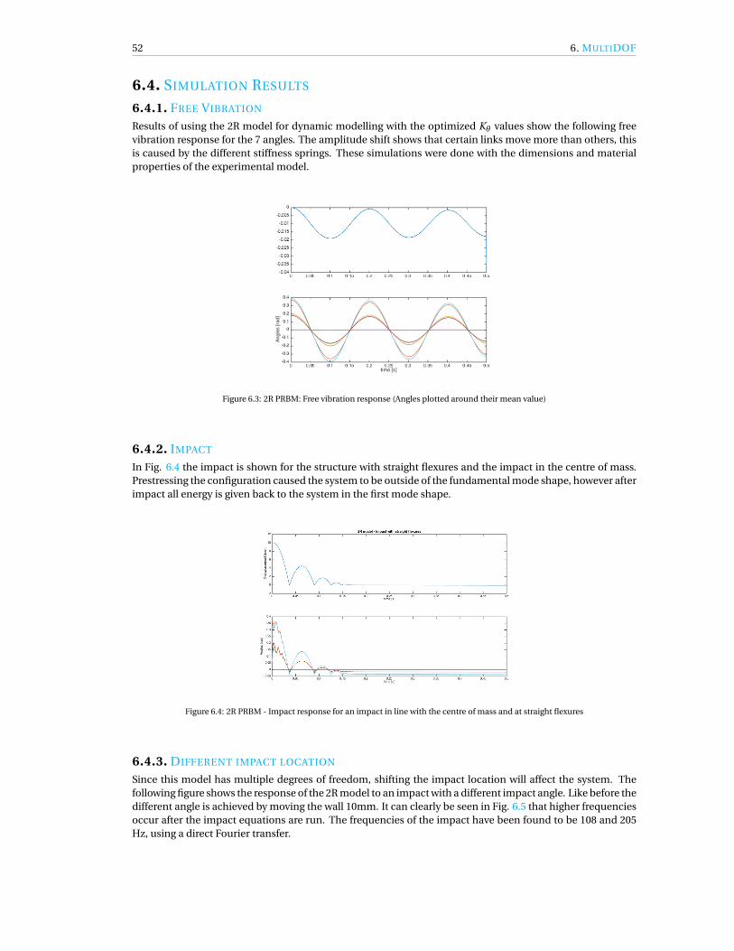
52 6. MULTIDOF

6.4. SIMULATION RESULTS

6.4.1. FREE VIBRATION

Results of using the 2R model for dynamic modelling with the optimized Kθ values show the following freevibration response for the 7 angles. The amplitude shift shows that certain links move more than others, thisis caused by the different stiffness springs. These simulations were done with the dimensions and materialproperties of the experimental model.

Figure 6.3: 2R PRBM: Free vibration response (Angles plotted around their mean value)

6.4.2. IMPACT

In Fig. 6.4 the impact is shown for the structure with straight flexures and the impact in the centre of mass.Prestressing the configuration caused the system to be outside of the fundamental mode shape, however afterimpact all energy is given back to the system in the first mode shape.

Figure 6.4: 2R PRBM - Impact response for an impact in line with the centre of mass and at straight flexures

6.4.3. DIFFERENT IMPACT LOCATION

Since this model has multiple degrees of freedom, shifting the impact location will affect the system. Thefollowing figure shows the response of the 2R model to an impact with a different impact angle. Like before thedifferent angle is achieved by moving the wall 10mm. It can clearly be seen in Fig. 6.5 that higher frequenciesoccur after the impact equations are run. The frequencies of the impact have been found to be 108 and 205Hz, using a direct Fourier transfer.

6.5. DISCUSSION 53

Figure 6.5: 2R PRBM - Impact response for impact in line with the centre of mass and 10mm from straight flexures

6.5. DISCUSSIONIn free vibration no higher frequencies are seen in the system. The principle Eigenmode dominates the sys-tem as expected and this is seen in the experiments.

Results for the impact occurring when the flexures are undeflected are exactly the same as the PRBDMresults and close to the experimental results. Adjusting the location of the wall, and therefore the angle of theimpact in contrast to the 1R model now has an effect on the response as opposed to the 1 degree of freedommodel. A higher frequency can be seen in the response when the velocity of the shuttle is not normal to thecontact surface at the moment of impact. The frequency that is observed is at a different frequency than thehigher Eigenfrequencies of the system.

In the response of the shuttle it can be seen that multiple impacts occur in the course of one oscillation,which cause more energy to be lost than is observed in the experiments. The impact equations and theimplementation in the equations of motion shows that the solving is not as robust as desired. Converging ofa solution is dependent on well chosen initial conditions.

More complex and more robust impact equations are necessary to describe the response more accurately.The velocity that is now used to calculate the velocities after impact is the velocity normal to the contactsurface. However, the velocity perpendicular to the contact surface also experiences an impact due to thesudden occurrence of friction on the system.

By inspecting the velocities that are calculated after the impact it is seen that different speeds are given tothe front and back flexure. Modelling the system as a pendulum also means that a mass is only described fromone side of the system. Therefore the impact equations are now run with a contact condition that containsinformation about half of the structure, which might change the outcome of the equations.

7MATERIAL TESTING - CARBONNANOTUBES

7.1. INTRODUCTION

Carbon nanotube structures are being investigated as a possible candidate for compliant MEMS structures.The structures being measured are fabricated at Brigham Young University (BYU). The carbon nanotubes(CNTs) are infiltrated with carbon to create a structure. To be able to use these structures as planar compliantmechanisms the material properties should be known. The aim of this research is to find the Young’s mod-ulus of the acquired composite material in planar direction. Therefore experiments have been performed tomeasure the Young’s modulus of the material.

7.2. MATERIAL

The structures that have been fabricated at BYU have densely grown carbon nanotubes which create a frame-work. This framework has been grown on an iron layer and is filled with carbon via chemical vapor deposi-tion. After the deposition the iron layer is removed by chemical etching. This results in a structure of carbonnanotubes infiltrated with carbon.

Figure 7.1: SEM-image CNT fabrication

55

56 7. MATERIAL TESTING - CARBONNANOTUBES

7.3. TEST STRUCTURESAfter guessing the Young’s modulus based on previous research, test structures are created. This guessedYoung’s modulus is used to design the test structure for experimental use. Cantilever beams are designed withthicknesses resembling the applications being developed at Flexous. For these thicknesses a measurementof the Young’s modulus is desired. The lengths of the test cantilevers have been chosen so the experiment isexpected to fit nicely in the sensor range.

Simulations were done for beam thicknesses of 10, 15 and 20µm and a design was created for this. Besidesthese thicknesses a higher force test is designed with beams of 100µm. For the simulations a Young’s modulusof 35 GPa is assumed which has been found for different CNT-devices in earlier research. The lengths werechosen so the data matched one of two available force sensors, with a range of 0−10 mN and 0−200 mN .

Figure 7.2: Results of ANSYS Simulations of Cantilever beams with different thicknesses

7.3.1. EXPERIMENTAL SETUPThe experiments are performed by deflecting the test mechanisms and using a force sensor to record thereaction force. The setup therefore consists of a linear precision stage for displacement data and a forcesensor for the reaction forces. Using force displacement data and linear beam theory the Young’s moduluscan be extracted. The linear precision stage used is the PI M-406. The force sensor used is the FEMTO-tools1g force sensor (FT-FS10000). Besides the sensor data the dimensions of the beam have been checked for theextraction of the Young’s modulus.

Figure 7.3: Block-scheme of experiment setup

Figure 7.4: (a) side view of FEMTO-tools sensor and test structure (b) top view

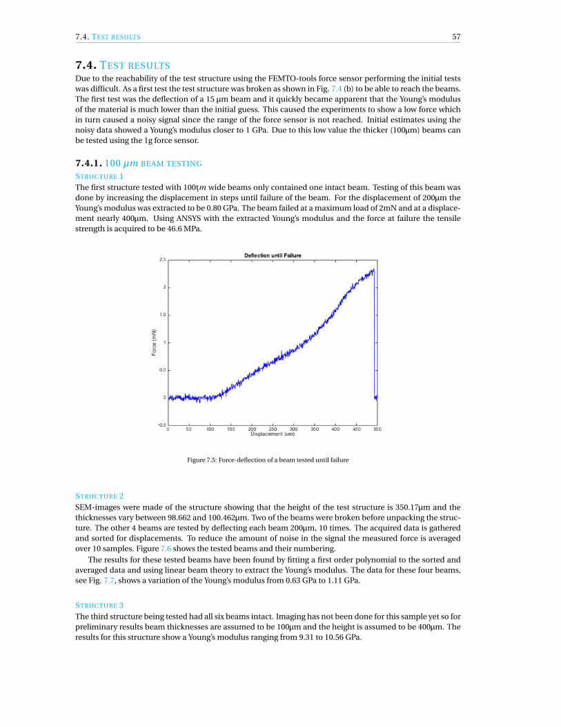
7.4. TEST RESULTS 57

7.4. TEST RESULTSDue to the reachability of the test structure using the FEMTO-tools force sensor performing the initial testswas difficult. As a first test the test structure was broken as shown in Fig. 7.4 (b) to be able to reach the beams.The first test was the deflection of a 15 µm beam and it quickly became apparent that the Young’s modulusof the material is much lower than the initial guess. This caused the experiments to show a low force whichin turn caused a noisy signal since the range of the force sensor is not reached. Initial estimates using thenoisy data showed a Young’s modulus closer to 1 GPa. Due to this low value the thicker (100µm) beams canbe tested using the 1g force sensor.

7.4.1. 100 µm BEAM TESTING

STRUCTURE 1The first structure tested with 100tm wide beams only contained one intact beam. Testing of this beam wasdone by increasing the displacement in steps until failure of the beam. For the displacement of 200µm theYoung’s modulus was extracted to be 0.80 GPa. The beam failed at a maximum load of 2mN and at a displace-ment nearly 400µm. Using ANSYS with the extracted Young’s modulus and the force at failure the tensilestrength is acquired to be 46.6 MPa.

Figure 7.5: Force-deflection of a beam tested until failure

STRUCTURE 2SEM-images were made of the structure showing that the height of the test structure is 350.17µm and thethicknesses vary between 98.662 and 100.462µm. Two of the beams were broken before unpacking the struc-ture. The other 4 beams are tested by deflecting each beam 200µm, 10 times. The acquired data is gatheredand sorted for displacements. To reduce the amount of noise in the signal the measured force is averagedover 10 samples. Figure 7.6 shows the tested beams and their numbering.

The results for these tested beams have been found by fitting a first order polynomial to the sorted andaveraged data and using linear beam theory to extract the Young’s modulus. The data for these four beams,see Fig. 7.7, shows a variation of the Young’s modulus from 0.63 GPa to 1.11 GPa.

STRUCTURE 3The third structure being tested had all six beams intact. Imaging has not been done for this sample yet so forpreliminary results beam thicknesses are assumed to be 100µm and the height is assumed to be 400µm. Theresults for this structure show a Young’s modulus ranging from 9.31 to 10.56 GPa.

58 7. MATERIAL TESTING - CARBONNANOTUBES

Figure 7.6: Test structure beams numbered

Figure 7.7: Extracted data for structure 2

BATCH 2A second batch of test structures contained 6 structures, the Young’s Modulus of these structures was mea-sured as described previously. The results for the Young’s modulus are given in table 7.1. For this batch thedata was also analyzed to see the energy lost during the cycle. The energy of the beam while retracting theforce sensor is lower.

7.4.2. DISCUSSIONA large variation in material properties has been found for beams that have been tested. In the first batch teststructure 3 showed approximately 10 times stiffer beams than the two previous test structures. The secondbatch showed more reliable results. The extracted Young’s modulus is around 2 GPa, however there are stilllarge variations between structures. The energy loss in the cycle is expected to be caused by hysteresis. Thehysteresis loop that is found also shows variations between beams and structures, the trend shows a loss of

7.4. TEST RESULTS 59

Figure 7.8: Extracted data for structure 3

Figure 7.9: Extracted data for structure 3

approximately 10 percent. This energy loss could, besides hysteresis, be caused by other factors. For examplethe sliding of the tip during actuation or the material properties of the sensor tip. In the current test setup it ishard to align height of the force sensor with the cantilever. Quick tests actuating the cantilevers at a differentheight showed that the results vary with around 6%. This is caused by part of the force deforming the beam intorsion rather than in bending. A solution should be found to align the force sensor, or a test structure shouldbe chosen which is not influenced by torsional effects.

8DISCUSSION

This chapter will provide a global discussion about the thesis. Previous chapters have a section with a discus-sion, some overlap will be present.

8.1. APPROACHDuring this thesis a method was developed with a single degree of freedom. The modelling has been fit toexperimental data of the testing mechanism. The fit coefficient of restitution (in fundamental mode shape)offers insight in the energy efficiency of an impact in a compliant mechanism. To try and predict the impactresponse of the test mechanism a new method was proposed. This overall approach to the problem wasfollowed and has shown some interesting results.

8.2. ENERGY EFFICIENCYThe energy efficiency of an impact in a compliant mechanism was tested for the parallel guiding mechanism.The results that have been shown show an asymmetry around the undeflected position and also asymmetryaround the centre of mass of the shuttle (resembling impact angle and location respectively).

8.2.1. IMPACT ANGLEThe three different situations of impact angles are exaggerated and visualized in Fig. 8.1. If the shuttle was notconnected to the flexures deflection will occur and the shuttle will maintain its x-velocity. The principle modein which the mechanism moves will require the velocity just before impact to be converted into a velocity 180degrees in the other direction. In case 1 this deflection causes an extension of the flexures. In case 2, theflexures will be loaded with a buckling force. In Fig 5.9(b) it is shown that in situation 3 more energy is lost.This suggests that more energy is caught in higher frequencies when the x-velocity of the shuttle is in thebuckling direction.

8.2.2. IMPACT POSITIONDifferent impact positions shows smaller asymmetric results around an impact in line with the centre of mass(Fig. 8.2). Fig 5.9(b) shows that a more energy is lost when impacting further away from the flexures. This issuspected to be caused by the direction of the moment around the centre of mass that is caused by the impactforce.

8.3. MULTI DEGREE OF FREEDOM MODELThe multi degree of freedom (DoF) model is based on the 2R-PRBM from literature. This model has beenconverted into a dynamic model and the same techniques that have been applied to the single DoF modelare used to create the equations of motion. The fundamental frequency of the acquired dynamic model havebeen matched by varying the Kθ parameters. An impact in line with the centre of mass and with undeflectedflexures shows the same result as the single DoF model. Extra energy loss is visible in the model when theimpact location is shifted, or the angle changed. The energy that is lost from the fundamental mode is shownto be caught in higher frequencies inside the system.

61

62 8. DISCUSSION

Figure 8.1: Varying angles between impact force and shuttle velocity

Figure 8.2: Varying impact locations with respect to the centre of mass

The impact response that is modelled with the dynamic 2R-PRBM has shown some issues with finding aconverging solution. During the course of a single impact the model shows that the system makes contactmultiple times. This will cause the system to lose a percentage of the energy (due to the coefficient of restu-tion) multiple times as well. The cause of this is suspected to be in the numerical integration of the system,and not be caused by the model itself. The impact is currently modelled by using a contact condition that ischecked every timestep. The derivative of the contact condition is used as the relative velocity normal to thecontact surface (of the impacting point). A problem is suspected to arise because the system is modelled asa seven link pendulum that is constrained on its end point. This has the drawback that the impact point isdescribed in the contact condition and the impact equations, from one side of the mechanism (through onlyone of the flexures). The calculated velocities by the impact equations show very non-linear effects becauseof this.

The impact equation that is currently used is a simple approach. To be able to more accurately describean impact response more complex equations are necessary that do not make as many assumptions. For in-stance the impact is now solely dependent on the relative velocity normal to the contact surface. The suddenoccurrence of friction will also have an impact effect on the mechanism, on the velocity perpendicular to thecontact surface.

9CONCLUSION AND RECOMMENDATIONS

9.1. CONCLUSIONSIn this thesis a technique for modelling the dynamic response of a compliant mechanism including impacthas been proposed. The method used is the pseudo-rigid-body dynamic model with rigid body impact equa-tions and has been applied to a general case study. The method is computationally efficient, however theimpact is greatly simplified with respect to the compliant mechanism. The single degree of freedom of thepseudo-rigid-body model is not able to deal with varying impact angles or locations as the energy can onlyreturn in the first mode shape.

Using the modelling an insight is found into the efficiency of compliant mechanisms subject to impactby fitting a coefficient of restitution in fundamental mode to the experimental data. The case study showsthat the parallel guiding mechanism conserves most energy when an impact is in line with the velocity of theimpacting body. As expected, impacting outside of the line of the centre of mass or impacting at an anglecauses energy to be lost in higher frequency motion. The amount of energy retained when impacting thebody closer to the mechanisms centre of compliance shows more energy is retained than impacting on theother side of the centre of mass.

9.1.1. MULTI DOFSince the pseudo-rigid-body model only contains a single degree of freedom, the effects of higher frequenciesin the system cannot be modelled. Therefore the effect of impact angle and position are not seen, becausethe energy can only be fed back into the first Eigenfrequency. To be able to predict the response of adding acontact the modelling should contain more degrees of freedom in which energy can be dissipated. A 2R (tworotation) pseudo-rigid-body model has been converted into a dynamic counterpart. Impacts being modelledwith the 2R model show higher frequencies in the response when the impact is not normal to the contactsurface. The frequencies that are seen do not match the frequency of the second planar mode shape.

9.1.2. CNTMaterial testing of carbon-nano-tube structures shows a large variation of material properties and is far fromthe initial guess of 35 GPa. This is most likely caused by a different filler material, carbon instead of iron. Thefirst batch of structures showed a factor 10 between the found Young’s moduli. The second batch showedmore reliable results and an experimentally acquired Young’s modulus around 2 GPa. However there is stillvariation between structures.

9.2. RECOMMENDATIONSUsing a single degree of freedom system to model the impact response of a compliant mechanism is an ef-ficient simplification. To be able to predict behaviour two directions can be taken, either expand the modelto contain multiple degrees of freedom, or use information about the impact angle and location to modelextra energy losses. This could be done with an additional coefficient which is used with the coefficient ofrestitution. The 2R-PRBM proposed shows that the first direction makes it possible to see higher frequencyinfluences.

63

64 9. CONCLUSION AND RECOMMENDATIONS

9.2.1. CNTThe carbon infiltrated CNT structures are a promising material for use in compliant micro mechanisms. Fab-rication has been shown to be very accurate. The source of the variation in measured material propertiesshould be looked for in the fabrication process. This will make designing structures for the material easier.More experiments should be done to also determine the out-of-plane Young’s modulus.

AMATLAB CODE

A.1. EQUATIONS OF MOTION - PRBDM

%% Parallel Guiding Mechanism %%%%%%%%%%%%%%%%%%%%%%%%%%%%%%%%%%%%%% __m3__ −> %%%%%%%%%%%%% | | %%%%%%%%%%%%% l1 l2 %%%%%%%%%%%%% | | %%%%%%%%%%%%% −−−−−−−−−− %%%%%%%%%%%%% / / / / / %%%%%%%%%%%%%%%%%%%%%%%%%%%%%%%%%%%%%%%%%clcclose allclear%% Derivation of equations of motion% symbolssyms th ph alph thetad phd alphd x1 y1 x2 y2 x3 y3 gamma K real% Material propertiesE = 3.21e9;rho = 1190;% Geometryl1 = 0.2;l2 = 0.2;l3 = 0.2;l4 = 0.2;w1 = 0.002;w2 = 0.02;d = 0.01;A1 = w1*d;A2 = w2*d;I1 = 1/12*d*w1^3;I2 = 1/12*d*w2^3;m1 = rho*l1*A1; % m1 = m3m2 = rho*l2*A2;m3 = m1;% state vectorxitmt = [x1 y1 th x2 y2 ph x3 y3 alph];% PRBM constantsr1 = gamma*l1;r3 = gamma*l3;J1 = (m1*l1^2)/12;J2 = (m2*l2^2)/12;J3 = (m3*l3^2)/12;% torsional springsk1 = 2*gamma*K*E*I1/l1;k2 = 2*gamma*K*E*I1/l1;k3 = 2*gamma*K*E*I1/l2;k4 = 2*gamma*K*E*I1/l2;

65

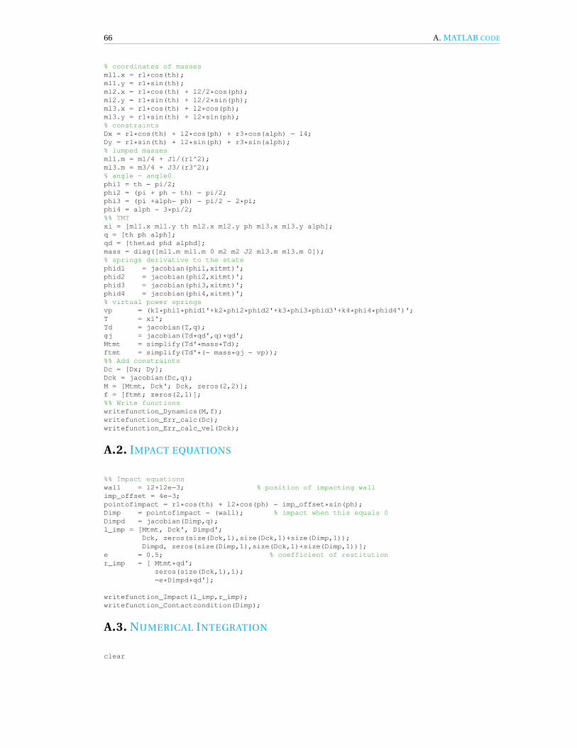
66 A. MATLAB CODE

% coordinates of massesml1.x = r1*cos(th);ml1.y = r1*sin(th);ml2.x = r1*cos(th) + l2/2*cos(ph);ml2.y = r1*sin(th) + l2/2*sin(ph);ml3.x = r1*cos(th) + l2*cos(ph);ml3.y = r1*sin(th) + l2*sin(ph);% constraintsDx = r1*cos(th) + l2*cos(ph) + r3*cos(alph) − l4;Dy = r1*sin(th) + l2*sin(ph) + r3*sin(alph);% lumped massesml1.m = m1/4 + J1/(r1^2);ml3.m = m3/4 + J3/(r3^2);% angle − angle0phi1 = th − pi/2;phi2 = (pi + ph − th) − pi/2;phi3 = (pi +alph− ph) − pi/2 − 2*pi;phi4 = alph − 3*pi/2;%% TMTxi = [ml1.x ml1.y th ml2.x ml2.y ph ml3.x ml3.y alph];q = [th ph alph];qd = [thetad phd alphd];mass = diag([ml1.m ml1.m 0 m2 m2 J2 ml3.m ml3.m 0]);% springs derivative to the statephid1 = jacobian(phi1,xitmt)';phid2 = jacobian(phi2,xitmt)';phid3 = jacobian(phi3,xitmt)';phid4 = jacobian(phi4,xitmt)';% virtual power springsvp = (k1*phi1*phid1'+k2*phi2*phid2'+k3*phi3*phid3'+k4*phi4*phid4')';T = xi';Td = jacobian(T,q);gj = jacobian(Td*qd',q)*qd';Mtmt = simplify(Td'*mass*Td);ftmt = simplify(Td'*(− mass*gj − vp));%% Add constraintsDc = [Dx; Dy];Dck = jacobian(Dc,q);M = [Mtmt, Dck'; Dck, zeros(2,2)];f = [ftmt; zeros(2,1)];%% Write functionswritefunction_Dynamics(M,f);writefunction_Err_calc(Dc);writefunction_Err_calc_vel(Dck);

A.2. IMPACT EQUATIONS

%% Impact equationswall = l2+12e−3; % position of impacting wallimp_offset = 4e−3;pointofimpact = r1*cos(th) + l2*cos(ph) − imp_offset*sin(ph);Dimp = pointofimpact − (wall); % impact when this equals 0Dimpd = jacobian(Dimp,q);l_imp = [Mtmt, Dck', Dimpd';

Dck, zeros(size(Dck,1),size(Dck,1)+size(Dimp,1));Dimpd, zeros(size(Dimp,1),size(Dck,1)+size(Dimp,1))];

e = 0.5; % coefficient of restitutionr_imp = [ Mtmt*qd';

zeros(size(Dck,1),1);−e*Dimpd*qd'];

writefunction_Impact(l_imp,r_imp);writefunction_Contactcondition(Dimp);

A.3. NUMERICAL INTEGRATION

clear

A.3. NUMERICAL INTEGRATION 67

close allclc% Material propertiesgamma = 0.8517;l1 = 40e−3;l2 = 80e−3;r1 = gamma*l1;%% Initial Conditionsxdisp = 0e−3;phi = asin(xdisp/r1);angle = pi/2;y0 = [angle+phi; 0; pi+angle+phi; 0; 0; 0];%% Numerical Integration − RK4% Time/Step sizeTend = 1;n = 15;h = Tend/(2^n);y = y0;% initiate state vectorstate = zeros(length(0:h:Tend),6);impacttimes = [];for t= 0:h:Tendstep = round((t/h)+1);if(Contactcheck(y) > 0) % When contact is made calculate new state using impact equations

[y, forces] = Impact(y);disp(['Impact at t = ' num2str(t)])impacttimes = [impacttimes; t];while(Contactcheck(y) > 0) % Untill out of contact area, do not use impact equations again

y = RK4(y,h);% Compute new state% Gauss−Newton Iteration for error projectiontol = 1e−13;j = 1;error = Error_calc(y);while (max(abs(error)) > tol && j≤10)[y, error] = errorprojection(y);j = j + 1;end

% y = errorprojection_v(y);state(step,:) = y; % save state in each time stepend

endy = RK4(y,h); % Compute new state% Gauss−Newton Iteration for error projectiontol = 1e−13;j = 1;error = Error_calc(y);while (max(abs(error)) > tol && j≤10)[y, error] = errorprojection(y);j = j + 1;end% y = errorprojection_v(y);state(step,:) = y; % save state in each time step% disp([num2str(t/Tend*100) ' %'])endt= 0:h:Tend;xdata = r1*cos(state(:,1));ydata = r1*sin(state(:,1));%% Plotfigure(2);set(gcf,'name','Parallel guiding Mechanism X−displacement','numbertitle','off')% grid onhold onplot(t,xdata*1000)% title('Damping Test')xlabel('time [s]')ylabel('X−displacement [mm]')legend('PRBDM−MATLAB')figureHandle = gcf; % Make all text size 14 and boldset(findall(figureHandle,'type','text'),'fontSize',14)hold off

68 A. MATLAB CODE

A.3.1. RUNGE-KUTTA 4TH ORDER FUNCTION

function [ ynew ] = RK4( y, h )%RK4 − Runge Kutta 4 numerical integration integrationk1 = Dynamics(y);k2 = Dynamics(y+h/2*k1);k3 = Dynamics(y+h/2*k2);k4 = Dynamics(y+h*k3);ynew = y + (k1 + 2*k2 + 2*k3 + k4)*h/6;end

A.3.2. ERROR PROJECTION FUNCTION

function [ y, error ] = errorprojection( y )%errorprojectionerror = Error_calc(y);D = Error_calc_vel(y);D_plus = D'*(D*D')^−1;∆ = D_plus*−error;y(1:7) = y(1:7) + ∆';end

A.4. EXAMPLE WRITEFUNCTION

function [] = writefunction_Dynamics(M,f)% The function Dynamics is automatically createdfid = fopen('Dynamics.m','w');fprintf(fid,'function [yd] = Dynamics(y, X)\n');fprintf(fid,'%% Automatically generated function, see main file\n');fprintf(fid,'\nth = y(1);\n');fprintf(fid,'ph = y(2);\n');fprintf(fid,'alph = y(3);\n');fprintf(fid,'thd = y(4);\n');fprintf(fid,'phd = y(5);\n');fprintf(fid,'alphd = y(6);\n');fprintf(fid,'gamma = 0.8517;\n');fprintf(fid,'K = X;\n');% M − matrixfprintf(fid,'M = [');for i = 1:size(M,1)−1for j = 1:size(M,2)−1

fprintf(fid,[char(M(i,j)) ', ']);endfprintf(fid,[char(M(i,size(M,1))) ';\n']);endfor i = 1:size(M,2)−1

fprintf(fid,[char(M(i,size(M,1))) ', ']);endfprintf(fid,[char(M(size(M,2),size(M,1))) '];\n']);% F − vectorfprintf(fid,'\nf = [ ');for i =1:size(f)−1

fprintf(fid,[char(f(i)) '; ']);endfprintf(fid,[char(f(size(f,1))) '];\n']);% Solving for accelerationsfprintf(fid,'\nsol = M\\f;\n');fprintf(fid,'yd = [y(4); y(5); y(6); sol(1:3)];\n');fprintf(fid,'\n');fprintf(fid,'end');fclose(fid);end

A.5. 2R MODEL

A.5.1. EQUATIONS OF MOTION

A.5. 2R MODEL 69

%% Parallel Guiding Mechanism %%% 2R %%%%%%%%%%%%%%%%%%%%%%%%%%%%%%%%%%%%%%%%%%%%%%%%%%%%%%%%%%%%%%%%%%%%%%%%%%%%%%%%%%%%%%%%%%%%%%%%%%%%%%%%%%%%%%%%%% __m3__ −> %%%%%%%%%%%%%%%%%%%%%%%%%%%%%%%%%%%%%%%%%%%%%%%%%%%%%%%% | | %%%%%%%%%%%%%%%%%%%%%%%%%%%%%%%%%%%%%%%%%%%%%%%%%%%%%%%% l1 l2 %%%%%%%%%%%%%%%%%%%%%%%%%%%%%%%%%%%%%%%%%%%%%%%%%%%%%%%% | | %%%%%%%%%%%%%%%%%%%%%%%%%%%%%%%%%%%%%%%%%%%%%%%%%%%%%%%% −−−−−−−−−− %%%%%%%%%%%%%%%%%%%%%%%%%%%%%%%%%%%%%%%%%%%%%%%%%%%%%%%% / / / / / %%%%%%%%%%%%%%%%%%%%%%%%%%%%%%%%%%%%%%%%%%%%%%%%%%%%%%%%%%%%%%%%%%%%%%%%%%%%%%%%%%%%%%%%%%%%%%%%%%%%%%%%%%%%%%%%%%%%%%%%%%%%%%%%%%clcclose allclear%% Derivation of equations of motion% symbolssyms tf1_1 tf1_2 tf1_3 t_par tf2_1 tf2_2 tf2_3 f1_1_x f1_1_y f1_2_x f1_2_y...

f1_e_x f1_e_y f2_0_x f2_0_y f2_1_x f2_1_y f2_2_x f2_2_y f2_e_x f2_e_y...tfd1_1 tfd1_2 tfd1_3 td_par tfd2_1 tfd2_2 tfd2_3 real

% Material propertiesE = 3.21e9;rho = 1190;% Geometryl1 = 0.2;l2 = 0.2;l3 = 0.2;l4 = 0.2;w1 = 0.002;w2 = 0.02;d = 0.008;A1 = w1*d;A2 = w2*d;I1 = 1/12*d*w1^3;I2 = 1/12*d*w2^3;m1 = rho*l1*A1; % m1 = m3m2 = rho*l2*A2;m3 = m1;% state vectorxitmt = [ f1_1_x f1_1_y tf1_1...

f1_2_x f1_2_y tf1_2...f1_e_x f1_e_y tf1_3...f2_0_x f2_0_y t_par...f2_1_x f2_1_y tf2_1...f2_2_x f2_2_y tf2_2...f2_e_x f2_e_y tf2_3...];

% PRBM constantsgamma0 = 0.1;gamma1 = 0.44;gamma2 = 0.46;syms K1 K2 real% K1 = 3.4710;% K2 = 2.0682;J1 = (m1*l1^2)/12;J2 = (m2*l2^2)/12;J3 = (m3*l3^2)/12;% lengths of PRBM beamsl11 = gamma1*l1/2;l12 = 2*gamma2*l1/2;l13 = gamma1*l1/2;l31 = gamma1*l3/2;l32 = 2*gamma2*l3/2;l33 = gamma1*l3/2;% mass 1 and 3 split into 3 partsm11 = m1*l11/l1;m12 = m1*l12/l1;m13 = m1*l13/l1;m31 = m3*l31/l3;m32 = m3*l32/l3;m33 = m3*l33/l3;% inertiaJ11 = (m11*l11^2)/12;J12 = (m12*l12^2)/12;

70 A. MATLAB CODE

J13 = (m13*l13^2)/12;J31 = (m31*l31^2)/12;J32 = (m32*l32^2)/12;J33 = (m33*l33^2)/12;% torsional springskf1_1 = 2*gamma1*K1*E*I1/l1;kf1_2 = 2*gamma2*K2*E*I1/l1;kf1_3 = 2*gamma2*K2*E*I1/l1;kf1_4 = 2*gamma1*K1*E*I1/l1;kf2_1 = 2*gamma1*K1*E*I1/l3;kf2_2 = 2*gamma2*K2*E*I1/l3;kf2_3 = 2*gamma2*K2*E*I1/l3;kf2_4 = 2*gamma1*K1*E*I1/l3;% endpoints of beamsf1_1_x = l11*cos(tf1_1);f1_1_y = l11*sin(tf1_1);f1_2_x = f1_1_x + l12*cos(tf1_2);f1_2_y = f1_1_y + l12*sin(tf1_2);f1_e_x = f1_2_x + l13*cos(tf1_3);f1_e_y = f1_2_y + l13*sin(tf1_3);f2_0_x = f1_e_x + l2*cos(t_par);f2_0_y = f1_e_y + l2*sin(t_par);f2_1_x = f2_0_x + l31*cos(tf2_1);f2_1_y = f2_0_y + l31*sin(tf2_1);f2_2_x = f2_1_x + l32*cos(tf2_2);f2_2_y = f2_1_y + l32*sin(tf2_2);f2_e_x = f2_2_x + l33*cos(tf2_3);f2_e_y = f2_2_y + l33*sin(tf2_3);% coordinates of massesf1_1_xm = l11/2*cos(tf1_1);f1_1_ym = l11/2*sin(tf1_1);f1_2_xm = f1_1_x + l12/2*cos(tf1_2);f1_2_ym = f1_1_y + l12/2*sin(tf1_2);f1_e_xm = f1_2_x + l13/2*cos(tf1_3);f1_e_ym = f1_2_y + l13/2*sin(tf1_3);f2_0_xm = f1_e_x + 1/2*l2*cos(t_par);f2_0_ym = f1_e_y + 1/2*l2*sin(t_par);f2_1_xm = f2_0_x + l31/2*cos(tf2_1);f2_1_ym = f2_0_y + l31/2*sin(tf2_1);f2_2_xm = f2_1_x + l32/2*cos(tf2_2);f2_2_ym = f2_1_y + l32/2*sin(tf2_2);f2_e_xm = f2_2_x + l33/2*cos(tf2_3);f2_e_ym = f2_2_y + l33/2*sin(tf2_3);% torsional spring (∆ angle: angle − angle0)pf1_1 = tf1_1 − pi/2;pf1_2 = (pi/2 + tf1_2 − tf1_1) − pi/2;pf1_3 = (pi/2 + tf1_3 − tf1_2) − pi/2;pf1_4 = (pi/2 + t_par − tf1_3);pf2_1 = (pi/2 + tf2_1 − t_par) − 2*pi;pf2_2 = (pi/2 + tf2_2 − tf2_1) − pi/2;pf2_3 = (pi/2 + tf2_3 − tf2_2) − pi/2;pf2_4 = tf2_3 − 3*pi/2;test_k_vec = [pf1_1; pf1_2; pf1_3; pf1_4; pf2_1; pf2_2; pf2_3; pf2_4];%% TESTING y0 = restposition% y0 = [pi/2*ones(1,3), 0 3*pi/2*ones(1,3)];% tf1_1 = y0(1);% tf1_2 = y0(2);% tf1_3 = y0(3);% t_par = y0(4);% tf2_1 = y0(5);% tf2_2 = y0(6);% tf2_3 = y0(7);% subs(test_k_vec) % Check if spring displacements are 0!%% Statexi = [ f1_1_xm f1_1_ym tf1_1...

f1_2_xm f1_2_ym tf1_2...f1_e_xm f1_e_ym tf1_3...f2_0_xm f2_0_ym t_par...f2_1_xm f2_1_ym tf2_1...f2_2_xm f2_2_ym tf2_2...f2_e_xm f2_e_ym tf2_3...

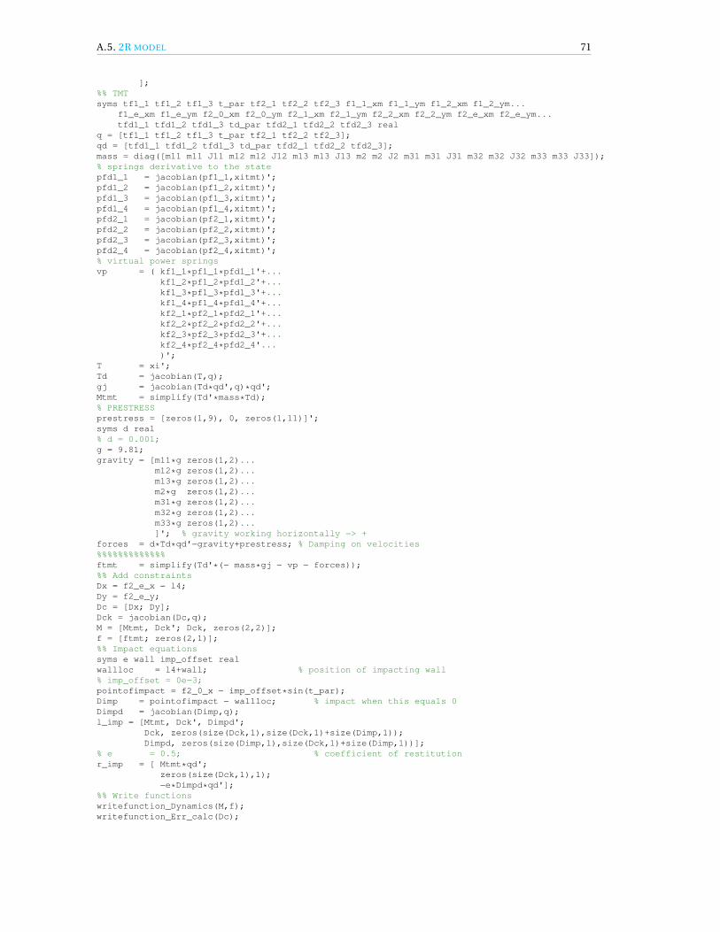
A.5. 2R MODEL 71

];%% TMTsyms tf1_1 tf1_2 tf1_3 t_par tf2_1 tf2_2 tf2_3 f1_1_xm f1_1_ym f1_2_xm f1_2_ym...

f1_e_xm f1_e_ym f2_0_xm f2_0_ym f2_1_xm f2_1_ym f2_2_xm f2_2_ym f2_e_xm f2_e_ym...tfd1_1 tfd1_2 tfd1_3 td_par tfd2_1 tfd2_2 tfd2_3 real

q = [tf1_1 tf1_2 tf1_3 t_par tf2_1 tf2_2 tf2_3];qd = [tfd1_1 tfd1_2 tfd1_3 td_par tfd2_1 tfd2_2 tfd2_3];mass = diag([m11 m11 J11 m12 m12 J12 m13 m13 J13 m2 m2 J2 m31 m31 J31 m32 m32 J32 m33 m33 J33]);% springs derivative to the statepfd1_1 = jacobian(pf1_1,xitmt)';pfd1_2 = jacobian(pf1_2,xitmt)';pfd1_3 = jacobian(pf1_3,xitmt)';pfd1_4 = jacobian(pf1_4,xitmt)';pfd2_1 = jacobian(pf2_1,xitmt)';pfd2_2 = jacobian(pf2_2,xitmt)';pfd2_3 = jacobian(pf2_3,xitmt)';pfd2_4 = jacobian(pf2_4,xitmt)';% virtual power springsvp = ( kf1_1*pf1_1*pfd1_1'+...

kf1_2*pf1_2*pfd1_2'+...kf1_3*pf1_3*pfd1_3'+...kf1_4*pf1_4*pfd1_4'+...kf2_1*pf2_1*pfd2_1'+...kf2_2*pf2_2*pfd2_2'+...kf2_3*pf2_3*pfd2_3'+...kf2_4*pf2_4*pfd2_4'...)';

T = xi';Td = jacobian(T,q);gj = jacobian(Td*qd',q)*qd';Mtmt = simplify(Td'*mass*Td);% PRESTRESSprestress = [zeros(1,9), 0, zeros(1,11)]';syms d real% d = 0.001;g = 9.81;gravity = [m11*g zeros(1,2)...

m12*g zeros(1,2)...m13*g zeros(1,2)...m2*g zeros(1,2)...m31*g zeros(1,2)...m32*g zeros(1,2)...m33*g zeros(1,2)...]'; % gravity working horizontally −> +

forces = d*Td*qd'−gravity+prestress; % Damping on velocities%%%%%%%%%%%%%ftmt = simplify(Td'*(− mass*gj − vp − forces));%% Add constraintsDx = f2_e_x − l4;Dy = f2_e_y;Dc = [Dx; Dy];Dck = jacobian(Dc,q);M = [Mtmt, Dck'; Dck, zeros(2,2)];f = [ftmt; zeros(2,1)];%% Impact equationssyms e wall imp_offset realwallloc = l4+wall; % position of impacting wall% imp_offset = 0e−3;pointofimpact = f2_0_x − imp_offset*sin(t_par);Dimp = pointofimpact − wallloc; % impact when this equals 0Dimpd = jacobian(Dimp,q);l_imp = [Mtmt, Dck', Dimpd';

Dck, zeros(size(Dck,1),size(Dck,1)+size(Dimp,1));Dimpd, zeros(size(Dimp,1),size(Dck,1)+size(Dimp,1))];

% e = 0.5; % coefficient of restitutionr_imp = [ Mtmt*qd';

zeros(size(Dck,1),1);−e*Dimpd*qd'];

%% Write functionswritefunction_Dynamics(M,f);writefunction_Err_calc(Dc);

72 A. MATLAB CODE

writefunction_Err_calc_vel(Dck);writefunction_Impact(l_imp,r_imp);writefunction_Contactcondition(Dimp);

A.5.2. OPTIMIZATION OF Kθ

MAIN FILE

clearclose allclc%% Import the 1R Resultsglobal xdatasingleDOFdata = load('1R.mat');tdata = singleDOFdata.t;xdata = singleDOFdata.xdata;%% Interpolate dataTend = 2;n = 10;h = Tend/(2^n);t = 0:h:Tend;xdata = interp1(tdata,xdata,t,'PCHIP')';%% Optimization variables: PRBDM parametersgamma0 = 0.1;gamma1 = 0.44;gamma2 = 0.46;K1 = 3.4710; % From paperK2 = 2.0682;X0 = [K1;K2];%% Perform the optimizationPROBLEM.objective = @RMSE;PROBLEM.solver = 'fmincon';PROBLEM.x0 = X0;PROBLEM.Aineq = [];PROBLEM.bineq = [];PROBLEM.Aeq = [];PROBLEM.beq = [];PROBLEM.lb = zeros(1,2);PROBLEM.ub = [15,15];PROBLEM.options=optimoptions('fmincon','MaxIter',50,'Display','iter−detailed','TolFun',1e−9,'TolX',1e−9);

warning('off','MATLAB:illConditionedMatrix')X = fmincon(PROBLEM);

xdataopt = PRBDM(X);xdata0 = PRBDM(X0);%% Plotfigure(1);set(gcf,'name','Parallel guiding Mechanism X−displacement','numbertitle','off')% grid onhold onplot(t,xdata*1000,'g','LineWidth',2)plot(t,xdataopt*1000,'−.')plot(t,xdata0*1000,'m')

title('Minimizing the RMS−error between 2R and 1R models')xlabel('time [s]')ylabel('X−displacement [mm]')legend('PRBDM','2R−optimized','2R−starting point')figureHandle = gcf; % Make all text size 14 and boldset(findall(figureHandle,'type','text'),'fontSize',14)hold off

OBJECTIVE FUNCTION

function [ rmse_x ] = RMSE(X)% RMSE.m% Calculates the root mean square error with respect to the ANSYS model% for a given gamma and Ktheta

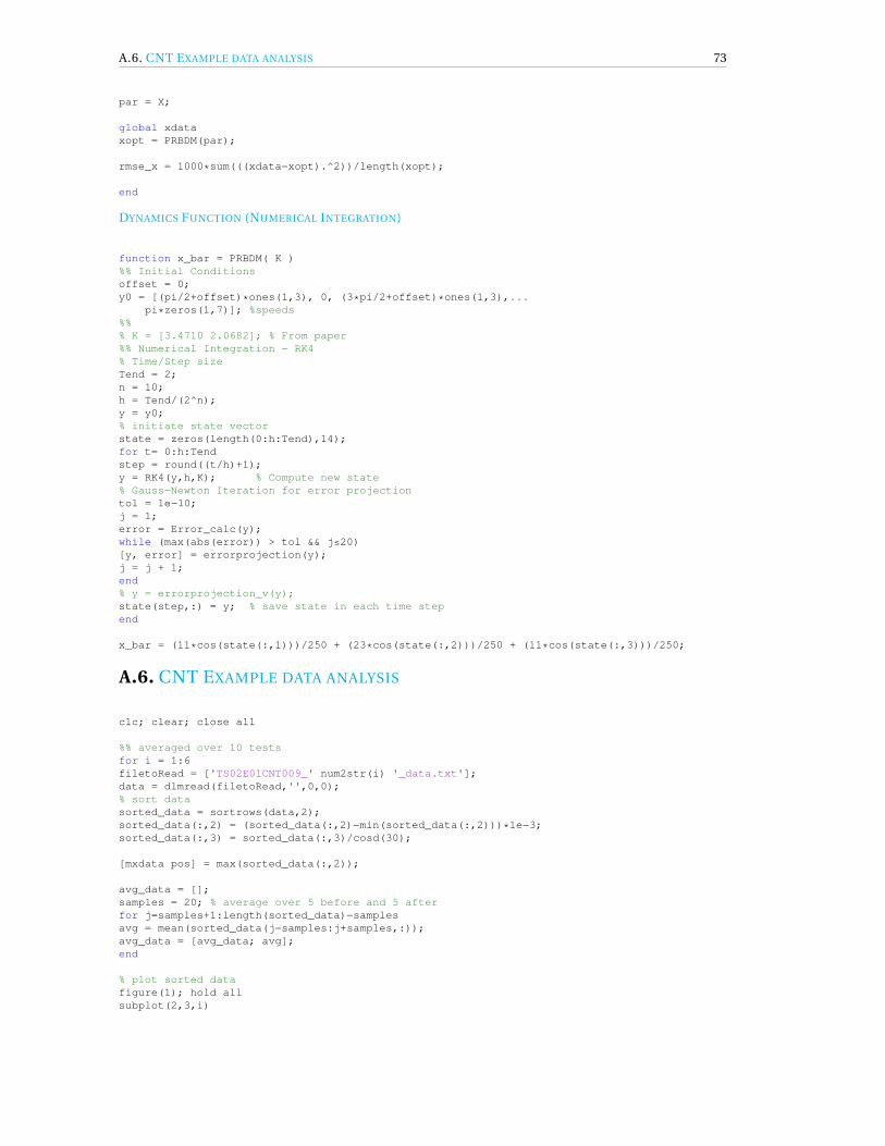
A.6. CNT EXAMPLE DATA ANALYSIS 73

par = X;

global xdataxopt = PRBDM(par);

rmse_x = 1000*sum(((xdata−xopt).^2))/length(xopt);

end

DYNAMICS FUNCTION (NUMERICAL INTEGRATION)

function x_bar = PRBDM( K )%% Initial Conditionsoffset = 0;y0 = [(pi/2+offset)*ones(1,3), 0, (3*pi/2+offset)*ones(1,3),...

pi*zeros(1,7)]; %speeds%%% K = [3.4710 2.0682]; % From paper%% Numerical Integration − RK4% Time/Step sizeTend = 2;n = 10;h = Tend/(2^n);y = y0;% initiate state vectorstate = zeros(length(0:h:Tend),14);for t= 0:h:Tendstep = round((t/h)+1);y = RK4(y,h,K); % Compute new state% Gauss−Newton Iteration for error projectiontol = 1e−10;j = 1;error = Error_calc(y);while (max(abs(error)) > tol && j≤20)[y, error] = errorprojection(y);j = j + 1;end% y = errorprojection_v(y);state(step,:) = y; % save state in each time stepend

x_bar = (11*cos(state(:,1)))/250 + (23*cos(state(:,2)))/250 + (11*cos(state(:,3)))/250;

A.6. CNT EXAMPLE DATA ANALYSIS

clc; clear; close all

%% averaged over 10 testsfor i = 1:6filetoRead = ['TS02E01CNT009_' num2str(i) '_data.txt'];data = dlmread(filetoRead,'',0,0);% sort datasorted_data = sortrows(data,2);sorted_data(:,2) = (sorted_data(:,2)−min(sorted_data(:,2)))*1e−3;sorted_data(:,3) = sorted_data(:,3)/cosd(30);

[mxdata pos] = max(sorted_data(:,2));

avg_data = [];samples = 20; % average over 5 before and 5 afterfor j=samples+1:length(sorted_data)−samplesavg = mean(sorted_data(j−samples:j+samples,:));avg_data = [avg_data; avg];end

% plot sorted datafigure(1); hold allsubplot(2,3,i)

74 A. MATLAB CODE

plot(sorted_data(:,2)*1e6,−sorted_data(:,3)*1e3,'b')hold on, plot(avg_data(:,2)*1e6,−avg_data(:,3)*1e3,'m','LineWidth',2)

% fit between min and max percentage of datal = length(avg_data(:,2));mn = round(0.25*l); % 40%mx = round(0.9*l); % 80%% mn = find(−avg_data(:,3)>4e−3,1); % 4 mN% mx = find(−avg_data(:,3)>10e−3,1); % 10 mN

% linear fitp = polyfit(sorted_data(mn:mx,2),−sorted_data(mn:mx,3),1);% plot fitx = avg_data(mn,2):1e−5:avg_data(mx,2);hold on, plot(x*1e6,(p(1)*x+p(2))*1e3,'g−−','LineWidth',3)% axis([−0.5 3.5 0 250])hold off% extract young's modulusl = 2400e−6;b = 400e−6;h = 100e−6;E=p(1)*l^3/3/(1/12*b*h^3);title(['E', num2str(i),' = ',num2str(round((E*1e−9)*100)/100),' GPa']);xlabel('Displacement (um)')ylabel('Force (mN)')if (i == 1)legend('Raw data','Averaged data','Linear fit')endend

BAPDL CODE

APDL-code (ANSYS) Parallel Guiding Mechanism. B.1.1. or B.1.2. can be added for a static or transient anal-ysis.

B.1. INITIAL TESTS

FINISH/CLEAR,START/TITLE, Parallel_Guiding

TE = 0.5DT = 0.0001! Preprocessing/PREP7ET,1,BEAM189MP,EX,1,3.21e9MP,PRXY,1,0.3MP,DENS,1,1190SECTYPE,1,BEAM,RECTSECDATA,0.002,0.01,5,5 ! 1 cm width and height with 5 segments eachSECTYPE,2,BEAM,RECTSECDATA,0.02,0.01,5,5K,1,0,0K,2,0,0.2K,3,0.2,0.2K,4,0.2,0L,1,2L,2,3L,3,4

SECNUM,1LESIZE,ALL,,,10,,1,,,1, ! Line divided into 10 segmentsLMESH,1LMESH,3SECNUM,2LMESH,2

D,1,ALLD,23,ALL

B.1.1. STATIC ANALYSIS

/SOLNLGEOM,ONOUTRES,ALL,ALLNSUBST,20AUTOTS,0

75

76 B. APDL CODE

D,2,Ux,0.05SOLVE

/POST1PLESOL, S,EQV, 0,1.0

/EFACET,1PLNSOL, U,SUM, 0,1.0AVPRIN,0, ,ETABLE,SMAXI,SMISC,32AVPRIN,0, ,ETABLE,SMAXJ,SMISC,37PLETAB,SMAXI,NOAV/ESHAPE,1/REPLOT

B.1.2. MODAL

/SOLUANTYPE,2MODOPT,SNODE,10,0,1000 ! Extract first 5 Eigen−modesMXPAND,10,LUMPM,0PSTRES,0SOLVEFINISH

/POST1SET,LISTSET,FIRSTPLDISPANMODE,10,0.5,,0

B.1.3. TRANSIENT ANALYSIS

! Load stepping/SOLUANTYPE,TRANSTRNOPT,FULL,NLGEOM, ONOUTRES,ALL,ALLAUTOTS,ON

TIME,.001KBC,1TIMINT,0NSUBST,2D,2,Ux,−30e−3LSWRITE,1

TIME,TEKBC,1TINTP,0TIMINT,1DELTIM,DTAUTOTS,ONDDELE,2,ALLLSWRITE,2

LSSOLVE,1,2,1

/POST26NSOL,2,2,U,X,UX_2,NSOL,3,2,U,Y,UY_2,XVAR,1PLVAR,2

B.1. INITIAL TESTS 77

B.1.4. TRANSIENT ANALYSIS WITH IMPACT

FINISH/CLEAR,START/TITLE, Parallel_Guiding! Preprocessing/PREP7ET,1,BEAM189! Add wall contactET,2,CONTA175KEYOPT,2,7,4ET,3,TARGE169R,1R,2,,,,0.01RMORE,0.001,,,,0.7, ! Coefficient of restitutionMP,EX,1,3.21e9MP,PRXY,1,0.3MP,DENS,1,1190SECTYPE,1,BEAM,RECTSECDATA,0.002,0.01,5,5 ! 1 cm width and height with 5 segments eachSECTYPE,2,BEAM,RECTSECDATA,0.02,0.01,5,5K,1,0,0K,2,0,0.2K,3,0.2,0.2K,4,0.2,0L,1,2L,2,3L,3,4REAL,1SECNUM,1LESIZE,ALL,,,10,,1,,,1, ! Line divided into 10 segmentsLMESH,1LMESH,3SECNUM,2LMESH,2D,1,ALLD,23,ALLK,5,0.22,0.15K,6,0.22,0.2L,5,6LMESH,4TYPE,2REAL,2ESEL,S,,,11,11ESURFALLSEL,ALLTYPE,3ESEL,S,,,31,32ESURF,ALLALLSEL,ALLTE = 0.5DT = 0.0000005/SOLANTYPE,TRANS ! Transient analysisTIMINT,ONTRNOPT,FULLLUMPM,0OUTRES,ALL,ALLNLGEOM,ONTINTP,0 ! Turn off amplitude decayD,62,ALLD,63,ALLD,64,ALLD,65,ALLD,66,ALLD,1,ALLD,23,ALLTIMINT,OFF

78 B. APDL CODE

D,2,UX,−120e−3TIME,.001NSUBST,2KBC,1LSWRITE,1TIMINT,ONTIME,TEDDELE,2,ALLKBC,1TINTP,0DELTIM,DTAUTOTS,ONOUTRES,ALL,100LSWRITE,2LSSOLVE,1,2,1/POST26NSOL,2,22,U,X,UX_2NSOL,3,22,U,Y,UX_2STORE,MERGEXVAR,1PLVAR,2

B.2. TEST STRUCTURE

B.2.1. SHUTTLE MODELLED AS BEAM

FINISH/CLEAR,START/TITLE, Parallel_Guidingheight = 0.04width = 0.08AL_thick = 0.02SS_thick = 0.0001OOP = 0.005! Preprocessing/PREP7ET,1,BEAM189! AluminiumMP,EX,1,70,de9MP,PRXY,1,0.3MP,DENS,1,2700! Spring SteelMP,EX,2,195e9MP,PRXY,2,0.3MP,DENS,2,7800 ! GUESS! AluminiumSECTYPE,1,BEAM,RECTSECDATA,AL_thick,OOP! Spring steelSECTYPE,2,BEAM,RECTSECDATA,SS_thick,OOPK,1,0,0K,2,0,heightK,3,width,heightK,4,width,0L,1,2L,2,3L,3,4! PMMAMAT,1SECNUM,1LESIZE,ALL,,,10,,1,,,1, ! Line divided into 10 segmentsLMESH,2! Spring steelMAT,2SECNUM,2LMESH,1LMESH,3D,22,ALL

B.2. TEST STRUCTURE 79

D,42,ALL

B.2.2. SHUTTLE MODELLED AS POINT MASS

FINISH/CLEAR,START/TITLE, Parallel_Guidingheight = 0.04width = 0.08AL_thick = 0.03SS_thick = 0.0001OOP = 0.008! Preprocessing/PREP7ET,1,BEAM189ET,2,MASS21KEYOPT,2,3,3R,11,53e−3

! AluminiumMP,EX,1,70e9MP,PRXY,1,0.3MP,DENS,1,2700e−99! Spring SteelMP,EX,2,180e9MP,PRXY,2,0.3MP,DENS,2,7800e−99 ! GUESS! AluminiumSECTYPE,1,BEAM,RECTSECDATA,AL_thick,OOP! Spring steelSECTYPE,2,BEAM,RECTSECDATA,SS_thick,OOPK,1,0,0K,2,0,heightK,3,width,heightK,4,width,0K,5,width/2,height+17.77e−3L,1,2L,2,5L,5,3L,3,4! PMMAMAT,1SECNUM,1LESIZE,ALL,,,10,,1,,,1, ! Line divided into 10 segmentsLMESH,2,3! Spring steelMAT,2SECNUM,2LMESH,1LMESH,4

TYPE,2REAL,11

KSEL,S,KP,,5NSLK,S

*GET,nummer,NODE,0,num,max

E,nummerALLSEL,ALL

BIBLIOGRAPHY

[1] Y.-Q. Yu, L. L. Howell, C. Lusk, Y. Yue, and M.-G. He, Dynamic modeling of compliant mechanisms basedon the pseudo-rigid-body model, Journal of Mechanical Design 127, 760 (2005).

[2] W. Wang and Y. Yu, New approach to the dynamic modeling of compliant mechanisms, Journal of Mecha-nisms and Robotics 2, 021003 (2010).

[3] R. van der Linde and A. Schwab, Lecture notes: Multibody dynamics b, (2002).

[4] A. S. . G. Delhaes, Lecture notes: Multibody dynamics b, wb1413, (2011).

[5] L. Howell, Compliant Mechanisms (John Wiley n Sons Inc.„ 2001).

[6] H.-J. Su, A pseudorigid-body 3r model for determining large deflection of cantilever beams subject to tiploads, Journal of Mechanisms and Robotics 1, 021008 (2009).

[7] Y.-Q. Yu, Z.-L. Feng, and Q.-P. Xu, A pseudo-rigid-body 2r model of flexural beam in compliant mecha-nisms, Mechanism and Machine Theory 55, 18 (2012).

81