- 1 -

Modelling wheat flour dough proofing behaviour: effects of mixing

conditions on porosity and stability

Kamal Kansoua*

, Hubert Chirona, Guy Della Valle

a*, Amadou Ndiaye

b, Philippe

Rousselc, Aamir Shehzad

a,d

aINRA, UR 1268 Biopolymères Interactions & Assemblages (BIA), BP 71267, 44316 Nantes

Cedex 3, France

bINRA, I2M, USC 927, CNRS, INRA, Université Bordeaux 1, F-33405 Talence, France

c Polytech’Paris-UPMC, Universite´ Paris 6, F-75252 Paris, France

dNational Institute of Food Science & Technology, University of Agriculture, Faisalabad,

Pakistan

* corresponding authors. E-mail adresses:

kamal.kansou@nantes.inra.fr ; dellaval@nantes.inra.fr

Tel: +33 (0)2 40 67 50 00

Fax: +33 (0) 2 40 67 50 43

Abstract

Kinetics of porosity and stability of dough expansion during proofing have been fitted with

Gompertz and Exponential models respectively, for 24 distinct mixing conditions and same

dough composition. Data for 10 conditions were used to relate the parameters of the models to

mixing variables, specific power and texturing time, through power regression models.

Interpretation of the relationships between the mixing variables and the parameters of the

Gompertz and Exponential models emphasizes the influence of dough rheological properties

on dough expansion during fermentation and likely on bubbles distribution. The prediction

performances of these porosity and stability models were evaluated using the root mean

square error (rmse) and mean absolute percentage error (mape), for time-series of the

remaining 14 mixing conditions. The results show that integrating the mixing variables into

the models significantly improves the prediction accuracy compared to control models whose

1

2

3

4

5

6

7

8

9

10

11

12

13

14

15

16

17

18

19

20

21

22

23

24

25

26

27

28

29

30

31

32

33

34

35

36

37

38

39

40

41

42

43

44

45

46

47

48

49

50

51

52

53

54

55

56

57

58

59

60

61

62

63

64

65

- 2 -

parameters values are arithmetic means. Finally we present an application where the mixing

variables are determined in order to obtain a dough exhibiting the desired features during

proofing, such as high levels of porosity and stability. Intensive mixing yields the best result

but a more interesting trade-off can be obtained with intermediary mixing processes.

1

2

3

4

5

6

7

8

9

10

11

12

13

14

15

16

17

18

19

20

21

22

23

24

25

26

27

28

29

30

31

32

33

34

35

36

37

38

39

40

41

42

43

44

45

46

47

48

49

50

51

52

53

54

55

56

57

58

59

60

61

62

63

64

65

- 3 -

Nomenclature

Es Specific mechanical energy delivered to the dough by mixing (J/kg)

Ps Specific power (W/kg)

tm Texturing time (s)

t Proofing time (mn)

Tfp, Td Dough temperature after premixing and after mixing, respectively (°C)

P(t) Porosity of the dough

R(t) Shape-ratio of the dough

Ga Parameter of the Gompertz model, maximum increase of porosity

Gb Parameter of the Gompertz model, maximum specific growth rate (mn-1

)

ti Parameter of the Gompertz model, time at the inflection point (mn)

Gd Parameter of the Gompertz model, porosity value at t=0

Ra Parameter of the Exponential model, maximum decrease of dough shape

ts Parameter of the Exponential model, time at the asymptotic phase (mn)

k0 Parameter of the regression models, outcome of the model obtained with Ps =

max(Ps) and tm = max(tm)

k1 Parameter of the regression models, power of the Ps term

k2 Parameter of the regression models, power of the tm term

Introduction

Proofing is the first fermentation step of the breadmaking process, during which the

expansion of gas bubbles builds up the cellular structure of bread crumb. Besides gas

production by yeast, bubbles expansion is governed by the rheological properties of the dough

imparted during mixing where the gluten network is developed (Bloksma, 1990). Despite the

importance of both stages, little is known about the influence of the mixing process on the

fermentation steps.

During wheat flour dough mixing, ingredients are transformed into a macroscopic

homogenous medium with visco-elastic properties, because of components hydration and

gluten network formation (Belton, 2005). The mechanical work supplied during mixing

distributes the flour constituents homogeneously, creates intermolecular associations between

the gluten proteins strands and incorporates air into the dough. This operation can be

1

2

3

4

5

6

7

8

9

10

11

12

13

14

15

16

17

18

19

20

21

22

23

24

25

26

27

28

29

30

31

32

33

34

35

36

37

38

39

40

41

42

43

44

45

46

47

48

49

50

51

52

53

54

55

56

57

58

59

60

61

62

63

64

65

- 4 -

monitored by the continuous recording of the torque, or mechanical power. Then during

fermentation, dough expands due to the yeast activity, which converts carbohydrates into gas,

mainly carbon dioxide (CO2), and alcohol. CO2 first dissolves in the liquid phase and then

evaporates, filling the nuclei of air created during mixing, and makes bubbles rising. The

cellular structure of the dough develops until the dough reaches a high porosity level, up to

70%. Crumb texture and important sensory properties of bread, such as crispness, are largely

determined by the fermentation conditions (Scanlon and Zghal, 2001; Primo-Martin et al.,

2010). Dough expansion and its stability are governed by the gas retention capacity of the

dough that reflects the rheological properties of the gluten matrix built during mixing

(Sahlström et al., 2004; van Vliet , 2008). A great deal of works aims at improving knowledge

of the development of the dough structure at the molecular scale and of the rheological

properties (Gujral & Singh, 1999; Peighambardoust et al., 2006). Few works have been

carried out at a process scale to gain a better understanding of macroscopic properties, such as

porosity (Bloksma, 1990) or dough stability (Shehzad et al., 2010), the latter being defined as

the capacity of a rounded dough to keep its shape during proofing. This is especially

important for free standing loaves such as French bread. Dough stability provides information

about the overall dough structure and strength. Indeed, in practice, bakers monitor dough

stability by observing the evolution of the dough roundness during the fermentation stage and

use this indicator to prevent any weakness during shaping, or dough collapse during proofing

and first stage of baking (Roussel and Chiron, 2002). Studies carried out at macroscopic scale

contribute to develop a global understanding of the phenomenon and real time control of the

fermentation process.

Several models of dough expansion during fermentation can be found in the literature.

Mechanistic models of bubble growth are comprehensive models including mass transfer

phenomena, visco-elastic, surface tension and coalescence effects, and bubble size

distribution (de Cindio and Correra, 1995; Hailemariam et al., 2007; Bikard et al., 2008).

However, applying such models to real cases is difficult because of the difficulty to provide

accurate measurements of properties for the models inputs or parameters, and also because of

their inherent conceptual and computing complexities.

More simple phenomenological models have been set to describe the dough expansion

at the macroscopic scale (Ktenioudaki et al., 2007; Bellido et al., 2009; Penner et al., 2009;

Soleimani Pour-Daman et al., 2011). All of them derive from experiments as described by

Romano, Toraldo, Cavella and Masi (2007) who set up a video image procedure in order to

capture the dough behaviour during proofing and fitted the sigmoid evolution of the volume,

1

2

3

4

5

6

7

8

9

10

11

12

13

14

15

16

17

18

19

20

21

22

23

24

25

26

27

28

29

30

31

32

33

34

35

36

37

38

39

40

41

42

43

44

45

46

47

48

49

50

51

52

53

54

55

56

57

58

59

60

61

62

63

64

65

- 5 -

or porosity, with a Gompertz model. This model was shown to fit satisfactorily X-ray

microtomography (XRT) observations in agreement with macroscopic ones (Shehzad et al.,

2010). Shehzad, Chiron, Della Valle, Kansou, Ndiaye and Reguerre (2010) completed this

approach with measurements of the dough shape-ratio evolution so to estimate dough

stability, and fitted it by a simple exponential decay model with a good matching level.

The parameters of these two models, Gompertz and Exponential, describe important

aspects of the dough expansion kinetics and can be readily related to observations with

technological interest. However, none of the previous works tried to predict the dough

behaviour during proofing from upstream factors, such as mixing conditions, in order to take

a step towards the control of the fermentation process. In this context, the goal of this work is

twofold: (1) to establish the relations between mixing conditions and dough expansion during

proofing at macroscopic scale, (2) to predict the dough behaviour during proofing from the

mixing conditions. For this purpose, this work presents an analytical approach to integrate the

variables of the mixing process into phenomenological models of the dough expansion during

proofing. The prediction performances of the models are assessed, and they are applied to the

selection of mixing conditions for the control of proofing .

Materials and Methods

Materials and experimental procedures

The dough was obtained by mixing wheat flour T55 ( Minoterie Giraudineau, F-44310

- Saint Colomban), containing 11 % protein and 14 % water, with other ingredients in the

same standard recipe, i.e by adding 62 % water, 2.5% fresh yeast, 2 % salt and 40 ppm

ascorbic acid to flour basis. A spiral mixer (Diosna SP12, Osnabrück, Germany) allowed the

continuous measurement of the mechanical power supplied to the dough and of the

temperature of the dough. Detailed description of the mixer is given by Shehzad et al. (2011).

Mixing involved two stages: initial blending to homogenize the ingredients, and texturing to

form the gluten network. In agreement with settings of conventional French bread making

process (Roussel and Chiron, 2002), the ingredients are first mixed at low speed (100 rpm) for

240 s, during the first phase of mixing. Then, texturing is performed under different mixing

processes, with speed varying between 80 and 320 rpm, and durations from 180 to 660 s. For

some trials, the temperature of ingredients was also modified in order to decouple dough

1

2

3

4

5

6

7

8

9

10

11

12

13

14

15

16

17

18

19

20

21

22

23

24

25

26

27

28

29

30

31

32

33

34

35

36

37

38

39

40

41

42

43

44

45

46

47

48

49

50

51

52

53

54

55

56

57

58

59

60

61

62

63

64

65

- 6 -

temperature and specific mechanical energy; the mass of dough was also changed to better fit

with professional practices. Finally, 24 different experiments were performed and the

operating conditions, detailed in Table 1, cover a wide range of mixing conditions. In

agreement with preceding study on energy and rheology approaches of dough mixing, the

variables selected for defining mixing conditions are: specific mechanical energy Es, power Ps

and texturing duration tm (Shehzad et al., 2011). The latter variables are directly related to

leverages of the mixing process (speed of the mixer and duration of the texturing phase).

Images of a rounded dough piece (m = 25g) during proofing in controlled ambience

(T=27 °C, HR=70%) were acquired every 5 min through digital camera for 180 min. The

whole procedure was described in detail by Shehzad et al. (2010). The volume V, measured

through the hypothesis of axial symmetry was converted into porosity P(t), and the dough

shape-ratio, i.e. the indicator of dough stability, was defined by the ratio R(t) = H / Lmax, H

and Lmax being respectively the height and the maximum width of the dough image at a

specific time interval. The image analysis computations were programmed on MATLAB as

explained in detail by Shehzad et al. (2010).

The experimental results compose a database containing observations of the mixing

conditions and time-series of porosity and shape-ratio for each of the 24 trials. Each

experiment was repeated three times. A standard deviation (SD) of 1 to 2 kJ/kg for Es, so a

relative standard deviation of about 5 % was computed from the replicates of mixing

experiments (Shehzad et al., 2011). The SD of the texturing time is less than 1 sec so the

relative SD is considered insignificant. Measurements of replicates of the specific power vary

of ± 3.5 W/kg, leading to a relative SD of 5%. The relative SD computed from all the

replicates of dough porosity follow-ups was on average slightly lower than 5% and around

15% for the dough shape-ratio. Those results are in agreement with the estimation of the

experimental error for this kind of dough follow-up performed by Shehzad et al. (2010). As

discussed further, the higher level of variability of shape-ratio measurement is mostly due to

initial shape of the dough bowl.

Analytical approach

Phenomenological models of proofing. Dough porosity evolution is a straightforward criterion

to describe the dough behaviour during proofing; bakers are accustomed to observe dough

volume to monitor the fermentation process. The porosity curve has a classical sigmoid shape:

initially slow, it becomes fast at an intermediate stage and stabilizes at the end of proofing. It

1

2

3

4

5

6

7

8

9

10

11

12

13

14

15

16

17

18

19

20

21

22

23

24

25

26

27

28

29

30

31

32

33

34

35

36

37

38

39

40

41

42

43

44

45

46

47

48

49

50

51

52

53

54

55

56

57

58

59

60

61

62

63

64

65

- 7 -

can be modelled using a Gompertz function, as proposed by Romano et al. (2007). Compared

to Romano's fit, with this experimental setup, the initial value of porosity is not zero and a

fourth parameter (Gd) is added to the function (Shehzad et al., 2010):

P t( )= Ga*exp -exp -Gb *e

Gat - ti( )

æ

è ç

ö

ø ÷

æ

è ç

ö

ø ÷ +Gd Eq. 1

As illustrated in Figure 1a, the parameter Ga is an approximation of the final volume increase

from the initial value, Gb is the maximum volume expansion growth rate, i.e. the slope at

inflection point, ti is the time for inflection point, Gd is such as Ga+Gd=P(t®+∞) with

Gd<<Ga, and e is the Neper number (≈2.72), t being the time of dough proofing. The

Gompertz model is applied on the first 140 minutes of the proofing stage, that is the time

value below which the variations of porosity are sufficiently regular, and a reasonable limit

regarding baking practices.

Bakers are also used to monitor the proofing by following the overall dough

roundness, which reflects dough stability (Shehzad et al., 2010). According to expert

statements, the definition of dough stability agrees with the capacity of a rounded dough piece

to keep its shape until the final stages of proofing (Roussel et al., 2010). During fermentation,

the dough exhibits a continuous decrease of the shape ratio R(t), reflecting a loss of stability.

When t < 90 min, the curve R(t) can be fitted by an exponential decay function, called

Exponential model (Shehzad et al., 2010):

R t( ) = H

Lmax

t( ) = Ra * exp -t

ts

æ

è ç

ö

ø ÷ +Rc Eq. 2

Here Ra = R(t=0) R( +¥®t ) is the overall loss of dough roundness, Rc corresponding to the

asymptotic value at R ( +¥®t ) we have Ra = R(t=0) Rc. To avoid any possible bias due to

hand rounding of the dough prior to measurement, all curves are homothetically shifted to the

same value of R(t=0), here 0.6. This means that after homothety, Ra+Rc = 0.6; so, only Ra

(or Rc) needs to be considered as a parameter of the model. Applying this treatment to all

H/Lmax(t) curves reduces the standard deviation to less than 5% instead of 15%. Figure 1b

indicates the meaning of the parameters of R(t) after homothety. ts is the starting time of the

stationary phase, this parameter is obtained by the interception between the asymptote at

1

2

3

4

5

6

7

8

9

10

11

12

13

14

15

16

17

18

19

20

21

22

23

24

25

26

27

28

29

30

31

32

33

34

35

36

37

38

39

40

41

42

43

44

45

46

47

48

49

50

51

52

53

54

55

56

57

58

59

60

61

62

63

64

65

- 8 -

R( +¥®t ) and the tangent at R(t=0); it is not affected by homothetic transformation.

Although function (Eq. 2) may not be valid for a proofing time exceeding 90 min, we prefer

to keep this simple function since this time interval is large enough to cover most proofing

conditions of the breadmaking process.

Integrating mixing variables into phenomenological models of dough proofing. The analytical

process that relates the mixing conditions to Gompertz and Exponential models of the

proofing process has four main steps, described in detail in the following:

1. the experimental dataset is split up in two parts, one to build the models (modelling

dataset), the other to assess the models performances (validation dataset);

2. parameters of the Gompertz and Exponential models (Eq. 1 and Eq. 2) are

determined by fitting on time-series of porosity and shape ratio of the modelling dataset;

3. the mixing variables Ps, tm, are integrated through regression models that predict the

parameters values of the Gompertz and Exponential models;

4. the models performances are assessed using the validation dataset.

Step 1. Selection of data for the modelling

The full dataset comprises time-series of porosity and shape-ratio of 24 trials that cover a

wide range of texturing conditions (Tab. 1), including the specific mechanical energy Es, the

average specific power Ps and the duration of the texturing phase tm. From the 24 trials a

representative sample of 10 trials is selected with regard to these three variables and

corresponding time-series of proofing are used to build the models; the experimental data of

the other trials are used to assess the model performances.

Step 2. Fitting the experimental curves of the selected trials

Experimental curves of porosity and shape-ratio of the selected trials are fitted with

respectively the Gompertz model, Eq. 1, and the Exponential model, Eq. 2. As mentioned

previously, we do not consider measurements beyond a time limit of 90 min for shape-ratio

and beyond 140 min for porosity. The outcome of the fitting stage is a list of values for the

parameters of the Gompertz and Exponential models, i.e. Ga, Gb, ti, Gd, Ra, ts.

Step 3. Integrating mixing variables

We use regression models to relate the Gompertz and Exponential models to the mixing

variables; the mixing variables are the explanatory variables and the models parameters are

1

2

3

4

5

6

7

8

9

10

11

12

13

14

15

16

17

18

19

20

21

22

23

24

25

26

27

28

29

30

31

32

33

34

35

36

37

38

39

40

41

42

43

44

45

46

47

48

49

50

51

52

53

54

55

56

57

58

59

60

61

62

63

64

65

- 9 -

the explained variables. The fitted values of the parameters generated at step 2, are used to

compute the coefficients of the regression models. The correlations are clearly non-linear and

no comparable models linking mixing and proofing have been proposed in the literature. We

chose power models to capture more realistically the power-type evolution of the parameters

along the specific energy (Es), as described further (Fig. 3). Moreover, given the importance

of power law in dough rheology, power models are likely to reflect physical laws of the

domain. In addition, knowing that the specific mechanical energy delivered during the mixing

process has a significant influence on dough behaviour during proofing (Shehzad et al., 2010)

and since specific energy is the product of specific power with texturing duration (Es = Ps .

tm), we assume that its influence can be taken into account by the power and the duration.

Hence, the regression models relating any parameter α of the Gompertz and Exponential

models to the mixing variables have the following generic expression:

a = k0 * Ps

max(Ps)

æ!

è!ç!

ö!

ø!÷!

k1

* tm

max(tm)

æ!

è!ç!

ö!

ø!÷!

k2

Eq. 3

with α any parameters of {Ga, Gb, ti, Gd, Ra, ts}. The ratios of Ps and tm by maximum values

allows to normalize the expression and handle dimensionless quantities. The Gompertz and

Exponential models combined with the regression models are called Por (Porosity model) and

Stab (Stability model):

Por:

ˆ P t( ) = ˆ G a * exp -exp -

ˆ G b*e

ˆ G at - ˆ t i( )

æ!

è!ç!

ö!

ø!÷!

æ!

è!ç!ç!

ö!

ø!÷!÷! + ˆ G d

with

ˆ G a = k0Ga

Pd

max(Pd )

æ!

è!ç!

ö!

ø!÷!

k1Ga

*tm

max(tm)

æ!

è!ç!

ö!

ø!÷!

k2Ga

ˆ G d = k0Gd

Pd

max(Pd )

æ!

è!ç!

ö!

ø!÷!

k1Gd

*tm

max(tm)

æ!

è!ç!

ö!

ø!÷!

k2Gd

Eq. 4

1

2

3

4

5

6

7

8

9

10

11

12

13

14

15

16

17

18

19

20

21

22

23

24

25

26

27

28

29

30

31

32

33

34

35

36

37

38

39

40

41

42

43

44

45

46

47

48

49

50

51

52

53

54

55

56

57

58

59

60

61

62

63

64

65

- 10 -

Stab:

ˆ R t( ) = ˆ R a* exp

t

ˆ t s

æ!

è!ç!

ö!

ø!÷! + ˆ R c

with

ˆ R a = k0Ra

Pd

max(Pd )

æ!

è!ç!

ö!

ø!÷!

k1Ra

*tm

max(tm )

æ!

è!ç!

ö!

ø!÷!

k2Ra

ˆ t s = k0ts

Pd

max(Pd )

æ!

è!ç!

ö!

ø!÷!

k1ts

*tm

max(tm )

æ!

è!ç!

ö!

ø!÷!

k2t s

Eq. 5

Step 4. Assessment of the models performances

Models performances are estimated by measuring the overall matching agreement between

experimental data and predicted values. Two indicators measuring the average prediction

error over time can be computed for that purpose following recommendation for comparable

works (Meade and Islam, 1995), namely the root mean square error (rmse) and the mean

absolute percentage error (mape):

rmse =

y t - ˆ y t( )2t=0

T

åT

mape =

y t - ˆ y t

y t

½!

½!½! ½!

½!½!

t=0

T

åT

*100

where yt is the experimental value, of porosity or shape-ratio, at time t, ŷt is the estimate at

time t and T is the total number of values (one per time-step). Rmse reflects the absolute error,

i.e. the distance between experimental and predicted values, whereas mape provides an

estimation of the percentage of error relatively to the experimental value. Therefore rmse help

comparing the models performances one to another while mape estimates the overall

prediction quality.

The performances of Por and Stab are compared to performances of two control

models called CPor (Control Porosity model) and CStab (Control Stability model), whose

parameters are the arithmetic means of the parameters of the fitted curves generated at step 2.

1

2

3

4

5

6

7

8

9

10

11

12

13

14

15

16

17

18

19

20

21

22

23

24

25

26

27

28

29

30

31

32

33

34

35

36

37

38

39

40

41

42

43

44

45

46

47

48

49

50

51

52

53

54

55

56

57

58

59

60

61

62

63

64

65

- 11 -

Rmse and mape values for CPor and CStab are references used to estimate the part of the

variability specifically explained by Ps and tm. CPor and Cstab are expressed by:

CPor:

( ) ( )

...

with nn

...Ga...GaGa Ga

with

Gd + ttGa

eGb exp exp Ga = tP̂

ni1

i

ÀÎ++

=

÷øö

çèæ

÷øö

çèæ -*--*

Eq. 6

CStab:

( )

...

with nn

...Ra...RaRa Ra

with

Rc + t

t exp Ra = tR̂

ni1

s

ÀÎ++

=

÷÷ø

öççè

æ-*

Eq. 7

with n the number of trials in the modelling dataset.

Fitting and statistic tools

WinCurveFit software (Kevin Raner software) was used to fit the data from the image

acquisition and find parameters of the Gompertz and exponential decay curves using the

Quasi-Newton procedure. The software computes the R-square (R²) values, the sum of

squares of the errors (SSE) and the standard errors of the parameters. Statistical treatments

were performed using R software with the stat package. Information about R and the

mentioned package can be found at: http://www.r-project.org.

Results and Discussion

Selection of mixing trials for modelling

1

2

3

4

5

6

7

8

9

10

11

12

13

14

15

16

17

18

19

20

21

22

23

24

25

26

27

28

29

30

31

32

33

34

35

36

37

38

39

40

41

42

43

44

45

46

47

48

49

50

51

52

53

54

55

56

57

58

59

60

61

62

63

64

65

- 12 -

The 24 trials cover a wide range of mixing conditions according to ES, tm and Ps (Tab. 1). The

graph presenting tm and Ps values (Fig. 2), scatters nicely the different trials into 8 groups of

comparable mixing conditions. Dough temperature at the beginning and mass vary slightly

from one trial to another (Tab. 1), their influence is not taken into account in the present work,

and their potential source of variability might be addressed in a specific study.

10 trials taken amongst the different groups were selected: B, C, D, F, G, H, I, N, R,

W; the corresponding time-series of porosity and shape-ratio for this set of trials compose the

dataset that will support the modelling procedure. Group 5 being rather large, specially

considering the range of Ps values, 3 trials were chosen to cover the different conditions, R, W

and I (Fig. 2).

Kinetic models of dough porosity and stability during proofing

The fitting of the experimental curves of the trials selected at step 1 are performed using the

Gompertz and Exponential models (Eq. 1 & 2), and their parameters values are provided in

Tables 2a and b, with standard errors and R². The models describe porosity and shape-ratio

kinetics with high accuracy (respectively R² > 0.99 and 0.98), which confirms the relevance

of these models to describe dough evolution during proofing (Romano et al., 2007; Chevallier

et al., 2010; Shehzad et al., 2010). Table 2b does not include values for the parameter Rc of

Eq. 2, since due to the homothety transformation Rc = 0.6 - Ra, as explained before. Tables 2

also report the arithmetic means, that are the parameters values of the control models, CPor

(Eq. 6) and CStab (Eq. 7), as explained in the Analytical approach section.

Results of the fitting for 2 trials, 1 with high-energy mixing (F) and 1 with low-energy

mixing (G) are shown in Figure 1. At first glance, the porosity kinetics (Fig. 1a) look less

influenced by the different mixing conditions than the dough shape-ratio (Fig. 1b). The

quickest evolution of porosity of F might be due to the greater increase of dough temperature

for higher energy, enhancing yeast activity and gas production, like the action of higher yeast

content (Romano et al., 2007). Conversely, the influence of energy on dough stability is

certainly more related to the dough rheological properties.

Values of the parameters in Tables 2 are consistent with results of Shehzad et al.

(2010), for which a similar experimental protocol was used. Comparing these numerical

values with dough proofing follow-ups performed by other studies is not straightforward,

since different protocols have been implemented and the recipes and mixing conditions may

1

2

3

4

5

6

7

8

9

10

11

12

13

14

15

16

17

18

19

20

21

22

23

24

25

26

27

28

29

30

31

32

33

34

35

36

37

38

39

40

41

42

43

44

45

46

47

48

49

50

51

52

53

54

55

56

57

58

59

60

61

62

63

64

65

- 13 -

vary greatly from the present study. At least, we can say, after converting porosity into

volume increase, that the values of Ga and ti are of the same order of magnitude as those

encountered by Romano et al. (2007) and Chevallier et al. (2010), who used the Gompertz

model to describe the dough volume expansion during proofing.

Models of dough proofing integrating mixing variables

Correlation coefficients between the mixing conditions and the parameter values resulting

from the fitting step are reported in Table 3. The correlations between the mixing variables

and the parameters values resulting from the fitting step are computed (Tab. 3). The

correlations being non-linear, they are determined using the Spearman-rank coefficient. All

the parameters of the models are correlated to the specific energy (Es) and most of them are

correlated to the specific power (Ps). The specific influence of the texturing time (tm) never

looks significant, however the combined influence of the power and the texturing duration

accounts for the overall higher correlation of the parameters with specific energy, since Es =

Ps.tm.

The high correlations levels (Tab. 3) motivates the incorporation of Ps and tm into

Gompertz and Exponential models, a purpose for which regression models were used. As

shown in Figure 3, the correlations observed between the parameters and the specific energy

are well fitted by power functions for 4 parameters of the 6 (Ra, ts, Ga and ti) (R² > 0.67).

The correlation patterns (Fig. 3) motivate the choice of the power regression models

presented in Analytical section, step 3 (Eq. 3) to represent the relations between the

parameters with Ps and tm. The coefficient values of the regression models show that the

parameters are rather well explained by Ps and tm, except for Gb and Gd (Tab. 4), k0 being the

intercept, k1 the exponent of the specific power (Ps) term and k2 the exponent of the texturing

duration (tm) term. In the following, we suggest some interpretations, on the basis of the sign

and significance of these exponents.

Previous findings have shown that the maximum volume expansion rate (Gb) and the

time value at the inflection point (ti) are significantly influenced by the yeast content and by

dough temperature at the end of mixing, while the maximum dough expansion, corresponding

to Ga, is not significantly influenced by the yeast content (Romano et al., 2007; Shehzad et

al., 2010). The present results show that Ga is mainly influenced by the specific power,

whereas the influence of the texturing duration is weaker but still significant (Tab. 4). The

mixing conditions can influence Ga through their role of dough rheological properties

1

2

3

4

5

6

7

8

9

10

11

12

13

14

15

16

17

18

19

20

21

22

23

24

25

26

27

28

29

30

31

32

33

34

35

36

37

38

39

40

41

42

43

44

45

46

47

48

49

50

51

52

53

54

55

56

57

58

59

60

61

62

63

64

65

- 14 -

(Dobraszczyk and Morgenstern, 2003; Shehzad et al., 2011; Rouille et al., 2005; Kim et al.,

2008; Connelly and McIntier, 2008; Gandikota and MacRitchie, 2005, amongst others).

Indeed Ga depends on the capacity for the dough to retain the gas; this property is correlated

with the elongational properties (van Vliet, 2008; Gandikota and MacRitchie, 2005),

supposed to be more developed after higher mixing energy. The time value at inflection point,

ti, is influenced equally by the specific power and the texturing duration (Tab. 4). In other

words, the greater the specific power and the texturing time, the shorter the time value at the

inflection point. Intensive and long mixing likely favours the activation of yeast during

proofing, because the dough at the start of the proofing contains many nuclei or because of

the higher temperature due to the viscous dissipation of mechanical energy (Shehzad et al.,

2011).

Table 4 also underlines the influence of the mixing conditions on the shape-ratio, or

dough stability,. Dough stability expresses the ability of gas cells to maintain their shape and

volume during expansion in order to avoid collapse and partial rupture of dough structure.

The loss of stability, represented by Ra, is negatively influenced by the mixing energy levels

(Fig. 3), which confirms results reported by Shehzad et al. (2010) for only 4 experimental

points. This trend could be explained by the role of elongational properties, which would

increase gas retention and global resistance to extension due to bubble growth (Bloksma,

1990; van Vliet, 2008), hence contributing to maintain the dough shape. Once again, our

results confirm that the specific power favours the promotion of gluten network and thus the

acquisition of elongational properties. But, looking at the decrease of ts when texturing time

increases (Tab. 4), they also suggest that, for a given amount of specific energy, shorter

texturing time (tm) decreases the rate of stability loss. This result may be attributed to the

dynamics of gas bubbles. Indeed, during proofing, gas bubbles grow up freely until a critical

time after which coalescence rapidly prevails and leads to a heterogeneous structure (Babin et

al., 2006); such a phenomenon could cause an overall loss of stability. Thus, a longer mixing

time, would favour a more homogeneous nucleation of gas cells, and then retards coalescence

and improves dough stability. An increased stability contributes to dough strength and

prevents dough from collapse during proofing and baking.

Assessing the performances of the models

Por, Stab, CPor and CStab are used to compute the porosity and the shape-ratio of the 14

trials; then the rmse and mape are computed for each model in order to compare the

1

2

3

4

5

6

7

8

9

10

11

12

13

14

15

16

17

18

19

20

21

22

23

24

25

26

27

28

29

30

31

32

33

34

35

36

37

38

39

40

41

42

43

44

45

46

47

48

49

50

51

52

53

54

55

56

57

58

59

60

61

62

63

64

65

- 15 -

simulations with the experimental points, the former allows to see whether the model

outperforms the control, the latter estimates the model performance. Results for the 10 trials

used to design the models are reported in Table 5a, and results for the 14 others trials, from

the validation data set, are reported in Table 5b. Table 5a allows to assess the error level of

the models and in Table 5b allows to estimate the predictive performance of the models. In

Table 5a, Por and Stab outperform the controls on 7 cases over 10. The average mape for Por

is 3.3% (± 1.2%) and 3.0% (± 2.4%) for Stab, therefore the overall agreement level between

the simulations and the experimental data is correct, even if the dispersion is high. Rmse

values of Table 5b show that over the 14 simulations of the validation dataset, the Por model

outperforms the control (CPor) in 9 cases, whereas Stab outperforms CStab in 12 cases. The

average mape is 6.8% (± 4.8%) for Por and 3.9% (± 2.3%) for Stab. The predictive

performances of both models are correct compared to the experimental error of about 5%,

however the performance of Stab is more prominent, in agreement with the correlation levels

observed previously (Tab. 4 and Fig. 3). In particular the fact that the performances of Stab

are at the same level between Tables 5a and 5b indicates a high level of robustness for this

model. Comparison with control models indicates that integrating mixing variables in the

Gompertz and Exponential models significantly improved the prediction capacity of the

models and the good performances of the models confirm the modelling choices.

Simulations of porosity kinetics by Por are correct for most trials (Fig. 4) except for K,

L, S, O and V for which mape > 8 % and rmse > 0.04. The uncertainty in these cases is also

evidenced by the gap between the experimental curve and the simulated one, locating out of

the envelope defined by the standard deviation. However, except O and K, Por still

outperforms Cpor as indicated by the rmse (Tab. 5b). In the case of trial S, the gap between

simulation and observation is due to the unexpectedly low experimental value of P(t=0). This

impairs the simulation performance, but the predicted kinetic globally follows the observed

one as shown by the graph. We believe that, in the cases L and V, the lack of fit is due to the

extreme value of Td (Tab. 1), i.e. the temperature of dough at the end of mixing. Under such

conditions the correlation between the temperature at the end of mixing and specific energy is

no more valid (Shehzad et al., 2011), and the effect of dough temperature on yeast activity is

no more simulated by the model.

The simulation results for the shape-ratio show that the simulations fit well with the

experimental data before 90 mn (Fig. 5). Two striking results are the good simulations of the

dough shape-ratio for a very low-energy mixing, trial S, and very high-energy mixing, trials

Q, V, X. Kinetics of shape-ratio resulting from intermediate-energy mixing (M, O) are also

1

2

3

4

5

6

7

8

9

10

11

12

13

14

15

16

17

18

19

20

21

22

23

24

25

26

27

28

29

30

31

32

33

34

35

36

37

38

39

40

41

42

43

44

45

46

47

48

49

50

51

52

53

54

55

56

57

58

59

60

61

62

63

64

65

- 16 -

correctly predicted. In the case of A, the prediction is just fair and underlines the limit of the

model at 90 mn, but the rmse values show that Stab outperforms CStab in this case.

Conversely, dough shape-ratio of E, L and T is not so well predicted, as seen from the gap

with the experimental curve, which exceeds the experimental error, mainly at longer proofing

times (t > 30 mn). The conditions of trials L and T are rather extreme with respect to the

texturing phase (660 sec for trial L, Tab. 1) and to the initial dough temperature and speed of

mixing arm (Tfp = 10.4°C, speed = 320 rpm for trial T, Tab. 1). This may have impacted

unexpectedly the dough stability and impaired the model performances, because specific

energy does not well predict dough temperature in these cases (Shehzad et al., 2011). Finally

results for trial E suggest the inability of Stab model to predict shape-ratio evolutions for

very-short texturing durations (tm = 180 s, Tab. 1), since the loss of stability is surprisingly

fast. Indeed, the shape-ratio kinetic of trial B of similar mixing energy level but with normal

mixing duration and very low specific power (Tab. 1), is much better predicted (mapeB =

2.81%, Tab. 5a). This comparison suggests that for short mixing durations and low energy,

the gluten network of the dough may not be well developed, which impacts significantly the

rheological properties (Bache and Donald 1998). Experiments results reported in Shehzad et

al. (2011) have confirmed the loose structure of the gluten network in case of sample E by the

large increase of viscoelastic modulus upon heating. So a minimum duration of texturing is

necessary to confer to the dough the required elongational properties and guarantee the

capacity to retain gases and support the dough expansion during fermentation. The Stab

model can be applied under these conditions.

From these results, we can conclude that the models can simulate the dough expansion

during proofing from texturing duration and specific power, providing that the mixing

conditions enable a sufficient structuring of the gluten network. Under this condition, the

models can be used to control the proofing process.

Controlling proofing from the mixing conditions

Since these models can be used to predict the dough behaviour during fermentation with a

reasonable accuracy from the mixing conditions, it is interesting to apply them to control, for

instance, the maximum dough porosity level (Ga), the time-value at the inflection point (ti)

and the loss of stability (Ra). Indeed, dough stability is more useful for free standing proofing

practice such as hearth baked breads, than for pan bread technology. In this purpose, values of

Ga, ti and Ra are computed in function of Ps and tm, corresponding response surfaces showing

1

2

3

4

5

6

7

8

9

10

11

12

13

14

15

16

17

18

19

20

21

22

23

24

25

26

27

28

29

30

31

32

33

34

35

36

37

38

39

40

41

42

43

44

45

46

47

48

49

50

51

52

53

54

55

56

57

58

59

60

61

62

63

64

65

- 17 -

the iso-value curves of these three parameters are represented as function of the mixing

variables (Fig. 6). The iso-curves correspond to a power law with an absolute value of

exponents less than 1, in agreement with the regression models (Tab. 4). With regard to these

three parameters, in a standard context of production, a commonly admitted optimum would

be to: (1) maximize the volume expansion by maximizing Ga, (2) minimize the proofing

duration, hence minimizing ti, and (3) maximize stability, i.e. minimize Ra.

The three objectives are not contradictory and the matching dough is produced with a

high-energy mixing. Straightforwardly, within the experimental range covered in this study

the curves of iso-value for Ga, ti and Ra indicate that the best solution for optima conditions is

obtained for highest specific power and lower mixing duration (Fig. 6), Ps = 145 W/kg and tm

= 660 sec, that is a fairly intensive mixing process with a spiral mixer for a free standing type

bread. However, the models predict a stabilization of the parameters values with the texturing

time and specific power (Fig. 6). In other terms, increasing specific power and mixing

duration may not present a significant benefit for the proofing beyond a given point. Different

trade-offs, more reasonable in term of energy and time consumed, could be envisaged. For

example, the space delimited by the lines 0.55<Ga<0.6, ti » 40 min and Ra » 0.15, is a good

target, since beyond these thresholds the parameters values little evolve (Fig. 6). To reach this

target, the superimposing iso-values curves return Ps ≈ 65 W/kg and tm ≈ 400 s (condition

noted S1), hence a specific energy of Es = 26 kJ/kg. Indeed, different conditions of mixing

may lead to the same energy level and it is interesting to use the models to predict how they

will affect proofing. In this purpose, let us consider the three mixing conditions of close

specific energy values (Tab. 6): starting from the condition S1, increasing power density at

the expense of texturing time (solution S2) slows down the dough rising, since ti is increased

by 3 min; conversely it favours the stability since Ra is decreased. In contrast, decreasing

specific power and increasing mixing duration (solution S3) leads to opposite effects, a more

rapid dough rising and an increased loss of stability.

Besides mixing performances in terms of power consumption and duration, it is important to

underline that, even for constant energy level, these changes will impact the cellular structure,

i.e., gas cells distribution, and thus final crumb texture. Indeed, a good agreement was found

between micro and macro-scales for dough porosity (Shehzad et al., 2010) and crumb texture

(Lassoued et al., 2007). In particular the time at the inflection point, ti, indicates the beginning

of interaction and coalescence between bubbles, leading to the development of a more or less

heterogeneous dough cellular structure (Babin et al., 2006, Shehzad et al., 2010). These

findings suggest that the loss of dough stability is linked to the evolution of bubble size

1

2

3

4

5

6

7

8

9

10

11

12

13

14

15

16

17

18

19

20

21

22

23

24

25

26

27

28

29

30

31

32

33

34

35

36

37

38

39

40

41

42

43

44

45

46

47

48

49

50

51

52

53

54

55

56

57

58

59

60

61

62

63

64

65

- 18 -

distribution. Under this hypothesis, our results can be explained by the fact that high-power

mixing would produce dough with smaller bubbles, homogeneously distributed and

displaying limited coalescence, due to elongational properties of the dough, and to limited

loss of stability. These conditions, such as S2 (Tab. 6), are more representative of industrial

processing where a homogenous crumb with fine cells is sought, like for current pan bread,

whilst reducing the time of use of overall process. Low-power mixing conditions, such as S3

(Tab. 6), would produce larger bubbles resulting from coalescence; this phenomenon would

affect dough stability and lead to more heterogeneous cellular structure, while low speed but

longer mixing would also favour the development of flavour. Those conditions match with the

production of traditional free standing French bread with heterogeneous crumb, larger voids

and rich flavour. Finally, the optimum bubble distribution would change depending on the

type of bread; therefore, including a description of this factor and seeking their relation with

elongational properties would enrich the models presented in this study. This is clearly an

open prospect for future works.

Conclusion

Simple phenomenological models were fitted to describe time-series of porosity and stability

during the proofing stage of wheat flour dough prepared under different mixing conditions.

Compared with preceding works, the loss of stability of the dough has been taken into

account. But, more important, variables defining the mixing process, specific power and

mixing duration, have been integrated using simple power law models for the parameters of

the phenomenological models. After having carefully assessed their performances, the power

and phenomenological models were used to simulate the kinetics of dough porosity and

stability. Results showed that specific power and duration of the mixing have distinct

influences on the different aspects of dough expansion during proofing. Mixing conditions,

especially specific power, strongly influenced dough stability underlining the link between

this property, the dough rheological properties, and likely bubbles distribution. Although

high-energy mixing yield the best results for proofing, these models could also be applied to

the optimization of the proofing stage by determining the relevant conditions of mixing power

and time. Ongoing work consists in ascertaining the relationship between bubble size

distribution within the dough and its stability and porosity.

1

2

3

4

5

6

7

8

9

10

11

12

13

14

15

16

17

18

19

20

21

22

23

24

25

26

27

28

29

30

31

32

33

34

35

36

37

38

39

40

41

42

43

44

45

46

47

48

49

50

51

52

53

54

55

56

57

58

59

60

61

62

63

64

65

- 19 -

References

Babin, P., Della Valle, G., Chiron, H., Cloetens, P., Hoszowska, J., Pernot, P., et al. (2006). Fast x-ray

tomography analysis of bubble growth and foam settling during bread making. Journal of Cereal

Science, 43, 393−397.

Bache I.C. & Donald A.M. (1998). The structure of the gluten network in dough: a study using

environmental scanning electron microscopy. Journal of Cereal Science, 28, 127-133.

Bellido G. G., Scanlon M. G. & Page J. H. (2009). Measurement of dough specific volume in

chemically leavened dough systems. Journal of Cereal Science, 49, 212-218.

Belton, P. S. (2005). New approaches to study the molecular basis of the mechanical properties of

gluten. Journal of Cereal Science, 41, 203-211.

Bikard J., Coupez T., Della Valle G. & Vergnes B. (2008). Simulation of bread making process using

a direct 3D numerical method at microscale. Part I: analysis of foaming phase during proofing.

Journal of Food Engineering, 85, 259–267

Bloksma A.H. (1990). Dough structure, dough rheology and baking quality. Cereal Foods World, 35,

237-244.

de Cindio B. & Correa S. (1995). Mathematical modelling of leavened cereal goods. Journal of Food

Engineering, 24, 379-403.

Chevallier S., Zúñiga R. & Le-Bail A. (2010). Assessment of Bread Dough Expansion during

Fermentation. Food and Bioprocess Technology, 1-9. http://dx.doi.org/10.1007/s11947-009-0319-3.

Connelly, R. K., McIntier, R. L. (2008). Rheological properties of yeasted and nonyeasted

wheat doughs developed under different mixing conditions. Journal of the Science of

Food and Agriculture, 88, 2309-2323.

Dobraszczyk, B. J. & Morgenstern M.P. (2003). Review: rheology and the breadmaking process.

Journal of Cereal Science, 38, 229-245.

Gandikota S. & MacRitchie F. (2005). Expansion capacity of doughs: methodology and applications.

Journal of Cereal Science, 42, 157–163.

Gujral H. S. & Singh N. (1999). Effect of additives on dough development, gaseous release and bread

making properties. Food Research International, 32, 691- 697.

Hailemariam L., Okos M. & Campanella O. (2007). A mathematical model for the isothermal growth

of bubbles in wheat dough. Journal of Food Engineering, 82, 466–477

Kim Y. R., Cornillon P., Campanella O. H., Stroshine R. L., Lee S. & Shim, J. Y. (2008).

Small and large deformation rheology for hard wheat flour dough as influenced by mixing and resting.

Journal of Food Science, 73, E1-E8.

Ktenioudaki A., Butler F., Gonzales-Barron U., Mc Carthy U., Gallagher E. (2009). Monitoring the

dynamic density of wheat dough during fermentation. Journal of Food Engineering, 95, 332–338.

Lassoued N., Babin P., Della Valle G., Devaux M-F. & Réguerre A-L. (2007). Granulometry of bread

crumb grain: contributions of 2D and 3D image analysis at different scale. Food Research

International, 40, 1087-1097.

1

2

3

4

5

6

7

8

9

10

11

12

13

14

15

16

17

18

19

20

21

22

23

24

25

26

27

28

29

30

31

32

33

34

35

36

37

38

39

40

41

42

43

44

45

46

47

48

49

50

51

52

53

54

55

56

57

58

59

60

61

62

63

64

65

- 20 -

Meade N., Islam T. (1995). Forecasting with growth curves: an empirical comparison, International

Journal of Forecasting, 11, 199–215.

Peighambardoust S.H., van der Goot A.J., van Vliet T., Hamer R.J & Boom R.M. (2006).

Microstructure formation and rheological behaviour of dough under simple shear flow. Journal of

Cereal Science, 43, 183–197

Penner A., Hailemariam L., Okos M. & Campanella O. (2009). Lateral growth of a wheat dough disk

under various growth conditions. Journal of Cereal Science, 49, 65–72.

Primo-Martin C., van Dalen G., Meinders M.B.J., Don A., Hamer R.H., & van Vliet T. (2010). Bread

crispness and morphology can be controlled by proving conditions. Food Research International, 43,

207-217.

Romano A., Toraldo G., Cavella S. & Masi P. (2007). Description of leavening of bread dough with

mathematical modelling. Journal of Food Engineering, 83, 142–148.

Rouillé J., Bonny J-M., Della Valle G., Devaux MF. & Renou JP. (2005)..

Effect of flour minor

components on bubble growth in bread dough during proofing assessed by Magnetic Resonance

Imaging. Journal of Agricultural and Food Chemistry, 53, 3986-3994.

Roussel P. & Chiron H. (2002). Les pains français. Evolution, qualité, production. Mae Erti. Vesoul,

France.

Roussel P., Chiron H., Della Valle G., Ndiaye A. (2010). Knowledge Collection about

quality descriptors and state variables of dough and breads for French breadmaking. http: / /www4.

inra. fr /cepia/Editions/glossaire-pains-francais

Sahlström S., Park W., Shelton D.R. (2004). Factors influencing yeast fermentation and the effect of

LMW sugars and yeast fermentation on hearth bread quality. Cereal Chemistry, 81, 328-335.

Scanlon MG. & Zghal MC. (2001). Bread properties and crumb structure. Food Research

International, 34, 841-864.

Shehzad A., Chiron H., Della Valle G., Kansou K., Ndiaye A. & Réguerre A.L. (2010). Porosity and

stability of bread dough determined by video image analysis for different compositions and mixing

conditions. Food Research International, 43, 1999-2005.

Shehzad A., Chiron H., Della Valle G., Lamrini B. & Lourdin D. (2011). Rheological and energetical

approaches of wheat flour dough mixing. Journal of Food Engineering. In Press.

doi.org/10.1016/j.jfoodeng.2011.12.008

Soleimani Pour-Daman A.R, Jafary A. & Rafiee Sh. (2011). Monitoring the dynamic density of dough

during fermentation using digital imaging method. Journal of Food Engineering, 107, 8–13.

van Vliet T. (2008). Strain hardening as an indicator of bread-making performance: A review with

discussion. Journal of Cereal Science, 48, 1-9.

1

2

3

4

5

6

7

8

9

10

11

12

13

14

15

16

17

18

19

20

21

22

23

24

25

26

27

28

29

30

31

32

33

34

35

36

37

38

39

40

41

42

43

44

45

46

47

48

49

50

51

52

53

54

55

56

57

58

59

60

61

62

63

64

65

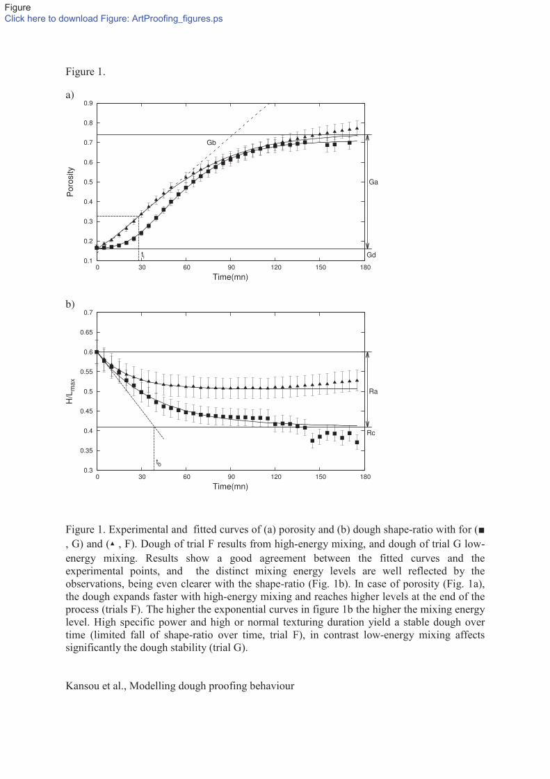
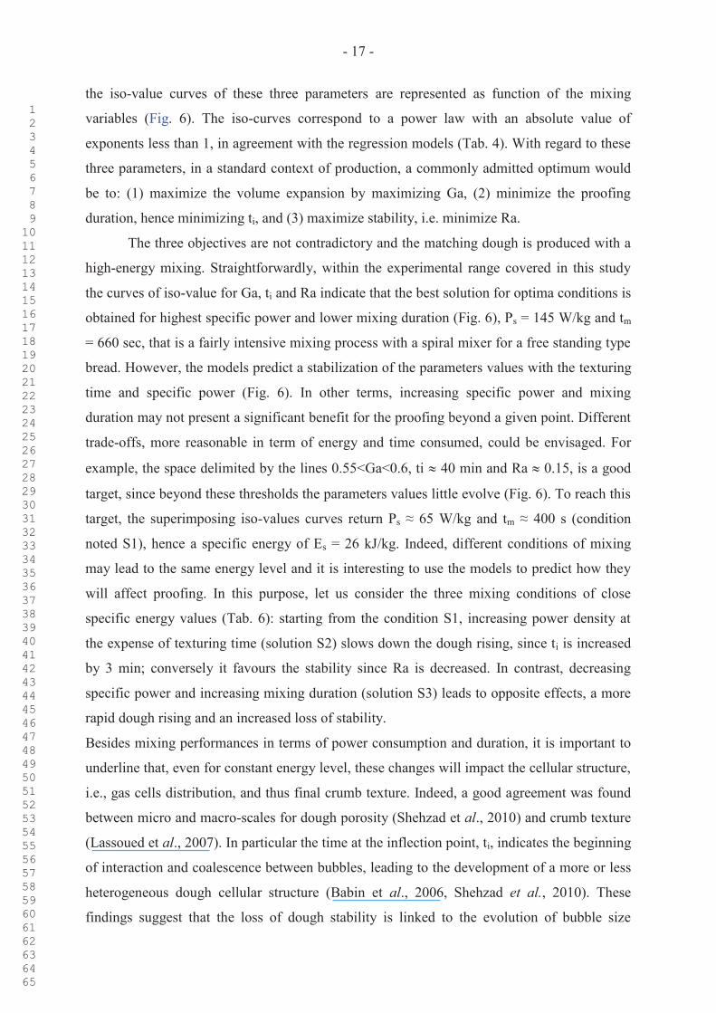
Figure 1.

0.1

0.2

0.3

0.4

0.5

0.6

0.7

0.8

0.9

0 30 60 90 120 150 180

Poro

sity

Time(mn)

a)

Gb

Ga

ti Gd

0.3

0.35

0.4

0.45

0.5

0.55

0.6

0.65

0.7

0 30 60 90 120 150 180

H/L

ma

x

Time(mn)

b)

Ra

tb

Rc

Figure 1. Experimental and fitted curves of (a) porosity and (b) dough shape-ratio with for (�

, G) and ( , F). Dough of trial F results from high-energy mixing, and dough of trial G low-

energy mixing. Results show a good agreement between the fitted curves and the

experimental points, and the distinct mixing energy levels are well reflected by the

observations, being even clearer with the shape-ratio (Fig. 1b). In case of porosity (Fig. 1a),

the dough expands faster with high-energy mixing and reaches higher levels at the end of the

process (trials F). The higher the exponential curves in figure 1b the higher the mixing energy

level. High specific power and high or normal texturing duration yield a stable dough over

time (limited fall of shape-ratio over time, trial F), in contrast low-energy mixing affects

significantly the dough stability (trial G).

Kansou et al., Modelling dough proofing behaviour

Figure 2.

0

100

200

300

400

500

600

700

0 20 40 60 80 100 120 140 160

Te

xtu

rin

g tim

e (

s)

Specific Power (W/kg)

Group_7 10<Es<13

Group_4b Es=27

Group_2 53<Es<61

Group_4a 30<Es<38.4

Group_6 8<Es<11

Group_5 7.5<Es<25.5

Group_3 50<Es<63

Group_1 74<Es<84

AB* C*

D*

L

E

F*

G* H*

I*

K J

M

N*

O

P

QR*

S T

U

VW* X

Figure 2. Scatter plot displaying the distribution of the 24 trials according to the mixing

variables, specific power and texturing duration. The trials selected for modelling are

indicated by the symbol (*). The points are encapsulated into boxes whose dimensions

represent the experimental error on specific power and texturing time. The results enable to

form 8 groups, for which the interval of specific energy level (Es) is indicated. Groups are

ordered so to reflect, first, the energy levels, then the power density and finally the mixing

duration. The group 1 is the group of trials with the high energy, high power density and high

mixing duration, trials of group 2 have high energy but normal mixing duration, trials of

group 3 have high energy but normal power density and so on up to the group 7 with low

energy level, low specific power and short mixing duration. The central group is the group 4a

with standard mixing conditions; the group 4b has the same energy level but combines higher

power density and shorter mixing duration.

Kansou et al., Modelling dough proofing behaviour

Figure 3.

0

0.05

0.1

0.15

0.2

0.25

0.3

0 10 20 30 40 50 60 70 80

Ra

Es (kJ/kg)

R2 = 0.83

20

30

40

50

0 10 20 30 40 50 60 70 80

ts

Es (kJ/kg)

R2 = 0.86

0.4

0.5

0.6

0.7

0.8

0 10 20 30 40 50 60 70 80

Ga

Es (kJ/kg)

R2 = 0.83

20

30

40

50

0 10 20 30 40 50 60 70 80

ti

Es (kJ/kg)

R2 = 0.67

0.005

0.006

0.007

0.008

0.009

0 10 20 30 40 50 60 70 80

Gb

Es (kJ/kg)

R2 = 0.36

0

0.05

0.1

0.15

0.2

0.25

0.3

0 10 20 30 40 50 60 70 80

Gd

Es (kJ/kg)

R2 = 0.45

Figure 3. Grid of graphs of the parameters of the Gompertz and Exponential models, Ra, ts,

Ga, Gb, ti, Gd determined via curve-fitting over the specific energy, Es, and fitted power-type

curves (a*xb). The standard deviations are provided in Tables 2 but error bars are not drawn

because they would represent the fitting performance which would be misleading here. Good

correlations between the parameters Ra, ts, Ga, ti and the mixing energy level emphasize the

relevance of the power regression model (Eq. 3) to relate the proofing parameters with the

mixing variables.

Kansou et al., Modelling dough proofing behaviour

Figure 4.

0

0.1

0.2

0.3

0.4

0.5

0.6

0.7

0.8

0.9

0 30 60 90 120 150 180

A A_Mod

0

0.1

0.2

0.3

0.4

0.5

0.6

0.7

0.8

0.9

0 30 60 90 120 150 180

E E_Mod

0

0.1

0.2

0.3

0.4

0.5

0.6

0.7

0.8

0.9

0 30 60 90 120 150 180

J J_Mod

0

0.1

0.2

0.3

0.4

0.5

0.6

0.7

0.8

0.9

0 30 60 90 120 150 180

K K_Mod

0

0.1

0.2

0.3

0.4

0.5

0.6

0.7

0.8

0.9

0 30 60 90 120 150 180

L L_Mod

0

0.1

0.2

0.3

0.4

0.5

0.6

0.7

0.8

0.9

0 30 60 90 120 150 180

M M_Mod

0

0.1

0.2

0.3

0.4

0.5

0.6

0.7

0.8

0.9

0 30 60 90 120 150 180

O O_Mod

0

0.1

0.2

0.3

0.4

0.5

0.6

0.7

0.8

0.9

0 30 60 90 120 150 180

P P_Mod

0

0.1

0.2

0.3

0.4

0.5

0.6

0.7

0.8

0.9

0 30 60 90 120 150 180

Q Q_Mod

0

0.1

0.2

0.3

0.4

0.5

0.6

0.7

0.8

0.9

0 30 60 90 120 150 180

S S_Mod

0

0.1

0.2

0.3

0.4

0.5

0.6

0.7

0.8

0.9

0 30 60 90 120 150 180

T T_Mod

0

0.1

0.2

0.3

0.4

0.5

0.6

0.7

0.8

0.9

0 30 60 90 120 150 180

U U_Mod

0

0.1

0.2

0.3

0.4

0.5

0.6

0.7

0.8

0.9

0 30 60 90 120 150 180

V V_Mod

0

0.1

0.2

0.3

0.4

0.5

0.6

0.7

0.8

0.9

0 30 60 90 120 150 180

Po

rosity

Time(mn)

X X_Mod

Figure 4. Porosity simulated kinetics against experimental data for the 14 trials used for

model validation. Experimental data are framed by dashed curves depicting the overall

standard deviation. The simulations apply only on the first 140 minutes, a time value larger

than the practical one. Results are good especially for average and high-energy mixing

process (A, M, P, Q, T, V, X). Model performances for mixing of lower energy levels are less

consistent, since the kinetic of U is well predicted while S is not.

Kansou et al., Modelling dough proofing behaviour

Figure 5.

0.3

0.4

0.5

0.6

0 30 60 90 120 150 180

A A_Mod

0.3

0.4

0.5

0.6

0 30 60 90 120 150 180

E E_Mod

0.3

0.4

0.5

0.6

0 30 60 90 120 150 180

J J_Mod

0.3

0.4

0.5

0.6

0 30 60 90 120 150 180

K K_Mod

0.3

0.4

0.5

0.6

0 30 60 90 120 150 180

L L_Mod

0.3

0.4

0.5

0.6

0 30 60 90 120 150 180

M M_Mod

0.3

0.4

0.5

0.6

0 30 60 90 120 150 180

O O_Mod

0.3

0.4

0.5

0.6

0 30 60 90 120 150 180

P P_Mod

0.3

0.4

0.5

0.6

0 30 60 90 120 150 180

Q Q_Mod

0.3

0.4

0.5

0.6

0 30 60 90 120 150 180

S S_Mod

0.3

0.4

0.5

0.6

0 30 60 90 120 150 180

T T_Mod

0.3

0.4

0.5

0.6

0 30 60 90 120 150 180

U U_Mod

0.3

0.4

0.5

0.6

0 30 60 90 120 150 180

V V_Mod

0.3

0.4

0.5

0.6

0 30 60 90 120 150 180

H/L

max

Time(mn)

X X_Mod

Figure 5. Shape-ratio simulated kinetics against experimental data for 14 trials used for model

validation. Experimental data are framed by dashed curves depicting the overall standard

deviation. Simulations apply on the first 90 minutes, as beyond the 100 minute irregular

evolution of the dough may be observed, e.g. trial A, as well as partial recovery of the dough

stability, e.g. trial M. The model performs well, in particular the simulations of S, V, X and Q

are striking as the kinetics were obtained for dough mixed under extreme conditions. On the

other hand discrepancy is encountered for L, T, and E kinetics.

Kansou et al., Modelling dough proofing behaviour

Figure 6.

(a) (c)

(b)

Figure 6. Iso-value curves for parameters Ga and ti of the Gompertz model and Ra of the

Exponential model, computed from the specific power Ps and the texturing duration tm. Ga

represents the maximum volume expansion of the dough during proofing, ti the time value at

the inflection point and Ra the loss of stability. The iso-value curves represent power

functions defined by the models (Eq. 3, 4, 5). The influence of the specific power prevails

over the texturing duration for Ra, whereas it is rather the opposite trend for ti, and the

influences are more balanced for Ga.

Kansou et al., Modelling dough proofing behaviour

Value surface for Ga parameter

Ga iso-value 0.6 0.55 0.5 0.45 0.4

5 25 45 65 85 105 125 145

Specific Power (W/kg)

60

120

180

240

300

360

420

480

540

600

660

Textu

ring t

ime (

s)

0.35 0.4 0.45 0.5 0.55 0.6 0.65

Value surface for ti parameter

ti iso-value 100 90 80 70 60 50 40

5 25 45 65 85 105 125 145

Specific Power (W/kg)

60

120

180

240

300

360

420

480

540

600

660

Textu

ring t

ime (

s)

30 40 50 60 70 80 90 100 110

Value surface for Ra parameter

Ra iso-value 0.55 0.5 0.45 0.4 0.35 0.3 0.25 0.2 0.15

5 25 45 65 85 105 125 145

Specific Power (W/kg)

60

120

180

240

300

360

420

480

540

600

660

Textu

ring t

ime (

s)

0.1 0.15 0.2 0.25 0.3 0.35 0.4 0.45 0.5 0.55 0.6

- 1 -

Table 1. Conditions of the mixing process for the 24 trials of the dataset

Units Total

Mass Speed tm

a Tfp

b SD

f Td

c SD Ps

d SD Es

e SD

Sample kg rpm (sec) °C °C °C °C W/kg W/kg kJ/kg kJ/kg

A 3 200 420 15.5 0.49 23 0.47 71 3.55 30 1.50

B 3 80 420 16.4 0.52 17.9 0.36 26 1.30 11 0.55

C 3 320 420 14.4 0.46 28.6 0.58 148 7.40 60.9 3.05

D 3 200 660 15.2 0.48 27.9 0.56 79 3.95 51 2.55

E 3 200 180 14.8 0.47 19 0.38 72 3.60 13 0.65

F 3 284 590 14.6 0.46 31.7 0.64 127 6.35 74.02 3.70

G 3 116 250 14.1 0.45 19.2 0.39 40 2.00 10 0.50

H 3 284 250 14.8 0.47 23 0.47 108 5.40 27 1.35

I 5 116 590 14.8 0.47 21.5 0.44 37 1.85 20 1.00

J 5 140 600 14.1 0.45 20.3 0.41 35 1.75 21.3 1.07

K 3 140 600 21.9 0.69 26.3 0.53 35 1.75 21 1.05

L 3 200 660 16.1 0.51 29.4 0.60 77 3.85 51.4 2.57

M 3 284 450 9.5 0.30 21.9 0.44 115 5.75 53.4 2.67

N 3 200 500 14.4 0.46 24.1 0.49 78 3.90 38.4 1.92

O 5 140 600 19 0.60 25 0.51 68 3.40 25.1 1.26

P 3 200 660 11.3 0.36 25 0.51 82 4.10 57 2.85

Q 10.5 320 610 16.5 0.52 33 0.67 103 5.15 62.7 3.14

R 10.5 80 610 16.5 0.52 19 0.38 13 0.65 7.8 0.39

S 3 80 450 10.4 0.33 13.5 0.27 18 0.90 8 0.40

T 3 320 450 10.8 0.34 26.3 0.53 126 6.30 56.9 2.85

U 3 80 610 20.6 0.65 22.6 0.46 22 1.10 13.7 0.69

V 3 320 610 20.8 0.66 35 0.71 134 6.70 81.5 4.08

W 3 80 610 20.8 0.66 23.2 0.47 20 1.00 12.3 0.62

X 3 320 610 22.1 0.70 36.2 0.73 137 6.85 83.5 4.18

atm. texturing time

bTfp. Temperature of the dough at end of pre-mixing stage

cTd. Temperature of the dough at end of mixing

dPs. Specific power during texturing stage

eEs. Specific mechanical energy supplied during texturing stage

fSD. Standard deviation, values are computed from the mean relative standard deviation of

each measure over the 24 trials.

- 2 -

Table 2. Fitted values of the parameters for (a) the Gompertz model (Eq. 1) and (b) the

Exponential model (Eq. 2)

(a)

Gompertz model

Groupa Trials Ga Gb ti (mn) Gd SSE R²

1 F 0.669 (0.030) b 0.007 (1.12E-4) 28.41 (2.39) 0.080 (0.024) 1.34E-3 0.999

2 C 0.590 (0.015) 0.007 (1.45E-4) 38.27 (1.16) 0.175 (0.011) 1.74E-3 0.998

3 D 0.631 (0.027) 0.006 (1.17E-4) 31.35 (2.17) 0.126 (0.021) 1.57E-3 0.998

4a N 0.602 (0.014) 0.007 (1.27E-4) 37.75 (1.02) 0.167 (0.010) 1.33E-3 0.999

4b H 0.593 (0.007) 0.007 (1.28E-4) 38.16 (0.95) 0.155 (0.009) 1.30E-3 0.999

5 I 0.582 (0.016) 0.006 (1.38E-4) 40.14 (1.20) 0.181 (0.011) 1.68E-3 0.998

5 W 0.520 (0.017) 0.008 (3.55E-4) 36.50 (1.42) 0.168 (0.013) 6.00E-3 0.994

5 R 0.507 (0.008) 0.007 (1.67E-4) 45.28 (0.65) 0.199 (0.005) 1.49E-3 0.998

6 B 0.548 (0.009) 0.007 (1.22E-4) 47.57 (0.67) 0.182 (0.005) 1.09E-3 0.999

7 G 0.549 (0.008) 0.008 (1.12E-4) 46.12 (0.41) 0.162 (0.003) 6.9E-4 0.999

Arithmetic mean 0.58 0.007 38.96 0.16

(b)

Exponential model

Groupa Trials Ra ts (mn) SSE R²

1 F 0.094 (4.68E-4)b 22.06 (0.36) 0.1E-4 0.999

2 C 0.078 (4.56E-4) 22.95 (0.43) 0.1E-4 0.996

3 D 0.127 (6.72E-4) 24.86 (0.40) 0.2E-4 0.999

4a N 0.150 (1.55E-3) 31.49 (0.84) 0.7E-4 0.998

4b H 0.138 (1.18E-3) 27.70 (0.66) 0.5E-4 0.998

5 I 0.181 (1.51E-3) 30.44 (0.67) 0.7E-4 0.999

5 W 0.176 (3.20E-3) 34.05 (1.51) 2.3E-4 0.995

5 R 0.220 (8.50E-3) 49.86 (3.68) 4.8E-4 0.992

6 B 0.167 (6.35E-3) 38.06 (3.28) 6.5E-4 0.985

7 G 0.189 (4.87E-3) 38.46 (2.23) 3.7E-4 0.993

Arithmetic mean 0.15 31.99 a this column refers to the group represented in Figure 2

b in brackets the standard error

- 3 -

Table 3. Correlationsa between the parameters of the fitted curves and the mixing variables

Ga Gb ti Gd Ra ts

Ps 0,83*** -0,41ns

-0,47ns

-0,66** -0,88*** -0,87***

tm -0,02ns

-0,26ns

-0,49ns

0,043ns

0,07ns

-0,06ns

Es 0,88*** -0,58* -0,75** -0,62* -0,93*** -0,96***

*** 99% significant level, ** 95% significant level, * 90% significant level, ns

non significant a Spearman-rank correlation coefficient

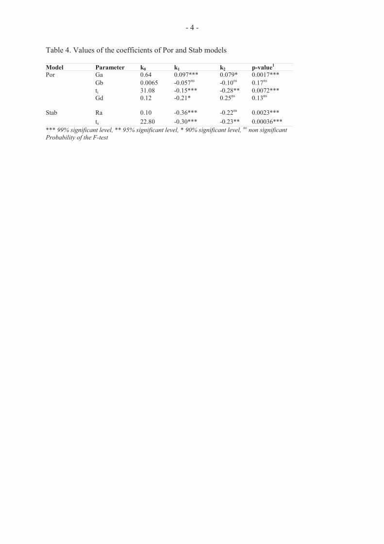
- 4 -

Table 4. Values of the coefficients of Por and Stab models

Model Parameter k0 k1 k2 p-value

1

Por Ga 0.64 0.097*** 0.079* 0.0017***

Gb 0.0065 -0.057ns

-0.10ns

0.17ns

ti 31.08 -0.15*** -0.28** 0.0072***

Gd 0.12 -0.21* 0.25ns

0.13ns

Stab Ra 0.10 -0.36*** -0.22ns

0.0023***

ts 22.80 -0.30*** -0.23** 0.00036***

*** 99% significant level, ** 95% significant level, * 90% significant level, ns

non significant

Probability of the F-test

- 5 -

Tables 5. Assessment of the performances of Por and Stab, compared to the controls, CPor

and CStab, for (a) the 10 trials used for modelling and (b) the 14 other trials. Boldface number

means the best performance among the model and the control.

(a)

Group Trials Por CPor Stab CStab

RMSE MAPE RMSE MAPE RMSE MAPE RMSE MAPE 1 F 0.095 3.572 0.091 2.708 0.004 0.637 0.034 5.703

2 C 0.013 2.665 0.024 5.281 0.018 3.205 0.047 7.943

3 D 0.008 1.650 0.021 4.485 0.009 1.720 0.011 1.802

4a N 0.021 3.759 0.025 5.088 0.015 2.625 0.002 0.381

4b H 0.015 3.073 0.010 1.574 0.010 1.795 0.006 0.883

5 I 0.021 4.563 0.017 3.823 0.019 3.856 0.023 4.618

5 W 0.020 3.521 0.022 2.613 0.006 0.986 0.015 2.847

5 R 0.009 1.473 0.023 5.027 0.013 2.473 0.023 4.327

6 B 0.018 3.483 0.032 6.969 0.015 2.809 0.007 1.224

7 G 0.018 5.543 0.039 10.492 0.006 1.098 0.018 3.300

(b)

Group Trials Por CPor Stab CStab

RMSE MAPE RMSE MAPE RMSE MAPE RMSE MAPE 1 X 0.016 2.512 0.033 5.908 0.013 2.367 0.039 6.623

1 V 0.044 8.067 0.060 11.297 0.003 0.561 0.023 3.783

2 M 0.016 3.440 0.015 2.819 0.002 0.251 0.018 3.161

2 T 0.018 3.699 0.023 5.232 0.025 4.474 0.005 0.974

3 Q 0.017 3.115 0.028 5.013 0.007 1.168 0.025 4.329

3 P 0.028 4.787 0.035 6.902 0.007 1.393 0.009 1.412

3 L 0.054 9.899 0.061 11.428 0.028 4.684 0.040 6.744

4a A 0.015 3.609 0.013 3.015 0.022 3.513 0.025 4.107

5 O 0.063 11.500 0.058 10.632 0.008 1.255 0.003 0.550

5 J 0.033 7.491 0.038 8.580 0.011 1.947 0.018 3.592

5 K 0.048 8.372 0.040 7.044 0.009 1.562 0.016 3.075

5 U 0.011 1.764 0.020 4.051 0.013 2.449 0.013 2.498

6 S 0.063 20.063 0.084 24.567 0.008 1.173 0.037 6.769

7 E 0.042 7.415 0.019 3.643 0.030 6.073 0.039 7.857

- 6 -

Table 6. Three mixing conditions with comparable specific energy levels and parameters of

the dough expansion during proofing

Mixing

conditions Ps (W/kg) tm (s) Es (kJ/kg) Ga ti (mn) Ra

S1 65 400 26.00 0.57 40.4 0.15

S2 110 240 26.40 0.57 43.1 0.14

S3 42 620 26.04 0.56 38.2 0.16