Modelling of high quality pasta drying: mathematical model and validation

www.elsevier.com/locate/jfoodeng

Journal of Food Engineering 69 (2005) 387–397

Modelling of high quality pasta drying: mathematicalmodel and validation

Massimo Migliori a, Domenico Gabriele a, Bruno de Cindio a,*, Claudio M. Pollini b

a Laboratory of Rheology, Department of Chemical Engineering and Materials, University of Calabria, Via P. Bucci Cubo 44/a,

I-87030 Arcavacata di Rende (CS), Italyb Pavan S.p.A., via Monte Grappa 8, I-35015 Galliera Veneta (PD), Italy

Received 10 November 2003; accepted 13 August 2004

Available online 18 October 2004

Abstract

The pasta drying process was studied using an engineering approach. The phenomena of mass and heat exchange between pasta

samples and air was modelled according to the classic transport approach applied to a hollow cylindrical shape pasta. Data from the

literature and from measurements were used to fix the material parameter values of both the air and dough phases. Theoretical cor-

relations were used to obtain a good estimate of mass and heat exchange coefficients between dough samples and air. The proposed

model was set by choosing the mass transfer coefficient as the unique optimisation parameter, determined by best fitting of the

experimental water content data obtained under given conditions in a static dryer. The model was then validated at different tem-

perature and air humidity drying profiles and a good agreement with the experimental results was found. Finally the model was

applied to different process conditions and the drying time was calculated from the simulations.

� 2004 Elsevier Ltd. All rights reserved.

Keywords: Drying; Food processing; Heat transfer; Mass transfer; Modelling; Pasta production

1. Introduction

In the last 10 years, owing to an increased market de-

mand for dry pasta in many countries, the requirements

of both product quality and production rate have in-

creased too. These two aspects are very often considered

in contrast each to the other because it is thought that

high production rates, characterized by somehow severeprocess conditions, induce thermal and mechanical

damages into the products. These aspects may strongly

decrease pasta quality as evidenced by nutrient loss,

bad colour, poor texture, marked consistency loss when

0260-8774/$ - see front matter � 2004 Elsevier Ltd. All rights reserved.

doi:10.1016/j.jfoodeng.2004.08.033

* Corresponding author. Tel.: +39 984 496708/496687; fax: +39 984

496655.

E-mail addresses: [email protected] (M. Migliori), d.gabriele@

unical.it (D. Gabriele), [email protected] (B. de Cindio),

[email protected] (C.M. Pollini).

overcooking, etc. Of course only a careful control of the

process conditions coupled to a deep knowledge of the

material properties, may avoid those undesired effects,

while still maintaining high production rates. Neverthe-

less, the production process is currently carried out in a

rather empirical way, because it is still based on the

practical knowledge of pasta-makers, instead of stand-

ing on very well consolidated process engineering basis.In fact, the choice of raw materials and process condi-

tions is made by following ‘‘rules of thumb’’ that do

not allow any control on the product quality, and they

do not match high production rates.

Starting from this point, it clearly appears that an

engineering approach has to be developed establishing

the influence of the main process variables on the final

product quality, in order to apply an effective produc-tion control. This objective may be achieved by making

a global model capable of simulating what happens

mailto:[email protected]

mailto:d.gabriele@



Nomenclature

aw water activity coefficient, –

b gradient pulse of strength in NMRmeasurements

C heat capacity, Jkg�1K�1

Cp specific heat, Jkg�1K�1

D water diffusivity, m2s�1

Ea activation energy, kJgmol�1

F echo attenuation in NMR measurements

h global heat exchange coefficient, Jm�2K�1

I signal intensity in NMR measurementsJh Colburn factor for heat transfer, –

Jm Colburn factor for mass transfer, –

k thermal conductivity, Wm�1K�1

kx global mass exchange coefficient, kgm�2 s�1

L pasta sample length, m

M molecular weight, dalton

N mass flux, kgm�2 s�1

P pressure, Pap� vapour pressure, Pa

q thermal flux, Wm�2K�1

R sample radius, m

r variable radius, m

Rg universal gas constant, Jgmol�1K�1

SQM square quadratic deviation, %

T1 air temperature in bulk phase, K

T temperature, Kt time, s

U dough water content on wet basis, w/w

UR1 relative water content of air in bulk phase,

w/w%

v1 air velocity, ms�1

x dough water content on dry basis, –

y molar fraction in air, –

yw,1 water molar fraction in air in bulkphase, –

Dimensionless numbers

Nu NusseltPr Prandtl

Re Reynolds

Sc Schimdt

Sh Sherwood

Greek symbols

D space variation

a shrinkage coefficient, –d pasta sample thickness, mm

b theoretical and optimised mass exchange

coefficient ratio, –

k water latent heat of vaporization, Jkg�1

q dough density, kgm�3

r time between 90� and 180� rf in NMR

measurements

w duration of the gradient pulse in NMRmeasurements

f magnetogyric ratio in NMR measurements

Subscripts

0 initial condition

a air

d dough

exp experimental valuef film condition

i generic point of calculation grid

sim simulation value

w water

Superscripts

eq equilibrium conditions

ext referred to external surfaceint referred to internal surface

388 M. Migliori et al. / Journal of Food Engineering 69 (2005) 387–397

during the process and therefore to predict ‘‘a priori’’

the values of the desired properties.

In this work attention was focused on the study and

modelling of the pasta drying process, because duringthis step pasta is subjected to rather severe conditions

that are fully responsible for the final product quality.

In fact, drying is usually realised by using wet hot air

with temperatures ranging between 80 and 120 �C, anda controlled relative humidity UR ranging between

40% and 70%. The actual industrial trend is to get

rather high production rates over 3–4000kg/h, that are

obtained by reducing the drying time by means of aprocess characterised by high temperature and low

moisture drying air, this choice in turn reduces the

microbiological risk because of the strong heat treat-

ment. Moreover, according to the market request for

high quality production, these severe process conditions

may cause a so-called ‘‘thermal damage’’ that is evi-

denced by a poor texture, a decrease in the mechanical

resistance, a lower nutrient content, a darker colour,etc. This kind of product obviously does not fit with

consumer expectations, even if safer from a microbio-

logical point of view, owing to the poorness of most

of the quality indices.

Dried pasta production process can be represented

schematically as a rather simple chain of unit operations

(see Fig. 1). Ingredients, basically water and durum

wheat flour, are usually mixed together under vacuumto give a dough with a water content percentage close

to 30% (wet basis). Then the resulting dough is sent into

an extruder press and finally extruded through a head in

order to obtain the desired pasta shape.

INGREDIENTS

MIXINGFORMING

(

DRYINGPACKAGING

(Sheeting, extrusion)

Fig. 1. Pasta production process flow sheet.

z

r

Rext

Rint

Rext

Rint

Fig. 2. Geometrical scheme of pasta sample.

M. Migliori et al. / Journal of Food Engineering 69 (2005) 387–397 389

The drying process is afterward carried out by

exploiting the humidity and temperature difference be-tween samples and air, causing the water content to de-

crease inside the sample. Thus the applied external

drying air temperature and humidity must be related

to the pasta properties as a function of time, to deter-

mine the optimal process conditions according to any gi-

ven pasta quality criterion. Therefore the aim of the

present work is to make available a predictive model

that gives the water loss occurring inside the pasta asresulting from the applied external conditions during

drying, allowing one to know ‘‘a priori’’ the resulting

transient water content profile inside the pasta. It should

be noted that drying of pasta requires several hours,

therefore any predictive model capable of predicting

transient water content is welcome, allowing a strong

reduction of expensive trials needed to find the best

operational conditions.

AIR

Temperature

Humidity

SAMPLE

RU

eqT

T

w,eqyw,y extw,∞

∞

Fig. 3. Air–dough interface scheme.

2. Mathematical modelling

The drying process of ‘‘short pasta’’ was modelled

using hollow cylindrical shaped pasta that was simplified

as a cylindrical shell with an infinite length. Because of

the small value of the ratio d/L, border effects can be ne-glected. In addition, the external surface of the sample

was supposed to be surrounded by hot moist air with

controlled properties (i.e., temperature T1 and relative

humidity UR1). Owing to the considered geometrical

shape, an azimuthal symmetry holds, and therefore only

r-direction variations were considered (Fig. 2). Conse-

quently, the heat transfer balance equations is written

as (Bird, Stewart, & Lightfoot, 1960):

qd � Cd �oTot

¼ 1

r� oor

r � kd �oTor

� �ð1Þ

where the thermal conductivity (kd) and heat capacity

(Cd) are assumed to be both temperature and water con-

tent dependent. The dough density (qd) has been as-

sumed as a constant because in a previous work (de

Cindio, Brancato, & Saggese, 1992) it was shown that

qd does not reasonably depend on temperature and, in

addition, even a weak dependence on water content

was observed. According to that the following final form

may be obtained for the mass-transfer equation if Fick�sdiffusion law is used to describe the water transport in-

side the dough:

oUot

¼ 1

r� oor

r � Dd �oUor

� �ð2Þ

In Eq. (2) U is the water content inside the dough ex-pressed on a wet basis (w.b.), i.e., the ratio of water

weight and total weight, and water diffusivity (Dd) de-

pends on temperature and water content. Moreover,

the general statement of assuming all the material

parameters as a function of T and U, leads to a system

of linked differential equations that was solved accord-

ing to well-determined boundary conditions for both

external and internal surfaces.

2.1. Boundary conditions

The solution of the differential equation system (Eqs.

(1) and (2)) needs two boundary conditions and one ini-

tial condition both for mass and energy transports. The

main hypothesis is the thermodynamic equilibrium con-

dition at the air–dough interface (Fig. 3) that, in turn, is


also assumed to coincide with the evaporation front.

This implies that the air and dough interface chemical

potentials must be equal. By writing this latter in terms

of water-activity it follows:

Pyeqw ¼ p�waw ð3Þ

where P is the pressure of the system, yeqw the water

molar fraction in air at equilibrium conditions, p�w the

vapour pressure and aw the water activity. In Eq. (3)

the vapour phase is assumed to behave as an ideal gas

solution, while the liquid phase is considered as a real

mixture, deviating from the Raoult solution chosen as

the reference state. Then the value of aw may be ex-

pressed by any constitutive equation relating wateractivity to the dough water content U.

The mass boundary condition stands on the continu-

ity of the mass flux at the air–dough interfaces, that at

the external surface reads:

�qdDd

oUor

��Rext

¼ N extw ¼ kextx Mwðyw;1 � ywjRextÞ ð4Þ

where the water mass flux N extw on the air side has been

written in terms of a global transport coefficient kextx ,

whilst the mass transfer mechanism inside the dough

has been assumed to be diffusive. In Eq. (4), Mw stands

for water molecular weight and y1 and yjRext for water

molar fraction of the drying air bulk and the air–dough

interface respectively. Of course, according to the as-

sumed equilibrium conditions at the interface, it followsthat:

yeqw ¼ ywjRext ð5ÞConcerning the heat transfer at the external interface,

owing to the equilibrium assumption at the interface

air–dough, the surface temperature corresponds to the

equilibrium temperature Teq

T eq ¼ T jRext ð6ÞAt the air–dough interface the continuity of heat flux

holds and may be written as:

kN extw � kd

oTor

��Rext

¼ qexta ¼ hext � ðT1 � T jRextÞ ð7Þ

where k is the water molar latent heat of evaporation.

The air-side thermal flux qexta has been written using a

global exchange coefficient hext, and the flux inside the

dough at the interface is expressed as the sum of two

terms: the first one is due to water evaporation while

the second one to the heat conduction.It should be noticed that during simultaneous mass

and heat transport, when it is possible to assume that

water diffusion inside the dough is fast enough to trans-

port a sufficient amount of water to the evaporating sur-

face, the system behaves like a wet bulb thermometer

(Bird et al., 1960). This means that the heat supplied

by the drying air is just equal to the heat absorbed as

a consequence of the evaporation. Thus in this case

Eq. (7) becomes:

qexta ¼ kN extw ð8Þ

This phenomenon leads to a constant temperature value

determined as a function of the equilibrium condition

expressed by Eq. (3) and known as the ‘‘wet bulb temper-

ature’’. It should be noticed that temperature does not

rise until this condition holds, i.e., until the amount of

water transported to the evaporating surface is capable

of compensating the drying air heat supply. Drying fur-

ther, the evaporation becomes insufficient and thereforethe surface temperature starts to rise, and consequently

a temperature gradient is found inside the dough.

The use of the global exchange coefficient hext and kextx

both for heat and mass transport at the external surface,

allows the fluxes to be related directly to the temperature

and the water molar fraction difference between air and

sample (Bird et al., 1960). By taking into account the

equilibrium, according to Eqs. (5) and (6), the twoboundary conditions expressed by Eqs. (4) and (7)

may be combined to obtain the following expression at

the external surface:

hext � ðT1 � T eqÞ ¼ k � kextx �Mw � ðyw;1 � yeqw Þ þ kdoTor

��Rext

ð9Þ

The second boundary condition for both heat and mass

transport must be referred to the internal surface. It

should be noticed that the transport phenomena occur-

ring in the hollow of the cylinder is rather difficult to

model because the air velocity is very low, and therefore

the classic transfer coefficients should not apply. Themass transfer mechanism was divided into two steps: a

radial-axial diffusion of water from the internal surface

up to the sample edge, and the water removal by the

air stream that grazes the sample. If the diffusive step

prevails, the exchange mechanism may be modelled as

the pure diffusive transport in a stagnant fluid (Bird

et al., 1960), and the corresponding expressions for both

heat and mass transfer may be applied. The use of thisrigorous approach is rather complex, whereas the contri-

bution to the total water removal is rather small; there-

fore, for the sake of simplicity, the transport steps have

been grouped using again an overall exchange coefficient

analogous to that introduced by Eq. (4). For the calcu-

lation of kintx and hint the same method used for the exter-

nal transport was applied but the air velocity was simply

assumed to be three orders of magnitude less than theexternal velocity. In this way, the evidence that the inter-

nal surface was not directly exposed to the air flux was

approximately taken into account.

The initial conditions assume constant uniform val-

ues of both temperature (T0) and water content (U0)

throughout the sample.

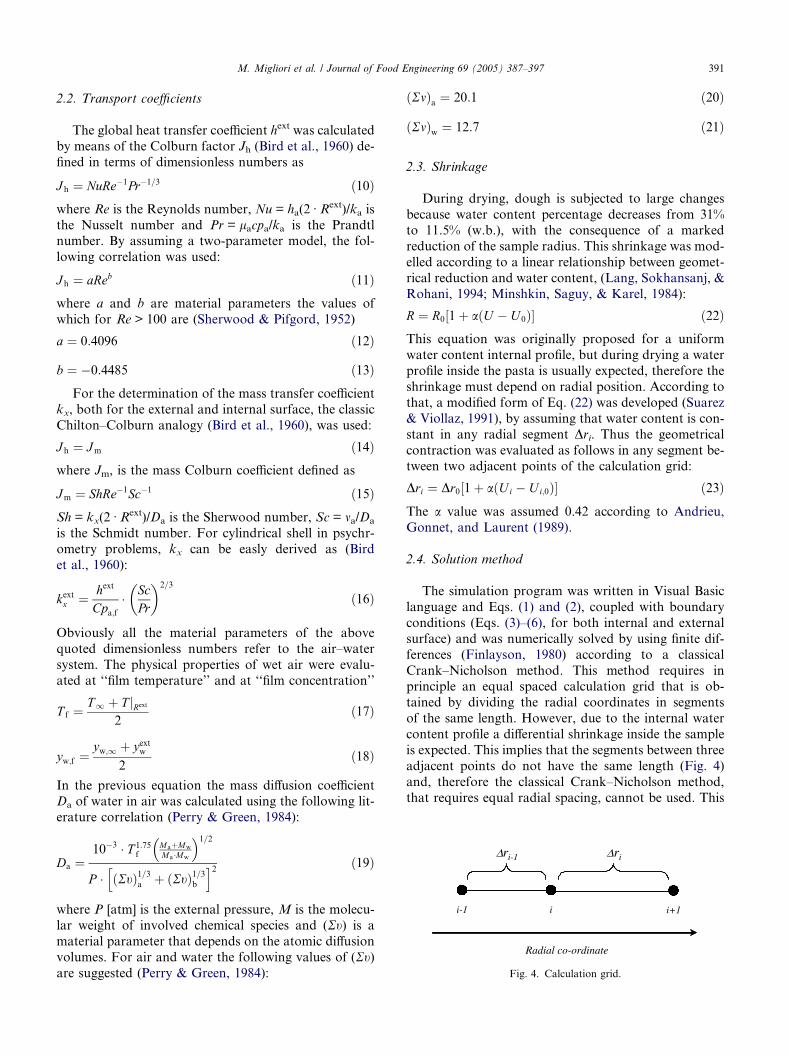
i-1 i i+1

ri-1 ri

Radial co-ordinate

∆ ∆

Fig. 4. Calculation grid.


2.2. Transport coefficients

The global heat transfer coefficient hext was calculated

by means of the Colburn factor Jh (Bird et al., 1960) de-

fined in terms of dimensionless numbers as

Jh ¼ NuRe�1Pr�1=3 ð10Þwhere Re is the Reynolds number, Nu = ha(2 Æ Rext)/ka is

the Nusselt number and Pr = lacpa/ka is the Prandtlnumber. By assuming a two-parameter model, the fol-

lowing correlation was used:

Jh ¼ aReb ð11Þwhere a and b are material parameters the values of

which for Re > 100 are (Sherwood & Pifgord, 1952)

a ¼ 0:4096 ð12Þ

b ¼ �0:4485 ð13ÞFor the determination of the mass transfer coefficient

kx, both for the external and internal surface, the classic

Chilton–Colburn analogy (Bird et al., 1960), was used:

Jh ¼ Jm ð14Þwhere Jm, is the mass Colburn coefficient defined as

Jm ¼ ShRe�1Sc�1 ð15ÞSh = kx(2 Æ Rext)/Da is the Sherwood number, Sc = ma/Da

is the Schmidt number. For cylindrical shell in psychr-

ometry problems, kx can be easly derived as (Bird

et al., 1960):

kextx ¼ hext

Cpa;f� Sc

Pr

� �2=3

ð16Þ

Obviously all the material parameters of the above

quoted dimensionless numbers refer to the air–water

system. The physical properties of wet air were evalu-

ated at ‘‘film temperature’’ and at ‘‘film concentration’’

T f ¼T1 þ T jRext

2ð17Þ

yw;f ¼yw;1 þ yextw

2ð18Þ

In the previous equation the mass diffusion coefficientDa of water in air was calculated using the following lit-

erature correlation (Perry & Green, 1984):

Da ¼10�3 � T 1:75

fMaþMw

Ma�Mw

� �1=2

P � ðRtÞ1=3a þ ðRtÞ1=3b

h i2 ð19Þ

where P [atm] is the external pressure, M is the molecu-

lar weight of involved chemical species and (Rt) is a

material parameter that depends on the atomic diffusion

volumes. For air and water the following values of (Rt)are suggested (Perry & Green, 1984):

ðRmÞa ¼ 20:1 ð20Þ

ðRmÞw ¼ 12:7 ð21Þ

2.3. Shrinkage

During drying, dough is subjected to large changes

because water content percentage decreases from 31%to 11.5% (w.b.), with the consequence of a marked

reduction of the sample radius. This shrinkage was mod-

elled according to a linear relationship between geomet-

rical reduction and water content, (Lang, Sokhansanj, &

Rohani, 1994; Minshkin, Saguy, & Karel, 1984):

R ¼ R0½1þ aðU � U 0Þ� ð22ÞThis equation was originally proposed for a uniform

water content internal profile, but during drying a water

profile inside the pasta is usually expected, therefore the

shrinkage must depend on radial position. According to

that, a modified form of Eq. (22) was developed (Suarez

& Viollaz, 1991), by assuming that water content is con-

stant in any radial segment Dri. Thus the geometrical

contraction was evaluated as follows in any segment be-tween two adjacent points of the calculation grid:

Dri ¼ Dr0½1þ aðUi � Ui;0Þ� ð23ÞThe a value was assumed 0.42 according to Andrieu,

Gonnet, and Laurent (1989).

2.4. Solution method

The simulation program was written in Visual Basic

language and Eqs. (1) and (2), coupled with boundary

conditions (Eqs. (3)–(6), for both internal and external

surface) and was numerically solved by using finite dif-

ferences (Finlayson, 1980) according to a classical

Crank–Nicholson method. This method requires inprinciple an equal spaced calculation grid that is ob-

tained by dividing the radial coordinates in segments

of the same length. However, due to the internal water

content profile a differential shrinkage inside the sample

is expected. This implies that the segments between three

adjacent points do not have the same length (Fig. 4)

and, therefore the classical Crank–Nicholson method,

that requires equal radial spacing, cannot be used. This

X

X

Time

Radiusr=0

X

Initial Thickness

Final Thickness

t=0

t=t1

t=t2

Fig. 5. Schematic representation of radius shrinkage.

Table 1

Parameters for pasta thermal conductivity calculation (Saravacos and

Maroulis, 2001)

ki [Wm�1K�1] 0.8

k0 [Wm�1K�1] 0.273

Ei [kJmol�1] 2.7

Ei [kJmol�1] 0.0


difficulty was overcome by assuming at each grid pointan equal radial interval Dr*, obtained as the arithmetical

average of two adjacent segments as follow:

Dr� ¼ Dri þ Driþ1

2ð24Þ

With this assumption, the Crank–Nicholson methodcan still be applied. For example, the water content first

derivative at any given i-point, may be calculated as:

oUor

��i

¼ Uiþ1 � Ui�1

Dr�ð25Þ

The adopted method leads to a linear equation system

that was solved by means of the classic Thomas�s algo-rithm. In addition, according to the r-grid is time-dependency, the Dri value must be supdated at each time

using Eqs. (17)–(24), by considering either the water

content or temperature profile calculated at the previous

time step. In Fig. 5 a scheme of radius contraction dur-

ing time is reported.

2.5. Simulation software

The solution method of the set of equation has been

implemented in a computer program written in Visual

Basic 6.0 language (Microsoft, USA). The prepared

software allows numerically solving the balance equa-

tion, by means of non-accessible subroutines, whilst

either material parameters or process conditions can

be set by the user. The final simulation results, i.e., tem-

perature and moisture content profiles, are available in aquick plot and may be converted and analysed by a nor-

mal calculation worksheet. In addition some other

important technological parameters linked to the drying

process such as shrinkage value and water activity may

be easily obtained from the main results. The program

has been organised in different frames grouping homol-

ogous properties and process parameters that can be

changed, also using a small database, according to thesimulative needs. This aspect does not have to be under-

rated because the software may be easily run, during

industrial production or research work, also from user

that are not get used to numerical calculation and mod-

elling. Finally, the effort dedicated to make the simula-

tion program friendly represents an important ‘‘follow

up’’ of the present study because the software may be di-

rectly connected to the PLC controllers of the entire

production cycle supplying predictive data to the con-troller with a meaningful reduction of the response time

of the control loop.

3. Materials and methods

3.1. Dough properties

Often it is rather difficult to have a good estimation of

thermal and physical properties of food. In the open lit-

erature several general semi-empirical model have been

proposed (Saravacos & Kostaropoulos, 1996), even

though all the properties are strongly dependent on

the considered food. Particularly concerning the dough

system, a high level of uncertainty on the properties

measurements is generally found, essentially due to botha water loss during measurement and a marked differ-

ence between raw materials. Therefore dough literature

data are often very different each from the other (Rask,

1989). In fact, many correlations have been proposed to

correlate dough thermal conductivity kd to water con-

tent and temperature. In this work the following four

parameters model was used (Saravacos & Maroulis,

2001):

kdðx; T Þ ¼1

1þ xk0 exp �E0

R1

T� 1

TRif

� ��

þ x1þ x

ki exp �Ei

R1

T� 1

TRif

� �� ð26Þ

where x is the dough water content on dry basis, ki, k0,Ei, E0 are dough material parameters (Table 1), T [�C] isthe dough temperature and TRif [�C] is a reference tem-

perature fixed at 60 �C (Saravacos & Maroulis, 2001).

For sake of simplicity, this model was used to obtain

an average value of kd in the range of temperature and

water content used in the process. By considering that

dough temperature ranges between 313 and 353K andthe relative humidity ranges between 30% and 10%

(w.b.), using Eq. (26) the following value of kd was

obtained:

Fig. 6. Scheme of the magnetic field pulse sequence in NMR

determination of water in dough diffusion.


kd ¼ 0:41W

m � K

� �ð27Þ

The dough density was calculated as function of mois-

ture (de Cindio et al., 1992):

qd ¼1

ð3:02 � U þ 6:46Þ � 10�4

kg

m3

� �ð28Þ

The heat capacity Cd was computed as a weighed

average of the heat capacities Ci of the dough main com-

ponents, i.e., water, starch and gluten (Andrieu et al.,

1989):

Cd ¼Xi

Ci � xi ð29Þ

The following values were used for the specific heat of

the single components (de Cindio et al., 1992):Water

Cw ¼ 4:184J

gK

� �ð30Þ

Starch

Cs ¼ 5:737 � T þ 1328J

gK

� �ð31Þ

Gluten

Cg ¼ 6:329 � T þ 1465J

gK

� �ð32Þ

Dough composition was obtained from data in Table 2.

Water diffusivity in dough was measured by the

NMR technique by using a Bruker NMR Spectrometer

(Bruker, USA), modified by Stelar (Milan, Italy) work-ing at a protonant resonance frequency of 80MHz.

The water diffusivity determination was carried out

using PFGSE (Pulsed Field gradient Spin-Echo) 1H-

NMR technique (Coppola, La Mesa, Ranieri, & Tere-

nzi, 1993) with an usual pulse sequence consisting of a

90� radio frequency (rf) pulse at t = 0 followed by a

180� rf pulse at t = r; this results in a spin-echo at

t = 2r. In addition to rf pulses, a pulsed magnetic fieldgradient is inserted on each side of the 180� rf pulse,

causing the attenuation of echo intensities. The parame-

ters associated with the rf and magnetic field gradient

pulse sequence are shown in Fig. 6. Assuming a free

Gaussian diffusion, the theoretical expression of echo

Table 2

Semolina flour composition

Water 14.78%

Protein 13.44%

Ash 0.87%

Wet Gluten 34.97%

Gluten 11.71%

Starch 24.23%

attenuation F is given by the well-known Stejskal–

Tanner equation (Coppola et al., 1993)

F ¼ IðbÞIð0Þ ¼ exp �ðnwbÞ2Dd Q� w

3

� �� ð33Þ

where s is the time between 90� and 180� rf pulses, I(g)and I(0) are the signal intensities at t = 2r in presence of

gradient pulses of strength b and in the absence of any

gradient pulses, respectively, f is the magnetogyric ratio,

w is the duration of the gradient pulses, H is the time be-

tween the leading edges of the gradient pulses (time of

the diffusion) and Dd is the water in dough diffusion.

The 90� rf pulse length was 9ls, H and b were heldconstant to 0.020s and 0.50T/m, respectively.

The length of the gradient field pulse w was changed

in the interval 0.001–0.006s while the gradient strength b

was calibrated using a reference sample of pure tri-

distilled water, with a known self-diffusion coefficient.

During the measurement, the gradient pulses direction

was along the concentration and therefore the water in

dough diffusion was detected.The echo amplitude was measured accumulating 32

scans. The temperature was controlled by airflow regu-

lation with a stability of ±0.2 �C.The results obtained for samples of vacuumed dough

with water content ranging between 33% and 22% (w.b.)

are reported in Table 3. It was not possible to perform

measurements on samples with a water content below

20%, because the signal was difficult to detect eitherfor the low intensity or the fast relaxation time due to

the bond water in the sample. Therefore for moisture

Table 3

Experimental water in dough diffusivity

Dough water content, w/w% Water diffusivity, cm2s�1

33 2.29 · 10�5

30 1.37 · 10�5

27 3.17 · 10�6

24 2.68 · 10�6

22 2.02 · 10�6


content below 22% the following semi-empirical model

was applied (Waananen & Okos, 1996):

Dw ¼ 1:2� 10�7 þ e � 8 � 10�5

P

� �

� exp � 6:6e�20x þ Ea

RgT

� �ð34Þ

where Dd is the water diffusivity in dough [m2s�1], P isthe pressure [kPa], x the water weight fraction on dry

basis (d.b.), i.e., the ratio of water weight and weight

of dry components, T is the temperature [K], Ea the acti-

vation energy, that was found to be equal to

22.6kJgmol�1 (Waananen & Okos, 1996), R gas univer-

sal constant and finally e the pasta porosity, that was as-

sumed as 0.26 (Xiong, Narsimnan, & Okos, 1991). By

combining measurements and correlations, water diffu-sivity Dd was obtained as a moisture multi-step function

as shown in Fig. 7.

The water liquid–vapour equilibrium was modelled

according to the classic Oswin constitutive equation

(Schuchmann, Roy, & Peleg, 1990) that relates the water

activity to water content:

aw ¼xa00

� 1=b001þ x

a00

� 1=b00 ð35Þ

where a00 and b00 are model parameters containing the

temperature dependence. The following values were

used according to Andrieu, Stamatopoulos, and

Zafiropoulos (1985):

a ¼ 0:154–1:22� 10�3 � T ð36Þ

b ¼ 7:8� 10�2–7:32� 10�3 � T ð37Þwhere T is expressed as Kelvin degrees. Because the pro-

posed model is valid when the water activity is higher

than 0.5, it was first checked to ensure that this limit

was not exceeded during drying. The water contentrange of interest is between 30% and 10%, correspond-

ing to aw values varying between 0.96 and 0.81, which

are always within the validity range of Eq. (35).

1

10

100

1000

5 10 15 20 25 30

Dough Humidity [%]

Wat

er d

iffu

sivi

ty [

cm2 s-1

*10

7 ]

35

Fig. 7. Multi-step function of water diffusivity in dough.

3.2. Drying tests

The proposed model was tested experimentally by

carrying out several drying tests under controlled condi-

tions by means of a pilot static dryer (Pavan S.p.A.,

Italy), equipped with devices capable of giving the aver-age temperature and water content of the samples dur-

ing the treatment.

Pasta samples were prepared adding 27.5% (of the

flour weight) of water to an industrial semolina flour

(Jolly Sgambaro Godego, Italy) the composition of

which is reported in Table 2. Samples were prepared

using an integrated machine (Mod. PA1, Pavan S.p.A.,

Italy) consisting of a vacuum mixer, a compressionscrew and a head-cutter apparatus. Ten kilograms of

semolina and 2.75kg of water were mixed for 15min

and the resulting dough was shaped as hollow cylindri-

cal samples, with a radius of 0.5cm, a length of 3.5–

5cm and 1mm thick. By taking into account the water

percentage of the flour, as reported in Table 2, the final

dough had a 0.325 w/w of moisture on a wet basis.

Several samples, about 12kg per run, were loaded inthe static drier (height 2m, width 1.5m, depth 1.5m) laid

down as a single layer on a series of trays. Drying was

obtained by air circulation, and an electronic device con-

trolled its humidity and temperature. During all the tests

the temperature and humidity of the drying hot moist

air was maintained at some fixed constant value. On

the other hand, the air velocity was always the same

by fixing the fan power. A direct measurement was doneduring the tests using an anemometer and a constant va-

lue of 0.5m/s was found for all the runs.

Even though the drier was equipped with a weight

cell to measure continuously the total water loss during

the experiment, to get more accurate sample water con-

tent values, the average water content was obtained

withdrawing five samples from the dryer every 10min

and measuring the weight by means of a thermo-balance(Sartorius, Germany). Every test was performed three

times and the results obtained were statistically analysed

by the ‘‘Few Sample Theory’’ (Kreyszig, 1970).

4. Model setting and validation

To verify the model reliability and check its sensitiv-ity to process parameter changes, the proposed model

was tested at different values of the main process varia-

bles temperature and humidity, following the experi-

mental program reported in Table 4. The results were

then compared to the simulation results coming out

from the mathematical model set with the geometrical

characteristics and initial conditions reported in Table

5. These conditions have been assumed to be constantfor all the simulation performed for this validation

work.

Table 4

Experimental plan for set and validation of the model

Treatment type T1 [K] UR1 [%] v1 [ms�1]

Verify 353 68 0.5

Validation 1 353 58 0.5

Validation 2 343 58 0.5

Table 5

Initial condition and geometrical characteristics in simulation

Length L [mm] 35

External diameter Rext [mm] 9.4

Averaged thickness d [mm] 10

Initial moisture U [%] 30

Initial temperature T0 [K] 303


A first experimental test was done in order to verify

the model validity by applying usual operating condi-tions T1 = 353K and UR1 = 68% as set points and

maintaining an air velocity value fixed to v1 = 0.5ms�1;

this last value has been maintained constant for all the

performed tests. In addition, the simulation results were

based on the physical properties and transport coeffi-

cient previously discussed. The comparison between

experimental and computed average water content pro-

files is shown in Fig. 8. It clearly shows that the trans-port coefficients computed with the proposed

correlations, gave a simulated water content profile that

largely exceeds the experimental one. This difference

may be ascribed mainly to the empirical correlation used

for computing the mass-transfer coefficient that assumes

a single infinite cylinder dipped in an infinite mass of

drying fluid. On the other hand, during the experimental

drying process several samples were dispersed through-out the tray, and the amount of water extracted was af-

fected by the particular pasta random orientation with

respect to the air flux, even though the bed was main-

tained as a single layer. As a direct consequence, the

mass flow was reduced with respect to the theoretical

one and thus the simulated drying process was found

to be much faster than the experimental process.

0

0.05

0.1

0.15

0.2

0.25

0.3

0.35

0 20 40 60 80 100 120 140

Time [min]

U [

w/w

]

Fig. 8. Comparison between experimental and simulated data with

theoretical correlations.

In order to overcome this problem, the mass flow

needs to be reduced. Therefore an optimised mass-ex-

change coefficient koptx was computed by considering

the ratio b between koptx and the calculated mass-ex-

change coefficient kx as an adjustable parameter:

b ¼ koptx

kxð38Þ

The optimisation technique was performed using a clas-

sic goodness test method based on the minimization of

the square quadratic deviation between experimentaland computed average water content. Therefore a per-

centage deviation SQM was defined as

SQM% ¼Xi

U exp;i � U sim;i

U exp;i

� �2

� 100 ð39Þ

where the sum is extended at any time to all the experi-

mental water content points of the considered assess-

ment drying test.

Different simulations were performed, with b rangingbetween 0.005 and 0.015, and the SQM% was calculated

for each simulation referring to the considered experi-

mental set up. The result is shown in Fig. 9, and a min-

imum value of SQM% = 0.63 was found corresponding

to b = 0.0085. Thus this value was chosen as the opti-

mum of b and a new computation was performed with

this value. As expected, a good agreement was found be-

tween the simulated and experimental curve (seeFig. 10), where a maximum error does not exceed 4%.

By the previous optimisation, the model was com-

pletely set and therefore it needed only to be validated

to check its sensitivity to different process conditions

as reported in Table 4. The first experimental trial was

conducted by setting the air moisture to 58% and main-

taining the air temperature at 353K. From these new

process conditions it was possible to check the modelsensitivity to evaporation velocity changes. In fact, by

lowering the air water content, the mass transfer driving

force increases according to Eq. (4), and therefore

dough water content should quickly decrease. The

experimental and simulated data obtained for these

process conditions are reported in Fig. 11. A rather

0.1

1

10

100

0.005 0.007 0.009 0.011 0.013 0.015

[-]

SQM

[%

]

β

Fig. 9. b optimisation curve.

0

0.05

0.1

0.15

0.2

0.25

0.3

0.35

0 20 40 60 80 100 120 140

Time [min]

U [

w/w

]

Fig. 10. Comparison between experimental and simulated data with

optimised exchange coefficient (T1 = 353K, UR1 = 68%).

0

0.05

0.1

0.15

0.2

0.25

0.3

0.35

0 20 40 60 80 100 120

Time [min]

U [

w/w

]

Fig. 11. Validation test at different temperature (T1 = 353K,

UR1 = 58%).

Table 6

Process condition for simulation

Treatment type T1 [K] UR1 [%] v1 [ms�1]

Strong 363 50 0.5

Mild 1 363 70 0.5

Mild 2 343 50 0.5


good agreement was found with a maximum difference

between the two curves of less than 12%.

To investigate the influence of temperature changes a

test was done by setting temperature at 343K and main-taining water content at 58%. It is expected that the

reduction in temperature decreases the heat flux sup-

plied to the sample and the process becomes slower. In

Fig. 12 the comparison between experimental and simu-

lated profiles is reported and again the agreement was

rather good as confirmed by a maximum error that is

0

0.05

0.1

0.15

0.2

0.25

0.3

0.35

0 20 40 60 80 100 120 140

Time [min]

U [

w/w

]

Fig. 12. Validation test at different air humidity (T1 = 343K,

UR1 = 68%).

always below 5%. Is clearly appears that the considera-

tion outlined above has been confirmed by the experi-

mental results.

5. Simulation tests and conclusions

In order to show how the proposed model can be

helpful for industrial applications, in this section an

example is proposed. The final water content can be ob-

tained by following different temperature and water con-

tent paths during the process. In particular, the high

temperature and low moisture value of the drying fluid

tend to accelerate the drying process, while slow proc-esses can be realised by using either low temperature

or high humidity values. Depending on the adopted

process conditions, the final water content value (fixed

at 0.115 w/w) is reached at different ‘‘process time’’, that

can be easily computed by the simulative model when

different drying conditions are applied, without making

any expensive experimental test. Starting from the con-

ditions reported in Table 4, simulations were performedapplying the conditions reported in Table 6 that simu-

late extreme drying conditions. From the results plotted

in Fig. 13, it clearly appears that the model gives large

drying velocity differences, and as a consequence a wide

range of process time values was determined and re-

ported in Table 7.

Finally it should be noticed that, as shown above, the

proposed simulative model avoids the rather expensiveand time consuming trial error technique of process

assessment, by drastically reducing the experimental

tests to only those considered interesting by the produc-

0

0.05

0.1

0.15

0.2

0.25

0.3

0.35

0 50 100 150 200

Time [min]

U [

w/w

]

StrongMild 1Mild 2Soft

Fig. 13. ‘‘Process time’’ calculation: drying simulations.

Soft 343 70 0.5

Table 7

Calculated process time

Treatment type Process time [min]

Strong 40

Mild 1 90

Mild 2 75

Soft 185


tion technologist. In addition, the simulative approach

allows simplifies the experimental plan when a new

product has to processed and different operating condi-

tions need to be tested. Concerning this approach, it

should be remarked that this is possible only using a

simulative approach because the ‘‘expert systems’’ cur-

rently widely used, and based on some questionable

numerical algorithms and not on physical models, andare rather stiff in the application.

In conclusion, this new engineering approach for dry

pasta production can be considered as a staring point to

model all the aspects of the process. In fact, the food

quality represents the main new challenge for the manu-

facturer. The quality concept has to bring together many

aspects such as nutritional control, microbiological

safety and texture-flavour characteristics. As for pasta,starting from a model able to predict the moisture de-

crease during the process, all the quality parameters

can be related to temperature and dough water content

and a more accurate process might be realised. More-

over, this approach allows the manufacturers to strongly

push the design of new products and processes, because

the use of simulative tools opens new ideas without

incurring the usual high research costs linked to pilottests.

Acknowledgments

This work was developed in the frame of PNR

TEMA 8 Industrial Research, granted by MURST that

is acknowledged. The authors acknowledge Serena

Avino for experimental tests and Francesco Carbone

for his work, essential for the proposed software prepa-

ration. Dr. Cesare Oliverio is also grateful acknowledged

for NMR measurements.

References

Andrieu, J., Gonnet, E., & Laurent, M. (1989). Thermal conductivity

and diffusivity of extruded durum wheat pasta. Lebensmittel-

Wissenschaft und Technologie, 22, 6–10.

Andrieu, J., Stamatopoulos, A., & Zafiropoulos, M. (1985). Equation

for fitting desorption isotherm of durum wheat pasta drying.

Journal of Food Technology, 20, 651–657.

Bird, R. B., Stewart, W. E., & Lightfoot, E. N. (1960). Transport

phenomena. London (UK): John Wiley & sons.

Coppola, L., La Mesa, C., Ranieri, G. A., & Terenzi, M. (1993).

Analysis of water self-diffusion in polycrystalline lamellar systems

by pulsed field gradient nuclear magnetic resonance experiments.

Journal of Chemical Physic, 98, 5087–5090.

de Cindio, B., Brancato, B., & Saggese, A. (1992). Modellazione del

processo di essiccamento di Paste Alimentari. University of Naples,

IMI-PAVAN Project—Final report.

Finlayson, B. A. (1980). Non-linear analysis in chemical engineering.

McGraw Hill Co.

Kreyszig, E. (1970). Introductory mathematical statistics. John Wiley &

Sons, Oxford University Press.

Lang, W., Sokhansanj, S., & Rohani, S. (1994). Dynamic shrinkage

and variable parameters in Bakker–Artema�s mathematical simu-

lations of wheat and canola drying. Drying Technology, 13(8/9),

2181–2190.

Minshkin, M., Saguy, I., & Karel, M. (1984). Optimization of nutrient

retention during processing: ascorbic acid in potato dehydration.

Journal of Food Science, 49, 1262–1266.

Perry, R. H., & Green, D. (1984). Perry�s Chemical Engineers�Handbook (6th ed.). New York (USA): McGraw-Hill.

Rask, C. (1989). Thermal properties of dough and bakery products: A

review of published data. Journal of Food Engineering, 9, 167–193.

Saravacos, G. D., & Kostaropoulos, A. E. (1996). Engineering

properties in food processing simulation. Computers and Chemical

Engineering, 20, S461–S466.

Saravacos, G. D., & Maroulis, Z. B. (2001). Transport properties of

food. New York-Basel (USA): Marcel Dekker Inc.

Schuchmann, H., Roy, I., & Peleg, M. (1990). Empirical models for

moisture sorption isotherms at very high water activities. Journal of

Food Science, 55, 759–762.

Sherwood, T. K., & Pifgord, R. L. (1952). Absorption and extraction

(2nd ed.). New York (USA): McGraw-Hill.

Suarez, J. C., & Viollaz, P. E. (1991). Shrinkage effect on drying

behaviour of potato slabs. Journal of Food Engineering, 13,

103–114.

Waananen, K. M., & Okos, M. R. (1996). Effect of porosity on

moisture diffusion during drying of pasta. Journal of Food

Engineering, 28, 121–137.

Xiong, X., Narsimnan, G., & Okos, M. R. (1991). Effect of

composition and pore structure on binding energy and effective

diffusivity of moisture in porous food. Journal of Food Engineering,

15, 189–208.

Modelling of high quality pasta drying: mathematical model and validation

Documents

Transcript of Modelling of high quality pasta drying: mathematical model and validation