modelling the behaviour of steel fibre reinforced concrete ...

MODELLING THE BEHAVIOUR OF

STEEL FIBRE REINFORCED CONCRETE PAVEMENTS

W.A. ELSAIGH

A dissertation submitted in partial fulfilment of the requirements for the degree of

Ph.D. of Engineering (Transportation Engineering)

In the

Faculty of Engineering

University of Pretoria

June 2007

DEDICATION

To my wife and son, Rasha and Mohamed, who sacrificed the most so that I could pursue my interests

ABSTRACT

MODELLING THE BEHAVIOUR OF

STEEL FIBRE REINFORCED CONCRETE PAVEMENTS

BY:

W.A. ELSAIGH

Supervisor: Prof. E.P. Kearsley

Co supervisor: Dr. J.M. Robberts

Department: Civil Engineering

University: University of Pretoria

Degree: Ph.D. of Engineering (Transportation Engineering)

Steel Fibre Reinforced Concrete (SFRC) is defined as concrete containing randomly oriented

discrete steel fibres. The main incentive of adding steel fibres to concrete is to control crack

propagation and crack widening after the concrete matrix has cracked. Control of cracking

automatically improves the mechanical properties of the composite material (SFRC). The most

significant property of SFRC is its post-cracking strength that can impart the ability to absorb large

amounts of energy before collapse.

Ground slabs are structural applications that could benefit from these advantageous features of the

SFRC. Many tests on SFRC ground slabs show that the material can offer distinct advantages

compared to plain concrete. In concrete road pavements, SFRC is particularly suitable for

increasing load-carrying capacity and fatigue resistance. Not surprisingly, recent years have

witnessed acceleration in full-scale tests of SFRC and eventually acceptance of its use in concrete

pavements. The use of SFRC in pavements has been slowed down by the absence of a reliable

theoretical model to analyse and design these pavements.

The analysis of ground slabs has traditionally been based on an elastic analysis assuming

un-cracked concrete. Using such a method for SFRC would ignore the post-cracking contribution

the SFRC can make to the flexural behaviour of the slab. Despite the growing trend of using

methods of analysis based on yield-line theory, which can consider the post-cracking strength of

SFRC, these methods were also found to underestimate the load-carrying capacity of SFRC ground

slabs. To effectively account for the post-cracking strength of SFRC in the analysis of such slabs

requires a method such as the finite element method.

I

In the present work, non-linear methods are used to model the behaviour of SFRC ground slabs

subjected to mechanical load. An analytical method is used to determine a tensile stress-strain

response for SFRC. In this method, the post-cracking strength of SFRC is taken into account and

hence the material model is sensitive to the element size used. The calculated stress-strain response

is utilised in finite element analysis of SFRC beams and ground slabs. A smeared crack approach is

used to simulate the behaviour of concrete cracking. The analytical method used to determine the

tensile stress-strain response, as well as the finite element model, are evaluated using results from

experiments on SFRC beams and ground slabs. The analytical results are found to compare well

with the observations. The non-linear methods are further used to study the effect of the material

model parameters as well as the support stiffness on load-displacement behaviour of SFRC ground

slabs.

The developed finite element model is shown to be more efficient compared to methods based on

the yield-line theory. This is because it produces the load-displacement behaviour of the SFRC

ground slab up to a reasonable limit and it provides the tensile stresses as well as the extent of

cracking of the slab at every point on the load-displacement response. Using the developed finite

element model will allow for considerable material saving since smaller slab thickness can be

calculated compared to analytical models currently in use.

II

ACKNOWLEDGEMENTS

The research work reported herein was carried out under the supervision of Professor E.P.

Kearsley and Dr. J.M. Robberts to whom the author is greatly indebted for their continued

encouragement, most constructive suggestions, valuable advice and guidance.

I would like to express my sincere gratitude to the staff at the Civil Engineering Laboratory of the

University of Pretoria for practical and administrative assistance. Thanks to the library personnel at

the Cement and Concrete Institute and at the University of Pretoria for providing and facilitating

access to literature. Finally, I would like to thank my family for all the encouragement, support and

all sacrifices they made so I could pursue my interest.

The author wishes to thank Grinaker-LTA for their financial support during the research and

Bekaert for donating the steel fibres.

III

TABLE OF CONTENTS

CHAPTER 1: INTRODUCTION

1.1 General………………………………………………………………………………………...1-1

1.2 Problem statement……………………………………………………………………………. 1-3

1.3 Research objectives and limitations………………..…………………………………………1-4

1.4 Brief description of work……………………………………………………………………...1-4

1.5 Research structure……………………………………………………………………………..1-5

CHAPTER 2: LITERATURE REVIEW

2.1 Introduction……………………………………………………………………………………2-1

2.2 Why use steel fibre reinforced concrete ……………………………………………………...2-2

2.3 Failure of SFRC ground slabs. .. …………………………………………………………..…2-3

2.4 Cracking models for concrete………………………………………………………………….2-5

2.5 Load-deflection behaviour of SFRC ground slabs……….…………………………………..2-10

2.6 Flexural properties of SFRC………………………………………………………………….2-13

2.7 Constitutive relationships for SFRC………………………………………………………….2-18

2.7.1 Tensile stress-strain responses based on law of mixture and pullout strength...……….2-18

2.7.2 Tensile stress-strain responses based on fracture energy….…………………………...2-24

2.7.3 Compressive stress-strain response..…………………………………………………...2-26

2.7.4 Yield surface……………………………………………………………..……………..2-27

2.8 Analysis of ground slabs……………………………………………………………………..2-31

2.8.1 Models for support layers……………………………………………………………...2-32

2.8.2 Review of previous finite element models for SFRC ground slabs….………………...2-34

2.8.2.1 Finite element model for SFRC ground slab

developed by Falkner et al. (1995 b)…………………………………………...2-34


developed by Barros and Figueiras (2001).…………………………………….2-37


developed by Meda and Plizzari (2004)……………….……………………….2-41

2.9 Summary and remarks..………………………………………………………………………2-44

IV

CHAPTER 3: DESCRIPTION OF THE EXPERIMENTAL MODEL

3.1 Introduction……………………………………………………………………………………3-1

3.2 Materials for concrete mixture………………………………………………………………...3-1

3.3 Slab test setup……….…………………………………………………………………………3-2

3.3.1 Plate-bearing test…..……………………………………………………………………. 3-2

3.3.2 SFRC slab test ……………………………………………………………………………3-3

3.4 The beam test…………………………………………………………………………………. 3-4

3.5 Cube and cylinder tests………………………………………………………………………...3-6

CHAPTER 4: MODELLING NON-LINEAR BEHAVIOUR OF

STEEL FIBRE REINFORCED CONCRETE

4.1 Introduction.…………………………………………………………………………………...4-1

4.2 Analysis method……………………………………………………………………………….4-1

4.2.1 Proposed stress-strain relationship..……………………………………………………..4-2

4.2.2 Moment-curvature response….…..……………………………………………………...4-3

4.2.3 Load-deflection response……………....………………………………………………..4-4

4.2.4 Implementation of the analysis method..………………………………………………. 4-7

4.3 Parameter study…………..…………………………………………………………………..4-10

4.3.1 Effect of changing cracking strength or corresponding strain…………………………4-11

4.3.2 Effect of changing residual stress or corresponding strain……………………………..4-13

4.3.3 Effect of changing ultimate strain…..………………………………………………….4-15

4.3.4 Remarks on the parameter study……..………………………………………………...4-15

4.3.5 Initial estimation for the stress-strain relationship..……………………………………4-17

CHAPTER 5: NON-LINEAR FINITE ELEMENT ANALYSIS FOR SFRC BEAM

5.1 Introduction……………………………………………………………………………………5-1

5.2 A brief description of the finite element programme.…………………………………………5-1

5.3 Stress-strain relationship……………………..………………………………………………..5-3

5.4 Finite element analysis of a single element…………………..………………………………..5-6

5.5 Finite element analysis of SFRC beam………………………………………………………..5-7

5.5.1 Geometry and boundary conditions.………………………………………………..…...5-7

5.5.2 Material model for finite element analysis of SFRC beam…….………………………..5-8

V

5.5.3 Results of the finite element analysis of the SFRC beam……………………………...5-10

CHAPTER 6: NON-LINEAR FINITE ELEMENT ANALYSIS FOR SFRC GROUND SLABS

6.1 Introduction……………………………………………………………………………………6-1

6.2 Modelling the plate-bearing test……………………………………………………………….6-1

6.2.1 Idealisation of the plate-bearing test……………………………………………………..6-2

6.2.2 Material model for the support layers…..………………………………………………..6-3

6.3 Model for SFRC ground slab…..……………………………………………………………...6-6

6.3.1 Idealisation of the SFRC ground slab..…………………………………………………..6-6

6.3.2 The SFRC slab-support interaction..…………………………………………………….6-8

6.3.3 Material model for the SFRC slab..……………………………………………………...6-9

6.3.4 Results of the finite element analysis of the SFRC ground slab..……………………...6-10

6.3.5 Comments on developed model.……………………………………………………….6-14

6.3.5.1 Load-carrying capacity of SFRC ground slabs………………………………...6-14

6.3.5.2 Cracking of the SFRC slab.……………………………………………………6-16

6.3.5.3 Response of the support..………………………………………………………6-17

6.4 Implementation of the modelling approach on ground slabs tested by other agencies………6-19

CHAPTER 7: PARAMETER STUDY ON STEEL FIBRE

REINFORCED CONCRETE GROUND SLABS

7.1 Introduction……………………………………………………………………………………7-1

7.2 Models for the SFRC ground slab……………………………………………………………..7-1

7.3 Effect of changing strength of concrete……………………………………………………….7-3

7.4 Effect of changing steel fibre content………………………………………………………….7-4

7.5 Effect of changing support stiffness…………………………………………………………...7-7

7.6 Effect of slab thickness……………….…..……………………………………………………7-8

7.7 Summary and remarks on the parameter study on the SFRC ground slabs…………………...7-9

CHAPTER 8: CONCLUSIONS AND RECOMMENDATIONS

8.1 Conclusions……………………………………………………………………………………8-1

8.2 Recommendations……………………………………………………………………………..8-3

CHAPTER 9: LIST OF REFERENCES

VI

APPENDIX A: DESIGN TABLES FOR STEEL FIBRES AND LOAD-CARRYING CAPACITY

FOR SFRC GROUND SLAB USING MEYERHOF FORMULA.

APPENDIX B: MATHCAD WORK SHEETS -THE TENSILE STRESS-STRAIN

RESPONSE OF THE SFRC BEAM TESTED BY Lim et al. (1987b).

APPENDIX C: MATHCAD WORK SHEETS -THE TENSILE STRESS-STRAIN RESPONSE

OF SFRC (15 kg /m3) AND CRACKING SUBROUTINE.

APPENDIX D: MATHCAD WORK SHEETS- THE TENSILE STRESS-STRAIN

RESPONSE FOR THE SFRC GROUND SLABS P3 AND P4.

LIST OF FIGURES

Figure 2-1: Crack controlling mechanism provided by steel fibres ……………………………...2-3

Figure 2-2: Typical load-displacement response of SFRC ground slabs

(Falkner and Teutsch, 1993) ………………………………………………………...2-4

Figure 2-3: Response of smeared-crack models (Weihe et al., 1998)..………..…………………..2-9

Figure 2-4: Comparison between SFRC and plain concrete ground slabs………………………2-10

Figure 2-5: SFRC and WWF reinforced concrete ground slabs

tested by Bischoff et al. (1996)……………………………………………………..2-11

Figure 2-6: Load-deflection responses (Elsaigh and Kearsley, 2002) ..………………………...2-13

Figure 2-7: Load-deflection responses of slabs that are simply supported on their four edges

(Sham and Burgoyne, 1986)..………………………………………………………2-14

Figure 2-8: Schematic load-deflection curve for SFRC beam loaded at third-points …………..2-15

Figure 2-9: Tensile stress-strain responses based on the law of mixture and steel fibre pullout

strength ……………………………………………………………………………..2-19

Figure 2-10: Finding the tensile stress for a single steel fibre from fibre pullout test…………..2-21

Figure 2-11: Tensile stress-strain responses based on the fracture energy ..……………………2-25

Figure 2-12: Biaxial strength of concrete – results of experimental

investigation conducted by Kupfer et al. (1969)……...……………………………2-28

Figure 2-13: Comparison between the behaviour of SFRC and plain concrete under

compression multi-axial state ……………………………………………………...2-29

Figure 2-14: Yield surfaces for concrete.………………………………………………………..2-30

Figure 2-15: Combination of Rankine and Drucker-Prager……………………………………..2-30

VII

Figure 2-16: Schematisation of a concrete slab on Winkler support model …………………….2-33

Figure 2-17: Schematisation of a concrete slab on half-space elastic support model …………...2-34

Figure 2-18: The finite element mesh for the model developed by Falkner et al. (1995 b) ……..2-35

Figure 2-19: The tensile stress-strain behaviour for the SFRC adopted by

Falkner et al. (1995 b) ……………………………………………………………..2-36

Figure 2-20: Comparison between the measured and the calculated load-displacement

responses for SFRC ground slab (Falkner et al., 1995 b) ………………………….2-37

Figure 2-21: The finite element mesh for the model developed by

Barros and Figueiras (2001) ……………………………………………………….2-38

Figure 2-22: The tensile stress-strain response adopted by Barros and Figueiras (2001) ……….2-39

Figure 2-23: Pressure-displacement response for the cork tested by

Barros and Figueiras (2001) ……………………………………………………….2-39

Figure 2-24: Nodal loads related to a downward pressure for eight-node shell element ………..2-40


responses for SFRC ground slab (Barros and Figueiras, 2001) …………………...2-41

Figure 2-26: The finite element mesh for the model developed by Meda and Plizzari (2004) ….2-41

Figure 2-27: The material response adopted by Meda and Plizzari (2004) ……………………..2-42

Figure 2-28: Crack patterns and the deformed shape for the SFRC slabs

(Meda and Plizzari, 2004) …………………………………………………………2-43


responses for SFRC ground slabs (Meda and Plizzari, 2004) …………………….2-43

Figure 3-1: Layout of the slab test ……………………………………………………………….3-2

Figure 3-2: Load-displacement response from the plate-bearing test ……………………………3-3

Figure 3-3: Photo shows the set up for slab test …………………………………………………3-3

Figure 3-4: The measured load-displacement response of the SFRC slab tested by

Elsaigh (2001) ………………………………………………………………………..3-4

Figure 3-5: Photo shows the beam-bending test ...……………………………………………….3-4

Figure 3-6: The load-deflection responses for the SFRC beams (Elsaigh, 2001) ...……………...3-5

Figure 3-7: photo shows the failure mode for the tested beams ………………………………….3-5

Figure 4-1: Proposed stress-strain relationship ………………………………………………….4-2

Figure 4-2: Stress and strain distributions at a section …………………………………………..4-3

Figure 4-3: Differential element from the beam ………………………………………………...4-4

Figure 4-4: Finding the moment-curvature distribution a long the beam ……………………….4-5

Figure 4-5: Finding the shear-shear strain distribution along the beam …………………………4-6

Figure 4-6: Direct tension and flexural specimens tested by Lim et al. (1987 a and b)..…………4-7

Figure 4-7: Assumed tensile stress-strain relationship for comparison

to experimental results of Lim et al. (1987 b).……………………………………….4-8

VIII

Figure 4-8: Experimental (Lim et al., 1987 a) and calculated M-φ and P-δ responses.…………..4-8

Figure 4-9: Correlation between tensile stress-strain responses

determined using various models.……………………………………………………4-9

Figure 4-10: Contribution of shear deflection to the total deflection of the beam………………..4-9

Figure4-11: Stress-strain curves – changing cracking strength and corresponding strain…...….4-11

Figure 4-12: Effect of changing strength on M-φ and P-δ responses..…………………………..4-12

Figure 4-13: Effect of changing elastic strain on M-φ and P-δ responses..……………………..4-13

Figure 4-14: Stress-strain curves for SFRC – changing residual stress or residual strain .……..4-13

Figure 4-15: Effect of changing residual stress on M-φ and P-δ responses ……………………..4-14

Figure 4-16: Effect of changing residual strain on M-φ and P-δ responses ……………………..4-14

Figure 4-17: Stress-strain curves for SFRC – changing ultimate strain …………………………4-15

Figure 4-18: Effect of changing ultimate strain on M-φ and P-δ responses …………………….4-15

Figure 4-19: Summary of the parameter study …………………………………………………..4-16

Figure5-1: Unloading behaviour adopted in MSC.Marc…….…………………………………...5-2

Figure 5-2: First estimate for the stress-strain response for the SFRC …………………………..5-3

Figure 5-3: Calculated stress-strain response for SFRC (15 kg/m3 hooked-end steel fibres)…….5-4

Figure 5-4: Comparison between calculated and measured P-δ responses.……..………….……5-4

Figure 5-5: Proposed and output compressive stress-strain relationship...……………………….5-5

Figure 5-6: The finite element mesh and boundary conditions for the single element.…………..5-6

Figure 5-7: Comparison between the input and the output tensile

stress-strain responses for the single finite element………………..………………...5-7

Figure 5-8: The mesh and boundary conditions for the beam …….……………………………..5-8

Figure 5-9: The deformed shape of the beam……………………………………………………5-10

Figure 5-10: Comparison of calculated and measured load-deflection

responses - finite element analysis……..…………………………………..………5-11

Figure 5-11: Effect of the number of layers on the load-deflection responses…………………..5-11

Figure 5-12: Distribution of the strains through the depth of the beam….………………………5-12

Figure 5-13: Distribution of the stresses through the depth of the beam……………………….. 5-12

Figure 5-14: Comparison between the input and the output tensile stress-strain responses……..5-13

Figure 5-15: Status of tensile stresses in the integration points

adjacent to the cracked element……………….……………………………………5-14

Figure 6-1: The mesh and the boundary conditions for the foamed concrete slab ………………6-2

Figure 6-2: Steps followed to generate the stress-strain response for the

foamed concrete support …….……………………………………………………….6-3

Figure 6-3: Computed and measured load-displacement responses for plate-bearing test ………6-4

IX

Figure 6-4: The stress-strain response for the foamed concrete support …………………………6-4

Figure 6-5: The deformed shape for the foamed concrete slab …………………………………..6-5

Figure 6-6: Comparison of the input and the output stress-strain responses

for foamed concrete – plate bearing test….………………………………………….6-5

Figure 6-7: The mesh and the boundary conditions for the SFRC slab ………………………….6-7

Figure 6-8: The loading plate …………………………………………………………………….6-8

Figure 6-9: The stress-strain response for SFRC containing 15 kg/m3 ………………………..…6-9

Figure 6-10: Computed and measured load-displacement responses for the

SFRC ground slab ………………………………………………………………….6-11

Figure 6-11: Deformed shape of the SFRC slab ………………………………………………...6-11

Figure 6-12: The progress of cracking in the SFRC slab ………………………………………..6-12

Figure 6-13: The input and the output tensile stress-strain

response for the SFRC slab - bottom ….…………………………………………...6-13

Figure 6-14: The input and the output tensile stress-strain

response for the SFRC slab - top….……….…….…………………………..……..6-13

Figure 6-15: The input and the output stress-strain responses

for the foamed concrete - slab test………..………………………………………...6-14

Figure 6-16: Crack pattern for SFRC ground slab at failure (Falkner and Teutsch, 1993) ……...6-16

Figure 6-17: Elastic and actual stress-strain responses used for foamed concrete ………………6-17

Figure 6-18: Comparison of load-displacement responses for SFRC ground slab using

elastic and actual support models …………………………………………………..6-18

Figure 6-19: Effect of the friction factor on the load-displacement

response of SFRC ground slab ………………..…………………………………..6-18

Figure 6-20: Effect of the separation stress on the load-displacement

response of SFRC ground slab ………………..…………………………………..6-19

Figure 6-21: Test set-up for the beams tested by Falkner and Teutsch (1993)….. ……………...6-20

Figure 6-22: The mesh and the boundary conditions for the SFRC slabs tested by

Falkner and Teutsch (1993) ………………………………………………………..6-21


SFRC ground slab P3 ……………………………………………………………...6-21


SFRC ground slab P4 ……………………………………………………………...6-22

Figure 6-25: Profiles on cross-section between the centres of edges of slab P3 ………………...6-22

Figure 6-26: Profiles on cross-section between the centres of edges of slab P4 ………………...6-23

Figure 7-1: The mesh and the boundary conditions for the hypothetical SFRC slab …………...7-2

Figure 7-2: Stress-strain curves – changing strength of SFRC ………………………………….7-3

Figure 7-3: Effect of changing strength on load-displacement responses ……………………….7-4

X

Figure 7-4: Stress-strain curves for SFRC – changing the steel fibre content …………………..7-4

Figure 7-5: Effect of changing steel fibre content on the load-displacement responses ………...7-5

Figure 7-6: Comparison of load-deflection responses for SFRC (Elsaigh and Kearsley, 2006) ..7-6

Figure 7-7: Stress-strain curves for SFRC used to study the effect of the support stiffness …….7-7

Figure 7-8: Effect of changing support stiffness on the load-displacement responses ………….7-7

Figure 7-9: Stress-strain curves for SFRC used to study the effect of slab thickness…………. .7-8

Figure 7-10: The load-displacement responses for thin SFRC ground slabs …………………….7-9

Figure B-1: Test setup for the beam ……………………………………………………………..B-1

Figure B-2: Schematic diagram for the stress-strain response …………………………………..B-1

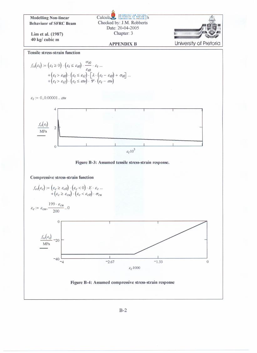
Figure B-3: Assumed tensile stress-strain response ……………………………………………..B-2

Figure B-4: Assumed compressive stress-strain response ……………………………………….B-2

Figure B-5: Measured and calculated moment curvature response …..………………………….B-6

Figure B-6: Output tensile stress-strain response ………………………………………………..B-7

Figure B-7: Output compressive stress-strain response ………………………………………….B-7

Figure B-8: Comparison between measured and calculated load-deflection responses ………..B-11

Figure C-1: Test set up for the beam …………………………………………………………….C-1

Figure C-2: Schematic diagram for the stress-strain response …………………………………..C-1

Figure C-3: Assumed tensile stress-strain response ……..……………………………………... C-2

Figure C-4: Assumed compressive stress-strain response………………………………………..C-2

Figure C-5: Calculated moment curvature response …………………………………………….C-5

Figure C-6: Output tensile stress-strain response ………………………………………………..C-6

Figure C-7: Output compressive stress-strain response ………………………………………….C-6

Figure C-8: Comparison between measured and calculated load-deflection responses ………..C-10

Figure C-9: Test set up for the beam…..……………………………….……………………….C-11

Figure C-10: Schematic diagram for the stress-strain response ………………………………..C-11

Figure C-11: Assumed tensile stress-strain response …..……………………………………....C-12

Figure C-12: Assumed compressive stress-strain response……………………………………..C-12

Figure C-13: Calculated moment curvature response ………………………………………….C-15

Figure C-14: Output tensile stress-strain response ……………………………………………..C-16

Figure C-15: Output compressive stress-strain response ……………………………………….C-16

Figure C-16: Comparison between measured and calculated load-deflection responses .……..C-20

Figure C-17: The developed subroutine to allow the input of a bilinear softening curve ……...C-21

Figure D-1: Test set up for the beam …..………………………………………………………..D-1

Figure D-2: Schematic diagram for the stress-strain response ……..………………………….. D-1

Figure D-3: Assumed tensile stress-strain response ………………..…………………………... D-2

Figure D-4: Assumed compressive stress-strain response………..…………………………….. D-2

Figure D-5: Comparison between measured and calculated load-deflection responses ………...D-6

XI

Figure D-6: Test set up for the beam ……………………………………………………………D-7

Figure D-7: Schematic diagram for the stress-strain response …………………………………..D-7

Figure D-8: Assumed tensile stress-strain response …..………………………………………... D-8

Figure D-9: Assumed compressive stress-strain response …..…………………………………. D-8

Figure D-10: Comparison between measured and calculated load-deflection responses ……...D-12

LIST OF EQUATIONS

Equation 2-1: Decomposition of the tensile strain for smeared cracking approach……….… …..2-8

Equation 2-2: Calculating the value of the shear transfer stiffness as proposed by

Swamy et al. (1987)……..………………………………………………………..2-9

Equation 2-3: Calculating flexural strength of concrete………………………………………...2-15

Equation 2-4: Calculating the equivalent flexural strength for SFRC…………………………..2-16

Equation 2-5: Calculating the residual flexural strength ratio for SFRC ……………………….2-16

Equation 2-6: Meyerhof formulae for the interior load case …………………………………....2-16

Equation 2-7: Calculating the radius of the relative stiffness of ground slab…………………...2-17

Equation 2-8: The limit moment of resistance for plain concrete ………………………………2-17

Equation 2-9: The limit moment of resistance for SFRC ……………………………………….2-17

Equation 2-10: Expression for equal load-carrying capacity for SFRC and plain concrete

ground slabs……………………………………………………………………...2-18

Equation 2-11: Calculating the depth of SFRC ground slab by comparing to equivalent

plain concrete slab………………………………………………………………2-18

Equation 2-12: Calculating the cracking strength of the SFRC using the law of mixture ..……2-19

Equation 2-13: Calculating the Young’s modulus of the SFRC using the law of mixture.……..2-19

Equation 2-14: Calculating the elastic strain for the SFRC using the law of mixture…..…….. 2-20

Equation 2-15: Calculating the tensile strength of a single steel fibre..………………………...2-21

Equation 2-16: Calculating the total tensile stress for a steel fibre content ……………………..2-21

Equation 2-17: Calculating the length efficiency factor for steel fibre ………………………….2-23

Equation 2-18: Calculating the critical steel fibre length ………………………………………..2-23

Equation 2-19: The parabolic curve for compressive stress-strain model

adopted by Lok and Xiao (1998) ………………………………………………..2-23

Equation 2-20: Calculating the cracking strain for the tensile stress-strain response

proposed by Lok and Xiao (1998) ………………………………………………2-24

Equation 2-21: Calculating the residual strain for the tensile stress-strain response

proposed by Lok and Xiao (1998) ……………………………………………...2-24

Equation 2-22: The compressive stress-strain model proposed by

Ezeldin and Balaguru (1992) ……………………………………………………2-26

XII

Equation 2-23: Calculating the material factor for the compressive stress-strain response

proposed by Izeldin and Balaguru ………………………………………………2-27

Equation 2-24: Calculating the reinforcing index for the compressive stress-strain response

proposed by Izeldin and Balaguru ………………………………………………2-27

Equation 2-25: The Winkler support model ………………………………………………….….2-33

Equation 2-26: Calculating the fracture energy for SFRC as proposed by

Barros and Figueiras (2001) …………………………………………………….2-38

Equation 3-1: Calculating Young’s modulus using results from beam-bending test……………...3-6

Equation 4-1: Expression for the stress-strain response for SFRC proposed in this research …..4-2

Equation 4-2: Expression for the strain distribution at a section of a beam ……………………..4-3

Equation 4-3: Expression for the axial force at a section of a beam …………………………….4-3

Equation 4-4: Expression for the moment equilibrium at a section of a beam ………………….4-3

Equation 4-5: Calculating the curvature at a section of a beam …………………………………4-4

Equation 4-6: Calculating the total deflection of a simply supported beam

subject to third-point loading …………………………………………………….4-5

Equation 6-1: Calculating the fracture energy………………………………………………….6-10

Equation 6-2: Calculating the area under the softening part of the tensile stress-strain

Response generated for an element size of 100 x 100 mm.……………………. 6-10

LIST OF TABLES

Table 2-1: Bond stress values adapted from existing research ………………………………….2-22

Table 3-1: Mix composition for the concrete matrix ..………. …………………………………. 3-1

Table 3-2: Compressive strength and Young’s modulus…………………………………………3-6

Table 5-1: Properties used in the numerical analysis ……………………………………………..5-3

Table 6-1: Properties of the SFRC ground slabs tested by Falkner and Teutsch (1993) ………..6-20

Table 7-1: Materials used for the support layer …………………………………………………..7-1

Table A-1: Design values for residual flexural strength ratio of SFRC (Bekaert, 2001) ………...A-1

XIII

LIST OF SYMBOLS

σ = Stress. = Cracking strength of a composite material. t0σ

mσ = Stress in the concrete matrix.

= Stress in the steel fibre. fσ

σui = Stress in the cross-section of a single steel fibre.

σfu = Ultimate fibre stress (fibre fracture stress).

σtu = Residual stress.

σtu’ = Second stage residual stress.

σcu = Compressive strength of SFRC.

321 σ and ,σ ,σ = Principal stresses.

= Flexural strength. ctf

ctf = . ct1.15f

= Post-cracking flexural strength calculated at a deflection value of length/300. 150 equ, ct,f

= Post-cracking flexural strength calculated at a deflection value of length/150. 300 equ, ct,f

= Post-cracking flexural strength calculated at a deflection value of 0.7 mm. eq.2f

= Post-cracking flexural strength calculated at a deflection value of 2.7 mm. 3 eq.f

fe,3 = Equivalent flexural strength.

fd = Design flexural strength for SFRC (fct + fe,3).

= Cube compressive strength. cuf

fs = Tensile strength of fictitious reinforcement element.

= Factor for shear (equals 6/5 for rectangular section). hsf

Re,3 = Residual flexural strength ratio (fct/fe,3).

τ = Shear stress.

= Average ultimate pullout bond strength. uτ

εc0 = Elastic compressive strain.

ε = Strain.

0εt = Cracking strain.

εt1 = Residual strain.

εtu = Ultimate tensile strain.

XIV

cuε = Ultimate compressive strain.

mε = Cracking strain of concrete matrix.

fpε = Strain relating to proportional limit in the stress-strain response of a steel fibre.

= Strain of the material or continuum. coε

= Strain of cracked material. crε

εbot = Tensile strain at bottom ligament of the beam cross-section.

εtop = Compressive strain at top ligament of the beam cross-section.

εR = Strain at proportionality limit of a fictitious reinforcement element.

γ = Shear strain.

γm = Maximum shear strain.

γc = Shear strain at any point on the shear force-shear strain relationship.

= Young’s modulus for of the composite (SFRC). E

mE = Young’s modulus for a concrete matrix.

= Young’s modulus for a steel fibre. fE

= . tcE E 0.5

Eu = Unloading modulus.

ψ = Slope of first softening part of the tensile stress-strain curve.

λ = Slope of the second softening part of the tensile stress-strain curve.

P = Vertical load.

Pmax = Maximum load obtained from beam-bending test.

Pe,3 = Mean load calculated at a deflection of 3 mm.

Pi = Interior load carrying capacity of ground slab.

F = Total force on a beam cross-section.

δ = Deflection of elevated beam or slab.

= Deflection due to moment. mδ

= Deflection due to shear. Vδ

Δ = Deflection of ground slabs or plates (distinguish from elevated beams or slabs).

M = Moment.

Mm = Maximum moment.

= Moment due to a unit load. uM

= Moments due to actual load. LM

Mc = Moment on the descending part of the moment-curvature relationship.

M0 = Limit moment of resistance of ground slab.

XV

φ = Curvature.

φm = Curvature corresponding to the maximum moment (Mm ).

φc = Curvature on the descending part of the moment-curvature relationship.

= Volume percentage of the steel fibres. fV

mV = Volume fraction of the concrete matrix.

= Effective volume fraction of the steel fibre. effV

V = Shear force.

Vm = Maximum shear force.

Vc = Shear force at any point on the shear force-shear strain relationship.

= Shear force due to a unit load. uV

= Shear forces due actual load. LV

A = Area of beam cross-section.

mA = Area fraction of the concrete matrix.

= Effective area fraction of the steel fibres. effA

= Surface area of single steel fibre. sA

= Cross-section area of a single steel fibre. fiA

A150 x 150, A100 x 100 = Area under the softening part of tensile stress-strain response.

oη = Orientation factor.

lη = Length efficiency factor.

= Critical fibre length required to develop the ultimate fibre stress. cL

= Length of a steel fibre. fL

L = Span of the beam.

Lr = Radius of relative stiffness of ground slab.

β = Material factor depending on the steel fibre type.

= Pressure. ρ

μ = Poisson’s ratio.

α = Threshold angle.

r = Radius of loading plate.

R.I. = Reinforcing index.

= Weight fraction of steel fibres. fw

Wf = Weight percentage of steel fibres.

= Crack width. w

h = Depth of a beam.

XVI

b = Width of a beam.

b0 = Unit width of a ground slab.

= Diameter of a steel fibre. fd

dsf = Depth of SFRC slab.

d = Depth of a slab.

d p = Depth of plain concrete slab.

dy , dx = Length and width of differential element.

a = Depth of neutral axis.

y = Variable representing the depth from neutral axis.

S1, S2, and S3 = Slopes on the load-deflection response of a SFRC beam.

X , Y, and Z = Orthogonal directions.

ΔX, ΔY and ΔZ = Displacement in the X, Y, and Z directions respectively.

θX, θY and θZ = Rotation in the X, Y and Z directions respectively.

lb = Width of the fracture process zone.

Ia, Ib , and Ic = Notations used for integration points of a finite element.

I = Second moment.

N1 and N2 = Notations used for nodes.

G = Shear modulus.

sG = Mean shear transfer stiffness in N/mm3.

= Fracture energy for SFRC. fG

Gf0 = Fracture energy for plain concrete.

C2, G5, G6 and G9 = Types of soil according to South African soil classification system.

K = Spring stiffness or modulus of subgrade reaction.

K1, K2, and K3 = Modulus of subgrade reactions- non-linear Pressure-displacement response.

XVII

CHAPTER 1

INTRODUCTION

1.1 General

Portland Cement Concrete (PCC), commonly known as concrete, is a man-made material primarily

manufactured from a mixture of Portland cement, fine and coarse aggregate as well as water. The

word “Cement” is derived from the Latin “Caementum” which was used by the Romans to denote

the rough stone or chips of marble from which a mortar was made. “Concrete” is derived from

“Concretus” which signifies “growing together” (Addis, 1986). Steel Fibre Reinforced Concrete

(SFRC) is defined as concrete manufactured by dispersing discontinuous discrete steel wires

(fibres) into concrete.

The increasing demand for improved load-carrying capacity in roads (which is the result of road

traffic becoming heavier) was first satisfied by strengthening the sub-base rather than by the use of

a wearing course with a load-carrying capacity of its own. It was quite natural that the first concrete

pavements were constructed of plain concrete. In the early days, deep sections were provided for

concrete ground slabs. Increased knowledge and experience in this field had substantially improved

the understanding of the behaviour of concrete and concrete pavements. Design methods have been

refined and thinner slabs were found adequate to carry loads and load repetitions similar to those

carried by the thicker slabs.

With the gradual growth in road traffic and increase in not only vehicle numbers but also

magnitude of axle loads in recent decades, it was a natural development to make un-reinforced

concrete pavement slabs thicker. It is a well-known fact that plain concrete is a material with a low

tensile strength compared to its compressive strength. A concrete ground slab is normally designed

using the flexural strength of plain concrete, which in normal reinforced concrete structures is

completely disregarded. Obviously, more in-depth thought is needed to improve the load-carrying

capacity of these concrete pavements. A natural step would appear to be the use of reinforcement

for strengthening concrete slabs.

Improved understanding of the behaviour of concrete pavement structures under different loading

and environmental conditions as well as advances in material engineering has led engineers to

improve concrete specifications. Recently, considerable interest has been generated in the use of

SFRC and other engineered concrete composites. The most significant influence of incorporating

1-1

steel fibres in concrete is to delay and control the tensile cracking of the composite material. This

imparts certain favourable properties to the concrete such as post-cracking strength and resistance

to fatigue. The improved engineering properties of SFRC make it a viable material for concrete

applications such as pavements. It is therefore not surprising that there have been phenomenal

developments and advances in the use of SFRC during the last three decades.

SFRC pavements were found to provide superior performance compared to plain concrete as it

allows reduction in the slab thickness and yet provide equivalent performance (Elsaigh et al.,

2005). The use of steel fibres in concrete enables designers to increase joint spacing (Parker and

Rice, 1977). Economics can be achieved not only with respect to the joint construction cost but also

by reducing the number of positions where distresses are likely to occur. Performance of previous

SFRC pavements also revealed that the use of steel fibres results in longer maintenance free

intervals compared to plain concrete, thus less interruption to traffic (Vandewalle, 1990). The

initial cost of SFRC pavements will be less than the cost of plain concrete only if the cost of the

steel fibres can be offset by a reduction in the cost of supplying and placing the smaller concrete

volume. However, from an economic point of view life cycle cost should justify the use of SFRC in

road pavements.

SFRC pavements were found to provide equivalent performance compared to conventionally

reinforced concrete pavements when equivalent amounts of reinforcement is used (Bischoff et al.,

2003). However, the SFRC is found to reduce construction time, as the steel fibres are added

directly as one of the concrete mix constituents, and no steel fixing or adjustment is required

(Association of Concrete Industrial Flooring Contractors, 1999). The adjustment of the steel mesh

is of particular concern, as it needs proper seating and care while placing and compacting the

concrete. The reduced construction time can result in early opening to traffic. In addition, saving

may also be made when considering the cost of the overlapping steel for the conventionally

reinforced concrete pavements. The steel fibres provide multi-directional reinforcement throughout

the thickness of the slab. The multidirectional reinforcement is useful for concrete pavements as it

not only prevents the breaking off at edges where conventional reinforcement is not present

(Grondziel, 1989) but also results in a slab section that is reinforced against both hogging and

sagging actions.

Despite the increased demand for higher load-carrying capacity and improved pavement behaviour,

the subject of ground slabs is not researched to the same extent as other structural elements.

Failures of ground slabs are too common and can have serious implications with respect to road

user cost and the general economy. Although the benefits of SFRC in pavements are reasonably

know, the analysis of SFRC pavements is less established. The use of SFRC in pavements has been

1-2

slowed down by the absence of a reliable theoretical method that can be used to design these

pavements. The research conducted here is aimed at promoting the use of SFRC in road pavements

by providing supporting research to convince road authorities of the benefits in using SFRC.

1.2 Problem statement

Numerical models for the analysis of SFRC ground slabs are scarce. Numerical models developed

to analyse plain concrete ground slabs cannot be applied to SFRC. Formulae based on elastic

analysis, such as Westergaard (1926), ignore the post-cracking strength contribution of the SFRC

to both the flexural strength and ductility of the slab. In fact, steel fibres mainly become active after

cracking of the concrete matrix, which means that the un-cracked analysis is not appropriate.

Modern design philosophies have abandoned “permissible stress” concepts in favour of utilising

the actual reserve strength of materials and members.

To determine the ultimate load-carrying capacity in many instances, it is necessary to proceed

beyond the initial cracking load and to evaluate the post-cracking strength reserve. Design formulae

based on the yield-line theory may provide an improved approximation of the ultimate load when

compared to the elastic theory approach such as models developed by Meyerhof (1962), Losberg

(1978), Rao and Singh (1986) and Silfwerbrand (2000). The yield-line analysis requires that the

material behaviour is ideally plastic and the yield lines are correctly hypothesised. These aspects

are crucial to the magnitude of the calculated load-carrying capacity using models based on yield-

line theory. The absence of ideal plastic behaviour dictates that yield-line analysis should not be

used to analyse elements made of SFRC that exhibits softening behaviour.

To effectively account for the non-linear material behaviour of SFRC in the analysis of concrete

pavements, non-linear finite element analysis is required. Finite element methods are increasingly

used to analyse various types of structures and it can be employed to analyse SFRC pavements.

More realistic results for the stresses and displacements of the ground slab can be obtained

including the load-displacement (P-Δ) response. However, the success of a finite element analysis

largely depends on how accurately the material behaviour, cracking behaviour, geometry, and

boundary conditions of the actual boundary problem are defined.

Several material models have been proposed to determine the tensile stress-strain (σ-ε) relationship

for SFRC due to the complexities associated with testing concrete in direct tension and measuring

the stresses and strains. In the past, two approaches have been used to determine the tensile σ-ε

relationship for SFRC. In the first approach, the laws of mixture are used in combination with

1-3

results from fibre pullout strength and direct tensile tests to predict the tensile σ-ε relationship (Lim

et al., 1987 a, Lok and Xiao, 1998). In the second approach, the tensile σ-ε relationship is

empirically determined using results from a deformation-controlled beam-bending test

(Vandewalle, 2003). However, the availability of steel fibres with a variety of physical and

mechanical properties, as well as various fibre contents being used, tends to complicate prediction

of the tensile σ-ε relationship of the SFRC using these approaches.

In recent years, the tensile σ-ε relationships have been determined by inverse analysis (back-

calculation) using flexural responses obtained from beam-bending test (Elsaigh et al., 2004, Alena

et al., 2004 and Østergaard and Olesen, 2005). The advantage of these methods is that the flexural

response of the SFRC can be obtained with minimal complexities compared to procedures

requiring results from direct tensile tests. The disadvantage is that these methods are numerically

demanding. However, the numerical solution capabilities of available computer programmes can be

utilised to readily perform the analysis.

1.3 Research objectives and limitations

The primary objectives of this research are:

(1) To develop a generalised analytical method that can be used to determine the tensile σ-ε

relationship for SFRC using experimental moment-curvature (M-φ) or load-deflection

(P-δ) results from beams.

(2) To propose a new method for analysing SFRC pavements, since existing methods are

inadequate. The proposed method utilises non-linear finite element technique to analyse

ground slabs subject to static mechanical loading. Thus provision can be made to include

the post-cracking strength of SFRC. The Loads due to change in weather conditions are

beyond the scope of this study.

(3) To determine the effect of steel fibre content, concrete strength, support stiffness and slab

thickness on the P-Δ behaviour of SFRC pavements.

1.4 Brief description of work

The work reported in this research includes results of both experimental and computational

modelling of SFRC beams and ground slabs. Experimental results obtained by the author in

previous studies are utilised as input for the developed computational modelling. The experimental

work included a full-scale slab test. The SFRC slab contained 15 kg/m3 steel fibres and was

supported by a foamed concrete slab cast on a relatively thick concrete floor. A plate-bearing test

1-4

was performed on the surface of the foamed concrete prior to casting of the SFRC slab.

Deformation-controlled beam-bending tests were conducted for SFRC beams manufactured using

concrete from the same batch used for the slabs. Cube and cylinder tests were also carried out to

determine the compressive strength and the Young’s modulus for the SFRC concrete. Experimental

studies conducted by other researchers were also utilised.

In the computational modelling, an inverse analysis method is developed to back-calculate the

tensile σ-ε relationship for SFRC. Non-linear finite element analyses are conducted on SFRC

beams and ground slabs whose material constitutive relationship is determined using the inverse

analysis. The results from the finite element analysis are compared to experimental result to verify

both the material and the finite element models. The combined approach of inverse analysis and

non-linear finite element modelling is further used to analyse SFRC beams and ground slabs

reported in other studies. Thereafter, the adjusted non-linear finite element model is utilised to

theoretically study the behaviour of SFRC ground slabs with respect to change in steel fibre

content, concrete matrix strength, support stiffness and the slab thickness.

Mathcad (2001), programming software with numerical solution capabilities, is used to perform the

calculations for the inverse analysis method. MSC.Marc (2003), general finite element computer

programme with capabilities to analyse low-tension materials, is used to perform the non-linear

finite element analysis.

1.5 Research structure

The study is structured as follows:

Chapter 1: Includes general introductory information and the motivation behind the use of SFRC in

pavements. The research problem and objectives as well as a brief description of the conducted

work are presented.

Chapter 2: Includes discussions on SFRC introducing the strengthening mechanisms provided by

the steel fibres and its effect in improving the mechanical properties of concrete. An overview is

presented for the main crack concepts used in numerical analysis. The overview includes the

discrete crack concept and elaborates on the smeared crack concept. Behavioural aspects of SFRC

beams and slabs are discussed including SFRC ground slabs and beams as well as the assessment

of post-cracking strength of SFRC. Existing constitutive material laws for SFRC are presented and

critically discussed. Yield surfaces that consider the biaxial stress states of combined tension and

compression is presented and discussed with respect to SFRC. Appropriateness of existing models

used to analyse SFRC ground slabs is discussed including methods based on elasticity theory,

1-5

yield-line analysis and non-linear finite element. A short introduction is provided for the most

popular support models. An elaborated critique is presented for existing non-linear finite element

models proposed for the analysis of SFRC ground slabs. The critique mainly includes the type of

finite element used, the material constitutive law, support model and the comparison between

experimental and calculated P-Δ responses. Finally a summary and remarks are given.

Chapter 3: Contains the description of the experimental procedures and test results for SFRC slab,

beams, cubes and cylinders as well as the plate-bearing test conducted on the surface of foamed

concrete.

Chapter 4: Includes the description of the generalised analysis method used to calculate the tensile

σ-ε relationship for SFRC. The method utilises the measured flexural response from beam-bending

test to indirectly determine the tensile σ-ε relationship of SFRC. The method is implemented and

evaluated by comparing calculated and measured tensile σ-ε, M-φ and P-δ responses for SFRC

reported in the studies conducted by Lim et al. (1987 a and b). It also includes results of a

parameter study conducted using hypothetical SFRC beams. The results of the parameter study

serve as an aid to adjust the tensile σ-ε relationship that would be initially assumed.

Chapter 5: Contains a brief description of the MSC.Marc programme. The analysis method

described in chapter 4 is used to determine the tensile σ-ε response for SFRC containing 15 kg/m3

of steel fibres using the P-δ response of SFRC beams. The calculated material model is used in

non-linear finite element analysis to analyse a hypothetical single element subjected to direct

tension. Thereafter, the SFRC beam is idealised using shell elements. The correlation between the

measured and calculated P-δ responses is discussed.

Chapter 6: This chapter starts with modelling the plate-bearing test conducted on the surface of the

foamed concrete slab. The constitutive σ-ε relationship for the foamed concrete is back calculated

using finite element analyses. Trial-and-error procedure was followed by changing the parameters

on the compressive σ-ε relationship for the foamed concrete until reasonable match was obtained

between the measured and calculated P-Δ responses. The constitutive relationship for the SFRC

beam, determined in chapter 5, is used in conjunction with the adjusted support model for the

foamed concrete to analyse the SFRC ground slab. Correlation between the calculated and

measured behaviour are discussed. The SFRC ground slabs tested by Falkner and Teutsch (1993)

are analysed to further appraise the computational modelling methods presented in this research.

1-6

Chapter 7: Includes the results of parameter analysis conducted for SFRC ground slabs.

Hypothetical SFRC slabs are used in the analysis. The support layers are made of a wide range of

typical support materials used in road pavements. The adjusted finite element model for the SFRC

ground slab is used to determine the effect of the strength of concrete matrix, support stiffness,

steel fibre content and the thickness of the SFRC slab.

Chapter 8: Contains the conclusions and recommendations.

Chapter 9: Contains the list of references.

Appendix A: Includes design values for hooked-end steel fibres and calculation of the load-carrying

capacity of SFRC ground slab using Meyerhof formula.

Appendix B: Includes the Mathcad work sheets showing the calculated tensile σ-ε response for the

SFRC beam tested by Lim et al. (1987 b).

Appendix C: Includes the Mathcad work sheets showing the results of the first estimate and the

adopted tensile σ-ε response for SFRC beam containing 15 kg/m3 of steel fibres. It also includes

the subroutine used to expand the cracking model of MSC.Marc to allow the input for bilinear

tensile softening behaviour.

Appendix D: Includes the Mathcad work sheets showing the calculated tensile σ-ε response for the

SFRC used in slabs P3 and P4 tested and reported by Falkner and Teutsch (1993).

1-7

CHAPTER 2

LITERATURE REVIEW

2.1 Introduction

Steel Fibre Reinforced Concrete (SFRC) is a composite material consisting of a concrete matrix

containing a random dispersion of steel fibres. The performance of some of the early SFRC

pavements was found not to demonstrate a marked performance improvement or any other overall

advantage when compared to conventional paving materials (Schrader, 1985). An evaluation study

conducted for some of these pavements concluded that the problems were limited to overestimation

of the effect of steel fibres (Packard and Ray, 1984). In contrast, some other SFRC pavements were

found to yield a convincing performance (Johnston, 1984). In recent years, advancement in the

physical and mechanical properties of steel fibres in addition to extensive laboratory studies on

SFRC led to the use of steel fibres in various pavement applications.

Field investigations have shown that SFRC has much greater spalling endurance compared to plain

concrete (Lankard and Newell, 1984). It was stated that cracks and joints of SFRC pavements do

not spall as much as they do in plain concrete even when loaded well beyond what would be

considered failure loads (Parker and Rice, 1977). An airfield survey conducted by Grondziel (1989)

showed that the use of SFRC reduced corner and edge break-off. This was attributed to the

improved shearing capacity of the SFRC. Elsaigh et al. (2005) conducted a full-scale experiment to

evaluate the use of SFRC for road pavements and compare its performance to plain concrete under

in-service traffic loading. The performance of thinner SFRC ground slabs was found comparable to

thicker plain concrete slabs.

A comparison between SFRC and plain concrete will show that SFRC exhibits superior properties,

such as notable improvements in both flexural strength and post-cracking strength. Ground slabs

are structural applications that could benefit from these advantageous features. The design of these

slabs is often based on an elastic analysis assuming un-cracked concrete. Using such a method for

SFRC would ignore the post-cracking contribution the SFRC can make to both the flexural strength

and post-cracking strength of the SFCR slab. However, the effect of the post-cracking strength can

be accounted for by using analysis methods based on yield line theory. The use of these methods

was found to underestimate the load-carrying capacity of SFRC ground slabs.

To effectively account for the behaviour of SFRC in the analysis of SFRC ground slabs requires a

method, for instance non-linear finite element methods using appropriate material and support

2-1

models. Many attempts to develop a tensile and compressive stress-strain (σ-ε) response for SFRC

were found in the literature. SFRC has a complex behaviour involving phenomena like cracking of

concrete and interactive effects between concrete and steel fibres. These special properties of SFRC

must be considered for all stages of the modelling and the computational process.

This chapter contains discussions on the behavioural and analytical aspects of SFRC with emphasis

on ground slabs. The main components of non-linear finite element analysis of SFRC slabs

including, constitutive material relations, representation of concrete cracking and support models

for ground slabs are also discussed. Reviews of previous finite element studies on SFRC ground

slabs are presented.

2.2 Why use steel fibre reinforced concrete?

There are several types of steel fibres that have been used in the past. Apart from other mix

constituents, there are four important steel fibre parameters found to affect the properties of the

composite, namely: type and shape, content, aspect ratio (the length divided by the diameter of

steel fibre) and orientation of fibres in the matrix. Early steel fibres were cut from drawn wire or

mill-cut, but these tend to de-bond from the concrete matrix when applying load to the composite.

Recently, efforts have been made to optimise these parameters to improve the fibre-matrix bond

characteristics and to enhance fibre dispersability (Soroushian and Bayasi, 1991). It was found that

SFRC containing hooked-end stainless steel wires has superior physical properties to straight

fibres. This was attributed to the improved anchorage provided and higher effective aspect ratio

than that for the equivalent length of straight fibre (Ramakrishnan, 1985).

Laboratory-scale tests conducted by many agencies and researchers indicate that the addition of

steel fibres to concrete significantly increases the total energy absorbed prior to complete

separation of the specimen (Johnston, 1985). The presence of steel fibres was also found to

improve fatigue properties (Johnston and Zemp, 1991), impact strength (Morgan and Mowat, 1984,

Banthia et al., 1995) and shear strength (Jindal, 1984, Minelli and Vecchio, 2006). The

improvement of the mechanical properties of SFRC is attributed to the crack controlling

mechanism. Bekaert (1999) suggested that two mechanisms play a role in reducing the intensity of

stress in the vicinity of a crack. These mechanisms are:

(1) Steel fibres near the crack tip resist higher loads because of their higher Young’s modulus

compared to the surrounding concrete. Refer to Figure 2-1(a).

(2) Steel fibres bridge the crack and transmit some of the load across the crack. Refer to

Figure 2-1(b).

2-2

(a) Steel fibres at the tip of crack resist the crack growth (Parker, 1974).

(b) Steel fibres across the crack transmit some tension (Bekaert, 1999).

Fibre

Crack

Bond force

Fibre

Crack

Figure 2-1: Crack controlling mechanism provided by steel fibres.

The ability of the steel fibres to resist crack propagation is primarily dependent on the bond

between the concrete and fibres as well as fibre distribution (spacing and orientation). The bond

between the concrete and fibres is the mechanism whereby the stress is transferred from the

concrete matrix to the steel fibres. The ability of the steel fibres to develop sufficient bond is

dependent on many factors, mainly:

(1) The steel fibre characteristics (surface texture, end shape and yield strength).

(2) The orientation of the steel fibre relative to the force direction.

(3) The properties of the concrete.

In view of the significance of bond, attempts have been made to improve it, either by modification

of the fibre characteristics or by matrix modification (Igarashi et al., 1996). It was suggested that if

the deformed part of crimped steel fibres or the hooks of the hooked-end steel fibres act effectively,

the fibre might fail by tensile yielding and rupture. In this case, it may appear that higher fibre yield

strength is more advantageous. However, microscopic studies revealed that the higher steel fibre

yield strength will result in more severe concrete matrix spalling around the steel fibre, thus

limiting the further improvement in its reinforcement efficiency. It’s therefore suggested that there

is an optimal range of the steel fibre yield strength within which the best combination of peak

pullout load and total energy absorption can be attained (Leung and Shapiro, 1999).

2.3 Failure of SFRC ground slabs

The behaviour of a centrally loaded SFRC slab is relatively linear up to the initial cracking at the

bottom face of the slab where tensile stresses are the highest. The response then deviates slightly

2-3

from linearity after cracking and the slab continues to carry load until the cracks have extended to

the edges and form a collapse mechanism. Substantial indentation occurs in the load introduction

zone, whilst the corners of the slab are lifted up. The complete loss of load-carrying capacity occurs

by punching shear (Bischoff et al., 2003). Based on the cracking progress, Falkner and Teutsch

(1993) distinguished between three different behavioural regions. Referring to Figure 2-2, these

three regions are:

(1) Region I: represents the initial un-cracked behaviour of the slab.

(2) Region II: is governed by the formation of small radial cracks in the central area where the

load is applied.

(3) Region III: represents the behaviour when the cracks spread in the slab until collapse.

Region IIIplastic behaviour

Region IIradial cracking

Region Iuncraked

Displacement

Load

Figure 2-2: Typical load-displacement response of SFRC

ground slab (Falkner and Teutsch, 1993).

Considerable energy is required for the crack to propagate to the surface and extend to the edges. It

is therefore necessary to consider the post-cracking behaviour when designing SFRC ground slabs.

A distinction can be made between two different types of failure in concrete pavements. The first is

a structural failure, which means that the pavement slab collapsed to the extent that the pavement is

incapable of sustaining the loads imposed upon it. The second is a functional failure, which may or

may not be accompanied by structural failure but is such that the pavement slabs will not carry out

the intended function without causing discomfort or without causing high stresses in the vehicle

that passes over it, due to roughness (Yoder and Witczak, 1975). Functional failure is often decided

upon by using measurements related to the riding quality of the road. However, the functional

failure of SFRC pavements is beyond the scope of this research.

2-4

Failure of ground slabs is typically based on serviceability issues, which deal with slab

performance before cracking and the slab fails the serviceability criteria when it cracks. However,

in service ground slabs often crack without total disruption of service. Coetzee and van der Walt,

(1990) suggested that structural failure occurs when a slab is cracked and the crack has developed

through the full depth along the sides of the slab. Falkner and Teutsch (1993) suggested that the

decisions on failure of SFRC ground slabs are to be made based on the acceptable level of

cracking. The load-carrying capacity of a SFRC ground slab can be determined based on the

chosen crack level.

Generally, higher deflection values are associated with thinner slabs. Deflection must be considered

when designing SFRC slabs because of the excessive deflections that might occur as a result of

thinner SFRC sections. High deflections can lead to un-serviceable conditions that might be

considered as functional failure of the pavement. In concrete road pavement design, the corner

deflection is normally used as a worse case scenario for the deflection of concrete ground slabs.

Corner loading was investigated by Beckett (1999) on two full-scale slabs measuring

5500 x 3000 x 150 mm and containing 20 kg/m3 and 30 kg/m3 of hooked-end steel fibre

respectively. Apart from the increase of the corner load capacity due to the increase of steel fibre

content, a reduction in vertical deflection value was found by increasing the steel fibre content

(Beckett, 1999). These findings correlate well with the effect of the steel fibre content on the

deflection of simply supported beam tested by Alsayed (1993).

2.4 Cracking models for concrete

The classical assumption about crack growth is that it is an essentially brittle process in which

strength perpendicular to the crack drops to zero as soon as the crack has formed (Chen, 1982). For

some materials this assumption is not fully correct as the tensile stress perpendicular to the crack

does not drop to zero right away but decreases gradually (softens) as the crack opens. A major

consequence of softening is that the material can neither be assumed to behave elastic-perfectly

plastic nor elastic-perfectly brittle. Instead, the behaviour can be dealt with using the concept of

elastic-softening formulation. Under the framework of finite element analysis of concrete

structures, the cracking of concrete is primarily categorised into discrete and smeared approaches.

In the discrete crack approach, introduced by Ngo and Scordelis (1967), a crack is modelled as a

geometrical discontinuity. The material behaves elastically until crack initiation, i.e. when

maximum principal stress exceeds the limiting tension stress of the material. At a particular load

beyond the cracking point the inter-element boundary nodes, where the limiting stress is exceeded,

are released. Hence, the particular element is subject to the assumed tension softening

2-5

stress-displacement relationship σ (w). This procedure is repeated with every load increment until

the energy ( fG ) is exhausted in a process zone and eventually failure occurs. The fracture process

zone is assumed to have a negligible thickness (hence the name discrete crack model). Fractured

nodes affect the neighbouring elements, thus requiring modification of the element topology in the

vicinity of the particular node. Several developments of discrete crack models exist. In general,

simple discrete crack models use special interface elements, which must either be placed initially in

predefined planes in the model in anticipation of cracks, or a re-meshing strategy is required for the

elements in the vicinity of the crack.

In the smeared crack approach, introduced by Rashid (1968), a cracked solid is represented to be a

continuum. In the earliest versions the effect of shear retention, Poison’s ratio and tension softening

were assumed to be negligible upon occurrence of crack initiation. In later versions, provisions

were made to consider these effects. For instance, the effect of shear was considered as a

percentage (shear retention factor) of the initial linear-elastic shear modulus ( ). The

representation of the tension softening behaviour of concrete in a “ smeared” manner through a

strain softening constitutive relation was first introduced by Bažant (1976) and further developed

by Bažant and Oh (1983). Beyond the cracking point, the micro-cracks are smeared over a crack

bandwidth and the material within this width is subject to the assumed tension softening

stress-strain relation (σ-ε). Under increased loading the growth of this band is simulated by

reducing the stiffness of the element/s (actually the stiffness at the Gauss points within it) that

attains the prescribed fracture criterion in the direction normal to the direction of propagation. On

the bases of extensive test data on plain concrete beams, Bažant and Oh (1983) recommended that

the crack bandwidth is equal to three times the maximum aggregate size used in concrete. If a

larger or smaller crack bandwidth is used, the softening σ(ε) relation must be adjusted in order to

ensure that the energy dissipation is unaltered. In analysis involving the smeared crack approach,

the element size can be set equal to the crack bandwidth. Therefore, the fracture energy should be

released over this width in order to obtain results that are objective with regard to mesh refinement.

Several researches have proposed different ways to relate the crack bandwidth to the size of finite

element. To this end, the analysis method will only ensure objectivity if localisation indeed occurs

in a single row of finite elements, for example: In the case of a beam in flexure, a single row or

single column of elements; and in the case of a slab, a diagonal series of elements. If this is not the

case, the fracture energy assigned to material points and scaled to finite element size leads to

erroneous estimation of toughness.

G

The discrete crack approach is deemed to best fit the natural conception of fracture since it

generally identifies fracture as a true geometrical discontinuity whereas a smeared representation is

2-6

deemed to be more realistic considering the “bands of micro-cracks” that form the blunt fracture in

matrix-aggregate composites like concrete. The discrete crack approach implies a continuous

change in nodal connectivity, which does not fit the nature of a finite element displacement

method, as the crack has to follow a predefined path along element edges. The smeared crack

approach is attractive because the original finite element mesh can be maintained and the

orientation of the crack planes are not restricted, hence it is easier to implement in non-linear

incremental analysis. However, it has generally been found to not only be somewhat less efficient

numerically than a discrete crack model but also to be somewhat mesh sensitive (Karihaloo, 1995).

In many cases there is little to choose between the discrete and smeared approaches and the choice

between them is a matter of convenience and might be limited only by the availability of a finite

element program. In some cases the choice is based on the purpose of the analysis. For instance, if

the overall P-δ response is desired, without regard for completely realistic crack patterns and local

stresses, the smeared-crack model is probably the best choice. If detailed local behaviour is of

interest, adaptations of the discrete-cracking model are useful (Chen, 1982). In some other cases

the choice is based on the nature of the cracking pattern of the boundary problem under

consideration. For instance, the smeared crack approach is more suitable for concrete structures

with densely distributed reinforcement and / or with redundant supports that can assure formation

of multiple cracks. To this end, the reinforcing action of the steel fibres in concrete affects the

nature of the cracking of SFRC structural elements in a manner that diffused crack patterns tend to

occur rather than discrete cracks. However, the final fracture is often dominated by a widening of a

single crack. To some extent, this situation is conceived to provide a true physical basis for

smeared crack concepts.

Smeared cracking concepts can be categorised into single-fixed, rotating and multiple fixed crack

formulations. The fundamental difference between the three formulations lies in the orientation of

the crack, which is either kept constant (single-fixed), or updated in a stepwise manner allowing

secondary cracks to develop if a predefined threshold angle is exceeded (multiple fixed), or

updated continuously (rotating). In the single-fixed smeared crack model, the orientation of the

crack (i.e. the direction which is normal to the crack plane) coincides with the maximum principal

stress orientation at crack initiation, and it remains fixed throughout the loading process. However,

the principal stresses can change their orientation and can exceed the tensile strength of the

concrete. In this case, the single-fixed smeared crack approach predicts a numerical response that is

stiffer than the experimental observations (Rots, 1988). In a rotating crack model as introduced by

Cope et al. (1980), the orientation of the crack plane is adjusted to remain orthogonal to the

direction of the current major principal stress, where it is assumed that the axis of principal stress

coincides with the axes of principal strain. The multiple fixed crack model, introduced by de Borst

2-7

and Nauta (1985), is an expansion of the fixed crack model in which the artificial stiffness of the

fixed crack model is avoided by allowing for the formation of secondary cracks. Once they have

been initiated, all existing cracks remain fixed in their initial orientation. The primary crack is

initiated analogous to the fixed crack model. Secondary cracks are activated, when the change in

principal stress direction, with regard to the previously activated crack, exceeds the threshold angle

(α).

In the smeared crack approach, two methods are used to represent the strain following crack

initiation. In one method the total strain is used while in the other method the strain is decomposed.

The latter method does seem to have some benefits over total strain. In this method, the strain is

decomposed into two components and the material is assumed to be no longer isotropic. Hence the

total strain ( ), which is related to the displacement of the nodal points of a particular element,

through the shape function, is divided into strain components describing the strain of the

“uncracked material” or continuum ( ) and the so-called crack strain ( ) by the relation as in

Equation 2-1:

ε

coε crε

crco εε ε += (2-1)

Comparing the performance of the three crack models, Rots (1988) stated that the difference

between single fixed, multiple fixed and rotating crack concepts and even the differences between

smeared and discrete approaches vanish if the lines of the mesh can be adapted to the lines of the

fracture in a boundary problem, which eliminates stress rotation beyond fracture. In the analysis

conducted by Weihe et al. (1998) on a tension-shear boundary problem, for identical material

parameters, the characteristic response differs significantly for three smeared crack models (refer to

Figure 2-3). The differences are caused by the rotation inherent to the boundary problem and the

fundamentally different assumptions inherent to these models. Figure 2-3 also shows that all

smeared crack models provide an immediate relaxation of the principal stress as the primary crack

is initiated. However, the fixed crack model exhibits a steady increase of the stress state as soon as

the principal axes of stress rotates significantly from the primary crack. Eventually, the principal

stress exceeds the critical stress limit. The rotating crack model shows a totally different behaviour.

The softening response follows the microphysical prescribed exponential decay exactly. The

response of the multiple fixed crack model is the same as the behaviour of the fixed crack model

until a secondary crack orientation is activated.

2-8

0.5 1.0 1.5 2.0 2.5 E-4Principal strain

Prin

cipa

l stre

ss (M

Pa)

0

0.5

1.5

1.0

Fixed Crack ModelMultiple Fixed Crack Model

Rotating Crack Model

Figure 2-3: Response of smeared-crack models (Weihe et al., 1998).

During the post-cracking stage, the cracked SFRC can still transfer shear forces through aggregate

interlock and /or due to the crack bridging action provided by the steel fibre reinforcement. Shear

stresses are transmitted over the crack faces but with reduced shear capacity. To account for the

effect of shear during the process of material degradation, the concept of a shear retention factor is

often used to couple the shear behaviour to the degradation of the material. The shear retention

factor relates the ratio of the post-cracking shear stiffness in the concrete to the pre-cracking shear

stiffness. It essentially serves the purpose of ascribing some shear strength to the cracked concrete.

In the literature a scatter of values ranging between zero and one were used. Hu and Schnobrich

(1990) stated that the particular value chosen for the shear retention factor is not critical for mode I

fracture but values greater than zero are necessary to prevent numerical instabilities. The mode I

refers to planar symmetric state of stress which causes a crack to open, i.e. the crack faces are

displaced normal to their plane, also referred to as opening mode. A constant value for the shear

retention factor might not be appropriate as the shear stiffness reduces as loading is increased

beyond the cracking point. Indeed, Swamy et al. (1987) relates the value of the shear transfer

stiffness to the crack width as in Equation 2-2.

1.751 x 2.5 ⎟⎠⎞

⎜⎝⎛=

wGs (2-2)

where sG is the mean shear transfer stiffness in N/mm3 and is the crack width in mm. w

2-9

2.5 Load-deflection behaviour of SFRC ground slabs

Extensive research has been conducted to investigate the influence of the steel fibres on the load

carrying capacity of ground slabs (Kaushik et al., 1989, Beckett, 1990, Falkner and Teutsch, 1993,

Bischoff et al., 1996, Elsaigh, 2001, Bischoff et al., 2003 and Chen, 2004). In these studies, full-

scale slab tests were conducted to compare the behaviour of centrally loaded SFRC slabs to plain

concrete or Welded Wire Fabric (WWF) reinforced concrete slabs. It was demonstrated that the

addition of the steel fibres increase the load-carrying capacity of ground slabs significantly.

Figure 2-4(a) and (b) show the load-displacement (P-Δ) responses from two investigations

conducted by Chen (2004) and Falkner and Teutsch (1993) respectively. It is prominent that SFRC

containing hooked-end steel fibres yields greater load-carrying capacity compared to both plain

concrete and SFRC containing mill-cut fibres (straight fibres having a relatively low tensile

strength). Figure 2-4(a) shows that the addition of 30 kg/m3 of hooked-end steel fibres resulted in

greater load-carrying capacity for the SFRC ground slab compared to addition of 20 kg/m3 of

similar steel fibres type.

Load

(kN

)

SFRC-20kg/m (hook-end)

3SFCR-30kg/m (hook-end)

3

SFRC-30kg/m (mill-cut)

3

Displacement (mm)

Plain concrete

(a) Chen (2004)

Displacement (mm)

(b) Falkner and Teutsch (1993)

SFRC-30kg/m (mill-cut)

3

Plain concrete

SFRC-20kg/m (hook-end)

3

Load

(kN

)

100

0

400

300

200

0 5 10 15 2020151050

320

220

120

20

Figure 2-4: Comparison between SFRC and plain concrete ground slabs.

Bischoff et al. (2003) conducted full-scale slab tests to investigate the performance of WWF and

SFRC. The slabs cast on either a loose or compacted subgrade with respective modulus of subgrade

reaction of 0.015 MPa/mm and 0.75 MPa/mm. In one group of slabs, hook-end steel fibres were

added to provide reinforcement at 0.16 percent (10 kg/m3) and 0.38 percent (30 kg/m3) by volume.

In a second group of slabs, WWF were placed in both a single layer located 50 mm below the top

face of the slab and double layers located 50 mm from top and bottom faces respectively. The size

2-10

of the WWF reinforcement was selected to provide 0.16 and 0.45 percent per volume for single

layer and double layers respectively. These amounts of WWF reinforcement were selected on the

basis of providing comparable post-cracking strength to the SFRC with respect to flexural beams.

Figure 2-5(a) shows the P-Δ response of SFRC and WWF reinforced concrete ground slabs on

loose subgrade. When equivalent amounts of either WWF or steel fibre reinforcement are used,

based on similar post-cracking strength values, the slabs exhibit comparable behaviour. For this

reason, SFRC can be considered a suitable alternative to WWF reinforcement of concrete ground

slabs. The difference in behaviour between the SFRC slab containing 0.38 percent by volume steel

fibres and the slab with the double layer WWF reinforcement arise mainly because of the layer

placed 50 mm above the bottom of the slab where it is more effective in resisting loading

associated with positive moments. It is worth noting that the results from bending-beam tests

containing double WWF layers (0.45 percent by volume) also showed greater post-cracking

strength compared to that of SFRC containing 0.38 percent by volume.

Figure 2-5(b) shows the P-Δ responses of SFRC ground slabs on loose and compacted subgrade.

The test results demonstrate the benefits of reinforcing concrete ground slabs using steel fibres to

compensate for poor or loose subgrade. Although the benefit of using SFRC for ground slabs

placed on poor subgrade is known, the amount of steel fibres needed to compensate for a particular

poor subgrade is unknown. An analysis method is required to optimise the support stiffness and the

steel fibre content for SFRC ground slabs to provide a desired load-carrying capacity.

0 10 20 30 400 10 20 30 40

100

200

300

400

Load

(kN

)

100

200

300

400

Load

(kN

)

Displacement (mm)Displacement (mm)

Loose subgradeSFRC - 30 kg/m3

Compacted subgrade SFRC - 10kg/m3

Loose subgrade SFRC - 10kg/m3

(b) Subgrade influence on SFRC slab response.

WWF - 2 layers 0.45 %

SFRC 0.38 % (30 kg/m )3

SFRC0.13 % (10 kg/m )3

WWF - 1layer 0.16 %

(a) Comparison between SFRC and WWF reinforced concrete ground slabs.

Figure 2-5: SFRC and WWF reinforced concrete ground slabs tested by Bischoff et al. (1996).

2-11

Several explanations for the increased carrying capacity of SFRC ground slabs have been

suggested. Besides the structural ductility of the statically indeterminate slab, it has been

recognised that the post-cracking strength of the steel fibre reinforced concrete is the reason behind

the increased carrying capacity of SFRC ground slabs (Kearsley and Elsaigh, 2003). Partial stress

redistribution can take place due to the statically indeterminate nature of the slab. The presence of

membrane action, also known as “arching action”, in a restrained slab further contributes to the

resistance. Restraint develops either because the ends of the slab are held from lateral movement by

the surrounding immovable concrete (Chen, 1982, Shentu et al., 1997) or due to friction between

the slab and the supporting layers (Chen, 2004). The punching shear resistance can also play a

significant role in increasing the bearing capacity of SFRC ground slabs. Experiments on

slab-column connections, suggests that the introduction of steel fibres decreases the angle of the

shear failure plane of the slabs which moves the failure surface away from the column face, hence

resulting in an increase in punching shear resistance, and therefore an increase in the bearing

capacity of the slab (Harajli et al., 1995).

The results from the static tests on the full-scale ground slabs presented in Figure 2-4 indicate that

an appreciable thickness reduction, depending on steel fibre content, is possible for SFRC ground

slabs when compared to counterpart plain concrete slabs. Indeed, it was found that about 16 percent

thickness reduction is possible if 15 kg/m3 of hooked-end steel fibres is used (Elsaigh, 2001).

Bischoff et al. (2003) stated that the thickness reduction is justified by the following arguments:

(1) The addition of steel fibres significantly increases the flexural capacity and therefore the

slab thickness can be reduced.

(2) The post-cracking strength of the SFRC allows for redistribution of stresses leading to an

increased load-carrying capacity and therefore the slab thickness can be reduced.

(3) The use of steel fibres improves the fatigue resistance of the concrete, allowing for a

smaller safety factor, which can lead to thinner slabs as the allowable stress is increased.

SFRC is deemed to be a superior material for concrete roads due to its improved mechanical

properties compared to plain concrete. Although support provided by the subgrade means that

bending stresses in pavements are generally low, the flexural capacity of the pavement remains an

important aspect to consider. This is especially so when the bending stresses increase significantly

due to uneven subgrade erosion, as is common in the case when the subgrade subsides at the

pavement corner or edge. In conventional reinforced concrete pavements, the steel reinforcement is

placed between the mid to two third depth to mainly resist stresses caused by changes in

environmental conditions (Paramasivam et al., 1994). The load-carrying capacity of a concrete

pavement can be enhanced by placing the reinforcement in the bottom of the slab. Thus allowing

the concrete in the bottom surface to crack and the reinforcement there to take up the positive

2-12

moment. Top reinforcement can also be provided especially at corners and edges to resist negative

moments (Losberg, 1961). SFRC and WWF reinforced concrete ground slabs were found to yield

similar load-carrying capacities when equivalent amounts of reinforcement are provided (Bischoff

et al., 2003). The steel fibres provide a slab cross-section that is reinforced against both hogging

and sagging bending stresses. These stresses can arise in road pavements not only as a result of

mechanical load but also as a result of curling and warping.

2.6 Flexural properties of SFRC

The flexural behaviour of SFRC is often studied using the load-deflection (P-δ) response derived

from beam specimens tested under displacement control. The addition of steel fibres enhances the

post-cracking strength of concrete. Figure 2-6 shows typical P-δ curves obtained for SFRC and

plain concrete beams (150 x 150 x 750 mm), subject to third point loading. It can be seen that the

plain concrete fails in a brittle manner while SFRC could withstand some load in the post-peak

stage. It can also be seen that the increase in the steel fibre content increases the magnitude of the

post-cracking strength (Elsaigh and Kearsley, 2002).

0102030405060

-0.5 0.0 0.5 1.0 1.5 2.0 2.5 3.0 3.5 4.0

Deflection at mid-span (mm)

Load

(kN

)

SFRC-30 kg/m3 (Hooked-end)

SFRC-15 kg/m3

(Hooked-end)Plain concrete

Figure 2-6: Load-deflection response (Elsaigh and Kearsley, 2002).

Although the magnitude of the flexural strength (calculated at the peak load) is increased when

steel fibres are added to the concrete, this increase is not significant and is often not the reason for

using steel fibres. This increase can also be attained through adjusting the concrete mixture design.

Statically determinate structures, such as simply supported beams, do not explain the full advantage

of using SFRC. When considering the P-δ responses of Figure 2-6 beyond the peak load, the beam

cannot sustain this peak load for greater deflection values. Therefore, these beams would have

failed at loads approximately equal to this peak load if load-controlled tests were performed rather

than displacement-controlled tests. Full advantage of the post-cracking strength of SFRC can only

be seen if plastic hinges and redistribution of stresses are taken into account in determining the load

bearing capacity (Nemegeer, 1996).

2-13

Investigating the curve in Figure 2-6, one can distinguish between three behavioural stages:

(1) Ascending part of the curve up to the peak load.

(2) Descending part immediately beyond the peak load referred to as a region of instability. In

this region unstable crack growth occurs, as the fracture energy does not match the elastic

energy release, leading to a rapid increase in deformation. The occurrence of this

deformation is faster than the response of the measuring devices (Chen et al., 1995).

De-bonding, slipping and straining of steel fibres are assumed to take place in this stage.

(3) A third part in which the curve stays relatively flat at a load less than the maximum load.

The P-δ responses in Figure 2-7 are for two slabs measuring 1000 x 1000 x 50 mm and simply

supported along their four edges. For the SFRC slab, the value of the peak load is reasonably

sustained to a greater deflection compared to the plain concrete slab. The SFRC slab behaved in a

ductile manner and sustained a peak load that is greater than the peak load sustained by the plain

concrete slab. Both the structural ductility and the post-cracking strength of the statically

indeterminate slabs were increased by the use of SFRC. Ductility at the structural level is achieved

due to the fact that material failure occurs locally and in a gradual manner, thus allowing stress

redistribution to take place.

Plain concrete

SFRC (30 kg/m - hook-end)3

Load

(kN

)

Deflection (mm)

0105 15

5

10

15

Figure 2-7: Load-deflection responses of slabs that are simply supported

on their four edges (Sham and Burgoyne, 1986).

The area beneath the P-δ curve of a beam tested in displacement control is a measure of the energy

required to achieve a certain deflection. This energy can be used to determine the post-cracking

strength, which can be incorporated in design methods to estimate the load carrying capacity of

SFRC members. The value of the post-cracking strength depends on the steel fibre type, steel fibre

content and deflection limit. Although, the significant effect of steel fibres on concrete post-cracking

2-14

strength is widely recognised, there is uncertainty regarding a method to quantify it. The following

three methods to interpret and calculate the ductility of SFRC are widely used:

(1) The ASTM C1018-97 method (1992) in which the energy absorbed up to a specified

deflection is normalized by the energy up to the point of first cracking.

(2) The Japanese Concrete Institute method (1983), which interprets the post-cracking

strength in absolute terms, as the energy required to deflect a beam to a mid-span

deflection of 1/150 of its span.

(3) The RILEM TC 162-TDF Method (2002) has been developed recently. In this method, a

notched beam subjected to a single load at mid span is used to generate the P-δ response.

In the method proposed by the Japanese Concrete Institute (1983) distinction should be made

between several different terms viz, the flexural strength ( ), the equivalent flexural strength

( ), the residual flexural strength ratio ( ) and design flexural strength ( ). The schematic

P-δ response in Figure 2-8 is used to define and interpret these terms.

ctf

e,3f e,3R df

P/2P/2

hb

L = 450 mm, b = h = 150 mm

L/3L/3L/3

=Actual Equivalent

L /150Deflection at mid-span

Load Pe,3

Pmax

Figure 2-8: Schematic load-deflection curve for SFRC beam loaded at third-points.

The is the stress at peak load on the P-δ response. It can be calculated as in Equation 2-3: ctf

2maxctbh

LPf = (2-3)

2-15

where = Peak load on the P-δ response. maxP

= Beam span. L

= Depth of the beam cross-section. h

= Width of the beam cross-section. b

The is derived from the mean load corresponding to a deflection of L/150 in a third-point

bending test and can be calculated as in Equation 2-4:

e,3f

2e,3e,3bh

LPf = (2-4)

where is the mean load calculated by dividing the area under the P-δ response by L/150. e,3P

The is the ratio between and . It represents the percentage of improvement of the

flexural strength caused by addition of steel fibres. It can be estimated using the specification

sheets provided by steel fibre manufacturer as in Table A-1 (refer to Appendix A) or it can be

calculated if experimental results are available as in Equation 2-5:

e,3R e,3f ctf

100ff

Rct

e,3e,3 = (2-5)

The Meyerhof (1962) formulae can be used to explain the application of in designing the

SFRC ground slabs. The strength term is modified to take the post-cracking strength of the SFRC

into account (refer to the numerical example given in Appendix A). The Meyerhof formula for the

interior load case is indicated in Equation 2-6:

e,3R

⎟⎟⎠

⎞⎜⎜⎝

⎛+=

roi L

2r1.6.MP (2-6)

where = Interior load-carrying capacity of the slab. iP

= Limit moment of resistance of the slab. oM

r = Radius of the loading plate.

rL = Radius of the relative stiffness of the slab.

2-16

The radius of the relative stiffness is given as in Equation 2-7:

( )25.0

2

3r

.-112.

E.d L⎟⎟

⎠

⎞

⎜⎜

⎝

⎛=

Kμ (2-7)

where = Young’ modulus for the slab material. E

= Depth of the slab. d

μ = Poisson’s ratio of the slab material.

K = Modulus of subgrade reaction.

The limit moment of resistance for plain concrete is given as in Equation 2-8:

6.db.fM

2o

cto = (2-8)

where = a unit width of the slab. ob

The limit moment of resistance for SFRC is given as in Equation 2-9. The flexural strength term is

modified to account for the post-cracking strength of the SFRC. The design flexural strength is

determined as fd = (1+Re,3/100) fct or the sum of and . e,3f ctf

6

2.dob.ctf

100e,3R

1oM ⎟⎟⎠

⎞⎜⎜⎝

⎛+= (2-9)

The relationship between the limit moment for plain concrete and SFRC can be useful. The

thickness of a SFRC ground slab can be estimated if the adequate thickness of a plain concrete slab

made from same parent concrete mixture is known. This can be achieved by comparing the load-

carrying capacity of both slabs by using the Meyerhof formula. All inputs to this formula are

approximately equal for both slabs except the flexural strength term and the thickness of the slabs.

The term [ rL2r1+ ] in Equation 2-6 is also assumed to be the same for both slabs. The change in

the value of this term due to the difference between the slabs thickness was found to be

insignificant. The load-carrying capacity of plain concrete with a thickness of ( ) and a flexural

strength of (f

pd

ct) can be calculated. The SFRC slab thickness ( ) that would take equal load to that

of the plain concrete slab can then be calculated taking into account that the flexural strength term

is equal to f

sfd

d.

2-17

For the plain concrete and the SFRC slabs to have equal load-carrying capacity, the moment terms

in Equation 2-8 and 2-9 has to be equal.

6

b x df x

100R

16

b x df o

2fs

cte,3o

2p

ct ⎟⎟⎠

⎞⎜⎜⎝

⎛+= (2-10)

By simplifying Equation 2-10, the thickness for the SFRC slab can be given as in Equation 2-11:

( )( )e,3

2p

sf R100100 x d

d+

= (2-11)

Kearsley and Elsaigh (2003) experimentally verified the adequacy of this comparative design

approach for ground slabs subject to static loading. Full-scale plain concrete and SFRC ground

slabs were designed using this approach. Static loads were applied at the centre of the slabs. The

measured P-δ responses show that the load-carrying capacity is approximately equal for both slabs.

Elsaigh et al. (2005) evaluated the validity of this comparative design approach with regard to

traffic loading using results from a trial road subject to in-service traffic. A plain concrete section

was designed to take approximately 60 x 103 E80s. This comparative design approach was used to

design the SFRC slabs. The road section started to show some distresses after 400 x 103 E80s. The

SFRC slabs were found comparable to the thicker plain concrete slabs.

2.7 Constitutive relationships for SFRC

The first pre-requisite for a successful finite element analysis is the definition of the constitutive

behaviour of the material. Different techniques have been proposed to predict the tensile σ-ε

response of SFRC. These techniques mainly include the laws of mixture and fracture energy.

2.7.1 Tensile stress-strain responses based on law of mixture and pullout strength

In these models, a volume-weighted sum of the concrete matrix and steel fibre responses are used

to predict the composite behaviour in the pre-cracking stage while fibre pullout tests are used to

predict the material behaviour in the post-cracking stage. The physical interaction between the

concrete matrix and the steel fibres is usually accommodated through efficiency factors.

2-18

Lim et al. (1987a) developed a method to predict the pre-cracking and the post-cracking tensile

behaviour of SFRC. The σ-ε response was modelled by considering the tensile behaviour of two

identical SFRC specimens. The first set of specimens was un-cracked while the second set was

pre-cracked. The parameters on the proposed σ-ε response were determined based on two different

approaches. The law of mixture was used to predict the parameters for the pre-cracking stage while

steel fibre pullout tests were used to determine the parameters of the post-cracking stage. In later

work the σ-ε response was appraised by comparing measured and predicted P-δ responses for

SFRC beams. The predicted P-δ responses, using the model, were found to match the measured

responses (Lim et al., 1987b). The idealised tensile σ-ε response is shown in Figure 2-9(a). The

notations in Figure 2-9 have been standardised to improve readability and eliminate confusion.

εtu εtuεt1

σt0

σtuσtu

σt0

E Etc

E

Strain Strain

Tens

ile st

ress

Tens

ile st

ress

(a) Lim et al. (1987a) (b) Lok and Xiao (1998)

Figure 2-9: Tensile stress-strain responses based on the law

of mixture and steel fibre pullout strength.

The law of mixture is applied to define the pre-cracking stage as indicated in Equation 2-12 and

Equation 2-13:

efffmmt0 AσAσσ += (2-12)

efffmm VEVEE += (2-13)

where = Ultimate stress of the composite. t0σ

mσ = Stress in the matrix.

= Stress in the steel fibre. fσ

2-19

mA = Area fraction of the matrix.

= Effective area fraction of the steel fibres. effA

mV = Volume fraction of the matrix.

= Effective volume fraction of the steel fibre. effV

= Young’s modulus for of the composite (SFRC). E

mE = Young’s modulus for the concrete matrix.

= Young’s modulus for the steel fibre. fE

Due to the random orientation of steel fibre in concrete, not all of fibres will be effective. However,

only those fibres parallel or nearly parallel to the tensile stress are effective in controlling a

particular crack. The amount of effective steel fibre is always of major concern when modelling

SFRC structures and correction factors are often introduced to estimate the amount of effective

steel fibres. The values for and equals the actual total areas and volumes of the steel

fibres in the concrete multiplied by a selected factor.

effA effV

The cracking strain of the SFRC ( 0εt ) is often assumed to be equal to the failure strain of the

concrete matrix (Pakotiprapha et al., 1983). However, experimental results revealed that the

first-crack strain of SFRC is larger than the cracking strain of the matrix and it increases with

increasing steel fibre content (Elsaigh and Kearsley, 2002). Based on the assumption that 0εt

increases linearly with the volume fraction of the steel fibre reinforcement, Nathan et al. (1977)

developed an empirical expression to calculate 0εt as shown in Equation 2-14:

( ) mmfpefft0 εεεVε +−= (2-14)

where mε is the cracking strain of the concrete matrix, fpε is the strain relating to the proportional

limit of the steel fibres.

Equation 2-14 indicates that when the volume fraction of fibres is zero, 0εt equals mε . Otherwise,

0εt increases proportionately with increasing amount of fibres. The use of this expression does not

imply that the steel fibres yield when the concrete matrix cracks.

In the cracked range, the behaviour is described by a combination of elastic deformation in the

un-cracked sections and crack widening based on the bond-slip behaviour of the steel fibres at the

crack. The ultimate tensile strength is related to the average ultimate pullout bond strength ( ) and uτ

2-20

steel fibre length ( ) as well as the steel fibre diameter ( ). Referring to Figure 2-10, the stress

in the cross-section of a single steel fibre ( ) can be calculated as in Equation 2-15 where and

denote surface area and cross-section area of a single steel fibre respectively. The total stress

corresponding to a certain effective volume of steel fibre ( ) can therefore be calculated as

indicated in Equation 2-16.

fL fd

uiσ sA

fiA

tuσ

fis

uui 2AA

τσ = (2-15)

ff

uefftu dL

τVσ = (2-16)

P

τu

concrete

Lf

2

Figure 2-10: Finding the tensile stress for a single

steel fibre from a fibre pullout test.

Table 2-1 shows values for the bond stress ( uτ ) adapted from three different experimental studies.

The variation in these results can be attributed to the different testing approaches followed by

different researchers. In the tests conducted by Leung and Shapiro (1999) straight steel fibres were

positioned to be inclined at 0, 30 and 60 degrees to the direction of the applied load. The embedded

length of the steel fibre was kept constant in all tests. The pullout test carried out in this way was

based on the fact that cracks in concrete member may intersect steel fibres at different angles. In

the study by Shannag et al. (1997), the inclination angle was kept constant at zero degrees while the

embedded lengths varied between 6, 12 and 18 mm. In the third study the angle of inclination and

the depth were kept constant (Lim et al. 1987a). These tests were conducted using special

specimens mainly made of cement-sand mortar that were prepared using different procedures than

those applied in the production of the SFRC. In these three studies, the pullout-extension curve was

established for the different specimens and the uτ was calculated by dividing the maximum pullout

load by the surface area of the embedded part of the steel fibre. This means that the assumption is

2-21

made that an average constant uτ exists along the whole embedded length of the fibre. Conclusive

recommendations for specifying uτ can hardly be drawn from these results. The availability of a

wide range of steel fibres and concrete matrix strengths contribute to an even greater uncertainty

over bond stress values.

Table 2-1: Bond stress values adapted from existing research.

1.75 - 4.6

Study Bond stress ( ) (MPa)τ u

Leung and Shapiro (1999)

Shanag et al. (1997)

Lim et al. (1987b)

2.4 - 3.7

5.9 - 6.9

The area and the volume of the effective steel fibres can be calculated by applying correction

factors to the actual volume of steel fibre added to the concrete mixture. Swamy and Al-Ta’an

(1981) suggested the following corrections:

(1) Orientation correction factor ( oη ). This is to account for the steel fibres, which are

inefficiently oriented with respect to the principal tensile stress at particular sections.

(2) Length efficiency factor ( lη ), defined as the ratio of the average steel fibre stress to

maximum steel fibre stress. This is to account for the varying stress at the end portions of

the steel fibre.

When steel fibres are uniformly dispersed in a large volume of concrete, they are expected to be

randomly oriented with equal probabilities of being oriented in different directions. Correction

must be made for those steel fibres that are ineffectively oriented in the volume space with respect

to the direction of tensile stress. However, the proper correction to be used is uncertain. Romualdi

and Mandel (1964) assumed an orientation correction factor equal to the ratio between average

projected lengths of the steel fibres in one direction and the total length of these fibres.

In the study conducted by Soroushian and Lee (1990), the orientation factor was estimated by

counting the effective steel fibres at fracture surfaces of nineteen SFRC beams. The beams,

measuring 152 x 152 x 457 mm, contained various amounts of steel fibres and were subject to

flexural loading. The steel fibres used were either straight or hooked-end with a length of 51 mm

and a diameter of 0.5 mm. The results obtained from the measurements showed that the average

oη is equal to 0.62. However, different size as well as shape of specimen will certainly lead to a

different value for oη . It is also interesting to note that not only the shape of the cast volume

2-22

influences the orientation of steel fibres but also the compaction method has a significant effect on

the manner that steel fibres align themselves. For example, steel fibres in concrete compacted by

means of table vibration tend to align themselves in planes at right angle to the direction of the

vibration (Edgington et al., 1974). The lη is determined by Nathan et al. (1977) as in Equation 2-

17 and Equation 2-18. These equations are incorporated in the material constitutive model

developed by Lim et al. (1987a).

⎪⎭

⎪⎬

⎫

⎪⎩

⎪⎨

⎧

≥

<=

cffc

cf

L Lfor LL

- 1

L Lfor 0.5 lη (2-17)

u

ffu c τ

d0.5.σL = (2-18)

where is the ultimate fibre stress (fibre fracture stress) and denotes the critical fibre length:

defined as half the fibre length required to develop the ultimate fibre stress when it is embedded in

the matrix.

fuσ cL

Lok and Xiao (1998) proposed a three stage model to predict the tensile σ-ε response for SFRC.

These three stages are the pre-cracking stage, immediately post-cracking stage and the

post-cracking stage as indicated in Figure 2-9(b). It differs from the model of Lim et al. (1987a) in

that a parabola was assumed for the first part of the σ-ε response and a middle stage was added.

The pre-cracked stage is represented by the parabolic curve as in Equation 2-19:

⎥⎥

⎦

⎤

⎢⎢

⎣

⎡

⎟⎟⎠

⎞⎜⎜⎝

⎛−⎟⎟

⎠

⎞⎜⎜⎝

⎛=

2

t0t0t0 ε

εεε2σ σ (2-19)

where σ and denote the stress and the corresponding strain at any point on the parabolic curve. εThe ultimate tensile stress ( t0σ ) is either measured from direct tensile tests or estimated by using

Equation 2-12. The corresponding tensile strain can be calculated using Equation 2-20. Based

on the parabolic relationship in Equation 2-19, the value of is determined as . The value of

t0ε

E tcE 2

tuσ is calculated using Equation 2-16. In the third stage of the σ-ε response, the concrete matrix is

assumed to be fully cracked with the steel fibres resisting all the tensile stresses. The value of is t1ε

2-23

calculated using Equation 2-21. As far as the tension failure is concerned, Lok and Xiao (1998)

suggested a value equal to 0.002 for the ultimate strain . tuε

tc

t0t0 Eε

σ= (2-20)

ftu

t1 Eε σ

= (2-21)

Some criticism has been levelled at the application of the “law of mixture concept” to predict the

tensile strength of SFRC. The law of mixture requires that the fibre pullout resistance be mobilised

to a large extent when the material reaches the peak stress. Soroushian and Bayasi (1987) suggested

that bond slippages in the order of 0.38 mm need to take place before the pullout resistance of steel

fibres in SFRC is mobilised. However, direct tension tests on SFRC indicate that the maximum

crack openings at ultimate stress are in the order of 0.005 mm, which is far below the values

needed for meaningful mobilization of the pullout resistance of steel fibres. This questions the use

of the law of mixture concept to determine the ultimate tensile strength of SFRC, and it indicates

that the pullout behaviour of fibres does not play a major role when the ultimate tensile stress of

SFRC is reached. Models based on law of mixture were however claimed to provide satisfactory

results when used to predict the response of SFRC beams (Lim et al., 1987 b).

2.7.2 Tensile stress-strain responses based on fracture energy

In these models the tensile σ-ε response for SFRC is developed using measured P-δ responses

generated from a simply supported beam subject to a displacement-controlled bending test. The

maximum tensile stress in the σ-ε response is determined as the stress with respect to the first crack

load (when the P-δ response first deviates from linearity) on the P-δ response. The post-peak

stresses and strains are calculated using the post-cracking strength based on the fracture energy of

the tested beam. This modelling procedure adopts a macro approach rather than the micro approach

adopted in the models presented in section 2.7.1.

Nemegeer (1996) proposed a tensile σ-ε response for SFRC by using a measured P-δ response

generated from third-point beam testing. The shape of the σ-ε response and its defining parameters

are shown in Figure 2-11(a). The ultimate tensile stress ( t0σ ) is estimated as a percentage of the

compressive strength. The 0εt is then calculated assuming equal Young’s modulus in tension and

compression. The post cracking flexural strengths ( ) and ( ) at deflection values of 150 equ, ct,f 300 equ, ct,f

2-24

span length/150 and span length/300 respectively are calculated according to the method of the

Japanese Concrete Institute (1983). The residual tensile stress after cracking and at the residual

tensile stress at assumed failure are calculated as 37 percent of the respective post-cracking flexural

strengths and respectively. The corresponding residual strain and failure strain

are estimated as fixed values of 0.001and 0.01 respectively.

150 equ, ct,f 300 equ, ct,f

εt0

Strain

0.45feq,2

0.37feq,3

0.01Strain

σt0

0.37fct,eq,150

0.37fct,eq,300

0.001 0.01Strain

Tens

ile st

ress

Tens

ile st

ress

Tens

ile st

ress

(a) Nemegeer (1996) (b) Vandewalle (2003) ( c) Dupont and Vandewalle (2003)

εtuεt0 εt0 ( + 0.0001)εt0

σt0 σt0

σtu`

σtu

Figure 2-11: Tensile stress-strain responses based on the fracture energy.

Vandewalle (2003) has suggested a similar shape to the tensile σ-ε response presented in Figure

2-11(a) but the stress and stain parameters are estimated differently. The P-δ response is generated

using a notched SFRC beam loaded at its mid span. The notched SFRC beam is cast and tested

according to the method described in the RILEM TC 162-TDF (2002). The proposed response is

shown in Figure 2-11(b). The ultimate tensile stress is calculated as the stress at initiation of

cracking (when P-δ response first become non-linear) on the P-δ response. The load corresponding

to initiation of cracking is determined as the highest load attained in the interval between 0 and

0.05 mm deflection in the measured P-δ response. The post cracking flexural strengths ( ) and

( ) at deflection values of 0.7 mm and 2.7 mm respectively are calculated according to the

recommendation of the RILEM TC 162- TDF (2002). The residual tensile stress after cracking and

at the residual tensile stress at assumed failure are calculated as 45 percent and 37 percent of the

respective post-cracking flexural strengths and respectively. The is then calculated

assuming equal Young’s modulus in tension and compression. The values of and are

estimated as and 0.01 respectively. Yi-ning et al. (2002) stated that for steel fibre

contents ranging between 20 and 60 kg/m

eq.2f

3 eq.f

eq.2f 3 eq.f t0ε

t1ε tuε

0001.0ε t0 +3, these strain values are satisfactory and relate to

deflections of 0.7 mm and 2.7 mm in the P-δ response of the notched beam.

Dupont and Vandewalle (2003) suggested a two level shape for the post-cracking part of the σ-ε

response (refer to Figure 2-11(c)). The pre-cracking stage of the response is established in a similar

manner to that of the σ-ε response proposed in Figure 2-11(b). The post-cracking part of the curve

2-25

is established by assuming that and correspond to Crack Tip Opening Displacements

(CTOD) of 0.5 mm and 3.5 mm respectively. Experimental tests have shown that a CTOD of 0.5

mm and 3.5 mm approximately correspond to strain values of 0.025 and 0.15 respectively. The

corresponding stresses

t1ε tuε

tuσ and tu`σ can be calculated using static force and moment equilibrium

for the cracked section of the beam by assuming specific values for the neutral axis depth.

In the σ-ε responses shown in Figure 2-11(a), (b) and (c), the tensile stress values at given strain

limits were derived from P-δ responses. In these methods, the strains on the tensile σ-ε curve were

empirically calculated based on the mid-span deflections of the beam specimen. The main concern

is the accuracy and objectivity of calculating horizontal strains using vertical deflections (Kooiman

et al., 2000). Tlemat et al. (2006) suggested that the main shortcoming of the RILEM tensile σ-ε

response lies in the accuracy of the procedure adopted for the selection of the initial slope of the

P-δ response. The procedure is subjective and therefore, it may not lead to the correct value of the

load at initial crack on the P-δ response. In addition, the assumptions with respect to the depth of

neutral axis are too simple to cater for the vast range of concretes with different matrix strength and

steel fibre contents. It should be born in mind that the stress parameters of the σ-ε response are

directly influenced by the values adopted for the load at initial crack and the neutral axis depths

assumed for a particular strain.

2.7.3 Compressive stress-strain response

Adding amounts of steel fibres in the range of 10 to 60 kg/m3 into concrete was found to have little

or no effect on cube compressive strength and Young’s modulus of the SFRC (Elsaigh and

Kearsley, 2002). Previous work shows that the compression σ-ε responses proposed for plain

concrete cannot adequately fit the post-peak response of SFRC (Ezeldin and Balaguru, 1992). In

the analysis of SFRC beams the compressive σ-ε response for plain concrete, as recommended by

BS 8110: 1985-Part 1, was used (Lok and Pei, 1998). Lok and Xiao (1999) recommend the use of

the σ-ε responses developed for plain concrete but with some modification to ultimate compressive

strain by using greater strain values for SFRC. Ezeldin and Balaguru (1992) proposed a uni-axial

compressive σ-ε response as indicated in Equation 2-22. The proposed σ-ε response was later

verified by experimental work conducted by Nataraja et al. (1999).

ββ

β

σσ

⎟⎠⎞⎜

⎝⎛+−

⎟⎠⎞⎜

⎝⎛

=

0

0

cu

εε1

εε

(2-22)

where σ and = The stress and corresponding strain at any point in the curve. ε

2-26

and = Ultimate compressive strength and corresponding strain. cuσ 0ε

β = Material factor depending on the steel fibre type.

The material factor ( β ) for hooked-end steel fibres is estimated empirically from Equation 2-23:

( ) 0.926R.I.0.71321.093 −+=β (2-23)

The reinforcing index (R.I.) for the hooked-end steel fibre relates to the weight fraction ( ) and

aspect ratio (

fw

ff dL ) of the steel fibres. The R.I. is calculated using Equation 2-24. The compressive

σ-ε response can be established if , R.I. cuσ and are known. 0ε

ff

f dL

.wR.I.= (2-24)

2.7.4 Yield surface

The σ-ε response for both tension and compression, discussed in the previous sections, were

developed relying on a uniaxial stress state. The strength of concrete elements can be properly

determined only by considering the interaction of various components of the state of stress. For

example, Kotsovos and Pavlovic (1995) explained the importance of the interaction of stresses by

using compressive test results of plain concrete cylinders under various levels of confining

pressure. It was found that a small confining pressure, of approximately 10 percent of the uniaxial

cylinder compressive strength, is sufficient to increase the load-carrying capacity of the tested

cylinder by as much as 50 percent of the original value. On the other hand, a small lateral tensile

stress of about 5 percent of the compressive strength of the cylinder is sufficient to reduce the load-

carrying capacity of the cylinder by approximately the same amount.

In general, the failure of structural element can be divided into crushing and cracking types.

Crushing indicates the complete rupture and disintegration of the material under compression.

Cracking indicates a partial or complete collapse of the material across the plane of cracking under

tensile stress states (Chen, 1982). The stress state in structures is often a combination of tension and

compression.

Kupfer et al. (1969) conducted and experimental investigation to study the biaxial strength of

concrete. In their experiment, prismatic concrete specimens measuring 200 x 200 x 50 mm were

subjected to biaxial stress combinations in the regions of biaxial compression, compression-tension

2-27

and biaxial tension. Three types of concrete with unconfined compressive strength of 19, 31.5 and

59 MPa were tested at 28 days. Within each region of stress combinations four different stress

ratios were chosen and six specimens were tested for each variable. Figure 2-12 shows the

relationship between the principal stresses (σ1 and σ2) at failure given for the three types of

concrete investigated.

Apart from the fact that the strength of concrete under biaxial compression is larger than under

uniaxial compression, the relative strength increase is almost identical for the three types of

concrete used. The large variation in the uniaxial strength of these three different concrete types has

no significant effect on the biaxial strength. In the range of compression-tension, the compressive

stress at failure decreases as the simultaneously acting tensile stress is increased. Under biaxial

tension the controlling biaxial tensile stress is almost independent of the stress ratio and therefore

the strength is almost the same as the uniaxial tensile strength. In other words, tension in one plane

of concrete element does not affect the tensile properties of the perpendicular plane.

-0.2

-0.2

-0.4

-0.4

-0.6

-0.6

-0.8

-0.8-1.0

-1.0

-1.2

-1.2 σcuσ1

σcuσ2

σ 2

σ 1=

0.22

σ 2

σ 1=

0.52

σ 2

σ 1=

19 MPa

31.5 MPa

59 MPa

Figure 2-12: Biaxial strength of concrete - results of experimental

investigation conducted by Kupfer et al. (1969).

2-28

Chern et al. (1992) investigated the influence of the presence of steel fibres on the behaviour of

SFRC under multi-axial stress. In their investigation straight steel fibres with a length of 19 mm

were used. The experimental results for plain concrete and SFRC cylinders are compared. The

SFRC contains approximately 80 kg/m3 of steel fibres (1 percent by volume). Figure 2-13 shows

that the addition of steel fibres to concrete has an insignificant effect on the behaviour of the

composite subjected to hydrostatic compression up to 70 MPa. It should be noted that this

confining pressure was approximately three times the uniaxial compressive strength. It can be

deduced that failure criteria, describing the compression behaviour under multiaxial stress state,

that were successfully used for plain concrete are also appropriate for SFRC.

050

100150200250

0 20 40 60 8

Confining pressure (MPa)

Axi

al st

ress

(MPa

)

0

Plain Concrete SFRC

Figure 2-13: Comparison between behaviour of SFRC and plain

concrete under compression multi-axial stress state.

In the finite element analysis of SFRC structures, various researchers have used different yield

surfaces to describe the compressive regime. For example, Falkner et al. (1995b) used Von Mises

and Hu et al. (2004) used the Mohr-Coulomb. The Von Mises yield surface can be described as a

cylinder in the principal stress space σ1, σ2, and σ3 (see Figure 2-14(a)). It assumes that yielding of

a material begins when the maximum shearing stress at a point reaches a certain value and it is

therefore insensitive to hydrostatic pressure. However, if yield is pressure-sensitive, the failure

surface will not be a cylinder parallel to the hydrostatic axis as the cross-sections parallel to the

deviatoric plane (plane perpendicular to hydrostatic axis) are different in size and need not be

geometrically similar (Chen, 1982). The yield stress in concrete clearly depends on the hydrostatic

pressure and therefore Mohr-Coulomb and Drucker-Prager yield criteria seem most suitable for

concrete. The Drucker-Prager yield surface is a smooth approximation of Mohr-Coulomb

(hexagonal shape in the deviatoric plane). It is a conical surface in the principal stress space for

which all cross sections are assumed to be geometrically similar and the only effect of the pressure

is to adjust the size of the cross sections in the various planes parallel to the deviatoric plane (see

Figure 2-14(b)).

2-29

σ3

σ1

σ2

σ3

σ1

σ2

σ3

σ1

σ2σ3

σ1

σ2

(b) Drucker-Prager(a) Von Mises

Deviatoric plane

Hydrostatic axis

Figure 2-14: Yield surfaces for concrete.

Finite element analyses conducted in this research involve uniaxial response of beams and biaxial

tension as well as biaxial compression stress states in slabs. These stress states can be modelled by

combining crack detection surfaces and compression yield criterion to bound the tensile cracking

and compressive yielding respectively. The maximum principal stress criterion of Rankine is

widely used (see Figure 2-15(a)). According to this criterion, brittle fracture of concrete takes place

when the maximum principal stress at a point inside the material reaches a value equal to the

tensile strength of the material regardless of the normal or shearing stresses that occur on other

planes through the point. This fracture surface is referred to as the fracture cut-off surface or

tension-failure surface or simply tension cut-off (Chen, 1982). The yield of concrete can be

described by a hydrostatic pressure dependent criterion such as Mohr-Coulomb or Drucker-Prager

yield criteria. In the presence of compressive stresses in the region of compression-tension the

cracking criterion must be adapted somewhat. Buyukozturk (1977) suggested that in a plane stress

state the tensile strength is a linear function of the compressive stress as shown by the dashed lines

in Figure 2-15(b).

σ2

σ1

Uniaxial tension

σ2

σ1

Biaxialtension

Uniaxial compression

Compression surface Biaxial

compression

Crack detection surface (Tension cut-off)

σ1

σ2

σ1

σ2

-σ1

-σ2

-σ1

-σ2

-σ1

σ2

-σ1

σ2

σ1

-σ2

σ1

-σ2

Tension-compression

Compression-tension

σt0

σt0 σt0

σt0

(a) Rankine (b) Rankine combined with Drucker-Prager

σσ

1

2

=

Figure 2-15: Combination of Rankine and Drucker-Prager.

2-30

2.8 Analysis of ground slabs

The thickness design of concrete ground slabs is the same as for other engineered structures where

the aim is to find the optimum thickness that will result in minimal cost and adequate performance.

In the assessment of SFRC ground slabs, ductility plays a decisive role in load-carrying capacity

and deformation behaviour of these slabs. Existing analytical models for structural design of

ground slabs can generally be divided into three categories:

(1) Methods based on elasticity theory, assuming an un-cracked structure.

(2) Methods based on yield line theory, assuming a cracked structure.

(3) Methods based on non-linear analysis. In these methods, the P-Δ response is computed

from which the ultimate load can be determined.

Westergaard (1926) was the pioneer in developing analytical models for analysing plain concrete

slabs supported on a Winkler foundation. Ioannides et al. (1985) conducted a study to re-examined

Westergaard’s equations. In their study, several empirical adjustments were considered and the slab

size requirements for the development of infinite slab responses were established. The Westergaard

model only enables us to determine when localised failure starts in perfect slabs, but it does not tell

about the consequences of this localised failure. In other words no indication is given whether this

leads to total failure or only to formation of harmless, small cracks (Henrik and Vinding, 1995).

Methods based on elastic analysis (assumes concrete deforms linearly up to failure), can however

hardly be applied to SFRC ground slabs, as they do not account for the post-cracking strength of

the SFRC. In fact, steel fibres become active after cracking of the concrete matrix so that the un-

cracked option is not appropriate for SFRC slabs.

Modern structural design codes of practice have abandoned “permissible stress” concepts in favour

of utilising the actual capacity of materials and members. A design approach based on the yield line

theory may provide an improved approximation of the load-carrying capacity of SFRC slabs

compared to the elastic theory approach. Models developed by Meyerhof (1962), Losberg (1978)

and Rao and Singh (1986) are based on yield line theory. These models were originally developed

to estimate the load-carrying capacity for plain and conventionally reinforced concrete ground

slabs. For these models to be used in designing SFRC, the strength term is changed and represented

as the sum of the post-cracking strength and the cracking strength (refer to Appendix A). This

modification will account for the stress redistribution as the result of incorporating steel fibres

(Kearsley and Elsaigh, 2003). However, there are two basic prerequisites for the yield line theory to

provide a good approximation for the ultimate load carried by concrete ground slabs. The first is

that the material behaviour is ideally plastic to allow for bending moment redistribution (Holmgren,

1993). This is not the case with the SFRC often used for ordinary ground slabs (Meda and Plizzari,

2-31

2004). The second is that the yield lines are correctly hypothesized. This prerequisite is crucial

because the magnitude of ultimate load is dependent on the pattern on the yield lines.

Falkner et al. (1995a) suggested a combination of the elastic theory and the yield line theory. They

proposed some procedures for adjusting the Westergaard formulae to model SFRC ground slabs. In

their proposed formula the load-carrying capacity is calculated by multiplying the load results

obtained from the Westergaard formula with a factor to account for the effect of the post-cracking

strength of the SFRC. These factors were determined from full-scale ground slab test results and

finite element analyses.

Conflicting opinions exist regarding the applicability of the numerical models discussed here for

SFRC ground slabs. Evaluation of these models is normally conducted by comparing measured

results from full-scale slab test to calculated load-carrying capacity using these numerical models.

It is often stated that certain models underestimate or accurately estimate the load-carrying capacity

of the SFRC slab (Kaushik et al., 1989; Beckett, 1990, Falkner et al., 1995a and Chen, 2004).

However researchers should be cautious when results from slab model tests are used to validate

numerical models that can be used to design pavement slabs, which differ from the model slabs

tested in the laboratory. The lack of edge restraint that is normally the case for slab models, allows

the slabs to lift up from the supporting layers at the edges and corners. This is often not the case for

pavement slabs as they are usually restrained by the next slab at joints (Bischoff et al., 2003).

If we are to seek a greater exploitation of SFRC, analysis should proceed beyond the initial

cracking point. Recently, non-linear finite element methods were implemented to analyse SFRC

ground slabs with different levels of success (Falkner et al. 1995b, Barros and Figueiras, 2001 and

Meda and Plizzari, 2004). The advantage of using non-linear finite element methods is that the

behavioural aspects can be obtained throughout the loading process. For example, the complete

P-Δ response and associated stresses within the SFRC slabs can be obtained which is not achieved

when using elastic theory or yield-line theory. Hence, an improved understanding of the behaviour

of the SFRC structure, greater safety and improved economy can be achieved when utilising non-

linear finite element methods. The accuracy of these methods is much dependent on the

appropriateness of the material constitutive model and the representation of the cracks.

2.8.1 Models for support layers

The inherent complexity of soil characterisations has led to idealised models to describe the

interaction between the soil and the slab. This complexity influences structural behaviour of

concrete ground slabs. It is often essential to model the effect of a foundation on the structure

2-32

without taking details of stress or deformation in the foundation itself into account. Toward this

end, various foundation models have been proposed and used in the analysis of ground slabs.

Winkler pioneered the modelling of subgrade in 1867 by introducing the concept of subgrade

reaction. Westergaard (1926) expanded the concept in subsequent years to model the interaction of

a rigid slab resting on soil foundation. The soil was modelled such that the force at a point of

contact between the slab and the support is only dependent on the displacement at the same point.

In other words, a certain pressure applied over a specific area causes uniform deformation over that

specific area but there is no other deformation in the adjacent soil (refer to Figure 2-16). The

standard method for obtaining the modulus of subgrade reaction in the field is prescribed in the

ASTM- D 1195 (2004). The load-displacement relation is indicated in Equation 2-25:

Δ= Kρ (2-25)

where K is the spring stiffness or modulus of subgrade reaction and Δ is the displacement under

the area due to the pressure . ρ

ρ

K

Figure 2-16: Schematisation of a concrete slab on a Winkler support model.

Another way of modelling the ground support is to use the semi-infinite continuum (half-space

elastic model). The material model of the support is defined by Young’s modulus and Poisson’s

ratio. The soil is modelled as an equivalent homogenous isotropic elastic layer of uniform

thickness, underlain by a rough rigid base layer (Poulos and Small, 2000). Figure 2-17 shows the

displacement profile due to the applied pressure. This support model allows the modelling of

ground supports that includes different layers with different stiffness (MacLeod, 1990). This is not

the case for Winkler’s model as the overall effect of support is modelled. The Winkler model and

the half-space elastic model provide significantly different responses when used to analyse a

pavement system. This is because of the different assumption used in these two models. The actual

behaviour of a ground support lies between the behaviours described by these two models (Zuhang,

1990 and Beckett, 2000).

2-33

E μ

ρ

Figure 2-17: Schematisation of a concrete slab on half-space elastic support model.

Soil pressure measurements beneath full-scale tests on two concrete ground slabs, conducted by

applying centre loading to the slab, have however shown that natural soil corresponds best to the

linear elastic behaviour hypothesis (Losberg, 1961). In general the assumption of linear elastic

behaviour of the soil-structure systems is assumed adequate and most appropriate for design

purposes (Wood, 2000).

In finite element analysis of slabs and plates supported on ground, the Winkler support is

extensively used (Cerioni and Mingardi, 1996, Shentu et al., 1997, Meda and Plizzari, 2004).

Barros and Figueiras (2001) further recommended that a multi-linear or parabola soil pressure-

displacement response be used instead of the linear response. Abbas et al. (2004) recommended the

use of the half-space elastic support model that can be simulated by using three-dimensional finite

elements. The shear deformation within the support and the usual singularities at the bottom of the

slab directly under point loads applied at the top can thus be avoided.

2.8.2 Review of previous finite element models for SFRC ground slabs

Finite element analysis has been used by many researchers to analyse SFRC ground slabs. In this

section, the non-linear finite element models developed by Falkner et al. (1995 b), Barros and

Figueiras (2001) and Meda and Plizzari (2004) will be reviewed. In these three researches, the

developed models were verified by comparing measured P-Δ responses to the response calculated

using the particular model. Different finite element types, support models and material models

were used.

2.8.2.1 Finite element model for SFRC ground slab developed by Falkner et al. (1995 b)

Falkner and Teutsch (1993) conducted a full-scale experiment on SFRC concrete ground slabs. In

their experiment P-Δ responses were generated by testing SFRC slabs measuring

3000 x 3000 x 150 mm and containing 20 kg/m3 of hooked-end steel fibres. The SFRC slabs were

cast on a 60 mm thick support placed on a rigid floor slab. The support material was either cork or

rubber with K-value equals to 0.025 and 0.05 MPa/mm respectively. The load was centrally

2-34

applied using a steel plate measuring 120 x 120 mm. A foil sheet was placed between the support

and the slab to reduce the influence of shrinkage and expansion stresses on the SFRC slab.

Falkner et al. (1995b) developed a finite element model for SFRC ground slabs. The results from

this experiment were used to verify the model. Due to symmetry, only a quarter of the slab was

modelled. Eight-node isoparametric brick elements were used for the slab and the support (see

Figure 2-18). However, the choice of single brick element over the thickness of the slab is not

objective, as it cannot capture the stress profile. This is especially true when the load proceeds

beyond the cracking point as a non-linear material is only represented at two integration points

through the depth.

P Planes of symmetry

Figure 2-18: The finite element mesh for the model developed by Falkner et al. (1995 b).

The behaviour of the SFRC was modelled by breaking the SFRC into a concrete element and an

“equivalent reinforcement” element as shown in Figure 2-19. The concrete element acts in the

un-cracked elastic state while the equivalent reinforcement elements acts in the cracked state. The

σ-ε response for the concrete element is determined using Young’s modulus and the flexural

strength. Young’s modulus for SFRC is assumed to be the same as that of plain concrete. The

flexural strength of the concrete element ( ctf ) is calculated to be 15 percent higher than the

flexural strength ( ) estimated from beam bending tests. This is to account for the effect of the

post-cracking strength of concrete (represented as a descending dotted curve on the left graph of

Figure 2-19). The beam tests were conducted in accordance with the method recommended by the

German Concrete Association (1991). During the load increments, after the flexural strength is

reached, the concrete element is assumed failed and only the steel fibres are effective and the

behaviour is then described by the fictitious reinforcing steel element. The behaviour of the

fictitious reinforcing steel element is described by Young’s modulus of the steel fibres and a

ctf

2-35

fictitious yielding strength (fs) is calculated by multiplying Young’s modulus of steel fibre by the

cracking strain (εR) of the concrete element. Von Mises yield surface is used to describe the biaxial

stress state (see the discussion in section 2.3.5.4)

= +SFRC

Plain ConcretePlain concrete Reinforcement

SFRC element Concrete element Fictitious reinforcement element= +

Strain Strain

Stre

ss

Stre

ss

Stre

ssStrain

fct fct ct = 1.15 ffct

εR εR

fs

Figure 2-19: The tensile stress-strain behaviour for the SFRC adopted by Falkner et al. (1995 b).

The use of equivalent reinforcement element means that a reinforcing bar that is equivalent to a

given steel fibre content is used. The reinforcing action of the steel fibres is assumed to be localised

at a depth equal to 55 percent of the thickness of the SFRC slab (Falkner et al., 1995 a). For finite

element mesh, the equivalent reinforcement element was overlaid with the plain concrete element.

The equivalent reinforcement element will only be active when the plain concrete element cracks.

The assumptions made for the material constitutive relationship are unjustifiable. The material is

assumed linear elastic up to a point determined as 1.15 times the flexural strength while the

behaviour of an “equivalent reinforcement” is used beyond this point for the cracked SFRC. An

unrealistic cracking point is obtained when using flexural strength to characterise the linear-elastic

part of the σ-ε response. However, tensile strength (less than flexural strength) should have been

used instead which will result in a lower load at the initial crack on the P-Δ response of the slab. In

addition, the theory on which the fixed 15 percent extra flexural strength is based is unclear. The

amount of this effect will certainly be affected by the concrete strength. The assumption regarding

localised reinforcement seems too crude for representing the nature of SFRC as steel fibres are

dispersed into the concrete matrix and not localised in a single plane. In this constitutive relation,

the post-cracking σ-ε response of SFRC is incorrectly represented by the ductile behaviour of the

equivalent reinforcement. The tensile σ-ε response for the SFRC used here (containing 20 kg/m3

steel fibres) is expected to soften beyond the cracking point rather than behave in a ductile manner

(refer to section 2.3.5).

Eight-node brick elements were used to simulate the support layer. The Young’s modulus for the

cork and the rubber was estimated as 1.4 and 6.6 MPa respectively. The interaction between the

slab and the support was simulated using a gap element. The gap element transfers compression

2-36

and considers the horizontal friction between the slab and the support. It also allows the SFRC to

lift up from the support when tensile forces are generated between the SFRC slab and the support.

This idealisation is believed to be more suitable compared to the use of springs, as both the effect

of Poisson’s ratio and shear stresses can be included in the deformations of the support layer. The

gap element is considered to provide an extra advantage to the modelling of ground slabs as it

allows the simulation of the horizontal interaction between the slab and the support layer.

Figure 2-20 shows the comparison between the measured and calculated P-Δ responses for a SFRC

ground slab. The calculated P-Δ response is shown to reasonably fit the measured response up to

185 kN. The measured and calculated responses start to diverge significantly at loads beyond 185

kN. The analysis has to some extent provided adequate results with respect to P-Δ response for the

tested slab. Nevertheless, the stresses and strains obtained during the analysis for the various load

increments are incorrect due to misrepresentation of the σ-ε response and due to the used of a

single element over the thickness of the slab. This casts doubt on whether this analysis can be

extrapolated to analyse ground slabs having different sizes or different material properties.

5 10 15 200

50

100

150

200

250

Measured by Falkner and Teutsch (1993)

Calculated by Falkner et al. (1993)

Displacement (mm)

Load

(kN

)


responses for SFRC ground slab (Falkner et al. , 1995 b).

2.8.2.2 Finite element model for SFRC ground slab developed by Barros and Figueiras (2001)

Barros and Figueiras (2001) also developed a finite element model to analyse SFRC ground slabs.

The experimental results from the full-scale test conducted by Falkner and Teutsch (1993) were

used to verify the model (refer to section 2.4.2.1). The finite element mesh for quarter of the SFRC

slab is shown in Figure 2-21.

2-37

P

Plane of symmetry

Plan

e of

sym

met

ry

Figure 2-21: The finite element mesh for the model developed by Barros and Figueiras (2001).

Eight-node shell element was used. The thickness of the shell was divided into 10 layers of equal

thickness. The use of shell elements is viewed to be suitable for analysing ground slabs. Several

layers can be specified over the thickness of the slab and therefore non-linear stress profiles can be

captured. The rotational degrees of freedom at shell element nodes should result in improved

bending behaviour of the slab compared to the brick elements used by Falkner et al. (1995b).

Cracking of the SFRC was simulated using multiple fixed smeared crack models. The tensile σ-ε

response in Figure 2-22 was used in the analysis. Equation 2-26 was used to estimate the fracture

energy for the SFRC used in the slab tested:

1.827f

f0f )(W 13.159 1.0

GG

+= (2-26)

where = The steel fibre weight percentage in the mixture. fW

= The fracture energy for SFRC. fG

= The fracture energy for plain concrete. It can be estimated from the recommendations f0G

given by the RILEM – 50-FMC Committee (1985).

Equation 2-26) was developed by using results from numerical simulation on notched SFRC beams

subject to third-point loading. The SFRC for these beams contained 0, 30, 45 and 60 kg/m3 of

hooked-end steel fibres. The compressive strength was between 30 and 60 MPa.

2-38

Strain

Tens

ile st

ress

Tens

ile st

ress

Average strain

(a) Pre-cracking phase (b) Post-cracking phase

Ec

G = fracture energyf

l = width of the fracture process zone

b

Gf

lb

Figure 2-22: The tensile stress-strain response adopted by Barros and Figuieras (2001).

The shape of the softening part of the tensile σ-ε response for the SFRC was obtained from the

numerical simulation conducted on notched beams. The width of the fracture process zone (lb) was

assumed to be equal to the square root of the area surrounding the Gauss point. A σ-ε response

with exponential softening shape was used to model the compression behaviour of the SFRC.

Non-linear springs were used to simulate the support layer instead of the elastic support assumed

by Falkner et al. (1995 b). The non-linear pressure-displacement response was established by

performing plate-bearing tests on a 60 mm rubber mat. The plate-bearing test was performed using

a 150 mm diameter steel plate. The non-linear response of the tested rubber is shown in

Figure 2-23. The springs were set to be orthogonal to the shell elements and applied to all its nodes.

The support contribution to the stiffness of the SFRC ground slab (combined structure of the

support and the SFRC slab) was calculated by adding the support stiffness matrix to the slab

stiffness matrix. At any sampling point where the SFRC slab loses contact with the support, the

spring corresponding to this sampling point does not contribute to the stiffness of the SFRC ground

slab. It should be noted that the lateral interaction between the slab and the support was neglected.

Pres

sure

(MPa

)

Displacement (mm)

K1 = 0.035

K2= 0.03

K3 = 0.025

0.1

0.250.5

Figure 2-23: Pressure-displacement response for the rubber tested by Barros and Figuieras (2001).

The method used to determine the pressure-displacement relationship for the non-linear springs is

sensitive to the size of the loading plate. The standard plate-bearing test is conducted by using a

2-39

plate with a diameter of 762 mm and the modulus of subgrade reaction is calculated at a deflection

of 1.25 mm (ASTM-D1195, 2004). A smaller diameter plate will yield substantially higher

k-values (Bekaert, 2001). Hence, different pressure-displacement relationships can be obtained for

the same support layer when using loading plates with various diameters. Therefore, the

extrapolation of the test results to establish a single non-linear pressure-displacement response for

the support material is doubtful. Nevertheless, the use of a non-linear constitutive material is

certainly a step forward towards improved idealisation of the support layers.

Cook et al. (2002) explained the risk involved in simulating foundations by means of discrete

springs. This is especially so when higher order elements are used. If a uniform pressure ( ρ ) is

applied downward on the surface of an eight-node element, the resulting nodal forces will be as

shown in Figure 2-24. The corner nodes carry upward loads while the mid side nodes carry

downward loads. However the sum of all eight nodal loads equals the applied pressure, as must be

the case. Therefore, each spring located at an element corner must have negative stiffness. This fits

the eight-node element used below the loading plate in the finite element model proposed by

Barros and Figuieras (2001). The springs only take compression and thus the corner nodes of this

element do not contribute to the stiffness of the SFRC ground slab.

ρ3

ρ3

ρ3

ρ12

ρ12

ρ12

ρ3

ρ12

Figure 2-24: Nodal loads related to a downward pressure for eight-node shell element.

Figure 2-25 shows the correlation between the experimental and calculated P-Δ responses for a

SFRC slab. In spite of the excellent correlation, Barros and Figueiras (2001) recommended that

more experiments should be conducted to refine the proposed constitutive laws for SFRC that were

utilised in the numerical formulation of the multi-fixed crack model. If the model is extrapolated to

analyse ground slabs with different sizes or different material properties, care should be given to

the non-linear constitutive relationship for the springs and the use of springs with high order finite

elements.

2-40

5 10 15 200

50

100

150

200

250

Measured by Falkner and Teutsch(1993)

Calculated by Barros and Figueiras (2001)

Displacement (mm)

Load

(kN

)


responses for SFRC ground slab (Barros and Figuieras, 2001).

2.8.2.3 Finite element model for SFRC ground slab developed by Meda and Plizzari (2004)

Meda and Plizzari (2004) developed a finite element model to analyse SFRC ground slabs. Two

SFRC slabs measuring 3000 x 3000 x 150 mm were manufactured and tested. The two slabs

contained 30 and 60 kg/m3 of hooked-end steel fibres respectively. The slabs were loaded in their

centres. To reproduce a Winkler foundation, neoprene supports with square base (100 x 100 mm)

and thickness of 20 mm were placed under the slabs at 333 mm centres in both directions. The

Modulus of the subgrade reaction for the neoprene was determined from plate-bearing test as 0.005

MPa/mm. The finite element mesh for the slab is shown in Figure 2-26. Four-node tetrahedral

elements were used. Interface elements were placed at positions along the medians and the

diagonals (where cracks are expected to occur).

P

Figure2-26: The finite element mesh for the model developed by Meda and Plizzari (2004).

2-41

The cracking of concrete was simulated using the discrete crack approach. The slabs were

considered as many elastic sub-domains linked by interface elements that simulate the cracks at

pre-defined position. These interface elements initially connect the sub-domains as rigid links and

start activating when the tensile stress at the interface reaches the specified cracking tensile strength

of the SFRC. As the crack propagates, stresses are transmitted between the crack faces according to

the stress-crack opening constitutive relationship. The stress-crack opening relationship was

determined by means of finite element simulations of experiments performed on notched beams

loaded at third-points. The parameters of the stress-crack opening relationship were determined by

means of trail-and-error until best fitting was obtained between the experimental and calculated

Load-Crack Mouth Opening Displacement (CMOD) responses. Figures 2-27(a) and (b) show the

pre-cracking and the post-cracking responses respectively. The tensile strength was measured from

uniaxial tests on cylindrical core specimens.

The neoprene supports were simulated by using truss elements acting vertically and placed at the

slab bottom surface and connected to the nodes. The use of truss elements implies that the

horizontal interaction between the slab and the support is ignored. Contrary to actual behaviour,

tensile stresses are generated in these truss elements when the slab lifts up as they are connected to

the slab. As a result, the total stiffness of the slab-support structure (ground slab) will be

influenced. In the experimental set-up, isolated neoprene supports are probably used to reduce or

eliminate the effect of assumptions usually made when modelling the support of ground slabs.

Consequently, the error in the calculated P-Δ response due to differences between the actual

support layer and the finite element simulation is minimised. The experimental set up is designed to

suit the finite element analysis rather than simulating real life ground slabs for which a continuous

support layer(s) is usually provided. Therefore, a finite element model that is suitable for the slabs

tested here is not necessarily valid for fully supported slabs.

Strain Crack opening(a) Pre-cracking response (b) Post-cracking response

Ec

Gf

σt0

G = Fracture energyf

σt0

Tens

ile st

ress

Tens

ile st

ress

Figure 2-27: The material response adopted by Meda and Plizzari (2004).

2-42

Figure 2-28 shows the crack shapes obtained from the experiment and the deformed shape obtained

from the analysis of the slabs. The final crack pattern resulting from the finite element analysis was

to some extend similar to the results of the experiment. However, the progress of cracking obtained

from analysis was found to differ from that observed in the experiment (Meda and Plizzari, 2004).

60 kg/m330 kg/m3

(a) the crack pattern obtained experimentaly (b) the deformed shape

Figure 2-28: Crack patterns and the deformed shape for the SFRC slabs (Meda and Plizzari, 2004).

Figure 2-29 shows the correlation between the measured and the calculated P-Δ responses. Based

on the presented results, the developed finite element model does not seem to reasonably predict

the actual P-Δ response. In addition, the analysis is shown to be insensitive to the fibre content. As

the differences in calculated P-Δ responses for SFRC containing 30 and 60 kg/m3 are insignificant.

200

150

100

50

0

Load

(kN

)

1 2 3 4 5Displacement (mm)

6 7 8 9 101 2 3 4 5 6 7 8 9 100

50

100

150

200

Displacement (mm)

Load

(kN

)

measuredanalysis

measuredanalysis

(a) SFRC -30 kg/m3 (b) SFRC-60 kg/m3


responses for SFRC ground slab (Meda and Plizzari, 2004).

2-43

This modelling approach has also been used by Sorelli et al. (2006) to model SFRC ground slabs

containing hybrid steel fibres (mixed size steel fibres). In the discrete crack modelling, the interface

elements were placed either on the medians or the diagonals instead of placing interface elements

at both medians and diagonals. An improved correlation was obtained between the measured and

calculated P-Δ responses.

2.9 Summary and remarks

The most significant influence of the addition of steel fibres to concrete has on the composite

material is to delay and control the tensile cracking. This improves the mechanical properties of the

composite material (SFRC). The post-cracking strength is especially useful in SFRC ground slabs

where redistribution of stresses can occur and therefore the load-carrying capacity of the slab can

be increased compared to plain concrete. The SFRC slabs were found to provide an equivalent

load-carrying capacity compared to conventionally reinforced concrete ground slabs when

equivalent percentages of reinforcement is provided.

Existing numerical models used to analyse ground slabs were found inadequate when used for

SFRC, as these numerical models do not properly account for the improved mechanical properties

of the SFRC. Non-linear finite element analysis can be used to take the post-cracking strength of

the SFRC into account thus yielding improved results with respect to actual load-carrying capacity

of the slabs. The representation of the cracks and the SFRC constitutive model are the prime

parameters affecting the accuracy of the non-linear finite element analysis.

The cracking of concrete has primarily been treated in two different ways. For concrete structures

with sufficient reinforcement to assure crack stabilisation, the smeared crack approach is more

appropriate than the discrete crack approach. The discrete crack approach is suitable for concrete

structures where the number of cracks is limited and the crack path is known. Different

formulations are available for the smeared crack approach such as the single-fixed crack, multiple

fixed crack and rotating crack formulation. The results of the analysis using these approaches

differ, especially beyond the cracking point.

Two approaches exist to model the tensile σ-ε response of the SFRC. In one approach, the law of

mixture as well as results from steel fibre pullout tests and results generated from beam direct

tension tests have been used. The law of mixture requires that the fibre pullout resistance be

mobilised to a large extent when the material reaches its peak stress. This was found not to be the

case for the SFRC. The steel fibre pullout tests were found to provide a wide range of results, as the

result is mainly dependent on test specimen preparation. Apart from the differences in the steel

2-44

fibre parameters, the length of steel fibres inserted into the concrete and the angle at which the steel

fibre is inserted into the concrete with respect to the surface of concrete plays a major role in the

value of the pullout strength. The direct tension test is cumbersome due to the complexity

associated with the gripping of the ends of tested specimen. An alternative approach to model the

tensile σ-ε response of the SFRC is to use the fracture energy calculated at specified deflection

values on a P-δ response generated by testing SFRC beams. This approach is successful to some

extent. Some concerns exist as these methods empirically relate vertical deflections on the P-δ

response to horizontal fixed strain values.

Although researchers have agreed on the general shape of the tensile σ-ε response, different

methods are used to determine the parameters defining this shape. The testing difficulties and

empirical idealisations inherent to existing tensile constitutive relationships are currently

hampering the widespread use of SFRC. An appropriate method is needed to determine the

parameters of the tensile σ-ε response. One of the aims of this research project will be to develop a

method for determining the tensile σ-ε response of SFRC. The resulting constitutive material

response is meant to overcome the deficiencies adherent to existing methods. This would

eventually enable implementation of SFRC ground slabs designs.

Uniaxial tensile σ-ε responses may be satisfactory to model the tensile behaviour of structural

elements that are subjected to biaxial tensile stresses. This is because the controlling biaxial tensile

stress is independent of the stress ratio and therefore the strength is almost the same as the uni-axial

tensile strength. The addition of steel fibres to concrete has an insignificant effect on the behaviour

of the composite subjected to confining pressure and therefore failure surfaces, describing the

compression behaviour under multi-axial stress state that were used for plain concrete are also

appropriate for SFRC.

Different models have been used for the support layers below the slab. In Winkler’s model, the soil

was represented in such a manner that the pressure applied over a specific area causes uniform

deformation over that specific area but not in the adjacent soil. It allows the modelling of the

overall effect of support and does not consider different layers. The use of this model in finite

element analysis of ground slabs cause singularities at the bottom of the slab directly under point

loads applied at the top. The half-space elastic model defining the Young’s modulus and Poisson’s

ratio was found adequate. The soil is modelled as an equivalent homogenous isotropic elastic layer

of uniform thickness, underlain by a rough rigid layer base. This support model allows the

modelling of different layers that have different stiffness and it also accounts for shear.

2-45

A robust non-linear finite element model is needed to analyse the SFRC ground slabs. The

developed model can be utilised to optimise the support stiffness, the steel fibre content and slab

thickness for SFRC ground slabs to provide a desired load-carrying capacity. Non-linear finite

element analysis of SFRC ground slabs has been conducted previously by other researchers.

Several shortcomings and virtues related to these models were pointed out and will serve as base

for the finite element analyses conducted in this research. The smeared crack concept will be

adopted to represent the cracking of SFRC, as it is more representative to the nature of the SFRC

cracking. Lower order shell elements (4-nodes) will be used to analyse the slab as it provides

rotational degrees of freedom at nodes which suits the bending behaviour of the slab and it can also

be divided into many layers and therefore the non-linear material relationship can be represented

through the thickness. Higher order shell elements can also be used based on the adequacy of

results obtained from the lower order shell elements. The deficiencies adherent to the use of springs

or truss elements to represent the support layers will be overcome by using eight-node brick

elements for the support layer. The interaction between the slab and the support will be idealised

using an approach similar to that used by Falkner et al. (1995b). Endeavour will be made to

investigate the use of a non-linear support material model.

2-46

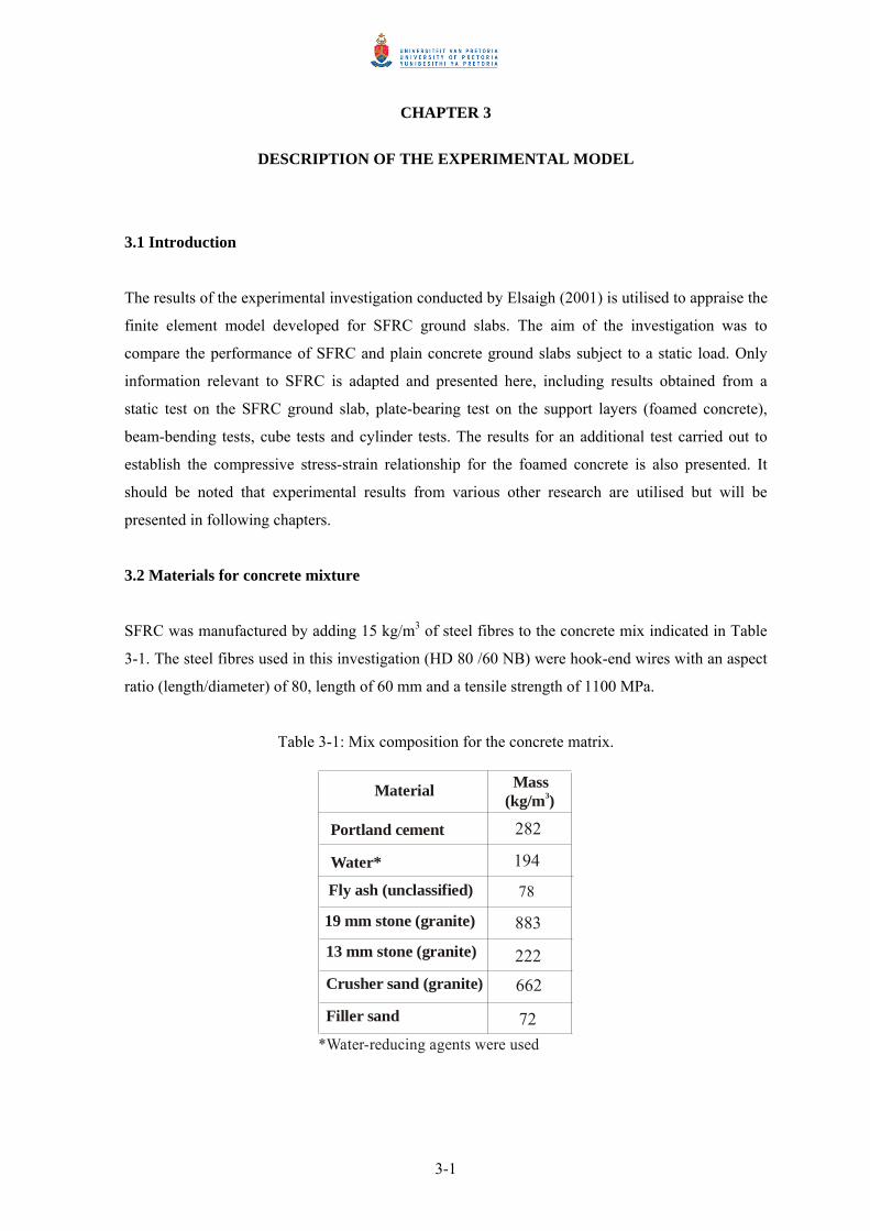
CHAPTER 3

DESCRIPTION OF THE EXPERIMENTAL MODEL

3.1 Introduction

The results of the experimental investigation conducted by Elsaigh (2001) is utilised to appraise the

finite element model developed for SFRC ground slabs. The aim of the investigation was to

compare the performance of SFRC and plain concrete ground slabs subject to a static load. Only

information relevant to SFRC is adapted and presented here, including results obtained from a

static test on the SFRC ground slab, plate-bearing test on the support layers (foamed concrete),

beam-bending tests, cube tests and cylinder tests. The results for an additional test carried out to

establish the compressive stress-strain relationship for the foamed concrete is also presented. It

should be noted that experimental results from various other research are utilised but will be

presented in following chapters.

3.2 Materials for concrete mixture

SFRC was manufactured by adding 15 kg/m3 of steel fibres to the concrete mix indicated in Table

3-1. The steel fibres used in this investigation (HD 80 /60 NB) were hook-end wires with an aspect

ratio (length/diameter) of 80, length of 60 mm and a tensile strength of 1100 MPa.

Table 3-1: Mix composition for the concrete matrix.

194

78

883

222

Material Mass (kg/m )3

Portland cement

Water*

Fly ash (unclassified)

19 mm stone (granite)

13 mm stone (granite)

Crusher sand (granite)

Filler sand

*Water-reducing agents were used

282

662

72

3-1

3.3 Slab test setup

A SFRC slab measuring 3000 x 3000 x 125 mm was cast on a foamed concrete slab resting on a

deep concrete floor. The dimensions of the SFRC slab and the support layers are shown in

Figure 3-1. The foamed concrete was chosen as a support material because it can readily be

moulded and kept bound until the end of the experiment. This was not possible with soil as

confining boundaries are necessary to contain earth layers. The foamed concrete and SFRC slabs

were cast in a shaded area and were covered by plastic sheets for 28 days before the tests were

conducted. Testing was conducted using a closed-loop testing system applying displacement at a

rate of 1.5 mm/min. The load was applied using a hydraulic twin jack pressing on a stiffened

loading plate (100 x 100 mm). The vertical displacements were measured by using Linear Variable

Displacement Transducers (LVDT). The LVDTs were mounted on a steel beam spanning over the

tested slabs.

P

Existing soil

High-strength concrete floor

Foamed concrete slabSFRC slab

Steel plate

3000

4000

125150

1000

Scale 1:50All dimensions are in mm

Figure 3-1: Layout of the slab test.

3.3.1 Plate-bearing test

A foamed concrete slab with casting density of 780 kg/m3 and measuring 8000 x 4000 x 150 mm

was cast on a concrete floor surface. The length of the slab was 8000 mm because the foamed

concrete slab was also used to support a plain concrete slab constructed adjacent to the SFRC slab.

The plate test was performed at the centre of the foamed concrete slab (between the concrete slabs)

thus preventing the densification of the support below both the SFRC and plain concrete slabs,

which would have influenced the results of the slab test. A plate-bearing test was conducted to

establish the load-displacement response (P-Δ) of the supporting material. A circular steel plate

with a diameter of 250 mm and a thickness of 40 mm was used.

Figure 3-2 shows the resulting P-Δ response from the plate-bearing test. It should be noted that this

response represents the behaviour of all the support layers together, including the interaction

3-2

between these layers, and not only the foamed concrete slab. The value of the modulus of the

subgrade reaction is determined as 0.25 MPa/mm. This is a relatively high value compared to the

values used for support layers made from soil materials often used for road pavements. The range

of values used for cement-stabilised soils is between 0.02 and 0.245 MPa/mm (Marais and Perrie,

2000). Both the stiffness of the foamed concrete and the rigid deep floor below the foamed

concrete played a role resulting in this high value for the modulus of the subgrade reaction.

0

50

100

150

0 1 2 3 4 5 6 7Displacement (mm)

Load

(kN

)

Figure 3-2: Load-displacement response from the plate-bearing test.

3.3.2 SFRC slab test

Figure 3-3 shows the setup for the slab test. The load was applied on a stiffened loading plate,

measuring 100 x 100 mm, placed in the centre of the slab.

Figure 3-3: Photo shows the set up for slab test.

The resulting P-Δ response is indicated in Figure 3-4. The SFRC slab sustained a maximum load at

a displacement of approximately 5 mm. Thereafter the load starts to decline. The maximum load

maintained in the test is approximately 655 kN.

3-3

0100200300400500600700

0 1 2 3 4 5 6 7 8 9 10 11 12Displacement (mm)

Load

(kN

)

Figure 3-4: The measured load-displacement response of the SFRC slab tested by Elsaigh (2001).

3.4 The beam test

Three beam specimens measuring 750 x 150 x 150 mm were cast using the same SFRC used for

the SFRC slab. The specimens were water cured for 28 days before testing. The beam tests were

conducted using a closed-loop Material Testing System (MTS) applying displacement at a rate of

0.02 mm/ second. The test set-up is shown in Figure 3-5. Mid-span deflections were measured by

using two LVDTs. The readings were taken at 100 Hz. The load was applied by using two bearing

rollers (one of them is a swivelling roller) 150 mm apart with their centre line coinciding with the

centre of the beam. The beam supports were 450 mm apart and bolted to the MTS testing bed. The

beams were cast and tested in accordance to the procedure prescribed by the Japanese Concrete

Institute (1983).

P /2 P /2

150 mm150 mm 150 mm

Beam cross-section 150 x 150 mm

Figure 3-5: Test setup for the beam-bending test.

3-4

Figure 3-6 shows the resulting P-δ response for the SFRC beams. Three behavioural stages can be

identified. In the second stage no data points were recorded (refer to the dotted line). This is

because the sequence of testing at this stage during the loading of the beam is faster than the

recording capability of the testing machine.

Range of experimental data

Deflection (mm)

Load

(kN

)

0 1 2 3 4 5

60

50

40

30

20

10

0

No data recorded

Figure 3-6: The load-deflection responses for the SFRC beams (Elsaigh, 2001).

Figure 3-7 shows the failure mode for the tested SFRC beams. The final failure is dominated by a

single major crack occurring at a plane close to the plane of symmetry. Although the beams have

cracked, they still did not disintegrate into two parts. This is due the bridging effect provided by the

steel fibres across the crack.

The plane of symmetry

Figure 3-7: photo shows the failure mode for the tested beams.

3-5

3.5 Cube and cylinder tests

Three cubes (150 x 150 x 150 mm) and two cylinders (150 diameter and 300 mm length) were

manufactured from the same material used in the SFRC slab and beams. They were water cured for

28 days before testing. The cubes were tested according to the procedure prescribed by Standard

Method: SABS Method 863:1994(1994) while the cylinders were tested according to the procedure

prescribed by the ASTM C 469-94a (1992). Six cores, with a 100 mm diameter, were taken from

different positions after the testing the SFRC slab. The cores were drilled, prepared and tested

according to SABS Method 865 (1982). The core strengths were converted to actual standard cube

strength using the conversion formula given in the British Concrete Society Technical Report No.

11 (Neville and Brooks, 1998). Apart from the cylinder test, the Young’s modulus is also estimated

using the results of the beam-bending test. The formula derived by Alexander (1982) is utilised as

indicated in Equation 3-1. The average results are summarised in Table 3-2.

Table 3-2: Compressive strength and Young’s modulus.

Cube strength (MPa)

Core strength (MPa)

Young’s modulus (GPa)

(Cylinder tests)

Young’s modulus (GPa)(Beam-bending tests)

47

52

27

28

( ) 323

.10μ1.d.1152161.

129623 (MPa) E

⎥⎥⎦

⎤

⎢⎢⎣

⎡+⎟

⎠⎞

⎜⎝⎛+=

LIL

δP. (3-1)

δP = The slop of the linear elastic part on the load-deflection response (N/mm2).

L = The supported span of the beam (mm).

I = The second moment of area of the beam cross-section (12bh 3

) (mm4).

h b, = The width and depth of the beam respectively (mm).

μ = Poisson’s ratio.

3-6

CHAPTER 4

MODELLING NON-LINEAR BEHAVIOUR

OF STEEL FIBRE REINFORCED CONCRETE

4.1 Introduction

The availability of steel fibres with a variety of physical and mechanical properties, as well as the

use of various fibre contents, tend to complicate prediction of the tensile stress-strain (σ-ε)

response of SFRC. The further complexities of testing concrete in direct tension and measuring

stresses and strains may be the reasons for the many proposed material models for SFRC.

However, the current international drive for establishing tensile σ-ε relationship for SFRC has

shifted towards inverse analysis (back-calculation) techniques. In these techniques flexural

response obtained from beam-bending test is used to back-calculate tensile σ-ε relationship.

Elsaigh et al. (2004) proposed a method to determine the tensile σ-ε relationship for SFRC utilising

experimental results obtained from beam third-point tests. Alena et al. (2004) have concurrently

proposed a similar method. Østergaard and Olesen (2005) and Østergaard et al. (2005) have

recently proposed an inverse analysis method that is based on the non-linear hinge concept

described by Olesen (2001). This method does however fall beyond the scope of this study.

In this chapter a generalised analytical method is proposed to determine the tensile σ-ε response for

SFRC. In this method the σ-ε relationship is determined from either the experimental moment-

curvature (M-φ) or load-deflection (P-δ) responses. A parameter study is conducted to not only

investigate the influence of each of the tensile σ-ε curve parameter on the M-φ and the P-δ

responses but also to serve as an aid to the user in adjusting the tensile σ-ε parameters.

4.2 Analysis method

In the analysis the M-φ and the P-δ responses are derived by assuming a σ-ε response. A trial and

error technique is followed, by adjusting the σ-ε relationship until the analytical results fit the

experimental results for either M-φ or P-δ. In the analysis, the following three-step procedure is

used to calculate the P-δ response of SFRC beams:

(1) Assume a σ-ε relationship for the SFRC.

(2) Calculate the M-φ response for a section; and

(3) Calculate the P-δ response for an element.

4-1

At the end of either steps (2) or (3) the results from the analysis are compared to experimental

results and adjustments are made to the σ-ε response until the analytical and experimental results

agree within acceptable limits.

4.2.1 Proposed stress-strain relationship The shape of the proposed σ-ε relationship used in this analysis is shown in Figure 4-1. The tensile

response is similar to that proposed by RILEM TC 162-TDF (2002) while the compression

response is assumed linear elastic up to a limiting strain εc0.

ε

σ

E

t0σ tu

σ cu

ε tu

ε cuε t0

ε c0ε t1

Tension

Compression

Figure 4-1: Proposed stress-strain relationship.

In Figure 4-1, σt0 and εt0 represents the cracking strength and the corresponding elastic strain. σtu

and εt1 represents the residual stress and the residual strain at a point where the slope of softening

tensile curve changes. εtu is the ultimate tensile strain. E is Young’s modulus for the SFRC. σcu and

εco are the compressive strength and the corresponding elastic strain. εcu is the ultimate compressive

strain.

The σ-ε relationship is expressed as follows:

( )( ) (( ) (⎪

⎪⎩

⎪⎪⎨

⎧

))<≤−+

<≤−+<≤<≤

=

tutttu

tttt

tc

ccucu

E

εεεεελσεεεεεψσεεεεεεεσ

εσ

11

1000

00

0

forforforfor

)(

(4-1)

Where: 0c

cuEεσ

=

01

0

tt

ttu

εεσσ

ψ−−

=

1ttu

tu

εεσ

λ−

−=

4-2

4.2.2 Moment-curvature response

The M-φ relationship at a section is calculated by making use of the following assumptions: • The σ-ε relationship of the material is known.

• Plane sections perpendicular to the centre plane in the reference state remain plane during

bending.

• Internal stress resultants are in equilibrium with the externally applied loads.

As part of the first assumption, the σ-ε relationship proposed in equations (4-1) is used and initial

values are assumed for the parameters. The second assumption applies to slender beams and

implies a linear distribution of strain so that the following relationships exists at a section (see

Figure 4-2b):

bottop ahy

ayy εεε ⎟

⎠⎞

⎜⎝⎛

−==)( (4-2)

b

h

dyy

a

ε top

φ

ε (y)σ ε( )

ε bot(a)

Cross section(b)

Strain(c)

Stress

(d)Stress

resultants

MF = 0N.A.

Figure 4-2: Stress and strain distributions at a section.

The final assumption is used to find the axial force F (which is equal to zero) and moment M

(which is equal to the applied moment):

( ) 0)()(

=== ∫∫ −−top

bot

dbadybFtop

aah

εε

εεσε

εσ (4-3)

( ) ∫∫ −==−−

top

bot

dbadybyMtop

aah

εε

εεεσε

εσ 2

2

)()( (4-4)

4-3

At a typical section there are two unknowns necessary to describe the strain distribution. For a

given strain distribution the stresses at a section (see Figure 4-2c) can be calculated using the σ-ε

relationship and equations (4-3) and (4-4) can be used to solve the two unknowns. The curvature at

a section is given by:

( )ahabottop

−==

εεφ (4-5)

The following procedure is followed to obtain the M-φ relationship:

(1) A value is selected for the bottom strain εbot.

(2) The top strain εtop is solved from equation (4-3) by following an iterative procedure in which

εtop is changed until F = 0.

(3) M and φ is calculated from equations (4-4) and (4-5) respectively. This produces one point on

the M-φ diagram.

(4) A new εbot is selected and steps (1) to (3) are repeated to until sufficient points have been

generated to describe the complete M-φ relationship.

4.2.3 Load-deflection response

The total deformation of a beam consists of two components: that is extension caused by the

moments (ε.dx) and shear distortion (γ.dx) caused by the shear force (Refer to Figure 4-3).

γγ.dx

dxdy

ε.dx

dydx

dydx

τ

τ

σσ

(a) (b) (c)

Figure 4-3: Differential element from the beam.

Because the effects of shear deformations on deflection of beams are usually relatively small

compared to the effects of flexural deformations, it is common practice to disregard them. However

for short beam specimens of the type normally specified for laboratory testing, the span-depth ratio

lies in the range of 3 to 4 and therefore shear stresses will contribute significantly to the total

deflections of the beam. At any loading point during the loading process, the total deflection of a

beam ( ) is estimated as the sum of the deflection due to moments ( ) and the deflection due to

shear forces ( ). The unit-load method is used to obtain the total deflection by integrating

curvature (

δ mδ

Vδ

EIM=φ ) and shear strain ( GAshfV .=γ ) along the beam (Refer to Equation 4-6).

4-4

∫∫ +=+=L

sh

LuL LuVm fGA

dxVVEI

dxMM

0

0

..δδδ (4-6)

Where: and are the moments due to a unit load and actual load respectively, uM LM EI is the

flexural rigidity, and are shear forces due to unit load and actual load respectively, uV LV shfGA

is the shearing rigidity of the beam (Gere and Timoshenko, 1991), is the factor for shear

(equals 6/5 for rectangular section).

shf

The deflections due to moments ( ) are calculated from the distribution of the curvature due to

moment (

mδ

φ ) along the beam where φ replaces EIMu in Equation (4-6). Consider the beam in

Figure 4-4(b) subjected to a variable load P. For moments up to the maximum moment Mm the

curvature is obtained from the M-φ relationship in Figure 4-4(a) yielding the dashed line in Figure

4-4(b). Beyond this point the analysis effectively switches to displacement control. It is assumed

that material having reached Mm (part BC of the beam) will follow the softening portion of the M-φ

relationship. For example; if the curvature in BC increases to φc, the moment will reduce to Mc.

Equilibrium requires the moments in parts AB and CD of the beam to reduce and the material here

is assumed to unload elastically, producing smaller curvatures for these parts. This is because

tensile stresses on the end thirds of the beam decrease as the crack width in the middle third

increases.

φφ m φ c

φ m

φ c

Mm

Mm

M

Mc

Mc

P/2 P/2

(a) Moment-curvature relationship

(b) Moment and curvatures distributions for an applied load P

A DB C

MP L

=6

L/3 L/3 L/3

Figure 4-4: Finding the moment-curvature distribution along the beam.

4-5

The deflections due to shear forces ( Vδ ) are calculated from the distribution of the shear strain (γ )

along the beam. Referring to the load configurations shown in Figure 4-5(b), the shear deflection in

the beam is due to the shear forces in part AB and CD. The fact that these two parts unload

elastically at the onset of the flexural cracks in part BC has resulted in less complexities compared

to that followed for the M-φ analysis. At any stage throughout the loading process of the beam,

shear strains on the γ−V response shown in Figure 4-5(a) are calculated using the measured P-δ

response by dividing the shear force by the shearing rigidity. This means the effect of shear forces

on deflection increases to reach the maximum at the peak load and decreases with increasing

displacement beyond this peak load.

The distribution of elastic shear strain (γ) through the depth of beams with un-cracked rectangular

sections is parabolic. As a result of shear strains, cross-sections of the beam that were originally

plane surfaces become warped. For the beam set up in Figure 4-4(b) and Figure 4-5(b), the shear

deformation is zero in the constant moment zone (BC). For this reason, it is justifiable to use the

bending formula derived for pure bending. The effects due to shear and moment were calculated

separately. The superposition concept was used to calculate the total deflection as the sum of both

effects. Therefore, the approach used is deemed to be sufficiently accurate. Care should be taken

when using this approach to calculate the P-δ response for beams having different loading

configurations.

γγ mγ c

γγ

Vm

Vm

V

Vc

V c

P /2 P /2

(a) Shear force - shear strain relationship

(b) Shear forces and shear strain distributions for an applied load P

A DB C

V P=2

L /3 L /3 L /3

Figure 4-5: Finding the shear-shear strain distribution along the beam.

It is generally accepted that the area under the tensile σ-ε curve represents the fracture energy. The

characteristics of the softening part of the tensile σ-ε curve is largely dependent on the size of the

4-6

element in which the crack occurs. When calculating the P-δ response using the method presented

here, the beam was divided into three elements and the crack was smeared over the constant

moment zone (part BC of the beam). It was also assumed that an infinite number of layers

(elements) exist through the depth of the beam. Therefore element size should carefully be selected

when using the calculated tensile σ-ε curve in finite element analysis.

4.2.4 Implementation of the analysis method

The experimental results obtained by Lim et al. (1987 a and b) are used to implement and test the

proposed analysis method by comparing calculated M-φ and P-δ responses to the experimental

results. In their experimental programme, SFRC specimens were tested in compression, direct

tension and flexure. Two series each of four mixes were cast. Only results of specimens containing

0.5 percent by volume (40 kg/m3) of hooked-end steel fibres, with 0.5 mm diameter and 30 mm

length, are discussed here. Figure 4-6 indicates the specimen size and test set up for direct tension

and flexural tests. The tensile specimens were tested in direct tension by a pair of grips on a servo-

controlled testing machine. The extension rate was set at 0.25 mm / min. The extensions were

monitored over a gage length of 200 mm. The flexural beam tests over a simply supported span of

750 mm and loaded at the third-point (refer to Figure 4-6(b)). The P-δ response was established

directly from the measurement. The curvature was derived from the strain readings using electrical

gages bonded onto the top and bottom faces of the beam. The average compressive strength and

Young’s modulus for the SFRC were determined as 34 MPa and 25.4 GPa respectively.

P /2 P /2

Beam cross-section 100 x 100 mm100 mm70 mm

100 mm

250 mm50 5075 75250 mm 250 mm 250 mm

(a) Direct tension specimen (b) Test set up for flexural test

Figure 4-6: Direct tension and flexural specimens tested by Lim et al. (1987 a and b).

The method proposed here was set up using Mathcad (2001). The shape of the tensile σ-ε

relationship is assumed as in Figure 4-1. The first estimation of for σt0, εt0, σtu, εt1, and εtu is made

based on the results of the direct tension test. A trial-and-error procedure is followed to adjust these

parameters until the calculated M-φ and P-δ responses match the experimental responses (refer to

4-7

Appendix B). Figure 4-7 shows the tensile σ-ε relationships predicted using the analysis method

and measured from direct tension test. Note that no experimental data were recorded immediately

beyond the maximum tensile stress.

Tens

ile st

ress

(MPa

)

0.002 0.004 0.006 0.008 0.01 0.012 0.014

Strain

Analysis methodExperimental

3.53

2.52

1.51

0.50

0

Figure 4-7: Assumed tensile stress-strain relationship for comparison

to experimental results of Lim et al. (1987 b).

Figure 4-8 shows the correlations between calculated and experimental M-φ and P-δ responses.

The analyses show some similarity between the shapes of the σ-ε relationship, the M-φ and

P-δ responses although they differ in magnitude. The analysis has however shown that the point

where the maximum tensile stress (2.8 MPa) in the material is first reached occurs in the pre-peak

regions of both the M-φ and P-δ responses (see the arrows of Figure 4-8). This means that to utilise

the full tensile capacity of the material, the analysis should incorporate the non-linear material

properties.

6Curvature (1/m) Deflection (mm)

Mom

ent (

kN-m

)

Load

(kN

)

0.02 0.10 0.060.04

2

0.08

0.2

0.6

0

0.8

0.4

1

0

4

6

8

0 1 2 53 4

ExperimentalAnalysis method

Figure 4-8: Experimental (Lim et al., 1987 a) and calculated M-φ and P-δ responses.

Figure 4-9 shows the comparison between tensile σ-ε relationships, developed using the various

models, and the resulting M-φ responses. The models proposed by Lim et al. (1987 a), Nemegeer

4-8

(1996) and Lok and Xiao (1998) were used to determine the tensile σ-ε relationship for the SFRC

tested by Lim et al. (1987a). The comparison excluded the models developed by Vandewalle

(2003) and Dupont and Vandewalle (2003), as they require results from notched beam test.

0 0.5 1.0 1.5 2.0 2.5 3.0 3.50

0.51

1.52

2.53

3.5

Strain x10- 4

Tens

ile st

ress

(MPa

)

Curvature (1/m)

Mom

ent (

kN-m

)

0.02 0.10 0.060.04 0.08

0.2

0.6

0

0.8

0.4

1

Experimental Lim et al. (1987a) Nemegeer (1996)

Analysis method (This study)

Lok and Xiao (1998a)

Figure 4-9: Correlation between tensile stress-strain responses determined using various models.

The main difference between these four models is the value of the residual strain (εt1), The

assumption made in the model of Lim et al. (1987 a) where εt1 is equal to the cracking strain (εt0)

resulted in a larger divergence between the experimental and calculated M-φ response in the region

immediately beyond the maximum moment. The higher value for σtu determined using the model

of Nemegeer (1996) resulted in an increased moment for the last part of the M-φ response.

Figure 4-10 shows the contribution of deflections due to shear as percentage of the total deflection.

The percentage of shear deflections up to the cracking point (εt0) is constant at approximately 4

percent. The contribution of shear deflection varies significantly beyond the cracking point of the

beam and it decreases to approximately 0.2 percent at the point of residual strain (εt1).

0

1

2

3

4

0 0.001 0.002 0.003 0.004 0.005 0.006 0.007 0.008

Shea

r def

lect

ion

Tota

l def

lect

ion

x 10

0

Tensile strain

εt1

εt0

Figure 4-10: Contribution of shear deflection to the total deflection of the beam.

4-9

For the beam with the dimensions and setup shown in Figure 4-6 (b), the contribution of shear to

the total deformation of the beam is negligible. This is not surprising as the span-depth ratio for this

beam is 7.5, which is sufficiently large to alleviate the effect of shear stresses on the mid-span

deflection. However, for deeper beam specimens the effect of shear deflection will be more

pronounced. For example, a beam measuring 150 x150 x 750 mm loaded at its third points and

supported over a span of 450 mm will result in a maximum shear deflection approximately 18

percent of the total shear refer to Appendix C). Thus shear deformation can be crucial with respect

to the tensile σ-ε relationship as the former is back calculated by fitting measured and calculated

P-δ responses.

The merit of the analysis procedure presented here is that it uses measured M-φ or P-δ responses

obtainable with minimal testing complexities compared to procedures requiring results from direct

tensile tests. In addition, the method utilises a macro approach as the influence of the steel fibre

parameters and the concrete matrix are reflected in the measured M-φ or P-δ responses. This is seen

as an advantage compared to procedures utilising a micro approach in which the fibre properties,

the concrete matrix properties and the fibre-matrix interaction have to be known.

4.3 Parameter study

The parameter study is conducted by changing parameters on the tensile σ-ε curve and then

calculating M-φ and P-δ responses using the analytical method described in section 4.2. The

parameters that define the tensile σ-ε of the SFRC (see Figure 4-1) are:

• Cracking strength σt0 and corresponding cracking strain εt0,

• Residual stress σtu and corresponding strain εt1, and

• Ultimate strain εtu.

In the analysis, only one parameter will be changed at a time while keeping all the other parameters

fixed. The main objective of the parameter study is to investigate the influence of the σ-ε

parameters on M-φ and P-δ responses. Subsequently, a systematic approach can be followed

leading to a faster arrival at the material σ-ε response. A secondary objective is to give an insight

into the behaviour of SFRC.

Hypothetical beams assumed for the parameter study have a section size of 150 x 150 mm and a

supported span of 450 mm. A Mathcad (2001) work sheet is set up and prepared to carry out the

calculations. Fifteen analyses were conducted (see Appendix B for sample of calculations).

4-10

4.3.1 Effect of changing cracking strength or corresponding strain

Figure 4-11(a) shows three σ-ε curves where only the tensile and compressive strengths are

changed, while in Figure 4-11(b) only the cracking strains are changed. These parameters are

studied together since changes to them also influence Young’s modulus. Three values for Young’s

modulus commonly encountered are investigated viz. 15, 25 and 35 GPa. When changing the

cracking strengths, the corresponding compressive strengths are assumed to be ten times the

magnitude of the cracking strengths while a reasonable fixed value is assumed when changing the

cracking strains.

15 GPa

25 GPa

35 GPa

εε

5.253.752.252.0

1.5e-4

15e-

4

-1.5

e-3

0.1

- 52.5- 37.5- 22.5

4.0

2.0

1.14

e-4

1.6e

-4 0.1

- 35

2.7e

-415

e-4

-1.0

e-3

-2.3

e-3

-1.4

e-3

(a) Changing strength (b) Changing elastic strain

σ (MPa)σ (MPa)

(Not to scale)(Not to scale)

E =

Figure 4-11: Stress-strain curves - changing cracking strength and corresponding strain.

The approximation with respect to the ratio between compressive and cracking strength (equals 10)

is justified by experimental results reported in other research. For example, Kupfer et al. (1969)

reported that the ratio of uniaxial cracking strength to compressive strength of concrete amounts to

0.11, 0.09, and 0.08 for concrete with compressive strength of 19, 31.5 and 59 MPa respectively

(refer to Figure 2-12 in section 2.3.5.4). The effect of steel fibres on these ratios is expected to be

insignificant. This is because the addition of steel fibre to concrete results in a marginal increase in

compressive strength (Burgess, 1992, Elsaigh, 2001) while the steel fibres are only active in

tension after the initiation of a crack in SFRC resulting in a negligible, or no increase in cracking

strength. The approximations made herein are thus considered reasonable for the types of normal

strength concrete often used in pavement applications.

It is worth noting that the relations between tensile and compressive strength, as well as Young’s

modulus can be significantly different to the approximations considered here, or specifically

4-11

engineered to be different, for some other cement-based composites, which is beyond the scope of

this research.

Figure 4-12 shows that an increase in tensile and compressive strength (and increase in Young’s

modulus), results in an increase in the magnitude of peak moment and peak load on the M-φ and

P-δ curves respectively. For example, increasing the cracking strength by 40 percent (from 3.75 to

5.25 MPa) leads to an increase on the peak load of approximately 36 percent. The pre-peak slope of

the curves as well as the slope immediately beyond the peak moment and the peak load become

steeper with increased strength. Although the M-φ and P-δ curves are curtailed to show only the

segments most affected by changing tensile stress, the complete responses indicate that the values

of moment and load reduce to zero when the tensile stress on the σ-ε curves reduces to zero.

0.1 0.2 0.3 0.4 0.50.00

20

60

80

40

456

32

01

0.00 0.080.02 0.04 0.06 0.10

Deflection (mm)Curvature (1/m)

Load

(kN

)

Mo m

ent (

kN.m

)

15 GPa25 GPa35 GPa

E =

Figure 4-12: Effect of changing strength on M-φ and P-δ responses.

Referring to Figure 4-13, an increase in cracking strain (which decreases Young’s modulus) results

in a decrease in the magnitudes of peak moment and peak load, while also increasing the curvature

and deflection corresponding to these peak values. For example, increasing the cracking strain by

69 percent (from 1.6 x10-4 to 2.7 x10-4) leads to an increase on the peak load of approximately 1.9

percent. Therefore, the change in the value of cracking strain is considered to result in a negligible

change in the values of peak moment and peak load. This also correlates well with the findings

presented in Figure 4-9. The slope of the first part of the curves as well as the slope immediately

beyond the peak moment and peak load decreases as Young’s modulus decreases. The M-φ and P-δ

curves are curtailed to show only the segments most affected by changing elastic strain (refer to the

discussion on Figure 4-12).

4-12

0

20

60

4030

50

10

0.1 0.2 0.3 0.40.0

4

5

3

2

0

1

0.00 0.020.005 0.01 0.015 0.030.025


Load

(kN

)

Mo m

ent (

kN.m

)

15 GPa25 GPa35 GPa

E =

Figure 4-13: Effect of changing elastic strain on M-φ and P-δ responses. 4.3.2 Effect of changing residual stress or corresponding strain

Changing the residual stress or the residual strain influences the slope of both curves beyond the

cracking strength of the σ-ε curve. On this part of the curve, the steel fibre parameters and content

play a major role in the composite tensile behaviour. As indicated in Figure 4-14(a) and Figure

4-14(b), two sets of analyses are performed. In the first set the magnitude of residual stress is

changed while in the second set the magnitude of residual strain is changed. A constant

compressive strength value, equal to ten times the cracking strength, is assumed in these two sets of

analysis.

ε

3.752.51.50.5

1.5e

-4

15e-

4

-1.5

e-3

0.1

-37.5

(a) Changing residual stress

σ (MPa)

25 G

Pa

ε

3.75

20e-

4

1.5

10e-

41.

5e-4

15e-

4

-1.5

e-3

0.1

-37.5

(b) Changing residual strain

σ (MPa)

25 G

Pa

10e-415e-420e-4

0.5 MPa1.5 MPa2.5 MPa (Not to scale)(Not to scale)

σtu = εt1 =

Figure 4-14: Stress-strain curves for SFRC - changing residual stress or residual strain.

Figure 4-15 indicates that increasing the residual tensile stress shifts up the last part of the M-φ and

P-δ responses while increasing the peak moment and the peak load. The increase in the elevation of

the last part is significant while the increase in peak moment and load is little. For example,

increasing the residual stress by 67 percent (from 1.5 to 2.5 MPa) increases the elevation of the last

4-13

part of the M-φ and P-δ responses an increases the peak load by approximately 67 percent and 4

percent respectively. It also flattens the part of the curve immediately beyond the peak moment and

the peak load. The M-φ and P-δ curves are again curtailed to only show the segments most affected

by changes in residual stress (refer to the discussion on Figure 4-12).

0.00 0.40.1 0.2 0.3 0.5

4

5

3

2

0

120

60

40

30

50

10

00.2 0.4 0.6 0.80.0 1.0

Curvature (1/m) Deflection (mm)Lo

ad (k

N)

Mom

ent (

kN.m

)

0.5 MPa

1.5 MPa

2.5 MPa

σtu =

Figure 4-15: Effect of changing residual stress on M-φ and P-δ responses.

Figure 4-16 shows that increasing the residual strain increases the peak moment and the peak load

as well as the corresponding curvature and deflection. For example, increasing the residual strain

by 33 percent (from 15x10-4 to 20x10-4) leads to an increase in the peak load of approximately 2

percent. In the process of determining the σ-ε relationship, the residual strain can be used to make

small corrections to the peak moment, peak load and the corresponding curvature and deflection.

The M-φ and P-δ curves are one more curtailed to show only the segments most affected by

changes in residual strain (refer to the discussion on Figure 4-12).

0.2 0.4 0.6 0.80.0

Load

(kN

)

20

60

40

30

50

100

Mom

ent (

kN.m

)

4

5

3

2

1

00.00 0.080.02 0.04 0.06


10e-415e-420e-4

εt1 =

Figure 4-16: Effect of changing residual strain on M-φ and P-δ responses.

4-14

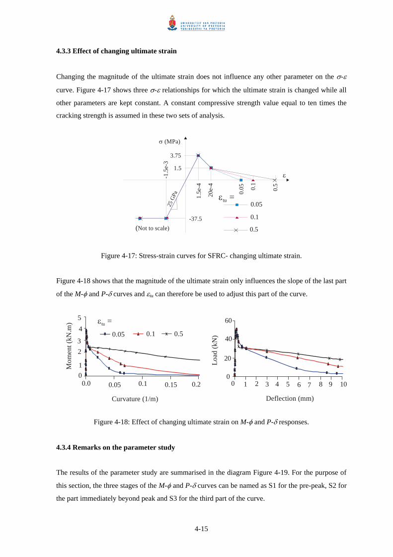
4.3.3 Effect of changing ultimate strain

Changing the magnitude of the ultimate strain does not influence any other parameter on the σ-ε

curve. Figure 4-17 shows three σ-ε relationships for which the ultimate strain is changed while all

other parameters are kept constant. A constant compressive strength value equal to ten times the

cracking strength is assumed in these two sets of analysis.

ε

3.75

0.5

1.5

0.05

1.5e

-4

-1.5

e-3

0.1

-37.5

σ (MPa)

25 G

Pa 20e-

40.05

0.1

0.5(Not to scale)

εtu =

Figure 4-17: Stress-strain curves for SFRC- changing ultimate strain.

Figure 4-18 shows that the magnitude of the ultimate strain only influences the slope of the last part

of the M-φ and P-δ curves and εtu can therefore be used to adjust this part of the curve.

20

60

40

02 4 6 80 10975310.0 0.20.05 0.1 0.15

45

32

10

Curvature (1/m) Deflection (mm)

Load

(kN

)

Mom

ent (

kN.m

)

0.05 0.1 0.5

εtu =

Figure 4-18: Effect of changing ultimate strain on M-φ and P-δ responses.

4.3.4 Remarks on the parameter study

The results of the parameter study are summarised in the diagram Figure 4-19. For the purpose of

this section, the three stages of the M-φ and P-δ curves can be named as S1 for the pre-peak, S2 for

the part immediately beyond peak and S3 for the third part of the curve.

4-15

Decreases the slope of S2

Increasing residual strength

Increases the slope of S1

Increases the elevation of S3

Decreases the slope of S3 Increasing ultimate strain

Increases the peak and M P

Increasing tensile strength

Increasing elastic strain


Increasing residual strain






Figure 4-19: Summary of the parameter study.

The assumed σ-ε relationship was successfully used to calculate the M-φ and P-δ responses and

therefore the process can be reversed to calculate a σ-ε relationship for SFRC if either the M-φ or

P-δ response is available. In fact, the calculated σ-ε response will be more accurate if the M-φ

response is used as fewer assumptions are involved in the analysis compared to the experimental

P-δ response. However, measuring the P-δ response is relatively common and much simpler than

measuring the M-φ response.

The parameter study highlighted that changing different parameters of the material can have a

similar influence, but with different magnitude, on the M-φ and P-δ responses. For example, an

increase in the peak load on the P-δ response can be achieved by changing one of four parameters

as shown in Figure 4-19. However, the most significant influence on the M-φ and P-δ responses is

obtained due to changes in the values of σt0. This is because the changes in the values of σtu, εt0, εt1

and εtu are considered to be too small compared to possible changes in the value of σt0. It should

not be deduced that the actual tensile σ-ε relationship for a particular SFRC is not unique as only

one parameter of the σ-ε relationship is changed while keeping all the other parameters fixed.

4-16

However, these parameters are interrelated in some cases and therefore changing the value of one

parameter leads to changes in the values of the other parameters. For example, changing the tensile

and compressive strengths is expected to influence the residual strength. This is because the

strength of concrete affects the characteristics of the fibre-matrix bond and thus influences the

post-cracking behaviour of the SFRC. Although the σ-ε relationships used in this analysis might

not represent realistic σ-ε responses, the results of the analysis are only indicative of the isolated

effect of each of these parameters.

The method proposed here makes use of a small number of assumptions. The major assumption is

the shape of the σ-ε relationship. The method can be applied to any selected σ-ε relationship that

contains an appropriate number of parameters to model the observed typical M-φ or P-δ response.

The proposed method is numerically demanding and therefore most suitable for computer

applications. The numerical solution capabilities of programs such as Mathcad (2001) can greatly

assist in the implementation of the method.

4.3.5 Initial estimation for the stress-strain relationship

An initial guess is required when determining the σ-ε relationship for SFRC. The initial guess will

be adjusted using information obtained from the parameter study conducted here. Based on the

experience gained from the analyses conducted in the previous sections, the following steps are

recommended for calculation of the σ-ε relationship:

(1) Establish the compression σ-ε relationship. Make a first estimate for the tensile σ-ε response.

(2) Assuming Young’s modulus is valid for tension too, adjust the peak M and peak P by

changingσt0.

(3) Make adjustment to the elevation of S3 by changing σtu. This will slightly change peak M,

peak P and the slope of S2.

(4) Make adjustments to the slope of S3 by changing εtu. This will slightly change the elevation.

(5) Make a small adjustment to the slope and elevation of S3 by adjusting the εt1. This will slightly

change the peak M and peak P.

(6) Make final correction to the peak M, peak P and the slope of S1 by changing either εt0 and / or

σt0. In step (1), the compression σ-ε relationship is established using the cube compressive strength

( ) and Young’s modulus (E) for the FRC. The value of and cuf cuσ cuε can be approximated as

and 0.0035 respectively. For the first estimate of the tensile σ-ε relationship, the following

general guidelines can be used:

cuf

4-17

• For plain concrete, the ratio between uni-axial tensile and compressive strength usually

ranges from 0.085 to 0.11 (Chen, 1982). Based on this ratio, the value of σt0 for SFRC can

be estimated as 0.1 times . cuf

• Assume that Young’s modulus generated from compression tests is valid for tension and

calculate εt0.

• Estimate σtu, as a percentage of σt0. The estimation can be based on the ratio between

flexural strength and the post-cracking strength values as provided by the steel fibre

manufacturer. For example, σtu can be estimated as 42 percent of σt0 if 15kg/m3 of RC-

80/60-BN hooked-end steel fibre is used, (Refer to the Table A-1 in Appendix A).

• Based on the recommendations of the RILEM TC 162-TDF (2002), the values of εt1 and εtu

can be estimated as (εt0 + 0.001) and 0.1 respectively.

4-18

CHAPTER 5

NON-LINEAR FINITE ELEMENT

ANALYSIS FOR SFRC BEAM

5.1 Introduction In this chapter, a brief description for the finite element programme is presented. The σ-ε

relationship is determined for SFRC containing 15 kg/m3 of hook-end steel fibres using the

proposed analysis method explained in chapter 4. A non-linear finite element model is proposed to

analyse the SFRC beam using the calculated σ-ε relationship. The results from the finite element

analysis are tested by comparison to experimental results presented in section 3.4. The aim of this

chapter is to determine and test the σ-ε relationship that will later be used to analyse a SFRC

ground slab manufactured using the same materials.

5.2 A brief description of the finite element programme

The MSC.Marc is a general-purpose finite element programme. It has the capability to analyse

SFRC structures by utilising the cracking model for low-tension materials. This cracking model

adopts single fixed crack formulations. Accordingly, a crack develops at an integration point

perpendicular to the direction of the maximum principal stress if the maximum principal stress in

the material exceeds the specified value. After an initial crack has formed, a second crack can form

perpendicular to the first crack. For perfectly smooth crack surfaces this assumption is always

correct, but if some residual shear stiffness is introduced, the cracks might occur at other angles.

The cracking model implemented in MSC.Marc does not cater for such effect. It is worth noting

that the choice of the single-fixed crack approach was made based on the availability of the finite

element programme.

The material loses all load-carrying capacity across the crack unless tension softening is included.

Stresses are transmitted between the crack faces according to the softening part of the σ-ε response.

These stresses diminish until there is no stress across the crack, thus no load carrying capacity

exists in tension. After crack formation, the loading can be reversed due to the redistribution of

stresses. In this case, the crack can close again, and partial stitching occurs. After load removal all

strains return to zero as indicated in Figure 5-1. When stitching occurs, it is assumed that the crack

has full compressive stress-carrying capability. In the analysis, provision is made for the

compressive strains to increase beyond the yield point. In this case, it is necessary to combine the

material model with yielding criteria defining the multi-axial stress state. The programme provides

5-1

several mathematical models to describe the yielding surface for concrete that can be incorporated

into the analysis. In analysis involving compression-compression and tension-tension, the yield

surfaces can be combined with crack detection surfaces to describe both the cracking and yielding

behaviour of the material.

ε

σ

E u

Figure 5-1: Unloading behaviour adopted in MSC.Marc.

The softening behaviour is characterised by a descending branch in the tensile σ-ε response. The

cracks at an integration point are uniformly distributed (smeared) over the area representing the

integration point. In view of that, the choice for the element size is vital to the results of the

analysis as the softening behaviour is dependent upon the fracture energy released after initiation of

cracking. In the programme, provision is made for input of a linear softening response. However,

the linear softening response is expandable to a bilinear or higher order response by writing special

subroutines as permitted in the programme.

The non-linear finite element analysis requires that the tolerance on convergence as well as the

maximum and minimum number of recycles needed to obtain convergence should be specified.

Two loading schemes are available, the fixed load increment and the automatic load increment

scheme (i.e. arc-length method). Different solution algorithms are available and can be employed in

the analysis. If the inputs to the programme are correct, convergence can be obtained by changing

the convergence tolerance, load increment scheme, iteration limits or the solution algorithm.

In non-linear finite element analysis, it is necessary to apply the load in increments and let each

load increment iterate to equilibrium state, within a specified tolerance, using a particular iteration

scheme. In MSC.Marc, the loads can be applied through the use of “time” curves. The “time” value

represents a variable, which denotes the intensity of the applied loads at a certain step. The choice

of “time” step size depends on several factors such as the level of non-linearity of the problems and

the solution procedure. The complete load history can be divided into several phases, where each

phase is applied at a specific time in the load history. Each phase applied in a specific time period

5-2

can be considered as a load case. In this way, the complete loading history can be defined. Note

that a load case is not necessarily identical to a load step. A load case may consist of several load

steps to reach the total load of the load case.

5.3 Stress-strain relationship

The method proposed in chapter 4 is utilised to calculate the σ-ε response using the measured P-δ

response for SFRC beam containing 15 kg/m3 of hook-end steel fibres. The concrete mix, test setup

and testing procedure are presented in chapter 3. A summary of the beam properties utilised in the

analysis are indicated in Table 5-1.

Table 5-1: Properties used in the numerical analysis

Young’s modulus

Poisson’s ratio

Cube strength

28 GPa

0.2

45 MPa

Form factor for shear 6/5

RemarkProperty Value

Measured ( )∗

Assumed

Measured ( )∗

Square section

(*) Average value

A first estimate of the tensile σ-ε relationship is shown in Figure 5-2 (a). The first estimation is

made based on the recommendations presented in section 4.3.5. The calculation using this response

is presented in Appendix C. The P-δ response using the first estimate is presented as dotted curve

in Figure 5-2(b).

0.1

11.6

e-4

16 e

-5

4.5

1.9-16e

-4

28 G

Paε

- 0.0

4

(Not to scale)

σ (MPa)

- 45.00

102030405060

Load

(kN

)

0 1 2 3 4 5

Deflection (mm)


Numerical analysis (First estimate)

(a) First estimate for the stress-strain response (b) Comparison between calculated and

measured load-deflection responses

Figure 5-2: First estimate for the stress-strain response for SFRC.

5-3

Figure 5-2(b) shows that the first estimate for the σ-ε relationship results in a peak load that is

slightly high while the elevation of the third segment of the P-δ response is too high. In the light of

the parameter study presented in chapter 4, the first adjustment is done to the P-δ response by

reducing the value of residual stress (σtu). A trial-and-error procedure is followed until the correct

elevation of the third segment of the curve is maintained. In the second step, the peak load is

decreased by reducing the value of the cracking strength (σt0). Finally, a reasonable match between

theoretical and experimental P-δ responses is achieved by minor changes in the values of the

residual strain (εt1) and the ultimate strain (εtu). The strategy to be followed for the trial-and-error

procedure is to apply a coarse reduction or increase step to the specific parameter while using finer

steps towards the close matching for the particular part of the adjusted curve. The adopted σ-ε

relationship and the calculated P-δ responses are shown in Figures 5-3 and 5-4 respectively. Close

agreement is found between the analytical and experimental results. Refer to Appendix C for the

calculation of the adopted σ-ε response.

- 45.0

4.2

13e-4

Tension (+)

Compression (-)

0.08

1.1

(Not to scale)

E=28

GPa

(MPa)σ

ε

Figure 5-3: Calculated stress-strain response for SFRC (15 kg/m3 hook-end steel fibres).

First crack

0 1 2 3 4 5

Deflection (mm)

0

10

20

30

40

50

60

Load

(kN

)

Numerical analysis (Adopted response)


Figure 5-4: Comparison between calculated and measured P-δ responses.

5-4

The recommendations presented in section 4.3.5 used to provide the first estimate is found to

overestimate the value of σtu by approximately 70 percent. This can be considered in future

analyses when giving initial estimation for the σ-ε response. However, the criterion to estimate the

remaining parameters of the σ-ε response is found to be adequate since it provided a close

estimation and therefore minor adjustments were required to determine the adopted response.

The analysis has shown that the point where the tensile stress (4.2 MPa) in the material is first

reached occurs in the pre-peak regions of the P-δ responses (see arrow in Figure 5-4). This

emphasises the fact that elasticity theory under-estimates the load carrying capacity for particular

structures. For example, for the analysis conducted here the peak load (52 kN) is higher by

approximately 63 percent compared to the load at the first crack (32 kN). Full tensile capacity of

the SFRC is only utilised when the analysis proceeds beyond the σt0 point. It is worth mentioning

that the peak load on the P-δ response corresponds to a tensile stress located in the part of the σ-ε

relationship between εt0 and εt1 (the first branch of the softening curve). These findings correlate

well with the analysis presented in section 4.2.4.

Figure 5-5 shows the comparison between the proposed and the output compressive σ-ε responses.

The compressive strain exceeds the value for εc0 (= 1.6 × 10–3) only at the last two points. In the

calculated P-δ responses, these two points correspond to deflections that are greater than a

deflection limit of 3 mm. The value of 3 mm represents the serviceability limit for deflection for

this beam (span/150) as prescribed by the procedure of the Japanese Institute of Concrete

(JCI-SF4, 1983). This means that within the desired practical part of the P-δ response, the

behaviour is dominated by cracking while the compression side of the beam remains elastic.

-50

-40

-30

-20

-10

0-0.0035 -0.0025 -0.0015 -0.0005

Strain

Stre

ss (M

Pa)Proposed Output

Figure 5-5: Proposed and output compressive stress-strain relationship.

5-5

5.4 Finite element analysis of a single element

A special cracking subroutine is developed to enable the input of a bilinear curve for the softening

part of the tensile σ-ε response of SFRC (refer to Appendix C). A single element subject to direct

tension is analysed to verify the developed subroutine. The direct tension is necessary to avoid

possible crack rotation in the analysed boundary problem. Hence, the numerical simulation of the

single-fixed crack approach implemented in the MSC.Marc fits the direction of the physical crack

that is expected to occur. If the input and the output σ-ε responses thoroughly match then the

developed subroutine is deemed to be correct.

Figure 5-6: shows the single finite element and the boundary conditions. Element type 3 of

MSC.Marc is used. It’s a four-node quadrilateral element developed for plane stress applications.

The displacements of the nodes of one side of the element are fixed in the X and Y-directions while

a displacement is applied to the nodes in the opposite side to create the direct tension in the

element.

ΔY = 0

X

Y

ΔX = 0

ΔX = 0

ΔY = 0

P

P

N1

Figure 5-6: The finite element mesh and boundary conditions for the single element.

Figure 5-7 shows the comparison between the input and the output σ-ε responses. The output

response is extracted at the integration point corresponding to the node designated (N1) (refer to

Figure 5-7). The input and the output σ-ε responses fits perfectly. The subroutine is shown to be

satisfactory and will be used in further analyses involving bilinear softening behaviour.

5-6

0

1

2

3

4

5

0 0.005 0.01 0.015 0.02 0.025 0.03 0.035 0.04

Strain

Tens

ile st

ress

(MPa

)

Input Output

Figure 5-7: Comparison between the input and the output tensile

stress-strain responses for the single finite element.

5.5 Finite element analysis of SFRC beam

This section includes the finite element simulation for the SFRC beam discussed in section 5.3. The

adequacy of the developed finite element model is tested by comparing the measured and computed

P-δ responses. The input and the output tensile σ-ε responses are compared to verify the

appropriateness of the single fixed crack approach used in MSC.Marc computer programme.

5.5.1 Geometry and boundary conditions

Because of symmetry, only a half of the beam is analysed. Element type 75 of MSC.Marc is used.

It is a four-node thick shell element with six degrees of freedom per node, which are three

displacements (ΔX, ΔY and ΔZ) and three rotations (θX, θY and θZ). The stiffness of this element is

formed using four-point Gaussian integration. The thickness is divided into layers and the stress

and stiffness states are calculated at representative points through the thickness. The layer number

convention is such that layer one lies on the side of the positive normal to the shell, and the last

layer is on the side of the negative normal. The programme requires that the number of layers to be

odd and the minimum number of layers is three.

The geometry of the beam is generated using an element size of 150 x 150 mm for the elements to

the left of the applied load while an element size of 150 x 75 mm is used for the element to the

right of the applied loads (refer to Figure 5-8). The displacements of the nodes representing the left

support are fixed in the Y and Z-direction permitting unconstrained expansion of the beam in the

5-7

X-directions. The displacement in the X-direction and the rotations about the Y-axis are

constrained along the symmetry line of the beam. The displacement in the X-direction of the left

support and the rotation about the Z-axis of the nodes along the symmetry line are constrained to

prevent rigid body movement (see Figure 5-8).

P/4

P/4

Z

YX

ΔZ = 0

ΔY = 0

ΔY = 0ΔX = 0

ΔZ = 0

θY = 0

θY = 0

θZ = 0

θZ = 0Ia

Ib

Ic

Figure 5-8: The mesh and boundary conditions for the beam.

The displacement controlled loading is simulated by increasing the displacement from zero to -5

mm using the time curve concept. The time is divided into ten-load cases applied consecutively.

Each load case is subdivided into a number of load steps, which determine the applied

displacement increment. The magnitude of the load steps is varied throughout the loading process

to ensure that the resulting P-δ response in the post-cracking region is captured sufficiently. The

loading sequence is based upon results of preliminary runs of the model. In the beginning, a single

load step is assumed which is further refined based on the coarseness of data points, the calculated

P-δ response, the output tensile σ-ε response and the convergence of the solution. This is necessary

as the material model includes sharp kinks at which slope change occurs.

5.5.2 Material model for finite element analysis of SFRC beam

The average (or smeared) σ-ε response for SFRC in Figure 5-3 is used. In tension, the maximum

principal tensile stress will be limited to the values of this tensile σ-ε response. Once the crack is

initiated, the orientation of the crack is fixed throughout the analysis. The tensile strength in a

particular direction reduces based on the softening part of the tensile σ-ε response. The crack

initiation is governed by the maximum tensile stress criterion, i.e., when the maximum principal

5-8

tensile stress exceeds the tensile strength, a crack is formed. Figure 5-5 indicates that the

compressive strain falls within the linear elastic region of the compression side of the beam for the

desired practical part of the P-δ response. However, for beams or slabs with different dimensions

and load setup, the strain magnitude could fall in the non-linear region. To account for all

possibilities, the uniaxial nonlinear compressive σ-ε response is adopted for all the finite element

analyses conducted in this research. When the principal stress components of SFRC are primarily

compressive, the response of the SFRC is modelled by the elastic-plastic theory. The

Drucker-Prager compression failure surface, together with a crack detection surface, was used to

model the failure surface of the SFRC.

The tensile σ-ε response in Figure 5-3 is determined from the analysis by smearing the crack over

the width of the constant moment span (150 mm) of the beam while assuming an infinity number

of layers through the depth of the beam. It should be born in mind that objective mesh can only be

achieved if the relationship between the element size and the fracture energy is considered.

Accordingly the finite element width is chosen as 150 mm while the depth of the beam is arbitrarily

divided into eleven layers. Additional analyses are conducted to study the effect of the number of

layers in the computed P-δ response.

The fracture energy for the elements having a width of 150 mm is the product of the area under the

softening part of the tensile σ-ε curve in Figure 5-3 and the crack smearing width (150 mm). If a

smaller or larger finite element size is to be used, the softening part of the σ-ε response will require

some adjustment, as the fracture energy should remain unchanged. For example, for a smaller

element size the area under the softening part of the σ-ε response needs to be increased until the

product of the element width and the calculated area equals the fracture energy for element size of

150 x 150 mm. The use of larger element sizes will require a reduction in the area below the

softening part of the σ-ε response.

For the same material, the fracture energy for an element having a width of 75 mm is double to that

of an element having a width of 150 mm. In this analysis the tensile σ-ε response in Figure 5-3 is

also applied to the element having a width of 75 mm. This is because only half of the beam is

modelled and therefore half of the fracture energy will be dissipated while cracking occurs in the

half of the constant moment zone of the beam. This would result in the same amount of fracture

energy if the full beam is modelled and an element having a width of 150 mm is used in the

constant moment zone.

5-9

In this analysis, the cracks are expected to only occur in the constant moment zone in which the

shear force is zero. Accordingly, a zero shear retention factor should be appropriate, as no shear

stresses are transmitted across these cracks. An arbitrary shear retention factor of 0.5 is chosen for

this analysis to avoid numerical instability that may arise when using a zero shear retention factor.

5.5.3 Results of the finite element analysis of the SFRC beam

Figure 5-9 shows the deformed shape of the beam. The finite element to the right of the load has

displaced in the negative Z-direction and rotated about the Y-axis. The maximum displacement

occurs in the nodes positioned at the symmetry line. On the other hand, the finite elements to the

left of the load have rotated about the node representing the support resulting in the inner element

displacing in the negative Z-direction while the outer element displacing in the positive Z-direction.

Z

YX

Z

X

Figure 5-9: The deformed shape of the beam.

Figure 5-10 shows the comparison between the computed P-δ response, obtained using the

developed finite element model, and the experimental results. The computed P-δ response is

generated by plotting double the sum of the reactions at loading points versus the vertical

(Z-direction) deflection at the nodes of the symmetry line for the consecutive increments. The

computed and the measured P-δ responses show a reasonable correlation.

5-10


Analysis (MSC. Marc)

0 1 2 3 4 5

Deflection (mm)

Load

(kN

)

0

10

20

30

40

50

60

Figure 5-10: Comparison of calculated and measured load-deflection

responses - finite element analysis.

Figure 5-11 shows the effect of the number of the layers through the depth of the beam. The use of

eleven layers seems to be appropriate for the analysed SFRC beam as the use of 21 layers does not

result in a significant change in the P-δ response. On the other hand, the use of five layers is found

to provide a reasonable match to the P-δ response determined using eleven layers except that a

second hump is present when using five layers. However, experimental data were not available at

the region where the hump occurs and therefore it is not possible to verify if a second hump

actually exists. It should be born in mind that the use of more layers allows better representation of

the constitutive through the depth of the beam but the economy of the analysis needs to be

considered.

0

10

20

30

40

50

60

0 1 2 3 4 5

Deflection (mm)

Load

(kN

)

5 Layers 11 Layers 21 Layers

Figure 5-11: Effect of the number of layers on the load-deflection responses.

5-11

Figure 5-12 and Figure 5-13 show the distribution of the strains and stresses through the thickness

of the analysed SFRC beam. The linear strain distribution correlates well to the assumption made

for the numerical method used to determine the tensile σ-ε relationship. The stress distribution

shows that the σ-ε relationship is reasonably represented through the depth of the beam. The

analysis also shows that no plastic deformation has taken place in the compression side of the beam

as the compressive strain and stress are below the value of 1.6 x 10-4 and 45 MPa respectively.

This correlates well with the results in Figure 5-5 and to the findings of the studies conducted by

Hannant (1978), Kooiman et al. (2000) and Robins et al. (2001).

Top

Tension

Bottom

Compression

-0.0010 0.0000 0.0010 0.0020 0.0030 0.0040 0.0050

Strain in the X-direction

Dep

th

Increment 10 Increment 1000 Increment 3500

Figure 5-12: Distribution of the strains through the depth of the beam.

Top

Tension

Bottom

Compression

-20 -15 -10 -5 0 5 10

Stress in the X-direction (MPa)

Dep

th

Increment 10 Increment 1000 Increment 3500

Figure 5-13: Distribution of the stresses through the depth of the beam.

5-12

Figure 5-14 shows the comparison between the input and the output σ-ε responses extracted at the

integration point (Ia) with respect to the layers 11, 10 and 9 through the depth of the beam. At the

integration point, the output and the input responses are found to correlate well. Except for the

layer 11 in the part of the curve beyond tensile strains of 0.004 where the input and output tensile

σ-ε response diverges. This seems to be caused by the numerical simulation used in which the

direction of the crack is fixed once the crack initiates (single-fixed crack approach). The rotating

crack approach is not implemented in the MSC.Marc (2003) and therefore it is not possible to fully

verify the cause of this difference.

Peak load

Strain

Strain

Input

Input

Output - Layer 11

Output - Layer 10

Output - Layer 9

Tens

ile st

ress

(MPa

)

0

2

3

4

5

Strain

0 0.01 0.02 0.03 0.04 0.05

0 0.01 0.02 0.03 0.04 0.05

Tens

ile st

ress

(MPa

)

0

2

3

4

5

Tens

ile st

ress

(MPa

)

0

2

3

4

5

0.005 0.01 0.0150

Figure 5-14: Comparison between the input and the output tensile stress-strain responses.

5-13

The finite element analysis has shown that the point where the cracking stress in the material is

reached occurs in the pre-peak regions of the P-δ response and thus the peak load occurs in the

post-cracking region of the σ-ε response (see arrow in Figure 5-14). This result confirms the

findings of the numerical analysis presented in section 5.3 and shows the value of incorporating

non-linear finite elements in the analysis of SFRC.

Figure 5-15 shows the status of tensile stress in the elements to the left of the loading point. The

tensile stresses were found to be less than the cracking stress at integration points named as (Ib) and

(Ic) (see Figure 5-8). This indicates that the boundary value problem has enforced localisation of

the crack in a single column of elements and therefore the prescribed fracture energy is indeed

dissipated computationally.

Input Output - Integration point (I )b

Tens

ile st

ress

(MPa

)

Strain

0 0.001 0.002 0.003

0

1

2

3

4

5

Figure 5-15: Status of tensile stresses in the integration points adjacent to the cracked element.

5-14

CHAPTER 6

NON-LINEAR FINITE ELEMENT

ANALYSIS FOR SFRC GROUND SLABS

6.1 Introduction

The analysis of SFRC ground slabs represents a complex problem of modelling, due to the

non-linearity of the structural response of SFRC, the support and the interaction between the slab

and support. For the modelling of SFRC ground slabs, it is not only essential to develop a material

model for the slab but it is also critical to develop an appropriate model to represent the behaviour

of the underlying support.

In this chapter, analyses are carried out for the SFRC ground slab with particulars given in

chapter 3. A finite element model, capable of simulating the non-linear behaviour of the SFRC slab

is proposed. An approximate model describing the behaviour of the support layers is developed

using results from a plate-bearing test. The same support model is adopted for the analysis of the

combined structure of the slab and the support. The material model developed and tested in chapter

5, for the SFRC containing 15 kg/m3 of steel fibres, is adopted for the analysis of the SFRC slabs.

The developed modelling approach, including the modelling procedure for SFRC and the

developed finite element model for ground slabs, is further evaluated by using experimental results

for SFRC ground slabs tested by Falkner and Teutsch (1993).

6.2 Modelling the plate-bearing test

The aim of this analysis is to develop an approximate model that describes the overall behaviour of

the support layers below the SFRC slab. The support layers are reduced to a single representative

slab having the dimensions of the foamed concrete slab. The foamed concrete slab is assumed to

rest on a rigid bed. The deformations within the 1000 mm deep, high strength, concrete floor are

expected to be insignificant compared to the deformations within the SFRC and foamed concrete

slabs. A trial-and-error procedure is followed to estimate a material model for the foamed concrete.

The material model of the foamed concrete is changed until calculated and experimental

load-displacement (P-Δ) responses are matched. The developed model for the support layers is

rather approximate and describes the overall behaviour regardless of the interaction between these

support layers (foamed concrete, concrete floor and the soil beneath the concrete floor).

6-1

6.2.1 Idealisation of the plate-bearing test

Due to symmetry, only a quarter of the foamed concrete slab is modelled. An equivalent square

loading plate, measuring 110 x 110 x 40 mm, is assumed instead of the circular plate used in the

experiment. This is to simplify the geometry and thus reduce the calculation required for the finite

element analysis. Element type 7 of MSC.Marc is used for the slab and the loading plate. It is a

three-dimensional, first order eight-node element. The stiffness of the element is formed using

eight-point Gaussian integration. A node in this element has three degrees of freedom; those are

displacements in X, Y and Z directions (ΔX, ΔY and ΔZ). Referring to Figures 6-1, a quarter of the

foamed concrete slab is approximated by a finite element mesh consisting of 450 elements while a

single element is used for the steel plate. Two layers of 75 mm each were specified for the foamed

concrete slab. The displacement of all the nodes at the bottom of the slab are constrained in the Z-

direction. The displacements for the nodes at the symmetry planes X = 0 and Y = 0 were

constrained in the X-direction and the Y-direction respectively.

X

Y

Z Symmetry plane

Sym

met

ry p

lane

Loaded area

Δ X =

0

(a)

Figure 6-1: The mesh and the boundary conditions for the foamed concrete slab.

6-2

The displacement is applied at the centre of the loading plate. The displacement-controlled loading

is simulated by increasing the displacement from zero to -10 mm using the time curve concept. The

time is divided into five load cases applied consecutively. It should be noted that the reaction of the

loading point is equal to a quarter of the applied load as only a quarter of the slab and the steel plate

are analysed.

6.2.2 Material model for the support layers

Foamed concrete is basically a hardened cement / binder paste containing high volume of voids.

Various percentages of polypropylene fibres are added to improve its shrinkage properties. Under

compressive load, the foamed concrete implodes as hardened cement / binder structure collapses to

fill the voids within its structure. Compared to normal concrete, the vertical strains are expected to

be much larger while lateral strain is much smaller.

A trail-and-error procedure is followed to generate the material model for the foamed concrete slab.

A linear elastic compressive σ-ε response is assumed, as in Figure 6-2a. The value of the Young’s

modulus is changed until the first parts of the calculated and experimental P-Δ responses are

matched. A value of 130 MPa and 0.05 was adopted for the Young’s modulus and Poisson’s ratio

respectively. The adopted Young’s modulus falls within the range of values suggested by the

American Concrete Institute Committee 523 (2000). A relatively low value is arbitrarily assumed

for Poisson’s ratio, as vertical strains are much larger than lateral strains. Several runs on the model

revealed that the value of Poisson’s ratio has a little effect.

In the next step a post-yielding part is added to the σ-ε response. The post-yielding part was

adjusted following the sequence in Figure 6-2 (b), (c), (d) and (e) until the entire calculated and

experimental P-Δ responses are matched as shown in Figure 6-3. The adopted compressive σ-ε

response is shown in Figure 6-4. The implosive collapse nature of the foamed concrete suggests

that the influence of the lateral pressure is insignificant and therefore, a cylindrical failure surface

parallel to hydrostatic axis seems to be appropriate. Accordingly, the Von Mises failure criterion is

assumed to govern the multi-axial response of the foamed concrete.

ε

σ

ε

σ

ε

σ

(a) (b) (c)

σ

ε

(d)

σ

ε

(e) Figure 6-2: Steps followed to generate the stress-strain response for the foamed concrete support.

6-3

For the steel plate, a linear elastic response is assumed throughout the analysis. Typical steel

characteristics were considered. The values for the Young’s modulus and the Poisson’s ratio were

assumed as 200 GPa and 0.3 respectively. The calculated P-Δ response of Figure 6-3 was generated

by plotting displacement and four times the reactions of the node (N2) for the consecutive

increments (refer to Figure 6-1).

020406080

100120140160

0 1 2 3 4 5 6

Displacement (mm)

Load

(kN

)

Experiment Analysis (MSC.Marc)

Figure 6-3: Computed and measured load-displacement responses for plate-bearing test.

00.20.40.60.8

11.2

0 0.05 0.1 0.15 0.2

Strain

Com

pres

sive

stre

ss (M

Pa)

Figure 6-4: The stress-strain response for the foamed concrete support.

Figure 6-4 suggests that the material behaves linear elastic until the peak compressive stress.

Thereafter, the stress capacity drops to approximately 55 percent of the peak stress and this stress is

sustained to a relatively large strain before complete collapse. The drop in the stress capacity seems

relate to the successive collapse of hardened paste filling the voids of foamed concrete. The micro

behaviour of foamed concrete is beyond the scope of this study and therefore only the macro

6-4

behaviour is considered. Although the foamed concrete material has shown softening in

compression, the foamed concrete slab exhibited hardening P-Δ response. This is because of the

structural ductility associated with slab structure as stresses are being redistributed to the adjacent

material. This can be seen in the deformed shape indicated in Figure 6-5.

X Y

Z

N2

Figure 6-5: The deformed shape of the foamed concrete slab.

Figure 6-6 shows the comparison between the adopted (input) and the output compressive σ-ε

responses. The output σ-ε response is extracted at the integration point corresponding to node (N2)

(refer to Figure 6-5). The extracted σ-ε response represents the Von Mises stresses and the total

equivalent strains during the consecutive increments. The developed finite element model for the

foamed concrete slab, including the material model, the geometry and the boundary conditions, will

be used when analysing the SFRC ground slab.

0

0.2

0.4

0.6

0.8

1

1.2

0 0.01 0.02 0.03 0.04 0.05 0.06 0.07 0.08

Strain

Von

Mis

es st

ress

(MPa

)

Input Output (MSC.Marc)

Figure 6-6: Comparison of the input and the output stress-strain

responses for the foamed concrete - plate-bearing test.

6-5

6.3 Model for SFRC ground slab

The SFRC ground slab presented in chapter 3 will be modelled. The aim is to develop and adjust a

finite element model that can be used to model SFRC ground slabs. The model developed in

section 6.2 is adopted as a support for the SFRC slab.

6.3.1 Idealisation of the SFRC ground slab

Because of symmetry, only a quarter of the slab is analysed. Element type 75 of MSC.Marc is used.

It is a four-node thick shell element with six degrees of freedom per node those are three

displacements (ΔX, ΔY and ΔZ) and three rotations (θX, θY and θZ). The stiffness of this element is

formed using four-point Gaussian integration. It has bending, membrane and transverse shear

capabilities which suites the ground slabs applications. The thickness is divided into layers and the

stress and stiffness are calculated at representative points through the thickness. The layer number

convention is such that layer one lies on the side of the positive normal to the shell, and the last

layer is on the side of the negative normal. In many finite element programmes the Mindlin shell

theory is implemented resulting in transverse shear distribution being constant through the

thickness of the element. In the formulation of element 75 of MSC.Marc, an extension has been

made such that a parabolic distribution of transverse shear is used. It is worth noting that this

distribution is approximate because it is based on the assumption that the stress in perpendicular

directions is independent of each other. The transverse shear strains are calculated at the middle of

the edges and interpolated to the integration points of the element.

Figures 6-7 shows the finite element mesh of the SFRC slab. A quarter of the slab is approximated

by finite element mesh consisting of 102 shell elements. The thickness of the slab is divided into

eleven layers (density of integration points through the thickness equals eleven). A single shell

element of type 75 is used for the square loading plate. The displacement of the nodes of the SFRC

slab and the loading plate at the symmetry planes X = 0 and Y = 0 were constrained in the X-

direction and the Y-direction respectively. The rotation of the nodes of the SFRC slab and the

loading plate at the symmetry planes X = 0 and Y = 0 were constrained in the Y-direction and in

the X-direction respectively. The rotation of the nodes at the symmetry planes of the SFRC slab

and the loading plate were also constrained in the Z-direction. The boundary conditions for the

foamed concrete slab remained unchanged. The size of the element used to model the SFRC slab is

chosen to be 150 x 150 mm. The selection is made based on the size of the element used when

developing the material model for the SFRC. This is necessary because the developed tensile σ-ε

response relates to a crack smearing width of 150 mm. The same tensile σ-ε response is applied to

the elements having a width of 75 mm. This is because only quarter of the slab is modelled and

6-6

therefore half of the fracture energy will be dissipated while cracking occurs in one strip of

elements on the centre line through the middle of two opposite edges. The same is assumed for the

other strip of elements perpendicular to the first one. In other words only half of the crack is

modelled when selecting quarter of the slab model. The two trapezium elements and the 50 x 50

mm element (as indicated in Figure 6-7) were necessary in order to adapt the mesh to the size of

the loading plate. The post-cracking part of the tensile σ-ε response therefore needs to be modified

for these three elements. Larger element sizes were used at the edges and corner of the slab. The

effect of this larger element size is expected to be insignificant on the P-Δ response for a slab

loaded at its centre.

Symmetry plane

θZ = 0θX = 0

θ Y =

0θ Z

= 0

ΔX =

0

Sym

met

ry p

lane

X

Y

Z Loaded area

Figure 6-7: The mesh and the boundary conditions for the SFRC slab.

Figure 6-8 shows the loading plate. The nodes of the loading plate are tied to the relevant element

(50 x 50 mm) in the SFRC slab. Through this tying, all the displacements and rotations of the

SFRC for the particular slab element are set to be dependent on the corresponding nodes of the

loading plate.

6-7

X Y

Z

P4

Figure 6-8: The loading plate.

The displacement controlled loading is simulated by increasing the displacement from zero to –10.

Smaller increment sizes were applied compared to that used for the analysis of the foamed concrete

slab. This is necessary in order to capture the behaviour at the points on the σ-ε response where the

slope of the curve changes.

6.3.2 The SFRC slab-support interaction

The contact between the SFRC slab and the support may constitute a domineering feature,

especially when plastic deformations are present. The contact between the SFRC slab and the

foamed concrete slab was represented by two deformable friction contact bodies with touching

contact. A deformable contact body is a set of elements that acts as a body in contact analysis. The

deformable contact body can contact other bodies and be contacted by other deformable bodies.

During the incremental procedure, each potential contact node is first checked to see whether it is

near a contact segment. The contact segments are faces of three-dimensional elements. Touching

contact means that two deformable bodies can either be in contact or can be separated. If a node is

found to be in contact, the node is constrained in the direction normal and tangential to the contact

body. Separation occurs when the tensile contact normal stress on a node in contact becomes larger

than the separation threshold stress. The contact is useful to connect independently meshed parts of

a structure or to connect two parts of a structure where different types of elements are used (i.e. to

connect shell elements and brick elements). For the analysis conducted here, two contact bodies are

specified separately for the SFRC slab and the foamed concrete slab. Initially, the SFRC slab is in

contact with the foamed concrete slab. A node in the SFRC slab will separate when the tensile

contact normal stress exceeds 0.01 MPa. This means that, at a specific node, the SFRC slab loses

6-8

contact with the foamed concrete slab when the tensile stress reaches 0.01 MPa and eventually the

node does not contribute to the total stiffness of the combined structure of the SFRC slab and the

foamed concrete slab. At nodes where the SFRC slab is in contact state with the support the contact

has the compressive σ-ε response described in Figure 6-4. The specified value for separation stress

(0.01MPa) was decided upon by performing several runs in the model. A friction factor of 0.1 was

assumed between the two contact surfaces. A sensitivity study is conducted to evaluate the effect of

the separation stress and the friction factor on the P-Δ response of the SFRC slab.

6.3.3 Material model for the SFRC slab

The uniaxial σ-ε response for SFRC in Figure 6-9 is used. In the finite element analysis of the slab,

the maximum principal tensile stress will be limited to the values of this tensile σ-ε response. A

cracking subroutine is used to allow for the input of the bilinear softening response in MSC.Marc

(refer to Appendix C). In the analysis, concrete is assumed to be a linear elastic isotropic material

in the pre-cracking stage. A combined criterion is used to simulate the biaxial tensile and

compressive behaviour of the SFRC. The crack initiation is governed by the maximum principal

tensile stress criterion whereas yielding and plastic behaviour in compression is governed by a

Drucker-Prager criterion. A constant shear retention factor of 0.5 is specified to account for the

contribution of the shear stresses in the post-cracking stage.

The adopted material model used here is based on a uniaxial response. This material model was

found to sufficiently model the behaviour of the SFRC beam as loading of the beam mainly

generates uniaxial bending. However, the loading of the SFRC slab is expected to generate a state

of biaxial bending. In view of this, it was assumed that a crack in a specific direction does not

influence the tensile σ-ε response of the material parallel to the crack. Kupfer (1982) suggested

that, under biaxial tension, the strength is almost the same as that of uniaxial tensile strength. Based

on this finding, the assumption made here is considered to be adequate.

-45.0

4.2

13e-4

Tension (+)

Compression (-)

0.08

1.1 (Not to scale)

E=28

GPa

(MPa)σ

ε

0.07

For element size = 50 x 50 mm

For element size = 150 x150 mm

Figure 6-9: The stress-strain response for SFRC containing 15 kg/m3.

6-9

The tensile σ-ε response is adjusted for finite elements smaller than 150 x 150 mm. The adjustment

is made for the post-cracking part of the curve based on fracture energy. The dotted line in Figure

6-9 represents the softening response used for the 50 x 50 mm and the trapezium elements. This is

not correct for the trapezium elements as their widths ranges between 50 and 150 mm. However, a

linear softening response calculated based on the average width (100 mm) of these elements was

found to cause insignificant change in the calculated P-Δ response. A linear softening response is

used for these elements because MSC.Marc only allows for the input of a single cracking

subroutine, which was reserved for elements measuring 150 x 150 mm and 75 x 150 mm. The

slope for the dotted line of Figure 6-9 is determined by keeping the fracture energy unchanged. The

fracture energy can be calculated as the product of the area (A150x150) under the softening part of the

tensileσ-ε response and the crack smearing width as indicated in Equation 6-1:

150x150f 150.A G = (6-1)

If the crack smearing width is changed to 100 mm, the area (A100x100) under the softening part of the

tensileσ-ε response can be calculated as indicated in Equation 6-2:

.100G

A f x100100 = (6-2)

The A100x100 can be used to determine the ultimate strain and therefore the slope of the linear

softening part for the tensileσ-ε response of an element with a width of 100 mm. The same

procedure can be followed to calculate the slope of the linear softening part for an element with a

width of 50 mm

6.3.4 Results of the finite element analysis of the SFRC ground slab

Figure 6-10 shows the correlation between the calculated and the experimental P-Δ responses. The

calculated P-Δ response is generated by plotting the vertical displacement and four times the

reactions at the loading node resulted from consecutive increments (refer to Figure 6-8). The

calculated and the experimental P-Δ responses reasonably match up to a vertical displacement of

approximately 3 mm. The calculated P-Δ response deviates significantly from the experimental

response beyond this deflection. The load drops after increment 256. The load drop coincides to the

extension of the bottom crack from the centre of the slab to the centre of the edges. The calculated

P-Δ response beyond increment 256 is unrealistic and should be discarded.

6-10

(Inc. 197)

(Inc. 12)

(Inc.256)

0

100

200

300

400

500

600

700

0 1 2 3 4 5 6 7 8Displacement (mm)

Load

(kN

)


Figure 6-10: Computed and measured load-displacement responses for the SFRC ground slab.

Figure 6-11 shows the deformed shape of the SFRC slab. At increment 256, the centre of the edges

and the corner of the SFRC slab moved up by approximately 3.5 mm and 6 mm respectively while

the centre moved down by approximately 3 mm. Beyond increment 256 the vertical displacement

at the corner increased significantly while the cracks extend from the centre of the slab bottom to

the bottom of centres of the edges.

Figure 6-11: Deformed shape of the SFRC slab.

6-11

Figure 6-12 shows the progress of cracking in the top surface (layer 1) and bottom surface (layer

11) of the SFRC slab. The initial crack occurred at increment 12 in the bottom of the slab and it is

limited to the element below the loading plate and the trapezium elements. The cracking result

obtained at increment 12 is not accurate as a slightly different result would be obtained if a bilinear

softening response is used for the tensile σ-ε response of these elements (refer to section 6.3.3).

The first crack on top of the SFRC slab occurred at increment 197. At increment 256, the crack

length increases to surround the loading area, but not to form a complete punching shear

mechanism while the bottom cracks extended to the centre of the slab edges. In the ground slab

context, these cracks at the bottom and the top of the slab are named as circumferential and radial

cracks respectively (Chen, 1982).

(a) Increment 12 Load = 80 kN

Bottom Top

(b) Increment 197 Load = 520 kN

(c) Increment 256 Load = 673 kN

Crack

Figure 6-12: The progress of cracking in the SFRC slab.

6-12

Figure 6-13 and 6-14 show the comparison between the adopted (input) and the output tensile σ-ε

responses of the SFRC slab. The output σ-ε responses were extracted at the integration point of two

cracked elements at the bottom and top of the slab. The extracted σ-ε responses represent the

maximum principal stresses and strains during the consecutive increments. The input and the

output σ-ε responses show good correlation up to a limit. In Figure 6-13, the input and the output

σ-ε responses matched until the end of the first softening part of the curve. Thereafter, the output

curve starts to deviate significantly from the input. This may attribute to the numerical formulations

of the fixed-crack model utilised by MSC.Marc to simulate cracking of low-tension materials. The

rotating crack approach is not implemented in the used programme and therefore it is not possible

to fully verify this difference. The tensile strain of the finite elements in the top of the SFRC slab

was small compared to the strain of the bottom elements (refer to Figure 6-14). The analysis is seen

to produce realistic results where the input and the output σ-ε responses match.

0

1

2

3

4

5

0 0.002 0.004 0.006 0.008

Strain

Tens

ile st

ress

(MPa

)

Input Output - Bottom

Figure 6-13: The input and the output tensile stress-strain response for the SFRC slab - bottom.

0

1

2

3

4

5

0 0.002 0.004 0.006 0.008

Strain

Tens

ile st

ress

(MPa

)

Input Output - Top

Figure 6-14: The input and the output tensile stress-strain response for the SFRC slab - top.

6-13

Figure 6-15 shows the comparison between the adopted (input) and the output compressive σ-ε

responses for the foamed concrete slab. The output σ-ε response represents the total strains and the

Von Mises stresses extracted at the integration point of a critical element. The input and the output

compressive stress-strain responses show good correlation up to the end of the analysis.

(Inc.176)

(Inc. 256)

00.20.40.60.8

11.2

0 0.05 0.1 0.15

Strain

Von

Mis

es st

ress

(MPa

)

Input Output (MSC.Marc)

Figure 6-15: The input and output stress-strain responses for the foamed concrete - slab test.

6.3.5 Comments on developed model

The analysis conducted here for the SFRC slab is to appraise the developed constitutive model and

finite element model. Care should be taken when selecting the boundary conditions, support

characteristics and the load position as well as the load configurations when using the results from

this analysis for SFRC pavements. It is necessary to consider the differences between the analysed

SFRC slab (model slab) and a pavement slab. For example, lack of edge restraint in the modelled

slab allows the slab to lift up at the corner and the edges.

6.3.5.1 Load-carrying capacity of SFRC ground slabs

The developed finite element models for the SFRC slab and for the support (foamed concrete) were

used to simulate the experimental behaviour of the supported SFRC slab up to a limit. The results

have provided an improved estimation for the load-carrying capacity of the SFRC slab compared to

existing theories used for designing SFRC ground slabs. For example, the maximum load

calculated for this slab using Meyerhof formulae is approximately 211 kN which is almost three

times less than the actual load (650 kN) (refer to Appendix A).

A valuable advantage of the developed non-linear finite element model is that it provides the

magnitude of displacement, the extent of the crack and the tensile stress level for each load point on

6-14

the P-Δ response. The results obtained from the finite element model can be utilised to design

SFRC ground slabs by using one of the following options:

(a) Assume the load-carrying capacity of the SFRC slab is the load at the point of crack initiation

keeping in mind that a large factor of safety is provided. For example, the load at initiation of the

crack (80 kN) for the analysed SFRC slab means a safety factor of approximately 8.1 is provided.

The use of this option is seen to result in an uneconomical design. The crack is found to be

localised and does not constitute failure (see Figure 6-12 a).

(b) Assume the load-carrying capacity corresponds to the load causing the first crack in the top

surface of the slab. This results in a reduced margin of safety. For example, the first crack on the

top surface of the SFRC slab (520 kN) is obtained at increment 197. This means a safety factor of

1.25 is provided. The load-carrying capacity can also be selected in the range of loads between the

initiation of the crack in the bottom of the SFRC slab and manifestation of cracks in the top of the

slab.

(c) The limit-state philosophy can be implemented by using the peak load achieved in the valid

part of the calculated P-Δ response corresponds to the range of increments at which the input and

the output σ-ε responses match as the ultimate load-carrying capacity (for example, the load

obtained at increment 256). Accordingly, either an un-cracked or a cracked slab will be designed

based on the magnitude of the applied safety factor. However, concrete pavement engineers tend to

not accept a cracked slab especially if the crack manifests in the surface although the slab can still

withstand the load. It is worth noting that the load calculated at increment 256 is approximately 6.7

percent higher than the load obtained at the same displacement from the measured P-Δ response.

(d) The load-carrying capacity and the level of cracking might not be the only limiting criteria. The

deflection should also be limited to an acceptable value for some field applications. In the P-Δ

response, the load-carrying capacity of the SFRC slab can be chosen based on the load at a

prescribed deflection. In the current design practice, deflection criterion does not exist to limit the

deflection of a slab.

(e) The load-carrying capacity of a SFRC slab can be based on the fatigue characteristics of the

SFRC. This is especially important for SFRC ground slabs subject to repetitive loads. For example,

the chosen fatigue model can be used to estimate the tensile stress level (tensile stress divided by

the cracking strength), which provides the desired number of load repetitions. The increment

6-15

number on the output σ-ε response that relates to the required stress level can be determined. The

load at this increment can be read off the calculated P-Δ response.

The developed finite element model can be used in thickness design of SFRC ground slabs. For a

given σ-ε response, the finite element model can be used several times to calculate the P-Δ

responses for SFRC slabs with different thicknesses. Based on the calculated P-Δ responses and the

method used to estimate the load carrying capacity of the ground slab (methods from (a) to (e)), the

thickness of the slab can thus be chosen.

6.3.5.2 Cracking of the SFRC slab

The lift of the corners and the centres of the edges shown in Figure 6-11 and the evolution of

cracking during the loading process shown in Figure 6-12 indicate that stress redistribution took

place after the initial crack occurred in the SFRC slab. The post-cracking strength of the SFRC

played a significant role in redistributing these stresses and thus increasing the load-carrying

capacity of the SFRC slab. In fact, full advantage of the tensile characteristics of SFRC can only be

utilized in statically indeterminate structures where plastic hinges and redistribution can occur.

The failure mechanism was not established while conducting the experiment for the analysed

SFRC ground slab, as the purpose of the experiment was only to compare the load-carrying

capacity of SFRC to that of plain concrete. However, the results of the finite element analysis

conducted here, indicate a failure mechanism similar to the mechanism obtained from an

experiment on SFRC ground slabs conducted by Falkner and Teutsch (1993) (refer to Figure 6-16).

(a) Bottom (b) Top

Figure 6-16: Crack pattern for the SFRC ground slab at failure (Falkner and Teutsch, 1993).

6-16

6.3.5.3 Response of the support

Referring to Figure 6-15, the foamed concrete reached the yield point at increment 176. Referring

to Figure 6-10, the calculated load corresponding to this increment is 440 kN which lies in the

range of loads between the initiation of a crack on the bottom surface and the top surface of the

SFRC slab. This can also be seen as a reasonable estimation for the load-carrying capacity of the

SFRC slab and can be added to the options (a), (b), (c), (d) and (e) presented in section 6.3.5.

Additional calculations were performed on the developed finite element model using an elastic

support. For the linear elastic material, values of 130 MPa and 0.05 were specified for the Young’s

modulus and the Poisson’s ration ratio respectively (same values used for the actual σ-ε response in

Figure 6-15). A relatively high elastic strain is specified to allow the material to deform elastically

up to a relatively high strain (refer to Figure 6-17).

(Inc. 176)

0

0.5

1

1.5

2

2.5

0 0.02 0.04 0.06 0.08 0.1 0.12 0.14

Strain

Com

pres

sive

stre

ss (M

Pa)

Actaul support Elastic support

Figure 6-17: Elastic and actual stress-strain response used for foamed concrete.

Figure 6-18 shows the comparison between the measured and the calculated P-Δ responses. The

calculated P-Δ responses using actual support and elastic support match up to increment 191. In

spite of the difference in the σ-ε responses beyond increment 176, the calculated P-Δ responses

match up to increment 191. It can be deduced that the P-Δ behaviour of the SFRC ground slab

between increment 176 and 191 is more influenced by the characteristics of the SFRC slab than the

characteristics of the foamed concrete. Beyond increment 191 the characteristics of the support

starts to dominate the behaviour of the SFRC ground slab. The maximum load calculated using the

elastic support is approximately 32 percent higher than the load obtained at the same displacement

from the experimental P-Δ response. This percentage is expected to reduce if a softer support and /

6-17

or higher strength concrete and steel fibre content is used for the SFRC ground slab. Keeping in

mind these factors, an elastic support can successfully be used for the support layers to obtain

satisfactory results from the finite element analysis of SFRC ground slabs.

(Inc. 176) (Inc. 191)

0100200300400500600700800900

0 1 2 3 4 5Displacement (mm)

Load

(kN

)

Experiment Actual support Elastic support

Figure 6-18: Comparison of load-displacement responses for the SFRC

ground slab using elastic and actual support models.

Figure 6-19 shows the effect of the friction factor on the P-Δ response of the SFRC ground slab.

The friction between the slab and the support seems to have insignificant effect on the behaviour of

a ground slab loaded at its centre.

0100200300400500600700

0 1 2 3 4 5

Displacement (mm)

Load

(kN

)

Experiment Friction factor = 0Friction factor = 0.3 Friction factor = 0.9

Figure 6-19: Effect of the friction factor on the load-displacement

response of SFRC ground slab.

6-18

Figure 6-20 shows the effect of the separation stress on the P-Δ response of the SFRC ground slab.

The separation stress seems to have significant effect on the behaviour of the slab. A value of 0.1

MPa or higher results in the SFRC and the foamed concrete slab to act as one element and therefore

increases the load-carrying capacity. A value of 0.01 or less causes the SFRC slab to lift up and

therefore provides P-Δ response that matches the experimental response.

0100200300400500600700800

0 1 2 3 4 5Displacement (mm)

Load

(kN

)

Experiment Separation stress = 0.01 MPaSeparation stress = 0.1 MPa Separation stress = 0.001 MPa

Figure 6-20: Effect of the separation stress on the load-displacement

response of SFRC ground slab.

6.4 Implementation of the modelling approach on ground slabs tested by other agencies

The analytical approach used to calculate the tensile σ-ε response for SFRC and the developed

finite element model for the SFRC ground slabs were further evaluated. The experimental results of

SFRC ground slabs tested by Falkner and Teutsch (1993) are utilised. In their experimental

programme, slabs measuring 3000 x 3000 x 150 mm and beams measuring 700 x 150 x150 mm

were manufactured and tested. The slabs were either cast on elastic cork or rubber that was 60 mm

thick and was placed on a rigid testing floor.

The slabs were centrally loaded via a hydraulic jack on a steel plate measuring 120 x 120 mm.

Only experimental results relevant to the SFRC ground slabs P3 and P4 are discussed here. The

experimental results of the P-Δ responses and the deformation profiles, on the cross-section

between the centres of the parallel edges of the slab, are compared to the theoretical results. The

properties for these two slabs are shown in Table 6-1.

6-19

Table 6-1: Properties of the SFRC ground slabs tested by Falkner and Teutsch (1993).

Slab P3

Average compressive strength of SFRC (MPa)

Young’s modulus of SFRC (GPa)

Young’s modulus of subbase material (MPa)

Slab P4Property

Steel fibre content (kg/m ) - hooked-end3 20 20

23.4 26.65

1.4 (Cork) 6.0 (Rubber)

39.9 45.1

The P-δ responses of the beams made from the parent SFRC mix of slab P3 and slab P4 were used

to calculate the σ-ε response. The average compressive strengths and the Young’s modulus are

given in Table 6-1. The method proposed in chapter 4 is used. The setup for the beam tests is

shown in Figure 6-21. The calculated σ-ε responses and the comparison between the measured and

the calculated P-δ responses for slab P3 and P4 are indicated in Appendix D.

P /2 P /2

200 mm200 mm 200 mm

Beam cross-section 150 x 150 mm Figure 6-21: Test set-up for the beams tested by Falkner and Teutsch (1993).

For the calculated σ-ε responses, the crack is smeared over a width of 200 mm (the width between

the applied loads). Accordingly, the size of the finite element is chosen to be 200 x 200 mm. Figure

6-22 shows the finite element mesh and boundary conditions for a quarter of the slabs. An

adjustment is made to the σ-ε responses for the 60 x 60 mm, the trapezium and the edge elements

in a similar manner as in section 6.3.3. Elastic supports having a Young’s modulus of 1.4 and

6.0 MPa were used for slab P3 and P4 respectively. Poisson’s ratio is assumed to be 0.35 for the

cork and the rubber. The rest of the details of the finite element analysis are kept the same as those

explained in section 6.3.

6-20

Symmetry plane

θZ = 0θX = 0

θ Y =

0θ Z

= 0

ΔX =

0

Sym

met

ry p

lane

X

Y

Z Loaded area

Figure 6-22: The mesh and the boundary conditions for the SFRC

slabs tested by Falkner and Teutsch (1993).

Figure 6-23 and Figure 6-24 show that the calculated and the experimental P-Δ responses

reasonably match up to a vertical displacement of approximately 3.8 and 2.5 mm for slab P3 and

P4 respectively.

0

50

100

150

200

250

0 1 2 3 4 5

Displacement (mm)

Load

(kN

)


Figure 6-23: Computed and measured load-displacement responses for the SFRC ground slab P3.

6-21

0

50

100

150

200

250

300

0 1 2 3 4 5

Displacement (mm)

Load

(kN

)


Figure 6-24: Computed and measured load-displacement responses for the SFRC ground slab P4.

In Figure 6-25 and Figure 6-26 the measured and the calculated profiles of the cross-section of the

slab between the centres of the parallel edges are compared for slabs P3 and P4 respectively. The

developed finite element model can not only be used to simulate the P-Δ response at the loading

point, but it can also be used to simulate the behaviour of the slabs at a distance from the loading

point. The material modelling approach for the SFRC and the developed finite element model can

be successfully used to simulate the non-linear behaviour of SFRC ground slabs.

Dis

plac

emen

t (m

m)

Distance from loading point (mm)

-1500 -1000 -500 0 500 1000 15000

-0.2-0.4-0.6-0.8


(a) 60 kN (b) 120 kN

Distance from loading point (mm)

Dis

plac

emen

t (m

m)

0 500 1000 1500-1500 -1000 -5000

-0.5

-1.0-1.5-2.0

Dis

plac

emen

t (m

m)

Distance from loading point (mm) Distance from loading point (mm)

Dis

plac

emen

t (m

m)

-1000 -500 0 500 1000

1500

(d) 220 kN

4

0

-4

-8

0 500 1000 1500-500-10000.5-0.5-1.5-2.5-3.5-4.5

( c) 180 kN

Figure 6-25: Profiles on cross-section between the centres of edges of slab P3.

6-22

Dis

plac

emen

t (m

m)

Dis

plac

emen

t (m

m)

Dis

plac

emen

t (m

m)

Dis

plac

emen

t (m

m)

(a) 40 kN (b) 120 kN

( c) 180 kN (d) 245 kN



150010005000-500-10000.20

-0.4

-0.8

150010005000-500-1000

-0.1

-0.2

0

0 500 1000-500-10000.5

-0.50

-1.0-1.5

0 500 1000-500-10001

0-1-2

-3

-1500

Figure 6-26: Profiles on cross-section between the centres of edges of slab P4.

6-23

CHAPTER 7

PARAMETER STUDY ON STEEL FIBRE

REINFORCED CONCRETE GROUND SLABS

7.1 Introduction

A parameter study is conducted to investigate the influence of concrete strength, steel fibre content

and the support stiffness on the P-Δ response of SFRC ground slabs. The parameter analysis is

conducted by changing parameters either on the tensile σ-ε curve or on the support material model.

The P-Δ responses are calculated using the finite element model presented in chapter 6. In the

analysis, only one parameter will be changed at a time while keeping the other parameters fixed.

The study will serve as an aid in adjusting the materials used when designing SFRC ground slabs

and give an insight into the behaviour of the SFRC ground slabs. The potential for ultra-thin SFRC

ground slabs will also be investigated by analysing a relatively thin SFRC slab.

7.2 Models for the SFRC ground slabs

Hypothetical SFRC slabs measuring 3000 x 3000 x 100 mm are assumed for the parameter study.

The support was made of typical pavement materials. In the last two analyses, the thickness of the

SFRC ground slab is changed to 50 mm to study the possibility for ultra-thin SFRC slabs. The

depth of the support was assumed to be 150 mm for all the analyses. Table 7-1 shows the various

support materials used in the analyses performed in this chapter. The codes C2, G5, G6 and G9

follow the classification for the South African road building materials. The values in Table 7-1 are

either estimated or adapted from the study conducted by Theyse et al. (1996). The cohesion and the

angle of friction served as inputs to the Drucker-Prager criterion used for the support material.

Poisson’s ratio was assumed to be 0.35 for all the support materials used here.

Table 7-1: Materials used for the support layer.

G5

G9

G6

500 MPa

150 MPa

250 MPa

C2

50 MPa

Angle of internal frictionClassification Young’s modulus

0.223( )∗

0.103

0.143

0.1(*)

Cohesion(MPa) (MPa)

3.60

2.88

1.60 (*)

5.50 (*)

(*) Estimated values

7-1

The SFRC slabs were centrally loaded by using a steel plate measuring 75 x 75 mm. The size of the

loading plate is chosen so that the quarter of the plate fits the size of the finite elements on the

symmetry planes. This is to avoid the complexities related to the use of trapezium and the smaller

elements when adapting the finite element mesh to the size of the loading plate (refer to section

6.3.1).

Figure 7-1 shows the finite element mesh and the boundary conditions for quarter of the

hypothetical slab. The mesh was kept unchanged for all the analyses. Several σ-ε responses were

used in the analyses. The σ-ε response developed in section 5.3 is used in some of the analyses

while assumed responses were used for the remainder of the analyses. The rest of the details of the

finite element model are kept the same as explained in section 6.3. The P-Δ responses at the loaded

point were compared to study the effect of the changed parameters. The P-Δ responses were

computed from the consecutive increments by plotting the displacements against four times the

reaction of the loaded node.

Symmetry plane

θZ = 0θX = 0

θ Y =

0θ Z

= 0

ΔX =

0

Sym

met

ry p

lane

X

Y

Z Loaded area

Figure 7-1: The mesh and the boundary conditions for the hypothetical SFRC slab.

7-2

7.3 Effect of changing strength of concrete

Figure 7-2 shows two tensile σ-ε curves for SFRC where only the tensile and compressive

strengths are changed. Changing the strength of concrete influences the Young’s modulus and the

elastic strain. Only the effect due to the change in the Young’s modulus is studied here. The

possible change in the value of the cracking strain is deemed to be limited and therefore not

considered. The σ-ε response representing the 45 MPa SFRC is similar to the model calculated for

SFRC containing 15 kg/m3 of steel fibres (refer to chapter 5). The σ-ε response representing the 75

MPa SFRC is arbitrarily assumed. The increase in the strength of the concrete is expected to

increase the post-cracking strength. For the purpose of this analysis, this effect is assumed to be

limited only to the first part of the softening curve in the σ-ε response. For the support, G9 material

is used (refer to Table 7-1). The thickness of the slab used in these analyses is 100 mm.

-45

4.2

13e-4

Tension (+)

Compression (-)

0.08

1.1

(Not to scale)

E=28

GPa

(MPa)σ

ε

7.5

-75E=50

GPa

75 MPa

45 MPa

Figure 7-2: Stress-strain curves - changing strength of SFRC.

Figure 7-3 shows that an increase in tensile and compressive strength, results in an increase in the

load-carrying capacity of the SFRC ground slabs. For example, at a displacement of 4 mm in the

P-Δ responses, the load is increased by approximately 39 percent due to an increase of 67 percent

in the strength of the concrete (from 45 MPa to 75 MPa). The improvement in the load-carrying

capacity is greater at higher displacements than for lower displacements. It also reduces the vertical

displacements for equal loads. This is especially useful for thin concrete pavements for which

erosion of the support, as the result of excessive deflection, dominates the failure (Canadian

Portland Cement Association, 1999).

7-3

Displacement (mm)

0 2 61

0

100

200

600

500

400

300

Load

(kN

)

3 4

Concrete compressive strength = 45 MPa

Concrete compressive strength = 75 MPa

Figure 7-3: Effect of changing strength on load-displacement responses.

7.4 Effect of changing steel fibre content

Changing the steel fibre content results in changing the post-cracking strength of the SFRC. This

influences the slopes of the softening part of theσ-ε curve. Figure 7-4 shows the σ-ε responses used

in the analysis. For the support, G9 material is used (refer to Table-7-1). The σ-ε response

representing the 45 MPa SFRC is similar to the model calculated for SFRC containing 15 kg/m3 of

steel fibres (refer to chapter 5). The σ-ε response for approximately 65 kg/m3 of similar steel fibres

is estimated based on the trends shown in Table A-1 (refer to Appendix A). The thickness of the

slab used for these analyses is 100 mm.

-45

4.2

13e-4

Tension (+)

Compression (-)

0.08

1.1 (Not to scale)

E=28

GPa

(MPa)σ

ε

Steel fibre content = 15 kg/m3

Steel fibre content

3.0

65kg/m3

Figure 7-4: Stress-strain curves for SFRC - changing the steel fibre content.

7-4

Figure 7-5 indicates that increasing the steel fibre content increases the load-carrying capacity of

the SFRC ground slab. It also improves the ductility of the SFRC slab. The SFRC slab with a

higher steel fibre content sustained the maximum load for greater displacement values. The

analysis showed that the increase in the load-carrying capacity, due the increase in steel fibre

content, is significant. At a deflection of approximately 3.5 mm, the addition of extra steel fibres

results in approximately 21 percent improvement in the load-carrying capacity. The increase in the

percentage of the steel fibre content does not mean an increase of similar percentage in the

load-carrying capacity of the SFRC slab. However, the presence of the steel fibres in ground slabs

was shown to increase the load-carrying capacity compared to plain concrete slabs. This was

demonstrated by many full-scale experiments comparing SFRC and plain concrete ground slabs

(refer to section 2.5 and Figure 2-4).

Steel fibre content = 15 kg/m3

Steel fibre content

Displacement (mm)

Load

(kN

)

0 2 4

100

200

300

400

500

600

01 3 5

65 kg/m3

Figure 7-5: Effect of changing steel fibre content on the load-displacement responses.

This influence of the increase in the steel fibre content was also proven from the experimental

investigation carried out by Elsaigh and Kearsley (2006). In the investigation, two steel fibre

contents of 35 and 65 kg/m3 were added to three concrete mixtures designed to yield cube

compressive strengths of 35, 65 and 95 MPa. Three SFRC beams were manufactured for each

mixture and loaded at their third-points after 28 days of water curing. The measured P-δ responses

are shown in Figure 7-6. These results indicate that increasing the steel fibre content dosage by

approximately 86 percent (from 35 to 65 kg/m3) led to insignificant improvement in the

post-cracking strength for the beams having a compressive strength of 35 MPa. However, the

increase is shown to be significant for beams with a compressive strength of 65 MPa. Increasing

the compressive strength to 95 MPa caused the beams to disintegrate immediately beyond the peak

load. This is because there were not enough steel fibres across the crack to sustain the peak load

7-5

attained. The results of this investigation showed that for every concrete compressive strength, a

range of useful steel fibre contents exists. Steel fibre content falling out of this range will have no

or little contribution to the post-cracking strength of SFRC. Therefore, adding a relatively high

steel fibre content to normal strength concrete or adding a relatively low steel fibre content to high

strength concrete is a waste of materials. Within the range of the useful steel fibre contents, an

increase in steel fibre content will result in an increase in the post-cracking strength. The upper

bound of the useful range of steel fibre content will be named as the optimum steel fibre content.

The optimum steel fibre content may differ for different types of steel fibres and different concrete

strength. This is because differences in the parameters of the steel fibres and matrix strength result

in different fibre-matrix characteristics that affect the P-Δ response. This should also be considered

when evaluating the effect of concrete strength on the P-Δ response (refer to section 7.3).

Deflection (mm)

Load

(kN

)

Load

(kN

)

Deflection (mm) Deflection (mm)Lo

ad (k

N)

0 1 2 3 4 5

100

80

60

40

20

0 1 2 3 4 5

100

80

60

40

20

100

80

60

40

20

0 1 2 3 4 5

(a) Compressive strength = 35 MPa (b) Compressive strength = 65 MPa Compressive strength = 95 MPa(c)

Deflection (mm) Deflection (mm) Deflection (mm)

Load

(kN

)

Load

(kN

)

Load

(kN

)

0 1 2 3 4 5

20406080

100

0 1 2 3 4 5

20406080

100

0 1 2 3 4 5

20406080

100

35 kg/m - hooked-end3 35 kg/m - hooked-end3 35 kg/m -hooked-end3

65 kg/m - hooked-end3 65 kg/m - hooked-end365 kg/m - hooked-end3

Figure 7-6: Comparison of the load-deflection Responses for SFRC (Elsaigh and Kearsley, 2006).

It can be deduced that higher steel fibre contents are necessary for higher strength concrete in

order to benefit the most from using steel fibres. This is necessary to ensure that sufficient steel

fibres are provided across the crack thus the tensile strength is adequate to sustain the entire or

some of peak load in the post-cracking stage. For high strength concrete, steel fibres with a high

tensile strength should perform better than steel fibres with a lower tensile strength. On the other

hand, adding higher (higher than the optimum) steel fibre contents to normal strength concrete will

make little difference.

7-6

7.5 Effect of changing support stiffness

The support materials G6 and G9 were used in the analysis (refer to Table 7-1). The material model

for the SFRC containing 15 kg/m3 was used and kept unchanged (refer to Figure 7-7). The slab

thickness used in these analyses is 100 mm.

-45

4.2

13e-4

Tension (+)

Compression (-)

0.08

1.1

(Not to scale)E=28

GPa

(MPa)σ

ε

Figure 7-7: Stress-strain curves for SFRC used to study the effect of the support stiffness.

Figure 7-8 indicates that increasing the support stiffness significantly increases the load-carrying

capacity of the SFRC ground slab. It also reduces vertical displacements for equal loads. For

example, at a displacement of approximately 4 mm in the P-Δ responses, the load is increased by

approximately 30 percent due to an increase of three times in the stiffness of the support (Young’s

modulus increased from 50 MPa to 150 MPa). This is similar to the effect obtained by increasing

the strength of the SFRC (refer to Figure 7-3). However, increasing the strength of the SFRC is

found to provide higher load-carrying capacity compared to increasing the support stiffness.

Displacement (mm)

0 1 2 3 5 64

G9 material

G6 material

Load

(kN

)

0

200

300

400

500

0

100

Figure 7-8: Effect of changing support stiffness on the load-displacement responses.

7-7

7.6 Effect of slab thickness

Based on the trends shown in section 7.3, section 7.4 and section 7.5, a potential for ultra-thin

SFRC pavements exists. This can be achieved by adding high steel fibre contents to high strength

concrete. Adding too little steel fibres cause little or no improvement to the behaviour of concrete

(refer to Figure 7-6(c)). Adding too much steel fibre can be wasteful while reducing the workability

of the SFRC. A support material having a relatively high stiffness is also required. In this analysis

two support materials and two SFRC materials were used. The materials C2 and G5 having a

relatively high stiffness were used for the support (refer to Table 7-1).

Figure 7-9 shows the σ-ε responses assumed for the analysis. Both σ-ε curves represent an

assumed SFRC made of high strength concrete and contain high steel fibre content. The Young’s

modulus of the SFRC is fairly estimated based on the cube strength of concrete (Holcim Material

Handbook, 2006). The cracking strength is assumed as 10 percent of the cube strength. The

residual strength is estimated as 90 percent of cracking strength. The thickness of the SFRC is

chosen to be 50 mm. These values were assumed arbitrarily.

-75

7.56.75

-150

15.0

15e-4

Tension (+)

Compression (-)

0.1

13.5 (Not to scale)

E=80

GPa

(MPa)σ

ε

E=50

GPa

150 MPa

75 MPa

Figure 7-9: Stress-strain curves for SFRC used to study the effect of slab thickness.

Figure 7-10 shows the P-Δ responses calculated for a relatively thin SFRC ground slab. Comparing

Figure 7-10 a and b, the load-carrying capacity of a 50 mm thick SFRC slab can be increased by

approximately three times by doubling the strength of the concrete, the support stiffness and using

a high steel fibre content. The influence of the support stiffness is greater for higher strength

concrete than for lower strength concrete. The trends shown here indicate that ultra-thin slabs can

7-8

be designed by manipulating the strength of concrete, the steel fibre content and the support

stiffness. The appropriate steel fibre content for a particular high strength concrete will need to be a

subject for further research.

Load

(kN

)

0

400 400

800 800

1200 12001400 1400

Load

(kN

)

01 2 3 4 5 60

Displacement (mm)0 1 2 3 4 5 6

Displacement (mm)

G5 material C2 material

(a) Concrete compressive strength = 75 MPa (b) Concrete compressive strength = 150 MPa

200

600

1000

600

1000

200G5 material C2 material

Figure 7-10: The load-displacement responses for thin SFRC ground slabs.

7.7 Summary and remarks on the parameter study on the SFRC ground slabs

Increasing the strength of concrete and the steel fibre content increases the load-carrying

capacity of the SFRC ground slabs. The increase due to concrete strength is larger than the

increase due to steel fibre content. The influence of the steel fibre content is not only dependent

on the steel fibre parameters but also dependent on the strength of concrete. An optimum steel

fibre content exists for different concrete strengths.

Increasing the support stiffness increases the load-carrying capacity of the SFRC ground slabs.

The increase is higher for higher strength concrete than for lower strength concrete. Increasing

the strength of concrete results in a larger increase in the load-carrying capacity compared to

increasing the support stiffness.

Theoretically an ultra-thin SFRC ground slab can be designed. This can be achieved by

providing a relatively hard support, using high strength concrete and optimum steel fibre

content. An economic design can be worked out by manipulating these three components.

7-9

CHAPTER 8

CONCLUSIONS AND RECOMMENDATIONS

8.1 Conclusions

The most significant influence of the addition of steel fibres in concrete is to delay and control the

tensile cracking of the composite material. This improves the flexural behaviour and increases the

post-cracking strength of the SFRC. The post-cracking strength is especially useful for SFRC

ground slabs where hinges can form and redistribution of stresses can occur and the load-carrying

capacity can thus be increased. SFRC pavements were found to provide superior performance

compared to plain concrete and provides equivalent performance compared to conventionally

reinforced concrete pavements with equivalent amounts of reinforcement. Existing numerical

models used to analyse ground slabs were found inadequate when used for SFRC, as these

numerical models do not properly account for the improved mechanical properties of the SFRC.

Non-linear finite element analysis can be used to take the post-cracking strength of the SFRC into

account thus yielding improved results with respect to actual load-carrying capacity of the slabs.

Hence the use of non-linear analyses allows thinner SFRC slabs to be specified compared to the

use of existing theories.

The tensile stress-strain (σ-ε) response for SFRC can be found if either the experimental

moment-curvature (M-φ) or load-deflection (P-δ) responses are available. The proposed method

makes use of a small number of assumptions. The major assumption is the shape of the

σ-ε response. The assumed shape for the σ-ε response provided P-δ responses that satisfactorily

agreed with experimental results. However, the method can be applied to any selected σ-ε

response that contains an appropriate number of parameters to model the observed typical M-φ or

P-δ behaviour. The merit of the calculation procedure is that it uses measured M-φ or P-δ

responses obtainable with minimal testing and measuring complexities compared to stress and

strain. The parameter study on SFRC beams highlights the importance of each of the σ-ε

parameters and shows the manner in which it influences the M-φ or P-δ responses. This

information can effectively be used to follow a systematic technique when adjusting σ-ε

parameters to find a M-φ or P-δ response. The σ-ε response calculated using the developed

numerical method is mesh size dependent. The area under the softening part of the σ-ε response is

mostly dependent on the width of the element that lies between the applied loads in the third-point

beam test used in the analysis. For finite element analysis, the size of the finite elements should be

8-1

selected based on this width. However, adjustments to the softening part are necessary if a smaller

or larger finite element size is used. The analysis has shown that the point where the material first

reaches its maximum tensile stress occurs in the pre-peak regions of both the M-φ and

P-δ responses. Hence, the analysis should proceed beyond the cracking stress in order to

appropriately evaluate the load-carrying capacity of the SFRC structures.

The calculated σ-ε response can be successfully used in non-linear finite element analysis to

model the P-δ response of SFRC beams. In the analysis, the input and the output σ-ε response

extracted at critical integration points match up to a point after which the curves diverge. This can

be caused by the numerical simulation used by the finite element software (MSC.Marc) in which

the direction of the crack is fixed once the crack initiates (single-fixed crack approach). The actual

crack may rotate and the direction of the maximum principal tensile stress changes accordingly.

Further analyses using rotating crack approach are recommended to investigate this matter.

However, the desired P-δ response was sufficiently calculated up to the limit where the input and

the output σ-ε response reasonably match.

The calculated tensile σ-ε response and the developed finite element model for SFRC slabs can be

used to satisfactorily model the behaviour of SFRC ground slabs. The uniaxial σ-ε response

calculated using the developed numerical method was found sufficient for modelling the biaxial

bending response of the analysed SFRC slabs. Thus the assumption that “a crack in a particular

direction does not influence the tensile strength of the material parallel to the crack direction”

seems to be valid. The validity of this assumption is deduced from the results of various analyses

as calculated P-Δ responses using this assumption were found to match the experimental

responses. It should be born in mind that several simplifying assumptions were also made in the

modelling approach and therefore additional investigation by conducting biaxial tensile tests is

recommended. The finite element size should relate to the crack smearing width assumed when

calculating the σ-ε response. Under the framework of the non-linear finite element analysis, the

smeared-cracking approach is found to sufficiently model the cracking behaviour of the SFRC

beams and slabs.

A valuable advantage of the developed non-linear finite element model is that it provides the load,

the displacement, the crack extent, the tensile strain and the tensile stress on the SFRC slab at any

load point on the P-Δ response. The developed finite element model can be used in thickness

design of SFRC ground slabs. For a given σ-ε response, the finite element model can be used

several times to calculate the P-Δ responses for SFRC slabs with different thicknesses. The

load-carrying capacity of these SFRC ground slabs can be determined based on the assumed

8-2

failure limit. The thickness of the slab can be selected depending on the value of the estimated

design load.

Increasing the strength of concrete and / or the steel fibre content increases the load-carrying

capacity of the SFRC ground slabs. The increase due to concrete strength is larger than the

increase due to steel fibre content. The influence of the steel fibre content is not only dependent on

the steel fibre parameters but also dependent on the strength of the concrete. This is because of the

fibre-matrix behaviour influences the general behaviour of the SFRC slab. Increasing the support

stiffness increases the load-carrying capacity of the SFRC ground slabs. The increase is higher for

higher strength concrete than for lower strength concrete. Increasing the strength of concrete

results in a larger increase in the load-carrying capacity compared to increasing the support

stiffness. Theoretically an ultra-thin SFRC ground slab can be designed. This can be achieved by

providing a relatively hard support, using high strength concrete and an optimum steel fibre

content. An appropriate design can be worked out by manipulating these three components.

8.2 Recommendations

The method used to calculate the σ-ε response for SFRC is numerically demanding. The

numerical solution capabilities of programs such as Mathcad can greatly assist in the

implementation of the method. As more measured P-δ responses become available for different

concrete strengths and various steel fibre contents, the σ-ε responses can be calculated using the

Mathcad work sheets. Thereafter, regression analysis can be used to find the relationships

between the parameters of the σ-ε response. These parameters can be grouped in two equations.

The dependent variables can be the compressive strength and the steel fibre content for the two

equations respectively. Compared to the use of the Mathcad work sheets, the equations resulting

from the regression analysis can lead to less complexities and calculation efforts in finding the σ-ε

response for SFRC. The parameters (type, strength and dimensions) of steel fibres and the test set

up should be kept unchanged for all selected experimental results. The developed regression

equations can be used to calculate σ-ε responses that relate to the particular steel fibre used and to

the element size inherent to the crack smearing width in the beam test. Further research can be

conducted to expand the numerical method used to calculate the σ-ε response to allow for

calculation of the crack width (w) at a specific tensile stress or a strain. This will allow the

estimation of the w in the SFRC structures. It can be used to decide on the failure of SRFC

structures if a w limit is specified. The crack width might be crucial to the durability of the

pavement if the SFRC is to be used in regions with severe weather conditions.

8-3

Apart from the availability of finite element software, the task of performing non-linear analysis is

not practical for many practicing engineers. A practical way is to create design tables that can

assist in the design of SFRC ground slabs. The availability of steel fibres with a variety of

mechanical and physical properties as well as the use of various fibre contents tend to complicate

the creation of such design tables at this stage. However, for specific types of steel fibres and

concrete strengths experimental work can be planned to cast SFRC beams having different steel

fibre contents. These beams can be tested to generate the P-δ responses and the relevant σ-ε

response can then be calculated. The developed finite element model can be used. The steel fibre

content and the thickness of the SFRC are changed every time. The obtained results can be used

to establish a design table for the type of the steel fibre and the concrete strength used.

The developed approach can be successfully used in the analysis and design of SFRC ground

slabs subject to interior loading. Further experiments are required to investigate its validity of the

edge and corner load cases. Loading caused by mechanical load might not be the only limiting

design factor especially for thin SFRC slabs. Thin slabs are thought to generate higher potential

for curling and warping. The combined effect of the stresses due to mechanical load and the

stresses due to moisture and temperature changes need to be considered. A finite element model

can be developed to assess the stresses due to moisture and temperature changes.

8-4

CHAPTER 9

LIST OF REFERENCES

Abbas, A.A., Pavlovic, M.N., and Kotsovos, M.D., 2004. Permissible Design of Ground-floor

Slabs. Proceedings of the Institution of Civil Engineers, Structure & Buildings 157. PP 385-393.

Addis, B.J., 1986. Fulton’s Concrete Technology. Portland Cement Institute, Midrand / South

Africa, 6th edition.

Alena, K., Kristek, V., and Broukalova, I., 2004. Material Model of FRC - Inverse Analysis.

Proceedings of the 6th International RILEM Symposium, Varrena / Italy. PP 857-864.

Alexander, M.G., 1982. A Simple Bending Test for Elastic and Rupture Moduli for Plain Concrete

and Mortar, Concrete / Beton, South Africa, V. 92, No. 27. PP 18-24.

Alsayed, S.H., 1993. Flexural Deflection of Reinforced Fibrous Concrete Beams. American

Concrete Institute, Structural Journal, V. 90, No. 1. PP 72-76.

American Concrete Institute Committee 523, 2000. Guide for Cast-in-Place Low Density Concrete.

ACI Manual of Concrete Practice: Part 5. ACI 523. IR-92. 8P.

American Standards, 1992. Test for Static Modulus of Elasticity and Poisson’s Ratio of Concrete in

Compression. ASTM C 469-87a.

American Standards, 1997. Standard Test Method for Flexural Toughness and First-Crack Strength

of Fiber-Reinforced Concrete (Using Beam with Third-Point Loading). ASTM C 1018-97.

American Standards, 2004. Standard Test Method for Repetitive Static Plate Load Tests of Soils

and Flexible Pavement Components, for Use in Evaluation and Design of Airport and Highway

Pavement. ASTM D 1195-64.

Association of Concrete Industrial Flooring Contractors, 1999. Steel Fibre Reinforced Concrete

Industrial Ground Floor: An Introductory Guide. Concrete ACIFC, V. 33, No. 10, United

Kingdom. 12 PP.

9-1

Banthia, N., Chokri, K., and Trottier, J.F., 1995. Impact Tests on Cement-Based Fiber Reinforced

Composites. Publications of the American Concrete Institute, SP.155-9, Detroit / United States of

America. PP 171-188.

Barros, J.A.O., and Figuieras, J.A., 2001. Model for the Analysis of Steel Fibre Reinforced

Concrete Slabs on Grade. Journal of Computers & structures (79). PP 97-106.

Bažant, Z.P., 1976. Instability, Ductility and Size Effect in Strain-softening Concrete. Journal of

Engineering Mechanics Division, ASCE, V. 102, No. EM2. PP 331-344.

Bažant, Z.P., and Oh, B.H., 1993. Crack Band Theory for Fracture of Concrete. Journal of

Materials and Structures, RILEM 16 (93). PP 155-177.

Beckett, D., 1990. Comparative Tests on Plain, Fabric Reinforced and Steel Fibre Reinforced

Concrete Ground Slabs. Concrete, V. 24, No. 3. PP 43-45.

Beckett, D., 1999. Corner and Edge Loading on Concrete Industrial Ground Floors Reinforced with

Steel Fibres. Concrete, V. 33, No. 3. PP 22-24.

Beckett, D., 2000. Concrete Industrial Ground Slabs. Proceedings of Design Applications of Raft

Foundations, ISBN 0727727656. PP 1-38.

Bekaert, 1999. Steel Fibers for the Pre-cast Industry. Bekaert NV. Dramix Technical Pamphlet.

Bekaert, 2001. Steel Fibre Reinforced Industrial Floors: Design In Accordance with the Concrete

Society TR34. Bekaert NV. Dramix manual.

Bischoff, P.H., Valsangkar, A.J., and Irving, J.A., 1996. Experimental Study of Concrete Floor

Slabs on Grade. Proceedings of the Canadian Society for Civil Engineering Annual Conference, V.

IIa, Monterial / Canada. PP 273-282.

Bischoff, P.H., Valsangkar, A.J., and Irving, J., 2003. Use of Fibres and Welded-Wire

Reinforcement in Construction of Slabs on Ground. Practice Periodical on Structural Design and

Construction, V. 8, No. 1, ASCE, ISSN 1084-0680. PP 41-46.

9-2

Burgess, I.C., 1992. Steel Fibre reinforced Concrete: A Viable Pavement Material. Proceedings of

the Symposium of Exploiting the Innovative Potential of Concrete, Concrete Society of Southern

Africa, Johannesburg / South Africa. 15P.

Buyukozturk, O., 1977. Nonlinear Analysis of Reinforced Concrete Structures, Computers and

Structures 7. PP 149-156.

Canadian Portland Cement Association, 1999. Thickness Design for Concrete Highway and Street

Pavements. Canadian edition / metric, Ottawa / Canada: The Association (EB 209.03P).

Cerioni, R., and Mingardi, L., 1996. Non-linear Analysis of Reinforced Concrete Foundation Plate.

Computers & Structures, V. 61, No. 1. PP 87-106.

Chen, W.F.,1982. Plasticity in Reinforced Concrete. McGraw-Hill, New York / United States of

America, 1st edition.

Chen, L., Mindess, S., Morgan, S.R., Shah, S.P., Johnston, C.D., and Pigeon, M., 1995.

Comparative Toughness Testing of Fibre Reinforced Concrete. Publication of the American

Concrete Institute, Detroit / United States of America, SP 155-3. PP 41-75.

Chen, S., 2004. Strength of Steel Fibre Reinforced Concrete Ground Slabs. Proceedings of the

Institution of Civil Engineers, Structures& Buildings 157, Issue SB2. PP 157-163.

Chern, J-C., Yang, H-J., and Chen, H-W., 1992. Behaviour of Steel Fibre Reinforced Concrete in

Multiaxial Loading. American Concrete Intstitute, Material Journal, V. 89, No.1. PP 32-40.

Coetzee, C.H., and van der Walt, N., 1990. The Potential of Thinner Concrete Pavements:

Evidence from Accelerated Testing. Proceedings the 6th International Symposium on Concrete

Roads, Madrid / Spain. PP 21-32.

Cook, R.D., Malkus, D.S., Plesha, M.E., and Witt, R.J., 2002. Concepts and Applications of Finite

Element Analysis. John Wiley and Sons, ISBN 0-471-35605-0.

Cope, R.J., Rao, P.V., Clark, L.A., and Norris, P., 1980. Modelling of Reinforced Concrete

Behaviour for Finite Element Analysis of Bridge Slabs. Numerical Methods for Nonlinear

Problems, 1st edition. Pineridge Press, Swansea V. 1, PP 457-470.

9-3

de Borst, R., Nauta, P. 1985. Non-orthogonal Cracks in a Smeared Finite Element Model.

Engineering Computations (2). PP. 35-46.

Dupont, D. and Vandewalle, L., 2003. Modelling SFRC with a Stress-strain Approach. Proceedings

of the International Symposium: Role of Concrete in Sustainable Development, Dundee / Scotland.

PP 103-112.

Edgington, J., Hannant, D.J., and Williams, R.I.T., 1974. Steel Fibre Reinforced Concrete. Current

Paper No. CP69 / 74, Building Research Establishment, Garston, Watford.

Elsaigh, W.A., 2001. Steel Fibre Reinforced Concrete Ground Slabs. M.Eng. Dissertation,

University of Pretoria / South Africa.

Elsaigh, W.A., and Keasley, E.P., 2002. Effect of Steel Fibre Content on Properties of Concrete.

Journal of Concrete / Beton , No.102 ,Midrand / South Africa. PP 8-12.

Elsaigh, W.A., Robberts, J.M., and Kearsley, E.P., 2004. Modelling Non-linear Behaviour of Steel

Fibre Reinforced Concrete. Proceedings of the 6th International RILEM Symposium, Varenna /

Italy. PP 837-846.

Elsaigh, W.A., Kearsley, E.P., and Robberts, J.M., 2005. Steel Fibre Reinforced Concrete for Road

Pavement Applications. Proceedings of the 24th Annual Southern African Transport Conference,

Pretoria / South Africa. 10 P.

Elsaigh, W.A., and Kearsley, E.P., 2006. Effect of Matrix Strength on Performance of Steel Fibre

Reinforced Concrete. Proceedings of the 3rd Young Concrete Engineers’ Practitioners’ and

Technologists’ Conference, Midrand / South Africa. 10 P.

Ezeldin, A.S., and Balaguru, P.N., 1992. Normal and High Strength Fibre reinforced Concrete

Under Compression. Journal of Materials in Civil Engineering 4(4). PP 415-427.

Falkner, H., and Teutsch, M., 1993. Comparative Investigations of Plain and Steel Fibre Reinforced

Industrial Ground Slabs. Institut Für Baustoffe, Massivbau und Brandschutz (IBMB) / Germany,

Report No. 102, ISBN 3-89288-078-6. 80 P.

Falkner, H., Huang, Z., and Teutsch, M., 1995a. Comparative study of Plain and Steel Fibre

Reinforced Industrial Ground Slabs. Concrete International, V. 17, No 1. PP 45-51.

9-4

Falkner, H., Huang, Z. and Teutsch, M. 1995b. Untersuchung des Trag-und Verformungsverhaltens

von Industriefußböden aus Stahlfaserbeton. Institut Für Baustoffe, Massivbau und Brandschutz

(IBMB) / Germany, Heft No. 117, ISBN3-89288-096-4. 187 P. (In German).

Gere, J.M., and Timoshenko, S.P., 1991. Mechanics of Materials. 3rd edition. ISBN 0412-368803.

German Concrete Association, 1991. Recommendations: Fundamental Principles for Evaluation of

Industrial Steel Fibre Concrete Floors (In German).

Grondziel, M., 1989. Restoration of Concrete Floors with Steel-Fibre Concrete for Aircraft at

Frankfurt Airport. Proceedings of the International Conference on Recent Developments in Fibre

Reinforced Cements and Concrete, London / United Kingdom. PP 610-619.

Hannant, D.J., 1978. Fibre Cements and Concretes. John Wiley and Sons, New York / United

States of America.

Harajli, M.H., Maalouf, D., and Khatib, K., 1995. Effect of Fibres on the Punching Shear Strength

of Slab-column Connections. Cement and Concrete Composites, V. 17, No. 2. PP 161-170.

Henrik, H., and Vinding, I.B., 1990. Fracture Mechanics in Design of Concrete Pavements. 2nd

International Workshop on The Theoretical Design of Concrete Pavements, Spain. PP139-164.

Holcim, 2006. Holcim Material Handbook. Published by Johnson Heydenberg Afrika, Holcim

South Africa. 2nd Edition.

Holmgren, J., 1993. The Use of Yield-line Theory in the Design of Steel Fibre Reinforced Concrete

Slabs. Proceedings of the Engineering Foundation Conference, Niagara–on– the-lake / Canada,

Published by the Geotechnical Engineering Division of the American society of Civil Engineers,

New York / United States of America.

Hu, H-T., and Schnobrich, W.C., 1990. Non-linear Analysis for Cracked Reinforced Concrete.

American Concrete Institute, Structural Journal, V. 87, No. 2. PP 199-207.

Hu, H-T., Lin, F-M., and Jan, Y-Y., 2004. Non-linear Finite Element Analysis of Reinforced

Concrete Beams Strengthened by Fibre-reinforced Plastics. Journal of Composite Structures (63).

PP 271-281.

9-5

Ioannides, A.M., Thompson, M.R, and Barenberg, E.J., 1985. Westergaard Solution Reconsidered.

Transportation Research Records 1043, Transportation Research Board (TRB), Washington D.C./

United States of America. PP 13-23.

Igarashi, S., Bentur, A., and Mindess, S., 1996. The Effect of Processing on the Bond and

Interfaces in Steel Fibre Reinforced Cement Composites. Journal of Cement and Concrete

Composites, V. 18, No. 5. PP 313-322.

Japanese Concrete Institute, 1983. Standards for Test Methods of Fibre Reinforced Concrete.

Method JCI-SF4.

Jindal, R.L., 1984. Shear and Moment Capacities of Steel Fibre Reinforced Concrete Beams.

International Symposium, American Concrete Institute, Detroit / United States of America. PP1-16.

Johnston, C.D., 1984. Steel Fibre Reinforced Concrete Pavement Trials. Concrete International.

PP 39-43.

Johnston, C.D., 1985. Toughness of Steel Fibre Reinforced Concrete. Proceedings of the Steel

Fibre Concrete US-Sweden Joint Seminar (NSF-STU), Swedish Cement and Concrete Research

Institute, Stockholm / Sweden. PP 333-360.

Johnston, C.D., and Zemp, W.R., 1991. Flexural Fatigue Performance of Steel Fibre Reinforced

Concrete: Influence of Fibre Content, Aspect Ratio, and Type. American Concrete Institute,

Material Journal, V. 88, No. 4. PP 374-383.

Karihaloo, B., 1995. Fracture Mechanics and Structural Concrete. Longman Group Limited. ISBN

0-582-2158-X.

Kaushik, S.K., Vasan, R.M., and Godbole, P.N., 1989. Analysis of Steel Fibre Reinforced Concrete

Pavements Based on Finite Element Analysis. International Conference on Recent Developments

in Fibre reinforced Cements and Concrete, London / United Kingdom. PP 620-629.

Kearsley, E.P., and Elsaigh, W.A., 2003. Effect of Ductility on Load Bearing Capacity of Steel

Fibre Reinforced Concrete Ground Slabs. Journal of the South African Institution of Civil

Engineering, Midrand / South Africa, V. 45, No. 1. PP 25-30.

9-6

Kooiman, A.G., van der Veen, C., and Walraven, J.C., 2000. Modelling the Post-cracking

Behaviour of Steel Fibre Reinforced Concrete for Structural Design Purposes. Heron Journal,

V. 45, No. 4, ISSN 0046-7316. PP 275-307.

Kotsovos, M.D., and Pavlovic, M.N., 1995. Structural Concrete: Finite-element Analysis for

Limit-state Design, Telford New York / United States of America, ISBN 0727720279.

Kupfer, H., Hilsdorf, H.K., and Rusch, H., 1969. Behaviour of Concrete Under Biaxial Stresses.

Journal of the American Concrete Institute, V. 66, No. 8. PP 656-666.

Lankard, D.R., and Newell, J.K., 1984. Preparation of Highly Reinforced Steel Fibre Reinforced

Concrete Composites. Proceedings of the International Symposium, American Concrete Institute,

Detroit / United States of America. PP 287-304.

Leung, C.K.Y., and Shapiro, N., 1999. Optimal Steel Fibre Strength for Reinforcement of

Cementitious Materials. Journal of Materials in Civil Engineering, V. 11, No. 2. PP 116-123.

Lim, T.Y., Paramasivam, P., and Lee, S.L., 1987a. Analytical Model for Tensile Behaviour of

Steel-fibre Concrete. American Concrete Institute, Materials Journal, V. 84, No. 4. PP 286-298.

Lim, T.Y., Paramasivam, P., and Lee, S.L., 1987b. Bending Behaviour of Steel-fibre Concrete

Beams. American Concrete Institute, Structural Journal, V. 84, No. 4. PP 524-536.

Lok, T-S., and Pei, J-S., 1998. Flexural Behaviour of Steel Fibre Reinforced Concrete. Journal of

Materials in Civil Engineering, V.10, No. 2. PP 77-97.

Lok, T-S., and Xiao J-R., 1998. Tensile Behaviour and Moment-Curvature Relationship of Steel

Fibre Reinforced Concrete. Magazine of Concrete Research, No. 4. PP 359-368.

Lok, T-S., and Xiao, J-R., 1999. Flexural Strength Assessment of Steel Fibre Reinforced Concrete.

Journal of Materials in Civil Engineering, V.11, No. 3. PP 188-196.

Losberg, A., 1961. Design Methods for Structurally Reinforced Concrete Pavements. PhD. Thesis,

Transactions No. 250, Chalmers University of Technology, Gőteborg.

Losberg, A., 1978. Pavements and Slabs on Grade with Structurally Active Reinforcement. Journal

of the American Concrete Institute, V. 75, Title No. 66. PP 647-657.

9-7

MacLeod, I.A., 1990. Analytical Modelling of Structural Systems. Ellis Horwood Limited, United

Kingdom.

Marais, L.R., and Perrie, B., 2000. Concrete Industrial Floors on the Ground. Cement & Concrete

Institute, Midrand / South Africa, ISBN 0-620-17284-3. 200 P.

MathSoft 2001, Mathcad 2001i, MathSoft International, (Knightway House, Park Street, Bagshot,

GU19 5AQ), United Kingdom.

Meda, A., and Plizzari, G.A., 2004. New Design Approach for Steel Fibre-Reinforced Concrete

Slab-on-Ground Based on Fracture Mechanics. American Concrete Institute, Structural Journal,

V.101, No. 3. PP 298-303.

Meyerhof, G.G., 1962. Load Carrying Capacity of Concrete Pavements. Journal of the Soil

Mechanics and Foundations Division, The American Society of Civil Engineers. PP 89-116.

Morgan, D.R. and Mowat, D.N., 1984. A Comparative Evaluation of Plain, Mesh and Steel Fibre

Reinforced Concrete. International Symposium, American Concrete Institute, Detroit / United

States of America. PP 305-318.

Minelli, F., and Vecchio, F.J., 2006. Compression Field Modelling of Fibre-Reinforced Concrete

Members Under Shear Loading. American Concrete Institute, Structural Journal, V.103, No. 2.

PP 244-252.

MSC.Marc, 2003. , Mentat V. 2003, MSC. Software Corporation, 2 Mac Arthur place, Santa Ana,

CA92707. United State of America.

Nataraja, M.C., Dhang, N., and Gupta, A.P., 1999. Stress-Strain Curves for Steel-Fibre Reinforced

Concrete Under Compression. Journal of Cement and Concrete Composites, No.21. PP 383-390.

Nathan, G.K., Paramasivam, P., and Lee, S.L., 1977. Tensile Behaviour of Fibre Reinforced

Cement Paste. Journal of Ferrocement, V. 7, No.2. PP 59- 79.

Nemegeer, D., 1996. Design Guidelines for Dramix Steel Wire Fibre Reinforced Concrete. Indian

Concrete Journal, V.70, No.10. PP 575-584.

Neville, A.M., and Brooks, J.J., 1998. Concrete Technology. Longman / United Kingdom, ISBN

0-582-98859-4.

9-8

Ngo, D., and Scordelis, A.C., 1967. Finite Element Analysis of Reinforced Concrete Beams.

Journal of American Concrete Institute V. 64, No 3. PP 152-163.

Olesen, J.F,. 2001. Fictitious Crack Propagation in Fibre-Reinforced Concrete Beams. Journal of

Engineering Mechanics, V. 127, No. 3. PP 272-280.

Packard, R.G. and Ray, G.K., 1984. Performance of Fibre-reinforced Concrete Pavements.

Proceedings of the International Symposium, American Concrete Institute, Detroit / United State of


Pakotiprapha, B., Pama, R.P., and Lee, S.L., 1983. Analysis of A Bamboo Fibre-Cement Paste

Composite. Journal of Ferrocement, V. 13, No. 2. PP 141- 159.

Paramasivam, P., Fwa, T.F., and Lau, C.M., 1994. Bending Behaviour of Concrete Sections with

Thin Cement Composite Overlay for Pavement Application. Publications of the American Concrete

Institute: Thin Reinforced Concrete Products and Systems edited by Balaguru, SP 146-7.

PP 91-110.

Parker, F.Jr., 1974. Steel Fibrous Concrete for Airport Pavement Applications. U.S. Army Engineer

Waterways Experiment Station. Federal Aviation Administration, Washington DC / United States

of America, Technical Report No. S-74-12. 205 P.

Parker, F.Jr. and Rice, J.L., 1977. Steel Fibrous Concrete for Airport Pavements. Proceedings of

the International Conference on Concrete Pavement Design, Purdue University / Unite States of


Poulos, H.G., and Small, J.C., 2000. Development of Design Charts for Concrete Pavements and

Industrial Ground Slabs. Design Applications of Raft Foundations, ISBN 0727727656. PP 39-70.

Østergaard, L., and Olesen, J.F., 2005. Method for Determination of Tensile Properties of ECC I:

Formulation and Parameter Variations. Proceedings of the International Workshop on High

Performance Fibre Reinforced Cementitious Composites in Structural Applications, Task Group A:

Standards for Materials and Testing, Honolulu / Hawaii. PP 60-67.

Østergaard , L., Walter, R., and Olesen, J.F., 2005. Method for Determination of Tensile Properties

of ECC II: Inverse Analysis and Parameter Variations. Proceedings of the International Workshop

9-9

on High Performance Fibre Reinforced Cementitious Composites in Structural Applications, Task

Group A: Standards for Materials and Testing, Honolulu / Hawaii. PP 68-74.

Ramakrishnan, V., 1985. Steel Fibre Reinforced Shotcrete (A State-of-the-Art Report).

Proceedings of Steel Fibre Concrete US-Sweden Joint Seminar (NSF-STU), Swedish Cement and

Concrete Research Institute, Stockholm / Sweden. PP 7-22.

Rao, K.S.S., and Singh, S., 1986. Concentrated Load-Carrying Capacity of Concrete Slabs on

Ground. ASCE Journal of Structural Engineering, V. 112, No. 12. PP 2628-2645.

Rashid, Y.R., 1968. Ultimate Strength Analysis of Prestressed Concrete Pressure Vessels. Nuclear

Engineering and Design V.7 No. 4. PP 34-344.

RILEM-50-FMC Committee, 1985. Draft Recommendation: Determination of Fracture Energy of

Mortar and Concrete by Means of Three-Points Bending Test on Notched Beams. Journal of

Materials and Structure 18 (106). PP 285-290.

RILEM TC 162-TDF, 2002. Test and Design Methods for Steel Fibre Reinforced Concrete:

Bending test - Final Recommendation. Journal of Materials and Structures, V.35. PP 579-582.

Robins, P., Austin, S., Chadler, J., and Jones, P., 2001. Flexural Strain and Crack Width

Measurement of Steel-Fibre-Reinforced Concrete by Optical Grid and Electrical Gauge Methods.

Cement and Concrete Research (31). PP 719-729.

Romualdi, J.P., and Mandel, J.A., 1964. Tensile Strength of Concrete Affected by Uniformly

Distributed and Closely Spaced Short Lengths of Wire Reinforcement. Journal of the American

Concrete Institute, V. 61, No. 6. PP 657-671.

Rots, J.G., 1988. Computational Modelling of Concrete Fracture. PhD. Thesis, Delft University of

Technology. The Netherlands.

Schrader, E.K., 1985. Fibre Reinforced Concrete Pavements and Slabs (A State-of-the-Art Report).

Proceedings of the Steel Fibre Reinforced Concrete US-Sweden Joint Seminar (NSF-STU),

Swedish Cement and Concrete Research Institute, Stockholm / Sweden. PP 109-131.

Sham, S.H.R., and Burgoyne, C.J., 1986. Load Tests on Dramix Steel Fibres Reinforced Concrete

Slabs. Imperial College of Science and Technology / United Kingdom, Department of Civil

9-10

Engineering, Concrete Laboratories, A report to Sir Frederick Snow and Partners Consulting

Engineers. 18 P.

Shannag, J., Brincher, R., and Hanssen, W., 1997. Pullout Behaviour of Steel Fibres from

Cement-Based Composits, Pergamon, Cement and Concrete Research, V. 27, No. 6. PP 925-936.

Shentu, L., Jiang, D., and Hsu, C-T.T., 1997. Load Carrying Capacity for Concrete Slabs on Grade.

Journal of Structural Engineering, V. 123, No. 1. PP 95-103.

Silfwerbrand, J., 2000. Design of Steel Fibre Reinforced Concrete Slabs on Grade. Proceedings of

the 5th International RILEM Symposium - Fibre-Reinforce Concrete. Lyon /France. PP 305-314.

South African Standard (SABS) 1982: Concrete Tests. The Drilling, Preparation and Testing of

Concrete Cores. SABS Method 865.

South African Standard (SABS) 1994: Concrete Tests. Compressive Strength of Hardened

Concrete. SABS Method 863.

Sorelli, L.G., Meda, A., and Plizzari, G.A., 2006. Steel Fibre Concrete Slabs on Ground: A

Structural Matter. American Concrete Institute, Structural Journal, V. 103, No. 4. PP 551-558.

Soroushian, P., and Bayasi, Z., 1987. Prediction of the Tensile Strength of Fibre Reinforced

Concrete: A Critique of the Composite Material Concept. Proceedings of the American Concrete

Institute - Fibre Reinforce Concrete: Properties and Applications. SP 105.

Soroushian, P., and Cha-Don Lee, C-D., 1990. Distribution and Orientation of Fibres in Steel Fibre

Reinforced Concrete. American Concrete Institute, Materials Journal, V. 87, No. 5. PP 433-439.

Soroushian, P., and Bayasi, Z., 1991. Fibre-Type Effects on the Performance of Steel Fibre

Reinforced Concrete. American Concrete Institute, Material Journal, V. 88, No. 2. PP 129-134.

Swamy, R., and Al-Ta’an, S.A., 1981. Deformation and Ultimate Strength in Flexure of Reinforced

Concrete Beams Made with Steel Fibre Concrete. Journal of the American Concrete Institute, V.78,

Title No. 36. PP 395-405.

9-11

Swamy, R., Jones, R., and Chiam, T., 1987. Shear Transfer in Steel Fibre Reinforced Concrete.

Publications of the American Concrete Institute, Fibre Reinforced Concrete Properties and

Applications, SP-105.

Theyse, H.L., De Beer, M., and Rust, F.C., 1996. Overview of the South African Mechanistic

Pavement Design Analysis Method. Transportek, CSIR, DP-96/005, Pretoria / South Africa. 43P.

Tlemat, H., Pilakoutas, K., and Neocleous, K., 2006. Modelling of SFRC Using Inverse Finite

Element Analysis. Journal of Materials and Structures, RILEM, V. 39 Issue 6. PP 221-233.

Vandewalle, M., 1990. The Use of Steel Fibre Reinforced Concrete In Heavy Duty Port

Pavements. Proceedings of the 6th International Symposium on Concrete Roads: Theme B, Madrid

/ Spain. PP 121-128.

Vandewalle, L., 2003. Design with σ-ε Method. Proceedings of the RILEM TC 162-TDF

Workshop: Test and Design Methods for Steel Fibre Reinforced Concrete-Background and

Experience, Bochum / Germany. 207 P.

Westergaard, H.M., 1926. Stresses in Concrete Pavements Computed by Theoretical Analysis.

Public Roads, V. 7, No. 2. PP 25-35.

Weihe, S., Kröplin, B., and de Borst, R., 1998. Classification of Smeared Crack Models Based on

Material and Structural Properties. Journal of Solids and Structures, V. 35, No. 12. PP 1289-1308.

Wood, L.A., 2000. Soil-structure Interaction. Design Applications of Raft Foundation, ISBN

0727727656. PP 205-242.

Yi-ning, D., Wei, H., Pfeuffer, M., and Yu-lin, Z., 2002. Stress-strain Analysis for Steel Fibre

Reinforced Concrete Under Flexural Load. Proceedings of the 5th International Symposium on the

Cement and Concrete, Shanghai / China. PP 454-461.

Yoder, E.J., and Witczak, M.W., 1975. Principles of Pavement Design. John Willy and Sons, 2nd

edition, ISBN 0-471-97780-2.

Zuhang, Y., 1990. Design Theory and Procedure of Concrete Pavements in China. Proceedings of

the 2nd International Workshop on the Theoretical Design of Concrete Pavements, Spain.

PP 401-415.

9-12

modelling the behaviour of steel fibre reinforced concrete ...

Documents

Transcript of modelling the behaviour of steel fibre reinforced concrete ...