Ocean DynamicsDOI 10.1007/s10236-011-0407-6

Mixed layer depth (MLD) variability in the southern Bayof Biscay. Deepening of winter MLDs concurrentwith generalized upper water warming trends?

Raquel Somavilla Cabrillo · Cesar González-Pola ·Manuel Ruiz-Villarreal · Alicia Lavín Montero

Received: 28 June 2010 / Accepted: 11 March 2011© The Author(s) 2011. This article is published with open access at Springerlink.com

Abstract Mixed layer depth (MLD) variability fromseasonal to decadal time scales in the Bay of Biscayis studied in this work. A hydrographic time seriesrunning since 1991 in the study area, a climatology ofthe upper layer vertical structure based on the topol-ogy of this temperature profile time series and a one-dimensional water column model have been used forthis purpose. The prevailing factors driving MLD vari-ability have been determined with detail, and agree-ment with observations is achieved. Tests carried outto investigate climatological profile skill to reproducethe upper layer temporal evolution have demonstratedits ability to simulate variability at seasonal time scalesand reproduce the most conspicuous events observed.This has enabled us to carry out a reconstruction ofthe MLD variability for the last 60 years in the studyarea. Favourable sequence of intense mixing eventsexplains interannual differences and cases of extraor-dinary deepening of winter mixed layer. The negativephase of the Eastern Atlantic pattern seems to deter-mine important interannual variability through intenseepisodes of cooling and mixing as in winter 2005 in

Responsible Editor: Pierre De Mey

R. Somavilla Cabrillo (B) · A. Lavín MonteroInstituto Español de Oceanografía, C.O de Santander,Promontorio de San Martin s/n, 39004, Santander, Spaine-mail: raquel.somavilla@st.ieo.es

C. González-PolaInstituto Español de Oceanografía, C.O de Gijón,Avda. Principe de Asturias 70, 33212, Gijón, Spain

M. Ruiz-VillarrealInstituto Español de Oceanografía, C.O de Coruña,Muelle de las Animas s/n, 15001, A Coruña, Spain

the Bay of Biscay. Low-frequency variability is alsoobserved. A very striking and unexpected shallowerwinter MLD during the 1970s and 1980s than thoseobserved from 1995 has been found. Simulation resultssupport this counter-intuitive outcome of shallowerwinter mixed layers concurrent with generalized upperwater warming trends reported on several occasionsfor the area. The long-term trends in MLD seem re-lated with decadal variability in the North AtlanticOscillation, being in phase and opposition with otherdeepening-shallowing cycles found from subtropical-to-subpolar areas in the North Atlantic.

Keywords Daily to decadal MLD variability ·One-dimensional model · Upper ocean climatology ·Warming trends · North Atlantic · NAO

1 Introduction

The mixed layer, where all tracers are almost homoge-neous, owes its own homogeneity to mixing processescaused by turbulence injected from the atmosphere. Itdefines the primary extent of the exchange of energyand mass between the atmosphere and the underly-ing ocean and the penetration of turbulence. Changeswithin this layer regulate the ocean–atmosphere as acoupled system through the heat storage preserved onit and its influence on surface currents (McCreary et al.2001; Seager et al. 2002; Montegut et al. 2004; Williset al. 2004). Besides that, changes within this layer area determinant of variability in physical and chemicalproperties that control the biological productivity in theocean. Most mixed layer depth (MLD) variability stud-ies have traditionally been focused in short-term time

Ocean Dynamics

scales (i.e. diurnal, intra-seasonal and seasonal), andthese frequencies dominate MLD variability. However,the lack of long time series of high-resolution verticalprofiles in the ocean has made long-term studies ofMLD variability to be quite infrequent.

The combination of long time series of hydrographicdata sets and oceanic models is a quite common fea-ture in mixed layer studies. The complex interac-tions among physics, chemical and biological processeshave motivated the development and use of a num-ber of models which try to give insight into theserelationships. In this work, we will combine the freedownloadable one-dimensional water column modelGeneral Ocean Turbulence Model (GOTM; availableat http://www.gotm.net) with a long-term oceanic timeseries running since the early 1990s in the southernBay of Biscay as part of an interdisciplinary monitoringprogram.

A number of simulations will be carried out with theaim of obtaining a better understanding of the localpatterns of variability in the upper ocean in relationshipwith atmospheric forcing. At the same time, these exer-cises allow to evaluate the performance of GOTM un-der different model configurations and diverse forcingdata and products against the actual series of profiles.After getting confidence in the results yielded by themodel, we will attempt to reconstruct the historical evo-lution of the upper ocean, including the winter MLDvariability, since the 1950s.

The structure of this paper is as follows: InSections 2, 3 and 4, the GOTM model, data sets andstudy cases to be carried out are described. The resultsand discussion are presented in Sections 5 and 6, begin-ning with the simulation of the upper level variabilityin oceanic waters of the Santander standard section(Sections 5.1 and 5.2) and then focusing on the analysisof the ability of the climatological profiles and theGOTM model to reproduce the upper layer variability(Section 5.3). After that, preliminary results obtainedfrom the application of the GOTM model to reproduceMLD variability in the last 60 years of the Bay of Biscayare analysed (Section 6). Finally, in Section 7, the mainfindings of the study are summarized.

2 The GOTM model

The study of the variability in mixed layer depthand upper ocean properties in oceanic waters ofthe southern Bay of Biscay will be addressed bymeans of simulations using the one-dimensional watercolumn model GOTM (Burchard 1999, available atwww.gotm.net). GOTM simulates vertical mixing and

advection processes in the ocean forced by momen-tum and buoyancy fluxes at the surface. A brief andextended review of GOTM model equations can befound in Burchard et al. (2006) and Umlauf et al.(2008). The equations for temperature (θ) and salinity(S) vertical distribution are written as follows:

∂tθ − ν ′∂zzθ + ∂z〈w′θ ′〉 = ∂z Iρ0 Cp

+ τr−1(θosb − θ) (1)

∂t S − ν ′′∂zzS + ∂z〈w′S〉 = S(P − E) + τr−1(Sosb − S)

(2)

where ν ′ denotes the molecular diffusivity of heat, Cp

denotes the heat capacity and ν ′′ denotes the molec-ular diffusivity of salt. The only source term in thesetemperature (Eq. 1) and salinity (Eq. 2) balance equa-tions results from the vertical divergence of shortwaveradiation, I, and net precipitation (P)–evaporation (E)balance, respectively. The second term on the right-hand side describes a relaxation of θ and S with timescale τr towards prescribed profiles θobs and Sobs. Thisrelaxation term is used to account for lateral unresolvedeffects. Vertical velocities are set to zero in this applica-tion; consequently, no vertical advection is considered.

GOTM allows a choice from the different turbulenceschemes, especially second-order turbulence closures,for simulating vertical turbulent diffusion in geophys-ical flows. Recent works from Burchard and Bolding(2001) and Umlauf and Burchard (2005) described thesoundness and reliability of these second moment tur-bulent closure schemes in representing the develop-ment of mixed layer through entrainment in stratifiedshear flows. We will use the k − ε model with second-moment closure by Cheng et al. (2002) which hasbeen shown to realistically simulate vertical mixing(Umlauf and Burchard 2005). A value of steady-stateRichardson number of Rist = 0.25 and length scale lim-itation were used. Parameterizations of mixing by inter-nal waves and double diffusion in stable stratificationfollowing Large et al. (1994) were introduced.

3 Data set

3.1 The Bay of Biscay

The present work deals with upper water variabilityin the southern Bay of Biscay, so we begin with ashort description of the area. The Bay of Biscay is anadjacent sea to the Eastern North Atlantic basin, andthe circulation patterns are weak in comparison withthe main North Atlantic currents west of the Iberian

Ocean Dynamics

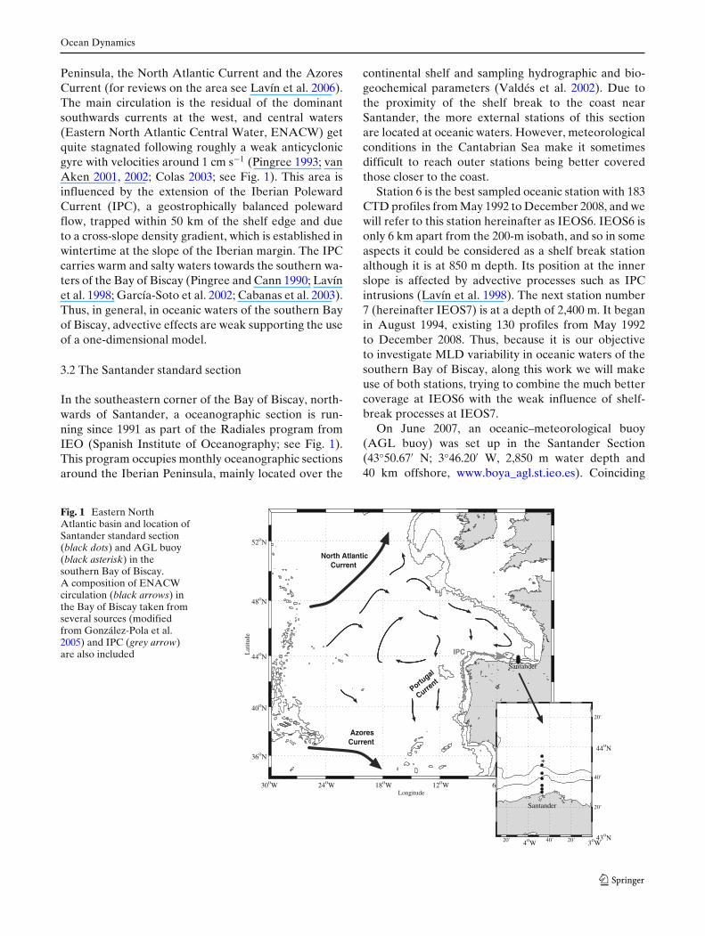
Peninsula, the North Atlantic Current and the AzoresCurrent (for reviews on the area see Lavín et al. 2006).The main circulation is the residual of the dominantsouthwards currents at the west, and central waters(Eastern North Atlantic Central Water, ENACW) getquite stagnated following roughly a weak anticyclonicgyre with velocities around 1 cm s−1 (Pingree 1993; vanAken 2001, 2002; Colas 2003; see Fig. 1). This area isinfluenced by the extension of the Iberian PolewardCurrent (IPC), a geostrophically balanced polewardflow, trapped within 50 km of the shelf edge and dueto a cross-slope density gradient, which is established inwintertime at the slope of the Iberian margin. The IPCcarries warm and salty waters towards the southern wa-ters of the Bay of Biscay (Pingree and Cann 1990; Lavínet al. 1998; García-Soto et al. 2002; Cabanas et al. 2003).Thus, in general, in oceanic waters of the southern Bayof Biscay, advective effects are weak supporting the useof a one-dimensional model.

3.2 The Santander standard section

In the southeastern corner of the Bay of Biscay, north-wards of Santander, a oceanographic section is run-ning since 1991 as part of the Radiales program fromIEO (Spanish Institute of Oceanography; see Fig. 1).This program occupies monthly oceanographic sectionsaround the Iberian Peninsula, mainly located over the

continental shelf and sampling hydrographic and bio-geochemical parameters (Valdés et al. 2002). Due tothe proximity of the shelf break to the coast nearSantander, the more external stations of this sectionare located at oceanic waters. However, meteorologicalconditions in the Cantabrian Sea make it sometimesdifficult to reach outer stations being better coveredthose closer to the coast.

Station 6 is the best sampled oceanic station with 183CTD profiles from May 1992 to December 2008, and wewill refer to this station hereinafter as IEOS6. IEOS6 isonly 6 km apart from the 200-m isobath, and so in someaspects it could be considered as a shelf break stationalthough it is at 850 m depth. Its position at the innerslope is affected by advective processes such as IPCintrusions (Lavín et al. 1998). The next station number7 (hereinafter IEOS7) is at a depth of 2,400 m. It beganin August 1994, existing 130 profiles from May 1992to December 2008. Thus, because it is our objectiveto investigate MLD variability in oceanic waters of thesouthern Bay of Biscay, along this work we will makeuse of both stations, trying to combine the much bettercoverage at IEOS6 with the weak influence of shelf-break processes at IEOS7.

On June 2007, an oceanic–meteorological buoy(AGL buoy) was set up in the Santander Section(43◦50.67′ N; 3◦46.20′ W, 2,850 m water depth and40 km offshore, www.boya_agl.st.ieo.es). Coinciding

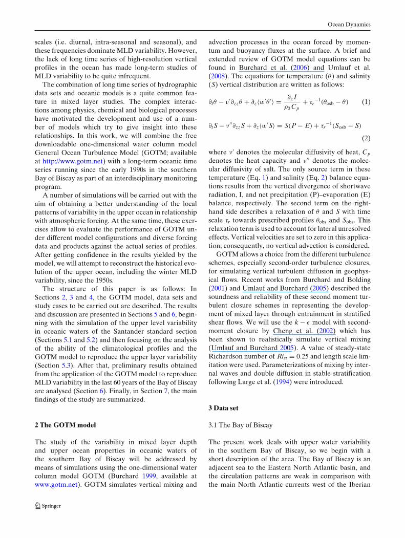
Fig. 1 Eastern NorthAtlantic basin and location ofSantander standard section(black dots) and AGL buoy(black asterisk) in thesouthern Bay of Biscay.A composition of ENACWcirculation (black arrows) inthe Bay of Biscay taken fromseveral sources (modifiedfrom González-Pola et al.2005) and IPC (grey arrow)are also included

Longitude

Lat

itude

30oW 24oW 18oW 12oW 6oW 0o

36oN

40oN

44oN

48oN

52oN

Santander

20’ 4oW 40’ 20’ 3oW 43oN

20’

40’

44oN

20’

Santander

North Atlantic Current

IPC

Azores Current

Portugal

Current

Ocean Dynamics

with its position, a new station number 9 has beenadded to the monthly sampling (hereinafter IEOS9).This station is, however, very close to IEOS7. The buoyis equipped with a large set of sensors that registerhourly the main atmospheric, hydrological and biogeo-chemical parameters at the air–sea interface, as well aswave data sensors and an Acoustic Doppler CurrentProfiler for the measurement of the currents in thefirst 100 m of the water column. The hourly data andheat fluxes estimation from AGL buoy, together withtemperature and salinity profiles measured at IEOS9,provide an accurate local source of forcing fields forcomparisons with large-scale meteorological products.

3.3 A climatological seasonality of the upperocean variability

The quite large and continuous set of CTD profiles se-ries from IEOS6 allowed the development of a methodfor characterizing the upper ocean variability, whichwas applied to construct a local climatology of the up-per layer vertical structure evolution in oceanic watersof the Santander standard section (González-Pola et al.2007). The new algorithm developed in that work pro-vides, besides an improved estimation of MLD whencompared with other previous algorithms, an accuraterepresentation of the seasonal and permanent thermo-cline beneath the mixed layer.

This set of climatological profiles will be also used tosimulate the upper layer variability in oceanic waters ofthe Santander standard section to investigate the com-bined capability of the climatological profiles and trueforcing running under the GOTM model to properlydescribe the upper layer temporal evolution. Positiveresults will enable us to use them to reproduce pastevolution and to speculate on future variability of theupper layer vertical structure under different climaticscenarios in this area.

3.4 Atmospheric forcing

The GOTM model is forced at the sea surface by theheat and momentum fluxes involved in the temperatureand U and V momentum equations, respectively, aswell as by the precipitation–evaporation balance par-ticipating in the salinity equation (see Eqs. 1 and 2).The atmospheric forcing represented by these fluxesis obtained from National Centers for EnvironmentalPrediction/National Center for Atmospheric Research(NCEP/NCAR) Reanalysis data set (Kalnay et al.1996) as six hourly data and with a spatial resolutionof 1.9◦ × 1.9◦.

Analyses carried out in order to evaluate theaccuracy of the NCEP estimates for turbulent heatfluxes, as well as for the local main meteorologicaland oceanic variables, against those computed fromthe AGL buoy and other meteorological data fromthe Spanish Agency of Meteorology (AEMET) haveshown a good agreement (Somavilla et al. 2009; Lavínet al. 2009; Somavilla 2010). The best matching withAGL buoy data is obtained for the closest grid pointfrom NCEP (44.76◦ N and 2.75◦ W) to the buoy positionthan for any multi-grid point average around the buoy.So, NCEP heat and momentum fluxes and precipitationtime series used in the different simulations will beextracted at this location.

In order to assess the impact of the accuracy ofatmospheric forcing on the results, we will also makeuse of hourly sensible, latent and momentum fluxesestimated from the AGL buoy measurements followingFairall et al. (1996) formulation (although AGL buoyis currently equipped with long and short wave radia-tive sensors, there are not available data for the timeperiod of this study and those data have been takenfrom NCEP/NCAR Reanalysis data set). We will alsoconsider the European Centre of Weather Meteoro-logical Forecast (ECWMF) reanalysis for comparisonpurposes.

4 Numerical experiments to be carried out

We will outline in this section the sequence of sim-ulation runs that we are going to perform explainingthe purpose of each. The specific settings of all runsare summarized in Table 1. The first experiments willtake advantage of the relatively extensive availableinformation in recent periods to explore the modelperformance and gain insight in the dominant processesaffecting the upper layer temporal evolution. The com-parison of these results with those obtained using theupper layer vertical structure climatology to simulatethe upper layer variability will assess us in the way thatwe must set the model in order to simulate periodswhere information is scarce.

The differences among model runs will be the pe-riod of simulation, the sources of air–sea forcings andthe background hydrographical field used to relax thewater column properties. Relaxing to hydrographicalprofiles is necessary to account for lateral advection,which affects density distribution and is not resolvedin a one-dimensional model. There is lateral advectionat time scales of the event variability of meteorologicalforcing in the area, particularly at IEOS6, that is notresolved by the monthly sampling (Somavilla 2010).

Ocean Dynamics

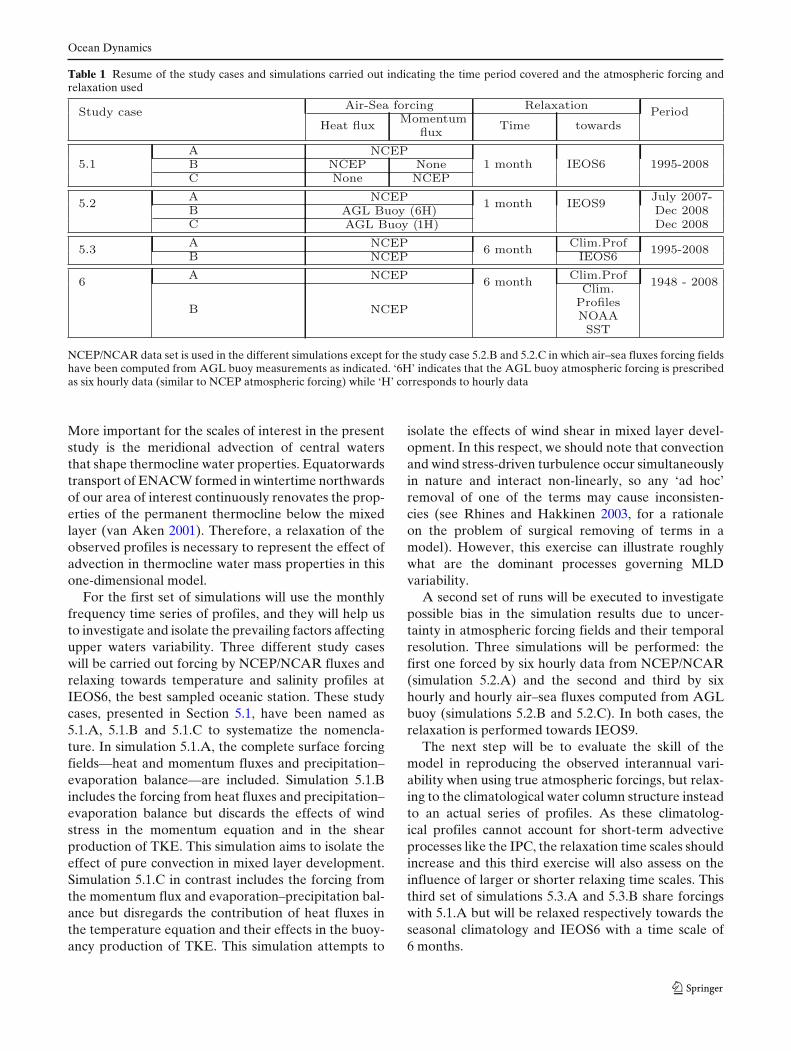
Table 1 Resume of the study cases and simulations carried out indicating the time period covered and the atmospheric forcing andrelaxation used

NCEP/NCAR data set is used in the different simulations except for the study case 5.2.B and 5.2.C in which air–sea fluxes forcing fieldshave been computed from AGL buoy measurements as indicated. ‘6H’ indicates that the AGL buoy atmospheric forcing is prescribedas six hourly data (similar to NCEP atmospheric forcing) while ‘H’ corresponds to hourly data

More important for the scales of interest in the presentstudy is the meridional advection of central watersthat shape thermocline water properties. Equatorwardstransport of ENACW formed in wintertime northwardsof our area of interest continuously renovates the prop-erties of the permanent thermocline below the mixedlayer (van Aken 2001). Therefore, a relaxation of theobserved profiles is necessary to represent the effect ofadvection in thermocline water mass properties in thisone-dimensional model.

For the first set of simulations will use the monthlyfrequency time series of profiles, and they will help usto investigate and isolate the prevailing factors affectingupper waters variability. Three different study caseswill be carried out forcing by NCEP/NCAR fluxes andrelaxing towards temperature and salinity profiles atIEOS6, the best sampled oceanic station. These studycases, presented in Section 5.1, have been named as5.1.A, 5.1.B and 5.1.C to systematize the nomencla-ture. In simulation 5.1.A, the complete surface forcingfields—heat and momentum fluxes and precipitation–evaporation balance—are included. Simulation 5.1.Bincludes the forcing from heat fluxes and precipitation–evaporation balance but discards the effects of windstress in the momentum equation and in the shearproduction of TKE. This simulation aims to isolate theeffect of pure convection in mixed layer development.Simulation 5.1.C in contrast includes the forcing fromthe momentum flux and evaporation–precipitation bal-ance but disregards the contribution of heat fluxes inthe temperature equation and their effects in the buoy-ancy production of TKE. This simulation attempts to

isolate the effects of wind shear in mixed layer devel-opment. In this respect, we should note that convectionand wind stress-driven turbulence occur simultaneouslyin nature and interact non-linearly, so any ‘ad hoc’removal of one of the terms may cause inconsisten-cies (see Rhines and Hakkinen 2003, for a rationaleon the problem of surgical removing of terms in amodel). However, this exercise can illustrate roughlywhat are the dominant processes governing MLDvariability.

A second set of runs will be executed to investigatepossible bias in the simulation results due to uncer-tainty in atmospheric forcing fields and their temporalresolution. Three simulations will be performed: thefirst one forced by six hourly data from NCEP/NCAR(simulation 5.2.A) and the second and third by sixhourly and hourly air–sea fluxes computed from AGLbuoy (simulations 5.2.B and 5.2.C). In both cases, therelaxation is performed towards IEOS9.

The next step will be to evaluate the skill of themodel in reproducing the observed interannual vari-ability when using true atmospheric forcings, but relax-ing to the climatological water column structure insteadto an actual series of profiles. As these climatolog-ical profiles cannot account for short-term advectiveprocesses like the IPC, the relaxation time scales shouldincrease and this third exercise will also assess on theinfluence of larger or shorter relaxing time scales. Thisthird set of simulations 5.3.A and 5.3.B share forcingswith 5.1.A but will be relaxed respectively towards theseasonal climatology and IEOS6 with a time scale of6 months.

Ocean Dynamics

The last step will be the analysis of mixed layer depthvariability in the last 60 years in the Bay of Biscay. Tworuns, 6.A and 6.B, will be performed towards the upperwaters climatology used in 5.3.A and that climatol-ogy modified to incorporate the slow decadal warmingin the Bay of Biscay. In general, all simulations areexecuted in a vertical domain of 500 m with 1 m verticalresolution and a time interval of 1 h.

5 Upper ocean variability and GOTM performancefrom the monthly oceanic series (1995–2008)

5.1 Seasonal to interannual evolution.Winter MLD variability

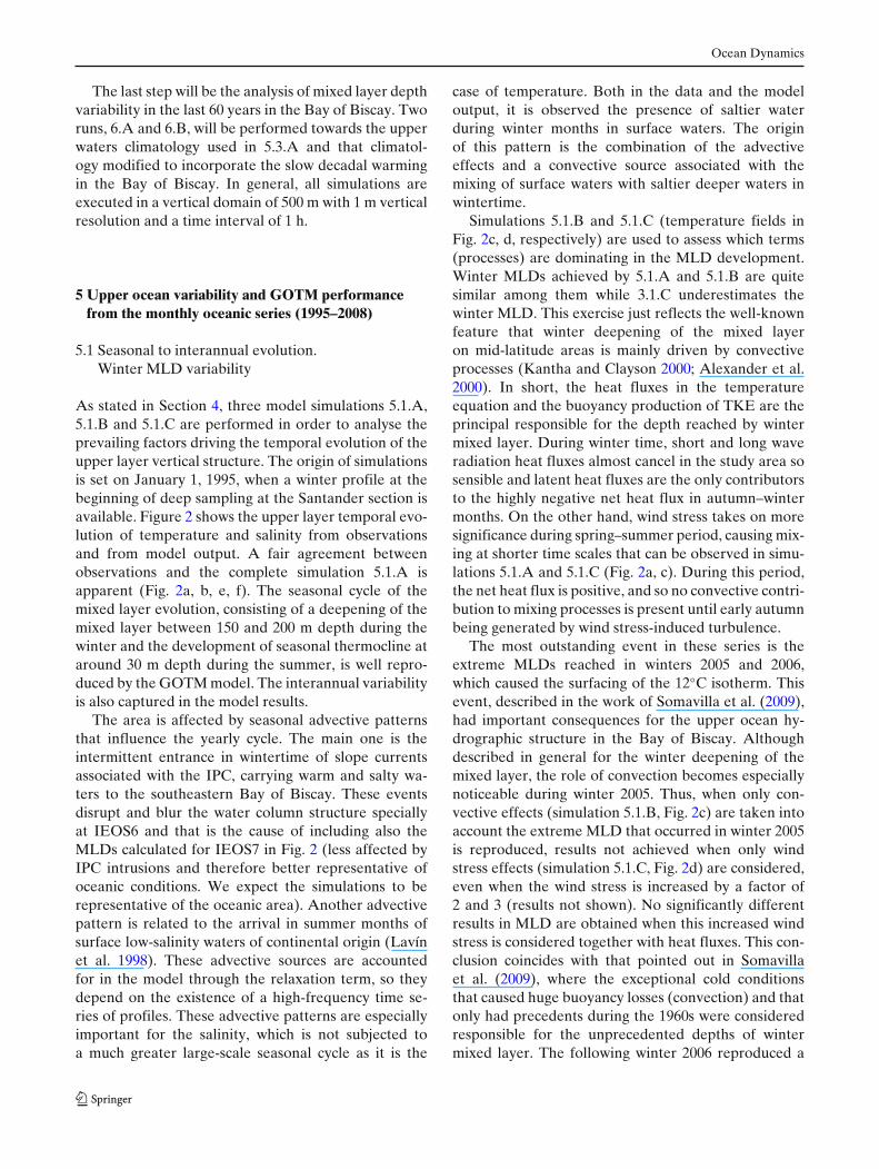
As stated in Section 4, three model simulations 5.1.A,5.1.B and 5.1.C are performed in order to analyse theprevailing factors driving the temporal evolution of theupper layer vertical structure. The origin of simulationsis set on January 1, 1995, when a winter profile at thebeginning of deep sampling at the Santander section isavailable. Figure 2 shows the upper layer temporal evo-lution of temperature and salinity from observationsand from model output. A fair agreement betweenobservations and the complete simulation 5.1.A isapparent (Fig. 2a, b, e, f). The seasonal cycle of themixed layer evolution, consisting of a deepening of themixed layer between 150 and 200 m depth during thewinter and the development of seasonal thermocline ataround 30 m depth during the summer, is well repro-duced by the GOTM model. The interannual variabilityis also captured in the model results.

The area is affected by seasonal advective patternsthat influence the yearly cycle. The main one is theintermittent entrance in wintertime of slope currentsassociated with the IPC, carrying warm and salty wa-ters to the southeastern Bay of Biscay. These eventsdisrupt and blur the water column structure speciallyat IEOS6 and that is the cause of including also theMLDs calculated for IEOS7 in Fig. 2 (less affected byIPC intrusions and therefore better representative ofoceanic conditions. We expect the simulations to berepresentative of the oceanic area). Another advectivepattern is related to the arrival in summer months ofsurface low-salinity waters of continental origin (Lavínet al. 1998). These advective sources are accountedfor in the model through the relaxation term, so theydepend on the existence of a high-frequency time se-ries of profiles. These advective patterns are especiallyimportant for the salinity, which is not subjected toa much greater large-scale seasonal cycle as it is the

case of temperature. Both in the data and the modeloutput, it is observed the presence of saltier waterduring winter months in surface waters. The originof this pattern is the combination of the advectiveeffects and a convective source associated with themixing of surface waters with saltier deeper waters inwintertime.

Simulations 5.1.B and 5.1.C (temperature fields inFig. 2c, d, respectively) are used to assess which terms(processes) are dominating in the MLD development.Winter MLDs achieved by 5.1.A and 5.1.B are quitesimilar among them while 3.1.C underestimates thewinter MLD. This exercise just reflects the well-knownfeature that winter deepening of the mixed layeron mid-latitude areas is mainly driven by convectiveprocesses (Kantha and Clayson 2000; Alexander et al.2000). In short, the heat fluxes in the temperatureequation and the buoyancy production of TKE are theprincipal responsible for the depth reached by wintermixed layer. During winter time, short and long waveradiation heat fluxes almost cancel in the study area sosensible and latent heat fluxes are the only contributorsto the highly negative net heat flux in autumn–wintermonths. On the other hand, wind stress takes on moresignificance during spring–summer period, causing mix-ing at shorter time scales that can be observed in simu-lations 5.1.A and 5.1.C (Fig. 2a, c). During this period,the net heat flux is positive, and so no convective contri-bution to mixing processes is present until early autumnbeing generated by wind stress-induced turbulence.

The most outstanding event in these series is theextreme MLDs reached in winters 2005 and 2006,which caused the surfacing of the 12◦C isotherm. Thisevent, described in the work of Somavilla et al. (2009),had important consequences for the upper ocean hy-drographic structure in the Bay of Biscay. Althoughdescribed in general for the winter deepening of themixed layer, the role of convection becomes especiallynoticeable during winter 2005. Thus, when only con-vective effects (simulation 5.1.B, Fig. 2c) are taken intoaccount the extreme MLD that occurred in winter 2005is reproduced, results not achieved when only windstress effects (simulation 5.1.C, Fig. 2d) are considered,even when the wind stress is increased by a factor of2 and 3 (results not shown). No significantly differentresults in MLD are obtained when this increased windstress is considered together with heat fluxes. This con-clusion coincides with that pointed out in Somavillaet al. (2009), where the exceptional cold conditionsthat caused huge buoyancy losses (convection) and thatonly had precedents during the 1960s were consideredresponsible for the unprecedented depths of wintermixed layer. The following winter 2006 reproduced a

Ocean Dynamics

400

200

0

Pre(

dbar

)

400

200

0

Pre(

dbar

)

400

200

0

Pre(

dbar

)

1995 1996 1997 1998 1999 2000 2001 2002 2003 2004 2005 2006 2007 2008 2009400

200

0

Pre(

dbar

)

12

14

16

18

20

22

400

200

0

Pre(

dbar

)

1995 1996 1997 1998 1999 2000 2001 2002 2003 2004 2005 2006 2007 2008 2009400

200

0

Pre(

dbar

)

Time (Years)

34.6

35

35.4

35.8

(a)

(b)

(c)

(d)

(e)

(f)

Tem

Fig. (a)

Observ

Fig. (b)

5.1.A

Fig. (c)

5.1.B

Fig. (d)

5.1.C

Sal

Fig. (e)

Observ

Fig. (f)

5.1.A

Fig. 2 Upper layer evolution from observations and model runsin the southern Bay of Biscay. a, e Temperature and salinity fromIEOS6 series of profiles. Black dots represent MLD estimationfollowing the González-Pola et al. (2007) algorithm applied toIEOS6 and IEOS7 temperature profiles. b, f Temperature and

salinity from simulation 5.1.A. Black line indicates MLD esti-mated from GOTM model as the depth of the turbulence surfacelayer (from simulated turbulent kinetic energy TKE). c Same asb for 5.1.B. d Same as b for 5.1.C

very deep mixed layer due to what is known as the re-emergence mechanism (Timlin et al. 2002), a processby which the low-stratification anomaly consolidatedduring a hard winter gets stored year-round beneaththe summer surface thermocline, thus facilitating theadvance of the newly formed mixed layer in the fol-lowing winter. The ultimate cause behind such a deep

mixed layer in year 2005 seems to be linked to a coupleof specific episodes of very strong buoyancy loss at theend of January and February. The second one triggereda sudden increase in MLD from ∼150 m on February25 to more than 330 m on March 8. This sequence ofevents is fairly well reproduced by the daily model runsof GOTM model.

Ocean Dynamics

5.2 Daily to seasonal surface variability. Reliabilityof atmospheric forcing fields

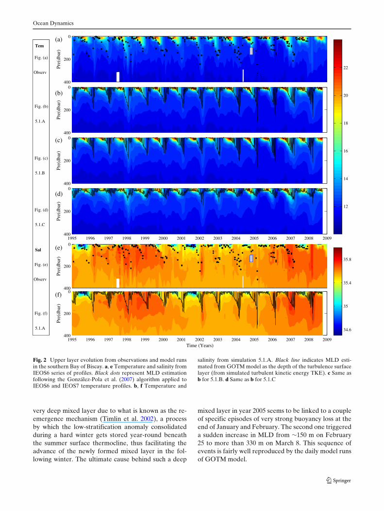
Figure 3 shows a comparison of sea surface temper-ature (SST) and sea surface salinity (SSS) of sim-ulation 5.1.A and IEOS6 data. Surface temperaturevariability is reasonably well represented, being themean difference �0.5◦C. Larger differences occur dur-ing spring and summer, peaking above 2.5◦C in somesporadic events and reaching even 4.5◦C in spring 1998.These differences disappear quickly at depth, pointingto uncertainty in atmospheric forcing fields used to runthe model as their cause. During summer months, aneventual overestimation of net heat flux would act ona very shallow mixed layer, leading to an excessivelylarge SST increase. Even so, the main anomalies alongthe series are well reproduced by modelled SST andSSS. We can highlight the cold summers of 2002 and2007, the abnormally warm summers of 2003 and 2006(Luterbacher et al. 2004, 2007), the extremely cold win-ter of 2005 (Somavilla et al. 2009), the warm autumn–winter periods of 1998 (Levitus et al. 2000) and 2006–2007 (Luterbacher et al. 2007) etc.

As pointed in Section 4, we take advantage of theavailability of data from the ODAS buoy AGL to inves-tigate the impact of changing the atmospheric forcingfields and their temporal resolution. Simulations 5.2.A,5.2.B and 5.2.C are designed to discriminate amongNCEP vs. AGL forcing fields (see Table 1). Note that

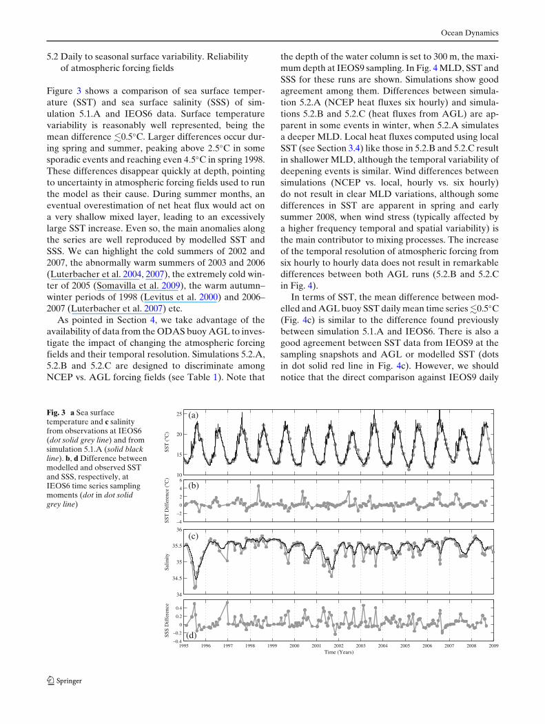
the depth of the water column is set to 300 m, the maxi-mum depth at IEOS9 sampling. In Fig. 4 MLD, SST andSSS for these runs are shown. Simulations show goodagreement among them. Differences between simula-tion 5.2.A (NCEP heat fluxes six hourly) and simula-tions 5.2.B and 5.2.C (heat fluxes from AGL) are ap-parent in some events in winter, when 5.2.A simulatesa deeper MLD. Local heat fluxes computed using localSST (see Section 3.4) like those in 5.2.B and 5.2.C resultin shallower MLD, although the temporal variability ofdeepening events is similar. Wind differences betweensimulations (NCEP vs. local, hourly vs. six hourly)do not result in clear MLD variations, although somedifferences in SST are apparent in spring and earlysummer 2008, when wind stress (typically affected bya higher frequency temporal and spatial variability) isthe main contributor to mixing processes. The increaseof the temporal resolution of atmospheric forcing fromsix hourly to hourly data does not result in remarkabledifferences between both AGL runs (5.2.B and 5.2.Cin Fig. 4).

In terms of SST, the mean difference between mod-elled and AGL buoy SST daily mean time series �0.5◦C(Fig. 4c) is similar to the difference found previouslybetween simulation 5.1.A and IEOS6. There is also agood agreement between SST data from IEOS9 at thesampling snapshots and AGL or modelled SST (dotsin dot solid red line in Fig. 4c). However, we shouldnotice that the direct comparison against IEOS9 daily

Fig. 3 a Sea surfacetemperature and c salinityfrom observations at IEOS6(dot solid grey line) and fromsimulation 5.1.A (solid blackline). b, d Difference betweenmodelled and observed SSTand SSS, respectively, atIEOS6 time series samplingmoments (dot in dot solidgrey line)

10

15

20

25

SST

(°C

)

(a)

–4

–2

0

2

4

6

SST

Dif

fere

nce

(°C

)

(b)

34

34.5

35

35.5

36

Salin

ity

(c)

1995 1996 1997 1998 1999 2000 2001 2002 2003 2004 2005 2006 2007 2008 2009–0.4

–0.2

0

0.2

0.4

SSS

Dif

fere

nce

Time (Years)

(d)

Ocean Dynamics

Fig. 4 a MLD fromsimulation 5.2.A (dash greyline), 5.2.B (solid grey line)and 5.2.C (solid green line)from July 2007 to December2009. b Sea surfacetemperature and d salinityfrom observations at IEOS9(dot solid red line) and AGLbuoy daily mean values(black line) and fromsimulation 5.2.A (dash greyline), 5.2.B (solid grey line)and 5.2.C (solid green line).c, e Difference betweenmodelled and AGL buoydaily means of SST and SSS,respectively, for simulation5.2.A (dash grey line) and5.2.B (solid grey line). Thedifference found in Section5.1 between IEOS6 timeseries and simulation 5.1.A isalso shown (dot solid greyline). The dot solid red line inc and e represents thedifference between IEOS9and AGL buoy daily mean ofSST and SSS at IEOS9sampling moments

0

50

100

150

200

ML

D (

m)

(a)

10

15

20

25

SST

(°C

)

(b)

–4

–2

0

2

4

6

SST

Dif

fere

nce

(°C

)(c)

34.5

35

35.5

36

Salin

ity

(d)

Jul Oct Jan Apr Jul Oct Jan–0.4

–0.2

0

0.2

0.4

SSS

Dif

fere

nce

Time (Years)

(e)

Sim.

5.2.A

5.2.B

5.2.C

In Situ

Data

AGLBuoy

IEOS9

IEOS6

2008 2009

interpolated values (as is mandatory whenever onlymonthly data is available) would yield much largerdiscrepancies (Fig. 4b). Thus, the inefficiency of IEOS9to resolve higher frequencies of variability is a sourceof error in SST.

In relation with this fact, the difference found be-tween simulation 5.1.A and IEOS6 is also shown inFig. 4c, e. There are not large SST difference excursionswithin these periods July 2007 to December 2008, soit is not possible to attribute such peaks to errors inthe atmospheric forcing fields. Extra runs have beenperformed to see whether finer vertical resolution(0.5 m) may improve the performance of the GOTMmodel, although this yields occasionally temperaturesup to 1.5◦C colder than the 1-m resolution standardruns, and the norm is to observe a similar overestima-tion of SST.

As expected, divergence between modelled and ob-served SSS is greater than for SST. Mesoscale struc-tures associated with the advection of low salinitywaters during summer months (Lavín et al. 1998) havea quite high-frequency variability, so they cannot beaccounted for properly through the relaxing term. Dur-

ing that time together with the presence of superficiallow salinity waters, a shallow halocline is observedat IEOS9 profiles that hinders mixing processes andthe entrainment of cold waters from below (Somavilla2010). The entire effect of this advection is poorlyrepresented in the one-dimensional simulations causingpartly the subestimation of SST in AGL buoy runs(5.2.B and 5.2.C) observed in Fig. 4 during summermonths. In general, the one-dimensional modelling ofvertical mixing processes can only obtain an approxi-mation of the SSS seasonal cycle.

5.3 Reproduction of the interannual variabilityfrom the climatological seasonality

The main goal of this section is to check whether theupper ocean variability from air–sea forcings (eithermeasured or derived from a reanalysis) can be repro-duced by the GOTM model relaxing towards a clima-tological (average) seasonal evolution of the verticalocean profiles. Figure 5 shows the temporal evolutionof temperature and salinity in the upper layers obtainedfrom simulations 5.3.A and 5.3.B (6-month relaxation

Ocean Dynamics

400

200

0

Pre(

dbar

)

400

200

0

Pre(

dbar

)

12

14

16

18

20

22

400

200

0

Pre(

dbar

)

34.6

35

35.4

35.8

12

13

14

15

Tem

pera

ture

(°C

) (d)

12

13

Tem

pera

ture

(°C

) (e)

1995 1996 1997 1998 1999 2000 2001 2002 2003 2004 2005 2006 2007 2008 200935.5

35.6

35.7

35.8

Salin

ity

Time (Years)

(f)

(a)

(b)

(c)

Tem

Fig. (a)

5.3.A

Fig. (b)

5.3.B

Sal

Fig. (c)

5.3.A y B

Fig. (d)

Tem100m.

Fig. (e)

Tem200m.

Fig. (f)

Sal200m.

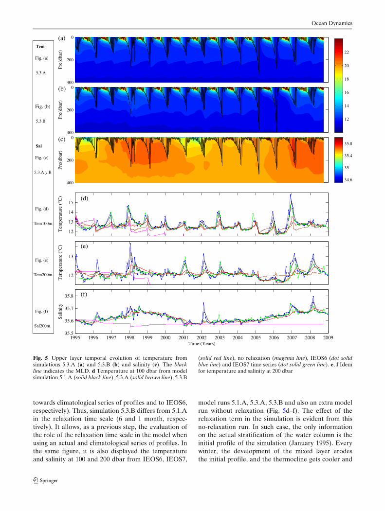
Fig. 5 Upper layer temporal evolution of temperature fromsimulations 5.3.A (a) and 5.3.B (b) and salinity (c). The blackline indicates the MLD. d Temperature at 100 dbar from modelsimulation 5.1.A (solid black line), 5.3.A (solid brown line), 5.3.B

(solid red line), no relaxation (magenta line), IEOS6 (dot solidblue line) and IEOS7 time series (dot solid green line). e, f Idemfor temperature and salinity at 200 dbar

towards climatological series of profiles and to IEOS6,respectively). Thus, simulation 5.3.B differs from 5.1.Ain the relaxation time scale (6 and 1 month, respec-tively). It allows, as a previous step, the evaluation ofthe role of the relaxation time scale in the model whenusing an actual and climatological series of profiles. Inthe same figure, it is also displayed the temperatureand salinity at 100 and 200 dbar from IEOS6, IEOS7,

model runs 5.1.A, 5.3.A, 5.3.B and also an extra modelrun without relaxation (Fig. 5d–f). The effect of therelaxation term in the simulation is evident from thisno-relaxation run. In such case, the only informationon the actual stratification of the water column is theinitial profile of the simulation (January 1995). Everywinter, the development of the mixed layer erodesthe initial profile, and the thermocline gets cooler and

Ocean Dynamics

deeper every year and MLD reaches deeper values pro-gressively. Thus, the relaxation in the model is neededto preserve realistic thermocline properties (hence thestratification) that, in the Bay of Biscay, is continuouslymodulated by northern large-scale advection.

Simulation 5.3.B (Fig. 5b) yields roughly a similarpattern of seasonal and interannual variability of MLDthan simulation 5.1.A (Fig. 6a, c), but some interest-ing differences arise. As time relaxation increases, thestrength of the advective component that maintains thepermanent thermocline diminishes. When a 6-monthrelaxation scale is used, waters tend to be fresher andcolder (Fig. 5d–f). This feature is related to the reduc-tion of the effect of the advection of warmer and saltierwaters from the IPC pulses induced by the increase intime relaxation. Simulation 5.3.B do show the interan-nual variability determined by IPC-transported watersand also the intense IPC years are evident (Fig. 5b, c),but events are more apparent in 5.1.A (Fig. 2b, e) whenwe relax tightly. Mixed layer depths are also slightlyaffected, being for instance deeper those obtained in1998 and 2003 by simulation 5.3.B (Fig. 6a, c). Thebiggest difference in winter MLD among both exercisesis found in 2006. Simulation 5.3.B provides a muchdeeper winter 2006 MLD than 5.1.A does, even exceed-ing that of 2005 (Fig. 6a, c). The very low stratificationachieved in winter 2005 below the seasonal thermoclineis over preserved year-round with a longer relaxationterm, thus easing the advance of the next year MLD(re-emergence). In agreement, temperature time seriesat 100 and 200 dbar shows colder values for simulation

5.3.B during winter 2006 (Fig. 5b, d, e). Actually, wecannot discard the presence of deeper MLD in 2006than in 2005 in the region. Although we did not capturesuch signal in our standard section, this may have beenmissed from a monthly series.

Simulation 5.3.A (Fig. 5a, c), relaxed towards cli-matological temperature profiles and salinity series ofobservations, provides essentially a similar pattern tothe initial simulation 5.1.A (similar years of deep andshallow MLD, see Fig. 6a, b). This result is of para-mount importance. It confirms the pre-eminence of lo-cal air–sea interaction as primary driver of winter MLDvariability, indicating that a climatological treatmentof the large-scale lateral advection allows the GOTMmodel to achieve a reliable water column evolution.In particular, for the extreme winter mixing of 2005,both simulations diagnose a similar MLD. As expected,differences arise in relationship with the effect of IPCintrusions in MLD detailed in the previous paragraph,an effect that is in no way accounted for when re-laxing to climatological profiles. Good examples arethe winters 1998, 1999 and 2007 that present a deeperMLD in 5.3.A (Fig. 6b respect to Fig. 6a). The absenceof warmer and saltier waters advected by the IPC isobserved through the colder and fresher water columnin simulation 5.3.A than for simulation 5.1.A in thoseyears (Fig. 5d–f).

The re-emergence event in 2006 supposes a chal-lenge for our climatological approximation. Advectedwaters reaching the point of interest in 2006 were ac-tually affected by the same large-scale atmospheric and

Fig. 6 a Mixed layerdevelopment computed frommodel simulation 5.1.A (solidblack line) and González-Polaet al. (2007) algorithmapplied to IEOS6 and IEOS7time series (red dots). b Idemfor MLD computed frommodel simulation 5.3.A andc MLD computed frommodel simulation 5.3.B

1995 1996 1997 1998 1999 2000 2001 2002 2003 2004 2005 2006 2007 2008 2009

0

100

200

300

400

500

ML

D (

m)

(a)

1995 1996 1997 1998 1999 2000 2001 2002 2003 2004 2005 2006 2007 2008 2009

0

100

200

300

400

500

ML

D (

m)

(b)

1995 1996 1997 1998 1999 2000 2001 2002 2003 2004 2005 2006 2007 2008 2009

0

100

200

300

400

500

ML

D (

m)

Time (Years)

(c)

Ocean Dynamics

mixed layer temperature anomaly in 2005 (see Figs. 6and 7 in the work of Somavilla et al. 2009) and, aswe know, the low-stratification anomaly still persistson its arrival. By relaxing to climatological profiles, weare incorrectly forcing the model towards a climato-logical state. However, simulation 5.3.A does show are-emergence signature replicating a deep mixed layerin 2006. It seems that setting a 6-month time scale weare relaxing slow enough to keep locally year-roundpart of the anomaly and reproduce (partially) the re-emergence event. It is observed how temperatures atdepth drifts just after winter 2005 in simulation 5.3.A(Fig. 5d, e), but the event in 2006 is not completely lost,and the coldest temperatures at 100 and 200 dbar areactually reached during the winter of 2005 and 2006.

In summary, simulation 5.3.A is able to reproducethe seasonal cycle and the most conspicuous eventsobserved at IEOS6 time series, which are direct con-sequence of atmospheric forcing. At the same time,short-term advective effects on the MLD like the IPCentrance are neglected. In this sense, if we peer intoisolated signatures of warm and salty water (e.g. 1998,2002 and 2007), we observe that simulations 5.3.A and5.3.B are more similar to IEOS7 data than to IEOS6(Fig. 5d–f). As said before, IEOS6 at the shelf-break ismuch more affected by shelf-slope advective processesthan IEOS7 (unfortunately the later station is muchpoorly sampled and several-month gaps complicate itsuse for relaxation purposes). Therefore, if we are in-terested in studying the mixed layer along an oceaniclarge-scale region, such avoidance of shelf-break ad-vective anomalies is a plus for the use of a climato-logical series for relaxing purposes. Finally, large-scaleadvection of anomalies like the 2006 re-emergence getspartially simulated with climatological series throughthe retention of the anomaly locally. The reproductionof such re-emergence phenomena depends of courseon an appropriate election of relaxation time scale andrequires the anomaly generated locally to be equivalentto that generated upstream and then advected.

In the next section, we will attempt to study pastconditions of the upper layer vertical structure usingthe GOTM model. We have seen that we need to relaxto a set of temperature and salinity profiles in order toaccount for the effect of large-scale lateral advectionin thermocline water properties and stratification. Wemust be aware that historical observations are sparsewith long gaps and information about large-scale oceanadvection variability is scarce. Any interpolated se-ries constructed from such scattered data, which evenskips whole winters without having a single profile,would add an important bias to the model runs (earlyoccurrence of mixed layer development and seasonal

thermocline and important variations in the final MLDreached at each time step). It can result in importanterrors and severe consequences when attempts aremade to couple physical model results with some othermodules such as biogeochemical ones (Friedrichs et al.2006). Within this section, we have demonstrated thatthe relaxation to a climatological series of profiles,carefully constructed from a large data set, results in afair reconstruction of the upper water variability in ourregion. We will therefore combine the use of this clima-tology, information about past states and the GOTMmodel with the aim of reconstructing the historicalwater structure evolution in our region.

6 Upper ocean variability in the long term(1949–2008)

6.1 Results of the long-term run. Constrainsand reliability

The availability of NCEP/NCAR reanalysis since 1948,together with the success achieved in the use of clima-tological profiles for estimating water column structure,allows us to carry out a simulation of the upper layertemporal evolution for the last 60 years in the Bay ofBiscay. The simulation was initiated on 1 January 1948(beginning of NCEP/NCAR Reanalysis data set) andfinished on 1 October 2008 with a time relaxation of6 months towards the climatological profiles. As theremaining simulations throughout this work, it was ex-ecuted for a vertical domain of 500 m with 1 m verticalresolution and a time step of 1 h.

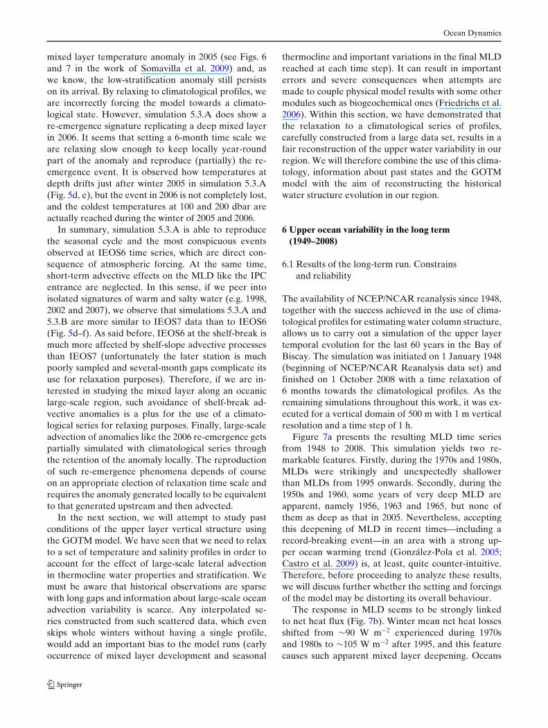
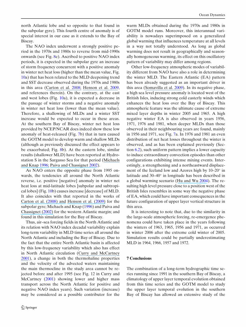
Figure 7a presents the resulting MLD time seriesfrom 1948 to 2008. This simulation yields two re-markable features. Firstly, during the 1970s and 1980s,MLDs were strikingly and unexpectedly shallowerthan MLDs from 1995 onwards. Secondly, during the1950s and 1960, some years of very deep MLD areapparent, namely 1956, 1963 and 1965, but none ofthem as deep as that in 2005. Nevertheless, acceptingthis deepening of MLD in recent times—including arecord-breaking event—in an area with a strong up-per ocean warming trend (González-Pola et al. 2005;Castro et al. 2009) is, at least, quite counter-intuitive.Therefore, before proceeding to analyze these results,we will discuss further whether the setting and forcingsof the model may be distorting its overall behaviour.

The response in MLD seems to be strongly linkedto net heat flux (Fig. 7b). Winter mean net heat lossesshifted from ∼90 W m−2 experienced during 1970sand 1980s to ∼105 W m−2 after 1995, and this featurecauses such apparent mixed layer deepening. Oceans

Ocean Dynamics

0

50

100

150

200

250

300

350

ML

D(m

)

(a)

50

100

150

Net

hea

t los

s (W

•m–2

) (b)

1950 1955 1960 1965 1970 1975 1980 1985 1990 1995 2000 20050.05

0.1

0.15

0.2

0.25

Mom

entu

m f

lux

(N•m

–2) (c)

Fig. 7 a Mixed layer development computed from GOTM model simulation 6.A for the last 60 years in the Bay of Biscay. b Wintermean net heat loss and momentum flux (c) from 1948 to 2008

are heat reservoirs, acting like a flywheel in mattersrelated to weather on time scales of weeks and longer.They gain heat during the spring and summer los-ing it slowly during fall and winter. Winter net heatloss increase observed since mid-1990s is ultimately acombination of variability of storminess activity andair temperature during winter months acting combinedwith excess of heat gained in summertime. Therefore,the first question is about the reliability of the forcingfields. The results of Section 5.2 indicate that MLDshow limited sensitivity to variation of atmosphericforcing products for a modern period. However, his-torical reanalysis data may have some bias, and forthis reason, NCEP/NCAR fluxes were compared withthose obtained from ECWMF Reanalysis data set. No

significant differences between both were found, soa potential bias in NCEP/NCAR atmospheric forcingwould be shared by ECWMF. On the other hand, bothreanalysis are affected by a similar coarseness that mayresult in limitations when small-scale physical processesare important. Nevertheless, for studies focused in in-terannual variability, the air–sea forcings have a large-scale character, thus generating similar effects in theupper layers in broad areas.

Apart from atmospheric forcing, another factor thatcould result in unrealistic behaviour of the model isthe water column structure imposed through relaxationto account for unresolved large-scale lateral advection.The climatology used so far was generated with CTDprofiles obtained during the 1990s and onwards at

Ocean Dynamics

IEOS6. It represents a warmer water column than thatin existence during the previous decades in this area,and stratification may have also varied in an unknownway. In principle, one could suspect that extractingthe ‘true’ NCEP heat fluxes from this extra-heatedwater column may result in an underestimation ofMLDs in previous decades. To overcome this issue, theclimatology was modified to incorporate the slowdecadal warming in the Bay of Biscay. The procedurewas to calculate the winter SST anomaly between theclimatology and the NOAA_ER SST (Smith et al.2008) and then using a low-passed version of suchanomaly to modulate the whole water column. We areaware of the caveats inherent to this approach, but weshould not forget that the climatology is only intendedfor accounting for missing the large-scale lateral ad-vection with a time scale of several months, and theinterannual variability should be determined by theshort-scale resolving model run. The purpose of thisexperiment is to avoid a systematic bias towards a toowarm water column for decades.

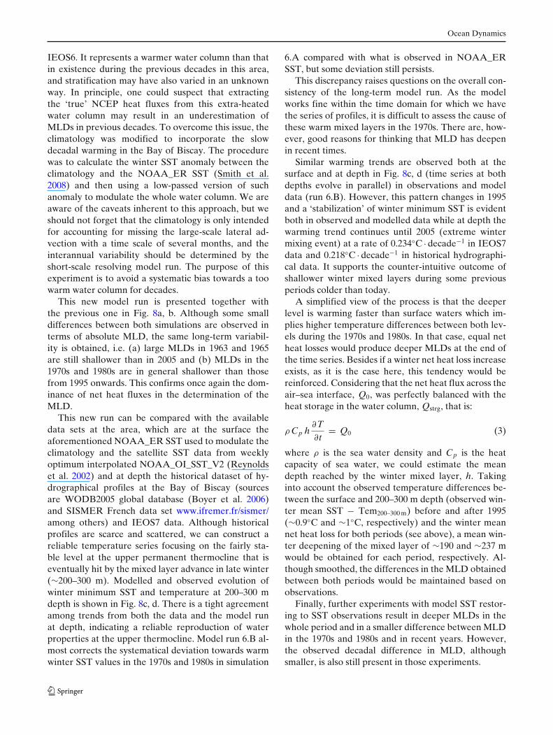
This new model run is presented together withthe previous one in Fig. 8a, b. Although some smalldifferences between both simulations are observed interms of absolute MLD, the same long-term variabil-ity is obtained, i.e. (a) large MLDs in 1963 and 1965are still shallower than in 2005 and (b) MLDs in the1970s and 1980s are in general shallower than thosefrom 1995 onwards. This confirms once again the dom-inance of net heat fluxes in the determination of theMLD.

This new run can be compared with the availabledata sets at the area, which are at the surface theaforementioned NOAA_ER SST used to modulate theclimatology and the satellite SST data from weeklyoptimum interpolated NOAA_OI_SST_V2 (Reynoldset al. 2002) and at depth the historical dataset of hy-drographical profiles at the Bay of Biscay (sourcesare WODB2005 global database (Boyer et al. 2006)and SISMER French data set www.ifremer.fr/sismer/among others) and IEOS7 data. Although historicalprofiles are scarce and scattered, we can construct areliable temperature series focusing on the fairly sta-ble level at the upper permanent thermocline that iseventually hit by the mixed layer advance in late winter(∼200–300 m). Modelled and observed evolution ofwinter minimum SST and temperature at 200–300 mdepth is shown in Fig. 8c, d. There is a tight agreementamong trends from both the data and the model runat depth, indicating a reliable reproduction of waterproperties at the upper thermocline. Model run 6.B al-most corrects the systematical deviation towards warmwinter SST values in the 1970s and 1980s in simulation

6.A compared with what is observed in NOAA_ERSST, but some deviation still persists.

This discrepancy raises questions on the overall con-sistency of the long-term model run. As the modelworks fine within the time domain for which we havethe series of profiles, it is difficult to assess the cause ofthese warm mixed layers in the 1970s. There are, how-ever, good reasons for thinking that MLD has deepenin recent times.

Similar warming trends are observed both at thesurface and at depth in Fig. 8c, d (time series at bothdepths evolve in parallel) in observations and modeldata (run 6.B). However, this pattern changes in 1995and a ‘stabilization’ of winter minimum SST is evidentboth in observed and modelled data while at depth thewarming trend continues until 2005 (extreme wintermixing event) at a rate of 0.234◦C · decade−1 in IEOS7data and 0.218◦C · decade−1 in historical hydrographi-cal data. It supports the counter-intuitive outcome ofshallower winter mixed layers during some previousperiods colder than today.

A simplified view of the process is that the deeperlevel is warming faster than surface waters which im-plies higher temperature differences between both lev-els during the 1970s and 1980s. In that case, equal netheat losses would produce deeper MLDs at the end ofthe time series. Besides if a winter net heat loss increaseexists, as it is the case here, this tendency would bereinforced. Considering that the net heat flux across theair–sea interface, Q0, was perfectly balanced with theheat storage in the water column, Qstrg, that is:

ρ Cp h∂T∂t

= Q0 (3)

where ρ is the sea water density and Cp is the heatcapacity of sea water, we could estimate the meandepth reached by the winter mixed layer, h. Takinginto account the observed temperature differences be-tween the surface and 200–300 m depth (observed win-ter mean SST − Tem200–300 m) before and after 1995(∼0.9◦C and ∼1◦C, respectively) and the winter meannet heat loss for both periods (see above), a mean win-ter deepening of the mixed layer of ∼190 and ∼237 mwould be obtained for each period, respectively. Al-though smoothed, the differences in the MLD obtainedbetween both periods would be maintained based onobservations.

Finally, further experiments with model SST restor-ing to SST observations result in deeper MLDs in thewhole period and in a smaller difference between MLDin the 1970s and 1980s and in recent years. However,the observed decadal difference in MLD, althoughsmaller, is also still present in those experiments.

Ocean Dynamics

0

100

200

300

400

500

Pre(

dbar

)

1950 1955 1960 1965 1970 1975 1980 1985 1990 1995 2000 2005

0

100

200

300

400

500

Pre(

dbar

)

12

14

16

18

20

22

11

12

13

SST

(°C

)

(c)

11.5

12

tem

200

(°C

)

(d)

–2

–1

0

1

2

NA

O I

ndex

(e)

1950 1955 1960 1965 1970 1975 1980 1985 1990 1995 2000 2005

8

11

14

Air

Tem

p.(°

C) (f)

(a)

(b)

Tem

Fig. (a)

6.A

Fig. (b)

6.B

Fig. (c)

SST

Fig. (d)

Tem.200

Fig. (e)

NAO

Fig. (f)

Air.Tem

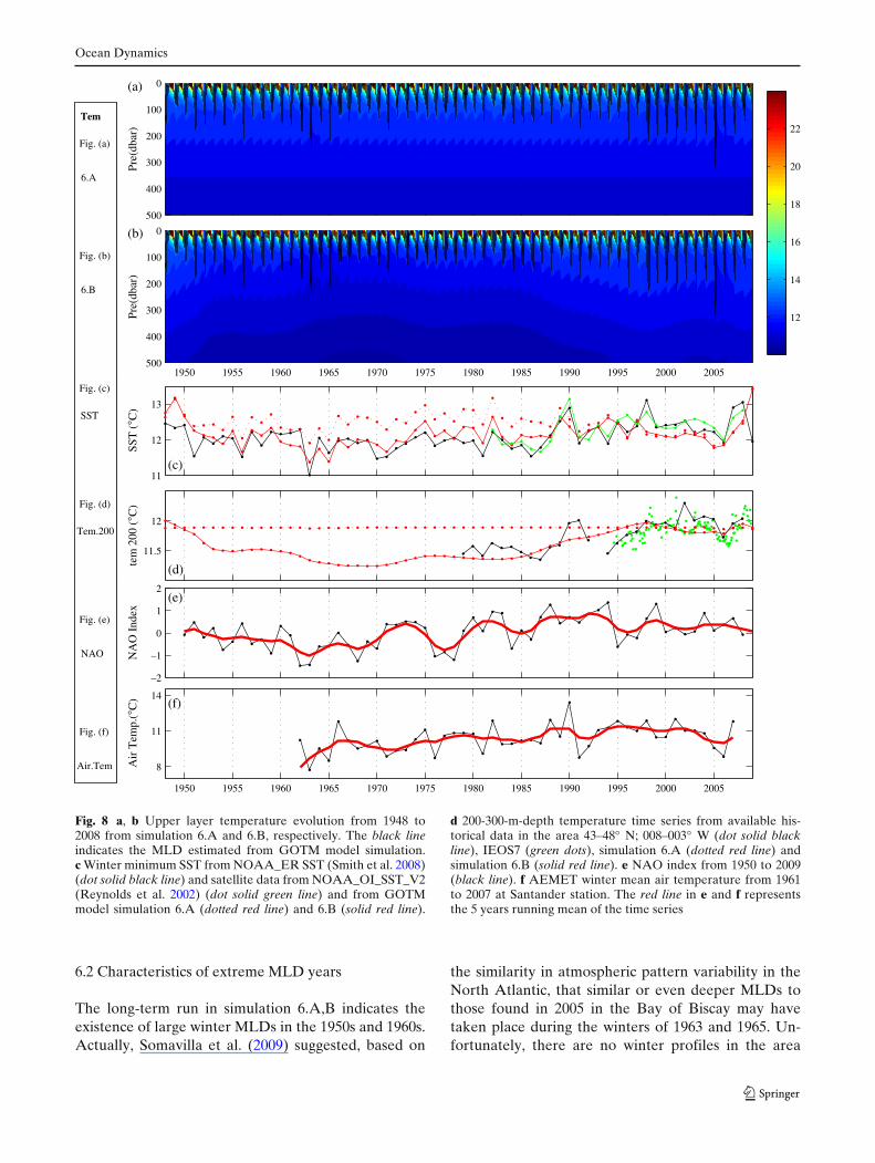
Fig. 8 a, b Upper layer temperature evolution from 1948 to2008 from simulation 6.A and 6.B, respectively. The black lineindicates the MLD estimated from GOTM model simulation.c Winter minimum SST from NOAA_ER SST (Smith et al. 2008)(dot solid black line) and satellite data from NOAA_OI_SST_V2(Reynolds et al. 2002) (dot solid green line) and from GOTMmodel simulation 6.A (dotted red line) and 6.B (solid red line).

d 200-300-m-depth temperature time series from available his-torical data in the area 43–48◦ N; 008–003◦ W (dot solid blackline), IEOS7 (green dots), simulation 6.A (dotted red line) andsimulation 6.B (solid red line). e NAO index from 1950 to 2009(black line). f AEMET winter mean air temperature from 1961to 2007 at Santander station. The red line in e and f representsthe 5 years running mean of the time series

6.2 Characteristics of extreme MLD years

The long-term run in simulation 6.A,B indicates theexistence of large winter MLDs in the 1950s and 1960s.Actually, Somavilla et al. (2009) suggested, based on

the similarity in atmospheric pattern variability in theNorth Atlantic, that similar or even deeper MLDs tothose found in 2005 in the Bay of Biscay may havetaken place during the winters of 1963 and 1965. Un-fortunately, there are no winter profiles in the area

Ocean Dynamics

to confirm or rule out such hypothesis. Nevertheless,the present simulations provide a tool to investigatefurther these events. In principle, simulated MLDs in1963 and 1965 are shallower than those observed in2005, and contrary to the suspicious period of the 1970s,modelled SST does not disagree much with respect toNOAA_ER data.

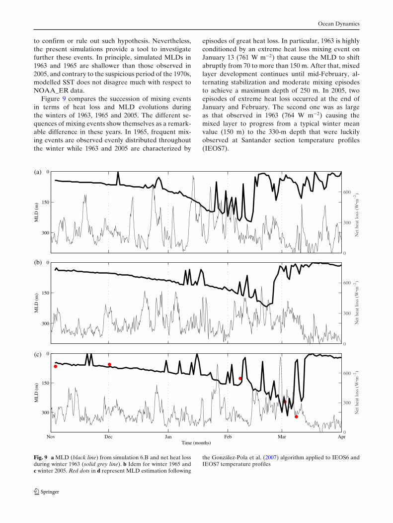
Figure 9 compares the succession of mixing eventsin terms of heat loss and MLD evolutions duringthe winters of 1963, 1965 and 2005. The different se-quences of mixing events show themselves as a remark-able difference in these years. In 1965, frequent mix-ing events are observed evenly distributed throughoutthe winter while 1963 and 2005 are characterized by

episodes of great heat loss. In particular, 1963 is highlyconditioned by an extreme heat loss mixing event onJanuary 13 (761 W m−2) that cause the MLD to shiftabruptly from 70 to more than 150 m. After that, mixedlayer development continues until mid-February, al-ternating stabilization and moderate mixing episodesto achieve a maximum depth of 250 m. In 2005, twoepisodes of extreme heat loss occurred at the end ofJanuary and February. The second one was as largeas that observed in 1963 (764 W m−2) causing themixed layer to progress from a typical winter meanvalue (150 m) to the 330-m depth that were luckilyobserved at Santander section temperature profiles(IEOS7).

0

150

300

ML

D (

m)

0

300

600

0

150

300

ML

D (

m)

0

300

600

Nov Dec Jan Feb Mar Apr

0

150

300

Time (months)

ML

D (

m)

0

300

600

Net

hea

t los

s (W

• m–2

)N

et h

eat l

oss

(W• m

–2)

Net

hea

t los

s (W

• m–2

)

(a)

(b)

(c)

Fig. 9 a MLD (black line) from simulation 6.B and net heat lossduring winter 1963 (solid grey line). b Idem for winter 1965 andc winter 2005. Red dots in d represent MLD estimation following

the González-Pola et al. (2007) algorithm applied to IEOS6 andIEOS7 temperature profiles

Ocean Dynamics

Although winter mixing and convection processesare mostly governed by the accumulated effect of heatloss throughout the winter, extraordinary convectionepisodes appear more likely to occur when heat loss isconcentrated in intense mixing events, rather than dis-tributed evenly but more weakly throughout the winter.This conclusion has also been pointed in other works(Marshall and Schott 1999; Vage et al. 2008). It is alsoworthy of mention, as previously discussed in Sections5.1 and 5.2, that wind stress-induced turbulence doesnot play a fundamental role in the generation of theseextreme mixing events. Thus, the highest wind stresswas registered in winter 1965 followed by 1963 and2005. On the contrary, it is the existence of strongair-sea temperature and relative humidity gradients in-volved in sensible and latent heat flux equations respec-tively what determines strong heat loss to occur duringwinter months.

6.3 Low-frequency variability in MLDand large-scale atmospheric patterns

Low-frequency and interannual variability in the extentof the winter MLD influence a number of key oceano-graphic processes, from modal water masses formationto primary production processes. Determining suchvariability from field data requires extensive data setswith enough coverage at the critical end-winter period,so there are actually few works in this field. Prominentexamples of description of long-term trends in MLDare Polovina et al. (1995) and Freeland et al. (1997) forthe North Pacific and Michaels and Knap (1996), Nilsenand Falck (2006) and Carton et al. (2008) for NorthAtlantic. The ultimate drivers of these low-frequencychanges in the MLD are large-scale atmospheric forc-ing patterns.

Although our exercise has been performed with aone-dimensional model, subjected to uncertainties inthe representation of the structure of the water column,the model runs and the relationship among trends inSST and in the upper permanent thermocline tem-perature suggest a pattern of shallower MLDs duringthe 1970s and 1980s and deeper ones since mid-1990sfor the southern Bay of Biscay. Taking into accountthe MLD cycles described for the North Atlantic andrecent reviews of the effects of the North Atlantic Os-cillation (NAO) on ocean and air–sea fields (Marshallet al. 2001; Visbeck et al. 2003; Hurrell and Deser 2009),we will discuss in this section the low-frequency MLDoscillation inferred in oceanic waters of the Santanderstandard section and its differences and similarities withother regions in the North Atlantic.

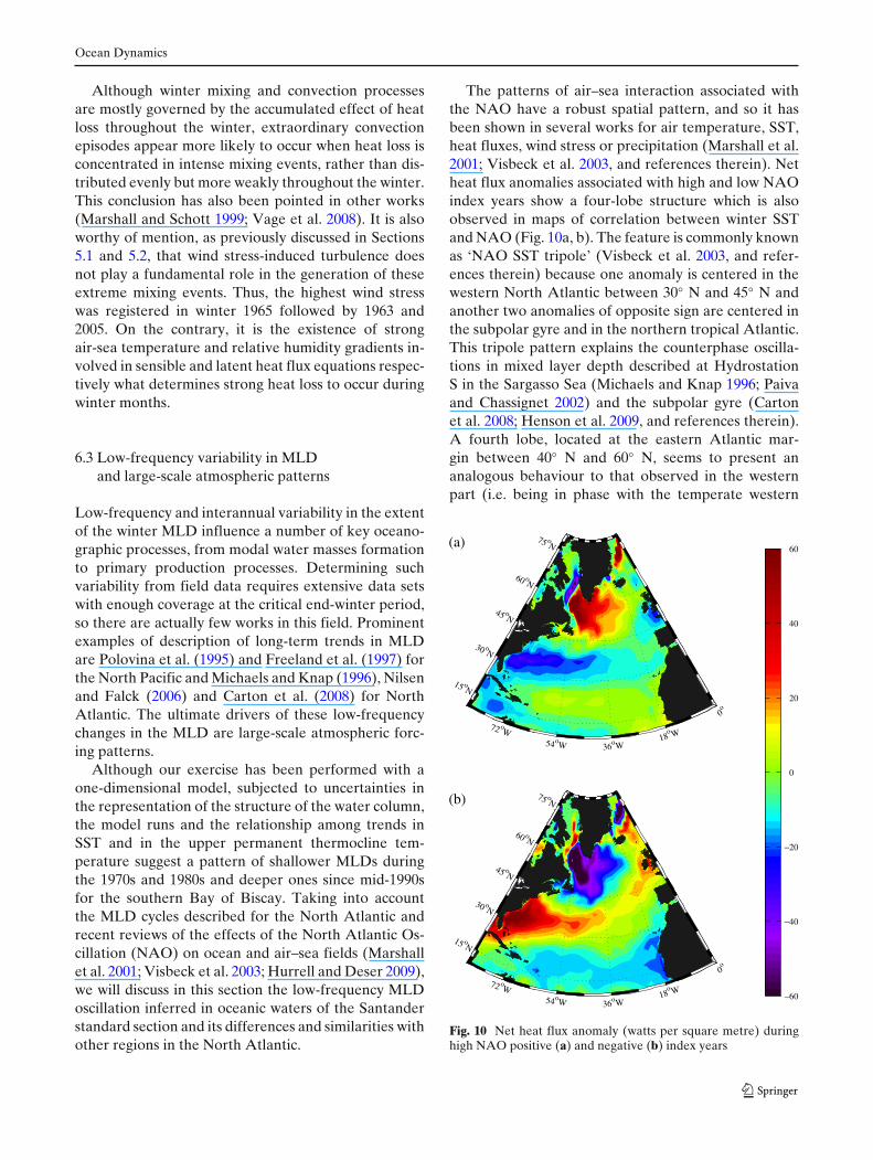
The patterns of air–sea interaction associated withthe NAO have a robust spatial pattern, and so it hasbeen shown in several works for air temperature, SST,heat fluxes, wind stress or precipitation (Marshall et al.2001; Visbeck et al. 2003, and references therein). Netheat flux anomalies associated with high and low NAOindex years show a four-lobe structure which is alsoobserved in maps of correlation between winter SSTand NAO (Fig. 10a, b). The feature is commonly knownas ‘NAO SST tripole’ (Visbeck et al. 2003, and refer-ences therein) because one anomaly is centered in thewestern North Atlantic between 30◦ N and 45◦ N andanother two anomalies of opposite sign are centered inthe subpolar gyre and in the northern tropical Atlantic.This tripole pattern explains the counterphase oscilla-tions in mixed layer depth described at HydrostationS in the Sargasso Sea (Michaels and Knap 1996; Paivaand Chassignet 2002) and the subpolar gyre (Cartonet al. 2008; Henson et al. 2009, and references therein).A fourth lobe, located at the eastern Atlantic mar-gin between 40◦ N and 60◦ N, seems to present ananalogous behaviour to that observed in the westernpart (i.e. being in phase with the temperate western

72 oW

54oW 36oW 18

o W

0o

15 oN

30 oN

45 oN

60 oN

75 oN

72 oW

54oW 36oW 18

o W

0o

15 oN

30 oN

45 oN

60 oN

75 oN

−60

−40

−20

0

20

40

60(a)

(b)

Fig. 10 Net heat flux anomaly (watts per square metre) duringhigh NAO positive (a) and negative (b) index years

Ocean Dynamics

north Atlantic lobe and so opposite to that found inthe subpolar gyre). This fourth centre of anomaly is ofspecial interest in our case as it extends to the Bay ofBiscay.

The NAO index underwent a strongly positive pe-riod in the 1970s and 1980s to reverse from mid-1990sonwards (see Fig. 8e). Ascribed to positive NAO indexperiods, it is expected in the subpolar gyre an increaseof storm frequency concurrent with a positive anomalyin winter net heat loss (higher than the mean value, Fig.10a) that has been related to the MLD deepening trendand SST decrease observed during the 1970s and 1980sin this area (Carton et al. 2008; Henson et al. 2009,and references therein). On the contrary, at the eastand west lobes (Fig. 10a), it is expected a decrease inthe passage of winter storms and a negative anomalyin winter net heat loss (lower than the mean value).Therefore, a shallowing of MLDs and a winter SSTincrease would be expected to occur in these areas.At the southern Bay of Biscay, winter net heat lossprovided by NCEP/NCAR does indeed show these lowanomaly of heat-released (Fig. 7b) that in turn causedthe GOTM model to develop warm and shallow MLDs(although as previously discussed the effect appears tobe exacerbated; Fig. 8b). At the eastern lobe, similarresults (shallower MLD) have been reported at Hydro-station S in the Sargasso Sea for that period (Michaelsand Knap 1996; Paiva and Chassignet 2002).

As NAO enters the opposite phase from 1995 on-wards, the tendencies all around the North Atlanticreverse, i.e. positive [negative] anomaly in winter netheat loss at mid-latitude lobes [subpolar and subtropi-cal lobes] (Fig. 10b) causes increase [decrease] of MLD.It also coincides with that reported in the works ofCarton et al. (2008) and Henson et al. (2009) for thesubpolar gyre; Michaels and Knap (1996) and Paiva andChassignet (2002) for the western Atlantic margin; andfound in this simulation for the Bay of Biscay.

Thus, air–sea forcing fields in the North Atlantic andits relation with NAO index decadal variability explainlong-term variability in MLD time series all around theNorth Atlantic and including the Bay of Biscay. Due tothe fact that the entire North Atlantic basin is affectedby this low-frequency variability which also has effectin North Atlantic circulation (Curry and McCartney2001), a change in both the thermohaline propertiesand the velocity of the advected waters maintainingthe main thermocline in the study area cannot be re-jected before and after 1995 (see Fig. 12 in Curry andMcCartney (2001) showing lower and higher masstransport across the North Atlantic for positive andnegative NAO index years). Such variation (increase)may be considered as a possible contributor for the

warm MLDs obtained during the 1970s and 1980s inGOTM model runs. Moreover, this interannual vari-ability is nowadays superimposed on a generalizedglobal warming that influences temperature at all levelsin a way not totally understood. As long as globalwarming does not result in geographically and season-ally homogeneous warming, its effect on this oscillatorypattern of variability may differ among regions.

Other low-frequency atmospheric modes of variabil-ity different from NAO have also a role in determiningthe winter MLD. The Eastern Atlantic (EA) patternhas been already suggested as an important driver inthis area (Somavilla et al. 2009). In its negative phase,a high sea level pressure anomaly is located west of theBritish Isles, inducing strong cold easterly winds whichenhances the heat loss over the Bay of Biscay. Thisatmospheric feature was the ultimate cause of extrememixed layer depths in winter 2005 and 1965. A highnegative winter EA is also observed in years 1956,1971, 1976 and 1981, when deeper MLDs than thoseobserved in their neighbouring years are found, mainlyin 1956 and 1971, see Fig. 7a. In 1976 and 1981 an evendistribution of net heat losses throughout the winter isobserved, and as has been explained previously (Sec-tion 6.2), such uniform pattern implies a lower capacityto induce extraordinary convection episodes than otherconfigurations exhibiting intense mixing events. Inter-estingly, a strengthening and a northeastward displace-ment of the Iceland low and Azores high by 10–20◦ inlatitude and 30–40◦ in longitude has been described ina global warming scenario (Hu and Wu 2004). The re-sulting high level pressure close to a position west of theBritish Isles resembles in some way the negative phaseof EA, which could have important consequences in thefuture configuration of upper layer vertical structure inthis area.

It is interesting to note that, due to the similarity inthe large-scale atmospheric forcing, re-emergence phe-nomena could have taken place in the years followingthe winters of 1963, 1965, 1956 and 1971, as occurredin winter 2006 after the extreme cold winter of 2005.Simulation results could be partially underestimatingMLD in 1964, 1966, 1957 and 1972.

7 Conclusions

The combination of a long-term hydrographic time se-ries running since 1991 in the southern Bay of Biscay, aclimatology of upper layer temporal evolution obtainedfrom this time series and the GOTM model to studythe upper layer temporal evolution in the southernBay of Biscay has allowed an extensive study of the

Ocean Dynamics

prevailing forces governing the seasonal, interannualand long-term MLD variability. Different simulationshave been carried out obtaining a high level of detail ofMLD variability and extreme phenomena observed atSantander standard section and good agreement withobservations.

As expected, the different simulations have shownthat on seasonal time scales, winter mixed layer devel-opment is mostly conducted by convection processeswhile wind stress is responsible for mixing events dur-ing the spring–summer season. The role of convectionprocesses is proved to be especially noticeable duringthe exceptional winter mixing occurred in winter 2005,coinciding with that noted in Somavilla et al. (2009).The sequence of events is also well simulated within asingle year MLD development, and the re-emergencephenomenon in winter 2006 responsible for the easyreproduction of a new deep and cold mixed layer is re-produced with different levels of success by the GOTMmodel in the different simulations.

On the other hand, the comparison of the resultsof the different simulations and the observed variabil-ity has shown that, although atmospheric forcing ismainly responsible for MLD variability and the extra-ordinary phenomena observed in oceanic waters of theSantander standard section, advective processes suchIPC whose intensity diminishes towards oceanic wa-ters can determine slight differences in the final depthreached by winter mixed layer.

Tests carried out to investigate climatological profileskill together with true forcing to reproduce the up-per layer temporal evolution in the southern Bay ofBiscay have demonstrated its ability to provide a fairreconstruction of the upper water variability in ourregion. They allow to account for the effect of large-scale lateral advection in thermocline water propertiesand stratification while avoiding the inclusion of shelf-break advective anomalies which is a plus for their usefor relaxing purposes in studying the mixed layer alongan oceanic large-scale region.

It has permitted a first trial of the reproduction ofthe last 60 years of MLD variability in the study area.Remarkable results have been obtained. Although incertain grade overestimated by simulation results, anunexpected period of shallower MLDs seems to haveoccurred during the 1970s and 1980s which would havebeen concluded from mid-1990s with a period of deep-ening trend in MLD. The reproduction of sea surfaceand 200 m depth temperature time series and the warm-ing trend at both levels supports the counter-intuitiveoutcome of shallower winter mixed layers concurrentwith generalized upper water warming trends reportedon several occasions for the area.

As found in other recent studies, long-term trendsin MLD in the southern Bay of Biscay seem to berelated to decadal variability in the NAO, being inphase and opposition to other cycles of deepening andshallowing trends in MLD found from subtropical-to-subpolar areas in the North Atlantic. Favourable se-quences of mixing events result in intense convectionprocesses explaining interannual differences and theextraordinary deepening of the winter mixed layer asoccurred in the years 2005, 1963 and 1965. The negativephase of the Eastern Atlantic pattern seems to deter-mine important interannual variability through intenseepisodes of cooling and mixing as occurred in the winterof 2005 in the Bay of Biscay.

Acknowledgements This work has been performed in relation-ship with the RADIALES, VACLAN and COVACLAN pro-jects (REN2003-08193-C03-01/MAR; CTM 2007-64600/MAR;www.vaclan-ieo.es) funded by the IEO and the Ministerio deCiencia e Innovación (Spain). We thank the technical and sci-entifical staff in the IEO-Radiales project and the crews of RVJosé Rioja and Cornide de Saavedra for support in samplingthe Santander Section. The authors also wish to thank twoanonymous reviewers for valuable and helpful comments on themanuscript. R. Somavilla was funded by a predoctoral FPI grantfrom IEO (Ministerio de Ciencia e Innovación, Spain) during thedevelopment of this work.

Open Access This article is distributed under the terms of theCreative Commons Attribution Noncommercial License whichpermits any noncommercial use, distribution, and reproductionin any medium, provided the original author(s) and source arecredited.

References

Alexander MA, Scott JD, Deser C (2000) Processes thatinfluence sea surface temperature and ocean mixed layerdepth variability in a coupled model. J Geophys Res105(C7):16823–16842

Boyer TP, Antonov JI, Garcia HE, Johnson DR, Locarnini RA,Mishonov AV, Baranova OK, Smolyar IV (2006) Worldocean database 2005. Data file. In: Levitus S (ed) NOAAatlas NESDIS, vol 60. US Government Printing Office,Washington, D.C., 190 pp

Burchard H (1999) Recalculation of surface slopes as forcing fornumerical water column models of tidal flow. Appl MathModel 23:737–855

Burchard H, Bolding K (2001) Comparative analysis of foursecond-moment turbulence closure for the oceanic mixedlayer. J Phys Oceanogr 31:1943–1968

Burchard H, Bolding K, Kühn W, Meister A, Neumann T,Umlauf L (2006) Description of a flexible and extendablephysical–biogeochemical model system for the water col-umn. J Mar Sys 61:180–211

Cabanas JM, Lavín A, García MJ, González-Pola C, Pérez ET(2003) Oceanographic variability in the northern shelf of

Ocean Dynamics

the Iberian Peninsula 1990–1999. ICES Mar Sci Symp 219:71–79

Carton JA, Grodsky SA, Liu H (2008) Variability of theoceanic mixed layer, 1960–2004. J Clim 21(5):1029–1047.doi:10.1175/2007JCLI1798.1

Castro M, Gómez-Gesteira M, Alvarez I, Gesteira J (2009)Present warming within the context of cooling–warming cy-cles observed since 1854 in the Bay of Biscay. Cont Shelf Res29:1053–1059

Cheng Y, Canuto V, Howard AM (2002) An improved model forthe turbulent PBL. J Atmos Sci 59:1550–1565

Colas F (2003) Circulation et dispersion lagrangiennes enAtlantique Nord-Est. Thesis, Universitè de Bretagne Occi-dentale. Numèro de ordre 943

Curry RG, McCartney MS (2001) Ocean gyre circulation changesassociated with the North Atlantic oscillation. J PhysOceanogr 31(12):3374–3400

Fairall C, Bradley E, Rogers D, Edson J, Young G (1996)Bulk parameterization of air–sea fluxes for tropical oceanglobal atmosphere coupled ocean atmosphere response ex-periment. J Geophys Res 101(C2):3747–3764

Freeland H, Denman K, Wong C, Whitney F, Jacques R (1997)Evidence of change in the winter mixed layer in the north-east Pacific Ocean. Deep Sea Res I 44(12):2117–2129

Friedrichs MAM, Hood R, Wiggert J (2006) Ecosystem modelcomplexity versus physical forcing: quantification of theirrelative impact with assimilated Arabian Sea data. Deep-SeaRes II 53:576–600

García-Soto C, Pingree RD, Valdés L (2002) Navidaddevelopment in the southern Bay of Biscay: climatechange and swoddy structure from remote sensing and insitu measurements. J Geophys Res 107(C8):3118–3118.doi:10.1029/2001JC001012

González-Pola C, Lavín A, Vargas-Yánez M (2005) Intensewarming and salinity modification of intermediate watermasses in the southeastern corner of the Bay of Biscay forthe period 1992–2003. J Geophys Res C: Oceans 110(5):1–14

González-Pola C, Fernández-Diaz JM, Lavín A (2007) Verticalstructure of the upper ocean from profiles fitted to physicallyconsistent functional forms. Deep Sea Res I 54(11):1985–2004. doi:10.1016/j.dsr.2007.08.007

Henson SA, Dunne JP, Sarmiento JL (2009) Decadal variabilityin North Atlantic phytoplankton blooms. J Geophys Res114. doi:10.1029/2008JC005139

Hu Z, Wu Z (2004) The intensification and shift of the annualNorth Atlantic oscillation in a global warming scenario sim-ulation. Tellus A 56(2):112–124

Hurrell JW, Deser C (2009) North Atlantic climate variability:the role of the North Atlantic oscillation. J Mar Sys 78:28–41. doi:10.1016/j.jmarsys.2008.11.026

Kalnay E, Kanamitsu M, Kistler R, Collins W, Deaven D,Gandin L, Iredell M, Saha S, White G, Woollen J, Zhu Y,Chelliah M, Ebisuzaki W, Higgins W, Janowiak J, MoKC, Ropelewski C, Wang J, Leetmaa A, Reynolds R,Jenne R, Joseph D (1996) The NCEP/NCAR 40-year re-analysis project. Bull Am Meteorol Soc 77(3):437–471.doi:10.1175/1520-0477(1996)077<0437:TNYRP>2.0.

Kantha LH, Clayson CA (2000) Small scale processes in geo-physical fluid flows. In: International geophysics, vol 67.Academic, New York

Large W, McWilliams JC, Doney S (1994) Oceanic vertical mix-ing: a review and a model with nonlocal boundary layerparameterization. Rev Geophys 32:363–403

Lavín A, Valdés L, Gil J, Moral M (1998) Seasonal andinter-annual variability in properties of surface water off

Santander, Bay of Biscay, 1991–1995. Oceanol Acta21(2):179–190

Lavín A, Valdés L, Sánchez F, Abaunza P, Forest J, Boucher P,Lazure P, Jégou AM (2006) The Bay of Biscay. The encoun-tering of the ocean and the shelf. In: Robinson AR, BrinkKH (eds) The seas, vol 14, chapter 24. Harvard UniversityPress, Cambridge, pp 933–1001

Lavín A, Somavilla R, Arteche J, Rodriguez C, CanoD, Ruiz-Villareal M (2009) The Spanish Institute ofOceanography (IEO) Coastal Observing System at thesouthern Bay of Biscay, new real-time development:the ocean–meteorological AGL buoy. In: IEEE confer-ence proceedings oceans 2009—Europe, 2009. Oceans’09.doi:10.1109/OCEANSE.2009.527823

Levitus S, Antonov JI, Boyer TP, Stephens C (2000) Warming ofthe world ocean. Science 287:2225–2229

Luterbacher J, Dietrich D, Xoplaki E, Grosjean M, Wanner H(2004) European seasonal and annual temperature variabil-ity, trends, and extremes since 1500. Science 303(5663):1499–1503. doi:10.1126/science.1093877

Luterbacher J, Liniger MA, Menzel A, Estrella N, Della-Marta PM, Pfister C, Rutishauser T, Xoplaki E (2007)Exceptional European warmth of autumn 2006 and win-ter 2007: historical context, the underlying dynamics,and its phenological impacts. Geophys Res Lett 34(12).doi:10.1029/2007GL029951

Marshall J, Schott F (1999) Open-ocean convection: observa-tions, theory, and models. Rev Geophys 37(1):1–64

Marshall J, Johnson H, Goodman J (2001) A study of the interac-tion of the North Atlantic oscillation with ocean circulation.J Clim 14:1399–1420

McCreary J, Kohler K, Hood R, Smith S, Kindle J, Fischer A,Weller R (2001) Influences of diurnal and intraseasonal forc-ing on mixed-layer and biological variability in the centralArabian Sea. J Geophys Res 106(c4):7139–7155

Michaels A, Knap A (1996) Overview of the US JGOFSBermuda Atlantic Time-series Study and the HydrostationS program. Deep Sea Res II 43(2–3):157–198

Montegut CD, Madec G, Fischer AS, Lazar A, Iudicone D (2004)Mixed layer depth over the global ocean: an examination ofprofile data and a profile-based climatology. J Geophys Res109(C12):C12003. doi:10.1029/2004JC002378

Nilsen JEO, Falck E (2006) Variations of mixed layer proper-ties in the Norwegian Sea for the period 1948–1999. ProgOceanogr 70(1):58–90. doi:10.1016/j.pocean.2006.03.014

Paiva A, Chassignet E (2002) North Atlantic modelling oflow-frequency variability in mode water formation. J PhysOceanogr 32:2666–2680

Pingree RD (1993) Flow of surface waters to the west of theBritish-Isles and in the Bay of Biscay. Deep-Sea Res II40(1–2):369–388

Pingree RD, Cann BL (1990) Structure, strength and seasonalityof the slope currents in the Bay of Biscay region. J Mar BiolAssoc UK 70(4):857–885

Polovina J, Mitchum G, Evans G (1995) Decadal and basin-scalevariation in mixed layer depth and the impact on biologicalproduction in the central and North Pacific, 1960–88. DeepSea Res I 42(10):1701–1716

Reynolds RW, Rayner NA, Smith TM, Stokes DC, Wang WQ(2002) An improved in situ and satellite SST analysis forclimate. J Clim 15(13):1609–1625

Rhines P, Hakkinen S (2003) Is the oceanic heat transport in theNorth Atlantic irrelevant to the climate in Europe? ASOFNewsletter, issue 1

Seager R, Battisti DS, Yin J, Gordon N, Naik N, ClementAC, Cane MA (2002) Is the gulf stream responsible for

Ocean Dynamics

Europe’s mild winters? Q J R Meteorol Soc 128(586):2563–2586

Smith T, Reynolds R, Peterson TC, Lawrimore J (2008)Improvements to NOAA’s historical merged land–oceansurface temperature analysis (1880–2006). J Clim 21:2283–2296

Somavilla R (2010) Effects of ocean–atmosphere interaction inthe upper layers of the Bay of Biscay. Thesis, University ofCádiz, Spain

Somavilla R, González-Pola C, Rodriguez C, Josey SA, SánchezR, Lavín A (2009) Large changes in the hydrographic struc-ture of the Bay of Biscay after the extreme mixing of winter2005. J Geophys Res c01001. doi:10.1029/2008JC004974

Timlin M, Alexander M, Deser C (2002) On the reemergence ofNorth Atlantic SST anomalies. J Clim 15(18):2707–2712

Umlauf L, Burchard H (2005) Second-order turbulence closuremodels for geophysical boundary layers. A review of recentwork. Cont Shelf Res 25:795–827

Umlauf L, Burchard H, Bolding K (2008) GOTM sourcecode andtest case documentation, version 4.0 edn. www.gotm.net

Vage K, Pickart RS, Moore GWK, Ribergaard MH (2008) Win-ter mixed layer development in the central Irminger Sea: theeffect of strong, intermittent wind events. J Phys Oceanogr38(3):541–565. doi:10.1175/2007JPO3678.1

Valdés L, Lavín A, Fernández de Puelles ML, Varela M, AnadonR, Miranda A, Camiñas J, Más J (2002) Spanish ocean ob-servation system. IEO core project: studies on time series ofoceanographic data. In: Flemming NC, Vallerga N (eds) Op-erational oceanography: implementation at the Europeanand regional scales. Elsevier, Amsterdam, pp 99–105

van Aken HM (2001) The hydrography of the mid-latitudeNortheast Atlantic ocean—part III: the subducted ther-mocline water mass. Deep-Sea Res I 48(1):237–267.doi:10.1016/S0967-0637(00)00059-5

van Aken HM (2002) Surface currents in the Bay of Biscay asobserved with drifters between 1995 and 1999. Deep Sea ResI 49(6):1071–1086

Visbeck M, Chassignet E, Curry RG, Delworth T, DicksonRR, Krahmann G (2003) The ocean’s response to NorthAtlantic oscillation variability. In: Hurrell J, Kushnir Y,Ottersen G, Visbeck M (eds) The North Atlantic Oscillation:climatic significance and environmental impact, geophysicalmonograph series, vol 134, chapter 6. American GeophysicalUnion, Washington, DC, pp 113–145

Willis J, Roemmich D, Cornuelle B (2004) Interannual variabilityin upper ocean heat content, temperature and thermostericexpansion on global scales. J Geophys Res 109(C12):C12036.doi:10.1029/2004JC002260