Processes that influence the mixed layer deepening during winterin the North Pacific

Yune Jeung Kang,1 Yign Noh,1 and Sang‐Wook Yeh2

Received 23 September 2009; revised 14 July 2010; accepted 3 August 2010; published 2 December 2010.

[1] The contribution of various forcing sources to the mixed layer depth (MLD) growthduring winter in the North Pacific was investigated by analyzing the Simple Ocean DataAssimilation and NCEP/NCAR reanalysis data during 1959–2004. It was found thatthe MLD growth can be mainly estimated from the heat budget analysis in the mixed layer,in which both the surface heat flux and the ocean heat transport are included. Theremaining difference is explained in terms of the effects of entrainment by wind stress andthe error in determining MLD due to a diffused thermocline. The contribution to the heatbudget from the ocean heat transport is positive in the Kuroshio region owing togeostrophic advection and eddy diffusion, but in the outer ocean it is negative north of27°N and positive south of it, influenced by Ekman advection. It was also found that thetransition to the stronger ocean heat transport and smaller MLD growth in the KuroshioExtension region occurs in 1985.

Citation: Kang, Y. J., Y. Noh, and S.‐W. Yeh (2010), Processes that influence the mixed layer deepening during winter in theNorth Pacific, J. Geophys. Res., 115, C12004, doi:10.1029/2009JC005833.

1. Introduction

[2] The ocean mixed layer plays a critical role in theclimate system by controlling the exchange of heat andmomentum between the atmosphere and the ocean. One ofthe most important features of the ocean mixed layer inunderstanding the climate system is how deep the mixedlayer depth (MLD) grows in winter, responding to the sur-face cooling.[3] It influences the climate system by modifying the sea

surface temperature (SST) through the entrainment of colderdeeper water into the mixed layer [e.g., Qu, 2003; Qiu andKelly, 1993; Kako and Kubota, 2009]. Carton et al. [2008]found that the years with deep winter‐spring MLD coincidewith the years in which winter‐spring SST is low. Tomita andNonaka [2006] found that the variance of SST anomalytends to be small where the mean MLD in March is deep inmost of the North Pacific. The winter MLD also determineshow deep heat and tracers entering through the sea surfacepenetrate and provides the essential information to predictbiogeochemical process in the ocean including carbon cycle[Fasham, 2003].[4] On the other hand, the fluid leaving the late winter

mixed layer can be subducted as mode waters, such as theSubtropical Mode Water formed from the Kuroshio Exten-sion (KE) region [Masuzawa, 1969; Suga et al., 2004;Hanawa and Tally, 2001; Qiu and Chen, 2006]. It can serve

as a sequestered heat reservoir that will reemerge throughvertical entrainment or lateral induction, modulating local orremote winter SST. The winter MLD also affects the winter‐to‐winter SST autocorrelation by preserving thermalanomaly, which is created in winter, below the seasonalthermocline in summer [Namias and Born, 1970; Alexanderand Deser, 1995]. Finally, the low‐frequency variability ofthe winter MLD in the North Pacific is closely related to theclimate variation such as the Pacific decadal oscillation(PDO) [Deser et al., 1996; Qiu and Chen, 2006; Dawe andThompson, 2007; Carton et al., 2008].[5] Extensive works have contributed to estimate the

distribution of MLD in the global ocean with the seasonaland interannual variation from various sources of observa-tion data [Kara et al., 2003a; de Boyer Montégut et al., 2004;Suga et al., 2004; Lorbacher et al., 2006; Oka et al., 2007;Carton et al., 2008; Ohno et al., 2009], model data[Oschlies, 2002; Kara et al., 2003b; Noh et al., 2002; Nohand Lee, 2008], and reanalysis data [Tomita and Nonaka,2006; Carton and Giese, 2008].[6] Various forcing sources are expected to influence the

mixed layer deepening during winter in the North Pacific,such as surface cooling, wind stress, and oceanic heattransport by advection and diffusion. There were variousattempts to investigate how the mixed layer deepening isaffected by these forcing sources [Deser et al., 1996;Alexander et al., 2000; Kara et al., 2000; Yasuda et al.,2000; Tomita and Nonaka, 2006] and to estimate the heatbalance in the mixed layer, or in the upper ocean, whichhelps us assess the relative importance of these forcingsources in mixed layer dynamics [Qiu and Kelly, 1993;Vivier et al., 2002; Qu, 2003; Doney et al., 2007; Kako andKubota, 2009].

1Department of Atmospheric Sciences/Global EnvironmentalLaboratory, Yonsei University, Seoul, South Korea.

2Department of Environmental Marine Sciences, Hanyang University,Ansan, South Korea.

Copyright 2010 by the American Geophysical Union.0148‐0227/10/2009JC005833

JOURNAL OF GEOPHYSICAL RESEARCH, VOL. 115, C12004, doi:10.1029/2009JC005833, 2010

C12004 1 of 14

[7] Nevertheless, no systematic study has been done yet tofind the relation between the MLD growth during winter andthe heat balance in the upper ocean. Moreover, previousworks usually aimed to understand how sensitively the MLDgrowth is affected by these forcing sources, or how closely itis correlated with them. In this paper, we attempt to clarifyhowmuch theMLDgrowth duringwinter in theNorth Pacificis contributed by these forcing sources and to which extent itcan be estimated in terms of them. For this purpose, weinvestigate the relation between the MLD growth in winterand the heat balance in the upper ocean. Furthermore, it isinteresting to understand how its characteristics respond tothe interannual variation of climate. In this paper, we attemptto clarify these questions by analyzing reanalysis data.

2. Data

[8] The following two data sets were used in this work: theSimple Ocean Data Assimilation (SODA) data set for variablesin the upper ocean and the wind stress [Carton andGiese, 2008]and the National Center for Environmental Prediction/NationalCenter for Atmospheric Research (NCEP/NCAR) reanalysisdata set for the surface heat and freshwater flux [Kalnayet al., 1996]. Monthly mean data were used for both cases.[9] The SODA system begins with a state forecast pro-

duced by an ocean general circulation model based onParallel Ocean Program numerics with an average 0.25° ×0.4° resolution and 40 vertical levels [Smith et al., 1992].Daily wind stress is provided by the European Centre forMedium‐Range Weather Forecasts Re‐Analysis 40 from1958 to 2001 and QuikSCAT/SeaWinds from 2001 to 2004.The surface heat flux is estimated using bulk formulas, but itis relatively unimportant in influencing the solution becauseof the assimilation of SST. Assimilated data is made by theoptimal interpolation method using all available hydro-graphic profile data as well as ocean station data, mooredtemperature and salinity data, and satellite data. Averages ofmodel output are remapped to the 0.5° × 0.5° grid (720 ×330 grid points). Spatial resolution of NCEP/NCARreanalysis data is T62 Gaussian grid with 192 × 94 gridpoints. For the analysis, both data were remapped to theresolution of 2° × 2° by multilinear interpolation to filter outmesoscale variability.[10] The domain of analysis was the latitudinal zone of

15°N–45°N in the North Pacific. We calculated the MLD bythe depth at which the temperature difference from the seasurface reaches DT = 0.5°C, as in the work of Locarniniet al. [2006]. For comparison, the MLD was also calculatedusing the criterion of the density difference from the surfaceasDs = 0.135 kgm−3. One can refer to the work of de BoyerMontégut et al. [2004], Noh and Lee [2008], or Holte andTalley [2009] for the sensitivity to various definitions ofMLD. Analysis was carried out over the period of 1959–2004.

3. Heat Budget Equations

[11] The heat budget of the winter mixed layer can berepresented asZ h2

0T z; t2ð Þ � T z; t1ð Þ½ �dz ¼ 1

�cp

Z t2

t1

Q0 tð Þdt ð1Þ

when the ocean heat transport is neglected, where t1 and t2represent the start and end of winter, h2 is the MLD at t = t2,r and cp are the density and heat capacity of sea water, andQ0 is the net surface heat flux into the ocean. Penetration ofsolar radiation is also neglected because MLD is sufficientlydeep.[12] However, the ocean heat transport plays an important

role in the heat budget of the mixed layer in certain regions,as in the western boundary current region or in the equa-torial ocean. In the presence of ocean heat transport, (1) ismodified to

Z h2

0T z; t2ð Þ � T z; t1ð Þ½ �dz ¼ 1

�cp

Z t2

t1

Q0dt þZ h2

0

Z t2

t1

F dtdz

þZ t2

t1

G z ¼ h2ð Þ dt; ð2Þ

where F and G(z = h2) represent the contributions from thehorizontal heat flux convergence and the vertical heat fluxat z = h2, respectively. Here the horizontal flux F can bedecomposed into advection by the Ekman velocity uE andthe geostrophic velocity uG, and horizontal diffusion byeddy diffusivity Ah as

F ¼ �r � uETð Þ � r � uGTð Þ þ r � AhrTð Þ: ð3Þ

The last term on the right‐hand side (RHS) of (2) is usuallynegligible if MLD is sufficiently deep [Dawe and Thompson,2007]. As suggested by Tomita et al. [2002], the horizontalheat flux below the mixed layer must be also included hereas long as its depth is shallower than the winter MLDbecause it is incorporated into the winter mixed layer ulti-mately. In the following, we will refer to the term in the left‐hand side of (2), representing the heat content variation, asHCV, the first term in the RHS of (2), representing thecontribution from the surface heat flux, as SHF, and thesecond and third terms combined, representing the contri-bution from the ocean heat transport, as OHT. Using theseterms, (2) can be rewritten as HCV = SHF + OHT. It shouldbe mentioned, however, that to represent the real heat fluxand heat content variation, the terms must be multiplied byrcp in (2).[13] By combining SHF and OHT, we can define the total

heat flux into the column of the mixed layer as

Q0* ¼ Q0 þ �cp

Z h2

0F dzþ G z ¼ h2ð Þ

� �; ð4Þ

and rewrite (2) as

Z h2

0T z; t2ð Þ � T z; t1ð Þ½ �dz ¼ 1

�cp

Z t2

t1

Q0* tð Þdt: ð5Þ

[14] In this paper, heat budget equations (1) and (2) (or (5))are used in two different ways. One is to estimate the heatbalance in the upper ocean up to the depth z = h2. The otheris to predict h2 numerically by assuming nonpenetrativeconvection, which assumes that MLD increases underconvection only until hydrostatic instability is removed(Figure 1) [Turner, 1973; Qiu and Chen, 2006]. Uniformtemperature is also assumed within the mixed layer after

KANG ET AL.: WINTER MLD IN THE N. PACIFIC C12004C12004

2 of 14

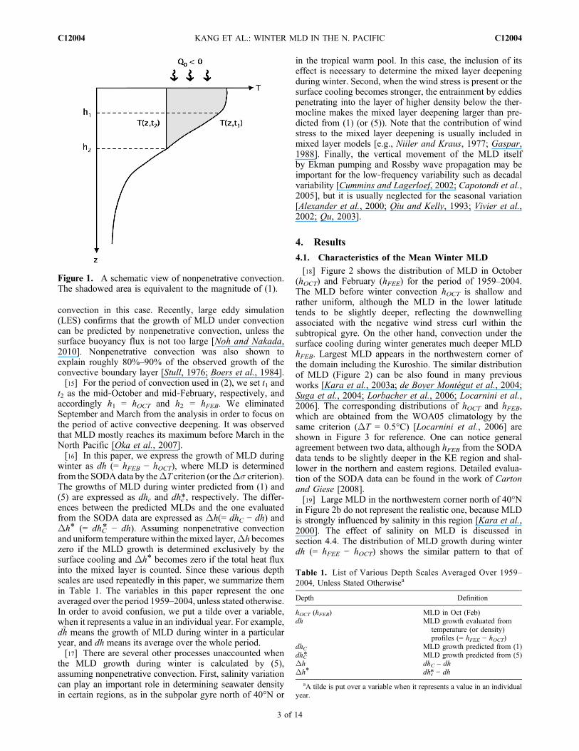
convection in this case. Recently, large eddy simulation(LES) confirms that the growth of MLD under convectioncan be predicted by nonpenetrative convection, unless thesurface buoyancy flux is not too large [Noh and Nakada,2010]. Nonpenetrative convection was also shown toexplain roughly 80%–90% of the observed growth of theconvective boundary layer [Stull, 1976; Boers et al., 1984].[15] For the period of convection used in (2), we set t1 and

t2 as the mid‐October and mid‐February, respectively, andaccordingly h1 = hOCT and h2 = hFEB. We eliminatedSeptember and March from the analysis in order to focus onthe period of active convective deepening. It was observedthat MLD mostly reaches its maximum before March in theNorth Pacific [Oka et al., 2007].[16] In this paper, we express the growth of MLD during

winter as dh (= hFEB − hOCT), where MLD is determinedfrom the SODA data by theDT criterion (or theDs criterion).The growths of MLD during winter predicted from (1) and(5) are expressed as dhc and dhc*, respectively. The differ-ences between the predicted MLDs and the one evaluatedfrom the SODA data are expressed as Dh(= dhC − dh) andDh* (= dhC* − dh). Assuming nonpenetrative convectionand uniform temperature within the mixed layer,Dh becomeszero if the MLD growth is determined exclusively by thesurface cooling and Dh* becomes zero if the total heat fluxinto the mixed layer is counted. Since these various depthscales are used repeatedly in this paper, we summarize themin Table 1. The variables in this paper represent the oneaveraged over the period 1959–2004, unless stated otherwise.In order to avoid confusion, we put a tilde over a variable,when it represents a value in an individual year. For example,d~h means the growth of MLD during winter in a particularyear, and dh means its average over the whole period.[17] There are several other processes unaccounted when

the MLD growth during winter is calculated by (5),assuming nonpenetrative convection. First, salinity variationcan play an important role in determining seawater densityin certain regions, as in the subpolar gyre north of 40°N or

in the tropical warm pool. In this case, the inclusion of itseffect is necessary to determine the mixed layer deepeningduring winter. Second, when the wind stress is present or thesurface cooling becomes stronger, the entrainment by eddiespenetrating into the layer of higher density below the ther-mocline makes the mixed layer deepening larger than pre-dicted from (1) (or (5)). Note that the contribution of windstress to the mixed layer deepening is usually included inmixed layer models [e.g., Niiler and Kraus, 1977; Gaspar,1988]. Finally, the vertical movement of the MLD itselfby Ekman pumping and Rossby wave propagation may beimportant for the low‐frequency variability such as decadalvariability [Cummins and Lagerloef, 2002; Capotondi et al.,2005], but it is usually neglected for the seasonal variation[Alexander et al., 2000; Qiu and Kelly, 1993; Vivier et al.,2002; Qu, 2003].

4. Results

4.1. Characteristics of the Mean Winter MLD

[18] Figure 2 shows the distribution of MLD in October(hOCT) and February (hFEE) for the period of 1959–2004.The MLD before winter convection hOCT is shallow andrather uniform, although the MLD in the lower latitudetends to be slightly deeper, reflecting the downwellingassociated with the negative wind stress curl within thesubtropical gyre. On the other hand, convection under thesurface cooling during winter generates much deeper MLDhFEB. Largest MLD appears in the northwestern corner ofthe domain including the Kuroshio. The similar distributionof MLD (Figure 2) can be also found in many previousworks [Kara et al., 2003a; de Boyer Montégut et al., 2004;Suga et al., 2004; Lorbacher et al., 2006; Locarnini et al.,2006]. The corresponding distributions of hOCT and hFEB,which are obtained from the WOA05 climatology by thesame criterion (DT = 0.5°C) [Locarnini et al., 2006] areshown in Figure 3 for reference. One can notice generalagreement between two data, although hFEB from the SODAdata tends to be slightly deeper in the KE region and shal-lower in the northern and eastern regions. Detailed evalua-tion of the SODA data can be found in the work of Cartonand Giese [2008].[19] Large MLD in the northwestern corner north of 40°N

in Figure 2b do not represent the realistic one, because MLDis strongly influenced by salinity in this region [Kara et al.,2000]. The effect of salinity on MLD is discussed insection 4.4. The distribution of MLD growth during winterdh (= hFEE − hOCT) shows the similar pattern to that of

Figure 1. A schematic view of nonpenetrative convection.The shadowed area is equivalent to the magnitude of (1).

Table 1. List of Various Depth Scales Averaged Over 1959–2004, Unless Stated Otherwisea

Depth Definition

hOCT (hFEB) MLD in Oct (Feb)dh MLD growth evaluated from

temperature (or density)profiles (= hFEE − hOCT)

dhC MLD growth predicted from (1)dhC* MLD growth predicted from (5)Dh dhC – dhDh* dhc* − dh

aA tilde is put over a variable when it represents a value in an individualyear.

KANG ET AL.: WINTER MLD IN THE N. PACIFIC C12004C12004

3 of 14

hFEB, but its latitudinal gradient is stronger (Figure 2c). Itsstandard deviation tends to be also large in the region withlarge dh (Figure 2d).[20] On the other hand, the magnitude of SHF is the

largest along the Kuroshio, and the latitudinal gradient ismuch weaker than in dh (Figure 4a). Dissimilarity in thedistributions of dh and SHF (Figures 2c and 4a) suggeststhat dh is also affected by factors other than SHF. A scatterdiagram between dh and SHF shows the negative correla-tion, but with large scattering (Figure 4b).

[21] Figure 5a shows the difference between dh and theone predicted from (1) dhC, i.e., Dh (= dhC − dh). We canalso calculate OHT by HCV – SHF in (2) with h2 = hFEB,using T(z, t) and Q0(t) from the SODA and NCEP/NCARreanalysis data, respectively (Figure 5b). Note that theadvection of heat in (3) can be calculated directly from thevelocity and temperature fields provided by the SODA data,but the data for eddy diffusivity are not available.[22] A remarkable resemblance is found between these

two distributions. Both Dh and OHT are positive south of

Figure 2. Distributions of (a) hOCT, (b) hFEB, (c) dh (= hFEB − hOCT), and (d) the standard deviation ofd~h.

Figure 3. Distributions from WOA05 climatology: (a) hOCT, (b) hFEB.

KANG ET AL.: WINTER MLD IN THE N. PACIFIC C12004C12004

4 of 14

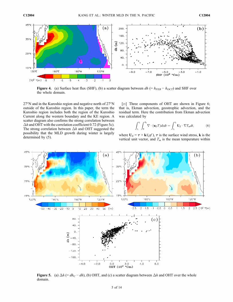
27°N and in the Kuroshio region and negative north of 27°Noutside of the Kuroshio region. In this paper, the term theKuroshio region includes both the region of the KuroshioCurrent along the western boundary and the KE region. Ascatter diagram also confirms the strong correlation betweenDh andOHTwith the correlation coefficient 0.72 (Figure 5c).The strong correlation between Dh and OHT suggested thepossibility that the MLD growth during winter is largelydetermined by (5).

[23] Three components of OHT are shown in Figure 6;that is, Ekman advection, geostrophic advection, and theresidual term. Here the contribution from Ekman advectionwas calculated by

Z t2

t1

Z0

h2

r � uETð Þdzdt ¼Z t2

t1

UE � rTmdt; ð6Þ

where UE = t × k/(rf ), t is the surface wind stress, k is thevertical unit vector, and Tm is the mean temperature within

Figure 4. (a) Surface heat flux (SHF), (b) a scatter diagram between dh (= hFEB − hOCT) and SHF overthe whole domain.

Figure 5. (a) Dh (= dhC − dh), (b) OHT, and (c) a scatter diagram between Dh and OHT over the wholedomain.

KANG ET AL.: WINTER MLD IN THE N. PACIFIC C12004C12004

5 of 14

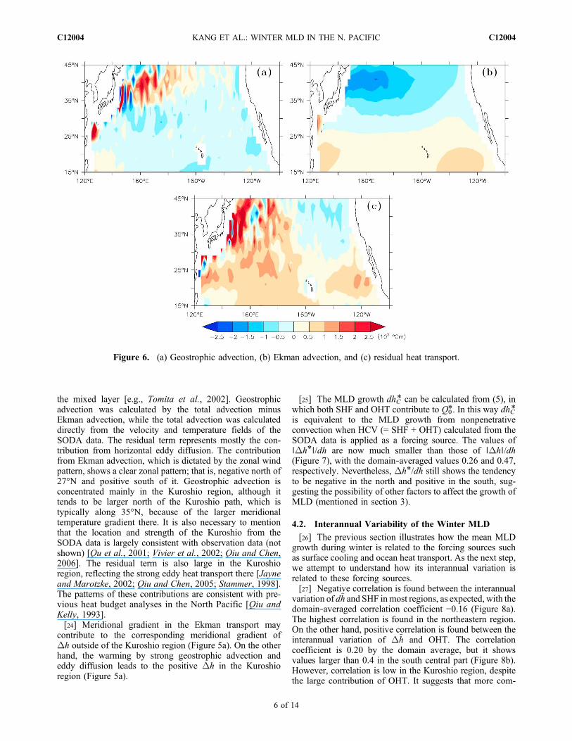
the mixed layer [e.g., Tomita et al., 2002]. Geostrophicadvection was calculated by the total advection minusEkman advection, while the total advection was calculateddirectly from the velocity and temperature fields of theSODA data. The residual term represents mostly the con-tribution from horizontal eddy diffusion. The contributionfrom Ekman advection, which is dictated by the zonal windpattern, shows a clear zonal pattern; that is, negative north of27°N and positive south of it. Geostrophic advection isconcentrated mainly in the Kuroshio region, although ittends to be larger north of the Kuroshio path, which istypically along 35°N, because of the larger meridionaltemperature gradient there. It is also necessary to mentionthat the location and strength of the Kuroshio from theSODA data is largely consistent with observation data (notshown) [Qu et al., 2001; Vivier et al., 2002; Qiu and Chen,2006]. The residual term is also large in the Kuroshioregion, reflecting the strong eddy heat transport there [Jayneand Marotzke, 2002; Qiu and Chen, 2005; Stammer, 1998].The patterns of these contributions are consistent with pre-vious heat budget analyses in the North Pacific [Qiu andKelly, 1993].[24] Meridional gradient in the Ekman transport may

contribute to the corresponding meridional gradient ofDh outside of the Kuroshio region (Figure 5a). On the otherhand, the warming by strong geostrophic advection andeddy diffusion leads to the positive Dh in the Kuroshioregion (Figure 5a).

[25] The MLD growth dhC* can be calculated from (5), inwhich both SHF and OHT contribute to Q0*. In this way dhC*is equivalent to the MLD growth from nonpenetrativeconvection when HCV (= SHF + OHT) calculated from theSODA data is applied as a forcing source. The values of∣Dh*∣/dh are now much smaller than those of ∣Dh∣/dh(Figure 7), with the domain‐averaged values 0.26 and 0.47,respectively. Nevertheless, Dh*/dh still shows the tendencyto be negative in the north and positive in the south, sug-gesting the possibility of other factors to affect the growth ofMLD (mentioned in section 3).

4.2. Interannual Variability of the Winter MLD

[26] The previous section illustrates how the mean MLDgrowth during winter is related to the forcing sources suchas surface cooling and ocean heat transport. As the next step,we attempt to understand how its interannual variation isrelated to these forcing sources.[27] Negative correlation is found between the interannual

variation of d~h and SHF inmost regions, as expected, with thedomain‐averaged correlation coefficient −0.16 (Figure 8a).The highest correlation is found in the northeastern region.On the other hand, positive correlation is found between theinterannual variation of D~h and OHT. The correlationcoefficient is 0.20 by the domain average, but it showsvalues larger than 0.4 in the south central part (Figure 8b).However, correlation is low in the Kuroshio region, despitethe large contribution of OHT. It suggests that more com-

Figure 6. (a) Geostrophic advection, (b) Ekman advection, and (c) residual heat transport.

KANG ET AL.: WINTER MLD IN THE N. PACIFIC C12004C12004

6 of 14

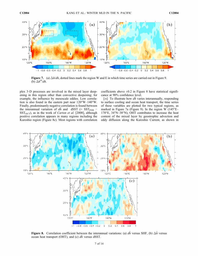
plex 3‐D processes are involved in the mixed layer deep-ening in this region other than convective deepening; forexample, the influence by mesoscale eddies. Low correla-tion is also found in the eastern part near 120°W–140°W.Finally, predominantly negative correlation is found betweenthe interannual variation of d~h and dSST (= SSTFEB −SSTOCT), as in the work of Carton et al. [2008], althoughpositive correlation appears in many regions including theKuroshio region (Figure 8c). Most regions with correlation

coefficients above ±0.2 in Figure 8 have statistical signifi-cance at 90% confidence level.[28] To illustrate how d~h varies interannually, responding

to surface cooling and ocean heat transport, the time seriesof these variables are plotted for two typical regions, asmarked in Figure 7a (Figure 9). In the region W (145°E–170°E, 34°N–38°N), OHT contributes to increase the heatcontent of the mixed layer by geostrophic advection andeddy diffusion along the Kuroshio Current, as shown in

Figure 8. Correlation coefficient between the interannual variations: (a) d~h versus SHF, (b) D~h versusocean heat transport (OHT), and (c) d~h versus dSST.

Figure 7. (a)Dh/dh, dotted lines mark the regionW and E in which time series are carried out in Figure 9.(b) Dh*/dh.

KANG ET AL.: WINTER MLD IN THE N. PACIFIC C12004C12004

7 of 14

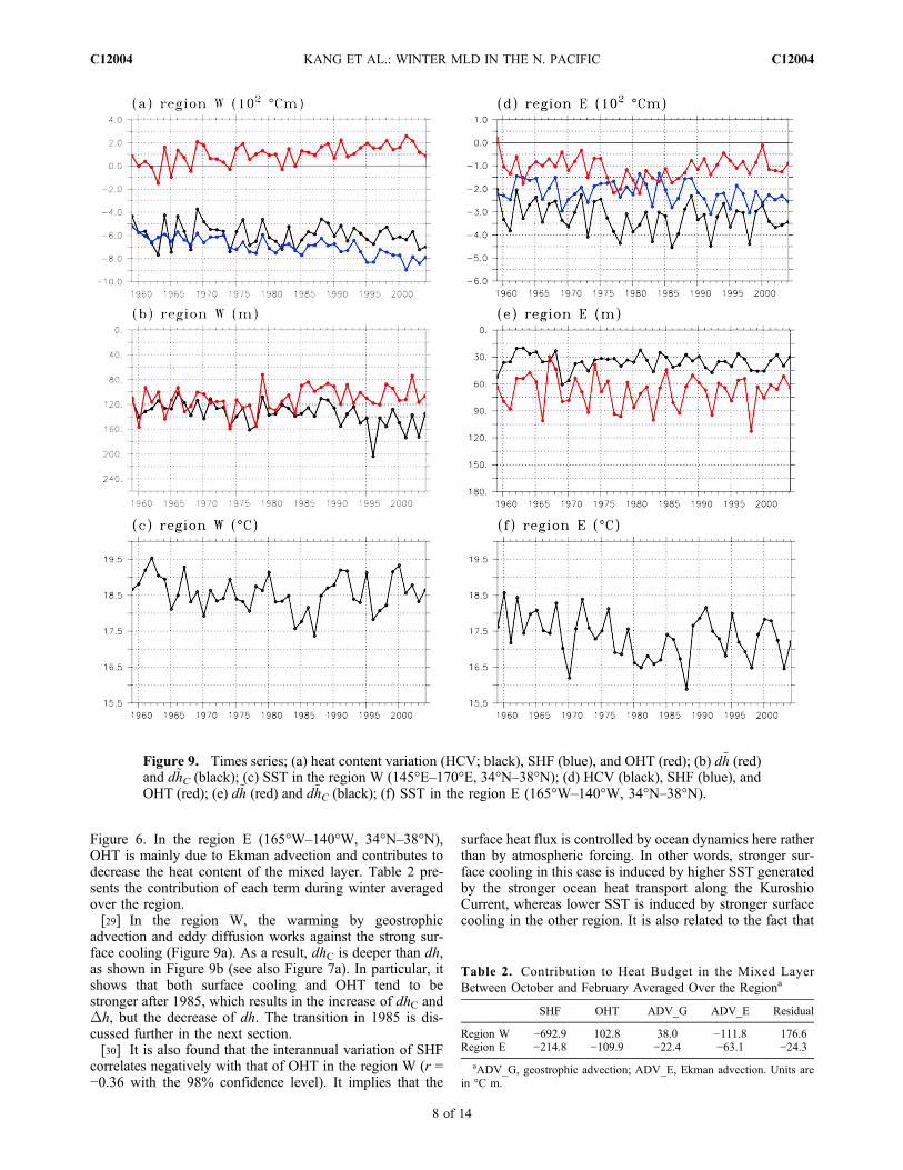
Figure 6. In the region E (165°W–140°W, 34°N–38°N),OHT is mainly due to Ekman advection and contributes todecrease the heat content of the mixed layer. Table 2 pre-sents the contribution of each term during winter averagedover the region.[29] In the region W, the warming by geostrophic

advection and eddy diffusion works against the strong sur-face cooling (Figure 9a). As a result, dhC is deeper than dh,as shown in Figure 9b (see also Figure 7a). In particular, itshows that both surface cooling and OHT tend to bestronger after 1985, which results in the increase of dhC andDh, but the decrease of dh. The transition in 1985 is dis-cussed further in the next section.[30] It is also found that the interannual variation of SHF

correlates negatively with that of OHT in the region W (r =−0.36 with the 98% confidence level). It implies that the

surface heat flux is controlled by ocean dynamics here ratherthan by atmospheric forcing. In other words, stronger sur-face cooling in this case is induced by higher SST generatedby the stronger ocean heat transport along the KuroshioCurrent, whereas lower SST is induced by stronger surfacecooling in the other region. It is also related to the fact that

Figure 9. Times series; (a) heat content variation (HCV; black), SHF (blue), and OHT (red); (b) d~h (red)and d~hC (black); (c) SST in the region W (145°E–170°E, 34°N–38°N); (d) HCV (black), SHF (blue), andOHT (red); (e) d~h (red) and d~hC (black); (f) SST in the region E (165°W–140°W, 34°N–38°N).

Table 2. Contribution to Heat Budget in the Mixed LayerBetween October and February Averaged Over the Regiona

SHF OHT ADV_G ADV_E Residual

Region W −692.9 102.8 38.0 −111.8 176.6Region E −214.8 −109.9 −22.4 −63.1 −24.3

aADV_G, geostrophic advection; ADV_E, Ekman advection. Units arein °C m.

KANG ET AL.: WINTER MLD IN THE N. PACIFIC C12004C12004

8 of 14

the positive correlation appears between d~h and dSST in thisregion, as shown in Figure 8c.[31] On the other hand, in the region E, both SHF and

OHT contribute to decrease the heat content of the mixedlayer during winter (Figure 9d), as OHT is dominated by thesouthward Ekman heat transport here (Table 2). As a result,d~hC is always shallower than d~h, as shown in Figure 9e (seealso Figure 7a). Significant correlation is found between d~hand SHF (r = −0.61 with the 99% confidence level), whichis also in agreement with the highest correlation in thisregion (Figure 8a). It is attributed to the fact that both thesouthward Ekman transport and surface cooling increasewith wind speed.

4.3. Transition in the Winter MLD Pattern

[32] It is well known that after the mid‐1970s climate shiftassociated with PDO, the wind stress over the central NorthPacific becomes stronger, the SST in the central andnorthern North Pacific becomes lower, and the SST in theequatorial and eastern North Pacific becomes higher[Mantua and Hare, 2002]. Figures 9d and 9f actually showthe tendency to the stronger southward Ekman transport andthe lower winter SST in 1975 in the region E, which islocated in the central Pacific.[33] However, the transition to smaller dh and larger

Dh occurs in 1985 in the region W, located in the KEregion, as shown in Figure 9b. The tendency to larger OHTafter 1985 is also observed in Figure 9a. The corresponding

transition to the decreased winter MLD and the enhancedhorizontal heat transport in the KE region is reported byYasuda et al. [2000] and Kelly [2004]. The appearance oflower SST during the 1980s, shown in Figure 9c, is also inagreement with previous reports [Deser et al., 1996; Yasudaet al., 2000; Seager et al., 2001]. Many studies suggestedthat the transition in the KE region, including the enhancedhorizontal heat transport and the decreased SST, occursseveral years after the transition in the wind stress patterndue to PDO in the mid‐1970s, via the oceanic adjustmentplayed by baroclinic Rossby waves propagating westwardfrom the central Pacific [Yasuda and Hanawa, 1997; Milleret al., 1998; Deser et al., 1999; Seager et al., 2001].[34] In order to investigate the transition in the char-

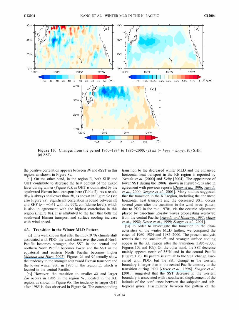
acteristics of the winter MLD further, we compared thecases of 1960–1984 and 1985–2000. The present analysisreveals that the smaller dh and stronger surface coolingappear in the KE region after the transition (1985–2000;Figures 10a and 10b). On the other hand, the SST decreasemainly appears north of 35°N and in the central Pacific(Figure 10c). Its pattern is similar to the SST change asso-ciated with PDO, but the SST change in the westernboundary is larger than in the central Pacific contrary to thetransition during PDO [Deser et al., 1996]. Seager et al.[2001] suggested that the SST decrease in the westernboundary is associated with a southward displacement of thelatitude of the confluence between the subpolar and sub-tropical gyres. Dissimilarity between the pattern of the

Figure 10. Changes from the period 1960–1984 to 1985–2000; (a) dh (= hFEB − hOCT), (b) SHF,(c) SST.

KANG ET AL.: WINTER MLD IN THE N. PACIFIC C12004C12004

9 of 14

changes of SHF and SST (Figures 10b and 10c) also indicatesthat the SST change may be due to the change in the oceancirculation rather than in the surface heat flux.[35] It is interesting, however, to observe that the strong

negative SHF anomaly appears in the region of negativeSST change east of Japan along 40°N, in the work bySeager et al. [2001], but it does not appear in the presentanalysis. The average period after the transition is muchshorter in the work by Seager et al. [2001] (1967–1975versus 1982–1990). It is expected that the strong negativeSHF anomaly, induced by the displacement of the polar

front after the transition, may decrease with time as a newlocal balance is approached between the atmosphere and theocean.[36] Figure 11a shows that Dh increases after 1985 in the

KE region, which is mainly due to the enhanced heattransport by the Kurosho Current, as illustrated in Figures 9aand 11b. Figure 12 shows the decomposition of the OHTdifference into three contributions: geostrophic advection,Ekman advection, and the residual term, similar to Figure 6.Enhanced geostrophic advection and eddy diffusion appear inthe Kuroshio region, which are due to the stronger Kuroshio

Figure 11. Changes from the period 1960–1984 to 1985–2000; (a) Dh (= dhC − dh), (b) OHT.

Figure 12. Changes from the period 1960–1984 to 1985–2000; (a) geostrophic advection, (b) Ekmanadvection, and (c) residual heat transport.

KANG ET AL.: WINTER MLD IN THE N. PACIFIC C12004C12004

10 of 14

Current (Figures 12a and 12c). It is also found that thestronger westerly wind stress along ∼40°N strengthens thesouthward Ekman transport (Figure 12b). A similar patternof change in geostrophic and Ekman advection is also foundin the work by Seager et al. [2001, Figure 5].

4.4. Other Factors That Influence the Winter MLD

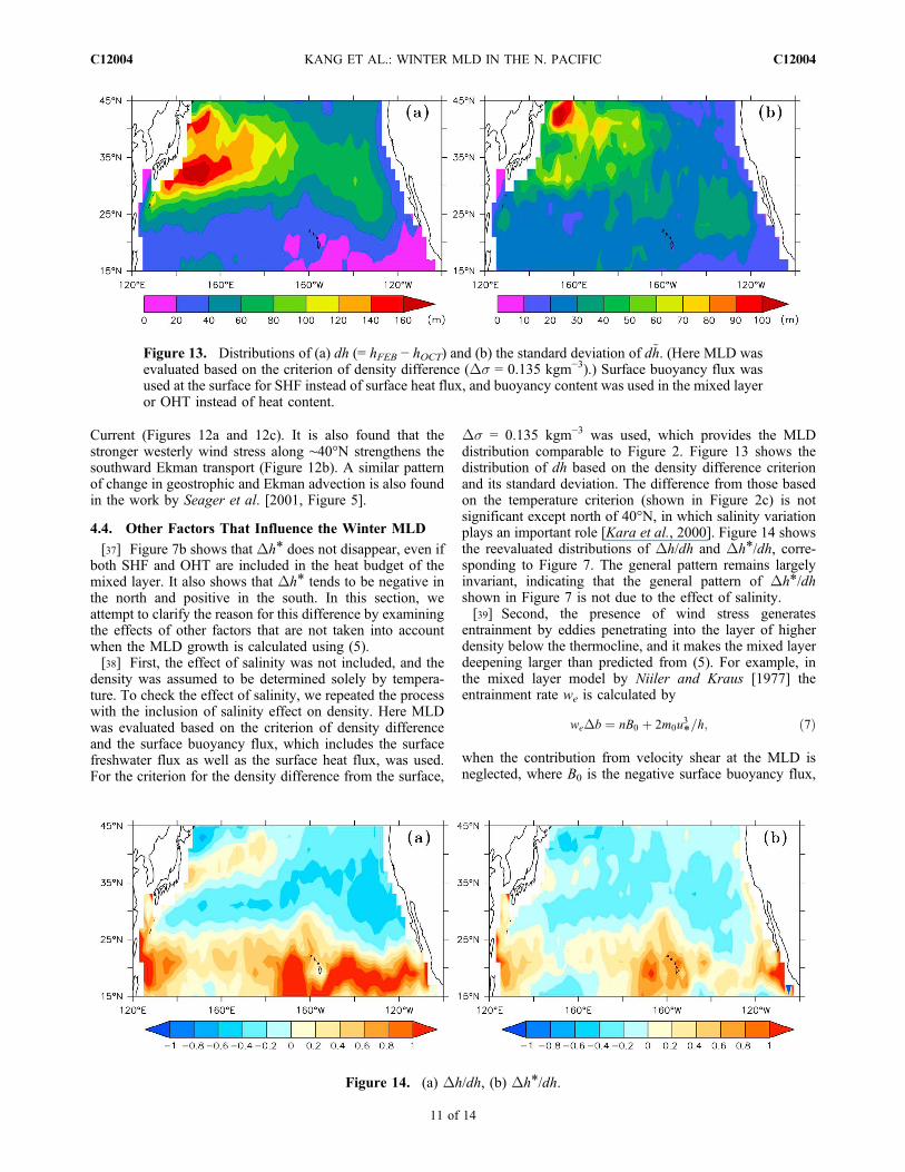
[37] Figure 7b shows that Dh* does not disappear, even ifboth SHF and OHT are included in the heat budget of themixed layer. It also shows that Dh* tends to be negative inthe north and positive in the south. In this section, weattempt to clarify the reason for this difference by examiningthe effects of other factors that are not taken into accountwhen the MLD growth is calculated using (5).[38] First, the effect of salinity was not included, and the

density was assumed to be determined solely by tempera-ture. To check the effect of salinity, we repeated the processwith the inclusion of salinity effect on density. Here MLDwas evaluated based on the criterion of density differenceand the surface buoyancy flux, which includes the surfacefreshwater flux as well as the surface heat flux, was used.For the criterion for the density difference from the surface,

Ds = 0.135 kgm−3 was used, which provides the MLDdistribution comparable to Figure 2. Figure 13 shows thedistribution of dh based on the density difference criterionand its standard deviation. The difference from those basedon the temperature criterion (shown in Figure 2c) is notsignificant except north of 40°N, in which salinity variationplays an important role [Kara et al., 2000]. Figure 14 showsthe reevaluated distributions of Dh/dh and Dh*/dh, corre-sponding to Figure 7. The general pattern remains largelyinvariant, indicating that the general pattern of Dh*/dhshown in Figure 7 is not due to the effect of salinity.[39] Second, the presence of wind stress generates

entrainment by eddies penetrating into the layer of higherdensity below the thermocline, and it makes the mixed layerdeepening larger than predicted from (5). For example, inthe mixed layer model by Niiler and Kraus [1977] theentrainment rate we is calculated by

weDb ¼ nB0 þ 2m0u3*=h; ð7Þ

when the contribution from velocity shear at the MLD isneglected, where B0 is the negative surface buoyancy flux,

Figure 13. Distributions of (a) dh (= hFEB − hOCT) and (b) the standard deviation of d~h. (Here MLD wasevaluated based on the criterion of density difference (Ds = 0.135 kgm−3).) Surface buoyancy flux wasused at the surface for SHF instead of surface heat flux, and buoyancy content was used in the mixed layeror OHT instead of heat content.

Figure 14. (a) Dh/dh, (b) Dh*/dh.

KANG ET AL.: WINTER MLD IN THE N. PACIFIC C12004C12004

11 of 14

Db is the buoyancy jump at MLD (z = h), and empiricalconstants are given by m0 = 0.39 and n = 0.21 [Davis et al.,1981]. With the neglect of the surface freshwater flux, B0 isgiven by B0 = −(ag/rcp)Q0, where a is the thermal expan-sion coefficient. To assess the contribution of wind stress,we examined the distribution of

WS ¼ 2m0

n

1

�g

Z t2

t1

u3*hdt; ð8Þ

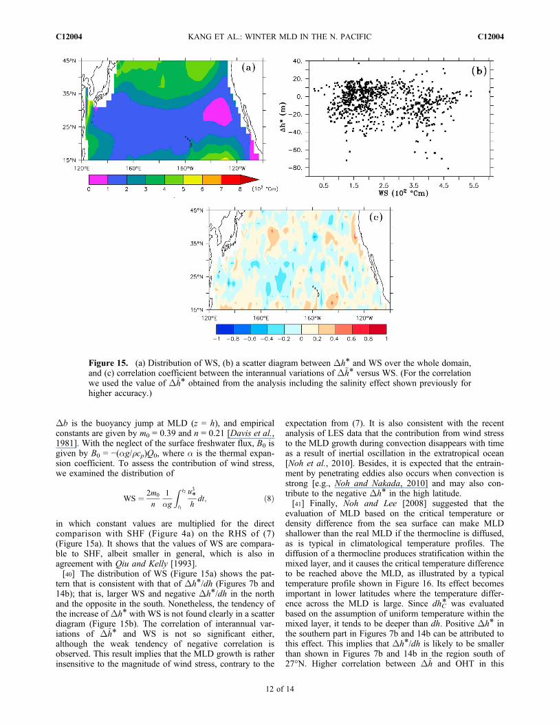
in which constant values are multiplied for the directcomparison with SHF (Figure 4a) on the RHS of (7)(Figure 15a). It shows that the values of WS are compara-ble to SHF, albeit smaller in general, which is also inagreement with Qiu and Kelly [1993].[40] The distribution of WS (Figure 15a) shows the pat-

tern that is consistent with that of Dh*/dh (Figures 7b and14b); that is, larger WS and negative Dh*/dh in the northand the opposite in the south. Nonetheless, the tendency ofthe increase of Dh* with WS is not found clearly in a scatterdiagram (Figure 15b). The correlation of interannual var-iations of D~h* and WS is not so significant either,although the weak tendency of negative correlation isobserved. This result implies that the MLD growth is ratherinsensitive to the magnitude of wind stress, contrary to the

expectation from (7). It is also consistent with the recentanalysis of LES data that the contribution from wind stressto the MLD growth during convection disappears with timeas a result of inertial oscillation in the extratropical ocean[Noh et al., 2010]. Besides, it is expected that the entrain-ment by penetrating eddies also occurs when convection isstrong [e.g., Noh and Nakada, 2010] and may also con-tribute to the negative Dh* in the high latitude.[41] Finally, Noh and Lee [2008] suggested that the

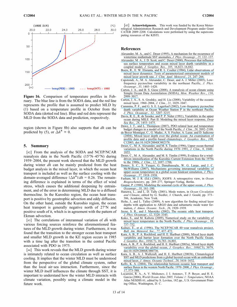
evaluation of MLD based on the critical temperature ordensity difference from the sea surface can make MLDshallower than the real MLD if the thermocline is diffused,as is typical in climatological temperature profiles. Thediffusion of a thermocline produces stratification within themixed layer, and it causes the critical temperature differenceto be reached above the MLD, as illustrated by a typicaltemperature profile shown in Figure 16. Its effect becomesimportant in lower latitudes where the temperature differ-ence across the MLD is large. Since dhC* was evaluatedbased on the assumption of uniform temperature within themixed layer, it tends to be deeper than dh. Positive Dh* inthe southern part in Figures 7b and 14b can be attributed tothis effect. This implies that Dh*/dh is likely to be smallerthan shown in Figures 7b and 14b in the region south of27°N. Higher correlation between D~h and OHT in this

Figure 15. (a) Distribution of WS, (b) a scatter diagram between Dh* and WS over the whole domain,and (c) correlation coefficient between the interannual variations of D~h* versus WS. (For the correlationwe used the value of D~h* obtained from the analysis including the salinity effect shown previously forhigher accuracy.)

KANG ET AL.: WINTER MLD IN THE N. PACIFIC C12004C12004

12 of 14

region (shown in Figure 8b) also supports that dh can bepredicted by (5), or Dh* ≅ 0.

5. Summary

[42] From the analysis of the SODA and NCEP/NCARreanalysis data in the North Pacific (15°N–45°N) during1959–2004, the present work showed that the MLD growthduring winter dh can be mainly predicted from the heatbudget analysis in the mixed layer, in which the ocean heattransport is included as well as the surface cooling with thedomain‐averaged difference ∣Dh*∣/dh = 0.26. The remain-ing difference is explained in terms of the effect of windstress, which causes the additional deepening by entrain-ment, and of the error in determining MLD due to a diffusedthermocline. In the Kuroshio region, the ocean heat trans-port is positive by geostrophic advection and eddy diffusion.On the other hand, outside the Kuroshio region, the oceanheat transport is generally negative north of 27°N andpositive south of it, which is in agreement with the pattern ofEkman advection.[43] The correlations of interannual variation of d~h with

various forcing sources reinforce the aforementioned fea-tures of the MLD growth during winter. Furthermore, it wasfound that the transition to the stronger ocean heat transportand smaller MLD growth in the KE region occurs in 1985with a time lag after the transition in the central Pacificassociated with PDO in 1975.[44] This work reveals that the MLD growth during winter

is intimately related to ocean circulation as well as surfacecooling. It implies that the winter MLD must be understoodfrom the perspective of the global climate system, ratherthan the local air‐sea interaction. Furthermore, since thewinter MLD itself influences the climate through SST, it isimportant to understand how the winter MLD interacts withclimate variation, possibly using a climate model in thefuture work.

[45] Acknowledgments. This work was funded by the Korea Meteo-rological Administration Research and Development Program under GrantCATER 2009‐2208. Calculations were performed by using the supercom-puting resources of the KISTI.

ReferencesAlexander, M. A., and C. Deser (1995), A mechanism for the recurrence ofwintertime midlatitude SST anomalies, J. Phys. Oceanogr., 25, 122–137.

Alexander, M. A., J. D. Scott, and C. Deser (2000), Processes that influencesea surface temperature and ocean mixed layer depth variability in acoupled model, J. Geophys. Res., 105, 16,823–16,842.

Boers, R., E. W. Eloranta, and R. L. Coulter (1984), Lidar observations ofmixed layer dynamics: Tests of parameterized entrainment models ofmixed layer growth rate, J. Clim. Appl. Meteorol., 23, 247–266.

Capotondi, A., M. A. Alexander, C. Deser, and A. J. Miller (2005), Low‐frequency pycnocline variability in the northeast Pacific, J. Phys.Oceanogr., 35, 1403–1420.

Carton, J. A., and B. S. Giese (2008), A reanalysis of ocean climate usingSimple Ocean Data Assimilation (SODA), Mon. Weather Rev., 136,2999–3017.

Carton, J. A., S. A. Grodsky, and H. Liu (2008), Variability of the oceanicmixed layer, 1960–2004, J. Clim., 21, 1029–1047.

Cummins, P. F., and G. S. E. Lagerloef (2002), Low‐frequency pycnoclinedepth variability at Ocean Weather Station P in the northeast Pacific,J. Phys. Oceanogr., 32, 3207–3215.

Davis, R. E., R. de Szoeke, and P. P. Niiler (1981), Variability in the upperocean during MILE. Part II: Modeling the mixed layer response, DeepSea Res., 28, 1453–1475.

Dawe, J. T., and L. Thompson (2007), PDO‐related heat and temperaturebudget changes in a model of the North Pacific, J. Clim., 20, 2092–2108.

de Boyer Montégut, C., G. Madec, A. S. Fischer, A. Lazar, and D. Iudicone(2004), Mixed layer depth over the global ocean: An examination ofprofile data and a profile‐based climatology, J. Geophys. Res., 109,C12003, doi:10.1029/2004JC002378.

Deser, C., M. A. Alexander, and M. S. Timlin (1996), Upper‐ocean thermalvariations in the North Pacific during 1970–1991, J. Clim., 9, 1840–1855.

Deser, C., M. A. Alexander, and M. S. Timlin (1999), Evidence for a wind‐driven intensification of the Kuroshio Current Extension from the 1970sto the 1980s, J. Clim., 12, 1697–1706.

Doney, S. C., S. Yeager, G. Danabasoglu, W. G. Large, and J. C.McWilliams (2007), Mechanisms governing interannual variability ofupper‐ocean temperature in a global ocean hindcast simulation, J. Phys.Oceanogr., 37, 1918–1938.

Fasham, M. J. R. (Ed.) (2003), JGOFS: A retrospective view, in OceanBiogeochemistry, pp. 269–277, Springer‐Verlag, Berlin.

Gaspar, P. (1988), Modeling the seasonal cycle of the upper ocean, J. Phys.Oceanogr., 18, 161–180.

Hanawa, L., and L. D. Tally (2001), Mode waters, in Ocean Circulationand Climate, edited by G. Siedler, J. Church, and J. Gould, pp. 373–386, Academic, New York.

Holte, J., and L. Talley (2009), A new algorithm for finding mixed layerdepths with application to ARGO data and subantartic mode water for-mation, J. Atmos. Oceanic. Tech., 26, 1920–1939.

Jayne, S. R., and J. Marotzke (2002), The oceanic eddy heat transport,J. Phys. Oceanogr., 32, 3328–3345.

Kako, S., and M. Kubota (2009), Numerical study on the variability ofmixed layer temperature in the North Pacific, J. Phys. Oceanogr., 39,737–752.

Kalnay, E., et al. (1996), The NCEP/NCAR 40‐year reanalysis project,Bull. Am. Meteorol. Soc., 77, 437–472.

Kara, A. B., P. A. Rochford, and H. E. Hurlburt (2000), Mixed layer depthvariability and barrier layer formation over the North Pacific Ocean,J. Geophys. Res., 105(C7), 16,783–16,801.

Kara, A. B., P. A. Rochford, and H. E. Hurlburt (2003a), Mixed layer depthvariability over the global ocean, J. Geophys. Res., 108(C3), 3079,doi:10.1029/2000JC000736.

Kara, A. B., A. J. Wallcraft, and H. E. Hurlbert (2003b), ClimatologicalSST and MLD predictions from a global layered ocean with an embeddedmixed layer, J. Atmos. Oceanic Technol., 20, 1616–1632.

Kelly, K. A. (2004), The relationship between oceanic heat transport andsurface fluxes in the western North Pacific: 1970–2000, J. Phys. Oceanogr.,17, 573–588.

Locarnini, R. A., A. V. Mishonov, J. I. Antonov, T. P. Boyer, and H. E.Garcia (2006),World Ocean Atlas 2005, Volume 1: Temperature, NOAAAtlas NESDIS 61, edited by S. Levitus, 182 pp., U.S. Government Print-ing Office, Washington, D. C.

Figure 16. Comparison of temperature profiles in Feb-ruary. The blue line is from the SODA data, and the red linerepresents the profile that is assumed to predict MLD by(1) based on a temperature profile in October from theSODA data (dotted red line). Blue and red dots represent theMLD from the SODA data and prediction, respectively.

KANG ET AL.: WINTER MLD IN THE N. PACIFIC C12004C12004

13 of 14

Lorbacher, K., D. Dommenget, P. P. Niiler, and A. Köhl (2006), Oceanmixed layer depth: A subsurface proxy of ocean‐atmosphere variability,J. Geophys. Res., 111, C07010, doi:10.1029/2003JC002157.

Mantua, N. J., and S. R. Hare (2002), The Pacific decadal oscillation,J. Oceanogr., 58, 35–44.

Masuzawa, J. (1969), Subtropical mode water, Deep Sea Res., 16, 463–472.

Miller, A. J., D. R. Cayan, and W. B. White (1998), A westward‐intensifieddecadal change in the North Pacific thermocline and gyre‐scale circula-tion, J. Clim., 11, 3112–3127.

Namias, J., and R. M. Born (1970), Temporal coherence in North Pacificsea‐surface temperature patterns, J. Geophys. Res., 75, 5952–5955.

Niiler, P. P., and E. B. Kraus (1977), One‐dimensional models of the upperocean, in Modelling and Prediction of the Upper Layers of the Ocean,edited by E. B. Kraus, pp. 143–177, Pergamon, Oxford.

Noh, Y., and W. S. Lee (2008), Mixed and mixing layer depths simulatedby an OGCM, J. Oceanogr., 64, 217–225.

Noh, Y., and S. Nakada (2010), Estimation of the particle flux from theconvective mixed layer by large eddy simulation, J. Geophys. Res.,115, C05007, doi:10.1029/2009JC005669.

Noh, Y., C. J. Jang, T. Yamagata, P. T. Chu, and C. H. Kim (2002), Sim-ulation of more realistic upper‐ocean processes from an OGCM with anew mixed layer model, J. Phys. Oceanogr., 32, 1284–1307.

Noh, Y., G. Goh and S. Raasch (2010), Examination of the mixed layerdeepening process during convection using LES, J. Phys. Oceanogr.,40, 2189–2195.

Ohno, Y., N. Iwasaka, F. Kobashi, and Y. Sato (2009), Mixed layer depthclimatology of the North Pacific based on Argo observations, J. Ocea-nogr., 65, 1–16.

Oka, E., L. D. Talley, and T. Suga (2007), Temporal variability of wintermixed layer in the mid‐to high‐latitude North Pacific, J. Oceanogr., 63,293–307.

Oschlies, A. (2002), Improved representation of upper ocean dynamics andmixed layer depths in a model of the North Atlantic on switching fromeddy‐permitting to eddy‐resolving grid resolution, J. Phys. Oceanogr.,32, 2277–2298.

Qiu, B., and S. Chen (2005), Eddy‐induced heat transport in the subtropicalNorth Pacific from Argo, TMI, and altimetry measurements, J. Phys.Oceanogr., 35, 458–473.

Qiu, B., and S. Chen (2006), Decadal variability in the formation of theNorth Pacific subtropical mode water: Oceanic versus atmospheric con-trol, J. Phys. Oceanogr., 36, 1365–1380.

Qiu, B., and K. A. Kelly (1993), Upper‐ocean heat balance in the KuroshioExtension region, J. Phys. Oceanogr., 23, 2027–2041.

Qu, T. (2003), Mixed layer heat balance in the western North Pacific,J. Geophys. Res., 108(C7), 3242, doi:10.1029/2002JC001536.

Qu, T., H. Mitsudera, and B. Qiu (2001), A climatological view of theKuroshio/Oyashio system east of Japan, J. Phys. Oceanogr., 31, 2575–2589.

Seager, R., Y. Kushnir, N. H. Naik, M. A. Cane, and J. Miller (2001),Wind‐driven shifts in the latitude of the Kuroshio‐Oyashio Extensionand generation of SST anomalies on decadal timescales, J. Climate,14, 4249–4265.

Smith, R. D., J. K. Dukowicz, and R. C. Malone (1992), Parallel ocean gen-eral circulation modeling, Physica D, 60, 38–61.

Stammer, D. (1998), On eddy characteristics, eddy transports, and meanflow properties, J. Phys. Oceanogr., 28, 727–739.

Stull, R. B. (1976), Mixed layer depth model based on turbulent energetics,J. Atmos. Sci., 33, 1260–1278.

Suga, T., K. Motoki, Y. Aoki, and A. M. Macdonald (2004), The NorthPacific climatology of winter mixed layer and mode waters, J. Phys.Oceanogr., 34, 3–22.

Tomita, T., and M. Nonaka (2006), Upper‐ocean mixed layer and winter-time sea surface temperature anomalies in the North Pacific, J. Clim., 19,300–307.

Tomita, T., S.‐P. Xie, and M. Nonaka (2002), Estimates of surface andsubsurface forcing for decadal sea surface temperature variability in themid‐latitude North Pacific, J. Meteorol. Soc. Japan, 80, 1289–1300.

Turner, J. S. (1973), Buoyancy Effects in Fluids, 306 pp., Cambridge Univ.Press, Cambridge.

Vivier, F., K. A. Kelly, and L. Thompson (2002), Heat budget in theKuroshio Extension region: 1993–99, J. Phys. Oceanogr., 32, 3436–3454.

Yasuda, I., T. Tozuka, M. Noto, and S. Koutetsu (2000), Heat balance andregime shifts of the mixed layer in the Kuroshio Extension, Prog.Oceangr., 47, 257–278.

Yasuda, T., and K. Hanawa (1997), Decadal changes in the mode waters inthe midlatitude North Pacific, J. Phys. Oceanogr., 27, 858–870.

Y. J. Kang and Y. Noh, Department of Atmospheric Sciences/GlobalEnvironmental Laboratory, Yonsei University, 134 Shinchon‐dong,Seodaemun‐gu, Seoul 120‐749, Korea. (noh@yonsei.ac.kr)S.‐W. Yeh, Department of Environmental Marine Sciences, Hanyang

University, Ansan, South Korea.

KANG ET AL.: WINTER MLD IN THE N. PACIFIC C12004C12004

14 of 14