Teleconnection Pattern Influence on Sea-Wave Climate in the Bay of Biscay

GONERI LE COZANNET, SOPHIE LECACHEUX, ETIENNE DELVALLEE, NICOLAS DESRAMAUT,CARLOS OLIVEROS, AND RODRIGO PEDREROS

BRGM, Orleans, France

(Manuscript received 22 December 2009, in final form 13 September 2010)

ABSTRACT

The potential modification of hydrodynamic factors, such as waves, is a source of concern for many coastal

communities because of its potential effect on shoreline evolution. In the northern Atlantic, swell is created by

storm winds that cross the Atlantic following west–east tracks. These tracks are shifted more southward or

northward depending on the season and on recurring large-scale atmospheric pressure anomalies, also called

teleconnection patterns. This study investigates the trends of sea-wave patterns in the Bay of Biscay and

relates their interannual variability to teleconnection patterns.

Sea-wave parameter time series from the 40-yr European Centre for Medium-Range Weather Forecasts

(ECMWF) Re-Analysis (ERA-40) show a satisfying correlation with an in situ buoy of Meteo-France during

the period they overlap. Using a k-means algorithm, data from this 44-yr-long time series were clustered into

a few sea-state modes, each of them corresponding to an observable sea state associated with an averaged

value for wave height, period, and direction.

This analysis shows that most of the increase in annual mean sea-wave height since the 1970s has occurred

because the relative frequency of occurrence of persistent observable sea states is evolving over time: from

1970 to 2001, the data indicate that energetic northwest swell becomes more frequent than low-energy in-

termediate sea states. Moreover, anomalies of the relative frequency of occurrence of observable sea states

are related to large-scale recurring pressure anomalies: principally, the Northern Atlantic Oscillation (NAO)

but also (during winters) the east Atlantic (EA) pattern, as well other teleconnection patterns of the Northern

Hemisphere (NOAA data).

1. Introduction

There are many recent studies presenting evidence of

increasing sea-wave height since the 1970s in the North

Atlantic. In the context of the increasing attractiveness of

coastal areas, there is growing concern that this trend will

continue in the future and combine with predicted sea

level rise to intensify shoreline erosion (Wang et al. 2004;

Nicholls et al. 2007; Dodet et al. 2010). Coastal sea waves

are one of the major factors of shoreline evolution: they

are created either by local winds (wind waves) or by storm

winds in the deep ocean, which then propagate to the

coast (swell). Coastal wave patterns are thus a function of

offshore sea-state conditions, near-shore winds, and local

bathymetry. Therefore, large-scale North Atlantic storm-

iness contributes to the local hydrodynamic forcing. This

paper investigates the relationship between large-scale

and local forcing by analyzing the evolution of trends of

sea-wave states in the Bay of Biscay and relating them to

climate variability in the northern Atlantic.

The trend of increasing sea-wave height in the northern

Atlantic is confirmed by analysis of visual data (Gulev and

Grigorieva 2004), in situ measurements (Fig. 1; Table 1;

Bacon and Carter 1991), hindcast models (Kushnir et al.

1997; Wang and Swail 2001, 2002; Dodet et al. 2010), and

remote sensing altimetry (Woolf et al. 2002). The trend

was related to recurrent large-scale atmospheric pressure

anomalies, also called teleconnection patterns. Bacon and

Carter (1993) established a positive correlation between

two in situ sea-wave height time series of the northern

Atlantic and the NAO (refer to Table 2 for expansion of

pattern names), which is the dominant teleconnection

pattern (Wallace and Gutzler 1981). This result is con-

sistent with the fact that the positive phase of the NAO is

associated with northward-shifted storm tracks (above

508N), with a pronounced northeastern orientation and

an increase in storm intensity (Rogers 1990). Moreover,

Corresponding author address: Goneri Le Cozannet, Coastal Risks

Unit, Natural Risks and CO2 Storage Security Division, BRGM, 3

Avenue Claude Guillemin, BP 36009, Orleans 45060, France.

E-mail: g.lecozannet@brgm.fr

1 FEBRUARY 2011 L E C O Z A N N E T E T A L . 641

DOI: 10.1175/2010JCLI3589.1

� 2011 American Meteorological Society

Woolf et al. (2002) revealed the influence of the EA pat-

tern on sea-wave height in the northern Atlantic, relating

the EA index to the position of Atlantic storm tracks:

during EA1 phases, storm tracks are located at lower lat-

itudes (between 358 and 508N) and have a zonal orienta-

tion (Rogers 1990). Therefore, indices of northern Atlantic

climate variability appear to be relevant features in ex-

plaining sea-wave variability and trends. This is consistent

with the fact that teleconnection patterns affect storminess

in regions of the North Atlantic in Fig. 1. The teleconnec-

tion patterns used in this paper are described in Table 2,

together with the associated trends in storminess, as

identified by Seierstad et al. (2007).

In the southern Bay of Biscay, however, the situation

is less clear. Dupuis et al. (2006) investigated the rela-

tionship between sea-wave parameters and teleconnec-

tion patterns. They analyzed a 20-yr time series from a

waverider buoy moored at 26-m depth off of Biscarosse

in the Bay of Biscay (Fig. 1; Table 1) and found a positive

correlation between the NAO and the wave period, but

they could not relate the NAO to sea-wave heights.

Moreover, they could not identify a significant trend dur-

ing the 20-yr period because the signal was highly insta-

tionary, the time series was relatively short, and the buoy

was positioned near the coast and was likely influenced by

coastal processes. More recently, Dodet et al. (2010) pro-

vided more insight on this issue by examining the spatial

patterns of the correlation between the winter NAO index

and single sea-wave parameters in the northeast Atlantic.

They modeled waves using the National Centers for En-

vironmental Prediction–National Center for Atmospheric

Research (NCEP–NCAR) reanalysis winds and found

that this index is well correlated with the peak wave period

over all of the Bay of Biscay, but that it fits poorly with the

90th-percentile sea-wave height. With respect to the mean

wave direction, the correlation worsens near the coast.

These spatial patterns are consistent with the conclusions

obtained by Dupuis et al. (2006) from the data of a single

waverider buoy.

In this paper, a different approach is used to investigate

how climate variability relates to local sea states in the Bay

of Biscay: rather than looking for a possible influence of

teleconnection patterns on a single sea-wave parameter,

such as wave height or period, a link with the observable

sea states is investigated. Similar to Butel et al. (2002),

observable sea states are defined here as a combination of

the significant wave height, mean wave period, and mean

wave direction. As a matter of fact, large-scale atmospheric

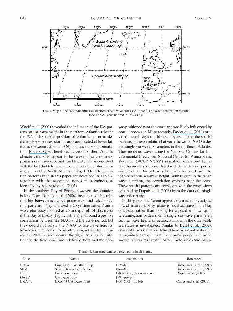
TABLE 1. Sea-state datasets referred to in this study.

Code Name Acquisition Reference

LIMA Lima Ocean Weather Ship 1975–88 Bacon and Carter (1991)

SEV Seven Stones Light Vessel 1962–86 Bacon and Carter (1991)

BISC Biscarosse buoy 1980–2000 (discontinuous) Dupuis et al. (2006)

GASC Gascogne buoy 1998–present

ERA-40 ERA-40 Gascogne point 1957–2001 (model) Caires and Sterl (2001)

FIG. 1. Map of the NA indicating the location of sea-wave data (see Table 1) and wave generation regions

(see Table 2) considered in this study.

642 J O U R N A L O F C L I M A T E VOLUME 24

patterns influence not only the wave height but also the

period and direction, and these are the three most im-

portant parameters to describe the sea-wave state from

a coastal morphodynamics point of view. This study tests

this approach on the Bay of Biscay and investigates the

following two questions:

(i) Can we relate the variability of local sea-wave states

to large-scale atmospheric conditions?

(ii) How can we explain the long-term trend of increasing

sea-wave height in terms of observable sea states?

This paper will proceed as follows. In section 2 (data and

methods), long-term wave data and methods for analyzing

sea states are presented together with the teleconnection

pattern data. The results of the trend analysis and the re-

lationship found between observable sea states and vari-

ous teleconnection patterns are presented in section 3 and

discussed in section 4. In section 5, the results are sum-

marized and their ability to answer the questions raised in

the introduction is discussed.

2. Data and methods

a. Wave data

This study uses the 40-yr European Centre for Medium-

Range Weather Forecasts (ECMWF) Re-Analysis (ERA-

40; Uppala et al. 2005), where the winds at 10 m above sea

level were used to model sea-wave parameters from

September 1958 to August 2002 (Sterl and Caires 2004),

providing 6-h estimates of spectral significant wave height

(H), mean wave period (T), and mean direction (D) on a

global 2.58 latitude 3 2.58 longitude grid. The significant

wave height (SWH), which is defined as the average height

of one-third of the largest waves, is a more common sea-

wave parameter than the spectral significant wave height.

In deep water, these two terms can be considered equal. In

the following, it will be just referred to as SWH.

The ERA-40 data point located at 458N, 58W near the

Bay of Biscay was chosen for this study because of its

offshore location, where it is minimally influenced by lo-

cal coastal processes, such as wave refraction, diffraction,

and bottom friction; moreover, it is also close to the

Gascogne buoy of Meteo-France (45.28N, 58W).

The ERA-40 reanalysis is not a homogeneous dataset

because it progressively assimilates more and more data

(e.g., remote sensing data since the 1970s). A detailed

review of these inhomogeneities can be found in Caires

and Sterl (2001). Nevertheless, Caires et al. (2004) vali-

dated the use of ERA-40 data for the analysis of wave

climate variability with comparisons to several datasets.

However, they also pointed out that using the ERA-40

dataset for the analysis of extremes is not recommended,

as SWH peaks are not well modeled. Thus, this study is

focused on the analysis of averaged wave modes.

Since the ERA-40 waves are generated using the ERA-

40 wind forcing only (there is no assimilation of waves

observations), Caires and Sterl (2003) validated this data-

set against available independent datasets, namely buoy

and altimeter measurements. They reported a bias in the

ERA-40 significant wave height data, with an underesti-

mation of the highest values, and they pointed out that this

bias tends to increase slightly with the mean wave period.

An underestimation of the monthly-mean period in the

Atlantic Ocean of approximately 20.5 s was reported

(Caires and Sterl 2001), but no validation was performed

at the basin scale for the directional wave data. Because

of inhomogeneities in the quality of the dataset, a proper

validation would require in situ directional wave obser-

vations during the entire span of the ERA-40 data.

As an additional evaluation of the precision and accu-

racy of ERA-40 wave parameters, we compared the

ERA-40 wave parameters from the point 458N, 58W with

the data of the Gascogne buoy of Meteo-France (45.28N,

58W) during the period in which the datasets overlap,

from July 1998 to August 2002. Twenty-nine outliers were

excluded from the Gascogne buoy dataset that was then

resampled at 6-h intervals to match the ERA-40 dataset

(see Figs. 2 and 3). The ERA-40 SWH appears to be

TABLE 2. Teleconnection patterns considered in this article and changes in storminess in the NA associated with a positive index value

of one standard deviation (see Fig. 1; Seierstad et al. 2007). Teleconnection patterns quoted here are those defined by Barnston and

Livezey (1987).

Shortening Teleconnection pattern

Associated storminess anomaly in NA for a positive

phase of the index (Seierstad et al. 2007)

NAO Northern Atlantic Oscillation Increased storminess in the south Greenland and Iceland regions;

decreased storminess off Spain

EA East Atlantic pattern Increased storminess in the central-eastern Atlantic

EA/WR East Atlantic/western Russia pattern

(also called Eurasian pattern type 2)

Decreased storminess in the Bay of Biscay. Increased storminess

in the central part of NA

EP/NP East Pacific/North Pacific pattern Increased storminess in the Bay of Biscay

WP West Pacific pattern WP pattern not creating significant storminess changes over

NA after Seierstad et al. (2007)

1 FEBRUARY 2011 L E C O Z A N N E T E T A L . 643

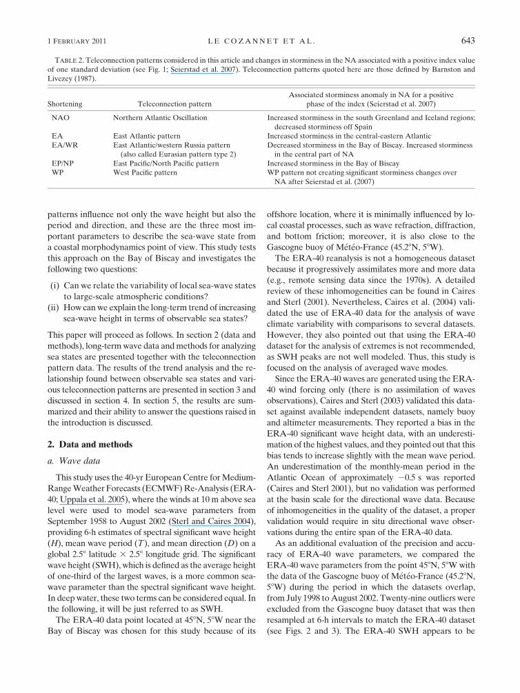
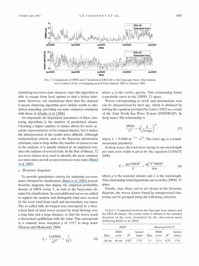
underestimated with a bias of 20.39 m (Table 3). The

linear correlation between the two datasets (see Fig. 2) is

very high (R2 5 0.93) and significant at the 0.05 confi-

dence level. A correction of the ERA-40 SWH values has

been applied to the 1958–2001 ERA-40 period, defined as

SWHERA40�C

5 1.18SWHERA40

1 0.00424. (1)

In the next steps of the analysis, sea-wave parameters

are normalized, so the effects of this correction are

limited to presenting more realistic SWH in the final

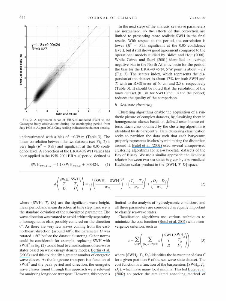
results. With respect to the period, the correlation is

lower (R2 5 0.75, significant at the 0.05 confidence

level), but it still shows good agreement compared to the

operational models studied by Bidlot and Holt (2006).

While Caires and Sterl (2001) identified an average

negative bias in the North Atlantic basin for the period,

the bias for the ERA-40 458N, 58W point is about 12 s

(Fig. 3). The scatter index, which represents the dis-

persion of the dataset, is about 17% for both SWH and

T, with an RMS error of 60 cm and 2.5 s, respectively

(Table 3). It should be noted that the resolution of the

buoy dataset (0.1 m for SWH and 1 s for the period)

reduces the quality of the comparison.

b. Sea-state clustering

Clustering algorithms enable the acquisition of a syn-

thetic picture of complex datasets, by classifying them in

homogeneous classes based on defined resemblance cri-

teria. Each class obtained by the clustering algorithm is

identified by its barycentre. Data clustering classification

seeks to partition the data such that each barycentre

properly represents its class by minimizing the dispersion

around it. Butel et al. (2002) used several unsupervised

clustering algorithms for sea-wave-state datasets of the

Bay of Biscay. We use a similar approach: the likeliness

relation between two sea states is given by a normalized

Euclidian scalar product in the fSWH, T, Dg space,

dhSWHi

Ti

Di

SWHj

Tj

Dj

i5

ffiffiffiffiffiffiffiffiffiffiffiffiffiffiffiffiffiffiffiffiffiffiffiffiffiffiffiffiffiffiffiffiffiffiffiffiffiffiffiffiffiffiffiffiffiffiffiffiffiffiffiffiffiffiffiffiffiffiffiffiffiffiffiffiffiffiffiffiffiffiffiffiffiffiffiffiffiffiffiffiffiffiffiffiffiffiffiffiffiffiffiffiffiffiffiffiffiffiSWH

i� SWH

j

sHs

!2

1T

i� T

j

sT

� �2

1D

i�D

j

sD

� �2vuut , (2)

where fSWHi, Ti, Dig are the significant wave height,

mean period, and mean direction at time step i, and sX is

the standard deviation of the subscripted parameter. The

wave direction was rotated to avoid arbitrarily separating

a homogeneous class possibly centered on the direction

08. As there are very few waves coming from the east-

northeast direction (around 608), the parameter D was

rotated 1608 before the dataset clustering. Other norms

could be considered; for example, replacing SWH with

SWH2 in Eq. (2) would lead to classifications of sea-wave

states based on wave energy density modes. Bertin et al.

(2008) used this to identify a greater number of energetic

wave classes. As the longshore transport is a function of

SWH2 and the peak period and direction, the energetic

wave classes found through this approach were relevant

for analyzing longshore transport. However, this paper is

limited to the analysis of hydrodynamic conditions, and

all three parameters are considered as equally important

to classify sea-wave states.

Classification algorithms use various techniques to

minimize the cost function (Butel et al. 2002) with a con-

vergence criterion, such as

s 5 �C2P

�fH

s,T,Dg2C

dhSWH

T

D

SWHg

Tg

Dg

i0B@

1CA, (3)

where fSWHg, Tg, Dgg identifies the barycenter of class C

for a given partition P of the sea-wave-state dataset. The

cost function is a function of the barycenters fSWHg, Tg,

Dgg, which have many local minima. This led Butel et al.

(2002) to prefer the simulated annealing method of

FIG. 2. A regression curve of ERA-40-modeled SWH vs the

Gascogne buoy observations during the overlapping period from

July 1998 to August 2002. Gray scaling indicates the dataset density.

644 J O U R N A L O F C L I M A T E VOLUME 24

classifying sea-wave-state datasets, since this algorithm is

able to escape from local optima to find a better mini-

mum. However, our simulations show that the classical

k-means clustering algorithm gives similar results to sim-

ulated annealing, providing sea-state estimates consistent

with those of Abadie et al. (2006).

An important site-dependent parameter of these clus-

tering algorithms is the number of predefined classes.

Choosing a higher number of classes allows for more ac-

curate representation of the original dataset, but it makes

the interpretation of the results more difficult. Although

mathematical criteria, such as the Bayesian information

criterium, exist to help define the number of classes to use

in the analysis, it is usually defined in an empirical way,

after the analysis of several trials. In the Bay of Biscay, 12

sea-wave classes were used to identify the most common

sea-wave states as well as rarer storm sea-wave states (Butel

et al. 2002).

c. Bivariate diagrams

To provide quantitative criteria for analyzing sea-wave

states obtained by classification, Butel et al. (2002) present

bivariate diagrams that display the empirical probability

density of SWH versus T, as well as the barycentre ob-

tained by classification. Several additional curves are added

to support the analysis and distinguish wind seas, created

by the local wind from swell and intermediary sea states.

The so-called fully developed seas correspond to a theo-

retical limit of wind waves created by wind blowing over

a long time and a large distance, so that the waves reach

a theoretical equilibrium with the wind. This corresponds

to a constant wave steepness j of 1/19.7 in deep water

(Pierson and Moskowitz 1964):

j 52pSWH

gT25

1

19.7, (4)

where g is the earth’s gravity. This relationship forms

a parabolic curve in the fSWH, Tg space.

Waves corresponding to swell, and intermediate seas

can be characterized by their age, which is obtained by

solving the equation provided by Carter (1982) as a result

of the Joint North Sea Wave Project (JONSWAP). In

deep water, this relationship is

SWH

T25 l

g

2pAge

� �1/3

, (5)

where l 5 0.0408 m21/3 � s2/3. The wave age is a nondi-

mensional parameter.

In deep water, the total wave energy in one wavelength

per unit crest width is given by the equation (USACE

2008)

E 5rgLSWH2

85

rg2T2SWH2

16p, (6)

where r is the seawater density and L is the wavelength.

This relationship forms hyperbolic curves in the fSWH, Tgspace.

Finally, once these curves are drawn in the bivariate

diagram, the waves classes found by unsupervised clus-

tering can be grouped using the following criterion:

TABLE 3. Comparison between the Gascogne buoy dataset and

the ERA-40 dataset. The scatter index is defined as the standard

deviation of the error normalized by the observation mean

(following Bidlot et al. 2002).

SWH Mean period (T)

Bias

RMS

error R2Scatter

index Bias

RMS

error R2Scatter

index

240 cm 60 cm 0.927 17% 2 s 2.5 s 0.75 17%

FIG. 3. Comparison of SWH and T modeled in ERA-40 vs the Gascogne buoy observations

over a subset of the overlapping period from January 2000 to January 2001.

1 FEBRUARY 2011 L E C O Z A N N E T E T A L . 645

d Waves lying between the Pierson–Moskowitz curve

(steepness 5 1/19.7) limit and the curve age 5 0.8 can

be considered as wind seas.d The most aged waves are usually considered as swell.

Typically, Butel et al. (2002) consider that waves lying

bellow the constant age curve that separates the wave

dataset in two equal parts can be considered as swell.d Other waves lying between the curve age 5 0.8 and the

swell limit used for the previous criteria can be con-

sidered as intermediate waves between swell and wind

sea (Aarnes and Krogstad 2001).d Curves showing iso-energy fluxes also enable the

identification of more energetic wave conditions as-

sociated with storms as well as low-energy waves.d Finally, waves showing similar direction or occurring

during the same season can also be grouped together.

Using these criteria allows to better identify the nature

of each wave class and to eventually group them upon

similarity.

d. Teleconnection patterns

Time series of teleconnection patterns are obtained

from the National Oceanic and Atmospheric Adminis-

tration (NOAA) Climate Prediction Center. The tele-

connection patterns used here are those described by

Barnston and Livezey (1987) and are obtained by ap-

plying an orthogonal-rotated principal component anal-

ysis of monthly 700-mb-height means over the Northern

Hemisphere.

3. Results

a. Wave climate in the Bay of Biscay

The 1958–2001 corrected sea-wave data from ERA-40

were classified into 12 modes using the k-means algorithm

(Table 4) and plotted in the bivariate diagram (Fig. 4).

Each identified class is described by its barycenter. The

seasonality of these wave classes, shown in Fig. 5, reveals

more energetic winter waves and lower energy summer

waves. The criteria provided in section 2c provide an ob-

jective framework based on wave age and energy flux

to distinguish these classes using the bivariate diagram

(Fig. 4). This enables the grouping of the 12 classes into

three wave types: swell, wind sea waves, and interme-

diate sea states.

As stated in section 2c, the duplets lying between the

curve age 5 0.8 and steepness 5 1/19.7 in Fig. 4 can be

considered as wind seas. Since class A is lying on the curve

age 5 0.8, and an eastern wind is associated with this class,

class A can be considered as wind waves associated with

winds coming from the continent.

The most aged waves (over age 5 6.56) are swell (classes

G–J). They can be divided into low-energy summer swell

(classes G and H) and high-energy winter swell (classes I

and J), hereafter called SWELL 1 and SWELL 2, respec-

tively. SWELL 1 are characterized by relatively low wave

heights, long periods, and a northwest direction. They

occur predominantly during the summer season and occur

during 32% of the ERA-40 period. SWELL 2 are char-

acterized by large wave heights, long periods, and north-

west directions. They are more frequent in winter and

occur during 17% of the ERA-40 period.

Classes between the ages of 0.8 and 6.56 represent in-

termediate sea states between swell and wind sea waves

(classes B–E, F, K, and L). In this range of wave heights,

these wave classes are characterized by low periods. They

can be divided into three groups: (i) low-energy inter-

mediate sea states, hereafter called INTER 1, that are

more frequent in summer (classes B–D); (ii) moderate-

energy intermediate sea states (INTER 2) that are more

frequent in winter (classes E and F); and (iii) high-energy

intermediate sea states (STORM) that correspond mainly

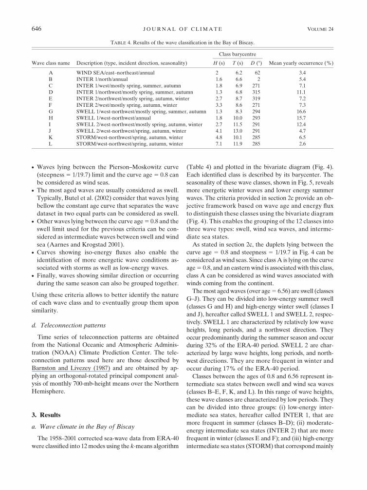
TABLE 4. Results of the wave classification in the Bay of Biscay.

Wave class name Description (type, incident direction, seasonality)

Class barycentre

Mean yearly occurrence (%)H (s) T (s) D (8)

A WIND SEA/east–northeast/annual 2 6.2 62 3.4

B INTER 1/north/annual 1.6 6.6 2 5.4

C INTER 1/west/mostly spring, summer, autumn 1.8 6.9 271 7.1

D INTER 1/northwest/mostly spring, summer, autumn 1.3 6.8 315 11.1

E INTER 2/northwest/mostly spring, autumn, winter 2.7 8.7 319 7.2

F INTER 2/west/mostly spring, autumn, winter 3.3 8.6 271 7.3

G SWELL 1/west-northwest/mostly spring, summer, autumn 1.3 8.3 294 16.6

H SWELL 1/west-northwest/annual 1.8 10.0 293 15.7

I SWELL 2/west-northwest/mostly spring, autumn, winter 2.7 11.5 291 12.4

J SWELL 2/west-northwest/spring, autumn, winter 4.1 13.0 291 4.7

K STORM/west-northwest/spring, autumn, winter 4.8 10.1 285 6.5

L STORM/west-northwest/spring, autumn, winter 7.1 11.9 285 2.6

646 J O U R N A L O F C L I M A T E VOLUME 24

to winter storms (classes K and L). Classes F, K, and L

actually include some wind sea waves. Nevertheless, be-

cause of their direction and of their barycentre being

located below the age 5 0.8 curve, they include more

intermediate sea states than wind seas and are considered

as such. All of these waves originate from the northwest,

except class B, which comes from the north. Those waves

are created by relatively gentle northwest winds, but their

development is limited by a geographical constraint: as

the British Isles are located north of the ERA-40 point,

the fetch cannot be sufficiently large to generate more

developed sea states.

The seasonality and wave flux energy criteria are used

to consider a group formed by STORM and SWELL 2

waves, which correspond to the most energetic waves and

will be referred to as SWELL 2 1 STORM hereafter.

Low and moderate energy intermediate waves (INTER 1

and INTER 2) will be referred to as INTER hereafter.

b. SWH trend

This paragraph investigates how the trend of increasing

wave height in the northeastern Atlantic since 1970 can

be explained using the above classification. From 1958 to

1970, no significant trend appears in the ERA-40 SWH

signal at the 458N, 58W node. Between 1970 and 2001,

however, an increase of 0.8 cm yr21 is calculated in the

annual mean SWH (Table 5), with a probability higher

than 99.3% for this trend to be significant. According to

the ERA-40 model, the trend leads to an increase of about

25 cm in SWH at the 458N, 58W node for the last 31 yr of

the reanalysis.

Three different assumptions can be made to interpret

this trend in terms of observable sea states: the increase in

sea-wave height could correspond to (i) an increase of the

average SWH of all or certain wave groups, (ii) a different

relative frequency of occurrence of already existing wave

groups, or (iii) the emergence of a new wave class.

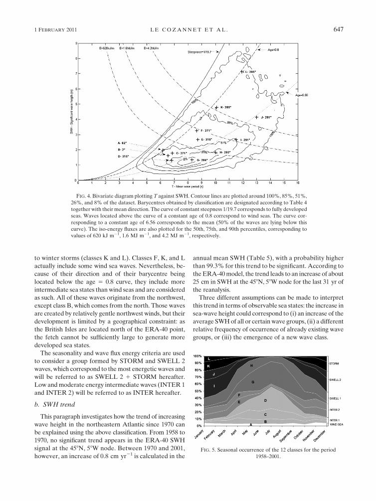
FIG. 4. Bivariate diagram plotting T against SWH. Contour lines are plotted around 100%, 85%, 51%,

26%, and 8% of the dataset. Barycentres obtained by classification are designated according to Table 4

together with their mean direction. The curve of constant steepness 1/19.7 corresponds to fully developed

seas. Waves located above the curve of a constant age of 0.8 correspond to wind seas. The curve cor-

responding to a constant age of 6.56 corresponds to the mean (50% of the waves are lying below this

curve). The iso-energy fluxes are also plotted for the 50th, 75th, and 90th percentiles, corresponding to

values of 620 kJ m21, 1.6 MJ m21, and 4.2 MJ m21, respectively.

FIG. 5. Seasonal occurrence of the 12 classes for the period

1958–2001.

1 FEBRUARY 2011 L E C O Z A N N E T E T A L . 647

Using geomorphological indicators of the French At-

lantic coast, Henaff (2008) suggests that 1985 was the

transition from a more zonal to a more meridional sea-

wave orientation. Hypothesis 3 was tested by classifying

ERA-40 sea-wave time series over two different periods—

from 1958 to 1984 and from 1985 to 2001—to identify the

appearance of new classes. The results of clustering over

these two different periods revealed similar barycentres,

thus refuting the hypothesis of the emergence of new sea-

state classes after 1985.

The relative importance of assumptions 1 and 2 can

be approximately estimated as follows: mean sea-wave

height over a given period can be calculated by adding

the weighted means of SWH over this period, for each

set C of the partition P of sea-wave states found after the

k-means clustering. Therefore, SWH being the mean

SWH for the 40 yr of the ERA-40, SWHX being the

mean of the significant wave height for the set X, and pX

being the relative frequency of occurrence of the set X

leads to the following equation:

SWH� SWH 5 �X2P

pX

(SWHX� SWH), (7)

which provides an approximation for small variations of

SWH over a given period:

DSWH 5 �X2P

pX

DSWHX

1 DpX

(SWHX� SWH). (8)

In this equation, the variations due to SWH changes

within a given class X and those due to the relative

frequency of occurrence changes pX are isolated. In

practice, the relative importance of the pX 3 DSWHX

terms dominate over the relative importance of DpX 3

SWHX terms, accounting for about 75% of SWH in-

crease. The three major contributions in Eq. (8) are

from pSWELL2 3 DSWHSWELL2, pINTER1 3 DSWHINTER1,

and DpINTER1

3 (SWHINTER1

� SWH), accounting for ap-

proximately 40%, 25%, and 15%, respectively, of SWH

increase. These trends correspond to the significant trends

in Table 5. Therefore, the identified sea-state classes re-

main persistent in time, and the evolution of relative fre-

quency of occurrence of these groups accounts for most

of the SWH trend between 1970 and 2001.

c. Links between teleconnection patterns andsea-wave states: Annual means

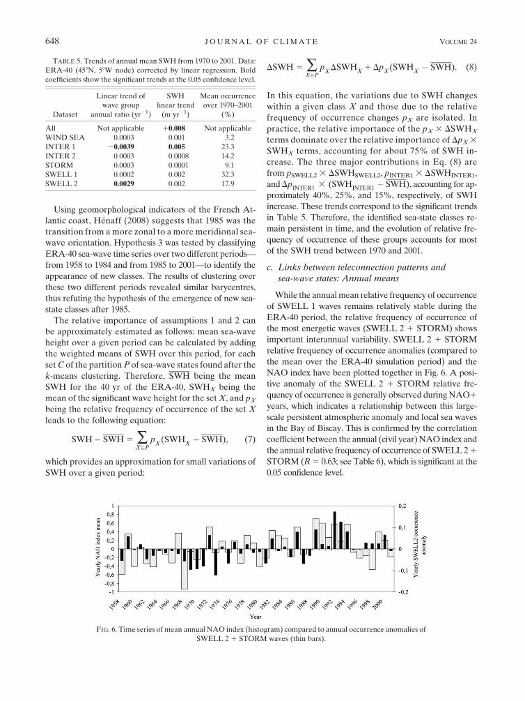
While the annual mean relative frequency of occurrence

of SWELL 1 waves remains relatively stable during the

ERA-40 period, the relative frequency of occurrence of

the most energetic waves (SWELL 2 1 STORM) shows

important interannual variability. SWELL 2 1 STORM

relative frequency of occurrence anomalies (compared to

the mean over the ERA-40 simulation period) and the

NAO index have been plotted together in Fig. 6. A posi-

tive anomaly of the SWELL 2 1 STORM relative fre-

quency of occurrence is generally observed during NAO1

years, which indicates a relationship between this large-

scale persistent atmospheric anomaly and local sea waves

in the Bay of Biscay. This is confirmed by the correlation

coefficient between the annual (civil year) NAO index and

the annual relative frequency of occurrence of SWELL 2 1

STORM (R 5 0.63; see Table 6), which is significant at the

0.05 confidence level.

TABLE 5. Trends of annual mean SWH from 1970 to 2001. Data:

ERA-40 (458N, 58W node) corrected by linear regression. Bold

coefficients show the significant trends at the 0.05 confidence level.

Dataset

Linear trend of

wave group

annual ratio (yr21)

SWH

linear trend

(m yr21)

Mean occurrence

over 1970–2001

(%)

All Not applicable 10.008 Not applicable

WIND SEA 0.0003 0.001 3.2

INTER 1 20.0039 0.005 23.3

INTER 2 0.0003 0.0008 14.2

STORM 0.0003 0.0001 9.1

SWELL 1 0.0002 0.002 32.3

SWELL 2 0.0029 0.002 17.9

FIG. 6. Time series of mean annual NAO index (histogram) compared to annual occurrence anomalies of

SWELL 2 1 STORM waves (thin bars).

648 J O U R N A L O F C L I M A T E VOLUME 24

Conversely, there are more waves of WIND SEA and

INTER during NAO2 years. The correlation coefficient

between the NAO index and the annual relative frequency

of occurrence of WIND SEA and INTER are 20.31 and

20.46, respectively (both significant at the 0.05 confidence

level; see Table 6).

Finally, the annual relative frequency of occurrence of

SWELL 1 and INTER 1 remain more stationary than the

other wave types over the ERA-40 period (Table 7).

Using the annual mean relative frequency of occur-

rence of waves types, no evidence of the influence of other

teleconnection patterns on sea-wave climate in the Bay

of Biscay could be found, with the exception of EA, which

is correlated with the INTER 1 relative frequency of oc-

currence and of EP/NP (a northern Pacific pattern), which

is correlated with SWELL 2 1 STORM. These results are

discussed in section 4.

d. Links between teleconnection patterns andsea-wave states: Winter means

During winter months, SWELL 1 waves become less

frequent so that SWELL 2 and STORM wave groups

become dominant (Fig. 5). Thus, during this season, the

sensitivity of waves to teleconnection pattern variability

is expected to be most apparent.

As a matter of fact, the correlation between the NAO

index and the SWELL 2 1 STORM relative frequency

of occurrence during winter is significant at the 0.05 con-

fidence level (R 5 0.58); in addition, the East Atlantic

pattern is also correlated with STORM 1 SWELL 2 rel-

ative frequency of occurrence anomaly during the winter

(R 5 0.56; significant at the 0.05 confidence level; Table 7).

If the period of interest is restricted to single months

during the winter, then the correlations show that the

relative influence of the NAO, EA, and EA/WR varies

from one month to another: whereas in January, February

and March, the NAO accounts for most of the variance of

the SWELL 2 1 STORM relative frequency of occur-

rence variability behaviors, the EA explains most of this

variance in December (R 5 0.56). In an attempt to explain

this, one can notice that EA explains 11% of the variance

of mean 700-mb height in December, while this value is

below 9.5% for all other months and is even below 5%

when February is excluded (Barnston and Livezey 1987).

Thus, this teleconnection pattern is expressed mostly in

December; therefore, during this month, a larger mani-

festation of EA would be expected.

4. Discussion

a. Use of clustering algorithm

Instead of analyzing a single sea-wave parameter, we

used a clustering algorithm to consider three wave pa-

rameters (significant height, period, and direction) equally

to finally enable the identification of observable sea states

and attempt to explain previously observed trends. From

a methodological point of view, this technique provides

a practical framework to describe long time series of wave

parameters with only several dominant modes.

An important issue is the sensitivity of the final results

to the classification. A key parameter to define is the

number of classes defined by the user prior to applying

the k-means algorithm. As stated above (see section 2b),

there is a trade-off between (i) few classes, potentially

causing oversimplification and poor representation of

the observed sea-wave signal, and (ii) many classes, ig-

noring the initial objective of simplifying the signal. Using

their knowledge of the hydrodynamic conditions in the

Bay of Biscay, Butel et al. (2002) showed that 12 classes

were an appropriate trade-off; however, this value is site

dependent and would need to be reconsidered in other

seas of the world.

Once the number of classes is chosen, bivariate dia-

grams can be used to qualify each class and group them.

Here, quantitative criteria can be used: mean direction of

each class, Pierson and Moskowitz spectrum (1964), wave

iso-age curves such as in Butel et al. (2002), and also en-

ergy fluxes (see sections 2c and 3a). Our experience from

the number of tests performed within this study is that the

TABLE 6. Correlation coefficient R between relative annual

frequency of occurrence for each wave group and relevant annual

teleconnection pattern indexices (civil year). Bold coefficients

show the significant correlations at the 0.05 confidence level.

NAO EA EA/WR EP/NP

WIND SEA 20.31 20.24 20.17 0.10

INTER 1 20.25 0.34 20.15 0.08

INTER 2 20.39 0.28 0.03 0.21

SWELL 1 20.20 0.06 0.10 20.23

SWELL 2 0.53 0.17 0.24 0.27

STORM 0.43 0.15 0.20 0.28

INTER 20.44 20.19 0.17 0.20

SWELL 2 1 STORM 0.63 0.20 0.14 0.34

TABLE 7. Correlation coefficient R between relative winter

(December–February) frequency of occurrence and relevant an-

nual teleconnection pattern indices (civil year) from 1957 to 2001.

Bold coefficients show the significant correlations at the 0.05 con-

fidence level.

NAO EA EA/WR EP/NP

SWELL 1 20.21 20.18 0.20 0.04

SWELL 2 0.40 0.18 0.58 0.23

STORM 0.25 0.52 20.57 0.15

WIND SEA 1 INTER 20.54 20.54 20.26 20.38

SWELL 2 1 STORM 0.58 0.56 0.16 0.33

1 FEBRUARY 2011 L E C O Z A N N E T E T A L . 649

sensitivity of the final results to the classification and

grouping mainly lies in the choice of an appropriate

number of classes. In other terms, once the classes cor-

respond to the main observable sea states, an extensive

analysis of the links between teleconnection patterns and

those sea-wave states can be performed.

b. Links between teleconnection patterns andsea-wave states: Annual means

Our results confirm that large-scale atmospheric

anomalies partly control the sea-wave climates in the Bay

of Biscay. With respect to the annual means, the corre-

lations found in Table 6 show that a more intense positive

NAO index generally leads to higher relative frequency of

occurrence of SWELL 2 and STORM and a smaller fre-

quency of occurrence of INTER, particularly INTER 2.

This can be related to typical storm tracks associated with

NAO1 and NAO2: NAO1 is associated with stronger,

northward-shifted winds over the northern Atlantic, while

NAO2 is associated with weaker southward-shifted winds.

This agrees with the interpretation of Dupuis et al. (2006):

as storm tracks shift northward to the Greenland–Iceland

region during NAO1, the waves travel a longer distance

to reach the Bay of Biscay. Consequently, when these

waves propagate to the Bay of Biscay, their height is

attenuated and their wavelength increases because of the

dispersive character of sea-wave propagation. The fact

that the largest waves and longest periods are associated

with positive phases of NAO is thus consistent with an

intuitive analysis.

Other correlations can be also related to intuitive

analysis: winds coming from the continent will typically

occur when the NAO index is negative, explaining the

significant correlation observed between WIND SEA

relative frequency of occurrence and NAO2.

With respect to the significant correlation between

EP/NP and SWELL 2 1 STORM relative frequency of

occurrence, this result might seem surprising; however,

it is consistent with the results of Seierstad et al. (2007),

who found an increase of one standard deviation of the

EP/NP index to be associated with a statistically signif-

icant increase of storminess in the Bay of Biscay.

As INTER 1 does not correspond to stormy winds, this

kind of wave was not a point of focus in previous studies.

However, Table 6 shows that the correlation of the INTER

1 relative frequency of occurrence with EA is significant.

This seems to correspond to the case where a positive EA

index is associated with relatively weak western winds,

creating waves over the eastern Atlantic, which causes in-

termediate seas in the Bay of Biscay.

Having mentioned those two specific cases, Table 6 con-

firms that when considering annual means, the NAO re-

mains the most relevant teleconnection pattern to consider

when relating the Bay of Biscay’s sea-wave states to tele-

connection patterns.

c. Links between teleconnection patterns andsea-wave states: Winter means

Table 7 confirms the links between local wave climate

and NAO in winter, but the influence of other tele-

connection patterns on sea waves can also be highlighted:

in Table 7, the correlation between EA and STORM can

be related to the results of Seierstad et al. (2007), who

showed that EA1 phases are associated with storms af-

fecting the east-central part of northern Atlantic region

(Fig. 1). The wave group STORM is thus related to typ-

ical EA1 storms, which are created closer to the Bay of

Biscay. They are thus characterized by larger wave heights

and shorter periods, which explains their proximity to the

wind sea theoretical limit (age 5 0.8) in Fig. 4.

Similarly, positive phases of the EA/WR pattern also

lead to more SWELL 2 waves and less STORM waves.

This is consistent with the fact that positive phases of this

pattern are associated with fewer storms in the Bay of

Biscay, according to Seierstad et al. (2007).

Nevertheless, it must be noted that nonintuitive re-

lationships between sea-wave state and teleconnection

patterns can also be reported. Another relation between

the WP pattern and positive anomalies of the SWELL 2

relative frequency of occurrence during winter remains

unexplained, as Seierstad et al. (2007) did not report sig-

nificant storm changes in the northern Atlantic for posi-

tive phases of the WP (Table 2).

This focus on winter sea-wave-state variability confirms

the influence of teleconnection patterns other than the

NAO. Most of this influence corresponds to basic intuitive

relations between teleconnection patterns, storminess,

and sea states, with the notable exception of the WP. In

this context, sea-wave height trends relate to climate var-

iability in the northern Atlantic. Particularly, the increase

of SWH from 1970 to 2001 can be related with recurring

yearly means NAO1 anomalies.

5. Conclusions

One major motivation to study sea-wave variability

is its possible consequences in terms of erosion of the

shoreline. In the Bay of Biscay, the 240-km-long Aqui-

taine sandy coast is exposed to energetic and slightly

shore-oblique waves that account for longshore currents

and drift (Komar and Inman 1970). Castelle et al. (2007)

extensively described the very active morphodynamic

processes of this environment, showing waves as an im-

portant forcing agent. Dodet et al. (2010) even suggested

that changing wave patterns could be an additional expla-

nation for increased erosion over the last 50 yr in western

650 J O U R N A L O F C L I M A T E VOLUME 24

Europe. In this context, this study focused on the two

questions set out in the introduction:

(i) Can we relate the variability of local sea-wave states

to large-scale atmospheric conditions?

A link exists between the annual relative fre-

quency of occurrence of wave types in the Bay of

Biscay and interannual variability of the NAO. Dur-

ing NAO1 periods, stronger winds cross the north-

ern Atlantic and create larger waves, here classified

as SWELL 2 1 STORM. NAO2 is characterized by

weaker winds and more southern-oriented winds over

the North Atlantic. The Bay of Biscay is then under

the influence of WIND SEA or INTER waves. The

correlation is even more obvious during the winter

season. The summer season is mostly characterized by

SWELL 1 waves that are not affected by NAO vari-

ability. The influence of other teleconnection pat-

terns on North Atlantic storminess is also confirmed:

EP/NP annually and EA, EA/WR, and, surprisingly,

WP in winter.

(ii) How can we explain the long-term trend of increasing

sea-wave heights in terms of observable sea states?

The long-term increasing trend since 1970 can be

explained mostly by an increase of the relative fre-

quency of occurrence of the most energetic swell

group (SWELL 2); then, to a lesser extent, by a de-

crease of the relative frequency of occurrence of low-

energy intermediate waves (INTER 1); and finally, by

an increase of mean sea-wave heights for this same

group.

From a methodological point of view, this study shows

the relevance of using sea-wave clustering to relate ob-

servable sea states to large-scale climate variability in-

dices. This approach makes the correlation between the

teleconnection patterns and sea-wave climates easier to

interpret. Key prerequisites are the existence of a suffi-

ciently long sea-wave data time series, including height,

period, and direction, and the existence of in situ obser-

vations to validate the data, if it originates from a model.

Acknowledgments. The ERA-40 sea-wave reanalysis

and teleconnection patterns from the historical archive of

NOAA were used for this study, which has been supported

by grants from the BRGM Research Directorate under the

Riscot project and the French National Research Agency

through the VULSACO project (ANR-06-VULN-009).

Financial support of the European Commission for trends

and bivariate analysis is gratefully acknowledged through

the FP7 MICORE (Contract 202798) and THESEUS

(Contract 244104) projects. We thank Dr. M. Yates-

Michelin, Dr. D. Idier, and anonymous reviewers for

their comments that led to improving this manuscript.

REFERENCES

Aarnes, J. E., and H. E. Krogstad, 2001: Partitioning sequences for the

dissection of directional ocean wave spectra: A review. EnviWave

Research Programme Rep., 23 pp. [Available online at http://

www.oceanor.no/projects/enviwave/PartitioningSequences.pdf.]

Abadie, S., R. Butel, S. Mauriet, D. Morichon, and H. Dupuis,

2006: Wave climate and longshore drift on the south Aquitaine

coast. Cont. Shelf Res., 26, 1924–1939.

Bacon, S., and D. J. T. Carter, 1991: Wave climate changes in the

North Atlantic and North Sea. Int. J. Climatol., 11, 545–558.

——, and ——, 1993: A connection between mean wave height and

atmospheric pressure gradient in the North Atlantic. Int.

J. Climatol., 13, 423–436.

Barnston, A. G., and R. E. Livezey, 1987: Classification, season-

ality, and persistence of low-frequency atmospheric circula-

tion patterns. Mon. Wea. Rev., 115, 1083–1126.

Bertin, X., B. Castelle, E. Chaumillon, R. Butel, and R. Quique,

2008: Longshore transport estimation and inter-annual vari-

ability at a high-energy dissipative beach: St. Trojan beach,

SW Oleron Island, France. Cont. Shelf Res., 28, 1316–1332.

Bidlot, J.-R., and M. W. Holt, 2006: Verification of operational global

and regional wave forecasting systems against measurements from

moored buoys. JCOMM Tech. Rep. 30, WMO/TD 1333, 16 pp.

[Available online at ftp://ftp.wmo.int/Documents/PublicWeb/

amp/mmop/documents/JCOMM-TR/J-TR-30/J-TR-30.pdf.]

——, D. Holmes, P. Wittmann, R. Lalbeharry, and H. S. Chen,

2002: Intercomparison of the performance of operational

ocean wave forecasting systems with buoy data. Wea. Fore-

casting, 17, 287–310.

Butel, R., H. Dupuis, and P. Bonneton, 2002: Spatial variability of

wave conditions on the French Atlantic coast using in-situ

data. J. Coastal Res., 36, 96–108.

Caires, S., and A. Sterl, 2001: Comparative assessment of ERA-40

ocean wave data. Proc. ECMWF Workshop on Re-Analysis,

Reading, United Kingdom, ECMWF, ERA-40 Project Rep.

Series 3, 353–368. [Available online at http://www.knmi.nl/

home/onderzk/oceano/waves/era40/reports/knmi1101.pdf.]

——, and ——, 2003: Validation of ocean wind and wave data using

triple collocation. J. Geophys. Res., 108, 3098, doi:10.1029/

2002JC001491.

——, ——, J.-R. Bidlot, N. Graham, and V. Swail, 2004: Inter-

comparison of different wind–wave reanalyses. J. Climate, 17,

1893–1912.

Carter, D. J. T., 1982: Prediction of wave height and period for

a constant wind velocity using the JONSWAP results. Ocean

Eng., 9, 17–33.

Castelle, B., P. Bonneton, H. Dupuis, and N. Senechal, 2007: Double

bar beach dynamics on the high-energy meso-macrotidal French

Aquitanian coast: A review. Mar. Geol., 245, 141–159.

Dodet, G., X. Bertin, and R. Taborda, 2010: Wave climate vari-

ability in the north-east Atlantic Ocean over the last six de-

cades. Ocean Modell., 31, 120–131.

Dupuis, H., D. Michel, and A. Sottolichio, 2006: Wave climate evolution

in the Bay of Biscay over two decades. J. Mar. Syst., 63, 105–114.

Gulev, S. K., and V. Grigorieva, 2004: Last century changes in ocean

wind wave height from global visual wave data. Geophys. Res.

Lett., 31, L24302, doi:10.1029/2004GL021040.

Henaff, A., 2008: Identification of geomorphological indicators of

incident waves direction along the Channel and the Atlantic

French coasts during the last 25 years, data analysis and

comparison with data of the EDF-LNHE numerical atlas of

waves (in French). Houille Blanche, 1, 61–71.

1 FEBRUARY 2011 L E C O Z A N N E T E T A L . 651

Komar, P. D., and D. L. Inman, 1970: Longshore sand transport on

beaches. J. Geophys. Res., 75, 5914–5927.

Kushnir, Y., V. J. Cardone, J. G. Greenwood, and M. A. Cane,

1997: The recent increase in North Atlantic wave heights.

J. Climate, 10, 2107–2113.

Nicholls, R. J., P. P. Wong, V. R. Burkett, J. O. Codignotto,

J. E. Hay, R. F. McLean, S. Ragoonaden, and C. D. Woodroffe,

2007: Coastal systems and low-lying areas. Climate Change

2007: Impacts, Adaptation and Vulnerability, M. L. Parry et al.,

Eds., Cambridge University Press, 315–356.

Pierson, W. J., and L. Moskowitz, 1964: A proposed spectral form

for fully developed wind seas based on the similarity theory of

A. A. Kitaigorodskii. J. Geophys. Res., 69, 5181–5190.

Rogers, J. C., 1990: Patterns of low-frequency monthly sea level

pressure variability (1899–1986) and associated wave cyclone

frequencies. J. Climate, 3, 1364–1379.

Seierstad, I. A., D. B. Stephenson, and N. G. Kvamstø, 2007: How

useful are teleconnection patterns for explaining variability in

extratropical storminess? Tellus, 59A, 170–181.

Sterl, A., and S. Caires, 2004: Climatology, variability and extrema

of ocean waves—The Web-based KNMI/ERA-40 Wave Atlas.

Int. J. Climatol., 25, 963–997.

Uppala, S. M., and Coauthors, 2005: The ERA-40 Re-Analysis.

Quart. J. Roy. Meteor. Soc., 131, 2961–3012.

USACE, 2008: Water wave mechanics. Coastal engineering

manual—Part II. U.S. Army Corps of Engineers Rep.,

II-1-1–II-1-121. [Available online at http://140.194.76.129/

publications/eng-manuals/em1110-2-1100/PartII/Part_II-Chap_1.

pdf.]

Wallace, J. M., and D. S. Gutzler, 1981: Teleconnections in the

geopotential height field during the Northern Hemisphere

winter. Mon. Wea. Rev., 109, 784–812.

Wang, X. L., and V. R. Swail, 2001: Changes of extreme wave

heights in Northern Hemisphere oceans and related atmo-

spheric circulation regimes. J. Climate, 14, 2204–2221.

——, and ——, 2002: Trends of Atlantic wave extremes as simu-

lated in a 40-yr wave hindcast using kinematically reanalyzed

wind fields. J. Climate, 15, 1020–1035.

——, F. W. Zwiers, and V. R. Swail, 2004: North Atlantic ocean

wave climate change scenarios for the twenty-first century.

J. Climate, 17, 2368–2383.

Woolf, D. K., P. G. Challenor, and P. D. Cotton, 2002: Variability

and predictability of the North Atlantic wave climate. J. Geo-

phys. Res., 107, 3145, doi:10.1029/2001JC001124.

652 J O U R N A L O F C L I M A T E VOLUME 24