1

REVISED PAPER Monitoring of Prestige effects on the coastal zone of Cantabria

The Prestige oil spill in Cantabria (Bay of Biscay). Part II. Environmental assessment and monitoring of coastal

ecosystems

José A. Juanes1, Araceli Puente1, José A. Revilla1, César Álvarez1, Andrés García1, Raúl Medina2, Sonia Castanedo2, Leandro Morante3, Santiago González4, Gerardo García-Castrillo5

1 Submarine Outfall and Environmental Hydraulics Group (GESHA). Dept. Ciencias y Técnicas del Agua y del Medio Ambiente. University of Cantabria. Avda. de los Castros s/n, 39005 Santander, Spain. Ph. 34 942 201704. juanesj@unican.es 2 Ocean and Coastal Research Group (GIOC). Dept. Ciencias y Técnicas del Agua y del Medio Ambiente. University of Cantabria. Avda. de los Castros s/n, 39005 Santander, Spain. 3 Centro de Investigaciones del Medio Ambiente (CIMA). Consejería de Medio Ambiente. Government of Cantabria. Avda. Rochefort sur mer s/n, 39300 Torrelavega, Cantabria. Spain. 4 Consejería de Ganadería, Agricultura y Pesca, Government of Cantabria. c/ Rodríguez, 5, 39002 Santander, Spain. 5 Museo Marítimo del Cantábrico, Government of Cantabria. San. Martín de Bajamar s/n, 39004 Santander, Spain.

2

ABSTRACT

Assessment and monitoring activities constituted two main tasks of the Emergency

Response System implemented by the Regional Government of Cantabria (N Spain)

after the Prestige oil spill. The assessment covered four types of environmental units:

estuaries, rocky shores, sand beaches and subtidal areas, up to a 300-meter depth.

Monitoring procedures included the chemical quantification of total hydrocarbons (TH)

and polycyclic aromatic hydrocarbons (PAHs) in water, sediments and benthic

organisms (clams and goose barnacles), and the analysis of structural changes in

intertidal communities.

Disturbance of oil cover was significantly more extensive in coastal areas, rather than in

estuarine areas, where 50,000 m2 were directly covered by fuel. Otherwise, the presence

of oil in subtidal areas was a rare event. Results from the bioeffects analyses were in

agreement with the overall impact assessments, pointing to the coastal habitats as the

areas where the bioavailability of toxic components from the Prestige spill presented a

significant level of risk.

KEYWORDS

Bioeffects, estuaries, Northern Spain, polycyclic aromatic hydrocarbons, rocky shores,

total hydrocarbons

3

INTRODUCTION

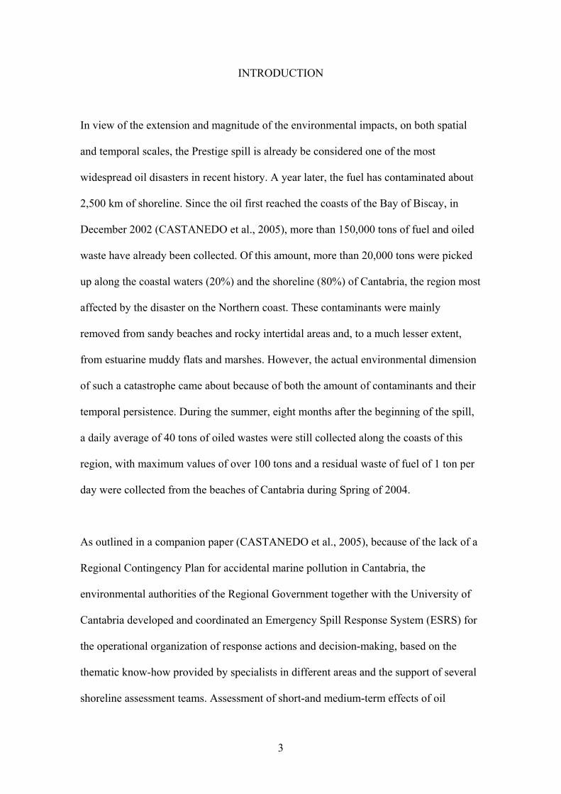
In view of the extension and magnitude of the environmental impacts, on both spatial

and temporal scales, the Prestige spill is already be considered one of the most

widespread oil disasters in recent history. A year later, the fuel has contaminated about

2,500 km of shoreline. Since the oil first reached the coasts of the Bay of Biscay, in

December 2002 (CASTANEDO et al., 2005), more than 150,000 tons of fuel and oiled

waste have already been collected. Of this amount, more than 20,000 tons were picked

up along the coastal waters (20%) and the shoreline (80%) of Cantabria, the region most

affected by the disaster on the Northern coast. These contaminants were mainly

removed from sandy beaches and rocky intertidal areas and, to a much lesser extent,

from estuarine muddy flats and marshes. However, the actual environmental dimension

of such a catastrophe came about because of both the amount of contaminants and their

temporal persistence. During the summer, eight months after the beginning of the spill,

a daily average of 40 tons of oiled wastes were still collected along the coasts of this

region, with maximum values of over 100 tons and a residual waste of fuel of 1 ton per

day were collected from the beaches of Cantabria during Spring of 2004.

As outlined in a companion paper (CASTANEDO et al., 2005), because of the lack of a

Regional Contingency Plan for accidental marine pollution in Cantabria, the

environmental authorities of the Regional Government together with the University of

Cantabria developed and coordinated an Emergency Spill Response System (ESRS) for

the operational organization of response actions and decision-making, based on the

thematic know-how provided by specialists in different areas and the support of several

shoreline assessment teams. Assessment of short-and medium-term effects of oil

4

pollution and monitoring of different compartments (i.e. water, sediments, biota) and

coastal biocoenoses represented two main functions included in the aforementioned

ESRS.

Although each spill event can be considered a unique blend of place, oil properties,

nature and human influences, current knowledge on oil fate and effects allows us to

understand and anticipate likely impacts and predict recovery (HAYES et al., 1992;

SLOAN, 1999). For this purpose, various resources and tools have been developed

during the last decade in the USA (cf. HAYES et al., 1992; MACDONALD et al., 1997;

NOAA, 2000; PETERSEN et al., 2002) in order to design and implement the

assessment and monitoring activities in a concise, systematic and standard format.

Furthermore, the numerous oil disasters that occurred in the 90´s have provided a

continuous experimental ground to improve assessment procedures and to validate

hypotheses on environmental damage (e.g. GUVEN et al., 1998; PETERSON, 2000;

GELIN, et al., 2003; FRENCH, 2003; GOMEZ et al., 2003; ZENETOS et al., 2004).

According to the NOAA (2000), the assessment programs consist of a systematic

approach that uses standard terminology to collect data on coastal oil conditions and

supports decision-making for shoreline clean-up. Depending on factors such as the

intensity, magnitude and duration of the spill, the types of habitat affected, the oil

conditions, etc. “geographic” and/or “hot spot” assessment programs may be

implemented. On the other hand, monitoring programs are used to estimate the

ecological effects of the fuel and to evaluate the recovery of coastal communities. As

established by MACDONALD et al. (1997), the characterization of the environmental

condition of contaminated sites by hazardous wastes includes three levels of concern: 1)

5

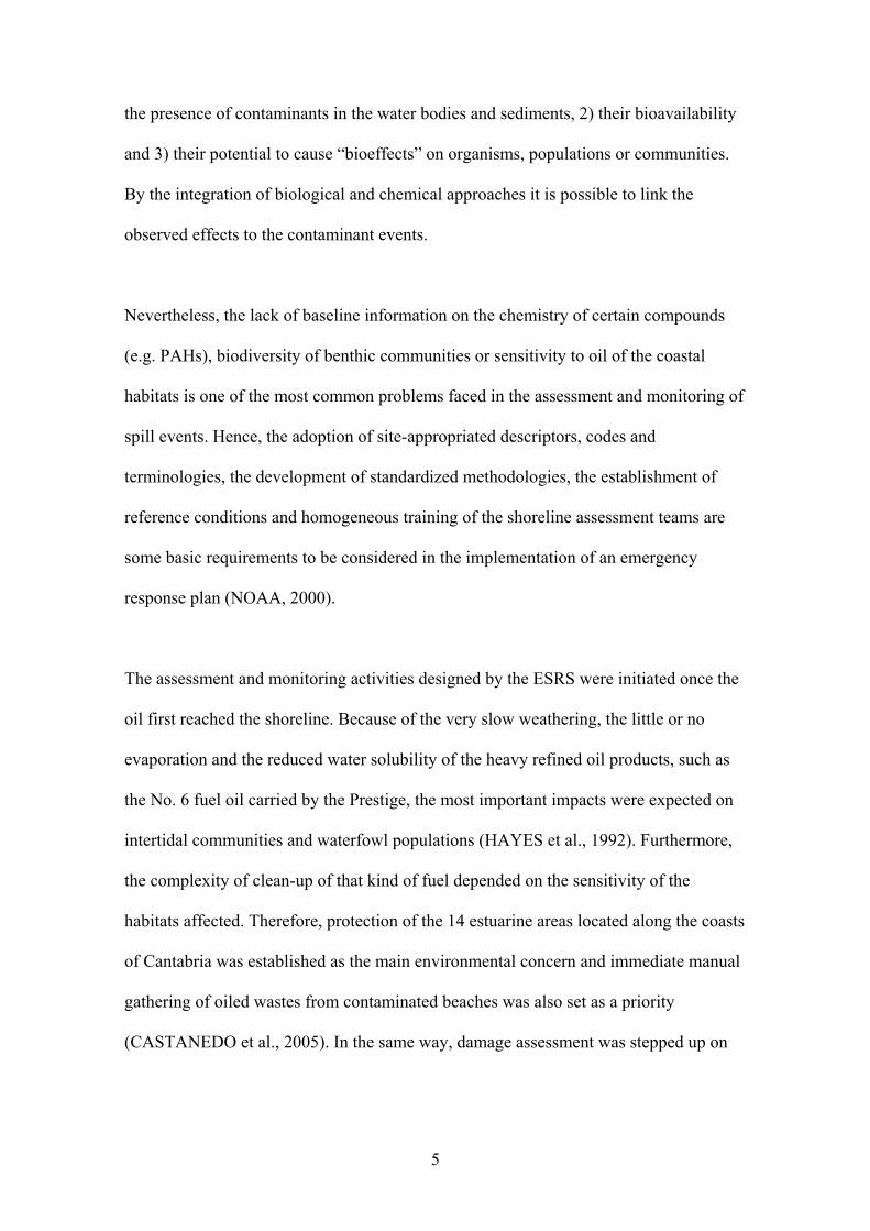
the presence of contaminants in the water bodies and sediments, 2) their bioavailability

and 3) their potential to cause “bioeffects” on organisms, populations or communities.

By the integration of biological and chemical approaches it is possible to link the

observed effects to the contaminant events.

Nevertheless, the lack of baseline information on the chemistry of certain compounds

(e.g. PAHs), biodiversity of benthic communities or sensitivity to oil of the coastal

habitats is one of the most common problems faced in the assessment and monitoring of

spill events. Hence, the adoption of site-appropriated descriptors, codes and

terminologies, the development of standardized methodologies, the establishment of

reference conditions and homogeneous training of the shoreline assessment teams are

some basic requirements to be considered in the implementation of an emergency

response plan (NOAA, 2000).

The assessment and monitoring activities designed by the ESRS were initiated once the

oil first reached the shoreline. Because of the very slow weathering, the little or no

evaporation and the reduced water solubility of the heavy refined oil products, such as

the No. 6 fuel oil carried by the Prestige, the most important impacts were expected on

intertidal communities and waterfowl populations (HAYES et al., 1992). Furthermore,

the complexity of clean-up of that kind of fuel depended on the sensitivity of the

habitats affected. Therefore, protection of the 14 estuarine areas located along the coasts

of Cantabria was established as the main environmental concern and immediate manual

gathering of oiled wastes from contaminated beaches was also set as a priority

(CASTANEDO et al., 2005). In the same way, damage assessment was stepped up on

6

muddy estuarine and sheltered rocky intertidal areas and monitoring efforts were more

intensively directed towards intertidal zones.

The randomly repeated contaminant events along the coasts of Cantabria have

conditioned the maintenance and the adaptation of the Emergency Spill Response

System throughout time, in order to manage very distinct situations (e.g. marine

protected areas, food quality, bathing zones). Therefore, failures and successes of this

ESRS represent a unique source of information for the design of Regional Contingency

Plans. For that purpose, the main goal of the present study is to analyze and discuss the

assessment and monitoring results registered during the first year after the Prestige spill

off the coast of Cantabria (December 2002 – December 2003).

METHODS

Study area

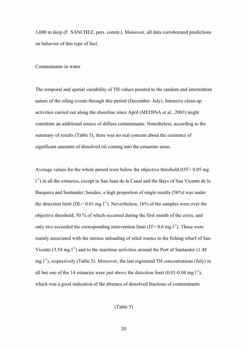
The assessment and monitoring analysis covered the intertidal habitats, including about

5,400 Ha of estuarine ecosystems and 200 km of rocky shores and sandy beaches, and

the soft bottom and rocky subtidal zones, down to a depth of 300 m, along the shoreline

of Cantabria (Figure 1). Considering the structural and functional points of view, four

types of environmental units were distinguished in the coastal zone of Cantabria:

estuaries, rocky shores, sandy beaches and subtidal areas. Specific shoreline sectors

were assigned to those general types and most of them were then divided into smaller

“segments”, according to the similarity of their geomorphologic features (Figure 1). A

7

geographic information system (GIS), based on 1:5,000-scale aerial photography and

1:25,000-scale topographic maps, provided the detailed information and the physical

support for their spatial delimitation. In consequence, a total of 35 polygonal segments

were registered within the 14 estuarine areas, another 38 corresponded to linear rocky

shore segments, included within the 20 coastal units of this type, and a further 21

segments were identified along the four subtidal units established. In addition, the 78

sandy beaches were considered indivisible units. Denomination of segments was

standardized by an alphanumeric code that included two numbers, referring to the

environmental unit and to the segment, respectively.

(Figure 1.)

Coastal assessment

In general terms, the methodology used for the damage assessment was based on that

proposed by the NOAA (2000), with the appropriate modifications in order to fit the

available human and technical resources, the spill properties and behavior and the

knowledge of specific ecological features of the different coastal habitats. The

widespread influence of the repeated oiling events along the coast of Cantabria justified

the application of an assessment procedure divided into three consecutive phases,

including: the assignation of sensitivity degrees to different coastal segments, the

reconnaissance of the spill’s extension and condition and the estimation of impacts.

Various procedures were applied for the assessment of the environmental units located

at the intertidal (estuaries, rocky shores and sandy beaches) and the subtidal areas. In the

8

first case, the concept of mapping and ranking the coastal environments on a scale of

relative sensitivity, developed by the NOAA (cf. PETERSEN et al., 2002), was applied.

For that purpose, a specific Environmental Sensitivity Index (ESI) for the coasts of the

Bay of Biscay was implemented (MEDINA et al., 2003). The main factors that

determined the gradation of that scale were the relative exposure to wave energy, the

shoreline slope, the type of substrate, the biological productivity, the persistence of oil

and the clean-up difficulty. The different categories of sensitivity of intertidal

environments to fuel considered in this work are listed in Table 1.

(Table 1)

A preliminary ESI classification of every coastal segment was established after the GIS

information. Validation of the proposed categories was carried out, always at low water

spring tides, by means of an aerial survey with helicopter and ground verification by sea

(pneumatic boats) and land visits. Furthermore, the main ESI for each segment was

complemented with secondary sensitivity values for specific coastal sites when

necessary. Complementary information on access points, shoreline impacts and

potential for burial was registered on topographic maps, field sketches and photographs

taken in situ.

Based on such primary information, a detailed description of the oiling extent and the

identification of the more sensitive resources (ecological, recreational, cultural) to fuel

were obtained from an intensive field campaign, using a modified version of the

shoreline assessment forms designed by the NOAA (2000), adapted to the actual

conditions of the coastal zone of Cantabria (MEDINA et al., 2003). In addition, the

9

shoreline assessment job-aid field guide (NOAA, 2000) was used for the estimation of

oil distribution (width and length of oil bands) and condition at both the surface and the

subsurface levels. Overall assessment of different environmental units was carried out

following each significant oiling event during the first four months (December-March);

however, further specific evaluations were developed as part of the monitoring of the

clean-up activities of sandy beaches and rocky shores (MEDINA et al., 2003). Records

of waste collected daily at the disposal points provided a reference point for the program

of daily activities of the shoreline assessment teams.

Two descriptors, the “oiled surface” and the “oil coverage”, summarized the semi-

quantitative estimation of impacts for each coastal segment. Four levels parameterized

the first variable, according to the percentage of the total surface with presence of fuel

for each segment (trace, < 1%; limited, 1-10%; broad, 10-60%; large-scale, >60%), as

an indicator of the spreading of the fuel. On the other hand, oil distribution within each

affected zone was ranked in three degrees (low, <5%; moderate, 5-50%; heavy, >50%),

showing the intensity of the oiling condition within the oiled surface. Preliminary

quantitative assessments (m2) of the total rocky shore substrates affected by fuel and the

actual oiled surfaces (total surface weighted by oil coverage) were also estimated all

along the shoreline.

Otherwise, the presence of oil on rocky and soft bottom subtidal habitats was evaluated

using specific procedures developed in this study (MEDINA et al., 2003). The

assessment in the shallower coastal areas, up to a depth of 15-18 m, was carried out

during three months (March-May) by trained divers along 70 transects placed at regular

intervals (ca. 2 miles), perpendicular to the shoreline. The distribution (abundance and

10

size) of surface tar balls was registered in segments of 50 meters, complemented with

systematic hand digging of sediments for evaluation of subsurface contaminants. The

substrate type (sand, gravel, cobble, blocks) and the dominant benthic communities in

those segments were also recognized from the video recording of the whole ride of

every transect line.

In deeper soft bottom subtidal zones, between 18 and 300 m, 30-minute trawls, at 3

knots, were used for detection of submerged tar balls. Twenty-three trials were carried

out between December and March, using commercial trawling fishing nets (mouth 22 m

long), covering partial surfaces of about 0.6 Ha. Results were referred to in terms of

abundance, size and weight of the collected tar balls. Oil stains in the different elements

of the trawling devices provided further information on frequency of contaminants on

the sea floor.

Monitoring of coastal ecosystems

The general monitoring methodology followed the principles proposed by

MACDONALD et al. (1997) for the bioassessment of aquatic areas contaminated by

hazardous wastes. This was specified in three types of studies: 1) chemical

quantification of contaminants in water and sediments, 2) bioaccumulation of

contaminants in benthic organisms and 3) structural changes on intertidal communities.

Because of the increasing and continuous oil contamination throughout the coastal area,

the systematic analysis of oil contaminants focused on the most sensitive units, the

estuarine areas. Thus, total hydrocarbons (TH) and selected polycyclic aromatic

hydrocarbons (PAH, Σ anthracene, fluoranthene, benzo(a)anthracene, benzo(a)pyrene,

11

benzo(g,h,i)perylene, benzo(k) fluoranthene, chrysene, indeno 1,2,3-c,d pyrene,

naphtalene, phenanthrene) were analyzed in water and sediment samples from 29

sampling points, located along the tidal gradients of the 14 estuarine areas. Stations

were distributed according to the specific surface and the ecological importance of the

different estuarine segments. Samples were always collected by hand and maintained in

clean glass containers, until processing at the Environmental Research Center of the

Government of Cantabria.

In all the outer points (mouth stations), two replicated surface water samples (1 liter

capacity) were collected between one and two hours before flow tide, at weekly

intervals during the first two months (December-January), fortnightly from February to

April and bimonthly until July, following an adaptive monitoring design according to

previous results (RINGOLD et al., 1996). Inner estuarine stations were sampled

approximately at monthly intervals. Total hydrocarbons were extracted with 1,1,2

trichlorotrifluorethane and determined, in a total of 350 samples, by infrared

spectrophotometry (2930 cm-1), following the APHA 5520 standard method. Otherwise,

PAHs were analyzed at seasonal intervals (100 samples) by liquid chromatography

(HPLC), using UV and fluorescence detectors, according to the EPA 610 method. In the

absence of national standards, “objective” and “intervention” TH thresholds (OT= 0.05

mg l-1; IT= 0.6 mg l-1) were adopted from the Holland normative for evaluation of

results. Likewise, the selection of the PAH compounds and the establishment of the

corresponding “objective value” (OV= 0.3 μg l-1) were carried out according to the

proposal of the NOAA, taking into account the specific composition of the fuel of the

Prestige (CEDRE, 2004).

12

In addition, sediment collections took place just following the first oiling event

(December) and after that, at a seasonal rhythm (January, March, July). Combined

samples, obtained after mixing four sediment replicates (ca. 300 g fresh weight),

collected on the surface layer of each station (ca. 100 m2), were used for granulometric

analysis and for determination of contaminants (TH and PAH) on subsamples dried at

room temperature. Total hydrocarbons were determined in 97 samples, by the same

technique as for the water samples, following the EPA 9071 standard procedure.

Likewise, the HPLC-based VPR C-88/11 standard method from the Holland legislation

was used for analyses of PAHs on selected sediment samples (n=43) after extraction

with petroleum ether. “Objective” and “intervention thresholds” were also adopted from

the Holland normative for evaluation of both the TH results (OT= 50 mg kg-1; IT= 5 g

kg-1) and the PAH results (OT= 1 mg kg-1; IT= 40 mg kg-1). Consequently, selection of

the specific PAH compounds to be analyzed was in agreement with that normative.

Bioaccumulation studies involved the measurement of tissue residues in indigenous

benthic organisms from estuarine and coastal areas, providing a direct evaluation of the

bioavailability of those compounds and, in the case of commercial resources, their

potential for human health risks. For that purpose, PAHs (Σ benzo(a)anthracene,

benzo(b)fluoranthene, benzo(k) fluoranthene, benzo(a)pyrene, dibenzo(a,h)anthracene,

incero(1,2,3-c)pyrene) were systematically analyzed on samples (ca. 250 g dry weight

flesh) of two sedentary species: clams (Tapes decussatus) from all the three regulated

shellfishery estuarine areas (S. Vicente de la Barquera, Bay of Santander and Santoña

Marshes), and goose barnacles (Pollicipes cornucopia) from 14 highly exposed

intertidal rocky sites all along the coastal region. Several samples were obtained from

February to June by professional harvesters, according to an adaptive monitoring design

13

based on the local availability of resources and the evolution of the analytical results.

Further controls of selected samples of goose barnacles were carried out during the next

Spring (2004), because of the highest bioavailability of those contaminants in the

coastal zones.

Complementary screening analyses were also carried out at the first trial (February) on

other estuarine (cockles and cultivated oysters) and rocky species (mussels and limpets).

Once in the laboratory, samples were frozen and sent to the National Food Insurance

Center for certified PAHs analyses. According to the Spanish normative, reference PAH

standard for healthy shellfish products is established at 200 μg kg-1 of dry weight flesh

(Σ 6 compounds).

Bioeffects on intertidal communities were studied at 15 coastal locations. The selection

of impacted and reference stations took into account the distance from oiled sites.

Preliminary semi-quantitative assessments of the zonation patterns were inventoried in

December, on low water spring tides by a systematic sampling design on 2,500 cm2

quadrats placed along a transect line from the low water to the high water marks. The

quadrat was divided into 10 x 10 cm grid squares to aid estimates of percentage cover of

the conspicuous macrobenthic species (seaweeds and invertebrates). Oil distribution and

condition in the surrounding areas were simultaneously evaluated. Subsequent semi-

quantitative assessments were carried out at seasonal intervals (January, March, July,

December). Otherwise, 625 cm2 quantitative samples were collected at the same

intertidal zones during the seasonal surveys, following a community-oriented

monitoring program that will continue for the next three years. The results of this work

will be synthesized at the end of the program.

14

Data management

The growing number of field data and the permanent demand for updating reports

required the development of a management interface, which allows for the synthesis of

all the basic information and its integration with the operational forecasting outputs

(CASTANEDO et al., 2005). Thus, storing and handling different types of assessment

and monitoring data were managed by means of the Emergency Spill Response

database, designed and implemented for a geographic information system (GIS),

following the design workflow suggested by Merise (NANCI and SPINASSE, 1996).

The interface applied to generate the physical implementation of the database (tables,

forms, requests) was Microsoft Access 2000. Input of different types of information

(alphanumeric, numeric, pictures, sketches) was carried out using precise forms, similar

to those employed in the fieldwork. Reports on different issues directed at the decision-

making process (temporal and spatial evolution of spill outs, impacts and bioeffects,

remediation actions, zonation patterns) were programmed in the same management

system (cf. MEDINA et al., 2003).

Graphic representation of assessment and monitoring results were based on a GIS

project (Arc View 3.2.), complemented with 1:5,000 aerial photography. Furthermore,

the comprehensive information acquired about different coastal features

(geomorphology, exposure, persistence of oil, difficulty of clean-up) constituted the

base for the Atlas of Sensitivity to fuel of the coastal environments of Cantabria that is

currently being implemented.

15

RESULTS

Oiling conditions of intertidal areas

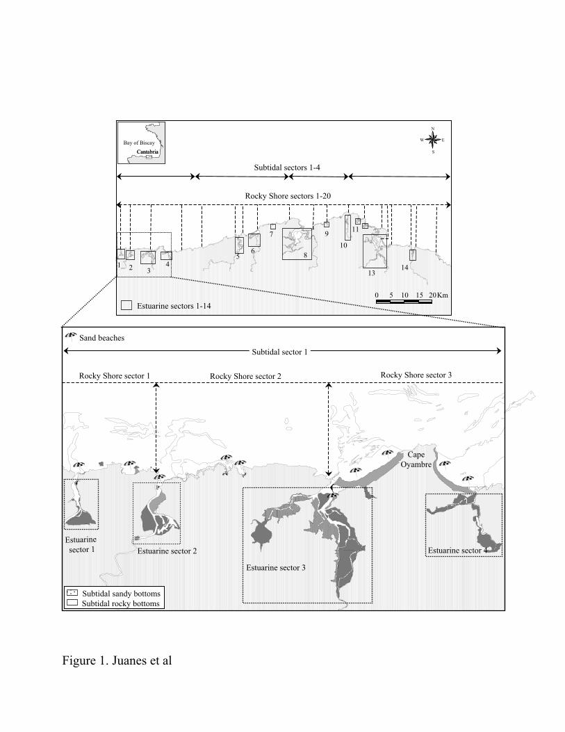
In general terms, environmental contamination from the Prestige spill was broadly

dispersed along the shoreline of Cantabria. The differential incidence of the oiling

events may be preliminarily estimated by the total amounts of oily waste collected at the

disposal points throughout the first year (Figure 2). The western coast of Cantabria

received a major and more continuous pressure of spill impacts than the eastern part.

Moreover, the coastal areas around Cape Oyambre (W Cantabria) and Cape Ajo (E

Cantabria) concentrated a high proportion of the total amount of collected fuel, mainly

in semi-exposed and sheltered mixed beaches, in which rocky substrates (cobbles,

blocks) were widely affected. These results are in agreement with the general forecast of

the oil spill model presented in the companion paper (CASTANEDO et al., 2005).

(Figure 2.)

Containment booms located at the mouth of the 14 estuarine areas (CASTANEDO et

al., 2005) prevented an ecological disaster, but the combination of adverse

oceanographic (spring tides) and meteorological conditions (Northwest fronts) brought

about the leaking of these barriers and the contamination of some marsh areas. Anyway,

the total amounts of oiled wastes collected in the outer part of the booms was much

greater than those gathered from marshes and wetlands.

16

Likewise, the temporal significance of these contaminant events may be anticipated

from daily records of oily waste collected all along the shoreline (Figure 3). More than

50% of these wastes were removed during the first three months (December-February),

following the most important oiling events. Moreover, a randomly continuous drop in

oiling episodes occurred throughout, their magnitudes being diminished by southerly

winds and increased by northwesterly ones (cf. Figure 9, CASTANEDO et al., 2005).

Significant amounts of fuel (about 40 tons per day on average) were still picked up from

the 78 sandy beaches throughout the bathing season (June-September 2003), with

maximum daily values above 100 tons. Further residual wastes of 1 ton of fuel per day

were collected from the beaches of Cantabria during Spring of 2004.

(Figure 3)

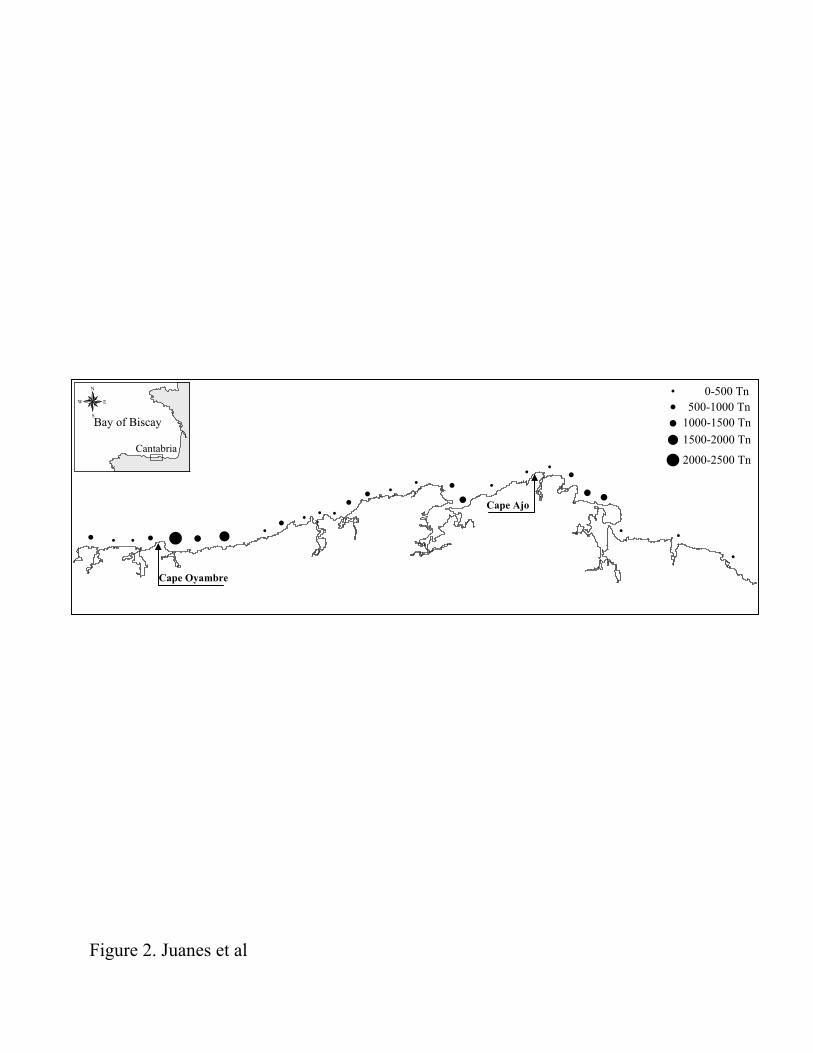
Semi-quantitative estimations of impacts were summarized according to the total oiled

surface and the oil coverage for each estuarine (Table 2) and rocky shore segments

(Table 3). Regarding the extension of the oiled estuarine areas, most of the affected

surfaces did not suffer any impact or did not reach 1% of the total segment (trace).

However, oiled surfaces up to 10 % of the total area (limited extension) were registered

in eight segments and broad impacts (10-60% of the total surface) were inventoried in

two specific ones, the Mogro area (segment 6.1) and the Quejo inlet (segment 11.2).

Otherwise, oil cover within the impacted estuarine areas was qualified in most cases as

moderate (<5%), but higher degrees were also registered in several segments of six

estuaries. Maximum values, between 20 and 40% of coverage, were reported from two

17

marsh areas (segments 6.2: Miengo and 11.2: Quejo) and from the rocky areas in the

inner inlets of Joyel (60% coverage). Containment booms of these estuaries showed

different technical problems because of the strong tidal and flood currents (cf.

CASTANEDO et al., 2005), which may explain the impacts observed in those marshes.

(Table 2)

Taking into account the total area of each estuarine segment, impacted surfaces were

scarcely significant; however, oiled surfaces were noteworthy in the local context of

some estuaries, mainly because of the deterioration of vegetated marshes in some

protected areas (e.g. segments 3.2: Rubin, 6.2: Miengo and 11.2: Quejo inlet). Hot spots

in this kind of environmental unit affected estuarine areas up to 3,000 m2.

In the case of rocky shores, a significant increase in the level of damage was observed.

Geographic distribution of impacts on rocky substrates followed that of wastes removed

along the shoreline (Figure 1), with the broader oiling areas occurring along the western

coast. In general terms, it was observed that the higher the sensitivity of a part of a

segment (Specific ESI, Table 3), the more extensive the oiled area and the oil coverage

of substrates.

Semi-exposed to sheltered rocky shores (ESI levels 4 to 6) registered the major impacts.

In a high proportion of the more sensible rocky segments, oiled surfaces reached values

over 10% of the total area and some of them exceeded 60% (Table 3). Likewise, cover

of oil in those segments attained moderate (5-50%) to heavy (>50%) levels because of

the presence of 5 to 50 cm diameter tar oil, of nearly solid consistency, coating the

18

rocky substrates. Pooled oil accumulated in sheltered rocky inlets, crevices and caves of

the western coast and oily films were common on the surface waters of many intertidal

pools.

(Table 3)

Quantitative assessments of the total impacted area (m2) and the actual oiled surface

(estimate of the m2 directly contaminated by fuel) in each rocky sector are shown in

Figure 4. According to these records, disturbance by oil cover was significantly more

extensive on rocky shores than in estuarine areas. Quantitative results confirmed the

relationship between the presence of the more extended oiled surfaces and the ESI

values of each specific sub-segment. Thus, more than 180,000 m2 of rocky shores were

affected by fuel, of which about 114,000 m2 were located in the proximities of sandy

beaches (semi-exposed rocky surfaces, ESI 5). For all of these areas, the surfaces that

were actually covered by fuel totaled 50,000 m2 with 95% corresponding to sites along

the western coast. Likewise, coverage on 14 oiled segments along the western coast was

over 1,000 m2 and six of them exceeded 3,000 m2. Comparing these results (Figure 4)

with those of Figure 2, it should be pointed that, in absolute terms, the most severe oil

impacts seem to be more related to the sensitivity of the different segments of a coastal

sector than to the amount of waste collected along its shoreline. In contrast, maximum

oiled surfaces on four segments on the eastern coast were only over 200 m2.

(Figure 4.)

Differences between the overall affected areas of each segment and the actual oiled

surfaces were higher in the rocky substrates of sandy beaches than on rocky shores,

19

because the surf zone acted as effective collecting points, preventing the fuel from

reaching the rocky areas at the rear. This effect was evident on the eastern coast, where

about 3,300 tons of oiled wastes were collected on some beaches of sectors 13 and 14

(cf. Figure 2), whose rocky substrates were barely affected by fuel (Figure 4).

Assessment of subtidal habitats

In agreement with the preliminary hypothesis, the presence of significant amounts of oil

in the subtidal bottoms of Cantabria was assessed as a rare event. Results of the 35 km

of diving runs along the shallow coastal areas (0-18 m), showed that fuel came out in

only 4 of the 70 subtidal transects, all of them located on the western coast. Sporadic tar

balls of 5 to 25 cm in diameter, with covers about 5 to 10 %, were present in segments

of about 100-m length of two transects on soft bottom areas close to gathering zones of

cast seaweeds; likewise, oil traces were detected in another two transects. On the other

hand, there was no evidence of oil residues on the most characteristic subtidal

communities dominated by seaweeds (Gelidium sesquipedale, Saccorhiza polyschides –

Laminaria ochroleuca, Cystoseira spp.) or the occurrence of contaminants on the

subsurface layer of sandy areas.

Likewise, the sporadic but constant oil stains registered on different elements of the

trawling device (bridles, ground ropes, net, cod-end), together with the reduced number

and size of tar balls collected by the fishing net (<250 g), pointed to the low probability

of persistence of significant accumulations of fuel in the deeper subtidal areas (Table 4).

These results fit in with those of the shallower areas and those obtained with the same

methodology by the Spanish Oceanographic Institute in marine areas between 300 and

20

3,000 m deep (F. SÁNCHEZ, pers. comm.). Moreover, all data corroborated predictions

on behavior of this type of fuel.

Contaminants in water

The temporal and spatial variability of TH values pointed to the random and intermittent

nature of the oiling events through this period (December–July). Intensive clean-up

activities carried out along the shoreline since April (MEDINA et al., 2003) might

constitute an additional source of diffuse contaminants. Nonetheless, according to the

summary of results (Table 5), there was no real concern about the existence of

significant amounts of dissolved oil coming into the estuarine areas.

Average values for the whole period were below the objective threshold (OT= 0.05 mg

l-1) in all the estuaries, except in San Juan de la Canal and the Bays of San Vicente de la

Barquera and Santander; besides, a high proportion of single results (56%) was under

the detection limit (DL= 0.01 mg l-1). Nevertheless, 16% of the samples were over the

objective threshold, 50 % of which occurred during the first month of the crisis, and

only two exceeded the corresponding intervention limit (IT= 0.6 mg l-1). These were

mainly associated with the intense unloading of oiled wastes in the fishing wharf of San

Vicente (3.54 mg l-1) and to the maritime activities around the Port of Santander (1.48

mg l-1), respectively (Table 5). Moreover, the last registered TH concentrations (July) in

all but one of the 14 estuaries were just above the detection limit (0.01-0.04 mg l-1),

which was a good indication of the absence of dissolved fractions of contaminants.

(Table 5)

21

Furthermore, PAH concentrations were below the detection limit (DL= 0.1 μg l-1) in all

the samples analyzed, which confirmed the slow weathering and low solubility of this

kind of fuel.

Contaminants in sediments

Results of TH in sediment samples showed a greater spatial variability than in estuarine

waters, though they seemed to present a higher constancy at the temporal scale for each

sampling point. Annual mean values and maximum TH records for each sector pointed

to the existence of different degrees of contamination (Table 6), ranging from

unpolluted or lightly polluted estuaries (e.g. Tina Mayor, San Juan de la Canal, Oriñon),

whose mean and maximum values were below the objective threshold (OT= 50 mg kg-

1), to the heavily-polluted estuaries (e.g. San Martin de la Arena), where high degrees of

contamination persisted for the whole period. However, in this scale, it is difficult to

clearly establish the relationship of these results with the oiling events.

Regarding a more concise analysis of results, it should first be noted that only 20% of

the samples were over the objective limit and the intervention threshold was not

exceeded in any case (IT= 5 g kg-1). Most of the lightly polluted sediment samples (< 36

mg kg-1) were collected in estuarine segments where the least important oiling impacts

were estimated (cf. Tables 2 and 6); the only exception was noticed in the Joyel Inlet, a

small segment that registered a severe oil impact. Conversely, some TH values

exceeding the objective threshold were related to sporadic or continuous oiling episodes

that occurred in the proximities of the sampling stations of several estuarine segments

22

(Bay of San Vicente, La Rabia, Pas). Otherwise, locally known oil sources (industrial

effluents, shipyards, harbors and marinas) other than the Prestige spill seemed to have a

great influence on the current pollution status of some estuarine segments (e.g. San

Martin de la Arena, Bay of Santander, Bay of Santoña) that were, in fact, not affected

by any oiling event. Finally, the combined effects from solid wastes lixiviate plus fuel

impacts might explain the persistence of high TH values in the Ajo Estuary.

(Table 6)

It was noteworthy that the higher values registered in oiled estuarine segments were in

the range of two to three times the objective threshold (83-155 mg kg-1), although

average values for all the estuaries were below or just above that limit (27.4-51.8 mg kg-

1). The maximum value was registered in one sample of the Bay of Santander (787 mg

kg-1), collected in the proximities of an industrialized area (shipyard, specific areas for

the break-up of ships) which was included for the comparison of contaminated sites.

Furthermore, seasonal results from San Martin de la Arena supported earlier pollution

status assessments for this estuarine area based on analyses of different toxic, persistent

and bioaccumulation contaminants (heavy metals, PCBs) in sediments (REVILLA et

al., 1999).

This may be partially validated by the results of polycyclic aromatic hydrocarbons

(PAHs) in the same samples (Table 7). Thus, the lowest mean and maximum PAH

values (most of them below the detection limit, DL= 0.1 mg kg-1)) were also registered

in sediments from all the lightly polluted estuaries (sectors 1, 2, 7, 9, 12 and 14).

23

Likewise, the highest PAH value was found in samples from La Rabia (sector 4, 14 mg

kg-1), one of the most impacted estuaries, even though it is well below the intervention

threshold (IT= 40 mg kg-1).

(Table 7)

In contrast, significant PAH values were not detected in any single sample from the

other three oiled estuarine sectors (Bay of San Vicente, Pas and Joyel). Furthermore,

contamination by PAH sediments close to industrial hot spots from sectors 8, and 13

(mainly related to maritime activities) seemed to reflect an important level of

contamination by aromatic compounds; however, very low values (max. 0.41 mg kg-1)

were registered in samples from the San Martin estuary, whose TH values showed the

most persistent hydrocarbon contamination. As stated by KING et al. (2004), all these

findings indicate the differential influence of several hydrocarbon sources in some

estuarine basins (e.g. urban/industrial discharges, combustion of fossil fuels) that

confound the interpretation of results.

Bioaccumulation

Results from the bioeffects analyses carried out were in agreement with the global

impact assessments in the different environmental units, pointing to coastal habitats as

being the areas where the bioavailability of toxic components from the Prestige spills

presented a significant level of risk.

Commercial shellfish species seemed to be unaffected by the sporadic and

geographically located inputs of hydrocarbons in the estuarine areas. All single PAH

24

records from the Bay of San Vicente and the Bay of Santoña varied from 5 to 83 μg kg-1

(dry weight flesh), well below the objective value (OT= 200 μg kg-1), showing a clear

homogeneity between the different harvesting areas within each estuary. Likewise,

seasonal average values for both estuaries did not reflect any significant difference in

the temporal scale (Figure 5). Concentrations of similar ranges were obtained for

samples of cockles and oysters collected after the first oiling event (December) in the

Bay of San Vicente. Furthermore, results of clam samples in the outer part of the Bay of

Santander (42 μg kg-1) also confirmed the non-bioaccumulation effects in the most

important shellfisheries of this estuary.

(Figure 5)

Conversely, heavy PAH contamination of clams (average values: 0.6 -18 mg kg-1) were

noticed in two small harvesting zones from the Bay of Santander, located in the inner

estuary, close to areas with a great pressure from different maritime activities (marina,

commercial harbor and shipyard). Intense contamination of sediments in this area has

already been referred to, even though no significant incidences were registered in

relation to the Prestige oil spills in this Bay.

In contrast, benthic organisms on the rocky shores were affected by fuel to a higher

degree. Even though there is no evidence of oil coating effects on any biological

community in the mid and low intertidal, the continuous exposure to oil wastes (tar,

films) on the coastal zone brought about the bioaccumulation of PAH compounds on

populations of the main commercial resource exploited in this area, the goose barnacle.

All the samples of this species collected in March along the western coast exceeded the

25

national standard for this contaminant (OT= 200 μg kg-1, Figure 6); similar results were

registered in samples of mussels collected along both the west and the east coasts, close

to Cape Oyambre (223 μg kg-1) and Cape Ajo (663 μg kg-1), respectively. However,

only 3 of the 12 samples of limpets attained significant PAH values (ca. 120-190 μg kg-

1), although below the objective threshold, which may suggest a preferential

bioavailability of fuel for the filter-feeding organisms.

(Figure 6)

Otherwise, significant reductions of the previous levels were registered during the

second survey (June) in most of the contaminated sites, showing a high capacity to

metabolize these toxic compounds. Residual hot spots still remained in sector 9 where

the extension and magnitude of the impacts were at that time very significant (cf. Figure

4). Local increases in PAH concentrations were observed in a few samples on the

eastern coast that might be related to the persistence of spills during the Spring. Later

analysis carried out in May 2004 demonstrated the total abatement of this contaminant

episode (max. PAH concentration: 1 μg kg-1).

Biodiversity and analyses of communities

Results from the semi-quantitative analyses carried out in the intertidal and subtidal

zones allowed for a more precise evaluation of the oil bioeffects on the littoral

ecosystems.

26

The 15 intertidal zones that were selected for the study of bioeffects corresponded to

semi-exposed coastal areas. The tidal range along this coast is about 4.5 m and the

general zonation pattern was quite homogeneous, showing local differences due to

several factors (exposure, slope) that modified the size of the more conspicuous belts

(Figure 7). According to the semi quantitative zonation analyses, the main impacts on

rocky shores were registered at the upper littoral fringe where diversity of benthic

organisms is very low. Thus, communities dominated by limpets and barnacles (Patella

spp. – Balanus perforatus – Littorina neritoides) experienced the most direct and critical

impact as a result of the plastering effect. Moreover, in a few sheltered zones at the rear

of sandy beaches, lower intertidal belts, colonized by a stratum of turf-like red

macroalgae and dispersed populations of Fucus spp, underwent severe coating effects.

Otherwise, the cover of oil was in any case detected in the mid littoral zone, where the

intertidal communities, dominated by calcareous red (Corallina spp.) and brown

macroalgae (Bifurcaria bifurcata - Halopteris scoparia), reach their maximum degree of

development and diversity.

(Figure 7)

In the case of the estuarine areas, the oil that crossed the containment booms reached the

higher intertidal area, coating the rocky substrates (most of them protection structures)

and the outer macrophytic individuals of vegetated marshes (Juncus sp., Halimione

portulacoides). On the other hand, there was no evidence of either significant amounts

of oil covering seaweed fields (Fucus spp., Ascophyllum nodosum) and sea grass

populations (Zostera spp.) in the mid to low intertidal areas, or the burial of fuel in the

muddy areas.

27

Regarding subtidal areas, qualitative evaluations, based on presence–absence video

recording analyses of the dominant macroalgae species, showed no evidence of short-

term effects on the most conspicuous and representative populations of this coastal

fringe (Gelidium sesquipedale, Saccorhyza polyschides–Laminaria ochroleuca,

Cystoseira spp.).

In any case, preliminary conclusions of the semi-quantitative assessment should be

contrasted with the results from the medium-term quantitative studies of the temporal

evolution of biodiversity and abundance of the different intertidal and subtidal

communities currently in progress (PUENTE et al., 2005).

LESSONS LEARNED AND CONCLUSIONS

The assessment and monitoring results shown in this paper provided a precise starting

point to qualify and quantify the overall impacts of the Prestige oil on the coastal

habitats of Cantabria, a region 450 nautical miles away from the contaminant source. As

outlined above, the intermittent oiling events brought about severe contaminant

episodes all along the coast, whose main preliminary consequences may be synthesized

in the 180,000 m2 of oiled rocky shores, with about 50,000 m2 of substrates directly

covered by fuel, 78 contaminated beaches and the deterioration of different marsh areas,

some of them included within nature reserves. Thus, regardless of further monitoring

results or information on impact assessment in other coastal regions closer to the sunken

28

ship, the Prestige spill may already be considered the most important environmental

disaster on the northern coast of Spain.

Oil spills at different scales should be considered to occur regularly along populated

coasts worldwide. In consequence, one of the most important actions to be performed

after the abatement of such a catastrophe is the critical analysis of two different aspects:

1) the evaluation of what kind of data, resources and action plans would have improved

the decision-making process; and 2) the validity and performance of the technical

measures actually implemented for the resolution of the crisis.

Different issues arise in relation to the first question, which may be summed up in the

development and implementation of a Regional Contingency Plan for the management

of spill events, once they threaten the integrity of coastal ecosystems. An atlas of

sensitivity to fuel, baseline data on different environmental compartments (intertidal,

subtidal, marshes, shellfisheries, recreation areas) and matrices (water, sediment, biota),

standardized methods (sampling, chemistry, taxonomy, impact assessment) and

validated reference quality thresholds were specific elements missed, at the time the fuel

first reached the shoreline of Cantabria, for the accurate design of the assessment and

monitoring work. Recurrent demands in that direction have arisen after many recent oil

spills (e.g. GELIN et al., 2003; McCAY, 2003).

The experience accumulated in Cantabria because of the Prestige oil spill has

demonstrated that, even though there was no specific knowledge of oil spills, the

combination of the expertise know-how of oceanography, modeling, marine biology,

marine chemistry and environmental engineering with a good coordination has resulted

29

in a suitable alternative to implement the Emergency Spill Response System. However,

this experience is useless unless it is integrated within a Regional Contingency Plan.

Regarding the second question, all findings illustrated the great difficulty in designing

sampling strategies that give representative information on the contamination of so

many estuarine and coastal zones versus randomly repeated oiling events. The

subjective perception of different social agents (politicians, citizens, fishermen,

ecologists, researchers) in the assessment of impacts (extent, effects) produces a great

inflation of questions to be answered with limited time, personnel and equipment.

Therefore, it is important to establish a scientific-based hypothesis in order to

concentrate the efforts on significant impacts.

In this way, assessment and monitoring activities carried out within the ESRS have

followed an experimental procedure focused on the specific concerns established by the

scientist, taking into account the knowledge of oil fate and effects (HAYES et al., 1992;

SLOAN, 1999) and the experience of recent oil spills (GUVEN et al., 1998;

PETERSON, 2000; GELIN, et al., 2003; FRENCH, 2003; GOMEZ et al., 2003;

ZENETOS et al., 2004). For instance, the development of an atlas of sensitivity for the

fuel in the coastal zone of Cantabria was a priority, because small amounts of oil wastes

may produce a significant impact on habitats highly sensitive to fuel (e.g. marsh areas,

rocky coves). Basic data to program the clean-up and monitoring activities is a result of

this information. On the other hand, the high variability of results in water samples plus

time and money consumption of instrumental analysis (e.g. PAH) pointed to the need of

using total hydrocarbons (TH) as a general indicator of contamination by fuel,

complemented by later PAH determinations on specific-case analysis.

30

Nevertheless, sometimes it is important to clearly establish the level of scientific

incertitude and the technical limitations for answering certain questions, some of them

related to the lack of baseline information on chemistry, biodiversity, etc, to the natural

variability of coastal ecosystems or to the prediction capacity about certain biological or

chemical processes. In this way, it should be noted that the multidisciplinary approach

applied for the development of the Emergency Spill Response System has improved the

general knowledge of specific requirements for the implementation of contingency

plans. However, further progress in this field must integrate the forecast of modeling of

oil spills (Where?, How much?, When?) with the modeling of biological responses

(impacted communities, bioaccumulation, etc) and the estimation of the appropriate

remediation techniques.

ACKNOWLEDGEMENTS

This work was supported by a contract between the Fundación Leonardo Torres

Quevedo of the University of Cantabria and the Empresa de Residuos de Cantabria of

the Regional Gouvernment of Cantabria. We are grateful to all the components of the

Environmental Assessment Teams for their assistance and dedication to fieldwork.

LITERATURE CITED

CASTANEDO, S., MEDINA, R., LOSADA, I.J.,.VIDAL, C., MÉNDEZ, F.J.,

OSORIO, A., JUANES, J.A. PUENTE, A., 2005. The Prestige oil spill in Cantabria

31

(Bay of Biskay). Part I: Operational forecasting system for quick response, risk

assessment and protection of natural resources. Journal of Coastal Research , in press.

CEDRE, 2004. Archives Prestige. Documentation des operations POLMAR. Archives

de Pollution, Cedre, vers. 1.1.

GELIN, A., GRAVEZ, V., EDGAR, G.J., 2003. Assessment of Jessica oil spill impacts

on intertidal invertebrate communities. Marine Pollution Bulletin, 46, 1377-1384.

GOMEZ GESTEIRA, J.L., DAUVIN, J.C., SALVANDE, M., 2003. Taxonomic level

for assessing oil spill effects on soft-bottom sublittoral benthic communities. Marine

Pollution Bulletin, 46, 562-572.

GUVEN, K.G., OKUS, E., UNLU, S., DOGAN, E., YUKSEK, A., 1998. Oil pollution

of marine organisms after Nassia tanker accident in the Black Sea, Bosphorus and the

Sea of Marmara. Turkish Journal of Marine Sciences, 4 (1), 3-10.

HAYES, M.O., HOFF, R., MICHEL, J., SCHOLZ, D., SHIGENAKA, G., 1992. An

introduction to coastal habitats and biological resources for oil spill response. Report

No. HAZMAT 92-4. Seattle, WA. National Oceanic and Atmospheric Administration.

KING, A.J., READMAN, J.W., ZHOU, J.L., 2004. Dynamic behavior of polycyclic

aromatic hydrocarbons in Brighton marina, UK. Marine Pollution Bulletin, 48, 229-239.

32

MACDONALD, D.A., MATTA, M.B., FIELD, L.J., CAIRNCROSS, C., MUNN,

M.D., 1997. The coastal resource coordinator´s bioassessment manual. Report No.

HAZMAT 93-1 (revised). Seattle, WA. National Oceanic and Atmospheric

Administration. 147 pp. + appendices.

McCAY, F.D., 2003. Development and application of damage assessment modeling:

example assessment for the North Cape oil spill. Marine Pollution Bulletin, 47, 341-

359.

MEDINA, R., JUANES, J.A., LOSADA, I., VIDAL, C., PUENTE, A., CASTANEDO,

S. (coord.), 2003. Programa de predicción, protección y evaluación del vertido del

buque Prestige en las costas de Cantabria. Tech. Rep. Fundación Leonardo Torres

Quevedo, University of Cantabria – Empresa de Residuos de Cantabria. Docs. I-VI +

appendices.

NANCI, D., SPINASSE, B., 1996. Ingénierie des systèmes d’information Merise.

Editions Sybex. Paris.

NOAA, 2000. Shoreline Assessment Manual. Third edition. HAZMAT Report 2000-1.

Seattle: Office of Response And Restoration, National Oceanic and Atmospheric

Administration. 54 pp. + appendices.

PETERSEN, J., MICHEL, J., ZENGEL, S., WHITE, M., LORD, C., PARK, C., 2002.

Environmental sensitivity index guidelines. Version 3.0. NOAA Technical

33

Memorandum NOS OR&R 11. Seattle: Office of Response And Restoration, National

Oceanic and Atmospheric Administration.

PETERSON, C.H., 2000. The Exxon Valdez oil spill in Alaska: acute, indirect and

chronic effects on the ecosystem. Advances in Marine Biology, 39, 3-84.

PUENTE, A., JUANES, J.A., CALDERÓN, J.G., GARCÍA, A., ECHÁVARRI, B.,

GARCÍA-CASTRILLO, G., 2005. Seguimiento de las comunidades bentónicas en

zonas estuáricas y costeras. In: Medina, R. and Juanes, J.A. (coord.), Desarrollo de

diversos programas de actuación encaminados a corregir los efectos de los vertidos del

fúel procedentes del buque Prestige en las costas de Cantabria. Tech. Rep. Fundación

Leonardo Torres Quevedo, University of Cantabria – Empresa de residuos de Cantabria,

Gouvernment of Cantabria (Spain): Anex I, 86 pp & 6 Appendices.

REVILLA, J.A., ALVAREZ, C., JUANES, J.A., GARCIA, A., PUENTE, A. 1999.

Estudios complementarios al estudio de alternativas e informe de impacto ambiental del

saneamiento del Saja-Besaya. Technical Report to the North Basin Water Authority,

Spanish Ministry of Environment, Madrid.

RINGOLD, P.L., ALEGRÍA, J., CZAPLEWSKI, R.L., MULDER, B.S., TOLLE, T.,

BURNETT, K. 1996. Adaptive monitoring design for ecosystem management.

Ecological Applications, 6, 745-747.

34

SLOAN, N.A., 1999. Oil impacts on cold-water marine resources: a review relevant to

Parks Canada´s evolving marine mandate. Parks Canada. National Parks, Ocassional

paper No. 11. Queen Charlotte, BC. 67 pp.

ZENETOS, A., HATZIANESTIS, J., LANTZOUNI, M., SIMBOURA, M.,

SKLIVAGOU, E., ARVANITAKIS, G., 2004. The Eurobulker oil spill: mid-term

changes of some ecosystem indicators. Marine Pollution Bulletin, 48, 122-131.

35

FIGURE CAPTIONS

Figure 1. Distribution of environmental units and detail of the coastal sectors delimited on the western coast of Cantabria. Figure 2. Total amounts of oily wastes collected on the shoreline (beaches, rocky coasts and estuaries) at different points of disposal during the first year (December 2002 – December 2003).

Figure 3. Total amounts of daily oiled wastes collected along the shoreline of Cantabria from December 2002 to December 2003 (both included).

Figure 4. Representation of total affected rocky surfaces and actual oiled surfaces (total surface x oil cover) in each coastal sector (m2). Figure 5. Temporal variation of PAH concentrations (μg kg-1 dry weight flesh) in clams collected within two regulated zones for shellfish cultivation in Cantabria, the Bay of San Vicente and the Bay of Santoña (Objective threshold: 200 μg kg-1dw). Figure 6. Temporal evolution of PAH concentrations (μg kg-1 of dry weight flesh) on goose barnacles collected along the coastal zone of Cantabria. (* No data. Objective threshold: 200 μg kg-1dw) Figure 7. Schematic representation of general zonation patterns corresponding to the gradient of semi-exposed intertidal conditions along the shoreline of Cantabria (EHWS: Extreme High Water Spring; ELWS: Extreme Low Water Spring).

Estuarine sector 3

Estuarine

sector 1 Estuarine sector 4

Subtidal sector 1

Rocky Shore sector 1 Rocky Shore sector 2 Rocky Shore sector 3

Subtidal sandy bottoms

Subtidal rocky bottoms

Sand beaches

Rocky Shore sectors 1-20

Subtidal sectors 1-4

Estuarine sectors 1-14

N

EW

S

Bay of Biscay

CantabriaCantabria

0 5 10 15 20Km

Estuarine sector 2

56

7

8

9

10

11

13144

321

Cape

Oyambre

Figure 1. Juanes et al

. 0-500 Tn. 500-1000 Tn.1000-1500 Tn.1500-2000 Tn.2000-2500 Tn

Bay of Biscay

Cantabria

N

EW

S

......

. . . . . ... . .

...

. .

.. .. .

.Cape Oyambre

Cape Ajo

Figure 2. Juanes et al

0

10

0

20

0

30

0

40

0

50

0

60

0

December -02

January-03

February-03

March-03

April-03

May-03

June-03

July-03

August-03

September-03

October-03

November-03

December-03

Tim

e (da

ys)

Oiled wastes (Tn)Fig

ure 3

. Juan

es et al

0

10000

20000

30000

40000

50000

Afe

cted

surf

ace

(m2)

Impacted surface

Oiled surface

1 2 3 4 5 6 7 8 9 1110 12 13 14 15 17 19 201816

Cape Ajo

Cape Oyambre

Figure 4. Juanes et al

0

20

40

60

80

100

120

140

Winter Spring Summer

PA

Hs

(ug

/kg

)

Bay of San Vicente

Bay of Santoña

Figure 5. Juanes et al

0

200

400

600

800

1000

1200

1400

1600

PH

As

(µg

kg

-1)

March

June

* * *

Objetive threshold

Cape Oyambre

Cape Ajo

Figure 6. Juanes et al

..

Ulva

Dictyota

Fucus

Caulacantus

Bifurcaria Cystoseira

Gelidium

Gigartina

Corallina

Laurencia Porphyra

Verrucaria

Lichina

Patella

Littorina

• Chthamalus

... . .... ...

.....

... .

...

...

.

..

..

. ...

...

.

..

..

. ...

...

.

..

..

.

...

...

.

..

..

.

...

...

.

..

..

.

...

...

.

..

..

....

...

.

..

..

.

...

...

.

..

..

....

...

.

..

..

....

...

.

..

..

....

...

.

..

..

...

...

.

..

..

....

...

.

..

.....

...

.

..

..

....

...

....

...

...

.

..

..

.

. .

.. ...

.

..

..

...

.

.... . .... .

. ...

.

..

....

.

....

. ...

....

.

.

.

....

. .. .

..

..

...

.

.....

....

.

..

.

..

. .. ..

..

.... .

.

.. .

. ..

..

..

.

.

.

....

. ...

.

..

...

.

....

. ...

.

..

...

...

. ....

..

....

. .. ... .

. .... . . ...

.. .... .

. .. .... .

.

..

....

. ...

. .

. ...

. .... .

. .... .. .... .. .... .. .... .

. .... . . .... .

..

. .... . . .... .

. .... .. .

. .... .

. .... .

. .... .

... . .... ...

.. ....

.. .... ..

.... ..

. ... ..

.... ..

. ... ..

.... ..

.

... ..

.... ..

.... ..

.... ..

.

... ..

.... ..

.... ..

.... ..

.

... ..

.... ..

.... ..

.... ..

.... ..

.... ..

.... ..

.... ..

... ..

.... ..

.... ..

.... ....

.

...

.

.. ..

.... ..

... ..

... ..

.... ..

.

. .

.. ..

.... ..

..... .

... .... .

. ...

.

.

.. ...... .

... ...

.. ...... .

... .. ... ..

..... .

..... ..

.

..

.

... .. .. .

..

.

.. .

... .. ... ..

..... .

... ...

.

.. ..... .

... ...

.

.. .... ... ..

.

.. ...

... .. ... .

.... . .

... .. .... .

. .. ... .

.

. .... .

. ..

. .

. .... .... .

. .... .. .... . . .... .

. ... .

. .... . . .... .

..

. .... . . .... .

. .... .. .

. .... .

. .... .

. .... .

. .... . . .... .. .... .... .... .

Bifurcaria

Barnacles

Gelidium

Corallina

Verrucaria. .... .. .... .

. .... .. .... .. .... .. .... .. .... .

ELWS

EHWS

ELWS

EHWS

EXPOSURE

Figure 7. Juanes et al

Table 1. ESI shoreline classification for the coasts of the Bay of Biscay.

ESI level DESCRIPTION

1 2 3 4 5 6 7 8 9 10

Exposed rocky cliffs Exposed rocky shores and man-made structures Exposed and semi exposed sand beaches Exposed and semi-exposed mixed (sandy-rocky) beaches Semi-exposed rocky shores Sheltered mixed (sand/cobble/boulder/rocky) beaches Sheltered rocky shores and man-made structures Sheltered tidal flats Sheltered vegetated tidal flats Salt marshes

Table 2. Summary of the worst semi-quantitative impact assessments registered on the coastal segments included in each of the 14 estuarine areas from December 2002 to

December 2003.

OILED SURFACE

(%)

OIL COVER

(%) ESTUARINE SECTOR SEGMENT ESI TOTAL

SURFACE(Ha)

< 1

1

-10

10-

60

> 6

0

< 5

5-5

0

> 5

0

1. Tina Mayor 1.1. Marsh area 10 56 2.1. Right margin 4 82

2. Tina Menor 2.2. Left margin 9 48 X X 3.1. Pombo inlet 8 106 X X 3.2. Rubin inlet 9 289 X X 3. Bay of San Vicente 3.3. Mouth area 4 63 X X 4.1. Zapedo inlet 8 30 4.2. La Rabia inlet 9 56 X X 4. La Rabia 4.3. Mouth area 4 12 X X 5.1. La Ribera beach 8 17 X X 5.2. Cuchia marsh 8-9 16 5.3. Miondo marsh 9 66 X X 5.4. Ostrera marsh 9 176

5. San Martín de la Arena

5.5. Inner area 7 6.1. Mogro area 9 121 X X

6. Pas 6.2. Miengo marsh 10 39 X X

7. San Juan de la Canal 7.1. Tidal inlet 8-9 2 X X 8.1. Cubas estuary 9 211 X X 8.2. Intertidal area 8 1115 X X 8.3. Inner tidal inlets 9 113 X X

8. Bay of Santander

8.4. Urban front 7 640 X X 9. Galizano 9.1. Tidal inlet 9 11 X X

10.1. Inner part 9 72 X X 10. Ajo

10.2. Outer part 7 40 X X 11.1. Joyel inlet 10 59

11. Joyel 11.2. Quejo inlet 9 21 X X

12. Victoria 12.1. Coastal lagoon 10 53 13.1. Boo inlet 9 199 X X 13.2. Argoños inlet 9-10 107 X X 13.3. Escalante inlet 9-10 155 13.4. Intertidal areas 9 988 13.5. Limpias 10 227 13.6. Rada 10 106

13. Bay of Santoña

13.7. Regaton beach 4 X X 14. Oriñón 14.1. Tidal inlet 9-10 66

Table 3. Summary of the worst semi-quantitative impact evaluations registered (December 2002 to December 2003) in the coastal segments within each of the 20 rocky shore sectors. Global ESI: sensitivity of the whole segment; Specific ESI: sensitivity for

the most affected section within the segment.

OILED SURFACE (%)

OIL COVER(%) ROCKY

SHORE SECTOR

SEGMENT

GL

OB

AL

ESI

SPE

CIF

IC E

SI

< 1

1-1

0

10-

60

> 60

< 5

5-5

0

> 5

0

1. Pechón 1.1. Tina Mayor - Tina Menor 2 4 X X 2.1. Tina Menor - Fraile Point 2 6 X X 2. Prellezo 2.2. Fraile Point - Lighthouse San Vicente 2 5 X X 3.1. Merón beach - Peñaentera Point 4 4 X 3.2. Peñaentera Point - Cape Oyambre 2 2 3. Oyambre 3.3. Cape Oyambre - La Rabia 4 4 X X 4.1. La Rabia - Comillas Point 2 5 X X 4. Comillas 4.2. Comillas Point - E Fonfría cove 2 6 X X 5.1. E Fonfría cove - Luaña beach 2 2 5. Trasierra 5.2. Luaña beach - E Sartén Point 2 4 X X 6.1. E Sartén Point - Calderón cove 1 6 X X 6.2. Calderón cove - Ballota Point 2 5 X X 6. Calderon 6.3. Ballota Point - Dichoso Point 1 4 X X

7. Suances 7.1. Dichoso Point - Cuerno Point 2 4 X X 8.1. Cuerno Point - Usgo beach E 1 1 8.2. Usgo beach E - Águila Point 2 4 8. Miengo 8.3. Águila Point - Canallave beach 3 4 X X 9.1. Canallave beach-S. Juan de la Canal 2 6 X X 9. Liencres/

Cueto 9.2. S. Juan de la Canal - Cape Menor 1 6 X X 10. Santander 10.1. Cape Menor - S. Marina Island 3 4 X X

11.1. S. Marina island - W Langre beach 2 5 X X 11. Langre 11.2. W Langre beach - E Galizano beach 3 4 X X 12.1. E Galizano beach - Cape Quintres 2 2 X X 12.2. Cape Quintres - E Cuberris beach 2 4 X 12. Ajo 12.3. E Cuberris beach - Cape Ajo 1 2 X 13.1. Cape Ajo - Cueva Point 2 5 X X 13.2. Cueva Point - Quejo Menor Point 2 5 X X 13. Isla 13.3. Quejo Menor Point - Mesa Point 4 4 X

14. Noja 14.1. Mesa Point - Águila Point 4 4 X X 15. Santoña 15.1. Buciero Mount 1 1 16. Laredo 16.1. Laredo beach – Canto Point 3 5 X X

17.1. Canto Point – W Erillo cove 1 5 17. Liendo 17.2. W Erillo cove -. Sonabia Point 1 5 X X

18. Oriñon 18.1. Sonabia Point - Langostera Point 2 3 19.1. Langostera Point - La Code 2 2 X X 19. Cérdigo 19.2. La Code - Rebanal Point 2 2 20.1. Rebanal Point - Cotolino Point 2 7 X X 20. Castro 20.2. Cotolino Point - Covarón Point 2 4 X

Table 4. Summary of results about presence of tar balls on sandy bottoms, between 18

and 300 m of depth, in different subtidal sectors, during the field campaigns of December 2002 and February 2003.

TRIALS OIL STAINS ON TRAWLING DEVICE

TAR BALLS COLLECTED SECTOR

Month # Max. # Max. length (cm) Max. # Max. weight

(g) Dec. 4 1 <5 0 0

1. Tina Mayor – Luaña Feb. 1 3 <5 1 100

Dec. 1 0 -- 0 0 2. Luaña – Cape Latas

Feb. 4 4 100 2 120

Dec. 4 1 30 1 250 3. Cape Latas – Cape Ajo

Feb. 3 19 100 1 60

Dec. 3 2 <5 0 0 4. Cape Ajo – Onton

Feb. 4 9 6 2 200

Table 5. Summary of results of total hydrocarbons values (TH, mg l-1) in estuarine

water samples (n= number of samples; x= mean value; S.D.= standard deviation; max= maximum value; <DL= number of values below the detection limit: 0.01 mg l-1; >OT= number of values over the “objective threshold”: 0.05 mg l-1; >IT= number of values

over the “intervention threshold”: 0.6 mg l-1).

ESTUARINE SECTOR n x S.D. max <DL >OT >IT

1. Tina Mayor 24 0.02 0.03 0.14 16 2 0 2. Tina Menor 24 0.03 0.04 0.16 12 3 0 3. Bay of San Vicente 43 0.12 0.53 3.54 23 7 1 4. La Rabia 43 0.04 0.06 0.30 18 10 0 5. San Martín de la Arena 15 0.03 0.03 0.11 7 3 0 6. Pas 23 0.02 0.01 0.06 13 1 0 7. San Juan de la Canal 11 0.14 0.17 0.54 3 5 0 8. Bay of Santander 46 0.06 0.21 1.48 22 6 1 9. Galizano 10 0.03 0.04 0.13 4 2 0 10. Ajo 21 0.05 0.08 0.36 12 6 0 11. Joyel 15 0.03 0.03 0.13 8 2 0 12. Victoria 14 0.03 0.04 0.15 6 2 0 13. Bay of Santoña 46 0.03 0.04 0.21 24 6 0 14. Oriñon 14 0.02 0.02 0.08 7 2 0

Table 6. Summary of results of total hydrocarbons values (TH, mg kg-1) in estuarine sediment samples (n= number of samples; x= mean value; S.D.= standard deviation; max= maximum value; <DL= number of values below the detection limit: 3 mg kg-1; >OT= number of values over the “objective threshold”: 50 mg kg-1; >IT= number of

values over the “intervention threshold”: 5 g kg-1).

ESTUARINE SECTOR n x S.D. max <DL >OT >IT

1. Tina Mayor 7 8.4 9.5 25.2 2 0 0 2. Tina Menor 7 6.8 6.6 17.8 3 0 0 3. Bay of San Vicente 14 27.4 18.2 83.0 0 1 0 4. La Rabia 11 51.8 54.7 155.0 3 5 0 5. San Martín de la Arena 4 182.1 148.6 382.0 0 3 0 6. Pas 7 36.2 37.7 109.0 0 2 0 7. San Juan de la Canal 3 15.8 14.4 36.2 0 0 0 8. Bay of Santander 13 76.7 207.5 787.0 4 2 0 9. Galizano 3 2.4 0.9 3.7 1 0 0 10. Ajo 7 33.8 36.9 82.0 2 3 0 11. Joyel 3 16.4 14.9 36.2 0 0 0 12. Victoria 3 6.4 2.4 8.3 0 0 0 13. Bay of Santoña 14 53.8 72.4 233.0 3 5 0 14. Oriñon 4 7.2 4.0 12.1 0 0 0

Table 7. Summary of results of polycyclic aromatic hydrocarbons values (PAH, mg kg-

1) in estuarine sediment samples (n= number of samples; x= mean value; S.D.= standard deviation; max= maximum value; <DL= number of values below the detection limit: 0.1 mg kg-1; >OT= number of values over the “objective threshold”: 1 mg kg-1; >IT=

number of values over the “intervention threshold”: 40 mg kg-1).

ESTUARINE SECTOR n x S.D. max <DL >OT >IT

1. Tina Mayor 3 0.09 0.02 0.10 2 0 0 2. Tina Menor 3 0.11 0.02 0.13 2 0 0 3. Bay of San Vicente 8 0.25 0.15 0.49 1 0 0 4. La Rabia 4 3.98 5.83 14.00 2 2 0 5. San Martín de la Arena 3 0.18 0.17 0.41 1 0 0 6. Pas 2 <0.10 -- -- 2 0 0 7. San Juan de la Canal 1 <0.10 -- -- 1 0 0 8. Bay of Santander 5 3.09 3.81 8.70 3 2 0 9. Galizano 1 <0.10 -- -- 1 0 0 10. Ajo 2 0.57 0.44 1.15 1 1 0 11. Joyel 2 <0.10 -- -- 2 0 0 12. Victoria 1 <0.10 -- -- 1 0 0 13. Bay of Santoña 6 0.71 1.03 2.94 2 1 0 14. Oriñon 2 <0.10 -- -- 2 0 0