Ple

ase

note

that

this

is a

n au

thor

-pro

duce

d P

DF

of a

n ar

ticle

acc

epte

d fo

r pub

licat

ion

follo

win

g pe

er re

view

. The

def

initi

ve p

ublis

her-

auth

entic

ated

ver

sion

is a

vaila

ble

on th

e pu

blis

her W

eb s

ite

1

Continental Shelf Research February 2014, Volume 74, Pages 60–76 http://dx.doi.org/10.1016/j.csr.2013.11.022 © 2013 Elsevier Ltd. All rights reserved.

Archimer http://archimer.ifremer.fr

Surface water circulation patterns in the southeastern Bay of Biscay: New evidences from HF radar data

Lohitzune Solabarrietaa, *, Anna Rubioa, Sonia Castanedob, Raúl Medinab, Guillaume Charriac, Carlos Hernándeza

a AZTI-Tecnalia, Herrera Kaia Portualdea z/g, Pasaia, Gipuzkoa 20110, Spain. b Instituto de Hidráulica Ambiental ―IH Cantabria‖, C/Isabel Torres, 15, Parque Científico y Tecnológico de Cantabria, 39011 Santander, Spain c DYNECO—Laboratoire de Physique Hydrodynamique et Sédimentaire IFREMER, ZI de la pointe du diable, CS 10070, 29280 Plouzané, France *: Corresponding author : Lohitzune Solabarrieta, tel.: +34 653733289 ; email addresses : lsolabarrieta@azti.es ; lohisola@hotmail.com

Abstract:

High frequency (HF) radar stations have been working operationally in the southeastern part of the Bay of Biscay since 2009. The (2) systems provide hourly surface currents, with 5 km spatial resolution and a radial coverage lying close to 180 km. The detailed and quantitative description of the spatial patterns observed by the HF radar offers new evidence on the main ocean processes, at different time scales, affecting a study area where surface currents show marked temporal and spatial variability. A clear seasonality in terms of sea surface currents and along-slope circulation is observed, with cyclonic and anticyclonic patterns during the winter and summer months, respectively. From the analysis of low-pass filtered currents, a key component of this seasonal variability is associated with the surface signature of the slope current (Iberian Poleward Current (IPC)). Clearly intensified over the upper part of the slope, this current circulates eastward off the Spanish coast and northward over the French shelves in winter.

Examination of the HF radar current fields reveals the presence of mesoscale structures over the area. At higher frequencies, an EOF (empirical orthogonal function) analysis of the inertial band-pass filtered data is used to study the complex spatial and temporal patterns associated with these processes and to evaluate quantitatively the relative contribution of the high frequency to the total variability, in space and time. Overall, inertial currents represent between 10 and 40% of the total variability; their contribution is significantly greater in summer and over the deeper part of the slope. Tides contribute much less than the total kinetic energy (KE), although their contribution over the shelf can be higher than that of the inertial oscillations, during winter.

Highlights

A seasonality in terms of sea surface current and along slope circulation is observed. ► Cyclonic and anticyclonic patterns are observed during winter and summer months. ► Surface signature of the slope current contributes to the seasonal variability. ► The presence of mesoscale structures in the area is reported. ► Globally, inertial currents represent 10 to 40% of the total variability.

Keywords: HF radar ; Surface circulation patterns ; Seasonal and mesoscale variability ; Inertial currents; Bay of Biscay ; Iberian Poleward Current (IPC)

1. Introduction

Scientific outputs obtained over past decades from High Frequency (HF) radar data, at

different locations around the world coastal ocean (e.g. Paduan and Rosenfeld; 1996,

Kohut and Glenn, 2003; Abascal et al., 2009; Gough et al., 2010; and Schaeffer et al.,

2011), attest to the potential of these systems Such data are used not only for

operational oceanography purposes, but also for undertaking research studies into ocean

surface processes. The installation (in January 2009) of 2 long-range HF radar systems

over-looking the southeastern Bay of Biscay, together with and its subsequent quasi-

continuous functioning, has permitted the establishment of a large data base of high-

frequency (hourly) and high spatial resolution (~ 5 km) surface current maps. This new

data set incorporates a large amount of information invaluable for the study of regional

surface water circulation together with the main underlying physical processes. These

observations permit a description of the spatial patterns associated with the main known

water circulation features, at different time scales; they are of particular interest in a

study area where surface currents show marked temporal and spatial variability.

The area covered by the HF radar is located off the coast of the Basque Country,

northern Spain, between 1ºW – 3º 30’W and 43º 30’N – 44º 40’N (Figure 1(a)). The

main morphological characteristic of the area is the large discontinuity in the orientation

of the coast (east-west along the Spanish coast, north-south along the southern French

coast). Further, the continental shelf offshore of the Spanish coast is narrow and is of

constant width (30-40 km on average); that off the French coast increases progressively,

with latitude. The continental shelf is incised by canyons; the most important are those

of Cap Breton and Cap Ferret’.

The complex bathymetry of the region together with the wind variability and the

thermohaline forcings, are the main physical factors responsible for the variability

observed; this is in terms of the ocean circulation and the spatial distributions of

biologic and environmental parameters (e.g. Bardey et al., 1999; Koutsikopoulos y Le

Cann, 1996; and Lavín et al., 2006).

One of the established features of the local circulation is the presence of a seasonal

slope current (known as Iberian Poleward Current; hereinafter IPC) that flows eastwards

at the Spanish coast and northwards at the French coast in winter (Frouin et al., 1990;

Haynes and Barton, 1990; Pingree and Le Cann, 1990, 1992a, 1992b). Vertically, the

IPC involves near-surface water masses from approx. 0 to 300 m (Le Cann and

Serpette, 2009).

Pingree and Le Cann (1990) showed that the mean slope current throughout the year is

relatively weak, although stronger currents are observed in winter; these are associated

with warm surface water, flowing along the northern Spanish slope. From in-situ data,

within the period 2008-2009, the most intense currents over the continental slope off the

coasts of the Basque Country collected coasts (of 0.4-0.5 m·s-1) have been observed at

the surface, from November to January (Rubio et al, 2013). Other evidence, from quasi-

synoptic in-situ ship-based observations in autumn–winter 2006–2007, are presented by

Le Cann and Serpette (2009). These investigators revealed much stronger currents (over

0.7 m·s-1) over the Spanish Cantabrian slope, to the west of the study area. Other authors

have provided evidences of this winter current, together with its role in controlling

surface drifters, in several investigations undertaken following the Prestige Oil Spill

along the northwestern Spanish coast (González et al, 2006, 2008; Castanedo et al,

2006; and Abascal et al, 2010).

During the stratified conditions in the water column (from June to October), weak

currents are observed over the slope (0.1-0.2 m·s-1), oriented mainly towards the South-

West (SW). The flow remains highly barotropic, although the vertical gradients of the

horizontal currents show higher vertical shear values over the first tens of meters (Rubio

et al., 2013). Mesoscale cyclonic and anticyclonic structures, generated by the

interaction of the IPC with the abrupt bathymetry irregularities, have been described

also by several authors (Pingree and Le Cann, 1990, 1992a, 1992b; Van Aken, 2002).

Namely, the South East (SE) Bay of Biscay (slope and open ocean areas, between the

Cap Breton and Cap Ferret canyons) is known for its intense mesoscale activity (Le

Cann and Serpette, 2009).

Over the continental shelf, the water circulation is controlled principally by the wind,

since the shelf is narrow with respect to tidal effects. Likewise there is no distinct

influence of a large river adjacent to the study area (OSPAR, 2000). The orientation of

the coastline, West-East on the western part and with a South-North axis over the

eastern part of the study area, together with the seasonal distribution of the prevailing

winds, explains the main directional control of coastal and shelf currents. The

prevailing wind affects ocean circulation over the area, on a wide range of time-scales

from seasonal variations to high-frequency processes associated mainly with breezes

(Fontán et al. 2009; Fontán et al., 2013; Fontán et al., Discussion).

During autumn and winter, the winds are mostly southwesterly and generate (averaged)

northern and eastern drift over the shelf. During spring, the wind regime changes to the

north-east, causing open sea currents to be towards the west-southwest, along the

Spanish coast. The summer situation is similar to that of spring, but the weakness of the

winds and the greater variability of the direction of the general drift make currents more

uncertain (González et al., 2002, 2004; Lazure 1997).

Previous studies of tidal currents within the study area result from punctual records of

the currents at 100 m depth (González et al., 2004); similarly from the results of

regional, platform and offshore models (Le Cann, 1990; Pairaud et al., 2008). Since the

intensity of the tidal currents is related strongly to the width of the continental shelf in

this area, tidal currents are observed to decrease from west to east and from north to

south, with values under 0.10 m s-1, for the most energetic (M2) component (Le Cann,

1990; Álvarez et al., 1997; Álvarez et al., 1998; and Pairaud et al., 2008). Finally, a

recently published study, based upon radar-derived currents from the same data set, but

restricted to 2009, has shown that the inertial oscillations present a 4D complex

distribution within the area (Rubio et al., 2011). Stronger oscillations near the surface

occur in summer, with a peak in Kinetic Energy (KE) at the centre of the study area,

over the lower part of the slope: the winter surface maximum is weaker and is located

farther to the northwest.

Radar data and other in-situ measurements will be compared here with similar

comparisons undertaken by other authors (Paduan and Rosenfeld, 1996; Kaplan et al.,

2005; and Paduan et al., 2006); this is in order to check the consistency of the results of

the present study, compared with their results.

As summarised briefly above, several studies (based up on in-situ data) have been

undertaken in the past, to describe the main characteristics of the surface water

circulation over the shelf and slope of the study area. However, mainly because these

studies were based upon punctual in-situ measurements, both in space and in time, there

are still significant gaps in knowledge. Indeed, a detailed description of the dominant

surface current patterns, related to different time-scales and incorporating both slope

and open sea regions, has not been undertaken.

Within the above context, the main objectives of this scientific contribution are to: (a)

study the consistency and applicability of HF radar data, to study the currents in the

study area; (b) study and describe the main water surface circulation patterns in the area,

in relation to seasonal, mesoscale and high-frequency variability such as inertial and

tidal; and (c) quantify the contribution of the different scale-processes, to the “total”

observed currents in the southeastern part of the Bay of Biscay.

In relation to the above objectives, the data and the analysis methods adopted are next

described. Section 3 describes the main results relating to the radar-derived current data

comparison, with other existing data for the region obtained in 2009. Sections 4 and 5

describe the results relating to seasonal, tidal and inertial variability. Finally, the main

results are discussed in Section 6, whilst the conclusions are presented in the same

section.

2. Data and methods

In addition to the HF radar data set, other in-situ data from independent sources are used

for assessing the performances of the Basque HF radar system and to complete the

information given by the radar, when suitable. The different data sets used, together

with the details of the analyses performed, are described below and are summarised in

Table 1.

2.1. HF Radar Data

The HF radar system used in this study forms part of the Basque Country’s in-situ

Operational Oceanography observational network; this consists of 6 coastal stations, 2

moored buoys and 2 long range CODAR-Seasonde HF radar systems, with one located

at Cape Higer and the second at Cape Matxitxako (Figure 1(a)). Both radars emit at a

central frequency of 4.525 MHz, with a 40 kHz bandwidth. With the aforementioned

configuration, each HF system provides hourly surface currents radial data with 5 km

radial resolution and a radial coverage lying close to 180 km. For a more detailed

description of HF radar technology, the reader is referred to Paduan and Rosenfeld

(1996) and Paduan and Graber (1997).

In order to avoid errors due to distortions in the theoretical ideally receive antenna

patterns and to obtain accurate radial velocity information (Kohut and Glenn, 2003), 2

antenna pattern calibration campaigns were undertaken in the summer of 2009 and

autumn 2011. Since the comparative results with other in-situ measurements, improved

when using measured antenna patterns over ideal patterns, the radials used in this study

have been processed with measured antenna patterns. The processing and analysis of

HF radar data has been undertaken using the Matlab toolbox “HFR_Progs”

(https://cencalarchive.org/~cocmpmb/COCMP-wiki/index.php/Main_Page). In order to

obtain total surface velocities, radial velocities from each antenna are combined in a

regular grid, through a least-squares fit of all radial velocities falling within a circle of

10 km radius around each node. For data quality control, a velocity threshold of 1.2 m·s-

1 (radial speeds over this value being disregarded) has been applied to the radial data.

Subsequently, the values of (2) uncertainty indicators have been calculated and

controlled, when deriving the total velocities from radials.

Firstly, with constant separation between radials and radial resolution, the spacing

between radials increases progressing in a radial direction away from the antenna.

Consequently, since the radius for the Least Square fitting (hereinafter, LS fitting) to

calculate total velocities is set constant at 10 km, the farther away the nodes are from

the antennae, the poorer is the quality of the information on the nodes. To avoid nodes

where uncertainties become important, the RMS difference between the measured radial

current and the radial current predicted by the model, used for the LS fitting of radials to

the totals, is calculated. In establishing a balance between optimal data quality, without

losing too much spatial and temporal coverage, radial velocities where this RMS

differences are over 0.18 m2·s-2 are excluded. Secondly, another major issue in the

calculation of total velocities from radials is the Geometric Dilution of the Precision

(GDOP), which increases considerably when the angles between radials become too

small. Although all radial measurements available are used to obtain the total velocities

at each node, a non-uniform radial uncertainty is calculated for each node and

component, from the measured radial uncertainty. When the uncertainty is > 8 cm·s-1,

data obtained for that node are disregarded. Finally, regarding the temporal resolution of

radials and corresponding total vectors, in relation to cross-spectra processing and

averaging, each hourly radial velocity is a running mean of 3 hours.

For the present investigation, hourly total velocity radar data for the period 2009 to

2011 are used. However, the availability of these data is not homogeneous throughout

the 3-years study period. Data gaps extending from a few hours to several weeks exist,

with 2011 being the period with the most continuous data series. The main periods of no

data are: January to mid-May 2010; August to mid-September 2010; and a large part of

December 2010. Besides these extended gaps, there are other shorter (10-15 days) gaps

in March, August and December 2009 (Figure 1(b)). Spatially, data availability

decreases with the distance from the antennae. The area enclosed by a radius of 100 km

from the coast is that with the highest data availability.

2.2. Mooring Data

Data series from 2 moored buoys located offshore Donostia (San Sebastian) and

Matxitxako Cape have been used; these form part of the in-situ measurement network of

the Basque Country Operational Oceanography System (owned by the Directorate of

Emergency Attention and Meteorology of the Basque Government). These buoys have

provided, since 2007, long data series which are invaluable for validation purposes, but

also for observing seasonal and interannual variability of large-scale processes.

The Donostia and Matxitxako buoys are located over the upper part of the continental

slope (Figure 1(a)), in water depths of 600 and 525 m, respectively (see Ferrer et al.

2009 and Rubio et al. 2013, for more details). The buoys are equipped with a surface

Acoustic Doppler Currentmeter (ADC, operating at 2MHz), which measures hourly

current speed and direction at a depth of 1.5 m below the surface. In addition to the

surface sensors, a downward-looking Acoustic Doppler Current Profiler (ADCP,

operating at 150 kHz) measures hourly currents, within 8 m vertical bins, over the upper

200 m of the water column. In addition to the moored buoy data-HF radar comparison,

the data within the first 200 m of the water column at Matxitxako, for the period 2009-

2011, are used: to study the along-slope component of the water circulation; and to

examine the vertical extension of the currents observed by HF radar, over the slope.

2.3. Drifter data

Since the main objective of this contribution is to provide a description of the spatial

variability observed over the whole of the area covered by the HF radar, additional

effort has been put into gathering other observational data from the area. This approach

was adopted to increase the number and spatial coverage of HF radar–in-situ data pairs,

for comparisons focusing upon the year 2009.

In relation to the above, data from 20 drifter buoys launched during several campaigns

within the Bay of Biscay have been used (Charria et al., 2013). All the buoys had

similar characteristics, with a surface float linked to a long (~10 m long×~1 m wide)

holey sock drogue, by a thin (~5 mm) cable, centred at 15 m depth. The position of the

buoys was transmitted by an ARGOS localization system, every hour. The drifter – HF

radar data pairs are used for comparisons in 2009, between 1ºW - 3ºW and 43º 21’N –

44º 42’N is represented in Figure 2(a). The temporal coverage of the data pairs is shown

in Figure 2(b). Note that the drifters were deployed during different cruises, covering

the period April – October 2009, mostly within a stratified water column.

2.4. Data analysis

Comparisons have been undertaken between total current velocities derived from HF

radar and the above-mentioned in-situ data, in order to assess the accuracy of the HF

radar data in the region (complementing the study of Rubio et al. (2011). The

comparisons have been made using East-West (U component) and South-North (V

component) total velocities; these are summarised in Table 2.

To compare initially HF radar data and drifter results, first of all, drifter time and

positions have been interpolated to integer hours (similar to the radar times).

Subsequently, the velocity of the nearest radar node to the position of the drifter, for

each hour, has been used to compare the outputs of both systems. In presenting the

results, the mean speeds and Root Mean Square (RMS) of each compared data series,

together with the correlation and RMS differences (RMSd) between in-situ and radar

data, are listed in Table 2..

In order to analyse the surface current patterns at different time-scales in the study area,

different filters have been applied to the radar data. Monthly averages are used to

provide a description of the main seasonal patterns. Then, a 10th-order digital

Butterworth filter (Emery and Thomson, 2001) has been applied, to each velocity

component of the time-series at each node: a low-pass filter (filtering out T<48 hour

signals) to isolate low frequency signals; and a band-pass (maintaining 14<TL<20 hour

signals), to isolate the inertial oscillations.

Finally, Empirical Orthogonal Function (EOF, henceforth) analysis, using singular

value decomposition, has been applied to low-pass and band-pass filtered data for the

period 2009-2011; this is in order to study large-scale, mesoscale and inertial currents.

The EOF analysis technique is effective in reducing large correlated data sets, into a

smaller number of orthogonal patterns ordered by their relative variance. Many authors

have applied this technique to radar data (Kaihatu et al., 1998; Kosro, 2005; Liu et al.,

2007, amongst others). EOF analysis requires the input data to be continuous and the

HF radar dataset used to have few gaps. Thus, in order to apply this particular

technique, the radar nodes with less than 50% of data have been omitted; further the

time-steps that had gaps at any node have been also withdrawn. With these restrictions,

a data matrix with 507 radar nodes and 330 days has been obtained to undertake an EOF

analysis which has been applied to the HF current data, considering the both velocity

components (U and V) as independent variables. Subsequently, the EOF analysis spatial

modes were obtained with their associated variance and temporal amplitude series for

the whole of the given temporal matrix. To analyse the temporal variation of the whole

period (2009-2011), reconstructing the original time axis, the time-gaps have been

reintroduced, at their initial positions. To study water circulation in the area, four EOF

modes have been analysed and the truncation criterion used is in accordance to North et

al., 1982.

3. Comparison with in-situ observations

As discussed previously by several authors (Paduan and Rosenfeld, 1996; Kohut and

Glenn, 2003; Ohlmann et al., 2007; and Kohut et al., 2006) the comparison between HF

radar-derived currents and current data obtained from in-situ platforms is not

straightforward; this is due to the specificities and own inaccuracies of the different

measuring systems. It has to be noted that at 4.5 MHz frequency, the measurements

made by the radar integrate currents vertically within the upper 2-3 m of the water

column (Laws, 2001). The nominal depth of the available data for comparisons are

punctual, ranging in depth from 1.5 m, to more than 10 m. Thus, it might expected that

vertical or horizontal shear in currents contribute also to the differences observed

between the measurements. Moreover, there are differences in spatial and temporal

averages: radar velocities are running averages of 3 hours and are representative of 2-3

m of water.

The comparison between the radar data and measurements from the Matxitxako and

Donostia buoys at 1.5 m depth and for 2009, shows: (a) correlation > 0.86 at

Matxitxako buoy in the East-West component, with RMS values lower than 9 cm·s-1;

and (b) a correlation for the Donostia buoy lying close to 0.5 in the same direction, with

RMS values > 10 cm·s-1 (Table 2). The spatial differences in the correlations have been

discussed in terms of the higher vertical shear and the higher variability of the current

regime observed offshore at Donostia, in Rubio et al. (2011). For 2009-2011 and in-situ

data at 12 m depth from the moored buoys, lower correlations and higher RMSd are

observed; this is consistent with the results of Rubio et al. 2011. At 12 m depth, the best

correlation value for the U component is 0.67 at Matxitxako buoy and 0.57 at Donostia

buoy. The RMS values lie between 8.9-14.8 cm·s-1. These lower values, compared with

the values obtained when using data from the moored buoys at 1.5 m, can be related to

the different measuring depth of both systems. As explained in Section 2.1, the HF radar

velocity corresponds to the integrated velocity over the upper 2-3 m of the water

column. Thus, it can be expected that the measurement lies nearer to that of the moored

buoy current-meter at 1.5 m.

Moored buoy velocities at 12 m and HF radar-derived velocities comparison has been

performed also for the well-mixed and stratified months separately (Table 2). In this

case, during months corresponding to mixed conditions (December to March) and a

stronger eastward circulation over the Spanish slope (associated with the winter IPC),

the correlation is higher in the U component of the velocity than during months

corresponding to stratified conditions (June to October). This pattern is observed for

both of the moored buoys. However, differences between these two periods are more

pronounced at Matxitxako, which influenced by the along-slope circulation.

The drifting buoys pseudo-Eulerian velocities and HF radar velocities comparisons are

also summarised in Table 2. Taking into account that most of these drifters were

deployed between May and September (Figure 2(b)), the results are to be compared

with those obtained between radar and moored buoys at 12 m during months of

stratified conditions. With slightly higher RMS (RMS-U=14.85 cm·s-1 and RMS-

V=14.30 cm·s-1), but similar coefficient of correlation (Corr-U=0.42 and Corr-V=0.46),

the results of the drifter-HF radar data comparisons for the whole of the study area are

in agreement with those obtained over the slope.

A previous intercomparison exercise using the data over the slope from the

aforementioned Donostia and Matxitxako buoys and the trajectory of one of the drifter

used here and located farther to the north, was presented previously in Rubio et al.,

(2011). In this comparison exercise, the best results were obtained from 1.5 m depth

current data from Matxitxako (where along-slope currents presented lower variability

and showed lower vertical shear). Moreover, in relation to spectral energies it was

observed that the dominant peaks, located around the diurnal, semi-diurnal and local

inertial (17.04 h) periods and derived from HF radar data, were in good agreement with

those obtained from in-situ data.

In general, the results of the present study show values of comparison (coefficient of

correlation and RMS) between the different measuring systems consistent with those

obtained by other authors (Paduan and Rosenfeld, 1996; Kaplan et al., 2005). Once

again, it is necessary to take into account the depth of the measurements of the different

in-situ systems used for comparison, the different measurement methods and the

distance between the radar antennae and the buoys, to evaluate the authenticity of the

results.

4. Large and mesoscale circulation

As explained in Section 1, the major benefit of the HF radar data is the possibility to

observe surface current patterns, with high temporal and spatial resolution, in an area

where until now only scarce and punctual measurements were available. Visual

examination of the hourly fields provides extensive information on the observable

processes in this area, ranging from mesoscale to seasonal scales. However, since the

hourly surface current fields for the 3 years of available HF radar data constitute a vast

data base, it is difficult to explain or resume these observations using few figures. For

this reason, with the objective of representing some of the commonly-observed surface

current patterns over the area, some selected ‘snapshots’ of hourly fields (superimposed

upon SST and Chl-a fields, when possible or suitable) are shown in Figure 3.

A main feature observed in winter-time (considering November as a winter month) is

the surface signal of the Iberian Poleward Current over the slope. In this area, other

authors and previous work provide estimates for the intensity and direction of the IPC

current from in-situ moorings along the slope; they suggest the continuity of the flow

between the Spanish and French shelf/slope from SST imagery (Le Cann & Serpette

2009; García-Soto et al., 2002; van Aken, 2002; and Pingree and Le Cann, 1992a,

1992b). The maximum radar-derived velocities observed for this flow are > 90 cm·s-1;

they are in accordance with values presented recently by other authors (Rubio et al.,

2013; Le Cann and Serpette, 2009). In the example given in Figure 3(a) for winter 2009,

the surface flow associated with the slope circulation is connected clearly with a marked

warm SST anomaly (+2ºC, with respect to waters overlying deeper floors), in

accordance with what is described in the literature. Figure 3(b) gives an example of

wind-driven flow, with uniform vectors oriented in the same direction. In this case, 0.3

m.s-1 surface speeds were measured, in response to the strong northwestern winds of 23

and 24 January (the KLAUS storm (González et al., 2009)).

In summer, the flow is much more variable, with mainly westward-oriented and weaker

currents, the presence of strong inertial oscillations and complex spatial patterns. Figure

3(c) provides an example of where the surface current off the Spanish coast is

intensified over the upper slope, flowing westwards with velocities around 0.35 m.s-1. In

the northern part of the domain, the flow is towards the north and northwest over deeper

flows and much less intense over the French shelf and slope. Other common feature

observed in summer is a more homogeneous wind-driven westerly flow, which induces

upwelling in the French coastal area (not shown).

Finally, at intermediate scales, the observation of the surface signature of mesoscale

cyclonic and anticyclonic eddies (between 50 and 80 km in diameter) is common over

the area. The surface signature of these structures is not always persistent, lasting only

for some hours or days; from the visual (non-exhaustive) examination of satellite

imagery, they do not have always a clear or persistent signature in SST and Chl-a. In the

examples provided in Figure 3(d) and Figure 3(e), an anticyclone is observed by the HF

radar. Velocities were 0.2-0.3 m.s-1 over several days, associated with a warm anomaly.

The images suggest that the warm core eddy is incorporating into its centre, nutrient-

rich (upwelled) cold waters, originating from the coastal area (see Figure 3(e)). Some

days later (unfortunately, no more cloud-free images were available) the eddy is

observed to interact with a smaller cyclone in the area (Figure 3(f)).

With the objective of giving a more detailed and quantitative analysis of the observed

patterns in the study area and at month and lowpass scales, first, monthly average

patterns and along slope circulation plots are presented in section 4.1. In section 4.2, the

results of the EOFs analysis applied to the data as described in section 2.4, are shown.

4.1. Monthly patterns and along slope circulation

The monthly means calculated for the low-pass filtered HF radar currents, when data

availability was sufficient, show a distinct seasonality with significant surface current

differences between summer and winter (November is included in winter months,

because of the similarities of it’s circulation with winter months) months. Figure 4

shows November 2009, January 2011, November 2011, September 2009, July 2010 and

May 2010 monthly current means and variance ellipses, associated with each current

vector. For the winter means (Figure 4(a1-a3)), a cyclonic circulation with stronger

currents over the slope characterises the (3) winter periods analysed. Interannual

variability is observed, in terms of the position of the centre and characteristics of the

cyclonic circulation. In winter 2009 (Figure 4(a1)), the cyclonic circulation shows a

closed pattern, with a central area with weaker currents near 2º 30’W and 43º 44’N,

together with a diameter around 100 km. Once again, a closed circulation appears in the

monthly mean of January 2011, but centred farther to the southwest (around 2º 45’W,

43º 42’N) and with a smaller diameter, of around 50 km. In November 2011, the

cyclonic circulation does not present a closed pattern, but the location of the area of

weaker currents coincides with that of November 2009. As observed in Figure 4(b1-b2),

this circulation reverses in summer, together with interannual and monthly variability.

For September 2009, the centre of the closed anticyclonic circulation is located around

2º30´W and 44ºN; it has a diameter of around 100 km. In July 2010, there is (once

again) an anticyclonic circulation, but centred near 3ºW and 44º10’N. As shown in the

monthly means, the currents are stronger in winter and weaker in summer months, with

intensification over the slope in winter and offshore in summer. Finally, the monthly

means during the reminded of the year show much more variable currents in space and

time, weaker speeds and no persistent clear structures. An example of the mean

circulation observed in the transition months is provided for May 2010 (Figure 4 (c)).

The highest variability in the currents is observed during the transition months, when

variance ellipses show large values, in comparison with the mean currents. Figure 4(c)

shows the average of May 2010: in most of the nodes, the variance is higher than the

mean current value. During the summer months, the variance is similar and higher than

during transition months but the values of the currents are also stronger. Thus, the

observed mean patterns are more persistent during summer, than in the transition

months. The winter period months (Figure 4(a)) show the highest variance ellipses and

the highest mean currents values. Hence, the winter months have the most persistent and

intense mean current patterns.

Focusing upon the time variability of the circulation over the slope, for the 3 year period

(2009-2011), the U component of the current in front of Cape Matxitxako (in a transect

perpendicular to the coast spanning 10 radar nodes from the shelf break to depths of

more than 2000 m over the slope (Figure 1)) is shown in Figure 5(a). The along-slope

currents, measured by the Matxitxako buoy, over the upper 150 m of the water column

and for the same period are shown in Figure 5(b). Firstly, the good agreement is

noticeable between both data sets, which suggest that over most of the time, the surface

observed patterns over the slope have a clear vertical signal affecting the upper 100 m

of the water column. This pattern is especially evident during winter months, in periods

when an eastwardly intense IPC is observed over the slope off Matxitxako (showed in

Figure 5): end of January-February and November 2009, November- December 2009,

October 2010, with U speeds over 0.70 m·s-1; and January- February and November-

December 2011, with U speeds over 0.60 m·s-1. From HF radar data, the meridional

extension of the surface eastward currents in the strongest events (where eastwards

currents are observed in all of the vertical levels measured by the ADCP at Matxitxako,

except at the end of December 2011 because there is no buoy data available) is variable.

During some episodes, the extension of the surface westwards flow is reduced and the

maximum values are located closer to the coast (maximum in areas over the shelf and

the upper slope, until 1000 m, as observed in January and February-March 2011). On

other occasions, it extends farther to the north, involving all the nodes in the selected

transect (as observed in December 2011). Two periods of clear and persistent westerly

currents are also identified (Figure 5), in August-September 2009 and June-August

2010.

4.2. EOF analysis to low-pass filtered data

The results of the EOF analysis applied on the T>48 h band are shown in Figure 6. The

first 4 EOFs explain 64% of the variance of the low-pass filtered surface circulation.

Mode 1 accounts for 28% of the variance; it shows a cyclonic pattern, with minimum

velocities of around 2º 45’W and 44ºN. The velocities are intensified over the slope. In

terms of the temporal variability, positive values are observed during winter, whilst

negative values predominate in the summer months. The strongest positive events last

for periods of several weeks (see, for instance, the period November- December 2009 or

the peaks in the period December 2010 to March 2011). Mode 1 accounts for a cyclonic

circulation during winter, whilst this circulation turns to anticyclonic during summer,

revealing a clear seasonality. Note the good agreement between the positive events in

the amplitude of Mode 1, with the periods of stronger and more persistent eastward

currents identified in Figure 5. Similarly, negative values of Mode 1 correspond to the

most persistent westerly currents in Figure 5. This observation is in agreement with the

description given in the preceding Section, for the slope and shelf currents in the area,

and with what has been identified in previous studies (Le Cann and Serpette 2009;

García-Soto, 2004; García-Soto et al., 2002; van Aken, 2002; Pingree and Le Cann,

1992; and Rubio et al, 2011). The time-series of the amplitude for Mode 1 suggests also

that winter currents are 3 times more intense than these in summer. Likewise, that

strong intensification events have similar durations of several weeks, with current

reversals between the strongest poleward currents (see for example, the winter period of

2010-2011). In terms of temporal variability, the summer-type circulation periods are

similar in duration throughout the 3 years analysed, occurring from May-June to the end

of September (in summer 2009, there is a data gap from June to July). The winter of

2010-2011 is the only one with no large data gaps: the winter-type circulation period

extends from November to April. This pattern contrasts with winter 2009, when the

regime changes to westerly predominant currents in March; this suggest a marked

interannual variability, in accordance with the results of previous investigations (Le

Cann, 2009; García–Soto and Pingree, 2012).

Mode 2 explains 16% of the variance; it presents a mostly unidirectional northeasterly

surface current, intensified over the western part of the study area (i.e. over deeper

water areas), with weak currents over the shelf. In terms of the temporal variability of

the amplitude associated with this mode, it can be observed the highest positive values

occurred during the last 3 months of 2011. The amplitude sign changes from negative to

positive during the remainder of the period analysed, with a less clear seasonality than

Mode 1. For example, negative values are observed during the winter 2010-2011; whist

from midway in 2011, to the end of the time-series, it is positive over most of the time,

with a positive trend.

Mode 3 explains some 12% of the variance. The flow is southeastward (Figure 6(c),).

Weaker currents are observed over the French slope, with more intense currents near the

Spanish coast and over the slope. This southwesterly flow reverses depending upon the

sign of the amplitude; this occurs repeatedly, throughout the year. In this mode, once

again, there is not any clear seasonality; this contrasts with what is observed for Mode

1.

Mode 4 explains some 10% of the variance. The spatial map for this mode (Figure 6(c))

presents two areas with closed circulation patterns: one with cyclonic polarization

centred at 2º 45’W, 43º 40’N; and a second, anticyclonic at 2º 12’W and 43º 45’N. The

flow is more intense over the northern and the western part of the study area; it is

weaker over the remainder of the area. The amplitude time-series shows positive values

in July-October 2009 and December 2010 to April 2011. The individual contribution of

the subsequent EOFs (not shown), to the total variance, is much less significant (< 5 %).

The derived spatial patterns and amplitudes present highly variable spatial-temporal

distributions.

On the basis of the monthly averages (Figure 4), the results of the EOF analysis can be

interpreted more easily; also, it is possible to relate them with the along-slope

circulation observed at the Matxitxako location, for the study period (Figure 5).

Mode 1 is that contributing the most to the seasonal variability observed in the area,

determining the cyclonic/anticyclonic polarization of the circulation. Modes 2, 3 and 4

add complexity to the circulation, contribute to the intensification of the along-slope

current and the presence of regional closed circulation patterns. For example, the

patterns observed in November 2009 and January 2011 result from the positive

amplitudes of Mode 1, and negative and positive amplitudes for Modes 2 and 3,

respectively. The modes contribute to close the pattern over the northwest of the domain

and to intensify the along-slope current along the Matxitxako transect. A different

situation occurs in November 2011, where positive and negative amplitudes for Modes

2 and 3, respectively, added to the positive amplitudes of Mode 1, generate a cyclonic

(but not closed) circulation. Finally, the strength and sign of Mode 4 displaces the

location of the centre of the cyclonic circulation. This is the case for the winter of 2010-

2011, where the amplitude of Mode 4 is positive, reinforcing the anticyclonic pattern of

Mode 1. Likewise, contributing to a closed cyclonic structure centred at 2º 45’W and

43º 43’N, as observed in the monthly mean for January 2011 (Figure 4(a2)). It

contributes as well to the intensification of the westward current over the slope, when

maximum values appear closer to the coast, than that for the rest of the winter periods

(Figure 5(a)).

During the summer period, Mode 1 is again very important. Negative values of the

amplitude for Mode 1 are observed during summer months, which contribute to an

anticyclonic tendency over the area. Interpreting the contribution of the subsequent

modes in summer is less straightforward than in winter, since there is much stronger

variability. During August-October 2009, for example, there is an anticyclonic closed

circulation; this results from negative values for Modes 1 and 3 and positive values for

Modes 2 and 4. However, the contribution of the different modes to the mean

circulation observed in July 2010, is less clear.

Similarly, during the months where monthly means do not show any clear patterns, the

way the main modes combine to reproduce the highly variable observed circulation is

difficult to interpret. Analysis of more years of data is needed, to study if there is any

additional systematically repeated pattern during the transition months.

Globally, whilst Mode 1 is responsible mainly for the seasonal variability observed in

the mean patterns, Modes 2 to 4 contribute to the observed interannual variability

described previously.

5. Tidal and inertial currents

Previous studies has demostrated that tidal (mainly, around the semidiurnal band) and

inertial currents (around the local inertial period, 17.04 h) are the main contributors to

the variability in the high-frequency band of water movements in the shelf and slope

areas of the SE Bay of Biscay (Rubio et al., 2011). With the objective of studying

quantitatively the spatial and temporal patterns associated with these frequency bands,

band pass-filters and EOF analysis have been applied to the data. Finally, the

contribution of these processes, to the total currents in space and time, is evaluated

quantitatively.

5.1. EOF analysis of the inertial currents

For studying inertial oscillations and their distribution within the study area, EOF

analysis has been applied to the inertial band-pass filtered data. Here, the first 4 modes

explain more than the 70% of the variance (Figure 7), with the first 2 modes being

responsible for almost 60%.

Mode 1 explains some 35% of the variance; it presents: a non-uniform current field with

the vectors oriented along a north/south axis over the south of the study area and along a

NE-SW axis in the northwest. Higher intensity is observed over the deeper part of the

slope, with less intense currents over the French shelf and over the upper part of the

slope off the Spanish coast. Similar to what is observed for the other three modes, the

amplitude time-series of the first mode shows an oscillating behaviour, with values

changing sign with the local inertial period (TL ~17.04 h); this has been determined

quantitatively on the basis of the spectral analysis of the series (not shown). The

amplitude of the oscillations shows a clear seasonal signal, with significantly higher

values in summer months, than in winter.. Some individual events can be highlighted

from the amplitude series of Mode 1, which can be identified also at the subsequent

modes. An example is the peak in September-October 2010, which is observed within

the 4 modes (with strong signal in Modes 1 and 2); likewise that at the end of October

2011, present in Modes 1 and 2.

The Mode 2 accounts for some 23% of the variance. The vector field is oriented along

the East/West axis; it is quite uniform and nearly unidirectional, for all of the study area

except for the shallowest shelf areas of the Spanish and French coasts; here, the field is

weaker. Note that vectors in the spatial pattern of Mode 2 are directed, for the most of

the domain, in a perpendicular direction to those in Mode 1. The Mode 3 explains some

11% of the variance; it shows a more complex distribution of current vectors, with a

central area where vectors are weaker (around 2º 36’W and 44ºN) together with an outer

zone. Furthermore, it intensifies in the southeastern part of the domain and weakens at

the northern border. The amplitude time-series suggests that 2009 is the year with

stronger oscillations associated with this mode. The Mode 4 (Figure 7(c-d)) explains

only 6% of the variance. Similar to Mode 3, there is a central area where the vectors are

weaker and, in this case, they are oriented in a perpendicular direction to those in the

3rd Mode. Weaker vectors are found near 2º 30’W and 44ºN, with intensification of the

current at the borders of the study area. The amplitude time-series for Mode 1 and 4

show slightly higher values for 2011 and a less intense seasonal modulation of the

amplitude. Each of the subsequent modes accounts for less than 4% of the variability

and present more complex distributions (not shown).

In order to interpret the results obtained, Modes 1 and 2, with a higher contribution to

the total variability, more uniform spatial patterns and vectors oriented in perpendicular

directions, are analysed jointly. Taking into account that the phase lag between the

amplitudes series of Modes 1 and 2 is ~TL/4, these two patterns combined reconstruct

complete inertial oscillations; these are intensified slightly in the centre and northwest

of the study area. In a similar way, Modes 3 and 4, with lower contributions to the total

variability, higher spatial gradients in terms of vectors intensity and a phase lag between

them of ~TL/4, will combine to reproduce a stronger oscillation in the outer part of the

domain and low amplitude oscillations over the central part. Considering all the modes ,

whilst Modes 1 and 2 contribute strongly to the seasonal modulation of the oscillations

over the study area and the intensification of the oscillations over the central part,

Modes 3 and 4 will contribute to the enhancement or weakening of the spatial gradients

of the amplitude of oscillations. As will be discussed below, this pattern is in agreement

with the seasonal distribution of the KE at this frequency band shown in Section 5.3;

likewise, observed by Rubio et al. (2011) for this data set, in 2009.

5.2. Contribution of the high-frequency band to the total currents

The quantitative contribution of the tidal and inertial currents, to the total variability

observed in the area, is shown in Figure 8. The relative contribution of these 2 processes

is variable, both in space and time; it tends to be more significant in summer, when the

intensity of the total currents is lower (Figure 7, low-pass filtered current EOFs). In

general terms, it can be observed that the inertial currents are mainly responsible for the

variability in the spectral band, from 12 to 24 hours. Overall, inertial currents represent

from 10 to 40% of the total variability with their contribution being significantly higher

in summer, when these oscillations are intensified at the surface by a stronger

stratification (Rubio et al., 2011). Spatially, their distribution presents a maximum in

energy over the deeper part of the slope in winter, but centred around 44ºN and 2º 30’W

in summer (in accordance with the analysis presented in Rubio et al. (2011), using data

for 2009). Conversely the major contribution of tides is globally between 10 and 15 %

of the total KE which occurs over the shelf, as expected, with intensification in the SE

part of the domain. Over the shelf, in both summer and winter, the tides are the high

frequency processes that contribute most to the observed total KE. Over time, inertial

currents present strong seasonality in terms of spatial averaged contribution to the total

KE. In general, their contribution is at a maximum from March to October, depending

upon the year. The contribution of tides to the spatially-integrated KE budget is much

less significant than that of the inertial currents, except for winter periods. At this time,

their contribution can be similar to that of the inertial currents, or greater (as happens for

January-February 2009 and January-February 2011).

6. Discussion and conclusions

The data obtained from the HF radar system of the southeastern Bay of Biscay,

available since the beginning of 2009, provide a large amount of information invaluable

for the study of the regional surface water circulation and the controlling physical

processes. Previous work using HF radar data (Paduan and Rosenfeld, 1996; Kout and

Glenn, 2003; Abascal et al., 2009; Gough et al., 2010; Schaeffer et al., 2011, among

others), attest to the potential of these systems for Operational Oceanography, together

with research. The present study aimed to provide a detailed and quantitative

description of the spatial patterns associated with the main known circulation features,

at different time–scales. Over the study area, surface currents present marked temporal

and spatial variability and where high-frequency and high spatial resolution

measurements were scarce, until now.

6.1. Data quality and agreement with previous observations

Although the quality of the SE Basque Country HF radar data over the slope of the

study area has been assessed in a previous publication (Rubio et al., 2011), additional

radar –in-situ and satellite data comparison are presented here in order to provide

estimations on the agreement between different measuring systems over the whole of

the domain covered. Despite the known differences between the different available

measurements used in the comparison, the agreement obtained show reasonable values,

consistent with those described by other authors (Paduan and Rosenfeld, 1996; Kaplan

et al., 2005). This observation reinforces the confidence in the results obtained by using

the Basque Country HF radar data, to analyse the surface circulation in the SE Bay of

Biscay.

The agreement of the results of this study, with previous observations from the area

(many from in-situ punctual measurements, in space or in time, and satellite imagery)

gives also a good indication of the quality and the potential of these new data. The

results obtained on the surface signature of one of the main known features of the

circulation in the area, the IPC, are consistent with the results of previous works (Le

Cann & Serpette 2009; García-Soto, 2004; García-Soto et al., 2002; van Aken, 2002;

and Pingree and Le Cann, 1992), in terms of the intensity of the currents and the

variability at seasonal scales. Finally, in terms of inertial currents, summer

intensification and a complex 2D distribution is observed, in accordance with the

analysis presented in Rubio et al., (2011), using data for 2009.

6.2. Surface circulation patterns at the SE Bay of Biscay.

The dominant signal over the area, indicated mostly by the first EOF mode (28 % of the

variance) of the low-pass filtered currents, reveals an along-slope circulation with a

marked seasonality. Clearly intensified over the upper part of the slope (Figure 6(a)) and

related strongly with the most persistent and strong westerly currents observed over the

slope (Figure 5), Mode 1 can be related to the surface signature of the slope current IPC

and its marked seasonality; this is in accordance with other descriptions of this current

presented in the literature (Pingree and Le Cann, 1992; García-Soto et al., 2002; García-

Soto, 2004; and Le Cann & Serpette 2009, to cite a few). The analysis of hourly HF

radar data and data from ADCP over the slope shows that, for the period analysed, the

current circulates eastward over the slope off the Spanish coast and northward over the

slope off the French coast, in winter, with speeds reaching up to 70 cm·s-1. An analysis

of the forcing mechanism driving the slope current in the area is out of the scope of this

paper, but is worth noting that several authors relate the variability of the IPC to

different forcings (buoyancy, the occurrence of south-westerly winds, JEBAR effect and

topography) and to different North Atlantic atmospheric teleconnection patterns

(Pingree and Le Cann, 1992a, 1992b; García-Soto et al., 2002; García-Soto, 2004; Le

Cann & Serpette 2009; van Aken, 2002; Garcia-Soto et al. 2012; and Esnaola et al.

2013). The strongest and more persistent easterly flows (in December 2009, January-

February 2010, November-December 2010 and January 2011) coincide with periods of

negative a NAO index (not shown, source:

http://www.cpc.ncep.noaa.gov/products/precip/CWlink/pna/norm.nao.monthly.b5001.c

urrent.ascii.table). Many authors relate this correlation with SST positive anomalies,

resulting from the advection of warmer surface waters by the IPC into the Bay of Biscay

(as shown in Figure 3(a)). Vertically, the good agreement between Figure 5(a) and

Figure 5(b), suggests that, most of the time, the surface observed patterns over the slope

have a clear vertical signal affecting, at least, the first 100 m of the water column. This

pattern is especially clear during the winter months, in periods when an intense IPC is

observed over the slope, along the Matxitxako transect.

In summer, the water circulation over the slope in the area is reversed and has intensities

3 times weaker than those observed in winter, with predominant (westerly) currents

over the Spanish slope. Mode 1 reveals, as well, the presence and persistence of eddy

mesoscale circulation within the area. As shown by the monthly means of November

2009 and January 2011, persistent cyclonic structures are observed in winter, whilst

persistent anticyclonic mesoscale eddies have been observed in summer (e.g. September

2009). Moreover, mesoscale and sub-mesoscale coherent structures developing/drifting

into the study area, such as those shown in Figure 3(d-e-f) are observed on several

occasions. The mesoscale activity in the SE Bay of Biscay, mainly between the Cap

Ferret and Cap Breton canyons, has been studied by several authors (Pingree and Le

Cann, 1992; García-Soto et al. 2002; Serpete et al., 2006; Caballero et al., 2008; and

Caballero et al, submitted), who relate eddy generation to the interactions of the slope

current with the complex bathymetry. Further, recent research relates the presence of an

anticyclonic surface circulation in the area, to the influence of NE winds (more frequent

in summer); likewise, a cyclonic surface circulation to SW winds in winter (Fontán et

al., 2013). Further research is needed: (a) to understand the physical mechanisms

driving these circulation patterns; and (b) to evaluate their contribution to the total

variance of the regional.

Modes 2, 3 and 4, with a weaker seasonal signal, add complexity to the circulation; they

contribute to the intensification of the along-slope current and modify the mesoscale

closed circulation patterns. Modes 2 and 3 show almost uniform currents, intensified

slightly over at the deeper part of the study area, oriented northeastwards for Mode 2

and southeastwards for Mode 3. The more uniform distribution of the currents in Mode

2, in terms of speed and direction, suggest that this variability is related to the dominant

(and seasonal) local wind regime in the area (in agreement with the findings of Fontan

et al. 2013). In any case, Mode 3, with cross-shelf oriented currents over the Spanish

and French shelf would be an important contributor to upwelling and downwelling

conditions in the coastal areas.

At frequencies ranging from several hours to one day, tidal and inertial currents add

complexity to these patterns. Concerning inertial currents, the EOF analysis applied to

the inertial band filtered data shows 2 main modes (Modes 1 and 2; these account for

60% of the variance), related to the seasonal modulation of the oscillations in the study

area and as well to their intensification in the central part. The latter observation is in

agreement with the seasonal behaviour of the KE in the near-inertial band shown in

section 5.2 and discussed already in Rubio et al., 2011. Modes 3 and 4, with oscillations

less intense over the central part, combine with modes 1 and 2 to modulate the

enhancement or weakening of the spatial gradients observed in the amplitude of the

oscillations.

The relative contribution of these processes to the total KE is variable both in space and

time (Figure 8). Globally inertial currents represent from 10 to 40% of the total

variability, being their contribution significantly higher in summer when these

oscillations are intensified at the surface by a stronger stratification (Rubio et al. 2011).

Spatially, their distribution presents an energy maximum over the deeper part of the

slope in winter and centred around 44ºN and 2º 30’W in summer (in accordance with

the analysis presented in Rubio et al., 2011, using data for 2009). Tides contribute much

less to the total KE, mainly over the shelf, although their contribution can be higher than

that of inertial oscillations during winter.

The analysis carried out in this study is the first attempt to improve our understanding of

surface water circulation at the SE Bay of Biscay. Although the 3 years of available data

have provided invaluable information to gain an insight into the surface circulation

patterns in the study area, the continuous addition of HF radar data to this data set

(during the coming years) will permit: the analysis of processes, such as the observed

interannual variability of surface currents; and to obtain enhanced statistical description

of the currents (i.e. long-term and extreme value distributions). Several studies relate the

variability of currents over the Bay of Biscay slope circulation to remote oscillations

(NAO, EA see, for instance, Le Cann and Serpette, 2009 and García-Soto and Pingree,

2012). More years data will permit analysisof this concept, with HF radar data.

Moreover, apart from the surface circulation description presented in this contribution,

the analysis of this database will permit investigation of the underlying physics; this is

an unavoidable requirement to the use of numerical modelling to represent correctly the

regional oceanic circulation. Applying ocean and coastal circulation models is

becoming common practice, in both hindcast and forecast mode (Paduan and Washburn,

2013). On the positive side in the Bay of Biscay, there are operational oceanography

systems providing daily forecast of currents (amongst other variables) that are being

used: as input for oil spill models (Olabarrieta et al., 2008); for the study of river plumes

(Ferrer et al., 2009), water quality models, biological models, etc. Having a long, high

resolution and reliable database obtained from HF radar data creates an invaluable

opportunity to increase the quality of these products. Models calibration and validation,

together with the assimilation of HF radar-derived currents into coastal ocean models

are some of expected benefits of using this database.

Acknowledgments

This study has been undertaken with the financial support of the Spanish Ministry of

Science and Innovation (National R&D&I Plan, ESTIBB CTM2009-12339 Project) and

Spanish Ministry of Science and Innovation under the Research Project BIA2011-

29031-C02-01. (SALTYCOR project). The work of L. Solabarrieta was supported by a

PHd grant of Fundación Centros Tecnológicos Iñaki Goenaga, whilst the work of A.

Rubio was supported partially by a Torres Quevedo grant (Spanish Ministry of Science

and Innovation, PTQ-08-03-08447). The authors thank the Directorate of Emergency

Attention and Meteorology, the Department of Industry, Trade and Tourism and

Department of Transport and Civil Works of the Basque Government. Part of this work

has been undertaken within the framework of the French EPIGRAM project

(ANR/LEFE-IDAO). The authors thank also the NERC Earth Observation Data

Acquisition and Analysis Service (NEODAAS) for supplying AVHRR and MODIS-

Aqua data and M. B. Collins for his contribution to the English and also to the whole

paper. Finally, we also thank the sampling staff of the Marine Research Division,

References

Abascal A. J., Castanedo S., Medina R., Losada I. J., Álvarez-Fanjul E., 2009.

Application of HF radar currents to oil spill modeling. Marine Pollution Bulletin,

58(2), 238-248.

Abascal A. J., Castanedo S., Medina R., Liste M., 2010. Analysis of the reliability of a

statistical oil spill response model. Marine Pollution Bulletin, 60. 2099-2110.

Álvarez, E., Pérez, B. and Rodríguez, I., 1997. A description of the tides in the Eastern

North Atlantic. Progress In Oceanography, Vol. 40, pp. 217-244.

Álvarez, E., B. Pérez, J.C. Carretero and I. Rodríguez, 1998. Tide and surge dynamics

along the Iberian Atlantic coast. Oceanologica Acta, 21(2): 131-143

Bardey, P., Garnesson P., Moussu G., Wald L., 1999. Joint analysis of temperature and

ocean colour satellite images for mesoscale activities in the Gulf of Biscay.

International Journal of Remote Sensing, 7: 1329-1341.

Caballero, A., Pascual, A., Dibarboure, G., Espino, M., 2008: Sea Level and Eddy

Kinetic Energy variability in the Bay of Biscay inferred from satellite altimeter data.

Journal of Marine Systems, Vol. 72, 116-134.

Caballero, A., Ferrer, L., Rubio, A., Charria, G., Taylor, B.H., Grima, N., submitted:

Monitoring of a quasi-stationary eddy in the Bay of Biscay by means of satellite, in

situ and model results. Deep Sea Research Part II.

Castanedo S., Medina R., Losada I. J., Vidal C., Méndez F. J., Osorio A., Juanes J. A.,

Puente A., 2006. The Prestige Oil Spill in Cantabria (Bay of Biscay). Part I:

Operational Forecasting System for Quick Response, Risk Assessment, and

Protection of Natural Resources. Journal of Coastal Research, 22(6): 1474-1489

Charria, G., Lazure, P., Le Cann, B., Serpette, A., Reverdin, G., Louazel, S., Batifoulier,

F., Dumas, F., Pichon, A., Morel, Y., 2013. Surface layer circulation derived from

Lagrangian drifters in the Bay of Biscay, Journal of Marine Systems, 109-110:

S060-076. doi:10.1016/j.jmarsys.2011.09.015.

Emery W. J. and Thomson R. E., 2001. Data Analysis Methods in Physical

Oceanography. Amsterdan, Elsevier Science.

Esnaola G., Sáenz J., Zorita E., Fontán A., Valencia V. and Lazure P. Daily scale

winter-time sea surface temperature variability and the Iberian Poleward Current in

the southern Bay of Biscay from 1981 to 2010. Ocean Sci. Discuss., 9, 3795–3850,

2012. doi:10.5194/osd-9-3795-2012

Ferrer, L., Fontán, A., Mader, J., Chust, G., González, M., Valencia, V., Uriarte Ad,

Collins, MB., 2009. Low-salinity plumes in the oceanic region of the Basque

Country. Cont. Shelf Res., 29 (8): 970-984.

Fontán, A., González, M., Wells, N., Collins, M., Mader, J., Ferrer, L., Esnaola, G.,

Uriarte, Ad., 2009. Tidal and wind-induced circulation within the southeastern limit

of the Bay of Biscay: Pasaia Bay, Basque coast. Cont. Shelf Res. 29 (8), 998–1007.

Fontán, A., 2013. University of the Basque Country. Variability in the air-sea

interaction spatial patterns and time-scales, within the southeastern Bay of Biscay.

PhD Thesis. 120 pp.

Fontán, A., Esnaola, G., Sáenz, J., and González, M., 2013: Variability in the air–sea

interaction patterns and time-scales within the Southeastern Bay of Biscay, as

observed by HF radar data, Ocean Sci., 9, 1-12, doi:10.5194/osd-9-1-2012, 2013.

Frouin R., Fiúza A.F.G., Âmbar I., Boyd T.J., 1990. Observations of a poleward surface

current off the coasts of Portugal and Spain during winter. Journal of Geophysical

Research, 95(C1): 679-691.

García-Soto, C., R. Pingree, L. Valdés, 2002. Navidad development in the southern Bay

of Biscay: Climate change and swoddy structure from remote sensing and in situ

measurements. Journal of Geophysical Research, 107(C8): doi:

10.1029/2001JC001012.

Garcia-Soto, C.,2004. ‘Prestige’ oil spill and Navidad flow.Journal of the Marine

Biological Association of the United Kingdom 84, 297–300.

García-Soto C. and Pingree R.D, 2012. Atlantic Multidecadal Oscillation (AMO) and

sea surface temperature in the Bay of Biscay and adjacent regions. Journal of the

Marine Biological Association of the United Kingdom, 92, pp 213-234

doi:10.1017/S0025315410002134.

González M., Gyssels P., Mader J., Fontán A., Del Campo A., Uriarte A., 2002. Estudio

de la dinámica marina y del medio físico de la costa comprendida entre Donostia-

San Sebastián y Baiona. Diputación Foral de Gipuzkoa.

González M., Uríarte A., Fontán A., Mader J., Gyssels P, 2004. Chapter 6, Marine

dynamics. Borja A. y Collins M. (Eds.). Oceanography and Marine Environment of

the Basque Country, Elsevier Oceanography Series nº 70: 133-157, Elsevier,

Amsterdam.

González M., Uriarte A., Pozo R., Collins M., 2006. The Prestige crisis: Operational

oceanography applied to oil recovery, by the Basque fishing fleet. Marine Pollution

Bulletin, 53(5-7): 369-374.

González M., Ferrer L., Uriarte A., Urtizberea A., Caballero A., 2008. Operational

Oceanography System applied to the Prestige oil-spillage event. Journal of Marine

Systems, 72(1-4): 178-188.

González M., Ferrer L., Fontán A., Rubio A., Mader, J. Del Campo A., Liria P.,

Hernández C., Cuesta L., Berregui J., Uriarte Ad., Collins M., 2009. Explosive

cyclogenesis of extra-tropical cyclone Klaus and its impact on the water column

stability in the Bay of Biscay. GLOBEC International Newsletter, Vol. 15(2):59(S).

Gough M. K., Garfield N., McPhee-Shaw E., 2010. An analysis of HF radar measured

surface currents to determine tidal, wind-forced, and seasonal circulation in the Gulf

of the Farallones, California, United States. Journal of Geophysical Research,

115(C4): C04019.

Haynes R. and Barton E.D., 1990. A poleward flow along the Atlantic coast of the

Iberian Peninsula. Journal of Geophysical Research, 95(C7): 11425-11441.

Kaihatu, J. M., Handler R. A., Marmorino G.O. and Shay, L. K., 1998. Empirical

Orthogonal Function Analysis of Ocean Surface Currents Using Complex and Real-

Vector Methods. Journal of Atmospheric and Oceanic Technology (American

Meteorological Society), vol 15. Issue 4, pp 927-941.

Kaplan M., Largier J., Botsford L.W., 2005. HF radar observations of surface

circulation off Bodega Bay (northern California, USA). Journal of Geophysical

Research, 110, C10020, doi:10.1029/2005JC002959.

Kosro, P. M., 2005. On the spatial structure of coastal circulation off Newport, Oregon,

during spring and summer 2001 in a region of varying shelf width. Journal of

Geophysical Research, 110, C10S06, doi:10.1029/2004JC002769.

Kohut, J. T., Glenn S. M., 2003. Improving HF Radar Surface Current Measurements

with Measured Antenna Beam Patterns. Journal of Atmospheric and Oceanic

Technology, 20(9): 1303-1316.

Kohut, J.T., Roarty, H.J. and Glenn S.M., 2006. Characterizing Observed

Environmental Variability with HF Doppler Radar Surface Current Mappers and

Acoustic Doppler Current Profilers: Environmental Variability in the Coastal Ocean.

IEEE Journal of Oceanic Engineering, Vol. 31, No. 4, October 2006, 876-884.

Koutsikopoulos C. and Le Cann B., 1996. Physical processes and hydrological

structures related to the Bay of Biscay anchovy. Scientia Marina, 60 (Supl. 2): 9-19.

Lavín, A., Valdes L., Sanchez F., Abaunza P., Forest A., Boucher J., Lazure P., Jegou

A.M., 2006. The Bay of Biscay: the encountering of the ocean and the shelf. En:

Robinson A.R. y Brink K. (Eds.). The Sea, Vol. 14B: The Global Coastal Ocean.

Interdisciplinary Regional Studies and Syntheses. Harvard University Press, 933-

1001.

Laws, K., 2001. Measurements of near surface ocean currents using HF radar. M.S.

thesis, University of California.

Lazure P., 1997. La circulation des eaux dans le Golfe de Gascogne. En: 10émes

rencontres interregionales de l´AGLIA. Saint Jean de Luz, 83-88.

Le Cann, B. 1990. Barotropic tidal dynamics of the Bay of Biscay shelf: observations,

numerical modelling and physical interpretation. Cont. Shelf Res., 10(8): 723-758

Le Cann B. and Serpette A., 2009. Intense warm and saline upper ocean inflow in the

southerna Bay of Biscay in autumn-winter 2006-2007. Continental Shelf Research,

29: 1014-1025.

Liu Y., Weisberg R. H., Shay L. K., 2007. Current Patterns on the West Florida Shelf

from Joint Self-Organizing Map Analyses of HF Radar and ADCP Data. Journal of

Atmospheric and Oceanic Technology, 24(4): 702-712.

Olabarrieta, M., S. Castanedo, A.D. Gutiérrez., 2008. A local Operational

Oceanography model. Procedures to establish a local operational oceanography

model and its application in the Cantabrian coast of Spain. Sea Technology, Vol. 49,

Nº 8, pp. 25-29.

OSPAR, 2000. OSPAR Quality Status Report 2000, Region IV. Bay of Biscay and

Iberian Coast. OSPAR Commission, London, 134 pp.

Ohlmann C., White P., Washburn L., Emery B., Terrill E., Otero M., 2007.

Interpretation of Coastal HF Radar–Derived Surface Currents with High-Resolution

Drifter Data. Journal of Atmospheric and Oceanic Technology, 24(4), 666-680.

Paduan J. D. and Rosenfeld L. K., 1996. Remotely sensed surface currents in Monterey

Bay from shore-based HF radar (Coastal Ocean Dynamics Application Radar.

Journal of Geophysical Research, 101(C9): 20669-20686.

Paduan, J. D., and H. C. Graber, 1997. Introduction to high-frequency radar: Reality and

myth, Oceanography, 10, 36–39.

Paduan, J. D., Kim K.C., Cook M.S., Chávez F. P., 2006. Calibration and validation of

Direction-Finding High-Frecuency of radar ocean surface currents observations.

Journal of Oceanic Engineering, 31(4), 862-875.

Paduan and Washburn, 2013. High-Frequency Radar Observations of Ocean Surface

Currents. Annu. Rev. Marine. Sci., 5:115-136.

Pairaud I. L., Lyard F., Auclair F., Letellier T., Marsaleix P., 2008. Dynamics of the

semi-diurnal and quarter-diurnal internal tides in the Bay of Biscay. Part 1:

Barotropic tides. Continental Shelf Research, 28(10-11), 1294-1315.

Pingree R.D. and Le Cann B., 1990. Structure, strength and seasonality of the slope

currents in the Bay of Biscay region. Journal of the Marine Biological Association

of the U.K., 70: 857-885.

Pingree R.D. and Le Cann B., 1992a. Anticyclonic Eddy X91 in the Southern Bay of

Biscay, May 1991 to February 1992. Journal of Geophysical Research, 97(C9):

14353-14367.

Pingree R.D. y Le Cann B., 1992b. Three anticyclonic Slope Water Oceanic eDDIES

(SWODDIES) in the southern Bay of Biscay in 1990. Deep-Sea Research, 39: 1147-

1175.

Rubio A., Reverdin G., Fontán A., González M., Mader J., 2011. Mapping near-inertial

variability in the SE Bay of Biscay from HF radar data and two offshore moored

buoys. Geophys. Res. Lett., 38(19): L19607.

Rubio A., Fontán A., Lazure P., González M., Valencia V., Ferrer L., Mader J.,

Hernández C., 2013. Seasonal to tidal variability of currents and temperature in

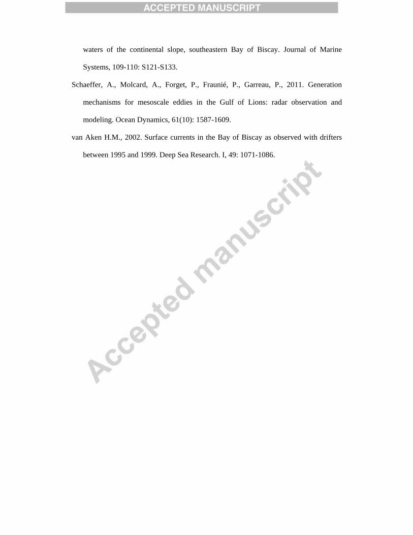
waters of the continental slope, southeastern Bay of Biscay. Journal of Marine

Systems, 109-110: S121-S133.

Schaeffer, A., Molcard, A., Forget, P., Fraunié, P., Garreau, P., 2011. Generation

mechanisms for mesoscale eddies in the Gulf of Lions: radar observation and

modeling. Ocean Dynamics, 61(10): 1587-1609.

van Aken H.M., 2002. Surface currents in the Bay of Biscay as observed with drifters

between 1995 and 1999. Deep Sea Research. I, 49: 1071-1086.

� �

Figure 1: Solabarrieta et. al. (a) Study area. Red crosses show the position of the HF Radar antennas at

Higer and Matxitxako Capes. Grey points correspond to the nodes of the regular grid used to build

radar-derived total current fields. Green points, highlight the nodes at which HF radar currents are used

to study the slope circulation (currents along this transect are shown in Figure 5.(a). Isobaths: 100, 200,

500, 1000, 2000m. Finally, red points give the position of the moorings whose data are used for radar-

derived and in-situ current comparisons carried out in section 3. (b) Percentage of the available radar

data, with respect to the HF radar total velocity nodes, used at Figure 1(a).

�

Figure 2: Solabarrieta et. al. (a) Spatial position of the joint drifter/radar information. Matxitxako and,

Donostia buoys are represented by black points). Isobaths: 200, 1000, 2000m. (b) Hours with radar and

drifter/radar jointly information, for each of the 20 drifters, during 2009 (for colour key, see figure 1(a).

�

Figure 3: Solabarrieta et. al. Snapshots of hourly radar-derived sea surface current fields for the study

area. The time slots plotted have been chosen in order to give an illustration of some of the most

commonly-observed patterns throughout the study period: (a) winter-time circulation with the surface

signal of the along slope poleward current (IPC) and the associated warm surface flow; (b) intense

southeastward currents in response to intense northwest winds associated with the passage of Klaus

explosive cyclogenesis storm in winter 2009; (c) summer-time circulation, with intensified westerly

currents over the Spanish slope, and (d,e,f) surface patterns associated with a well-defined anticyclonic

mesoscale eddy. Its signal on SST and Chl-a satellite data is shown in (d) and (e), respectively; the

interaction of this anticyclone with a smaller cyclone in the area, some days later, is shown in (f). Dates

used are: (a) 24/11/2009 13:59 for SST satellite data and 24/11/2009 00:00 HF radar data;

(b)24/01/2009 09:00; (c) 22/09/2010 09:00; (d, e) 27/12/2011 12:36 and 27/12/2011 12:50 for SST and

Chl-a concentration, respectively, and 29/12/2011 19:00 for HF radar data; and (f) 31/12/2011.

Isobaths: 200, 1000, 2000m

�

Figure 4: Solabarrieta et. al. Current mean and variance ellipses of: (a) Winter time (a1) November 2009

(a2) January 2011 and (a3) November 2011; (b) Summer time (b1) September 2009; and (b.2) July 2010;

and (c) Intermediate time May 2010. Isobaths: 200, 1000, 2000m

�

Figure 5: Solabarrieta et. al. (a) Eastward (positive) – westward (negative) along-slope currents at the HF

radar nodes, within the transect shown in Figure 1. Dashed lines indicate the position in latitude at the

longitude of the transect of the 200m, 1000m and 2000m isobaths (dashed lines) and Matxitxako buoy

(solid line). (b) Eastward (positive) – westward (negative) along-slope currents at Matxitxako buoy, with

depth. White spaces correspond to data gaps. Triangles and stars indicate some events during winter and

summer periods, respectively, described in the text.

�

Figure 6: Solabarrieta et. al. Results of the EOF analysis applied to low-pass filtered data. (a) Modes

1(left) and 2 (right) spatial maps and (b) Modes 1 (upper) and 2 (lower) amplitude time-series. (c) Modes

3 (left) and 4 (right) spatial maps and (d) Modes 3 (upper) and 4 (lower) amplitude time-series. Triangles

and stars mark summer and winter periods, explained during this paper. Isobaths: 200, 1000, 2000m

�

Figure 7: Solabarrieta et. al. Results of the EOF analysis applied to inertial band pass filtered data. (a)

Modes 1(left) and 2 (right) spatial maps and (b) Modes 1 (upper) and 2 (lower) amplitude time-series. (c)

Modes 3 (left) and 4 (right) spatial maps and (d) Modes 3 (upper) and 4 (lower) amplitude time-series.

�

Figure 8: Solabarrieta et. al. Contribution (percentages) to the total kinetic energy (KE) of the variability

contained in the (a,c) inertial and (b,d) tidal bands, for (a,b) summer-type circulation months (temporal

mean of spatial distributions for July, August and September) and (c,d) winter-type circulation months

(temporal mean of spatial distributions for November, December and January). Isobaths (grey lines): 200,

1000 and 2000m. (e) Time evolution of the spatial average (for all the nodes) of the KE contained in the

total currents (solid grey line, left y axis) and inertial (solid black line, right y axis) and tidal (dotted black

line, right y axis) bands. (f) Time evolution of the contribution (percentages) to the total kinetic energy

(KE) of the variability contained in the (solid black line) inertial and (dotted black line) tidal bands (the

sum of both contributions is plotted using a solid grey line).

�

� �

Table 1: Brief description of the data and their characteristics.

DATA POSITION

TYPE

OF

DATA

YEAR

S

TEMPORAL

RESOLUTION

(hours)

SPATIAL

RESOLUTION

(km)

DEPTH OF

MESURING

(m)

DATA

SOURCE

HF Coastal Radar

Matxitxako: 43º 27.3' N 02º 45.2' W Remote

2009 2010 2011

1 5 0-3 Basque goverment Higer

43º 23.5' N 01º 47.7' W

Offshore buoys

Donostia: 43º 33.6’ N 02º 1.8’ W In-situ 2009 1 - 1.5 Basque

goverment Matxitxako: 43º 36’ N 02º 41.4’ W

Drifters 43º 21’ N – 44º 42’ N 1-3º W

In-situ 2009 - - 15 See Charria et al. 2013

Table 2: RMS values of In-Situ Data and Radar data. Mean Speed of In-Situ and radar data. Correlation of U and V velocity components, between in-situ and radar data. RMSd values between in-situ and radar

data

* Rubio et al., 2011

In-Situ Data

Measu- rement depth (m)

Time period

RMS (cm·s-1) Mean Speed Corr-u In-situ-Radar data

Corr-v In-situ-Radar data

RMSd-u (cm·s-1])In-situ-Radar data

RMSd-v (cm·s-1])In-situ-Radar data

In-Situ data Radar node In-Situ data Radar node

u v u v u v u v

Matxitxako* 1.5 2009 0.16* 0.10* 0.13* 0.08* - - - - 0.86* 0.64* 8.09* 8.12*

Donostia* 1.5 2009 0.12* 0.11* 0.11* 0.12* - - - - 0.53* 0.34* 10.38* 12.88*

Matxitxako 12 01-Jan-2009 /07-Sep-2011 13.88 8.20 14.32 9.21 5.30 -2.28 4.09 0.22 0.66 0.50 11.12 8.97

Donostia 12 01-Jan-2009 /15-Oct-2010 9.72 6.84 12.40 13.07 2.75 -0.01 3.84 4.20 0.49 0.27 10.95 13.09

Matxitxako 12 Well mixed months 20.03 8.98 18.55 8.69 13.30 2.05 11.10 0.62 0.67 0.46 12.38 9.46

Donostia 12 Well mixed months 13.23 7.79 14.70 16.40 5.84 1.03 6.06 9.27 0.59 0.20 11.49 16.41

Matxitxako 12 Stratified months 9.03 8.58 11.84 9.73 1.14 2.57 0.31 0.31 0.51 0.57 10.70 8.89

Donostia 12 Stratified months 8.77 6.76 11.91 11.61 1.67 0.28 2.66 2.51 0.44 0.32 11.07 11.52

Drifters 15 May-Sep-2009 (See Figure 2.b) 13.99 13.67 13.77 13.84 -0.88 -0.33 -1.49 -1.14 0.42 0.46 14.85 14.30

.

�

� �

A seasonality in terms of sea surface current and along slope circulation is observed

Cyclonic and anticyclonic patterns are observed during winter and summer months

Surface signature of the slope current contributes to the seasonal variability

The presence of mesoscale structures in the area is reported

Globally, inertial currents represent 10 to 40% of the total variability.

�

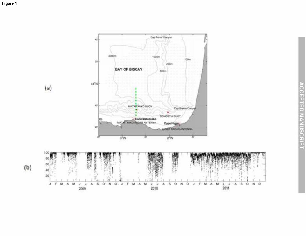
Figure 1

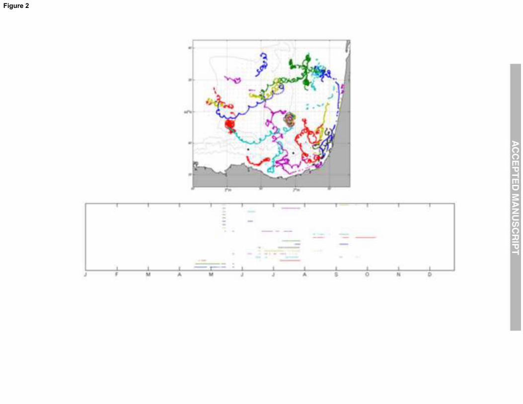
Figure 2

Figure 3

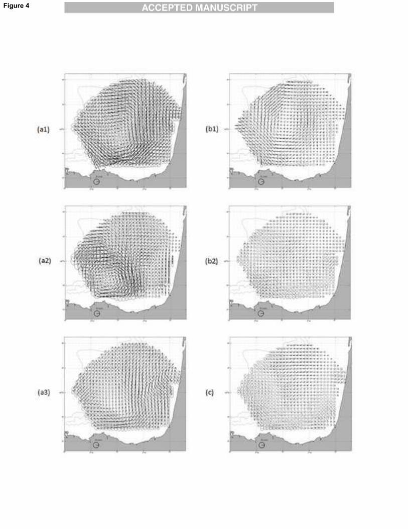
Figure 4

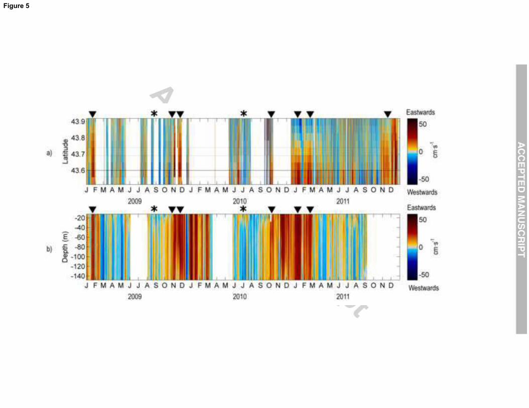
Figure 5

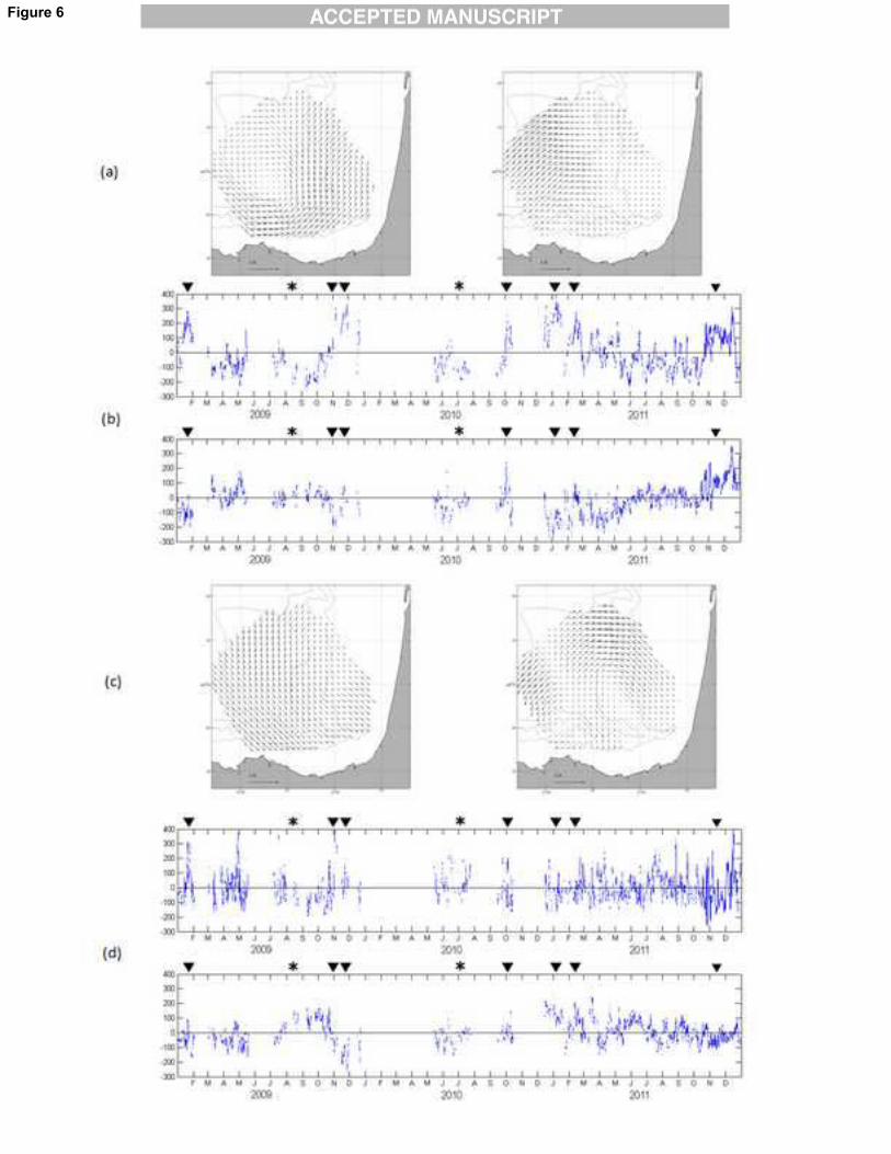
Figure 6

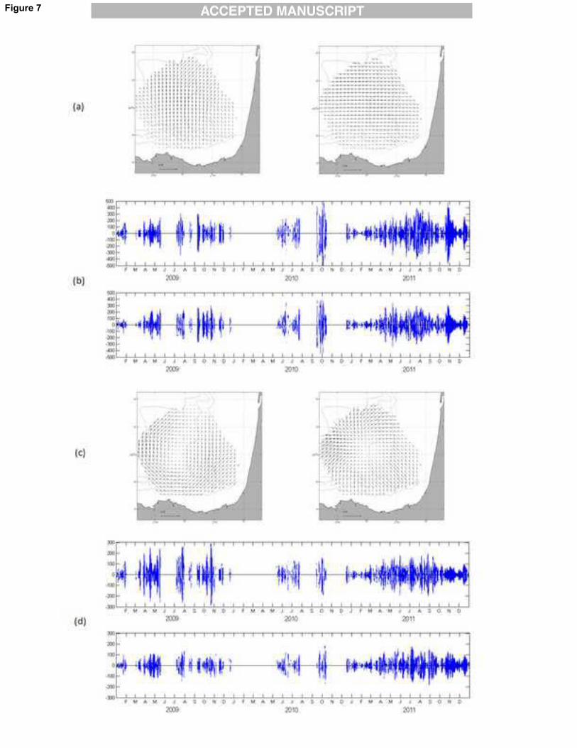
Figure 7

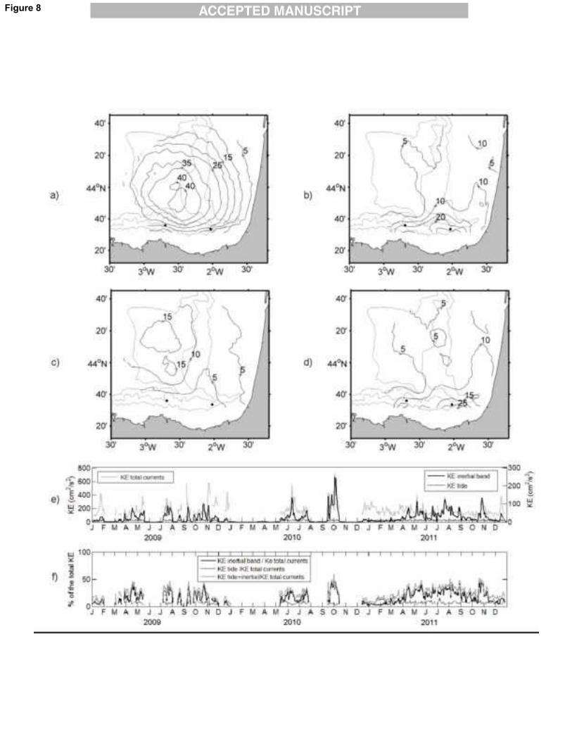
Figure 8