Long-Term Stochastic Reservoir Operation Using a Noisy Genetic Algorithm

Water Resour Manage (2010) 24:3159–3172DOI 10.1007/s11269-010-9600-5

Long-Term Stochastic Reservoir Operation Usinga Noisy Genetic Algorithm

Ruan Yun · Vijay P. Singh · Zengchuan Dong

Received: 29 August 2009 / Accepted: 22 January 2010 /Published online: 24 March 2010© Springer Science+Business Media B.V. 2010

Abstract To deal with stochastic characteristics of inflow in reservoir operation,a noisy genetic algorithm (NGA), based on simple genetic algorithms (GAs), isproposed. Using operation of a single reservoir as an example, the results of NGAand Monte Carlo method which is another way to optimize stochastic reservoiroperation were compared. It was found that the noisy GA was a better alternativethan Monte Carlo method for stochastic reservoir operation.

Keywords Genetic algorithms · Noisy genetic algorithms · Monte Carlo ·Optimization · Reservoir operation

1 Introduction

Genetic algorithms (GAs), formulated by Holland in the mid 1970s (Holland 1975),have proven to be effective in searching large, complex solution spaces. Besideslinear programming, dynamic programming and non-linear programming, simpleGAs or standard GAs have been applied for deterministic reservoir operation

R. Yun (B) · Z. DongState Key Laboratory of Hydrology, Water Resources and Hydraulic Engineering,Hohai University, Nanjing 210098, Chinae-mail: [email protected]

R. YunSchool of Civil Engineering, Shandong University, Jinan 250061, China

V. P. SinghDepartment of Biological & Agricultural Engineering, Texas A&M University,College Station, TX 77843, USAe-mail: [email protected]

3160 R. Yuan et al.

(Oliveria and Loucks 1997; Wardlaw and Sharif 1999; Huang et al. 2002; Ahmedand Sarma 2005; Jothiparkash and Shanthi 2006; Momtahen and Dariane 2007;Cheng et al. 2008). For stochastic reservoir operation, it is advantageous to developand implement reservoir control policies that yield acceptable results over a rangeof inflow conditions. To deal with stochastic characteristics of inflow, besides sto-chastic linear programming (SLP), stochastic dynamic programming (SDP), chanceconstrained programming (CCP), one approach is Monte Carlo method (Labadie2004), in which optimizing many realizations or scenarios the desired solution ofthe reservoir operation problem is obtained using the average, regression or othermethods.

Noisy genetic algorithms (NGAs) are standard GAs that operate in noisy oruncertain environment. Unlike Monte Carlo method which requires extensive re-alizations to obtain reasonably accurate solutions for uncertain environment (forreservoir operation, the stochastic characteristics of inflow are one of the reasonsfor uncertain conditions), a NGA uses a special type of fitness function, referredto as ef fective fitness function, to deal with uncertain environment (Branke 2002).A NGA has been shown to perform well without sampling a large number ofrealizations in the network design (Wu et al. 2005). Smalley et al. (2000) appliedNGAs to risk-based ground water remediation problems. Aly and Peralta (1999)used NGAs incorporating parameter uncertainty to ground water remediation andwatershed management. However, NGAs have not been applied for stochasticreservoir operation.

The aim of this study therefore is to propose a NGA to deal with the stochasticcharacteristics of inflow in reservoir operation. To evaluate its effect on stochasticreservoir operation, results from the NGA and Monte Carlo method are compared.As an illustrative example, a model of a single reservoir operation is given inSection 2. A simple GA and Monte Carlo method are applied for stochastic reservoiroperation in Section 3 and a NGA is proposed and applied in Section 4. In thelast section, a discussion of results is given and conclusions are stated. In addition,all programming used in this study are coded under the environment of Matlab2007.

2 Deterministic and Stochastic Models of Reservoir Operation

2.1 Model of Reservoir Operation

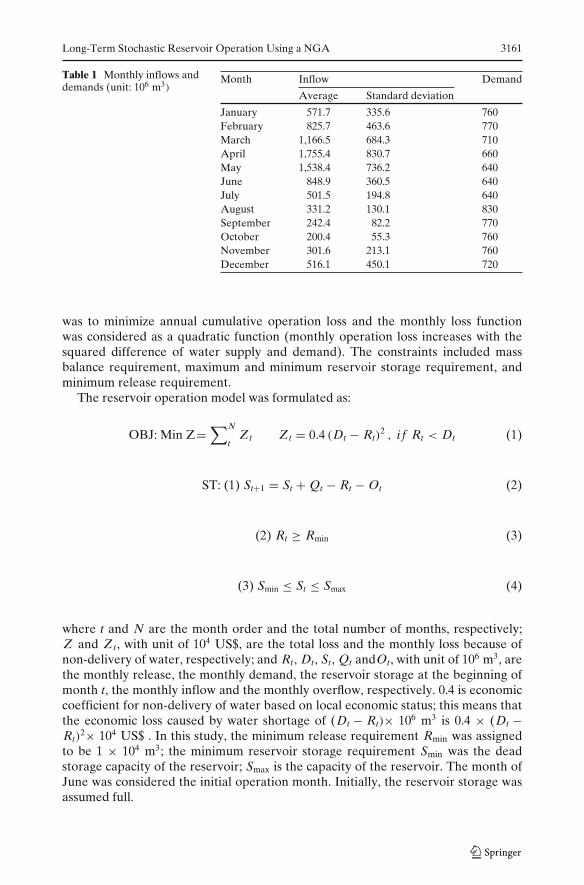
As an illustrative example, a single reservoir in China was selected to evaluate aNGA and compare it with Monte Carlo method. It is an annual regulated multi-purpose reservoir, with a capacity of 4,440 × 106 m3 and a dead storage capacity of40 × 106 m3. To simplify computation, water supply was considered as the only op-erational aim of the reservoir. Forty one years of monthly inflow data were availableas historical time series. The means and standard deviations of monthly inflows anddemands are given in Table 1. According to the plan of the reservoir, monthly waterdemands were fixed for recent years. Monthly evaporation and leakage have beensubtracted from monthly inflows before optimization. In the reservoir operationmodel, the decision variable was monthly water release. The objective function

Long-Term Stochastic Reservoir Operation Using a NGA 3161

Table 1 Monthly inflows anddemands (unit: 106 m3)

Month Inflow Demand

Average Standard deviation

January 571.7 335.6 760February 825.7 463.6 770March 1,166.5 684.3 710April 1,755.4 830.7 660May 1,538.4 736.2 640June 848.9 360.5 640July 501.5 194.8 640August 331.2 130.1 830September 242.4 82.2 770October 200.4 55.3 760November 301.6 213.1 760December 516.1 450.1 720

was to minimize annual cumulative operation loss and the monthly loss functionwas considered as a quadratic function (monthly operation loss increases with thesquared difference of water supply and demand). The constraints included massbalance requirement, maximum and minimum reservoir storage requirement, andminimum release requirement.

The reservoir operation model was formulated as:

OBJ: Min Z=∑N

tZt Zt = 0.4 (Dt − Rt)

2 , i f Rt < Dt (1)

ST: (1) St+1 = St + Qt − Rt − Ot (2)

(2) Rt ≥ Rmin (3)

(3) Smin ≤ St ≤ Smax (4)

where t and N are the month order and the total number of months, respectively;Z and Zt, with unit of 104 US$, are the total loss and the monthly loss because ofnon-delivery of water, respectively; and Rt, Dt, St, Qt andOt, with unit of 106 m3, arethe monthly release, the monthly demand, the reservoir storage at the beginning ofmonth t, the monthly inflow and the monthly overflow, respectively. 0.4 is economiccoefficient for non-delivery of water based on local economic status; this means thatthe economic loss caused by water shortage of (Dt − Rt)× 106 m3 is 0.4 × (Dt −Rt)

2× 104 US$ . In this study, the minimum release requirement Rmin was assignedto be 1 × 104 m3; the minimum reservoir storage requirement Smin was the deadstorage capacity of the reservoir; Smax is the capacity of the reservoir. The month ofJune was considered the initial operation month. Initially, the reservoir storage wasassumed full.

3162 R. Yuan et al.

For this model, the decision variable, monthly water release, was further ex-pressed as:

Rt = βt Dt (5)

where β t is the restriction coefficient of water release and its value is between 0 and1 (in order to facilitate the search of optimal βt, the value of βt in GA was set tobe between 0 and 2). In other words, the monthly restriction coefficient of waterrelease β t, instead of the monthly water release Rt, becomes the decision variable.One candidate solution or decision policy can be expressed as β = {β1, β2, β3, β4, β5,β6, β7, β8, β9, β10, β11, β12}, where βt (t = 1, 2,. . . , 12) is for the t-th month.

2.2 Deterministic and Stochastic Situations

If only one realization of monthly inflows, for example, average monthly inflows,is considered for reservoir operation, the operation will be deterministic and itcan be addressed using deterministic programming methods, such as simple GAs.For deterministic reservoir operation with average monthly inflows, from averagemonthly inflows and monthly water demands given in Table 1, a prior optimalsolution of β∗

t = 1.0 (t = 1, 2,. . . , 12) or β∗ = {1.0, 1.0, 1.0, 1.0, 1.0, 1.0, 1.0, 1.0, 1.0, 1.0,1.0, 1.0} can be derived. In this situation, the objective or annual cumulative operationloss is 0 US$.

If the random variability of monthly inflows, as reflected by standard deviationin Table 1, is considered, then deterministic reservoir operation becomes stochasticreservoir operation and it can be dealt with using stochastic programming methods,such as, SDP and Monte Carlo method. In this study, a NGA was proposed to dealwith the stochastic characteristics of inflows, and results from the NGA and MonteCarlo method are compared.

3 Simple GA and Monte Carlo Method

3.1 Components of a Simple GA

A simple GA starts from initializing a population of candidate solutions or indi-viduals (in this study, candidate solutions are decision policies or monthly waterreleases). These candidate solutions are usually random and spread throughout thesearch space. A typical algorithm then uses three operators, selection, crossover, andmutation, to direct the population approaches to the global optimum. Wardlaw andSharif (1999) have evaluated simple GAs for reservoir operation. The componentsof a simple GA used in this study are described briefly as follows.

(1) A chromosomal representation of a decision policy: Two of the mostly usedrepresentations are binary representation (decision policies are presented by astring of 0 or 1) and real representation (decision policies are presented by astring of real numbers). Comparing binary representation and real represen-tation, a number of researchers prefer real representation to binary represen-tation (Wardlaw and Sharif 1999; Haupt and Haupt 2004). In this study, realrepresentation was adopted and decision policies, the restriction coefficients


of water release βt (t = 1, 2,. . . , 12) in each month, were represented by realnumbers.

(2) A model for creating an initial population of decision policies. The individualsin the initial population were generated entirely at random.

(3) An evaluation function to determine the fitness of each individual. The eval-uation function in simple GA is called fitness function and, in this study,it is the objective function in the model of reservoir operation, i.e., Eq. 1.For linear constraints and bounds in the model, mutation and crossover thatonly generate feasible candidate solutions were used; this means that all thelinear constraints and bounds were satisfied at every generation throughoutoptimization.

(4) A selection approach to choose better individuals. Goldberg and Deb (1989)compared various selection methods, and indicated a preference for tourna-ment selection. In this study, tournament selection was adopted and a tour-nament size of 4 was used, which means one best individual was chosen forthe mating pool from 4 randomly selected individuals among the populationin the current generation. For the convergence of simple GAs to the globaloptimum, according to Rudolph (1994), an elite number of 1 was chosen toprevent premature convergence.

(5) A crossover approach and a mutation approach to reproduce offspring.Crossover and mutation are two ways for simple GAs to create new offspring.There are several crossover types and mutation types. Haupt and Haupt (2004)discussed parameter setting of simple GAs and suggested that type of crossover,crossover rate, method of selection (roulette wheel or tournament) are notof much importance; population size and mutation rate, however, have asignificant impact on the ability of simple GAs to find acceptable optimaldecision policies. In this study scattered crossover and the most straightforwardmutation type, uniform mutation, were adopted.

3.2 Setting Parameters of Simple GA

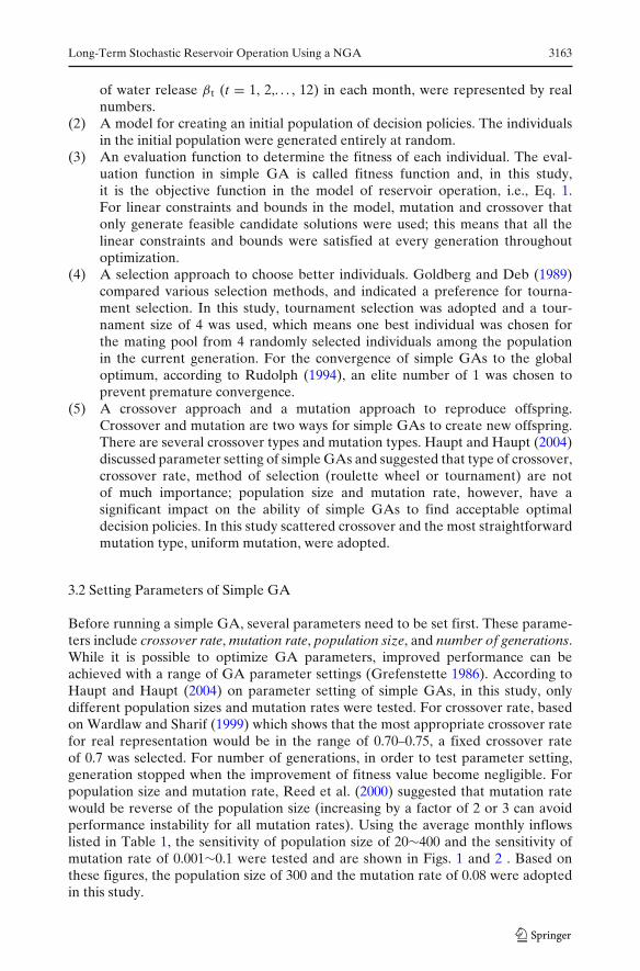
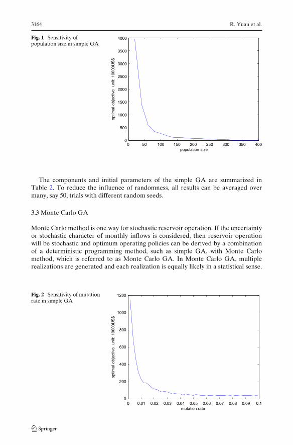
Before running a simple GA, several parameters need to be set first. These parame-ters include crossover rate, mutation rate, population size, and number of generations.While it is possible to optimize GA parameters, improved performance can beachieved with a range of GA parameter settings (Grefenstette 1986). According toHaupt and Haupt (2004) on parameter setting of simple GAs, in this study, onlydifferent population sizes and mutation rates were tested. For crossover rate, basedon Wardlaw and Sharif (1999) which shows that the most appropriate crossover ratefor real representation would be in the range of 0.70–0.75, a fixed crossover rateof 0.7 was selected. For number of generations, in order to test parameter setting,generation stopped when the improvement of fitness value become negligible. Forpopulation size and mutation rate, Reed et al. (2000) suggested that mutation ratewould be reverse of the population size (increasing by a factor of 2 or 3 can avoidperformance instability for all mutation rates). Using the average monthly inflowslisted in Table 1, the sensitivity of population size of 20∼400 and the sensitivity ofmutation rate of 0.001∼0.1 were tested and are shown in Figs. 1 and 2 . Based onthese figures, the population size of 300 and the mutation rate of 0.08 were adoptedin this study.

3164 R. Yuan et al.

Fig. 1 Sensitivity ofpopulation size in simple GA

0 50 100 150 200 250 300 350 4000

500

1000

1500

2000

2500

3000

3500

4000

population size

optim

al o

bjec

tive

uni

t: 10

000U

S$

The components and initial parameters of the simple GA are summarized inTable 2. To reduce the influence of randomness, all results can be averaged overmany, say 50, trials with different random seeds.

3.3 Monte Carlo GA

Monte Carlo method is one way for stochastic reservoir operation. If the uncertaintyor stochastic character of monthly inflows is considered, then reservoir operationwill be stochastic and optimum operating policies can be derived by a combinationof a deterministic programming method, such as simple GA, with Monte Carlomethod, which is referred to as Monte Carlo GA. In Monte Carlo GA, multiplerealizations are generated and each realization is equally likely in a statistical sense.

Fig. 2 Sensitivity of mutationrate in simple GA

0 0.01 0.02 0.03 0.04 0.05 0.06 0.07 0.08 0.09 0.10

200

400

600

800

1000

1200

mutation rate

optim

al o

bjec

tive

uni

t: 10

000U

S$


Table 2 Components and initial parameters of a simple GA

Component and Type and value Component and Type and valueparameter parameter

Representation Real Crossover Scattered, 0.7Range of initial population [0,2] Mutation Uniform, 0.08Selection Tournament, 4 Population size 300Elite 1 Generation inf

For each realization generated by Monte Carlo method, the optimization of reservoiroperation becomes deterministic and is solved independently by using the simpleGA. The final optimal solution can be deemed as the average of optimal solutionsof multiple scenarios. To fully consider the uncertainty of monthly inflows, extensiverealizations, say 1,000 realizations, can be used. But the computational burden ofMonte Carlo GA would be 1,000 times the computational burden in the deterministicsolution obtained by the simple GA.

3.4 Stochastic Reservoir Operation using Monte Carlo GA

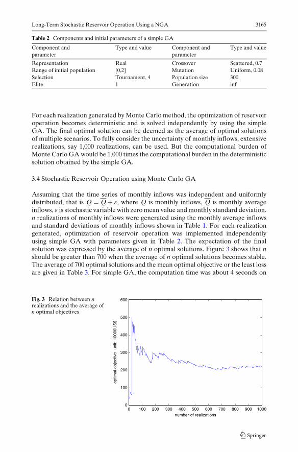
Assuming that the time series of monthly inflows was independent and uniformlydistributed, that is Q = Q + ε, where Q is monthly inflows, Q is monthly averageinflows, ε is stochastic variable with zero mean value and monthly standard deviation.n realizations of monthly inflows were generated using the monthly average inflowsand standard deviations of monthly inflows shown in Table 1. For each realizationgenerated, optimization of reservoir operation was implemented independentlyusing simple GA with parameters given in Table 2. The expectation of the finalsolution was expressed by the average of n optimal solutions. Figure 3 shows that nshould be greater than 700 when the average of n optimal solutions becomes stable.The average of 700 optimal solutions and the mean optimal objective or the least lossare given in Table 3. For simple GA, the computation time was about 4 seconds on

Fig. 3 Relation between nrealizations and the average ofn optimal objectives

0 100 200 300 400 500 600 700 800 900 10000

100

200

300

400

500

600

number of realizations

optim

al o

bjec

tive

uni

t: 10

000U

S$

3166 R. Yuan et al.

Table 3 Optimal solution ofstochastic reservoir operationby Monte Carlo GA

Month Jan. Feb. Mar. Apr. May Juneβt 1.0003 1.0006 1.0009 1.0008 1.0005 1.0004

Month July Aug. Sept. Oct. Nov. Dec.βt 1.0007 1.0002 1.0006 1.0283 1.0002 1.0041

Mean objective Z = 206.9384 × 104 US$

a computer of 2 GB memory and 2.0 GHz CPU. For Monte Carlo GA, the simpleGA needs to be run 700 times, and the computation time was about 46 minute and40 seconds (4 × 700 = 2,800 s).

4 Noisy GA

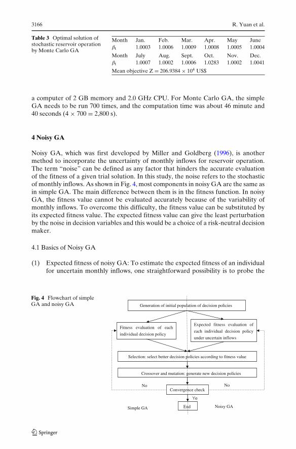
Noisy GA, which was first developed by Miller and Goldberg (1996), is anothermethod to incorporate the uncertainty of monthly inflows for reservoir operation.The term “noise” can be defined as any factor that hinders the accurate evaluationof the fitness of a given trial solution. In this study, the noise refers to the stochasticof monthly inflows. As shown in Fig. 4, most components in noisy GA are the same asin simple GA. The main difference between them is in the fitness function. In noisyGA, the fitness value cannot be evaluated accurately because of the variability ofmonthly inflows. To overcome this difficulty, the fitness value can be substituted byits expected fitness value. The expected fitness value can give the least perturbationby the noise in decision variables and this would be a choice of a risk-neutral decisionmaker.

4.1 Basics of Noisy GA

(1) Expected fitness of noisy GA: To estimate the expected fitness of an individualfor uncertain monthly inflows, one straightforward possibility is to probe the

Fig. 4 Flowchart of simpleGA and noisy GA Generation of initial population of decision policies

Fitness evaluation of each

individual decision policy

Selection: select better decision policies according to fitness value

Crossover and mutation: generate new decision policies

Convergence check

End

Ye

No

Expected fitness evaluation of

each individual decision policy

under uncertain inflows

Simple GA Noisy GA

No


fitness landscape at several random points in its neighborhood and calculate itsmean value. If f (x, e) is the fitness function of a solutionx in an environment(monthly inflows) e, then in the presence of uncertain monthly inflows, priorto evaluation, solution x can be disturbed by a quantity of δ, i.e., x→x + δ.Then, the objective of optimization in the noisy GA would be to minimizethe expected performance E( f (x + δ)) over the possible disturbance. Givena probability density function p(δ) of disturbance δ, the expected fitness can becalculated as

f (x) = E ( f (x + δ)) =∫ ∞

−∞p (δ) • f (x + δ) dδ (6)

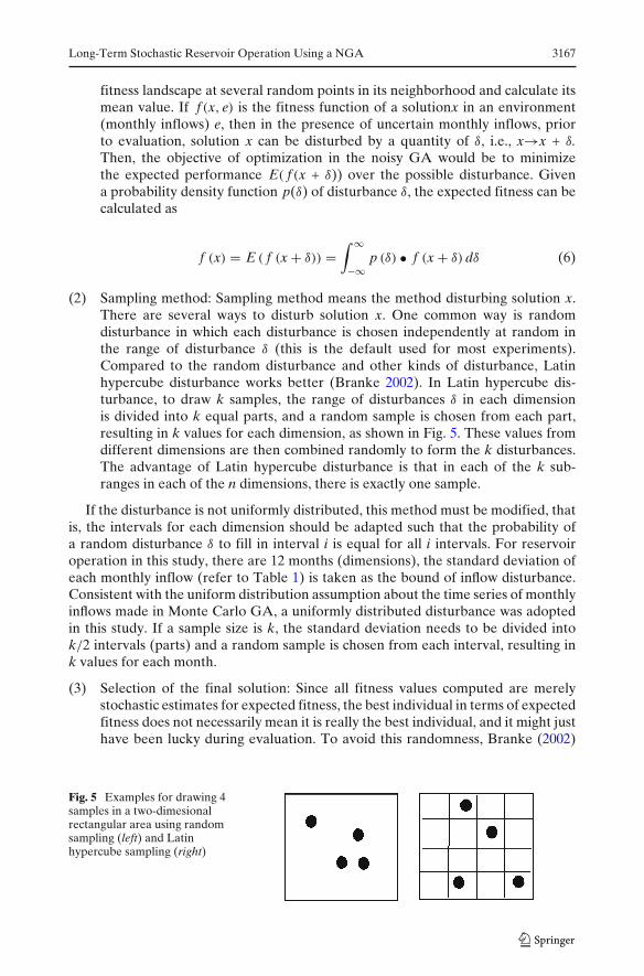
(2) Sampling method: Sampling method means the method disturbing solution x.There are several ways to disturb solution x. One common way is randomdisturbance in which each disturbance is chosen independently at random inthe range of disturbance δ (this is the default used for most experiments).Compared to the random disturbance and other kinds of disturbance, Latinhypercube disturbance works better (Branke 2002). In Latin hypercube dis-turbance, to draw k samples, the range of disturbances δ in each dimensionis divided into k equal parts, and a random sample is chosen from each part,resulting in k values for each dimension, as shown in Fig. 5. These values fromdifferent dimensions are then combined randomly to form the k disturbances.The advantage of Latin hypercube disturbance is that in each of the k sub-ranges in each of the n dimensions, there is exactly one sample.

If the disturbance is not uniformly distributed, this method must be modified, thatis, the intervals for each dimension should be adapted such that the probability ofa random disturbance δ to fill in interval i is equal for all i intervals. For reservoiroperation in this study, there are 12 months (dimensions), the standard deviation ofeach monthly inflow (refer to Table 1) is taken as the bound of inflow disturbance.Consistent with the uniform distribution assumption about the time series of monthlyinflows made in Monte Carlo GA, a uniformly distributed disturbance was adoptedin this study. If a sample size is k, the standard deviation needs to be divided intok/2 intervals (parts) and a random sample is chosen from each interval, resulting ink values for each month.

(3) Selection of the final solution: Since all fitness values computed are merelystochastic estimates for expected fitness, the best individual in terms of expectedfitness does not necessarily mean it is really the best individual, and it might justhave been lucky during evaluation. To avoid this randomness, Branke (2002)

Fig. 5 Examples for drawing 4samples in a two-dimesionalrectangular area using randomsampling (left) and Latinhypercube sampling (right)

3168 R. Yuan et al.

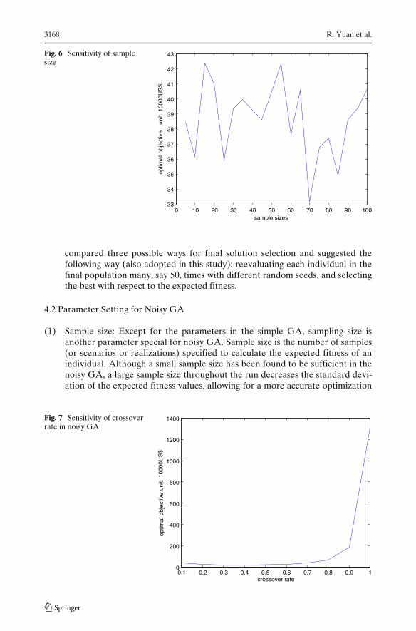
Fig. 6 Sensitivity of samplesize

0 10 20 30 40 50 60 70 80 90 10033

34

35

36

37

38

39

40

41

42

43

sample sizes

optim

al o

bjec

tive

un

it: 1

0000

US

$

compared three possible ways for final solution selection and suggested thefollowing way (also adopted in this study): reevaluating each individual in thefinal population many, say 50, times with different random seeds, and selectingthe best with respect to the expected fitness.

4.2 Parameter Setting for Noisy GA

(1) Sample size: Except for the parameters in the simple GA, sampling size isanother parameter special for noisy GA. Sample size is the number of samples(or scenarios or realizations) specified to calculate the expected fitness of anindividual. Although a small sample size has been found to be sufficient in thenoisy GA, a large sample size throughout the run decreases the standard devi-ation of the expected fitness values, allowing for a more accurate optimization

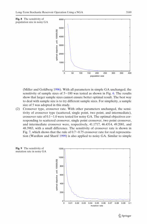
Fig. 7 Sensitivity of crossoverrate in noisy GA

0.1 0.2 0.3 0.4 0.5 0.6 0.7 0.8 0.9 10

200

400

600

800

1000

1200

1400

crossover rate

optim

al o

bjec

tive

unit:

100

00U

S$


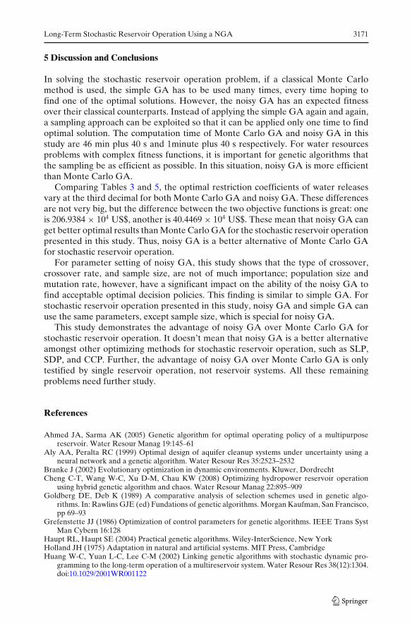
Fig. 8 The sensitivity ofpopulation size in noisy GA

0 50 100 150 200 250 300 350 4000

1000

2000

3000

4000

5000

6000

population size

optim

al o

bjec

tive

uni

t: 10

000U

S$

(Miller and Goldberg 1996). With all parameters in simple GA unchanged, thesensitivity of sample sizes of 5∼100 was tested as shown in Fig. 6. The resultsshow that larger sample sizes cannot ensure better optimal result. The best wayto deal with sample size is to try different sample sizes. For simplicity, a samplesize of 5 was adopted in this study.

(2) Crossover type, crossover rate. With other parameters unchanged, the sensi-tivity of crossover type (scattered, single point, two point, and intermediate),crossover rate of 0.1∼1.0 were tested for noisy GA. The optimal objectives cor-responding to scattered crossover, single point crossover, two point crossover,and intermediate crossover were, respectively, 41.1717, 46.4314, 49.2081, and48.3983, with a small difference. The sensitivity of crossover rate is shown inFig. 7, which shows that the rule of 0.7∼0.75 crossover rate for real representa-tion (Wardlaw and Sharif 1999) is also applied to noisy GA. Similar to simple

Fig. 9 The sensitivity ofmutation rate in noisy GA

0 0.01 0.02 0.03 0.04 0.05 0.06 0.07 0.08 0.09 0.10

200

400

600

800

1000

1200

mutation rate

optim

al o

bjec

tive

uni

t: 10

000U

S$

3170 R. Yuan et al.

Table 4 Components and parameter setting of noisy GA

Component and Type and value Component and Type and valueparameter parameter

Representation Real Crossover Scattered, 0.7Range of initial population [0,2] Mutation Uniform, 0.08Selection Tournament, 4 Population size 300Elite 1 Generation infSample Latin Hypercube, 5

GA, the type of crossover, crossover rate are not of much importance to theability of noisy GA to find acceptable optimal decision policies. In this study,scattered crossover and crossover rates of 0.7 were adopted.

(3) Population size and mutation rate: Because of the stochastic nature of fitnessfunction, population size in the noisy GA has different influence on GA’s searchability compared to the simple GA. In noisy GA, the population size is a criticalfactor and it is never too small (Branke 2002). Furthermore, in noisy GA, thepositive effect of an increased sample size is reduced by an increased populationsize and when the population size is increased to infinity, the sample size shouldnot make any difference. With other parameters unchanged, the sensitivity ofpopulation size of 20∼400 was tested and shown in Fig. 8. Comparing Figs. 1and 8, it can be concluded that the same population size of 300 can be appliedin both noisy GA and simple GA.

With other parameters unchanged, the sensitivity of mutation rate 0.001∼0.1wastested for the noisy GA and is shown in Fig. 9. Comparing Figs. 2 and 9, it canbe concluded that the same mutation rate of 0.08 can also be applied in both noisyGA and simple GA.

Parameters of the noisy GA are summarized in Table 4. Similar to simple GA, toreduce the influence of randomness, all results can be averaged over 50 trails withdifferent random seeds.

4.3 Stochastic Reservoir Operation using Noisy GA

The noisy GA, with parameters shown in Table 4, was used to solve the stochasticreservoir operation problem introduced in Section 2. The optimal solution and theoptimal objective are given in Table 5. The computation time was about 1minute and40 seconds on a computer of 2 GB memory and 2.0 GHz CPU.

Table 5 Optimal solution ofstochastic reservoir operationby a noisy GA

Month Jan. Feb. Mar. Apr. May Juneβt 1.00 1.00 1.00 1.00 1.00 1.00

26 16 42 33 37 34

Month July Aug. Sept. Oct. Nov. Dec.βt 1.00 1.00 1.00 1.00 1.00 1.00

21 34 3 3 15 28

Mean objective Z = 40.4469 × 104US$


5 Discussion and Conclusions

In solving the stochastic reservoir operation problem, if a classical Monte Carlomethod is used, the simple GA has to be used many times, every time hoping tofind one of the optimal solutions. However, the noisy GA has an expected fitnessover their classical counterparts. Instead of applying the simple GA again and again,a sampling approach can be exploited so that it can be applied only one time to findoptimal solution. The computation time of Monte Carlo GA and noisy GA in thisstudy are 46 min plus 40 s and 1minute plus 40 s respectively. For water resourcesproblems with complex fitness functions, it is important for genetic algorithms thatthe sampling be as efficient as possible. In this situation, noisy GA is more efficientthan Monte Carlo GA.

Comparing Tables 3 and 5, the optimal restriction coefficients of water releasesvary at the third decimal for both Monte Carlo GA and noisy GA. These differencesare not very big, but the difference between the two objective functions is great: oneis 206.9384 × 104 US$, another is 40.4469 × 104 US$. These mean that noisy GA canget better optimal results than Monte Carlo GA for the stochastic reservoir operationpresented in this study. Thus, noisy GA is a better alternative of Monte Carlo GAfor stochastic reservoir operation.

For parameter setting of noisy GA, this study shows that the type of crossover,crossover rate, and sample size, are not of much importance; population size andmutation rate, however, have a significant impact on the ability of the noisy GA tofind acceptable optimal decision policies. This finding is similar to simple GA. Forstochastic reservoir operation presented in this study, noisy GA and simple GA canuse the same parameters, except sample size, which is special for noisy GA.

This study demonstrates the advantage of noisy GA over Monte Carlo GA forstochastic reservoir operation. It doesn’t mean that noisy GA is a better alternativeamongst other optimizing methods for stochastic reservoir operation, such as SLP,SDP, and CCP. Further, the advantage of noisy GA over Monte Carlo GA is onlytestified by single reservoir operation, not reservoir systems. All these remainingproblems need further study.

References

Ahmed JA, Sarma AK (2005) Genetic algorithm for optimal operating policy of a multipurposereservoir. Water Resour Manag 19:145–61

Aly AA, Peralta RC (1999) Optimal design of aquifer cleanup systems under uncertainty using aneural network and a genetic algorithm. Water Resour Res 35:2523–2532

Branke J (2002) Evolutionary optimization in dynamic environments. Kluwer, DordrechtCheng C-T, Wang W-C, Xu D-M, Chau KW (2008) Optimizing hydropower reservoir operation

using hybrid genetic algorithm and chaos. Water Resour Manag 22:895–909Goldberg DE, Deb K (1989) A comparative analysis of selection schemes used in genetic algo-

rithms. In: Rawlins GJE (ed) Fundations of genetic algorithms. Morgan Kaufman, San Francisco,pp 69–93

Grefenstette JJ (1986) Optimization of control parameters for genetic algorithms. IEEE Trans SystMan Cybern 16:128

Haupt RL, Haupt SE (2004) Practical genetic algorithms. Wiley-InterScience, New YorkHolland JH (1975) Adaptation in natural and artificial systems. MIT Press, CambridgeHuang W-C, Yuan L-C, Lee C-M (2002) Linking genetic algorithms with stochastic dynamic pro-

gramming to the long-term operation of a multireservoir system. Water Resour Res 38(12):1304.doi:10.1029/2001WR001122

http://dx.doi.org/10.1029/2001WR001122

3172 R. Yuan et al.

Jothiparkash V, Shanthi G (2006) Single reservoir operation policies using genetic algorithm. WaterResour Manag 20:917–929

Labadie JW (2004) Optimal operation of multireservoir systems: state-of-the-art review. J WaterResour Plan Manage 130:93–111

Miller BL, Goldberg DE (1996) Optimal sampling for genetic algorithms. In: Dagli et al.(eds) Intelligent engineering systems through artificial neural networks (ANNIE’96), vol 6,pp 291–296

Momtahen S, Dariane AB (2007) Direct search approaches using genetic algorithms for optimizationof water reservoir operating policies. J Water Resour Plan Manage 133:202–209

Oliveria R, Loucks DP (1997) Operating rules for multireservoir systems. Water Resour Res 33:839–852

Reed P, Minsker B, Goldberg DE (2000) Designing a competent simple genetic algorithm for searchand optimization. Water Resour Res 36:3757–3761

Rudolph G (1994) Convergence properties of canonical genetic algorithm. IEEE Trans Neural Netw5(1):96–101

Smalley JB, Minsker BS, Goldberg DE (2000) Risk-based in situ bioremediation design using a noisygenetic algorithm. Water Resour Res 36:3043–3052

Wardlaw R, Sharif M (1999) Evaluation of genetic algorithms for optimal reservoir system operation.J Water Resour Plan Manage 125:25–33

Wu J, Zheng C, Chien C-C, Zheng L (2005) A comparative study of Monte Carlo simple geneticalgorithm and noisy genetic algorithm for coast-effective sampling network design under uncer-tainty. Adv Water Resour 29:899–911

Long-Term Stochastic Reservoir Operation Using a Noisy Genetic Algorithm

Documents

Transcript of Long-Term Stochastic Reservoir Operation Using a Noisy Genetic Algorithm