lb-phd-all.pdf - Telenet
276
INTEGRATION OF SCHEDULING AND CONTROL IN HOLONIC MANUFACTURING SYSTEMS Jury : Proefschrift voorgedragen tot Prof. dr. ir. E. Aernoudt (voorzitter) het behalen van het doctoraat Prof. dr. ir. H. Van Brussel (promotor) in de toegepaste wetenschappen Prof. dr. ir. D. Van Oudheusden (promotor) Prof. dr. P. B. Luh (University of Connecticut) door Prof. dr. W. Herroelen Prof. dr. ir. J.-P. Kruth Luc BONGAERTS Dr. ir. P. Valckenaers 98D11 UDC 658.513 December 1998 KATHOLIEKE UNIVERSITEIT LEUVEN FACULTEIT TOEGEPASTE WETENSCHAPPEN DEPARTEMENT WERKTUIGKUNDE AFDELING PRODUCTIETECHNIEKEN, MACHINEBOUW EN AUTOMATISERING Celestijnenlaan 300B – B-3001 Heverlee (Leuven), Belgium
-
Upload
khangminh22 -
Category
Documents
-
view
2 -
download
0
Transcript of lb-phd-all.pdf - Telenet
INTEGRATION OF SCHEDULING AND CONTROLIN HOLONIC MANUFACTURING SYSTEMS
Jury : Proefschrift voorgedragen totProf. dr. ir. E. Aernoudt (voorzitter) het behalen van het doctoraatProf. dr. ir. H. Van Brussel (promotor) in de toegepaste wetenschappenProf. dr. ir. D. Van Oudheusden (promotor)Prof. dr. P. B. Luh (University of Connecticut) doorProf. dr. W. HerroelenProf. dr. ir. J.-P. Kruth Luc BONGAERTSDr. ir. P. Valckenaers
98D11UDC 658.513 December 1998
KATHOLIEKE UNIVERSITEIT LEUVEN FACULTEIT TOEGEPASTE WETENSCHAPPEN DEPARTEMENT WERKTUIGKUNDE AFDELING PRODUCTIETECHNIEKEN, MACHINEBOUW EN AUTOMATISERING Celestijnenlaan 300B – B-3001 Heverlee (Leuven), Belgium

(c) Katholieke Universiteit Leuven Faculteit Toegepaste WetenschappenArenbergkasteel, B-3001 Heverlee (Belgium)
Alle rechten voorbehouden. Niets uit deze uitgave mag worden vermenigvuldigd en/ofopenbaar gemaakt door middel van druk, fotokopie, microfilm, elektronisch of op welkeandere wijze ook zonder voorafgaandelijke schriftelijke toestemming van de uitgever.
All rights reserved. No part of the publication may be reproduced in any form by print,photoprint, microfilm or any other means without written permission from the publisher.
D/1998/7515/44ISBN 90-5682-143-1UDC: 658.513

Aan Geoffrey,Dat ik mijn peterschap nu naar behoren kan beginnen vervullen.

Voorwoord — Preface
ii
VoorwoordToen ik in 1992 op PMA begon te werken, was mijn eerste opdracht te definiërenwat ik de volgende zes jaar zou doen. Geïntrigeerd door ons flexibel assemblage-systeem, en in overleg met Paul, koos ik voor productiebesturing van flexibele pro-ductiesystemen. Enerzijds was er al zoveel werk gedaan in dat domein (vooral inverband met fijnplanning), maar anderzijds bleken de problemen verre van opgelost.Terwijl het inzicht stilaan groeide — samen met het onderzoeksgroepje, werd eenvolledige productiebesturing ontwikkeld die ons assemblagesysteem robuuster zoumaken tegen storingen. Het resultaat van dat werk heeft u nu voor u, in de vorm vandit doctoraatsproefschrift.
Nu die zes jaar voorbij zijn, wil ik in de eerste plaats mijn dank uitdrukkenvoor mijn promotor, prof. Van Brussel, voor zijn steun tijdens mijn doctoraat, voorde vrijheid die hij mij gelaten heeft en voor zijn vele vragen en opmerkingen, die(soms lange tijd later) toch wel dikwijls essentieel bleken. Ook prof. Van Oudheus-den wil ik danken voor zijn interesse en waardevolle hulp in mijn onderzoek, o.a.toen hij mij op het gepaste moment interessante links naar Operations Research gaf,en (achteraf toch) voor de prangende vragen die mij de puntjes op de i hielpen zet-ten. Ook heb ik steeds graag samengewerkt met prof. Kruth, die op een gedreven entoch sympathieke manier zijn eigen inzet op de anderen overdroeg. Ook dank ik henalle drie voor de toch wel aanzienlijke inspanning die ze geleverd hebben als ledenvan het leescomité. Als één van hen er niet bij geweest was, was dat ongetwijfeld aandeze tekst te zien. I would also like to thank Prof. Peter Luh for many things, likediscussing Holonic Manufacturing, and teaching me Lagrangian Relaxation, butalso what the American Hospitality really means. It always is a joyful occasionwhen I have the opportunity to meet you and your family. Verder zou ik ook nogProf. Herroelen willen danken, waarvan ik leerde wat scheduling is, en waarmee (enmet wiens onderzoeksgroep) ik tijdens mijn doctoraat boeiende maar soms te weinigfrequente contacten had. En ook aan Paul, the leader of the band, voor de inspiratieen de visie, het opbouwen van ons onderzoeksgroepje, het binnenbrengen van pro-jecten en het buitenhouden van administratief werk, en voor zoveel meer.
Ook wil ik mijn mede-holons danken voor al die jaren boeiend werk en aan-gename collegas. Ongetwijfeld in de eerste plaats Jo, voor het systeembeheer vanmijn computer, voor de genadeloze discussies over holonics (en al of niet aanver-wante onderwerpen), voor (of ondanks?) het experimenteren met mijn computers enmeer van dat moois. Voor Patrick, de held van de ARENA. For Yanming, the com-puter wizard. For François, for giving us FACCS. For Ludmila, always ready tohelp us. Voor Jan, dikwijls medestander in de GOA-vergaderingen. Voor Indra, eentoffe collega waardoor ik een groot respect voor Indonesië heb gekregen. Voor To-

Preface — Voorwoord
iii
ny1, absurd in de humor, maar verder met de voeten op grond. Voor Geert, de com-plan-man. Y para Cari, porque Barça había ganado. Voor Marnix, die onze scha-kelaars kon assembleren en mijn kotleven een welkomstdrink gaf. Voor Jurgen enzijn run-away robot, met ambiance in de keet. For Hong, for teaching me some Chi-nese. And Yuki, things have just started for you, but I look forward to our future co-operation.
In het bijzonder ook een dikke danku aan het secretariaat en de dienst infor-matica. Als de nood het hoogst was (en dringend), kon ik altijd zonder problemenrekenen op Ann, Karin, Carine, Lieve en Luc (zeker in die laatste weken). En op Jan,Philippe, en Paul. Als er dan technisch iets echt in de knoei zat, en het werd hope-loos, was er nog altijd Hans. Ook voor die enkele keren dat ik de mensen van dewerkplaats nodig had, Dirk, Vigo, Eddy, en Frans, want ook zij stonden altijd klaar.Als voorbeeld voor het aanpakken van een doctoraat, en voor het leveren van detemplate waarmee dit doctoraat geschreven is, en voor de aangename ontmoetingen,bedankt, Wim. Wie ook steeds voor iedereen klaar staat, persoonlijk en voor hetuitleggen van electronica, is Prof. Van Herck. Ook Polleke, Raymond, Fernand, hetwas aangenaam werken met u. E tante grazie anche a te, Jean-Pierre, per il tuo ai-uto al lovoro dell'ultimo momento. Ook nog bedankt aan al die collegas op PMAwaar ik mee samengewerkt en plezier gemaakt heb. Ook bedankt voor de occasio-nele samenwerking met de mensen van IB, de faculteit economie en het WTCM.
Natuurlijk ben ik ook dank verschuldigd aan onze thesisstudenten die we aldie jaren gehad hebben: Luc, Vincent, Yves, Joost, Patrick (opnieuw), Ronny, Koen,Gert, Kris, Olivier, Kris, Yuki, Gregorz, Dariusz.
In all these years, I had a lot of contacts with people all over the world. Ithink, on a personal level, this alone already made worth a lot of troubles and ef-forts I went through to finish this thesis. I certainly want to mention the good times Ihad at UCONN, feeling proud too when the UCONN huskies were going for cham-pion. I also had interesting discussions, learnt a lot and made good friends in theEsprit working groups CIMDEV/CIMMOD, IiMB and IMS-WG. I also was so fortu-nate never to feel alone on conferences and travels, in Europe, in the States, and inJapan. Throughout these travels, I also had quite a few contacts with industry. Wewere stressed from the very beginning how important industrial relevance is for ourresearch. Therefore, it always felt good to see that industry is interested in the workwe are doing, and is transferring the results to industrial applications, via projectslike MASCADA en HANDS, via bilateral contacts, supporting us when needed,coming to us when they feel they need it, and receiving us at their facilities when wefeel we need it. Ik ben dan ook blij dat een aantal Vlaamse bedrijven hun interessebetoond hebben in ons onderzoek. Ik roep de Vlaamse industrie op om hun vragenen verlangens beter kenbaar te maken2 zodat we, in ieders belang, elkaars belangenbeter op elkaar afstemmen en de samenwerking tussen universiteit en industrie tot opeen vergelijkbaar niveau krijgen als onze buurlanden.
1 met speciale vermelding voor het PMA-weekend.2 en aan de Vlaamse onderzoekers om meer en beter te luisteren naar de industrie…

Voorwoord — Preface
iv
Tenslotte wil ik graag familie en vrienden bedanken. Voor het plezier maken,voor de fijne tijd dat de boog niet altijd gespannen stond, voor de rondjes die we sa-men liepen, voor het glaasje wijn voor ‘t slapengaan3, por el fuego y la alegría querecibí durante los ultimos años, maar ook voor de steun als het moeilijk ging, mijhelpen relativeren als ik me weer druk maakte, kortom, voor zoveel meer als ik on-der woorden kan brengen. En, last but not least, aan mijn ouders, die dit allemaalhebben mogelijk gemaakt.
3 en voor het nalezen van de Nederlandstalige samenvatting. Peter.
v
AbstractIn manufacturing, both industry and academia are more and more considering opti-misation of the manufacturing system as a whole. This calls, amongst others, for in-tegration of scheduling and control. However, disturbances from within or outsidethe manufacturing system constitute a major problem to achieve the desired optimi-sation.
The objective of this thesis is to design a manufacturing control system with ahigh performance, also under disturbances. A promising concept to realise this ob-jective is the paradigm of holonic manufacturing — a highly distributed approach tomanufacturing that provides sufficient structure to tackle the complexity of indus-trial-size manufacturing systems.
This thesis presents three generic concepts for holonic manufacturing control:• hierarchy in distributed systems;• distribution of decision power between hierarchical and distributed entities; and• concurrent scheduling and schedule execution.These concepts result in a control architecture and an interaction mechanism thatcombine the best of hierarchical and heterarchical control. This approach requires,next to reactive scheduling, also algorithms to autonomously execute a given sched-ule under disturbances. This thesis presents several heuristic algorithms for scheduleexecution and one based on perturbation analysis. The results are illustrated with animplementation and experiments on a flexible assembly system testbed.

Abstract
vi

vii
Beknopte samenvatting
Integratie van fijnplanning enbesturing in holonische productiesystemen
Een globale aanpak voor het besturen van productiesystemen wordt meer en meereen noodzaak, en leidt bijvoorbeeld tot de integratie van fijnplanning en besturing.Een belangrijk probleem daarbij is dat storingen in de productie het uitvoeren vaneen planning bemoeilijken, in die mate dat het nut van plannen soms in twijfel wordtgetrokken.
Het doel van deze thesis is het ontwerp van een productiebesturing die effec-tief gebruik kan maken van een geoptimaliseerde planning, ook als er storingen op-treden. Daarvoor werd inspiratie gevonden bij het concept van holonische systemen:Dat zijn fel gedistribueerde systemen die bestaande uit intelligente, autonome en sa-menwerkende agenten die een gemeenschappelijk doel nastreven.
De resultaten van deze thesis bestaan uit een aantal concepten voor holoni-sche werkvloerbesturing, die uitgewerkt zijn in een besturingsarchitectuur en eenaantal besturingsalgoritmen. Een holonische besturingsarchitectuur bestaat uit ma-chine- en orderagenten, die door onderlinge onderhandeling snel reageren op storin-gen, en geadviseerd worden door een centrale fijnplanner, die de planning optimali-seert. Daarbij is het belangrijk dat de beslissingsbevoegdheid aanwezig blijft op deverschillende hiërarchische niveaus, en dat de fijnplanning en plannings-uitvoeringgelijktijdig gebeuren. Deze aanpak vergt — naast de reactieve-planningsalgoritmen,die reeds in de literatuur beschreven staan — de ontwikkeling van planningsuitvoe-ringsalgoritmen. Voor deze thesis zijn vier dergelijke algoritmen ontwikkeld en ge-implementeerd (drie heuristische en één gebaseerd op perturbatie-analyse). Experi-menten hebben aangetoond dat deze aanpak een hogere performantie kan leverendan hiërarchische en heterarchische besturing.

Beknopte samenvatting
viii
ix
Samenvatting
1. Inleiding
1.1 ProbleemstellingDoorheen de geschiedenis is het succes van een samenleving dikwijls bepaald ge-weest door de efficiëntie en de effectiviteit waarmee ze haar schaarse productiemid-delen kon gebruiken. Productiebeheer is nooit een sinecure geweest, ook niet in dehuidige industriële context, ook niet met de komst van de computer.
Een van de kritische aspecten van productiebeheer is het plannen en on linebesturen van het productiesysteem. Het verschil in performantie tussen een goede eneen slechte planning is dikwijls aanzienlijk en men heeft aangetoond dat de rekentijdnodig voor het berekenen van een optimale planning excessief hoog is voor proble-men van een realistische grootte. Bovendien wordt de kwaliteit van een planning,zelfs al heeft ze een goede performantie, vaak nadelig beïnvloed door het optredenvan storingen. Dit is een van de belangrijke redenen waarom de onderzoeksresultatenvan de voorbije decennia op het gebied van fijnplanning niet of slechts bij mondjes-maat werden toegepast in industriële situaties.
De eerste implementaties van computer-geïntegreerde werkvloerbesturings-systemen zijn hiërarchisch ontwikkeld. Hiërarchische besturingssystemen zijn eenbelangrijke stap voorwaarts ten opzichte van gecentraliseerde besturingen, maar blij-ken traag te reageren op storingen. Een veelbelovend alternatief zijn de hiërarchie-loze besturingssystemen, ook wel heterarchische besturingen genoemd. Ze zijn geba-seerd op het mechanisme van een vrijemarkteconomie en hebben op dezelfde maniereen adaptief, zelfregelend karakter. Ze nemen echter ook de onvoorspelbaarheid overen het is moeilijk om met heterarchische systemen de globale performantie te opti-maliseren.
1.2 DoelstellingenHet doel van deze thesis is de ontwikkeling van een productiebesturing die een hogeen betrouwbare performantie levert en toch goed en snel reageert op storingen. Hetuitgangspunt daarvoor is dat dergelijk gedrag kan ontstaan door een goede combina-tie van hiërarchische en heterarchische principes. Daarvoor moeten de nodige con-cepten geconcipieerd worden, die algemeen bruikbaar zijn over een brede waaier vanproductiesystemen en -omstandigheden. Daarnaast moet er echter ook een onder-zoeksprototype gebouwd worden dat de uitgedachte concepten uitwerkt en toetst aande realiteit. Dit alles omvat de uitwerking van een besturingsarchitectuur en het ont-werp van een aantal besturingsalgoritmen om het beoogde doel te bereiken. In deloop van het mijn doctoraatswerk werd het duidelijk dat het onderwerp van deze the-
Samenvatting
x
sis een typisch toepassingsdomein is van het concept van holonische productiesyste-men, zoals gedefinieerd door Suda (1989, 1990), en uitgewerkt in het IMS-programma1 (Hayashi, 1993).
1.3 VerwezenlijkingenDe resultaten van deze thesis bestaan uit drie belangrijke besturingsconcepten, uit-gewerkt in een architectuur en een aantal algoritmen. Concreet heeft dat geresulteerdin een prototype-implementatie, waarop experimenten met numerieke resultatenwerden uitgevoerd.
Een eerste belangrijk besturingsconcept is de invoering van hiërarchie in ge-distribueerde systemen. Dit concept resulteert in een besturingsarchitectectuur diezowel hiërarchische als heterarchische besturing ondersteunt. Het basisprincipe vandie architectuur is dat hij bestaat uit een tandemoplossing van een fijnplanningsholonen een on-line-werkvloerbesturingsholon.
Een tweede concept behelst het verdelen van beslissingsbevoegdheid over deverschillende agenten in het systeem. Dit concept blijkt krachtiger dan het beurte-lings toekennen van de volledige beslissingsbevoegdheid aan die agenten. Om dit temodelleren is een model voor de beslissingsbevoegdheidsverdeling uitgewerkt.
Ten derde stelt deze thesis het concept van gelijktijdige fijnplanning en plan-ningsuitvoering voor. Dit concept laat toe om snel te reageren op storingen en tochde performantie te optimaliseren. De concrete realisatie hiervan is een samenwer-kingsmodel op basis van Petrinetten. Uit dit model volgt dat niet alleen reactieve-planningsmethoden (zoals reeds beschreven in de literatuur — zie hoofdstuk 2) no-dig zijn, maar ook on-line-besturingsalgoritmen om een planning uit te voeren. Dezethesis toont een aantal voorbeelden van dergelijke planningsuitvoeringsalgoritmen entoont aan — aan de hand van praktische implementaties en experimentele resultaten— dat het gebruik van dergelijke algoritmen een hogere performantie geeft aan deproductiesystemen.
Deze thesis heeft ook concrete bijdragen geleverd aan het GOA-project vande afdeling PMA van de K.U.Leuven over holonische productiesystemen en aan hetHMS-project in het internationale IMS-programma. De besturingsarchitectuur dieontwikkeld is voor deze thesis was een startpunt voor de ontwikkeling van een holo-nische referentiearchitectuur (Wyns, 1999). De algoritmen zijn voorbeelden die aan-geven hoe de algemene concepten over holonische productiesystemen effectief kun-nen toegepast worden.
1.4 Overzicht van de thesisDeze thesis is gestructureerd als volgt. Het tweede hoofdstuk geeft een overzicht vande bestaande literatuur over fijnplanning, werkvloerbesturing en besturingsarchitec-turen. Daarbij is zowel de meer traditionele hiërarchische aanpak als de recentereheterarchische aanpak behandeld. Het derde hoofdstuk schetst het kader van holoni-sche productiesystemen en plaatst de resultaten van deze thesis in een breder kader.
1 Intelligent Manufacturing Systems.
Samenvatting
xi
De echte resultaten worden beschreven vanaf hoofdstuk 4. Dat hoofdstuk be-schrijft de ontwikkelde concepten en de besturingsarchitectuur die daaruit resulteer-de. Hoofdstuk 5 modelleert de samenwerking tussen holons aan de hand van Petri-netten. Hoofdstuk 6 beschrijft de planningsuitvoeringsalgoritmen.
De drie laatste hoofdstukken sluiten de thesis af. Hoofdstuk 7 beschrijft depraktische implementaties voor deze thesis. Hoofdstuk 8 beschrijft de experimentendie uitgevoerd zijn om de verbeteringen van holonische systemen numeriek aan tetonen. Hoofdstuk 9 vat alle belangrijke besluiten nog eens samen.
2. LiteratuurstudieDe literatuurstudie definieert eerst de gebruikte terminologie voor werkvloerbestu-ring en bakent daarmee het onderzoeksgebied voor deze thesis af. De rest van de li-teratuurstudie is geordend rond de tegenstelling tussen de hiërarchische en heterar-chische besturing.
2.1 Werkvloerbesturing: fijnplanning en on line besturingHet onderzoeksgebied van deze thesis is beperkt tot de besturingslogica voor werk-vloerbesturing. Werkvloerbesturing (shop floor control) is het korte-termijngedeeltevan het bedrijfsbeheer dat zich bezig houdt met de productie. Het omvat het beslis-singsproces om beschikbare productiemiddelen toe te kennen aan de uit te voerenoperaties, in een geschikte volgorde. Een van de belangrijkste taken van werkvloer-besturing is het nemen van de besturingsbeslissingen, kortweg de ‘besturingslogica’(manufacturing control) of ‘productiemiddelentoekenning’ (resource allocation) ge-noemd.
Een typisch werkvloerbesturingssysteem omvat een fijnplanner en een on linebesturing. Beide subsystemen nemen soortgelijke beslissingen (toekenning van ma-chines en een starttijd aan alle uit te voren operaties), maar de fijnplanner probeertde planning zoveel mogelijk te optimaliseren. De on line besturing (ook wel dispat-cher genoemd) moet de planning uitvoeren en daarbij alle beslissingen in real timenemen.
Een belangrijk aspect van fijnplannen is dat dit dikwijls een NP-compleetprobleem is. Dit betekent dat de rekentijd nodig om tot een optimale oplossing tekomen zeer sterk stijgt (exponentieel of sneller) naarmate de parameters stijgen diede grootte van het probleem bepalen. Voor reële problemen betekent NP-compleetheid meestal dat het niet haalbaar is om een optimale oplossing te zoeken.Het heeft echter wel zin om te zoeken naar verbeteringen van de bestaande oplos-sing, ook al moet men niet hopen de optimale oplossing te vinden. Omdat dit opti-malisatieproces toch wel rekenintensief is, wordt fijnplannen meestal op voorhand(off line) uitgevoerd.
2.2 Hiërarchische besturingDe traditionele aanpak voor CIM (computer integrated manufacturing — computer-geïntegreerde productie) is gebaseerd op het principe van hiërarchische besturing. Ineen dergelijk systeem worden de uit te voeren taken opgesplitst in deeltaken, en elke

Samenvatting
xii
deeltaak weer in kleinere deeltaken. Na een functionele analyse komt men tot eenaantal modules, die gestructureerd zijn in een boomvormige hiërarchie. Tussen demodules wordt enkel gecommuniceerd in verticale richting: een zogenaamde mees-termodule geeft bevelen aan zijn slaafmodules, die de bevelen strikt opvolgen en deresultaten en sensorinformatie terugkoppelen naar de hogere niveaus.
De onderzoeksresultaten in verband met hiërarchische besturing refererenmeestal naar de ontwikkeling van referentiearchitecturen voor werkvloerbesturing.Zo ontwikkelde NIST de AMRF-architectuur (Jones, 1986, Senehi, 1994), en hetCOSIMA-project de PAC-architectuur (Bauer, 1991). Met deze architecturen wer-den behoorlijke resultaten behaald, maar het bleek dat een dergelijke aanpak leidt totstrakke en rigide software, die moeilijk aanpasbaar is. Ook op operationeel niveauzijn er problemen met hiërarchische besturing, omdat ze traag reageren op storingenen het productiesysteem op die manier verlamd wordt tot de storing is opgelost.
Typische bouwblokken in een hiërarchische structuur zijn een fijnplanner eneen dispatcher, die de planning uitvoert door de juiste machines op het gepaste mo-ment aan te sturen. Op die manier ontstaat reeds een drielagige hiërarchie, met eencommandostroom die naar beneden gaat en een informatiestroom die naar bovengaat.
Fijnplanningsalgoritmen vormen al tientallen jaren een van de onderwerpenvan operationeel onderzoek. In de eerste instantie zoekt men naar snellere algoritmenof algoritmen die een hogere performantie leveren. De bereikte resultaten gaan vansnelle maar duidelijk sub-optimale dispatchingregels over kennisgebaseerde metho-den (zoals ISIS, OPIS en CORTES, ontwikkeld aan Carnegie Mellon University),omgevingszoekalgoritmen, metaheuristieken (zoals simulated annealing en geneti-sche algoritmen) tot theoretisch behoorlijk onderbouwde technieken zoals Lagrange-relaxatie. Een algemeen principe is wel dat de kwaliteit van de resulterende planningtoeneemt met de rekentijd die hoort bij een bepaald algoritme.
Sinds duidelijk werd dat de resultaten van planningsonderzoek nauwelijksgebruikt werden, onder andere vanwege de problemen met storingen, is de focus vanhet onderzoek uitgebreid naar onderwerpen als reactieve fijnplanning. (Reactievefijnplanning houdt in dat men een bestaande planning aanpast aan veranderende om-standigheden.) Ook op architectureel gebied is men de problemen met strikte hiërar-chische systemen beginnen aanpakken door de ontwikkeling van gemodificeerd-hiërarchische architecturen. Dergelijke systemen laten ook communicatie toe tussenmodules die niet in een meester-slaafrelatie tot elkaar staan en geven de lagere mo-dules een zekere vorm van autonomie. Ze blijven echter vasthangen aan een duide-lijke taakverdeling tussen alle modules, hetgeen de problemen van rigiditeit niet fun-damenteel oplost.
Het aspect on line besturing is in veel mindere mate bestudeerd dan fijnplan-ning. In een hiërarchisch systeem is de taak van zo een besturing dan ook duidelijkafgebakend en vergt het ook niet zoveel inspanning om die besturingen te imple-menteren. Het meeste onderzoek spitste zich dan ook meestal toe op de softwareas-pecten van de besturingen of het gebruik van formele modellen voor discrete-gebeurtenissystemen, zoals Petrinetten.
Samenvatting
xiii
2.3 Heterarchische besturingToen duidelijk werd dat hiërarchische systemen moeite hadden om te reageren opstoringen, ontstond een compleet nieuwe benadering voor de sturing van productie-systemen: heterarchische besturing. Heterarchische besturing is een in hoge mate ge-distribueerde besturing die elke vorm van hiërarchie afzweert. Zo een besturingwordt geïmplementeerd door een groep autonome agenten — aparte, samenwerken-de computerprocessen met elk hun eigen initiatief — met een hoge mate van auto-nomie, i.e. zonder gecentraliseerde controle.
De eerste publicaties over heterarchische besturing beschreven vooral de con-cepten, of simpele implementaties op basis van dispatchingregels (Vamos, 1983,Hatvany, 1985, Duffie, 1986). Zij wezen op de eenvoud van implementatie en hetrobuust gedrag onder storingen. Ook werd de analogie tussen multi-agentsystemenen marktprincipes uitgewerkt. Het contract net protocol definieert een coördinatie-protocol om het werk te verdelen onder de agenten. Vele algoritmen baseren zichook op de wet van vraag en aanbod, om zo capaciteitsbeperkingen te modelleren enop te leggen (uitgetest door Debels et al., 1998). Een aantal technieken gebruikenmarktmechanismen ook voor optimalisatie (Luh, 1993, Gou, 1994), hetgeen vaakdichter aanleunt bij gedistribueerde fijnplanning.
Eén van de meest veelbelovende aspecten van gedistribueerde systemen is hetpotentieel van emergent gedrag: door de interactie van eenvoudige gedragingen (inde verschillende agenten) ontstaat een niet-triviale (maar gewenste) nieuwe eigen-schap van het systeem. Een voorbeeld daarvan is de zogenaamde ‘onzichtbare hand’,bekend in de economie (en waarop de marktmechanismen voor productiesturing ge-baseerd zijn): door het invoeren van machineprijzen moet er aan de capaciteitsbe-perkingen niet expliciet voldaan worden, maar wordt vraag en aanbod in evenwichtgehouden door de agenten (leveranciers en klanten) in de markt. Een ander voor-beeld van mogelijk emergent gedrag is gebaseerd op het gedrag van mieren. Veel-belovend is ook het werk op bionische productiesystemen, die potentiaalvelden engenetische algoritmen gebruiken voor de sturing van de werkvloer. Meer toegepast ishet werk van Tharumarajah (1997), die expliciet fijnplanningsproblemen aanpakt.
Toch zijn niet alle problemen opgelost met heterarchische besturing. Het isniet gemakkelijk om dit concept toe te passen op echt grote problemen (bijvoorbeeldhet beheer van een hele fabriek, of een hele werkvloer), dikwijls vanwege bijvoor-beeld de communicatie-overhead. Een fundamenteler probleem is echter de inherenteonvoorspelbaarheid van heterarchische systemen, en het feit dat ze meestal geen mo-gelijkheid toestaan tot globale optimalisatie.
2.4 ConclusieZowel hiërarchische als heterarchische systemen vormen waardevolle bijdragen totde huidige stand van het onderzoek. Om echter optimalisatie en robuustheid tegenstoringen te combineren, moet er gezocht worden naar een combinatie van beide be-naderingen. Dat is juist het doel van deze thesis.
Samenvatting
xiv
3. Holonische productiesystemenHolonische productiesystemen (Holonic Manufacturing Systems — HMS) zijn sterkgedecentraliseerde productiesystemen die opgebouwd worden uit een verzamelingmodulaire, gestandaardiseerde, autonome, samenwerkende en intelligente bouwste-nen, "holons" genaamd.
Het HMS concept is gebaseerd op het pionierswerk van Arthur Koestler(1967) en Nobelprijswinnaar Herbert Simon over complexe systemen. Hierbij intro-duceerde Koestler het woord "holon", dat een samenvoeging is van het Grieksewoord "holos" (het geheel) en het achtervoegsel "-on" wat op een deeltje wijst zoalsin proton en neutron. De toepassing van de concepten van holonische systemen opproductie werd uitgewerkt binnen het IMS-programma, een wereldwijd onderzoeks-programma voor productiesystemen.
Twee essentiële aspecten van dergelijke holons zijn hun autonomie en hunvermogen tot samenwerken. Hierbij dient de autonomie tot het lokaal verwerken vanstoringen zonder de ondersteuning door hiërarchisch hoger gelegen holons. Ander-zijds zorgen samenwerkingsmechanismen ervoor dat een globale optimalisatie doorhet systeem wordt nagestreefd. In de loop van het doctoraatsonderzoek bleek datmijn ontwikkelingen — binnen het beperkt kader van productiesturing voor flexibeleproductiesystemen — parallel liep met het HMS-project. In die zin zijn vele resulta-ten van mijn thesis concrete uitwerkingen van de soms abstracte ideeën waarmee hetHMS project gestart was.
Aan de K.U.Leuven (afdeling PMA) werd de voorbije jaren heel wat onder-zoek verricht naar holonische productiesystemen. Wyns (1999) ontwikkelde een re-ferentiearchitectuur voor holonische productiesystemen. Die bestaat uit een basis-structuur van product-holons, orders-holons en productiemiddel-holons, die ge-structureerd worden aan de hand van object-georiënteerde concepten zoals speciali-satie en aggregatie. Die basisstructuur wordt aangevuld met stafholons, gecentrali-seerde experten die de holons in de basisstructuur advies geven in verband met ge-specialiseerde taken of overkoepelende problemen. Ikzelf heb onderzoek verrichtnaar productiesturing. Vanginderachter en Tanaya (Kruth, 1996) werken aan eenholonische on line werkvoorbereider en NC-controller.
Naast autonomie en samenwerking is in die samenwerkingsverbanden ookgebleken dat de mogelijkheid tot evolutionaire ontwikkeling noodzakelijk is in eenholonisch systeem. Bij het ontwerp van holonische modules mag men zich niet op dearchitectuur baseren. Om een vlotte herconfigureerbaarheid te bekomen moet de re-alisatie van de architectuur de laatste fase zijn van het systeemontwerp en niet hetuitgangspunt. Door hiërarchie toe te laten in een systeem van autonome elementen,zijn complexe, adaptieve systemen gemakkelijker te ontwerpen.
Praktisch gezien worden holonische productiesystemen geïmplementeerd metmulti-agenttechnologie, m. a. w., holons zijn agenten die werken volgens de holoni-sche concepten. Ook objectoriëntatie, softwareherbruikbaarheid en herconfigureer-baarheid zijn belangrijke aspecten. Om dat te bereiken wordt ook gedacht aan meergeavanceerde technieken zoals machine-leren en zelf-organiserende systemen. Maar

Samenvatting
xv
ook de mens, als meest flexibele en intelligente factor in het productieproces, maaktinherent deel uit van het holonisch productiesysteem.
4. Generisch model voor holonische productiebestu-ringDit hoofdstuk beschrijft het generisch gedeelte van de resultaten van deze thesis. Hetbegint met een aantal algemeen bruikbare concepten voor holonische werkvloerbe-sturing. Daarna wordt een statisch model (een besturingsarchitectuur) voorgesteld,dat de structuur van het besturingssysteem beschrijft. Een volgende paragraaf toonthoe de verdeling van beslissingsbevoegdheid kan beschreven worden. Tenslottetoont een dynamisch model hoe de verschillende holons samenwerken. Samen vor-men die concepten en modellen het generisch model voor holonische productiebestu-ring.
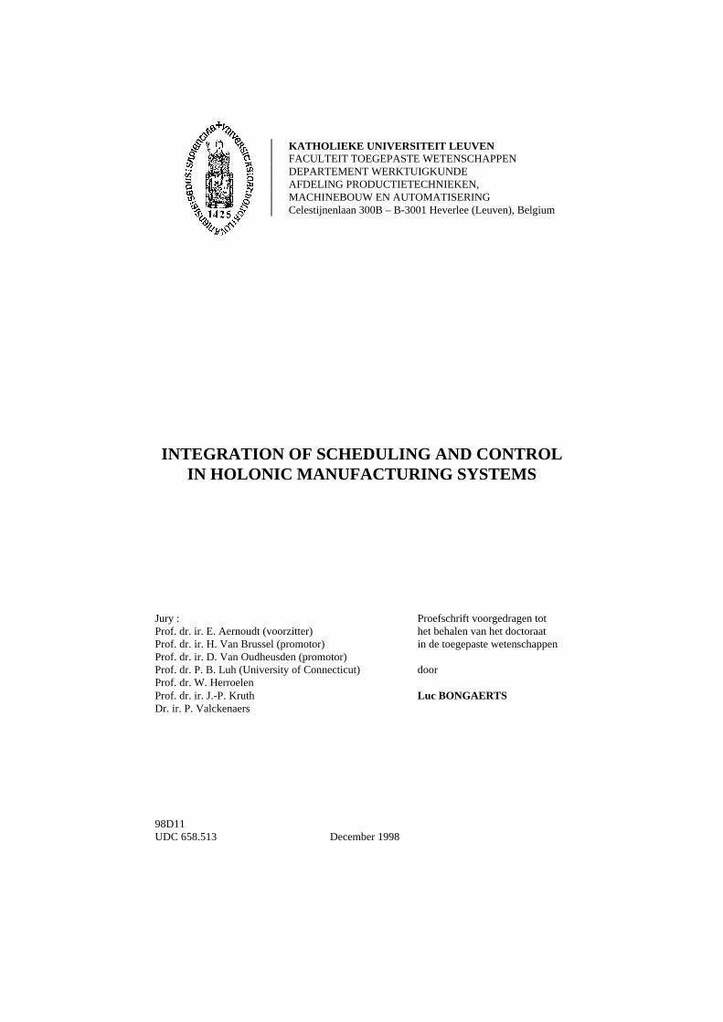
4.1 Algemene conceptenOm robuustheid tegen storingen te combineren met de voorspelbaarheid en optimali-satie van performantie, wordt voorgesteld om hiërarchische elementen te integrerenin een gedistribueerd (multi-agentgebaseerd) besturingssysteem (figuur 1). De resul-terende besturingsarchitectuur heeft dan een aantal autonome lokale holons, die dooronderlinge onderhandeling het werk onder elkaar wel kunnen verdelen, maar daarinbijgestaan worden door gecentraliseerde holons, stafholons genaamd.
S
R1 R2 O1 O2
Advice andCentralisedagent
Local agents
Negotiation
Figuur 1. Hierarchie in gedistribueerde systemen. R1 enR2 zijn machineholons (resource holons), O1 en O2 zijnorderholons. S is een stafholon.
Om dit concept te motiveren, is het interessant om te kijken naar de mecha-nismen die hiërarchische en heterarchische systemen hun goede eigenschappen ge-ven. Het emergente en reactieve gedrag van heterarchische systemen ontstaat juistdoor de interacties tussen de individuele gedragingen van elke agent / elk holon. Hië-rarchische systemen halen hun voorspelbaarheid juist door de coördinerende rol die
Samenvatting
xvi
het centrale element speelt, en hun hoge performantie doordat dat centraal elementtijd en moeite steekt in een optimalisatieproces. Bovendien hebben zowel lokale alsgecentraliseerde holons hun eigen vaardigheden en opportuniteiten. Lokale holonshebben meer up-to-date en gedetailleerde informatie over de entiteiten die ze behe-ren, en kunnen daarom ook sneller en gepaster reageren op storingen. Maar gecen-traliseerde holons hebben een overzicht over het hele systeem, wat hun toelaat omgecoördineerd acties uit te voeren en de implicaties op de globale performantie tedoorgronden. Het loont dus de moeite om te onderzoeken of de combinatie van hië-rarchische en heterarchische systemen ook de voordelen van beide oplevert.
Een tweede concept van deze thesis is het verdelen van beslissingsbevoegd-heid over alle holons, en dat op verschillende niveaus. Dit komt eigenlijk neer op deondubbelzinnige toepassing van het vorige concept. Om hierarchie in gedistribueer-de systemen in te voeren zonder de beslissingsbevoegdheid effectief te distribueren,zou men afwisselend hiërarchisch en heterarchisch moeten werken. Maar het resulte-rende systeemgedrag zou eerder houterig zijn, en zou ook de nadelen van hiërarchi-sche en heterarchische systemen combineren, zelfs als men op het juiste moment zouswitchen tussen beide werkingsmodes. Door beslissingbevoegdheid te verdelen, ont-staat er een zachte overgang tussen hiërarchische en heterarchisch gedrag, waarbijalle holons bijdragen tot de beslissingen volgens hun eigen kennis en vermogen. Be-langrijk is dat de holons zo kunnen samenwerken zonder in een meester-slaafrelatiete vervallen.
Tenslotte wordt ook het concept voorgesteld om gelijktijdig te fijnplannen endie planning uit te voeren. Zo kan snel gereageerd worden op storingen terwijl defijnplanner toch de tijd gegeven wordt om zijn planning te optimaliseren. Bemerk datdit concept tot nog toe weinig toegepast werd: ofwel werd het planningsalgoritmesterk vereenvoudigd (en versneld) zodat de reactie op storingen snel genoeg was(maar ten koste van de performantie); ofwel was de on line besturing zeer eenvoudig,waardoor de reactie op storingen ver van optimaal was. Bij het gelijktijdig optimali-seren en uitvoeren van een planning wordt er op verschillende niveaus gereageerd opstoringen. De lokale holons reageren onmiddellijk, zodat de productie niet stilvalt,maar ook de planner zal reageren op de storing en zijn planning eraan aanpassen,ook al is dat niet ogenblikkelijk.
Dit concept kan wel niet zonder verder onderzoek toegepast worden. Hetvergt immers de samenwerking tussen een reactieve fijnplanner en een intelligenteon-line-werkvloerbesturing. Reactieve-planningsalgoritmen vormen geen probleem,want zij worden al enkele jaren bestudeerd, en er bestaat dan ook genoeg literatuurover, met inbegrip van heel wat algoritmen en numerieke resultaten. Er zijn echterweinig of geen algoritmen voor een intelligente on-line-werkvloerbesturing. Er isnood aan algoritmen die een fijnplanning autonoom kunnen uitvoeren, wat betekentdat ze die planning kunnen volgen onder normale condities, maar ervan afwijken (enop de juiste manier) wanneer nodig. Deze thesis levert enkele bijdragen op dit ge-bied, maar er is nog heel wat werk te doen. Tenslotte is ook de samenwerking zelfbelangrijk en niet altijd triviaal, omdat beide systemen verder evolueren terwijl ze de
Samenvatting
xvii
planning optimaliseren en uitvoeren, wat betekent dat ze een model van elkaars ge-drag nodig hebben.
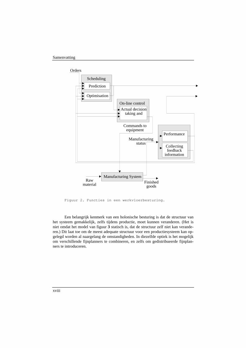
4.2 Statisch modelOm de architectuur van een holonisch besturingssysteem te beschrijven is een sta-tisch model nodig van de holons in het systeem. Dit model identificeert welke func-ties nodig zijn om een holonisch productiesysteem te besturen en met welke holonsdie functies uitgevoerd worden. Zo een model schetst ook de relaties tussen de ho-lons en de manier waarop ze zullen samenwerken (maar voor een volledig en accu-raat beeld van de architectuur moet ook de dynamica beschreven worden — zie ver-der).
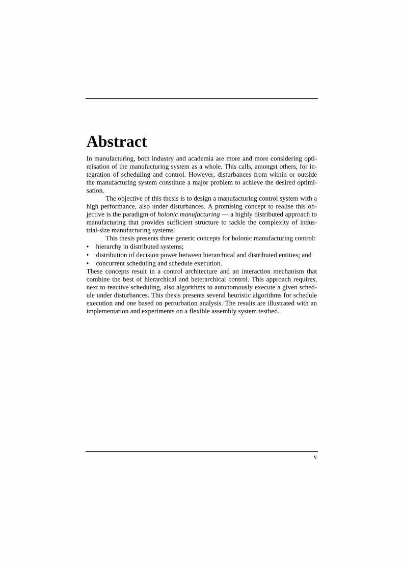
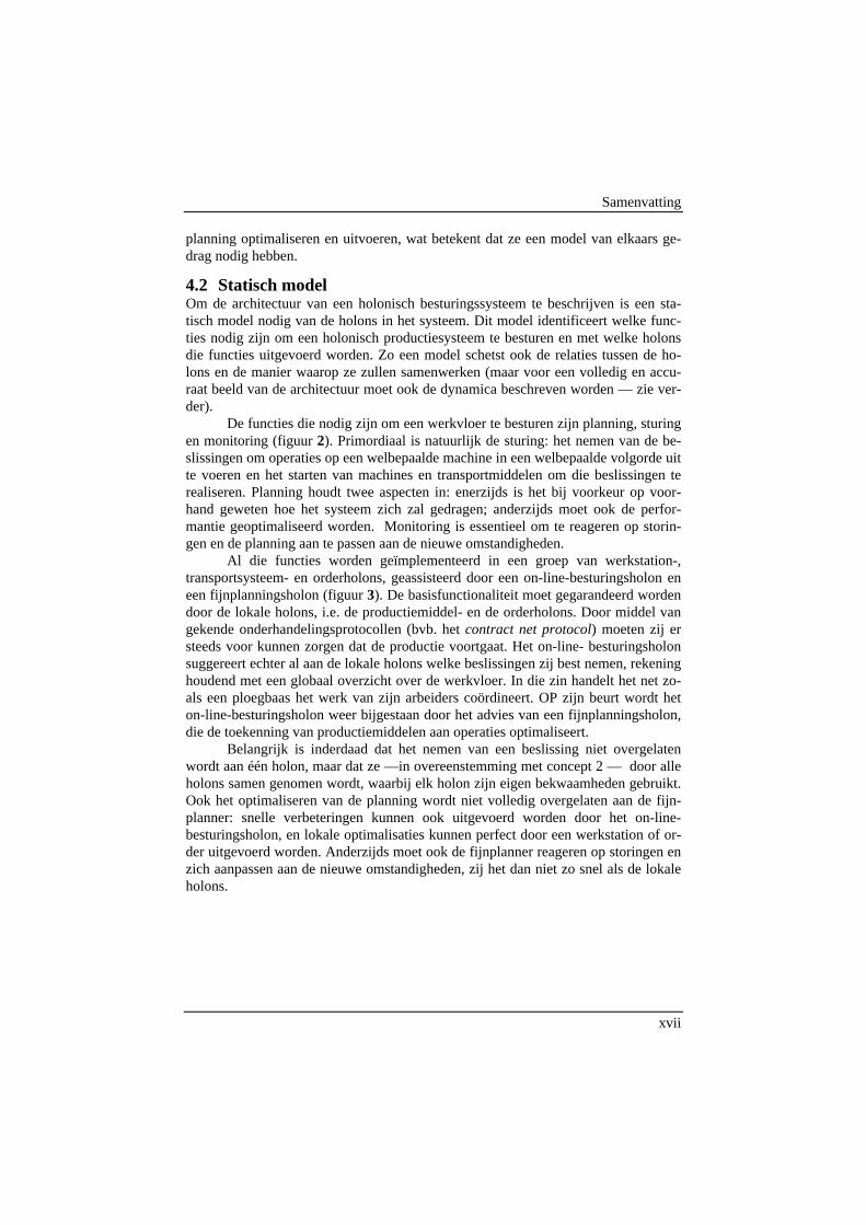
De functies die nodig zijn om een werkvloer te besturen zijn planning, sturingen monitoring (figuur 2). Primordiaal is natuurlijk de sturing: het nemen van de be-slissingen om operaties op een welbepaalde machine in een welbepaalde volgorde uitte voeren en het starten van machines en transportmiddelen om die beslissingen terealiseren. Planning houdt twee aspecten in: enerzijds is het bij voorkeur op voor-hand geweten hoe het systeem zich zal gedragen; anderzijds moet ook de perfor-mantie geoptimaliseerd worden. Monitoring is essentieel om te reageren op storin-gen en de planning aan te passen aan de nieuwe omstandigheden.
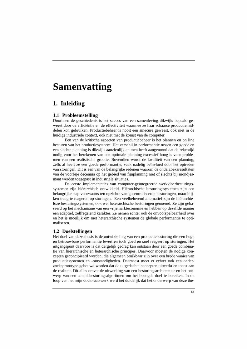
Al die functies worden geïmplementeerd in een groep van werkstation-,transportsysteem- en orderholons, geassisteerd door een on-line-besturingsholon eneen fijnplanningsholon (figuur 3). De basisfunctionaliteit moet gegarandeerd wordendoor de lokale holons, i.e. de productiemiddel- en de orderholons. Door middel vangekende onderhandelingsprotocollen (bvb. het contract net protocol) moeten zij ersteeds voor kunnen zorgen dat de productie voortgaat. Het on-line- besturingsholonsuggereert echter al aan de lokale holons welke beslissingen zij best nemen, rekeninghoudend met een globaal overzicht over de werkvloer. In die zin handelt het net zo-als een ploegbaas het werk van zijn arbeiders coördineert. OP zijn beurt wordt heton-line-besturingsholon weer bijgestaan door het advies van een fijnplanningsholon,die de toekenning van productiemiddelen aan operaties optimaliseert.
Belangrijk is inderdaad dat het nemen van een beslissing niet overgelatenwordt aan één holon, maar dat ze —in overeenstemming met concept 2 — door alleholons samen genomen wordt, waarbij elk holon zijn eigen bekwaamheden gebruikt.Ook het optimaliseren van de planning wordt niet volledig overgelaten aan de fijn-planner: snelle verbeteringen kunnen ook uitgevoerd worden door het on-line-besturingsholon, en lokale optimalisaties kunnen perfect door een werkstation of or-der uitgevoerd worden. Anderzijds moet ook de fijnplanner reageren op storingen enzich aanpassen aan de nieuwe omstandigheden, zij het dan niet zo snel als de lokaleholons.
Samenvatting
xviii
Manufacturing status
Commands to equipment
Orders
Finished goods
Raw material
Manufacturing System
Scheduling
Prediction
Optimisation
Performance
Collecting feedback
information
Actual decision taking and
On-line control
Figuur 2. Functies in een werkvloerbesturing.
Een belangrijk kenmerk van een holonische besturing is dat de structuur vanhet systeem gemakkelijk, zelfs tijdens productie, moet kunnen veranderen. (Het isniet omdat het model van figuur 3 statisch is, dat de structuur zelf niet kan verande-ren.) Dit laat toe om de meest adequate structuur voor een productiesysteem kan op-gelegd worden al naargelang de omstandigheden. In diezelfde optiek is het mogelijkom verschillende fijnplanners te combineren, en zelfs om gedistribueerde fijnplan-ners te introduceren.
Samenvatting
xix
On-line Manufacturing Control Holon
Reactive Scheduling Holon
Order Holon
Resource Holon
Figuur 3. Statisch model van de holons in een holonischeproductiebesturing.
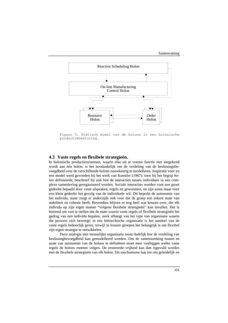
4.3 Vaste regels en flexibele strategieën.In holonische productiesystemen, waarin elke uit te voeren functie niet toegekendwordt aan één holon, is het noodzakelijk om de verdeling van de beslissingsbe-voegdheid over de verschillende holons nauwkeurig te modelleren. Inspiratie voor zoeen model werd gevonden bij het werk van Koestler (1967): toen hij het begrip ho-lon definieerde, beschreef hij ook hoe de interacties tussen individuen in een com-plexe samenleving georganiseerd worden. Sociale interacties worden voor een grootgedeelte bepaald door vaste afspraken, regels en gewoonten, en zijn soms maar vooreen klein gedeelte het gevolg van de individuele wil. Dit beperkt de autonomie vanhet individu, maar zorgt er anderzijds ook voor dat de groep een zekere mate vanstabiliteit en cohesie heeft. Bovendien blijven er nog heel wat keuzen over, die elkindividu op zijn eigen manier “volgens flexibele strategieën” kan invullen. Het isboeiend om vast te stellen dat de mate waarin vaste regels of flexibele strategieën hetgedrag van een individu bepalen, sterk afhangt van het type van organisatie waarindie persoon zich beweegt: in een hiërarchische organisatie is het aandeel van devaste regels behoorlijk groot, terwijl in lossere groepen het belangrijk is om flexibelzijn eigen strategie te ontwikkelen.
Deze analogie met menselijke organisatie toont dadelijk hoe de verdeling vanbeslissingbevoegdheid kan gemodelleerd worden. Om de samenwerking tussen enmate van autonomie van de holons te definiëren moet men vastleggen welke vasteregels de holons moeten volgen. De resterende vrijheid kan dan ingevuld wordenmet de flexibele strategieën van elk holon. Dit mechanisme laat toe om geleidelijk en
Samenvatting
xx
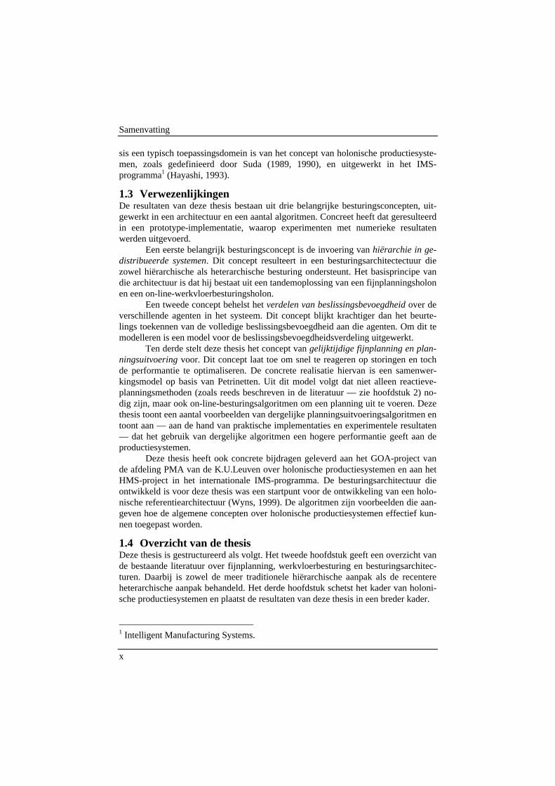
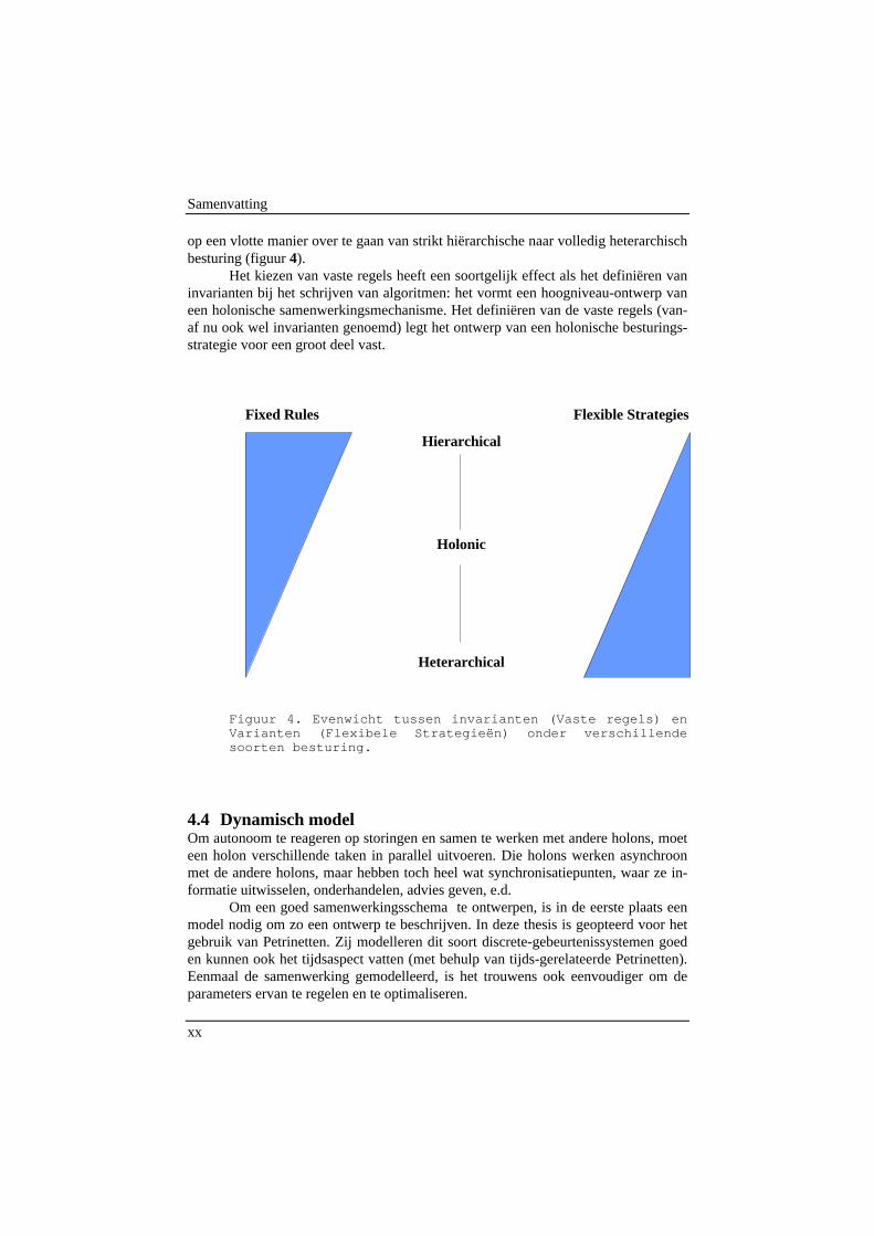
op een vlotte manier over te gaan van strikt hiërarchische naar volledig heterarchischbesturing (figuur 4).
Het kiezen van vaste regels heeft een soortgelijk effect als het definiëren vaninvarianten bij het schrijven van algoritmen: het vormt een hoogniveau-ontwerp vaneen holonische samenwerkingsmechanisme. Het definiëren van de vaste regels (van-af nu ook wel invarianten genoemd) legt het ontwerp van een holonische besturings-strategie voor een groot deel vast.
Flexible StrategiesFixed Rules
Hierarchical
Holonic
Heterarchical
Figuur 4. Evenwicht tussen invarianten (Vaste regels) enVarianten (Flexibele Strategieën) onder verschillendesoorten besturing.
4.4 Dynamisch modelOm autonoom te reageren op storingen en samen te werken met andere holons, moeteen holon verschillende taken in parallel uitvoeren. Die holons werken asynchroonmet de andere holons, maar hebben toch heel wat synchronisatiepunten, waar ze in-formatie uitwisselen, onderhandelen, advies geven, e.d.
Om een goed samenwerkingsschema te ontwerpen, is in de eerste plaats eenmodel nodig om zo een ontwerp te beschrijven. In deze thesis is geopteerd voor hetgebruik van Petrinetten. Zij modelleren dit soort discrete-gebeurtenissystemen goeden kunnen ook het tijdsaspect vatten (met behulp van tijds-gerelateerde Petrinetten).Eenmaal de samenwerking gemodelleerd, is het trouwens ook eenvoudiger om deparameters ervan te regelen en te optimaliseren.
Samenvatting
xxi
Een voorbeeld van een dergelijk samenwerkingsmodel is gegeven in het vol-gende hoofdstuk. Het handelt over de modellering van gelijktijdige fijnplanning enplanningsuitvoering.
5. Samenwerking in holonische productiebesturingDit hoofdstuk beschrijft aan de hand van enkele voorbeelden hoe samenwerking ineen holonische productiesturing kan ontworpen worden. Deze voorbeelden zijn nietgenerisch voor alle holonische oplossingen, maar geven wel een concreet beeld vande besturing. In deze samenvatting wordt de meeste aandacht gegeven aan de sa-menwerking tussen het fijnplanningsholon en het on-line-besturingsholon, die ge-lijktijdig een fijnplanning berekenen respectievelijk uitvoeren. Andere voorbeeldenworden — zeker in de samenvatting — minder gedetailleerd overlopen.
Voor het modelleren van de samenwerking wordt gebruik gemaakt van Petri-netten, die de uit te voeren taken van elk holon op een hoog niveau van aggregatiebeschrijven. Naargelang de noodzaak worden de Petrinetten uitgebreid met tijd,voorwaarden, stochasticiteit, besturingsplaatsen, e.d.
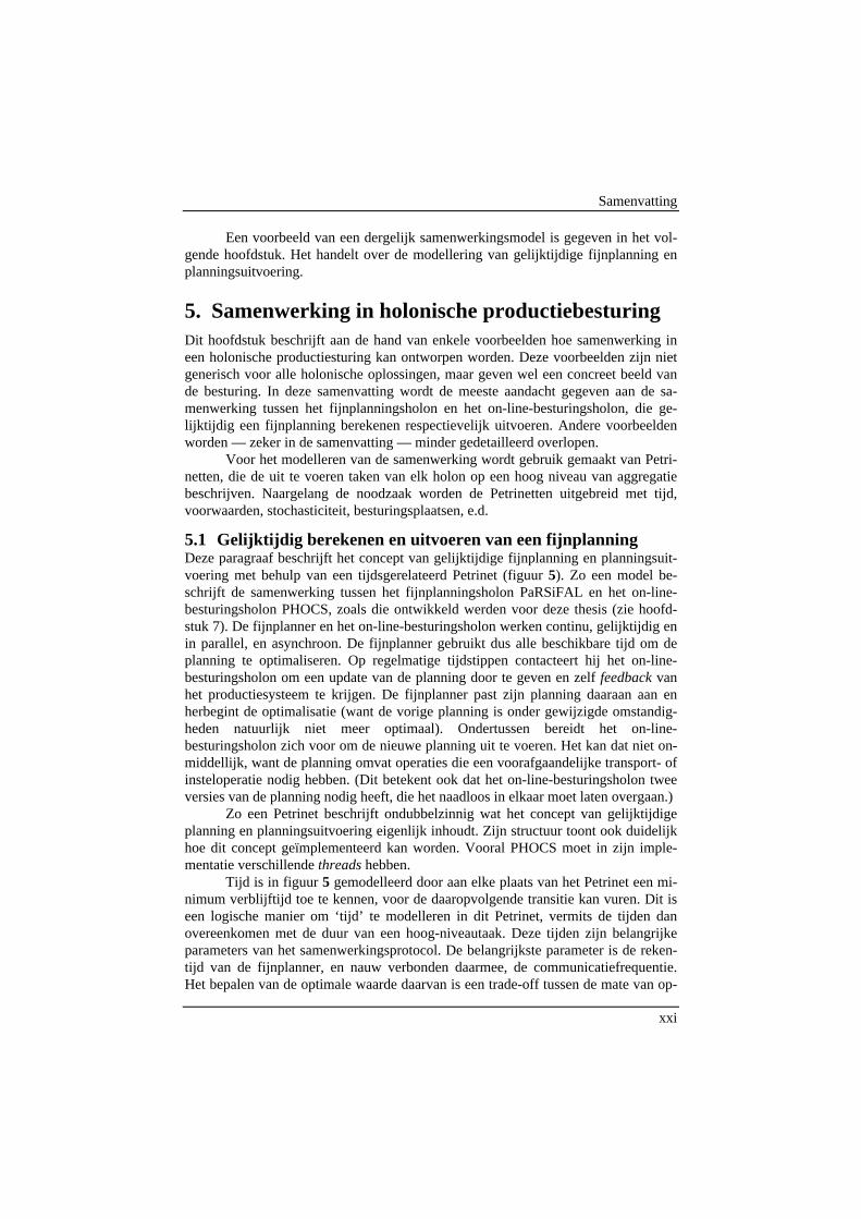
5.1 Gelijktijdig berekenen en uitvoeren van een fijnplanningDeze paragraaf beschrijft het concept van gelijktijdige fijnplanning en planningsuit-voering met behulp van een tijdsgerelateerd Petrinet (figuur 5). Zo een model be-schrijft de samenwerking tussen het fijnplanningsholon PaRSiFAL en het on-line-besturingsholon PHOCS, zoals die ontwikkeld werden voor deze thesis (zie hoofd-stuk 7). De fijnplanner en het on-line-besturingsholon werken continu, gelijktijdig enin parallel, en asynchroon. De fijnplanner gebruikt dus alle beschikbare tijd om deplanning te optimaliseren. Op regelmatige tijdstippen contacteert hij het on-line-besturingsholon om een update van de planning door te geven en zelf feedback vanhet productiesysteem te krijgen. De fijnplanner past zijn planning daaraan aan enherbegint de optimalisatie (want de vorige planning is onder gewijzigde omstandig-heden natuurlijk niet meer optimaal). Ondertussen bereidt het on-line-besturingsholon zich voor om de nieuwe planning uit te voeren. Het kan dat niet on-middellijk, want de planning omvat operaties die een voorafgaandelijke transport- ofinsteloperatie nodig hebben. (Dit betekent ook dat het on-line-besturingsholon tweeversies van de planning nodig heeft, die het naadloos in elkaar moet laten overgaan.)
Zo een Petrinet beschrijft ondubbelzinnig wat het concept van gelijktijdigeplanning en planningsuitvoering eigenlijk inhoudt. Zijn structuur toont ook duidelijkhoe dit concept geïmplementeerd kan worden. Vooral PHOCS moet in zijn imple-mentatie verschillende threads hebben.
Tijd is in figuur 5 gemodelleerd door aan elke plaats van het Petrinet een mi-nimum verblijftijd toe te kennen, voor de daaropvolgende transitie kan vuren. Dit iseen logische manier om ‘tijd’ te modelleren in dit Petrinet, vermits de tijden danovereenkomen met de duur van een hoog-niveautaak. Deze tijden zijn belangrijkeparameters van het samenwerkingsprotocol. De belangrijkste parameter is de reken-tijd van de fijnplanner, en nauw verbonden daarmee, de communicatiefrequentie.Het bepalen van de optimale waarde daarvan is een trade-off tussen de mate van op-

Samenvatting
xxii
timaliteit van de (her-)planning en de reactiesnelheid op storingen. De tijd nodigvoor communicatie (zenden en ontvangen) kan beschouwd worden als een constanteparameter (gegeven de probleemgrootte en de snelheid van het intranet). De tijd diePHOCS nodig heeft om zich aan te passen aan de nieuwe planning is in principe ookeen gegeven constante. Door deze tijd optimistisch in te schatten kan de globalesysteemperformantie echter verbeteren, zodat deze tijd een regelbare parameterwordt. In de huidige implementatie is die waarde gekozen op 80 % van de nodigewaarde. Interessant is ook dat de analyse van al deze tijden bevestigt dat het systeem(en bijhorend Petrinet) in de meeste omstandigheden periodisch en begrensd is.
On-line manufacturing control holon
Reactive scheduling holon
t9
p7: On-line control system Phocs is idling
t2
t1
t7
t6
t8
t5
t4
p3: Generate additional
p6: Adapting model according to feedback
p5: Receiving feed-back
p4: Sending schedule
p2: Calculating schedule
p1: Scheduler is idling
p8: Waiting for new schedule
p9: receiving schedule
p10: sending
p12: setting up for new schedule p14:
executing new schedule
p13: executing outdated schedule
t3 p11: Dummy node
Figuur 5. Tijdsgerelateerd Petrinetmodel van de samenwer-king tussen het on-line-besturingsholon PHOCS en de reac-tieve fijnplanner PaRSiFAL.
Samenvatting
xxiii
5.2 Samenwerking tussen lokale holons en stafholonsEen ander samenwerkingsmechanisme dat bestudeerd werd in de thesis is dat tussenlokale holons en stafholons. Lokale holons zijn in principe in staat om door onder-handeling zelf tot een oplossing te komen, maar kunnen daarin bijgestaan wordendoor stafholons. Dit vergt een extensie van het contractnetprotocol, dat voorziet ineen onderhandelingsmechanisme tussen aanbieders en bieders. In een holonisch sys-teem is er ook een plaats voor een bemiddelaar, zoals het stafholon. Een model daar-voor wordt besproken in de volledige tekst.
5.3 Herplannen na belangrijke gebeurtenissenEen verbetering van het voorgaande samenwerkingsprotocol tussen fijnplanner enon-line-besturingsholon bestaat erin om niet alleen periodisch, maar ook na belang-rijke gebeurtenissen te herplannen. Het idee is dat het bij belangrijke storingen, zoalsnieuwe orders of machineuitval, niet interessant is om te blijven verder rekenen aande planning die toch al verouderd is. Dit houdt in dat er moet geïdentificeerd wordenwat een belangrijke storing is, en hoelang er dan opnieuw moet geoptimaliseerdworden. De thesis presenteert een ontwerp van een dergelijk samenwerkingsmecha-nisme, echter zonder het in detail uit te werken.
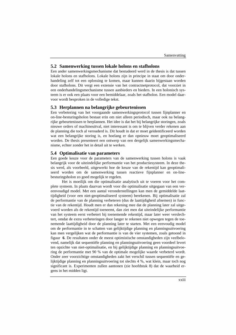
5.4 Optimalisatie van parametersEen goede keuze voor de parameters van de samenwerking tussen holons is vaakbelangrijk voor de uiteindelijke performantie van het productiesysteem. In deze the-sis werd, als voorbeeld, uitgewerkt hoe de keuze van de rekentijd kan geoptimali-seerd worden om de samenwerking tussen reactieve fijnplanner en on-line-besturingsholon zo goed mogelijk te regelen.
Het is moeilijk om die optimalisatie analytisch uit te voeren voor het com-plete systeem. In plaats daarvan wordt voor die optimalisatie uitgegaan van een ver-eenvoudigd model. Met een aantal veronderstellingen kan men de gemiddelde laat-tijdigheid (voor een niet-geoptimaliseerd systeem) berekenen. Bij optimalisatie zalde performantie van de planning verbeteren (dus de laattijdigheid afnemen) in func-tie van de rekentijd. Houdt men er dan rekening mee dat de planning later zal uitge-voerd worden als de rekentijd toeneemt, dan ziet men dat uiteindelijke performantievan het systeem eerst verbetert bij toenemende rekentijd, maar later weer verslech-tert, omdat de extra verbeteringen door langer te rekenen niet opwegen tegen de toe-nemende laattijdigheid door de planning later te starten. Met een eenvoudig modelom de performantie in te schatten van gelijktijdige planning en planningsuitvoeringkan men vergelijken wat de performantie is van de vier systemen, zoals getoond infiguur 6. De resultaten onder de meest optimistische omstandigheden zijn veelbelo-vend, namelijk dat sequentiële planning en planningsuitvoering geen voordeel levertten opzichte van niet-optimalisatie, en bij gelijktijdige planning en planningsuitvoe-ring de performantie met 90 % van de optimale mogelijke waarde verbeterd wordt.Onder zeer voorzichtige omstandigheden zakt het verschil tussen sequentiële en ge-lijktijdige planning en planningsuitvoering tot slechts 4 %, wat klein, maar toch nogsignificant is. Experimenten zullen aantonen (zie hoofdstuk 8) dat de waarheid er-gens in het midden ligt.
Samenvatting
xxiv
Tav,csse
Tav,opt_sched
Tav,opt_sched_dyn_envir
Tav,fair
[min]
0 250 500 750 10000
50
100
150
200
calculation time scheduler [min]
aver
age
tard
ines
s
Figuur 6. Kwantitatieve vergelijking van off-line-planningsmethoden, dispatching, sequentieel plannen enplanninguitvoeren en van gelijktijdig plannen en plan-ningsuitvoeren. Dit voorbeeld is gebaseerd op de meestoptimistische formulering van het probleem, maar geeftgoed de mogelijke verbeteringen aan. Voor verdere gege-vens wordt verwezen naar de volledige beschrijving inhoofdstuk 5.
6. Holonische besturingsalgoritmesBij het zoeken naar holonische besturingsalgoritmes is de aandacht vooral gegaannaar planningsuitvoering, vermits er al heel wat planningsalgoritmes bestaan die rea-geren op storingen. Dit hoofdstuk beschrijft een aantal van die algoritmes op basisvan het kader van vaste regels en flexibele strategieën, zoals dat gedefinieerd is inhoofdstuk 4. Een ander algoritme, op basis van perturbatie-analyse, bouwt zijn ge-

Samenvatting
xxv
drag op een theoretisch beter uitgewerkt kader, en bedient zich niet expliciet van dieregels en strategieën.
6.1 Definitie planningsuitvoeringPlanningsuitvoering is de functie die inhoudt dat de toekenningen van operaties aanmachines en de volgordes van operaties zoals die voorgesteld worden door de plan-ning, ook effectief worden uitgevoerd, maar op een intelligente manier: als er storin-gen zijn, mag van de planning afgeweken worden.
Een on-line-besturingsalgoritme doet aan autonome planningsuitvoering alshet door gebruik te maken van de planning, duidelijk sneller kan reageren op storin-gen dan een reactieve planning, en toch de optimalisatie van de planning kan gebrui-ken. In andere woorden, de uiteindelijke performantie moet gecorreleerd zijn aan deperformantie van de fijnplanner.
Het is belangrijk te vermelden dat autonome planningsuitvoering geen een-voudige taak is. Eigenlijk is het onmogelijk om op een optimale manier een planninguit te voeren (als er storingen optreden, en zonder zelf te herplannen), als de plan-ning enkel voorgesteld wordt als een Ganttkaart. Dat kan aangetoond worden meteen voorbeeld. In dat voorbeeld wordt een storing geïnduceerd bij de uitvoering vaneen planning, waarbij het niet meteen duidelijk is wat de juiste reactie op die storingis. Het blijkt dat de juiste keuze afhangt van de relatieve dringendheid van verschil-lende operaties. Maar die dringendheid hangt zelf weer af, gekoppeld via een net-werk van andere operaties, van de uiteindelijke laattijdigheid die orders eventueelzouden oplopen ten gevolge van die storing. In deze thesis wordt een oplossing ge-zocht voor dit probleem door het invoeren van extra advies van de fijnplanner aanhet on-line-besturingsholon.
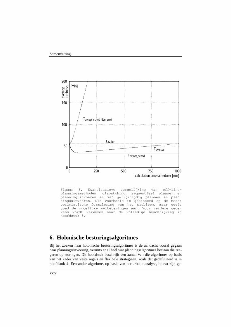
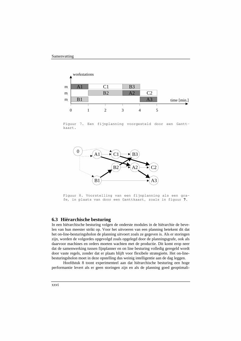
6.2 Planning voorgesteld door een grafeZowel voor het definiëren van vaste regels en flexibele strategieën als voor het ont-werpen van autonome planningsuitvoeringsstrategieën kan het handig zijn om deplanning voor te stellen als een grafe, en niet alleen door een Ganttkaart (figuur 7).Deze grafe bestaat uit knopen, die de operaties voorstellen, en bogen, die de volgor-debeperkingen tussen de operaties voorstellen (figuur 8). Die volgordebeperkingenzijn natuurlijk zeker en vast de technologische volgordebeperkingen, maar ook debeperkingen die volgen uit de volgorde van de operaties op een productiemiddel inde planning. Ook het bestaan van een vroegst toegelaten starttijd voor een order (re-lease date) creëert een volgordebeperking die in de grafe kan gemodelleerd worden.
Men kan aantonen dat de voorstelling van die planning als een grafe equiva-lent is aan de klassieke Gantt-kaart, als de originele planning een actieve planning is.Dit betekent dat de starttijd voor elke operatie onder beide voorstellingen dezelfdeis. De starttijd van een operatie in een grafe kan berekend worden door de vroegstmogelijke starttijd van elke operatie te berekenen langsheen de pijlen van de grafe, testarten vanaf de vroegst toegelaten starttijd van elk order. Zo kan men ook de per-formantie berekenen van de hele planning.
Samenvatting
xxvi
0 1 2 3 4 5
m1
m2
m3 time [min.]
workstations
A1
B1
C1B2
B3A2
A3C2
Figuur 7. Een fijnplanning voorgesteld door een Gantt-kaart.
0A1 C1 B3
B2 A2 C2
B1 A3
Figuur 8. Voorstelling van een fijnplanning als een gra-fe, in plaats van door een Ganttkaart, zoals in figuur 7.
6.3 Hiërarchische besturingIn een hiërarchische besturing volgen de onderste modules in de hiërarchie de beve-len van hun meester strikt op. Voor het uitvoeren van een planning betekent dit dathet on-line-besturingsholon de planning uitvoert zoals ze gegeven is. Als er storingenzijn, worden de volgordes opgevolgd zoals opgelegd door de planningsgrafe, ook alsdaarvoor machines en orders moeten wachten met de productie. Dit komt erop neerdat de samenwerking tussen fijnplanner en on line besturing volledig geregeld wordtdoor vaste regels, zonder dat er plaats blijft voor flexibele strategieën. Het on-line-besturingsholon moet in deze opstelling dus weinig intelligentie aan de dag leggen.
Hoofdstuk 8 toont experimenteel aan dat hiërarchische besturing een hogeperformantie levert als er geen storingen zijn en als de planning goed geoptimali-
Samenvatting
xxvii
seerd is, maar dat deze performantie snel zakt als er storingen komen. Ook is het ge-drag van hiërarchische besturing goed voorspelbaar.
6.4 Heterarchische en gecentraliseerde autonome besturingIn heterarchische systemen worden alle beslissingen genomen door autonome agen-ten, die met elkaar communiceren en onderhandelen om de productie te runnen.Daarbij zweert men elke vorm van hierarchie af. Heterarchische besturing is veelbe-lovend wat betreft het reageren op storingen, omdat een reactief gedrag automatischontstaat uit de interacties tussen de verschillende agenten.
De onderzochte implementaties van heterarchische besturing zijn gebaseerdop vrije-marktmechanismen en klassieke dispatchingregels. Debels en Hermans(1998) implementeerden voor hun eindwerk op PMA een marktmechanisme dat debeslissingen van elk order deed afhangen van een machinekostprijs, een transport-kostprijs en de levertermijn (due date). Zelf implementeerde ik een gecentraliseerdevorm van autonome besturing, waarbij orders machines kozen op basis van de laag-ste belasting, en machines een operatievolgorde kozen op basis van orders met devroegste levertermijn (earliest due date). Hiervoor werden op een gecentraliseerdemanier dezelfde beslissingsregels gebruikt als men normaal in een gedistribueerdebesturing op basis van dispatchingregels zou gebruiken. Essentieel is natuurlijk datin beide implementaties geen gebruik werd gemaakt van een voorspellende en opti-maliserende fijnplanner. Het systeemgedrag werd dus volledig beschreven door deflexibele strategieën van de on line besturing.
Het reactief gedrag tegen storingen wordt experimenteel bevestigd in hoofd-stuk 8, maar daar wordt ook getoond dat heterarchische systemen een lagere perfor-mantie hebben en minder voorspelbaar zijn dan de klassieke hiërarchische systemen.
6.5 Heuristische holonische planningsuitvoeringsalgoritmenVoor deze thesis zijn drie heuristische besturingsalgoritmen ontwikkeld die een fijn-planning autonoom kunnen uitvoeren doordat ze een gedeeltelijke autonomie krij-gen. Ze worden voor een gedeelte gebonden door vaste regels, maar die laten hunnog voldoende vrijheid om zelf, volgens hun eigen flexibele strategieën, te reagerenop storingen.
Een eerste algoritme (STA — short term autonomy) geeft het on-line-besturingsholon autonomie voor een korte termijn. Het mag alleen die operaties uit-voeren die gepland zijn in ‘de nabije toekomst’ (geparametriseerd door een parame-ter Tresched), maar mag die operaties dan wel uitvoeren in een volgorde en op machi-nes die het zelf kiest.
Een tweede algoritme (AID — autonomy if disturbances) krijgt autonomie alser storingen ontdekt worden. Dit wordt praktisch geïmplementeerd door beperkin-gen, opgelegd door de vaste regels, te laten wegvallen als ze verouderd zijn (eventu-eel getemperd of versneld door een positieve of negatieve buffertijd in te voeren diedefinieert wanneer een beperking verouderd is).
Een derde algoritme (LDFS — limited deviation from schedule) staat een be-perkte afwijking van de planning toe. Dit betekent dat de on-line besturing de opera-

Samenvatting
xxviii
ties moet uitvoeren rond de geplande starttijd, maar dat omwisselingen van operatieskunnen zolang dat niet resulteert in grote afwijkingen van de planning.
In de volledige tekst worden die drie algoritmen formeel gedefinieerd doormiddel van de voorstelling van een planning als een grafe.
Deze drie algoritmen hebben met elkaar gemeen dat ze proberen de goedekenmerken van een planning te extraheren, zonder zich te houden aan minder be-langrijke beperkingen als er storingen zijn. Op die manier zijn ze holonisch, doordatze proberen robuustheid tegen storingen te combineren met het gebruik van een cen-traal geoptimaliseerde planning. Het blijven echter heuristische methoden, gebaseerdop gezond verstand. Hun uiteindelijke performantie moet dan blijken uit experimen-ten. Daarom beschrijft de volgende paragraaf ook een planningsuitvoeringsalgoritmeop basis van een meer theoretisch gefundeerde afleiding.
6.6 Planningsuitvoering op basis van perturbatie-analyseOm een planning naar behoren uit te voeren, wil dit algoritme daadwerkelijk gebruikmaken van extra advies van de planner. Er was reeds vermeld dat zo een adviesnoodzakelijk is om steeds tot goede beslissingen te komen, omdat er in een Gantt-kaart essentiële informatie ontbreekt. Het probleem is dat een on line besturing moetweten hoe lokale beslissingen de globale performantie beïnvloeden.
Dit algoritme gebruikt daarom perturbatie-analyse (PA). De fijnplanner stelthet resultaat van zijn berekeningen voor als een grafe, en leidt daaruit een aantal lo-kale beslissingspunten af (namelijk één voor elke pijl in de grafe: de vroegst moge-lijke starttijd voor de eindknoop van de pijl, tenminste voor wat betreft de beperkinguitgedrukt door die pijl). Daardoor wordt het mogelijk de globale performantie uit tedrukken in functie van lokale beslissingspunten. Het is dan mogelijk om voor elkepijl de partiële afgeleide van de globale performantie naar de vroegst mogelijkestarttijd voor die pijl off line te berekenen en door te geven aan de on line besturing.
Het on-line-besturingsholon zal dan op zijn beurt dat advies gebruiken. Voorelk beslissingspunt zal het een aantal alternatieven vooropstellen. Het berekent deimpact van elk alternatief op de vroegst mogelijke starttijden van elke relevante pijlin de grafe. Het is dan mogelijk om de impact van elk alternatief op de globale per-formantie te schatten door linearisatie (De afwijking in performantie wordt geschatdoor de som van de producten van de afwijking in vroegst mogelijke starttijd met debijhorende partiële afgeleide). De verschillende alternatieven worden geëvalueerd opbasis van hun verbetering of verslechtering van de globale performantie.
Men kan zich afvragen of het zin heeft om een dergelijk niet-lineair systeemte lineariseren. Echter, de bestaande alternatieven om een planning uit te voeren zijnzelfs helemaal niet gebaseerd op één of andere reflectie naar performantie toe. Bo-vendien wordt de on line besturing niet volledig aan haar lot overgelaten als er sto-ringen komen: er wordt ondertussen een nieuwe planning berekend, maar zolang dieniet gereed is, moet de on line besturing verder werken met de bestaande planning.Het gebruik van perturbatie-analyse is dus enkel nodig voor korte-termijnbeslissingen. De experimenten in hoofdstuk 8 bevestigen trouwens dat de re-sultaten best bevredigend zijn.
Samenvatting
xxix
6.7 BesluitDit hoofdstuk heeft drie heuristische planningsuitvoeringsalgoritmen en één theore-tisch gefundeerd algoritme voorgesteld. Een belangrijk aspect van holonische pro-ductiebesturing is dat het algoritme niet opgelegd wordt door de architectuur, en bij-gevolg dat er gemakkelijk tussen algoritmen kan gewisseld worden. Dit komt ook totuiting in de implementaties.
7. Ontwerp en implementatiesDe concepten en algoritmen ontwikkeld voor deze thesis werden geïmplementeerd ineen onderzoeksprototype-besturing voor een flexibel assemblagesysteem. Dit proto-type bestaat uit een reactieve fijnplanner PaRSiFAL, een on-line-besturingsholonPHOCS en een aantal lokale holons (werkstationholons, orderholons en een trans-portsysteemholon). Elk holon is geïmplementeerd als een agent (een apart computer-proces), elk met een eigen gebruikersinterface. De holons communiceren met elkaarvia een asynchroon boodschap-gebaseerd protocol over ethernet.
Het testbed is een flexibel assemblagesysteem met zes werkstations, die inwillekeurige volgorde te bezoeken zijn. Het productiesysteem heeft dus de lay-outvan een job-shop. De werkstations zijn verbonden via een flexibel transportsysteem,dat de orders transporteert via lopende banden op paletten.
PaRSiFAL bevat een aantal planningsalgoritmen. Enkele zijn eenvoudigedispatchingregels (FIFO, EDD en aanvullingen daarop). Er zijn ook enkele omge-vingszoekalgoritmen die via de eerst gevonden dalende helling op zoek gaan naareen lokaal optimum. Er zijn ook algoritmes die de afdalingsmethode toepassen voorverschillende startoplossingen en algoritmes die uit een lokaal optimum proberenontsnappen door de structuur van de oplossing te herorganiseren.
PHOCS bestuurt het productiesysteem door de paletten te beheren, transport-verzoeken uit te sturen, set-ups te commanderen en operaties te starten. Op die ma-nier maakt hij beslissingen over het toekennen van operaties aan machines en het se-quensen daarvan op die machines. In PHOCS kan men via een menu de productiemanueel (interactief) sturen. Men kan ook kiezen uit een reeks besturingsalgoritmen(zoals beschreven in hoofdstuk 6) om de productie te runnen.
8. ExperimentenDit hoofdstuk beschrijft de experimenten die uitgevoerd werden om de nieuwe, ho-lonische benadering voor productiebesturing te toetsen aan hiërarchische en heterar-chische besturing. Daarom wordt de performantie van de verschillende algoritmen(hiërarchische, heterarchische, en de vier holonische algoritmen) vergeleken vooreen aantal testproblemen onder een aantal scenario’s. Die scenario’s verwijzen zowelnaar productieomstandigheden zonder storingen als naar omstandigheden met mo-delfouten, stochastische afwijkingen van de geplande duur en machine-uitval. Hetdoel van die experimenten is niet alleen het vergelijken van de resulterende systeem-
Samenvatting
xxx
performantie met en zonder storingen, maar ook de vergelijking van de voorspel-baarheid van al die benaderingen.
Eerst werd nagegaan hoe repeteerbaar experimenten zijn. Voor een experi-ment van ongeveer 1000 s werd voor hiërarchische besturing een repeteerbaarheidvan 2 s (standaardafwijking) opgemeten. Wel kan die repeteerbaarheid verslechteren(tot een kleine 10 s) als het optimalisatiegedrag van de fijnplanner stochastische ef-fecten vertoont. Voor heterarchische systemen is de voorspelbaarheid veel slechter(25 s voor de gemiddelde performantie en 70 s voor de gemiddelde standaarddevia-tie van een individueel order). Holonische systemen (als ze zich naar behoren gedra-gen) zitten daar ergens tussenin, met een voorspelbaarheid van 10 s voor de gemid-delde performantie tot 25 s voor individuele orders.
disturbancescenario.
Hierar-chical
STA(Hol.)
AID(Hol.)
LDFS(Hol.)
PA(Hol.)
Heterar-chical
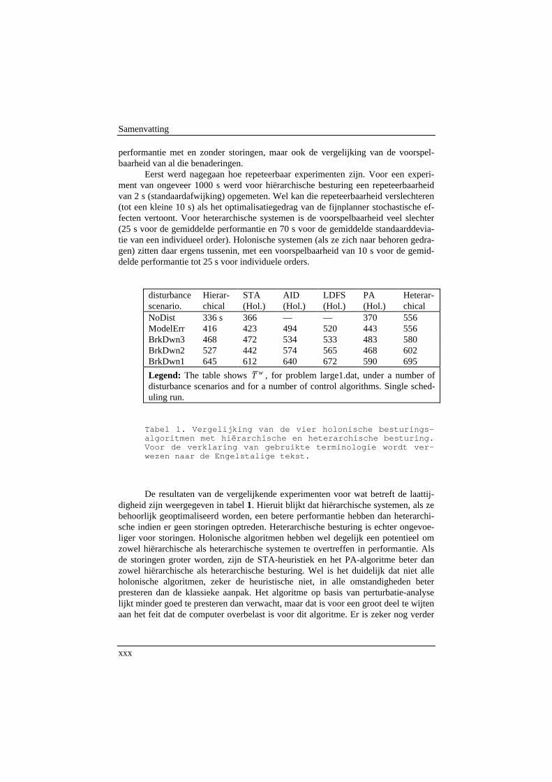
NoDist 336 s 366 — — 370 556ModelErr 416 423 494 520 443 556BrkDwn3 468 472 534 533 483 580BrkDwn2 527 442 574 565 468 602BrkDwn1 645 612 640 672 590 695
Legend: The table shows wT , for problem large1.dat, under a number ofdisturbance scenarios and for a number of control algorithms. Single sched-uling run.
Tabel 1. Vergelijking van de vier holonische besturings-algoritmen met hiërarchische en heterarchische besturing.Voor de verklaring van gebruikte terminologie wordt ver-wezen naar de Engelstalige tekst.
De resultaten van de vergelijkende experimenten voor wat betreft de laattij-digheid zijn weergegeven in tabel 1. Hieruit blijkt dat hiërarchische systemen, als zebehoorlijk geoptimaliseerd worden, een betere performantie hebben dan heterarchi-sche indien er geen storingen optreden. Heterarchische besturing is echter ongevoe-liger voor storingen. Holonische algoritmen hebben wel degelijk een potentieel omzowel hiërarchische als heterarchische systemen te overtreffen in performantie. Alsde storingen groter worden, zijn de STA-heuristiek en het PA-algoritme beter danzowel hiërarchische als heterarchische besturing. Wel is het duidelijk dat niet alleholonische algoritmen, zeker de heuristische niet, in alle omstandigheden beterpresteren dan de klassieke aanpak. Het algoritme op basis van perturbatie-analyselijkt minder goed te presteren dan verwacht, maar dat is voor een groot deel te wijtenaan het feit dat de computer overbelast is voor dit algoritme. Er is zeker nog verder
Samenvatting
xxxi
onderzoek nodig om de performantie van deze systemen verder te verbeteren en omde betrouwbaarheid van de experimenten te verhogen.
Deze experimenten tonen aan dat er zeker voordeel te halen is uit het invoe-ren van hierarchie in gedistribueerde productiebesturing. Ook het verdelen van debeslissingsbevoegdheid over verschillende holons biedt een betere performantie danafwisselend (afhankelijk van de toestand van het systeem) hiërarchisch en heterarchi-sche te gaan werken.
Het gebruik van gelijktijdige fijnplanning en planningsuitvoering werd reedsin eerdere hoofdstukken geanalyseerd wat betreft de performantie. Deze analyse wasechter gebaseerd op enkele vereenvoudigende aannamen. Experimenten hebben aan-getoond dat deze aannamen realistisch waren.
9. BesluitHet optreden van storingen is een van de belangrijke belemmeringen om succesvolgebruik te maken van optimaliserende fijnplanners in de industrie. Het concept vanholonische productiesystemen is een veelbelovend paradigma om deze problematiekaan te pakken. Door zich te baseren op dit paradigma, levert deze thesis een aantalbijdragen op het gebied van holonische productiebesturing. Een aantal concrete con-cepten zijn voorgesteld om robuustheid tegen storingen te combineren met een hogeperformantie. Er werden een besturingsarchitectuur en een aantal besturingsalgorit-men ontwikkeld om die concepten te realiseren. Implementaties en experimentenhebben het potentieel van holonische productiebesturing aangetoond.
Het onderzoek naar holonische besturingsalgoritmen is echter nog maar netgestart, en er is zeker nog vraag naar nieuwe en betere algoritmen. Er blijven trou-wens nog heel wat problemen over met het fijnregelen van de parameters van die al-goritmen. De zoektocht naar zelfregelende systemen belooft dus nog interessant teworden. Een ander fundamenteel probleem van autonome systemen is hun onvoor-spelbaar gedrag, dat we eigenlijk nauwelijks begrijpen, en zeker nog niet onder con-trole kunnen houden.
Toch denk ik dat de tijd rijp is om de ontwikkelde concepten industrieel toe tepassen. Productiebesturing is een snel groeiende markt, en vanuit de industrie bestaater duidelijk vraag naar verdere onderzoek en ontwikkeling van geavanceerde werk-vloerbesturingen.

Samenvatting
xxxii

xxxiii
Symbols and notations
GuidelinesUpper case Roman font is to be used for• the constants defining the problem size (K, N, Ni, ...);• the performance measures; and• order-related constants and variables.Lower case Roman font is to be used for:• indices• operation-based constants and variables (also the decision variables)Upper case Greek font is used for:• the schedule, and other complex structures;• important parametersLower case Greek font is to be used for• other parametersScript fonts (e.g. A , M , O) are to be used for sets.
List of SymbolsGeneralx mean value of variable x.
x w weighted mean value of variable x, weighted according to weighing vectorw.
δxy Kronecker delta for variable x : δxy = 1 if x=y, otherwise δxy = 0.t general variable for time .min f(x) minimum value of f(x) for all applicable values of x.max f(x) maximum value of f(x) for all applicable values of x.arg min f(x) value of x for which f(x) is minimal. Ties are broken by selecting
the first value found.
Sets, Set Cardinalities and Indices for Manufacturing ControlM the set of all workstations.A the set of auxiliary resources.O the set of orders.K = # M : number of workstations.
Symbols and notations
xxxiv
A = # A : the number of auxiliary resources.N = # O : number of orders.Ni number of operations of order i.mk workstation k.ra auxiliary resource a.oj operation j.(i,j), ij operation j of order i.k index for a workstation.i index for order.j index for an operation of an order.a index for auxiliary resources.
Problem Definition for Manufacturing Controlwi weight of order i (importance).Di due date of order i.Ri release date of order i.Ci the order completion time of order i.Si the slack time of order i.bij start time of operation (i,j) (primary decision variable).cij finish time (completion time) of operation (i,j).dij duration (processing time) of operation (i,j).di,j,k duration (processing time) of operation (i,j) if executed at workstation mk.di,j,h duration (processing time) of operation (i,j), given it will be executed at
workstation hi,j (i.e. after the alternative workstation is selected ). Actu-ally, di,j,h is short for
ijhjid ,, .
Hi,j set of alternative workstations for operation (i,j).hi,j,l alternative workstation l for operation (i,j).l index for alternative workstations.hi,j selected alternative workstation for operation (i,j) (primary decision vari-
able).SUo1,o2 the set-up time on machine hi1,j1 between operations (i1,j1) and (i2,j2).TRk1,k2 the transportation time from workstation mk1 to workstation mk2.AUXo1,o2 the auxiliary operation time between operations o1 and o2, be it set-up
time SUo1,o2 or transportation time TRk1,k2.s index for successor operation.Sij set of successor operations of operation (i,j).p index for a predecessor operation.Pij set of predecessor operations of operation (i,j).δi,j,t,k Kronecker delta for operation (i,j): δi,j,t,k = 1 if operation (i,j) occupies
workstation mk at time t, otherwise δi,j,t,k = 0.Mtk the capacity of workstation mk at time t.uk(t,t+∆t) utilisation of workstation k between time t and t+∆t.
Symbols and notations
xxxv
Performance Measures for Manufacturing ControlΛ Performance measure of a schedule (in general).Fi Flow time of an order.Ti Tardiness of an order.Q Throughput.WIP Work in Process.WIPb0 WIP defined for the real start time of orders:
WIPb0(t) = #{i ∈ O | bi,0 < t < Ci}.WIPR WIP defined for the release date of orders:
WIPR(t) = #{i ∈ O | Ri < t < Ci}.Q=Q∆t Throughput, measured during ∆t:
. } {#
)()(t
tCttitQtQ i
t ∆
≤≤∆−∈== ∆
O
Heterarchical and Holonic ControlH the set of all agents / holons.ϕ a holon ϕ.πijh the price for workstation h for operations (i,j) (in a market-based algo-
rithm).ψ1, ψ1 tunable scale factors.
Modelling Co-operation and TimingThor the time horizon.Lsched schedule length.Tresched time at which the new schedule will be available.TPaRSiFAL the rescheduling period of PaRSiFAL (the inverse of the frequency).Θ duration of a decision process.Θsched duration of the scheduling process (the calculation time).ΘOMC control lag of the OMC process.P(k) problem definition of a schedule at time instance k.X(t) decision variables at time t.Y(t) system state at time t.A(k) advice generated by scheduler at time instance k.Σ the schedule Σ, in general, and/or represented as a graph.Σp the sub-schedule Σ (represented as a graph) referring to the technological
precedence constraints.Γ explicit representation of a (sub-)schedule as a graph.ηimpr improvement ratio for an optimising scheduling algorithm (relative differ-
ence in performance between the initial solution and the optimal solution).
Symbols and notations
xxxvi
τsched improvement time decay (for an exponentially modelled schedule im-provement schema): the time after which, if the improvement rate remainequal to the initial improvement rate, the optimal value would be reached.
Specific Schedule Execution AlgorithmsΣ∆T near future schedule, with length ∆T (STA algorithm). Tresched = t + ∆T (+
buffer time).TX buffer time (as a parameter in the AID algorithm).TR relaxation time (as a parameter in the LDFS algorithm).ζ temporal constraint .e edge of a graph (Perturbation Analysis).E cut of a graph: the set of arcs partitioning the graph in two subgraphs.εe earliest start time, related to edge e.δΛ/δεe partial derivative of Λ to εe.ΓH head of schedule (subgraph of graph Σ).ΓB body of schedule (subgraph of graph Σ).ΓD subgraph of Σ containing done operations.ΓBu subgraph of Σ containing executing (‘Busy’) operations.ΓP subgraph of Σ containing pending operations.bhead,ij start time of operation i,j of the schedule head.NE number of edges in cut E.tcut time defining the cut E of the schedule graph.tdec time when the resource allocation decision has to be made.
GlossaryActive schedule. A schedule where no operation can be started earlier without de-
laying another operation or violating some constraints (French, 1982, p. 156).Agents. Independent co-operating computer processes that can act on their own ini-
tiative. There is no unified and generally accepted definition of an agent,amongst others because of lacking consensus on the intelligence of an agent.Do all independent co-operating computer processes with some initiative fitthe definition of an agent, or do they have to fulfil certain requirements onstructure, standards, protocols or requirements? Bussmann (1998) states that“Multi-agent systems can best be characterised as a software technology thatis able to model and implement individual and social behaviour in distributedsystems.“

Symbols and notations
xxxvii
Algorithm. Well-described procedure to come to a solution. According to somedefinitions (in traditional computer science or O.R), algorithms provide opti-mal solutions, while heuristics do not. In this thesis, the term ‘algorithm’ isused as a generic term, referring to optimal or heuristic algorithms.
Autonomy. The capability of an entity to create and control the execution of its ownplans and/or strategies.
Benchmark. A benchmark for a certain problem area is a set of representativeproblems and a set of solutions to that set of problems, including the quanti-tative results (usually obtained through experiments). It enables the fair com-parison of different approaches to that problem area. Benchmarking is theprocess of setting up a complete benchmark, or contributing a part to it (e.g.defining problems, or providing solutions and experimental results). (Ringer,1995).
Co-operation. A process whereby a set of entities develops mutually acceptableplans and executes these plans.
Discrete Event System (DES). A system that differs from a continuous time systemin that it only changes state on specific moments in time (events) and remainsconstant otherwise.
Dispatching. The implementation of a schedule taking into account the currentstatus of the production system (Bauer, 1991).
Due date. Time by which an order should preferably be finished.ERP system (Enterprise Requirements Planning). A concept developed by Gart-
ner Group describing the next generation of manufacturing business systemsand manufacturing resource planning (MRP II) software (Intentia, 1998). It isan integrated suite of software applications to address their financial, ordermanagement, materials management and manufacturing information require-ments. It incorporates the client/server architecture and uses graphical userinterfaces (GUIs).
Executable operation. An operation becomes executable from the moment that theall its predecessor operations are done. From the moment an operation isstarted, it is not called executable anymore.
Extended Graph with Generalised Temporal Constraints (EGGTC). Graphwhere the arcs between the nodes cannot only represent precedence con-straints as “the operation of the predecessor node should end before the op-eration of the successor node can start”, but also more general temporal con-straints, as described by Sadeh et al. (1988).
Finite State Machine. A model for the description of discrete event systems with afinite number of states and transitions between those states (Cassandras,1993).
Flexibility. The property of a system that it is able to adapt to a wide range of situa-tions (Valckenaers, 1993).
Symbols and notations
xxxviii
Flexible Manufacturing System (FMS). A manufacturing system with a high de-gree of flexibility, usually consisting of automatically controlled NC ma-chines and/or robots. Often completely automated (or to a large degree), in-cluding tool exchange, transport, and control.
Flow Pattern. A model of how orders flow through a manufacturing system: all or-ders visiting only one machine (single processor); all orders visiting severalmachines, always in the same sequence (flow shop), all orders visiting severalmachines, with a sequence depending on each individual order (job shop),etc. A flow pattern usually corresponds to a certain factory layout.
Flow Shop. A flow pattern where every order visits several machines, but all ordersvisit these machines in the same sequence.
Flow time. Time an order resides in the system.Formal Language. A modelling language for discrete event systems with a rigorous
mathematical foundation (Ramadge, 1989).Gantt chart. A two-dimensional chart to represent the solution of a scheduling
problem (the schedule) (Gantt, 1919). It shows time along the horizontal axisand the resources along the vertical axis. Each rectangle on the chart repre-sents an operation of an order that is allocated to certain time slots on that re-source.
Heterarchical control. A highly distributed form of control, implemented by a sys-tem of independent agents without centralised or explicit direct control (Lin,1994).
Hierarchical Control. A typical (proper) hierarchical control architecture containsseveral control modules arranged in a pyramidal structure, where each distinctlevel has its own purpose and function. The established hierarchy is used aswell as the basis for structuring the system, as for controlling the system. In ahierarchical control system, the flow of commands typically goes top-down,and flow of feedback information bottom-up. The relationships between themodules are limited to master-slave relationships between parent and childnodes in a tree shaped hierarchy. The breaking down of commands into sub-commands for subordinates is often based both on technological (process ori-ented) and logistical considerations.
Holarchy. A system of holons that can co-operate to achieve a goal or objective.The holarchy defines the basic rules for co-operation of the holons andthereby limits their autonomy.
Holon. An autonomous and co-operative building block of a manufacturing systemfor transforming, transporting, storing and/or validating information andphysical objects. The holon consists of an information processing part andoften a physical processing part. A holon can be part of another holon (de-fined by the HMS consortium, (Valckenaers, 1997)).
Holonic Manufacturing System (HMS). A highly decentralised manufacturingsystem, consisting of autonomous, co-operating agents, called 'holons', and a
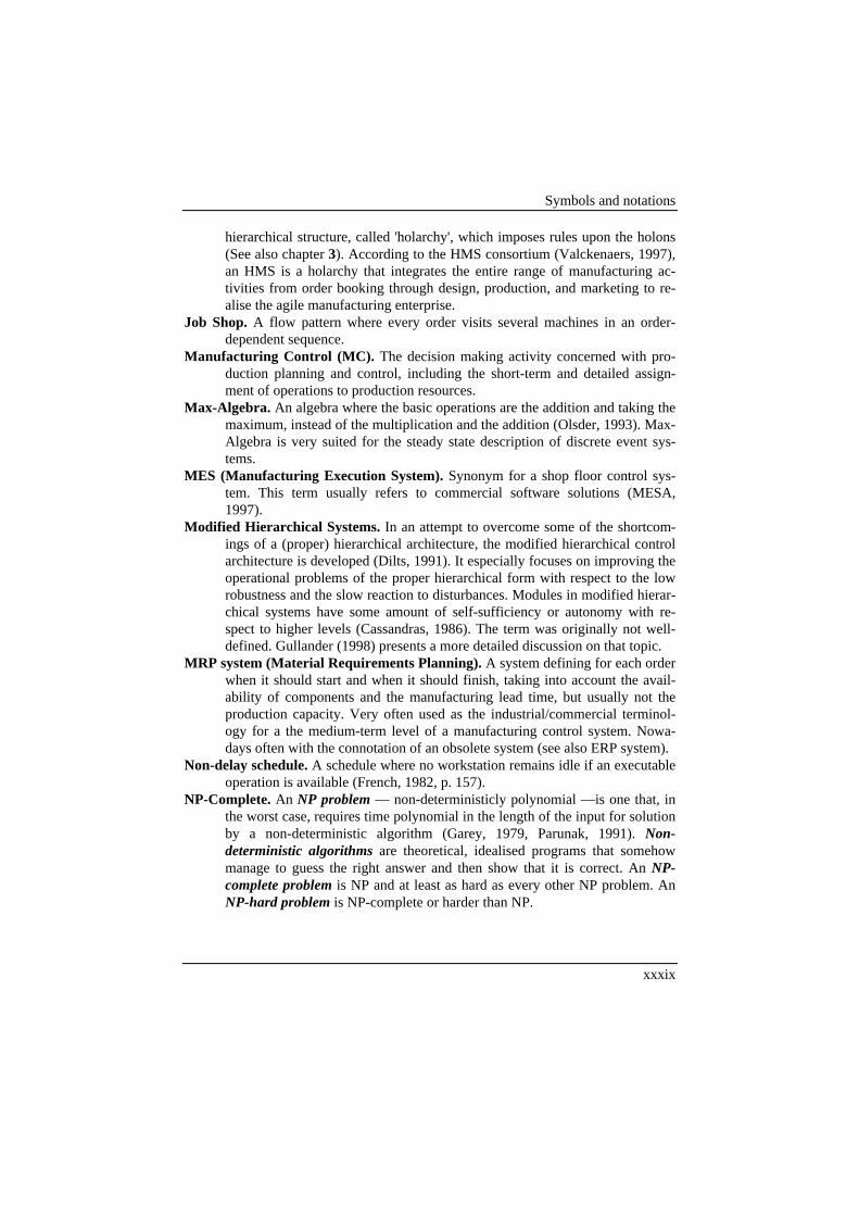
Symbols and notations
xxxix
hierarchical structure, called 'holarchy', which imposes rules upon the holons(See also chapter 3). According to the HMS consortium (Valckenaers, 1997),an HMS is a holarchy that integrates the entire range of manufacturing ac-tivities from order booking through design, production, and marketing to re-alise the agile manufacturing enterprise.
Job Shop. A flow pattern where every order visits several machines in an order-dependent sequence.
Manufacturing Control (MC). The decision making activity concerned with pro-duction planning and control, including the short-term and detailed assign-ment of operations to production resources.
Max-Algebra. An algebra where the basic operations are the addition and taking themaximum, instead of the multiplication and the addition (Olsder, 1993). Max-Algebra is very suited for the steady state description of discrete event sys-tems.
MES (Manufacturing Execution System). Synonym for a shop floor control sys-tem. This term usually refers to commercial software solutions (MESA,1997).
Modified Hierarchical Systems. In an attempt to overcome some of the shortcom-ings of a (proper) hierarchical architecture, the modified hierarchical controlarchitecture is developed (Dilts, 1991). It especially focuses on improving theoperational problems of the proper hierarchical form with respect to the lowrobustness and the slow reaction to disturbances. Modules in modified hierar-chical systems have some amount of self-sufficiency or autonomy with re-spect to higher levels (Cassandras, 1986). The term was originally not well-defined. Gullander (1998) presents a more detailed discussion on that topic.
MRP system (Material Requirements Planning). A system defining for each orderwhen it should start and when it should finish, taking into account the avail-ability of components and the manufacturing lead time, but usually not theproduction capacity. Very often used as the industrial/commercial terminol-ogy for a the medium-term level of a manufacturing control system. Nowa-days often with the connotation of an obsolete system (see also ERP system).
Non-delay schedule. A schedule where no workstation remains idle if an executableoperation is available (French, 1982, p. 157).
NP-Complete. An NP problem — non-deterministicly polynomial —is one that, inthe worst case, requires time polynomial in the length of the input for solutionby a non-deterministic algorithm (Garey, 1979, Parunak, 1991). Non-deterministic algorithms are theoretical, idealised programs that somehowmanage to guess the right answer and then show that it is correct. An NP-complete problem is NP and at least as hard as every other NP problem. AnNP-hard problem is NP-complete or harder than NP.

Symbols and notations
xl
On-line Manufacturing Control or on-line shop floor control (OMC / OSFC).The part of manufacturing control taking immediate decisions about resourceallocation.
Operation. Subtask of an order.Order. Task, usually composed of subtasks, that has to be executed for a customer.Performance graph. Graph that expresses schedule performance in function of cal-
culation time for a certain scenario (e.g. for static problems, for dynamicproblems).
Petri-net. A bipartite graph, consisting of transitions and places, used for describingand analysing discrete event systems (Petri, 1962, Peterson, 1981).
Predecessor operation. An operation oi,j1 of order i is a predecessor operation ofoperation oi,j2 if, for technological reasons, operation oi,j1 has to be executed(and to be finished) before operation oi,j2 can start.
Process (as computer terminology). A process is an independent piece of softwarerunning as a separate program on a computer. The operating system createsan environment in which the program can live, provides it with services likeprocessor, memory and I/O access, and protects it from other processes run-ning simultaneously on the same computer. Process can communicate withother processes in various ways (via sockets, files, semaphores, etc.), but theyusually cannot share memory.
Process Planning. A function that defines how products can be made, including theoverall process plan defining the possible sequences of operations for themanufacturing of a product and the detailed operation process planning, pre-scribing the parameters of the individual manufacturing processes.
Range of a partial derivative. The interval over which a partial derivative remainsvalid (i.e. over which it exists and is equal to the current value). For non-linear functions, it usually is a singleton. For linear functions, it is infinite. Forpiecewise linear functions, it is a finite interval.
Regular performance measure. A regular performance measure is a performancemeasure that does not deteriorate if some of the operation start times arescheduled earlier.
Resource Allocation. Deciding for all tasks when to happen and with which re-sources.
Resource. Object or material required for the execution of a task. Usually a piece ofequipment, usually only available with limited capacity.
Robust schedule. The property of a schedule that its performance does not deterio-rate (too much) if situation on the shop floor changes (machine breakdowns,stochastic disturbances, modelling errors, etc.).
Robustness. The property of a system that its performance remains acceptable if thecircumstances change. In manufacturing control, it refers to the degree inwhich the performance deteriorates if disturbances occur.
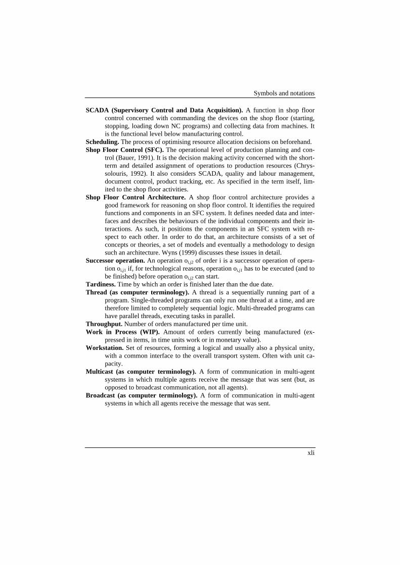
Symbols and notations
xli
SCADA (Supervisory Control and Data Acquisition). A function in shop floorcontrol concerned with commanding the devices on the shop floor (starting,stopping, loading down NC programs) and collecting data from machines. Itis the functional level below manufacturing control.
Scheduling. The process of optimising resource allocation decisions on beforehand.Shop Floor Control (SFC). The operational level of production planning and con-
trol (Bauer, 1991). It is the decision making activity concerned with the short-term and detailed assignment of operations to production resources (Chrys-solouris, 1992). It also considers SCADA, quality and labour management,document control, product tracking, etc. As specified in the term itself, lim-ited to the shop floor activities.
Shop Floor Control Architecture. A shop floor control architecture provides agood framework for reasoning on shop floor control. It identifies the requiredfunctions and components in an SFC system. It defines needed data and inter-faces and describes the behaviours of the individual components and their in-teractions. As such, it positions the components in an SFC system with re-spect to each other. In order to do that, an architecture consists of a set ofconcepts or theories, a set of models and eventually a methodology to designsuch an architecture. Wyns (1999) discusses these issues in detail.
Successor operation. An operation oi,j2 of order i is a successor operation of opera-tion oi,j1 if, for technological reasons, operation oi,j1 has to be executed (and tobe finished) before operation oi,j2 can start.
Tardiness. Time by which an order is finished later than the due date.Thread (as computer terminology). A thread is a sequentially running part of a
program. Single-threaded programs can only run one thread at a time, and aretherefore limited to completely sequential logic. Multi-threaded programs canhave parallel threads, executing tasks in parallel.
Throughput. Number of orders manufactured per time unit.Work in Process (WIP). Amount of orders currently being manufactured (ex-
pressed in items, in time units work or in monetary value).Workstation. Set of resources, forming a logical and usually also a physical unity,
with a common interface to the overall transport system. Often with unit ca-pacity.
Multicast (as computer terminology). A form of communication in multi-agentsystems in which multiple agents receive the message that was sent (but, asopposed to broadcast communication, not all agents).
Broadcast (as computer terminology). A form of communication in multi-agentsystems in which all agents receive the message that was sent.
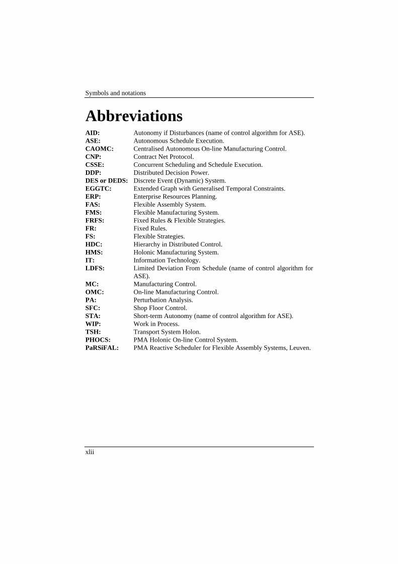
Symbols and notations
xlii
AbbreviationsAID: Autonomy if Disturbances (name of control algorithm for ASE).ASE: Autonomous Schedule Execution.CAOMC: Centralised Autonomous On-line Manufacturing Control.CNP: Contract Net Protocol.CSSE: Concurrent Scheduling and Schedule Execution.DDP: Distributed Decision Power.DES or DEDS: Discrete Event (Dynamic) System.EGGTC: Extended Graph with Generalised Temporal Constraints.ERP: Enterprise Resources Planning.FAS: Flexible Assembly System.FMS: Flexible Manufacturing System.FRFS: Fixed Rules & Flexible Strategies.FR: Fixed Rules.FS: Flexible Strategies.HDC: Hierarchy in Distributed Control.HMS: Holonic Manufacturing System.IT: Information Technology.LDFS: Limited Deviation From Schedule (name of control algorithm for
ASE).MC: Manufacturing Control.OMC: On-line Manufacturing Control.PA: Perturbation Analysis.SFC: Shop Floor Control.STA: Short-term Autonomy (name of control algorithm for ASE).WIP: Work in Process.TSH: Transport System Holon.PHOCS: PMA Holonic On-line Control System.PaRSiFAL: PMA Reactive Scheduler for Flexible Assembly Systems, Leuven.
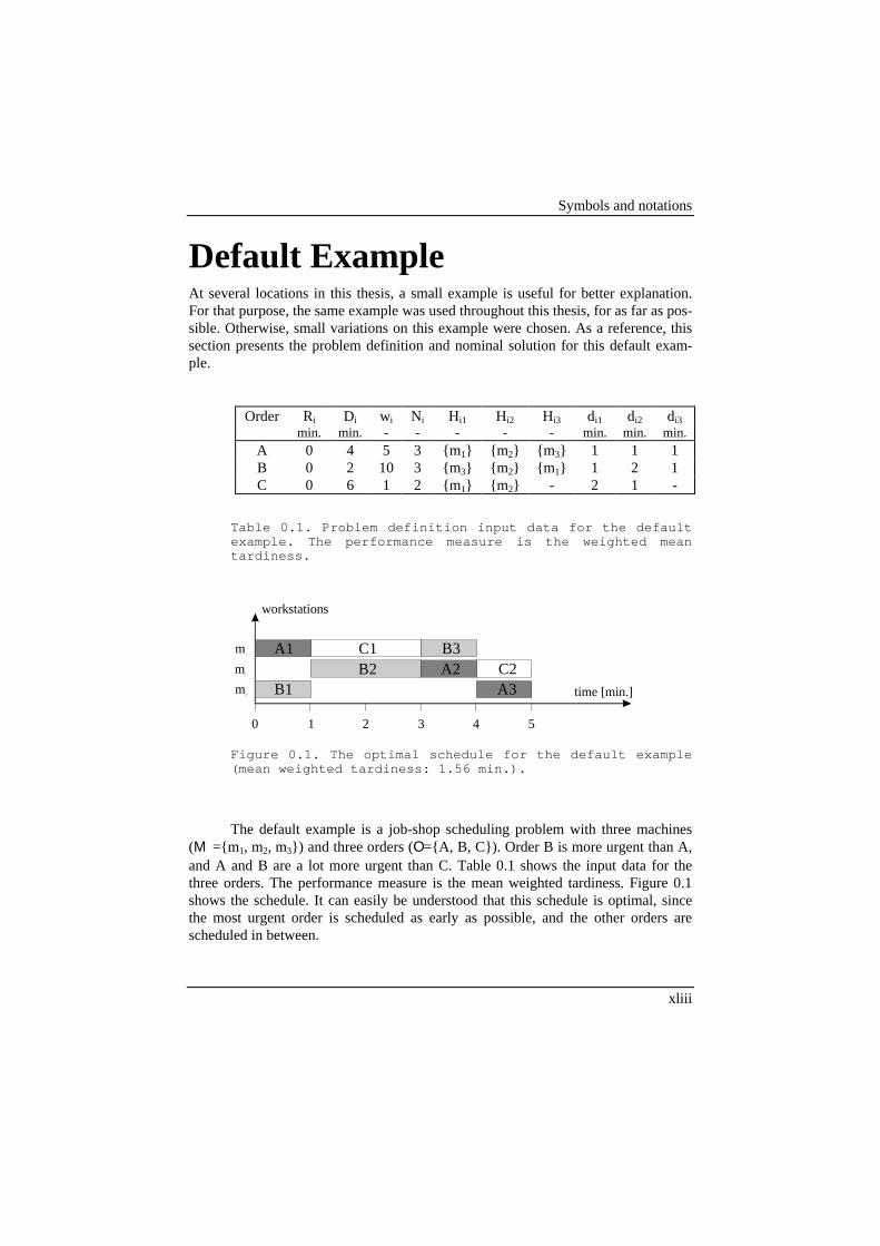
Symbols and notations
xliii
Default ExampleAt several locations in this thesis, a small example is useful for better explanation.For that purpose, the same example was used throughout this thesis, for as far as pos-sible. Otherwise, small variations on this example were chosen. As a reference, thissection presents the problem definition and nominal solution for this default exam-ple.
Order Ri Di wi Ni Hi1 Hi2 Hi3 di1 di2 di3
min. min. - - - - - min. min. min.A 0 4 5 3 {m1} {m2} {m3} 1 1 1B 0 2 10 3 {m3} {m2} {m1} 1 2 1C 0 6 1 2 {m1} {m2} - 2 1 -
Table 0.1. Problem definition input data for the defaultexample. The performance measure is the weighted meantardiness.
0 1 2 3 4 5
m1
m2
m3 time [min.]
workstations
A1
B1
C1B2
B3A2
A3C2
Figure 0.1. The optimal schedule for the default example(mean weighted tardiness: 1.56 min.).
The default example is a job-shop scheduling problem with three machines(M={m1, m2, m3}) and three orders (O={A, B, C}). Order B is more urgent than A,and A and B are a lot more urgent than C. Table 0.1 shows the input data for thethree orders. The performance measure is the mean weighted tardiness. Figure 0.1shows the schedule. It can easily be understood that this schedule is optimal, sincethe most urgent order is scheduled as early as possible, and the other orders arescheduled in between.

Symbols and notations
xliv

xlv
Table of ContentsVoorwoord — Preface................................................................................................iiAbstract....................................................................................................................... vBeknopte samenvatting .............................................................................................viiSamenvatting (Dutch Summary) ................................................................................ ixSymbols and Notations ........................................................................................xxxiiiGlossary ............................................................................................................... xxxviAbbreviations...........................................................................................................xliiDefault Example .....................................................................................................xliiiTable of Contents..................................................................................................... xlv
Chapter 1: Introduction............................................................................................... 11.1 Terms of Reference........................................................................................... 11.2 Shop Floor Control ........................................................................................... 2
1.2.1 Definition of Shop Floor Control............................................................... 21.2.2 Shop Floor Control Functions.................................................................... 41.2.3 Classification of Manufacturing Systems................................................... 5
1.3 Scheduling ........................................................................................................ 61.3.1 Definition................................................................................................... 61.3.2 Mathematical Model for Job Shop Scheduling .......................................... 61.3.3 Gantt Chart................................................................................................. 91.3.4 Why scheduling is difficult ...................................................................... 10
1.4 On-line Manufacturing Control....................................................................... 111.5 Problem Formulation ...................................................................................... 111.6 Objectives ....................................................................................................... 13
1.6.1 Scope ....................................................................................................... 131.6.2 Holonic Systems as Source of Inspiration................................................ 141.6.3 Continuous scheduling, concurrently with on-line control....................... 141.6.4 Approach ................................................................................................. 16
1.7 Overview of the thesis..................................................................................... 161.7.1 Main contributions................................................................................... 161.7.2 Detailed overview .................................................................................... 18
Chapter 2: Literature Survey..................................................................................... 212.1 Introduction..................................................................................................... 212.2 Traditional Shop Floor Control Research ....................................................... 22
2.2.1 SFC Architectures.................................................................................... 22
Table of Contents
xlvi
2.2.2 Scheduling ............................................................................................... 242.2.3 Automated On-line Control of Manufacturing Systems........................... 28
2.3 New Approaches to Shop Floor Control......................................................... 292.3.1 Modified Hierarchical Architectures........................................................ 292.3.2 New developments in scheduling............................................................. 302.3.3 New Developments in On-line Manufacturing Control ........................... 352.3.4 Distributed Scheduling and Control......................................................... 37
2.4 Industrial Practice ........................................................................................... 402.5 Conclusions..................................................................................................... 41
Chapter 3: Holonic Manufacturing Systems ............................................................. 433.1 Introduction..................................................................................................... 433.2 Concepts behind Holonic Manufacturing ....................................................... 44
3.2.1 The Roots of Holonics ............................................................................. 443.2.2 Holonic Manufacturing Systems.............................................................. 453.2.3 Additional sources of inspiration ............................................................. 463.2.4 Practical requirements for holonic manufacturing ................................... 47
3.3 Literature Survey on Holonic Manufacturing ................................................. 473.4 Reference Architecture for Holonic Manufacturing........................................ 50
3.4.1 Basic Holons............................................................................................ 503.4.2 Aggregation and Specialisation................................................................ 523.4.3 Staff Holons ............................................................................................. 523.4.4 Resource Allocation versus Process Control ........................................... 543.4.5 Modelling................................................................................................. 543.4.6 Reconfigurability ..................................................................................... 543.4.7 Conclusion ............................................................................................... 55
3.5 Resource Allocation in Holonic Manufacturing.............................................. 553.6 Process Control in Holonic Manufacturing..................................................... 573.7 Implementations at the PMA Testbeds ........................................................... 583.8 Conclusions..................................................................................................... 60
Chapter 4: Control Architecture for Holonic Manufacturing.................................... 614.1 Introduction..................................................................................................... 614.2 Concepts ......................................................................................................... 62
4.2.1 Hierarchy in Distributed Control ............................................................. 624.2.2 Distributed Decision Power ..................................................................... 664.2.3 Simultaneous and Asynchronous Scheduling and Schedule Execution ... 68
4.3 Functional and Structural Models ................................................................... 734.3.1 Modelling requirements ........................................................................... 734.3.2 Functional Model for Holonic Manufacturing Control ............................ 744.3.3 Structural Model for Holonic Manufacturing Control ............................. 764.3.4 Operation ................................................................................................. 77
Table of Contents
xlvii
4.3.5 Implications and remarks ......................................................................... 834.4 Modelling Distributed Decision Power........................................................... 84
4.4.1 Background.............................................................................................. 844.4.2 Fixed Rules in Holonic Systems .............................................................. 854.4.3 Fixed Rules as Requirements or Fixed Rules as Description Method...... 864.4.4 Prescriptive Approach.............................................................................. 864.4.5 Descriptive Approach .............................................................................. 874.4.6 Flexible Strategies.................................................................................... 884.4.7 Conclusion ............................................................................................... 88
4.5 Modelling Framework for the Interaction Mechanism.................................... 884.5.1 Requirements ........................................................................................... 894.5.2 Petri nets to model the interaction mechanism......................................... 89
4.6 Conclusion ...................................................................................................... 90
Chapter 5: Interaction Mechanism............................................................................ 915.1 Introduction..................................................................................................... 915.2 Basic Design of the Interaction Mechanism.................................................... 92
5.2.1 Timed, Stochastic, Conditional and Controlled Petri Nets ...................... 935.2.2 Interaction between Scheduling Holon and OMC Holon......................... 965.2.3 Interaction between Order Holon and Resource Holon ......................... 1015.2.4 Interaction Between Local Holons and Staff Holons ............................. 1085.2.5 Conclusion ............................................................................................. 109
5.3 Timing Issues................................................................................................ 1105.4 Event Based Rescheduling............................................................................ 1135.5 Parameter Optimisation ................................................................................ 115
5.5.1 Parameters to be Tuned.......................................................................... 1165.5.2 Basic Analysis of CSSE......................................................................... 1095.5.3 Conservative Analysis of CSSE............................................................. 1135.5.4 Conclusion ............................................................................................. 115
5.6 Inter-Holon Communication ......................................................................... 1155.7 Conclusion .................................................................................................... 116
Chapter 6: Holonic Control Strategies ................................................................... 1196.1 Introduction................................................................................................... 1196.2 Schedule execution ....................................................................................... 1206.3 Schedule represented as a graph ................................................................... 124
6.3.1 Precondition on the Schedule................................................................. 1246.3.2 Recursive Formula for the Starting Time of an Operation..................... 1256.3.3 Graph ..................................................................................................... 1256.3.4 Performance........................................................................................... 127
6.4 Literature review........................................................................................... 1276.5 Hierarchical Control ..................................................................................... 128
Table of Contents
xlviii
6.5.1 Informal Description.............................................................................. 1286.5.2 Formal Description ................................................................................ 129
6.6 Heterarchical Control.................................................................................... 1296.6.1 Informal Description.............................................................................. 1296.6.2 Formal Description ................................................................................ 130
6.7 Centralised Autonomous On-line Control..................................................... 1326.7.1 Informal Description.............................................................................. 1326.7.2 Formal Description ................................................................................ 133
6.8 Heuristic Holonic Control Strategies ............................................................ 1346.8.1 Short Term Autonomy ........................................................................... 1356.8.2 Autonomy if Disturbances ..................................................................... 1366.8.3 Limited Deviation from Schedule .......................................................... 1376.8.4 Conclusion ............................................................................................. 138
6.9 Schedule Execution with Perturbation Analysis ........................................... 1396.9.1 Basic Idea .............................................................................................. 1396.9.2 Co-operation Schema: Overall View ..................................................... 1406.9.3 Definition of Local Decision Parameters ............................................... 1406.9.4 Performance in Function of Local Decision Parameters ........................ 1426.9.5 Calculations for the Scheduling Holon .................................................. 1436.9.6 Calculations for the OMC Holon ........................................................... 1476.9.7 Examples................................................................................................ 1486.9.8 Concluding Remarks.............................................................................. 154
6.10 Conclusion .................................................................................................. 155
Chapter 7: Design and Implementation................................................................... 1577.1 Introduction................................................................................................... 1577.2 The Software Design Process ....................................................................... 1577.3 Testbeds ........................................................................................................ 1597.4 Design ........................................................................................................... 162
7.4.1 PaRSiFAL.............................................................................................. 1627.4.2 PHOCS .................................................................................................. 1687.4.3 Design Workstation Holons ................................................................... 1717.4.4 Design Order Holons ............................................................................. 1727.4.5 Design Transport System Holon ............................................................ 172
7.5 Implementation ............................................................................................. 1737.6 Conclusions................................................................................................... 174
Chapter 8: Experiments .......................................................................................... 1758.1 Introduction................................................................................................... 1758.2 Design of experiments .................................................................................. 175
8.2.1 Literature survey: ................................................................................... 1758.2.2 Approach taken ...................................................................................... 176
Table of Contents
xlix
8.2.3 Overview................................................................................................ 1808.3 Testability ..................................................................................................... 180
8.3.1 Goal ....................................................................................................... 1808.3.2 Repeatability .......................................................................................... 1808.3.3 Generalisation ........................................................................................ 1838.3.4 Predictability.......................................................................................... 1848.3.5 Conclusion ............................................................................................. 185
8.4 Hierarchy in Distributed Control .................................................................. 1858.4.1 Performance degradation of hierarchical control under disturbances .... 1858.4.2 Missed Opportunities of Heterarchical Control ..................................... 1888.4.3 Comparison with Holonic Control Strategies ........................................ 189
8.5 Distributed Decision Power .......................................................................... 1898.6 Concurrent Scheduling and Schedule Execution .......................................... 1908.7 Assessment of Holonic ASE Control Algorithms ......................................... 1928.8 Conclusion .................................................................................................... 193
Chapter 9: Conclusions ........................................................................................... 1959.1 Main Results ................................................................................................. 1959.2 Recommendations for Future Work.............................................................. 196
References............................................................................................................... 199
Appendix A: Matlab program to analyse CSSE...................................................... 221

Table of Contents
l

1
Chapter 1
Introduction
This introductory chapter is organised as follows. Section 1.1 sketches the researchdomain for which this thesis is relevant. Sections 1.2, 1.3 and 1.4 explain the basicconcepts and terminology in this problem domain. Section 1.5 formulates the prob-lems in manufacturing control that motivated this research. It leads to the scope andobjectives, presented in section 1.6. Section 1.7 presents an overview of the thesisand identifies the main contributions.
1.1 Terms of ReferenceEven in these post-industrial times, manufacturing is one of the cornerstones of oursociety. For several years, research has focused on several aspects of manufacturing,from the individual processes towards the management of virtual enterprises, butseveral aspects, like shop floor control, still have relevant problems in industry andremain challenging areas of research.
This thesis focuses on the operational level of production planning and con-trol systems, normally referred to as shop floor control (SFC — Bauer, 1991) ormanufacturing control (MC). SFC is the decision making activity concerned with theshort-term and detailed assignment of operations to production resources (Chryssol-ouris, 1992). It comprises the scheduling and control aspects in manufacturing. Sincethe upsurge of computer control, SFC problems were addressed extensively in re-search (see chapter 2). Nowadays, also in industry, computer based SFC is being in-troduced on a wide scale.
SFC proves to be a very complex problem. To start with, many optimisationproblems in manufacturing, like scheduling, are computationally complex problems,which means that the calculation time needed for finding the optimal solution growsbeyond reasonable bounds for a realistic size of the problem (Garey, 1979, French,1982, Parunak, 1991, Herroelen, 1991). Secondly, the shop floor is continuouslysubject to all kinds of disturbances, ranging from modelling errors and stochastic de-viations on the expected operation processing time to rush orders and machinebreakdowns (Lin, 1994, p. 171, Peeters, 1998). Thirdly, manufacturing systems tendto be at the edge of chaos (Waldrop, 1992, Dooley, 1996). Systems with almostidentical initial conditions can evolve towards totally different situations.
Improving SFC performance is an important issue in manufacturing. Due tothe ever increasing competition, short and reliable delivery times are essential, with-out room for concessions on product cost or quality (Valckenaers, 1997). SFC af-
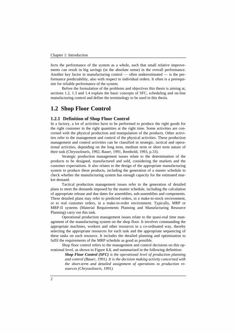
Chapter 1: Introduction
2
fects the performance of the system as a whole, such that small relative improve-ments can result in big savings (in the absolute sense) in the overall performance.Another key factor in manufacturing control — often underestimated — is the per-formance predictability, also with respect to individual orders. It often is a prerequi-site for reliable performance of the system.
Before the formulation of the problems and objectives this thesis is aiming at,sections 1.2, 1.3 and 1.4 explain the basic concepts of SFC, scheduling and on-linemanufacturing control and define the terminology to be used in this thesis.
1.2 Shop Floor Control
1.2.1 Definition of Shop Floor ControlIn a factory, a lot of activities have to be performed to produce the right goods forthe right customer in the right quantities at the right time. Some activities are con-cerned with the physical production and manipulation of the products. Other activi-ties refer to the management and control of the physical activities. These productionmanagement and control activities can be classified in strategic, tactical and opera-tional activities, depending on the long term, medium term or short term nature oftheir task (Chryssolouris, 1992, Bauer, 1991, Rembold, 1993, p.33).
Strategic production management issues relate to the determination of theproducts to be designed, manufactured and sold, considering the markets and thecustomer expectations. It also relates to the design of the appropriate manufacturingsystem to produce these products, including the generation of a master schedule tocheck whether the manufacturing system has enough capacity for the estimated mar-ket demand.
Tactical production management issues refer to the generation of detailedplans to meet the demands imposed by the master schedule, including the calculationof appropriate release and due dates for assemblies, sub-assemblies and components.These detailed plans may refer to predicted orders, in a make-to-stock environment,or to real customer orders, in a make-to-order environment. Typically, MRP orMRP-II systems (Material Requirements Planning and Manufacturing ResourcePlanning) carry out this task.
Operational production management issues relate to the quasi-real time man-agement of the manufacturing system on the shop floor. It involves commanding theappropriate machines, workers and other resources in a co-ordinated way, therebyselecting the appropriate resources for each task and the appropriate sequencing ofthese tasks on each resource. It includes the detailed planning and optimisation tofulfil the requirements of the MRP schedule as good as possible.
Shop floor control refers to the management and control decisions on this op-erational level, as shown in Figure 1.1, and summarised in the following definition:
Shop Floor Control (SFC) is the operational level of production planningand control (Bauer, 1991). It is the decision making activity concerned withthe short-term and detailed assignment of operations to production re-sources (Chryssolouris, 1991).
Chapter 1: Introduction
3
Grey boxes indicate manufacturing control activities
...
...
Supply chain management
...
Engineering
Financial management
Personnel management
MRP
Purchasing
CapacityPlanning
Master Production Schedule
Demand Forecast
Facility planning
Manufacturing planning
...
Quality Management
Document Control
Maintenance
Process
Data capturing
Monitoring
Manufacturing Control
Marketing
Sales
non manufacturing activities
short term: operational planning: Shop Floor
medium term: tactical
physical activities
Management and Control
long term: strategic
Figure 1.1. Definition of Shop Floor Control and rela-tions of SFC with other activities in the enterprise. SFCexplicitly refers to the activities on the shop floor,and as such, it does not include pure office activitieslike sales, marketing, etc. This figure also situatesmanufacturing control (see subsection 1.2.2) with respectto SFC.

Chapter 1: Introduction
4
1.2.2 Shop Floor Control FunctionsThe main function of SFC is resource allocation, also called manufacturing con-trol. As stated above, resource allocation is also performed at the tactical and strate-gic level of production management. SFC refers to the operational level of resourceallocation only. This usually includes a detailed short-term scheduler, which plansand optimises the resource allocation on beforehand, considering all production re-quirements and constraints (Bauer, 1991). Typically, scheduling has a total time spanranging between a few weeks and a day, and a time granularity ranging from days tillbelow minutes. When the schedule is calculated, it is implemented on the shop floorby a dispatcher, taking into account the current status of the production system(Bauer, 1991). This function is called on-line manufacturing control (OMC). Dur-ing OMC, the status of the vital components in the system is monitored.
Shop floor control also covers process management (Mesa, 1997). Processmanagement includes machine and process monitoring and control, but also the op-erational level activities for process planning. The process planning function defineshow products can be made, including the overall process plan defining the possiblesequences of operations for to manufacture a product and the detailed operation pro-cess planning, prescribing the parameters of the individual manufacturing steps. Intraditional manufacturing systems, process planning provides shop floor control witha single sequence of operations to be executed for each product. Recently, processplanning is considering more flexible solutions, based on the use of alternativeroutings, and alternative machine allocations. The use of alternative routings, mod-elled e.g. by precedence graphs (French, 1982,), dynamic precedence graphs(Valckenaers, 1993) or Petri nets (Detand, 1993) enables shop floor control to selectthe best sequence of operations depending on the machine load and unforeseen dis-turbances. The use of alternative resources for an operation gives similar opportuni-ties. Process management also includes operational aspects of manufacturing systemdesign, layouting and configuration. Depending on the flexibility of the manufactur-ing system, the manufacturing system may be adaptable on short term. It are theseshort-term modifications and set-ups that are managed by shop floor control.
Shop floor control further needs to provide information to people and ma-chines at the right moment. It therefore has to collect, store and retrieve these dataand provide them to the people in the right quantity and level of aggregation. Thisfunction includes data capturing from the machines and the analysis of these rawdata. It also is concerned with the management of the programs for NC-machines,and with quality and labour management (MESA, 1997).
Shop floor control relates to several other activities in an enterprise, like mar-keting, design, process planning, sales, purchasing, medium and long term planning,distribution, and servicing, to which it has to interface. Via the sales function, neworders are introduced in the shop. Orders can be directly assigned to customers, orthey may be stock replenishment orders, in a make-to-stock environment. In industry,very often mixtures of a make-to stock and make-to-order environment are found andpragmatically dealt with. Traditionally, shop floor control considers sales as a blackbox, generating orders with a stochastic distribution. Medium-range planning pro-

Chapter 1: Introduction
5
vides shop floor control with due dates and release dates for orders. It defines for alarge amount the performance objectives for shop floor control. In this thesis, duedates and release dates for orders are given and fixed.
1.2.3 Classification of Manufacturing SystemsThe characteristics of a manufacturing system like production volume, flexibility andlayout, have a major influence on its control. The complexity of the resource alloca-tion optimisation (“scheduling”, see below) and on-line control problems dependstrongly on the layout. Therefore, manufacturing control strategies differ considera-bly according to the corresponding layout.
Manufacturing systems and subsystems are often categorised according totheir production volume and their flexibility. Traditionally, the targeted productionvolume and flexibility of a manufacturing system are inversely proportional: high-volume manufacturing systems have a limited flexibility. Typical production typesrange from continuous production, over mass production, large batch manufacturing,discrete manufacturing, to one-of-a-kind and project-wise manufacturing. This thesisis restricted to discrete manufacturing and one-of-a-kind production.
Within discrete manufacturing, manufacturing systems are classified by theirlayout (usually related to the way products flow through the manufacturing system).The rest of this subsection surveys the main production layouts relevant for this the-sis. The single machine model (French, 1982, Bauer, 1991) has the most simplelayout. It consists of a single machine that performs all operations. Therefore, ordersusually are not further decomposed into operations. The identical processors model(French, 1982, p. 200) is similar to the single machine model, but consists of multi-ple, identical machines. A flow shop (French, 1982, Ch. 5) consists of different ma-chines, processing orders with multiple operations, where• each operation is to be executed on a specific machine;• all operations of an order have to be executed in a fixed sequence;• all orders have to visit the machines in the same sequence.A job shop is the same as a flow shop, except that each order can visit the machinesin a different sequence. This thesis focuses on the job shop layout, as it is the mostgeneral case.
These layout models refer to more specific manufacturing systems, like facto-ries with a bottleneck, lines, flexible manufacturing systems (FMS), or flexible flowshops (FFS). For some aspects of the control of factories with a bottleneck, the sin-gle machine model performs quite adequately (Goldratt, 1984, French 1982). As-sembly lines usually are flow shops with limited or no opportunities for orders over-taking each other. Flexible manufacturing systems are extended job shops (ElMagrini, 1996, Bongaerts, 1998), where• operations of orders follow a sequence allowed by a precedence graph instead of
a fixed operation sequence;• different workstations can perform the same operation; and• transport and set-up have to be modelled.
Chapter 1: Introduction
6
Recently (Peeters, 1997, Lei, 1997, Bussmann, 1997), flexible flow shops are be-coming more important: they inherit the layout and properties of flow shops, buthave an increased flexibility with respect to machines selection, operation sequenc-ing and sometimes even routing flexibility. In this respect, they are mathematicallymore similar to job shops. However, while all routings are feasible, some routingsare highly preferable. In this way, they combine the efficiency and transparency of aflow line with the reactivity and flexibility of a job shop. Such manufacturing sys-tems are promising to break the compromise between flexibility and high volumeproduction as it is found in traditional manufacturing systems.
1.3 Scheduling
1.3.1 DefinitionScheduling is defined as the process of optimising resource allocation decisions onbeforehand. Resource allocation is deciding for all tasks when to happen and withwhich resources (Parunak, 1991). In literature, the difference between these twoterms is not always made. For this thesis however, the difference is important.
Scheduling is an optimisation process, and thus refers to one or more goals(also called objectives, or performance criteria). Typical performance criteria in amanufacturing context are:• the throughput (Q), defined as the number of orders the manufacturing system
finishes per time unit;• the work-in-process inventory (WIP), defined as the number of orders in the
system which are not finished yet;• the mean order flow time (or lead time, F , defined as the difference between the
order finish time and the order start time); and• the mean order tardiness T (The tardiness is the difference between the order
finish time and the due date, if this difference is positive. Otherwise, the tardinessis 0.).
The resource allocation process usually is subject to constraints. In practicalsituations, not all possible resource allocation decisions are feasible. Typical con-straints express the limited capacity of a resource, or precedence relations betweenoperations.
1.3.2 Mathematical Model for Job Shop SchedulingFor a clear understanding of scheduling and manufacturing control, it is often helpfulto define a mathematical model of the scheduling problem. Such a model is stronglydependent on the specific manufacturing system focused at. Therefore, this subsec-tion defines a mathematical model for (extended) job shop scheduling that is directlyrelated to the problem under the study scope of this thesis. The model can be repre-sented as follows.
To define the symbols, suppose the manufacturing system consists of Mworkstations mk, with k ranging from 0 till M-1. Let M denote the set of worksta-tions. There also are A auxiliary resources ra in the system, with “a” ranging from 0
Chapter 1: Introduction
7
till A-1. If necessary, these auxiliary resources can be distributed among the work-stations. Let A denote the set of auxiliary resources. Consider the set of orders O,with N orders i, for i ranging from 0 till N-1. Each order i has• a release date Ri, denoting the time an order enters the system;• a due date Di, denoting the time the order should be ready; and• a weight wi, denoting the importance of an order.Each order i has a number of operations (i,j), for j ranging from 0 to Ni -1. Each op-eration (i,j) can be executed on a set of alternative workstations
Hi,j = {hi,j,l ∈ M | hi,j,l can execute operation (i,j).}, (1.1)
(for l ranging from 0 to #Hi,j - 1). If operation (i,j) can be executed on workstation k(i.e. if mk ∈ Hi,j), it has a duration di,j,k, otherwise, di,j,k is undefined. If the duration isthe same for all alternative workstations, di,j,k can be simplified to di,j. Given thesedata, the resource allocation process selects which workstation hi,j will execute op-eration (i,j) and at which time bi,j it will start. In other words, hi,j and bi,j are the deci-sion variables. ci,j is the resulting completion time of operation (i,j):
hjiijij dbc ,,+= , (1.2)
where hjid ,, is short for ijhjid ,, . Ci is the order completion time:
1, −=iNii cC . (1.3)
The resource allocation problem is subject to capacity constraints and prece-dence constraints. Capacity constraints express that a machine can only execute oneoperation at the same time. To introduce a mathematical formulation of the capacityconstraints, Hoitomt (1989) and Luh (1993) use a formulation with discretised time tand Kronecker deltas:
1)-M0,1,2,...,=k ;T1,2,...,=(t , hor,,, tkij ktji M≤δ∑ , (1.4)
where Mtk is the capacity of workstation mk at time t, and δi,j,t,k = 1 if operation (i,j)occupies workstation mk at time t, and otherwise δi,j,t,k = 0. Thor is the time horizon.Another way to represent capacity constraints is by pairs of inequalities:
, or
: if
:),(),( ),,(),,(
1111222222222221111111
2211
,,
22112211
jijijihjijijijijihjiji
jiji
bSUdbbSUdb
hh
jijijiji
≤++≤++
=≠∀
(1.5)
where SUi1j1,i2j1 is the set-up time on machine hi1,j1 between operations (i1,j1) and(i2,j2). For auxiliary resources, like pallets or tools, similar constraints can be de-fined.
Precedence relations can be modelled with sequences of operations (French,1982, Ch. 1), with precedence graphs (e.g. French, 1982, Ch. 4, Hoitomt, 1990),simple fork-join precedence constraints (Luh, 1993), assembly trees (Czerwinski,1994, Lei, 1997), dynamic precedence graphs (Valckenaers, 1993) or non-linearprocess plans (Detand, 1993, Kruth, 1994). A good compromise between flexibility
Chapter 1: Introduction
8
and modelling complexity are precedence graphs. Precedence graphs can also bemapped to the following set of inequalities:
);2,...,20,1,=;1,...,10,=( , ijiisijsij SsNjNibTRc ∈−−≤+ , (1.6)
where (i,s) is a successor operation of (i,j), Sij is the set of successor operations of(i,j) and TRijs is the transport time between operation (i,j) and (i,s). The same set ofinequalities can also be written as:
);1,...,2,1=;1,...,20,1,=( , ijiijipjip PpNjNibTRc ∈−−≤+ , (1.7)
where (i,p) is a predecessor operation of (i,j) and Pij is the set of predecessors of (i,j).By convention and without loss of generality, (i,0) is an operation without predeces-sors and (i,Ni-1) is an operation without successors. A special type of precedenceconstraint refers to the release date of an order:
R b i Ni i≤ −,0 2 1 , ( = 0,1, , ..., ) , (1.8)
The experienced reader may notice that this representation of the schedulingproblem does not yet cover all situations and does not model all possible sources offlexibility in full detail. For instance, and-or graphs can better model choicesamongst processes that imply different sets of operations. For machines with multi-ple capacity, the exact modelling of set-ups and loading becomes more complex.However, complete modelling of the scheduling problem becomes too complex toaddress in a generic way and too problem specific to describe in this thesis. Themodel of the scheduling problem described in this thesis is the result of what I con-sider to be a good compromise between genericity and modelling complexity.
The performance objectives considered in this thesis are the mean order flowtime and the mean order tardiness. They can easily be expressed in function of theoperation start times. The mean flow time F is the time the order stays in the sys-tem. Depending on the definition of the order entry time, two definitions are possi-ble:
( )F F F F C b
C b
Nav b b av i i
i ii= = = = − =
−∑0 0 0
0
( )
( )
,
,(1.9)
is the most general definition for flow time. It rewards detailed scheduling and on-line control processes that minimise flow time (and inventory) by postponing thestarting time of an operation. However, since postponing operations for flow timeminimisation makes the schedule more susceptible to disturbances, the responsibili-ties of shop floor control with respect to inventory minimisation usually are limitedto the decrease of the order completion times. Therefore, the MRP system deter-mines the time the order may enter the system. The corresponding definition for flowtime is as follows:
( )F F C R
C R
NR R av i i
i ii= = − =
−∑( )
( ). (1.10)
As indicated in equation (1.9), the flow time F refers by default to the first definition.The mean tardiness T reflects the delivery reliability:
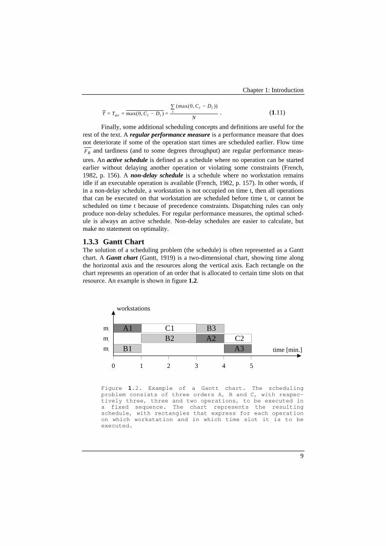
Chapter 1: Introduction
9
T T C D
C D
Nav i i
i ii= = − =
−∑max( , )
(max( , ))
0
0. (1.11)
Finally, some additional scheduling concepts and definitions are useful for therest of the text. A regular performance measure is a performance measure that doesnot deteriorate if some of the operation start times are scheduled earlier. Flow time
RF and tardiness (and to some degrees throughput) are regular performance meas-
ures. An active schedule is defined as a schedule where no operation can be startedearlier without delaying another operation or violating some constraints (French,1982, p. 156). A non-delay schedule is a schedule where no workstation remainsidle if an executable operation is available (French, 1982, p. 157). In other words, ifin a non-delay schedule, a workstation is not occupied on time t, then all operationsthat can be executed on that workstation are scheduled before time t, or cannot bescheduled on time t because of precedence constraints. Dispatching rules can onlyproduce non-delay schedules. For regular performance measures, the optimal sched-ule is always an active schedule. Non-delay schedules are easier to calculate, butmake no statement on optimality.
1.3.3 Gantt ChartThe solution of a scheduling problem (the schedule) is often represented as a Ganttchart. A Gantt chart (Gantt, 1919) is a two-dimensional chart, showing time alongthe horizontal axis and the resources along the vertical axis. Each rectangle on thechart represents an operation of an order that is allocated to certain time slots on thatresource. An example is shown in figure 1.2.
0 1 2 3 4 5
m1
m2
m3 time [min.]
workstations
A1
B1
C1B2
B3A2
A3C2
Figure 1.2. Example of a Gantt chart. The schedulingproblem consists of three orders A, B and C, with respec-tively three, three and two operations, to be executed ina fixed sequence. The chart represents the resultingschedule, with rectangles that express for each operationon which workstation and in which time slot it is to beexecuted.
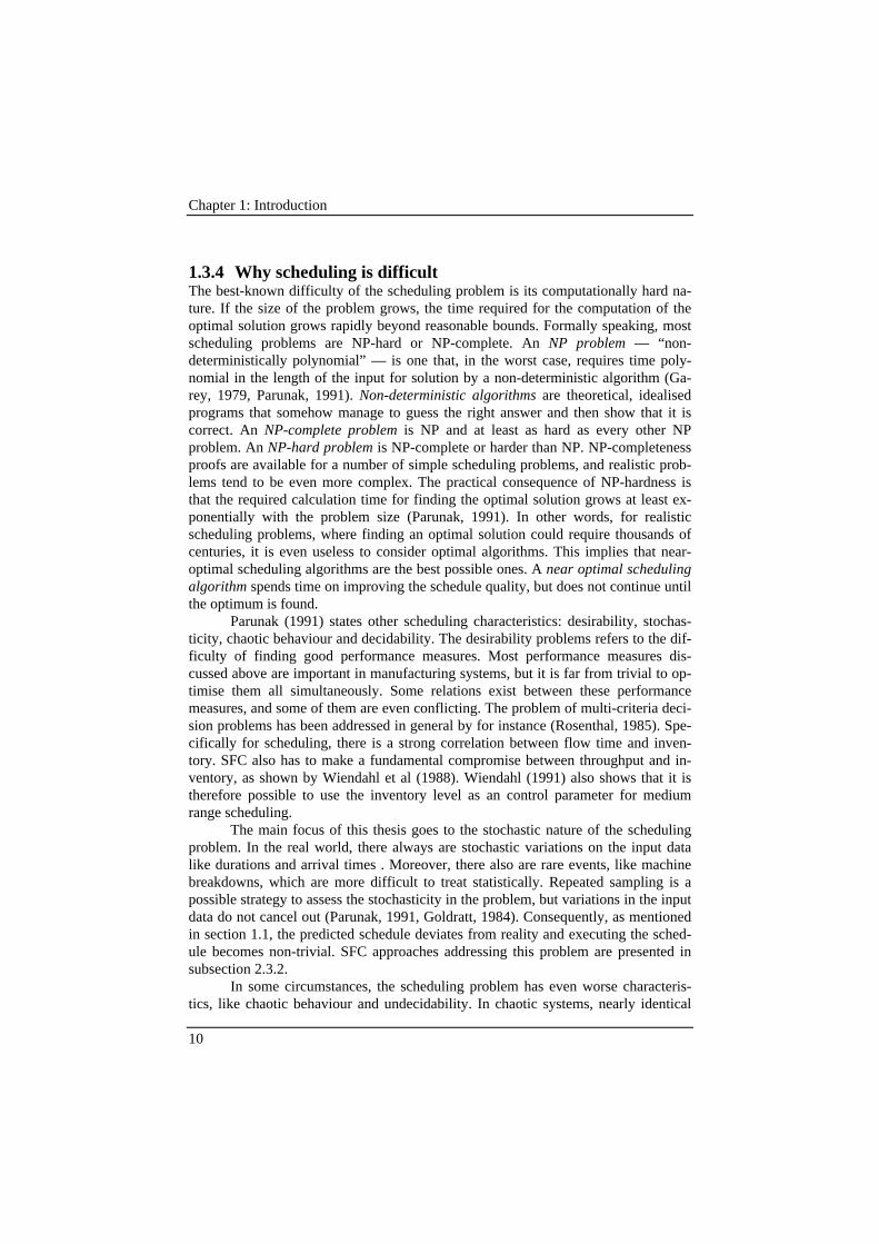
Chapter 1: Introduction
10
1.3.4 Why scheduling is difficultThe best-known difficulty of the scheduling problem is its computationally hard na-ture. If the size of the problem grows, the time required for the computation of theoptimal solution grows rapidly beyond reasonable bounds. Formally speaking, mostscheduling problems are NP-hard or NP-complete. An NP problem — “non-deterministically polynomial” — is one that, in the worst case, requires time poly-nomial in the length of the input for solution by a non-deterministic algorithm (Ga-rey, 1979, Parunak, 1991). Non-deterministic algorithms are theoretical, idealisedprograms that somehow manage to guess the right answer and then show that it iscorrect. An NP-complete problem is NP and at least as hard as every other NPproblem. An NP-hard problem is NP-complete or harder than NP. NP-completenessproofs are available for a number of simple scheduling problems, and realistic prob-lems tend to be even more complex. The practical consequence of NP-hardness isthat the required calculation time for finding the optimal solution grows at least ex-ponentially with the problem size (Parunak, 1991). In other words, for realisticscheduling problems, where finding an optimal solution could require thousands ofcenturies, it is even useless to consider optimal algorithms. This implies that near-optimal scheduling algorithms are the best possible ones. A near optimal schedulingalgorithm spends time on improving the schedule quality, but does not continue untilthe optimum is found.
Parunak (1991) states other scheduling characteristics: desirability, stochas-ticity, chaotic behaviour and decidability. The desirability problems refers to the dif-ficulty of finding good performance measures. Most performance measures dis-cussed above are important in manufacturing systems, but it is far from trivial to op-timise them all simultaneously. Some relations exist between these performancemeasures, and some of them are even conflicting. The problem of multi-criteria deci-sion problems has been addressed in general by for instance (Rosenthal, 1985). Spe-cifically for scheduling, there is a strong correlation between flow time and inven-tory. SFC also has to make a fundamental compromise between throughput and in-ventory, as shown by Wiendahl et al (1988). Wiendahl (1991) also shows that it istherefore possible to use the inventory level as an control parameter for mediumrange scheduling.
The main focus of this thesis goes to the stochastic nature of the schedulingproblem. In the real world, there always are stochastic variations on the input datalike durations and arrival times . Moreover, there also are rare events, like machinebreakdowns, which are more difficult to treat statistically. Repeated sampling is apossible strategy to assess the stochasticity in the problem, but variations in the inputdata do not cancel out (Parunak, 1991, Goldratt, 1984). Consequently, as mentionedin section 1.1, the predicted schedule deviates from reality and executing the sched-ule becomes non-trivial. SFC approaches addressing this problem are presented insubsection 2.3.2.
In some circumstances, the scheduling problem has even worse characteris-tics, like chaotic behaviour and undecidability. In chaotic systems, nearly identical

Chapter 1: Introduction
11
original conditions can lead to wide divergence in subsequent behaviour, making ac-curate scheduling and control difficult. Undecidable problems are problems forwhich it is proven that no program exists to solve it. Parunak (1991) addresses theseproblems in detail, and surveys available and future solutions for them.
1.4 On-line Manufacturing ControlBauer et al. (1991) define dispatching as the implementation of a schedule takinginto account the current status of the production system. This definition takes theexistence of a scheduler for granted. The dispatcher has to execute the schedule, re-acting to disturbances as quickly as possible. Therefore, the dispatcher has no time tooptimise its decisions. The task of a dispatcher seems to be straightforward, such thatusually, only simple heuristics are used for decision taking.
A more general term is on-line manufacturing control. As suggested by itsname, on-line manufacturing control refers to that part of manufacturing control thattakes immediate decisions. Traditionally, it is a synonym of “dispatching”. However,some new manufacturing paradigms that do not use scheduling, require a more gen-eral term that is not based on scheduling. Moreover, in the manufacturing world,“dispatching” refers to simple decision making, while on-line manufacturing controlalso refers to more advanced methods. (Originally, “dispatching” refers to promptand quick decision making (Makins, 1982). However, due to the NP-complete natureof resource allocation, dispatching in manufacturing quickly got the meaning of ap-plying simple priority rules.) Using an analogy, on-line manufacturing control is thetask of a foreman. Similar to dispatching, on-line manufacturing control has to reactquickly to disturbances, such that it cannot optimise the performance with time-intensive computations. The remainder of this thesis uses the term on-line manufac-turing control if the difference between dispatching and on-line (manufacturing)control is not important.
On-line manufacturing control also covers some more practical functions. Itincludes the management, downloading and starting of NC-programs on due time.While Bauer (1991) defines monitoring as a separate module, data acquisition andmonitoring (with a so-called SCADA system — Supervisory Control And Data Ac-quisition) is often performed by the on-line (manufacturing) control system. On-linemanufacturing control is not involved with process control, like adjusting the pa-rameters in the machining process or calculating the trajectory of a robot. If no con-fusion is possible, “on-line manufacturing control” often is shortened to “on-linecontrol”.
1.5 Problem FormulationThe current requirements for an SFC system are high. The SFC system has to main-tain a high performance and cost efficiency for the manufacturing systems, whilecoping with disturbances. It should enhance flexibility. Meanwhile, the SFC softwareitself should also be cheap and easy to reconfigure and to adapt to changing require-
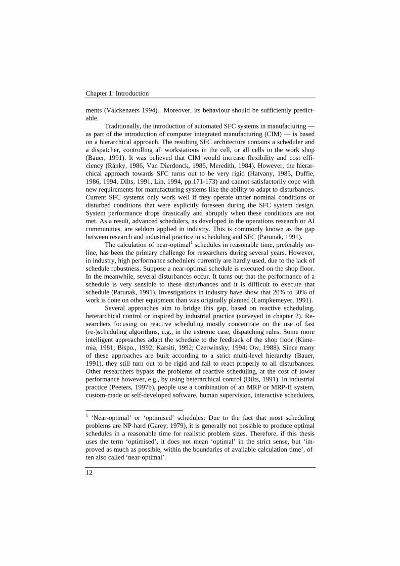
Chapter 1: Introduction
12
ments (Valckenaers 1994). Moreover, its behaviour should be sufficiently predict-able.
Traditionally, the introduction of automated SFC systems in manufacturing —as part of the introduction of computer integrated manufacturing (CIM) — is basedon a hierarchical approach. The resulting SFC architecture contains a scheduler anda dispatcher, controlling all workstations in the cell, or all cells in the work shop(Bauer, 1991). It was believed that CIM would increase flexibility and cost effi-ciency (Ránky, 1986, Van Dierdonck, 1986, Meredith, 1984). However, the hierar-chical approach towards SFC turns out to be very rigid (Hatvany, 1985, Duffie,1986, 1994, Dilts, 1991, Lin, 1994, pp.171-173) and cannot satisfactorily cope withnew requirements for manufacturing systems like the ability to adapt to disturbances.Current SFC systems only work well if they operate under nominal conditions ordisturbed conditions that were explicitly foreseen during the SFC system design.System performance drops drastically and abruptly when these conditions are notmet. As a result, advanced schedulers, as developed in the operations research or AIcommunities, are seldom applied in industry. This is commonly known as the gapbetween research and industrial practice in scheduling and SFC (Parunak, 1991).
The calculation of near-optimal1 schedules in reasonable time, preferably on-line, has been the primary challenge for researchers during several years. However,in industry, high performance schedulers currently are hardly used, due to the lack ofschedule robustness. Suppose a near-optimal schedule is executed on the shop floor.In the meanwhile, several disturbances occur. It turns out that the performance of aschedule is very sensible to these disturbances and it is difficult to execute thatschedule (Parunak, 1991). Investigations in industry have show that 20% to 30% ofwork is done on other equipment than was originally planned (Lampkemeyer, 1991).
Several approaches aim to bridge this gap, based on reactive scheduling,heterarchical control or inspired by industrial practice (surveyed in chapter 2). Re-searchers focusing on reactive scheduling mostly concentrate on the use of fast(re-)scheduling algorithms, e.g., in the extreme case, dispatching rules. Some moreintelligent approaches adapt the schedule to the feedback of the shop floor (Kime-mia, 1981; Bispo., 1992; Karsiti, 1992; Czerwinsky, 1994; Ow, 1988). Since manyof these approaches are built according to a strict multi-level hierarchy (Bauer,1991), they still turn out to be rigid and fail to react properly to all disturbances.Other researchers bypass the problems of reactive scheduling, at the cost of lowerperformance however, e.g., by using heterarchical control (Dilts, 1991). In industrialpractice (Peeters, 1997b), people use a combination of an MRP or MRP-II system,custom-made or self-developed software, human supervision, interactive schedulers,
1 ‘Near-optimal’ or ‘optimised’ schedules: Due to the fact that most schedulingproblems are NP-hard (Garey, 1979), it is generally not possible to produce optimalschedules in a reasonable time for realistic problem sizes. Therefore, if this thesisuses the term ‘optimised’, it does not mean ‘optimal’ in the strict sense, but ‘im-proved as much as possible, within the boundaries of available calculation time’, of-ten also called ‘near-optimal’.
Chapter 1: Introduction
13
control software for warehousing and/or paper based techniques to control the shopfloor. These solutions work, but are sub-optimal, expensive and very hard to change(Chryssolouris, 1992).
As chapter 8 will show, there is a fundamental trade-off between the perform-ance that a scheduler can obtain and the reactivity of the system to disturbances.Moreover, this trade-off depends on the specific manufacturing system and its state.The selection of a hierarchical or heterarchical control architecture reflects thistrade-off. Currently, the adaptation of the SFC system to the situation on the shopfloor is not well supported.
1.6 ObjectivesThe goal of this thesis is the development of a shop floor control system that com-bines high and predictable performance with robustness against disturbances. Pre-dictability implies the existence of a schedule, such that global performance as wellas the performance of individual orders can be reliably estimated in advance. Highperformance refers to the possibility to optimise that schedule with respect to globaloperational performance measures, like throughput, work in process, flow time andtardiness. Robustness against disturbances denotes that the performance degradationcaused by disturbances (like machine breakdowns or delayed operations) is as smallas possible. In a broader sense, it also means that performance should increase asmuch as possible if some unexpected opportunities would arise.
1.6.1 ScopeSince shop floor control is a huge research area, the scope of this thesis is restrictedto manufacturing control on the shop floor. Manufacturing control involves the deci-sion making logic for resource allocation, which is more relevant for performanceoptimisation and reaction to disturbances than the other SFC functions. Therefore,this thesis does not aim at original contributions about process management, provid-ing information on the shop floor, interfacing to the machines, interfacing to other ITsystems in the enterprise. For these aspects, the reader is referred to more specialisedworks (Iwata, 1989, Tönshoff 1991, Van Zeir, 1997, Kruth, 1998, Herroelen, 1981,Lin, 1994, pp. 175-178, Arentsen, 1995).
As mentioned, shop floor control strongly depends on the type of manufac-turing system. Therefore, even though this thesis has been striving for generic solu-tions, a certain limitation in scope is required for practical reasons. This thesismainly aims at discrete manufacturing, and more specifically at a job shop layout —which is the most generic model for discrete manufacturing. For the software imple-mentations, a further limitation in scope is required. The implementation targets thePMA flexible assembly system, which can be modelled as an extended job shop (seesubsection 1.3.2). The performance measures used in the implementations and ex-periments are the weighted mean tardiness and (to a limited degree) the mean flowtime.
This thesis does not aim at original contributions about the software devel-opment process. The software developments aim at the maturity of a research pro-
Chapter 1: Introduction
14
totype, but are based on the current state of practice in the software design process,rather than on the emerging new design methodologies. These aspects have been in-vestigated in detail for instance by Biemans (1989), Bertrand (1990), Heikkilä(1992), Timmermans (1993), Wyns (1999), and Rannanjärvi (1998).
1.6.2 Holonic Systems as Source of InspirationTo accomplish the objectives presented above, inspiration was found in social sci-ences, more specifically, in holonic system theory, proposed by Koestler (1967).This theory is based on two observations.
The first observation is from Herbert Simon (1969) who concludes, from his‘parable of the two watchmakers,’ that complex systems will evolve from simplesystems much more rapidly if there are stable intermediate forms than if there arenot. Simon’s analysis reveals why every complex adaptive system is hierarchic (in aloose sense).
The second observation, made by Koestler while analysing hierarchies andstable intermediate forms in living organisms and social organisation, is that — al-though it is easy to identify sub-wholes or parts — “wholes” and “parts” in an ab-solute sense do not exist anywhere. This made Koestler propose the word holon,which is a combination from the Greek holos = whole, with the suffix -on which, asin proton or neutron, suggests a particle or part. The term describes the hybrid natureof sub-wholes/parts in real-life systems. Holons simultaneously are self-containedwholes to their subordinated parts, and dependent parts when seen from the inversedirection.
Koestler also points out that holons are autonomous self-reliant units, whichhave a degree of independence and handle contingencies without asking higherauthorities for instructions. Simultaneously, holons are subject to control from (mul-tiple) higher authorities. The first property ensures that holons are stable forms,which survive disturbances. The latter property signifies that they are intermediateforms, which provide the proper functionality for the bigger whole.
Since human — holonic — organisations are often well-organised groups ofpeople, where individuals exhibit a remarkable ability to autonomously react to dis-turbances, it is interesting to investigate whether a “holonic” manufacturing systemwould also be able to combine an optimised performance with a high robustnessagainst disturbances. This idea, originating from Suda (1989, 1990), was the startingpoint of the international research initiative on Holonic Manufacturing Systems(HMS), which was launched under the umbrella of the IMS programme (IntelligentManufacturing Systems — Hayashi, 1993). This thesis aims at the verification of thisidea for manufacturing control. Chapter 3 elaborates this idea and surveys the workon holonic manufacturing that has been done up to now.
1.6.3 Continuous scheduling, concurrently with on-line controlApparently, most current manufacturing control systems, both in industry as in aca-demic literature, do not seem to contain continuously operating schedulers. Theyperform manufacturing control:• with a sequential execution of scheduling and dispatching;
Chapter 1: Introduction
15
• with a non-intelligent dispatcher that completely obeys the operation allocationsand sequences as given in the schedule; or
• without any optimising scheduler at all.Some recent developments propose a reactive scheduler that is continuously opera-tional, monitoring the production for disturbances and reacting to them when theyoccur. The dispatcher then waits until the scheduler presents a new solution. For thatreason, the scheduler has to calculate the new solution as fast as possible and conse-quently has no time to optimise its decision.
Note that schedule optimisation is a time-consuming process. It may be im-possible to find the optimal solution for a scheduling problem in reasonable time, butit is still possible to optimise the schedule as much as possible. The more time isavailable for calculations, the closer to optimal the schedule performance can be.Unfortunately, long calculation times are undesirable when the manufacturing con-trol system has to react to disturbances. Therefore, the manufacturing control systemis faced with a dilemma and has to make a trade-off between reaction time andschedule optimisation.
The question is whether a different approach to organise scheduling and dis-patching would not give a better solution. If scheduling is performed continuously,and concurrently with on-line control, the scheduler could optimise performancewhile the dispatcher could react to disturbances. Thus, instead of reacting to distur-bances by rescheduling only (in other words, starting the optimisation process again),it could a l s o be done by looking at the existing schedule (and the actual state of thesystem) and take intelligent resource allocation decisions immediately. This ap-proach relieves the time pressure on the rescheduling process. This way, the reactiontime to disturbances could be short, while the available time for optimisation couldbe an order of magnitude higher. Of course, both systems should then co-operate toco-ordinate their decisions.
To see the advantages of this approach, it is compared with the existing ones.Compared to the approach of sequential scheduling and dispatching (meaning forinstance that a schedule is produced during the night and used the next day), concur-rent scheduling and on-line manufacturing control enables to adapt the schedule todisturbances earlier (in day time), optimise the resource allocation for the rest of thatday and keep the schedule feasible for that day. Compared to a system with only anon-intelligent dispatcher, the dispatcher is replaced by a more intelligent on-linemanufacturing control system with more responsibility. It enables the on-line manu-facturing control system to react to disturbances immediately and it allows thescheduler to spend more calculation time on the rescheduling process, improvingboth reactivity and schedule performance. Compared to systems without optimisingscheduler, it is obvious that a system reacting as fast, but possessing the advice froma near-optimal scheduler could perform at least as good and probably better.
This thesis aims at elaborating this idea (chapter 4, 5 and 6) and validating itwith an implementation (chapter 7) and experiments (chapter 8).
Chapter 1: Introduction
16
1.6.4 ApproachTo achieve the objectives of high, predictable and robust manufacturing control,based on holonic concepts and concurrent scheduling and schedule execution, thefollowing approach has been taken.
The generic objectives of this thesis are the developments of holonic conceptsfor manufacturing control and the corresponding control architecture. The conceptsindicate generally applicable guidelines for the development of manufacturing con-trol systems. The architecture represents the structure of such a system (chapter 4).
The thesis also aims at the elaboration of these concepts in a specific case (theextended job shop). This requires the design of an interaction mechanism that de-fines how the entities in the control architecture co-operate (chapter 5). It also re-quires the conception of holonic control strategies that define the decision logic ineach individual entity (chapter 6).
Finally, this thesis wants to validate these results with the design, implemen-tation (chapter 7) and evaluation (chapter 8) of a research prototype.
1.7 Overview of the thesis
1.7.1 Main contributionsThe main contributions of this thesis are the following:• the development of holonic manufacturing control concepts;• the development of a holonic control architecture;• the design of an interaction mechanism for concurrent scheduling and schedule
execution in holonic manufacturing; and• the development of holonic on-line manufacturing control algorithms.
Since 1993, the HMS consortium (1997) has been translating the conceptsthat Koestler (1967) developed for social organisations and living organisms into aset of appropriate concepts for manufacturing industries. This thesis reports on theK.U.Leuven contributions to the HMS research initiative with respect to manufac-turing control, which resulted in the following concepts:• Hierarchy in distributed control (HDC). The distributed manufacturing control
system is hierarchically organised by adding centralised advisory entities.• Concurrent scheduling and schedule execution (CSSE). Scheduling and on-line
control are performed continuously and in parallel (see 1.6.3).• Distributed Decision Power (DDP). The overall decision process is the result of
the interactions of the decision processes in the individual entities (including thecentralised advisory entities).
These concepts were elaborated in the control architecture, the interaction mecha-nism and the control algorithms as shown in figure 1.3.
Based on the concepts of HDC and CSSE, a holonic control architecture wasdeveloped, which identifies the holons required in the system (chapter 4). It consistsof resource and orders holons, supported by a scheduler holon (a reactive scheduler)and an on-line control holon. The scheduler holon and the on-line control holon form
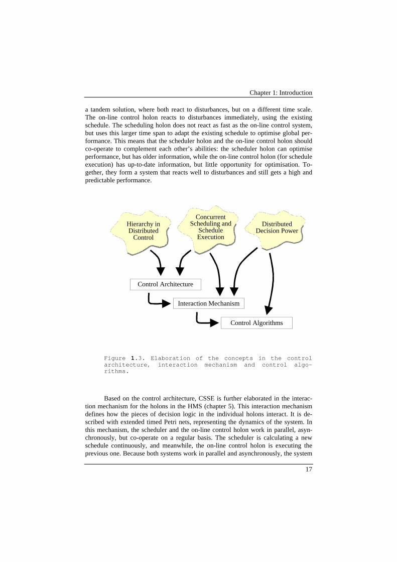
Chapter 1: Introduction
17
a tandem solution, where both react to disturbances, but on a different time scale.The on-line control holon reacts to disturbances immediately, using the existingschedule. The scheduling holon does not react as fast as the on-line control system,but uses this larger time span to adapt the existing schedule to optimise global per-formance. This means that the scheduler holon and the on-line control holon shouldco-operate to complement each other’s abilities: the scheduler holon can optimiseperformance, but has older information, while the on-line control holon (for scheduleexecution) has up-to-date information, but little opportunity for optimisation. To-gether, they form a system that reacts well to disturbances and still gets a high andpredictable performance.
Hierarchy in Distributed
Control
Control Algorithms
Interaction Mechanism
Control Architecture
Concurrent Scheduling and
Schedule Execution
Distributed Decision Power
Figure 1.3. Elaboration of the concepts in the controlarchitecture, interaction mechanism and control algo-rithms.
Based on the control architecture, CSSE is further elaborated in the interac-tion mechanism for the holons in the HMS (chapter 5). This interaction mechanismdefines how the pieces of decision logic in the individual holons interact. It is de-scribed with extended timed Petri nets, representing the dynamics of the system. Inthis mechanism, the scheduler and the on-line control holon work in parallel, asyn-chronously, but co-operate on a regular basis. The scheduler is calculating a newschedule continuously, and meanwhile, the on-line control holon is executing theprevious one. Because both systems work in parallel and asynchronously, the system
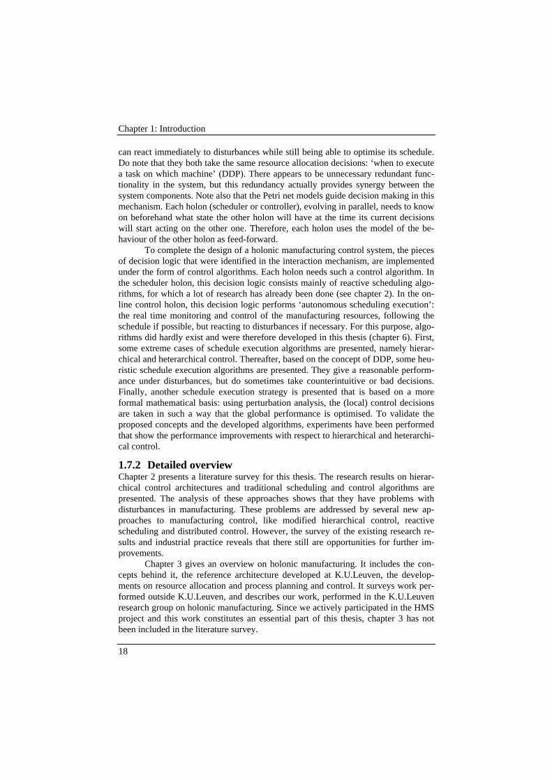
Chapter 1: Introduction
18
can react immediately to disturbances while still being able to optimise its schedule.Do note that they both take the same resource allocation decisions: ‘when to executea task on which machine’ (DDP). There appears to be unnecessary redundant func-tionality in the system, but this redundancy actually provides synergy between thesystem components. Note also that the Petri net models guide decision making in thismechanism. Each holon (scheduler or controller), evolving in parallel, needs to knowon beforehand what state the other holon will have at the time its current decisionswill start acting on the other one. Therefore, each holon uses the model of the be-haviour of the other holon as feed-forward.
To complete the design of a holonic manufacturing control system, the piecesof decision logic that were identified in the interaction mechanism, are implementedunder the form of control algorithms. Each holon needs such a control algorithm. Inthe scheduler holon, this decision logic consists mainly of reactive scheduling algo-rithms, for which a lot of research has already been done (see chapter 2). In the on-line control holon, this decision logic performs ‘autonomous scheduling execution’:the real time monitoring and control of the manufacturing resources, following theschedule if possible, but reacting to disturbances if necessary. For this purpose, algo-rithms did hardly exist and were therefore developed in this thesis (chapter 6). First,some extreme cases of schedule execution algorithms are presented, namely hierar-chical and heterarchical control. Thereafter, based on the concept of DDP, some heu-ristic schedule execution algorithms are presented. They give a reasonable perform-ance under disturbances, but do sometimes take counterintuitive or bad decisions.Finally, another schedule execution strategy is presented that is based on a moreformal mathematical basis: using perturbation analysis, the (local) control decisionsare taken in such a way that the global performance is optimised. To validate theproposed concepts and the developed algorithms, experiments have been performedthat show the performance improvements with respect to hierarchical and heterarchi-cal control.
1.7.2 Detailed overviewChapter 2 presents a literature survey for this thesis. The research results on hierar-chical control architectures and traditional scheduling and control algorithms arepresented. The analysis of these approaches shows that they have problems withdisturbances in manufacturing. These problems are addressed by several new ap-proaches to manufacturing control, like modified hierarchical control, reactivescheduling and distributed control. However, the survey of the existing research re-sults and industrial practice reveals that there still are opportunities for further im-provements.
Chapter 3 gives an overview on holonic manufacturing. It includes the con-cepts behind it, the reference architecture developed at K.U.Leuven, the develop-ments on resource allocation and process planning and control. It surveys work per-formed outside K.U.Leuven, and describes our work, performed in the K.U.Leuvenresearch group on holonic manufacturing. Since we actively participated in the HMSproject and this work constitutes an essential part of this thesis, chapter 3 has notbeen included in the literature survey.
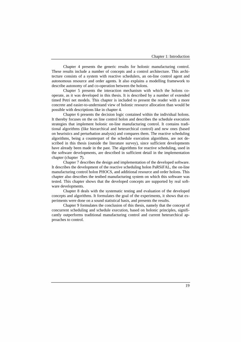
Chapter 1: Introduction
19
Chapter 4 presents the generic results for holonic manufacturing control.These results include a number of concepts and a control architecture. This archi-tecture consists of a system with reactive schedulers, an on-line control agent andautonomous resource and order agents. It also explains a modelling framework todescribe autonomy of and co-operation between the holons.
Chapter 5 presents the interaction mechanism with which the holons co-operate, as it was developed in this thesis. It is described by a number of extendedtimed Petri net models. This chapter is included to present the reader with a moreconcrete and easier-to-understand view of holonic resource allocation than would bepossible with descriptions like in chapter 4.
Chapter 6 presents the decision logic contained within the individual holons.It thereby focuses on the on line control holon and describes the schedule executionstrategies that implement holonic on-line manufacturing control. It contains tradi-tional algorithms (like hierarchical and heterarchical control) and new ones (basedon heuristics and perturbation analysis) and compares them. The reactive schedulingalgorithms, being a counterpart of the schedule execution algorithms, are not de-scribed in this thesis (outside the literature survey), since sufficient developmentshave already been made in the past. The algorithms for reactive scheduling, used inthe software developments, are described in sufficient detail in the implementationchapter (chapter 7).
Chapter 7 describes the design and implementation of the developed software.It describes the development of the reactive scheduling holon PaRSiFAL, the on-linemanufacturing control holon PHOCS, and additional resource and order holons. Thischapter also describes the testbed manufacturing system on which this software wastested. This chapter shows that the developed concepts are supported by real soft-ware developments.
Chapter 8 deals with the systematic testing and evaluation of the developedconcepts and algorithms. It formulates the goal of the experiments, it shows that ex-periments were done on a sound statistical basis, and presents the results.
Chapter 9 formulates the conclusion of this thesis, namely that the concept ofconcurrent scheduling and schedule execution, based on holonic principles, signifi-cantly outperforms traditional manufacturing control and current heterarchical ap-proaches to control.

Chapter 1: Introduction
20

21
Chapter 2
Literature Survey
This chapter surveys literature on hierarchical and modified hierarchical controlarchitectures; off-line, dynamic, and reactive scheduling; and centralised and dis-tributed on-line manufacturing control concepts and algorithms. It also describesindustrial practice.
2.1 IntroductionThe goal of this chapter is to survey the relevant literature on manufacturing control.Thereby, an important distinction is made between the so-called “traditional ap-proaches” (section 2.2) and the “new” ones (section 2.3). The traditional approachesrefer to research results that are now considered as valuable contributions to thesubject in the past, but for which several problems remained. They form the baselinefrom which recent and on-going research is starting. The new approaches refer torecent and on-going research in the same or adjacent fields as this thesis. One couldargue about what to consider as “traditional” research and what is “recent” work, butthis discussion is not considered important. What is important is that the research ef-forts described in section 2.3 address the same problems as this thesis, while section2.2 reports on solutions (both older and recent ones) for earlier problems. As a con-sequence, for a fair comparison, this thesis should be compared with the approachesdescribed in section 2.3, rather than with the ones of section 2.2.
Section 2.2 surveys the traditional research on shop floor control (SFC). Re-search on enterprise-wide integration in the eighties led to development of hierarchi-cal SFC architectures. Traditional Operations Research (O.R.) for manufacturing fo-cused mainly on algorithms, especially for scheduling. Some early work was alsodone on the control aspects of SFC.
Section 2.3 discusses the more recent developments on SFC. Several re-searchers are continuing with hierarchical control, trying to solve the existing prob-lems by developing modified hierarchical architectures. Not referring to hierarchicalsystems, but implicitly building on the same concepts, several new approaches onscheduling and control have been proposed, like reactive scheduling and FMS1 con-trol based on discrete event system theories. The two final subsections of 2.3 de-scribe new manufacturing paradigms, based on distributed control, that were devel-oped to obtain more agility and robustness against disturbances.
1 FMS: Flexible Manufacturing Systems

Chapter 2: Literature Survey
22
Section 2.4 compares the results of the current research efforts with the in-dustrial practice. It describes to which degree research results are implemented andto which degree industry adopts alternative approaches to the prevailing research. Ittries to analyse the notorious gap between theory and practice and identifies the rea-sons for this gap.
The conclusion reveals that valuable work is being done by a lot of research-ers, but that optimisation and robustness against disturbances both are importantissues, that have to be combined to come to workable solutions in industrial systems.This combination is exactly what this thesis aims at.
2.2 Traditional Shop Floor Control ResearchThe so-called “traditional” research on SFC addressed problems that are consideredto be solved sufficiently for this thesis. This research, to a large extent correspondingto the eighties, encompasses several accomplishments on SFC architectures, sched-uling algorithms and on-line control, which are described in this section. This sectionalso reviews the problems left over that motivated current research (described in thisthesis and in section 2.3).
2.2.1 SFC ArchitecturesAn architecture provides a good framework for reasoning on shop floor control. Itidentifies the required functions and components in an SFC system. It defines neededdata and interfaces and describes the behaviours of the individual components andtheir interactions. It positions the components in an SFC system with respect to eachother. In order to do that, an architecture consists of a set of concepts or theories, aset of models and eventually a methodology to design such an architecture. Wyns(1999) discusses these issues in detail.
Most existing SFC architectures are based on the concept of hierarchy. Simon(1969, chap. 7) defines a hierarchic system as a system composed of interrelatedsubsystems, each of the latter being in turn hierarchic in structure, until some lowestlevel of elementary subsystem is reached. Hierarchy is an essential paradigm totackle complexity, as Simon (1969) illustrates by his Watchmakers' parable. There-fore, current hierarchical architectures are superior to monolithic architectures. Theyare less complex to develop and more easy to change, or in other words, with thesame design effort, they can provide a higher functionality.
Some well-known hierarchical architectures are the AMRF (Jones 1986, Se-nehi et al. 1994), the PAC architecture (Bauer, 1991), and MPCS (Biemans, 1989,1989b). The National Institute of Standards and Technology (NIST), formallyknown as National Bureau of Standards (NBS), first developed the AMRF (Jones,1986). It consists of a tree-shaped architecture with a fixed number (five) of hierar-chical levels: facility, shop, cell, workstation, and equipment. Classical com-mand/feedback control flow is only to the immediate subordinate/supervisor level.However, some data can be shared across several levels, for instance by means of ashared database. Also sensor information can be fed into every level. PAC — TheProduction Activity Control architecture is a result of the ESPRIT project COSIMA

Chapter 2: Literature Survey
23
(COntrol Systems for Integrated MAnufacturing) (Duggan, 1991, Bauer, 1991).They divide production planning and control in three hierarchical activities: strate-gic, tactical, and operational. Shop floor control concerns the operational level. Theshop is separated into a set of product based manufacturing cells controlled by PACcontrollers. These PAC controllers are supervised by a Factory Co-ordination (FC)level. The discussion of MPCS is outside the scope of this thesis (Wyns, 1999).
A good example to explain how the SFC architecture characterises manufac-turing control, is the PAC architecture. It consists of a scheduler, a dispatcher, amonitor, and several movers and producers. The scheduler generates a planningbased upon known constraints, capacities, and list of orders. The dispatcher may de-viate from this planning based upon the actual status of the shop floor given by themonitor. The dispatcher passes instructions to the movers and producers. On a higherlevel, the Factory Co-ordination amongst others co-ordinates work between PACcells and performs medium term planning, like an MRP system.
Medium range planning
Short range scheduling
Customer orders
Batch orders& due dates
Delayed orders
Completed and executing
orders
Productdefinitions
Res
ourc
e av
aila
ble
acco
rdin
g to
pla
n
Actual resource
Order monitoring
Commands to equipment
Figure 2.1. Functional diagram (using IDEF-0 — Bauer,1991) for the relationships between medium range plan-ning, detailed short range scheduling and dispatching.
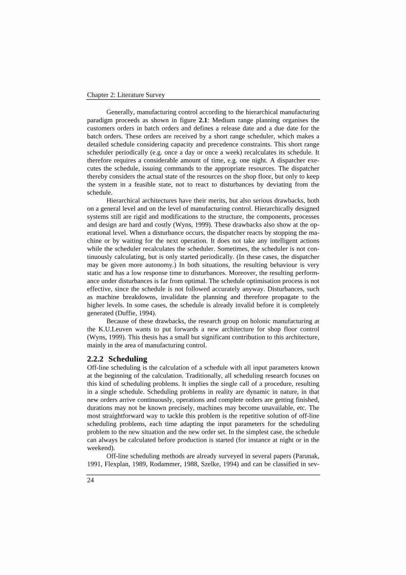
Chapter 2: Literature Survey
24
Generally, manufacturing control according to the hierarchical manufacturingparadigm proceeds as shown in figure 2.1: Medium range planning organises thecustomers orders in batch orders and defines a release date and a due date for thebatch orders. These orders are received by a short range scheduler, which makes adetailed schedule considering capacity and precedence constraints. This short rangescheduler periodically (e.g. once a day or once a week) recalculates its schedule. Ittherefore requires a considerable amount of time, e.g. one night. A dispatcher exe-cutes the schedule, issuing commands to the appropriate resources. The dispatcherthereby considers the actual state of the resources on the shop floor, but only to keepthe system in a feasible state, not to react to disturbances by deviating from theschedule.
Hierarchical architectures have their merits, but also serious drawbacks, bothon a general level and on the level of manufacturing control. Hierarchically designedsystems still are rigid and modifications to the structure, the components, processesand design are hard and costly (Wyns, 1999). These drawbacks also show at the op-erational level. When a disturbance occurs, the dispatcher reacts by stopping the ma-chine or by waiting for the next operation. It does not take any intelligent actionswhile the scheduler recalculates the scheduler. Sometimes, the scheduler is not con-tinuously calculating, but is only started periodically. (In these cases, the dispatchermay be given more autonomy.) In both situations, the resulting behaviour is verystatic and has a low response time to disturbances. Moreover, the resulting perform-ance under disturbances is far from optimal. The schedule optimisation process is noteffective, since the schedule is not followed accurately anyway. Disturbances, suchas machine breakdowns, invalidate the planning and therefore propagate to thehigher levels. In some cases, the schedule is already invalid before it is completelygenerated (Duffie, 1994).
Because of these drawbacks, the research group on holonic manufacturing atthe K.U.Leuven wants to put forwards a new architecture for shop floor control(Wyns, 1999). This thesis has a small but significant contribution to this architecture,mainly in the area of manufacturing control.
2.2.2 SchedulingOff-line scheduling is the calculation of a schedule with all input parameters knownat the beginning of the calculation. Traditionally, all scheduling research focuses onthis kind of scheduling problems. It implies the single call of a procedure, resultingin a single schedule. Scheduling problems in reality are dynamic in nature, in thatnew orders arrive continuously, operations and complete orders are getting finished,durations may not be known precisely, machines may become unavailable, etc. Themost straightforward way to tackle this problem is the repetitive solution of off-linescheduling problems, each time adapting the input parameters for the schedulingproblem to the new situation and the new order set. In the simplest case, the schedulecan always be calculated before production is started (for instance at night or in theweekend).
Off-line scheduling methods are already surveyed in several papers (Parunak,1991, Flexplan, 1989, Rodammer, 1988, Szelke, 1994) and can be classified in sev-

Chapter 2: Literature Survey
25
eral categories. For some problems, efficient algorithms exist to find the optimal so-lution. For most problems, optimal algorithms exist, but may require excessive cal-culation time. If the optimal solution cannot be found in reasonable time, heuristicsare used. The simplest heuristics use dispatching rules. Several other heuristics buildon techniques developed in artificial intelligence. Neighbourhood search techniques,in particular metaheuristics, have also provided some powerful algorithms for near-optimal schedules. Another technique is based on Lagrangian Relaxation. Some ap-proaches also use discrete event system theories to develop schedules.
Optimal Solutions and Mathematical ProgrammingFor some simple scheduling problems, efficient algorithms exist to calculate the op-timal solutions (French, 1982, Bauer, 1991, Chryssolouris, 1992, Rembold, 1993).For instance, for the single processor scheduling problem, the Earliest Due Date(EDD) dispatching rule provides an optimal solution for the minimisation of maxi-mum tardiness. Usually, real-life problems are more complex than these academicproblems, but sometimes, by using a simplified model and applying the results to thereal situation, the scheduling problem can be successfully solved (e.g., scheduling afactory with a single bottleneck as a single processor scheduling problem — Gol-dratt, 1984). An industrial survey (Peeters, 1997b) showed that, sometimes, thephysical design of manufacturing system is modified such that the correspondingscheduling and control problem is easier. Do note that it is generally accepted thatbasic knowledge on these academic problems is necessary for the understanding ofthe fundamental properties of scheduling, needed to solve real-world problems.
Most scheduling problems can also be solved optimally, provided that enoughcalculation time is available. Often, they can be formulated as a (mixed) integer pro-gramming problem. Due to the NP-complete nature of these problems, completeenumeration of all possibilities quickly becomes prohibitively time consuming.However, in some situations, efficient branch and bound methods (French, 1982, Ch.7, Aanen, 1993, Hatzikonstantis, 1992), dynamic programming techniques, and zero-one integer programming may provide optimal solutions for reasonable (and usable)problem sizes in reasonable time (from minutes to hours). Rodammer (1988) surveysseveral of these algorithms.
DispatchingIf the calculation time required for optimal solutions is beyond reasonable bounds, itis necessary to use heuristic solutions, like dispatching (which do not yield optimalsolutions). Dispatching with priority rules is the best known heuristic for schedulingand is surveyed in detail by Joshi (1994) and Panwalker (1977). Using dispatchingrules, schedules can be produced almost instantaneously. Because of their simplicity,they are also used quite often in industry and in flexible manufacturing and assemblysystems. Dispatching rules however tend to yield a low and unpredictable perform-ance. For instance, the already mentioned EDD rule is often used for job shopscheduling for tardiness minimisation, sometimes (but certainly not always) withreasonable performance.
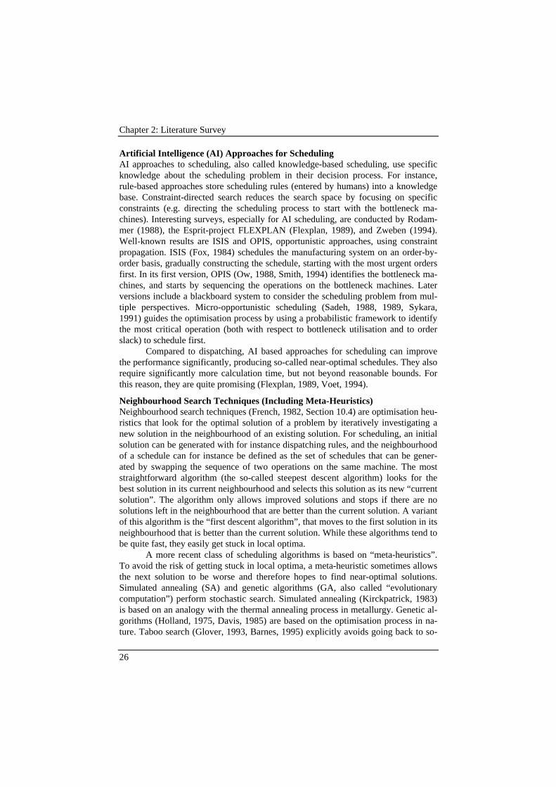
Chapter 2: Literature Survey
26
Artificial Intelligence (AI) Approaches for SchedulingAI approaches to scheduling, also called knowledge-based scheduling, use specificknowledge about the scheduling problem in their decision process. For instance,rule-based approaches store scheduling rules (entered by humans) into a knowledgebase. Constraint-directed search reduces the search space by focusing on specificconstraints (e.g. directing the scheduling process to start with the bottleneck ma-chines). Interesting surveys, especially for AI scheduling, are conducted by Rodam-mer (1988), the Esprit-project FLEXPLAN (Flexplan, 1989), and Zweben (1994).Well-known results are ISIS and OPIS, opportunistic approaches, using constraintpropagation. ISIS (Fox, 1984) schedules the manufacturing system on an order-by-order basis, gradually constructing the schedule, starting with the most urgent ordersfirst. In its first version, OPIS (Ow, 1988, Smith, 1994) identifies the bottleneck ma-chines, and starts by sequencing the operations on the bottleneck machines. Laterversions include a blackboard system to consider the scheduling problem from mul-tiple perspectives. Micro-opportunistic scheduling (Sadeh, 1988, 1989, Sykara,1991) guides the optimisation process by using a probabilistic framework to identifythe most critical operation (both with respect to bottleneck utilisation and to orderslack) to schedule first.
Compared to dispatching, AI based approaches for scheduling can improvethe performance significantly, producing so-called near-optimal schedules. They alsorequire significantly more calculation time, but not beyond reasonable bounds. Forthis reason, they are quite promising (Flexplan, 1989, Voet, 1994).
Neighbourhood Search Techniques (Including Meta-Heuristics)Neighbourhood search techniques (French, 1982, Section 10.4) are optimisation heu-ristics that look for the optimal solution of a problem by iteratively investigating anew solution in the neighbourhood of an existing solution. For scheduling, an initialsolution can be generated with for instance dispatching rules, and the neighbourhoodof a schedule can for instance be defined as the set of schedules that can be gener-ated by swapping the sequence of two operations on the same machine. The moststraightforward algorithm (the so-called steepest descent algorithm) looks for thebest solution in its current neighbourhood and selects this solution as its new “currentsolution”. The algorithm only allows improved solutions and stops if there are nosolutions left in the neighbourhood that are better than the current solution. A variantof this algorithm is the “first descent algorithm”, that moves to the first solution in itsneighbourhood that is better than the current solution. While these algorithms tend tobe quite fast, they easily get stuck in local optima.
A more recent class of scheduling algorithms is based on “meta-heuristics”.To avoid the risk of getting stuck in local optima, a meta-heuristic sometimes allowsthe next solution to be worse and therefore hopes to find near-optimal solutions.Simulated annealing (SA) and genetic algorithms (GA, also called “evolutionarycomputation”) perform stochastic search. Simulated annealing (Kirckpatrick, 1983)is based on an analogy with the thermal annealing process in metallurgy. Genetic al-gorithms (Holland, 1975, Davis, 1985) are based on the optimisation process in na-ture. Taboo search (Glover, 1993, Barnes, 1995) explicitly avoids going back to so-

Chapter 2: Literature Survey
27
lutions (or regions) that have already been explored. They can all escape from localoptima and provide high-quality solutions.
Several researchers have applied these algorithms to scheduling (Uckun,1993, Chiu, 1997, Fortemps, 1996 , Musser, 1993, Crauwels, 1998). These near-optimal approaches do obtain better results than dispatching rules, but also use aconsiderable amount of calculation time. Often they allow a trade-off between cal-culation time and schedule performance. The performance of stochastic searchmethods (SA and GA) in function of the calculation time is also stochastic, but isfairly easy to predict on a statistical basis.
Lagrangian RelaxationA new approach to job shop scheduling, which is gaining importance, is based onLagrangian relaxation (Hoitomt, 1989, 1990, 1993b). Based on a firm mathematicalbasis, the capacity constraints of a scheduling problem, which cause the schedulingproblem to be coupled over all orders, can be relaxed and replaced by a penalty costfor using that resource. An iterative procedure yields a near-optimal selection of ma-chine prices, such that a nearly feasible schedule is produced with a high perform-ance. The relaxation of the capacity constraints is quite similar to the mechanism thatruns a free-market economy. A thorough discussion on scheduling with Lagrangianrelaxation is outside the scope of this thesis, but is given by Bongaerts (1994b).
Like meta-heuristics, this approach yields a high performance, but using con-siderable calculation time. What makes this approach interesting is that it provides alower bound on the optimal cost, and thus guarantees that the solution found iswithin a known margin from the optimal solution.
Discrete Event System Control TheorySome researchers propose to approach the scheduling problem using control theoryand discrete event systems theory (DES). Their work is described in subsections2.3.2 and 2.3.3. While these approaches provide SFC with a formal modellingframework, they do not really address the computational complexity of the schedul-ing problem. When analysing non-trivial manufacturing scheduling problems, theyhit the same computational bounds as other scheduling approaches. As a conse-quence, they often use DES control theory to model the problem and resort to otherscheduling techniques (Lee, 1994, Peng, 1996, Chiu, 1997) for decision taking.
ConclusionsThe results of the literature survey for scheduling are summarised in the followingconclusions:• Striving for optimal solutions for all scheduling problems is an unrealistic ap-
proach, due to the computational complexity (Parunak, 1991).• It makes sense to optimise schedule performance. Near-optimal approaches do
obtain a higher performance than dispatching rules, but they also use a consider-able amount of calculation time (Crauwels, 1998).
• Therefore, the selection of a scheduling algorithm depends on a trade-off be-tween calculation time and schedule performance. To express this trade-off, wedefine a performance graph for a certain scheduling problem and a number of
Chapter 2: Literature Survey
28
scheduling algorithms. It is a graph that expresses the performance of these algo-rithms for the given scheduling problem in function of the calculation time theyrequire. Constructive algorithms (which create a schedule from scratch) are rep-resented by a single point in the performance graph. Iterative improvement algo-rithms are represented by a curve in the performance graph, since their calcula-tion time can be tuned. Figure 2.2 shows two examples of such a performancegraph (Crauwels, 1998, Shahookar, 1991).
• It remains difficult to compare algorithms using performance graphs. Since a per-formance graph is constructed for a single scheduling problem, it requires allauthors to solve the same problem. It is commonly agreed (Parunak, 1998, Cava-lieri, 1998, Ringer, 1995, Shahookar, 1991) that benchmarking is a time-consuming job that requires a lot of co-ordination among researchers.
• Given a performance graph, it is still necessary to make the trade-off and select ascheduling algorithm. Currently, such decisions are made, based on commonsense. We did not find guidelines in literature to make this trade-off.
b.a.
Figure 2.2. Performance graphs for some scheduling algo-rithms, expressing the performance value in function ofthe calculation time used. Figure (a) depicts the per-formance graph for a genetic algorithm for a one-machinesequencing problem (two versions). Source: Crauwels(1998, fig. A.3). Figure (b) presents a similar graph forlayout planning using a genetic algorithm (GASP) andsimulated annealing (TimberWolf 3.3). Source: Shahookar(1991).
Chapter 2: Literature Survey
29
2.2.3 Automated On-line Control of Manufacturing Systems
Automated on-line control of manufacturing systems was initially applied to flexiblemanufacturing systems. Often, the main focus was on process related issues, like as-sembly (NNS — Alami, 1985, 1986), robot applications (WRAP — Carayannis,1988) or machining (COPPS — Hultmann, 1987). However, with respect to manu-facturing control, this work was nothing more than a proof of feasibility. Most FMScontrollers used simple algorithms, like dispatching rules, for manufacturing control.As a result, the performance and predictability of the system was far from optimal.Sometimes, higher investment costs were made than theoretically needed, such thatthe resource allocation was simplified and dispatching rules could yield an accept-able performance (e.g. equipping all workstations with all tools to obtain a multipleidentical processors scheduling problem).
2.3 New Approaches to Shop Floor ControlWhile the previous section surveys existing solutions and their remaining problems,this section describes how other researchers up to now have tried to address theseproblems.
2.3.1 Modified Hierarchical ArchitecturesIn an attempt to overcome some of the shortcomings of a (proper) hierarchical ar-chitecture, the modified hierarchical control architecture was developed (Dilts,1991). It especially focuses on improving the operational problems of the proper hi-erarchical form with respect to the low robustness and the slow reaction to distur-bances. Modules in modified hierarchical systems have some amount of self-sufficiency or autonomy with respect to higher levels (Cassandras, 1986).
The modification lies in the fact that more functions are allocated to the lowerlevel controllers, and that peer modules on the same level can communicate directly.The strict master-slave relationships in proper hierarchical systems are loosened,such that low-level modules can autonomously react to disturbances (Dilts, 1991).
Examples of the modified hierarchical architecture usually are improvementsof existing hierarchical architectures. MSI — the Manufacturing Systems Integrationarchitecture is a follow-up of the AMRF architecture, also developed by NIST (Se-nehi, 1994). Peer-to-peer communication in the MSI architecture is possible by in-formation sharing via databases. This communication is however limited to control-lers on the same hierarchical level and to the exchange of information only. Allcommunication for control and feedback is still performed between the immediatesubordinate and supervisory levels. Each hierarchical controller receives a produc-tion plan (schedule) from its supervisory controller. MSI identifies several types ofpossible errors and mentions dynamic scheduling, reallocation of resources, and dy-namic process planning as error recovery means (Senehi, 1992). Only if the errorcannot be resolved at the current control level, the fault is to be propagated to thehigher control level.

Chapter 2: Literature Survey
30
Elaborating on the initial PAC architecture, several researchers have devisedmodified hierarchical architectures. Maglica (1996, 1996b) and Gullander (1995,1996) extend the autonomy of the producer and mover modules by supplying themwith their own state module, in this way reducing the central role of the monitormodule. Hierarchical communication overhead is also reduced by allowing produc-ers and movers to synchronise their work directly with handshake signals. Zwegers(1997) even implemented a modified hierarchical version of PAC within a multi-agent system.
Building on MPCS, Arentsen introduces the Factory Activity Control model(FACT) for make-to-order and engineer-to-order manufacturing (Arentsen, 1995). InFACT, process planning is close to the shop floor and process plans are generated onshort notice, such that they can be based on the actual availability of the worksta-tions. This maintains a high flexibility. FACT allows “direct requests” betweenworkstations for unexpected situations. Examples are “direct tool request” or “directinspection request” which are sent by a workstation to a tool preparation station orquality control station in case of tool breakage or quality problems.
Summarising, modified hierarchical architectures are significant improve-ments of the proper hierarchical ones, but most disadvantages of hierarchical systemsremain. While building firmly on existing solutions, they remain in the original para-digm of hierarchical systems. All functionality and robustness is designed and im-plemented explicitly. Therefore, modified hierarchical systems remain very predict-able, but they do not take advantage of the possible emergent behaviour and robust-ness as heterarchical systems (see subsection 2.3.4 and 2.3.5) do.
2.3.2 New developments in schedulingDuring the last decade, the research community has understood that existing sched-uling algorithms are not really applied in industry, because the real-life complexityof industrial plants is not sufficiently considered. Traditionally, the scheduling prob-lem was considered to be s t a t i c and d e t e r m i n i s t i c . However, to start with,the industrial scheduling problem is a d y n a m i c problem, meaning that new ordersarrive continuously. In an academic context, the dynamic scheduling problem wasformally defined as all orders having different (non-zero) release dates (Chryssol-ouris, 1992). It was implied that all orders and their release dates are known at thebeginning of the problem, and a solution can be calculated off-line, in a singlescheduling run. The dynamic scheduling problems becomes more industrially rele-vant if it refers to a continuous control problem: orders come in continuously, andproduction continues meanwhile. Such a problem implies that the schedule is to berecalculated repetitively.
Secondly, the input data for the scheduling problem are not perfectly knownat the time the schedule is calculated. In other words, the scheduling problem iss t o c h a s t i c , which in industrial terminology corresponds to the occurrence ofdisturbances. These disturbances may show themselves as “rush orders” (the arrivalof new orders is a dynamic process), stochastic variations on the duration of an op-eration, or the occurrence of major disturbance events, like machine breakdowns andorder scrapping. As mentioned in chapter 1, the schedule performance drops rapidly

Chapter 2: Literature Survey
31
if disturbances occur (Parunak, 1991, Ow, 1988, Smith, 1995). One could thus con-clude that the schedule needs to be adapted to the new situation as fast as possible.But on the other hand, as was concluded in section 2.2.2, schedule optimisation is atime consuming process. In other words, the computational complexity of schedulingbecomes an even more important problem in the industrial context. (For complete-ness, it should be mentioned that also practical problems hinder the application ofadvanced scheduling techniques in industry2).
Static Dynamic
Deterministic
Stochastic
Off-line scheduling
Stochastic considerations in scheduling
Dynamic Scheduling
Reactive Scheduling
ProactiveScheduling
Scheduling architectures
Scheduling environments
SurroundingFrameworks
Distributed Scheduling
Figure 2.3. Relationship between off-line scheduling,stochastic scheduling, dynamic scheduling, reactivescheduling, proactive scheduling, distributed scheduling,scheduling architectures and scheduling environments.
These different perspectives on the scheduling problem led to different ap-proaches to solve it (see Figure 2.3). The traditional perspective in the academicworld was static and deterministic and led to the development of off-line schedulingalgorithms, as surveyed in section 2.2.2. Scheduling techniques addressing the de-terministic, dynamic scheduling problem are dynamic scheduling algorithms. The
2 Examples of these practical problems are the cost of software development, the dif-ficulty of gathering accurate data, and the limited degree of automation in supervi-sory control.
Chapter 2: Literature Survey
32
static stochastic scheduling problem is considered by a number of approaches, whichwe will refer to as stochastic scheduling algorithms. Reactive schedulingalgorithms, considering disturbances in a dynamic environment, are techniquesdealing both with the dynamic and stochastic nature of the scheduling problem. Mostreactive scheduling methods, however, do not foresee the stochastic effects, but reacton them. Only proactive scheduling takes into account the risk for disturbances in itsschedule, instead of reacting to them when they happen. The above solutions for thescheduling problem are all algorithmic solutions. An alternative (or complementary)approach to many of these problems can be found in structural solutions, which wewill call scheduling architectures. Research tackling the practical aspects of thescheduling problem, like for instance software reuse, are called scheduling envi-ronments (Dorn, 1996), but are not further discussed in this survey.
Instead of classifying the scheduling research according to the problemsaddressed, it is also possible to consider the underlying technology for classificationpurposes. Doing so, an important class of scheduling algorithms is distributedscheduling. It refers to scheduling techniques for which the algorithm is distributedover a number of computer processes that combine their calculation power and theirlocal knowledge to optimise the global performance (see section 2.3.4).
Dynamic SchedulingTo address the “industrial” dynamic scheduling problem, many researchers(Connors, 1994, Hoitomt, 1993, Luh, 1993, Czerwinski , 1994, Ow, 1988, Prosser,1989, Sadeh, 1988, 1989, Sycara, 1991, Chang, 1994) find a solution in dispatchingrules or other very fast algorithms, in order not to keep the resources waiting whilescheduling (rescheduling).
Some researchers investigate the basic aspects of the problem by looking atsimple scheduling problems, like the one-machine scheduling problem or the parallelmachine scheduling problem (Ovacik, 1995). Ovacik (1995) also uses the solutionfor this simple problem as a module in a job scheduling context with machine set-uptimes. Kimemia and Gerschwin (1981, 1983) considered the dynamic schedulingproblem for a flow shop, with a limited number of products. Because this number islimited, it is feasible to maintain all products in stock and formulate the schedulingproblem as a flow problem, which can be solved using continuous decision variables.This way, the scheduling problem is reduced to a coupled set of differential equa-tions, which is not NP-complete. Interesting to note is that they were the first ones toconsider the scheduling problem as a control problem (see also subsection 2.3.3).
For larger scale and more complex problems, dynamic schedulers are oftenbased on simulation: Nkasu (1995) uses a simulation-based approach for an assem-bly line balancing problem, and Gupta (1995) for improving MRP systems. Alsosome commercial schedulers, like TEMPO, are based on simulation.
Stochastic Considerations in SchedulingApproaches addressing the static and stochastic scheduling problem typically usequeuing models, simulations, or other probabilistic models. Koo (1995) combinesqueuing models with static capacity planning algorithms for static planning prob-

Chapter 2: Literature Survey
33
lems. Nkasu (1995) and Gupta (1995) (see supra) also use simulation to considerstochasticity. Wellman (1995) explicitly includes the stochastic aspects in the objec-tive function and uses simulation and genetic algorithms for the optimisation.
Reactive (and Proactive) SchedulingResearch is currently focused on the reactive scheduling problem (Szelke, 1994).Parunak (1991) discusses some structural solutions to the reactive scheduling prob-lem, like the introduction of buffers and more reliable machines. Operational solu-tions to deal with disturbances are rescheduling, deferred commitment and tweaking.Also Luh (1993) explicitly refers to the dynamic and stochastic nature of the sched-uling problem and identifies three challenges for the research community: (i) developefficient solution methodologies that can generate near-optimal solutions with meas-urable performance; (ii) perform “what if” analysis to examine the impact of distur-bances and (iii) develop efficient methods for schedule reconfiguration to accommo-date these changes (“tweaking”, see infra).
One of the most used approaches to obtain reactive scheduling is reschedul-ing: restarting the scheduling process from scratch, given the new information re-garding the status of the manufacturing system. For many researchers, again, like fordynamic scheduling, this problem is then reformulated as an efficiency problem. Forinstance, Bispo (1992) explicitly aims at an algorithm with polynomial complexityand therefore proposes a rolling scheduling horizon. A complete schedule is com-puted (using beam search) for a small number of parts (the “rolling group”), but onlyits first steps are executed. New parts can enter the rolling group based on their pri-ority. Then, the schedule is calculated again.
Deferred commitment scheduling (Parunak, 1991) delays detailed decisionsas long as possible to minimise exposure to the unexpected. For instance, by distrib-uting schedule decisions throughout the control hierarchy of the factory, detailed de-cisions are made as refinements of higher level decisions during the operation of thesystem, i.e. based on more recent information (Fox, 1985). The same principle canalso be applied in heterarchical control (Shaw, 1985 — see also infra). As a result,the risk of disturbances is considerably lower. Moreover, deferring commitment alsopreserves flexibility (Valckenaers, 1993).
Tweaking refers to techniques for correcting an existing schedule as theworld deviates from expectations without complete rescheduling (Parunak, 1991).Cassandras (1993) provides a strong mathematical basis for tweaking by using per-turbation analysis for discrete event systems. Especially when perturbation analysisis applied to stochastic systems, Cassandras has investigated under which conditionsperturbation analysis provides an unbiased estimate of the global performance (bothfor infinitesimal and finite perturbations). Luh (1993) and Czerwinski (1994) useLagrangian relaxation for scheduling and propose to use the resulting Lagrangianmultipliers to make rescheduling decisions. These multipliers are a good estimate forthe resource prices at each moment and can therefore be used to decide whether toreroute parts to a certain resource or not, or whether to have a machine idle or not.To the best of our knowledge, this idea is not implemented yet. A similar one isimplemented by Chang (1994), who developed a nominal scheduling and a fast

Chapter 2: Literature Survey
34
rescheduling algorithm based on Lagrangian relaxation for a flexible flow shopscheduling problem. (After a disturbance, the constraints for the problem areupdated. Using the same multipliers, and possibly a short optimisation phase, theresulting dual solution is made feasible for the new situation). Several other ap-proaches consider and combine feedback and “feed forward”, like simulation tech-niques, knowledge bases, and performance forecasts (Banks, 1993, Tayanithi, 1992,Karsiti, 1992). An interesting approach, albeit in a different domain, is the develop-ment of a reactive scheduling algorithm for airline crew scheduling, where the num-ber of the rescheduling options is limited by the introduction of natural constraints(Stoykovic, 1998). For instance, the available number of crew members that can re-place somebody is limited by the physical location (hard constraint), but it is alsodesirable that the number of people whose schedule is affected, is minimal (soft con-straint).
An important thread in reactive scheduling research, often corresponding totweaking, is found in the knowledge-based scheduling community (Flexplan, 1989,Zweben, 1994, Szelke, 1994). OPIS (Smith, 1994, 1995, see also subsection 2.2.2)has become the best known example of reactive scheduling. For that purpose, OPIShas a blackboard-based control architecture where the current schedule is stored, to-gether with all unscheduled tasks and requests for schedule repair. A number of ex-pert modules are capable of solving sub-problems for schedule generation and revi-sion. A “Top Level Manager” (TLM) opportunistically guides the search by callingthe right expert modules for the right sub-problems in the right sequence. Therefore,the TLM aggregates the incoming events, prioritises and analyses them, and formu-lates the right sub-problems. The required knowledge for the TLM is stored in aknowledge base. Typical expert modules are the order scheduler, the resourcescheduler, the right shifter, the left shifter and a demand swapper (swapping two op-erations on a machine). Other approaches, similar to OPIS, are Microboss (Sadeh,1989, Sycara, 1991), and CAMPS (Miyashita, 1997), moving towards distributedimplementations. Another knowledge-based reactive schedulers is SONIA (Collinot,1988), mainly differing from OPIS in that the reactive scheduling experts are alsoapplied for backtracking in the predictive scheduling phase. DAS (Prosser, 1989) isa distributed asynchronous scheduler, consisting of three levels of problem solvingagents, which add and delete constraints to the scheduling problem to obtain a feasi-ble (but not optimised) solution.
Proactive scheduling (Szelke, 1995) is an extension of reactive schedulingthat aims at preventing foreseeable disturbances, by considering them in the scheduleas soon as the they are known, and before they can invalidate the schedule. To reachthat goal, the performance trends are monitored in real time and statistically proc-essed to better predict the processing times of operations and to anticipate machinefailures. How this is to be done is not stated.
Scheduling ArchitecturesUp to now, the approaches discussed are all algorithmic solutions to the schedulingproblem. However, also structural solutions may provide significant improvementson the overall performance of a manufacturing system. For instance, in the past, the

Chapter 2: Literature Survey
35
scheduling problem was hierarchically decomposed in several sub-problems (me-dium-term and short-term planning, load/unload scheduling, the machine allocationproblem, the sequencing problem, transportation scheduling, etc.). Such a decompo-sition is a structural solution for the computational complexity of the schedulingproblem (Cruz, 1978). (To sketch the idea: using complete enumeration, a size 100sequencing problem requires approximately 25 . 10149 more calculation time than 10size 10 problems.) Consequently, almost everybody (Ahn, 1993, Shmilovici, 1992,Crama, 1994, Khator, 1994, Kim, 1994, Blazewicz, 1992, Bussmann, 1994, DSMI,1997, Romanowski, 1998) assumes some form of hierarchical decomposition of thescheduling problem.
It is interesting to survey how new scheduling architectures provide a struc-ture for an improved organisation of the scheduling software. Singh and Hindi(1991) provide a systematic analysis of the hierarchical decomposition of the sched-uling problem. This decomposition is based on the dimensionality of the controlproblem, the physical distribution of the controlled entities, the time scale involved,the amount of interactions between subsystems, and the required degree of aggrega-tion. Addressing the different time scales in scheduling and on-line control, Dugganand Browne (1991) propose the concept of Production Activity Control (PAC) withan off-line scheduler and an on-line dispatcher to execute the schedule. A similar ap-proach was proposed by Chryssolouris (1991, 1992, 1994), who elaborated it in acommercial software package (MADEMA). Schmidt (1996) considered the needsfor an architecture for reactive scheduling. He distinguishes predictive productionscheduling and reactive production scheduling (also called on-line control). In thisarchitecture, he applies case based reasoning techniques, but he does not allow con-tinuous operation of both predictive and reactive scheduling, such that the usable al-gorithms are limited to the very fast ones.
Recently, several researchers (Duffie, 1986, Hatvany, 1985) proposed a dis-tributed approach to shop floor control (both for scheduling and on-line control).While this implies a lot of new algorithmic developments, it is in the first place anew structural solution to the shop floor control problem, with the potential of emer-gent behaviour (see subsection 2.3.4).
2.3.3 New Developments in On-line Manufacturing ControlCompared to scheduling, on-line manufacturing control (OMC) is a more recent re-search domain and not very structured yet. To start with, the difference betweenscheduling and OMC is not always clearly made. For this thesis, scheduling refers toan optimising and predictive process, while OMC refers to a control process thatstarts each individual operation and reacts to each individual event. It also involvesstarting the auxiliary operations like transport and set-up and co-ordinating these de-cisions with the real operations.
A large group of researchers on Discrete Event Systems is applying their re-sults on the control of manufacturing systems. Some people present controllers basedon formal models, others use rule-based approaches towards control. There also areresults in the area of software design and development for manufacturing systems.Finally, an important thread is focusing on distributed control (see subsection 2.3.4).
Chapter 2: Literature Survey
36
Discrete Event SystemsDiscrete event (dynamic) systems (DES or DEDS) (Cassandras, 1993) differ fromcontinuous time systems in that they only change state on specific moments in time(events) and remain constant otherwise. But when they change, they change in mac-roscopic ways. A typical example is a manufacturing system. Several modellingtechniques exist for DES, like for instance Petri nets (Petri, 1962, Peterson, 1981),max algebra (Olsder, 1993), finite state machines (modelled with State Space Dia-grams — Cassandras, 1993, automata — Cassandras, 1993 or with formal languages— Ramadge, 1989). These techniques are surveyed by Ben-Naoum et al. (1995).
Research on discrete event systems has promised major breakthroughs inmanufacturing control, because of its similarity to control theory for continuous sys-tem. Since the DES theories provide a formal modelling framework, it was hopedthat corresponding optimal supervisory control algorithms could be developed. Ro-dammer (1988) reviews several approaches for scheduling based on control theory.Utopia
While these formal modelling approaches significantly contribute to a clearand unambiguous communication and documentation of ideas and concepts and pro-vide a mathematical basis for control, the use of analysis and optimisation techniqueshas only obtained limited success. After all, they hit the same hard border of NP-completeness that is encountered in all scheduling approaches. Typical examples ofhow to apply DEDS theory to manufacturing, are given by Lauzon (1996), Lee(1994) and Zeigler (1993), who built a real-time controller based on Petri nets. Deci-sions are based on ordinary dispatching rules, instead of by using a detailed sched-uler. The main merits of DEDS theory are the development of deadlock-free con-trollers. For optimisation, timed models are needed, together with scheduling meth-ods described above.
Other mathematical modelsBecause modelling manufacturing systems at the required level of detail with DEDSmodels becomes quite cumbersome, some researchers present alternative formalmodelling approaches that are specifically aimed at manufacturing. Basically, thesemodels represent machines, orders and capacity and precedence constraints, and en-able schedulers and controllers to reason in this framework.
For instance, REDS (Hadavi, 1990) (Requirements Driven Scheduling), is amanufacturing control system that uses the formal model representing constraints inthe scheduler also for its on-line control part. The actual control algorithm uses DSR,a dynamic priority rule.
Similarly, the HIMAC project (Vallauri, 1995) developed a manufacturingalgebra, enabling the precise and accurate description of a manufacturing system inthe appropriate level of detail. The model is suited for hierarchical and modularmanufacturing control systems. The control algorithms used in the HIMAC projectare based on heuristics and neural networks, and serve mainly to demonstrate the useof the manufacturing algebra.
Chapter 2: Literature Survey
37
Petit (1996) presents Albert-II, a formal yet expressive modelling languageand applies it to manufacturing. Interesting is the fact that Albert-II is applicable toagent-based concepts.
Comparing to DEDS based approaches, these approaches offer similar bene-fits with respect to formal modelling and are less biased towards deadlock avoid-ance.
Rule based approachesOther authors focus more on the algorithms themselves, and present rule based ap-proaches for manufacturing control. Often, these rules are a collection of dispatchingrules (Shmilovici, 1992). In the MADEMA approach (Chryssolouris, 1991, 1992),they are extracted from human experts to form an expert system. Chryssolouris(1991b) also use machine learning techniques to determine the correct rule in a cer-tain situation.
Software developmentsSeveral authors also consider the flexibility of control software and its developmentcost. Valckenaers (1993) presents an architecture for a multi-agent control systemthat imposes minimal constraints on the control algorithms, optimising its flexibility.It is implemented in FACCS (Flexible Assembly Cell Control System). RapidCIM(Joshi, 1995, 1995b, Smith, 1992) is a development environment that automaticallygenerates FMS control software.
Distributed controlAnother important thread in manufacturing control research is based on distributedapproaches, and explained below (subsection 2.3.4).
2.3.4 Distributed Scheduling and Control
Distributed Manufacturing ParadigmsSince the eighties, several researchers, like Vamos (1983), Hatvany (1985), or Duf-fie and Piper (1986), proposed heterarchical control as a new paradigm for manu-facturing for an improved reactivity to disturbances, compared to the paradigm ofhierarchical control. Heterarchical control (Lin, 1994) is a highly distributed formof control, implemented by a system of independent agents without centralised orexplicit direct control. Agents3 are independent co-operating computer processes thatcan act on their own initiative. Control decisions are reached through mutual agree-ment and information is exchanged freely among the participating agents.
3 There is no unified and generally accepted definition of an agent, amongst othersbecause of lacking consensus on the intelligence of an agent. Do all independent co-operating computer processes with some initiative fit the definition of an agent, or dothey have to fulfil certain requirements on structure, standards, protocols or require-ments? Bussmann (1998) states that “Multi-agent systems can best be characterisedas a software technology that is able to model and implement individual and socialbehaviour in distributed systems.“

Chapter 2: Literature Survey
38
The concepts for heterarchical control are derived from biological metaphorsand analogies to the free market economy. In biological systems and market econo-mies, reactivity to disturbances emerges almost automatically from simple mecha-nisms in the behaviour of individual agents and the interactions between these be-haviours. Therefore, heterarchical control architectures offer similar prospects of re-duced complexity, high flexibility and a high robustness against disturbances inmanufacturing. Hence, there is for instance no need for explicit reactive scheduling.Experiments (Duffie, 1994) and theoretical considerations (Hoitomt, 1989, Gou,1994) have partially proven these expectations. (For instance, resource capacity con-straints, coupling the resource allocation optimisation problem over multiple orders,are difficult to treat in a traditional scheduling approach, but are automaticallyobeyed in a market economy, using the law of offer and demand.) Moreover, distrib-uted approaches to manufacturing control are backed up by the large research com-munity on multi-agent systems. They define agent architectures (Rao, 1991,Wooldridge, 1995) and communication mechanisms (Smith, 1980, Stirling, 1992)and investigate what are the basic mechanisms that make agents systems work(Müller, 1998) or not (Werner, 1996).
Several new shop floor control approaches are based on distributed control,like the fractal factory, bionic and genetic manufacturing and holonic manufacturing.In the fractal factory (Warnecke, 1992), a robust and decentralised manufacturingsystem is based mostly on human involvement. In bionic (Okino, 1992, 1993) andbiological manufacturing systems (Ueda, 1992, 1993, 1997), self-organising manu-facturing systems are developed on the basis of distributed systems and a variety ofmodern computational techniques, like genetic algorithms, neural networks, artificiallife, etc. Iwata (1994) developed random manufacturing systems, based on autono-mous machines, dynamic machine grouping, tender-based task allocation and a re-ward and penalty driven shop floor control algorithm. (Chiu, 1995) developed a dis-tributed algorithm for dynamic scheduling, based on machine learning using simula-tion and genetic algorithms. At the same time, the holonic manufacturing paradigmwas conceived, but these developments (including our contributions) are described inchapter 3.
Based on the concept of distributed control, many distributed approaches forshop floor control have been proposed, both for scheduling and for manufacturingcontrol (surveyed by Dilts, 1991).
Distributed SchedulingDistributed scheduling refers to scheduling techniques for which the algorithm isdistributed over a number of agents that combine their calculation power and theirlocal knowledge to optimise the global performance. While distributed scheduling ispromising for several other reasons (parallel computation4, simplified software
4 Parallel computation may lead to a decreased calculation time. Obviously, ne-glecting communication overhead, Npr processors can do the same calculations Npr
time faster than a single processor. Specific algorithms for distributed scheduling caneven further decrease the calculation time, because of an efficient decomposition of
Chapter 2: Literature Survey
39
structure — Duffie, 1987, Bussmann, 1998), the main motive for its application is itspotential to automatically react to disturbances.
Many researchers move towards distributed implementations of their algo-rithms for parallel computation. Sycara (1991) proposes a distributed opportunisticscheduling approach (from the ISIS and OPIS family — Smith, 1994), that is basedon bottleneck detection and precedence constraint propagation. Gou (1994) and Ha-segawa (1994) propose a distributed Lagrangian relaxation approach.
Often, the scheduling process is distributed to better react to disturbances.OPIS (Smith, 1994) requires a distributed (blackboard) architecture to allow multi-perspective scheduling, in other words, to allow the individual scheduling experts tocontribute at the right time and only then. For the same reason, also Microboss(Sadeh, 1989, Sycara, 1991), CAMPS (Miyashita, 1997), SONIA (Collinot, 1988),and DAS (Prosser, 1989) are distributed schedulers. Tharumarajah (1996) proposesa behaviour-based approach to scheduling where the entities interact with their envi-ronment only, as an alternative to purely reactive control through negotiation amongagents. While the robustness against disturbances really emerges automatically fromthe behaviour of each agent, performance does not grow beyond that of simple dis-patching rules.
Distributed Control AlgorithmsSeveral types of distributed control algorithms implement the concepts of heterarchi-cal control (Duffie, 1994). A large variety of heterarchical control algorithms aredistributed versions of existing scheduling and control algorithms5. Like for distrib-uted scheduling, the advantages are often limited to parallel computing and a simpli-fied software development process. Promising are the algorithms based on emergentbehaviour, like market-based, biological-metaphor based and behaviour based algo-rithms. A special case is Lagrangian relaxation.
Some algorithms are based on existing centralised algorithms like dispatchingrules (Panwalker, 1977, van de Mortel-Fronczak, 1997), network search algorithms(Fox, 1984, Ramos, 1996, Sousa, 1997), or expert-system-based scheduling tech-niques (Schmidt, 1996, Heidari, 1991). Van de Mortel-Fronczak (1997) did someexperiments to compare the results of centralised and distributed implementations ofdispatching rules. Ramos (1996) and Sousa (1997) propose a distributed schedulingmethod based on the contract net protocol and on forward and backwards propaga-tion of precedence constraints to reduce the search space. They explicitly considerthe risks involved with concurrent negotiation and present a conflict avoidance algo-rithm. Sousa (1997) also includes a renegotiation phase to react to disturbances.Based on the information flow in business planning, Heidari (1991) developed adistributed control architecture, which can be equiped with general purpose and spe-cific scheduling rules. Perkins (1994) investigated the stability versus performance
the problem (which sometimes leads to implementations of distributed algorithms ona single computer — Gou, 1994, Wyns, 1998, Debels, 1998).5 As already mentioned, some distributed control algorithms also perform some kindof optimisation, such that the border between scheduling and control is fading.
Chapter 2: Literature Survey
40
issues in distributed scheduling. Moriwaki (1992) presents an object oriented modelof the manufacturing system and describes the results of using this model to generatea prototype distributed scheduling system that can cope with disruptions. Ra-maswamy (1995) combines an off-line scheduling algorithm based upon Lagrangianrelaxation with distributed on-line control based on a market mechanism.
Emergent behaviour is seen in market-based, biological-metaphor based andbehaviour based algorithms. Market based approaches relax the capacity constraintsof a manufacturing system and replace it by a pricing mechanism. If the demands arehigher than the offer, the price rises. It is interesting to note that Luh (1993) providesa framework, based on Lagrangian relaxation to show why market-based approachesimplicitly consider capacity constraints. Auction based mechanisms use a similarconcept, but use a centralised auctioneer to come to a joint decision, mimicking realauctions (Clearwater, 1996). Biological manufacturing systems perform resource al-location based on potential field functions (Ueda, 1997). Tharumarajah (1996, 1997)defines behaviour based scheduling to further reduce the interaction between agents.
Heterarchical control turned out to be very robust and reactive against distur-bances, especially because of its emergent behaviour. However, banning all forms ofhierarchy, most approaches for heterarchical control do not consider optimisationimportant, because in reality, ‘schedules are broken down by disturbances anyway’.Predictability and stability of distributed systems usually is also lower than in cen-tralised ones. It is believed that in very unstructured environments, heterarchicalcontrol without explicit schedulers can be the most suitable approach. In other situa-tions, however, the incorporation of a scheduler in a distributed system would en-hance the stability, predictability and performance (see also chapter 8). Anotherproblem is more practical by nature. Many heterarchical algorithms need to be prop-erly fine-tuned, which is a quite labour intensive work.
2.4 Industrial PracticeIndustry often uses simple but robust tools for the resource allocation problem, likeinteractive schedulers, human involvement and self-developed software, often incombination with an MRP or MRP II system. An interactive scheduler, also calledleitstand scheduler, is a collection of graphic toolboxes and GUIs to assist humanschedulers (Lampkemeyer 1991, Jackson, 1989). Many factories use MRP or MRP-II systems to create a medium range schedule. The drawbacks of MRP are alreadywidely discussed in several papers (Euwe, 1996). The major disadvantages of MRPare its rigidity; the oversimplified model of the manufacturing system and its capac-ity; the tremendous amount of data that have to be entered in the Bill Of Materialsand the lack of feedback from the shop floor. For the execution of an MRP-schedule,several approaches are used. At Caterpillar Belgium (Gosselies), 1995, the MRPsystem is linked with an automated warehousing and transportation system. Thecontrol software for warehousing can under certain conditions be used as a tool forcontrol of the shop floor. In the Alcatel Bell plant for Printed Circuit Board assem-bly, Geel, Belgium, 1994, the MRP-schedule is executed by printing out all ordersfor transport jobs and the assembly job list for each machine, on a daily basis. This is
Chapter 2: Literature Survey
41
partially automated by self-developed software. The programmers combine the proc-ess planning, the scheduling and the NC-programming work on a ad-hoc basis. How-ever, the system still is to a large extent operated by humans. Some commercial shopfloor control software is reviewed in (Chaar, 1993).
However, industry hardly uses advanced scheduling and control concepts re-sulting from the research community, because of several reasons (Parunak, 1991):The main reasons are the computational complexity of the scheduling problem andthe sensitivity of a schedule to disturbances. Due to the computational complexity, itis difficult to provide a near-optimal schedule on-line. Due to the disturbances thatoccur on the shop floor, it is difficult to execute a given schedule by a shop floorcontrol (SFC) system. Investigations in industry have shown that 20% to 30% ofwork is done on other equipment than was originally planned (Lampkemeyer, 1991).
Recently, industry is becoming interested in the resource allocation problem.End users have realised that small percentage-wise improvements on their entirefactory really pay off in the absolute sense (Peeters, 1997b, Bussmann, 1997, Wilt-shire, 1997). They understand that logistic performance is a key element in theirbusiness. Software vendors are gradually implementing the concepts developed inthe last 10 years, culminating in a major breakthrough at the end of the nineties.Major players are SAP, BaaN and Oracle (on the enterprise level), and Siemens,IBM, Digital, Fanuc-GE on the shop floor. Interesting surveys are given in (NN,1997, NN, 1997b). Also, a lot of larger and smaller software and consulting compa-nies now have entered the market.
2.5 ConclusionsThe following bullet points summarise the research results on shop floor control cur-rently available and identify the remaining problems, for which solutions are cur-rently lacking:• A large number of scheduling techniques exist, in academic literature as well as
in industry. They reach varying levels of performance optimisation, but there is afundamental trade-off between the calculation time required for a scheduling al-gorithm and its performance. How to make this trade-off has not been systemati-cally investigated.
• The problem of disturbances has become a major issue in scheduling research.Consequently, reactive scheduling, which addresses the dynamic and stochasticaspects of scheduling, now is one of the main research threads in scheduling.
• The reactive scheduling research has been quite successful: it resulted in severalcommercial products (MADEMA — Chryssolouris, 1992b, 1994, Microboss —Sadeh, 1989, Red Pepper — Zweben, 1994, Goukens, 1997).
• Still, the problem of disturbances on the shop floor is not considered solved(Peeters, 1997, 1997b, Bussmann, 1997). The implementation of a reactivescheduling system is costly and time-consuming. The trade-off between scheduleoptimisation and reaction time is still an issue.

Chapter 2: Literature Survey
42
• An alternative to better scheduling and control algorithms may be found instructural solutions to the shop floor control problem. For instance, the hierarchi-cal decomposition of the scheduling problem is a structural solution that allevi-ates the computation complexity of the scheduling problem. Also proactivescheduling implies a structural change in manufacturing control, in that thescheduler has to anticipate disturbances instead of reacting to them.
• Current on-line manufacturing control (OMC) algorithms are concerned mainlywith real-time decision making. Performance is not a real issue. If schedule opti-misation is foreseen in the manufacturing system, OMC follows the schedule ex-actly as planned. Often, scheduling is not foreseen, or included in the OMC sys-tem. In that case, real-time aspects are critical and the control algorithms are lim-ited to fast rule-based approaches, yielding a performance comparable to dis-patching rules.
• Heterarchical control provides a very different, highly distributed structure to themanufacturing system. It turned out to be very robust and reactive against distur-bances, especially because of its emergent behaviour. However, banning allforms of hierarchy, it cannot perform global optimisation. (Distributed schedul-ing algorithms exist for some problems, but the computational complexity re-mains a problem.) More essential might even be that the behaviour of a systemunder heterarchical control can be hardly predicted.
It appears to us that there is still room for structural improvements in shop floorcontrol. Although scheduling is time-consuming, there are no approaches known tous6 that are continuously optimising the schedule. Therefore, this thesis is looking fora new structural solution that integrates continuous scheduling in shop floor control.The following chapters will present a new (holonic) approach to further improve therobustness against disturbances and combine that with a high and predictable per-formance.
6 Also Singh (1991) identifies this gap.
43
Chapter 3
Holonic Manufacturing Systems
This chapter gives an introduction to the concepts of holonic manufacturing.Holonic manufacturing (Valckenaers, 1994, 1995, Sugimura, 1997, Moriwaki,1992) is a highly distributed approach for the development and operation of manu-facturing systems, but distinguishes itself from the other distributed approaches byexplicitly introducing hierarchy in the system (Bongaerts, 1998b). Compared to thetraditional hierarchical systems, this hierarchy should be flexible, dynamic and re-configurable. For resource allocation in holonic manufacturing, it means that to-tally distributed algorithms (for instance based on a market mechanism) are sup-plemented with a reactive scheduler, as described in (Bongaerts, 1997b) and in thisthesis. This chapter explains how holonic manufacturing originated in the IMS pro-gramme from the application of the ideas of Koestler to the manufacturing world. Itcontains a literature survey of holonic manufacturing. It reports on the results onholonic manufacturing obtained at the K.U.Leuven on shop floor control architec-tures, resource allocation and process control.
3.1 Introduction This chapter aims at a triple goal:• It shows how holonic manufacturing systems (HMS) can combine a high per-
formance with robustness against disturbances.• It describes the concepts behind HMS and surveys the research results that were
achieved in parallel with this thesis (including those of the K.U.Leuven researchgroup on holonic manufacturing).
• It explains how this thesis applies holonic manufacturing to manufacturing con-trol.
During the course of my doctoral research, it became clear that the approach I wastaking towards the integration of scheduling and control for manufacturing systems,contained the same concepts in a particular case as holonic manufacturing did ingeneral. Therefore, my research was embedded in the K.U.Leuven research group onholonic manufacturing. This chapter explains the general concepts behind holonicmanufacturing, as they will be used throughout the thesis.
In a nutshell, holonic manufacturing systems are highly distributed manufac-turing systems with room for hierarchical elements (Bongaerts, 1998b). Consideringthe fact that it tries to combine the best of both hierarchical and heterarchical sys-
Chapter 3: Holonic Manufacturing Systems
44
tems, it is believed to be a solution to the problems addressed in the previous chap-ters.
This chapter has the following structure. First, it explains the concepts behindholonic systems and holonic manufacturing systems. Second, it surveys work onholonic manufacturing throughout the world. Third, it presents the K.U.Leuven ref-erence architecture for holonic manufacturing. Fourth, it overviews the K.U.Leuvenresearch on holonic resource allocation. Fifth, it briefly touches holonic processcontrol. Sixth, it shows the K.U.Leuven testbeds on holonic manufacturing. Finally,it identifies the contributions of the K.U.Leuven and my personal ones in the field ofholonic manufacturing.
3.2 Concepts behind Holonic Manufacturing
3.2.1 The Roots of Holonics1
The term “holonic” is derived from the word “holon”, which was introduced byKoestler (1967). The word holon is a combination from the Greek holos = whole,with the suffix -on which, as in proton or neutron, suggests a particle or part. Twoobservations impelled Koestler to propose this word.
The first observation is from Herbert Simon (1969) who concludes, from his‘parable of the two watchmakers,’ that complex systems will evolve from simplesystems much more rapidly if there are stable intermediate forms than if there arenot. Simon’s analysis reveals why every complex adaptive system is hierarchic (in aloose sense).
The second observation, made by Koestler while analysing hierarchies andstable intermediate forms in living organisms and social organisations, is that — al-though it is easy to identify sub-wholes or parts — “wholes” and “parts” in an ab-solute sense do not exist. This made Koestler propose the word holon to describe thehybrid nature of sub-wholes/parts in real-life systems; holons simultaneously areself-contained wholes to their subordinated parts, and dependent parts when seenfrom the inverse direction.
Koestler also points out that holons are autonomous self-reliant units, whichhave a degree of independence and handle contingencies without asking higherauthorities for instructions. Simultaneously, holons are subject to control from (mul-tiple) higher authorities. The first property ensures that holons are stable forms,which survive disturbances. The latter property signifies that they are intermediateforms, which provide the proper functionality for the bigger whole.
Finally, Koestler defines a holarchy as a hierarchy of self-regulating holonswhich function (a) as autonomous wholes in supra-ordination to their parts, (b) asdependent parts in sub-ordination to controls on higher levels, (c) in co-ordinationwith their local environment.
1 The roots of holonics were already explained in subsection 1.6.2, but are repeatedhere to preserve the cohesion of this chapter.
Chapter 3: Holonic Manufacturing Systems
45
3.2.2 Holonic Manufacturing SystemsHolonic manufacturing originated in the framework of the Intelligent ManufacturingSystems (IMS) programme. IMS probably is the largest research programme everlaunched on manufacturing. Prof. Yoshikawa from Tokyo University originally pro-posed it with the objective of creating a manufacturing science that can meet theneeds of the next century. IMS was conceived as a ten-year pre-competitive basicresearch programme, supported by the governments of the major industrialisedcountries, for their industries and academics to participate. In 1993-1994, Australia,Canada, the EC, EFTA, Japan, and the US have undertaken a feasibility study forIMS, which comprised six subprojects, or so-called “test cases” (Hayashi, 1993).Since then, international co-operation continued with varying intensity. Since 1997,Europe again fully participates in the IMS projects.
The fifth IMS test case was entitled ‘Holonic Manufacturing Systems: systemcomponents of autonomous modules and their distributed control,' also called HMS.After the IMS feasibility study, research on holonic manufacturing has mainly con-tinued in Japanese domestic IMS projects and in some nationally funded projects inthe rest of the world. K.U.Leuven (the PMA division) continues its efforts in a na-tionally funded research project called GOA/HMS – Concerted Research Action2 onHolonic Manufacturing Systems. Lasting 4 years, this project combines PMA’sknowledge in flexible shop floor control (Valckenaers, 1993, 1995), non-linear proc-ess planning (Detand, 1993), reactive scheduling (Valckenaers, 1994c, 1995, Bon-gaerts, 1994), and machine controllers (Kruth, 1994b) to develop a holonic archi-tecture for production systems and implement two prototypes or testbeds. In 1997,HMS became one of the first fully endorsed IMS projects. Currently, K.U.Leuvenparticipates in the International HMS Consortium via HANDS, the work package onassembly.
The task of the HMS consortium is to translate the concepts that Koestler de-veloped for social organisations and living organisms into a set of appropriate con-cepts for manufacturing industries. The goal is to attain in manufacturing the benefitsthat holonic organisation provides to living organisms and societies, i.e., stability inthe face of disturbances, adaptability and flexibility in the face of change, and effi-cient use of available resources. The HMS concept combines the best features of hi-erarchical and heterarchical organisation (Dilts, 1991). It preserves the stability ofhierarchy while providing the dynamic flexibility of heterarchy.
During the feasibility study, the HMS consortium developed the following listof definitions to help understand and guide the translation of holonic concepts into amanufacturing setting (Valckenaers, 1997):• Holon: An autonomous and co-operative building block of a manufacturing sys-
tem for transforming, transporting, storing and/or validating information andphysical objects. The holon consists of an information processing part and oftena physical processing part. A holon can be part of another holon.
2 In Dutch: “Geconcerteerde Onderzoeksactie”.
Chapter 3: Holonic Manufacturing Systems
46
• Autonomy: The capability of an entity to create and control the execution of itsown plans and/or strategies.
• Co-operation: A process whereby a set of entities develops mutually acceptableplans and executes these plans.
• Holarchy: A system of holons that can co-operate to achieve a goal or objective.The holarchy defines the basic rules for co-operation of the holons and therebylimits their autonomy.
• Holonic manufacturing system: a holarchy that integrates the entire range ofmanufacturing activities from order booking through design, production, andmarketing to realise the agile manufacturing enterprise.
• Holonic attributes: attributes of an entity that make it a holon. The minimum setis autonomy and co-operativeness.
3.2.3 Additional sources of inspirationWhile the roots of the HMS concept are insights provided by Koestler (1967) in thenature of real-life complex adaptive systems, PMA has been looking for additionalsources of inspiration. Waldrop (1992) presents a number of fundamental propertiesof complex adaptive systems, like autocatalytic sets, positive feed-back and the cou-pling between system development and the future environment in which such systemwill reside. Van Brussel et al. (1995) investigate how the understanding of thesemechanisms may contribute to the design and development of complex adaptivesystems in manufacturing.
The emergence of complex adaptive systems requires the existence of anautocatalytic set: a set of elements that catalyses the creation of its own elements. Inbiology, this property refers to the generation of offspring. In manufacturing and in-formation technology, it means that software that has gained an early and wide mar-ket share, gets early and plenty support for the further development and testing ofthat software, and for that reason alone becomes better than the competitive prod-ucts.
The autocatalytic set is a system characterised by positive feedback. Thepresence of its members increases the rate at which new set elements are created,which in turn increases this rate even further. An undesirable consequence of posi-tive feedback, which cannot be ignored, since it has significant impact, is lock-in: thesystem becomes locked in the solution that it selects first; a huge effort is required toswitch at a later instant. The system becomes history-dependent or path-dependent.Developers of complex artefacts must be aware of lock-in. However, they are facinga dilemma: early solutions that are “marginally-good-enough” and manage to be-come member of an autocatalytic set, ordinarily become winners in a competitiveworld. Developers are well aware that this results in sub-optimal solutions, but donot have an established methodology to avoid it.
The coupling between the development of a system and its future environ-ment is a third factor that influences the development of complex adaptive systems.The future environment of a complex system may depend on the success that systemwill have. While (ab)using this principle may lead to success (lock-in) of that system,
Chapter 3: Holonic Manufacturing Systems
47
optimising the goals of individuals to the detriment of global goals, understandingthe mechanisms behind it may protect the customers or competitors of the locked-insolution against the drawbacks of lock-in. This reasoning lead to design principlesthat preserve flexibility, like 'low and late commitment' (Valckenaers, 1993).
3.2.4 Practical requirements for holonic manufacturingAs reasoning on autonomy, co-operation and complex adaptive systems may seemquite abstract, work on holonic manufacturing has considered from the beginninghow these concepts lead to specific requirements for manufacturing systems.
From the outset, the prevalent software technology to implement the con-cepts of holonic manufacturing appeared to be intelligent co-operating agents, alsocalled multi-agent systems (Wooldridge, 1995, Stirling, 1993, Rao, 1991). Multi-agent systems are also used in heterarchical control, and provide the software withopportunities for taking the initiative to take autonomous decisions.
Secondly, the hope to combine the best of hierarchical and heterarchical con-trol formed a practical inspiration source for the research on holonic manufacturing.Holonic manufacturing systems shall combine the high and predictable performancepromised by hierarchical systems with the robustness against disturbances and theagility of heterarchical systems.
Thirdly, holonic manufacturing shall address the problem of rising costs forthe development and maintenance of complex software. It shall avoid the rigidity ofhierarchical systems and shall fully support the system evolution to comply withchanging requirements (e.g. new products, new or evolving technologies, unpre-dictable demands). Reuse of components shall reduce development costs, improvesoftware quality and ease the migration towards a new paradigm like holonic manu-facturing. Consequently, reconfigurability of the HMS is an important aspect.
Fourthly, to ease the operation of a holonic manufacturing system, this latterneeds to be self-configuring, learning and self-organising. The increased flexibilityresulting from an agile and reconfigurable manufacturing system may put a high loadon the system operators, such that the holons in a HMS shall assist the operator tocontrol the system: holons shall autonomously select appropriate parameters settings,find their own strategies and build their own structure.
Fifthly, holonic manufacturing shall preserve a place for the human in thesystem, since he/she is the most flexible, and intelligent component in the system.
Sixthly, holonic manufacturing shall consider an evolutionary approach toimplement all the above requirements. Since the requirements are quite ambitious, itis more pragmatic to plan intermediate steps towards the fully intelligent manufac-turing system. This provides a smoother migration path towards holonic manufac-turing and ensure the ability of the system to support continuous adaptation, migra-tion and evolution.
3.3 Literature Survey on Holonic ManufacturingHolonic manufacturing is being developed within the HMS consortium, whichPMA/K.U.Leuven belongs to from the beginning. This section describes the results
Chapter 3: Holonic Manufacturing Systems
48
obtained in research that was conducted parallel to ours, with a main focus on re-source allocation and the corresponding control architecture. In the HMS consortium(HMS Consortium, 1997), research is structured according to the following workpackages:• SYS-ENG (system engineering) is a generic work package to develop a holonic
manufacturing architecture and design methodology.• SYS-OP (system operation) focuses on system operation and optimisation issues
on a generic level.• HORMS focuses on resource allocation.• HMU is a process-related work package on machining units.• HFIX works on Holonic Fixturing.• HANDS deals with holonic handling systems (like assembly systems).• HOLOMOBILE investigates transport via autonomous guided vehicles (AGVs)
in holonic manufacturing systems.Since 1993, the holonic manufacturing idea has gradually gained momentum and isnow also adopted by non-members of the HMS consortium (Zwegers, 1997b, Lan-ger, 1998, Sousa, 1997, Kim, 1998).
In holonic manufacturing research, several papers have already identified awhole range of holons, but — except for Van Brussel (1998) and Wyns (1999) — aunifying holonic reference architecture is still lacking. Suda (1989, 1990) proposedtwo categories of holons: the hard type, like machining, assembling, examining andtransporting, and the soft type, like marketing, planning, developing and designingholons. Moriwaki (1992), and Sugimura (1997) presented a scheduling architecturewith autonomous agents for the workpieces as well as for the equipment (includingtransportation). He thereby designed an object-oriented data model of the manufac-turing system. Hasegawa, Gou, Luh et al. (1994) presented a holonic assembly plan-ning and scheduling architecture, in which they defined product, part, machine, ma-chine type, operation and co-ordinator holons. McFarlane (1995) defined holons forprocessing, negotiation, scheduling, input/output, tracking, diagnosis, data storage,recovery and configuration. This is applied in a simulated industrial testbed for a rodmill layout with cooling holons, valve control holons and maintenance holons.Christensen (1994) added the concept of a system engineering holon. Tharumarajah(1997) presented production units, co-ordination units, shops, clients and processesas agents in a behaviour-based approach to shop floor control. According toTönshoff (1995), the use of centralised resource allocation and centralised shop floorcontrol should be prohibited in holonic manufacturing. Tönshoff argues that holonicmanufacturing systems shall be heterarchical, employing peer-to-peer relationshipsas the backbone of shop control. However, in that paper, he does not propose anyspecific algorithm for resource allocation. Seidel (1994) models the architecture of aHMS using whole-part relationships. Kádár (1997) describes a framework for devel-oping distributed manufacturing systems around a commercial simulation environ-ment. Wyns (1996) describes a holonic workstation architecture, additionally identi-fying resource allocation holons and process control holons. Bongaerts et al. (1997)defines a partial architecture for shop floor control, defining order holons, worksta-
Chapter 3: Holonic Manufacturing Systems
49
tion holons, transport system holons, shop floor control holons, and schedulingholons. Kruth (1996) defines a partial architecture for an NC holon, defining a CAPPholon and a process plan monitoring holon. Briefly, many people have been workingon holonic manufacturing, but there has not been an overall view of the manufactur-ing system yet. More results have already been obtained for the intra-holon archi-tecture. Heikkilå (1992) presents a PEM-based architecture. Christensen (1994) usesfunction blocks to model the behaviour of a holon. Rao (1991) presents the BDI ar-chitecture for multi-agent systems, which Bussmann (1998) uses as an intra-holonarchitecture. The research on intra-holon architecture will hopefully result in mid-dleware software for the development of holonic manufacturing systems (Corgnati,1998, Kim, 1998).
Also holonic resource allocation was investigated by several researchers.Some of them started from a quite heterarchical setting. Ramos (1996, 1996a) andSousa (1997) propose a distributed scheduling methods based on the contract netprotocol and on forward and backwards propagation of precedence constraints. Tön-shoff (1995) proposes a completely heterarchical method for distributed resourceallocation, where agents perform simulations in virtual worlds. Márkus (1996, 1996b)and Váncza (1998) propose a market mechanism for task allocation in HMS. Mori-waki et al. (1992) propose an on-line scheduling mechanism in an object-orientedframework. Gradually, it becomes clear that flat heterarchical control and ignoringoptimisation aspects have severe limitations. In order to include opportunities foroptimisation, Gou, Hasegawa, and Luh (1994) defines a distributed scheduling algo-rithm based upon Lagrangian relaxation concepts. It requires a centralised co-ordinator which guides the individual resource holons to increase or lower their pricebased on the global feasibility or unfeasibility of the current schedule. Also Kádár etal. (1997) discovers the need for centralised elements and proposes the coupling of amulti-agent control system with a genetic algorithm (Monostori, 1998, 1998b). Thereasons why hierarchy in distributed systems is essential in holonic manufacturing,are summarised by Bongaerts, Monostori and McFarlane (1998b). While this con-cept is getting acceptance now, the implications to resource allocation have not yetbeen studied. This thesis addresses precisely that issue. Totally distributed algo-rithms (for instance based on a market mechanism) are supplemented with a reactivescheduler. While the reactive scheduler is calculating an updated schedule, theautonomous agents execute the existing schedule (see infra).
Less important for this thesis, but worthwhile to mention is that holonicmanufacturing is also applied to process related issues, like machining, assembly,continuous processes and mobile robotics. Bengoa (1996) and several HMS partnersin Japan (Bongaerts, 1997f) work on holonic machining units. Sensor integration(Bongaerts, 1997f) and novel assembly strategies (Arai, 1997) form part of the re-search on holonic assembly. Agre (1994) and McFarlane (1995) apply holonic con-trol on continuous processes such as steel manufacturing. Research on holonic trans-port systems considers AGV architectures, sensor integration in AGVs, autonomousprogramming of AGVs and co-operation and co-ordination strategies for fleets of
Chapter 3: Holonic Manufacturing Systems
50
AGVs (Schaeffer, 1998). Toh (1998) plans to use the concept of holonic manufac-turing for human organisations.
3.4 Reference Architecture for Holonic Manufac-turingA reference architecture is an abstraction of a generic solution3 that provides a setof models, a set of coherent engineering and design principles, and eventually a setof tools and a methodology used in a specific domain (Wyns, 1996, 1999). It aims atstructuring the design of a specific system architecture by defining a unified termi-nology, a generic system structure, the kinds of system components, their responsi-bilities, dependencies, interfaces, data, behaviour (interactions), constraints, designrules, and models to represent all these aspects.
This section gives an overview of PROSA, the holonic reference architecturefor manufacturing systems as developed at PMA/K.U.Leuven (Van Brussel, 1998,Wyns, 1999). It mainly is an inter-holon architecture, identifying the kind of holons,their responsibilities, and the structure in which they interact. The internal structureof the holons is not so important for this thesis.
The basic architecture consists out of three types of basic holons: orderholons, product holons, and resource holons. They are structured using object-oriented concepts like aggregation and specialisation. Staff holons can be added toassist the basic holons with expert knowledge (Bongaerts, 1996).
3.4.1 Basic HolonsThere are three types of basic building blocks in a holonic manufacturing system(HMS): product holons, resource holons, and order holons (Figure 3.1).
A product holon holds the process and product knowledge to ensure the cor-rect fabrication of the product with sufficient quality. It acts as an information serverto the other holons in the HMS. A product holon provides consistent and up-to-dateinformation on the product life-cycle, user requirements, design, and process planand bill of material.
A resource holon consists of a physical part, namely a production resource inthe HMS, and of an information processing part that controls the resource. It offersproduction capacity and functionality to the surrounding holons (Wyns, 1996). Itholds the methods to allocate the production resources, and the knowledge and pro-cedures to organise, use and control these production resources to drive production.A resource holon is an abstraction for the production means such as machines, fur-naces, conveyors, pipelines, pallets, components, raw materials, tools, tool holders,material storage, personnel, energy, floor space, etc.
3 This is not a tautology. A system architecture is an abstraction of a specific solu-tion.

Chapter 3: Holonic Manufacturing Systems
51
An order holon represents a manufacturing order. It is an active entity re-sponsible for performing the work correctly and on time. It explicitly captures all in-formation and information processing of a job (Valckenaers, 1996).
Orderholon
Productholon
Resourceholon
Processknowledge
Productionknowledge
Processexecutionknowledge
Holonic Manufacturing System
Figure 3.1. The Basic Holons.
For a minimalistic implementation of a manufacturing system, it suffices tohave a holarchy consisting of these three basic holon types. For instance, assume theuse of a heterarchical control approach, based on a market concept, (Dilts, 1991;Joshi, 1994). In such implementation, product holons are created based on real orforecasted market demand. These product holons determine themselves how theproduct can be produced on the (dynamically changing) set of resource holons. Theymaintain all technical information needed for the fabrication of an instance of theproduct. When an order holon arrives in the system, it will first discover what itneeds via the respective product holon. The order holon will negotiate with all rele-vant resource holons to have itself produced by them. As such, the order holon takescare of the logistical aspects (the resource allocation). When an operation starts, theorder holon lets the product holon and the resource holons co-operate to perform thetechnical part of the operation.

Chapter 3: Holonic Manufacturing Systems
52
The main contribution of this basic control architecture is to get, eventually,everything manufactured in the face of disturbances, uncertainty and change, butwith limited guarantees about when and where exactly.
At the same time, if the reference architecture would be limited to this simplebasic control architecture, it would have serious drawbacks. First, in a entire factory,there is a large amount of holons (thousands of products, orders and resources), suchthat it is difficult to understand and manage such an unstructured pool of holons.More importantly, it does not provide predictable performance, even when the envi-ronment behaves according to predictions, nor does it offer opportunities for optimi-sation. The next subsections describe how the architecture addresses these issues.
3.4.2 Aggregation and SpecialisationInteraction between a large number of low level agents results in complex systembehaviour that is difficult to understand, to control and to predict (Waldrop, 1992).Structuring the agents in a hierarchy is the appropriate solution to tackle this com-plexity (Koestler, 1967).
Therefore, aggregated holons are defined as a set of related holons that areclustered together and form in their turn a bigger holon with its own identity. An ag-gregation hierarchy is formed, which is open-ended at the top and at the bottom.Depending on the scope of the observer, holons are split up into their sub-holons ortreated as a whole. The aggregation hierarchy is not necessarily a tree-shaped one:holons may belong to multiple aggregations. Aggregated holons can dynamicallychange their contents depending on particular needs of the system. They may evenemerge out of the self-organising interaction of holons. Examples of aggregation canbe found for resources, orders, and products.
A second classification concept is specialisation, which is derived from ob-ject-oriented methodologies. The aforementioned basic building blocks sometimesstill are too abstract to reason about their place in an architecture. Specialisationseparates the holons with respect to their manufacturing characteristics. For instance,for the resource holarchy, usually transport holons and production holons like work-stations are very different types of resources.
3.4.3 Staff HolonsThe heterarchical control architecture, described above, empowers the basic holonsto take all decisions that are necessary to achieve the production goals. The moretraditional centralised/hierarchical control architectures outperform this basic systembut only under stable and predictable conditions. The basic architecture performsbetter in uncertain and more turbulent situations.
The K.U.Leuven Holonic Manufacturing Control architecture incorporates amechanism to have the advantages of both without the disadvantages. It preservesthe empowerment of the basic holons, and it gives these basic holons the support ofstaff holons. These staff holons offer the functionality that is typically found in thehigher levels of hierarchical control systems. The main difference is that staff holonshave an advisory role (Figure 3.2).

Chapter 3: Holonic Manufacturing Systems
53
To avoid that hierarchy introduces rigidity in the system, hierarchical controlelements should not enforce their decisions to the basic holons in an inflexible way.Instead, they should have an advisory role in the production process. This change issimilar to the shift from line functions to staff functions in human organisations(Hommes, 1980). Therefore, we define staff holons as holons that consider somefacets of the problems of other “client” holons and provide this client holon with suf-ficient information such that it can take the correct decision about that problem. Inother words, staff holons assist other holons to do their work. It is noteworthy thatalso in a human organisation, as stated in (Hommes, 1980), one of the main goals forthe introduction of staff functions is to reduce the work load of line functions by pro-viding them with expert knowledge.
Figure 3.2. Staff holons. For resource allocation, ascheduler is a typical staff holon. For process control,CAM, CAPP and CAD are typical staff holons.
Examples of staff holons are schedulers, process sequence planners, CAD-systems, and even MRP-systems. The most important staff holon in the HolonicManufacturing Control System prototype is a reactive short-range scheduler, as ex-plained in the remainder of this thesis.
The concept of basic holons enhanced with staff holons decouples the robust-ness and agility of the system from system optimisation: due to the distributed basicarchitecture, the HMS delivers robustness and agility and is simple to extend and re-configure. The optimisation of the HMS is done by optional staff functions. When,due to disturbances and changes in the system, the hierarchical staff holons perform
Chapter 3: Holonic Manufacturing Systems
54
poorly, the advice may be ignored and the basic holons, taking autonomous actions,continue to do their work. On the other hand, when disturbances are totally absent, aHMS can be configured such that the basic holons do execute (in a hierarchical way)the decisions of the staff holons. Usually, however, decision power shall be distrib-uted between basic holons and staff holons, as will be shown (for resource alloca-tion) in the following chapters. This configuration is determined by the holarchy,which defines the basic rules for co-operation of the holons and thereby limits theirautonomy.
3.4.4 Resource Allocation versus Process ControlOften, it is possible to simplify the architecture by limiting it to a certain viewpoint,suitable for a specific application. The structure of the entire holarchy can usually befairly well decomposed in a resource allocation (sub-)holarchy and a process control(sub-)holarchy.
The resource allocation holarchy (order holons, resource holons, and staffholons like the on-line shop floor control holon and the reactive scheduling holon)represents the logistic chain. It focuses on the reservation and allocation of equip-ment to tasks, aiming at good overall system performance, also under disturbances.
The process control holarchy (CAD-holon, CAPP-holon, product holon andthe process control part of the resource holon) represents the technical chain, focus-ing on the design of the product and the planning and execution of the process.
The most important advantage of this dual holarchy is the fact that it shieldsthe resource allocation holarchy from the process control hierarchy. Orders, for in-stance, mainly focus on resource allocation. Products mainly focus on process plan-ning and execution. Resources typically are part of both holarchies. However, theirproposed structure explicitly takes into account this dual nature of their task (Wyns,1996). Sometimes, the consideration of the interaction of resource allocation andprocess control yields additional advantages, as shown by Wyns (1997).
3.4.5 ModellingAn essential element of a manufacturing architecture is providing a modellingframework for the components in a manufacturing system, their functions, interfaces,interactions, and the structure in which they operate. Wyns (1999) and Van Brussel(1998) propose to use UML, the unified modelling language, to represent the neededmodels. UML is a modelling framework for object-oriented design and programmingthat resulted from the co-operation of Booch, Jacobson and Rumbaugh (Fowler,1997). The main advantage of a modelling framework is the standard representationmethod.
3.4.6 ReconfigurabilityReconfigurability is an important requirement for holonic manufacturing systems,since it is a way to make them cope with changes. It should be possible to add, mod-ify, replace and remove modules to, in and from HMSs. Moreover, the optimal con-figuration may depend on the specific system and situation on the shop floor (as
Chapter 3: Holonic Manufacturing Systems
55
shown for manufacturing control in chapters 4 and 7). Consequently, the HMSshould reconfigure itself to maintain its optimal configuration.
Therefore, a holonic architecture itself shall be reconfigurable. This impliesthat the very structure of the system can be modified, even while the system is run-ning. This concept is quite new, compared to traditional architectures. For instance, ahierarchical architecture imposes a strict hierarchical control structure to the system,which remains unchanged. A heterarchical system imposes a flat control structure tothe system. A holonic architecture does not impose a fixed control structure. Instead,it allows the structure to be variable, by allowing temporary hierarchies, multiple hi-erarchies and by loosening the definition of hierarchy, as explained by Simon (1969)or Valckenaers (1996).
To achieve this reconfigurability, the HMS needs a meta-model and meta-control. A meta-model is a model the HMS has of itself, and contains the system ar-chitecture. Bongaerts (1996) presents such a model. Meta-control is the process ofdefining the right meta-model and setting the right parameters over time. Both themeta-models and meta-control can be implemented both centrally (with a so-called“meta-controller”) and distributedly (so-called “without meta-controller”). The con-cept of meta-models and meta-control is still recent and subject to future research.Possible approaches for the implementation of meta-control are, in increasing degreeof autonomy:• interactive reconfiguration (reconfiguration decisions are made by humans);• centralised heuristic reconfiguration rules;• reconfiguration based on experimental data;• model-based reconfiguration rules (a model is defined to express how reconfigu-
ration decisions affect the global performance, such that the optimal configura-tion can be determined);
• reconfiguration based on machine learning; and• distributed reconfiguration.
3.4.7 ConclusionA reference architecture on holonic manufacturing is presented, based on order, re-source, product and staff holons. Important contributions are the separation of manu-facturing control and process control, and the reconfigurability of the architecture.
This architecture was developed within the framework of the GOA/HMSproject, mainly by Wyns (1999). However, for the development of a reference ar-chitecture, teamwork in a multi-disciplinary group is essential. In this respect, I ac-tively contributed to this work, mainly on resource allocation aspects, as described inchapter 4. The concept of staff holons is a generalisation of having a reactive sched-uler in a autonomous multi-agent schedule execution system, as presented in the re-mainder of this thesis.
3.5 Resource Allocation in Holonic ManufacturingManufacturing control in holonic manufacturing, and more specifically resource al-location, is the one of the main themes in the GOA/HMS project of PMA. With re-

Chapter 3: Holonic Manufacturing Systems
56
spect to resource allocation, this thesis is the principal contribution to that project.This section describes how the chapters of this thesis fit within the complete pictureof holonic manufacturing control at PMA.
Table 3.1 presents a functional view on holonic manufacturing control andgives an overview of the functionality within the PMA prototype HMS. The controlsystem provides three control layers, situated between medium-range planning andthe equipment controllers. The middle layer consist of two sub-layers, which havedistinct responsibilities. These layers are discussed shortly below.
The first layer of the Holonic Control System keeps the manufacturing systemin an admissible state. Examples of inadmissible states are: deadlock, starvation orrepetitive exclusion, races and thrashing. The research has addressed one of these(deadlock) to investigate and demonstrate how the Holonic Control System handlesthis (Wyns, 1997). This layer only constrains the system, it does not command thesystem directly.
The second layer consists of two sub-layers. The co-operating sub-layercommands the manufacturing system. It takes the actual control decisions based onthe advice from the layer above and feedback from the production proc-esses/equipment. Chapter 4 and 5 discuss in detail how this co-operation works andhow it affects the architecture. Chapter 6 addresses the corresponding algorithms.
Research revealed that this co-operation of the second layer with the reactivescheduler inevitably makes the system dependent on the proper operation of this
Category In the prototype
4. Medium range planning —
3. Reactive short-range scheduling The PaRSiFAL system(chapter 7).
2. Schedule execution:
a) co-operation Holonic ControlAlgorithms (chapter 6).
b) autonomy Research in early stages.
1. Prevention and handling ofpathological situations: deadlocks,races, starvation, thrashing,...
Deadlock prevention(Wyns et al., 1997).
0. Equipment controllers —
Table 3.1. Functionality in a Holonic Control Sys-tem.
Chapter 3: Holonic Manufacturing Systems
57
scheduler. Since scheduling is NP-hard, heuristics are unavoidably used in this thirdlayer. This has two implications. First, with heuristics, there rarely is any guaranteeabout scheduling performance when the situation changes. Second, there often willbe margin for performance improvement by enhancing and tuning the schedulingheuristic.
The above prompted the desire to make the control architecture more forgiv-ing toward schedule quality. This would simultaneously make the system more ro-bust and lower the barrier against optimising scheduling performance through ex-perimentation. The solution is to augment the schedule execution system with a“schedule critique” ability, which enables it to assess autonomously the plausibilityand quality of the advice from the reactive scheduler in layer 3. If the advised sched-ule violates given criteria, the schedule execution system will warn the human super-visor(s) and even autonomously overrule the advice with sub-optimal but robust al-ternatives. Note how this design fully complies with the Holonic Systems paradigm,requiring autonomy next to co-operation.
The third layer, reactive short-range scheduling, completes the system. It op-timises the overall production performance. Note that this view on the control systemmakes abstraction of whether the layers are distributed or not. The main objective isto design the system such that multiple vendors can supply different pieces, not adistributed implementation per se.
3.6 Process Control in Holonic ManufacturingThe process planning and execution holarchy — called process control — takes careof the functions ranging from product design, and process planning to on-line pro-duction, processes and monitoring. Most work in holonics does not include the entiredesign process, but interfaces the holonic production system with existing CAD sys-tems. Process planning includes the sequence planning of operations (also calledroute planning), the process or machine selection, the set-up planning, fixture designand production, tool selection, and the specific operation planning itself (includingtool paths, and process parameters, like cutting speeds).
A typical process planning and execution holarchy could look like this(Kruth, 1996): products and resources contain the basic information and methods toplan and execute all processes. However, when a product is created (because there isan order for it in an engineer-to-order environment or because it was initiated bymarketing), it first gets itself a geometry via the CAD system and the (human) de-signers. Then, it gets itself analysed such that technological features (CAPP-features)are extracted. Using this information, the sequence planning holon (a staff holon)defines the necessary operations and the possible operation sequences. The off-lineprocess planning holons (that can differ for different types of operations) extract theCAM-features (the machine dependent features) for each CAPP-feature. Theythereby consider the resources to use (like machines, fixtures), the operation types,and the workstations types able to execute the operation. If necessary, they can splitup CAPP features into several CAM-features or join several of them to one CAMfeature. These sequence planning and off-line process planning holons should co-

Chapter 3: Holonic Manufacturing Systems
58
operate with the resource holons to account for their abilities, available capacity andstatus. The final process planning step is done on-line inside the machine, definingthe exact operation parameters like the tool, the cutting parameters, the tool path, etc.The operation is started however when triggered by orders in the resource allocationholarchy (Wyns, 1996).
At PMA/K.U.Leuven, the following results on holonic process control wereobtained. Van Zeir (1997) presents a feature based process planning system, devel-oped in the COMPLAN project, and its extension to a blackboard-based, distributedprocess planning system, where expert modules co-operate to combine process andenterprise specific knowledge to come to an overall process plan (sequences, processand machine selections, fixture design, set-up planning, tool selection, quality con-trol, selection of process parameters, time and cost calculations, and so on). One ofthe major advantages of this approach is the interactive nature of the process plan-ning process. Moreover, it is possible to incorporate the process planning knowledgein small autonomous and reusable units. This enables the fruitful co-operation ofhuman and computer experts, and makes it easier to integrate process planners fordifferent process types (e.g. machining, heat treatment and grinding). It also allowsthe system to combine the advantages of early and late process planning. It is possi-ble to postpone process planning decisions as long as possible, and come back ontaken decisions if disturbances cause replanning. However, if some decisions need tobe taken on time, for instance to prepare the necessary auxiliary resources, this ap-proach enables the expert to do so without taking all decisions at that early instant intime.
Van Ginderachter (Kruth, 1998) is developing a feature based NC machine,using product holons, sequence planning staff holons, and resource holons. The NCmachine can autonomously react to disturbances because it understands the meaningof its actions. Reactive process planning can take place at different levels, balancingthe severity of the problem with the appropriate action. Products and orders negoti-ate — order specific and during production — about appropriate actions.
Tanaya (1995) and Kruth (1996) present a holonic NC controller. It is anopen NC-controller, based on the device driver concept (Valckenaers, 1993), butextended to allow multilevel and in-process reaction to disturbances. Tanaya there-fore incorporates a hierarchy of instructions, and analyses the causes and costs of aninterruption to take the appropriate decision.
3.7 Implementations at the PMA TestbedsSince 1985, the PMA/K.U.Leuven research on manufacturing systems is being im-plemented on a testbed flexible assembly system (FAS), described by Valckenaers etal. (1994c, 1995) (See Figure 3.3). It consists of six workstations and a transportsystem. The transport between the workstations in the FAS is performed by a con-veyer belt driven pallet transport system, providing random routing within the FAS.When needed, also the human worker can execute transport operations. There arefour robotic workstations. There also is one manual workstation for load-ing/unloading, for repair and inspection work. A magazine workstation is available
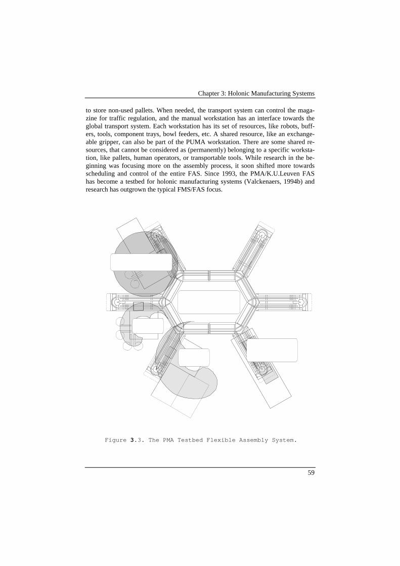
Chapter 3: Holonic Manufacturing Systems
59
to store non-used pallets. When needed, the transport system can control the maga-zine for traffic regulation, and the manual workstation has an interface towards theglobal transport system. Each workstation has its set of resources, like robots, buff-ers, tools, component trays, bowl feeders, etc. A shared resource, like an exchange-able gripper, can also be part of the PUMA workstation. There are some shared re-sources, that cannot be considered as (permanently) belonging to a specific worksta-tion, like pallets, human operators, or transportable tools. While research in the be-ginning was focusing more on the assembly process, it soon shifted more towardsscheduling and control of the entire FAS. Since 1993, the PMA/K.U.Leuven FAShas become a testbed for holonic manufacturing systems (Valckenaers, 1994b) andresearch has outgrown the typical FMS/FAS focus.
Figure 3.3. The PMA Testbed Flexible Assembly System.
Chapter 3: Holonic Manufacturing Systems
60
A second testbed for holonic manufacturing at the K.U.Leuven is a five axisMAHO milling machine. Its use is mainly for testing the concepts of process control.It will be equiped with a holonic device driver and a holonic feature-based NC-controller, and may be assisted by process planning experts.
Finally, the research on holonic manufacturing is being applied in industrialresearch projects with the ALCATEL/BELL plant in Geel and with the Mercedesplant in Sindelfingen (Brückner, 1998). However, a major obstacle for the intro-duction of advanced manufacturing control is the impossibility to test academicprototypes on real factories, since the costs and risks would be prohibitive. There-fore, the testbeds used for manufacturing control are computer simulation models.Using ARENA (Kelton, 1998), a tool for discrete-event system simulation, it is pos-sible to simulate the underlying production system with visual and statistical veri-fication of the model. The simulation models can be controlled externally via socketsand real time communication. This way, the control system has no means to distin-guish between the simulation and the real production system (if properly modelled).This approach enables the development and tuning of advanced manufacturing con-trol systems before installation in the actual production plant. In addition, it permitsthe design and evaluation of alternative/enhanced/upgraded production plants incombination with advanced control. In short, this creates a tool to assess major in-vestment analysis for production facilities.
3.8 Conclusions This chapter has shown that holonic manufacturing is a highly distributed approachtowards manufacturing, based on the ideas of Koestler. Holonic manufacturing aimsat a high robustness against disturbances, combined with a high and predictable per-formance. These ideas are implemented with multi-agent systems, consisting ofautonomous and co-operative units (“holons”).
PMA/K.U.Leuven has developed a reference architecture for holonic manu-facturing, which identifies product holons, order holons, and resource holons as ba-sic building blocks, assisted by staff holons where appropriate.
To validate these concepts and implement them in industry, it is necessary tobuild a prototype holonic manufacturing control system. That is the aim of the re-mainder of this thesis. The next chapter applies holonics to the integration of sched-uling and on-line manufacturing control and develops a corresponding manufactur-ing control architecture. Chapter 5 defines the interaction mechanism between theholons in the HMS and chapter 6 describes the control algorithms within the holons.
61
Chapter 4
Control Architecture for HolonicManufacturing
This chapter presents a control architecture for holonic manufacturing, containinggeneric concepts, a functional model and a structural model for a holonic manu-facturing control system, and a modelling framework to describe the interactionmechanism between holons (chapter 5) and the control algorithms within a holon(chapter 6).
4.1 Introduction The goal of a control architecture for holonic manufacturing control is to model thestructure of the resulting manufacturing control system. It thereby focuses on the de-cision-making logic and disregards other aspects, like e.g. the software design(Wyns, 1999). The control architecture presented here contains:• Three generic concepts, forming the basic guidelines for the design and imple-
mentation of a holonic manufacturing control system (section 2);• A functional model to identify the functions that are to be performed in holonic
manufacturing control (section 3);• A structural model to identify which holons are required and what their respon-
sibilities are, i.e. mapping the holons to the required functions (section 3);• A modelling framework to describe the interaction mechanism between the
holons (section 5).• A modelling framework to describe the control algorithms within a holon. Tradi-
tional ways to describe a control algorithm are flow-charts or pseudo code, but aholonic approach requires a high-level description method (section 4).
Note that the functional and the structural models are static models, while the inter-action mechanism and the control algorithms model the dynamics of the system.
The generic concepts are:• Hierarchy in distributed control (HDC): Holonic manufacturing control shall be
performed by a multi-agent control system with local agents, assisted by hierar-chical (centralised) agents.
• Distributed decision power (DDP): Decision power shall be distributed not onlyamong the local agents, but also between local and centralised agents.
Chapter 4: Control Architecture for Holonic Manufacturing
62
• Simultaneous and asynchronous scheduling and schedule execution (CSSE): De-cision power shall also be distributed between optimising agents (“schedulers”)and on-line manufacturing control agents, resulting in concurrent scheduling andschedule execution.
The control architecture, presented in this chapter, aims at a generic design.The functional and structural models have a reasonable degree of genericity. How-ever, it turns out to be difficult to design a unique an interaction mechanism or aunique control algorithm that would be applicable to all manufacturing systems. In-stead, two generic modelling frameworks are presented to describe these application-specific elements of the design of a manufacturing control system. The elaboration ofan interaction mechanism following the holonic concepts is presented in chapter 5.After the interaction mechanism is defined, the control system design is to be com-pleted with control algorithms within each holon. Using the modelling framework ofsection 4, chapter 6 presents several holonic control algorithms for on-line manu-facturing control.
4.2 ConceptsThe research for this thesis was conducted in a traditional way, starting from a prob-lem definition and the definition of a research project, towards the final implementa-tion and testing of a research prototype. However, during the course of this Ph.D.,several concepts were discovered that are valid for manufacturing control in general.Three of these concepts are considered fundamental for this thesis. This section pre-sents them as assertions, and provides a motivation for them.
4.2.1 Hierarchy in Distributed ControlIn chapter 2, hierarchical and heterarchical solutions for manufacturing control weresurveyed. Hierarchical control involves a command–response structure betweenhigh level and low level entities while heterarchical control is achieved by allowinga high level of autonomy and decision making to be available to low level entities,independent of the overall plant operations. As mentioned, many hierarchical sys-tems tend to have problems with reactivity to disturbances, while heterarchical con-trol turned out to have problems with global optimisation and predictability (Dilts etal., 1991).
Holonic manufacturing tries to blend the best of both hierarchical and heter-archical control while avoiding their drawbacks. Entities are provided with a degreeof autonomy to react to disturbances, but are readily integrated with the rest of thesystem through co-operative mechanisms to strive for a common global optimum.How to achieve these ideas in manufacturing control is expressed in the followingconcept.

Chapter 4: Control Architecture for Holonic Manufacturing
63
Assertion 1.
To combine robustness against disturbances with performance optimisationand predictability, the incorporation of hierarchy in a dis tr ibutedcontrol system is proposed. The resulting control architecture has a ba-sic structure of autonomous co-operating local agents, that are capable ofnegotiation with each other in order to achieve production targets. Thatbasic structure is extended with centralised agents (for instance a sched-uler agent) to co-ordinate the behaviour of the local agents (Figure 4.1).
In this context, local agents are defined as the agents controlling specific resources,like workstations or transportation systems, or controlling specific orders. On thecontrary, a centralised agent is defined as a single agent that provides services for agroup of local agents. Note that, according to this definition, it is not necessary that acentralised agent is used by all agents in the entire plant. Centralised agents can ap-pear at all levels of aggregation in the factory.
S
R1 R2 O1 O2
Advice andCentralisedagent
Local agents
Negotiation
Figure 4.1. Hierarchy in distributed systems.
MotivationThis assertion is motivated as follows. The emergent, reactive properties of heterar-chical control can only be realised if the underlying system structure allows multipleagents. To implement hierarchical control, the existence of centralised agents shouldbe allowed. Combining both kind of agents in one architecture, each with their ownskills and abilities, is to combine the strengths of hierarchical and heterarchical con-trol.
Local agents have a better local model of the resources or orders they control.This model is more up to date, more detailed and more correct than the one an over-all centralised agent would have. Also the local control logic (for instance about set-up optimisation) may be more suited to local conditions than the logic a centralisedagent would use. Local agents can also react faster to disturbances. Last but not least,
Chapter 4: Control Architecture for Holonic Manufacturing
64
a society of local agents can be designed to show emergent behaviour (such that sev-eral desirable system properties emerge automatically from the interaction of simplelocal behaviours).
Centralised agents have an overview of the entire system. They have a betterability to co-ordinate the decisions in the overall system, allowing for a coherent de-cision taking and for global optimisation. More specifically, they can better modelthe interactions between local agents and evaluate the resulting repercussions on theglobal performance.
Reasoning on a more abstract level, Simon (1969, chap. 7) explains why allcomplex adaptive systems have a natural tendency towards hierarchy1: they just can-not exist without hierarchy. He illustrates this with the Watchmakers' parable, usingsimple probability calculus to show that non-hierarchical systems have no chance tosurvive disturbances. Koestler (1967) takes up these ideas to develop the theory ofholonic systems. Remember that elements in a complex, adaptive system were called“holons”, exactly because of their double-faced character, consisting of an autono-mous and an integrative tendency. The autonomous tendency corresponds to the tra-ditional design of heterarchical systems, where agents were as autonomous as possi-ble, reacting to all kinds of disturbances. The integrative tendency reflects the striv-ing for global optimisation, naturally leading to hierarchical systems (in the loosesense). Both Simon (1969) and Koestler (1967) refer to examples in biological sys-tems and social organisations to support their theory.
A totally different style of argumentation is based on case studies. Severalauthors who have applied multi-agent technology to manufacturing control, espe-cially the pragmatic ones who apply it to real-life manufacturing systems, discoverthat there is indeed a need for hierarchical elements in multi-agent systems. Buss-mann (1994) reported that their attempt for going completely heterarchical failed,and that they “still” needed to implement some central agents. Kádár (1997) andMonostori (1998, 1998b) discovered similar difficulties, appearing when the size ofthe manufacturing system grows, and share K.U. Leuven’s ideas on holonic manu-facturing (Bongaerts, Monostori, McFarlane, Kádár, 1998). Toczylowski andWalczak (1997, 1997b) also presented a multi-agent system with schedulers in it,taking a pragmatic approach to FMS control. Corgnati and Pepe (1998) believe inthe concepts for holonic manufacturing, amongst others because it provides a feasi-ble migration path for industrial systems. Even Duffie (1997) admits that his researchon heterarchical control does not strive for implementations that are completelywithout hierarchy, but rather wants to discover all system properties that can emergefrom the interaction of behaviours of individual agents. There are some authors whodisregard (Sousa, 1997) and even deny (Tönshoff, 1995) this concept, but when pre-senting their research results, it is difficult for them to identify what is new to holonicmanufacturing in comparison with heterarchical control. Of course, these case stud-ies do not form a real proof. Therefore, chapter 8 will provide experimental evidenceof this concept.
1 a “loose” hierarchy, as Simon (1969) defines.
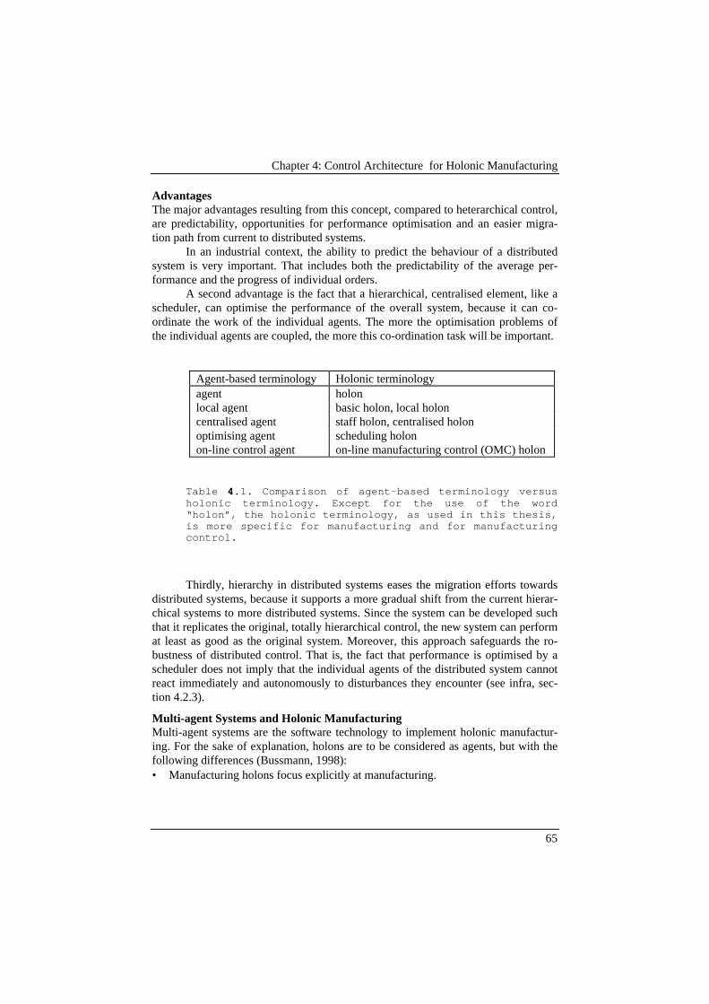
Chapter 4: Control Architecture for Holonic Manufacturing
65
AdvantagesThe major advantages resulting from this concept, compared to heterarchical control,are predictability, opportunities for performance optimisation and an easier migra-tion path from current to distributed systems.
In an industrial context, the ability to predict the behaviour of a distributedsystem is very important. That includes both the predictability of the average per-formance and the progress of individual orders.
A second advantage is the fact that a hierarchical, centralised element, like ascheduler, can optimise the performance of the overall system, because it can co-ordinate the work of the individual agents. The more the optimisation problems ofthe individual agents are coupled, the more this co-ordination task will be important.
Agent-based terminology Holonic terminologyagent holonlocal agent basic holon, local holoncentralised agent staff holon, centralised holonoptimising agent scheduling holonon-line control agent on-line manufacturing control (OMC) holon
Table 4.1. Comparison of agent-based terminology versusholonic terminology. Except for the use of the word“holon”, the holonic terminology, as used in this thesis,is more specific for manufacturing and for manufacturingcontrol.
Thirdly, hierarchy in distributed systems eases the migration efforts towardsdistributed systems, because it supports a more gradual shift from the current hierar-chical systems to more distributed systems. Since the system can be developed suchthat it replicates the original, totally hierarchical control, the new system can performat least as good as the original system. Moreover, this approach safeguards the ro-bustness of distributed control. That is, the fact that performance is optimised by ascheduler does not imply that the individual agents of the distributed system cannotreact immediately and autonomously to disturbances they encounter (see infra, sec-tion 4.2.3).
Multi-agent Systems and Holonic ManufacturingMulti-agent systems are the software technology to implement holonic manufactur-ing. For the sake of explanation, holons are to be considered as agents, but with thefollowing differences (Bussmann, 1998):• Manufacturing holons focus explicitly at manufacturing.

Chapter 4: Control Architecture for Holonic Manufacturing
66
• Holons not only include the information processing part. If applicable, holonsinclude the physical objects they are managing. Holons also (are to) consider thehuman integration.
• Holonic manufacturing systems are multi-agent systems with some hierarchicalstructure.
In practice, the term agents or holons can be used interchangeably, as summarised intable 4.1. Since, occasionally, this gives rise to discussions, this text from now onrefers to (manufacturing) holons instead of agents, unless where the difference is tobe made explicit.
To be continued...This abstract concept becomes more concrete in the following sections. Section 4.3describes the control architecture that results from this concept, and gives examplesof centralised agents (like the scheduler) and local agents (like the orders and theworkstations). Chapter 7 discusses the application of the concept to the developedsoftware.
4.2.2 Distributed Decision PowerManufacturing control systems with a structure as suggested in the previous subsec-tion have both distributed and centralised control capabilities. An initial idea was tosearch for a combination of robustness against disturbances and performance optimi-sation by switching from hierarchical to heterarchical control at the right time. Sucha system becomes autonomous when disturbances occur, and it follows the schedulewhen there are no disturbances (Valckenaers, 1994b). However, the results are notsatisfactory yet. The resulting behaviour remains heterarchical respectively hierar-chical, implying that the drawbacks of heterarchical or hierarchical control remainpresent.
In order to truly combine the best of both hierarchical and distributed control,it is not sufficient to allocate decision power to centralised holons only (hierarchical)or to local holons only (heterarchical). This leads to the second concept.
Assertion 2.
To combine robustness against disturbances with performance optimisationand predictability, decision power needs to be distributed between the cen-tralised (staff) holons and the local holons.
This results to the manufacturing control system operating as follows. The central-ised holons operate concurrently with local holons and contribute to the same deci-sion making processes as the local holons. The local holons maintain their decisionmaking autonomy, but may request advice from the central holons, the so-called staffholons. In this way, the staff holons can co-ordinate and optimise the overall behav-iour of the system.
Essential in this concept is that there is no command-response relationshipbetween staff holons and local holons. Since the staff holons only give advice, the

Chapter 4: Control Architecture for Holonic Manufacturing
67
local holons do not strictly have to obey them. The advice is considered as a nominalplan, but local holons can deviate from it when necessary. This results in a joint de-cision taking.
As the resource allocation for each operation is performed by some localholon, as well as by one or more staff holons, the decision-making functionality isindeed redundant. However, this functional redundancy is not superfluous, since theholons with the same functionalities have different skills and abilities, as mentionedin the previous subsection.
Since the decision-making functionality is distributed over several holons in aredundant way, some conflict resolution mechanisms are necessary. In other words,not only the decision-making functionality, but also the decision-making authorityneeds to be distributed over the holons. This implies that local holons have someautonomy, but also that the autonomy may be reduced in favour of the staff holons.With a low degree of autonomy, the local holons consider the advice as commands,and obey them strictly. With a high degree of autonomy, the advice will be almostignored. Depending on the situation on the shop floor, a compromise has to be madebetween autonomy and obedience. Important elements in this compromise are per-formance and operational guarantees in order to improve the predictability of thesystem. Section 4.4 shows how to model this compromise. Chapter 6 gives some ex-amples of how to make this compromise.
MotivationThe concept of distributed decision power provides the control architecture withmore flexibility than a hierarchical or heterarchical control architecture. Hierarchicalcontrol puts all decision power in the higher levels, and heterarchical control puts itall in the local agents. If the control architecture supports the distribution of decisionpower, it can emulate the traditional solutions as degenerated cases of the generalmodel. Therefore, the proposed solution should be dominant to the traditional (hier-archical and heterarchical) approaches (i.e. at least as good as them).
A trivial solution to distribute decision power between staff holons and localholons could be an approach that switches between hierarchical and heterarchicalcontrol, depending on the importance of disturbances occurring. However, as shownin chapter 8, such an approach does not give satisfactory results, because it not onlycombines the advantages, but also the drawbacks of both approaches.
Remember that in heterarchical control, it is the distributed control mecha-nism that provides heterarchical control with robustness against disturbances. Whenintroducing hierarchy in a system, a similar distribution of decision power, accordingto the abilities present at each hierarchical level, is desirable to maintain the sameinnate robustness against disturbances.
Of course, such high-level reasoning can provide us with a clue on how to ad-dress the problem, but preferably, it is backed up with experimental evidence.Chapter 8 describes the experiments performed to proof these concepts.
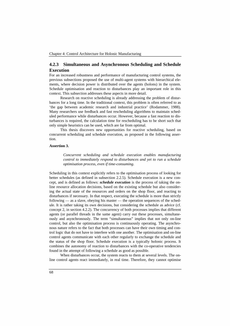
Chapter 4: Control Architecture for Holonic Manufacturing
68
4.2.3 Simultaneous and Asynchronous Scheduling and ScheduleExecutionFor an increased robustness and performance of manufacturing control systems, theprevious subsections proposed the use of multi-agent systems with hierarchical ele-ments, where decision power is distributed over the agents (holons) in the system.Schedule optimisation and reaction to disturbances play an important role in thiscontext. This subsection addresses these aspects in more detail.
Research on reactive scheduling is already addressing the problem of distur-bances for a long time. In the traditional context, this problem is often referred to as‘the gap between academic research and industrial practice’ (Rodammer, 1988).Many researchers use feedback and fast rescheduling algorithms to maintain sched-uled performance while disturbances occur. However, because a fast reaction to dis-turbances is required, the calculation time for rescheduling has to be short such thatonly simple heuristics can be used, which are far from optimal.
This thesis discovers new opportunities for reactive scheduling, based onconcurrent scheduling and schedule execution, as proposed in the following asser-tion.
Assertion 3.
Concurrent scheduling and schedule execution enables manufacturingcontrol to immediately respond to disturbances and yet to run a scheduleoptimisation process, even if time-consuming.
Scheduling in this context explicitly refers to the optimisation process of looking forbetter schedules (as defined in subsection 2.2.5). Schedule execution is a new con-cept, and is defined as follows: schedule execution is the process of taking the on-line resource allocation decisions, based on the existing schedule but also consider-ing the actual state of the resources and orders on the shop floor, and reacting todisturbances if necessary. In that respect, executing the schedule is more than strictlyfollowing — as a slave, obeying his master — the operation sequences of the sched-ule. It is rather taking its own decisions, but considering the schedule as advice (cf.concept 2, in section 4.2.2). The concurrency of both processes implies that differentagents (or parallel threads in the same agent) carry out these processes, simultane-ously and asynchronously. The term “simultaneous” implies that not only on-linecontrol, but also the optimisation process is continuously operating. The asynchro-nous nature refers to the fact that both processes can have their own timing and con-trol logic that do not have to interfere with one another. The optimisation and on-linecontrol agents communicate with each other regularly to exchange the schedule andthe status of the shop floor. Schedule execution is a typically holonic process. Itcombines the autonomy of reaction to disturbances with the co-operative tendenciesfound in the attempt of following a schedule as good as possible.
When disturbances occur, the system reacts to them at several levels. The on-line control agents react immediately, in real time. Therefore, they cannot optimise
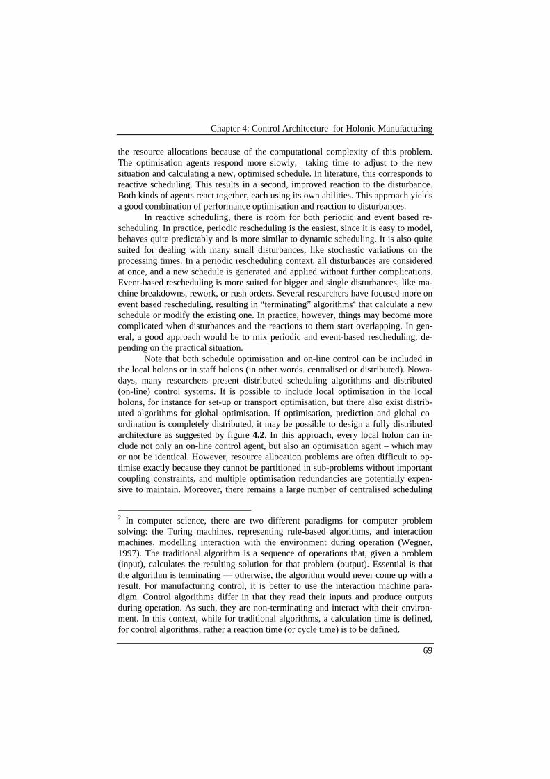
Chapter 4: Control Architecture for Holonic Manufacturing
69
the resource allocations because of the computational complexity of this problem.The optimisation agents respond more slowly, taking time to adjust to the newsituation and calculating a new, optimised schedule. In literature, this corresponds toreactive scheduling. This results in a second, improved reaction to the disturbance.Both kinds of agents react together, each using its own abilities. This approach yieldsa good combination of performance optimisation and reaction to disturbances.
In reactive scheduling, there is room for both periodic and event based re-scheduling. In practice, periodic rescheduling is the easiest, since it is easy to model,behaves quite predictably and is more similar to dynamic scheduling. It is also quitesuited for dealing with many small disturbances, like stochastic variations on theprocessing times. In a periodic rescheduling context, all disturbances are consideredat once, and a new schedule is generated and applied without further complications.Event-based rescheduling is more suited for bigger and single disturbances, like ma-chine breakdowns, rework, or rush orders. Several researchers have focused more onevent based rescheduling, resulting in “terminating” algorithms2 that calculate a newschedule or modify the existing one. In practice, however, things may become morecomplicated when disturbances and the reactions to them start overlapping. In gen-eral, a good approach would be to mix periodic and event-based rescheduling, de-pending on the practical situation.
Note that both schedule optimisation and on-line control can be included inthe local holons or in staff holons (in other words. centralised or distributed). Nowa-days, many researchers present distributed scheduling algorithms and distributed(on-line) control systems. It is possible to include local optimisation in the localholons, for instance for set-up or transport optimisation, but there also exist distrib-uted algorithms for global optimisation. If optimisation, prediction and global co-ordination is completely distributed, it may be possible to design a fully distributedarchitecture as suggested by figure 4.2. In this approach, every local holon can in-clude not only an on-line control agent, but also an optimisation agent – which mayor not be identical. However, resource allocation problems are often difficult to op-timise exactly because they cannot be partitioned in sub-problems without importantcoupling constraints, and multiple optimisation redundancies are potentially expen-sive to maintain. Moreover, there remains a large number of centralised scheduling
2 In computer science, there are two different paradigms for computer problemsolving: the Turing machines, representing rule-based algorithms, and interactionmachines, modelling interaction with the environment during operation (Wegner,1997). The traditional algorithm is a sequence of operations that, given a problem(input), calculates the resulting solution for that problem (output). Essential is thatthe algorithm is terminating — otherwise, the algorithm would never come up with aresult. For manufacturing control, it is better to use the interaction machine para-digm. Control algorithms differ in that they read their inputs and produce outputsduring operation. As such, they are non-terminating and interact with their environ-ment. In this context, while for traditional algorithms, a calculation time is defined,for control algorithms, rather a reaction time (or cycle time) is to be defined.
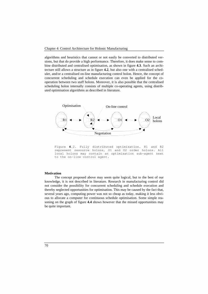
Chapter 4: Control Architecture for Holonic Manufacturing
70
algorithms and heuristics that cannot or not easily be converted to distributed ver-sions, but that do provide a high performance. Therefore, it does make sense to com-bine distributed and centralised optimisation, as shown in figure 4.3. Such an archi-tecture still allows a structure as in figure 4.2, but also one with a centralised sched-uler, and/or a centralised on-line manufacturing control holon. Hence, the concept ofconcurrent scheduling and schedule execution can even be applied for the co-operation between two staff holons. Moreover, it is also possible that the centralisedscheduling holon internally consists of multiple co-operating agents, using distrib-uted optimisation algorithms as described in literature.
R2R1 O1 O2Local holons
Negotiation
Optimisation On-line control
Figure 4.2. Fully distributed optimisation. R1 and R2represent resource holons, O1 and O2 order holons. Alllocal holons may contain an optimisation sub-agent nextto the on-line control agent.
MotivationThe concept proposed above may seem quite logical, but to the best of our
knowledge, it is not described in literature. Research in manufacturing control didnot consider the possibility for concurrent scheduling and schedule execution andthereby neglected opportunities for optimisation. This may be caused by the fact that,several years ago, computing power was not so cheap as today, making it less obvi-ous to allocate a computer for continuous schedule optimisation. Some simple rea-soning on the graph of figure 4.4 shows however that the missed opportunities maybe quite important.

Chapter 4: Control Architecture for Holonic Manufacturing
71
R2
S
R1 O1 O2
Advice &feed-back
Central (staff)holon
Local holons
Negotiation
Optimisation
On-line control
Figure 4.3. Holonic architecture, with combined distrib-uted and centralised optimisation.
Qs c h e d
A: Performance Parsifal for static problems
Schedule calculation
B: Performance Parsifal
for Dynamic Problem
C: Performance Phocs
Tardiness
time
D: Performance Parsifal and Phocs Co-operating
Figure 4.4. Qualitative performance graphs for a numberof situations. Performance graphs (cf. subsection 2.2.2)express the performance of a scheduling algorithm infunction of the available calculation time. Because ofthe qualitative nature of figure, no units nor algorithmswere indicated. In this example, tardiness was chosen asa performance measure, because it is easy to understandand to provide good qualitative graphs.
Figure 4.4 shows in a qualitative way how performance is related to calcula-tion time. Define the performance graph as the function that expresses the perform-ance of a manufacturing control system (or a manufacturing control strategy) in
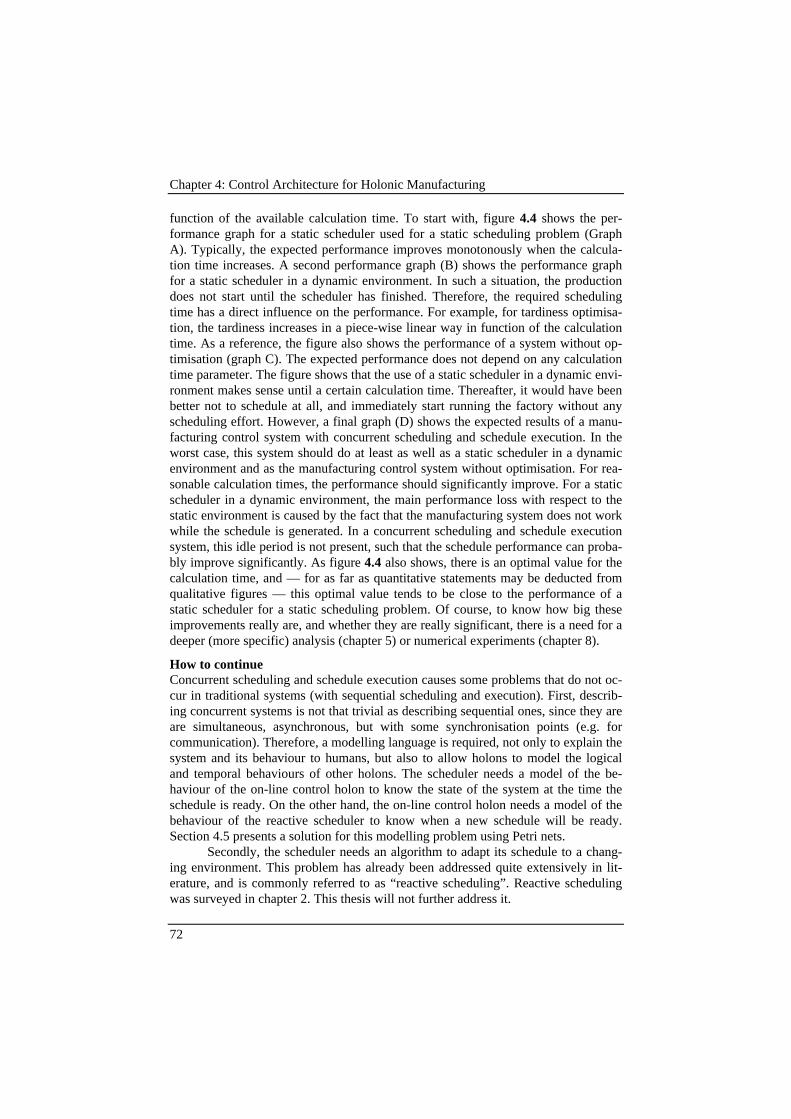
Chapter 4: Control Architecture for Holonic Manufacturing
72
function of the available calculation time. To start with, figure 4.4 shows the per-formance graph for a static scheduler used for a static scheduling problem (GraphA). Typically, the expected performance improves monotonously when the calcula-tion time increases. A second performance graph (B) shows the performance graphfor a static scheduler in a dynamic environment. In such a situation, the productiondoes not start until the scheduler has finished. Therefore, the required schedulingtime has a direct influence on the performance. For example, for tardiness optimisa-tion, the tardiness increases in a piece-wise linear way in function of the calculationtime. As a reference, the figure also shows the performance of a system without op-timisation (graph C). The expected performance does not depend on any calculationtime parameter. The figure shows that the use of a static scheduler in a dynamic envi-ronment makes sense until a certain calculation time. Thereafter, it would have beenbetter not to schedule at all, and immediately start running the factory without anyscheduling effort. However, a final graph (D) shows the expected results of a manu-facturing control system with concurrent scheduling and schedule execution. In theworst case, this system should do at least as well as a static scheduler in a dynamicenvironment and as the manufacturing control system without optimisation. For rea-sonable calculation times, the performance should significantly improve. For a staticscheduler in a dynamic environment, the main performance loss with respect to thestatic environment is caused by the fact that the manufacturing system does not workwhile the schedule is generated. In a concurrent scheduling and schedule executionsystem, this idle period is not present, such that the schedule performance can proba-bly improve significantly. As figure 4.4 also shows, there is an optimal value for thecalculation time, and — for as far as quantitative statements may be deducted fromqualitative figures — this optimal value tends to be close to the performance of astatic scheduler for a static scheduling problem. Of course, to know how big theseimprovements really are, and whether they are really significant, there is a need for adeeper (more specific) analysis (chapter 5) or numerical experiments (chapter 8).
How to continueConcurrent scheduling and schedule execution causes some problems that do not oc-cur in traditional systems (with sequential scheduling and execution). First, describ-ing concurrent systems is not that trivial as describing sequential ones, since they areare simultaneous, asynchronous, but with some synchronisation points (e.g. forcommunication). Therefore, a modelling language is required, not only to explain thesystem and its behaviour to humans, but also to allow holons to model the logicaland temporal behaviours of other holons. The scheduler needs a model of the be-haviour of the on-line control holon to know the state of the system at the time theschedule is ready. On the other hand, the on-line control holon needs a model of thebehaviour of the reactive scheduler to know when a new schedule will be ready.Section 4.5 presents a solution for this modelling problem using Petri nets.
Secondly, the scheduler needs an algorithm to adapt its schedule to a chang-ing environment. This problem has already been addressed quite extensively in lit-erature, and is commonly referred to as “reactive scheduling”. Reactive schedulingwas surveyed in chapter 2. This thesis will not further address it.

Chapter 4: Control Architecture for Holonic Manufacturing
73
Thirdly, the on-line SFC system needs a special algorithm to react to distur-bances while also obeying the global schedule. This problem has hardly got attentionin literature. Chapter 6 presents some algorithms for schedule execution. Scheduleexecution is a new niche in manufacturing research, and will be an interesting subjectin the future research on holonic manufacturing.
Fourthly, also the co-operation between scheduling and schedule executionholons involves a lot of decision taking. To start with, it refers to the design of peri-odic, event-based or hybrid rescheduling schemes. Secondly, a lot of parameters inthe interaction mechanism have to be defined. The tuning of these parameters issometimes called “meta-control”. Meta-control in general is a huge and importantresearch domain for holonic manufacturing, but is outside the scope of this thesis.Chapter 5 further discusses the design of an interaction mechanism.
4.3 Functional and Structural ModelsA functional and a structural model make up the heart of the holonic control archi-tecture. They concretise the concepts developed in the previous section and providea more formal description of the manufacturing control system. This section firstpresents what has to be modelled, then gives a functional and a structural model formanufacturing control and discusses the consequences.
The functional and structural models described in this paragraph are devel-oped in conjunction with PROSA, the K.U.Leuven reference architecture on holonicmanufacturing (Wyns, 1999), as described in chapter 3.
4.3.1 Modelling requirementsAccording to the CIM-OSA reference architecture (CIM-OSA, 1990, Vernadat,1993), an architecture contains a functional view, an informational view, a resourceview, and an organisational view. These views represent different models, looking atthe system from different viewpoints. Other architectures and reference architecturespresent similar views.
The holonic control architecture presents a functional model and a structuralmodel. The functional model describes the functions required for manufacturingcontrol (subsection 4.3.2). In other words, it describes the goal of the system. Im-portant is that the functional description of the system does not describe who is per-forming these functions (Bauer, 1991, Vernadat, 1993).
It is the structural model that identifies the holons required and structures theset of holons by describing their relationships (subsection 4.3.3). It also maps thefunctions to the responsible holons. Due to the distributed decision power, however,functions are not to be allocated to a single holon. Therefore, it is also necessary tomodel the responsibilities of the holons, and make sure the joint responsibilities ofall holons, partially overlapping, can cover all functions required. The responsibili-ties of the holons are identified by describing how they operate.
The functional and structural models, presented here, give only a partial viewon the reference architecture. Since the models are static, they cannot provide a de-tailed view on the operation of the system. The informational view and the organisa-

Chapter 4: Control Architecture for Holonic Manufacturing
74
tional view are mostly outside the scope of this thesis. Informational aspects aremostly computer science oriented. Organisational aspects are more concerned withthe design of control algorithms and the problem of tuning the plant, which is par-tially treated in the remainder of this thesis. The resource view, as defined by CIM-OSA, maps partially to the structural aspects of the structural model presented here.
The structural model of a holonic manufacturing control system should con-tain the following elements.• It should be able to model the holons corresponding to agents found in typical
heterarchical control systems, like orders and resources. They correspond to the“basic holons” as defined in the PROSA architecture (Wyns, 1999). This is re-quired to benefit from the advantages of distributed control and emergent be-haviour, like autonomous reaction to disturbances.
• It should model centralised manufacturing control agents, or staff holons, likee.g. schedulers. These staff holons are to bring the advantages of hierarchy in theHMS.
• The control architecture shall remain flexible. The type of control holarchy to bechosen shall not be defined by the holonic manufacturing control architecture onbeforehand. On the contrary, since the optimal control strategy depends on theproperties and the state of the system and its environment, it shall be possible tochange the control strategy during operation (see also section 4.4). To achievethis flexibility, the architecture should be reconfigurable. Moreover, a holonic ar-chitecture shall support multiple hierarchies. In a strict hierarchy, each parentnode can have several child nodes, but each child node can only have one parentnode, such that the architecture gets very rigid. If nodes are allowed to belong tomultiple hierarchies, parallel control channels can be added as needed, withouttaking away the child nodes of other holons. This corresponds to the concepts ofdistributed decision power, and is further discussed in section 4.4.
• Self-configurability. Since an entire spectrum of control architectures is possible,the architecture shall support its own evolution, both on long term, to adapt to theevolution of the system, as on short term, to adapt to the situation on the shopfloor.
4.3.2 Functional Model for Holonic Manufacturing ControlOne of the major functions of a manufacturing control system is the allocation of re-sources to orders and operations. This includes scheduling, on-line control andmonitoring (Figure 4.5). The scheduling function has two sub-functions: predictionand optimisation. Knowing on beforehand how resources will be allocated is impor-tant not only for human aspects but also for the timely co-ordination of activities onthe shop floor. The goal of optimisation is quite obvious, but is sometimes consid-ered to be of secondary importance (and thus optional — Duffie, 1987). Monitoringserves the a-posteriori measurement and analysis of performance, but is also requiredfor the generation of feedback information to react to disturbances. On-line control isconcerned with the actual decision taking, using the schedule and reacting to distur-bances.

Chapter 4: Control Architecture for Holonic Manufacturing
75
Manufacturing status
Commands to equipment
Orders
Finished goods
Raw material
Manufacturing System
Scheduling
Prediction
Optimisation
Performance
Collecting feedback
information
Actual decision taking and
On-line control
Figure 4.5. Functional model for manufacturing control.
For comparison, this functional decomposition can be viewed in the frame-work of MESA International (1997), the manufacturing execution systems associa-tion. MESA defined 11 functions for shop floor control, 5 of which form part ofmanufacturing control. These functions are:• Resource allocation and status, basically managing resources and selecting re-
sources for operations;• Operations/detailed scheduling, basically doing sequencing;• Dispatching production units, basically doing on-line control;• Maintenance management; and• Performance analysis.

Chapter 4: Control Architecture for Holonic Manufacturing
76
The comparison shows that the industrial and pragmatic view of MESA coincideswith the functional model presented in this thesis (except for the maintenance as-pects). This thesis adds the structuring as provided in figure 4.5.
4.3.3 Structural Model for Holonic Manufacturing ControlFigure 4.6 presents the structural model for holonic manufacturing control. It pres-ents the holons required for a holonic manufacturing control system at three levels.On the lowest level (the level of the local holons), order holons and resource holons(like workstations and the transport system) can co-operate to co-ordinate all workthat needs to be done. This is accomplished by negotiation protocols as known inheterarchical control.
On a higher level, an on-line manufacturing control (OMC) holon co-ordinates the work of orders and resources, similar to the job of a foreman in a fac-tory. Since orders and resources are able to perform all work by themselves, theywould not really need the OMC holon, but the existence of the OMC holon enablesco-ordination on a global scale.
On the upper level, a scheduling holon co-operates with the OMC holon tocombine global performance optimisation with reaction to disturbances. The sched-uling holon is continuously calculating the near-optimal global schedule for the fu-ture. Meanwhile, the OMC holon takes care of disturbances that occur when execut-ing the current schedule. The scheduler can focus on optimising, without repetitiveinterrupts from shop floor disturbances. On the other hand, the OMC holon can fol-low a global schedule, and at the same time react to disturbances. The OMC holoncan react a lot faster to disturbances than a reactive scheduler could. In other words,the scheduler has a lot more time available for rescheduling than in typical reactivescheduling systems.
The existence of one or more centralised scheduling holons does not preventthe local holons to optimise their local performance too. Using the most recent in-formation and the most detailed model of themselves, local holons have good op-portunities to do so. There also exist some schedule optimisation algorithms (Gou,1994, 1998) that are very suited for distributed implementations, because the localperformance measures directly reflect global performance optimisation. However, asexplained above, fully distributed optimisation algorithms — i.e. without any cen-tralised element — up to now did not work, because of insufficient co-ordinationpossibilities.
Basically, holonic manufacturing control is performed by the co-operation ofthe order holons, the resource holons, the OMC holons and scheduling holons. Newin holonic manufacturing is that functions are not mapped in a one-to-one relation-ship to holons. Different holons, centralised as well as local ones, have complemen-tary abilities to perform these functions, and should therefore perform them together,in co-operation. Therefore, prediction, optimisation, decision taking, monitoring andreaction to disturbances are functions present in all these holons, to a greater orlesser degree.
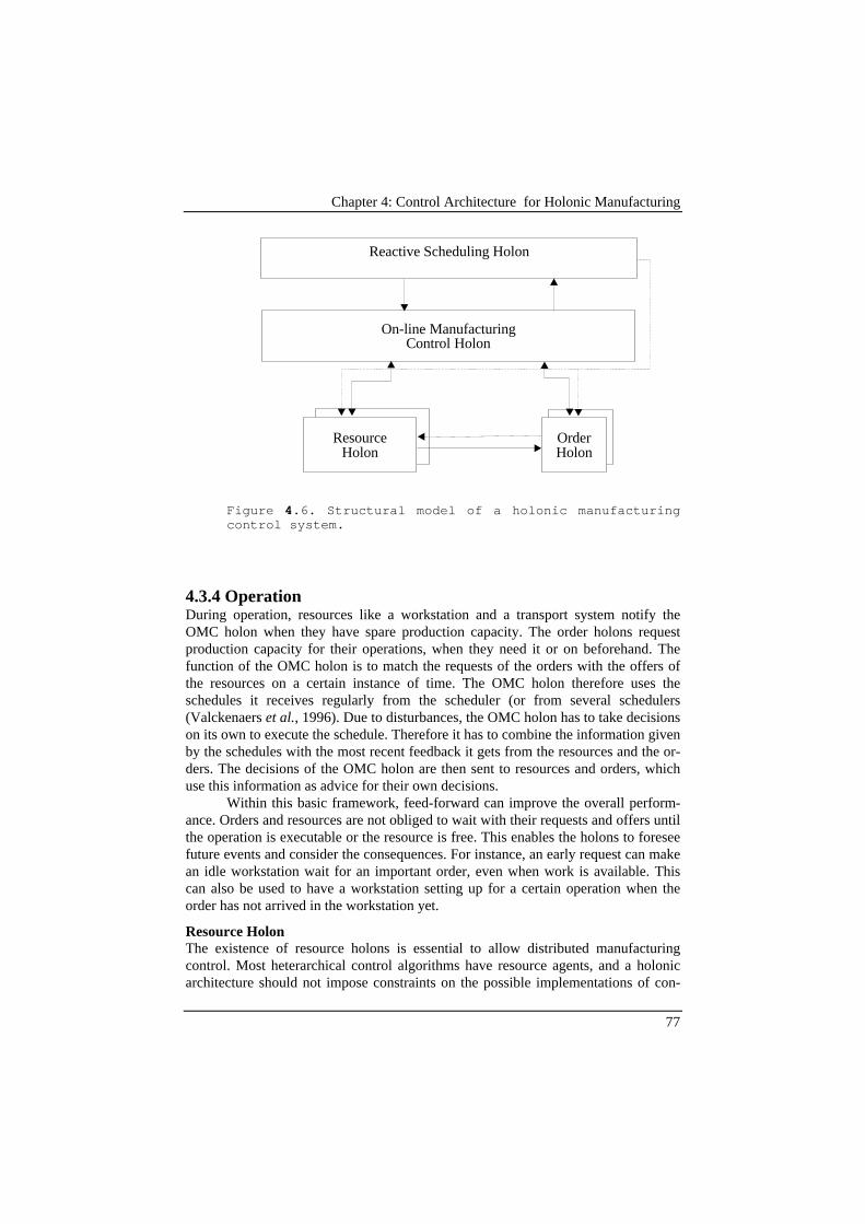
Chapter 4: Control Architecture for Holonic Manufacturing
77
On-line Manufacturing Control Holon
Reactive Scheduling Holon
Order Holon
Resource Holon
Figure 4.6. Structural model of a holonic manufacturingcontrol system.
4.3.4 OperationDuring operation, resources like a workstation and a transport system notify theOMC holon when they have spare production capacity. The order holons requestproduction capacity for their operations, when they need it or on beforehand. Thefunction of the OMC holon is to match the requests of the orders with the offers ofthe resources on a certain instance of time. The OMC holon therefore uses theschedules it receives regularly from the scheduler (or from several schedulers(Valckenaers et al., 1996). Due to disturbances, the OMC holon has to take decisionson its own to execute the schedule. Therefore it has to combine the information givenby the schedules with the most recent feedback it gets from the resources and the or-ders. The decisions of the OMC holon are then sent to resources and orders, whichuse this information as advice for their own decisions.
Within this basic framework, feed-forward can improve the overall perform-ance. Orders and resources are not obliged to wait with their requests and offers untilthe operation is executable or the resource is free. This enables the holons to foreseefuture events and consider the consequences. For instance, an early request can makean idle workstation wait for an important order, even when work is available. Thiscan also be used to have a workstation setting up for a certain operation when theorder has not arrived in the workstation yet.
Resource HolonThe existence of resource holons is essential to allow distributed manufacturingcontrol. Most heterarchical control algorithms have resource agents, and a holonicarchitecture should not impose constraints on the possible implementations of con-
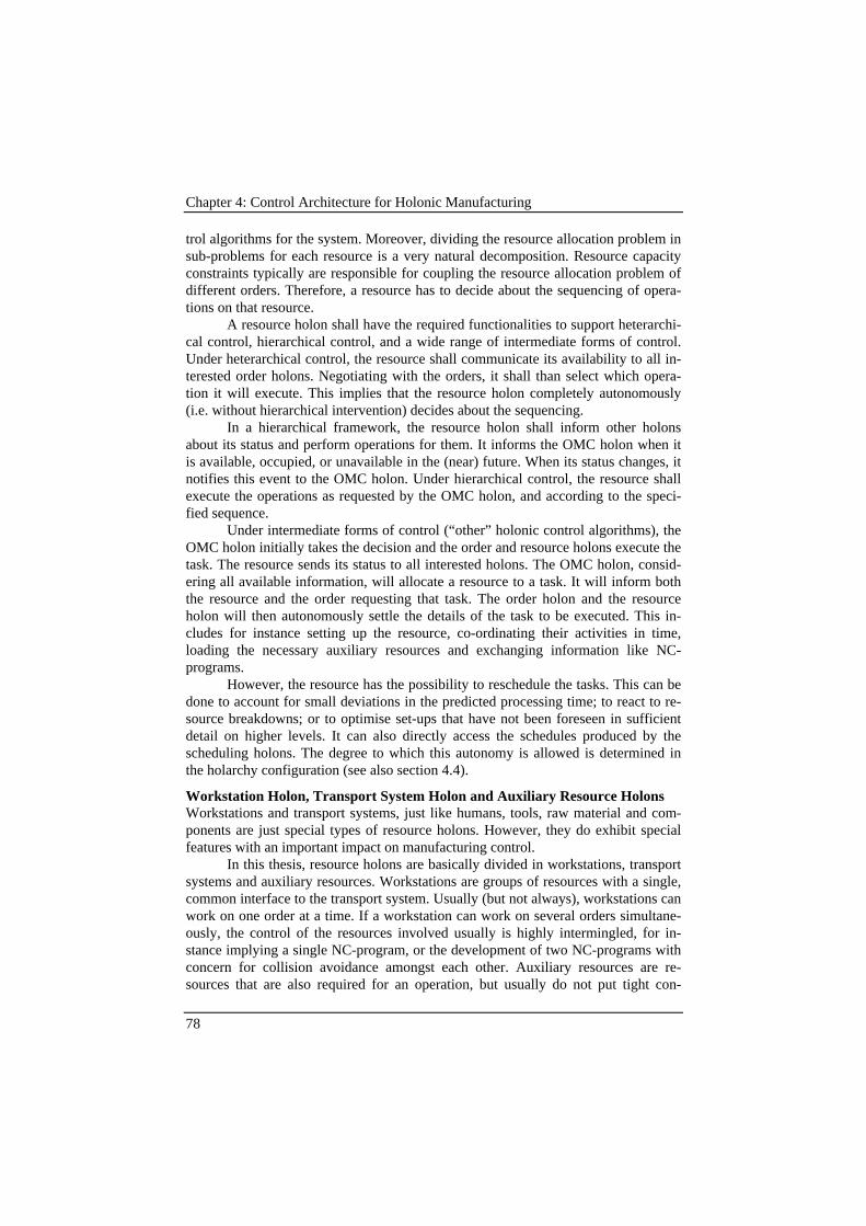
Chapter 4: Control Architecture for Holonic Manufacturing
78
trol algorithms for the system. Moreover, dividing the resource allocation problem insub-problems for each resource is a very natural decomposition. Resource capacityconstraints typically are responsible for coupling the resource allocation problem ofdifferent orders. Therefore, a resource has to decide about the sequencing of opera-tions on that resource.
A resource holon shall have the required functionalities to support heterarchi-cal control, hierarchical control, and a wide range of intermediate forms of control.Under heterarchical control, the resource shall communicate its availability to all in-terested order holons. Negotiating with the orders, it shall than select which opera-tion it will execute. This implies that the resource holon completely autonomously(i.e. without hierarchical intervention) decides about the sequencing.
In a hierarchical framework, the resource holon shall inform other holonsabout its status and perform operations for them. It informs the OMC holon when itis available, occupied, or unavailable in the (near) future. When its status changes, itnotifies this event to the OMC holon. Under hierarchical control, the resource shallexecute the operations as requested by the OMC holon, and according to the speci-fied sequence.
Under intermediate forms of control (“other” holonic control algorithms), theOMC holon initially takes the decision and the order and resource holons execute thetask. The resource sends its status to all interested holons. The OMC holon, consid-ering all available information, will allocate a resource to a task. It will inform boththe resource and the order requesting that task. The order holon and the resourceholon will then autonomously settle the details of the task to be executed. This in-cludes for instance setting up the resource, co-ordinating their activities in time,loading the necessary auxiliary resources and exchanging information like NC-programs.
However, the resource has the possibility to reschedule the tasks. This can bedone to account for small deviations in the predicted processing time; to react to re-source breakdowns; or to optimise set-ups that have not been foreseen in sufficientdetail on higher levels. It can also directly access the schedules produced by thescheduling holons. The degree to which this autonomy is allowed is determined inthe holarchy configuration (see also section 4.4).
Workstation Holon, Transport System Holon and Auxiliary Resource HolonsWorkstations and transport systems, just like humans, tools, raw material and com-ponents are just special types of resource holons. However, they do exhibit specialfeatures with an important impact on manufacturing control.
In this thesis, resource holons are basically divided in workstations, transportsystems and auxiliary resources. Workstations are groups of resources with a single,common interface to the transport system. Usually (but not always), workstations canwork on one order at a time. If a workstation can work on several orders simultane-ously, the control of the resources involved usually is highly intermingled, for in-stance implying a single NC-program, or the development of two NC-programs withconcern for collision avoidance amongst each other. Auxiliary resources are re-sources that are also required for an operation, but usually do not put tight con-
Chapter 4: Control Architecture for Holonic Manufacturing
79
straints on manufacturing control. Of course, the definition of what are workstations,transport systems and auxiliary resources is to some degree a design decision foreach specific system.
Properties leading to such a classification are the capacity, consumability,modifiability and the static or dynamic nature of the resource. While most resourcescan be modelled as having a capacity of performing one task at a time, some can per-form several tasks at once (sometimes in batches, sometimes not, sometimes withincreased durations while heavily loaded). Some resources are consumed during op-eration, implying a cost and the risk for stock breakage (e.g. tools and components).Some resources modify their state during operations, implying that some combina-tions of resource allocations are difficult or impossible (e.g. pallets and machineswith set-ups). Some resources are static and always remain within one workstation,some resources are dynamic, since they can be exchanged between workstations.
In the remainder of this text, workstation holons refer to static resources setsthat are capable of doing only one operation at a time (“single capacity”) and have asingle interface to the transport system.
The transport system holon is a complex resource holon, with several differ-ent aspects. It often is a multi-holon system by itself. Except for Bussmann (1994),van Acker (1996) and Malewicz (1996), the control of transport systems up to nowhas got little attention in the research community. The transport system holon hidesthe internal transportation details from other holons. The clients (order and OMCholon) will ask for transportation from one workstation to another, but will not knowthe route taken or the AGVs used. Hence, it is not trivial to define its remaining ca-pacity. In our implementation, we use the estimated arrival time of the order to itsgoal position to convey the transport capacity. It is not trivial to define the commandmessages either. If transportation commands are issued separately for each transpor-tation tasks, the transport system holon has to decide about the sequencing of allpallets going to the same station. Since this sequencing process may have a large im-pact on global performance, the other holons have to provide more information ontheir preferences. In our implementation, we not only ask for transport between twostations, but we also add time or sequence constraints (which can be relaxed if nec-essary).
Since the transport system is already complex by itself, often it will not or notin sufficient detail be scheduled by the scheduling holon itself. This means activitieshave to be executed which are not explicitly scheduled. Since the route of an order ishighly dependent of the scheduling decisions, the order holon cannot foresee the re-quired transportation time either. Therefore, the OMC holon should provide the nec-essary data to the order holon such that the order holon can negotiate in a proper waywith the transport system holon.
Auxiliary resources can be modelled as resource holons, but often, it is notnecessary to include intelligent, autonomous and co-operative agents in the auxiliaryresources (in other words, they do not have to be holons). For dynamic auxiliary re-sources, it is required however to model them as objects in the system, which holonscan reason about.
Chapter 4: Control Architecture for Holonic Manufacturing
80
Order HolonFrom an architectural point of view, it is essential that also an order is an autono-mous entity (a “holon”), since it is required if not for all, at least for several forms ofdistributed control algorithms. Again, since a holonic architecture should not imposeconstraints on the possible implementations of control algorithms for the system, thisimplies the existence of order holons. In a similar way as with resource holons, thedecomposition of the resource allocation problem over order holons is very natural,since orders can manage the precedence constraints between their operations.Moreover, they have to make the final decision about the selection of resources fortheir operations. Wyns (1999] gives an additional number of reasons to define orderholons, in a context wider than manufacturing control.
Also order holons shall support different types of control. Under heterarchicalcontrol, the order itself takes care of resource allocation. It therefore negotiates withresource holons and with other order holons to obtain the needed resources for itsoperations, and starts them. Heterarchical control allows working without SFC andwithout scheduler.
Under hierarchical control — emulated by a holonic manufacturing controlsystem — the order requests resources for every operation to the OMC holon and theOMC holon will then match order and resources. Then order and resource holonswill autonomously negotiate about the further finishing of their task. The order re-quests resources only if previous tasks have been executed. However, it can also dopre-requests to ask for resource reservations. This enables the execution of inserted-idletime schedules, but it does require the orders to have a fair model of their envi-ronment if the overall performance is not to be jeopardised.
Under intermediate, holonic forms of control, the order holon receives com-mands from the OMC holon, but can override these decisions if estimated necessary.One could also imagine a configuration where the order directly gets a schedule fromthe scheduling holon.
The order holon also contains its own information: the client information andorder deadlines; the precedence constraints; the handle to the product informationand the process related state information (Wyns, 1997).
Scheduling HolonA scheduling holon performs optimisation of the resource allocation process, sincethe OMC holon, being an on-line control system, cannot perform optimisation in anappropriate way. As a consequence, the scheduler holon has more time to performthe optimisation process. Usually however, the scheduler only has a simplified andless up-to-date model of the manufacturing system. It therefore needs to co-operateintensively with the OMC holon (see infra). Often, different aspects of the manufac-turing process are optimised by different schedulers, for instance, one for the overallshop floor, one for maintenance, and one for the transportation system.
Moreover, these scheduling holons are reactive schedulers that continuouslyimprove their schedule. They require a reactive encapsulation of the scheduling algo-rithm, that reads feedback, adapts the scheduling problem according to the feedback,performs scheduling, using the results of the previous schedule and sends the sche-
Chapter 4: Control Architecture for Holonic Manufacturing
81
dule to the OMC holon and continues its work. Such a reactive scheduler can workperiodically or on an event-driven basis (see also section 4.5).
Finally, a scheduling holon also is responsible for providing a prediction ofthe overall behaviour of the manufacturing system. This prediction is used to provide(internal or external) customers with an estimated finishing time for their order.
On-line Manufacturing Control HolonThe main function of an on-line manufacturing control (OMC) holon is the on-lineco-ordination of the local holons (orders and resources) in their decision makingprocess. Because this co-ordination needs to be on-line, it cannot successfully beperformed by a scheduling holon. Distributing this function over different holonswas considered. With the right decomposition of the problem, sometimes verypromising results were achieved (for instance with heterarchical control, marketmechanisms, etc.). However, at this moment there is no completely generic solutionavailable to successfully decompose the problem such that centralised co-ordinationbecomes superfluous.
The OMC holon is a complex holon and an important contribution of this the-sis. To describe the functionality of the OMC holon in more detail, figure 4.7 pres-ents an operational specification3 of the OMC holon. For manufacturing control, fourfunctions can be derived: interfacing, structural control, the on-line decision taking,and monitoring.
The implementation of the interfacing function shall consider the autonomousand co-operative nature of holons in an HMS. The OMC holon communicates con-currently and asynchronously with the resource holons, the order holons and thescheduler holon to accept work requests, manufacturing requests and new schedules.This communication should be non-blocking for all parties, in order to maintain theautonomy of the holons.
Structural control refers to the avoidance of pathological states, like dead-locks, starvation, nervousness, etc. Structural control can be performed by the localholons as well as by staff holons like schedulers or the OMC holon. Typically,structural control can be appropriately implemented using a constraining controllayer, rather than a deciding one. It monitors the system state and prevents decisionsthat would bring the system in an unacceptable state, but it does not impose decisionsitself. As an example, Wyns (1996, 1999) has investigated the issue of deadlockavoidance in holonic manufacturing. This thesis does not consider it further.
3 An operational specification of a computer program (or, in this case, a holon) is aspecification method that describes the requirements for that program by presentinga possible way to implement it.

Chapter 4: Control Architecture for Holonic Manufacturing
82
Shop floor organiser
Schedule Entry
Transport SystemHolon
Neighbour Holon Data
Shop floor control rules
Monitoring
Requestmfg.
Requestwork
Register newschedulers
Register neworders
On-line Manufacturing Control Holon
Register newresources
WorkstationHolon
OrderHolon
SchedulerHolon
Figure 4.7. Operational specification of the OMC holon.
The core functionality of the OMC holon (for manufacturing control) is thetimely decision making. At the right time, decisions have to be made on the alloca-tion of resources to activities requested by the order holons, and these decisions haveto be transmitted to the local holons as advice. The decisions taken by the shop floororganiser are based on the schedule and the current manufacturing situation. In sub-section 4.2.3, these function was defined as “schedule execution”. How this decisionis to be made, depends on control strategy chosen, as shown in chapter 6. Once a de-cision is made, it is communicated to the resources as well as to the order holons.These resource and order holons will from then on autonomously perform the activi-ties requested by the OMC holon. When finished, they report back to the interfaceagents to continue their work.
Since the manufacturing model used by the scheduler often has only a limitedamount of detail, the schedule cannot contain all decisions that have to be made.Therefore the SFC system has to make additional resource allocation decisions. E.g.,while schedulers sometimes neglect transport and/or set-up, the SFC system shouldmaintain consistency in the shop with respect to transport and set-up.

Chapter 4: Control Architecture for Holonic Manufacturing
83
The monitoring function of the OMC holon traces the manufacturing data andfeeds this information back to the scheduler holons.
4.3.5 Implications and remarksThe structural model presented in the previous subsections has a number of implica-tions. To start with, it represents an architecture that remains very flexible with re-spect to the implementation of a control algorithm. This is the reason why an archi-tecture is proposed that consists of resources and orders as local holons, and on-linemanufacturing control holons and schedulers as staff holons. For some algorithms,some holons may not be necessary. In the general case, however, manufacturingcontrol is performed by all these holons together.
Secondly, while the structural model may be static, the holonic manufacturingcontrol system itself does not have to. The design explicitly requires the system toremain operational if some holons become (temporarily) unavailable. It is also re-quired that holons can be added to the system at run time. With that in mind, themodel presented could be called quasi-static, rather than static. It is however static inthat sense that is shows only a snapshot of the system at that time instead of showinghow the system evolves over time.
To describe the operation of the system, a static model is clearly not enough.Because of the flexibility designed into the architecture, the operation of the systemis still quite open. Amongst others, this is due to the fact that functions are redun-dantly implemented in different holons. To continue the design and configuration ofa holonic manufacturing control system, it should be possible to model the distribu-tion of decision power more formally and unambiguously. For that purpose, the nextsection presents a modelling framework.
In the K.U.Leuven Holonic Reference Architecture PROSA, specialisationand aggregation is more explicitly considered than was shown in this section. Ofcourse, these concepts remain valid for the structure of a holonic manufacturingcontrol system as proposed in this thesis. The specialisation aspect was only superfi-cially discussed for resources, but can be extended for order and staff holons. Theaggregation aspect can be implemented by applying the same structure repetitively todifferent levels of aggregation.
A final remark reiterates on the issue of distributed versus centralised optimi-sation, as discussed in section 4.2.3. As already mentioned, having (centralised) staffholons does not prevent the use of optimisation in the local holons, nor does it pro-hibit the staff holons to implement distributed algorithms internally. The structuralmodel presented in this section does not describe the control algorithms themselves,so it does not model the internal structure of the staff holons either. Control algo-rithms are given in chapter 6, but for this thesis, no distributed algorithms were im-plemented in the staff holons.
4.4 Modelling Distributed Decision PowerIf functions are carried out by several holons together, it is not easy to model the ex-act distribution of decision power. A model is required to describe the autonomy of
Chapter 4: Control Architecture for Holonic Manufacturing
84
the holons and its limitations. Moreover, the architecture proposed in the previoussection was conjectured to combine reactivity to disturbances with predictability andhigh performance. How to achieve this combination is still an unsolved question.This section presents a possible approach for the problem based on the concept offixed rules and flexible strategies (FRFS — Koestler, 1967).
4.4.1 BackgroundWhen Koestler (1967, chapter III) defined the term “holonic” for explaining com-plex systems, he mentioned that holons (for instance, individuals in a society) behaveaccording to fixed rules but flexible strategies. The fixed rules (FR) form a patternof rule-governed behaviour, which lends stability and cohesion to the group. In otherwords, they form a contract between the holons. The individuality — or autonomy— of a holon is expressed by its flexible strategies (FS). In military organisationsand tribal societies, the fixed rules tend to be quite strong, while in a contemporarysociety, flexible strategies are considered more important. Again, the similarity ofthe requirements of human societies and manufacturing control systems suggests auseful analogy. Applying it to holonic manufacturing, the aspired combination of hi-erarchical and heterarchical system properties may be obtained and described by im-plementing the hierarchical aspects of the system in fixed rules. The remaining deci-sion power for the individual holons can than be filled out with their own flexiblestrategies, like in heterarchical systems. The fixed rules are to impose the perform-ance and operational guarantees, while the flexible strategies should take care of re-activity and robustness. This trade off is illustrated in Figure 4.8.
A similar source of inspiration, closer to home, is found in computer science.The concept of invariants was introduced into computer science at the end of theseventies (Berg et al., 1982; de Bakker, 1980) within the field of algorithmic cor-rectness theory. In general, an invariant refers to a property of a system that remainsconstant under different conditions, over time, over different representations, etc. Incorrectness theory, invariants are logical propositions that (should) remain truethroughout the execution of the program (or the algorithm). These invariants areused to prove the correctness of an algorithm a posteriori. More interesting howeveris that these invariants are also used during the design of the algorithm, such that thealgorithms are correct from the beginning. This section aims at using similar invari-ants in holonic systems to help the designer develop distributed control algorithmsthat are understandable and predictable on an overall level. The invariants corre-spond to the fixed rules as defined above.

Chapter 4: Control Architecture for Holonic Manufacturing
85
Flexible StrategiesFixed Rules
Hierarchical
Holonic
Heterarchical
Figure 4.8. Balance of Fixed Rules (Invariants) andFlexible Strategies (“Variants”) in Different Manufactur-ing Control Configurations.
4.4.2 Fixed Rules in Holonic SystemsThe most straightforward way to obtain operational guarantees is by giving directcommands to the local holons in a holonic manufacturing system (HMS). This ap-proach however would take away all autonomy from the holons, turning them intoslaves.
As an alternative, we propose to use fixed rules (or invariants) to obtain per-formance and operational guarantees. A fixed rule (or invariant) is a logical propo-sition that expresses the requirements of the behaviour of a holonic control algo-rithm. It is a contract imposed on the HMS to guarantee predictability and to de-scribe the behaviour in aggregate terms. That contract specifies which global systemproperties the HMS will guarantee to be true. Rather than imposing decisions, fixedrules impose constraints on the behaviour of one holon with respect to the otherones. By defining the limits of autonomy, the fixed rules also define the autonomy(“the freedom to act”) itself. Typically, fixed rules define the autonomy of the localholons (resources and orders) with respect to staff holons, or the autonomy of theOMC holon with respect to a scheduling holon.
These fixed rules are hierarchically imposed on the local holons and aim toprovide a predictable behaviour. Within the remaining decision space, the localholons use their flexible strategies to take the rest of the decisions. The more strin-gent the fixed rules are, the less the local holons are autonomous, and the more the
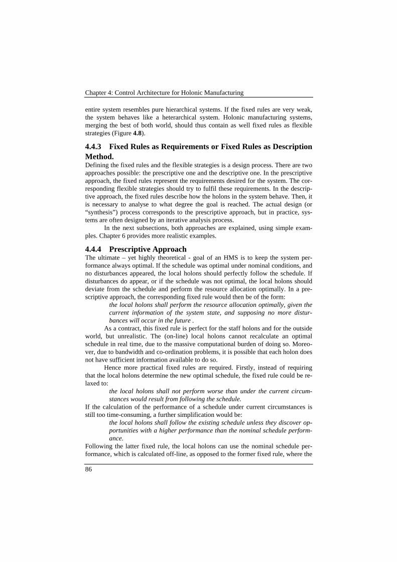
Chapter 4: Control Architecture for Holonic Manufacturing
86
entire system resembles pure hierarchical systems. If the fixed rules are very weak,the system behaves like a heterarchical system. Holonic manufacturing systems,merging the best of both world, should thus contain as well fixed rules as flexiblestrategies (Figure 4.8).
4.4.3 Fixed Rules as Requirements or Fixed Rules as DescriptionMethod.Defining the fixed rules and the flexible strategies is a design process. There are twoapproaches possible: the prescriptive one and the descriptive one. In the prescriptiveapproach, the fixed rules represent the requirements desired for the system. The cor-responding flexible strategies should try to fulfil these requirements. In the descrip-tive approach, the fixed rules describe how the holons in the system behave. Then, itis necessary to analyse to what degree the goal is reached. The actual design (or“synthesis”) process corresponds to the prescriptive approach, but in practice, sys-tems are often designed by an iterative analysis process.
In the next subsections, both approaches are explained, using simple exam-ples. Chapter 6 provides more realistic examples.
4.4.4 Prescriptive ApproachThe ultimate – yet highly theoretical - goal of an HMS is to keep the system per-formance always optimal. If the schedule was optimal under nominal conditions, andno disturbances appeared, the local holons should perfectly follow the schedule. Ifdisturbances do appear, or if the schedule was not optimal, the local holons shoulddeviate from the schedule and perform the resource allocation optimally. In a pre-scriptive approach, the corresponding fixed rule would then be of the form:
the local holons shall perform the resource allocation optimally, given thecurrent information of the system state, and supposing no more distur-bances will occur in the future .
As a contract, this fixed rule is perfect for the staff holons and for the outsideworld, but unrealistic. The (on-line) local holons cannot recalculate an optimalschedule in real time, due to the massive computational burden of doing so. Moreo-ver, due to bandwidth and co-ordination problems, it is possible that each holon doesnot have sufficient information available to do so.
Hence more practical fixed rules are required. Firstly, instead of requiringthat the local holons determine the new optimal schedule, the fixed rule could be re-laxed to:
the local holons shall not perform worse than under the current circum-stances would result from following the schedule.
If the calculation of the performance of a schedule under current circumstances isstill too time-consuming, a further simplification would be:
the local holons shall follow the existing schedule unless they discover op-portunities with a higher performance than the nominal schedule perform-ance.
Following the latter fixed rule, the local holons can use the nominal schedule per-formance, which is calculated off-line, as opposed to the former fixed rule, where the

Chapter 4: Control Architecture for Holonic Manufacturing
87
local holons have to find the actualised schedule performance themselves. However,the latter fixed rule condemns the local holons to wait until favourable opportunitiesappear. Since the existing schedule would usually be near-to-optimal and the conse-quences of disturbances would mostly have a negative impact on the schedule per-formance, these fixed rules would lead to a rather conservative and hierarchical be-haviour.
In total, it appears to be to difficult to define workable prescriptive fixedrules. The next subsection shows that a design process that iteratively defines de-scriptive fixed rules leads to better results.
4.4.5 Descriptive ApproachIn the descriptive approach, fixed rules describe how the system behaves with a cer-tain control algorithm. The control algorithm itself can be distributed, hierarchical,or any holonic algorithm somewhere in between. Defining the fixed rules corre-sponds to an high-level description of the control algorithm. The details are de-scribed in the flexible strategies. In other words, instead of trying to find the singlebest possible fixed rule, such that the performance is as good as possible, the fixedrules describe how a given algorithm controls the system by modelling the distribu-tion of decision power over different holons (local holons and staff holons). This ap-proach models the compromise between autonomy and obedience in the co-operationbetween holons on different levels.
Examples of fixed rules and flexible strategies (FRFS) are most easy to un-derstand for degenerated cases like strictly hierarchical and flatly heterarchical sys-tems. A third example describes a simple holonic algorithm somewhere in between,using plain English. Chapter 6 presents several holonic control strategies using FRFSin a graph theory based framework.
Hierarchical control is governed completely by fixed rules:FR: All operations shall be executed on the resource the schedulersuggested, and in the sequence given by the schedule for the different re-sources. If multiple resources can be used for a single operation, the se-quence given by each resource schedule shall be followed. The schedulershall not provide a schedule with unfeasible sequences.
A fixed rule guarantees the system behaviour very explicitly. However, it quicklyhalts the entire system when a machine breaks down. There is no room for flexiblestrategies.
Under heterarchical control, there are no fixed rules, since all decisions aretaken using flexible strategies. All autonomy is granted to the resource and orderholons, which can react quickly to disturbances, according to their own ideas. How-ever, they do not co-ordinate their work with a global scheduling holon, making theirwork very unpredictable and (sometimes) low in performance.
Using less extreme fixed rules, more subtle forms of co-operation are possi-ble. A careful but reactive behaviour would be described by the following fixed rule:
All operations shall be executed on the resource and in the sequence givenby the schedule, unless local holons (as well order as resource holons) canexplicitly proof that they have an alternative sequence or allocation with a

Chapter 4: Control Architecture for Holonic Manufacturing
88
guaranteed better performance (provided that the estimates for durationsof operations and down times are accurate).
For instance, a workstation could decide to first perform another operation than theone scheduled first, because it knows it can finish it before the other order would ar-rive in the workstation. Such control strategies effectively provide a better combina-tion of performance and robustness against disturbances than either hierarchical orheterarchical control can do.
4.4.6 Flexible StrategiesOnce the fixed rules are defined, the flexible strategies can still be chosen. Severalapproaches are possible, ranging from simple heuristics and dispatching rules tomodel based approaches. A very attractive idea is the use of market-based algorithmsfor the flexible strategies, since these algorithms are very robust against disturbances.Other approaches may be based on neural networks, or interactive (human based)control. In chapter 6, an automated control algorithm based on perturbation analysisis presented.
4.4.7 ConclusionIn holonic manufacturing, it makes sense to distribute decision power over holons ondifferent hierarchical levels. The question how to do so is not trivial. Therefore, firsta model was presented to describe how the decision power is distributed. This modeluses fixed rules (invariants) for the holons in the system. The remaining autonomycan then be used by each individual holon to follow its own flexible strategies. Sec-ondly, an attempt was made to deduct fixed rules as overall system requirements.Since this synthesis process is not that simple, the design of good fixed rules is to beperformed by the repetitive analysis of candidate fixed rules, until an balanced dis-tribution of decision power is obtained.
4.5 Modelling Framework for the InteractionMechanismThe presented holonic control architecture consists of a number of holons: autono-mous, co-operating agents. The second step in the design of a holonic manufacturingcontrol system is the definition of their interactions. This step is described in chapter5, but first, a modelling framework is required to model the interaction mechanism.This section provides such a framework, based on Petri nets.
4.5.1 RequirementsAll these holons (scheduler, on-line SFC, workstation and order) work in parallel.The scheduler is calculating continuously, and meanwhile, the on-line OMC holon iscontrolling the system. Meanwhile, all workstation holons are continuously control-ling their own workstation (implying scheduling, execution and monitoring). Also,all order holons are continuously scheduling, executing and monitoring the opera-tions of the orders.

Chapter 4: Control Architecture for Holonic Manufacturing
89
This parallel operation is a logical consequence of their autonomy, since theyhave to be able to react to disturbances. Thereby, the holons operate asynchronously,meaning that the timing and sequencing of the events that trigger their decisionstaking are unrelated. However, the holons also have to co-operate to achieve a globalgoal, implying a lot of interactions between them: they exchange information, giveadvice and negotiate among them. In practice, this results to occasional synchronisa-tion points.
Consequently, the modelling framework has to provide tools to describe thedynamics of the system: how holons operate concurrently, asynchronously and withoccasional synchronisation points. The resulting model is to serve four purposes:• First, a model of the interaction mechanism is useful to describe the operation of
the system in an unambiguous and easily understandable way.• Secondly, such a model supports the analysis of the interactions between holons.
A formal analysis provides a better framework for implementing, debugging andfine-tuning the system than mere intuition.
• Thirdly, formal models can be included in the decision making software. Thisway holons can base their decisions on the model they have of other holons.
• A formal model also supports the optimisation of the tuneable parameters.
4.5.2 Petri nets to model the interaction mechanismThis thesis has chosen timed Petri nets (Petri, 1962, Peterson, 1981) to model theinteraction between holons, as a modelling language. The nodes represent high levelreasoning processes in the holons, and the transitions represent synchronisationpoints between holons or between parallel threads within a holon. Transitions canalso be used — just for the clarity of presentation — to separate reasoning processesof a different nature, even when no synchronisation is necessary. Initial tokens canbe located in a “reasonable” place at start-up, or special start-up places can be mod-elled. In this timed Petri net, time is modelled with minimum staying times for tokensin a place.
(Timed) Petri nets are very suited for this kind of modelling, since they de-scribe concurrency and asynchronicity in an unambiguous yet easy to understandway. They are also based on the concept of discrete events determining the evolutionof the system. Because these models are high-level representations, their size re-mains limited. Finally, it is easy to deduct the structure of control algorithms fromsuch a Petri net. These algorithmic structures can be directly mapped to pseudo-codeor flow diagrams.
The design of an interaction mechanism between holons is application-specific. Therefore, examples of such an interaction mechanism are found in chapter5.
4.6 ConclusionThis chapter has presented three basic new concepts for holonic manufacturing con-trol and presented the corresponding modelling mechanisms to accurately describethe resulting system design. To combine robustness against disturbances with per-
Chapter 4: Control Architecture for Holonic Manufacturing
90
formance optimisation and predictability, the incorporation of hierarchy in a dis-tributed control system is proposed. This concept results in a holonic manufacturingcontrol architecture, explained with a functional and structural model. In holonicmanufacturing control, the decision power needs to be distributed among the holonsaccording to their abilities. To formally describe the distribution of decision power, amodelling framework is proposed, based on fixed rules and flexible strategies. Thedistribution of decision power leads to the concept of concurrent scheduling andschedule execution, combining an optimisation process with a reactive process formanufacturing control.
The concepts developed in this chapter form a generic basis for holonicmanufacturing control (the implementation of the control architecture for a specificsystem is almost straightforward — see chapter 7); however, they require the furtherimplementation of more application specific software components. First, the con-tinuous operation of a reactive scheduler requires the existence of reactive schedul-ing algorithms. Reactive scheduling algorithms do already exist for several years,and are described extensively in literature (surveyed in chapter 2), and are outsidethe scope of this thesis. Secondly, the proposed architecture requires the function of“schedule execution”. Chapter 6 provides a set of algorithms, ranging from heuristicto model based algorithms, to perform schedule execution. That chapter also showshow fixed rules and flexible strategies can be defined to describe the autonomy ofthe holons involved.
However, before the control algorithms within each holon can be developed,the interaction mechanism between the holons is to be designed. This chapter hasproposed timed Petri nets as a suitable modelling framework for the design of an in-teraction mechanism. The design itself is presented in the next chapter.

91
Chapter 5
Interaction Mechanism
Petri models can be used to model the interaction mechanism between holons. Thischapter presents models for concurrent scheduling and schedule execution accord-ing to the concepts of periodic and event-based rescheduling. It shows with someexamples that also the co-operation with other holons can be modelled. By analys-ing the timing aspects of these Petri nets, it is possible to calculate response times ofeach holon to disturbances. A second analysis shows why concurrent schedulingand schedule execution outperforms traditional approaches for manufacturing con-trol.
5.1 IntroductionThe previous chapter presented a control architecture for holonic manufacturing,which includes a structural model to identify the holons present in the HMS. Thesecond step in the design of a holonic manufacturing control system is the design ofthe interaction mechanism that makes these holons co-operate.
Though generic, the structural model is easily applicable to a specific manu-facturing system (see chapter 7, or Corgnati, 1998). However, it turned out to behard to model the interaction mechanism for a holonic manufacturing system in away that is both generic and concrete.
Therefore, this chapter describes the design of the interaction mechanism as itwas developed for our implementation. This design defines the interactions betweenthe holons and the tasks they have to perform in between. It considers sequencing,parallelism and timing of the interactions and the tasks. It results in a co-operationprotocol for the holons and identifies where and when decision-making logic is re-quired in the individual holon. The design is analysed with Petri nets, as proposed inchapter 4, and some of its parameters are further optimised.
Since concurrent scheduling and schedule execution (CSSE) is a new con-cept, this chapter pays special attention to modelling the co-operation between a re-active scheduling holon and an OMC holon.
This chapter is structured as follows. First, using Petri nets, the basic designof the interaction mechanism is presented for all relevant types of holons. Each Petrinet models one holon, or at most two interacting holons. These Petri nets are linkedwith global transitions, such that, all together, they form a large Petri net. Second,the timing aspects of the interaction mechanism are analysed. This includes the iden-tification of parameters that can be tuned. Third, the notion of event based reactive
Chapter 5: Interaction Mechanism
92
scheduling is elaborated. Fourth, the parameters identified in the interaction mecha-nism are optimally tuned based on the former analysis. Fifth, the protocols and mes-sage contents of inter-holon communication are discussed.
5.2 Basic Design of the Interaction MechanismThe interactions between holons may become quite complex and difficult to de-scribe. Yet, this description is necessary, in the first place to convey the design of theinteraction mechanism among users. However, also the holons themselves often re-quire models of each other’s behaviour. They often work in parallel on the sameproblems, and come to decisions that may influence the decision process of otherholons. Using such a model, holons may decide to limit or extend their autonomy,for instance to adapt to a deteriorated schedule.
This section uses Petri nets to describe the interactions at an aggregated level.Petri nets can model discrete event systems in varying levels of detail. There alsoexist a lot of extensions to Petri nets to model time, stochasticity, conditions andcontrol, such that extended Petri nets have become a very rich modelling language.Peterson (1981) and David (1993) present good surveys on Petri nets and their ex-tensions.
An important remark however is that there exist several variants of these ex-tended Petri nets (EPN). This implies that the user of Petri nets should make his ownselection of EPN for his application. Consequently, he has to clearly define whatspecific definition he uses.
5.2.1 Timed, Stochastic, Conditional and Controlled Petri NetsThe selected extended Petri nets are timed, stochastic, conditional and controlledPetri nets. To introduce time in the model, each transition shall define for all its inputplaces a minimum delay time dpi that a token has to remain in input place pi, beforethe transition is allowed to fire. This timing mechanism will normally reduce the de-cision space in the Petri net: if two transitions both have tokens in their input places,the transition being enabled is the one that fires first. If both would fire at the sametime, the result is not defined (yet). In other words, both possibilities would have tobe considered.
Stochastic Petri nets use the same mechanism, but instead of defining theminimum delay time as fixed, it is defined as a stochastically distributed time. Ofcourse, the resulting properties of the Petri net also become stochastic, making theanalysis of stochastic Petri nets significantly more complex.
In conditional Petri nets, transitions may have additional conditions con-nected to them that are to be fulfilled before the transition can fire. In the modelspresented here, the possible transitions that can be in conflict are to have mutuallyexclusive conditions. The use of conditional Petri nets can simplify the model sig-nificantly.
Controlled Petri nets are Petri nets where certain places (the so-called “con-trol places”) can be switched externally to marked or unmarked. A transition thatfires, requires a token to be present in its normal places and in its control places, but

Chapter 5: Interaction Mechanism
93
does not consume tokens from the control places. Controlled Petri nets can be usedto reduce the undefinedness of a Petri net.
Other extensions, like coloured, prioritised, or hybrid Petri nets are not re-quired for this chapter.
An important issue in Petri nets is to which degree the resulting behaviour ofthe system is deterministic (read: predictable). The highest degree of predictability iswhen the sequence and timing of transition firings is identical for all possible samplepaths of the Petri net — in other words, if there is only one sample path1. Anotherlevel is for instance when the sequence of transition firings is identical for each sam-ple path. A lower level, but still usable, is when the sequence of transition firings isidentical, except for a bounded number of firings. Literature does not report on for-mal definitions for predictability in Petri nets. Therefore, throughout the remainderof this chapter, the issue of predictability will be discussed in a rather ad-hoc man-ner, depending on the Petri net under consideration.
Models are used for a variety of goals. The main goal of the modellingframework surveyed above is to describe the operation of the system, not to simulateit. For instance, in conditional Petri nets, it is possible to define conditions that can-not be directly evaluated from the Petri net marking. The Petri net rather serves thedesign process, in that the software structure may directly reflect the Petri net struc-ture. For instance, concurrent processes in the Petri net map with threads2 of proc-esses3 in a multi-threaded multi-process operation system like OS/2, Windows NT,or Unix. The Petri nets presented here are also used as software documentation tool.
If the Petri net is not a conditional or controlled one, it is possible to simulatethe model without having to define external input or control logic. In that case, mod-els for subsystems can be automatically combined into one big model. Moreover, itcould be possible to generate the model of a subsystem automatically, and even tohave holons exchange their meta-models amongst each other and use them in theirdecision process. However, these models tend to explode, reducing the readability
1 A sample path for a given Petri net (or any other DES model) is defined as follows.Given the set of functions that express the output of a system in function of time —for a Petri net, the system output is the marking of that Petri net, or more general, thestate of the DES model —, a sample path is any member of that set (Cassandras,1993, p. 18).2 A thread (in computer jargon) is a sequentially running part of a program. Single-threaded programs can only run one thread at a time, and are therefore limited tocompletely sequential logic. Multi-threaded programs can have parallel threads, exe-cuting tasks in parallel.3 A process (in computer jargon) is an independent piece of software running as aseparate program on a computer. The operating system creates an environment inwhich the program can live, provides it with services like processor, memory and I/Oaccess, and protects it from other processes running simultaneously on the samecomputer. Process can communicate with other processes in various ways (via sock-ets, files, semaphores, etc.), but they usually cannot share memory.

Chapter 5: Interaction Mechanism
94
and understandability of the model. For the automatic use of such interaction models,this approach may be used, but this thesis did not study that aspect.
On-line manufacturing control holon
Reactive scheduling holon
t9
p7: On-line control system Phocs is idling
t2
t1
t7
t6
t8
t5
t4
p3: Generate additional
p6: Adapting model according to feedback
p5: Receiving feed-back
p4: Sending schedule
p2: Calculating schedule
p1: Scheduler is idling
p8: Waiting for new schedule
p9: receiving schedule
p10: sending
p12: setting up for new schedule p14:
executing new schedule
p13: executing outdated schedule
t3 p11: Dummy node
Figure 5.1. Timed Petri net model of the co-operation be-tween PHOCS and PaRSiFAL, the OMC holon and the reactivescheduling holon.
5.2.2 Interaction between Scheduling Holon and OMC HolonTo illustrate the concept of concurrent scheduling and schedule execution (CSSE),figure 5.1 presents a timed Petri net (TPN) model for the interaction between the re-active scheduling holon, PaRSiFAL, and the OMC holon, PHOCS, that were devel-oped for this thesis (see also chapter 7). It represents a scheduler and an OMC holonthat operate in parallel, simultaneously and asynchronously. The behaviour of theorder and workstation holons is modelled in the next subsection. When the scheduleris started (transition t8), the schedule is calculated. PaRSiFAL sends the schedule toPHOCS, reads feedback, uses this information and adapts its schedule. To adapt the

Chapter 5: Interaction Mechanism
95
schedule, PaRSiFAL updates its data model with the feedback data, and calculates anew schedule. Instead of calculating a new schedule from scratch, it would be possi-ble to implement reactive scheduling algorithms like tweaking (see subsection 2.3.2),which use the previous schedule to find good solutions more quickly. This howeveris considered complementary to the work performed for this thesis and out of scope.After PHOCS receives the schedule and while PaRSiFAL reschedules, PHOCSmerges the existing schedule with the new one, and commands auxiliary operations(like transport and set-up) for the newly scheduled operations (place p12). To executethe schedule, PHOCS triggers the orders and resources to take action at the righttime.
Such a Petri net is very suited to convey the main structure of the holons. Thestructure of the reactive scheduler algorithm is fairly easy: a continuous loop ofscheduling, sending receiving and adapting. The on-line control system PHOCS be-haves like a server, being always ready to receive a new schedule, but never askingfor one itself. It has to perform three tasks in parallel: executing the existing schedule(chapter 6), setting up for a new schedule and (waiting for) communication withPaRSiFAL. Section 5.4 presents a different structure for both holons to enable eventbased rescheduling.
Time is modelled by imposing a minimum waiting time dpi in the places pi ofthe Petri net, such that the transitions still fire instantaneously. When all input placesof a transition are enabled and all tokens have stayed in the input place for at leastthe minimum waiting time, the transition fire immediately. Transitions t8 and t9 arecontrolled transitions, modelling the start-up of PaRSiFAL and PHOCS respectively.The model considers the time needed for the calculation of the schedule (dp2) , forsending the schedule (dp4 = dp9) and the feedback (dp5 = dp10), for changing the modelaccording to the feedback (dp6) and for setting up the system according to the sched-ule (dp12). All other durations dpi are zero.
This Petri-net is conflict-free, since it is an event graph if transitions t8 and t9
are omitted (and since these transitions are never enabled anymore after start-up).Place p11 is a dummy place, needed to model the possibility to send a new schedulewhen PHOCS is still setting up for the previous schedule.
The reachability graph for this Petri net is unbounded (in places p11 and p12)if the initial markings and the timing constraints are not considered. However, it ispossible to construct a bounded reachability graph for this Petri net because transi-tion t6 will fire immediately when enabled and transition t7 will always fire after atime tp12. How to calculate the firing time of each transition is shown in section 5.3.
The reactive scheduling process presented here is periodic. This means thatthe scheduler calculates a new schedule after a fixed amount of time. An alternativeapproach would be event based rescheduling, but that includes several additional is-sues, as shown in section 5.4.
Another issue is the smooth transition from one schedule to another. To exe-cute an operation according to schedule, several actions have to be done (allocationof an operation to a workstation, moving the corresponding order to that workstation,deciding about the sequence of operations in that workstation, performing the set-up,

Chapter 5: Interaction Mechanism
96
starting the operation and performing the tear-down of that workstation). Obviously,all these actions, resulting from the current schedule, should be coherent. However,if the schedule is updated, there are operations for which some preparatory actionsare already started, but for which other actions are still to be done. A smooth transi-tion from one schedule to another requires that all those operations be still executedaccording to the old schedule. This implies that the new schedule cannot be
Fig. 5.6
Fig. 5.5
Fig. 5.4
p11: operation done
p10: check if successor operations for this operation are executable, tear down workstation and release resources
p9: execute operation
p8: prepare for operation
p7: find resources for an operation
p6: finished
p5: release resources like a pallet
CONDITION: if operations executable
p4: ready to perform operations
CONDITION: if no more operations to
p3: get pallet
p2: notify existence
t6
p1: ready to start
t8
t11
t5
t4
t10
t9
t7
t3
t2
Order holon
t1
Figure 5.2. Timed Petri net model for the order holon.
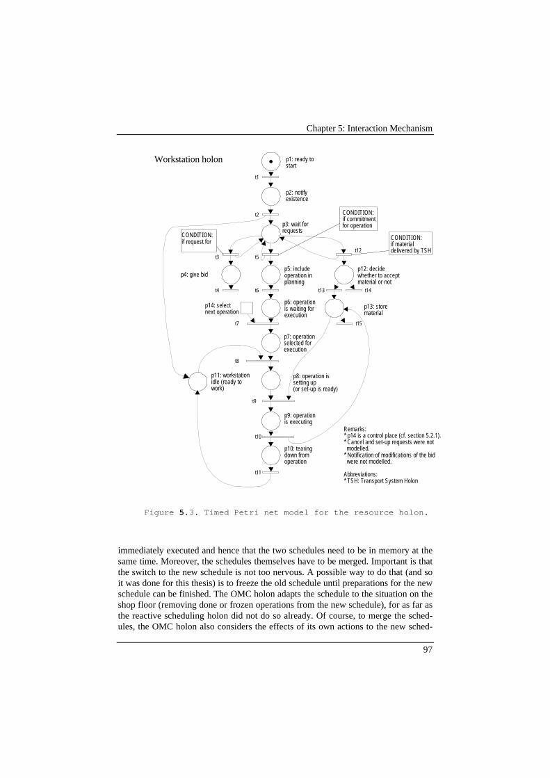
Chapter 5: Interaction Mechanism
97
p14: select next operation
p11: workstation idle (ready to work)
p12: decide whether to accept material or not
p13: store material
p10: tearing down from operation
p9: operation is executing
p8: operation is setting up (or set-up is ready)
p7: operation selected for execution
p6: operation is waiting for execution
Remarks: * p14 is a control place (cf. section 5.2.1).* Cancel and set-up requests were not modelled.* Notification of modifications of the bid were not modelled.
Abbreviations: * TSH: Transport System Holon
p5: include operation in planning
t12t5t3
t15
t13
t11
t10
t8
t7
p4: give bid
CONDITION: if material delivered by TSH
CONDITION: if commitment for operation
CONDITION: if request for
t14t4 t6
p3: wait for requests
p2: notify existence
p1: ready to start
t9
t2
Workstation holon
t1
Figure 5.3. Timed Petri net model for the resource holon.
immediately executed and hence that the two schedules need to be in memory at thesame time. Moreover, the schedules themselves have to be merged. Important is thatthe switch to the new schedule is not too nervous. A possible way to do that (and soit was done for this thesis) is to freeze the old schedule until preparations for the newschedule can be finished. The OMC holon adapts the schedule to the situation on theshop floor (removing done or frozen operations from the new schedule), for as far asthe reactive scheduling holon did not do so already. Of course, to merge the sched-ules, the OMC holon also considers the effects of its own actions to the new sched-
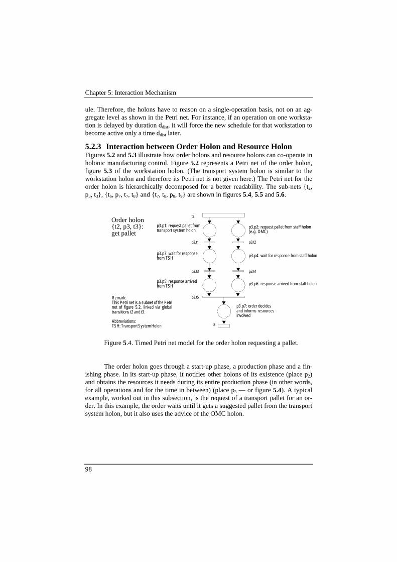
Chapter 5: Interaction Mechanism
98
ule. Therefore, the holons have to reason on a single-operation basis, not on an ag-gregate level as shown in the Petri net. For instance, if an operation on one worksta-tion is delayed by duration ddist, it will force the new schedule for that workstation tobecome active only a time ddist later.
5.2.3 Interaction between Order Holon and Resource HolonFigures 5.2 and 5.3 illustrate how order holons and resource holons can co-operate inholonic manufacturing control. Figure 5.2 represents a Petri net of the order holon,figure 5.3 of the workstation holon. (The transport system holon is similar to theworkstation holon and therefore its Petri net is not given here.) The Petri net for theorder holon is hierarchically decomposed for a better readability. The sub-nets {t2,p3, t3}, {t6, p7, t7, t8} and {t7, t8, p8, t9} are shown in figures 5.4, 5.5 and 5.6.
p2.t3
p3.p4: wait for response from staff holonp3.p3: wait for response from TSH
p3.p5: response arrived from TSH
p3.t4
p3.t2
p3.p6: response arrived from staff holon
p3.p2: request pallet from staff holon (e.g. OMC)
Remark: This Petri net is a subnet of the Petri net of figure 5.2, linked via global transitions t2 and t3.
Abbreviations: TSH: Transport System Holon
p3.p7: order decides and informs resources involved
p3.t5
p3.p1: request pallet from transport system holon
t3
p3.t1
t2Order holon {t2, p3, t3}: get pallet
Figure 5.4. Timed Petri net model for the order holon requesting a pallet.
The order holon goes through a start-up phase, a production phase and a fin-ishing phase. In its start-up phase, it notifies other holons of its existence (place p2)and obtains the resources it needs during its entire production phase (in other words,for all operations and for the time in between) (place p3 — or figure 5.4). A typicalexample, worked out in this subsection, is the request of a transport pallet for an or-der. In this example, the order waits until it gets a suggested pallet from the transportsystem holon, but it also uses the advice of the OMC holon.

Chapter 5: Interaction Mechanism
99
p7.p4: satisfactory set of bids available
p7.p7: advice from staff holon received
p7.p6: wait for advice from staff holon
RemarksThis Petri net is a subnet of the Petri net of figure 5.2, linked via global transitions t6, t7 and t8.
Abbreviations: p7.t4: receive bidp7.t5: recieve last bid
CONDITION: if bids are not satisfactory
p7.t6p7.t3
t7
p7.t7
p7.p5: send request for advice to staff holon(s)
t8
Order holon{t6, p7, t7, t8}: find resources
p7.p9: send acknowlegde to workstation ('commit')
p7.p8: take decision: select workstation
CONDITION: if all / enough satisfactory bids in
p7.p3: wait for bids / advice
CONDITION: if not all / not enough bids
p7.p2: multicast request for bids to workstations
p7.p1: identify possible resources
p7.t5p7.t4
p7.t9
p7.t8
p7.t2
p7.t1
t6
Figure 5.5. Timed Petri net model for the order holon al-locating resources to one of its operations.
In the production phase of the order, it spawns a new thread every time anoperation becomes executable (meaning that the preceding operations have beenexecuted). Communicating with the resources, it selects a workstation to allocate tothe operation and starts preparing for it (transport and set-up). Note that the orderstill has the opportunity to change its mind on the allocation, as long as the operationis not started yet. Once the operation is started, control is given to the workstationand the order waits for the operation to finish. Thereafter, it may be necessary to per-form a tear-down of the workstation. Finally, the order releases the allocated re-sources.
Looking at the allocation of a workstation to an operation in more detail, fig-ure 5.5 shows that a suitable resource is looked for as well by a multicast4 request forbids to the resources themselves, as by the request for advice to staff holons. After
4 Multicast communication (as computer terminology) is a form of communicationin multi-agent systems in which multiple agents receive the message that was sent (asopposed to broadcast communication, where all agents receive the message).

Chapter 5: Interaction Mechanism
100
all (or sufficient) bids and advice have come in, the order takes his own decision andinforms the winning workstation of it. Figure 5.6 shows how the operation is eventu-ally prepared for, considering transport, set-ups and the possibility to cancel the set-up operation (however considering the cost of such a decision should it be taken).
If all operations are done, the order enters its finishing phase and releases thetransport pallet.
p8.p11: consider switching to other set-up
p8.t12
p8.t14 p8.t15
p8.t13
p8.t11p8.t10 p8.p5: wait until right time for set-up
p8.p6: request set-up
p8.p7: wait for set-up finished
p8.p8: set-up finished
p8.p4: arrived
p8.p3: wait for arrival
p8.p2: request
p8.p1: wait until right time to move
p8.p10: send request to cancel to workstation.Set "cancel preparation" variable for this operation.
p8.p9: decide whether or not to switch to other set-up for this operation
RemarksThis Petri net is a subnet of the Petri net of figure 5.2, linked via global transitions t7, t8 and t9. Place p8.p11 is a control place.
Abbreviations: C : Condition: if "Cancel preparation" variable has been set for this operationt28 : New information comes in that may lead to a cancel preparation decision. Transitions t8.t1, t8.t3, t8.t4, t8.t6, and t9 are also conditional: if "Cancel Preparation" variable has not been set for that operation.
p8.t9
CONDITION: if decision is
CONDITION: if decision is NO
p8.t8
p8.t7
t8
Order holon{t7, t8, p8, t9}: prepare for operation
C
C
C
t9
p8.t6
p8.t5
p8.t4
p8.t3
p8.t2
p8.t1
t7
Figure 5.6. Timed Petri net model for the order holonpreparing for an operation.
The resource holon has a similar start-up, and basically assumes the role of aserver holon (A server provides services to holons, thereby not easily taking initia-tive itself). It waits until it gets• requests for a bid;• requests for the actual execution of an operation; and
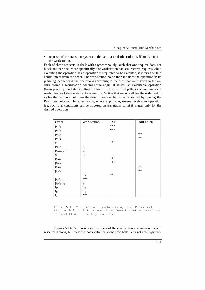
Chapter 5: Interaction Mechanism
101
• requests of the transport system to deliver material (the order itself, tools, etc.) tothe workstation.
Each of these requests is dealt with asynchronously, such that one request does notblock another one. More specifically, the workstation can still receive requests whileexecuting the operation. If an operation is requested to be executed, it infers a certaincommitment from the order. The workstation holon then includes the operation in itsplanning, sequencing the operations according to the bids that were given to the or-ders. When a workstation becomes free again, it selects an executable operation(from place p6) and starts setting up for it. If the required pallets and materials areready, the workstation starts the operation. Notice that — as well for the order holonas for the resource holon — the description can be further enriched by making thePetri nets coloured. In other words, where applicable, tokens receive an operationtag, such that conditions can be imposed on transitions to let it trigger only for thedesired operation.
Order Workstation TSH Staff holonp3.t1 ***p3.t3 ***p3.t2 ***p3.t4 ***t3 ***p7.t2 t3
p7.t4, p7.t5 t4
t7 t5
p8.t2 ***p8.t3 ***p7.t6 ***p7.t7 ***
t12 ***p8.t5 ***p8.t6, t9 t9
t10 t10
t11 t11
t8 ***
Table 5.1. Transitions synchronising the Petri nets offigures 5.2 to 5.6. Transitions denominated as “***” arenot modelled in the figures above.
Figures 5.2 to 5.6 present an overview of the co-operation between order andresource holons, but they did not explicitly show how both Petri nets are synchro-

Chapter 5: Interaction Mechanism
102
nised. This synchronisation can be done by joining the Petri nets into one big one.Unfortunately, Petri nets lose a lot of their appeal when they become big5. Alterna-tive approaches are the use of global places and composition by rendez-vous (David,1993). The use of global places is a notational shortcut whereby the overall Petri netis divided in sub-nets that only share common places (the so-called global places).Composition by rendez-vous is the dual approach, whereby certain transitions are“global” over multiple sub-nets. One therefore needs to specify which transitions inboth Petri nets fire synchronously. Table 5.1 summarises these transitions. The tablealso identifies transitions of the order that are to be synchronised with transitions inother holons, not modelled here, like the Transport System Holon (TSH) and a staffholon.
Note also that in the Petri nets shown here, some simplifications were made.To start with, due to incoming requests, or some internal changes, a workstation maydecide to update its bids. The Petri nets have not modelled this behaviour, not for theworkstation, nor for the order. However, if such a bid changes significantly, the or-der may decide to cancel its request with that workstation and go and look for an-other workstation. The cancellation mechanism was modelled in the order holon, butnot in the workstation holon. (The reader may check that it could be modelled with 6extra transitions and 1 additional place.) The workstation model does not representthe incoming requests from the orders for set-ups either.
The resulting Petri nets can be analysed with respect to liveness and predict-ability. For the orders, it is easy to see that the Petri net evolves towards a finalmarking, namely with one token in p6 and N tokens in p11. (As defined in chapter 2,N is the number of operations of an order.) Interpreting the conditions of transitionst4 and t6, one can see t6 only fires N times, after which eventually t4 is enabled. If t8
fires very easily, a so-called spinlock may occur, meaning that some tokens neverreach their final place. In this case, it means an operation is prepared for, but beforethe operation can start, the workstation changes ideas again, and needs to set up for adifferent operation. In practice, this could lead to so-called starvation6, meaning theorder can never finish its operation. Do note also that transition t8 and t9 are in con-flict. The conflict is to be resolved using control logic, in that transition t8 has to betriggered explicitly, otherwise t9 is the default transition to fire. This is made moreexplicit in the conditional transitions p8.t8 and p8.t9 of the refined Petri net of figure5.6. Also in figures 5.4 and 5.5, conflicts are resolved because the transitions in thePetri nets are conditional.
The workstation Petri net of figure 5.3 can be analysed in a similar way. Atfirst sight, this Petri net is unbounded: the number of requests for bids, the number ofrequests for executing an operation and the number of parts delivered by the trans-port system are unbounded. This however reflects the reality as it should, and conse-
5 What have Petri nets in common with pet alligators? When they grow up, they losea lot of their appeal... ;-)6 Starvation refers to the situation where an agent waits indefinitely because it al-ways looses from other agents when competing for resources (Valckenaers, 1993).

Chapter 5: Interaction Mechanism
103
quently, as well for the model as in practice, it is necessary to put a limit on thesenumbers. To start with, some of these numbers are quantities of physical objects,such that these numbers do not grow beyond reasonable bounds. Moreover, in prac-tical IT systems, the number of messages pending (the number of tokens in places p4,p5 and p12) is limited by the software itself. Further on, it is easy to see that this Petrinet does not reach a final state. Instead, it reaches a stationary behaviour with• one token in p3;• one token travelling around between places p8, p9, p10, and p11; and• tokens spawning from transitions t3, t5 and t12 until they disappear with transitions
t4, t8 and t15.
5.2.4 Interaction Between Local Holons and Staff HolonsIn holonic manufacturing, the role of staff holons is not negligible, since they areneeded for global co-ordination and optimisation. This was also shown in the Petrinet models presented above. As well orders as resource holons communicate withstaff holons on a regular basis to ask for staff holon advice on the decisions theyhave to take.
The simplest model is presented in figure 5.4, where a pallet needs to be allo-cated to an order. The order requests a pallet from the transport system as well asfrom a staff holon. The final decision is made by the order only when it has receivedand processed the responses from both the transport system holon and the staffholon.
Figure 5.5 presents a more elaborated example, where the bidding processbetween the local holons runs in parallel with the co-operation with the staff holon.Again, the final decision is based on all information. How to take the decision re-quires the development of algorithms as presented in chapter 6.
A third example is involved with the sequencing decisions taken by the work-station, presented in figure 5.3. The negotiation process, especially with the staffholons, is not shown in detail. However, it basically comes down to making the deci-sion process beyond control place p14, considering advice from the staff holons andthe results of the bidding process performed in p4.
By introducing staff holons in the co-operation schema, is should be men-tioned that the communication protocol may become fundamentally more complex.Most negotiation protocols are based on the contract net protocol (CNP — Smith,1980, Baker, 1988). In the CNP, holons7 are (dynamically) categorised as managersand contractors (or customers and suppliers, in a manufacturing context) and the ba-sic communication is bipolar. Introducing staff holons, the communication protocolbecomes tri-polar, being communication between three types of parties. Extrapolat-ing the contract net protocol for three parties can give rise to a large set of possibleprotocols, defining how these parties come to an agreement. Though it is an inter-
7 Holons or agents. The contract net protocol was developed for communication in amulti-agent system, not for holonic manufacturing systems. However, it is possible toapply the CNP also in a holonic manufacturing system.
Chapter 5: Interaction Mechanism
104
esting topic for further research, this thesis has considered it to be out of scope andhas chosen for simple ad-hoc implementations of such a tri-polar co-operationmechanism (see section 7.4.2).
5.2.5 ConclusionThis section has described on a high level how holons communicate, negotiate andco-operate. It gave examples on the co-operation between two staff holons, betweentwo local holons and between a staff holon and a local one. It thereby describes whatfunctions they perform, how they work in parallel, and how they synchronise. Thisdescription is done using a well-known modelling language like Petri nets. This alsosupports the analysis of the interaction mechanism where necessary.
Modelling the interaction mechanism with Petri nets is useful in the first placeto describe and document the design and implementation of a holonic manufacturingsystem. Documenting the design of the interaction mechanism is a prerequisite toeven start discussing the quality of such a design. While flow charts and pseudo codeare fine for sequential programs, parallel programs require a more powerful descrip-tion method.
Secondly, the use of Petri nets supported the logical analysis (and later onalso the timing analysis) of the interaction mechanism. Such an analysis would alsohave been possible without formal model, but Petri nets provide a thorough and sys-tematic approach.
Thirdly, with this approach, some concepts behind holonic manufacturingwere accurately described. The Petri nets presented above show that the bidding pro-cess between local holons and the request for advice proceed in parallel, and that theresults of both processes are to be combined to come to a carefully considered deci-sion.
This section has not modelled the complete holonic manufacturing controlsystem in detail. For instance, the transport system holon was not modelled, and sev-eral aspects of the modelled holons were not modelled, or only at a very high level.
5.3 Timing IssuesThe Petri net models described in the previous section have been analysed with re-spect to their logical operation. It can be interesting to analyse the timing aspects ofsuch a co-operation too, for a variety of reasons. This section does not aim at givinga comprehensive analysis of all possible timing effects. To start with, it limits itselfto the analysis of the co-operation aspects between a scheduling holon and an OMCholon (Figure 5.1). Further on, it restricts itself to those timing issues relevant for theparametrisation of the interaction mechanism. (An earlier occasion where timing wasalso considered, was in subsection 5.2.2, where considering the event timing wasnecessary to prove the boundedness of the Petri net of figure 5.1.)
Except for the fact that co-operation between scheduling and OMC is an im-portant concept in holonic manufacturing, this timing analysis is also necessary be-cause the both holons need a model of each other’s behaviour. The scheduler has toknow at what time the on-line SFC system will start executing the new schedule, and
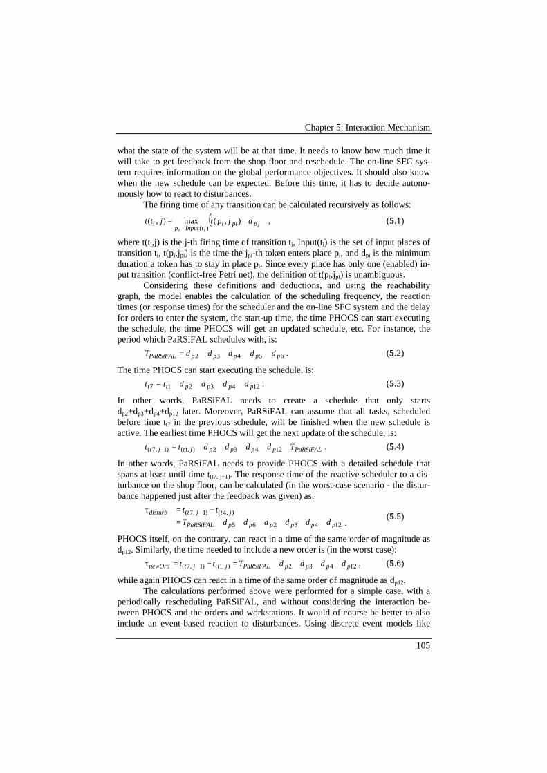
Chapter 5: Interaction Mechanism
105
what the state of the system will be at that time. It needs to know how much time itwill take to get feedback from the shop floor and reschedule. The on-line SFC sys-tem requires information on the global performance objectives. It should also knowwhen the new schedule can be expected. Before this time, it has to decide autono-mously how to react to disturbances.
The firing time of any transition can be calculated recursively as follows:
( )i
iippii
tInputpi djptjtt +=
∈),(max),(
)(, (5.1)
where t(ti,j) is the j-th firing time of transition ti, Input(ti) is the set of input places oftransition ti, t(pi,jpi) is the time the jpi-th token enters place pi, and dpi is the minimumduration a token has to stay in place pi. Since every place has only one (enabled) in-put transition (conflict-free Petri net), the definition of t(pi,jpi) is unambiguous.
Considering these definitions and deductions, and using the reachabilitygraph, the model enables the calculation of the scheduling frequency, the reactiontimes (or response times) for the scheduler and the on-line SFC system and the delayfor orders to enter the system, the start-up time, the time PHOCS can start executingthe schedule, the time PHOCS will get an updated schedule, etc. For instance, theperiod which PaRSiFAL schedules with, is:
65432 pppppPaRSiFAL dddddT +++= + . (5.2)
The time PHOCS can start executing the schedule, is:
1243217 pppptt ddddtt ++++= . (5.3)
In other words, PaRSiFAL needs to create a schedule that only startsdp2+dp3+dp4+dp12 later. Moreover, PaRSiFAL can assume that all tasks, scheduledbefore time tt7 in the previous schedule, will be finished when the new schedule isactive. The earliest time PHOCS will get the next update of the schedule, is:
PaRSiFALppppjtjt Tddddtt +++++=+ 12432),1()1,7( . (5.4)
In other words, PaRSiFAL needs to provide PHOCS with a detailed schedule thatspans at least until time t(t7, j+1). The response time of the reactive scheduler to a dis-turbance on the shop floor, can be calculated (in the worst-case scenario - the distur-bance happened just after the feedback was given) as:
1243265
),4()1,7(
ppppppPaRSiFAL
jtjtdisturb
ddddddT
tt
++++++=−=τ +
.(5.5)
PHOCS itself, on the contrary, can react in a time of the same order of magnitude asdp12. Similarly, the time needed to include a new order is (in the worst case):
12432),1()1,7( ppppPaRSiFALjtjtnewOrd ddddTtt ++++=−=τ + , (5.6)
while again PHOCS can react in a time of the same order of magnitude as dp12.The calculations performed above were performed for a simple case, with a
periodically rescheduling PaRSiFAL, and without considering the interaction be-tween PHOCS and the orders and workstations. It would of course be better to alsoinclude an event-based reaction to disturbances. Using discrete event models like
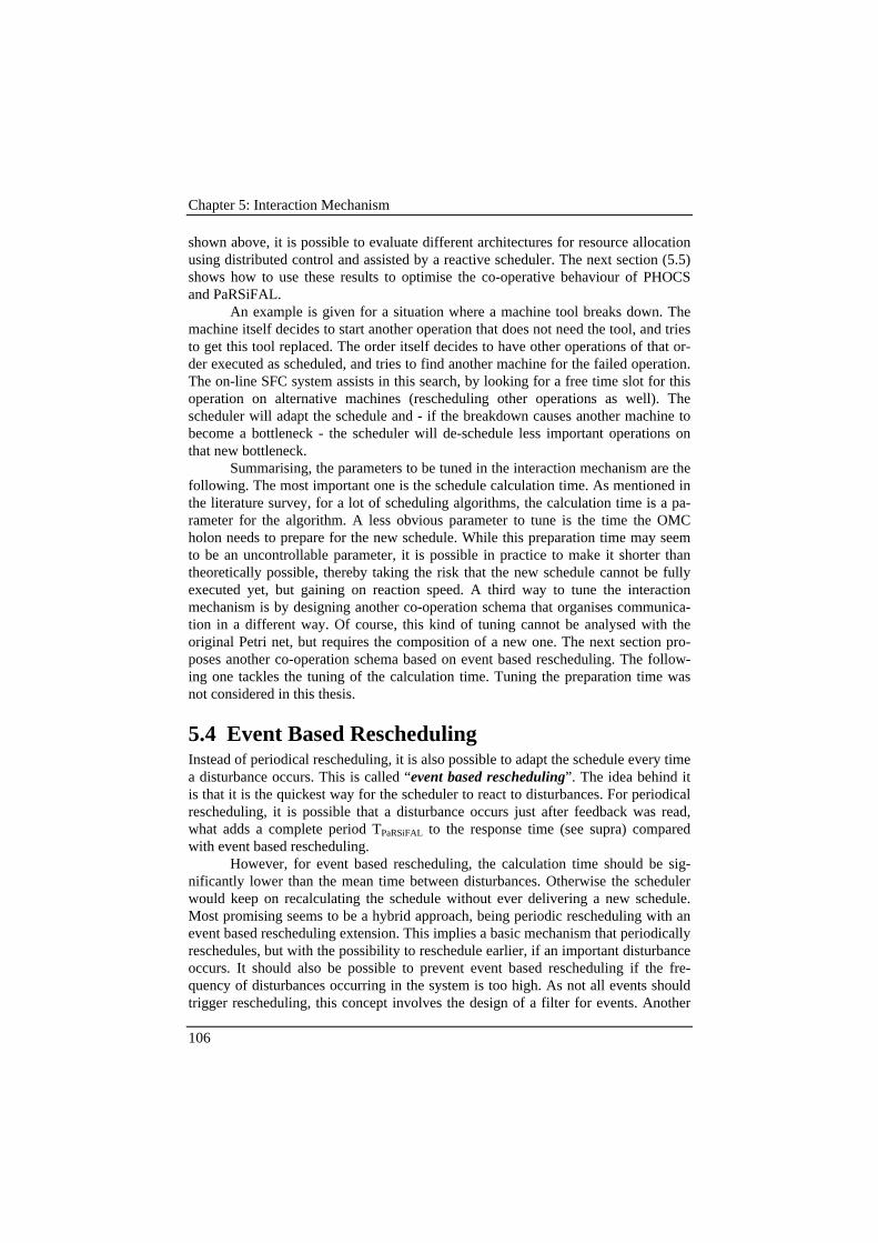
Chapter 5: Interaction Mechanism
106
shown above, it is possible to evaluate different architectures for resource allocationusing distributed control and assisted by a reactive scheduler. The next section (5.5)shows how to use these results to optimise the co-operative behaviour of PHOCSand PaRSiFAL.
An example is given for a situation where a machine tool breaks down. Themachine itself decides to start another operation that does not need the tool, and triesto get this tool replaced. The order itself decides to have other operations of that or-der executed as scheduled, and tries to find another machine for the failed operation.The on-line SFC system assists in this search, by looking for a free time slot for thisoperation on alternative machines (rescheduling other operations as well). Thescheduler will adapt the schedule and - if the breakdown causes another machine tobecome a bottleneck - the scheduler will de-schedule less important operations onthat new bottleneck.
Summarising, the parameters to be tuned in the interaction mechanism are thefollowing. The most important one is the schedule calculation time. As mentioned inthe literature survey, for a lot of scheduling algorithms, the calculation time is a pa-rameter for the algorithm. A less obvious parameter to tune is the time the OMCholon needs to prepare for the new schedule. While this preparation time may seemto be an uncontrollable parameter, it is possible in practice to make it shorter thantheoretically possible, thereby taking the risk that the new schedule cannot be fullyexecuted yet, but gaining on reaction speed. A third way to tune the interactionmechanism is by designing another co-operation schema that organises communica-tion in a different way. Of course, this kind of tuning cannot be analysed with theoriginal Petri net, but requires the composition of a new one. The next section pro-poses another co-operation schema based on event based rescheduling. The follow-ing one tackles the tuning of the calculation time. Tuning the preparation time wasnot considered in this thesis.
5.4 Event Based ReschedulingInstead of periodical rescheduling, it is also possible to adapt the schedule every timea disturbance occurs. This is called “event based rescheduling”. The idea behind itis that it is the quickest way for the scheduler to react to disturbances. For periodicalrescheduling, it is possible that a disturbance occurs just after feedback was read,what adds a complete period TPaRSiFAL to the response time (see supra) comparedwith event based rescheduling.
However, for event based rescheduling, the calculation time should be sig-nificantly lower than the mean time between disturbances. Otherwise the schedulerwould keep on recalculating the schedule without ever delivering a new schedule.Most promising seems to be a hybrid approach, being periodic rescheduling with anevent based rescheduling extension. This implies a basic mechanism that periodicallyreschedules, but with the possibility to reschedule earlier, if an important disturbanceoccurs. It should also be possible to prevent event based rescheduling if the fre-quency of disturbances occurring in the system is too high. As not all events shouldtrigger rescheduling, this concept involves the design of a filter for events. Another
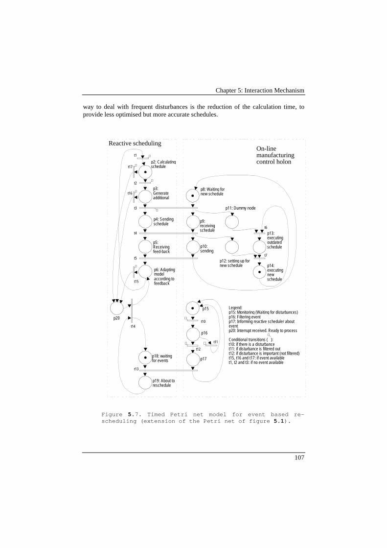
Chapter 5: Interaction Mechanism
107
way to deal with frequent disturbances is the reduction of the calculation time, toprovide less optimised but more accurate schedules.
p20
p15
t11
t12
t10
t17
t16
t15
t13
p19: About to reschedule
p18: waiting for events
t14
Legend: p15: Monitoring (Waiting for disturbances)p16: Filtering event p17: Informing reactive scheduler about eventp20: Interrupt received. Ready to process
Conditional transitions ( ): t10: if there is a disturbancet11: if disturbance is filtered outt12: if disturbance is important (not filtered)t15, t16 and t17: if event availablet1, t2 and t3: if no event available
p16
p17
On-line manufacturing control holon
Reactive scheduling
t2
t1
t7
t6
t5
t4
p3: Generate additional
p6: Adapting model according to feedback
p5: Receiving feed-back
p4: Sending schedule
p2: Calculating schedule
p8: Waiting for new schedule
p9: receiving schedule
p10: sending
p12: setting up for new schedule p14:
executing new schedule
p13: executing outdated schedule
t3 p11: Dummy node
Figure 5.7. Timed Petri net model for event based re-scheduling (extension of the Petri net of figure 5.1).
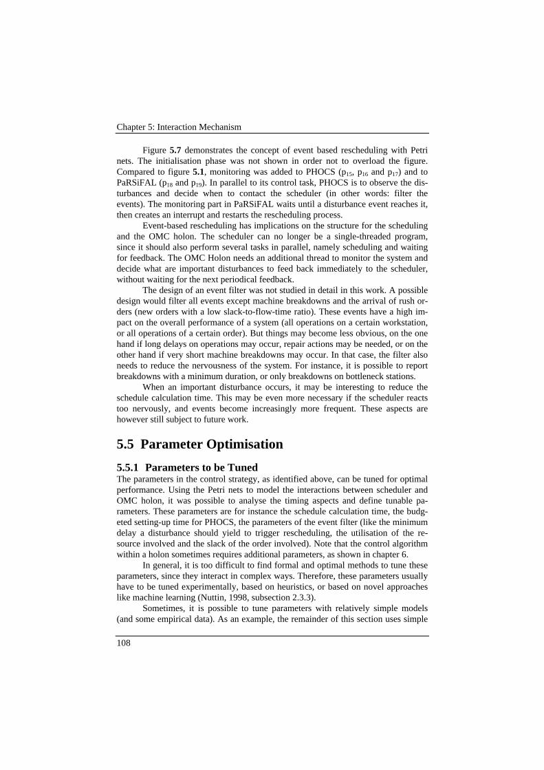
Chapter 5: Interaction Mechanism
108
Figure 5.7 demonstrates the concept of event based rescheduling with Petrinets. The initialisation phase was not shown in order not to overload the figure.Compared to figure 5.1, monitoring was added to PHOCS (p15, p16 and p17) and toPaRSiFAL (p18 and p19). In parallel to its control task, PHOCS is to observe the dis-turbances and decide when to contact the scheduler (in other words: filter theevents). The monitoring part in PaRSiFAL waits until a disturbance event reaches it,then creates an interrupt and restarts the rescheduling process.
Event-based rescheduling has implications on the structure for the schedulingand the OMC holon. The scheduler can no longer be a single-threaded program,since it should also perform several tasks in parallel, namely scheduling and waitingfor feedback. The OMC Holon needs an additional thread to monitor the system anddecide what are important disturbances to feed back immediately to the scheduler,without waiting for the next periodical feedback.
The design of an event filter was not studied in detail in this work. A possibledesign would filter all events except machine breakdowns and the arrival of rush or-ders (new orders with a low slack-to-flow-time ratio). These events have a high im-pact on the overall performance of a system (all operations on a certain workstation,or all operations of a certain order). But things may become less obvious, on the onehand if long delays on operations may occur, repair actions may be needed, or on theother hand if very short machine breakdowns may occur. In that case, the filter alsoneeds to reduce the nervousness of the system. For instance, it is possible to reportbreakdowns with a minimum duration, or only breakdowns on bottleneck stations.
When an important disturbance occurs, it may be interesting to reduce theschedule calculation time. This may be even more necessary if the scheduler reactstoo nervously, and events become increasingly more frequent. These aspects arehowever still subject to future work.
5.5 Parameter Optimisation
5.5.1 Parameters to be TunedThe parameters in the control strategy, as identified above, can be tuned for optimalperformance. Using the Petri nets to model the interactions between scheduler andOMC holon, it was possible to analyse the timing aspects and define tunable pa-rameters. These parameters are for instance the schedule calculation time, the budg-eted setting-up time for PHOCS, the parameters of the event filter (like the minimumdelay a disturbance should yield to trigger rescheduling, the utilisation of the re-source involved and the slack of the order involved). Note that the control algorithmwithin a holon sometimes requires additional parameters, as shown in chapter 6.
In general, it is too difficult to find formal and optimal methods to tune theseparameters, since they interact in complex ways. Therefore, these parameters usuallyhave to be tuned experimentally, based on heuristics, or based on novel approacheslike machine learning (Nuttin, 1998, subsection 2.3.3).
Sometimes, it is possible to tune parameters with relatively simple models(and some empirical data). As an example, the remainder of this section uses simple

Chapter 5: Interaction Mechanism
109
MATLAB calculations to numerically assess concurrent scheduling and scheduleexecution (CSSE — Concept 3, subsection 4.2.3). Other examples were not elabo-rated in this thesis.
5.5.2 Basic Analysis of CSSEThe concept of CSSE (subsection 4.2.3) was motivated by a qualitative analysis ofthe resulting system performance. Figure 5.1, in the beginning of this chapter, gave aformal representation of this concept. This subsection presents a more quantitativeanalysis (for a more specific example) to provide a stronger proof of the concept.Meanwhile, it also presents a calculation scheme to determine the optimal schedulecalculation time, based on a trade-off between reaction speed and (re)scheduling per-formance.
Consider a job-shop scheduling problem with tardiness minimisation. Definethe schedule length Lsched as the makespan that a “fair” scheduler (e.g. a simple OMCsystem using dispatching rules) would reach for the current set of orders8. A typicallydifficult scheduling problem would be one where some orders will be tardy, but notall. This infers the average due date would not be very early (then all orders wouldbe tardy), nor very late (then none would be tardy). Assume that the schedulingproblem and the “fair” schedule have the following characteristics:• All orders have a release date Ri = 0.
• The average due date 3
2 schedav
LD
⋅= .
• The standard deviation of the due dates over the orders is small and can be ne-glected.
• The minimum flow time for the orders in the system 3min
schedLf = .
• 2/3 of the orders can be finished before time 3
2 schedL⋅.
• The flow time of the remainder of the orders is uniformly distributed over the
remaining 3
schedL (i.e. between
3
2 schedL⋅and schedL ).
Thus, using the fair scheduler, one third of the orders would be tardy, two thirdswould be on time. The resulting average tardiness can then be estimated as (see fig-ure 5.8):
8 Of course, in a dynamic environment, finished orders continuously leave the sys-tems and new orders continuously enter, but in a steady state system, the amount ofwork entering would roughly equal the amount leaving, such that the loading of themanufacturing system remains constant. A more formal definition of Lsched could be:
KdLji
jisched
= ∑
,,2, ,
with di,j the duration of operation j of order i and K the number of workstations.Lsched,2 is a reasonable (but optimistic) approximation of Lsched.
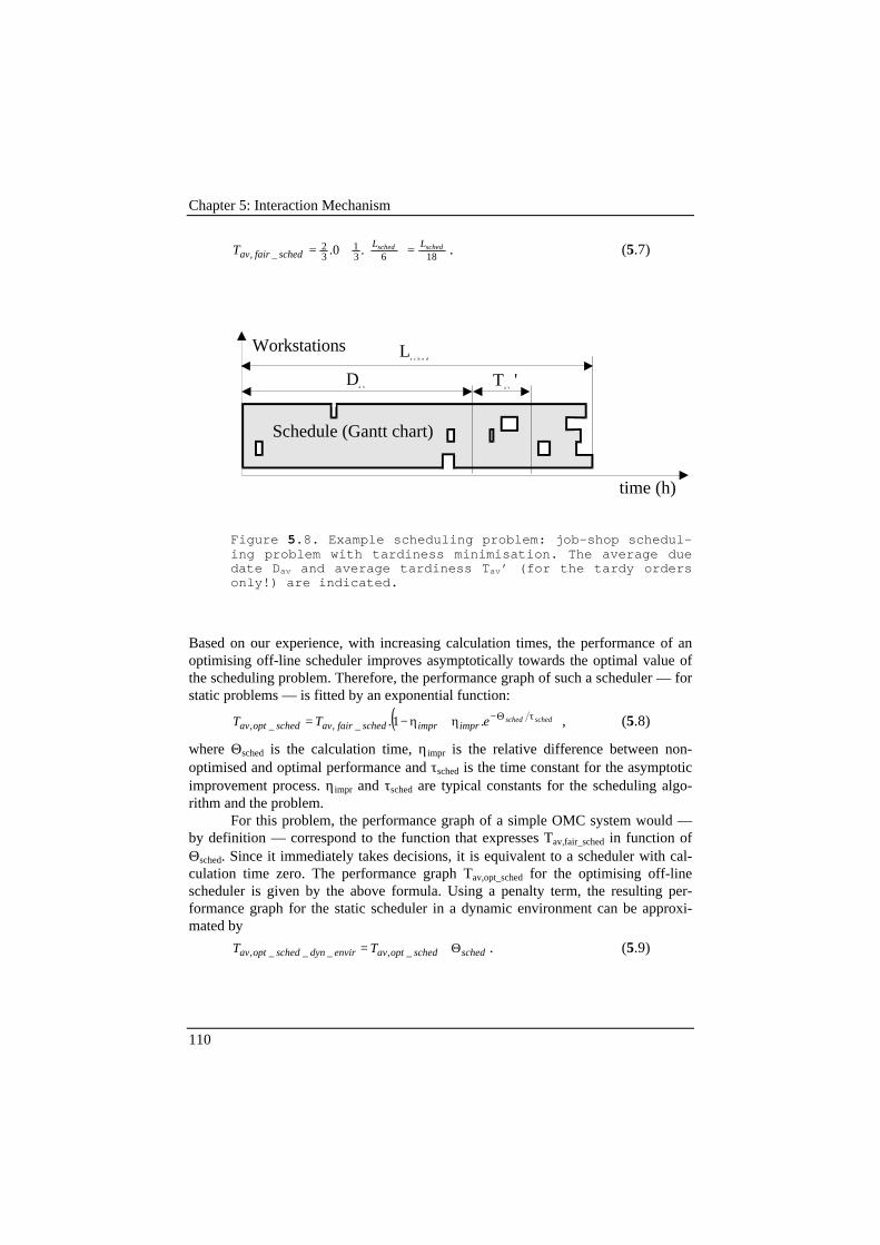
Chapter 5: Interaction Mechanism
110
18631
32
_, .0. schedsched LLschedfairavT =
+= . (5.7)
'T a v
D a v
L s c h e d
Workstations
time (h)
Schedule (Gantt chart)
Figure 5.8. Example scheduling problem: job-shop schedul-ing problem with tardiness minimisation. The average duedate Dav and average tardiness Tav’ (for the tardy ordersonly!) are indicated.
Based on our experience, with increasing calculation times, the performance of anoptimising off-line scheduler improves asymptotically towards the optimal value ofthe scheduling problem. Therefore, the performance graph of such a scheduler — forstatic problems — is fitted by an exponential function:
( )schedschedeTT imprimprschedfairavschedoptavτΘ−η+η−= .1._,_, , (5.8)
where Θsched is the calculation time, ηimpr is the relative difference between non-optimised and optimal performance and τsched is the time constant for the asymptoticimprovement process. ηimpr and τsched are typical constants for the scheduling algo-rithm and the problem.
For this problem, the performance graph of a simple OMC system would —by definition — correspond to the function that expresses Tav,fair_sched in function ofΘsched. Since it immediately takes decisions, it is equivalent to a scheduler with cal-culation time zero. The performance graph Tav,opt_sched for the optimising off-linescheduler is given by the above formula. Using a penalty term, the resulting per-formance graph for the static scheduler in a dynamic environment can be approxi-mated by
schedschedoptavenvirdynschedoptav TT Θ+= _,___, . (5.9)
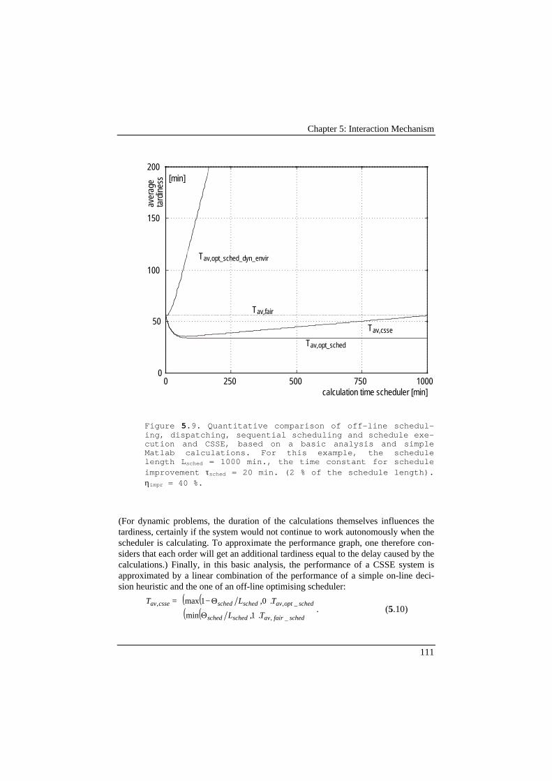
Chapter 5: Interaction Mechanism
111
Tav,csse
Tav,opt_sched
Tav,opt_sched_dyn_envir
Tav,fair
[min]
0 250 500 750 10000
50
100
150
200
calculation time scheduler [min]
aver
age
tard
ines
s
Figure 5.9. Quantitative comparison of off-line schedul-ing, dispatching, sequential scheduling and schedule exe-cution and CSSE, based on a basic analysis and simpleMatlab calculations. For this example, the schedulelength Lsched = 1000 min., the time constant for scheduleimprovement τsched = 20 min. (2 % of the schedule length).ηimpr = 40 %.
(For dynamic problems, the duration of the calculations themselves influences thetardiness, certainly if the system would not continue to work autonomously when thescheduler is calculating. To approximate the performance graph, one therefore con-siders that each order will get an additional tardiness equal to the delay caused by thecalculations.) Finally, in this basic analysis, the performance of a CSSE system isapproximated by a linear combination of the performance of a simple on-line deci-sion heuristic and the one of an off-line optimising scheduler:
( )( )( )( ) schedfairavschedsched
schedoptavschedschedcsseav
TL
TLT
_,
_,,
.1,min
.0,1max
Θ+
Θ−=. (5.10)
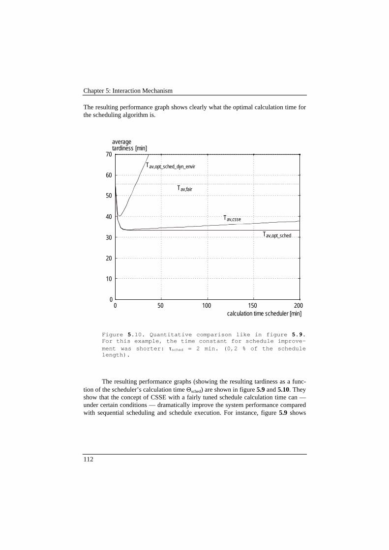
Chapter 5: Interaction Mechanism
112
The resulting performance graph shows clearly what the optimal calculation time forthe scheduling algorithm is.
Tav,csse
Tav,opt_sched
Tav,opt_sched_dyn_envir
Tav,fair
calculation time scheduler [min]
averagetardiness [min]
0 50 100 150 2000
10
20
30
40
50
60
70
Figure 5.10. Quantitative comparison like in figure 5.9.For this example, the time constant for schedule improve-ment was shorter: τsched = 2 min. (0,2 % of the schedulelength).
The resulting performance graphs (showing the resulting tardiness as a func-tion of the scheduler’s calculation time Θsched) are shown in figure 5.9 and 5.10. Theyshow that the concept of CSSE with a fairly tuned schedule calculation time can —under certain conditions — dramatically improve the system performance comparedwith sequential scheduling and schedule execution. For instance, figure 5.9 shows

Chapter 5: Interaction Mechanism
113
that applying off-line algorithms with a time constant τsched of 20 minutes9 for aproblem with a time horizon of 16 h. (for instance corresponding to two shifts ofwork) can never outperform dispatching rules. For a better scheduler, with a timeconstant τsched of only 2 minutes, sequential scheduling and schedule execution (i.e.only using off-line scheduling) only reaches 70 % of its potential improvement (from57 min. to 41 instead of from 57 to 33 min.)10. The envisaged performance of aCSSE system would reach more than 90 respectively 98.5 % of its potential (thesevalues are to be read from the graph in figures 5.9 and 5.10). Note that these resultswere obtained for reasonably logical values of schedule length and calculation time.One could argue that some assumptions were taken quite optimistically. These com-ments are further elaborated in the next paragraph. Basically, however, these figuresalready show the potential of addressing the scheduling problem in a structural way.
5.5.3 Conservative Analysis of CSSEIn the previous subsection, several assumptions were taken that may have given anoverly optimistic view on CSSE. Of course, there is no doubt that these models aresimplifications of reality, but some assumptions are indeed debatable. This para-graph will identify these arguments and assess their consequences on the aboveanalysis.
The previous paragraph modelled the effect of delaying the execution of theschedule in the traditional off-line scheduling approach as a penalty equal to the de-lay itself (equation 5.9). One could argue that this penalty was over-estimated. Let ustherefore refine the model with some common sense reasoning. Suppose that initially(for small values of Θsched), only the orders that were already tardy, get an additionaltardiness. Gradually, more orders will be tardy, until by time Lsched/3, all orders aretardy. This can be approximated as
∫
∫ −Θ+
=sched
sched
sched
sched
L
L
L
Lsched
envirdynschedoptav
dCCN
dCCNCDC
T
3
3___,
).(
).()).(,0max(
, (5.11)
where C is the finishing time of an order; N(C).dC is the amount of orders finishingbetween C and C+dC; and D(C) the due date of the orders finishing at time C.
A second comment could be made on the model for estimating the perform-ance of CSSE. If a schedule is only available after half of the production is already 9 Intuitively, one can imagine that τsched and the calculation times used in practicehave the same order of magnitude. E.g., with a calculation time Θsched = τsched, 63 %of the potential improvements are obtained, for Θsched = 2.τsched, 84 % and forΘsched = 3.τsched, 95 %. Larger calculation times would only yield marginal additionalimprovements.10 In this text, performance is often expressed as a ‘percentage of potential improve-ment’. This refers to the difference between the performance of a fair scheduler(0 %) and the optimal performance (100 %).
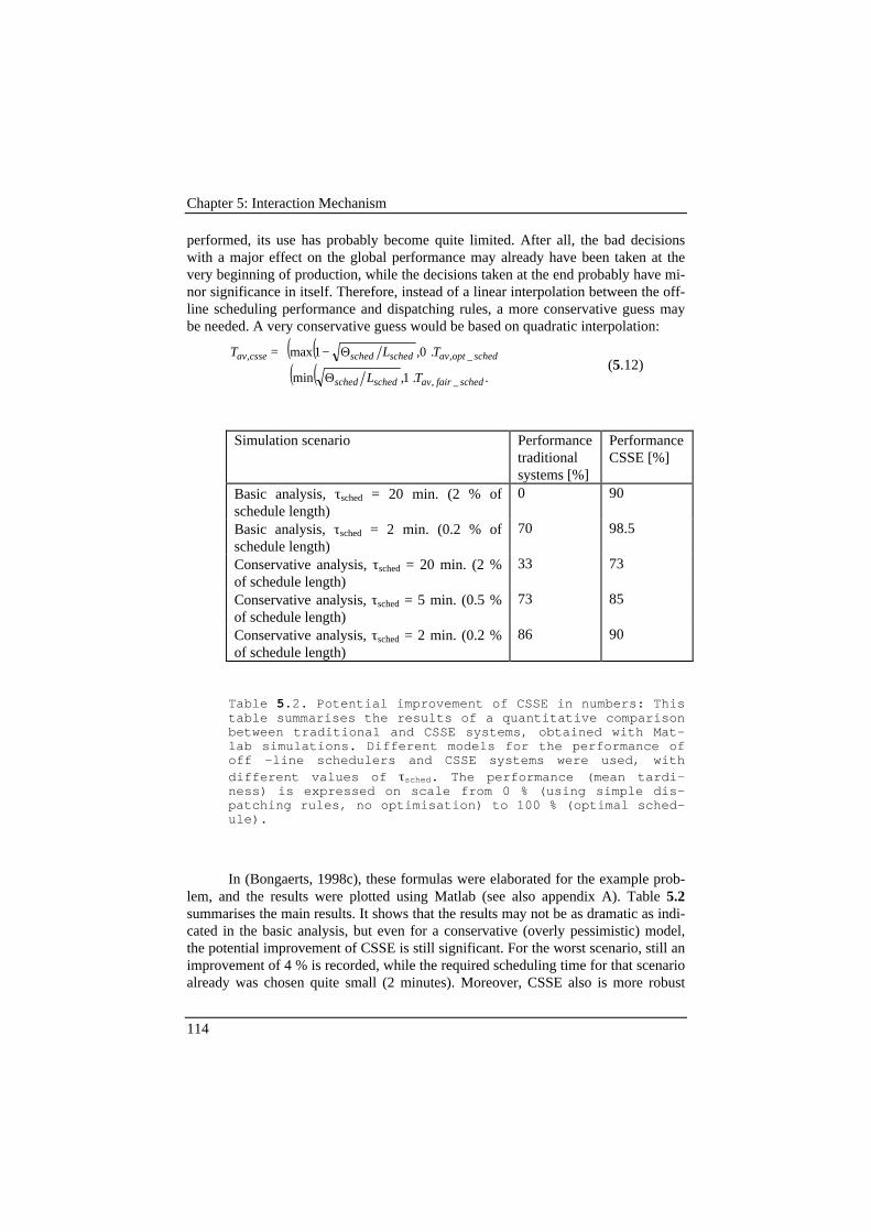
Chapter 5: Interaction Mechanism
114
performed, its use has probably become quite limited. After all, the bad decisionswith a major effect on the global performance may already have been taken at thevery beginning of production, while the decisions taken at the end probably have mi-nor significance in itself. Therefore, instead of a linear interpolation between the off-line scheduling performance and dispatching rules, a more conservative guess maybe needed. A very conservative guess would be based on quadratic interpolation:
( )( )( )( ) ..1,min
.0,1max
_,
_,,
schedfairavschedsched
schedoptavschedschedcsseav
TL
TLT
Θ+
Θ−=(5.12)
Simulation scenario Performancetraditionalsystems [%]
PerformanceCSSE [%]
Basic analysis, τsched = 20 min. (2 % ofschedule length)
0 90
Basic analysis, τsched = 2 min. (0.2 % ofschedule length)
70 98.5
Conservative analysis, τsched = 20 min. (2 %of schedule length)
33 73
Conservative analysis, τsched = 5 min. (0.5 %of schedule length)
73 85
Conservative analysis, τsched = 2 min. (0.2 %of schedule length)
86 90
Table 5.2. Potential improvement of CSSE in numbers: Thistable summarises the results of a quantitative comparisonbetween traditional and CSSE systems, obtained with Mat-lab simulations. Different models for the performance ofoff -line schedulers and CSSE systems were used, withdifferent values of τsched. The performance (mean tardi-ness) is expressed on scale from 0 % (using simple dis-patching rules, no optimisation) to 100 % (optimal sched-ule).
In (Bongaerts, 1998c), these formulas were elaborated for the example prob-lem, and the results were plotted using Matlab (see also appendix A). Table 5.2summarises the main results. It shows that the results may not be as dramatic as indi-cated in the basic analysis, but even for a conservative (overly pessimistic) model,the potential improvement of CSSE is still significant. For the worst scenario, still animprovement of 4 % is recorded, while the required scheduling time for that scenarioalready was chosen quite small (2 minutes). Moreover, CSSE also is more robust
Chapter 5: Interaction Mechanism
115
than traditional approaches. The results of table 5.2 show the performance for an op-timal selection of the calculation time. Graphs like 5.9 and 5.10 show however thatCSSE is significantly less affected by the optimality the calculation time is tunedwith, such that CSSE is more robust indeed.
5.5.4 ConclusionThis section has assessed the potential of the concept of concurrent scheduling andschedule execution (CSSE). With simple models and MATLAB calculations, CSSEwas compared with the sequential scheduling and schedule execution and with non-optimising control. Depending on the problem parameters (mainly reflecting therelative calculation speed of the scheduling algorithm) and on the assumptions, thepossible improvements range from 4 to 90 % of the theoretical optimum.
To obtain more accurate performance graphs, future research should furtheranalyse the structure of scheduling problems and collect more empirical data. Usingcoarse approximations, this section has already estimated upper and lower bounda-ries for performance. This analysis has identified a structural problem of sequentialscheduling and schedule execution, which may explain why the traditional optimis-ing (off-line) scheduling algorithms are seldom applied in industry.
5.6 Inter-Holon CommunicationThe interaction mechanism defined in this chapter has implications on the require-ments for inter-holon communication. In a typical hierarchical framework, informa-tion exchanged between modules are schedules, (start, stop and interrupt) com-mands, feedback information, status reports, etc (Senehi, 1994). In heterarchicalsystems, typical messages include task announcements (or requests for bids), “willbid” announcements, bids, awards (or purchase orders), contracts, and cancellationmessages (Smith, 1980, Baker, 1988). Lin (1994) describes how these messages cancontain information on price, quality and time. This section discusses some addi-tional aspects of the contents and the protocol for communication in an HMS as wasdiscovered in this thesis.
To start with, holons need a model of the world around them: not only of thephysical world they are reasoning about, but also of the other holons they co-operatewith. Part of this model is (quasi-)static: order holons need to know which worksta-tions they can use; the scheduler holon requires information on the number of work-stations, their abilities, their IP addresses; it also requires the address of the OMCholon(s), etc. In the implementation built for this thesis, this information is stored indata files11 (see chapter 7).
11 In an industrial-size holonic manufacturing system, a more flexible and self-organising approach will be necessary. A possible design that provides all holonswith the right “meta-information”, is based on a name-server (Wyns, 1999). Thatname-server would store that information in a datastructure similar to the one pre-sented by Bongaerts (1996) or Van Brussel (1998) and would distribute it to theother holons.
Chapter 5: Interaction Mechanism
116
In this thesis, special attention was paid to the communication between thescheduler and OMC holon. It is obvious that a scheduler and an OMC holon shouldexchange Gantt Charts, performance objectives and feedback information. Interest-ing is that system performance can be improved by exchanging additional informa-tion. Chapter 6 shows that the OMC holon requires more information about theschedule than just a Gantt chart if it wants to execute a schedule autonomously,without doing a complete rescheduling itself in case of disturbances. Chapter 6 alsogives an example of how to extend the communication protocol with additional ad-vice.
A second example where communication protocols are to become more ad-vanced are transport system holons. Very often, a transport system holon is a com-plex multi-resource holon itself, and yet not modelled or not modelled in detail byother holons. Because of this, it may be hard to know how long it takes to executetransport commands. The duration might for instance depend on the traffic. There-fore, in the margin of this doctoral research, some research was performed on thedefinition of more advanced communication protocols for transport tasks (Malewicz,1996). It is for instance possible to add a desired arrival time with each transporttask. One may also add the available slack to the command. Moreover, it is possibleto negotiate about the duration of transportation. Sometimes, for instance if it is notpossible to resequence pallets in a workstation, like in the PMA Flexible AssemblySystem (FAS), it is necessary to add sequencing constraints to the transport task.This aspect of manufacturing control is still subject to further research.
To implement the concept of fixed rules and flexible strategies, as defined insection 4.4, it is necessary to communicate the fixed rules amongst the holons. Thisincludes the definition of a meta control language. In the implementations for thisthesis, meta control was enforced by interaction with the user or by a simple ad-hocmessage format. The specific fixed rules that are imposed, are described in the fol-lowing chapter.
No doubt, the reader has noticed by now that this thesis does not present ageneric model for communication, with a standard and well-considered messageformat. Another question to be solved is whether communication is to be performedby information push (broadcasting, multi-casting) or information pull (client-serverlike message interchange), by some more advanced concepts like event notificationprotocols, or by a mixture of them. Indeed, these matters do not belong to the thesisscope, and are dealt with in more detail in work package 2 of the International HMSproject (Sys-Op).
5.7 ConclusionThis chapter has presented some specific models of the interaction mechanism be-tween holons. These models describe the interactions among staff holons, among lo-cal (order and resource) holons and between local holons and staff holons. They canalso describe timing aspects. Most of this chapter was dedicated to the co-operationbetween a scheduling and an OMC holon. The models describe the concept of con-current scheduling and schedule execution (CSSE), first for periodic rescheduling,
Chapter 5: Interaction Mechanism
117
later also for event-based rescheduling. Finally, some remarks were made on the de-sign of a communication protocol.
Interesting contributions of this chapter were the use of Petri nets to describethe design of programs operating in parallel, and, more importantly, the numericalanalysis of the timing aspects (like response times) of the co-operation between ascheduler and an OMC holon. In reactive scheduling, traditionally a trade-off ismade between available calculation time for performance optimisation and requiredreaction time to disturbances. A quantitative analysis (based on Matlab simulations)has shown that the new co-operation schema (based on CSSE) can combine rapidreaction to disturbances with a high system performance. Of course, this analysis inMatlab may give an idea about the expected results, but relies on simplified models.Chapter 8 will provide real numerical evidence to clearly assess the improvements ofour approach.

Chapter 5: Interaction Mechanism
118
119
Chapter 6
Holonic Control Strategies
This chapter presents the algorithms behind holonic manufacturing control. Holo-nic algorithms can be described with the concept of fixed rules and flexible strate-gies (FRFS), or as autonomous schedule execution strategies (ASE). Traditionalcontrol strategies like hierarchical and heterarchical control can also be modelledwith FRFS and ASE. Three new heuristic schedule execution strategies implementholonic manufacturing in an intuitive way. A new ASE algorithm using perturba-tion analysis performs holonic manufacturing control with a sound theoreticalfoundation.
6.1 IntroductionChapter 4 showed that a holonic manufacturing control architecture contains ascheduler, an on-line manufacturing control holon (OMC) and a number of localholons. Chapter 5 elaborated the interaction mechanism between these holons. Tocomplete the design of a holonic manufacturing control system, this chapter definesthe control logic within each holon (i.e. the control algorithms).
With respect to control algorithms, the contribution of this thesis is mainlyfocused on on-line manufacturing control. Using traditional terminology, thiswould be called intelligent (on-line) dispatching. The control algorithms within thescheduler holon are optimising reactive scheduling algorithms, as already exten-sively described in literature (see chapter 2). Notice also that the main focus on thisthesis was on the co-operation between a centralised reactive scheduler and a cen-tralised on-line manufacturing control holon, such that, to a large degree, the con-trol logic within the local holons is outside the scope of this thesis. (This is subjectof the doctoral research of Peeters — 1997).
The approach taken to develop OMC algorithms uses the modelling formal-isms developed above: autonomous schedule execution algorithms (ASE) and deci-sion power distribution (DDP) rules — defining fixed rules and flexible strategies(FRFS). As a case study for DDP and FRFS, three heuristic holonic control strate-gies were developed. This chapter also presents an algorithm for ASE, based onperturbation analysis. This algorithm is to be used as a flexible strategy that canbetter exploit its autonomy by using the schedule as advice.
This chapter has the following structure. First, the definition of autonomousschedule execution (given in subsection 4.2.3) is further refined and some analysis
Chapter 6: Holonic Control Strategies
120
shows that this task is not as trivial as usually considered. The following sectionpresents a new way to represent a schedule, based on graph theory. This represen-tation method is to be used in later sections. Before describing the new controlstrategies, a short reference is made to the existing work in literature. It states howthe new approaches relate to hierarchical and heterarchical control, and identifiessome projects with similar aspirations as this chapter. The next sections model hi-erarchical and heterarchical control in the newly proposed framework to comparethem with the new approaches and show that they are more rigid. Thereby, onesection will also look at a centralised way of performing autonomous (on-line) con-trol, as implemented for this thesis. However, this section on centralised autono-mous control still does not present new control logic. That changes with section 6.8and 6.9. Section 6.8 describes several heuristic strategies to combine hierarchicaland heterarchical control, thereby using the formalism of fixed rules and flexiblestrategies to distribute decision power. Section 6.9 presents a schedule executionalgorithm based on perturbation analysis. This is an example of a model-based ap-proach to have an autonomous OMC holon use the advice of a scheduling holon.Finally, the conclusion shows that both intuitive and model-based approaches pro-vide the OMC holon with capable algorithms. A quantitative evaluation of the al-gorithms is found in chapter 8.
6.2 Schedule executionSchedule execution was defined in chapter 4, when the concept of concurrentscheduling and schedule execution (CSSE) was proposed. Summarised, it comesdown to taking the manufacturing control decisions, while the schedule is alreadycalculated and available, but also while disturbances occur that invalidate the ex-isting schedule. It refers to cutting the knot and making the final decision for anoperation, given the current state of the shop floor. Thereby, it can use the advicefrom the schedule but has the liberty to deviate from the schedule.
Before discussing existing and new approaches for schedule execution, it isimportant to realise that schedule execution is not a trivial task. Typically, theschedule contains its information in the form of a Gantt chart, expressing when andwhere each task is to be executed. However, this section shows that it is impossibleto construct a good strategy to execute a near-optimal schedule that deals withdisturbances autonomously and does not have to perform rescheduling itself, if theGantt chart (and the objective function) are the only available information of theschedule. The Gantt chart just does not contain sufficient information for that1.This is shown in the following example.
Consider a job-shop scheduling problem with three machines and three or-ders (table 6.1). Order B is more urgent than A, and A and B are a lot more urgentthan C. In figure 6.1, the schedule is shown. It can easily be understood that thisschedule is optimal, since the most urgent order is scheduled as early as possible, 1 Or at least, the information in the Gantt chart is not presented in the right form.

Chapter 6: Holonic Control Strategies
121
and the other orders are scheduled in between. Suppose the SFC system is autono-mously executing the schedule. It already started operations A1 and B1, and iswaiting for either of them to be finished, in which case it would normally start op-erations B2 and C1. However, due to a temporary lack of components, operation A1takes more time to complete. When A1 is finally finished, the question can beraised whether the current schedule should be followed or whether operation C1should be skipped. For a human scheduler, given the relative importance of the or-ders, the right answer is obvious, namely to skip operation C1. He understands thatthe delay of operation C1 is not propagated through the schedule in such a way thatorders become tardy. However, for a computer, this conclusion could not have beendeducted with the performance objectives and the information contained in theGantt-chart only. It was necessary to consider how local decisions propagatethrough the rest of the schedule (via the machine sequencing relations and the or-der precedence constraints) and how they affect the global performance.
Job-shop-scheduling problem with three machines (=={m1, m2, m3}) andthree orders (?={A, B, C}). All operations of an order are to be executedin a fixed sequence.Performance criterion: weighted mean tardiness.Order Ri Di wi Ni Hi1 Hi2 Hi3 di1 di2 di3
min. min. - - - - - min. min. min.A 0 4 5 3 {m1} {m2} {m3} 1 1 1B 0 2 10 3 {m3} {m2} {m1} 1 2 1C 0 6 1 2 {m1} {m2} - 2 1 -
Table 6.1. Problem definition input data for the defaultexample.
Figure 6.1. An example of problems that occur when exe-cuting a schedule. This Gantt chart represents an opti-mal schedule for the scheduling problem defined in table6.1, but if A1 takes 1 time unit more to complete thanexpected, it is best to skip operation C1.
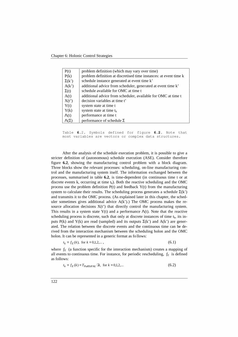
Chapter 6: Holonic Control Strategies
122
P(t) problem definition (which may vary over time)P(k) problem definition at discretised time instances: at event time kΣ(k’) schedule instance generated at event time k’A(k’) additional advice from scheduler, generated at event time k’Σ(t) schedule available for OMC at time tA(t) additional advice from scheduler, available for OMC at time tX(t’) decision variables at time t’Y(t) system state at time tY(k) system state at time tk
Λ(t) performance at time tΛ(Σ) performance of schedule Σ
Table 6.2. Symbols defined for figure 6.2. Note thatmost variables are vectors or complex data structures.
After the analysis of the schedule execution problem, it is possible to give astricter definition of (autonomous) schedule execution (ASE). Consider thereforefigure 6.2, showing the manufacturing control problem with a block diagram.Three blocks show the relevant processes: scheduling, on-line manufacturing con-trol and the manufacturing system itself. The information exchanged between theprocesses, summarised in table 6.2, is time-dependent (in continuous time t or atdiscrete events k, occurring at time tk). Both the reactive scheduling and the OMCprocess use the problem definition P(t) and feedback Y(t) from the manufacturingsystem to calculate their results. The scheduling process generates a schedule Σ(k’)and transmits it to the OMC process. (As explained later in this chapter, the sched-uler sometimes gives additional advice A(k’).) The OMC process makes the re-source allocation decisions X(t’) that directly control the manufacturing system.This results in a system state Y(t) and a performance Λ(t). Note that the reactivescheduling process is discrete, such that only at discrete instances of time tk, its in-puts P(k) and Y(k) are read (sampled) and its outputs Σ(k’) and A(k’) are gener-ated. The relation between the discrete events and the continuous time can be de-rived from the interaction mechanism between the scheduling holon and the OMCholon. It can be represented in a generic format as fo llows:
,...2,1,0for ),( == kkft Ek , (6.1)
where fE (a function specific for the interaction mechanism) creates a mapping ofall events to continuous time. For instance, for periodic rescheduling, fE is definedas follows:
,...2,1,0for ,)( =⋅== kkTkft PaRSiFALEk (6.2)
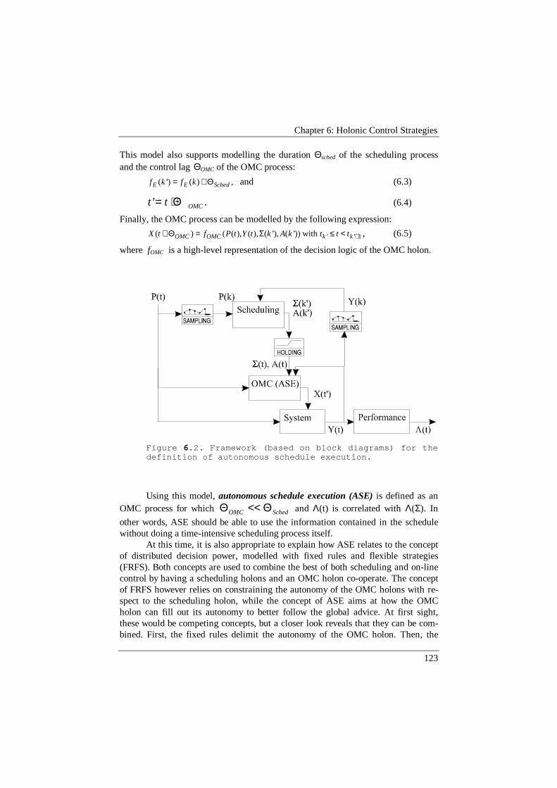
Chapter 6: Holonic Control Strategies
123
This model also supports modelling the duration Θsched of the scheduling processand the control lag ΘOMC of the OMC process:
,)()’( SchedEE kfkf Θ+= and (6.3)
t t OMC’ .= + Θ (6.4)
Finally, the OMC process can be modelled by the following expression:
1’’ with ))’(),’(),(),(()( +<≤Σ=Θ+ kkOMCOMC tttkAktYtPftX , (6.5)
where fOMC is a high-level representation of the decision logic of the OMC holon.
Figure 6.2. Framework (based on block diagrams) for thedefinition of autonomous schedule execution.
Using this model, autonomous schedule execution (ASE) is defined as anOMC process for which Θ ΘOMC Sched<< and Λ(t) is correlated with Λ(Σ). In
other words, ASE should be able to use the information contained in the schedulewithout doing a time-intensive scheduling process itself.
At this time, it is also appropriate to explain how ASE relates to the conceptof distributed decision power, modelled with fixed rules and flexible strategies(FRFS). Both concepts are used to combine the best of both scheduling and on-linecontrol by having a scheduling holons and an OMC holon co-operate. The conceptof FRFS however relies on constraining the autonomy of the OMC holons with re-spect to the scheduling holon, while the concept of ASE aims at how the OMCholon can fill out its autonomy to better follow the global advice. At first sight,these would be competing concepts, but a closer look reveals that they can be com-bined. First, the fixed rules delimit the autonomy of the OMC holon. Then, the

Chapter 6: Holonic Control Strategies
124
OMC holon has to fill out its remaining autonomy using some algorithm. For thisalgorithm, more traditional (heterarchical) approaches like dispatching rules, mar-ket-based or behaviour-based control can be used. Instead of these heterarchicalcontrol strategies, ASE algorithms can be used such that the advice of the schedulercan still be taken into account, even if it is not binding. (Once again, it can be no-ticed that this explanation refers only to the co-operation between centralised staffholons, but a similar same reasoning can be done for the co-operation between staffholons and local holons — e.g. a centralised scheduling holon and distributedOMC holons.)
This chapter presents several control strategies, based on FRFS or ASE, or acombination of them. The first (heuristic) solutions are mostly focused on FRFS.Once the fixed rules are defined, some approaches for the flexible strategies areproposed, but these are less essential. A following section describes an ASE algo-rithm based on perturbation analysis, which is an advanced flexible strategy in thatit can decide for itself when to obey the schedule and when to deviate. Then, it ispossible to grant more autonomy to the OMC holon such that it can even better re-act to disturbances.
6.3 Schedule represented as a graphFuture sections require a formal model of the schedule to reason about fixed rules,flexible strategies and autonomous schedule execution. FRFS enables to defineautonomy and co-operation in holonic manufacturing systems more precisely. Thischapter expresses fixed rules (or “invariants”) with respect to a certain schedule. Itthereby limits itself to the resource allocation problem for job shops, as done in therest of this thesis.
Often, reasoning about resource allocation and scheduling decisions can bemade easier if the schedule is not represented (solely) by a Gantt chart, which mapseach operation with a set of resources and a start time, but rather by a graph. Thisgraph consists of a node for each operation, and an edge for each temporal relationbetween operations. Temporal relations may be:• the technological precedence constraints between the operations of a single or-
der.• the precedence relations originating from the sequencing decisions made by the
scheduler for each resource. Implicitly, these precedence relations capture thecapacity constraints.
• all other hard timing constraints as defined in the scheduling problem, like theorder release date. (A “hard constraint” is a constraint that cannot be relaxed.)
6.3.1 Precondition on the ScheduleFor the operational level of resource allocation, the focus on WIP minimisation isnot that important anymore. Usually, in short-range scheduling in an environmentfull of disturbances, nobody wants to delay an operation if it can be executed with-out delaying another operation. Therefore, the proposed approach is limited to the
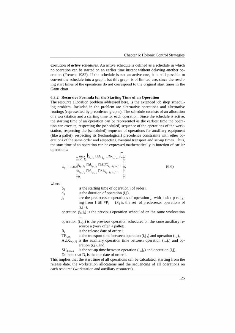
Chapter 6: Holonic Control Strategies
125
execution of active schedules. An active schedule is defined as a schedule in whichno operation can be started on an earlier time instant without delaying another op-eration (French, 1982). If the schedule is not an active one, it is still possible toconvert the schedule into a graph, but this graph is of limited use, since the result-ing start times of the operations do not correspond to the original start times in theGantt chart.
6.3.2 Recursive Formula for the Starting Time of an OperationThe resource allocation problem addressed here, is the extended job shop schedul-ing problem. Included in the problem are alternative operations and alternativeroutings (represented by precedence graphs). The schedule consists of an allocationof a workstation and a starting time for each operation. Since the schedule is active,the starting time of an operation can be represented as the earliest time the opera-tion can execute, respecting the (scheduled) sequence of the operations of the work-station, respecting the (scheduled) sequence of operations for auxiliary equipment(like a pallet), respecting its (technological) precedence constraints with other op-erations of the same order and respecting eventual transport and set-up times. Thus,the start time of an operation can be expressed mathematically in function of earlieroperations:
( )
++
++
++
=
=
i
jijijiji
jijijiji
jjijijiPp
ij
R
USdb
AUXdb
TRdb
b
kkkkkk
aaaaaa
pppij
,
,
,max
max
,,,,,
,,,,,
,,,,..1
, (6.6)
wherebij is the starting time of operation j of order i,dij is the duration of operation (i,j),jp are the predecessor operations of operation j, with index p rang-
ing from 1 till #Pij (Pij is the set of predecessor operations of(i,j).),
operation (ik,jk) is the previous operation scheduled on the same workstationk,
operation (ia,ja) is the previous operation scheduled on the same auxiliary re-source a (very often a pallet),
Ri is the release date of order i,TRi,jp,j is the transport time between operation (i,j p) and operation (i,j),AUXia,ja,i,j is the auxiliary operation time between operation (ia,ja) and op-
eration (i,j), andSUik,jk,i,j is the set-up time between operation (ik,jk) and operation (i,j).Do note that Di is the due date of order i.
This implies that the start time of all operations can be calculated, starting from therelease date, the workstation allocations and the sequencing of all operations oneach resource (workstation and auxiliary resources).
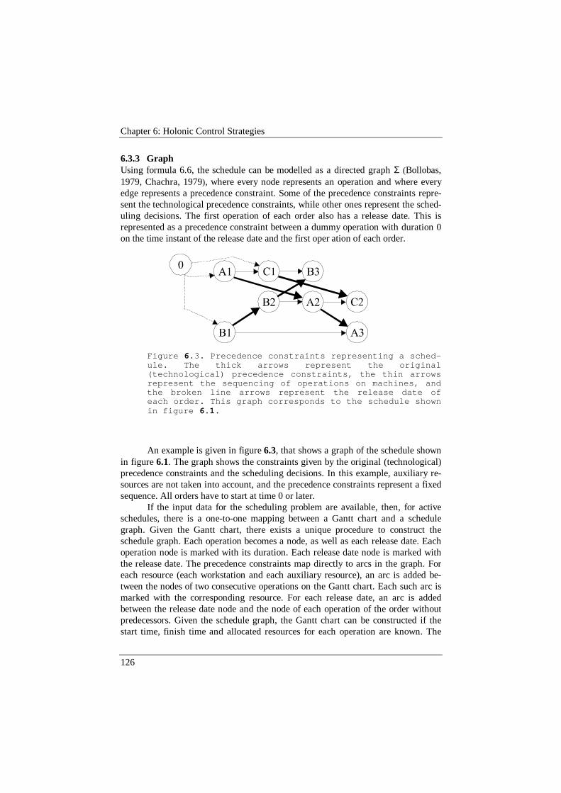
Chapter 6: Holonic Control Strategies
126
6.3.3 GraphUsing formula 6.6, the schedule can be modelled as a directed graph Σ (Bollobas,1979, Chachra, 1979), where every node represents an operation and where everyedge represents a precedence constraint. Some of the precedence constraints repre-sent the technological precedence constraints, while other ones represent the sched-uling decisions. The first operation of each order also has a release date. This isrepresented as a precedence constraint between a dummy operation with duration 0on the time instant of the release date and the first oper ation of each order.
Figure 6.3. Precedence constraints representing a sched-ule. The thick arrows represent the original(technological) precedence constraints, the thin arrowsrepresent the sequencing of operations on machines, andthe broken line arrows represent the release date ofeach order. This graph corresponds to the schedule shownin figure 6.1.
An example is given in figure 6.3, that shows a graph of the schedule shownin figure 6.1. The graph shows the constraints given by the original (technological)precedence constraints and the scheduling decisions. In this example, auxiliary re-sources are not taken into account, and the precedence constraints represent a fixedsequence. All orders have to start at time 0 or later.
If the input data for the scheduling problem are available, then, for activeschedules, there is a one-to-one mapping between a Gantt chart and a schedulegraph. Given the Gantt chart, there exists a unique procedure to construct theschedule graph. Each operation becomes a node, as well as each release date. Eachoperation node is marked with its duration. Each release date node is marked withthe release date. The precedence constraints map directly to arcs in the graph. Foreach resource (each workstation and each auxiliary resource), an arc is added be-tween the nodes of two consecutive operations on the Gantt chart. Each such arc ismarked with the corresponding resource. For each release date, an arc is addedbetween the release date node and the node of each operation of the order withoutpredecessors. Given the schedule graph, the Gantt chart can be constructed if thestart time, finish time and allocated resources for each operation are known. The

Chapter 6: Holonic Control Strategies
127
allocated resources for each operation are extracted from the resource sequencingarcs in the schedule graph2. The starting time of each release date node is containedwithin the node marking. The starting time of each operation node is calculatedwith formula 6.6, on condition that the schedule is active. The finish time of eachnode is calculated with equation 6.7 (the former equation 1.2):
c b dij ij ijh= + . (6.7)
The resulting schedule graph Σ can then be defined as:
{ }ijiii
jiji
RbRjiR
bbjiji
such that nodedummy a is )),(,(
procedure above in the defined wasarcan
and ,)),(),,((
),(
),(),(2211
2211
≥
≤
=Σ U
, (6.8)
where o1 = (i1,j1) and o2 = (i2,j2) are scheduled operations. In other words, Σ is theunion of the set of arcs sequencing the operations on a resource and the set of arcsimposing release dates.
6.3.4 PerformanceThe objective function L (the schedule performance) is a function of the start timesof all operations. Using the dummy operations (with a known start time) and for-mula 6.6, all start times can be calculated, and therefore also the value of the globalperformance L.
For instance, for the weighted mean tardiness, the objective function L is alinear function of the tardiness of each order, and the tardiness is a piece-wise lin-ear function of the start time of the last operation of each order. Thus, for the ex-ample already shown, the global performance index L of the schedule can be writ-ten as:
),0max(.
),0max(.
),0max(.
22
33
33
CCCC
BBBB
AAAA
Ddbw
Ddbw
Ddbw
−++−++−+=Λ
,
(6.9)
where wi is the weight of order i, representing its relative importance; and Di is thedue date of order i, representing the date the order should preferably be ready. wi
and Di are given.
2 The alert reader would argue that the allocated resources cannot be extracted fromthe schedule graph if only one operation uses a specific resource, since then, no se-quencing arcs for that resource would exist. This problem is mathematically re-solved by introducing resource start-of-availability nodes (dummy nodes for eachresource, similar to the release date nodes) and an additional arc between that nodeand the first operation scheduled on that resource.

Chapter 6: Holonic Control Strategies
128
6.4 Literature reviewTwo types of on-line manufacturing control strategies are already well-known: hi-erarchical and heterarchical control. Both can be considered as extreme cases ofholonic control strategies. Both approaches were already discussed in chapter 2.The following subsections describe their behaviour in detail to position hierarchicaland heterarchical control with respect to holonic manufacturing.
When looking in literature for similar approaches towards manufacturingcontrol algorithms as the ones presented in this thesis, there are surprisingly few.For ASE, some researchers have come quite close to it, without calling it scheduleexecution. The HIMAC project (Vallauri, 1995) developed an algebra for manu-facturing in order to apply it for the development of manufacturing control algo-rithms. Although their work seemed to be leading to similar concepts as ASE, nonew algorithms were developed in that project.
Chapter 2 already described the work on scheduling with Lagrangian re-laxation, developed at the University of Connecticut (Luh, 1993, 1998). These ideascan also be used for on-line control. Note that the Lagrangian multipliers, whichare optimised during the scheduling process, represent the severeness of the relaxedconstraints and can therefore be used to identify which machines are bottlenecksduring certain periods. Such a multiplier represents the cost of that machine at thattime instant. With this information, it should be possible to design well-performingheuristics for on-line control. To our knowledge, this idea was not yet further elabo-rated at the University of Connecticut.
6.5 Hierarchical Control
6.5.1 Informal DescriptionIn hierarchical control (the traditional approach), all decision power is hierarchi-cally decomposed along the branches of the hierarchical control tree. In the sched-uling context, hierarchical control usually implies the existence of a centralisedscheduler, on a higher level. On-line control just acts as a buffer — a “cache” — toexecute decisions that have already been taken by the scheduler. Literature is notvery specific about this, but presumably, on-line control has the autonomy to halt ifsome disturbance would invalidate the schedule. (Not halting would cause unfeasi-bilities or crashes…)
If disturbances occur only seldom, hierarchical control works well, but fromthe moment disturbances occur with a higher frequency, performance deterioratesdramatically. In strict hierarchical control, the events are propagated upwards,where they are reacted upon at the right level, and then the appropriate control ac-tions are propagated downwards again to the manufacturing devices. This implieson-line control does not take other actions than reporting the problem to a reactive
Chapter 6: Holonic Control Strategies
129
scheduler. Only after the reactive scheduler produced a new schedule3, to be exe-cuted by on-line control (the dispatcher), the disturbance is reacted upon. For in-stance, when a machine breaks down, the dispatcher keeps all operations scheduledon that machine waiting, until a new schedule is generated. Operations on othermachines may continue. However, since the waiting operations on the broken downmachine are predecessors operations of operations on other machines, also the workon these machines is halted. This way, a machine breakdown in strict hierarchicalcontrol propagates rapidly through the manufacturing system, seriously affectingglobal performance (Frizelle, 1998). These findings were verified with a hierarchi-cal control algorithm described in subsection 6.5.2, using the implementation de-scribed in chapter 7 and evaluated in chapter 8.
6.5.2 Formal DescriptionFor a formal description of OMC according to the hierarchical control approach,the schedule is represented as a graph (cf. section 6.3). Then, the fixed rules andflexible strategies are defined for this control strategy.
Let Σ be the schedule generated by the scheduler (represented as a graph).Let Σp be the graph constructed by taking the union of all order precedence graphs,in other words, let Σp be the sub-graph of Σ that only considers technological con-straints. In figure 6.3, Σp consists of the thick arrows of the graph Σ. Σ and Σp aregiven.
Let 8 be the set of all agents (or holons). Let ϕS be the (centralised) sched-uling holon. Let 8B be the set of basic holons ϕB (local agents: resources and or-ders), to a certain degree subject to the control of ϕS. The goal of this subsection isto find a way to express the degree in which 8B is subject to the control of ϕS. Forthis simple example, let’s suppose 8 is the union of 8B and {ϕS}.
By definition, a manufacturing control system 8 is hierarchical if and only if8B exactly follows the schedule (complete obedience). By definition, exactly fol-lowing the schedule means keeping the resource allocation for each operation andthe operation sequencing on each resource; in other words, if the operations areexecuted according to the precedence constraints expressed in Σ. Therefore, in hi-erarchical control, the fixed rules (FR) and flexible strategies (FS) for 8B are asfollows:
FR: Every agent ϕB shall respect the precedence constraints expressed in Σ. (6.10)
FS: There is no room for flexible strategies for the basic holons in 8B. (6.11)
3 i.e., at predefined times for periodic rescheduling (see subsection 5.2.2 and equa-tion 5.5) or after a rescheduling delay for event-based rescheduling (see section5.4).

Chapter 6: Holonic Control Strategies
130
This means that on-line manufacturing control is only to enforce the scheduleprecedence graph, and has no decision space of its own. By relying completely onfixed rules, the system behaviour is defined very explicitly. However, these rulesquickly halt the entire system when a machine breaks down.
6.6 Heterarchical Control
6.6.1 Informal DescriptionTo overcome the disadvantages associated with hierarchical control, several re-searchers, like Hatvany (1985), or Duffie et al. (1986), proposed a heterarchical ap-proach. Heterarchical control (Lin et al., 1994) is a highly distributed form ofcontrol, implemented by a system of independent co-operating processes or agentswithout centralised or explicit direct control. (In “true” heterarchical control, cen-tralised elements are “forbidden”.) Control decisions are reached through mutualagreement and information is exchanged freely among the participating agents.
Heterarchical control offers interesting prospects of a high robustnessagainst disturbances in manufacturing. Especially if reactive system propertiesemerge automatically from the behaviour of the individual agents, heterarchicalcontrol is very appealing. In practice, however, only a limited set of heterarchicalcontrol algorithms really exhibits emergent behaviour. Moreover, it has turned outthat heterarchical control, banning all forms of hierarchy, has problems to deliverglobally optimised performance. More essential might even be that the behaviour ofa system under heterarchical control can be unpredictable, which is at odds with theneeds of most manufacturing operations! Finally, not often mentioned in literature,but certainly true, is the fact that many, if not all, heterarchical control algorithmsrequire considerable tuning before yielding adequate performance.
In this section, only one heterarchical control strategy will be described,based on free-market principles. Hereby, order agents compete with each other forscarce resources, based on a pricing mechanism: if demand for a workstation is toohigh, prices for that workstation rise, otherwise, they go down. The described algo-rithm is based on an implementation by Debels and Hermans (1998), working atPMA on their master thesis.
6.6.2 Formal DescriptionFor a formal description of heterarchical OMC, the description of the fixed rules forthe basic holons is fairly easy. Using the definitions given in subsection 6.5.2, thebasic holons 8B have full autonomy if and only if they only have to obey the tech-nological precedence constraints expressed in Σp. This actually comes down tostating that the scheduler does not take a single decision, and that all decisionpower remains in the basic holons. One could say that under heterarchical control,there are no fixed rules, since all decisions are taken using flexible strategies.
On the other hand, the formal description of the flexible strategies the basicholons use for their decision taking, is not so trivial. In the implementation of De-

Chapter 6: Holonic Control Strategies
131
bels and Hermans (1998), there is no separate optimisation part in the basic holons.All decisions are based on on-line control only (no look-ahead). They also presumea fixed sequencing of operations within one order. The description of their localdecision logic, given below, uses the Petri nets presented in subsection 5.2.3. Figure5.2 to 5.6 present the behaviour of order and workstation holons. Heterarchicalcontrol ignores the communication with staff holons as modelled in these Petrinets. In the Petri nets, four decision points can be identified:• The allocation of pallets to orders (decision taken in place p3 of the order holon
TPN — more specifically, p3.p1, p3.p3, p3.p5 and p3.p7 —, while negotiatingwith a transport system holon);
• The allocation of a workstation to an operation (decision taken in place p7 of theorder holon — p7.p2, p7.p3, p7.p4 and p7.p8 — in negotiation with place p4 of theworkstation holon);
• The sequencing of the operations on a workstation (decision taken in place p5,p7 and p14 of the workstation holon, taking into consideration the results of thenegotiation phase performed in places p7 of the order holon and p4 of the work-station holon. These decisions are backed up by operations p12 and p13 of theworkstation holon, taking care of transportation within the workstation); and
• Orders cancelling their commitment to the resource, if needed (place p8.p9 ofthe order holon).
In Debels’ (1998) implementation, the allocation of pallets to orders is doneon a first come, first served basis. If no more pallets are available, the transportsystem holon waits until a pallet is released (or a new pallet is added to the system)and then allocates the pallet to the requesting order.
For the allocation of a workstation to an operation, Debels presents severalmarket-based mechanisms. In the simplest version, the price πk for a resource mkequals the number of operations having selected that resource.
}and selectedalready is resource),{(# , kjik m hji ==π . (6.12)
The order selects the workstation with the lowest price for that operation. In a laterversion, Debels presents the following workstation price πijk for an operation (i,j):
),0max(...)( 2,,1 iiktikijk DtwTt −ψ+ψ+π=π . (6.13)
where Ti,t,k the transportation time is to get from the current position of order i attime t to the required position (mk), and ψ1 and ψ2 are tuneable scale factors (alsoensuring dimensional correctness). Note that the price is function of time via thefinal term and indirectly via the transportation time. This pricing mechanism doesnot only consider workstation capacity constraints, but also balances machine costversus transport delay. Moreover, it adds a cost if the order is tardy. Note that thispricing mechanism considers as well throughput, flow time as tardiness. The scalefactors can reflect that trade-off.
For the sequencing of operations within one workstation, the same pricingmechanism is used. A resource will first perform the operation with the highest bid.
Chapter 6: Holonic Control Strategies
132
If an order is already executing some operations on a workstation, it will considerleaving the station or not, using the same pricing mechanism. As a tie-breaker, op-erations are sequenced on a first come, first served basis.
Finally, orders can withdraw their commitment to a resource. In the Debels’implementation, the price of an order may rise when it is already moving to aworkstation. Therefore, the order reconsiders entering the workstation when itreaches the workstation input buffer. It again uses the same pricing mechanism,and decides to enter if the price for this workstation is still the lowest. Normally,this should not cause reallocations, unless the capacity term πk of the workstationprice has risen signif icantly.
There is still room for a lot of improvement in this implementation. A firstimprovement could be on the pricing mechanism, to define prices that better reflectthe cost structure of a resource allocation problem. (For instance, making the ca-pacity term πk function of the duration of the operation; reflecting the transport de-lay in the tardiness term; and defining operation due dates for the operations suchthat orders become rush orders already if their remaining slack4 is used.) Secondly,heterarchical control does not forbid look-ahead, such that the effect of decisions onthe eventual tardiness is better estimated. Thirdly, if the remaining communicationbandwidth is used for multi-stage negotiation, decisions are based also on the deci-sions of future operations, such that the pricing levels evolve to more natural val-ues. Many of these concepts were addressed by Gou (1994, 1998) and Luh (1998)for distributed scheduling. Taking up these results for OMC would be very prom-ising.
Although these improvements were not implemented, to our opinion, theDebels’ implementation is representative for heterarchical control. It correspondswell to other heterarchical control algorithms described in literature. Sufficienttime was spent for the implementation and tuning of the algorithms (3 months onalgorithms only, thus not including the development of the software framework).Therefore, this implementation can serve as a reference to compare the results ofpure heterarchical control with holonic control as developed for this thesis.
Summarising, in heterarchical control, all autonomy is granted to the re-source and order agents, resulting in the following fixed rules (FR) and flexiblestrategies (FS) for 8B:
4 The slack Si of an order i is defined as the buffer time an order has to be finishedbefore its due date:
∑−−=−
=
1
0
iN
jijiii dRDS . (6.F1)
The remaining slack Srem,i of an order i at a time t is defined as the remaining buffertime to order has to reached completion before its due date:
∑∀
−−= finishedyet not is ),(:
, ),max()(jij
ijiiirem dRtDtS . (6.F2)
Chapter 6: Holonic Control Strategies
133
FR: There are no fixed rules for the agents ϕB (except that they shall respect the technological precedence constraints expressed in Σp). (6.14)
FS (1) Pallets are allocated to orders according to the FIFO rule. (2) An operation (i,j) is allocated to the workstation k
with the lowest price πijk (as defined in equation 6.13). (3) A workstation k sequences operations by first selecting
the operation (i,j) with the highest price πijk. (6.15)
In this approach, resource and order agents react quickly to disturbances, accordingto their own ideas. However, they do not co-ordinate their work with a globalscheduler, making their work very unpredictable and (sometimes) low in perform-ance.
6.7 Centralised Autonomous On-line Control
6.7.1 Informal DescriptionThis section presents a centralised autonomous OMC algorithm (CAOMC). It is aresource allocation strategy for a staff OMC holon that completely ignores theschedule. It therefore completely relies on its own decision power, using dispatch-ing rules for sequencing and similar simple rules for the allocation of operations toworkstations. In that respect, this control strategy resembles the kind of algorithmsused in industrial cell controllers.
The CAOMC algorithm was developed for this thesis to study the effects ofon-line control without scheduling advice — in other words “centralised heterar-chical control”. Since this thesis mainly focuses on the integration of schedulingand on-line control, a centralised implementation of heterarchical control is suffi-cient to compare the potential of completely autonomous (“heterarchical”) algo-rithms versus autonomous schedule execution algorithms.
By comparing CAOMC with ASE algorithms, one can study the implica-tions of varying degrees of autonomy for the OMC holon with respect to the sched-uling holon. The degree of distribution in on-line control does not interfere withthat comparison. For implementation, it implies one can focus on the co-operationbetween two staff holons only.
On the other hand, by comparing CAOMC with really distributed heterar-chical control, it is possible to find the appropriate degree of distribution. Thequestion is whether a centralised form of co-ordination between basic holons paysoff with respect to completely heterarchical control. Though interesting, this thesisdoes not discuss these matters in detail.
Chapter 6: Holonic Control Strategies
134
6.7.2 Formal DescriptionFor a formal description of CAOMC, first all holons are to be identified. Thereaf-ter, the fixed rules and flexible strategies for all interacting holons have to be de-fined. Again, let 8 be the set of all holons:
{ } { } { } { }OMCSOROMCSB ϕ∪ϕ∪∪=ϕ∪ϕ∪= 8888 , (6.16)
where 8B is the set of all basic holons, 8R is the set of all resource holons, 8O is theset of all order holons, ϕS is the scheduling holon and ϕOMC is the OMC holon.ϕOMC takes a central role, in that all communication goes via this holon. ϕB andϕOMC interact to distribute and execute the work to be done. ϕS and ϕOMC interact toexchange the schedule. There is no direct interaction between ϕB and ϕS.
In CAOMC, the interactions between ϕB and ϕOMC are completely defined byfixed rules and not by flexible strategies. The OMC holon controls the basic holonscompletely hierarchically, leaving no autonomy for them. It turns the basic holonsinto slaves, obeying their master, and switches off their intelligence. The transportsystem holon gets commands to allocate pallets to orders and to move orders toworkstations. The order holons also get commands to move, to start set-ups and tostart working on the workstation. The workstation holons get commands to startset-ups and to start working on the workstation. The only remaining autonomy ofthe basic holons is the synchronisation of these commands, and start the transpor-tation, set-up or processing operation if all holons involved are ready.
For the interactions between ϕS and ϕOMC, CAOMC defines the following setof fixed rules and flexible strategies. For ϕOMC, there are no fixed rules, implyingthat ϕOMC is completely autonomous with respect to ϕS. Using the formalism of sub-section 6.5.2, ϕOMC only has to obey the technological precedence constraints ex-pressed in Σp. Therefore, all decision power resides with the OMC holon, which isthe only holon in this control strategy with flexible strategies.
The flexible strategies of the OMC holon are implemented with dispatchingrules, as mentioned above. Like in subsection 6.6.2, four types of decisions are to betaken. For the allocation of pallets to orders, a first-come first-served strategy isused. For the allocation of a workstation hi1,j1 to an operation (i1,j1), COA selectsthe workstation, if possible, where the order has already gone to or is going to, orotherwise the workstation “with the least work in queue”:
{ }( )hijHh
ji mhjijihji
==∈
and executable is ),(),(#minarg11
11 . (6.17)
Allocation of workstations to operations is done from the moment the operation be-comes executable. For the sequencing of operations on a workstation, the imple-mented COA algorithm uses the EDD (earliest due date) dispatching rule(sequencing all operations that have requested the workstation). If a tie-break isneeded, FIFO (first-in, first-out) is used. Finally, cancellations are not performed inthe implemented COA algorithm.

Chapter 6: Holonic Control Strategies
135
Summarising, CAOMC is governed by the following fixed rules (FR) andflexible strategies (FS) are for 8B and ϕOMC:
FR: The agents ϕB shall immediately obey all commands givenby ϕOMC (unless when these commands violate thetechnological precedence constraints expressed in Σp).ϕOMC is not subject to any fixed rules. (6.18)
FS: The agents ϕB have no flexible strategies. ϕOMC allocates operations to workstations according to equation 6.17. ϕOMC sequences operations according to EDD. (6.19)
6.8 Heuristic Holonic Control StrategiesThis section presents a set of holonic control strategies (as opposed to the previoussections) that are based on heuristics and common sense ideas. The three algo-rithms described are “short term autonomy” (STA), “autonomy if distur-bances” (AID) and “limited deviation from schedule” (LDFS). These algo-rithms are examples of possible control solutions, rather than the only and uniquecandidates for holonic manufacturing control.
For each algorithm, the following subsections describe the basic ideas andthe general structure and then present the corresponding fixed rules and flexiblestrategies (FRFS). At the end of each subsection is a short qualitative evaluation ofthe algorithm. A truly exper imental analysis is found in chapter 8.
6.8.1 Short Term AutonomyThe “Short Term Autonomy” heuristic (STA) distributes decision power over theholons by granting autonomy to the OMC holon for a short term and keeping theremainder of the decision power in the scheduling holon. In other words, thescheduler sends a part of the schedule (referring to the near future) to the OMCholon. The OMC holon limits itself to the execution of the operations contained inthe near future schedule Σ∆T (until time Tresched), but has complete autonomy to exe-cute that schedule using its own flexible strategies (following the schedule or devi-ating from it). However, operations scheduled later than Tresched could not be exe-cuted yet. This implies the OMC holon can react quickly to disturbances on a shortterm. For longer-term reactions, the OMC holon has to obey the scheduler holon,but since the scheduler is also reactive, a new schedule is produced anyway.
The resulting behaviour is that the schedule is roughly followed. Undernormal conditions, the execution time of an operation is shifted with maximally thelength ∆T of the near future schedule Σ∆T. (Exceptions may occur for long-lastingoperations and transport time delays.) If disturbances appear, they are quickly re-acted upon. Moreover, since Σ∆T does not contain many operations, the decision

Chapter 6: Holonic Control Strategies
136
space for OMC is small enough and local optimisation is still feasible for an on-linecontrol holon.
Again, the autonomy of the OMC holon is described with fixed rules(invariants), modelled by a graph. STA uses the same holons as defined forCAOMC (subsection 6.7.2), and the same fixed rules for the interactions between8B and ϕOMC. To model partial autonomy between ϕS and ϕOMC as suggested by theconcept of holonic manufacturing, we define a graph Σ’, such that Σp is a sub-graphof Σ’ and Σ’ is a sub-graph of Σ. For STA, Σ’ is defined as follows:
( )
<≤Σ∈=Σ
or ),(
and operations are and ),()(’
ji oreschedopji
jijiresched bTboo
ooooT . (6.20)
The fixed rule that defines the co-operation between ϕS and ϕOMC is as follows:
FR: ϕOMC shall execute all operations according to the precedence constraints expressed in Σ’ (equation 6.20). (6.21)
Of course, Σ’ contains a lot of redundant precedence constraints. They can be easilyremoved, or, in practical implementations, it is even possible to avoid to create re-dundant precedence constraints. Moreover, it is not really a problem. Note thatTresched is still a parameter of the algorithm. For instance, for the resource allocationproblem defined in figure 6.1, the resulting graph Σ’ (for Tresched = 2) is shown infigure 6.4. STA fills out the remaining decision space with the following flexiblestrategies:
Figure 6.4. Fixed rules for STA, represented as prece-dence constraints in graph Σ’. The thick arrows repre-sent the original (technological) precedence con-straints, belonging to Σp. Only the relevant arrowswhere drawn (between operations on the same worksta-tion). An example of a redundant arrow is the one be-tween B2 and A3 (in dotted line).
Chapter 6: Holonic Control Strategies
137
FS: ϕOMC allocates operations to workstations according to equation 6.17; ϕOMC sequences operations according to EDD, (6.22)
which are the same strategies as CAOMC uses.Observe also that the definition of a graph Σ’ is a flexible mechanism to de-
fine heuristic holonic control algorithms. The definition of Σ’ in equation 6.20 re-sults in the STA algorithm, but there is a whole range of possible co-operation al-gorithms for 8 that can be developed by defining the corresponding Σ’.
STA manages to combine hierarchical control and heterarchical controlsuch that the schedule is roughly followed, and still there is a fast reaction to dis-turbances. But it does not really use the schedule as advice: rather, it obeys parts ofit and ignores the rest.
6.8.2 Autonomy if DisturbancesThe “autonomy if disturbances” heuristic (AID) aims to distribute decision powerin a better way than STA. It considers the schedules as advice, which it will followin principle (if no disturbances occur). However, when the scheduling advice be-comes unfeasible or clearly sub-optimal, the OMC holon autonomously adapts tothe prevailing situation and tries to approximate the advised schedule as good aspossible, according to its own ideas. AID will therefore utilise the availability ofalternative equipment and/or alternative feasible operation sequences to autono-mously handle disturbances. It is based on the idea that hierarchical control workswell if no disturbances occur, but is very poor if they do occur. To find out whetherdisturbances occur, the algorithm checks whether it runs behind or ahead of sched-ule.
Using FRFS, the co-operation between scheduler and OMC holon can beformally modelled. The same holons and the same interactions between 8B andϕOMC are defined as above. Again, to express the fixed rules, the graph Σ’ is de-fined:
+≥++ΣΣ∈
Σ∈=Σ
and \),(
or ),(
and operations are and
),()(’
, Xoooopji
pji
ji
ji
TtAUXdboo
oo
oo
oot
jiii
,(6.23)
where TX is an extra buffer time, AUXoi,oj is the set-up time between operations oi
and oj, if (oi,oj) refers to a sequencing constraint on a workstation and AUXoi,oj isthe transport time between operations oi and oj, if (oi,oj) refers to a sequencing con-straint on a pallet. (For other kinds of auxiliary resources, AUXoi,oj is to be furtherdefined.) The corresponding fixed rules for ϕOMC are as follows:
FR: ϕOMC shall execute all operations according to the precedence constraints expressed in Σ’ (equation 6.23). (6.24)
Chapter 6: Holonic Control Strategies
138
TX can be used to tune the algorithm. Notice that Σ’ is function of time: while timeelapses, precedence constraints with predecessor operations that are overdue, areremoved from the set of fixed rules. AID uses the same flexible strategies asCAOMC and STA:
FS: ϕOMC allocates operations to workstations according to equation 6.17; ϕOMC sequences operations according to EDD, (6.25)
While OMC under hierarchical control would wait for the production systemto arrive in (or return to) a state where the schedule can be precisely followed, AIDhandles disturbances autonomously. Likewise, AID utilises the information gener-ated by the scheduler to make globally better decisions than an “orthodox” heterar-chical design. However, the system has the tendency to behave very hierarchical ifit gets ahead of schedule (as a whole) or very heterarchical if it gets behind sched-ule (on a global level). This effect is attenuated because the reactive scheduleradapts its schedule to the new situation on the shop floor, but it remains a problem.
6.8.3 Limited Deviation from ScheduleAnother idea to give limited autonomy to an OMC holon, is to allow a limited de-viation from the schedule (LDFS). To a certain degree, the sequencing and thetiming constraints given by the schedule are relaxed for instance to allow swappingtwo neighbouring operations.
To model this type of partial autonomy, there is a need for a more powerfulmethod to model partial autonomy than described above. Therefore, the concept ofa precedence graph is extended. We define an extended graph with generalisedtemporal constraints EGGTC as a graph where the nodes and arrows have addi-tional attributes. The nodes have a duration attribute, and the arrows have general-ised temporal constraint as attribute. A complete description of generalised tempo-ral constraints is given by Sadeh et al. (1988). Briefly, a generalised temporal con-straint is an extension of a precedence constraint, which states the beginning of thesecond operation should be later than or equal to the end of the first one. UsingEGGTCs, it is possible to express conditions like “between the first operation andthe second one should be a buffer time of at least ten minutes.” In other words, it ispossible to increase the autonomy of ϕOMC not only by omitting precedence con-straints, but also by relaxing them, i.e. replacing them by weaker temporal con-straints.
To model LDFS, using this formalism, first the following EGGTC is de-fined:
( )
+≤++=ζ
Σ∈ζ=Σ
and )( ),,()(
Rooooo
jijiRLDFS TbAUXdb
,ooooT
jjiii
, (6.26)
Chapter 6: Holonic Control Strategies
139
where TR is the time the constraint is relaxed with (a parameter of the algorithm),and ζ is the generalised temporal constraint, as defined in the above formula. Thecorresponding fixed rule is as follows:
FR: ϕOMC shall respect the temporal constraints defined in the EGGTC ΣLDFS (equation 6.26). (6.27)
The flexible strategies are the same as for CAOMC, STA and AID:
FS: ϕOMC allocates operations to workstations according to equation 6.17; ϕOMC sequences operations according to EDD, (6.28)
LDFS is complementary to AID, in that both concepts can be used simulta-neously. AID decreases the number of constraints, while LDFS relaxes the con-straints themselves. It is believed that LDFS provides additional possibilities fortuning the system. However, since it rather represents a trade-off between hierar-chical and heterarchical control than a combination, it is possible that LDFS ismost interesting if used in combination with other heuristics that better merge theproperties of hierarchical and heterarchical control. LDFS would then rather be anadditional parameter than a separate approach.
6.8.4 ConclusionThis section has presented three heuristic strategies for holonic manufacturingcontrol. They were simple to develop, based on common sense (or on well-knownconcepts like bottleneck theory). They were described using the fixed rules andflexible strategies (FRFS).
The algorithms developed are holonic in that they combine robustness andoptimisation in some way: they use the schedule, relying on the optimisation wherepossible, but react to disturbances autonomously when necessary. However, the de-veloped algorithms have the tendency to swap completely to either hierarchical orheterarchical control, rather than combining the decision power of scheduling andOMC holon in the best conceivable way. Chapter 8 presents the experimental re-sults for these algorithms.
One of the major gaps in the control strategies presented, is the absence ofalgorithms for autonomous schedule execution (ASE) that really use the scheduleas advice: taking advantage of it if possible, but without clinging to it if inappropri-ate. Up to now, the flexible strategies used were mostly based on dispatching rules.An alternative would be the use of market-based algorithms, but they would not beany better in using the schedule. Truly interesting would be the use of interactivealgorithms, but interactions between human and computerised holons is a completearea of research on its own. The following section presents a flexible strategy thatexplicitly focuses on autonomous schedule execution.

Chapter 6: Holonic Control Strategies
140
6.9 Schedule Execution with Perturbation Analysis
6.9.1 Basic IdeaThe goal of this section is the development of a suitable algorithm for autonomousschedule execution (ASE). This algorithm is a flexible strategy that uses advicefrom the scheduler, contrary to the flexible strategies based on dispatching rules, asdescribed in section 6.8.
As was mentioned in section 6.2, a Gantt chart does not contain sufficientinformation to execute a schedule autonomously. Therefore, the scheduler has toprovide additional advice. In the previous sections, the scheduling holon alreadyexpressed the schedule as a graph, and informed OMC of the bottlenecks and rushorders. This section addresses the problem of schedule execution directly: the OMCholon needs to know how local decisions affect the global performance. With thisknowledge, its goals are directly expressed in function of its own decisions, suchthat it can indeed take local decisions according to a global optimum.
A mathematical technique designed specifically for this problem is Pertur-bation Analysis (PA, also called sensitivity analysis — Cassandras (1993) describesthe application of this technique to discrete event systems). In PA, the global per-formance is expressed in function of local parameters. Partial derivatives of theglobal performance to these local parameters are calculated. Then, in standard PA,the global performance is linearised in function of the local parameters, using thesepartial derivatives. In this way, local decisions explicitly conform to the global goal.
These partial derivatives need to be defined and calculated off-line (by thescheduling holon) and in such a way that the OMC holon can instantly derive thecorrect local decision from this advice and the on-line manufacturing data. How-ever, if a schedule is represented as a Gantt chart, it is not obvious to even definethese partial derivatives. Therefore, the schedule is again represented as a graph(see section 6.3). This allows to define and formulate the local decision parameters(εe) and the partial derivatives exactly (cf. following subsections). With an efficientcalculation schema, the scheduler can prepare these data. During on-line control(see subsection 6.9.6), a number of local decision alternatives (“choices”) are de-fined and evaluated according to the local decision parameters and the partial de-rivatives, thereby making local decisions with a global view, but based on real-timedata. For each alternative, the effect on the values εe is calculated. This calculationis simple, but non-generic in that it depends strongly on the specific disturbanceencountered. When the values for ∆εe are known, ∆Λ is calculated. The alternativewith the best ∆Λ is selected.
Does it make sense to linearise such a highly non-linear system? Yes, itdoes, since the linearisation is used to make fast decisions, while around this fastcontrol loop, another feed-back mechanism exists, namely reactive schedulingcontained in the scheduling holon. Moreover, chapter 8 shows with experimentaldata that the results are satisfa ctory (see chapter 8).
Chapter 6: Holonic Control Strategies
141
6.9.2 Co-operation Schema: Overall ViewThe basic idea, presented above, leads to the following overall co-operationschema:• The schedule is represented as a graph. The local decision parameters ee are
defined, and the global performance L is expressed in function of the ee. Thiscan be done in a way generic for the entire schedule.
• The scheduling holon calculates the partial derivatives dL/dee off-line.• The OMC holon defines, for each decision, a set of decision alternatives
(“choices”). For each alternative, the effect on the values ee and the resultingDL are calculated. The alternative with the best DL is selected.
6.9.3 Definition of Local Decision ParametersTo define the local decision parameters, the schedule is represented as a graph Σ. Ifthe schedule is active (i.e. with no “unnecessary” delays, see section 6.3.2), the cal-culation times of all operations can be extracted from graph Σ, and thus, the graphand the Gantt chart are equivalent representations of the schedule. In other words,the graph “matches” with the schedule (see section 6.3.3). This approach requiresthe schedule to be active. If this constraint is not satisfied, the schedule contains“unnecessary” delays. In that case, it can still be executed, but the delays of the op-erations as imposed by the schedule cannot be followed in the suggested approach.
Next, some additional definitions are needed (illustrated in figure 6.5). Oneach instant of time tcut , the schedule can be partitioned in a set of operations thatstart before tcut and a set of operations that start at time tcut or later. The graph ΓH,that is a subgraph of Σ and consists only of operations starting before tcut is calledthe "schedule head". The graph ΓB, that is a subgraph of Σ and consists of the otheroperations is called the "schedule body". The set E of edges (the arrows) of thegraph that connect a node (an operation) of the schedule head with a node of theschedule body, is called the "cut" E. The union of the two subgraphs ΓH and ΓB andthe cut E is again the original graph Σ. If the schedule is feasible, then all edgesbetween the schedule head and the schedule body are oriented in the direction fromschedule head to schedule body. In graph theory, one can prove that a cut is suffi-cient to define the schedule head and the schedule body, if the graph Σ is con-nected5. (There can be situations where the graph is not connected. This howeveronly affects the implementation, and not the concepts behind this approach.)
5 By definition, a graph Σ is connected if and only if every pair of its nodes isjoined by at least one simple chain. A simple chain is a finite sequence of edgessuch that every edge has exactly one node in common with the previous edge andall nodes are distinct (Chachra, 1979).
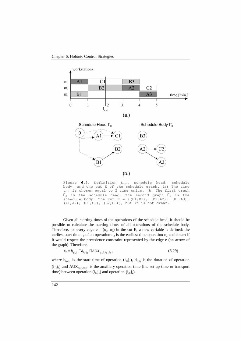
Chapter 6: Holonic Control Strategies
142
Figure 6.5. Definition tcut, schedule head, schedulebody, and the cut E of the schedule graph. (a) The timetcut is chosen equal to 2 time units. (b) The first graphΓH is the schedule head. The second graph ΓB is theschedule body. The cut E = {(C1,B3), (B2,A2), (B1,A3),(A1,A2), (C1,C2), (B2,B3)}, but it is not drawn.
Given all starting times of the operations of the schedule head, it should bepossible to calculate the starting times of all operations of the schedule body.Therefore, for every edge e = (o1, o2) in the cut E, a new variable is defined: theearliest start time ee of an operation o2 is the earliest time operation o2 could start ifit would respect the precedence constraint represented by the edge e (an arrow ofthe graph). Therefore,
22111111 ,,,,, jijijijie AUXdb ++=ε , (6.29)
where bi1,j1. is the start time of operation (i1,j1), di1,j1 is the duration of operation
(i1,j1) and AUXi1,j1,i2,j2. is the auxiliary operation time (i.e. set-up time or transporttime) between operation (i1,j1) and operation (i2,j2).
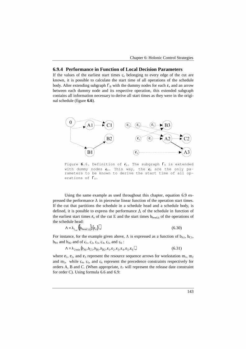
Chapter 6: Holonic Control Strategies
143
6.9.4 Performance in Function of Local Decision ParametersIf the values of the earliest start times ee belonging to every edge of the cut areknown, it is possible to calculate the start time of all operations of the schedulebody. After extending subgraph ΓB with the dummy nodes for each ee and an arrowbetween each dummy node and its respective operation, this extended subgraphcontains all information necessary to derive all start times as they were in the origi-nal schedule (figure 6.6).
Figure 6.6. Definition of ee. The subgraph ΓB is extendedwith dummy nodes ee. This way, the ee are the only pa-rameters to be known to derive the start time of all op-erations of ΓB.
Using the same example as used throughout this chapter, equation 6.9 ex-pressed the performance L in piecewise linear function of the operation start times.If the cut that partitions the schedule in a schedule head and a schedule body, isdefined, it is possible to express the performance L of the schedule in function ofthe earliest start times ee of the cut E and the start times bhead,ij of the operations ofthe schedule head:
{ }{ }( )eijheadt bcut
ελ=Λ ,, , (6.30)
For instance, for the example given above, L is expressed as a function of bA1, bC1,bB1 and bB2 and of e1, e2, e3, e4, e5, and e6 :
( )6543212111min2 ,,,,,,,,, εεεεεελ=Λ BBCA bbbb , (6.31)
where e1, e2, and e3 represent the resource sequence arrows for workstation m1, m2
and m3, while e4, e5, and e6 represent the precedence constraints respectively fororders A, B and C. (When appropriate, e7 will represent the release date constraintfor order C). Using formula 6.6 and 6.9:
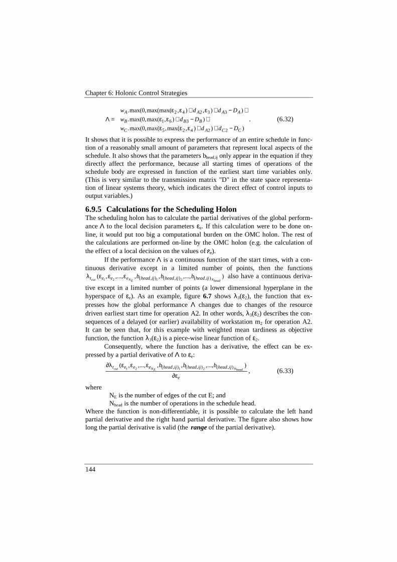
Chapter 6: Holonic Control Strategies
144
))),max(,max(,0max(.
)),max(,0max(.
)),),max(max(,0max(.
22425
361
33242
CCAC
BBB
AAAA
Dddw
Ddw
Dddw
−++εεε+−+εε
+−+ε+εε=Λ . (6.32)
It shows that it is possible to express the performance of an entire schedule in func-tion of a reasonably small amount of parameters that represent local aspects of theschedule. It also shows that the parameters bhead,ij only appear in the equation if theydirectly affect the performance, because all starting times of operations of theschedule body are expressed in function of the earliest start time variables only.(This is very similar to the transmission matrix "D" in the state space representa-tion of linear systems theory, which indicates the direct effect of control inputs tooutput variables.)
6.9.5 Calculations for the Scheduling HolonThe scheduling holon has to calculate the partial derivatives of the global perform-ance Λ to the local decision parameters εe. If this calculation were to be done on-line, it would put too big a computational burden on the OMC holon. The rest ofthe calculations are performed on-line by the OMC holon (e.g. the calculation ofthe effect of a local decision on the values of ee).
If the performance Λ is a continuous function of the start times, with a con-tinuous derivative except in a limited number of points, then the functions
),...,,,,...,,( ),(),(),( 2121 headNENcut ijheadijheadijheadeeet bbbεεελ also have a continuous deriva-
tive except in a limited number of points (a lower dimensional hyperplane in thehyperspace of εe). As an example, figure 6.7 shows λ3(ε2), the function that ex-presses how the global performance Λ changes due to changes of the resourcedriven earliest start time for operation A2. In other words, λ3(ε2) describes the con-sequences of a delayed (or earlier) availability of workstation m2 for operation A2.It can be seen that, for this example with weighted mean tardiness as objectivefunction, the function λ3(ε2) is a piece-wise linear function of ε2.
Consequently, where the function has a derivative, the effect can be ex-pressed by a partial derivative of Λ to εe:
e
ijheadijheadijheadeeetheadNENcut
bbb
∂ε
εεε∂λ ),...,,,,...,,( ),(),(),( 2121 , (6.33)
whereNE is the number of edges of the cut E; andNhead is the number of operations in the schedule head.
Where the function is non-differentiable, it is possible to calculate the left handpartial derivative and the right hand partial derivative. The figure also shows howlong the partial derivative is valid (the range of the partial derivative).

Chapter 6: Holonic Control Strategies
145
Figure 6.7. The function l3(e2) expresses how the globalperformance L changes due to changes of the resourcedriven earliest start time e2 for operation A2. In otherwords, l3(e2) describes the consequences of a delayed (orearlier) availability of workstation m2 for operationA2.
The scheduling holon calculates off-line the partial derivative of the globalperformance measure to the earliest start time defined by each arrow in the sched-ule graph. After the schedule has been generated, it calculates the function λt-cut foreach tcut(i,j) corresponding with the scheduled start time of an operation (i,j). Foreach edge e of the cut E, the value of (6.33) is calculated. Along with the schedulein Gantt chart format, the graph representation and the values of the partial deriva-tives (6.33) are sent to the OMC holon (cf. place p3 in the Petri net of figure 5.1).
There are several alternative algorithms to calculate these partial deriva-tives. The easiest one to understand is based on simulation. For every edge in thegraph, a simulation shows the effect on the global performance. For this trivial al-
gorithm, the calculation time stays well below )( 3operNO , where Noper is the total
number of operations in the schedule.A second algorithm resembles CPM, an algorithm to calculate the critical
path in project scheduling. Starting with the operations scheduled latest in time andcalculating backwards along the schedule graph, the constraints contributing to (alimit on) the performance are identified and marked with their contribution. Fortardiness optimisation, this marking refers to the contribution to the tardiness for
each order. This algorithm has a calculation time well below )( 2operNO .
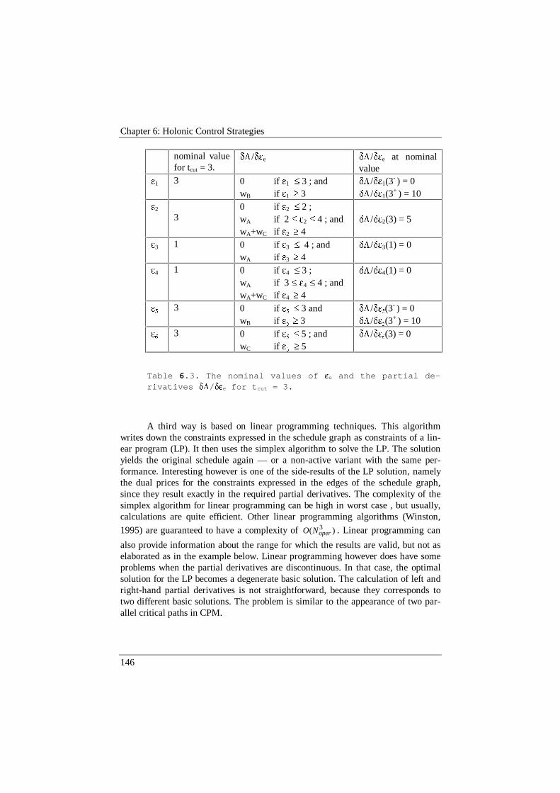
Chapter 6: Holonic Control Strategies
146
nominal valuefor tcut = 3.
dL/dee dL/dee at nominalvalue
e1 3 0 if e1 � 3 ; andwB if e1 � 3
dL/de1(3- ) = 0
dL/de1(3+ ) = 10
e2
30 if e2 � 2 ;wA if 2 � e2 � 4 ; andwA+wC if e2 � 4
dL/de2(3) = 5
e3 1 0 if e3 � 4 ; andwA if e3 � 4
dL/de3(1) = 0
e4 1 0 if e4 � 3 ;wA if 3 � e4 � 4 ; andwA+wC if e4 � 4
dL/de4(1) = 0
e5 3 0 if e5 � 3 andwB if e5 � 3
dL/de5(3- ) = 0
dL/de5(3+ ) = 10
e6 3 0 if e6 � 5 ; andwC if e6 � 5
dL/de6(3) = 0
Table 6.3. The nominal values of ee and the partial de-rivatives dL/dee for tcut = 3.
A third way is based on linear programming techniques. This algorithmwrites down the constraints expressed in the schedule graph as constraints of a lin-ear program (LP). It then uses the simplex algorithm to solve the LP. The solutionyields the original schedule again — or a non-active variant with the same per-formance. Interesting however is one of the side-results of the LP solution, namelythe dual prices for the constraints expressed in the edges of the schedule graph,since they result exactly in the required partial derivatives. The complexity of thesimplex algorithm for linear programming can be high in worst case , but usually,calculations are quite efficient. Other linear programming algorithms (Winston,
1995) are guaranteed to have a complexity of )( 3operNO . Linear programming can
also provide information about the range for which the results are valid, but not aselaborated as in the example below. Linear programming however does have someproblems when the partial derivatives are discontinuous. In that case, the optimalsolution for the LP becomes a degenerate basic solution. The calculation of left andright-hand partial derivatives is not straightforward, because they corresponds totwo different basic solutions. The problem is similar to the appearance of two par-allel critical paths in CPM.
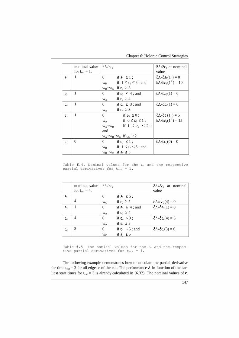
Chapter 6: Holonic Control Strategies
147
nominal valuefor tcut = 1.
dL/dee dL/dee at nominalvalue
e1 1 0 if e1 � 1 ;wB if 1 � e1 � 3 ; andwB+wC if e1 � 3
dL/de1(1- ) = 0
dL/de1(1+ ) = 10
e3 1 0 if e3 � 4 ; andwA if e3 � 4
dL/de3(1) = 0
e4 1 0 if e4 � 3 ; andwA if e4 � 3
dL/de4(1) = 0
e5 1 0 if e5 � 0 ;wA if 0 � e5 � 1 ;wA+wB if 1 � e5 � 2 ;andwA+wB+wC if e5 � 2
dL/de5(1- ) = 5
dL/de5(1+ ) = 15
e7 0 0 if e7 � 1 ;wB if 1 � e7 � 3 ; andwB+wC if e7 � 3
dL/de7(0) = 0
Table 6.4. Nominal values for the ee and the respectivepartial derivatives for tcut = 1.
nominal valuefor tcut = 4.
dL/dee dL/dee at nominalvalue
e2
40 if e2 � 5 ;wC if e2 � 5 dL/de2(4) = 0
e3 1 0 if e3 � 4 ; andwA if e3 � 4
dL/de3(1) = 0
e4 4 0 if e4 � 3 ;wA if e4 � 3
dL/de4(4) = 5
e6 3 0 if e6 � 5 ; andwC if e6 � 5
dL/de6(3) = 0
Table 6.5. The nominal values for the ee and the respec-tive partial derivatives for tcut = 4.
The following example demonstrates how to calculate the partial derivativefor time tcut = 3 for all edges e of the cut. The performance L in function of the ear-liest start times for tcut = 3 is already calculated in (6.32). The nominal values of ee
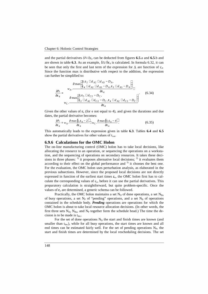
Chapter 6: Holonic Control Strategies
148
and the partial derivatives dL/dee can be deducted from figures 6.5.a and 6.5.b andare shown in table 6.3. As an example, dL/de4 is calculated. In formula 6.32, it canbe seen that only the first and last term of the expression for L are function of e4.Since the function max is distributive with respect to the addition, the expressioncan further be simplified to:
4
224222
25
4
33324
322
4
,
,,0max
.
,
,,0max
.
∂ε
−++ε−++ε
−+ε∂
+∂ε
−+ε−++ε
−++ε∂
=∂ε
Λ∂
CCACCA
CC
C
AAAAA
AAA
A
DddDdd
Dd
w
DdDdd
Ddd
w. (6.34)
Given the other values of ee (for e not equal to 4), and given the durations and duedates, the partial derivative becomes:
( ) ( )4
4
4
4
4
4,0max.
2,1max.
∂ε−ε∂+
∂ε−ε∂=
∂εΛ∂
CA ww . (6.35)
This automatically leads to the expression given in table 6.3. Tables 6.4 and 6.5show the partial derivatives for other values of tcut.
6.9.6 Calculations for the OMC HolonThe on-line manufacturing control (OMC) holon has to take local decisions, likeallocating the resource to an operation, or sequencing the operations on a worksta-tion, and the sequencing of operations on secondary resources. It takes these deci-sions in three phases: 1) it proposes alternative local decisions; 2) it evaluates themaccording to their effect on the global performance and 3) it chooses the best one.For the evaluation, the OMC holon uses perturbation analysis, as elaborated in theprevious subsections. However, since the proposed local decisions are not directlyexpressed in function of the earliest start times ee, the OMC holon first has to cal-culate the corresponding values of ee, before it can use the partial derivatives. Thispreparatory calculation is straightforward, but quite problem-specific. Once thevalues of ee are determined, a generic schema can be followed.
Practically, the OMC holon maintains a set ND of done operations, a set NBu
of busy operations, a set NP of “pending” operations, and a set NB of operationscontained in the schedule body. Pending operations are operations for which theOMC holon is about to take local resource allocation decisions. (In other words, thefirst three sets ND, NBu, and NP together form the schedule head.) The time the de-cision is to be made is tdec.
For the set of done operations ND the start and finish times are known (andsmaller than tdec), while for all busy operations, the start times are known and allend times can be estimated fairly well. For the set of pending operations NP, thestart and finish times are determined by the local rescheduling decisions. The set
Chapter 6: Holonic Control Strategies
149
NP itself is constructed by taking the next few operations of the schedule, until agiven time tcut.
Usually, as a rule of thumb, the set NP contains the first two or three opera-tions in the near future on each workstation. Because the set NP of pending opera-tions is quite small, and often only limited or no interdependencies exist betweenpending operations on different workstations, there are only a small number of re-scheduling strategies (cf. infra). For the operations of the schedule body, the OMCholon presumes that the existing schedule is followed. To take the decision, theOMC holon calculates the effect of each alternative decision on the values ee of thecut at time tcut, such that it can also estimate the effect on L (linear estimation). Thestrategy with the lowest cost increase is selected as the rescheduling decision. Theadvantage of this approach is that the OMC holon can take all its decisions veryfast.
The problem-specific nature of OMC requires the use of examples to furtherexplain how the algorithm works. The next subsection shows these examples todemonstrate autonomous schedule execution.
6.9.7 ExamplesThis subsection presents five examples of different control scenarios to further de-scribe ASE using PA. The cases examined in this subsection are:• An operation is delayed.• An operation finishes earlier.• A machine breaks down.• An operation is delayed and the next operation on that workstation can be exe-
cuted on another workstation• An operation cannot be executed due to a machine failure, but an operation of
another type can still be executed on the same machine.
An operation is delayed.Consider the same problem, defined in figure 6.1, as used throughout this chapter.Suppose operation A1 is delayed with half a time unit and could only be finished attime 1.5 (see figure 6.8). Thus, at time tdec=1.5, the OMC holon has to make thefollowing resource allocation decisions.
Possible alternative decisions are indicated by the constraints affected by thedelay of operation A1: to account for the modified capacity and precedence con-straints, rescheduling workstation m1 and order A is considered. To limit the num-ber of alternatives, only the first operations of workstation m1 (C1 and B3) and thenext operation of order A (A2) are considered. Thus, the alternative decisions are:1) keep the schedule, 2) swap C1 and B3, and 3) swap A2 and C2. (Observe that alsoworkstation m2 is rescheduled in order to reschedule operation A2.) Even if therewould still be operations left on workstation m1 after operation B3, it would not bereally necessary to investigate other sequences. The reason is that the swap B3-C1offers for the moment enough flexibility to move non-urgent operations like C1backwards, while the urgent operations (like B3) can still remain at their scheduled
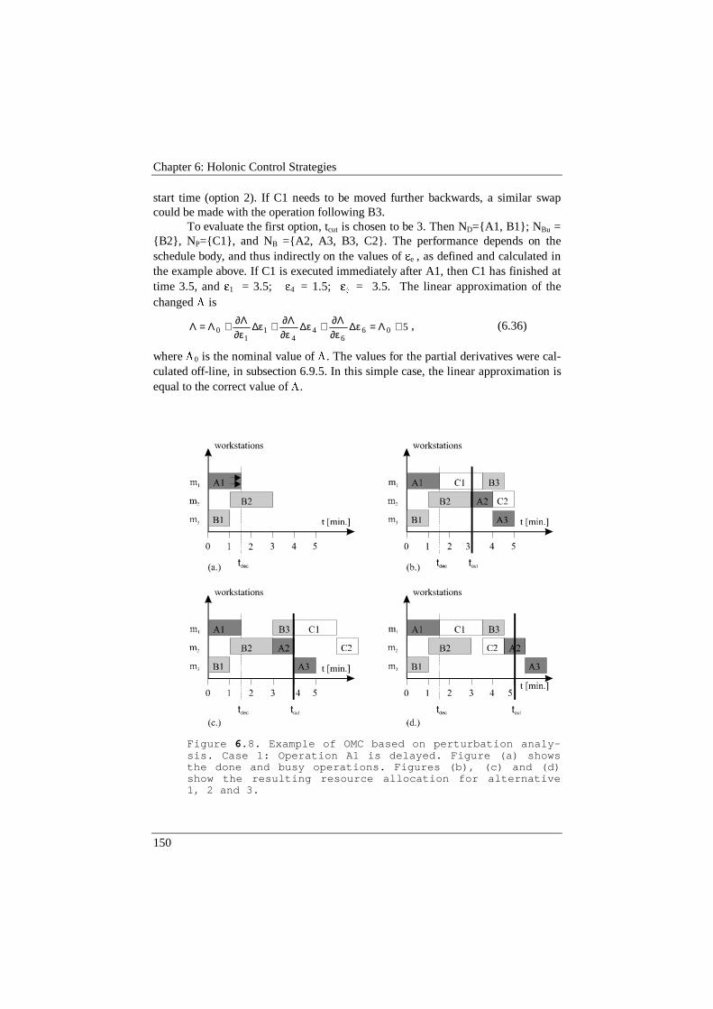
Chapter 6: Holonic Control Strategies
150
start time (option 2). If C1 needs to be moved further backwards, a similar swapcould be made with the operation following B3.
To evaluate the first option, tcut is chosen to be 3. Then ND={A1, B1}; NBu ={B2}, NP={C1}, and NB ={A2, A3, B3, C2}. The performance depends on theschedule body, and thus indirectly on the values of ee , as defined and calculated inthe example above. If C1 is executed immediately after A1, then C1 has finished attime 3.5, and e1 = 3.5; e4 = 1.5; e6 = 3.5. The linear approximation of thechanged L is
5066
44
11
0 +Λ=ε∆∂ε
Λ∂+ε∆∂ε
Λ∂+ε∆∂ε
Λ∂+Λ=Λ , (6.36)
where L0 is the nominal value of L. The values for the partial derivatives were cal-culated off-line, in subsection 6.9.5. In this simple case, the linear approximation isequal to the correct value of L.
Figure 6.8. Example of OMC based on perturbation analy-sis. Case 1: Operation A1 is delayed. Figure (a) showsthe done and busy operations. Figures (b), (c) and (d)show the resulting resource allocation for alternative1, 2 and 3.
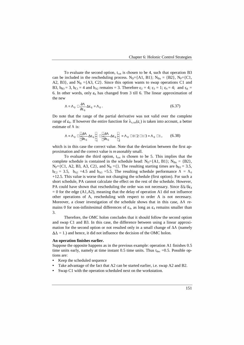
Chapter 6: Holonic Control Strategies
151
To evaluate the second option, tcut is chosen to be 4, such that operation B3can be included in the rescheduling process. ND={A1, B1}; NBu = {B2}, NP={C1,A2, B3}, and NB ={A3, C2}. Since this option wants to swap operations C1 andB3, bB3 = 3, bC1 = 4 and bA2 remains = 3. Therefore e2 = 4; e3 = 1; e4 = 4; and e6 =6. In other words, only e6 has changed from 3 till 6. The linear approximation ofthe new
066
0 Λ=ε∆∂ε
Λ∂+Λ=Λ . (6.37)
Do note that the range of the partial derivative was not valid over the completerange of e6. If however the entire function for lt,cut(e6) is taken into account, a betterestimate of L is:
11120 002
661
66
0 +Λ=⋅+⋅+Λ=
ε∆
∂εΛ∂+
ε∆
∂εΛ∂+Λ=Λ , (6.38)
which is in this case the correct value. Note that the deviation between the first ap-proximation and the correct value is re asonably small.
To evaluate the third option, tcut is chosen to be 5. This implies that thecomplete schedule is contained in the schedule head: ND={A1, B1}; NBu = {B2},NP={C1, A2, B3, A3, C2}, and NB ={}. The resulting starting times are bB3 = 3.5,bC2 = 3.5, bA2 =4.5 and bA3 =5.5. The resulting schedule performance L = L0
+12.5. This value is worse than not changing the schedule (first option). For such ashort schedule, PA cannot calculate the effect on the rest of the schedule. However,PA could have shown that rescheduling the order was not necessary. Since dL/de4
= 0 for the edge (A1,A2), meaning that the delay of operation A1 did not influenceother operations of A, rescheduling with respect to order A is not necessary.Moreover, a closer investigation of the schedule shows that in this case, DL re-mains 0 for non-infinitesimal differences of e4, as long as e4 remains smaller than3.
Therefore, the OMC holon concludes that it should follow the second optionand swap C1 and B3. In this case, the difference between using a linear approxi-mation for the second option or not resulted only in a small change of DL (namelyDL = 1.) and hence, it did not influence the decision of the OMC holon.
An operation finishes earlier.Suppose the opposite happens as in the previous example: operation A1 finishes 0.5time units early, namely at time instant 0.5 time units. Thus tdec =0.5. Possible op-tions are:• Keep the scheduled sequence• Take advantage of the fact that A2 can be started earlier, i.e. swap A2 and B2.• Swap C1 with the operation scheduled next on the workstation.
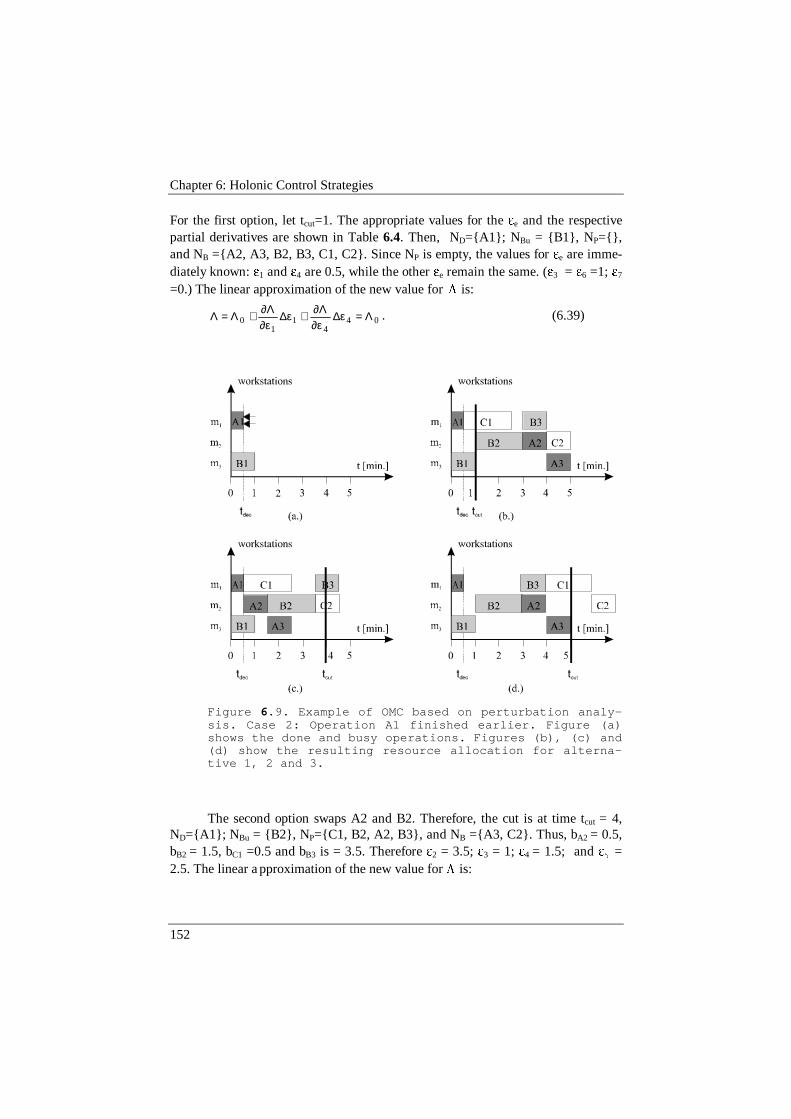
Chapter 6: Holonic Control Strategies
152
For the first option, let tcut=1. The appropriate values for the ee and the respectivepartial derivatives are shown in Table 6.4. Then, ND={A1}; NBu = {B1}, NP={},and NB ={A2, A3, B2, B3, C1, C2}. Since NP is empty, the values for ee are imme-diately known: e1 and e4 are 0.5, while the other ee remain the same. (e3 = e6 =1; e7
=0.) The linear approximation of the new value for L is:
044
11
0 Λ=ε∆∂ε
Λ∂+ε∆∂ε
Λ∂+Λ=Λ . (6.39)
Figure 6.9. Example of OMC based on perturbation analy-sis. Case 2: Operation A1 finished earlier. Figure (a)shows the done and busy operations. Figures (b), (c) and(d) show the resulting resource allocation for alterna-tive 1, 2 and 3.
The second option swaps A2 and B2. Therefore, the cut is at time tcut = 4,ND={A1}; NBu = {B2}, NP={C1, B2, A2, B3}, and NB ={A3, C2}. Thus, bA2 = 0.5,bB2 = 1.5, bC1 =0.5 and bB3 is = 3.5. Therefore e2 = 3.5; e3 = 1; e4 = 1.5; and e6 =2.5. The linear a pproximation of the new value for L is:
Chapter 6: Holonic Control Strategies
153
5.7066
44
22
30 −Λ=ε∆∂ε
Λ∂+ε∆∂ε
Λ∂+ε∆∂ε
Λ∂+∆⋅+Λ=Λ BB tw . (6.40)
If however the entire function for lt,cut (e4) is taken into account, L = L0. In thiscase, if the OMC holon uses the simplest algorithm, it would have favoured theswap. With the more correct expression, the correct value would have made clear tothe OMC holon that both options up to now are equal.
For the third option, the cut remains the same. All starting times remain thesame with respect to the nominal schedule, except for operation C1. C1 only startsat time t=4, and thus gets a cost increase of 0 or 1, depending on whether the sim-ple or elaborated expression for L is chosen.
Therefore, option number two is chosen (swapping A2 and B2). If the effectof Dee is completely taken into account, as in the second part of some examples,then again the completely correct decision is taken. In this case, also when simpli-fying the problem, one of the optimal solutions would have come out. However, ifthe calculation of DL is simplified, and the data were slightly different, the OMCholon would have chosen a non-optimal solution. But even then, small changes inee change the performance only slightly. The solution found would still be near-optimal.
A machine breaks down.Suppose that workstation m1 breaks down after operation A1 for half a time unit.(The repair time for the station is known in advance.) This is very similar to thefirst scenario, except that operation A2 can be started earlier. Possible options are:• Keep the scheduled sequence• Swap C1 and B3.• Swap A2 and B2.
Following a similar approach as above, the resulting increase in tardinessfor the three options is 5, 1, and 5 respectively. The second option is thus selected ,swapping the operations C1 and B3. Again, the correct decision is taken.
An operation is delayed and the next operation on that workstation can be exe-cuted on another workstationLet’s resume the first example, where operation A1 is delayed for half a time unit,and could be finished at time 1,5. However, in this case, there is an additional pos-sibility to reschedule: operation C1 can also be executed on workstation m3, butthen it takes 3.1 time units to complete. This is a non-trivial example, because theallocation of operation C1 to workstation m3 induces a delay on order A. Therefore,a compromise needs to be made between a delay on order C and one on order A.The first part of this example assumes that the decision that reacts to the distur-bance, is taken after operation A1 is finished. Thereafter, some variations are sug-gested.
To evaluate the additional option (moving operation C1 to workstation m3.),consider that the decision is taken at time t=1,5. Therefore, tcut is chosen to be 3.
Chapter 6: Holonic Control Strategies
154
Then ND={A1, B1}; NBu = {B2}, NP={C1}, and NB ={A2, A3, B3, C2}. Sinceworkstation m3 is free at time t = 1,5 , bC1 = 1,5. Then, e1 = 1.5; e3 = 4.6; e4 =1.5; e6 = 4.6. (The other ee values did not change.) The linear approximation of Lbecomes:
( ) 3)6.1(0)5.0(0)6.0(5)3(0)5.1(0 00
66
44
22
23
313
31
10
+Λ=⋅+⋅+⋅+⋅+−⋅+Λ=
ε∆∂ε
Λ∂+ε∆∂ε
Λ∂+ε∆∂ε
Λ∂
+
ε∆
∂εΛ∂+
ε∆
∂εΛ∂+ε∆
∂εΛ∂+Λ=Λ
. (6.41)
Compared to the two previously evaluated options, this one is worse than swappingoperations C1 and B3. However, if C1 would not take that much time on worksta-tion m3, it would have been a better solution.
Moreover, a closer look at this problem shows that another option couldhave been examined. If the decision to reschedule C1 would have been made ear-lier, namely immediately after operation B1 had finished, the cost of allocating C1to workstation m3 would have been cheaper (L0 + 0,5). A small practical problem isthe fact that the initiative to reschedule should then be triggered by the order in-stead of the workstation. A bigger problem is the fact that the decision to reallocateC1 to workstation m3 may depend on information that is not available yet: the firstoption (keeping the schedule as it is) cannot be evaluated as long as the finish timeof operation A1 is not known. If a fair estimate can be given (e.g. if the cause of thedelay is well known), there is no problem. If, however, the only information avail-able is the fact that the operation should actually already have finished, it would bebetter to explicitly consider schedule execution methods that take into account sto-chastic information. The approach presented in this chapter does not explicitly ac-count for stochastic information. At most an estimated average delay time would beintroduced (maybe even equal to zero).
An operation cannot be executed due to a machine failure, but an operation ofanother type can still be executed.At time t = 0, workstation m1 cannot perform operation A1 because of a machinefailure. It would take half a time unit to repair this resource. However, while theresource is being repaired, it is possible to perform other operations on workstationm1, that do not need this resource. For instance, C1 can immediately be executed onm1. One could even specify that an additional set-up time of 0,1 time unit is neededdue to the sudden change.
Possible options to handle this disturbance are the following.• The schedule remains unchanged.• The operations A1 and C1 are swapped.• The operations C1 and B3 are to be swapped after operation A1 has been fin-
ished. This possibility does not really have to be evaluated, because this choicecan still be made after operation A1 has been finished. It may however be inter-
Chapter 6: Holonic Control Strategies
155
esting to evaluate this option already at this decision point, because it wouldnever be evaluated anymore if option 2 is selected over option 1.
Using similar calculations as above, the resulting increase in tardiness is 5,1.5 and 1 for the respective options (including the set-up time as mentioned). Thus,the third option is chosen.
Note however that this third option had to look into the future. The questionremains how far in the future should be looked for valid alternatives. It is a com-promise between the number of options that would have to be evaluated and theperformance that can be reached. The further the OMC holon looks into the future,the larger NP (set of operations that are to be rescheduled) becomes, such that therescheduling task gets more and more complex. If NP contains all operations of theschedule and NB is empty, then the OMC holon has to perform a complete resched-uling. (The co-operation then is reduced to almost nothing: the scheduler just deliv-ers an initial schedule that the OMC holon could optimise). The main issue is thata fundamental compromise has to be made between autonomy and co-operation ofthe OMC holon and the reactive scheduler, and that this compromise depends onthe situation on the shop floor. For instance, if the third option would not have beenselected for evaluation, the second option would have been chosen, evaluation couldhave been faster, while the solution would be only slightly worse (DL of 1,5 insteadof 1).
6.9.8 Concluding RemarksSummarising, this section presents an algorithm for executing a schedule, based ona graph representation of a schedule and the use of partial derivatives for estimat-ing the effect of local decisions to the global goal (perturbation analysis). Exampleshave shown that the use of partial derivatives is feasible for that purpose. The pre-sented solution is a generic concept that combines fast reaction to disturbances withoptimisation. Compared to other approaches to the resource allocation problem, anyscheduling technique can be used, also off-line schedulers. Reaction to disturbancesnot only is quick, it also explicitly considers the optimisation of the global goal,using the existing schedule as advice. Therefore, this is a holonic algorithm formanufacturing control.
The examples have also shown that this algorithm yields a good overall be-haviour for the ASE problem. Using a standard approach, with a simplelinearisation mechanism, the algorithm usually picks the best rescheduling option,and almost always a good one. Even better results can be obtained when the algo-rithm considers finite differences for the PA. This extension improves the perform-ance to near-optimal levels, but also increases the computational load. (Other pos-sible improvements are considering more operations in the set NP and triggeringadditional events.) Realistic test results are to complement the examples presentedabove (see chapter 8). Of course, the decisions taken by the OMC holon are not al-ways optimal (this would imply an entire rescheduling run, which is an NP-hardproblem), but at least they address the schedule execution problem like an intelli-gent foreman would.
Chapter 6: Holonic Control Strategies
156
This approach controls nervousness to stay below reasonable bounds. Itkeeps a good homeostasis of the schedule when few disturbances occur. Normally,the local decisions of the OMC holon would not increase the schedule performanceif the situation would not have changed. (If the schedule would not at least be a lo-cal optimum, the scheduler would not have done its optimisation job properly).
This algorithm also computationally performs well. Because the partial de-rivatives are calculated off-line, the approach is suited for on-line control. It out-performs a similar approach based on simulations for each alternative instead ofusing partial derivatives, by an order of magnitude O(Noper), where Noper is the totalnumber of operations.
However, there still is need for further research. The link with linear pro-gramming techniques is interesting for further investigations, because it provides apowerful mathematical framework for the use of perturbation analysis in scheduleexecution. For instance, while in the current approach, the local-search process ofthe OMC holon is quite ad-hoc, an LP-based approach may be more structured.Also, with sensitivity analysis, it may be possible to consider the effects of a swapof two operations more efficiently (by removing one constraint and adding anotherone).
It was noticed that the use of perturbation analysis on the schedule graphleads to a CPM-like analysis, with several critical paths. Instead of using the re-sulting partial derivatives for on-line control, it could also be possible to interpretthe meaning of these critical paths and base the decision logic on these interpreta-tions. For instance, it could be a fixed rule that OMC shall not idle machines thatare on a critical path. Note that the propagation of tardiness through the schedulegraph is similar to way flows move through a network, such that efficient LP solu-tion procedures for minimum-cost network flow problems (Winston, 1995) may besuccessfully applied to the OMC problem.
Note also that the local search process within the OMC holon is similar tothe reactive scheduling process, albeit for a limited local search under real-timeconstraints. Undoubtedly, it is possible to find more efficient local search tech-niques than the local enumeration technique applied today.
Also the stochastic aspects deserve more attention. Ho (1988) and Cassan-dras (1993) have further developed perturbation analysis to calculate partial de-rivatives when the model becomes stochastic. Such an extension would result in aproactive behaviour, but it was not further investigated in this thesis. An early ap-proach (and a very simple one) to address the stochastic nature of (project) sched-uling is PERT (Wiest, 1977).
6.10 ConclusionThis chapter has presented several control strategies for holonic manufacturingcontrol. Some are based on the distribution of decision power, using fixed rules andallowing flexible strategies for the schedule execution holons. One algorithm to fill
156 bis
out the autonomous decision power in a holonic way is based on perturbationanalysis.
It is important that a holonic control architecture supports multiple controlstrategies. There is a large set of possible holonic control algorithms, and thischapter did not attempt to present the best ones for all situations. The heuristiccontrol strategies presented are examples, sketching the main idea. Also the algo-rithm using perturbation analysis may still be improved (as discussed in subsection6.9.8).
The performance of the presented algorithms will be firmly demonstratedwith experimental results, as shown in chapter 8. Note however that performance inse is not the only criterion to compare algorithms. Some strategies are to performbetter over a wider range of applications. For such algorithms, it is appropriate togive more autonomy to the OMC holon. Therefore, if the ASE algorithm is moreintelligent, the fixed rules may become less important. Also, ASE algorithms thatare easier to implement may be preferred over marginally better ones with a highimplementation cost.
157
Chapter 7
Design and Implementation
This thesis focused its developments in the first place at the PMA/K.U.Leuvenflexible assembly system testbed. For the manufacturing control of that testbed, areactive scheduling holon PaRSiFAL and an OMC holon PHOCS were developedas the main elements of the test set-up. PaRSiFAL is equiped with a first descentschedule optimisation algorithm. Next to that, simple versions of workstationholons, the transport system holon and order holons were implemented.
7.1 IntroductionThe concepts, control architecture and algorithms designed for this thesis are ap-plied to the PMA/K.U.Leuven flexible assembly system (the "PMA FAS"). Thiscomprises the development of the manufacturing control software, including a re-active scheduler PaRSiFAL, an OMC holon PHOCS and a set of resource and orderholons. The software was mainly tested on the PMA FAS, but the developed soft-ware is applicable to a large range of automated job-shop type manufacturing sys-tems.
This chapter explains the practical test set-ups used for this thesis and de-scribes the software design and implementation. It also describes the schedulingalgorithms used. It is appropriate to include the scheduling algorithms in thischapter on implementations, since this thesis did not aim at the development of newscheduling algorithms. It rather used existing algorithms, to be found in literaturein abundance.
7.2 The Software Design ProcessThe last twenty years, the software design process has significantly im-
proved. Starting from a functional approach, with stepwise refinement and func-tional decomposition, an evolution was seen towards object-oriented design. Re-cently, a tendency has come towards active objects, or “agents”, which exchangeinformation over the Internet or intranet.
Along with this evolution, modelling languages and CASE tools were pro-posed to support the design and implementation process. For a functional approachto software engineering, IDEF was one of the better known modelling languages,especially IDEF-0 for the functional description and IDEF-1 for a relational data

Chapter 7: Design and Implementation
158
model. For object-oriented techniques, several modelling languages existed, com-peting with one another (Booch, 1991, Rumbaugh, 1991, Jacobson, 1992). Most ofthese modelling languages were supported with CASE tools. In practice, however,the use of these CASE tools was quite tedious for non-professional programmersand not very widespread.
The real breakthrough only came recently, with the definition of UML (theUnified Modelling Language — Rumbaugh, 1997). It originated from the unifica-tion of the three major modelling languages for object-oriented design, existing atthat time, and is now an widely accepted de-facto standard for the software docu-mentation. Important is also that UML is supported by several CASE tools. Thebest known example is Rational Rose ® (Fowler, 1997), a mature and practicalCASE tool that supports the complete development process from requirementsanalysis to design and implementation (Corgnati, 1998).
For this thesis, the chosen development methodology is object-based design.Object-based design, to be differentiated from object-oriented design, aims at thedevelopment of a powerful data model, describing the problem and the structure ofthe solution, forming the backbone of the software. Further developments are thenbuilt, in different modules, on top of this data structure. As long as the underlyingdata model remains valid, the further developments, modifications and mainte-nance of the software is relatively easy. Compared to object-oriented design, it doesnot require the extensive use of inheritance and polymorphism, nor does it requirethe programmer to shift away from the traditional stepwise refinement approach.Therefore, object-based design is substantially easier than a good object-orienteddesign.
The development process for the holons developed for this thesis is split upin the following phases:• Firstly, the data model for the holon is designed, such that the problem input
data, the solution, and the state of the system and the software are completelymodelled. This model can be designed, implemented and tested before the restof the software is developed. In practice, the resulting data structure could bereused to a large extent over the different holons.
• Secondly, the individual functions for all holons are defined. These functionsare grouped in different modules, accessible via a menu program. Basic func-tions are always the functions to view and alter the data model. Other functionsare derived from the interaction mechanism as described in chapter 5. Thesemodels also define the communication protocol between holons.
• The design and implementation of the individual modules is the third phase.Each module can be implemented and tested separately, easing the developmentand debugging process. An additional advantage is that functionality is gradu-ally added to the program.
• Finally, a module is added to sequence and combine the right functions at theright time automatically. This module converts the interactive, menu-driven
Chapter 7: Design and Implementation
159
program in an autonomous holon, with its own initiative and controlling its ownbehaviour.
The software developed in this thesis is documented in a pragmatic way.Originally, the data model is described with simple IDEF-1 like diagrams, showingthe interactions amongst the objects. These diagrams were re-drawn for this thesisusing UML. The functions are described as a list of modules. The design of the in-dividual modules is then straightforward. The composition of functions into anautonomous holon is documented with Petri nets, as already shown in chapter 5).Similarly, the algorithms used are also explained at other places, mainly in chapter6. In this chapter, only the scheduling algorithms used (which are no original con-tributions of this thesis) are described or a reference to the correct literature isgiven. Where necessary, the co-operation was modelled in more detail with theUML collaboration diagrams.
One could ask why this thesis did not apply fully object-oriented designprinciples and standard modelling languages like UML in its entirety. It is impor-tant to realise that the use of object-oriented design principles is not easy and usu-ally requires a few iterations before reaching the appropriate quality. Object-oriented design therefore only starts to pay off for large software projects were re-use is an important issue. In a university context, where all software is only a re-search prototype, this full-fledged approach was not deemed necessary nor efficient.With respect to UML, the software design and implementation, including thedocumentation, were already finished before the breakthrough of UML. A completepost-facto modelling of the existing design in UML was not considered to yieldsufficient added value to justify the efforts. Only there where deemed useful, UMLwas used as a description tool. After all, the main focus of this thesis was not onsoftware design but on manufacturing control.
7.3 TestbedsThe most important testbed for this thesis is the PMA FAS, developed since 1983.This system serves as an experimental platform for research on programming, con-trol and scheduling of flexible assembly systems. Figure 7.1 shows the layout of thatsystem. It contains a transport system, six workstations and some auxiliary equip-ment.
The transport system enables asynchronous transportation of pallets. Thepallets are pulled by motorised bands (conveyer belts) along segments. The seg-ments have been arranged to form a central loop and six external deviation loops,connected on the ring. Each deviation loop forms a workstation with a FIFO buffer.To control transport, one has to decide whether pallets respectively enter, pass, orleave a station. This layout provides the FAS with flexible routing. The size of thepallets (20 cm x 30 cm) confines the production to products of moderate size. Cur-rently, there are two types of pallets, depending on the type of products to be made:
electric switches and LEGO constructions. The system can assemble the differenttypes of products simultaneously.

Chapter 7: Design and Implementation
160
Figure 7.1. The K.U.Leuven/PMA flexible assembly system,as testbed for research on holonic manufacturing.
The PMA FAS contains four workstations with assembly robots:• One PUMA 500 from Unimation.• Two SCARA robots from IBM.• A Pragma A3000 from DEA.The use of robots gives opportunities for flexibility. Flexibility is limited by theworkspace, the approach direction, the accuracy of the robots and mostly by thenumber of component feeders that can be installed in the workspace of a robot. Inpractice, often not all flexibility is used because of excessive programming efforts toimplement the flexibility. The fifth workstation is used as a manual operator station(amongst others for loading, unloading, repair and inspection). A magazine work-
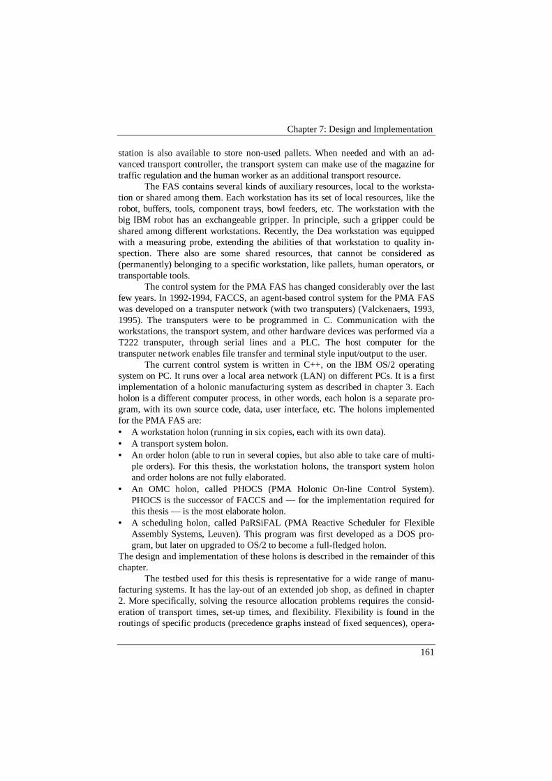
Chapter 7: Design and Implementation
161
station is also available to store non-used pallets. When needed and with an ad-vanced transport controller, the transport system can make use of the magazine fortraffic regulation and the human worker as an additional transport resource.
The FAS contains several kinds of auxiliary resources, local to the worksta-tion or shared among them. Each workstation has its set of local resources, like therobot, buffers, tools, component trays, bowl feeders, etc. The workstation with thebig IBM robot has an exchangeable gripper. In principle, such a gripper could beshared among different workstations. Recently, the Dea workstation was equippedwith a measuring probe, extending the abilities of that workstation to quality in-spection. There also are some shared resources, that cannot be considered as(permanently) belonging to a specific workstation, like pallets, human operators, ortransportable tools.
The control system for the PMA FAS has changed considerably over the lastfew years. In 1992-1994, FACCS, an agent-based control system for the PMA FASwas developed on a transputer network (with two transputers) (Valckenaers, 1993,1995). The transputers were to be programmed in C. Communication with theworkstations, the transport system, and other hardware devices was performed via aT222 transputer, through serial lines and a PLC. The host computer for thetransputer network enables file transfer and terminal style input/output to the user.
The current control system is written in C++, on the IBM OS/2 operatingsystem on PC. It runs over a local area network (LAN) on different PCs. It is a firstimplementation of a holonic manufacturing system as described in chapter 3. Eachholon is a different computer process, in other words, each holon is a separate pro-gram, with its own source code, data, user interface, etc. The holons implementedfor the PMA FAS are:• A workstation holon (running in six copies, each with its own data).• A transport system holon.• An order holon (able to run in several copies, but also able to take care of multi-
ple orders). For this thesis, the workstation holons, the transport system holonand order holons are not fully elaborated.
• An OMC holon, called PHOCS (PMA Holonic On-line Control System).PHOCS is the successor of FACCS and — for the implementation required forthis thesis — is the most elaborate holon.
• A scheduling holon, called PaRSiFAL (PMA Reactive Scheduler for FlexibleAssembly Systems, Leuven). This program was first developed as a DOS pro-gram, but later on upgraded to OS/2 to become a full-fledged holon.
The design and implementation of these holons is described in the remainder of thischapter.
The testbed used for this thesis is representative for a wide range of manu-facturing systems. It has the lay-out of an extended job shop, as defined in chapter2. More specifically, solving the resource allocation problems requires the consid-eration of transport times, set-up times, and flexibility. Flexibility is found in theroutings of specific products (precedence graphs instead of fixed sequences), opera-
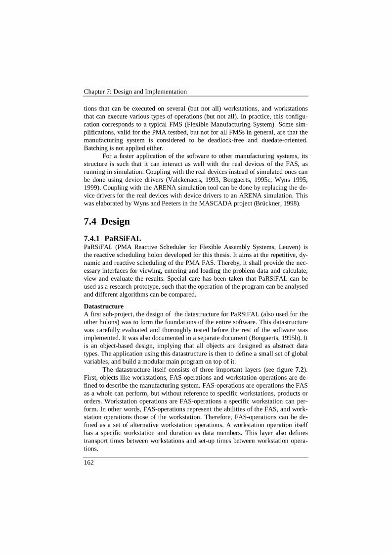
Chapter 7: Design and Implementation
162
tions that can be executed on several (but not all) workstations, and workstationsthat can execute various types of operations (but not all). In practice, this configu-ration corresponds to a typical FMS (Flexible Manufacturing System). Some sim-plifications, valid for the PMA testbed, but not for all FMSs in general, are that themanufacturing system is considered to be deadlock-free and duedate-oriented.Batching is not applied either.
For a faster application of the software to other manufacturing systems, itsstructure is such that it can interact as well with the real devices of the FAS, asrunning in simulation. Coupling with the real devices instead of simulated ones canbe done using device drivers (Valckenaers, 1993, Bongaerts, 1995c, Wyns 1995,1999). Coupling with the ARENA simulation tool can be done by replacing the de-vice drivers for the real devices with device drivers to an ARENA simulation. Thiswas elaborated by Wyns and Peeters in the MASCADA project (Brückner, 1998).
7.4 Design
7.4.1 PaRSiFALPaRSiFAL (PMA Reactive Scheduler for Flexible Assembly Systems, Leuven) isthe reactive scheduling holon developed for this thesis. It aims at the repetitive, dy-namic and reactive scheduling of the PMA FAS. Thereby, it shall provide the nec-essary interfaces for viewing, entering and loading the problem data and calculate,view and evaluate the results. Special care has been taken that PaRSiFAL can beused as a research prototype, such that the operation of the program can be analysedand different algorithms can be compared.
DatastructureA first sub-project, the design of the datastructure for PaRSiFAL (also used for theother holons) was to form the foundations of the entire software. This datastructurewas carefully evaluated and thoroughly tested before the rest of the software wasimplemented. It was also documented in a separate document (Bongaerts, 1995b). Itis an object-based design, implying that all objects are designed as abstract datatypes. The application using this datastructure is then to define a small set of globalvariables, and build a modular main program on top of it.
The datastructure itself consists of three important layers (see figure 7.2).First, objects like workstations, FAS-operations and workstation-operations are de-fined to describe the manufacturing system. FAS-operations are operations the FASas a whole can perform, but without reference to specific workstations, products ororders. Workstation operations are FAS-operations a specific workstation can per-form. In other words, FAS-operations represent the abilities of the FAS, and work-station operations those of the workstation. Therefore, FAS-operations can be de-fined as a set of alternative workstation operations. A workstation operation itselfhas a specific workstation and duration as data members. This layer also definestransport times between workstations and set-up times between workstation opera-tions.
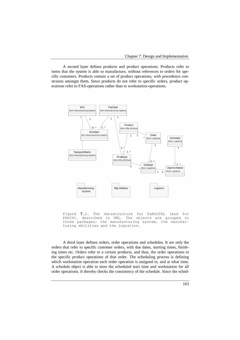
Chapter 7: Design and Implementation
163
A second layer defines products and product operations. Products refer toitems that the system is able to manufacture, without references to orders for spe-cific customers. Products contain a set of product operations, with precedence con-straints amongst them. Since products do not refer to specific orders, product op-erations refer to FAS-operations rather than to workstation-operations.
Schedule(from Logistics)
Manufacturing System
Mfg Abilities Logistics
TransportMatrix(from Manufacturing System)
Wst(from Manufacturing System)
*
WstOper(from Manufacturing System)
0..*
1
FasOper(f ro m M anu factu ri ng System)
1..*
1
Product(from Mfg Abil ities)
Order(from Logistics)*
1
ProdOper(f rom M fg Abiliti es)
1..*
1
1..*
1
1..*
OrdOper(from Logistics)
1..*
1
*1
OperSchedule(from L ogistics)
1..*
1
1..*1
1
1..*1..*
1
1*
1
1..*1
*1
0..* 1..*
11
1..*
*1
Figure 7.2. The datastructure for PaRSiFAL (and forPHOCS), described in UML. The objects are grouped inthree packages: the manufacturing system, the manufac-turing abilities and the logistics.
A third layer defines orders, order operations and schedules. It are only theorders that refer to specific customer orders, with due dates, starting times, finish-ing times etc. Orders refer to a certain products, and thus, the order operations tothe specific product operations of that order. The scheduling process is definingwhich workstation operation each order operation is assigned to, and at what time.A schedule object is able to store the scheduled start time and workstation for allorder operations. It thereby checks the consistency of the schedule. Since the sched-
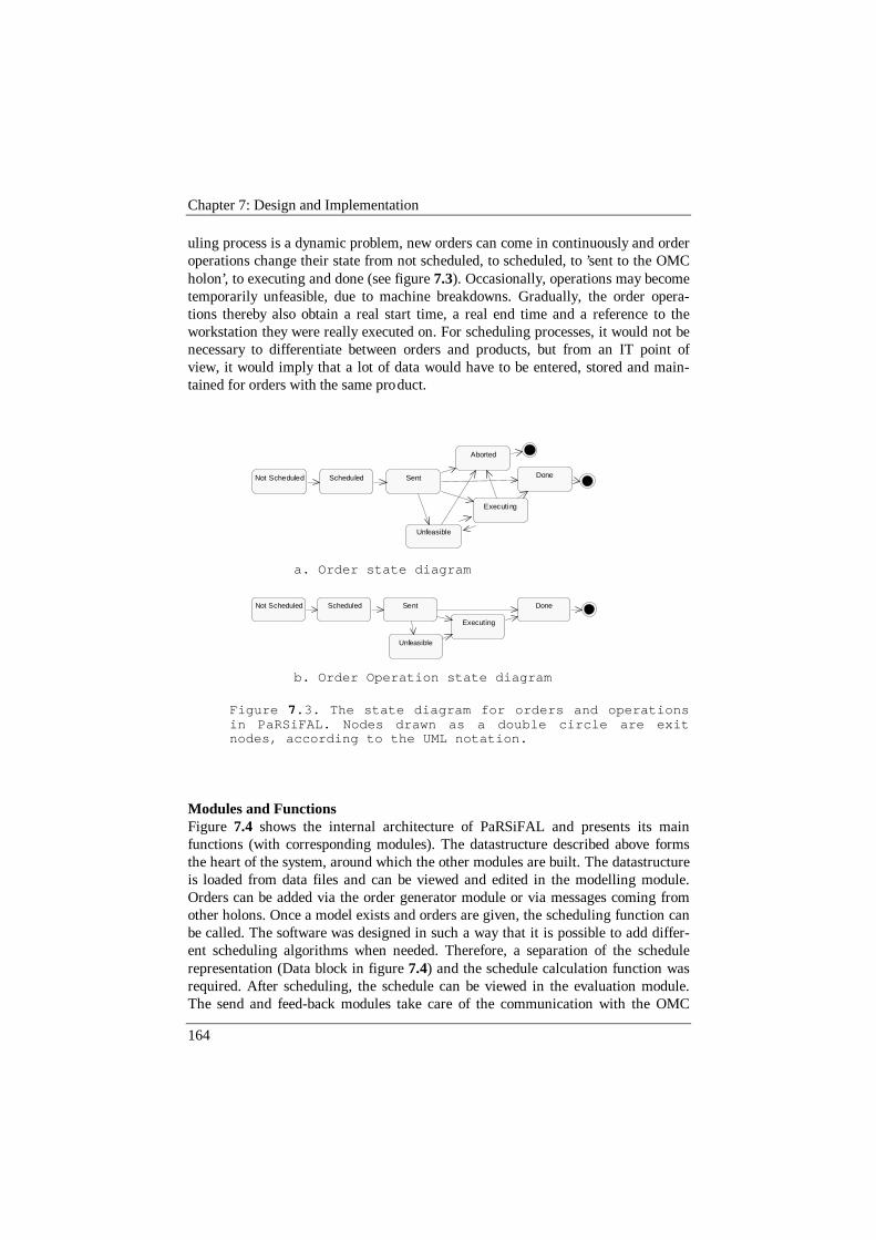
Chapter 7: Design and Implementation
164
uling process is a dynamic problem, new orders can come in continuously and orderoperations change their state from not scheduled, to scheduled, to ’sent to the OMCholon’, to executing and done (see figure 7.3). Occasionally, operations may becometemporarily unfeasible, due to machine breakdowns. Gradually, the order opera-tions thereby also obtain a real start time, a real end time and a reference to theworkstation they were really executed on. For scheduling processes, it would not benecessary to differentiate between orders and products, but from an IT point ofview, it would imply that a lot of data would have to be entered, stored and main-tained for orders with the same product.
Not Scheduled Scheduled Sent
Unfeasible
Executing
Done
Aborted
a. Order state diagram
Not Scheduled Scheduled Sent
Unfeasible
Executing
Done
b. Order Operation state diagram
Figure 7.3. The state diagram for orders and operationsin PaRSiFAL. Nodes drawn as a double circle are exitnodes, according to the UML notation.
Modules and FunctionsFigure 7.4 shows the internal architecture of PaRSiFAL and presents its mainfunctions (with corresponding modules). The datastructure described above formsthe heart of the system, around which the other modules are built. The datastructureis loaded from data files and can be viewed and edited in the modelling module.Orders can be added via the order generator module or via messages coming fromother holons. Once a model exists and orders are given, the scheduling function canbe called. The software was designed in such a way that it is possible to add differ-ent scheduling algorithms when needed. Therefore, a separation of the schedulerepresentation (Data block in figure 7.4) and the schedule calculation function wasrequired. After scheduling, the schedule can be viewed in the evaluation module.The send and feed-back modules take care of the communication with the OMC
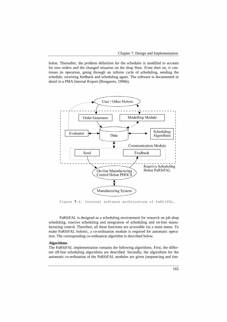
Chapter 7: Design and Implementation
165
holon. Thereafter, the problem definition for the scheduler is modified to accountfor new orders and the changed situation on the shop floor. From then on, it con-tinues its operation, going through an infinite cycle of scheduling, sending theschedule, receiving feedback and scheduling again. The software is documented indetail in a PMA Internal R eport (Bongaerts, 1996b).
Figure 7.4. Internal software architecture of PaRS iFAL.
PaRSiFAL is designed as a scheduling environment for research on job shopscheduling, reactive scheduling and integration of scheduling and on-line manu-facturing control. Therefore, all these functions are accessible via a main menu. Tomake PaRSiFAL holonic, a co-ordination module is required for automatic opera-tion. The corresponding co-ordination algorithm is described below.
AlgorithmsThe PaRSiFAL implementation contains the following algorithms. First, the differ-ent off-line scheduling algorithms are described. Secondly, the algorithms for theautomatic co-ordination of the PaRSiFAL modules are given (sequencing and tim-
Chapter 7: Design and Implementation
166
ing of functions). Finally, the algorithm to adapt the existing schedule problem ac-cording to the feedback information is presented.
The first algorithm is a simple dispatching heuristic based on the earliestdue date rule (EDD). When an operation becomes executable (i.e. when all itspredecessor operations are scheduled), it first decides on the workstation to allocatethe operation to. This algorithm assigns the operation to the fastest workstation forthis operation. Then, it sequences operations on a workstation based on the EDDrule. There are however two modifications to this rule. First, because of capacityconstraints on the pallet, operations of a single order cannot be executed in parallel,even if the precedence constraints allow it. This implies that an executable opera-tion becomes temporarily unavailable again when another operation of that order isscheduled. Secondly, because of transport times, it is possible that the most urgentoperation according to EDD cannot be started before another operation could al-ready be finished on that workstation. This algorithm would not want to spoil thatopportunity, and uses the available slot to first schedule the other operation instead(“sneaking in”). If there are several alternatives to schedule before the originalchoice, again preference is given to the one of an order with the earliest due date.Note that this algorithm also accurately models the transportation system, in that itwould account for a transportation time if and only if a transportation operation isreally required. If two operations of the same order are scheduled consecutively on aworkstation, no transport is required.
A second algorithm is based on the same structure, but parametrised with anarray of priorities, one for each operation. Again, a dispatching scheduler producesthe schedule, but now the dispatching rule is to schedule the operation with thehighest priority first. The priority is also used to sequence operations of the sameorder. In this case, the possibility to have operations sneak in on a workstationschedule before another order can arrive at that station, was not used, because itmay cause nervous behaviour in the schedule. This nervousness negatively affectsthe schedule performance. Moreover, by tuning the priorities differently, the samebehaviour can still be produced, but in a better controlled way.
A third scheduling algorithm is a first descent algorithm based on the previ-ous priority scheduler. Since each array of priorities defines a schedule, a total of
)!( 10∑ −
=Ni iN possible schedules can be produced for a certain problem, where Ni is
the number of operations of an order i and N is the total number of orders. Tryingout all these possibilities would be computationally prohibitive. Therefore a neigh-bourhood search was defined, whereby a neighbourhood of a schedule is defined asa schedule produced with the same priorities, except for two operations thatswitched their priorities. Descent algorithms keep on improving the schedule untilall neighbourhoods of the schedule have a worse performance. This way, the sched-uler reached a local optimum. (For PaRSiFAL, the performance is the weightedmean tardiness). PaRSiFAL uses a first descent algorithm, meaning it selects thefirst schedule from the neighbourhood with a better performance. It is well-known(and confirmed by our experiments) that these local optima are often a lot worse
Chapter 7: Design and Implementation
167
than the global optima. Therefore, the first descent algorithm is applied on variousinitial solutions. A first set of initial solutions is produced by dispatching rules likeEDD and FIFO. A second set of solutions is generated by order-based scheduling(the orders are scheduled one by one). A third way to produce initial solutions is byjoining the operations of an order that are consecutively executed on the sameworkstation (in other words, avoid pre-emption).
Of course, these are only relatively simple algorithms compared to the realmof literature on schedule optimisation. Alternatives considered were simulated an-nealing and Lagrangian relaxation (Bongaerts, 1994b). Because the optimisationresults obtained via the first descent algorithm (with different initial solutions) weresatisfactory to demonstrate the statements made in this thesis, and due to the diffi-culties encountered with transportation when using Lagrangian relaxation, thesealternatives were not further investigated.
The algorithm for the automatic co-ordination of the PaRSiFAL modules ispresented in figure 7.5. It describes the sequencing and timing of functions likereading the new orders, scheduling the problem, sending the schedule, readingfeedback and adapting the scheduling problem to the new situation. In that respect,it is similar to the Petri net figures in chapter 5, but it adds timing and parametersto these functions. Interesting is that an adaptation time is foreseen to switch fromthe current to the future schedule. This is required because the execution of a newschedule requires all pallets to be at the right location — which requires transpor-tation time. Secondly, a buffer time is foreseen, such that the manufacturing systemwould not get starved without schedule if it would perform its schedule faster thanestimated.
Finally, an algorithm is required to adapt the scheduling problem to thefeed-back information from the shop floor. Feedback about done or executing op-erations is quite trivial to account for in the new scheduling problem. However,while the schedule is being calculated, some other operations that were already sentto the shop floor will also be finished. When and how is not precisely known at thetime the scheduling problem needs to be defined. Moreover, this information alsodepends on the decisions of the OMC holon. Therefore, the scheduling holons hasto use a simplified model of the behaviour of the OMC holon. Roughly speaking,this algorithm supposes that all sent operations are executed according to plan, asearly as possible for the shop floor, based on the constraints posed by the operationsalready done. If the OMC holon can already make a good estimate of the startingtime of some of these operations, it will do so when sending feedback. Such an es-timate is for instance easy to make for operations already waiting in the workstationqueue.
7.4.2 PHOCSThe OMC holon, developed for this thesis, is called PHOCS: the PMA Holonic On-line Control System. It is an OMC staff holon, as described above (see chapter 4). Itis a centralised holon, assisting the basic holons (order and resource holons) in

Chapter 7: Design and Implementation
168
their decisions. PHOCS itself is guided by a scheduling staff holon, in casu PaRSi-FAL. Considering that PHOCS is mainly a research prototype, for which the mainfocus is on the co-operation between a scheduler and an OMC holon, the co-
cycleTime = calculationTime + SENDTIME + FEEDBACKTIME
while TRUE {
readNewOrders()
StartTimeOfSchedule = presentTime() + calculationTime+ SENDTIME + adaptationTime;
doScheduling(startTimeOfSchedule, calculationTime)
tillTime = presentTime() + cycleTime + SENDTIME + adaptationTime + scheduleOverlapTime
sendSchedule(tillTime)
getFeedback()
adaptProblemDefinition()
}
Figure 7.5. PaRSiFAL co-ordination algorithm. Times writ-ten in capitals, like SENDTIME and FEEDBACKTIME are con-stants (but to be identified for the problem). Pre-sentTime() is the current time of the clock, and needs tobe measured. The other times are variables, which can bechosen as parameters of the algorithm. Independent pa-rameters are calculationTime, adaptationTime and sched-uleOverlapTime. AdaptationTime is the time needed for theOMC holon to prepare for the new schedule. ScheduleOver-lapTime is the duration of the period in which the newand the old schedule overlap. It is a buffer time used tomake sure the OMC holon gets enough work to keep on work-ing, even if some operations would not be available andif operations would be finished earlier than expected. Toa large degree, the value is adaptationTime is determinedby the characteristics of the manufacturing system. Itcan, however, be tuned over a small range: setting adap-tationTime to its most optimistic value makes the OMCholon take into account the optimised schedule faster, atthe risk of causing infeasibilities in the schedule. Inthe PaRSiFAL implementation, adaptationTime is set to theaverage transportation from the central loop to a work-station. ScheduleOverlapTime was set to 20 % of calcula-tionTime. Summarising, calculationTime is the only re-maining independent parameter to be tuned.
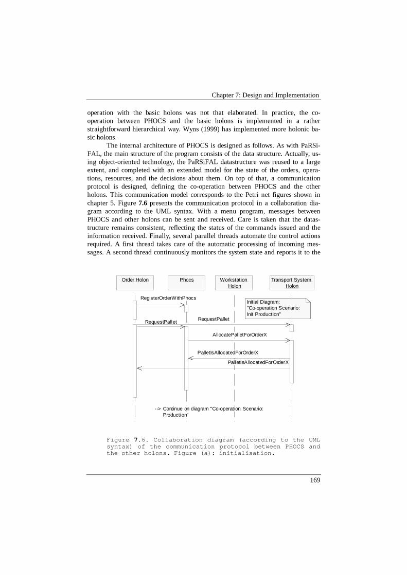
Chapter 7: Design and Implementation
169
operation with the basic holons was not that elaborated. In practice, the co-operation between PHOCS and the basic holons is implemented in a ratherstraightforward hierarchical way. Wyns (1999) has implemented more holonic ba-sic holons.
The internal architecture of PHOCS is designed as follows. As with PaRSi-FAL, the main structure of the program consists of the data structure. Actually, us-ing object-oriented technology, the PaRSiFAL datastructure was reused to a largeextent, and completed with an extended model for the state of the orders, opera-tions, resources, and the decisions about them. On top of that, a communicationprotocol is designed, defining the co-operation between PHOCS and the otherholons. This communication model corresponds to the Petri net figures shown inchapter 5. Figure 7.6 presents the communication protocol in a collaboration dia-gram according to the UML syntax. With a menu program, messages betweenPHOCS and other holons can be sent and received. Care is taken that the datas-tructure remains consistent, reflecting the status of the commands issued and theinformation received. Finally, several parallel threads automate the control actionsrequired. A first thread takes care of the automatic processing of incoming mes-sages. A second thread continuously monitors the system state and reports it to the
PhocsOrder Holon Workstation Holon
Transport System Holon
--> Continue on diagram "Co-operation Scenario: Production"
RegisterOrderWithPhocs
RequestPalletRequestPallet
AllocatePalletForOrderX
PalletIsA llocatedForOrderX
PalletIsAllocatedForOrderX
Initial Diagram: "Co-operation Scenario: Init Production"
Figure 7.6. Collaboration diagram (according to the UMLsyntax) of the communication protocol between PHOCS andthe other holons. Figure (a): initialisation.
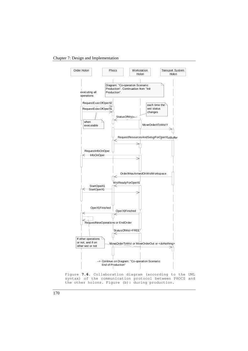
Chapter 7: Design and Implementation
170
PhocsOrder Holon Workstat ion Holon
Transport System Holon
when executable
each time the wst status changes
executing all operations
--> Continue on Diagram: "Co-operation Scenario: End of Production"
If other operations or not, and if on other wst or not
RequestExecOfOperX1
RequestExecOfOperX2
StatusOfWst=...
WstReadyForOperX1StartOperX1
RequestInfoOnOper
InfoOnOper
StartOperX1
OperX1FinishedOperX1Finished
RequestNewOperat ions or EndOrder
StatusOfWst=FREE
MoveOrderXToWstY
OrderXHasArrivedAtBeginningOfWstBufferRequestResourcesAndSetupForOperX1
OrderXHasArrivedOnWstWorkspace
MoveOrderToWst or MoveOrderOut or <doNothing>
Diagram: "Co-operation Scenario: Production". Continuation from "Init Production".
Figure 7.6. Collaboration diagram (according to the UMLsyntax) of the communication protocol between PHOCS andthe other holons. Figure (b): during production.
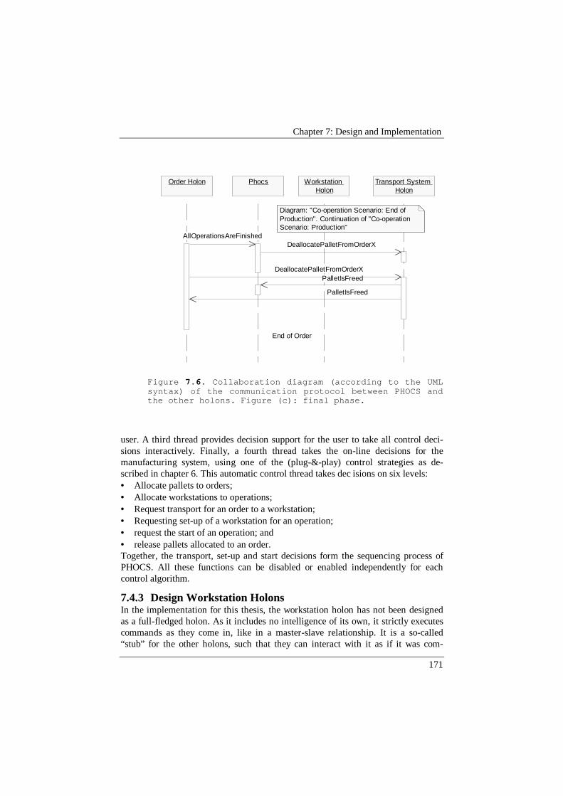
Chapter 7: Design and Implementation
171
PhocsOrder Holon Workstation Holon
Transport System Holon
End of Order
AllOperationsAreFinishedDeallocatePalletFromOrderX
DeallocatePalletFromOrderXPalletIsFreed
PalletIsFreed
Diagram: "Co-operation Scenario: End of Production". Continuation of "Co-operation Scenario: Production"
Figure 7.6. Collaboration diagram (according to the UMLsyntax) of the communication protocol between PHOCS andthe other holons. Figure (c): final phase.
user. A third thread provides decision support for the user to take all control deci-sions interactively. Finally, a fourth thread takes the on-line decisions for themanufacturing system, using one of the (plug-&-play) control strategies as de-scribed in chapter 6. This automatic control thread takes dec isions on six levels:• Allocate pallets to orders;• Allocate workstations to operations;• Request transport for an order to a workstation;• Requesting set-up of a workstation for an operation;• request the start of an operation; and• release pallets allocated to an order.Together, the transport, set-up and start decisions form the sequencing process ofPHOCS. All these functions can be disabled or enabled independently for eachcontrol algorithm.
7.4.3 Design Workstation HolonsIn the implementation for this thesis, the workstation holon has not been designedas a full-fledged holon. As it includes no intelligence of its own, it strictly executescommands as they come in, like in a master-slave relationship. It is a so-called“stub” for the other holons, such that they can interact with it as if it was com-
Chapter 7: Design and Implementation
172
pletely holonic. However, the workstation holon is not equipped with any sequenc-ing or pricing mechanism to autonomously take care of manufacturing control. Itwas not connected to any hardware either. Instead, the operations on the machineswere simulated by a delay. Stochastic variations and machine breakdowns can besimulated too, using a “breakdown schedule”, loaded from data files.
It has — on a smaller scale — the same structure as PaRSiFAL and PHOCS:it is based on a datastructure, upon which a menu program is implemented that en-ables interactive message sending and handling. Then, an automatic control threadand a bootstrap scenario are added.
The control loop can be modelled as a simple state machine. Starting fromthe idle state, an incoming message for the allocation of the workstation and a re-quest for the right set-up have the workstation change state to “setting-up”. Theworkstation therefore autonomously interacts with the order holon to know whichoperation to start. When the set-up is finished, the workstation waits for a startcommand. At the completion of the operation, it informs PHOCS and the corre-sponding order and starts a tear-down of the workstation. When completed, it againinforms PHOCS that its state has switched to idle again.
7.4.4 Design Order HolonsAlso the order holon implementation was not completely elaborated as an autono-mous holon. It has a similar structure as the workstation holon, with a datastruc-ture, a set of functions to send and receive messages, and an interactive (menu-driven) or automatic control thread. Its autonomy is limited in that• it obeys commands coming from PHOCS or other staff holons;• this obedience is hard-coded; and• it does not contain the control algorithms for heterarchical decision taking.The order holon can take care of one or more orders simultaneously. In otherwords, it is possible to put all orders in one order holon, have one order holon foreach individual order, or distribute a set of orders over a limited set of ordersholons, such that the computational load is spread over the available set of comput-ers. The order holon can also send a synchronisation message to all holons whenstarting the system, such that all holons can start at the same time. This feature isespecially useful to have repeatable experiments for testing and benchmarking.
The specific control algorithm present in the current implementation worksas follows. Each order has its own control thread. Each order waits until it reachesits release date. It then requests a pallet and waits for it to get allocated. (In this hi-erarchical control mode, it sends its requests to both the resource involved and theOMC staff holon.) From then on, the order holon requests execution for all execu-table operations to PHOCS. When authorised, it requests execution of that opera-tion to the workstation allocated for it. The order holon waits for the operation tofinish (getting informed by the workstation holon) and informs the other holons in-volved about the new state of the order. When new operations become executable,the order holon starts the same process for them. When all operations are finished,the order releases the pallet (by sending a message to the transport system holon).
Chapter 7: Design and Implementation
173
7.4.5 Design Transport System HolonThe transport system holon is similar in nature to the workstation holon, but sig-nificantly more complex. To start with, a lot more autonomy is expected from thetransport system, as process plans usually do not foresee an NC program for trans-port, or an explicit and detailed routing for the products. The transport system alsohas to deal with multiple transportation tasks simultaneously, implying autonomousdecision taking (like sequencing and selection of alternatives for all these tasks).Moreover, transportation is — especially in assembly — an important factor in theoverall system flexibility and performance, such that its effects are not neglectable.
The complexity of these problems was long underestimated, but recently,they got some attention, for example from Bussmann (1994) and van Acker (1996),and now also in some IMS projects, like metamorphic material handling systems(MMHS) and holomobiles (part of the HMS project). The problem is quite formida-ble and was only treated in the margin of this thesis (Malewicz, 1996).
For the actual implementation for this thesis, the design of the transportsystem holon is a server that receives and processes transport commands. Itlaunches a separate thread for each transport task. Since the implementation is atransport system stub (it does not control the real transport devices), it only gener-ates delays for the transport tasks. For each task, a first delay is defined by the dis-tance from the starting point to the buffer of the destination workstation. A seconddelay models the transport time through the buffer of the workstation to the workspace, considering queuing effects of other orders in the workstation buffer. It ispossible to add precedence constraints to a transportation task, such that orders canenter the workstation buffer in the desired sequence (possibly making the order waituntil the other orders arrive). Note that the transport system holon also takes care ofthe allocation and de-allocation of pallets to orders.
A second implementation of the transport system holon is developed byWyns (1999). It connects to the real transport system (via serial lines and a PLC),or to an ARENA simulation of the transport system (via sockets), using theARENA model to define the delays, rather than picking the values from a trans-portation time matrix. This implementation is compatible with the holons describedin this thesis, but was not used often because of the practical implications whenperforming experiments.
7.5 ImplementationThe software is written in C++ (IBM C++ on OS/2). During development, parts ofthe code have been ported to and from DOS (Borland C++), HP/UNIX andsun/UNIX, and the version at that time was source-code compatible on these 3 sys-tems. Consequently, the software is to a large degree platform independent. Most ofthe software is fairly well documented to university standards (Bonneville, 1994,Bongaerts, 1995b, 1996b, 1996c).
The software was kept quite spartan with respect to the user interface. Onlywhere needed, graphical output is produced. This is mainly limited to the presenta-
Chapter 7: Design and Implementation
174
tion of a Gantt chart for the schedule and the progress report, which provides ageneral overview of the schedule and the schedule execution process. The user in-terface of the rest of the program is a keyboard-driven menu, enabling fast interac-tive control for users accustomed to the program. Through the use of data files (foroptions, parameters, manufacturing system and order input data), the configurationof the rest of the system is simplified and accelerated. The resulting manufacturingdata can be logged in detail in output and log files, accessible for EXCEL for fur-ther analysis.
The software relies heavily on inter-process communication among holonson the same PC and on different PCs, and between holons and manufacturing de-vices. The communication between holons is based on an asynchronous, ASCII-based point-to-point communication protocol via sockets on TCP/IP. This messag-ing system is developed jointly with Wyns (1999). Communication with manufac-turing devices is performed via serial lines, using the device driver mechanism(Valckenaers, 1993). Timing and synchronisation are other important aspects fromthe implementation point of view. Internally, all holons (except the schedulerholon) refer to time in seconds since January 1970 (the Unix standard). Time isread from the operating system, and all used PCs could be synchronised with ex-isting OS/2 tools. The implementation in C++ also relied heavily on the Booleantype definition and the use of a self-developed container class. All these auxiliaryfunctions were properly stored in software libraries.
7.6 ConclusionsThe aim of this chapter was to show that the concepts proposed in this thesis arebacked up with real software developments. The software runs a holonic manufac-turing control system for a testbed flexible assembly system. It consists of a reactivescheduling holon, called PaRSiFAL, an OMC holon, called PHOCS, and a set oforder and resource holons.
The software developments were based on reasonable designs, with the ap-propriate design quality for university research prototypes. I believe this kind ofquality is useful and minimally required, even for university prototypes. However,this thesis did not aim at improvements in the software development process, andtherefore its developments would not score favourably if (unjustly) compared withthe newest state of the art software design technology.
The software described in this chapter is used for the experiments describedin the next chapter. Also for that purpose, this chapter has described the developedsoftware in sufficient detail to properly describe the test set-up for the experiments.
175
Chapter 8
Experiments
This chapter describes the experiments performed for this thesis. It checks the re-peatability of the experiments and the predictability of hierarchical, heterarchicaland holonic control. It provides numerical results for the on-line manufacturingcontrol algorithms defined in chapter 6 and uses these results to validate the con-cepts presented in chapter 4.
8.1 IntroductionThis thesis has presented several concepts on manufacturing control, a control ar-chitecture, an interaction mechanism and a set of heuristic and model-based controlalgorithms. This chapter describes the design of the experiments performed to vali-date the concepts, the architecture and the algorithms, reports on their results andpresents the resulting conclusions. Note that benchmarking is a hard task, especiallyin manufacturing control. Test set-ups and problems are very specific, but the ex-perimental results are to be generalised over a wide range of applications, consider-ing a variety of parameters, lay-outs, product and order mixes, stochastic effects, NP-completeness and other non-linearities.
This chapter has the following structure. First, the overall approach is pre-sented. The next section considers the issue of repeatability and predictability. Thestructure of the remainder of the chapter reflects the main concepts presented in thisthesis: hierarchy in distributed control, distributed decision power and concurrentscheduling and schedule execution. Finally, the presented control algorithms arecompared with traditional control algorithms and among themselves with respect topredictability, performance and robustness.
8.2 Design of experiments
8.2.1 Literature survey:Before reporting on the design and results of the experiments, it is useful to reviewsimilar work in literature. An important general reference is the theory on design ofexperiments (Lossie, 1996). It provides a general methodology for conducting ex-periments, including• defining the goal of the experiment;• defining a system to be tested, with input and output parameters;
Chapter 8: Experiments
176
• defining the number of experiments, and the parameters used for each one ofthem; and
• a number of guidelines and caveats for the analysis.An important element of the theory on design of experiment is that a complete set ofexperiments, for all possible combinations of variations of input parameters requiresa huge amount of time. With a limited number of tests, it is possible to estimate theeffect of each parameter separately. The theory also shows that with only a few ex-periments more (and a well designed experiment), the statistical accuracy of the setof experiments improves significantly.
Specific experimental results on manufacturing control are scarce in literature(especially when differentiating manufacturing control from scheduling). Somebenchmark definitions exist on scheduling (Ringer, 1995). Duffie (1994) providesexperimental results for their heterarchical control algorithm, but without comparingthem with other approaches. Cavalieri (1998) reports on experiments involving twodistributed control algorithms. He implemented and compared a fully distributedheterarchical control algorithm (Lin, 1994) with distributed solution combined with acentralised (non-optimising) scheduler (Camarinha-Matos, 1996). The experimentalresults were preliminary but reported that the fully heterarchical control approachprovided better performance.
For holonic manufacturing, very few experimental results on manufacturingcontrol exist. To our knowledge, only Valckenaers (1994) reported on a comparisonof hierarchical, heterarchical and holonic control strategies under different scenarios.The so-called holonic control strategies did not significantly outperform the otherapproaches, but research on holonic manufacturing had only just started at that time(such that no mature holonic control algorithms were available).
8.2.2 Approach takenThe main elements in the test set-up are the reactive scheduler PaRSiFAL and theOMC holon PHOCS, described in chapter 7. The performance of any tests involvingthese holons is depending mainly on the interaction mechanism and the algorithmsused in both holons: the rescheduling algorithm and the OMC algorithm. This thesisdid not aim at new contributions in scheduling, nor in reactive scheduling. This isreflected in the experiments, in that the required schedule is not always optimisedon-line (during the tests) but loaded from file. For similar reasons, the ASE algo-rithms can be compared for a test scenario where only one schedule is generated andexecuted without further reactive scheduling.
Practically, each experiment in the following section is presented as follows.First, the goals of each experiment are defined. Then, a set of test problems and testconditions is defined. This includes the complete description of the manufacturingsystem, the product and order data, and the disturbance scenarios. Then, the set ofalgorithms to be compared is defined, together with all their parameters. Each algo-rithm is tested with an appropriate number of runs. The resulting data are analysedand interpreted, after which a conclusion is drawn. (Of course, all details about inputand output data could not possibly be included in this thesis, and are found in a tech-

Chapter 8: Experiments
177
nical report (Bongaerts, 1998d) and in data and result files. They are partially gener-ated automatically during the test runs).
When designing the experiments, it was hoped that a limited set of aggregateinput parameters could successfully characterise the problem. If this would be possi-ble, one could design a set of test problems spanning a wide range of productionsystems and production scenarios. Examples of such parameters are the load of thesystem, the number of orders and workstations, the average processing time, the av-erage order slack (and the order slack standard deviation). Also some models couldbe designed that estimate performance measures for these aggregate input parametersfor ideal cases. In that way, it would be possible to assess the performance of eachalgorithm with respect to an ideal value. However, it turned out that this is a hugetask, and not essential for this thesis. Instead, a more feasible solution was the defi-nition of a set of benchmark problems. A benchmark is a set of problem definitionsspanning the problem space under study, and the results of a number of default solu-tions for these problems (Ringer, 1995). The definition of these benchmark problemsis often based on a more intuitive approach.
Problem name N ΣNi Descriptionorders3.dat 4 61 Initial data set. Static problem (all release
dates are 0). High pre-emption flexibility.High precedence constrainedness (but somerouting flexibility). Mix of electric switchesand Lego towers. Very tight due dates.
orders3f.dat 4 61 Same as order3.dat, but with varying releasedates.
large1.dat 20 223 A “large” set of orders. Rather static. Rea-sonably low pre-emption flexibility. Varyingdegree of precedence constrainedness. Mix ofelectric switches, Lego towers, shorties, andflexies. Tight due dates.
lar1loos.dat 20 171 A large set of orders. Similar to large1.dat,but with another order mix. Loose due dates.
cont1.dat 40 359 Continuously entering orders. Reasonably (butnot fully) balanced inflow. Loose due dates.Broad order mix. High variance on due datetightness.
Table 8.1. Definition test problems. N refers to the num-ber of orders, ΣNi to the number of operations.
For most of the tests involved, the manufacturing system used is the PMAFAS. The products used are electric switches (figure ), requiring work on 5 worksta-

Chapter 8: Experiments
178
tions (in 14 operations), with a rather fixed routing, but with a lot of pre-emptionflexibility1 (a visit to a workstation can sometimes be divided in up to 6 parts). An-other popular product is a tower made in LEGO (19 operations) with a lot of routingflexibility, but enough precedence constraints limiting this flexibility. Also theLEGO tower has pre-emptable operations. Other test products are a short-lastingone, called “S4” (a LEGO product with only 4 operations), and a number of “type F”products (products with 5 to 7 operations but without precedence constraints). Otherproducts are more standard job shop products, with fixed routings and without pre-emption. With these products, order mixes can be composed with many or few or-ders, with tight or loose due dates, with heavily loaded or under-utilised workstationsand with a small or large variety on these parameters. Also, dynamic manufacturingcontrol problems (with continuously entering orders) are to be defined. Table 8.1shows the set of test problems, generated with these input data in mind.
Spring
Contact Plate
Switching Part
Upper Part
Bridge
Bolt
Base Part
Clamp
Nut
Contact Blok
Lower Blok
EXPLODED VIEW
Figure 8.1. Exploded view of an electric switch.
1 A product definition is more flexible if an operation can be interrupted, or “pre-empted”, during production. In discrete manufacturing, operations can only be pre-empted at certain time instants, such that a long operation is split up in sub-operations. A product with a high pre-emption flexibility contains several consecu-tive short-lasting operations on a workstation instead of a single long-lasting opera-tion.
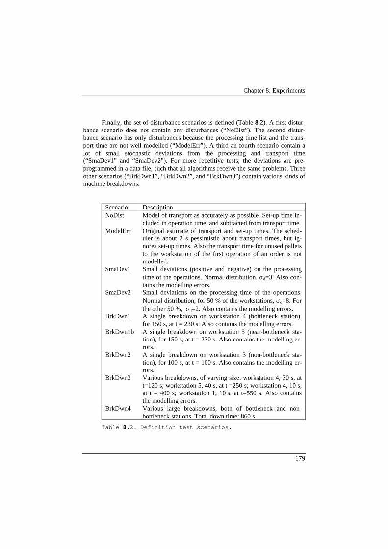
Chapter 8: Experiments
179
Finally, the set of disturbance scenarios is defined (Table 8.2). A first distur-bance scenario does not contain any disturbances (“NoDist”). The second distur-bance scenario has only disturbances because the processing time list and the trans-port time are not well modelled (“ModelErr”). A third an fourth scenario contain alot of small stochastic deviations from the processing and transport time(“SmaDev1” and “SmaDev2”). For more repetitive tests, the deviations are pre-programmed in a data file, such that all algorithms receive the same problems. Threeother scenarios (“BrkDwn1”, “BrkDwn2”, and “BrkDwn3”) contain various kinds ofmachine breakdowns.
Scenario DescriptionNoDist Model of transport as accurately as possible. Set-up time in-
cluded in operation time, and subtracted from transport time.ModelErr Original estimate of transport and set-up times. The sched-
uler is about 2 s pessimistic about transport times, but ig-nores set-up times. Also the transport time for unused palletsto the workstation of the first operation of an order is notmodelled.
SmaDev1 Small deviations (positive and negative) on the processingtime of the operations. Normal distribution, σd=3. Also con-tains the modelling errors.
SmaDev2 Small deviations on the processing time of the operations.Normal distribution, for 50 % of the workstations, σd=8. Forthe other 50 %, σd=2. Also contains the modelling errors.
BrkDwn1 A single breakdown on workstation 4 (bottleneck station),for 150 s, at t = 230 s. Also contains the modelling errors.
BrkDwn1b A single breakdown on workstation 5 (near-bottleneck sta-tion), for 150 s, at t = 230 s. Also contains the modelling er-rors.
BrkDwn2 A single breakdown on workstation 3 (non-bottleneck sta-tion), for 100 s, at t = 100 s. Also contains the modelling er-rors.
BrkDwn3 Various breakdowns, of varying size: workstation 4, 30 s, att=120 s; workstation 5, 40 s, at t =250 s; workstation 4, 10 s,at t = 400 s; workstation 1, 10 s, at t=550 s. Also containsthe modelling errors.
BrkDwn4 Various large breakdowns, both of bottleneck and non-bottleneck stations. Total down time: 860 s.
Table 8.2. Definition test scenarios.
Chapter 8: Experiments
180
8.2.3 OverviewThe experiments performed for this thesis seek to answer the following questions:• Is it possible to gather experimental data with a sufficient reliability? Are the re-
sults statistically significant? How many experiments are to be conducted tocome to conclusive evidence? Is there a difference in predictability between dif-ferent approaches?
• What are the advantages of introducing hierarchy in distributed systems? Doesthis concept provide a higher performance than traditional hierarchical and heter-archical systems?
• Does the concept of distributed decision power yield a higher performance thansolutions with decisions taken by a single holon?
• Does concurrent scheduling and schedule execution pay off? Were the assump-tions taken in chapter 5 realistic?
• Do holonic algorithms for ASE provide a better performance than their hierarchi-cal or heterarchical counterparts?
• Is the performance of holonic manufacturing control better than its hierarchical orheterarchical counterparts? Always, or under which conditions?
This set of questions corresponds to the structure of the remainder of this chapter.
8.3 Testability
8.3.1 GoalBefore starting the actual experiments to compare different approaches towardsmanufacturing control, it is essential to check the reliability of the experiments. Thefirst requirement is that the tests are repeatable. Secondly, the conclusions drawnfrom the experiments should be valid over a wide enough range of manufacturingsystems and circumstances, such that the conclusions can be generalised. Thirdly, theexperiments should examine the degree of predictability of manufacturing systems,certainly whether hierarchical control and heterarchical control differ that much inpredictability.
8.3.2 RepeatabilityRepeatability is the basic precondition to perform experiments. Experiments are re-peatable if an experimental test set-up with the same input parameters and under thesame circumstances can produce the same results. ‘Under the same circumstances’refers to the fact that all controllable parameters are chosen identical. By definition,uncontrollable parameters cannot be controlled, and are exactly the cause that identi-cal experiments produce different results (unless the system is fundamentally sto-chastic).
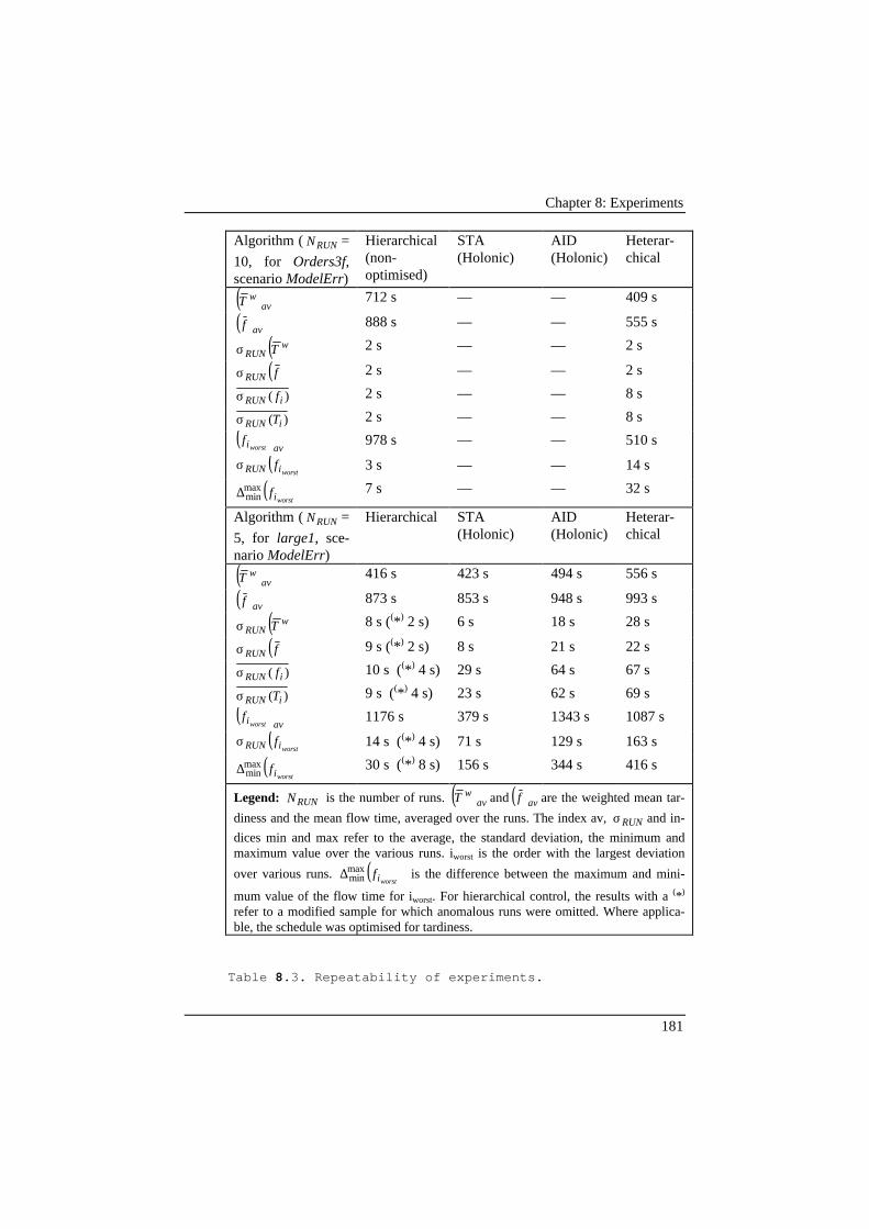
Chapter 8: Experiments
181
Algorithm ( RUNN =
10, for Orders3f,scenario ModelErr)
Hierarchical(non-optimised)
STA(Holonic)
AID(Holonic)
Heterar-chical
( )avwT 712 s — — 409 s
( )avf 888 s — — 555 s
( )wRUN Tσ 2 s — — 2 s
( )fRUNσ 2 s — — 2 s
)( iRUN fσ 2 s — — 8 s
)( iRUN Tσ 2 s — — 8 s
( ) aviworst
f 978 s — — 510 s
( )worstiRUN fσ 3 s — — 14 s
( )worstif
maxmin∆ 7 s — — 32 s
Algorithm ( RUNN =
5, for large1, sce-nario ModelErr)
Hierarchical STA(Holonic)
AID(Holonic)
Heterar-chical
( )avwT 416 s 423 s 494 s 556 s
( )avf 873 s 853 s 948 s 993 s
( )wRUN Tσ 8 s ((*) 2 s) 6 s 18 s 28 s
( )fRUNσ 9 s ((*) 2 s) 8 s 21 s 22 s
)( iRUN fσ 10 s ((*) 4 s) 29 s 64 s 67 s
)( iRUN Tσ 9 s ((*) 4 s) 23 s 62 s 69 s
( ) aviworst
f 1176 s 379 s 1343 s 1087 s
( )worstiRUN fσ 14 s ((*) 4 s) 71 s 129 s 163 s
( )worstif
maxmin∆ 30 s ((*) 8 s) 156 s 344 s 416 s
Legend: RUNN is the number of runs. ( )avwT and ( )avf are the weighted mean tar-
diness and the mean flow time, averaged over the runs. The index av, RUNσ and in-
dices min and max refer to the average, the standard deviation, the minimum andmaximum value over the various runs. iworst is the order with the largest deviation
over various runs. ( )worstif
maxmin∆ is the difference between the maximum and mini-
mum value of the flow time for iworst. For hierarchical control, the results with a (*)
refer to a modified sample for which anomalous runs were omitted. Where applica-ble, the schedule was optimised for tardiness.
Table 8.3. Repeatability of experiments.

Chapter 8: Experiments
182
The approach taken for the repeatability tests is as follows. A resource allo-cation problem is solved several times consecutively. Care is taken to control allpossibly relevant parameters as good as possible (e.g. not running other processes onthe computer, not introducing stochastic effects in the problem, avoiding the effectsof human intervention and machine interfacing, synchronising the start-up of all pro-grams). This is done for a number of resource allocation problems and for a numberof manufacturing control strategies. A good indicator for repeatability is the samplestandard deviation of the individual and aggregate performance measures resultingfrom these test runs.
Practically, the performance measures examined are average weighted tardi-ness (as an objective) and flowtime (as an indicator). The problems considered areorders3f.dat and large1.dat, under one scenario with few disturbances (ModelErr —which has no stochastic effects). The control algorithms tested are strict hierarchicalcontrol, heterarchical control (CAOMC algorithm) and the heuristic holonic algo-rithms STA (“short term autonomy”) and AID (“autonomy if disturbances” — seechapter 6). The tests were performed without interaction with real mechanical de-vices (with the order and resource “stubs”), to focus the experiments on the repeat-ability of the control system, rather that on the underlying manufacturing system. Foreach case, between 5 and 10 repetitive runs are performed.
The results are summarised in table 8.3. For a small problem (orders3f.dat),the standard deviation on the average performance is always small (2 s), even forheterarchical control. For the performance of individual orders, the deviation maybecome bigger. Problems of more realistic size have a higher standard deviation forheterarchical control.
A closer analysis shows that for the small problem, heterarchical control se-lects randomly between two resource allocation sequences. (Because the interactionbetween the orders is relatively small, there are only two sequences.) Partitioning thesample in the corresponding classes results in a high repeatability (small deviation)for the individual orders for both sequences: 2 s again.
One could wonder where the stochastic variations come from, in a system thatis well-controlled (in simulation, and without deliberate stochastic effects). There aretwo major effects making the phenomenon stochastic. First, time is measured dis-cretely (in seconds), which may give rise to a discretisation error. Secondly, the con-trol system runs on a multi-tasking system with parallel threads and processes, com-municating on the PC and over Ethernet. Such systems are known to produce sto-chastic variations on their processing times.
Summarising, for hierarchical control, the repeatability of the experiments σis 2 s, implying that a single run is sufficient for convincing evidence. For heterar-chical control and to a lesser degree holonic control, it is essential to do experimentsover a number of runs, and average out the results. The resulting confidence interval
Chapter 8: Experiments
183
is then estimated using Student’s t distribution with (n-1) degrees of freedom for a
confidence level (1-a) (Kelton, 1998, Neter, 1978)2.
n
stX n 2/1,1 α−−± (8.1)
For instance, since for heterarchical control the sample standard deviation of themean weighted tardiness is 28 s (for 5 experiments), the estimated mean weighted
tardiness ( ) ( )( ) ( )ss 3555652877.2556 ±=⋅±=avwT (for a confidence level of 95 %,
and 4 degrees of freedom).
8.3.3 GeneralisationNext to repeatability, another possible problem when basing conclusions on experi-mental data, is the generalisation issue: Can the conclusions drawn from the experi-ments be generalised over a complete range of manufacturing systems? This is notrivial question, since there is huge amount of parameters characterising the problem,and the resource allocation has some considerable non-linearities.
A systematic approach to answer this question could be as follows. First, sim-plified analytical models are defined to express the performance of the system infunction of a set of aggregated input parameters. These aggregated input parametersare to reduce the huge set of input parameters to a manageable size. Typical aggre-gated input parameters are for instance the load of the system (the number of ordersper workstation), the size of the system (the number of workstations), the averageduration of an operation, the average number of operations per order, the relative av-erage order slack, etc. A typical model could be that the system throughput is pro-portional to the number of workstations divided by the average duration of a com-plete order. Secondly, tuneable parameters in that model are collected and identi-fied. Therefore, a large number of experiments are to be performed, such that thevalues for these parameters can be identified. Thirdly, it is to be checked that thepredicted performance with this identified model corresponds to reality, implyingeven more experiments. Then, if the deviation of the model from the real data isrelatively small (a small standard deviation of the sample), a reliable generic modelof the manufacturing has been defined. Then, the experiments should be performedover the complete range of aggregated input parameters to measure for values of theparameters, one algorithm performs better than another one. An initial attempt forthis approach was made (Swiercz, 1996), but it turned out to be quite a formidableproject. No satisfying results were obtained for this idea. Since this is no essentialpart of this thesis, an alternative approach was sought for.
To prove the potential improvements of the holonic approach over a widerange of situations, the defined test problems had to be sufficiently different. Thisidea was considered when defining the problems shown in table 8.1. A potentialdrawback is that when the improvements of a certain algorithm are not systematically
2 The symbols used here are standard notation in statistics (Kelton, 1998, Neter,1978) and are not further explained in this thesis.
Chapter 8: Experiments
184
better over those of another algorithm, possible explanations of this anomaly cannotbe backed up with statistical evidence.
8.3.4 PredictabilityIt is generally assumed that heterarchical control is less predictable than the tradi-tional hierarchical systems. But it is interesting to check this general assumption withexperimental data. Therefore, using the experiments described in subsection 8.3.2,this subsection tries to answer the questions about predictability.
The results of table 8.3 show that hierarchical control has a much higher re-peatability than heterarchical control. Hierarchical control provides a deviation onthe average and individual performance (flow time and tardiness) ranging between 2s and 10 s. Expressing these values relative to a total flow time3 of 873 s, the repeat-
ability of hierarchical control results in a deviation s of 1 % and better. (The valueof 10 s is mostly due to an anomaly: for a single experiment run, the schedule opti-misation time was just too short to reach the same level of optimisation as in theother runs. This resulted in a slightly different schedule).
For the same problems, heterarchical control performs a lot worse, especiallyfor large, non-trivial problems with considerable interactions, and especially whenlooking at the individual performance. The average standard deviation on individualorder performance for heterarchical control is 8 % (69/873). Such a standard devia-tion can easily result in variations reaching up to 40 % (as it did in the experimentsfor the uncertainty on the individual order flow time4). Even for the average flowtime, the uncertainty reaches a level of 2 % standard deviation (22/873). Holoniccontrol behaves better, especially for the individual order predictability. The heuris-tic holonic control strategy STA reaches a predictability of 1% standard deviation forthe average flow time, which is comparable to hierarchical (however, it is still largewhen comparing with the modified sample results for hierarchical control). For theindividual orders, the uncertainty level of holonic control is limited to 3% (withworst case values up to 15 %). The other holonic control heuristic AID apparentlyhas a predictability much closer to heterarchical control. Note that indeed chapter 6had already mentioned that one of the drawbacks of the heuristic strategies, like theAID algorithm, is that they tend to behave like only heterarchical or only hierarchicalcontrol according to the circumstances, rather than merging the two control ap-proaches.
3 Throughout this chapter, a relative increment or decrement in tardiness perform-ance is not expressed with respect to the tardiness, but with respect to the flow time(obtained for hierarchical control without disturbances). It is senseless to definerelative differences in tardiness as the difference divided by the absolute value of thetardiness, since tardiness depends too much on the input data (tightness or loosenessof the due dates) to be used as a characteristic time. The tardiness can even be zero.4 It is known that the extreme values (like the maximum difference) of a sample is astatistically unreliable parameter. It is however an intuitively appealing parameter.
Chapter 8: Experiments
185
8.3.5 ConclusionSummarising, the experimental data are gathered with an intrinsic repeatability of 2 sstandard deviation for experiments with a duration of 1000 s. However, heterarchicalcontrol strategies inherently have an unpredictable behaviour, where the system fol-lows completely different trajectories in the state space. This kind of control resultsin significantly worse repeatability, with a standard deviation of 25 seconds on theaverage performance measures (flow time and tardiness) and an average standarddeviation of 70 s for the performance of individual orders (again, for an experimentwith an average flow time of 750 s — thus 3 % and 10 %). The predictability ofholonic control strategies (represented here by the STA and AID algorithm) issomewhere in between. STA provides significantly better results than heterarchicalcontrol (1 % respectively 3 % for average and individual performance), thereby im-proving the predictability of holonic control with respect to heterarchical control.However, some degree of uncertainty seems to be the price one has to pay for a moreagile behaviour.
8.4 Hierarchy in Distributed ControlIn chapter 4, when proposing the concept of hierarchy in distributed control, it wasstated that hierarchical systems are not robust against disturbances, and that heterar-chical systems suffer from low and unpredictable5 performance. The concept of hier-archy in distributed control was to combine the best of both worlds, while avoidingtheir drawbacks. This section provides experimental proof to support these state-ments.
8.4.1 Performance degradation of hierarchical control under dis-turbancesA first set of experiments shows that hierarchical control has a well-optimised per-formance if no disturbances occur, but that this performance degrades rapidly whenthey start to appear. In order to show that, hierarchical control performance is meas-ured for a number of test problems as defined in table 8.1, under the disturbance sce-narios described in table 8.2. For these experiments, the required calculation time isnot taken into account as a penalty for optimisation. More specifically, the testproblem is optimised off-line, and when the calculations are finished (a local opti-mum is reached), the resulting schedule is stored. During the experiment, the sched-ule is loaded and sent to the OMC holon PHOCS once. PHOCS than follows theschedule hierarchically, without further schedule updates. This set of experiments isto show the effect of schedule degeneration for a single schedule.
The results of the first set of experiments is shown in table 8.4. For the chosenexample (large1.dat) under hierarchical control, the tardiness performance degradesfrom 51 % (336/656, under nominal conditions) to 98 % (645/656, with several largemachine breakdowns). Under heterarchical control, the difference in performance is
5 The unpredictable nature of heterarchical control was already shown above.

Chapter 8: Experiments
186
less (21 % — or (695-556)/656), but the performance remains inferior to hierarchi-cal control under all circumstances (106 % compared to 98 %).
Performance predicted byscheduler
( )avwT
( )avf
265 s
593 s
Disturbance scenario. Hierar-chical
STA(Holonic)
AID(Holonic)
Heterar-chical
No disturbances.(NoDist)
( )avwT
( )avf
336 s
656 s
366 s
685 s
—
—
556 s
993 s
Modelling error.(ModelErr)
( )avwT
( )avf
416 s
873 s
423 s
853 s
494 s
948 s
556 s
993 s
Small stochasticdeviations.(BrkDwn3)
( )avwT
( )avf
468 s
781 s
472 s
805 s
534 s
832 s
580 s
928 s
One breakdown.(BrkDwn1b)
( )avwT
( )avf
527 s
845 s
442 s
791 s
574 s
876 s
602 s
939 s
Multiple break-downs.(BrkDwn4)
( )avwT
( )avf
645 s
947 s
612 s
926 s
640 s
944 s
695 s
1023 s
ModelErr forlonger lastingtest problem(cont1.dat)
( )avwT
( )avf
235 s
760 s
182 s
731 s
434 s
894 s
219 s
699 s
Remarks: Test problem: large1.dat. Single scheduling run. On-line sched-uling time 2 s (Schedule has already been optimised off-line, for tardiness).
Table 8.4. Excerpt from the results, showing as well theperformance degradation under disturbances for differentcontrol algorithms, as the missed opportunities forheterarchical control. Each line represents a disturbancescenario (see table 8.2). One single schedule is made,and — without reactive scheduling — is slowly degrading.The lowest line presents the results for a different,longer-lasting scheduling problem, showing that the per-formance degradation becomes more important over time(The difference between the real and modelled situationeventually becomes so large that the performance of hier-archical control drops below that of heterarchical con-trol).

Chapter 8: Experiments
187
The last line of table 8.4 shows the results for a different problem (cont1.dat),which lasts twice as long as the previous problem (large1.dat). This experiment wasperformed without any update on the schedule. For hierarchical control, the perform-ance degradation quickly becomes quite drastic: even only due to modelling errors,the performance of hierarchical control drops below that of heterarchical control (foras far as the difference is statistically reliable). This drastic performance degradationis easy to explain: each small deviation from schedule (if not absorbed by localslack) is accumulated (and not averaged) to form a large delay that increases the av-erage flow time and tardiness as a whole. The reason is that the start times of all op-erations are strongly coupled via the workstation and order schedule constraints.Moreover, on average, the schedule of problem cont1.dat is older than that oflarge1.dat. Therefore, at the end of the experiment, the schedule for cont1.dat be-comes less optimised for the current situation. What is even worse is that, especiallyat the end of the experiment, hierarchical control impedes taking the obvious deci-sions: suppose the scheduler foresaw a resource contention and decided to solve it bysequencing two operations o1 and o2 in the sequence (o1, o2); if, due to the changedsituation, o2 can be finished before o1 can start, then by imposing the scheduled se-quence, hierarchical control needlessly delays operation o2.
Performance predicted byscheduler
( )avwT
( )avf
124 s
678 s
Disturbance scenario. Hierarchical STA(Holonic)
Heterarchical
NoDist ( )avwT
( )avf
160 s
719 s
165 s
694 s
219 s
699 s
ModelErr ( )avwT
( )avf
222 s
785 s
185 s
708 s
219 s
699 s
BrkDwn4 ( )avwT
( )avf
461 s
1053 s
363 s
856 s
393 s
903 s
Remarks: Test problem: cont1.dat. Continuous rescheduling (period: 600 s— first on-line scheduling run : duration 2 s — at the start, the schedule wasalready optimised off-line, for tardiness).
Table 8.5. Excerpt from the results, showing as well theperformance degradation under disturbances for differentcontrol algorithms, as the missed opportunities forheterarchical control. Continuous rescheduling.
Chapter 8: Experiments
188
A second set of experiments (see table 8.5) shows the results of a reactivescheduling system set-up (but still for hierarchical control). Again, there is a per-formance degradation of 45 % for hierarchical control: apparently as large as for thesingle scheduling run, but note these tests refer to another test problem. Of course,when disturbances occur, all systems tend to yield a lower performance. For heterar-chical control, the corresponding performance degradation is 24 %. This time, heter-archical control seems to perform better than hierarchical control, but it would bepreferable to base such statements on more statistically reliable results.
8.4.2 Missed Opportunities of Heterarchical ControlCompared to optimising schedulers, used in hierarchical control, heterarchical con-trol cannot obtain the same performance, especially not under normal conditions(without disturbances). This subsection support this statement using numerical datafrom the previous experiments.
Using the same test problems as above (tables 8.4 and 8.5), the best heterar-chical control algorithm implemented is compared with the results of a hierarchicalsolution (as well the predicted — scheduled — performance as the resulting per-formance using hierarchical control). The shorter the problem lasts, the better theimprovements coming from scheduling appear. For large1.dat (not really a smallproblem — table 8.4), hierarchical control yields up to 34 % ((556-336)/656) betterperformance than heterarchical control (for nominal performance — scenario No-Dist). With such an improvement, it is clear that it pays off to optimise the schedule,certainly when an efficient scheduling algorithm is available and the orders areknown a little bit in advance of their release date. Even under heavy disturbances,performance of the implemented hierarchical control system stays better (8 % —(695-645)/656) than its heterarchical counterpart. For the continuous operation ex-ample (cont1.dat — table 8.5), the results for heterarchical control get better: underheavy disturbances, heterarchical control outperforms hierarchical control by 9 %((461-393)/719).
Since this thesis did not aim at schedule optimisation algorithms or reactivescheduling, the calculation speed of the implemented scheduling algorithms is notconsidered an issue, and the schedule was optimised off-line. This experimental ap-proach may have favoured hierarchical control, but note that the first descent algo-rithms are very simple scheduling algorithms, and in this case even hardly optimised.The durations of the operations are short in comparison to industrial situations (suchthat the penalty for a longer scheduling duration is relatively high). Section 8.6 ad-dresses the timing aspects of scheduling (using figures 8.2), like the performancedegradation under increased calculation time.

Chapter 8: Experiments
189
8.4.3 Comparison with Holonic Control StrategiesHolonic control strategies implement the concept of hierarchy in distributed control.If this concept is better than traditional hierarchical control, and better then heterar-chical control, it should show up in the performance of holonic control strategies.6
Again, the same experiments as presented in table 8.4 and table 8.5 are used.Table 8.4 shows that the performance degradation for holonic control (the STA heu-ristic) is not that large as for hierarchical control. Moreover, the performance itselfremains at comparable levels as hierarchical control (maximally 5 % worse), whenthere are few and small disturbances. Under larger disturbances, the holonic controlalgorithm STA outperforms both hierarchical control and heterarchical control (byup to 13 % — (527-442)/656 for a single scheduling run). Note that these resultswere obtained for only a simple heuristic control strategy, like STA. More advanced,model based approaches may even provide better results (see section 8.7).
These results show that holonic control reacts better to disturbances than hi-erarchical control, and that heterarchical control has a worse performance thanholonic control in case no disturbances occur. Holonic control provides a bettertrade-off between optimisation and reactiveness than traditional hierarchical controlor the fully distributed heterarchical approach.
8.5 Distributed Decision PowerIf decision power would not be distributed between hierarchical levels, the mostholonic alternative would be to switch from hierarchical to heterarchical control atthe right time. This section demonstrates that hierarchy in distributed control withoutdistributed decision power (in other words, by switching control modes) yields aninferior performance to the holonic control algorithms as described in chapter 6.
Practically, the comparison (between holonic control — with distributed deci-sion power — and switching control modes — without distributed decision power) ismade by plotting the performance degradation in function of the disturbance size fordifferent control approaches. If, for every possible size of the disturbance, the per-formance of holonic control would be dominated by either hierarchical or heterarchi-cal control, switching control modes could be the better option (provided thatswitching itself would not cause disturbances). However, the previous experiments(table 8.4 and 8.5) confirm that this is not the case.
On several occasions, with varying degrees of disturbances, holonic controloutperforms both hierarchical and heterarchical control. This implies that switchingcontrol modes is certainly worse than holonic control. A more detailed analysis of
6 The careful reader may notice that this is not equivalent to the statement that theconcept of hierarchy in distributed systems is better if the presented holonic controlalgorithms have a better performance — which is the statement we would like toprove. Therefore, strictly speaking, this kind of experiments cannot prove the con-cept. But it is a hard job to find watertight evidence for abstract concepts.

Chapter 8: Experiments
190
the experimental data explains this effect. Both hierarchical and heterarchical controlhave their disadvantages, which cannot by avoided when switching from one to theother. Moreover, the holonic control paradigm leaves a lot more flexibility for thedevelopment of control algorithms, what is likely to lead to a higher performance. Itwas hoped that holonic control would outperform or equal hierarchical and heterar-chical control under all circumstances, but this result was not yet obtained. It couldbe attempted by switching control modes, but the problem is probably more funda-mental: a trade-off has to be made between agility and reduction of nervousness.
Distributed decision power was modelled and implemented using fixed rulesand flexible strategies. It was to be complementary to autonomous schedule execu-tion algorithms (ASE). The question whether it pays off more to improve the distri-bution of decision power than the development of autonomous schedule executionalgorithms is difficult to answer, and was not addressed in this thesis.
8.6 Concurrent Scheduling and Schedule ExecutionThe concept of concurrent scheduling and schedule execution (CSSE) was analysedusing Matlab calculations and a simplified model (see section 5.5 and appendix A).Such calculations give a good indication of the possible improvements of CSSE.They provide insight to understand why the concept works. Because they are basedon simplified models, the resulting conclusions are also more generic. However, theyare based on some assumptions that need to be verified with experimental data.
To start with, it was assumed that the performance improvements obtained byoptimising a schedule are exponential in function of the calculation time required. Ofcourse, the shape of such a performance graph depends on the specific algorithmused. For first descent algorithms (the algorithm used for this thesis), the exponentialnature of the performance graph is confirmed by experiments. For a static schedulingproblem, the performance of the optimised schedule is plotted against the requiredcalculation time, as shown in figure 8.2. The example problem used for this experi-ment is large1.dat7. More experimental data are contained in a technical report (Bon-gaerts, 1998d).
A second assumption to be backed up by experiments is the model for per-formance degradation caused by delaying the execution of a schedule. Chapter 5 pre-sented a simple and a conservative model for this phenomenon. Again, for a staticscheduling problem, experiments were performed to validate this model. Figure 8.2also presents the results of this validation and shows that the real (measured) per-formance degradation is even worse than the modelled one.
7 One may notice that the performance improvement of the first descent scheduler isnot that high: the schedule gets stuck in a local optimum. However, by re-organisingthe priorities defining a solution for the first descent scheduler, the quality improvessignificantly. This was also how the off-line schedule optimisation process was per-formed. However, since reorganising is still done on the initiative of the operator, itwas difficult to incorporate this reorganising in the automatic scheduler.
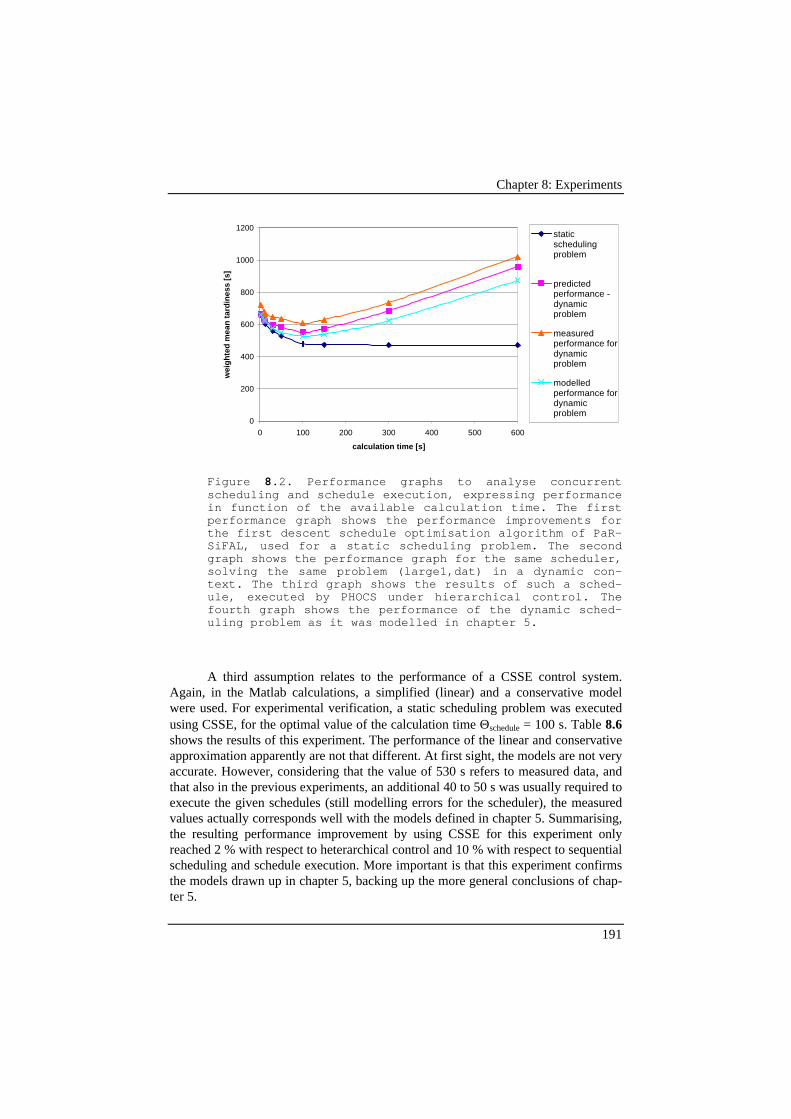
Chapter 8: Experiments
191
0
200
400
600
800
1000
1200
0 100 200 300 400 500 600
calculation time [s]
wei
gh
ted
mea
n t
ard
ines
s [s
]staticschedulingproblem
predictedperformance -dynamicproblem
measuredperformance fordynamicproblem
modelledperformance fordynamicproblem
Figure 8.2. Performance graphs to analyse concurrentscheduling and schedule execution, expressing performancein function of the available calculation time. The firstperformance graph shows the performance improvements forthe first descent schedule optimisation algorithm of PaR-SiFAL, used for a static scheduling problem. The secondgraph shows the performance graph for the same scheduler,solving the same problem (large1,dat) in a dynamic con-text. The third graph shows the results of such a sched-ule, executed by PHOCS under hierarchical control. Thefourth graph shows the performance of the dynamic sched-uling problem as it was modelled in chapter 5.
A third assumption relates to the performance of a CSSE control system.Again, in the Matlab calculations, a simplified (linear) and a conservative modelwere used. For experimental verification, a static scheduling problem was executedusing CSSE, for the optimal value of the calculation time Θschedule = 100 s. Table 8.6shows the results of this experiment. The performance of the linear and conservativeapproximation apparently are not that different. At first sight, the models are not veryaccurate. However, considering that the value of 530 s refers to measured data, andthat also in the previous experiments, an additional 40 to 50 s was usually required toexecute the given schedules (still modelling errors for the scheduler), the measuredvalues actually corresponds well with the models defined in chapter 5. Summarising,the resulting performance improvement by using CSSE for this experiment onlyreached 2 % with respect to heterarchical control and 10 % with respect to sequentialscheduling and schedule execution. More important is that this experiment confirmsthe models drawn up in chapter 5, backing up the more general conclusions of chap-ter 5.

Chapter 8: Experiments
192
Description ( )avwT
Performance measured for control algorithm STA, withΘschedule = 100 s
530 s
Predicted performance for CSSE according to linear ap-proximation
484
Predicted performance for CSSE according to conservativeapproximation
498
Remarks: Experiment: large1.dat, scenario noDist, control algorithmSTA, first short scheduling run to start production, then scheduling for 100s.
Table 8.6. Results of the experiment to validate CSSE.
8.7 Assessment of Holonic ASE Control AlgorithmsFinally, after assessing the proposed concepts for holonic manufacturing, it is time toevaluate the performance of holonic control algorithms. Therefore, the three pro-posed heuristic ASE algorithms and the PA-based ASE algorithm are compared withhierarchical and heterarchical control under a variety of disturbance scenarios.
In these experiments, the scheduling holon PaRSiFAL only has a singlescheduling run, in other words, the reactive scheduling ability of the PaRSiFAL isswitched off. PaRSiFAL sends the schedule down to the OMC holon PHOCS, whichthen executes the schedule autonomously. Therefore, this kind of experiments spe-cifically assess the ASE capabilities of the individual algorithms.
The results of these experiments are shown in table 8.7. It shows that theholonic control algorithms outperform the heterarchical control implementation inmost of the cases, especially when there are few disturbances. (In other, longer-lasting experiments, not shown in the table, heterarchical control performs better.)
The holonic control algorithms usually — when there are few disturbances —have a performance between that of hierarchical and heterarchical control. Some al-gorithms obtain a comparable performance as hierarchical in case of few or no dis-turbances. When there are more disturbances, several holonic control strategies out-perform hierarchical control. More interesting however is to note that there are sev-eral cases where holonic control algorithms outperform both hierarchical and heter-archical control, such that holonic control becomes dominant on these occasions.

Chapter 8: Experiments
193
disturbancescenario.
Hierar-chical
STA(Hol.)
AID(Hol.)
LDFS(Hol.)
PA(Hol.)
Heterar-chical
NoDist 336 s 366 — — 370 556ModelErr 416 423 494 520 443 556BrkDwn3 468 472 534 533 483 580BrkDwn2 527 442 574 565 468 602BrkDwn1 645 612 640 672 590 695
Legend: The table shows wT , for problem large1.dat, under a number ofdisturbance scenarios and for a number of control algorithms.
Table 8.7. Comparison of all tested control strategiesfor a single scheduling run.
It is also interesting to compare the different holonic control algorithmsamongst each other. On most occasions, the heuristic control algorithms STA givesthe best results. The AID algorithm and the LDFS algorithm also behave holonicly,but are clearly inferior in performance to STA. STA provides a similar performanceas the PA algorithm. However, while the decisions of STA are heuristic that rathermakes a trade-off between following the schedule or reacting to disturbances, PA isbetter in deciding when to follow the schedule and when to deviate. Unfortunately,the computational load of PA in the current implementation is quite big and in-creases the inter-operation time on a workstation by one or two seconds. Since manyoperations only last 10 or 12 seconds, this phenomenon has an considerable negativeeffect on the performance, counteracting the improved decision making. Furthertuning and some algorithm engineering can probably solve the problem, but is notimplemented.
An interesting question remaining is to what degree the optimal manufactur-ing control strategy depends on the properties and the state of the manufacturingsystem and its environment. The experiments performed seem to indicate that such adependency indeed exists. However, to find conclusive experimental evidence withgood statistical reliability comprises still a considerable amount of work and is out-side the scope of this thesis. It is interesting however to investigate this phenomenonin more detail, since it probably leads to guidelines for tuning the control system andthe design of a meta-controller.
8.8 ConclusionThis chapter has collected experimental evidence for a number of statements made inthis thesis and for the developed concepts and control algorithms presented. To startwith, it was shown that hierarchical control indeed suffers from serious performancedegradation if disturbances occur, and that heterarchical control suffers from missedopportunities for performance optimisation. Secondly, the three concepts for holonic

Chapter 8: Experiments
194
manufacturing control, presented in chapter 4, were supported with specific experi-ments. The developed control algorithms presented in chapter 6 were compared withrespect to their performance under disturbed and undisturbed conditions. Generally,the conclusion is that the suggested approaches can provide important improvementsfor the overall performance compared to the traditional hierarchical and heterarchicalcontrol paradigms.
195
Chapter 9
Conclusion
9.1 Main ResultsAiming at industrially relevant solutions to bridge the gap between scheduling re-search and shop floor control, this thesis has presented a number of contributions tomanufacturing control. One of the major issues in manufacturing control is robust-ness against disturbances, especially in combination with performance optimisationand predictability. To address this issue, this thesis has proposed a number of newconcepts, resulting in the design and implementation of an advanced manufacturingcontrol system.
The first concept proposed is hierarchy in distributed control. An architecturethat is based on a set of co-operating agents promises robustness against distur-bances. If that architecture also supports hierarchical elements, it is to combine thisrobustness with opportunities for performance optimisation and predictability.
Secondly, distributed decision power is essential to fully exploit the possi-bilities of hierarchy in distributed control. Distributed decision power is modelledwith fixed rules between the agents and flexible strategies for each agent to fill outits individual autonomy. These ideas were developed in a new approach to on-linemanufacturing control, called “autonomous schedule execution (ASE)”. ASE refersto the task of an on-line control system to run production according to a schedule,but to deviate from that schedule when necessary.
Thirdly, concurrent scheduling and schedule execution (CSSE) is proposedas a way to decrease the response time needed to react to disturbances, withoutmaking concessions on available schedule optimisation time.
These concepts agree well with the holonic manufacturing paradigm, ex-plained in chapter 3. Holonic manufacturing is a highly distributed approach tomanufacturing, inspired by theories on complex adaptive systems, like living organ-isms and social organisations (Koestler, 1967). These ideas are implemented withmulti-agent systems, consisting of autonomous and co-operative units (“holons”).
To design a holonic manufacturing control system, this thesis developed acontrol architecture for holonic manufacturing, a corresponding interaction mecha-nism and several control algorithms. The control architecture consists of a society oflocal holons (resource and order holons), assisted in their decision making by ascheduler holon and an on-line manufacturing control holon (OMC).
Chapter 9: Conclusion
196
The second phase of the design process is the development of an interactionmechanism to define how the holons co-operate. This interaction mechanism is mod-elled with timed Petri nets. Special attention was paid on the co-operation betweenthe reactive scheduler and the OMC holon. They form a tandem solution where bothreact to disturbances, but on a different time scale (CSSE). With a simplified analyti-cal model, it was shown that the potential performance improvements of CSSE aresignificant.
To complete the design, the decision logic in each individual holon is to bedeveloped. This thesis has focused on algorithms for (centralised) on-line manufac-turing control. Three heuristic algorithms are based on the distribution of decisionpower, which imposes fixed rules and allows flexible strategies for the schedule exe-cution holons. An advanced algorithm to autonomously react to disturbances and yetto use the advice from the scheduler is based on perturbation analysis.
The designed holonic manufacturing control system was implemented for aflexible assembly system and validated with numerical tests, both under nominalconditions and under disturbances. The resulting tests show that differences in per-formance can reach up to 40 % in weighted mean tardiness (expressed relative to theaverage flow time). Experiments show that holonic control can yield improvementsof 10 % reduction in weighted mean tardiness compared to the best of either hierar-chical or heterarchical control.
9.2 Recommendations for Future WorkLooking back at the last six years of work, and at the last year of writing, it is time tostop discussing what has been done, and open a window to the future. How large aresearch domain may seem at the beginning of a research project, it is even larger atthe end of it.
Work on holonic manufacturing control has only started, and there still re-mains a lot of work on the development of control algorithms. It should be possibleto still significantly improve the performance of heuristic control strategies based onFRFS, for instance by exploiting the structure of the resource allocation problem orapplying common scheduling knowledge like bottleneck theory and opportunisticscheduling. Also the algorithm based on perturbation analysis still contains a lot ofpotential for improvements, for instance by applying better local search techniques,by exploiting the mathematical structure of the problem with linear programmingtechniques or by addressing the stochastic nature of the problem (cf. subsection6.9.8).
A fundamentally challenging approach for manufacturing control is the questfor emergent behaviour. This innate potential for emergent behaviour is one of theappealing characteristics of multi-agent systems. However, how to design emergentbehaviour in control algorithms, is far from trivial. For the problem setting of thisthesis, we seek for emergent reaction to disturbances. For instance, Peeters (1997)may discover interesting new concepts for manufacturing control, based on ant be-haviour.
Chapter 9: Conclusion
197
A second direction for future research is the configuration and reconfigura-tion of manufacturing control systems, including the tuning of all parameters (the so-called “meta-control”). For the developments in this thesis, parameters were ofcourse given a value, but it is an overly complex task to tune all these parametersoptimally, based on analytical models or empirical results. Instead, a systematic ap-proach is required, for instance based on machine learning or human-machine inter-action.
A third question is how manufacturing control relates to chaotic behaviour.What makes a manufacturing system unpredictable? What are the exact drawbacksof chaotic behaviour, and how to address these problems? Can limiting the autonomyof the agents reduce chaos? How can that be done without the loss of agility? Thisresearch domain, engaging with chaos theory, is simultaneously academically chal-lenging and highly industrially relevant.
To my opinion, future research directions of a more practical nature are:• the control of transportation systems and flexible flow shops;• the co-operation between human and IT holons on the shop floor;• the complexity of the software development process for manufacturing control;• the benchmarking problem for manufacturing control1.All these problems were experienced during the development of a holonic manufac-turing control systems, and often confirmed on industrial tours.
Finally, it is encouraging to see that industrial relevance is gaining more andmore importance in academia and that industry is keen on applying the developedconcepts in their products and factories. I was lucky enough to start my researchwork in environment stressing industrial relevance repetitively, and finishing myPh.D. when time has come for industrial applications. That was one of the reasonswhat made this research area so attractive to me. I hope to be able to continue thiswork on the edge of science and industry, implementing the manufacturing systemsof tomorrow and investigating the ones of the day after. I can only ask you, reader, tojoin us or continue working in this wonderful area.
Luc BongaertsLeuven, 29 September, 1998
1 It would be interesting to define and identify a mathematical model of the perform-ance in function of the input parameters. Such a system approach would further theunderstanding of manufacturing systems as a whole. Moreover, identifying themaximally achievable performance and highlighting possible improvements, the in-dustrial relevance of such a model would be considerable.

Chapter 9: Conclusion
198
199
References
AANEN E., G.J. GAALMAN and W.M. NAWIJN, 1993, A scheduling approachfor a flexible manufacturing system, Int. J. Prod. Res, V. 31, N.10, pp. 2369-2385.
AGRE, J, ELSLEY, McFARLANE, D., CHENG, J., GUNN, B., 1994 (April),Holonic Control of a Water Cooling System for a Steel Rod Mill, Proceedingsof Rensselaer's 4th International Conference on Computer Integrated Manu-facturing and Automation Technology.
AHN J., W. HE, A. KUSIAK, 1993. Scheduling with Alternative Operations ,Transactions on Robotics and Automation V.9 N.3 p.297-303.
ALAMI, R., and CHOCHON, H., 1985, Programming of Flexible assembly cell:task modelling and system integration, Proc. of the IEEE int. Conf. onRobotics and Automation, pp. 901-907.
ALAMI, R., and CHOCHON, H., 1986, NNS, a knowledge-based on-line system foran assembly workcell, Proc. of the IEEE int. Conf. on Robotics andAutomation, pp. 603-609.
ARAI T., Y. AIYAMA, Y. SASAHI, 1997 (11-13 May). Holonic Storage: AnAssembly and Storage Cell by Manipulation Using Environments, Proceed-ings of the 29th CIRP International Seminar on Manufacturing Systems,Osaka University, Japan, pp. 221-226.
ARENTSEN, A. L., 1995, A generic architecture for Factory Activity Control, PhDthesis, University of Twente, Enschede, The Netherlands.
BAKER, A. D., 1988, Complete Manufacturing Control Using a Contract Net: ASimulation Study, IEEE Transactions, p.100-109.
BANKS, 1993, Complexity Reduction: Interruption Analysis in Flexible Manufac-turing Systems, Journal of Manufacturing Systems V.12 N.2 p.153.
BARNES J., M. LAGUNA, and F. GLOVER, 1995, An Overview of Tabu SearchApproaches to Production Scheduling Problems, in: Intelligent SchedulingSystems, Ed. D. E. Brown, W. T. Scherer, Kluwer Academic Publishers,London, pp. 101-128.
BAUER, A., R. BOWDEN, J. BROWNE, J. DUGGAN and G. LYONS, 1991. ShopFloor Control Systems, From design to implementation, Chapman & Hall,London.
BENGOA A., S. GLUCK, H.J. JACOBS, R. BUENO, 1996, An Approach toHolonic Components in control of Machine Tools, CIRP Annals, pp. 437-440.
References
200
BEN-NAOUM L., R. BOEL, L. BONGAERTS, B. DE SCHUTTER, Y. PENG, P.VALCKENAERS, J. VANDEWALLE, V. WERTZ, 1995, MethodologiesFor Discrete Event Dynamic Systems, Journal-A, Benelux quarterly journalon automatic control, Vol. 36, No. 4 pp. 3-14.
BERG, H.K. , W.E. Boebert, W.R. Franta and T.G. Moher, 1982. Formal Methodsof Program Verification and Specification, Prentice-Hall.
BERTRAND, J.W.M., J. WIJNGAARD, J.C. WORTMANN, 1990. Productioncontrol systems: a structural and design-oriented approach, Elsevier, Am-sterdam.
BIEMANS, F.P.M., 1989, A Reference Model for Manufacturing Planning andControl, Ph.D. thesis, University of Twente, Enschede.
BIEMANS, F.P.M., and C.A. VISSERS, 1989b, A Reference Model for Manufac-turing Planning and Control System, Journal of Manufacturing Systems, V.8,N.1, pp. 35-46.
BISPO, C., J. SENTIEIRO, and R. HIBBERD, 1992. Adaptive scheduling for highvolume shops. In: IEEE Transactions on Robotics and Automation, V. 8, N.6.
BLAZEWICZ J., H. A. EISELT, G. FINKE, G. LAPORTE, J. WEGLARZ, 1992,Scheduling Tasks and Vehicles in a Flexible Manufacturing System,International Journal of Flexible Manufacturing Systems, V. 4, N. 1, p. 5.
BOLLOBAS, B., 1979. Graph Theory, An Introductory Course, Springer-Verlag,New York.
BONGAERTS, L., 1993. Discrete Event Systems: performance evaluation, internalreport for IUAP50-WP4-group (Discrete Event Systems.), K.U.Leuven.
BONGAERTS L., 1994. Integratie van fijnplanning en besturing van flexibele pro-duktiesystemen, Internal Report, K.U.Leuven, PMA 94R45 (in Dutch).
BONGAERTS L., 1994b. Report on Specialisation in the use of Lagrangian Re-laxation for Scheduling of Flexible Assembly Systems (IBM scholarship), In-ternal Report, K.U.Leuven, PMA 94R46.
BONGAERTS, L., P. VALCKENAERS, H. VAN BRUSSEL, J. WYNS, 1995 (24-28 June). Schedule Execution for a Holonic Shop Floor Control System, Procof the Advanced Summer Institute, NOE for ICIMS (the Network of Excel-lence on Intelligent Control and Integrated Manufacturing Systems), Lisboa,Esprit, pp. 115-124.
BONGAERTS, L., V. FESTRAETS, Y. VAN CAUWENBERGHE, 1995b. GenericScheduling Datastructure (Software Documentation), Tech. Rep.PMA95R44, K.U. Leuven.
BONGAERTS, L., G. VANHEES, K. DONDERS, 1995c. Device driver for theCRS-Robot Arm (Software Documentation), Tech. Rep. PMA95R66, K.U.Leuven.
BONGAERTS, L., J. WYNS, J. DETAND, H. VAN BRUSSEL, P.VALCKENAERS, 1996 (26-27 September). Identification of ManufacturingHolons, European Workshop on Agent Oriented Systems in Manufacturing,Daimler-Benz, Berlin, pp. 57-73.

References
201
BONGAERTS, L., 1996b (15 January). Generic Dynamic and Reactive SchedulerPARSIFAL v 1.0 (Software Documentation), Tech. Rep. PMA96R02, K.U.Leuven.
BONGAERTS, L., 1996c. Device driver for Generating postscript files for printing(Software Documentation), Tech. Rep. PMA96R03, K.U. Leuven.
BONGAERTS L., P. VALCKENAERS, H. VAN BRUSSEL, P. PEETERS, 1997(11-13 May). Schedule Execution in Holonic manufacturing systems, Pro-ceedings of the 29th CIRP International Seminar on Manufacturing Systems,Osaka University, Japan, pp. 209-215.
BONGAERTS L., H. VAN BRUSSEL, P. VALCKENAERS, P. PEETERS, 1997b(14-17 July), Reactive Scheduling in Holonic Manufacturing Systems: Ar-chitecture, Dynamic Model and Co-operation Strategy, Proceedings of ASI97 (Advanced Summer Institute - Network of Excellence on Intelligent Con-trol and Integrated Manufacturing Systems), Budapest.
BONGAERTS L., HENDRIK VAN BRUSSEL, PAUL VALCKENAERS, 1997c(17-18 September). Schedule Execution using Perturbation Analysis, Inter-national Symposium on Non-Linear dynamics in production processes andsystems, Hannover, Germany.
BONGAERTS, L., P. JORDAN, P. TIMMERMANS, P. VALCKENAERS and J.WYNS, 1997d. Evolutionary development in shop floor control. Computersin Industry. V. 33 N. 2-3, pp.: 299-308.
BONGAERTS L., 1997e. Schedule Execution using Perturbation Analysis, Tech.Rep. PMA97R06, K.U. Leuven.
BONGAERTS L., 1997f. Report of visit to Japan, 9/5/97 till 4/6/97, (Mainly onHolonic Manufacturing in Japan) Travel report PMA, K.U. Leuven.
BONGAERTS L., H. VAN BRUSSEL, P. VALCKENAERS, 1998 (16-21 May).Schedule Execution using Perturbation Analysis, IEEE International Confer-ence on Robotics and Automation, Leuven, Belgium.
BONGAERTS L., L. MONOSTORI, D. McFARLANE, B. KÁDÁR, 1998b (15-17April). Hierarchy in distributed shop floor control, Proc. of IMS-EUROPE1998, the First International Workshop on Intelligent Manufacturing Systems,Ed. Esprit Working group on IMS & EPFL, Lausanne, pp.97-114.
BONGAERTS L., 1998c. Numerical Analysis of Concurrent Scheduling and Sched-ule Execution, Tech. Rep. PMA 98R035, K.U. Leuven.
BONGAERTS L., 1998d. Experimental Results for Holonic Manufacturing Control,Tech. Rep. PMA 98R051, K.U. Leuven.
BONNEVILLE, F., J. WYNS, L.BONGAERTS, 1994 (31 May). FACCS (FlexibleAssembly Cell Control System: Implementation Description + SoftwareDocumentation), Tech. Rep. PMA94R71, K.U. Leuven.
BOOCH, G., 1991, Object Oriented Design with Applications, Benja-min/Cummings, Redwood City, California, USA.
BRÜCKNER S., 1998 (November). MASCADA: Manufacturing Control SystemsCapable of Managing Production Change and Disturbances, Newsletter ofAgentLink, Ed. Wooldridge, N.1 V.1, pp.16-19.

References
202
BUSSMANN S., 1994. A multi-agent approach for dynamic, adaptive scheduling ofmaterial flow, Proceedings. of MAAMAW-94.
BUSSMANN S., 1997. Analysis and Evaluation of Change and Disturbances in In-dustrial Plants, Deliverable WP 1 of the Esprit project Mascada.
BUSSMANN S., 1998 (15-17 April). An agent-oriented architecture for holonicmanufacturing control, Proc. of IMS-EUROPE 1998, the First InternationalWorkshop on Intelligent Manufacturing Systems, Ed. Esprit Working groupon IMS & EPFL, Lausanne, pp.1-12.
CAMARINHA-MATOS L. M., R. J. RABELO, 1996. Deriving particular agilescheduling systems using the holos methodology. Studies in Informatics andControl, V.5, N.2, pp.89-106.
CARAYANNIS, G. and MALOWANY, A.S., 1988, Robot cell programmingenvironments: the creation of abstract machines and their effect onprogramming, Research report, McGill University, Canada.
CASSANDRAS C. G., 1986, Autonomous Material Handling in Computer Inte-grated Manufacturing, Modelling and Design of Flexible ManufacturingSystems, Elsevier Science Publishers, Amsterdam.
CASSANDRAS, C. G., 1993. Discrete Event Systems, Modelling and PerformanceAnalysis, Irwin, Boston.
CAVALIERI S., M. TAISCH, M. GARETTI, 1998, An experimental benchmarkingof two multi-agent systems for production scheduling and control, Proc. ofIMS-EUROPE 1998, the First International Workshop on Intelligent Manu-facturing Systems, Ed. Esprit Working group on IMS & EPFL, Lausanne, pp.133-154.
CHAAR J. K., D. TEICHROEW, R. A. VOLZ, 1993. Developing ManufacturingControl Software: A Survey and Critique, International Journal of FlexibleManufacturing Systems, V. 5, N. 1, pp. 53-88.
CHACHRA V., P.M. GHARE, J.M. MOORE, 1979. Applications of Graph TheoryAlgorithms, North Holland, New York.
CHANG, S.H., D.-Y. LIAO, 1994, Scheduling Flexible Flow Shops with no set-upeffects, IEEE Transactions on Robotics and Automation, Special Issue onComputer Integrated Manufacturing, Vol.10, N.2 p.112-122.
CHIU C., Y. YIH, 1995. A learning based methodology for dynamic scheduling in adistributed manufacturing system, International Journal of ProductionResearch, V.33, N.11, pp. 3217-3232.
CHIU Y-F, L-C FU, 1997, A GA embedded Dynamic Search Algorithm over a PetriNet Model for an FMS Scheduling, Proc. of 1997 IEEE Conf. on Roboticsand Automation, Albuquerque, New Mexico.
CHRISTENSEN J., 1994 (1 December), Holonic Manufacturing Systems - InitialArchitecture and standard directions, in Proceedings of the first EuropeanConference on Holonic Manufacturing Systems, Hannover, Hannover, IFW-Hannover.
CHRYSSOLOURIS G. 1991. An Approach for Allocating Manufacturing Resourcesto Production Tasks, Journal of Manufacturing Systems V.10 N.5 p. 368.
References
203
CHRYSSOLOURIS G. 1991b. The Use of Neural Networks in DeterminingOperational Policies for Manufacturing Systems, Journal of ManufacturingSystems V.10 N.2 p. 166-175.
CHRYSSOLOURIS, G., 1992. Manufacturing Systems, Theory and Practice,Springer-Verlag, New York.
CHRYSSOLOURIS G., 1992b. A Decision Making Approach to the Operation ofFlexible Manufacturing Systems, International Journal of FlexibleManufacturing Systems V.4 N.3/4 p.309.
CHRYSSOLOURIS G., 1994. An Approach to Real-Time Flexible Scheduling,International Journal of Flexible Manufacturing Systems V.6 N.3 p.235.
CIM-OSA, 1990 (7-8 March). CIM-OSA: Draft European prestandard (ENV),Proceedings of the ESPRIT-CIM workshop on CIM-OSA (ComputerIntegrated Manufacturing, Open Systems Architecture), Annex, Brussels.
CLEARWATER S.H., R. COSTANZA, 1996, Saving Energy using Market-BasedControl, Chapter 10 in: Market-Based Control, A Paradigm for DistributedResource Allocation, Ed. S.H. Clearwater, World Scientific, Singapore, New-Jersey, London, Hong-Kong, pp. 253-273.
COLLINOT A., C. LEPAPE, and C. PINOTEAU, 1988, SONIA, A knowledge -based scheduling system, Artificial Intelligence Engineering, V.3, N.2, pp.86-94.
CONNORS D., G. FEIGIN, D. YAO, 1994. Scheduling Semi-Conductor Lines usinga Fluid Network Model, Transactions on Robotics and Automation V.10 N.2p.88-98.
CORGNATI S., N. PEPE, 1998, A Proposal for a Development Infrastructure,Technical Memo for the HMS/Hands project, SESAM, Torino, Italy.
CRAMA Y., A.W.J. KOLEN, A.G. OERLEMANS, F.C.R. SPIEKSMA, 1994,Minimizing the Number of Tool Switches on a Flexible Machine, Internat. J.of Flexible Manufacturing Systems, V. 6, N. 1, p. 33-54.
CRAUWELS H., 1998, A Comparitive Study of Local Search Methods for One-Machine Sequencing Problems, PhD. thesis K.U.Leuven.
CRUZ J.B., 1978, Leader-Follower Strategies for Multilevel Systems, IEEE Transon Automatic Control, V. AC 23, N.2 p.244-255.
CZERWINSKI C. S., LUH, P., 1994, Scheduling Products with Bill of MaterialUsing an Improved Lagrangian Relaxation Technique, IEEE Transactions onRobotics and Automation, Vol.10, N.2 p.99-111.
DAVID R., 1993 (June 7-11). Petri net modelling, Lecture Notes of the Belgian-French-Netherlands’ Summer School on Discrete Event Systems, Spa,Belgium, Ed. Graduate School of Systems and Control, Belgium,Groupement de Recherche Automatique du CNRS, France, and Systems andControl Theory Network, The Netherlands.
DAVIS L., 1985, Job Shop Scheduling with Genetic Algorithms, Proc. on anInternat. Conf. on Genetic Algorithms and Their Applications, Carnegie-Mellon University, pp. 231-236.
References
204
de BAKKER, J., 1980. Mathematical Theory of Program Correctness, Prentice-Hall. (part of the Prentice-Hall International Series in Computer Science,series editor C.A.R. Hoare).
DEBELS O., C. HERMANS, 1998, Opvangen van storingen en veranderingen inproductiesystemen, Graduation thesis K.U.Leuven, Mechanical EngineeringDept. 98EP25 / Computer Science Dept.
DETAND J., 1993, A Computer Aided Process Planning System Generating Non-Linear Process Plans, PhD Thesis, KU Leuven, October 1993 (ISBN 90-73802-23-7).
DETAND J., P. VALCKENAERS, H. VAN BRUSSEL, J.P. KRUTH, 1996 (29-31October). Holonic Manufacturing Systems research at PMA-K.U.Leuven,proceedings of PCM96, Pacific Conference on manufacturing, Seoul, Korea(Korea Association of Machinery Industry), Vol. II, pp. 131-140.
DILTS D.M., N.P. BOYD, H.H.WHORMS, 1991, The Evolution of ControlArchitectures for Automated Manufacturing Systems, Journal ofManufacturing Systems, Vol. 10, N. 1, pp. 79-93.
DOOLEY, K. J. 1996. Chaotic Dynamics and Autonomous Agents inManufacturing, Working paper, University of Minnesota,http://www.me.umn.edu/~kdooley/chaoman.html.
DORN, J. GIRSCH, M. and VIDAKIS, N., 1996, A Reusable Framework for theConstruction of Intelligent Interactive Schedulers, Proceedings of the Inter-national Conference on Advances in Production Management Systems(APMS '96) Kyoto, November, pp. 637-644. See also related information:http://www.dbai.tuwien.ac.at/proj/DejaVu.
DSMI, 1997, Design Maintenance Systems, http://www.desmaint.com/.DUFFIE, N.A. and R. S. PIPER, 1986, Non-hierarchical Control of Manufacturing
Systems, Journal of Manufacturing Systems, Vol. 5, No. 2.DUFFIE, N.A. and R. S. PIPER, 1987, Non-hierarchical Control of a Flexible
Manufacturing Cell, Robotics and Computer integrated Manufacturing, Vol.3, No. 2, pp 175-179.
DUFFIE, N. A., and V.V. PRABHU, 1994, Real Time Distributed Scheduling ofHeterarchical Manufacturing, Journal of Manufacturing Systems V.13, N.2,p. 94.
DUFFIE, N.A., 1997 (4 February). Continuous feedback control of event timing,Presentation given at PMA, K.U.Leuven.
DUGGAN, J., J. BROWNE, 1991, Production Activity Control: A Practical Ap-proach to Scheduling, International Journal of Flexible Manufacturing Sys-tems, Vol. 4, pp79-103.
EL MAGRINI H., and J. TEGHEM, 1996 (February 19-23). Efficiency ofmetaheuristics to schedule general flexible job-shop, Pre-prints of the NinthInternational Working Seminar on Production Economics, Innsbruck, Austria,Vol.2, pp. 343-363.
References
205
EUWE M., 1996. Planning systems in the next century (I), Proceedings of ASI 96(Advanced Summer Institute of the Network of Excellence on IntelligentControl and Integrated Manufacturing Systems), Toulouse.
FLEXPLAN, 1989 (June), FLEXPLAN, Knowledge Based Planning and Control inManufacturing Environments, analysis report, Deliverable 1, Esprit Project2457.
FLOSS P., J.TALAVAGE, 1990, A Knowledge-Based Design Assistent forIntelligent Manufacturing Systems, Journal of Manufacturing Systems V.9N.2 pp.87-102.
FORTEMPS Ph., Ch. OST, M.PIRLOT, J. TEGHEM, D. TUYTTENS, 1996, UsingMetaheuristics for Solving a Production Scheduling Problem in a ChemicalFirm. A Case Study. Int. J. Production Economics, V.46-47, pp. 13-26.
FOWLER M., and K. SCOTT, 1997, UML Distilled, Applying the standard ObjectModelling Language, Addison Wesley, Reading, Mass.
FOX M. S. and S. F. SMITH, 1984 (July), ISIS, A Knowledge Based System forFactory Scheduling, IEEE Expert Systems, V. 1, N. 1, pp. 25-49.
FOX M. S. and K. G. KEMPF, 1985. Opportunistic Scheduling for Robotic Assem-bly, Proc. of the IEEE Int. Conf. on Automation and Robotics, pp.880-889.
FRENCH S., 1982, Sequencing and Scheduling, An Introduction to the Mathematicsof the Job-Shop, John Wiley & Sons, Chichester, England.
FRIZELLE G., D. MCFARLANE, L. BONGAERTS, 1998 (14-17 June), Distur-bance measurement in manufacturing production systems, Proceedings of theASI-98 of NOE on ICIMS (Advanced Summer Institute '98 of the EspritNetwork of Excellence in Intelligent Control and Integrated ManufacturingSystems), Bremen.
GANTT H.L., 1919, Organising for Work. Harcourt, Brace and Howe, New York.GAREY M.R., and D.S. JOHNSON, 1979, Computers and Intractability: A Guide
to the Theory of NP-Completeness, W.H. Freeman, San Francisco.GLOVER F., M. LAGUNA, E. TAILLARD, and D. de WERRA, 1993, Tabu
Search, Annals of Oper. Res. V. 41.GOLDRATT E.M., COX J., 1984, The Goal, a Process of Ongoing Improvement,
North River Press, Croton-on-Hudson (N.Y.).GOU L., T. HASEGAWA, P. LUH, S. TAMURA, J. OBLAK, 1994 (October),
Holonic Planning and Scheduling for a Robotic Assembly Testbed, Rens-selaer's fourth International Conference on Computer Integrated Manufactur-ing and Automation Technology, Rensselaer Polytechnic Institute, New York,USA.
GOU L., P. B. LUH, Y. KYOYA, 1998, Holonic Manufacturing Scheduling:Architecture, Cooperation Mechanism, and Implementation, Computers inIndustry, Special Issue on Intelligent Manufacturing Systems (Guest Editor:P. Valckenaers), V. 37, N. 3, pp. 213-231.
GOUKENS L., 1997 (24 April), Scheduling op de rooster, Trends, pp. 38-39 (indutch).
References
206
GULLANDER P., M. FABIAN, S-A. ANDREASSON, B. LENNARTSON, A.ADLEMO, 1995, Generic Resource Models and a Message-Passing Struc-ture in an FMS Controller, Proc. of the IEEE International Conference onRobotics and Automation, Nagoya.
GULLANDER P., 1996. Architecture for Flexible Cell Control Systems, ChalmersUniversity of Technology, Licentiate thesis.
GULLANDER P., L. BONGAERTS, J. WYNS, 1998 (6-8 October), Comparison ofReference Architectures: Chalmers Modified Hierarchical Architecture vs.K.U.Leuven Holonic Architecture, Proc. IIM-98, the Esprit Conference onIntegration in Manufacturing, Göteborg. Published as paper in: Series: Ad-vances in Design and Manufacturing, "Changing the ways we work, Shapingthe ICT-solutions for the next century", N. Mertensson, R. Mackay and S.Bjvergvinsson, eds., IOS-Press, Amsterdam, ISBN 90 5199 426 5, 1998,Vol. 8, 710-719.
GUPTA S.M, and L. BRENNAN, 1995. MRP Systems under supply and processuncertainty in an integrated shop floor control environment, InternationalJournal of Production Research, V.33, N.1, pp. 201-220.
HADAVI K., M.S. SHAHRARAY, K. VOIGHT, 1990, REDS, A DynamicPlanning, Scheduling and Control System for Manufacturing, Journal ofManufacturing Systems V.9 N.4 p.332-344.
HASEGAWA T., L. GOU, S. TAMURA, P.B. LUH, J.M. OBLAK, 1994 (June),Holonic Planning and Scheduling architecture for manufacturing, Proc. ofthe Int. Conference on Cooperating Knowledge-based systems.
HATVANY, J., 1985, Intelligence and cooperation in heterarchic manufacturingsystems, Robotics & Computer-Integrated Manufacturing, Vol. 2, No. 2, pp.101-104.
HATZIKONSTANTIS L., and C.B. BESANT, 1992, Job-Shop Scheduling UsingCertain Heuristic Search Algorithms, Int. J. Adv. Manuf. Tecnol., V. 7, pp.251-261.
HAYASHI, H., 1993, The IMS International Collaborative Program, Proceedingsof the 24th Int. Symp. on Industrial Robots (ISIR), Japan Industrial RobotAssociation.
HEIDARI F., 1991, Issues in scheduling automated manufacturing systems,Technical Report Keele University.
HEIKKILÄ T. and J. RONING, 1992. PEM-Modelling: A Framework for DesigningIntelligent Robot Control. In Journal of Robotics and Mechatronics, vol.4,no.5.
HERROELEN W. S., 1981, Plant layout and materials handling, Acco Leuven.HERROELEN W. S., 1991. Scheduling and sequencing, Lecture notes K.U.Leuven,
department E.T.E.W.HMS CONSORTIUM, 1997, Holonic Manufacturing System (HMS) Web Site,
http://hms.ifw.uni-hannover.de/.HO Y.C., 1988 (August), Perturbation Analysis Explained, IEEE Trans. on Auto-
matic Control, V. AC-33, N.8, pp. 761-763. Also appeared in: Modelling and

References
207
Control of Automated Manufacturing Systems, Ed.: A. Desrochers, IEEEComputer Society Press, pp. 201-203.
HOGEWEG, P., and HESPER, B., 1979, Heterarchical Self-Structuring SimulationSystems: Concepts and Applications in Biology. Methodology in SystemsModelling and Simulation, North-Holland Pub. Co., Netherlands, pp. 221-223.
HOITOMT, D., LUH, P., MAX, E. and PATTIPATI, K., 1989 (May). ScheduleGeneration and Reconfiguration for Parallel Machines, Proc. of the 1989IEEE int. Conf. on Robotics and Automation, pp. 528-533.
HOITOMT D., P. LUH, K. PATTIPATI, 1990 (May), A Lagrangian RelaxationApproach to Job Shop Scheduling Problems, Proc. 1990 IEEE Int. Confer-ence on Robotics and Automation, Cincinnati, Ohio, USA, pp. 1944-1949.
HOITOMT, D., LUH, P., 1993 (May). Scheduling the Dynamic Job Shop, IEEEInternat. Conference on Robotics and Automation, Atlanta, Ga, USA.
HOITOMT D., P. LUH, K. PATTIPATI, 1993b, A Practical Approach to Job-ShopScheduling Problems, IEEE Trans. on Robotics and Automation, V. 9, N. 1.
HOLLAND J.H., 1975. Adaptation in Natural and Artificial Systems, Universityof Michigan Press.
HOMMES J., T. GERAADS, 1980. Van arbeidskunde naar bedrijfskunde, H.E.Stenfert Kroese BV, Leiden-Antwerpen (in Dutch).
HULTMAN, J., 1987 (February), COPPS: a software system for defining andcontrolling actions in a mechanical system, Research report, RKLLAB,Linköping, Zweden.
INTENTIA, 1998, The MOVEX system, http://www.intentia.com/.ISHII N., 1994, A Mixed Dispatching Rule Approach in FMS Scheduling,
International Journal of Flexible Manufacturing Systems V. 6, N. 1., p. 69.IWATA K., J. FUKUDA, 1989, A New Proposal of Dynamic Process Planning of
Machine Shop, Proc. of the CIRP International Workshop on Computer-Aided Process Planning, Hannover, pp. 78-83.
IWATA K., M. ONOSATO, 1994, Random Manufacturing System: a New Conceptof manufacturing systems for production to order, Annals of the CIRP Vol.43/1, pp. 379-384.
JACKSON, S., BROWNE, J., 1989. An Interactive Scheduler for Production Activ-ity Control, Int. J. Computer Integrated Manufacturing, V.2, N.1, pp. 2-15.
JACOBSON I., 1992, Object-oriented software engineering, Addison-WesleyReading (Mass.).
JONES, A.T. and C.R. MCLEAN, 1986, C.R., A Proposed Hierarchical ControlModel for Automated Manufacturing Systems, Journal of ManufacturingSystems, Vol 5, No 1, pp. 15-26.
JOSHI S. B., J.S.SMITH, 1994, Computer Control of Flexible ManufacturingSystems, Research and Development, Chapman & Hall, New York.
JOSHI, S.B., J.S. SMITH, C.D. PEGDEN, 1995. RapidCIM: An approach to rapiddevelopment of control software for FMS control, Proc. of the 27th CirpSeminar on Manufacturing Systems, pp. 51-58, Michigan, 1995.

References
208
JOSHI S. B. , 1995b, An overview of the RapidCIM methodology, Collection ofWWW pages, http://wimpy1.psu.edu/rapidcim/rapid.html.
KÁDÁR B., L. MONOSTORI, E. SZELKE, 1997 (June 10-13). An object orientedframework for developing distributed manufacturing architectures, Proc. ofthe Second World Congress on Intelligent Manufacturing Processes andSystems, Ed. L. Monostori, Budapest, Hungary, pp. 548-554.
KARSITI M.N., J.B. CRUZ Jr. and J.H. MULLIGAN Jr. 1992. Simulation studies ofMultilevel Dynamic Job Shop Scheduling using Heuristic Dispatching Rules,Journal of Manufacturing Systems V.11 N.5 p.346.
KARSITI M.N., J.B. CRUZ Jr. and J.H. MULLIGAN Jr. 1992b. Performance Fore-casts as Feedback for Schedule Generation, Journal of Manufacturing Sys-tems, V.11 N.4 p.326.
KELTON W.D. R.P. SADAWSKI, D.A. SADOWSKI, 1998, Simulation withArena, McGraw-Hill, Boston.
KEMPENAERS, J; PINTE, J.; KRUTH, J.-P.; DETAND, J., 1994 (September, 11-14). A Collaborative Process Planning and Scheduling System. 14th ASMEInt. Computers in Engineering (CIE94) Conf.; Minneapolis.
KHATOR S.K., L.C. LEUNG, 1994, Intermediate Tool Requirements Planning forFMS, J. of Manufacturing Systems, V. 13, N.1, pp. 9-19.
KIM Y.D. and C.A. YANO, 1994, A New Branch and Bound Algorithm for LoadingProblems in Flexible Manufacturing Systems, International Journal ofFlexible Manufacturing Systems V. 6, N. 4, p.361.
KIM H.J., B.-W. CHOI, 1998 (15-17 April). Intelligent Agents for holonic manu-facturing system over CORBA, Proc. of IMS-EUROPE 1998, the First Inter-national Workshop on Intelligent Manufacturing Systems, Ed. Esprit Workinggroup on IMS & EPFL, Lausanne, pp. 395-406.
KIMEMIA, J. and S. GERSCHWIN, 1981. An Algorithm for the Computer Controlof Production in a Flexible Manufacturing System, Proc. IEEE, pp.628-633.
KIMEMIA, J. and S. GERSCHWIN, 1983, An Algorithm for the Computer Controlof Flexible Manufacturing Systems, IEE Transactions, V15, N.4, p.353.
KIMURA, F., 1993. A Product and Process Model for Virtual ManufacturingSystems, Annals of the CIRP, Vol. 42/1, pp. 147-150.
KIRCKPATRICK S., C.D. GELATT Jr., and M.P. VECCHI, 1983, Optimisation bySimulated Annealing, Science, Vol 220, No 4598, pp. 671-680.
KOESTLER, A., 1967, The Ghost in the Machine, Hutchinson & Co, London (Sec-ond Edition: Arkana Books, London, 1989).
KOO P.H., C.L. MOODIE, J.J. TALAVAGE, 1995. A Spreadsheet Model ApproachFor Integrating Static Capacity Planning And Stochastic Queuing Models,International Journal of Production Research, V.33, N.5, pp. 1369- 1385.
KRUTH, J.-P.; DETAND, J.; VAN ZEIR, G.; KEMPENAERS, J; PINTE, J., 1994(September, 11-14). Opportunistic Process Planning: A knowledge basedtechnique for CAPP applications. 14th ASME Int. Computers in Engineering(CIE94) Conf.; Minneapolis.
References
209
KRUTH J.P., DETAND J., INDRA TANAYA P., 1994b. A prototype NC controllerdriven by a feature based part description, 3rd Pacific Conference on Manu-facturing, conference proceedings, pp 535-544, Jakarta.
KRUTH J-P., J. DETAND, P.I. TANAYA, T. VAN GINDERACHTER, J. WYNS,1996 (25 Oct). An NC Holon architecture, CNMU96, Machine tool nationalconference, 24-Bucharest, Romania, Politehnica University of Bucharest.
KRUTH J.-P., T. VAN GINDERACHTER, P. INDRA TANAYA, P.VALCKENAERS, 1998 (14-17 June). A distributed architecture for taskbased machine control, Proceedings of ASI '98, Advanced Summer Institute,Annual Conference of the ICIMS-NOE (Esprit Project 9251), Bremen, Ger-many.
LAMPKEMEYER, U., B. C. SCHMIDT, J. DETAND, 1991 (29-31 May). Flex-plan, Knowledge based Planning and Control in Manufacturing Environ-ments (Description of the Main Modules). In: Proceedings of CIM-Europe7th Annual Conference, Torino, Italy.
LANGER G., and A. BILBERG, 1998, The architectural foundations for agent-based (holonic) shop floor control, Proc. of the 8th International Conferenceon Flexible Automation and Intelligent Manufacturing (FAIM98), Portland,Oregon, USA, July 1- 3, 1998.
LARSEN N.E., 1992 (June 11-12). Effects from use of alternative routings, 24thCIRP seminar on Manufacturing Systems, Copenhagen, Denmark.
LAUZON S.C., A.K.L. MA, J.K. MILLS, and B. BENHABIB, 1996, Application ofDiscrete-Event-System Theory to flexible Manufacturing, IEEE Control Sys-tems, pp. 41-48.
LEE D.Y, and F. DiCESARE, 1994. Scheduling Flexible Manufacturing SystemsUsing Petri Nets and Heuristic Search, Transactions on Robotics and Auto-mation V.10 N.2 pp.123-132.
LEI M., MITCHELL M.T., 1997, A preliminary Research of Market Appraoch forMass Customization Assembly Planning and Scheduling, Technical ReportHong Kong University of Science and Technology, Dept. of IndustrialEngineering and Engineering Management.
LIN G. Y., SOLBERG, J. J., 1994, Autonomous control for open manufacturingsystems, in ‘Computer Control of Flexible Manufacturing Systems’, edited bySanjay B. Joshi and Jeffrey S. Smith, Chapman & Hall.
LOSSIE M., 1996 (December), Experimental design and analysis, lecture notes,PMA, K.U.Leuven, Belgium.
LUH P., D. HOITOMT, 1993, Scheduling of Manufacturing Systems Using the La-grangian Relaxation Technique, IEEE Trans. on Automatic Control, V. 38,N. 7.
LUH, P., X. ZHAO, and Y. WANG, 1998 (May). Lagrangian Relaxation NeuralNetwork for Job Shop Scheduling, Proc. of the 1998 IEEE int. Conf. onRobotics and Automation, Leuven. Belgium, pp. 1799-1804.
References
210
MAGLICA, R., 1996, Using a functional architecture to support structured robotintegration, Proc. of the 28th CIRP International Seminar on ManufacturingSystems, Johannesburg.
MAGLICA, R., 1996b, On Programming and Control of Robots in Flexible Manu-facturing Cells, PhD thesis, Chalmers University of Technology.
MAKINS, M., (Ed.), 1982, Collins Concise English Dictionary, HarperCollins Pub-lishers.
MALEWICZ, G., (1996) Transport System Holon, 1996. Graduation thesis for War-saw University of Technology, Tempus Bursary at K.U.Leuven, also avail-able as a K.U.Leuven Technical Report PMA96R32, K.U.Leuven.
MÁRKUS A., T. KIS, J. VÁNCZA, and L. MONOSTORI, 1996, A Market Ap-proach to Holonic Manufacturing, CIRP Annals, Vol. 45/1, pp.433-436.
MÁRKUS A., and J. VÁNCZA, 1996b, Are Manufacturing Agents Different?Proceedings of the European Workshop on Agent-Oriented Systems inManufacturing, Ed. S. Albayrak, S. Bussmann, (Daimler-Benz AG and T.U.Berlin), Berlin, Germany, pp. 86-103.
McFARLANE D.C., 1995 (25-28 June). Holonic Manufacturing Systems incontinuous processing: concepts and control requirements, Preprints of theAdvanced Summer Institute (ASI) 95 of the N.O.E. on Intelligent Control ofIntegrated Manufacturing Systems, Lisboa, Portugal, Alfamicro.
MEREDITH, J., 1984, The economies of computer Integrated Manufacturing, FallIndustrial Engineering Conference Proc. (also available in “CIM Systems,Selected Readings”, Eds. J.W. Nazemetz, W. Hammer Jr., R. P. Sadowski,IEE).
MESA, 1997, Manufacturing Execution Systems, http://www.mesa.org/.MIYASHITA K., 1997 (June 10-13). CAMPS, A Constraint-Based Architecture for
Multiagent Planning and Scheduling, Proc. of the Second World Congress onIntelligent Manufacturing Processes and Systems, Ed. L. Monostori,Budapest, Hungary, pp. 217-222.
MONOSTORI, L., J. HORNYÁK, B. KÁDÁR, 1998. Approaches to managingchanges and uncertainties in manufacturing, Annals of the CIRP, Vol. 47,No. 1 (paper sent for publication).
MONOSTORI, L., J. HORNYÁK, B. KÁDÁR, 1998b. Novel Approaches to pro-duction planning and control, Proc. of IMS-EUROPE 1998, the First Inter-national Workshop on Intelligent Manufacturing Systems, Ed. Esprit Workinggroup on IMS & EPFL, Lausanne, pp. 115-132.
MORIWAKI T., N. SUGIMURA, Y Y. MARTAWIRYA, S. H. WIRJOMARTONO1992. Production scheduling in autonomous dsitributed manufacturingsystem, PED-Vol. 56, Quality Assurance Through Integration ofManufacturing Processes and Systems, ASME.
MÜLLER J.P., H.V.D. PARUNAK, 1998, (June 24-26). Multi-agent Systems inManufacturing, Proc. of INCOM 98, The 9th IFAC Symposium on Informa-tion Control Problems in Manufacturing, Nancy, France, Vol. I, pp. 165-170.
References
211
MUSSER K.L., J.S. DHINGRA, and G.L. BLANKENSHIP, 1993 (May),Optimisation Based Job Shop Scheduling, IEEE Trans. on Autom. Control.,V. 38, N. 5, pp. 808-813.
NETER J., W. WASSERMAN, G.A. WHITMORE, 1979, Applied Statistics, (3rdEdition, 1988), Allyn and Bacon, Boston.
NKASU, M. M., K.H. LEUNG, 1995, A stochastic approach to assembly linebalancing, International Journal of Production Research, V.33, N.4, pp. 975-991.
NN, 1997 (June). Logistic Guide 97, Industrial Systems, V. 13, N. 271, pp. 34-55,Ed.: Business & Management Editions Brussels bvba, (in Dutch).
NN, 1997b (November 4-6), CIM Catalogue 1997, NEC, Birmingham, UK, Ed. In-dependent Exhibitions Ltd., Weybourne House, 2 London Street, Chertsey,Surrey KT16 8AA, UK.
NUTTIN M., 1998, Learning Approaches to Robotics and Manufacturing, Ph.D.Dissertation 98D10, K.U.Leuven, PMA Division.
OKINO N., 1992. A Prototyping of Bionic Manufacturing System. Proc. ofICOOMS'92, pp. 297–302.
OKINO N., 1993. Bionic Manufacturing Systems, in “Flexible ManufacturingSystems, Past, Present, Future”, Ed. J. Peklenik, CIRP, Faculty of MechanicalEngineering, Ljubljana, pp. 73-95.
OLSDER G.J., 1993 (June 7-11), Max Algebra Approach to Discrete Event Systems,Lecture Notes of the Belgian-French-Netherlands’ Summer School onDiscrete Event Systems, Spa, Belgium, Ed. Graduate School of Systems andControl, Belgium, Groupement de Recherche Automatique du CNRS, France,and Systems and Control Theory Network, The Netherlands.
OVACIK, I. M., R. UZSOY, 1995. Rolling Horizon Procedures for DynamicParallel Machines Scheduling with sequence dependent set-up times,International Journal of Production Research, V.33, N.11, pp. 3173-3192.
OW, P.S., SMITH, S.F., FOX, M. S., and A. THIREZ, 1988. Reactive Plan Revi-sion, Proceedings of the CAIA-88, pp.77-82.
PANWALKER S.S. and W. ISKANDER, 1977. A survey of scheduling rules,Operations Research, V.25, N.1, pp. 45-61.
PARUNAK, H. V. D., 1991. Characterising the Manufacturing Scheduling Prob-lem. In: Journal of Manufacturing Systems, Vol. 10, No. 3, pp. 241-258.
PARUNAK H.V.D., K. SYKARA, N. SADEH, S. BUSSMANN, H. KITANO, D.KINNY, 1998 (July, 6), Panel discussion on Benchmarking, ICMAS’98(IC6P), Agents’ World, Paris, France.
PEETERS P, 1997. Ontwikkeling van een agent-gebaseerd produktiebesturings-systeem voor flexibele flowshops, Aanvraag IWT-beurs, Technical ReportK.U.Leuven, PMA (in Dutch).
PEETERS P, L. BONGAERTS, J. WYNS, P. VALCKENAERS, 1997b. SeveralVisits in Belgian Factories, performed in the period between 1995 and 1997.
PEETERS P, HEIKKILAE T, VALCKENAERS P, 1998. Changes and Distur-bances in the PCB Assembly Industry , submitted to IiM'98, Goeteborg.
References
212
PENG Y., 1996, Simulation and Control of Flexible Manufacturing Systems UsingModular Petri Net Models, Ph.D. Dissertation 96D1, K.U.Leuven, PMA Di-vision.
PERKINS J.R., C. HUMES JR., and P.R. KUMAR, 1994, Distributed Scheduling inFlexible Manufacturing Systems: Stability and Performance, Transactions onRobotics and Automation V.10 N.2 pp.133-141.
PETERSON J.L., 1981, Petri Net Theory and the Modelling of Systems, PrenticeHall.
PETIT M., and E. DUBOIS, 1996 (26-27 September). A Formal Framework forManaging Evolution in Manufacturing Systems, European Workshop onAgent Oriented Systems in Manufacturing, Daimler-Benz, Berlin, pp. 125-136.
PETRI C.A., 1962, Kommunikation mit Automaten, PhD. Thesis Universität Bonn,Germany.
PROSSER, P., 1989. A Reactive Scheduling Agent, in: Planning, Scheduling, Rea-soning about Actions, pp.1004-1009.
RAMADGE, P.J.G., and W.M. WONHAM, 1989. The control of discrete eventsystems, Proc. IEEE, Vol. 77, pp. 81-98.
RAMASWAMY S.E., S.B. JOSHI, 1995, Distributed Control of Automated Manu-facturing Systems, Proc. of the 27th Cirp Seminar on Manufacturing Systems,pp. 411-420, Michigan.
RAMOS C., P. SOUSA, 1996 (September 26-27). Scheduling Orders inManufacturing Systems using a Holonic Approach, Proceedings of theEuropean Workshop on Agent-Oriented Systems in Manufacturing, Ed. S.Albayrak, S. Bussmann, (Daimler-Benz AG and T.U. Berlin), Berlin,Germany, pp. 80-85.
RAMOS C., 1996b. A Holonic Approach for Task Scheduling in ManufacturingSystems, Proceedings of the IEEE International Conference on Robotics andAutomation, 1996.
RÁNKY P., 1986, Computer Integrated Manufacturing (An Introduction with CaseStudies), Prentice Hall, Englewood Cliffs, N.J.
RANNANJÄRVI L. and T. HEIKKILÄ, 1998. Software development FORHOLONIC MANUFACTURING systems, Computer in Industry, special issueon IMS, V37, N.3, pp. 233-253.
RAO A.S. and M.P. GEORGEFF, 1991. Modelling Rational Agents within a BDIarchitecture, Proc. pf the 2nd International Conference on Principles ofKnowledge Representation and reasoning, pp. 473-484. Eds: R. Fikes, E.Sandewall. Moran Kaufmann Publishers inc.
REMBOLD, U., B.O. NNAJI, A. STORR, 1993. Computer Integrated Manufactur-ing and Engineering, Addison-Wesley Publishing Company, Wokingham,England.
RINGER M., B. FOX, 1995, Planning and Scheduling Benchmarks, benchmarkssecretary of the AAAI Special Interest Group in Manufacturing, URL:http://www.neosoft.com/~benchmrx/.

References
213
RODAMMER, F.A. en WHITE, K.P., 1988. A recent survey of production sched-uling, IEEE-trans. on Systems, Man. and Cybernetics, Vol 18, No. 6.
ROMANOWSKI C.F., R. NAGI, 1998 (7-9 October), Data Mining Techniques forPreventive Maintenance in Agile Manufacturing, Proc. of the InternationalConference on Agile, Intelligent and Computer-Integrated Manufacturing(CAICIM’98), Rensselaer Polytechnic Institute, Troy, NY.
ROSENSCHEIN and ZLOTKIN, 1994. Rules of Encounter: Designing Conventionsfor Automated Negotiation amongst Computers, MIT Press.
ROSENTHAL, R. E. , 1985, Concepts, theory and techniques-principles of multi-objective optimisation, Decision Science, vol. 16, pp. 133-152.
RUMBAUGH, J., M. BLAHA, W. PREMERLANI, S. EDDY, W. LORENSEN, W.,1991, Object Oriented Modelling and Design, Prentice Hall, EnglewoodCliffs, NJ, USA.
RUMBAUGH J, G. BOOCH, I JACOBSON, 1997, The Unified Modelling Lan-guage (UML) ver. 1.0, Rational Co., California, USA.
SADEH, N., M. S. FOX, 1988. Preference propagation in temporal capacity con-straint graphs - Technical report CMU-CS-88-193, Computer Science De-partment, Carnegie Mellon University, Pittsburgh.
SADEH N., M. S. FOX, 1989. Focus of attention in an activity based scheduler -Proc. NASA Conf. Space Telerobotics, NASA, Bethesda.
SCHAEFFER C., M. HÖPF and G. DENGEL, 1998, WP 7 HOLOMOBILES,Holonic Control Systems driving AGVs, Official HMS Web Site,http://hms.ifw.uni-hannover.de/agvsim/agv_sim.html.
SCHMIDT, G., 1996 (February 19-23). Case-Based Reasoning for ProductionScheduling, Pre-prints of the Ninth International Working Seminar onProduction Economics, Innsbruck, Austria, Vol. 1, pp 169-175.
SEIDEL D., M. MEY, 1994, IMS - Holonic Manufacturing Systems: System Com-ponents of Autonomous Modules and their Distributed Control, also knownas ‘The Book’ of the HMS project (IMS-TC5).
SENEHI M.K., S. WALLACE, and M.E. LUCE, 1992 (April). An architecture forManufacturing Systems Integration, Proceedings of ASME ManufacturingInternational Conference, Dallas, Texas.
SENEHI M.K., Th.R. KRAMER, S.R. RAY, R. QUINTERO and J.S. ALBUS,1994, Hierarchical control Architectures from shop level to end effectors,chapter 2 of “Computer Control of Flexible Manufacturing Systems, Researchand Development”, Ed. S. B. Joshi and J.S.Smith, Chapman & Hall, NewYork, pp. 31-62.
SHAHOOKAR K. and P. MAZUMDER, 1991 (June), VLSI Cell PlacementTechniques, ACM Computer Surveys, Vol. 23, No. 2.
SHAW M.J.P. and A. B. WHINSTON, 1985. Automatic Planning and FlexibleScheduling, a Knowledge Based Approach, Proc. of the IEEE Int. Conf. onAutomation and Robotics, pp. 890-894.
References
214
SHMILOVICI A., O. MAIMON, 1992, Heuristics for Dynamic Selection andRouting of Parts in Flexible Manufacturing Systems, Journal ofManufacturing Systems V.11 N.4 p.285.
SIMON H. A., 1969. The sciences of the artificial, MIT Press, (2nd ed.: 1981),Cambridge (Mass.).
SINGH M.G. and K. HINDI, 1991. A Multilevel Multilayer Framework forManufacturing Control, J of Intelligent and Robotic Systems, V4, N1, p75.
SINGH, M., 1996. Systems Approach to Computer-Integrated Design and Manu-facturing, Computer, John Wiley & Sons, New York.
SMITH, R.G., 1980, The Contract Net Protocol: High-Level Communication andControl in a Distributed Problem Solver, IEEE Transactions on Computers,Vol. C-29, No. 12.
SMITH, J. S. and JOSHI, S. B., 1992, Reusable Software Concepts for FlexibleManufacturing System Control, International Journal of Computer IntegratedManufacturing, Vol. 5, No. 3, pp. 182-196.
SMITH S.F., 1994, OPIS, A Methodology and Architecture for Reactive Scheduling,appeared in: Intelligent Scheduling, Zweben and Fox (Eds.), MorganKaufmann Publishers, San Francisco, pp. 29-66.
SMITH S. F., 1995. Reactive Scheduling Systems, appeared in "Intelligentscheduling systems", Brown, Donald E. (ed), Kluwer Academic publ. Boston(Mass.), (ISBN/ISSN : 0-7923-9515-8).
SOUSA P., C. RAMOS, 1997 (June 10-13). A Dynamic Scheduling Holon forManufacturing Orders, Proc. of the Second World Congress on IntelligentManufacturing Processes and Systems, Ed. L. Monostori, Budapest, Hungary,pp. 542-547.
STIRLING W.C., 1993 (October), Coordinate Intelligent Control via EpistemicUtility Theory, IEEE Control Systems Magazine, V. 13, N. 5, pp. 21-89.
STOYKOVIC M., F. SOUMIS, J. DESROSIERS, 1998 (August), The OperationalAirline Crew Scheduling Problem, Transportation Science, V. 32, N. 3, pp.232-245.
SUDA H., 1989. Future Factory System formulated in Japan, Techno Japan, Vol.22, No 10.
SUDA H., 1990. Future Factory System formulated in Japan (2), Techno Japan,Vol. 23, No 3.
SUGIMURA N., Y. TANIMIZU, T. YOSHIOKA, 1997 (May 11-13). A Study onObject-Oriented Modelling of Holonic Manufacturing System, Proceedings ofthe 29th CIRP International Seminar on Manufacturing Systems, Osaka,Japan, pp. 215-220.
SWIERCZ D., Testing and Evaluation of Manufacturing Systems, 1997. Graduationthesis for Warsaw University of Technology, Tempus Bursary at K.U.Leuven,also available as a K.U.Leuven technical report PMA 97R039.
SYCARA K.P., S.F. ROTH, N. SADEH, M.S. FOX, 1991. Resource Allocation inDistributed Factory Scheduling - IEEE Expert, Vol 6, No. 1, p. 29-40.
References
215
SZELKE E., R.M. KERR, 1994. Knowledge Based Reactive Scheduling - State ofthe Art, Int. Journal of Production Planning and Control, Vol. 5, pp. 124-145.
SZELKE E., L. MONOSTORI, 1995 (Sept. 11-15), Reactive and proactivescheduling with learning in reactive operation management, Proceedings ofIFIP International Working Conference on Managing ConcurrentManufacturing to Improve Industrial Performance, Seattle, Washington,USA, pp. 456-483.
TANAYA, P. I., J. DETAND and J.P. KRUTH, 1995 (August 28-30). Holonic Ma-chine Controller. Proceedings of the joint final conference of the CIMDEVand CIMMOD Esprit Working Groups, entitled: Co-operation in manufac-turing: CIM at work, Kaatsheuvel, The Netherlands, pp. 375-396. Also pub-lished in Computers In Industry, Vol.33, pp323-333, 1997.
TAYANITHI, MANIVANNAN, J. BANKS, 1992, A Knowledge Based SimulationArchitecture to Analyse Interruptions in a Flexible Manufacturing System,Journal of Manufacturing Systems V.11 N.3 p.195.
THARUMARAJAH, A., J. WELLS, L. NEMES, 1996. Comparison of bionic,fractal and holonic manufacturing system concepts, International Journal ofComputer Integrated Manufacturing, Vol. 9, No.3, pp. 217-226.
THARUMARAJAH A., A.J. WELLS, 1997. A Behavior-Based Approach toScheduling in Distributed Manufacturing Systems, Integrated Computer-Aided Engineering, V.4, N.4, pp. 235-249.
TIMMERMANS P.J.M., 1993. Modular design of information systems for shopfloor control, Ph.D. thesis, Eindhoven University of Technology.
TOCZYLOWSKI E. and A. WALCZAK, 1997 (July 14-18), On multi-agentdistributed control architecture for CIM systems, Proc. of ASI'97 (Life CycleApproches to Production Systems, Management, Control, Supervision),Budapest, Hungary July 14-18, 1997 pp. 269-274.
TOCZYLOWSKI E., M. CYZIO, R. KRUPA, K. MAIK, T. SIKORSKI, A.WALCZAK, 14-18, 1997b (July 14-18), Laboratory model of a computerintegrated manufacturing system, Proc. of ASI'97 (Life Cycle Approches toProduction Systems, Management, Control, Supervision), Budapest, HungaryJuly, pp.297-303.
TOH K.T.K., S.T.NEWMAN and R. BELL, 1998, An Information Systems Archi-tecture for Small Metal Working Companies, the Institution of MechanicalEngineers (IMechE), Journal of Engineering Manufacture, Part B, Vol. 212,pp. 87-103.
TÖNSHOFF H.K., F.N. RUDOLPH, 1991. Feature oriented design, a base forsimultaneous engineering, Proceedings of the MSTF’91, 5th InternationalConference on the Manufacturing Science and Technology of the Future,Enschede.
TÖNSHOFF H.K., M. WINKLER, 1995 (21-23 May). Shop Control for HolonicManufacturing Systems, Proceedings of the 27th CIRP International Seminaron Manufacturing Systems, Ann-Arbor, Michigan, USA, pp. 329-336.
References
216
UCKUN S., S. BAGCHI, K. KAWAMURA, Y. MIYABE, 1993 (October),Managing Genetic Search in Job Shop Scheduling, IEEE Expert, V.8, N. 4,pp. 15-14.
UEDA K., 1992. An Approach to Bionic Manufacturing Systems Based on DNA-Type Information. Proc. of ICOOMS '92, pp. 303–308.
UEDA, K. 1993. A Genetic Approach toward Future Manufacturing Systems, in“Flexible Manufacturing Systems, Past, Present, Future”, Ed. J Peklenik,CIRP, Faculty of Mechanical Engineering, Ljubljana, pp. 221-228.
UEDA K., J. VAARIO, 1997 (May 11-13). The Biological Manufacturing System,Adaptation to Growing Complexity and Dynamics in Manufacturing Envi-ronment, Proceedings of the 29th CIRP International Seminar on Manufac-turing Systems, Osaka University, Japan, pp. 39-44.
VALCKENAERS, P., 1993, Flexibility for Integrated Production Automation, PhD.thesis K.U.Leuven.
VALCKENAERS, P., H. VAN BRUSSEL, F. BONNEVILLE, L. BONGAERTSand J. WYNS, 1994 (13-15 June). IMS Test Case 5: Holonic ManufacturingSystems. Preprints of IMS'94 IFAC/IFIP/IFORS workshop, Vienna.
VALCKENAERS, P., F. BONNEVILLE, H. VAN BRUSSEL, L. BONGAERTS,and J. WYNS, 1994b (10-12 October). Results of the Holonic Control SystemBenchmark at KULeuven. In: Proc. of Rensselaer's 4th InternationalConference on Computer Intergrated Manufacturing and AutomationTechnology (CIMAT), Troy, NY, Rensselaer Polytechnic Institute pp.128-133.
VALCKENAERS P., H. VAN BRUSSEL and L. BONGAERTS, 1994c. Program-ming, Scheduling, and Control of Flexible Assembly Systems, ASI'94 - Pa-tras.
VALCKENAERS P., H. VAN BRUSSEL, L. BONGAERTS, and F.BONNEVILLE, 1995. Programming, Scheduling, and Control of FlexibleAssembly Systems, Computers in Industry (special issue on CIMIA), V. 26, N.3, pp. 209-218.
VALCKENAERS, P., L. BONGAERTS, J.WYNS, 1996 (2-6 June). Planningsystems in the next century (II), Proceedings of the Advanced SummerInstitute (ASI) 96 of the N.O.E. on Intelligent Control of IntegratedManufacturing Systems, Toulouse, France, LAAS CNRS, Toulouse, France,pp. 289-295.
VALCKENAERS P., H. VAN BRUSSEL, L. BONGAERTS, J. WYNS, 1997.Holonic Manufacturing Systems. Integrated Computer-aided Engineering,Vol. 4, No. 3, pp.191-201, Wiley-Interscience.
VALCKENAERS P., H. VAN BRUSSEL, L. BONGAERTS, J. WYNS, P.PEETERS, 1998, (June 24-26). Holonic Manufacturing Control atK.U.Leuven, Proc. of INCOM 98, The 9th IFAC Symposium on InformationControl Problems in Manufacturing, Nancy, France, Vol. I, pp. 143-148.
VALLAURI M., 1995 (September 28-30), HIMAC — Hierarchical Managementand Control in Manufacturing Systems, Esprit Basic Research Project 8141,

References
217
Proceedings of the first workshop “A New Mathematical Approach to Manu-facturing Engineering”, Chania, Crete.
VAMOS, T, 1983. Co-operative Systems – An Evolutionary Perspective, IEEEContinuous Systems Magazine, V.3, N.2, pp. 9-14.
van ACKER, B., 1996. Internal Transport System within Factory Activity Control,Master Thesis PT-595, University of Twente.
VAN BRUSSEL H., P. VALCKENAERS, 1990, Hierarchical control of a genericflexible assembly cell - Journal of Applied Manufacturing Systems, Vol. 3/1,p. 25-33.
VAN BRUSSEL H., 1994 (1 December) Holonic Manufacturing Systems, the visionmatching the problem, Proc. of First European Conf. on HolonicManufacturing Systems, Hannover, IFW-Hannover.
VAN BRUSSEL H., P. VALCKENAERS, 1994b, A Theoretical Model to PreserveFlexibility in Flexible Manufacturing Systems, NATO ASI Series E:Information and Collaboration Models of Integration, edited by Shimon Nof,Kluwer Academic Publishers, pp. 89-104.
VAN BRUSSEL H., P. VALCKENAERS, L. BONGAERTS, J. WYNS, 1995 (Oc-tober 24-26). Architectural And System Design Issues In Holonic Manufac-turing Systems, Presented at 3rd IFAC Workshop on Intelligent Manufactur-ing Systems (IMS '95), Bucharest Romania.
VAN BRUSSEL H., HENDRIK, JO WYNS, PAUL VALCKENAERS, LUCBONGAERTS, PATRICK PEETERS, 1998, Reference Architecture forHolonic Manufacturing Systems, Computers in Industry, special issue onIMS, V. 37, N.3, pp.: 255-276.
van de MORTEL-FRONCZAK J.M. and J.E. ROODA. 1997 (February). A CaseStudy in the Design of Control Systems for Flexible Production Cells. In Pro-ceedings of MIM'97, Vienna, Austria, pp. 243-248.
VAN DIERDONCK R., D. GOSSELIN, 1986, Computer Integrated Manufacturingin de jaren 90, published after a study using the Delphi methodology, per-formed by joint Arthur-Andersen Technivisie Steering Group, Technipress,Zellik, Belgium.
VAN ZEIR G., 1997, A Blackboard-Based CAPP system for Non-Linear ProcessPlans, Ph.D. Dissertation 97D6, K.U.Leuven, PMA Division.
VÁNCZA J., and A. MÁRKUS, 1998 (15-17 April). Holonic Manufacturing withEconomic Rationality, Proc. of IMS-EUROPE 1998, the First InternationalWorkshop on Intelligent Manufacturing Systems, Ed. Esprit Working groupon IMS & EPFL, Lausanne, pp. 383-394.
VERNEDAT, F., 1993, CIMOSA: Enterprise Modelling and Enterprise IntegrationUsing a Process-based Approach, Information Infrastructure Systems forManufacturing, IFIP Transactions B-14, Amsterdam, Elsevier Science B.V.(North Holland).
VERWEIJ M.J. and A.J.R. ZWEGERS, 1996 (November). Analysis and Design ofProduction and Control Structures, Proceedings of Advances in Production

References
218
Management Systems conference (APMS '96), (N. Okino, H. Tamura, and S.Fujii (eds.)), pp. 177-182, Kyoto, Japan.
VOET M., P. DEWILDE, M. BENOY, W. HERROELEN, 1994, Finite Scheduling,State-of-the-market, Ernst & Young Management Consultants, Brussel, ISBN90-74452-03-5.
WALDROP, M., 1992. COMPLEXITY, The emerging science at the edge of orderand chaos, Viking, Penguin group.
WARNECKE H-J., 1992, Die Fraktale Fabrik, Revolution der Unternehmenskultur.Springer, Berlin, (in German).
WEGNER P., 1997 (May), Why Interaction is More Powerful than Algorithms,Communications of the ACM, Vol. 40, No. 5, pp. 80-91.
WELLMAN M., D. D. GEMMILL, 1995. A Genetic Algorithm Approach toOptimisation of Asynchronous Automatic Assembly Systems, InternationalJournal of Flexible Manufacturing Systems, V. 7, N. 1, pp. 27-46.
WERNER E., 1996, (July). What Ants Cannot Do, Lecture Notes in Computer Sci-ence, J. Peram (ed.), Springer Verlag.
WIENDAHL H.-P., 1988. The Throughput Diagram - An Universal Model for theIllustration, Control and Supervision of Logistic Processes - Annals of theCIRP, Vol. 37 N. 1, 465-468.
WIENDAHL H.-P., 1991, Logistic Analysis of Production Process by OperatingCurves. Annals of the CIRP, Vol. 40, N. 1, 475-478.
WIEST J.D., LEVY F.K., 1977, A management guide to PERT/CPM, Prentice Hall,Englewood Cliffs, NJ.
WILTSHIRE M., 1997 (October 1), Big savings for vehicle company, FinancialTimes, p. IT 6.
WINSTON W.L., 1995, Introduction to Mathematical Programming, Applicationsand Algorithms, Wadsworth Publishing Company, Belmont.
WOOLDRIDGE M.J., N.R. JENNINGS, 1995, Intelligent Agents: Theory andPractice, The Knowledge Engineering Review, Vol 10, N.2, pp. 115-152.
WYNS, J., 1995, PLC Device Driver under OS/2 Warp, Tech. Rep. PMA95R91,K.U. Leuven.
WYNS J., H. VAN BRUSSEL, P. VALCKENAERS, L. BONGAERTS, 1996 (May15-17). Workstation Architecture in holonic manufacturing systems,Proceedings of the 28th CIRP International Seminar on ManufacturingSystems, Johannesburg, South Africa, Ed. Z Katz, Rand Afrikaans University,pp. 220-231.
WYNS, J., T. VAN GINDERACHTER, P. VALCKENAERS, H. VAN BRUSSEL,1997 (May 11-13). Integration of resource allocation and process control inholonic manufacturing systems. Proc. of 29th CIRP International Seminar onManufacturing Systems, Osaka, Japan, CIRP, 57-62.
WYNS J., 1999, Architecture for holonic manufacturing systems - The key to sup-port evolution and reconfiguration, Ph.D. Dissertation, K.U.Leuven, PMADivision.
References
219
ZEIGLER, KIM, 1993. Extending DEVS-Schema to Knowledge Based Simulationfor Real-Time Event Based Control, Transactions on Robotics and Automa-tion V. 9. p. 351.
ZWEBEN M. and M. S. FOX, 1994, Intelligent Scheduling, Morgan KaufmannPublishers, San Francisco.
ZWEGERS A., R. SCHRIJVER, A.S. ALGUACIL, 1997. Modelling of an agentbased control system for a model factory with the specification language χ,Report EUT/BDK/88, ISBN 90-3860-569-2, Eindhoven University of Tech-nology.
ZWEGERS A.J.R., M.J. VERWEIJ and R. VAN DEN BERG, 1997b (May).Flexibel produceren door middel van holonic manufacturing, CA-Techniek,The Netherlands, pp. 22-26 (in Dutch).

References
220
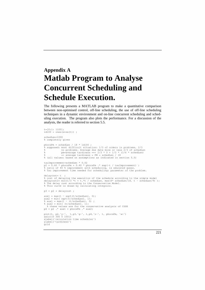
221
Appendix A
Matlab Program to AnalyseConcurrent Scheduling andSchedule Execution.The following presents a MATLAB program to make a quantitative comparisonbetween non-optimised control, off-line scheduling, the use of off-line schedulingtechniques in a dynamic environment and on-line concurrent scheduling and sched-uling execution. The program also plots the performance. For a discussion of theanalysis, the reader is referred to section 5.5.
t=[0:1: 1100];id100 = ones(size(t)) ;
schedLen=1000% completely given
phocsPm = schedLen / 18 * id100 ;% supposed: most difficult situation: 1/3 of orders in problems, 2/3% no problems. Average due date more or less 2/3 of schedLen% pm=average tardiness ==> 2/3 * 0 + 1/3 * (1/6 * schedLen)% => average tardiness = PM = schedLen / 18% (all values: based on assumptions as indicated in section 5.5)
tauImprovement=schedLen * 0.02p2 = 0.60 * phocsPm + 0.40 * phocsPm .* exp(-t / tauImprovement) ;% ratio of 40 % improvement with scheduling, is educated guess.% Tau improvement time needed for scheduling: parameter of the problem.
delaycost= t ;% cost of delaying the execution of the schedule according to the simple modeldelaycost2= min(1/3 *t + t.*t / schedLen, max(4* schedLen/18, t - schedLen/9) );% The delay cost according to the Conservative Model.% This curve is drawn by calculating integrals.
p3 = p2 + delaycost ;
aux1 = max(1 - sqrt(t/schedLen), 0);aux2 = min( sqrt(t/schedLen), 1);% aux1 = max(1 - (t/schedLen), 0) ;% aux2 = min( (t/schedLen), 1); % these values are for the conservative analysis of CSSEp4 = p2 .* aux1 + phocsPm .* aux2;
plot(t, p2,'y-', t,p3,'g-', t,p4,'r-', t, phocsPm, 'w:')axis([0 300 0 100])xlabel('calculation time scheduler')ylabel('tardiness')grid

Appendix A: Matlab Program to Analyse CSSE
222

223
If language were liquid,
it would be rushing in,
instead here we are in a silence,
more eloquent than any word could ever be.
These words are too solid,
they don’t move fast enough,
to catch the blur in the brain,
that flies by, and is gone.
Susanne Vega, 1986, Language, in: Solitude Standing.