Late Quaternary palaeoceanography of - CORE

Late Quaternary palaeoceanography of

the eastern Indian Ocean based on

benthic f oraminif era

Stefano Davide MURGESE

A thesis submitted for the degree of Doctor of Philosophy of the

Australian National University

_March 2003

Except where otherwise acknowledged in the text, this thesis represents original research by the author

_ ..... ~Oo · L_O L9~ -lano avi~,e~

ACKNOWLEDGEMENTS

My main acknowledgement goes to Patrick De Deckker: his approach to

environmental and palaeoenvironmental studies has been a major source of ideas

during this PhD. Lateral thinking is the fundamental requirement when studying the

environment, as atmosphere, oceans and land are all part of a unique system. I an1

indebted to him for encouraging me to begin this journey through the Quaternary. It

has been a fundan1ental step in expanding n1y perception of the philosophy behind the

processes regulating the environment and the delicate equilibriun1 in which they are

n1aintained.

He also helped n1e to improve my English by patiently reviewing my written

works. A special thanks goes to him for the chance he gave me to participate in the

scientific cruise TIP2000 on board the French vessel R. V Marion D71fresne.

My understanding of benthic foraminifera ecology has significantly improved

thanks to Professor Alexander Altenbach. Our long conversations regarding the

ecology and palaeoecology of these microorganisms proved to be of great sti1nulation

for the evolution of this research. I really appreciated the time spent in Gennany,

where 1 had the opportunity to consult the benthic foran1inifera collection of the

Departn1ent of Geo- and Environmental Sciences of the University of Munich. I also

thank Professor Altenbach and his wife~ Maren, for their hospitality during n1y tin1e in

Munich. My ideas about the oceanography and palaeoceanography of the eastern

Indian Ocean assumed a more organised structure thank to the discussions with Dr.

Franz Gingele about physical properties of water masses and the use of proxies in

palaeoceanographic research. Dr. Linda Radke gave me access to the statistical

software package CANOCO and shared with me her experience in n1tdtivariate

analysis. Dr Fran9ois Guichard hosted myself and my colleague, Michelle Spooner,

during the weeks spent in France at CNRS in Gif-Sur-Yvette. Fran9ois helped us

during the core-sampling operations. I also wish to thank him also for the data

provided for the cores BAR9403 and SH/9048. I ain also grateful to Judith Shelley for

the help the that she gave for preparing samples for isotope analyses, to Joe Cali, who

ran isotope analyses at RSES, and to Arne Sturm, who ran isotope analyses for

Fr 10/95 GCJ 7 san1ples.

Finally, I am grateful to Prof. Donata Violanti for her constant support and for

giving me access to the Department of Earth Sciences facilities in Turin, during the

time spent back in Italy.

To:

Valeria

Luigina e Franco

ABSTRACT

The distribution of the Recent benthic foran1inifera fron1 the eastern Indian Ocean

and their application for the reconstruction of palaeoceanographic conditions for this

region, during the Late Quaternary, are discussed herewith. The thesis is articulated in

two phases: ( 1) the study of the distribution of the Recent benthic foran1inifera and the

relationships with the surrounding environment, (2) the analysis of the benthic

foraminifera faunal content and 8 13C record of Cibicidoides wuellerstorfi fron1 three

deep-sea cores from the eastern Indian Ocean: Fr 10/95 GC'J 7, Fr J 0/95 GC5,

SH/9016 and BAR9403. In order to understand the factors influencing benthic foraminiferal distribution in

the eastern Indian Ocean, 57 core tops are investigated. Quantitative foraminiferal

analysis (%), Detrended Correspondence Analysis (DCA), Canonical Correspondence

analysis (CCA) and correlation matrix are used to define ecological structures.

Two groups of species are identified by 1neans of the first DCA ordination axis.

The first group includes three taxa: Oridorsalis tener umbonatus, Episto,ninella

exigua and Pyrgo murrhina whose percentage increases with depth. These three taxa

prefer a cold and well-oxygenated environment, where the carbon flux to the sea floqr

is low. 0. t. umbonatus and P. murrhina are interpreted as indicators of reduced food

availability, while E. exigua could be associated with periodic (seasonal) pulses of

organic matter to the sea floor. The second group of taxa includes Numn1oloculina

irregularis and Cibicidoides pseudoungerianus, typical of shal1ow depths. C.

pseudoungerianus is correlated with a warm environment characterised by high

carbon-flux rate. N. irregularis is associated with low-salinity levels, high dissolved

oxygen concentrations and its distribution mirrors the distribution of the Antarctic

Intern1ediate Water for this region. Based on the second ordination-axis scores, two other species are identified as

environn1entally significant: Uvigerina proboscidea and Bulin1ina aculeata. The

distribution of U proboscidea is mainly limited to low latitudes, where the carbon

flux rate is high, due to higher primary productivity levels at the sea surface, and

oxygen levels are low, because of the organic matter oxidation and the conten1porary

presence of oxygen-depleted Indonesian Intermediate Water (IIW) and N otih Indian

Intermediate Water (NIIW). B. aculeata is present at low latitude in areas

characterised by high phosphate concentration and where refractory phytodetritus is

eventually transported down-slope from the shelf. The opportunistic behaviour of this

species, indicated by high dominance levels characterising it, could relate the presence

of B. aculeata to seasonal inputs of food. The infauna} species are correlated with high carbon-flux rates and low dissolved

oxygen concentrations, while the porcellaneous taxa are correlated with high

dissolved-oxygen and low-salinity levels. Benthic foraminifera from the deep-sea cores are analysed by means of Q - mode

Factor analysis. The 8 13C record of C. wuellerstorfi is measured to gather infonnation

about past intermediate- and deep-water circulations. The benthic forarninifera

accumulation rate (BF AR) and the accumulation rates (AR) of B. aculeata, E. exigua

and U proboscidea are calculated in order to investigate episodes of increased

organic-1natter supply to the sea floor. The co-variance of the organic matter supply and dissolved-oxygen levels affected

the distribution of benthic foraminifera during the last 60 Kyrs. Below 1800 m, under

conditions of reduced deep-water circulation (low 8 13C of C. wuellerstorfi) and

increased carbon-flux rate (high BF AR and B. aculeata, E. exigua and U. prohoscidea

AR), B. aculeata dominated the benthic foraminiferal assemblage. In presence of a

more oligotrophic environment (low BFAR and B. aculeala, E. exigua and U.

proboscidea AR)~ characterised by active deep-water circulation (high 8 13C of C.

wuellers/01:fi), 0. t. ionhonatus (BAR9403) and C. wuellersto,~fi (Fr 10/ 95 GC5, SHJ9016 and BAR9403) don1inated the benthic foraminifera fauna. Above 1800 n1

and south of 20°S, the presence of strong bottom currents and the lateral advection of

sn1a1l amounts of organic matter, favoured the suspension feeder C. --vvuellerstmfi.

Under extremely high dissolved-oxygen levels, determined by the increased influence

of the Antarctic Intermediate Water (high 8 13C of C. wuellerstorji) and reduced

organic-n1atter supply, N. irregularis and G. subglohosa dominated the benthic

foraminifera assemblage. The reduction of oxygen levels and a n1ore stratified water column favoured the species U proboscidea and B. robusta.

These considerations allowed the reconstruction of the palaeoceanographic

evolution of the eastern Indian Ocean during the Late Quaternary:

• For 60 - 3 5 Kyr BP, conditions of higher productivity ( con1pared to the Present) at the sea surface were suggested for the Banda Sea.

• For 35 - 15 Kyr BP, still high productivity characterised the Banda Sea. Offshore Java and Sumatra, the prevailing NW-Monsoon reduced the intensity of the South Java Upwelling System and the organic n1atter supply to the sea floor. Strong and oxygenated bottom currents were present offshore Western

Australia. For the Last Glacial Maximum, a reduction of deep-water

circulation characterised the eastern Indian Ocean, while n1ore active circulation was recorded at intermediate depths. The enhancement of SE

Monsoon caused the South Java Upwelling System to increase its intensity,

thus the amount of organic matter to the sea floor. Higher productivity

otishore Java and Sumatra and in the Banda Sea favoured an increase of

productivity off the no1ih coast of Western Australia. Arid conditions over Australia, further reduced the amount of nutrients supplied to the ocean maintaining low-productivity levels off the west coast of Western Australia. At

the same time the Antarctic Intermediate Water was present north of 22°S.

• For 15 - 5 Kyr BP, increased precipitation levels led to the formation of a lowsalinity water cap at the sea surface reducing productivity over the Banda Sea and offshore Java and Sumatra. Off the north coast of Western Australia, the

nutrients injected into the ocean by the rivers maintained productivity levels

sin1ilar to those recorded for the LGM. Off the west coast of Western Australia, freshwater injected by the rivers deepened the nutricline, preventing

any increase of organic matter supply to the sea floor.

• For 5 Kyr BP - Present, a reduction of precipitation levels led to a slight increase of South Java Upwelling System intensity. In the Banda Sea, productivity levels were like those recorded for the Present. Off the Western Australian coast an increased influence of the oxygen-depleted Indonesian Intennediate Water and the Leeuwin Current engendered a more stratified

water column, characterised by low dissolved-oxygen levels.

CONTENTS

Introduction 1

PART I: The study of Recent benthic foraminifera from the eastern Indian Ocean 5

I. Benthic foraminifera ecology and palaeoecology of application for

palaeoceanographic studies 6

2. Materials and methods 11

2.1 The use of total assen1blages and the problems related to

taphonon1ic processes, which occur within the mixed sedin1ent

layer 16

3. Oceanography of the eastern Indian Ocean 22

3.1 The Indonesian Throughflow 23

3 .2 Surface currents 26

3 .3 Intermediate waters 27

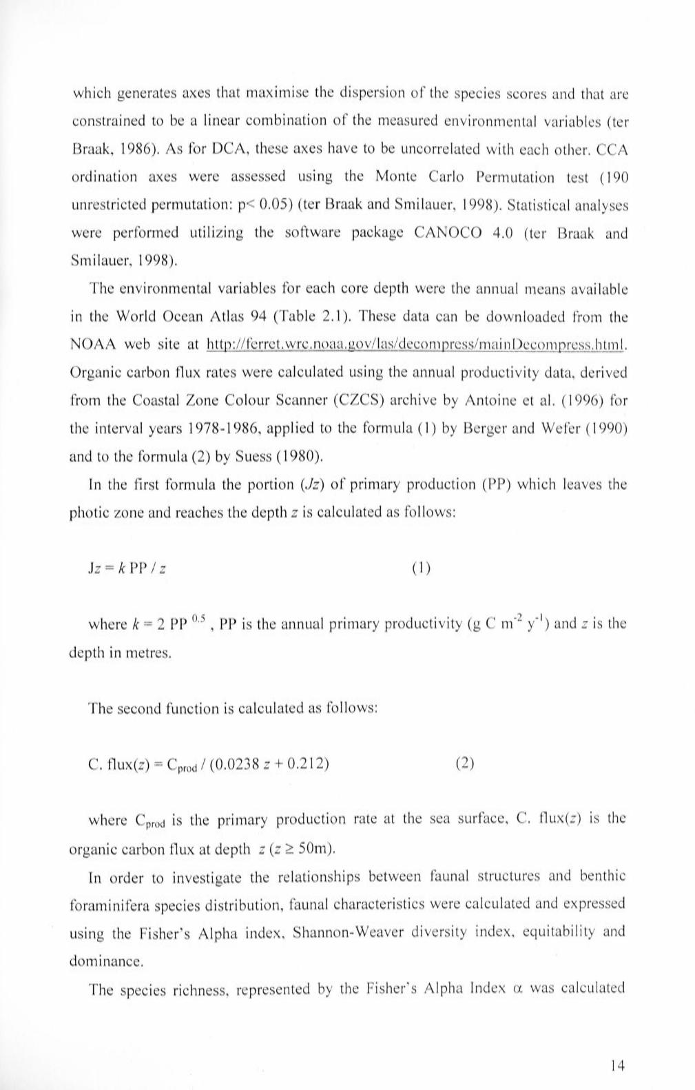
3.3.1 The Southern Sector 29

3.3.2 The Central Sector 29

3.3.3 The Northern Sector 36

3.4 Bottom and Deep waters 36

3.5 Productivity at the sea surface 39

4. Results 44

4.1 Detrended Con·espondence Analysis (DCA) 44

4.2 Environmental variables-fauna! characteristics correlation

matrix 47

4.3 Correlation between percentages of the species and the

environmental variables-fauna} characteristics 48

4.4 Canonical Correspondence Analysis (CCA) 55

4.5 Correlation between the agglutinated, calcareous infauna} and

porcellaneous taxa and the environmental variables-fauna}

characteristics 5 7

5. Discussion 5 8

5 .1 Faunal groups 62

6. Conclusions 64

PART II: The Late Quaternary palaeoceanography of the eastern Indian Ocean 66

7. The Late Quaten1ary palaeoceanography of the eastern Indian Ocean

based on benthic foraminiferal evidences 67

7 .1 Previews work 67

7 .2 What could benthic foran1inifera reveal? 68

8. Materials and Methods 70

8.1 Gravity core Fr 10/95 GCJ 7 71

8.2 Gravity core Fr 10/95 GC5 72

8.3 Piston core SHJ9016 74

8.4 Piston core BAR9403 75

8.5 Micropalaeontological analysis 77

8.5.1 Benthic Foraminifera Accumulation Rate (BFAR):

applications and problems 78

8.6 Isotope analysis 80 8.6.1 Methodology 80

8.7 Chronology 81

8.7.1 Gravity core Frl0/95 GCJ7 81

8.7.2 Gravity core Frl0/95 GC5 81

8.7.3 Piston core SHl9016 82

8.7.4 Piston core BAR9403 82

9. Results 85

9.1 Gravity core Fr 10/95 GC 17 85

9.1.1 Fr 10/ 95 GC'J 7: Factor Analysis 85

9.1.2 Fr 10/95 GCJ 7: faunal characteristics 88

9.1.3 Fr 10/ 95 GCJ 7: Benthic Foraminifera Accumulation

Rate (BF AR) and accumulation rates calculated for B. aculeata, E. exigua and U proboscidea 89

9.2 Gravity core Fr 10/95 GC5 93

9.2.1 Fri 0/95 GC5: Factor Analysis 94

9.2.2 Fr 10/95 GC5: faunal characteristics 97

9.2.3 Fr 10/95 GC5: Benthic Foraminifera Accumulation

Rate (BF AR) and accu1nulation rates calculated for B. aculeata, E. exigua and U. proboscidea 99

9.3 Piston core SH19016 101

9.3.1 SH/9016: Factor Analysis 101

9.3.2 SH/9016: faunal characteristics 105

9.3.3 SHJ9016: Benthic Foraminifera Accun1ulation Rate

(BF AR) and accumulation rates calculated for B. acuf eata, E.

exigua and U. proboscidea 106

9.4 Gravity core BAR9403 110

9.4.1 BAR9403: Factor Analysis 110

9.4.2 BAR9403: faunal characteristics 116

9.4.3 BAR9403: Benthic Foraminifera Accumulation Rate

(BF AR) and accumulation rates calculated for B. aculeata, E.

exigua and U proboscidea 116

9.5 8 13C results 120

9.6 Factor Analysis of the species abundance datasets: evaluating

the n1atrix closure effect 122

l 0. Discussion 126

10.1 The 8 13C distribution in the Indian Ocean 126

10.1.1 The 8 13C signal of the water masses, the carbon

isotopes fractionation and the use of C. wuellerstorfi as a

proxy to detect water carbon chemistry variations 126

10.1.2 The mean 8 13C Interglacial - Glacial variation for the

Indian Ocean 12 7

10.1.3 8 13C trends fron1 the cores collected from the eastern

Indian Ocean 128

10.2 The distribution of C. wuellerstorjz and G. subglobosa of

application for the study of palaeoceanography of the eastern

Indian Ocean 13 3

.. 11

10.3 Gravity core Fr 10/95 GCJ 7 135

10.4 Gravity core FrJ0/95 GC5 139

10.5 Piston core SHJ9016 142

10.6 Piston core BAR9403 144

l 0.7 The Palaeoceanography of the eastern Indian Ocean during

the Late Quaternary 148

1 0. 7 .1 6 2 - 3 5 K yr BP 14 8

1 0. 7 .2 3 5 - 15 K yr BP 14 8 10.7.3 15 - 5 Kyr BP 149

10.7.4 5 Kyr BP - Present 150

11. Correl usions 15 5

12. General Conclusions 159

12.1 The study of Recent benthic foraininifera 159

12.2 The study of the cores: benthic foraminifera 160

12.3 The study of the cores: eastern Indian Ocean

palaeoceanography during Late Quaternary 161

12.4 The study of the cores: fauna! turnover 162

12.5 Future research 163

References 165

APPENDICES

Taxonon1ic references Appendix Al Appendix A2 Appendix A3 Appendix A4 Appendix AS Appendix B Appendix C

LIST OF TABLES

TABLE

2.1 List of studied sample giving coordinates of each core, depth and

environmental variables measured or calculated at each site

4.1 Variance explained by each one of the four axes

4.2 Detrended Correspondence Analysis results for the reduced

species database. Scores of the species for axes 1, 2, 3 and 4

4.3 Correlation matrix between DCA ordination axes and the·

environn1ental variables-fauna! characteristics

111

Page

18

45

45

48

4.4 Correlation coefficients between the relative percentages of

benthic foraminifera species used for statistical analysis and the

environmental variables-fauna! characteristics considered in this

study

4.5 Intereset correlations between the first two ordination axes

calculated by means of Canonical Correspondence Analysis and

the environmental variables-fauna! characteristics considered in

this study

4.6

8.1

Correlation coefficients

agglutinated, infauna}

between the percentages of the

and porcellaneous taxa and the

environ1nental variables-fauna! characteristics considered in this

study

List of the cores used in this study

8.2 Number of benthic foraminifera species included for statistical

analyses in each core and average number of specimens counted

for each core

8.3

9.1

9.2

External errors of the two mass spectrometers used for isotope

analyses

Q-mode Factor Analysis (Principal Components) results for the

reduced species dataset of gravity core Fr I 0/95 GC'J 7: scores

for varimax Factors 1, 2 and 3

Factor loadings for the 46 samples from gravity core Fr I 0/95

GC17

9.3 Q-mode Factor Analysis results for the reduced species dataset of

gravity core Fr 10/ 95 GC5: species scores for varimax Factors 1

50

55

57

70

78

81

85

87

and 2 94

9.4 Factor loadings for the 46 san1ples from gravity core Fr 10/95

GC5

9.5 Q-mode Factors Analysis (Principal Components) results for the

reduced species dataset of piston core SH/9016: factors scores

for varimax Factors 1 and 2

9.6 Factor loadings for the 46 samples from piston core SH/9016

lV

95

101

103

9. 7 Q-mode Factors analysis (Principal Components) results for the

reduced species dataset of piston core BAR9403: factors scores

for varimax Factors I, 2, 3 and 4

9.8 Factor loadings for the 53 samples from piston core BAR9403

9.9 8 13C (%0) isotope data of C. wuelferstor_fz vs. PDB in Frl0/ 95

GCJ 7, Fr 10/95 GC5, SHJ9016 and BAR9403

9.10 Factor Analysis results for the species abundance datasets for the

four cores: don1inant species factor scores, cumulative variance

explained by the axes

l 0.1 Location, depth and I-G 8 13C difference measured for the cores

collected from the Indian Ocean

LIST OF FIGURES

FIGURE

2.1 Map of the eastern Indian Ocean and location of the cores

studied

2.2 Location of the core studied and distribution of the water 1nasses for

2.2

3.1

3.2

3.3

this region

Overview of the processes a±Iecting the generation of the benthic

foraminifera assemblage

Monsoon winds direction

Them1ocline circulation for the Indonesian Archipelago

Temperature-salinity diagrain along the path of Indonesia

Throughflow, showing the transformation of Pacific Central

Water into Indonesian Intermediate Water and subsequently into

110

112

120

123

129

Page

12

13

17

22

23

Indian Central Water 24

3 .4 Schematic near-surface current systems of the Indonesian

Throughflow region

3.5 Map showing the geographical position of the seven locations

used here to docu1nent chemical and physical properties of

V

26

3.6

3.7

3.8

3.9

3.10

3 .11

3.12

3.13

3.14

3.15

3.16

3.17

3.18

intermediate waters in the eastern Indian Ocean and the limits of

the three sectors identified by water masses characteristics

Temperature versus Salinity diagram for Location 1

Plots of oxygen levels versus depth for each of the seven

locations mentioned in the text



Ten1perature versus Salinity diagram for Location 4

Transect showing the dissolved oxygen levels between Australia

and Bali (in millilitres per litre)

Te1nperature versus Salinity diagram for Location 5


Te1nperature versus Salinity diagram for Location 7

Bottom topography of the Indian Ocean

Density levels [ cr4] (Kg m ·3) at the bottom of the Indian Ocean

Deep circulation pattern in the Indian Ocean basins

Te1nperature profile for the eastern Indian Ocean Region near

Sunda Strait. Seasonal variation of the thermal structure

3.19 Sea-surface chlorophyll levels for (a) the month of August

[Southeastern Monsoon] and (b) February [Northwestern

Monsoon]

3.20 Sediment discharge (106 t y- 1) fron1 the Indonesian Archipelago

28

29

30

32

32

33

34

35

35

36

37

38

39

40

42

and Papua New Guinea 43

3 .21 Am1ual mean primary productivity (g C m ·2 y- 1) at the sea-

surface in the eastern Indian Ocean estimated from satellite data 43

4.1 Distribution of the most common species (percentage >2% in at

least 10 samples) versus depth (m b.s.l.) 44

4.2 Values of the environmental variables and faunal characteristics

considered in this study versus depth

4.3 Species showing highest co1Telation with depth

4.4 Diagram showing the correlation between the distribution of C.

pseudoungerianus and carbon flux, calculated using (a) Suess ·

Vl

49

52

(1980) [C. flux(z)] and (b) Berger and Wefer (1990) [Jz]

formulae

4.5 N irregularis has higher percentages south of 20°S, for

environments characterised generally by high dissolved-oxygen

concentration

4.6 Percentages of U. proboscidea plotted versus carbon flux

calculated using Berger and Wefer (1990) [Jz], Suess (1980) [C.

flux(z)] formulae and dissolved-oxygen concentration

4.7

4.8

Percentage of B. aculeata plotted versus phosphate

concentration. This species has higher percentages for high

phosphate concentration levels

Diagrain showing the relationships between the environmental

variables and fauna! characteristics (arrows) and the first two

CCA axes (see text for further explanation)

5.1 Diagram to show the relationship between U proboscidea

percentages, dissolved-oxygen concentration, carbon flux

calculated using Berger and Wefer (1990) [Jz] and Suess (1980)

[C. flux (z)] formulae and depth versus latitude

5.2 Diagran1 to show (a) B. aculeata percentages and phosphate

concentration plotted versus latitude and (b) B. aculeata

percentages plotted versus depth

8.1

8.2

8.3

8.4

8.5

Location of the selected cores from the eastern Indian Ocean

Lithological log of Gravity core Fr 10/95 GCJ 7

Lithological log of Gravity core Fr 10195 GC5

Lithological log of Piston core SH19016

Lithological log of Piston core BAR9403

8.6 8 180 curves for the four studied cores from the eastern Indian

8.7

Ocean

Linear sedimentation rates calculated for the selected cores from

the eastern Indian Ocean using the Analyseries software (Paillard

et al., 1996)

9.1 Factor loadings for the san1ples of Fr 10/95 GCJ 7 calculated for

each one of the three factors and plotted versus age (Kyr BP)

.. Vll

53

53

54

54

56

61 -

62

71

73

74

75

76

83

84

90

9 .2 Diagram showing the percentages of those species, which

dominate the benthic foraminiferal faunas in the three groups of

san1ples, from gravity core Fr 10/95 GC 17, identified by means

of the Factor Analysis

9.3 Faunal characteristics calculated for each sample fron1 gravity

core Fr 10/95 GC 17

9.4 Gravity core Fr 10/95 GC 17: (a) Benthic Foraininifera

Accumulation Rate (BF AR) and (b) accumulation rates of B.

a cul eat a (blue line), E. exigua (green line) and U proboscidea

(red line)

9.5 Factor loadings for the sainples of Fr 10195 GC5 calculated for

each one of the two factors and plotted versus age (Kyr BP)

9.6 Diagram showing the percentages of those species from gravity

core Fr 10/95 GC5, identified by n1eans of Factor Analysis

9.7 Faunal characteristics calculated for each sample from gravity

core Frl0/95 GC5

9.8 Gravity core Fr 10/ 95 GC5: (a) Benthic Foraminifera

Accumulation Rate (BF AR) and (b) accun1ulation rates of B.

acufeata (blue line), E. exigua (green line) and U proboscidea

(red line)

9.9 Factor loadings for the samples of SHJ9016 calculated for the

two factors and plotted versus age (Kyr BP)

9 .10 Diagram showing the percentages of those species from piston

core SHl9016, identified by means of Factor Analysis

9.11 Fauna! characteristics calculated for each sample from piston

core SHf 9016

9.12 Piston core SH 19016: ( a) Benthic F oran1inifera Accumulation

Rate (BFAR) and (b) accumulation rates of B. acufeata (blue

line), E. exigua (green line) and U. proboscidea (red line)

9.13 Factor loadings for the samples of BAR9403 calculated for the

four factors and plotted versus age (Kyr BP)

9.14 Diagram showing the percentages of those species from piston ·

core BAR9403, identified by means of Factor Analysis

Vlll

91

92

93

96

97

98

100

104

105

108

109

114

115

9 .15 Fauna1 characteristics calculated for each sample from piston

core BAR9403 118

9.16 Piston core BAR9403: (a) Benthic Foraminifera Accumulation

Rate (BF AR) and (b) accumulation rates of B. aculeata (blue ·

line), E. exigua (green line) and U. proboscidea (red line)

9.17 Factor loadings calculated using the species percentage (red line)

[F 1 (%), F2 (%) and F3(%)] and the species abundance (green

119

dashed line) [Fl(n/g), F2(n/g) and F3(n/g)] datasets 124


[Fl(%) and F2 (%)] and the species abundance (green dashed

line) [Fl (n/g) and F2(n/g)] datasets 124


[F 1 (%) and F2 (%)] and the species abundance (green dashed

line) [F 1 (n/g) and F2(n/g)] datasets 125

9 .20 Factor loadings calculated using the species percentage ( red line)

[Fl(%), F2 (%), F3(%) and F4(%)] and the species abundance

(green dashed line) [Fl(n/g), F2(n/g), F3(n/g) and F4(n/g)]

datasets

10.1 Location of the deep-sea cores (solid circles) utilised to calculate

the average I-G 813C difference for the Indian Ocean

10.2 Mean I-G 813C difference calculated for the cores fron1 the

Indian Ocean

10.3 813C curves for the four cores studied in this research for the last

35 Kyrs

10.4 Values of the environmental variables considered in this study

n1easured for each sample dominated (high percentage) by C.

wuellerstorfi and G. subglobosa, at Present

l 0.5 (a) Downcore variations in relative abundance (%) of dominant

benthic foraminiferal species and (b) downcore variations in

benthic foraminiferal accumulation rates (BF AR) and

accumulation rates (AR) of B. aculeata, U. proboscidea, E.

exigua for the four studied cores

10.6 The situation of the eastern Indian Ocean at 30 Kyr BP

. IX

125

130

1 3 1

132

1 ') ') .).)

147

1 5 1

10.7 The situation of the eastern Indian Ocean at 18 Kyr BP 152

10.8 The situation for the eastern Indian Ocean between 15 and 5 Kyr

BP 153

10. 9 The situation for the eastern Indian Ocean at 5 Kyr BP 154

X

INTRODUCTION

The oceans' water 1nasses play an i1nportant role in the Planet Earth System. The

oceanic global circulation represents the medium through which heat, nutrients and

dissolved gasses are transported for thousands of kilometres, supplying the most

remote part of the globe and influencing climate and biological activity all over the

world. The El Nifio Southern Oscillation represents one of the most exhaustive

examples to understand the links between ocean dynamics, the atn1osphere and global

climate. Changes in the oceanographic setting and wind regimes of Pacific Ocean

have enormous repercussions all over the world, suppressing upwelling phenomena

offshore Chile and Peru (Shaffer et al., 1997), causing drought over Australia and

Indonesia and detennining rainfall increase over central Africa (Dawson and O'Hare,

2000).

One of the principal aims of modern research is to develop instruments to assist in

predicting future changes in terrestrial climate. To achieve this, the availability of

long-tern1 observations is crucial. In this sense, palaeoceanographic investigations

appear to be a suitable path to follow in order to understand how, in the past, cli1nate

and oceans changed and to provide long-term data series to apply to modern climatic

models.

The study of Quaternary climate revealed the presence of glacial cycles, with

periods of I 00 Kyrs, 43 Kyrs and 23 Kyrs in phase with Ea1ih' s orbital cycles:

eccentricity, obliquity and precession (lmbrie and Shackleton, 1976; Imbrie and

Imbrie, 1980). Recently it has been shown how the two sho1ier climatic cycles were

directly driven by obliquity and precession, while the I 00 Kyrs cycle was the result of

orbital changes effects combined with the expansion of the global ice-sheet cover

(Imbrie et al. , 1993 ). Climatic changes during the course of the Quaternary had a great

impact on the oceans. Increased or decreased polar ice-sheet cover and differences in

temperature gradients between high- and low-latitudes strongly affected the

production and circulation of water masses (Rahmstorf, 2002). During the Last

Glacial Maximum, due to the expanded Artie ice-sheet cover, the production of North

Atlantic Deep Water (NADW) diminished, leading to a global reduction of deep

water circulation (Duplessy et al., 1989). At the san1e time, the latitudinal shift of the

Polar Front and the Subtropical Convergence (Prell et al., 1980) favoured a n1ore

1

vigorous circulation at intermediate depths (Duplessy et al., 1989). Con1puter

generated 1nodels, designed to reconstruct past oceanic circulation, have indicated a

similar scenario (Ganopolski et al., 1998). These changes in the ocean circulation

patterns reduced the amount of heat transported from the low latitudes to the high

latitudes, ainplifying the temperature-reduction effect caused by din1inished solar

irradiance in the polar regions, during glacial phases (Williams et al., 1998).

Moved by the growing concern about the actual temperature rise, recent studies

have investigated . the CO2 levels in the atmosphere during the Quaternary and their

relationships with temperature changes (Bamola et al., 1987). The analysis of air

bubbles trapped in the polar ice has allowed, so far, the study of the atmospheric

concentration of CO2 during the last 420 Kyrs (Petit et al., 1999). Results indicate

high CO2 concentrations during interglacial (280-300 p.p.m.v.) and low

concentrations during glacial phases (180-200 p.p.m.v), suggesting the existence of a

strong relationship between global temperature and CO2 levels (Petit et al., 1999). A

possible mechanism, for such CO2 variations, is the reduction of Antarctic deep-water

production during glacial periods (Francois et al., 1997; Sigman and Boyle, 2000).

Another mechanism, potentially contributing to lower CO2 levels during the past, is

the increased export of organic matter to the sea floor due to increased productivity at

the sea surface. Sigman and Boyle (2000) suggest that the decrease in the production

of deep-waters at high latitude was also accompanied by a more efficient utilization of

nutrients by the phytoplankton, which led to increased productivity in the Subantarctic

Zone during glacial phases. The idea behind this model is that seawater iron

concentration influences the ability of phytoplankton to exploit nutrients: the "iron

hypothesis" (Martin, 1990). Laboratory experiments have shown how diato1ns utilise

nutrients more efficiently in presence of high iron concentrations (Takeda, 1998).

According to the "iron hypothesis", increased wind strengths during the glacial

periods led to an increased transport of dust from the continents to the oceans,

increasing the concentration of iron at the sea surface (Petit et al., 1999). The

intensification of wind regimes during the Last Glacial Maximum also strengthened

the intensity of oceanic upwelling cells at low latitude, causing productivity to

increase (Sarnthein et al., 1988). The real contribution of each of these processes to

the reduction of CO2 levels is still debated, as many other factors (e .g. bion1ass

reduction over the continents, global changes in alkalinity of the oceans, sea surface

2

temperature variations, etc.) played a role in influencing atn1ospheric CO2

concentration.

The analysis of different proxies from deep-sea core sediment, collected from

various parts of the world, can provide information about the evolution of oceans and

climate: benthic foraminifera are one of these proxies. These microorganisms, vvith

their good fossil preservation potential, are a reliable means through which to describe

processes occurring at the sea floor as well at the surface of the oceans.

During the last decade the links between benthic fora1ninifera distribution, water

mass properties and productivity levels at the sea surface have been extensively

investigated. The infonnation acquired allowed the successful use of these

microorganisms as palaeoceanographic proxies in order to reconstruct past sea-surface

productivity levels (Mackensen et al., · 1994; Kuhnt and Hess, 1999), the extension of

the oxygen minimum zone ( den Dulk et al., 1998) and the carbonate undersaturation

of the water masses (Miao and Thunell, 1996). Most studies on benthic foraminifera

have been focused on the Atlantic and the Pacific Oceans and few of the works fro111

the Indian Ocean were related to the eastern paii of this basin (Corliss, 1979a; Corliss,

1979b; Van Marie, 1988; Wells et al., 1994 ).

Aims of the thesis

The eastern Indian Ocean circulation is under the influence of the monsoonal

climate and of the Indonesian Throughflow. The latter represents a major con1ponent

of the global circulation model , as the volume of water, which moves from the Pacific

to the Indian Ocean, is approximately the same of the volume of water involved in the

fom1ation of the North Atlantic Deep Water (Schmitz, 1995; Schn1itz, 1996;

Ganachaud and Wunsch, 2000). With the Indonesian Throughflo\V · a considerable

an1ount of heat absorbed from the atmosphere by Pacific Waters is transported to the

Indian Ocean (Ganachaud and Wunsch, 2000). In order to understand past variations

of the oceans ' circulation, the investigation of the evolution of the Inda-Pacific region

is crucial.

During the last decade four oceanographic cruises took place in the eastern Indian

Ocean: Shiva (1990), Bara! (1994), FrJ0/95 (1995) and Fr 2/96 (1'996). These

scientific expeditions collected a large number of gravity and piston cores fron1 the

region. This core dataset represents a valuable source of information for i111proving

the knowledge about the palaeoenvironmental evolution of the eastern Indian Ocean

during the Late Quaternary.

This thesis will investigate the environmental variables that influence the

distribution of Recent benthic foran1inifera. The results obtained will be then applied

to the study of fossil assemblages in order to reconstruct the palaeoceanographic

evolution of the eastern Indian Ocean for the last 60 Kyrs.

1. Recent benthic foraminifera will be studied using a dataset of 57 core tops. A

number of environmental variables will be measured in order to obtain inforn1ation

about water mass properties (ten1perature, salinity, dissolved-oxygen concentration)

and nutrient concentrations (phosphate, nitrate). Links between benthic f oram ini fera

distribution and processes at the sea surface will be investigated by considering the

sea-surface primary-productivity levels and the carbon-flux rate at the sea floor. The

relationships between foran1inifera and environment will be analysed by means of

statistical analyses ( ordination techniques and correlation matrix).

2. The palaeoceanographic evolution of the eastern Indian Ocean will be studied by

analysing the benthic foraminifera faunal content of selected cores from this region.

Statistical analyses, plus the information acquired about the distribution of Recent

foraminifera, will be used to interpret the faunal changes observed in the cores.

3. The 8 13C of Cibicidoides wuellerstorfi will be measured to investigate the past

intern1ediate- and deep-water circulation and variations of organic matter supply to

the sea floor.

4

PART I: The study of Recent benthic f oraminif era f oraminif era from the eastern Indian Ocean

s

1. Benthic foraminifera ecology and palaeoecology of application for

palaeoceanographic studies.

Benthic foraminifera are abundant in 1narine sedin1ents. They are present at all

latitudes and also have a good fossil preservation potential. For these reasons, they

represent a useful tool for oceanographic and palaeoceanographic studies. During the

last thirty years much research has been conducted in order to define the links

between the ecology of these microorganisms and the environment in which they live.

Several studies have successfully determined links between distribution of benthic

foraminifera, water masses patterns and characteristics. Streeter (1973) used benthic

foraminifera to trace water mass flow in the North Atlantic. He distinguished three

n1ajor asse1nblages, one associated to cold and deep waters ( <2°C), which he called

?Epistominella umbonijera assemblage, another associated to less cold waters (2-3°C)

nan1ed Epistominella exigua - Cibicidoides wuellerstorjz assemblage and a third

associated to warn1er waters (3-4 °C), the Uvigerina hollicki assemblage. Anderson

( 1975) studied benthic foraminifera from the Weddell Sea and identified six

assemblages defining a relationship between their distribution and water 1nass

characteristics, such as CaCO3 saturation and salinity. In the Southern Ocean, Corliss

( 1979a) was able to define two major fauna! assen1blages for the region. The first one

is dominated by E. umbonifera, Planulina wuellerstorfi, Globocassidulina

subglobosa, Pullenia bulloides, Oridorsalis tener and is associated to Antarctic

Botton1 Water (AABW). The second assemblage is marked by a strong dominance of

Uvigerina spp. and E. exigua and is related to Indian Bottom Water (IB W). The

author showed that transition from one assemblage to another is determined by the

availability of calciu1n carbonate in bottom waters. In the Eastern Indian Ocean, along

the Ninetyeast Ridge, Peterson ( 1984) identified distinctive benthic foran1inifera

faunas, which showed defined links with the hydrology of that region. In this study,

the assemblage dominated by G. subglobosa, Pyrgo spp., Uvigerina peregrina,

Eggerella brady, is associated to Indian Deep Water (IDW), while the one dominated

by Nuttalides unzbonifera and E. exigua con·esponds to Indian Bottom Water (IBW).

Denne and Sen Gupta ( 1991) pointed out a relation between Gulf of Mexico water

masses and five benthic foraminifera assemblages. These authors were also able to

6

distinguish two other assemblages 1nainly related to the oxygen content of the water:

one assen1blage ( dominated by Nonionella opin1a, Bolivina barbata, Buli,nina

marginata, Bolivina alata) is related to oxygen-depleted waters of Mississippi Delta

and the other (represented by Albaminella turgida) is typical of oxygen-rich habitats.

Further research focused on relationships that exists between benthic foran1inifera

distribution and specific water masses properties. Some of these works underlined

how the oxygen content of the pore water plays an important role as well as the

oxygen content of the overlying water masses. Miller and Lohmann ( 1982), for

example, found a correlation between Globobuliminal Bulimina assemblage and the

oxygen minimum zone of the north-east United States continental slope. These

authors observed also how U peregrina is not influenced by the dissolved oxygen in

the water column but instead is related to the amount of organic carbon content and

low oxygen levels within the sedi1nent. Moodley and Hess ( 1992) conducted an

experiment on living benthic foraminifera. They noticed that deep-dwelling species

(Ammonia beccarii, Elphidium excavatum, Quinqueloculina sen1,inulum) had very

low-oxygen requirements. Moodley et al. (1998) conducted laboratory experi1nents on

specin1ens of Quinqueloculina seminula and described the capability of this species to

withstand anaerobic conditions. They reported how the survival of the studied

specimens appeared to be limited by the formation of H2S within the sediment.

Factors such as the level of tolerance to low-oxygen conditions or the food

availability concur to define specific n1icrohabitats within the sedin1ent for different

species. Corliss ( 1985) was able to put in evidence a vertical stratification of the taxa

within the samples studied. He distinguished epifaunal species found living close to

the sediment/water interface. These taxa showed a preference for an oxygenated

environment (Hoeglundina elegans, P. wullerstorfi, Cibicidoides spp.). Species like

C'hilostomella oolina, Globobulimina affinis, Melonis barleeanu,n were found

preferentially in the deeper part (5-8 cm) of the sediment and were referred as

infauna! species. These kinds of taxa seem to be well adapted to low-oxygen levels.

Jorissen et al. ( 1995) studied benthic foraminifera from the Adriatic Sea and

developed a conceptual model to explain microhabitat preferences in tern1 of organic

flux to the seafloor and depth of the redox front in the sediment: the TROX model. In

this model, under oligotrophic conditions, the vertical distribution of the species is

controlled by the availability of food. Under eutrophic conditions, the n1aximum depth

at which fauna can survive is detennined by the thickness of the oxygenated layer in

7

the sediment. In regions where bottom water oxygenation, salinity and ten1perature

are uniform the study of benthic foraminifera shows how the sediment organic carbon

content is the main factor that controls fauna! patterns (Rathburn et al., 1996). Other

studies from the Arabian Sea point out that under a pronounced OMZ oxygen is no

n1ore a limiting factor because 1nany of the species present in that region are already

adapted to withstand low oxygen conditions (Jannik et al., 1998). This study of

samples collected in and below the OMZ, shows how, within this severely oxygen

depleted environment, benthic foraminifera position in the sedin1ent is 1nainly related

to the amount or type of food that reaches the sea floor. Son1e species, such as B.

dilatata, Bulin1ina exilis, U. peregrina, seem to prefer unaltered organic matter.

Below the OMZ, where the organic matter appears to be reduced and altered,

opportunistic species (E. exigua, Bulimina aculeata, M barleeanum, Rotalinopsis

semiinvoluta) are abundant.

The existing data allow to distinguish four major patterns 1n the vertical

distribution of benthic foraminifera ( J orissen, 1999). A "type A", representing

epifaunal-shallow infauna! species, includes those species showing highest abundance

in the top-n1ost level of the sediment (0-2 cm). A "type B ", representing shallow

infaunal-transitional species, is composed by the taxa that can live in the upper part as

well as deeper in the sediment (0-4 c1n). A "type C", which includes the species

presenting mainly downcore maxima ( 4-5 cm), and the "type D", which is typical of

those species showing high abundance at the surface (0-1 cm) and in the deeper paii

of the sedi1nent (6-7 cm).

The preference of foraminifera for certain microhabitats determines differences in

the morphology of their test. The epifaunal species are usually characterised by a

plano-convex, biconvex test, without large pores (but if found they only occur on one

side) and trochospiral or milioline coiling (Corliss and Chen, 1988). Such test shape

can result advantageous in order to remain attached to the substrate in presence of

current and the position of the aperture is well suited for feeding and loco1notion

(Corliss, 1991 ). The shallow infauna! species have pores all over their test and are

characterised by uni serial, triserial or planispiral coiling ( Corliss and F ois, 1 991 ). In

this group the test is also characterised by ornamentation which could represent a

useful way of ren1aining in the top-most level of the sediment or for mantaining the

same orientation within the sedin1ent ( Corliss, 1 991 ). Intermediate infauna! species

have generally planispiral coiling, rounded periphery and pores over the entire test. It

8

appears that these pores can enhance gas exchange especially in a low-oxygen

environment (Corliss, 1985). Deep-infauna! taxa characterised by planispiral or

triserial coiling and ovate or cylindrical test.

The an1ount of organic matter sinking from the sea surface controls the patterns of

some species (Lutze and Coulboum, 1983; Mackensen et al. , 1985). Organic matter

availability is an important factor linking benthic foraminifera to productivity level at

the sea surface. Some benthic foraininifera species bloom when phytodetri tus reaches

the sea floor (Gooday, 1988; Gooday, 1993). For example, Gustafsson and Nordberg

(2001) reported a seven-fold increase of Stainforthia .fus[formis population size as a

consequence of spring phytoplankton bloom. Laboratory experi1nents have also

shown how Cribrostomoides subglohosum increases individual bodyn1ass in the

presence of a food pulse (Altenbach, 1992). In the Norwegian Sea, Altenbach and

Sarnthein ( 1989) found a positive correlation between the distribution of C.

wuellerstorfi and E. exigua and the a1nount of organic matter in the sediment. Loubere

( 1 991 ), who studied assemblages fro1n the equatorial Pacific Ocean, focused on a set

of samples fro1n an area where productivity at the sea surface was apparently the only

variable affecting the sea-floor community. This author identified an assemblage

don1inated by U peregrina, M barleeanum and C. wuellerstor.fi associated to higher

productivity and another assemblage dominated by E. umhonifera related to lower

productivity.

The presence of organic matter at the sea floor and its subsequent oxidation causes

depletion in oxygen in sedin1ent pore-water, thus low-oxygen tolerant species have

been observed. Under eutrophic conditions, infauna! taxa are the most abundant,

while under oligotrophic conditions and higher oxygen levels, opportunistic epifaunal

species dominate the faunas (Gooday and Rathburn, 1999). In areas of coastal

upwelling along the western African coasts, Schmied! et al. (1997) found that benthic

foraminifera assemblages vvere dominated by elevated standing stocks, low diversities

and a large number of infauna! taxa, such as: Uvigerina , Melonis, Bolivina, Bulirnina,

Globobulimina and Cassidulina. On the other hand, offshore, under more oligotrophic

conditions, the asse1nblages were dominated by epifaunal species, such as: E. exigua,

N. un1bonifera. Futher, Kuhnt et al. ( 1999) determined the relationship existing

between benthic foran1inifera from South China Sea and organic flux down to the sea

floor. This study showed how the species related to food supply occupied infauna!

9

microhabitat ( U. peregrzna, Bolivina robusta, Bolivina pacijica, Trifarina bradyi,

Rosalina concinna, Cassidulina crassa, Epistominella rugosa and G. qffinis).

The rate of organic matter oxidation is reduced under disoxic condition and its

burial within the sediment is therefore more efficient. Under these conditions '

k-strategist/deep-infaunal species, which rely on refractory phytodetritus, find optin1al

conditions and consequently their abundance increases (Jannik et al., 1998). Already,

Rathbum and Corliss (1994) described a positive correlation between the abundance

of deep-dwelling/low-oxygen tolerant species and high nutrient flux to the sea floor.

These authors noticed how C. oolina, Chiloson1ella ovoidea, Globobulimina spp. and

Valvulineria mexicana take advantage of the sediment subsurface accumulations of

organic carbon. A similar trend between the abundance of deep-infauna! taxa (B.

alata, Chilostomella spp., Globobulimina spp.) and mineralised organic matter was

described also for the Mediterranean Sea by De Rijk et al. (2000). In the Arabian Sea,

Kurbjeweit et al. (2000) interpreted the positive correlation between Chloroplastic

Pigment Equivalents in the sediment and the taxa G. q.ffinis, Lagenanunina

d[fjlug[forn1,is, B. aculeata and M barleeanum as an indication for their preference for

altered phytodetritus.

The study of modern assemblages is therefore necessary to acquire a better

understanding of the factors that influence the distribution of benthic fora1ninifera.

This is a fundainental procedure for using the remains of these microorganisn1s as a

proxy of past oceanographic conditions.

The eastern Indian Ocean is characterised by complex circulation systems at the

sea surface and at intermediate depth. As a consequence, environ1nental variables

present strong latitudinal gradients in the water column. The monsoonal climate is

responsible for the strong seasonality of the South Java Upwelling Systen1 and,

together with the Indonesian Throughflow, for a significant difference in primary

productivity between Indonesia and Australia. In this first part, fifty-seven core tops

collected offshore Western Australia and offshore Java and Sumatra Islands have been

analysed in order to investigate eventual links that may relate benthic foran1inifera to

the oceanographic processes in these regions. Statistical analyses have been

performed to define the relationships between the distribution of benthic foraminifera

species and the environmental parameters measured for the studied area. ·

10

2. Materials and Methods

A total of 57 core tops was utilised for this study (figure 2.1 ). 44 gravity cores were

collected during two cruises offshore Western Australia: Fr 10/95 in 1995 and Fr 2/96

in 1996, using the RV Franklin. The remaining 13 core tops were sampled from

trigger cores collected during two other cruises offshore Java and Sun1atra: Shiva in

1990, Barat in 1994, using the RV Baruna Jaya.

While short trigger cores (60cm) minimize the loss of surface n1aterial when

collecting sainples from the sea floor, gravity cores may not return samples at the

sediment-water interface. However, the set of core tops utilised for this study is the

same used by Martinez et al. ( 1998a), who sampled the cores on board of the RV

Franklin soon after recovery, in order to avoid contamination and n1ixing.

The cores were collected from the upper-bathyal (~ 700 m b.s.l.) to the abyssal

zone (~ 4500 m b.s.l.), within a depth ranges of the water masses similar to those

signalled for the water n1asses present in this region (figure 2.2).

Samples used for this study were obtained from the first 1 to 2 cm of each core.

About 3 cc. of material from each sample was soaked in a dilute (3%) hydrogen

peroxide solution until clays had fully disaggregated, then washed wi~h a gentle water

jet through a 63 µm sieve and the coarse fraction was then dried at 40°C.

All the benthic foran1inifera of the total assemblage from the fraction > 150 ~Lm of

each sample were counted. When the number of specimens in the sediment was less

than 70 individuals, more material was washed and added for counting.

Benthic foraminifera were identified and mounted on a slide and the absolute

nu1nber of specimens for each species was recorded. Fragments of Rhabdam,nina sp.,

Rhizan1mina sp. , and the other tubular-shaped species were considered to indicate the

presence of at least one specimen in the sample. An average of 241 specimens per

sample was identified and counted. The fraction > 150 µm was selected in order to

allow a comparison with previous works such as those of Corliss (1979a) and

Peterson (1984).

301 species were identified (see Appendix Al and Taxonomic references). The

san1ples from cruises Fr J 0/95 and Fr 2196, were those utilised by Martinez et al.

( 1998a), who studied planktonic foraminifera. While the volume of sediment taken

1 1

was recovered, the lack of records related to the dry weight of sedin1ent did not allow

to express the abundance (n/g) of each species.

goo

oo

10°

20°

30°

goo

100°

89407. 89 89436. • 4

~ •

89437 · I\

89438 • . · ~ -89440 ·: -

110° 120°

•.. $9045 . ; I"

89441 • .• 89442 .· · ·

Indian Ocean

100°

· Fr2-16 fr2 :15• • ,Fr2°17

. · ·. . Fr2-20 Fr2-19• • Fr2-2 1

· Fr2-24 Fr2-25 Fr2-2J• • • Fr2-26

Fr 1 -:12 • Fr l-1 i Fr1-13• • •Fr1-10

Fr2-14• · eFr1-15 •Fr1-14 .

Fr1~15• ; ···. · Fr2-12 fr1-'17• ·· .

·Fr2-11 Fr1-18• Fr2-13•• Fr1 -19

Fr2- 10t • • . Fr2-9 _ Fr1 , 20 /

Fr1-21• Fr2- 7• •

Fr1-22 Fr1 -23 •• .

Fr2-2 • • '· Fr2-3 I.

Fr1 -28 z Fr1-27 ·• Fr1-29 Fr2-1

110° 120°

130°

130°

Fig. 2.1 - Map of the eastern Indian Ocean and location of the cores studied.

140°

oo

10°

20 °

30°

140°

The abbreviations beside each core location indicate the cruise during which the each core was collected (prefixes Fri = Fr/0195, Fr2 = Fr2/96, B = Barat, S = Shiva). The number after each abbreviation indicates the number of the core top.

For this reason, the absolute number of specimens for each species was converted

as the percentage of total foraminifera present in each sample. Those species present

with a percentage >2% in at least 1 sample were used for statistical analyses. In order

to acquire useful information for application to palaeoenvironn1ental and

palaeoecological studies, agglutinated taxa, which presented poor preservation

potential and were not found when analysing the fossil faunas from sel_ected cores

from the same area (see sections 8, 9 and 10), were eliminated from the database.

Note that the genera Fissitrina, Lagena, Lenticulina, Oolina and Parc{fissurinu were

12

present in many samples with high species diversity.

0 ·r--------- .,-----------.---------------------

SICW •

-.

--------...------ .. • • . . .. ;. • • • AAIW :

• _- IIW ·- • •

I •• I I

•

I •

• NIJW •

. (/)

500

1000

1500

2000 ·-·• • - • - • - • • - • • •a A • • ,_ ._ W • • • • _. • ..., • - I. • - • .. .. • • ,. • • - • • • • • .

. .0

E -2500

3000 --

:5 3500 C.

• • •• • • • •

• - • • I •• 1ow• • • • • • • ~ 4000 -~----------~----------------------------------

4500 • AABW 5000 ... -- ··1···· ·· 1 · . ... I --

35 25 15 5 Latitude S

Fig. 2.2 - Location of the cores studied and water masses distribution for this region.

0

SICW = South Indian Central Water; AAIW = Antarctic Intermediate Water; IIW = Indonesian Intermediate Water; NIIW = North Indian Intermediate Water; IDW = Indian Deep Water; AABW = Antarctic Bottom Water.

The percentage of each species was generally low ( <2.5% ). Therefore, all the

species belonging to these genera and used for statistical analyses were grouped

together as Fissurina spp., Lagena spp. , Lenticulina spp., Galina spp. and

Parafissurina spp.

A total of 7 5 taxa was utilised for Detrended Correspondence Analysis (DCA) and

Canonical Correspondence Analysis (CCA). The DCA is a type of ordination

particularly suitable for databases with many zeros and for unimodal response 1nodels

in which the abundance of any species follows a normal distribution (Jongman et al.,

1987). DCA algorithm generates axes that maximise the dispersion of the species

scores and that are constrained to be uncorrelated with each other (Jongman et al. ,

1987). The axes are calculated in such a way that at any point, on the ith axes , the

mean value of the site scores on the subsequent axes is zero, avoiding in this way the

"horseshoe effect" (Jongman et al. , 1987). Canonical Correspondence Analysis

(CCA) was then performed in order to explore the relationship between environmental

variables and benthic foraminifera distribution. CCA is a direct gradient analysis,

13

which generates axes that maximise the dispersion of the species scores and that are

constrained to be a linear combination of the measured environmental variables (ter

Braak, 1986). As for DCA, these axes have to be uncorrelated with each other. CCA

ordination axes were assessed using the Monte Carlo Permutation test ( 190

unrestricted permutation: p< 0.05) (ter Braak and S1nilauer, 1998). Statistical analyses

were performed utilizing the software package CANOCO 4.0 (ter Braak and

Smilauer, 1998).

The environmental variables for each core depth were the annual 1neans available

in the World Ocean Atlas 94 (Table 2.1). These data can be downloaded fro111 the

NOAA web site at http: / !ferret. \Vrc.noaa.gc)\:/ las/decon1press/111ainl)econ1press. htm I.

Organic carbon flux rates were calculated using the annual productivity data, derived

from the Coastal Zone Colour Scanner (CZCS) archive by Antoine et al. (1996) for

the interval years 1978-1986, applied to the formula ( 1) by Berger and Wefer ( 1990)

and to the fonnula (2) by Suess ( 1980).

In the first formula the portion (Jz) of primary production (PP) which leaves the

photic zone and reaches the depth z is calculated as follows:

Jz = k PP I z (1)

where k = 2 PP 0·5

, PP is the annual prin1ary productivity (g C 111-2 y- 1) and z is the

depth in metres.

The second function is calculated as follows:

C. flux(z) = Cprod / (0.023 8 z + 0.212) (2)

where Cprod is the pnmary production rate at the sea surface, C. flux(z) 1s the

organic carbon flux at depth z (z > 50m).

In order to investigate the relationships between faunal structures and benthic

foraminifera species distribution, faunal characteristics were calculated and expressed

using the Fisher's Alpha index, Shannon-Weaver diversity index, equitability and

do1ninance.

The species richness, represented by the Fisher's Alpha Index a was calculated

14

following the formula:

a= (N*(l-x))/x

where N is the number of taxa and x is a constant related to the ratio N/S (S =

nu1nber of species) (Willian1s, 1964)

The grade of heterogeneity of each sample has been assessed calculating the

Shannon-Weaver Index [H(S)] with the following formula:

s

H(S) = - Ipdn p; i= I

where S is the number of species present in the sample and p; is the percentage of

the ith species divided by 100. The higher is the value of the index~ the higher is the

grade of differentiation of the species in the sample (Murray, 1991 ).

The H(S) index was then used to calculate the equitability [E] of each san1ple

(Murray, 1991):

E - e H(S)

The do1ninance [DJ was calculated as the percentage of the most abundant species

of each sa1nple ( den Dulk, 2000).

In order to investigate eventual relationships between fauna! groups and the

environment, the percentages of the species belonging to the agglutinated taxa, the

presun1ed calcareous-infauna! species and to the porcellaneous species, were sumn1ed

separately. The total percentage of each group (Table 2.1) was then correlated with

the environmental variables considered in this research.

The selection of the species belonging to the calcareous infauna! group was n1ade

on the basis of the results of researches conducted in different parts of the world

(Appendix B).

1 5

2.1 The use o,f total assemblages and the problen1s related to taphonon1ic

processes, which occur within the mixed sediment layer.

When studying Recent benthic foraminifera, the use of total assen1blages in1plies

analysing a combination of living plus dead specimens, collected, as in this case, fron1

the first centimetres of the sediment. Within this interval, the scarcely compacted

sediment undergoes continuous mixing. This situation has repercussion on the

composition of the total assemblage, since the foraminifera tests are produced and

deposited in a non-steady environ1nent. The n1icropalaeontological (,(,signar\

recovered from a sediment sample, represents the result of a time - average, which is

the process through which fossils of different ages are mixed into a single assemblage

(Martin, 1999). This phenomenon is caused by the fact that a foraminiferal generation

time is n1uch shorter than the rate of sediment accumulation. "The total assen1blage

represents an average, with the advantage of elin1inating short-tern1 noise" (Martin,

1999), but, since the total-assemblage includes living plus dead speci1nens, it is

i1nportant to define the similarity degree between the dead- and the Ii ving-assemblage

and understand the processes responsible for the eventual differences observed

between the two.

The dead-assemblage 1s produced by the living species, within the upper

centimetres of the sediment (Loubere, 1990) and should reflect the con1position of the

living-assemblage at the site where it is found (De Stigter et al. , 1999). The duration

of the permanence within the mixed layer by an empty test, will determine higher or

lower exposure to all the taphonomic processes. These can cause the compositional

differentiation between the dead-assemblage and the living-assen1blage. For example,

bottom currents can transport allochthonous ·tests fron1 elsewhere, or specimens from

the living-assen1blage can be carried away in the same way (De Stigter et al., 1999).

Deep-borrowing macrobenthos activity can cause mixing of older material with

younger material or vice versa (Rathburn and Miao, 1995). Another factor which can

differentiate the living- from the dead-assemblage is the selective destruction of tests

(Murray and Alve, 2002). In environments characterised by active carbonate

dissolution, assemblages dominated by agglutinated species can result fron1

assemblages initially dominated by calcareous species, after selective dissolution of

calcareous tests (Murray and Alve, 1999). Preservation of calcareous tests can also be

favoured by bacterial sulfate-reduction consequently resulting in an alkalinity increase

16

(Martin, 1999). In condition of normal carbonate concentration, soft- or iron oxide

cemented agglutinated taxa are more subjected to destruction rather than calcite

cemented agglutinated taxa or calcareous species (De Stigter et al., 1999; Murray and

Alve, 1999). In areas characterised by low sedimentation rate, long permanence-time

within the mixed layer can cause the loss of shallow-dwelling species, detern1ining an

over-representation of infauna! taxa in the dead-asse1nblage (Loubere, 1990). Test

production rate may also play a role in the process of differentiation betvveen the

living- and the dead-assen1blage (Edelman-Furstenberg et al., 2001 ). Where the

selective loss of shallow dwelling species is minimized, their high test-production

rate, compared to infauna! species with lower turn-over rate, may cause the opposite

situation (De Stigter et al., 1999). The processes, which can take place within the

mixed layer and take part in the creation of the fossil assemblage (long-term) and of

the total assemblage (short-term), are illustrated in figure 2.3.

reworklng of tb.$$-ir foramlnHera lnlo recent

s~dirnetH

Fig. 2.3 - Overview of the processes affecting the generation of the benthic foraminifera assemblage (copied from De Sigter et al., 1999).

17

Table 2.1 - List of studied sample giving coordinates for each core, depth, environmental variables measured or calculated and the faunal characteristics at each site. (* = gCm-2fl; # = pressure calculated for the site's depth)

Sample Latitude (S) Longitude (E) Depth (m) Salinity %0 Temperature °C Oxygen (ml/I) Pressure dbar# Phosphate (pmol/1) Frl-5 14°00.55' s 121 °01.58' E 2472 34.73 1.96 3.44 2552.34 2.05 Frl-7 14°42.58' s 120°32.74' E 1445 34.67 3.41 2.55 1491.96 2.35 Fri-IO l 8°08 .93' S 116°01.29' E 1462 34.69 "'I "'I 6 .) . .J 2.84 1509.52 2.55 Fr 1-1 l 17°38.57' s 114°59.93' E 2458 34.73 1.92 3.45 253 7 .89 2.13 Fr 1-12 18°14.7' s 114°59.63' E 2034 34.73 2.43 3.17 2100.ll 2.16 Frl-13 18°49.26' s 113°58.26' E 1454 34.67 3.39 2.74 150 l.26 2.69 Fr 1-14 20°02.71' s 112°39.73' E 997 34.64 5.07 ) "") __ .)_ l 029.40 2.24 Frl-15 19°53.75' s ll2° 13.37'E 1393 34.66 3.8 l 2.62 1438.27 2.35 Fr 1-l 6 20°59.83' s 112°59.35' E 1221 34.65 4.43 2.35 1260.68 2.30 Fr 1-17 22°07.74' s · 113°30.l l' E 1093 34.63 4 .65 2.37 1128.52 2.17 Fr I - l 8 22°59.64' s 112°49 .86' E 1055 34.63 4.69 2.73 1089.29 2.17 Fr 1-19 24° 14.ll'S I I 0°00.18' E 1974 34.72 2.41 3.37 2038.16 2.20 Fr 1-20 24°44.67' s 111 °49.75' E 841 34.54 5.49 "'I 6"" .) . .) 868.33 1.85 Fr 1-2 1 25°59.78' s 111 °38.09' E 982 34.54 4.49 3.30 l 0 I 3 .92 2.03 Fr 1-22 26°59.52' s l 12°00.3 l' E 1049 34.53 4.24 3.47 1083.09 2.05 Fr 1-23 28°44. 7' S l l 2°46.97' E 2470 34.74 1.94 3.80 2550.2 8 1.99 Frl-24 28°45.04' s 113°03.87' E 1577 34.61 3.07 .... ""4 .) . .) 1628.25 2.02 Fr 1-25 28°43.93' s 113°22.08' E 1010 34.48 4.36 3.74 1042.83 1.93 Fr l -26 29° 14.42' s 113 °33.48' E 1738 34.68 2.57 3.49 1794.49 2.15 Fr 1-27 30°30.14' s l 14 ° I 6. 64' E 843 34.45 5.38 4 "I') . .) .) 870.40 l.77 Fr 1-28 30°04.88' s 114°08.51' E 1440 34.62 2.99 3.86 1486.80 2.0 l Fr 1-29 30°59.51' s 114°35.37' E 1220 34.53 3.46 3.51 1259.65 2.04 Fr2- I 31 °06.64' s 114°32.89' E 2530 34.72 1.92 3.82 2612.23 2.15 Fr2-2 29°20.95' s 112°56 .91 ' E 3377 34.73 1.60 4.30 3486.75 1.97 Fr2-3 29° 17.78'S 112°56.58' E .., .., 4,.,

.) .) .) 34.73 1.57 4.30 3451.65 2.03 Fr2-4 28°43.02' s l l "" 0 ?"" ~?' E .) _.)_.)_ 936 34.48 4.73 3.95 966.42 1.89 Fr2-5 28°23 .55' s 113 °09.57' E 735 ""4 -) .) _)_ 6.55 4.83 758.89 1.4 7 Fr2-7 26°58.76' s 111 °20.13' E 3090 34.73 1.65 3.98 3190.43 2.09 Fr2-9 24°44.83' s I 08°29.26' E 2534 34.74 1.98 3.70 2616.36 ') o--· ) ........

00

Table 2.1 - (continued).

Sample Latitude (S) Longitude (E) Depth (m) Salinity %0 Temperature °C Oxygen (ml/I) Pressure dbal Phosphate (pmol/1) Fr2-I0 24°27.85' s l 08°30.61' E 2852 34.74 1.81 3.85 2944.69 2.0 l Fr2-l l 23 °57.161 s l 08°22. l 41 E 2404 34.74 1.97 3.67 2482. l 3 2.06 Fr2- l 2 23 °44.23 1 s 108°31.91' E 2100 34.72 2.39 3.42 2168.25 2.13 Fr2-13 23°43.75' s 107°42.71 1 E 3189 34.73 l.65 3.94 32g2.64 1.96 Fr2- l 4 19°24.641 s l l 0°30.41 E 4335 34.72 l.21 4.33 4475.89 · 2.0 l Fr2-15 12° 14.41 1 s 110°25.7' E 3446 34.72 l.35 4.02 3558 .00 2.00 Fr2- l 6 12° 11.291 s 111 °30.45 1 E 2714 34.74 l.79 3.64 2802.21 2.06 Fr2-17 12°14.81 s 112°44.27 1 E 2571 34.74 l.96 3.47 2654.56 2.12 Fr2- l 9 14°34.95 1 s 113 °30.491 E 3355 34.73 1.47 4.02 3464.04 2.00 Fr2-20 14°34.95 1S 113°30.49'£ 2497 34.74 l.95 3.46 2577.29 2. IO Fr2-2 l 14°48.68 1 s 114°16.37' E 2919 34.73 1.61 3.75 3013.87 2.03 Fr2-23 16°54.81 1 s 113°20.141 E 1967 34.73 2.43 3.17 2030.93 2.22 Fr2-24 16°55.61 1 s 114° 15.461 E 1603 34.70 ........ 9 .) . .) 2.84 1655.10 2.55 Fr2-25 16°54.65 1 s 115° 15.91 E 1666 34.70 3.39 2.73 1720.15 2.45 Fr2-26 16°54.01 s 115°3 l.0 1 E 1958 34 .73 ') 4 .... -· .) 3.17 2021.64 2.15 B9407 0°26.22 1 s 96°49.5 1 E 3460 34.71 l.40 3.80 3572.45 2.13 B9412 0°49.38 1 s 97°54.061 E 2602 34.74 2.07 3.25 2686.57 2.29 B9436 l 0 38.041 S 96° 16.381 E 3295 34.72 1.58 3.59 3402.09 2.17 B9437 1 °3 l.08 1 s 96°21.12 1 E 2680 34.74 2.06 3.22 2767.10 2.30 B9438 2°54.42 1 s 97°44.4 1 E 3668 34.7 l l.44 3.44 3787.21 2.02 B9440 3° 10.l41 S l 00°01.3 81 E 1495 34.85 4.12 2.18 1543.59 2.23 B9441 5°06.661 s 101 °51.12 1 E 1099 34.77 5.19 1.63 I 134.72 2.44 B9442 6°04.56 1 s 102°25.08 1 E 2542 34.75 l.99 .... 2 ....

.) . .) 2624.62 ') .... 5 _ , .)

S90I I 7°26.917' s 122°09.833 1 E 1750 34.59 3.54 2.17 1806.88 l. 78 S9024 9°03.352 1 s 119°31.321 1 £ 1075 34.57 4.25 2.27 1109.94 7 ...,7

- . .J

S9039 9°26.2 1 s I 07°55.8' E 3130 34.72 1.41 .... 5 .... _, . _, 323 I. 73 2.22 S9040 7°41.2' s I 07°27.3' E 700 34.76 6.91 1.59 722.75 2.18 S9045 5°39.26' s 101 °54.2'E 2340 34.75 2.21 2.99 2416.05 2.44

..........

"°

N 0


Sample Nitrate (µmol/1)

Frl-5 29.81

Frl-7 26.74

Frl-10 36.59

Frl -1 l 35.15

Fr 1-12 35.14

Fr 1-13 32.51

Frl-14 32.59

Frl-15 32.70

Fr 1-16 34.33

Fr 1-17 33.32

Frl-18 34.54

Frl-19 32.17

Frl-20 27.0 l Fr 1-21 3 1.11 Fr 1-22 33.63 Fr 1-23 35.45 Fr 1-24 36.40 Fr 1-25 32.84 Fr 1-26 33.26 Frl-27 23.98 Fr 1-28 36.06 Fr 1-29 33.83 Fr2-1 33.41 Fr2-2 30.63 Fr2-3 31.9 I Fr2-4 32.59 Fr2-5 24.31 Fr2-7 32.27

PP* Jz* C. flux(z) *

150 1.49 2.54 125 1.93 3.61

100 l.37 2.86

100 0.81 1.70 100 0.98 2.06

100 1.38 2.87

100 2.01 4.18

100 1.44 3.00 100 1.64 3.42

100 1.83 3.8 l

100 l.90 3.95

100 1.01 2.12 100 2.38 4.94 100 2.04 4.24 100 1.91 3.97 100 0.81 1.69 100 1.27 2.65 100 1.98 4.12 100 1. 15 2.41 100 2.37 4.93 100 1.39 2.90 100 1.64 3.42

100 0.79 1.65 100 0.59 1.24 100 0.60 1.25 100 2.14 4.45 100 2.72 5.65 100 0.65 1.36

H(S) E D (%)

2.89 18.02 11.32 3. 1 1 22.32 8.44

2.63 13.93 12.64 2.86 17.38 11.76 2.80 16.48 11.16 3.0 l 20.29 6.62

3 .11 22.50 11.26

3.18 24.01 9.19 ., l ., .) . .) 22.88 7.16

3.03 20.69 15. 11

2.94 18.88 9.86

3.04 21.00 8.91

3.06 21.38 7.95 2.65 14.17 20.22

3.13 22.77 8.89 2.73 15.38 9.47 2.54 12.63 19.18 3. I 8 24.03 8.03

3.09 21.92 9.36 2.88 17.86 8.98

2.85 17.37 8.08 2.98 19.68 6.76 2.80 16.51 10.53

2.57 13.01 I 9.51

2.43 11.40 8.04 3.29 26.72 7.13

3.08 21.71 7.39 2 .56 13 .00 9.43

Agglutinated Infauna! Poree I laneous No. of a % % % s ecimens 32.57 5.66 33.96 10.06 159 26.29 5.37 35.29 21.48 391 32.12 12.09 38.46 l 0. 71 182 33.21 4.90 46.08 19.73 204 33.47 5.36 41.96 21.98 224 45.10 13 .91 33 .11 5.66 1 5 l 34.77 7.79 43.29 8.20 462 31.95 7.95 35.75 12.93 881 29.43 14.07 32.74 5.38 391 34.56 l 0.93 46.62 3.96 3 l 1 30.43 11.27 45.07 16.48 71 24.92 5.28 44.55 8.21 ., 0.,

.) .)

34.22 10.23 42.05 11.76 88 28.98 12.36 42.70 8.77 178 27.65 8.89 25.93 15.00 135 35.14 16.84 35.79 11.43 95 31.29 9.59 28.77 I 3.48 73 40.77 10.37 26.76 10.26 299 36.41 5.99 32.21 4. l 1 267 30.86 6.17 32.10 5.92 162 38.50 8.08 45.45 5.76 99 41.68 7.90 29.12 8.76 443 41.51 15.79 28.20 14.29 266 24.51 10.37 34.15 25.28 164 .,,, ?6 .) ..) . "- 21.43 27.68 6.86 I 12 29 .61 2.43 32.02 8.48 659 45.30 7.39 33.66 9.27 514 39.75 25.16 27.67 5.41 159


Nitrate (µmol/1) PP* Jz* C. flux(z) * H(S) E D (%) Agglutinated [nfaunal Poree! laneous No. of Sample a % % % s ecimens Fr2-9 31.99 100 0.79 1.65 2.7 l 15.04 I 9 .67 25.19 ,.., 8" .) . .) 37.16 8.85 183 Fr2- l 0 34.78 100 0.70 1.47 2.87 l 7.59 7.48 28 .00 8.84 29.25 12.93 147 Fr2- I I 31.89 100 0.83 1.74 2.58 13 .18 21.15 25.09 5.38 37.69 5.38 260 Fr2-l 2 32.51 100 0.95 1.99 2.55 12.80 35.74 18.02 3.41 32.20 3.96 7",.., .).)

Fr2-13 3 l.62 100 0.54 1.3 l 2.85 17.30 10.99 22.75 4.40 31.87 16.48 91 Fr2- l 4 32. l 0 100 0.46 0.97 2.11 8.23 33.2 l 10.26 2.50 16.79 8.21 560 Fr2- l 5 32.45 150 1.07 1.82 2.52 12.47 24.71 21.25 11.76 21.18 11.76 85 Fr2-16 33.49 150 1.35 ? ,.., I -·-' 2.61 13.58 16.67 20.12 11.40 27.19 8.77 114 Fr2-17 33.35 150 1.43 2.44 2.67 14.50 16.00 26.58 10.00 40.00 15.00 100 Fr2-19 34.10 150 1.10 l.87 2.07 7.96 11.43 41. l l 20.00 22.86 11.43 70 Fr2-20 35 .18 125 1.12 2.10 2.41 1 l. 15 29.49 15.61 5.62 30.90 13.48 356 Fr2-2 I 33.05 125 0.96 l.79 2.86 17.38 7.69 24.65 10.26 26.50 10.26 117 Fr2-23 34.97 100 1.02 2.13 2.85 17.34 9.46 20.59 4.11 42.47 4.11 73 Fr2-24 35.72 100 1.25 2.61 2.93 18.73 9.94 28.59 5. 71 45.45 5.92 473 Fr2-25 32.69 100 1.20 2.51 2.66 14.35 28.80 22.17 5.76 27.75 5.76 19 I Fr2-26 35.09 100 1.02 2.14 2.68 14.65 10.95 26. IO 4.38 39.42 8.76 137 89407 32.37 150 1.06 l.82 0.87 2.39 79.61 8.73 2.46 5.41 0.00 407 89412 33.66 150 1.41 2.41 2.61 13.55 10.39 41.46 24.68 22.08 0.00 77 89436 34.32 150 1.12 1. 91 2.52 12.39 32.53 20.08 5.91 23.15 0.00 203 89437 33.53 150 1.37 2.34 2.38 10.77 22.82 20.42 3.46 26.30 0 .00 289 89438 36.44 150 l.00 1. 71 2.97 19.48 1 ,.., ,.., ,..,

.) . .) .) 11.61 3 .02 18.46 0.00 298 89440 39.92 150 2.46 4.19 2.62 13.75 7.83 21. l l 2.22 25 .56 0.00 90 89441 36.43 150 ,.., ,..,4

.) . .) 5.69 1.79 6.01 50.96 42.53 5.22 46.09 0.00 l 15 89442 34.56 150 l .45 2.47 2.68 14.59 20.00 9.66 7.69 68.27 0.00 104 S90I I 37.84 150 2. 10 3.58 2.74 15.45 10.59 29.12 9.09 56.97 1.82 165 S9024 32.42 150 3.42 5.81 2.39 10.94 17. 11 28.33 5.49 68 .63 ,.., 5,.., 255 .) . .)

S9039 33.24 150 1.17 2.01 2.71 14.99 12.00 29.56 21.05 23.68 5.26 76 S9040 34.58 150 5.25 8.89 2.68 14.51 I 0.31 16.96 6.40 71.20 0.00 125 S9045 36.45 150 1.57 2.68 ,.., ,.., i

.) . .) .... 27.69 10.3 1 24.25 16.49 3 7. 1 l 14.43 97

N __.

3. Oceanography of the eastern Indian Ocean

The oceanography of the eastern Indian Ocean is complex because of the

contemporary influence of the monsoonal climate, which causes periodical reversal of

the flow direction of surface currents, and of the influence of the Indonesian

Passageway, which connects Indian and Pacific Oceans (Tomczak and Godfrey, I 994;

Schmitz, 1996). · -

During January-February (boreal winter) , the high-pressure system present over

Asia, combined with the low-pressure system over the Indian Ocean, generates

northeastern winds blowing from SE Asia to NW Western Australia (Northwestern

Monsoon). Conversely, during July-August (boreal summer), the intense warming

over Southeast Asia creates a zone of low pressure centred on Arabia, Pakistan and

NE India. In consequence of this gradient pressure, a southwesterly wind systen1

blows over SE Asia (Southeastern Monsoon) (Tchernia, 1980) (figure 3 .1 ).

100° 110° 120° 130°

oo

10°

20° ,.

~-• .. 30° 30°

100° 110° 120° 130°

(a)

Fig. 3.1 - Monsoon winds direction (after Tchemia, 1980)

ITF = Inter-Tropical Front

100° 110° 120° 130°

... ··- . . .

100° 110° 1200 130°

(b)

a) Northwestern Monsoon (January-February), with winds blowin g from Asia over th e Indian Ocean. b) Southeastern Monsoon (July-August), with winds blowing from the Indian Ocean towards As ia.

22

3. 1 The Indonesian Throughjlow

The higher steric height in the Pacific Ocean, compared to that in the Indian Ocean,

generates a flow that moves from the former to the latter ocean passing through the

Indonesia Archipelago: this is the Indonesian Throughflow (ITF). The botton1

topography of the area surrounding the many Indonesian islands is comp I icated. lt is

characterised by a series of deep basins connected by limited and shallow sills

(Tomczak and Godfrey, 1994). The Indonesian seas are acting as a "dilution" basin:

rain occurs at all times of the year and for this reason, in these basins, water that

enters from the Pacific is progressively diluted and becomes fresher. In the global

circulation the main source for the Indonesian Through-flow is the upwelled deep

water fron1 the Pacific Ocean (Schmitz, 1995; Zhang et al. , 1998; Ganachaud and

Wunsch, 2000). The inflow and the outflow affects the entire water column: fron1 the

North Pacific (Godfrey et al., 1993) and, in a reduced amount, from the South pacific

waters enter the Indonesian Archipelago passing trough the Sulawesi Sea and the

Halan1era Sea respectively (Gordon and Fine, 1995) (figure 3.2).

115°

10°

115°

125° ,. .

. IA . - ~ ,-~ -~ "

'>----i ~- •

. , ' '

125°

Longitude E

10°

Fig. 3.2 -Thermocline circulation for the Indonesian Archipelago (after Gordon and Fine, 1995). For the Pacific Ocean: NECC = North Equatorial Counter Current; SEC = South Equatorial Current.

23

Once they enter the Indonesian Seas, tidal currents produce strong mixing \vhich

preserves the temperature stratification and causes complete homogenisation of the

salinity field (Van Aken et al., 1988) (figure 3.3). After this process, the Pacific's

characteristics tend to disappear originating the Indonesian Water (IW), at sea surface,

and the Indonesian Intermediate Water (IIW), at intermediate depth (Fieux et al.,

1996a).

30,----------,-------...... --------

T°C

20 IW,

10

0--~-~-------- -~---.....,_~...__- ~---..J 34.0 35., 0 s

Fig. 3.3 - Temperature-salinity diagram along the path of Indonesian Throughflow, showing the transformation of Pacific Central Water into Indonesian Intermediate Water and subsequently into Indian Central Water (copied from Tomczak and Godfrey, 1994). The South Pacific Central Water (SPCW) passes through Halamahera Sea (HS) into the South Banda Sea (BS) and Timor Sea (TS). The North Pacific Central Water (NPCW) passes through the Makassar Strait (MS) into the Timor Sea (TS). Both are then converted into the Indian Central Water. IW = Indonesian Water; IIW = Indonesian Intermediate Water.

The main ITF inlets and outlets are only 1500 m deep at the most whereas the

Indonesian basins have a maximum depth of 4500 m, except for the deeper (6000 m)

Weber Deep. In these deep basins waters renovating rate is low, determining a long

permanence time. In the deepest part of this system ages of 120 years have been

24

found and after such a long time, water mass that flows out in the Indian Ocean

becon1es strongly depleted in oxygen (less than 2ml/l) (Postma and Mook, 1988).

The major outlets of the Throughflow are the Lombok Strait, through which only

the shallower component of the ITF can pass, and the Tim or and Sawu Seas, \Vhere

the sill depth is 1500 m (Gordon and Fine, 1995; Molcard et al. , 2001). Here, waters

from Indonesia interact with Indian Ocean surficial and intern1ediate water n1asses

(Fieux et al., 1996a).

The strength of ITF is influenced by the monsoonal regime. During the

Northwestern Monsoon, the Ekman transport associated to the winds direction is

opposite to the flow from the Indonesian Archipelago to the Indian Ocean. During this

time, the ITF is at its minimum. On the contrary, during the Southeastern Monsoon

Ekman transport and ITF have the san1e direction. In this period of the year, the ITF is

at its 1naximum (Wijffels et al., 1996). Of interest also is that an impo1:ant flux of heat

from the Pacific to the Indian Ocean is associated to the Indonesian Throughflow. The

n1ovement of warm waters through the Indonesian Archipelago reduces temperature

in the equatorial Pacific, shifts the Warm Pool and atmospheric deep convection

centres to the west (Schneider, 1998).

Many studies have presented different estimates or measurements of the volume of

water transported by the Indonesian Throughflow. This variability is linked to the

nature of the models used to describe ocean circulation, in case of theoretical n1odels,

or to the different time of the year when the measurements were made. Describing the

oceanic circulation with a three layers model, Zhang et al. ( 1998) proposed for the

Indonesian Throughflow a volun1e of 26 Sv. In their three layers global circulation

model Ganachaud and Wunsch (2000) calculated a Throughflow intensity of 16 ± 5

Sv. Fieux et al. (1994), during August 1989, measured an ITF intensity of 18.6 ± 7

Sv. Schmitz ( 1995) and Schmitz (1996), using a four layers model , estimated a 10 Sv

ITF, while Meyers ( 1996) proposed an annual mean transport for the first 400 m of 5

Sv. The analysis conduced by Toole and Warren (1993) suggested a transport of 7 Sv.

Fieux et al. (19966) during February-March 1992 measured an intensity of the flux of

2.6 ± 7 Sv.

25

3. 2 Sur.face currents

In the eastern Indian Ocean, the monsoonal climate influences mainly the northen1

hemisphere oceanic circulation, but its effects are felt also south of the equator.

During the Northwestern Monsoon the general picture of the oceanic circulation over

this sector is the one illustrated in figure 3.4.

9Q c,

1 O"

20 "

30 ''

.. . , 100°

Indian Ocean

110" 120" 130<' ·140'' --------F

Pacific

· j~.- Ocean O''

1 O"

40° '-------'--------'-------.L...----......1-.------1....J 40"

14 0 ') 9Q c 100° ·11 O" 120"' 130°

Fig. 3.4 - Schematic near-surface current systems of the Indonesian Throughflow region (after Wijffels et al., 1996). IMC= Indian Monsoon Current; ECC = Equatorial Counter Current; SJC = South Java Current; SEC = South Equatorial Current; EGC = Equatorial Gyral Current; LC = Leeuwin Current; WA = Western Autral ian Current.

West of Sumatra, the Indian Monsoon Current joins the Equatorial Counter Current

and together they flow eastward as the South Java Current (SJC) (Wijffels et al. ,

26

1996). Once the SJC reaches 15° S, it flows westwards in the Southern Equatorial

Current. From the Timor Sea, waters that originated in the Banda Seas move

southwest as the Leeuwin Current (LC). This current of low salinity and wann water

flows along the Western Australia coasts, driven by the difference in steric height that

exists between northwest Western Australia and southern Western Australia

(Cressvvell, 1991 ). Parallel to the LC, there is the northward flow of the south Indian

Ocean Gyre: the Western Australian Current (WA) (Pearce, 1991 ). Close · to the

Australian coasts, along the upper slope, the Western Australian Current flows below

the less dense LC (Pearce and Creswell, 1985).

When the winds change direction, during the Southeastern Monsoon, the SJC

reverses its flow moving this time westward (Tomczak and Godfrey, 1994), while the

LC continues to flow along the coast of Western Australian, but this time with a

minor strength (Pearce and Creswell, 1985).

3. 3 Intermediate waters

Within a depth range of 300 m to 1500 m, four n1ajor intermediate water 1nasses

are present in the region (figure 2.2).

In the southern sector of the south Indian Ocean, at the Subtropical Convergence

(STC), an excess of evaporation over precipitation determines the fonnation of salty

and warm water that sinks and moves northward as the South Indian Central Water

(the SICW) (Tchernia, 1980). The SICW is defined by high salinity levels (>35) and

by ten1perature between 8°C and l 6°C.

Offshore Western Australia, at a depth of 1000 m, a combination of a salinity

minimum (34.4), a potential temperature of 4-5°C and dissolved oxygen levels about

4.214 ml/I are indicating the presence of the Antarctic Intermediate Water (AAIW)

(Rochford, 1961; Ton1czak and Godfrey, 1994). This water mass originates in the

Southern Ocean, at the Antarctic Polar Frontal Zone (AFZ) and derives from the

sinking of the Antarctic Circumpolar Current ACC mixed to upwelled deep waters

(Brown et al., 1989). From there, the AAIW spreads both east and west in the Indian

Ocean (Toole and Warren, 1993). It is possible to detect the AAIW up to 15°S

(Wijffels et al., 1996); here, it interacts with the westward flowing Indonesian

Intermediate Water (IIW).

27

The IIW represents the intem1ediate component of the ITF and originates in the

Banda Sea (Rochford, 1961; Van Aken et al., 1988). It is characterised by a salinity of

34.6-34.7 and a temperature of 5°C (Fieux et al., 1996a).

In the northern sector of the region another intermediate water is present. It is the

North Indian Intermediate Water, which is characterised by high salinity (> 34.65)

and low oxygen levels ( 1.8 n11/l) (Rochford, 1961; Fieux et al., 1996a). The NIIW

originates in the northern Indian Ocean, in the Arabian Sea, and reaches the

southeasten1 Indian Ocean flowing across the equator near Sumatra (Rochford, 1961;

Fieux et al., 1994; Bray et al. , 1997).

The differences in oxygen levels and salinity of these three water masses divide the

region in three n1ajor domains: the northern, the central and the southern sectors

(Brown et al., 1989). A temperature/salinity diagram and the oxygen values from

seven different locations in the eastern Indian Ocean easily indicate the n1odifications

that occurred during the lateral mixing of these water masses (figure 3.5).

100° 110° 120° 130° 140°

oo

10° 10°

20° 20°

Australia sector

30° 30° ~.__,,.;-•- .,-.....

:,,.;__; ... ~- --..,"""1

100° 110° 120° 130° 140°

Fig. 3.5 - - Map showing the geographical position of the seven locations used here t6 document chemical and physical properties of intermediate waters in the eastern Indian Ocean and the limits of the three sectors identified by water masses characteristics (after Brown et al., 1989).

28

3. 3.1 The Southern Sector

In the southernmost part of this sector the AAIW and the SICW occupy the

inte1mediate levels in the water column. At Location 1, the temperature/salinity

scatter plot of the entire water column shows the typical profile found in the southern

Indian Ocean (figure 3.6). The salinity minimum indicates the presence of the AAIW

(700 - 900 m). Above, there is the SICW. Both these water masses are characterised

by high oxygen values (figure 3. 7a). The situation is different at Location 2 (figure

3.8). Here the AAIW and the SICW interact \Vith the IIW, as it is pointed out by the

reduction of the oxygen levels of the former two water masses (figure 3.7b).

~ z

Temperature versus Salinity at Location 1

30

25 +----------------------------

20 -·--------------------------Clt--- -- ----------- ---- -- ·

• • • • ~ 15 · C. E ., I-

10 -l----------SIC_W_ O_;_S_.42-6m-~--5~--"20><c-m_l/1 _

7• '------•--•--------

• •

5 +------------- ------------- - - ------- -AAIW 0 , 4.214 ml/I ......

9)mw o-1--~---,--~- --,--~---,--~---,-----.-----r--~----~-----r----. 33.2 33.4 33 .6 33.8 34 34 .2 34.4 34 .6 34 .8 35 35 .2 35.4 35.6 35.8 36 36.2 36.4 36 .6 36 .8

Salinity

Fig. 3.6 - Temperature versus Salinity diagram for Location 1. At intermediate depths, oxygen levels are high because of the presence of the SICW and the AAIW. The salinity minimum reflects the AAIW. At great depth, salinity increasing is due to the presence of the IDW (data obtained from the World Ocean Atlas 1994 - Annual means ; the values are referred to the entire water column).

3. 3. 2 The Central Sector

In the Central Sector, the IIW flows from the Indonesian Archipelago into the

Indian Ocean. At Location 3, the temperature/salinity profile shows the typical IIW

features (low salinity for the entire \Yater column) (figure 3. 9).

29

Oxygen levels at Location 1

oxygen (ml/I) 0 2 4 6

0 ---,-----r--------.-, --~I.---,

-500 - .-;a -1000 - ,···

-E -1500 . -- -2000 - e .c c. -2500 - e a,

Cl -3000 e -3500 e -4000 e -4500 •

(a)


oxygen (ml/I) 0 1 2 3 4 5 6

0 ,,,.. , .. -500

-1000 •

- -1500 ~ E • - -2000 • .c -a. -2500 - • a,

Cl -3000 • -3500 - • -4000

-4500

(c)


oxygen (ml/I) 0 1 2 3 4 5 6

0

-500

(

--,---- --.,: ,-----7

• • I -1000

E-1500

~-2000

c.-2500 a,

Cl -3000

-3500

-4000

-4500 -

• •

(b)


oxygen (ml/I) 0 1 2 3 4 5 6

0 -,----,-----,---- , •• __, •• -,------,

-500 -

\.

-1000

E-1500 - • --2000 e .c c.-2500 a,

Cl -3000

-3500

-4000

-4500

(d)

• • • • •

Fig. 3.7 - Plots of oxygen levels versus depth for each of the seven locations me11tioned in the text. (data obtained from the World Ocean Atlas 1994 - Annual means)

30

Oxygen levels at Location 5 Oxygen levels at Location 6

oxygen (m 1/1) 0 1 2 3

0 - <-· -500 -

-1000 -

- -1500 E • - -2000 • .c ... -2500 -a. • (1)

0 -3000 • -3500

-4000

-4500

(e)

-E -.c .... a. (1)

0

Fig. 3.7 - (continued) .

4 5 6 0 • ,-·- ----r----, 0

-500

-1000

- -1500 E - -2000 .c ....

-2500 -a. (1)

0 -3000

• -3500

-4000

-4500


oxygen (ml/I)

0 1 2 3 4

0 • • •• -500

-1000

-1500 • -2000 •

-2500 • -3000 • -3500 • -4000 • -4500

(g)

5

oxygen (ml/I)

1 2 3 4 5 6 ( --,- -.,-~--~--,

•

6

• • • •

(f)

• •

31

~ ::,

~ $ Q.

E ., ,-.


30 ···············-····· ·························•······· ··································· ······ ···· •···················· ········•····• ········································• ··············•··························· ············-----·-········· ···········•·······························•······•·

• • 25 +----------------------·-----+---------------------------·

20

1 5

10

• ..

•

r----------·------------------.=---------------- - --~

• •

SICW (0 2 5 .14\1 - 4 .80~

1-----------------~c-,....-,,:::::::::-::,:;:::=:::+-----.. __ ¥ y -----------------• • •

5 -t------------------~~ \--------• IDW

0 +--------,------,-------,-------c----,----,---.-----c----,----,----,---c---,-------s 33 .2 33 .4 33 .6 33 .8 34 34 .2 34 .4 34 .6 34 .8 35 35 .2 35 .4 35 .6 35 .8 36 36 .2 36 .4 36 .6 36 .8

Salinity

Fig. 3.8 -Temperature versus Salinity diagram for Location 2. Salinity and temperature values recorded for this location are slightly different from those at Location I. The IIW influence is seen by a change in oxygen concentration (see figure 3.7b) (data obtained from the World Ocean Atlas 1994 - Annual means; the values are referred to the entire water column).

~ 3 ~ .. Q.

E .. ,-.

Temperature versus Salinity Location 3

30

... ,._

25 +---------------__,-.___ ______________________ -------

20

1 5

10

. 5 +-----------------1,:,l-rrrrr--------------------------j l llVV

o +---,----,----,c---r--------r--,-----,-----,-----,---,-----,-----,----,----,---~--,----~ 33 .2 33 .4 33 .6 33 .8 34 34 .2 34 .4 34 .6 3 4 .8 3 5 35 .2 35 .4 35 .6 35 .8 36 36 .2 36 .4 36 .6 36 .8

Salin ity

Fig. 3.9 -Temperature versus Salinity diagram for Location 3. Below the thermocline, the presence of the IIW is marked by a fairly uniform salinity (constant at 34.6) for the entire water column (data obtained from the World Ocean Atlas 1994 - Annual _means ; the values are referred to the entire water column)

32

Below the thermocline, the water column is homogenous, with salinity levels

constant around 34.6. At Location 4, the salinity mini1num at 1000 m and the low

oxygen levels marks the presence of the IIW (figure 3.10, 3.7d).


30 ················••·•······· ... • .. · ..

' A

25 -i-------- ----------=4'------------ --- --------------·' ...

A

20 -t-·- ----------------'·"-------- - - __________ ___ ,

~ ::, ... -; t 15 +-----------·------Q. - --------------- ·-------·· -------, E A Mixing between the SIIC and the NIIW . O " is

the southern sectors . This feature indicates

~ ()_ SICW + NIIW still high (3 .083 /3 327 ml/I) , but not like in

10 -~ ---------------+-..........,,.'--- - - -2ki:i~hge ~li~~,;_ater with low c~:_~ in oxy~_'.:_ ________ j

... IIW (0 2 is low 1 .996 ml/I) ~

5 +------ -"--------\.1!-f¼l-- - --- - -------·-----·--

1,:: IIW and IDW mixing

33 .2 33 .4 33 .6 33 .8 34 34 .2 34 .4 34 .6 34 .8 35 35 .2 35 .4 35 .6 35 .8 36 36 .2 36 .4 36 .6 36 .8

Salinity

Fig. 3.10 - Temperature versus Salinity diagram for Location 4. The interaction between the SICW and the NIIW is represented by the salinity maximum between 200 m and 600 m. The salinity minimum , at depths between 700 m and I 000 m, is due this time to the presence of the IIW (data obtained from the World Ocean Atlas 1994 - Annual means; the values are reterTed to the entire water column)

At depths between 200 m and 700 m, the IIW interacts with the SICW and the

NIIW, that come from the south and the north respectively. The salinity peak seen in

the profile marks the mixing processes at this depth range. The oxygen section

between Australia and Indonesia (see figure 3.11) allows to distinguish between the

SICW from the NIIW. The NIIW is mainly located in the northern part of the section

and is marked by very low oxygen levels. The SICW flows along Australian coast and

is characterised by higher oxygen levels. These two water masses are separated by a

hydrological front seen below the thermocline down to 700 m (Fieux et al., 1994).

From the North Australian Basin, the IIW flows westward along Java and Sumatra

coasts (Rochford, 1961; Tomczak and Godfrey, 1994).

33

-700 ··

I -900

I!

i - 1100 .t

·1300 ·

·1500

-3000

--4000 .

-5000

-6000 -

2.5~

,, ,.--~ I ,.._/

I

,' 2.0

" I I-., I

' ' ' '

2.0

,---, I I I 1.8 I I I I I

-200

.:__::-----~_;::i: .......... :::=:i:=-~-"'-:,;;:::;;;::i-f-,--,-:: __ :--,_-_ -,+-,----fr--,---,---4--,---,---+ ·500 , ...........

-- , ,I

I

~ .,,~2.1---------- ,..._/-

--------3.0---------1 ---------3.5-----------------4.0-----

-- 700

· -900

~ f ·· -1100 •·

·2000

.. -3000

r-4--6000 ·19 -18 -17 · 16 -15 ·14 ·13 · 12 · 11 ·10 -9 .3

latitude

Fig. 3.11 - Transect showing the dissolved oxygen levels between Australia and Bali (in millilitres per litre) (copied from Fieux et al., 1994). North of I 4°S, between 200 dbar and 800 dbar, low oxygen levels indicate the N IIW. South of this latitude, for a similar depth range, oxygen concentration is higher, due to the presence of the SICW. Depth is expressed as dbar.

Close to the northernmost part of Java, at Location 5, the temperature/salinity

profile is in agreement with the IIW (figure 3.12). Between 300 m and 600 n1, a

salinity maximum marks the presence of the NIIW. Oxygen remains low between the

depth range occupied by the NIIW and the IIW (< 2 ml/I) (figure 3.7e). Further north,

at Location 6 (figure 3 .13), the salinity maximum seen at Location 5 is more intense

and oxygen levels are still low (figure 3.7f). The influence of the northern origin

NIIW on the IIW is stronger at this latitude.

34


30

.... •

25 ---- ------- ----.~ ------------------------------------,

• 20 ------- ---- ------ -------------------------------- -, •

~ :J • ~ ~ 15 +---------------------- --- -------------------E • ., I-

• • 10 -----------~---------------- -----------------------------

=-------------- N IIW 3 0 0 m O ~ 2 . 0 1 9 m 1/1 • 400 m O ~ 1 .990 ml /I

: 500m O , 1 .863ml/1

-------~ 5 -t---------- - -------,,t-----------------------------mix with IIW (900 m 0 2 1 .944 ml/I )

j IDW

0 +---,------.---,------,-----,---.-- --,-------,.----------.----..----.---------,----,----,--------.-----r--.-----i 33 .2 33 .4 33 .6 33 .8 34 34 .2 34 .4 34 .6 34 .8 35 35 .2 35 .4 35 .6 35 .8 36 36 .2 36.4 36 .6 36 .8

Salinity

Fig. 3.12 - Temperature versus Salinity diagram for Location 5. At intermediate depths, the NIIW and the IIW interact. Both water masses are characterised by low oxygen levels, but NIIW presents a higher salinity (causing the salinity maximum in the diagram) (data obtained from the World Ocean Atlas 1994 - Annual means; the values are referred to the entire water column).

~ ~ ~ ., a. E ., I-


30

·-. • •

25 +---------------- - - ---------------------

20

15

10

•

•

•

• • • NIIW (O ~ 1 .689 m /1)

• • • IIW (0 2 1 .676 - 1 .Zl.2_ m 1/ 1) I s L----------~ ~==========~·t-------------------- ----\

\ , !OW

0 +---,--~----~----.---.----r-----..-----.----..----.-----,-----r---..------,---.----.----; 33 .2 33 .4 33 .6 33 .8 34 34 .2 34 .4 34 .6 34 .8 35 35 _2 35.4 35 .6 35 .8 36 36 .2 36 .4 36 6 36 .8

Salinity

· Fig. 3.13 -Temperature versus Salinity diagram for Location 6. The influence of the 11 W is reduced and below the thermocl ine salinity levels are higher ( data obtained from the World Ocean Atlas 1994 - Annual means; the values are referred to the entire water' column)

3. 3. 3 The Northern Sector

In the Northern Sector, the temperature/salinity profile shows only the presence of

the NIIW at intermediate depth (figure 3.14). High salinity levels characterise the

depth range between 125 m and 1500 n1, reaching values of 35 around 600 n1 water

depth. There, oxygen levels are extremely low: they do not exceed 2 ml/I (figure

3.7g).


30 ···•·· ·································"•"••···························

•• • • • •

25 ;--------------------------------------·---------

• 20 -;--------------------------------------,

• ., 2 • "' ~ 15 C. t---------------------------------------E ., • I-

• NIIW (0 2 0 .898 ml/I) -•

• 10 +-------------------------------------------------• • • • 5 -r--------------------,------------------------' ,i .-

• • IDW

0 +----~---~----~-~-~-~-~-~-~-~-~-~------33 .2 33 .4 33 .6 33 . 8 34 34 .2 34 .4 34 .6 34 .8 35 35 .2 35 .4 35 .6 35 .8 36 36 .2 36 .4 36 .6 36 .8

Salinity

Fig. 3.14 - Temperature versus Salinity diagram for location 7. At intermediate depths, only the NIIW is present. The salinity maximum seen at Location 6 is here more accentuated, reaching value >35 (data obtained from the World Ocean Atlas 1994 - Annual means; the values are referred to the entire water column).

3. 4 Botton1 and Deep waters

The Indian Ocean is considered to be an important element of the ocean global

. circulation. The net gain of heat characterising this basin is the expression of the

conversion of deep waters coming from the Atlantic and the Southern Oceans in

intermediate waters (Schmitz, 1995; Schmitz, 1996; Godfrey and Rintoul, 1998;

Zhang et al., 1998; Ganachaud and Wunsch, 2000). The Ninetyeast Ridge and the

36

Central Indian Ridge separate the Warton Basin from the Central Indian Basin and the

latter from a series of interconnected basins in the western part of Indian Ocean

respectively (figure 3.15). The Warton Basin is a stretched basin and it is located in

the eastern side of this ocean. In the central part of this basin water depth can reach

6000 m. It is delimited by the Ninety East Ridge west, by the Australian continental

shelf and the Indonesian Archipelago east and by the Southeast Indian Ridge south.

20° 40° 60° 80° 100° 120° 140°

Fig. 3.15 - Bottom topography of the Indian Ocean (copied from Scmhitz, 1996).

The deepest water mass in the region 1s the Antarctic Bottom Water (AABW)

(Warren, 1981; Tomczak and Godfrey, 1994). It presents an average salinity of 34.7

and a potential temperature between 0.8°C and 1 °C. Bottom water circulation is

strongly conditioned by the topography of this area. There are few locations where the

AABW can enter the Warton Basin. South of Australia, where the South Indi?n Ridge

sector is characterised by fracture systems, Southern Ocean origin bottom water enters

the South Australia Basin and the Warton Basin (Toole and Warren , 1993) (figure

37

3.16). The AABW then flows northward along the eastern flank of the Ninety East

Ridge until the basin becomes too shallow (less than 4000 m). Part of the AABW, on

its northward flow, spreads trough a discontinuity along the Ninety East Ridge in the

Indian Central Basin (Warren, 1981). The remaining part upwells in the northern

sector of the basin and then flows southward as deep water (Schmitz, 1995;

Srinivasan et al., 2000) (figure 3.17). The AABW fills the Indian Ocean below 3800

m (Tomczak and Godfrey, 1994).

Fig. 3.16 - Density levels [cr4] (Kg m-3) at the bottom of the Indian Ocean (copied from Schmitz,

1996) Density lines describe the AABW pattern in the Indian Ocean. This water mass enters the Warton Basin flowing through discontinuities in the Southeast Indian Ridge and on its northward flow enters the Central Indian Basin through a discontinuity of the Ninetyeast Ridge.

Above the AABW, there is the Indian Deep Water (IDW), which originates from

the mix between deep waters flowing from the Atlantic and Southern Oceans (Toole

and Warren, 1993; Tomczak and Godfrey, 1994; Macdonald and Wunsch, 1996;

Ganachaud and Wunsch, 1998) and from bottom water, upwelled in the northern part

of Indian Ocean (Schmitz, 1995; Zhang et al., 1998; Srinivasan et al., 2000): Bottom

water from the Southern Ocean flows northward where it is progressively depleted in

38

oxygen and raised in salinity, phosphate, nitrate and silica. Then it upwells and flows

this time southward as the IDW (Toole and Warren, 1993). On its way towards the

Southern Ocean the upper part of this water enters the Timar Sea below 1400 n1 (Van

Bennekon1 et al., 1988; Fieux et al. , 1994). In the Warton Basin, the IDW is present

between 2000 n1 and 3800 m. Here, this water mass is characterised by a salinity

maximum of 34. 75 and a potential temperature of 2°C.

2 · - ········

I I- 3 tl. Lt,J 0

--~

· ···· - ···· ··- •'·'

... .... . ·.--·- ·~···-"··,.- · .......... .

--~

· ~

I

. 0UTF L0Vv •D E- r: P. J l. ;\-.,./ [ .. :: r-1

. \- _ ., ,. ,. l l ···>·•---,----- - •"-"•·· - ···,·,·,. - ...... ...... .......... ._ .

INFLOW BOTTOM L. ,1\.''iEH . 5~-----------------------.,,,

N

Fig. 3.17 - Deep circulation pattern in the Indian Ocean basins (cop ied froin Srinivasan et. al, 2000) Bottom water upwells and feeds the southward return flow at a lower depth.

3. 5 Productivity at sea surface

Upwelling systems are present along the eastern boundaries of the Atlantic and

Pacific Oceans due to the Trade Winds action and Ekman transport. This particular ,

scenario is different along the Indian Ocean's eastern boundary: there , the poleward

flow of the LC is strong enough to override the wind-driven equatorward flow. The

39

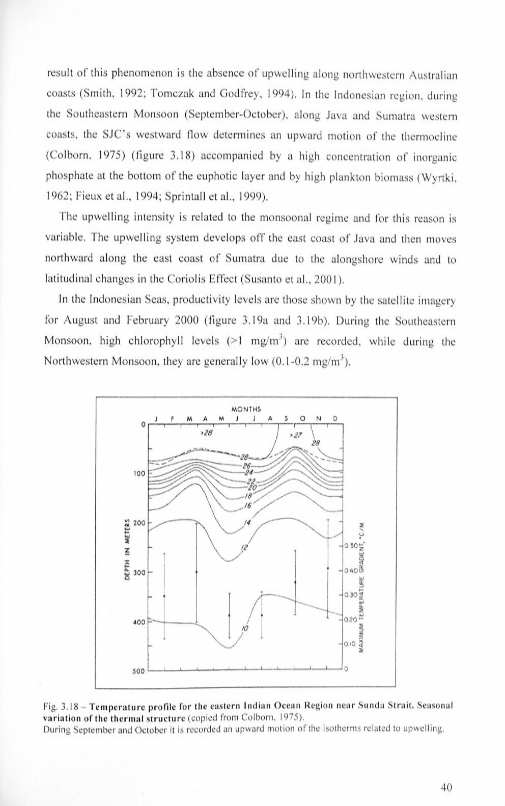
result of this phenon1enon is the absence of upwelling along northwestern Australian

coasts (Smith, 1992; Tomczak and Godfrey, 1994). In the Indonesian region, during

the Southeastern Monsoon (September-October), along Java and Sumatra western

coasts, the SJ C's westward flow determines an upward motion of the thennocl ine

( Co 1 born, 197 5) (figure 3 .18) accompanied by a high concentration of inorganic

phosphate at the bottom of the euphotic layer and by high plankton bion1ass (Wyrtki,

1962; Fieux et al., 1994; Sprintall et al., 1999).

The upwelling . intensity is related to the monsoonal regime and for this reason is

variable. The upwelling system develops off the east coast of Java and then n1oves

northward along the east coast of Sumatra due to the alongshore winds and to

latitudinal changes in the Coriolis Effect (Susanto et al., 2001 ).

In the Indonesian Seas, productivity levels are those shown by the satellite in1agery

for August and February 2000 ( figure 3 .19a and 3 .19b ). During the Southeastern

Monsoon, high chlorophyll levels (> I mg/m3) are recorded, while during the

Northwestern Monsoon, they are generally low (0.1-0.2 mg/m3).

MONTHS J FM AM J JASON D

0 >28 >21

100

~ 200 2 w ' I- <.:, w 0

~ 0.50~-z w

6 I <t I- a::: ~ 300 0.40t'.' 0 w

Cl'. ::, r---- 0 .30~ w

------- (l_

2 w

400 I 0.20 r-I

2 /0 ::,

// 2

0 .10 ~ 2

500 0

Fig. 3.18 _ Temperature profile for the eastern Indian Ocean Region near Sunda Strait Seasonal variation of the thermal structure ( copied from Colborn, I 975). During September and October it is recorded an upward motion of the isotherms related to upwelling.

40

The concentration of the chlorophyll at the sea surface is not the same for the entire

region as a west-east phytoplankton biomass gradient is present (Wyrtki , 1958). In

August-September, the eastern Banda Sea and the Arafura Sea are characterised by

higher chlorophyll levels while more oligotrophic conditions are present in the

Sulawesi Sea (Kinkade et al., 1997). This difference in productivity levels between

the two regions is related to the "unbalance" between the water outflow to the Indian

Ocean and the inflow of surficial waters from the Pacific Ocean and the consequent

vertical advection of intermediate Banda and Arafura Seas waters which compensates

this deficit (Wyrtki, 1958). During January-February, a slight increase in chlorophyll

in the Makasar Strait is related to rivers runoff (Kinkade et al., 1997).

Rainfall contributes to increase the amount of organic n1atter produced at the sea

surface. Over Indonesia, rain occurs nearly all time of the year (Kripalani and

Ashwini, 1997; McBride, 1998) and rainfall levels are between 2500 and 3000 mn1

per annu1n (Arya et al., 1999). Under these conditions rivers deliver a large amount of

sediment to the ocean (Milliman and Meade, 1983; Milliman et al. , 1999) (figure

3.20).

Material delivered by the rivers represents an important source of nutrients, which

favours phytoplankton growth at the sea surface (Parsons and Takahashi , 1973;

Pettine et al., 1999). An opposite situation characterises northwestern and western

Western Australia, where rainfalls are less abundant and more concentrated in defined

periods of the year. Southwestern Western Australia is affected by rainfalls n1ainly

during winter, while further north rainfalls are more frequent in summer and are

linked to the monsoonal regime (Srikanthan and Stewart, 1991 ). In this context, the

amount of sediment discharged by the rivers in the ocean is sensitively less than that

recorded for Indonesia (Milliman and Meade, 1983). These differences between

northwest Western Australia and Indonesia explain the productivity gradient at the sea

surface existing between these two regions ( figure 3 .21 ).

41

' . • . ., s "' ·• ' , ·•-·· ,. -· " ~. : .. ".. ·• ".. . ' • ,.. ,..... , !J'• ~- I· I. l!I p • • 1111 ·~-

,a ---~-------..;•;.71e1c;_-" ....... (a)

01 .02 :)3 .05 2 3 s 10 1s 2u 30 so

Chlorophyll a Concentration mg/m3

Fig. 3.19 - Sea-surface chlorophyll levels for (a) the month of August [Southeastern Monsoon] and (b) February [Northwestern Monsoon] (obtained from the SEAWIFS satellite imagery archive) .

42

1 o-1'

Fig. 3.20 - Sediment discharge (106 t f 1) from the Indonesian Archipelago and Papua New

Guinea (copied from Milliman et al., 1999) Arrows width is proportional to annual load. Letters S, J, B, C, T and NG refer to Sumatra, Java, Borneo, Sulawesi (Celebes), Timor and New Guinea, respectively.

100" 11a·· 120·· ! 3G..:

- IO'· -10·

Indian Ocean

-20'

Aust~ lia

.30·· ,JI.I'·

100(' llil"

.Fig. 3.21 - Annual mean primary productivity (g C m-2 f 1) at the sea surface rn the eastern

Indian Ocean estimated from satellite data (after Antoine et al. , 1996).

43

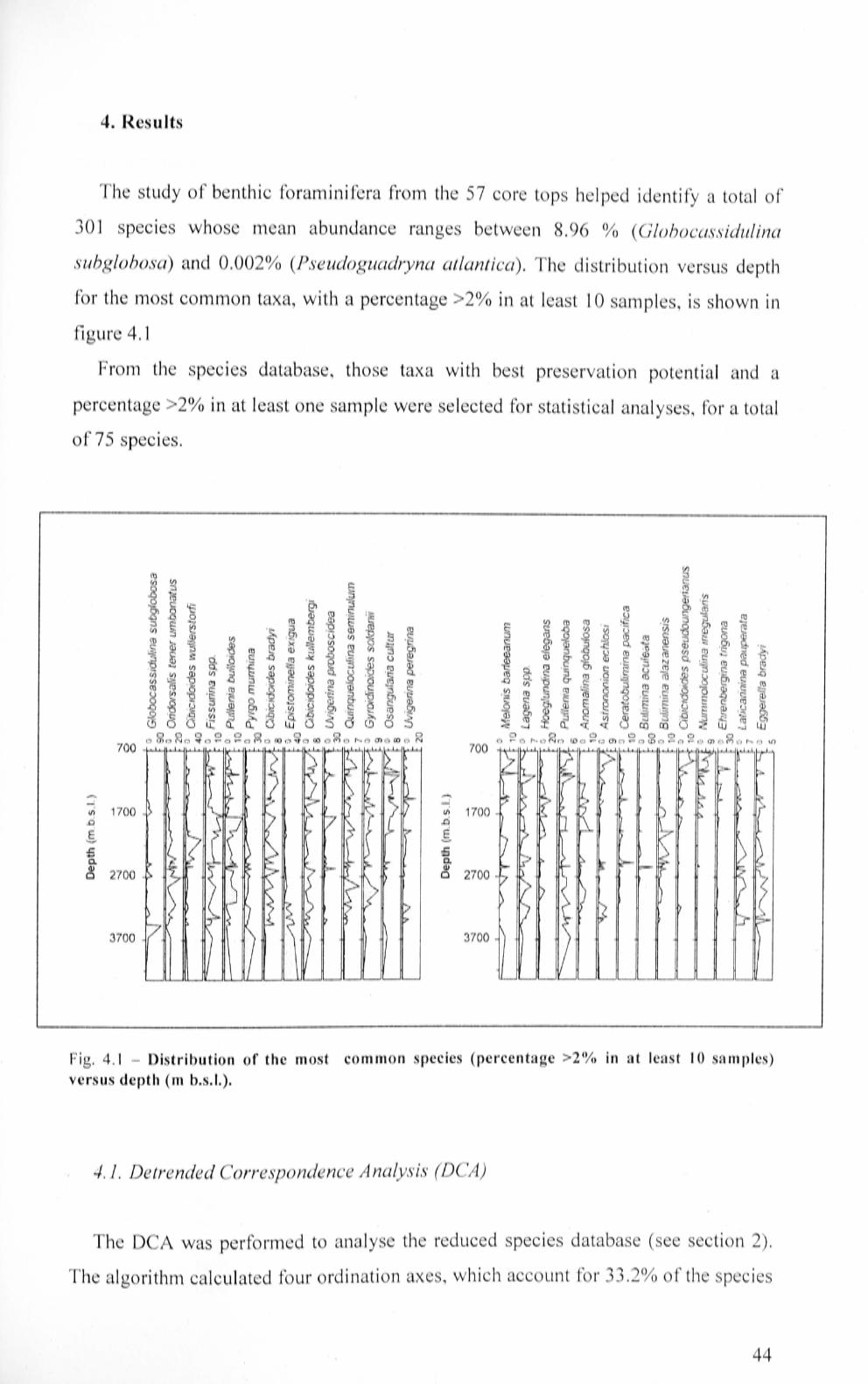
4. Results

The study of benthic foraminifera from the 57 core tops helped identify a total of

301 species whose mean abundance ranges between 8.96 % (Globocassidulina

subglobosa) and 0.002% (Pseudoguadryna atlantica). The distribution versus depth

for the most common taxa, with a percentage >2% in at least 10 samples, is shown in

figure 4.1

From the species database, those taxa with best preservation potential and a

percentage >2% in at least one sample were selected for statistical analyses, for a total

of 75 species.

V)

(1J :::i

~ C: (/J s::: CJ 0 .Q ..... 5 ·c:: VJ 0 ~ -~ :3 (l) ·c::: -. a 4:::: cc ? ~ OJ 0 Q) (1J .s :::::: CJ cu ..Q -0

~ .Q Q) s::: c:: ~ (1J (1J S: V)

0 Qi Ci; e :::i E: ~ C: 'iii ;;; (/J ·3:._ §i ,_ u © (1J (1J ;=a ..Q V) CJ ~ !ll c:: ::.i <n .. G V) "C s -§ :::i 0 Q 0 (1J cc C: ~ 0 (b co V) i::: ~ (/J 0 C: 0, Qi ::.i ~ a.. ".n

(l) Q) f §-.._

] (I) >< ~ ~ ·:::.. C: (l) e (l) 0 (1J V) DJ (i) ::.i .Q (.) C: V) ~ ~ n, (\J

~ (1J :;:: C: .s .Q ~ .Q c::

(.) !!? (l) (l) 0- Q (l) .~ Q -:::: r;: t; :::i (l) ci 0 (1J e ~ V) (l) N (1J Q ~ (l) !ll c:: OJ ~ ~ ....., C/) Q_ :::::: t V) :::::: V) ro l:::: Q. ~ ·3 c::

~ CJ (1j V) c:: (l) V) :::i ~ (l)

~ Q (.) ~ ·c:: a.. (1; a co (l} (.J ·- % ..Q (/J (/J Q '5 ~ (1j 2> (/J '-":: ~ .Q ::.i C:

.£ Q 0 (1J co ..Q V) 0- ·c.: .2 u 0 ,::: (1J c;; (1J ,...

0 ;:: Ql C: "S C: c:: -!::: en

l ~ 0 !ll C:

~ (1J

~ .S: (1J c:: c:: 0 -~ (U co 0 c:: ·c:: CJ V, ·c: ~ :'Q ::.i '5 Ol ·c:: ~ ::; c:: 0 .Q :3 0 Qi ti, c::: E j - c:: (1J 0 B 0 ..... 0- ·a c:: Ql

~ iii (l) £ ~ u ~ Q) .Q Cl (/J Ql 2> (.) -~ 0 -~ s (1J .ei Ql 0 i:i ~ -S2 0, i:i :::::: ~ 13 .... OJ '§ :::: Q ·c:: -~ ::; ::,... ~

:::. ::; ::,... V) :::. Ql (iJ ~ C: (/J (l)

0 :;E -i::: cu OJ (.!) 0 0 l.l. a.. a.. 0 (5 ~ 0 (.!) 0 ~ ~ ...J a.. <:( <:( 0 Q) Q) l1J ....J l1J 0 0 0 0 0 0 0 0 0 0 0 0 0 0 0 0 0 c m oNa ~ o ~ o ~ c M o OOo~ o OO o M a r--- c m c:> C:O o N 0 - C, f"--<.? Nr::> m c - c m c - c m o - o - o m c M o ~ c l{)

700 700

- --: CJ) 1700 (/) 1700 ..0 .Cl

-S E .J::: J:: .... ....

0. a. cu (I)

0 2700 0 2700

3700 3700

Fig. 4.1 - Distribution of the most common species (percentage >2% m at least IO samples) versus depth (m b.s.l.).

4.1. Detrended Correspondence Analysis (DCA)

The DCA was performed to analyse the reduced species database (see section 2).

The aloorithm calculated four ordination axes, which account for 33.2% of the species b

44

variance. The variance justified by each axis is listed in Table 4.1. The first two axes

represent more than 50% of the variance explained with the DCA and for this reason

only these two have been considered for further analysis. Species scores and weights

are listed in Table 4.2. The scores indicate the degree of correlation of each species

with each axis; the species ' weight indicates the influence of species on the analysis

(ter Braak and Smilauer, 1998; Dale and Dale, 2002).

Table 4.1 - Variance explained by each one of the four axes.

Axis Axl Ax2 Ax3 Ax4

Variance of 14.2 % 8.4 % 5.7% 4.6% species data

Table 4.2 -- Detrended Correspondence Analysis results for the reduced species database. Scores of the species for axes 1, 2, 3 and 4 (for species codes see Appendix A 1 ). In bold are indicated those species which present both high score on axes 1 or 2 and high weight

CODE AX! AX2 AX3 AX4 WEIGHT Aaglob -0.36 -0.03 -0.22 0.12 38.07 Astrech 0.16 -0.45 0.22 -0.07 32.75 Blql 1.66 1.54 -0.73 0.12 3.78 Bolro 1.12 0.65 0.59 0.36 5.17 Bolsem 0.37 -0.21 -0.43 -0.39 I 0.42 Brdi I.IO 0.86 0.54 -0.40 8.68 Brsem -0.41 0.3 I -0.63 -0. 12 5.74 Buac 0.07 I. 13 -0.23 0.38 31.96

Bualz -0.48 0.02 -0.40 -0.16 35.45 Buco 0.27 0.85 0.03 -0.28 17.95 Buma 1.57 3.80 0.12 -0.75 0.69

Cascr 0.68 -0. 10 0.01 -0 .07 11.01

Caslae 0.35 -0 .03 -0.44 -0.32 30.77

Cassre -0 .82 0. IO -0.62 -0 .87 13.62

Cerpa 0.18 0.06 -0 .02 -0.07 32.27

Chol 1.03 0.49 -0.29 0.44 11.57

Cibr 0. 16 -0. I 6 0.07 0.13 61.03

Ciku 0.08 -0 .13 0.11 0. IO 58.36

Cipse 0.97 0.11 0.29 -0.33 29.65

Cirob -0. 11 -0.40 0.06 0.59 19.84

Ciwul 0.71 -0.04 -0 . 10 -0.02 88.24

Cisp -0. 19 0.08 0.14 -0.06 14.42

Egbr -0.20 0.09 -0.10 -0.07 34.44

Ehtr 0.49 -0.29 0.88 0.60 23.39

Epex -0.91 0.03 0.29 0.05 60.39

Exum -0.29 -0.46 1.19 -1 .22 14.8

Fispp -0 . I 9 0.05 -0.06 0.03 80.71

Furfs -0.28 0.49 -0.25 0. 17 8.0 I

Galo 1.00 -0.47 0.08 -0. 16 20.04

45


CODE AXl AX2 AX3 AX4 WEIGHT Glcsb -0.21 0.00 -0.02 -0 . 17 112.68 Glpa 1.42 1.68 -0.39 0.14 3.04 Gyral 0.11 0.00 -0.05 -0 .06 11.97 Gyrlmk 0.31 -0 .85 -1.06 0.04 12.64 Gyror -0.23 -0. 13 0.06 0.25 29.42 Gyrpo -0.84 -0.28 0.01 -0.12 22.4 Gyrso 0. 12 -0.05 -0.0 I -0.09 53.68 Hoel 0.14 0.07 -0.06 -0.06 52.09 Hurin 1.44 -0.78 -0. 17 0.26 4.51 Hyba 1.6 I 3.31 -0.21 -0.39 1.29 Karbr 0.29 -0.24 0.38 -0.04 21.33 Laspp -0 . 14 -0.02 -0 . 15 -0.01 49.79 Lespp 0.37 0.31 0.24 -0.05 21.29 Ltpa -0.53 0.03 -0. 10 0.42 32.26 Meba 0.43 0.19 0.19 0.02 44.4 Mepo -1.09 -0.39 0.58 -1. 15 3.5 I Miob 1.15 -0 .80 -0 .34 0.00 5.62 Mtcom 0.85 2. 14 -0 .03 0. 18 3.49 Nntu 1.60 -0 .64 -1 .78 0.67 0.8 Numir 1.32 -0.76 -0 .28 -0.05 21.21 Oospp -0.52 -0.09 -0.21 0. 16 29.28 Ortu -0.35 0.06 0.01 0.08 88.34 Oscu 0.34 -0 . 16 -0.07 -0.20 46.97 Paspp -0 .21 -0.15 -0. 19 -0.20 20.71 Pu5 -0.17 -0.02 0.00 0.04 49.91 Pubu -0.20 0.09 0.08 -0.05 72.37 Pyde 0.12 -0.06 0. 16 0. 19 33 .73 Pye! 1.32 -0.72 0.63 0. 14 6.37 Pylu -0.23 -0.21 0.23 -0.28 10.74 Pyu -0.49 -0.07 -0.07 0.01 73.14

Qusem -0.02 -0.21 -0. 13 0.01 50.96 Quve -0. 18 -0.59 0.01 0.60 I 1.16 Rbta 0.99 -0.60 -0.31 -0.05 12 .91 Redi 1.42 -0.33 -0.35 -0.22 0.85 Sbull -0.41 -0.29 -0.26 0.54 22.54 Sgmsch 0.25 0.24 0.29 0. 10 27.21

Stxca -0.42 0.08 0.18 . 0.40 16.99 Stxcu 0.76 -0.25 0.26 0. 11 5. 15 Troo 0.94 0.11 -1 .21 0.27 4.1 ::,

Trtr 0.61 -0.54 -0.72 -0 .26 15.72

Txag -1.20 -0.43 0.92 -0 .31 · 0.82

Txlyt 0.88 -0 .32 0.81 0.81 9.27

Txpgr 1.40 -0.11 -1.39 0.57 1.79

Uvpe 0.05 0. 19 0.03 0.00 48.8

Uvprob 0. 19 0.50 0.06 -0.13 56.22

Vlsp 1.17 -0 .81 -0. 24 0.20 2.44

46

The analysis of axis 1 allowed the identification of two groups of species. Species

with negative score and high weight (in order of occurrences given in brackets):

Oridorsalis tener umbonatus (55) , Pyrgo murrhina (50) and Epistominella e.xigua

( 40). Species with positive score and high weight: Cibicidoides pseudoungerianus

(27) and Nummoloculina irregularis (15).

Based on the scores of axis 2, two species are characterised by high weight and

positive score: Uvigerina proboscidea ( 43) and Bulin1ina aculeata (23).

The first two · axes of DCA were correlated to the environmental variables and

faunal characteristics at each site (Table 4.3). The correlation n1atrix shows a

significant correlation of axis 1 with most of the environmental variables taken into

account except for the phosphate- and nitrate-concentrations and for the pri111ary

productivity levels at the sea surface. This axis is negatively (r < -0.60) correlated

with the following variables: depth, pressure and salinity; it shows a positive

correlation ( r > 0.60) with temperature and carbon flux ( calculated applying the two

formulae used in this study). A minor positive correlation exists between axis 1 and

Fisher's Alpha Diversity Index, Shannon Index and equitability, while an opposite

correlation links this axis with dominance. Axis 1 is also weakly correlated with

longitude, latitude and dissolved-oxygen concentration. Axis 2 shovvs a significant

co1Telation with the following environn1ental variables: longitude, dissolved-oxygen

concentration, salinity, phosphate, primary productivity at the sea surface, carbon flux

( calculated applying the two formulae used in this study) and fauna! characteristics

( a , H(S), E, D). The variable characterised by the best correlation (r = -0.52) with this

axis is dissolved-oxygen concentration.

4. 2 Environmental variables-fauna! characteristics correlation matrix

The environmental variables and faunal characteristics considered in this study

appear to be related to water depth (Table 4.3). Those variables that are positively

correlated to depth are: pressure, salinity, dissolved-oxygen concentration,

dominance, primary productivity and longitude. Those characterised by a negative

correlation are: temperature, carbon flux (Jz, C. flux (z)), H(S) , E and a (figure 4.2).

However, two relevant parameters are not related to any depth variation: (a)

dissolved-oxygen concentration is negati vely correlated with phosphate and nitrate;

47

/\x I

Ax2

Lal.

Long.

Depth

Diss. oxygen

(b) primary productivity at the sea surface is strongly correlated with longitude.

Table 4.3 - Correlation matrix between OCA ordination axes and the environmental variablesfaunal characteristics. In bold are indicated those correlations significant at p < 0.05.

C: (!.)

bO ->-- N X .f'

.__.,

.c 0 0.. X

bO a. ui - ...... ui C: E (fl ::J

N C: 0.. (fl 0 i:;::

X X ~ (fl 11) ~ (/)

0 11) ell OJ. ~ 0.. <l'.'. <l'.'. .....l 0 0 '- N .__.,

.....l (/) f- 0.. 0.. z 0.. -, u I 0

1.00

0.06 1.00

0.36 -0.09 1.00

-0.31 0.48 0.56 1.00

-0.90 -0.09 0.29 -0.36 1.00

-0.37 -0.52 -0.44 -0 .0 I 0.50 1.00

Salinity -0.69 0.28 0.49 -0.40 0.61 -0 . 15 1.00

Temp. 0.88 0.15 -0. 19 0.22 -0.91 -0.45 -0.60 1.00

Press . -0.90 -0.09 0.29 -0.36 1.00 0.50 0.61 -0.91 1.00

Phosp. -0 .08 0.34 0.41 -0. 15 -0.08 -0.63 0.40 -0.07 -0.08 1.00

Nit . -0. 19 0.21 0.37 -0.24 0. 13 -0.45 0.46 -0.24 0. 13 0.40 1.00 pp -0 .22 0.42 0.86 -0.45 0.31 -0.25 0.37 -0.20 0.31 0. 14 0.25 1.00

Jz 0.72 0.48 0.21 0.03 -0.70 -0.57 -0.34 0.84 -0.70 0.02 -0.08 0.29 1.00

C. llux(z) 0.82 0.37 0.05 0. 11 -0.80 -0.51 -0.48 0.92 -0.80 -0.03 -0. 17 0.12 0.98 1.00

1-l(S)

E

D

a

0.52 -0.27 -0.53 0.56 -0.53 -0.09 -0.37 0.41 -0.53 -0.05 -0. 17 -0.44 0.18 0.27 1.00

0.58 -0.35 -0.55 0.52 -0.55 -0 .02 -0.47 0.45 -0.55 -0.08 -0.28 -0.47 0.19 0.30 0.91 1.00

-0.41 0.19 0.42 -0.45 0.42 0.09 0.24 -0.33 0.42 0.04 0.06 0.34 -0. 18 -0 .24 -0.91 -0.74 1.00

0.44 -0.37 -0.46 0.39 -0.42 0.02 -0.37 0.33 -0.42 -0.06 -0.15 -0.34 0. 12 0.20 0.82 0.85 -0.68 1.00

4. 3 Correlation between the percentages of the speczes and the environmental

variables-_faunal characteristics

The correlation coefficients between the percentages of the taxa considered for

DCA as well as the environmental variables and the fauna! characteristics were also

calculated (Table 4.4). The analysis of coefficients was carried out assuming the n1ean

percentage of each species as indication of the taxon ' s relevance. The five species

individuated by means of DCA appear to be related to the environn1ental variables

and the faunal characteristics considered in this study, in particular with those whose

correlation with the DCA ordination axes is high.

0. t. umbonatus, E. exigua and P. murrhina show a significant positive correlation

primarily with depth (figure 4.3) and pressure, while to a lesser degree with salinity

and, with the exception of 0. t. umbonatus, the dissolved-oxygen concentration.

48

ex.

D

E

H(S)

C. flux (z)

Jz

pp

Nitrate

Phosphate

Dissolved oxygen

Salinity

Temperature

o~--------------------------0 l{)

0 0

A =: .!A [\ j r/\1 ~ --..._;;xq~ V> ?'?;V

1 o-:r-_____________________ _:__ ___ _

0 t---

0 0

0 0 t---

0 0 I'-..-

0 0 t--N

Depth (m. b.s.l.)

0 0 t--("') .

Fig. 4.2 - Values of the environmental variables and faunal characteristics considered in this

study versus depth. . PP = Primary Productivity at the sea surface ; Jz = carbon flux calculated using Berger and Wefer (1990) formula; C. flux (z) = carbon flux calculated using Suess ( 1980) formula; H(S) = ShannonWeaver Index; E = Equitability; D = Dominance; a= Fisher's Alpha Index.

49

Table 4.4 - Correlation coefficients between the relative percentages of benthic foraminifera species used for statistical analyses and the environmental variables-fauna! characteristics considered in this study. In bold are indicated those correlations significant at p > 0.05. For species codes see Appendix A I.

c:: V bi)

Species Code

Lat. Long. Depth Temp. c:: >-. b Press. Phosp. Nit. pp Jz 1-l(S) E D a

Aaglob

/\strcch

Bolro

Bolsem

Blql

Brdi

8rsem

Buac

8ualz

Buco

Buma

Cascr

Cas lae

Cassre

Cerpa

Chol

Cibr

Ciku

Cipse

Cirob

Ciwul

Cisp

Egbr

Ehtr

Epex

Exum

Fispp

Furfs

Galo

Glpa

Glcsb

Gyral

Gyrlmk

Gyror

Gyrpo

Gyrso

1-lurin

Hoel

Hyba

Karbr

Laspp

Ltpa

(f) (f)

0

0.07 0. 18 0.03 -0. 16 0.32 -0 . 16 0.03 0.28 0.32 -0. 18 -0.25 -0.25 0. 12 0.05 -0.2 1 0.02 -0.34 0. 14 -0.15 0.25 -0.38 0.33 -0 . 15 -0.41 -0.57 -0 .2 1 0.08 0.16 0.22 0.23 -0 .22 0.20 -0.04 0. 16 -0.31 0.34 -0.17 -0.42 -0.31 0.12 0.03 -0.14 0.17 0.22 0.19 0.21 -0.09 0.16 -0 .2 1 0.15 -0.23 0. 14 -0.22 0. 13 -0 .23 -0. 11 -0 . IO -0.21 0.04 0.09 0.25 0.29 -0.23 0.27 0.00 0.21 -0.28 0.27 -0.35 -0.13 -0.28 0.02 -0.06 0. IO 0.42 0.40 0.12 0. 12 -0.12 0.02 0.00 0.05 -0.36 0.46 -0.08 -0.45 -0.36 0.05 0.06 -0.07 0.39 0.42 0.11 0.10 -0 .07 0.07 0.00 0. 15 0.03 -0.12 0. 14 -0.0 I 0.03 0.05 0.09 -0. IO -0. 15 -0.14 0.08 0. IO -0 .02 0.08 0.23 -0.14 0.00 -0 .05 0. 15 -0 13 0.00 0.27 0.13 0.22 0.07 0.03 -0.32 -0.27 0.31 -0.31

-0.0 I 0.03 0. 13 -0.29 0.32 0.04 0. 13 0.16 0.17 -0.09 -0.29 -0.31 0.09 0.0 I -0.11 -0.03 0.05 0.04 -0.24 0.26 0. 14 -0.35 -0.24 0. 15 0.08 0.0 I 0.37 0.35 -0.02 -0.05 -0.04 -0. 17 0.17 -0 .08 -0.22 0.40 0. 13 -0.37 -0 .22 0.05 0.07 0.21 0.65 0.59 -0.07 -0. IO -0.0 I -0. 15

-0.20 0.11 -0.32 0.30 -0.25 -0. 12 -0.32 -0.06 -0 .05 -0.16 0. 18 0.23 0.20 0.21 -0.20 0.30 -0 .25 0.08 -0.30 0.14 -0.24 -0.04 -0.30 -0.09 0.17 -0.12 0. 12 0. IS 0.17 0.17 -0. 14 0. 18 -0 .08 -0.12 0. 14 -0.26 0.26 0.09 0.14 0.02 0.05 -0.16 -0.29 -0.29 0.00 -0.05 0.08 -0.07 -0.08 0.33 -0 . 18 0.07 0.05 -0.23 -0.18 0.12 0.12 -0.08 0.03 0.04 0.24 0.21 -0.24 0.27 0.06 0.04 -0.28 0.35 -0 .22 -0.03 -0.28 -0. 13 -0.27 0. IO 0.35 0.37 0.08 0.21 0.02 0.05

-0. 15 -0.02 -0.29 0.31 -0.33 -0.04 -0.29 -0. 18 -0.06 -0.04 0.20 0.25 0.44 0.43 -0.47 0.52 -0.09 -0. 15 -0 .26 0.26 -0.28 -0.03 -0.26 -0.07 -0.02 -0.05 0. 11 0. 17 0.30 0.27 -0.38 0.24 -0 .2 1 0. 12 -0.59 -0.58 -0.58 -0 .05 -0.59 -0.36 -0.40 -0. IO 0.67 0. 73 0.21 0.22 -0.26 0. 19 -0.20 0.20 0. 11 -0. 11 -0 .09 0.21 0. 11 -0.15 -0.13 -0.02 -0. 15 -0. 14 0.22 0.21 -0. 18 0.30 -0 .06 -0.02 0.06 -0. 15 0.19 -0 .03 0.06 0.08 -0.02 -0. 13 -0. 19 -0. 19 -0.07 -0. 18 0.08 -0.20 -0.29 0. 19 -0.30 0.36 -0.41 0.15 -0.30 -0.34 -0.27 -0 . 13 0.33 0.38 0.28 0.36 -0 .2 1 0. 17 0.08 -0. 13 0.20 -0. 19 0. 19 0.14 0.20 -0. 12 0. IO 0. 14 -0.06 -0. IO -0. IO -0.22 -0 .0 I -0 .24

-0.09 0. 14 -0.29 0.25 -0.28 -0 . 19 -0.29 0.11 -0.02 -0.17 0. 11 0. 17 0.12 0.09 -0 .05 0.07 0.27 -0.29 0. 73 -0.52 0.29 0.37 0. 73 -0 . 14 0.0 I 0.27 -0.38 -0.44 -0.45 -0.49 0.32 -0.43

-0 .04 -0.05 0.26 -0.08 -0.06 0.24 0.26 -0.16 -0.15 -0. 11 -0. I I -0. IO -0.30 -0.26 0. 19 -0.28 -0.13 0. IO 0. 15 -0.31 0.21 0.08 0.15 0.01 0. 17 -0.20 -0.32 -0.33 0. 18 0.07 -0.2 1 0.06 0. IO 0.02 0.14 -0. 11 0. 13 -0 .05 0.14 0.08 0.02 0.19 0.00 -0.05 0.03 -0.04 -0.03 -0.06

-0.02 -0.05 -0.48 0.50 -0. 19 -0.33 -0.48 0.07 0.02 -0.03 0.40 0.43 0.27 0.32 -0.24 0.29 0.07 0. 12 -0.30 0.40 -0.28 -0. 18 . -0.30 -0.05 -0. 12 0.17 0.57 0.55 0. 12 0. 13 -0 . IO 0.03 0.37 -0.39 0.24 -0 .2 1 0. 16 0.03 0.24 0.07 0. IO 0.24 -0. 13 -0. 17 -0.62 -0.44 0.71 -0.40 0.10 0.26 -0.13 0.08 0.0 I -0.27 -0. 13 0. 10 0. 11 0. 14 0. IO 0.07 0.09 0.04 -0.04 0. I I

-0.41 0. 16 -0.04 -0.07 -0. 14 0.18 -0.04 -0.08 0.06 -0.25 -0. 13 -0. IO 0.30 0.44 -0. 16 0.36 0.06 -0.09 0. 18 -0 . 14 0. 15 0.05 0. 18 0. IO 0.09 0.05 -0. 17 -0. 17 0. 13 0. 13 -0. 13 0. 14 0.05 -0.34 0.53 0.33 -0.46 0.30 0.53 -0. 12 0.05 0.05 -0.39 -0.44 -0.17 -0.23 0. 12 -0.25

-0.30 0.27 -0.26 -0.23 0.19 -0.07 -0.26 -0.06 -0.06 -0.27 0.03 0.09 0.27 0.22 -0.32 0.20 -0.21 0.27 -0.35 -0.4 t 0.3 t 0.0 I -0.35 -0. 14 -0.42 -0. 14 0.21 0.27 0.34 0.49 -0. 19 0.21 0.05 0.20 -0.28 0. 15 0. 14 -0.34 -0.28 0.34 0. 18 -0 . 15 0.05 0.07 0.24 0.22 -0.27 0.03 0. 17 0.05 -0.28 -0. 03 0.4 t -0.38 -0.28 0.08 -0.01 0.25 0. 71 0.64 -0.02 -0.06 -0.04 -0. 14

-0 .24 0.14 -0.41 -0.43 0.35 -0.07 -0.41 -0.13 -0.05 -0.32 0. IO 0.20 0. 12 0.07 -0.09 0. 15 -0 .03 -0.08 0.09 0.20 -0.08 -0.03 0.09 -0 .08 0.14 -0.05 -0.04 -0.06 0.23 0. 18 -0.23 0.26 0.03 -0.09 0.39 0.29 -0.39 0.26 0.39 0.05 0.04 0. 13 -0.32 -0.37 0.06 -0.04 -0. I I 0. 15

50


C: V

0 bl) ,-..

Species ;;.-.. N

Lat. C: X -Long. Depth Temp. 0 Press. Phosp. Nit. pp Y. Code Jz :::; H(S) E D (X ro ~ (./') vi

·r,

u 0

Lcspp 0.21 0.04 -0.35 -0.12 0.51 -0.52 -0.35 -0.06 0.11 0.21 0.58 0.55 0.10 0.07 -0.09 0.16 Mtcom 0.32 0.14 -0.20 -0.14 0.24 -0.41 -0.20 0.08 0.11 0.38 0.51 0.43 0.04 0.00 -0.06 0.00 Meba -0. 15 0.04 -0.39 -0.42 0.4 I -0.0 I -0.39 -0.13 -0.19 -0.06 0.33 0.38 0.05 0.08 -0.08 0.06 Mepo -0.10 -0.05 0.26 0.12 -0.20 0.20 0.26 -0. 11 -0.09 -0.14 -0.2 1 -0.22 -0.17 -0. 17 0.16 -0. 18 Miob -0.35 0.21 -0.33 -0.56 0.42 0.35 -0.33 -0.48 -0.57 -0.24 0.24 0.33 0.36 0.54 -0.22 0.34 Nntu -0.26 0.11 -0.21 -0.26 0.20 0.26 -0.2 1 -0.32 -0. 12 -0. I 5 0.10 0.15 0.20 0.29 -0.14 0.29 Numir -0.52 0.25 -0.54 -0.78 0.54 0.39 -0.54 -0.50 -0.48 -0.35 0.30 0.42 0.41 0.55 -0.24 0.42 Oospp 0.05 -0.02 0.42 0.26 -0.45 0.27 0.42 -0.07 0.14 0.12 -0.38 -0.41 -0.06 -0 .19 -0.03 -0.03 Ortu 0.10 -0.20 0.52 0.46 -0.59 0.25 0.52 0.03 0.11 0.12 -0.48 -0.53 -0.21 -0.31 0.14 -0.21 Oscu -0.16 0.31 -0.55 -0.25 0.39 -0.44 -0.55 0.31 0.09 -0.25 0.20 0.26 0.34 0.33 -0.28 0.24 Paspp -0.32 0.18 0.07 0.02 -0.12 0.28 0.07 -0.21 -0.17 -0.27 -0.22 -0. 19 0.06 0.06 -0.03 0.09 Pubu 0.19 0.25 0.12 0.06 -0.16 -0.11 0.12 -0.02 0.07 0.14 -0.02 -0.07 0.14 0.07 -0.16 0.02 Pu5 0.09 -0.12 0.09 -0.01 0.04 0.09 0.09 -0.20 -0.11 0.16 0.05 0.04 0.10 0.06 -0.18 0.2 I Pyde -0.02 0.15 -0.23 -0.18 0.14 -0.15 -0.23 0.12 -0.10 -0.01 0.09 0.12 0.25 0.20 -0.26 0.25 Pycl -0.38 0. 15 -0.46 -0.65 0.44 0.09 -0.46 -0.21 -0.21 -0.31 0.24 0.35 0.25 0.31 -0.16 0.25 Pylu -0.12 0.01 0.10 -0.13 -0.03 0.30 0.10 -0.19 -0.33 -0.04 -0.07 -0.05 -0.0 I -0.03 -0 .05 -0.02 Pyu 0.25 -0.37 0.60 0.35 -0.52 0.32 0.60 -0.08 0.16 0.29 -0.37 -0.44 -0.26 -0.36 0. 11 -0.34 Qusem -0.53 0.22 -0. 16 -0.21 0.02 0.23 -0.16 -0.06 -0.06 -0.61 -0.27 -0.16 0.38 0.35 -0.33 0.28 Quve -0.19 0.23 0.11 0.00 -0.14 0.18 0. 11 -0.15 0.04 0.00 -0. 10 -0. 11 0.09 0.06 -0.08 0.24 Redi -0.09 -0.0 1 -0.23 -0.28 0.25 0.00 -0.23 -0.09 0.02 -0.04 0.21 0.24 0. 15 0.18 -0. 13 0.10 Rbta -0.36 0.24 -0.47 -0.49 0.43 0.07 -0.47 -0.21 -0.20 -0.28 0.23 0.32 0.34 0.45 -0.25 0.29 Sgmsch 0.04 -0. 10 -0. 16 -0.03 0.11 -0.16 -0.16 0.29 -0.03 -0.03 0.07 0.09 0.14 0. 15 -0.18 0.27 Stxca -0.01 -0.06 0.23 0.17 -0.22 0.14 0.23 0.02 -0.05 0.02 -0.20 -0.22 -0.10 -0.12 0. 12 -(}.05

Stxcu -0.03 0.09 -0.26 -0.06 0.28 -0.22 -0 .26 0.00 0.04 -0.07 0.15 0.19 0.09 0.10 -0. 13 0.03

Shu ll -0.25 0.14 0.26 0.06 -0.16 0.46 0.26 -0.39 -0 .2 1 -0. 13 -0.22 -0 .2 1 0.19 0.21 -0. 19 0.15

Txag -0.13 -0.05 0.36 0.13 -0.23 0.25 0.36 -0.14 -0. 11 -0.17 -0.26 -0.26 -0.13 -0. 13 0.02 -0. 13

Txlyt -0.10 0.15 -0.34 -0.30 0.31 -0.25 -0.34 0.07 -0. I 0 -0. 12 0.21 0.25 0.20 0.22 -0.08 0.13

Txpgr -0.25 0.15 -0.23 -0.29 0.19 0.18 -0.23 -0.23 -0.07 -0.14 0.12 0.17 0.20 0.26 -0.15 0.26

Trtr -0.30 0.15 -0.24 -0.15 0.22 0.04 -0.24 -0. 16 -0. 11 -0.17 0.11 0.16 0.38 0.52 -0.19 0.39

Trgo -0.19 0.25 -0.19 -0.21 0.06 -0.02 -0.19 -0.09 0.12 -0.06 0.07 0.08 0.11 0.09 -0.09 0.17

Uvpe -0.16 0.06 -0.20 0.06 0.10 -0.21 -0.20 0.38 0. 10 -0.36 -0.07 -0.02 0.06 -0.02 -0. 10 -0 .02

Uvprob 0.17 0.24 -0.27 -0.04 0.34 -0.49 -0.27 -0.02 0.10 0.22 0.46 0.42 0.04 -0.04 -0.01 -0 .04

Vlsp -0.24 0.18 -0.31 -0.44 0.28 0.06 -0.31 -0. 11 -0 . 15 -0.20 0.14 0.21 0.33 0.49 -0.20 0.32

51

Ill

.ri

I .!! .., Q.

~

Oridorsalis tener b t

Cibicidoides um ona us Epistominel/a exigua p yrgo murrhina pseudoungerianus

(o/o) (0/o .) (%) (%) 0 5 10 1 5 20 0 10 20 30 40 O 1 O

1oor....___.__...___,___..,__JL___....-t-----..L...,__j__..._....l_-'-----fs;;--'-L__..__2.Lo__._...::..::300 2 4 6 __....---'------'-

1700

2700

3700

\ <\

t ·-- ~

..c::_

J .. -.-~ ·'.·,. L ✓ .· ?>--__

Fig. 4.3 - Species showing highest correlation with depth.

Nummoloculina irregularis

(%)

6

'.ercentages of 0 . t. umbonatus, E. exigua and P. murrhina (listed in order of mean percentage) increase when depth increases, while an opposite trend characterises the percentages of C. pseudoungerianus and N. irregularis (listed in order of mean percentage).

0 t. umbonatus, P. murrhina and E. exzgua have a negative correlation with

temperature and carbon flux (Jz and C. flux(z)). E. exigua and P. murrhina also show

a negative co1Telation with the faunal diversity, while being directly related to

dominance.

On the other hand, C. pseudoungerianus and N. irregularis are characterised by

opposite trends, being negatively correlated with depth (figure 4.3) and pressure and

positively with temperature. C. pseudoungerianus shows high correlation with carbon

flux (Jz and C. flux(z)) (figure 4.4a and 4.4b ). N. irregularis 1s correlated with

salinity, dissolved oxygen (figure 4.5) and the faunal diversity.

U proboscidea is positively correlated with the carbon flux (Jz and C. flux(z)) and

negatively with dissolved-oxygen concentration (figure 4.6) . The distribution of B.

aculeata is related to phosphate concentration (figure 4. 7) and dominance, while it is

· negatively correlated with fauna! diversity.

52

Cibicidoides pseudoungerianus Cibicidoides pseudoungerianus (%) (%)

0 1 2 3 4 5 6 7 8 9 10 0 1 2 3 4 5 6 7 8 9 10

I -L . .L..1 .LL 5.0

I 8.0

7.0

_I 40

6.0 ':,..

1 ':,.. "<~-

(_) . Ol 5.0 \ ry 3.0 '------_ ~ E '-~ . .!::!, .. ~ u )( -- 0) ''> ::l . ~ ~-I;: --:-==:== __ N

4.0 -:,

u ·- ----==- --= -----2.0 ~ 3.0 :c--20

1 0

·1.0

0.0 0.0

(a) (b)

Fig. 4.4 - Diagram showing the correlation between the distribution of C. pseudoungerianus and carbon flux, calculated using (a) Suess (1980) IC. flux(z)I and (b) Berger and Wefer (1990) jJz l formulae.

Salinity

34 4 34.5 34 6 34.7 34 8 34.9 1.5

0

5

10

20

30

Dissolved oxygen

(ni/1) 2.5 3.5 4.5 5.0


(%) 0 123456789 ....--~~~~~-,L~~- '-i

----_ _ . .::::.=:--

Fig. 4.5 _ N. irregularis has higher percentages south of 20°S, for environments characterised

generally, by high dissolved-oxygen concentration.

53

....... I

Uvigerina probosci dea ("10)

0 10 20 30 0 t--···-···· ·········-~~ .-····-····"··-··········-···-··-··"

~ 2 I

E u O')

· -._./

N -,

Uvige rina proboscidea (%)

0 10 20 30 0 . . __ L..___,__;···-··-·..l-... _._._, .... _ .... _ ..

...I

1.0 , - ~

>, N 30

I

~

G ·.,./-.:.- ---~ 4.0 ~ ··-··- ---N °:) .. _, 50 I >< . \ :l \

: 6.0 · .· :---\

.\ •·. \

\ 7.0 . :\

:\ \

8.0

..___.;..._.....;._;_; ................................ _ ........ .

Uvigerina proboscidea (%)

0 10 20 30 2 -;---___,_---='=~ ---··_: ··-··-··· ··--··--) ,~:-

'-. '-'-.,

'" '•"-....

. ___ _;

Fig. 4.6 - Percentages of U. proboscidea plotted versus carbon flux calculated using Be rge r and Wefer (1990) jJzl, Suess (1980) jC. tlu x(z) I formulae and dissolved-oxygen concentration. The percentage of this species shows higher values when carbon flux reaches values around 2-3 gCm-2f I and when dissolved-oxygen concentration is lower than 31111/l.

Bulimina aculeata

60

50

40

(%) 30

20

10

0 8 8 8 iS r-, N r-, r-, N

~ ~ ~ ~ ~ ~ ~ ~ ~ ~ m N N N N N N N N N ~

Phosphate (µmol/1)

Fig. 4.7 _ Percentage of B. aculeata plotted versus phosphate concentration (µmol/1). T his spec ies · has higher percentages for high phosphate concentration levels.

54

4. 4 Canonical Correspondence analysis (CCA)

In order to evaluate how well the environmental variables and faunal

characteristics explain the distribution of the identified species a Canon ical

Correspondence Analysis (CCA) was performed. The total variance explained by the

algorithm is 30.7%. This value is close to the percentage of variance exp lained by

n1ean of DCA. CCA produced axes that are mirror-like to those produced by DCA. In

any case, the relationships species-axes are the same as those given by the indirect

gradient analysis. In Table 4.5, the interset correlations between the environmental

variables, fauna! characteristics and the canonical axes are given. The relationship

between species distribution and depth is indicated also by this ordination technique,

as underlined by the strong correlation between the first axis and this variable. A

similar observation can be made for temperature, salinity and carbon flux. There is

also a significant correlation between the second axis of the CCA and two

environmental variables: dissolved-oxygen concentration and phosphate. The

relationships between the environmental variables, the Canonical Correspondence

axes, the five species individuated by DCA are shown in figure 4.8 . 0. t. umbonatus,

E. exigua and P. nntrrhina are on the right-hand side of the diagram and show a close

relationship with depth. C. pseudoungerianus and N. irregularis are on the left-hand

side, showing a negative correlation with this parameter. The second taxon shows a

correlation with the three indexes calculated to measure the fauna! diversity. U.

proboscidea is negatively correlated with dissolved-oxygen concentration; B.

aculeata is directly related to phosphate concentration.

Table 4.5 _ lntereset correlations between the first two ordination axes calculated by means of Canonical Correspondence Analysis and the environmental variables-fauna ! characteristics considered in this study. High positive and negative correlations are indicated in bold.

CCAI CCA2

Latitude 0.31 -0.52

Longitude -0 .34 -0 .0 I

Depth 0.91 0.16

Dissolved Oxygen 0.35 0.78

Salinity 0.71 -0.41

Temperature -0.88 -0.09

Pressure 0.91 0.16

55


CCAI CCA2

Phosphate 0.10 -0.61

Nitrate 0.22 -0.43 pp 0.22 -0.29

Jz -0.73 -0.29

C. tlux(z) -0.83 -0.20

H(S) -0.54 0.22

E -0.59 0.33

D 0.41 -0.13

a -0.34 0.32

-11 Dissolved oxygen

I /

I

/ E~ .._a I H(S)_ ~Nu~ . / .. ----._, , mi~~ :

~ '~ '·,. '

~- - ~ 1 / ------·- - ----- ~ ~~:::s, >, . 1 . _ _______ Depth

Pressure

Longitude cp;e -----=~-- : · :,_-.-~;.;--- -- -------- ---- - ----------- - -- --- --- . :..(- --- . -- - -:::::--::::. - - ·------ --- ~ ., . -- --- -- - - - -- - --- -- -- - --- ----- -- -- - - --- -- -

--------- ~ - r' I '~ ~J?~u ... --·-----------1/.,,..,,,.,.. • ; '\ ~-------........ T em peratur:,_--------=-~_..,..,,..-- Uvprot i \ \~\ ~;--------.. ..... ._

..,_--- ~--- Bua<: ~ \ '\, '\ ' , ,, D C. flux (z) _/""'- : \ '\ \ ' "-,

v__,/"" , , \ • ~ Jz ~ \ ~ pp '-,,~

: \ \\ ~ : \ •\ ~ ' 1 Nitrate\ Salinity \ \ i \atitude

Phosphate

'----------- ---------'---------------------··-·----·----------

Fig. 4.8 - Diagram showing the relationships between the environmental variables, fauna! • characteristics (arrows) and the first two CCA axes (see text for further explanation). The length of the arrows indicates the influence of the variables on the axes and the angles between the arrows and the axes are inversely proportional to the correlation variable-axis. The five species individuated with DCA are also plotted on the diagram and their position outlines their relationships with the CCA axes and with the environmental variables. Species codes: Cipse = C. pseudoungerianus; Numir = N. irregularis; Ortu = 0. t. umbonatus; Epex = E. exigua; Pyu = P. murrhina; Uvprob = U. proboscidea; Buac = B. aculeata.

56

4. 5 Correlation between the agglutinated, calcareous infauna! and porcellaneous

taxa and the environn1ental variables-fauna! characteristics

In order to investigate the relationship between the three groups of benthic

foran1inifera (agglutinated, calcareous infaunal [hereafter refe1Ted as infaunal] and

porcel laneous ), the measured environmental variables and the fauna1 characteristics

the correlation matrix shown in Table 4.6 was calculated.

Table 4.6 - Correlation coefficients between the percentages of the agglutinated, calcareous infauna! and porcellaneous taxa and the environmental variables-fauna! characteristics considered in this study. Those correlations significant at p > 0.05 are indicated in bold.

Agglutinated Infauna! Poree I laneous Latitude -0 . 11 0.01 -0.38 Longitude 0.05 0.32 0.09 Depth 0.17 -0.51 -0 . 14 Dissolved oxygen 0.15 -0.54 0.39 Salinity 0.05 -0.08 -0.44 Temperature -0.17 0.46 0.08 Pressure 0.17 -0.51 -0.14 Phosphate 0.05 0. I 9 -0.31 Nitrate 0.01 0.11 -0.31 pp 0.05 0.00 -0.21 Jz -0.16 0.54 -0.06 C. tlux(z) -0. 17 0.53 0.02 H(S) 0.28 0.21 0.37 E 0.23 0.12 0.40 D -0.29 -0.20 -0.32

a 0.49 0.06 0.33

The distribution of the agglutinated group is positively correlated with a and H(S),

while it shows a negative correlation with dominance. The infauna} species

distribution is negatively correlated with dissolved oxygen, depth, an<l pressure, while

it is positively correlated with Jz, C. flux(z) , temperature and longitude. The

porcellaneous taxa distribution is negatively correlated with salinity, latitude,

phosphate and nitrate concentrations and dominance. This group of species shows a

positive correlation with dissolved oxygen, equitability and a.

57

5. Discussion

The distribution of the 75 species analysed here appears to be controlled by depth.

On the basis of the score sign on axis 1 and the weight of each species, two major

groups of taxa were identified: one is negatively correlated with depth (species with

positive score on axis 1) and the other is characterised by an opposite trend (species

with negative score on axis 1 ).

The first group is dominated by C. pseudoungerianus and N irregularis, whose

distribution is limited to the upper water column between 700 m and 2000 m water

depth (figure 4.3), where water temperature is warm.

The distribution C. pseudoungerianus is strongly correlated to carbon flux and this

species becomes abundant when this paran1eter is > 1.5-2 gCm-2y- 1 (figure 4.4). A

limited distribution of this species to the upper part of the water column was observed

by other studies where it is indicated to be typical of neritic-bathyal (Barbieri , 1 998)

and bathyal settings (Spencer, 1996). In the Atlantic Ocean, C. pseudoungerianus is

indicated as a species present in samples from the first 1500 m of the water colun1n,

where carbon-flux rate is higher than 2 gCm-2y- 1 (Altenbach et al. , 1999).

N irregularis is a miliolid taxon, whose distribution is related to low salinity and

to prevalently high dissolved-oxygen concentration: in the eastern Indian Ocean, these

two conditions are verified mainly south of 20°S (figure 4.5). The low salinity level

(34.4), which characterises the latitudinal and depth range where this species is found,

is due to the presence of the Antarctic Intermediate Water (AAIW). High dissolved

oxygen concentrations are related to two major factors: the presence of the AAIW,

whose oxygen concentration is > 4 ml/I, and low primary productivity level at the sea

surface ( figures 3 .21 ), which in tum determines low organic-carbon flux to the sea

floor. In an environment where the an1ount of organic matter reaching the sea floor is

scarce, the consequent oxygen depletion related to its oxidation is minin1al.

Furthermore~ miliolid taxa have already been associated with increased ventilation in

the Arabian and the South China Seas ( den Dulk et al. , 2000; Huang, 2002).

The second group includes three species: 0. t. umbonatus, E. exigua and P.

murrhina. The distribution of these three taxa is strongly controlled by depth (figure

4.3). In this region the measured variables - with the exception of phosphate and

58

nitrate - are all correlated with depth: any variation of this latter determines a

modification of the other parameters. According to the correlations between species

percentages and the environmental variables, (). t. umbonatus, E. exigua and P.

murrhina find better conditions in a deep environn1ent characterised by low water

temperature, which is relatively well oxygenated and oligotrophic, where the amount

of organic matter reaching the sea floor is reduced and/or concentrated in specific

periods. In the eastern Indian Ocean, 0. t. umbonatus was found to be abundant in

deep water (>2500 m) by Corliss (1979a) and Peterson ( 1984 ), who both associated

this species to Antarctic Bottom Water and Indian Deep Water respectively. In the

Atlantic Ocean, the Sulu Sea and the South China Sea, 0. t. umbonatus percentages

have been observed to rise with increasing depth and decreasing organic carbon

values (Mackensen et al., 1985; Miao and Thunell, 1993; Rathburn and Corliss,

1994 ). Rathburn and Corliss ( 1994) mentioned the capability of this species to make

use of limited amounts of food.

E. exigua has been observed to inhabit phytodetritus layers deposited on the sea

floor (Gooday, 1988; Gooday, 1993; S1nart et al., 1994). This species is known to

behave as an r-strategist (Jannik et al., 1998), being able to grow and reproduce

rapidly in the presence of phytodetritus (Kurbjeweit et al., 2000), thus becon1ing the

most abundant taxon and determining high-dominance levels. This last condition is

verified for the samples in which £. e.xigua is found. This adaptative mechanism

could favour its appearance in presence of pulsed fluxes of organic 1natter in an

environment prevalently characterised by oligotrophic conditions. These pulses could

be related to the monsoonal climate: the change of wind direction determines the

presence/absence of the South Java Upwelling System, offshore Java and Sumatra,

and, by affecting rainfall levels, the ainount of riverine discharge offshore northwest

W estem Australia.

In the Indian Deep Water assemblage, as defined by Peterson (1984), one of the

relevant taxa among Pyrgo spp., was P. murrhina. In the Sulu Sea, Miao and Thunell

(1993) found that the abundance of their P. murrhina asse1nblage was negatively

correlated with sediment organic carbon content and positively correlated with the

thickness of the oxygenated layer in the sediment.

On the basis of DCA weight species and their scores on axis 2, it is possible to

isolate two tax a: U proboscidea and B. acuf eat a. U. proboscidea is correlated with

carbon flux and with dissolved-oxygen concentration. The percentage of this species

59

is higher for values of carbon flux > 1.5-2 gCm2y- 1 and low dissolved-oxygen

concentration ( <3n11/l) (figure 4.6). In this region, these conditions are verified mainly

for intermediate depth. In one case (san1ple B9442), when the percentage of this taxon

is higher below 2000 m, the carbon flux is still above the indicated threshold. This

aspect could indicate that the distribution of U. proboscidea is related to the co

variance of these two parameters: oxygen and carbon flux. At the sea floor, these two

parameters are correlated: the dissolved-oxygen concentration is given by the value

typical of each water mass combined with the oxygen depletion due to the oxidation

of the organic n1atter. The distribution of U. proboscidea is mainly lin1ited north of

25°S and between a 700-2000 m depth. These spatial ranges are characterised by two

factors: ( a) the presence of oxygen-depleted water masses such as Indonesian

Intennediate Water (IIW) and North Indian Intermediate Water (NIIW) and (b) high

primary productivity at the sea surface, with consequent high carbon flux (figure 5.1).

In the Sulu Sea, Rathburn and Corliss (1994) observed that, for the area studied,

the abundance of U. proboscidea was associated to high-organic carbon values

irrespective of bottom-water oxygen levels. Miao and Thunell ( 1993) identified in the

Sulu Sea the Uvigerina spp. assemblage abundant above 1500 m. This assen1blage is

associated to the shallowest oxygen penetration in the sediment and the higher carbon

content in the surface sediments. In the Indian Ocean, U proboscidea has been

utilised in palaeoenvironmental studies by Gupta and Srinivasan (1992) and by Wells

et al. (1994), as its abundance is correlated to past enhanced productivity periods,.

B. aculeata is associated with high phosphate concentration (figure 4.7) and high

dominance level. The distribution of this taxon is mainly limited to low latitude ( off

shore Java and Sumatra), where phosphate concentration (figure 5.2a) and primary

productivity (figure 3 .21) are high, in an area with a steep slope, which could favour

downward advection of part of the organic matter sunk to the shelf. The higher

phosphate concentration recorded within that depth range is associated with the

phosphate enrichment of the Indian Deep Water during its northward pattern: the

organic matter received from the sea surface and the continental margins causes

enrichment in nutrients (Toole and Warren, 1993). The preference of B. aculeata for

refractory organic matter (Jannik et al., 1998; Kurbjeweit et al. , 2000) could explain a

situation where a more degraded organic matter is then sporadically transported from

the shelf to the depth where this species shows higher percentages in this region

60

(1300-2500 m) (figure 5.2b ). The relationship with dominance could then be related

to an opportunistic behaviour (Jannik et al., 1998), marked by periods of high

reproduction (r-strategist) related to this unpredictable/pulsed food-availability

( caused by seasonal events, sporadic lateral advection from the shelf and terrigenous

inputs).

(%)

0 15 30 1.5 0 k ··········'················'···················•······-···••! .

f.! l

'

' ! .

I

I

2.5

"O C Q>

> (])

0 C'l >,

Ill >< Ill 0 Q

(mi/I )

3.5 4.5

-. N .c ..__,

>< .....

N a. ""') = tl)

;:;:: Q

u

(mbs.l)

0.5 1.5 2.5 3.5 4.5 5.5 0.5 2.5 4.5 6.5 8.5 600 1600 2f.300 3600 4500

I

I

I

I I ·~ •i I

I I I

I I ..

Fig. 5.1 - Diagram to show the relationship between U. proboscidea percentages, dissolved-oxygen concentration, carbon flux calculated using Berger and Wefer (1990) jJzl and Suess (1980) jC. flux (z)I formulae and depth versus latitude. The distribution of U. proboscidea appears to be controlled by two factors: carbon flux and oxygen levels. This species shows higher percentages when carbon flux is ~ I .5-2 gCm 2f I and dissolvedoxygen concentration <3ml/l. The latitudinal and depth range where this species is mainly found corresponds to areas characterised by high carbon-flux rate and by the presence of two oxygen-depleted intermediate water-masses: IIW and NIIW. Water masses: AAIW = Antarctic Intermediate Water; IIW = Indonesian Intermediate Water: NIIW = North Indian Intermediate Water; IDW = Indian Deep Water; AABW = Antarctic Bottom Water. The boundaries of the water masses are represented by dashed lines to indicate the lateral and/or vertical mixing between them.

61

0

5

(/) 0

~ 15 :::::, .....

.:; ro

...J

25

30 _

Bulimina aculeata (%)

0 10 20 30 40 50 60 1.40

(a)

Phosphate (p rrol/1)

1.75 2.40 2.75


0 10 20 30 40 50 60 0 1--'~~--_j~ _ l___._ _ __j_ ___ L • •.

_ ,ooo l ~ 2000r E :

; !~ Q. s:--Q)' t:= ====----0 r v

3000 .]

r i

i

4000 ! ~-------J

(b)

Fig. 5.2 - Diagram to show (a) B. aculeata percentages and phosphate concentration plotted versus latitude and (b) B. acu/eata percentages plotted versus depth. The distribution of this species is limited mainly to low latitude where phosphate concentration 1s higher and for a depth range between 1300 m and 2800 m.

5.1 F aunal groups

The percentages of three benthic foraminiferal faunal groups were correlated with

the environmental variables considered in this study.

The agglutinated taxa display a preference for assemblages characterised by high

diversity. This faunal pattern could derive fron1 competitiveness deficiency.

The infauna! species group seems to be typical of a shallow and warm environment

characterised by high carbon-flux rate and low dissolved-oxygen concentration. The

positive correlation with longitude could reflect the fact that these conditions are

found close to the continental-shelves margins, in areas characterised by high pri1nary

productivity at the sea surface. In the eastern Indian Ocean, primary productivity at

the sea surface is characterised by a NW-SE gradient: values increase while n1oving

fron1 off the west coast of Western Australia towards the Indonesian region and the

62

Banda Sea (figure 3 .21 ). At shallow depths along this gradient, not only does the

carbon flux increase, but also the dissolved-oxygen concentration decreases, due to

the presence of oxygen-depleted water masses (IIW and NIIW) and the oxidation of

the organic matter. The tendency of infauna! taxa to thrive under enhanced carbon

flux was already reported by Rathburn and Corliss ( 1994 ), Schmied! et al. ( 1997) and

Gooday and Rathburn ( 1999). The studied area is characterised by prevalently

oligotrophic conditions. In such an environment, the living conditions for infauna!

species become progressively favourable (Jorissen et. al, 1995): the higher is the

amount of organic matter reaching the sea floor, the higher percentage of this can be

buried within the sediment, representing an increased food source for the infauna! taxa

(Fontanier et al., 2002).

The porcellaneous species, on the other hand, seen1 to prefer environmental

conditions characterised by low salinity, high dissolved-oxygen coricentration, low

concentration of nutrients and high species-diversity. These conditions are present

mainly in the southern region, where, as indicated when discussing the distribution of

N. irregularis, the presence of AAIW determines low salinity levels and, together

with a reduced amount of organic matter to sea floor determined by the low prin1ary

productivity levels at the sea surface, high dissolved-oxygen concentrations. This

supports the observations from other regions, which indicate this group of taxa to be

indicative of enhanced ventilation during the past ( den Dulk et al. , 2000; Huang et al. ,

2002).

63

6. Conclusions

This study links benthic foraminifera from 57 core-tops from the eastern Indian

Ocean with the environmental variables that influence their distribution. The possible

relationships between foraminiferal distribution and oceanographic characteristics in

this area have been investigated considering different variables identifying water

masses described for the region: temperature, salinity and oxygen. Nutrients, such as

nitrate and phosphate, were also considered. In order to define possible links with

processes occurring at the surface of the ocean, levels of prin1ary productivity were

used to estimate organic carbon flux at the sea floor, utilising two different forn1ulae:

one by Suess (1980) and the other by Berger and Wefer ( 1990).

The distribution of benthic foraminifera appears to be controlled by depth and the

first ordination axis produced by both the ordination techniques :ised is strongly

correlated with this factor. Correlation coefficients and Canonical Correspondence

Analysis (CCA) outline how several of the measured environ1nental variables are

significantly correlated to this parameter. Therefore, the observed faunal depth-related

patterns appear to be the consequence of a co-variation of different factors:

ten1perature, carbon flux, salinity, dissolved oxygen, phosphate.

Detrended Correspondence Analysis (DCA) was performed on a group of selected

species (section 2) in order to define the relationship between benthic foraminiferal

faunas , environmental variables and faunal characteristics.

Two groups of species were individuated by the first ordination axis:

( 1) 0 . t. umbonatus, E. exigua and P. murrhina whose percentage increases with

depth. These three taxa prefer a cold and well-oxygenated environment, where the

carbon flux to the sea floor is low. In this group of species, two taxa are interpreted as

indicators of reduced food availability: 0 . t. umbonatus and P. murrhina. E. exigua is

characterised by high percentages and dominates the faunas of the samples in which it

is found. This feature is interpreted as the expression of an opportunistic behaviour (r

strategist) triggered by pulsed fluxes of organic matter to the sea floor. E. exigua

could be a seasonality indicator and its blooms could be associated with the presence

of the South Java l Jpwelling System, offshore Java and Sumatra, or an increased

riverine discharge offshore northwest Western Australia.

(2) C. pseudoungerianus and N. irregularis: these two speci es are typical of

64

shallow depths. C. pseudoungerianus is typical of a warm environment and where the

carbon-flux rate is high. The distribution of N. irregularis is associated to low salinity

and well-oxygenated waters. The presence of this species is mainly limited south of

20°S, between 700 m and 2000 m, a depth range that coincides with the AAIW ones.

In this area, the contemporary presence of AAIW, characterised by low salinity and

high dissolved-oxygen concentration, and low primary productivity (which causes

low oxygen consumption at the sea floor) create the ideal conditions for this species.

Two other species were individuated by means of axis 2 of DCA: U. proboscidea

and B. aculeata. U proboscidea thrives in areas characterised by carbon flux > 1.5-2

gC1n2y- 1 and low dissolved-oxygen concentration. These conditions are verified for

latitudes, where higher primary productivity at the sea surface determines higher

carbon-flux rate and low oxygen levels are due to organic matter oxidation and the

contemporary presence of oxygen-depleted intermediate water masses (IIW and

NIIW). B. aculeata is present at low latitude in areas characterised by high phosphate

concentration and high primary productivity. The depth range (1300-2800 m) of this

species, the morphology of the area where it reaches its peak, combined with

observations from other basins, could indicate a preference of this taxon for refractory

phytodetritus transported down-slope fron1 the shelf, where the an1ount of organic

matter fro1n the sea surface is higher. The high don1inance levels associated with this

species may indicate an oppo1iunistic behaviour determined by the rarity of these

inputs of food: for this reason B. aculeata could be associated to seasonal events.

The three major groups of taxa (agglutinated, infauna! and porcellaneous) were

correlated with the environmental variables and faunal characteristics considered in

this study. In essence, the infauna} and the porcellaneous taxa in this region display

significant distributional patterns. The first group of species is indicative of high

carbon-flux rates and low dissolved-oxygen concentrations, while the second group of

species indicates high dissolved-oxygen and low salinity levels.

65

PART II: The Late Quaternary palaeoceanography of the eastern Indian Ocean

66

7. Late Quaternary palaeoceanography of the eastern Indian Ocean based on

benthic foraminiferal evidences.

7. 1 Previous work

The eastern Indian Ocean is an important region in order to understand the

mechanis1ns ruling the global oceanic circulation (Wjiffels et al. , 1996). In addition, a

large number of . oceanographic studies were conducted in order to describe the

oceanic process which take place in this area (Wyrtky, 1958; Wyrtky, 1962; Fieux et

al., 1994; Fieux et al., 1996; Godfrey, 1996; Gordon and Fine, 1996; Wj iffels et al.,

2002). Therefore, the study of the palaeoceanographic evolution for the eastern Indian

Ocean during the Late Quaternary represents an important step towards reconstructing

the environn1ental modifications recorded for this region.

At the present the excess of precipitation over evaporation is responsible for the

presence of a low-salinity water cap over the Indo-Pacific Warm Pool region

(To1nczak and Godfrey, 1994). This low-saline water flows into the eastern Indian

Ocean, preventing upwelling phenomena off the western Australian coast (Pearce,

1991) and reducing the effectiveness of the South Java Upwelling Systen1 (Wyrtki,

1962). Studies on pollens transported to the sea from the continents during the past

indicate, for the period between 40 and 14 Kyr BP, more arid conditions and reduced

precipitations over the Australasian region (van der Kaars, 1991; van der Kaars and

Dam, 1995; van der Kaars and Dam, 1997; van der Kaars and De Deckker, 2002). In

this scenario, sea-surface and intermediate waters salinity levels for the Indo _ Pacific

Warn1 Pool region were higher (Martinez et al. , 1998b) and, together with 1nodified

intermediate and deep-water circulations (Duplessy et al. , 1988; Duplessy et al., 1989;

Rutberg et al. , 2000), a different situation could have characterised the eastern Indian

Ocean before MIS 1.

Most research from this region has focused on past sea-surface conditions (Okada

and Wells, 1997; Martinez et al. , 1997; Martinez et al. , 1998a; Martinez et al., 1998b;

Takahashi and Okada, 2000; Gingele et al. , 2001; Spooner, 2001 ; Gingele et al.,

2002), as well as on the situation at the sea floor (Van Marle, 1988; Van Marie. 1989;

McCorkle et al., 1994; Wells et al. , 1994; Veeh et al. , 2000).

Results obtained, so far, regarding the palaeoceanographic setting for the eastern

Indian Ocean during the LGM would suggest a different pattern for the LC

67

accompanied by an increased intensity of the South Java Upwelling Syste1n (Martinez

et al., 1999; Takahashi and Okada, 2000; Gingele et al. 2001) and increased

productivity for the Banda Sea (Spooner, 2001 ). Conflicting results were obtained

fron1 off the west coast of Western Australian. While Prell et al. ( 1980) and Wells and

Wells ( 1994) indicated a decreased sea-surface temperature during the LGM,

Martinez et al. ( 1999) suggested no significant te1nperature variation. The use of

different proxies has also provided contradictory answers regarding the productivity

levels: some (benthic foraminifera accumulation rate, sediment uranium content,

CaCO3 mass accumulation rate, benthic foraminifera distribution) would indicate

increased productivity (McCorkle et al., 1994; Wells et al., 1994), while others (8 13C

of C. wuellerstorji, nannoplankton, planktonic foraminifera) would suggest a situation

similar to the present (Wells et al., 1994; Okada and Wells, 1997; Martinez et al.,

1999). Furthermore the absence of data related to the sea floor fron1 the Indonesian

region does not allow a complete reconstruction for the palaeoenvironmental

condition of the entire eastern Indian Ocean. This fragmented picture may hide the

explanation for the ambiguous records reported from offshore Western Australia.

7. 2 What could benthic foramin(fera reveal?

In this second part of this thesis, four cores collected from offshore Western

Australia, Java and Sumatra and from the Banda Sea will be studied. The inforn1ation

obtained about the distribution of the Recent benthic foraminifera from the eastern

Indian Ocean will be utilised to interpret changes of the benthic foran1inifera faunal

content for each core. The 8 13C of C. wuellerstorfi will also be analysed in order to

detect variations of the intermediate- and deep-water circulation and/or increased

ainounts of organic matter at the sea floor. The aim of this study is to investigate

possible links between eventual variations of sea-floor faunal patterns and the

palaeoceanographic changes, which previous research indicated for the sea surface. In

this respect, the analysis of benthic foraminifera and of the 813C of C. wuellerstorji

will be used to answer the following questions:

• How cli1natic changes during the last 40 Kyrs affected the distribution of

benthic foraminifera?

68

• How did the intensity of the intermediate- and deep-water circulation change?

• Did productivity levels off the west coast of Western Australia increase during

the LGM, following a reduction or absence at that site of the LC and/or the

establishment of intermediate-water upwelling?

• Was the AAIW - IIW front located at a different latitude during the past?

• Did the productivity of the Banda Sea increase during the past, as analysis on

planktonic foraminifera would suggest?

• Did the strength of the South Java Upwelling System increase during the

LGM?

69

8. Materials and methods

Four cores (Table 8.1) selected from the collections of cores recovered during Fr

10/95, Fr 2/96, Baral and Shiva cruises were studied for detailed

micropalaeontological analysis covering the last 30 to 60 Kyr. The selection of the

cores is based on the information available regarding the oceanography of the region

and the results obtained fron1 analysis of the benthic foran1inifera extracted from the

57 core-tops. The location of the cores is illustrated in figure 8.1.

Table 8.1 - List of the cores used in this study. BAR = Baral; SHI = Shiva .

Core

Fr I 0/95 GCl7

Frl0/95 GC5

SHI9016

BAR9403

Type

gravity core

gravity core

piston core

piston core

Latitude S Longitude E

22°07.74 ' 113°30.11 '

14°00.55 ' 121°01.58 '

8°27.35 ' 127°53.83 '

5°49.20 ' 103°61.90 '

Water depth (m)

1093

2452

1802

2034

Sampling interval Previous work

(cm)

4

4

4

5

Martinez et al. , 1999

Takahashi et al., 2000

Gingele et al. , 200 I

van der Kaars and De Deckker, 2002

Martinez et al. , 1999

Ginge le et al. , 200 I

Ahmad et al. 1995

Spooner, 200 I

Gingele et al. , 200 l

70

go o

oo

-10 °

-20°

-30"

--400

90°

<.;

100°

Indian Ocean

100°

110° 120° 130°

Fr10/95 GC5 •

' { Australia

·,._ • ..• ,_.,_

; .. ---··· .. ·· ,;~- -.·, ..

___ .,..

110° 120° 130°

Fig. 8.1 - Location of the selected cores from the eastern Indian Ocean.

8.1 Gravity core Fr 10/95 GCJ 7 ·

140°

-10°

-20 °

-30"

--40 0

140°

This core was collected during cruise Fr 10/95, off the west coast of Western

Australia. The top 178 cm of the core were used for micropalaeontological analysis.

Along the core, two clay units are recognized on the basis of their colour (figure 8.2).

The top 88 cm of the core are represented by yellowish brown clay. A transition

interval between 88 cm and 108 cm separates the first section from the second; these

latter 70 cm are represented by greyish-olive clay. Below 80 cm, minor bioturbation is

observed and, between 160 cm and 170 cm, non-parallel lan1ination is also present.

71

The samples used for benthic foraminifera analysis were taken every 4 cm fron1 the

set of samples taken by Martinez et al. (1999), who sampled the core at 2 cm

intervals.

Fr 10/95 GCJ 7 was recovered at near 22°S at 1093 m water depth. These latitude

and depth ranges correspond to the area where the IIW and the AAIW undergo lateral

mixing today (Fieux et al., 1996a). This phenomenon is marked by the dissolved

oxygen concentration, which, in this area, is characterised by values inter111ediate

between those typical of AAIW (>4ml/l) and IIW ( <2 ml/1) , respectively. Core

Fr 10195 GCJ 7 corresponds to the southernmost site where the species U. proboscidea

is found on the sea floor today. This taxon is interpreted as indicative of low-oxygen

levels and, relative to this area, a high carbon-flux rate . Any variation of the benthic

foraminifera fauna could therefore be indicative of modifications of the past patterns

of the intermediate water masses and/or palaeoproductivity levels at the sea surface.

8.2 Gravity core FrJ0/95 GC5

This core was collected during Fr 10/95 cruise off the Australian Northwest Shelf.

The top 122 cm of the core were utilised for micropalaeontological analysis. This

section of the core consists of greyish olive clay, with alternating lan1inations and

minor bioturbation (figure 8.2). Planktic foraminifera from this core were previously

studied by Martinez et al. (1999), who sampled the core every 2 cm. From that same

material, samples taken every 4 ctn were used for benthic foraminifera analysis.

The core was recovered from a water depth of 2452 m, where at Present the species

that are related to shallow environments (C. pseudoungerianus and N. irregularis) are

replaced by taxa, which prefer deeper environments ( 0. t. un1bonatus, E. exigua and

P. nntrrhina). The water depth of gravity core Fr 10/95 GC5 is also within the depth

range where at Present B. aculeata is found in this region. Faunal changes detected by

analysing benthic foraminifera from this core could be indicative of past changes of

the sea-surface productivity.

72

0

Gravity core Fr10/95 GC17 10

20

30

40 yellowish brown (1 0YR5/4)

50

60

70

- 80 E u - 90 .c.

J .., C. Cl,)

100 0 transition from ye llowish brown (1 0YR5/4) to greyish olive (7 .5Y5/2 )

110 J 120

J 130

greyish olive (7 .5Y5/2) 140

150 J

foram clay

160 -- J minor bioturbation

170

180 J non para llel lamination

Fig. 8.2 - Lithological log of gravity core Fr I 0/95 GC 17 (adapted from Martinez et. al , I 999). The log covers only the interval sampled for this study.

73

0

J Gravity core Fr10/95 GC5 10

20

J 30

40 j - 50 E u greyish olive (5Y5/2) - j .c 60 -0. (1)

0 70

80 j 90

J foram clay

100

110 j minor bioturbation

120 j pa ralle l lamination

130

Fig. 8.3 - Lithological log of gravity core Fri 0/95 GC5 (adapted from Martinez et. al , 1999). The log covers only the interval sampled for this study.

8. 3 Piston core SH/9016

Piston core SHI9016 was collected east of Timar in the Timar Passage, at a depth

of 1802 m. The top 163 cm of this core were examined for benthic foraminifera

analysis. The sediment of the section studied is consists predominantly of grey or

olive-grey clay, with sandy levels at 160 cm and lamination between 50 cm and 60 c1n

(figure 8.4).

The depth, at which this core was taken is close to the depth range where at Present

the faunal change between shallow and deep taxa is recorded and also within the

depth range where B. aculeata and U proboscidea are found. This core is believed to

provide information about changes of the primary productivity levels for the Banda

Sea as well as past ventilation of the Indonesian basins.

74

0

Piston core SH/9016 10

light grey (5Y7/1)

20

30

40 dark grey (7.5Y6/1)

50

60

- 70 E u

..c: 80 -a. Q)

Q 90 dark grey (7 .5Y6/ 1)

100

110

120

130

140 forarn clay

150 greyish olive (7 .5Y5/2) forarn sand

160 parallel lamination

170

Fig. 8.4 - Lithological log of piston core SH 19016 (adapted from Spooner, 200 I). The log covers only the interval sampled for this study

8. 4 Piston core BAR9403

This core was recovered offshore of Sun1atra, west of its southern extremity at a

depth of 2034 m. The first 276 cm of this core were sampled every 5 cm. The top 105

cm of the core consist of light ye llow clay. Below 105 cm, the sediment consists of by

greyish olive clay, with some levels (155 cm and 245-255 cm) where the sediment is

sandier (figure 8.5).

75

0

10

20

30

40

50 light yellow (5Y7/3)

60

70

80

90

100

110

120

- J E 130 u greyish olive ( 5Y6/2) -£; 140 0. a, 0

150

160

170

180

190

200 _

210

220 greyish olive (5Y6/2)

230

240

250

260

270

Fig. 8.5 - Lithological log of piston core BAR9403. The log covers only the interval sampled for this study.

Piston core BAR9403

foram clay

foram sand

f minor bioturbation

The depth of this core, as for SH/9016 and FrJ0/95 GC5, is within the depth range

where at Present the fauna} turnover between shallow and deep species is recorded,

76

and it is also within the depth range of B. aculeata and [ !. proboscidea. BAR9403 is

located in an area under the influence of the South Java Upwelling Systen1 and

therefore fauna! changes of benthic foraminifera, if related to any variation of the

productivity at the sea surface, could provide information about n1odifications of past

upwelling intensity.

8. 5 Micrapalaeontolagical analysis

The analysis of the benthic foraminiferal faunas from gravity cores Fr J 0/95 GCJ 7

and Fr 10/95 GC5 was completed on the same samples processed by Martinez et al.

( 1999), who studied the cores at 2 cm intervals (3cc. in volume). Samples were dried

in an oven to obtain dry weight and then soaked in a dilute (3%) hydrogen peroxide

solution until the clays had fully disaggregated. Samples were then washed with a

gentle water jet through a 63 µm sieve and the coarse fraction dried at 40°C. For

piston cores SH/9016 and BAR9403, approximately 5-6 cc. of sediment were

processed following the same procedure mentioned above. Sampling intervals were 4

cm for SHl9016 and 5 cm for BAR9403.

Speci1nens from the > 150 µm fraction of each sainple were isolated, counted and

mounted on 1nicropalaeontological slides. In order to compare the results of the study

of benthic foraminifera from the core with the result of the analysis of the core-tops,

the absolute number of individuals for each species was converted as the percentage

of total foraminifera present in each sample.

Species present with a percentage >2% in at least I sample were used for statistical

analyses. Similar to the situation observed for the core tops, the specimens belonging

to the genera Fissurina, Lagena, Lenticulina, Galina and Parajissurina were present

in many samples with high species diversity. For this reason, all the species belonging

to these genera and used for statistical analysis were grouped together as Fissurina

spp., Lagena spp. , Lenticulina spp. , Galina spp. and Parajissurina spp.

The program STATISTICA 5.0 was used to perform Q - mode Factor Analysis

(Principal Components) on the species dataset of each core. The number of species

>2% in at least one sample varied and the number of taxa included for statistical

analyses for each core is listed in table 8.2.

77

Table 8.2 - Number of benthic foraminifera species included for statistical analyses in each core

and average number of specimens counted for each core.

No. of species

Average number of specimens counted

Fr/0/95 GC/ 7

53

171

Fr/0/95 GC5

36

336

SH/9016 BAR9403

56 62

184 358

The use of species percentages can affect the statistical analysis due to 1natrix

closure problems (Loubere and Qian, 1997). In order to assess the eventual presence

of such an effect, the Factor Analysis was also run on a dataset, where species were

represented as the number of individuals per gram of dry sediment (n/g).

Based on the percentages of species identified in the samples, the faunal diversity

(expressed as the Fisher's Alpha index (a), the Shannon-Weaver index H(S), the

equitability (E) and the dominance (D)), the percentage of agglutinated taxa, the

percentage of porcellaneous taxa and the percentage of presu1ned infauna! calcareous

benthic foraminifera were calculated.

8.5. I Benthic Foraminifera Accumulation Rate (BFAR): applications and problems

A linear relationship between the accumulation rate of benthic foran1inifera

(BF AR) and the amount of organic matter reaching the sea floor was outlined by

Herguera and Berger ( 1991) and by Herguera and Berger ( 1994 ). BF AR has been

used worldwide as a proxy to estimate variations of the past carbon-flux rate to the sea

floor (Struck, 1995; Thon1as et al. , · 1995; Loubere, 1996; Herguera, 2000; Diester

Haass and Zahn, 2001; Diester-Haass et al. , 2002; Rasmussen et al. , 2002 ;). However,

recent studies from the Arabian Sea found that the relationship between BF AR and

organic carbon (Corg) is not valid for suboxic/dysoxic environments, where extremely

low-oxygen levels can play a major role in controlling the population of benthic

foraminifera by reducing the predation by macro-fauna (Naidu and Malmgren, 1995 ;

den Dulk et al., 2000). The analysis of the cores allowed the identification of levels

characterised by the presence of parallel lamination for gravity core Fr l 0/95 GC5

and piston core SHJ9016. In the first case, laminations are alternating with bioturbated

78

levels, while in the second case the laminations are limited to a short interval related

to the LGM (figures 8.3 and 8.4). These observations do not support the idea of past

reduced dissolved-oxygen concentrations comparable with those recorded for the

Arabian Sea. Another factor that could undennine the reliability of BFAR is

represented by the taphonomic processes affecting the benthic foraininiferal

assemblage before its definitive burial, with the consequent loss of ~pecimens in the

fossil assemblage (see section 2.1 ). For the eastern Indian Ocean, the selective

dissolution of calcareous foraminiferal tests is excluded, as the lysocline is presently

indicated at a depth of 2400 m, north of l 5°S, and at a depth of 3600 m south of l 5°S

(Martinez et al. , 1998a), deeper than the sites studied here. The selective destruction

of soft-cemented agglutinated foraminifera is instead a phenomenon recorded for the

analysed samples, but it affects a minimal percentage of the total assemblage and

should not preclude the use of BF AR. Finally, since the BF AR is a function of the

linear sedin1entation rate (LSR), this parameter needs to be carefully determined. For

the examined cores, LSR was calculated using the Analyseries software (Paillard et

al. , 1996). The values obtained were integrated, where possible (see section 8. 7), by

AMS measurements (figure 8. 7).

The total number of foraminifera isolated in each sample was used to calculate the

benthic foraminifera accumulation rate (BF AR), following the formula proposed by

Herguera and Berger (1991):

BFAR = (F) · (LSR) · (DBS) [n/cm2Kyr];

where F is the abundance of foraminifera (n/g) , LSR is the linear sedimentation

rate (cm/Kyr) and DBS is the dry bulk sediment (g/cm3) [g = grams of dry sediment].

The accumulation rate (AR) of the species (B. aculeata, U proboscidea, E.exigua) ,

quantitatively relevant in all cores (see Appendices 2-5) and at the Present correlated

with carbon-flux or associated with the presence of organic matter at the sea floor,

was calculated applying Heguera and Berger's (1991) formula as follows:

AR= (n/g) · (LSR) · (DBS) [n/cm2Kyr];

where n/g indicates the abundance of species in the sample. As these species are

related to the presence of organic matter at the sea floor (B. aculeata and £. exigua) or

79

high carbon-flux rate and low dissolved-oxygen levels ( U. proboscidea) (see section

5), their AR was used to assess conditions of enhanced supply of organic n1atter to the

sea floor and/or reduced oxygen levels.

8. 6 Isotope analyses

8. 6. 1 Methodology

The 8 180 record of planktonic foraminifera was measured in order to produce an

age model for the studied cores, while the 813C isotopic signal frorn the benthic

foraminifera was n1easured in order to acquire information about the deep-water

circulation and/or the presence of organic matter at the sea floor.

The species used for isotope analyses were: C. wuellerstor.fi for benthic

foraininifera, Globigerinoides saccul[fer (without a sac-like final chamber) and

Globigerinoides ruber (white variety) for planktic foraminifera.

C. wuellerstorfi occupies an epifaunal microhabitat (Lutze and Thiel, 1988) and the

isotopic composition of its test appears in equilibrium with the TCO2 of the ainbient

deep water mass (Duplessy et al., 1984; Altenbach and Sarnthein, 1989). For this

reason, the isotopic trend of this species reflects the one characterising the water at the

sea floor (Duplessy et al., 1984).

The methodology followed for the preparation of the samples for isotopic analyses

is the san1e for the two types of foraminifera. A number of specimens suffident to

reach the minimum weight of material ( 180 µg) detectable by the mass spectrometer,

were handpicked from each sample from the >250 µm fraction. Speci1nens were then

washed in alcohol and placed in an ultrasonic cleaner for 5 seconds (up to IO seconds

when processing benthic foraminifera), in order to eliminate any contaminating

residual adhering to the foraminifer test. Oxygen- and carbon-isotopic data obtained

are reported in the usual 8 notation, which is referred to the PeeDee belen1nite (V

PDB) standard. Samples were calibrated against the National Bureau of Standards

calcite (NBS-19), assuming values of 818Ov-ro8 = -2.20 %0 and 813 Cv-PDB = -1.95 %0.

Analyses were conducted utilising a Finnigan-MAT 251 mass spectrometer at the

Research School of Earth Sciences (RSES) at the Australian National University

(ANU). Isotopes analyses of benthic foraminifera fro1n gravity core Fr 10/ 95 GCI 7

80

were processed in the same way using the Finnigan-MAT 251 n1ass spectron1eter at

the Geomar Insitute, Germany. The external errors related to the tv'ro spectron1eters

are reported in Table 8.3.

Table 8.3 - External errors of the two mass spectrometers used for isotope analyses.

Finnigan-MAT 251

RSES-ANU 0.05 %0 0.08 %0

Geomar, Kiel 0.08 %0 0.06 %0

8. 7 Chronology

8. 7.1 Gravity core Fr 10/95 GCl 7

The age n1odel for Fr 10/9 5 GC 17 was proposed by Ma1iinez et al. ( l 999), who

based it on the 8 180 record of G. sacculifer (without a sac-like final chamber). The

isotope record was calibrated against the SPECMAP chronology (Maiiinson et al.,

1987) using the Analyseries software (Paillard et al., 1996).

That model was supplemented by 13 AMS 14C dates (van der Kaars and De

Deckker, 2002). The section studied here covers the last 30 Kyr BP (figure 8.6). The

estimated linear sedimentation rate is given in figure 8. 7.

8. 7. 2 Gravity core Fr 10/95 GC5

The age model for Fr 10/95 GC5 was proposed by Gingele et al. (2001), who used

a combination of the 8180 record of G. saccul[fer (0-93cm), as measured by Martinez

et al. , ( 1999), and the 8 180 record of G. ruber (93-122cm) (figure 8.6). Due to the

different habitats characterising the two species, a value of 1 %0 was subtracted fron1

all the 8180 values of G. ruber (Gingele et al. , 2001 ). The isotope record for this core

was calibrated against the SPECMAP chronology (Maiiinson et al., 1987) using the

Analyseries software (Paillard et al., 1996). This procedure allowed the identification

81

of the following marine isotope events: 1.1, 2.0 and 3.0. The base of the studied

section was given an age of 35 Kyr BP.

One AMS date is available for the sample 57-58cm, which has a calibrated age of

20.4 Kyr BP (Gingele et al., 2001 ). The calculated linear sedin1entation rate is

presented in figure 8. 7.

8. 7. 3 Piston core SHJ9016

The age model for piston core SHJ9016 is the one proposed by Gingele et al.

(2001) and Spooner (2001) (figure 8.6). Chronology of the core is based on the 8180

record of G. ruber. The base of the studied section was given an age of 62 Kyr BP

and, by calibrating the 8 180 curve against the SPECMAP chronology (Martinson et

al., 1987), using the Analyseries software (Paillard et al., 1996), the following isotope

events were identified: 1.1, 2.0, 3 .0 and 4.0. The calculated linear sedimentation rate

is given in figure 8. 7.

8. 7. 4 Piston core BAR9403

The age model for piston core BAR9403 is based on the 8180 of G. ruber (figure

8.6). The isotope curve was calibrated against the SPECMAP chronology (Martinson

et al., 1987) using the Analyseries software (Paillard et al., 1996). After calibration

and comparison of the BAR9403 8180 isotopic curve with the age model proposed by

Gingele et al. (2002) for piston core BAR9442 (which was recovered in the vicinity of

BAR9403 and with similar sedimentation rate), the following 8180 isotope events

were identified: 1. 1, 2.0 and 3.0. The-base of the section studied was given an age of

33.2 Kyr BP. The calculated linear sedimentation rates are given in figure 8.7.

82

l()

0 G l()

~ t---.. C)

~ "t-

1...... 0 u_ G I....

l() (1)

..Q

~ -C) ~ ~ G I._ u_ I.... 1......

<o -.:--C) 0) -

(Y) C) ""1--C')

0:: ~ ~ ·- -- -::J --.)

() (..) (..) (..) m m I.I) (fJ

J: (/) I.... (1)

..Q

2

q: co I... Q)

..Q

2 (9 ci (:) ~

0 0 cc, co

0 cc,

0 co

.....- .....- .....- ~

lC t.-0 ~.,o r,o

0.2 2 .1 1 4 0 3 04 3. 5

0

5

10

15

20

25 -n.. a::i I... 30 >, ~ .._,

Cl) 35 0, <(

40

45

50

55

60

Marine Isotope Stage 2

Fig. 8.6 - 8180 curves for the four studied cores from the eastern Indian Ocean. Age models for Fr I 0/95 GC 17 and Fr I 0/95 GC5 are those proposed by Martinez et al. ( 1999); age model for SH/9016 is the one proposed by Gingele et al. (200 I) and Spooner (200 I). Grey shading indicates Marine Isotope Stage 2.

83

Linear sedimentation rate (cm/Kyr)

Fr10/95 GC17

u, -,----------------

Fr10!95 GC5 C") ··- I

· ...

r ..

-SH/9016

N

0 ...-

-Ci) i---

- . co

,...._

BAR9403 (!)

LO

'<;T

0 LO 0 LO 0 LO 0 L,/') 0 l.{) 0 LO 0 ..- ~ N 0J C") C0 '<;T -.;t' I.{) LO <D

Age (Kyr BP )

Fig. 8.7 - Linear sedimentation rates calculated for the selected cores from lhe eastern Indian Ocean using the Analyseries software (Paillard et al., 1996).

84

9. Results

9.1 Gravity core Fr 10/95 GCl 7

A total of 182 benthic foraminifera species were recognised in the san1ples

collected fron1 core Fr 10/95 GCl 7 (Appendix A2), with average percentages ranging

between 6.5% (N. irregularis) and 0.004% (Tr[farina bradyi). From this dataset, 53

species characterised by a percentage >2% in at least one sample were selected for

statistical analyses.

9.1.1Fr10/95 GCl 7: Factor analysis

Q- 1node Factor analysis (Principal Components) calculated three varimax factors,

which accounted for 77% of the total variance of the 53 species analysed. The species

scores related to these two axes are listed in Table 9.1

Table 9.1 - Q-mode Factor Analysis (Principal Components) results for the reduced species dataset of gravity core Fr 10/95 GC/7: scores for varimax Factors 1, 2 and 3. Those species, which present high score on FI, or F2, or F3, and high mean percentage, are indicated in bold.

Species Fl F2 F3 Mean%

Astrononion echolsi -0.43 -0.48 0.59 1.54

Bolivina robusta 3.23 -0.72 0.11 4.44

Bolivinita quadrilatera -0.55 -0.49 0.01 0.98

Brizalina dilatata 0.88 -1.08 0.22 1.92

Bulimina aculeata -0.53 0.63 -0.98 0.71

Bulimina alazanensis -0.45 -0.72 -0.58 0.71

Bulimina costata -0 . 17 0 ., ., - ,.) .) -0.55 0.70

Ceratobulimina pacifica 0.24 -0.35 1.07 2.65

Chilostomella oolina -0.22 -0.43 -0 .56 0.66

Cibicidoides bradyi 0.48 -0.04 2.10 3.91

Cibicidoides kullenbergi -0.37 0. 12 0.14 1.60

Cibicidoides pseudoungerianus 0.40 0.80 0.93 3.44

Cibicidoides robertsonianus -0.42 -0.46 -0.36 0.61

Cihicidoides wuellerstorfi -0.16 4.21 0.18 5.0 I

Dentalina inornata -0.35 -0.66 -0 .82 0.06

85

Table 9.1 - continued.

Species Fl F2 F3 Mean% Dorothia bradyana -0.50 -0.04 -0.81 0.35 Ehrenbergina trigona 0.01 3.08 -1.00 3.84 Epistominella umbon[fera -0.27 -0.67 -0.40 0.52 Fissurina spp. -0.27 0.27 -0.43 1.29 Fursenkoinafus{formis -0.35 -0.39 -0.45 0.62 Cavefinopsis lobatulus -0.06 -0.15 0.20 1.86 Globocassidulina subglobosa -0.49 -1.05 4.86 5.03 Cyroidinoides orbicularis -0.09 -0.71 0.44 1.50 Gyroidinoides polius -0.37 -0.49 -0.82 0.18 Cyroidinoides soldanii -0.07 -0.38 -0.04 1.21 Hauerinella incostans -0.53 0.22 -0.63 0.87 Hoeglundina elegans -0.15 1.51 -0.35 2.79 Karreriella bradyi -0.27 -0.04 -0.78 0.66 lagena spp. -0.24 -0.30 -0.48 0.84 lenticufina spp. -0.12 -0.64 -0.40 0.68 /v/artinottiella communis -0.38 -0.59 -0.59 0.26 /v!elonis barleeanum -0.08 -0.52 -0.21 1.16 Melonis pompilioides -0.61 -0.65 -0.25 0.42 Miliolinella oblonga -0.36 -0.30 -0.27 0.97 Nummoloculina contraria -0.57 -0.41 -0.14 0.77 Nummoloculina irregularis 0.58 1.40 3.04 6.79 Oridorsalis tener umbonatus 0.07 -0.34 0.15 1.62 Osangularia cultur 0.20 -0.41 0.73 2.36 Pullenia bulloides -0. I 9 -0.09 -0.21 1.29 Pullenia quinqueloba -0.19 -0.49 -0.29 0.86 Pyrgo elongata -0.32 -0.31 -0.21 0.97 Pyrgo murrhina -0.13 -0.13 0.07 1.47 Quinqu.eloculina seminulum 0.18 0.57 0.12 2.62 Robertina tasmanica -0.36 -0.39 -0 . 19 0.94 Sigmoilopsis schlumbergeri -0.40 -0.41 -0.06 1.03 Sphaeroidina bulloides 1.03 0.24 0.29 2.97 Textularia lythostrota -0.52 -0.03 -0.80 0.37 Textularia pseudogramen -0.40 -0.10 -0.49 0.79 Triloculina subvalvularis -0.30 -0.21 -0.39 0.89 Triloculina tricarinata -0.19 -0.21 -0.11 1.37 Uvigerina peregrina -0.60 2.95 0.50 3.18 Uvigerina proboscidea 5:72 0.15 -1.08 6.04

Fl is dominated by two taxa (their number of occurrences is given in brackets): U.

proboscidea ( 46) and B. robusta ( 46). F2 is dominated by C. wuellerstor.fi ( 46) and

F3 is dominated by G. subglobosa ( 45) and N. irregularis ( 46). As shown by colun1n

five in Table 9 .1, all these taxa are characterised by high mean %.

86

Table 9.2 - Factor loadings for the 46 samples from gravity core Fr/0/95 GC/7. Factor loadings >0.70 are indicated in bold.

Sample depth Age (Kyr BP) Fl F2 F3 0-1 cm 0 0.89 0.01 0.20 3-4 cm 0.44 0.91 0.08 0.28 5-6 cm 0.74 0.96 0.05 0.11 9-10 cm 1.13 0.94 0.06 0.24 l3-l4cm 1.33 0.94 0.05 0.11 17-18cm 1.53 0.93 0.05 0.10 21-22 cm 1.82 0.94 0.05 0.21 25-26 cm 2.18 0.90 0.05 0.24 29-30 cm 2.55 0.92 0.11 0.13 33-34 cm 2.92 0.82 0.18 0.30 37-38 cm 3.29 0.78 0.30 0.29 41-42 cm 3.66 0.65 0.27 0.38 45-46 cm 4.03 0.39 0.05 0.63 49-50 cm 4.33 0.36 0.22 0.64 53-54 cm 4.62 0.33 0.20 0.71 57-58 cm 4.91 0.19 0.08 0.85 61-62 cm 5.72 0.22 -0.0 I 0.85 65-66 cm 6.54 0.19 0.04 0.91 69-70 cm 7.03 0.29 0.07 0.86 73-74 cm 7.52 0.27 0.14 0.85 77-78 cm 7.92 0.24 0.18 0.79 81-82 cm 8.21 0.20 0.37 0.75 85-86 cm 8.76 0.22 0.22 0.85 89-90 cm 9.55 0.22 0.21 0.85 93-94 cm 10.34 0.11 0.12 0.85 97-98 cm I 1.13 0.46 0.38 0.57

101-102 cm 11.92 0.00 0.23 0.84 105-106 cm 12 .7 1 0.26 0.17 0.86 109-110 cm I 3.44 0.21 0.32 0.63

l13-114cm 13.46 0.12 0.06 0.82 I 17-1 I 8 cm 14.91 0.28 0.19 0.80 121-122 cm 15.92 0.1 I 0.34 0.60

125-126 cm 17. 16 0.04 0.53 0.47

127-128 cm 17.89 -0.02 0.2 I 0.16

133-134 cm 20.10 0.09 0.88 0.10

137-138 cm 21.57 0.06 0.82 0.07

141-142 cm 22.51 0.09 0.75 0.02

145-146 cm 22.93 0.08 0.88 0.18

149-150 cm 23.36 0.10 0.91 0.16

l53-154cm 24.41 0.09 0.81 0.36

l57-158cm 25.46 0.07 0.95 0.18

161-162 cm 26.51 0.07 0.92 0.08

165-166 cm 27.57 -0.05 0.95 0.10

169-170 cm 28.62 0.17 0.90 0.17

173-174 cm 29.67 0.12 0.86 0.08

177-178 cm 30.72 0.18 0.88 0.13

87

Factor analysis also calculated the factor loadings for each sample (Table 9.2) and

trends related to Fl , F2 and F3 are plotted in figure 9.1. Three groups of san1ples were

identified on the basis of the factor loadings:

• Group 1: -samples with high factor loadings on F 1 ( 4 Kyr BP - Present).

• Group2: sainples with high factor loadings on F3 (17 - 4 Kyr BP).

• Group3: samples with high factor loadings on F2 (31 - 17 Kyr BP).

The percentages of the three groups of taxa, which dominated the three factors, are

plotted in figure 9.2. C. wuellerstorfi dominated the benthic foraminiferal fauna fron1

31 to 18 Kyr BP (termination of MIS3 - mid MIS2), G. subglobosa and N. irregularis

showed highest percentages between 17 and 4 Kyr BP (mid MIS2 - mid MIS I). B.

robusta and U proboscidea dominated during the last 4 Kyrs (late MIS I).

9.1. 2 Fr 10/95 GC 17: fauna! characteristics

For each sample, the following parameters, which provide faunal characteristics

were calculated: the percentage of agglutinated taxa, the percentage of porcellaneous

taxa, the percentage of infauna! taxa, Fisher' s Alpha index (a), Shannon-Weaver

index (H(S)), equitability (E) and dominance D (figure 9.3). Species included in the

infaunal taxa are listed in Appendix B.

Agglutinated species percentage constantly decreased from nearl.y 12%, 31 Kyr

BP, to 7.56%, 24 Kyr BP (termination of MIS]). For the entire MIS2 and MISl , these

species were present in low percentages, ranging between 3 % and 6%. Porcellaneous

taxa followed three different trends. From 31 to 24 Kyr BP (termination of MIS3),

this group of species was characterised by lower percentages (about 16%). Between

24 and 8 Kyr BP (MIS2 - early MIS 1 ), the percentage of these taxa was higher

(>20%), while for the last 8 Kyrs, percentages were generally below 10%. The

percentage of the infauna! taxa increased from 31 to 17 Kyr BP, passing fron1 28 to

41 %. Between 17 and 4 Kyr BP, this group displayed values always <30%. Values

ranging between 30 and 40% were recorded for the last 4 Kyrs (late MIS 1 ).

Diversity index curves followed similar patterns. The a , H(S) and E were

characterised by high values (>22, > 3.4 and >32 respectively) until 4 Kyr BP. Lower

88

values were recorded from that age until the Present (late MIS 1) ( <22, <3 .4 and <32

respectively). Dominance followed an opposite trend, showing higher values for the

last 4 Kyrs (> 14%) and lower values before ( < 14%).

9.1.3 Gravity core Fr 10/95 GCJ 7: Benthic Foramin(fera Accumulation Rate

(BF AR) and accunntlation rates calculated .for B. aculeata, E. exigua and U

proboscidea

Benthic F oraminifera Accumulation Rate (BF AR), calculated for the gravity core

Fr 10/95 GC~J 7 samples, ranged between 600 and 800 n/cm2Kyr (n=number of benthic

foraminifera), from 32 to 15 Kyr BP (termination of MIS3 - termination of MIS2),

following a rather regular pattern (figure 9.4a). At 13 Kyr BP, BF AR decreased

reaching a value of 30 I n/cm2Kyr. This minimum was followed by a sudden increase,

with a peak of 922 n/cm2Kyr, at 10 Kyr BP. BF AR decreased again during the

following 5 Kyr, reaching another minimum value at 5 Kyr BP (317 n/cm2Kyr).

During the last 5 Kyrs, BFAR increased until 1 Kyr BP, reaching 799 n/cm2Kyr and

then decreased to 54 7 n/cm2Kyr, for the Present.

The accumulation rate (AR) calculated for the species B. aculeata, E. exigua and

U proboscidea is plotted in figure 9 .4b. E. exigua was never found in the benthic

foraminiferal assemblage at this core site. B. aculeata displayed generally very low

values during the last 30 Kyrs, with an accumulation rate of ~20 n/cm2Kyr recorded

before the LGM. U proboscidea AR remained below 50 n/cm2Kyr between 30 Kyr

BP and 4 Kyr BP. During the last 4 Kyrs, U. proboscidea AR increased reaching a

maximum value of 210 n/cm2Kyr, at 1 Kyr BP.

89

Fr10/95 GC17

F1

F2

F3

I MIS1 I MIS2 I M!S3 I Group1 Group2 Group3

0

/\ ·.

\ I\ \ . . \ r -.. . I ;\ '\ I \ f"', I \ v.,.__✓ \_,-,---,\I I\,,\

✓ vi ✓ \ r-----✓· ..... , /'---._ __,...___/'--... : ~ ___,- .. ----., I . ' / \ I / \!

O ~--r--------r-1 ---,-------,-----r----7.--~---,-1------r--..---, ---__J i

0 0 -;,-----.--------------,.-----------~

~ I f ; i

i !

r-....._~_,,.,,,.-......,___ A I '·'-I'-- i ' I,, "-__.... ..

l ~ I \ , . I '✓ I

l

I ~ --?--,---:---:---..------------+1;\ ___ +1--~----------l o / \ I

i ;' \ :

: ~ '\ / I ! !'·1 I\ I 11 I I i . / i\ ) ~--\j \j I / !/\ / \ . / \1 V ,-~ . / V o 't' .......... T .......... ,. V ........................... .... ............. , ...................... , ................. ·, ................... , ...... . o .......... , ................. T ................. , .................. r ...

I

i i

I l i ~

I

--- .. ·-··--··-·· .... ••·· .. - ..... --- -........... -._· __ _ ___ ............................................................................ ..

,-,/''-\ ~ ,--,, I · . v \ ; \r--\ I .... \;' J \

v \ '\ '°-+-----------------\---------------l

0 : ' \ i

!. . ) \ J, I , rvvv i i

~ l 0 -+, -~-----..--, -.......---........----,----,,-----~---,-1------.----,lc----r--...,.......J

0 LO

Age (Kyr BP)

0 N

0 M

Fig. 9.1 - Factor loadings for the samples of Fr/0/95 GC/ 7 calculated for each one of the three factors and plotted versus age (Kyr BP). · Three groups of samples are identified on the basis of the factor loadings on the three axes : Group I, which includes samples characterised by high factor loadings on Factor I, Group2, which include samples with high factor loadings on Factor 3, and finally Group3, which include those sam pl es with high factor loadings on Factor 2. At the top of the diagram, Marine Isotope Stages are shown.

90

Fr10/95 GC17

Uvigerina proboscidea (¾)

Bolivina robusta (%)

Nummoloculina irregu/aris (%)

Globocassidulina subglobosa (%)

Cibicidoides wueilerstorfi (%)

MIS1 MIS2 I MIS3 I 0

Group1 Group2 Group3 f') ···r---.--------------_:_ _______ -,

J I

0 N -· ··-··-··•--·--·

~ o . 11 j\ l .,... -· ~ I/\

... \' I l

I

I

--~ ----··- ··-·-···-·-····------

tn..,....--.......---------,,.--------~ I l I : : I • ' /'j /~

.\ '\ ;' \_,,__ / \I / L" / l/\ ,\ l\11 , 1/ / ,/ 1 \ t'\ (D - J\J V ,· \j \ , I J ' I A ' I V L.------ \ I \ 'V V ~ \ ~- L

0 +--"--,r-"-'L.,-,---.,--.,--,-!. -------,-1--r--~,--.--....,-J,

0 N -,----,,...----------.-----------,1

0

/\ i\ 1:--:J \ l\ t\

. 'v-·,J I / \

. ✓ ·\,/\ . I '

. I '\,

I I I I

i !

~ .-----,...-------- ----------~!

>, I '\ i \ I I \

I.. f\ , \ I \ '\ , . / ,,/ I 0

I \ I \ 1

/ \ ( ',J' lO - • ~ / -'- -,___/- / . '1

. " .'VV/ \ \/\ /\/ . ..__, . . V I . . O I l I

0 I.[) C ......

Age (Kyr BP )

I 0 ,~ ' L,'")

N

I

0 (Y)

Fig. 9.2 - Diagram showing the percentages of those species, which dominate the benthic foraminiferal faunas in the three groups of samples, from gravity core Fr/0/95 CC l 7, identified by means of the Factor Analysis. At the top of the diagram, Marine Isotope Stages are shown. Vertical lines indicate the three groups individuated by means of factor loadings.

91

Fr10/95 GC17 I MIS1 I MIS2 I MIS3 I LC) ...---r--------- ----- -------~

Agglutinated (%)

o ····t------,·--.---,-----r--~-···,---·----,---,---------,·--~-r-··

0 M -··i-----------------------~

Porcellaneous (%) ✓' /\/, ,A__ A.

j"\ . \__ . ✓( V '--.. ___ .,--"'. . / ,.____ / "-...

Vl ' . --.- -,J "-· I "-. . '--- . . .

o--r---,----r--.,..--r---,----r--.---,---.-----,-----r--........J

0 l.{ ) ... ····-····· ························•·········•········ ············• -····-················-··-·········-···· ········· ········ ·············· ·-· ················ ···························- ·· ····························· .... ················-·

Infauna! (%)

0 - - ~ ~~--r -.-----r-----,----'----,· ··--·--· ; •··-···-·-·-·,--····-·-····T-·

CL It-,.. r--\ /~ /" I - \

- 1· v 'v"- ' \ I \ /'-----.J \ ,"----..... ,/'·.. / ----i · 'J , /'-.. .,..~ . .._.J · V \ ,,; ._...,., v V\ : i\ I , - -

\ /V \-;J V

~ -t---,---,-1 ---,----,lr----i----,-----r----------__JT

H(S) - \J~ ,.-,,✓

\ I ,N M -+---'-----.-1 ---,---,1r----i----,-!----r----------__11

0 Lt) . ·····--··----··---····--·--··········--·--···--·-··········---········-·-····--··-·-·-······-·······---······-····---··································· ······ ·······-

E

C r -----, N

-,----; -·---·-r-··

cc N

fv\ D I~ 1\

- J VI /\ ✓---- /'\ I

~ / \...._,,✓---" ' j'--./ I .....____.,...,...--......"'; -✓

I \,-----,...,-,,.,...1 I,{)

0 u, 0 L.i t"::• u, 0 .,... r - N N r')

Age (Kyr BP)

Fig. 9.3 - Faunal characteristics calculated for each sample from gravity core Fr/0/95 CCI 7. Percentages of Agglutinated, Porcellaneous and Infauna! taxa; a: Fisher 's Alpha index, H(S): ShannonWeaver index; E: equitability; D: dominance. At the top of the diagram, Marine Isotope Stages are shown.

92

I MIS1 0 Ii) 0)

0 u.") co

0 Ii) r---... ~ 0

~ I.O (0

N

E 0 ~ Ii)

C: ll) - 0 ll) ~

0 It) (")

0 ll) N

0 LO

g N

8 N

-... ~ N 0 E 0

~ .....

C: -

0

Fr10/95 GC17

I MIS2

0 I.O 0 ..... ..... N

Age (Kyr BP)

0 .....

Age (Kyr BP)

I

It) C'\I

II) N

MIS3 I

0 (")

(a)

0 (")

(b)

Fig. 9.4 - Gravity core Frl0/95 GC17: (a) Benthic Foraminifera Accumulation Rate (BFAR) and (b) accumulation rates of B. aculeata (blue line), E. exigua (green line) and U. proboscidea (red line). (a) The curve indicates the BF AR ( expressed as number of benthic foraminifera accumulated over I cm2 each thousand years) variations during the last 30 Kyrs. (b) E. exigua was not found in the samples from this core. B. aculeata AR was extremely low before the LGM. U proboscidea AR increased during the last 5 K yrs. At the top of the diagram, Marine Isotope Stages are shown

9.2 Gravity core Frl0/95 GC5

A total of 87 benthic foraminif era species were recognised in the samples collected from core FrJ0/95 GC5 (Appendix A3). Their average percentages ranged between 16.36% (B. aculeata) and 0.01 % (Robertina tasmanica). The species present in at least one sample with a percentage >2% were processed by means of Factor Analysis, for a total of 36 taxa.

93

9. 2.1 Fr 10/95 GC5: Factor analysis

The two vanmax factors, calculated by Q - mode Factor analysis (Principal

Components), explained 80% of the total species variance. Species scores calculated

by means of Factor analysis are listed in Table 9.3.

Table 9.3 - Q-mode Factor Analysis results for the reduced species dataset of gravity core Fr/0/95 GC5: species scores for varimax Factors 1 and 2. Those species, which present both high score on FI or F2 and high mean percentage, are indicated in bold.

Species Fl F2 Mean% Astrononion echolsi 0.91 -0.04 6.47 Bulimina acu/eata -1.06 5.67 16.36 Bulimina costata -0.05 -0.18 1.32 Cassidulina laevigata 0.07 -0.17 1.59 Ceratobulimina pacifica -0 .77 -0.32 1.19 Chilostome!fa oolina 2.12 0.71 5.67 Cibicidoides bradyi -0.81 -0.27 1.45 Cibicidoides robertsonianus -0.62 -0.33 0.24 Cibicidoides wuellerstorfi 3.49 0.09 11.46 Epistominella exigua 1.59 0.58 10.51 Fissurina spp. 0.41 -0.20 3.18 Globobulimina a_ffinis -0.32 -0.24 0.43 Globobulimina pacifica -0.56 -0.27 0.18 Globocassidulina subglobosa -0.53 -0.22 2.11 Gyroidinoides orbicularis -0.33 -0.23 0.96 Hoeglundina elegans -0.11 -0.29 1.86 lagena spp. -0.49 -0.27 0.73 laticarinina pauperata -0.56 -0.29 0.47 !vlelonis pompilioides -0.10 -0.21 1.09 Galina spp. -0.50 -0.23 0.51 Oridorsalis tener umbonatus 1.90 0.29 9.25

Osangularia cultur -0.59 0 ..,.., - ,_)_) 0.10 Para_fissurina spp. -0.21 -0.21 1.04

Pullenia bulloides -0.42 -0.28 1.06

Pullenia quinqueloba -0.55 -0.17 0.57

Pyrgo depressa -0.62 -0.29 0.37

Pyrgo murrhina 1.58 -0.1 I 5.69

Pyrgo sp. -0.28 -0.30 0.4

Quinqueloculina seminulum -0.34 -0.26 0.92

Quinqueloculina venusta -0.64 -0.25 0.62

Robertinoides bradyi -0.68 -0.30 0.32

Sigmoilopsis schlumbergeri -0.42 -0.28 0.38

Sphaeroidina bulloides -0.60 -0.20 1.67

Uvigerina peregrina 1.02 -0.13 3.14

Uvigerina porrecta -0.59 -0.33 0.10

Uvigerina proboscidea -0.34 -0.12 1.65

94

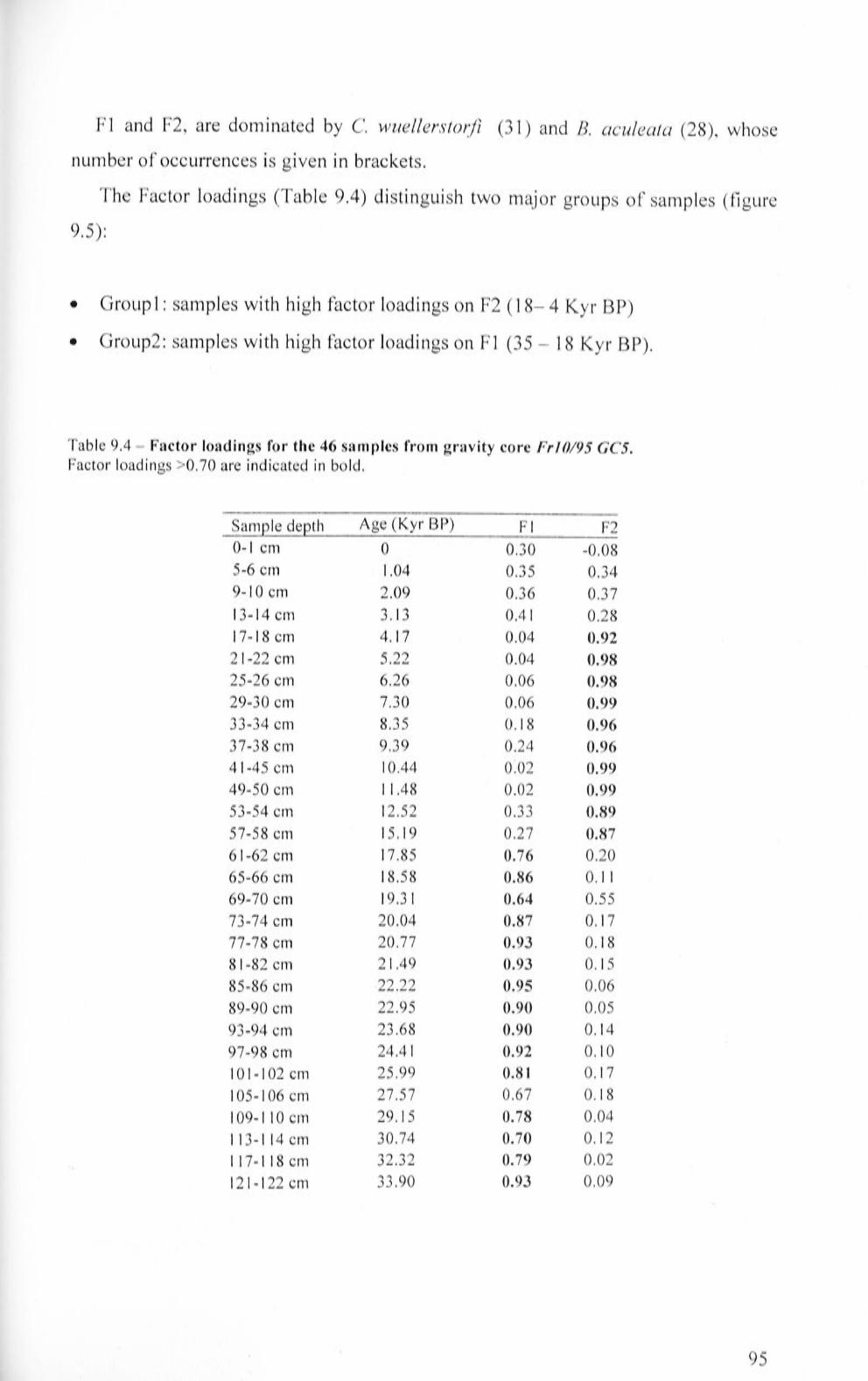
Fl and F2, are dominated by C. wuellerstorfi (31) and B. aculeata (28), whose

number of occurrences is given in brackets.

The Factor loadings (Table 9.4) distinguish two major groups of samples (figure

9.5):

• Group 1: san1ples with high factor loadings on F2 ( 18- 4 Kyr BP)

• Group2: samples with high factor loadings on F 1 (35 - 18 Kyr BP).

Table 9.4 - Factor loadings for the 46 samples from gravity core Fr/0/95 GCS. Factor loadings >0.70 are indicated in bold.

Sam12le de12th Age (Kyr BP) Fl F2 0-1 cm 0 0.30 -0.08 5-6 cm 1.04 0.35 0.34 9-10 cm 2.09 0.36 0.37 13-14 cm 3. I 3 0.41 0.28 17-18 cm 4.17 0.04 0.92 21-22cm 5.22 0.04 0.98 25-26 cm 6.26 0.06 0.98 29-30 cm 7.30 0.06 0.99 33-34 cm 8.35 0.18 0.96 37-38 cm 9.39 0.24 0.96 41-45 cm 10.44 0:02 0.99 49-50 cm 11.48 0.02 0.99 53-54 cm 12.52 0 ., ., . .) .) 0.89 57-58 cm 15.19 0.27 0.87 61-62 cm 17.85 0.76 0.20 65-66 cm 18.58 0.86 0.11 69-70 cm 19.31 0.64 0.55 73-74 cm 20.04 0.87 0.17 77-78 cm 20.77 0.93 0.18 81-82 cm 21.49 0.93 0. 15 85-86 cm .22.22 0.95 0.06 89-90 cm 22.95 0.90 0.05 93-94 cm 23.68 0.90 0.14 97-98 cm 24.41 0.92 0.10 IO 1-102 cm 25.99 0.81 0.17

I 05-106 cm 27.57 0.67 0. I 8 I 09-110 cm 29.15 0.78 0.04 113-1 14 cm 30.74 0.70 0.12

117-118cm 32.32 0.79 0.02

121-122 cm 33.90 0.93 0.09

95

In figure 9.6, the percentages of the species that dominate the two factors are

plotted versus age (Kyr BP). C. wuellersto,~fi showed the highest percentages

between 35 and 18 Kyr BP (termination of MIS3 - mid MIS2). Between 18 and 4 Kyr

BP (termination of MIS2 - mid MIS 1 ), B. aculeata do111inated the benthic

foraminiferal fauna.

Fr10/95 GC5

F1

F2

0

I MIS1 I M!S2 I MlS3 I Group1 Group2

---,-----.....----- ------,,----------"-··-····-··-···--/~~~."-...... ------·,

/\ ( \'\\ // I \ I \ ~ / I. \ ' \ ,/ •.'- //

. I I . . ', / ... ., f : V ✓ ··

........................................................................................... ,,,· , . ,,,,_,,,,,,,,-~-- .. ,,, .· ,,,,,, .. ,·,,,,,._ .. ,.,,, ... _,,,, ... ,,, .. ,_.,,,,. ,,,,, ... ,,,

.. . / .. 1, . . . . /

_.✓- ;~-. I ......____ I

· 1 --:- .· /'\ /

\ I \ I \ I \ . l I . / I . / L ... :..--~· \ . l ~...,

~ ••• ........ . ... . ..... • r •b• ·•s .... ~ .... 1 · n•--n•••••••r ••••- ••• • -• .. r--• ...... ,. ............... ! .................................... , ................ , .................. T ................ , ................ T ..

Ci> 0

<;)'

C

0 '

,.,,...,...·"\ I \J I I I l I

0

r-~-...... ... ..,,,,..---....... ..... ( •..• -.... · •·.. . . .· , ,~-'- ·~-)

I

I.!) 0 fJl ~ ,,.-

. t \ ' . \ \ I \

I \ \

/ l..-' ~ .i " . - /,-- \ ~ \ I ..____,, \ /'·,

0 N

\..,J \ / ' -----✓-✓

Age (Kyr BP)

Fig. 9.5 - Factor loadings for the samples of Fr/0/95 GC5 calculated for each one of the two factors and plotted versus age (Kyr BP). Two groups of samples are identified on the basis of the analysis of their scores on the two axes: Group 1, which includes samples characterised by factor loadings on F 1, and Group2, which includes samples with high factor loadings on F2. At the top of the diagram, Marine Isotope Stages are shown

96

Fr10/95 GC5


Cibicidoides wuellerstorfi (%)

I MIS1 I MIS2 I MIS3 I Group1 Group2

g,----,r------- ------------~

0 N

0 ..-

0 0 ..- 0

N

Age (Kyr BP)

/

Fig. 9.6 - Diagram showing the percentages of those species from gravity core Frl0/95 GC5, identified by means of Factor Analysis. At the top of the diagram, Marine Isotope Stages are shown. Vertical lines indicate the limits of the two groups of samples individuated by means of the factor loadings.

9.2.2 Frl0/95 GC5:faunal characteristics

As for Fri 0/95 GCJ 7, the total percentages of agglutinated, porcellaneous and

infauna! taxa (for the species included in this last group see Appendix B), a, H(S), E,

D were calculated for each core san1ple (figure 9.7).

97

Fr10/95 GCS

Agglutinated(%)

Porcellaneous (%)

Infauna!(%)

CX

H(S)

E

D

I MIS1 MIS2 I MfS3

I.{),--------------- ----- --

; _··· \/\ ;\ I 7 __ . __ -,-, I / \\ /'.._,,,,.., _ / --• \ II\. I / ·,---~- \ ,· I ' ______ // l 0 -t-_,...........'---t '\ _-¥-,,,- ,---,----,- ..,...-_____::\~,_/ -.----'"·;._• -✓-. :'.._,,,-~-----~

g ~------------- ---- ----- - -~

0 r <) -~--·······-··•·············•·······················-·····--- --····•·••······················-··-··-··-••···-················•··········-··········

~ \ ~ .. \ /'

... ·~ --_,_~_,,.---~ --1.D . ······· ·····r······ ·· ····-r············, ··-········r ············ · ········•····r········ ····r ······ ·· ··r··············r········ ······· • ····•·•······· · ··········-·· 1 ··············,············ r·'

. \ I

co \_/"· ('.J

.-~---------~-----,-/~-;:: ~ - ---, I ~ --,----.---/ .... , -----lt---1 ·--·-::..-,,_--..-c.-:.:- -- ./ ' ·~

\__ __ --./.,,-·~"'-~, / I ~_v_· ·--···-· .. ·-··-·.---,---~- --~ r·-·--·····,···-····r.J

~------------------- ------ ~ l[) \ N - \

·· v~ I.I) \ ~-·

•D

0 (0

~-

l I

/'/':-./'-, . / _, \

I -· "-...__.. -. \

0

I , I •. . . •"'---~

.... ('4 i

_,__~I

0 -· I I

0 LO

r

r·-·---· ..

0 ("'J

Age (Kyr BP)

L()

N

--------~--I l

r· .. ··-·-··-,····· ........... r 0 (")

I.() (Y')

Fig. 9.7 - Faunal characteristics calculated for each sample from gravity core Fr/0/ 95 GC5. Percentages of Agglutinated, Porcellaneous and Infauna! taxa; a : Fisher 's Alpha index , H(S): ShannonWeaver index; E: equitability; D: dominance. At the top of the diagram, Marine Isotope Stages are shown.

98

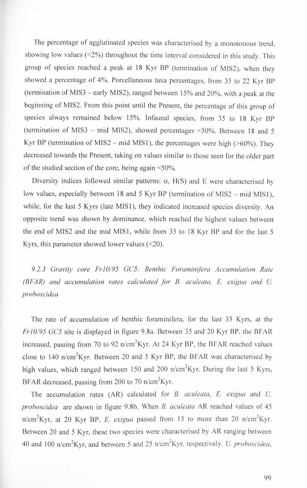
The percentage of agglutinated species was characterised by a monotonous trend,

showing low values ( <2%) throughout the ti1ne interval considered in this study. This

group of species reached a peak at 18 Kyr BP (termination of MIS2), when they

showed a percentage of 4%. Porcellaneous taxa percentages, from 35 to 22 Kyr BP

(termination of MIS3 - early MIS2), ranged between 15% and 20%, with a peak at the

beginning of MIS2. From this point until the Present, the percentage of this group of

species always remained below 15%. Infaunal species, from 35 to 18 Kyr BP

(termination of MIS3 - mid MIS2), showed percentages <50%. Between 18 and 5

Kyr BP (termination of MIS2 - mid MIS 1 ), the percentages were high (>60% ). They

decreased towards the Present, taking on values similar to those seen for the older paii

of the studied section of the core, being again <50%.

Diversity indices followed similar patterns: a, H(S) and E were characterised by

low values, especially between 18 and 5 Kyr BP (termination of MIS2 - n1id MIS 1 ),

while, for the last 5 Kyrs (late MIS 1 ), they indicated increased species diversity. An

opposite trend was shown by dominance, which reached the highest values between

the end of MIS2 and the mid MIS 1, while from 3 5 to 18 Kyr BP and for the last 5

Kyrs, this paran1eter showed lower values ( <20).

9. 2. 3 Gravity core Fr 10/95 GC5: Benthic Foramin~fera Accu,nulation Rate

(BF AR) and accumulation rates calculated .for B. aculeata, E. exigua and U.

proboscidea

The rate of accumulation of benthic foraminifera, for the last 3 5 Kyrs, at the

Frl0/95 GC5 site is displayed in figure 9.8a. Between 35 and 20 Kyr BP, the BFAR

increased, passing fro1n 70 to 92 n/cm2Kyr. At 24 Kyr BP, the BF AR reached values

close to 140 n/cm2Kyr. Between 20 and 5 Kyr BP, the BF AR was characterised by

high values, which ranged between 150 and 200 n/cm2Kyr. During the last 5 Kyrs,

BFAR decreased, passing from 200 to 70 n/cn12Kyr.

The accumulation rates (AR) calculated for B. aculeata, E. exzgua and U.

proboscidea are shown in figure 9.8b. When B. aculeata AR reached values of 45

n/cm2Kyr, at 20 Kyr BP, E. exigua passed from 15 to more than 20 n/cm2Kyr.

Between 20 and 5 Kyr, these two species were characterised by AR ranging between

40 and 100 n/cm2Kyr, and between 5 and 25 n/cm2Kyr, respectively. U. proboscidea,

99

despite it never reached high AR during the last 30 Kyrs, displayed values close to 5

n/c1n2Kyr soon after 20 Kyr BP, until the present.

Fr10/95GC5

MIS1 MIS2 MIS3

0

0 0 I.() 0 ll) 0 IO T"" T"" N IN ('I) <")

Age (Kyr BP) (a)

0 0 ... 0 m

0 CX)

0 - ~ ... >- 0 ~ (0

N E 0

~ ll)

0 - 'V

g

~ 0 .,...

0

0 0 tO 0 I.O 0 I() ...... ..- N N ('I) (")

Age (Kyr BP) (b)

Fig. 9.8 - Gravity core Frl0/95 GC5: (a) Benthic foraminifera Accumulation Rate (BFAR) and (b) accumulation rates of B. aculeata (blue line), E. exigua (green line) and U. proboscidea (red line). (a) The curve indicates the BFAR (expressed as number of benthic foraminifera accumulated over 1 cm2 each thousand years) variations during the last 30 Kyrs. (b) The highest AR values calculated for the three selected species are recorded for the period between 20 and 5 Kyr BP. At the top of the diagram, Marine Isotope Stages are shown

100

9. 3 Piston core SHf 9016

The analysis of benthic foraminifera species, extracted from san1ples fron1 piston

core SHJ9016, led to the identification of 138 taxa (Appendix A4), with mean

percentages ranging between 14.03% (B. aculeata) and 0.01 % (Guttulina pacifica).

Those species present with a percentage >2% in at least one sample were selected for

Q - n1ode Factor Analysis (Principal Components). A total of 56 species were

selected for the statistical analysis.

9.3. I SHJ9016: Factor Analysis

Factor analysis calculated two vanmax factors, explaining 82. 7% of the total

variance of the species distribution. Species scores related to the two factors are listed

in Table 9 .5.

Table 9.5 - Q-mode Factors Analysis (Principal Components) results for the reduced species dataset of piston core SH /90 I 6: species scores for varimax Factors I and 2. Those species, which present high score on FI, or F2, and high mean percentage, are indicated in bold.

Species Fl F2 Mean%

Anomalina globulosa -0.30 -0 .50 0.50

Astrononion echolsi 0.36 0.54 2.92

Bolivina robusta -0.39 -0.43 0.40

Bulimina aculeata 6.61 -2.02 14.03

Bulimina costata -0.34 0.1 I 1.17

Buliminella elegantissima -0.37 -0.66 0.21

Cassidulina crassa -0.34 -0.68 0.23

Cassidufina laevigata 0.25 0.25 2.49

Ceratobulimina pacifica -0.52 0.27 0.96

Chifostomelfa uofina -0.53 1.17 1.98

Cibicidoides bradyi 0.80 0.80 4.15

Cibicidoides kuffenbergi -0.48 -0.17 0.51

Cibicidoides pseudoungerianus -0.46 0.44 I. 18

Cibicidoides robertsonianus -0 .34 -0 .62 0.31

Cibicidoides wuefferstorfi 0.48 2.90 5.72

Cibicidoides sp. -0.30 -0.65 0.35

Dent al ina communis -0.40 -0.52 0.27

Eggerella bradyi -0 .33 -0.50 0.46

Ehrenbergina trigona -0.11 -0.52 0.87

101


Species Fl F2 Mean% Epistominel/a exigua 0.62 -0.79 2.17 Fissurina spp. 0.91 2.03 5.56 Gavelinopsis lobatulus -0.16 -0.41 0.90 Glohocassidulina elegans -0.49 -0.27 0.38 Globocassidulina subg!obosa 0.08 2.70 4.66 Gyroidinoides alt{formis -0.34 -0.50 0.42 Gyroidinoides orbicularis -0.15 0.35 1.74 Gyroidinoides soldanii -0.29 -0.50 0.51 Hoeglundina elegans -0.32 0.71 1.82 Karreriella bradyi -0.34 -0.71 0.24 lagena spp. 0.05 -0.15 1.63 laticarinina pauperata -0.35 -0.38 0.52 lenticulina spp. -0.39 -0.33 0.54 Martinottiella communis -0.33 -0.51 0.47 Melonis barleeanum 0.64 -0.27 2.71 Melonis pompilioides -0.17 -0.76 0.54 Nummoloculina irregularis -0.38 -0.39 0.51 Oolina spp. -0.37 -0.55 0.36 Oridorsalis tener umbonatus 0.66 1.22 4.17 Parqfissurina spp. -0.24 0.02 1.17 Pullenia bulloides 0.30 2.71 4.86 Pullenia quinqueloba 0.09 0.25 2.05 Pyrgo depressa -0.15 0.08 1.37 Pyrgo murrhina -0.04 -0.07 1.51 Pyrulina gutta -0.41 -0.68 0.11 Quinqueloculina lamarckiana -0.41 -0.54 0.31 Quinque!oculina seminulum -0.27 0. 13 1.25

Quinqueloculina venusta -0.28 -0.71 0.36

Robertina tasmanica -0.40 -0.70 0.14

Robertinoides brady -0.41 -0.73 0.10

Sigmoilopsis schlumbergeri -0.23 -0.24 0.96

Siphotextularia sp. -0.41 -0.67 0.11

Sphaeroidina bulloides -0.42 -0.15 0.71

Triloculina tricarinata -0.21 -0.30 0.92

Uvigerina proboscidea 1.47 2.79 7.71

Valvulineria araucana -0.16 -0.88 0.45

FI is dominated by B. aculeata (25), while F2 is dominated by C. wuellerstor.fi

(35) (the number of occurrences of the species is given in brackets). The species

identified by Factor Analysis are characterised by high n1ean percentages.

Factor loadings for each san1ple are listed in table 9.6. By means of these varues, it

is possible to identify two groups of samples (figure 9. 9):

• Group 1: samples with high loadings factor on F2 ( 15 Kyr BP - Present).

102

• Group2: samples with high loadings factor on Fl (62 - 15 Kyr BP).

Table 9.6 - Factor loadings for the 46 samples from piston core SH/9016. Factor loadings >0.70 are indicated in bold.

Sample depth Age (Kyr BP) Fl F2

0-1 cm 0 0.12 0.69 4-5 cm 1.15 0.14 0.81 8-9 cm 3.44 0.11 0.77 12-13 cm 4.59 0.16 0.86 16-17 cm 5.50 0.13 0.89 22-23 cm 6.89 0.13 0.88 26-27 cm 8.03 0.08 0.80 32-33 cm 9.18 0.16 0.87 36-37 cm I 0.33 0.18 0.82 42-43 cm I 1.48 0.05 0.81 46-47 cm 12.94 0.16 0.72 52-53 cm 15.17 0.34 0.77 56-57 cm 16.00 0.80 0.50

58-59 cm 17.85 0.92 0.20

62-63 cm 19.32 0.91 0.18

66-67 cm 21.53 0.95 0.13

72-73 cm 23.01 0.97 0.02

76-77 cm 25.53 0.88 0.35

82-83 cm 27.43 0.87 0.41

86-87 cm 30.28 0.78 0.48

92-93 cm 32.18 0.69 0.62

96-97 cm 35.03 0.85 0.42

102-103 cm 36.92 0.95 0.1 I

I 06-107 cm 39.77 0.98 -0.08

1l2-1l3cm 41.67 0.75 0.45

116-117 cm 44.52 0.98 -0.04

122-123 cm 46.41 0.98 0.06

126-127 cm 49.26 0.95 0.18

132-133 cm 51.0 I 0.90 0.26

136-137 cm 52.99 0.96 -0.02

142-143 cm 54.19 0.99 -0.0 I

146-147 cm 57.37 0.92 0.16

152-153 cm 58.96 0.91 0.25

156-157 cm 60.75 0.92 0.26

162-163 cm 61.95 0.94 0.10

Percentages of the species characterised by the highest factor scores on the two

axes are plotted in figure 9.10. From 62 to 15 Kyr BP, B. aculeata dominated the

benthic foraminiferal fauna, while C. wuellerstorfi dominated during the last 15 -Kyrs.

103

SH/9016

F1

F2

0)

0

I MIS1 I MIS2 I Group1

MIS3

Group2

o-+--.----,----,---.--.---....---a--.----,---.---.--r--~-.-----,---r--.:.-~~~---,-~---__j I

0 0 N

U') N

Age (Kyr BP)

0 U')

l[) l[)

0 CD

Fig. 9.9 - Factor loadings for the samples of SH/9016 calculated for the two factors and plotted versus age (Kyr BP). Two groups of samples are identified on the basis of the factor loadings on the axes: Group I, which includes samples characterised by high factor loadings on Factor 2 and Group2, which include samples with high factor loadings on Factor I. At the top of the diagram, Marine Isotope Stages are shown.

104

SH/9016 I MIS1 I MIS2 I MIS3

Group1 Group2 ~~-----,r---------------



0 (')

0 0 01

I.CJ N

0 n

Age (Kyr BP)

0 lI)

L() 0 lO CD

Fig. 9.10 - Diagram showing the percentages of those species from piston core SH/9016, identified by means of Factor Analysis. At the top of the diagram, Marine Isotope Stages are shown. Vertical lines indicate the limits of the two groups of samples individuated by means of the factor loadings.

9. 3. 2 SHl9016: fauna! characteristics

Percentages of the agglutinated, porcellaneous and infauna! species ( for the species

included in this last group see Appendix B), together with the values calculated for a,

H(S), E and D are plotted in figure 9 .11.

The agglutinated species showed low percentages ( <4%) for the tin1e interval

studied from piston core SHJ9016. Before 18 Kyr BP (termination of MIS4 -early

MIS2), agglutinated species were characterised by percentages always · <2%.

Percentages >2% were recorded between 18 and 5 Kyr BP (1nid MIS2 - late MIS 1 ).

During the last 5 Kyrs, these taxa, again, had percentages <2%. Between 62 and 27

105

Kyr BP (termination of MIS4 - early MIS3), the porcellaneons taxa showed

percentages between 2% and 8%. After, and until 18 Kyr BP (mid MIS3 - early

MIS2), the percentages were always <2%. Higher values were reached by these

species for the last 18 Kyrs (termination of MIS2 - MIS 1 ). The infauna! taxa follovved

two major patterns. Before 15 Kyr BP (termination of MIS4 - n1id MIS2), they were

characterised by percentages >75% (reaching 88%, during early MIS3). Their

percentages were lower (generally <75%) for the last 15 Kyrs (termination of MIS2 -

MIS 1 ). During this period, the percentages showed an irregular pattern, ranging

between 64% and 77%.

Diversity indices ( a, H(S), E) calculated for the samples of SH/9016 displayed

similar trends. Before 16 Kyr BP (termination of MIS4 - n1id MIS2), they were

characterised by low values (<20, <3.8 and <28 respectively) , while, during the last

16 Kyrs (termination of MIS2 - MIS 1 ), they increased, maintaining higher values

con1pared to the former time interval. Dominance was characterised by an inverse

pattern, showing high values (> 15%) during the period comprised between

tennination of MIS4 and early- mid-MIS2 (62 Kyr BP - 16 Kyr BP), and low values

( <15%) during the last 16 Kyrs.

9. 3. 3 Piston core SH/9016: Benthic F oramin[fera Accunntlation Rate (BF AR) and

accumulation rates calculated for B. aculeata, E. exigua and U proboscidea

The curve related to the Benthic Foraminiferal Accumulation Rate (figure 9.12a),

for piston core SH/9016 samples, displays two major patterns. Between 62 and 20

Kyr BP, BFAR was characterised by high values (>200 n/cm2Kyr) with a peak of 326

n/cn12Kyr, at 23 Kyr BP. After 15 Kyr BP, the accumulation rate of benthic

foran1inifera decreased, maintaining values close to 100 n/cm2Kyr, which decreased 7 to 50 n/cm-Kyr, for the Present.

The accumulation rate of B. aculeata mirrored the BF AR trend (figure 9.126 ).

Between 62 and 15 Kyr BP, B. aculeata AR ranged between 20 and 90 n/cm2Kyr.

After 15 Kyr BP, this species was absent at this site. E. exigua showed a sin1ilar

pattern, with AR ranging between 5 and 20 n/cm2Kyr, before 15 Kyr BP, and

disappearing after that period. U proboscidea was still present after 15 Kyr BP, but as

for the other two species, it displayed higher AR values (> IO n/cm2Kyr ) between 62

106

and 15 Kyr BP. During the last 15 Kyrs, U. proboscidea AR decreased constantly

from 10 to 5 n/cm2Kyr, for the Present.

107

SH/9016 I MIS1 I MIS2 I MIS3 I~ I -.:::-

C')

Agglutinated (%) N

..-

0

CX)

<D

Porcellaneous (%) V'

N ) 0

0 (J) - --------

0 co

lnfaunal (%)

0 (.!)

0 ~

CJ. 0 r0

0 N

,.....___ 0 ..-

u LO C")

H(S) 0 /\f 0 C")

0 LO

N

l.()

-.:::-0 ..;t-

0

E C")

0 \ N

0 ,-

0 ~

0 C")

D 0 N

0 r--

0

0 l{) 0 l{) 0 l{) 0 ll) 0 \!) 0 l{) 0 .,.... .,.... N N C') C') '"I" "1' ll) ll) (.0

Age (Kyr BP)

Fig. 9.11 - Fauna I characteristics calculated for each sample from piston core SH/9016. Percentages of Agglutinated, Porcellaneous and Infauna! taxa; a: Fisher 's Alpha index, H(S): ShannonWeaver index; E: equitability; D: dominance. At the top of the diagram, Marine Isotope Stages are shown.

108

SH/9016

I MISl I MIS2 I MIS3 I~ I 0 0 (Y)

-.... >, 0 ~ 0

N N

E ~ C - g

.....

0

0 0 I,(') 0 lO 0 lO 0 lO 0 I,.() 0 ..... ..... N ('I.I ('t) ('t') "if' "l,f' ID ID CD

Age (Kyr BP) (a) 0 0 ..-0 0)

0 «> 0 - " '-

~ 0 N <O

E 0 ~ I.O C .._

0 v

0 c,')

0 N

0 ,....

0

..- ..-

Age (Kyr BP) (b)

Fig. 9.12 - Piston core SH/9016: (a) Benthic foraminifera Accumulation Rate (BFAR) and (b) accumulation rates of B. aculeata (blue line), E. exigua (green line) and U. proboscidea (red line). (a) The curve indicates the BFAR (expressed as number of benthic foraminifera accumulated over 1 cm2 each thousand years) variations during the last 30 Kyrs. (b) The highest AR values calculated for the three selected species are recorded between 62 and 15 Kyr BP. At the top of the diagram, Marine Isotope Stages are shown.

109

9. 4 Piston core BAR9403

Ninety-three benthic foraminifera species were identified (Appendix AS) in

BAR9403 samples. Their mean percentages ranged between 17.8% (B. aculeata) and

0.0 I% (Bolivina albatrossi). Similar to the procedure followed for the species

identified in samples from the other cores, the taxa showing a percentage >2% in at

least one sample were selected for Q- mode Factor analysis (Principal Components).

9.4.1 BAR9403: Factor Analysis

Factor analysis calculated four varimax factors, which explained 85.33% of the

variance of the species distribution. The species scores are listed in Table 9.7.

Table 9.7 - Q-mode Factors analysis (Principal Components) results for the reduced species dataset of piston core BAR9403: factor scores for varimax Factors I, 2, 3 and 4. Those species, which present high score on FI, or F2, or F3 or F4 and high mean percentage, are indicated in bold.

Species Fl F2 F3 F4 Mean%

Allomorphina pac[fica -0.30 -0.18 -0.13 -0.44 0.26

Anomalina globu!osa -0.09 -0.34 -0.50 -0.10 0.30

Astrononion echolsi -0.06 -0 .23 -0.56 0.30 0.80

Bolivina robusta -0. 12 -0.25 -0.40 -0.38 0.25

Bolivinita quadrilatera -0.03 -0.25 -0 .20 -0.44 0.57

Brizalina semilineata -0.22 -0.27 -0.3 I -0.33 0.15

Bulimina aculeata 7.48 0.55 -1.08 -0.63 17.79

Bulimina costata 0.0 I 0.92 0.88 -0.53 3.34

Bulimina exilis -0.16 0.39 -0 .34 -0.75 0.83

Cassidufina laevigata 0.16 0.79 -0.16 0.16 3.08

Ceratobulimina pacifica -0.14 -0.28 -0.38 -0.42 0.12

Chi!ostomella oolina -0.18 -0.0 I 0.57 1.23 2.62

Cibicidoides bradyi -0. 11 -0.29 -0. 10 0.88 1.57

Cibicidoides pseudoungerianus -0.17 -0.43 -0.3 I 0.30 0.56

Cibicidoides robertsonianus -0.24 -0.31 -0.08 -0.46 0.14

Cibicidoides wuellerstorfi 0.46 0.10 -0.03 5.83 7.56

Eggerella bradyi -0.19 -0.30 -0.05 -0.36 0.36

Epistominella exigua 0.98 -1.04 6.93 -0 .96 7.82

Fissurina spp. -0.07 -0.24 -0.05 -0.13 0.89

Fursenkoina bradyi -0.18 -0.27 -,0.20 -0.53 0.19

F ursenkoi na fits iform is -0.06 0.40 -0.26 0.26 2.06

110


Species Fl F2 F3 F4 Mean %

Fursenkoina sp. -0.22 -0.31 -0.19 -0.45 0.12 Gavelinopsis lobatulus -0.05 -0.30 -0.47 -0.13 0.46 Globobulimina affinis -0.22 -0.09 0.47 ·-0.30 1.16 Glohobulimina pac{fica -0.21 -0.33 0.41 0.04 1.03 Globocassidulina subglobosa 0.16 -0.43 -0.01 0.76 1.94 Gyroidinoides orbicularis -0.22 -0.33 -0.41 0.67 0.69 Gyroidinoides polius -0.27 -0.33 0.17 0.19 0.74 Gyroidinoides soldanii -0.21 -0.14 -0.46 -0.33 0.30 Hoeglundina elegans 0.26 0.22 -0.38 0.76 2.70 Hyalinea balthica -0.26 -0.20 -0.02 -0.47 0.28 Karreriella bradyi -0.28 -0.27 -0.08 -0.34 0.22 lagena spp. -0.25 -0.35 0.05 -0.22 0.35 Lenticulina spp. -0.26 -0.14 -0.19 -0.48 0.27 loxostomum karrerianum -0.26 -0.27 -0.06 -0.45 0. I 8 Melonis barleeanum -0.40 0.08 -0.0 I 1.68 2.18

Melonis pompilioides -0.26 -0.29 -0.15 -0.47 0.08 Mifiolineffa subrotunda -0.24 -0.16 -0.27 -0.57 0.11 Nonioneffa bradyi -0.24 -0.16 -0.35 -0.48 0.19

Nummofoculina irregufaris -0.22 -0.12 -0.30 -0.58 0.18

Oridorsalis tener umbonatus -0.64 7.22 0.69 -0.11 11.28

Osangufaria cultur -0. 16 -0.11 -0.47 -0.29 0.36

Parafissurina spp. -0. I 5 -0.21 -0.36 -0.43 0.24

Pullenia bulfoides -0.24 -0.31 0.23 0.01 0.80

Puffenia quinqueloba -0.19 -0.32 0.02 -0.18 0.51

Pyrgo depressa -0.16 -0.03 -0.39 -0.40 0.51

Pyrgo lucernufa -0.24 0.04 -0.45 -0.60 0.21

Pyrgo murrhina -0.05 0.94 1.74 0.50 4.63

Pyrgo serrata -0.09 -0.12 -0.29 -0.58 0.46

Quinqueloculina seminufum -0.25 -0.13 -0.21 -0.34 0.34

Quinquefoculina venusta -0.17 0.73 -0.35 -0.82 1.43

Robertinoides brady -0.11 -0.26 -0.35 -0.53 0.19

Sigmoilopsis schlumbergeri -0. I 7 -0.03 -0.74 0.89 1.35

Siphogenerina raphanus -0.26 -0.18 -0.28 -0.58 0.04

Siphotextularia catenata -0.19 -0.03 -0.36 -0.58 0.29

Sphaeroidina buffoides -0.22 -0.38 -0.07 0.01 0.48

Spirofocufina tenuis -0.26 -0.14 -0.40 -0.45 0.13

Triloculina tricarinata -0.26 -0. 1 I -0.41 -0.47 0. I 7

Uvigerina peregrina 0.10 -0.54 0.85 1.60 3.11

Uvigerina proboscidea 0.32 -0.35 0.56 2.43 4.13

Valvulineria araucana 0.30 -0.17 0.09 -0.42 1.77

The four factors are dominated by four taxa all characterised by high . mean

percentages. F 1 is dominated by B. aculeata ( 43), F2 is dominated by 0. t. umbonatus

(51), F3 is don1inated by E. exigua (44) and F4 is dominated by C. wuellerstor_fz (53)

111

(number of occurrence is given in brackets).

The loading factors (Table 9.8) identify four groups of samples (figure 9.13):

• Group 1: samples with high factor loadings on F3 (3 Kyr BP - Present).

• Group2: samples with high factor loadings on F4 (15 - 3 Kyr BP).

• Group]: samples with high factor loadings on Fl (27 - 15 Kyr BP).

• Group4: smnples with high factor loadings on F2 (33 - 27 Kyr BP).

The percentages of the species, which dominate the four factors, are plotted in

figure 9.14. 0. t. u,nbonatus showed the highest percentages from 33 to 26 Kyr BP

(termination of MIS3 - M1S2), while values between 10% and 20% were recorded

between 15 and 2 Kyr BP (termination of M1S2 - late MIS 1 ). B. aculeata showed

high percentages (>30%) from 26 until 15 Kyr BP (MIS2). Between 4 and 2 Kyr (late

MIS 1 ), this species was characterised by percentages ranging between 10% and 20%.

E. exigua reached percentages> 10%, at 33 Kyr BP, between 24 and 20 Kyr BP (early

MIS2) and during the last 3 Kyrs. C. wuellersto,ji was characterised by high relative

percentage between 12 and 5 Kyr BP (termination of MIS2 - late MIS 1 ). This taxon

reached percentages> 10% between 30 and 28 Kyr BP (mid MIS3 ).

Table 9.8 - Factor loadings for the 53 samples from piston core BAR9403. Factor loadings >0.70 are indicated in bold.

Sample depth Age (Kyr BP) Fl F2 F3

0-1 cm 0 0.02 0 ,.,,., . .).) 0.53

5-6 cm 0.58 0.12 0.25 0.89

10-11 cm 1.16 0.12 0.25 0.79

15-16 cm 1.74 0.12 0.26 0.88

20-21 cm 2.32 0.39 0.32 0.77

25-26 cm 2.76 0.70 0.53 0.40

30-31 cm 3.21 0.55 0.29 0.62

35-36 cm 4.09 0.54 0.42 0.35

39.5-40.5 cm 4.98 0.74 0.56 0.05

F4

0.39

0.22

0.26

0.01

0.16

0.02

0. 16

0.42

0.13

112


Sample depth Age (Kyr BP) Fl F2 F3 F4

45-46 cm 5.86 0.26 0.67 0.07 0.22 50-51 cm 6.75 0.28 0.49 0.11 0. 71 55-56 cm 7.63 0.07 0.12 0.37 0.71 60-61 cm 8.52 0.16 0.52 0.52 0.41 65-66 cm 9.40 -0.03 0.85 0.29 0.23 70-71 cm 10.29 0.01 0.77 0.24 0.51 75-76 cm I 1.17 0.08 0.40 0.19 0.77 80-81 cm 12 .06 0.08 0.31 0.10 0.82 85-86 cm 12.37 0.07 0.3 I 0.42 0.69 90-91 cm 12.78 0.03 0.13 -0.02 0.82 95-96 cm 13.50 0.20 0.52 0.10 0.63 I 00-101 cm 14.23 -0.09 0.47 -0.05 0.32 l05-106cm 14.95 0.58 0.38 -0.02 0.49

110-111 cm 15.68 0.70 0.54 -0.04 0.36

115-116 cm I 6.40 0.88 0.27 -0.03 0. 19

120-121 cm 17. I 3 0.90 0.22 -0.06 0.19

125-126 cm 17.85 0.98 0.08 -0.03 0.03

130-131 cm 18.74 0.92 0.10 0.05 0.11

135-136 cm 19.64 0.94 0.1 I 0.02 0.00

140-141 cm 20.53 0.97 0.13 0.09 0.03

145-146 cm 21.43 0.99 0. IO 0.04 0.00

150-151 cm 22.32 0.93 0.19 -0.0 I 0.19

155-156 Clll 23.21 0.94 0.16 0.11 0.18

160-161 cm 24.11 0.95 0.14 0.27 -0.02

165-166 cm 24.77 0.87 0.03 0.46 -0.02

170-171 cm 25.42 0.93 0.23 0.21 0.05

175-l76cm 25.82 0.94 0.08 0.31 0.01

180-18 I cm 26.22 0.99 0.12 0.08 0.00

185-186 cm 26.62 0.84 0.16 0.50 -0.0 I

190-191 cm 27.02 0.97 0.15 0.11 0.05

195-196 cm 27.42 0.86 0.44 0.02 0.02

200-201 cm 27.61 0.72 0.36 0.24 0.28

205-206 cm 27.81 0.21 0.89 0.14 0.19

210-211 cm 28.21 0.89 0.14 0.19 0.18

215-216cm 28.61 0.60 0.66 0.32 0.19

230-231 cm 29.81 0.28 0.74 0.24 0.40

235-236 cm 30.21 0.69 0.64 0.23 0.12

240-241 cm 30.61 0.27 0.84 0.24 0.27

245-246 cm 31.01 0.36 0.62 0.24 0.47

255-256 cm 31.80 0.32 0.90 0. 16 0.13

260-261 cm 32.20 0.04 0.87 0.13 0.11

265-266 cm 32.60 0.42 0.78 0.21 0.10

270-271 cm 33.00 0.57 0.38 0.64 0.06

275-276 cm 33.40 0.40 0.75 0.42 0.11

113

BAR9403

F1

F2

F3

F4

O')

0

"<T 0

,-

0 '

0 ,-

0)

0

I MIS1

Group1 Group2

J

I MIS2 I MIS3 I Group3 Group4

J

.. j . .· .... ·.:_····· ✓.·· ' . . ; . . . . . .

. ·- .

,o +-----r-------r-----r--.--.---.,__--,-----r------r------,---'--,------.--J ~ _;/--/

I

0)

0

. .. . . . -

. . · .. .. : .•.· .. · ·.. . · ...

. . . . .

;\ . .

..

. .. . \ .j

. ·•· J\/\ 0 -+--~----~-~---,--.----''-r----,---~-----,--..L-..------,--l

I

0 LO ,-

0 N

Age (Ky r BP)

LO N

Fig. 9.13 - Factor loadings for the samples of BAR9403 calculated for the four factors and plotted versus age (Kyr BP). Four groups of samples were identified on the basis of the factor loadings on the axes: Group I, which includes samples characterised by high factor loadings on Factor 3, Group2, which include samples with high factor loadings on Factor 4, Group] , which includes samples with hi gh factor loadings on Factor I and Group4, which includes samples with high factor loadings on Factor 2. At the top of the diagram, Marine Isotope Stages are shown .

114

BAR9403 I MIS1 I MIS2 I MIS3 I Group1 Group2 Group3 Group4

0 l()

::::-'<t

/1/VJIA g . Bulimina acu/eata (%)

0

~''il :,1

.-, VA ~-

D

~ ,-----,-------,.------~---

C,

Oridorsalis ten er umbonatus (%} N . 1\v0 JI./ . V

Epistomine/la exigua {%)


0

v\ r · o .. ... ,. •-f' " · ... ,,....., ·- - ,-r._..__,.~ sfL-....;.....-...._....,--,,-~ ... T- ·----,-, · ... · .... ,' ··--·, ...

0 r')

0 \ 0~ /11 f'·J

I \ J ~ 0

~

v~ J "--J

0

;: -,----.-------r------~--~

C 0 N

Age (Kyr BP)

l.") N

0 (")

Fig. 9. 14 - Diagram showing the percentages of those species from piston core BAR9403, identified by means of Factor Analysis. At the top of the diagram, Marine Isotope Stages are shown. Vertical I in es indicate the I im its of the two groups of samples individuated by means of the factor loadings.

115

9. 4. 2 BAR9403: .fauna! characteristics

Faunal characteristics (agglutinated taxa %, porcellaneous taxa %, infauna! taxa %

[Appendix BJ, a, H(S), E and D) are plotted in figure 9.15.

Between 33 Kyr BP and 15 Kyr BP (MIS3 - termination of MIS2), the

agglutinated species percentages were always <5%. They were characterised by high

percentages for the last 15 Kyrs (termination of MIS2 - MIS 1 ), ranging between 3%

and 14.5%. Porcellaneous taxa percentages before 27 Kyr BP were > 15%. Between

27 and 15 Kyr BP (mid MIS3 - mid MIS2) values decreased, being <15%, and

increased again during the last 16 Kyrs. Infaunal taxa were <40% before 27 Kyr BP.

Between 27 and 13 Kyr BP, percentages were always >50%, with a peak of 68% ( 17

Kyr BP). During the last 10 Kyrs, this group of species displayed percentages <60%,

ranging between 28% and 57%.

Diversity indexes a, H(S) and E followed sin1ilar patterns. Before 25 Kyr BP, a

values remained below the limit of 10, while H(S) and E displayed a more irregular

patterns, ranging between 2.5 and 3 and between 10 and 20 respectively. Between 25

and 16 Kyr BP, they were characterised by lower values (<10 a, <2.75 H(S) and <15

E). Only at 18 Kyr BP, did their values exceed the indicated thresholds. For the last

16 Kyrs (termination of MIS2 - MIS 1 ), diversity indexes displayed high values,

indicating high fauna! diversity. Before 25 Kyr BP, don1inance values ranged between

20% and 3 0%. Values increased, exceeding 3 0%, between 25 and 15 Kyr BP. During

the last 15 Kyrs, dominance was characterised by values below 20%.

9.4.3 Piston core BAR9403: Benthic Foraminifera Accumulation Rate (BFAR) and

accumulation rates calculated.for B. aculeata, E. exigua and U proboscidea

The BFAR curve (figure 9.16a) showed values ranging between 71 and 240

n/cm2Kyr, for the period between 33 and 27 Kyr BP. Between 27 and 15 Kyr BP,

BF AR was generally higher, reaching values >250 n/cm2Kyr. After 15 Kyr BP,

BFAR was characterised by lower values. Between 15 and 10 Kyr BP, BFAR

decreased passing from 180 to 90 n/cm2Kyr and between 10 and 5 Kyr BP, it ranged

between 160 and 53 n/cm2Kyr. During the last 5 Kyrs, BF AR decreased, reaching a

value of 20 n/cm2Kyr, for the Present.

116

The accumulation rate of B. aculeata reached values > 30 n/cniKyr, between 27

and 15 Kyr BP, with a peak of 170 n/cm2Kyr at 23 Kyr BP (figure 9.16b ). After 15

Kyr BP, this species was nearly absent. A small increase in B. aculeata AR was

recorded for the last 5 Kyrs. E. exigua was characterised by high AR, between 27 and

15 Kyr BP, ranging between 10 and 60 n/cm2Kyr. After 15 Kyr BP, the AR of this

taxa was nearly 0. It increased again during the last 5 Kyrs, reaching values > 10

n/cm2Kyr. U proboscidea followed a pattern similar to the former two species,

although it was characterised by lower AR values compared to the other two taxa.

Between 27 and 15 Kyr BP, U. proboscidea AR ranged between 5 and 20 n/cm2Kyr.

After 15 Kyr, this species displayed AR values <5 n/crn2Kyr, with an isolated peak at

5 Kyr BP, when it reached an AR of 15 n/cm2Kyr.

117

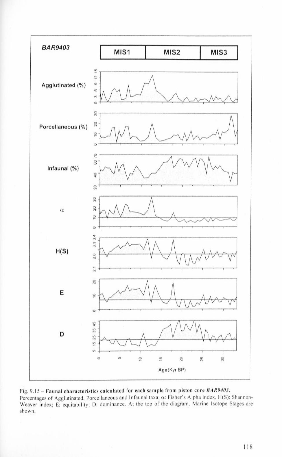
BAR9403

I.() ...... N ......

Agglutinated (%) 0)

<O

C")

0

0 C")

0

Porcellaneous (%) N

0 ......

0

0 r--

0 <O

Infauna! (%) 0 '-:t

0 N

0 C")

0 0, N

0 ......

0

'-:t C")

.... ,:.-j

H(S) <O N

,-

N

00 N

E 00 ,-

00

I.() -q-

I.()

D C")

I.()

N

I.() ..--

I.()

I MIS1 I

0 0 ....

MIS2

0 N

Age(Kyr BP)

I

I.() N

MIS3 I

Fig. 9.15 - Faunal characteristics calculated for each sample from piston core BAR9403.

Percentages of Agglutinated, Porcellaneous and Infauna! taxa; a: Fisher ' s Alpha index, H(S): ShannonWeaver index; E: equitability; D: dominance. At the top of the diagram, Marine Isotope Stages are shown.

118

BAR9403

I MIS1 I MIS2 I MIS3 I 0 0 ~

0 0 C") -'->,

~ 0 N 0 E N

~ -0 0 ..-

0

0 0 It) 0 It) 0 ..- .- ('.J N C")

Age (Kyr BP) (a)

0 O> ..-0 a:, .... 0 <O .... 0 ,q--'- ..-

>, 0 ~ N

N ..-E 0

0 ~ -r-

C 0 - (0

0 <O

0 V

0 N

0

0 II) ~ lO 0 ..- ,... ('\I (II)

Age (Kyr BP) (b)

Fig. 9.16 - Piston core BAR9403: (a) Benthic foraminifera Accumulation Rate (BFAR) and (b) accumulation rates of B. aculeata (blue line), E. exigua (green line) and U. proboscidea (red line). (a) The curve indicates the BF AR ( expressed as number of benthic foraminifera accumulated over 1 cm2 each thousand years) variations during the last 3 0 K yrs. (b) The highest AR values calculated for the three selected species are recorded between 27 and 15 Kyr BP. A slight increase of AR values is still present for the last 5 Kyrs, with values below 30 n/cm2Kyr. At the top of the diagram, Marine Isotope Stages are shown

119

9.5 813C results

813C values obtained from the test co1nposition of C. wuellersto,ji spec1111ens,

collected from the four cores, are listed in table 9.9.

Table 9.9 - 8 13C (%0) isotope data of C. wuellerstorfl vs. PDB m Fr/0/95 GC/7, Fr/0/95 GC5, SH/9016 and BAR9403.

Samples l/ 1C Samples 813C

Samples 811c Samples

81'C Fr/0195 GC/ 7 Fr/0195 GC5 SH/9016 BAR94()3

0-1 cm 0.61 0-1 cm 0.33 0-1 cm 0.46 0-1 cm 0.33

3-4 cm 0.65 5-6 cm 0.25 4-5 cm 0.48 30-31 cm 0.36

5-6 cm 0.66 9-10 cm 0.20 8-9 cm 0.59 35-36 cm 0.26

9-10 cm 0.67 13-14 cm 0.22 12-13 cm 0.53 50-51 cm 0. 13

13-14 cm 0.57 17-18 cm 0.09 16-17 cm 0.46 55-56 cm 0.06

17-18 cm 0.58 21-22 cm 0.0 I 22-23 cm 0.34 65-66 cm 0.04

21-22 cm 0.69 25-26 cm -0.06 32-33 cm 0.44 70-71 cm 0.21

25-26 cm 0.67 29-30 cm -0.05 36-37 cm 0.42 80-81 cm 0.02

29-30 cm 0.67 33-34 cm 0.0 I 42-43 cm 0.33 85-86 cm -0 .04

33-34 cm 0.74 37-38 cm 0.01 46-47 cm 0.22 90-91 cm 0.07

37-38 cm 0.59 41-45 cm 0.03 52-53 cm 0.01 95-96 cm 0. 13

41-42 cm 0.66 45-46 cm -0. 11 56-57 cm 0.20 I 05-106 cm 0.10

45-46 cm 0.68 49-50 cm -0.07 58-59 cm 0.11 l15-116cm -0.13

49-50 cm 0.69 53-54 cm -0 . 10 62-63 cm -0.01 120-121 cm -0.07

53-54 cm 0.67 57-58 cm -0 .03 66-67 cm 0.16 130-131 cm 0.06

57-58 cm 0.66 61-62 cm -0.10 72-73 cm 0.13 135-136 cm 0.10

61-62 cm 0.67 65-66 cm -0.02 76-77 cm 0.09 145-146 cm 0.07

65-66 cm 0.68 69-70 cm -0.0 I 82-83 cm 0.26 150-151 cm -0.07

69-70 cm 0.48 73-74cm -0.02 86-87 cm 0.22 160-161 cm -0.07

73-74 cm 0.51 77-78 cm -0.04 92-93 cm 0.13 165-166 cm -0.16

77-78 cm 0.57 81-82 cm 0.01 96-97 cm 0.27 170-171 cm 0.13

81-82 cm 0.56 85-86 cm 0.03 102-103 cm 0.25 180-181 cm -0. 15

85-86 cm 0.58 89-90 cm -0.03 1l2-113cm 0.24 l85-186cm 0.05

89-90 cm 0.54 93-94 cm 0.06 116-117 cm 0.11 190-191 cm -0.07

93-94 cm 0.44 97-98 cm -0.04 122-123 cm 0. 15 200-20 I cm -0 .09

97-98 cm 0.53 I 0-102 cm 0.11 132-133 cm 0.11 205-206 cm -0. 12

IO 1-102 cm 0.33 105-106 cm 0. 10 136-137 cm -0.07 210-211 cm -0. 11

105-106 cm 0.62 I 09-110 cm 0.04 142-143 cm 0.04 2l5-216cm -0. 10

I 09-110 cm 0.56 1l3-l14cm 0.09 146-147 cm -0.01 220-221 cm -0. 10

113-114 cm 0.47 117-118 cm 0.20 225-226 cm -0.03

117-118 cm 0.40 121-122 cm 0.21 230-231 cm -0. 17

121-122 cm 0.58 240-241 cm -0.05

255-256 cm -0.05

120


Samples o11c Samples 811c Samples 810c Samples ;sue Fr/0/95 GC/7 Fr/0195 GC5 Sf-I /9() 16 BAR9403

125-126 cm 0.42 152-153cm -0. 10 270-271 cm 0.00

127-128 cm 0.57 156-157 cm -0.04 275-276 cm 0.08 133-134 cm 0.45 162-163 cm -0. 03

137-138 cm 0.34

141-142 cm 0.38

145-146 cm 0.51

149-150 cm 0.22

153-154 cm 0.64

157-158cm 0.42

161-162 cm 0.44

165-166 cm 0.36

169-170 cm 0.45

173-174 cm 0.43

l77-l78cm 0.61

The values obtained with the 813C analysis of C. wuellerstorfi from Fr 10/ 95 GCJ 7

range between 0.74%0 and 0.22%0. The maximum value (0.74%0) is measured for the

specin1ens collected from sample 33-34 cm (3 Kyr BP) and the minimum (0.22%0)

from the sample 149-150 cm (23 Kyr BP). The analysis related to the time interval

between 31 Kyr BP (177-178 cm) and 7 Kyr BP (69-70 cm) gave values, which

ranged between 0.22%0 and 0.64%0. Isotopic values obtained for the last 7 Kyrs are all

>0.5%o.

The 8 13C values from Frl0/ 95 GC5 range between 0.33%0 and - 0.11%0. The

n1inin1um value (-0.11 %0) was obtained with the analysis of C. wuellerstor_fi

specimens from sample 45-46 cm (11 Kyr BP), wh~le the n1aximum value (0.33%0) is

related to sample 0-1 cm (Present). The trend shown by 813C appears regular with

values constantly decreasing from 0.21%0, at 35 Kyr BP (121-122 cm), to 0.03%0, at

11 Kyr BP, and then constantly increasing during the last 11 Kyrs, reaching a value of

0.33%0 for the Present (0-1 cm).

8 13 C values from SHJ9016 range between 0.59%0 and-0.1%0. The n1aximum value

(0.59%0) is recorded for the sample 8-9 cm (3 Kyr BP) and the mini1num (-0.10%o) for

the sample 152-153 cm (59 Kyr BP). The isotopic data follow a pattern characterised

by the presence of two points where the values reach two minima. After a slight

121

decrease, between 62 (162-163 cm) and 59 Kyr BP (152-153 c1n), when 8 13C passed

from -0.03%0 to -0.10 %0, 813C increased, reaching 0.27%0, 35 Kyr BP. It showed a

new relative minimum (-0.01 %0), at 19 Kyr BP (62-63 cm), and the constantly

increased until the Present.

The 813

C record for BAR9403 obtained from C. wuellersto,fi displays values

ranging between 0.36%0, for the sample 30-31 cm (3 Kyr BP), and -0.17%0, for the

sample 230-231 cm (30 Kyr BP). Two major patterns characterised the 8 13C values.

The first begins at 33 Kyr BP (8 13C = 0.08%0, sample 275-276 cm) and ends at 16 Kyr

BP (813

C = -0.13%0, sample 115-116 cm), when isotopic values ranged between

0.13%0 (25 Kyr BP, sample 170-171 cm) and -0.17%0 (30 Kyr BP, sample 230-

231 cm), and were characterised by prevalently negative sign: The second pattern

includes mostly positive values, which showed an overall increase from 16 Kyr BP

until the Present, ranging between -0.04%0, 12 Kyr BP (85-86 cm), and 0.36%0, 3 Kyr

BP (30-31 cm).

9. 6 Factor Analysis of the speczes abundance datasets: evaluating the matrix

closure effect

The species abundance (number of foraminifera per gram of dry sediment n/g)

datasets for the four studied cores were analysed by n1eans of Q - 1node Factor

Analysis (Principal Components). The varimax factors identified for these datasets are

dominated by the same taxa identified with the species percentages datasets analysis

(Table 9 .10). The nun1ber of varimax factors, calculated for each core, and the

cun1ulative variance, explained by the factors, are also indicated in Table 9.10. The

complete list of the species scores and samples loading-factors are presented in

Appendix C.

The comparison between the factor loadings calculated for the species percentage

and the species abundance datasets did not reveal any major difference between the

two trends (figure 9.17, 9.18, 9.19, 9.20). This would suggest that the matrix closure

effect is absent or minimal. For this reason, the species percentage results can be

considered reliable and since their format allows a direct comparison with the core

tops species dataset, this data format will be utilised for the discussion of the results.

122

Table 9.10 - Factor Analysis results for the species abundance datasets for the four cores: dominant species factor scores, cumulative variance explained by the axes.

Core

Fr/0/95 CC/ 7 Fr/0/ 95 CC 17 Fr/0/95 CCJ 7 Frf 0/95 CC 17

Fr/0/ 95 CC I 7

Fr/0/ 95 CC5

Fr/0/ 95 CC5

SH/9016

SH/9016

BAR9403 BAR9403 BAR9403

BAR9403

Species

Uvigerina proboscidea Bolivina robusta Cibicidoides wuellerstorfi Clobocassidulina subglobosa Nummoloculina irregularis

Cumulative variance%

Bulimina aculeata Cibicidoides wullerstorfi


Bulimina aculeata Cibicidoides wuellerstorfi


Bulimina acu!eata Oridorsalis tener umbonatus Epistominella exigua Cibicidoides wue!lerstorfi


Fl

11.76

6.70

-0.24 -0.67 1.02

60

-1.72

5.25

61

11.13

0.90

67

10. 71

-0.86 1.49 0.70

60

F2

0.32 -1.09 8.44

-2.08 2.57

74

9.94 -0.02

84

-3.17 4.75

85

0.80 10.31 -1.41 -

0.19

76

F3 F4

-2 .32 0.57 0.04 9.57

5.65

83

-1.55 -0.90 0.96 -0.25 9.93 -1.37

-0.07 8.11

82 86

123

Fr10/95 GC17

F3(%) F3(n/g)

O~-+----,----,----,.---~--=-~--~~o

d

F2(%) F2(n/g)

..... ..... ~ 0 0 ci ' t

0) O> ci ci

F1(%) F1(n/g}

,;;.. ..... ci 0

J t

0 I() 0 l,O 0 IO 0 ..... .... N N l"')

Age (kyr BP)

Fig. 9.17 - Factor loadings calculated using the species percentage (red line) [Fl(%), F2 (%) and F3(%)] and the species abundance (green dashed line) [Fl(n/g), F2(n/g) and FJ(n/g)] datasets. The patterns followed by the two series are very similar, especially when factor loadings are characterised by high values.

F2{°/4)

F1(%)

Fr10/95 GC5 mr---;;;;-~~~=;;;;::-------------,m o o

..... ..... 9 9 0 0 ,- .....

0 0 o4,-_ _.:..:;.__ __ ~..;;..--.--.----..--,--.--..--.---,,--r-o

0 0 ..... I{) ..... 0 N

Age (kyr BP)

10 N

0 M

F2{n/g)

F1(n/g)

Fig. 9.18 - Factor loadings calculated using the species percentage (red line) [Fl(%) and F2 (%)] and the species abundance (green dashed line) [Fl(n/g) and F2(n/g)] datasets. The patterns followed by the two series are very similar, especially when factor loadings are characterised by high values.

124

SH/9016 q q ..... ..... O> ci ,.._,

r-,.. ci ci F2(%) I()

I{) F2(n/g) 0 c:i (">

d

..... ci

..... .... ci 0 I

' q

0 ..... ..... (0

co c:i d

f1(%) a,

CQ c:i 0 F1(nfg)

'V v c:i d

N

"" ci ci

0 0 d d

0 IO 0 IC) 0 ll) 0 IO ~ ll) 0 IO 0 ..... .- N N (<) (") v I[) I[) co

Age (kyr BP)

Fig. 9.19 - Factor loadings calculated using the species percentage (red line) [Fl(%) and F2 (%)] and the species abundance (green dashed line) [Fl(n/g) and F2(n/g)] datasets. The patterns followed by the two series are very similar, especially when factor loadings are characterised by high values.

BAR9403 ....

F4(%) F4(n/g}

..-.-d ci

I . .... .....

F3(%) F3(n/g)

..... ..-ci ci I I

..... .....

F2(%) F2(n/g)

..... ci 0 I

.... r

F1(%) F1(n/g)

'<'"" ~

0 0 I I

0 lO a II) a ID 0 .... .... N N (")

Age (kyr BP)

Fig. 9.20 - Factor loadings calculated using the species percentage (red line) [Fl(%), F2 (%), F3(%) and F4(%)) and the species abundance (green dashed line) [Fl(n/g), F2(n/g), F3(n/g) and F4(n/g)] datasets. The patterns followed by the two series are very similar especially, when factor loadings are characterised by high values.

125

10. Discussion

The analysis of benthic foraminifera and of the 81 JC of C. wuellerstorji fron1 the

four selected cores allowed the identification of different fauna! patterns, which can

be interpreted as a consequence of past environmental changes.

ln this section the isotopic signal of C. wuellerstorfi and its significance will be

discussed. The faunal changes for each of the four cores will be then considered

separately. Finally, the results from each core will be correlated in an attempt to

understand environmental changes, which took place in the eastern lndian Ocean

during the Late Quaternary.

10.1 The distribution of 8 3 C in the Indian Ocean

10.1.1 The 8 3C signal of vvater masses, carbon isotopes fractionation and the use

of C. wuellerstorfi as a proxy to detect water carbon chen1istry variations

The distribution of 8 1 JC in the oceans is mainly controlled by photosynthesis and

the consequent production of organic matter, and by the m1x1ng of water masses

characterised by different 81 JC signal (Levinton, 1982). At the sea surface, the

preferential uptake of 12C during photosynthesis determines enrichment in IJC and the

complete consumption of nutrients determines a 10% reduction of the TCO2 reservoir,

with a 8 13C enrichment of 2%o, compared to the 8 13 C mean ocean value (Curry et al.,

1988). Part of the organic matter produced at the sea surface sinks to the sea floor

where it is oxidised. This process determines the release of 12C which reduces the

13C/ 12C ratio and lowers the 8 13 C of TCO2. Thus, the 8 13 C of the water column is

characterised by higher values at the sea surface and lower values at the sea floor

(Berger, 1979). Deep-water formation is localised at high latitude, where heat

exchange between shallow water and the atmosphere reduces water temperature and

increases its density (Tomczak and Godfrey, 1994); water then sinks into the deep

ocean carrying the 8 13C resulting from phytoplankton activity (Rohling and Cooke,

1999). Along its path, the 8 13 C composition of deep water masses varies as a function

of two factors: mixing with other \Vater masses and the oxidation at the sea floor of

126

the organic 1natter, which comes from the sea surface (Duplessy et al. , 1988;

Mackensen and Bickert, 1999). As such, the 8 13C values of water n1ass decreases as

they moves from their area of origin, due to the progressive oxidation of the organic

matter: this is called the ageing effect by Duplessy et al., 1988.

A useful proxy to detect past variations of the 813C of deep waters is the epifaunal

benthic foraminiferal species C. wuellerstorfi. This taxon secretes its calcite test close

to the bottom water 8 13Ci cOc (Bickert, 2000; Curry and Lohmann, 1982; Zahn et al. ,

1986). Duplessy et al. ( 1984) demonstrated that:

8'Jc 13 fi IC02 = 1.04 8 C C. wuellerstor_ z - 0.096

Past changes in bottom water 8 13C IC0:> , reflecting transfer of 13C-depleted

terrestrial or shallow-marine organic carbon to the oceanic reservoir and/or changes in

the oceans CO2 concentration can be detected by measuring the 8 13C of C.

wuellerstor_fz. In areas which were not characterised by an increased export of organic

matter to the sea floor during the past, the 8 13C of C. vvuellerstor_fi gives only the

water mass signal. In areas of past high-productivity levels at the sea-surface, the

increased flux of organic matter at the sea floor causes further depletion in 13C in the

deep water that is reflected during the calcification of C. wuellersto,:fi test (McCorkle

et al. , 1997).

10.1. 2 The mean 8 3 C Interglacial - Glacial variation for the Indian Ocean

Past variations at global scale of deep water 8 13C values emerged from the analysis

of deep-sea cores collected from the three major oceans, with the 8 13C generally lower

at the LGM, compared to the Holocene record (Duplessy et al. , 1984; Curry et al. ,

1988; Samthein et al., 1988). This phenomenon is attributed to the reduction of the

continental biosphere and the consequent transfer of organic carbon depleted in 13C to

the oceans (Shackelton, 1977; Adan1s et al, 1990). Calculations made on the data

obtained from cores collected worldwide in the oceans suggest a 8 13C 0.46%0 n1ore

negative during the LGM (Curry et al. , I 988). This value represents the mean ·of the

differences between the interglacial 8 13C and glacial 8 13C (I-G 813

C), calculated for

the four ocean basins. When these basins are considered separately the difference

127

varies from ocean to ocean (Curry et al., 1988). In the eastern Indian Ocean, the 1-G

813

C difference reported by Duplessy et al. (1989) is 0.32%0. This value is much lower

than the depletion recorded for the Southen1 Ocean (0.8%0) or for the Atlantic Ocean

(0.5%o) (Curry et al., 1988). The I-G 8 13C difference proposed for the eastern Indian

Ocean is similar to the difference for the entire Indian Ocean. The latter has been

calculated here considering a dataset of 36 deep-sea cores collected from the eastern,

northern and western parts of this ocean (figure 10.1 ). The cores used for this

calculation are listed in Table 10.1. The average I-G 8 13C differences calculated for all

the cores, as well as for the cores collected above and below 2000 m, are illustrated in

figure 10.2.

The I-G 8 13 C differences range between -0.29%0 ( offshore South Australia) and

0.7%0 (Bay of Bengal). For the cores collected at intermediate depths, the I-G 8 1JC

difference is on average smaller (0.23%0) than 0.32%0, while, for deep waters, the I-G

8 1 JC difference is larger (0.3 7%o ). Duplessy et al. (1989) explained this phenon1enon

by suggesting that a strengthened intermediate water circulation and a more sluggish

deep-water circulation determined this gradient at 2000 m depth. A gradient between

intermediate- and deep-water masses during the LGM for the Indian Ocean was

already proposed by Kall el et al. ( 1988). A similar result is reported for the Pacific

Ocean (Herguera et al., 1992), suggesting that this situation could have been common

for both the Indian and Pacific basins (Wells et al. , 1994).

10. 1. 3 8 3 c~ trends from the cores collected from the eastern Indian Ocean

The 8 1JC curves related to the last 35 Kyrs for the four studied cores are shown in

figure 10.3. The depletion measured for the LGM at the Fr 10195 GCJ 7 site is well

above the average calculated for the Indian Ocean. This would suggest a n1ore intense

circulation at intermediate depths. The values recorded for Fr 10/95 GC5 reflect the

condition present in the Indian Ocean during the LGM, with 8 1 JC values lower than

0.32%0, indicating a reduced deep-water circulation. An increased amount of organic

matter to the sea floor could be suggested for F 10/95 GC5, where the 8 13 C shows a

depletion > 0.32%0 during the period between 10 and 5 Kyr BP. The isotopic record

for BAR9403 would indicate a reduced deep-water circulation for the LGM. The 813C

also shows values <0.32%0 for the period between 30 and 22 Kyr BP. This data

128

supports the idea of a more stratified water column off Java and Sumatra before the

LGM (Gingele et al., 2002). Values measured for the LGM for SH/9016 are lower

than the 8 13C Indian Ocean average depletion. Considering that this core was

collected at a depth of 1802 m, a smaller depletion than or sin1ilar to 0.32%0 depletion

would be expected. This could indicate conditions of reduced circulation (Gingele et

al. 2001) paralleled by an increased amount of organic matter at this site.

Table I 0.1 - Location, depth and 1-C 8 13C difference measured for the cores collected from the Indian Ocean. In the last column the authors of the papers from which these data were taken are indicated. For the original references related to each one of the listed cores, refer to Naqvi et al. ( 1994), Ahmad et al. ( 1995), Sarnth ien et al. ( 1988) and McCorckle et al. ( 1998).

Core Latitude Longitude E Depth (m) 1-G Authors 0 11C difterence

RS I 02-GC09 33 °3' s 128° 16' 769 -0.29 McCorckle et al. ( 1998) RS53-GC04 19°35' s 113°32' 956 0.22 McCorckle ct al. (1998)

RS53-GC09 20°03' s 112°55' 962 0.01 McCorckle et al. ( 1998)

RS I 02-GC 13 33 °49' s 130°48' 1008 0.1 McCorckle et al. ( 1998)

Frl0/95GCl7 22°07' s 113 °30' 1093 0.19 This study

14807-1 16.56' S 118°50' 1186 0.31 Sarnthein et. Al ( 1988)

RS53-GC 11 20°53' s 112°2' 1432 0.23 McCorckle et al. ( 1998)

RSI02-GCl4 34°22' s 130°25' 1502 0.24 McCorckle et al. ( 1998)

MD76-l27 12°05'N 75°54' 1610 0.58 Sarnthein ct. Al ( 1988)

MD76-128 13°08' N 73°19' 1712 0.22 Sarnthein et. Al ( 1988)

SHl9016 8°27' s 127°53' 1802 0.35 This study

MD76- I 25 8°35' N 75°2' 1878 0.31 Sarnthein et. Al ( 1988)

MD76-l 35 14°26' N 50°0 I' 1895 -0.03 Sarnthein et. Al ( 1988)

MD79-254 17°53' N 38°4' 1934 0.62 Sarnthein et. Al ( 1988)

RS53-GC06 19°32'S 112°45' 1979 0.39 McCorckle et al. ( 1998)

RSI02-GCl5 34°35' s 130° 15' 2003 0.24 McCorckle et al. ( 1998)

BAR9403 5°29' s 103°37' 2034 0.4 This study

RC 12-334 13°21' N 96°12' 2140 0.7 Naqvi et al. ( 1994)

RS53-GC07 18°54' s 112°37' 2256 0.57 McCorckle et al. ( 1998)

MD77-202 19° 13' N 60°40' 2427 0.31 Sarnthein et. Al ( 1988)

MD77-203 20°41' N 59°34' 2442 0.2 Sarnthcin et. Al ( 1988)

RSI 02-GC 16 34°45' s 130°85' 2495 0.25 McCorckle et al. ( 1998)

Fri 0/95 GC5 14°00' s 121 °0 I ' 2542 0.36 This study

RS53-GC 15 29°22' s 113° 13' 2750 0.38 McCorckle et al. ( 1998)

V34-55 6°02' s 88°57' 2992 0.2 McCorckle et al. ( 1998)

RSI02-GC17 34°53' s 130°33 ' 3001 0.36 McCorckle et al. ( 1998)

RC 12-339 9° 12' N 90° 31' 3010 0.5 Naqvi et al. ( 1994)

SHl9014 5°46' s 126°58' 3163 0.04 Ahmad et al. ( 1995 )

Y34-54 6°05' s 89° I' 3254 0.4 McCorckle et al. ( 1998 )

SO28-5 6°39' N 61 °08 ' 3335 0.43 Sarnthein et. Al ( 1988)

S042-57 20°54' N 63 °07' 3422 0.57 Sarnthcin et. Al ( 1988)

RS 102-GC 18 34°57' s 130°04 ' 3504 0.28 McCorckle et al. ( 1998)

V34-53 6°07' s 89°35 ' 3812 0.62 McCord:le et al. ( 1998)

SO28-l 1 5°23' N 60° 15' 3859 0.31 Sarnthein et. Al ( 1988)

SO28-5 1 °24' N 67°21 ' 4101 0.36 Sarnthein et. Al ( 1988)

Y34-5 I 6° 11' S 89°58' 4382 0.48 McCorckle ct al. ( 1998)

129

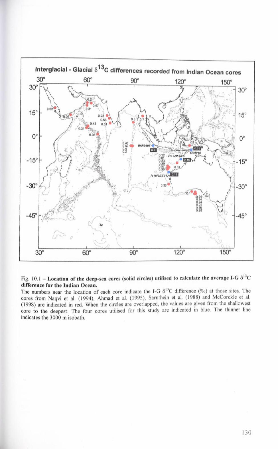
Interglacial - Glacial ~ 13c differences recorded from I d" o n ,an cean cores

3():'1'~-~~---r6Q_o ___ __:9()ro-· ___ __!1=.;20';--o----..,.............~-1~5~0o~ 300

15° 15°

oo oo

-15°

-30°

-45°

300 60° 900 120° 150°

Fig. I 0.1 - Location of the deep-sea cores (solid circles) utilised to calculate the average I-G 813C difference for the Indian Ocean. The numbers near the location of each core indicate the I-G 813C difference (%0) at those sites. The cores from Naqvi et al . (1994), Ahmad et al. (1995), Sarnthein et al. (1988) and McCorckle et al. (1998) are indicated in red. When the circles are overlapped, the values are given from the shallowest core to the deepest. The four cores utilised for this study are indicated in blue. The thinner line

indicates the 3000 m isobath.

130

en Q) '-0 0

II--0 ... Q) .c E ::s z

Cores from Indian Ocean 24r-~-~--,----.---..-----..---~~ 22 20 1 s Mean 0.32 o/oo 16 14 12 10 8

6 4

2 0 ----:~~~"""~~~~~~~~~~~~

0.2 0 0.2 0.4 0.6 0.8

Depth < 2000 m 9

8

7 . Mean 0.23 %0 6

5

4

3

2

1

0 -0.4 0.2 0 0.2 0.4 0.6 0.8

Depth > 2000 m 9

8

7 Mean 0.37 %0 6

5

4

3

2

1

0 -0.1 0 0.1 0.2 0.3 0.4 0.5 0.6 0.7

8 13( %0

(A)

Expected normal

(8)

Expected normal

(C)

Expected normal

Fig. 10.2 - Mean I-G 813C difference calculated for the cores from the Indian Ocean. (a) Mean I-G 813C difference calculated for the entire core dataset (Table 1.1); (b) mean I-G 8

13C

difference calculated for the cores collected at intermediate depth; (c) mean I-G o13C difference

calculated for the cores collected from a depth >2000 m. On the left hand-side of each diagrfil}\ the number of cores for each group is indicated. The red line indicates the expected normal distribution for each one of the three datasets.

131

813C C. wuellerstorfi %0

co 0

I'--0

(D

0

Fr10/95 GC17 LO

0

"<:t' 0

(")

0

N 0

(")

0

N 0

Fr10/95 GC5 ..--0

0

..--0

I

N 0

I

l[)

0

"<:t' ci (")

SH/9016 ci N 0

...... 0

0 ...... 0

(")

0

N 0

BAR9403 ...... 0

0 0

..--0

I

N 0

I

0 0 LO 0 LO 0 LO ..-- ..-- N N (") (")

Age (Kyr BP)

Fig. I 0.3 - 8 13C curves for the four cores studied in this research for the last 35 Kyrs. The horizontal reference line represents the 1-G 8 13C difference calculated for the Indian Ocean. The curve related to Fr J 0/ 95 CC 17 fol lows the typical pattern recorded at intermediate depths for the Indian Ocean, displaying a 8 13C depletion at the LGM smaller than the Indian Ocean mean. For the other three cores, the 81:,C depletion at the LGM is larger than 0.32 %0.

132

(J)

..0

-S .c ...., a. Q,)

Cl

10.2 The distribution of C. wuellerstorfi and G. subglobosa o_f application .for the

study o_fpalaeoceanography o_f the eastern Indian Ocean

Varimax factors 1 (FrJ0/95 GC5), 2 (Frl0/95 GCJ7 and SHl9016), and 4

(BAR9403) calculated by Q - mode Factor Analysis are dominated by the species C.

wuellerstorji. Varin1ax factor 3 (Fr 10/95 GC 127) is dominated by G. subglobosa. The

analysis of the core tops revealed that C. wuellerstorfi and G. subglobosa are two

cosn1opolitan species com1nonly present in all the sainples (see Appendix A 1 ). In

order to understand the environmental conditions which for the Present favour, these

tvvo taxa, the values of the environmental variables measured for each sample

do1ninated (highest percentage) by these species were considered and were compared

with those n1easured at Fr 10/95 GCJ 7, Fr 1095 GC5, SHJ9016 and BAR9403

locations (figure I 0.4).

Temperature Salinity

0 1 2 :; 4 5 ),! J-1 .3 3-1 .6 35

105/J J. 1150

!250 ·-1

1J51J -j 1451) -~

1~~0 ··1

,e,;c •l 1750 ··1 1850 ~

! 1D50 ~

l 2050 7 ?. tSG .. f

·1 22~~ ·i 'S-, ·1 .,.,<>{, ·1

·I 2-4.511 .. i

2.550 .. 1 26.50 ..

. 275(} ·

Dissolved Oxygen Phospha~ Nitrate

2 ,: A ;) !:l 3.2 3.6 ,1 ':.$ ·1.8 2.1 2 .. t. 2.7 3 2g 30 37. 3,l 35 :,rn ·Jt){J

PP Jz C.flux(z)

t5f.l :·rs o

, r·· ~ .. -····--·· ·· C. wueflerstorfi

r

I · • ... G, subglobosa

' I I

Fig. I 0.4 _ Values of the environmental variables considered in this study measured for each sample dominated (high percentage) by C. wuel/erstorfi and G. subglobosa, for the Pr~sent. The circles indicates the values for the environmental variab les measured for the four studied cores iocations, for the Present [Fr J 0/95 CC I 7 ( I 093 m b.s.1.), SH /9016 ( 1802 m b.s.l.), BA R9403 (2043 m b.s. I.), Fr I 0/95 GC 5 (2452 rn b.s. I.)]

133

Today, C. wuellerstorji and G. subglobosa dominate (highest percentage) the

benthic foraminiferal assemblage for those samples characterised by ten1perature and

salinity levels similar to those recorded for the four studied cores locations. Nitrate

and phosphate levels measured for the four cores display values ranging above and

below the levels measured for the samples dominated (highest percentage) by the two

taxa.

These species seem to prefer an environment characterised by higher dissolved

oxygen concentration and lower carbon-flux rate than those recorded today for the

four cores locations. Also, sea-surface primary productivity levels for the studied

cores display the identical or lower values than those recorded for the samples where

C. wuellerstorfi and G. subglobosa are the don1inant (highest percentage) species.

These data indicate a preference of these two taxa for an oligotrophic and well

oxygenated environment.

Studies of living (rose-Bengal stained) specimens support this interpretation. C.

wuellerstorfi is a species typical of environments characterised by low carbon-flux

rate (Altenbach, 1992; Burke et al., 1993; Mackensen et al., 1985; Altenbach et al.,

1999) or by pulsed fluxes of organic matter (Mackensen et al., 1985) .. In presence of

reduced organic matter supply from the sea surface, the oxygen consumption for its

oxidation is reduced, favouring high dissolved-oxygen concentrations. A well

ventilated environment can also be associated to active bottom water circulation.

Lutze and Thiel (1988) described C-,. wuellerstorji as an epifaunal-suspension-feeder

species, adapted to this kind of environment and able to exploit the organic n1atter

laterally advected by bottom currents (Lutze and Thiel, 1988).

G. subglobosa has been associated with low carbon-flux rates 1n other studies

(Loubere and Banonis, 1987; Loubere et al. , 1988; Burke et al., 1993; Faridduddin

and Loubere, 1997; Schmied! et al., 1997). The analysis of the core tops revealed that

G. subglobosa is a species commonly present in all the samples. This taxon is strongly

correlated with low faunal diversity. In the core-top samples, large numbers of G.

subglobosa are found only when this taxon displays the highest percentage of the

assemblage; when other species are characterised by higher percentages, it is present

with fewer specimens, outlining a competitiveness deficit (Appendix A 1 ). Loubere et

al. (1988) associated this species with a low carbon-flux and to low percentages of

planktonic species typical of high productivity areas. These authors explained this

behaviour by speculating that this species is adapted to a low food supply: when

134

organic matter increases, G. subglobosa is unable to compete with species that are

quicker at utilising the food source. Also in this case, the preference for this taxon for

a well-oxygenated environment can be related to the low amount of organic matter at

the sea floor and the consequent low-oxygen consumption for its oxidation.

10. 3 Gravity core Fr 10/9 5 GC 17

Five species dominated the benthic foraminiferal assemblage at Fr J 0/95 GCJ 7

site, during different periods of the Late Quaternary (figure 10.5a). Between 31 and

18 Kyr BP, C. wuellerstorfi dominated the fauna. This species was replaced by N.

irregufaris and G. subglobosa, which dominated until 4 Kyr BP. For the last 4 Kyrs,

the foraminiferal assemblage was dominated by U. proboscidea and B. robusta.

The high percentages of C. wuellerstorfi between 31 and 18 Kyr BP would suggest

oligotrophic conditions and increased ventilation (see section 10.2), where sporadic

amounts of organic matter were laterally advected by active bottom cu1Tents. At

Present, the presence of a low salinity and less dense water, represented by the

southward-flowing LC offshore Western Australia, causes a deepening of the

nutricline, thus preventing the production of organic matter and determining

conditions of low productivity at the sea surface. During MIS3, a different pattern for

the LC was suggested by Gingele et al. (2001 ), who indicated the absence/reduction

of this current at this site. Under such a scenario, the absence of a low salinity cap at

the sea surface could have caused an upward shift of the nutricline towards the photic

layer, thus enhancing a slight increase in the production of organic matter. The

presence of a shallower nutricline, during MIS3-early MIS2, is suggested by studies

on nannofossils (Takahashi and Okada, 2000). During MIS3, the increased percentage

of N. dutertrei was indicated by Martinez et al. ( 1999) as a consequence of a

shallower and n1ore productive nutricline. The 813

C of C. wuellerstorfi, between 31

and 18 Kyr BP, displayed the lowest values recorded for the entire section, being

0.22%0 lower than the modem-day values (figure 10.3). This value does not indicate a

significant increase of the amount of organic matter at the sea floor. Furthermore, the

BF AR and low accumulation rates of U proboscidea and B. aculeata would indicate

oligotrophic conditions, as they did not display higher values , compared to those

recorded for the period after 20 Kyr BP (figure 10.5b ). The low relative percentage of

135

infaunal species recorded for this period ( figure 9 .3 ) could be the consequence of an

environment more suitable for epifaunal suspension feeder species ( e.g. better adapted

to exploit the organic matter transported by bottom current). This supports the idea of

a more active circulation at inte1mediate depths towards the end of MIS3 and the early

phase of MIS2. The reduced amount of clay, relative to silt, during MIS3 was the

consequence of an intense bottom current, which prevented the deposition of the

finest sediment particles (Gingele et al., 2001 ). The higher percentage of agglutinated

taxa, during this period, would suggest the presence of more corrosive intermediate

water, but the high percentage of porcellaneous taxa contradicts this interpretation.

The increased percentage of agglutinated taxa could then be explained considering

that calcareous infauna! species and agglutinated ones occupy a similar microhabitat.

Due to adverse conditions, a reduction in competitiveness of the first group of taxa

could have led to a relative increase of the second.

The benthic foraminiferal fauna dominated by C. wuellersto,~fi was replaced by

another one, dominated by N. irregularis and G. subglobosa, with the onset of the

LGM, (figure 10.5a). At Present, the distribution of N. irregularis is correlated with

low productivity levels at the sea surface and with the distribution of AAIW (see

sections 5 and 6) and G. subglobosa with low carbon flux-rate and high dissolved

oxygen concentrations.

High percentages of N. irregularis between 17 and 4 Kyr BP could indicate an

increased influence at this latitude by the AAIW over the scarcely oxygenated IIW

and a situation of low productivity at the sea surface. The presence in this assemblage

of G. subglobosa and the reduced percentage of infauna} taxa for this period (figure

9.3) would substantiate this observation.

C. wuellerstorfi 813C values for this period are higher compared to those recorded

before 20 Kyr BP. During glacial times, the mass reduction of the continental

biosphere induced a reduction of 0.32%0 of the n1ean isotopic composition of the total

dissolved CO2 in the eastern Indian Ocean (Duplessy et al. , 1989); the 813

C depletion

recorded for the same period at this site is 0.19%0. The smaller variation compared to

the global signal was explained by Duplessy et al. , (1989) as the result of an enhanced

ventilation of the intermediate water masses during the LGM. Prell et al. (1980)

indicated a northward shift of the Polar Front and the Sub-Tropical Convergence by

5°-10° and by 5° respectively in the Indian Ocean, with an increased northward

136

influence of the AAIW, up to 20°S. Since gravity core Fr I 0/95 GCJ 7 is located

~22°S it would have been within the influence of the AAIW, during the LGM. The

percentage of agglutinated taxa during this period was low (<5%) (f:gure 9.3), while

the relative abundance (%) of porcellaneous species remained close to 20%. This

seen1s to contradict the concept of a more "corrosive" AAIW during MIS2, as

indicated by the high percentage of porcellaneous species.

At the same time, more arid conditions over the Australasian rea1on led to a b

reduction of rainfall ( van der Kaars, 1991; van der Kaars and Dam, 199 5; Gingele et

al., 2001; De Deckker et al., 2002; van der Kaars and De Deckker, 2002). The arid

conditions and the reduced precipitation caused a reduction of the riverine discharge

to the ocean (Gingele et al., 2001) and may have caused a decrease in the an10Lmt of

nutrients for the phytoplankton, causing low primary productivity conditions. Another

factor, which may have prevented the productivity enhancement off the west coast of

Western Australia, could have been the increased intensity of the South Java

Upwelling System (see section 10.6). This phenomenon could have increased the

steric height between the northern and the southern eastern Indian Ocean, determining

a southward Ekman transport and a geostrophic-flow off the west coast of Western

Australia, thus suppressing an eventual upwelling of intermediate water (Martinez et

al. , 1999). The presence of a less productive nutricline seems to be confirmed by the

low percentages of N dutertrei between 20 and 5 Kyr BP (Martinez et al., 1999). The

period between 14 and 5 Kyr BP was characterised by wetter climate with heavier

su1n1ner rain (van der Kaars and De Deckker, 2002). The resulting increased riverine

discharge could have resulted in an increase of the amount of nutrient injected into the

sea and higher primary productivity. The isotopic record does not substantiate this

scenario, as the 8 13C of C. wuellerstorfi maintained values similar to those measured

for the LGM. It may be that the large amount of freshwater injected into the sea by the

rivers engendered a low-salinity cap at the sea surface, causing a temporary deepening

of the nutricline and a reduction of primary productivity. The BF AR peaks can be

attributed to minor and sporadic events characterised by increased production of

organic matter (figure 10.56 ). The fact that these events are not recorded by any

fauna! change can be explained considering that, under conditions of strong bottom

currents and well-oxygenated water, the preservation of a relatively small amount of

organic matter at the sea floor could have been greatly prevented~ due to lateral

137

transport and/or rapid oxidation. High dissolved-oxygen concentrations at

intermediate depths and low productivity at the sea surface seem to have been

maintained until 4 Kyr BP, when the assemblage dominated by N. irregularis and G.

subglohosa was replaced by one dominated by U. proboscidea and B. robusta (figure

10.5a). At Present, U proboscidea is mainly found at low latitudes, where higher

primary productivity at the sea surface determines higher carbon-flux rate with low

oxygen levels resulting from the oxidation of the organic matter and the conten1porary

presence of oxygen-depleted intermediate water masses (IIW and NIIW) (see sections

5 and 6). The distribution of B. robusta is limited to intermediate depths (700 - 2000

m) and to environments with low dissolved-oxygen concentrations (Table 4.4). A

relationship between this taxon and low-oxygen levels was already described for the

Australian-Irian Jaya continental margin by Van Marle ( 1988). Conditions of low

dissolved-oxygen concentration could have been the consequence of the increased

influence of the IIW in this area. During the last 5 Kyrs, the LC increased its strength

(De Deckker, 2001; van der Kaars and De Deckker, 2002); the presence of a low

salinity water cap, typical of the LC, could have also engendered a more stratified

water column. Similar to what happened at the sea surface, the influence of the

Indonesian waters at intermediate depths, with IIW becoming more important, could

explain a reduction of dissolved-oxygen concentrations. The high percentage of U.

proboscidea and B. robusta would suggest this situation. Another factor, which

corroborates the hypothesis of scarce oxygenation, is represented by the faunal

characteristics of the benthic foran1iniferal assemblage during the last 5 Kyrs. Low

diversity (a, H(S), E) and high dominance are recorded for this period (figure 9.3),

suggesting a fauna which thrived under low-oxygen conditions (Lutze and Coulbourn,

1983; Denne and Sen Gupta, 1991; Sen Gupta and Machain-Castillo, 1 993; J annik et

al., 1998; den Dulk, 2000). The decreased percentage of porcellaneous taxa and the

increased percentage of infauna! species would also point to a less oxygenated

environment. At Present, porcellaneous species are correlated with low salinity and

high dissolved-oxygen levels, while infaunal species tend to increase when oxygen

decreases. These two opposite trends recorded for the last 5 Kyrs would then suggest

reduced ventilation at intermediate depths compared to the past.

Another factor which could contribute to low-oxygen condition, is the oxidation of '

organic mater at the sea floor. The 813C of C. wuellersto1:fi recorded for the last 5

138

Kyrs, which shows the highest values 1neasured, do not confim1 this hypothesis.

Therefore, conditions of increased productivity during the last 5 Kyrs are not

substantiated by the isotopic record. The BFAR for this period of time gives values

similar to those recorded for the former 25 Kyr and does not indicate any productivity

increase (figure 10.5b ). The increased percentages of U proboscidea and infauna!

taxa would also suggest increased carbon-flux rate. In this case, in the presence of low

dissolved-oxygen levels, the oxidation of organic matter would be slower. Under

these conditions the "'food" availability at the sea floor could have increased, even

with no variation of primary productivity at the sea surface.

10.4 Gravity core Fr 10/95 GC5

The species C. wuellerstorfi and B. aculeata displayed the highest percentages

among the benthic foraminiferal fauna during two different periods of the last 35 Kyrs

(figure 10.5a). C. wuellerstorfi dominated from 35 Kyr BP until 18 Kyr BP and B.

aculeata dominated from 18 Kyr BP until 4 Kyr BP.

As for gravity core Fr 10-95 GCJ 7, the late MIS3 and early MIS2 for Fr 10/95 GC5

are characterised by the dominance of C. wuellersto1fi. As previously discussed, this

species should indicate an environment where the sporadic amount of organic matter

was laterally advected by active bottom currents. The peaks displayed by the AR

curve of the opportunistic species E. exigua ( see sections 5 and 6) ( figure 10 .5 b)

corroborate the idea of pulsed inputs of organic matter in an oligotrophic

environment. Environmental conditions more suitable for suspension feeders are also

confirmed by the reduced percentages of infaunal taxa (figure 9. 7). This period seen1s

to be characterised by an increased importance of botton1 current activity. The C.

wuellerstorfi 8 13C curve (figure 10.3) displayed values consistently higher than those

recorded for the LGM. The percentage of N. dutertrei showed values similar to those

recorded for the late Holocene (Martinez et al., 1999) and the same is valid for the

BF AR (figure 10.5b ). These data do not substantiate increased productivity at the sea

surface, compared to the Present. At 18 Kyr BP, C. wuellerstorfi was replaced by B.

aculeata (figure 10.5a). This last taxon is at Present correlated with low diversity and

relatively high phosphate-concentration in the water (Table 4.4) with periodic inputs

of organic matter to the sea floor (see sections 5 and 6). The appearance of B.

139

aculeata coincided with an increase of the accumulation rate of E. exigua (figure

10.5b ). E. exigua maintained high AR values for the time during which B. aculeata

displayed high percentages (20-54 % ), suggesting that the presence of this latter

species coincided with conditions of increased organic matter supply. Between 20 and

5 Kyr BP, the high values of BFAR (figure IO.Sb) indicate conditions of enhanced

export of organic n1atter to the sea floor. Analyses on Recent and living (stained)

benthic foran1inifera show a relationship between the abundance of B. aculeata, the

sediment organic carbon content (Collins, 1989; Mackensen et al., 1993; Miao and

Thunell, 1993; Rathbum and Corliss, 1994) and shallow oxygen penetration within

the sedi1nent (Miao and Thunell, 1996). The distribution of B. aculeata also correlates

with high organic-carbon flux (>2 gC/m2yr) in the Atlantic and Southern Oceans

(Altenbach et al. 1999; Altenbach, personal communication). As discussed earlier, the

increased BF AR and E. exigua AR point to an increased amount of ''food" reaching

the sea floor. The organic matter oxidation could have then induced oxygen depletion

at the sea floor and in the sediment pore-water, thus creating the ideal conditions for

B. aculeata to thrive. A correlation between B. aculeata relative abundance (%) and

high carbon-flux rates during the past has been reported from the South China Sea,

the Sulu Sea and the eastern Indian Ocean (Wells et al., 1994; Miao and Thunell,

1996; Jian et al., 1999; Jian et al., 2001 ). An enhanced food supply to the sea floor

could have been caused by two phenomena. For the period related to the LGM, the

South Java Upwelling System was more efficient (see section 10.6) (Martinez et al.,

1999; Takahashi and Okada, 2000). This could have determined increased organic

n1atter supply to the sea floor and together with the Banda Sea's high productivity

(see section 10.5) (Barawjdjaia et al., 1993; Spooner et al., submitted), a higher

carbon-flux rate at the sea floor, off the north coast of Western Australia would have

occurred. Increased productivity during the LGM in the Timor Sea was also suggested

by Muller and Opdyke (2000). The mass accumulation rate of organic carbon

measured for this core (Maeda, 2003), was higher at the LGM con1pared to late N1IS3

- early MIS2, further supporting the idea of increased productivity at the sea surface.

As discussed in section 10.1.3 , the low 8 13C of C. wuellerstorfi during the LGM can

be associated with a reduced deep-water circulation, which in turn could have caused

low-oxygen conditions. The faunal characteristics related to the assemblage

dominated by this species indicate low diversity and high dominance, pointing

140

towards low-oxygen conditions (Lutze and Coulbourn, 1983; Denne and Sen Gupta,

1991; Sen Gupta and Machain-Castillo, 1993; Jannik et al. , 1998; den Dulk, 2000),

similar to what was seen for gravity core Fr 10195 GC 17. Fron1 the data obtained from

Frl0/95 GC5, it is possible to extrapolate that a less ventilated environment (8 13C of

C. wuellerstorfi) and an increased amount of organic matter (E. exigua AR and

BF AR) at the sea floor could have created favourable conditions for B. aculeata. After

the LGM, the persistent low values of 8 13C of C. vvuellerstorji, the high percentage of

B. aculeata, the high values of E. exigua AR and BF AR could be the consequence of

another process. From 14 Kyr BP until 5 Kyr BP this region was characterised by

substantial summer rains (Veeh et al., 2000; van der Kaars and De Deckker, 2002).

The consequent increased fluvia1 discharge, with more nutrients injected into the sea,

would have favoured phytoplankton bloon1s. This hypothesis is further supported by

the values 1neasured for the mass accumulation rate of the organic carbon (Maeda,

2003). At the transition between MIS2 and MIS 1, a peak for this parameter is

paralleled by the highest percentages of B. aculeata (figure 10.5a). The percentage of

N. dutertrei, which was already high during the LGM, also reached tbe highest values

during this period, thus indicating a more productive nutricline (Martinez et al.,

1998b ). For the last 5 Kyrs, the benthic foraininiferal fauna was characterised by high

diversity (figure 9.7) and no particular taxon seemed to dominate the assemblage. The

species characterised by the highest percentages during this period were C.

wuellerstorji, G. subglobosa and E. exigua (see Appendix A3), suggesting prevalent

oligotrophic conditions. The BF AR values were similar to those recorded between 35

and 18 Kyr BP (figure 10.5b ). The high value displayed by the 813

C of C.

wuellerstorji, the low percentage of N. dutertrei (Martinez et al. , 1999) and the low

mass-accumulation-rate of organic carbon (Maeda, 2003), would suggest conditions

of reduced carbon-flux to the sea floor; this being the lowest record~d of the last 35

Kyrs.

141

10. 5 Piston core SHf 9016

Two species, B. aculeata and C. vvuellerstorfi, dominated the fauna] assen1blage

during the last 62 Kyrs. B. aculeata characterised the benthic foran1iniferal

assernblage from 62 until 15 Kyr BP and C. wuellerstorfi dominated fro1n 15 Kyr BP

until the Present.

The high percentage of B. aculeata (figure 10.5a) indicates extremely favourable

environn1ental conditions for this species during the period in which it dominated the

foraininiferal assen1blage. The BF AR and the accumulation rates of E. exigua and U.

proboscidea were higher than today, suggesting conditions of increased "food"

availability at the sea floor (figure 10.56) for MIS3 and MIS2. The past situation in

the Banda Sea was quite different from today, with more arid conditions causing a

reduction in rainfall (Barmawidjaja et al., 1993; van der Kaars and Dain, 1995) . The

excess of evaporation over precipitation engendered conditions of higher sea-surface

salinity (Martinez et al., 1997; Martinez et al., 1998b; De Deckker et al., 2002; van

der Kaars and De Deckker, 2002). In this situation, the absence of a freshwater cap

allowed a shoaling of the thermocline, with a consequent extension of the Deep

Chlorophyll Maximum (DCM) in shallower waters, thus enhancing primary

productivity (Barmawidjaja et aL, 1993; Spooner et al. et al., submitted). This change

was paralleled by increased N dutertrei percentages (Bam1awidjaja et al., 1993;

Spooner et al. et al., submitted). The cause of higher productivity could have been the

intensified vertical advection of Banda Sea intermediate waters, due to a strengthened

Southeastern Monsoon (Spooner et al., subn1itted), or the influx of a nutrient-enriched

Pacific Water (Barmawidjaja et al., 1993). The prevailing eastward direction of the

South Java Current during this period (Gingele et al., 2002) and the contemporaneous

increased productivity in the southe111 South China Sea (Wang et al., 1999; Jian et al.,

2001) indicate an intensified Northwestern Monsoon for this period. The influx of a

nutrient-enriched Pacific Water is a more likely possibility, considering that during

glacial stages productivity increased in the Western Pacific (Herguera and Berger,

1 991; Burke et al., 1993; Herguera and Berger, 1 994) and that Banda Sea waters and

Pacific Intermediate waters also displayed a similar evolution during glacial and

interglacial times (A .. hmad et al. , 1995). Another source of nutrients could have been

the sediment transported to the sea by winds or by rivers (Maiiinez et al., 19986) fron1

the en1erged shelf of the Java Sea (Hantoro, 1997). Between 62 and 15 Kyr BP, the

142

high AR of U proboscidea (figure 10.5b ), which today is also associated with

oxygen-depleted environments (see sections 5 and 6), would also indicate a less

ventilated environment. The flux of organic matter to the sea floor and its oxidation

could have led to oxygen depletion at the sea floor. The high don1inance level (figure

9 .11 ), which characterises the assemblage dominated by B. aculeata, as discussed

before, would suggest this scenario. Another cause for a reduced oxygenation could

have been a reduced deep-water circulation, as the interpretation of the C.

wuellerstorfi 813C signal in the eastern Indian Ocean would indicate. A less active

circulation at this site during MIS2 and part of MIS3 is also suggested by

sedimentological analysis (Gingele et al., 2001 ). It is possible that the increased input

of organic 1natter in an already poorly-ventilated environment, similar to what seen

for Fr I 0/ 95 GC5 during the LGM, created favourable conditions for R. aculeata. This

taxon was replaced by the suspension feeder species C. wuellerstorfi, at 15 Kyr BP.

The high percentage of this species during the last 15 Kyrs (figure 10.5a) could

indicate a reduced flux of organic matter to the sea floor, accon1panied by a

strengthening of the bottom currents. According to the results presented in section 6,

the absence of E. exigua would indicate a reduced amount of organic matter at the sea

floor and the constant decrease of U proboscidea AR would correspond to conditions

of low carbon-flux rate and increased ventilation ( figure 10.5b ). The BF AR calculated

for this period was 2-3 times lower than that recorded during the previous 45 Kyrs

(figure 10.5b ). This change coincides with the onset of the last deglaciation and the

climatic shift towards conditions similar to moden1 ones ( van der Kaars and Dain,

1997). Coinciding with this climatic change, the sea level rose, submerging the

Indonesian platfo1ms (Chappell et al., 1996) and precipitation increased (Martinez et

al., 1997; Martinez et al., 1998b; De Deckker et aL, 2002; van der Kaars and De

Deckker, 2002). Under these conditions, the formation of a freshwater cap, due to the

excess of rainfall over evaporation, caused the deepening of the DCM and the

consequent reduction of productivity at the sea surface (Barmawidjaja et al., 1993).

The occun·ence of this phenomenon is also confirmed by the decrease of N. dutertrei

percentages, recorded for this site from 15 Kyr BP until today (Spooner et al. ,

submitted). At the same time, productivity in the Western Pacific diminished

compared to the glacial period, reducing the nutrients content of the Pacific ·waters

entering the Indonesian Archipelago (Herguera and Berger, 1991; Burke et al., 1993;

143

Herguera and Berger, 1 994 ). The presence of more intense bottom currents 1s

indicated not only by the lower U. proboscidea AR, but also by higher silt

sedimentation relative to clay (Gingele et al., 2001 ).

10. 6 Piston Core BAR9403

The benthic foran1inifera species 0 . t. umhonatus, E. exzgua, B. aculeata and C.

wuellerstorfi, characterised the benthic foraminiferal fauna at different times during

the last 33 Kyrs.

0. t. un1bonatus was the most abundant species until 26 Kyr BP (figure 10.5a). The

study of the core tops associated this species with a deep and cold environn1ent,

characterised by a low carbon-flux rate (Table 4.4). The percentage for this taxon,

close to 30%, during this period, would indicate conditions of low productivity at the

sea surface as also suggested by BFAR (figure 10.56 ). Circulation offshore Java and

Sumatra was different at that time: sea-surface currents, under the influence of

strengthened Northwestern Monsoon (Gingele et al. , 2002), and intermediate waters

were characterised by a prevalent eastward flow. Under these conditions , the

upwelling, which at Present is associated with the Southeastern Monsoon and the

westward flow of the SJC, would have been suppressed or greatly reduced. The

isotopic signal (low 8 13C of C. wuellerstorfi) can then be attributed to enhanced

stratification of the water column, which allowed the bloom of the giant diatom

Ethmodiscus rex (De Deckker and Gingele, 2001; Gingele et al., 2002). The situation

changed at 26 Kyr BP, when 0. t. umbonatus was replaced by B. aculeata, which

dominated the benthic foraminiferal assemblage between 26 and 15 Kyr BP, reaching

percentages close to 50 % (figure 10.5a). Similarly to B. aculeata, another species, E.

exigua, showed increased percentage at this time. As discussed in sections 5 and 6,

the distribution of this species outlines the preference of this taxon for a deep

environn1ent, with pulsed fluxes of organic matter. The high BFAR (figure 10.56)

values would suggest an increased input of organic matter to the sea floor for this

period. High carbon-flux rate is also suggested by the increased AR of U.

proboscidea, (figure 10.56 ). This species would also indicate reduced oxygen levels

(see sections 5 and 6) and together with the low 813

C of C. wuellersto1:fi, would

suggest a reduced deep-water circulation. Towards the LGM, the monsoonal clin1ate

144

changed, with the weakening of the Northwestern Monsoon and the strengthening of

the Southeastern Monsoon (Wang et al., 1999; Jian et al., 2001; Gingele et al., 2002).

Thjs, combined with the absence of the low-saline water cap (present today)

(Martinez et. al, 1999), caused an increase of the intensity of the South Java

Upwelling System (Martinez et al., 1999; Muller and Opdyke, 2000; Takahashi and

Okada, 2000; Gingele et al., 2002). The E. exigua percentage peak would also suggest

increased inputs of organic matter from the sea surface. The high U proboscidea AR

corroborates this hypothesis and indicates an enhanced flux of organic n1atter to the

sea floor. As seen for the other cores, the B. aculeata bloom coincided with increased

food supply and low-oxygen levels at the sea floor. The reduced percentage of E.

exigua after 20 Kyr BP may be seen as the consequence of con1petition between these

two species, which, in the presence of constant and significant ainount of organic

n1atter, would favour B. aculeata. This latter aspect can be related to the fact that in

the presence of a high organic-matter oxidation-rate, oxygen depletion at the sea floor

would occur. Together with a reduction of deep-waters circulation, oxygen depletion

could have played a major role in li1niting E. exigua, thereby favouring B. aculeata.

Low oxygen conditions are also suggested by the high value of don1inance (D),

which, during this period, reached the highest values recorded for the entire core

( figure 9 .15 ). At the same time, the high percentage of infauna! taxa ( figure 9 .14),

which at Present are correlated with high carbon-flux rate and low-oxygen levels (see

sections 5 and 6), would support this hypothesis. Around 15 Kyr BP, 0. t. umbonatus

and C. wuellerstorfi became the most important species (figure 10.5a). The

environmental interpretation of these taxa has been already discussed, as together they

would indicate a 1nore oligotrophic environment characterised by intense botton1

currents. Different factors substantiate this interpretation: low E. exigua and U

proboscidea AR (figure 10.5b ), the constant decrease of BF AR (figure 10.5b) and the

low percentage of infauna} taxa (figure 9.15) (indicating an environment more

suitable for suspension feeders). The opening of the Sunda Strait, due to sea-level rise

and the increased precipitation (Ganssen et al., 1988; van der Kaars and Dan1, 1995),

contributed to an injection of less saline water into the SJC path, inducing a low

salinity water cap, which reduced the effectiveness of the South Java Upwelling

System (Martinez et al., 1999). During the last 5 Kyrs, B. aculeata, first and E.

exigua, later, replaced the O. t. un1bonatus - C. wuellerstorfi dominated assen1blages.

Again, this would suggest an increased food supply to the sea floor. However, the

145

BF AR does not fully corroborate this interpretation, or at least point to a sn1all

increase compared to the one recorded for the past. This slight productivity variation

at the sea surface can be associated with a reduced precipitation over the Australasian

region during the last 5 Kyrs, compared to the period from 14 to 5 Kyr BP (Ganssen

et al., 1988; van der Kaars and De Deckker, 2002). A similar event could have also

taken place in this area, by reducing the low-salinity water cap importance over the

South Java Upwelling System region and favouring a 1ninimal primary productivity

enhancement at the sea surface.

146

Fr 10195 GC17 Fr10/95 GCS SH/9016 BAR9403

--- - - ;:I?. -~ - ?fl. ?fl. 'cf!. rf!. '#. 0

0 - -- -;fl - - - -- - - ti) -'e co co - ~ 'E ~ 'E cf. 'E - ~ ?f!. 0 0 .2 -.9 ti) ·~ - .9 - .9 ~ - .9 '#. 0 -~ .Q 0 .s ~ .s ~ 5 .s ~ -~ ~ i -9? .Q :l ltJ ~ (1J ~ .Q (IJ ,92 ~ - 0) ~ ~ 1 I t:n .Q ::) . -- Q) E ~ '§ -~ e .Q a ~ a § ::, ; .9)

e ~ (.) ~ {I) Cl.. (1J (\J ....: (1J

(.) (!j <: ::j ai ai (.) ai ti d ai (j U,j

0 20 0 20 0 15 0 30 0 20 0 60 0 30 0 50 0 15 0 40 0 60 0 40 0 30 0 ~~ ....,..._~ ~....c-.... r-'---st-"-i +--'-,i,1-'---1 ~~ +--+~

5 10 15

- 20 ~ 25 >, 30 ~ 35 • 40 ~ 45

50 55 60

0.. en ... >-~ '-J

& c(

0

5

10

15

20

25 30

35

40

45

50

55

60

Fr 10/95 GC17

~ ~! er !J "G 4:

a::: !I i rt ID 5. GI CX) a:i :foi

200 1000 0 300

(a)

Fr10/95GC5

~ ~l a: SI~ a::: j ~

~ g ·f CX) a:i ::i ui

0 300 0 100 0

(b)

SH/9016 BAR9403

~ ~ ~ =i:: ~ ! ~ sj~ .is -

a::: I i a::: 11~ ~ K~ rt . e~ Q. GI

co ai ::iui co ad ui 400 0 100 0 400 0 200

l 3: • en i w

Fig. 10.5 - (a) Downcore variations in relative abundance(%) of dominant benthic foraminiferal

species and (b) downcore variations in benthic foraminiferaJ accumulation rates (BFAR) and

accumulation rates (AR) of B. aculeata, U. proboscidea, E. exiguaf or the four studied cores.

147

10. 7 The Palaeoceanography of the eastern Indian Ocean during the Late

Quaternary

The samples analysed 1n this study allow the reconstruction of the

palaeoceanographic evolution of the eastern Indian Ocean covering the last 60 Kyrs.

The correlation between the variation of the benthic foraminifera faunal patterns, the

8 13C of C. vvuellerstorfi, the BFAR and the accumulation rates of B. aculeata, E.

exigua and U proboscidea have been interpreted as the consequence of important

oceanographic and climatic changes, which took place in this region over tin1e

10. 7.1 62-35 Kyr BP

For the period between 62 and 35 Kyr BP, the available data allow the

reconstruction of the environmental evolution of the Banda Sea (SH/9016). During

this time, a benthic foraminiferal assemblage dominated by B. aculeata indicates

conditions of enhanced productivity at the sea surface and increased organic n1atter

flux to the sea floor accompanied by possibly reduced ventilation. Enhanced organic

matter supply could have been determined by the influx of nutrient-enriched Pacific

waters into the Indonesian Achipelago and/or an increased sediment contribution from

the nearby emerged land.

10.7.2 35-15KyrBP

Between 35 and 15 Kyr BP (figure I 0.6), while in the Banda Sea conditions were

si1nilar to those for the previous 25 Kyrs, a different situation existed along the

western Australian coast. Here, conditions of lower productivity ( compared to the

Banda Sea) and active bottom (Fr 10/95 GC5) and inte1mediate (Fr 10/ 95 GC 17)

currents were indicated by the presence of C. wuellersto1/i .. Offshore Java and

Sumatra (BAR9403), a more stratified water column and a less active South Java

Upwelling System determined conditions of scarce circulation at the sea flo"or and

reduced carbon-flux rate. In this type of environment an assemblage dominated 0. t.

148

un1bonatus thrived until 26 Kyr BP. At the transition between MIS2 and MIS] the '

Southeastern Monsoon intensification and the increased effectiveness of the South

Java Upwelling Systen1 determined conditions of high productivity at the sea surface.

Enhanced organic matter flux to the sea floor and the consequent oxygen depletion

favoured B. aculeata and E. exigua bloo1ns. A reduction of oxygen levels, due to a

reduced circulation and organic matter oxidation, probably caused the disappearance

of E. exigua and favoured B. aculeata. Approaching the LGM (figure 10. 7), off the

north coast of Western Australian the influence of a more efficient South Java

Upwelling System, togeth~r with reduced deep-water circulation were indicated by

the high percentage of B. aculeata. Off the west coast of Western Australia, two low

food tolerant species replaced C. wuellerstorfi: N. irregularis and G. subglobosa. Arid

conditions over the region caused a considerable reduction of nutrient input to the sea.

At intern1ediate depths ( I 000 m), the circulation intensity was more vigorous than at

the present and the AAIW front was located further north ( ~20°S).

10.7.3 15-5KyrBP

At 15 Kyr BP (figure 10.8), important changes are recorded at all the core sites,

except for Fr 10/95 GCJ 7. A wetter climate, accompanied by an increased riverine

discharge and sea-level rise, led to the formation of a freshwater cap over the

Indonesian region, thus deepening the thermocline and reducing the productivity level

in the Banda Sea and the intensity of the South Java Upwelling System, offshore Java

and Sumatra. In these areas, B. aculeata was replaced by C. wuellerstor_fi and by 0. t.

umbonatus and C. wuellerstorfi, respectively. This replacement indicates conditions

of reduced food supply to the sea floor and more intense deep-water circulation. Off

the west coast of Western Australia, a presun1ed sin1ilar freshwater cap, might have .

deepened the nutricline, precluding any possibility of enhanced productivity. Low

food supply conditions were still indicated by the presence of 1V. irregularis and G.

subglobosa. Off the north coast of Western Australia, the injection of nutrients into

the sea by rivers increased productivity and enhanced the carbon-flux rate. These

conditions favoured B. aculeata, which displayed high percentages after 15 Kyr BP

only for this site.

149

10. 7. 4 5 Kyr BP - Present

The reduction in precipitation, during the last 5 Kyrs (figure I 0. 9), caused shoaling

of the nutricline off Java and Sumatra and induced increased fertility in that area. This

was accompanied by increased percentages of B. aculeata, first, and E. exigua, later.

Rainfall reduction and the LC, well established along its modern pattern, detern1ined

conditions of low productivity off the north coast of Western Australia. A more

stratified water column and an increased influence of IIW, over the AAIW, created

conditions of low dissolved-oxygen concentrations off the west coast of Western

Australia as indicated by the dominance by U. proboscidea and B. robusta.

150

50

oo

_50

-1D°

-15°

-20°

_250

900

The eastern Indian Ocean at 30Kyr BP

Indian Ocean

120° 130°

Pacific Ocean

50

I c..r ~ Q~

-10°

-15°

-200

Australia -25°

_300 _____________ --,i....,.;; ___ ..,. __________________ 300

90° 100° 110°

Areas characterised by low carbon-ffux rate and bottom currents With high dissolved-oxygen levels

Are:as characterised by a stratlffed water column

120° 130°

-

Areas characterised by Increased carbon-flux rate and reduced deep-waters circulation

D Exposed shelf areas

Fig. 10.6-The situation of the eastern Indian Ocean at 30 Kyr BP. The Banda Sea was characterised by the influx of more nutrients-enriched Pacific waters which, with the absence of the freshwater cap at the sea surface and a shallower thermocline, determined conditions of increased carbon-flux rate to the sea floor. The oxidation of the organic matter, together with reduced deep-water circulation, reduced oxygen levels, created favourable conditions for B. aculeata. Offshore Java and Sumatra a more stratified water column and prevailing NE Monsoon inhibited the South Java Upwelling System, determining conditions of reduced carbon-flux to the sea floor and favouring the presence of 0. t. umbonatus. Offshore Western Australia, active and oxygenated bottom-waters and low carbon-flux rate at the sea floor were indicated by the presence of C. wuellerstorfi.

151

50

oo

_50

-10°

-15°

-25°

The eastern Indian Ocean at 18 Kyr BP (LGM)

100°

Indian Ocean ·

130°

Pacific Ocean

i -=-r .. J o~~

Australia

oo

_50

-1Q°

-15°

-20°

_250

_300 ________ ..._ _____ __a,; ___ ..._ ______________ -30° 900 100° 1100

Areas characterised by low carbon.flux rate and bottom currents with high dissolved-oxygen levels

D Exposed shelf areas

120° 130°

Areas characterised by increased carbon-flux rate and reduced deep-waters circulation

Fig. 10.7 -The situation of the eastern Indian Ocean at 18 Kyr BP. Conditions of increased carbon-flux rate at the sea floor were maintained in the Banda Sea, while offshore Java and Sumatra the increased effectiveness of the South Java Upwelling System, determined a carbon-flux rate increase at the sea floor, as indicated by the presence of B. aculeata and E. exigua. The oxygen depletion, due to the reduced deep-water circulation and the organic matter oxidation, favoured B. aculeata, while E. exigua disappeared. The influence of the higher productivity over the Indonesian region determined increased carbon-flux rate off the north coast of Western Australia. This and the reduced deep-water circulation created optimal conditions for B. aculeata. Off the west coast of Western Australia, high-oxygen levels were indicated by N trregularis, which with G. subglobosa replaced C. wuellerstorfi, due to a further organic matter supply reduction, probably the consequence of arid conditions over the continent. The AAIW influence was recorded up to 20°S.

152

90°

5°

oo

_50

-10°

-15°

-200

-25°

The eastern Indian Ocean between 15 and 5 Kyr BP

100°

Indian Ocean

110° 120°

Fr10/95 GC17 .

130°

Pacific Ocean

i~ a,- C <1-

0~

Australia

50

oo

, _50

-10°

-15°

-20°

-25°

_300 _______ .__ _____ __.~ __ _.._ ____________ __. _300

900 10()° 110°

Low..salinity water cap

Freshwater plumes and runoff

Areas characterised by low c.arbon.ftux rate and bottom currents with high dissolved-oxygen 1-evels

120° 130°

Areas characterised by increased carbon-flux rate

D Emerged shelf areas at 12 Kyr BP

Fig. 10.8 -The situation for the eastern Indian Ocean between 15 and 5 Kyr BP. The presence of a low-salinity water cap due to increased rainfall determined conditions of reduced carbon-flux rate at the sea floor in the Banda Sea and offshore Java and Sumatra. Also, increased deepwaters circulation characterised these two regions. These two conditions are suggested by the presence of C. wuellerstorfi and 0. t. umbonatus. Similarly a low-salinity water cap was present off the west coast of Western Australia, where N irregularis and G. subglobosa still dominated the benthic foraminiferal fauna. The increased riverine runoff favoured increased carbon-flux rate, offshore northern coast of Western Australia, as B. aculeata was still present with high percentages.

153

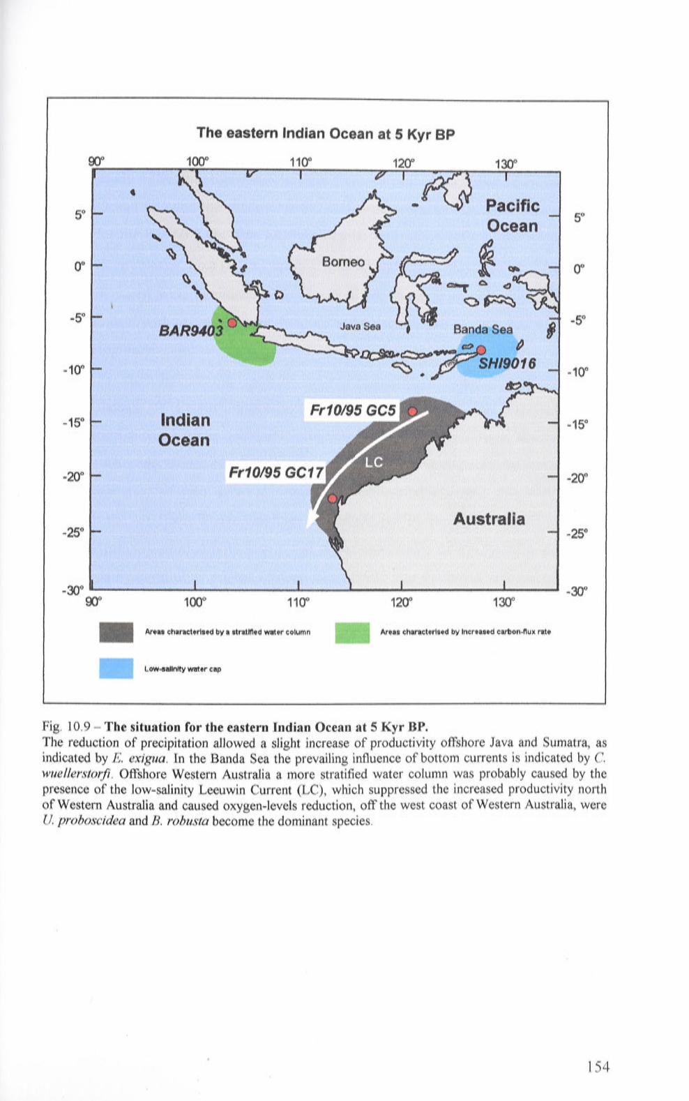
• 50

.50

-10°

-15°

-200

-25° '

The eastern Indian Ocean at 5 Kyr BP

100°

Indian Ocean

11Q° 120° 130°

Pacific Ocean

f. c-,. 6 <1

0~

Java Sea Banda Sea

~~ I ~~ ~H/9016 · . .,

~ ·

Australia ·

50

, _50

-10°

-15°

. -20"

-25°

_300 ------------- -"""-__ _.. __________ ....., __ ___, -30° 00° 100° 11cr 120° 130°

- Areas characterised by a .stratified water column - Area.s characterised by Increased carbon-flux rate

Low-salinity water cap

Fig. 10.9 -The situation for the eastern Indian Ocean at 5 Kyr BP. The reduction of precipitation allowed a slight increase of productivity offshore Java and Sumatra, as indicated by E. exigua. In the Banda Sea the prevailing influence of bottom currents is indicated by C. wuellerstorfi. Offshore Western Australia a more stratified water column was probably caused by the presence of the low-salinity Leeuwin Current (LC), which suppressed the increased productivity north of Western Australia and caused oxygen-levels reduction, off the west coast of Western Australia, were U. proboscidea and B. robusta become the dominant species.

154

11. Conclusions

The study of benthic foraminifera from four selected cores collected in the eastern

Indian Ocean allowed the reconstruction of the palaeoceanographic evolution of the

region for the last 60 Kyrs. The benthic foraminifera fauna, BF AR, the accu111ulation

rate of three selected taxa (B. aculeata, E. exigua and U. proboscidea) and the 8 13C of

C. wuellersto,ji were examined. The observed variations of trends of all the proxies

correlate well with the palaeoceanographic and palaeoclin1atological changes reported

for this region.

By means of Factor Analysis (Principal Components), the species whose

distribution through ti1ne could be interpreted as indicative of past environn1ental

changes were identified. The distribution of these species appeared to be contra I led by

the co-variance of two factors: organic-matter availability and dissolved-oxygen

levels at the sea floor. These variables are influenced by processes related to the sea

surface (primary productivity levels and presence/absence of low-salinity water cap)

as well as by conditions related to deep circulation. The increased amount of organic

matter at the sea floor and its oxidation causes oxygen depletion. In the presence of a

poorly ventilated environment, this further oxygen depletion can have a relevant

impact for the ecosystem at the sea floor. On the other hand, in a scarcely oxygenated

environment organic matter can be better preserved, becoming a longer-term '"food"

resource for the meiofauna.

Different faunal patterns were observed at different depths:

1) below 1800 m, B. aculeata and E. exzgua were correlated with conditions of

increased organic matter supply to the sea floor. Con1petition and reduced dissolved

oxygen levels ( due to a reduced deep-water circulation and organic-matter oxidation)

favoured B. aculeata and caused E. exigua to disappear, while in the presence of

pulsed inputs of organic matter, but without significant oxygen depletion, E. exigua

prevailed. The species C. wuellerstorfi and 0. t. umbonatus thrived in oligotrophic

conditions. C. wuellerstorfi also indicated increased deep-water circulation and

increased oxygenation;

155

2) for depths ~ I 000 m and south of 20°S, C. wuellerstorfi indicates ol igotrophic

conditions where reduced amounts of organic matter were laterally advected by active

bottom currents, characterised by high dissolved-oxygen levels. The species G.

suhglobosa and N. irregularis were associated with an extre1ne low carbon-flux rate

and high dissolved-oxygen levels. This last condition was probably related to an

increased influence of AAIW. U. proboscidea and B. robusta became abundant in the

presence of low dissolved-oxygen levels and a more stratified water column.

The 813

C of C. wuellerstorfi confirms the presence of an hydrological front in the

Indian Ocean during the LGM:

(I) below 1800 m, the 8 13C of C. wuellerstorji followed a pattern similar to the one

observed elsewhere in the Indian Ocean, showing a depletion >0.32%0 during the

LGM. This would indicate conditions of reduced deep-water circulation;

(2) at,___, I 000 m, the 8 13C of C. wuellerstorfi depletion was <0.32%0, at the LGM. This

is in agreement with the isotopic signal recorded from other parts of the Indian Ocean

and would indicate a more active intermediate-water circulation.

High values of BF AR indicate conditions of enhanced organic matter supply to the

sea floor. The accumulation rates of B. aculeata, E. exigua and U. proboscidea

allowed to identify periods characterised by increased organic matter supply and

reduced oxygen levels ( U. proboscidea)

These observations led to identify important differences between the actual

situation of the eastern Indian Ocean and past oceanographic and climate changes

repo1ied for this region:

• a link between the processes taking place at the sea floor and the climatic changes

recorded for the region during the past was found. Precipitation levels determined the

presence/absence of a low-salinity water cap at the sea surface [ with a consequent

deepening or shoaling of the thermocline (Banda Sea)] and controlled the amount of

nutrients injected into the sea by rivers ( off the north coast of Western Australia). The

presence of a low-salinity layer also reduced the intensity of the South Java Upwelling

System. These factors affected productivity levels and organic matter supply at the sea

156

floor influencing the distribution of benthic foraminifera. Also, monsoonal wind

regi1nes controlled the intensity of the South Java Upvvelling Syste1n and hence

productivity levels over that area.

• As indicated above, the 813

C of C. wuellerstorfi appeared to be controlled by

intermediate- and deep-water circulations. The results obtained suggest 1nore active

circulation for intermediate depths ( ~ 1000 m) and reduced circulation below 1800 m

during the LGM. Conditions of more/less active circulation controlled dissolved

oxygen levels, thus affecting the benthic foraminiferal fauna.

• During the LGM, off the west coast of Westen1 Australia, productivity did not

increase. This is indicated by: (a) a benthic foraminiferal assemblage dominated by G.

subgf obos a and N. irreguf aris, (b) the 8 13C of C. wueff erstorfi depletion, which was

lower than the one expected for this period, and ( c) the BF AR pattern, which was

characterised by values similar to the Present. This scenario would have been the

consequence of more arid conditions, with a reduced amount of nutrients injected into

the ocean by rivers, and a steric southward-flow along Australian coasts (this latter

was engendered by an increased intensity of the South Java Upwelling System).

• Today the occurrence of N. irregufaris n1irrors the distribution of AAIW in the

eastern Indian Ocean and porcellaneous taxa are correlated with low-salinity and high

dissolved-oxygen levels. The high percentages of these taxa recorded off the west

coast of Western Australia suggest an increased influence of AAIW at latitudes notih

of 20°S for the LGM. The replacen1ent of the assen1blage dominated by N. irregufaris

and G. subgf obos a by the assemblage dominated by U. proboscidea and B. robusta, at

~5 Kyr BP would indicate an increased influence of the oxygen-depleted IIW and a

more stratified water column, due to the presence of the LC.

• The productivity of the Banda Sea was higher during the past, con1pared to the

present, as suggested the by the high BF AR and high percentages of B. acufeta. This

species was also favoured by the oxidation of organic matter and reduced deep-water

circulation (low values of 8 13C of C. wueff erstorfi), which led to low dissolved

oxygen levels conditions at the sea floor.

• The high percentages of B. aculeata and E. exigua recorded off Java and Sumatra

during the LGM indicate a more intense South Java Upwelling System and increased

organic matter supply to the sea floor. Conditions of reduced oxygen levels

157

determined by the oxidation of the organic matter and reduced deep-water circulation

favoured B. aculeata, which prevailed over E. exigua.

158

12. Genera) conclusions

The aim of this research was to define the potential use of benthic foraminifera

fro1n the eastern Indian Ocean in order to reconstruct the palaeoceanographic

evolution of this region during the Late Quaternary. This work consisted of two major

parts:

(1) the analysis of Recent benthic foraminifera present in 57 core tops collected fro1n

the eastern Indian Ocean and the study of the relationships between their distribution

and the environmental variables n1easured for this region. These environ1nental

variables were related to the water masses described for this region ( depth,

temperature, salinity, oxygen levels, pressure) and nutrient levels (phosphate and

nitrate concentrations). Possible links between primary-productivity levels at the sea

surface and the benthic foraminifera distribution were also investigated by calculating

the carbon-flux rate at the sea floor using Suess ( 1980) and Berger and Wefer (1990)

fonnulae;

(2) the study of the benthic foraminifera fauna! content of four cores (Fr 10/95 GC 17,

Frl 0/95 GC5, B9403 and SHJ9016) collected from this region. The inforn1ation

acquired about the distribution of Recent foraminifera, together with the isotopic

record of 8 13C of C. wuellerstorfi. and the BF AR, were used to interpret the observed

faunal changes displayed by the benthic foraminifera species. This approach permitted

an understanding the processes, which may have led to such modifications, and the

reconstruction of the palaeoceanographic evolution of the eastern Indian Ocean for the

last 60 Kyrs.

12.1 The study of Recent benthic foran1inifera

The analysis of benthic foraminifera from 57 core-tops san1ples allowed the

identification of the environmental variables that influence their distribution (sections

5 and 6). The distribution of Recent benthic foraminifera from the eastern Indian

Ocean appeared to be controlled by depth, as the first axes of both DCA and CCA

indicated. Many of the measured environmental variables proved to be correlated vvith

159

depth and therefore the depth-related benthic foraminifera distribution was interpreted

as the consequence of the co-variance of different factors: temperature, carbon flux ,

salinity, dissolved oxygen and phosphate. In accordance with this, the species (). t.

un1honatus, P. nn,rrhina and E. exigua are typical of deep (>2000 m), cold, well

oxygenated and oligotrophic environ111ents, where pulsed fluxes of organic 111atter

associated with seasonal events are exploited by E. exigua. At depths <2000 n1, where

temperature and carbon-flux rate are higher, two species show higher percentages: C.

pseudoungerianus and N irregularis. This latter taxon is also strongly correlated with

high dissolved-oxygen levels and low salinity. Its distribution mirrors the distribution

of AAIW for this region.

The distribution of two other taxa, U. proboscidea and B. aculeata, is not

correlated with depth, but is controlled by other factors. U. proboscidea is related to

low dissolved-oxygen levels and high carbon-flux rate. The relationship between the

distribution of this species and low-oxygen concentration is associated with the

oxygen depletion caused by oxidation of the organic matter and the presence of

oxygen-depleted water masses (IIW and NIIW). B. aculeata is correlated with high

phosphate concentrations of the water and high dominance. These two characteristics

have been interpreted as related to the presence of organic matter and to an

opportunistic behaviour.

The study of the distribution of infauna!, agglutinated and porcellaneous species

outlined links between two of these groups and the environmental variables

considered. Infauna! species are correlated with increasing carbon-flux rate and low

dissolved-oxygen levels, while the porcellaneous taxa are correlated with low salinity

and high dissolved-oxygen levels.

12. 2 The study of the cores: bent hie foraminifera

The availability of organic matter and oxygen levels at the sea floor influenced the

distribution of benthic foraminifera in the eastern Indian Ocean (section 10). The four

selected cores provided information about benthic foran1inifera fauna} changes

relative to the last 60 Kyrs. These variations proved to be correlated with the

environmental and climatic changes already reported for this region (variations of

precipitation levels, monsoonal-winds intensity, intermediate- and bottom-waters

circulations). The faunal changes observed for the region followed different patterns,

160

depending on the depth of the cores. For depths > 1800 m, B. aculeata displayed high

percentages during periods of increased organic matter supply and reduced deep

water circulation. South of Java and Sumatra, in the early phase of increased

productivity, E. exigua was also present, but oxygen depletion (due to organic n1atter

oxidation and reduced ventilation) caused this species to disappear. During periods

characterised by oligotrophic conditions, the benthic foraminiferal fauna was

dominated by 0. t. umbonatus and in presence of active deep-water circulation, also

by C. wuellerstorfi. For depths <1800 m, south of 20°S, C. wuellersto,fi indicated

oligotrophic conditions and active bottom currents. N irregularis and G. subglobosa

characterised periods of extremely reduced organic-matter supply and increased

influence of AAIW north of 22°S. U. proboscidea and B. robusta were associated

with reduced oxygen levels, due to a n1ore stratified water colu1nn, for the presence of

the LC along is modern pattern, and the presence of the oxygen depleted IIW, south

of 22°s.

The isotopic record of 8 13C of C. wuellersto,:fi gave indications about the

circulation at the sea floor for the past. The values measured for this region follow the

trend recorded for the eastern Indian Ocean during the last glacial phase. While a

general depletion of 0.32%0 is expected for that period, the depletion recorded for the

cores under the influence of deep waters is higher, indicating a reduced deep-water

circulation (Duplessy et al., 1989). On the other hand, at intermediate depths (Fr I 0/95

GCJ 7), the depletion recorded for the LGM is <0.32%0, suggesting a more active

intermediate-water circulation (Duplessy et al., 1989).

The benthic foraininifera faunal patterns, together with the 813

C of C. wuellersto1/i,

the BF AR and the accumulation rates of B. aculeata, E. exigua and U. proboscidea

allowed to reconstruct the palaeoceanographic evolution of the eastern Indian Ocean

for the Late Quaternary (section 10.6).

12. 3 The study of the cores: eastern Indian Ocean palaeoceanography during the

Late Quaternary

During the Late Quaternary, the situation over the eastern Indian Ocean was

different from today. Due to more arid conditions, between 60 and 15 Kyr BP, the

low-salinity water cap, which today occupies the topmost part of the water column,

161

was absent. This caused a shoali ng of the nutricline and favoured conditions of

increased productivity in the Banda Sea. During the LGM, the intensity of the

Southeastern Monsoon increased, causing the productivity to increase offshore Java

and Sumatra and off the north coast of Western Australia. These primary productivity

changes were paralleled by a reduction of deep-water circulation, which favou red

conditions of low-oxygen levels in deep environments. Between 15 and 5 Kyr BP,

increased precipitation levels and the consequent formation of a low-salinity water

cap determined low-productivity conditions offshore Java and Sumatra and in the

Banda Sea. On the other hand, the nutrients injected into the ocean by rivers, fostered

productivity off the north coast of Western Australia. For the last 5 Kyrs, reduced

productivity levels, compared to the past, characterised the Banda Sea and the ocean

off the north coast of Western Australia, while a slight increase of South Java

Upwelling System intensity was recorded.

Productivity levels off the west coast of Western Australia remained low during the

last 30 Kyrs. At the same time, important changes of the intennediate waters and

surface-current circulation were recorded. Prevailing high dissolved-oxygen

conditions were n1aintained in this area from 30 until 5 Kyr BP. A more active

intermediate-water circulation was present at the LGM, when AAIW front was

located north of 22°S. During the last 5 Kyrs, the oxygen-depleted IIW become n1ore

influent over this area and a stratified water column was the consequence of the LC,

well along its modern pattern.

12. 4 The study of the cores: fauna! turnover

The choice of cores for palaeoceanographic analyses was based on the information

acquired about the distribution of Recent benthic foraminifera (PART I). In order to

investigate possible variations of carbon-flux rate during the past, cores depth had to

be within the range of 2000 m, as today this is the depth at which the faunal species

correlated with oligotrophic conditions are replaced by species correlated to high

carbon-flux rate. The benthic foraminifera trends recorded for the past 60 Kyrs

·indicated that this supposed fauna! change did not take place. Instead, due to increased

carbon-flux rate and reduced oxygen levels, B. aculeata became the most important

species between 1800 and 2500 m. Studies from the Pacific and Atlantic Oceans

indicate Uvigerina spp. as a typical species from areas characterised by enhanced

162

productivity (Lutze and Colburn, 1983; Loubere, 1991; Altenbach et al., 1999). This

observation would suggest that palaeoceanographic studies from the eastern Indian

Ocean should consider B. aculeata as indicative of periods characterised by increased

input of organic matter to the sea floor accompanied by reduced oxygen levels. Thi s

result is in agreement with those obtained by Loubere (1998), who outlined

significant differences between Pacific and NW Indian Ocean faunas below 2000 m '

with the Pacific high-productivity species U peregrina becoming less iniportant in

the NW Indian Ocean assemblages, due to the high seasonality characteris ing thi s

area.

12. 5 Future research

The study of Recent benthic foran1inifera from the eastern Indian Ocean proved to

be important for gathering information that can then be applied in palaeoceanographic

studies. The use of core-tops allowed the analysis of the relationships between benthic

foraminifera distribution, water masses, nutrients concentration and carbon-flux rate.

Studies on living (Rose-Bengal stained) specimens have shown how other factors

also control the distribution of these microorganisms (Jorissen et al., 1995; Van der

Zwaan et al., 1999; Murray, 2001 ). The use of box cores and multicorers has proved

to be one of the best procedure for obtaining samples for the study of the eco logy of

benthic foran1inifera (Jannik et al., 1998; Kuhnt et al., 1999; Wollenburg and Kuhnt,

2000; Heinz et al., 200 I). These coring devices allow the recovery of the undisturbed

sediment-water interface and the overlying bottom water. Samples recovered

following this procedure would allow direct measure1nents of the characteristics of the

water above the sedi1nent (temperature, oxygen concentration, 8s w 13

C, etc ... ).

Furthermore data about the vertical benthic foraminifera distribution with in the . '

sediment need to be acquired. The identification of infaunal species made in this

research was based on observation of living (Rose-Bengal stained) speci1nens fron1

other parts of the oceans. The infauna! species percentage trend has provided useful

information about changes of the oxygen levels and carbon-flux rates during the past.

·A definition of benthic foramini fera microhabitat based on direct observations from

the eastern Indian Ocean would improve the quality and the accuracy of such

palaeoenvironmental interpretation.

163

Box cores and n1ulticorers also allow the analysis of pore-water properties, such as

the oxygen concentration. These data would provide an estimate of the sedin1ent

oxygenated layer thickness. Direct analysis of the sediment could then focus on the

granulometry, total carbon and organic carbon content.

A better understanding of the ecology of benthic foraminifera from the eastern

Indian Ocean will be a fundamental step for any future palaeoceanographic research,

which will include the analysis of these microrganisms.

For future palaeoceanographic research the study of more cores collected fro1n

offshore Java and Sumatra is recommended, as more palaeoceanographic studies,

based on benthic foraminifera from that area, are needed. Generally, a larger number

of cores collected from the eastern Indian Ocean and longer sediment-records should

be investigated in order to understand analogies and differences between the LGM

and the Penultimate Glaciation. Cores collected at depths > and < 2000 n1 would

allow the reconstruction of palaeoenvironmental conditions for bathyal and abyssal

settings, which, as shown in this thesis, followed different patterns through time.

Cores collected at intermediate depths, south and north of 22°S, should be recovered

in order to investigate the northward shift of the AAIW, which took place a the LGM.

Furthermore, the analysis of the 8 13 C of C. wuellerstorfi fro1n more cores, would

allow an increase in the accuracy of the calculated mean I-G 813

C difference for the

eastern Indian Ocean.

As discussed in section 11, benthic foraminifera have proved to be a reliable

palaeoceanographic tool , but in this case their faunal changes were affected by the co

variance of the carbon-flux rate and the dissolved-oxygen level. The combined

analysis of benthic foraminifera and proxies CaCO3 and Corg MARs (as seen for

gravity core Fr J 0/95 GC5) would probably help to better define the links between

faunal changes and eventual past variations of primary productivity levels.

164

References.

Ada1ns, J.M., Faure, H., Faure-Dernard, L., McGlade, J.M. and Woodward, F.I., 1990. Increases in carbon storage from the Last Glacial Maxin1un1 to the present. Nature, 348: 711-714.

Ahmad, S.M. , Guichard, F., Hardjawidjaksana, K., Adisaputra, M.K. and Labeyrie, L.D., 1995. Late quaternary palaeoceanography of the Banda Sea. Marine Geology, 122(4): 385-397.

Altenbach, A. V ., 1992. Short term processes and patterns in the foraminiferal response to organic flux rates. Marine Micropaleontology, 19: 119-129.

Altenbach, A.V. and Samthein, M., 1989. Productivity Record in Benthic Foraminifera. In: W.H. Berger, V.S. Smetacek and G. Wefer (Editors), Productivity of the Ocean: Present and Past. John Wiley & Sons Lin1ited, S. Bernhard, Dahlem Konferenzen, pp. 255-269.

Altenbach, A.V., Pflaumann, U., Ralph., S., Thies, A., Timm, S. and Trauth, M. , 1 999. Scaling and distributional patterns of benthic foraminifera with flux rates of organic carbon. Journal of Forarniniferal Research, 29(3): 173-185.

Anderson, J.B., 1975. Ecology and distribution of foraminifera in the Weddell Sea of Antarctica. Micropaleontology, 21 ( 1 ): 69-96.

Antoine, D., Andre, J.-M. and Morel, A., 1996. Oceanic primary production 2. Estimation at global scale from satellite ( coastal zone color scanner) chlorophyll. Global Biogeochemical Cycles, 10(1): 57-69.

Arya, L.M., Dierolf, T.S., Sofyan, A., Widjaja-Adhi, I.P.G. and van Genuchten, M.T., 1999. Significance of macroporosity and hydrology for soil management and sustainability of agricultural production in a hun1id-tropical environment. Soil Science, 164(8): 586-601.

Barbieri, R., 1998. Foraminiferal palaeoecology at the Tortonian-Messinian boundary, Atlantic Coast of Northwestern Morocco. Journal of Foran1iniferal

Research, 28(2): 102-123. Barker, R. W., 1960. Taxonon1ic notes on the species figured by H. B. Brady in his

Report on the foraminifera dredged by H.M.S. Challenger during years 1873-1876. Society of Economic Paleontologists and Mineralogists,

Special Publication 9: 1-238. Barn1awidjaja, B.M., Jorissen, F.J., Puskaric, S. and van der Zwaan, G.J., 1992.

Microhabitat selection by benthic foraminifera in the Northern Adriatic Sea. Journal of Foran1iniferal Research, 22: 297-317.

Barmawidjaja, B.M., Rohling, E.J., van der Kaars, S., Vergnaud Grazzini, C. and Zachariasse, W.J. , 1993. Glacial conditions in the Northern Molucca Sea region (Indonesia). Palaeogeography Palaeoclimatology Palaeoecology,

101: 147-167. Bamola, J.M., Raynaud, Y.S. and Lorius, C., 1987. Vostok ice core provides 160,000-

year record of atmospheric CO2. Nature, 329: 408-414. Berger, W.H., 1979. Stable isotope in foraminifera. Society of Economic

. Paleontologists and Mineralogists, 6: 156-198. Berger, W.H. and Wefer, G. , 1990. Export production: seasonality and intermittency,

and palaeoceanographic implications. Palaeog~ography, Palaeoclimatology, Palaeoecology, 89(Global and Planetary Section): 245 -

254. Bernhard, J.M., 1992. Benthic foraminiferal distribution and biomass related to pore-

165

water oxygen content: central California continental slope and rise. DeepSea Research, 39(3/4): 585-605.

Bernhard, J.M. and Sen Gupta, B.K. , 1999. Foraminifera of oxygen-depleted environments. In: B.K. Sen Gupta (Editor), Modern Foran1inifera. Kluwer Academic Publisher, Dordrecht, pp. 201-216.

Bickert, T., 2000. Influence of Geochemical Processes on Stable Isotope Distribution in Marine Sediments. In: D. Schulz-Horst and M. Zabel (Editors), Marine geochemistry. Springer-Verlag, Berlin, pp. 309-334.

Bray, N.A. Wijffels, S.E., Chong, J.C., Fieux, M., Hautala, S., Meyers, G. and Morawitz, W.B.L. , 1997. Characteristics of the Indo-pacific Throughflow in the eastern Indian Ocean. Geophysical Research Letters, 24(21 ): 2569-2572.

Brown, J., Colling, A., Park, D., Phillips, J., Rothery, D. and Wirght, J., 1989. Ocean Circulation. The Open University in association with Pergamon Press, Exeter, 25 l pp.

Burke, S.K., Berger, W.H., Coulburn, W.T. and Vincent, E., 1993. Benthic Foraminifera in box core ERDC l 12, Ontong Java Plateau. Joun1al of Foraminiferal Research, 23(1): 19-39.

Buzas, M.A., Culver, S.J. and Jorissen, F.J., 1993. A statistical evaluation of the microhabitats of living (stained) infauna! benthic forari1inifera. Marine Micropaleontology, 20: 311-320.

Chappell, J., Omura, A., Esat, T., McCulloch, M., Pandolfi, J ., Ota, Y. and Pillans, B., 1996. Reconciliation of Late Quaternary sea levels derived fron1 coral terraces at Huon peninsula with deep-sea oxygen isotope records. Eaiih & Planetary Science Letters, 141 (1-4): 227-236.

Colborn, J.G., 1975. The Thermal Structure of the Indian Ocean. Contribution from the Hawaii Institute of Geophysics. University of Hawaii ( contribution no. 653 ). International Indian Ocean Expedition oceanographic monographs, 2. University Press of Hawaii , Honolulu, 173 pp.

Collins, L.S., 1989. Relationships of environn1ental gradients to n1orphologic variations within Bulhnina aculeata and Bulin1ina n1arginata, Gulf of Maine area. Journal of Foraminiferal Research, 19(3): 222-234.

Corliss, B.H., 1979a. Recent Deep-Sea benthic Foraminiferal Distributions in the Southeast Indian Ocean: Inferred Bottom Water Routes and Ecological Implications. Marine Geology, 31: 115-138.

Corliss, B.H., 19796. Taxonon1y of Recent deep-sea benthonic foraininifera from the southeast Indian Ocean. Micropaleontology, 25( 1 ): 1-19.

Corliss, B.H., 1985. Microhabitats of benthic foraminifera within the deep-sea

sediments. Nature, 314: 435-438. Corliss, B.H., 1991. Morphology and microhabitat preferences of benthic foran1inifera

from the northvvest Atlantic Ocean. Marine Micropaleontology, 17: 195-

236. Corliss, B.H. and Chen, C., 1988. Morphotype patterns of Norwegian Sea deep-sea

benthic foraminifera and ecological implications. Geology, 16: 716-71 9. Corliss, B.H. and Fois, E., 1991. Morphotype Analysis of Deep-Sea Benthic

Foraminifera from the Northwest Gulf of Mexico. Palaios, 5: 589-605. Cresswell, G.R., I 991. The Leeuwin Current - observation and recent models. _Journal

of the Royal Society of Western Australia, 74: 1-14. Curry, W.B. and Lohn1ann, K.C., 1982. Carbon Isotopic Changes in Benthic

Foraminifera from the Western South Atlantic: Reconstruction of Glacial

166

Abyssal Circulation Patterns. Quaternary Research, 18(2): 218-235.

Curry, W.B., Duplessy, J.C., Labeyrie, L.D. and Shackleton, N.J. , 1988. Changes in

the distribution of the 8 13C of deep water I:CO2 between the Last

Glaciation and the Holocene. Paleoceanography, 3(3): 317-341.

Dale, A.L. and Dale, B., 2002. Application of ecologically based statistical treatn1ents

to micropalaeontology. In: S.K. Hasslett (Editor), Quaternary

environmental micropalaeontology. Arnold Publisher, London, pp. 259-286.

Dawson, A.G. and O'Hare, G., 2000. Ocean-atmosphere circulation and global

climate: The El-Nino-Southern Oscillation. Geography, 85(Part 3): 193-208.

De Deckker, P., 2001. Records of Environmental Changes in the Australian Sector of

Pep II Point to Broad Trends of Climate Change. PAGES News, 9(2): 4-5.

De Deckker, P. and Gingele, F.X., 2001. On the occurrence of the giant diato1n

Ethmodiscus rex in a 80 Ka record from a deep-sea core, southeast of

Sumatra, Indonesia: implications for tropical palaeocenaography.

Palaeogeography, Palaeoclimatology, Palaeoecology, 183: 31-43.

De Deckker, P., Tapper, N.J. and van der Kaars, S., 2002. The status of the Inda

Pacific Warn1 Pool and adjacent land at the Last Glacial Maximum. Global

and Planetary Change, 35: 25-35. De Rijk, S., Jorissen, F.J., Rohling, E.J. and Troelstra, S.R. , 2000. Organic flux

control on bathymetric zonation of Mediterranean benthic foran1inifera.

Marine Micropaleontolgy, 40: 151-166.

De Stigter, H.C., Jorissen, F.J. and van der Zwaan, G.J., 1998. Bathy1netric

distribution and n1icrohabitat partitioning of live (Rose-Bengal stained)

benthic foraminifera along a shelf to bathyal transect in the southern

Adriatic Sea. Journal of Foraminiferal Research, 28( 1 ): 40-65.

De Stigter, H.C., van der Zwaan, G.J. and Langone, L., 1999. Differential rates of

benthic foraminiferal test production in surface and subsurface sedin1ent

habitats in the southern Adriatic Sea. Palaeogeography, Palaeoclimatology,

Palaeoecology, 149: 67-88. den Dulk, M., 2000. Benthic foraminiferal response to Late Quaternary variations in

surface water productivity and oxygenation in the northern Arabian Sea,

Universiteit Utrecht, Utrecht, 205 pp. Denne, R.A. and Sen Gupta, B.K. , 1991. Association of bathyal foraminifera vvith

water masses in the northwestern Gulf of Mexico. Marine

Micropaleontology, 17: 1 73-193. Diester-Haass, L. and Zahn, R., 2001. Palaeoproductivity increase at the Eocene

Oligocene climatic transition: ODP/DSDP sites 763 and 592.

Palaeogeography Palaeoclimatology Palaeoecology, 172( 1-2): 153-170.

Diester-Haass, L., Meyers, P.A. and Vidal , L. , 2002. The late Miocene onset of high

productivity in the Benguela Current upwelling system as part of a global

pattern. Marine Geology, 180(1-4): 87-103. Duplessy, J.C., Shackleton, N.J., Matthews, K.R., Prell , W., Ruddiman, W.F., Carlap,

M. and Hendy, C.G., 1984. 813 C Record of Benthic Foraminifera in the

Last Interglacial Ocean: Implications for the Carbon Cycle and the Global

Deep Water Circulation. Quaternary Research, 21 (2): 225-243. .

Duplessy, J.C., Shackleton, N.J., Fairbanks, R.G. , Labeyrie, L., Oppo, D. and Kallel,

N., 1988. Deepwater source variations during the last climate cycle and

their impact on the global deepwater circulation. Paleoceanography, 3(3):

167

343-360. Duplessy, J.C., Labeyrie, L., Kallel, N. and Julliet-Leclerc, A., 1989. Intermediate and

Deep Water characteristics during the Last Glacial Maxin1un1. In: A. Berger, S. Schneider and J.C. Duplessy (Editors), Clin1ate and GeoScience. Kluwer Academic Publisher, Boston, pp. 105-120.

Edelman-Furstenberg, Y. , Scherbacher, M., Hemleben, C. and Almogi-Labin, A., 2001. Deep-sea benthic foraminifera from the central Red-Sea. Journal of Foraminiferal Research, 31: 48-59.

Ernst, S., Duijnstee, I. and van der Zwaan, B. , 2002. The dynamics of the benthic foraminiferal microhabitat: recovery after experimental disturbance. Marine Micropaleontology, 46(3-4): 343-361.

Faridduddin, M. and Loubere, P ., 1997. The surface ocean productivity response of deeper benthic foraminifera in the Atlantic Ocean. Marine Micropaleontology, 32: 289-310.

Fieux, M. Andrie, C., Delecluse, P., Ilahude, A.G., Kartavtsteff, A., Mantisi, F., Molcard, R. and Swallow, J.C. , 1994. Measurement within the PacificIndian Ocean Throughflow region. Deep-Sea Research I, 41 (7): 1091-1130.

Fieux, M. Andrie, C., Charriaud, E., Ilahaude, A.G., Metzl, N., Molcard, R. and Swallow, J.C., 1996a. Hydrological and chlorofluoromethane of the Indonesian Thorughflow entering the Indian Ocean. Journal of Geophysical Research, 10l(C5): 12,433 -12,454.

Fieux, M., Molcard, R. and Ilahude, A.G., 19966. Geostrofic transport of the PacificIndian Oceans troughflow. Journal of Geophysical Research, 101 (CS): 12,421-12,432.

Fontanier, C., Jorissen, J.F., Licari, L., Alexandere, A. Anschutz, P. and Carbonel, P., 2002. Live benthic foraminiferal faunas from the Bay of Biscay: faunal density, composition and n1icrohabitats. Deep-Sea Research I, 49: 751-

785. Francois, R., Altabet, M.A. , Yu, E.F., Sigman, D.M. , Bacon. M.P., Frank, M.,

Bohrman, G. , Bareille, G. and Labeyrie, L.D., 1997. Contribution of southern ocean surface-water stratification to low atmospheric CO2 concentrations during the last glacial period. Nature, 3 89( 6654 ): 929-93 5.

Ganachaud, A. and Wunsch, C., 1998. Large Scale Oceanic Nutrient and Oxygen Fluxes. International WOCE Newsletter, 32: 12-15.

Ganachaud, A. and Wunsch, C., 2000. Large scale Oceanic Circulation, Mixing, Bottom Water Formation and Property Fluxes from the WOCE Hydrographic Data. W.O.C.E. Report: 26-30.

Ganopolski, A., Rahmstorf, S. , Petoukhov, V. and Claussen, M., 1998. Simulation of modern and glacial climates with a coupled global model of intennediate con1plexity. Nature, 391(6665): 351-356.

Ganssen, G., Troelstra, S.R., Faber, B., Van Der Kaars, W.A. and Situmorang, M., 1988. Late Quaternary palaeoceanography of the Banda Sea, eastern Indonesian piston cores (Snellius-II expedition, cruise GS). Neetherlands Journal of Sea Research, 22(4): 491-494.

Gingele, F., De Oeckker, P. and Hillebrand, C.-D. , 2001. Late Quaternary fluctuations of the Leeuwin Current and palaeoclimates on the adjacent land i:nasses -clay mineral evidence. Australian Journal of Earth Sciences, 48: 1-8.

Gingele, F.X., De Deckker, P. , Girault, A. and Guichard, F., 2002. High-resolution history of the South Java Current during the past 80 Ka. Palaeogeography,

168

Palaeoclimatology, Palaeoecology, 183: 247-260.

Godfrey, J.S., Hirst, A.C. and Wilkin, J., 1993. Why does the Indonesian

Throughflow Appear to Originate from the North Pacific? Journal of Physical Oceanography, 23: 1087-1098.

Godfrey, J.S. and Rintoul , S.R., 1998. The Role of the Oceans in the Southern

Hemisphere Climate. In: D.J. Karoly and D.G. Vincent (Editors),

Meteorology of the Southern Hemisphere. American Meteorological Society, Boston, pp. 3 81.

Gooday, A.J., 1988. A response by benthic Foraminifera to the deposition of phytodetritus in the deep-sea. Nature, 332: 70-73.

Gooday, A.J., 1993. Deep-sea benthic foraminifera species which exploit

phytodetritus: Characteristic features and controls on distribution. Marine Micropaleontology, 22: 187-205.

Gooday, A.J., 1994. The biology of deep-sea foraminifera - a review of some

advances and their applications in paleoceanography. Palaios, 9(1): 14-31.

Gooday, A.J. and Rathburn, A.E., 1999. Temporal variability in living deep-sea benthic foraminifera: a review. Earth-Science Reviews, 46: 187-212.

Gordon, A. and Fine, R., 1995. Pathways and Strength of the Indonesian Throughflow. U.S. WOCE Report: 20-21.

Gupta, A.K. and Srinivasan, M.S., 1992. Uvigerina proboscidea abundances and

palaeoceanography of the northern Indian Ocean DSDP Site 214 du1~ing

Late Neogene. Marine Micropaleontology, 19: 355-367.

Gustafsson, M. and Nordberg, K., 2001. Living (stained) benthic foran1iniferal

response to primary production and hydrography in the deepest part of the Gullmar Fjord, Swedish West Coast, with comparison to Hoglund' 1927

material. Journal of F oraminiferal Research, 31 (1): 2-11.

f-Iantoro, W.S., 1997. Quaternary sea level variations in the Pacific-Indian ocean gateways - response and impact. Quaternary International, 37: 73-80.

Herguera, J.C., 2000. Last glacial palaeoproductivity patterns in the eastern equatorial

Pacific: benthic foraminifera records. Marine Micropaleontology, 40: 259-

275. Herguera, J.C. and Berger, W.H., 1991. Palaeoproductivity from benthic foran1inifera

abundance: Glacial to postglacial change in the West-Equatorial Pacific.

Geology, 19: 1173-1176. Herguera, J.C. and Berger, W.H. , 1994. Glacial to postglacial drop in productivity in

the western equatorial Pacific: Mixing rate vs. nutrient concentrations.

Geology, 22: 629-632. Herguera, J.C., Jansen, E. and Berger, W.H. , 1992. Evidence for a bathyal front at

2000 111 depth in the Glacial Pacific, based on a depth-transect on Ontong

Java Plateau. Paleoceanography, 7(2): 273-288. Heinz, p ., Hemleben, C. and Kitazato , H. , 2001. Time-response of cultured deep

benthic foraminifera to different algal diets. Deep-Sea Research I, 49: 517-

537. Huang, B., Jiang, z., Cheng, z. and Wang, S.X., 2002. Foraminiferal response to

upwelling variations in the South China Sea over the last 220,000 years.

Marine Micropaleontology, 4 7: 1-15. Imbrie, J. and Shackleton, N.J. , 1976. Variations in Earth's Orbit: Pacen1ak~r of the

Ice Ages. Science, 194: 1121-1132. Imbrie, J. and Imbrie, J.Z. , 1980. Modelling the Climate Response of Orbital

Variations. Science, 207: 943-953.

169

Imbrie, J., Berger, A., Boyle, E.A., Clemens, S.C. , Duffy, A. , Howard, W.R., Kukla, G., Kutzbach, J., Martinson, D.G., McIntyre A. , Mix, A.C., Molfino, B., Morley, J.J., Peterson, L.C. , Pisias, N.G. , Prell, W.L. , Raymo, M.E. and Shackleton, N.J., 1993. On the structure and origin of major glaciation cycles.2. The 100,000-year cycle [Review]. Paleoceanography, 8( 6): 699-735.

Jannik, N.T., Zachariasse, W.J. and Van der Zwaan, G.J. , 1998. Living (Rose Bengalstained) benthic foraminifera from the Pakistan continental marain b

(northern Arabian Sea). Deep-Sea Research I, 45: 1483-1513. Jian, Z., Wang, L., Kienast, M., Sarnthein, M. , Kuhnt, W. , Lin, H. and Wang, P.,

1999 . . Benthic foratniniferal palaeocenaography of the South China Sea over the last 40,000 years. Marine Geology, 156: 159-186 .

.Tian, Z., Huang, B., Kuhnt, W. and Lin, H., 2001. Late Quaternary Upwelling and East Asian Monsoon Forcing in the South China Sea. Quaternary Research, 55: 363-370.

Jongn1an, H.G., ter Braak, C.J.F. and van Tongeren, O.F.R., 1987. Data analysis in con1munity and landscape ecology. Pudoc, Wageningen, 299 pp.

Jorissen, F.J., 1999. Benthic foran1iniferal microhabitats below the sediment-water interface. In: B.K. Sen Gupta (Editor), Modern Foraminifera. Kluwer Academic Press, Great Britain, pp. 161-179.

Jorissen, F.J., Barmawidjaja, D.M., Puskaric, S. and van der Zwaan, G.J., 1992. Vertical distribution of benthic foraminifera in the northern Adriatic Sea: the relation with the organic flux. Marine Micropaleontology, 19: 131-146.

Jorissen, F.J., Buzas, M.A., Culver, S.J. and Kuehl, S.A., 1994. Vertical distribution of living benthic foraminifera in submarine canyons off New Jersey. Journal of Foraminiferal Research, 24(1): 28-36.

Jorissen, F.J., de Stigter, H.C. and Widmark, J.G.V. , 1995. A conceptual model explaining benthic foraminiferal microhabitats. Marine Micropaleontology, 26: 3-15.

Jorissen, F.J., Wittling, I., Peypouquet, J.P., Rabouille, C. and Relexans, J.C., 1998. Live benthic foraminifera faunas off Cape Blanc, NW-Africa: Con1munity structure and n1icrohabitats. Deep-Sea Research I, 45: 2157-2188.

Kallel, N., Labeyrie, L., Julliet-Leclerc, D. and Duplessy, J.C., 1988. A deep hydrological front between intermediate and deep water n1asses in the glacial Indian Ocean. Nature, 333: 651-655.

Kinkade, C., Man-a, J., Langdon, C. , Knudson, C. and Ilahude, A.G., 1997. Monsoonal differences in phytoplankton biomass and production in the Indonesian seas - tracing vertical mixing using temperature. Deep-Sea Research Part I-Oceanographic Research Papers, 44( 4): 581-592.

Kripalani, R.H. and Ashwini, K., 1997. Rainfall variability over South-East Asia -Connections with Indian n1onsoon and ENSO extremes: new perspectives . Inten1ational Journal of Climatology, 1 7: 115 5-1168.

Kurbjeweit, F., Schmied! , G., Schiebel, R. , Hemleben, Ch. , Pfannucke, 0. Wallmann, K. and Shafer, P. , 2000. Distribution, biomass and diversity of benthic

· forarninifera in relation to sediment geochemistry in the Arabian Sea.

Deep-Sea Research II, 47: 2913-2955. Kuhnt, W., Hess, S. and Jian, Z. , 1999. Quantitative composition of benthic

foraminiferal assemblages as a indicator for organic carbon flux rates in the South China Sea. Marine Geology, 156: 123-157.

170

Levinton, J.S., 1982. Marine ecology. Prentice-hall , Englewood Cliffs (N.J.), 526 pp. Loubere, P., 1990. Taphonomic Process and Species Microhabitats in the Living to

Fossil Assemblage Transition of Deeper Water Benthic Foraminifera. Palaios, 5: 3 75-381.

Loubere, P ., 1991. Deep-sea benthic foraminiferal assen1blage response to a surface ocean productivity gradient: a test. Paleoceanography, 6(2): 193-204.

Loubere, P ., 1996. The surface ocean productivity and bottom water oxygen signals in deep water benthic foraminiferal assemblages. Marine Micropaleontology, 28: 247-261.

Loubere, P., 1998. The impact of seasonality on the benthos as reflected in the assemblages of deep-sea foraininifera. Deep-Sea Research I, 45: 409-432.

Loubere, P. and Banonis, G., 1987. Benthic Foraminifera assemblage response to the onset of northern hemisphere glaciation: paleoenvironmental changes and species trends in the northeast Atlantic. Marine Micropaleontology, 12: 161-181.

Loubere, P. and Qian, H. , 1997. Reconstructing paleoecology and paleoenvironmental variables using factor analysis and regression: some limitations. Marine Micropaleontology, 31: 205-217.

Loubere, P., Banonis, G. and Jakiel , R. , 1988. G. subglobosa (Brady): environ1nental control of species abundance and specimen test size. Journal of F oraminiferal Research, 18(1 ): 6-15.

Lutze, G.F. and Coulboum, W.T. , 1983. Recent benthic foran1inifera from the continental margin of Northwest Africa: community structure and distribution. Marine Micropaleontology, 8: 361-401.

Lutze, G.F. and Thiel , H., 1988. Epibenthic foraminifera from elevatt:d microhabitats: C. wuellerstor.fi and Planulina ariminensis. Journal of Foraininiferal Research, 19: 153-158.

Macdonald, A.M. and Wunsch, C. , 1996. An estimate of global ocean circulation and heat fluxes. Nature, 382: 436-439.

Mackensen, A. and Bickert, T., 1999. Stable Carbon Isotopes in Benthic Foran1inifeta: Proxies for Deep and Bottom Water Circulation and New Production. In: G. Fischer and G. Wefer (Editors) , Use of Proxies in Paleoceanography: Examples from the South Atlantic. Springer-Verlag, Berlin Heidelberg, pp. 229-254.

Mackensen, A., Sejrup, H.P. and Jansen, E. , 1985. The distribution of living benthic foraminifera on the continental slope and rise off Southwest Norway. Marine Micropaleontology, 9: 275-306.

Mackensen, A., Futterer, D.K. , Grobe, H. and Schmied!, G. , 1993. Benthic foraminiferal assemblages from the eastern South Atlantic Polar Front reoion between 35° and 57° S. Marine Micropaleontology, 22: 33-69.

Mackensen, 0

A., Grobe, H. , Hubberten, H.W. and Kuhn, G. , 1994. Benthic foraminiferal assemblages and the 8 13C signal in the Atlantic sector of the Southern Ocean: Glacial to Interglacial contrasts. In: R. Zahn, T.F. Pedersen, M.A. Kaminski and L.D. Labeyrie (Editors), Carbon Cycling in the Glacial Ocean: Constrains on the Ocean's Role in Global Change. Springer-Verlag, Berlin Heidelberg, pp._ 105-13 5. .

Maeda, L., 2003. Interaction between global climate changes and fluctuations of palaeoceanography in the Inda-Pacific Warm Pool during the late Quaten1ary, PhD Thesis , Sendai , 131 pp.

Martin, J.H. , 1990. Glacial-Interglacial CO2 change: The Iron Hypothesis.

171

Paleoceanography, 5(3): 1-13. Martin, R.E., 1999. Taphonomy and temporal resolution of foran1iniferal

assemblages. In: B.K. Sen Gupta (Editor), Modern Foran1inifera. Kluvver Academic Pubilsher, Great Britain, pp. 281-298.

Martinez, J.I., Dedeckker, P. and Chivas, A.R., 1997. New estin1ates for salinity changes in the Western Pacific Warm Pool during the Last Glacial Maximum - oxygen-isotope evidence. Marine Micropaleontology, 32(3-4): 311-340.

Martinez, J.I., Taylor, L., De Deckker, P. and Barrows, T.T., 1998a. Planktonic foraminifera from the eastern Indian Ocean: distribution and ecology in relation of the Western Pacific Warm Pool (WPWP). Marine Micropaleontology, 34: 121-151.

Martinez, J.I., De Deckker, P. and Barrows, T.T., 1998b. Palaeoceanography of the Western Pacific Warm Pool during the Last Glacial Maximu111 - of significance to long-term climatic monitoring of the maritime continents. In: P. Bishop, A.P. Kershaw and N. Tapper (Editors), Environmental and Human History and Dynamics of the Australian Southeast Asian Region. Catena Verlag.

Martinez, J.I., De Deckker, P. and Barrows, T.T., 1999. Palaeoceanography of the last glacial 1naximum in the eastern Indian Ocean: planktonic foran1iniferal evidence. Palaeogeography, Palaeoclimatology, Palaeoecology, 14 7: 73-99.

Martinson, D.G., Pisias, N.G., Hays, J.D., Imbrie, J., Moore, T.C. and Shackleton, N.J., 1987. Age dating the Orbital Theory of the Ice Ages: development of a high-resolution O to 300,000 chronostratigr~phy. Quaternary Research, 27: 1-29.

McBride, J., 1998. Indonesia, Papua New Guinea, and Tropical Australia: The Southern Hemisphere Monsoon. In: D.J. Karoly and D.G. Vincent (Editors), Meteorology of the Southern Hemisphere. American Meteorological Society, Boston, pp. 235.

McCorkle, D.C., Corliss, B.H. and Farnham, C.A., 1997. Vertical distributions and stable isotopic compositions of live ( stained) benthic foraminifera fron1 the North Carolina and Califon1ia continental margins. Deep-Sea Research Part I-Oceanographic Research Papers, 44(6): 983-1024.

McCorkle, D.C. , Heggie, D.T. and Veeh, H.H., 1998. Glacial and Holocene stable isotope distributions in the Southeastern Indian Ocean. Paleoceanography,

13(1): 20-34. Meyers, G., 1996. Variations of Indonesian Throughflow and El Nifio/Southen1

Oscillation. Journal of Geophysical Research, 101 (CS): 12,255-12,263. Miao, Q.M. and Thunell , R.C., 1993. Recent deep-sea benthic foraminiferal

distributions in the South China and Sulu Seas. Marine Micropaleontology, 22( 1-2): 1-32.

Miao, Q.M. and Thunell, R.C. , 1996. Late Pleistocene-Holocene distribution of deep-sea benthic foraminifera in the South China sea and Sul u sea -palaeoceanographic implications. Journal of Foraminiferal Research,

26(1): 9-23. Miller, K.G. and Lohmann, G.P., 1982. Environmental distribution of Recent _ benthic

· foraminifera on the northeast United States continental s!ope. Geological

Society of America Bulletin, 93: 200-~06. . . . Millin1an, J.D. and Meade, R.H. , 1983. World-wide delivery of nver sed1n1ent to the

172

ocean. Journal of Geology, 91(1): 1-21. Millin1an, J.D. , Farnsworth, K.L. and Albertin, C.S., 1999. Flux and fate of fluvial

sediments leaving large islands in the East Indies. J oumal of Sea Research. 41(1-2): 97-107. ,

Molcard, R., Fieux, M. and Symasudin, F., 2001. The Throughflow within the Ombai Strait. Deep-Sea Research I, 48: 1237-1253.

Moodley, L. and Hess, C., 1992. Tolerance of Infaunal Benthic Foraminifera for Low and High Oxygen Concentrations. Biological Bulletin, 183: 94-98.

Moodley, L., van der Zwaan, G.J., Rutten, G.M.W., Boom, R.C.E. and Kempers, A.J., 1998. Subsurface activity of benthic foraminifera in relation to pore-water oxygen content: laboratory experiments. Marine Micropaleontology, 34: 91-106.

Muller, A. and Opdyke, B.N ., 2000. Glacial-interglacial changes in nutrient utilization and palaeoproductivity in the Indonesian Throughflow sensitive Timor Trough, easternmost Indian Ocean. Paleoceanography, 15(1 ): 85-94.

Murray, J. W., 1991. Ecology and palaeoecology of Benthic Foraminifera. Longman Scientific & Technical, Harlow, Essex, England, 397 pp.

Murray, J.W., 2001. The niche of benthic foraminifera, critical thresholds and proxies. Marine Micropaleontology, 41: 1-7.

Murray, J.W. and Alve, E., 1999. Taphonomic experiments on 111arginal 111arine foraminiferal assemblages: how much ecological information is preserved? Palaeogeography, Palaeoclimatology, Palaeoecology, 149: 183-197.

Naidu, P.D. and Mahngren, B., 1995. Do benthic foraminifer records represent a productivity index in oxygen minimum zone areas? An evaluation fron1 the Oman Marin, Arabian Sea. Marine Micropaleontology, 26: 49-55.

Okada, H. and Wells, P., 1997. Late Quaternary nannofossil indicators of clin1ate change in two deep-sea cores associated with the Leeuwin cu1Tent off Westen1 Australia. Palaeogeography Palaeocli111atology Palaeoecology,

131 (3-4 ): 413-432. Paillard, D., Labeyrie, L. and Yiou, P., 1996. Machintosh prograin performs time-

series analysis. Eos. Trans. AGU, 77: 379. Parsons, T.R. and Takahashi, M., 1973. Biological Oceanographic Processes.

Pergamon Press, Toronto, 186 pp. Pearce, A.F ., 1991. Eastern boundary currents of the southern hemisphere. J oumal of

the Royal Society of Western Australia, 74: 35-45. Pearce, A.F. and Creswell , G., 1985. Ocean Circulation Off Western Australia and

The Leeuwin Current, CISRO Division of Oceanography - Information

Service. Peterson, L.C., 1984. Recent abyssal benthic foraminiferal biofacies of the eastern

equatorial Indian Ocean. Marine Micropaleontology, 8: ~ 79-519. Petit, J.R., Jouzel, J. , Raynaud, D., Barkov, N.l., Barnola, J.M., Basile, I., Bender, M.,

Chappellaz, J. , Davis, M., Delaygue, G., Delmotte, M., Kotlyakov, V.M., Legrand, M. , Lipenkov, V.Y. , Lorius, C., Pepin, L., _Rit~, C., Saltzman, E. and Stievenard, M., 1999. Climate and atmosphenc h1story of the past 420,000 years from the Vostok ice core, Antarctica. Nature, 399(6735):

429-436. Pettine, M. Patrolecco, L., Manganelli, M., Capri, S. and Farrace, M.G:, 1999.

Seasonal variations of dissolved organic matter in the northern Adriatic Sea. Marine Chen1istry, 64(3): 153-169.

Postina, H. and Mook, W.G. , 1988. The transport of water through the east Indonesian

173

deep-sea basins, a con1parison of Snellius-I and -II results. Netherlands Journal of Sea Research, 22(4): 373-381.

Prell, W.P., Hutson, W.P., Williams, D.F., Be, A.W.H., Geitzenauer, K. and Molfino, B., 1980. Surface circulation of the Indian Ocean durino the Last Glacial Maximu111, Approxiamtively 18,000 yr B.P. Quaternary

0

Research, 14(3): 309-336.

Rasmussen, T.L., Thomsen, E., Troelstra, S.R., Kuijpers, A. and Prins, M.A., 2002. Millennial-scale glacial variability versus Holocene stability: changes in planktic and benthic foraminifera faunas and ocean circulation in the North Atlantic during the last 60 000 years [Review]. Marine Micropaleontology, 47(1-2): 143-176.

Rahmstorf, S., 2002. Ocean circulation and climate during the past 120,000 years [Review]. Nature, 419(6903): 207-214.

Rathbum, A.E. and Corliss, B.H., 1994. The ecology of living (stained) deep-sea benthic foraminifera from the Sulu Sea. Paleoceanography, 9( 1 ): 87-150.

Rathburn, A.E. and Miao, Q.M., 1995. The taphono1ny of deep-sea benthic foraminifera: comparison of living and dead assemblages from box and gravity cores taken in the Sulu Sea. Marine Micropaleontology, 25: 127-149.

Rochford, DJ., 1961. Hydrology of the Indian Ocean. Australian Journal of Marine and Freshwater Research, 12(2): 129-150.

Rohling, E.J. and Cooke, S., 1999. Stable oxygen and carbon isotopes in foran1iniferal carbonate shells. In: B.K. Sen Gupta (Editor), Modern Foraminifera. Kluwer Academic Publisher, Great Britain, pp. 239-258.

Rutberg, R.L., Hemming, S.R. and Goldstein, S.L., 2000. Reduced North Atlantic Deep Water flux to the glacial Southern Ocean inferred from neodyn1iun1 isotope ratios. Nature, 405(6789): 935-938.

Sarnthein, M., Winn, K., Duplessy, J.C . and Fontugne, M.R., 1988. Global variations of surface ocean productivity in low and mid latitudes: influence on CO2 reservoirs of the deep ocean and atn1osphere during the last 21,000 years. Paleoceanography, 3(3): 361-399.

Shaffer, G., Pizarro, 0., Djurfeldt, L., Salinas, S. and Rutllant, J., 1997. Circulation and low-frequency variability near the Chilean coast - remotely forced fluctuations during the 1991-92 El Nifio. Journal of Physical Oceanography, 27(2): 217-235.

Schmied!, G., Mackensen, A. and Muller, P.J., 1997. Recent benthic foraminifera from eastern South Atlantic Ocean: Dependence on food supply and water masses. Marine Micropaleontology, 32: 249-287.

Schmied!, G. de Bovee, F., Buscail , R., Charriere, B. , Hemleben, Ch., Medemach, L. and Picon, P., 2000. Trophic control of benthic foraminiferal abundance and microhabitat in the bathyal Gulf of Lions, western Mediterranean Sea. Marine Micropaleonotology, 40: 167-188.

Schn1itz, W.J. , 1995. In the Interbasins-Scale Thermohaline Circulation. Reviews of

Geophysics, 33(2): 151-173. . Schmitz, W.J., 1996. On the World Ocean Circulation: Volume II. The Pacific and . Indian Oceans I A Global Update. WOHI-96-08, Woods Hole

Oceanographic Institution, Woods Hole. . . Schneider, N., 1998. The Indonesian Throughflow and the global climate system.

Journal of Climate, 11(4): 676-689. . . . . . Sioma D M d Boyle E.A. 2000. Glacial/interglacial vanat1ons 1n atmosphenc

0 n, . . an , ,

174

carbon dioxide [Review]. Nature, 407(6806): 859-869. Sen Gupta, B.K. and Machain-Castillo, M.L., 1993. Benthic foraminifera in oxygen

poor habitats. Marine Micropaleontology, 20: 183-201. Shackleton, N.J., 1977. 13C in Uvigerina: Tropical rainforest history and the equatorial

Pacific carbonate dissolution. In: N. Anderson and A. Malahof (Editors), Fate of Fossil Fuel CO2 in the Oceans. Plenum, New York.

Sn1art, C.W., King, S.C., Gooday, A.J., Mun-ay, J.W. and Thomas, E., 1994. A benthic foraminiferal proxy of pulsed organic matter paleofluxes. Marine Micropaleontology, 23(2): 89-99. -

S1nith, R.L. , 1992. Coastal upwelling in the modern ocean. In: C.P. Sun1merhayes, W.L. Prell and K.C. Emeis (Editors), Upwelling Systen1s: evolution since · the Early Miocene. The Geological Society, London, pp. 9-28.

Spencer, R.S. , 1996. A n1odel for improving the precision of paleobathymetric estimates - an example from the northwest Gulf of Mexico. Marine Micropaleontology, 28(3-4): 263-282.

Spooner, M. I., Barrows, T.T. , De Deckker, P. and Paterne, M., (subn1itted). Late Quaternary Palaeoceanography of the Banda Sea, with implications for past 1nonsoonal climates. Paper submitted to Global and Planetary Change.

Sprintall, J., Chong, J., Syamsudin, F., Morawitz, W., Hautala, S., Bray, N. and Wijffels, S., 1999. Dynamics of the South Java Current in the IndoAustralian Basin. Geophysical Research Letters, 26(16): 2493-2496.

Srikanthan, R. and Stewart, B.J., 1991. Analysis of Australian rainfall data with respect to climate variability and change. Australian Meteorological Magazine, 39: 11-20.

Srinivasan, A., Rooth, C.G.H., Top, Z. and Olson, D.B., 2000. Abyssal upwelling in the Indian Ocean: Radiocarbon diagnostic. Journal of Marine Research, 58: 755-778.

Streeter, S.S., 1973. Bottom Water and Benthonic Foraminifera in the North Atlantic: Glacial-Interglacial Contrasts. Quaternary Research, 3: 131-141.

Struck, U., 1995. Stepwise postglacial n1igration of benthic foran1inifera into the abyssal Northeastern Norwegian Sea. Marine Micropaleontology, 26( 1-4):

207-213. Suess, E., 1980. Particulate organic carbon flux in the ocean-surface productivity and

oxygen utilization. Nature, 288: 260-263. Susanto, R.D., Gordon, A.L. and Zheng, Q.N. , 2001. Upwelling along the coasts of

Java and Sumatra sand its relation to ENSO. Geophysical Research

Letters, 28(8): 1599-1602. Takahashi, K. and Okada, H. , 2000. The paleoceanography for the last 30,000 years in

the Southeastern Indian Ocean by means of calcareous nannofossils. Marine Micropaleontology, 40: 83-103.

Takeda, S., 1998. Influence of iron availability on nutrient consumption ratio of diatoms in oceanic waters. Nature, 393(6687): 774-777.

Tchemia, P. , 1980. Descriptive Regional Oceanography. Pergamon, Oxford, 252 pp. ter Braak, C.J., 1986. Canonical Correspondence Analysis: a new eigenvector

technique for multivariate direct gradient analysis. Ecology, 67(5): 1167-

1179. ter Braak, C.J.F. and Sn1ilauer, P. , 1998. Canoco Reference Manual 2nd Use~s' Guide

to Canoco for Windows: Software for Canonical Community Ordination (version 4). Microcon1puter Power, New York, 352 pp. .

Thoinas, E., Booth, L., Maslin, M. and Shackleton, N.J., 1995. Northeastern Atlantic

175

benthic fora1ninifera during the last 45 ,000 years - changes in productivity seen from the bottom up [Review]. Paleoceanography, 10(3): 545-562.

Tomczak, M. and Godfrey, J.S. , 1994. Regional Oceanography: an introduction. Pergamon, London, 422 pp.

Toole, J.M. and Warren, B.A. , 1993. A hydrographic section across the subtropical South Indian Ocean. Deep-Sea Research I, 40(10): 1973-2019.

Van Aken, H.M., Punjanan, J. and Saimima, S. , 1988. Physical aspects of the flushing of the east indonesian basins. Netherlands Journal of Sea Research, 22( 4): 315-339. .

Van Bennekom, A.J., Kastoro and Patzert, W.C., 1988. Recirculation in the Banda Sea Throughflow, traced with dissolved silica. Netherlands Journal of Sea Research, 22(4): 355-359.

van der Kaars, W.A., 1991. Palynology of eastern Indonesian n1arine piston-cores: a Late Quaternary vegetational and climatic record of Australasia. Palaeogeography, Palaeoclimatology, Palaeoecology, 85: 239-302.

van der Kaars, W.A. and Dam, M.A.C. , 1995. A 135 ,000-year re~ord of vegetational and climatic change fron1 the Bandung area, West-Java, Indonesia. Palaeogeography Palaeoclimatology Palaeoecology, 117(1-2): 55-72.

van der Kaars, S. and Dam, R., 1997. Vegetation and climate change in West-Java, ~ndonesia during the last 135,000 years. Quaternary Inten1ational , 37: 67-71.

van der Kaars, S. and De Deckker, P., 2002. A Late Quaternary pollen record from deep-sea core Frl 0/95 GC 17 offshore Cape Range Peninsula, Northwestern Australia. Review of Palaeobotany & Palynology, 120: 17-39.

Van der Zwaan, G.J., Duijnstee, I.A.P. , den Dulk, M., Ernst, S.R. , Jannik, N.T. and Kouwenhoven, T.J., 1999. Benthic foran1inifers: proxies or proble1ns? A review of paleocological concepts. Earth-Science Reviews, 46(1-4 Special

Issue): 213-236. Van Marle, L.J., 1988. Bathymetric distribution of benthic foraminifera on the

Australia-Irian Jaya continental margin, eastern Indonesia. Marine Micropaleontology, 13: 97-152.

Van Marle, L.J., 1989. Recent and fossil benthic foran1inifera and Late Cenozoic paleobathy1netry of Seram, eastern Indonesia. Netherlands Journal of Sea

Research, 24(4): 445-457. Veeh, H.H., McCorkle, D.C. and Heggie, D.T. , 2000. Glacial/Intergalcial variations

of sedimentation on the West Australian continental margin: constrain from excess 230Th. Marine Geology, 166: 11-30.

Wang, L., Samthien, M. , Erlenkeuser, H. , Grimalt, J.O. , Grootes , P., Heilig, S. , Ivanova, E., Keinast, M., Pelejero, C. and Pflaumann, U., 1999. East Asian monsoon during the Late Pleistocene: high-resolution sediment records from the South China Sea. Marine Geology, 156: 245-284.

Warren, B.A., 1981. Deep circulation of the World Ocean. In: B.A. Warren and C. Winsch (Editors), Evolution of Physical Oceanography. MIT Press,

Ca1nbridge, MA, pp. 6-41 . Wells, P.E. and Wells, G.M. , 1994. Large-scale reorganization of ocean currents

offshore Western Australia during the Late Quaternary. Marine

Micropaleontology, 24: 157-186. Wells, P.E., Wells, G.M., Cali , J. and Chivas , A.R. , 1994. Response of deep-sea

benthic foraminifera to Late Quaternary clin1ate changes, southeast Indian

176

Ocean, offshore Western Australia. Marine Micropaleontology, 23: 185-229.

Wijffels, S.E., Nan, B., Hautala, S., Meyers, G. and Morawitz, W.M.L., 1996. The WOCE Indonesian Throughflow Repeat Hydorgraphy Sections: I 10 and IR6. International WOCE Newsletter, 24: 25-28.

Willian1s, C.B., 1964. Patterns in the Balance of Nature. Academic Press, London, 324 pp.

Williams, M., Dunkerley, D., De Deckker, P., Kershaw, P. and Chappel, J. , 1998. Quaternary Environ111ent. Arnold, London, 327 pp.

Wollenburg, J.E. and Kuhnt, W., 2000. The response of benthic foraminifers to carbon flux and primary production in the Arctic Ocean. Marine Micropaleontology, 40: 189-231.

Wyrtki, K., 1958. The water exchange between the Pacific and the Indian Oceans in relation to upwelling processes. Oceanography, 16: 61-65.

Wyrtki, K., 1962. The upwelling in the region between Java and Australia during the south-east monsoon. Australian Journal of Marine and Freshwater Research, 12(2): 217-225.

Zahn, R., Winn, K. and Sarnthein, M., 1986. Benthic foraminiferal 8 13 C and accumulation rates of organic carbon ( Uvigerina peregrina and C1ibicidoides vvuellerstorfi). Paleoceanography, 1: 27-42.

Zhang, X.-H., Oberhuber, J.M., Bacher, A. and Roeckner, E., 1998. Interpretation of inter basin exchange in an isopycnal ocean model. Climate Dynainics, 12: 725-740.

177

APPENDICES

TAXONOMIC REFERENCES

Agglutinated species listed in alphabetical order

Alveolophragmium scitulum (Brady) = Alveolophragmum scitulum (Brady) , Barker, 1960, p. 70, pl. 34, figs. 11, 12; this thesis pl. 2, fig. 12

Alveolophrag,nhun subglobosum (G. 0. Sars) = Alveolophragmium subglobosum (G. O. Sars ), Barker, 1960, p. 70, p I. 34, fig. 7, 8, 10, 14; this thesis p I. 2, fig. 5

An1mobaculites agglutinans (d'Orbigny) = Haplophragmium agglutinans (d'Orbigny), Brady, 1884, p. 30 I, pl. 32, figs, 19, 20, 24-26; Ammobaculites agglutinans (d'Orbingy), Barker, 1960, p. 66, pl. 32, figs. 19-21 , 24-26; Hess, 1998, p. 55, fig. 4; this thesis pl. 1 fig. 14

Ammodiscus incertus (d'Orbigny) = Ammodiscus incertus (d ' Orbigny) , Barker, 1960, p. 78, pl. 38, fig. la, b; Ingle et al. , 1980, p.131, pl. 9, fig. 9; this thesis pl. 2, fig. 10

An1molagena clavata (Parker & Jones) = Ammolagena clavata (Parker & Jones), Barker, 1960, p. 84, pl. 41, figs. 12-16; this thesis pl. 2, figs. I, 2

Cystam,nina pauciloculata (Brady)= Trochammina pauciloculata Brady, Brady, 1884, p. 344, pl. 41, figs. 1, 2; Cystammina pauciloculata (Brady), Barker, 1960, p. 84, pl. 41, fig. 1, 2; this thesis pl. 2, figs. 3

Dorothia scabra (Brady) = Dorothia scabra (Brady), Barker, 1960, p. 90, pl. 44, figs. 12, 13; Boltovskoy, 1978, p. 158, pl. 3, fig. 32; this thesis pl. 3, fig. I 0

Eggerella bradyi (Cushman)= Verneuilina pygmaea (Egger), Brady, 1884, p. 385, pl. 47, figs. 4-7; Eggerella bradyi (Cushman), Wells et al. , 1994, p. 192, pl. I, figs. 1 I, I 6; this thesis pl. 3, fig. 3

Eggerella propinqua (Brady)= Verneuilina propinqua Brady, Ellis and Messina, 1940, p. 23 841, figs. 8-14; Eggerella propinqua (Brady), Barker, 1960, p. 96, pl. 4 7, figs. 8-12; this thesis pl. 3, fig. 2

Eggerella scabra (Williamson)= Eggerella scabra (Williamson), Barker, 1960, p. 96, pl. 47, figs. 15-17; this thesis pl. 3, fig. 4

Glomospira charoides (Jones & Parker) = Glomospira charoides (Jones & Parker), Barker, 1960, p. 78, pl. 38, figs. 10-16; this thesis pl. 2, fig. 7

Glomospira gordialis (Jones & Parker)= Glomospira gordialis (Jones & Parker), Barker, 1960, p. 78, pl. 38; Hess, 1998, p. 61 , pl. 6, fig. 1; this thesis pl. 2, fig. 8

Hyperammina friablis Brady = Hyperamina friabilis Brady, Barker, 1960, p. 46, pl. 23 , figs. 1-3, 5, 6; this thesis pl. I, fig. 3

Karreriella bradyi (Cushman)= Guadryna pupoides d'Orbigny, Brady, 1884, p. 378, pl. 46, figs. 1-4; Karreriella bradyi (Cushman), Van Marie, 1988, p. 147, pl. 5, figs.

23, 24; this thesis pl. 3, fig. 7 Karreriella novanglie (Cushman) = Karreriella novanglie (Cushamn), Barker, 1960, p.

94, pl. 46, figs. 8-1 O; Hess, 1998, p. 63, pl. 8, fig. 7; this thesis pl. 3, fig. 8 Karrerulina apicularis (Cushman)= Guadryna siphonella Reuss, Brady, 1884, p. 382, pl.

46, figs. 17-19; Karrerulina apicularis (Cushman), Barker, 1960, p. 94 , pl. 46 , figs. 17-19; Sven, 1992, p.25 , pl. 3, fig. 4; Hess, 1998, p. 64, pl. 8, fig. I; this thesis pl. 3,

fig 6 lnvolutina intermedia (Hoglund)= lnvolutina intermedia (Hoglund)?, Barker, 1960, p.78 ,

Taxonomic References

pl. 38, fig. 4; this thesis pl. 3, fig. 1 Martinoltiella co,nmunis (d'Orbigny) = Clavulina communis d'Orbigny, Brady, 1884, p.

394, pl. 48 , figs. 1-13; Martinottiella communis (d'Orbigny), Barker, 1960, p. 98, pl. 48, figs. I, 2, 5; this thesis pl. 3, fig. 12

Martinottiella com,nunis (d'Orbigny) var. perparva (Cushman) = Listarella communis (d'Orbigny) var. perparva Cushman, Ellis and Messina, 1940, p. 11182, fig. Sa, b; Martinottiella communis (d'Orbigny) var. perparva (Cushman) [according to Barker ( 1960)] this thesis pl. 3, fig. 1 I

Praemassilina arenaria (Brady) = Praemassilina arenaria (Brady), Barker, 1960, p. 16, pl. 8, fig 12a, b: this thesis pl. 4, fig. 2

Psammopshaera parva Flint= Psa,nmosphaera parva Flint, Barker, 1960, pl. 36, pl. 18, figs. 2-4; this thesis pl. 2, fig. 6

Pseudoguadryna atlantica (Bailey) = Pseudoguadryna atlantica · (Bailey), Wells et al., 1994, p. 192, pl. I, figs. 2, 6; this thesis pl.3 fig. 9

Recurvoides sp. this thesis pl.2, fig. 11 Reophax bacillaris Brady = Reophax bacillaris Brady, Barker, 1960, p. 62, pl. 30, figs.

23, 24: this thesis pl. I, fig. 5 Reophax d[fjlugiformis Brady = Reophax d(fflug(formis Brady, Barker, 1960, p. 62, pl.

30, fig. 1-4; Hess, 1998, p. 67, p I. 2, figs. 7-9; th is thesis pl. 1, fig. 6 Reophax distans Brady= Reophax distans Brady, Brady, 1884, p. 296, pl. 31, figs. 18-22;

Barker, 1960, p. 64, pl. 31, figs. 18-22; this thesis pl. I, fig. 7 Reophax nodulous Brady= Reophax nodulosa Brady, Brady, 1884, p. 294, pl. 3 I, figs. 1-

9; Reophax nodulosus Brady, Barker, 1960, p. 64, pl. 31, figs. 1-9; this thesis pl. l , fig. 8

Reophax pilul(fer Brady = Reophax pilulifer Brady, Barker, 1960, p. 62, pl. 30, figs. 18-20; this thesis pl. 1, fig. 12

Reophax scorpiurus Monfort= Reophax scorpiurus Monfort, Brady, 1844, p. 291, pl. 30, figs. 12-13; Barker, 1960, p. 62, pl. 30, figs , 12, 14-17; Hess, 1998, p. 68, pl. 3, fig. 10; this thesis pl. 1, fig. 10

Reophax sp. this thesis pl. I, fig. I 1 Reophax spiculifer Brady = Reophax .spiculifera Brady, Brady, 1884, p. 295, pl. 31 , figs.

16, 17; Reophax spicul(fer Brady, Barker, 1960, p. 64, pl. 31, figs. 16, 17; Hess, 1998, p. 68, pl. 3, figs. 3; this thesis pl. I, fig. 9

Rhabdan1mina abyssorum M. Sars = Rhabdammina abyssorum M. Sars, Brady, l 884, p. 266-268, pl. 21, figs. 1-8, 10-13; Barker, 1960, p. 42, pl. 21, figs. 1-13: this thesis

pl. I fig. 1 Rhizam,nina algaeformis Brady = Rizhammina algaeformis Brady, Brady, 1884, p. 274-

277, pl. 28, figs. 1-12; Sven, 1992, p. 36, pl. 1, fig. 1; this thesis pl. 1, fig. 2 Sacca,nmina sphaerica Sars = Saccammina sphaerica Sars, Brady, 1884, p. 253-255, pl.

18, figs. 11-15; Barker, 1960, p. 36, pl. 18, figs. 11-15, 17; this thesis pl. I, fig. 14 Saccorhiza ramosa (Brady) = Hyperammina ramosa Brady, Brady, 1884, p. 261 , pl. 23,

figs. 15-19; Saccorhiza ramosa (Brady), Barker, 1960, p. 46, pl. 23, figs. 15-19;

this thesis pl. I, fig. 4 Sigmoilopsis schlumbergeri (Si lvesrti ) = Planispira celat~ (Costa), Brady, 1884, p. 197,

pl. 8, figs. 1-4; Sigmoilopsis schlumbergeri (Silvestri), Wells et al., 1994, p. 195 , pl.

2, fig. 7; this thesis pl. 6, fig. 3

Taxonomic References

Siphotextul~ria catenata (Cushman) = Textularia catenata (Cushman), Ellis and rvles~ina, 1940, p. 21646, figs. 39a, b, 40; Siphotextularia catenata (Cushman), Corliss, 1979, p.5 , pl. I, fig. 7; this thesis pl. 3, fig. 13

Siphotextularia curta (Cushman) = Siphotextularia curta (Cushman) Hermelin 1989 ' ' ' p.31, pl. I, fig. 4; this thesis, pl. 3., fig. 14

Textularia agglutinans d'Orbigny = Textularia agglutinans d'Orbigny, Brady, 1884, p.363, pl. 43, figs. 1-3; Barker, 1960, p. 88, pl. 43 , figs. 1-3; this thesis pl. 3, fig. 15

Textularia lateral is Lal icker = Textularia lateralis Lal icker, Wells et al. , 1994, p. 192, pl. I, figs. 3, 4, 7, 8; this thesis pl. 4, fig. I

Textularia lythostrota (Schwager) = Textularia lythostrota (Schwager), Hermelin, 1989, p. 30, pl. 1, figs. 2-5; this thesis pl. 3, fig.5

Textularia pseudogramen Chapman & Parr= Textularia pseudogramen Chapman & Parr, Parker, 1960, p. 88, pl. 43, figs. 9-1 O; Yan Marie, 1988, p. 139, pl. l , fig. 14; this thesis pl. 3, fig. 16

Throcammina globigerinfformis (Parker & Jones) = Haplophragmium globigerin[formis (Parker & Jones), Brady, 1884, p.312, pl. 35, fig. IO; Trochammina ex gr. globogerin[forn1is (Parker & Jones), Hess, 1998, p. 73 , pl. 7, figs. 1-3; this thesis pl. 2, fig. 9

Thurammina papillata Brady= Thurammina papillata Brady, Barker, 1960, p. 74, pl. 36, figs. 7-18; this thesis pl. 2, fig. 4

Calcareous species listed in alphabetical order

Allomo,phina pac{/ica Cushman & Todd = Allomorphina pac[fica Cushamn & Todd, Hermelin, p. 76, pl. 14, figs. I, 2; this thesis pl. 12, figs. I, 2

Amphicoryna scalaris (Batsch) = A,nphicoryna scalaris (Batch), Barker, 1960, p. 134, pl. 63, figs. 28-31; Van Marie, 1988, p. 145, pl. 4, fig. 22 ; this thesis pl. 8, fig. 7

Anomalina globulosa (Chapman & Parr) = Anomalina globulosa (Chapman & Parr), Barker, 1960, p. 117, pl. 94, figs. 4, 5; this thesis pl. 14, figs. 10, I I

Astrononion echolsi Kennet= Astrononion echolsi Kennet, Anderson , 1975, p.94, pl. 11 , fig.4; Corliss, 1979, p.8, pl. 3, figs. 16-17; Mead, 1985, p.235 , pl. 4, figs. 3, 4; this thesis pl. I 0, fig. I

Bolivina albatrossi Cushman = Bolivina albatrossi Cushman , Pflum and Frerichs, 1976, p. I I 0, pl. 1, figs. 5, 6; Sven, 1992, p. 40, pl. 5, fi g. 2; this thesis pl. 6, fig. 5

Bolivina robusta Brady= Bolivina robusta Brady, Cushman, 1942, p.17 , pl. 2 fig. 2; Van Marie, 1988, p. 139, pl. I, fig. 26; Hess, 1998, p. 76, pl. I 0, fig. 3; this thesis pl. 6,

fig. 6 Bolivina seminuda Cushman= Bolivina pseudopunctata Hoglund , Phleger et al. , 1953 , p.

36, pl. 7, figs. 20, 21; Bolivina seminuda Cushman , Cushman, 1942, p. 26, pl. 7 fig. 6; Hermelin, 1989, p. 60, pl. I 0, figs. 17, 18; this thes is pl. 6, fig. 8

Bolivinita quadrilatera (Schwager) = Textularia quadrilatera (Schwager), Brady, 1884, p.358, pl. 42, figs. 8-12; Bolivinita quadrilatera (Schw_ager) , _Cushma~ , 1942, p. 2, pl. I, figs. 1-4; Barker, 1960, p. 86, pl. 42 , figs. 8-1 2; this thesis pl. 6, figs. 9, 10

Brizalina semilineata Belford = Brizalina semilineata Belford, Van Mar I e, 1988, p. 147, pl. 5, figs. 7, 8; this thesis pl. 6, fig. 7

Taxo no mi c Referen ces .., .)

Bulimina aculeata d'Orbigny = Bulimina aculeata d'Orbigny, Brady, 1884, p. 406, pl. 51, figs. 7-9; Van Marie, 1988, p. 147, pl. 5, fig. 17; Sven, 1992, p. 45, pl. 5, fig. 9a, b; den Dulk, 2000, p. 167, pl. 2, figs. 2, 3; this thesis pl. 6, fig. 11

Bulimina alazanensis Cushman= Bulimina alazanensis Cushman, den Dulk, p. 167, pl. 2, fig. 5; Hess, 1998, p. 76, pl. 10, fig. 1 O; this thesis pl. 6, fig. 13

Bulimina costata d'Orbigny = Bulimina costata d'Orbigny, Barker, 1960, p. I 04, pl. 51, figs. 1 I, 13; this thesis pl. 6, fig. 12

Bulimina marginata d'Orbigny = Bulimina marginata d'Orbigny, Brady, 1884, p. 405, pl. 51, figs. 3~5; Murray, 1971, p.119, pl. 19; this thesis pl.6, fig.14

Cassidulina crassa d'Orbigny = Cassidulina crassa d'Orbigny, Brady, 1884, p. 429, pl. 54, figs 4, 5; Boltovsky, 1978, p. I 54, pl. 2, fig. 19; Van Marie, 1991, p. 9, figs. 13-15; this thesis pl. I 0, figs. 7, I 0

Cassidulina laevigata d'Orbigny = Cassidulina laevigata d'Orbigny var. carinata Silvestri, Barker, 1960, p. 110, pl. 54, figs. 2, 3; Cassidulina laevigata d'Orbigny, Hess, 1998, p. 77, pl. 13, fig. 8; this thesis pl. 10, figs. 8, 9

Cassidulina re_flexa Galloway & Wissler = Cassidluina reflexa Galloway & Wissler, Phleger et al., 1953, p. 45-46, pl. I 0, figs. 6, 7; this thesis pl. 11, figs. 9, I 0

Ceratobulimina pacifica Cushman & Harris = Bulimina contraria Brady (not Reuss), Brady, 1884, p. 409, pl. 54, fig. 18a, b; Ceratobulimina pac[fica Cushman & Harris, Cushman and Harris, 1937, p. 176, pl. 29, fig. 9a-c; Van Marie, 1988, p. 143, pl. 3, figs. 21-23; this thesis pl. 11, figs. 5, 6

Chilostomella oolina Schwager = Chilostomella oolina Schvvager, Barker, 1960, p. I 14, pl. 55, figs. 12-14, 17, I 8; Ingle et al., 1980, p. 132, pl. 6, figs. 9, IO; Van Marie, 1991, p. 128, pl. I 0, figs. 12, 13; this thesis pl. 11, fig. 4

Cibicidoides bradyi (Trauth)= Cibicides bradyi (Trauth), Barker, 1960, p.196, pl. 95~ fig. 5a-c; Pflum and Frerichs, 1976, p.114, pl. 3, figs. 6, 7; den Dulk, 2000, p. 168, pl. 6, fig. 2a, b; Cibicidoides bradyi (Trauth), Corliss, 1979, p. 9, pl.3, figs. 1-3 ; Hermelin , 1989, p. 85, pl. 17, figs. 2-4; this thesis pl. 14, figs. 4, 5

Cibicidoides kullenbergi Parker = Cibicides kullenbergi Parker, Phleger et al., 1953, p. 49, pl. 11, figs. 7, 8; Pflum and Frerichs, 1976, p. 112, pl. 2, figs. 6-8; Cibcidoides kullenbergi (Parker), Corliss, 1979, p. I 0, pl. 3, figs. 4-6; th is thesis pl. 14, fig. 3

C. kullenbergi is characterised by a biconvex test. The centre of the umbilical side is flat or slightly depressed. The periphery is marked by the thickening of chambers wall.

Cibicidoides pseudoungerianus (Cushman) = Truncatulina ungeriana d'Orbigny, Brady, 1884, p. 664, pl. 94, fig. 9; Cibicides pseudoungerianus (Cushman), Barker, 1960, p. 194, pl. 94, fig. 9; Cibicidoides cf. pseudoungerianus (Cushman), Pflum and Frerichs, p. 112, pl. 2, fig. 9, p. 114, pl. 3, figs. I, 2; Cibicdoides pseudoungerianus (Cushman), Hess, 1998, p. 78, pl. 16, figs. 1, 2; this thesis pl. 14, figs. I, 2

C. pseudoungerianus is characterised by a biconvex test, with chambers slightly depressed to~ards the margin ;_ the umbilical side is characterised by the presence of a convex umbonal plug 1n the

central area and the periphery is strongly keeled .

Cibicidoides robertsonianus (Brady) = Truncatulina robertsoniana Brady, 1884, p. 664, pl. 95 , fig. 4; Cibicides robertsonianus (Brady), Pflum and Frerichs, 1976, p. 114,

Taxonomic References 4

pl. 3, figs. 3-5; Cibicidoides robertsonianus (Brady), van Morkhoven et al., 1986, p. 41 , pl. 1 I, fig. I a-c; this thesis pl. 14, figs. 6, 9

Cibicidoides wuellerstorfi (Schawager) = Planulina wuellerstor.fi (Schwager), Phleger et

al., 1953 , p. 49, pl. 11 , figs. 1, 2; Cibicides wuellerstorfi (Schwager), Boltovskoy,

1978, pl. 3, fig. 19-21 , Cibicidoides wuellerstorfz (Schwager), Hess, 1998, p. 78 , pl. 16, figs. 5-7; this thesis pl. 14, figs. 7, 8

Cornu.spira involvens (Reuss) = Cornuspira involvens (Reuss), Barker, 1960, p. 22, pl. I I, figs. 1-3; this thesis pl. 5, fig. 13

Cymbaloporretta squammosa (d'Orbign y) = Cymbaloporretta squammosa (d' Orbigny),

Barker, 1960, p. 210, pl. 102, fig. 13 ; this thesis pl. 12, figs. 9, 12

Dentalina communis (d'Orbigny) = Nodosaria (Dentalina) communis d' Orbigny, Brady,

1884, p. 504, pl. 62, figs. 19-22; Dentalina communis (d'Orb igny) , Barker, 1960, p.

130, pl. 62, figs. 21 , 22; Boltovskoy, 1978, p. 157,pl. 3, fig. 3; Hess, 1998, p. 79, pl. 11, fig. 13 ; this thesis, pl. 7, fi g. 12

Dentalina gutLifera d'Orbign y = Dentalina guttifera d'Orbigny, Barker, 1960, p. 130,pl. 62 , figs. I 0-12; this thesis pl. 8, fig. I

Dentalina intorta (Dervieux) = Dentalina intorta (Dervieux), Barker, 1960, p. 13 I, pl. 62,

figs. 27-31; Hess, 1998, p. 79, pl. 11 , figs. 12, 14; this thesis pl. 8, fig. 2

Dentalina subsoluta (Cushman) = Nodosaria (Dentalina) subsoluta Reuss, Brady, 1884,

p.503, pl. 62 , figs. 13-16; Dentalina subsoluta (Cush,nan), Barker, 1960, p.130, pl.

62 , figs. 13-16; this thesis pl. 8, fig. 5 Discopulvinulina subbertheloti (Cushman) = Discorbina bertheloti (d'Orbigny), Brady,

1884, p. 650, pl. 89, fig. I 0a, b; Discorbis subbertheloti (C ushman), Barker, p. 184,

pl. 89, fig. I 0a-c; this thesis pl. 12, figs. , 4, 5 Ehrenbergina trigona Goes= Ehrenbergina serrata (Reuss), Brady, 1884, p. 434, pl. 55 ,

figs. 2, 3; Ehrenbergina trigona Goes, Phleger et al. 1953, p. 46, pl. I 0, figs. 12, 13 ;

this thesis pl. 8, figs. 3, 4 Episton1inella exigua (Brady) = Pulvinulina exigua Brady, Brady 1884, p. 696, pl. I 03,

figs. 13, 14; Episto,ninella exigua (Brady), Phleger et al., 1953, p. 43., pl. 9, figs. 35 ,

36; den Dulk, 2000, p. 169, pl. 7, fig. 4a-b; this thesis pl. 11 , figs. 11-14

Epistominella un1bonifera (Cushman) = Truncatulina pygmaea Hantker, Brady, p. 666,

pl. 95 , figs. 9, 1 0; Epistominella (?) umbon{fera (Cushman), Phleger et a l. , 1953, p.

43 , pl. 9, figs. 33, 34; Epistominella umbonifera (Cushman), Corli ss, 1979, p. 7, pl.

2, figs. 10-12; this thesi s pl. l 1, figs. 7, 8 Fissurina cf. marginata (Montagu) = Fissurina marginata (Montagu), Hermel in , 1989, p.

48 , pl. 7, figs. 1, 2; this thesis pL 8, fig. 15 Fissurina orbignyana Seguenza = Lagena orbignyana (Seguenza), Cushman, 1933, pl. 6,

figs. 7, 8, 11 ; Fissurina orbignyana (Seguenza), Barker, 1960, p. 124, pl. 59, figs.

18, 20; this thesis pl. 9, fig. l Fissurina seminiformis (Schwager) = Fissurina seminiformis (Schwager), Barker, 1960,

p. 124, pl. 9, figs. 28-30 ; this thesis pl. 9, fig. 2 Fissurina submarginata (Boomgart) = Fissurina submarginata (Boomgart), Barker,

1960, p. 124, pl. 59, figs. 21, 22; this thesis pl. 9, fig. 3 Fursenkoina bradyi (Cushman) = Virgulina bradyi Cushman, Phleger et al. 1953, p. I 15 ,

pl. 24, fig. I; this thesis pl. 7, fig. 9 . . Fursenkoina earlandi (Parr) = Fursenkoina earlandi (Parr), V 1olant1 , 2000, p. 485 , pl. 3,

Taxonomic Refer·ences 5

fig. 5; this thesis pl. 7, fig. 10

Fursenkoina Ji,siformis (Parr) = Fursenkoina _fus{formis (Parr), Violanti, 2000, p. 485, pl. 3, fig. 7; this thesis, pl. 7, fig. I I

Gavelinopsis lobatulus (Parr) = Discorbina isabelleana Brady (not d'Orbigny), Brady,

1884, p. 646, pl. 88, fig. I; Gavelinopsis lobatulus (Parr) , Barker, 1960, p. 182, pl.

88, fig. I; Yan Marie, 1991 , p. 151 , pl. 14, figs, 10-12; this thesis pl. 12, figs . 7, 8

Glohobulimina affinis (d'Orbigny) = Globobulimina affinis (d ' Orbigny), Hess, 1998, p. 81 , pl. I 0, fig. 13 ; this thesis pl. 6, fig. 15

Globobulimina pacifica Cushman = Globobulimina pacffica Cushman, Ingle et al., 1980,

p. 136, pl. 2, figs. 7, 8; Yan Marie, 1991, p. 90, pl. 5, figs. 11 , 12; this thesis pl. 6

fig. 16 Globocassidulina elegans (Sidebottom) = Globocassidulina elegans (Sidebottom), Hess,

1998, p. 81, pl. 13 , fig. 13; this thesis pl. 1 I , figs. 1, 2 Globocassidulina subglobosa (Brady) = Cassidulina subglobosa Brady, Brady, 1884, p.

430, pl. 54, fig. 17; Globocassidulina subglobosa (Brady), Yan Marie, 1988, p.

143, pl. 5, fig. 22; Van Marie, 1991 , p. 120, pl. 10, figs. I 0, 11; Hess, 1998, p. 81,

pl. 13, fig. 14; this thesis pl. 11 , fig. 3 Globulina 111.inta (Roemer) = Globulina minuta (Romer), Barker, 1960, p. 148, pl. 71 ,

figs. 15, 16; this thesis pl. 9, fig. 7 Gyroidinodes polius (Phleger & Parker) . Eponides polius Phleger & Parker, Phleger et

al , 1953, p. 21, pl. 11 , figs. I , 2; Gyroidina polia (Phleger & Parker), den Dulk,

2000, p. 170, pl. 8, fig. 3a-c; Gyroidinoides polius (Phleger & Parker), Mead, 1985,

p.238, pl. 5, figs.4-7; this thesis pl. 13 , fig 3, 6 Gyroidinoides all{formis (Stewart & Stewati) = Gyroidina soldanii d'Orbigny var.

all[formis Stewart & Stewart, Stewart and Stewart, 1930, p. 67, pl. 9, fig. 2;

Gyroidinoides soldanii (d 'Orbigny), Jones, 1994, p. 106, pl. I 07, fig. 6a-c; this

thesis pl. 13 , figs. 4, 5

C. altiformis is considered a Gyroidinoides according to the criterion already followed by Corli ss

( 1979), since Gyroidinoides has " .. . an extensive interio-marginal aperture, which extends from the

umbilicus to the peripeh,y, with umbilical .flaps that do not attach below ... ", while Cyroidina,

according to d'Orbigny, has a small aperture close to the periphery.

Gyroidinoides lamarckianus (d'Orbingy) = Gyroidina lamarckiana (d'Orbigny), Phleger

et al. 1953, p. 41, pl. 8, figs. 33, 34; Hess, 1998, p. 82, pl. 15, figs. 7-9; this thesis

pl.13, fig.9

C. /amarckianus, similarly to G. altiformis is considered a Gyroidinoides (see above).

Hanzawaia nipponica Asano = Hanzawiaia nipponica Asano, Van Marie, 1988, p. 145 ,

pl. I , figs. 19-20; Van Marie , 1991 , p. 137, pl. 12 , figs. 3-7; this thesis pl. 12, figs.

3, 6 Hauerinella inconstans (Brady) = Hauerinella inconstans (Brady), Barker, 1960, p. 24,

pl. 12, figs. 5, 7, 8; this thesis pl. 6, fig. 2 Hyalinea balthica (Shroter) = Hyalinea balthica (Shroter), den Dulk, 2000, p. 170, pl. 4,

fig. 9a, b; this thesis pl. 13 , fig. 7 Lagena gracillima (Seguenza) = Lagena gracillima (Seguenza), Barker, 1960, p. I 16, pl.


56, figs. 19-26; this thesis pl. 8, fig. 8 Lagena laevis (Montagu) = Lagena laevis (Montagu), Cushman , 1933, pl. 4, fig. 5a, b;

Barker, 1960, p. 118, pl. 57, figs. 14, 15, 16, 17,? 18; this thesis pl. 8, fig. 12 Lagena stelligera Brady= Lagena stelligera Brady, Barker, 1960, p. I 19, pl. 57 , figs. 35 ,

36; this thesis pl. 8, fig. I 3 Lagena striata (d'Orbigny) = Lagena striata (d ' Orbigny), Cushman , 1930, p. 32, pl. 8,

fig. 8a, b; Barker, 1960, p. I 18, pl. 57, figs. 22, 24; this thesis pl. 8, fig. 14 Laticarinina pauperata (Parker & Jones) = Pulvinulina pauperata Parker & Jones,

Brady, I 884, p. 696, pl. l 04, figs. 3- I l; Laticarinina halophora (Stache), Barker, p. 2 I 4, pl. l 04, figs. 3, 11; Laticarinina puperata (Parker & Jones), Boltovskoy, 1978, p. 162, pl. 4, fig. 32; Yan Marie, 1991, p. 153, pl. 15, figs. 13-15; this thesis pl. 14, fig. 12

Lenticulina ca/car (Linnaeus) = Cristellaria ca/car (Linnaeus), Brady, 1884, p. 550, pl. 70, figs. 9-12; Lenticulina ca/car (Linnaeus), Jones, 1994, p. 81, pl. 70, figs. 9-12; this thesis pl. 9, fig. 11

Lenticulina gibba (d'Orbingy) = Cristellaria gibba d'Orbigny, Brady, 1884, p. 546, pl. 69, figs. 8, 9; Lenticulina gibba (d'Orbigny), Van Marie, 1988, p. 145, pl. 1, fig. 21; Hess, 1998, p. 85, pl. 13, fig. 1; this thesis pl. 9, fig. 9

Lenticulina iota (Cushman)= Cristellaria cultrata Brady (not De Monfoti), Brady, 1884, p. 550, pl. 70, figs. 4-6; Lenticulina iota (Cushman), Barker, 1960, pl. 70, figs. 4-6; this thesis pl. 9, fig. 10

Lenticulina paeregrina (Schwager) = Cristellaria variablis Reuss, Brady, 1884, p. 541, pl. 68, figs. I I -16; Lenticulina paeregrina (Schwager), Barker, 1960, p. 144, pl. 68, figs. I 1-16; this thesis pl. 9, fig. 8

Lenticulina rotulata (Lamarck) = Criste Ilaria rotulata (Lamarck), Brady, 1884, p. 54 7, pl. 69, fig. 13 ; Lenticulina thalmanni Hessland, Barker, 1960, p. 144, pl. 69, fig. 13; this thesis pl. 9, fig 12

Melonis barleeanum (Williamson) = Gavelinonion barleeanum (Williamson), Barker, 1960, p. 224, pl. I 09, figs. 8, 9; Melonis barleeanum (Williamson), Corliss, 1979, p. I 0, pl. 5, figs. 7, 8; Wells et al. , 1994, p. 197, pl. 3, figs. 11, 12; Hess, 1998, p. 84, pl. 13, fig. 5; this thesis pl. I 0, figs. 3, 4

Melonis po,npilioides (Fitcher & Moll) = Nonionina pompilioides (Fitcher & Moll), Brady, 1884, p. 727, pl. I 09, figs. I 0, 11 ; Melonis pompilioides (Fitcher & Moll), Ingle et al., 1980, p. 142, pl. 9, figs. 14, 15 ; Van Marie, 1991, p. 187, pl. 20, figs. 4-6; this thesis pl. l 0, figs. 5, 6

Nfiliolinella oblonga (Montagu) = Mifiolinella (?) oblonga (Montagu), Barker, 1960, p. I 0, pl. 5, fig. 4a, b; this thesis pl. 5, figs , 7, 8 ·

Nodosaria radicula (Linnaeus) = Nodosaria radicula (Linnaeus), Barker, 1960, p. 128, pl. 61, figs. 28-31 ; this thesis pl. 8, fig. 6

Nonionella turgida (Williamson) = Noninella turgida (Williamson), Violanti , 2000, p.

487, pl. 5; this thesis pl. 10, fig. 2 Nummoloculina contraria (d'Orbigny) = Nummolculina contraria (d'Orbigny), Barker,

1960, p. 4, pl. 2, figs. 1-3; this thesis pl. 4, fig. 3 Numn1oloculina irregularis (d 'Orbigny) = Biloculina irregularis d' Orbigny, Brady, 1884,

p. 140, pl. I, figs. 17, 18; Nummolculina irregularis (d'Orbigny), Barker, 1960, p. 2, pl. l, figs. 17, 18; Van Marie, 1991 , p. 68 , pl. 4, fig.3 ; Sven, 1992, p. 77, pl. 4,


fig. 14; this thesis pl. 4, figs. 4, 5 Oolina globosa (Montagu) = Oolina globosa (Montagu), Barker, 1960, p. I 14, pl. 56,

figs. 1-3; this thesis pl. 9, fig. 4 Oridorsalis tener umbonatus (Reuss) = Pulvinulina umbonata (Reuss), Brady, 1884, p.

695, pl. I 05, fig. 2; Oridorsalis tener (Brady) var. umbonatus (Reuss), Boltovskoy, 1978, p. 162, pl. 5, figs. 5, 6; Oridorsalis umbonatus (Reuss), Van Marie, 1988, p. 148, pl. 3, figs. I 0, 15 ; Oridorsalis tener umbonatus (Reuss), Pflum and Frerichs, 1976, p.120, pl. 6, figs. 5-7; this thesis pl. 12, figs. 10, 11

Osangularia cultur (Parker & Jones) = Truncatulina culler (Parker & Jones), Brady, 1884, p. 668 , pl. 96, fig. 3; Osangularia culter (Parker & Jones), Van Marie, 1988, p. 148, pl. 2, figs. 18-20; Osangularia cultur (Parker & Jones), Wells et al., 1994, p: 199, pl. 4, fig. 3; this thesis pl. 11 , figs. 12, 13

Planulina ari,ninensis d'Orbigny = Planulina ariminensis d'Orbigny, Barker, 1960, p. 192, pl. 93 , figs . I 0, 11 ; van Morkhoven et al., 1986, p. 38, pl. 10, figs. 1-4; this thesis pl. 13 , fig. 8

Parafissurina lateralis (Cushman) = Para.fissurina lateralis (Cushman), Barker, 1960, p. 116, pl.56, figs, 17, 18;Jones, 1984, p.1 28, pl.6,figs. II, 12;VanMarle , 1991 ,p. 24, pl. 2, fig. 18; this thesis pl. 9, fig. 13

Parajissurina sp. this thesis pl. 9, fig. 14 Pullenia bulloides (d'Orbingy) = Pullenia sphaeroides (d'Orbigny), Brady, 1884, p. 615,

pl. 84, figs , 12, 13; Pullenia bulloides (d'Orbigny), Hess, 1998, p. 87, pl. 13 , figs. 9,

10; this thesis pl. 10, figs. 11 , 12 Pullenia quinqueloba (Reuss) = Pullenia quinqueloba (Reuss), Brady, 1884, p. 617, pl.

84, figs. 14, 15; Van Marie, 1988, p. 148, pl. 3, fig. 5; Hess, 199_8, p. 87, pl. 13 ,

figs. I I, 12; this thesis pl. I 0, fig. 13 Pyrgo con1ata (Brady) = Pyrgo comata (Brady), Barker, 1960, p. 6, pl. 3, fig. 9a, b; this

thesis pl. 4, fig. 6 Pyrgo depressa (d'Orbigny) = Biloculina depressa d'Orbigny, Brady, 1884, p. 145, pl. 2,

fig. 12, 16; Pyrgo depressa (d'Orbigny), Wells et al. , 1994, p. 195, pl. 2, figs. 3, 6;

this thesis pl. 4, figs. 7, 8 Pyrgo elongata (d'Orbigny) = Biliculina elongata d' Orbigny, Brady, 1884, p. 144, pl. 2,

fig. 9; Pyrgo elongata (d'Orbigny), Barker, 1960, p. 4, pl. 2, fig. 9a, b; this thesis

pl. 4, fig. 10 Pyrgo laevis Defrance= Pyrgo laevis Defrance, Barker, 1960, p. 4, pl. 2, figs. 13, 14; this

thesis pl. 4, fig. 12 Pyrgo murrhina (Schwager) = Pyrgo murrhina (Schwager), van Morkhoven et al., 1986,

p. 50, pl. 15 , figs. 1, 2; Hess, 1998, p. 88, pl. 9, fig. 1; this thesis pl. 5, figs. I, 2 Pyrgo serrata (L. W. Bailey)= Pyrgo serrata (L.W. Bailey), Barker, 1960, p. 6, pl. 3, fig.

3a-c; this thesis pl. 4, fig. 9 Pyrulina extensa (Cushman)= Pyrulina extensa (Cushman), Cushman, 1933, p. 39, pl. 9,

fig. 12; this thesis pl. 9, fig. 6 Pyrulina .fusiformis (Roemer) = Pyrulina fusiformis (Roemer) , Barker, 1960, p. 148, pl.

71, figs. 17-19; this thesis pl. 9, fig. 5 . Quinqueloculina !amarckiana d'Orbigny = Jvfiliolina cuvieriana d'Orb1gny, Brady, 1884,

p. 162, pl. 5, fig. 12; Quinqueloculina lamarckiana d'Orbigny, Jones, 1994, p. 21 ,

pl. 5, fig. 12; this thesis pl. 5, figs. 1 I, 12


Quinquefoculina sen1inulum (Linnaeus) = Miliolina seminulum (Linnaeus), Brady, 1884,

p. 157, pl. 5, fig. 6; Quinqueloculina seminulum (Linnaeus), Van Marie, 1991 , p. 65, pl. 3, figs. 11-13; this thesis pl. 5, fig. IO

Quinqueloculina venusta Karrer = Mifiolina venusta (Karrer), Brady, 1884, p. 162, pl. 5

fig. 5; Quinqueloculina venusta Karrer, Boltovskoy, 1978, p. 167, pl. 6, figs. 32-33; this thesis pl. 5, fig. 9

Quinqueloculina sp. this thesis pl. 5, fig. 6 Rectobolivina colu,nellaris (Brady) = Sagrina columellaris Brady, Brady, 1884, p. 581 ,

pl. 75 , figs. 15-17; Rectobolivina columellaris (Brady), Yan Marie, 1991, p. 94, pl. 6, figs. 12, 13; this thesis pl. 8, fig. 9

Rectobolivina dimorpha (Parker & Jones) = Sagrina dimorpha Parker & Jones, Brady,

1884, p. 582, pl. 76, figs. 1-3; Rectobolivina dimorpha (Parker & Jones), Van Marie, 1988, p. 148, fig. 2; this thesis pl. 8, fig. IO

Rectoglandulina comatula (Cushman) = Rectoglandulina comatula (Cushman), Barker,

1960, p. 134, pl. 64, figs. 1-5 ; this thesis pl. 8., fig. 11 Sphaeroidina bulloides d' Orbigny = Sphaeroidina bulloides d'Orbigny, Hess, 1998, p.

90, pl. 9, fig. 14; this thesis 6, fig. 4 Spiroloculina communis Cushman & Todd = Spiroloculina communis Cushman & Todd,

Barker, 1960, p. 20, pl. 10, figs. 3, 4; this thesis pl. 4, fig. l

Triloculina subvalvularis Parr = Trifoculina subvalvularis Parr, Barker, 1960, p. 8, pl. 4,

figs. 4, 5; this thesis pl. 5, fig. 3 Trioculina tricarinata d'Orbigny = Trilocufina tricarinata d'Orbigny, Van Marie, 1988,

p. 149,pl. 4, fig. 24; Hermelin , 1989, p. 38, pl. 3, figs. 6, 7; this thesis pl. 5, figs. 4,

5 Uvigerina peregrina Cushman = Uvigerina pygmaea Brady (not d'Orbigny), Brady,

1884, p. 575, pl. 74, figs. l I, 12; Uvigerina peregrina Cushman, Boltovskoy, 1978,

p. 171 , pl. 8, fig. 4; Ingle et al., 1980, p. 146, pl. 3, fig. 6; Wells et al., 1994, p. 199,

pl. 4, figs. 12, 13 ; this thesis pl. 7, figs. 1-4 Uvigerina porrecta Brady = Uvigerina porrecta Brady, Brady, 1884, p. 274, pl. 8, figs.

15-16; Boltovskoy, 1978, p. 171 , pl. 8, fig. 20; this thesis pl. 7, fig. 8 Uvigerina proboscidea Schwager = Uvigerina proboscidea Schwager, Boltovskoy, p.

171, pl. 8, figs. 22, 23; Van Marie, 1991, p. 106, pl. 8, figs. 12-14; Wells et al.,

1994, p. 199, pl. 4, figs. 9, 10, 14; this thesis pl. 7, figs. 5-7

Valvulineria sp. this thesis pl. 13 , figs. 1, 2


References.

Anderson, J.B. , 1975. Ecology and distribution of foraminifera in the Weddell Sea of Antarctica. Micropaleontology, 21 ( 1 ): 69-96.

Barker, R. W. , 1960. Taxonomic notes on the species figured by H. B. Brady in his Report on the foraminifera dredged by H.M.S. Challenger during years 1873-1876. Society of Economic Paleontologists and Mineralogists, Special Publication 9: 1-238.

Boltovskoy, E., 1978. Late Cenozoic benthonic foraminifera of the N inetyeast Ridge (Indian Ocean). Marine Geology, 26: 139-175.

Brady, H.B. , 1884. Report on the foraminifera dredged by H.M.S. Challenger during the years 1873-1876. Report on the Scientific Results of the Voyage of H.M.S. Challenger during the years 1873-1876, Zoology, 9: 814.

Corliss, B.H., 1979. Taxonomy of Recent deep-sea benthonic foraminifera from the southeast Indian Ocean. Micropaleontology, 25( I): 1-19.

Cushman, J.A. , 1933. The Foraminifera of the Tropical Pacific Collections of the "Albatross," 1899-1900. Part 2 - Lagenidae to Alveolinidae. Smithsonian Institution United States National Museum - Bulletin 161, Washington D.C., 79 pp.

Cush1nan, J.A. and Harris, R. W., 1937. Some notes on the genus Ceratobulimina. Cushman lab. Foram. Res., Contr. 3/4: 171-179.

Cushman, J.A. , 1942. The Foraminifera of the Tropical Pacific Collections of the "Albatross," 1899-1900. Part 3 - Heteroheliciclide and Buliminide. Smithsonian Institution United States National Museum - Bulletin 161, Washington D. C., 67

pp. den Dulk, M. , 2000. Benthic foraminiferal response to Late Quaternary variations in

surface water productivity and oxygenation in the northern Arabian Sea, Universiteit Utrecht, Utrecht, 205 pp.

Ellis, B.R. and Messina, A.R., 1940. Catalogue of Foraminifera. American Museum of Natural History, I 3(Special Publication).

Heremelin, J.O.R. , 1989. Pliocene benthic foraminifera from the Ontong-Java Plateau (western Equatorial Pacific Ocean): fauna! response to changing paleoenvironment. Cushman Foundation for Foraminiferal Research , Special

publication 26: 143. Hess, S., 1998. Distribution patterns of recent benthic foraminifera in the South of China.

Berichte Reports, Geol.-Palaont. Inst. Univ Kiel, 91, Kiel, 173 pp. Ingle, J.C.J. and Kolpack, R.L., 1980. Benthic foraminiferal biofacies, sediments and

water masses of the southern Peru-Chile Trench area, southeastern Pacific.

Micropaleontology, 26(2): 113-150. . . Jones, R. W ., 1994. The Chai lenger foraminifera. Oxford University Press, Oxford , 149

pp. . Mead, G.A. , 1985. Recent benthic foraminifera in the Polar Front region of the southwest

Atlantic. Micropaleontology, 31 (3): 221-248. . . . Murray, J.W. , 1971. An Atlas of British Recent Foramin1ferids. Henemann Education

Books Ltd., London.

Taxonomic References I 0

Pflum, C.E. and Frerichs, W.E., 1976. Gulf of Mexico deep-water foraminifers. Cushman Foundation for Foraminiferal Research , Special publication 14: 125.

Phleger, F.B., Parker, F.L. and Peirson, J.F. , 1953. North Atlantic Foraminifera. Repoti of the Swedish Deep-Sea Expedition, 7: 1-122.

Stewart, R.E. and Stewart, K.C. , l 930. Post miocene foraminifera from the Ventura Quadrangle, Ventura County, California; twelve new species and variety. Journal of Paleontology, 4( 1 ): 60-72.

Sven, T., 1992. Recent deep-sea foraminifera from surface sediments of the Gulf of Guinea (West Africa) - Taxonomy, Distribution, Ecology and Grain size fraction. Berichte Reports, Geol.-Palaont. Inst. Univ Kiel , 59, Kiel , 155 pp.

van Morkoven, F.P.C.M., Berggren, W.A. and Edwards, A.S., 1986. Cenozoic Cosmopolitan Deep-Water Benthic foraminifera. Elf Aquitaine, Pau (France), 421 pp.

Van Marie, L.J., 1988. Bathymetric distribution of benthic foraminifera on the AustraliaIrian Jaya continental margin, eastern Indonesia. Marine Micropaleontology, 13: 97-152.

Van Marie, L.J., 1991. Eastern Indonesia, Late Cenozoic smaller benthic foraminifera, Verhandelingen der Konniklijke Academie van Wetenschappen, Adf. Natuurkunde, Eereste Reeks, deel 34, Amsterdam, 328 pp.

Violanti, D., 2000. Morphogroup Analysis of Recent Agglutinated Formainfers off Terra Nova Bay, Antarctica (Expedition 1987-1988). In: G. Faranda, L. Guglielmo and A. Ianora (Editor), Ross Sea Ecology. Springer-Verlag, Berlin Heidelberg, pp. 479-492.

Wells, P., Wells, G., Cali, J. and Chivas, A. , l 994. Response of deep-sea benthic foraminifera to Late Quaternary climate changes, southeast Indian Ocean, offshore Western Australia. Marine Micropaleontology, 23: 185-229.

T axonomic References I I

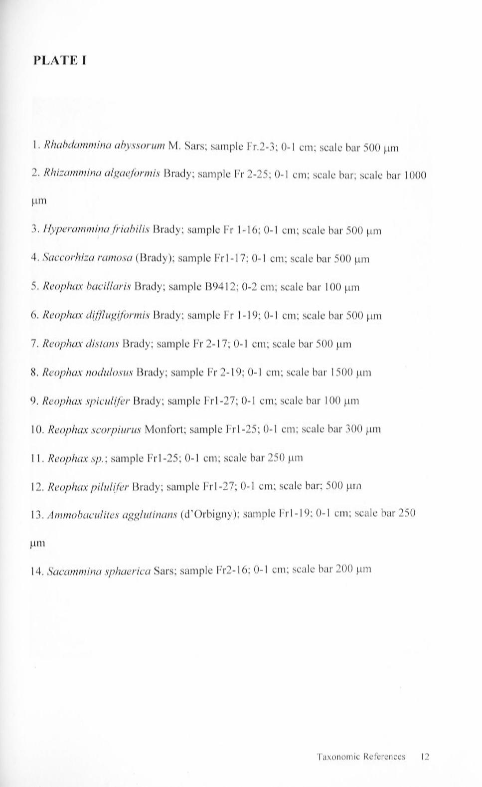
PLATE I

1. Rhabdammina abyssorun1 M. Sars; sainple Fr.2-3; 0-1 cm; scale bar 500 ~Ln1

2. Rhizam,nina algaefonnis Brady; sample Fr 2-25; 0-1 cin; scale bar; scale bar 1000

µ111

3. Hyperammina friabilis Brady; sample Fr 1-16; 0-1 cm; scale bar 500 µ111

4. Saccorhiza ramosa (Brady); sample Frl-17; 0-1 c1n; scale bar 500 µ1n

5. Reophax bacillaris Brady; sample B9412; 0-2 cm; scale bar 100 µ1n

6. Reophax dtffiugiformis Brady; san1ple Fr 1-19; 0-1 cm; scale bar 500 ~Lm

7. Reophax distans Brady; san1ple Fr 2-17; 0-1 c1n; scale bar 500 µ111

8. Reophax nodulosus Brady; san1ple Fr 2-19; 0-1 cm; scale bar 1500 µ111

9. Reophax spicultfer Brady; sa1nple Frl-27; 0-1 cn1; scale bar 100 µ111

10. Reophax scorpiurus Monfort; sa1nple Frl-25; 0-1 c111; scale bar 300 ~L111

11. Reophax sp.; sample Frl-25; 0-1 cm; scale bar 250 µm

12. Reophax pilul£fer Brady; sample Fr 1-27; 0-1 cm; scale bar; 500 µrn

13. An1n1obaculites agglutinans (d'Orbigny) ; san1ple Frl-19; 0-1 c1n; scale bar 250

µ111

14. Sacamn1ina sphaerica Sars; sample Fr2-16; 0-1 cm; scale bar 200 µm


PLATE I


PLATE II

1, 2. A1n1nolagena clavata (Parker & Jones)

1. sa1nple Fr 2-19; 0-1 c1n; speci1nen attached to a G. ,nenardii test; scale bar

500 µrn

2. san1ple B943 7; 0-2 c1n; speci1nen attached to a P. n1urrhina test~ scale bar

500 ~Ln1

3. Cysta,nmina pauciloculata (Brady); sa1nple Fr 1-15; 0-1 c1n; scale bar 200 µ111

4. Thurammina papillata Brady; sample Fr2-1; 0-1 cn1; scale bar 500 ~tn1

5. Alveolophragmiu,n subglobosun1 (G. 0. Sars); sample Fr2-3; 0-1 c1n; scale bar 500

µ1n

6. Psa,nmosphaera parva Flint; san1ple Frl-17; 0-1 c1n; scale bar 400 ~tn1

7. Glomospira charoides (Jones & Parker); san1ple Fr2-1; 0-1 cn1; scale bar 200 ~tn1

8. Glo1nospira gordialis (Jones & Parker); sa1nple Fr 1-1 O; 0-1 cn1; scale bar 200 µ111

9. Throca1nn1ina globigeriniformis (Parker & Jones); sample Frl-17; 0-1 cn1; scale bar

700 µm

10. Am,nodiscus incertus ( d'Orbigny); sample Fr2-1; 0-1 cm; scale bar 200 ~tn1

11. Recurvoides sp.; sample Fr2-3; 0~1 cm; scale bar 500 µ1n

12. Alveolophragmiu1n scitulum (Brady); sample Fr2-7; 0-1 cm; scale bar 500 µn1


PLATE II


PLATE III

l. Jnvolutina intermedia (Hoglund); sample S9011 ; 0-2 cn1; scale bar 1000 µn1

2. Eggerella propinqua (Bardy); sample Fr2-7; 0-1 c111; scale bar 500 µm

3. Eggerella bradyi (Cuslu11an); sample Fr 1-15 ; 0-1 cm; scale bar 500 µ111

4. Eggerella scabra (Williamson); sai11ple Fr 1-17; 0-1 c111; scale bar 100 µ111

5. Textularia lythostrota (Schwager); sample Frl-14; 0-1 cm; scale bar 400 ~tn1

6. Karrerulina apicularis (Cush111an); sample Fr2-27; 0-1 c111; scale bar 200 µ111

7. Karreriella bradyi ( Cushman); san1ple Fr 1-15; 0-1 cm; scale bar 200 µ111

8. Karreriella novanglie (Cushman); sample Frl-17; 0-1 c111 ; scale bar 200 µ111

9. Pseudoguadrina atlantica (Bailey); sample Frl-15 ; 0-1 cm; scale bar 500 µn1

10. Dorothia scabra (Brady); sample Frl-14; 0-1 cm; scale bar 500 µ111

11. Martinottiella co,nmunis ( d ' Orbigny) var. perparva (Cushman); sample S9024~ 0-

2 cm; scale bar 300 µn1

12. Martinottiella communis (d ' Orbigny); sa111ple S9040; 0-2 cn1 ; scale bar 300 µ111

13. Siphotextularia catenata (Cushman); san1ple Fr2-15 ; 0-1 cm; scale bar 300 µm

14. Siphotextularia curta (Cushman); sai11ple Frl-15 ; 0-1 cn1; scale bar 400 µm

15. Textularia agglutinans d ' Orbigny; sample Fr2-16; 0-1 cm; scale bar 25 0 µ111

l 6. Textularia pseudogramen Chapn1an & PaiT; sample Fr2-28; 0-1 c111 ; scale bar 300

µn1


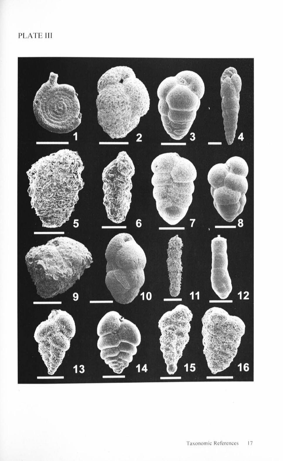
PLATE III


PLATE IV

1. Textularia lateralis Lalicker; sample Fr 1-14; 0-1 cm; scale bar 500 µ111

2. Prae,nassilina arenaria (Brady); sample Fr 2-4; 0-1 cm; scale bar 1000 µ1n

3. Numn1oloculina contraria (d'Orbigny); sample Fr 1-29; 0-1 cm; scale bar 300 ~Ln1

4, 5. Num1nolculina irregularis (d'Orbigny)

4. san1ple Fr 2-4; 0-1 cn1; scale bar 100 µ111

5. sample Fr 2-4, 0-1 cm; scale bar l 00 µ111

6. Pyrgo co,nata (Brady); sainple 2-5; 0-1 c111; scale bar 400 µ111

7, 8. Pyrgo depressa (d'Orbigny)

7. sample Fr2-l 2; 0-1 cn1; scale bar 500 µm


9. Pyrgo serrata (L.W. Bailey); sa1nple Fr 1-21; 0-1 c111; scale bar; 400 µ111

10, 11. Pyrgo elongata ( d 'Orbigny)


11. san1ple Fr 2-4; 0-1 cn1; scale bar 250 ~Ln1

12. Pyrgo laevis Defrance; sample Fr-15; 0-1 cn1; scale bar 400 µm


PLATEIV


PLATE V

1, 2. Pyrgo 1nurrhina (Schwager)

1. sample Fr 1-5; 0-1 cn1; scale bar 400 µ1n

2. sa1nple Fr 1-5; 0-1 cm; scale bar; ventral view 400 µm

3. Triloculina subvalvularis Parr; sample Fr 2-4; 0-1 c1n; scale bar 300 µm

4, 5. Triloculina tricarinata d'Orbigny

4. sa1nple Fr 1-17; 0-1 cn1; scale bar 100 µm

5. sainple Fr 1-7; 0-1 c1n; scale bar 100 µm

6. Quinqueloculina sp.; sample Fr 1-16; 0-1 cn1; scale bar 100 µ1n

7, 8. Miliolinella oblonga (Montagu)

7. sa1nple Fr 2-5; 0-1 cn1; scale bar 200 µ1n

8. sa1nple Fr 2-5; 0-1 cm; scale bar 200 µn1

9. Quinqueloculina venusta Karrer; sainple Fr 2-14; 0-1 cn1; scale bar 300 µ111

10. Quinquelocuina se,ninulum (Linnaeus); sainple Fr 1-17; 0-1 c1n; scale bar 300 ~Ln1

11, 12. Quinqueloculina la,narckiana d' Orbigny

11. san1ple Fr 1-13; 0-1 c1n; scale bar 400 µ1n

12. sample Fr 1-7; 0-1 cn1; scalebar300 µm

13. Cornuspira involvens (Reuss); sample Fr 2-4; 0-1 c1n; scale bar 400 µ1n

Taxonorn ic References 20

PLATE V


PLATE VI

1. Spiroloculina co,nmunis Cuslunan & Todd; sainple Fr 2-5; 0-1 cn1; scale bar 200

µ1n

2. Hauerinella inconstans (Brady); sample Fr 1-7; 0-1 c1n; scale bar 250 ~tm

3. Sigmoilopsis schlun1bergeri(Silvestri); sample Fr 1-23; 0-1 c1n; scale bar 300 µn1

4. Sphaeroidina bulloides d'Orbigny; sample Fr 2-2; 0-1 cm; scale bar 300 µm

5. Bolivina albatrossi Cushman; Fr 1-17; 0-1 cm; scale bar 200 µm

6. Bolivina robusta Brady; Fr 1-17; 0-1 cm; scale bar 200 µm

7. Brizalina se,nilineata Belford; Fr 1-12; 0-1 cn1; scale bar 200 ~tn1

8. Bolivina seminuda Cushman; Fr 1-17; 0-1 cn1; scale bar 200 µ1n

9, 10. Bolivinita quadrilatera (Schwager)


10. san1ple S9024; 0-2 cn1; scale bar 250 µm

11. Bulin1ina aculeata d'Orbigny; B9442; 0-2 cn1; scale bar 250 µin

12. Buli1nina costata d'Orbigny; Fr 1-19; 0-1 cm; scale bar 200 µm

13. Bulimina alazanensis Cuslunan; Fr 2-20; 0-1 c1n; scale bar 100 ~un

14. Bulimina n1arginata d'Orbigny; S9040; 0-2 cm; scale bar 200 µ111

15. Globobulimina a/finis ( d'Orbigny) ; Fr 2-5; 0-1 cm; scale bar 500 µ1n

16. Globobulin1ina pacifica Cushman; Fr 2-4; 0-1 cm; scale bar 500 µm


PLATE VI


PLATE VII

1-4. Uvigerina peregrina Cushman


2. sainple Fr 2-12, 0-1 cn1; scale bar 500 µm

3. sa1nple B9412; 0-2 cn1; scale bar 500 µm

4. sample B9438; 0-2 cm; scale bar 500 µ1n

5-7. Uvigerina proboscidea Schwager


6. sample Fr 1-7; 0-1 ctn; scale bar 200 µn1

7. sample Fr 2-21; 0-1 cm; scale bar 200 µ1n

8. Uvigerina porrecta Brady; san1ple S9024; 0-2 cm; scale bar 200 µ1n

9. Fursenkoina bradyi (Cushman); sainple Fr 1-11; 0-1 cn1; scale bar 250 ~un

10. Fursenkoina earlandi (Parr); sample Fr 2-2; 0-1 ctn; scale bar 300 µ111

11. Fursenkoina jitsfformis (Parr); san1ple S9024; 0-2 cn1; scale bar 250 µn1

12. Dentalina conununis ( d'Orbigny); satnple Frl-16; 0-1 cn1; scale bar 500 µm


PLATE VII


PLATE VIII

I. Dentalina gutt(fera d'Orbigny; sa1nple Frl-27; 0-1 cm; scale bar 300 ~un

2. Dentalina intorta (Dervieux); sa1nple B9437; 0-2 c1n; scale bar 500 µ1n

3, 4. Ehrenbergia trigona Goes

3. smnple Fr 1-21; 0-1 cm; scale bar 200 µ1n

4. sample Fr 1-21; 0-1 c1n; scale bar 200 ~un

5. Dentalina subsoluta (Cushman); sample Fr 1-15; 0-1 cm; scale bar 300 ~tn1

6. Nodosaria radicula (Li1u1aeus); sample Fr 1-1 O; 0-1 cn1; scale bar 100 µ111

7. Amphicroyna scalaris (Batsch); sample Fr 2-4; 0-1 cm; scale bar 1 CO µn1

8. Lagena gracillima (Seguenza); sa1nple Fr 2-4; 0-1 cm; scale bar 200 µ1n

9. Rectoboivina colu,nellaris (Brady); sample Fr 2-5; 0-1 cn1; scale bar 500 µ111

10. Rectobolivina dimorpha (Parker & Jones); sample B9441; 0-2 cn1; scale bar 200

~llll

11. Rectoglandulina comatula (Cushn1an); sample Fr 2-11; 0-1 cm; scale bar 200 µ111

12. Lagena laevis (Montagu); san1ple Fr 2-5; 0-1 cn1; scale bar 300 µm

13. Lagena stelligera Brady; san1ple Fr 1-15; 0-1 c1n; scale bar 200 µ111

14. Lagena striata (d'Orbigny); san1ple Fr 2-2; 0-1 cm; scale bar 300 µ1n

15. Fissurina cf. ,narginata (Montagu); sample Fr 1-15; 0-1 c1n; scale bar 500 ~un


PLATE VIII


PLATE IX

1. Fissurina orbignyana Seguenza; sample Fr 1-24; 0-1 cm; scale bar 500 µ111

2. Fissurina sen1iniforn1is (Schwager); sample Fr 2-11; 0-1 cn1; scale bar 500 µ111

3. Fissurina submarginata (Boomgrat); sample Fr 1-27; 0-1 cn1; scale bar 200 ~t111

4. Oolina globosa (Montagu); sa1nple Fr 2-11; 0-1 cm; scale bar 200 µ111

5. Pyrulina fusformis (Roe1ner); san1ple Fr 2-21; 0-1 cm; scale bar 300 µ1n

6. Pyrulina extensa (Cushman); sample Fr 2-20; 0-1 cm; scale bar 300 µ111

7. Globulina 1ninuta (Roemer); sample Fr 2-19; 0-1 cm; scale bar 300 µ111

8. Lenticulina paeregrina (Schwager); sample Fr 1-17; 0-1 cm; scale bar 200 µm

9. Lenticulina gibba (d'Orbigny); sample Fr 2-5; 0-1 cn1; scale bar 250 ~un

10. Lenticulina iota (Cushman); san1ple Fr 1-14; 0-1 cn1; scale bar 200 µ1n

l l. Lenticulina calcar (Linnaeus); san1ple Fr 1-14; 0-1 cm; scale bar 300 µ111

12. Lenticulina rotulata (Lamarck); sample B9452; 0-2 cm; scale bar 1000 µ111

13. Parafissurina lateralis Cushman; sa1nple Fr 2-24; 0-1 cm; scale bar 250 µ111

l 4. Parafissurina sp.; san1ple Fr 1-20; 0-1 cm; scale bar 200 µ111


PLATEIX


PLATEX

1. Astrononion echolsi Ke1u1et; san1ple Fr 2-5; 0-1 c1n; scale bar 200 µ111

2. Nonionella turgida (Williamson); sample Fr 2-5; 0-1 cn1; scale bar 300 µ1n

3, 4. Melonis barleeanun1 (Willian1son)

3. sa1nple Fr 1-21; 0-1 cm; scale bar 150 µm

4. san1ple Fr 1-11; 0-1 c1n; scale bar 200 µ1n

5, 6. Melonis pon1pilioides (Fitcher & Moll)

5. sainple Fr 2-12; 0-1 cn1; scale bar 200 µ111

6. san1ple Fr 2-1 O; 0-1 cn1; scale bar 200 µm

7, 10. Cassidulina crassa d'Orbigny;

7. san1ple Fr 1-14; 0-1 c1n; scale bar 150 µ111

10. sa1nple Fr 1-17; 0-1 cm; scale bar 100 µ1n

8,9. Cassidulina laevigata d' Orbigny

8. san1ple Fr 1-25; 0-1 c1n; scale bar 150 ~un

9. san1ple Fr 1-25; 0-1 cm; scale bar 150 µm

11 , 12. Pullenia bulloides ( d ' Orbigny)

11. san1ple Fr 1-13; 0-1 cn1; scale bar 200 µ1n

12. sa1npleFr 1-14; 0-1 cm; scalebar200 µm

13. Pullenia quinqueloba (Reuss); san1ple Fr 2-23; 0-1 cn1; scale bar 100 µ1n


PLATEX

Taxonomic References 3 I

PLATE XI

1, 2. Globocassidulina elegans (Sidebottom)

1. sa111ple Fr 2-24; 0-1 c1n; scale bar 200 µ111

2. sainple Fr 1-19; 0-1 cm; scale bar 200 µ1n

3. Globocassidulina subglobosa (Brady); sample Fr 2-20; 0-1 cm; scale bar 300 µ111

4. Chiloston1ella oolina Schwager; sample Fr 1-7; 0-1 c111; scale bar 200 ~un

5, 6. Ceratobulimina pactfica Cushn1a11 & Harris


6. sample Fr 1-5; 0-1 c1n; scale bar 300 µm

7, 8. Epistominella umbon[fera (Cushman)

7. sample Fr 2-14; 0-1 cm; scale bar 300 µm

8. sainple Fr 2-14; 0-1 cm; scale bar 300 µm

9, 10. Cassidulina reflexa Galloway & Wissler

9. sa1nple Fr 2-1; 0-1 cn1; scale bar 300 µ111

10. san1ple Fr 2-9; 0-1 cm; scale bar 250 µ111

11, 14. Episton1inella exigua (Brady)


14. sa111ple Fr 2-14; 0-1 cn1; scale bar 200 µ111

12, 13. Osangularia cultur (Parker & Jones)


13. san1ple Fr 1-29; 0-1 c1n; scale bar 200 µ111


PLATE XI

Taxonomic References ,..., ,..., _) _)

PLATE XII

1, 2. Allomorphina pacifica Cush1nan & Todd

1. sainple Fr 1-19; 0-1 cn1; scale bar 250 µ111


3, 6. Hanza1;JJaia nipponica Asano



4, 5. Discopulvinulina subbertheloti (Cushman)



7,8. Gavelinopsis lobatulus (Parr)

7. sa1nple Fr 1-29; 0-1 cn1; scale bar 300 µm

8. sa1nple Fr 2-1 0; 0-1 cm; scale bar 300 µm

9, 12. Cymbaloporretta squammosa (d'Orbigny)


12. sample 2-5; 0-1 c1n; scale bar 150 µm

10, 11. Oridorsalis tener un1bonatus (Reuss)



Taxonorn ic References 34

PLATE XII


PLATE XIII

l, 2. Valvulineria sp.



3, 6. Gyroidinoides polius (Phleger & Parker)

3. sainple Fr 1-23; 0-1 c1n; scale bar 200 µm


4, 5. Gyroidinoides altiformis (Stewart & Stewart)


5. sainple Fr 2-4; 0-1 cn1; scale bar 200 µ1n

7. Hyalinea balthica (Shroter); san1ple S9024; 0-2 cm; scale bar 300 µ1n

8. Planulina arinrzinensis (d'Orbigny); sample S9040; 0-2 cm; scale bar 200 ~Ln1

9. Gyroidinoides lanrzarckianus ( d'Orbigny); sa1nple Fr 2-12; 0-1 cn1; scale bar 300

~l111


PLATE XIII

Taxonomic References 3 7

PLATE XIV

1, 2. Cibicidoides pseudoungerianus (Cushn1an)



3. Cibicidoides kullenbergi Parker

3. smnple Fr 1-5; 0-1 cm; scale bar 250 µn1

4, 5. Cibicidoides bradyi (Trauth)


5. smnple Fr 1-13; 0-1 cm; scale bar 200 µn1

6, 9. Cibicidoides robertsonianus (Brady)

6. sample Fr 2-12; 0-1 cn1; scale bar 200 µn1

9. sample Fr 1-29; 0-1 cn1; scale bar 200 µm

7, 8. Cibicidoides wuellerstorfi (Schwager)

7. sa1nple Fr 1-29; 0-1 cm; scale bar 500 µ1n


10, 11. Anow1alina globulosa (Chapn1an & Parr)


11. smnple Fr 1-28; 0-1 cn1; scale bar 200 µ1n

12. Laticarininapauperata (Parker & Jones); sample Fr 2-12; 0-1 cn1; scale bar 600

~Lill

Taxonomic References 3 8

PLATE XIV


)> -0 -0 (l) ::J 0..

>< )>

-0 ~ uo (l)

APPENDIX Al

Species

A.llomorphina pacifica

A.lveolopbragmium crassimaxgo

A.lveolophragmium ringens

A.lveolophragmium s ci tulum

A.lveolophragmium subglobosum

A.lveolophragmium viesneri

A=baculites agglutinans

A=baculites inte=dius

Ammobaculites sp .

Ammod.iscus incertus

A:mmDdiscus pacificus

AalmDlagena clavata

Ammom.a.rginul ina £oliaceus

Amphistagi na lassonii

Amphicoryna proxima

Amphi coryna scalris

Anomal ina globulosa

Astacolus crepidulus

Astacolus insolitus

A.strononion echlosi

A..strononion stelligerum

Bigenerina nodosaria

Bolivina albatrossi

Bolivina d.ecussata

Bolivina pseudoplicata

Bolivina robusta

Balivina sem.inuda

Bol i vina spissa

Boli vina sp .

Bolivinita quadrilatera

Brizalina dilatata

Bri zalina sam.il ineata

Briz:alina sp ,

Bulim.ina aculeata Bulim.ioa alaza.oensis

Bulim.ina costata

Bulim.ioa gibba

Buli..wina marginata

Bulim.ioa striata

Bulim.ioalla elegantissima

Bulim.ioella sp . Ca.n cris oblungus

Ca~sidulina carinata

Cassidulina crassa

Cassidulina laevigata carinata

Caratobuli.m.ina pacifica

Chilostomella oolina

Cibicides lobatulus

Cibicidoid.es bradyi

Cibicidoid.es kullobergi

Cibicidoides pseudou.ngeria.nus

Cibicidaid.es robertsonianus

Cibicidoid.es ungerianus

Cibcidoides wuellerstor£i

Cibicidoid.es .sp .

Cornuspi,ra carina. ta

Cornuspira involvsns

Cornuspira sp .

Cornuspiroides primitivu~

Cyambaloporretta squa.mosa

Cyclammina ca.ocellata

Cystammin• pauciloculata

Dentalina advena

Dentalina communis

Dentalina filiform.is

Dentalioa guttifera

Dantalina inoroata

Dentalioa intorta

Code

Allpa

Alvcr

Alvri

Alvsi

Alvug

Alvwi

Abag

Ab i n Absp

Adsin Adspa

Amlc

Afol Aphle

Amphpx

Amphsl Aagl ob

Atacre

Atains Astrech

Astrst

Bina

Bolab Bolde

Bolpse

Bolro Bolsem

Boli ss

Bolsp

Blql Brdi

Brsem

Brsp

Buac Bualz Buco

Bugi Buma Bustr

Bumel

Bumsp Canob Casri

easer

Casale

Cerpa

Chol

Clob

Cibr Ciku Cipse

Cirob

Ciung Ci wul Cisp Coca

Coin

Cosp Csppr Cyasq Cyca Cyspa Dead

Deco Defi Degu Dein

Deter

Frl- 5

0 , 63

3 , 77

0,63

0 , 63

1, 2 6

7,55

0 , :;3 1 , 89

1 , 89

l, 2 6

3 , 14

9 ,4 3

l , :: 6

2 , 52

Frl- 7

1, 28

0 , 2 6

0 , 26

3 , 8 4

1 , 28

0,77

0 , 77

1 , 7 9

1 , 53

1, 2 8

2 , 5€

1,53

1, 02

5 , 37

(1, :•

,) , ;1

lj , 2 €

Frl-1 0

l, .i.. 0

0 , 55

0 , 55

3,85

0 , 5 5

4, 4 0

1 , l 0

1 , 65

5 , 4 9

0 / 5 5

0 , 5 5

rrl-11 0 ,4 '?

0 , 49

0 ,4 9

3 , 43

0 , 98

2 , 45

0 , 49

2 , 94

2 , .J 5

4, 90

0 , 4 9

1,n 2 , -l 5

0 , 4 9

2 I .:} 5

0 ,4 9

"') ::. 1 .:... , --= () I -! ':?

r"r l - 12

0 ,4 5

0 , 4 5

0 , 4 5

0 , 89

0 , 4 5

0 , 4 5

0 , 4 5

6 , 25

l, 34

4, 02

0 , 4 5

0 I 4 5

0 , 8 9

2 , '.23

1 , 79

0 , 89

(J , 4 5

5 , 3 ,,

ij , 139

r) I .} _j

:rl-13

0 , €,6

I) , 61S

3 , 31

0 , 66

0 , 66

0 ,6 6

0 , 66

0 , 66

0 , 66 (i , 6G

2 , 65

1 , 99

3 , 31

5 , 31J

l , 3_:

C: 1 60

Core- tops Species ~-;,

Frl-i4

G, 22 0 , :;:::2

0 , 22

=:i ' -l 3

0 , 22

2 , 16

5, 19

0 , 4 3

2 , 81

0 , €5 0 , 2:2

1 , 08

0 , 22

0 , :22

l , 52

~ , .!. ':,

0 , 4 3

2 , 91

4 , 33

0 , 87

0 ,2~

a, 4 4

0 , ,5 5

:; , 4 3

.~ .... -. IJ I .:..:...

o,:~

Fr l - 15

0 , 23

1 , 36

0 , 11

1, 02

0 , 11

0 , 4 5

0 , 11

3 , 63

0 , 3 .J

1 , 02

0 , 11

0 , 3 4

0 , 4 5

0,23

2, 04

0 , 11

0 , 11

2, 33

3 , 06

l , 59

0 , 11

9, 19

(! ' q ~

0 , 11

frl - 16

3,58

1 , 28

2 , SE.

0 , 26

0 ,2 6

0 , 77

o , ~6

0 , 26

1 , 28

5 , 63

5 , €3

1 , 79

1 , 2.9

6 , 39

0,26

(i , 2-:

::1 I =· l

Fr l - :i. 7

0 , 32

0 , 32

1 , 29

0 , 96

0 ,3 2

0 , 32

0 , 32 0 ,3 2

5 , 79

0 , 96

6 , 4 3

0 , 32

0 , 32

1 , 29

2 ,5 7

2 , 25

3 , 5 4

2 , 25

0 , 96

0 , 32

2 , 57

r; , 32

(, , 3Z

Fr l - 18

1, :.l l

1, 41

1, 41

1 , 4 1

:,s:

2,82

4 , 23

Z , 8.2

2,82

l , 4 1

5 , 63

1 , 41

: [! - 19

0 , 33

0 , 33

r; , 99

0 , 66

0 , 66

8 , 58

-l , 62

1, c-5

0 , 33

2 , 97

0 , 33

0 ,3 3

l , :i 8

3 , 30

6 , 6,)

(I , :} ;

C~l- 2()

1 , 14

l, 14

7 ,95

2,27

1 , 1 4

1, 14

2 , ::7

1 , 14

5 , &8 4 , 55

6 , 8.2

7 77 .!.. 1 .:... .

1 , l .;

Fr l - .21

2 , 81

1, 12

l , 12 0 , 56

2 , 81

1 , 139

0 , 5 (;

l I l:

3, 37

0 , 5 c 0 , 56

0 , 56

Frl-.:~

0 , 74

0 , 74

I) ' 7 4

0 , 74 o, 74

0 , 74

1, 4 8

7 77 .:.. , .:....:...

5 , 19

4, 4 4

5, 19

8 / 8 9

0 , 7-!

t rl - 23

l, OS

2 , 11

1, 05

6 , 32

l , 05

l , G 5

8 , 4Z

4 ' ;: l

l, :~• 5

3 , l ~

1 , 05

1 , 0':-

Frl-24

1, 37

0 , 85

1 , 37

l , 37

2' 7 4

~r l - '.25

0 , 33

2 , 01

0 , 33

0 , 67

0 , 33

0 , 33

~.35

1 , ;jl)

l , 00

3 , 68

3 , 68

:: , 34

1,00

6 , tj2

1 , 0(1

1 , •jG

Frl - 26

l, 12

0 , 75

0 , 75

0 , 75

l, 1 ~

0 , 75

0 , 37

3 , 00

1, 12

4, 87

0 , 37

3, :5

3,75

1) , 7 5

0 , 37

1 , 50

I) , ;5

J / 3:

(:, 3;

I 3-:-

..... 0 ..... ~

:::::l C

3 u (l) -: 0 -+i (/]

-0 (l) 0

:::::l ...J (D :::::l (/]

::J (l) ~ 0 ::;-(/]

~

3 -0 (l)

n 0 C :::::l ~ (/]

0.. ~ ..... ~

0 -+i u (l) :J ..... ::r 0

6 ., ~

3 :::::l

~ -: ~

~ 0 3 ~

::;Cl)

0 0 -: (D

I ..... 0

-0 (/]

~

3 -0 (D (/)

z C 3 u (l) ., (/)

~ ., (D

(JO

< (l) :::::l P) (/]

-0 (l) ., 0 (l) :::::l ..... P)

(JO (l)

0 ~ ~

:::::. (l)

> ~ ~ ~ 2 0 ~

X > ~

APPENDTX Al Core-tops Species 'Vi,

Spe ci~s Code Frl-;:7 Fr l - 28 Frl-2 9 Fr 2- l Fr 2-2 Fr~-J Fr2-4 Fr2-5 Fr 2 - 7 =~2. - 9 Fr2-1 0 r" r2-il Fr:2 - !2 Fr2 - 13 Fr2 - l~ fr:>-15 Fr':'-16 Fr:' - l": Fr'.:""·-1; Allomorphina pacifica Allpa 0 , 23 0 , 38 - - - 0 , l .J

Alveolophragmium crassimargo Alvcr

Alveolophragmium ringens Alvri

Alveolophragmium scitulum Alvsi - - - 0 , 63 Alveolophragmium subglobosum Alvug - - 0 , 68 1 , 88 0 , 61 6 , 25 - - 1 , 26 0 , •S ·3 0 , 38 - 0 , 18 1 , 18 A.lveolophragmium viesneri Alvwi - - - 0 , 63

Ammobaculites agglutinans Abag

Ammobaculites intermed.ius Abin 0 , 23 0 , 38 0 , 3i)

Ammobaculites sp . Absp

Ammodiscus incertus Adsin

Ammodis c us pacificus Adspa 1 , 50 - - - 0 , 68

Ammolagena clavata Amlc - 0 , 23 1, 13 - - - - - - - l, 75 1, 1)1) l , 4 3 Ammomarginu.lina .foliaceus A£ol - - - - - 0 , 63

Amphistegina lessonii Aphle

Amphicoryna proxima Amphpx

Amphicoryna scalris Amphsl - - - 0 , 15 0 ,19

Anomalina globulosa Aaglob 2 , 02 0 ,4 5 1,sa - 0 , 89 0 , 30 0 , 39 3 , 14 1 , 0 9 2 , 0 4 1 , 92 0 , iJ l 2 , 20 - 1 , l 8 - 1, 00 l , 4 3 Astacolus crepidulus Atacre

Astacolus inso.litus Atains

Astronooion e chlos i Astrech 5,99 3 , 15 ~ ~- 2 , 4 4 4, 4 6 1 , 21 2 , 92 0, 55 - (), 1-l 4 , 4 0 0 , 71 - 0 , 88 3,00 ~ I .!..V

Astrononion stelligerum Astrst 0 ,1 9 Bigenerina nodosaria Bina

Bolivina a.Lbatros.1Ji Bolab

Bolivina d.ecussata Bolde Bolivina pseudoplicata Bolpse - - 0 , .23

Bolivina robusta Bolro

Bolivina sem.inuda Bolsem 2 , 02 0 ,4 5 - - 0 , 30 0 , 78 - 0 , 18 1, 00 Bolivina spissa Boliss Bolivina sp . Bolsp - - - 0 , 15 Bolivinita quadrilatara Blql 1, 20 2 , 02 6 , 53

Brizalina d.ilatata Brdi - - 0 , 23 Brizali~a sem.ilineata Brsem 0 , 75 0 , 19 - 0 , 38 - - 0, Bi: Brizalina sp , Brsp - 0 , 4 5 Bulimina a c uleata Bua.c 8 , 08 - - - - - - 0 , 55 - 7 , 02 l , 00 Buli.mina alaza.nensis Bualz 0,23 1 , 50 1,22 - 0 , 91 0 , 19 1, 8 9 2 ,7 3 0 , 68 0 , 77 0 , 55 - 0 , 18 0 , 8 8 4 , 00 1 , 4 3 Bulimina costata Buco 1, 1 3 0 , 15 0 , 19 - 1,23 - 1, 00 Bulimino1 gibba Bugi Bulim.ina marginata Buma - - o ·1 a ,'--

Bulimina striata Bustr - - - - 0 , -;_7 l , OrJ Buliminalla elegantissima Bumel 0 , 60 1, 0 l 0,23 Buliminalla sp . Bumsp - 0 , 39 Cancris oblungus Ca.nob - 0 , 69 0 ,3 8 Cassidulina carinata Casri 1, 80 3 , 03 3 , 83 0,38 - 0 , 61 0 , 39 1 , 64 0 , 68 0 , 38 2 , 86 2 , 1)0 Cassidulina c ras.sa easer 3 , 03 1 , 13 0 , 38 - 0 , 30 - 0 , 63 - 0 , 38 Cassidulioa laevigata c arinata Casslc 3 , 38 - - 2, 19 1 , 3 6 2 , 69 2,05

)> Ceratobulim.ina pacifica Cerpa 1 , 58 2 , 63 0 , 7 E 1, :'6 0 , 68 0 , 77 1 , ;'3 - 0 , 88

"O Chilostomalla oolina Chol 1, 0 l 0 , 76 4,C:,7 0, 5 4 "O Cibicidss loba t:ulus Clob 1J , 00 1, 0 l 1 , 35 0 / 4 6 (1 , 53 - I} , 38 0 , l 4 - l , 0(> (1) Cibicidoidss bradyi Cibr 5,39 3 , 03 5 , 86 0 , 75 1,22 2 , 68 2 I .J3 3 , 31 <l , 40 0 ,55 ~ I 08 0 , 35 n ~., 4 , 40 (), 18 -l, 71 0 , 83 2 , 00 2 , 86 ::::1 ~ , :.... '

0.. Cibicidoidas kullnbergi Ciku 4, 19 3,03 4, ,:is 0 , 75 0 , 61 2 , 68 5 , 61 1 , 1 7 1, 89 0 , 5 5 3 , 40 0 I 77 0 , 82 4, 4 0 - 2 , 35 1 , 7 5 ;_ , ,)'j : , 9 6 -· Cibicidoides pseudoungerianus Cips e 8 , 98 l, 0 l 1 , 35 X - 3,03 5 , ·~ 4 - - 2 , 20

)> Cibicidoidss robartsonia..:.us Cirob 0 , 60 1, 80 0 , 61 2 , 68 IJ , 91 0 , 19 1 , 26 1 , 36 0 , 38 0 , 41 1, 1 a 0 , 3,? - 2 I 2.6 Cibicidoidas Wlgerianus Ciung Cibcidoidas wuellerstorfi Ciwul 0 , 60 1 , 58 ,) , 38 0 , 89 l i (l 6 0 , 39 2 , 52 19 , 67 5 , 4 4 21 , 15 35 , 7 4 7 , 69 ~, 79 S , ~4 G, 14 4 , 00 4,2S Cibicidoidas sp . Cisp 1, zo - 2 , I() 1,22 4, .J 0 1 , ; 5 - 1 , 1(:

-0 Cornuspi:ra carinata Coca - 0 , 19 P) Corouspira. involvens Coin - l , 0 l 0 , 90 0 , 15 !) / 39

(IQ Co.r:Duspira sp . Cosp 1 , 0 l (1)

t·0 Cornuspiroides primitivus Csppr - - 0 , 39 Cyambaloporretta squamosa. Cyasq 1 , 13 l),]8 ( 1 , 15 l, 95 Cyclammina cancallata Cyca 0 , 00 (1 1 -?O 0 , 38 0 , •Sl 1:1 I -39 1 , 89 ::. , 7: - - 1 , 18 - 2 I::• 6 Cysta.mmina pauciloculata Cyspa - 0 , .23 3 I 5 7 0 , .;.3 Dentalina advena Dead 0 , 68 i) / 19 Dentalina co.mmunis Deco !) / .3 s 0 , 19 /) I 5 s (J , :: l I l 1) I), 71 Dentalina filiformis Defi Daotalina guttifara Degu 0 , 60 Dentalioa inorna. t:a Dein Dantalina intorta Deter - - lj / 8 ~ - tj I '5) - () , ,S8

APPENDIX Al Corc-10ps Species ~,;.

Species Code Fr2-20 Fr 2 - 2l Fr2-23 Fr2-2 4 Fr2 - 25 Fr:2-213 B9 41)7 39412 B9'136 89437 B9438 B944 1) a9.J 4 l 39 4 4;: 59011 39024 59039 59040 59(145 Al.lomorphina pacifica Allpa - 0 , 21

Al.veolophragmium crassimAigo Alvcr - 0 , 2 1

Al.veolophragmium ringens Alvri

Alveolophragmiwn scitulwn Alvsi

Alveolophragmium subglobosum Alvug - 0 , 85 0 , 63 0 , 35 - - - 1, 32 1 , 03 Alveolophragmiwn viesneri Alvwi

Ammobaculites agglutinans Abag 0 , 21

Ammobaculites intenned.ius Abin - - - - - - - 0 , 61 Ammobaculites sp . Absp

Ammodiscus incertus Adsin

Ammod.iscus pacificus Adspa - - - - 2 , 60 - - - 2,63

Ammolagena clavata Amlc 0 , 56 - - 0 , 35

Ammomarginulina foliaceus A£ol

Amphistegina lessonii Aphle - - - - - I} , 87

Amphicoryn• proxima Amphpx

Amphicoryna scalris Amphsl - - - - - 0 , 87 - 0 , 39 Anomalina globulosa Aaglob 0 , 56 4, 27 8 , 11 4, 23 3,66 5 , 8 4 0 , 25 l , 30 0 , 69 I) , 3 4 5 , 56 2 , 42 1,32 Astacolus crepidulus Atacre

Astacolu~ insoli tus Atains 0 , 28 Astrononion ecblosi Astrech 0 , 28 0 ,8 5 - 0,63 1,05 0 , 73 I}, 25 - l, 97 ~ ~~ - i, 32 ~ / LL

Astrononion stelligerum A,otrst

Bigenerina nodos~ria Bina

Bolivina ~lbatrossi Bolab - - - - - - 0,39 - 0 , 80 Bolivina decussata Bolde 1, 12 - - 0,21 Bolivina pseudoplicata Bolpse

Bolivina robu5ta Bolro - - - - - 1 , 21 l, i 8 Bolivina sem.inuda Bolsem 0 , 28 0 , 21 - - - - 1, ,) 3 Bolivina spi!Hila Boliss - - - - - - - 0 , 39 Bolivina sp . Bolsp

Bolivinita quad.rilatera Blql - - - - 10 , 59 l , 60 Brizalina dilatata Brdi - - - - - 1 , 11 - 0,61 - 3 , 20 Brizalina sam.ilineata Brsem - 0 , 42 o, 52 - 0 ,96 Brizalina "P , Brsp Bulimina aculeata Buac 8 , 11 9, 9 4 3 , 66 2 , 19 - - 1 , 7 4 50, 96 - 3,92 1 , 32 6 ,4 0 9 , 28 Bulim.ina alazanensis Bualz 3 , 37 2 , 56 1, 3 5 2 , 5 4 4, 19 2, 19 l, JO 0 , 99 l , 7 3 1, 11 0 , 61 - 6 , l 9 Bulim.ina cos t.il ta Buco 1,35 - 3 , 65 1,92 0 , 61 1 , 32 6 , 40 Bulimina gibba Bugi 0 , 73 Buli.m.ina marginata Buma - - - 0 , 87 - 0 , 39 11 ,20 Bulimina .striata Bustr

Buliminell~ elega..otissima Bumel Buliminella "P · Bumsp Caner is oblungus Canob Ca ssidulina carinata Casri 0,28 2 ,70 0 , 85 1 , 05 l , 3 0 0, 35 3 , 33 0 , 87 1, 2 l 0,78 2 , 63 l. ,;o 1 , 03 Ca .ssidulina cras.sa easer - 0 , 4 9 0 , 35 0 , 87 - 0 ,39 Cassidulina laevigata carinata Casslc I , 35 0 , 21 l, 4 6 - - - 4, l S - I} , 61 Ceratobulimina pacifica Cerpa ::'. , 70 0 , 63 l , (I 5 0 , 73 - 1 , 30 0 , 35 1 , 11 2 / 61 l, 82 2 , 75

)> Chilostomella oolina Chol - 0 , 99 - -, ~~ 2, 8 9 2. , 75 "D

.!. ' ~,t_

"D Cibicides lobatulus Clob - - 0, 52 0 , 73 (;, 99 0 , 35 l, la (1) Cibicidoidas bradyi Cibr 0 , 4 2 0 ,5 2 0 , 73 r, , 4 9 l , ';·7 0 , 69 1 , 1)1 4 , 4 4 5 , 2: '1, 85 1, 5.., 1, 32 6, 19 ::i Cibicidoides kullnbergi Ciku 0,56 0 ,85 .2 I 7 I) 0 , 85 1, 5 7 0 , 7 3 - 5 , 19 0,99 2 ,4 2 ., '" 6, 67 l , 7 4 0,96 l , 21 0 ,39 3,95 2,06 0. - ' :J..,

Cibicidoid.es pseudoungerianus Cipse - 0 , 4 9 0 , 35 3 , 33 0 , 87 2 , 4 2 2 , 35 -, , 2() X C.il:icidoides robertsonianus Cirob 0 , 85 0 , ;2 1, 0 5 - 1, 30 0 , 69 )> Cibicidoides ungeria.nus Ciung - - l , 30 - - 0 , 3 4

Cibcidoid.es vuellerstorfi Ciwul J, 65 4 -,-, , - 8 , 11 -1 , oz 2, 6::: 5 , l l 5 , 19 (1, 99 3 , 46 3 , 36 5, S 6 l, 7 4 2 , 42 .:1 ..,. ., • .L. E,59 : , 4() 7,22

Cibicidoide s sp . Cisp I) ' ;:g 0 , 2 l. l , .: :: 2 1 ~ lj

""CJ Corn uspiFa c arioata Coca

l=l) Cornuspira involvens Coin ao Cornuspira sp . Cosp (1)

\..,.J Co.rnuspi roides prim.itivus C,oppr Cy.unbaloporretta squamosa Cyasq Cyclamm.ina ca.nce lla ta Cyca o, ss rJ, 21 0, 5:2 i) , 7 3 o, :s l , 3(: 1, ~;; c, , 34 - - 2 , 0 ,) Cystammina pauciloculata Cyspa Dentalioa advena Dead Dentalina COIIDDunis Deco - !) , : s - - 1)' 3.J - 0 I ,'3 / Dentalioa £iliform.is Defi Dentalina guttifera Degu Dentalina inornata Dein Den~alina intorta Detar - ,') , 35

APPENDTX Al Core-tops Species '?fl

Species Code fr l -5 frl - 7 frl-10 frl-11 frl-12 Fr 1- 13 frl - 14 Frl-15 frl-l6 f,:1-1"' fr! - B fr l -19 Fri-ZO frl - 21 :'rl-22 :'rl-23 Frl-24 Frl- 25 Fri - 26

Dentalina neugeboreni Deneu

Dentalina subsoluta Deasub - 0 , 2:: 0 ,2 6 0,66 - 0 , 37

Dentalia sp . Desp 0 ,63 - - - 0 , 11

Discopuivinu1ina araucana D:spa.ra

Discopulvinulina subbertheloti Dspber - - - 0 , 11 - 1, 12

Dorothia brady.wa Dobr

Dorothia axilis Doex - - - 0 ,32

Dorthia pseudaturris Doptr

Dorothi.ai £cabra Dose - - () , 26

Eggerella bradyi Egbr 1 , 26 1, 02 1 , 10 0 ,4 9 - 0 , 43 Q , 34 0 , 26 0 , 32 0 , 66 l , 14 2 ,22 1 , 05 2,74 1, 0() 0,75

Eggerella propinqua Egpr - - 0 , 66

Eggerel.la sea.bra Eggsc - - 1,02 0 , 20 0 ,3 3

Eggere.lla sp . Eggsp - 0 , 26 - - Ci , 32 - - 0 , 33

Ehrenberg in a trigona Ehtr l , 2 6 2 , 05 9, 3 4 2 , 65 3 , 68 2 , 38 7 ,1 0 0 ,9 6 1, 14 20,22 4, 4 4 - 0 , 33

Elphidiwn crispwn Elcr - - - - 0 , 32 - - - 0 , 75

Elphidiwn incertwn Elin - - - - - - - 0, 37

Elphidiwn macellum Elma - - - 0 , 33

EPistom.inella exigua Epex 3, 14 0 ,7 7 2 , 4 5 5 , 80 2, 65 0 ,23 - 1 , 41 0 , 66 1 , 14 0 , 56 0 , 74 0, 37

EPistominella umbonifera Exum - 0 , 22 - 0 , 32 - 4, 5 5 4, 4 4 - o, 33

EPonid.es regularis Epre - 0 , 55

Eponid.es twnidu.ls Eptum - 0, 4 5 0 , 22 - 0 , 26

Eponid.es .sp . Epsp - - 0 , 615 - - 0 , 74

Fissurina alveolata Fisal 0,26 0 , 55 0, 4 9 0 , 45 0 , 4 3 0 ,6 8 0 ,3 3

Fissurina auricul~ta Fisaur - 0 , 11

Fi•surina bra.dyi Fisbr

Fissurina clathrat~ Fiscl - - - l, 12 0 , 74

Fi$surina ere.bra Fiscrbr 0 , 26 0 , 98 - - - 0,66 l , 14 0 , 56 - 3 , 16 - 0 , 3,

Fissu.rina ;fimbriata Fisfi - 0,89

Fissurina karguelensis Fiske - 0 , 89 - 0 , 33 - - 0 , 33 6 , 7 4 Fissurina marginat~ Fi.sma 0 , 63 1, 02 - 0 , 98 1 , 34 0 , 87 0 , 57 0, 51 - 0 , 99 l, 14 1 , l2 l, .J 8 - 0 ,3 3 0 , 3 7 Fissurina orbigny.wa Fiser - 0,55 1, 4 7 0 , 89 1 , 32 0 , 22 0 , 3 4 - 1, 41 0 , 66 1 , 12 0 , 7 4 1 , 05 1, 37 0 , 33 Fis3urina semim.arginata Fissern - - 0 , 89 0 , 66 0 , 4 5 - - - 0 , 33 - - 0 , 37 Fissurina sem.iniformis Fismnf

Fissurina submargina ta Fissub - 0 , 77 1 , 10 l , 7 9 - 0,57 0 , 2-5 - 1 , 41 0 , 66 0 ,56 - 1, 05 0 , 33 Fi.ssurin• trigono - margna t:a Fistrma - - - - - - - - 0 , 33 Fissurina v iesneri Fiswie - 0 , 43 - 0 , 26 - - - 1 , 05 Fissurina sp . Fi.ssp 0 , 63 1,28 0,98 0 , 4 5 0 , 66 0 , 79 1 , 02 - 0 , 6€ 0,56 0 , 7 4 3 , 16 0,,57 1, 87 Froncticularia kien.sis Froke

Fursenkoina bradyi Furbr 0 , 98 - 0, 11 - 0 , 66

Fursenkoina d.avisii Furda

FUrsen.koina earland.i Furea

Fursenkoina fusiform.is Furfs 0 , 26 0 ,4 9 - 0 , 21J - 0 ,99 Fursen.koina punctata Furpu - - - - 1, 41 F'tlrsen.koina sp . Fursp - - 0 , 32

Gavelinopsis lobatulus Galo 3 , 07 1, 10 2 , 65 0 , 65 1 , 36 0 , 26 3 , 22 1, 41 2,27 - - 2 , 74 2 , 34 Globobul.i..m.ina a;ffinis Glaf - - - - 0 , 32

)> Globobul.i..m.ina paci;fica Glpa - - - - 0 ,9 6

'"O Globobul.i..m.ina pupioides Glpu

'"O Globocassidulina eleg.ws Glcel 0 , 63 0 , 55 1 , 96 0 , 89 0 , 66 - - 0 , 33 1 , 1)5 (t) Globocassidulina subglobo sa Glcsb 11, 32 2 , 05 2 , 7 5 11, 7 6 11 , 16 1 , 99 11 , 2 ,s 5 , 68 5,37 3 , 5 4 7, O.J 3, 96 4,5 5 0 ,5 6 5 I 19 8 , 42 19 , 18 8 , 03 2 , 25 :::l Globulina gibba Gbugi 0... -· Gl obulina m.inuta Gburni 0 , 98 X

)> Glomospira gordia.lis Glmgo 0 , 5 5 0 , 22 0 , 23 Glomospira cbaroidas Glmch - - 0 , 5 5 0 , 4 9 1 , 34 0 , ':,;5 0 , .:J 3 rj , : 1 0 , 32 - 1 , 05 1 , 6 -:' I) , 75 Guttu.lina pacifica Gupa

Gyroidina cf . gemma Gige

'v Gyroidino idas altifo rmis Gyral 1 , 89 - - 1,99 0 , 2:2 0 , 4 S - - l, 37 (J , 75 p, Gyroidinoides lamarckianus Gyrlmk - 0,98 0 , 2.i 0 I 4 5 lj 1 2 6 1 , 37 0 ,3 3 : , 25

(JQ Gyroid.inoides orbicularis Gyror 0 ,77 0 , 5 5 1 , 4 7 - 2 , 65 l , 3,:, 0 , 5"7 1 , 79 2 , 57 0 , 99 - - 0 , 74 - l , a: (t)

.j:::.. Gyroidinoidas p o .lius Gyrpo 0 , 63 - 0 , 4 9 - 0 , 66 0 , 9l •j , ~ 6 0 , 33 - I) I 7 -4 1, 05 Gyroidinoidds soldanii Gyrso 0,63 1 , 79 3 , 30 - 1, 3.J ::.. f 99 ~ I 81 l , ~= 3 , C1 1 , 93 7 , 0 4' 3 , .53 3 , 41 1, 69 0 I ., 4 2 , l l 5 , 4 e l , 34 4, ';;:/

Gyroid..J.noidas sp . Gyrsp - - - o, n 0 I 11 - - i) I 33 - 0 , 37

Halophragmoides c a.oariensis Halen - - 0 , l l -Ha..nzawaia nipponica Hnwni 0 ,63 0 , .215 0 , 55 I) , 22 - 1 'Q - , o_ 1), :.{3 (1 , 7 s Haudrinalla incostans Hurin 2 , 81 - - ;J / i 1 0 , 64 - 0 , 06 Ci , 7-:J O, E7 0 , 37

Hoaglw,dina e.legans Hoel l , 8 9 8, 4 4 9 , J 4 5 , 39 7 , S 9 1 , 99 1, 95 7 / ~ 6 3 , ;:; 4 0 , 96 1 , 41 5 , 61 1 , 14 l , l: " "" ~ , 05 l ,, 8 , 99 :.... / L:....

Hyalinea balthica Byba 0 , ]'1

Hypera.mm.ina cylindrica Bypcy - I) / 5:,

Hypera.mm.ina friabilis Hypfri !) , .:t 9 0 , :SIS (J , :\:• - •) , 33 Hypera.mm.ina malvoiansis Hypma

APPENDfX Al Core-raps Species ~.,~.

Species Code Frl-27 F:cl-28 Frl-29 Fr2 -l Fr2-2 Fr2-3 Fr2--1 Fr2-5 Fr2 - 7 Fr2-9 Fr2 - 10 ,~2 - 11 FrZ-L' tr2- l3 Fr2-i4 fr2-15 ::r:'-1 ~ Fr2-! 7 fr2-19 Dentalina neugeboreni Deneu

Dentalina subsoluta Deasub - - 0 , 39

Dentalia sp . Desp - - - I), 15

Discopulvinulina araucana Dspara - - - - 0 , 19

Discopulvinulina subbertheloti Dspber - 0, 38 - I), 30 0 , 97

Dorothia bradyana Dobr - - 0 , 19

Dorothia exilis Doex

Dorthia pseudoturris Doptr - - - 0 , 15

Dorothia scabra Dase 1 , 0 l 0 , 23 - - Q , 15

Eggerella bradyi Egbr - 2 , 02 0 , 23 0 , 75 4, 27 - 0 , 1 5 1 , : 7 1 , 2 G 0 , 55 1 , 36 I) , 77 0 , 95 1 , 10 0, 36 3, 51 Eggerella propinqua Egpr

Eggerella s cabra Eggsc 0, -15 - 1,26 0 ,55 - 0 , 14

Eggerella sp . Eggsp - - - 0 , 63

Ehrenbergina trigona Ehtr - 1, 0 l - - 1) , 31) - 0 , 14

Elphidium crispum Elcr - - 1 , 13 1 , 13

Elphidium incertum Elin - - 0 , 23 . - - 0 , 39

Elphidium macellum Elma 0 , 60

Epistom.inella exigua Epex - - 1 , 13 19, 51 4, 4 6 - - 2 , 73 7 , 48 1 , 92 1 , 36 4, 40 33,21 24 , 71 5,26 3,00 11 , 43

Epistom.inella umbonifera Exum 2 , 40 - - 0 , 76 I) , 39 - 0 , 55 0 , 38 0 , 14 22 , 32

Eponides regularis Epre

Eponides tum.iduls Eptum

Eponides sp . Epsp - - - 0, 38 - - - - - - - 0, 18 Fissurina alveolata Fisal - 0 , 61 0 ,8 9 - - 0, 63 0 ,55 l , 15 0 , 41 - 1 , 4 3 Fis~urina au.ricul~ta Fisaur - - - - - 0 ,38 Fis.surina bradyi Fisbr - - - - - 0,55

Fissurina clathrata Fiscl

Fis.surina crebra Fiscrbr - - 0 ,4 5 0 , 38 0 , 61 0 , B9 0 ,3 0 0 , 39 - - 2 , 72 - 0 , 95 l, 18 Fissurina fi.mbriata Fisfi

Fissurina kerguelensis Fiske - 0 , 23 - - 0 , 63 Fissurina marginata Fisma 0 , 60 1, 0 l 1, 13 0,75 0 , 61 2 , 68 0 ,4 6 0 , 78 - 0 , 55 0 , 14 1, l 0 0 , 18 - 2 , 00 Fissurina orbignyana Fisor 1, 01 0 , 68 - 1, 22 0 , 89 0 , 55 - 1 , 15 0 , 95 - 1,75 Fissurina se.mimarginata Fissem 0, 60 - - 0 , 38 Ci , 8 9 - 0 , 63 - - 1, 18 Fissurina sem.inifo.cmis Fismnf - - - - - 1, 09 - 1, 5 4 Fi ssurina submarginata Fissub - 1 , 0 l - - 1 , 7 9 0,19 0 , 63 0 , 55 - 1, 10 0 , 5 4 Fissurina trigo no - m.a.rgnata Fistrma Fissurina viesneri Fiswie 0 ,6 0 - 0 , 38 Fissurina sp . Fissp - 0 , 23 1, 50 1 , 22 0 , 99 0, 19 0 , 63 1 , 64 3,4 0 0 , 77 1, 50 - 1 , 18 Frondi c ularia kieasis Froke Fursenkoina bradyi Furbr - - 1 , 22 0,55 0,38 0 , 27 Fursen.koina d.avisii Furda Fursenkoina earland.i Furea - - - 0 , 61 Fursen.koina :.fusiform.is Furfs - 0 , 23 2 , 4 4 - - - 1, l 8 1, QC,

Fursen.koina punctata Furpu

Fursen.koina sp . Fursp - 0 , 61 - - - - 1 , l B Gavelinopsis lobatulus Galo 1 , 80 2 , 70 1 , 67 1 , 7 5 - 0 , 68

Globobulim.ina affinis Glaf - 0 , 15 0 , 39

)> Globobulim.ina pacifica Glpa - - l, 82 0 , 97

-0 Globobuli.m.ina pupioides Glpu

-0 Globocassidulina elegans Glcel - - - - - 0 , l .J (1) Globocassidulina subglobosa Glcsb 4 , 79 3 , 03 4,05 10 , 5 3 5 , 4 9 5 , 36 7 , 13 2,33 3 , 14 4,92 2 , 72 6 , 5 4 ., , 09 6,59 2 , 14 3,53 7,o: 11 , 00 2 , 86 ::i 0. Globulina gibba Gbugi

X Globul ina minuta Gbumi - fj I 19 - - 1 , -13

)> GlomDspira gordialis Glmgo - I) , 89 Glomospira cbaroidas Glmch 0,23 2 , 63 0 , 89 - 2 , 5: - 1,00 1 , .J 3 Guttulina pacifica Gupa - 0, l?

Gyroidina cf. gamma Gige - C, , 61

u Gyroidin o ides altiform.is Gyral 0 , 60 - 0, 38 0 , ! 9 0 , 55 0 ,6 8 - 0 / 41 0 / 18 ~ / 7 5 Pl Gyroidinoides lamarckianus Gyrlmk 2 , 02 6 , 76 7,5: 1, 7 9 0 , 61 0 , 19 I) , 63 0 , 55 0 , 68

(JO Gyroidinoides orbicularis Gyror 0 , 60 - 0, 4 5 1, 13 0 , 01 - 2, 7 3 0 , 19 2, 52 0 , 55 2, 0 4 (1 , 14 l , 10 Q , 8S1 1 , 18 0 , '33 4, 29 (!)

VI Gyroidinoides polius Gyrpo - ,) , 68 C: / 38 2 , 4 4 2 , ;;s - 1,89 1, ,S4 <l, 08 l , 5 ~ l , 50 l , 10 I) , S 4 - 2, (',O

Gyroidinoides s old.anii Gyrso 4, 19 - .!.. , 52 4 , 14 l , 2:: 1:1 , 89 2 ' -l3 ;: , 1 ~ 1,80. Z, 19 4 , ()8 {_) , 38 1, SG 1 , l 0 0 , 18 l, 7 S 1 , (!0 Gyroidinoides sp . Gyrsp - 0 , 75 - (1, 15 l, 2 6 Halophragmoides canariensis Hal en 0 , 63 - !J, 33 Hanzawaia nipponica Hnwni 0 , 75 - 0 , ~ l 0 , 97 Hauerinella incostans Hurin - 1, 3 S - 0 , .;i. l , 3 0 Ho aglundina elagans Hoe l 2, • O l , 50 1, 83 r) , 80 3 , 95 (J , S9 0 , 63 (, , 38 0 , 55 1, 00 Hyalin ea balthica Hyba 0 , 61) - Q , 15 Hyperamm.ina cylindrica Hypcy Hyperammi.na friabi lis Hypfri il , 23 G, 63 0 , 68 !) , 38 1} ' 8 f3 l , -l 3 Hyperammioa ma.lvolensis Hypma - - 0 , 63

APPENDfX Al Core-lops Species u~,

Speci .a s Code Fr 2 - 20 Fr2 - 21 Fr2-23 FrZ - 24 Fr2 - 25 f r2 - 26 89 407 89412 8943€ 89 43; 89438 39.J4 0 89 441 B9 ~ 42 59011 59024 S9039 590 4,) S9 0 45 Dentalina neugeboreni Deneu - - - - - - - - - - I, 3.2

Dentalina subsoluta Deasub

Dentalia •P • Desp - - - - - i , 11 o, a1 Discopulvinulina araucan.a Dspara

Discopulvinulina subbertbeloti Dspber

Dorothia bradya.na Dobr

Dorotbia exilis Doex - - 0 ,4 2

Dorthia pseudoturris Do ptr

Dorotbia scabra Dose

Eggerella bradyi Egbr 2 , 53 3 , 42 1 , 35 ,) , 8 5 l, 05 0 , 73 0 , 4 9 l , 30 2 , 96 l, 38 1 , 3 -1 1 , 11 0 , 61 0,39 1 , 32 2 , 40 2,(16

Eggerella propinqua Egpr

Eggerel.la s c abra Eggsc - - - - - - - - 0 , 87

Eggerel.la sp . Eggsp

Ehrenbergina trigona Ehtr - 2 , 5'3 0 , 63 1 , 05 - - 2 , 4 6 - 0 , 3 4 - 3 , 03

Elphid.ium crispum Elcr

Elphid.iwn incertum Elin

Elpnidium macellum Elma

Epistomine.lla exigua Epex 2 , 53 4 , 27 2 , 70 0 , 85 3,66 5 , 11 6 , 88 3,9 0 19 , 21 4, 50 22 , 82 l , 11 - 2 , 88 0 , 61 - 17 , 11

Epistominella umbo nifera Exum 1 , 7 1 - 1, 23 0 , 4 9 1 , 38 1 , 34 0 , 87

Eponides regu.laris Epre - - - - - - - - I) , 6!

Eponides tumiduls Eptum

Eponides sp , Epsp - 2 , 70

Fissurina alveolata Fisal - 1 , 35 0 , 21 1 , 57 0 , 73 - 1 , 30

Fissurina auricul~ta Fi saur - - - - - - 1 , 32 Fissurina bradyi Fisbr - - 0 , 61

Fissurina clath.rat• Fiscl

Fissurina crebra Fiscrbr 0 , 56 0 , 42 - l , 4 6 o, ~s 0 , 4 9 0 , 35 - - 0 , 80 1 , 03 Fissurina fimbriata Fisfi

Fissurina kerguelenais Fiske 0 , 85 - 0 , 21 l, 30 (j , 4 g 0 , 35

Fissurina. m.arginata Fisrna 0 , 28 1 , 35 0 , 4 2 1, 05 2 , 92 1 , 38 - 1 , 11 l , 7 .J 0 , 96 3 , 03 3 , 1 4 - 0,80 1 , 03 Fi ssurina orbignyana Fisor 1 , 71 2 , 70 0 , 42 0 , 52 2 , 19 0 , 25 1) ' ,J 9 0 , 35 0 , 67 - 1, 82 0 , 78 - 1 , 03 Fi~suri na se.m..i.marginata Fisse.m - - 0 , 21 I) , .J 9 l, 01 - 0 , 78 Fissurina sem.inifo.rm.i s Fi smnf

Fi ssurina su..bm..tzginata Fisaub - 2,56 1, 4 8 l , 05 0 , 73 - 0 , 99 0 , 35 1 , 68 1 , 11 0 , 96 - - l , 3~ 1 , 03 F i .ssurina tr igono - margna ta Fi strma - - - - - - 0 , 35 Fi5surina wi esoeri Fi swie - - 0 , 6 1 Fi ssurina •P · Fiasp l, 1;:; 0 , 63 - 0 , 73 1 , 30 l , 97 l, 38 1 , 0 l - 0 , 39 Frondi c ularia kiansis Froke - - - 0 , 87 Fursenkoina bradyi E'urbr 0,28 0 , 21 - 0 , 73 - 0 , 96 Furseo.koina davi s ii E'urda - - - - - - 1 , 0 3 Fursenkoina earla.nd.i Furea

F\Jrsenkoina .fusiform.is E'urfs - O, o3 - - I) , 4 9 - - - 0 , 61 0 , 78 - l, 0 3 Fursenkoina punctata Furpu

Fur.9en.koina sp . E'ursp

Gavelinopsis .lobatulus Galo - 0 , 4 9 ,S, 67 4 , 35 Gl obobulimina affini s Glaf

Globobulimina pacifica Glpa - - - - - - - 2 , 35 1 , 32 1 , 60 )> Globobu.limina pupioides Glpu - - - - - 1 , 5-., v Globo c assidulina elegans Glcel 1, .:18 l, 5 7 l , 4 s v (D Globocass idulina subgl ob o .5a Glcsb 29 , 49 7 , 69 6 , 76 9 , 51 2 8, 80 l O, 95 79 , 6 1 5 , 19 .2:2 I l: 32,53 i 3 , 09 11 , 11 7 ' g 3 0 , 96 3 , €4 i , 96 l , 3;' 5 , ;;o 6 , 19 ::i Gl obulina gibba Gbugi - - l , 03 0.

Globulina minuta Gbumi - l, 35 (! / 5 2 >< Glomc~pira gordialis Glmgo - - - - G, 25 )> Glomospir.a charoides Glmc h - - I) , 5;' o , :5 l, 30 IJ , 99 0 , 35 L1 , 34 0 , 96 :2,EJ 4 , 1:

Guttulina pacifica Gupa 0 , 35 Gyroidina cf . gemma Gige

u Gyroid.inoides al.tifo rmis Gyral - I) , 63 l , 5 7 1, 11 1:- I S7 .2 , :1 2 0 , 39

p) Gyroid.inoides lamarckia.nus Gyrlmk 0, 21 rJ , 25 (IQ Gyroid.ino ides orbicular i s Gyror 1 , 12 3, -12 o, as l , QS 0 , 25 1 , 30 2 / ~ '3 0 , 119 0 , is: 2 , 2:;: r) , 8' 0 , 96

(D Gyro id.inoides polius Gyrpo 2,53 l , 7 l - 0 , -;i.q 3 / 94 l 1 7 3 3 , 1)2 - 0 , s-:-

0\ Gyroid.i n o ides solda.nii Gyrs o l , l 2 7,09 :: I / l~I 0 , 63 2,09 ~, l 9 r) I : ':J (I / ,59 l , 68 2 , 61 3 , 03 l , 9G 3 , 95 0 , ,3i) 3 , 09 Gyroidinoides sp . Gyrsp - l , 11 Halophragmoides canariensi s Halen Ha.nz a.wa. ia nipponi c a Hnwn i - - - - - r) , 87

Raue.rinella in costa..os Hur in Hoeglundina e lagans Hoel 0, 8-l 6 , s a ~ , OS ,; , 3 4 2 , 09 6, 5 7 .!. , 31) 1 , 38 1 , 3.J 13 , 3 3 l , " .j 0 , 90 r) , 61 ;: , 7 5 (! , 8:)

Hyal in aa baltbica Hyba - - - - , , 53 5 , CG Hyperamm.ina cylindrica Hypcy

Hyperamm.ina friabi.lis Hypfri 0 , 85 Hyperamm.ina. malvolensis Hypma

APPENDIX Al Core-tops Species '!~.

Species Code Frl- 5 Frl - ; Frl-10 Fr 1-11 Frl- 12 Frl - 13 frl-1-l Frl-15 trl - 16 Frl-1 7 ,rl-1 8 F.rl-19 F::l-Z1) :r1--:i1 :rl-Z'.' Fr l-Z3 E'rl- 7'-I Frl- 25 ?r l - 26

Karreriella apicularis Karap - I) , 66 0 , 2~ G, ~ C 1 , 29 - - - - 0 , 67

Karrarialla bradyi Karbr 0, 63 - 1 , 10 - 0 , 66 1, 30 0 , 91 0 , 51 0 , 96 1, 4 l - 2 , 27 2 , 81 :2 , 22 1 , 05 2 , ';:.! 1), 67 0 , 75

Karrerielia nova.ngliae Karno - 1 , 10 - - 0 , 34 1, 0~ - - o, cc Involutina tenuis Inta

Lagana acuticostata Laatu

Lagana advena Laadv - - - 0 ,2 6 - - 0 , ; ~ 0 , 33

Lagana elagantissima Laela - 0,9 8

Lagena favoso-pu.nctata Lafvp

Lagana feildeniana Lafld 0 , 5 1 - - 0,66 0 , 43 0 , 11

Lagena formosa Lafor 0,63 0, 77 - 0 , 89 - - - - - 1 , 37 - 0 , 37

Lagana gracilis Lagra - - - - - I) , 11 0 ,32

Lagena gracillima Lagml - - - - 1, 4 1

Lagena hispida Lahis - 1 , l .J

Lagana hispidula lahpd - - - - - 0 , 32

Lagana laavis Lalvs 0,55 1, 4 7 1 , 79 0 , 66 1 , 30 0 , 34 0 , 51 - 0 , 66 - - 0 , 74 l , 05 - 0 , 33 0 , 37

Lagena meridionalis Lamer

Lagena plumigera Laplu 0 , 63 - - 0,22 0 , 23 - 0 , 33

Lagena radiato-marginata Larmg - - - - - - - 0 , 33

Lagena stelligara Lastg - - - 0 , 33

Lagena striata Lastr - - - - - 1, 37

Lagena sulcata Lasul 0 , 215 - 0 ,4 5 0 , 22 0, 11

Lagena tru.ncata Latru

Lagena sp . Lasp - 0 , 51 0 , 98 0 , 4 5 - - 0 , 23 0 , 32 - - 0 , 33 0, 37

Laticarinina pauperata Ltpa 0,63 - 1 , 65 0,98 0 , 4 5 1, 99 - 1, 59 0 ,51 0 , 64 l, 32 1 , 14 1 , 05 l, 37 0 , 33 0 , ;5

Lanticulina atlantica Leat

Lanticulina ca.lcar Leca - 0 , 22

Lanticulina cu.ltur Lael 0, 51 0 , 43

Lanticulina gibba Legi - - - 0 , 4 5 G, 66 0 , 23 0 , 26 0 ,9 6 - - 1 , 14 0 , 56 - 1, 37 0 , 33

Lenti~ulina l.imbosa Leli - - - 0 , 22 - - 1 , 41

Lenticulina orbicularis Leor - - - 0 , 32

Lenticulina peregrina Lepe - - - - 0 , 32

Lenticulina rotulata Lero - - 0 , 43

Lenticulina vortex Levo

Lenticulina sp . Lesp - - 0 , 66 - 0 ,2 6

Litotuba lituiformis Lbli - 0 , 11 Loxostomum karrerianum Lxka Loxostomum limbatum Lxli

Marginulina glabara Magl

Margiaulina obesa Maob 0 , 63 0 , 51 0 , 55 - 0 , 89 0 , 60 1, 08 0 , 23 0 , 2 6 - O,S E. Marginulina subullata Ma.sub - - - - - - - - - - 0 , 37 Margi nu.Lina sp . Masp - 0 , 55 Marsipalla cylindrica Mrcy - - - - - - - 0,33 Marsipella aloogata Mrel 0 , 7 .J Mdrtinottiella commmunis Mtcom - o , ~2 0 , l l 0 , 32 Martioottiella perparva Mtpr

Melonis barleea.num Meba 1, 26 0, 51 0 , 55 0 , 98 - 3 , 97 1 , 30 l, 82 2 , 05 0 , 3~ 9 , 86 0,99 .j, 5 5 2 , 81 0 , 7-l - - 2 , 0 1 l , 50 )> Melonis pompilioides Mepo 0 , 63 - - - n, 11 - - - - - - 0 , 67

-0 Miliolinella oblooga Miob 1 , 02 - 0 , 4 5 0 , 23 0 , 32 - - - 1, 00 -0 Miliolioalla subrotunda Miab l , 2 6 1,02 0 , .J 3 iJ , 11 0 , r:>'1 - - - 0 , 33 (1) ::i Neocooorbina t:ergue.mi Nete 0. Nodosaria calomo.rpha Ndca X Nodosaria iofl.exa Ndix - 0 , 32

)> Nodnsaria radicula Ndrd - 0 , 5 5 0 I;: ~ - l, 14 - 1 , 37 0 .,., , ~'

Nodosaria simplex Ndspx Nodosaria sp. Ndsp Nonion ge.rma..nicum Noge

u No nioo sp . Nosp 0 , 63 - - - - - - - 0 , 33 p, (IQ Nonionella bradyi Nnbr 0,98 0 , 87 - - - 0 , 37

(1) Noniooella iridea Nnir 0,77 0 I 4 5 0 , .2: C1, ! l 0 , 5 l - - - 0 ,5 6 - - 1) , 37 -....J Nooiooella turgi da Nntu

Noniooalla sp . Nnsp - - - - - - (1 , 2.S

Nu.mmol oculina contra.ria Nwnco 1 , 53 o, n 0 / 11 0 / 5 :5 1 , .J 8 l , 37 l ·1 -, I ,_.:,_ Nummoloculina irregu.laris Numir 1 , 53 - Q , 5 7 3,22 - 4, 0 l l, l Z

Oolina apicula~a Ooap

Oolina dasmophora Code

Oolina exagona Ooex - I) , ~:2 0 , ~ l Oolina felsinea Oofe 0 , zr:. 1 , 4 7 ,j / --l 5 fj I::: Oolin.a globosa Oogl 1, ~•S () , 26 0 , 55 0, 98 lj , ~ 5 - 0 , .i l 1j , : 0 - .!.. , (!5 1 .., -; , ~

Oolina melo Oome - - - - 0 , .J 3

APPENDlX Al Core-tops Species %,

Specigs Code 1:rl-7-7 frl-2~ frl-29 Cr:' - 1 , r2-:: fr:->-J Fr~ - 4 , r2-5 : r2-7 Fr2-9 fr ? -10 ~r:-11 :r~ - 1~ frZ-l3 Fr2-l-i :r.2-1:i Fr2-16 ,r~-17 Fr:- 19 Karreriella apicularis Karap 0 , 60 0 , 90 2 , 26 0 , 61 ! , i 9 - 3 , l ~ l r-1 0 , 68 I]/ 38 - 1, 18 :,00 ' - .

Karreriella bradyi Karbr - 0 , 61 1,36 - l,CH ( ; I 77 0 , 0:8

Karreriella nova.ogliae Karna - 0 , 38 - 0 , i 9 - - ,) , 38

Involutina tenui.s Inte - - - 0 , 38 - - 0 , 19

Lageoa a.cu ti cos ta ta Laatu - - - - I) , 15

Lagena advena Laadv - 0 , 38

Lageoa elegaotissima Laele

Lageoa favoso-punctata Lafvp 0 , 23

Lageoa feild.eoiaoa Lafld 0 , 23 - - - - 0 , 78 - 0 , 55 2 ,2 0 1 , 18

L•geoa formosa Lafor 1 , 01 0 , 75 0 , 89 - 0 , 19 - 0 , 55 1,36 1, 5 4

L.;,geoa gracilis Lagra

Lageoa gracillima Lagml - 0 , 23 0 , 38 I) , 61 - 0 ,1 5 0,58 0 , 63 0 , 55 1 , 36

Lageoa bispida Lahis - - - - - - - 0 , 18 - l , 4 3 Lageoa bispidula lahpd - - - - 0 , 55 0 , 38 0 , 41 1 , 10 0 , l 8 - l, -l 3 Lagena laevis Lalvs - 1 , 01 1) , 68 0 , 75 1 , 22 1 , 79 - 0 , 39 - - 2, 0 4 1 , 15 1) , 41

Lageoa m.eridiooalis Lamer

Lageoa plwnigera Laplu - 0 , 4 5 - - - - - CJ, 38 0 , 41

Lageoa radiato-margioata Larrng

Lageoa stelligera Lastg

Lagena striata Lastr - 1 , 01

Lageoa .sulcata Lasul - - - 0 , 19

Lagena tru.ncata Latru - - - - - 0 , 38 Lageoa sp . La.sp - - - - - - - 0 , 77 1 , 10

Laticarinina pauperata Ltpa - 0 , 23 0 , 38 3 , 05 3,57 Ct , 58 0 , 63 3, 28 4,0 8 2 , 31 0 , 95 3 , 53 2 , 63 5 , 71 Leoticulioa atlaotica Leat

Lenticulina calcar Leca.

Lenticulina cult:ur Lecl

Leoticulioa gibba Legi - - 0 , 38 0 , 89 0 , 15 0 , 78 - 0 , 55 ,) , 68 0 , 38 0 , 55 0 , 36 1 , 18

Lenti c ulina lim.bo~a Leli

Lenticulina orbicularis Lear

Lenticulina peregrina Lepe - - - - 0 , 15 0 , 39

Leoticulioa rotulata Lero - - - - - 0 , 1 4 Lenticulina vortax Levo 0 , 60 Lenticu.lina sp . Lesp

Litotuba lituifonn.is Lbli Loxostomw:n karrerianum Lxka Loxo.stomum limbatum Lxli 0 , 39 Margioulioa gla.bara Magl - 0 , 19 Marginulina obesa Maob 0 / 4 5 - 0 , 89 0, 15 0 , 79 - 0 , 69 0 , 27 l , 18 Margioulioa subullata Masub Marginulina sp . Masp - 0 , 63 o, 6a 0 , J.. 4

Mars ipella cyliodrica Mrcy - - - 0 , 19 - l , 43 Marsipella eloogata Mral Martinottiella com:z.tmIWli~ Mtcom - 0 , 19 Martioottiella perparva Mtpr

Mel onis barleea.num Meba 7 , 78 5, 05 2,25 2 , 26 0 , 61 4, 8 '5 3 , 31 ~ c; -::.., - ~ 0 , 5 5 - - :l , 64 1 , . 3 ~, 39

)> Meloois pompilioides Mepo - 0 , 7 S 1 , 3;S 13 , 92 - 5 , 00 -0 Miliolioella oblooga Miob l , 20 - 1, 13 0 , 89 l , 06 , ,, - I) , le -0

.!... t ' L

(D Miliolioella subrotunda Misb 0, 61) I) , 23 0 , 38 :::i Neoconorbina terquam.i Nete - 0,91J - 0 , 19 CL Nodosaria calomorpha Ndca ....... :x Nodo.51aria inflexa Ndix

)> Nodosaria. radl.cula Ndrd Nodosaria simplex Nd.spx - lj ' 1 -l Nodosaria sp . Ndsp No aion ge.rma..nicum Noge

u Nonion sp . Nosp - - 0 , 55 1 , l 0 1 , 18 ~ 1 8€ p) (JQ Nooiooella bradyi Nnbr 0 , 60 l, I) l - - - - - : / or.,

(D Noni o n ell a iridea Nnir - - 0 , Z3 - (j I 19 00 Nonionella turgida Nntu - J,03 0 , , 5 - - G, l S l , 9-S

Nonionella sp . Nnsp - I) , 33 - - ·) , 61 0 , 39 - - 1,n Nummol oculina contraria Nurnco ,:, , 60 l. 01 O,J:-8 - ,) , 01 Nummo l oculina irregu.la.ris Numir 3 , 38 1, 13 S, 1 ,:. / I 39

Oolina api c ulata Oo ap - l , I) l Oolioa desmopb ora Oode - - - - 1 , 1 0 Oolina exagooa Oo ex - - - (j , 3~ Oolioa .falsioea Oofe - - 0 , '.23 ;j , 3 .:. - - (i ' 3 .~ 1j ' ! • - 0 , lB l , rJ (: ! / .:I 3 Ool.ina globo sa Oogl 0 , 75 l , "9 - (t , 39 - 1, 6~ () , 7"'! 0 , s l 1) I 3 13 I 1 ,:,

- I - V l , 7 5 l , ljl]

Oolioa melo Oome

APPENDlX AI Core -tops Species o/.,

Speci:s Code fr 2 - 20 Fr2-21 f r2 - 23 Fr~-24 fr ;:-25 Fr 2-:2'~ s:;qo1 2 9412 89436 8943 / 89 08 89 • -i O 59-l-l l 394:!~ S90i l s~•j24 59,)3~ S904) S90 -l 5

Karreriella apicularis Kara.p - - - - 1 , 30 - 0 , 01 2 , €3 2,0~

Karreriella bradyi Karbr 0 , 84 0,85 1 , 35 l, 4 8 0 , 52 - 0 , 25 1,30 I) , 4 9 0 , 6: - 1, 21

Karreriella nova.ngliae Ka.rno 0 , 56

Involutina tanui.s Inte

Lagena acuticostata Laatu

Lagana advena Laadv

Lagena alagantissima Laele - - 0,73

Lagena favoso-punctata Lafvp

Lagena feildaniana Lafld - - - - - 0 ,49 0,35

Lagena forIDDsa Lafor - 0 , 85 - 0 , 21 0 ,73 - 0 , 49 0 , 35 0 , 87 - 0 , 61 0 , 80

Lagena gracilis Lagra 0 , 42

Lagana gracillima Lagml - - - - 0 ,87

Lagena bispida Lahis

Lagena bispidula lahpd 0 , 56 0,21 - - 0 ,9 9 0,35 0 , 67

Lagena laevis Lalvs 0 , 84 0 , 85 0 , 42 - 0 , 25 - - l , 0 4 1, 01 1 , 11 0 , 87 0,39 1 , 32

Lagena maridionalis La.mer - - - - - - - - 0 , 61 0 , 39

Lagena plumigera Laplu - 0 , 85 - 0 , 21 - 0 , 25

Lagena r~diato - marginata Larmg - - - - l , 30

Lagana stelligera Lastg - 0 , 63 - 0 , 73

Lagena striata Lastr - - - - - - - - 0 , 87 0,78

Lagena sulcata Lasul 0,28 - - - - 0,9 9 - 0, 87 0 , 80

Lagena tru.ncata Latru

Lagena sp . Lasp - - - - 0 ,4 9 - - 1, 7 ,J 0 , 61 0, 39

Laticarinina pauperata Ltpa - 1 , 71 1 , 90 0,52 3 , 90 0 ,4 9 0 , 35 0 , 96 0, 61 0 ,39 1 , 32 4 , 12

Lenti c ulina atlantica Leat - - - - - - - 0 , 61

Lent i culina calca.r Leca

Lenticulina cultur Lecl

Lenti culina gibba Lagi 0,28 0 , 85 - 0 , 63 - 0 , 25 1, 30 0 , 4 9 0 , 34 1 , 11 1, 7 4 - 0 , 61 0 , 78 0 , 80 Lenti c ulina limbosa Leli

Lenticulina orbicu.l•ris Leor

Lenticulina peregrina Lepe - - - 0, 87 1 , 2 1 0 ,3 9 Lenticulina rotulata Lero - - - - - - 0 , 61 Lenticulina vortex Levo

Lenticulina sp . Lesp - - - - 0 , 61 1 , 60 Litotuba litu i formis Lbli

Loxostomum karreria.num Lxka - - - - - - 0 , 80 Lox o stolIIUlD l.imbatum Lxli Margi nulina glabara Magl Marginul i na obesa Mao b 0 , ;'8 0 ,6 3 0 , 5~ 0,73 - - - 0 , 87 - - 1,3 2 Margi nulina subullata Masub Margi nul i na sp . Masp - - 0 , 4 2

Marsipella cylindri c a Mrc y

Mars i pella elongata Mrel Mar tin o ttiella commmunis Mtcom - l, 30 - - 2 I 4 ~ 3 , 92 1, 61) 1 , 0 3 Martino ttiella pezparva Mtpr - - - - 0 ,7 8

Mel onis barleeanum Meba 0 ,4 2 - 0, 7 3 1 , 30 - 3 , 36 4, 4 4 - 5, 77 l , 82 4, 31 l , 32 1 , 60 2, 06

)> Mel onis p ompilioides Mepo 0 ,;'5 - 0 , 35

-0 Miliolin e l la oblo nga Miob

-0 Mi l i ol i nella subrotunda Mi sb - - 0 , 87 (t) Neocon o r.bioa terquem.i Nete - 0 , 39 ::i 0. Nod.Dsari a c alomD.>:pha Ndc a - - 0 , 39 -· Nod.Dsari a in£ lexa Ndix X

)> Nodosa.ri a rad.i c ula Ndrd - I) , 5:;: - - - o , a7 - 0 , 39 Nodosari a simplex Ndspx No d o saria sp . Ndsp - 0 , 52 l, 3(1

No n ion germa.n i c um Noge - - - - 1 , 5 7

-0 No a ion s'p . No sp p) No nionella bradyi Nnbr ao Nonionella i ridea Nn ir - - 1 , 7 ~ (t) - - 0 , 81)

'° No n ionella tur gida Nn tu Nonionella s p . Nnsp Nummol oculina contraria Numc o Nummol.ocul i na irr egu.lari5 Num i r Ool ina api c u.lata Ooap - 0 , 69 Ool i na desmop bor a Oode Ool ina e x a goo a Ooex - - - - 0 , 3 4 Ooli na f els i nea Oo fe

Oolin a globo s a Oogl G, 28 0 , s:: l , 35 () , 4_: ,j / 52 1 , .:! E. I) , " 9 0 , 35 l , 0 l - 0 , 39 1 , 3: - l, (, 3 Ool i na mel o Come - - 0 ,5 2

APPENDfX Al Core-lops Species ~-..

Species Code Frl - 5 Frl-7 Frl-10 Frl-11 Frl-P Fr 1-13 frl-1-i Frl - 15 Fri-16 Frl-17 Frl- 18 !'rl-19 F~i-20 Frl-21 Frl-:' 7• :r!-:>3 Fri-:~ rrl-25 f' rl-2•: Oolina ovum Ooov - - - - - (j , 5 ~ 2 , 7 -i

Oolina se.m.inuda Cose

Oolina striato-ptmcata Oosp - - - - - 0 , 66

Oolin.& torquata Ootq

Oolina sp . Oosp

OridDrsalis tener s tell.a tus Orts - I) , 4 5 0 , 22 0 , 11 0 , 64 - 0 , 33 0 , 75

Ori dorsal.is tenar umbonatu.s Ortu 5 , 6 6 2 , 30 2 , 75 5 , 88 4 , 91 5 , 30 1, 95 3 , 8 6 2 I 81 1, 61 1, 4 1 o , 60 2 , 25 5 , 1 9 9 , 47 1, 37 3, 01 3,00 OridDrsal.i.s sp . Orsp

Osangul.aria cul.tur Oscu 3 , 14 4 , 8 6 4, 4 0 0 , 4 9 0 , 89 l, 99 3 , 68 4 , r) 9 3 , 58 3 , 86 4, 62 2 , 27 0 , 56 6 , 67 l , 05 5, 4 8 3 , 68 4, 12 Parafissurina lateralis Pala - 0 , 4 5 - 0 , 77 l , 41 0 , 66 l , 1-l 0 , 56 0 , 33

Parafissurina sp . Pasp 0 , 63 0 , 51 0 ,4 9 - 0 , 11 - - 0 , 66 l , 05 - c, , 33

Pa.rafrondicul.a.ria sp . Prsp - - - - - - 2 , 7 ~

Patellina jugosa Ptju - - - - - - 0, 37

Pelosina rotundata Pero - - - - - - - - - 0 ,3 3

Planulina arim.inensis Plar

Pleurostomella .&lternans Psal - - - 0 , , 4

Pleurostomella sp . Ps.rsp - - 0 , 4 5 0 , 66

Praemas~illina arenaria Paear - 0 , 55

Psa=asphaera p.&rva Pmpa - - - - - c, , 32

PseudDguadryna .&tl.antica Psoat - - - - - - 0 , 11

Pul.lenia bul.1.oid.es l?ubu 4 , 4 0 4, 60 2 , 20 4 , 90 <J , 91 3 , 97 3 , 46 3 , 1)6 1,28 0 , 96 1 , 4 l 2 , 64 3 , <J l 0 , 56 3 , 70 3 ,l o J , 01 0 , 37 Pulleni• osloensis Puos - - - 0 , 11 2 , 27

Pullenia quadrilobata Pu4

Pullenia quinqueloba PuS 0 , 63 0 , 51 l, l 0 0 , 98 0 , 4 5 1 , 32 2 , 16 0 , 68 1, 28 0,96 4 , 23 0 , 33 l , 14 - l , 05 l , 3 4 0 , 75 Pullenia simplex Pusi 0 , 77 - - - 0,22 - - 1 , 1 4

Pullenia ~ubcarinata Pusbc Pullenia sp . Puap - - - - 0 , 22 Pyrgo d.epressa Pyde 1 , 26 3 , 07 0 , 55 0 , 98 0 , 4 5 2 , 65 0 , 87 1, 59 2 , 05 0 , 32 4 , 23 0,66 1 , 14 4 , 4 9 1, 4 8 2 , 11 1 , 67 1, 1 2 Pyrgo eleong• ta Pyel 0 , 66 - - 0 , 3 2 1 , 4 1 - - 2 , 25 0 , 7 4 1 , 00 0 , 37 Pyrgo laavis Pylae - - 0 , 11 - - 0 , 33

Pyrgo lu c ernula Pylu - - - 0 , 4 5 0 , 66 0 , 22 0 , l l - - 1 , 14 - - - 0 , 37 Pyrgo murrhin.a Pyu 1 , 89 1 , 7 9 2 , 75 2, 4 5 2 , 23 0 , 66 2,16 l, 4 8 0 , 51 0 , 96 3 , 63 2 , 27 - 1 , 4 9 1 , 05 3 , 01 4 , 0, Pyrgo .serrata Pyse - - - - - 0 , 56

Pyrgo vaspertilio Pyve - - - 0 , 66 - - - - - - 0 ,3 3 Pyrgo sp . Pysp 1,26 - - 0 , 43 0 , 11

Pyrgoella sphera Pgyf 1 , 28 0 , 11 0 , 64 - 2 , 21 3 , 37 l , 4 8 - 2 , 7 4 1 , 67 l, 87 Pyrgoella sp . Pgysp Pyrul.ina angusta Pyra - 0 , 4 9 0 , 89 0 , 66 - - - 0 , 37 Pyrulina extensa Pyrex - - - 0 ,22 0 , 11 - - 1 , 0 5 Pyrulina fusifo.r::mis Pyrf - 0 , 4 9

Pyrulina gutta Pyrgu - - - 0 , 51 - - 1 , 37 0 ,3 3 0 , 37 Quinqueloculina cf . au.beria.na Quau 0 , 26

Quinqueloc ul i na contorta Quco Qu i nquelocul.ina gr.anulo -costata Qugc

Quinqueloculina inmata Quin

)> Qu i nquel o culioa lamarc kiana Qulk 0 , 63 l , 02 0 , 55 - l , 32 - o.~3 - - 1, '59 0 , 7 4 0 , 33

'U Quinqueloc ulina sam.inulwn Qusem 0 , 63 1, 2 8 2 , 75 1, 96 3,57 2 , 65 0 , lo5 3 , 86 l , 02 : , 25 1, H 2 , 31 1, 14 5 , 06 ? ,, 4, 2 1 2 , '4 ;: , 01 2 , 25 - 1 t...L

'U Quinquqloc ul i na stelligera Qutg (!) ::; Quinqueloculina venusta Quve 1 , 89 0 ,55 - 1, 34 - - - - 2 , 25 1, 05 1, 37 0.. Quinqueloc ulina sp . Qusp 0,63 0 , 4 9 - - 0 , 26 0 , 33 1 , €9 -· >< Rectobolivioa c olumel.laris Reco

)> Rectobolivina d.i.morpha Redi - - - - - 0 , 32 - - - - 0 , 33 Rec toglandul.ina comatula Rgco

Re c toglandul. i na cf . rotunda ta Rgro - - - - 0 , 23 Re c toglandul.ina torrid.a Rg t o - 0 , i 1

-0 Recurvoi des turbunatis Rctu p:i Re ophax ba c illaris Re o ba (JO (!) Reophax d.ifflugifo nni.s Re odif (J , '56

Re ophax d.i stans Reos t n - - - - lj , 33 0 Re ophax gutt i fer Ro egu I) , 32

Reophax n odulo sus Re a n o 0 , -l 5 - 0 , 3;: Reophax p i lulifer Re opi - 0 , 55 - - 0 , 3;: Reophax s c o.rpius Re a se - - - - 1, 4 l - - r; , 67 Reopbax sp i culifer Reoplf - - - - - - l , 3: (1 I f:_,7

Re ophax sp . Re o sp - 0 , 4 9 0,45 !j / €6 0 ,22 0 , l l Reussella simplex Rlls i Reussella spinulo sa Rl lsp 0 , 63 Rhabclamm.ina abyssorum Rhay - 0 , ~ 9 0 , 1l 0 , 26 rj , 3~ 0 , 33 1 , 1-l - l , (1 S 0 , 33 Rbizammina algaefonni.s Rial 0 , 55 0 , ~ ·:1 0 , 4 5 !) , 61? I) , 11 (1 , 2 ·S - 1 , 4 l 0 , 33 - 0 , 7~ - Jj , 33 1j , j /

APPENDTX Al Core-tops Species 0 ·0

Spe c ies Code F r !-27 F r l - 28 Frl-29 Fr Z- 1 Fr2 - 2 Fr2 - 3 Fr2 - 4 F r : - 5 Fr~ - 7 Fr2 - 9 fr 2 - 10 F ~2 - ll =~ :-' - !~ Fr .2 - 13 F'r /-1.,J F r.2 - 15 Fr~ - 16 ~r~ - i7 F r 2 - !~

Oolina ovum Ooov

Oo.lina sem.inuda Dose - - - - 0 , 6 8 - - 1 , 10 O, J,S

Oolina striato-puncata Oosp

Oolina torquata Ootq ·- - 0, 19 - - - - - - 1 , .J 3

Oolina sp . Oosp

Oridorsalis tener stell•tus Orts - 0 , 2 3 0 , 7 5 , 1 , 22 - 0 , 4 6 0 , 63 1 , 09 0 , 68 O, 7 7 O, 1 4

Oridorsalis tener umbonatus Ortu 3 , 03 1 , 80 3 , 3 8 4 , 88 8 , 0 4 2 , .J 3 0 , 5 8 9 , 4 3 9 , 6 -l 2 , 72 11 , 5 4 7 , 64 9 , 89 5 , 89 3 , 53 1'5 , € 7 3 , 00 4 , 29

Oridorsalis sp . Orsp

Osangularia cultur Oscu 2 , 99 2 , 02 2 , 93 0 , 7 5 - 0 , 91 0 , 3 9 0 , 55 - 0 , 77 0 , 8 2 - 1 , 75 2 , 00

Parafissurina lateralis Pala 0 , 6 0 2 , 02 - 0 , 38 - 0 , 89 0 , 58 l , 89 O, 77 O, 27 - - 2 , 00

Parafissurina sp . P.osp 0 , 4 5 0 , 61 - 0 , 39 1 , 89 l , 6 4 1 , 5 4 0 , 14 - 0 , 54 0 , 88

Parafrondicularia sp . Prsp 4 , 19

Patellina jugosa Ptju

Pelosina rotundata Pero - - 0 , 61

Planulina ari.m.inensis Plar

Pleurostomella alternans Psal - - - - - - 0 , 68 0 , 14 - 1 , 43

Pleurostomella sp . Pssp

Praemas.,.illina arenaria Paear 0 , 60 - - 0 , 15 - O, 63

Psammosphaera parva Pmpa

Pseudoguadryna atlantica Psoat

Pulleniabulloides Pubu 1 , 80 - 4 , 50 0 , 75 1, 22 3 , 57 2 , 58 0 , 78 6 , 92 7 , 65 .J, 0 8 3 , 08 l , 23 1 , 1 0 4 , 29 3 , 53 3 , 51 1 , 00 2 , 86

Pullenia osloensis Puos 0 , 60

Pullenia quadriloba t• Pu4

Pullenia quinquelob• Pu5 1 , 8 0 - 0 , 90 1 , 13 1 , 22 1 , 79 1, 8 2 3 , 1 1 3 , 14 3 , 83 2 , 72 2, 31 1 , 09 1 , 10 3 , 53 2 , 63 l , 00 4, 29

Pullenia simplex Pusi 1 , 01 - 0 , 6 1

Pullenia subcarinata Pusbc

Pullenia sp . Pusp

Pyrgo depressa Pyde - 1 , 0 1 0 , 4 5 0 , 75 - 0 , 7 6 0 , 78 - 1 , 6 4 0 , 38 0 , 41 1, 10 O, 1 8 O, 88 2 , 00 1 , 4 3

Pyrgo eleongata Pyel 0 , 6 0 0 , 90 - 1 , 52 0 , 5 8

Pyrgo laevis Pylae - - 0 , 15

Pyrgo lucernula Pylu 2 , 4 0 0 , 23 1 , 13 0 , 1 5 0 , 39 0 , 63 0 , 38 0 , 4 1 1 , 1 0 O, 54 3 , 53

Pyrgomurrhina Pyu 1 , 20 8 , 08 0 , 23 2 , 63 5 ,4 9 7 , 1 4 1 , 52 1 , 5 6 1 , 89 4, 92 6 , 1 2 2 , 69 2 , 05 10 , 9 9 5 , a 9 5 , 88 6 , 1 4 10 , 00 8 ,5 7

Pyrgo serrata Pyse - - - - - - - o, 88

Pyrgo vespertilio Pyve - O, i5

Pyrgo sp . Py sp l, 01 - - 0 , 3 0 0 , l 9 0 , 3 8 - O, l 9 O, 8 8

Pyrgo ell.a sphera Pgyf 4 , 19 ~ ,O .J - 0 , 1 9

Pyrgo ella sp . Pgysp - 0 , 2 3

Pyrulina angusta Pyra - - 0 , 19 1 , 26 0 , 5 5 O, 6 8

Pyrulina extensa Pyrex 0 , 61 - 1 , 10 O, 18 l, 4 3

Pyrul i na fu s ifo rm.is Pyrf - I} , 19 0 , 63 O, E&

Pyrul ina gutta Pyrgu 1 , 01 - 0, 38 1 , 22 0 , 89

Qu i nqueloc ulina cf . auberia.na Quau

Qu i nquelo culina contorta Quco 1 , 13

Quinqueloculina granulo -costata Qugc 0 , 60

Quinqueloc ulina in.ma t:a Quin - - 0 , 15

)> Quinquelo culin.a lamarc k i ana Qulk O, 60 - - 0 , 19

"'O Quinqueloc ulina saminulum Qusem 2 , 40 2 , 02 1 , 13 2 , 63 1 , 83 1 , 79 4,4 0 1 , 95 3 , 1 4 1 , 09 ~, 1 ;: 1 , 54 1 , 09 3 , 3 0 0 , 36 l , 18 2 , 0fJ

-g Quinquqloculina st:ell i gera Qutg - - - O, 30

:::i Quinquelo culina venust:a Quve 1 , 0 1 0 , 45 l , 13 0 , 89 0 , 15 - - - O, 7 1 l , 18 1 , 43

0.. Qu i nquelo cul i na sp . Qusp - O, 15

>< Rec t ob o livi na c olumellaris Reco - - O, 15 O, 19

)> Ra e t ob o l i vin;;i d..imorpha Red:i. - - 4 , 8 6

Re c t:o glandul ina comatula Rgc o - - O, 38

Re c tog·l andulina c f . r o tund.a.ta Rgro

Re c t o glandulina torrid.a Rgto

-0 Re c urvoides turbu.natis Rc tu - - O, 89

rfo Re ophax 'bac illaris Re o ba - - - - :J , BS _ 1 , 4 3

(1) Reophax difflugi:to rmis Reo dif

Raopha.x d.ista.n s Re o stn - O, Gl !,79 0 , 63 - 0 , 8e ~ , 00

Re o p h ax gu t:t i fe r Ro egu - 1,

4 3 R eopba.x a o dul o sus Re o no 0, 89 t) , ,:;3 - - _ _ l, 4].

Reopbax p i lul i fer Re opi 0 , iiO

Ra opbaxscozpi us Re a s e 0 ,89 - - _ l , ~3

Raophax spicul i fer Reoplf ! , Q 1 O, ~ 3

Reophax s p . Re o sp 1) , 38 O, 61

Reu s sella simpl ex Rlls i 1 , 20 0,23

Reussel l a sp i nulosa Rllsp

Rh abd..3.mm.ina. abyss o rum Rhay - tJ , 23 i) , 38 ,) , ,)1 Ci, 89 i) , 1 9 f) , G:> 1j1

3t' l, 18 0 , 88 l , (ii) l , -i3

Rh i zammi oa. a l gaefo.z:m.is Ri al 0 , 60 - 1) , €1 - Ci , l.9 r.: , 1~ _ 0 , 88 1 , (iO l , -13

APPENDIX Al Core-tops Species %

S!)ecies Code Fr2 - 20 Fr.2-21 Fr2-23 Fr;:'-24 FrZ-::'.5 Fr2-2 iS 894 07 29412 33436 B943 7 39-138 3944 0 B9<JH B9442 :39,j : l .3 9024 S9039 S9 0 40 590-i =· Oolina OVUlll Ooov

Oolina sam.inuda Oose - - - - - - 1 , 03

Oolina striato-puncata Oosp

Oolina torquata Ootq

Oolina sp . Oosp 0 , 28 - - 1 , 4 8 - 1,32

Oridor.salis tener stel.latus Orts - 1, 35 - - - - - - - 0 ,39

Oridorsa.lis tener um.bona tu~ Ortu 5,34 3 , 42 6 , 76 2 , 11 3 , 66 3 , 65 0,49 10 , 39 3 , 94 5, 54 6, 38 3,33 1 , 7 4 12 , 50 4, 2 -l 0 , 78 11, 84 0 , 80 2 / i)6

Oridorsa.lis sp . Orsp - - - - - l , 51)

Osangu.laria cu.ltur Oscu 1,12 - 4, 05 6 , 77 4 , 71 2,19 - - - 1, IJ 4 2 , 22 6, 9'; 3, 03 - - 1 , 03

Parafissurina lateralis Pala - - 0 , 42 - 0 ,49 - - 0 , 61

Para£issurina sp . Pasp 1, 40 1, 35 o, 63 0 , 52 - 0 , 25

Para£rondicularia sp . Prsp

Patel.Lina jugosa Ptju

Pelosina rotundata Pero

Planu1ina ari.m.inen~is Plar - - - - 0 , 39 0,80

Pleurostomella alterna.ns Psal - 0 ,4 2

Pleurostome.l.la sp . Pssp

Praemassi.llina arenaria Paear

Psammo.spbaera parva Pmpa

Pseudoguadryna at.lantica Paoat

Pu.l.lenia bu.l.loides Pubu 6, 4 '5 6, 84 2 , 70 2 , 11 1 , 5 7 6 , 57 l, 23 5 , 19 2 , 4 6 4, 15 1,68 2 , 22 l, 7 4 9 , 70 8, .2 4 1,32 2,4 0 4, 12

Pullenia osloensis Puos - - - - - - - - - 1, 03

Pul.lenia quadri.lobata Pu4 - - - - 0 , 61

Pu.l.lenia quinque.loba Pu5 0 , 84 0,85 l, 35 1,90 2 , 19 1 , 23 1, 30 1, 97 1 , 04 4, 03 1 , 11 5 , ~.2 1 , 21 1,57 3,95

Pul.lenia si.mp.lex Pusi 1 , 35 Pu.l.lenia subcarinata Pusbc - - - - - 0 , 61

Pu.l.lenia sp . Pusp

Pyrgo depressa l?yde 0 , 84 1, 71 0 ,21 0 , 52 0 , 73 - 2 , 60 0 , 49 0 , 35 0 , 67 1, 11 0 , 61 1 , 57 2,63 1 , 03

Pyrgo e.leonga ta Pyel

Pyrgo laevis Pylae - - 0 , 49

Pyrgo .lucernu.la l?ylu 1 , 35 - - 0 , 49 - 1, 03

Pyrgo murrhina Pyu 9 , 83 6 , 8 4 1, 35 2 , 96 3 , 14 3 , 65 1, 7~ - 8,37 9 , 00 18 , 4 6 1, 11 4 , 35 2 , 88 - - 2, 63 l ,} , 31

Pyrgo serrata l?yse - - 1 , 30 0 ,9 6

Pyrgo vesperti.lio Pyve

Pyrgo sp . Pysp 0 , 28 - - 0 , 25 0 , 49 - - - - - 0 , 39

Pyrgoe.l.la sphera Pgyf

Pyrgoe.l.la sp, Pgysp

Pyru.lina angus ta Pyra 0 , 8 4 0 , 21 0,73 - 0 , 3 4

Pyzu.lina extensa Pyrex 0 , 28 1, 71 - - - 0 , 4 9 0 , 34

Pyru.lina :fusiformis l?yrf 0,85 - - 0 , 73 - - - - - 0 , 39 Pyru.lina gutta l?yrgu

Quinque.locu.lina cf. auheria.oa Quau

Quinque.locu.lina contorta Quco

Quinquelocu.lina granulo-costata Qugc

Quinqueloculina inmata Quin

Quingueloculina .lamarckia..na Qulk - 1 ,3 0 0 , 4 9 - 0 , 61

)> Quinque.loculina sem.ioulum Qusern 1, 4 I) 0 , 85 l , 3:, 2 , 5 4 2 , 09 4,38 1, 30 I) , .j 9 ~ , 08 0 , 67 - - - 0 ,39 - - 2 , 06

-0 Quinqug.loculina stelligara Qutg -0 Quinqueloculina venusta Quve 0 I 85 - - - !) I 87 (1) :::i Quinqueloculina sp . Qusp 0. Rectobolivina columel.lari s -· Reco - - 0 , 87 - - I} , 39 0 , 8(1

>< Rectobolivina d..imorpba Redi - - l , 7-!

)> Rect:oglandu.lina coma tu.la Rgco - 0 , 35 Rectoglandulina cf . rotunda ta Rgro Rec toglandulina torrida Rgto - - 0, 21

Recurvoi,des turbu.natis Rctu 7J Reopbax baci.l.laris Reeba - .1, 3 0 P)

(IQ Reopbax diff.lugiformis Reodif (1) Raopha..x d.ist:a..os Reostn - o,:s l 1 3G 0 , 8 7 0 , 61 L 3Z

t-J Reophax guttifer Roegu

Reopba.x nodulosus Reano 0 , 85 0,Zl o . ~5 1 , 31) Reopbax pi.lulifer Reopi

Reopha..x sco zpius Re a se - - 0 , 5 2 0 , 73 Reopbax spiculifer Reoplf

Reopbax sp . Reosp - - - - !. , 3: Reussella s i mplex Rlls i

Reussalla spinulosa Rllsp

Rbabdamm.ina abyssorum Rhay - - o, :s 1 , 30 - 0 , 35 () / 8-:' 0 , 61 L, 3Z J_ / ,j3

Rhizammina algaeformis Rial 0 ,.2 8 0 , 85 - (1 I 21 0 , 5 .2 {) , 73 - - - - 0 , .S l

APPENDIX Al Core-lops Species %

Species Code Fd-5 Frl-7 Frl - 1 0 Frl-11 frl-12 frl - 13 Fr l-14 Frl - 15 Frl-16 Frl- 17 Frl- 18 fr l -19 Fr l - 20 Fr l - 21 Frl-22 Frl-23 Frl-2'1 Frl-25 Frl-26

Rober tin a oceani ca Rboc - - - - - 0 , 7 4

Robertina tasmanica Rbta - 2 , 05 1,1 0 0 ,8 7 0 , 7 9 0 , 32 - 2,22 1, ns 1, 37 1 , 00 0 , 37

Robertinoides brady Robbr l, IJ2 - 0 , 66 0 , 2 6

Rosalina concinna Rsca - - - - - - - - - - 0, 33

Rosalina globularis Rsgl

Saccamina sphaerica Sasp - 0 , 55 - - - 0 , 11 - - 0 , 33

Saccorhiza ra.mosa Sera - 0 , 55 0 , 45 0 , 66 0 , 22 0 , 11 O, 26 0 , 32 - l , 05

Sagrinel.la sp . Sgr - - - - - 0 , 9l - - - 0, 37

Saracenaria i ta.lica Sari t Sigmoilopsis schlumbergeri Sgmsch 0 , 63 1 , 28 1 , 10 0 ,4 9 0 ,4 5 3 , 97 0 , 65 2 , 27 3 , 0 7 0 ,64 1 ,41 1,32 2 , 27 0 , 56 2 ,9 6 4, 21 - 0 , 67 0 , 37

Siphoeggarella siphone.lla Sphsph - - - 0 , 26

Siphonina bardyana Siphbr 0 , 63

Siphotextularia catenata St:.cca 0 , 51 0 , 49 0 , 4 5 0 , 66 ~ . 34 0 , 51 0 , 32 0 , 33 1, 12 - 2 , 11 - 0 , 75

Siphotextularia curta Stxcu 0 , 77 - - 0 , 65 0 , 77 0 , 32 2 , 82

Siphotextu.laria sp . Stx9p - - - 0 , 66

Sphaeroidina bulloides Sbull - - - - 0 , 23 1, 53 0 , 96 - 2 , 11 1, 00

Spiroloculina communis Srcom

Spiroloculina depressa Srdep - 0, 55 - 0 , 23 - - - - 0 , 33

Spiroloculina rotunda Srrot - - - - - 1 , 3 7 0,33

Spiro.locu.l i na tenui.s Srten

Spiro.locu.lina tenuiseptata Sr9pt

Stain.torthia complanata Stfco - - 0 , 32

Stain.torthia concava Stfcnv - - 0 , 56

Techni tel.la bradyi Tchb - - - - - - 1 , 37

Techni tel.la legumen Tchle

Textu.laria agg.lutinan.s Txag

Textulari a conica Txco - - - 0 , 56

Textu.laria goesii Txoe.9 - - - - - - 1 , 69

Textu.laria .latera.lis Txlat 1 , 28 0 , 55 - - 0 , 87 1 , 02 0 , 77 - 1 , 69

Textularia lytho strota Txlyt 0,63 - - - 0 , 87 O, l l 1 , 28 3,93 - - l , IJO

Textularia porrecta Txpo

Textu.lario1 pseudogra.men Txpgr - 0 , 26 - - - - 0 , 23 - - - - 0 , 67

Textu.laria sp . Txsp

Thurammina papi.llata Thpa

To.lypammina schaudinni Tos c h - 0 , 5 5

To lypammina -"P . Tosp

Trifarina angul.o sa Tfan 1), 26

Tri.fari na bradyi Tfbr

Tril oculina cuneata Trcu

Trilocu.lina dubia Trdu

Trilo c ulina i nsignis Trin

)> Trilocul. i oa subvalvularis Trsu 1 , 79 - - 0 , 32 - 1, 12 - 1 , 37

u Tri.locu.lina tricarinata Trtr - 1, 79 0 , 98 0 , 22 Cr , 11 0 , 51 1 , 93 0 , 33 1 , 37 1 , 3 4 2 , 25 -0 Triloculina tr.1gonu.la Trgo 0 , 63 0 , 51 0 , 22 - 0 , 33 z, 74 - I) , 75

(D T · 1 l ' ' ::, r.1 ocu J.na sp . Trsp - - - - - - O 1 5 t

0.. Trochammina in.fl a ta Trhin

X Trocha.mmina globigerini.tormis Trhgl - ,) , 55 0 , G6 o, ;:: 3 , 07 0 , 64 - - l , 1)5 0 , 37

)> Trochammina p i gmaaa Trhpi

Trochammina guadricamerata Trhq

Trochammina sp . Tr hsp - - 0 , .:6 - - - l, 05

Ovigeri na b i s pida Uvhi - 0 , 51 0, 55 0 , 23 0 , 51 0 , 64 1 , 41 1 , 1 ~ O, 56

-0 Uvigerinfiperegrina Uvpe 0 , 7': l~ 1 G4 0 , 98 1 , J .:j 6 , 6? .!. , "?3 6 , 0 : :-! , 35 0 , 96 1 , 41 8 , 91 3 , -11 4 , 49 6 , 85 1 , 1)(., l , 87

Jg Ovigerina porrecta Uvpr

('D Ovigerina proboscidea Uvprob 3 , 14 2 , ()5 2 , <1 5 1, 79 0 , 66 3 , ~~. 3 , !:11 ! , 79 15 , 11 8, 4S l , 98 - ~ , 96 l , 3 -1 Ovigerina sp . Uv sp - 1 , 10 - O, 33

VJ Vaginu.lioopsis sub.legumen Vgsleg - 0 ,55 O,~~ O, ll O, :Z:6 - 1 , 1-l - () ,"31

Vaginulinopsis tasma...ai c a Vgsta - 0 , 4 9

Vaginulinopsi3 sp . Vg s sp

Valvulineria arauc a.na Vl v a ,j , 51 (.,1 1 22 O, 23 (, , 2·':: :: , t)l

Virgulioa r otunda ta Virtnf - - I) , 32

Vu.lvu.l i na p ennatu.la Vuvpe

APPENDfX Al Core-tops Species %

Species Code Frl - 27 Fr l-28 Frl-29 Fr2 - l Fr2 - 2 Fr2 - 3 Fr2 -4 Fr2-5 f r2 - 7 Fr 2- 9 Fr2 - 10 fr:' - 11 Fr2 - 12 Fr2-13 f r2 - 14 Fr2 - 15 Fr:2 -1 6 Fr2-17 Fr2-l9

Robertina ocea..oica Rboc

Robertina tasm.a.n i ca Rbta 0 , 60 l , 01 1 , 13 0 , 38 - 1 , 06 2 , 53

Robertinoides brady Robbr - - - - 0 , 19

Rosalina concinna Rsco - - 0 , 15

Rosalina globularis Rsgl - - 1 , 13 - 0 , 97

Saccam.ina sphaerica Sasp - - 0 , 63 - l, 7 5 l , 00

Saccorhiza ramosa Sera 0 , 60 - 0 , 23 0 , 38 - 0 , 19 0 , 63 - - 1 , 00 Sagrinella sp . Sgr - - - - - 0 , 41

Sa.racenaria italica Sarit

Sigmoilopsis scblwnbergeri Sgmsch 0,60 0 ,45 1 , 50 0 ,89 0 , 61 0, 19 0 , 63 - - 0 ,3 8 0 , 27

Sipboeggerella siphonella Sphsph

Siphonina bardyana Siphbr - - - 0 , 15

Siphotextularia catenata Stxca 0 , 60 o, 23 - - - 2 , 52 - 1 , 36 0 ,7 1 1 , 09 1 , 10 0 , 5 4 5, 88

Siphotextularia curta Stxcu - 0 , 68 - 0 , 58

Siphotextularia sp . Stxsp - - - - - - - 1 , 4 3 Sphaeroidina bulloides Sbull - 0 , 68 0 , 38 3 , 05 2 , 68 1 , 06 4 , 28 4, 4 0 0 , 55 2 , 04 - 0 , 2"7 1 , 10 l, 18 3 , 51 1 , 00 1 , 4 3 Spiroloculina communis Srcom l, 20 - 0 , 23 - .J , 15 0 , 39

Spiroloculina depressa Srdep

Spiroloculina rotunda Srrot 0 , 60 - - I), 30 0 , 19

Spiroloculina tenuis Srten - 0 , 45 - - - -Spiroloculina tenuiseptata Srspt - 0 , 23

Stainforthia complanat. Stfco - - - - - - - 1) , 71

Stain£orthia concava Stfcnv

Technitella bradyi Tchb

Technitella leguman Tchle - 0 , 23 - - 0 , 19 o, 63 - - - - 1, 00 Textularia agglutinans Txag - - 1, :6 - 2 , 20 1, 4 3 Taxtularia conica Txco

Textularia goesii Txoes l, 80 1, 01 - - 0 , 15 0 , 58 Textularia lateralis Txlat - 0 , 23 Textularia lytbostrota Txlyt - 0 , 4 5 Textularia porrecta Txpo - - 0 , 61 - - - - - l, 43 Textularia pseudogra.men Txpgr - 3 , 03 0 , 30 1 , l 7 - - - 0 , 14 Textularia sp . Txsp - - - - 1 , 13 Thurammina papilla.ta Thpa 0 , 38 Tolypammina schaudinni Tosch

To lypammina sp . Tosp

Trif.arina a.agulosa Tfan

Trifarina bradyi Tfbr 0 , 58 Triloculina cuneata Trcu - 0 , €8 0 , 31) 0 , 39 Triloculina dubia Trdu - - 0 , 23

Triloculina. insigni.s Trin

Triloculina subva.Lvula.ris Trsu - 1, 0 l 0 , 4 5 0 , 61 0 , 39

• Triloculina tricarinata Trtr l, 35 4, 51 1,21 2 , 9~ 0 , 55 ,) , 68 0 , 18 1 , 00 -0 Triloculina trigonula Trgo 3,03 0 , 19 -0

(1) Triloculina sp . Trsp l, 01 - 0, ~l - - 0 / 19

:::l Trochamm.ina ioflata Trhin 0 , 38 l ? r= ' - J

0... Trochammina globigeriniformis Trhgl 1, 13 o , ,;1 0 , 19 0 , 63 0 , 35 - - l , 7 5 X Trocbamm.ina pigmaea Trhpi - 0 , 8 9

• Trocha.mm.ina quadrica.merata Trhq

Trocba.mm.i.oa sp . Trhsp - 0 , 4 5 Uvigerina h i spida Ovhi - - l , GO Uvigerina pdregrina Uvpe 3 , (r3 1 , lJ 6 , 71 - 0 , 15 (J , 39 3 , 28 1 , 3 1S 1 , 5 4 3 , 3;: 8 , 79

v Ovigerio'a porrecta Uvpr 0 , 23 0 ,5 5 Pl

(JQ Ovigerina proboscidea Uvprob : ' ~ 0 l , 0 l 0 , 75 € , ll - 0 , 61 l, 95 Ci , IJ3 0,55 - 4 / 2 3 3 , 8~ 3,30 : , 35 1 , 75 16 , 00 (1) Ovigarina sp . Uvsp

Vagi nulioopsis sublegumeo Vgsleg - - 0 , 23 0,38 +:,.

Vagioulinopsis tasma..ni c a Vgsta

Vaginul in ops is sp . Vgssp 0 , l 5 Valvulineria araucana Vlva - 1, 35 - 0 , 78

Virgulina rotunda ta Virtnf

Vulvulioa pennatula Vuvpe - - 0 , 3(1

APPENDIX A I Core-lops Species %

Species Code ,r2-2 0 , r2 - 21 ,r.2-23 Fr 2 - 2 4 Fr 2 - 25 Fr 2-26 B9407 B94 12 894 36 89437 8 943 8 B9<J4G 89441 89442 59011 5902 4 59•)39 5%4,, 59045

Robertina oceanica Rboc

Robertina ta.sma.nica Rbta - - 0 , 21 0 , 52 - - - - 1, 11

Robertinoid.es brady Robbr

Rosalina concinna Rsco

Rosalina globulari5 Rsgl

Saccamina sphaerica Sasp - - 0,35 0 , 87

Saccorhiza ramosa Sera - - - - - - 0 , 87 0 , 96 1 , 21 - 2 , 63 - 1 , 0 3

Sagrinella sp . Sgr 1 , 97 0 , 42

Saracenaria italica Sarit - - - - 0 , 35 - 1, 11 - 0 , 39

Sigmoi.lopsis schlumbergeri Sgmsch - - 1, 35 0 ,4 2 - 6 ,4 9 - - - - 2 , 88 0 ,39 2 , 63 1, 60 1 , (13

Siphoeggerella .siphone.l.la Sphsph

Siphonina bardyaoa Siphbr

Siphotextularia catenata Stxca - - 0 , 4 2 1, 5 7 0 , 7 3 1 , 30 - - - 0 , 87 1, 92

Siphotextu.laria curta Stxcu 0 , 8 4 0 , 85 - - - - 1 , 11

Siphotextularia sp. Stxsp

Sphaeroidioa bu.Lloid.es Sbull 0 , B 4 4,27 - 0 , 4 2 0,52 2 , 19 0 , 99


Spirolocu.lioa depre5sa Srdep - - 0 , 25 - - - - 1 , 5 7

Spiroloculioa rotunda Srrot

Spirolocu.lioa tenuis Srten

Spiroloculina tenuisepta ta Srspt

Stainforthia complaoata Stfco - - 0 , 21 - - - - - 0 ,87

Stainforthia coocava Stfcnv

Techoitella bradyi Tc hb

Techoite.l.la legumeo Tc hle

Textularia •gglutioa..c~ Txag

Textularia conic• Txco

Textularia goesii Txoes

Textu.laria lateralis Txlat - - - - - - - - 0 , 61 0 , 39 Textularia lythostrota Txlyt - - 0 , 42 - - 0 , 87 Textu.laria porrecta Txpo

Textu.laria pseudogramBn Txpgr - - - - - - - - - - 0 , 39 Textularia sp . Txsp - - - - - - - - - 0 ,8 0 Thuramm.ina papi.l.lata Thpa Tolypamm.ioa s chaud.inn i Tosch - - - 1 , 30 To.lypamm.ioa sp . Tosp - 0 , 73

Trifarin• aogu.losa Tfan

Trifarina bradyi Tfbr - - - - - 0 , 39 Triloculina cuneata Trcu Tri.locu.lioa dubia Trdu

Trilocu.lioa i ns igni a Trio 0 , 21

)> Trilocu.lina subvalvu.laris Trsu

Triloculina tricarinata Trtr 1, 12 - - l , 11 1, 7 4 -0 -0 Triloculina trigoau.la Trgo - - - - 0, 61 l , 1 B

(1) Triloculina sp . Trsp ::i Trocha.mmina inflata Trhin 0..

>< Trochammioa globigeriniformis Trhgl - 0 , 85 0 , 52 0 , 25 0 , 35 fJ , 34 0 , 96

)> Trochamm.iaa pigmaea Trhpi Trochammioa quadrica.merata Trhq - - - - - - - - 1 , 32 Trochamm.ina sp . Trhsp l , CJ

Uvigerina hispida Uvhi 0 , 52 - - ~' 01) Ovigerin~ peregrina Uvpe l , ·,59 9 , -i 6 5 , 50 .., ,...,_.

1, 3G :;:: , -1 : 0 , 3-! 2 , 61 1 , 92 iJ , 39 ~ I 1) (1 3 , 09 u ) , (jiJ

~ Uvigerioa porrecta Uvpr 1 , L~ 1 ~, 1 , 4 6 0 , .;9 0 , 61 '! / 1 e , ~ rJQ Uvigerina proboscidea Uvprob 5 , rS~ 0 , 85 5 c.:i 1 , 5 7 1 , 4 6 0 , 25 1 , 30 2 , 08 7, 8 3 (J , 96 20 , 0(1 8 / 2.J l2 , rjfJ

Cl) Ovige.rina sp . Uvsp - - - - - - 0 , 20

Ul Vaginulinopsis sublegu.meo Vgs leg I) , 21

Vaginulin ops i s tas.ma.oica Vgsta Vagioulinopsi s sp . Vgssp Valvul ineria araucana Vlva - - 0, 8 5

Virgu.lina rotundata Virtnf - - - 0 , 87 Vulvulina pen.natula Vuvpe - - - - C· , 3 9

APPENDIX A2 Fr I Oi9 ~ GC I 7 Spec ies '\,

,...... n > 13-14 cm 17-18 cm 21-22 cm 25-26 c:m 29-30 cm 33-34 em 31-38 cm ::r Species Code 0- 1 c:m 3 - 4 cm 5-6 cm 9-1 0 cm 41 - 42 cm 4 5- 4 0 cm 4 9 -50 cm 53-54 cm 57-58 cm 0 (1) .'ll.lomo.rphina pacifica Allpa 0 , 32 - - - C ~ ,...... A.lveolophragmium ringens Alvri 0 , 32 - - - - 0 ::::l ,...... ,......

~ A.lveolophragmium subglobosum Alvug 1, 29 - - p.) (/l

A=obaculites sp . Absp - - - - - 0 ~-. 0.. ~ ' "- ::l p.) Ammod.iscus incertus Adsin 0 ,96 - - C ,......

'.Z Ammonia heccarii Ambe 0 ,4 0 - 0 ,39 - 0 , 49 0 , 73 0 ,5 6 fj , .,~ 0 ,45 3 p.)

Amphicoryna scalris Arnphsl 0 ., ? - - - 0- 0 t, ' ~- -+i

Amphicoryna Arnphsp - 0 , 40 - - - - (1) CT sp . -:

Anomalina globulosa Aaglob 0 , 35 1,59 0 ,4 0 O, JS 1, 4 0 - 0,73 0,5E l, 87 1, 3 5 0 (1) ~ ::l >< Astacolus crepidulus A ta.ere - - - - - -+i ,......

Astrech 0 , 32 0 , 79 (j I 37 1, 3~ l , 58 G, 98 1, 63 2 I 4 4 2, 9~ 2 , 69 3, 61 4,36 (/l ::r Astrononion echolsi

"'O Astrononion stelligerum Astrst - - - - - - - (1) 0 > Bigenerina nodosaria Bina 0 , 32 - - - - - - 0 o' Bolivina albatrossi Bolalb 0 , 32 - - - 3 -: N

p.) Bolivina robusta Bolro 5,79 12,50 9,69 1, 32 9 , 56 i4 , 68 13 , 6'5 11, 3: 7, 54 11, 1 7 9,24 5 , 29 8,76 2,89 4, 8 2 3, 59 (1)

3 ::l Bolivina seminuda Bol,sem 0 , 4 5 0 ,4 9 - 0,49 0 , 73 0 ,56 (/l -

Blql 0 , 96 0 , 35 l,~5 0 , 45 - 0 ,4 9 - 1, 4 4 0 , 73 l , 2 5 -· ::l Bolivinita quadrilatera - 0 , 9 0 ::::i (ti' Brizalina dilatata Brdi 6 ,44 3 ,47 5,61 3 , 57 2 , 57 5 , 56 1,32 3 , 53 4, 2 2 2 , 91 .2, 72 1, 92 6,57 2 ,89 1,87 4,3/o (1)

Brizalina sem.ilineata Br.sem - - - - - - - p.) ~ Brizal.ina sp . Brsp - - 0 , 39 - 0

::ti ::::, Bu.li.m.ina aculeata Buac - - - - - - - - - d (/l Bulimina a.lazanen.sis Bualz 0 , 32 0 ,4 0 0 , 40 - 1, 53 0 , 49 1, 4 4 - 1, 12 0 , 62 - p.) 3 Bulim.ina costata Buco 0 , 32 0 , 35 - 1, 19 0 , 1 9 !J, 4 5 0 ,39 2 ,15 - 2 , 17 2 I 8 8 0 , 73 1 , 12 1 , 8' 0 , 4 5 3 Bulim.ina margina ta Burna - - - - - "'O ~ Buliminella elegantissi..ma Burnel - - (1) -Buliminella sp. Burnsp - - - - - - - ~ CassiduJ.ina carinata Ca.sri - - - - '6

vi Cassidulina crassa Ca.scr 1 , 29 0 , 35 1, 59 0 , 37 l, 19 0 ,4 5 0 ,39 0,53 0 ,9 8 0 , 54 o, 49 - 1, 79 Ceratobulimina pacifica Cerpa. 2 ,5 7 1, 4 2 2 , 4 8 2 , 39 5,15 2 ,78 3 , 8 4 5 , 98 l, 53 0,49 4,35 5 , 29 3 , 65 4 , 4 9 2 ,5 0 4,9 3 a Chilosto m.ella. oolina Chol 2,26 1 , 39 - 1 , 19 1, 13 0 , -10 l , 3: 0,78 1, 53 0 , 49 0 , 5~ 0 , IJ: 0 , 45 n -Cibicid.es lobatulus Clob - - -Cibicidoides bradyi Cibr 3 , 54 3 , 13 3 , 57 3,97 3,68 3 , 57 2 , 23 3 , 53

"-1 3,52 4,37 4 , 89 5 , 29 6 , 57 l , 11 7,23 5,38 (/l

Cibicidoides kullenbergi Ciku 2 , 26 0 , 69 1,25 0 , 79 0 , 37 0 , 79 - 1 , 97 - 0 , 98 0,54 2 , 4 4 0 , 73 ~ , 25 - 0,90 p)

Cibicidoides pseudoungerianus Cipse 0 ,9 6 3 ,4 7 4 , 59 5, 16 4, 41 '.: , 3 9 -= . ~4 1, 57 3 , 16 3, 4 0 4,35 2 , S 8 5, 8 4 6 , 74 4 / s 2 4,93 3 Cibicidoides robert:sooianus Cirob 0 , 32 0 , 79 0 , 5 3 0 ,96 0,96 0,73 - 0 , 6: 0 / .;5 "'O Cibicidoides wuellar.storfi Ciwul 2,57 3 , 13 1 , 25 3 , 1 7 0 , 74 1, 98 3 I s 4 1 , 97 : , 51 2 , 91 4, 8 9 3 , 85 l, 4 6 2 ,25 5, 4_: 3, 14 (1)

(/l Cibicidoides sp . Cisp 0 , 35 0, 51 0,40 - - 1, S7 0 , 90 Cornuspira carinata Coca - - 0 ,4 9 - z Cornuspira involvens Coin 0 , 32 - 0 , 45 1, 19 1 , 53 C Cornuspira sp . Cosp - - - - - 3 Co rnuspiroides pri.mitivus Csppr - - - - - - 0-

(D Cyambaloporratta squamosa Cyaaq - 0 , 39 0 , 49 0,90 -:

(/l Cyclammina cancellata Cyca 0 , 32 - - - - p.) Dentalina co.mmu.nis Deco - - - - - 0, 5,5. 0 , .J 5 -:

(1) Dentalina filiformis Defi - - C, , 40 - - - - - -

OQ

• Dentalina inornata Dein 2 ,55 - - - -Dentalina subsoluta Deasub - - - - <

"'O - (1) "'O Dentalina sp . Desp - 0 , 40 0 / 4 5 0 , 53 - ::l

(1) Discopulvinulina araucana Dspara - - - - p ::l C/l 0.. Discopulvinulina subberthelo t i Dspber - 0 ,:; 1 0 ,4 0 - --· Dorothia bradyana Dobr - "'O X - (D

• Dorothia exilis Do ex 0 , 2~ - - ..., 0

N Eggerella bradyi Egbr 0 , 3= (J , 3 5 ;) , -l C, 0 , 37 - l , 53 (j I~ 9 O, t!S l , 4E 1, 1: (1) Eggerella s ea.bra Eggsc - - - - ::::i ,...... Eggerella sp . Eggsp 0 , 3: - - - - - p)

(fQ u Ehxen.bergina trigona Ehtr () I :it 0 , 69 :,55 0 ' 4 (1 1) ' 7 4 i , 19 0 , 75 4, s: 4 0~ 4, 3 5 4 , S 8 ~ / 3:::'. ] / ~ s ~ , 5,) .3,59 CD

p) Elphidium crispum Elcr (: , 3:: - - 0 (JC (D Elphidium incertum Elin - ;J , --:l S - -+i

Epistaminella umbo nifera Exum 0 , 3~ l ' '4 (J / 51 (j / 4 j ~ Ci , 45 l, 16 0 , J~ 0 , ..,i S· 1, 92 0 , 73 1, l;:: 1, 2 5 !~ / ~ 5 FJ_ponides regulaxis Epre - 0 , 35 1 , 3: Eponides tumiduls Epturn 1, 3? l , ~ 5 0 ,4 0 Eponides sp . Epsp - c, I 3;

APPENDTX A2 Fr l fl/95 GCl7 Species %

seecies Code · 61 - 62 cm 65 - 66 cm 69-7 0 cm 73-74 cm 77-7B cm B1 -82 cm 85-86 cm 89 - 90 an 93-94 cm 9 7 -9 B cm 1 0 1 -102 cm 105 - 1 0 6 cm 109 - 110 cm 113- 114 cm 117 11 8 cm

Allomo:rphina pacifica Allpa - - - - 0 , 47 0,36 (, , 3Z - o, :s 0 , 49 Q , 30

Alveolophragmium ringens Alvri

Alveolophragmium subglobosum Alvug

Ammobac ulites sp . J>.b.sp - 0, 8 S 0 , 42 - 1 , :7

Ammod.iSCU.5 incertus Adsin

Ammonia beccarii Ambe - 0 , 50 0 , 44 0, 4: 0 , 42 C, , 36 - 0 , 28 - 0 , 36

Amphicocyna scalri.5 Amphsl

Amphicocyna sp. Amphsp 0 , 50

Anomalina globulosa Aaglob 0 , 93 0 , 5 0 0 , 53 0 , 8S 0,47 0 , 42 0 , 72 0 , 96 1 , 6 3 o, ::::s I) ' ~ 9 0,91

Astacolus crepidulus Atacre

A..strononio n echolsi Astrech 3 , 74 2 , 4 6 2 , 13 2 I 65 1 , 69 2 , 8 4 0 , 42 3 , 6: 1 , 59 0 , 91 1 , 12 2 , 78 2 , 94 ~ t 7 4 l , 4 4

Astrononion stelligerum Astrst

Bigenerina nodosari~ Bina

Bol i vin,. albatrossi Bolalb - - 0 , 42 - - - 0 , 28

Bolivina robusta Bolro 5 , 56 2 , 46 3 , 19 1 , 77 2 , 1:::: 2 , 3 4 1, 69 3 , 62 3 , 16 l , e 3 2 , 25 2 , 50 2 , 46 3 , 3 5 5 , 54

Bolivina seminuda Bolsem - 0 , 82 0 , 86 0 , 42 - - - - 0 , 29 0 , 28

Bolivinita quadrilatera Blql 1 , 64 1, 6 4 0 , 88 0 ,4 7 0 ,4 2 1 , S: 1 , 59 1, 37 1 , 97 2,22 3 , 4 3 3 , 4 9 2 Is 9

Brizal.ina dilatata Brdi 5 , 56 5 , 33 2 , -56 2 , 65 1 , 27 0 , 47 :,12 1 , 45 0 , 3~ 1 , 39 0 , 9S 0 , 91 ~ I i 7

Brizalina semilineat• Brsem

Brizalioa sp . Brsp

Bulimioa aculeata Bu ac - - - - - - - 0 , 26 lj , 35

Buli.mina alazanensis Bualz 0 , 50 - 0 , 47 - 0 , 46 0 , 29 0 , 83 0 ,.J 9 2,74 0 , 72

Bu.lim.ina costata Buco - 1 , 23 - 1 , 33 - 0 , 47 2, i 2 0 , 3 ii 0 , 64 - i) , 29 0 , 56

Buli.mioa marginata Buma. - 0 , 53 - 0 , 47 0 / 4 ~ - 0 , 35

Buli.minella elegantissima Burnel - 0 , 44 - - 0 , 28 - G, 35

Buli.mioella s p . Bumsp

Cassidu.lina carinata Casri - - - o , 3o - - 0, 49 - 0,72

Cassidu.lina cra.s sa Caacr 0 , 50 - 0 , 42

Ceratobuli.mina pacifica Cerpa 4 , 63 4 , 58 3 , 19 4 / -12 5 , 58 '~7 J , L... 4 I 2 4 1 , 45 2 , 87 1 , 37 2 , 89 3 / 56 2 , 4-S ~,74 2 , 53

Chilostom.ella oolina Chol 0 , 93 - 0 , 32 - 1 , 44 1 , 39 1 , 97 :2 , 13 1 , 83

Cibicidas lobatulus Clob - - - () , 56 - 0 , 35

Cibicidoidas bradyi Cibr 7 , 47 7 , 79 5 , 85 7 , 52 8 , 5S 7 , 48 r or o , _,o 4, 35 2 , 55 2 , 7 4 2 , 89 2 , 50 l , 4 8 2,74 3 , 97

Cibicidoidas kullenbergi Ciku 0 , 93 2, S 7 1, 60 1 , 3 3 2 , 12 2 , 34 4 , .'.? 4 2 , 5 4 0 , 96 2 , 74 3 , 93 1 , 39 0 , 49 1, 22 1 , 8 6

Cibicidoidas pseudoungerianus Cipse 2,78 3 , 69 3, 19 3 , 97 2 , 12 4 , 26 4, 24 5 , 72 1 , 92 4, 57 4 , 2 1 3,56 4, 41 2 , 4 4 1 , ~ 4 Cibi c idoides robertsonia..nu~ Cirob - 1 , 23 1 , 64 1 , 33 0 , 4 2 l, 4 2 0 , 42 1 , 4 5 0 , 64 1 , 83 0 , 28 0 , 70 1 , 4 4

Cibi cidoides wuellerstorfi Ciwul l, 8 5 3 , 28 2 , 13 0 , 88 2 , 1 2 3 , 74 2 , 1~ 2 , 90 4 , 4 6 5 , 23 4 , 7 8 3 / 8 9 4 , 41 3 , 96 3,97

Cibicidoidas sp . Ci ap 1 , €4 - 0 , 4: - 0 ,4 2 - 1, 27 - - 1, 11 0, .J9 1, 2 2

Cornuspira carinata Coca - - 0 , 46

Cornuspira involvens Coin C, 47 G, 4~ - 0 , 29 0 , ~8 0 , 49 0 , 91 Cornu.spira sp . Cosp - - - - - 0,28

Cornuspiroidas primitivu~ Csppr 0 , 47

Cyambaloporretta squamosa Cyasq - 0 , 85 1 , 4: 0 , 36 0 , 64 1, 46 0 , 35

Cyc lamm.ina canc el.la ta Cyca

Dentalina c ommunis Deco 0 , 93 0, 4: 0 , 29

Dental i na f i lifo rmis Defi

)> Dental i na inoraata Dein

-0 Dental i na subsoluta Deasub - - 0 , 4,:

-0 Dentalina sp . Desp - 0 , 53 0 , 4 .J 0 , 46 0 , 8 4 0,28 (1)

Di s copulvinulina Dspara ::; arauc ana

a. Discopulvi nulind subbertheloti Dspber - 1, f,4 0, 4,: 0 , 3? 0 , 84 0 , 93 -· X Dorothia bradyana Dobr - - 0 , 85 (j , 6 4 0 , 2 9

)> Dorothia exi lis Doex

t---,.) Eggerella bradyi Egbr (1 , 50 1 , 64 0 / :J4 O,e :: - 1, 8: fj , 3:: - 0 I 7t)

Egge rel la .s c abra Eggsc Eggarella sp. Eggsp 0 I 51j

v Ehranbergina t x igona Ehtr 0 , 93 1 , :? (J , 53 0 I 8 s I) / :35 ~Is 7 0,85 2 , 54 (,' r,, 4 J , 05 l c.' ' , ~' c,4 ,j , 35 l , 4 .J Pl Elphi dium c r i spum Elcr ao (1) Elphi dium i n c e r tum Elin

N Epis t omi nella umbonifera Exum o , s,3 - 1 / 13 0 , 4 .) (J I -1.: l, -l2 (j I --12 l , 6: rj , 96 (· , ~Si 0 , S 3 (j , 'j t', 0 , 3 ,: Epo n ides regul ari s Epre 0 ,53 ( t, 32

Eponide s t=duls Eptum E:po nidas sp . Epsp 1,: ::.

APPENDlX A2 Frlll/95 GC l 7 Species• :,

seecles Code l 2l-l22 cm 1 2 5 - 1 26 cm 121-12B cm l33-l34 cm l37 -l 38 cm 141-142 cm 145 - 146 cm 149-150 cm 153 -154 cm l57-l58 cm l6l - l 62 cm l65-l66 on 16i-l"J O cm l73-l 74 cm 17 7- 17B cm

AJ..lomozphina pacifica_ Allpa

AJ.veo.lophragmium ringens Alvr i

AJ. veolophragmi um subglobosum Alvug

.Ammobaculites sp. Absp

.Ammodiscus incertus Adsin

Ammonia becca.rii Ambe

Amphicoryna scalris Amphsl - - - 0 , 32 - 0 , 3Z

Amphico.ryoa sp. Amphsp - - (; I '.29 - - - 1) , 27 0 , J3

Anomalina globulosa Aaglob 0 , 72 0,7:: 0 , 19 0 , 33 - 0 , 32 0 , 32 0 , 34

Astacolu.s crepidulus Atacre - - - 0 ,29

Astrononion echolsi Astrec h 0,97 1 , 79 1 , 3 6 i,28 1, 8 6 0 , 83 0 , 88 0 , 31 0 ,5 8 0 , 95 0 ,3 2 1, 8 7 0 / 3 3 :;: , 55

Astrononi o n stelligerum As trst - - 0 , 19

Bigenerina nodosaria Bina

Bolivina albatrossi Bola.lb 0 , 36 0 , 33 - 0 , 28 1 , 17 0 , 3 1 C, I 39 I) , 32 0 , 32 0 , 5 4

Bolivi na robusta Bolro 1 , 93 2 , 16 1 , 3 6 1 , 2 B 1 , 55 1 , 4 2 1, 17 0 , 62 1, 16 0 , 95 0 , 95 0 ,54 l, ~2 1, 3 3 2 , 67

Bol i vina .seminuda Bolsem 1 , 4 5 U, 72 0 , 19 0 , 6.J - 0 , 29 - 0 , 3~ - - 0 , 64

Bolivini ta quadrilatera Blql 2 , 90 3 , 94 0 , 98 c, , 96 - 0 , 03 0 , 59 0 , 31 1 , lE- 0,95 0 , 95 0 ,8 2 0 , i:8 1) , 33 0,32

Brizalina dilatata Brdi 1 , 2 8 0 , 39 0 , 33 o,~e - 0 , 19

Bri zalina semi.lineata Brse.m - 0,39 - - - 0 , 3 3

Brizalina ap . Brap - 0 , 78

Buli.mina aculeata Buac 0 , 2 4 0 , 36 1 , 17 1 , 63 0 , 62 3 , 33 1, 1 7 ~ ,4 9 3 , 16 2 , 5 4 2 , 22 3 , 27 3 , 40 2,33 4, 7 8

Bulim.ina alaza.nensis Bualz 3 , 38 l , 4 3 14,17 0 , 33 - 0 , 26 0 , 39 0 I 32 - 0 , 32

Bulim.ina costat~ Buco 2 ,1 6 0 , 19 G, 3 3 0 , 32 0 ,4 2 1 , 76 0 ,9 3 0 , 97 0 , 32 0 , 27 1 , 2~ tj I J 3 1 , 27

Bulimina m.arginata BW!Ul

Buli.minella elegantissi.m.a Bumel 0 , 48 0 , 72 1 , 55 0 , 33 - 0 , 88 0,62 1 , 16 0 , 95 0,32 0 , 27 0 , 3 4 U,33

Buli.mioella sp . Bumsp - - 0 , 33

Cass idulina c arinata Casri 0 , 2 4· 0,58 0 , 33 - (J ' 8 ~ 0 , 8 8 1 , 9.J 0 , 95 0,32 O,S2 0 , 66 0 , 33 0 , 32

Cassidulina cra.ssa easer 0 , 24 0 , 19 - 0 , 31

Ceratobuli.mina pac ifica Cerpa 2 , 4~ 2 , 67 0 , 78 1 '" - , O_i 1 , 55 0 I 63 1 , 7 6 1, 25 1, 94 0,95 1 , 63 1,8 2 2 , i)ij 0 , 96

Chilostomella oolina Chol 1 , 4 5 1 , 8 6 1, 42 0 , 59 1, 2 5 0 , 19 0 , 3: o , ~7 0 ,9 1 0 , 67 1 , ~7

Cibicides lobatulus Clob - 0 , 33 - 0 , 83 0 , 59 0, 93 - - 0 , 95 0 ,54 1, 8 2 0 , 96

Cibicidaides bradyi Cibr 1 , 93 1 ,79 1, 9 4 2 , 2 q 1 , 8 6 2 , 78 2 , 35 3 , 12 2 , 71 2 , 5 4 2 , 22 2 , 1 7 0 , 91 1 , 00 '.2 , 23

Cibicidaides kullenbergi Ciku 1 , 29 2 ,1 6 1, 9 4 2 , 8 8 1,86 2 , 76 2 , 35 1 , 5 6 1, 55 3, 1 7 2 , 53 2 , 17 0 , 68 C, I ] 3 0 , 32

Cibicidaides pseudoungerianus Cip:se 1,70 2,16 0 , 58 1 , 63 2 , 80 3 , 13 2 , 3 5 2 ,4 9 2 , 7 1 4, 13 2 , 85 4 , 6:2 ~,74 8 , 00 4 , 78

Cibicidaides robert.so oia.nus Cirob ;: , 90 0 , 36 0 , 98 0 , 62 1,2 5 0 , 29 - 0 , 58 0 , 32 0 ,6 3 0 , 27 0 , 3 4 1 , 33 0 , 6 4

Cibicidaides wuellerstorfi Ciwul 4 , 8 4 5 , 18 2 , 91 12 , 18 7 , 76 6 , 42 8 , 54 9 , 35 7 , 36 1~ , 63 9, 18 l .J, 95 1, 3 3 16 , 33 9 , 6 7

Cibicidaides sp . Ci:sp 0 , 4 8 o,n 1 , 9 4 1 , 63 0,93 0,59 0 , 62 1 , 16 0 , 95 - 1 / 3 3 0 ,64

Cornuspira c ari nata Coca 0 / 3 3 0 , 19

Coznuspira. involvens Coin 0,3~ 0,78

Cornuspira sp . Cosp

Cornuspiroides pri.m.itivus Csppr 0 , ?4

C"yambaloporretta squamosa cyasq 0 ,4 8 - 0 , 29 - 0 , 3~ 0 , '2.7 - 0 , 32

C"yclammina cancallata Cyca

Dentalina communis Deco o, :.i 0 , 36 0 , 19 - o, ::~ 0 , 3:

Dentalina fili£ormi s Defi

)> Dentalina inornata De in

-cJ Dentalina subsoluta. Deasub G, ~-4 0 , 26

-cJ Dentali.na sp . Desp 0,:4 lj , 3 i; 0 , 33 - - 1, ljtj (1) :::::i Discopulvinulina araucan~ Dspara 0 , 19

a. Discopulvinulin~ .subberthelo ti D:spber 1j , 7: - - l, 3 ,5 0 , 63 0 / 3 2 tj , J::

>< Doroth ia braciyana Dobr - 0 , 39 0 , E,4 0 , 93 - G, :9 0 , 93 ij , 7 8 1, 59 1, 58 1, 3 0 2 , 13 ~ , 1:,7 1,27

)> Dorothia axil i s Doex

t-0 Eggerel.la bradyi Egbr 0 , ~ 4 0 , 36 0 , 58 0 , 33 0 , 3:::'. 0 , 4 : - 0 , 95 0 , 67 0 , 6~

Eggerel.la ..5cabra Eggsc - o, ~s I

Eggere.l.la sp . Eggsp

u Ehranbergina t:ri g o na Ehtr 3 , 86 c , :' J.. 5, 6 3 1: , 51j 15 , .: 2 16,42 l I s s S, 9: 5,6:::'. ., ' 90 7, 91 :,69 5 ' 1 7 ) I ~ , I -..;_

p) ... , ' .,

(IQ Elphidium crispum Elcr - 0 , 19 (1) E.lphidium incert:um El i n

vJ Epistominel la umbonifera Exum (J I _:;4 0 , 3,S ( 1 , 58 0 , 33 - 0 , ::s 0 , 7:-3

Eponides regulari s Epre

Epo nides tumiduls Eptwn

Eponides sp . Epsp

APPENDIX A2

• '"O '"O (D

:::i n. ><

• t'0

7J PJ ao (D

~

Sl'.ecles

Fissurina spp .

Fu.rse.nkoina davisii

Fursenkoina ea.rlandi

Fursenkoina £usiformis

Fursankoin.:;i sp .

Gavelinopsis lobatulus

Globobulimina affinis

Globobul.imina notovata

Globobulimina pacifica

Globocassidulina subglobosa

Glomospira charoid.e5

Gyroidinoidas altifozmis

Gyroidinoides lamarckianus

Gyroidinoides orbicul.u-is

Gyroidinoid.es polius

Gyroidinoides sold=ii

Gyroic!inoides sp.

Ha.nzawaia nipponica

Hauerinella incostans

Ho eglundina eleg.a.ns

Karreriella bradyi

Karreriella nova.ngliae

Karrerulina apicularis

Lagana spp .

Laticarinina pauperata

Lanitculina spp .

Marginulina obesa

Marginulina subullata

Margi nulina sp .

Marsipella cylindrica

Martinottiella communis

Mel onis barleeanmn

Melonis pompilioides

Miliolinella oblonga

Miliolinalla subrotunda

Nodosaria inflaxa

Nodosaria rad.icula

Nod.osaria sp .

Nonionella bradyi

Nonionella iridea

Nonionella turgid.a

Nonionel.la sp .

Nummoloculina contraria


Oolina spp.

Oridorsalis tener stellatus

Oridorsalis tener umbonatus

Osangularia cultur

Parafissurina spp .

Patellina jugosa

Praeglobobulimina subspinescens

Praemassillina arenaria

Psa.mmosphaera parva

Pullenia bulloides

Pullenia quinqueloba

Pyrgo com.a ta

Pyrgo depressa

Pyrgo elongata

Pyrgo lucernula

Pyrgo murrhina

Pyrgo serrata.

Pyrgo vespertilio

Pyrgo sp .

Coda

Fispp

Furda

Furea

Furfs

Fursp

Galo

Glaf

Glno

Glpa

Glcsb

Cllmch

Gyral

Clyrlmk

Clyror

Gyrpo

Gyrso

Gyrsp

Rnwn i

Burin

Hoel

Karbr

Karno

Karap

Laspp

Ltpa

Lespp

Maob

Masub

Masp

Mrcy

Mtcom

Meba

Mepo

Miob

Misb

Ndix Ndrd Ndsp

Nnbr Nnir

Nntu

Nnsp

Numco

Nurnir

Oospp

Orts

Ortu

Oscu

Paspp

Ptju

Paesb

Paear

Pmpa

Pubu

Pu5

Pyco

Pyde

Pyel

Pylu

Pyu

Pyse

Pyva

Pysp

0 - 1 cm

0 , 32

U' "? , , _

3 I 2 2

0 , 32

0 , 96

3 , 54

0 , 32

2 , 57

1, 93

0 , 6 4

0 , 96

0 , 96

1, 29

0 , 96

0 , 64 1 , 68

0 , 32

0 , 32

0 , 32

0 , 6 4

0 , 3 2

3 , 86

0 , 64

1 , GB

3 , 86

1J , 3 '.2

/J , 96 0 , 9•S

0 ,3: i) I 3::

0 , 06

3-4. c:::m

1 , 39

0 , 69

1, 39

6 , 2 5

0 , 35

0 , 6 9

2 , 8 3

0 , 35

1, 39

1 , 39

0 , 69

0 , 63

5 , 56

1, 42

2 , 8 3

: , 4 4

1, 39

0 , 35

l , 4 :

(J , 69

5-6 c.m

1 , 54

2 , 4 8

1 , 5 4

0 , 51

0 , 5 1 2 , 55

0 , 51

1, 5 4

2 , 55

1 , 25

1 , 5 4

0 , 51

0 , 51

0 , 51

4 , 59

0 , 5 1

1 , 54

3 / 61

0 , 51

0 , 51

1 , S 4

,;, , 51

Sl-10 cm

0 , 79

1, 59

3 , 57

2 , 39

1, 98

0 ,4 0

2 , 3 9

0 , 79

0 ,4 0

1, 98 0 ,4 0

1, 98

0 ,4 0 0 , 4 0

3 , 57

3 , 17

2 , 78 0 , 40

1 , 59 0 , ;9

0 , 79

1 , 13

1)-14 cm

0 , 37

0 , 7 4

1, 1 3

0 , 74

2 , 9 4

3 , 39

1 , 13

0 , 37

3 , 39

0 , 37

1 , 13

0 , 37

0 , 37

0 , 37

5 , 15 0 , 37

G, 74

2 , 57

0 , 7 4

0 , 37

1 , -1 8

1, 4 o

0 . _:-;,

Fr!Oi95 GC 17 Species ~·u

17 - 18 cm

ij I 79

1 , 15

2 , 3 9

1, 1 9

0 ,4 0

3 , 57

1, 98

0 , 40

o,~o

1, 19

4 , 70

2 I 7 ;,

: , 3 9

0 , 4 (1

.5 , 95

1 , i 9

1 , 38

ij , 7 S·

21-22 cm

o, ea

0 , 45

2 , 6 4

4 , 8 5

0 , 45

1, 76

0 ,4 5

0 ,4 5

0 , 45

0 , 45

0 , 45

0 , 8 8

0 , 88

2 , 6 4

0 , <1 5

0 , 4 5

8 , 8~

0 ,4 5 3 , s: 0 ,4 5

0 , .J 5

0 I 8 ~•

G, SS

O, ES

0 , 45

25-25 cm

(.1 -:to

0 , 39

0 , 39

2 , 75

0 , 39

0 , 78

1, 5 7

4 , 3 1

0 ,7 6

1 , 18

0 , 3 9

0 , 39

2 , 3 5

0 , 78

0 ,7 S

(, , 39

6 , 27

0 , 39

1, 97

2 , 3 5

2 , 35

1, 97

0 , 39

0 , IS

' o-- , ..J:J

29-30 cm

l , 53

0 ,5 3

4, 22

3 , 16

o, 53

0 ,5 3

1, 5 8

1 , 58

0 , 53 0 , 53

1 , 55

2 , 15

0 , 53

0 ,5 3

5 ,5 3

0 , 53

2 , 15

0 , 5 3

1, 5.?-

1 , 5 3

1 , 58

1, 5 ;.

l , S3

33-34 cm

1 , 34

(j , -l 9

4 , 37

2 ,4 3

1, 4 6

1 , 4 6

0 , 98

0 , 98 0 ,4 9

3, 8 8

8 , 25

1, 4 6

3 , 40 0 ,4 9

0 , 98

1 , 4 6

lj 1 4 9

o ,~ 9

2 / 4;.

37-38 cm

ij , 54

2 ,1'

0 , 5 4 2 , 7'].

0 , 5 4 2 , 7 2

0,54

0 , 5 4

0 , 5 4

1 , 87

0 ,54

2 , 1 ;

0 ,54

0 ,54

7, 65

2 , 72

0 , 5 4

1 , 87

1 , S 7

0 ,54

: , 1:

/) I 5 ~

3, ::

H-42 cm

l , 4 4

3 "7 ' 0 .

1, 92

1 , 4 4

1 , 4 4

0, 49

0 , 96

1, 4 4

1 , 4 4

0 , 49 0 , 96

0 , 96

1, 4 4

2 , 4 4

0 ,4 9

0 ,4 9

0 ,4 9

5 0 c, ,.,_ ..,

0 ,4 9

1 , 9,:

2 , 88

0 , 49

0 , :' •S

0 , 96

Ci , 9 •:i

0 I ?.S

45-46 cm ":! ,.. ,. .., , <JJ

0 , 73

0 , 73

5 , 19

2 , 19

·o, 7 3

0 , 73

2 I 19

0 , 73

1 , 4 6

i , 4 6

0 , 7 3

5 , 29

() , 7}

2 , lS·

1, 4 6

0 , 73 l I -1 1;

2 , '.:":

49-50 cm

: ' 1.:

2 , 89

0 , 56

2 , 8 9

2 , 89

2 , S9

1, 12

1 , 12

0 , 56

1, l ~

I) , 56

1 , 12

9, 5•S

.::'. , 89

1 , 69

0 ,5 .S

1 , 12

1 , 1:

~, i~ 3

1 , 6~

1 , l:

53 - 54 cm

0 , 62

!. , ~ 5

1, 8 'i

7 / 2 3

3 , Gl

1 , 25

1, 2 5

3, 1 2

0 , 62

0 , 62

1 , 25

1 , 67

0 , 62

0,62

3 , 61

1 , 25

~ I g:

() I iS2

(: , 62

0 / 6:2 l I f:,-,

1 , :? 3

5 7-58 cm

0 , 90

2 , 70

(I / 90

1,76

l , 3 5

3 , 14

0 , 45

0 , 4 5

2 , 70

0 , 45

0 , 4 5

0 , 90

2 , 2 4

0 , 45

4 , SJ

1 , 79

3 , 14 0 , 45

1 , 35 tj I Li j

0 , 45

1 , 3 5

C: I ~5

APPENDIX A2

)> -0 -0

(l;)

::l 0.

X

)> N

'"'O p)

(JO (l;)

V,

Se_ecles

Fissurina spp.

Fursenkoina davisii Fursenkoina earlandi

Fursenkoina fusiform.is Fursenkoina sp.


Globobuli.mina affinis

Globobuli.mina notovata

Globobuli.mina pacifica

Globocassidulina subglobO$a

Glomospira charoid.es

Gyroidinoides altifonnis

Gyroidinoid.es lamarckianus

Gyroidinoides orbicularis

Gyroidinoid.es polius

Gyroidinoid.es soldanii

Gyroidinoides sp .

Hanzawaia nipponica

Hauerinella incostan3

Hoeglundina elegans

Karreriella bradyi

Karreriella novangliae

Karrerulina apicula.ris

Lagena spp .


Lenitculina spp.

Marginulina obesa


Marginulina sp .


Martinottiell~ conmnmis

Melonis barleeanum

Malonis pompilioides

Miliolinalla oblonga

Miliolinella subrotunda

Nodosaria infls.xa

Nodosaria rad.icula

Nodosaria sp .

Nonionella bradyi

Noni onella iridea

Nonionella turgida

Nonionella sp .

Nummol oculina contraria

Nummoloculina irregularis Oolina spp .

Oridorsalis tener stellatus


Osangularia cultur

Parafissurina spp .

Patellina jugosa Praeglobobuli.m.ina subspinescen~

Prae.m.assi1lina arenaria

Psammosphaera parva

Pullenia bulloides

Pullenia qui~queloba Pyrgo comata

Pyrgo dapressa Pyrgo elongata

Pyrgo luc ernula.

Pyrgo mu.rrhina

Pyrgo serrata

Pyrgo vespertilio

Pyrgo sp .

Code

Fispp

Furda

Fure:a

Furfs

Fursp

Galo

Glaf

Glno

Glpa

Glcsb

Glmch

Gyral

Gyrlmk

Gyror

Gyrpo

Gyrso

Gyrsp

Hnwni

Burin

Hoel

Karbr

Karna

Karap

Laspp

Ltpa

Lespp

Maob

Masub

Hasp

Mrcy

Mtcom

Meba

Mepo

Miob

Misb

Ndix

Ndrd

Ndsp

Nnbr

Nnir

Nntu

Nnsp

Numco

Numir

Oospp

Orts

Ortu

Oscu

Paspp

Ptju

Paesb

Paear

Pmpa

Pubu

PuS

Pyco

Pyde

Pyel

Pylu

Pyu

Pyse

Pyve

Pysp

61 - 62 cm

1 , 8 5

0 , 93

1, 8 5

1 , 1 9

1,85

1, 8 5

1,85

~ . 78

0 , 93

0 , 93

0 , 93

1 , 85

9 , 26

3 , 74

0 , 93

0 , 93

/j , '33

1 , 85

(j I 93

65 - 66 cm

0 , s:::

1 , 64

0 , 82

0 , 50

0 , 50

13 , 11

0 , 82

0 , 50

0 ,5 0

0 , 62

1 , 23

0 , 50

0 , 82

1 , 64

0 , 82

7 , 79 0 , 50

1, 64

::'. , £J 6

0 , 50

1, 2 3

~ , t.JS

0 / 82 o, so lj / 50

1 , ~ 3

69-70 cm

2 ,13

1, 64

0 , 53

1, 16

0 , 53

2 , 13

1 , 60

2 , 66

1, 64

2 , 13

1, 60

0,53

0 , 53

4,26

7 , 98

3 , 19 4 , 79

1 , 6.J

0,53

1, 6 1)

0 , 53

73 - 74 cm

0, ~ 4

3, 54

8 , 65

2 , 21

2 I 21

1, 33

0 , 4 4

0 , 4 4 0 , 4 4

0 , 4 4

1, 3 3

0 ,44

2 , 65

7,80

1, 3 3

3,97

0 , 88

0 , B 8 l, 77

i) , 8 8

i) / -14

0 / -:l ~

77 -78 cm

1 , 2 7

0 , 85

::: , 54

9 , 32

: , 54

2 ,1 2

0 ,4 2

2 , 12

0 , 65

0 , 85

0 , 85

4 , 66

0 , 85

0 , 4:'

0 ,4 ?

5 , 5o

0,42

1 , 27

3 , 39

0 ,4 2

l ' cS 1 , ':-9

1 --- I - /

l , :7

: '1:

Frl0/95 GCI 7 Species'},.

81 - 82 cm

0 , 93

0 , 47

1 , 42

0 ,4 7

9 , 35

2 , 3 4

1, 4~

0 , 4 7 0 ,4 7

1, 42

0 ,4 7

0 / 4:

0 ,4 7

0 , 47

0 ,4 7

0 , 47

5 , 67

1 , 42

~ , 8 4 0 ,4 7

0 , 93

1 , •E

0 , 4 7

lj I 93

: I 3 4

() I 4 7

85-86 cm

0 , S 5

l, --:_7

9 , 75

1, 69

0 , S5

0, 42

(j I q 2

1,27

0 ,42

0 ,4 2

2 I 12

0 , 65

0 , 85

O, S5

S , 58

0 ,4 2

3 , 39

2 , 97

(1 I 3 5

l 7· 7 ' -

() I 4 :'.

(! / ss 1 ~.,

' -

l , :•

(J I 4~

89-90 cm

l, S 7

0 , 36

3 , 99

1,6 7

8 , 70

2 , 90

2 , 1 7

0 , 36

1, 6 7

1, 4 5

QI 7 2

0 , 72

1, 87

0 ,7 2

l, Bl

0 , 36

0 , 36

0,36

1, 8 7

1 , 87

0 , 36

1 , 4 5

1 , 8 1

1, 4 5

2 , 1 7

0 , 72

: I 1 7

93-94 cm

0 , 64 0 , 32

l,~I

13 , 38

0 , 64

3 , 53

0 , 32

1 , 27

1, 59

0 ,64

0 , 32

0 , 32

0 ,64

1, 3c

2 , 23

2 , 23

0 , 32

0 , 32

1,60

i; , 9 ,;

1 , 27

0 / 3:

2 , 55 1, : ·c

0 , 64

2 I 87

0 , 32

3 / s ":'

0 , 64

97 - 9B cm

0 / 46

0 ,91

1 , 83

0 , 91

6 , 85

2 I 28

1 , 6 3

0 ,91

1 , 37

0 , 91

0 , 91

i, 37

0 ,4 6 1 , 3 7

0 ,4 6

0 , 46

4, 5 7

l, 8 3

4 / 5 7

0 , 4 6

0 , S l

2 , 2t:

1 , 8 3

0 , 91

,j I 4 t:

3 , 20

101-102 cm

0, :::9

1 , i2

0 , 56

0 , 8 4

11, 52

0 , ?6

1 , 97

o, 29

1, 4 4

l, 97

0 , 29

0 , 29

1 , 4 4

0 , 56

0 , 56

1 , 44

1, 69 2 , 53

1 , '14

7 , 22 0 ?C ' - ,

:: I 53 1, -1 .J

0 , 29

3 , 65

l, 4 '1 o . ~4 0 , :'9

1 , 69

105 -106 cm

0 , 5~

1, 39

(J , 83

3,33

9 , 72

1,67

1, 94

0 , 28

2 , 78

0,56

1, 67

2 , 50

1 , 39 1,67

0 , 83

9 , 17

1 , 67

4 , 17

0 , :'8

1 , 11

1, 3 9

O, 5E 0 / 5 ,:.

1 , 11

0 / : ~

109-110 cm 1 1 3 - 114 cm

l , £J8 0 , 91

2 , 46

l , 4€

4 , 92

3, 43

0 ,49

1 , 4 8

0 , 99

2 , 94

0 , 98

0 ,49

1 , 4 8

1,97

0 , 98

o,~9

0 , 49

12,75

2 , 94

0 ,4 9

0 / 9f:_

1 , .JS

') , -'.19

G, ':19

2 , 46

0 , 70

1 , 5~ 0 , 70

::: , 4 4

7 , 62

0,35

2 I 7':)

1,22

0 , 35

0 , 91

1 , 8 3

o, 35

0 , 70 0 , 70

2,7 4

1 , 52 1, S 3

0, 70

0 , 35

0 , 35

0 , 35

0 , 91

7,93

1 , 52

3 , 35

0 , 91

i,52 1) ,3 5

0 , 35 0 , 91

1 , 52

::: ' 13

117-118 c:m

0, 72

1,83

~ I i 7

1 , 44

0,36 9 , 25

0 , 36

0,72

1 , 4 4

2 , 17

4, 69

0,36

0, 72 0 , 36

0 ,3 6

1, 44 1, a3

l , 8 €

0 , 36

1 , S3

7 , 94

3 , 25

::'. ,53

l, 4 4

1 , 44

1 , 6 3

o, •: 0 , 1:

: I 53

APPENDfX A2

)> -0 -0

(D ::i Q.

X

)> 1·0

-0 PJ

[JC:, (D

0\

S_eecies

Fissurina spp .

Fursenkoina davisii

Fursen.koina earland.i

Fursen.koina fusiformis

Fursenkoina sp .


Globobulim.ina affinis

Globobuli.m.ina notovata

Globobuli.m.ina pacifica

Globocassidulina subglobosa

GloIJJDspira charoidas

Gyroid.inoides altiformis

Gyroid.inoides l.,marckianus

Gy.roid.inoides orbicularis

Gyroid.inoides polius

Gyroid.inoides soldanii

Gyroidinoides sp .

Hanzavaia nipponica

Hauerinella incostan5

Hoeglundina elegans

Karreriella bradyi

Karreriella novangliae

Karrerulioa apicu.la.ri s

Lagena spp .


Lenitculina spp .

Marginulina obesa


Marginulina sp.


Ma.rtinottiella conmruni s

Me.lonis barleeanum

Melonis pompilioides

Miliolinalla oblonga

Miliolinella subrotunda

Nodosaria infle.xa

Nodasaria radicula

Nodosaria sp .

Nonionella bradyi

Nonionalla iridea

Nonionella turgida

Nonionella sp.

Nunnnoloculina contraria


Oolina spp.

Orid.Drsalis tener stellatus


Osangularia cultur

Para£issurina spp.

Patellina jugosa

Praeglobobuli..mina subspinescans

Prae.massillina a.reoaria

Psammosphaera parva

Pullenia bulloides

Pullenia guipgueloba

Pyrgo comata

Pyrgo depressa

Pyrgo elongata

Pyrgo lucenrnla

Fyrgo murrhina

Pyrgo serrata

Pyrgo vespertilio

Pyrgo sp .

Code

Fispp

Furda

Furea

Furfs

Fursp

Galo

Glaf

Glno

Glpa

Glcsb

Glmch

Gyral

Gyrlmk

Gyror

Gyrpo

Gyrso

Gyrsp

Hnwn i

Burin

Ho"'l Ka.rbr

Karna

Karap

Laspp

Ltpa

Lespp

Haob

Hasub

Hasp

Mrcy

Mtcam

Heba

Hepa

Miob

Mish Ndix

Ndrd

Ndsp

Nnbr Nnir Nntu Nnsp

Numca

Numir

Oospp

Orts

Ortu

Oscu

Paspp

Ptju

Paesb

Paear

Pmpa

Pubu

Pu5

Pyco Pyde

Pyel Pylu

Pyu

Pyse Pyve

Pysp

121 - 1 2 2 cm

0 , 7~

0 , 9 7

0 , 4 8

3 , 38

6 , 28

2 , 66

0 , 72

0 , 72

0 ,4 8

5 , 3 1

0 ,7 2

0 , 2 4

0 , 97

0 , 2 4

o , ~ 4

3 , 38

0 , 97

0 , ~4

0 , 2 4

0 , 4 S

1, 28

1 , 93

7 , 25

0 , 12

4 , 59

0 , 24

1 , 23

0,:2

1 , 7LJ

0 , 97

0 , 48

0, :;;:-1

(J ' : -I

125-126 cm

0 , 36

1 , 79

0 , 36

2 , 59

3 , 94

0 , 36

l, 4 3

1 , 4 3

1 , 7 5

5 , 73

1 , 79

0 , 36

0 , 36

1, 75

1 , 79

1 , 75

0 , 36

l , 4 3

8 , 97

0 , 72

1 , ,3

1, 4 3

(J , 7:

1 , 79

1 , 4 3

: , 1 \~

127-128 cm

: , 34

0 , 19

0 , 19

2 , 52

0 , 39

2 , 52

0 , 19

0 , 39

0 , 39

1, 17

3 , 69

1 , 9 4

0 , 78

0 , 98

0 , 78

0 ,1 9

1, 55

0 , 1 9

1, 17

0 ,1 9

0 , 19

0 , 19

0 , 39

1 , 55

5 , 63

2 , 1 4

5 , 2 4

0 , 19

0 , 19

0 , 39

1 , 36

0 , 78

0 , 5,S

0 / 19

0 , 3 9

Cl , 39

133-134 c:m

1 , 9:

0 , 33

0 , 33

0 , 33

0 , 33

0 , 6 4

1 , 26

0 , 64

0 , 6 4

6 , 74

0 , 64

2 , 56

0 , 96

0 , 33

0 , 64

0, 33 1, 63

0 , 3 3

0 , 64

0 , 64

0 , 64

6 , 90

1 , 26.

1 , 28

0 I 33

1 , :28

0 , 96

0 , 9E

:j I 96

0 , 96

0 , 33

137 - 13B cm

2 , 48

0 , 32

:? , .4 8

0 , 62

0 , 32

1 , 2 4

C, / 62

0 , 32

0 , 93

0 , 62

3 , 4 2 6 , 83

1, 5 5

1 , 55

0 , 62

0 , 32

C, , 3 ~

3 , 1 6

0 , 32

0 , 62 6 , 21

0 , 32

1 , 2 4

0 , 93

1 , : 4

0 , 6: 0 , 93 () , 6: 0 , 3:

Frl0/95 GCl7 Species%

141 - 14 2 c::rn

1 , :5

0 , 4~

3 , 5 4

0 , 63

0 ,4 2

0 , 63

0 , 28

0 , 28

2 , 92

5 , 00

2 , 50

1, ;;7

1, 4 2

0 , 26

2 , 29

0 , 4 2

0 , 28

l , 4 2

1 , 4 2

6 ,4 6

0,2S

1 , 42

1 , 25

1, 67

1 , .;16

G, .28

1 , 25

1 , 25 0 , .:! :

0 , .:3

0 / .28

0 , 63

145-146 cm

1 , 17

0 , 59

0 , 59

0 , 5':,

0 12 9

0 , 8 8

0 , 29

0 , 59

1, 76

5, 67

0 , 8 8

2 ,5 3

0 , 29

0 , 29

0 , 59

0 , 59

1, 1 7

0 , ?9

O, c9

1 , 4 7

8 , 54

1, 4 7

0 I 8 s

0 , 80

o, ::9 o, ss 0 , 59

o , ~s, l , 17

149-150 cm

4 , 3C

0 , 93

0 I 31

0 , 62

0 , 31

0 , 93

0 , 31

3, 7 4

5 , 30

0 , 62

0 , 62

0 , 62

0 , 31

0 , 31

0 , 31

0 , 93

0, 31

0 , 31

0 , 02

1, 25 7 , 48

0 , 6:

0 , 62

l , 56

0 , 31

lj , 31

l , '37

0 , 93 1 , S:

153-154 cm

1, 3 6

0 , 19

0 , 1 9

:2 , 97

2 , 13

0 , 19

0 , 3S

0 ,7 8

0 ,5 8

0 , 58

3 ,4 9

3 , 29

0 , 97

0 , 97

0 , 58

0 , 39

0 , 19

0 , 19

0 , 78

1, 34

0 , 58

0 , 19

0 , 78

8 , 91

0 , 9: 1, 3 6

1 , 3 6

0 , 19

1, 94

1 , 2 6

(J I ]/

tj I 39

0 / 3:,! (1 , 7S

,j , 13

Ci , 13

157-158 cm

i , ~s,

G, 95

0 , E

0 , 63

0 , 63

0 , 32

0 , 63

1, 27 4, 1 3

0 , 95

0 , 63

0 , 32

0 , 9 5

1 , 59

0 , 63

(\ 0 7 . , .,J.;..

0 , 95

6 , 67

0 , 95 1, 59

0 , 32

1 , '27

1 .,,

' - .

O, E:3

1 , 59

:) I :. ::

0 , 63

161-162 crn

4 , 11

0 , 63

1 , 27

0,32

0,63

0 , 95

4, 11

0 , 63

2 , 22 4, 11

0 , 95

0 , 63

0 , 95

0 132

0 , 32

0 , 95

0 , 63

0 , 32

4 , 11

1 , 5S

1 , 53

1 , 5S

0 , 32

!) , ~-= 0 / ~3

2 , 85

165 - 166 cm

1,92

o , ~1

0 , 27

3 , S3

0 , 27

0 , 54

0 , 27

0 , 27

0 , 54

1, 3 6

6 , 79

1, 3 6

0 , 5 4

1 , 36

0 , 62

0 , 82

0 , 27

0 , 5 4

0 , 27

0 ,54

0 , 5 4

0 , 54 4 , 77

(j ' 8: 1, 3 6

1 , 8 7

1 , 87

o, a:

0 , 27

169-170 cm

l , 8 ~

:: I 13

1 , 22 0 , 3 4

0 , 3 '-l

1 , 22

0 / 3 4

0 , 34

1 , :?2

5 , 17

1 , 82

0 , 68

0 , 68

(;, 3 4

0 , 3 4

0 , 3 4

0 , 68

0 , 34

0 I 3 4

0,68

6 , 27

0 , 3 4

0 , 91

lj , 3 4

1 , 8:

0 , 3 4

1 , 2::: i , 5:;_:

(I / 3 4

1 , 8 2

0 , ~ ~

•) , 3 --1

1 1 3 - 1 7 4 cm I ,··-. - I <; ,

1,00

0 , 33

0,67

0 , 33

0 , 33

0 , 33

0 , 33

0 , 3 3

0 , 67

2 , 67

l , 67

0 , 33

0 , 13

0 , 33

0 , 33

C, 33

1 , 00 ' ':" ") ...J1 _,,_)

0 , 33

rj I 33

l , 3 3

0 , 33

2 I ( )(!

l , (1(;

- ., 0 u , .)..) :: , ?. 3 (, , ~ 3

17 7- 1 7 8 cm

1,9:

1 -~ - I - t

0 I 32

1, 59

1 , 59

0,64

0 , 32

0,32

0 , 32

1 , 27

3 , 82

1 , 59

1 , 59

0 , 96

0, 3~

0 , 96

0 , 32

G, 3~

0,64

3 , 53

1 , 59

1 , ss 0, 32

G, 32

1 , :7

(J I 3:::

1 c c ,~, 0 / 3: tj / 3: 1j , 3 =

APPENDIX A2 Fr 10/9:i GC I 7 Species %

Seecles Cod e 0-1 cm 3 - 4 cm 5-6 cm Sil -10 cm 13-14 cm 17-1 8 cm 21-22 cm 25-26 cm 29-30 cm 33 -3 4 cm 37 - 38 cm 41 - 42 cm 45- 4 6 cm 4 9-50 cm 53 -5 4 cm 57 - 5B cm

Pyrulina cylindroides Pycl

Pyrulina ext.ansa Pyrex - 0 , 35

Pyrulina fusiformis Pyrf - - - - 0 , 56

Quinqueloculina lamarckiana Qulk 0 , 51 - 0 ,~ 9

Quinqueloculina seminu.lum Qusem ;:: , 2 6 3 , 13 1 , 25 3 , 11 5 ,1 5 3 , 17 0 , 88 3 , 1 '1 1 , 15 3 I 88 2 , 72 0 , 96 1 , 4 6 2,&9 0 ' 6~ 2 I ~4

Quinqueloculina venusta Quve

Quinquelocu.lina sp . Qusp

Rectobolivina cli.morpba Redi 0 , 32 - (, , 45

Reophax guttifer Roegu 0 , 32

Reopha.x nodulosus Reano Q, 32

Reopbax pilulifer Reopi 0 , 32

Reussella simplex Rllsi

Rhabdammina abyssorum Rhay 0 , 32

Rhiza.mm.i.na algaeformis Rial 0 , 40 0 , 37 - 0 , 53

Robertina tasmanica Rbta 0 , 32 0 , 69 l , ~5 0 , 79 0 , 40 0 , 45 0 , 78 1 , 58 0 ,4 9 0 ,54 0 ,4 9 1, 4 6 0 , 56 1, 87 o, so Robertinoides brady Robbr - 0 , 51

Saccorhiza ram.osa Sera 0 , 3 2

Sagrinella sp . Sgr

Saracenaria it.ilica Sarit - - - 0 , 78 0 , 56 0 , .JS

Sigmoilopsis schlumbergeri Sgmsch 0 , 64 1 , 25 0 ,4 0 O, i 4 0 ,4 5 0 ,7 8 0 , 53 1, 94 1, 8 7 0 ,43 1 , 4 6 1, 12 ~,50 2, .:; q

Siphogenerina rapha.nus Sphrah

Sipbotextularia c atenata Stxca 0 , 32 - - 0 ,4 0 0 , 39 (1 ' 54 - 1 ,4 6 o,sc Siphotextulari~ curta Stxcu 0 , 32 - 0 , .J O

Sphaeroidina bulloides Sbull 0,96 4 , 51 5 , 12 5 , 16 2 , 94 6 , 17 7 , 8 4 4 ?"') ' -- 3 , 4 0 7 , 69 4 , 33 5 , 19 3 , 38 5 , 42 1, 7 9


Spiroloculina depressa Srdep - - 0 , 73

Spiroloc ulina elevata Srele

Spiroloc ulina rotunda Srrot - 0 , 49

Spiroloculina tenuiseptata Srspt - - - 0 , 90

Stainforthia complanata Stfco 0 , 32

Tec hni tella bradyi Tchb 0 , 69 0 ,4 0

Textularia agglutinans Txag

Textularia goasii Txo es

Textu.lari a lateralis Txlat

Te.xtulari a lythostrota Txlyt

Textularia porrecta Txpo - - 0 ,4 5

Textularia pseudogramen Txpgr 1 , 7 4 0 ,51 0 , 40 0 , 37 0 , 40 0 , 49 0 , 54 0 , 49 0 , 73 0 , 56 lj ' .JS

Textularia sp . Txsp - - - 0 , 62

Trifarina bradyi Tfbr

Trilocul i na cuneata Trcu 0 , 45 0 ,5 6

)> Triloculina i nsignis Tr i n - 0 , 35 1 , : S 0 , 79 0 , 4 5 0 , 53

-0 Triloculina subval vulari s Trsu 0 , 32 0 , 35 0 , 51 1, S 4 0 , 4 0 0 ,4 5 2 , 4 3 1 , 4 4 2 / 19 0 , 56 0 , 6: 0 , .JS

-0 Triloculina tricarinata Trtr 1,93 1 , 4: 1 , 54 0 , 79 1 , U 1 ,5 9 0 , 78 2 , 51 0 , 9o 1 , 63 0 , 9o 1 , 8 7 1,79 (1) ::i Triloc ul ina trigonula Trgo 0,35

0. Tri l ocul i na sp . Trsp - - 0 , .JS

X Trochammina globigeriniformis Trhgl 0 , 64

)> Uvigerina peregrina Uvpe 0,90 3 , 4 7 1 , :2 5 o,:s 1 ,l 0 l, 59 0 , 45 0 , 53 0 , 49 1 , 57 0 ,4 9 0 , 73 G, 5C- l ,.,=, 0 , 9 1) ' , v .;,. I~_,

tv Uvigerina porrecta Uvpr

I OVigerina proboscidea Uvprob 15, 7 6 16, 3,: 19 , 90 14 , 29 2 6 / 13 19 , 8 .J : 2, 2 1S 13,33 1 9 , 6(1 l, l 9 9 , 7~ 6 , :5 0 I 7 3 3 , 38 =' 5()

l - c -, ) -.,

Ov igerina sp. Uvsp

u Vaginulina spinigera Vas i n 0 , 37 PJ Vaginul i na subelegans Vasub cro - (I I 45• (1) Valvulineria sp . Vlsp C, I 53

-....J

APPENDIX A.2 Frllli95 GCl7 Species":•

seecle• Code 61-62 cm 65-66 cm 69-70 cm 73-74 cm 77-7B cm 81-82 cm 85-B 6 cm B9 - 90 cm 93-94 cm 97-98 en 101-102 cm 105-106 cm 109-110 cm 113-114 cm 117-118 cm

Pyrulina cylindroidas Pycl - 0 I .:}7

Pyrulina axtensa Pyrex

Pyrulina fusiformis Pyrf

Quinquelocu.lina lamarckiana Qulk 0 , 50 - - 0 ,3;: 0 , 29 0,35 0,36

Quinqueloculina seminulum Qusem 1 , 85 1 , 134 2 , 66 3 / 54 0 ,8 5 2 , 8 4 2 / 12 2,17 3 , a 2 2 , 74 3 , 65 7,22 2 ,94 1,52 1,44

Quinqueloculina venusta Quve - 0 , 53

Quinqueloculina sp . Qusp - - - 0 , E

Rectobolivina di.mDzpha Redi 0 , 44 - - - - 0,56 0,35 0 , 72

Reophax guttifer Roegu

Reopha.x nodulosus Reano

Reophax pilulifer Reopi

Reuss el la si.ll!plex Rllsi

Rhabdamm.ina abyssorum Rhay

Rhiza.mmina algaeformis Rial

Robertina tasmanica Rbta 0 , 93 1, 2 3 0 , 44 1,27 - 1, 27 l,S 7 ~ , 23 :! I 7 4 1 , 69 G, 6 3 1 , 97 0,70 1, 8 3

Robertinoidas brady Robbr - - 0 , 36

Saccorhiza ram.osa Sera

Sagrinella sp . Sgr - - fJ, 4 7

Saracenaria italica Sarit

Sigmoilopsis schlumbergeri Sgmsch 1 , 8 5 2, 4 9 1, 64 1,33 0 ,85 0 ,4 7 2, 12 0 , 36 1,92 1 , 4 4 0,83 - 1, 8 3 1 , 8 3

Siph ogenerina raphanus Sphrah

Sipbotextularia catenata Stxca - 0,85 0 , 72

Siphotaxtularia curta Stxcu

sphaeroidina bulloidas Shull 1 , 85 1, 64 1, 60 4, 87 3 , 3 9 5, 14 ~.54 1, 8 l 1, 59 4, 20 1 , 97 1, 67 2 , 94 2 , 13 ~ , 17

spiroloculina communis Srcorn

spiroloculina dapressa Srdep - 0 / 8 2 - - 0 ,56 0 , 28

spi.roloculina elevata Srele

spiroloculina rotunda Srrot 0,50 - (J , 4 2 0 , 36 - 0 ,4 6 0 , 29

spiroloculina tenuiseptata Srspt - - 0 , 4 4 - - - 0,28 0 , 35

Stainforthia complanata Stfco

Tec hnitella bradyi Tchb

Textularia agglutinans Txag

Textularia goe3ii Txoe.s - 0, 56

Te.xtu.laria latera.lis Txlat - 0 , 4 2 - 0 ,5 6 0 , ]S 0 , 35

Textularia lythostrota Txlyt - - - - 0 , 36

Textularia porrecta Txpo 0 , 93 - 0 , 4 4 (J , 42 - 0 , S5

Textularia p.seudogra.men Txpgr 0 , 93 I) , 50 0 , 53 0 , 83 - 0 , 42 0, 6 .J 1, 3 7 1 , 4 4 l , 3 9 1,97 1 , 2 2 1 , S 3 Te.xtu.laria sp . Txsp - 1, 64 - 1 , 12

'.l'rifarina bradyi Tfbr

Triloculina cuneata Trou - - 0 , 4 6

)> Tri.locu.lina in.signis Trin - 0 , 4 4 0 , 3 ~ 0 , 46 - - 0 , 3 5

-0 Triloculina subvalvul.aris Trsu 1,85 0 , 82 0 , 53 0 , 8S 0,85 0 ,4 7 1 , :7 l , <J5 0 , 32 1 , 8 3 1, 12 0 , 28 1 , 97 0 ,3 5

-0 Triloculina tricarinata Trtr 4, 63 0 , 50 1, 64 0,88 (/ I 4 7 1 , 4 5 1, 27 _2 I 26 1 , 97 """ 1 , 97 3 , 66 1, 83 ;., ,.:.;.

(1) Tr i loculina trigonula Trgo 0 ,4 2 - - - 0 , 29 :::; 0.. Triloculina sp . Trsp

>< Troc hammina. globigeriniformis Trhgl

)> [lviger i na peregrina Uvpe o , ~3 1, 64 ~ , 66 5 , 7 :i 1 , ~3 1, 75 6 , 78 l, 5 1 1 , 2: 3 / ~{j 1, 1J9 2 , 7S (J / 41:: 1 ,4 4

t'-.J CJvigerina porrecta Uvpr

Uvigerina proboscidea Uvprob 0 , 93 2 I 4 6 3 , 72 3 , 5 4 q / ?4 3 , :7 3 , 3 9 :2 , 17 1 , 9 2 0: / 8 5 0 , 29 ~• / 8':' 2 I .J6 G, 91 2 , 53 Uvigerina "P.· Uvsp 0 / .:I 4

-0 Vaginulina spinigera Vasin 1:1) Vaginulina subelegans Vasub

(IQ (1) Valvulineria sp . Vlsp 0 , 93 - - 0 , 36 - - ;j -, C 0 , 49 0 / "7(J 0 / ..,-,

• -" 00

APPEND IX A2 Fr i 11/95 GC 17 Species%

Seecles Code 121-122 em 1 2 5 -12 6 c:m 127-12B em 133-134 cm 137-13B cm 141 - 142 cm 145-146 cm 149- 150 em 153-154 em 157-15 8 cm 161-162 em 165 - 166 cm 169- 170 cm 173-174 cm 171-17 B cm

Pyrulina cylindroide.o Pycl

Pyrulina extensa Pyrex

Pyrulina fusiform.is Pyrf

Quinqueloculina lamarckiana Qulk - - 0 , 39 0 , 33 0 , 3 2 0 , 62 0 , 39 fj I 3: 0 , 27 0 , 66 0,33 0 , E 4

Quinqueloculina seminulmn Qusem 3 , l S 2 , e: 3 , 69 2 , 2 4 ? , 4 8 3 , 75 4, 39 2 ,.J 9 2 , 33 3 , 49 2,53 3 , 53 3 , 40 3 , 00 :: , 2 3

Quinquelocu.lina vanusta Quve 0 , 32 0 , 29 - - 0 , 3'.: - - 0 ,34 0 , 33

Quinqueloculina sp . Qusp - - o,n - o , ~9 (1 , 32 0 , 32 - 0,34 0 ,96

Rectobolivina ctimo.rpha Redi 0 , 24 - 1, 17 0 , 96 0 , 89 - 0 , 32

Reophax guttifer Roegu

Reophax nodulosus Reono

Reophax pilulifer Reopi

Reuss ell a simplex Rllsi - - - 0 , 29

Rhabda.mmina abys.oorum Rhay

Rhizamm.ina algaefo.z:m.is Rial

Robartina tasmanica Rbta 1 , 26 :? I 87 1, 17 0 , 64 0 , 32 0 , 28 0 , 8 8 1 , 2 5 1 , 3 6 0 , 63 0,32 1,36 0 , 68 0, 67

Robertinoid.es brady Robbr - 0 , 28

Saccorhiza ramosa S e ra

Sagrinella sp . Sgr

Saracena.ria i talica Sarit - 0 , 33 - - 0 , 3'.: 0 , 27

Sigmoilopsis .och.lumbergari Sgmsch 0 , 72 2 , 97 1, 17 1, 26 1 , 2 4 0 , 42 0 , 8S 0 , 31 0 , 76 0 , 63 0,82 1 , 62 1, 00 0 , 96

Siphogenerina raphanus Sphrah - 0 , 3 4

Siphote.xtula..ria catenata Stxca 0 , 24 0,39 0 , 33 0 , 62 0 , 58 - 1, 55 0 , ::!7 0 , 3 4 0 , 67

Siphotextularia curta Stxcu o, ~s 0 , 31

Sphaeroidina bu.lloicuo.o Sbull 0 , 4 8 1 , 79 2 , 24 3 , 1 6 3, 33 ~ , 35 1 , 5 6 1 , 9 .J 2 , 54 3 , 80 0 , 8'.: 2 , 4 3 1 , 67 1, :1

Spiroloculina communis Srcom - - 0 ,3:

Spiroloculina cuopressa Srdep 0 , 36 - - 0 ,4 2 0 , 3 1 0 / 1 s - 0 ,54

Spiroloculina elevata Srele 0 , 2 4 - 0 I 32

Spiroloculina rotunda Srrot 0,36 0 , 64 - - - - 0 , 67 0 , 3'.:

Spirolocu.lina tenuiseptata Srspt 0 , 19 - - 0 , 19 - - 0 , 32

Stainforth i a complanata Stfco

Tec hnitel.la bradyi Tchb

Te.xtularia agglutinans Txag - - - 0 , 33

Ta.xtulari~ goesii Txoes - 0 ,1 9 - - 1 , 8 2 1, 00 0 , 64

Textularia lateralis Txlat - 0 , 36 0 , 19 0 , 3 3 - - 0 , 59 1, 2 5 0 , 56 1 , 27 0 , 27 0 , 9 1 0 ,3 3

Textularia lythostrota Txlyt 0 , 6'.: 0 I :!8 0 , 29 0 , 93 0 , 5B 1,:: 0 , 63 1, 9:: 0 I 3 4 1 , 3 3 0 ,9 6

Textularia p o rrec ta Txpo

Te.xtulari a pseudogram.en Txpgr 0 ,4 8 1, 7 S 0 , 58 c, , 96 1 / ~ 4 0 , 63 1, 4 7 0 , 62 0 , 97 Ci 1 '53 1 , 56 1 , 36 ::! I 7 4 1, 3 3 1 , 59

Te.xtularia sp . Txsp 0 , 36 0 , 32 o, ~s - 0 , 78 - - - 0 , 3::

Trifarina bradyi Tfbr 0 , 19

Triloculina c uneata Trcu

)> Triloculina i n:signi s Tr i n - 0 I 3: (J , 31 - 0 , 3 2

-0 Triloculina subval vu.laris Trsu 0 , 97 0 , 30 1, 1; 1 , 63 0 , 93 0 , ::s 1 , 1 7 0 , 0~ 1 , 16 1 , 59 0 , ::i3 0 ,8 2 1, e:: l, 33 0 , 96

-0 Triloculi.na tricarinata Trtr 1 , 93 0 , 36 2 , 3.J 0 , 6 4 1 , 55 0 , 63 : , 35 '.: , 19 1, l 15 1 ,.., 0 ,9 5 1 , 92 0 , 68 1 , Otl ' '? , - - , - J

(l) Triloculina trigonula Trgo - () , 3: - 0 , 34 :::i 0.. Tr1loculina sp . Trsp - - ,; , 3 4

>< Trocha.mmina globigerinifoi::mis Trhgl

)> Uvigerina paragrina Uvpe 0 , 97 0 , 7: c, , 78 J. : 5 3 , 73 ~ ,~ 9 4 , 69 1 , 2 S 3 I 8 s 1 , 1 E 7 , '.28 8 I 15 o, .:,;:; 11 , 00 S , 9:

t-..J Uviger i na porrecta Uvpr - - - G, 3'.:

Ovigerina proboscidea Uvprob 1,93 0 , 1: 0 , 9S ~ , :4 1 , 55 l , 88 1 , 7 6 ? -, " 1 , 74 : / 54 ' '" lj , 5 4 3 , 95 4 ? O 3 , 8:: _, I • ":I - ' .:... _ ' ~, Uvigeri na "P. · Uvsp - - - - - 1) I :: :

-0 Vaginulina spinigera Vasin p) Vagi nulina subelegans Vasub

(IQ (1) Valvulinaria sp . Vlsp (• ..., s 0 , 53 0 , 6? ;) I ..., E (, , 95 Ci / q:, o,~7 ,, I - ._

'-D

APPENDIX A3 Fr l 0/95 GC5 Species%

,..... n > :::, (1) 0 ....... C ~ 0 :::l ....... ,.....

~ ~ (/)

0.. M :::l ~ C

,.....

2 3 ~

0 rr -+i 0 SEecies Code 0-1 cm 5-6 cm 9 - 10 cm. 13 - 1 4 cm 17-18 cm 21-22 cm 25 -26 cm 2 9 - 30 cm 33 - 3 4 cm 37-38 Cl1l 41 - 42 cm .f. 5 - <1 6 cm 49 50 cm 53-5 4 cm 51 - 58 c.m 61-62 cm(1)

Allomorphina pacifica Allp& 0 , 66 .., v C,. 31 (1) ~

Anomal i na globulo5a Aaglob 0.63 0,66 - - - 0 :::l X Astacolus c capi d.ulu.s A.ta.ere - - -+i ,...,. (/) :::,

A.s tron o nion a c h o l•i Astrach ~,80 2 I €7 8 , 36 7,28 o , 7 4 4, 55 4,4 0 4, 1 2 1, 65 .3, 31 4, 55 4 , 11 1 , 26 5, S5 7,61) 9,22 '"'CJ - · Boli via• sa.m.inud.4 Bolsern o, s~ - O,cS 1) , 37 u, 41 Q,3 3 (1) 0 > Bo livina. Bolsp - 0 , 37 0 , 4 5

0 b1 sp . -Bri zalina aem.il i n•ata Brsem 0,63 o , 8s 0,66 1, 36 0 , 3 7 - - 3 .., w

~ Bri z.s.lina sp . Brsp - - - - (1)

3 Bulimina aculeata Bu.a.c - 8, 00 8 , 36 5,96 32 I 12 48 , 04 4 5, 79 4 9 , 48 4 / 5; 3 E, 7 5 46, 3 C 46 , 52 53, 14 2 4, 48 24 , !42 3,25 :::l

(/) -Bu.li.minM C05t4t4 Buco 0, BS 1 , 82 l, 47 1, 3 7 ,), 7 4 - 1, 36 0 , 62 0 , 4 2 1, ~ 4 l, 65 1,32 -· :::l

Bul.i.mina ma.rginata Buma - - :::l ~

Buluninella sp . Blllll5p 0,63 - - (1) .., Cassidulina cra•a• C&scr 1, 27 - - 1,32 - ~ ~

0 Cassidul ina laevigat• Caslaa - 1, 36 0, 4 5 0,37 1. 72 0, 37 1. c:;9 2,27 1 , 27 G, 8 4 1 , 66 z I 31 0,60 ::r ~ Cara tohuli.mina pacifica Carpa 7,59 8 , 00 6,25 1, 32 4, 1 S 0, 4 5 0 , 34 0,37 0, 45 0 ,3 2 0,33 (/) 0 Chilosto.mella oolina Chol 1, 33 0,89 2,73 3, 60 6, 87 15, 97 9, 63 6, 82 7, 91 6,28 9, 54 L, ~7 5,26 ~ ::::J

....;

Cibicida5 lobatulus Clob 0,63 - - - - - - 3 ~ Cibi cidoida5 br•dyi Cibr 1 , 90 S , 33 5,36 7, 95 5 , 70 0, 37 ,) , 34 I) , c:.s 0, 4 5 0 , 32 0, 84 0,67 1 ,32 ~

Cibicidoidas kullanbergi Ci ku 1,90 - 1,99 - 0 , 67 (1) -C.ibi cidoid.e., p••udoungerianu.s Cipsa 1, 27 - - - - ~ Ci.biaidoide., robactsonianu• Cirob 3 , 16 l, 33 0,89 0 , 66 - - - - 'O Cibicidoida., wuall•r• torfi Ciwul 9, 4 9 1. 67 1,71 7,95 6,74 8. 1 s 4,76 6,87 1 , 33 S, 93 S, 4 5 3, 16 5,29 4, S8 4, 9 5 9,55 V)

Cibicido.ida.s sp . Cisp 1,27 - 0, 33 C'.l cycla.mmin,s c anc allata cyca 2, 5 3 n Deotalina communi• Deco - 0 , 32 0 , 67 V)

O.nta.lina. sp . Oesp 1. 90 - 0, 4 5 - L1 , 3 3 (./l

Dorotbi • bradyana Oobr - - - p,

Eggarella bradyi Egbr 1, 27 0, 9 9 0, 37 0 , 33 0, 45 0 , 32 0, 33 0 ,66 3 Ehrenhergi oa tcigona Ehtr 1 , 2 7 - '"'CJ

Epistominella exigua Epex 3, 16 E,67 5,36 11 , 26 9 , 33 4, 55 l, g S 4, q7 B, 4 9 12, 58 S, 00 9 , 54 1, ~6 1 4 , 18 1 2 , 21 lS,79 (1)

Epistominella umbonifera Exum - 0 , 37 (/)

Fi .,suri na spp . Fispp 1, 2 7 2. t:7 5,36 5, 30 1, 55 1. ,) o 0 , 7 3 0 , ].7 1) , 99 2 , 27 0, 34 1,66 4,62 0 ,66 2'. FUr•ankoina br•dyi Furbr - 0, 32 C FUrsan.lcoina fU1Jifoz:m.is Furfs 0, 67 - 3 Globobuluni na aff.inis Glaf 0 , 5Z 1 , 36 0 , 37 0, 37 0 , 33 0 ,45 0, 42 0 , 41 0 , 66 v Globobulilnina pacifica Glpa 1, OG 0, 37 0 , 34 0, 3 7 0 , 33 I), 45 0,32 (D

Globocaasidulina alegan• Glcel 0,63 .., (./l

Globocassidulina subglobo•a Glcsb 11, 39 6 , c S 4, 64 5, 19 3, 18 1, 99 0 , 65 0 /: q l, 0:6 1, 82 1, 27 0, 42 l. 2 4 1, 99 3 ,29 p:i

Globulina minuta Gbwni - .., Gl omospira c haroides Glmch

(1)

Gyroid.inoidas altifoz:mis Gyral 1, ~(1 C, , 3 3 {JQ

)> Gyroid.inoidas iA.m4rc k ianu• Gyrlmk 0,8~ - < '"'CJ Gyroidinoides orbicularia Gyror 3, 57 :::, 7 3 l, 0,) 1. 3 3 1), 69 0 , 7 '1 (l , 6€ 0 , q2 0 , 33 0 , 6£

(1) :::l

-0 Gyroid.inoidea p olius Gyrpo 0,03 0,06 - l, JZ (1) Gyroidinoid.a5 ~o ldanii Gyrso 0,63 L1.3~ -

\:))

::::J 1, 65 (/)

p_. Cyroidinoidss sp . Gyrsp - '"'CJ

>< Hanz4waia nippooica Hnwni I) / 6 3 (t)

Hoeglu.ndina elagans Hoel 1, 9 ,} 4, 01) 5,36 2,cS l, 36 1, 00 ( 1 I ~ / 1 , 3:4 1) , S'? 0 I 4 5 ,} , 3 2 0 , 4 2 1, : ~ 1, (;,J 2 , '53 ri )> Karrari a ll a br4dyi Karbr 0,63 (j / 33 - (1)

w ::; ,..... p,

{JQ

-0 (1)

0) 0 {JC

(I) -+i

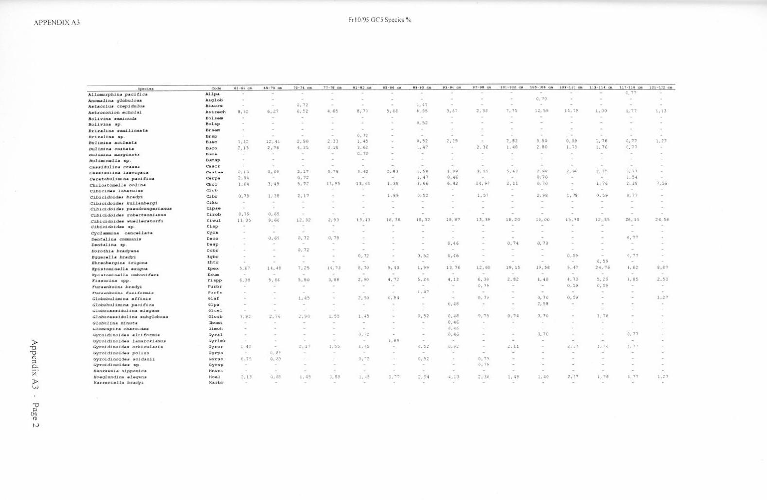
APPENDIX A3 Fr I 0/95 GC5 Species ~,,o

seacios Code 65 - 66 cm 69 - 70 cm 13-74 cm 7 7-7 B cm 81 - 8 2 cm B5 - 86 cm 851 - 90 cm 93 - 94 cm !n - 98 cm 101- 102 cm 105 - 106 Clll 10 9 - 11 0 cm 113 11 4 cm 11 7- 1 1 8 cm 121-122 c m

A.l.lomorphin• p•cifica Al.lp.t. 0, 71

Anomaiina giobuioaa. Aaglob - 0,70

A.staco.lu.s crepidu.lu.s Atacra 0,72 - 1, 47

Astrononion e c ho.l.si A:strech a/ 5~ 6, 27 c., :.:2 4, 65 e,10 5, cc- 8,95 3,67 2,36 7,75 12, 59 l q, 7 '? 1,00 1, 7 7 ! , 13

Bolivin• sam..inud.a Balsam

Bolivia• sp . Bolsp i), 52

Briz•lin• semilinaat• Brsam

Bcizalin• sp . Brsp - I), 72

Buli.m.ina aculaata Buac 1, <l 2 12 , 41 2,90 ., ") ") '-1 -'.J 1, 45 i) , 52 2,25 2,82 3,50 0 , 59 1, 7 6 0,77 1,27

Bul.imin• coa ta ta Buco 2, l 3 2,76 4, 35 3, 18 3, 62 1, 4 7 2. 36 1, 48 2, 80 1,78 1 , 7 6 0,77

Bulimia• m.argin•t• Buma - C,72

Buiiminaiia sp . Bumsp

CaaJJiduiia.o cras.sa easer

C•••idulina laavig•t• Casla.a 2 , 13 0,69 2, 1 7 0,78 3, 62 2 I 82 1,58 1, 38 3, 15 5, 63 2,98 2 , 9c 2,35 3,17

Ceratobu.li.mioa pacific• Cerpa. 2 , 84 0 ,72 1, 4 7 0 I 4 6 - 0 ,7 0 - 1, 54

Chilostomalla oolina Chol 1 , 64 3, 45 5,n 13 , 9 5 13, 4 3 1. 38 3,66 6,42 14, S7 2 I 11 0,70 1,76 2,3S 7, 5;

Ci.bicid.a• lob.otuius Clob

Ci.bicid.oid.e• brady:i. Cibr 0, 79 1, 38 2, 1 7 1, BS 0,52 1, 57 2, 98 1, 7 9 0, 5S 0,77

Ci.bicid.oid.as ku..l.ianbergi Ciku

Cibicidoida• pseudoungerianus Cips_a

Cibicidoides robart•oni•nus Cirob 0 , 7S O,c9

CWicidoida.s lfl.lell•r•torfi Civul 11 , 35 9,66 12,32 2 ,93 13, 4 3 16, 36 1 8 , 32 18, 8 7 13 , 39 le, 20 10 , 00 15,?8 12, 35 26,15 24,5E

Ci.bicid.oidaa sp . Cisp

Cyclammina cancell•ta Cyca

Dantalin• coJmID.U1ls Deco - 0 , 69 0,7~ 0, 7 8 - o. 77

Oent4lina sp . Desp 0 ,4 6 - 0,7 4 0,70

Dorotbi• bradyana Dobr o. 72

Eggaraii. bradyi Egbr (), 72 0,52 0,46 - 0. 59 0, 77

Ehr•nb•rgin• trigona Ehtr - 0 , 59

rpistom.inalla exigua Epex 5,67 1 4, 4 8 7 / 2 5 14, 7 3 8, 7(1 9, 4 3 1, 99 1 3, 7 6 1 2 ,6 0 19, 15 1 ?, 58 9, 4 7 24,76 -1, E.~ 8, 87

1:pistominella umbonif•r• Exum

Fi .s.surina spp . Fispp 6, 38 S,6C 5,80 3, 88 2, 9(1 4, 7 2 5, 24 4, 13 6 , 30 2,82 1 , 40 4, 7 3 S,29 3 , S5 2 , 53

FUraankoin• bradyi Furbr - - 0,7S - o. 59 0 , 5S

FUrsenkoina fusiformis Furfs 1, 4 7

Globobuli.m.ina affinis Glaf 1, 4 5 2 ,90 0 , 9 4 ~ o . 7 3 0 ,7 0 0 , 59 - 1,27

Giobobuii.min .o p.oci~ica Glpa 0 ,4 6 2, 98

Globocassidulina alagans Glcal

Globocassidulina subgloboaa Glcsb 7 / 92 2,76 2,90 1, 55 1, 4 5 - 0 , 52 0 ,4 6 Q,7S 0,74 0, 70 l, 76

Giobuiin.o minut.o Gbumi 0 ,4 6

G.Lomospira cbaroid.es Glmch 0 , .:!6

Gyroid.inoid.as altifo rmi• Gyral - 1) , 7~ 0, 40 - ,J . 7 (I 0,77

)> Gyroidinoidas la.marckianus Gyrlmk l, 8 9

'"O G_yroidinoidas orbicuiaris Gyror 1, 4 2 2, l 7 1, 55 1, 4 5 ,), 5~ (1 ' 9: 2, 11 2,37 l, 7 €_. 3, 7 "7

'"O Gyroidinoid.as poliu..s Gyrpo 0 , Cl: (1) Gyroicti noid.es solc:Llni i Gyrso 0, 79 V, 6':< - 0 , 12 o . 52 0 , 7; :::l Cl. Gyroid.inoides sp . Gyrsp ,) , 79

X H•nzava i a nlpponica Knwni

HoeglW1d.in4 elegans Hoel 2, 1 3 0 ,69 1, 4 5 3, 68 l, 4 5 3 , 1 7 2, ,;4 4. i 3 2, 36 1, 4 8 1, 4 Q ' ,., l, 1 6 3, 7 7 1, 2 7 )>

~'..;

K4rrerieiia bradyi Karbr w

I

-0 Pl ao (1)

N

APPENDI X A3

)> -0 -0

(1) :::; 0... X

)> l,..)

-0 p)

(JQ (1)

l,..)

Sp e c ie3

Lagena spp .

Laticarinina pauparata

L•n ti cu.Lina spp .

Md.rginu.lina oba$4

Marginu.lina subu.llata

Ma.rginulina sp .

M.ctrtinottie.l.la commuaia

Martinottia.l.la perparva

Melonis bar.laaanum

Melonis pompi.lioid.es


Miliolinella sub.rotunda

Nodos4ria radi cu.la

Nonion sp .

Nummolocu.Lina ircegu.Laris

Oolina spp . Oridorsa.Lis tener umbonatus

Orid.orsa..li:1 .sp .

Osangularia cultur

Pa.r•fiasu.rina. spp .

Para~rond.icu.laria sp ,

Pullenia bulloida•

Pullenia quinqualoba

Pu.1 1.ania sp .

Pyrgo depressa

Pyrgo luc arnu.L,

Pyrgo murrhina

Pyrgo vesparti.Lio

Pyz:go sp .

Py.rulina fusiform.is Quinqueloculina illlD4ta

Quinqualoculina 1Alll4rc kiana

Quinquelocu.lina aeminu.lum

Quinquqloculina stell i ge.ra

Quinqualoculina veousta

Quinqualoculina sp .

Rectobolivina d.i.morph4

RBussella si..oFlex

Robartina tasmanica

Roba rtinoid.es brady

Sardcanaria italica

Sigmoilops ia schlumbargeri

Siphoegg•r e lla ~ iphone ll4

Siphotaxtularia catanata

Siphotaxcularia curta

Sphaeroidina bulloidas

Textuiaria lataralia

Tr i loculina subvalvularis

Triloculina tri carinaca

Uvigerina p eregrina

Vvigari na porre c ta Uvigarin4 proboa c idQa

Uvigarina sp .

Valvul .1 nsria. sp .

Code

Laspp

Lt:p"

Laspp

Maob

Masub

Masp

Mtcom

Mtpr

MebA

M.apo

Mi.ob

Misb

Ndrd

Nosp

Numir

Oospp

Ortu

O.rsp

Oscu

Po.spp

Prsp

Pubu

Pu5

Pusp

Pyde

Pyl.u

Pyu

Pyve

Pysp Pyrf

Quin Qul.k Qusam

Qut:g

Quve

Qusp

Rad.i

R.ll.si

Rbto.

Robbr

Sarit

Sgmsch

Sphsph

Stxca

stxcu

Sbul.l.

Txl.o.t

Trsu

Trtr

uvp ..

Uvpr

Uvprob

Uvsp

Vl.sp

0 - 1 cm

1 , 27

0 , 63

0 , 63

1 , 27

0 , 63

1 , 27

0 , 63

1, 27

5 , 70

3, 1 6

0, 63

4, 4 3

1 , 27

1, 90

1, 27

0 , 63 0 , 63

1 , 91)

0 , c3

0 , 63

0 , 63

I), E 3

0, 63

0, C3

3, 16

5 - 6 cm

2 , 61

2,67

1, 67

4 1 ,JO

1, 33

1 , 33

2 , 07

2 , 67

2 , 67

l. ; 3

8, 1)1)

9 , 33

9 - 10 cm

l , 7 9

0 , 89

0 , 8 9

1, 7~

0 , as 4 , 4 6

0 , 89

2 , 68

1, 79

0 , 89

l, 7 9

0 , 89

7 , 14

.l , 7"

i) , 39

13 - 1 4 cm

0 , 66

0 , 6C

0, 66

~ , 93

1 , 32 0 , 66

3 , 97

1 , 99

0 , 66

3 , 31

3 , 31

3 , 31

6 , 02

,), QC,

0, EG

l, 9 ~

Frl0/95 GC5 Species %

17 - 1 8 cm

1 , 36

1 , 55

0 , 52

0 , 52

0 ,5 2

0 / 52

E, 7 4

0 , 52

0 , 52

I, 36

1 , 55 0 , 52

0 , 52

0 , 52

'O? L ' ' ~

0,52 ci, :,::

:'., 60

21 - 22 cm

0 , 4 5

0 . 4 5

1 , 00

1, 0,)

1 0 , 00

0 ,4 5

1 , 36

0 , q 5

2 , :1

0 , 4 5

0 , 4 5

l , Q,)

,) . '1:, 1, (J(I

IJ, q .$

2 5 - 2 6 cm

0 , 73

,:, , 37

l , 4 7

0 , 37

9 , 4 2

(I , 37

I) , 37

4, 2 9

0 , 3 7

0 , 37

0 , 73

( 1 , 3 7

1 , 99

.1., 4 ·7

::: ' so

29 - 30 cm

0 , 6~

0 , 3 4

0 , 3 4

0 , 3 4

7, 9 4

1, 39

0 , 69

4, 82

0 , 3 4

0 , 3 4

0 , 3 4

1 . ]9

0 , 34 ,} , 3 4

1 , 3S'<

,:i, c.~

(i , ·3 ~

33 - 34 cm

I, l 7

0 , 37

0 , 37

/J, 37

2 , 95

0 , 74

2 , 2 1

l, 1 7

l, o 5

1, 11

0 , 3 7

0 , 37

0 , 7 4

l. 4 8

z. ::: !

37 - 38 cm

0, 33

0 , 3 3

0 , 33

1 , 99

0 , 33

0 , 33

6 , c:::

0 , 3 3

•J , 33

2 I 98

tl , 33

0 , 66

2 , 32

l. 06

4 1 - 4 2 cm

0 , 45

0 , 4 5

0 ,4 5

4, 55

2 , 27

1, B2

0 , 45

3 , 18

0 , 4 5

I) , 4 5

5 , 1j1)

1 , g 2

1, ( 1U

1) I 4 5

4S - i6 cm

0 , 3Z

0, 32

0 , 3:

0 , 63

0 , 32

1, 27

6 , 96

0 , 95

1 , 27

0 , 32

0 , 32

4 , 11

0 , 03

0 , 32

l , 58

0 , 32

2 , 53

l , 9(1

4 9 - 5 0 cm

0, q 2

0, 4 2

o . ..i :

1, E7

0 , 8 4

5 , 29

1 , 26

,) , 4 2

2 I 9 3

0 , 8 4

0 , 8 q

,) , 4 2

0 , 11,2

(I , 4 2

3 , 35

1) ' 42

53 - 5 ~ cm

0, 41

0, 41

0 , H

0, 41

0 , 93

0 , 41

2 ,7 5

7 , 5 4

1 , 66

0 , 4 1

4, 98

5,39

0 , 8 3

2 I 7 5

0 , 41

( t, 4 1

0 , 4 l

2 , 75

l. 66

5 7- 58 cm

C1 , 3 3

0,33

1 , 00

/J , 67

1 , 65

1 1, ~2

0, 33

1, 65

0 , 33

2 / 31

1 , 00

0 , 07

2 , 31

I), 3 3

l, •JO

0 , 33

0 , 3 3

O, E7

,) / 3 3

,:, , ~ .3

(l , 0 7

L, 0(1

(I I 3 2

61 - 6 2 CJ'II

0, 66

1, 32

0,6&

1j, cc

r, , 66

G, 60

17, 7E

I, 32

1 , 3 2

B, 55

0 , 66

1 , 32

3,29

(),66

1 , lZ

:? , ~ ~·

0, 66

APPENDIX AJ Fr10195 GC5 Species%

seecie• Code 65-66 cm 69 -70 cm 73-74 cm 77-78 cm 81-82 cm 85-86 cm 89 -90 cm 93 - 94 cm 97 - 98 cm 101-102 cm 105-106 cm 109- 110 cm 113 - 114 cm 11 7-11 8 cm 121 -122 cm

Lagana spp . Laspp 0,79 0 , 69 0 , 72 0,78 0 ,72 0 , "4 ,) , 46 ·), 7 4 1, 4 I) 0, 5,. l, 76 l. ~7

Laticarinina pauparata Ltpa 0, 69 1 , 4 5 C, 5: 0 , 7 9 ~ , l i - 0,59

L4inticulina spp. Lespp 0 / 72 G,5: 1)' 46 l, 4 8 o, 70 ,) , 5:i

Marginulina oba•a Ma.ob - 0,73 - 0 ,?4

Hacginulina aubullata Ma.sub

Md.rginulioa sp . Masp

M.artinottialla. commu.ni.s Mtcom 0, 72 0,72 ,) , 7 7

Mart:inottial.la perparva Htpr

Melonis ba.rlea•num Maba 1, 4 7 1, 4 8 l, 18

Melonis pompilioid.es Hepo 2 ,6 9 0 , 72 2,33 2, 17 1, 89 l, 58 1, 38 D,79 1, 4 ,) 2,37 0 , 59 3, 8 5 2,53

Miliolioalla ~blonga Hiob

Miliolinella •ubrotund.a Hisb

Noclos•ria rad.icula Ndrd

Nonion ap . Nosp

Nummoloculina. irragularis Numir 0 , 72 0, 7 4

Oolina spp . Oospp 0 , 69 1, 89 - o,s s 1, 7 6 1, 5 4

Oridor.s•lis taoar umbonatu.. Ortu 12 ,1 7 9 , 66 11, 59 8, 53 1, 14 1, 38 8,38 12, 84 13 , 39 12., 97 11, 19 15, 98 5, 2 9 6,92 12, 6E

Oridoraalis sp. Orsp

Osangularia. cultur Oscu

Para.fissurina spp . P&spp 0, 7 9 0 - " 0 , 78 1, 45 0 ,94 1, 47 2,~s 0 , /9 1, 4 8 3, 50 0 , 59 0 , 5, " ?0 _, , 0.:.. '-1 _,v

Parafrond.icularia sp . Prsp

Pulleoi4 bulloid.es Pubu 1, 4 2 1, 8 9 0,52 0 ,4 6 ,:, , 79 0 , 70 l, 18 4 / 62 1,2 7

Pullania quinqueloba PuS - (1 , sz l, <JS 2, 37 0, 5 9 0 , 77

Pu.llenia sp . Pusp 1, 38 0 ,7 2 I) , 7 2 l, 1 8 0, 77

Pyrgo dapressa Pyde 0, 7 9 1, 38 0,72 0 , 78 l), 7 7

Pyrgo lucernu.la. Pylu - - 0 ,4 6

Pyrgo murrhina Pyu 5, 67 6,90 5 , 72 6 , 22 3 / 62 7,55 14 , 14 1 <l, 68 11, 81 8, 4 6 5,59 9, 47 11, 76 5,38 1, 13

Pyrgo ve~partilio Pyva

Pyrgo sp . Pysp 0,79 0 , 72 2, 94 0, 92 0 , 19 0,74 2 , 96 l, 76 l, 5 4 3,8 (1

Pyrulioa f'uJSit'ormi.s Pyrf

Quinqua.loculina inm.ata Quin

Quinqualoculina lam.srckiana Qulk

Quinqueloculina aem.i.nulum Qusem 1, 4 2 0 ,69 2 , 9t) 0,72 1 , 89 3, 1 :.J. 0, 92 ::._ I :,o 0 , 59 (l, 77

Qu.inquqloculina stalligara Qutg

Quinqu•loculina venusta Quva 0, 7 8 C, 7 2 1 , 4 7 0 , 4 6 0,70 1) ,59

Quinqualocu.lina sp . Qusp

Re ctoboli viOa dimocpha Redi 0 , 4 6

Reussalla si.ztq:>lex Rllsi

Rober tin• tasmanica Rbta

Robertinoid.es brady Robbr - 2, 11 0 , 7l)

Saracenaria italica Sa.rit

sigmoi lopsis schlumbargeri Sgmsch 0,79 0 ,72 (1 , ~•4 (J,5.2 (1, 92 0 , 70 1,27

Siphoeggerelia siphonella Sphsph

Siphotextuiaria catenata Stxca )> Siphotextularia curt4 Stxcu 0, 59

-0 Sphaeroid.ina bulloidas Sbull 2, 1 ~ ~,6Si 2, l 7 0,78 2, 17 l, 89 0 , ,j £ l, S": ;',98 1 , 18 0 , 7 7 l, ;'7

-0 (l) Textu1Aria i&teralis Txlat

:::l Triloculina subvaivularis Trsu c1, 7 2 (I , 7 4

CL Trilocuiina. tricarinata Trtr l, 4 Z L) I 7 8 (l , 74 0 , 5-=, -· >< Uvigerind peregcina Uvpe 5, 67 6,;'7 S, 9 ,) 4' b) ::., s: 11, 33 5 , 2!J 2 I 7:, 2, :I!} 2 , 62 6 , 99 ~ , lB 2,53 ; ;o C· , .;,:; .:., _,,_

)> Uvigerin4 porrecta Uvpr

L,J Uvigerina proboscid.ea Uvprob ;'' 13 0 ,69 _::' ~•I) 1)' 7 s 2, l 7 0, 9~ 1, 4 7 1J' ~= 1, 81:1 0 , ss:. l. t 7 ~ 3 ,, 2 I 53 Uvigerina sp . Uvsp Vai vu.lineria sp . Vlsp

-0 p:i

(JO (1)

.j::,..

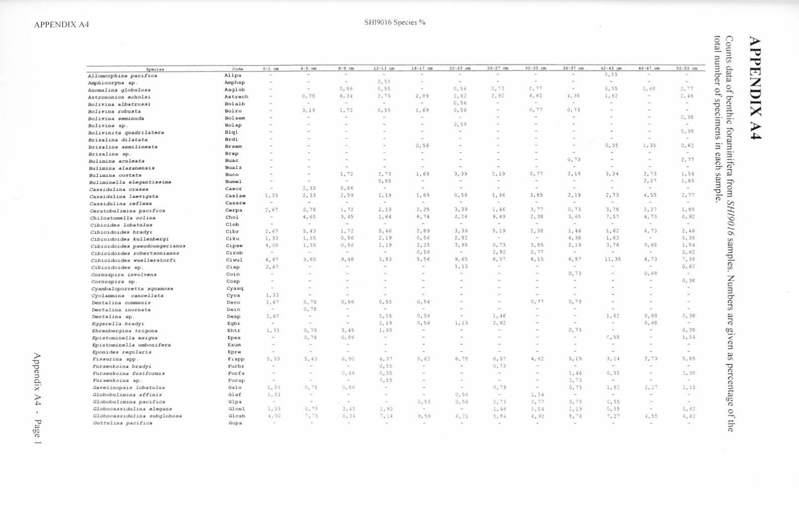
APPENDIX A4 Sf-119016 Species%

...... n > 0 ...... 0 ~ C ~ ::i ::i ......

~ C C/l

seecie.s Coda 0-1 cm 4 - 5 cm 8 - 9 cm 12 - 1 3 cm 16-17 cm 22-23 cm 26-27 cm 32-33 cm 36 - 37 on 42 - 43 on 4 6-47 cm 52-53 cm ::i 0.. ~ Allomorphina pacifica .IUlpa - - - -...;

~ - - - 0 , 55 - CT ...... z Amphicoryna sp . Arnphsp - - - 0 , 55 - - - - - (1) ~ -, 0 Anomalina globulosa Aaglob - 0 I 8 6 0 , 55 0 , 56 0 , 7 3 0 ,77 - 0 , 55 0 , 68 2 , 77 0 -ti ~ Astrononion echolsi A.strech - 0 , 78 6 , 34 2 , 73 2 , 89 ? ~~ 2 , 92 4 , 62 4,38 1 , 62 - 2 , 4 6 -,,

- Iv.:. CT Bolivina albatrossi Bolalb - - 0 ,56 - - - C/l <"O ~

3 , 13 1 , 72 -0 ::i X Bolivina robusta Bolro - 0 , 55 1 , 69 ,] , 56 - 0 , 77 0 , 73 - - (1) .-t-

Bolivina seminuda Bolsem - - - - - - - - - 0 ,3 8 (') ::r

Bolivina sp . Bolsp - - - - 0 , 56 - - - - - 3 (') > Bolivinita quadrilatera Blql - - - - 'J , 38 (1) o' ::i +-,

Brizalina dilatata Brdi - - - C/l -, ~

Brizalina semilineata Brsem - 0 ,5 6 - 0 , 55 1,35 0 , 62 -· 3 :::;

Bri.zalina sp . Brsp - - - - - - - (1) :::; Bulimina a c uleata Buac - - - - - - 0 , 73 - 2 , 77 ~

Bulimina alazanensis Bualz - - - - - - - -("') ~ - ::r -,

Bulimina cos ta ta Buco - - 1, 7 2 2 , 73 1,69 3 , 39 2 , 19 0 , 77 2 , 19 3 , 2 4 2 , 73 1 , 5 4 C/l ~

Buliminella elegantissima Bumel - - - 0 , 55 - - 2 , 27 l , 85 ~ =ti Ca ssidu1ina crassa easer - 2 , 33 0 , 86 - - - - - - - - 3 0

Cassidulina laevigata Caslae 1,33 2 , 33 2 , 59 2 , 19 1 , 69 \j I 5 6 1,46 3 , 85 2 , 19 2 , 7 3 4 , 55 2 , 77 -0 3

Cassidulina reflexa Cassre - - - - - - - - -(1)

V)

Ceratobulimina pacifica Cerpa 2 , 67 0 , 78 1 , 72 2 ,1 9 2 , 25 3 , 39 j_ , 4 E 3 , 77 0 , 73 3 , 78 2, :n 1 , 85 ::r:: Chilostomalla oolina Chol - 4, 65 3 , 45 1,64 6 , 74 2 , 26 9 , 49 2 , 38 3 , 65 7 ,5 7 4,73 0 , 92 -'O Cibicides lobatulus Clob - - - - - - - - - a Cibicidoides bradyi Cibr 2 , 67 5 ,4 3 1 , 72 5 , 46 2 , 89 3 , 39 5,19 2 , 38 1 , 4 6 1 , 62 4,73 2 , 46 -°" Cibicidoide s kullenbergi Ciku 1 , 33 1 , 55 0 , 86 2 / 19 0 , 56 2 , 82 4 , 38 1, 82 - G, 38 C/l

Cibicidoides pseudoungerianus Cipse 4, 00 1 , 55 0 , 86 2 , 19 2 , 25 3 , 95 0 , 73 3 , 85 2 , 19 3 , 78 o, 6e 1 , 54 ~

Cibicidoides robertsonianus Cirob - - 0 , 5 6 2 , 92 0 , 77 - - - 0 , 62 3 Cibicidoides wuellerstorfi Ciwul 6 , 67 3 , 88 9 , 48 3 , 83 5 / 56 9,65 6 , 57 6 ,1 5 6 , 57 11 , 35 4,73 7 , 38 -0

Cibicidoides sp. Cisp 2 , 67 - - - 1,13 - 0 , 62 (1) C/l

Cornuspira invo.lvens Coin - - - - - 0 , 73 - 0 , 68

Cornuspira sp . Cosp - - - - - - - - - - 0 , 38 z C

Cyambaloporretta squamosa Cyasq - - - - - ::l Cyclammina cancellata Cyca 1 , 33 - - - - - - - - ....J

v Dentalina communis Deco 2 , 67 0 , 79 0 , 86 0 , 55 0,56 - 0 , 77 IJ ' 7 3 - - (1) -, Dentalina inornata Dein - 0 , 78 - - C/l

Dentalina sp . Oesp 2,67 - 0 , 55 1J ' 50 - 1 , 46 1 , 6:2 0 , 68 0 , 38 PJ

Eggerella bradyi Egbr - - 2 , 1 9 0 , 56 1 , 13 2 , 92 - - 0 , 68 -,

- - (P

Ehrenbergina trigona Ehtr 1, 33 0 , 78 3 ,4 5 1,93 - - - 0 , 73 - 0 , 38 (JO

Epistominella exigu a Epex - 0 ,78 G,8 6 - - - C, 55 1, 5-1 < Epistominella umbonifera Exum - - - - - - - - (1)

::i Eponides regularis Epre - - -

)> - - - - -

Fissurina spp . Fispp 5 , 33 5 , 4 3 6 , 90 4 , 37 5,C:2 6 , 78 6 , 57 ~

-0 4 I 62 5 , 19 3 , :2 -i 2 , "7 3 5 , 85 C/l

-0 Fursenkoina bradyi Furbr - 0 , 55 - I) / 7 3 - -0 (P Fursenkoina f usiformi s Furfs i} I 86 0 ,55

(P

:::; - - - l , 4 6 0 , 55 ,J , 38 -,

0... FUrsenkoina sp. Fursp - 0 , 55 - - /J I f 3 - - ("') (P

>< Gavelinopsis lobatulus Galo 1, 33 0 , 78 0 , 86 - - - 0 , 73 - 0 , 73 1 , 82 ~ , 27 2 , 15 ::i ...... )> Globobulimina affinis Glaf 1 , 3 3 - - tJ , SE 1 , S 4 - - - ~

~ Globobul.unina pacifica Glpa - - Ci I .s 6 0 , 56 ,:, I I _3 1] , 77 ,J , 7 3 ,'j / 55 - (JC (P

Globocassidulina elegans Glcel 1 , 33 0,' S 3 , 45 l , 33 - 1 , 4 6 1 , 54 2 I 19 0 , 55 0 , 62 I 0

Globocassidul i na s ubglobosa Glcsb 4 / ,Jlj -, , ; 5 ,5 , 3 .:1 7 , 14 9 , 56 ,:,. , ::21 5 ,B4 t: , 32 8 , "".: E, 7 , '27 -l , 55 , - ·? '1 I C,_ ---+i

u Gu ttulina pacifica Gupa - - ...... o:i

- - - ::r (JO (P

(1)

APPENDIX A4 SHI9016 Species%

Sfecie5 Code 56-57 cm 58 - 59 cm 62 -63 cm 66-67 cm 72- 7 3 cm 76-77 cm 82-83 cm 86 - 87 cm 92-93 cm 96-97 cm 102-103 cm 106-107 cm

Allomorphina pacifica Allpa

Amphicoryna sp. Arnphsp

Anomalina globulosa Aaglob 2 , 34 1 , 38 0 , 31 0 , 99 0 , 95 - 1 , 00 - 0 t 3~

Astrononion echolsi Astrech 2 , 7 3 3 , 67 3 , 74 2 , 63 2 , 85 3 , 33 4 , 5 5 4 , 4 9 - 3 , 28 1 , 71 0 , 84

Bolivina albatrossi Bolalb

Bolivina robusta Bolro 0 , 31 0 , 32 0 , 67 - 0 , q 5 0 , 34

Bolivina se.minuda Bolsern

Bolivina sp. Bolsp - 0 , 92 0 , 31 0 , 66 - 0 , 4 5 - - 0 , 33 0 , 34

Bolivinita quadrilatera Blql - 0 ,4 6 0,62 - 0 , 3:? 1 , 35 - - D, 68

Brizalina dilatata Brdi - - - 0 , 45

Brizalina se.milineata Brsern 0 ,4 0 - 0 , 66 0 ,3 2 - - 0 , 4 5 0 , 34 1, 31

Bri.zal.ina sp . Brsp - 0 , 31

Buli.mina aculeata Buac 12 , 90 18 , 87 2 , 57 22 , 70 26 , 58 15 , 67 15 ,7 7 11 , 75 1 , 58 16 , 66 2 3 , 97 38 , 2~

Buli.mina alazanensis Bualz 0 ,4 6 - - - 0 ,4 5 - 0 , 33

Buli.mina costata Buco - 2 , 19 0 , 66 2 , 53 1 , 33 1 , '.JO 0 , 90 2 , 4 8 0 ,98 1 , 3 1 0 ,4 2

Buli.minella elega.ntissima Burnel 0 , 78 0 , 33 - - 0 , 34

Cassidu1ina crassa easer 0 , 46 - 0 , 32 0 , 33 1,00 0 , 4 5 - 0 , 33

Cassidulina laevigata Caslae 2 , 73 5 , 55 5 , 92 3 , 95 2 , 53 2 , 67 2 , 25 0 , 90 1 , 76 2 , 30 0 , 68 1,27

Cassidulina reflexa Cassre - - - 0 , 3 2

Ceratobuli.mina pacifies Cerpa 0 , 78 0 , 4 6 - 0 , 33 0 ,3 2 0 ,3 3 - - 0 , 3 4 0 ,4 2

Chilostomella oolina Chol 0 , 46 0 ,66 0 , 95 0 , 67 1, 35 0 , 90 1 , 37 0 , 33 0 , 68 1 , 69

Cibicides lobatulus Clob

Cibicidoides bradyi Cibr 1 , 95 3 , 2 1 0 , 62 1 , 97 2 , 53 2 , 33 4, 55 1 , 21 4,96 3 , 28 5 , 14 5, 4 6

Cibicidoides kullenbergi Ciku 0 , 78 0 ,31

Cibicidoides pseudoungerianus Cipse - 0 , 33 - 1 , 00 0 , 4 5 2 , 39 - 1 , 27

Cibicidoides r obertsonianus Cirob - - 0 ,3 3 - 0 , 33 0 , 90 0 , 68 - 0 , 3 4

Cibicidoides wuellerstorfi Ciwul 8 , 59 5 , 4 6 7 , 4 8 6 , 58 5 , 70 8 , 33 9 , 46 7 , 2 9 8 , 87 5 , 92 4 , 79 3 , 78

Cibicidoides sp. Cisp 0 , 40 - 0 , 31 0 , 99 0 ,3 2 0 ,3 3 - 0 , 4 5 0 , 34 - - 0 , 4 2

Cornuspira invo.lvens Coin - 0 , 46


Cyambaloporre t ta squamo.sa Cyasq 0 ,4 6

Cyclamm.ina cancellata Cyca

Dentalina communis Deco 0 ,4 0 - - - 0 , 3 3 0 , 45 - - J , 66

Dentalina inornata Dein

Dentalina sp . Desp - 0 , 46 ,J , 31 - 0 , 95

Eggerella bradyi Egbr 0 , 40 - - 0 , 63 0 , 67 0 , 4 5 0 , 90 0 , 34 0 , 98 0 , 34 0 , 4 2

Ehrenbergina trigona Ehtr 0 , 40 0 , 4 6 2 , 4 9 2 , 22 1 , 3 3 1 , 35 1 , 21 0 , 34 0 , 98 0 , 34 0 , 8 4

Epistominella exigua Epex 3,5 2 2 , 75 3 , 43 .:! , 28 6 , 65 6 , 00 3 , 15 :2 , 2 4 2 , q 8 1 , 64 1 , '10 5 , 4 2

Epistominella umbonifera Exum 0 , 40 0 , 31 0 , 33 0 ,33

)> Eponides regularis Epre - - - 0 , 45

-0 Fissurina spp . Fispp 5,86 2 , 75 3 , 4 3 5 , 91 3 , 4 B 8,67 4,55 8 , 14 C, 83 5 , 57 8 / 22 5 , 4 E

-0 Fursenkoina bradyi Furbr 0 , 78 - C, J3 (t) FUrsenkoina fusiformis Furfs 0 , 78 - - iJ,33 1 , 1Jl) 0 ,4 5 0 , 34 ::J 0. Fursenkoina sp . Fursp

X Gavelinopsis lobatulus Galo 0 , 7B ]_ / 2 9 2 t 1 ':) 0 , 3~ 1 , 00 0 I 4 5 l , 21 2 , 39 0 , 33 1. ,1 0 / 2-'.!

)> Globobulimina affinis Glaf 0 , 40

~ Globobulimina pacifica Glpa 0 , 4 CJ 0, 4 6 - - - 0 , 4 5 0 , ~5 - - - G 1 4 2

Globocassidulina elegans Gl cel - - 0 , jJ

Globoca ssidulina subglobosa Glcsb 6 / ~ s s / 96 4 / 6°7 5 , S 9 1 , 30 :? , 3 3 4 / ') 5 :. , 4 3 5 , 82 .., -~ 3 , 82 3 , 36 _, 1 0 I

v Guttulina pacifica Gupa p.:i

cro (1)

N

APPENDIX A4 SHI90!6 Species 0,'o

seecies Code 112 - l.13 cm 11 6-11 7 =i 1 22-1 23 =i 1 2 6 - 12 7 cm 132- 133 cm 136- 13 7 cm 142 -1 43 cm 146- 147 cm 152-15 3 cm 156- 15 7 cm 162 - 163 cm

Aiiomoi:phina pacifica Allpa

Amphicoryna sp . Arnphsp 0 , 32

Anomaiina giobuiosa Aaglob 0 , 65 - - - - - 1 , 00 l , 18

Astrononion echoisi },.strech 4,54 3 , 49 4,73 6 , 4 3 4, 19 3 , 13 1 , 37 3 , 24 l, 33 2 , 75 3 , 33

Boiivina aibatrossi Bolalb 0 , 32

Boiivina robusta Bolro - 0 , 32 - 0 , 32 ,) , 31 1,37 - - 0 , 67

Boiivina sem.inuda Bolsem

Boiivina sp . Bolsp - - - - 0 , 33 - - 0 , 33

Boiivinita quadriiatera Blql 0 , 32 - - 0 , 32 0 , 31 - - - 0 , 33

Brizaiina diiatata Brdi 0 , 65 - 0 , 32 - 0 , 32

Brizaiina sem.iiioea ta Brsem 1 , 29 - 0 , 34 0,97 0 , 65 - - 0 , 39 1 , 00

Brizaiina sp . Brsp

Buiim.ina acuieata Buac 11, 32 3 2 , 62 26 , 81 2 1, 15 1 8 , 80 3 1 , 97 33, 66 21 , 62 1 6, 67 18 , 82 21 ,1 2

Buiim.ina aiazanansis Bualz

Buiimina cos ta ta Buco 0 , 65 0 , 32 - 0 , 65 0 , 33 - 1 , 00 1 , 18 1, 32

Buiim.ineiia eiegantissima Bumel 0 , 32 - - o, 65 - - 0 , 33 0 , 33

Cassiduiina crassa easer 0 , 98 - 0 , 67 0 , 31

Cassiduiina iaevigata Caslae 0 , 32 2 , 7 4 1 , 26 2 , 68 1, 9 4 1 , 5 7 2 , 29 1, 62 6 , 00 3 , 53 3 , 33

Cassiduiina refiexa Cassre

Ceratobuiim.ina pacifica Cerpa - 0 , 35 - - 0 , 32 1, 57 - 1, 82 0 , 67 - 0 , 67

Chiiostomaiia ooiina Chol - 1 , 83 0 , 32 2 ,1 3 0 , 97 0 , 63 1, 63 2 , 73 1 , 33 0 , 78 Q , 67

Cibicides iobatuius Clob - - - - - - - 0 , 33

Cibicidoides bradyi Cibr 1 , 32 4, 57 5 , 68 5 , 3 4 6 , 4 5 5 , 96 4, 2 5 5 , 95 7 , 33 5 , 98 10 , 00

Cibicidoides kuiienbergi Ciku - - - 0 , 32 - 0 , 33 0 , 33 0 , 3 9 0 , 33

Cibicidoides pseudoungerianus Cipse 1 , 9 4 - 0 , 95 - 0, 32 0 , 9 4 - - 2 , 33 1 , 5 7 C, 67

Cibicidoides robertsonianus Cirob - 0 , 35 0 , 32 0 , 34 0 , 32 - 0 , 33 0 , 67 0, 39 0 , 67

Cibicidoides wueiierstorfi Ciwul 2 , 91 1 , 83 ? "? _ , ..J- 2 , 1 3 5 , 4 8 4, 7 5 5 I 2 3 3, 78 3 , 67 2 , 35 3 , 33

Cibicidoides sp. Cisp - 0 , 67 0 , 32 - 0 , 65 1 , 33 1, 1 8 0 , 33

Cornuspira invoivens Coin


Cyambaioporretta squamosa Cyasq

Cyciammina canceiiata Cyca

Dentai i na c ommunis Deco - 0 , 35 - - 0 , 32

Den taiina inornata Dein

Dentaiina sp . Desp - 0 , 35 0,64 - - 0 , 65 1, 82 - 1 , 1 8 0 , 3 3

Eggereiia bradyi Egbr 0 , 32 0,35 0 , 95 - - - 0 , 55 0 , 33 0 , 39 0 , 6:

Ehrenbergina trigona Ehtr 1 , 29 1 , 26 1 , 68 1 , 2 9 0 , 94 1, 37 2 / 16 0 , 33 Q t 67

Ep i stomineiia exi gua Epex 2 t 91 3,35 -l, 7 3 2 , 13 1 , 29 1 , 57 1, 9, 1, 6 :? 2 , 33 3 , 1 4 4 , 29

Ep i stomineiia umboni£era Exum

)> Eponides reguiaris Epre

Fissurina spp . Fispp 8,96 3 , 96 6,39 ; , 21 4 , 8 4 3 , 4 5 7 , 19 11, 89 5 , C7 3 , 53 4 / 62 "O "O Fursenko ina bradyi Furbr - - - - 0 , 33 0 , 3 9 0 , 33

(1) Fursenkoina ::;

fusiformis Furfs - - ,) ' 3'.'.

0. .Fursenko ina sp . Fursp

-· X Gaveiin opsis i 0batuius Galo 2 ?7 ' - 1), 35 ·J , .l ~ 1 , 3-l 0 , 32 0 , 31 - 1 , 62 1 , 00 - 0 , 67

)> ciob obuiim.ina affinis Glaf - - 0 , 33

+:>- c iobobuii.mina pa c ifi c a Glpa - - - ') , 33 - - 0 , 33

c iob ocassid uiina eiegans Glcel

cio b ocass i dui i na subgiobosa Glcsb 5 , 83 3 ,96 .:i / 4 2 4 , 36 2,2C- 0,63 1,63 - 2 , 33 7 , 59 3 , -53

-0 p)

Guttuiina pa c ifi c a Gupa - 0 , 35

cro (1)

l,J

APPENDIX A4 SHI90 I 6 Species%

SE:ec i es Co d e 0 - 1 cm 4 - 5 cm B-9 cm 1 2 -13 cm 1 6 - 1 7 cm 22- 2 3 cm 2 6-2 7 cm 32 - 3 3 =i 36 - 37 cm 42- 43 cm 46 - 47 cm 52- 53 cm

Gyroidino ides altiformis Gyral - 2 , 33 - 0 , 56 1 , 13 1 , 46 ;j , 17 - 0 , 55 - 0,38

Gyroidinoides lamarckianus Gyrlmk - - - - 0 , 73 - l , 4 6 - 0 , 68

Gyroidinoides orbiculari s Gyr o r - 3,88 0,86 2,73 2 , 89 3,95 ~ , 18 1 , 5 ~ 0 , 73 3,24 :: , 2 7 0 , 9 2

Gyroidinoides p olius Gyrpo - - - 0 , 55 0 , 56 - - - - - 0 , 68

Gyroidinoides s o ldani i Gyrso 1 , 55 2 , 59 1 , 12 0 , 56 0 , 77 - - - 0 , 62

Gyroidinoi des sp . Gyrsp - 0 , 86 - - 0 , 73 - - 1 , !32

Hanzawa i a nipponica Hnwni - ,) 1 86

Haueri nella incostans Hurin

Hoeglundina elegans Hoel - 3 ,1 8 3 ') 0 ,- ~ 3 , 38 1 , 13 2 , 19 3 , 85 4 , 38 7 , 27 2 , 27 5 , 5 ~

Karreri ella bradyi Karbr - - - - - 2 , 1 9 - - - 0 , 68 ,] , 38

Lagena spp . Laspp - 3 , 4 5 1 , 93 3 ,9 3 1 , 6 9 0 , "73 1 , 5 4 1 , 4 6 0 , 55 1 , 35 1 , 5 4

Laticarin i na pauperata Ltpa - 1 , 55 0 , 86 1 , 93 1 , 1 3 0 , 73 0 , 77 0 , ,3 0 , 5 5 1, 35 l , Z4

Lenti c ulina sp . Lesp 1 , 33 0 , 86 1,93 - 1 , 69 1 , 4 6 0 , 77 2 , 1 9 0 , 55 1 , 35 0 , 62

Margi nulina obesa Maob - - 0 , 73 ,} , 77 - - 1 , 35 0 , 38

Margi nulina sp . Masp 0 , 55 0 , 56 0 , 56 0 , 73

Mars i pella cylind.ri c a Mr c y 1 , 33

Martin o ttiella communis Mtcom 1 , 33 - - O, 55 1 , 1 2 - 0 , 7 3 - 2 , 19 0 , 55 1 , 35

Mart i n o t tiella perparva Mtpr

Mel onis barl eeanum Meba 1 , 33 3 , 18 1 , 72 0 , 5 5 1 , 12 1 , 13 0 , 7 3 2 , 38 0 , 73 1 , 82 0 , 92

Malo n i s p ompilioi des Mepo - 0 , 86 1 , 64

Mi liolinel la oblo nga Miob - 0 , 86 0 , 55 0 , 56 1 , 13 - - - ,} ,5 5 0 , 68 0 , 38

No d o s aria radicula Ndrd - - - - - 1 , 4 6

No d o s ar i a sp . Ndsp

Nonionel la bradyi Nnbr 0 , 78

Nonione lla iridea Nnir

No o ionel la turg i da Nntu

Non i one l l a sp . Nns p

Nummoloculina con tra ria Numco

Nu=olocu lina irregular i s Numir - - - - 0 , 56 2. , 82 - 2 , 38 0 , 7 3 - 2 , 73 l , 5 4

Oolin a s p. Oosp - 0 , 78 0 , 86 () / 5 5 1 , 12 0 , 5 6 2 , 19 - - - 1 , 35

Oridorsali s ten er umbon a t us Ortu 5 , 33 6 , 22 1, 72 3 , 83 7 , 33 2 , 8 2 2 I 92 5 , 38 5 , 1 9 1 , 8'.? 2 I 7 3 1, 5 4

Osangularia c ultu r Oscu 0 , 78 - - - 0 , 73 1 , 8 2 1 , 35 1 , 24

Parafissurina sp . Pasp 1 , 33 4 , E6 3 , 45 0 , 55 1 , 1? 1 , 69 - 2 , 38 - 1 , 82 1 , 35 0 , 92

Patellina jugosa Ptju

Plan ulioa arimin e nsis Plar

Pl e uro s t om.ella alte roans Psal - - - - - - - 0 , 38

P seudoguad.ryoa atlan tica Psoa t - - - - 1 , 4 6 ,) , 55 - 1 , 2 4

Pullen ia bulloide s Pubu 6 , 67 6,98 6 , 90 11, 4 8 8 , n 5 I 65 6 , 57 3 I 85 2 , 92 3 , 78 5 , 4 5 -l , 6:?

Pullenia quin quelob a Pu5 1 , 33 3 , 18 2 , 59 3,83 2 , 89 2 , 26 2 , 13 Ci , 7/ i) ' I) 1 , 62 0 , 0-~ '.2 , 15

)> Pulle oia sp . Pusp - - C+ , 56

-0 Pyrgo d epressa Pyde 5 , 33 1,55 Q, 86 2 , 73 1 , lZ l , 13 (j ~ 1 2 , 38 C, , 55 ,J , 68 3 , 38 . ' -

-0 Pyrgo l uc ernula Pylu - - - - - 1 , 5 ~ (1) Pyrgo murrhina Pyu 2 , 61 l,55 1 , 72 1 , 12 0 , 56 :::i

CI i J 0 ' , -, Z, 19 1 , 3: 1 , 35 J , C ?i

0.. Pyrgo vespertilio Pyve - - - ,) , 5 5

X Pyrgo sp . Pysp 1 , 33 1,55 - - - l , 6S - - O, E8

)> Pyrulina angus ta Pyra C• , 7--: 0 , 7?,

+::>- Pyr uli na cyl i ndroi des Pycl - - ,) , 7 3

Pyr ul i na exte nsa Pyrex

Pyrulina fusifo rmis Pyrf - ,J , 5 tS - 0 I 1:08 u Pyr ulina gut t a Pyrgu - - - 2 / 2 ,: - ~:i / : 3 p)

- - 0, 6:2

(JO (1)

+::>-

APPENDIX A4

)> ""O ""O

(1) ::::; 0.

X

)> .µ.

'"'O PJ uo (1)

u ·,

s,ea c1. ea

Gyroidinoides altiforrnis

Gyroidinoides laro.arckianus

Gyroidinoides orbicularis

Gyroidinoides polius

Gyroidinoides soldanii

Gyroidinoides sp .

Hanzawaia nipponica

Hauerinella incostans

Hoeglundina elegans

Karreriella bradyi

Lagena spp .

Latioarinina pauperata

Len ticulina sp.

Marginulina obesa

Marginulins sp .


Martinottiella communis

Martinottiella perparva

Melonis barleeanum

Melonis p ompilioides


No d o saria radicula

Nodosaria sp.

Nonio nella bradyi

Nonionella iridea

Nonionella turgida

Non ionella sp .

Nummo loculina c ontraria

Nummo l oculina irregularis

Ool i na s p .

Or i d o rsal i s tener umbo natus

Osangularia cultur

Par afi ssurina sp .

Patellina jugo sa

Planu l ina ariminen s is

Pleuro stomella alterna ns

Pseudo guadryna atlantica

Pullenia bullo ides

Pullen i a quinqueloba

Pullen.ta s p .

Pyr go depressa

Pyrgo lu c e r nula

Pyrgo murrhina

Pyrgo ve s pertilio

Pyrgo s p .

Pyr ulin a angu s ta

Pyrul i n a c y lindro idas Pyrul i na extensa

Py:tul .1 n a f us i f ormi s

Py rulina gu t t a

Codo

Gyral

Gyrlmlc Gyro r

Gyrpo Gyrso

Gyrsp Hnwni

Hurin

Hoel

Karbr

i.aspp

Ltpa

Lesp

Maob Masp

Mrcy Mtcom

Mtpr

Meba Mepo

Miob Ndrd Ndsp

Nnbr

Nnir

Nntu

Nnsp

Nwnc o

Nwnir

Oosp Ortu

Os c u

Pa ap

Ptju

Pl ar Psal Psoa t

Pubu

Pu5

Pu s p

Pyde Pylu

Pyu

Pyve

Py 'lp

Py r a

Pycl Pyre x

Pyrf

Pyrgu

56 - 5 7 c:rn

2 , 34

0 , 7 8

3 , 52

1 , 56

1 , 1 7

0 , 40

2 , 3 4

1 , 56

J , 13

0 , 78

l , 95

7 , 31

0 , 78

1 , 1:

2 , 34

0 , ;J ,J

0 , 4 0

5 8 - 59 c:rn

0 , 46

1 , 38

0 , 92

1 , 83

0 , 92

5 , 4 6

0 , -1 6

0 , 4 E

0 , 4 6

0 , 92

1 , 38

0 , -16

0 , 92

2 , 2 :J

1 , 83

2 / 29

~ t 29 0, ,16

6 2 - 63 cm

0 , 93

tJ , 62

1 , 25

0 , 93

0 , 31

0 , 31

0 , 93

2 , 19

0 , 02

2 , 19

1 , g:

1 , 2 5

2 , 4 9

1 , 56

0 , 3 L

4, JE 0 , 31

0 , J 1

Sl-11901 6 Species%

6 6 - 67 cm

0 , 06

1 , 97

0 , 33 1 , 3 2

0 , 99

:: , 3 3

0 , 99

0 , 3 3 0 , 3 3

0 , :3 3

0 , 33

2 , 3 3

0 , 33

0 , 99

1 , 97

0 , 9 9

2 , 97 0 , 33 0 , 33

0 , 99

1 , 64

0 , 9;1

IJ , ~9

1 , 32

0 , J 3

72 - 73 cm

2 , 2~

0 , 32

2 , 53

1 , 58

0 , 3 2

0 , 3 2 1, 5 8

0 , 3 2 0 , 32

1 , '.! 7

2 , 85

0 , 32

1 , 90

2 , 53

1 , 27

0 , 95 ,) , 63

l , 58

7 6 - 7 7 cm

IJ , 33

0 , E7

0 , 67

0 , 33 3 , 33

2 , f:7

0 , 3 3

0 , 3 3

,) , 33

1 , 00

2 , 6 7

0 , 3 3

0 , 33

0 , 3 3

4 , 00

1 , 6 7

0 , 3 3

4 , 3 3

2 , 00

0 , 67

0 , 33

fj I 67

8 2 - 8 3 cm

,) , 4 5

0 , 4 5

'1 , 25

0 , 45 0 , 4 5

3 , 1 5

0 , 4 5

0 , 4 5

0 , 4 5

2 , 25 1 , 00

0 , 4 5

4, 5 5

0 , 4 5

4 , 95

1 , 8 2

1 , JS

• C l , ·'-'

8 6- 87 cm

1 , 2 1

0 , 4 5

0 , 90

0 , -1 5

0 , 45

0 , 30

1 , 62

2 , 2 4 0 , 4 5

0 , 9 0

1 , 6 2

0 , 45 4 , 4 5

2 , 2 4

0 , 90 0 ,4 5 6 , 8 8

0 , 90

;3 , 4 8

2 , 83

2 , 2 4

lj , 90

92 - 9 3 cm

0 , 6?,

l , 3,

0 , 3 4 0 , 68

0, 68

0 , 3 4 2 , 4 e

0 , 34

0 , 34

1 , 2 4

0 , 6 8

0 , 68

0 , 3 4

2 , 39

0 , 3 4 2 , 4 8

0 , 3 •J

7 , 85

1 , 7>:

1 , 24

3 , 41

0 , 3 ·1

9 6 - 9 7 cm

0 , 33

1 , J l

0 , 98

0 , 9 5

0 , 38 0 , 66

0 , 33 0 , 3 3

0 , 33

4 , 26

0 , 98

6 , 23

3 , 28

0 , 33

'I 0'"1 - , 1.1.:..

) , 28

0 , 66

•,J, oc

I) , J3

1 02 - 103 cm

l , 71

0 , 34

2 , ~ 5

0 , 3 4

0 , 68

7 , 53

0 , 3 4 0 , 34

0 , 34

6 , 57

0 , J-1

0 , 3 4

0 , 68

3 , 7 7

0 , 68

) I ..J 1

0 , 34

106- 1 07 cm

0 , 42

1 , 69

0 , 4 2

0 ,4 2 2 , 18

0 , £12

0 , ,12

4 , 2 2

0 , 4 2

1 , 27

1 , 27

2 I 1 8

1 , 69

0 , 4 2

,) , 4 2

APPENDIX A4 SH190l6 Species%

s:eeciea Code ll2 - 113 cm 116-117 cm 122-123 cm 126 -127 c:m 13 2- 133 cm 136 - 137 cm 142-1 43 cm .l.46 - 147 cm 1.52-153 cm 156-157 cm 162 -153 cm

Gyroidinoides altifonnis Gyral 0,7G - ,) ' 3 .J 0 , 65 0 , 3i - 0 , 33

Gyroidinoides lamarckianus Gyrlmk

Gyroidinoides orbicularis Gyror 1 , 94 0 , 70 1 , 26 1 , 3 ~ 0 , 97 0 , 63 0 , 65 3 , 78 1 , 67 1, 18 1 , 98

Gyroidinoides polius Gyrpo - - - - 0 I 67

Gyroidinoides soldanii Gyrso 0 ,6 5 1 , 83 0 , 32 0 , 34 0 , 32 0 ,3 1 - 0 , 55 ,), 33

Gyroidinoides sp . Gyrsp

Hanzawaia nipponica Hnwni 0,32 - 0 , 34

Hauerinella incostans Hurin - - - - - - - - 0 , 33

Hoeglundina elegans Hoel 0 , 32 0 , 35 1 , 67 0 , 65 0 , 9 4 i) , 3] 0,55 2 , 00 1 , 97 1, 65

Karreriella bradyi Karbr 0 , 3'.! - 0 , 34 0 , 65 0 , 65 - - 0 , 39 0 , 67

Lagena spp . Laspp 0 , 98 2 , 4 4 2 , SL 1, 68 1 , 6 1 2 , 58 2, ~ 9 1 , 62 2 ·, 00 1, 57 1,65

Laticarinina pauperata Ltpa - - 0 , 64 0 , 3 4 0 , 65 0 ,31 - 0 , 55 0 , 07

Lenticulina sp . Lesp - 0 , 6 4 0 , 67 0 , 65 0 , 63 - 0 , 55 0 , 67 0 , 39 ,J , 3 3

Marginulina obesa Maob 0 , 32 0 , 32 - 0 , 05 0 , 31 0 , 33 - 0 , 33 0 , 39 0 , 33

Marginulina sp. Masp

Marsipella cylindrica Mrcy

Martinottiella communis Mtcom 0 , 32 0 , 70 0 , 34 0 , 32 0 , 31 0 I 65

Martinottiella perparva Mtpr - - - - 1 , 62 - - 1,32

Melonis barleeanum Meba 4,27 6 , 98 3 , ,J 7 4,70 2 , 93 2_ I 19 4 , 92 3 , 78 3 , 00 2 , 35 2 I 64

Melonis pompilioides Mepo - - - - - 6 , 90 0,98 - 3,0 0 1 , 57

Miliolinella oblonga Miob

Nodosaria radicula Ndrd - - - - 0 , 33 0 , 39

Nodosaria sp. Ndsp 0 , 65 - 0,32 0 , 03 - - - 0 , 33

Nonionella bradyi Nnbr

Nonionella iridea Nnir 0 , 65

Nonionella turgida Nntu - - 0 , 32

Nonionella sp . Nnsp

NlllIJIDOloculina contraria Numco - - - - - - 0 , 39

Nwmnoloculina irregular is Numir 0 , 34 - 0 , 63 - - 0 , 67

Oolina sp . Oosp 0 , 32 0 , 35 0 , 64 0 , 34 - 0 , 3l - - - 0 , 33

Oridorsalis tener umbonatus Ortu 3 , 56 4,2 7 4,73 5 , 37 8 , 65 5 , 64 5, 5 6 3,78 6 , 00 3 , 92 5 , 62

Osangularia cultur Oscu - 0 , 32 - - - 0 ,3 3

Parafissurina sp . Pasp 1 , 29 1 , 22 - 0 , 34 0 , 32 0 , 31 0 , '35 1 , 8~ 1, 33 1 , 18 0 , 67

Patellina jugosa Ptju - - - - - - 1 , 97

Planulina arim.inensis Plar - - 0 , 32

Pleurostomella alternans Psal 0 , 98 0 , 35 - 0 ' 3:i 0 ,3 2 0 , 31 - 0 , 67

Pseudoguadryna atlantica Psoat

Pullenia bulloides Pubu 3 , 24 3 , 96 2 , 52 6 , 71 8 , 80 4,72 2 , 61 4, 32 4 , 00 3 , 92 Ci I 33

Pullania quinqueloba PuS 2 , 27 0 , 70 J , iS 2 , 68 2 , 26 1 , 25 1 , 97 1 , 82 3 , 00 3 , 92 1 , 00

)> Pullenia sp. Pusp

"O Pyrgo depressa Pyde 1 , O'.Z 0 , 91 0 , 32 1, 68 0 I 65 1,89 - 0 , 55 2 , 33 1 ,1 8 2 , 6~

"O Pyrgo lu c ernula Pylu - 0 , 3~ - - - - 0 , 33 (1) :J Pyrgo murrbina Pyu 1 , '32 1, 83 0 , 32 1 , €:7 :? , 59 1, 2 5 i) , 65 1, 62 0 , 33 1 , 18 0 , 33

0... Pyrgo vespertilio Pyve - - - - - - 0 , 55 -· >< Pyrgo sp . Pysp 0 , 65 - - 0 , 32 - - 0 . 33

)> Pyrulina angusta Pyra

~ Pyrulina cylindroides Pycl

Pyrulina extensa Pyrex

Pyrulina fusifonnis Pyrf u CJ Pyrulina gut ta Pyrgu

ao (1)

°'

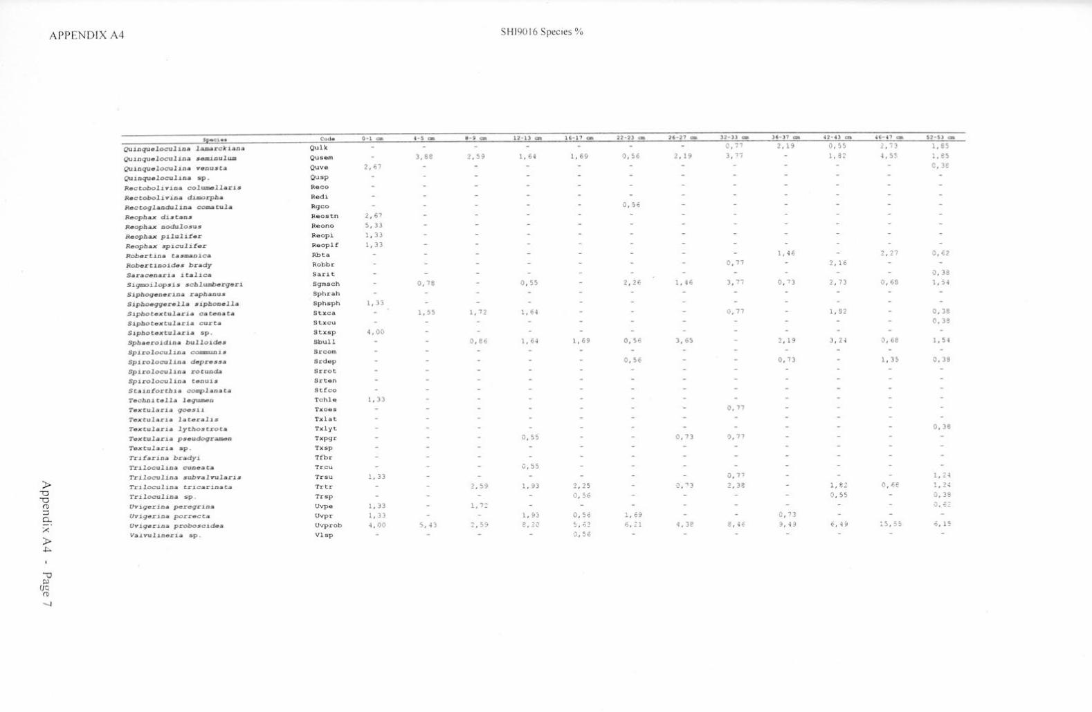
APPENDIX A4 S 1-1190 I 6 Species %

SEaci es Code 0-1 cm 4-5 cm 8-9 cm 12 - 13 cm 16 - 17 cm 22-23 cm 26-27 cm 3 2- 33 cm 36- 37 on 42- 43 CIU H - 47 on 5 2-53 cm

Quinqueloculina lamarckiana Qulk - - - - 0 , 17 2 , 19 0,55 2 , (3 1 , 85

Quinqueloculina semioulwn Qusem 3 , 88 2 ,5 9 1 , 64 1,69 0 , 56 .2 , 19 3 , 77 - 1 , 82 4, 5 :, 1 , 85

Quinqueloculina venusta Quve 2 , 67 - - - - - - 0 , 38

Quinqueloculina sp . Qusp

Rectobolivina columellaris Reco

Rectobolivina dimorpha Redi

Rectoglandulina comatula Rgco - - - 0 ,5 6

Reophax distans Reostn 2 , 67

Reophax nodulosus Reano 5 , 33

Reophax pilulifer Reopi 1 , 33

Reophax spiculifar Reoplf 1, 33

Rober tin a tasma.nica Rbta - - - - - - 1 , 4 6 - 2. , 27 0 ,6 2

Robertinoides brady Robbr - - - - - 0 , 77 - 2 , 16

Saracenaria i tali ca Sarit - - - - - - - 0 , 38

Sigmoilopsis schlu.mbergeri Sgmsch - 0,78 - 0 , 55 - 2 , 26 1 , 46 3 , 77 0 , 73 2 , 73 0 , 68 1 , 5 4

Siphogenerina raphanus Sphrah

Siphoeggerella siphonella Sphsph 1 , 33

Siphotextularia catenata Stxca - 1 , 55 1,72 1 , 64 - 0 , 77 - 1 , 32 - 0 , 38

Siphot,,xtularia curta Stxcu - - - - - - - - 0,38

Siphotextularia sp . Stxsp 4, 00

Sphaeroidina bulloides Shull - - 0 , 86 1 , 64 1,6 9 0 , 56 3 , 65 2 , 19 J ' 2 .J 0 , 68 1 , 54

Spiroloculina conmru.nis Srcom

Spiroloculina depressa Srdap - - - - 0 , 56 - 0 , 73 - 1 , 35 0 , 38

Spiroloculina rotunda Srrot

Spiroloculina tenuis Srtan

Stainforthia complanata Stfco

Tec hnitella legumen Tc hle 1, 33

Textularia goesii Txoes - - - - - 0 , 77

Textularia lataralis Txlat

Textularia lythostrota Txlyt - - - - - - 0 , 38

Textularia pseudo gramdn Txpgr - 0 , 55 - - 0 , 73 0,77

Textularia sp . Txsp

Trifarina bradyi Tfbr

Triloculina cuneata Trcu - - 0 , 55

Triloculina subval vularis Trsu 1 , 33 - - - 0 , 77 - - 1 , 2 4

• Triloculina tricarina ta Trtr 2,59 1 , 93 ~ , 25 0 , :3 2 , 38 - 1,82 0 / 68 1 , 2 4 u Triloculina Trsp - - 0 , 56 - 0 , 55 0 , 38 '"O

sp . - -(l) Uvigerina peregrina Uvpa 1 , 33 - 1 , 7 '2 - - - - 0 , ,:.2 ::i Uvigerioa p o rrec ta Uvpr 1,33 - 1 , 9~ 0 , 56 1, 69 0 , 73 0...

--· Uvigerina probosc idea Uvprob 4,00 5 , B ·2 I 59 8 , 20 c:. ,- ·') 6 , Z l 4 , 38 B, 4E 9 , B 6 , 4 9 15 , :-5 I) , 1 S ;..<:

J,o:>_

• Va.i. vu.lineri a sp . Vlsp - - - 0 , 56

~

I

u p)

(JO (l)

-.J

APPENDIX A4 SHI9016 Species%

seacias Code 56- 57 cm 58 - 59 cm 62-63 cm 66-67 en 72-73 cm 76-77 cm 82 - 83 en 86-87 cm 92-93 cm 96 - 97 cm 102-103 en 106-107 cm

Quinque.locu.lina .lamarckiana Qulk - 0 , 46 - 0,99 - 0 , 34 - - 0 , 42

Quinque.locu.lina sem.inu.lum Qusem 0 , 78 0 , 46 0 , 93 1 , 32 0 , 63 0 , 33 0 ,4 5 0 , 4 5 1 , 24 1) , 60 0 , 34 0 , 84

Quinque.locu.lina venusta Quve 0 , 78 0 , 46 - 1 ?, - 0 , 45 - 1 , 76 - 0 , 84 , -Quinque.locu.lina sp . Qusp - - 0 , 62

Rectobo.livina co.lum.e.l.laris Raco

Rectobo.livina di.morpha Redi - - - 0 , 33

Rectog.landu.lina coma tu.la Rgco - - - - - - - o,~ s Reophax distans Reostn

Reopbax nodu.losus Reano

Reophax pi.lu.lifer Reopi

Reopbax spicu.lifer Reoplf

Robertina tasmanica Rbta - 0,33

Robertinoides brady Robbr - 0 , 46

Saracenaria i ta.lica Sarit

Sigmoi.lopsis sch.lumbergeri Sgmsch 1, 1 7 l, B3 1, 25 0 , 99 - - 0 , 90 1, 2 4 0,33 2 , 74

Sipbogenerina raphanus Sphrah - - - - 0 , 33

Sipboeggere.l.la siphone.l.la Sphsph

Siphotextu.laria catenata Stxca 0 , 78 - 0 , 31 0 , 33 - 0 , 33 0 , 45 0 , 4 5 0 , 68 0 , 33

Siphotextu.laria curta Stxcu - 1 , 83 - 0 , 32 0 , 33 - - 0 , 66 D, 68

Sipho textu.laria sp . Stxsp

Sphaeroidina bu.l.loides Sbull 0 ,4 0 - - 0 , 99 0 ,3 2 1 , 00 1 , 35 - 0 , 68 0 , 33 - 0 , 42

Spiro.locu.lina communis Srcom - - - - - - - - - 0 , 42

Spiro.locu.lina depressa Srdep 0 ,4 0

Spiro.locu.lina rotunda Srrot

Spiro.locu.lina tenuis Srten

Stainforthia comp.lanata Stfco - - - 0 , 33

Te c hnite.l.la .legwnen Tchle

Textu.laria goesii Txoes

Textu.laria .latera.lis Txlat - 0, 93

Textu.laria .lythostrota Txlyt

Textu.laria pseudogra.men Txpgr - 0 , 46 - 0 , 33 - 0 ,4 5 0 , 34 0 , 33

Textu.laria sp . Txsp - 0 , 46 - 0 , 32

Trifarina bradyi Tfbr - - - - 0,33 - - 0 , 33

Tri.locu.lina cuneata Trcu

)> Tri.locu.lina subva.lvu.laris Trsu 0 , 40 0,46

Tri.locu.lina tricarinata Trtr 0 , 78 0 , 46 0 , 62 0,33 0 , 63 0 , 67 1 , 82 2 , 24 1 , 24 C·, 33 ,) , 3 4 1 , 69 "O "O Tri.locu.lina sp . Trsp

(1) Uvigerina peregrina Uvpe 0,46 0 , 93 0 , 33 1,9 0 1 , 00 - - 0 , 33 0 , 34 :::; 0... Uvigerina porrecta Uvpr - 0 , 4E G, 33 0 , 32 1,00 - 0 , .JS - - 0 , 4 ~

X Uvigerina proboscidea Uvpro b 7 , 4 ~ 9 , CJ l,SS 5 / 92 7 , 59 8 , 213 1 , 8 2 8 , 97 12 , 63 9 ,1 8 7 , 51 E, 72

)> Va.I vu.lineria sp . Vlsp c, , 4 0 0 , 4,;: 0 / 3J. 0 I 95 u , 67 - - - 0 / 66 0 , 68 , ')7 .J.. , - '

~

I

'""CJ p:l

(fQ (1)

00

APPENDIX A4 SHl9016 Species ~-~

SEac iaa Code 11 2-113 cm 116- 11 7 cm 1 22-123 cm 1 2 6 - 1 27 cm 132- 133 cm 13 6-137 cm 142-143 cm l-1 6- 147 cm 152 -153 <= 156 - 15 7 cm 1 6 2 - 1 6 3 cm

Quinqual.ocul.ina 1.a.marckiana Qulk - - - 0 , 32 - - - 0 , 3'3

Quinqual.ocul.ina seminul.um Qusem 1 , 29 0 , 35 2 , 52 1 , 34 2 , 93 0 , 98 1 , 62 1 , 00 1 , 18

Quinqual.ocul.ina venusta Quve 0 , '32 1 , 52 ,) , 67 0 , 65 0 , 65 - - 0 , 33

Quinquel.ocul.ina sp. Qusp

Rectobol.ivina col.umal.1.aris Reco - - - 0 , 32

Rectobol.ivina dimorpha Redi

Rec togl.andul.ina coma tul.a Rgco

Reophax distans Raostn

Reophax nodul.osus Reano

Reophax pil.ul.ifer Reopi

Reophax spicul.ifer Reoplf

Rober tin a tasmanica Rbta - - - - - 0 , 31

Robertinoides brady Robbr

Saracenaria ital.ica Sarit

Sigmoil.opsis schl.umbergeri Sgmsch 1 , 29 0 , 35 0 , 34 0 , 65 0 , 65 2 , 73 0 , 33 1 , 57 1 , 98

Siphogenerina raphanus Sphrah

Siphoeggarel.1.a siphonel.1.a Sphsph

Siphotextul.aria catenata Stxca 0 , 32 - 1 , 2 E 1 , 3 4

Siphotextul.aria curta Stxcu - - 0 , 32 O, E7 0 , 31

Siphotextul.aria sp . Stxsp

Sphaeroidina bul.1.oides Sbull 0 , 65 0 , 35 0 , 32 - 0 , 32 0 , 31 - 0 , 33 0 , 39 0 , 07

Spirol.ocul..1na c onn:nunis Srcom

Spirol.ocul.ina depressa Srdep - - 0 , 3q - - 0 , 33 0 , 55

Spirol.oc ul.ina rotund.a Srrot 0,32

Spirol.ocul.ina tenuis Srten - - - - 0 , 31 - - 0 , 33

Stainforthia compl.ana ta Stfco

Technitel.1.a 1.egumen Tchle

Textul.aria goes i i Txoes

Textul.aria 1.a teral.is Txlat

Textul.aria 1.ythostrota Txlyt

Textul.aria pseudogrBIDBn Txpgr 0 , 32 - ,) , 32 ,J , 3 4 0 , 33

Textul.aria sp . Txsp

Trifarina bradyi Tfbr - - - - - 0 , 39 0 , 33

Tril. o cul. i na cunaata Trcu

Tri l.oc ul.ina sub val. vul.aris Trsu - - - (, I ]4 0 , 32 - - - ,) , 33

)> Tril.o c ul. i na tri c arina. ta Trtr 0 , 98 1, 22 1, fj,g 0 / 3 4 0 , 65 0 , 31 0 , 98 2 , 16 0 , 3] 0 , 78 0 , 3} '"O Tril.ocul.ina Trsp - - - 0 , :< 4 '"O sp .

(D Uvi gerina peregrina Uvpe - 1, 5 3 - (1 , 67 ,J , 9 4 - 0 , 55 - 0 , 33 ::i 0. Uv igerina porrec ta Uvpr - 0 , 65 - - 0 I 3 9 0 , 33

- · Uvigerina probosc idea Uvprob 11 , 32 6 , E '7,89 7 , 38 <l,52 E, 90 6 , 8 i3 5 , 95 7 I 33 1 , 98 6 / 9~ X

)> Val. vul.ineri a sp . Vlsp 0 , 3: 1, 2 :2 :?,:e 1 , 67 1 , 29 0, 31 1 - .,

- I ..) • 0 , S 5 0 , 3J i) , 39 1 , GO

..i::.. I

'u Pl

(JO (D

\0

.APPEND IX .--\:i

)> -0 -0

CTI ::l 0.

>< )> VI

iJ PJ

(IQ (1)

5,2_•cia s

illomocphina p.aciti c a

.Ammobaculita.s &mflri c .-i.nu.s

A..no m.;r.l i na globulo.1 .1.

U t rononion achol.s i

Bo l i n.n.a .ili lb.a tro .1 .u .

Bol.1 nn.a r ebus ca.

Ba li vina .:s•m.i.nU.CU

Bo liv-in.a s p .

Boli v-i n.1. CJ.I qu.ad.ril.a t•ra

Briz.ali n.a d..l.l.a t .il. t.t

Bri za.li n.a ,em.il.1.ne.at.a

Buli.ui.n.a a.cul•.a ta.

Bul.i..min.a .ala.z.anen.1 i ,

Bul i .mi.n..ti CO !I t .a t.a

9ul:unin.a (.I.JCili .1

k1im..1.n.1 g:i.bb.a

Buliml.n.a margin.;,, t•

C• ., ;sidulin..- cro1 J1.s.a

C.a•.s idu.Ll.n.a l.ti6tvig• t •

C•r• t obu .ll.llU.n.a p.ac1 l1. c .a

Ch.l.lo .. comull.l oolin.a.

Cibic1dtu l ob.a culu.11

Ci.bicidoict.u bradyi

Cibic1.do1.CW .. p .. 111udounoeri anu.,

Clbi c1.doi d.e.11 cob6trt.:11on.1. a.nu..

Cib1.cidoid.e;s V'll6t llar.1torl 1.

C.i..bic.ido.Lct...w • p .

Cornuspir.a involvan.s

O.nc .. 1.1.n.a c o mm:un.i,

Dltn c .allnJ1 .-ub.solu c.a Oen c.al .i n..ri •p .

Doroth i.a b.c:.dy.an.a

Egg .. r •ll a br;,,dyi

.E'h.r" nb•rg1n.i crigo n..a

1:pi.111 t o m.inal.l.a axi guil.

Epi .11 t o .m.in6tll .1 umbo n.l.l•ca

F1..11.11urin~ • PP .

FurJien.kOl.Oil. br;,,dyi

f\J r., an.koin.1 a.arl.andi

fu.r.11•nkoin.a t.'u .11 iloruu .11

Fur.s•n.koina "P .

G.av .. .11.no p.si.:11 l o b.a c-ulu .5

Globobul.l..lD.l.n.:.t .alll.,u .:11

Globabuli.nu. n.a p.a c.il1.co1

Glo b oc.assidulin.:. .11 ubglob0J1.t

Gyro i d.J.noidu.- .al t i l o rnu. .11

Gyro.idino1d,r,.:11 l.1oU1Lo&cc kii1,nu.:11

Gyro1d.J.no.1.da.s 0L:bicul.ar1 .s

Gyroid.inoide.5 poliu.s

Gyro id.J.noid.,, .1olCUn.1.1

Gyroid.J.no i. cL.u •P .

H.u1z.ava11 J1 n i ppon1.c.a

H.;,,uar.int:t.ll.t inco.s t: ,uu

Ho •~ lund.J.n.:.i e lwg.1.ru

Hy.alinu..1. b .a .l ch.t. c .a

K..t rr• ru.li n .a .apicul.ar.1.:1

K.:lrrari,tll ..t. n av:.ngli .;h1

K..arr•.r: ... .al l.a br.ad y1.

L.ag•n.i ~pp .

L.ati c :.1rin.1n .1 p a upt.ir.a c.a

Lanciculin.;i •PP •

Lo.xo .,co uu...un Jc.:irr•r-i. .&m . .1111

~ A.llpa.

Abam

Ju.g lob

~tn,ch

Bola.lb

Bol ro

Bol s4llll

BoLsp

Blql

Brdi

Brsam

Bu.ac

Bu.alz

Buco

Buax a

Bugl

Bum.

Ca.s c r

C.i, l a.a

c .. rp.a.

Chol

Clob

C1.br

Cips•

Ci rob

Ci1,1ul

Ci•p

Co.1.n

04tCO

Oe.a•ub

D•.sp

Oobr

Eqbr

Ehtr

£pax

Exum

F.1..:ipp

Furbc

Fur.a,1,

Furl,

Fur.sp

Galo

Gl.il.l

Glp.a

GlcMb

Gyr.al

Gyrlmk

Gycoc

Gyrpo

Gyrao

Gyr ap

Hn"'n.l

Hur 1. n

Ho al

Hyb .t.

K.1.r.iip

Ka..cno

K.arbr

La!1pp

L tp .a

Lolipp

Lxka

BAR9-W3 Species 0,;,

0-l cm 5 - G cm 10 - ll CIIII lS - 1' 20 - 21 25-:?6 JO - llca l S - 16 li . 5 - 40 . S cm ,t,5 - ·U 50 - 51 c::m. 55-56

,...,. (") ~

S. o ~ !::. § ~ ::l ,...,. ,,,,_ C C/l . \,,,,

3 0. ~ CT ~ l ...._J

,o - n cm ,s - u cs 10-11 ca 1s -1, c::m 10 - u CD a s - u aa iO - i l c::a 95 - U o:i 100- 101 ca ~ 0,) 2 0 0 ~ -+i -+i ~ (/) ~ )-al( -0 ::l ~ ("[) .-+ (") ::r 3 (") ~ CTI a1 ~ ~ --, Ul

p)

3· 3 ("[) 3 p)

(") ~ ::r --, (/) p)

e: • ~ 0

-0 --~ ("[)

~ :::i:._ :::,::, 'O ~ c:::, w (/l

PJ 3

-0 ("[) (/)

z C

3 CT ("[) --, (/)

PJ --, ("[)

(JQ

< ("[)

:::l p) (/)

-0 (1) --, (") ("[)

::J ,...,. p)

(IQ ("[)

0 -+i ,...... _, (1)

APPENDIX ..-\5

)> "'O -0

(l)

:J 0.

>< )> VI

'u c:i

CfO (1)

1'0

!l.f.• Ci ,u

.U.loworphin• p•cifi ca

A.mmob.aculi t&JI .merl.C,iLDUJI

Anom.alin. globulos.a

.A...11 trononion a choL:1i

Bolill'in.A a.lb•trOJI.Sl.

Boli V'l..n. robu.s c.a

Boli vin..t J1am.inud.a

Bolinn.il sp .

Boli n.ni c.i qt..Uid..cil..a Cara

Briz.alin.a d.i.l.at:.at:.i

Brizal.i.n.il .sam.il.ina.ata.

Bul.l.min.1. 41.CU.la.a t..a

Bu.li.m.in. al.az.a.nan..,i.a

Bu.limin.... co• t• t:•

Bul..Lmin.1 -.xi.li.s

Bu.li.min.a gibb.a

Bul.J...min..t margin.a t:.a

C.i.11.siduli.n..a cr;,,.,..s.a

C.a.s.sidu.lin.;I l.aariga ta

Car.a c.abu~ poi.citic.a

Chilo.stomell.i oolin.

Cl.bicide.s lob;,,. ruliu

Ci.bicido.idaJ1 br..adyl.

CibicidoidaJI p.,audoungeri.a.nuJ1

Cibicidoid.e• rabart.soni.nu.s

CibicidoiciaJI .-Utitller•torti

Cib1.cido.1. C:WJ1 31p .

Co.rnuspir.a involvan.s

O.nt.alina communi • Den t-1.La.n..a ,.ub.,olu t•

Don t.a.lina ap .

Dorothi.a br.1dy.iln.ill

Eggarell.a br.adyi

Eh.r11nbarg:i.n.a cr1.gon.:.

Ep.1. .. c:om.1.n•ll.a ax.1.gu..1.

E'p.1..st:o mioal.l;a umbon.i.L•r.a

Fi .11sur1.n..a spp .

fu.r.sanko1.n. br.ady1.

f'ur.seoko1.n..a e..1.r.La.nd.i

fu.r.s~n.k"Ol.n.il fu..11it'Orm.i-'

i\J.r.111-,nkoin.a. sp .

G.ave.l inop..11 i .s lob.a culu.,

Globobuli.min.a .aft'1.n1.s

Globobulimin• p.aci Li c .a

Globoc.a.s..111.duli.n.a subglobo .. .a

Gyroid.inoide..11 .altifo.rmi.1

Gyroid.inoide.s l.a...tl:l..lrck .1.anu.s

Gyroid.i.noiCW.s o.cbicul.ari.,

Gyroictino.1de.s poliu.s

Gyroidinoic:ut.s .sol!U.ni1.

Gyro1.d.l.no1.d.e.s sp .

H.;.n.z.awa1..a nippon.i.c.a

H..luerinall~ l.nCOll t.an,

Hoaglund.in. •lag.a.n.s

Hy.al .100.11 b .al. th..lc.J

Ka.rrerulin.a .a.p.1cul.ari.s

K.arrer.1•.lli nov.anglia•

Ka.rrur1.oll.a. bradyi

Lo1gen. spp .

L.a ticarinin.i. p.Jupar.a ta

Lon t:icu.l.iJL. app .

Loxo.stomum k.arrer1..1.num

Code

Al.lp.a

Ab= 4glob

Astrech

Bol .. lb

Bolro

Balsam

Bolsp

Blql

Brdi

Bc• em

Bu.ilc

Bual2

Buco

Bu•xs

Bugi

a~ C.ilscr

C.ilslae

c.rp .. Chol

Clob

C1.br

Cip• ti

Ci.rob

Ci wul

Ci .sp

Coin

Deco

Oe.il• ub

Oesp

Dobr

Eqbr

Eh'tr

Epex

Exum F1. .. pp

Furbc

Fure ..

Fur ts

Fur.sp

Galo

Glaf

Glpa

Glcsb

Gyr.ill

Gyrlmk

Gyror

Gyrpo

Gyr.so

Gyr.sp

Hn..,ni

Hurin

Hoel

Hyba

Karap

K.t.rno

K~rbr

L.aspp

Ltp.t.

Laspp

Lxh

1os-10, 110 - 111 011 115 -11' 120-121 cm 125-126

, :1

BAR9.J03 Species%

110 - lll us-u, l •0-141

. , ,.

HS - lH 150-151 155 - lSf uo-1n 165 - Ui 110-111 115-11' 110 - 111

APPENDIX A.5

)> "O "O

(1) :::::l 0.

X )> U\

v p)

(IQ (1)

L,..)

.s,e.oci•• A.llomoq:,hina p;;aci.fica

Ammobaculi te.:1 .americ.anl.13

Anouu..lin• globuloaa.

A.:, trononioo o chol._.i

Boli nn..i a.lba. tro.s.,i

Bo li Yin. robu., t•

Bal.i vin.1. .,am.inud.a

Bolinn.a. .,p ,

Bali v:i.nl ta qiad.ril..t ter.1.

Briz;;al in.;1. dil.at;;at.l

Bri.z.ilin.a .uuri lina• t.a.

Buli.mir...a acu.lw.t ta

Bulimina al.tz..1.nen.s i .s

Bu.lim.in.a CO.'.!I t.t t.a

Bulimin;;a axili.,

Bu.Li.min.a gibb.t

Bull.JD.in.a margin..tta.

Ca. .,.s idu.l.1.n.1 cra.s .,.;a

C.aJ1J11 idulin.a l..aia vi.ga t.a

Cara. tobu.J.i.m.in.a. pa.ci.tica

Chilo.stoma ll.a oolin.a

CibiciC:Uu l.oba. tulu.,

Ci.bicidoicUu1 bradyi

Cib1cido.1CUIJ1 p,-,udoungeri.v1u.,

Cihicid.oicU.u robart.,on.i~u.s

Clbicido:i.d.u wu•llar.11 tor.ti

Cibicidoida.'.!I •P .

Co.rnuspira involvao.s

Ount•lin.a

Oen t.alina. .sub.:110.lut.a

!)(.tnt.il.lin.a sp .

Dorothi.t brady.a.n.a

E9gen,llil br.1dy1

Eh.renbe rgiru tr.1.gon.a

Epi stom.inell.a axigu.a.

Epi•tom.inell .a. umbonif.,r.a.

Fis.su.rin.a spp .

rur.,ankoiru br.adyi

rur.,ankoina 6t.ar la.ndi

Fu.r.s6tn.koin• fusifoonis

li'U.rsenkoin.a •p .

G.ava.linopai..1 l ob.a tulu.s

Globobul.Lmin.a .at'!in.1..,

Glabobulim.in.a p.acific.a

Globoc.aJ1.sidulin• subglobo .:1.a

Gyroid.inoide.t .-1 ti fonni,s

Gy.roid.ino.1.dcu1 l..unilrcki;,.nu..s

Gy.roid.inoide.11 o.t:bicul..i.ri.11

Gy.roid.l.noiCUI.., pol.iu.:1

Gycoid.inoida..r .told.anii

Gyro.idinoida.s sp ,

ff.-nz.lwoti .a nipponic.a

H.,1uorin.,Jl.a .1.ncoJ1t.a.n.s

Ho aglwid.J.ru, •lwg.1.J1.s

Hy.allna.a b.d th.J.c..io

K.lrrarul.1.n..a .apicul.ari .s

K.r.ror.1.all.a. nova.ngli.a.a

K.:l r.ren. r1l l.a br;;;idyi

L.ag-,n.1 spp .

L-t tic.11.rinin.a p;,.upar.a c.a Len Cl.CUlJ.n.a .spp ,

Loxo.scowum k.arrari.anum

Cod•

Al lp"'

Ah.-m

A.olglob

A.s tr a ch

Bel .alb

Bolco

Bol.3am

Bol!Sp

Blql

Brd.1

Brsam

Bu.ac

Bu.a.1-z

Buco

BUMX.:S

Buq1.

Bum& C.iscr

C.a.sl.1.a

Cacpol

Chol

Clob

Cibr

Cipse

Ci rob

Ciwul

Ci.sp

Coin

Deco

Oe.a:1ub

De s p

Oobr

Egbr

Ehtr

Epex

Exum Fi.spp

Furbr

Furaa

Fur ts

Fursp

Galo

GL1it

Glp.i

Glcllb

Cyr.al

Gyrlmk

Gyror

Gyrpo

Gyrso

Gyrsp

Hnwni

Hurin

Hoel

Hyba

K.trilp

K.arno

K;,.rbr

L.a..spp

Ltp.a

Lo spp

Lxk.1.

115 - llifi UO-lH liS-196 200-201

BAR9.:J03 Species 0 o

205-206 Zl0-211 215 - 21' 2l0-2ll 21s-21 , 2i0 -2 H c:111 2t5 - 2H 255-256 2 60 -261 2,s -2 u 210- 211 215-216

- , --

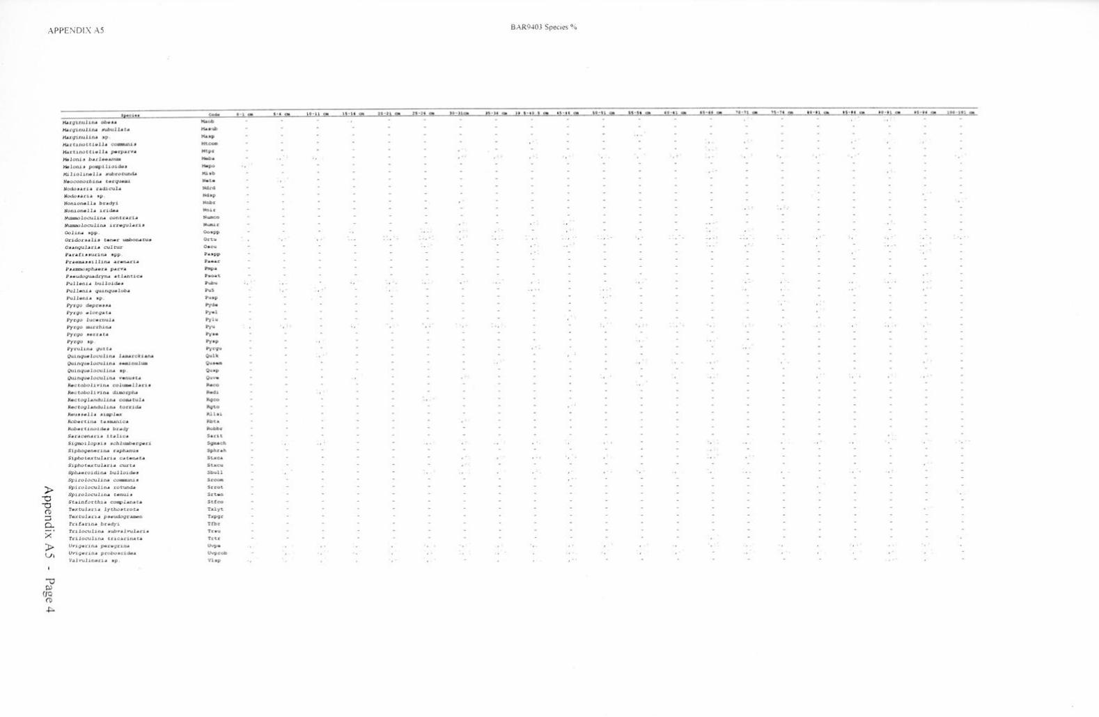
APPE NDIX AS

• -0 -0

(1) ::; 0.

>< )> U)

-0 p)

cro (1)

.j:::,..

Specie•

~rginu.11.n.il obii .s.il

J-til rginulin.a subull.t t a

M..rginulin.a s p.

M.artino ttia.11.a coll!IZll.lni..J1

H.ilrtino ttl.ti .1 1.a ~rp.ilrv.t

Melo ni., b.il.rlaa..num

Me looi.s pompil.101.do .11

Mil iol 1. n el l.i1 subrocun..d.l

Neoconocbin..a tacquaau.

No do .sa.r i .t rad.icul.a

NodD.sa ria sp .

No n.1onel.l.il br.adyi

Noniona.11.-. irid.e,1

Nummolocul.in.a contr.i. ri .a

Nummoloculin.a irragul..t ri .111

Oolin• spp .

Oridor!ja.li., t e n a r umboniileu.,

O.siilngu.L;ari • cul tu.r

Par a .fi .s .surin.il .11pp .

Pr.;aama.s.s 2.l l.in.11 _.raru.ri.;a

P .s .umnosph,;u1 r.a parv.a.

P.11•udo9u..aclcyn.a .;a tl.ncica

Pull,10i .;a bullo.Lda.11

Pul l • n.i .;a qll..l.nquo lob .;,,

Pull,mi.a .11p .

Pyrgo d.epra.t.!11.il

Pyrgo .t l ong.a c .a

Pyrgo luc • rnul..r.

Py rgo ururrh.in.a

Pyrgo .H:t rriil t•

Pyrgo .11p .

Pyruiln.:. gut t..r.

Qu.J.nqu•loc..-1.Jlin,. 1.a.marc ki.nA

Qu.1nqua l ocu.l.i.n.;a .sam.inulum

Qu.inqualocul .i.n.;a •p .

Quinqualocul.in• v• nu_, t.i

Ractobol.1. v in.1 col umall ..t c2. •

Ra c tobo l in. n.;a d..l.morph..l

RAtccoq l.andulin• com.a rul.1

Rac t ogl.andul.1.n.:. torr.1~

Rau.11 .s.111 1 .a .si.mpl"-X

Robarcin.;a t • .YttU..Oic•

Robartinoid.t.lll br.ady

S.ar.a c an• r1.a it.a l.ic.t

Sigmo1..lop .s 1 .s schlumba rgu ri

Siphogone rin.a r.;aph..l.nu .s

Siphotaxt:ul.ari .J c .at11n.at .;a

Siphotaxrul .. ri.a curt .a

Sph.aaroidin.a bullol.dt..s

.Spiroloculin.a commwu.J

.Spiroloculin.a rotund.a

Sp1ro1ocu1.i.n.a canui.s

St.ain.forch1.a cottrp l.il.niilt.a

Ta1xtu liilr.1.;a 1ytho .s t:rot411

Te.xtu l iilrl. A p.,~udoqr.mdn

rr2.f.:.r.1n.a br.adyi

Tr2.loC'\J l i na .1ub v.alvu l.1 ri M

Trilocul.2. n.a tr.1 c.ar1.n..a ta

Uv1garin.a ~rlitgrin.a

Uv:i9t1L· in..i pro bo.scidd.a

Val vul.1nur1 .a .sp .

~da

Ha.ob

Ha.aub

Ma•p

Htcom

Mtpr

Meba

Hape

Misb

Neta

Ndrd

Hd.sp

Nnbc

Nnir

Nwncc

Nunuc

Oo.spp

Orcu

O• cu

P:u1pp

Pill.e.t.r

l'mp•

P9o .t.t.

Pubu

PuS

Pusp

Pydo

Pyol

Pylu

Pyu

Py•• Pysp

Pycq,,

Qulk

Qus-.m

Qu»p

Quva

Raco

Rad1.

Rqco

Rqco

Rllsi

Rb<• Robbr

Sar i. t

Sgm..sch

Sphr<lh

St.XCil

St.x.c u

Sbull

Srcom

Sr rat

Srtan

Stfco

Txlyt:

Txpgr

Ttbc

T r a u

Trtr

Uvpo

Uvprob

Vlsp

BAR9403 Species %

0 - l CII 5 - , CD 10-11 15 - 1' 2 0 -2 1 ~5 -2 6 OIi J O- llc:m l S - 16 39 . 5 - 40 . 5 cm -1 5--U SO - 51 ss -s, ,0 -,1 c::m ,s-u 70-71 75 - H 10 - 11 15- 16 C11 iO - U iS - U 10 0 - 10 1

. , --·

APPENDIX A..5

)> -0 -0

(1) :J Cl...

>< )> VI

v p)

(JO (1)

VI

5.e_•cl.•• Ma.rginulin. ob•.sa M.,;,t.rginulina subu.lla t•

H..,,rginul.in. sp .

H.artinottiall.a communi.s

H.trtinottiall.il perpa.rv;;r,

Melani., b«rleaanum

Malon.i.s po~il.i oides

Mili olinsll• subro r:wid.t

Neoconorbin.. tarquemi.

Nodo..!l.ari• .rad.icul..r.

Nodos•.ri.a sp .

N'oniontt.ll.il br•dyi

l/onionlill l.l• iridaa

M.nomo.locu.lin.a con tr•ri• Nummolo cu.lin.a irregu.l.iri.s

Dolin.a spp .

Oridor.a.1li.s t•n•r umbon.. tu:1

o.,.1ngu.la.ri.1 cu.l tur

Paroilfi.,surin.a spp .

Pr..aam..i..ss i .l.lin.a .a.ran.aria.

Pa.mmosph.lera p.a.rva

Paaudagu..;ad..ryn.l • tl..ntic.a.

Pu.llani.a. bulloide.s

Pu.llani.a. quinqualo b.t

Pullao.i.t •P ·

Pyrgo dapra.s.sel

Pyrgo alo ng• tel

Pycgo l.ucernuU

Pyrgo murrhlniil.

Pyrgo sarr.ill t.a.

Pyrgo •P •

Pyrulin.. guttel

Qw..nqualo culin.a l.ill.ll1arc.ki ~

Quinquelo culi ~ •em:1.nu.J.um

Qui nqualo cu.li n• .sp .

Quinqu• l o culin. venu.s tel

Ra c tobo li vina c olUIDd l l.ari.s

Ractobol1 vin.. di.morph.a

Ro c t o gl.1..nduli,u. c o m.;&tul.a.

Re c t o gl.i.ndul.:Ln.a torrid.ii

Reus.,ell.a si.mpla.x

Ro.bart i n.a t.a.s:m..ni c •

Rab"rti n o .1.da.s br.tdy

S .t. r .ac en.ari a J. t.1.li c •

Sigmoi.lop:1 i s ., c hli.l111bargeri

S .1.pho genlitrin• r.1.phanu.s

S i pho tax tul.ari.a. C ,ii t ena. t•

Sipho tauc tu l •ri.a curt.a

Spluaroidin.a bulloi d.o.s

Spiro locu.li n..ii c ommuni.,

Spi r o l o culin. ro t:und..

Spirolocul.1.n.- tanui.s

St.» i n.for thi.i. complan.a ta

•raxtular.1.a lytho .i t ro t.:1

'l'e.xtu l a r ia p.:1eudogra.men

Tr1 .farin• br.ady1

Trilocul i na subv• lvu.Li ri .s

Tr1.loculin..i tr1c ..& r1na t a

Uvi.ga1 rin• p~regrin.

Uv:iga r.1. na. probos ci daa

V.» lvu linar 1• sp .

BA.R9403 Species %

~e 105-105 110-111 cm 115 - lU 120 - 121 125-126 1.10-131 135-1315 HO - Hl 145 - 146 15O-l.Sl 155-155 l60 - Ul 1'5 - lU 110 - 111 115 - 1 i6 110 - Ul

Maob

Masub

M.sp

Mtcorn

Mtpr

Mab• M<,po

Mish

Neta

Hdrd

Nd.!ip

Hnbr

Hnir

Humco

Nwnir

Oo.spp

Ort.u

Oscu

Paspp

P.a.e;,,r

Pmp•

Pso .ilt

Pubu

Pu5

Pusp

Pyda

Pyel

Pylu

Pyu

Pysa

Pysp

Pyrgu

Qulk

Qu.s•m

Qusp

Quva

Rac o

Rodi Rg c o

Rgto

RllJii

Rbt•

Robbr

S.t.ri t

Sgm.,ch

Sphrah

Stxca.

Stxcu

Shull

Srcom

Srrot

Sr ten

S t. tea

Txlyt

Txpg r

Tfbr

T r su

Trtr

Uvpe

Uvprob

Vl s p

APPENDIX A5

)> '"O '"O (I)

:::::i 0-

>< )> VI

u p)

CJQ (I)

°'

a.2,ac i ••

H.arginulin.i. obe.11.a

M.l rginulin.a .-ubu.lla ta

1-Urg1nu.lirut .sp .

Ma.rtirwttial.l"" co.mun.mi ,.

H.;t. rtinott.1.alla pacp.arva

HMlo n i .s b arlaa.num

liltlon.i, pomp.1.l .ioida .s

Hiliolin•ll• subrotunda

N• o cono.cbin..a terqu•mi

Nodo•ari .a r•dicul.a

Nodo.iiari o1 .sp .

Honionall• br..adyi

Uonione.lla 1.r.1.WI•

M..uni:Poloculin.a con trari .a

Hummolocu.lio.il irragu.lari .s

Dolin.a • PP .

Or1.dor.a.1..li.s timer umbon.a tt.u

0 .11.angul•ri• cultur P .a r.a t".1J11 .surin.a app .

Pr.t.e-.aJ11J11 illin.a ""r an.ari a,

P .ll.uzimosph.ae r .a p.arv.a

.PJ11audogua.d.ryn..t .a tl.anticA

Pu.lla n.L.a bul.loida•

Pul.l•ru.• quinqualob.a

Pu.lla n.i.a sp .

Pyrgo dapre .:u.a

Pyrgo • long• t•

Pyrgo lucarnul .a

Pyrgo murrhl n.a

Pyrr;o J11arr.a t:.a

Pyrgo J1p .

Pyru.lin.a gutt•

Quinqualocu.l.J.n.a l.am.arcCi~

Quinqualocu.l1n.a .sominul um

Quinqu.tloculin.a a p .

Qu.J.nque.loculin..a va nu.s t.a

RMctoboliv:in.a colwzw;,ll.ari.s

Rectoboli n.n.a cu..JDD.rph...a

lwct09l iil.J"ldulin• com..ri tul •

Ra c t o gl.andul .1n.a tor.n.d.a

.R.8u•J11al.l.a • ;uuplax

Rablitrtin.a t..a.sm.uU.c.a

Rab• rt1.no1.daJ11 br.:1.dy

S .a.r.ac en.ari• i t:.alic.a

Sigmoilop.s.1 J1 .schl umba rgeri

Siphogenarin.a r.aph.:...nu.s

Siphotaxtul.ari.a c;;aten.a t.i

S1photaxtul.u.·1.J curc ..a

sph.a a .roid.in• bulloida.s

Spiroloculin.a cowmun..i,

Spiroloculin.a rotund.

5))1.rolocu.lin.a CttO\l.l..S

Sc-1in.tocth.i.a compl~• t.ai

Ta.xtulii.r:l.Ji lytho .ll tro t.1.

Taxt:ul.::.ri.a p.seudogr.aJl>Qn

Tri.la .n.n..i. br.adyi

Tnlocul.1n.a su.bv.alvul.ari.s

Trilucul.1.n.a trica.rin.a c.a Uv:z.ge r ino1 peragri iu

Uv:i.g-.rin.a probo .s cide•

V-11 vuline ri.a. sp ,

BAR.9403 Species 0, ;,

~•s-1a, u o-1n 115 - 196 20 0 - 201 205 -206 210 -.2 11 215 - 21' 2 3 0-231 235-236" 240-241 H 5 - .:? H 2ss - 2s, 2150 - 261 255-26' 270-2'11 CII 21 5 - ~H

Maob

Ma•ub

H.il..!lp

Mtcom

Htpr -· Hepo

Misb

Ha t e

Ndrd

Nd.sp

Nnbr

Nnir

Numco

Numi r

Oo•pp

Ortu

Oscu

P~•PP

Pae.ill.r

Pmp•

Paoat

Pubu

Pu5

Pu.sp

Pyde

Pye l

Pylu

Pyu

Pysa

Py•p

Pyrqu

Qulk

Qu• am

Qu3p

Quva

Reco

Redi

Rgco

Rgto

R.11.si

Rbta

Robbr

s-.ri t

Sgmsch

Sphr .llh

StXC.l

Stxcu

Shull

Srcom

Sr rot

Sr ten

St.fee

Txlyt

Txpgr

Tfbr

Trs u

Trt r

Uvpe

Uvprob

Vl5p

APPENDIX B

List of the calcareous infauna) species

Species References Dataset

Amphicoryna proxima 2 CT,a

Amphicoryna scalris 2 CT,a

Amphicoryna sp. 2 CT,a,c

Astacolus crepidulus 2 CT,a,b

Astacolus insolitus 2 CT,a

Astrononion ec/zolsi 17* CT,a,b,c,d

Astrononion stelligerum 17* CT,a,b

Bolivina albatrossi 20 CT,a,c,d

Bolivina decussata 20 CT,a,c,d

Bolivina pseudoplicata 20 CT,a,b,c,d

Bo/ivina robusta I CT

Bolivina seminuda 20 CT

Bolivina spissa 20 CT

Bolivina sp. 20 CT,b,c,d

Bolivinita quadrilatera 21 CT,a,c,d

Brizalina dilatata 4, 14,15 CT,a,c,d

Brizalina semilineata 3 CT,a,b,c,d

Briza/ina sp. 3 CT,a,b,c

Bulin1i11a aculeata 3,8, 16, 19 CT,a,b,c,d

Bulimina alazanensis 3,8, 16 CT,a,c,d

Bulimina costata 3,8, 16 CT,a,b,c,d

Bulimina exilis 3,8,16 d

Buli111i11a gibba 3,8, 16 CT,d

Bulimina marginata 3,8, 16 CT,a,b

Bulimina striata 3,8, 16 CT

Buliminel/a elegantissima 20 CT,a,c

Bu/iminella sp. 20 CT,a,b

Cassidulina crassa 21* CT,a,b,c,d

Cassidulina /aevigata 21 CT,a,b,c,d

Cassidu/ina rejlexa 21* CT,c

Ceratobulimina pacifica 2 CT,a,b,c,d

Chilostomella oolina 3,5 , 11 , 16,21 CT,a,b,c,d

Dentalina advena 2 CT

Dentalina ctjmmunis 2 CT,a,b,c,d

Dentalina flliformis 2 CT,a

Dentalina guttifera 2 CT

Dentalina inornata 2 CT,a,c

Dentalina intorta 2 CT

Dentalina neugeboreni 2 CT

Dentalina subso/uta 2 CT,a,d

Dentalina sp. 2 CT,a,b,c,d

Eherenbergina trigona 2 CT,a,b,c,d

Fissurina spp. 2 CT,a,b'. c,d

Fursenkoina bradyi 3,7 CT,b,c ,d

Fursenkoina davisii 3,7 CT,a

Appendi x B - Page I


Fursenkoina earlandi 3,7 CT,a,d

Fursenkoina fusiformis 3,7 CT,a, b,c,d

Fursenkoina punctata 3,7 CT

Fursenkoina sp. 3,7 CT,a,c,d

Glohobulimina a/finis 3,5,7, 12, 15, 18.2 1 CT,a, b,c,d

Glohobulimina notovata 3 * ,5, 7 *, I 2 *. I 5 *, I 8 * ,2 I * a

Globobulimina pacijica 3*,5,7*, 12*, 15 *, 16, 18*.2 1* CT,a,b,c,d

Globobulimina pupoides 3*,5. 7*, I 2*. I 5*, 18*,2 1 * CT

Gyroidinoides altiformis 21 CT,a,b,c,d

Gyroidinoides lamarckianus 21* CT,a,b,c,d

Gyroidinoides orbicu/aris 21 CT,a, b,c,d

Gyroidinoides polius 2 1* CT,a, b,c,d

Gyroidinoides soldanii 21* CT,a, b,c,d

Gy roidinoides sp. 21* CT,a,b,c,d

Lagena spp. 2 CT,a, b,c,d

Lenticulina spp. 3, 1 I CT,a, b,c,d

Marginulina glabara 2 CT

Nlarginulina obesa 2 CT,a,b,c,d

Marginulina subullata 2 CT,a, b,d

!Harginulina sp. 2 CT,a, b,c,d

Melonis har/eeanum 3,7,9,2 1 CT,a, b,c,d

Nlelonis pompilioides 17 CT,a, b,c,d

Nodosaria calomorpha 2 CT

Nodosaria injlexa 2 CT,a

Nodosaria radicula 2 CT, b,d

Nodosaria simplex 2 CT,a

Nodosaria sp. 2 CT,a,c,d

Nonion germanicum 3* I 8* '

CT

Nonion sp. 18 CT,c

Nonionel/a hradyi 6* CT,a,c,d

Nonionel/a iridea 6* CT,a,c,d

Nonionella turgida 3,6,20 CT,a,c

Nonionella sp. 6* CT,a,c

Oolina spp. 2 CT,a,b,c,d

Parafissurina spp. 2 CT,a,b,c,d

Pleurostomella alternans 13 CT

Pleurostome/la sp. 13* CT

Pullenia bulloides ..., CT,a,b,c,d _,

Pullenia quinqueloba 3* CT,a,b,c,d

Pullenia sp. 3* CT,a,b,c,d

Rectobolivina columellaris 2 CT,c,d

Rectobolivina dimorplza 2 CT,a, b,c,d

Rectoglandulina comatula 2 c,d

Rectoglandulina torrida 2 d

Saracenaria italica 2 CT,a,b,c ,d

Trifarina bradyi 3* CT,a,c,d

Uvigerina peregrina 10,2 1 CT,a,b,c,d

Uvigerina porrecta I 0* 2 1 * '

CT,a, b,c

Uvigerina proboscidea I 0* 2 1 * '

CT,a,b,c,d

Appendix 8 - Page 2


Uvigerina sp. 10* 21 * '

CT,a,b

Vaginulinopsis suhlegumen 2 CT,a

Vaginulinopsis tasmanica 2 CT,a

Vaginulinopsis sp. 2 CT

References No. Dataset

Corliss ( I 985) CT = Core tops

Corliss and Chen ( 1988) 2 a= Fr/0/ 95 GC/ 7

Corliss ( 1991) 3 b = Fr I 0/95 GC5

Barmawidjaia et al. ( 1992) 4 c=SH/9016

Bernhard ( 1992) 5 d = BAR9403

J orissen et al. ( 1992) 6

Buzas et al. (1993) 7

Miao and Thunnel ( 1993) 8

Gooday ( 1994) 9

Jorissen et al. ( 1994) 10

Rathburn and Corliss ( 1994) I 1

Faridduddin and Loubere ( 1997) 12

McCorkle et al. ( 1997) 13

De Stigter et al. ( 1998) 14

Jannik ( 1998) 15

Jorissen et al. ( 1998) 16

Ben hard and Sen Gupta ( 1999) 17

Gooday and Rathburn (1999) 18

Schm iedl et al. (2000) 19

Ernst et al. (2002) 20

Fontanier et al. (2002) 21

Note: Corliss and Chen (1985) classification \Vas applied only for those species for

which a direct observation on living (Rose-Bengal stained) specin1ens \Vas not

available. Taxa classified as infaunal following this method are characterised by sn1al1

percentages and do not exert a big influence on the general trend of Infauna! Species

group.

* = references classifying comparable species, or species differently named.

Appendi x B - Page 3

APPENDIX C

Q- mode Factor Analysis (Principal components) of the species-abundance (n/g)

data sets.

1) Fr 10/95 GCJ 7: factor scores for the three Q- mode varimax-factors.

Species Fl F2 F3 Species Fl F2 F3

Allomorpltina pacijica -0.20 -0.29 -0.19 Dentalina subsoluta -0. 19 -0.27 -0.38

Alveolophragmium ringens -0. 15 -0.28 -0 .32 Dentalina sp. -0.20 -0.29 -0. 16

A /veolopltragmium suhglohosum -0.08 -0.29 -0.34 Discopulvinulina araucana -0. 18 -0.28 -0.47

Ammobaculites sp. -0.23 -0.29 -0 .09 Discop11/vi1111/ina subherthe/oti -0.24 -0. 12 -0.32

Ammodiscus pacijicus -0. 10 -0.29 -0.33 Dorothia bra[~vana -0 .32 0.86 -0.3 I

Ammonia beccarii -0. 15 -0.36 -0 .04 Dorothia exilis -0.15 -0.28 -0 .14

Amphicoryna scalris -0.16 -0.24 -0.33 Eggerella bradyi -0.05 -0. 18 -0. 06

Amphicoryna sp. -0.1 7 -0.22 -0 .30 Eggerella scabra -0 .18 -0.27 -0.32

Anomalina globulosa -0 .07 -0.38 0.34 Eggerella sp. -0. 16 -0.29 -0.28

Astacolus crepidulus -0. 18 -0.26 -0 .32 Ehrenbergina trigona 0.05 6.50 -1 .69

Astrononion ec/10/si -0 .39 -0.20 2.05 Elphidium crispum -0. 15 -0.28 -0.32

Astrononion stelligerum -0. 18 -0.26 -0.3 I Elphidium incertum -0.16 -0.28 -0 .3 1

Bigenerina nodosaria -0. 15 -0.28 -0.32 Epistominella umbonifera 0.08 -0.41 0.36

Bolivina midwayensis -0.21 -0.02 -0.35 Eponides regularis -0.09 -0.31 -0.28

Bolivina robusta 6.70 -1.09 0.57 Eponides tumiduls 0.0 I -0.30 -0 .3(1

Bolivina seminuda -0.20 -0.20 -0.09 Eponides sp. -0. 18 -0.31 -0 .22

Bolivinita quadrilatera -0.50 -0.08 1.00 Fissurina alveolata -0. 18 -0.28 -0 .28

Brizalina dilatata 2.25 -1.44 1.35 Fissurina crebra -0. 18 -0.28 -0 .29

Brizalina semilineata -0. 18 -0.25 -0.32 Fissurina kerguelensis -0.19 -0.29 -0.29

Brizalina sp. -0. 16 -0.29 -0 .32 Fissurina marginata -0. 17 -0.28 -0.14

Bulimina acu/eata -0.43 2.08 -0.9 1 Fis.rnrina orbignyana -0.20 -0.38 -0.07

Bulimina alazanensis -0.33 -0 .40 0.07 Fissurina semimarginata -0. 17 -0 .29 -0 .29

811/imina costata 0.20 0.20 0.03 Fissurina submarginata -0.12 -0.27 -0.25

Bulimina marginata -0.21 -0.29 -0.19 Fissurina wiesneri -0. 18 -0.27 -0.21

Buliminel/a elegantissima -0.30 0.09 -0 .32 Fissurina sp. 0.03 1.42 -0 .59

811/iminella sp. -0. 18 -0.26 -0 .32 Fursenkoina davisii -0.33 -0.31 0.04

Cassidulina carinata 0.30 -0.3 7 -0 .28 Fursenkoina earlandi -0. 18 -0.28 -0.3 1

Cassidulina crassa -0 .29 0.23 -0.37 Fursenkoina Jusiformis -0.21 -0.13 -0.30

Ceratobulimina pacijica 0.84 -0. 19 2.77 Fursenkoina sp. -0. 17 -0.25 -0.27

C/1ilostomella oolina 0.24 0.10 -0.07 Gavelinopsis lobatulus 0.32 0.41 1.19

Cibicides lobatulus -0.24 0.26 -0.42 Globobulimina a/finis -0 . 17 -0. I 9 -0.21

Cibicidoides bradyi I.I I 0.09 4.50 Globobulimina notovata -0.19 -0.23 -0.30

Cibicidoides kullenbergi -0.24 0.92 1.10 Globobulimina pacijica -0.04 -0 . 14 -O J I

Cibicidoides pseudoungerianus 1.07 1.93 2.20 Globocassidulina subglobosa -0.67 -2 .08 9. 57

Cibicidoides robertsonianus -0.23 0.00 0.37 Glomospira charoides -0. 15 -0.28 -0 .32

Cibicidoides wuellerstorfi -0.24 8.44 0.04 Gyroidinoides altiformis -0. 15 -0.25 -0 .32

Cibicidoides sp. -0.33 0.14 0.12 Gyroidinoides lamarckianus -0.25 -0. 18 -0 .19

Cornuspira carinata -0 . 15 -0 .24 -0 .31 Gyroidinoides orbicularis 0.37 -0.64 1.75

Cornuspira involvens -0.05 -0 .34 -0 .20 Gyroidinoides po/ius -0.08 0.03 -0.42

Corn11spira sp. -0. 18 -0.28 -0 .29 Gyroidinoides soldanii 0.41 0.00 0.88

Comuspiroides primitivus -0. I 9 -0.27 -0 .27 Gyroidinoides sp. -0. 10 -0.28 -0.32

Cyambaloporretta squamosa -0.25 -0 .21 0.00 Hanzawaia nipponica -0.23 -0 .07 -0.31

Cyclammina cancel/ala -0 . 15 -0.28 -0 .32 Hauerinella incostans -0.44 1.29 -0.27

Dentalina communis -0 .24 -0 .28 -0.28 Hoeglundina elegans 0.09 3.58 -0.22

Dent a/in a filiformis -0. 15 -0 .28 -0. 15 Karreriella apicu!aris -0.08 -0.29 -0.34

Dentalina inornata 0.01 -0 .29 -0.32 Karreriella bradyi 0.04 0.8 1 -0.47

Appendix C - Page I


Karreriella novangliae -0.20 -0.21 -0 .3 I Pyrgo sp. -0. I 8 -0.28 -0.29

Lagerw Jormosa -0 . I 8 -0.28 -0.25 Pyrgoella sphera -0. I 9 -0. 13 -0.35

Lagena graci/is -0. 13 -0.28 -0.33 Pyrulina cylindroides -0 . 11 -0 .26 -0.27

Lagena /1i.\pid11/a -0. 10 -0.28 -0.33 Pyrulina extensa 0.22 0.46 1.03

Lagena /aevis 0.01 -0.46 0.1 I Pyrulina Jusiformis -0. 21 -0.15 -0.28

Lagena plumigera -0.22 -0 .30 -0.12 Quinqueloculina lamarckiana -0. 19 -0.0 I -0.29

Lage,w striata -0.23 0.49 -0.51 Quinqueloculina seminulum 0.77 I .69 0.86

Lagena .mlcata -0. 11 -0.29 -0.35 Quinque/oculina ve11usta -0.20 -0.10 -0.34

Lagemr sp. -0. 17 -0.26 -0.27 Quinqueloculina sp. -0.19 -0.17 -0.31

Laticarinina pauperata -0. 15 -0.27 -0.32 Rectobolivina dimorplrn -0. 14 0.07 0.64

Lenticulina ca/car -0.09 -0 .32 -0.25 Reophax guttifer -0.23 -0 . 19 -0.22

Le11ticuli11a crassa -0.16 -0.27 -0.08 ReopltCL'C. nodulosus -0. 15 -0.28 -0 .32

Lenticulina cultur 0.07 -0.39 -0.08 Reophm:: pilulifer -0. 15 -0.28 -0.32

Lenticulina gibba -0. 15 -0.28 -0.32 Reussella simplex -0. 15 -0.28 -0.32

Lenticulina orbicularis -0. 17 -0.27 -0.28 Rhabdammina abyssorum -0.09 -0.28 -0.34

Lenticulina peregrina -0 . 11 -0.33 -0.20 Rhizammina algaeformis -0. 18 -0.26 -0.32

Lenticulina rotulata -0. 11 -0. I 7 -0.34 Robertina tasmanica -0. 14 -0.28 -0.31

Lenticulina sp. -0 .20 0.22 -0. 11 Robertinoides bra{~)! -0.15 -0.28 -0.32

Marginu/ina obesa -0.04 -0. 19 -0. 17 Saccorhiza ramosa -0. 14 -0.23 -0.29

Marginulina subu!lata -0. 18 -0.25 -0.32 Sagrinella sp. 2.30 0.90 1.1 3

Margimilina sp. -0. 19 -0.31 -0.25 Saracenaria ita/ica -0. I 5 -0.28 -0.32

Marsipella cylindrica 0.37 -0. 16 0.55 Sigmoilopsis schlumbergeri -0.22 0.02 0.89

Martinottiella comminis -0.54 -0.33 0.63 Sip/,ogenerina rapltanus -0 .19 -0.27 -0 .28

Melonis bar/eeanum -0.16 0.28 0.48 Siplwtextularia catenata -0. 18 -0.25 -0.32

Melonis pompilioides -0.02 -0. 15 -0.33 Siphote.\111/aria curta -0.18 -0.25 -0.32

Miliolinella oblonga -0. 18 -0.25 -0.31 Spltaeroidina bulloides -0.24 -0.22 -0. 19

Miliolinella subrotunda -0.07 -0.21 0.01 Spiroloculina communis -0. I 9 -0.25 -0 .3 1

Nodosaria injlexa -0. 15 -0.28 -0.32 Spiroloculina depres.rn -0. 19 -0.16 -0.23

Nodosaria radicula -0. 11 -0.21 -0.33 Spiroloculina elevata -0.22 -0.27 -0. 19

Nodosaria sp. -0 .2 1 -0.32 -0.20 Spiroloculina rotunda -0.15 -0.28 -0.32

Nonionella bnu~vi -0 .21 -0.21 -0.09 Spiroloculina tenuiseplata -0. 12 -0.18 -0.36

Nonionella iridea -0. 12 -0.29 -0.28 Stainforthia complanata -0. 18 -0.28 -0.29

No nionella turgida -0. 18 -0.28 -0.28 Tecltnitel/a brturyi -0. 10 -0.28 -0.33

Nonionella sp. -0.23 0.00 -0.39 Textularia agglutinans -0. 18 -0.28 -0.31

Nummoloculiiw contraria -0 .53 0.08 0.77 Textularia goesii -0. 14 -0.28 -0 .29

N11mmoloc11/i11a irregularis 1.02 2.57 5.65 Textularia lateralis -0.18 -0.24 -0.28

Oolina exagona -0. 16 -0.28 -0.31 Textularia (vtlwstrota -0 . I 3 -0.28 -0.32

Oolina g!obosa -0 . 11 -0.25 -0.24 Te.\1ularia porrecta 0.0 1 -0.24 -0.33

Oolina sp. -0. 11 -0.29 -0.33 Textularia pseudogramen -0. 19 -0.26 -0.28

Oridorsalis tener ste/latus -0.13 -0.28 -0.32 Textularia sp. -0.04 0.43 0.26

Oridorsalis tener umbonatus 0.63 0.03 1.16 Trifarina brat(l'i 0.18 0.4 1 0.67

Osangularia cultur 0.82 -0 .21 2.12 Triloculina cuneata -0. 18 -0.25 -0.31

Parafissurina latera!L-. -0 . 19 -0.27 -0.27 Triloculina insignis -0.28 0. 15 -0.3 1

Parafissurina sp. -0 . 16 -0.28 -0 .31 Triloculina subvalvularis -0 .26 0.45 -0.46

Patellina jugosa -0.21 -0.30 0.05 Triloculina tricarinata -0. 19 0.00 -0.34

Praeglobob11/imi11a s11hspi11esce11s -0.09 -0.19 -0.33 Triloculina trigonula -0.20 0.68 0.06

Praemassillina arenaria -0. 13 -0.28 -0 .32 Triloculina sp. -0.23 -0 .32 -0.09

Psammospltaera pan,a -0.15 -0.28 -0.32 Troclia111111i11a globigeri11iformis -0.26 -0.20 -0. 15

Pu/lenia bulloides -0. 18 -0.25 -0.32 Uvigerina hispida -0. 15 -0.29 -0.26

Pullenia quadrilobata -0.19 -0 .28 -0.28 Uvigerina peregrina -0.80 5.99 1.20

Pu/lenia quinqueloba 0.20 -0. 11 0.48 Uvigerina porrecta -0. 18 -0.25 -0.3 I

Pyrgo comata 0.22 0.59 0.49 Uvigerina proboscidea 11 .76 0.32 -2 .32

Pyrgo depressa -0. 19 -0.27 -0.28 Uvigerina sp. -0. 18 -0.25 -0 .28

Pyrgo e/ongata -0. 19 -0.26 -0 .30 Vaginulina spinigera -0 .16 -0.28 -0.32

Appendi x C - Page 2

Species Fl F2 F3 Species Fl F2 FJ

Pyrgo lucernula 0. 14 0.19 0.26 Vaginulina subelegans -0. 16 -0.28 -CJ.JI

Pyrgo murrhilla -0 .07 0.23 0.60 Valulineria sp. -0 .0 1 -0.0 I 0.15

Pyrgo serrata -0.22 0.03 -0 .29 Virgulina rotundata -0.24 -0.0 I -0.21

Pyrgo vespertilio -0. 16 -0.28 -0.31

2) Fr l 0/95 GCJ 7: factor loadings for the three Q- mode vari1nax-factors.

Sample Fl F2 F3 Sample Fl F2 F3

0-1 cm 0.87 0.12 0.28 93-94 cm 0.20 0.23 0. 85

3-4 cm 0.89 0. 16 0.34 97-98 cm 0.48 0.45 0.60

5-6 cm 0.94 0.14 0.19 101-102 cm 0.12 0.34 0.84

9-IO cm 0.90 0.17 0.32 105-I06 cm 0.33 0.29 0.83

13-14 cm 0.94 0.12 0.16 109-110 cm 0.28 0.41 0.66

17-18 cm 0.92 0. 13 0.18 113-114 cm 0.23 0.24 0.82

21-22 cm 0.92 0.11 0.25 117-118 cm 0.34 0.3 1 0.79

25-26 cm 0.87 0.16 0.32 121-122 cm 0.22 0.44 0.65

29-30 cm 0.90 0.19 0.22 125-126 cm 0.16 0.5 8 0.55

33-34 cm 0.78 0.27 0.39 127-128 cm 0.08 0.34 0.33

37-38 cm 0.74 0.38 0.38 133-134 cm 0.15 0.88 0.20

41-42 cm 0.62 0.37 0.49 137-138 cm 0.14 0.83 0. 19

45-46 cm 0.42 0.16 0.69 141-142 cm 0.16 0.78 0.16

49-50 cm 0.39 0.31 0.67 145-146 cm 0.16 0.87 0.28

53-54 cm 0.37 0.32 0.73 149-150 cm 0.19 0.89 0.26

57-58 cm 0.27 0.20 0.84 153-154 cm 0.18 0.79 0.44

61-62 cm 0.29 0.12 0.86 157-158 cm 0.15 0.92 0.27

65-66 cm 0.26 0.14 0.90 161-162 cm 0.17 0.90 0.22

69-70 cm 0.35 0.19 0.85 165-166 cm 0.05 0.94 0.20

73-74 cm 0.31 0.24 0.85 169-170cm 0.25 0.87 0.28

77-78 cm 0.30 0.28 0.80 173-174 cm 0. 19 0.86 0.17

81-82 cm 0.27 0.42 0.75 177-178 cm 0.26 0.86 0.26

85-86 cm 0.29 0.29 0.83

89-90 cm 0.29 0.31 0.82

3) Fr 10/95GC5: factor scores for the two Q- n1ode varimax-factors.


Allomorphina pacijica -0.28 -0. 15 -0. 28 Cibicides lobatu/us -0.31 -0.17 -0.23

Anomalina globulosa -0 .30 -0. 17 -0. 15 Cibicidoides brady i -0.43 -0.06 2.82

Astacolus crepidulus -0 .23 -0. 16 -0.40 Cibicidoides kullengbergi -0.39 -0.19 0.34

Astrononion ec/10/si 2.41 0.25 2.23 Cibicidoides pse11do1111geria1111s -0.45 -0.24 0.84

Bo/ivina seminuda -0 .29 -0 .09 -0.40 Cibicidoides robertsonianus -0.34 -0.18 -0.07

Bolivina sp. -0.27 -0. 13 -0.4 1 Cibicidoides wul/erstorfi 5.25 -0.02 2.93

Brizalina semilineata -0.37 -0. 14 0.05 Cibicidoides sp. -0.34 -0. 18 -0.08

Brizalinasp. -0.26 -0.15 -0.43 Cy clammina cancel/ata -0.39 -0.22 0.25

Bulimina aculeata -1 .72 9.94 0.36 Dentalina communis -0.22 -0. 13 -0.40

Bulimina costata 0.49 0.02 -0.72 Dentalina sp. -0.27 -0.16 -0.26

Bulimina marginata -0.26 -0.15 -0.43 Dorothia bradyana -0.27 -0. 15 -0.39

Buliminella sp. -0.3 1 -0.17 -0.23 Eggerel/a brady i -0.27 -0. 17 0.06

Cussidulina crassa -0.34 -0. 15 -0.07 Ehrenbergina trigona -0.32 -0.18 -0.09

Cassidulina laevigata 0.68 0.02 -0.99 Epistominel/a exigua 4.54 1.49 -0.60

Ceratobulimina pacijica -0.87 -0.28 4.13 Epistominella umbonifera -0.29 -0 .14 -0.40

Chilostomel!a oolina 2.8 I I . 12 -J.66 Fissurina sp. 1.28 -0 .09 0.95


Species Fl F2 F3 Species Fl F2 FJ

Fursenkoina bradyi -0.23 -0.15 -0.45 Parafrondicularia sp. -0.29 -0.14 -0.40

Furse11koi11afusiformis -0.25 -0 .14 -0.41 Pul/enia hulloides -0.28 -0.19 I .SO

Globohulimi11a affinis 0.00 -0 .09 -0.62 Pul/enia quinqueloba -0.16 0.07 -0 .29

G/ohobulimina pacifica -0.24 -0.09 -0.43 Pullenia sp. -0 .22 -0.18 -0. 11

Globocassid11/i11a elegans -0.31 -0. 17 -0 .23 Pyrgo depressa -0.27 -0. 12 0.30

(,'/o/,11c{ls.~id11/i11" .mh,:loh,,.m -0.51 -0. 11 4.20 Pyrgo lucemula -0. 36 -0.16 0.07

G/obulina minuta -0.27 -0. 15 -0.41 Pyrgo murrltina 3.33 0.08 - 1.86

Glomospira cltaroides -0.27 -0 .15 -0.41 Pyrgo vespertilio -0.34 -0.18 -0.07

Gyroidinoides altiformis -0 .30 -0.20 0.07 Pyrgo sp. 0. 14 -0.18 -0.54

Gyroidi11oides /amarckia1111s -0.24 -0 .16 -0 .3 1 Pyrulina fusiformis -0 .30 -0.14 -0 .32

Gyroidinoides orbicularis 0.02 -0.08 0.25 Quinqueloculina inmata -0.31 -0.17 -0.23

Gyroidinoides polius -0 .27 -0 .16 -0 . 17 Q11i11q11e/oc11/i11a /amarckiana -0.3 1 -0. 17 -0 .23

Gyroidinoides so/danii -0.23 -0. 13 -0. 15 Q11i11q11eloc11/ina semi1111/11111 0.04 -0. 12 0.39

Gyroidinoides sp. -0.25 -0. 15 -0.44 Quinquq/oculina stelligera -0.37 -0.20 0.09

Ham:.awaia nipponica -0.31 -0 . 17 -0.23 Quinqueloculina venusta -0.28 -0.05 0.56

Hoeglwulina elegans 0.37 -0 .21 1.33 Quinqueloculina sp. -0.29 -0.14 -0 .37

Karreriella bradyi -0.31 -0.16 -0.24 Rectobolivina dimorp/,a -0.27 -0 .15 -0.41

lagena sp. -0. 16 -0.12 0.50 Reussella simplex -0.31 -0.1 7 -0.23

laticarinina pauperata -0.21 -0. 13 0.29 Robertina tasmanica -0.29 -0.14 -0.39

lenticulina sp. -0.17 -0 .16 -0.44 R obertinoides brady -0.32 -0.1 J 0.3 1

Marginulina ohesa -0.27 -0 .1 J -0.29 Saracenaria italica -0.3 1 -0.17 -0.23

Marginulina .mbullata -0.29 -0 . IJ -0.40 Sigmoilopsis scl,/umbergeri -0.03 -0.12 -0.53

Marginulina sp. -0 .29 -0.14 -0.40 Siplweggerella siplwnella -0 .31 -0.17 -0.23

1'1,fartillottie/la co1111111111is -0.23 -0 .15 -0.40 Siphotextularia catenata -0.35 -0.11 -0.06

Martinottiella perparva -0.29 -0.14 -0.3 7 Siphotextularia curta -0.27 -0. 15 -0.41

Melonis harleeanum -0.23 -0. 13 -0. IJ Sphaeroidina bulloides -0 .27 0.00 2.55

Melonis pompilioides 0.32 -0.07 -0.58 Stilostomella abyssorum -0 .3 1 -0. 17 -0.23

Miliolinel/a ob/onga -0 .31 -0. 15 -0 .23 Stilostomella injlexa -0.3 1 -0. 17 -0.23

Miliolinella .mbrotunda -0.34 -0. 17 -0.07 Stilostomella sp. -0.29 -0.14 -0.39

Nodosaria radicula -0.29 -0.14 -0.40 Textularia lateralis -0.3 1 -0 .17 -0.23

Nonion sp. -0.31 -0.17 -0.23 Triloculina subvalvularis -0.2 1 -0.14 -0 .4 1

N11mmoloc11/i11a irreg11/aris -0 .30 -0 .06 -0.05 Triloculina tricarinata -0.30 -0.15 0.20

Oolina sp. -0. 19 -0.06 -0.04 Uvigerina peregrina 1.97 -0.0 I -1 .90

Orir/11~11/i.1· lc11er umh111111l11.~ 3.76 0.71 1.86 Uvigerina porrecta -0.42 -0.23 0.4 1

Oridorsa/is sp. -0.29 -0.14 -0.39 Uvigerina proboscidea 0.03 0. 10 1.06

Osangularia cultur -0.42 -0 .23 0.41 Uvigerina sp. -0.29 -0.14 -0.39

Parafissurina sp. 0.26 -0 .02 -0.52 Valvulineria sp. -0.29 -0.13 -0.40

4) Fr 10/95 GC5: factor loadings for the two Q- mode varimax-factors.

Sample Fl F2 Sample Fl F2 Sample Fl F2

0-1 cm 0.35 -0.02 45-46 cm 0.10 0.99 85-86 cm 0.93 0.11

5-6 cm 0.49 0.38 49-50 cm 0.07 0.99 89-90 cm 0.93 0. 11

9-10 cm 0.48 0.40 53-54 cm 0.43 0.87 93-94 cm 0.93 0.19

13-14 cm 0.59 0.34 57-58 cm 0.39 0.86 97-98 cm 0.93 0.14

17- 18 cm 0.16 0.92 61-62 cm 0.86 0.26 101 -I02 cm 0.90 0.22

21-22 cm 0.08 0.97 65-66 cm 0.84 0.17 l05-106 cm 0.82 0.25

25-26 cm 0.13 0.98 69-70 cm 0.73 0.56 109- 110 cm 0.86 0.I l

29-30 cm 0.09 0.98 73-74 cm 0.88 0.23 I 13-114 cm 0.85 0. 19

33-34 cm 0.20 0.94 77-78 cm 0.92 0.21 11 7- 118cm 0.78 0.07

37-38 cm 0.29 0.95 81-82 cm 0.90 0.19 121-1 22 cm 0.92 0. 13

41-45 cm 0.06 0.98

Appendix C - Page 4

5) SHJ9016: factor scores for the two Q - mode varimax-factors.

Species Fl F2 Species Fl F2

Allomorpltina pacijica -0.21 -0.43 Gyroidinoides orbicularis 0.06 1.20

Amplticoryna sp. -0. 21 -0.42 Gyroidinoides polius -0.20 -0.35

Anomalina globu/osa -0 .10 0.04 Gyroidinoides soldanii -0.10 0.00

Astrononion echolsi 0.86 1.38 Gyroidinoides sp. -0 .22 -0 .J0

Bolivi11a a/hatrossi -0 .10 -0.46 Hanzawaia nipponica -0 . 18 -0.41

Bolivi11a robusta -0.21 -0.42 Hauerinel/a i11costans -0. 19 1.80

Bolivina seminuda -0 .26 0.10 Hoeglwzdi11a elegans -0.19 -0.47

Bolivi11a sp. -0 .21 -0.44 Karreriella bradyi -0 .15 -0 .27

Bolivinita quadrilatera -0 . 12 -0.44 lagena truncata 0.43 0.45

Brizalina dilatata -0 . 17 -0.46 lagena sp. -0 .22 -0.39

Brizalina semilineata -0.08 -0.27 laticarini11a pauperata -0 .22 -0.39

Brizalina sp. -0 .19 -0.47 lenticuli11a crassa -0.21 -0 .42

811/imina aculeata I I. 13 -3.17 lenticulina peregrina -0.22 0.14

811/imina a/azanensis -0 . 18 -0 .46 Lenticulina sp. -0 .20 0.20

B11/imina costata -0 .19 0.93 Marginulina obesa -0. 13 -0.29

Buliminella elega11tissima -0 .20 -0.19 Marginulina sp. -0.24 -0.3 I

Cassidufina crassa -0 . 16 -0.24 Marsipella cyli11drica 1·.36 0.18

Cassidulina laevigata 0.72 1.06 Martinottiel/a comminis 0.12 -0.37

Cassidulina rejlexa -0 .19 -0.47 Martinottiella perparva -0.29 -0. 17

Ceratohulimina pacijica -0.49 1.12 Melonis barleeanum -0 .22 -0 .39

Chilostomella oolina -0 .59 2.42 Me/onis pompilioides -0.15 0.0 1

Cibicides lobatulus 1.51 1.65 Miliolinella oblonga -0. 11 -0.49

Cihicidoides bra{f;yi -0.41 0.50 Nodosaria radicula -0.20 -0.37

Cihicidoides kullenbergi -0.43 1.34 Nodosaria sp. -0. 10 -0.47

Cibicidoides pseudoungerianus -0 .17 -0. 15 Nonionel/a bradyi -0. 17 -0.4 1

Cibicidoides rohertsonianus -0 .09 -0.22 Nonionella iridea -0. 19 -0.46

Cihicidoides wuellerstorji 0.90 4.75 Nonionella turgida -0. 19 -0.47

Cibicidoides sp. -0.19 -0.47 Nonionel/a sp. -0 .18 -0.47

Cornuspira involvens -0 .21 -0 .39 Nummoloculina contraria -0. 17 -0.46

Cornuspira sp. -0 .21 -0.44 Nummoloculina irregularis -0.22 0.21

Cyamha/oporretta squamosa -0. 19 -0.47 Oolina g/ohosa -0.21 -0.43

Cyc!ammina cancellata -0 .22 -0.39 Ooli11a sp. -0.19 -0.08

Dentalina communis -0 .27 -0 .03 Oridorsalis tener umhonatus 1.23 2.21

Dentalina inornata -0 .22 -0.41 Osangularia cultur -0.20 -0.15

Dentalina sp. -0.16 -0 .20 Parafissurina I ateralis -0.27 -0.24 .

Eggerel/a bradyi -0 . 16 0.01 Parafissurina sp. 0.00 0.49

Ehrenbergina trigona 0.18 -0.06 Patellina jugosa -0. 19 -0.46

Epistominel/a exigua 1.40 -0 .50 Planuli11a ariminensis -0. 13 -0.45

Epistominella umhonifera -0 .20 -0.46 Pleurostomella alternans -0. 19 -0.24

Eponides regularis -0 . 17 -0.46 Pseudoguadryna atlantica -0. 11 -0.47

Fissurina bradyi -0.20 -0.46 Pullenia builoides 0.43 0.99

Fissurina sp. 1.57 3.34 Pullenia quinque/oha 0.52 4.34

Fursenkoina bradyi -0. 18 -0.38 Pullenia sp. -0.21 -0.43

Fursenkoina fusiformis -0.22 -0.20 Pyrgo depressa -0.21 -0.42

Fursenkoina sp. -0 .22 -0.38 Pyrgo lucernula 0.08 0.77

Gavelinopsis /obatulus 0.10 0. 15 Py rgo murrlzina -0. 18 -0.38

Globobulimina a/finis -0.25 -0.24 Pyrgo vespertilio -0.23 -0.37

Glohobulimina pacijica -0.43 0.35 Pyrgo sp. -0.20 -0.46

G!obocassidulina e!egans 0.25 4.47 Pyrulina angusta -0.22 -0.39

Globocassidulina subglobosa -0.22 -0.21 Pyrulina cylindroides -0.26 -0.22

Guttulina pacijica -0.19 -0.47 Py rulina e.xtensa -0.24 -0. 13

Gyroidinoides altiformis -0. 17 0.0 I Pyru/inafusiformis 0.29 0.59

Gyroidinoides lamarckianus -0.24 -0.29 Py ru!ina gutta -0. 18 -0.44

A ppendix C - Page 5

Species Fl F2 Species Fl F2

Q11i11que/oculina lamarckiana -0 .25 0.01 Spiro/oculina depressa -0. 19 -0.47

Quinque/oculina seminulum -0. 11 0.90 Spirolocuiina rotunda -0.22 -0.]9

Qui11q11e!oculina venusta -0 . 19 -0 .47 Spiroloculina tenuis -0.21 -0.39

Quinqueloculina sp. -0.05 -0.3 I Stainforthia complanata -0.20 0.0l

Rectobolivina columellaris -0.24 -0.24 Stilostomella lepidula -0.08 -0.4 7

Rectoholivina dinwrpha -0. 19 -0.46 Stilostomella sp. -0.27 -0 .24

Rectoglandulina comatula -0.19 -0.47 Tee/mite/la legumen -0 .22 -0.39

Reopluu distans -0 .29 -0. 17 Textularia goesii -0. 17 -0.46

Reoplwx nodu/osus -0.22 -0.39 Textularia lateralis -0.21 -0.4]

Reopl,ax pilulifer -0.22 -0.39 Textu/aria lythostrota -0.22 -0.38

Reoplwx !Jpiculifer -0 .25 -0.32 Textularia pseudogramen -0 .2 l -0.26

Robertina tasmanica -0.21 -0.42 Textularia sp. 0.02 0.28

Robertinoides brady -0.25 -0.28 Trifarina hrar~vi -0.18 -0.47

Saracenaria italica -0.21 -0.44 Triloculina cuneata -0.21 -0.44

Sigmoilopsis schlumbergeri -0.31 0.56 Triloculina subva/vularis -0.22 -0.41

Siplwgenerina raphanus 0.00 0.40 Triloculina tricarinata -0. 18 -0 .32

Siplzoeggerella siphonella -0.20 -0.46 Triloculina sp. -0. 18 -0.47

Siphote.\1ularia catenata -0.22 -0.39 Uvigerina peregrina -0.02 -0.34

Siphote.\1ularia curia -0.19 -0.47 Uvigerina porrecta -0.20 -0.13

Siplwte.\111/aria sp. -0.21 -0.29 Uvigerina prohoscidea 2.47 4.55

Sp/,aeroidina bulloides -0.20 -0.46 Valvulineria sp. -0 .19 -0.46

Spiroloculina communis -0.19 -0.47 Virgulina rotundata 0.15 -0.55

6) SHJ9016: factor loadings for the two Q- mode vari1nax-factors.

Sample Fl F2 Sample Fl F2 Sample Fl F2

0-1 cm 0.15 0.66 56-57 cm 0.78 0.54 1l2-l13cm 0.74 0.51

4-5 cm 0.21 0.84 58-59 cm 0.91 0.27 116-117 cm 0.98 0.04

8-9 cm 0.19 0.81 62-63 cm 0.90 0.26 122-123 cm 0.97 0. IJ

12-13 cm 0.21 0.87 66-67 cm 0.94 0.2 1 l26-127cm 0.93 0.26

16-17 cm 0. 19 0.90 72-73 cm 0.97 0.10 132-133 cm 0.88 0.33

22-23 cm 0. 19 0.89 76-77 cm 0.86 0.4 1 136-137 cm 0.96 0.05

26-27 cm 0.16 0.84 82-83 cm 0.85 0.46 142-143 cm 0.98 0.05

32-33 cm 0.23 0.88 86-87 cm 0.77 0.53 146-147 cm 0.91 0.23

36-37 cm 0.23 0.84 92-93 cm 0.68 0.65 152-153 cm 0.89 0.35

42-43 cm 0.13 0.85 96-97 cm 0.83 0.46 156-157 cm 0.90 0.33

46-47 cm 0.22 0.76 102-103 cm 0.95 0. 18 162-163 cm 0.93 0.19

52-53 cm 0.38 0.80 I 06-107 cm 0.98 -0 .0 1

7) BAR9403: factor scores for the four O - mode varimax-factors. ,,_.,

Spec ies Fl F2 F3 F4 Species Fl F2 F3 F4

Allomorphina pacijica -0.26 -0.09 0.03 -0. 18 Bulimina alazanensis -0. 13 -0. 14 -0.23 -0.3 I

Ammobaculites americanus -0. 17 -0 .20 -0.09 -0.36 Bulimina costata 0.14 1.50 1.36 -0.50

Anomalina globu/osa 0.02 -0.30 -0 .48 0.25 Bulimina exilis -0.08 0.76 -0.29 -0.69

Astrononion ec/10/si 0.06 -0. 18 -0 .57 0.80 Bulimina gibba -0. 16 -0.21 -0.22 -0.22

Bolivina albatrossi -0. 15 -0. 17 -0. 19 -0.37 Bulimina marginata -0. 13 -0. 17 -0 .20 -0.34

Bolivina robusta 0.00 -0 .16 -0.36 -0. 15 Cassidulina crassa -0. 14 -0. 16 -0.20 -0.36

Bolivina seminuda -0 . 11 -0.18 -0.23 -0.33 Cassidulina laevigata 0.35 1.24 -0.04 0.58

Bolivina sp. -0.0 l -0. 17 -0 .27 -0 .28 Ceratobulimina pacijica -0.05 -0 .21 -0.32 -0. 18

Bolivinita quadrilatera 0.11 -0. 15 -0.09 -0.25 Chilostome/la oolina -0. I J. 0. 1.5 0.92 1.92

Brizulina dilatata -0. 15 -0. 15 -0.23 -0.32 Cibicides /obatulus -0. 15 -0. 17 -0.20 -0.36

Brizalina semilineata -0. 15 -0. I 9 -0.23 -0.07 Cibicidoides brar~vi -0.02 -0 .3 I 0.06 1.6 1

Bulimi11u aculeata I 0.71 0.80 -1 .55 -0.90 Cibicidoides pseudoungerianus -0.09 -0.43 -0.23 079


Species Ft F2 F3 F4 Species Fl F2 F3 F4

Cihicidoides robertsonianus -0. I 8 -0.24 0.09 -0.26 Nonionella iridea -0.18 -0. 18 -0.21 -0 .2 1

Cihicidoides wullerstorfi 0.70 0.19 -0.07 8. 11 Nummo/oculina contraria -0. IJ -0.16 -0.21 -0.38

Cihicidoides sp. -0.16 -0 .09 -0. I 8 -0.43 Nummo/oculina irregu/aris -0.14 0.02 -0.22 -0.40

Cornuspira involvens -0.14 -0. 18 -0.1 9 -0.36 Oolina sp. -0.17 -0.07 0.03 -0 .46

Dentalina COl1111llllliS -0. 15 -0 . 17 -0. 19 -0.37 Oridorsalis tener umbonatus -0.86 I 0.31 0.% -0 .25

Dentalilw suhsoluta -0. 18 -0.16 -0. 12 -0.33 0.rnngularia cultur -0 .08 OJJ I -0.45 0.00

Dentalina sp . -0. 13 -0 . 19 -0.05 -0.40 Parafis.mrim1 sp. -0 .05 -0.10 -0.30 -0.23

Dorothia brar~vana -0. 17 -0.09 -0 . 17 -0.42 Praemassillina arenaria -0. 14 -0. 18 -0.19 -0 .36

Eggerella hradyi -0. I I -0.24 0.14 -0. 12 Psammosplwera parva -0.15 -0 .16 -0. 19 -0 .37

Ehrenbergina trigona -0. 15 -0. 17 -0. 19 -0.36 Pseudoguadryna atlantica -0. 14 -0. 18 -0 .23 -0.29

Epistominella exigua 1.49 -1.41 9.93 -1 .37 Pu/lenia bulloides -0.19 -0.26 0.52 0.35

Epistomine/la umhonifera · -0. I 8 -0 . 16 -0. 12 -0.33 Pullenia quinqueloba -0. 12 -0.27 0.22 0. 11

Fissurina sp. 0.06 -0. 16 0.12 0.16 Pu/lenia sp. -0.15 -0. 18 -0.22 -0.29

Fursenkoina bradyi -0 .09 -0. I 8 -0.08 -0.36 Pyrgo depressa -0.06 0. 16 -0.36 -0.20

Fursenkoina ear/andi -0. I 5 -0. I 7 -0 .20 -0.25 Pyrgo elongata -0.12 -0.2 1 -0.2 1 -0.26

Fu rsenkoi na fusiformis 0.06 0.68 -0. 18 0.74 Pyrgo lucernula -0. 17 0.2 1 -0.41 -0.40

Fursenkoina sp. -0. 15 -0.24 -0.06 -0 .23 Pyrgo murrltina 0.04 1.45 2.57 0.83

Gave/inopsis lobatu/us 0.08 -0.24 -0.45 0.20 Pyrgo serrata 0.04 0.02 -0 .21 -0.44

Glohohu/imina ajjinis -0. I 6 0.04 0.85 -0 .08 Pyrgo sp. -0 .17 0.05 -0.13 -0.40

Globobulimina pacijica -0.15 -0.29 0.74 0.39 Pyrulina gutta -0.16 -0 . 11 -0.21 -0 .35

Glohocassidulina subglobosa 0.38 -0.45 0.12 1.37 Quinqueloculina lamarckiana -0.17 -0.14 -0.12 -0.36

G)1roidinoides altiformis -0. 11 -0.22 -0.24 -0.04 Quinqueloculina seminulum -0.19 (l.00 -0.10 -0.10

Gyroidinoides lamarckianus -0 . I 5 -0. 19 -0.14 -0 . 16 Quinqueloculina venusta -0.08 1.24 -0 .3 1 -0.80

Gy roidinoides orhicularis -0.16 -0.30 -0.38 1.25 Quinqueloculina sp. -0. 13 -0.17 -0.19 -0.37

Gyroidinoides polim -0.24 -0.30 0.43 0.61 R ectobolivina colume/laris -0.13 -0.24 -0.17 -0 .25

Gyroidinoides soldanii -0. I 3 -0.04 -0.43 -0.02 Rectobolivina dimorplw -0.17 -0.20 -0.09 -0J6

Gyroidinoides sp. -0. 14 -0 .21 -0.25 -0.17 Rectoglandulina comatula -0 .15 -0. 15 -0. 17 -0.40

Hanzawaia nipponica -0. 15 -0 .17 -0 . 19 -0.37 Rectoglandulina torrida -0.16 -0. 13 -0.21 -0 . .37

Hau erinella incostans -0.14 -0. 18 -0 . 17 -0 .37 Reussel/a simplex -0.1 5 -0. 17 -0.20 -0 .36

Hoeglundina elegans 0.50 0.47 -0.36 1.31 Robertina tasnumica -0. 15 -0.14 -0.17 -0.36

Hyalinea halthica -0.21 -0 . 10 0.16 -0.28 Robertinoides brar(v 0.0 I -0. 17 -0.28 -0 .34

Karreriel/a apicu/aris -0. 17 -0.20 -0.09 -0.36 Saracenaria italica -0. 15 -0.19 -0.20 -0.3 1

Karreriella bradyi -0.23 -0.20 0.08 -0.09 Signwilopsis scltlumbergeri -0.09 0.03 -0.81 1.70

Karreriella novangliae -0. I 3 -0 .18 -0.20 -0.36 Sipltogenerina rapltanus -0. 19 -0.06 -0.18 -0.41

Lagena sp. -0.20 -0 .31 0.26 0.06 Siphotextularia catenata -0. 11 0.14 -0.30 -0.40

Laticarillina pauperata -0. 12 -0.20 -0.25 -0.23 Siplrotextularia curia -0.14 -0. 15 -0. 18 -0.33

Lenticuli11a sp. -0.20 -0.02 -0.06 -0 .27 Splzaeroidina bulloides -0. 15 -0)5 0.09 0.38

Loxostomum karrerianum -0.21 -0.20 0.12 -0.24 Spiroloculina communis -0.16 -0. 13 -0.2 1 -0 .37

Marginulina obesa -0.17 -0.24 -0 .07 -0 . 18 Spiroloculina rotunda -0.15 -0.20 -0.21 -0 .27

Marginulina subullata -0 . 15 -0. 17 -0.20 -0.34 Spiroloculina tenuis -0.21 -0.04 -0 .35 -0. I 9

Marginulina sp. -0. 15 -0 .12 -0. 15 -0.34 Stainfortltia complanata -0. 15 -0. 17 -0. 19 -0.37

Martinottie/la communis -0.14 0.10 -0.28 -0.30 Textularia lythostrota -0.16 -0. 17 -0 .21 -0 .3 1

Martinottiella perparva -0. 15 -0 . 12 -0. 15 -0.38 Textularia pseudogramen -0 . 14 -0. 18 -0. 19 -0.36

Melonis barleeanum -0.43 0.24 0. 13 2.59 Trifarina brady i -0. 14 -0. 18 -0.19 -0.36

Me/011is pompilioides -0.20 -0.22 0.00 -0.26 Triloculina subva/vu/aris -0. 13 -0. 18 -0.20 -0.35

Mi/iolinella subrotunda -0. 18 -0.03 -0. 18 -0.40 Triloculina tricarinata -0.20 (J.00 -0.36 -0 .21

Neoconorbina terquemi -0. 17 -0.20 -0.08 -0 .3 7 Uvigeri11a peregrina 0.26 -0.70 1.40 2.5 1

Nodosaria radicula -0. 15 -0 .17 -0.19 -0.37 Uvigerina proboscidea 0.56 -0.33 0.89 3.45

Nodosaria sp. -0. 16 -0. 17 -0.21 -0.3 1 Valvulineriasp. 0.57 -0.08 O.J I -0.2 1

Nonionella bradyi -0.17 -0.07 -0.28 -0.23

Appendix C - Page 7

8) BAR9403: factor loadings for the four Q- n1ode varimax-factors.

Sample Fl F2 F3 F4 Sample Fl F2 F3 F4

0-1 cm 0.06 0.36 0.54 0.43 140-141 cm 0.96 0. I 5 0. 11 0.05

5-6 cm 0.15 0.28 0.87 0.25 145-146 cm 0.98 0. 11 0.05 0.02

10-11 cm 0.15 0.27 0.77 0.29 150-151 cm 0.92 0.20 0.00 0.21

15-16 cm 0.15 0.28 0.87 0.05 155-156 cm 0.93 0. 17 0.12 0.20

20-21 cm 0.41 0.34 0.75 0.19 160-161 cm 0.94 0.15 0.27 -0 .0 1

25-26 cm 0.69 0.53 0.41 0.05 165-166 cm 0.87 0.05 0.46 -0.0 I

30-31cm 0.55 0.31 0.62 0.19 170-171 cm 0.92 0.24 0.22 0.07

35-36 cm 0.54 0.43 0.36 0.43 175-176 cm 0.93 0.09 0.32 0.03

39.5-40.5 cm 0.73 0.56 0.07 0. 16 180-181 cm 0.98 0. 13 0.08 0.01

45-46 cm 0.29 0.66 0.11 0.28 185-186 cm 0.84 0.17 0.50 0.01

50-51 cm 0.30 0.49 0.14 0.70 190-191 cm 0.97 0.16 0.12 0.07

55-56 cm 0.1 I 0. 16 0.39 0.71 195-196 cm 0.86 0.45 0.03 0.05

60-61 cm 0.18 0.52 0.51 0.43 200-201 cm 0.71 0.38 0.26 0.30

65-66 cm 0.01 0.84 0.31 0.27 205-206 cm 0.23 0.88 0.15 0.20

70-7 l cm 0.04 0.76 0.25 0.52 210-211 cm 0.88 0.16 0.20 0.20

75-76 cm 0.1 I 0.41 0.21 0.76 215-216 cm 0.60 0.65 0.32 0.21

80-81 cm 0.12 0.32 0.14 0.82 220-221 cm 0.55 0.77 0.1 9 0.18

85-86 cm 0.11 0.33 0.43 0.69 225-226 cm 0.80 0.35 0.23 0.30

90-91 cm 0.06 0.16 0.01 0.83 230-231 cm 0.30 0.73 0.25 0.41

95-96 cm 0.22 0.52 0.14 0.64 235-236 cm 0.69 0.63 0.23 0.13

100-101 cm -0.04 0.48 0.00 0.40 240-241 cm 0.29 0.83 0.25 0.28

105-106 cm 0.57 0.39 0.04 0.52 245-246 cm 0.37 0.61 0.25 0.4 7

110-111 cm 0.70 0.54 -0 .0 I 0.38 255-256 cm 0.33 0.89 0.17 0. 15

115-116 cm 0.88 0.28 -0.01 0.20 260-261 cm 0.06 0.87 0. 15 0. 14

120-121 cm 0.89 0.23 -0.04 0.21 265-266 cm 0.43 0.77 0.23 0.14

125-126 cm 0.98 0.09 -0 .0 I 0.06 270-271 cm 0.57 0.39 0.64 0.08

130-131 cm 0.91 0.12 0.08 0. 16 275-276 cm 0.41 0.74 0.42 0.13

135-136 cm 0.93 0.13 0.05 0.04

Appendix C - Page 8

Late Quaternary palaeoceanography of - CORE

Documents

Transcript of Late Quaternary palaeoceanography of - CORE