Late Quaternary sea ice history in the Indian sector of theSouthern Ocean as recorded by diatom assemblages§

Xavier Crosta a;�, Arne Sturm b, Leanne Armand c, Jean-Jacques Pichon a

a De¤partement de Ge¤ologie et Oce¤anographie, UMR-CNRS 5805 EPOC, Universite¤ de Bordeaux I, Avenue des Faculte¤s,33405 Talence, France

b GEOMAR ^ Research Center for Marine Geosciences, University of Kiel, Wischhofstrasse 1^3, 24148 Kiel, Germanyc Antarctic CRC, University of Tasmania, GPO Box 252-80 Hobart, Tasmania 7001, Australia

Received 31 October 2002; received in revised form 16 June 2003; accepted 18 June 2003

Abstract

A Modern Analog Technique (MAT5201/31) has been applied to fossil diatom assemblages to provide down-coreestimates of February sea-surface temperatures (SSTs) and of sea ice duration over the past 220 000 years at 56‡40PS,160‡14PE. At the core location, sea ice progression lagged the SST drop by V1 ka at interglacial^glacial transitions,and sea ice retreat was almost synchronous to the SST increase at glacial^interglacial terminations. Sea ice increasedcontinuously during glacial periods to reach its maximum extent at the end of glacial times, although SSTs werealmost constant during glacials. This indicates that SSTs are the major parameter determining the advance and retreatof sea ice at transitions, but that the sea ice advance during glacial conditions may be related to positive feedbacks ofthe ice on albedo, air temperature and meridional wind stress. The strong correlation (r=0.75) between sea iceduration at the core location and the Vostok CO2 record argues for a control of Antarctic sea ice extent onatmospheric CO2 concentration via the modification of the ocean-to-atmosphere gas balance.> 2003 Elsevier B.V. All rights reserved.

Keywords: Paleoceanography; Antarctic Ocean; sea ice; diatoms

1. Introduction

Sea ice is an important parameter of the climatesystem that in£uences energy and gas balances,and deep ocean convection (Budd, 1975; Ackley,

1980). The ice acts as a blanket insulating theocean surface from the atmosphere, hence reduc-ing the transfer of energy, water vapor and gas(Bentley, 1981; Wu et al., 1997). Sea ice has agreater re£ecting ability than open water, thusreducing the absorption of short-wave radiation(Ebert et al., 1995). The seasonal sea ice cyclein£uences deep ocean convection via salt injectionduring winter freezing, and freshwater formationduring summer meltback (Foldvik and Gam-melsrEd, 1988; Gordon, 1991). Besides having aphysical in£uence, sea ice also a¡ects biota andsinking particle £ux (Fisher et al., 1988; Abel-

0377-8398 / 03 / $ ^ see front matter > 2003 Elsevier B.V. All rights reserved.doi:10.1016/S0377-8398(03)00072-0

§ Supplementary data associated with this article can befound at 10.1016/S0377-8398(03)00072-0* Corresponding author. Tel. : +33-5-40-00-33-18;

Fax: +33-5-40-00-08-48.E-mail addresses: crosta@epoc.u-bordeaux.fr (X. Crosta),

asturm@geomar.de (A. Sturm), leanne.armand@utas.edu.au(L. Armand), pichon@epoc.u-bordeaux.fr (J.-J. Pichon).

MARMIC 950 2-2-04

Marine Micropaleontology 50 (2004) 209^223

R

Available online at www.sciencedirect.com

www.elsevier.com/locate/marmicro

mann and Gersonde, 1991). Sea ice serves as asubstrate and a shield to numerous micro-organ-isms such as diatoms. Diatoms are inoculated intothe open water environment during summer melt-back, where they can bloom in favorable condi-tions induced by the sea ice melt (Horner, 1984;Wilson et al., 1986). Higher diatom cell concen-trations have often been reported at the ice edgemeltback zone, in contrast to the open ocean(Kang and Fryxell, 1993). A schematic overviewof Antarctic sea ice impacts on the SouthernOcean is presented by ¢gure 1 in Gersonde andZielinski, 2000.Sea ice is very sensitive to climate change and

its large variation in seasonal cover can have, inturn, an important impact on the environment.Despite this, few studies on historical sea ice var-iability have been conducted. Of those few, mosthave focused on the Last Glacial Maximum andsuggest that sea ice extent was greater during win-ter in the austral Southern Ocean (Hays et al.,1976; CLIMAP, 1981; Cooke and Hays, 1982;Crosta et al., 1998a) and in the boreal North At-lantic (Weinelt et al., 1996; de Vernal et al., 2000).To date, three down-core studies of Antarctic seaice conditions have been performed, but two donot provide su⁄cient insight into past sea ice dy-namics, because they only span a short time peri-od (Hodell et al., 2001; Shemesh et al., 2002), andthe third only indicates the presence/absence ofsea ice (Gersonde and Zielinski, 2000). Here, wepresent a statistically based down-core record ofsea ice duration through the last two climaticcycles, which allows us to document the variabil-ity of sea ice progression and retreat in the Indiansector of the Southern Ocean, south of Australia(56‡40PS, 160‡14PE).

2. Material and methods

2.1. Stratigraphy

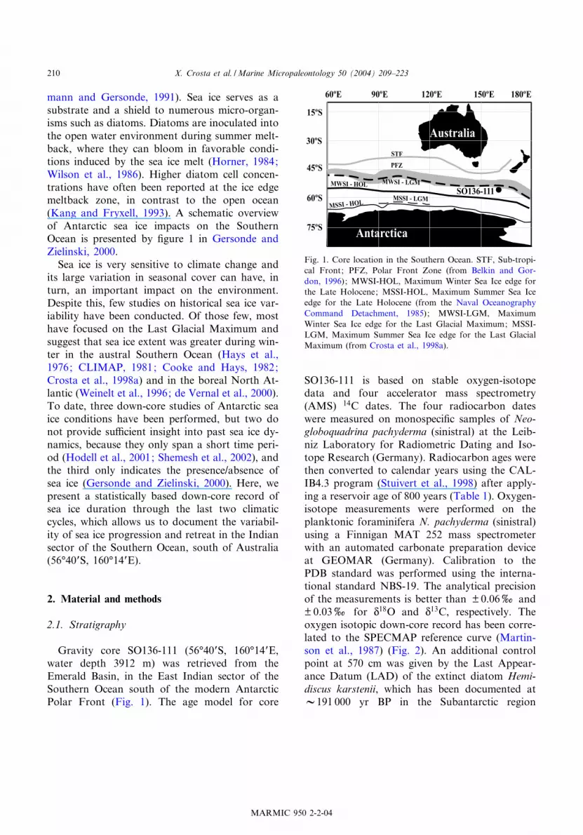
Gravity core SO136-111 (56‡40PS, 160‡14PE,water depth 3912 m) was retrieved from theEmerald Basin, in the East Indian sector of theSouthern Ocean south of the modern AntarcticPolar Front (Fig. 1). The age model for core

SO136-111 is based on stable oxygen-isotopedata and four accelerator mass spectrometry(AMS) 14C dates. The four radiocarbon dateswere measured on monospeci¢c samples of Neo-globoquadrina pachyderma (sinistral) at the Leib-niz Laboratory for Radiometric Dating and Iso-tope Research (Germany). Radiocarbon ages werethen converted to calendar years using the CAL-IB4.3 program (Stuivert et al., 1998) after apply-ing a reservoir age of 800 years (Table 1). Oxygen-isotope measurements were performed on theplanktonic foraminifera N. pachyderma (sinistral)using a Finnigan MAT 252 mass spectrometerwith an automated carbonate preparation deviceat GEOMAR (Germany). Calibration to thePDB standard was performed using the interna-tional standard NBS-19. The analytical precisionof the measurements is better than S 0.06x andS 0.03x for N

18O and N13C, respectively. The

oxygen isotopic down-core record has been corre-lated to the SPECMAP reference curve (Martin-son et al., 1987) (Fig. 2). An additional controlpoint at 570 cm was given by the Last Appear-ance Datum (LAD) of the extinct diatom Hemi-discus karstenii, which has been documented atV191 000 yr BP in the Subantarctic region

Fig. 1. Core location in the Southern Ocean. STF, Sub-tropi-cal Front; PFZ, Polar Front Zone (from Belkin and Gor-don, 1996); MWSI-HOL, Maximum Winter Sea Ice edge forthe Late Holocene; MSSI-HOL, Maximum Summer Sea Iceedge for the Late Holocene (from the Naval OceanographyCommand Detachment, 1985); MWSI-LGM, MaximumWinter Sea Ice edge for the Last Glacial Maximum; MSSI-LGM, Maximum Summer Sea Ice edge for the Last GlacialMaximum (from Crosta et al., 1998a).

MARMIC 950 2-2-04

X. Crosta et al. /Marine Micropaleontology 50 (2004) 209^223210

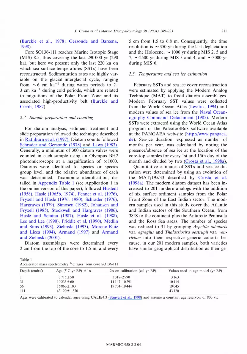
(Burckle et al., 1978; Gersonde and Barcena,1998).Core SO136-111 reaches Marine Isotopic Stage

(MIS) 8.5, thus covering the last 290 000 yr (290ka), but here we present only the last 220 ka onwhich sea surface temperatures (SSTs) have beenreconstructed. Sedimentation rates are highly var-iable on the glacial^interglacial cycle, rangingfrom V6 cm ka31 during warm periods to 2^3 cm ka31 during cold periods, which are relatedto migrations of the Polar Front Zone and itsassociated high-productivity belt (Burckle andCirrili, 1987).

2.2. Sample preparation and counting

For diatom analysis, sediment treatment andslide preparation followed the technique describedin Rathburn et al. (1997). Diatom counts followedSchrader and Gersonde (1978) and Laws (1983).Generally, a minimum of 300 diatom valves werecounted in each sample using an Olympus BH2photomicroscope at a magni¢cation of U1000.Diatoms were identi¢ed to species or speciesgroup level, and the relative abundance of eachwas determined. Taxonomic identi¢cation, de-tailed in Appendix Table 1 (see Application 1 inthe online version of this paper), followed Hustedt(1958), Hasle (1965b, 1974), Fenner et al. (1976),Fryxell and Hasle (1976, 1980), Schrader (1976),Hargraves (1979), Simosen (1982), Johansen andFryxell (1985), Stockwell and Hargraves (1986),Hasle and Semina (1987), Hasle et al. (1988),Lee and Lee (1990), Priddle et al. (1990), Medlinand Sims (1993), Zielinski (1993), Moreno-Ruizand Licea (1994), Armand (1997) and Armandand Zielinski (2001).Diatom assemblages were determined every

2 cm from the top of the core to 1.5 m, and every

5 cm from 1.5 to 6.8 m. Consequently, the timeresolution is V350 yr during the last deglaciationand the Holocene, V1000 yr during MIS 2, 5 and7, V2500 yr during MIS 3 and 4, and V3000 yrduring MIS 6.

2.3. Temperature and sea ice estimation

February SSTs and sea ice cover reconstructionwere estimated by applying the Modern AnalogTechnique (MAT) to fossil diatom assemblages.Modern February SST values were collectedfrom the World Ocean Atlas (Levitus, 1994) andmodern values of sea ice from the Naval Ocean-ography Command Detachment (1985). ModernSSTs were extracted using the World Ocean Atlasprogram of the PaleotoolBox software availableat the PANGAEA web-site (http://www.pangaea.de). Sea-ice duration, expressed as number ofmonths per year, was calculated by noting thepresence/absence of sea ice at the location of thecore-top samples for every 1st and 15th day of themonth and divided by two (Crosta et al., 1998a).Quantitative estimates of SSTs and sea-ice du-

ration were determined by using an evolution ofthe MAT5195/33 described by Crosta et al.(1998a). The modern diatom dataset has been in-creased to 201 modern analogs with the additionof six surface sediment samples from the PolarFront Zone of the East Indian sector. The mod-ern samples used in this study cover the Atlanticand Indian sectors of the Southern Ocean, from38‡S to the continent plus the Antarctic Peninsulaand the Ross Sea areas. The number of specieswas reduced to 31 by grouping Azpeitia tabularisvar. egregius and Thalassiosira oestrupii var. ven-rickae into their respective generic cohorts be-cause, in our 201 modern samples, both varietieshave similar geographical distribution as their ge-

Table 1Accelerator mass spectrometry 14C ages from core SO136-111

Depth (cmbsf) Age (14C yr BP) S 1c 2c on calibration (cal yr BP) Values used in age model (yr BP)

1 3 715S 50 3 318^2 990 3 16331 10 235S 60 11 147^10 291 10 41456 16 860S 100 19 704^19 444 19 045111 43 120S 1 870 43 120

Ages were calibrated to calendar ages using CALIB4.3 (Stuivert et al., 1998) and assume a constant age reservoir of 800 yr.

MARMIC 950 2-2-04

X. Crosta et al. /Marine Micropaleontology 50 (2004) 209^223 211

neric species (Crosta et al., 1998a). This version ofour transfer function will hereafter be referred toas MAT5201/31.Estimates are a simple average of the modern

values associated with the analogs chosen by theMAT. They are generally calculated on ¢ve ana-logs except when the dissimilarity threshold of0.25 (75% of resemblance between the fossil as-semblage and the modern one) is crossed. Belowthree analogs the MAT does not give an estimate;the fossil assemblage is considered to have nomodern equivalent.

The interdependence coe⁄cient between seaice duration and SSTs in the modern database(n=117) is 0.60, providing a determination coef-¢cient of 0.36. In our database, therefore, only36% of the modern distribution of sea ice isexplained by the modern distribution of SSTs,hence indicating that it is statistically possible toreconstruct both parameters with a single data-base.The reconstruction of the modern distribution

of SSTs and sea ice duration by MAT5201/31 issimilar to MAT5195/33, as used in Crosta et al.

Fig. 2. Age model of core SO136-111 based on four AMS 14C dates, indicated by asterisks (see also Table 1), and N18O of Neo-

globoquadrina pachyderma sinistral (thick line) compared to SPECMAP stack (thin line) (Martinson et al., 1987). LAD H. karste-nii, Last Appearance Datum of the extinct diatom Hemidiscus karstenii. Grey shaded areas represent glacial Marine IsotopicStages.

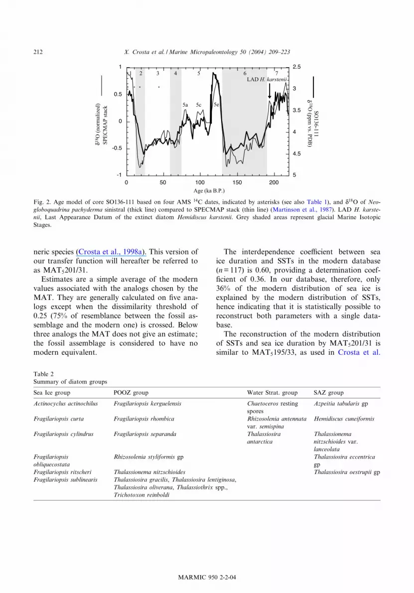
Table 2Summary of diatom groups

Sea Ice group POOZ group Water Strat. group SAZ group

Actinocyclus actinochilus Fragilariopsis kerguelensis Chaetoceros restingspores

Azpeitia tabularis gp

Fragilariopsis curta Fragilariopsis rhombica Rhizosolenia antennatavar. semispina

Hemidiscus cuneiformis

Fragilariopsis cylindrus Fragilariopsis separanda Thalassiosiraantarctica

Thalassionemanitzschioides var.lanceolata

Fragilariopsisobliquecostata

Rhizosolenia styliformis gp Thalassiosira eccentricagp

Fragilariopsis ritscheri Thalassionema nitzschioides Thalassiosira oestrupii gpFragilariopsis sublinearis Thalassiosira gracilis, Thalassiosira lentiginosa,

Thalassiosira oliverana, Thalassiothrix spp.,Trichotoxon reinboldi

MARMIC 950 2-2-04

X. Crosta et al. /Marine Micropaleontology 50 (2004) 209^223212

(1998a,b). The correlation coe⁄cients, mean stan-dard error of the estimate and mean residual are0.96, 0.95 and 0.75 for February SSTs, and 0.99,0.35 and 0.3 for sea ice cover, respectively (Fig.3), and are equivalent to the previous version ofthe Crosta et al. (1998a,b) transfer function. Theslopes of the linear regression between estimatedand observed SSTs (1.016) and sea ice presence(0.994) are, however, more robust in the new ver-sion (Fig. 3) than in the previous one (0.889 and0.993, respectively).Quantitative estimates have been restricted to

the upper 6.8 m because of non-analog situationsdeeper in the core in relation to high relativeabundances of the extinct diatom Hemidiscus kar-stenii.

3. Results

3.1. Down-core diatom assemblages

Sixty diatom species or groups of species wererecognized in core SO136-111, of which only 31were used in the transfer function. Diatom specieshaving a similar environmental preference, as de-termined by Q-mode factor analysis (Crosta et al.,1998a), were grouped together (Table 2) and theircumulative abundances plotted in correspondence

to SSTs and sea ice presence (Fig. 4). Four dia-tom groups were identi¢ed and de¢ned as the ‘SeaIce group’, represented by species linked to thepresence of sea ice, the ‘Permanent Open OceanZone group’ (POOZ group), represented by Ant-arctic open ocean species, the ‘Water Strati¢ca-tion group’, represented mainly by Chaetocerosresting spores, and the ‘Subantarctic Zone group’(SAZ group), represented by warm water species.Down-core relative abundances of the 31 speciesand of the diatom groups are detailed in Appen-dix Table 2 (see Application 2 in the online ver-sion of this paper).In core SO136-111, the ‘Sea Ice group’ is com-

posed of six species or species groups (Table 2), ofwhich Actinocyclus actinochilus, Fragilariopsis cur-ta and Fragilariopsis ritscheri are the most prom-inent. The ‘Sea Ice group’ is present in traceamounts during MIS 7 and increases rapidly atthe 7/6 transition to reach 2^3% of the diatomassemblage (Fig. 4). Sea ice diatoms account for2^3% of the assemblage during all MIS 6 anddecrease abruptly to nil at Termination II. Theyare almost absent during MIS 5, except duringcold stadials when they appear episodically. The‘Sea Ice group’ starts increasing again at 80 kaBP, more or less continuously, to reach a maxi-mum relative abundance of 4% at 23 ka BP.Abundance then drops within a few thousand

Fig. 3. Reconstruction of the modern distribution of February SSTs (a) and sea ice duration (b) by MAT5201/31 (modi¢ed fromCrosta et al., 1998a). The modern peri-Antarctic sediments used in this reconstruction cover the Atlantic and Indian sectors ofthe Southern Ocean from 35‡S to the continent plus the Antarctic Peninsula and Ross Sea areas. SSTs, Sea surface temperatures;R, correlation coe⁄cient; Mres, mean residual (the residual being the di¡erence between the observed value and the estimate);Msee, mean standard error of estimate (the standard error being the deviation of the ¢ve modern values associated with thechosen analogs).

MARMIC 950 2-2-04

X. Crosta et al. /Marine Micropaleontology 50 (2004) 209^223 213

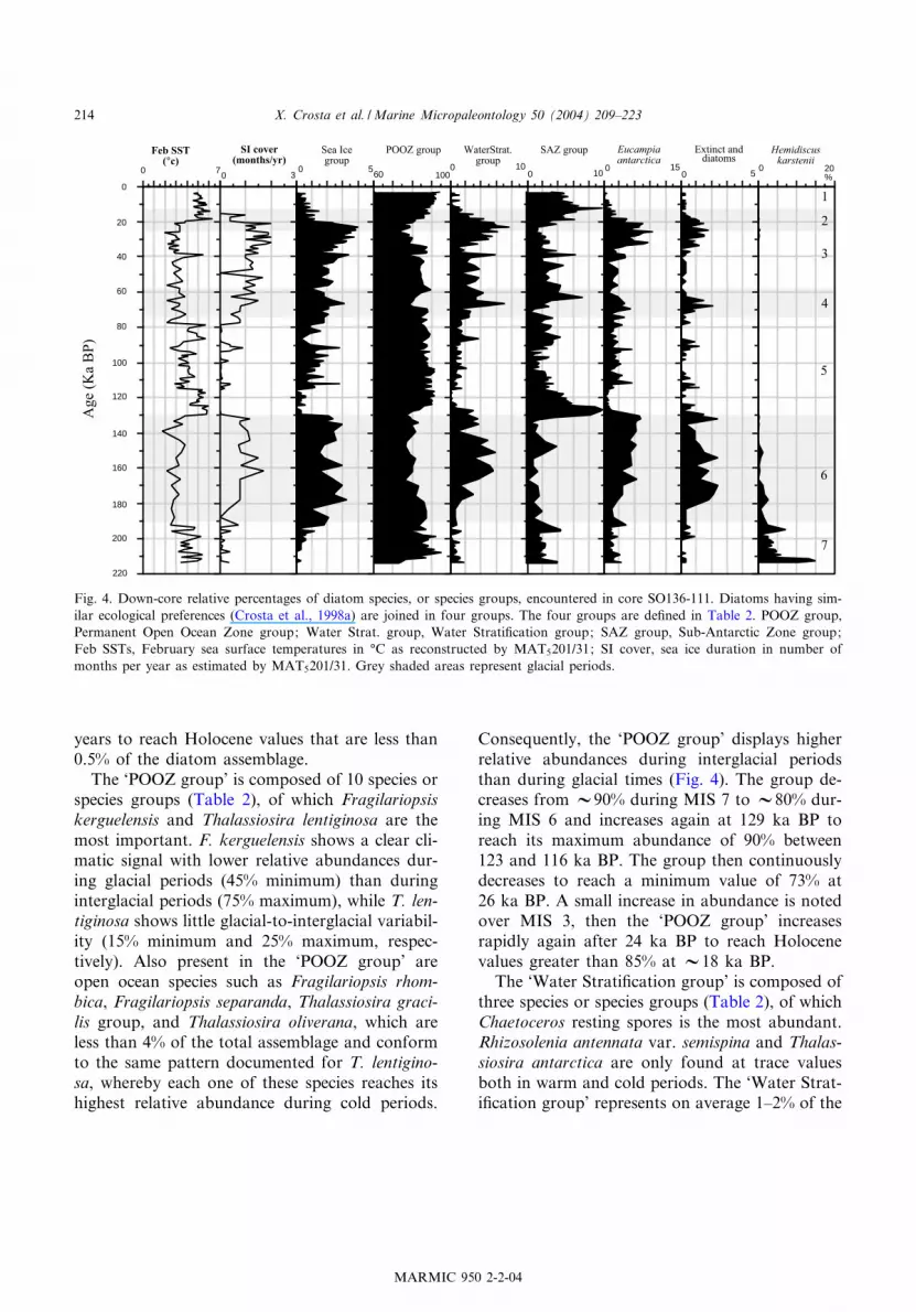
years to reach Holocene values that are less than0.5% of the diatom assemblage.The ‘POOZ group’ is composed of 10 species or

species groups (Table 2), of which Fragilariopsiskerguelensis and Thalassiosira lentiginosa are themost important. F. kerguelensis shows a clear cli-matic signal with lower relative abundances dur-ing glacial periods (45% minimum) than duringinterglacial periods (75% maximum), while T. len-tiginosa shows little glacial-to-interglacial variabil-ity (15% minimum and 25% maximum, respec-tively). Also present in the ‘POOZ group’ areopen ocean species such as Fragilariopsis rhom-bica, Fragilariopsis separanda, Thalassiosira graci-lis group, and Thalassiosira oliverana, which areless than 4% of the total assemblage and conformto the same pattern documented for T. lentigino-sa, whereby each one of these species reaches itshighest relative abundance during cold periods.

Consequently, the ‘POOZ group’ displays higherrelative abundances during interglacial periodsthan during glacial times (Fig. 4). The group de-creases from V90% during MIS 7 to V80% dur-ing MIS 6 and increases again at 129 ka BP toreach its maximum abundance of 90% between123 and 116 ka BP. The group then continuouslydecreases to reach a minimum value of 73% at26 ka BP. A small increase in abundance is notedover MIS 3, then the ‘POOZ group’ increasesrapidly again after 24 ka BP to reach Holocenevalues greater than 85% at V18 ka BP.The ‘Water Strati¢cation group’ is composed of

three species or species groups (Table 2), of whichChaetoceros resting spores is the most abundant.Rhizosolenia antennata var. semispina and Thalas-siosira antarctica are only found at trace valuesboth in warm and cold periods. The ‘Water Strat-i¢cation group’ represents on average 1^2% of the

Feb SST(°c)

0 7

SI cover(months/yr)

Sea Icegroup

0 105

Hemidiscuskarstenii

Extinct anddiatoms

Eucampiaantarctica

POOZ group WaterStrat.group

SAZ group

15 20%0

0 050

1001006030

140

Ag

e (K

a B

P)

0

200

180

160

120

100

80

60

40

20

220

2

4

6

1

3

5

7

Fig. 4. Down-core relative percentages of diatom species, or species groups, encountered in core SO136-111. Diatoms having sim-ilar ecological preferences (Crosta et al., 1998a) are joined in four groups. The four groups are de¢ned in Table 2. POOZ group,Permanent Open Ocean Zone group; Water Strat. group, Water Strati¢cation group; SAZ group, Sub-Antarctic Zone group;Feb SSTs, February sea surface temperatures in ‡C as reconstructed by MAT5201/31; SI cover, sea ice duration in number ofmonths per year as estimated by MAT5201/31. Grey shaded areas represent glacial periods.

MARMIC 950 2-2-04

X. Crosta et al. /Marine Micropaleontology 50 (2004) 209^223214

diatom assemblage during MIS 7 and MIS 5, andit accounts for 2^4% of the assemblage duringglacial periods (Fig. 4). The relative abundanceof the group episodically increases up to 6% at67 and 22 ka BP.The ‘SAZ group’ is composed of ¢ve species or

species groups (Table 2), of which the Azpeitiatabularis group, Thalassionema nitzschioides var.lanceolata and the Thalassiosira oestrupii groupare the most prominent. Their maximum relativeabundances are around 6%, 6% and 3%, respec-tively, during warm periods. Consequently, the‘SAZ group’ shows a clear climatic signal withlow relative abundance during cold periods andhigh relative abundance during warm periods(Fig. 4). Maximum relative abundances of 10%are encountered during climatic optima at 128^125 ka BP and 13^11 ka BP.The February SST signal in core SO136-111 is

chie£y linked to down-core variations in theabundance of the ‘POOZ group’ (Fig. 4). Thetwo records are nevertheless in disagreement dur-ing the early Holocene and the early MIS 5e,when SSTs are the warmest and when the‘POOZ group’ abundances are decreasing. SSTsare then a function of the high ‘SAZ group’ abun-dances. The sea ice signal is directly linked to thedown-core distribution of the ‘Sea Ice group’,although its peak abundance at 22 ka BP is notre£ected in the sea ice presence signal (Fig. 4). Atthis time, sea ice estimates may be reduced by thepeak abundance of the ‘Water Strati¢cationgroup’. This indicates that the ‘Water Strati¢ca-tion group’ has some relation to sea ice cover, butit is not the main contributor. Indeed, the analogsselected by the MAT5201/31 method through theglacial periods have been chosen from modern seaice edge samples with 2^5% of sea ice diatoms andalmost no Chaetoceros resting spores. Moreover,quantitative estimates are here very similar withor without Chaetoceros resting spores in the mod-ern database.The abundance of extinct reworked diatoms os-

cillates down-core between 0.5% (during intergla-cial periods) to 2% (maximum of the total diatomassemblages during cold intervals) (Fig. 4), indi-cating that the core is little a¡ected by reworkingand lateral transport.

3.2. Down-core reconstruction of SSTand sea ice

Although core SO136-111 is 9 m long, SSTsand sea ice are only reconstructed on the ¢rst6.8 m (last 213 ka BP) due to non-analog situa-tions deeper in the core caused by high relativepercentages of the extinct diatom Hemidiscus kar-stenii. Diatom preservation based on the size ofthe poroids, the number of valve fragments, thenumber of species, and the average dissimilaritybetween fossil and modern samples guaranteesgood analog situations in the ¢rst 6.8 m. Stan-dard deviations of the estimates calculated byMAT5201/31 are on average 1.5‡C during inter-glacial times and 2.5‡C during glacial times. Theaverage standard deviation of the sea ice estimatesis 1.1 months per year when sea ice is present. Theaverage dissimilarity (indicating the degree ofsimilarity between a fossil assemblage and thechosen analogs) is around 0.1. Down-core esti-mates SSTs and sea ice presence and their associ-ated standard errors are detailed in Appendix Ta-ble 3 (see Application 3 in the online version ofthis paper).February SSTs were 3^4‡C cooler during gla-

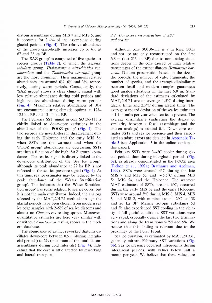
cial periods than during interglacial periods (Fig.5a), as already demonstrated in the POOZ area(Pichon et al., 1992a; Brathauer and Abelman,1999). SSTs were around 4‡C during the lateMIS 7 and MIS 5c, and V5.5‡C during MIS5e, MIS 5a, and the Holocene. The warmestMAT estimates of SSTs, around 6‡C, occurredduring the early MIS 5e and the early Holocene.SSTs were around 3‡C during MIS 6, MIS 4, MIS3, and MIS 2, with mimina around 2‡C at 138and 26 ka BP. Marine isotopic sub-stages 5dand 5b also experienced SST cooling in the vicin-ity of full glacial conditions. SST variations werevery rapid, especially during the last two termina-tions and along the transitions 5e/5d and 5/4. Webelieve that this ¢nding is relevant due to theproximity of the Polar Front.Sea ice duration, as estimated by MAT5201/31,

generally mirrors February SST variations (Fig.5b). Sea ice presence occurred infrequently duringinterglacial periods, with values below half amonth per year. We believe that these values are

MARMIC 950 2-2-04

X. Crosta et al. /Marine Micropaleontology 50 (2004) 209^223 215

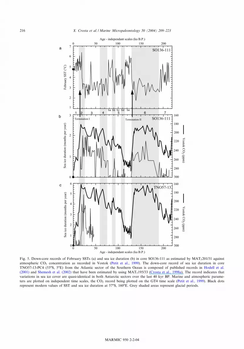
Fig. 5. Down-core records of February SSTs (a) and sea ice duration (b) in core SO136-111 as estimated by MAT5201/31 againstatmospheric CO2 concentration as recorded in Vostok (Petit et al., 1999). The down-core record of sea ice duration in coreTNO57-13-PC4 (53‡S, 5‡E) from the Atlantic sector of the Southern Ocean is composed of published records in Hodell et al.(2001) and Shemesh et al. (2002) that have been estimated by using MAT5195/33 (Crosta et al., 1998a). The record indicates thatvariations in sea ice cover are quasi-identical in both Antarctic sectors over the last 40 kyr BP. Marine and atmospheric parame-ters are plotted on independent time scales, the CO2 record being plotted on the GT4 time scale (Petit et al., 1999). Black dotsrepresent modern values of SST and sea ice duration at 57‡S, 160‡E. Grey shaded areas represent glacial periods.

MARMIC 950 2-2-04

X. Crosta et al. /Marine Micropaleontology 50 (2004) 209^223216

not relevant because they are smaller than 2c ofthe modern average standard error of 0.35 monthper year (Fig. 3b). The core location was thus seaice covered only during glacial stages. However,maximum estimates of sea ice for 2 months peryear indicate that the winter ice edge was justnorth of 57‡S at this longitude. The estimatesalso indicate that sea ice was never present duringsummer. Over the MIS 7/6 transition, sea icestarted to expand 193 ka BP to reach its maxi-mum duration, and thus extent, by 161 ka BP(Fig. 5b). Sea ice was then present at the corelocation V1.2 months per year on average until133 ka BP. The retreat of the ice cover occurredabruptly in one episode at Termination II. Thecore site was completely ice-free from 130 ka BPthrough V78 ka BP, except for one short period90 ka BP. At 78 ka BP, sea ice started to expandagain to reach a maximum duration of 2 monthsper year 28 ka BP. Sea ice then quickly vanishedfrom the core location in one episode 16 ka BP.Since 16 ka BP, sea ice has probably not reachedthe core site’s latitude.The SSTs and sea ice cover records are not

quite anti-correlated in either their timing or theirtrends. February SSTs lead sea ice expansion atinterglacial^glacial transitions and are almost si-multaneous with sea ice retreat at both Termina-tions. During the MIS 7/6 transition, FebruarySSTs decreased 194 ka BP, while sea ice coverincreased 193 ka BP, i.e. 1 ka later (Fig. 5a,b).During the MIS 5/4 transition SSTs decreased79 ka BP, leading sea ice expansion by 1 ka. Dur-ing both Terminations, SST and sea ice variationsare almost synchronous; both changed 133 and21 ka BP. Trends in SSTs and sea ice duration,as estimated by MAT5201/31, also show some dis-crepancies. SSTs tend to increase over the courseof MIS 6 until 147 ka BP when they suddenlydecrease for a few thousand years. The SSTdrop 147 ka BP is not re£ected by a subsequentincrease in sea ice duration (Fig. 5a,b). SST esti-mates are on average 3‡C during MIS 4 and MIS3, and around 2.6‡C through the LGM. Sea iceduration at the core location is continuously in-creasing during the same period. SSTs are there-fore not the sole factor in£uencing the sea icedynamics on glacial^interglacial cycles.

4. Discussion

4.1. Climatic implication of SST and sea icerecords

The down-core record of sea ice duration inSO136-111 is not continuous over the last twoclimatic cycles (Fig. 5b), being a re£ection of itsposition in the modern POOZ. Sea ice is thenexpected to be present at the core location onlyduring glacial times. The core is nevertheless suit-able to document the dynamics of sea ice advanceand retreat on glacial^interglacial transitions. Weobserve that the same sea ice growth and with-drawal pattern occurred over the core site duringMIS 6, MIS 4 and MIS 2. The advance phase insea ice coverage occurring at all interglacial^gla-cial transitions (Fig. 5b). The sea ice advance gen-erally lags the drop in SSTs by V1 ka (Fig. 5a).Sea ice appears to have stabilized and reachedmaximum duration at the end of the glacialstages. At the core location, the ice’s maximumduration was completed between 32 and 21 kaBP, similar to the evidence for maximum sea icepresence between 28 and 20 ka BP in coreTNO57-13-PC4 from the Atlantic sector of theSouthern Ocean (Shemesh et al., 2002) (Fig. 5c).From 32 to 21 ka BP, SSTs were not signi¢cantlylower than those during MIS 4 and MIS 6, indi-cating that SSTs are not the only factor determin-ing sea ice extent. Sea ice retreats very quickly insingle events when summer SSTs rise above 3.2‡C.Sea ice appeared and disappeared in less than a1000 years, con¢rming the sensitivity of this pa-rameter as shown by modeling studies (Gildorand Tziperman, 2000, 2001).Results from cores SO136-111 and TNO57-13-

PC4, from two distinct oceanic basins, indicatethat SSTs may be the major factor in determiningthe advance and retreat of sea ice in the EastIndian sector of the Southern Ocean at intergla-cial^glacial transitions and terminations. Theocean’s surface, however, needs to reach the crit-ical freezing temperature for sea ice to form(31.8‡C). We presume this would have beenachieved at the site of core SO136-111 duringwinter, since our minimum February SST esti-mates are at V2‡C. In the modern ocean, the

MARMIC 950 2-2-04

X. Crosta et al. /Marine Micropaleontology 50 (2004) 209^223 217

locations where our database indicates FebruarySSTs are 2‡C it also indicates that August SSTsare around 30.3‡C (Levitus, 1994). Such lowSSTs are presumed capable of sustaining sea icecover at the sea ice edge. We assume that theV1 ka lag in sea ice expansion related to thedrop in SSTs at interglacial^glacial transitions(Fig. 5a,b) is linked to a delay in reaching seaice sustainable SSTs. Conversely, at the intergla-cial^glacial terminations, the ocean surface isquickly warmed above the freezing temperatureat the core location. Sea ice retreat is thereforealmost synchronous to SST increases (Fig. 5a,b).Irrespective of these observations, results from

core SO136-111 indicate that SST changes cannotsolely explain the increase in sea ice duration dur-ing glacial periods, because surface oceanic tem-peratures were relatively stable during glacialtimes. An increase in SSTs during the course ofMIS 6 is found to be concomitant to an increaseof the sea ice duration (Fig. 5a,b). The sea iceadvance during glacial conditions, as expectedfrom the increase in sea ice duration, may thenbe related to positive feedbacks of sea ice on al-bedo, air temperature and meridional wind stress.Modeling studies have shown that sea ice expan-sion increases albedo and induces cooling of at-mospheric temperatures, which in turn results inthe creation of more sea ice (Gildor and Tziper-man, 2000, 2001). This positive feedback also in-creases the thermal gradient between the Equatorand the Austral Pole, leading to more vigorousmeridional winds that transport the newly formedsea ice northwards. These phenomena were espe-cially enhanced in the Weddell Sea region relativeto the open ocean, hence explaining why sea iceduration in the Atlantic sector was twice as highas that reported in the Indian sector of the South-ern Ocean. Evidence presented by Shemesh et al.(2002) indicates sea ice duration of 4 months peryear at 53‡S, 5‡E during MIS 2 in core TNO57-13-PC4, while here we estimate a sea ice durationof 2 months per year south of Tasmania in coreSO136-111 (Fig. 5b,c).We suggest that sea ice ceases its northward

expansion when an equilibrium state betweenfreezing, northward advection (under the controlof air^sea cooling) and melting at the sea ice edge

(under the control of oceanic heat input) is at-tained. This equilibrium is very fragile and a mi-nor variation of any factor is su⁄cient to promotea change in sea ice cover and, therefore, sea iceduration at a given location.

4.2. Sea ice impact on atmospheric CO2

concentrations

Modeling studies have shown that the SouthernOcean may drive glacial^interglacial variations ofatmospheric CO2 concentrations through biologi-cal (Sarmiento and Toggweiler, 1984; Moore etal., 2000) and physical processes (Toggweiler,1999; Stephens and Keeling, 2000). Increased gla-cial sea ice extent has been postulated to be re-sponsible for a 67 ppm lowering of atmosphericpCO2 (Stephens and Keeling, 2000). Although theamplitude of the CO2 reduction due to sea icechanges is still under debate (Morales Maquedaand Rahmstorf, 2002), there is geological evidencethat sea ice may control atmospheric CO2 varia-tions. Shemesh et al. (2002) have shown that thesouthward retreat of sea ice at Termination Ileads nutrient proxies by V1 ka and atmosphericpCO2 increase by V2 ka. They concluded thatsea ice may be the trigger to gas exchange andbiological activity variations impacting on atmo-spheric CO2 concentrations.Core SO136-111 extends our knowledge of sea

ice history back to MIS 7. An almost perfect ¢tbetween sea ice duration in core SO136-111 andVostok CO2 record can be observed over the last220 ka BP (Fig. 5b). Using the software Analys-eries (Paillard et al., 1993), the anti-correlationbetween the above-mentioned two records hasbeen calculated at 30.75. The correlation coe⁄-cient would be even better if negative sea ice val-ues were allowed when CO2 concentrations arevery high during MIS 5 and the Holocene. Evi-dence for the presence of sea ice disappears fromcore SO136-111 V21 ka BP (Fig. 5b) and fromcore TNO57-13 V20 ka BP (Fig. 5c), hence lead-ing the increase in atmospheric CO2 by V2^3 ka.At Termination II, our sea ice record is tuned tothe SPECMAP reference curve (Martinson et al.,1987) and lags the CO2 increase. But a recentstudy, based on uranium/thorium dating of corals

MARMIC 950 2-2-04

X. Crosta et al. /Marine Micropaleontology 50 (2004) 209^223218

Fig. 6. Comparison of February SSTs and sea ice duration in core SO136-111 with insolation curves (Berger, 1978). Parametersestimated by MAT5201/31 are represented by black lines; insolation curves are represented by grey lines. (a) SSTs versus insola-tion at 65‡N for the 15th of June, (b) SSTs versus insolation at 15‡N for the 15th of June, (c) SSTs versus insolation at 15‡S forthe 15th of January, (d) SSTs versus insolation at 60‡S for the 15th of January, (e) sea ice cover versus insolation at 65‡N forthe 15th of June, (f) sea ice cover versus insolation at 15‡N for the 15th of June, (g) sea ice cover versus insolation at 15‡S forthe 15th of January, (h) sea ice cover versus insolation at 60‡S for the 15th of January.

MARMIC 950 2-2-04

X. Crosta et al. /Marine Micropaleontology 50 (2004) 209^223 219

from the Bahamas (Henderson and Slowey, 2000),indicates that the mid-point of the penultimatedeglaciation should be 135S 2.5 ka BP. We calcu-lated the o¡set introduced by shifting the Termi-nation II mid-point from 130 ka BP (Martinson etal., 1987) to 135 ka BP (Henderson and Slowey,2000). We changed the age of Termination mid-point, discarded the three control points we hadfrom MIS 6 and used the LAD of Hemidiscuskarstenii as an external control point at 191 kaBP. Ages have been linearly interpolated betweenthe two dates by assuming a constant sedimenta-tion rate. Although we know it was certainly notthe case, this solution is the more robust becauseof the lack of control points other than SPEC-MAP for this period. The sea ice presence recordis then decreasing at 139.6 ka BP, instead of the133 ka BP when tuned to SPECMAP (Martinsonet al., 1987), hence leading the CO2 increase byV1.5 ka. In that case, the lead of sea ice retreatover CO2 increase at Termination II is thereforeof the same order as the one observed at Termi-nation I.If we cannot rule out the possibility that both

sea ice presence and atmospheric CO2 respondindependently to an external forcing factor, wethink that the close ¢t between the two parame-ters and the V2 ka lead of sea ice on CO2 con-centrations at glacial^interglacial terminationssupports modeling studies (Stephens and Keeling,2000), which suggest sea ice is the main control onatmospheric CO2 concentration changes on gla-cial^interglacial cycles. Additional continuousand high-resolution down-core records of sea iceduration are urgently required to determinewhether Antarctic sea ice can control glacial^in-terglacial cycles, through its impact on atmo-spheric pCO2 (Henderson and Slowey, 2000),and Pleistocene rapid climate instabilities, asstressed in recent modeling studies (Gildor andTziperman, 2000, 2001; Keeling and Stephens,2001a,b).

4.3. Relationship of sea ice duration to insolationchanges

Down-core records of SSTs and sea ice dura-tion in core SO136-111 have been compared to

summer and winter insolation variations fromNorthern and Southern Hemisphere low andhigh latitudes (Fig. 6). Insolation data are fromBerger (1978). The ¢t between Southern OceanSSTs and low-latitude insolation of the NorthernHemisphere is especially strong, particularly dur-ing the last climatic cycle (Fig. 6a,b). When theage is greater than 160 ka BP the relationship isaltered, certainly in relation to a less satisfactorytime control in core SO136-111. Conversely, therelationship between SSTs and Southern Hemi-sphere insolation is less obvious with low insola-tion synchronous to cold SSTs and warm SSTsover the last two climatic cycles (Fig. 6c,d). Thecorrelation between sea ice duration and insola-tion is even less obvious (Fig. 6e^h). It neverthe-less seems that sea ice is present only when mid-month summer insolation variations at low lati-tudes is reduced (Fig. 6f,g).Long-trend variations in Southern Ocean SSTs

and sea ice cover may then originate fromchanges in Northern Hemisphere low-latitude in-solation, as already hypothesized by Waelbroecket al. (1995) and Labeyrie et al. (1996). Insolationchanges may then be transferred to both hemi-spheres via atmospheric processes. The impacton SSTs is faster in the Southern Hemisphere inrelation to a quicker reaction time of the southernsurface waters (Labeyrie et al., 1996; Brathauerand Abelman, 1999). High Northern Hemispherelatitudes were covered by continental ice caps dur-ing glacial periods and induced a latency time toexternal forcing. Conversely, high SouthernOcean latitudes were covered by sea ice, whichreacted more rapidly to insolation changes. Var-iations in sea ice extent may, in turn, have a¡ectedthe upwelling branch of the thermohaline circula-tion and therefore the deep-water formation inthe North Atlantic as shown by modeling studies(Keeling and Stephens, 2001a,b). This can explainthe lag of variations in the £ux of NADW relativeto changes in the Southern Ocean (Brathauer andAbelman, 1999).

5. Conclusion

Deep-sea sediment core SO136-111 from

MARMIC 950 2-2-04

X. Crosta et al. /Marine Micropaleontology 50 (2004) 209^223220

56‡40PS, 160‡14PE provides the ¢rst quantitativereconstruction of sea ice duration over the lasttwo excentricity-controlled climatic cycles. Seaice advance at interglacial^glacial transitions andsea ice retreat at terminations were very rapid andmainly related to SST changes. Conversely, sea iceadvance during full glacial periods, when SSTswere relatively stable, is believed to result froma positive feedback of sea ice on atmospheric pro-cesses such as albedo, air temperatures and zonalwinds, thus enabling a northward migration ofthe winter ice edge to V55‡S at 160‡E.The close relationship between sea ice duration

and atmospheric CO2 concentration, as recordedin the Vostok ice core over the last 220 ka BP,argues for a control of CO2 changes by variationsin Antarctic sea ice extent. Changes in SouthernOcean ice cover, and SSTs, appear related to var-iations in low-latitude insolation of the NorthernHemisphere rather than local insolation. Becausesea ice cover surrounding the Southern Ocean ishighly sensitive, the response of sea ice to insola-tion variability would be quicker than in theNorthern Hemisphere. In return, the rapid varia-tions in Antarctic sea ice may have a¡ected thestability of the Austral upwelling branch of thethermohaline circulation through changes in thefreshwater budget, hence in£uencing the climateof the Northern Hemisphere, and possibly provid-ing the switch between glacial and interglacial pe-riods (Gildor and Tziperman, 2000, 2001; Keelingand Stephens, 2001a,b). To con¢rm the role ofAntarctic sea ice on global climate, additionalstudies of sea ice cover and extent are urgentlyrequired.

Acknowledgements

We thank Michel Cruci¢x, Jacques Giraudeau,Rainer Gersonde, Anne de Vernal, and FionaTaylor for constructive discussions. We alsothank Julianne Fenner and two anonymous re-viewers for helpful comments that improved themanuscript. We personally thank people from theSO136 TASQWA cruise. We also thank the La-mont-Doherty Earth Observatory Deep-Sea Sam-ple Repository that provided some surface sedi-

ments to improve our modern database. Financialsupport for this study was provided by CNRS(Centre National de la Recherche Scienti¢que),PNEDC (Programme National d’ Etude de la Dy-namique du Climat), and Missions Scienti¢quesdes Terres Australes et Antarctiques FrancXaises(IPEV-TAAF). This is a DGO Contribution No.1484.

References

Abelmann, A., Gersonde, R., 1991. Biosiliceous particle £ux inthe Southern Ocean. Mar. Chem. 35, 503^536.

Ackley, S.F., 1980. A review of sea-ice weather relationships inthe Southern Hemisphere. In: Allision, A. (Ed.), Proceed-ings of the Canberra Symposium: Sea Level, Ice, and Cli-matic Change, I. IAHS Publ. 131, 127^159.

Armand, L., 1997. The use of diatom transfer functions inestimating sea-surface temperature and sea-ice in coresfrom the southeast Indian Ocean. Ph.D. Thesis, AustralianNational University, Canberra.

Armand, L.K., Zielinski, U., 2001. Diatom species of the ge-nus Rhizosolenia from Southern Ocean sediments: Distribu-tion and taxonomic notes. Diatom Res. 16, 259^294.

Belkin, I.M., Gordon, A.L., 1996. Southern Ocean fronts fromthe Greenwich meridian to Tasmania. J. Geophys. Res. 101(C2), 3675^3696.

Bentley, C.R., 1981. Some aspects of the cryosphere and itsrole in climatic change. In: Denton, G.H., Hugues, T.J.(Eds.), The Last Great Ice Sheets. Wiley-Interscience, NewYork, pp. 207^220.

Berger, A., 1978. Long-term variations of caloric insolationresulting from the Earth’s orbital elements. Quat. Res. 9,139^167.

Brathauer, U., Abelman, A., 1999. Late Quaternary variationsin sea surface temperatures and their relationship to orbitalforcing recorded in the Southern Ocean (Atlantic sector).Paleoceanography 14, 135^148.

Budd, W.F., 1975. Antarctic sea-ice variations from satellitesensing in relation to climate. J. Glaciol. 15, 417^527.

Burckle, L.H., Clarke, D.B., Shackleton, N.J., 1978. Isochro-nous last-abundant-appearance datum (LAAD) of the dia-tom Hemidiscus karstenii in the sub-Antarctic. Geology 6,243^246.

Burckle, L.H., Cirrili, J., 1987. Origin of the diatom ooze beltin the Southern Ocean: implications for the late Quaternarypaleoceanography. Micropaleontology 33, 82^86.

CLIMAP, 1981. Seasonal reconstructions of the Earth’s sur-face at the Last Glacial Maximum. Geol. Soc. Am. MapChart Ser. MC-36.

Cooke, D.W., Hays, J.D., 1982. Estimates of Antarctic Oceanseasonal sea-ice cover during Glacial intervals. In: Crad-dock, C. (Ed.), Antarctic Geoscience. International Union

MARMIC 950 2-2-04

X. Crosta et al. /Marine Micropaleontology 50 (2004) 209^223 221

of Geological Sciences. The Union of Wisconsin Press, Se-ries B 4, pp. 1017^1025.

Crosta, X., Pichon, J.J., Burckle, L.H., 1998a. Application ofmodern analog technique to marine Antarctic diatoms: Re-construction of the maximum sea ice extent at the last gla-cial maximum. Paleoceanography 13, 284^297.

Crosta, X., Pichon, J.J., Burckle, L.H., 1998b. Reapprisal ofseasonal Antartic sea-ice extent at the last glacial maximum.Geophys. Res. Lett. 25, 2703^2706.

de Vernal, A., Hillaire-Marcel, C., Turon, J.L., Matthiessen,J., 2000. Reconstruction of sea-surface temperature, salinity,and sea-ice cover in the northern North Atlantic during thelast glacial maximum based on dinocyst assemblages. Can.J. Earth Sci. 27, 725^750.

Ebert, E.E., Schramm, J.L., Curry, J.A., 1995. Disposition ofsolar radiation in sea ice and upper ocean. J. Geophys. Res.C 100, 15965^15975.

Fenner, J., Schrader, H.J., Wienigk, H., 1976. Diatom phyto-plankton studies in the Southern Paci¢c Ocean, compositionand correlation to the Antarctic Convergence and its paleo-ecological signi¢cance. In: Hollister, C.D., Craddock, C.(Eds.), DSDP Init. Reports 35, 757^813.

Fisher, G., Fu«etterer, D., Gersonde, R., Honjo, S., Ostermann,D., Wefer, G., 1988. Seasonal variability of particle £ux inthe Weddell Sea and its relation to ice cover. Nature 335,426^428.

Foldvik, A., GammelsrEd, T., 1988. Notes on Southern Oceanhydrography, sea-ice and bottom water formation. Palaeo-geogr. Palaeoclimatol. Palaeoecol. 67, 3^17.

Fryxell, G.A., Hasle, G.R., 1976. The genus Thalassiosira :some species with a modi¢ed ring of central strutted pro-cesses. Nova Hedwigia, Beih. 54, 67^98.

Fryxell, G.A., Hasle, G.R., 1980. The marine diatom Thalas-siosira oestrupii : structure, taxonomy and distribution. Am.J. Bot. 67, 804^814.

Gersonde, R., Barcena, M.A., 1998. Revision of the upperPliocene-Pleistocene diatom biostratigraphy for the norma-tive belt of the Southern Ocean. Micropaleontology 44, 84^98.

Gersonde, R., Zielinski, U., 2000. The reconstruction of lateQuaternary Antarctic sea-ice distribution - the use of dia-toms as a proxy for sea-ice. Palaeogeogr. Palaeoclimatol.Palaeoecol. 162, 263^286.

Gildor, H., Tziperman, E., 2000. Sea ice as the glacial cycles’climate switch: Role of seasonal and orbital forcing. Pale-oceanography 15, 605^615.

Gildor, H., Tziperman, E., 2001. A sea ice climate switchmechanism for the 100-kyr glacial cycles. J. Geophys. Res.106 (C5), 9117^9133.

Gordon, A.L., 1991. The Southern Ocean: Its involvement inglobal change. In: Proceedings of the International Confer-ence on the Role of the Polar Regions in Global Change,June 11^15, 1990. University of Alaska Fairbanks, Fair-banks, AK, 249^255.

Hargraves, P.E., 1979. Studies on marine plankton diatoms.IV. Morphology of Chaetoceros resting spores. Nova Hed-wigia, Beih. 64, 99^120.

Hasle, G.R., 1965b. Nitzschia and Fragilariopsis speciesstudied in the light and electron microscope. III. The genusFragilariopsis. Skr. Nor. Vidensk. - Akad. Oslo 18, 1^45.

Hasle, G.R., 1974. Some marine plankton genera of the dia-tom family Thalassiosiraceae. Nova Hedwigia, Beih. 45, 1^67.

Hasle, G.R., Semina, H.J., 1987. The marine planktonic dia-toms Thalassiothrix longissima and Thalassiothrix antarcticawith comments on Thalassionema spp. and Synedra reinbol-dii. Diatom Res. 2, 175^192.

Hasle, G.R., Sims, P.A., Syversten, E.E., 1988. Two recentStellarima species: S. microtrias and S. stellaris (Bacillario-phyceae). Bot. Mar. 31, 195^206.

Hays, J.D., Lozano, J.A., Shackleton, N., Irving, G., 1976.Reconstruction of the Atlantic and Western Indian OceanSectors of the 18.000 BP Antarctic Ocean. In: Cline, R.M.,Hays, J.D. (Eds.), Investigation of Late Quaternary Pale-oceanography and Paleoclimatology. Geol. Soc. Am.Mem. 145, 337^372.

Henderson, G.M., Slowey, N.C., 2000. Evidence from U-Thdating against Northern Hemisphere forcing of the penulti-mate deglaciation. Nature 404, 61^66.

Hodell, D.A., Kanfoush, S.L., Shemesh, A., Crosta, X.,Charles, C.D., Guilderson, T.P., 2001. Abrupt cooling ofAntarctic surface waters and sea ice expansion in the SouthAtlantic sector of the Southern Ocean at 5000 cal yr BP.Quat. Res. 56, 191^198.

Horner, R., 1984. Do ice algae produce the spring phytoplank-ton bloom in seasonally ice-covered waters? In: Koeltz, O.(Ed.), Proceedings of the 7th Diatom Symposium, Philadel-phia, 1982. Koenigstein, pp. 401^409.

Hustedt, F., 1958. Diatomeen aus der Antarktis und dem Su«-datlaktik. Reprinted from ‘Deutsche Antarktishe Expedition1938/1939’, Band II. Geographische-Kartographische An-stalt ‘Mundus’, Hamburg, 191 pp.

Johansen, J.R., Fryxell, G.A., 1985. The genus Thalassiosira(Bacillariophyceae): studies on species occuring south of theAntarctic Convergence. Phycologia 24, 155^179.

Kang, S.H., Fryxell, G.A., 1993. Phytoplankton in the Wed-dell Sea, Antarctica: Composition, abundance and distribu-tion in water-column assemblages of the marginal ice-edgezone during austral autumn. Mar. Biol. 116, 335^348.

Keeling, R.F., Stephens, B.B., 2001a. Antarctic sea ice and thecontrol of Pleistocene climate instability. Paleoceanography16, 112^131.

Keeling, R.F., Stephens, B.B., 2001b. Correction to ‘Antarcticsea ice and the control of Pleistocene climate instability’.Paleoceanography 16, 330^334.

Labeyrie, L.D., Labracherie, M., Gorfti, N., Pichon, J.J.,Vautravers, M., Arnold, M., Duplessy, J.C., Paterne, M.,Michel, E., Duprat, J., Caralp, M., Turon, J.L., 1996. Hy-drographic changes of the Southern Ocean (Southeast Indi-an Sector) over the last 230 kyr. Paleoceanography 11, 57^76.

Laws, R.A., 1983. Preparing strewn slides for quantitative mi-croscopical analysis : A test using calibrated microspheres.Micropaleontology 24, 60^65.

MARMIC 950 2-2-04

X. Crosta et al. /Marine Micropaleontology 50 (2004) 209^223222

Lee, J.H., Lee, J.Y., 1990. A light and scanning electron mi-croscopic study on the marine diatom Roperia Tessalata(Roper)Grunow. Diatom Res. 5, 325^335.

Levitus, S., 1994. World Ocean Atlas, Disc 1, Objective: An-alysed Temperature Fields. U.S. Dep. Comm., Washington,DC.

Martinson, D.G., Pisias, N.G., Hays, J.D., Imbrie, J., Moore,T.C., Shackleton, N.J., 1987. Age dating and the orbitaltheory of the ice ages: Development of a high resolution 0to 300.000 year chronostratigraphy. Quat. Res. 27, 1^29.

Medlin, L.K., Sims, P.A., 1993. The transfert of Pseudonotiadoliolus to Fragilariopsis. Nova Hedwigia, Beih. 106, 323^334.

Moore, J.K., Abbott, M.R., Richman, J.G., Nelson, D.M.,2000. The Southern Ocean at the Last Glacial Maximum:A strong sink for atmospheric CO2. Glob. Biogeochem.Cycles 14, 455^475.

Morales Maqueda, M.A., Rahmstorf, S., 2002. Did Antarcticsea-ice expansion cause glacial CO2 decline? Geophys. Res.Lett. 29, 111^113.

Moreno-Ruiz, J.L., Licea, S., 1994. Observations on the valvemorphology of Thalassionema nitzschoides (Grunow) Hus-tedt. In: Marino, D., Montresoy, D. (Eds.), Proceedings ofthe 13th Symposium on Living and Fossil Diatoms, Mare-tea, Italy, 1^7 Sept., 1994. Biopress, Bristol, pp. 393^413.

Naval Oceanography Command Detachment, 1985. Sea IceClimatic Atlas: Volume 1, Antarctic. Asheville, Preparedunder Commander, Naval Oceanography Command.

Paillard, D., Labeyrie, L., Yiou, P., 1993. Macintosh programperforms time-series analysis. EOS Trans. AGU 77, 379.

Petit, J.R., Raynaud, D., Barkov, N.I., Barnola, J.M., Basile,I., Benders, M., Chappellaz, J., Davis, M., Delaygue, G.,Delmotte, M., Kotlyakov, V.M., Legrand, M., Lipenkov,V.Y., Lorius, C., Pepin, L., Ritz, C., Saltzman, E., Stieve-nard, M., 1999. Climate and atmospheric history of the past420 000 years from the Vostok ice core, Antarctica. Nature399, 429^436.

Pichon, J.J., Labeyrie, L.D., Bareille, G., Labracherie, M.,Duprat, J., Jouzel, J., 1992a. Surface water temperaturechanges in the high latitudes of the Southern Hemisphereover the Last Glacial-Interglacial cycle. Paleoceanography 7,289^318.

Priddle, J., Jordan, R.W., Medlin, L.K., 1990. Famille Rhizo-soleniaceae. In: Medlin, L.K., Priddle, J. (Eds.), Polar Ma-rine Diatoms. British Antarctic Survey, Natural Environ-ment Research Council, Cambridge, pp. 115^127.

Rathburn, A.E., Pichon, J.J., Ayress, M.A., DeDeckker, P.,1997. Microfossil and stable-isotope evidence for changesin Late Holocene paleoproductivity and paleoceanographicconditions in the Prydz Bay region of Antarctica. Palaeo-geogr. Palaeoclimatol. Palaeoecol. 131, 485^510.

Sarmiento, J.L., Toggweiler, J.R., 1984. A new model for the

role of the oceans in determining atmospheric pCO2. Nature308, 621^624.

Schrader, H.J., 1976. Cenozoic planktonic diatom biostratig-raphy of the Southern Paci¢c Ocean. In: Hollister, C.D.,Craddock, C., et al. (Eds.), DSDP Init. Reports 35, 605^671.

Schrader, H.J., Gersonde, R., 1978. Diatoms and Silico£agel-lates. Micropaleontological counting methods and tech-niques - An exercise on an eight meters section of the lowerPliocene of Capo Rossello. In: Zachariasse, A., et al. (Eds.),Utrecht Micropaleontol. Bull. 17, 129^176.

Shemesh, A., Hodell, D., Crosta, X., Kanfoush, S., Charles,C., Guilderson, T., 2002. Comparison between records ofSouthern Ocean sediments and polar ice CO2 during thelast glacial-interglacial transition. Paleoceanography 17,1056, 10.1029/2000PA000599.

Simosen, R., 1982. Note on the diatom genus Charcotia M.Peragallo. Bacillaria 5, 101^116.

Stephens, B.B., Keeling, R.F., 2000. The in£uence of Antarcticsea ice on glacial-interglacial CO2 variations. Nature 404,171^174.

Stockwell, D.A., Hargraves, P.E., 1986. Morphological vari-ability within resting spores of the marine diatom genusChaeoceros Ehrenberg. In: Ricard, M. (Ed.), Proceedingsof the 8th Symposium on Living and Fossil Diatoms. S.Koeltz, Koenigstein, pp. 81^95.

Stuivert, M., Reimer, P.J., Braziunas, T.F., 1998. High preci-sion radiocarbon age calibration for terrestrial and marinesamples. Radiocarbon 40, 1127^1151.

Toggweiler, J.R., 1999. Variation of atmospheric CO2 by ven-tilation of the ocean’s deepest water. Paleoceanography 14,571^588.

Waelbroeck, C., Jouzel, J., Labeyrie, L., Lorius, C., Labrach-erie, M., Stievenard, M., Barkov, N.I., 1995. A comparisonof the Vostok ice deuterium record and series from SouthernOcean core MD88-770 over the last two glacial-interglacialcycles. Clim. Dyn. 12, 113^123.

Weinelt, M., Sarnthein, M., P£aumann, U., Schulz, H., Jung,S., Erlenkeuser, H., 1996. Ice-free nordic seas during theLast Glacial Maximum? Potential sites of deepwater forma-tion. Paleoclimates 1, 283^309.

Wilson, D.L., Smith, W.O., Nelson, D.M., 1986. Phytoplank-ton bloom dynamics of the western Ross Sea ice-edge. I.Primary productivity and species speci¢c production.Deep-Sea Res. 33, 1375^1387.

Wu, X., Simmonds, I., Budd, W.F., 1997. Modeling of Ant-arctic Sea-ice in a General Circulation Model. J. Clim. 10,593^609.

Zielinski, U., 1993. Quantitative estimation of palaeoenviron-mental parameters of the Antarctic Surface Water in theLate Quaternary using transfer functions with diatoms.Ph.D. Thesis, Alfred Wegener Institute for Polar and Ma-rine Research, D-27568 Bremerhaven, 148 pp.

MARMIC 950 2-2-04

X. Crosta et al. /Marine Micropaleontology 50 (2004) 209^223 223