Extracting Expressive Performance Information

from Recorded Music

by

Eric David Scheirer

B.S. cum laude Computer ScienceB.S. Linguistics

Cornell University (1993)

Submitted to the Program in Media Arts and Sciences,School of Architecture and Planning

in partial fulfillment of the requirements for the degree of

Master of Science in Media Arts and Sciences

at the

MASSACHUSETTS INSTITUTE OF TECHNOLOGY

September 1995

© Massachusetts Institute of Technology 1995. All rights reserved.

Author.........................

Certified by ........... . .

Program in Media Arts and Sciences,School of Architecture and Planning

August 11, 1995

..................Barry Vercoe

Professor of Media Arts and SciencesThesis Supervisor

A ccepted by ...................... .... ...........Stephen A. Benton

Chairman, Departmental Committee on Graduate StudentsProgram in Media Arts and Sciences

-ASHUSETTS 1N, T

OF TECHNOLOGY

OCT 2 6 1995 atth

LIBRARIES

Extracting Expressive Performance Information

from Recorded Music

by

Eric David Scheirer

Submitted to the Program in Media Arts and Sciences,School of Architecture and Planning

on August 11, 1995, in partial fulfillment of therequirements for the degree of

Master of Science in Media Arts and Sciences

Abstract

A computer system is described which performs polyphonic transcription of known solopiano music by using high-level musical information to guide a signal-processing system.This process, which we term expressive performance extraction, maps a digital audio rep-resentation of a musical performance to a MIDI representation of the same performanceusing the score of the music as a guide. Analysis of the accuracy of the system is presented,and its usefulness both as a tool for music-psychology researchers and as an example of amusical-knowledge-based signal-processing system is discussed.

Thesis Supervisor: Barry VercoeTitle: Professor of Media Arts and Sciences

Extracting Expressive Performance Informationfrom Recorded Audio

by

Eric David Scheirer

Readers

C ertified by .... ............. ......... ..... . ...................................

John Stautner

Director of Software Engineering

Compaq Computer Corporation

Certified by...... ... . . .

Michael HawleyAssistant Professor of Media Arts and Sciences

Program in Media Arts and Sciences

Contents

1 Introduction and Background

1.1 Expressive Performance . . . . . . . . .

1.2 Transcription . . . . . . . . . . . . . . .

1.2.1 Existing systems . . . . . . . . .

1.3 Using Musical Knowledge . . . . . . .

1.4 Overview of Thesis . . . . . . . . . . . .

2 Description of Algorithms

2.1 Initial Score Processing . . . . . . . . . . . . . . . . . .

2.1.1 The score-file . . . . . . . . . . . . . . . . . . . .

2.1.2 Extracted score-file information . . . . . . . . .

2.2 Tuning . . . . . . . . . . . . . . . . . . . . . . . . . . . .

2.2.1 Global tuning via sweeping reference frequency

2.2.2 Potential improvements to tuning algorithm . .

2.3 Main Loop . . . . . . . . . . . . . . . . . . . . . . . . .

2.3.1 Onset extraction . . . . . . . . . . . . . . . . . .

2.3.2 Release Extraction . . . . . . . . . . . . . . . . .

2.3.3 Amplitude/Velocity Measurement . . . . . . . .

2.3.4 Tempo Re-Estimation . . . . . . . . . . . . . . .

2.3.5 Outputs . . . . . . . . . . . . . . . . . . . . . . .

3 Validation Experiment

3.1 Experimental Setup . . . . . . . . . . . . . . . . . . . . . . . . . . . . . . .

3.1.1 Equipment . . . . . . . . . . . . . . . . . . . . . . . . . . . . . . . .

3.1.2 Performances . . . . . . . . . . . . . . . . . . . . . . . . . . . . . . .

6

6

7

8

. . . . . . . . . 10

. .. . . . . 11

12

. . . . . . 13

. . . . . . 13

. . . . . . 16

. . . . . . 17

. . . . . . 17

. . . . . . 18

. . . . . . 18

. . . . . . 19

. . . . . . 25

. . . . . . 25

. . . . . . 27

. . . . . . 28

3.2 Results . . . . . . . . . . . . . . . . . . . . .

3.2.1 Onset Timings . . . . . . . . . . . . .

3.2.2 Release Timings . . . . . . . . . . . .

3.2.3 Amplitude/Velocity . . . . . . . . . .

4 Discussion

4.1 Stochastic Analysis of Music Performance

4.2 Polyphonic Transcription . . . . . . . . . . .

4.3 Evidence-Integration Systems . . . . . . . . .

4.4 Future Improvements to System . . . . . . .

4.4.1 Release timings . . . . . . . . . . . . .

4.4.2 Timbre modeling . . . . . . . . . . . .

4.4.3 Goodness-of-fit measures . . . . . . .

4.4.4 Expanded systems . . . . . . . . . . .

4.5 The Value of Transcription . . . . . . . . . .

. . . . . . . . . . . . . . . . . 33

. . . . . . . . . . . . . . . . . 33

. . . . . . . . . . . . . . . . . 39

. . . . . . . . . . . . . . . . . 41

44

. . . . . . . . . . . . . . . . . 44

. . . . . . . . . . . . . . . . . 46

................. 47

................. 47

................. 47

................. 48

................. 48

................. 49

.. . .. .. .. .. .. ... 50

5 Conclusion

5.1 Current state of the system . . . . . . . . . . . . . . . . . . . . . . . . . . .

5.2 Concluding Remarks . . . . . . . . . . . . . . . . . . . . . . . . . . . . . .

6 Acknowledgments

Chapter 1

Introduction and Background

In this thesis, we describe a computer system which performs a restricted form of musical

transcription. Given a compact disc recording or other digital audio representation of

a performance of a work of solo piano music, and the score of the piece of music in

the recording, the system can extract the expressive performance parameters encoded in the

recording - the timings (onset and release) and velocities (amplitudes) of all the notes in

the performance.

This initial chapter discusses the main tasks investigated - expressive performance

analysis and musical transcription - and a discussion of the advantages of using the score

to guide performance extraction. A section describing the content of the rest of the thesis

concludes.

1.1 Expressive Performance

When human musicians perform pre-composed music, their performances are more than

a simple reading of the notes on the page in front of them; they add expressive variation

in order to add color, individuality, and emotional impact to the performance. As part of

the process of building music-understanding computer systems, we would like to study

and analyze human expressive performance. Such analysis helps with the goal of building

machines that can both understand and produce humanistic musical performances.

Typically, research into expressive performance - for example, that of Palmer [16] -

uses sophisticated equipment such as the B6sendorfer optical-recording piano to transcribe

performances by expert pianists into symbolic form for analysis by the researcher. This

method has several disadvantages; most notably, that such equipment is expensive and

not available to every researcher, and that the range of performers whose performances

can be analyzed is limited to those who are willing and able to "come into the laboratory"

and work with the music-psychological researcher.

Construction of a system which performed automatic transcription of audio data (from

compact discs, for example) would greatly aid the process of acquiring symbolic musical

information to be used for analysis of expressive musical performances. It would allow

researchers to collect data of this sort in their own laboratory, perhaps using only a typical

personal computer; and it would allow the use of performances by many expert perform-

ers, including those who are no longer living, to be analyzed and compared. There is

an extremely large "database" of digital music available recorded on compact disc, and

robust automated methods for processing it into symbolic form would allow us to bring

all of it to bear.

Typical methods for transcription (see section 1.2.1 below) work via a signal-processing

approach exclusively; that is, to attempt to build digital filtering systems for which the

input is the audio signal and the output is a symbolic stream corresponding to the written

music. Such systems have met with limited success, but in general cannot deal with music

in which more than two-voice polyphony is present.

However, due to the nature of the problem which we are attempting to solve, we

can place additional restrictions on the form of the system; in particular, a system which

takes as known the piece of music being performed can make use of the information in

the music to extract with high precision the expressive parameters (timing and amplitude

information) present in a particular performance. Stated another way, if we take as known

those aspects of the music which will remain constant between performances, it becomes

much easier to extract the features which vary between performances.

1.2 Transcription

Musical transcription of audio data is the process of taking a digital audio stream - a

sequence of sampled bits corresponding to the sound waveform - and extracting from it

the symbolic information corresponding to the high-level musical structures that we might

see on a page. This is, in general, an extremely difficult task; we are still a great distance

from being able to build systems which can accomplish it generally for unknown music.

The difficulty comes from the fact that it is often difficult to distinguish the fundamental

frequencies of the notes in the musical score from their overtones, and consequently to

determine exactly how many notes are being played at once.

It is precisely this problem that use of the score helps us to avoid; we know exactly

which notes will be occurring in the performance, and can make a fairly accurate guess of

their order of occurrence, if not their onset timings. As we shall see, once we are armed

with this information, it is a significantly easier problem to extract accurate timings from

the digital audio stream.

Palmer [16] suggests certain levels of timing accuracy which can be understood as

benchmarks for a system which is to extract note information at a level useful for under-

standing interpretation. For example, among expert pianists, the melody of a piece of

music typically runs ahead of its accompaniment; for chords, where it is indicated that

several notes are to be struck together, the melody note typically leads by anywhere from

10-15 ms to 50-75 ms, or even more, depending on the style of the music. Thus, if we are

to be able to use an automated system for understanding timing relationships between

melodies and harmony, it must be able to resolve differences at this level of accuracy or

finer.

5 ms is generally taken as the threshold of perceptual difference (JND) for musical

performance [4]; if we wish to be able to reconstruct performances identical to the original,

the timing accuracy must be at this level or better.

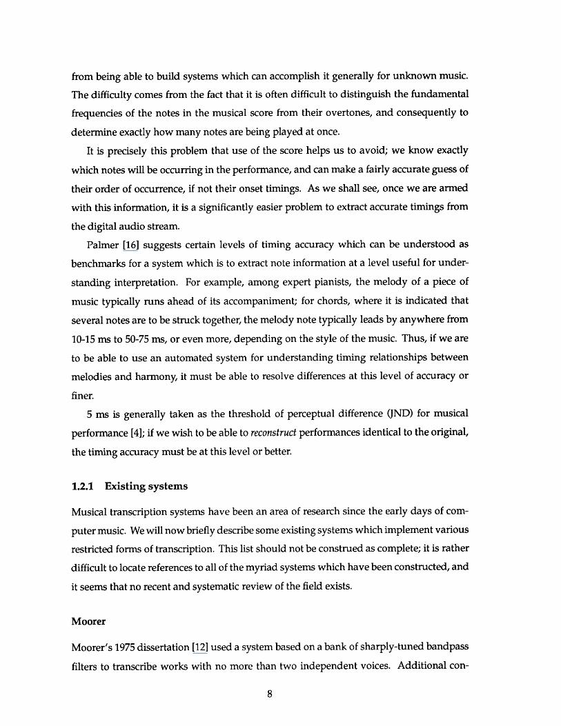
1.2.1 Existing systems

Musical transcription systems have been an area of research since the early days of com-

puter music. We will now briefly describe some existing systems which implement various

restricted forms of transcription. This list should not be construed as complete; it is rather

difficult to locate references to all of the myriad systems which have been constructed, and

it seems that no recent and systematic review of the field exists.

Moorer

Moorer's 1975 dissertation [12] used a system based on a bank of sharply-tuned bandpass

filters to transcribe works with no more than two independent voices. Additional con-

straints were placed on the allowable musical situations for input: notes must be at least

80 ms in duration, voices must not cross, and simultaneous notes cannot occur where one

note's fundamental frequency corresponds to an overtone of the other.

Within this framework, the system was a success at transcribing violin and guitar duets.

Only rough timing accuracy was required, as the results were "quantized" to be similar to

the original score.

Stautner

In his 1983 MS thesis, Stautner [21] used frequency-domain methods to attempt to model

the human auditory system, basing his filter parameters on findings from research into

the auditory physiology. He combined this so-called "auditory transform" with principal

components analysis techniques, and was able to use the resulting system to detect onsets

in performances on pitched tabla drums.

Schloss and Bilmes

Schloss [20] and Bilmes [1], in 1985 and 1993 respectively, built systems which could tran-

scribe multi-timbral percussive music for the purpose of analyzing its expressive content.

Both were successful, although they had slightly different goals. Schloss's work, like

Moorer's, was attempting to extract human-readable transcription, and was not appar-

ently able to handle multiple simultaneous onsets. This system was, however, successful

at reproducing notation of human drum performance.

Bilmes's transcription system was part of a larger system for the analysis of expressive

timing in percussive music. It modeled small deviations in timing around an overall

tempo structure, and could extract multiple simultaneous or nearly-simultaneous onsets

by different instruments.

Maher

Maher's system ([10], [11]) build on Moorer's work, attempting to ease some of the restric-

tions there. His system, also for duet transcription, does allow harmonically-related on-

sets to occur simultaneously. It requires that the voices are restricted to "non-overlapping"

ranges; that is, that the lowest note of the upper voice be higher than the highest note of the

lower. With these constraints, the system successfully transcribes vocal, clarinet-bassoon,

and trumpet-tuba duets.

Inokuchi et al

Seiji Inokuchi and his collaborators at Osaka University in Japan have been conducting

research into transcription for many years. Unfortunately, many of the references for their

work are not yet available in English. What publications are available [7] suggest that

their work is frequency-domain based, and can cope with a variety of musical situations,

including the "ambiguity of the human voice" and several-voice polyphony.

Hawley

Hawley describes a system for frequency-domain multi-voice transcription of piano music

in his PhD dissertation [5]. Although relatively few details are provided, it seems to be

able to handle two or more simultaneous notes. It is not clear how robust the system is, or

to what degree it works in a stand-alone automated fashion.

1.3 Using Musical Knowledge

Traditionally, transcription systems have been built via signal processing from the bottom

up. The method we examine here for performing transcription contains two layers: a high-

level music-understanding system which informs and constrains a low-level signal-processing

network.

Why cheating is good

It seems on the surface that using the score to aid transcription is in some ways cheating, or

worse, useless - what good is it to build a system which extracts information you already

know? It is our contention that this is not the case; in fact, score-based transcription is an

useful restriction of the general transcription problem.

It is clear that the human music-cognition system is working with representations

of music on many different levels which guide and shape the perception of a particular

musical performance. Work such as Krumhansl's tonal hierarchy [8] and Narmour's multi-

layered grouping rules [13], [14] show evidence for certain low- and mid-level cognitive

representations for musical structure. Syntactic work such as Lerdahl and Jackendoffs' [91,

while not as well-grounded experimentally, suggests a possible structure for higher levels

of music cognition.

While the system described in this thesis does not attempt to model the human music-

cognition system per sel, it seems to make a great deal of sense to work toward multi-layered

systems which deal with musical information on a number of levels simultaneously. This

idea is similar to those presented in Oppenheim and Nawab's recent book [151 regarding

symbolic signal processing.

From this viewpoint, score-aided transcription can be viewed as a step in the direction of

building musical systems with layers of significance other than a signal-processing network

alone. Systems along the same line with less restriction might be rule-based rather than

score-based, or even attempt to model certain aspects of human music cognition. Such

systems would then be able to deal with unknown as well as known music.

1.4 Overview of Thesis

The remainder of the thesis contains four chapters. Chapter 2 will describe in detail the

algorithms developed to perform expressive performance extraction. Chapter 3 discusses

a validation experiment conducted utilizing a MIDI-recording piano and providing quan-

titative data on the accuracy of the system. Chapter 4, Discussion, considers a number of

topics: the use of the system and the accuracy data from chapter 3 to perform stochastic

analysis of expressively performed music, the success of the system as an example of an ***

evidence-integration or multi-layered system, possible future improvements to the system,

both in the signal-processing and architectural aspects, and some general thoughts on the

transcription problem. Finally, chapter 5 provides concluding remarks on the usefulness

of the system.

'And further, it is not at all clear how much transcription the human listener does, in the traditional senseof the word - see section 4.5

Chapter 2

Description of Algorithms

In this chapter, we discuss in detail the algorithms currently in use for processing the score

file and performing the signal processing analysis1 . A flowchart-style schematic overview

of the interaction of these algorithms is shown in figure 2-1.

Figure 2-1: Overview of System Architecture

'All code is currently written in MATLAB and is available from the author via the Internet. E-maileds @media .mit. edu for more information

Briefly, the structure is as follows: a initial score-processing pass determines predicted

structural aspects of the music, such as which notes are struck in unison, which notes

overlap, and so forth. We also use the score information to help calculate the global tuning

(frequency offset) of the audio signal. In the main loop of the system, we do the following

things:

" Find releases and amplitudes for previously discovered onsets.

" Find the onset of the next note in the score.

" Re-examine the score, making new predictions about current local tempo in order to

guess at the location in time of the next onset.

Once there are no more onsets left to locate, we locate the releases and measure the

amplitudes of any unfinished notes. We then write the data extracted from the audio file

out as a MIDI (Musical Instrument Digital Interface) text file. It can be converted using

standard utilities into a Standard Format MIDI file which can then be resynthesized using

standard MIDI hardware or software; it is also easy to translate this format into other

symbolic formats for analysis.

We now describe each of these components in detail, discussing their current operation

as well as considering some possibilities for expanding them into more robust or more

accurate subsystems.

2.1 Initial Score Processing

The goal of the initial score processing component of the system is to discover "surface"

or "syntactic" aspects of the score which can be used to aid the signal-processing compo-

nents. This computation is relatively fast and easy, since we are only performing symbolic

operations on well-organized, clean, textual data. This step is performed before any of the

digital audio processing begins.

2.1.1 The score-file

A few words about the organization and acquisition of the score-file are relevant at this

point. For the examples used in this thesis, the data files were created by hand, keying in

4 4 4 801 125 250 622 250 375 633 375 500 554 500 750 545 750 1000 556 1125 1187 577 1187 1250 588 1250 1375 609 1375 1437 58

10 1437 1500 5711 1500 1750 5812 1625 1750 6713 1750 2000 5514 1750 1875 7015 1875 2000 6216 2000 2250 61

Figure 2-2: The score-file representation of the first two bars of the Bach example (fig 2-3.),which is used in the validation experiment in Ch. 3.

a numeric representation of the score as printed in musical notation. An example of the

score-file is shown in figure 2-2.

The first line of the score-file contains the time signature and metronome marking for

the music. The first two values are the meter (4/4 time, in this case), and the second are the

tempo marking (quarter note = 80). The subsequent lines contain the notes in the score,

one note per line. Each bar is divided into 1000 ticks; the second and third columns give

the onset and release times represented by the note's rhythmic position and duration. The

fourth column is the note's pitch, in MIDI pitch number (middle C = 60, each half-step up

or down increases or decreases the value by one).

There is still useful information in the notated representation that is not preserved in

this data format. For example, the printed score of a piece of music (fig. 2-3) groups

the notes into voices; this aids the performer, and could potentially be a guide to certain

aspects of the extraction process - for example, building in an understanding of the way

one note in a voice leads into the next.

There are also miscellaneous articulation marks like staccato/legato, slurs, and pedal

markings which affect the performer's intention for the piece. A rough estimate of these

could be included by altering the timings of the note - the release timing in particular -

Mo~to Mepawq & Thw~ rvtr

a-4.

10 PON

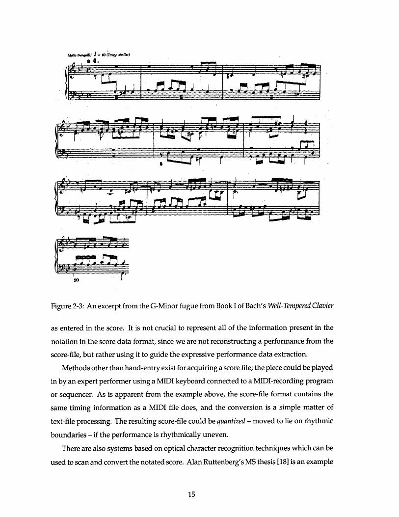
Figure 2-3: An excerpt from the G-Minor fugue from Book I of Bach's Well-Tempered Clavier

as entered in the score. It is not crucial to represent all of the information present in the

notation in the score data format, since we are not reconstructing a performance from the

score-file, but rather using it to guide the expressive performance data extraction.

Methods other than hand-entry exist for acquiring a score file; the piece could be played

in by an expert performer using a MIDI keyboard connected to a MIDI-recording program

or sequencer. As is apparent from the example above, the score-file format contains the

same timing information as a MIDI file does, and the conversion is a simple matter of

text-file processing. The resulting score-file could be quantized - moved to lie on rhythmic

boundaries - if the performance is rhythmically uneven.

There are also systems based on optical character recognition techniques which can be

used to scan and convert the notated score. Alan Ruttenberg's MS thesis [18] is an example

of such a system.

2.1.2 Extracted score-file information

The specific kinds of syntactic information which are extracted from the score-file are those

which have an influence on the attack- and release-finding algorithms described in the next

section. In particular:

* We are interested in knowing whether notes overlap or not. In particular, we can tag

a note as monophonic if there are no notes overlapping it at all. The first few notes

of the Bach fugue shown in figure 2-3 are examples of monophonic notes. If a, and

a2 are the attack (onset) times of two notes as given in the score, and r, and r2 their

release times, then the notes overlap if and only if

a1 2 a2 and a1 < r2

or r1 2 a2 and ri r2

or a2 > a1 and a2 < rl

or r2 a1 and r2 ri.

For each note, we keep track of all the other notes which overlap it, and tag it as

monophonic if there are none.

* We also wish to know what notes are struck simultaneously as a chord with what

other notes. This processing is simple - just compare the attack times of all pairs of

notes, and mark the ones that are simultaneous. If we are working from a score-file

which is not absolutely metronomic (for example, one which was played in via a

MIDI keyboard by an expert performer), we can use a "simultaneous within c" rule

instead.

* The final task done by the score-processing component is to use the metronome

marking from the score to guess timings for all of the attacks and releases based

on their rhythmic placements and durations. These timings will be adjusted as we

process the digital audio representation and are able to estimate the actual tempo,

which is rarely the same as the notated tempo.

2.2 Tuning

2.2.1 Global tuning via sweeping reference frequency

It is important, since we are often using very narrow-band filters in the processing of

the audio signal, that the center frequencies of the filters be as well-tuned to the piano

recorded in the signal as possible. Fig 2-4 shows the difference between using a filter

which is out-of-tune and using one which is in-tune with the audio signal. The graph

shows the RMS power of the A above middle C, played on a piano tuned to a reference

frequency of approximately 438 Hz, filtered in one case through a narrow bandpass filter

with center frequency 438 Hz, and in the second through a filter with the same Q, but with

center frequency 432 Hz.

Filter in Tune with Signal0

% -10

-20

Filter out-of-Tune with Signal

0.80.4Time (s)

Figure 2-4: Ripple occurs when the bandpass filters are not in tune with the audio signal.

The signal filtered with the out-of-tune filter has a "rippled" effect due to phasing with

the filter, while the filter which is in-tune has a much cleaner appearance. We also can see

that the total power, calculated by integrating the curves in fig 2-4, is greater for the in-tune

than the out-of-tune filter. This suggests a method for determining the overall tuning of

the signal - sweep a set of filters at a number of slightly different tunings over the signal,

and locate the point of maximum output power:

p = argmax J[A(t) * H(t, r)dt]2

r

where A(t) is the audio signal and H (t, r) is a filter-bank of narrow bandpass filters, with

the particular bands selected by examining the score and picking a set of representative,

frequently-occuring pitches, tuned to reference frequency r. The result p is then the best-

fitting reference frequency for the signal.

2.2.2 Potential improvements to tuning algorithm

This method assumes that the piano making the recording which is being used as the audio

signal is perfectly in-tune with itself; if this is not the case, it would be more accurate,

although much more computation-intensive, to tune the individual pitches separately.

It is not immediately clear whether this is an appropriate algorithm to be using to

calculate global tuning for a signal in the first place. We are not aware of any solutions

in the literature to this problem, and would welcome comments. The smoothness of the

curve in figure 2-5, which plots the power versus the reference tuning frequency, suggests

that the algorithm is well-behaved; and the fact that the peak point (438 Hz) does line up

with the actual tuning of the signal (determined with a strobe tuner) makes it, at least, a

useful ad hoc strategy in the absence of more well-grounded approaches.

2.3 Main Loop

The main loop of the system can be viewed as doing many things roughly in parallel:

extracting onsets and releases, measuring amplitudes, estimating the tempo of the signal,

and producing output MIDI and, possibly, graphics. As the system is running on a single-

processor machine, the steps actually occur sequentially, but the overall design is that of a

system with generally parallel, interwoven components - the release detector is dependant

on the onset detector; and both are dependant on and depended on by the tempo predictor.

It should be understood that the signal-processing methods developed for this system

are not particularly well-grounded in piano acoustics or analysis of the piano timbre; most

580

0

5 0 0 -- - -- -- - .. . .. .. .. .. .-- -- --. .. ..- --.-- -- - - -- -.-- - --- - - -- - -

4 6 0 -- - -- . .. . . . . . .. . . . . . .. . . . . . .. . . . .

4 40 --- -- - . . .. .. . .. . .. .-- -- -. ...--- -. ..---. .-.-

420435 440 445

Reference pitch (Hz)

Figure 2-5: The behavior of the tuning algorithm.

of the constants and thresholds discussed below were derived in an "ad-hoc" fashion

through experimentation with the algorithms. It is to be expected that more careful

attention to the details of signal processing would lead to improved results in performance

extraction.

2.3.1 Onset extraction

The onset-extracting component is currently the most well-developed and complex piece

of the signal-processing system. It uses information from the score processing and a num-

ber of empirically-determined heuristics to extract onsets within a given time-frequency

window.

In summary, there are four different methods that might be used to extract onset timings

from the signal; the various methods are used depending upon the contextual information

extracted from the score, and further upon the patterns of data found in the audio signal.

We will discuss each of them in turn.

High-frequency power

When the score information indicates that the note onset currently under consideration is

played monophonically, we can use global information from the signal to extract its exact

timing; we are not restricted to looking in any particular frequency bands. One very

accurate piece of the global information is the high-frequency power - when the hammer

strikes the string to play a particular note, a "thump" or "ping" occurs which includes

a noise burst at the onset. If we can locate this noise burst, we have a very accurate

understanding of where this onset occurred.

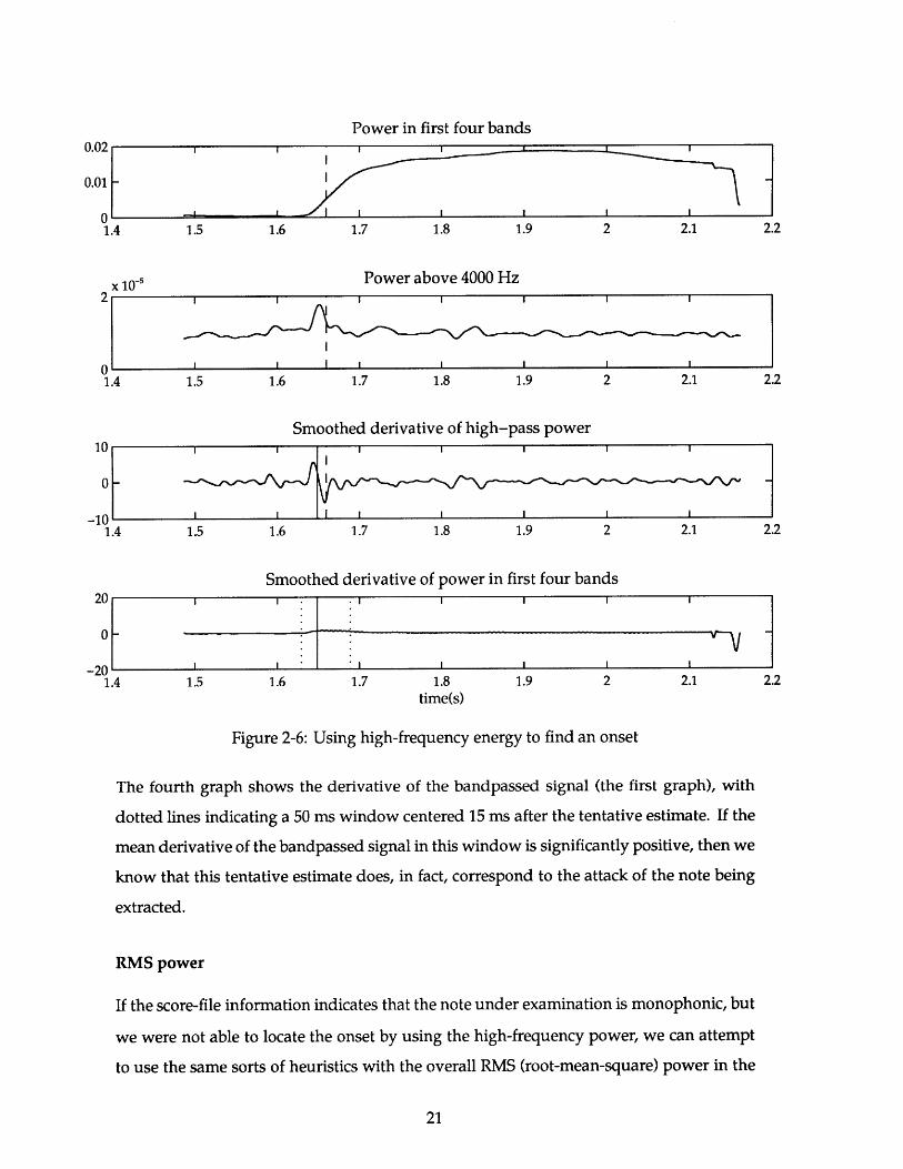
Figure 2-6 shows how the algorithm uses this information. The upper trace shows the

power summed in the first four harmonic bands, based from the fundamental frequency of

the note under consideration. We calculate this information by using two-pole, two-zero

HR filters tuned with center frequencies at the fundamental and first three overtones of

the pitch to be extracted. The Q (ratio of center frequency to bandwidth) of the filters is

variable, depending upon the musical situation. In cases where there are no notes nearby

in time and frequency for a particular overtone, we use Q = 15; this is increased as notes

approach in frequency. If a note is struck within 100 ms and one half-step of this pitch, we

use the maximum, Q = 60.

In the first three graphs in fig 2-6, the dashed line shows the "guess" received from the

tempo-estimation subsystem (see section 2.3.4).

The second trace shows the power filtered at 4000 Hz and above. A 10th order Cheby-

shev type I filter is used; this filter has an excellent transition to stopband, but a fair amount

of ripple in the passband. This tradeoff is useful for our purposes, since accuracy of high-

pass response is not crucial here. In the trace, we can easily see the "bump" corresponding

to the onset of the note.

In the third graph of the figure, we see the derivative of the second graph. The vertical

scale of this graph has been normalized by the overall variance, so that we can measure

the magnitude of the derivative in terms of the noise in the signal. (This is essentially

equivalent to low-pass filtering and rescaling by the maximum value, but quicker to

compute in MATLAB). In this scaled space, we look for the closest point to the onset guess

which is above 2.5 standard deviations of noise above zero, and select that as the tentative

estimate. This point is marked with a solid vertical line in the third and fourth traces of

figure 2-6

It is still possible that we have found a peak in the high-frequency power which

corresponds to the wrong note; we can check the power in the bandpass-filtered signal

to check whether the harmonic energy is rising at the same time the noise burst occurs.

Power in first four bands

Power above 4000 Hzx 10-'

Smoothed derivative of high-pass power

1.5 1.6 1.7 1.8 1.9 2 2.1 2.2

Smoothed derivative of power in first four bands

1.5 1.6 1.7 1.8 1.9 2 2.1 2.2time(s)

Figure 2-6: Using high-frequency energy to find an onset

The fourth graph shows the derivative of the bandpassed signal (the first graph), with

dotted lines indicating a 50 ms window centered 15 ms after the tentative estimate. If the

mean derivative of the bandpassed signal in this window is significantly positive, then we

know that this tentative estimate does, in fact, correspond to the attack of the note being

extracted.

RMS power

If the score-file information indicates that the note under examination is monophonic, but

we were not able to locate the onset by using the high-frequency power, we can attempt

to use the same sorts of heuristics with the overall RMS (root-mean-square) power in the

0.02

1.4

-10 '1.4

20 -

0-

-20 -1.4

signal. This is shown in figure 2-7.

Power in first four bands0.02

0.01 -

011 1.05 1.1 1.15 1.2 1.25 1.3 1.35 1.4 1.45

RMS power in signal

1 1.05 1.1 1.15 1.2 1.25 1.3 1.35 1.4 1.45

Smoothed derivative of RMS power in signal

1 1.05 1.1 1.15 1.2 1.25 1.3 1.35 1.4 1.45 1.

Smoothed derivative of power in fundamental bandE1.05 1.1 1.15 1.2 1.25 1.3 1.35 1.4 1.45

Time (s)

Figure 2-7: Using RMS power to find an onset

The RMS power method is exactly analogous to the high-frequency power method

described above. We calculate the overall RMS power in the signal (the second graph in

figure 2-7), take its derivative, and look for a peak close to our original guess (the third

graph). If we find a suitable peak in the RMS derivative, we look at the bandpass-filtered

power in a narrow window around the estimate to ensure that the RMS peak lines up with

a peak in the harmonic power of the note being extracted.

5

0

-5

5

0

-5

Comb filtering

If the high-frequency and RMS power information does not enable us to extract the onset

of the note, we give up trying to use global sound information and instead focus on the

harmonic information found in the fundamental and overtones of the desired note. We

build a comb-like filter by summing the outputs of two-pole, two-zero filters tuned to the

first 15 overtones (or fewer if the note is high enough that 15 overtones don't fit in under

the Nyquist frequency of the digital audio sample) filter the audio with it, and calculate

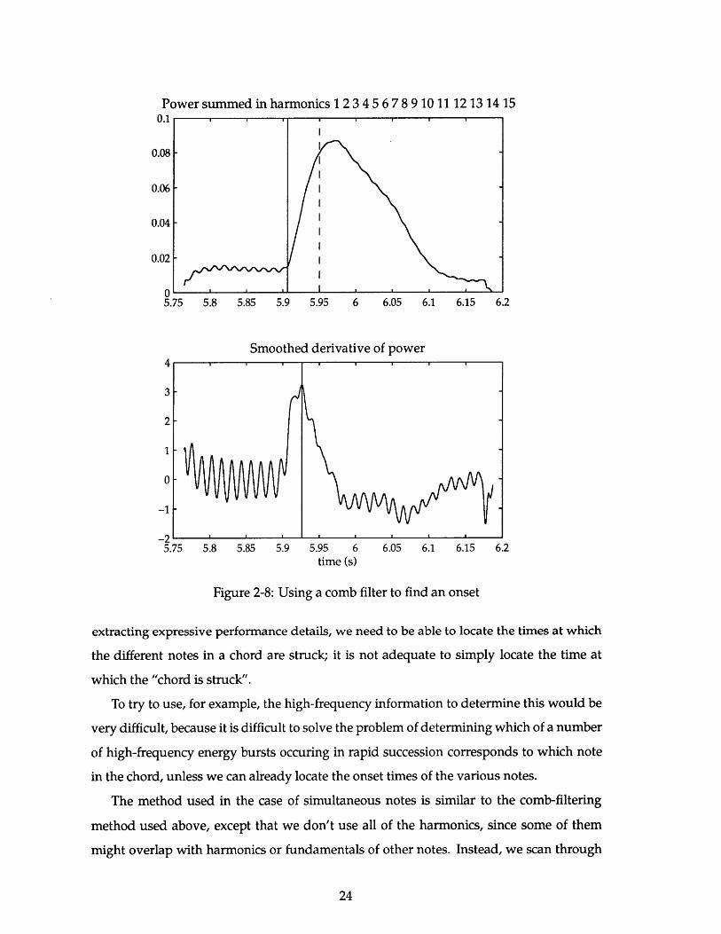
the power and derivative of power of the result (see figure 2-8).

We can see by comparing fig 2-8 to figs 2-6 and 2-7 that the harmonic signal, even

containing the high harmonics, is much more blurred over time than the high-pass or RMS

power. This is partially due to the fact that the relatively high-Q filters used (Q = 30 in

the example shown) have a fairly long response time, and partially due to a characteristic

of the piano timbre: the low harmonics, which dominate the power of the sum, have a

slower onset that the high harmonics.

We mark an onset at the point where the rise in the harmonic energy begins. We locate

this point by looking for the sharpest peak in the derivative, and then sliding back in time

to the first positive-going zero crossing (in the derivative). This is the point in the filtered

signal at which the rise to the peak power begins.

It is, of course, likely that there is a bias introduced by this method, as compared against

the more precise techniques described above; that is, that the point at which the rise to peak

in the comb-filtered signal occurs is not the perceptual point at which the onset occurs, as

it is with the high-frequency power. Biases of this sort can be resolved statistically using

analysis of validation data (see Chapter 3).

Selected bandpass filtering

The above three techniques for onset extraction are all used for notes which are struck

monophonically; in the case where a note is struck "simultaneously" with other notes

as part of a chord, we cannot use them. This is because an expert pianist does not

actually play the notes in a chord at exactly the same time; the variance in onset is an

important characteristic of expressive phrasing, used to separate the chord into notes

in musically meaningful ways, or to change the timbre of the chord. Thus, as part of

Power summed in harmonics 12 3 4 5 6 7 8 9 10 1112 13 14 150.1r 1 1 1 1 1 I

0 1 '5.75 5.8 5.85

S4

3-

2-

1- iA

-2'5.75 5.8

5.9 5.95 6 6.05 6.1 6.15 6.2

moothed derivative of power

5.85 5.9 5.95 6time (s)

6.05 6.1 6.15 6.2

Figure 2-8: Using a comb filter to find an onset

extracting expressive performance details, we need to be able to locate the times at which

the different notes in a chord are struck; it is not adequate to simply locate the time at

which the "chord is struck".

To try to use, for example, the high-frequency information to determine this would be

very difficult, because it is difficult to solve the problem of determining which of a number

of high-frequency energy bursts occuring in rapid succession corresponds to which note

in the chord, unless we can already locate the onset times of the various notes.

The method used in the case of simultaneous notes is similar to the comb-filtering

method used above, except that we don't use all of the harmonics, since some of them

might overlap with harmonics or fundamentals of other notes. Instead, we scan through

0.08

0.06

0.04

0.02

the list of notes which are struck at the same time (calculated during the initial score-

processing step), and eliminate harmonics of the note being extracted if they correspond to

any harmonics of the notes on the simultaneous list. The fundamental is always used, on

the assumption that the power in the fundamental bin will dominate power representing

overtones of other notes.

After selecting the set of overtones to use in the filter for the particular note, we filter,

calculate power and derivative of power, and locate the onset in these curves using the

same method as in the comb-filter case.

2.3.2 Release Extraction

The release extraction component is similar to the final method (selected band-filter) de-

scribed for onset detection; however, rather than only considering harmonics as "compet-

ing" if they come from other simultaneous onsets, we consider all of the notes which, in

the score, overlap the note under consideration. If any of these notes have fundamentals or

harmonics which compete with a harmonic of the current note, we eliminate that harmonic

from the filter.

To find the release using this filter, we construct a time-window beginning at the onset

of the note, which was extracted in a previous iteration of the main loop, and slide forward

in time until we find the peak power, which is the negative-going zero crossing in the

derivative of the filtered signal. From there, we scan forward until we find one of two

things:

* The filtered power drops to 5% of the peak power. (fig 2-9).

* The signal begins to rise again to another peak which is at least 75% as high-power

as the peak power. (fig 2-10).

The earliest point in time at which either of these two things occur will be selected as

the release point of the note.

2.3.3 Amplitude/Velocity Measurement

Amplitude information is extracted from the signal using a very simple method; we use

the selected bandpass-filter data already calculated for the release time extraction. We

0.03

0.025

O 0.02

0 0.015

0.01

0.005

0-0.4 1.2 1.4 1.6

Figure 2-9: The release point is found where the filtered power drops below 5% of peak.

0.03

0.025

0 0.02

0.015

0.01

0.005

0 0.2 0.4 0.6 0.8Time (s)

Figure 2-10: The release point is found where a rise to another peak begins.

look for the maximum value of the output of the filter within the window demarcated by

the extracted onset and release times, and rescale it depending on the number of bands

selected for the filter (since the output magnitude of the filter increases as more bands are

used). This is shown in fig 2-11.

0.035

0.6 0.8 1Time (s)

0.02

0.018

0.014 - I

1.20.25-- - - -- - - - - 1.3-- --.--- -- -1--- -- -- -- -- -- 5-

0 0 .0 12 - - - - - - - ---.. . . .. . . -. . .. .-.- ..- -- - - - ---.- - --.- --. .-.- -- -

V. 0 .0 1 -- -- - - -- - -- - - --- - - --- - --- --.. .-- - -- - -- - -- - -- - -.-- --.-- - .-.- .

0 .0 0 8 -- . .. .-. .-. -. . .. .-. . . . . . .-. . .. . .-.

0.006 --..-..-..-..-

0.004-1.2 1.25 1.3 1.35 1.4 1.45

time (s)

Figure 2-11: The amplitude of a note is extracted by picking the point of maximum powerwithin the attack-release window.

2.3.4 Tempo Re-Estimation

The tempo estimator is currently a very simple component, but it has proven empirically

to be robust enough for the musical examples used for developing and validating the

system. This subsystem is used for creating the "window" within which onset extraction

is performed. This is currently the only way the system as whole stays "on course", so it

is very important that the estimation be accurate.

If the next note to be extracted is part of a chord, and we have extracted other notes

from the same chord, we set its predicted onset time to be the mean time of onset of the

extracted notes from the same chord. If it is a monophonic note, we plot the last ten notes'

extracted onset times versus their onset times as predicted by the score, and use a linear fit

to extrapolate expected onset times for the next few notes. Figure 2-12 shows an example

of this process.

In the onset-detection subsystem, this tempo estimate is used to create a window in

which we look for the onset. The heuristics described in section 2.3.1 work very well if

there is exactly one note of the correct pitch within the window. If there are more than one,

5-

1-

00 1 2 3 4 5 6

Score time (s)

Figure 2-12: We estimate tempo by fitting a straight line through recently extracted onsets(points marked ), and use this fit to extrapolate a guess for the next onset to be extracted(marked 'o')

the onset-detection algorithms might well pick the wrong one; if there are none, we will

find the "false peak" which most resembles a note peak, and thus be definitely incorrect.

The window is defined by looking at the extraction time of the last note, and the predicted

time of the next two (or, if the predicted time is the same for the next two, as far forward

as needed to find a note struck at a different time); the window begins one-quarter of the

way back in time from the predicted onset of the current note to the extracted onset of the

previous note, and goes 95% of the way forward to the predicted onset of the next note.

2.3.5 Outputs

During the execution of the main loop, the data generated are saved to disk and displayed

graphically, to book-mark and keep tabs on the progress of the computation. The sys-

tem currently takes about 15 sec for one cycle of release/amplitude/onset/tempo-track

through the main loop, running in MATLAB on a DEC Alpha workstation. Given the

un-optimized nature of the code, and the generally slow execution of MATLAB, which is

an interpreted language, it is not unreasonable to imagine that an optimized C++ version

of the system might run close to real-time.

MIDI data

The extracted data is converted to a MIDI file representation before output. Utilities to

convert MIDI to score-file format, and vice versa, have also been written; in general, it is a

simple process to convert a MIDI text file to any other desired text-file format containing

the same sort of information. The only non-obvious step in the MIDI file generation is

selecting note velocities. As there is no "standard" mapping of MIDI note velocities to

sound energy, or sound energy to MIDI velocity, it seems the most desirable tack is simply

to model the input-output relationship and invert it to produce velocity values.

See chapter 3 for details on the comparison of input velocity to extracted amplitude

measurement - in summary, we calculate a velocity measurement via a logarithmic scaling

curve.

Graphics

Graphic data is also created by the system during the main loop - tempo curves similar to

that shown, which show the relationship between timing in the score and timing extracted

from the performance, and piano-roll MIDI data (fig 2-13, to monitor the progress of the

algorithms.

For building analysis systems useful to music-psychological researchers, other graphi-

cal techniques for representing timing data, and particularly expressive deviation, should

be investigated.

H .... .

.- ..............

I.

..... .......

..-.- .-. -.--.-.-.-.--- - - - - - - - - - - - - - - - - - -

0 1 2 3 4 5 6 7 8 9 10Performance time (s)

Figure 2-13: Part of a piano-roll style score extracted from a performance of the Bachexample (fig 2-3).

70 F-

65 [-

60

55 I- -

50F

"4

. . . . . . . . . . . . . . . . . . . . . . .

. . . . . . . . . . . . . . . . . . . . . . .

. . . . . . . . . . . .

. . . . . . . . . .

Chapter 3

Validation Experiment

This chapter describes a validation experiment conducted to analyze the accuracy of timing

and velocity information extracted by the system. We will begin by describing the setup

used to construct a "ground truth" against which the extracted data can be compared.

We then analyze in detail the performance of the system using the experimental data,

presenting results on each of the extracted parameters (attack time, release time, velocity).

3.1 Experimental Setup

3.1.1 Equipment

To analyze the accuracy of the timing and velocity information extracted by the system, a

validation experiment was conducted using a Yamaha Disclavier MIDI-recording piano.

This device has both a conventional upright piano mechanism, enabling it to be played as

a standard acoustic piano, and a set of sensors which enable it to capture the timings (note

on/off and pedal on/off) and velocities of the performance in MIDI format. The Disclavier

also has solenoids which enable it to be used to play back prerecorded MIDI data like a

player piano, but this capability was not used.

Scales and two excerpts of selections from the piano repertoire were performed on

this instrument by an expert pianist; the performances were recorded in MIDI using the

commercial sequencer Studio Vision by Opcode Software, and in audio using Schoeps

microphones. The DAT recording of the audio was copied onto computer disk as a digital

audio file; the timing-extraction system was used to extract the data from the digital audio

stream, producing an analysis which was compared to the MIDI recording captured by

the Disclavier.

It is assumed for the purposes of this experiment that the Disclavier measurements of

timing are perfectly accurate; indeed, it is unclear what method could be used to evaluate

this assumption. One obvious test, that of re-synthesizing the MIDI recordings into audio,

was conducted to confirm that the timings do not vary perceptually from the note timings

in the audio. The Disclavier is a standard instrument for research into timing in piano

performance; its accuracy is the starting point for dozens of studies into the psychology of

musical performance.

As we shall see in the discussion below, the extraction errors from the system are

often audible upon resynthesis. As no such audible errors are produced by resynthesizing

Disclavier recordings, it is reasonable to conclude at least that the error of extraction

overwhelms any errors in Disclavier transcription.

3.1.2 Performances

There were eight musical performances, totaling 1005 notes in all, that were used for the

validation experiment. The performer was a graduate student at the Media Lab who

received a degree in piano performance from the Julliard School of Music.

Three of the performed pieces were scales: a chromatic scale, played in quarter notes

at m.m. 120 (120 quarter notes per minute) going from the lowest note of the piano (A

three octaves below middle C, approximately 30 Hz) to the highest (C four octaves above

middle C, approximately 4000 Hz); a two-octave E-major scale played in quarter notes at

m.m. 120; and a four-octave E-major scale played in eighth notes at m.m. 120. Each of the

two E-major scales moved from the lowest note to the highest and back again three times.

Additionally, three performances of excerpts of each of two pieces, the G-minor fugue

from Book I of Bach's Well-Tempered Clavier, and the first piece "Von fremden Uindern und

Menschen" from Schumann's Kinderszenen Suite, op. 15, were recorded. The score for

the excerpts used for each of these examples are shown in fig 2-3 and 3-1. All three Bach

performances were used in the data analysis; one of the Kinderszenen performances was

judged by the participating pianist to be a poor performance, suffering from wrong notes

and unmusical phrasing, and was therefore not considered.

These pieces were selected as examples to allow analysis of two rather different styles

of piano performance: the Bach is a linearly-constructed work with overlapping, primarily

horizontal lines, and the Schumann is vertically-oriented, with long notes, many chords,

and heavy use of the sustain pedal.

I I -E

-- --------------- ----- ---

00

-5to,

F - ",*,-"-*,--,----- -. 1-11"...- - R

P f 6rt - it-, IF! ort- -- --------------- ---------------------

Of t F9

£r~in.uemmw.~ V 2.

Ic

;tol

Figure 3-1: The Schumann excerpt used in the validation experiment

3.2 Results

Figs 3-2 to 3-12 show selected results from the timing experiment. We will deal with

each of the extracted parameters in turn: onset timings, release timings, and velocity

measurements. In summary, the onset timing extraction is successful, and the release

timing and amplitude measurement less so. However, statistical bounds on the bias and

variance of each parameter can be computed which allow us to work with the measurement

to perform analysis of a musical signal.

3.2.1 Onset Timings

Foremost, we can see that the results for the onset timings are generally accurate to within

a few milliseconds. Fig 3-2 shows a scatter-plot of the recorded onset time (onset time as

recorded in the MIDI performance) vs. extraction error (difference between recorded and

extracted onset time) from one of the Schumann performances. The results for the other

pieces are similar.

1

A ii

* )-to Sos"'e g

25

2 C. ....... ................... . ...- - - - .- ....-..X x

15 -

x > x xx xx

x X x

- XX:

-10 .--- - --- - -- -. - . --- -- . -X --..-- - -

Xxx X X

-15 -- - - - - - -

x: x . : x

:X X

-25 I

0 5 10 15 20 25 30 35 40 45Recorded onset time (s)

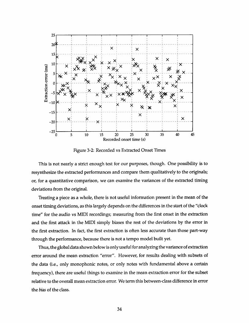
Figure 3-2: Recorded vs Extracted Onset Times

This is not nearly a strict enough test for our purposes, though. One possibility is to

resynthesize the extracted performances and compare them qualitatively to the originals;

or, for a quantitative comparison, we can examine the variances of the extracted timing

deviations from the original.

Treating a piece as a whole, there is not useful information present in the mean of the

onset timing deviations, as this largely depends on the differences in the start of the "clock

time" for the audio vs MIDI recordings; measuring from the first onset in the extraction

and the first attack in the MIDI simply biases the rest of the deviations by the error in

the first extraction. In fact, the first extraction is often less accurate than those part-way

through the performance, because there is not a tempo model built yet.

Thus, the global data shown below is only useful for analyzing the variance of extraction

error around the mean extraction "error". However, for results dealing with subsets of

the data (i.e., only monophonic notes, or only notes with fundamental above a certain

frequency), there are useful things to examine in the mean extraction error for the subset

relative to the overall mean extraction error. We term this between-class difference in error

the bias of the class.

Fig 3-3 shows the standard deviation of onset timing extraction error for each of the

eight pieces used (in order, the chromatic scale, the two-octave E major scale, the four-

octave E major scale, the three performances of the Bach, and the two performances of the

Schumann). We can see that the standard deviation varies from about 10 ms to about 30

ms with the complexity of the piece. Note that the second performance of the Schumann

excerpt has an exceptionally high variance. This is because the tempo subsystem mis-

predicted the final (rather extreme) ritardando in the performance, and as a result, the last

five notes were found in drastically incorrect places. If we throw out these outliers as

shown, the variance for this performance improves from 116 ms to 22 ms.

120

2oct 4oct jsbl jsb2 jsb3Piece

schl sch2

Figure 3-3: Onset error standard deviation for each performance.

Fig 3-4 shows histograms of the deviation from mean extraction error for a scale, a

Bach performance, and a Schumann performance. For each case, we can see that the

distribution of deviations is roughly Gaussian or "normal" in shape. This is an important

feature, because if we can make assumptions of normality, we can easily build stochastic

estimators and immediately know their characteristics. See the Discussion section for

more on this topic.

We can also collect data across pieces and group it together in other ways to examine

100 -.---

80 -- .-.:

60 -- .-.-

40

High vaiiance due to outliers

Variance with outliers remov

..... .....20F---

chrm.

..

ed

Four-Octave Scale

01 " " " In "IIIIIIIIIII In I 1

-100 -80 -60 -40 -20 0 20 40 60 80 100

Bach Excerpt

-80 -60 -40 -20

rii--0 20 40 60 80

Schumann Excerpt25

20

S15

~10

5

0-10 0 -80 -60 -40 -20 0 20 40 60 80 100

Onset Extraction Error (ns)

Figure 3-4: Onset error deviation frequencies for each of three performances.

possible systematic biases in the algorithms used. The upper graph in fig. 3-5 shows the

bias (mean) and standard deviation of onset timing extraction error collected by octave.

We see that there is a slight trend for high notes to be extracted later, relative to the correct

timing, than lower notes. Understanding this bias is important if we wish to construct

30 - -

20---

0 2--

10

0'-100

------ --- -

100

F1FL

--..-.-.-.--

-..-.-.-.---

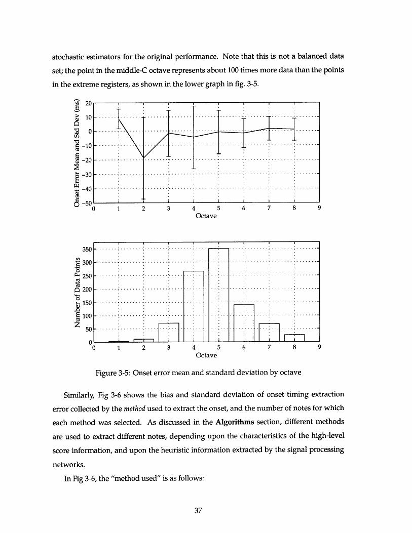
stochastic estimators for the original performance. Note that this is not a balanced data

set; the point in the middle-C octave represents about 100 times more data than the points

in the extreme registers, as shown in the lower graph in fig. 3-5.

20

10

0

-10

-20

-30

-40

50n0 1 2 3 4 5 6 7

Octave

350

300

250

200

150

100

50

8 9

0 1 2 3 4 5 6 7 8 9Octave

Figure 3-5: Onset error mean and standard deviation by octave

Similarly, Fig 3-6 shows the bias and standard deviation of onset timing extraction

error collected by the method used to extract the onset, and the number of notes for which

each method was selected. As discussed in the Algorithms section, different methods

are used to extract different notes, depending upon the characteristics of the high-level

score information, and upon the heuristic information extracted by the signal processing

networks.

In Fig 3-6, the "method used" is as follows:

. .. .- --.

- - -- - - - - - - - - - -

-

-- -. .

- - - -.

-..-.-.-..-.-.-.

--- -----..

60

4 0 -- . . . .. . . . .. . ... . . . . . . .- -. . . .. . .-. . ...-. .

20 --.- .- .-.-.-

0 -- .- .--20 -- -... . -. ...- .

-40

500

400

300

200 -

100 r

A B C DExtraction Method

Extraction Method

Figure 3-6: Onset error mean and standard deviation by extraction method

* [A] No notes were struck in unison with the extracted note, and there is sufficient

high-frequency energy corresponding with positive derivative in the fundamental

bin to locate the note.

* [B] No notes were struck in unison with the extracted note. High frequency energy

could not be used to locate the note, but RMS power evidence was used.

* [C] No notes were struck in unison with the extracted note; but there was not sufficient

high frequency or RMS evidence to locate the note. The comb-filter and derivative

method was used. These are, in general, represent "hard cases", where the audio

signal is very complex.

* [D] There were notes struck in unison with the extracted note, so high-frequency and

----- - --- - - - - i _

- . .. .-. .-. .-. .. . ..-. . . ..-.. . ..-.. .. .-.. .. . -. .

-. . . .. . .-. . . . . . .-. . . . . . .-. ..-. .-. .-

- - - - - - - -

-. . -. -. .- . - .........................

RMS power methods could not be used. The allowable overtones and derivative

method were used.

We can see that there is a bias introduced by using method C, and relatively little by

other methods. In addition, it is clear that the use of the high-frequency energy or RMS

power heuristics, when possible, leads to significantly lower variance than the filtering-

differentiation methods. It is a good sign that the method with the lowest error variance -

the high-frequency energy method - is also the most commonly used.

3.2.2 Release Timings

The scatter-plot of recorded release timing for one of the E major scale performances is

shown in fig 3-7. As can be seen, there is similarly high correlation between recorded and

extracted values as in the onset data. We can also observe a time relation in the data -

this is due to the bias of release timing by pitch. The three "cycles" visible in the data

correspond to the three motions up and down the scale.

We can additionally plot recorded duration vs extracted; we see that there is not nearly as

much obvious correlation, although there is still a highly statistically significant correlation

between the data sets. These data are shown in fig 3-8.

The histograms of duration extraction error for three example pieces are shown in fig

3-9. We see that, as with onset timing, the extraction error is distributed approximately

normally for the scale and Bach examples; the shape of the distribution for the Schumann

example is less clear. The Schumann example is obviously the most difficult to extract

durations for, due to the sustained, overlapping nature of the piece.

The overall standard deviation of error for durations is 624 ms. We can see from looking

at fig 3-10, which plots duration error and standard deviation of error vs. recorded note

duration, that much of this error actually comes from duration bias. There is a strong bias

for extracted durations towards 500 ms notes - that is, short notes tend to be extracted

with incorrectly long durations, and long notes tend to be extracted with incorrectly short

durations.

1000

500

0

-500

-1000 r-1500' ' x '

0 5 10 15 20 25 30Recorded release time (s)

35 40 45

Figure 3-7: Recorded vs extracted release time.

X XXx----- X -- - - -XX-- -- - -- X .Nx- "?

X XX XX

1.21 -

0.8 ---

0.6 ---

0.4 -

0.21-

0 0.2 0.4 0.6 0.8 1 1.2 1.4 1.6 1.8 2Recorded duration (s)

Figure 3-8: Recorded vs extracted duration

40

1.6

1.4> XXx:-----.-.------

.V --XX

X

X xX,

xX X

XX

x

- ----

: x

Four-Octave Scale40

30---

20---

0-2000 0 500 1000 1500

Bach Excerpt

Schumann Excerpt25

20 ...

15 ...-

10 -5---

5 ....

V-2000 -1500 -1000 -500 0 500 1000 1500Duration Extraction Error (ins)

Figure 3-9: Duration extraction error histogram. Positive values indicateextracted durations were longer than the recorded values.

2000

notes whose

3.2.3 Amplitude/Velocity

A scatter-plot of recorded velocity against extracted log amplitude relative to the maximum

extracted amplitude is shown in fig 3-11. As with duration, there is a high degree of

41

-1500 -1000 -500

- - -- - - - - - - - - - - - - - - - - - - - - - - -

----- -n--- --.-.--.--.--..-.-

2000

2000

HF H mFr= r-,2

-- .- ----.

-. .. . .

0 200 400 600 800 1000 1200 1400 1600 1800 2000Recorded duration (ns)

Figure 3-10: Duration extraction bias and standard deviationduration.

of error as a function of note

correlation in the data, with r = .3821.

We can correct for the unit conversion between abstract MIDI "velocity" units in the

recorded data and extracted log amplitude energy values by calculating the regression

line of best fit to the fig 3-11 scatter-plot - y = 7.89 - 79.4x - and using it to re-scale the

extracted values.

When we treat the amplitude data in this manner, we see that once again, the noise

from extraction error is quite nicely representable as a Gaussian distribution (fig 3-12),

with standard deviation of error equal to 13 units on the MIDI velocity scale.

1000

500 F-.

-5001

-1000k

-1500 '

.. .. ... .. .. .. .. . . . . . . . . . . . . .

. . . . . . . . . . . .

. . . . . . . . . . . . . . . . .. .. ... .. .. ..

-. . .- - . .. - -

- .

0

-0.5

-1

-1.5

-2

-2.5

-3

-3.5

-4

-4.5

xXx X XX

xx

- x -- --x x

x --:- -

- --. . ...- -

---.----.--x-.

---- X -

- -SX.

0 10 20 3 40 0 60 70 80 10 20 30 40 50 60 70 80

Recorded velocity

Figure 3-11: Recorded MIDI velocity vs extracted amplitude

-30 -20 -10 0 10 20 30 40 5Velocity extraction error (MIDI velocity units)

Figure 3-12: Histogram of rescaled velocity extraction error

-- - -

- .x -N- . . .

-

-- - -

- .-

- -

-

Chapter 4

Discussion

There are a number of different levels on which this work should be evaluated: as a

tool for music-psychology research, as an example of a system which performs musical

transcription, and as an example of a multi-layered system which attempts to integrate

evidence from a number of different information sources to understand a sound signal.

We will consider each of these in turn, discuss ways in which the current system could be

improved, and conclude with some thoughts on the value of transcription systems.

4.1 Stochastic Analysis of Music Performance

Part of the value of the sort of variance-of-error study conducted in the Results section is

that we can treat extracted data as a stochastic estimator [17] for the actual performance,

and make firm enough assumptions about the distribution of the estimation errors that we

can obtain usable results.

It is clear that some aspects of expressive music performance can be readily analyzed

within the constraints of the variance in extraction discussed above. For example, tempo

is largely carried by onset information, and varies only slowly, and only over relatively

long time-scales, on the order of seconds. Even the worst-case performance, with standard

deviation of extraction error about 30 ms, is quite sufficient to get a good estimate of

"instantaneous tempo" at various points during a performance.

To illustrate this, assume that two quarter notes are extracted with onsets 1.2 seconds

apart, say at t1 = 0 and t 2 = 1.2 for the sake of argument. We can assume, then, that

these extractions are taken from Gaussian probability distribution functions (pdf's) with

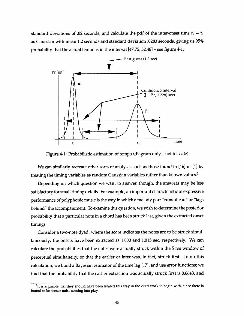
standard deviations of .02 seconds, and calculate the pdf of the inter-onset time t2 - t1

as Gaussian with mean 1.2 seconds and standard deviation .0283 seconds, giving us 95%

probability that the actual tempo is in the interval [47.75, 52.48] - see figure 4-1.

Best guess (1.2 sec)

Pr [on] M_,_I

Confidence Interval([1.172, 1.228] sec)

I II II III

I I I

to ti time

Figure 4-1: Probabilistic estimation of tempo (diagram only - not to scale)

We can similarly recreate other sorts of analyses such as those found in [16] or [1] by

treating the timing variables as random Gaussian variables rather than known values.1

Depending on which question we want to answer, though, the answers may be less

satisfactory for small timing details. For example, an important characteristic of expressive

performance of polyphonic music is the way in which a melody part "runs ahead" or "lags

behind" the accompaniment. To examine this question, we wish to determine the posterior

probability that a particular note in a chord has been struck last, given the extracted onset

timings.

Consider a two-note dyad, where the score indicates the notes are to be struck simul-

taneously; the onsets have been extracted as 1.000 and 1.015 sec, respectively. We can

calculate the probabilities that the notes were actually struck within the 5 ms window of

perceptual simultaneity, or that the earlier or later was, in fact, struck first. To do this

calculation, we build a Bayesian estimator of the time lag [17], and use error functions; we

find that the probability that the earlier extraction was actually struck first is 0.6643, and

'It is arguable that they should have been treated this way in the cited work to begin with, since there isbound to be sensor noise coming into play.

that the later extraction was actually first is .2858, assuming that the standard deviation is

the worst-case of 25 ms - see figure 4-2.

Pr [on]a struck first

p struck first

.timeFu 4-2: Esiato of ti

mnFgure 4-2:ortiantisect of rth strigina prrmaes (dagram cetanly capoturse.

4.2 Poypmhsnic Trancriputin ytse nawd areyo uia tls

Thieah exmehatsnhs ortvofc laydphoy ithe scorehc enbls polphoengix- tran

"samehtyle";eitolsphotyindisingushabe romvera oinal performance de tochumann but

heavy use of the damper pedal, and so has sections where as many as nine notes are

sustaining at once. The most common musical cases that are not represented among the

example performances analyzed above are very dense two-handed chords, with six or

eight notes struck at once, very rapid playing, and extreme use of rubato in impressionistic

performance.

It is anticipated that any of these situations could be dealt with in the current architec-

ture, although the tempo-follower would have to be made more robust in order to handle

performance which are not well-modeled by linear tempo segments. This is generally a

solvable problem, though - see [22] for an example.

4.3 Evidence-Integration Systems

The evidence integration aspects of the system are the most novel, and at the same time,

the least satisfying. It is very difficult to build architectures which allow the use of data

from many sources simultaneously; the one for this system is perhaps not as sophisticated

as it could be. For example, the current system does not have the ability to use knowledge

discovered in the attack (other than the timing) to help extract the release. Similarly, it

would be quite useful to be able to examine the locations of competing onsets and decays

in the extraction of parameters for a note with overlapping notes.

4.4 Future Improvements to System

There are many directions which contain ample room for improving the system. Obviously,

more work is needed on the release- and amplitude- detecting algorithms. It is expected

that more accurate amplitude information could be extracted with relatively little difficulty;

the results here should be considered preliminary only, as little effort has currently gone

into extracting amplitudes.

4.4.1 Release timings

Release timings are another matter; they seem to be the case where the most sophisticated

processing is required in a system of this sort. Fig 4-3 shows the major difficulty When a

note (for example, the C4 in fig 4-3) is struck after but overlapping a note which has the

fundamental corresponding to an overtone (the C5), the release of the upper note becomes

"buried" in the onset of the lower. It does not seem that the current methods for extracting

release timings are capable of dealing with this problem, and that instead, some method

based on timbre-modeling would have to be used.

Piano-Roll Score

------ ----- ---------------------- ------------------

........................

-- - - - - - - - - - " -- - - - - - - - - - - -

.......................

-- - - - - - - - - -

......................Overlap

.......................------ ----- - - - - - - - - - - -.............................

........................- - - - - - - - - - - -.............................................................................................. - - - - - - - - - - - -.........................................................................................-- - - - - -- - - - - - - - - - - - - - - - -

------------ ............. X.

Energy Contours

t

Figure 4-3: A release gets buried by overlapping energy from a lower note.

4.4.2 Timbre modeling

One potential method for improving the ability of the system in general would be to have

a more sophisticated model of the timbre of a piano built in. If we could accurately predict,

given the velocity of a particular onset, the various strengths and amplitude profiles of the

overtones, we could "subtract" them from the signal in an attempt to clean it up. Such a

model might also provide training for a pattern-matching system, such as a eigenvector-

based approach, to transcription.

4.4.3 Goodness-of-fit measures

It would improve the robustness of the system greatly to have a measure of whether the

peak extracted from the signal for a particular note has a "reasonable" shape for a note

peak. Such a measure would allow more careful search and tempo-tracking, and also

C5

Pitch

C4

Time

Energy

C5

Energy

C4

enable the system to recover from errors, both its own and those made by the pianist.

Such a heuristic would also be a valuable step in the process of weaning a system such

as this one away from total reliance upon the score. It is desirable, obviously, even for a

score-based system to have some capability of looking for and making sense of notes that

are not present in the score. At the least, this would allow us to deal with ornaments such

as trills and mordents, which do not have a fixed representation; or with notes added or

left out in performance, intentionally or not.

There are other methods possible for doing the signal-processing than those actually

being used. One class of algorithms which might be significantly useful, particularly

with regard to the abovementioned "goodness of fit" measure, is those algorithms which

attempt to classify shapes of signals or filtered signals, rather than only examining the signal

at a single point in time. For example, we might record training data on a piano, and use an

eigenspace method to attempt to cluster together portions of the bandpass-filtered signal

corresponding to attacks and releases.

4.4.4 Expanded systems

Ultimately, it remains an open question whether a system such as this one can be expanded

into a full-fledged transcription system which can deal with unknown music. Certainly,

the "artificial intelligence" component, for understanding and making predictions about

the musical signal, would be enormously complex in such a system.

One of the major successes of the work described in this thesis is a demonstration that

being able to "guess" or "predict" the next note in the score leads to much better success

in transcription than simple signal-processing alone. Thus, gains in research in building

symbolic music-processing systems, such as those which operate on MIDI input rather than

digital audio, might be able to be used in conjunction with signal-processing systems to

build synthetic listeners.

As one example of this, work is currently in progress on a "blackboard system" ar-

chitecture (see, eg, [15]) for investigation of these issues. An initial system being built

using this architecture will attempt to transcribe "unknown but restricted" music - the set

of four-part Bach chorales will be used - by development of a sophisticated rule-based

system to sit on top of the signal processing.

4.5 The Value of Transcription

Polyphonic transcription systems, as discussed in Section 1.2.1, have long been an area of

interest in the computer music community, at some times nearly acquiring the status of a

"touchstone" problem in the music-analysis field. 2

Why is this so? We submit that it is for several reasons. Obviously, having a working

transcription system would be a valuable tool to musicians of all sorts - from music

psychologists to composers (who could use such a tool to produce "scores" for analysis of

works of which they had only recordings) to architects of computer music systems (who

could use it as the front-end to a more extensive music-intelligence or interactive music

system).

Another reason, we claim, that so much effort has been invested in the construction of

transcription systems is that on the surface, it seems as though it "should be" possible to

build them, because the necessary information "must be" present in the acoustic signal.

While this feeling seems to underlie much of the work in this area, it is so far drastically

unjustified.

This point relates to a final reason, which is based on a hypothesis of the human music

cognition system - that human listeners are doing something rather like transcription in-

ternally as part of the listening process. Stated another way, there is an implicit assumption

that the musical score is a good approximation to the mid-level representation for cognitive

processing of music in the brain.

It is not at all clear at this point that this hypothesis is, in fact, correct. It may well be

the case that in certain contexts (for example, densely orchestrated harmonic structures),

only a schematic representation is maintained by the listener, and the individual notes are

not perceived at all. Since it is exactly this case that existing transcription systems have

the most difficulty with, perhaps we should consider building transcription systems with

other goals in mind than recreating the original score of the music.

In particular, building systems which can build human-like representations from an

audio stream would be adequate to supplant transcription for at least two of the three

above-mentioned goals. For music psychologists, it is obviously only necessary to be able

2A reviewer of a paper based on this work termed the problem of automatic polyphonic transcription "areef littered with the wreckage of dozens of theses."

to extract parameters from music at a level similar to that possible by human performers;

and for architects of interactive music systems, while it might be desirable to extract more

detailed information, it is clearly (since humans are quite good at music performance with

the ears they have) not necessary.

Even for composers, or jazz musicians who wish to produce fixed records of perfor-

mances to study on paper, a representation which contains only the information a human

perceives in the music (say, a melodic improvisation, a bass line, and a harmonic and

rhythmic structure) would be quite an asset, even if it didn't tell the complete story.

Chapter 5

Conclusion

In this chapter, we will present some brief concluding remarks to sum up the research

described in this thesis. The value of the system in its current state is discussed, and some

thoughts on transcription as a goal for computer-music researchers are presented.

5.1 Current state of the system

As mentioned above, the code for the system is currently about 1500 lines of MATLAB

code, and is considered to be in a "research" state. There is not currently a user interface

or methods facilitating the acquisition of score file or digital audio samples from compact

disc recordings of music. As a result, the system as a whole is probably not adequate as

a tool for end-user music psychologists at the current time. In order to be a useful tool

for end users, the current framework of score- and signal-processing should be assembled

along with a "user-friendly" front-end and data manipulation system.

The results of the validation experiment, particularly for extraction of onset timings,

indicate that the accuracy of the system is high enough to be useful for music-psychological

analysis of expressive timing, particularly to collect information on onset timings. Thus,

it would be a valuable undertaking to assemble a "production quality" system of the sort

outlined here, which could help the user to input the score (or scan it in, etc), digitize

the audio input, and automatically process the score, producing estimates of the extracted

variables and their estimated variance.

If such a system were written in C or C++, with careful attention paid to efficiency

in the filtering and other signal-processing operations, it would run perhaps an order of

magnitude faster than the current system does and approach real-time.

5.2 Concluding Remarks

This thesis has described a system which is relatively successful at performing polyphonic

transcription of known piano music from a digital audio signal and a score. It produces

MIDI performances of the expressively-performed originals which, while not indistin-

guishable, are generally rough imitations, containing the "earmarks" of the performance

in terms of tempo variation and phrasing.

While the system cannot be considered to perform full-fledged polyphonic transcrip-

tion (since it relies on a previously-known score), the method of its construction, incorpo-

rating information from several levels, points at potentially useful methods for building

more robust and independent systems in the future.

Chapter 6

Acknowledgments

I would like to thank all of my officemates in the Machine Listening Group at the MIT

Media Laboratory for their support and encouragement through the process of conduct-

ing research and preparing this document, particularly Michael Casey for his always-

illuminating discussions and Dan Ellis and Keith Martin for their comments during the

revision process.

Prof. Carol Krumhansl at Cornell University deserves much credit for her support and

enthusiasm when I was an undergraduate working with her; it is because of her that I am

involved in the study of music cognition at all, and at the Media Laboratory in particular.

My friends in real life and on the Internet - Jean Donaldson, Thomas Colthurst, Seth

Padowitz, Mike Sheehy, Jenine Abarbanel, Kristen Ankiewicz, Paul Lord, and the whole

Nerdsholm gang - have often provided a far-too-welcome distraction from the rigors of

the graduate student life.

The original idea for the research in this thesis was suggested to me by Teresa Marrin in

the Media Lab; Charles Tang provided a great service by providing the piano performances

in Ch. 3.

Finally, deepest love and thanks go to my parents, Dr. James and Dr. Mary Ann Scheirer,

for their love, support, and encouragement all these years.

Bibliography

[1] Jeff Bilmes. Timing is of the essence: Perceptual and computational techniques for

representing, learning, and reproducing expressive timing in percussive rhythm.

Master's thesis, MIT Media Laboratory, 1993.

[2] Edwin Fischer. J.s. bach: The well-tempered clavier. Compact Disc Recording, 1989.

[31 Glenn Gould. J.s. bach: The well-tempered clavier, book i. Compact Disc Recording,

1993.

[4] Stephen Handel. Listening. MIT Press, Cambridge, MA, 1989.

[5] Michael Hawley. Structure out of Sound. PhD thesis, MIT Media Laboratory, 1993.

[6] Keith Jarrett. J.s. bach: The well-tempered clavier, book i. Compact Disc Recording,

1988.

[7] Haruhiro Katayose and Seiji Inokuchi. The kansei music system. Computer Music

Journal, 13(4), 1989.

[81 Carol Krumhansl. Cognitive Foundations of Musical Pitch. Oxford University Press,

Oxford, 1991.

[9] Fred Lerdahl and Ray Jackendoff. A Generative Theory of Tonal Music. MIT Press,

Cambridge, MA, 1983.

[10] Robert Maher. An Approach for the Separation of Voices in Composite Musical Signals.

PhD thesis, University of Illinois at Urbana-Champaign, 1989.

[11] Robert Maher. Evaluation of a method for separating digitized duet signals. J. Audio

Eng. Soc., 38(12), 1990.

[12] James Moorer. On the Segmentation and Analysis of Continuous Musical Sound by Digital

Computer. PhD thesis, CCRMA - Stanford University, 1975.

[13] Eugene Narmour. The Analysis and Cognition of Basic Melodic Structures. University of

Chicago Press, Chicago, 1990.

[14] Eugene Narmour. The Analysis and Cognition of Melodic Complexity. University of

Chicago Press, Chicago, 1993.

[15] Alan Oppenheim and S. Hamid Nawab. Symbolic and Knowledge-Based Signal Process-

ing. Prentice-Hall, Inc, 1992.

[16] Caroline Palmer. Timing in Skilled Music Performance. PhD thesis, Cornell University,

1989.

[17] Athanasios Papoulis. Probability, Random Variables, and Stochastic Processes. McGraw-

Hill, New York, NY, third edition, 1991.

[18] Alan Ruttenberg. Optical reading of typeset music. Master's thesis, MIT Media

Laboratory, 1991.

[19] Andras Schiff. J.s. bach: The well-tempered clavier, book i. Compact Disc Recording,

1984.

[20] W. Andrew Schloss. On the Automatic Transcription of Percussive Music -from Acoustical

Signal to High-Level Analysis. PhD thesis, CCRMA - Stanford University, May 1985.

[21] John Stautner. The auditory transform. Master's thesis, MIT, 1982.

[22] Barry Vercoe. The synthetic performer in the context of live performance. In Proc. Int.

Computer Music Conf., 1984.