Fuzzy Logic Controller for Frequency Regulation of a Hydro ...

University of Calgary

PRISM: University of Calgary's Digital Repository

Graduate Studies The Vault: Electronic Theses and Dissertations

2018-04-13

Fuzzy Logic Controller for Frequency Regulation of a

Hydro and Wind Based Isolated Hybrid Micro-grid

Pal, Suvajit

Pal, S. (2018). Fuzzy Logic Controller for Frequency Regulation of a Hydro and Wind Based

Isolated Hybrid Micro-grid (Unpublished master's thesis). University of Calgary, Calgary, AB.

doi:10.11575/PRISM/31791

http://hdl.handle.net/1880/106503

master thesis

University of Calgary graduate students retain copyright ownership and moral rights for their

thesis. You may use this material in any way that is permitted by the Copyright Act or through

licensing that has been assigned to the document. For uses that are not allowable under

copyright legislation or licensing, you are required to seek permission.

Downloaded from PRISM: https://prism.ucalgary.ca

UNIVERSITY OF CALGARY

Fuzzy Logic Controller for Frequency Regulation of a Hydro and Wind Based Isolated Hybrid

Micro-grid

by

Suvajit Pal

A THESIS

SUBMITTED TO THE FACULTY OF GRADUATE STUDIES

IN PARTIAL FULFILMENT OF THE REQUIREMENTS FOR THE

DEGREE OF MASTER OF SCIENCE

GRADUATE PROGRAM IN ELECTRICAL AND COMPUTER ENGINEERING

CALGARY, ALBERTA

APRIL, 2018

© Suvajit Pal 2018

ii

Abstract

Operation of an isolated hybrid micro-grid requires a system to be capable of regulating the

system frequency as well as the voltage. The operation of a hydro power plant combined with a

wind power plant and a solar power plant is analyzed in this thesis. The main balancing mechanism

of the proposed hybrid micro-grid is the hydro power plant. Speed governor of hydro power plant

and wind pitch controller of wind power plant are implemented using both conventional PI and

Fuzzy logic based controllers. A supervisory controller, that will supervise individual controllers

and determine the desired power generation of hydro and wind power generating units, is also

proposed. By monitoring the system frequency, voltage and active power of various power

generating units under various operating conditions, it is concluded that the proposed control

scheme provides reliable system frequency and voltage regulation, and energy management.

iii

Acknowledgements

I would like to express my highest gratitude to my Supervisor, Dr. Om Malik, for his

diligent support and guidance all through the various stages of my thesis during its preparation as

also its completion.

My deep regard also for the Members of the Examination Committee who have vetted the

thesis.

I would also like to convey my thanks to the University of Calgary for giving me an

opportunity to perform my studies.

I am also delighted to appreciate my neighbors and friends for giving me their whole-

hearted support throughout these years.

I wish to convey my special thanks to my father, mother, elder brother and sister-in-law

who were the cardinal source of inspiration for the achievement of my goal.

Finally, I will ever remain indebted to Almighty God for his blessings that has paved the

way for me to complete the study.

iv

Table of Contents

Abstract ..................................................................................................................................................... ii

Acknowledgements .................................................................................................................................. iii

List of Tables .......................................................................................................................................... vii

List of Figures and Illustrations ............................................................................................................. viii

List of Symbols, Abbreviations and Nomenclature ............................................................................... xiii

CHAPTER 1 : INTRODUCTION ............................................................................................................ 1

1.1 Operational Overview of a Hybrid Micro-Grid .................................................................................. 4

1.2 Energy Management Strategies .......................................................................................................... 6

1.3 Operational Requirement .................................................................................................................... 7

1.3.1 Wind Requirement ........................................................................................................................... 8

1.3.2 Solar Requirement ........................................................................................................................... 9

1.3.3 Hydro Requirement ........................................................................................................................ 10

1.4 Power System Control ...................................................................................................................... 11

1.4.1 Voltage Stability: ........................................................................................................................... 12

1.4.2 Frequency Stability: ....................................................................................................................... 12

1.5 Definition of the Project .................................................................................................................... 13

1.5.1 Problem Definition ......................................................................................................................... 14

1.5.2 Contribution of the Thesis.............................................................................................................. 15

1.5.3 Outline of the Thesis ...................................................................................................................... 15

CHAPTER 2 : MODELLING OF THE HYBRID MICRO-GRID ......................................................... 17

2.1 Hybrid Power System Configuration ................................................................................................ 18

2.2 Photovoltaic Power Plant .................................................................................................................. 19

2.2.1 PV Array ........................................................................................................................................ 20

2.3 Wind Power Plant ............................................................................................................................. 23

2.3.1 Wind Turbine Modeling ................................................................................................................ 27

2.3.2 Permanent Magnet Synchronous Generator: ................................................................................. 29

2.3.2.1 Modeling of a PMSM in abc-Three-phase Reference Frame ..................................................... 29

2.3.2.2 Modeling of PMSM in dq-Axes Reference Frame .................................................................. 31

2.3.2.3 Power and Torque Analysis of a PMSM .................................................................................... 33

2.3.3 Simulink Model ............................................................................................................................. 34

2.4 Hydro Power Plant: ........................................................................................................................... 36

2.4.1 Hydraulic Turbine .......................................................................................................................... 38

2.4.1.1 Flow Rate Measurement ............................................................................................................. 38

v

2.4.1.2 Head Measurement .................................................................................................................... 39

2.4.1.3 Penstock design ........................................................................................................................... 40

2.4.1.4 Turbine Dynamics ..................................................................................................................... 42

2.4.2 Hydraulic Speed Governor............................................................................................................. 45

2.4.3 Excitation System .......................................................................................................................... 46

2.4.4 Synchronous Machine .................................................................................................................... 48

2.5 Power Converter for Solar and Wind ................................................................................................ 52

2.5.1 Three Phase Rectifier: .................................................................................................................... 52

2.5.2 Three Phase Inverter: ..................................................................................................................... 55

2.6 Chapter Summary ............................................................................................................................. 58

CHAPTER 3 : LOCAL CONTROLLERS AND SUPERVISORY CONTROLLER ............................ 59

3.1 Outline of the Local Controllers of the Hybrid Miro-Grid ............................................................... 59

3.2 Solar Maximum Power Point Tracking Controller ........................................................................... 60

3.2.1 MPPT Methodology: ..................................................................................................................... 62

3.2.2 Boost Converter ............................................................................................................................. 65

3.2.2.1 Modes of Operations ................................................................................................................... 65

3.3 PID/PI Controller .............................................................................................................................. 67

3.3.1 Wind Pitch Actuator PI Controller: ............................................................................................... 69

3.3.1.1 Maximum Wind Energy Capture and Desired Rotor Speed Calculation: .................................. 71

3.3.2 Hydro Governor PI Controller ....................................................................................................... 73

3.3.3 Tuning Methods ............................................................................................................................. 75

3.4 Fuzzy Logic Controller ..................................................................................................................... 76

3.4.1 System Design Steps ...................................................................................................................... 80

3.4.2 Wind Fuzzy Pitch Controller ......................................................................................................... 82

3.4.3 Hydro Fuzzy Governor Controller ................................................................................................. 86

3.5 Supervisory Controller ...................................................................................................................... 90

3.5.1 Energy management schemes ........................................................................................................ 91

3.5.1.1 Communication-based energy management schemes ................................................................. 91

3.5.1.1.1 Centralized Energy Management Scheme ............................................................................... 91

3.5.1.1.2 Decentralized Energy Management Scheme ........................................................................... 92

3.5.1.2 Communication-less Energy Management Schemes .................................................................. 93

3.5.2 Details of Supervisory Controller .................................................................................................. 95

3.5.2.1 Wind Pitch Signal Supervisory Controller .................................................................................. 96

3.5.2.2 Energy Management Supervisory Controller............................................................................ 100

3.5.3 Wind Speed Measurement ........................................................................................................... 103

vi

3.6 Chapter Summary ........................................................................................................................... 104

CHAPTER 4 : STUDY OF DIFFERENT SCENARIOS OF THE HYBRID MICRO-GRID ............. 106

4.1 Design Assumptions ....................................................................................................................... 106

4.2 Change in Load Active Power ........................................................................................................ 108

4.3 Change in Load Reactive Power ..................................................................................................... 116

4.4 Increase in Wind Speed .................................................................................................................. 123

4.5 Sudden Change in Wind Speed ....................................................................................................... 128

4.6 Decrease in Wind Speed ................................................................................................................. 134

4.7 Change in Solar Irradiance and Temperature.................................................................................. 137

4.8 Changes in Atmospheric Conditions ............................................................................................... 141

4.9 Load Power Change During Off-peak Hours.................................................................................. 146

4.10 Chapter Summary ......................................................................................................................... 149

CHAPTER 5 : CONCLUSIONS AND FUTURE WORK ................................................................... 151

5.1. Conclusions .................................................................................................................................... 152

5.2. Main Contributions ........................................................................................................................ 153

5.3. Future Work ................................................................................................................................... 154

References: ............................................................................................................................................ 156

Appendix: ............................................................................................................................................ 1777

A.1 Solar Panel Parameters ................................................................................................................. 1777

A.2 Wind Turbine Parameters ............................................................................................................ 1777

A.3 PMSG Parameters for Wind Turbine [58] ................................................................................... 1788

A.4 Hydro Tunnel and Penstock Parameters ...................................................................................... 1788

A.5 Hydro Reservoir Parameters ........................................................................................................ 1788

A.6 Hydraulic Speed Governor Parameters ...................................................................................... 17979

A.7 Hydro Excitation System Parameters ......................................................................................... 17979

A.8 Hydro Synchronous Generator Parameters .................................................................................. 1800

A.9 Direct Inverter Voltage Controller Parameters ............................................................................ 1811

A.10 Base Parameters ......................................................................................................................... 1811

B.1 Parameters of MPPT .................................................................................................................... 1822

B.2 Parameter of Boost Converter ...................................................................................................... 1822

B.3 Parameter of Wind PI Pitch Controller ........................................................................................ 1822

B.4 Parameter of Hydro PI Speed Governor Controller ..................................................................... 1822

B.5 Parameter of Energy Management Supervisory Controller ......................................................... 1822

vii

List of Tables

Table 1.1 - Standard Frequency Limit .......................................................................................................... 8

Table 2.1 - Variables of Synchronous Machine Model [84] ....................................................................... 49

Table 2.2 - Subscripts of Synchronous Machine Variables [84] ................................................................ 49

Table 3.1 - Fuzzy Rules for Pitch Controller .............................................................................................. 86

Table 3.2 - Fuzzy Rules for Hydro Governor Control ................................................................................ 90

Table 3.3 - Advantages and Disadvantages of Different Energy Management Schemes ........................... 94

Table 4.1 - ∆PHG and ∆f for PI and Fuzzy Controller ............................................................................... 114

Table 4.2 - Maximum Voltage Fluctuation ............................................................................................... 121

viii

List of Figures and Illustrations

Figure 2-1 - Block Diagram of Hybrid Micro-Grid Power System ............................................................ 19

Figure 2-2 - Block Diagram of the PV System ........................................................................................... 20

Figure 2-3 - Schematic Model of Solar Cell ............................................................................................... 21

Figure 2-4 - MATLAB/Simulink Library PV Array................................................................................... 22

Figure 2-5 - Standard Functions and Blocks of PV Array in MATLAB .................................................... 23

Figure 2-6 - General Structures of Three Different Types of Wind Turbines ............................................ 25

Figure 2-7 - Block Diagram of Wind Power Plant ..................................................................................... 27

Figure 2-8 - Power Coefficient vs. Tip Speed Ratio ................................................................................... 28

Figure 2-9 - Cross-Section View of the PMSM ......................................................................................... 30

Figure 2-10 - The dq-axes Equivalent Circuits of a PMSM ....................................................................... 33

Figure 2-11 - Standard Functions and Block of Wind Turbine in MATLAB ............................................. 35

Figure 2-12 - Generator Output Power ....................................................................................................... 35

Figure 2-13 - Block Diagram of Hydro Power Plant .................................................................................. 38

Figure 2-14 - Block Diagram of Tunnel and Penstock Water Dynamics ................................................... 41

Figure 2-15 - Block Diagram of the Hydraulic Turbine ............................................................................. 44

Figure 2-16 - Block Diagram Non-Linear Hydraulic Turbine in MATLAB .............................................. 44

Figure 2-17 - Block diagram of Hydraulic Turbine Speed Governor ......................................................... 45

Figure 2-18 - Block Diagram of Gate Servomotor Model .......................................................................... 46

Figure 2-19 - Block Diagram of Excitation System.................................................................................... 47

Figure 2-20 - Equivalent Circuits of Synchronous Machine Y Connected Stator Windings ...................... 48

Figure 2-21 - Full-Bridge Rectifier Circuit under Resistive Load .............................................................. 53

Figure 2-22 - Output Voltage Waveform of Figure 2-21 ............................................................................ 54

Figure 2-23 - Equivalent Circuit of Figure 2-21 ......................................................................................... 54

Figure 2-25 - Block Diagram of Direct Inverter Voltage Controller .......................................................... 56

ix

Figure 2-26 - Three -Phase-Inverter Controller in MATLAB .................................................................... 57

Figure 3-1 - Solar Power and Current Graph at Different Temperatures .................................................... 61

Figure 3-2 - Solar Power and Current Graph at Different Solar Irradiance ................................................ 61

Figure 3-3 - Block Diagram of PV System ................................................................................................. 62

Figure 3-4 - Flowchart of MPPT Algorithm ............................................................................................... 64

Figure 3-5 - Circuit Diagram of Boost Converter ....................................................................................... 65

Figure 3-6 - Charging Mode of Boost Converter ........................................................................................ 66

Figure 3-7 - Discharging Mode of Boost Converter ................................................................................... 67

Figure 3-8 - Charging and Discharging Waveform of Boost Converter ..................................................... 67

Figure 3-9 - Block Diagram of Wind PI Pitch Controller ........................................................................... 70

Figure 3-10 - Block diagram of Hydraulic Turbine Speed Governor ......................................................... 75

Figure 3-11 - Block diagram of Fuzzy logic controller .............................................................................. 78

Figure 3-12 - Fuzzy Logic Controller Design Steps ................................................................................... 81

Figure 3-13 - Wind Pitch Fuzzy Logic Controller ...................................................................................... 83

Figure 3-14 - Membership function of 𝜔𝑒𝑟𝑟𝑜𝑟 ............................................................................................ 84

Figure 3-15 - Membership function of ∆𝜔𝑒𝑟𝑟𝑜𝑟 ......................................................................................... 85

Figure 3-16 - Membership function of 𝛽𝑟 .................................................................................................. 85

Figure 3-17 - Hydro Speed Governor Fuzzy Logic Controller ................................................................... 87

Figure 3-18 - Membership Function of E ................................................................................................... 88

Figure 3-20 – Membership Function of GO ................................................................................................ 89

Figure 3-21 - Block Diagram of Overall Control Configuration ................................................................ 95

Figure 3-22 - Block Diagram of Angle Selector ......................................................................................... 97

Figure 3-23 - Algorithm of Wind Pitch Signal Supervisory Controller for Angle Selector ....................... 98

Figure 3-24 - Algorithm of Energy Management Supervisory Controller................................................ 101

Figure 4-1 - Active Power using PI Controller ......................................................................................... 110

Figure 4-2 - Active Power using Fuzzy Controller ................................................................................... 110

x

Figure 4-3 - Active Power of Hydro Power plant ..................................................................................... 111

Figure 4-4 - Mechanical Power (pu) of Hydro Turbine ............................................................................ 112

Figure 4-5 - Gate Opening (pu) of Hydro Turbine ................................................................................... 112

Figure 4-6 - Reactive Power using PI Controller ...................................................................................... 113

Figure 4-7 - Reactive Power using Fuzzy Controller................................................................................ 113

Figure 4-8 - Load Apparent Power ........................................................................................................... 114

Figure 4-9 - Load Power Factor ................................................................................................................ 114

Figure 4-10 - Power Generation Set Point of HG ..................................................................................... 114

Figure 4-11 - Wind Pitch Signal Graph .................................................................................................... 115

Figure 4-12 - Frequency Graph ................................................................................................................. 116

Figure 4-13 - Active Power when Inductive Load Increases .................................................................... 117

Figure 4-14 - Active Power with only Resistive Load Change ................................................................ 118

Figure 4-15 - Active Power when Inductive Load Decreases ................................................................... 119

Figure 4-16 - Voltage excitation Change (pu) .......................................................................................... 119

Figure 4-17 - Reactive Power Generation of HG...................................................................................... 120

Figure 4-18 - Reactive Power Distribution when Inductive Load Increases ............................................ 120

Figure 4-19 - Reactive Power Distribution when only Resistive Load Increases ..................................... 121

Figure 4-20 - Reactive Power Distribution when Inductive Load Decreases ........................................... 121

Figure 4-21 - Voltage Fluctuation (%) ...................................................................................................... 121

Figure 4-22 - Wind Speed Change ............................................................................................................ 123

Figure 4-23 - Pitch Angle (deg) Graph ..................................................................................................... 124

Figure 4-24 - Wind Turbine Rotor Speed (pu) using PI Controller .......................................................... 125

Figure 4-25 - Wind Turbine Rotor Speed (pu) using Fuzzy Controller .................................................... 125

Figure 4-26 - Wind Turbine Power Co-Efficient at Various Wind Speeds .............................................. 126

Figure 4-27 - Active Power of Hybrid Micro-grid.................................................................................... 126

Figure 4-28 - Power Generation Set Point of WG .................................................................................... 127

xi


Figure 4-30 - Wind Pitch Signal ............................................................................................................... 128

Figure 4-31 - Wind Speed Variation ......................................................................................................... 129

Figure 4-32 - Pitch Angle Graph............................................................................................................... 129

Figure 4-33 - Rotor Speed (pu) of Wind Turbine ..................................................................................... 130

Figure 4-34 - Wind Turbine Power Co-Efficient Graph ........................................................................... 131





Figure 4-39 - Wind Speed Variation ......................................................................................................... 134

Figure 4-40 - Rotor Speed Graph .............................................................................................................. 135

Figure 4-41 - Wind Turbine Power Co-Efficient Graph ........................................................................... 135




Figure 4-45 - Solar Irradiance (W/m2) Graph ........................................................................................... 138

Figure 4-46 - Atmospheric Temperature () Graph ................................................................................ 138

Figure 4-47 - PV Input Voltage Graph ..................................................................................................... 139

Figure 4-48 - Duty Cycle of MPPT controller .......................................................................................... 139

Figure 4-49 - DC link Voltage Graph ....................................................................................................... 139


Figure 4-51 - Active Power Generation of HG ......................................................................................... 140


Figure 4-53 - Wind Speed (m/s) Graph .................................................................................................... 141

Figure 4-54 - Solar Irradiance (W/m2) Graph ........................................................................................... 142

xii

Figure 4-55 - Atmospheric Temperature () Graph ................................................................................ 142

Figure 4-56 - Wind Turbine Rotor Speed (pu).......................................................................................... 143







Figure 4-63 - Wind Turbine Rotor Speed (pu).......................................................................................... 147

Figure 4-64 - Active Power of Hybrid Micro-Grid ................................................................................... 148



xiii

List of Symbols, Abbreviations and Nomenclature

General Notation

∆f Frequency Deviation

Vrms RMS Voltage

Vd, Vq, V0 Voltages in dq0 reference frame

∆PHG Maximum Power deviation of HG in per unit

ωe Electrical angular speed of the rotor in per unit

ωm Mechanical angular speed of the rotor in per unit

ωerror Wind turbine rotor speed error in per unit

Pload Active load power in per unit

PV Array Parameters

IPV Photovoltaic current (A)

I0 Saturation current of the diode (A);

U Solar cell voltage (V)

Q Elementary charge (1.6021x10-19 Coulombs)

T Reference temperature of solar cell

K Boltzmann constant (1.3806x10-23 J/K)

RS Series resistance (Ω)

RP Shunt resistance(Ω)

C Capacitor (F)

PPV Active power of solar power plant in per unit

Wind Generator Parameters

Pm Mechanical output power in per unit

PWind Active power of wind power plant in per unit

xiv

cp Wind turbine performance coefficient

Ρ Air density

A Turbine blades swept area

vwind Wind speed (m/s)

Λ Tip speed ratio

Β Pitch angle of the blades

Tm Mechanical torque of wind turbine in per unit

Permanent Magnet Synchronous Generator Parameters

fa, fb, fc MMFs of the a, b and c phase windings

θr Angle between the d-axis and the stationary a-

axis

Vas, Vbs , Vcs three-phase stator voltages

ias , ibs, ics instantaneous three-phase stator currents

Rs stator winding resistance

λas, λbs , λcs instantaneous flux linkages

Laa, Lbb, and Lcc Three phase self-inductances

Lab, Lac , Lba , Lbc, Lca , Lca Three phase mutual inductances

λr rotor flux linkage

vabc Three phase stator voltages

vds , vqs instantaneous stator voltages in dq-axes

ids, iqs instantaneous stator currents in the dq-axes

Ld , Lq dq-axis inductances

P number of poles

𝑝 Pole pairs

Pabc Electrical power in abc reference frame

Pdq Electrical power in dq reference frame

ed, eq Back EMFs in the dq-axes reference frame

xv

λd, λq dq-axes flux linkages

J Total equivalent inertia

Te Electromagnetic torque in per unit

Tunnel and Penstock Parameters

Qr Discharge water flow rate

Vr Water mean flow speed

Ar Cross-sectional area

Hd Dynamic head established by pump-turbine unit

Qd Dynamic flow established by pump-turbine unit

Hs Total available static head

Tw Water starting time of the pipe segment

L Length of the water tunnel

U0 Water velocity

G Gravity constant

H0 Dynamic water head

Q0 Water flow at nominal operation

A Cross sectional area of the penstock

Turbine Parameters

Phydro Active power of hydro power plant in per unit

G Opening of the wicket gates in per unit

Qnl No load water flow in per unit

Pm Mechanical output power from the turbine in per

unit

Hd Dynamic head in per unit

Qd Dynamic flow in per unit

xvi

Hydraulic Speed Governor Parameters

Ka Servomotor gain

ta Servomotor time constant

Rp Static gain of hydraulic speed governor

Excitation System Parameters

Vfd Exciter voltage

Ef Regulator’s output

Tr Stator terminal voltage transducer time constant

KA Main regulator gain

Ta Main regulator time constant

Ke Exciter gain

Te Exciter time constant

Tb Lead-lag compensator time constant

Tc Lead-lag compensator time constant

Kf Derivative feedback gain

Tf Derivative feedback time constant

Efmin Lower limit of voltage regulator output

Efmax Upper limit of voltage regulator output

Synchronous Machine Parameters

V Voltage

I Current

Φ Flux

xvii

R Resistance

L Inductance

T Time constant

−d Direct axis quantity

−q Quadrature axis quantity

−R Rotor quantity

−s Stator quantity

−l Leakage quantity

−m Magnetizing quantity

−f Field winding quantity

−k Damper winding quantity

−kq1 Second damper winding in quadrature axis

−kq2 Third damper winding in quadrature axis

∆ωm Mechanical Speed variation in per unit

H Inertia constant

Tm Mechanical torque in per unit

Te Electromagnetic torque in per unit

Kd Damping factor

ωm(t) Mechanical speed of the rotor in per unit

ω0 Synchronous Speed of operation in per unit

𝑝 Pole pairs

F Friction factor

Abbreviations/Acronyms

Symbol Definition

HG Hydro Power Plant

WG Wind Power Plant

PV System Solar Power Plant

FLC Fuzzy Logic Controller

xviii

NB Negative big

NM Negative medium

Z Zero

PM Positive medium

PB Positive big

NS Negative small

PS Positive small

VPLL Virtual Phase Lock Loop

MPPT Maximum Power Point Tracking

DFIG Doubly-Fed Induction Generator

CHAPTER 1 : INTRODUCTION

According to the US Energy Information Administration (EIA) energy outlook 2013 report,

net electricity consumption is expected to increase from 3481 billion kilowatthour (BkWh) in 2011

to 4930 BkWh in 2040 with an average annual rate of 9 %. Emission of Carbon-di-oxide (CO2)

from the power sector is expected to grow from 17.81 million metric tons (Mton) in 2011 to 83

Mton in 2040 [1]. In the coming years, due to the increase of electricity demand, fuel consumption

will increase significantly [2]. A conventional electrical power plant wastes more than 60% of the

fossil fuel energy as heat [3]. Therefore, efficient and emission free methods of power generation

from fossil fuel-based power plants are essential to mitigate ever growing concern due to

breakneck depletion of fossil fuel reserve, carbon footprint on the environment and global

warming.

The environment is being contaminated with greenhouse gases (GHG) which may create many

problems in climate resulting in severe consequences. Use of fossil fuel-based conventional power

resources is responsible for a major part of the GHG emissions. According to the present scenario,

fossil fuels like coal, oil and natural gas supply about 86% of global primary energy. Fossil fuel-

based power plants generate more than 66% of global electricity [4, 5]. Massive GHG emissions

are the main cause of global warming, acid rain, urban smog which is affecting the environment

directly. If the emission is not controlled in future, it will show drastic increase in the average

global temperature in the range of 1.4 °C to 5.8 °C during the 1990 to 2100 period [6, 7].

In the present era, due to the industrial growth, power demand has increased significantly

causing distinctive shortfalls in power supply. Deficits are mitigated through the developments of

2

national grid connected systems where all the power generation sources are connected based on

zonal requirements. An “electricity grid” consists of multiple networks, multiple power generation

sources and multiple operators with different levels of communication and coordination which is

mostly controlled manually. Formerly, power storage has been helpful in reducing transmission

losses and improvement of the transmission efficiency to some extent [8].

According to the development of energy management systems and electricity generation

technologies, an attractive alternative is the production of electricity under the micro-grid concept

which includes power generators close to the consumers, the use of local resources, modern

communications, control systems and network topologies [9]. For this solution, many other factors

such as development of tools and applications for design, resource allocation and finding

investment need to be taken care of [10]. The execution process will be very complicated as every

location has different geographical topology and resource availability, environmental factors and

social consequences. This needs strategic planning for the proper distribution of energy in various

locations. For fast and efficient energy distribution, an intelligent and effective system is required

that can manage both energy demand and power availability from different resources without any

human intervention. The concept of micro-grid reduces losses, brings electrical power generation

close to the consumers as well as opens new markets for alternative energy production. The

improvement in efficiency and reliability of the micro-grid will be helpful not only to save

consumers money but also to reduce CO2 emissions [8, 11].

In conventional power systems, electrical power is primarily sent from the sending end to the

receiving end as per the consumers’ requirement with minimum losses. While transmitting power

to the consumers, power changes because of the variation of load, disturbances induced within the

length of transmission line and the level of power generation. For this reason, the term power

3

system stability is highly important. For a given initial operating condition, power system stability

is the ability of an electrical system to regain a state of operational equilibrium after being

subjected to a physical disturbance. Formerly, transient instability has been the primary stability

problem on most systems and has been the main concern in terms of industrial stability. As power

systems have evolved through extending interconnections, use of new technologies, controls and

operation in highly stressed conditions, different forms of system instability have emerged [12].

For example, voltage stability, frequency stability and interarea oscillations have become greater

concerns than in the past.

As the micro-grid is comprised of several small distributed generators with their different

dynamic properties and electrical characteristics, the regionally limited integrated system faces

challenges in operation, specifically in an off-grid or islanded scenario [13]. System stability is the

most important variable while operating under such conditions. Stability should be maintained

within the specified limits to ensure a dependable operation of the system.

When the renewable energy resources such as wind, solar, hydro, etc. are integrated,

operational intermittency affects the overall stability of the system. As an example, in case of a

wind power plant, wind power is directly related to the wind velocity. As the wind speed varies,

wind power will change and that will impact the system load power, voltage and frequency. To

stabilize the system frequency and voltage, and supply adequate power to the load, some other

power generation is required. Another type of power generation means a hybrid system having

multiple power sources.

For several decades, diesel and gas electrical power generating units have been used as power

sources for remote areas. Therefore, the concept of micro-grid has been in use for quite a long

4

time. On the other hand, many renewable energies like solar, wind, hydro, bio-mass are sufficient

to generate enough power. But all renewable power resources or alternative energies are directly

or indirectly dependent upon the weather and climate change. Reliability becomes the major

concern for renewable energy resources. To incorporate renewable energy resources in a micro-

grid, more than one power resources need to work together in different combinations as a single

unit to meet the common load demand. In that case, the micro-grid will be considered as a hybrid

micro-grid. A hybrid micro-grid will not necessarily have only renewable energy as power source.

It can have both fossil fuel-based conventional and renewable power resources which entirely

depends upon the design of the hybrid micro-grid.

A typical hybrid micro-grid combines the benefits of using renewable power resources with

the reliability of using controllable fossil fuel-based conventional generators. With the fossil fuel-

based power generators, it is possible to ensure a reliable operation, energy supply to the loads and

store power during low demand operation [14]. Many other elements are introduced to ensure the

reliability of the system such as batteries, dump load, fuel cells, larger power generating units etc.

They are used to balance the energy within the system.

Implementation of multiple stabilizing mechanisms in a power system certainly needs good

control systems to manage all the different stabilizing mechanism.

The objective of this thesis is to develop a control system that will ensure system stability

of different stabilizing mechanisms of a hybrid micro-grid under various operational scenarios.

1.1 Operational Overview of a Hybrid Micro-Grid

The concept of a hybrid micro-grid is to provide electricity to remote rural areas where national

grid is not available or national grid is used when net power generation of local power generating

5

units is not sufficient for the load.

As per the previous discussion, a hybrid micro-grid comprises of different renewable power

generation resources with different operating conditions and balancing mechanism with a

supplementary power source to ensure system stability.

A strong balancing mechanism can be used to encourage more usage of renewable power

generation like solar and wind. The ideal combination would be weather dependent renewable

energy resources like solar and wind with less weather dependent energy resource like hydro. This

will reduce the weather dependency of the renewable energy resources and ensure least cost of

production. Solar and wind power plants are directly dependent on the change of weather, such as

solar irradiance and wind speed, respectively. In addition to this, fluctuation of wind velocity and

solar irradiance can be very fast. Moreover, fuel for wind and solar power plants cannot be stored.

On the contrary, change of river water stream is not very fast and water can be stored in a reservoir

as fuel for hydro power plant. Besides, the power production cost of hydro is the least compared

to other power generating units. Moreover, water flow in hydro power plant is faster and that takes

comparatively less time to respond [15].

In this thesis, solar power or photovoltaic arrays (PV Arrays) and wind power (WG) are the

renewable power resources and a hydro power plant is used as the balancing mechanism to

counterbalance the energy mismatch in different operating situations.

A number of studies [16 - 21] have focused on optimizing renewable energy hybrid power

systems with conventional generation system as backup and very few studies are on renewable

power generation system as backup. A theoretical study of hypothetical facilities, which consists

of wind power and hydropower, is described in [22]. Another study on solar and hydro hybrid

6

power system which can provide continuous electrical power is analyzed in [23]. The

characteristics of an off-grid hybrid renewable energy system and their implications regarding the

reliability of the system are discussed in [24, 25].

Coordination of balancing mechanism can be done using an energy management system.

Energy management system’s strategies are enlisted in the next section.

1.2 Energy Management Strategies

For stable operation of a hybrid micro-grid, power distribution of each generator should be

controlled efficiently. This power distribution or energy management can be done mainly in two

ways such as communication-based and communication-less techniques. In communication-based

energy management technique, system gets input from all the power generating units, whereas in

communication-less energy management technique, system does not get any input from the power

generators and considers overall change of behavior.

For the distribution of power generation in a hybrid micro-grid, such a system needs to consider

a few objectives for operation. Objectives are as follows [14, 26]:

• Best Economical Operation: Here, the objective is to minimize the operation and maintenance

costs. Conventional, hydro and fossil fuel-based power generating units should be operated under

the best efficiency conditions.

• Highest Reliability: The main objective is to increase system reliability by implementing

back-up contingency generators and more frequent scheduled maintenance.

• Lowest Carbon Footprint: Usage of renewable power resources should be increased to

minimize the use of conventional generators.

7

• Service Delivery Optimization: Service delivery needs to be increased. That means

generator runtime should increase. It involves higher production and maintenance costs.

• Component Lifecycle Optimization: Objective is to maximize every component’s lifetime.

• Load Optimization: Load optimization aims to optimize system operation through demand

side management. System should extract maximum power from the generating units in all

conditions and store maximum energy for balancing mechanism.

• Best Quality of Supply: Electricity quality variables are prioritized, such as frequency,

harmonic distortion, voltage range, etc.

In a real system, several objectives are implemented to ensure a reliable operation of the

system. Moreover, it is necessary that the hybrid micro-grid system satisfies some operational

requirements. Operational requirements that a hybrid micro-grid should comply with are described

in the following section.

1.3 Operational Requirement

A system is considered as normal when the voltage and frequency remain within the specified

range while transmitting power from generator to the load.

According to the standard of Alberta Electric System Operator (AESO), which is set in the

Electric Utilities Act (EUA), voltage level and voltage range should vary within +/- 10% of the

nominal voltage level.

Nominally Alberta Interconnected Electric System operates at 60 Hz AC.

Similarly, nominal frequency operation when loads are connected to the grid should be in the

8

span mentioned in Table 1.1 [27]:

Table 1.1 – Standard Frequency Limit

Under-frequency Limit Over-frequency Limit Minimum Time

60.0-59.5 Hz 60.0-60.5 Hz N/A (continuous operating range)

59.4-58.5 Hz 60.6-61.5 Hz 3 minutes

58.4-57.9 Hz 61.6-61.7 Hz 30 seconds

< 56.4 Hz > 61.7 Hz instantaneous trip

1.3.1 Wind Requirement

Typically, a wind energy conversion system consists of three major devices of wind plant that

converts wind energy to electrical energy. The first device is the rotor which consists of two or

three fiber glass blades joined to a hub that contains hydraulic motors. According to the wind

condition, hydraulic motor changes the blade pitch angle so that the turbine can operate efficiently

at varying wind speeds. This rotor converts the wind kinetic energy to mechanical energy. Next

device is the power generator which converts the mechanical energy into electrical energy. This

electrical energy needs to go through a third device, a power converter, which will connect the

electrical power generation source to the consumers’ load.

Wind turbines are designed for specific atmospheric conditions. Design and construction of

the plant are done taking the suppositions of the wind climate to which the wind turbine will be

exposed. Another important consideration while designing a wind turbine is the class of the wind

turbine. Wind turbine classes are determined according to the normal and common wind conditions

of a site [28].

In this thesis, mathematical modeling of the wind turbine is implemented. Therefore, a couple

9

of specifications to generate wind power for the Hybrid micro-grid need to be known. The output

power or torque of a wind turbine is determined by several factors. They are turbine speed, rotor

blade tilt, rotor blade pitch angle, size and shape of turbine, area of turbine, rotor geometry and

wind speed [29]. The mathematical model of the wind turbine can be developed from the

relationship between the output power and some variables. From the power of wind turbine,

electrical power generator can be designed. Specification of power generator is also very

important. Apart from that, power converter details are equally important to design a converter

and its controllers. A mathematical model of wind plant is essential for understanding the behavior

of wind turbine over its region of operation and also modelling gives an overview of wind turbine’s

performance [29].

1.3.2 Solar Requirement

Solar power plant generates power when solar irradiation hits the PV panel. Output of the PV

panel is DC power. To connect DC power to the consumer AC load, a power converter is used.

Besides, to extract maximum power from the solar power plant, a maximum power point tracking

system is necessary.

Development of solar plant design requires a pre-feasibility study which is dependent on the

amount of energy resource and energy yielding possibility evaluation. Design needs consideration

of other site related requirements and constraints. The plant design gets improved during the

feasibility study which considers site measurements, site topography, environmental and social

considerations [30].

Other crucial design features are PV module types, tilting angle, mounting and tracking

systems, power converter and module arrangement. Generally, the feasibility study also develops

10

design specifications for the equipment [30].

Solar energy resource relies on solar irradiation of the geographic location and other local

issues like shading. Initially, solar resource assessment can be done based on satellite data or other

sources. During project development, ground based data provides more accurate data which helps

the tracking system to operate more efficiently in order to extract maximum power.

For designing the mathematical model of a solar power plant, amount of solar irradiation,

specifications of PV module, tracking system details and converter details are essential.

1.3.3 Hydro Requirement

In the case of a hydro power plant, the flow of water is the fuel to generate power. A stream of

river water gets stored behind a dam in a reservoir. This water comes through penstock and hits

hydro turbine blades. The turbine converts the kinetic energy to mechanical energy. Rotor of the

turbine is connected to a generator which converts mechanical energy into electrical energy.

Hydro turbine type and speed are determined from the net head and maximum flow of water.

The water flow is dependent on the river or stream where the turbine is installed.

Many considerations are taken into account for designing hydro power plant. These are [31]:

• Flow rate measurement: For medium to large rivers, the most conventional and efficient

method of measuring is area-velocity method, involving the measurement of the cross-

sectional area of the river and the average velocity of the water through it. It is a

functional approach for calculation of the stream flow with minimum effort.

• Penstock design: Penstocks are used to carry water from the intake to the power house.

11

They can be installed over or under-ground, depending on factors such as the nature of

the ground itself, the penstock materials, the atmospheric temperature and the

environmental requirements.

• Head measurement: The gross head is the vertical distance between the water surface

level and the waterway for the reaction turbines (such as Francis and Kaplan turbines)

and the nozzle level for the impulse turbines (such as Pelton, Cross-flow turbines).

• Turbine power: All hydro-electric generation depends on the flow of water. Stream

flow is the fuel of a hydro-power plant and without it, power generation stops.

• Generator Power: Generator converts the mechanical power of the turbine to electrical

power.

For the mathematical design of the hydro power plant, specifications of water flow rate, penstock

details, water reservoir details, turbine details and power generator details are essential.

1.4 Power System Control

With the growth and development of power systems, some necessary requirements for power

quality and operation have been identified. They are the stability of frequency, voltage and always

improving levels of reliability [32].

Standard voltage level provides a fair performance and a longer useful life for the consumers'

electrical devices. So, the voltage plays an important role in the power quality provided by utilities

of electric energy distribution [33]. Power system frequency has become a clear indicator

regarding certain and stable grid operation. Frequency deviations above or below the nominal

operating value can be very precarious for power system operation, especially at low frequencies

12

[34]. According to [35-36], when frequency deviation persists in the system for long duration, it

affects system’s operation, safety, reliability and efficiency. Eventually, frequency deviation

damages consumers’ equipment too.

1.4.1 Voltage Stability:

All electrical equipment connected to the power system is designed to operate at a nominal

voltage. Electrical equipment’s life and performance will vary to a great extent as the difference

between the voltage supplied by the utility and its nominal voltage goes high or low. It is definite

that for a utility, greater voltage tolerance means lower cost of power production and maintenance.

For consumers and manufacturers of these devices, the situation is exactly opposite. If the

permissible range of voltage variation is smaller, manufacturing cost of such equipment will be

less [33].

The process of voltage regulation in electricity distribution system should commence from the

planning phase considering the characteristics and quality requirements of electrical load.

In the case of a hybrid micro-grid, the voltage variation appears if the power demand goes

higher or lower than the power generation. In a dynamic system, whenever the power demands or

weather changes happen, specifically in solar and wind plant, the balancing mechanism of the

hybrid micro-grid needs time to respond. Then voltage drop appears in the system. If the energy

distribution is not accurate, the voltage mismatch remains in the system which will consequently

affect consumer equipment.

1.4.2 Frequency Stability:

Frequency deviations in a power system are produced due to imbalance between demanded

power and the total generated power of the power generating units. Therefore, the primary task of

13

the frequency control system is to match power generation and load power.

As an energy conversion device, the output characteristics of a synchronous generator depend

on the energy balance between its mechanical energy input and output electrical energy. When

equilibrium is achieved, the generator will operate at a steady state. The frequency of the output

power mainly depends on the continuous load demand and the mechanical energy supplied by the

prime-mover. Whenever there is a change in the load or the power input, this equilibrium can be

disrupted momentarily. Hence, the frequency of the output power will deviate from its steady state

value. As the operating characteristics of different energy resources are different, increase or

decrease of the power demand will be shared in different proportions by different power generating

units. The characteristic of the frequency variation to the load change is often known as the

frequency droop [36 - 37].

In case of the hybrid micro-grid, some power generation resources have a direct prime mover

control like hydro, biogas, tidal, wind etc., while others like Solar, have power electronic devices

for the frequency control. For the load and weather changes, frequency control of integrated

multiple power generating units becomes difficult. Individual frequency controllers of all power

generating units need to be in sync with each other.

1.5 Definition of the Project

Most electrical systems or micro-grids are supplied by only one kind of energy source, e.g.

wind, solar, utility etc. Different power generating resources such as hydro, wind, tidal, fuel cells,

batteries, etc. will have different voltage and current characteristics. Multiple power generating

units ensure optimal usage of power generation and they are more economical. In this scenario,

multiple power converters are essential for multiple power sources. Solar, wind and hydro power

14

resources are considered as power generating units of the hybrid micro-grid in this thesis.

For balancing efficiency and performance of the hybrid micro-grid system, power control

strategy is essential. The strategy of power flow control needs to be designed in such a way that it

can maintain adequate balance between the generation of power and the demand of power at the

consumer end. Frequent power demand variations and unpredictable weather changes are

unavoidable which create uncertainties in a hybrid micro-grid. Also, nonlinear, time varying

subsystems and often slow responsive systems add more complexities to the hybrid micro-grid

system. Hence, an online control strategy for continuous and quick power management based on

fuzzy logic is proposed.

In this thesis, an efficient energy management controller and individual controllers for each

generating unit along with multiple power converters are proposed to run a stable and reliable

hybrid micro-grid successfully.

1.5.1 Problem Definition

The primary need of integrated power generation is the capability of interfacing and controlling

several power generating units at low cost. Various controllers and power converters are useful for

combining several energy sources whose power capacity is dissimilar, but similar voltage level is

maintained at the consumer end. An ideal hybrid micro-grid could accommodate a variety of power

resources and combine their advantages automatically. Major objectives of this project are listed

below:

• Maintain the system frequency within the operational limits of the system.

• Design and analyze a power converter topology for hybrid energy system.

15

• Smooth operation of the power generating units’ local controllers to ensure system

stability.

• Develop control strategies to stabilize the system when weather and load change.

• Develop a control strategy for the integration and energy management of renewable

energy resources.

1.5.2 Contribution of the Thesis

The main contributions of this thesis are given below,

(i) Design and implementation of Fuzzy logic controllers to regulate the pitch angle for

variable wind speed of wind turbine.

(ii) Design and implementation of Fuzzy logic controllers for governor speed control of

hydro power plant.

(iii) Development of a supervisory controller to manage active power distribution of a hybrid

micro-grid power system in islanded mode.

1.5.3 Outline of the Thesis

A hybrid micro-grid consisting of solar, hydro and wind power generating units with their

individual control strategies to integrate three energy resources in case of changing weather and

load conditions is described in the thesis. Development of control strategies to regulate the

operation of a hybrid micro-grid power system operating in islanded mode and managing the

power of three different generators with an online supervisory controller are also emphasized.

• Literature review of hydro, solar and wind power plants and their working principles

16

are presented in chapter 2.

• Design and implementation of individual PI as well as Fuzzy logic controllers for both

hydro and wind, and implementation of power management strategy for the proposed

hybrid energy system are described in chapter 3. Detailed design of supervisory

controller is included here. Apart from that, to extract maximum power from solar

power plant, maximum power point tracking (MPPT) controller is implemented.

Design and implementation of the MPPT are discussed in detail.

• Results and analysis of a simulation study on the power management strategy along

with all individual controllers for solar, wind and hydro are presented in chapter 4.

Comparative analysis of performance with PI and Fuzzy logic individual controllers is

also given in this chapter.

• Conclusions arrived at and the future scope of the project are described in Chapter 5.

17

CHAPTER 2 : MODELLING OF THE HYBRID MICRO-GRID

In this chapter, various components of the hybrid micro-grid power system are planned,

designed and implemented as mathematical models. All these models are tested at different test

scenarios using the MATLAB/Simulink simulation tool to investigate system voltage and

frequency stability under various disturbances.

The hybrid micro-grid power system consists of solar (photovoltaic), hydro and wind

power plants. Firstly, individual components are implemented and later all the individual

components are combined to make a hybrid micro-grid power system model.

Overview of all the individual controllers for each component is discussed in this chapter.

For example, for wind speed change, power output of the wind turbine can be controlled by pitch

angle controller. Reference point for pitch angle controller is the reference angular rotor speed of

the power generator which is calculated from the reference point of wind power. On the contrary,

hydro has reference power as well as speed as reference point. Solar irradiation and atmospheric

temperature is uncontrollable. That’s why solar system does not have any reference point to

control, but it has maximum power point tracking controller to extract maximum amount of power

under all conditions.

Models of all the components of the proposed hybrid micro-grid are described in the

following sections. Firstly, overview of hybrid micro-grid related to this thesis is described in

section 2.1. Secondly, descriptions of all the components of the micro-grid are given in sections

2.2 through 2.5. Lastly, summary of all the components discussed in this chapter is given in section

2.6.

18

2.1 Hybrid Power System Configuration

In this study, the hybrid micro-grid is comprised of three different power generating units

such as, photovoltaic (PV) generator system, wind generator (WG) and hydro generator (HG).

Some investigations of a similar kind of hybrid power system for the electrification of rural areas

have been done in the literature [38 - 41]. Each study has different ways of implementation of the

hybrid micro-grid. Their power converter concept, structure, system specifications are completely

different from each other. In this thesis, working principles of the components are adopted from

them and implemented in MATLAB/Simulink environment. Block diagram of the implemented

system is presented in Figure 2-1.

The nominal phase to phase root-mean-square (rms) voltage level (Vrms) of the hybrid

micro-grid at the consumer end is 380 V. The generated power is distributed amongst the system

generators in the following ways: nominal power of PV system is 100 kW, nominal power of WG

is 2 MW and nominal power of HG is 6 MW. Therefore, the maximum power generation capacity

of the hybrid micro-grid is 8.1 MW.

This maximum capacity of power generation is only available when solar irradiation and

wind speed remain at rated value and hydro has enough stored water in the reservoir.

As the solar and wind power generations, being entirely weather dependent, are

unpredictable, the power balancing mechanism of the hybrid micro-grid depends on the hydro

power plant. In this case, at normal but not rated wind velocity and rated solar radiation, both

power generating units (PV system and WG) together can provide 1.6 MW power. If they operate

at rated condition, they can provide maximum 2.1 MW power. As hydro is the balancing

mechanism in the hybrid micro-grid, calculation of hydro stream and water head changes is

considered out of scope of this study.

19

The dynamics and models of each component are presented in detail in the following

sections. The PV system is described in Section 2.2, the WG and its dynamics are described in

Section 2.3, the HG model is described in section 2.4, the power converter used for PV system and

WG are described in section 2.5 and lastly, chapter summary is described in section 2.6.

2.2 Photovoltaic Power Plant

Photovoltaic array, which is composed of modules, is considered as the fundamental power

conversion unit of a PV system. The PV array has nonlinear characteristics and is quite expensive.

Moreover, it takes a long time to get the operating curves of PV array under varying operating

conditions. In order to overcome these obstacles, common and simple models of solar panel have

been developed and integrated in many engineering software including MATLAB/Simulink. PV

Photovoltaic Arrays

MPPT Controller

DC - AC Converter

Wind Turbine Dynamics

Permanent Magnet

Synchronous Generator

AC - DC - AC Converter

Tunnel, Penstock Water Dynamics

Turbine Dynamics

Synchronous Generator

Consumer Load

𝑃𝑆𝑜𝑙𝑎𝑟

𝑃𝑊𝑖𝑛𝑑

𝑃𝐻𝑦𝑑𝑟𝑜

𝑃𝐿𝑜𝑎𝑑

Figure 2-1 - Block diagram of Hybrid Micro-Grid Power System

20

array converts sunlight to electricity. Generated power of PV array is DC power. To connect DC

power to AC consumer grid, a power converter is required. Details of PV array are described in

section 2.2.1. Details of power converter are described in section 2.5. To extract maximum power

from the PV array, MPPT controller is used which is described in chapter 3. A block diagram of

the PV system is given in Figure 2-2.

2.2.1 PV Array

A solar cell as an electronic device converts sunlight into electricity directly. The most

common material used to convert the solar energy is a crystalline silicon semiconductor. PV diodes

have two layers of semiconductor material placed in contact with one another. “n-type”

semiconductor is comprised of electrons and the other layer is a “p-type” semiconductor with

numerous holes [42].

When solar energy (photons) strikes the solar cell, electrons get loosened from the atoms

in the semiconductor material. It creates electron-hole pairs which ultimately produces electrical

current [43].

Normally, a PV system consists of solar cells (PV arrays), connections, protective parts,

supports, converters etc.

The schematic model of solar cell can be perceived by an equivalent circuit that consists

of a current source in parallel with a diode (Figure 2-3) [44].

PV ARRAYS

PV ARRAYS

MPPT

CONTROLLER

MPPT

CONTROLLER

DC -AC

POWER

CONVERTER

DC -AC

POWER

CONVERTER

LOAD

LOAD

Figure 2-1 - Block Diagram of the PV system

21

The p-n junction has a certain depletion layer capacitance, which is typically neglected for

modelling solar cells. When inverse voltage increases, the depletion layer becomes wider and the

capacitance reduces. Thus, solar cells represent variable capacitance whose magnitude depends on

the present voltage. This effect is considered by the capacitor (C) located in parallel to the diode.

For the simplicity of the calculation, variable capacitance value is considered as zero [45].

Series resistance (RS) consists of both the contact resistance of the cables as well as the

resistance of the semiconductor material itself. The “leakage currents” at the photovoltaic cell

edges are indicated by the parallel or shunt resistance RP. This is usually within the 1 kΩ region.

Therefore, it hardly has any effect on the current-voltage characteristic [45].

For the ideal model, RS, RP and C components can be neglected. But in this thesis, RS, RP

are considered for the calculation of the solar power output.

The diode is the prime component that determines the current-voltage characteristic of the

cell. The output of the current source is directly proportional to the photons falling on the cell.

According to the Shockley equation, the open circuit voltage (OCV) of the circuit increases

logarithmically with current. This entire process describes the interdependence of current and

voltage in a solar cell [45].

Solar cell voltage and current equations are expressed in Equation 2.1 and 2.2, respectively,

Figure 2-3 – Schematic Model of Solar Cell

Figure 2-3 – Schematic model of Solar Cell

22

[46]:

𝐼 = 𝐼𝑃𝑉 − 𝐼0 (𝑒𝑞𝑉

𝑘𝑇 − 1) (2.1)

𝑉 =𝑘𝑇

𝑞𝑙𝑛 (1 −

𝐼−𝐼𝑃𝑉

𝐼0) (2.2)

k - Boltzmann constant (1.3806x10-23 J/K);

T - Reference temperature of solar cell;

q - Elementary charge (1.6021x10-19 Coulombs);

V - Solar cell voltage (V);

I0 - Saturation current of the diode (A);

IPV - Photovoltaic current (A).

Equations 2.1 and 2.2 lead to the development of a MATLAB/Simulink model for the PV

array presented in Figure 2-4.

The PV array model consists of two Simulink blocks: the solar irradiance - temperature

block and the PV array block.

The solar radiation and temperature block give different values at different points of time.

Figure 2-4 – MATLAB/Simulink Library PV array

Figure 2-4 – MATLAB/Simulink Library PV array

23

This is done by using standard MATLAB/Simulink modules and functions. This block allows to

select different types of pattern for the solar radiation and temperature [47].

The PV array block implements the mathematical model of the current generation

depending on solar radiation and atmospheric temperature. The PV array in MATLAB/Simulink

implements the equivalent circuit of a solar cell as shown in Figure 2-3. Standard functions and

blocks of MATLAB/Simulink are used to obtain this model. Its structure is presented in Figure 2-

5. Parameters for the PV array model are listed in Appendix A.1.

The output of the PV array is connected to a power converter block for the conversion of

DC power to AC power to connect consumer grid. Standard Simulink library is used for the design

of the PV system.

2.3 Wind Power Plant

As renewable and green power resource, wind power plant provides electrical power with

minimal environmental pollution and without any worry about future depletion of wind reserve

compared with coal and natural gas.

Similar to common power generation processes, a wind turbine converts kinetic energy

into mechanical power and the generator converts the mechanical power into electrical power

Figure 2-5 – Standard Functions and Blocks of PV Array in MATLAB

24

which is fed to the consumer grid. Electrical power generation of wind power plant involves

mechanical aerodynamics, electrical and control engineering. To increase the efficiency of wind

turbine and meet the operational requirements of consumer grid, different kinds of technology

have been tried and implemented. Currently three types of wind turbines are in common use. Block

diagrams of these three types of wind turbines are shown in Figure 2-6 [48, 49]. A description of

these types of wind turbines is as follows:

(a) Fixed speed wind turbine with an asynchronous squirrel cage induction generator (IG)

which is directly connected to the consumer grid via a transformer.

(b) Variable speed wind turbine with a doubly-fed induction generator (DFIG) and blade

pitch controller.

(c) Variable speed wind turbine using a permanent magnet synchronous generator which

is connected to the consumer grid through a full-scale converter. This is called direct drive (DD)

wind turbine.

With the application of new technologies, cost of utility-scale wind power generation has

dropped more than 80% over the last 20 years [50]. According to a recent study, the cost of

electrical power generation of wind power plant is less than 5 cents/kWh. This is the actual cost

of production without considering other economic benefits such as production tax credit [49, 51].

Compared to the cost of fossil fuel-based conventional power plants, generation cost of wind

power plant is very attractive. Moreover, it does not need any expensive pollution emission control

equipment.

25

(a) Fixed speed wind turbine with an induction generator

(b) Variable-speed wind turbine with a doubly-fed induction generator

(c) Variable-speed wind turbine with a permanent magnet synchronous generator

Eventually, in the future, wind power is likely to be considered as common electrical

energy resource. In that event, associated requirements of conventional generation technologies

such as supply of reactive power to the transmission system, stability improvement, power factor

correction and others, need to be applied to wind turbines [49].

Consequently, it is necessary to decide which type of wind turbine should be selected.

Compared to induction generator, which is connected to the consumer grid directly, the indirect

consumer grid connection of wind turbine including DFIG and DD is more efficient as it can run

at a variable wind speed. Furthermore, indirect consumer grid connected wind turbines can control

reactive power to improve power quality for electrical grid. This advantage is especially useful for

Figure 2-6 – General Structures of Three Different Types of Wind Turbines

26

a weak electrical grid as wind turbines operate mostly at remote locations. Therefore, currently

indirect consumer grid connection of wind turbines is widely used even though its initial costs is

higher. Apart from that, it has energy losses at power converter level. Harmonic distortions may

appear at the consumer grid by power electronics devices and consequently, may reduce power

quality.

To improve the performance of indirect consumer grid connected wind turbines, different

technologies are being applied. Among two types of indirect consumer grid connected system, DD

is more reliable and less expensive which is used for the modeling of wind turbine in this thesis.

This type of wind turbine is combined with permanent magnet synchronous generator (PMSG)

and AC -DC - AC converter with a rating of 100% of the rated wind power. Since it does not need

the gear box, the weight at the hub height can be lowered a lot with no operational and maintenance

cost of gear box. Initial cost of DD type wind turbine is higher than other types of wind turbines

because the capacity of converter must match the maximum output power of the generator. But it

saves operational and maintenance cost of gear box in the long run.

Therefore, wind power plant in this thesis consists of wind turbine, PMSG, AC-DC-AC

power converter. Wind turbine modeling is described in section 2.3.1. PMSG is described in

section 2.3.2 and power converter is described in section 2.5. Block diagram of the proposed wind

power plant is shown in Figure 2-7.

27

2.3.1 Wind Turbine Modeling

The wind turbine mathematical model is based on [52 – 55]. The mechanical power output

of the wind turbine is expressed by Equation 2.3.

𝑃𝑚 = 𝑐𝑝(𝜆, 𝛽)

𝜌𝐴𝑏

2𝑣𝑤𝑖𝑛𝑑

3 (2.3)

Here, 𝑃𝑚 is the mechanical output power of the wind turbine, 𝑐𝑝 is performance coefficient

of the wind turbine, 𝜌 is the air density, 𝐴𝑏 is the turbine blades swept area, 𝑣𝑤𝑖𝑛𝑑 is the wind

speed, 𝜆 is the tip speed ratio (TSR) of the rotor blade tip speed to wind speed and 𝛽 is the pitch

angle of the blades. The turbine swept area is established by the design of the blades of the wind

turbine. The air density 𝜌 at sea level is 1.205 kg/m3, according to [14, 56]. The performance

coefficient 𝑐𝑝 is defined by Equation 2.4 [53].

𝑐𝑝(𝜆, 𝛽) = 𝑐1(𝑐2 𝜆𝑖⁄ − 𝑐3𝛽 − 𝑐4)𝑒−𝑐5 𝜆𝑖⁄ + 𝑐6𝜆 (2.4)

Here, 𝑐1, 𝑐2, 𝑐3, 𝑐4, 𝑐5 and 𝑐6 are fixed coefficients describing the wind turbine dynamics

as defined in [53], and 𝜆𝑖 is given by Equation 2.6 below.

The mathematical models that define the tip speed ratios 𝜆 and 𝜆𝑖 are expressed in

Equations 2.5 and 2.6 [14, 52, 53].

𝜆 =

𝑅 ∗ 𝜔𝑊𝐺

𝑣𝑤𝑖𝑛𝑑 (2.5)

WIND TURBINE

WIND TURBINE

PMSG

PMSG

AC - DC - AC

POWER

CONVERTER

AC - DC - AC

POWER

CONVERTER

LOAD

LOAD

Figure 2-7 – Block Diagram of Wind Power Plant

28

1

𝜆𝑖=

1

𝜆 + 0.08−

0.035

𝛽3 + 1 (2.6)

Here, 𝑅 is the radius of the blades of the wind turbine and 𝜔𝑊𝐺 is the angular speed of the

turbine rotor. As expressed in Equation 2.5, the value of 𝜆 depends on the blade angle, angular

speed and wind speed. The relation between 𝑐𝑝 and λ, when β is equal to zero degree, is shown in

Figure 2-8. It can be noticed that the optimum value of 𝑐𝑝 is about 0.48 when λ is equal to 8.

Maximum power extraction from wind turbine can be achieved when the turbine operates at an

optimum 𝑐𝑝 (𝑐𝑝−𝑜𝑝𝑡). Therefore, it is necessary to adjust the pitch angle with wind speed variation

to extract maximum power. This will eventually change the rotor speed and wind turbine will

operate at an optimum λ (λopt) [57]. Pitch angle control is implemented in this thesis. Details of

pitch angle controller are described in Chapter 3.

The wind turbine parameters are dependent on the implemented wind turbine design. In

this study, the wind turbine parameters are based on [58, 59], where the wind turbine presents the

following characteristics: cut-in speed of 5 m/s, normal operating wind speed of 10 m/s and rated

speed is 12m/s. When wind speed reaches 12m/s, generator gives the maximum power (2 MW)

Figure 2-8 – Power Coefficient vs. Tip Speed Ratio

Figure 2-8 – Power Coefficient VS Tip Speed Ratio

29

output. Based on the wind turbine power rating, radius of the blade is selected at 39 m [58, 59].

The wind turbine parameters are presented in Appendix A.2.

2.3.2 Permanent Magnet Synchronous Generator:

Permanent magnet synchronous machine (PMSM), used as generator in this thesis, plays a

prime role in direct-drive wind power generation system for transforming the mechanical power

into electrical power. For steady-state and dynamic characteristics of wind energy conversion

system, mathematical modeling of the PMSG is the key prerequisite. In this section, the

mathematical model of PMSG in both dq - reference frame and abc - three-phase reference frame

is described. The PMSG’s power and torque analyses are given in section 2.3.2.3.

2.3.2.1 Modeling of a PMSM in abc-Three-phase Reference Frame

Several important assumptions need to be made before developing the mathematical model

of the PMSM: (1) the damping effect in the rotor is negligible, (2) the magnetic saturation effects

are neglected, (3) the eddy current and hysteresis losses are neglected, (4) the back electromotive

force (EMF) induced in the stator windings is sinusoidal, (5) all equations of the permanent magnet

synchronous machine can be used for both generator and motor modes. The direction of the current

flow decides the operational modes of the machine. In a simpler way, during the operation in the

generator mode at the positive polarity of the terminal of a device, direction of the current is out

of that terminal [60].

A cross-sectional view of a three-phase, two-pole PMSM is shown in Figure 2-9. In this thesis,

the number of poles of PMSG is 22 but for the simplicity of calculation as described below, it is

considered as a two-pole equivalent. MMFs (fa, fb and fc) of the a, b and c phase windings, induced

by the time varying three-phase AC currents in these stator phase windings, are denoted by the

30

fixed abc axes. Direction of the permanent magnet flux in the d-axis, fixed at the rotor. 𝜃𝑟 , denotes

the angle between the d-axis and the stationary a-axis. Rotational speed of dq-axes is the same as

the angular speed of the rotor.

The state space relationship of the terminal voltages of the permanent magnet synchronous

machine, with the phase stator currents and the phase flux linkages, is defined in Equation 2.7

[61- 62]:

(2.7)

Here, 𝑉𝑎𝑠, 𝑉𝑏𝑠 , 𝑉𝑐𝑠 are the instantaneous a, b, and c three-phase stator voltages and 𝑖𝑎𝑠 , 𝑖𝑏𝑠

and 𝑖𝑐𝑠 are the instantaneous three-phase stator currents, 𝑅𝑠 is the stator winding resistance per

phase, and 𝜆𝑎𝑠, 𝜆𝑏𝑠 and 𝜆𝑐𝑠 are the instantaneous flux linkages induced by the three-phase AC

[

𝑉𝑎𝑠

𝑉𝑏𝑠

𝑉𝑐𝑠

]=[

𝑅𝑠 0 00 𝑅𝑠 00 0 𝑅𝑠

] . [

𝑖𝑎𝑠

𝑖𝑏𝑠

𝑖𝑐𝑠

]+𝑑

𝑑𝑡[

𝜆𝑎𝑠

𝜆𝑏𝑠

𝜆𝑐𝑠

]

Figure 2-9 – Cross-Section View of the PMSM [60]

Figure 2-9 – Cross-section view of the PMSM [60]

31

currents and the permanent magnets. Relationship of instantaneous flux linkages is expressed in

Equation 2.8 [60 - 61]:

(2.8)

Here, 𝐿𝑎𝑎, 𝐿𝑏𝑏, and 𝐿𝑐𝑐 are the self-inductances of the a, b, and c three-phases, 𝐿𝑎𝑏, 𝐿𝑎𝑐 ,

𝐿𝑏𝑎 , 𝐿𝑏𝑐, 𝐿𝑐𝑎 , 𝐿𝑐𝑎 are the mutual inductances between these phases, while, 𝜆𝑟 , is the rotor flux

linkage caused by the permanent magnet. The self-inductances and mutual inductances are all

functions of 𝜃𝑟. Thus, all the inductances are time varying parameters.

2.3.2.2 Modeling of PMSM in dq-Axes Reference Frame

In the three-phase system of PMSM, the phase quantities like stator voltages, stator

currents, and flux linkages are time varying quantities. By applying Park's transformation, the

phase quantities are converted to a rotating two axes reference frame. The abc to dq0

transformation is expressed in Equation 2.9 and transformation from dq0 to abc is expressed in

Equation 2.10 [63].

(2.9)

[

𝜆𝑎𝑠

𝜆𝑏𝑠

𝜆𝑐𝑠

]=[𝐿𝑎𝑎 𝐿𝑎𝑏 𝐿𝑎𝑐

𝐿𝑏𝑎 𝐿𝑏𝑏 𝐿𝑏𝑐

𝐿𝑐𝑎 𝐿𝑐𝑏 𝐿𝑐𝑐

].[𝑖𝑎𝑠

𝑖𝑏𝑠

𝑖𝑐𝑠

]+[

𝜆𝑟 𝑐𝑜𝑠𝜃𝑟

𝜆𝑟 cos (𝜃𝑟 −2𝜋

3)

𝜆𝑟 cos(𝜃𝑟 +2𝜋

3)

]

[

𝜆𝑎𝑠

𝜆𝑏𝑠

𝜆𝑐𝑠

]=[𝐿𝑎𝑎 𝐿𝑎𝑏 𝐿𝑎𝑐

𝐿𝑏𝑎 𝐿𝑏𝑏 𝐿𝑏𝑐

𝐿𝑐𝑎 𝐿𝑐𝑏 𝐿𝑐𝑐

].[𝑖𝑎𝑠

𝑖𝑏𝑠

𝑖𝑐𝑠

]+[

𝜆𝑟 𝑐𝑜𝑠𝜃𝑟

𝜆𝑟 cos (𝜃𝑟 −2𝜋

3)

𝜆𝑟 cos(𝜃𝑟 +2𝜋

3)

]

[

𝑣𝑑

𝑣𝑞

𝑣0

]=√2

3

[ 𝑐𝑜𝑠𝜃𝑟 cos(𝜃𝑟 −

2𝜋

3) cos(𝜃𝑟 +

2𝜋

3)

−𝑠𝑖𝑛𝜃𝑟 −sin(𝜃𝑟 −2𝜋

3) −sin(𝜃𝑟 +

2𝜋

3)

√2

2

√2

2

√2

2 ]

.[

𝑣𝑎

𝑣𝑏

𝑣𝑐

]

[

𝑣𝑑

𝑣𝑞

𝑣0

]=√2

3

[ 𝑐𝑜𝑠𝜃𝑟 cos(𝜃𝑟 −

2𝜋

3) cos(𝜃𝑟 +

2𝜋

3)

−𝑠𝑖𝑛𝜃𝑟 −sin(𝜃𝑟 −2𝜋


2𝜋

3)

√2

2

√2

2

√2

2 ]

.[

𝑣𝑎

𝑣𝑏

𝑣𝑐

]

32

The inverse Park's transformation is:

(2.10)

In Equations 2.9 and 2.10, 𝑣𝑎𝑏𝑐 and 𝑣𝑞𝑑0 can represent the stator voltages, stator

currents and flux linkages of the AC machine. Under balanced conditions, 𝑣0 = 0. The voltage

function of the PMSM in the dq-axes reference frame is expressed in Equation 2.11 and 2.12

[61-62, 64]:

(2.11)

(2.12)

Here, 𝑣𝑑𝑠 and 𝑣𝑞𝑠 are the instantaneous stator voltages in the dq-axes reference frame. 𝑖𝑑𝑠

and 𝑖𝑞𝑠 are the instantaneous stator currents in the dq-axes reference frame. Here, 𝑅𝑠 is the stator

resistance. 𝐿𝑑, 𝐿𝑞 are the d-axis and q-axis inductances, respectively, 𝜔𝑒 is the electrical

angular speed of the rotor and 𝜆𝑟 is the peak/maximum phase flux linkage as the PMSM has

rotor-mounted permanent magnets. According to Equations (2.11) and (2.12), the equivalent

circuits of the PMSM in the dq-axes reference frame can be drawn as shown in Figure 2-10.

𝑣𝑑𝑠= 𝑅𝑠 𝑖𝑑𝑠+ 𝐿𝑑𝑑𝑖𝑑𝑠

𝑑𝑡 + 𝜔𝑒𝐿𝑞𝑖𝑞𝑠

𝑣𝑑𝑠= 𝑅𝑠 𝑖𝑑𝑠+ 𝐿𝑑𝑑𝑖𝑑𝑠

𝑑𝑡 - 𝑤𝑒𝐿𝑞𝑖𝑞𝑠

𝑣𝑞𝑠= 𝑅𝑠 𝑖𝑞𝑠+ 𝐿𝑞𝑑𝑖𝑞𝑠

𝑑𝑡− 𝜔𝑒𝐿𝑑𝑖𝑑𝑠 − 𝜔𝑒𝜆𝑟

𝑣𝑞𝑠= 𝑅𝑠 𝑖𝑞𝑠+ 𝐿𝑑𝑑𝑖𝑞𝑠

𝑑𝑡+ 𝑤𝑒𝐿𝑑𝑖𝑑𝑠 + 𝑤𝑒𝜆𝑟

[

𝑣𝑎

𝑣𝑏

𝑣𝑐

]=√2

3

[ 𝑐𝑜𝑠𝜃𝑟 −𝑠𝑖𝑛𝜃𝑟

√2

2

cos(𝜃𝑟 −2𝜋

3) −sin(𝜃𝑟 −

2𝜋

3)

√2

2

cos(𝜃𝑟 +2𝜋


2𝜋

3)

√2

2 ]

.[

𝑣𝑑

𝑣𝑞

𝑣0

]

[

𝑣𝑎

𝑣𝑏

𝑣𝑐

]=√2

3

[ 𝑐𝑜𝑠𝜃𝑟 −𝑠𝑖𝑛𝜃𝑟

√2

2

cos(𝜃𝑟 −2𝜋

3) −sin(𝜃𝑟 −

2𝜋

3)

√2

2

cos(𝜃𝑟 +2𝜋


2𝜋

3)

√2

2 ]

.[

𝑣𝑑

𝑣𝑞

𝑣0

]

33

Relationship between rotor electrical angular speed and rotor mechanical angular speed

is defined in Equation 2.13.

(2.13)

Here, P is the number of poles in the machine.

2.3.2.3 Power and Torque Analysis of a PMSM

For any PMSM, the input electrical power in motor mode is expressed in the abc reference

frame in Equation 2.14.

(2.14)

or in the dq-axes reference frame, Equation 2.14 can be expressed as:

(2.15)

In the motoring mode, the active power is the power that is transformed to mechanical

power by the machine, which can be expressed in Equation 2.16 [60, 62].

(2.16)

where, (2.17)

and (2.18)

Figure 2-10 – The dq-axes Equivalent Circuits of a PMSM

Figure 2-10 – The dq-axes equivalent circuits of a PMSM

𝜔𝑒= (𝑃

2) 𝜔𝑚

𝑤𝑒= (𝑃

2) 𝑤𝑚

𝑃𝑑𝑞 = 3

2(𝑣𝑑𝑠𝑖𝑑𝑠 + 𝑣𝑞𝑠𝑖𝑞𝑠)

𝑃𝑑𝑞 = 3

2(𝑣𝑑𝑠𝑖𝑑𝑠 + 𝑣𝑞𝑠𝑖𝑞𝑠)

𝑃𝑒𝑚 = 3

2(𝑒𝑑𝑖𝑑𝑠 + 𝑒𝑞𝑖𝑞𝑠)

𝑃𝑒𝑚 = 3

2(𝑒𝑑𝑖𝑑𝑠 + 𝑒𝑞𝑖𝑞𝑠)

𝑒𝑑 = -𝜔𝑒𝐿𝑞𝑖𝑞𝑠 = -𝜔𝑒𝜆𝑞

𝑒𝑑 = -𝑤𝑒𝐿𝑞𝑖𝑞𝑠 = -𝑤𝑒𝜆𝑞

𝑃𝑎𝑏𝑐 = 𝑣𝑎𝑠𝑖𝑎𝑠 + 𝑣𝑏𝑠𝑖𝑏𝑠+ 𝑣𝑐𝑠𝑖𝑐𝑠

𝑃𝑎𝑏𝑐 = 𝑣𝑎𝑠𝑖𝑎𝑠 + 𝑣𝑏𝑠𝑖𝑏𝑠+ 𝑣𝑐𝑠𝑖𝑐𝑠

𝑒𝑞 = 𝜔𝑒𝐿𝑑𝑖𝑑𝑠 + 𝜔𝑒𝜆𝑟 = 𝜔𝑒𝜆𝑑

𝑒𝑞 = 𝑤𝑒𝐿𝑑𝑖𝑑𝑠 + 𝑤𝑒𝜆𝑟 = 𝑤𝑒𝜆𝑑

34

Here, 𝑒𝑑 and 𝑒𝑞 are the back EMFs in the dq-axes reference frame, and 𝜆𝑑, 𝜆𝑞 are the

dq-axes flux linkages. Substituting expressions (2.17) and (2.18) into (2.16), the active power

can be re-expressed in Equation 2.19.

(2.19)

Hence, the electromagnetic torque developed by a PMSM can be deduced as follows:

(2.20)

Or,

(2.21)

Here, P is the number of poles in the machine. The mechanical equation of motion is

expressed in equation 2.22 [65].

(2.22)

Here, 𝑇𝑚 is the output torque of the wind turbine from the side of generator shaft and J is

the total equivalent inertia.

2.3.3 Simulink Model

The wind power system model consists of four Simulink blocks: wind turbine block,

PMSG block, AC-DC Rectifier block and DC- AC inverter energy conversion module.

In the wind turbine block, wind turbine equations are mathematically modeled which

gives torque as output considering wind speed and pitch angle. This is done by using standard

MATLAB/Simulink modules and functions. This block provides 0.75 per unit (pu) power at

normal wind speed and gives 1pu power when wind reaches the rated wind speed. The Simulink

block of the model is shown in Figure 2-11.

𝑃𝑒𝑚 =3

2𝜔𝑒( 𝜆𝑑𝑖𝑞𝑠 - 𝜆𝑞𝑖𝑑𝑠 )

𝑃𝑒𝑚 =𝑤𝑒( 𝜆𝑑𝑖𝑞𝑠 - 𝜆𝑞𝑖𝑑𝑠 ) 𝑇𝑒 =

𝑃𝑒𝑚𝜔𝑒𝑃2

=3

2(𝑃

2) ( 𝜆𝑑𝑖𝑞𝑠 - 𝜆𝑞𝑖𝑑𝑠 )

𝑇𝑒 =𝑃𝑒𝑚𝑤𝑒𝑃2

=3

2(𝑃

2) ( 𝜆𝑑𝑖𝑞𝑠 - 𝜆𝑞𝑖𝑑𝑠 ) 𝑇𝑒 =

3

2(𝑃

2) ( 𝜆𝑟𝑖𝑞𝑠 + (𝐿𝑑 − 𝐿𝑞)𝑖𝑞𝑠 𝑖𝑑𝑠 )

𝑇𝑒 =3

2(𝑃

2) ( 𝜆𝑑𝑖𝑞𝑠 + (𝐿𝑑 − 𝐿𝑞)𝑖𝑞𝑠 𝑖𝑑𝑠 )

𝑇𝑚 - 𝑇𝑒 = J 𝑑

𝑑𝑡𝜔𝑚

35

In the next module, PMSG takes torque output of the wind turbine as input and converts

torque to electrical power. The PMSG module implements the mathematical equivalent circuit

mentioned in section 2.3.2. Standard functions and blocks of MATLAB/Simulink are used to

obtain this model. Specification of the PMSG is mentioned in appendix A.3. Base angular speed

of rotor and base wind speed are mentioned in appendix A.10. At wind speed 5 m/s, generator

starts to output power and at wind speed 12 m/s, it reaches 1 pu. Generator output power with

respect to wind speed is shown in Figure 2-12.

Figure 2-11 – Standard Functions and Block of Wind Turbine in MATLAB

Figure 2-11 – Standard functions and block of Wind Turbine in MATLAB

Figure 2-12 – Generator Output Power

Figure 2-12 – Generator Output Power

36

2.4 Hydro Power Plant:

Hydro-electric power is another form of renewable energy resource as it comes from flowing

water. When water is in motion, electrical power is generated. Potential energy of water is

converted into kinetic energy when the water is falling by the force of gravity. This kinetic energy

of the flowing water rotates blades or vanes of the hydraulic turbine. This is how kinetic energy

is converted into mechanical energy. The turbine turns the generator rotor which converts this

mechanical energy into electrical energy and the system is called hydro-electric power plant [66].

According to the international energy agency (IEA), 16% of the world's electrical power

comes from large-scale-hydro-electrical power plants [67]. However, such kind of projects

require large dams, flood control, environmental impact control and land impoundment [68].

This kind of power plant has more than 10 MW power generation capacity, whereas small-hydro-

electrical power plants generally generate electrical power up to 10 MW. In remote areas, they

are a robust and reliable form of sustainable energy supply. There is another alternative source

of energy generation which is micro-hydro-electrical power plant. Micro-hydro-electrical power

plant is the smallest type of hydro-electrical energy system generating between 5-100 kW power.

Small- hydro-electrical power plant is considered for the balancing mechanism of the proposed

hybrid micro-grid in this project. Primarily, feasibility study of a hydro power plant is done from

enough information on river discharge at a possible plant site [69].

In this thesis, maximum electrical power generation capacity of HG is considered as 6 MW.

During off peak load, the requirement of electrical power generation from HG, which is the main

balancing mechanism of the proposed hybrid micro-grid, may come down to zero. In that case,

hydro turbine should be in operation at its minimal power to avoid cavitation. For a 6 MW power

37

hydro plant, minimum operating power will be 1.5 MW which might be higher compared to the

load demand at off peak hours. Therefore, instead of considering single electrical power

generator of 6 MW, two 3 MW electrical power generating units need to be considered. Besides,

lower power rating of generators decreases the maintenance and the operating cost. The lower

power rating of generator will also decrease the minimal electrical power generation. The

minimum power rating of hydro power plant in this thesis is considered as 0.75 MW. For the

simplicity of the model implementation, instead of two 3MW power generating units, one 6 MW

power generating unit is employed in this thesis considering minimum power generation of 0.75

MW electrical power. For the mathematical model of a small HG, mainly five mathematical

blocks are taken into consideration. Firstly, for the hydraulic turbine (HT), which converts water

kinetic energy into mechanical energy, water reservoir details, water discharge flow rate or water

dynamics, penstock details and hydraulic turbine details are considered in designing the

mathematical model of the hydro turbine. Hydraulic turbine is explained in section 2.4.1. To

convert the mechanical energy into electrical energy and connect the electrical power to

consumer grid, power generator is necessary. Synchronous generator has been used as power

generator in this thesis. Details of synchronous generator are explained in section 2.4.4. To

control power generation of the generator, mechanical power needs to be governed. This

controller varies the water flow through the turbine to control its speed or mechanical power

output. Consequently, it controls the generator power output. Generator’s speed and system

frequency can be adjusted by the governor. Speed control is done by changing the position of

wicket gate opening by servo motor. Details of the speed governor are described in section 2.4.2.

Whenever there is a change in load, voltage drop appears in the system. To stabilize the voltage,

38

excitation controller helps. It changes the field excitation of the generator as per the requirement

to maintain the voltage stability. Excitation system is explained in section 2.4.3. Block diagram

of the proposed hydro power plant is shown in Figure 2-13.

2.4.1 Hydraulic Turbine

While designing the hydraulic turbine for small-hydro-electrical power plants, there are

many considerations that need to be taken into account. Mathematical modelling of a hydraulic

turbine involves the details of water flow rate, water reservoir or head, details of penstock and

turbine dynamics.

2.4.1.1 Flow Rate Measurement

To measure the water discharge flow rate, many methods are available. A conventional

method for medium to large rivers is velocity-area method involving the measurement of the

cross-sectional area of the river and the average velocity of the water through it. It is a very useful

approach for determining the stream flow with minimum effort. As the velocity of water flow

horizontally and vertically is not constant, it is necessary to measure the water velocity at a

number of points to get the ultimate value. The velocity can be measured by a floating object

SPEED

GOVERNOR

SPEED

GOVERNOR

SERVO

MOTOR

SERVO

MOTOR

LOAD

LOAD

HYDRAULIC

TURBINE

HYDRAULIC

TURBINE

SYNCHRONOUS

GENERATOR

SYNCHRONOUS

GENERATOR EXCITATION

SYSTEM

EXCITATION

SYSTEM Figure 2-13 – Block Diagram of Hydro Power Plant

Figure 2-13 – Block diagram of hydro power plant

39

which is located in the center of the stream flow. To calculate the cross-sectional area of a natural

water course, it should be separated into a series of trapezoids [70].

Then, the flow rate can be represented by Equation 2.23.

(2.23)

Here, 𝑄𝑟 is discharge water flow rate of the river or stream, 𝑉𝑟 is the estimated water

mean flow speed and 𝐴𝑟 is the cross-sectional area.

In this thesis, the hydro power plant at Mahoning Creek is taken into consideration for

the design. According to the statistics, mean discharge water flow rate is 7.645 m3/s and in the

year 2017, maximum discharge water flow rate was 38.79 m3/s [71]. These measurements are

used for the design of the hydraulic turbine. But for the simplicity of mathematical modelling,

online calculations are done in the pu concept.

2.4.1.2 Head Measurement

The gross head (𝐻𝑔) is the upright distance between the water surface level at the intake and

at the tailrace for the reaction turbines (such as Francis and Kaplan turbines) and the nozzle level

for the impulse turbines (such as Pelton, Turgo and Cross-flow turbines) [72]. As mentioned

before, the thesis focuses on Mahoning Creek hydro electrical power plant. Height of the

reservoir for this plant is 57 m and the length is 282.245 m [73]. These measurement values are

used while designing the hydraulic turbine.

The modern electronic digital levels give an automatic display of height and distance with

measurement accuracy of 0.4 mm. Measurements given by Global Positioning Systems (GPS)

are already in practice. The GPS receiver is the ideal equipment for field positioning and rough

𝑄𝑟= 𝐴𝑟 * 𝑉𝑟 (m3/s)

𝑄𝑟= 𝐴𝑟 * 𝑉𝑟 (m3/s)

40

mapping. Once the gross head is known, the static head (𝐻𝑠) can be computed by simply

subtracting the losses along with its path, such as open channel loss, trash rack loss, intake or

inlet to penstock loss, gate or valve loss and penstock friction loss. For the simplicity of

calculation, losses are not considered in mathematical calculations. Change of static head (𝐻𝑠)

during operation is considered as out of scope of this thesis.

During the operation of the hydro power plant, based on the flow of water 𝑄𝑟 and the cross-

sectional area 𝐴𝑟, the level of water in the reservoir can be computed using Equation 2.24 [74].

𝐻𝑟 = ∫𝑄𝑟

𝐴𝑟 𝑑𝑡 (2.24)

Next comes the relationship between the turbine head and gate opening. Equation 2.25

defines the relationship among the turbine head, turbine flow and gate opening [75].

𝑑 = (𝑑

)2

(2.25)

Here, 𝑑 is the dynamic head, 𝑑 is the dynamic flow of water, denotes opening of the

wicket gate controlled by the output of the speed governor and the bar above each variable

indicates that the value is in per unit. Details of the water reservoir are listed in Appendix A.5.

2.4.1.3 Penstock design

Penstocks and tunnels are used to convey water from the reservoir to the power house.

Before penstock, to prevent the river trash from getting inside the entrance flume, bars at certain

spacing, which is called trash rack, are placed in a slanting position at an angle of 60° to 80° with

horizontal. Trash track design is considered out of scope for the mathematical design of hydraulic

turbine. Penstock can be installed over or under the ground depending on factors such as the

nature of the ground itself, the penstock materials, the ambient temperature and the

41

environmental requirements.

The internal penstock diameter (𝐷𝑝) can be estimated from the flow rate, pipe length and

gross head as [70]:

(2.26)

where 𝑛𝑝 = Manning's coefficient.

𝑄 = water flow rate (m3/s).

𝐿𝑝 = penstock length in (m).

𝐻𝑔 = gross head in (m).

Penstock pipe should be rigid enough to handle pressure without danger of deformation in

the field. Penstock details of Mahoning Creek hydro power plant are 3.048 m in diameter and

332.23 m in length. Mathematical design of the penstock and tunnel water dynamics is done in

pu concept. Water dynamics of penstock is one the most important considerations regarding the

time delay related to the turbine response.

In Figure 2-14, 𝐻𝑠 is the total available static head, 𝐻𝑑 is the dynamic head established by

𝐷𝑝 = 2.69 * (𝑛𝑝2 ∗ 𝑄2 ∗

𝐿𝑝

𝐻𝑔)

0.1875

𝐷𝑝 = 2.69 * (𝑛𝑝2 ∗ 𝑄2 ∗

𝐿𝑝

𝐻𝑔)

0.1875

Figure 2-14 - Block Diagram of Tunnel and Penstock Water Dynamics

𝟏

𝑻𝒘𝒔

𝑯𝒔

𝑯𝒔

𝑯𝒅

𝑯𝒅

𝑸𝒅

𝑸𝒅

42

the turbine unit, 𝑄𝑑 is the dynamic flow of water and 𝑇𝑤 is the water starting time of the pipe

segment [76]. 𝑇𝑤 is defined by Equations 2.27 and 2.28 [77]. 𝐻𝑙𝑜𝑠𝑠 is the head loss in the system

due to the frictional coefficients which is considered as zero in the thesis for the simplicity of

calculation.

𝑇𝑤 =

𝐿𝑈0

g𝐻0 (2.27)

𝑈0 =

𝑄0

𝐴 (2.28)

In Equation 2.27, 𝐿 represents the length of the water tunnel, 𝑈0 is the water velocity, g is

the gravity constant and 𝐻0 is the hydraulic water head. In Equation 2.28, 𝑄0 is the water flow

at nominal operation of the turbine and 𝐴 is the cross-sectional area of the penstock. Therefore,

𝑇𝑤 represents the time required for a specific head of 𝐻0 to accelerate the water in the penstock

from standstill to the water velocity, 𝑈0. Usually, 𝑇𝑤 at full load has a value that lies between 0.5

and 4.0 seconds [77]. As the water flow rate varies with respect to load, starting time also varies.

According to the report of Mahoning Creek hydro power plant [71], mean rate of water flow is

7.645 m3/s and maximum goes to 38.79 m3/s. In this thesis, water flow rate at maximum load is

considered for the calculation of starting time. All the water flow rate and head parameters

mentioned in the previous sections are used to calculate 𝑇𝑤. All parameters of hydro tunnel and

penstock model are listed in Appendix A.4.

2.4.1.4 Turbine Dynamics

Stream flow is the fuel of a hydro-power plant and without it, power generation ceases.

Regardless of the water path through penstock, the generated power in a turbine converting water

43

potential energy is given in Equation 2.29 [66, 68].

(2.29)

𝜌 = water density (1000 Kg/m3)

𝐻𝑛 = net Head (m)

Q = water flow rate (m3/s)

g = gravity acceleration constant (9.8 m/s2).

𝜂𝑡= turbine efficiency (normally 80-90%).

The turbine efficiency (𝜂𝑡) is defined as the ratio of power supplied by the turbine

(mechanical power transmitted by the turbine shaft) to the absorbed power (hydraulic power

equivalent to the measured discharge under the net head). Francis type reaction turbine is used

in this thesis. Therefore, 𝐻𝑛 is the entire available head of the system. Besides, mathematical

design of hydraulic turbine is done in pu concept.

The per unit power output of the hydraulic turbine is given by Equation 2.30 [75].

𝑚 = 𝑑(𝑑 − 𝑛𝑙) (2.30)

Here, 𝑛𝑙 is the per unit no load flow and 𝑚 is the per unit mechanical output power from

the turbine. This power output is the mechanical power input to the synchronous machine model.

Block diagram of the hydraulic turbine is shown in Figure 2-15.

𝑃𝑡 = 𝜌 ∗ 𝑔 ∗ 𝐻𝑛* Q * 𝜂𝑡

𝑃𝑡 = 𝜌 ∗ 𝑔 ∗ 𝐻𝑛* Q * 𝜂𝑡

44

The block called “Tunnel and Penstock Water Dynamics” refers to the model presented in

section 2.4.1.3, Figure 2-14. 𝑛𝑙 is considered as zero in this thesis for the simplicity of the

calculation.

Simulink implementation of the non-linear hydraulic turbine is done using MATLAB/

Simulink library function in pu concept. Mathematical modelling of the hydro turbine is shown

in Figure 2-16. A single power generating unit is considered in this thesis for the simplicity of

implementation, Design and control of hydraulic turbine is also considered as a single unit.

Controlling two turbines and their operating conditions are considered out of scope of this thesis.

To control the speed of the hydraulic turbine, a speed governing controller needs to be

introduced which helps to maintain the frequency standard by changing the wicket gate position

Figure 2-15 – Block Diagram of the Hydraulic Turbine

Figure 2-15 – Block diagram of the hydraulic turbine

Figure 2-16 – Block Diagram Non-Linear Hydraulic Turbine in MATLAB

Figure 2-16 – Block diagram non-linear hydraulic turbine in MATLAB

45

and controlling the water flow rate. For this control hydraulic speed governing system is required

which is described in the next section.

2.4.2 Hydraulic Speed Governor

The hydraulic speed governor operates to control the wicket gate opening which helps to

control the mechanical power output of the hydro turbine. In this thesis, hydraulic speed governor

control is designed considering two hydraulic turbines as one single unit. The speed governor

regulates the mechanical power being provided by the turbine to the synchronous machine when

operating as a generator. The model implemented for the speed governor is based on [76, 78]

where the speed governor for the hydraulic turbine comprises of a PID governor system and a

servomotor connected to the hydraulic turbine model. The block diagram of the speed governor

is depicted in Figure 2-17.

The wicket gate servomotor is modeled by a second order system as shown in Figure 2-18.

Figure 2-17 - Block diagram of Hydraulic Turbine Speed Governor [78]

46

The classic speed governor uses a PID controller to regulate the opening of the wicket gates

through the operation of the servomotors. In this study, it is proposed to replace the PID controller

of the speed governor model with a Fuzzy Logic controller to improve the performance of the

system.

The proposed PI and Fuzzy Logic controllers regulate the opening of the wicket gate to

provide frequency regulation of the system by compensating the required power mismatch.

Mathematical model of the implemented speed governor is available in the MATLAB/

Simulink Library. The hydraulic turbine speed governor parameters are extracted from [75, 79]

and are presented in Appendix A.6. The PID parameters of this governor are shown in Appendix

B.1.

2.4.3 Excitation System

The synchronous machine requires field current to produce power. Excitation system is the

component that provides and regulates such current. The excitation system is in charge of

regulating the voltage of the machine and the system [80]. The excitation system is connected to

the synchronous machine during both synchronous generator and motor operations.

The voltage regulation is provided by the excitation systems of the generator. The

Figure 2-18 - Block Diagram of Gate Servomotor Model

47

mathematical model of excitation system is based on [81, 82]. The excitation system is defined

by the transfer function as shown in Equation 2.31.

𝑉𝑓𝑑

𝑒𝑓=

1

𝐾𝑒 + 𝑠𝑇𝑒 (2.31)

In this hybrid micro-grid, wind and solar have inverter control where the reactive power is

not getting controlled and it tries to maintain unity power factor. In the system, whenever there

is a power mismatch or disturbance, voltage will be affected. As the balancing mechanism of the

hybrid micro-grid, excitation system tries to compensate the voltage fluctuation by controlling

the excitation voltage.

The selected excitation system model is the IEEE Standard DC1A Excitation System. A

built-in model is available in MATLAB/Simulink library [82]. The block diagram of the

excitation system model is presented in Figure 2-19.

Since, the synchronous machine model is based on the d-q reference frame, a d-q

transformation is implemented at the input of the model to calculate the positive sequence

terminal voltage of the synchronous machine. The voltage magnitude is calculated by using

Figure 2-19 - Block Diagram of Excitation System [82]

48

Equation 2.32.

|𝑉| = √𝑉𝑑

2 + 𝑉𝑞2 (2.32)

Parameters of the excitation system model, extracted from [78, 81, 82], are listed in

Appendix A.7.

2.4.4 Synchronous Machine

Synchronous machine uses a salient-pole rotor and it can be operated as a synchronous

generator or as a synchronous motor. Rating of the synchronous machine is 6600 V, 6 MVA.

Rating of the machine is considered as a single generator instead of considering two electrical

power generators in this thesis for the simplicity of the model implementation. The mathematical

model of the synchronous machine is divided in two parts, electrical and mechanical. Both

models are implemented based on [83, 84].

The electrical section of the synchronous machine in the d-q reference frame is modeled by

a sixth-order state-space model. Electrical models of the synchronous machine in d-q axis are

presented in Figure 2-20.

The definition of variables and various subscripts of the equivalent circuits depicted in

Figure 2-20 - Equivalent Circuits of Synchronous Machine Y Connected Stator Windings [84]

𝝎𝒆𝝋𝒅 𝝎𝒆𝝋𝒒

49

Figure 2-20 is presented in Tables 2.1 and 2.2, respectively.

Table 2.1 - Variables of Synchronous Machine Model [84]

Abbreviation Definition

R Resistance

L Inductance

V Voltage

i Current

φ Flux

Table 2.2 - Subscripts of Synchronous Machine Variables [84]

Subscripts Definition

d, q d and q axis quantity

s Stator quantity

l, m

Leakage and magnetizing

inductance

f, k

Field and damper winding

quantity

50

In this study, the mathematical model of the synchronous machine is comprised of Equations

2.33-2.44 [84].

𝑉𝑑 = 𝑅𝑠𝑖𝑑 +

𝑑

𝑑𝑡𝜑𝑑 + 𝜔𝑒𝜑𝑞 (2.33)

𝑉𝑞 = 𝑅𝑠𝑖𝑞 +

𝑑

𝑑𝑡𝜑𝑞 − 𝜔𝑒𝜑𝑑 (2.34)

𝑉′𝑓𝑑 = 𝑅′𝑓𝑑𝑖′𝑓𝑑 +

𝑑

𝑑𝑡𝜑′𝑓𝑑 (2.35)

𝑉′𝑘𝑑 = 𝑅′𝑘𝑑𝑖′𝑘𝑑 +

𝑑

𝑑𝑡𝜑′𝑘𝑑 (2.36)

𝑉′𝑘𝑞1 = 𝑅′𝑘𝑞1𝑖′𝑘𝑞1 +

𝑑

𝑑𝑡𝜑′𝑘𝑞1 (2.37)

𝑉′𝑘𝑞2 = 𝑅′𝑘𝑞2𝑖′𝑘𝑞2 +

𝑑

𝑑𝑡𝜑′𝑘𝑞2 (2.38)

𝜑𝑑 = 𝐿𝑑𝑖𝑑 + 𝐿𝑚𝑑(𝑖′𝑓𝑑 + 𝑖′𝑘𝑑) (2.39)

𝜑𝑞 = 𝐿𝑞𝑖𝑞 + 𝐿𝑚𝑞𝑖′𝑘𝑞 (2.40)

𝜑′𝑓𝑑 = 𝐿′𝑓𝑑𝑖′𝑓𝑑 + 𝐿𝑚𝑑(𝑖𝑑 + 𝑖′𝑘𝑑) (2.41)

𝜑′𝑘𝑑 = 𝐿′𝑘𝑑𝑖′𝑘𝑑 + 𝐿𝑚𝑑(𝑖𝑑 + 𝑖′𝑓𝑑) (2.42)

𝜑′𝑘𝑞1 = 𝐿′𝑘𝑞1𝑖′𝑘𝑞1 + 𝐿𝑚𝑞𝑖𝑞 (2.43)

𝜑′𝑘𝑞2 = 𝐿′𝑘𝑞2𝑖′𝑘𝑞2 + 𝐿𝑚𝑞𝑖𝑞 (2.44)

The mathematical model of the synchronous machine does not consider the magnetic

saturation of the rotor and stator iron cores. Due to this, the magnetic characteristics of the

machine present a linear behavior. The load angle and excitation system are the variables which

get influenced by the magnetic saturation of the cores [85].

As presented in [86], the load angle calculation and its variation are very important for

51

the design of a rotor position controller.

While performing system stability studies, the system performance under extreme

conditions, for example fault in the system, sudden loss of the generating unit [32, 87], is

analyzed thoroughly. Therefore, when performing such studies, it is important to consider the

generator load angle. This thesis is focused on evaluating the performance of the system under

normal operation. Therefore, loss of stability is not anticipated, and hence system fault conditions

are not considered.

The mechanical section of the model is based on the mathematical model presented in [88]

and is defined by Equations 2.45 and 2.46.

∆𝜔𝑚(𝑡) =1

2𝐻∫(𝑇𝑚 − 𝑇𝑒)

𝑡

0

𝑑𝑡 − 𝐾𝑑∆𝜔𝑚(𝑡) (2.45)

𝜔𝑚(𝑡) = ∆𝜔𝑚(𝑡) + 𝜔0 (2.46)

Here, ∆𝜔𝑚 is the speed variation with respect to the speed of operation, 𝑇𝑚 is the

mechanical torque, 𝑇𝑒 is the electromagnetic torque, 𝐾𝑑 is the damping factor representing the

effect of damping windings, 𝜔𝑚(𝑡) is the mechanical speed of the rotor and 𝜔0 is the speed of

operation or synchronous speed for synchronous machine. Inertia constants of hydraulic turbine

and generator of the hydro power plant are considered as single unit, represented as 𝐻.

The implemented synchronous machine model can be found in the MATLAB/Simulink

library [84, 88]. All parameters of the synchronous machine model are given in Appendix A.8.

Base angular speed of rotor is mentioned in appendix A.10

52

2.5 Power Converter for Solar and Wind

In this thesis, power converters are required for both Solar and Wind generation sources. Solar

generates DC power. To connect solar power generating unit with consumer load, DC to AC power

converter is required. PV arrays are connected with load using a controlled inverter. On the other

hand, the permanent magnet synchronous generator of wind power plant generates uncontrolled,

variable frequency AC power. Variable frequency generated power needs AC-DC-AC converter

to connect with consumers’ load. AC-DC-AC converter has both rectifier and inverter. In WG,

rectifier is uncontrolled, but inverter has direct inverter voltage controller. In this thesis, controller

of inverter is the same for both PV and WG systems.

2.5.1 Three Phase Rectifier:

Rectification is a conversion process of alternating input voltage to direct output voltage. As

the output power of the WG system is controlled by the pitch angle, generator output is not being

controlled by the rectifier. Therefore, three-phase diode bridge rectifier is used in this thesis. In

diode rectifier, the output voltage cannot be controlled. In three-phase topology, diodes are used

to convert AC power to DC with an output current filter.

This section provides a novel rectifier topology for variable wind speed with PMSG based

wind generation [89]. It is observed from Figure 2-21 that only diodes are present in this topology.

Thus, it gives advantages like low cost, low power loss and high reliability.

The full-bridge rectifier is more common since it provides a high output voltage and less

ripple. A full-bridge circuit under a resistive load where va, vb, and vc are three phase voltages is

shown in Figure 2-21. Output voltage waveform of the full bridge circuit is shown in Figure 2-22.

53

The easiest way to approach the full-bridge rectifier circuit of Figure 2-21 is to consider it as a

combination of a positive commutating diode group D1, D2, and D3 and a negative commutating

diode group D4, D5, and D6. Since no commutating inductance is included, at any given time,

only two diodes are conducting simultaneously - one from the positive group and the other from

the negative group. Figure 2-21 can be expressed as Figure 2-23. Only one diode from the upper

group is conducting during the positive cycle and only one diode among the lower group is

conducting during the negative cycle. The relationship of output voltage vo is given in Equation

2.47 [90].

(2.47)

where vo1 and vo2 are the output voltages of the positive and negative commutating diode

groups to ground, respectively.

vo = v

o1 - v

o2

Figure 2-21 - Full-Bridge Rectifier Circuit under Resistive Load

54

The average output voltage of rectifier is given in Equation 2.48 where 𝑇 is the time period

[90],

(2.48)

𝑉0= 1

𝑇/6 ∫ 𝑉𝑎

𝑇/4

𝑇/12 dt

Figure 2-23 - Equivalent Circuit of Figure 2-21

Figure 2-22 - Output Voltage Waveform of Figure 2-21

55

2.5.2 Three Phase Inverter:

An inverter converts DC power to AC power using multiple switches and modulation

controller. In this thesis, inverters are used to convert solar power and also wind power. In this

case, specifically insulated gate bipolar transistors (IGBT) based 3-phase inverter is used. IGBTs

are used in 3-phase inverters that have numerous applications like variable-frequency drives which

control the speed of AC motors, solar inverters, and other similar inverter applications [91].

IGBTs have the advantage of high input impedance as the gate is insulated. IGBT has rapid

response ability, good thermal stability, simple driving circuit, good ability to withstand high

voltage, snubber-less operation and short-circuit protection [91]. The IGBT is a voltage controlled

device which has ability to turn ON/OFF very quickly. A typical application of a three-phase

inverter is shown in Figure 2 - 24.

The output voltage of a three-phase inverter is controlled by pulse-width modulation (PWM).

By turning the transistor on and off several times output voltage is controlled. The output voltage

Figure 2-24 - Equivalent Circuit of Three -Phase-Inverter

56

is an average of the peak voltage for a period of time when the transistor is on.

In this thesis, direct inverter voltage regulation controller is used to control inverter output.

The controller directly generates duty-cycles to regulate the system voltage based on voltage error.

Direct inverter voltage control is applied where the desired voltage amplitude and its phase

angle dictate the real and reactive power transfer [92]. The proposed inverter control strategy for

the islanded system is illustrated by Figure 2-25.

Operation of the direct inverter voltage controller is described below [93]:

The desired voltage amplitude and its phase angle are obtained by imposing two

reference values, Vd,ref and Vq,ref in a dq reference frame. The value of Vq,ref is set to

zero for unity power factor and Vd,ref is set to 1 pu.

The decoupling process of abc to dq transformation is called Park's Transformation

[94]. It takes the time-varying voltages in abc sequence from the voltage measuring

devices and converts it into dq reference frame values.

The load voltage is regulated by Proportional Integral (PI) voltage regulator which

Figure 2-25 - Block Diagram of Direct Inverter Voltage Controller [93]

57

acts depending on error voltage.

PI voltage regulator gives two control signals in dq reference frame as its output.

The reverse Park's transformation (dq0/abc) [94] is used adding the zero sequence

components to d and q components.

Three output signals in abc sequence go through PWM generator to generate the

IGBT gate pulses.

Moreover, the direct voltage controller must maintain the frequency in the isolated grid. As

the frequency of the system is standard and constant, frequency is imposed through modulating

signals of the inverter control by means of a frequency oscillator [95].

Wind and Solar inverter controller does not control the reactive power and tries to give unity

power factor as per the design. Therefore, system reactive power is controlled by the excitation

system of the synchronous generator of HG.

The inverter controller is designed and built using MATLAB/Simulink library. A Virtual

Phase locked loop (VPLL) is used to replace the frequency oscillator which supplies 60 Hz system

frequency. MATLAB/Simulink model of the proposed controller is shown in Figure 2-26.

Parameters of direct voltage controller are listed in Appendix A.9.

Figure 2-26 - Three -Phase-Inverter Controller in MATLAB

58

2.6 Chapter Summary

The mathematical model of the hybrid micro-grid, proposed in this thesis, is defined in this

chapter. It helps to test and design the proposed control strategies. The proposed control strategies

are explained in detail in the next chapter.

The hybrid micro-grid in this chapter comprises of implementation of a PV system, wind

generator module, hydro power module and the converters used in the system. Each component is

modelled by a mathematical model of high order to test and evaluate the dynamic response of the

hybrid micro-grid.

Additionally, this chapter describes the equations to get the ultimate output and also describes

the necessity of each controller to ensure system stability. Individual functions and working

principles of each component, which helps to understand how the controllers are going to react to

each variable condition, are described.

Apart from that, the specifications used for each component in this system are described with

their literature review.

The power converters used in the system with their working principle and reasons of

implementation are also given in this chapter.

Mathematical models of different components of the proposed hybrid micro-grid have been

implemented, tested and analyzed in the MATLAB/Simulink simulation software.

59

CHAPTER 3 : LOCAL CONTROLLERS AND SUPERVISORY CONTROLLER

This chapter is focused on local controllers and supervisory energy management controller.

Local controllers of the hybrid micro-grid such as maximum power point tracking controller for

the solar power plant, pitch controller for wind power plant and speed governor for hydro power

plant are described in this chapter. Local controllers act on the operational set points in order to

compensate for the mismatched power to maintain the standard system frequency. Local

controllers of hydro and wind power plant are implemented both in conventional PI and Fuzzy

logic for comparative analysis. A control strategy is implemented to supervise the operation of the

hybrid micro-grid. This control strategy is called the supervisory control.

Implementation models for all local controllers are presented in this chapter. Section 3.1

presents an outline of the local controllers along with the supervisory controller of the hybrid

micro-grid. After that, design analyses of the Solar MPPT, PI/proportional-integral-derivative

(PID) Controller, Fuzzy Controller and Supervisory Controller are given in sections 3.2 through

3.5. To conclude, a summary of all controllers is given in Section 3.6.

3.1 Outline of the Local Controllers of the Hybrid Miro-Grid

Local controllers of the hybrid micro-grid are the following individual controllers which

help to achieve the desired power. The desired power assigned to local controllers is calculated by

the energy management supervisory controller and communicated to them. In this thesis, there are

three power generating units – Solar Power (PV system), Wind Power (WG) and Hydro Power

(HG). Solar power generation cannot be controlled as it depends upon the solar irradiation and

60

atmospheric temperature. Therefore, the controller used with the PV system helps to extract

maximum power at different operating scenarios. The controller implemented here is an MPPT

controller.

Wind power generation depends on the wind velocity. If the wind velocity is very low,

there is no power generation from the WG. When the wind velocity is higher than the maximum

speed limit, power generation becomes zero to save the wind turbine from damage. If the wind

speed is higher than the rated speed but below the maximum wind speed limit, power generation

needs to be maintained at rated power. All these conditions are controlled by the wind pitch

controller and the supervisory controller.

Hydro is used as a balancing mechanism in this thesis. When the load power is more than

the net generated power, voltage in the system drops and there is also an impact on the system

frequency. To maintain frequency at rated value, a speed governor, which controls the wicket gate

opening of the hydro power plant, needs to be implemented.

Lastly, a supervisory controller, that will supervise the individual controllers and determine

the desired power generation of all power generating units except PV system, is proposed. The

supervisory controller checks all the conditions and decides the set points for the local controllers.

3.2 Solar Maximum Power Point Tracking Controller

Primarily, power-voltage (P-V) and current-voltage (I-V) graphs of a solar array are

dependent on the amount of solar irradiation and atmospheric temperature. The solar irradiation

changes depending on the weather. Various control mechanisms are available that can track this

change and alter the power generation of a solar cell at the consumers’ end to meet the required

61

load demand. When there is higher solar irradiation, input of PV array will be higher and hence,

power generation will increase. Open circuit voltage increases with the increase of solar irradiation

[96]. Figure 3-1 shows how electrical power generation varies with temperature and Figure 3-2

shows the impact of solar irradiance on electrical power generation and voltage. Figures 3-1 and

3-2 are simulated using PV array parameters, as mentioned in Appendix A.1.

Figure 3-1 – Solar Power and Current Graph at Different Temperatures

Figure 3-2 – Solar Power and Current Graph at Different Solar Irradiance

62

Efficiency of a solar cell is very low. In order to increase the efficiency, various methods

can be applied to match the source and load power properly. One such method is the MPPT. This

technique is used to obtain the maximum possible power from a varying source. In the PV system,

the I-V curve is non-linear which creates difficulty to generate constant power for a certain load.

This is done by utilizing a boost converter whose duty cycle is varied by using an MPPT algorithm.

A boost converter is used on the inverter side and PV array is the source for this power converter.

Block diagram of a PV system is shown in Figure 3-3.

3.2.1 MPPT Methodology:

Many methods can be used for maximum power point tracking. Few of them are listed

below [97]:

• Perturb and Observe method (P&O method)

• Incremental Conductance method

• Constant Voltage method

• Short Current Pulse method

• Artificial Neural Network method

Among them, perturb and observe method is the most common method. Smaller number

of sensors are used for this method. In this method, operating voltage is sampled. According to the

PV ARRAYS DC - DC

CONVERTER INVERTER LOAD

MPPT

V I DUTY CYCLE

Figure 3-3 – Block Diagram of PV System

63

algorithm, operating voltage changes in the direction of ∆𝑃/ ∆𝑉 sample. If ∆𝑃/∆𝑉 is positive, the

algorithm increases the voltage value towards the maximum power point (MPP) until ∆𝑃/∆𝑉 is

negative. This iteration is continued until the algorithm finally reaches the MPP. When the rate of

variation in solar irradiation is very fast, this algorithm does not work properly. The voltage never

actually reaches an exact value but perturbs around the MPP [98, 99].

A flow chart of the algorithm is shown in Figure 3-4 [100]. Firstly, the algorithm reads the

value of current and voltage from the PV array. Next, power is calculated from the measured

voltage and current. The values of voltage and power at kth instant are stored. Then using the

previous instance values stored at (k-1)th position, power is calculated from the measured values.

The power and the voltage at (k-1)th instance are subtracted from the values at the kth instance to

check whether the power output has reduced or increased from the previous value. In both

conditions, algorithm also checks whether the voltage is going down or up compared to the

previous value. If power increases and voltage decreases, duty cycle will decrease and if voltage

increases, duty cycle will increase. On the contrary, if power decreases and voltage increases, duty

cycle will decrease and if voltage decreases, duty cycle will increase. Parameters for the MPPT

controller are given in Appendix B.1.

64

Figure 3-4 – Flowchart of MPPT Algorithm [100]

Start

Read V(k), I(k)

from PV Array

P(k)= V(k)* I(k)

∆𝑷(𝒌) = 𝑷(𝒌) − 𝑷(𝒌 − 𝟏)&

∆𝐕(𝒌) = 𝐕(𝒌) − 𝐕(𝒌 − 𝟏)

∆𝑷(𝒌) > 𝟎

∆𝑽(𝒌) > 𝟎

Increase

Duty Cycle

Decrease

Duty Cycle

∆𝑽(𝒌) > 𝟎

Increase

Duty Cycle

Decrease

Duty Cycle

Return

No Yes

No Yes Yes No

∆𝑷(𝒌) = 𝟎

No

Yes

65

3.2.2 Boost Converter

A boost converter steps up the input voltage magnitude to the required output voltage

magnitude without the use of a transformer. The energy absorption and injection process of a boost

converter are performed mainly by four components which are inductor, high frequency electronic

switch, diode and output capacitor. At constant switching frequency adjusting on and off duration

of the switch is called pulse width modulation switching. In this process, power can be supplied to

the load at a voltage greater than the input voltage magnitude. Manipulation of the duty cycle of

the switch causes voltage change and that is the control strategy [101, 102]. The average output

voltage is controlled by on and off duration of the switch. Circuit diagram of a boost converter is

shown in Figure 3-5. Parameters for boost converter are given in Appendix B.2.

3.2.2.1 Modes of Operations

A boost converter has two modes of operation. Those are based on the closing and opening of

the switch. The first mode is known as the charging mode of operation when the switch is closed.

The second mode is known as the discharging mode of operation when the switch is open [102].

Charging Mode:

In this mode of operation, the switch remains closed. The inductor is charged by the source

through the switch. The charging current is exponential in nature but for simplicity it is assumed

Figure 3-5 – Circuit Diagram of Boost Converter

Diode

66

to be linearly varying [101]. During this mode, energy is stored in the inductor. The diode stops

the flow of current from the source to the load. The demand of the load is met by discharging the

capacitor. Circuit diagram in charging mode is shown in Figure 3-6.

Discharging Mode:

In this mode of operation, the switch remains open. The diode is forward biased [101]. Source

and inductor start to discharge together. They charge the capacitor and meet the load demand.

Inductor current falls until the switch is turned on again. Energy stored in the inductor transfers to

the load. Therefore, the output voltage is greater than the input voltage [103]. Circuit Diagram in

discharging mode is shown in Figure 3-7. Output voltage equation of boost converter is expressed

in Equation 3.1.

(3.1)

Here, 𝑉𝑜𝑢𝑡 is the output voltage, 𝐷 is duty cycle, and 𝑉𝑖𝑛 is input voltage [104 - 108]. Charging

and discharging waveforms of boost converter are shown in Figure 3-8.

𝑉𝑜𝑢𝑡= 1

1−𝐷 𝑉𝑖𝑛

Figure 3-6 – Charging Mode of Boost Converter

Diode

67

3.3 PID/PI Controller

The PI or PID controllers are the most popular and common controllers used in industry

because of their robustness and simplicity. A survey has shown that 90% of control loops in the

industry are of the PI or PID structure [109]. These controllers are widely adopted for industrial

application due to their simple structure, uncomplicated design and low implementation cost. As

both PI and PID controllers are fixed parameter controllers, proper design and tuning methods are

essential.

For designing a controller, process model identification is very important. Controller takes

Figure 3-7 – Discharging Mode of Boost Converter

Figure 3-8 – Charging and Discharging Waveform of Boost Converter

Diode

68

the decision based on the identified model. Process model can be determined from the range of

control signals, range of desired output, specifications of the actuator, etc. [110]. With the

understanding of control design, it has been established that the controller should reduce the effect

of load disturbances, avoid wide noise in measurement and be robust towards moderate changes

in process characteristics [111].

The PID controller takes present, past and future error into consideration. A PID controller

uses control loop feedback method. PID method is composed of three controllers [112].

Proportional controller, integral controller and derivative controller depend upon the present error,

the accumulation of past error and prediction of future error, respectively. The sum of these three

controllers is used to adjust the error to its minimal.

In industry, PI controller is more popular than the PID controller. PI controller eliminates

forced oscillations and steady state errors from the system [113]. The controller output, u(t), is fed

into the system as the modified variable input [114].

(3.2)

(3.3)

The 𝑢𝑏𝑖𝑎𝑠 term is constant. Typically, it sets to the value of u(t) when the controller is

switched over to automatic mode from manual. This helps achieve a steady state output with zero

error when the controller is turned on. The two tuning values for a PI controller are proportional

controller gain ( 𝐾𝑃 ) and integral time constant (𝑡𝑖). The value of 𝐾𝑃 is a gain multiplier of the

proportional error and integral term. A higher value of 𝐾𝑃 makes the controller more aggressive

and its response increases error. The input to the controller is error e(t).

u(t)=ubias+KPe(t)+ KI ∫ e(t)t

0 dt

𝐾𝐼 = 𝐾𝑃

𝑡𝑖

69

3.3.1 Wind Pitch Actuator PI Controller:

Pitch control system tries to match the optimal relation between the mechanical power

absorbed by the wind generator and rotor speed. When wind speed is below the rated value, pitch

angle will always track the desired power curve and try to reach desired power point. If the wind

speed is above the rated wind speed, pitch angle will limit the output power generation of wind

generators at rated value to prevent any mechanical damage to turbine caused by overload [115].

Over the past six decades, PI controllers have been used for different process control

applications in the industry. It is mentioned in [116] that there is no significant benefit in using a

PID controller for pitch control as PI controller gives good and satisfactory performance. PI

controllers have been used to control pitch angle in variable speed wind energy conversion systems

[117]. A lot of research has been going on recently on adaptive and fuzzy controllers [118, 119].

In this thesis, both PI and Fuzzy controllers are implemented for the same scenarios to do

comparative analysis.

70

As shown in Figure 3-9, the proposed controller is based on the speed deviation, 𝜔𝑒𝑟𝑟𝑜𝑟 , from its

reference value:

(3.4)

(3.5)

Here, 𝐾𝑃𝛽 and 𝐾𝐼𝛽 are the proportional and integral gains, respectively, and 𝜔𝑚_𝑑𝑒𝑠𝑖𝑟𝑒𝑑 is

desired mechanical rotor speed of the generator.

The pitch actuator is a hydraulic or electromechanical device that permits rotation of the

turbine blades around their longitudinal axis. The implementation of reliable control strategy is

possible mostly through pitch control in commercial wind turbines. In this thesis, pitch actuator is

modeled as a first-order dynamic system, Equation 3.6, with amplitude and rate saturation as

𝝎𝒎_𝒅𝒆𝒔𝒊𝒓𝒆𝒅

𝝎𝒎

𝑲𝑷𝜷+ 𝑲𝑰𝜷

𝒔

𝜷𝒎𝒂𝒙

𝜷𝒎𝒊𝒏

𝟏

𝝉

𝟏

𝝉

𝟏

𝒔

𝜷 𝜷.

-

+

𝜷∗

Figure 3-9 – Block Diagram of Wind PI Pitch Controller

𝝎𝒆𝒓𝒓𝒐𝒓

𝛽∗= 𝜔𝑒𝑟𝑟𝑜𝑟 (𝐾𝑃𝛽+ 𝐾𝐼𝛽

𝑠)

𝜔𝑒𝑟𝑟𝑜𝑟 =𝜔𝑚 - 𝜔𝑚_𝑑𝑒𝑠𝑖𝑟𝑒𝑑

𝐀𝐜𝐭𝐮𝐚𝐭𝐨𝐫

71

shown in Figure 3-9 [120].

(3.6)

Here, 𝜏 is the time constant of the actuator, 𝛽 and 𝛽∗ are the actual and desired pitch angles,

respectively. In this thesis, range of pitch angle 𝛽 is considered between 0 degree and 30 degrees.

The pitch angle varies at a maximum rate of ±10°/s [120].

In fact, the pitch actuator generally presents a hard constraint on the speed response besides

the natural amplitude saturation. To reduce the effect of high loads, sudden change in wind velocity

and rate saturation limits of the pitch actuator, pitch angle should not reach its limit during normal

operation of the turbine. For instance, high frequency load change and large corrections in the

pitch angle might cause fatigue damage to the mechanical devices. These limitations need to be

considered in the controller design procedure to avoid high activity of the pitch actuators since it

might damage the pitch actuators as well as cause unstable modes of operation [120].

3.3.1.1 Maximum Wind Energy Capture and Desired Rotor Speed Calculation:

Whenever there is a change in the wind speed, it will change the rotor speed. Any change

in the rotor speed changes the tip-speed ratio leading to power coefficient variation. In this way, it

is unavoidable that this variation will not affect power generation. When there is a variation of

wind speed, the main objective is to extract maximum power with less oscillation in the system.

On the other hand, in case of stronger winds, it is necessary to waste part of the excess energy of

the wind in order to avoid any damage to the wind turbine. Therefore, all wind turbines are

designed with some sort of power control. The standard control keeps the turbine operating at the

peak of its 𝑐𝑝(𝜆, 𝛽) curve. There are two significant problems with this standard control.

= 𝑑𝛽

𝑑𝑡 = -

1

𝜏 𝛽 +

1

𝜏

72

Firstly, calculation to determine 𝑐𝑝(𝜆, 𝛽) becomes difficult because blade aerodynamics

change over time. Second, even when it is assumed that 𝑐𝑝(𝜆, 𝛽) can be accurately determined and

considered as maximum via simulation or experiments, wind speed fluctuations are very fast

compared to the wind turbine response. Indeed, tight tracking of the maximum 𝑐𝑝(𝜆, 𝛽) would

lead to high mechanical stress and transfer aerodynamic fluctuations into the power system [121].

In this scenario, the proposed controller considers the desired reference wind power and

the optimal tip speed ratio as two main variables. According to the wind speed and mismatched

power, desired power is provided by the energy management supervisory controller of the system.

The reference rotor speed is calculated from the desired power which helps to change the pitch

angle of the turbine blade to provide the desired power [121]. Therefore, it is necessary to calculate

the reference rotational speed of the turbine from the desired wind power for the pitch controller

as shown in Figure 3-9. Equation of mechanical power of wind turbine is referred from Equation

2.3 and shown in Equation 3.7.

(3.7)

Aerodynamic torque ( 𝑇𝑎 ) equation for wind turbine is defined in Equation 3.8 [120].

(3.8)

Here, R is the radius of the wind turbine blade and

(3.9)

where 𝑐𝑝(𝜆, 𝛽) is referred from Equation 2.4.

If the tip speed ratio (𝜆) is considered as optimal and present pitch angle is known, wind

𝑃𝑚 = 𝑐𝑝(𝜆, 𝛽)𝜌𝐴𝑏

2𝑣𝑤𝑖𝑛𝑑

3

𝑇𝑎 = 𝑐𝑞(𝜆 )𝜌𝜋

2𝑅3𝑣𝑤𝑖𝑛𝑑

2

𝑐𝑞(𝜆) =𝑐𝑝(𝜆, 𝛽)

𝜆

73

power coefficient can be calculated which ultimately helps to calculate the desired rotor speed. If

𝑐𝑝(𝜆, 𝛽) value is known, aerodynamic torque for the wind turbine can be measured with the

calculated value of 𝑐𝑝(𝜆, 𝛽), optimal tip speed ratio and present wind speed. Further, the reference

rotor speed can be calculated from the measured aerodynamic torque and the desired wind power

given by the energy management supervisory controller. Relationship of desired wind power

(𝑃𝑟𝑒𝑓) with aerodynamic torque (𝑇𝑎) and rotor speed (𝜔𝑚) is expressed in Equation 3.10.

(3.10)

This equation can be rearranged as,

(3.11)

In this thesis, 𝜔𝑟𝑒𝑓𝑒𝑟𝑒𝑛𝑐𝑒 is considered as 𝜔𝑚_𝑑𝑒𝑠𝑖𝑟𝑒𝑑 in the wind pitch angle controller

section. The desired electrical wind power calculation is done by the energy management

supervisory controller. The description of energy management supervisory controller can be seen

in section 3.5.2. Parameters for the PI pitch controller are given in Appendix B.3.

3.3.2 Hydro Governor PI Controller

Basically, governor control system for hydraulic turbines is a feedback control system

which senses the power output of the generating unit and the speed of the hydroelectric installation.

It controls the rate of water discharge by changing wicket gate position depending on the difference

between actual operating point and the reference point. Governor control system controls the speed

and power output of the hydroelectric turbine. Governing system comprises of the following

sections.

a) Control section

𝑃𝑟𝑒𝑓 = 𝑇𝑎 * 𝜔𝑚

𝜔𝑚_𝑑𝑒𝑠𝑖𝑟𝑒𝑑= 𝜔𝑟𝑒𝑓𝑒𝑟𝑒𝑛𝑐𝑒 = 𝑃𝑟𝑒𝑓

𝑇𝑎

74

b) Mechanical hydraulic Actuation section

The control section may be analog electronic or digital electronic. Actuator can be

hydraulic controller and motor controller. In this thesis, servomotor is used to control the wicket

gate opening of the hydraulic turbine.

Actuator system compares the desired turbine actuator position command with the actual

actuator position and changes the gate opening [122].

The hydro turbine governor is a major part of hydro power plant. It is basically used for

two purposes - firstly, it controls mechanical power at the shaft of the generator which ultimately

produces electrical power. And secondly, it controls the variation of speed of the generator so that

the system frequency remains constant. Mainly, the hydro turbine governor consists of

hydroelectric servo system, the controller and hydraulic turbine. The mathematical modelling and

block formation have been described in the previous chapter. Components of this model are

connected in such a manner that the generated frequency remains constant. This controller is

designed and implemented considering two hydraulic turbines as one single unit as discussed in

the previous chapter for the simplicity of implementation.

A block diagram of the hydro turbine governor is shown in Figure 3-10. The first element

of the governor is PID controller. The error in speed and deviation of power enter as inputs to the

controller. Controller gives the desired gate position as output which is the input for hydro-

electrical servo motor. PID controllers ensure faster speed response by providing both transient

and steady state response. In the case of isolated micro-grid operation, the derivative term (D) of

the PID controller is important for system stability, but in the case of an interconnected hybrid

system, use of high derivative gain will lead to oscillations or instability [123]. In this thesis, hybrid

75

micro-grid has multiple power generating units. Therefore, D term is considered as zero [124].

According to the input signal, servo motor controls the gate opening. Position of the gate opening

is used to control water flow rate which helps regulate system frequency. Parameters of the hydro

PID speed governor are given in Appendix B.4.

3.3.3 Tuning Methods

The basic equation for a PID controller is shown in Equation 3.12 [125]:

(3.12)

Here, 𝐺𝑃𝐼𝐷(𝑠) is the controller, 𝐾𝑃 is the proportional gain, 𝑇𝑖 is the integral constant and

𝑇𝑑 is the derivative constant. The procedures to find the values of these gain constants are known

as tuning methods.

Controller must be designed considering all possible conditions. The possible conditions

are load disturbances, sensitivity to measurement noise, robustness to model uncertainty and the

ability to follow the set-point. Non-linear system dynamics, potential disturbances and the process

uncertainty are the major concerns [126, 127]. The first step in any tuning process is to decide, in

𝐺𝑃𝐼𝐷(𝑠) = 𝐾𝑃 (1 +1

𝑇𝑖𝑠+ 𝑇𝑑s)

Figure 3-10 –Block diagram of Hydraulic Turbine Speed Governor

76

advance, the exact requirements for determination of any control parameters. The system which

needs to be controlled must be anticipated and the desired operating conditions of the system must

be known. Once all the requirements are known, the controller can be designed to meet the required

performance criteria and manage the process effectively.

Manual tuning methods generally depend on being able to test the response of a system

manually and then adjust the PID gains until a satisfactory response is achieved. Sometimes,

approximated values are also used. Next these values will be adjusted manually to achieve the

required performance.

In industry, PID tuning software is used to ensure consistent results. This software uses the

same methods of manual tuning to increase the time response and also to improve standardization

[126].

3.4 Fuzzy Logic Controller

Fuzzy logic controller (FLC) provides a formal methodology for representing,

manipulating and implementing a human’s heuristic knowledge about how to control a system.

The fuzzy controller is an artificial decision maker that operates in a closed-loop system in real

time. It gathers plant output data, compares it to the reference input and then decides what the plant

input should be to meet the performance objectives [128]. The design of the fuzzy controller

depends on experience of a human expert.

The main advantage of the fuzzy control method is to control the processes that are too

complex to be mathematically modelled. The membership functions must be optimally determined

to design an efficient FLC. Many factors related to hydro power plant and wind power plant are

77

subjective and difficult to quantify. In case of wind power plant, relationship of wind generator

output and pitch angle is nonlinear as it depends on many other factors, whereas, in hydro power

plant, relationship of rotor speed with electrical power output in speed governor depends on many

factors such as behavior of servo mechanism, hydraulic turbine and power generator. FLC tries to

improve the system performance by evaluating these conditions. Choice of rules and membership

functions has a great influence on the performance of the FLC. The fuzzy linguistic variable

performance can be easily characterized by common terms as: Good – Moderate – Bad, Strong –

Average – Weak, High-Medium-Low etc. Each term is called a linguistic modifier. Hence, a fuzzy

set is formed when a linguistic variable is combined with a linguistic modifier. Fuzzy arithmetic

can be solved either manually or in MATLAB Software. Application of Fuzzy Logic [129, 130]

in this thesis comprises of three stages. Fuzzy logic controller is depicted in Figure 3-11.

1. Fuzzification (Assigning input and output variables, converts the classical or crisp values

to Fuzzy Sets)

2. Fuzzy Logic Rules and Fuzzy Inference Methods (e.g. Mamdani Inference Method)

3. De-fuzzification (Converts the Fuzzy Set to Classical or Crisp Values)

78

Fuzzification: Fuzzification is the process of decomposing a system input into one or more

fuzzy sets. Many types of curves can be used, but triangular or trapezoidal shaped membership

functions are the most common because they are easier to represent in embedded controllers.

Fuzzification is a mathematical concept which generalizes the characteristic functions of input to

membership functions. Supposedly, M and N are two fuzzy subsets of X. Intersection (M∩N) and

union (MUN) are defined as follows: (M∩N) (x)= min(M(x), N(x)), (MUN) (x)= max(M(x), N(x)).

A simple fuzzification is usually based on min and max operations [131].

Fuzzy Rules and Fuzzy Inference Methods: Mamdani inference method, as defined in

MATLAB Software, expects the output membership functions to be fuzzy sets. After the

aggregation process, there is a fuzzy set for each output variable that needs de-fuzzification. It

enhances the efficiency of the de-fuzzification process because it greatly simplifies the

computation required. Depending on the nature of the controller, two types of fuzzy control rules

are used in the design of FLC. They are state evaluation fuzzy control rules and object evaluation

fuzzy control rules [132]. Type of rules used for all controllers in this thesis are state evaluation

Fuzzification De-fuzzification Fuzzy Inference

Methods

Fuzzy Rules

Input Output

Figure 3-11 –Block diagram of Fuzzy logic controller

FLC

79

fuzzy control rules. Fuzzy control rules of this type evaluate the process state e.g. state, state error

or state integral and compute a fuzzy control action.

De-fuzzification: It is the process of producing a crisp or quantifiable result or output in

fuzzy logic from obtained fuzzy output sets and corresponding membership degrees. Most

common and useful de-fuzzification technique is “Centre of Gravity Method” (COG). In the

“Centre of Gravity Method”, the first step of de-fuzzification is to "cut off" parts of the triangular

graphs to form trapezoids or other shapes. Then “The Centroid” of this shape which is called the

fuzzy centroid is evaluated. The “Centre of Gravity Method” is very popular and is used widely

for calculation [132]. The de-fuzzified value which is denoted as 𝑍0 using COG method is defined

in Equation 3.13 [128, 132].

(3.13)

Here, 𝑤𝑗 indicates the sample element, 𝜇𝑧(𝑤𝑗) is the membership function, and n represents the

number of elements in the sample.

𝑍0=∑ 𝜇𝑧(𝑤𝑗)𝑤𝑗

𝑛𝑗=1

∑ 𝜇𝑧(𝑤𝑗)𝑛𝑗=1

80

3.4.1 System Design Steps

A fuzzy controller can be designed in a few steps, as mentioned below. Design steps are shown

in Figure 3-12.

1. Define the system's functional requirements: System behavior, magnitude of disturbances

need to be considered for designing the controller.

2. Define the system parameters: Here, input-output process relationships are determined.

3. Define the system parameters in terms of fuzzy sets: In this step, each process variable and

control variable in the system are decomposed into a set of fuzzy regions. These regions

are given unique names [133].

4. Formulate control rules: This step involves writing the rules that tie the input variables to

the output variables.

5. Select a method of de-fuzzification: This is the final part of creating the basic fuzzy model.

6. Run simulation tests: Simulations are carried out to compare results with the conventional

system.

7. Validation: A verification is made that all designs and simulation test results are correctly

identified and specified within a set of tolerances.

8. Fine tune the production system: Tuning of the system is done by making appropriate

modifications in the fuzzifier, de-fuzzifier or in the rule-base strategies.

9. Re-validation: Revalidation is done to verify that the system consistently operates within a

specified set of tolerances under test conditions. This is usually done after tuning the

system.

81

Define the system’s

functional requirements

Define system parameters:

Control variables and

Process Variable

Define Control variables

and Process Variable in

terms of Fuzzy sets

Formulate Control Rules

Determine the method of

De-fuzzification

Run simulation test

Validate result with

conventional controllers

Run simulation test Revalidate result

Check performance of a

system and determine if

modifications are

necessary

Figure 3-12 – Fuzzy Logic Controller Design Steps

82

3.4.2 Wind Fuzzy Pitch Controller

Previously, the pitch controller of the wind turbine has been designed as a conventional

pitch controller. PI based pitch controller is designed with rotor speed deviation error as input. The

desired rotor speed is calculated from the desired electrical power of the wind turbine. If the desired

power is less than the electrical power generation, then the pitch angle must increase. Similarly, if

the electrical power generation needs to be increased, pitch angle must go down. These operations

are considered mostly when wind speed is above the rated wind speed. Moreover, when wind

generated electrical power is higher than the desired power, pitch controller comes into the picture.

When the wind speed increases, the wind turbine mechanical power increases simultaneously. To

control the mechanical power, rotor speed needs to go down to maintain desired electrical power

output.

When wind speed increases above the rated wind speed, blade pitch angle increases which

automatically reduces rotor speed and the power coefficient. This helps to maintain the mechanical

power output to its desired value. On the other hand, the energy management supervisory

controller sets electrical wind power generation as rated power even though wind speed increases.

This eventually limits the generator rotor speed reference to the desired value and controls rotor

speed by changing blade pitch angle. This is how electrical power stays constant even if the wind

speed increases above the rated speed. On the other hand, when desired electrical power is lower

than the generated electrical power and wind speed is higher, pitch angle must increase to reduce

rotor speed and decrease electrical power generation. While designing the fuzzy controller, above

mentioned scenarios and requirements need to be considered.

Here, in this thesis, to do comparative analysis, PI controller is replaced with fuzzy

83

controller. Therefore, input of the controller is rotor speed deviation. To develop the control

system, classical Fuzzy Logic Control steps have been followed [134, 135] as under:

(i) Fuzzification: The operation directed towards determining the input and output

membership functions.

(ii) Inference Scheme: Setting up the rules.

(iii) De-fuzzification: The operation directed towards converting the fuzzy result of the

rules into a crisp output signal [135].

The wind turbine rotor speed error (𝜔𝑒𝑟𝑟𝑜𝑟 ) and its derivative (∆𝜔𝑒𝑟𝑟𝑜𝑟) have been chosen

as input parameters. The rotor speed error is measured from the desired rotor speed and the actual

rotor speed. Besides, the reference desired rotor speed is calculated from the desired set wind

power given by energy management supervisory controller as described in section 3.5. Some

literature on wind turbine pitch controller with rotor speed error as input of fuzzy controller is

available. In this thesis, the fuzzy model designed here is based on the approach proposed in [135

- 141]. Controller output signal is the change of control signal ∆ U(k). The value of control signal

at sampling time (k-1) is U(k-1) which is added to the output signal of fuzzy logic controller and

the required control signal U(k) is obtained [141]. Wind pitch fuzzy logic controller is shown in

Figure 3-13.

FLC

𝜔𝑒𝑟𝑟𝑜𝑟

∆𝜔𝑒𝑟𝑟𝑜𝑟

r

U(k-1)

∆U(k)

U(k)

Figure 3-13 – Wind Pitch Fuzzy Logic Controller

84

The input membership functions are developed by observing the turbine behavior under

different turbulence intensity and mean wind velocities. Rotor speed error range is considered

between [-1,1] and the derivative range is considered between [-1, 1] pu.

As shown in Figures 3-13 and 3-14, five membership functions have been implemented for

each input. Input variables for both rotor speed error 𝜔𝑒𝑟𝑟𝑜𝑟 and rate of change of rotor speed error

∆𝜔𝑒𝑟𝑟𝑜𝑟 are negative big (NB), negative medium (NM), Zero (Z), positive medium (PM), positive

big (PB).

Figure 3-14 – Membership function of 𝝎𝒆𝒓𝒓𝒐𝒓

85

The pitch rate (𝛽𝑟) is the output parameter and it ranges between [-1 1]. The actuator limit

for the rate of change is -10/+10 deg/sec. Seven membership functions have been used to describe

the output of pitch controller. Output variables are NB, NM, negative small (NS), Z, positive small

(PS), PM and PB. The output membership functions are shown in Figure 3-16.

According to the input and output membership functions, 25 fuzzy rules have been

implemented. Rules are described in Table 3.1. The aggregate of a fuzzy set encompasses a range

of output values in order to find a single output value from the fuzzy set. In this thesis, the “Centre

of Gravity” method, which returns the center of output area, is applied.

Figure 3-15 – Membership function of ∆𝝎𝒆𝒓𝒓𝒐𝒓

Figure 3-16 – Membership function of 𝜷𝒓

86

Table 3.1 – Fuzzy Rules for Pitch Controller

𝜔𝑒𝑟𝑟𝑜𝑟

NB NM Z PM PB

∆𝜔𝑒𝑟𝑟𝑜𝑟

NB NB NB NB Z Z

NM NM NB NS Z Z

Z NS NS Z PS PS

PM Z PS PM PM PM

PB Z PM PB PB PB

3.4.3 Hydro Fuzzy Governor Controller

Fuzzy logic has an advantage over other control methods due to the fact that it is not

sensitive to plant parameter variations. The fuzzy logic control approach consists of three stages,

namely: fuzzification, fuzzy control rules engine and de-fuzzification. To design the fuzzy logic

load frequency control, the speed difference from the measuring system along with power

difference are taken as inputs for FLC. Rotor speed is compared with reference speed to find speed

deviation and generated power is compared with the desired power set by energy management

supervisory controller to find power deviation. Speed and power deviation, considered as errors of

this system, are combined as shown in Figure 3-10, to become the error and its rate of change as

the inputs for FLC. The output control signal of FLC is the control signal for the gate opening

mechanism. The gate opening mechanism consists of servomotor. This control signal drives the

servomotor which internally controls the gate opening. The design of this controller is similar to

that of the wind fuzzy pitch controller. Block diagram of hydro speed governor fuzzy logic

87

controller is shown in Figure 3-17. Shapes of the membership functions of error, derivative error

and output signal are chosen from [142]. However, manual tuning is done for the fuzzy controller

to optimize its operation.

(i) Fuzzification:

The fuzzification stage is determined by the choice of the range, shape and number of

membership functions [143 - 145]. Five triangular membership functions are chosen for both input

and output variables.

Five triangular functions are chosen for input variable error “E”. The range of the input

variable is [-0.1 0.1]. Linguistic variables for the input variable error “E” are NB, NM, Z, PM and

PB. Similarly rate of change of error “∆ E” is also considered as another input. Range of the “∆ E”

is [-0.06 0.06]. The membership functions of the input variables error E and “∆ E are shown in

Figures 3-18 and 3-19, respectively.

FLC

E(k)

∆E (k)

U(k-1)

∆U(k)

U(k)

Figure 3-17 – Hydro Speed Governor Fuzzy Logic Controller

88

The range of the output variable of the gate opening “GO” is [-0.1, 0.1]. Linguistic

variables of output variable control signal “GO” are NB, NM, Z, PM and PB. The membership

functions of the output variable control signal “GO” is shown in Figure 3-20.

Figure 3-18 – Membership Function of E

Figure 3-19 – Membership Function of ∆ E

89

(ii) Inference Scheme:

In the inference process, each rule depends on the input variable error “E” and rate of

change of error “∆ E” from fuzzification module. In this process clipped fuzzy set is formed which

represents the overall fuzzy output variable. These clipped fuzzy sets are then aggregated to

compute single value [144].

Hydro fuzzy controller has five linguistic variables of input error & rate of change of error,

and five linguistic variables of control signal as output. Fuzzy rules are shown in Table 3.2.

Figure 3-20 – Membership Function of 𝐆𝐎

90

Table 3.2 – Fuzzy Rules for Hydro Governor Control

E

NB NM Z PM PB

∆E

NB PB PB PM Z Z

NM PB PM PM NM NM

Z PM PM Z NM NM

PM PM Z NM NM NB

PB Z NM NM NB NB

(i) De-fuzzification:

It is the last step in the fuzzy inference scheme [145 -147]. Here, “Centre of Gravity” type

de-fuzzification method is implemented. The centroid method computes control signal for gate

opening. The system results are carried out by using MATLAB/Simulink.

Some literature on the speed governor control of hydraulic turbine with fuzzy logic

controller is available. The above mentioned FLC is designed based on references [142, 148-150].

3.5 Supervisory Controller

In the hybrid micro-grid application scenario, one of the challenging tasks is to reduce large

energy imbalances. The uncertainty in power supply from renewable energy source based

distributed generators (DG) and the dynamic nature of electrical power consumption are the

reasons for energy imbalance [151, 152]. To overcome the power imbalance, balancing mechanism

needs to be implemented in hybrid micro-grid. In this thesis, hydro power plant is the balancing

91

power generating unit whose generation can be controlled to resolve the power instability in the

system. A controller is essential which will observe the power generation of other power

generating units of hybrid micro-grid and send control signal to the balancing power generating

unit.

3.5.1 Energy management schemes

For sound operation of a hybrid micro-grid in both grid-connected and stand-alone modes,

proper energy management strategies are very important. These energy management schemes

determine output power of each DG, which is then fed to the control system of interfacing

converters as the control tracking references. In general, power management schemes of hybrid

micro-grids can be classified into communication-based and communication less schemes.

3.5.1.1 Communication-based energy management schemes

In the communication-based energy management schemes, the system information

(current, voltage, power, etc.) is communicated in the hybrid micro-grid to determine operation

point of each DG. These schemes take full advantage of intelligence in the integration of the

computing and communications technologies in order to determine the output powers of each DG.

Considering the distances of power sources, level of security, cost, and available technologies,

appropriate communication method is determined. In general, the communication-based energy

management schemes can be divided into centralized and decentralized energy management

schemes [153 - 154]. These schemes are explained below.

3.5.1.1.1 Centralized Energy Management Scheme

This strategy is also known as supervisory energy management. In general, master-slave

control and central mode strategies belong to centralized energy management strategies. In this

92

scheme, one centralized control system makes decisions and determines operation points of DGs.

This control center receives all the measured signals from all power generating units of hybrid

micro-grid and sets the operating points of DGs based on the objectives and the constraints. The

objectives and the constraints are minimizing system operation and maintenance costs,

environmental impact (carbon footprint), maximizing system efficiency, etc. [154-157].

In this scheme, the measured hybrid micro-grid data are sent to the central system and the

objective of this is to provide the load power with high reliability.

The advantage of this centralized control scheme is that the central system receives all the

data of the system. Based on the available information, the energy management system can achieve

optimization. However, heavy computation burden and reliability are the main drawbacks of this

energy management scheme. Any failure in the communication system may cause overall shut

down of the system.

3.5.1.1.2 Decentralized Energy Management Scheme

In decentralized energy management scheme, all the local controllers are connected

through a communication bus. This bus is used to exchange data among DGs’ controllers. In this

energy management system, each local control system knows the operation point of other

converters [154 -155, 158].

This strategy has some advantages over centralized strategy. For example, it is easy to

extend the control system to newly added energy sources with plug-and-play feature. Moreover,

requirements for computation of each controller are reduced [153, 154]. However, failure in the

communication link may create problem in the system.

In addition to centralized and decentralized energy management schemes, a combination

93

of these schemes will produce a hybrid centralized and decentralized scheme. In this hybrid

strategy, DGs are divided into groups. In each group, centralized scheme is used, which is

responsible for local optimization within the group. Among different groups, decentralized energy

management scheme is utilized for global optimization. Such a hybrid strategy could be suitable

for large systems with interconnected micro-grids [159 - 161].

3.5.1.2 Communication-less Energy Management Schemes

The main idea of communication-less energy management strategy is that every DG unit

will be able to operate independently when communication is too difficult or costly. In these

methods, each energy source has its own local controller without having communication links with

the other controllers.

Frequency and voltage droop control methods are probably the most popular strategy in

communication-less energy management [162, 163].

This strategy has obvious advantages: There is no communication requirement, so the

control strategy is more reliable. Also, the control system is expandable with true plug-and-play

function. However, there are some potential issues. In this method nonlinear loads are not

considered and the nonlinear current sharing among DG units cannot be addressed directly.

Table 3.3 gives the idea of advantages and disadvantages of different energy management

schemes.

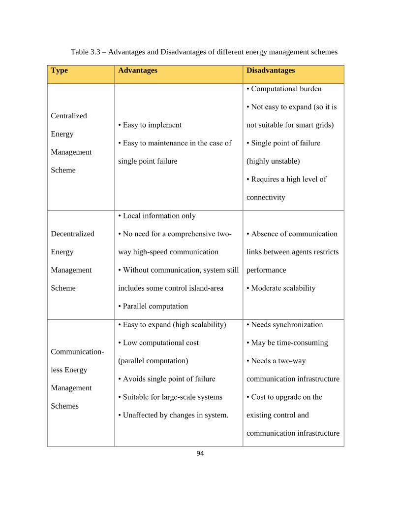
94

Table 3.3 – Advantages and Disadvantages of different energy management schemes

Type Advantages Disadvantages

Centralized

Energy

Management

Scheme

• Easy to implement

• Easy to maintenance in the case of

single point failure

• Computational burden

• Not easy to expand (so it is

not suitable for smart grids)

• Single point of failure

(highly unstable)

• Requires a high level of

connectivity

Decentralized

Energy

Management

Scheme

• Local information only

• No need for a comprehensive two-

way high-speed communication

• Without communication, system still

includes some control island-area

• Parallel computation

• Absence of communication

links between agents restricts

performance

• Moderate scalability

Communication-

less Energy

Management

Schemes

• Easy to expand (high scalability)

• Low computational cost

(parallel computation)

• Avoids single point of failure

• Suitable for large-scale systems

• Unaffected by changes in system.

• Needs synchronization

• May be time-consuming

• Needs a two-way

communication infrastructure

• Cost to upgrade on the

existing control and

communication infrastructure

95

3.5.2 Details of Supervisory Controller

Here, in this thesis, centralized control has been chosen for the simplicity and the accuracy of

the controller. Supervisory controller gets the signal from all individual power generating units

and decides the operational set-points for individual controllers. Therefore, the proposed hybrid

micro-grid has supervisory controller and three individual controllers. Block diagram of overall

control configuration for the proposed hybrid micro-grid is shown in Figure 3-21.

Wind Pitch Signal

Supervisory Controller

Energy Management


Pitch

Controller

Angle

Selector

Pitch

Actuator

Wind

Power

Plant

Speed

Governor

Controller

Hydro

Power

Plant

PV Arrays MPPT

Controller Inverter

Load


PLoad

PWind

PHydro

PPV

PHydro

Set Point

PHydro

Set Point

PWind Set Point

PWind Set Point

Wind

Pitch

Signal

Wind Pitch Signal

β

PLoad

PWind

PHydro

PPV

Wind Speed

β

Figure 3-21 – Block Diagram of Overall Control Configuration

96

In this case, inputs of the supervisory controller are electrical active power generation of PV

system, WG & HG, blade pitch angle, wind speed and total load power. Electrical distribution is

the final stage in the delivery of electricity to end users. In a physical power system, there are

multiple power distribution feeders. Power measurements of all distribution feeders will provide

the total load power in the system. The load power and measured electrical power of all distributed

electrical power generators help to decide the desired power from each power generating unit [164,

165]. Supervisory controller also decides when the pitch angle controller will be in operation.

Otherwise a fixed pitch angle is provided to the pitch actuator. Details of supervisory controller

are given in section 3.5.2.1 and section 3.5.2.2.

3.5.2.1 Wind Pitch Signal Supervisory Controller

The WG operating regions below and above rated wind speed are the major operating

regions. In these regions, maximum power point tracking control and pitch control are usually

used. When wind speed is below the rated speed, wind turbine normally operates in the MPPT

mode to extract maximum power from wind although wind energy curtailment might be required

under certain conditions, such as low load demand during off peak hours [166]. MPPT control

operates at the maximum power point to generate maximum power from the current wind speed,

but for wind energy curtailment, a different control method needs to be implemented. Conventional

methods of MPPT control are tip-speed ratio control, hill-climb searching control and power signal

feedback control. A few advanced MPPT control methods are also available, such as decreased

torque gain control, adaptive torque gain control [167, 168, 169].

Wind energy curtailment is essential when wind speed is above the rated speed and power

generation of WG needs to be maintained at rated power. When power generation of WG is

97

reduced to the desired power level that is lower than the available power generation, this is called

wind energy curtailment [170]. Wind energy curtailment is required when wind speed is below the

rated speed and load demand is less than the total power generation of WG. Wind energy

curtailment can be implemented using various control methods such as pitch actuator control, rotor

speed control, soft-stall control, etc. [171]. Pitch actuator control is a widely used control technique

to regulate the output power of WG [171]. In the proposed control strategy, pitch actuator

controller is used for all wind speed conditions with the help of angle selector and wind pitch

actuator supervisory controller. Firstly, when wind speed is below or at rated speed and load

demand is higher than the power generation of WG, pitch angle of WG remains at zero to extract

maximum power. Secondly, whenever wind energy curtailment is required, pitch actuator

controller comes into operation to control the power generated by the WG.

Supervisory controller in this thesis mainly controls the electrical power generation of wind

power plant and hydro power plant. When wind speed is below rated speed and load power is

higher than the total rated power generation by both PV system and wind power plant, pitch angle

should be at zero and pitch controller must be disconnected at that moment to extract maximum

power from WG. Whenever wind speed is higher than the cut-off wind speed, pitch angle must be

at its maximum and pitch controller remains disconnected. Otherwise pitch controller should be in

operating condition. When the wind speed is higher than the rated speed, wind electrical power

needs to be controlled to keep it at rated power. On the other hand, when wind speed is below rated

speed and the load demand is lower than the electrical power generation of wind power plant, pitch

controller should be in operating condition to decrease the electrical power generation of WG in

islanded mode. In this scenario, hydro power must be at its minimum power. In the previous

98

chapter, it is discussed that during off peak load, hydro power may run at its minimum power -

0.75 MW to avoid cavitation. The mentioned scenarios can be implemented by a multiple switch

(Angle Selector) and a control signal from angle pitch signal supervisory controller. Figure 3-22

shows the block diagram of the angle selector. Angle selector implemented here is based on the

approach proposed in [58, 172, 173].

Algorithm of the wind pitch signal supervisory controller for pitch angle selector is shown in

Figure 3-23. Steps to select wind pitch signal of angle selector are mentioned below.

1. Get initial state of wind speed.

2. Check whether the wind speed is equal or lower than the rated wind speed.

3. If wind speed is lower than rated wind speed, check whether hydro power generation is at

its minimum or not.

4. If hydro electrical power is at its minimum, wind pitch signal will be 1. Otherwise it will

be 2.

5. When wind speed is greater than cut-off wind speed, wind pitch signal will be 3.

Pitch Actuator

Pitch

Controller

90°

0°

Figure 3-22 – Block Diagram of Angle Selector

Wind Pitch Signal

2

1

3

99

6. When wind speed is in between rated and cut-off wind speed, wind pitch signal will be 1.

Start

Vwind <=

Rated Speed

No

Yes

Phydro

<= 0.75MW

No Yes

Wind Pitch Signal = 2


Vwind >=

Cut-out Speed

Yes



No

Figure 3-23 – Algorithm of Wind Pitch Signal Supervisory Controller for Angle Selector

100

3.5.2.2 Energy Management Supervisory Controller

Energy management supervisory controller decides the desired power of each power

generating unit of the hybrid micro-grid except PV system. Supervisory controller mainly

considers the mismatched power along with other few considerations to take the decision which

power generating unit will increase or decrease electrical power generation. Mismatched power or

balanced load is calculated from the total electrical generated power and total load power demand.

Power generation of all power generating units and load demand is measured in per unit concept.

Parameter of base power is mentioned in Appendix A.10. Depending on the wind speed, pitch

angle, wind and hydro electrical power generation, supervisory controller takes decision. The

supervisory controller implemented here is based on the approach proposed in [164]. Steps to find

the desired power of hydro and wind power plant are described below. Algorithm of the

supervisory controller is shown in Figure 3-24. Parameters for energy management supervisory

controller are given in Appendix B.5.

1. Get initial state of hydro (Phydro), wind (Pwind), solar (Ppv) and load (Pload) electrical

power.

2. Evaluate balance load power (∆P) by subtracting net electrical power generation from

electrical load power.

3. If ∆P is equal to zero, new hydro and wind desired power remain at previous values.

4. If ∆P is negative (lower than zero), power generation needs to be decreased. It checks

whether electrical power generation at hydro power plant is at its minimum or not.

5. If hydro electrical power generation is more than 0.75 MW, hydro power decreases.

Otherwise wind power decreases.

101

6. If ∆P is greater than zero, power generation needs to be increased. Further it checks

whether wind speed is within cut-in and cut-out speed.

7. If wind speed is not within cut-in and cut-out wind speed, hydro power increases.

Otherwise it checks whether pitch angle is greater than zero or not.

8. If pitch angle is greater than zero, it further checks whether wind electrical power

generation is at its rated power or not.

9. If electrical power generation of wind power plant is below rated power, wind power

increases. Otherwise hydro power increases.

102

Start

Check Ppv, Pwind, Phydro, Pload

Evaluate Balance Load (∆𝑷)= Pload – (Pwind + Phydro + Ppv )

∆𝑷 = 𝟎

Yes

No

Cut-in Speed >Vwind <Cut-

out Speed

∆𝑷 < 𝟎 No

Yes

Pitch Angle >0

Yes

No

Pwind < 2MW No

Yes

No Yes

Hydro Power

Increases

Hydro Power

Increases

Hydro Power

Increases Wind Power

Increases

Phydro<=

0.75 MW

No

Hydro Power

Decreases

Yes

Wind Power

Decreases

Return

Figure 3-24 – Algorithm of Energy Management Supervisory Controller

103

3.5.3 Wind Speed Measurement

For both wind pitch signal supervisory controller and energy management supervisory

controller, wind speed measurement is essential. In case of wind pitch signal supervisory

controller, wind pitch actuator controller comes into operation whenever wind energy curtailment

becomes necessary. Primarily, this algorithm takes the decision when pitch actuator controller will

come into operation depending upon the wind speed at that moment and also power generation of

HG. On the other hand, energy management supervisory controller takes wind speed into

consideration when load demand increases to decrease pitch angle and increase power generation

of WG.

Wind speed can be measured mainly in three ways, such as mechanically (cup anemometer

with a vane), ultrasonic and laser-based devices. Mechanical sensors use moving parts and connect

to data recording devices. These sensors physically move with changes in the wind and give

readings of speed and direction. An ultrasonic sensor or sonic anemometer functions without any

moving parts. This is also called sonic wind profiler or a sodar (sound detection and ranging) unit.

This detects wind speeds and directions at several levels up to 300m. Instruments used in this

device are small enough to mount on a nacelle. Further, laser wind sensor mounts atop the turbine

nacelle to measure real-time horizontal and vertical wind speed and directions in front of the

turbine. This sensor looks out to 300m ahead of the turbine to measure wind speed and direction

as it approaches the turbine blades [174]. Moreover, it provides 20 seconds advance notice which

is enough to change the angle of the blades so that the turbine can control the wind power while

reducing strain on its parts [174, 175]. Laser wind sensors seem to be a good solution to acquire

accurate and real-time data of wind speed. This data is critically important for the wind turbines

104

with adjustable blades. However, the impact of atmospheric interference, like fog, turbulences on

laser signals, needs to be analyzed [176]. The installation cost of cup anemometer increases rapidly

corresponding to the increase of height at which the anemometer is installed [177]. On the contrary,

laser source is more economical and compact which enhances the potential of laser wind sensors

for mass production. Due to compactness, portability and cost-efficiency, laser wind sensors have

a strong potential for use in the control of wind turbines [178].

In this thesis, both wind pitch signal and energy management supervisory controllers use

wind speed measurement as one of the inputs which can be implemented using laser wind sensors.

Simulation of wind speed measurement is considered out of scope for this thesis.

3.6 Chapter Summary

This chapter describes the strategies implemented to develop the design of the local controllers

and the supervisory controller for an isolated hybrid micro-grid. The local controllers’ designs

presented in this chapter are: MPPT Controller, PI/ PID controller and Fuzzy controller. Moreover,

wind pitch signal and energy management supervisory controllers are also described in this

chapter.

Firstly, MPPT controller describes how solar power tries to maintain the maximum power

under different weather conditions. Algorithm of the controller along with DC-DC converter is

described in this section.

Secondly, PI/PID controllers working principles are briefly described in this chapter. The

implementation of each PI controller both for pitch of wind power plant and speed governor of

hydro power plant are described here. The PI tuning method used in this thesis is also mentioned

in this chapter.

105

Thirdly, to do a comparative analysis, all the individual controllers of wind and hydro power

plants are implemented in Fuzzy logic also. Design of Fuzzy controllers is described in this

chapter.

Finally, different kinds of energy management system are elaborated. To control the pitch

angle at various conditions, wind pitch signal for angle selector is also implemented and described

in this section. To supervise each local controller, an energy management supervisory controller

is implemented. Algorithm and implementation of the wind pitch signal and energy management

supervisory controllers are described in this chapter. In this thesis, centralized energy management

supervisory controller has been used. For both wind pitch signal and energy management

supervisory controllers, wind speed measurement is necessary. Various methods of wind speed

measurement are also discussed in this chapter.

106

CHAPTER 4 : STUDY OF DIFFERENT SCENARIOS OF THE HYBRID MICRO-

GRID

The control strategy and the designed control system are described in detail in the previous

chapter. Results of the various simulation studies executed to test the performance of the control

system under various operating scenarios are presented in this Chapter. The control system is tested

by varying the wind and solar energy in the system as well as by introducing sudden changes in

the system load. A total of 8 studies have been performed to test the operation of different

controllers.

A few assumptions, described in Section 4.1, are considered while designing the proposed

hybrid micro-grid. A sudden change only in active load power is simulated in Section 4.2 and a

sudden change in load reactive power along with load active power is tested in Section 4.3. System

response to the wind speed increment is simulated in Section 4.4. Section 4.5 evaluates the system

performance under wind disturbance. Similarly, when wind speed decreases, system response is

simulated in Section 4.6. Test results of the change of solar irradiance and atmospheric temperature

are described in section 4.7. In the event of change of solar irradiance, atmospheric temperature

and wind speed, system responses are simulated in section 4.8. Lastly, load power change during

off-peak hours is tested in section 4.9. To conclude, a chapter summary is presented in Section

4.10.

4.1 Design Assumptions

A hybrid micro-grid is an electrical power system which supplies power to a network of

electrical components. Electrical power is supplied by the power generating units – solar, wind

and hydro power plants - in the proposed hybrid micro-grid. The total electrical power consumed

107

by all users connected to the distribution network and also the electrical power loss in all parts of

the network, are together called power system load. Power system electrical load power can be

categorized in various ways, mainly as base load and peak load. Base load is the minimum

electrical power demand on an electrical supply system over a 24 hours period. This is the

minimum amount of electric power delivered at a steady rate. In the system, at least one of the

generators should be in operation always to provide base load power. This kind of electrical load

power is also referred to as continuous load.

In a real power system, electrical power demand varies throughout the day. Peak load is

the highest demand of electrical power in a particular period of time. During this period, electrical

power demand is significantly higher than the average electrical power demand. In this case, a

number of generating units in the system together try to supply the high demand of load. In this

thesis, base load capacity of the hybrid micro-grid is considered as 4 MW. Maximum power

generation of PV system and wind power plant together can be 2.1 MW which is less than the base

load power. Because of this consideration, the balancing mechanism of the micro-grid - hydro

power plant - will be in running condition at all time.

There are a couple of advantages in keeping hydro power plant in running condition all the

time. Firstly, it helps to maintain the reference frequency. In the proposed hybrid micro-grid, wind

power plant and PV system are connected to the consumers’ load with power electronic converters

which do not have any inertia. Even though wind power plant has wind turbine rotor inertia, the

output electrical power of PMSG is connected to the load using AC-DC-AC power converter

which nullifies the presence of inertia in the system at the consumer end. This system inertia is

often considered as one of the vital system parameters upon which the synchronized operation of

108

the system is based. Inertia in the rotating masses of the synchronous generators and turbines

determines the immediate frequency response to the overall system instability. Therefore,

synchronous generator of the hydro power plant provides inertia in the proposed hybrid micro-grid

and helps to maintain the frequency standard.

Secondly, as power converters of WG and PV systems do not have reactive power control,

excitation system of the hydro power plant controls the reactive power. As hydro power plant of

the proposed hybrid micro-grid always remains in running condition, reactive power control for

reactive load power change will be done by the excitation system of HG. During peak load

condition, the maximum electrical load power demand can reach up to 6 MW because the

maximum electrical power generation capacity of hydro power plant is 6 MW. For the proposed

hybrid micro-grid, hydro power plant is the main balancing mechanism. When wind and solar

power plants are in running condition, hydro power plant will provide the required electrical power

deficit. On the other hand, when wind speed is below cut-in or above cut-off speed and there is no

solar irradiance, hydro alone will provide the load power.

Different scenarios of wind speed variations, change of solar irradiance, atmospheric

temperature and load power demand are simulated and described in the following sections.

4.2 Change in Load Active Power

In this scenario, initial condition of electrical active and reactive load at the consumer end

are 4.11 MW and 2.83 MVAR, respectively. In this condition, wind speed is 10 m/s. Therefore,

electrical power generation of WG is not at rated power. On the other hand, solar irradiance and

atmospheric temperature are considered at their rated values. Here, solar irradiance is considered

109

as 1000 W/m2 and atmospheric temperature is 25. Electrical power generation of solar power

plant is at rated power.

In this scenario, at first active load power is 4.11 MW and it changes to 4.61 MW at 20

seconds. Changes of 0.5 MW active load power are done in this scenario. Load reactive power

remains constant throughout this time. In this case, wind speed, solar irradiance and atmospheric

temperature also remain constant. As wind speed, solar irradiance and atmospheric temperature

are constant and electrical active power changes, power generation of HG will change to mitigate

the load demand. In this scenario, energy management supervisory controller will increase the set

point for hydro power plant which will eventually increase the power output of HG. As the HG

needs to increase the power generation, speed governor of HG increases the gate opening. This

eventually increases the mechanical power of the hydro turbine and ultimately increases electrical

power generation. Speed governor is designed using both PI and FLC to do a comparative analysis.

In this case, the load power demand is higher than the electrical power generation of WG.

Therefore, to extract maximum power from WG, pitch angle is at zero and wind pitch signal is at

2. In this scenario, the active power of the proposed hybrid micro-grid for both PI and Fuzzy

controllers is shown in Figures 4-1 and 4-2, respectively.

110

It is seen from Figures 4-1 and 4-2 that electrical power generation of HG changes to

mitigate the load power demand. Active power change of HG is shown in Figure 4-3.

Figure 4-1 – Active Power using PI Controller

Figure 4-2 – Active Power using Fuzzy Controller

111

Conventional PI controller has higher peak overshoot and longer settling time compared to

the FLC. Maximum Power deviation of HG (∆PHG) for PI controller is 0.357 MW whereas for

Fuzzy controller ∆PHG is 0.105 MW. In case of PI controller, power overshoot is significantly

higher than Fuzzy controller. For larger load change, power overshoot become more for PI

controller than FLC. This oscillation of power generation of HG also impacts the power generation

of other generating units in the micro-grid. Apart from the power overshoot, settling time is longer

in case of PI controller than Fuzzy controller. This hydro electrical power change is done by the

mechanical power input to the synchronous generator. Mechanical power input of HG for both PI

and FLC methods is shown in Figure 4-4.

Figure 4-3 – Active Power of Hydro Power plant

112

Firstly, peak overshoot of PI controller is higher than FLC which can be determined from

initial 10 seconds of load power change. After 10 seconds of load power change, mechanical power

almost gets stabilized when FLC is in operation. On the contrary, when PI controller is in

operation, oscillation persists. Speed governor mainly changes the gate opening which changes the

mechanical power output of the hydro turbine. Gate opening of the hydro turbine by the speed

governor with PI and fuzzy control is shown in Figure 4-5.

Figure 4-5 shows similar kind of results as mechanical power output of HG - Figure 4-4.

As seen, Fuzzy controller provides better response than the PI controller.

Figure 4-4 – Mechanical Power (pu) of Hydro Turbine

Figure 4-5 – Gate Opening (pu) of Hydro Turbine

113

In this scenario, only the active load power changes and reactive power remains unchanged.

When active load power changes reactive power of all the generating units gets disturbed and

gradually gets settled to the previous value. Reactive power of the proposed hybrid micro-grid for

both PI and Fuzzy controllers is shown in Figures 4-6 and 4-7, respectively.

As active power changes and reactive power remains constant, both apparent power and

power factor change. Load apparent power and load power factor are shown in Figures 4-8 and 4-

9, respectively.

Figure 4-6 – Reactive Power using PI Controller

Figure 4-7 – Reactive Power using Fuzzy Controller

114

In this scenario, energy management supervisory controller changes the power generation

set point for speed governor controller of HG as per the load demand and net power generation.

Figure 4-10 shows the power generation set-point of HG.

Figure 4-8 – Load Apparent Power

Figure 4-9 – Load Power Factor

Figure 4-10 – Power Generation Set Point of HG

115

To maintain pitch angle at zero and extract maximum power from WG, wind pitch signal

remains at zero. Figure 4-11 shows the wind pitch signal for this scenario.

In this case, the maximum frequency deviation (∆f) for PI and Fuzzy controller is almost

the same but Fuzzy controller shows significant improvement in maximum power deviation of HG

and settling time. Apart from this, multiple load changes have been carried out for the same

scenario. The obtained ∆PHG and ∆f for both controllers with multiple load changes are given in

Table 4.1. The ∆f for all load changes are within the limits defined by standard EUA [27].

Table 4.1 – ∆PHG and ∆f for PI and Fuzzy Controller

PI Controller Fuzzy Controller

Load Power Change ∆PHG ∆f ∆PHG ∆f

1 MW 0.78MW 0.165 Hz 0.195 MW 0.094 Hz

0.8 MW 0.62 MW 0.105 Hz 0.155 MW 0.068 Hz

0.6 MW 0.455 MW 0.052 HZ 0.117 MW 0.049 Hz

0.5MW 0.357 MW 0.041 Hz 0.105 MW 0.04 Hz

0.2 MW 0.125 MW 0.022 Hz 0.065 MW 0.021 Hz

Table 4.1 shows that the maximum power deviation of HG, when FLC is in operation, is

comparatively smaller than PI controller. Frequency deviation of the system remains almost the

Figure 4-11 – Wind Pitch Signal Graph

116

same until 0.6 MW load power change. At 1 MW load power change, frequency deviation is the

maximum. Figure 4-12 shows the frequency deviation for both controllers at 1 MW load power

change. In Figure 4-12, fuzzy controller gives better response in frequency than PI controller.

4.3 Change in Load Reactive Power

In this scenario, initial load and atmospheric conditions remain the same as given in Section

4.2. In the proposed hybrid micro-grid, voltage excitation of HG changes to compensate the

reactive load power change, but the speed governor of HG and pitch controller of WG play no role

in the change of load reactive power. All studies in this section are performed with the Fuzzy

individual controllers only.

A change of both active and reactive load power by increase and decrease of inductive

load, and change of resistive load are performed in this scenario. Firstly, for increase of inductive

load, load apparent power is changed from 5MVA, 0.822 lagging power factor to 5.356 MVA, 0.8

Figure 4-12 – Frequency Graph

117

lagging power factor. Next, for resistive load change, load apparent power is changed from 5MVA,

0.822 lagging power factor to 5.156 MVA, 0.835 lagging power factor. In this case, only the load

active power changes and load reactive power remains the same. Lastly, for decrease of inductive

load, load apparent power is changed from 5MVA, 0.822 lagging power factor to 4.97 MVA,

0.8667 lagging power factor. All load changes are performed at 20 seconds of the simulation.

Active load power change is 0.2 MW for all the three conditions. Active load power change for

these conditions is shown in Figure 4-13, Figure 4-14 and Figure 4-15.

Figure 4-13 – Active Power when Inductive Load Increases

118

As atmospheric conditions are constant, electrical power generation at HG increases to

compensate the load demand. As discussed earlier, WG and PV system do not have reactive power

control in the proposed hybrid micro-grid. When there is a change of reactive power demand,

voltage excitation of hydro synchronous generator is adjusted accordingly to deliver the

mismatched power.

Figure 4-14 – Active Power with only Resistive Load Change

Figure 4-15 – Active Power when Inductive Load Decreases

119

Figure 4-16 shows the voltage excitation change in the system when there is a change in

the load reactive power. When inductive load increases, voltage excitation increases to provide

more inductive power. In case of increase of active load power without any reactive load power

change, voltage excitation remains constant after initial transient. On the contrary, when inductive

load demand decreases, voltage excitation decreases.

As the reactive load power changes, primarily reactive power generation of HG changes to

compensate for the mismatched power. Figure 4-17 shows how reactive power of HG varies with

respect to these three conditions.

Figure 4-16 – Voltage excitation Change (pu)

120

When inductive load power increases, reactive power generation of HG increases but

reactive power generation of other power plants ultimately remains constant. Figure 4-18 shows

the reactive power of the hybrid micro-grid when inductive load increases.

When only active load power changes in the system, reactive power generation of all

electrical power generating units changes initially and gets stable eventually at the same value.

Figure 4-19 shows the reactive power of the system when resistive load power changes.

Figure 4-17 – Reactive Power Generation of HG

Figure 4-18 – Reactive Power Distribution when Inductive Load Increases

121

When inductive load decreases, hydro power plant decreases the reactive power generation

to mitigate the load demand but reactive power generation of other electrical power generating

units finally remains the same. Figure 4-20 shows the reactive power of the hybrid micro-grid

when inductive load decreases.

Figure 4-19 – Reactive Power Distribution when only Resistive Load Increases

Figure 4-20 – Reactive Power Distribution when Inductive Load Decreases

122

As system voltage fluctuation essentially depends on the load reactive power, voltage

fluctuation becomes the main concern in this scenario. Figure 4-21 shows the voltage fluctuations

for all the three conditions mentioned earlier.

In this scenario, voltage fluctuations are comparatively more for inductive load change

than resistive load change, but they remain within the voltage limit set by EUA. This scenario is

tested with multiple reactive load changes. Table 4.2 shows the maximum voltage fluctuations for

different load changes.

Table 4.2

When inductive load increases, maximum voltage fluctuation is more compared to

decrease of inductive load for all reactive load change conditions.

Maximum Voltage Fluctuation

Load Power Change Inductive Load Increases (%) Inductive Load Decreases (%)

0.2 MVAR, 0.2 MW 0.63 -0.28

0.35 MVAR, 0.2 MW 1.4 -0.8

0.5 MVAR, 0.2 MW 1.94 -1.27

1 MVAR, 0.2 MW 3.6 -2.9

Figure 4-21 – Voltage Fluctuation (%)

123

4.4 Increase in Wind Speed

In this scenario, initial load and atmospheric conditions are the same, as given in Section

4.2. There is no change in electrical load, solar irradiation and atmospheric temperature in this

scenario.

Initially, the wind speed is 10 m/s. A step change of 2 m/s in wind speed is done after every

20 seconds. At 20 seconds, wind speed becomes 12 m/s which is the rated wind speed. Next wind

speed goes above the rated wind speed and reaches 14 m/s at 40 seconds. At 60 seconds, wind

speed becomes the rated wind speed and lastly, wind speed goes down to 10 m/s at 80 seconds.

Wind speed change is shown in Figure 4-22.

As the wind speed changes to the rated speed, wind turbine rotor speed increases to the

rated rotor speed and electrical power reaches its maximum rated power. When wind speed goes

above the rated speed, wind pitch signal changes to 1 from 2 and then pitch controller comes into

operation. Pitch angle increases to reduce the wind turbine rotor speed and limits the power

Figure 4-22 – Wind Speed Change

124

generation of WG. The pitch controller is implemented using both PI and FLC algorithms. Figure

4-23 shows the pitch angle graph for this scenario.

At 40 seconds, when wind speed goes above the rated speed, pitch angle starts increasing

and when wind speed comes down to the rated value at 60 seconds, pitch angle gradually decreases

to zero. Fuzzy controller shows smaller peak overshoot and settling time than PI controller.

When wind speed increases, rotor speed of wind turbine also increases. Therefore, between

20 and 40 seconds, the rotor speed increases and at that time, pitch angle is zero. When wind speed

goes above the rated speed, rotor speed initially increases and comes down to the rated rotor speed.

Figure 4-24 and Figure 4-25, respectively, show the rotor speed for both PI and Fuzzy controllers.

Figure 4-23 – Pitch Angle (deg) Graph

125

When PI controller is in operation, settling time of rotor speed is longer than Fuzzy

controller. When the rotor speed goes down and the pitch angle is greater than zero, wind turbine

power co-efficient also goes down. Otherwise when wind speed is at rated or less than rated speed

and the pitch angle is zero, wind turbine power co-efficient stays at its maximum to extract

maximum power from the wind turbine. Wind turbine power co-efficient graph is shown in Figure

4-26.

Figure 4-24 – Wind Turbine Rotor Speed (pu) using PI Controller

Figure 4-25 – Wind Turbine Rotor Speed (pu) using Fuzzy Controller

126

As the wind speed changes, active power generation of WG changes. Because of the change

in WG power generation, electrical power generation of HG changes to mitigate the mismatched

power and maintain constant load power demand. Active power of the hybrid micro-grid for this

scenario is shown in Figure 4-27 for both PI and Fuzzy controllers.

In this scenario, as the wind speed goes to the rated wind speed at 20 seconds, active power

of WG increases to the rated electrical power. After 40 seconds, wind speed further increases to

Figure 4-26 – Wind Turbine Power Co-Efficient at Various Wind Speeds

Figure 4-27 – Active Power of Hybrid Micro-grid

127

14 m/s which is greater than the rated wind speed. In this condition, electrical power generation of

WG remains at the rated power until wind speed goes below the rated wind speed.

As wind speed varies, energy management supervisory controller changes the set point for

both HG and WG according to the load demand and total power generation. In this scenario, when

wind speed is below or at the rated speed, wind pitch signal supervisory controller sets the wind

pitch signal to 2, to keep wind pitch angle at zero. Wind pitch signal becomes 1 when wind speed

goes above the rated speed. As wind speed goes up, power set point of WG changes until wind

speed reaches the rated speed and power set point of HG decreases gradually to maintain constant

load power demand. Figures 4-28, 4-29 and 4-30 show power set points, respectively, for WG &

HG and wind pitch signal for this scenario.

Figure 4-28 – Power Generation Set Point of WG

128

In this scenario, as the wind speed changes, power generation of WG and HG changes.

This leads to frequency and voltage fluctuations in the system. But frequency and voltage

fluctuations are very small and stay within the standard limit set by EUA.

4.5 Sudden Change in Wind Speed

In this scenario, initial load and weather conditions are the same as given in Section 4.2.

Keeping electrical load power, solar irradiation and atmospheric temperature the same, system

response is observed when the wind speed changes starting at 20 s as shown in Figure 4-31.


Figure 4-30 – Wind Pitch Signal

129

When wind speed varies fast, wind turbine rotor speed increases rapidly which creates

disturbance in the system. Pitch angle needs to increase to control the wind turbine rotor speed

when wind speed is above the rated wind speed. The pitch controller is implemented using both

PI and FLC algorithms. Figure 4-32 shows how pitch angle varies with respect to the wind speed.

Figure 4-31 – Wind Speed Variation

Figure 4-32 – Pitch Angle Graph

130

When wind speed reaches the rated wind speed, wind pitch signal changes from 2 to 1 and

pitch controller starts to change the pitch angle according to the rotor speed error. In Figure 4-32,

change in pitch angle with both controllers starts at the same time, but FLC shows faster response

compared to the PI controller. Overshoot with Fuzzy controller is slightly higher than PI controller

in this case.

This pitch angle has direct impact on the wind turbine rotor speed. Figure 4-33 depicts the

rotor speed change of wind turbine for both PI and Fuzzy Controllers.

In the case of Fuzzy controller, rotor speed almost gets settled when wind speed stays above

the rated speed. But PI controller struggles to stabilize the rotor speed. Moreover, rotor speed of

PI controller shows more overshoot than Fuzzy controller in this scenario. As pitch angle increases,

Figure 4-33 –Rotor Speed (pu) of Wind Turbine

131

power co-efficient of the wind turbine comes down as shown by the Cp graph in Figure 4-34.

Power generation of WG is directly proportional to the wind turbine power co-efficient.

When wind speed increases, wind turbine mechanical power goes high which increases the

electrical power output. In this case, as Cp goes down, power generation of wind turbine remains

around the rated power. This scenario is tested using both PI and Fuzzy controllers individually.

Active power of the hybrid micro-grid using both methods is shown in Figure 4-35.

Figure 4-34 – Wind Turbine Power Co-Efficient Graph

132

When power generation of WG increases, power generation of HG decreases to maintain

the constant load power demand. When FLC is in operation, power oscillation is comparatively

smaller than with the PI controller. Therefore, FLC shows better results than the PI controller.

Load power demand in this scenario is constant. Even though in different power generating units

power generation changes, total power generation and power factor remain unaffected in this case.

As wind speed changes, active power generation of WG changes which ultimately impacts the

system frequency and voltage, but they remain within the standard limit.

As wind speed changes, power generation of WG changes. Consequently, power

generation of HG needs to be changed which is done by the supervisory energy management

controller. Initially, when wind speed is below the rated speed, wind pitch signal is at 2 to keep

the pitch angle at zero. Wind pitch signal supervisory controller brings the pitch controller in


133

operation by changing wind pitch signal from 2 to 1. Figures 4-36, 4-37 and 4-38 show power set

points, respectively for WG & HG and wind pitch signal for this scenario.




134

4.6 Decrease in Wind Speed

In this scenario, initial condition of atmospheric conditions and electrical load are the same

as mentioned in Section 4.2. Electrical load power, solar irradiation and atmospheric temperature

remain constant in this scenario. System response, when wind speed goes down, is evaluated in

this section. In this scenario, wind speed does not go above the rated speed. Hence, pitch angle

remains at zero and pitch controller remains inoperative. Therefore, all the results are tested with

the proposed Fuzzy individual controllers.

Initially, wind speed is 10 m/s and it changes in steps of 2 m/s every 20 seconds. At 20

seconds, wind speed changes to 8 m/s and it becomes 6 m/s at 40 seconds. At 60 seconds, it changes

to 8 m/s and at 80 seconds, it goes back to 10 m/s. The wind profile is shown in Figure 4-39.

When wind speed varies, wind turbine rotor speed changes. Rotor speed graph for this

scenario is shown in Figure 4-40.

Figure 4-39 – Wind Speed Variation

135

As the wind speed is below the rated speed and load power demand is higher than the

power generation of WG, pitch angle is zero. When wind speed changes and stays below the rated

speed, pitch angle remains zero. In this condition, power co-efficient stays at its maximum. Cp

graph for this scenario is shown in Figure 4-41.

As the wind speed decreases, the rotor speed comes down which eventually decreases the

power generation of WG. Similarly, when wind speed increases, power generation of WG

increases. As the system load power is constant, power generation of HG changes according to the

Figure 4-40 – Rotor Speed Graph

Figure 4-41 – Wind Turbine Power Co-Efficient Graph

136

power generation of WG. Active power of hybrid micro-grid for this scenario is shown in Figure

4-42.

In this scenario, total power generation of the system remains constant. Therefore, apparent

power and power factor at the consumer end do not change. Frequency and voltage fluctuations of

the system remain within the standard limit set by EUA.

As wind speed decreases, power generation of WG decreases and consequently, power

generation of HG needs to increase to maintain the constant load demand. To keep pitch angle at

zero, wind pitch signal remains at 2 and pitch controller remains inoperative. Figures 4-43 and 4-

44 show power set point of HG and wind pitch signal, respectively, for this scenario.


137

4.7 Change in Solar Irradiance and Temperature

In this scenario, initial condition of load and atmospheric conditions are same as given in

Section 4.2. In this case, wind speed and load power remain constant. Solar irradiance and

atmospheric temperature vary over the period of time. As change in power generation of PV system

is very low, impact on local controller will be minimal. Therefore, all studies are performed using

the proposed Fuzzy individual controllers in this scenario. Solar irradiance and atmospheric

temperature graphs are shown in Figure 4-45 and Figure 4-46, respectively.



138

When solar irradiance increases, both power generation and voltage of PV system increase.

On the contrary, when atmospheric temperature increases, voltage and power generation decrease.

In this scenario, when solar irradiance and temperature increase, electrical power generation

increases but voltage at PV array decreases. The generated power of PV system is transmitted to

the consumers through MPPT controller and inverter. When PV input voltage decreases, duty cycle

of MPPT controller, which is fed to the boost converter, increases. As duty cycle of the MPPT

controller increases, voltage output of the boost converter increases to maintain constant DC

voltage across inverter. PV input voltage, duty cycle for the boost converter and DC link voltage

are shown in Figure 4-47, Figure 4-48 and Figure 4-49.

Figure 4-45 – Solar Irradiance (W/m2) Graph

Figure 4-46 – Atmospheric Temperature () Graph

139

As solar irradiance increases, power generation of PV system increases. Figure 4-50 shows

the active power of the hybrid micro-grid for this scenario.

Figure 4-47 – PV Input Voltage Graph

Figure 4-48 – Duty Cycle of MPPT controller

Figure 4-49 – DC link Voltage Graph

140

When power generation of PV system increases, power generation of HG decreases to

maintain the constant load demand. Figure 4-51 shows the change in power generation of HG.

As the change of electrical power is very low compared to the load power demand,

frequency and voltage fluctuations are almost negligible in this scenario. When power generation

of PV system increases, power generation set point of HG needs to decrease to maintain constant

load demand. In this scenario, wind speed remains constant and power generation of WG is lesser


Active Power

Figure 4-51 – Active Power Generation of HG

141

than the load power demand. Therefore, wind pitch signal stays at 2 to keep pitch angle at zero.

Figure 4-52 shows the power set point of HG.

4.8 Changes in Atmospheric Conditions

Initial condition of load and atmospheric conditions are same as given in Section 4.2.

Consumers’ load does not change in this case, but wind speed, solar irradiance and atmospheric

temperature vary. Impact of these changes on the system is analyzed here. Changes in wind speed,

solar irradiance and atmospheric temperature are shown in Figures, 4-53, 4-54 and 4-55,

respectively.


Figure 4-53 – Wind Speed (m/s) Graph

Active Power

142

As wind speed increases, wind turbine rotor speed initially increases but gradually settles

down at the rated speed. Increment of pitch angle limits the wind turbine rotor speed at the rated

speed. When wind speed goes above the rated speed, wind pitch signal changes to 1 from 2 and

wind pitch controller comes into operation. Figures 4-56 and 4-57 show wind turbine rotor speed

and pitch angle, respectively.

Figure 4-54 – Solar Irradiance (W/m2) Graph

Active Power

Figure 4-55 – Atmospheric Temperature () Graph

Active Power

143

This scenario is implemented in both PI and FLC methods. Figure 4-57 shows that pitch

angle change using FLC is faster than PI controller. Overshoots of both PI and Fuzzy controllers

are almost the same. As pitch angle changes faster in case of Fuzzy controller, wind turbine rotor

speed also gets settled faster than with the PI controller. Peak overshoot of wind turbine rotor speed

is higher in case of PI controller than FLC.

As atmospheric conditions change in the same time span, electrical power generation of

both PV system and WG varies over the period of time. Figure 4-58 shows the active power of the

Figure 4-56 – Wind Turbine Rotor Speed (pu)


144

proposed hybrid micro-grid using both PI and FLC methods for this scenario.

In Figure 4-58, Fuzzy controller shows lesser oscillation than the PI controller. Being the

balancing mechanism of the system, power generation of HG changes to match the constant load

power demand in this scenario.

As wind speed, solar irradiance and atmospheric temperature vary, power generation of

WG and PV system varies. Power generation set point of HG and WG also varies to retain the

constant load power demand by the supervisory controller. Wind pitch signal supervisory

controller changes wind pitch signal from 2 to 1 to bring wind pitch controller in operation when

wind speed goes above the rated speed. Electrical power set point for WG, HG and wind pitch

signal are shown in Figures 4-59, 4-60, 4-61, respectively.


145




146

4.9 Load Power Change During Off-peak Hours

In this scenario, initial condition of load at consumers’ end is considered as 2.85 MW active

load power and 1.85 MVAR as reactive power. In this condition, wind speed is 12 m/s. Therefore,

electrical power generation of WG is at rated power. On the other hand, solar irradiance is

considered as 1000 W/m2, atmospheric temperature is 25 and power generation of PV system is

at rated power.

In this case, power generation of HG is at its minimum 0.75 MW. When load power

demand decreases, power generation of WG needs to be reduced as electrical power generation of

HG cannot be decreased further to avoid cavitation. In this scenario, load demand decreases at 20

seconds by 0.5 MW and increases again at 30 seconds. At 20 seconds, wind pitch angle increases

which reduces the rotor speed. Eventually, power generation of WG decreases. On the contrary,

wind pitch angle decreases when load demand increases. When wind pitch angle decreases at 30

seconds, wind turbine rotor speed increases and power generation of WG increases. In this

scenario, wind pitch signal is 1. Hence, pitch controller is in operation to control the power

generation of WG. The pitch angle change for this scenario is shown in Figure 4-62.


147

As the pitch angle increases, rotor speed decreases to reduce power generation of WG. It

increases to the rated speed when load demand increases. Figure 4-63 shows wind turbine rotor

speed graph using both PI and Fuzzy Controllers. FLC shows slightly smaller overshoot and

settling time compared to the PI controller.

As the wind turbine rotor speed and pitch angle change, wind turbine power co-efficient

also changes. As the wind turbine power co-efficient changes, active power generation of WG

changes. Power generation of other power generating units remains constant in this case. Active

power of the hybrid micro-grid using both PI and Fuzzy controllers for this scenario is shown in

Figure 4-64.

Figure 4-63 – Wind Turbine Rotor Speed (pu)

148

In this scenario when load demand decreases, power generation of HG remains constant to

avoid cavitation. Therefore, power generation of WG needs to decrease according to the load

demand change. During this condition wind pitch signal supervisory controller keeps wind pitch

signal at 1. When load demand decreases, energy management supervisory controller decreases

power generation set point of WG to increase pitch angle and decrease power generation of WG.

Figure 4-65 and Figure 4-66 show the power generation set point of WG and wind pitch signal,

respectively.


Figure 4-64 – Active Power of Hybrid Micro-Grid

149

4.10 Chapter Summary

Two different controllers and the proposed control strategy have been tested under several

load powers, wind speed, solar irradiation and atmospheric temperature disturbances. Results of

the simulated scenarios show that the proposed control strategy can provide reliable frequency and

voltage regulation of the system when sudden disturbances are introduced.

Active load power change and its impact on the speed governor of the HG are described in

section 4.2. Speed governor is implemented in both PI and FLC methods. Comparative analysis of

both controllers has been done for this scenario.

As WG and PV system do not have reactive power control in the proposed hybrid micro-

grid, excitation system of HG reacts to the reactive power change in the system. In section 4.3,

reactive power control of the proposed hybrid micro-grid is described.

Increase of wind speed and system response to the change are shown in section 4.4. Test

results of pitch angle change with respect to wind speed and its impact on the system are described


150

in this section. Pitch controller is also implemented using both PI and FLC. Comparative analysis

of both methods and their effect on the system are analyzed here.

Sudden wind speed variation and its impact on the system stability are described in section

4.5. Section 4.6 gives the idea of how system reacts when wind speed decreases.

Change in solar irradiance and atmospheric temperature have significant influence on the

electrical power generation of PV system. Test results of these changes given in sections 4.7 and

.4.8 show how system responds when various atmospheric conditions change simultaneously.

Lastly, section 4.9 describes how WG controls power generation for low load power

demand during off-peak hours.

151

CHAPTER 5 : CONCLUSIONS AND FUTURE WORK

The focus of this thesis is the design of Fuzzy logic controllers for the individual controllers

of WG and HG. The pitch controller of WG and speed governor of HG are designed using Fuzzy

logic as well as conventional PI approach. A supervisory controller is proposed to control all

individual controllers in the system. Design of the supervisory controller and individual controllers

to regulate the operation of the proposed hybrid micro-grid is presented in this study. The main

objectives of the research are to:

1. Develop a control strategy to regulate the operation of three power generating units

of a hybrid micro-grid, i.e. solar power plant, wind power plant and hydro power plant.

2. Use the hydro power plant as a balancing mechanism which operates by the defined

energy management strategies to provide voltage and frequency regulation of the system.

The implementation of balancing mechanism ensures a reliable operation of the isolated

hybrid micro-grid. At the same time, FLC based local controllers of WG and HG provide improved

system performance compared to the conventional PI local controllers.

The supervisory controller uses the hydro power plant as the main balancing mechanism.

During low power demand condition, power generation of HG may decrease to its lowest limit.

During this condition, supervisory controller needs to control power generation of WG as a

balancing mechanism.

Power generation of PV system depends primarily upon weather conditions. Therefore,

controlling power generation of PV system becomes difficult. In this thesis, a conventional MPPT

152

controller is proposed to extract maximum power from the PV system. The conclusions obtained

from the results of this thesis are described in this chapter.

5.1. Conclusions

The control system, implemented to regulate the operation of the balancing mechanism of

the hybrid micro-grid, is based on two types of controllers – a supervisory controller and individual

controllers for each generator. The supervisory controller brings individual controllers in operation

by observing the load power demand, weather conditions and power generation of individual

power generating units. Moreover, supervisory controller helps to regulate the power generation

set-points for WG and HG. The supervisory controller sends signal to the angle selector of wind

pitch angle actuator and decides operational set-points to regulate the running status of individual

controllers.

There are four individual controllers. These controllers provide frequency regulation to the

hybrid micro-grid and extract maximum energy. Pitch controller regulates wind turbine rotor speed

and power generation. Hydro speed governor regulates the power generation and frequency of

hydro power plant. Excitation controller of HG controls the reactive power demand of the system.

Lastly, conventional MPPT controller of PV system controls the DC link voltage and power

generation.

The designed controllers and implemented control strategy have been tested under different

power loading, wind speeds, solar irradiance and atmospheric temperature scenarios. Results of

the simulated scenarios show that the implemented controllers are capable of providing frequency

and voltage regulation to the system while maintaining the operational limits of the standard power

153

system. Also, the simulation results of the designed Fuzzy logic individual controllers show

improvement in the performance of the frequency regulation of the proposed hybrid micro-grid.

Moreover, supervisory controller gives satisfactory results for different disturbances introduced in

the power system.

5.2. Main Contributions

The contributions of this study are listed below:

- Development of Fuzzy wind pitch controller:

Wind pitch controller is essential for smooth operation of wind power plant. WG cannot

operate below and higher than certain wind speeds. Wind pitch angle changes to control the rotor

speed of the wind turbine when wind speed is higher than the rated speed but lower than the cut-

off speed. On the other hand, when wind speed is below the rated speed but above the cut-in speed,

pitch angle changes depending upon the load power demand. This wind pitch controller is

implemented in FLC method. To do the comparative analysis, wind pitch controller is

implemented in conventional PI controller also. Both conditions provide stable response, but

Fuzzy logic controller gives improved performance compared to PI in different operating

conditions. Wind pitch controller is tested under different power loading and wind speed changes

scenarios in order to verify the controller performance and capability of providing power

regulation to the hybrid micro-grid.

- Development of Fuzzy Speed Governor Controller of HG:

Speed governor controller of hydro power plant mainly provides frequency regulation to

the hybrid micro-grid. HG being the main balancing mechanism of the proposed hybrid micro-

154

grid, power generation of HG changes to mitigate the mismatched power in the system. Apart from

that, speed governor of HG tries to maintain the standard frequency in the system. This speed

governor is implemented in FLC method. For comparison, conventional PI speed governor

controller is also implemented. Both controllers are tested in different load and weather conditions.

In all these scenarios, FLC shows better results compared to the PI controller.

- Implementation of a Supervisory Controller:

A supervisory controller has been implemented to regulate the selection of the balancing

mechanisms in order to maintain the voltage and frequency standard of the hybrid micro-grid.

Wind pitch angle supervisory controller decides when pitch angle controller should come in to

operation depending upon the wind speed and power demand. Similarly, the energy management

supervisory controller changes operational set points for both pitch controller of WG and speed

governor of HG depending on various conditions. Performance of the supervisory controller is

evaluated under different scenarios. Supervisory controller maintains the frequency of the system

between the defined frequency limits.

5.3. Future Work

In this thesis, the implemented control strategy includes pitch controller of WG, speed

governor controller of HG and supervisory controller. Here, two turbines of HG are considered as

one for the simplicity of implementation. Two separate hydraulic turbines and their control can be

implemented for the detailed analysis of the proposed hybrid micro-grid. Moreover, multiple

power generating units of WG, HG and PV system can be considered in a hybrid micro-grid for

more reliable operation of the system.

155

Similarly, the speed governor controller of HG and pitch controller of WG have

been designed using FLC and PI methods. Other types of modern controllers, such as neural

networks can be implemented in order to evaluate their performance and any further improvements

in frequency regulation.

Reactive power control in the proposed hybrid micro-grid depends entirely on the

excitation controller of HG. Reactive power reference is considered as zero for the inverter

controller of WG and PV system. Inverter reactive power control can be implemented for both

WG and PV systems to provide better voltage regulation in the system.

Power generation of PV system is controlled by conventional P&O MPPT

controller to extract maximum energy. There are various advanced methods available as MPPT

controller which can be used for better performance of the PV system.

In this thesis, supervisory controller takes online decisions based on the load demand,

power generation and weather conditions. Other advanced predictive control methods can be

introduced for the design of the supervisory controller for better and stable operation of the system.

The implemented control strategy and frequency regulators are based on the system

configuration. In this study, the system is comprised of a WG and PV system with HG as balancing

mechanism to regulate the frequency of the system. Therefore, by changing the configuration of

the hybrid micro-grid, introducing some kind of energy storage systems, dump loads and power

resources, new control strategies can be investigated.

156

References:

1. T. M. Pavlovi, I. S. Radonji, D. D. Milosavljevi, and L. S. Panti, "A review of concentrating

solar power plants in the world and their potential use in Serbia," Renewable and

Sustainable Energy Reviews, vol. 16, pp. 3891-3902, 2012.

2. M. S. Jamel, A. Abd Rahman, and A. H. Shamsuddin, "Advances in the integration of solar

thermal energy with conventional and nonconventional power plants," Renewable and

Sustainable Energy Reviews, vol. 20, pp. 71-81, 2013.

3. IRENA. (2013, Renewable power generation costs in 2012: An overview. Available:

http://irena.org/DocumentDownloads/Publications/Renewable%20Generation%20Costs

%202012.pdf

4. M. Basu, "A simulated annealing-based goal-attainment method for economic emission

load dispatch of fixed head hydrothermal power systems," International Journal of

Electrical Power & Energy Systems, vol. 27, pp. 147-153, 2005.

5. R. Gopalakrishnan and A. Krishnan, "A novel combined economic and emission dispatch

problem solving technique using non-dominated ranked genetic algorithm," European

Journal of Scientific Research, vol. 64, pp. 141-151, 2011.

6. D. C. Walters and G. B. Sheble, "Genetic algorithm solution of economic dispatch with

valve point loading," Power Systems, IEEE Transactions on, vol. 8, pp. 1325-1332, 1993.

7. Pazheri, F. R. "Tri-generation based hybrid power plant scheduling for renewable resources

rich area with energy storage." Energy Conversion and Management 103 (2015): 717-725.

8. Vijayapriya, Tamilmaran, and Dwarkadas Pralhadas Kothari. "Smart grid: an

overview." Smart Grid and Renewable Energy 2, no. 4 (2011): 305.

157

9. H. Tai and E. Hogain, "Behind the Buzz: Eight smart-grid trends shaping the industry,"

IEEE Power and Energy Magazine, vol. 7, no. 2, Mar. 2009.

10. R. Dugan, "Challenges in Considering Distributed Generation in the Analysis and Design

of Distribution Systems," IEEE/PES General Meeting, 2008.

11. Martinez-Cid, R., and E. O'Neill-Carrillo. "Sustainable microgrids for isolated systems."

In Transmission and Distribution Conference and Exposition, 2010 IEEE PES, pp. 1-7.

IEEE, 2010.

12. Kundur, Prabha, John Paserba, Venkat Ajjarapu, Göran Andersson, Anjan Bose, Claudio

Canizares, Nikos Hatziargyriou et al. "Definition and classification of power system

stability IEEE/CIGRE joint task force on stability terms and definitions." IEEE

transactions on Power Systems 19, no. 3 (2004): 1387-1401.

13. M. B. Delghavi, “Advanced Islanded-Mode Control of Microgrids,” The University of

Western Ontario, 2011.

14. P. Manjarres, “Automatic Operation of a Stand-Alone Hybrid Power System with

Frequency Regulation by Fuzzy Logic and Binary Control,” 2013.

15. Bhandari, Binayak, Shiva Raj Poudel, Kyung-Tae Lee, and Sung-Hoon Ahn.

"Mathematical modeling of hybrid renewable energy system: A review on small hydro-

solar-wind power generation." international journal of precision engineering and

manufacturing-green technology 1, no. 2 (2014): 157-173.

16. Misak S, Prokop L. Off-grid power systems. In: Environment and electrical engineering

(EEEIC), 2010 9th international conference on 2010. p. 14–7. Farahat S, Jahromi MAY,

Barakati SM. Modeling and sizing optimization of stand-alone hybrid renewable energy

158

systems. In: International conference on mechanical, nanotechnology and cryogenics

engineering (ICMNC). Kuala Lumpur, Malaysia; 2012.

17. Posadillo R, Luque RL. Approaches for developing a sizing method for standalone PV

systems with variable demand. Renewable Energy 2008;33:1037–48.

18. Engin M. Sizing and simulation of PV–wind hybrid power system. Int J Photoenergy 2013.

19. Koutroulis E, Kolokotsa D, Potirakis A, Kalaitzakis K. Methodology for optimal sizing of

stand-alone photovoltaic/wind-generator systems using genetic algorithms. Sol Energy

2006;80:1072–88.

20. Markvart T. Sizing of hybrid photovoltaic–wind energy systems. Sol Energy 1996;57:277–

81.

21. Diaf S, Notton G, Belhamel M, Haddadi M, Louche A. Design and technoeconomical

optimization for hybrid PV/wind system under various meteorological conditions. Appl

Energy 2008;85:968–87.

22. Jaramillo OA, Borja MA, Huacuz JM. Using hydropower to complement wind energy: a

hybrid system to provide firm power. Renewable Energy 2004;29:1887–909.

23. Margeta J, Glasnivic Z. Feasibility of the green energy production by hybrid solar + hydro

power system in Europe and similar climate areas. Renew Sustain Energy Rev

2010;14:1580–90.

24. Ahn SH, Lee KT, Bhandari B, Lee GY, Lee CS, Song CK. Formation strategy of

renewable energy sources for high mountain off-grid system considering sustainability. J

Korean Soc Precision Eng 2012;29:958–63.

159

25. Bhandari, Binayak, Kyung-Tae Lee, Caroline Sunyong Lee, Chul-Ki Song, Ramesh K.

Maskey, and Sung-Hoon Ahn. "A novel off-grid hybrid power system comprised of solar

photovoltaic, wind, and hydro energy sources." Applied Energy 133 (2014): 236-242.

26. R. Iea-pvps, “Overview of Supervisory Control Strategies including a MATLAB ®

Simulink ® Simulation Tool,” Int. Energy Agency, vol. IEA-PVPS T, pp. 1–26, 2012

27. Technical Requirements for Connecting to the Alberta Interconnected Electric System

(IES) Transmission System

28. "Wind project planning: Wind turbine classes" Vestas. Accessed October 2011.

29. Manyonge, Alfred Wanyama, R. M. Ochieng, F. N. Onyango, and J. M. Shichikha.

"Mathematical modelling of wind turbine in a wind energy conversion system: Power

coefficient analysis." Applied mathematical sciences 6, no. 91 (2012): 4527-4536.

30. “Utility-Scale Solar Photovoltaic Power Plants”, International Finance Corporation 2015,

2121 Pennsylvania Avenue, N.W. Washington, D.C. 20433

31. Nasir, Bilal Abdullah. "Design of micro-hydro-electric power station." International

Journal of Engineering and Advanced Technology 2, no. 5 (2013): 39-47.

32. P. Kundur and N. J. Balu, Power system stability and control. New York, NY: McGraw-

Hill, 1994.

33. Felber, L. A., H. Arango, B. D. Bonatto, and M. R. Gouvea. "Voltage regulation in electric

energy distribution substations." In Transmission and Distribution Conference and

Exposition: Latin America (T&D-LA), 2010 IEEE/PES, pp. 846-852. IEEE, 2010.

34. J. Bucciero and M. Terbrueggen, “Interconnected Power System Dynamics Tutorial,”

EPRI, Final Report TR- 107726-R1, Jan. 1998.

160

35. H. Bevrani, Robust power system frequency control, 2nd Edition. Springer, 2014.

36. Horta, Ricardo, Jairo Espinosa, and Julián Patiño. "Frequency and voltage control of a

power system with information about grid topology." In Automatic Control (CCAC), 2015

IEEE 2nd Colombian Conference on, pp. 1-6. IEEE, 2015.

37. Zhang, Zhihao, Xinhong Huang, Jin Jiang, and Bin Wu. "A load-sharing control scheme

for a microgrid with a fixed frequency inverter." Electric power systems research 80, no.

3 (2010): 311-317.

38. Chapter 2: Kenfack J, Neirac FP, Tatietse TT, Mayer D, Fogue M, Lejeune A. Microhydro-

PVhybrid system: sizing a small hydro-PV-hybrid system for rural electrification in

developing countries. Renew Energy 2009;34:2259–63.

39. Bekele G, Tadesse G. Feasibility study of small Hydro/PV/Wind hybrid system for off-

grid rural electrification in Ethiopia. Appl Energy 2012;97:5–15.

40. Abdullah, A. G., A. Risdiyanto, and A. B. D. Nandiyanto. "Hybrid Energy System Design

of Micro Hydro-PV-biogas Based Micro-grid." In IOP Conference Series: Materials

Science and Engineering, vol. 180, no. 1, p. 012080. IOP Publishing, 2017.

41. Lakshmi, G., P. Rama Rao, and Y. Palleswari. "Hybrid solar-wind-hydro renewable energy

system." WJMS 10, no. 4 (2014): 243-251.

42. Raha, Syamasree, and Suvajit Pal. "A Study on the Present Environmental Scenario due to

Pollution by Conventional Energy Sources—and Remedies: Solar Cell with

Nanotechnology." Strategic Planning for Energy and the Environment 30, no. 2 (2010): 8-

19.

161

43. Lorenso, E. (1994). Solar Electricity Engineering of Photovoltaic Systems. Artes Graficas

Gala, S.L., ISBN: 84-86505-55-0, Spain

44. Markvart, T., Castaner, L. (2003). Practical Handbook of Photovoltaics, Fundamentals

and Applications, Ed. Elsevier, ISBN 1-85617-390-9, Oxford, UK

45. Patel, M. R. (1999). Wind and solar power systems, CRC Press LLC, ISBN 0-8493-1605-

7, Boca Raton, Florida

46. Bica, Dorin, Cristian Dragos Dumitru, Adrian Gligor, and Adrian-Vasile Duka. "Isolated

Hybrid Solar-Wind-Hydro Renewable Energy Systems." In Renewable Energy. InTech,

2009.

47. Dumitru, C.D., Gligor, A. (2008a). Power Quality Analysis Of A System Based On

Renewable Energy Supplying A Local Distribution Network, Acta Electrotehnica, Special

Issue: Proceedings of the 2nd International Conference on Modern Power Systems MPS

2008, 12-14 nov. 2008, pag. 224-226, ISSN 1841-3323

48. P.B. Eriksen, T. Ackermann, and etc. “System Operation with High Wind Penetration”,

IEEE Power & Energy Magazine, pp.65-74, Nov/Dec, 2005

49. Zhang, Yi, and Sadrul Ula. "Comparison and evaluation of three main types of wind

turbines." In Transmission and Distribution Conference and Exposition, 2008. T&D.

IEEE/PES, pp. 1-6. IEEE, 2008.

50. Camacho, Eduardo F., Tariq Samad, Mario Garcia-Sanz, and Ian Hiskens. "Control for

renewable energy and smart grids." The Impact of Control Technology, Control Systems

Society (2011): 69-88.

51. “Wind Power Today”, American Wind Energy Association (AWEA)

162

[online]. Available: http://www.awea.org/pubs/factsheets/WindPowerToday_2007.pdf

52. MATHWORKS Inc., “Wind Turbine.” [Online]. Available:

http://www.mathworks.com/help/physmod/sps/powersys/ref/windturbine.html.

53. S. Heier, Grid integration of wind energy: onshore and offshore conversion systems. John

Wiley & Sons, 2014.

54. S. M. Muyeen, J. Tamura, and T. Murata, Stability augmentation of a grid-connected wind

farm. Springer Science & Business Media, 2008.

55. N. A. Ahmed and M. Miyatake, “A stand-alone hybrid generation system combining solar

photovoltaic and wind turbine with simple maximum power point tracking control,” Conf.

Proc. - IPEMC 2006 CES/IEEE 5th Int. Power Electron. Motion Control Conf., vol. 1, pp.

242–248, 2007.

56. S. K. Kim, E. S. Kim, and J. B. Ahn, “Modeling and control of a grid-connected wind/PV

hybrid generation system,” Proc. IEEE Power Eng. Soc. Transm. Distrib. Conf., no. 1, pp.

1202–1207, 2006.

57. El-Tamaly, Hassan H., and Ayman Yousef Nassef. "Tip speed ratio and Pitch angle control

based on ANN for putting variable speed WTG on MPP." In Power Systems Conference

(MEPCON), 2016 Eighteenth International Middle East, pp. 625-632. IEEE, 2016.

58. Uehara, Akie, Alok Pratap, Tomonori Goya, Tomonobu Senjyu, Atsushi Yona, Naomitsu

Urasaki, and Toshihisa Funabashi. "A coordinated control method to smooth wind power

fluctuations of a PMSG-based WECS." IEEE Transactions on Energy Conversion, vol. 26,

no. 2, pp. 550–558, 2011.

59. Howlader, Abdul Motin, Naomitsu Urasaki, Atsushi Yona, Tomonobu Senjyu, and Ahmed

163

Yousuf Saber. "Design and implement a digital H∞ robust controller for a MW-class

PMSG-based grid-interactive wind energy conversion system." Energies, vol. 6, no. 4, pp.

2084–2109, 2013.

60. Huang, Nantao. "Simulation of power control of a wind turbine permanent magnet

synchronous generator system." (2013).

61. A. E. Fitgerald, J. C. Kingsley, and S. D. Umans, Electric Machinery. New York:

McGraw-Hill, 1990.

62. Patil, Kedar, and Bhinal Mehta. "Modeling and simulation of variable speed wind turbine

with direct drive permanent magnet synchronous generator." In Green Computing

Communication and Electrical Engineering (ICGCCEE), 2014 International Conference

on, pp. 1-6. IEEE, 2014.

63. R. M. Park, “Two-reaction theory of synchronous machines, pt. I: Generalized

method of analysis,” AIEE Trans., vol. 48, pp. 716–730, July 1929.

64. MATHWORKS Inc., “Permanent Magnet Synchronous Machine” [Online]. Available:

https://www.mathworks.com/help/physmod/sps/powersys/ref/permanentmagnetsynchron

ousmachine.html

65. Gajewski, Piotr. "Analysis of a wind energy converter system with pmsg generator."

Czasopismo Techniczne 2015, no. Elektrotechnika Zeszyt 1-E (8) 2015 (2015): 219-228.

66. CelsoPenche: "Layman's guidebook on how to develop a small hydro site", Published by

the European Small Hydropower Association (ESHA), Second edition, Belgium, June,

1998.

164

67. International Energy Agency ,“Water Enegy Nexus”. [Online]. Available:

https://www.iea.org/publications/freepublications/publication/WorldEnergyOutlook2016

ExcerptWaterEnergyNexus.pdf

68. Dilip Singh: "Micro-hydro-power", Resource Assessment Handbook, An Initiative of the

Asian and Pacific Center for Transfer of Technology, September, 2009.

69. Reichl, Fabian, and Jochen Hack. "Derivation of Flow Duration Curves to Estimate

Hydropower Generation Potential in Data-Scarce Regions." Water 9, no. 8 (2017): 572.

70. CelsoPenche: "Layman's guidebook on how to develop a small hydro site", Published by

the European Small Hydropower Association (ESHA), Second edition, Belgium, June,

1998.

71. USGS 03036000 Mahoning Creek at Mahoning Creek Dam, PA. Link:

https://waterdata.usgs.gov/usa/nwis/uv?03036000

72. Nasir, Bilal Abdullah. "Design considerations of micro-hydro-electric power plant."

Energy Procedia 50 (2014): 19-29.

73. Hydro Review: Adding Power to a Non-Powered Dam: Mahoning Creek. Link:

http://www.hydroworld.com/articles/hr/print/volume-33/issue-8/cover-story/adding-

power-to-a-non-powered-dam-mahoning-creek.html

74. MATHWORKS Inc., “Water Tank Simulink Model.” [Online]. Available:

http://www.mathworks.com/help/slcontrol/gs/watertank-simulink-model.html.

75. J. Liang and R. G. Harley, “Pumped storage hydro-plant models for system transient and

long-term dynamic studies,” IEEE PES Gen. Meet. PES 2010, pp. 1–8, 2010.

76. Demello, F. P., R. J. Koessler, J. Agee, P. M. Anderson, J. H. Doudna, J. H. Fish, P. A. L.

165

Hamm et al. "Hydraulic-turbine and turbine control-models for system dynamic studies."

IEEE Transactions on Power Systems 7, no. 1 (1992): 167-179. Harvard

77. P. Kundur, E. Neal, J. Balu, and M. G. Lauby, Power System Stability and Control, 7th ed.

New York, 1994.

78. MATHWORKS Inc., “Hydraulic Turbine and Governor.” [Online]. Available:

http://www.mathworks.com/help/physmod/sps/powersys/ref/hydraulicturbineandgoverno

r.html.

79. S. M. Islam, “Increasing wind energy penetration level using pumped hydro storage in

island micro-grid system,” Int. J. Energy Environ. Eng. 2012, pp. 1–12, 2012.

80. IEEE Std 421.1, IEEE standard definitions for excitation systems for synchronous

machines, vol. 2007, no. July. 2007.

81. IEEE Std 421.5, IEEE Recommended Practice for Excitation System Models for Power

System Stability Studies. 2006

82. MATHWORKS Inc., “Excitation System.” [Online]. Available:

http://www.mathworks.com/help/physmod/sps/powersys/ref/excitationsystem.html.

83. P. C. Krause, O. Wasynczuk, S. D. Sudhoff, and S. Pekarek, Analysis of Electric

Machinery and Drive Systems, 3rd ed. John Wiley & Sons, 2013.

84. MATHWORKS Inc., “Synchronous Machine.” [Online]. Available:

http://www.mathworks.com/help/physmod/sps/powersys/ref/synchronousmachine.html.

85. M. L. Awad, “Modeling of Syncronous Machines for System Studies,” University of

Toronto, 1999.

86. S. Kuehl, P. Landsmann, and R. M. Kennel, “Compensating angle estimation errors caused

166

by magnetic saturation in anisotropy-based sensorless control schemes,” 3rd IEEE Int.

Symp. Sensorless Control Electr. Drives, SLED 2012, no. 6, 2012.

87. J. Grainger and W. Stevenson, Power System Stability. McGraw-Hill, 1994.

88. MATHWORKS Inc., “Simplified Synchronous Machine.” [Online]. Available:

http://www.mathworks.com/help/physmod/sps/powersys/ref/simplifiedsynchronousmachi

ne.html.

89. P. Tenca, A. A. Rockhill, T. A. Lipo, and P. Tricoli, “Current source topol-ogy for wind

turbines with decreased mains current harmonics, further reducible via functional

minimization,” IEEE Trans. Power Electron., vol. 23, no. 3, pp. 1143–1155, May 2008.

90. Batarseh, Issa. Power electronic circuits. John Wiley, 2004.

91. El-Saadawi, MS Kandil MM, and AE Hassan KM Abo-Al-Ez. "Performance analysis of a

biomass microturbine DG for rural electrification." (2009).

92. G. Jóos, B.T. Ooi, D. McGillis, F.D. Galiana, and R. Marceau, “The Potential of

Distributed Generation to Provide Ancillary Services”, in Proc. 2000 IEEE Power

Engineering Society Summer Meeting, Vol.3, 2000.

93. El-Saadawi, MS Kandil MM, and AE Hassan KM Abo-Al-Ez. "Performance analysis of a

biomass microturbine DG for rural electrification." (2009).

94. Chee-Mun Ong, “Dynamic Simulation of Electric Machinery Using MATLAB/

SIMULINK”, Prentice Hall, [Book], 1997.

95. Galdi, V.; Piccolo, A.; Siano, P.; ”Dynamic Performances and Control of Dispersed

Generators Connected through Inverter”. International Conference on Computational

Intelligence for Modeling, Control and Automation, Volume 1, 28-30 Nov. 2005.

167

Page(s):1060 – 1065.

96. Huan-Liang Tsai, Ci-Siang Tu, and Yi-Jie Su, “Development of Generalized Photovoltaic

Model Using MATLAB/SIMULINK”, Proceedings of the World Congress on Engineering

and Computer Science 2008 WCECS 2008, October 22 - 24, 2008, San Francisco, USA.

97. Berrera, M., A. Dolara, R. Faranda, and S. Leva. "Experimental test of seven widely-

adopted MPPT algorithms." In PowerTech, 2009 IEEE Bucharest, pp. 1-8. IEEE, 2009.

98. E. V. Solodovnik, S. Liu, and R. A. Dougal, “Power controller design for maximum power

tracking in solar installations,” IEEE Trans. Power Electron., vol. 19, no. 5, pp. 1295–1304,

Sep. 2004.

99. D. Rajapakse and D. Muthumuni, “Simulation tools for photovoltaic system grid

integration studies,” in Proc. Electr. Power Energ. Conf. (EPEC 2009), Oct., pp. 1–5.

100. MATHWORKS Inc., “Implement maximum power point tracking algorithms for

photovoltaic systems using MATLAB and Simulink ” [Online]. Available:

https://www.mathworks.com/discovery/mppt-algorithm.html.

101. Manoj Kumar, F. Ansari, A.K. Jha ―Maximum power point tracking using perturbation

and observation as well as incremental conductance algorithm‖,IJREAS , ISSN 2294-3905,

Vol.1,Issue 4 (2011), pp.19-31.

102. Pandiarajan N., Ramaprabha R., Ranganath Muthu, ―Application of circuit model for

photovoltaic energy conversion systems‖, research article.

103. Masri, S. and Chan, P.W., 2010, June. Design and development of a dc-dc Boost converter

with constant output voltage. In Intelligent and Advanced Systems (ICIAS), 2010

International Conference on (pp. 1-4). IEEE.

168

104. Ned Mohan, Tore M. Undeland, and Williams P. Robbins, Power Electronics: Converters,

Applications, and Design, 3rd ed., John Wiley &Sons: USA, 2003, pp. 161-197.

105. T. F. Wu, and Y. K. Chen, “Modeling PWM DC/DC converter out of basic converter

units,” IEEE Trans. On Power Electronics, vol. 13, no. 5, pp. 870-881, 1998.

106. B. M Hasaneen, and Adel A. Elbaset Mohammed, “Design and simulation of DC/DC

boost converter,” Power System Conf. MiddleEast, pp. 335-340, 2008.

107. H. Mahmood, and K. Natarajan, “Parasitics and voltage collapse of the DC-DC boost

converter,” Canadian Conf. on Electrical and Computer Engineering, pp. 273-278, 2008.

108. Ahmad Al Nabulsi, Muneer Al Sabbagh, Rached Dhaouadiand Habib-ur Rehman, “A 300

watt cascaded boost converter design for solar energy systems,” International Conf. on

Electric Power and Energy Conversion Systems, pp. 1-4, 2009.

109. Yamamoto S, Hashimoto I. Present status and future needs: The view from Japanese

industry[C]//Chemical Process Control-CPCIV. Proceedings of the Fourth International

Conference on Chemical Process Control, Texas. 1991.

110. Astrom K J. PID controllers: theory, design and tuning[J]. Instrument Society of America,

1995.

111. Panagopoulos H, Åström K J, Hägglund T. Design of PID controllers based on constrained

optimisation[J]. IEE Proceedings-Control Theory and Applications, 2002, 149(1): 32-40.

112. K. Astrom, K. and T.Hagglund, ‘’PID Controllers: Theory, Design, and Tuning’’,

Instrument Society of America, ISBN 1-55617-516-7, 1995

113. Rao, K. Smriti, and Ravi Mishra. "Comparative study of P, PI and PID controller for speed

control of VSI-fed induction motor." International Journal of Engineering Development and

169

Research 2, no. 2 (2014): 2740-2744.

114. Airikka, P. "PI controller tuning rules for optimal load disturbance response." In Control

Conference (ECC), 2001 European, pp. 2358-2363. IEEE, 2001.

115. Wang, Yinsong, and Ri Hai. "Power control of permanent magnet synchronous generator

directly driven by wind turbine." rn 2 (2013): 60.

116. J. Jonkman, S. Butterfield, W. Musial and G. Scott, “Definition of a 5-MW Reference Wind

Turbine for Offshore System Development,” Technical Report NREL/TP-500-38060, Feb.

2009.

117. I. Poultangar, R. Shahnazi and M. Sheikhan, “RBF neural network based PI pitch controller

for a class of 5-MW wind turbines using particle swarm optimization algorithm,” ISA

Transactions Vol.51, pp. 641–648, 2012. [Online]. Available: http://dx.doi.org/

doi:10.1016/j.isatra.2012.06.001

118. Y. Qi and Q. Meng, “The Application of Fuzzy PID Control in Pitch Wind Turbine,” Proc.

of International Conference on Future Energy, Environment, and Materials, Energy

Procedia, Vol.16, pp. 1635-1641, 2012. [Online]. Available: http://dx.doi.org/

doi:10.1016/j.egypro.2012.01.254

119. P. Garasi, M. Watanabe and Y. Mitani, "Power smoothing of wind turbine generator using

Fuzzy-PI pitch angle controller," Proc. of IEEE Power Engineering Conference (AUPEC),

pp. 1-5, 2014. [Online]. Available: http://dx.doi.org/ DOI: 10.1109/AUPEC.2014.6966531

120. Wang, Yinsong, and Ri Hai. "Power control of permanent magnet synchronous generator

directly driven by wind turbine." rn 2 (2013): 60.

121. Beltran, Brice, Tarek Ahmed-Ali, and Mohamed El Hachemi Benbouzid. "Sliding mode

170

power control of variable-speed wind energy conversion systems." IEEE Transactions on

Energy Conversion 23, no. 2 (2008): 551-558.

122. Schleif, F. R., and A. B. Wilbor. "The coordination of hydraulic turbine governors for

power system operation." IEEE Transactions on Power Apparatus and Systems 7 (1966):

750-758.

123. N. Kishora, R.P. Sainia, and S.P. Singhb, A Review on Hydropower Plant Models and

Control, Renewable and Sustainable Energy Reviews, vol. 11, 2007, pp.776-796.

124. Naghizadeh, R. A., S. Jazebi, and B. Vahidi. "Modeling hydro power plants and tuning

hydro governors as an educational guideline." International Review on Modelling and

Simulations (I. RE. MO. S) 5, no. 4 (2012): 3427-3430.

125. A. O'Dwyer, Handbook of PI and PID ControllerTuning Rules. London: Imperial College

Press, 2003.

126. Culberg, J., Michael Negnevitsky, and Kashem M. Muttaqi. "Hydro-turbine governor

control: theory, techniques and limitations." (2006).

127. Åström, Karl Johan, and Tore Hägglund. PID controllers: theory, design, and tuning. Vol.

2. Research Triangle Park, NC: Isa, 1995.

128. Fuzzy Control, Kevin M. Passino, Stephen Yurkovich, Department of Electrical

Engineering, The Ohio State University.

129. Zadeh, L.A. (1975):„The concept of a linguistic variable and its application to approximate

reasoning‟, Information sciences Vol. pp199-249, 1975.

130. Zadeh, L.A. (1996):„Fuzzy logic = computing with words‟, IEEE Transactions on fuzzy

systems Vol. 4(2), pp103-111.

171

131. Biswas, S., Roy, P.K. and Datta, S. (2008):„Impact of Fertiliser in a Catchment Area:

Assessment by Using Fuzzy Logic‟, IJAAR, 22-Jan-2008.

132. C. C. Lee, "Fuzzy Logic In Control Systems: Part I", IEEE Trans, on Systems, Man, and

Cybernetics, Vol. 20, No. 2, Mar/Apr 1990.

133. E. Cox, "Fuzzy Fundamentals", IEEE Spectrum, October 1992, pp. 58-61. a. J. P. King, "A

Vendor's Contribution To Computer System Software Validation", Pharmaceutical

Engineering, Sept/Oct. 1992.

134. Putrus G., Narayana M., Jovanovic M., Leung P. S. :, “Maximum power point tracking for

variable-speed fixed-pitch small wind turbines”, 20th International Conference on

Electricity Distribution Prague, 8-11 June 2009

135. Musyafa, A., A. Harika, I. M. Y. Negara, and I. Robandi. "Pitch angle control of variable

low rated speed wind turbine using fuzzy logic controller." International Journal Of

Engineering & Technology IJET-IJENS 10, no. 05 (2010).

136. Scherillo, F., L. Izzo, D. P. Coiro, and D. Lauria. "Fuzzy logic control for a small pitch

controlled wind turbine." In Power Electronics, Electrical Drives, Automation and Motion

(SPEEDAM), 2012 International Symposium on, pp. 588-593. IEEE, 2012.

137. Gao, Feng, Daping Xu, and Yuegang Lv. "Pitch-control for large-scale wind turbines based

on feed forward fuzzy-PI." In Intelligent Control and Automation, 2008. WCICA 2008. 7th

World Congress on, pp. 2277-2282. IEEE, 2008.

138. Prats, M. M., J. M. Carrasco, E. Galvan, J. A. Sanchez, and L. G. Franquelo. "A new fuzzy

logic controller to improve the captured wind energy in a real 800 kW variable speed-

variable pitch wind turbine." In Power Electronics Specialists Conference, 2002. pesc 02.

172

2002 IEEE 33rd Annual, vol. 1, pp. 101-105. IEEE, 2002.

139. Viveiros, C., Rui Melício, J. M. Igreja, and Víctor Manuel Fernandes Mendes.

"Supervisory control of a variable speed wind turbine with doubly fed induction generator."

Energy Reports 1 (2015): 89-95.

140. Batista, C., M. A. M. Prats, J. M. Carrasco, E. Galván, and J. A. Sánchez. "Fuzzy Logic

Application for Improving Captured Energy for Variable Speed and Blade Pitch wind

Turbines." Power Electronics Inteligent Motion Power Quality PCIM (2001).

141. Pachauri, Rupendra Kumar, Harish Kumar, Ankit Gupta, and Yogesh K. Chauhan. "Pitch

Angle Controlling of Wind Turbine System Using Proportional-Integral/Fuzzy Logic

Controller." In Proceedings of 3rd International Conference on Advanced Computing,

Networking and Informatics, pp. 55-63. Springer, New Delhi, 2016.

142. Yousef, Ali M., Jabril A. Khamaj, and Ahmad Said Oshaba. "Steam-hydraulic turbines

load frequency controller based on fuzzy logic control." Research Journal of Applied

Sciences, Engineering and Technology 4, no. 15 (2012): 2375-2381.

143. G.J. Klir and B. Yuan , “Logic Fuzzy Sets and Fuzzy,” Prentice-Hall of India, New Delhi,

ch.1-12,pp.11- 338,1997

144. Dranko, B. and Hellendoorn, H. and Reinfrank, M. (1996). An Introduction to Fuzzy

Control, (Narosa publishing house, New Delhi), pp. 1-12, 37-144.

145. K. Tanaka ( Translated by T. Tiimira, ) “ An Introduction to Fuzzy for Logic for logic

Practical Applications”, springer- Verlag, New York, Ch. 4,5,pp.86- 136,1997.

146. R.R. Mudholkar, S.R. Sawant, G. G., Tengshe, and A. B. Bagwan, “Fuzzy logic

Transformer Design Algorithm”, Active and Passive Elec. Comp., 1999, Vol. 22, pp.17-29.

173

147. T. Clifford, G.L. Bodhe and V.K. Kondawar “Towards Intelligent Control System Design:

The Fuzzy Paradigm” Journal of Instrument Society of India. Vol-28(1) , pp 1-11, 1998

148. Çam, Ertuğrul. "Application of fuzzy logic for load frequency control of hydroelectrical

power plants." Energy conversion and management 48, no. 4 (2007): 1281-1288.

149. Xu, Chang, and Dianwei Qian. "Governor design for a hydropower plant with an upstream

surge tank by GA-based fuzzy reduced-order sliding mode." Energies 8, no. 12 (2015):

13442-13457.

150. Nanaware, R. A., S. R. Sawant, and B. T. Jadhav. "Fuzzy Based Turbine Governor for

Hydro Power Plant." power electronics 14: 15.

151. Pourbabak, Hajir, Tao Chen, Bowen Zhang, and Wencong Su. "Control and Energy

Management System in Microgrids." arXiv preprint arXiv:1705.10196 (2017).

152. H. K. Nunna, A. M. Saklani, A. Sesetti, S. Battula, S. Doolla, and D. Srinivasan,“Multi-

agent based Demand Response management system for combined operation of smart

microgrids,” Sustainable Energy, Grids and Networks, vol. 6, pp. 25–34, jun 2016.

153. Nehrir MH, Wang C, Strunz K et al (2011) A review of hybrid renewable/alternative

energy systems for electric power generation: configurations, control, and applications.

IEEE Trans Sustain Energ 2(4):392–403

154. Katiraei F, Iravani R, Hatziargyriou N et al (2008) Microgrids management. IEEE Power

Energ Mag 6(3):54–65 [24] Colet-Subirachs A, Ruiz-Alvarez A, Gomis-Bellmunt O et al

(2012) Centralized and distributed active and reactive power control of a utility connected

microgrid using IEC61850. IEEE Syst J 6(1):58–67

155. Tan KT, Peng XY, So PL et al (2012) Centralized control for parallel operation of

174

distributed generation inverters in microgrids. IEEE Trans Smart Grid 3(4):1977–1987

156. Wang C, Nehrir MH (2008) Power management of a stand-alone wind/photovoltaic/fuel-

cell energy system. IEEE Trans Energy Conver 23(3):957–967

157. Cheng YJ, Sng EKK (2006) A novel communication strategy for decentralized control of

paralleled multi-inverter systems. IEEE Trans Power Electron 21(1):148–156

158. Ren F, Zhang M, Sutanto D (2013) A multi-agent solution to distribution system

management by considering distributed generators. IEEE Trans Power Syst 28(2):1442–

1451

159. Guerrero JM, Vasquez JC, Matas J et al (2011) Hierarchical control of droop-controlled

AC and DC microgrids—A general approach toward standardization. IEEE Trans Ind

Electron 58(1):158–172

160. Dou CX, Duan ZS, Liu B (2013) Two-level hierarchical hybrid control for smart power

system. IEEE Trans Automat Sci Eng 10(4):1037–1049

161. Jiang Z, Dougal RA (2008) Hierarchical microgrid paradigm for integration of distributed

energy resources. In: Proceedings of the Power and Energy Society general meeting—

Conversion and delivery of electrical energy in the 21st century (PES’08), Pittsburgh, 20–

24: 8 pp

162. Chandorkar MC, Divan DM, Adapa R (1993) Control of parallel connected inverters in

standalone AC supply systems. IEEE Trans Ind Appl 29(1–1):136–143

163. Guerrero JM, De Vicun˜a G, Matas J et al (2004) A wireless controller to enhance dynamic

performance of parallel inverters in distributed generation systems. IEEE Trans Power

Electron 19(5):1205–1213

175

164. Manas, Munish. "Renewable energy management through microgrid central controller

design: An approach to integrate solar, wind and biomass with battery." Energy Reports 1

(2015): 156-163.

165. Einan, Mohsen, Hossein Torkaman, and Mahdi Pourgholi. "Optimized Fuzzy-Cuckoo

Controller for Active Power Control of Battery Energy Storage System, Photovoltaic, Fuel

Cell and Wind Turbine in an Isolated Micro-Grid." Batteries 3, no. 3 (2017): 23.

166. Ahmad, Mukhtar. Operation and Control of Renewable Energy Systems. John Wiley &

Sons, 2017.

167. Zhang, Xiaolian, Can Huang, Sipeng Hao, Fan Chen, and Jingjing Zhai. "An improved

adaptive-torque-gain MPPT control for direct-driven PMSG wind turbines considering wind

farm turbulences." Energies 9, no. 11 (2016): 977.

168. Inoue, Yukinori, Shigeo Morimoto, and Masayuki Sanada. "Control method for direct

torque controlled PMSG in wind power generation system." In Electric Machines and Drives

Conference, 2009. IEMDC'09. IEEE International, pp. 1231-1238. IEEE, 2009.

169. Johnson, Kathryn, Lee Jay Fingersh, Mark Balas, and Lucy Pao. "Methods for increasing

region 2 power capture on a variable speed HAWT." In 42nd AIAA Aerospace Sciences

Meeting and Exhibit, p. 350. 2004.

170. Kane, Laura, and Graham Ault. "A review and analysis of renewable energy curtailment

schemes and Principles of Access: Transitioning towards business as usual." Energy Policy

72 (2014): 67-77.

171. Zhichao, Zhou, and Wang Chengshan. "Output power curtailment control of variable-

speed variable-pitch wind turbine generators." In Power and Energy Engineering Conference

176

(APPEEC), 2014 IEEE PES Asia-Pacific, pp. 1-7. IEEE, 2014.

172. Busca, Cristian, Ana-Irina Stan, Tiberiu Stanciu, and Daniel Ioan Stroe. "Control of

permanent magnet synchronous generator for large wind turbines." In Industrial Electronics

(ISIE), 2010 IEEE International Symposium on, pp. 3871-3876. IEEE, 2010.

173. Howlader, Abdul Motin, Naomitsu Urasaki, Atsushi Yona, Tomonobu Senjyu, and Ahmed

Yousuf Saber. "Design and implement a digital H∞ robust controller for a MW-class PMSG-

based grid-interactive wind energy conversion system." Energies 6, no. 4 (2013): 2084-2109.

174. Windpower Engineering & Development, “How is wind measured for wind turbines?”

[Online]. Available: https://www.windpowerengineering.com/test-measurement/how-is-

wind-measured/

175. MIT Technology Review, “Laser Sensors for Wind Turbines” [Online]. Available:

https://www.technologyreview.com/s/411149/laser-sensors-for-wind-turbines/

176. Liu, Xian, and Hsiao-Chun Wu. "Performance analysis of lidar for smart wind turbines."

In Communications (ICC), 2015 IEEE International Conference on, pp. 758-763. IEEE,

2015.

177. Honrubia, A., A. Vigueras, E. Gomez, M. Mejıas, and Ignacio Lainez. "Comparative

analysis between lidar technologies and common wind speed meters." In World Wind

Energy Conference. 2010.

178. Rodrigo, Peter John, Qi Hu, and Christian Pedersen. "Development of semiconductor laser

based Doppler lidars for wind-sensing applications." In Humanitarian Technology

Conference (R10-HTC), 2015 IEEE Region 10, pp. 1-4. IEEE, 2015.

177

Appendix:

A.1 Solar Panel Parameters

Parameter Value

Parallel Strings 66

Series-connected/ string 5

Cells/ module (Ncell) 96

Photovoltaic Current ( ) 6.0092 A

Diode Saturation Current ( ) 6.30 x10-12

RP 269.5934

RS 0.37152

Rated Temperature (T) 25 C

k 1.3806 10-23 J/K

A.2 Wind Turbine Parameters

Parameter Value

0.5176

116

0.4

5

21

0.0068

R 39 m

Inertia (Jeq) 10,000 kg.m2

air density 1.205 kg/m3

Wind Cut-in Speed 5 m/s

Wind Cut-out Speed 24 m/s

Wind Rated Speed 12 m/s

𝐼𝑃𝑉

𝐼0

°

178

A.3 PMSG Parameters for Wind Turbine [58]

Parameter Value

Nominal Power 2x106 VA

𝑅𝑠 50 𝜇ohms

𝐿𝑑 0.0055 H

𝐿𝑞 0.00375H

Field Flux Linkage 136.25 V. s/rad

Viscous Damping 0.01 N.m.s

𝑝 11

A.4 Hydro Tunnel and Penstock Parameters

Parameter Value

2.46 s

0

1 p.u.

38.79 m3/s

7.2966 m2

5.317 m/s

9.81 m/s2

72.74 m

3.048 m

332.232 m

A.5 Hydro Reservoir Parameters

Parameter Value

Length 282.245 m

Width 54-154 m

Height 57 m

179

A.6 Hydraulic Speed Governor Parameters

Parameter Value

3.333

0.07 s

0.05

A.7 Hydro Excitation System Parameters

Parameter Value

20x10-3 s

300

0.001 s

1

0 s

0 s

0 s

0.001

0.1 s

-11.5 p.u.

11.5 p.u.

180

A.8 Hydro Synchronous Generator Parameters

Parameter Value

Nominal Power 6x106 VA

Line-to-Line Voltage 6600 Vrms

Nominal Frequency 60 Hz

1.305 p.u.

0.296 p.u.

0.252 p.u.

0.474 p.u.

0.234 p.u.

0.18 p.u.

1.01 s

0.053 s

0.1 s

2.8544x10-3 p.u.

H 3.2 s

F 0 p.u.

𝑝 2

181

A.9 Direct Inverter Voltage Controller Parameters

Parameter Value

Vd,ref 1

Vq,ref 0

Kp 0.4

Ki 500

A.10 Base Parameters

Parameter Value

Base wind speed 12 m/s

Base angular

speed of rotor 377 rad/s

Base Power 6 MW

182

B.1 Parameters of MPPT

Parameter Value

Initial Value for D (Boost converter duty cycle) 0.5

3x10-4

Dmax 0.58

Dmin 0.38

B.2 Parameter of Boost Converter

Parameter Value

L 5x10-3 H

C 1.5x10-5 F

B.3 Parameter of Wind PI Pitch Controller

Parameter Value

1.163

9.85

B.4 Parameter of Hydro PI Speed Governor Controller

Parameter Value

2.5

10

0

B.5 Parameter of Energy Management Supervisory Controller

Parameter Value

Increment value used to

increase/decrease 3x10-4

Fuzzy Logic Controller for Frequency Regulation of a Hydro ...

Documents

Transcript of Fuzzy Logic Controller for Frequency Regulation of a Hydro ...