Variable Step-Size Constant Modulus Algorithm Employing Fuzzy Logic Controller

Wireless Pers Commun (2010) 54:237–250DOI 10.1007/s11277-009-9723-2

Variable Step-Size Constant Modulus AlgorithmEmploying Fuzzy Logic Controller

A. Özen · I. Kaya · B. Soysal

Published online: 18 April 2009© Springer Science+Business Media, LLC. 2009

Abstract The Constant Modulus Algorithm (CMA), although it is the most commonlyused blind equalization technique, converges very slowly. The convergence rate of the CMAis quite sensitive to the adjustment of the step size parameter used in the update equation asin the Least Mean Squares (LMS) algorithm. A novel approach in adjusting the step size ofthe CMA using the fuzzy logic based outer loop controller is presented in this paper. Inspiredby successful works on the variable step size LMS algorithms, this work considers designinga training trajectory that it overcomes hurdles of an adaptive blind training via controllingthe level of error power (LOEP) and trend of error power (TOEP) and then obtains a morerobust training process for the simple CMA algorithm. The controller design involves withoptimization of training speed and convergence rate using experience based linguistic rulesthat are generated as a part of FLC. The obtained results are compared with well-known ver-sions of CMA; Conventional CMA, Normalized-CMA [Jones, IEEE conference record of thetwenty-ninth asilomar conference on signals, systems and computers (Vol. 1, pp. 694–697),1996], Modified-CMA [Chahed, et al., Canadian conference on electrical and computerengineering (Vol. 4, pp. 2111–2114), 2004], Soft Decision Directed-CMA (Chen, IEE Pro-ceedings of Visual Image Signal Processing, 150, 312–320, 2003) for performance measureand validation.

Keywords Blind training · CMA · Variable step-size · Fuzzy logic control ·Linguistic rule · Manual optimization

A.Özen · I. Kaya (B)Department of Electrical and Electronics Engineering, Karadeniz Technical University, Trabzon, Turkeye-mail: [email protected]

A. Özene-mail: [email protected]

B. SoysalDepartment of Electrical and Electronics Engineering, Atatürk University, Erzurum, Turkeye-mail: [email protected]

123

238 A. Özen et al.

1 Introduction

Adaptive equalizers are usually employed in communication systems to cancel theInter-Symbol-Interference (ISI) caused by a frequency selective channel. Conventional adap-tive equalizers periodically use the training sequences to execute perfect frame synchroni-zation and guide the training process, and they also prevent catastrophic error propagation.Therefore, a portion of transmission bandwidth is wasted. Blind training techniques offerbetter bandwidth efficiency by allowing the channel estimation and equalizations based onlyon the received signal with no training symbols. While many blind training algorithms havebeen proposed in the last 20 years, due to its simplicity, good performance, and robustness,the CMA [1,2] is widely used in practice. Perhaps one of the important drawbacks of theCMA is its relatively slow convergence, which becomes ever more significant as wirelessapplications involving rapid changes in channel characteristics become more prominent [3].

Blind adaptive filtering using the CMA [1,2] utilizes a constant step size to change itscoefficients in response to the changing environment. Using a large step size will cause a fastinitial convergence, but result in larger fluctuation in the steady state; the results are oppo-site when a small step size is used. Therefore, the choice of the step size reflects a trade-offbetween misadjustment and speed of convergence. The convergence rate of the CMA is quitesensitive to the step size parameter used in the update equation. There are many methodsavailable to select different step size for the CMA during the different stages of adaptation.Among them the most commonly used is the automatic switching scheme [4] that utilizes alarge step size during the transient state and switches to a smaller step size during the steadystate. Other step size variation methods include:

(i) Controlling the step size, for an efficient implementation, by using the signal vectorenergy, ‖xn‖2, which is computed recursively as in the normalized LMS algorithm byDouglas L. Jones [18].

(ii) The step size is adjusted by using a time varying step size parameter due to the squaredEuclidian norm of the channel output vector by Chahed et al. [19].

(iii) A concurrent CMA and Decision Directed (DD) blind equalization scheme is presentedby De Castro et al. [5]. Specifically, let w = wc + wd , where minimization of the costfunction of the CMA is justified by the weight vector wc and minimization of decisionbased Mean Square Error (MSE) is justified by the decision directed (DD) equalizercoefficients wd .

(iv) An alternative scheme that operates a CMA equalizer and a Soft Decision Directed(SDD) equalizer concurrently is proposed by Chen [20]. The CMA part is identical tothat of the concurrent CMA and DD scheme. The SDD equalizer is designed to maximizelog of the local a posteriori probability density function (PDF) criterion by adjusting wd

using a stochastic gradient algorithm. However, the performance analyses have shownthat these techniques have error floors which are close to what the CMA produces.

On the other hand, there are quite a lot of successful works in the literature controlling thestep size parameter of least mean squares (LMS) algorithm obtaining a better convergenceand error performance using analytical or fuzzy logic based approaches [6–9]. The variablestep-size methods are also applied to CMA using analytical and recursive optimization tech-niques, as in the work by Du Zhimin et al. [10]. However, this work, inspired by [6–9], aimsto design a training trajectory for the simple CMA algorithm using fuzzy logic controller(FLC) loop which provides a simple and more deterministic control on the training trajectory.Although the use of a FLC loop for CMA is new by this work, the work is also extended tooptimize training trajectory using the Fuzzy rule decision table (RDT). The RDT developed

123

Variable Step-Size Constant Modulus Algorithm Employing Fuzzy Logic Controller 239

for the CMA algorithm is initiated by the FLC controller developed for the LMS algorithm,but the finalized RDT for the CMA has appeared to be different than those using a trainingsequence based adaptation procedure such as conventional LMS [7–9].

Next section introduces the conventional CMA algorithm and discusses its training fea-tures in the channel equalization. Section 3 presents the proposed Fuzzy Logic Controller andprovides an example for the FLC operation. Section 4 explains how a Fuzzy Rule DecisionTable is obtained and optimized for the best training trajectory. Section 5 gives a comparativeperformance analysis of adaptive blind equalization techniques. Finally Sect. 6 provides thecomplexity comparisons and the paper is concluded in Sect. 7.

2 Blind Channel Equalization

The output of a wideband channel vk is given by

vk =L−1∑

i=0

hi xk−i + ηk (1)

where xk is the transmit data sequence, hi is the i th tap coefficients of the tapped-delay-linefilter model of a channel, L is the tap number of the channel, ηk is the additive white Gaussiannoise (AWGN) component and k is the time index. It should be mentioned here that in thisstudy no offset frequency is considered and the samples are in symbol spaced, so the mainequations holds for the case of strict carrier and symbol synchronizations. A linear transversalequalizer (LTE) or a soft decision data directed decision feedback equalizer (DFE) is used forblind equalizations since first the irreducible phase error occurs [11] and secondly incorrecthard decision drives a DFE training to an instable region (called error propagation) whichoccurs more often in a blind training. Therefore, a LTE is used in this study and it has anoutput xk calculated by

xk =N∑

i=0

wivk−i (2)

where N + 1 is the tap number of LTE and wi are the LTE coefficients. For an ordinarytraining case, the error function of an equalizer is calculated by εk = xk−Loffset − xk , where atraining sequence, known by both end of transmission, transmitter and receiver, is available.Here, the number indicated by Loffset is attained for the adjustment of the centre tap of equal-izer filter. However, if a training sequence is not issued in the transmission, one of the blindalgorithms has to be applied to recover the transmit data. For the adaptive blind training, theCMA algorithm is one of the best training techniques that it uses the cost function

JCMA(W ) = E{(∣∣xk

∣∣2 − �2)2}

(3)

where W is the equalizer coefficient vector described as W = [w0, w1, . . . , wN ]T , the super-script [.]T indicates the transpose of the matrix [.], E {} is the expectation operator, xk is thekth estimate of the equalizer filter given by Eq. 2, and �2 is a real positive constant calculatedby �2 = E{|xk |4}/E{|xk |2} using the transmit data.

It should be noted here that if Wopt is obtained verifying the cost function (3), JCMA(Wopt),it produces the same results as Wx = exp( jφ)Wopt, 0 ≤ φ ≤ 2π so, the algorithm alwaysproduces a phase error which can not be corrected by the CMA criterion (see [20,11]),therefore the phase of estimated symbol is not processed by a hard detector directly. The

123

240 A. Özen et al.

defined problem has to be solved by further operations using schemes either a differentialmodulation or a phase compensating coding technique.

The error function to verify CMA criterion is

εk = xk(�2 − ∣∣xk∣∣2

) (4)

and similar to the stochastic gradient algorithm the adaptation of W according to [1,2] isgiven by

wi = wi + μεkv∗k−i , i = 0, 1, . . . , N (5)

where μ is the step size parameter of CMA, εk is the kth estimate of error function usingCMA criterion and v∗

k−i is the complex conjugate of vk−i .

3 The Fuzzy Logic Controller

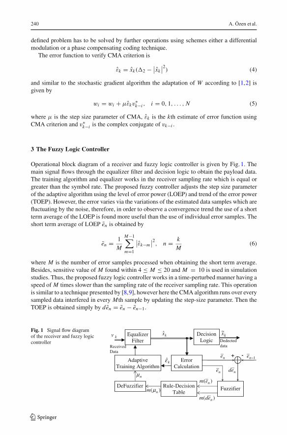
Operational block diagram of a receiver and fuzzy logic controller is given by Fig. 1. Themain signal flows through the equalizer filter and decision logic to obtain the payload data.The training algorithm and equalizer works in the receiver sampling rate which is equal orgreater than the symbol rate. The proposed fuzzy controller adjusts the step size parameterof the adaptive algorithm using the level of error power (LOEP) and trend of the error power(TOEP). However, the error varies via the variations of the estimated data samples which arefluctuating by the noise, therefore, in order to observe a convergence trend the use of a shortterm average of the LOEP is found more useful than the use of individual error samples. Theshort term average of LOEP en is obtained by

en = 1

M

M−1∑

m=1

∣∣εk−m∣∣2

, n = k

M(6)

where M is the number of error samples processed when obtaining the short term average.Besides, sensitive value of M found within 4 ≤ M ≤ 20 and M = 10 is used in simulationstudies. Thus, the proposed fuzzy logic controller works in a time-perturbed manner having aspeed of M times slower than the sampling rate of the receiver sampling rate. This operationis similar to a technique presented by [8,9], however here the CMA algorithm runs over everysampled data interfered in every M th sample by updating the step-size parameter. Then theTOEP is obtained simply by den = en − en−1.

Fig. 1 Signal flow diagramof the receiver and fuzzy logiccontroller

EqualizerFilter

AdaptiveTraining Algorithm

DecisionLogic

ErrorCalculation

FuzzifierDeFuzzifier Rule-DecisionTable

kv

ReceivedData

kx kx~

Dedected data

kε

)( nem

)( nedm

ne

)( nm μ

nμ ned

ne 1−ne+ -

123


The proposed approach is based on the principle of fuzzy logic developed by Zadeh [12],which is used to handle the linguistic concepts. It consists of three main processors, namely:Fuzzifier, Rule Decision Table, and Defuzzifier, which map the input variables into a suitablestep size for the weight adaptation of CMA. The fuzzy logic controller (FLC) adjusts thesystem input by observing the system output and by using the history of the information orcriteria accumulated as an expert [7,13].

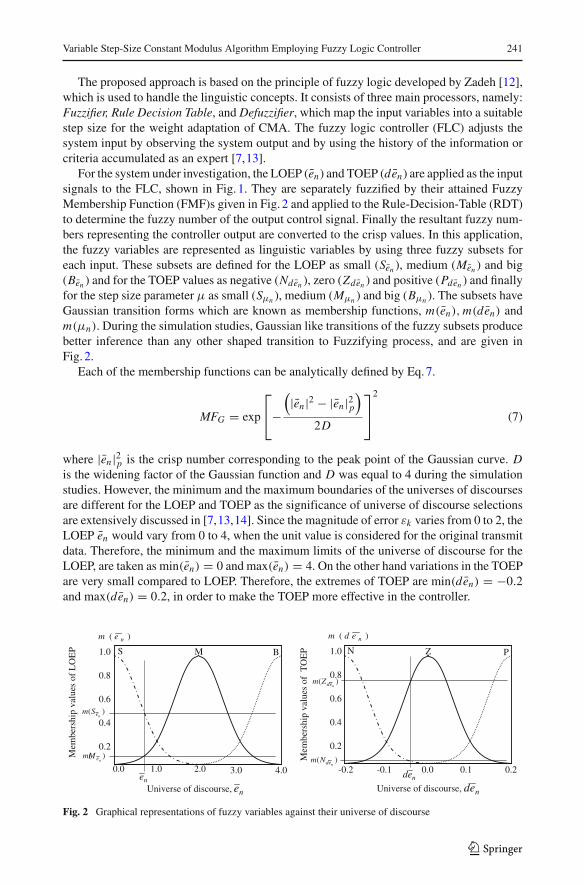
For the system under investigation, the LOEP (en) and TOEP (den) are applied as the inputsignals to the FLC, shown in Fig. 1. They are separately fuzzified by their attained FuzzyMembership Function (FMF)s given in Fig. 2 and applied to the Rule-Decision-Table (RDT)to determine the fuzzy number of the output control signal. Finally the resultant fuzzy num-bers representing the controller output are converted to the crisp values. In this application,the fuzzy variables are represented as linguistic variables by using three fuzzy subsets foreach input. These subsets are defined for the LOEP as small (Sen ), medium (Men ) and big(Ben ) and for the TOEP values as negative (Nden ), zero (Zden ) and positive (Pden ) and finallyfor the step size parameter μ as small (Sμn ), medium (Mμn ) and big (Bμn ). The subsets haveGaussian transition forms which are known as membership functions, m(en), m(den) andm(μn). During the simulation studies, Gaussian like transitions of the fuzzy subsets producebetter inference than any other shaped transition to Fuzzifying process, and are given inFig. 2.

Each of the membership functions can be analytically defined by Eq. 7.

MFG = exp

⎡

⎣−(|en |2 − |en |2p

)

2D

⎤

⎦2

(7)

where |en |2p is the crisp number corresponding to the peak point of the Gaussian curve. Dis the widening factor of the Gaussian function and D was equal to 4 during the simulationstudies. However, the minimum and the maximum boundaries of the universes of discoursesare different for the LOEP and TOEP as the significance of universe of discourse selectionsare extensively discussed in [7,13,14]. Since the magnitude of error εk varies from 0 to 2, theLOEP en would vary from 0 to 4, when the unit value is considered for the original transmitdata. Therefore, the minimum and the maximum limits of the universe of discourse for theLOEP, are taken as min(en) = 0 and max(en) = 4. On the other hand variations in the TOEPare very small compared to LOEP. Therefore, the extremes of TOEP are min(den) = −0.2and max(den) = 0.2, in order to make the TOEP more effective in the controller.

1.0

0.6

0.2

0.4

0.8

4.03.00.0 1.0 2.0

)( nem

Universe of discourse, ne

S M B 1.0

0.6

0.2

0.4

0.8

0.20.1-0.2 -0.1 0.0

)( nedm

Universe of discourse, ned

Mem

bers

hip

valu

es o

f T

OE

P N Z P

)(neSm

Mem

bers

hip

valu

es o

f L

OE

P

)(neMm

ne ned

)(nedZm

)(nedNm

Fig. 2 Graphical representations of fuzzy variables against their universe of discourse

123

242 A. Özen et al.

Table 1 The rule decision tablefor μn of CMA

m(en) (LOEP)\m Nden Zden Pden(den) (TOEP)

Sen Bμn1 Mμn

2 Sμn3

Men Sμn4 Sμn

5 Sμn6

Ben Mμn7 Sμn

8 Sμn9

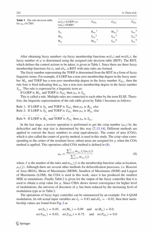
After obtaining fuzzy numbers via fuzzy membership functions m(en) and m(den), thefuzzy number of μ is determined using the assigned rule decision table (RDT). The RDT,which defines the control actions to be taken, is given in Table 1. Since there are three fuzzymembership functions for en and den , a RDT with nine rules are formed.

The fuzzy number representing the TOEP is determined from the RDT in a form of fuzzylinguistic terms. For example, if LOEP has a non-zero membership degree in the fuzzy num-ber Men and TOEP has a non-zero membership degree in the fuzzy number Nden , then therule four is fired indicating that μn has a non-zero membership degree in the fuzzy numberSμn . This rule is expressed by a linguistic term as:

If LOEP is Men and TOEP is Nden then μn is Sμn

This is called a rule. Multiple rules are connected to each other by the term ELSE. There-fore, the linguistic representation of the rule table given by Table 1 becomes as follows:

Rule 1: If LOEP is Sen and TOEP is Nden then μn is Bμn elseRule 2: If LOEP is Sen and TOEP is Zden then μn is Mμn else

… … … … … … …Rule 9: If LOEP is Ben and TOEP is Pden then μn is Sμn .

In the last stage, a reverse operation is performed to get the crisp number (μn) by thedefuzzifier and the step size is determined by this way [7,13,14]. Different methods areapplied to convert the fuzzy numbers to crisp equivalencies. The center of area (COA),which is also called the center of gravity method, is used in this study. The crisp value corre-sponding to the center of the resultant fuzzy subset areas are assigned for μ when the COAmethod is applied. This operation called COA method is defined in (8).

μn =∑J

j=1 mμn ( j)μn( j)∑J

j=1 mμn ( j)(8)

where J is the number of the rules and mμn ( j) is the membership function value at location,μn( j). Although there are several other methods for defuzzification processes, i.e. Bisectorof Area (BOA), Mean of Maximums (MOM), Smallest of Maximums (SOM) and Largestof Maximums (LOM), the COA is used in this work, since it has produced the smallestMSE in simulations. Finally Table 2 is given for the output of the fuzzy controller that it isused to obtain a crisp value for μ. Since CMA shows slower convergence for higher levelof modulations, the universe of discourse of μ has been reduced by the increasing level ofmodulation type as in Table 2.

The operations of fuzzy logic controller can be summarized by an example: For 4-QAMmodulation, let nth actual input variables are en = 0.83 and den = −0.02, then their mem-bership values are found from Fig. 2 as

m(Sen ) = 0.45, m(Men ) = 0.09 and m(Ben ) = 0.0,

m(Nden ) = 0.03, m(Zden ) = 0.75, and m(Pden ) = 0.0

123


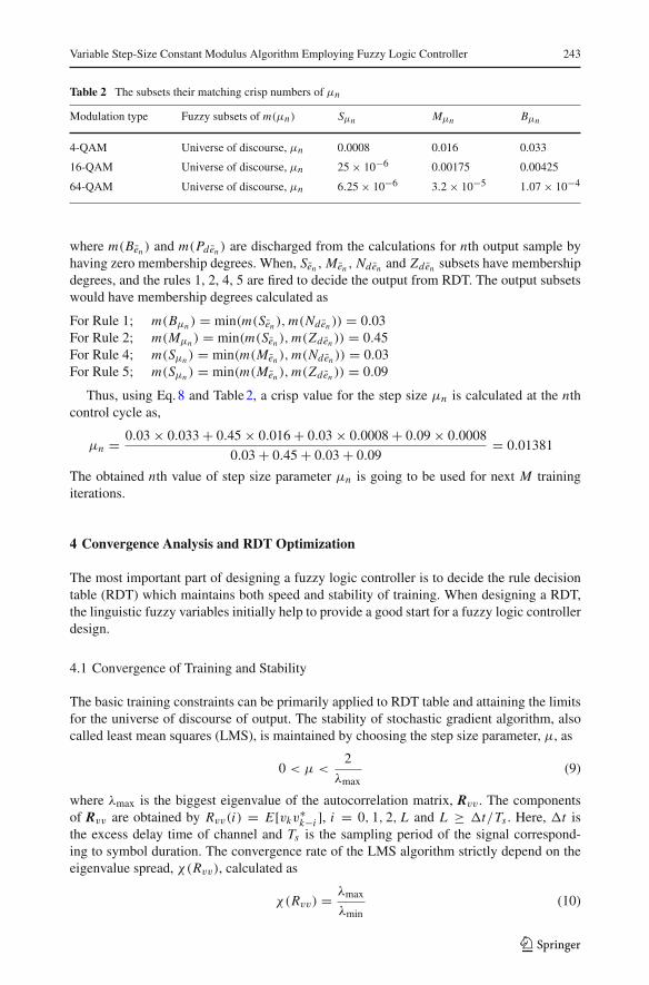
Table 2 The subsets their matching crisp numbers of μn

Modulation type Fuzzy subsets of m(μn) Sμn Mμn Bμn

4-QAM Universe of discourse, μn 0.0008 0.016 0.033

16-QAM Universe of discourse, μn 25 × 10−6 0.00175 0.00425

64-QAM Universe of discourse, μn 6.25 × 10−6 3.2 × 10−5 1.07 × 10−4

where m(Ben ) and m(Pden ) are discharged from the calculations for nth output sample byhaving zero membership degrees. When, Sen , Men , Nden and Zden subsets have membershipdegrees, and the rules 1, 2, 4, 5 are fired to decide the output from RDT. The output subsetswould have membership degrees calculated as

For Rule 1; m(Bμn ) = min(m(Sen ), m(Nden )) = 0.03For Rule 2; m(Mμn ) = min(m(Sen ), m(Zden )) = 0.45For Rule 4; m(Sμn ) = min(m(Men ), m(Nden )) = 0.03For Rule 5; m(Sμn ) = min(m(Men ), m(Zden )) = 0.09

Thus, using Eq. 8 and Table 2, a crisp value for the step size μn is calculated at the nthcontrol cycle as,

μn = 0.03 × 0.033 + 0.45 × 0.016 + 0.03 × 0.0008 + 0.09 × 0.0008

0.03 + 0.45 + 0.03 + 0.09= 0.01381

The obtained nth value of step size parameter μn is going to be used for next M trainingiterations.

4 Convergence Analysis and RDT Optimization

The most important part of designing a fuzzy logic controller is to decide the rule decisiontable (RDT) which maintains both speed and stability of training. When designing a RDT,the linguistic fuzzy variables initially help to provide a good start for a fuzzy logic controllerdesign.

4.1 Convergence of Training and Stability

The basic training constraints can be primarily applied to RDT table and attaining the limitsfor the universe of discourse of output. The stability of stochastic gradient algorithm, alsocalled least mean squares (LMS), is maintained by choosing the step size parameter, μ, as

0 < μ <2

λmax(9)

where λmax is the biggest eigenvalue of the autocorrelation matrix, Rvv . The componentsof Rvv are obtained by Rvv(i) = E[vkv

∗k−i ], i = 0, 1, 2, L and L ≥ �t/Ts . Here, �t is

the excess delay time of channel and Ts is the sampling period of the signal correspond-ing to symbol duration. The convergence rate of the LMS algorithm strictly depend on theeigenvalue spread, χ(Rvv), calculated as

χ(Rvv) = λmax

λmin(10)

123

244 A. Özen et al.

where λmin is also the smallest eigenvalue of Rvv . A stepsize, μ > 0, is enough to providea convergence, however there is no clear definition for an adequate value for μ. Severaldiscussions and analyses on the effect of eigenvalue spread on the convergence speed havebeen made by Haykin in [15].

For the blind equalization case the stochastic gradient algorithm turns into form of CMAand its stability and convergence constraints are also maintained by the eigenvalues of Rvv

as Eq. 11, using the evaluation of [16] for a stable training.

0 < μ <2

γ λmax(11)

Here, γ = E[3x2k−koffset

− �2], koffset is a certain delay indicating the cursor symbol in theequalizer filter, xk is the kth transmit symbol, �2 is the modulus value in Eq. 3. The value ofγ provides an inequality γ ≥ 3 for higher order of quadratic amplitude modulation, wheremodulation order is greater or equal to 4. Equation 11 stands for mean convergence constraintof CMA, however the mean-square stability constraint of μ is different, as in [16], as

0 < μ <2γ

r2γ T r{Rvv} (12)

Here, r2γ = E[γ 2

k ], γk = 3x2k−koffset

− �2 and Tr{Rvv} = ∑Li=0 |λi | ≥ λmax. Therefore,

mean square stability constraint refers smaller or equal values for the maximum value of μ

than what Eq. 11 provides. Thus, the stability region of μ for CMA is much narrower thanwhose using the LMS.

On the other hand, in practice a maximum value much smaller than the constraint providedby Eq. 12 is chosen for μ, without relating the eigenvalue. The proposed method also refersto choose a maximum for the universe of discourse of μ smaller than the constraint valuestated by Eq. 12, as given by Table 2.

It is clearly explained in the book by E. Cox [17], a Fuzzy logic controller (FLC) worksfor possibilities in a plant to be controlled, where the theory and as well as its implementationis different than whom using a probabilistic approach using the statistical signal processing.Therefore, maximum constraints of Eq. 12 can not be stated the exact constraints of FLC.The FLC can tolerate larger values of μ, because it is design to maintain all possibilities offuzzy inputs, i.e. LOEP and TOEP in the proposed fuzzy outer loop controller, in its RDT.An analytical evaluation of the universe of discourse of μ based on the eigenvalue analysiscan be made which is left for further studies of this work. However, since the adaptation ofμ is much sensitive to RDT table of FLC, this work extensively searches the best RDT forCMA.

4.2 Design of Training Trajectory and Optimization

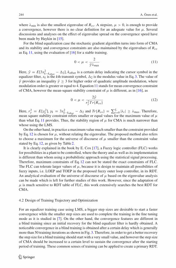
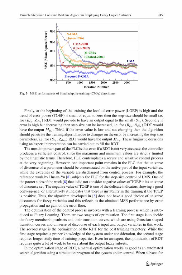
For an equalizer training case using LMS, a bigger step sizes are desirable to start a fasterconvergence while the smaller step sizes are used to complete the training in the fine tuningmode as it is studied in [7]. On the other hand, the convergence features are different ina blind training since an initial recovery for the blind equalizer filter is hardly obtained. Anoticeable convergence in a blind training is obtained after a certain delay which is generallymore than 50 training iterations as shown in Fig. 3. Therefore, in order to get a better recoverythe step size for a blind training should start with a very small value, and however the step sizeof CMA should be increased to a certain level to sustain the convergence after the startingperiod of training. These common senses of training can be applied to create a primary RDT.

123


0 500 1000 1500 2000 2500 30005E-2

1E-1

2E-1

3E-1

5E-1

Iteration Number

MSE

[M

ean

Squa

re E

rror

]

Proposed F-CMA

CMA

N-CMA(Jones-1996)

CMA-SDD(Chen-2002)

M-CMA(Chahed-2004)

Fig. 3 MSE performances of blind adaptive training (CMA) algorithms

Firstly, at the beginning of the training the level of error power (LOEP) is high and thetrend of error power (TOEP) is small or equal to zero then the step-size should be small i.e.for (Ben , Zden ) RDT would provide to have an output equal to the small (Sμn ). Secondly iferror is high but decreasing then step size can be increased, i.e. for (Ben , Nden ) RDT wouldhave the output Mμn . Third, if the error value is low and not changing then the algorithmshould penetrate the training algorithm due to changes on the error by increasing the step sizeparameters, i.e. for (Sen , Zden ) RDT would have the output Mμn . These linguistic decisionsusing an expert interpretation can be carried out to fill the RDT.

The most important part of the FLC is that even if a RDT is not very accurate, the controllerproduces a sufficient control, since the maximum and minimum values are strictly limitedby the linguistic terms. Therefore, FLC contemplates a secure and sensitive control processat the very beginning. However, one important point remains in the FLC that the universeof discourse of a parameter should be concentrated on the active part of the input variables,while the extremes of the variable are discharged from control process. For example, thereference work by Husan-Yu [8] subjects the FLC for the step-size control of LMS. One ofthe poorer sides of the work [8] that it did not consider negative values of TOEP in its universeof discourse set. The negative value of TOEP is one of the delicate indicators showing a goodconvergence, or alternatively it indicates that there is instability in the training if the TOEPis positive. Thus, the algorithm developed in [8] does not have a good choice of universediscourses for fuzzy variables and this reflects to the obtained MSE performance by errorpropagation and no gain on the error floor.

The optimization of the control process involves with a learning process which is intro-duced as Fuzzy Learning. There are two stages of optimization. The first stage is to decidethe fuzzy membership subsets and their transition curves, which are using Gaussian shapedtransition curves and universe of discourse of each input and output variables in this work.The second stage is the optimization of the RDT for the best training trajectory. While thefirst stage requires a proper knowledge of the system under consideration, the second stagerequires longer study time of training properties. Even for an expert, the optimization of RDTrequires quite a bit of work to be sure about the output fuzzy subsets.

In the optimization stage of RDT, a manual optimization works as good as an automatedsearch algorithm using a simulation program of the system under control. When subsets for

123

246 A. Özen et al.

the input variables are limited, a few rules are issued, i.e. in the proposed system only ninerules are used, nR = 9. The output subsets are also limited by linguistic subsets; here threeoutput subsets are used, nS = 3, given by Table 2. Therefore, the maximum combinationsof RDT would be equal to nS power nR (= nnR

S , which would be equal to 39 = 19683 forthe system given above). However, with the mentioned expert view these options can bereduced to less than hundred trails. During the simulation studies it has been observed that,optimization of a training trajectory has several hidden rules that an expert view can easilymiss the point. For example, in a Rayleigh channel when error is high, because of somedifficult channel impulse responses, the training can not provide an initial convergence thatbigger step sizes do not help, the step size has to be reduced. These rare conditions haveslight changes on the RDT made during optimization iterations that an expert can not predictbeforehand. Finally, the optimization of RDT can be automated by software that it seeks forthe best MSE curve, or even for the best BER curve obtained, by iteratively checking everycombination of RDT.

5 Computer Simulation Results

Since a Rayleigh Fading Scenario has been found too difficult for a blind equalization byproducing high error floor, it was generally not preferred for the performance analysis, insteada selected channel profiles have been used as in [4,20]. However, because of high per-formance obtained by the proposed technique, a three taps frequency selective Rayleighfading exponential decay channel profile is used. The exponential decay channel profile isobtained by

∣∣h′l

∣∣ = 1√2πτRMS

e−Kτ τl (13)

where∣∣h′

l

∣∣ is the amplitude of lth tap of channel before the Rayleigh process, τRMS is the RMSdelay spread of the channel, Kτ is the exponential decay constant indicating the channel ISIlevel and τl is the delay of lth tap calculated by τl = lTs . For the simulations, these parametersare chosen as τRMS = 50 ns, Kτ = 1.0 and the symbol period of the samples Ts = 42ns. Thechannel is averaged over 1,000 Rayleigh fading channel profile for the mean square error(MSE) performance curves in Fig. 3 and bit-error-rate performance curves in Fig. 4. HereQAM (=4-QAM), 16-QAM and 64-QAM modulated transmit sequences of 4,000 symbolsare prepared using randomly selected data bits. Here, a 63 bits PseudoNoise (PN) is placedto payload data in order to detect phase error of estimated data at the output of equalizerfilter and the phase error is corrected before making a decision for BER calculations. The PNsequence insertion to a transmit sequence is normally not possible, but here it is only usedfor the phase correction process. As it is explained above the phase correction is not possiblewhen using CMA and either a differential modulation or a phase correction technique has tobe used to solve this problem.

In this paper, MSE and BER performances of a seven taps linear transversal equalizer(LTE) filter are presented. If the number of LTE taps is smaller than the ISI cancellation fea-ture of equalizer becomes limited and if the number of LTE taps is greater than the trainingslows down based on the definitions in [15]. The performance of the proposed F-CMA blindequalizer is compared with that of the N-CMA [18], M-CMA [19] and CMA-SDD [20] incomputer simulations using the conventional CMA blind equalizer as a benchmark. Table 3provides the simulation parameters of the algorithms (μ for the CMA, μm and αm for theM-CMA, αn and σn for the N-CMA, and μc, μd and ρ for the CMA-SDD). The given values

123


0 10 20 30 403E-2

5E-2

1E-1

2E-1

3E-1

5E-1

SNR in dB

BE

R [

Bit

Err

or R

ate]

CMA

N-CMAJones-1996

M-CMAChahed-2004

CMA-SDDChen-2002

ProposedF-CMA

Proposed F-CMA

4-QAM

16-QAM

64-QAM

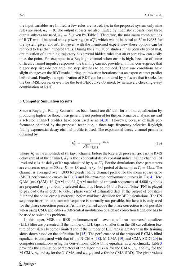
Fig. 4 BER performances of adaptive blind equalizations

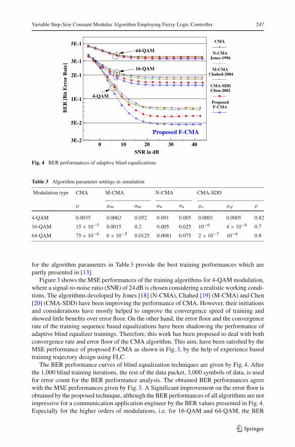
Table 3 Algorithm parameter settings in simulation

Modulation type CMA M-CMA N-CMA CMA-SDD

μ μm αm αn σn μc μd ρ

4-QAM 0.0035 0.0062 0.052 0.091 0.005 0.0001 0.0005 0.82

16-QAM 15 × 10−5 0.0015 0.2 0.005 0.025 10−6 4 × 10−6 0.7

64-QAM 75 × 10−6 6 × 10−5 0.0125 0.0081 0.075 2 × 10−7 10−6 0.8

for the algorithm parameters in Table 3 provide the best training performances which arepartly presented in [13].

Figure 3 shows the MSE performances of the training algorithms for 4-QAM modulation,where a signal-to-noise ratio (SNR) of 24 dB is chosen considering a realistic working condi-tions. The algorithms developed by Jones [18] (N-CMA), Chahed [19] (M-CMA) and Chen[20] (CMA-SDD) have been improving the performance of CMA. However, their initiationsand considerations have mostly helped to improve the convergence speed of training andshowed little benefits over error floor. On the other hand, the error floor and the convergencerate of the training sequence based equalizations have been shadowing the performance ofadaptive blind equalizer trainings. Therefore, this work has been proposed to deal with bothconvergence rate and error floor of the CMA algorithm. This aim, have been satisfied by theMSE performance of proposed F-CMA as shown in Fig. 3, by the help of experience basedtraining trajectory design using FLC.

The BER performance curves of blind equalization techniques are given by Fig. 4. Afterthe 1,000 blind training iterations, the rest of the data packet, 3,000 symbols of data, is usedfor error count for the BER performance analysis. The obtained BER performances agreewith the MSE performances given by Fig. 3. A Significant improvement on the error floor isobtained by the proposed technique, although the BER performances of all algorithms are notimpressive for a communication application engineer by the BER values presented in Fig. 4.Especially for the higher orders of modulations, i.e. for 16-QAM and 64-QAM, the BER

123

248 A. Özen et al.

0 10 20 30 40-10

-8

-6

-4

-2

0

2

SNR in dB

MSE

(dB

)

CMA

N-CMAJones-1996

M-CMAChahed-2004

CMA-SDDChen-2002

ProposedF-CMA

Proposed F-CMA

Fig. 5 MSE versus SNR performances of adaptive blind equalizations for 16-QAM

performances are degraded significantly. However, it can be easily seen that a convolutionalcoding and maximum likelihood sequence estimation or turbo type error control decoder caneasily clear the error floor where the price is paid for coding rate.

For an insight into real performances of the algorithms, Fig. 5 shows the MSE perfor-mances of blind training algorithms. Here, the MSE performances are obtained during theBER calculations of 16-QAM modulations after training. It can be easily shown that theperformance improvement of the proposed method is very significant.

6 Computational Complexity Comparisons

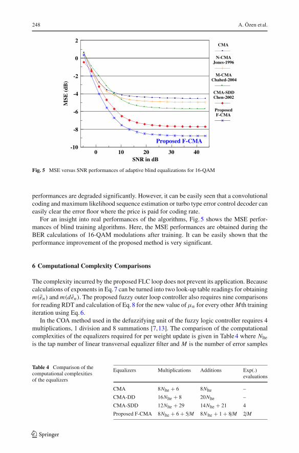
The complexity incurred by the proposed FLC loop does not prevent its application. Becausecalculations of exponents in Eq. 7 can be turned into two look-up table readings for obtainingm(en) and m(den). The proposed fuzzy outer loop controller also requires nine comparisonsfor reading RDT and calculation of Eq. 8 for the new value of μn for every other M th trainingiteration using Eq. 6.

In the COA method used in the defuzzifying unit of the fuzzy logic controller requires 4multiplications, 1 division and 8 summations [7,13]. The comparison of the computationalcomplexities of the equalizers required for per weight update is given in Table 4 where Nlte

is the tap number of linear transversal equalizer filter and M is the number of error samples

Table 4 Comparison of thecomputational complexitiesof the equalizers

Equalizers Multiplications Additions Exp(.)evaluations

CMA 8Nlte + 6 8Nlte –

CMA-DD 16Nlte + 8 20Nlte –

CMA-SDD 12Nlte + 29 14Nlte + 21 4

Proposed F-CMA 8Nlte + 6 + 5/M 8N lte + 1 + 8/M 2/M

123


averaged in Eq. 6. The computational complexity per weight update of the proposed schemeis similar to whom using the CMA, CMA-DD or CMA-SDD.

7 Conclusion

In this paper, a novel low complexity blind equalization scheme based on fuzzy logic outerloop controller has been proposed. It has been shown that a combination of fuzzy logicand CMA equalizer provides an effective and robust way for adaptive blind equalization.Compared with a state of art low complexity blind training schemes, namely the recentlyintroduced N-CMA [18], M-CMA [19] and CMA-SDD [20] blind equalizer training algo-rithms, the proposed F-CMA blind equalizer has simpler in computational requirements,faster convergence and lower steady state error. This new blind equalizer offers practicalalternatives to blind equalization of QAM and multi-level QAM modulation communica-tions and provides significant convergence improvement over the conventional adaptiveblind training techniques. The most important feature of FLC is its ability to be initiated bythe experience based linguistic control terms which, works very effectively even if they arenot optimized and the optimization of the algorithm is also an easy task as it is explained inthe paper.

References

1. Godard, D. N. (1980). Self recovering equalization and carrier tracking in two dimensional data commu-nication systems. IEEE Transactions on Communications, 28(11), 1867–1875.

2. Treichler, J. R., & Agee, B. G. (1983). A new approach to multipath correction of constant modulussignals. IEEE Transactions on Acoustics Speech and Signal Processing, ASSP-28, 459–472.

3. Schirtzinger, T., et al. (1985). A comparison of three algorithms for blind equalization based on theconstant modulus error criterion. In Proceedings of IEEE ICASSP (pp. 1049–1052).

4. Weerackody, V., & Kassam, S. A. (1991). Variable step size blind adaptive equalization algorithms. InIEEE international symposium on circuits and systems (pp. 718–721).

5. De Castro, F. C. C., et al. (2001). Concurrent blind deconvolution for channel equalization. In Proceedingsof ICC (pp. II-366–II-371).

6. Chen, W. Y., & Haddad, R. A. (1990). A variable step size LMS algorithm. In Proceedings of the 33rdmidwest symposium on circuits and systems (Vol. 1, pp. 423–426).

7. Özen, A., Kaya, I., & Soysal, B. (2007). Design of a fuzzy based outer loop controller for improvingthe training performance of LMS algorithm. In Third international conference on intelligent computing,ICIC 2007 August 21–24 (Vol. 2, pp. 1051–1063). Qingdao, China.

8. Lin, H.-Y., et al. (2005). An adaptive robust LMS employing fuzzy step size and partial update. IEEESignal Processing Letters, 12(8), 545–548.

9. Sanubari, J. (2003). Fast convergence LMS adaptive filters employing fuzzy partial updates. In TENCON2003, conference on convergent technologies for Asia-Pacific region (Vol. 4, pp. 1334–1337), Oct. 15–17,2003.

10. Zhimin, D., et al. (2001). Novel variable step size constant modulus algorithms for blind multiuser detec-tion. In IEEE VTS 54th vehicular technology conference, VTC 2001 Fall (Vol. 2, pp. 673–677), Oct. 7–11,2003.

11. Baykal, B. (2004). Blind channel estimation via combining autocorrelation and blind phase estimation.IEEE Transactions on Circuits and Systems-I: Regular Papers, 51(6), 1125–1131.

12. Zadeh, L. A. (1965). Fuzzy sets. Information and Control, 8, 338–353.13. Özen, A. (2005) A Fuzzy based outer loop controller design improving the performance and convergence

speed in high data rate digital communication receivers. Ph.D. Thesis, Graduate School of Natural andApplied Science, KTU, Trabzon, July 2005.

14. Eminoglu, I., & Altas, I. H. (1996). A method to form fuzzy logic control rules for a PMDC motor drivesystem. Elsevier Electric Power System Research, 39, 81–87.

15. Haykin, S. (2002). Adaptive filter theory, (4th ed.). New Jersey: Prentice Hall Inc.

123

250 A. Özen et al.

16. Nascimento, V. H., & Silva, M. T. M. (2008). Stochastic stability analysis for the constant-modulusalgorithm. IEEE Transactions on Signal Processing, 56(10, Part 1), 4984–4989.

17. Cox, E. (1994). The fuzzy systems handbook. London: Academic Press, Inc.18. Jones, D. L. (1996). A normalized constant modulus algorithm. In IEEE conference record of the twenty-

ninth asilomar conference on signals, systems and computers (Vol. 1, pp. 694–697).19. Chahed, I., et al. (2004). Blind decision feedback equalizer based on high order MCMA. In Canadian

conference on electrical and computer engineering (Vol. 4, pp. 2111–2114).20. Chen, S. (2003). Low complexity concurrent constant modulus algorithm and soft decision directed

scheme for blind equalization. IEE Proceedings of Visual Image Signal Processing, 150, 312–320.

Author Biographies

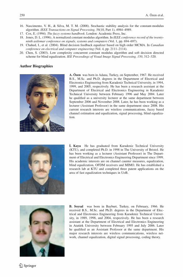
A. Özen was born in Adana, Turkey, on September, 1967. He receivedB.S., M.Sc. and Ph.D. degrees in the Department of Electrical andElectronics Engineering from Karadeniz Technical University, in 1994,1999, and 2005, respectively. He has been a research assistant at theDepartment of Electrical and Electronics Engineering in KaradenizTechnical University between February 1996 and May 2004. Laterhe qualified as a university lecturer at the same department betweenSeptember 2006 and November 2008. Later, he has been working as alecturer (Assistant Professor) in the same department since 2008. Hiscurrent research interests are wireless communications, fuzzy basedchannel estimation and equalization, signal processing, blind equaliza-tion.

I. Kaya He has graduated from Karadeniz Technical University(KTU), and completed Ph.D. in 1998 in The University of Bristol. Hehas been working as a lecturer (Assistant Professor) in The Depart-ment of Electrical and Electronics Engineering Department since 1999.His academic interests are on channel caunter measures, equalization,blind equalization, OFDM receivers and MIMO. He has established aresearch lab at KTU and completed three patent applications on thearea of fast equalization techniques in UoB.

B. Soysal was born in Bayburt, Turkey, on February, 1966. Hereceived B.S., M.Sc. and Ph.D. degrees in the Department of Elec-trical and Electronics Engineering from Karadeniz Technical Univer-sity, in 1989, 1998, and 2004, respectively. He has been a researchassistant at the Department of Electrical and Electronics Engineeringin Atatürk University between February 1995 and July 2006. Laterhe qualified as an Assistant Professor at the same department. Hismajor research interests are wireless communications, wireless net-work, channel equalization, digital signal processing, coding theory.

123

Variable Step-Size Constant Modulus Algorithm Employing Fuzzy Logic Controller

Documents

Transcript of Variable Step-Size Constant Modulus Algorithm Employing Fuzzy Logic Controller