An analysis of constant modulus algorithm for array signal processing1

Signal Processing 73 (1999) 81—104

An analysis of constant modulus algorithmfor array signal processing1

Dan Liu!, Lang Tong",*

! Globespan Semiconductor Inc., 100 Schulz Drive, Red Bank, NJ 07701, USA" School of Electrical Engineering, Cornell University, Ithaca, NY 14853, USA

Received 25 September 1997; received in revised form 4 August 1998

Abstract

The constant modulus (CM) cost function is analyzed for array signal processing. The analysis includes arbitrarysource types. It is shown that CM receivers have the signal space property except in two special cases. Local minima ofCM cost function are completely characterized for the noiseless case. In the presence of measurement noise, the existenceof CM local minima in the neighborhood of Wiener receivers is established, and their mean squared error (MSE)performance, output power, estimation bias and residual interference are evaluated. Numerical examples are presented todemonstrate the effects of signal statistics on the locations of CM local minima. ( 1999 Published by Elsevier ScienceB.V. All rights reserved.

Zusammenfassung

Fur die Arraysignalverarbeitung wird die Kostenfunktion des konstanten Betrages (CM) untersucht. Die Analyseschlie{t beliebige Quellentypen ein. Es wird gezeigt, da{ CM-Empfanger mit Ausnahme von zwei Spezialfallen dieSignalraumeigenschaft besitzen. Lokale Minima der CM-Kostenfunktion werden im rauschfreien Fall vollstandigcharakterisiert. Liegt Me{rauschen vor, dann wird die Existenz der lokalen Minima in der Nahe von Wiener-Empfan-gern gezeigt, und ihr mittlerer quadratischer Fehler (MSE), die Ausgangsleistung, der Schatzoffset und die Reststorungwerden berechnet. Numerische Beispiele werden prasentiert, um die Effekte der Signalstatistik auf die Lage der lokalenMinima bei CM zu zeigen. ( 1999 Published by Elsevier Science B.V. All rights reserved.

Resume

On analyse la fonction cout Module Constant (CM) pour le traitement d’antenne. L’analyse prend en compte dessources de type arbitraire. On montre que les recepteurs CM jouissent de la propriete dite de l’espace signal sauf dansdeux cas particuliers. Les minima locaux de cette fonction cout CM sont completement caracterises en l’absence de bruit.En presence de bruit de mesure, l’existence de minima locaux au voisinage des recepteurs de Wiener est etablie, et leursperformances en termes d’Erreur Quadratique Moyenne (MSE), de puissance de sortie, de biais, et d’interference

*Corresponding author. Tel.: #1 607 255 4085; fax: #1 607 255 9072; e-mail: [email protected] work was supported in part by the National Science Foundation under Contract NCR-9321813 and by the Office of Naval

Research under Contract N00014-96-1-0895 and by the Advanced Research Projects Agency monitored by the Federal Bureau ofInvestigation under Contract No. J-FBI-94-221.

0165-1684/99/$ — see front matter ( 1999 Published by Elsevier Science B.V. All rights reserved.PII: S 0 1 6 5 - 1 6 8 4 ( 9 8 ) 0 0 1 8 6 - 8

residuelle sont evaluees. Des exemples numeriques sont presentes pour illustrer les effets des statistiques des signaux surles positions des minima locaux CM. ( 1999 Published by Elsevier Science B.V. All rights reserved.

Keywords: Array processing; Beamforming; Source separation; Blind equalization and estimation

Notations

( ) )T transpose( ) )H Hermitian( ) )s Moore—Penrose inverse [8, p. 434]EM ) N expectation operatorExE

p p-norm defined by pJ+DxiDp.

ExEA 2-norm defined by JxHAxIn

n]n identity matrixel a unit column vector with 1 at the lth entry

and zero elsewhereCn n-dimensional complex vector spaceCnCm the set of all n]m complex matricesCA range of AAs [8, p. 430]CAM range of I!AAs

1. Introduction

Since the inception of the constant modulus al-gorithm (CMA) in 1980, proposed first by Godard[3] and later independently by Treichler and Agee[11], CMA has been successfully implemented invarious applications including equalization formicrowave radio links and blind beamforming inarray signal processing. Although originally in-vented for the equalization of a single-user inter-symbol interference (ISI) channel, it has beenrecognized, first by Gooch and Lundell [4], thatCMA applies also to the multiuser beamformingproblem where the objective is to estimate one orall the source signals from an array of receivers. Theso-called constant modulus array [4,5,8] is perhapsthe first application of CMA in array processing.

Despite the similarity between the equalizationand beam-forming problems, there are several keydifferences. In beam forming, different users mayhave different signal constellations whereas in(single user) equalization, all symbols are identi-cally distributed. It is also possible that some inter-ference may come from impulsive noise sources

that have super-Gaussian2 statistics. Effects of sig-nal or interference statistics on the performance ofCM receivers have so far not been characterized.The second important difference is that the channelresponse matrix for the beam-forming problemdoes not have the (block) Toeplitz structure. Initia-lization techniques effective in the equalizationproblem [10] cannot be applied, which makes theinitialization of CMA in beam-forming applica-tions much more critical.

There are two classes of approaches when CMAis applied to beam-forming problems. The multi-stage CM array [6,8,9] estimates source signalssequentially. At the first stage, CMA is used toestimate one of the source signals. Which source isextracted first depends on the initialization ofCMA, and it is usually unknown. The contributionof the estimated source is then subtracted from thereceived signal according to the mean squared er-ror (MSE) criterion. This process continues until allsources are extracted. If the estimate at every stageis close to the minimum mean squared error(MMSE) estimate, this process approximates theMMSE estimate of all source signals obtained bythe Wiener receiver; see [8,9] for the analysis. WhenCMA at the first stage fails to converge or itsestimate has a large MSE, its error accumulatesthrough different stages, and the multistageCMA approach may not perform well. The secondclass of approaches obtain the signal estimatein a single step. One example is the algebraicCMA (ACMA) proposed by Van der Veen [12].Unlike multistage CMA, these approaches are notsubject to estimation error propagation. Unfortu-nately, there is a lack of analysis for these algo-rithms about how well they behave in the presenceof noise.

2A source is super- (sub-) Gaussian when E(DsD4)/(E(DsD2))2'(()E(Ds

GD4)/(E(Ds

GD2))2 where s

Ghas the Gaussian distribution.

82 D. Liu, L. Tong / Signal Processing 73 (1999) 81–104

1.1. Main results and related work

In this paper, we perform an analysis of CMA atthe first stage for the multistage CMA array ap-proach. Such an analysis is especially importantsince all subsequent stages depend on the applica-tion of CMA at the first stage. Furthermore, thesame analysis can also be applied to other stageswhen, as we shall show in this paper, the CMreceiver at the first stage closely approximate theWiener receiver. We summarize next the main re-sults of this paper with comments of related work.

¹he signal space property: Section 3 gives theCM cost function in the general form followed bythe proof of the signal space property of CM re-ceivers. A receiver is said to have the signal spaceproperty if its coefficient vector is in the columnspace of the array response matrix, which is indeedthe case for Wiener receivers. Such a property issignificant when there are more sensors than sour-ces. We show in Section 3 that CM receivers dohave the signal space property except for in twospecial cases (i) there is no noise; and (ii) there areno sub-Gaussian sources. When there is no noise,there are infinitely many local minima, each can begenerated from a minimum in the signal subspace.Specifically, CM local minima are made of cosets ofthe noise subspace generated from local minima inthe signal space. Hence, it is sufficient to analyzeCM local minima in the signal subspace. When thereare no sub-Gaussian sources, we show that CMreceivers are in the orthogonal complement of thesignal subspace spanned by the columns of the arrayresponse matrix associated with the super-Gaussiansources. In other words, a CM receiver filters out allsuper-Gaussian sources. The signal space propertyof CMA is first obtained for equalization problemin [13—15]. The results presented in Section 3 aremore general and its proof is more direct.

CM local minima: the noiseless case: The resultspresented in Section 4 address the following ques-tion: where are CM local minima when there is nonoise? Foschini [2] was the first to show that allCM local minima inverse the channel matrix for theequalization problem. We consider here the generalsource condition including signals with arbitrary(sub-Gaussian, Gaussian and super-Gaussian)sources. We show that when there exist sub-Gaus-

sian sources, a receiver is a local minimum of theCM cost function if and only if it perfectly extractsa sub-Gaussian source. When sources are super-Gaussian or Gaussian, two special cases are ad-dressed separately assuming the number of sourcesequals to the number of sensors. (i) If all sources aresuper-Gaussian, the minimum of CM cost functionis unique up to a phase rotation. The output of theCM receiver in this case includes signals from allsources. (ii) If the sources are Gaussian and superGaussian, all receivers with a fixed output powerand orthogonal to the columns of the array re-sponse matrix corresponding to the super-Gaus-sian sources are CM local minima. Thecharacterization of CM local minima for the noise-less case is therefore complete.

CM local minima: the noisy case: In Section 5, weanalyze CM local minima assuming the presence ofnoise in the same spirit of Zeng et al. [14]. Focusingon the case of sub-Gaussian sources, our resultsgeneralize that in [14] to include signals with differ-ent distributions. We derive tests for the existenceof CM local minima in the neighborhood of Wienerreceivers. These local minima are referred to as theWiener type CM local minima. Also presented areMSE bounds, output power conditions, and prop-erties of receiver bias and residue interference.

Numerical examples: The goal of Section 6 istwofold. First, we evaluate, through the use of anexample, the quality of the MSE bounds derived inSection 5. Second, we study the effects of the statis-tics of interfering signals. We demonstrate thata super-Gaussian interference may remove a CMreceiver of a sub-Gaussian source from the neigh-borhood of its Wiener receiver, a case that has notbeen reported elsewhere. Since such an exampledoes not exist when there is no noise as shown inSection 4, it highlights the significant difference be-tween the noiseless and noisy cases. We also dem-onstrate the behavior of CM receiver when sourcesare closely located.

2. The problem

Consider a multiple-input multiple-output modelshown in Fig. 1:

x"Hs#w, (1)

D. Liu, L. Tong / Signal Processing 73 (1999) 81—104 83

Fig. 1. The model.

where s¢(s1,s2,2,s

M)T3CM is the vector of source

signals, H3CNCM is the (unknown) array responsematrix, w¢(w

1,w

2,2,w

N)T3CN is the additive

noise, x¢(x1,x

2,2,x

N)T3CN is the received signal

vector.A linear estimate y of one element of s, say s

1, is

obtained by

y"f Hx"qHs#f Hw, (2)

where f3CN is the estimator response vector, andq¢HHf3CM is the (conjugate) total system re-sponse. This model is illustrated in Fig. 1. A con-stant modulus (CM) estimator is defined by a localminimum of the CM cost

JM ( f )¢EM(DyD2!r)2N"EM(D f HxD2!r)2N, (3)

where r is referred to as the dispersion constant. Ingeneral, r can be choosen arbitrarily, resultingmerely a scaling factor in the local minima of theabove optimization. Conventionally, if s

iis to be

estimated, we set r"EDsiD4/EDs

iD2 so that when there

is no noise and under the general condition speci-fied in Theorem 2, s

1can be estimated perfectly by

a global minimum of Eq. (3).In analyzing local minima of the CM cost func-

tion, we shall make the following assumptions:A1: H3CNCM has full column rank.A2: Source vector s is non-Gaussian with indepen-

dent components, zero-mean with E(ssH)"I,and symmetrical.

A3: w is Gaussian with zero mean and covariancep2I, and it is independent of s.

Assumption A1 implies that the number of sensorsis no less than the number of sources, and no twosources have exactly the same propagation path.The extension to non-full column rank cases can beobtained by following [15]. A2 includes the possi-

bility of sources having different statistics exceptthe case when all sources are Gaussian. When sis Gaussian, it is shown in Section 3 that, all re-ceivers having output power equal to r/2 are globalminima.

3. The CM cost function and the signal spaceproperty

Under A2 and A3, the CM cost function inEq. (3) has the following form:

JM ( f )"2E f E4R!2rE f E2R#M+

m/1

nmDeHm

HHf D4#r2,

(4)

where

R¢E(xxH)"HHH#p2IN, (5)

nm¢cum(s

m,sHm,sm,sHm)"EDs

mD4!2"r

m!2. (6)

Some insights can be gained by examining terms inEq. (4). Note that E f E2R is the output power of thereceiver. Hence, the CM cost is affected primarilyby the output power of the receiver and the fourth-order terms of the system response eH

mHHf weighted

by the signal cumulant nm. It is evident that for

a super-Gaussian source sm, n

m'0, A CM receiver

tends to minimize the corresponding term eHmHHf.

On the other hand, for a sub-Gaussian source,A CM receiver tends to enhance the correspondingterm in the system response. These, of course, mustbe accomplished with considerations of the outputpower term. Note here that if all sources are Gaus-sian, n

m"0 for all m. The minimization of the CM

cost leads to receivers whose output power is r/2. Ingeneral, CM estimators for this case are not useful,which is the reason we have assumed that thesource vector s is a non-Gaussian.

Analyzing the cost function in Eq. (4) directly iscumbersome. Most existing analyses transformthe optimization of receiver coefficients to theoptimization of the system response q¢HHf.Unfortunately, the optimization of f3CN is ingeneral not equivalent to the optimization ofq3Q¢Mq¢HHf D f3CNN except for the case whenH is square and full rank. For example, when thereare more sensors then sources, the analysis of CM


cost function is complicated by the existence of thenull (noise) space of H. The following theorem es-tablishing the signal space property of CM re-ceivers makes the analysis of CM receivers inQ possible.

Theorem 1. Assume that CHM is not empty, i.e.,N'M, and p2'0.

1. If one of the sources is sub-Gaussian, then all localminima of JM ( f ) (4) are in the signal subspace CH,each with power satisfying

E f E2R'r

2. (7)

2. If one of the sources is sub-Gaussian, then all localminima of the optimization constrained by CH

minf|CH

JM ( f ) (8)

whose output power are greater than r/2 are localminima of the unconstrained minimization of JM ( f ).

3. If there is no sub-Gaussian sources, then

G f D E f E2R"r

2, f3CHMXCH

'H (9)

is the set of global minima of JM ( f ), where CH'is

the space spanned by the columns of H corre-sponding to the Gaussian sources.

Proof. See Appendix A.

Remark. CM receivers have a clear preference tosignals with smaller cumulants. When there aresub-Gaussian sources, CM receivers retrieve onlythe sub-Gaussian sources. When there are onlyGaussian and super-Gaussian sources, CM re-ceivers filter out all super-Gaussian sources. CMreceivers admit super-Gaussian signals only whenall sources are super-Gaussian and M"N orp2"0, as shown in Theorem 2.

With Theorem 1, when there is at least one sub-Gaussian source, the optimization of JM ( f) is equiva-lent to the constrained optimization in Eq. (8),which is equivalent to the optimization ofq¢HHf3CM,

J(q)"2EqE4U!2rEqE2U#M+

m/1

nmDq

mD4#r2, (10)

where

U¢EM(s#Hsw)(s#Hsw)HN

"IM#p2(HHH)~1"HsR(HH)s. (11)

Eq. (10) is obtained by substituting f"(HH)sqinto Eq. (4). If q

#is a minimum of J(q) defined in

Eq. (10), then the corresponding CM minimum canbe obtained by

f#"(HH)sq

#(12)

whose output power is greater than r/2. Note thatin the noiseless case, the set of CM local minima isthe coset of CHM generated from the optimization ofJ(q). Consequently, we shall from now on focus onthe minimization of J(q) in CM.

4. Minima of CM cost function: the noiseless case

The goal of this section is to establish the relationbetween the set of local minima of J(q) and the setof desirable system responses that completely elim-inate the interference from other users. Withoutloss of generality, we assume that the first M

~users

are sub-Gaussian followed by M0

Gaussian sour-ces, and the last M

`signals are super-Gaussian.

The complete characterization of CM local minimais given by the following theorem which generalizesthat of Foschini [2].

Theorem 2. Consider the CM cost function J(q) inEq. (10). ¸et K be the set of local minima of J(q).

1. If there are sub-Gaussian sources (M~'0),

then K is the set of perfect receivers for the sub-Gaussian sources,

K"Gqmem K DqmD2"

r

rm

, 1)m)M~H. (13)

2. If all sources are super-Gaussian (M~"M

0"0),

then

K"Gq K DqmD2"r

nm(2g

M#1)

, m"1,2,2,MH,(14)


where

gM¢

M+

m/1

1

nm

, (15)

3. If sources are a mix of Gaussian and super-Gaus-sian signals (M

~"0,M

0'0), then

K"Gq D EqE2"r

2, q

m"0, ∀m'M

0H. (16)

Proof. See Appendix B.

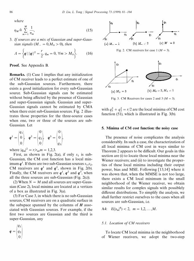
Remarks. (1) Case 1 implies that any initializationof CM receiver leads to a perfect estimate of one ofthe sub-Gaussian sources. Furthermore, thereexists a good initialization for every sub-Gaussiansource. Sub-Gaussian signals can be estimatedwithout being affected by the presence of Gaussianand super-Gaussian signals. Gaussian and super-Gaussian signals cannot be estimated by CMAwhen there exist sub-Gaussian sources. Fig. 2 illus-trates those properties for the three-source caseswhen one, two or three of the sources are sub-Gaussian. Let

q1"Aq10

0 B, q2"A0

q20 B, q3"A

0

0

q3B,

where DqmD2"r/r

m,m"1,2,3.

First, as shown in Fig. 2(a), if only s1

is sub-Gaussian, the CM cost function has a local min-imum q1. If there are two sub-Gaussian sources s

1,s2,

CM receivers are q1 and q2, shown in Fig. 2(b).Finally, the CM receivers are q1, q2 and q3, whenall the three sources are sub-Gaussian (Fig. 2(c)).

(2) When N"M and all sources are super-Gaus-sian (Case 2), local minima are located at a verticesof a box as illustrated in Fig. 3(a).

(3) For Case 3, in which there is no sub-Gaussiansources, CM receivers are on a quadratic surface inthe subspace spanned by the columns of H asso-ciated with Gaussian sources. For example, if thefirst two sources are Gaussian and the third issuper-Gaussian, any

q"Aq1

q20 B

Fig. 2. CM receivers for case 1 (M"3).

Fig. 3. CM Receivers for cases 2 and 3 (M"3).

with q21#q2

2"r/2 are the local minima of CM cost

function (51), which is illustrated in Fig. 3(b).

5. Minima of CM cost function: the noisy case

The presence of noise complicates the analysisconsiderably. In such a case, the characterization ofall local minima of CM cost in ways similar toTheorem 2 appears to be difficult. Our goals in thissection are (i) to locate those local minima near theWiener receivers; and (ii) to investigate the proper-ties of these local minima including their outputpower, bias and MSE. Following [13,14] where itwas shown that, when the MMSE is not too large,there exists a CM local minimum in the smallneighborhood of the Wiener receiver, we obtainsimilar results for complex signals with possiblelydifferent distributions. To simplify the analysis, weshall further restrict ourselves to the cases when allsources are sub-Gaussian, i.e.

A4: E(DsmD4)(2, m"1,2,2,M.

5.1. Location of CM receivers

To locate CM local minima in the neighborhoodof Wiener receivers, we adopt the two-step


approach by Zeng and Tong in [13]. First, a com-pact neighborhood of the Wiener receiver is definedusing parameters relevant to the receiver MSE per-formance. Second, parameters are chosen such thatthe CM cost function on the boundary of the neigh-borhood is strictly greater than a reference insidethe neighborhood. By the Weierstrass theorem, thisneighborhood must contain at least one local min-imum. Before we proceed in defining the neighbor-hood that captures a CM receiver, let us recall theWiener receiver defined as one that minimizes themean square error

J8(q)¢E(Dy!s

1D2)"EqE2U!qHe

1!eH

1q#1. (17)

The Wiener receiver for signal s1

is the minimum ofthe above optimization

q8"arg minJ

8(q)"U~1e

1. (18)

Again, without loss of generality, we shall restrictour discussion of estimating s

1throughout this

section.

5.1.1. The neighborhoodThe neighborhood is defined through a special

parameterization of the system response q. Givenan estimator of s

1, denote its system response by

q¢hA1

qIB, (19)

where h is the receiver gain of s1

and qIis the vector

of coefficients corresponding to the (relative) resi-due interference from other users. Suppose theWiener receiver

q8"h

8A1

q8IB. (20)

The neighborhood B(q8,d

U,h

L,h

U), illustrated in

Fig. 4, is a slice of a cone centered around theWiener receiver q

8with receiver gain h3[h

L,h

U],

B(q8,d

U,h

L,h

U)¢Gq¢hA

1

qIB: h

L)h)h

U,

EqI!q

8IEC¢d)d

UH, (21)

Fig. 4. The region B.

where C is the submatrix of U by removing the firstcolumn and row. The ‘width’ of the cone is specifiedby d

Uwhich is, as shown in [14], the maximum

extra unbiased MSE3 among all receivers in theneighborhood, i.e,

d2U" max

q|B(q8,dU,hL,hU) GKMSEA1

h8

q8B!MSEA

1

hqBKH.

(22)

Here MSE(q) stands for the mean square error ofan estimator with system response q.

5.1.2. The location of CM local minima

Select the reference q3"h

3AA1

q8IBB where h

3is

such that JAh3A1

q8IBB is minimized, i.e.,

h3"argmin

hJAhA

1

q8IBB, (23)

q3"h

3AA1

q8IBB. (24)

We aim to choose hL, h

Uand d

Uso that (i) q

3is

inside the neighborhood; and (ii) the CM cost onthe boundary of B(q

8,d

U,h

L,h

U) is strictly greater

3Given an estimator of s1, let the system response be

q"hA1

qIB. The estimate y of s

1has the form y"qTs#noise

term"hs1#other terms orthogonal to s

1. Because E(yDs

1)"

hs1, y is a conditionally biased estimate of s

1. Scaling the esti-

mate y by 1/h, we have a (conditionally) unbiased estimateu¢(1/h)y of s

1, i.e. E(u!s

1Ds1)"0. See also [1].


than J(q3). Consequently, a CM receiver is located

in B(q8,d

U,h

L,h

U). The following theorem describes

such a procedure.

Theorem 3. Given the ¼iener receiver q8"

h8A

1

q8IB, let q

3be defined by Eq. (24). ¼ith cumu-

lants niof the sources, define

n.*/

¢ min1xmxM

MnmN, r

.*/¢n

.*/#2, (25)

PI¢diagGA

n2

n.*/B

1@4,2,A

nM

n.*/B

1@4

H. (26)

¸et hL

and hU

be determined by

hL¢ min

0xdxdUS!c

1(d)!c

1(d)2!4c

2(d)c

02c

2(d)

,

(27)

hU¢ max

0xdxdUS

!c1(d)#c

1(d)2!4c

2(d)c

02c

2(d)

,

(28)

where

c0¢

r2

2#n1h28#n

.*/h28EP

Iq8I

E44

, (29)

c1(d)¢!2rAd2#

1

h8B, (30)

c2(d)¢2Ad2#

1

h8B

2#n

1#n

.*/(d#EP

Iq8I

E4)4).

(31)

¸et dU

be the smallest positive root of D(d)¢c1(d)2!4c

2(d)c

0.

(a) ¼ith dispersion constant r"EDs1D4/EDs

1D2"

EDs1D4, if

h8'maxG1!

2

3(2!r.*/

),

1!J4#16r!9rr

.*/!r#2

20!9r.*/

!r H (32)

and

dU(Eq

8IE2, (33)

then there exists a local minimum of J(q) in B(q8,d

U,

hL,h

U).

(b) ¸et q#is the local minimum of J(q) in B(q

8,d

U,

hL,h

U), then

limp?0

B(q8,d

U,h

L,h

U)"lim

p?0

Mq#N"lim

p?0

Mq8N. (34)

Proof. See Appendix C.

Theorem 3 gives sufficient conditions of the exist-ence of a CM receiver in the neighborhood of theWiener receiver. Given the Wiener receiver and thedistribution of source signals, one can checkthe two conditions given in Eqs. (32) and (33), bothdepend on the distributions of source signals.If they are satisfied, then there exists a CM re-ceiver in the neighborhood of the Wiener receiver.Table 1 gives the maximum value of MSE of theWiener receiver for QAM sources to satisfy Eq. (32)assuming that r"r

.*/. As to Eq. (33), polynomial

D(d) needs to be calculated first, then its smallestpositive root d

U. When the noise is small enough,

for any sources, a root of D(d) can always be foundless than Eq

8IE2

and Eq. (32) can be satisfied withh8

close to 1, which means that there must bea local minimum of J(q) in the neighborhood ofthe Wiener receiver. Part (b) of Theorem 3 gives theresult consistent with the noiseless case. Asmeasurement noise becomes zero, the neighbor-hood defined by B(q

8,d

U,h

L,h

U) shrinks to one, the

Wiener receiver. We note that the above theoremdoes not cover those local minima not in the vicin-ity of Wiener receivers.

5.2. Output power, bias and MSE of CM receiver

In Section 3, it is shown that the output power ofany CM receiver is greater than r/2 when there is atleast one sub-Gaussian source. In this section, theupper bound of the output power of the local min-ima of J(q) is obtained for the case that all thesources are sub-Gaussian. Further, we compare theoutput power, bias, residue interference of CM re-ceiver in the region B(q

8,d

U,h

L,h

U) with that of the

Wiener receiver, and give the MSE bounds of theCM receiver.


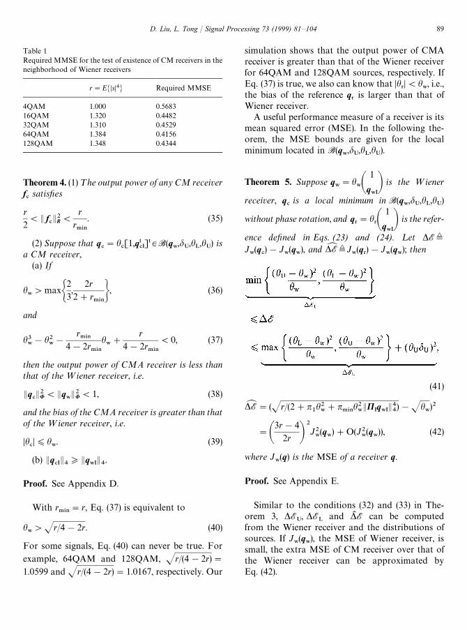
Table 1Required MMSE for the test of existence of CM receivers in theneighborhood of Wiener receivers

r"EMDsD4N Required MMSE

4QAM 1.000 0.568316QAM 1.320 0.448232QAM 1.310 0.452964QAM 1.384 0.4156128QAM 1.348 0.4344

Theorem 4. (1) ¹he output power of any CM receiverf#

satisfies

r

2(E f

#E2R(

r

r.*/

. (35)

(2) Suppose that q#"h

#[1,q5

#I]53B(q

8,d

U,h

L,h

U) is

a CM receiver,(a) If

h8'maxG

2

3,

2r

2#r.*/H, (36)

and

h38!h2

8!

r.*/

4!2r.*/

h8#

r

4!2r.*/

(0, (37)

then the output power of CMA receiver is less thanthat of the ¼iener receiver, i.e.

Eq#E2U(Eq

8E2U(1, (38)

and the bias of the CMA receiver is greater than thatof the ¼iener receiver, i.e.

Dh#D)h

8. (39)

(b) Eq#IE4*Eq

8IE4.

Proof. See Appendix D.

With r.*/

"r, Eq. (37) is equivalent to

h8'Jr/4!2r. (40)

For some signals, Eq. (40) can never be true. For

example, 64QAM and 128QAM, Jr/(4!2r)"

1.0599 and Jr/(4!2r)"1.0167, respectively. Our

simulation shows that the output power of CMAreceiver is greater than that of the Wiener receiverfor 64QAM and 128QAM sources, respectively. IfEq. (37) is true, we also can know that Dh

3D(h

8, i.e.,

the bias of the reference q3

is larger than that ofWiener receiver.

A useful performance measure of a receiver is itsmean squared error (MSE). In the following the-orem, the MSE bounds are given for the localminimum located in B(q

8,d

U,h

L,h

U).

Theorem 5. Suppose q8"h

8A1

q8IB is the ¼iener

receiver, q#is a local minimum in B(q

8,d

U,h

L,h

U)

without phase rotation, and q3"h

3A1

q8IB is the refer-

ence defined in Eqs. (23) and (24). ¸et *E¢J8(q

#)!J

8(q

8), and *EY ¢J

8(q

3)!J

8(q

8); then

(41)

*EY "(Jr/(2#n1h28#n

.*/h28EP

Iq8I

E44)!Jh

8)2

"A3r!4

2r B2J28(q

8)#O(J2

8(q

8)), (42)

where J8(q) is the MSE of a receiver q.

Proof. See Appendix E.

Similar to the conditions (32) and (33) in The-orem 3, *E

U, *E

Land *K E can be computed

from the Wiener receiver and the distributions ofsources. If J

8(q

8), the MSE of Wiener receiver, is

small, the extra MSE of CM receiver over that ofthe Wiener receiver can be approximated byEq. (42).


6. Numerical results

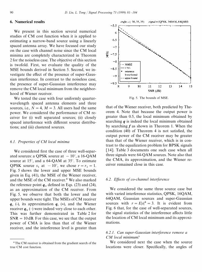
We present in this section several numericalstudies of CM cost function when it is applied toestimating a narrow-band source using a linearlyspaced antenna array. We have focused our studyon the case with channel noise since the CM localminima are completely characterized in Theorem2 for the noiseless case. The objective of this sectionis twofold. First, we evaluate the quality of theMSE bounds derived in Section 5. Second, we in-vestigate the effect of the presence of super-Gaus-sian interference. In contrast to the noiseless case,the presence of super-Gaussian interference mayremove the CM local minimum from the neighbor-hood of Wiener receiver.

We tested the case with four uniformly quarter-wavelength spaced antenna elements and threesources, i.e., N"4, M"3. All users had the samepower. We considered the performance of CM re-ceiver for (i) well separated sources; (ii) closelyspaced interference with different source distribu-tions; and (iii) clustered sources.

6.1. Properties of CM local minima

We considered first the case of three well-separ-ated sources: a QPSK source at !10°, a 16-QAMsource at 15°, and a 64-QAM at 35°. To estimateQPSK source s

1at !10°, we chose r"r

1"1.

Fig. 5 shows the lower and upper MSE boundsgiven in Eq. (41), the MSE of the Wiener receiver,and the MSE of the CM receiver.4 We also markedthe reference point q

3, defined in Eqs. (23) and (24),

as an approximation of the CM receiver. FromFig. 5, we observe that both the lower and theupper bounds were tight. The MSEs of CM receiverq#

(-), its approximation q3

(*), and the Wienerreceiver q

8(—) were indeed very close to each other.

This was further demonstrated in Table 2 forSNR"10 dB. For this case, we see that the outputpower of CMA is less than that of the Wienerreceiver, and the interference level is greater than

4The CM receiver is obtained from the gradient search of thetrue CM cost function.

Fig. 5. The bounds of MSE.

that of the Wiener receiver, both predicted by The-orem 4. Note that because the output power isgreater than 0.5, the local minimum obtained bysearching q is indeed the local minimum obtainedby searching f as shown in Theorem 1. When thecondition (40) of Theorem 4 is not satisfied, theoutput power of the CM receiver may be greaterthan that of the Wiener receiver, which is in con-trast to the equalization problem for BPSK signals[14]. Table 3 documents one such case when allthree signals were 64-QAM sources. Note also thatthe CMA, its approximation, and the Wiener re-ceiver remained close in this case.

6.2. Effects of co-channel interference

We considered the same three source case butwith varied interference statistics, QPSK, 16QAM,64QAM, Gaussian sources and super-Gaussiansources with r"EDsD4"3. It is evident fromFig. 6 that, for the case of well-separated sources,the signal statistics of the interference affects littlethe location of CM local minimum and its approxi-mations.

6.2.1. Can super-Gaussian interference remove aCM local minimum?

We considered next the case when the sourcelocations were closer. Specifically, the angles of


Table 2CMA and MMSE at SNR"10dB ([!10°,15°,35°], [QPSK,16QAM,64QAM])

System response coefficients Output power EqIE44

CMA q#

[0.757,0.122#0.198i,0.021!0.108i] 0.7269 0.0094MMSE q

.[0.788,0.123#0.200i,0.022!0.118i] 0.7878 0.0083

Reference q3

[0.757,0.118#0.192i,0.022!0.113i] 0.7268 0.0083

Table 3CMA and MMSE at SNR"10dB ([!10°,15°,35°], [64QAM,64QAM,64QAM])

System response coefficients Output power EqIE44

CMA q#

[0.822,0.135#0.219i,0.022!0.114i] 0.8574 0.0101MMSE q

.[0.788,0.123#0.200i,0.022!0.118i] 0.7878 0.0083

Reference q3

[0.822,0.128#0.208i,0.024!0.123i] 0.8572 0.0083

Fig. 6. The effect of interference signal constellation.

arrival were !10°, 0° and 35°, which means thatinterference from the second user was closer to thedesired signal. Fig. 7 shows the MSE of CM re-ceiver for the QPSK source s

1with the interference

s2varied from 64-QAM to a super-Gaussian source

r2"6. In this case, we observed that the effects of

interference constellation is not significant whenthey were sub-Gaussian. However, when the inter-ference s

2was changed to super-Gaussian with

r2"6, the MSE behavior of CM receiver at lower

Fig. 7. The effect of interference signal constellation.

SNR region showed significant difference from thecase when s

2was 64-QAM. For the noiseless case,

we have already shown in Theorem 2 that thepresence of super-Gaussian interference has no ef-fect on the location of the CM receiver for a sub-Gaussian source, which was indeed verified at highSNR region. At low SNR, this example appeared toshow the contrary. Table 4 gives the CM coeffi-cients for the three users at SNR"10dB. It ap-peared that, initialized at their Wiener receivers, all


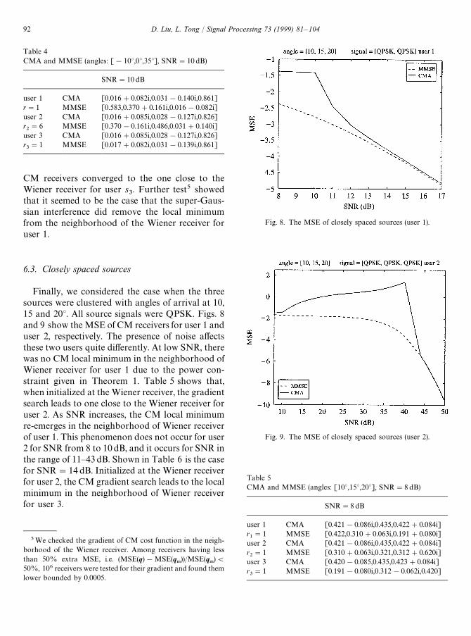
Table 4CMA and MMSE (angles: [!10°,0°,35°], SNR"10 dB)

SNR"10 dB

user 1 CMA [0.016#0.082i,0.031!0.140i,0.861]r"1 MMSE [0.583,0.370#0.161i,0.016!0.082i]user 2 CMA [0.016#0.085i,0.028!0.127i,0.826]r2"6 MMSE [0.370!0.161i,0.486,0.031#0.140i]

user 3 CMA [0.016#0.085i,0.028!0.127i,0.826]r3"1 MMSE [0.017#0.082i,0.031!0.139i,0.861]

CM receivers converged to the one close to theWiener receiver for user s

3. Further test5 showed

that it seemed to be the case that the super-Gaus-sian interference did remove the local minimumfrom the neighborhood of the Wiener receiver foruser 1.

6.3. Closely spaced sources

Finally, we considered the case when the threesources were clustered with angles of arrival at 10,15 and 20°. All source signals were QPSK. Figs. 8and 9 show the MSE of CM receivers for user 1 anduser 2, respectively. The presence of noise affectsthese two users quite differently. At low SNR, therewas no CM local minimum in the neighborhood ofWiener receiver for user 1 due to the power con-straint given in Theorem 1. Table 5 shows that,when initialized at the Wiener receiver, the gradientsearch leads to one close to the Wiener receiver foruser 2. As SNR increases, the CM local minimumre-emerges in the neighborhood of Wiener receiverof user 1. This phenomenon does not occur for user2 for SNR from 8 to 10 dB, and it occurs for SNR inthe range of 11—43dB. Shown in Table 6 is the casefor SNR"14 dB. Initialized at the Wiener receiverfor user 2, the CM gradient search leads to the localminimum in the neighborhood of Wiener receiverfor user 3.

5We checked the gradient of CM cost function in the neigh-borhood of the Wiener receiver. Among receivers having lessthan 50% extra MSE, i.e. (MSE(q)!MSE(q

.))/MSE(q

.)(

50%, 106 receivers were tested for their gradient and found themlower bounded by 0.0005.

Fig. 8. The MSE of closely spaced sources (user 1).

Fig. 9. The MSE of closely spaced sources (user 2).

Table 5CMA and MMSE (angles: [10°,15°,20°], SNR"8 dB)

SNR"8 dB

user 1 CMA [0.421!0.086i,0.435,0.422#0.084i]r1"1 MMSE [0.422,0.310#0.063i,0.191#0.080i]

user 2 CMA [0.421!0.086i,0.435,0.422#0.084i]r2"1 MMSE [0.310#0.063i,0.321,0.312#0.620i]

user 3 CMA [0.420!0.085,0.435,0.423#0.084i]r3"1 MMSE [0.191!0.080i,0.312!0.062i,0.420]


Table 6CMA and MMSE (angles: [10°,15°,20°], SNR"14 dB)

SNR"14 dB

user 1 CMA [0.600,0.361#0.073i,0.125#0.052i]r1"1 MMSE [0.589,0.321#0.065i,0.061#0.026i]

user 2 CMA [0.129!0.054i,0.368!0.073i,0.597]r2"1 MMSE [0.321!0.067i,0.335,0.325#0.065i]

user 3 CMA [0.127!0.053i,0.367!0.073i,0.598]r3"1 MMSE [0.061!0.026i,0.325!0.065i,0.585]

7. Conclusion

Blind beam forming based on the constantmodulus cost function has several distinct advant-ages, especially when all sources are sub-Gaussian.The most important is, perhaps, the connectionbetween the Wiener and CM receivers. When thereis no noise and all sources are sub-Gaussian, alllocal minima of CM cost function are global andthey perfectly estimate all the sources. When thereis noise, we have shown in this paper that thosesources whose MMSE is not too large can also beestimated by CM receiver with similar MSE. Infact, CM receivers for these sources are approxim-ately scaled Wiener receivers. This means that theCM array approach is close to the MMSE estimateof all the sources provided that, at each stage, theMMSE of some source is not too large and appro-priate initialization is used. There are cases, how-ever, that there is no CM receiver in theneighborhood of the Wiener receiver. In this case,the CM array cannot extract this source accurately,and significant error propagation may occur.

When there are mixed sources, it should be cau-tioned that the presence of super-Gaussian sourcesmay remove CM local minima from the neighbor-hood of Wiener receivers at low SNR. When thereis no noise and at least one sub-Gaussian source, weshow that CM receivers filter out all Gaussian andsuper-Gaussian sources. When all sources are eitherGaussian or super-Gaussian, CM receivers filter outall super-Gaussian sources. It is perhaps not surpris-ing that CM cost function tends to favor sub-Gaus-sian over Gaussian and super-Gaussian sources,and Gaussian sources over super-Gaussian sources.

For further reading, see [3].

Acknowledgements

The authors wish to thank the anonymous re-viewer for the careful reading and comments thathelped to improve the presentation of the paper.

Appendix A. Proof of Theorem 1

To prove case 1, assume, without the loss ofgenerality, that n

1(0. Let f 0 be a local minima,

and * f"* fH#* fHM, then

JM ( f 0)!JM ( f 0#* f)"M2(E f E4R!E f#*f E4R)

!2r(E f 0E2R!E f 0#*f E2R)N (A.1)

#GM+

m/1

nm(DeH

mHHf 0D4!DeH

mHH( f 0#*fH)D4)H (A.2)

"D1#D

2. (A.3)

To show that all CM local minima are in thesignal subspace, we consider the following twoscenarios: (a) f 0"f 0HM3CHM; (b) f 0"f 0H#f 0HM,f 0H3CH,f 0HM3CHM, f 0HMO0.

For (a), because n1(0, and (A1), there exists

*fH3CH and an arbitrarily small e such that

D2"

M+

m/1

nm(DeH

mHHf 0HMD4

!DeHm

HH( f 0HM#*fH#*fHM)D4)

"!

M+

m/1

nmDeHHH*fHD4"!en

1'0. (A.4)

Since f 0HMO0, and p2'0, there exists a *fHM3CHM

such that

Ef 0E2R!Ef 0#*fE2R

"Ef 0HME2R!Ef 0HM#*fHME2R!E*fHE2R"0,

i.e.,

D1"0. (A.5)


From Eqs. (A.5) and (A.6), we have JM ( f 0)'JM ( f 0#*f ). Therefore, f 0 can not be a local min-imum. The same technique can also be used toshow that f0HM"0 for case (b).

We show next that all CM local minima in thiscase must have output power greater than r/2. Letf 0H be a CM local minimum and E f 0HE2R(r/2. Letf"*fHM#f 0H , where *fHM3CHM. It can be verified that

JM ( f )"JM ( f 0H )#2E*fHME4R#2E*fHME2R(2E f 0H E2R!r).

(A.6)

Because the last term of the above equation isnegative, there exists *fHM small enough thatJM ( f )(JM ( f 0H ). Hence Ef 0HE2R*r/2. To exclude theequality, one can always find a f 0H#*fH such that(2E f 0H#*fHE2R!r)(0.

To show case 2, we show that any local minimumin CH with output power greater than r/2 is alsoa local minimum with no constraint. Considera small perturbation *f"*fH#*fHM of such a lo-cal minima f 0H . From Eq. (A.6),

JM ( f 0H#*f )"JM ( f 0#*fH)#2E*fHME4R#2E*fHME2R(2E f 0H#*fHE2R!r) (A.7)

'JM ( f 0)#2E*fHME4R#2E*fHME2R(2E f 0H

#*fHDD2R!r). (A.8)

Because E f 0HE2R'r/2, there exists a small neigh-borhood around 0 such that the last term in theabove inequality is positive. Therefore, JM ( f 0H#*f )'JM ( f 0H ).

To prove case 3, we consider the case when thefirst M

`sources are super-Gaussian, i.e., n

i'0 for

i"1,2,M`

and zero otherwise. Let f 0NCHMXCH'

be a local minimum. Because of (A1), there exists anarbitrary small e'0 and *fH such that

( f 0#*fH)HH"(1!e ) f 0HH.

Since p2'0, choosing *fHM such that E*fHME2"(1!(1!e)2)E f 0#*fHE2R, we have

E f 0E2R"D f 0#*f E2R,

M`

+i/1

niDeHiHH( f 0#*f )D4(

M`

+i/1

niDeHiHHf 0D4.

This contradicts that f 0 is a local minimum. Nowconsider any local minimum f 0, then

JM ( f 0)"2E f 0E4R!2rE f 0E2R#M`

+m/1

nm(DeH

mHHf 0D4#r2

"2E f 0E4R!2rE f 0E2R.

It is easy to see that E f 0E2R"r/2.

Appendix B. Proof of Theorem 2

For the noiseless case, U"IM

. The CM cost function is given by

J(q)"2EqE42!2rEqE2

2#

M+

m/1

nmDq

mD4#r2. (B.1)

The gradient of J(q) is

£qHJ(q)"4EqE2q!2rq#2Qq"2(2EqE2IM!rI

M#Q)q, (B.2)

where,

Q"diagMn1Dq

1D2,2,n

MDq

MD2N.

The stationary points are given by

2EqE2!r#nmDq

mD2"0 or q

m"0, m"1,2,2,M. (B.3)


This implies that when there are K non-zero entries qmj, j"1,2,2,K, in a stationary point q, we have three

possibilities:S0: q"0.S1: n

minmj'0, ∀i, j"1,2,2,K,

Dqmj

D2"r

nmj

(2gK#1)

, gK¢

K+j/1

1

nmj

, (B.4)

EqE2"gK

2gK#1

r. (B.5)

S2: nmj"0, j"1,2,2,K,

EqE2"r

2. (B.6)

Next we will check the stationary points and obtain the local minima of J(q).The Hessian matrix of Eq. (B.1) is

£q£qHJ(q)"4EqE2I#4qqH!2rI#4Q, (B.7)

which, according to K, has the following three forms at the stationary points defined in S1:(i) when K"M,

£q£qHJ(q)"4qqH#2r

2gM#1

I, (B.8)

(ii) when 1(K(M,

£q£qHJ(q)"

!2r

2gK#1

}2rr

m1

nm1

(2gK#1)

4qm1

qHm2 *

}

4qHm1

qm2

2rrm2

nm2

(2gK#1)

* }!2r

2gK#1

; (B.9)

(iii) when K"1,

£q£qHJ(q)"

2r(2!rm1

)

rm1 }

2r(2!rm1

)

rm1 2r

2r(2!rm1

)

rm1 }

2r(2!rm1

)

rm1

. (B.10)


Since £q£qHJ(q)Dq/0"!2rI(0, q"0 is a local maximum.

1. First, we show case 1 (M~'0): If all sources corresponding to non-zero entries of q are super-Gaussian,

i.e., rmj'2,

!2r

2gK#1

"

2r(2!rmj

)

nmj(2g

K#1)

(0, (B.11)

K2rr

m1

nm1

(2gK#1)

4qm1

qHm2

4qHm1

qm2

2rrm2

nm2

(2gK#1) K"

4r2(rm1

rm2!4)

nm1

nm2

(2gK#1)2

'0. (B.12)

Hence £q£qHJ(q) is indefinite and the stationary point is not stable. If all sources corresponding tonon-zero entries of q are sub-Gaussian, i.e., r

mi(2, then

!2r

2gK#1

'0 (B.13)

and

K2rr

m1

nm1

(2gK#1)

4qm1

qHm2

4qHm1

qm2

2rrm2

nm2

(2gK#1) K(0. (B.14)

Eqs. (B.13) and (B.14) again imply that £q£qHJ(q) of Eq. (B.9) is indefinite; therefore, there is no localminimum when 2)K)M and n

mjO0.

When rmj"2, j"1,2,2,K, consider a stationary point q in S2,

q"q~

q0

q`

"

0

q00

, EqE2"Eq0E2"

r

2. (B.15)

If M~'0, there exists a small enough

*q"*q

~*q

00

such that

Eq#*qE2"r

2.

Thus J(q#*q)!J(q)"+M~

m/1nmD*q

mD4(0, which means q given in S2 are not local minima.

When K"1, we have

2r(2!rm1

)

rm1

'0 iff rm1(2.

Therefore, q"qmem

is a local minimum iff rm(2. This proves

K"Gqmem K DqmD2"

r

rm

, 1)m)M~H. (B.16)


2. Now let us consider case 2 (M`"M): From r

m'2, m"1,2,2,M, it is easy to see that Eqs. (B.10) and

(B.9) are indefinite and Eq. (B.8) is positive definite, i.e.,

K"Gq"(q1,q

2,2,q

M)T,Dq

mD2"

r

nm(2g

M#1)H.

3. Finally, assume M~"0,M

0'0: Considering

q"

q~

q0

q`

in Eq. (B.15), if M~"0, for any *qO0, J(q#*q)!J(q)'0, which implies that q is a local minimum.

Appendix C. Proof of Theorem 3

The proof has four steps: (i) express the CM cost function using the extra MSE d defined in Eq. (21) and thereceiver gain h and h

8; (ii) give the reference q

3; (iii) prove there is a local minimum in B(q

8,d

U,h

L,h

U); and (iv)

verify that when noise variance goes to 0, CM receiver goes to the Wiener receiver.

1. Suppose that q8"h

8AA1

q8IBB is the Wiener receiver for s

1. For any receiver

q"hAA1

qIBB,

it can be shown [13,14] that

EMy2N"EqE2U"DhD2A1

h8

#d2B. (C.1)

According to Eq. (C.1), the CM cost function J(q) is then given by

J(q)"2Ad2#1

h8B

2DhD4!2rAd2#

1

h8BDhD2#(n

1#n

.*/EP

IqIE44)DhD4#r2, (C.2)

where PIand n

.*/are defined as in Eqs. (26) and (25), respectively.

In the following, Eq. (C.2) will be used to locate the local minima of J(q).

2. Choose reference q3¢h

3A1

q8IB with the minimum CM cost:

JAhA1

q8IBB"

2

h28

DhD4!2r

h8

DhD2#(n1#n

.*/EP

Iq8I

E44)DhD4#r2. (C.3)

From

LJ

LDhD2"2C

2

h28

#(n1#n

.*/EP

Iq8I

E44)DDhD2!

2r

h8

"0, (C.4)


we get

Dh3D2"

rh8

2#h28(n

1#n

.*/EP

Iq8I

E44). (C.5)

Thus,

J(q3)"

2

h28

r2h28

[2#h28(n

1#n

.*/EP

Iq8I

E44)]2

!

2r

h8

rh8

2#h28(n

1#n

.*/EP

Iq8I

E44)#(n

1#n

.*/EP

Iq8I

E44)

r2h28

[2#h28(n

1#n

.*/EP

IqIE44)]2

#r2

"

r2[2#h28(n

1#n

.*/EP

Iq8I

E44)]

[2#h28(n

1#n

.*/EP

Iq8I

E44)]2

!

2r2

2#h28(n

1#n

.*/EP

Iq8I

E44)#r2

"r2!r2

2#h28(n

1#n

.*/EP

Iq8I

E44)

(C.6)

"r2!rDh

3D2

h8

. (C.7)

Since the noise variance p2'0, we have C'Inq~1

. Then

PIqIE4"EP

IqI!P

Iq8I#P

Iq8I

E4

)EPI(q

I!q

8I)E

4#EP

Iq8I

E4

(EqI!q

8IEC#EP

Iq8I

E4

"d#EPIq8I

E4.

Therefore,

J(q)!J(q3)"C2Ad2#

1

h8B

2#n

1#n

.*/EP

IqIE44DDhD4

!2rAd2#1

h8BDhD2#r2#

r2

2#h28(n

1#n

.*/EP

Iq8I

E44)

!r2'C2Ad2#1

h8B

2#n

1#n

.*/(d#EP

Iq8I

E4)4DDhD4

!2rAd2#1

h8BDhD2#

r2

2#h28(n

1#n

.*/EP

Iq8I

E44)"c

2(d)DhD4#c

1(d)DhD2#c

0. (C.8)

3. To show that there is CM receiver in B(q8,d

U,h

L,h

U), we need to show the CM cost of every point on the

boundary of B(q8,d

U,h

L,h

U) is greater than that of reference q

3and the reference is inside B(q

8,d

U,h

L,h

U).

(a) Consider all points on the peripheral surface Sp"Mq:Eq

I!q

8IEC"d

U,h

L)h)h

UN shown in Fig. 10.

First we need to show c2(d)'0, ∀d3(0,Eq

8IE2).


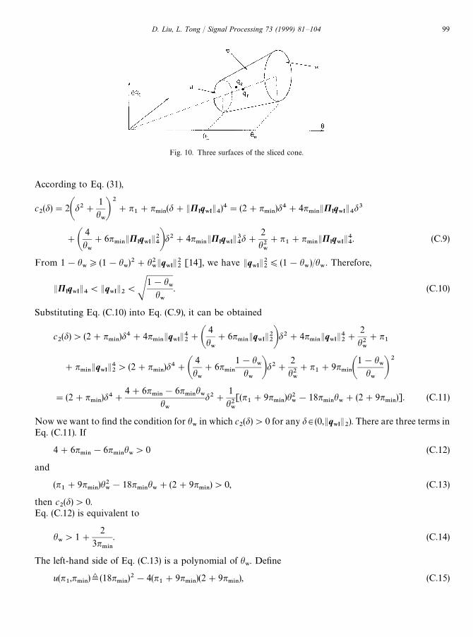
Fig. 10. Three surfaces of the sliced cone.

According to Eq. (31),

c2(d)"2Ad2#

1

h8B

2#n

1#n

.*/(d#EP

Iq8I

E4)4"(2#n

.*/)d4#4n

.*/EP

Iq8I

E4d3

#A4

h8

#6n.*/

EPIq8I

E24Bd2#4n

.*/EP

Iq8I

E34d#

2

h28

#n1#n

.*/EP

Iq8I

E44. (C.9)

From 1!h8*(1!h

8)2#h2

8Eq

8IE22

[14], we have Eq8I

E22)(1!h

8)/h

8. Therefore,

EPIq8I

E4(Eq

8IE2(S

1!h8

h8

. (C.10)

Substituting Eq. (C.10) into Eq. (C.9), it can be obtained

c2(d)'(2#n

.*/)d4#4n

.*/Eq

8IE42#A

4

h8

#6n.*/

Eq8I

E22Bd2#4n

.*/Eq

8IE42#

2

h28

#n1

#n.*/

Eq8I

E42'(2#n

.*/)d4#A

4

h8

#6n.*/

1!h8

h8Bd2#

2

h28

#n1#9n

.*/A1!h

8h8B

2

"(2#n.*/

)d4#4#6n

.*/!6n

.*/h8

h8

d2#1

h28

[(n1#9n

.*/)h2

8!18n

.*/h8#(2#9n

.*/)]. (C.11)

Now we want to find the condition for h8

in which c2(d)'0 for any d3(0,Eq

8IE2). There are three terms in

Eq. (C.11). If

4#6n.*/

!6n.*/

h8'0 (C.12)

and

(n1#9n

.*/)h2

8!18n

.*/h8#(2#9n

.*/)'0, (C.13)

then c2(d)'0.

Eq. (C.12) is equivalent to

h8'1#

2

3n.*/

. (C.14)

The left-hand side of Eq. (C.13) is a polynomial of h8. Define

u(n1,n

.*/)¢(18n

.*/)2!4(n

1#9n

.*/)(2#9n

.*/), (C.15)


then Eq. (C.13) is equivalent to

18n#Ju(n1,n

.*/)

2(n1#9n

.*/)

(h8(

18n.*/

!Ju(n1,n

.*/)

2(n1#9n

.*/)

. (C.16)

It is easy to see

u(n1,n

.*/)"4[!2n

1!9n

.*/(2#n

1)]'4[!2n

1]'4n2

1,

hence, (18n.*/

!Ju(n1,n

.*/))/2(n

1#9n

.*/)'1, which means h

8((18n

.*/!Ju(n

1,n

.*/))/2(n

1#9n

.*/)

is always true.Now we have shown that c

2(d)'0, ∀d3(0,Eq

8IE2), when Eq. (32) holds.

Also we know 0(dU(Eq

8IE2; therefore,

J(q)!J(q3)'c

2(d

U)DhD4#c

1(d

U)DhD2#c

0*0, ∀q3S

p. (C.17)

(b) Now we check the points on the upper surface SU

defined by h"hU,0)d)d

U. Since

DhD2"(hU)2*

!c1(d)#Jc

1(d)2!4c

2(d)c

02c

2(d)

, (C.18)

and c2(d)'0, then the polynomial c

2(d)DhD4#c

1(d)DhD2#c

0*0. Thus, J(q)!J(q

3)'0. Similarly,

J(q)!J(q3)'0 ∀q3S

L.

(c) Finally, we verify that (hL)2(Dh

3D2((h

U)2. From Dh

3D2"!c

1(0)/2c

2(0) and Eqs. (27) and (28), it can be

obtained easily.4. In the end, we examine the case as the noise variance pP0. From Eqs. (29)—(31), we have

limp?0

c0"lim

p?0

r2

2#n1h28#n

.*/h28EP

Iq8I

E44

"r,

limp?0

c1(d)"!2r(d2#1),

limp?0

c2(d)"2(d2#1)2#n

1#n

.*/d4,

limp?0

D(d)"4r2(d2#1)2!4r[(2(d2#1)2#n1#n

.*/d4],"4r(n

1!n

.*/)d4#8rn

1d2.

So

limp2?0

dU"0

and

limp2?0

hL"lim

p?0

hU"1"h

8.

Appendix D. Proof of Theorem 4

1. It has already been shown that E f#E2R'r/2 in Section 3. Define a function for any f such that E f ER"1,

/(k, f )¢JM (Jkf )"(2#n.*/

EPHHf E44)k2!2rk#r2, (D.1)


where

P¢diagGAn1

n.*/B

1@4,2,A

nM

n.*/B

1@4

H,then

L/(k, f )

Lk"2(2#n

.*/EPHHf E4

4)k!2r. (D.2)

The minimum of /(k, f ) is achieved at

k0"

r

2#n.*/

EPHHf E44

. (D.3)

Since n.*/

(0, and EPHHf E44)EHHf E4

2(Ef E4R"1,

E f#E2R"k

0(

r

n.*/

#2"

r

r.*/

.

2. Now consider a local minimum of J(q) in B(q8,d

U,h

L,h

U).

(a) Any point in B(q8,d

U,h

L,h

U) can be represented by Jkq, where EqE2U"Eq

8E2U"h

8and 0)k(R.

Define

/(k,q)¢J(Jkq)"2h28k2!2rh

8k#n

.*/EP

IqE4

4k2#r2. (D.4)

From (d/dk)/(k,q)"0, the minimum Jkq must have

k"rh

82h2

8#n

.*/EPqE4

4

. (D.5)

If k(1, then Eq#E2U(Eq

8E2U. In order to get the condition for k(1, we adopt the following two steps:

(i) Bound EPqE44

by DhD and h8: Since

EPqE44(EqE4

4"DhD4#Ehq

IE44)DhD4#Ehq

IE42)DhD4#(q5Uq!DhD2)2"DhD4#(h

8!DhD2)2,

then

k(rh

82h2

8#n

.*/(DhD4#(h

8!DhD2)2

"

rh8

2n.*/

DhD4!2n.*/

h8DhD2#r

.*/h28

. (D.6)

Define a polynomial of DhD as

p(DhD)¢2n.*/

DhD4!2n.*/

h8DhD2#r

.*/h28!rh

8, (D.7)

then p(DhD)'0 results in k'1. It is easy to see that if

2n.*/

h8#JD

4n.*/

(DhD2(2n

.*/h8!JD

4n.*/

, (D.8)

then p(DhD)'0, provided that

h8'

2r

2#r.*/

, (D.9)

which means D"4n.*/

h8(n

.*/h8!2r

.*/h8#2r)'0.


(ii) Bound DhD by h8: According to qtUq"DhD2(d2#1/h

8)"h

8, and d2(Eq

8IE22((1!h

8)/h

8, we know

h28

2!h8

)DhD2)h28.

It can be shown that

2n.*/

h38!2n

.*/h28#r

.*/h28!rh

8*0Nh2

8(

2n.*/

h8!J*

4n.*/

and

h8'

2

3N

h28

2!h8

'

2n.*/

h8#J*

4n.*/

.

Therefore, Eq#E2U(Eq

8E2U(1 and Dh

#D)h

8, when Eqs. (36) and (37) hold.

(b) Prove by contradiction. Suppose that Eq#IE4(Eq

8IE4. Let

qK#¢h

#A1

q8IB. (D.10)

Obviously, qK#3B

p(q

8,d

U,h

L,h

U), and EqK

#E4'Eq

#E4. According to Eq. (C.1),

EqK#E2U"

h2#

h8

)Ad2##1

h8Bh2

#)Eq

#E2U. (D.11)

Also we have known EqK#E2U'r/2, therefore

J(qK#)(J(q

#) (D.12)

which contradicts that q#

is the CMA minimum in B(q8,d

U,h

L,h

U).

Appendix E. Proof of Theorem 5

*E"J8Ah#A

1

q#IBB!J

8(q

8)"1!2ReMh

#N#Dh

#D2Ad2

##

1

h8B!(1!h

8)

"

Dh#D2!2ReMh

#Nh

8#h2

8h8

#Dh#D2d2

#. (E.1)

If h#is real,

*E"(h

#!h

8)2

h8

#h2#d2#. (E.2)

Thus, we obtain the bounds in Eq. (41):

*EY "(h3!h

8)2

h8

"Ah3

Jh8

!Jh8B

2. (E.3)


According to Eq. (C.5),

h3

Jh8

"

(rh8)1@2

h1@28

(2#n1h28#n

.*/h28EP

Iq8I

E44)1@2

, (E.4)

hence,

*EY "(Jr/(2#n1h28#n

.*/h28EP

Iq8I

E44)!Jh

8)2.

From Eq. 100, we have

h3

Jh8

"A1!n1r A1!h2

8!

n.*/n1

h28EP

Iq8I

E44B

~1@2

"1#n1

2rA1!h28!h2

8

n.*/n1

EPIq8I

E44B#OA1!h2

8!h2

8

n.*/n1

EPIq8I

E44B.

Since

1!h28!h2

8

n.*/n1

EPIq8I

E44"(1#h

8)(1!h

8)!h2

8

n.*/n1

EPIq8I

E44"2J

8(q

8)#O(J

8(q

8))

and

Jh8"(1!J

8(q

8))1@2"1!1

2J8(q

8)#O(J

8(q

8)),

then

h3

Jh8

!Jh8"C1#

n1

2r2J

8(q

8)D!C1!

1

2J8(q

8)D#O(J

8(q

8))

"

3r!4

2rJ8(q

8)#O(J

8(q

8)),

i.e.

*EY "A3r!4

2r B2J28(q

8)#O(J2

8(q

8)). (E.5)

References

[1] J.M. Cioffi, G.P. Dudevoir, M.V. Eyuboglu, G.D. Forney,Jr. MMSE decision feedback equalization and coding-PartI and II, IEEE Trans. Commun. COM-43 (10) (October1995) 2582—2604.

[2] G.J. Foschini, Equalizing without altering or detectingdata, Bell Syst. Tech. J. 64 (October 1985) 1885—1911.

[3] D.N. Godard, Self-recovering equalization and carriertracking in two-dimensional data communication systems,IEEE Trans. Commun. COM-28 (11) (November 1980)1867—1875.

[4] R.P. Gooch, J.D. Lundell, The CM array: An adaptivebeamformer for constant modulus signals, in: Proc.ICASSP 86 Conf., Tokyo, April 1986, pp. 2523—2526.

[5] A.V. Keerthi, A. Mathur, J.J. Shynk, Cochannel signalrecovery using the MUSIC algorithm and the constantmodulus array, IEEE Trans. Signal Process Lett. 2 (Octo-ber 1995) 191—194.

[6] A.V. Keerthi, J.J. Shynk, A. Mathur, Steady-state analysisof the multistage constant modulus array, IEEE Trans.Signal Process. SP-44 (4) (April 1996) 948—962.

[7] P. Lancaster, M. Tismenetsky, The Theory of Matrices,Academic Press, New York, NY, 1984.

[8] J.J. Shynk, R.P. Gooch, The constant modulus array forcochannel signal copy and direction finding, IEEE Trans.Signal Process. SP-44 (3) (March 1996) 652—660.

[9] J.J. Shynk, A. Mathur, A.V. Keerthi, R.P. Gooch, Conver-gence properties of the multistage constant modulus arrayfor correlated sources, IEEE Trans. Signal Process. 45(January 1997) 280—286.

[10] L. Tong, H. Zeng, Channel-surfing re-initialization for theconstant modulus algorithm, IEEE Signal Process Lett.4 (March 1997) 85—87.

[11] J.R. Treichler, B.G. Agee, A new approach to multipathcorrection of constant modulus signals, IEEE Trans.Acoust. Speech Signal Process. ASSP-31 (2) (April 1983)459—472.


[12] A. van der Veen, A. Paulraj, An analytical constantmodulus algorithm, IEEE Trans. Signal Process. SP-44 (5)(May 1996) 1136—1155.

[13] H. Zeng, L. Tong, On the performance of CMA in thepresence of noise some new results on blind channel es-timation: performance and algorithms, in: Proc. 27th Conf.Information Sciences and Systems, Baltimore, MD, March1996, pp. 890—894.

[14] H. Zeng, L. Tong, C.R. Johnson, Relationships betweenCMA and Wiener receivers, IEEE Trans. Inform. Theory44 (4) (July 1998).

[15] H. Zeng, L. Tong, C.R. Johnson, An analysis of con-stant modulus receivers, IEEE Trans. Signal Process.,accepted.


An analysis of constant modulus algorithm for array signal processing1

Documents

Transcript of An analysis of constant modulus algorithm for array signal processing1