AUTOMOTIVE CONSTANT & PROGRESSIVE FORCE CRASHES

By

Brian Paul Wiegand, P.E.

An Excerpt from an Unpublished Paper

Intended to be Presented at the

74th Annual International Conference

of the

Society of Allied Weight Engineers, Inc.

May 2015 Permission to publish this paper, in full or in part, with

credit to the Author and to the Society, may be obtained by request to:

Society of Allied Weight Engineers, Inc. P.O. Box 60024, Terminal Annex

Los Angeles, CA 90060

The Society is not responsible for statements or opinions in papers or discussions at its meetings. This paper meets all regulations for public

information disclosure under ITAR and EAR

ABSTRACT

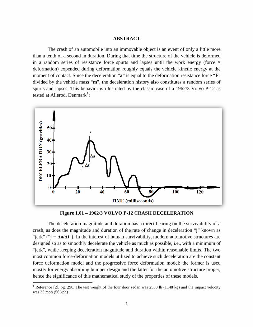
The crash of an automobile into an immovable object is an event of only a little more than a tenth of a second in duration. During that time the structure of the vehicle is deformed in a random series of resistance force spurts and lapses until the work energy (force × deformation) expended during deformation roughly equals the vehicle kinetic energy at the moment of contact. Since the deceleration “a” is equal to the deformation resistance force “F” divided by the vehicle mass “m”, the deceleration history also constitutes a random series of spurts and lapses. This behavior is illustrated by the classic case of a 1962/3 Volvo P-12 as tested at Allerod, Denmark1:

Figure 1.01 – 1962/3 VOLVO P-12 CRASH DECELERATION

The deceleration magnitude and duration has a direct bearing on the survivability of a crash, as does the magnitude and duration of the rate of change in deceleration “j” known as “jerk” (“j = Δa/Δt”). In the interest of human survivability, modern automotive structures are designed so as to smoothly decelerate the vehicle as much as possible, i.e., with a minimum of “jerk”, while keeping deceleration magnitude and duration within reasonable limits. The two most common force-deformation models utilized to achieve such deceleration are the constant force deformation model and the progressive force deformation model; the former is used mostly for energy absorbing bumper design and the latter for the automotive structure proper, hence the significance of this mathematical study of the properties of these models.

1 Reference [2], pg. 296. The test weight of the four door sedan was 2530 lb (1148 kg) and the impact velocity was 35 mph (56 kph)

1

DERIVATION OF CONSTANT & PROGRESSIVE FORCE CRUSH EQUATIONS

The kinetic energy of a vehicle at the time of contact (“t = 0”) with an immovable object is:

𝑲𝑬 = ½ 𝒎𝒆 𝑽𝟎𝟐

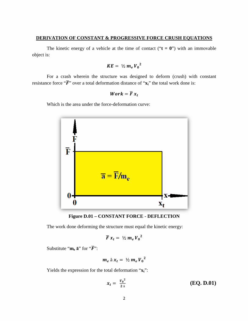
For a crash wherein the structure was designed to deform (crush) with constant resistance force “𝑭�” over a total deformation distance of “xt” the total work done is:

𝑾𝒐𝒓𝒌 = 𝑭� 𝒙𝒕

Which is the area under the force-deformation curve:

Figure D.01 – CONSTANT FORCE - DEFLECTION

The work done deforming the structure must equal the kinetic energy:

𝑭� 𝒙𝒕 = ½ 𝒎𝒆 𝑽𝟎𝟐

Substitute “me ā” for “𝑭�”:

𝒎𝒆 ā 𝒙𝒕 = ½ 𝒎𝒆 𝑽𝟎𝟐

Yields the expression for the total deformation “xt”:

𝒙𝒕 = 𝑽𝟎𝟐

𝟐 ā (EQ. D.01)

2

Knowing any two of the three variables [the total deformation “xt”, the velocity at impact “V0”, the average (constant) deceleration “ā” makes the situation totally determinate. For a constant deceleration from some initial velocity “V0” the equations of motion for the deformation “x” and the velocity “V” at any time “t” after contact (“t = 0”) are well known2.

The “x” function is:

𝒙 = 𝑽𝟎 𝒕 − ā𝒕𝟐

𝟐 (EQ. D.02)

Which when plotted looks like:

Figure D.02 – CONSTANT FORCE CRUSH vs TIME

The “V” function is:

𝑽 = 𝑽𝟎 − ā 𝒕 (EQ. D.03)

Which when plotted looks like:

2 Reference [1], pg. 398.

3

Figure D.03 – CONSTANT FORCE VELOCITY vs TIME

So if “xt” and “V0” are known, then “ā” is also (other than “ 𝐚� = 𝐅� 𝐦𝐞⁄ ”) knowable by means of Equation D.01, and the time necessary for the total3 crash event to transpire “tm” may be calculated by means of either Equation D.02 or D.03. The constant force acceleration versus time plot looks like (obviously):

Figure D.04 – CONSTANT FORCE ACCELERATION vs TIME

3 This is excluding the possibility of some “spring-back”, which is likely. “Spring-back” extends the period of the crash event, and is an undesirable occurrence.

4

For a crash wherein the structure was designed to progressively deform (“F” and “a” increase linearly with “x”) the situation is slightly more complicated. The work done deforming the structure is still equal to the area under the force-deflection curve, but that area is a little more difficult to define:

Figure D.05 – PROGRESSIVE FORCE - DEFLECTION

To define the situation one may begin with the following statements regarding the change in “x” and “V” over a short time interval “Δt”:

𝜟𝒙 = 𝑽� ∆𝒕

∆𝑽 = −𝒂 �∆𝒕

The time interval “Δt” is equal to “𝚫𝐱/𝑽�”, which allows for the elimination of the time variable by substitution in the velocity equation:

∆𝑽 = −𝒂 � ∆𝒙 𝑽��

Which can be rearranged:

∆𝑽 𝑽� = −𝒂 � ∆𝒙

Summing and taking the limiting values as the small interval values go toward zero:

𝐥𝐢𝐦∆𝑽→𝟎

�𝑽 �∆𝑽 = 𝐥𝐢𝐦∆𝒙→𝟎

�−𝒂 � ∆𝒙

5

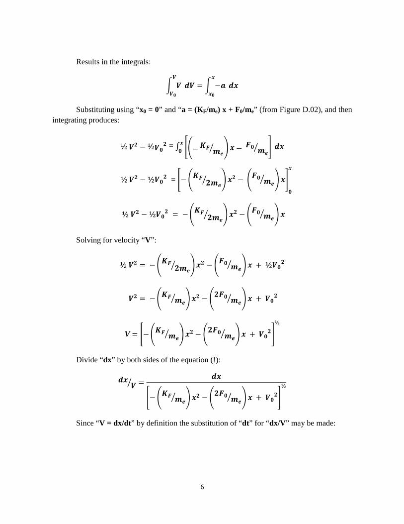
Results in the integrals:

� 𝑽𝑽

𝑽𝟎 𝒅𝑽 = � −𝒂

𝒙

𝒙𝟎 𝒅𝒙

Substituting using “x0 = 0” and “a = (KF/me) x + F0/me” (from Figure D.02), and then integrating produces:

½ 𝑽𝟐 − ½𝑽𝟎𝟐 = ∫ ��−𝑲𝑭 𝒎𝒆

� �𝒙 − 𝑭𝟎 𝒎𝒆� �𝒙

𝟎 𝒅𝒙

½ 𝑽𝟐 − ½𝑽𝟎𝟐 = �−�𝑲𝑭𝟐𝒎𝒆� �𝒙𝟐 − �𝑭𝟎 𝒎𝒆

� �𝒙�𝟎

𝒙

½ 𝑽𝟐 − ½𝑽𝟎𝟐 = −�𝑲𝑭𝟐𝒎𝒆� �𝒙𝟐 − �𝑭𝟎 𝒎𝒆

� �𝒙

Solving for velocity “V”:

½ 𝑽𝟐 = −�𝑲𝑭𝟐𝒎𝒆� �𝒙𝟐 − �𝑭𝟎 𝒎𝒆

� �𝒙 + ½𝑽𝟎𝟐

𝑽𝟐 = −�𝑲𝑭 𝒎𝒆� �𝒙𝟐 − �𝟐𝑭𝟎 𝒎𝒆

� �𝒙 + 𝑽𝟎𝟐

V = �−�𝑲𝑭 𝒎𝒆� �𝒙𝟐 − �𝟐𝑭𝟎 𝒎𝒆

� �𝒙 + 𝑽𝟎𝟐�½

Divide “dx” by both sides of the equation (!):

𝒅𝒙𝑽� =

𝒅𝒙

�−�𝑲𝑭 𝒎𝒆� �𝒙𝟐 − �𝟐𝑭𝟎 𝒎𝒆

� �𝒙 + 𝑽𝟎𝟐�½

Since “V = dx/dt” by definition the substitution of “dt” for “dx/V” may be made:

6

𝒅𝒕 =𝒅𝒙

�−�𝑲𝑭 𝒎𝒆� �𝒙𝟐 − �𝟐𝑭𝟎 𝒎𝒆

� �𝒙 + 𝑽𝟎𝟐�½

And the indefinite integrals may be formed:

�𝒅𝒕 = �𝒅𝒙

�−�𝑲𝑭 𝒎𝒆� �𝒙𝟐 − �𝟐𝑭𝟎 𝒎𝒆

� �𝒙 + 𝑽𝟎𝟐�½

The left hand integral evaluates simply to “t”, but evaluation of the right hand integral requires the use of a standard integral solution form4:

𝒕 = ∫ 𝒅𝒙√𝑿

= 𝟏√−𝒄

𝑺𝒊𝒏−𝟏 � −𝟐𝒄𝒙−𝒃�𝒃𝟐−𝟒𝒂𝒄

� , 𝒊𝒇 𝒄 < 0

Where:

𝑿 = 𝒄 𝒙𝟐 + 𝒃 𝒙 + 𝒂

c = - (KF/𝒎𝒆)

b = - (2F0/𝒎𝒆)

a = V02

So the solution is:

𝒕 = 𝟏

�𝑲𝑭 𝒎𝒆⁄ 𝑺𝒊𝒏−𝟏 �

(𝟐𝐊𝐅 𝒎𝒆⁄ )𝒙 + 𝟐𝐅𝟎 𝒎𝒆⁄

�𝟒𝐅𝟎𝟐 𝒎𝒆𝟐 + 𝟒𝐕𝟎𝟐𝐊𝐅 𝒎𝒆⁄⁄

� + 𝒄𝒐𝒏𝒔′𝒕. 𝒐𝒇 𝒊𝒏𝒕𝒆𝒈𝒓𝒂𝒕𝒊𝒐𝒏

The evaluation of the “constant of integration” is accomplished in the usual way through the use of the initial values “t = 0, x = 0”:

𝟎 = 𝟏

�𝑲𝑭 𝒎𝒆⁄ 𝑺𝒊𝒏−𝟏 �

𝟐𝐅𝟎 𝒎𝒆⁄

�𝟒𝐅𝟎𝟐 𝒎𝒆𝟐 + 𝟒𝐕𝟎𝟐𝐊𝐅 𝒎𝒆⁄⁄

� + 𝒄𝒐𝒏𝒔′𝒕. 𝒐𝒇 𝒊𝒏𝒕𝒆𝒈𝒓𝒂𝒕𝒊𝒐𝒏

𝒄𝒐𝒏𝒔′𝒕. 𝒐𝒇 𝒊𝒏𝒕𝒆𝒈𝒓𝒂𝒕𝒊𝒐𝒏 = − 𝟏

�𝑲𝑭 𝒎𝒆⁄ 𝑺𝒊𝒏−𝟏 �

𝟐𝐅𝟎 𝒎𝒆⁄

�𝟒𝐅𝟎𝟐 𝒎𝒆𝟐 + 𝟒𝐕𝟎𝟐𝐊𝐅 𝒎𝒆⁄⁄

�

4 Reference [3], pg. 374, form no. 195.

7

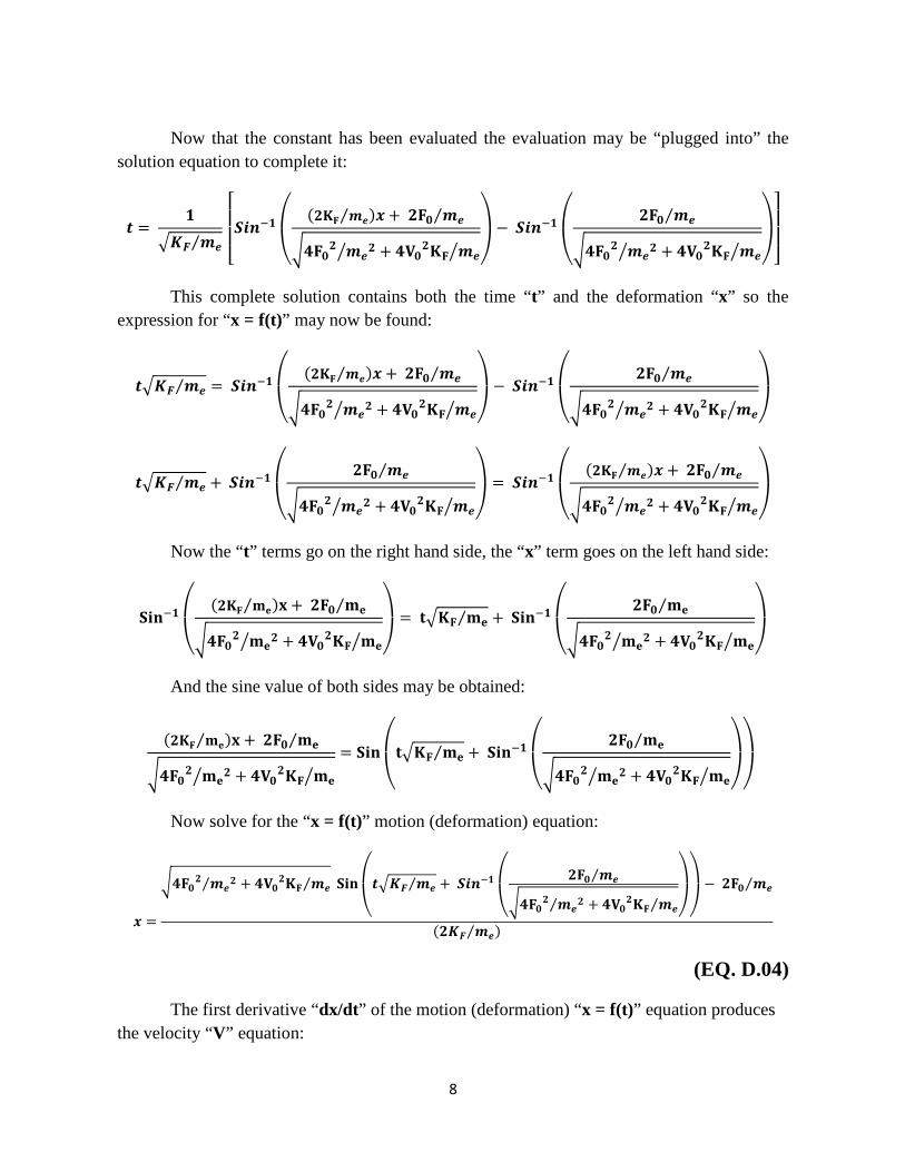
Now that the constant has been evaluated the evaluation may be “plugged into” the solution equation to complete it:

𝒕 = 𝟏

�𝑲𝑭 𝒎𝒆⁄

⎣⎢⎢⎡𝑺𝒊𝒏−𝟏

⎝

⎛ (𝟐𝐊𝐅 𝒎𝒆⁄ )𝒙+ 𝟐𝐅𝟎 𝒎𝒆⁄

�𝟒𝐅𝟎𝟐 𝒎𝒆𝟐 + 𝟒𝐕𝟎𝟐𝐊𝐅 𝒎𝒆�� ⎠

⎞− 𝑺𝒊𝒏−𝟏

⎝

⎛ 𝟐𝐅𝟎 𝒎𝒆⁄

�𝟒𝐅𝟎𝟐 𝒎𝒆𝟐 + 𝟒𝐕𝟎𝟐𝐊𝐅 𝒎𝒆�� ⎠

⎞

⎦⎥⎥⎤

This complete solution contains both the time “t” and the deformation “x” so the expression for “x = f(t)” may now be found:

𝒕�𝑲𝑭 𝒎𝒆⁄ = 𝑺𝒊𝒏−𝟏

⎝

⎛ (𝟐𝐊𝐅 𝒎𝒆⁄ )𝒙 + 𝟐𝐅𝟎 𝒎𝒆⁄

�𝟒𝐅𝟎𝟐 𝒎𝒆𝟐 + 𝟒𝐕𝟎𝟐𝐊𝐅 𝒎𝒆�� ⎠

⎞− 𝑺𝒊𝒏−𝟏

⎝

⎛ 𝟐𝐅𝟎 𝒎𝒆⁄

�𝟒𝐅𝟎𝟐 𝒎𝒆𝟐 + 𝟒𝐕𝟎𝟐𝐊𝐅 𝒎𝒆�� ⎠

⎞

𝒕�𝑲𝑭 𝒎𝒆⁄ + 𝑺𝒊𝒏−𝟏

⎝

⎛ 𝟐𝐅𝟎 𝒎𝒆⁄

�𝟒𝐅𝟎𝟐 𝒎𝒆𝟐 + 𝟒𝐕𝟎𝟐𝐊𝐅 𝒎𝒆�� ⎠

⎞ = 𝑺𝒊𝒏−𝟏

⎝

⎛ (𝟐𝐊𝐅 𝒎𝒆⁄ )𝒙 + 𝟐𝐅𝟎 𝒎𝒆⁄

�𝟒𝐅𝟎𝟐 𝒎𝒆𝟐 + 𝟒𝐕𝟎𝟐𝐊𝐅 𝒎𝒆�� ⎠

⎞

Now the “t” terms go on the right hand side, the “x” term goes on the left hand side:

𝐒𝐢𝐧−𝟏

⎝

⎛ (𝟐𝐊𝐅 𝐦𝐞⁄ )𝐱 + 𝟐𝐅𝟎 𝐦𝐞⁄

�𝟒𝐅𝟎𝟐 𝐦𝐞𝟐 + 𝟒𝐕𝟎𝟐𝐊𝐅 𝐦𝐞�� ⎠

⎞ = 𝐭�𝐊𝐅 𝐦𝐞⁄ + 𝐒𝐢𝐧−𝟏

⎝

⎛ 𝟐𝐅𝟎 𝐦𝐞⁄

�𝟒𝐅𝟎𝟐 𝐦𝐞𝟐 + 𝟒𝐕𝟎𝟐𝐊𝐅 𝐦𝐞�� ⎠

⎞

And the sine value of both sides may be obtained:

(𝟐𝐊𝐅 𝐦𝐞⁄ )𝐱 + 𝟐𝐅𝟎 𝐦𝐞⁄

�𝟒𝐅𝟎𝟐 𝐦𝐞𝟐 + 𝟒𝐕𝟎𝟐𝐊𝐅 𝐦𝐞��

= 𝐒𝐢𝐧

⎝

⎛𝐭�𝐊𝐅 𝐦𝐞⁄ + 𝐒𝐢𝐧−𝟏

⎝

⎛ 𝟐𝐅𝟎 𝐦𝐞⁄

�𝟒𝐅𝟎𝟐 𝐦𝐞𝟐 + 𝟒𝐕𝟎𝟐𝐊𝐅 𝐦𝐞�� ⎠

⎞

⎠

⎞

Now solve for the “x = f(t)” motion (deformation) equation:

𝒙 =

�𝟒𝐅𝟎𝟐 𝒎𝒆𝟐 + 𝟒𝐕𝟎𝟐𝐊𝐅 𝒎𝒆⁄⁄ 𝐒𝐢𝐧

⎝

⎛𝒕�𝑲𝑭 𝒎𝒆⁄ + 𝑺𝒊𝒏−𝟏

⎝

⎛ 𝟐𝐅𝟎 𝒎𝒆⁄

�𝟒𝐅𝟎𝟐 𝒎𝒆𝟐 + 𝟒𝐕𝟎𝟐𝐊𝐅 𝒎𝒆⁄⁄ ⎠

⎞

⎠

⎞− 𝟐𝐅𝟎 𝒎𝒆⁄

(𝟐𝑲𝑭 𝒎𝒆⁄ )

(EQ. D.04)

The first derivative “dx/dt” of the motion (deformation) “x = f(t)” equation produces the velocity “V” equation:

8

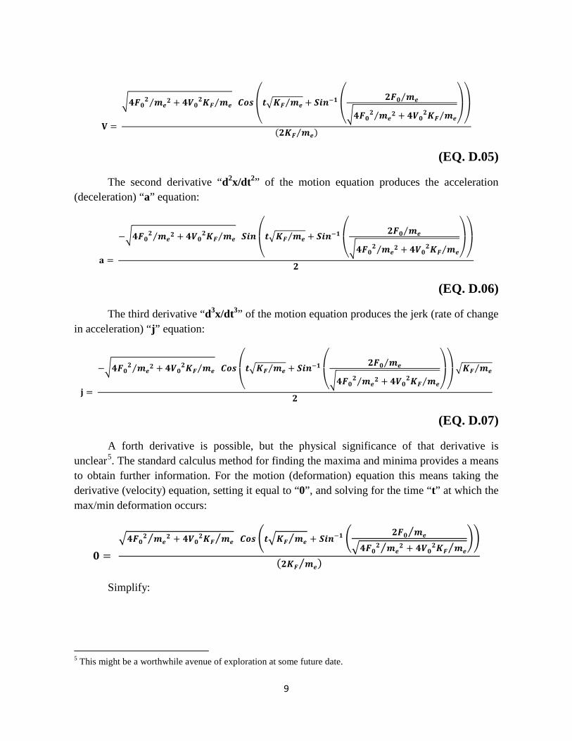
𝐕 =

�𝟒𝑭𝟎𝟐 𝒎𝒆𝟐 + 𝟒𝑽𝟎𝟐𝑲𝑭 𝒎𝒆⁄⁄ 𝑪𝒐𝒔

⎝

⎛𝒕�𝑲𝑭 𝒎𝒆⁄ + 𝑺𝒊𝒏−𝟏

⎝

⎛ 𝟐𝑭𝟎 𝒎𝒆⁄

�𝟒𝑭𝟎𝟐 𝒎𝒆𝟐⁄ + 𝟒𝑽𝟎𝟐𝑲𝑭 𝒎𝒆⁄ ⎠

⎞

⎠

⎞

(𝟐𝑲𝑭 𝒎𝒆⁄ )

(EQ. D.05)

The second derivative “d2x/dt2” of the motion equation produces the acceleration (deceleration) “a” equation:

𝐚 =

−�𝟒𝑭𝟎𝟐 𝒎𝒆𝟐 + 𝟒𝑽𝟎𝟐𝑲𝑭 𝒎𝒆⁄⁄ 𝑺𝒊𝒏

⎝

⎛𝒕�𝑲𝑭 𝒎𝒆⁄ + 𝑺𝒊𝒏−𝟏

⎝

⎛ 𝟐𝑭𝟎 𝒎𝒆⁄

�𝟒𝑭𝟎𝟐 𝒎𝒆𝟐⁄ + 𝟒𝑽𝟎𝟐𝑲𝑭 𝒎𝒆⁄ ⎠

⎞

⎠

⎞

𝟐

(EQ. D.06)

The third derivative “d3x/dt3” of the motion equation produces the jerk (rate of change in acceleration) “j” equation:

𝐣 =

−�𝟒𝑭𝟎𝟐 𝒎𝒆𝟐 + 𝟒𝑽𝟎𝟐𝑲𝑭 𝒎𝒆⁄⁄ 𝑪𝒐𝒔

⎝

⎛𝒕�𝑲𝑭 𝒎𝒆⁄ + 𝑺𝒊𝒏−𝟏

⎝

⎛ 𝟐𝑭𝟎 𝒎𝒆⁄

�𝟒𝑭𝟎𝟐 𝒎𝒆𝟐⁄ + 𝟒𝑽𝟎𝟐𝑲𝑭 𝒎𝒆⁄ ⎠

⎞

⎠

⎞�𝑲𝑭 𝒎𝒆⁄

𝟐

(EQ. D.07)

A forth derivative is possible, but the physical significance of that derivative is unclear5. The standard calculus method for finding the maxima and minima provides a means to obtain further information. For the motion (deformation) equation this means taking the derivative (velocity) equation, setting it equal to “0”, and solving for the time “t” at which the max/min deformation occurs:

𝟎 = �𝟒𝑭𝟎𝟐 𝒎𝒆

𝟐 + 𝟒𝑽𝟎𝟐𝑲𝑭 𝒎𝒆⁄⁄ 𝑪𝒐𝒔 �𝒕�𝑲𝑭 𝒎𝒆⁄ + 𝑺𝒊𝒏−𝟏 � 𝟐𝑭𝟎 𝒎𝒆⁄�𝟒𝑭𝟎𝟐 𝒎𝒆

𝟐⁄ + 𝟒𝑽𝟎𝟐𝑲𝑭 𝒎𝒆⁄��

(𝟐𝑲𝑭 𝒎𝒆⁄ )

Simplify:

5 This might be a worthwhile avenue of exploration at some future date.

9

𝟎 = 𝑪𝒐𝒔

⎝

⎛𝒕�𝑲𝑭 𝒎𝒆⁄ + 𝑺𝒊𝒏−𝟏

⎝

⎛ 𝟐𝑭𝟎 𝒎𝒆⁄

�𝟒𝑭𝟎𝟐 𝒎𝒆𝟐� + 𝟒𝑽𝟎𝟐𝑲𝑭 𝒎𝒆� ⎠

⎞

⎠

⎞

Take the inverse cosine of both sides of the equation:

𝑪𝒐𝒔−𝟏(𝟎) =

⎝

⎛𝒕�𝑲𝑭 𝒎𝒆⁄ + 𝑺𝒊𝒏−𝟏

⎝

⎛ 𝟐𝑭𝟎 𝒎𝒆⁄

�𝟒𝑭𝟎𝟐 𝒎𝒆𝟐� + 𝟒𝑽𝟎𝟐𝑲𝑭 𝒎𝒆� ⎠

⎞

⎠

⎞

Since this is a trigometric function it is periodic with multiple “n π/2” max/min values for the inverse cosine of “0”:

𝒏 𝝅/𝟐 =

⎝

⎛𝒕�𝑲𝑭 𝒎𝒆⁄ + 𝑺𝒊𝒏−𝟏

⎝

⎛ 𝟐𝑭𝟎 𝒎𝒆⁄

�𝟒𝑭𝟎𝟐 𝒎𝒆𝟐� + 𝟒𝑽𝟎𝟐𝑲𝑭 𝒎𝒆� ⎠

⎞

⎠

⎞

Solve the above for time “tm” at which these max/min values of the motion (deformation) equation would occur:

𝒕𝒎 =𝒏𝝅𝟐−𝑺𝒊𝒏

−𝟏� 𝟐𝑭𝟎 𝒎𝒆⁄

�𝟒𝑭𝟎𝟐 𝒎𝒆𝟐� +𝟒𝑽𝟎

𝟐𝑲𝑭 𝒎𝒆��

�𝑲𝑭 𝒎𝒆⁄ (EQ. D.08)

“Plugging” this value for the time of occurrence of the max/min values of the motion (deformation) equation (Eq. D.08) into the motion equation (Eq. D.04) produces the following max/min values “xt” of the motion:

𝒙𝒕 =�𝟒𝐅𝟎𝟐 𝒎𝒆

𝟐 + 𝟒𝐕𝟎𝟐𝐊𝐅 𝒎𝒆�� 𝐒𝐢𝐧�𝒏𝝅𝟐� − 𝟐𝐅𝟎 𝒎𝒆⁄

(𝟐𝑲𝑭 𝒎𝒆⁄ )

Since the sine of multiple “n” values of “π/2” (90o) is “±1” the max/min values “xt” of the motion (deformation) equation are:

𝒙𝒕 =±�𝟒𝐅𝟎𝟐 𝒎𝒆𝟐+𝟒𝐕𝟎𝟐𝐊𝐅 𝒎𝒆�� − 𝟐𝐅𝟎 𝒎𝒆⁄

(𝟐𝑲𝑭 𝒎𝒆⁄ ) (EQ. D.09)

10

The plot of the sinusoidal motion (deformation) equation (Eq. D.04) with the max/min values of the motion (deformation) function (Eq. D.09) indicated is as follows:

Figure D.06 – PROGRESSIVE CRUSH MOTION vs TIME PLOT

Mathematically the motion function is continuous; an uncritical acceptance of this function would have one believe that the vehicle in question is condemned to an eternal series of crashes which results in a deformation up to a certain point, followed by a restitution, resulting in a new deformation, etc., sort of like an automotive Sisyphus. This can be used as an example of the dangers of blindly accepting mathematical (or computer) results; there is no escape from the need for human judgment. In reality the motion in question is limited to the shaded portion of the “x = f(t)” plot.

The maxima and minima for the velocity (Eq. D.05) and the acceleration (Eq. D.06) functions may be found in the same fashion as was done for the motion function with the corresponding plots. The velocity function has the following max/min value “Vm” and plot:

𝑽𝒎 =±�𝟒𝐅𝟎𝟐 𝒎𝒆𝟐+𝟒𝐕𝟎𝟐𝐊𝐅 𝒎𝒆��

(𝟐𝑲𝑭 𝒎𝒆⁄ ) (EQ. D.10)

The plot of the cosine velocity equation (Eq. D.05) with the max/min values of the velocity function (Eq. D.10) indicated is as follows:

11

Figure D.07 – PROGRESSIVE CRUSH VELOCITY vs TIME PLOT

The acceleration function has the following max/min value “am” and plot:

𝒂𝒎 =±�𝟒𝐅𝟎𝟐 𝒎𝒆𝟐+𝟒𝐕𝟎𝟐𝐊𝐅 𝒎𝒆��

𝟐 (EQ. D.11)

The plot of the sinusoidal acceleration (deceleration) equation (Eq. D.06) with the max/min values of the acceleration function (Eq. D.11) indicated is as follows:

Figure D.08 – PROGRESSIVE CRUSH ACCELERATION vs TIME PLOT

12

As noted previously for the motion function, all these trigonometric functions are continuous, but the relevant portions are indicated by shading. The progressive crush situation is now fully defined, and the equations describing the characteristics of constant force and progressive force crushes provide a significant set of “tools” for automotive crash kinetic energy dissipation planning.

The constant force deformation model, which produces an extremely high “jerk” level at onset, is relegated mainly to the low intensity realm of bumper design. However, the constant force deformation model does make the most efficient use of the available crush distance while keeping deceleration at (under) some desired level.

The progressive force deformation model does not make as efficient use of the available crush distance, but ensures a smooth deceleration curve with a minimum of jerk. The progressive model also ensures that the maximum deceleration level employed will be proportional to the severity of the crash, and no higher6.

Most vehicles employ structure based on both models, and in a severe crash will produce deformation, velocity, and acceleration traces as follows. Note that the bumper crush will dissipate very little of the kinetic energy, but will use a significant amount of the available crush distance; this is the essence of the argument against mandating effective bumper strength standards7.

However, with proper design criteria it should be possible to essentially avoid an “either or” scenario and obtain appropriate crush behavior for both survivability and damage resistance; it’s mainly a matter of intelligent design and the will to execute such design.

6 A “low speed” impact of minimal kinetic energy might crush the vehicle structure only a few inches, with a corresponding low deceleration level. The same structure, in a “high speed” crash, might deform the vehicle structure for the full available deformation length and incur the designed for maximum deceleration level. However, as for crashes at an even greater speed… 7 The “10 mph” (16 kph) constant force bumper of the illustrative example used nearly 25% of the available crush distance to dissipate about 4% of the kinetic energy in a 50 mph (80 kph) crash.

13

Figure D.09 – CRASH DEFORMATION, VELOCITY, AND ACCELERATION

14

REFERENCES

[1] Beer, Ferdinand P.; and E. Russell Johnston Jr., Vector Mechanics for Engineers: Dynamics, NYC, NY; McGraw-Hill Book Company, 1962.

[2] Patrick, Laurence M. (Editor); 8th Stapp Car Crash and Field Demonstration Conference, Detroit, MI; Wayne State University Press, 1966.

[3] Selby, Samuel M; and Robert C. Weast, George L. Tuve; Standard Mathematical Tables, Cleveland, OH; Chemical Rubber Co., 1967.

15