Flow sensor instrumentation employing differential pressure reading

FLOW SENSOR INSTRUMENTATION

EMPLOYING DIFFERENTIAL PRESSURE

READING

Bruno Bestle Turrin1,2

, Alexandre Rodrigues da Silva1,2

, Fuad Kassab Jr.1

1Laboratório de Automação e Controle da Universidade de São Paulo

2KTK Ind. Imp. Exp. Com. De Equip. Hosp. LTDA

[email protected]; [email protected]; [email protected]

Abstract- This paper presents an analysis of flow sensors

found in the market today that uses the differential pressure technology to measure flow at mechanical pulmonary ventilator

respiratory circuits. It proposes a set of differential pressure transducers for the reading of the resistance element in order to get a readout resolution equal or smaller than 0.15L/min within

the regular measuring range for mechanical ventilation, which is from 0 to 150L/min. It also suggests an internal geometry for the resistance element to reduce pneumatic noise in the differential

pressure measuring. In this paper is shown a decrease on the standard deviation value of the differential pressure reading for the same ranges in the same test condition. It is shown that the

proposed geometry for the new nozzle decreases the measurement pneumatic noise in 47.5% in average. Finally, it is shown that the combination of three differential sensors, reading

different ranges, achieves the desired resolution and measuring range.

I. INTRODUCTION

The respiratory flow measurement is extremely important

for the pulmonary ventilator. With this measurement the

ventilator can determine the volume delivered to the patient

calculated through its integral, and can determine if there is

any fault at the respiratory circuit like a disconnection, a leak

or an occlusion. However, for this to be possible, it is

necessary that the sensor would have a good resolution

reading in a large range of values.

The flow measurement by the means of the differential

pressure is an application of the Bernoulli equation and the

continuity equation. A very known application is the Venturi

tube. The variation in the section area causes a difference

between the inlet pressure and the outlet pressure of the

nozzle that is proportional to the flow rate.

Illustration 1 – The Venturi tube and its pressure drop[1]

The pressure drop on the nozzle is also influenced by the

flow regimen. Depending if it is more or less turbulent its

characteristic curve changes its linearity. This effect is shown

on the development of this paper.

The pressure drop curve determination will be done

experimentally for this study. For this, will be employed an

IMT PF300[2] which is capable of reading either flow as well

as differential pressure and communicate the results to the

computer using the serial or the USB port.

It was used a bxa type curve to adjust the data results

because the flow rate through a nozzle can be determined by:

QA2

1A2

A1

22.

P

1

2

[3]

(1)

Isolating the pressure drop, in equation (1), as function of

the flow rate we will have the following equation:

PQ

2

2 A22

1A2

2

A12

Q2

K

(2)

It is also shown that as the flow regime gets less turbulent

and tends to be laminar, the P function tends to be linear

[4]. It means that the coefficient “b” in the bxa function

tends to 1 as the flow regime tends to be laminar.

II. UNITS

Initially, measurements were made with the current nozzle

to determine the differential pressure curves versus the flow

rate in two different conditions: first one with low pneumatic

noise and the second one with high pneumatic noise.

Then the same tests were made with a new nozzle with a

different internal geometry to reduce the pneumatic noise.

During the tests, 6000 different differential pressure

values versus input flow values were measured. For data

analysis, the flow values were grouped in 2.5L/min ranges, in

which were made the mean and the standard deviation

calculation on the differential pressure measurements.

Needle valve

Pressure

regulator valve

Resistance

element

in

test

Conection

Compressed

air

line

Flow Sensor

Defferential

pressure

sensor

IMT

PF300

RS 232 DATA

Manual valve adjusment

to change the flow within

the measuring range

Illustration 2 – Connection diagram during the resistance element test

mailto:[email protected]



All measurements were made with an IMT PF300, flow

and pressure analyzer, widely used on the mechanical

pulmonary ventilation business.

To force an increase in the pneumatic noise, an elbow was

used right before the nozzle like shown in the figures bellow:

Illustration 3 – Connection with the long silicon hose (with less

pneumatic noise).

Illustration 4 – Connection with the elbow close to the nozzle

(turbulence induced by the sudden change of direction)

A. NOZZLE DEVELOPMENT

Changing the flow rate at the nozzle by opening and

closing of the needle valve, were obtained the results shown

at illustration 5.

From the data obtained we can observe that as the flow

rate increases, it also increases the measured differential

pressure and its deviation.

Current Sensor without Turbulence

0

2

4

6

8

10

12

14

16

0 50 100 150 200Flow [L/min]

Pre

ssu

re D

elta[c

mH

2O

]

Standard Deviation of the pressure diferential for each 2,5

L/min range

-2

0

2

4

6

8

10

12

14

16

0 50 100 150 200

Flow[L/min]

Pre

ssu

re D

elta

[cm

H2O

]

(a)

Current Adult Sensor Curve with turbulence

0

2

4

6

8

10

12

14

16

0 50 100 150 200Flow [L/min]

Pre

ssu

re D

elta

[cm

H2O

]

Standard Deviation of the Differential pressure in each 2,5

L/min range

-2

0

2

4

6

8

10

12

14

16

0 50 100 150 200

Flow [L/min]

Pre

ssu

re D

elta

[cm

H2O

]

(b)

Illustration 5 – The above graphs show all pressure differential and flow

data measured. It is shown below the differential pressure mean values in 2.5L/min ranges and the standard deviation ± value. With less

pneumatic noise (a). With a higher pneumatic noise (b).

Using the mean differential pressure at each 2.5L/min

range to fit a bxa curve type, we could observe a large

variation in the pressure drop values between the test with

less pneumatic noise and the one with the elbow connection

inducing a higher pneumatic noise.

There are several possible phenomenological explanations

to this effect that are discussed in the DISCUSSIONS section.

The adjusted curve to the first experiment is shown below:

Vector1 P Data_nozzle_11

Vector1F Data_nozzle_1

0

Ka

Kb

Kc

pwrfit Vector1F Vector1 P

1

1

0

Ka

Kb

Kc

1.253 103

1.814

0.043

R2 9.997 101

P1nozzle flow( ) Ka flowKb

The Data_nozzle_1 variable has the data from the first

experiment that has less turbulence. The pwrfit function is a

Mathcad® (Mathsoft Apps) procedure that does a least

squares regression and is used to adjust the data to a

cxa b curve. The coefficient “c” is ignored so that when

the flow is equal to zero then the pressure drop is also equal

to zero. The Data_nozzle_2 variable has the data from the

second experiment that uses the elbow to induce a higher

pneumatic noise.

Vector2 P Data_nozzle_21

Vector2F Data_nozzle_2

0

Ka2

Kb2

Kc2


1

1

0

Ka2

Kb2

Kc2

1.161 104

2.211

0.308

R2 9.863 101

P2nozzle flow( ) Ka2 flowKb2

The adjusted curves for the two cases are visibly different

as their coefficients have different values; however, drawing

each of the adjusted curves makes the difference even more

visible.

Illustration 6 – Experimental data of the present sensor and its adjusted

curves

On the lower flow values, less than 30L/min, the two

curves are practically the same. However, as the flow rate

increases and with the increase of the pneumatic noise

induced by the elbow, the two curves go further apart.

If we compare the two curve values using the first one,

with less pneumatic noise, as reference, we will have the

following results:

0

66

i

Vector1 Pi

Vector2 Pi

661.522

(4)

0

66

i

Vector1 Pi

Vector2 Pi

Vector1 Pi

660.31

(5)

The mean difference module between the two pressure

drop curves values is 1.522 cmH2O. And the mean relative

module deviation is 31%.

This variation, that decreases a lot the possible resolution

for this nozzle, is due to the internal sensor geometry.

The current nozzle has several sudden variations in the

passage area; most of them are orthogonal to the inlet flow

direction.

To decrease these effects it was necessary to develop a

new internal geometry that offered the necessary resistance to

allow the flow reading resolution, and would not cause an

abrupt variation in the passage area. To smooth the passage

area variation, corners were rounded and V profiles were

added.

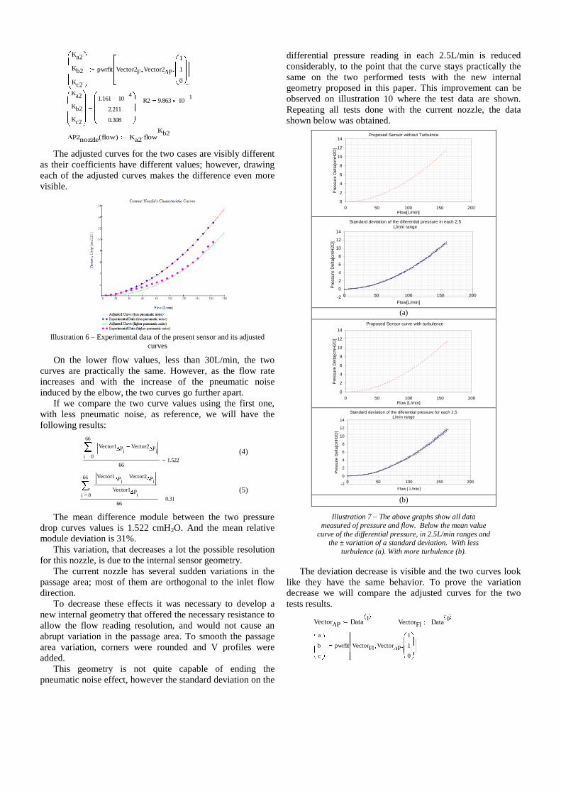
This geometry is not quite capable of ending the

pneumatic noise effect, however the standard deviation on the

differential pressure reading in each 2.5L/min is reduced

considerably, to the point that the curve stays practically the

same on the two performed tests with the new internal

geometry proposed in this paper. This improvement can be

observed on illustration 10 where the test data are shown.

Repeating all tests done with the current nozzle, the data

shown below was obtained.

Proposed Sensor without Turbulnce

0

2

4

6

8

10

12

14

0 50 100 150 200Flow[L/min]

Pre

ssu

re D

elta

[cm

H2

O]

Standard deviation of the diferential pressure in each 2,5

L/min range

-2

0

2

4

6

8

10

12

14

0 50 100 150 200

Flow[L/min]

Pre

ssu

re D

elta

[cm

H2

O]

(a)

Proposed Sensor curve with turbulence

0

2

4

6

8

10

12

14

0 50 100 150 200Flow [L/min]

Pre

ssu

re D

elta

[cm

H2

O]

Standard deviation of the diferential pressure for each 2,5

L/min range

-2

0

2

4

6

8

10

12

14

0 50 100 150 200

Flow [ L/min]

Pre

ssure

Delta[c

mH

2O

]

(b)

Illustration 7 – The above graphs show all data

measured of pressure and flow. Below the mean value

curve of the differential pressure, in 2.5L/min ranges and the ± variation of a standard deviation. With less

turbulence (a). With more turbulence (b).

The deviation decrease is visible and the two curves look

like they have the same behavior. To prove the variation

decrease we will compare the adjusted curves for the two

tests results.

Vector P Data1

VectorFl Data

0

a

b

c

pwrfit VectorFl Vector P

1

1

0

a

b

c

8.105 104

1.884

0.021

R2 9.999 101

P1new_nozzle flow( ) a flowb

Vector2 P Data21

Vector2F Data2

0

a2

b2

c2


1

1

0

a2

b2

c2

8.605 104

1.871

0.064

R2 9.995 101

P2new_nozzle flow( ) a2 flowb2

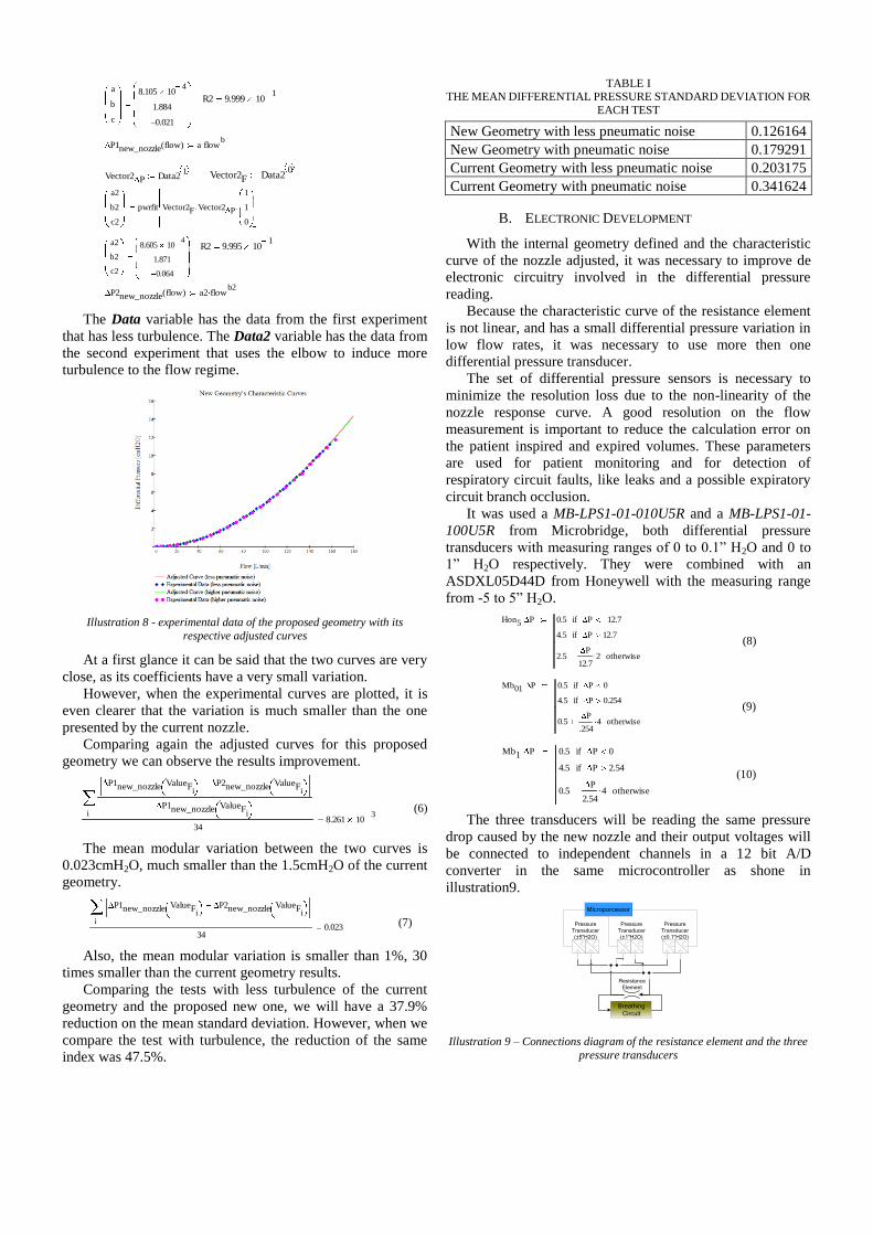
The Data variable has the data from the first experiment

that has less turbulence. The Data2 variable has the data from

the second experiment that uses the elbow to induce more

turbulence to the flow regime.

Illustration 8 - experimental data of the proposed geometry with its

respective adjusted curves

At a first glance it can be said that the two curves are very

close, as its coefficients have a very small variation.

However, when the experimental curves are plotted, it is

even clearer that the variation is much smaller than the one

presented by the current nozzle.

Comparing again the adjusted curves for this proposed

geometry we can observe the results improvement.

i

P1new_nozzle ValueFi



348.261 10

3

(6)

The mean modular variation between the two curves is

0.023cmH2O, much smaller than the 1.5cmH2O of the current

geometry.

i



340.023

(7)

Also, the mean modular variation is smaller than 1%, 30

times smaller than the current geometry results.

Comparing the tests with less turbulence of the current

geometry and the proposed new one, we will have a 37.9%

reduction on the mean standard deviation. However, when we

compare the test with turbulence, the reduction of the same

index was 47.5%.

TABLE I THE MEAN DIFFERENTIAL PRESSURE STANDARD DEVIATION FOR

EACH TEST

New Geometry with less pneumatic noise 0.126164

New Geometry with pneumatic noise 0.179291

Current Geometry with less pneumatic noise 0.203175

Current Geometry with pneumatic noise 0.341624

B. ELECTRONIC DEVELOPMENT

With the internal geometry defined and the characteristic

curve of the nozzle adjusted, it was necessary to improve de

electronic circuitry involved in the differential pressure

reading.

Because the characteristic curve of the resistance element

is not linear, and has a small differential pressure variation in

low flow rates, it was necessary to use more then one

differential pressure transducer.

The set of differential pressure sensors is necessary to

minimize the resolution loss due to the non-linearity of the

nozzle response curve. A good resolution on the flow

measurement is important to reduce the calculation error on

the patient inspired and expired volumes. These parameters

are used for patient monitoring and for detection of

respiratory circuit faults, like leaks and a possible expiratory

circuit branch occlusion.

It was used a MB-LPS1-01-010U5R and a MB-LPS1-01-

100U5R from Microbridge, both differential pressure

transducers with measuring ranges of 0 to 0.1” H2O and 0 to

1” H2O respectively. They were combined with an

ASDXL05D44D from Honeywell with the measuring range

from -5 to 5” H2O.

Hon5 P 0.5 P 12.7if

4.5 P 12.7if

2.5P

12.72 otherwise

(8)

Mb01 P 0.5 P 0if

4.5 P 0.254if

0.5P

.2544 otherwise

(9)

Mb1 P 0.5 P 0if

4.5 P 2.54if

0.5P

2.544 otherwise

(10)

The three transducers will be reading the same pressure

drop caused by the new nozzle and their output voltages will

be connected to independent channels in a 12 bit A/D

converter in the same microcontroller as shone in

illustration9.

Resistance

Element

Microporcessor

Breathing

Circuit

Pressure

Transducer

(±5"H2O)

Pressure

Transducer

(±1"H2O)

Pressure

Transducer

(±0.1"H2O)

Illustration 9 – Connections diagram of the resistance element and the three

pressure transducers

The response curves for the microcontroller are described

bellow:

AD12H5 P RoundHon5 P

4.54095 1

(11)

AD12M01 P RoundMb01 P

4.54095 1

(12)

AD12M1 P RoundMb1 P

4.54095 1

(13)

Illustration 10– Transducer response curves versus the pressure drop caused

by flow rate in the nozzle

At Illustration 10 we can observe that the small range

transducers saturate first but with a high measurement

resolution. We can also observe that the higher range

transducer saturates over 160 L/min with low measurement

resolution for low flow rates.

The resolution can be calculated dividing the difference of

two consecutive values of the flow rate by the A/D value

variation.

(14)

(15)

(16)

It is possible that the resolution could tend to infinite

because of the rounding function of the A/D converter. It

means that there is no resolution between the two consecutive

flow values, or that the resolution in that point is greater than

the difference between the two values. To avoid this problem

a condition was added to the Resolution functions above that

will return zero if the difference between the A/D values of

the two flow rate values is equal or smaller than zero.

At illustration 11 we can observe that the ±5”H2O sensor

resolution is larger than 0.25L/min by increment in the A/D

value up until the measurement value is over 20L/min. For

flow rate values below 10L/min the resolution is greater than

0.5L/min and can reach 2.5L/min.

Illustration 11 – The 3 transducers resolution curves

Also we can observe that the 1”H2O transducer’s

resolution is already smaller than 0.25L/min by increment at

the A/D converter before getting to 10 L/min, and the

0.1”H2O transducer’s resolution is never greater than

0.2L/min by increment at the A/D converter.

The three differential pressure transducer curves were

combined to reach the “smaller than 0.15L/min” resolution

requirement in all its measurement range. For that, a new

function was designed, which is the sum of all A/D values of

all transducers.

AD12sum P AD12H5 P AD12M01 P AD12M1 P (17)

Recalculating the measurement resolution the same way it

was done previously for each the transducers individually we

will have the function below:

(18)

Illustration 12 – The 3 transducers resolution curve

It can be observed that the resolution stays below

0.1L/min in all measuring range. From 0 to 60L/min the

resolution is smaller than 0.05L/min.

Finally, the entire resolution curve is smaller than the

specified at the beginning of this paper.

III. DISCUSSIONS

The pneumatic noise mentioned before may be cause by

an increase in the turbulence of the flow regime and other

singularity effects.

What is very clear in the test results of the current nozzle

is that as flow rate increases that pneumatic noise greatly

Ressum f1 f2 0 AD12sum P1new_nozzle f2 AD12sum P1new_nozzle f1 0if

f2 f1

AD12sum P1new_nozzle f2 AD12sum P1new_nozzle f1

otherwise

ResH5 f1 f2 0 AD12H5 P1new_nozzle f2 AD12H5 P1new_nozzle f1 0if

f2 f1

AD12H5 P1new_nozzle f2 AD12H5 P1new_nozzle f1

otherwise

ResM01 f1 f2 0 AD12M01 P1new_nozzle f2 AD12M01 P1new_nozzle f1 0if

f2 f1

AD12M01 P1new_nozzle f2 AD12M01 P1new_nozzle f1

otherwise

ResM1 f1 f2 0 AD12M1 P1new_nozzle f2 AD12M1 P1new_nozzle f1 0if

f2 f1

AD12M1 P1new_nozzle f2 AD12M1 P1new_nozzle f1

otherwise

increases in the measurement of the pressure drop. That can

be explained by the fact that the greater the flow rate is,

greater is the gas velocity that goes through the nozzle and

greater is the Reynolds number.

vdRe

[5]

The Reynolds number indicates the gas flow regime and it

is directly proportional to its velocity. The greater the velocity

is the larger is the coefficient and more turbulent will the

regime be. The flow velocity effect can be observed in the

two tests. However, this effect has a greater intensity at the

second test that uses the elbow. The regime interference is so

large that the current nozzle response curve changed.

At the current internal geometry, the passage area

variations are done in an abrupt manner that contributes to the

turbulence increase and for the vortices effect.

Illustration 13 – Current nozzle internal geometry

As soon as the flow inputs the current nozzle it faces

several orthogonal walls to the flow direction (illustration

13). The variation is so abrupt that the sensor characteristic

response is changed.

The abrupt variation in the passage area causes

disturbance in the flow regime that will change the pressure

drop at the nozzle. This effect is visible when there is a body

immersed in an open flow steam.

(b) plate

Illustration 14 – Flow lines for an abrupt area variation (a) and for a smooth

area variation (b). [6]

If the body offers an abrupt change to the flow direction

both in the beginning of its geometry and the end, it will

create several vortices which will make it difficult to measure

pressure at this point.

For the flow regime not to be altered, or at least, not

perturbed a lot, the passage area variation must be designed in

a tapered manner like it is shown in illustration 14(b).

To minimize these effects the internal geometry was

changed in order to minimize the disturbance in the flow

regime and to try to avoid the oscillation in the differential

pressure reading even if the input flow regime is already

perturbed as it was with the elbow connection. The developed

geometry is shown at illustration 15.

The flow lines at illustration 15 show how if the input

flow is not perturbed by turbulence or any other phenomena

the internal geometry will not contribute to its disturbance,

and if the input is already perturbed the internal geometry will

contribute to its stabilization.

Illustration 15 – Flow lines inside the resistance element with the new

geometry

The results shown in the tests made with this new internal

geometry show that the stabilization in the pressure drop

reading is considerable and as the only change made to the

system was the internal geometry it is probably the current

internal geometry that causes the oscillation on the reading.

Concerning the electronic development, the resolution

was only possible to achieve because the three transducers

had complementary ranges. I would be best if the transducer

response was not linear and had square root relation between

the output tension and the input differential pressure. This

way, the transducer would have a high gain at low differential

pressure values increasing the resolution of the reading when

the pressure drop on the nozzle has a low gain in terms of the

flow rate passing through the nozzle.

IV. CONCLUSIONS

This paper presented problems due to pneumatic noise

found in differential pressure sensors and also related to

resolution of the measurements done by these sensors.

It was presented a proposition of internal geometry of the

nozzle that, by the results of the experimental tests covered in

this paper, decreased the turbulence effect at the sensor

measurement and also achieved a better measurement

precision in the same conditions that the current nozzle.

Finally, with the combination of three differential

pressure transducers it was possible to reach the specified

reading range of 0 to 150L/min as well as the reading

specification of 0.15L/min.

ACKNOLEGEMENTS

We would like to thank the LAC and KTK support for

the development of this paper.

REFERENCES

[1] Nakayama, Y. - Introduction to Fluid Mechanics / Y.

Nakayama (ISBN 0 340 67649 3) page. 62-65

[2] imtmedical ag Gewerbestrasse 8 9470 Buchs SG

Switzerland www.imtmedical.com

[3]Nakayama, Y. - Introduction to Fluid Mechanics / Y.

Nakayama (ISBN 0 340 67649 3) page. 63

[4] White, Frank M. – Fluid Mechanics Fourth Edition –

McGraw-Hill – page 329 to 349.


Nakayama (ISBN 0 340 67649 3) page. 46


Nakayama (ISBN 0 340 67649 3) page 148

Flow sensor instrumentation employing differential pressure reading

Documents

Transcript of Flow sensor instrumentation employing differential pressure reading