TN 19: Gradient Elution In Ion Chromatography - Thermo Fisher
Kg
Ka
b
a
ARR1AA
KCKPPNP
1
g(ib[Totwemt
0d
Journal of Chromatography A, 1218 (2011) 1153–1169
Contents lists available at ScienceDirect
Journal of Chromatography A
journa l homepage: www.e lsev ier .com/ locate /chroma
inetic performance limits of constant pressure versus constant flow rateradient elution separations. Part I: Theory
. Broeckhovena, M. Verstraetena, K. Choikhetb, M. Dittmannb, K. Wittb, G. Desmeta,∗
Vrije Universiteit Brussel, Department of Chemical Engineering (CHIS-IR), Pleinlaan 2, 1050 Brussels, BelgiumAgilent Technologies Germany GmbH, Hewlett-Packard Str. 8, Waldbronn BW 76337, Germany
r t i c l e i n f o
rticle history:eceived 4 October 2010eceived in revised form6 December 2010ccepted 19 December 2010vailable online 28 December 2010
eywords:onstant pressureinetic plot methodeak capacitylate heightumerical simulationressure effects
a b s t r a c t
We report on a general theoretical assessment of the potential kinetic advantages of running LC gradientelution separations in the constant-pressure mode instead of in the customarily used constant-flowrate mode. Analytical calculations as well as numerical simulation results are presented. It is shown that,provided both modes are run with the same volume-based gradient program, the constant-pressure modecan potentially offer an identical separation selectivity (except from some small differences induced bythe difference in pressure and viscous heating trajectory), but in a significantly shorter time. For a gradientrunning between 5 and 95% of organic modifier, the decrease in analysis time can be expected to beof the order of some 20% for both water–methanol and water–acetonitrile gradients, and only weaklydepending on the value of VG/V0 (or equivalently tG/t0). Obviously, the gain will be smaller when thestart and end composition lie closer to the viscosity maximum of the considered water-organic modifiersystem. The assumptions underlying the obtained results (no effects of pressure and temperature on theviscosity or retention coefficient) are critically reviewed, and can be inferred to only have a small effecton the general conclusions. It is also shown that, under the adopted assumptions, the kinetic plot theoryalso holds for operations where the flow rate varies with the time, as is the case for constant-pressureoperation. Comparing both operation modes in a kinetic plot representing the maximal peak capacity
versus time, it is theoretically predicted here that both modes can be expected to perform equally wellin the fully C-term dominated regime (where H varies linearly with the flow rate), while the constantpressure mode is advantageous for all lower flow rates. Near the optimal flow rate, and for linear gradientsrunning from 5 to 95% organic modifier, time gains of the order of some 20% can be expected (or 25–30%fact5–10
when accounting for thepressure safety margin of
. Introduction
Neglecting any possible adverse effects of viscous heating, aiven chromatographic system will reach its kinetic optimumdefined as efficiency or peak capacity per unit of time) when its operated at the maximal pressure (�P = �Pmax). This has alreadyeen clearly demonstrated in the early days of chromatography1,2] and also holds in isocratic as well as in gradient elution [3].he latter has recently been demonstrated in a mathematically rig-rous way and also allowed to extend the so-called kinetic plotheory [4–6] from isocratic to gradient elution operations [3]. The
ork on the gradient kinetic plot theory presented in [3] focusedxclusively on constant flow rate (cF) operations, because this is theode wherein all modern HPLC instruments are being operated. In
his mode, the maximal pressure is however only reached during a
∗ Corresponding author. Tel.: +32 02 629 32 51; fax: +32 02 629 32 48.E-mail address: [email protected] (G. Desmet).
021-9673/$ – see front matter © 2010 Elsevier B.V. All rights reserved.oi:10.1016/j.chroma.2010.12.086
that the constant pressure mode can be run without having to leave a% as is needed in the constant flow rate mode).
© 2010 Elsevier B.V. All rights reserved.
brief instant, i.e. the instant at which the gradually varying mobilephase mixture that is being pumped through the column reachesits viscosity maximum. During the other moments of the run, themobile phase is less viscous, so that the inlet pressure automati-cally drops. This suggests that a cF-gradient elution only makes asub-optimal use of the available pressure during most of its run.As can be deduced from plots of the viscosity � as a function ofthe fraction of organic modifier � (see e.g. Refs. [7–10] or Fig. S-1in the Supporting Material, SM), running a gradient from 5 to 95%methanol for example leads to an initial pressure that only makesup about 60% of the maximal pressure (which is reached when thecomposition in the column is about 50–50%), while the pressure atthe end of the gradient even only amounts up to about 50% of themaximal pressure. For water-acetonitrile mixtures, these percent-
ages respectively become 90% at the 5% composition and about 50%at the 95% composition.As a consequence, it seems worthwhile to investigate whethergradient elution separations can be kinetically improved by leavingthe constant flow mode and maintain the maximal pressure during

1154 K. Broeckhoven et al. / J. Chromatogr. A 1218 (2011) 1153–1169
Nomenclature
Symbol listA column cross section (m2)C concentration (mol/m3)cF constant flow rate operationcP constant pressure operationDax lumped axial dispersion coefficient (m2/s)Dm molecular diffusion coefficient (m3/s)dp particle size (m)fV gradient program imposed at the column inlet as a
function of V′
F mobile phase flow rate (m3/s)FF flow rate during a cF-mode run (m3/s)Fmax maximum experimental flow rate (m3/s)FP,av volume average flow rate in the cP-mode run (m3/s)�Fav,% relative increase in average flow rate of cP vs. cF
modeH (local) plate height (m)Heff column length averaged effective plate height (m)ID inner diameter (m)k retention coefficientkloc local retention coefficientkloc,e local retention coefficient at point of elutionKV0 u0-based column permeability (m2)KPL kinetic performance limitL column length (m)nc number of components in the samplenp peak capacityPF,av volume averaged inlet pressure in the cF-mode run
(Pa)PF,max maximum column pressure experienced during a
cF-run (Pa)�P column pressure drop (Pa)�Pmax maximum allowed column or instrument pressure
drop (Pa)�PFP,av% relative increase in average operating pressure of cP
vs. cF modet time (s)tG gradient time (s)tm time spend by a component in the mobile phase (s)tR retention time (s)ts time spend by a component in an adsorbed state (s)tV volume-based reconstructed time, see Eq. (16) (s)t0 column dead time (s)�t% relative reduction of the retention time of cP vs. cF
mode in real time unitsT temperature (K)uR retained species velocity (m/s)u0 unretained species velocity (m/s)V volume (m3)VG gradient volume (m3)Vm volume of mobile phase passing through column
when analytes are in the mobile phase (m3)VR retention volume or the volume pumped through
the column at the instant at which the peak centroidelutes from the column (m3)
Vs volume of mobile phase passing through columnwhen analytes are arrested in the stationary phase(m3)
V′ dimensionless volume, defined as V′ = V/V0V0 column dead volume, defined as A εT L (m3)x axial position in the column (m)x′ dimensionless axial position in the column, defined
as x′ = x/L.
Greek symbolsεT total porosity� fraction of organic modifier in mobile phase�e fraction of organic modifier in mobile phase at the
end of the gradient�0 fraction of organic modifier in mobile phase at start
of the gradient� viscosity (Pa s)�̄ average column viscosity (Pa s)� column length rescaling factor, defined in Eq. (30)� reduced mobile phase velocity, defined as
� = u0 dp/Dm
((
(
� corrected pressure, defined as � = KV0 �P/L2 (Pa)V volumetric standard deviation (m3)
the whole gradient run, so as to operate the system at its kineticoptimum during the entire gradient run.
Contemplating on a comparison between this constant pressuremode (cP-mode) and the constant flow rate mode (cF-mode), thefollowing key questions readily emerge:
(i) can the cP-mode and the cF-mode produce identical selectiv-ities (i.e. can the cP-mode and the cF-mode lead to the samerelative peak elution patterns)?
ii) what is the decrease in analysis time that can be realizediii) how will the variable flow rate induced by the cP-mode affect
the band broadening processiv) what is the overall difference in peak capacity and critical pair
resolution that can be expected?(v) is the length-extrapolation underlying the kinetic plot method
[4–6] still valid?
Question (i) is raised because a general (i.e. sample-independent) comparison of the cF- and the cP-mode is onlypossible under the condition of an equal selectivity. Namely, if bothmodes would lead to a different separation selectivity, it would bepossible to improve one mode with respect to the other by sepa-rately optimizing the gradient program used in the cP-mode andthat used in the cF-mode. The outcome of this optimization wouldthen depend on the retention behavior of the sample components,and the generality of the comparison would be lost.
In the present part I of our study, analytical as well as numeri-cal calculations are presented that provide a theoretical answer toquestions (i–v). In part II, the presented calculations are verifiedexperimentally by performing a number of cF-mode and cP-modeoperations.
Before proceeding, it is important to consider that, despite thefact that the gradient programs in any modern instrument aredefined in time units, the analytes in fact follow the mobile phasegradient they experience in the volumetric units. This has beenabundantly demonstrated by various authors, of which most ofthem started from the seminal work of Freiling [11] and Drake[12]. A good overview of the different contributions to the theoryof gradient elution can be found in [13–15]. The prevalence of vol-ume over time can for example be inferred from the fact that allearly gradient elution expressions were established in volumetricunits [16–19]. Physically, the necessity to work in volumetric coor-dinates can be understood by considering a gradient program as
a succession of very short isocratic elution steps [11–13]. Duringeach time step, the analytes are displaced isocratically over a vol-ume dV/(1 + k), wherein k is the retention factor corresponding tothe elution strength � prevailing during this step. Since the elu-tion during this step is isocratic, the retention factor experienced
matog
dwtwc
savTtwni
2
aehd
nrEaTxo(toEmtomeana
wtasaw
(mvtutus((
K. Broeckhoven et al. / J. Chro
uring the given elution step will be independent of the rate withhich the given volume dV is fed to the column. As a consequence,
he distance over which the analytes will migrate during this stepill only depend on the elution volume dV and the mobile phase
omposition �, but not on the duration dt of the step.To simplify the notation and calculations, the calculations pre-
ented in the following sections (Sections 2–8) are made under thessumption of an isothermal operation and by assuming that theiscosity and the local retention factor are pressure-independent.he consequences of these assumptions are critically reviewed athe end of the paper in Section 9. Other simplifying assumptionsere that the organic modifier is not-retained, that the peaks arearrow [20,21] and that the gradient dwell time and dwell volume
s negligibly small.
. Employed model and numerical solution method
To support and illustrate the presented analytical calculations,numerical simulation study has been undertaken to model the
ffect of the operation mode on the separation performance. Thisas been done by solving the following time-dependent and one-imensional axial dispersion model:
∂C
∂t= Dax,i · ∂2C
∂x2− uR · ∂C
∂x(with i = 1, nc) (1)
∂�
∂t= Dax,� · ∂2�
∂x2− u0 · ∂�
∂x(2)
Eq. (1) represents the mass balance of the analytes and is solvedc times (nc is the number of components in the sample) for eachun, while Eq. (2) represents the mass balance of the mobile phase.q. (2) is solved using an inlet boundary condition wherein � variest the column inlet according to a given gradient elution program.wo types of gradient programs were considered: one wherein � at= 0 varies as a function of the elapsed time (t-based gradient) andne wherein � at x = 0 varies as a function of the pumped volumeV-based gradient). For the cF-mode, the velocity u0 was fixed. Forhe cP-mode, u0 was calculated after each time step on the basisf the governing column-averaged viscosity using Darcy’s law (seeq. (5) further on) with a fixed inlet pressure, corresponding to theaximal pressure found during the cF-mode simulations. Because
he uR-velocity (with uR = u0/(1 + kloc)) considered in Eq. (1) dependsn the local value of the retention coefficient, the simulations auto-atically incorporate the effect of peak compression [20–23]. The
xact expressions employed for Dax (which depended on the local knd Dmol-values as well as on the value of u0), as well as the adoptedumerical values for the different constants appearing in the modelre given in SM, part 3.
The independent set of equations determined by Eqs. (1) and (2)as solved by applying the finite difference method to discretize
he spatial derivatives (4th order for ∂C/∂x; 3rd order for ∂2C/∂x2)nd using a 4th-order Runge–Kutta algorithm to solve the resultinget of ordinary differential equations with respect to the time. Theccuracy of this numerical method was demonstrated in previousork [3].
Practically relevant chromatographic conditions were chosendp = 2 �m, εT = 0.7, T = 30 ◦C, column ID 2.1 or 4.6 mm) and the
obile phase properties were based on experimentally measuredalues of water-methanol and water-acetonitrile mixtures [7]. Ashe numerical results were found to scale with the simulated col-mn length in agreement with the theoretical expectations, most of
he simulations (except those belonging to a series of control sim-lations conducted to investigate the effect of the column length,ee e.g. Fig. S-6 in the SM) were run on a relatively short column1.2 cm) to keep the simulation time (tsim) within acceptable limitsi.e. between 2 and 5 days), since tsim ∝ L2. The simulated columnr. A 1218 (2011) 1153–1169 1155
pressures ranged from the B-term regime of the van Deemter curve(�P = 10 bar) to far into the C-term regime (600 bar).
The retention behavior of the test compounds was simulated byexpressing that the logarithm of their local retention factor was aeither a linear or a quadratic function of the local mobile phase com-position. This allowed to demonstrate that the obtained results alsohold under non-linear solvent strength conditions [18,21,23,24].
3. Relation between time and volume in gradient elution
3.1. General relationship between V and t
Assuming the non-compressibility of the liquid, the relationbetween the pumped volume and the elapsed time can generallybe written as:
dV
dt= F(t) (3)
3.1.1. Constant F-modeIn the cF-mode, the flow rate is a constant (F(t) = FF) so that Eq.
(3) readily integrates into:
V = FF · t (4)
3.1.2. Constant P-modeIn the cP-mode on the other hand, the flow rate will inevitably
vary with the time during a gradient elution, because of the varyingaverage column viscosity �̄ (t) appearing in Darcy’s law (�Pcol is agiven constant in the cP-mode):
F(t)A · εT
= u0(t) = KV0 · �Pcol
�̄(t) · L(5)
In Eq. (5), �̄(t) is the column-length averaged viscosity of themobile phase occupying the column at time t:
�̄(t) =∫ 1
0
�(x′, t) · dx′ (6)
As is described in detail in SM (Section 1.1), by writing �̄(t) interms of run volume and by introducing a dimensionless volumeV′ (V′ = V/V0, with V0 = A εT L) and a dimensionless position in thecolumn x′ (x′ = x/L), Eq. (6) can be directly expressed in terms of theimposed volumetric gradient program fV as:
�̄(V ′) =∫ 1
0
�(fV (V ′ − x′)) · dx′ (7)
Integrating Eq. (3) with the aid of Eqs. (5) and (6), and introduc-ing a corrected pressure � (� = KV0 �P/L2), it is found that:
t = 1�
·∫ V ′
0
�̄(V ′) · dV ′ (8)
The general relation between time and the pumped volume inthe cP-mode is now given by the combination of Eqs. (7) and (8),readily showing that, under the adopted assumptions, the rela-tion between V and t in the constant cP-mode only depends onthe applied (volume-based) gradient program fV and on the rela-tion between the mobile phase viscosity and its composition �. Theexplicit solution of the combination of Eqs. (7) and (8) is discussedin Section 5.
3.2. Equivalence between time-based and volume-based gradientprograms
As already mentioned in Section 1, the selective migration ofthe analytes under gradient conditions is exclusively determined
1 matog
bupanu(
pgvlmdAtceccbtev
V
tgap
3
tydfabv
msWteCtaiswcstefrdtswst
156 K. Broeckhoven et al. / J. Chro
y how the mobile phase composition � varies with the run vol-me. Despite this fact, mobile phase gradients are customarilyrogrammed in time and not in volume. This is due to the fact thatll modern instruments operate in the cF-mode, for which it makeso difference whether the gradient is programmed in time or vol-me, because both are in this case anyhow linearly related via Eq.4).
In the cP-mode, this parallelism no longer holds. Given therevalence of volume over time, this implies that gradient pro-rams that are run in the cP-mode should be directly established inolumetric units. The latter however poses no fundamental chal-enge. Provided the pumped gradient volume can be continuously
etered, changing � as a function of the pumped volume is not fun-amentally different from changing it as a function of elapsed time.lso, programming a volume-based gradient such that it produces
he same selectivity as a given time-based gradient program in theF-mode is quite straightforward due to the linear relationship thatxists between V and t in the cF-mode. Using Eq. (4), even the mostomplex time-based gradient program established for use in theF-mode can readily be transformed into an equivalent volume-ased gradient program by transforming the characteristic times
i appearing in the original time-based program (with ti = ta, tb, tc,tc.) into the corresponding characteristic volumes Vi needed in theolume-based program (Vi = Va, Vb, Vc, etc.) using:
i = FF · ti (9)
To illustrate this, Table 1 shows how a relatively complexime-based gradient program, involving a non-linear part (see theradient trace added to Fig. 1), can be directly turned into an equiv-lent volume-based program. The actual equivalence between bothrograms is further discussed in Section 4.
.3. Time- versus volume-based chromatograms
Although it was certainly not unusual to see chromatogramshat were plotted as a function of the eluted volume in the earlyears of chromatography [16], nearly all chromatograms are nowa-ays plotted in time units. This preference for time units originatesrom the early stages of automation of HPLC, wherein the gener-tion of a constant flow and a constant paper feed was found toe easier than providing precise real-time value for passed eluentolume and referencing a detector signal to it.
Nevertheless, it should be kept in mind that time-based chro-atograms only provide a truthful representation of the separation
tate in the column when the separation is run in the cF-mode.hen the flow rate is not a constant, as is the case in the cP-mode,
he time-based chromatogram can be misleading. This can forxample be understood from the following thought-experiment.onsider an isocratic separation run at a constant flow rate andhat the different compounds of the sample elute from the columnt regular time intervals. Also assume that the band broadening isndependent of the flow rate. If one would subsequently repeat theame separation but double the flow rate halfway the separation,hile still recording the chromatogram in the time-based mode, it
an be expected that the absolute distance between the peaks in theecond part of the corresponding chromatogram will only be half ofhat in the first part of the chromatogram because the peaks wouldlute at double speed while the mutual selectivity between the dif-erent components is retained (the flow rate has no effect on theetention factor or the selectivity in the isocratic mode). The smalleristance between the peaks would however suggest that the selec-
ivity of the column in the second part of the separation would bemaller than in the first part. This is however in conflict with theell-established fact that a change in flow rate cannot change theelectivity in an isocratic run so that one can only conclude thathe time-based chromatogram is indeed misleading. Plotting the
r. A 1218 (2011) 1153–1169
same accelerated separation in volumetric coordinates, the peaksin the first and the second part of the chromatogram would stillbe equally spaced because the double flow rate indeed halves theelution time but not the elution volume.
Time-based chromatograms can also be misleading in terms ofpeak width. In the column, the peaks have a certain spatial width,characterized by a spatial- or volume-based variance. In case of avariable flow rate, this volume-based variance can only be truth-fully measured (apart from a (1 + ke)-factor [25]) if the detectorsignal is read-out in volumetric units. In time units, the double flowrate in the second part of the separation in the thought-experimentwould lead to peaks that would appear only half as wide as they arein the separation where the flow rate was not accelerated halfway.
The misleading effect occurring when a time-axis chro-matogram would be used under cP-conditions is illustrated in Fig. 1,where first a cF-mode separation is considered (running the com-plex gradient program shown in Table 1). In this mode (see Fig. 1aand b), volume and time are linearly related so that the time-and the volume-based chromatograms look identical provided thesame relative scale for V and t is used. Considering the correspond-ing cP-mode separation on the other hand, time and volume are nolonger linearly related so that the time- and volume-based chro-matogram no longer display the same relative elution pattern (cf.Fig. 1c and d). The difference in apparent selectivity between thetime- and volume-based chromatogram types is largest for the twolast eluting components. This is due to the fact that the representedexample relates to a case wherein the relation between t and V devi-ates most strongly from linearity at the end of the separation (seeFig. S-2 of the SM). The latter can also be noted from the fact that,compared to the first linear part, the second linear part of the gra-dient is in time units much steeper in the cP-mode (Fig. 1c) than inthe cF-mode (Fig. 1a).
4. Effect of the operation mode on the elution pattern(separation selectivity)
The relative elution pattern mentioned in the discussion of Fig. 1here above is customarily quantified by the retention factors ofthe different analytes. Depending on the selected x-axis of thechromatogram (time- or volume-based), either a volume-based(Section 4.1) or a time-based retention factor (Section 4.2) will beobtained. Although it has been shown in Section 3.3 that only thevolume-based chromatograms provide a correct representation ofthe actual separation selectivity inside the column, we also pro-vide the equations for the retention times and factors that will beobserved in the real time- chromatogram as these expressions canbe used to calculate the gain in analysis time that can be obtainedby switching from the cF- to the cP-mode.
4.1. Selectivity in the volume-based chromatograms
In a volume-based chromatogram, the retention factor of a givenanalyte is defined as:
keff,V = VR − V0
V0= V ′
R − 1 (10)
wherein VR is the volume pumped through the column at theinstant at which the center of mass (peak centroid) elutes fromthe column.
Adopting the classical treatment of Snyder [16,18] and Jandera[14,19], the value of keff,V can be readily calculated by expressing
that, at the moment at which the peak centroid has been displacedover a volume dVm in the mobile phase, a given volume dVs willhave passed “unnoticed” through the peak centroid, i.e. withouthaving generated any additional displacement of the peak. As such,the volume dVs corresponds to the volume passing through the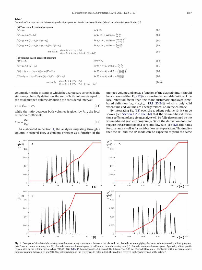
K. Broeckhoven et al. / J. Chromatogr. A 1218 (2011) 1153–1169 1157
Table 1Example of the equivalence between a gradient program written in time coordinates (a) and in volumetric coordinates (b).
(a) Time-based gradient programf(t) = �0 for t < ta (T-1)
f(t) = �0 + a · (t − ta) for ta < t < tb with a = �b−�0tb−ta
(T-2)
f(t) = �0 + a · (tb − ta) + b · (t − tb) for tb < t < tc with b =(
�c−�btc−tb
)n(T-3)
f(t) = �0 + a · (tb − ta) + b · (tc − tb)n + c · (t − tc) for tb < t < tc with c = �end−�ctend−tc
(T-4)
and with:�b = �0 + a · (tb − ta)�c = �0 + a · (tb − ta) + b · (tc − tb)n (T-5)
(b) Volume-based gradient programf (V) = �0 for V < Va (T-6)
f(t) = �0 + a · (V − Va) for Va < V < Vb with a = �b−�0Vb−Va
(T-7)
f (t) = �0 + a · (Vb − Va) + b · (V − Vb) for Vb < V < Vc with b =(
�c−�bVc−Vb
)n(T-8)
V < Vc
cst
d
wr
d
c
F(rg
f(V) = �0 + a · (Vb − Va) + b · (Vc − Vb)n + c · (V − Vc) for Vb <
and with:�b = �0 + a · (Vb − Va)�c = �0 + a · (Vb − Va) + b · (Vc − Vb)n
olumn during the instants at which the analytes are arrested in thetationary phase. By definition, the sum of both volumes is equal tohe total pumped volume dV during the considered interval:
V = dVm + dVs (11)
hile the ratio between both volumes is given by kloc, the localetention coefficient:
Vm = dVs
kloc(12)
As elaborated in Section 1, the analytes migrating through aolumn in general obey a gradient program as a function of the
ig. 1. Example of simulated chromatograms demonstrating equivalence between thea) cF-mode, time-chromatogram, (b) cF-mode, volume-chromatogram, (c) cP-mode, timepresented by the red line (see also Eqs. (T1)–(T10) in Table 1). Column length = 1.2 cm anradient running between 10 and 90%. (For interpretation of the references to color in tex
with c = �end−�cVend−Vc
(T-9)
(T-10)
pumped volume and not as a function of the elapsed time. It shouldhence be noted that Eq. (12) is a more fundamental definition of thelocal retention factor than the more customary employed time-based definition (dtm = dts/kloc [15,21,23,24]), which is only validwhen time and volume are linearly related, i.e. in the cF-mode.
By integrating Eq. (12) over the gradient volume VR, it can beshown (see Section 1.2 in the SM) that the volume-based reten-
tion coefficient of any given analyte will be fully determined by thevolume-based gradient program fV. Since the derivation does notrequire the assumption of a constant flow rate (see SM), this holdsfor constant as well as for variable flow rate operations. This impliesthat the cF- and the cP-mode can be expected to yield the samecF- and the cP-mode when applying the same volume-based gradient program:e-chromatogram, (d) cP-mode, volume-chromatogram. Applied gradient profile
d ID = 4.6 mm, V0 = 0.03 mL, cF-mode flow rate = 1.2 mL/min with a methanol–watert, the reader is referred to the web version of the article.)
1 matog
kr
Ntfl
4
g
k
ttc
t
w
t
cv(
bI
t
wb
t
ctb
5c
sgvc
stbbts
t
fr
158 K. Broeckhoven et al. / J. Chro
eff,V-value provided the same volume-based gradient program isun in both modes. This is illustrated in Fig. 1.
The above calculation parallels the recent work presented byikitas and Pappa-Louisi investigating the problem of retention
ime prediction of mobile phase gradient elution under variableow rate [13,26–28].
.2. Selectivity in the time-based chromatogram
In a time-based chromatogram, the effective retention factor isenerally defined as:
eff,t = tR − t0
t0(13)
Knowing from the above section that the volume VR neededo elute a given component from the column is independent ofhe operation mode, we can put V = VR in resp. Eqs. (4) and (8) toompare the expected elution time in the cF-mode (cf. Eq. (3)):
R = VR
FF(14a)
ith that in the cP-mode:
R = 1�
∫ V ′R
0
�̄(fV (V ′)) · dV ′ (14b)
Both expressions only return the same tR provided �̄ remainsonstant, as is the case in an isocratic run. Since �̄ will generallyary with the pumped volume during a gradient separation, Eqs.14a) and (14b) will generally lead to different tR-values.
The two operation modes in general also lead to a differentreakthrough time for an unretained component (t0-time marker).
n the cF-mode, this component will elute after a time t0, given by:
0 = V0
FF(15a)
hereas an unretained component will elute at a time determinedy Eq. (7) in the cP-mode:
∗0 = 1
�
∫ 1
0
�̄(V ′) · dV ′ (15b)
Again both values will generally differ when �̄ varies during theourse of the separation. To prevent any misunderstanding withhe generally adopted definition of t0 (Eq. (15a)), an asterisk haseen added to the t0-symbol used in Eq. (15b).
. Relation between time-based and volume-basedhromatograms and introduction of reconstructed time axis
The previous sections have emphasized the importance ofwitching from time to volumetric units to establish gradient pro-rams and record chromatograms in cases where the flow ratearies with the time, as is the case in the presently investigatedP-mode.
Although there are no fundamental limitations to make thiswitch, it might be uncomfortable to analysts who are accustomedo thinking and reasoning in time units. To circumvent this possi-le “mental” objection, the volumetric units can, if desired, readilye turned into a volume based reconstructed time tV by dividinghe original volume data by the flow rate FF used in the cF-modeeparation one is comparing with:
V = V
FF(16)
As the reconstructed time tV is based on a simple linear trans-ormation of the volume-coordinate, programming gradients andecording chromatograms in reconstructed time units is fully
r. A 1218 (2011) 1153–1169
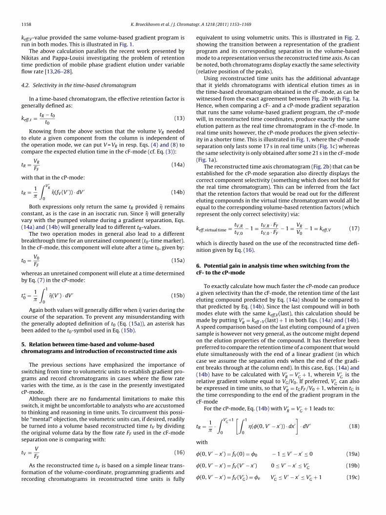
equivalent to using volumetric units. This is illustrated in Fig. 2,showing the transition between a representation of the gradientprogram and its corresponding separation in the volume-basedmode to a representation versus the reconstructed time axis. As canbe noted, both chromatograms display exactly the same selectivity(relative position of the peaks).
Using reconstructed time units has the additional advantagethat it yields chromatograms with identical elution times as inthe time-based chromatogram obtained in the cF-mode, as can bewitnessed from the exact agreement between Fig. 2b with Fig. 1a.Hence, when comparing a cF- and a cP-mode gradient separationthat runs the same volume-based gradient program, the cP-modewill, in reconstructed time coordinates, produce exactly the sameelution pattern as the real time chromatogram in the cF-mode. Inreal time units however, the cP-mode produces the given selectiv-ity in a shorter time. This is illustrated in Fig. 1, where the cP-modeseparation only lasts some 17 s in real time units (Fig. 1c) whereasthe same selectivity is only obtained after some 21 s in the cF-mode(Fig. 1a).
The reconstructed time axis chromatogram (Fig. 2b) that can beestablished for the cP-mode separation also directly displays thecorrect component selectivity (something which does not hold forthe real time chromatogram). This can be inferred from the factthat the retention factors that would be read out for the differenteluting compounds in the virtual time chromatogram would all beequal to the corresponding volume-based retention factors (whichrepresent the only correct selectivity) via:
keff,virtual time = tV,R
tV,0− 1 = tV,R · FF
tV,0 · FF− 1 = VR
V0− 1 = keff,V (17)
which is directly based on the use of the reconstructed time defi-nition given by Eq. (16).
6. Potential gain in analysis time when switching from thecF- to the cP-mode
To exactly calculate how much faster the cP-mode can producea given selectivity than the cF-mode, the retention time of the lasteluting compound predicted by Eq. (14a) should be compared tothat predicted by Eq. (14b). Since the last compound will in bothmodes elute with the same keff,V(last), this calculation should bemade by putting V ′
R = keff ,V (last) + 1 in both Eqs. (14a) and (14b).A speed comparison based on the last eluting compound of a givensample is however not very general, as the outcome might dependon the elution properties of the compound. It has therefore beenpreferred to compare the retention time of a component that wouldelute simultaneously with the end of a linear gradient (in whichcase we assume the separation ends when the end of the gradi-ent breaks through at the column end). In this case, Eqs. (14a) and(14b) have to be calculated with V ′
R = V ′G + 1, wherein V ′
G is therelative gradient volume equal to VG/V0. If preferred, V ′
G can alsobe expressed in time units, so that V ′
R = tGFF /V0 + 1, wherein tG isthe time corresponding to the end of the gradient program in thecF-mode
For the cP-mode, Eq. (14b) with V ′R = V ′
G + 1 leads to:
tR = 1�
·∫ V ′
G+1
0
[∫ 1
0
�(�(0, V ′ − x′)) · dx′]
· dV ′ (18)
with
�(0, V ′ − x′) = fV (0) = �0 − 1 ≤ V ′ − x′ ≤ 0 (19a)
�(0, V ′ − x′) = fV (V ′ − x′) 0 ≤ V ′ − x′ ≤ V ′G (19b)
�(0, V ′ − x′) = fV (V ′G) = �e V ′
G ≤ V ′ − x′ ≤ V ′G + 1 (19c)

K. Broeckhoven et al. / J. Chromatogr. A 1218 (2011) 1153–1169 1159
F ) voluS
wptVa(e
(
t
tiitfb
�
wrP
ig. 2. Identical elution pattern obtained when plotting a cP-mode separation in (aame separation conditions as in Fig. 1.
herein Eq. (19a) expresses that the column is filled with a mobilehase with composition �0 at the start of the separation, and thathis volume is gradually flushed out during the period wherein′ ≤ 1. Eq. (19c) expresses that once the gradient program is finishedt the inlet, it still takes the elution of one additional void volumecorresponding to one unity of the reduced volume V′) before thend of the gradient reaches the end of the column.
For the cF-mode, � = �max = constant, so that the integral in Eq.18) can simply be replaced by:
R = 1�
· �max · (V ′G + 1) (20)
Defining the gain in analysis time �t% as the relative reduction ofhe retention time in both modes (and calculated in real time units),t should first be noted that this gain is also equal to the averagencrease in flow rate �Fav,% that can be realized when switching tohe cP-mode. Directly applying Darcy’s law, this relative gain is inact also equal to the relative increase in pressure �PFP,av% that cane realized when going from the cF- to the cP-mode, so that:
t% = (tR,cF−mode − tR,cP−mode)tR,cF−mode
= (FP,av − FF )FF
= �FFP,av%
(PF,max − PF,av)
=PF,max= �PFP,av% (21)
herein PF,av is the volume averaged inlet pressure in the cF-modeun, FP,av is the average flow rate in the cP-mode run and whereinF,max is the maximum pressure experienced during a cF-run (see
metric coordinates and in (b) reconstructed time axis coordinates (using tV = V/FF).
resp. Fig. 4a and c further on for a graphical illustration of PF,av, FP,av
and PF,max).Subsequently filling in the cF-mode and the cP-mode analysis
time expression into Eq. (21) yields:
�t% =
∫ V ′G
+10
[∫ 10
�(�(0, V ′ − x′)) · dx′]
· dV ′
�max · (V ′G + 1)
− 1 (22)
Tables 2–5 show the results produced by Eq. (22) for linearwater–methanol (Tables 2 and 3) and water–acetonitrile gradi-ents (Tables 4 and 5). For each mixture type, the whole space ofpossible start and end compositions is covered in steps of 5%. Inaddition, also two strongly different degrees of gradient steepnesshave been considered for each mixture type: a very steep gradient,with V ′
G = VG/V0 = 3 (Tables 2 and 4) and a rather shallow gradientwith V ′
G = VG/V0 = 15 (Tables 3 and 5).The tabulated data were calculated using the relation between
the viscosity and the fraction organic modifier obtained in [7] fora pressure of 500 bars (intermediate pressure between columninlet and outlet for a separation run at 1000 bar) and a tempera-ture of 30 ◦C. For methanol, two second order polynomial fittingswere used (for the intervals 0 < � < 50 and 50 < � < 100 vol.% MeOH),
whereas for acetonitrile, a second order and third order polyno-mial were used (for the intervals 0 < � < 20 and 20 < � < 100 vol.%ACN respectively). A fitting quality of SSE < 0.5% was obtained. Theexpression for the fits, as well as their graphical representation, isgiven in SM (see Fig. S-1). The SM also contains tables for other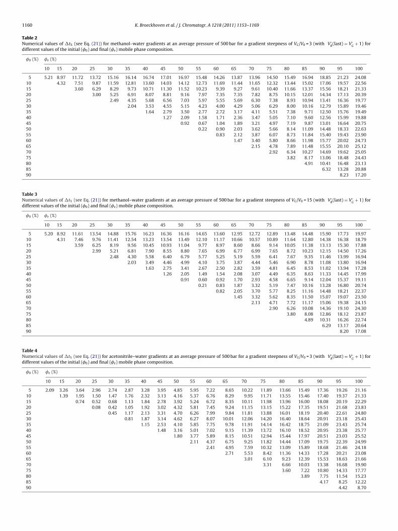
1160 K. Broeckhoven et al. / J. Chromatogr. A 1218 (2011) 1153–1169
Table 2Numerical values of �t% (see Eq. (21)) for methanol–water gradients at an average pressure of 500 bar for a gradient steepness of VG/V0 = 3 (with V ′
R(last) = V ′
G+ 1) for
different values of the initial (�0) and final (�e) mobile phase composition.
�0 (%) �e (%)
10 15 20 25 30 35 40 45 50 55 60 65 70 75 80 85 90 95 100
5 5.21 8.97 11.72 13.72 15.16 16.14 16.74 17.01 16.97 15.48 14.26 13.87 13.96 14.50 15.49 16.94 18.85 21.23 24.0810 4.32 7.51 9.87 11.59 12.81 13.60 14.03 14.12 12.73 11.69 11.44 11.65 12.32 13.44 15.02 17.06 19.57 22.5615 3.60 6.29 8.29 9.73 10.71 11.30 11.52 10.23 9.39 9.27 9.61 10.40 11.66 13.37 15.56 18.21 21.3320 3.00 5.25 6.91 8.07 8.81 9.16 7.97 7.35 7.35 7.82 8.75 10.15 12.01 14.34 17.13 20.3925 2.49 4.35 5.68 6.56 7.03 5.97 5.55 5.69 6.30 7.38 8.93 10.94 13.41 16.36 19.7730 2.04 3.53 4.55 5.15 4.23 4.00 4.29 5.06 6.29 8.00 10.16 12.79 15.89 19.4635 1.64 2.79 3.50 2.77 2.72 3.17 4.11 5.51 7.38 9.71 12.50 15.76 19.4940 1.27 2.09 1.58 1.71 2.36 3.47 5.05 7.10 9.60 12.56 15.99 19.8845 0.92 0.67 1.04 1.89 3.21 4.97 7.19 9.87 13.01 16.64 20.7550 0.22 0.90 2.03 3.62 5.66 8.14 11.09 14.48 18.33 22.6355 0.83 2.12 3.87 6.07 8.73 11.84 15.40 19.43 23.9060 1.47 3.40 5.80 8.66 11.98 15.77 20.02 24.7365 2.15 4.78 7.89 11.48 15.55 20.10 25.1270 2.92 6.34 10.27 14.69 19.62 25.0575 3.82 8.17 13.06 18.48 24.4380 4.91 10.41 16.48 23.1385 6.32 13.28 20.8890 8.23 17.20
Table 3Numerical values of �t% (see Eq. (21)) for methanol–water gradients at an average pressure of 500 bar for a gradient steepness of VG/V0 = 15 (with V ′
R(last) = V ′
G+ 1) for
different values of the initial (�0) and final (�e) mobile phase composition.
�0 (%) �e (%)
10 15 20 25 30 35 40 45 50 55 60 65 70 75 80 85 90 95 100
5 5.20 8.92 11.61 13.54 14.88 15.76 16.23 16.36 16.16 14.65 13.60 12.95 12.72 12.89 13.48 14.48 15.90 17.73 19.9710 4.31 7.46 9.76 11.41 12.54 13.23 13.54 13.49 12.10 11.17 10.66 10.57 10.89 11.64 12.80 14.38 16.38 18.7915 3.59 6.25 8.19 9.56 10.45 10.93 11.04 9.77 8.97 8.60 8.66 9.14 10.05 11.38 13.13 15.30 17.8820 2.99 5.21 6.81 7.90 8.55 8.80 7.65 6.99 6.77 6.99 7.65 8.72 10.23 12.15 14.50 17.2625 2.48 4.30 5.58 6.40 6.79 5.77 5.25 5.19 5.59 6.41 7.67 9.35 11.46 13.99 16.9430 2.03 3.49 4.46 4.99 4.10 3.75 3.87 4.44 5.46 6.90 8.78 11.08 13.80 16.9435 1.63 2.75 3.41 2.67 2.50 2.82 3.59 4.81 6.45 8.53 11.02 13.94 17.2840 1.26 2.05 1.49 1.54 2.08 3.07 4.49 6.35 8.63 11.33 14.45 17.9945 0.91 0.60 0.92 1.70 2.93 4.58 6.65 9.14 12.04 15.37 19.1150 0.21 0.83 1.87 3.32 5.19 7.47 10.16 13.28 16.80 20.7455 0.82 2.05 3.70 5.77 8.25 11.16 14.48 18.21 22.3760 1.45 3.32 5.62 8.35 11.50 15.07 19.07 23.5065 2.13 4.71 7.72 11.17 15.06 19.38 24.1570 2.90 6.26 10.08 14.36 19.10 24.3075 3.80 8.08 12.86 18.12 23.8780 4.89 10.31 16.26 22.7485 6.29 13.17 20.6490 8.20 17.08
Table 4Numerical values of �t% (see Eq. (21)) for acetonitrile–water gradients at an average pressure of 500 bar for a gradient steepness of VG/V0 = 3 (with V ′
R(last) = V ′
G+ 1) for
different values of the initial (�0) and final (�e) mobile phase composition.
�0 (%) �e (%)
10 15 20 25 30 35 40 45 50 55 60 65 70 75 80 85 90 95 100
5 2.09 3.26 3.64 2.96 2.74 2.87 3.28 3.95 4.85 5.95 7.22 8.65 10.22 11.89 13.66 15.49 17.36 19.26 21.1610 1.39 1.95 1.50 1.47 1.76 2.32 3.13 4.16 5.37 6.76 8.29 9.95 11.71 13.55 15.46 17.40 19.37 21.3315 0.74 0.52 0.68 1.13 1.84 2.78 3.92 5.24 6.72 8.35 10.11 11.98 13.96 16.00 18.08 20.19 22.2920 0.08 0.42 1.05 1.92 3.02 4.32 5.81 7.45 9.24 11.15 13.15 15.22 17.35 19.51 21.68 23.8325 0.45 1.17 2.13 3.31 4.70 6.26 7.99 9.84 11.81 13.88 16.01 18.19 20.40 22.61 24.8030 0.81 1.87 3.14 4.62 6.27 8.07 10.01 12.06 14.20 16.40 18.64 20.91 23.18 25.4335 1.15 2.53 4.10 5.85 7.75 9.78 11.91 14.14 16.42 18.75 21.09 23.43 25.7440 1.48 3.16 5.01 7.02 9.15 11.39 13.72 16.10 18.52 20.95 23.38 25.7745 1.80 3.77 5.89 8.15 10.51 12.94 15.44 17.97 20.51 23.03 25.5250 2.11 4.37 6.75 9.25 11.82 14.44 17.09 19.75 22.39 24.9955 2.41 4.95 7.59 10.32 13.09 15.89 18.68 21.46 24.1860 2.71 5.53 8.42 11.36 14.33 17.28 20.21 23.0865 3.01 6.10 9.23 12.39 15.53 18.63 21.6670 3.31 6.66 10.03 13.38 16.68 19.9075 3.60 7.22 10.80 14.33 17.7780 3.89 7.75 11.54 15.2385 4.17 8.25 12.2290 4.42 8.70

K. Broeckhoven et al. / J. Chromatogr. A 1218 (2011) 1153–1169 1161
Table 5Numerical values of �t% (see Eq. (21)) for acetonitrile–water gradients at an average pressure of 500 bar for a gradient steepness of VG/V0 = 15 (with V ′
R(last) = V ′
G+ 1) for
different values of the initial (�o) and final (�e) mobile phase composition.
�0 (%) �e (%)
10 15 20 25 30 35 40 45 50 55 60 65 70 75 80 85 90 95 100
5 2.07 3.18 3.46 2.70 2.37 2.40 2.71 3.29 4.10 5.12 6.32 7.68 9.19 10.81 12.55 14.36 16.24 18.17 20.1310 1.37 1.88 1.34 1.23 1.45 1.95 2.69 3.65 4.80 6.13 7.61 9.22 10.95 12.78 14.69 16.65 18.65 20.6815 0.72 0.43 0.55 0.96 1.63 2.52 3.61 4.89 6.33 7.92 9.63 11.45 13.36 15.35 17.38 19.45 21.5420 0.07 0.39 0.96 1.76 2.77 3.98 5.36 6.91 8.59 10.39 12.30 14.29 16.34 18.45 20.58 22.7225 0.44 1.12 2.04 3.16 4.47 5.95 7.59 9.36 11.24 13.22 15.28 17.41 19.57 21.75 23.9430 0.80 1.83 3.06 4.48 6.06 7.80 9.66 11.64 13.71 15.85 18.05 20.28 22.53 24.7835 1.14 2.49 4.03 5.72 7.56 9.53 11.61 13.78 16.01 18.30 20.62 22.95 25.2740 1.47 3.13 4.95 6.91 9.00 11.19 13.46 15.81 18.19 20.61 23.03 25.4445 1.79 3.74 5.84 8.06 10.37 12.78 15.24 17.74 20.27 22.79 25.3050 2.10 4.34 6.71 9.17 11.71 14.31 16.94 19.60 22.24 24.8755 2.41 4.93 7.56 10.26 13.01 15.80 18.59 21.38 24.1360 2.71 5.51 8.39 11.32 14.28 17.24 20.18 23.0865 3.01 6.09 9.22 12.37 15.51 18.63 21.7070 3.31 6.66 10.03 13.38 16.70 19.96
aiantgad
isrgffidbticf
Ttomgbaglsrdgd
icg
ib
the order of some 20%, i.e. in agreement with the data shown inTables 2–3. Similar to what could already be observed in the firstexample (Fig. 1a and c), Fig. 3a shows that the cP-mode not onlyaccelerates the last eluting compounds but can also accelerate the
Fig. 3. Overlap of cF-mode (red) and cP-mode (black) chromatogram in (a) real
75808590
verage column pressures (e.g. for 300 bar and 50 bar, correspond-ng to a column operating pressure of respectively 600 and 100 bar)nd for gradients where the last component elutes at V ′
R = V ′G and
ot at V ′R = V ′
G + 1 (=moment of elution of end of gradient) as ishe case in Tables 2–5. If desired, a simplified version of the inte-ral given in Eq. (22) can be approximated using a discrete sumpproach wherein the gradient is divided in short segments (as e.g.escribed in [13,26–28]).
A first general observation that can be made from Tables 2–5s that the relative gain is only weakly affected by the gradientteepness, as the values for the same �0- and �e-case only varyelatively weakly between the steep gradient case and the weakradient case (compare corresponding data entries in Tables 2 and 3or water-methanol gradients and compare between Tables 4 and 5or water-acetonitrile gradients). The gain for methanol gradientss always larger for the fastest gradient, with a maximum absoluteifference in �t% of 4.1% for a gradient running from 5 to 100%etween the two presented steepnesses. For acetonitrile gradients,he largest difference in �t% in only 1.1% and in some cases the gains even slightly larger in case of the more shallow gradient. For theases with V ′
R = V ′G , the behavior is more complex as can be seen
rom Tables S-3, S-4, S-6 and S-7 in the SM, part 4.The most important observation that can be made from
ables 2–5 is the order of magnitude of the gain in analysis timehat can be expected when switching to the cP-mode. For the casef a typical scouting gradient running between 5 and 95% of organicodifier, the entries for the 5–95%-case in Tables 2–5 show that this
ain will be very similar for the ACN- and the MeOH-case and cane expected to lie around 19.5% for methanol-based gradients andround 18.7% for ACN-based gradients (average of both consideredradient steepness values). When the start and/or end compositionie closer to the viscosity maximum, the analysis time gain becomesmaller as well, thus reflecting that the margin over which the flowate can be increased becomes smaller. For a 20–80% MeOH gra-ient for example, the gain is reduced to some 8.3%. For a 40–60%radient, the potential analysis time advantage of the cP-mode evenrops to less than 2%.
The potential gain in analysis time of the cP-mode is furtherllustrated in Fig. 3, showing a set of simulated cF-mode and
P-mode chromatograms for the case of a linear, volume-basedradient running between 5 and 95% of methanol.Considering the overlap of the cF- and cP-mode chromatogramsn real time units (Fig. 3a), the gain in analysis time obtainedy switching to the cP-mode (black chromatogram) is indeed of
3.61 7.22 10.81 14.36 17.833.89 7.76 11.57 15.28
4.17 8.27 12.264.43 8.73
time and (b) volume for a volume-based gradient running between 5% and 95%methanol–water (linear gradient, VG/V0 = 9 in the volume-program mode or tG/t0 = 9in the time-program mode). Simulated column length is 1.2 cm and column diameter2.1 mm, the particle size 2 �m and �Pmax = 101.2 bar, corresponding to u0 = 3.2 mm/sfor the cF-mode. (For interpretation of the references to color in text, the reader isreferred to the web version of the article.)
1 matog
ecici
7
ctfatfn
effis
mq
H
wcl
tba((Trae[cc
cdnp
H
rc
n[fuhbcAh
162 K. Broeckhoven et al. / J. Chro
arly eluting peaks. This is due to the fact that the mobile phaseomposition in the beginning of a 5–95% methanol–water gradients still far away from the viscosity maximum, so that the flow ratean also be significantly increased in the beginning of the gradientn the cP-mode.
. Effect of operation mode on separation efficiency
If the efficiency (band broadening) of the separation is not a criti-al issue (i.e. when the achieved separation resolution is sufficient),he advantage of switching to the cP-mode can readily be quantifiedrom the relative analysis time gains cited in the previous sectionnd in Tables 2–5. However, when the considered cF-mode separa-ion is limited by the resolution of a critical pair or when it suffersrom an insufficient peak capacity, also the separation efficiencyeeds to be taken into account.
Unlike the selectivity, which can be kept identical, small differ-nces in separation efficiency cannot be avoided when switchingrom the cF-mode to the cP-mode. This can for example be notedrom the small differences in peak height between the correspond-ng peaks in Fig. 3b (compare height of black and red peaks). Aimilar observation can be made from Figs. S-3b and S-4b of the SM.
As shown by Giddings [2], the separation efficiency is deter-ined by the band broadening, which in turn can be rigorously
uantified via the plate height H, defined as:
= �2x
x(23)
herein �2x is the increase in spatial variance of the band in the
olumn when its centroid has moved from the inlet to a positionocated at a distance x from the inlet.
In the literature, there has always been some reluctance towardshe use of the plate height concept under gradient conditionsecause H can only be assessed by estimating the spatial vari-nce from the measured time-based variance which tends to be1 + kloc,e)2 times larger than the spatial variance in the columnkloc,e is the local retention factor at the moment of elution) [25].o correct for this, the value of kloc,e needs to be known and thisequires additional measurements or calculations. It is furthermoren additional source of errors. Nevertheless, as shown by Poppet al. [20], Gritti and Guiochon [21] and recently also by our group3] and Neue et al. [25], there is no fundamental impediment toontinue using the plate height concept under gradient elutiononditions.
Doing so, and neglecting in a first instance the effect of peakompression, it can be shown (see SM, Section 1.3 for the detailederivation) that the effective gradient plate height Heff of a compo-ent can be described as a single function of the volumetric gradientrogram fV given by [29,30]:
eff =∫ keff,V +1
0
H(fV (V ′))1 + kloc(fV (V ′))
· dV ′ (24)
Eq. (24) holds without any restriction on the nature of the flowate (constant or not), and hence holds for both the cF- and theP-mode case.
In case of an appreciable peak compression, the Heff-valueseed to be corrected by a so-called peak compression factor G2
17,20–22]. As shown in SM (Section 1.5), the conclusion followingrom Eq. (24), i.e. that Heff is fully determined by the relative vol-metric gradient fV and is independent of the column length, still
olds when accounting for peak compression effects. This coulde confirmed via the conducted simulations, since the numericalode automatically also simulates the peak compression effect [3].n example of a numerical proof is given in SM (Fig. S-6), showingow that the calculated values for the diverse peaks in the chro-r. A 1218 (2011) 1153–1169
matogram of the example considered in Fig. 1 indeed vary in aperfectly linear way with L.
Since the H-expression that needs to be used in Eq. (24) dependon Dm, kloc and u0, and it is shown in Section 1.3 of the SM that theanalytes will experience the same kloc- and Dm-history provided thesame volume-based gradient program is used, the only differencebetween a cF- and a cP-mode separation conducted with the samevolume-based gradient program is the difference in mobile phasevelocity u0. Hence, the expected difference in band broadeningbetween the cP-mode and the cF-mode should be fully determinedby the relation between the plate height and the velocity. As advo-cated by Giddings [31], this relation can most conveniently berepresented as a plot of the reduced plate height (h = H/dp) versusthe reduced velocity (� = u0 dp/Dm). It is therefore instructive to firstconsider how the two variable parameters determining the valueof the reduced velocity (i.e. u0 and Dm) change during the course ofa cF- and a cP-mode run.
For this purpose, Fig. 4a first shows a typical pressure trace fora linear gradient in the cF-mode. According to Darcy’s law (see Eq.(5)), this trace is also linearly proportional to the column-averagedviscosity �̄ (Fig. 4b). Still, according to Darcy’s law, the pressuretrace is also inversely proportional to the flow rate that can berealized when switching to the cP-mode (see Fig. 4c). Furthermoremaking the assumption that the gradient is sufficiently flat, so thatthe local viscosity at the peak center (�peak) remains close to thecolumn-averaged value �̄, and assuming that Dm varies inverselyproportional with the change in viscosity (i.e. neglecting for exam-ple the dependency of the association factors on the mobile phasecomposition in the Wilke-Chang expression), the local Dm-values(Fig. 4d) experienced by the peak during the course of its elutionare also inversely proportional to the P-trace measured in Fig. 4a.
In the cF-mode, the flow rate and u0 remain constant whileDm will typically follow a trajectory as depicted in Fig. 4d. It canhence be inferred that the reduced velocity, which is proportionalto u0 dp/Dm, will follow a trajectory that is inversely proportionalto Dm, i.e. proportional to the P-trace depicted in Fig. 4a and the �-trace depicted in Fig. 4b. An example of the reduced velocity historyexperienced by the peaks eluting in the cF-mode can be followedfrom the I–II–III trajectory added to the methanol curve in Fig. 4b.Starting at point I, the reduced velocity will first increase until theviscosity maximum is reached (point II) and will then decreaseagain to finally reach a new minimum at point III. In the cP-modeon the other hand, both u0 and Dm vary during the course of the elu-tion. They however do so in a more or less parallel way (cf. Fig. 4band d), at least provided �peak and �̄ do not differ too much. As a con-sequence, the peak will always experience about the same reducedvelocity at any instant during the elution.
The above can be summarized as:
cP-mode : v ∼= constant (25a)
cF-mode : v ≤ vcP-mode (25b)
The reduced velocity trajectories experienced in both modes arevisualized in Fig. 5, for three typical cases of the velocity: a veloc-ity in the B-term dominated range, a velocity near the minimum ofthe van Deemter curve and a C-term dominated velocity. For the cP-mode, the velocity trajectory reduces to a single dot according to Eq.(25a). Considering the assumptions underlying Eq. (25a), this singledot representation only holds to a first approximation and has onlybeen preferred here for the clarity of the presentation (the single dotapproximation was not used during the simulations) and to empha-
size the fact that the reduced velocity anyhow varies over a muchwider range in the cF-mode. In this mode, the reduced velocity willgenerally vary from point I over II to III when the mobile phase gra-dient passes through a viscosity maximum somewhere between itsbegin and endpoint. If the gradient would incidentally start or end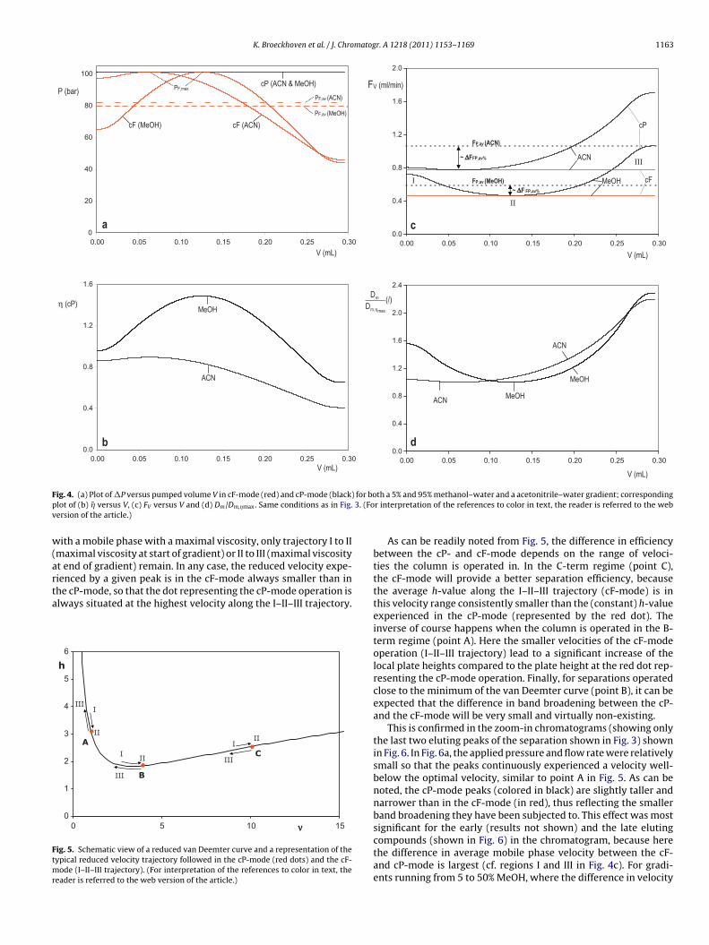
K. Broeckhoven et al. / J. Chromatogr. A 1218 (2011) 1153–1169 1163
0
20
40
60
80
100
0.300.250.200.150.100.050.00
0.0
0.4
0.8
1.2
1.6
0.300.250.200.150.100.050.00
V (mL)
η (cP)
V (mL)
P (bar)
a
b0.0
0.4
0.8
1.2
1.6
2.0
2.4
0.300.250.200.150.100.050.00
0.0
0.4
0.8
1.2
1.6
2.0
0.300.250.200.150.100.050.00
FV (ml/min)
V (mL)
(/)D
D
maxm,
m
η
c
d
V (mL)
F for bop 3. (Fov
w(arta
Ftmr
ig. 4. (a) Plot of �P versus pumped volume V in cF-mode (red) and cP-mode (black)lot of (b) �̄ versus V, (c) FV versus V and (d) Dm/Dm,�max. Same conditions as in Fig.ersion of the article.)
ith a mobile phase with a maximal viscosity, only trajectory I to IImaximal viscosity at start of gradient) or II to III (maximal viscosityt end of gradient) remain. In any case, the reduced velocity expe-
ienced by a given peak is in the cF-mode always smaller than inhe cP-mode, so that the dot representing the cP-mode operation islways situated at the highest velocity along the I–II–III trajectory.0
1
2
3
4
5
6
151050
I
II
III
h
II
IIII
II
IIII
A
B
C
ν
ig. 5. Schematic view of a reduced van Deemter curve and a representation of theypical reduced velocity trajectory followed in the cP-mode (red dots) and the cF-
ode (I–II–III trajectory). (For interpretation of the references to color in text, theeader is referred to the web version of the article.)
th a 5% and 95% methanol–water and a acetonitrile–water gradient; correspondingr interpretation of the references to color in text, the reader is referred to the web
As can be readily noted from Fig. 5, the difference in efficiencybetween the cP- and cF-mode depends on the range of veloci-ties the column is operated in. In the C-term regime (point C),the cF-mode will provide a better separation efficiency, becausethe average h-value along the I–II–III trajectory (cF-mode) is inthis velocity range consistently smaller than the (constant) h-valueexperienced in the cP-mode (represented by the red dot). Theinverse of course happens when the column is operated in the B-term regime (point A). Here the smaller velocities of the cF-modeoperation (I–II–III trajectory) lead to a significant increase of thelocal plate heights compared to the plate height at the red dot rep-resenting the cP-mode operation. Finally, for separations operatedclose to the minimum of the van Deemter curve (point B), it can beexpected that the difference in band broadening between the cP-and the cF-mode will be very small and virtually non-existing.
This is confirmed in the zoom-in chromatograms (showing onlythe last two eluting peaks of the separation shown in Fig. 3) shownin Fig. 6. In Fig. 6a, the applied pressure and flow rate were relativelysmall so that the peaks continuously experienced a velocity well-below the optimal velocity, similar to point A in Fig. 5. As can benoted, the cP-mode peaks (colored in black) are slightly taller andnarrower than in the cF-mode (in red), thus reflecting the smallerband broadening they have been subjected to. This effect was most
significant for the early (results not shown) and the late elutingcompounds (shown in Fig. 6) in the chromatogram, because herethe difference in average mobile phase velocity between the cF-and cP-mode is largest (cf. regions I and III in Fig. 4c). For gradi-ents running from 5 to 50% MeOH, where the difference in velocity
1164 K. Broeckhoven et al. / J. Chromatogr. A 1218 (2011) 1153–1169
V (mL)
0.000
0.002
0.004
0.006
0.008
0.010
0.012
0.300.290.280.270.260.25
0.000
0.002
0.004
0.006
0.008
0.010
0.012
0.300.290.280.270.260.25 V (mL)
a
b
cFcP
cF
cP
cP
cF
cP
cF
0.000
0.002
0.004
0.006
0.008
0.010
0.012
0.300.290.280.270.260.25
(/)C
C
max
(/)C
C
max
(/)C
C
max
V (mL)
c
cP cF
cP
cF
Fig. 6. Overlap of cF-mode (red) and cP-mode (black) chromatogram of thetwo last eluting compounds (k = 8 and 9) for a volume-based gradient runningbetween 5% and 95% methanol–water (linear gradient, VG/V0 = 9 in the volume-program mode or tG/t0 = 9 in the time-program mode) for three different cP-modeoperating pressures (a) �Pmax = 10 bar, corresponding to u0 = 0.32 mm/s for the cF-mode; (b) �Pmax = 50 bar, corresponding to u0 = 1.6 mm/s for the cF-mode and (c)�ui
bnmif
t
FF (mL/min)
σV,av (mL)
0.0007
0.0009
0.0011
0.0013
0.0015
3.02.52.01.51.00.50.0
a
45
55
65
75
85
3.02.52.01.51.00.50.0FF (mL/min)
np (/)
b
cF
cP
cP
cF
Fig. 7. (a) Evolution of the volumetric peak standard deviation V as a function of
this F-value is only an approximation of the true velocity history in
Pmax = 600 bar, corresponding to u0 = 19.2 mm/s for the cF-mode. Simulated col-mn length is 1.2 cm and ID = 2.1 mm. (For interpretation of the references to color
n text, the reader is referred to the web version of the article.)
etween the cP- and the cF-mode is only pronounced at the begin-ing of the gradient, the improved efficiency of the cP-mode wasost pronounced for the early eluting compounds. Similarly, an
mproved efficiency is only noted for the late eluting compoundsor gradients of 50–95% methanol (results not shown).
Considering a velocity close to the optimum velocity (Fig. 6b)he difference in band broadening is clearly much smaller than in
the mobile phase flow rate fV (mL/min) for cF- (red) and cP-mode (black) for fixedlength (=1.2 cm) column. (b) Corresponding values of the peak capacity as a functionof flow rate. Other conditions the same as Fig. 3. (For interpretation of the referencesto color in text, the reader is referred to the web version of the article.)
Fig. 6a. This is in full agreement with the fact that the difference inplate heights between a cP- and cF-mode operation is anyhow smallnear the optimum velocity (cf. point B of Fig. 5). When the coveredrange of velocities is fully situated in the C-term dominated regime(cf. point C of Fig. 5), as is the case for the separation represented inFig. 6c, the cF-mode yields narrower peaks than the cP-mode. This isagain in full agreement with the observation that can be made fromFig. 5, showing that the I–II–III trajectory followed in the cF-modein the C-term range leads to smaller h-values than the h-value cor-responding to the single dot velocity of the cP-mode. Once again,this effect is more pronounced for the late eluting compounds forgradients running from 50 to 95% methanol (see SM, Fig. S-5a onthe right hand side) on the one hand and for the early eluting com-pounds for gradients from 5 to 50% (see SM, Fig. S-5b on the lefthand side).
The efficiency of the chromatograms shown in Fig. 6 (and ofsome additional cases with a different velocity) are further quanti-fied in Fig. 7a, showing how V,av, the volumetric band standarddeviation averaged over all the individual peaks of the chro-matogram, varies as a function of the flow rate. Since it is difficult todefine a characteristic flow rate for the cP-mode operation (F is nota constant), the cP-mode data have simply been plotted versus theF-value of the corresponding cF-mode case (same �Pmax). Although
the cP-mode, it perfectly suits the purpose of visualizing the trendthat was already visible in the chromatograms shown in Fig. 6: thecP-mode produces narrower bands than the cF-mode in the rangeof sub-optimal flow rates, whereas the opposite is true in the range

matog
ocb(vw
i
h
ttafl
-
-
-
8to
tr
R
wpcrimrbl
cdtcrce
n
doooapc
K. Broeckhoven et al. / J. Chro
f low flow rates above the optimal flow rate. The cP- and cF-modeurves shown in Fig. 7a also clearly display the typical van Deemterehavior: V,av decreases steeply with F in the low velocity regionB-term behavior), then goes through a minimum (thus fixing thealue of the optimal flow rate), and subsequently increases againith F in the high velocity region (C-term behavior).
Approximating the h-curve underlying the observations maden Figs. 6 and 7 with the basic van Deemter model, for which:
= A + B
v+ C · v (26)
he above findings can be rationalized in a simplified form by statinghat the relative change in h (�h%) resulting from the switch fromcF- to a cP-operation is directly related to the average increase inow rate and pressure as:
in B-term dominated regime:
�h%∼ 1�Fav%
∼ 1�Pav%
(since h∼1v
) (27a)
around velocity optimum:
�h% ∼= 0 (since h is independent of v) (27b)
in C-term dominated regime:
�h%∼�Fav%∼�Pav% (since h∼v) (27c)
. Combined effect: comparison of the peak capacity andhe kinetic performance limit of cF-mode and cP-modeperations
The obvious measure combining selectivity (discussed in Sec-ion 4) and efficiency (discussed in Section 7) is the separationesolution Rs. In a volume-based chromatogram, Rs is defined as:
s,V = VR,i − VR,i−1
4 · (V,i + V,i−1)/2(28)
herein i and i − 1 are the annotation numbers of two successiveeaks. Since only the volume-based chromatogram provides theorrect separation information in the cP-mode (see Section 3.3), theesolution that would be measured in a time-based chromatograms not considered here. On the other hand, the resolution one would
easure in a time reconstructed-chromatogram as the one rep-esented in Fig. 2b would correspond exactly to that determinedy Eq. (28), because this chromatogram is obtained by a perfectly
inear rescaling of the volume-based chromatogram.Typically, the resolution value would be reported for the criti-
al pair of the chromatogram. When discussing the performance ofifferent chromatographic systems under gradient elution condi-ions, it has however become more customary to report the peakapacity. Although many different definitions exist, the most cor-ect estimate of the column peak capacity one can read out from ahromatogram is that based on the sum of the resolution values ofach subsequent peak pair [32,33]
p = 1 +nc∑
i=1
RS,V,i = 1 +nc∑
i=1
VR,i − VR,i−1
2 · (V,i + V,i−1)(29)
Eq. (29) is indeed the closest one can get to the exact integralefinition of peak capacity (see e.g. Eq. (1) in Ref. [33]). A numberf possible variants can be derived from Eq. (29). One could leave
ut the peak with i = 0 (dead volume marker), in which case np isnly counted starting from the first sample peak, and/or one coulddd an extra term covering the space between the last eluting com-ound and the point where the end of the gradient elutes from theolumn.r. A 1218 (2011) 1153–1169 1165
In the present study, the question whether the np-value shouldbest be based on either tG or on (tR,last − t0) or on (tR,last − tR,first) hasbeen simply circumvented by tuning the retention properties of thecomponents of the numerical sample such that they would coverthe complete elution window, having retention volumes rangingbetween V0 and V0 + VG.
Fig. 7b shows the peak capacity calculated using Eq. (29) for thesimulated chromatograms that were also used to establish Fig. 7a.In agreement with the effects observed in Fig. 7a, Fig. 7b shows thatthe cP-mode can be expected to lead to a smaller peak capacity inthe high velocity or flow rate range (C-term dominated regime),whereas the opposite would occur in the low velocity range (B-termdominated regime).
A drawback of the peak capacity plot in Fig. 7b is that it pro-vides no direct information about the speed of the separation or thekinetic performance limits of the technique. This information is hid-den in the flow rate and in the unused pressure potential (all but thehighest flow rate data points relate to conditions where the pres-sure is sub-maximal). To circumvent this problem, and transformeach different data points of either Fig. 7a or 7b into a data pointlying at the kinetic performance limit (KPL), the so-called kineticplot theory can be used [3–5,34–36]. According to this theory,recently extended gradient elution conditions [3], this transforma-tion can be done using the so-called column length rescaling factor�:
� = �Pcol,max
�Pcol,exp(30)
This � is a readily obtainable experimental parameter. The valueof �Pcol,exp is the maximum column pressure drop experiencedduring the gradient run (in the cP-mode this is simply the oper-ating pressure), whereas �Pcol,max is the pressure maximum of thecolumn or the pump. This �-value (note that each considered exper-imental velocity leads to a different value) can then be applied inbelow transformation expressions to turn the experimentally mea-sured tR,exp and np,exp into their corresponding values at the KPL ofthe system [3]:
tR,KPL = � · tR,exp (31)
np,KPL = 1 +√
� · (np,exp − 1) (32)
As shown in [3], the only condition underlying the validity ofthe KPL-transformation is that keff,V and Heff should be indepen-dent of the column length. The theoretical derivations presentedin Sections 4 and 7 show that the column length only interferes inthe expression for both keff (see Eq. (S-13) in the SM) and Heff (Eq.(24)) via the reduced volume V′ (with V′ = pumped volume/V0 andV0 = εT A L). Since Eqs. (S-13) and (24) furthermore only depend onfV(V′), one can hence expect to find the same value for keff and Heffprovided the same fV(V′)-program is run on each different lengthcolumns. Under this condition, even the degree of peak compres-sion can be expected to be identical (see SM, Section 1.5). Sincerunning the same fV(V′)-program corresponds to keeping the gra-dient program identical in reduced volumetric coordinates, thecondition to obtain identical keff,V- and Heff-values only requiresthat the characteristic volumes Va, Vb, etc. appearing in the gradientprogram are linearly scaled with the column length so as to main-tain the same dimensionless values of V ′
a, V ′b, etc. (with V ′
a = Va/V0,V ′
b= Vb/V0, etc.). This condition is in agreement with the condi-
tions proposed for the length-independency of keff,V by Snyder andDolan [37] and Jandera [14].
Since the expressions for keff,V and Heff established in Sections 4and 7 did not require to assume that the flow rate is kept constant,it can be concluded that the KPL-transformation equations given byEqs. (30)–(32), originally established in [3] for the cF-mode, shouldalso hold in the cP-mode.

1166 K. Broeckhoven et al. / J. Chromatogr. A 1218 (2011) 1153–1169
0.01
0.1
1.0
10.0
100.0
1000.0
100010010
(1)
(2)
(3)
tR (min)
np (/)
Fig. 8. Kinetic plot showing the total required analysis time tR as a function of therequired peak capacity (np) for cF (red squares) and cP operation (black triangles) fora fixed length column (=1.2 cm) (open symbols, dotted lines) and the correspond-ing kinetic performance limit (KPL, �Pcol,max = 600 bar, full symbols, full lines). Samecpo
cFrl(roadbocpu[
salmcitdstodr
crasfsefctt
0
30
60
90
120
5004003002001000
0
2
4
6
8
2251751257525
np (/)
cP
ACN/water
tR (min)tR (min)
cP
cF
cFnp (/)
Fig. 9. Kinetic plot showing the KPL of Fig. 8 in linear axis for constant flow (red
acetonitrile–water data lie to the right of the methanol–water data,
onditions as Fig. 3. The meaning of the arrows is discussed in the text. (For inter-retation of the references to color in text, the reader is referred to the web versionf the article.)
The graphical representation of the establishment of the KPL-urve for the simulated cF- and cP-mode separations is shown inig. 8. The dashed curves represent the fixed length column dataelating to the simulations already represented in Fig. 7. The fulline curves were obtained via the KPL-transformation using Eqs.30)–(32), whereas the blue and green dot data were obtained byedoing the simulations on a column with a different length andperating at the maximal pressure, but with the same flow ratend using the same gradient program in reduced volumetric coor-inates as the original column. As can be noted, the agreementetween the KPL-prediction and the actual performance measuredn the different length columns is perfect, despite the complex peakompression and variable flow rate effects. This agreement hencerovides a clear numerical proof for the validity of the KPL-theorynder cP-mode operation conditions, similar to that delivered in3] for the cF-mode (see Section 9 for the adopted assumptions).
The two KPL-curves (solid lines) in Fig. 8 provide a comprehen-ive view of the kinetic advantage of the cP-mode for the case of5–95% water-methanol gradient. The cP-mode curve everywhere
ies below the cF-mode curve, indicating a better kinetic perfor-ance, although the difference vanishes towards the left bottom
orner of the plot, i.e. for separations conducted in the C-term dom-nated regime [4,36]. Progressively moving upward along the curve,he flow rate relating to the different data points progressivelyecreases until the most rightward data point is reached, usuallyituated in the B-term dominated regime. Fig. 8 hence shows thathe largest advantage for the cP-mode would be observed whenperating in the B-term regime. This is however a range that is sel-om used in practice, because it is in this case always possible toeduce the analysis time by switching to a larger particle size.
Investigating the difference between the cF- and the cP-modeurves in more detail, the effect of the prevailing (average) flowate on this difference can readily be understood from the arrowsdded to Fig. 8. These arrows indicate how the KPL shifts whenwitching from the cF- to the cP-mode for a selected number of dif-erent flow rate cases. Since the selectivity does not change whenwitching from the cF- to the cP-mode, the observed shifts arexclusively due to a reduction of the analysis time and/or a dif-
erence in band broadening (represented here in terms of the peakapacity). The direction of the arrows hence always consists of aime reduction component (downward shift, directly proportionalo �Fav,%, see Eq. (21)) and a component representing the changesquares) and constant pressure (black triangles) for an acetonitrile–water gradient(open symbols, dotted lines) and a methanol–water gradient (full symbols, full lines)both running from 5 to 95%. (For interpretation of the references to color in text, thereader is referred to the web version of the article.)
in peak capacity originating from the difference in band broaden-ing (horizontal shift). In the B-term dominated regime (arrow 1),the net result of both changes leads to a double gain (arrow shiftstowards lower right corner): h decreases with �Pav,% (see Eq. (27a))and the total analysis time also decreases with �Pav,%. Near the opti-mum velocity (arrow 2), the arrow shifts purely downward becauseits horizontal component, representing the difference in h, is virtu-ally zero (see Eq. (27b)). In the C-term dominated regime (arrow 3),the arrow shifts downward (over a distance that is again propor-tional to �Pav,%) but also to the left (because now h increases with�Pav,%, see Eq. (27c)). When both effects are equally strong (whichwill occur when the flow rate is situated deep enough in C-termrange so that Eq. (27c) holds), they will cancel out, explaining thefact that the cP-mode and the cF-mode curve slowly tend towardseach other in the C-term dominated part of the KPL-curve.
This implies that the cP-mode is only really beneficial (with netrelative gains in the order of the values cited in Tables 2–5) for sep-arations conducted in columns that operate near the optimal flowrate when being subjected to the maximal pressure. This is howevera condition with a high practical relevance because it is the con-dition for which any type of chromatographic particles achievesits kinetic optimum, i.e. the so-called Knox and Saleem limit [1].Using Knox’ optimal performance expressions [38] with � = 800,�opt = 3 and hmin = 2, and considering the case of 2 �m particles,a compound with Dm = 10−9 m2/s and a maximal operating pres-sure of 1200 bar, it is found that the kinetic optimum is achieved incolumns with a length of about 10–15 cm and lasting about 30 min(assuming the last component elutes around keff,V = 10) when usingmethanol-based gradients (assuming �av = 1.2cP) and also about10–15 cm long and lasting about 20 min when using acetonitrile-based gradients (assuming �av = 0.7cP and assuming Dm reduces inproportion to �av).
The potential kinetic advantage of the cP-mode operation can bequantified in more detail from Fig. 9, where the KPL-curves shownin Fig. 8 are now represented in linear coordinates and where alsoa zoom-in of the lower range of the curve is provided. As can benoted, the kinetic advantage of switching to the cP-mode is verysimilar for the acetonitrile–water gradient (dashed line curves)and the water-methanol gradient (full line curves), at least forthe presently considered 5–95% gradient span. The fact that the
and thus provide a better kinetic performance, is a direct conse-quence of the lower viscosity of the former.
Another way to compare the kinetic performance of the cF andcP-mode is given in Fig. S-7 in the SM, which represents the rela-

matog
tIcstottt
9
avTpaopata
stietveecspacdratvietmtmcsse
aiud
�
whco
h
K. Broeckhoven et al. / J. Chro
ive gain in analysis time as a function of the desired peak capacity.n other words, this graph gives an indication on how far the KPLurves in Fig. 8 and 9 lie apart vertically. The curve presented therehow that the gain in analysis time for a given efficiency is lowerhan those given in Tables 2–5 for short analysis times (C-termperation), but becomes larger than expected for higher analysisimes (B-term operation). Once again, this is due to the fact thathe kinetic plot method incorporates the effect of both the analysisime and the efficiency.
. Some remarks concerning the adopted assumptions
The results in the preceding sections were all obtained byssuming isothermal operation conditions and assuming that theiscosity and the local retention factor are pressure-independent.hese assumptions however clearly do not hold under ultra-highressure conditions. In this case, the inevitable viscous heatingutomatically leads to a non-isothermal operation, with the devel-pment of both spatial and temporal (because of the varying mobilehase composition) temperature gradients. There is furthermorelso abundant experimental evidence and theoretical proof thathe viscosity and the retention factor can no longer be considereds constant under ultra-high pressure conditions [7,39,40].
In the discussion of the adopted assumptions, we will first con-ider the two operation modes separately and focus on only one ofhe conditions underlying the validity of the kinetic plot method,.e. that the viscosity is independent of the column length or themployed pressure. Doing so, it is first of all important to realizehat the developed viscous friction heat is determined by both theiscosity and the pressure evolution inside the column [41]. How-ver, the pressure is a given constant in the cP-mode, whereas itsvolution is fully determined by the viscosity in the cF-mode. As aonsequence, it can be said that the generated viscous heat is exclu-ively determined by the viscosity. Since it can be inferred that theattern with which the viscosity will vary as a function of the rel-tive time (or the relative run volume) will be independent of theolumn length provided the same gradient program is imposed inimensionless volumetric units, it can also be expected that theelative viscous heating history of the separation will be identicals well. The elevated pressure and viscous heating effects affectinghe mobile phase viscosity during the measurement of the highestelocity data point on the fixed-length column will hence also occurn any different length columns that is subjected to the same gradi-nt program. As a consequence, it can be inferred that the effect ofhe elevated pressure and the concomitant viscous heating on the
obile phase viscosity can be properly taken into account by basinghe entire KPL-transformation on the viscosity observed during the
easurement of the highest velocity data point on the fixed-lengtholumn. Using similar argumentation, it can be inferred that theame approach (i.e. use the retention factor observed when mea-uring the highest velocity data point) should be adopted for theffective retention factor keff.
The above considerations for � and keff are identical to thoselready formulated for the constant flow rate gradient kinetic plotn the SM of [3], where it was stated that, in order to account forltra-high pressure and viscous heating effects on �, the �-factorefined in Eq. (30) should in fact be written as:
(F) = �Fmax · Fmax
F(33)
hile a factor (1 + keff,Fmax )/(1 + keff ) should be added to the right
and side of Eq. (31) to properly calculate the retention times thatan be expected when the KPL is calculated for the highest possibleperating pressure.A moderating remark that should be made is that the above onlyolds provided the thermal boundary conditions do not change
r. A 1218 (2011) 1153–1169 1167
with the column length. The latter would pose no problem pro-vided it would be possible to operate the columns in a perfectlythermostatted or perfectly adiabatic mode. In practice, however,these idealized conditions are difficult to realize and it might hencebe that the thermal conditions will vary slightly with the col-umn length because of the changing ratio of column endfittingsto column mantle surface or because of the use of coupled columnsystems. Such changes have indeed already been reported [42] andwill introduce a small length dependency on the observed Heff andkeff.
Another requirement underlying the validity of the KPL-transformation is that the effective plate height should beindependent of the applied pressure and the concomitant vis-cous heating. This is a requirement that obviously cannot be metexactly, because the plate height depends on the diffusion coeffi-cient and the retention factor (cf. Section 1.3 of the SM) and theseare in general pressure- and temperature-dependent. However,both parameters have an opposite effect on both the diffusion coef-ficient and the retention factor, so that their effect to some extentcompensates for one another, at least when the thermal boundaryconditions of the column are close to adiabatic [41]. This conditionis satisfied for columns hanging in a still-air oven, but not for forced-air ovens, where it is well-known that viscous heating can lead tovery steeply increasing plate height curves in the C-term regime[42–44]. Obviously, the compensation of the effect of pressure andtemperature on the plate heights can never be exact, not even underperfectly adiabatic conditions, and will hold better for one classof components than for another. Nevertheless, the effect generallyremains limited up to pressures of 1000–2000 bar [41] so that theKPL-extrapolation can still be done within a reasonable range ofaccuracy. The problem that pressure and viscous heating lead toa non-exact KPL-extrapolation is not unique to cP-operations, butalso shows up to the same extent for isocratic separations as wellas for cF-gradient elution separations. In both cases, the accuracyof KPL-extrapolation has already been experimentally investigatedup to pressures of 600 bar (gradient elution) [3] and 1000 bar (iso-cratic elution) [42] on typical commercial instruments (both forcedand still air ovens) and columns. In any case, it was found that theextrapolation error was always less than 10% (less than 3% for iso-cratic separations in a still-air oven). This error was mainly dueto differences in thermal conditions (it is difficult to maintain thesame thermal boundary conditions if going form a single short col-umn to longer and or coupled column systems), as well as to thefact that the employed different-length columns already intrinsi-cally had a slightly different efficiency, apart from any pressure orviscous heating issues [3,42].
Turning now to the effect of ultra-high pressures on the compar-ison of the cP- and the cF-mode, it should be recognized that bothmodes inevitably display a different pressure trajectory (P = Pmax
in the cP-mode, whereas pressure varies quite strongly with thetime in the cF-mode). As a consequence, differences in the effectof viscous heating and high pressures on the mobile phase viscos-ity and the effective retention factor of the analytes are difficultto avoid. Nevertheless, because viscous heating and elevated pres-sures have an opposite effect on � and keff,V, it can be expected thatthe net effect will remain relatively small. This can be understoodas follows. Typically, the maximal difference in average pressurebetween the cP- and the cF-mode will lie around 20% (highest val-ues in Tables 2–5). Such a difference in pressure can be expectedto gives rise to some 4% increase in viscosity. However, becauseof the higher operating pressure, also the viscous heating will be
significant. Given that most columns are relatively close to adia-batic conditions, and given that the effect of temperature on theviscosity is larger than that of pressure, the net effect of the higheroperating pressure in the cP-mode can be expected to lead to a netreduction of the viscosity (only this effect will be very small, below
1 matog
1trb6lwasbapaowtt
ieopttsacc
1
bamescttciblcbirpmbvt
taarstaifl
w
168 K. Broeckhoven et al. / J. Chro
%, as a rough estimate). Nevertheless, this reduction implies thathe cP-mode can be expected to produce even slightly higher flowates (and hence shorter analysis times than those predicted on theasis of the isobaric and isothermal assumptions made in Sectionand leading up to Tables 2–5). Similar argumentation can be fol-
owed for the effective retention factor. For most small moleculareight compounds, the net effect of pressure and viscous heating
lso tends towards a reduction of keff with increasing inlet pressure,o that one can expect that the keff-values in the cP-mode mighte somewhat smaller than in the cF-mode. This would lead to andditional reduction of the elution time of the last eluting com-ound. However, this effect is not entirely positive, since it wouldlso imply a reduction of the sample-based peak capacity (becausef the reduction of the available retention window). The changeould certainly also lead to differences in selectivity, but this can
urn out either positively or negatively depending on the nature ofhe compounds.
The above considerations certainly need to be investigated moren-depth in a follow-up study. The conclusions of this study can bexpected to be highly complex, not only because they will dependn the nature of the sample compounds, but also because the tem-erature trajectory in the column inevitably depends highly on thehermal boundary conditions (which in practice are difficult to con-rol and describe) as well as on the events preceding the actualeparation, because, due to the thermal inertia, part of the temper-ture profile in the column is always reminiscent of the heating orooling effects occurring during the preceding run or the precedingolumn preconditioning run.
0. Conclusions
Provided both modes are run with the same reduced volume-ased gradient program, the constant-pressure (cP) mode can offern identical separation selectivity as the constant-flow (cF) rateode (except from some small differences induced by the differ-
nce in pressure and viscous heating trajectory). Depending on thetart and end composition of the gradient mixture, the cP-modean obtain this given selectivity in a shorter time. The potentialime gain can be expected to depend only weakly on the slope ofhe gradient and on the nature of the organic modifier. The gainan also be expected to be directly proportional to the relativencrease in average operating pressure �Pav% that can be realizedy switching to the cP-mode. As a consequence, the gain will be
argest for gradients covering the largest span in mobile phase vis-osity (this range runs between 50 and 95% for methanol/water andetween 20 and 95% for acetonitrile/water). For a typical scout-
ng gradient running between 5 and 95% of organic modifier, theelative time gain for the execution of a complete linear gradientrogram can be expected to be of the order of some 20% for bothethanol–water and acetonitrile–water systems. Smaller gains can
e expected when the start and end composition lie closer to theiscosity maximum of the considered water-organic modifier sys-em.
Operating under variable flow rate conditions, as is the case inhe cP-mode, the recorder signal should no longer be plotted asfunction of the time but as a function of the pumped volume,
s the former does not correctly represent the actual separationesolution that is achieved inside the column. If desired, the tran-ition between time and volume coordinates can be “softened” inhe mind of the practitioner by introducing a reconstructed time
xis (see Section 5). This reconstruction is very straightforward, ast only requires that the actual run volume is divided by a nominalow rate.Programming gradients as a function of the volume in such aay that they produce the same selectivity as a time-based gradient
[[[[[
r. A 1218 (2011) 1153–1169
program run in the cF-mode is straightforward and can proceed viathe very simple Eq. (9). The resulting expressions for the effectiveretention factor and the retention factor at the moment of elutionin the case of a linear gradient for example remain fully similar tothose obtained for a time-based linear gradient (see Eqs. S-34 andS-35 in the SM).
The condition of an identical reduced volume-based gradientprogram is also the only necessary condition to obtain effec-tive gradient plate heights that are independent of the columnlength and to allow for a reliable kinetic performance limit (KPL)extrapolation. This even holds when taking the effect of peak com-pression into account (see Section 1.5 in the SM). Although thelength-independency of Heff and keff, as well as the validity of theKPL-extrapolation might be might be affected by ultra-high pres-sure and/or viscous heating effects on the viscosity of the mobilephase and on the retention coefficients of the compounds, it can beinferred that these effects remain relatively small for the currentlyavailable operating pressures.
The cF- and cP-operation mode may lead to small differences inseparation efficiency, depending on whether they are compared onthe basis of a flow rate situated in the B-term or the C-term range ofthe van Deemter curve. In the B-term range, the cP-mode leads toan additional decrease of the band broadening, in proportion withthe inverse of �Pav%. In the C-term dominated regime, the width ofthe bands increases in proportion to �Pav% so that in this regime thecF-mode offers the best efficiency when comparing both systemsfor the same pressure. Around the minimum of the van Deemtercurve, both operation modes lead to a similar efficiency.
Combining the effect on the elution time and the efficiency intoa kinetic plot representing the maximal peak capacity versus time,it turns out that both modes perform as well in the full C-termdominated regime, while the cP-mode has a clear advantage foroperations that are run around the van Deemter or in the B-termdominated regime, where the gain is maximal. Near the optimalflow rate, and for linear gradients running from 5 to 95% organicmodifier, time gains of the order of some 20% can be expected (or25–30% when accounting for the fact that the cP-mode can be runwithout having to leave a pressure safety margin of 5–10% as isneeded in the cF-mode).
Acknowledgements
K.B. and M.V. gratefully acknowledge research grants from theResearch Foundation – Flanders (FWO Vlaanderen).
Appendix A. Supplementary data
Supplementary data associated with this article can be found, inthe online version, at 10.1016/j.chroma.2010.12.086.
References
[1] J.H. Knox, M. Saleem, J. Chromatogr. Sci. 7 (1969) 614.[2] J.C. Giddings, Dynamics of Chromatography – part 1, Marcel Dekker, New York,
USA, 1965.[3] K. Broeckhoven, D. Cabooter, F. Lynen, P. Sandra, G. Desmet, J. Chromatogr. A
1217 (2010) 2787.[4] G. Desmet, D. Clicq, P. Gzil, Anal. Chem. 77 (2005) 4058.[5] U.D. Neue, LC–GC Eur. 22 (2009) 570.[6] P.W. Carr, X.L. Wang, D.R. Stoll, Anal. Chem. 81 (2009) 5342.[7] J. Billen, K. Broeckhoven, A. Liekens, K. Choikhet, G. Rozing, G. Desmet, J. Chro-
matogr. A 1210 (2008) 30.[8] D. Guillarme, S. Heinisch, J.L. Rocca, J. Chromatogr. A 1052 (2004) 39.[9] H. Colin, J.C. Diez-Masa, G. Guiochon, T. Czjkowska, I. Miedziak, J. Chromatogr.
167 (1978) 41.10] J.W. Li, P.W. Carr, Anal. Chem. 69 (1997) 2550.11] E.C. Freiling, J. Phys. Chem. 61 (1957) 543.12] B. Drake, Ark. Kemi. 8 (1955) 1.13] P. Nikitas, A. Pappa-Louisi, Anal. Chem. 77 (2005) 5670.14] P. Jandera, J. Chromatogr. A 1126 (2006) 195.
matog
[[[[[[[[[[
[
[[
[[[[
[[[
[
[
[[[
[
K. Broeckhoven et al. / J. Chro
15] M. Martin, J. Liq. Chromatogr. 11 (1988) 1809.16] L.R. Snyder, J. Chromatogr. 13 (1964) 415.17] L.R. Snyder, D.L. Saunders, J. Chromatogr. Sci. 7 (1969) 195.18] L.R. Snyder, J.W. Dolan, J.R. Gant, J. Chromatogr. 165 (1979) 3.19] P. Jandera, J. Churacek, J. Chromatogr. 91 (1974) 223.20] H. Poppe, J. Paanakker, M. Bronckhorst, J. Chromatogr. 204 (1981) 77.21] F. Gritti, G. Guiochon, J. Chromatogr. A 1212 (2008) 35.22] U.D. Neue, D.H. Marchand, L.R. Snyder, J. Chromatogr. A 1111 (2006) 32.23] F. Gritti, G. Guiochon, J. Chromatogr. A 1145 (2007) 67.24] P.J. Schoenmakers, H.A.H. Billiet, R. Tijssen, L. de Galan, J. Chromatogr. 149
(1978) 519.25] U.D. Neue, H.B. Hewitson, T.E. Wheat, J. Chromatogr. A 1217 (2010)
2179.26] A. Pappa-Louisi, P. Nikitas, A. Zitrou, Anal. Chim. Acta 573–574 (2006) 305.
27] P. Nikitas, A. Pappa-Louisi, K. Papachristos, C. Zisi, Anal. Chem. 80(2008) 5508.28] K. Papachristos, P. Nikitas, J. Chromatogr. A 1216 (2009) 2601.29] G. Desmet, K. Broeckhoven, Anal. Chem. 80 (2008) 8076.30] U.D. Neue, J. Chromatogr. A 1079 (2005) 153.31] J.C. Giddings, J. Chromatogr. 13 (1964) 301.
[[
[[
r. A 1218 (2011) 1153–1169 1169
32] J.C. Giddings, Unified Separation Science, Wiley/Interscience, New York, 1991.33] U.D. Neue, J. Chromatogr. A 1184 (2008) 107.34] T.J. Causon, E.F. Hilder, R.A. Shellie, P.R. Haddad, J. Chromatogr. A 1217 (2010)
5057.35] T.J. Causon, E.F. Hilder, R.A. Shellie, P.R. Haddad, J. Chromatogr. A 1217 (2010)
5063.36] G. Desmet, D. Clicq, D.T.-T. Nguyen, D. Guillarme, S. Rudaz, J.-L. Veuthey, N.
Vervoort, G. Torok, D. Cabooter, P. Gzil, Anal. Chem. 78 (2006) 2150.37] L.R. Snyder, J.W. Dolan, Adv. Chromatogr. 38 (1998) 115.38] J.H. Knox, J. Chromatogr. Sci. 18 (1980) 453.39] M.M. Fallas, U.D. Neue, M.R. Hadley, D.V. McCalley, J. Chromatogr. A 1209 (2008)
195.40] M.M. Fallas, U.D. Neue, M.R. Hadley, D. McCalley, J. Chromatogr A 1217 (2010)
276.
41] U.D. Neue, M. Kele, J. Chromatogr. A 1149 (2007) 236.42] D. Cabooter, F. Lestremau, A. de Villiers, K. Broeckhoven, F. Lynen, P. Sandra, G.Desmet, J. Chromatogr. A 1216 (2009) 3895.43] M.M. Fallas, M.R. Hadley, D.V. McCalley, J. Chromatogr. A 1216 (2009) 3961.44] K. Kaczmarski, J. Kostka, W. Zapała, G. Guiochon, J. Chromatogr. A 1216 (2009)
6560.
Copyright © 2022 FDOKUMEN