Forecast of hourly average wind speed with ARMA models in Navarre (Spain

Solar Energy 79 (2005) 65–77

www.elsevier.com/locate/solener

Forecast of hourly average wind speed with ARMA modelsin Navarre (Spain)

J.L. Torres a,*, A. Garcıa a, M. De Blas a, A. De Francisco b

a Department of Projects and Rural Engineering, Public University of Navarre, Edificio Los Olivos, 31006 Pamplona, Spainb Department of Forestry Engineering, Polytechnic University of Madrid, Ciudad Universitaria, 28040 Madrid, Spain

Received 4 February 2004; received in revised form 28 September 2004; accepted 28 September 2004

Available online 3 November 2004

Communicated by: Associate Editor Cornelis P. van Dam

Abstract

In this article we have used the ARMA (autoregressive moving average process) and persistence models to predict

the hourly average wind speed up to 10 h in advance. In order to adjust the time series to the ARMAmodels, it has been

necessary to carry out their transformation and standardization, given the non-Gaussian nature of the hourly wind

speed distribution and the non-stationary nature of its daily evolution. In order to avoid seasonality problems we have

adjusted a different model to each calendar month. The study expands to five locations with different topographic char-

acteristics and to nine years. It has been proven that the transformation and standardization of the original series allow

the use of ARMA models and these behave significantly better in the forecast than the persistence model, especially in

the longer-term forecasts. When the acceptable RMSE (root mean square error) in the forecast is limited to 1.5 m/s, the

models are only valid in the short term.

� 2004 Elsevier Ltd. All rights reserved.

Keywords: Time series; Wind speed; Forecasting

1. Introduction

The forecast of hourly average wind speed 1–10 h in

advance, and thereby the power output of wind farm, is

of interest for the operation of conventional electric

power plants that are connected to the same power grid

as those conversion systems (Geerts, 1984; Sfestos,

2000). This is particularly important in weak grids.

The modeling and prediction of time series of hourly

0038-092X/$ - see front matter � 2004 Elsevier Ltd. All rights reserv

doi:10.1016/j.solener.2004.09.013

* Corresponding author. Tel.: +34 948 169 175; fax: +34 948

169 148.

E-mail address: [email protected] (J.L. Torres).

average wind speed has been a subject of attention to

a large number of researchers. The initial studies carried

out used a Monte Carlo method to generate simulations

when the parameters of the wind speed distribution were

known. The series obtained using this method presented

the weakness of not considering the autocorrelation of

the hourly average wind velocities. Later, Chou and

Corotis (1981) included the effect of autocorrelation,

but they did not consider the non-Gaussian nature of

the wind speed distribution. Brown et al. (1984) pro-

posed a method that took into account the autocorre-

lated nature, the daytime non-seasonality, and the

non-Gaussian shape of the wind speed distribution,

applying a pure autoregressive model (AR) to a series

ed.

mailto:[email protected]

Nomenclature

v2 statistic distribution chi-square

(dimensionless)

/i autoregressive parameters (dimensionless)

hj parameters of moving average (dimen-

sionless)

l(t), r(t) mean and standard deviation periodic func-

tions (m/s)

an,y white noise variables (m/s)

AIC Akaike Information Criterion

ARMA Autoregressive Moving Average

B delay operator

BIC Bayesian Information Criterion

C scale factor of Weibull distribution (m/s)

ck autocovariance coefficients (m/s)

d number of days of the month

un,n partial autocorrelations coefficient

(dimensionless)

K shape factor of the Weibull distribution

(dimensionless)

L maximum delay considered (h)

m exponent of transformation

M mean of the Mn,y series

MABE mean absolute error (m/s)

Mn,y transformed value of wind speed

n subindex indicating the hour of a registered

datum in a given month, i.e. n 2 [1,744] for

a 31 days month

N number of hours of the month

p order of the autoregressive process

q order of the moving average process

rk autocorrelation coefficient (dimensionless)

RMSE root mean square error (m/s)

s standard deviation of the series (m/s)

Sm skewness statistic (dimensionless)

T total number of parameters estimated

Vn,y speed of the time series of a given month for

the year y (m/s)

Y number of years considered

y subindex indicating the year of a registered

datum in the series time

66 J.L. Torres et al. / Solar Energy 79 (2005) 65–77

of data observed in one month. They pointed out that it

would be more appropriate to use wind speed data from

several years for each given month, despite the fact that

the process would become more cumbersome and the

formulas used would have to be modified. Geerts

(1984) used an ARMA model for a single series one year

long with the same goal of forecasting wind speed values

in a relatively short term. The author compared the re-

sults with those obtained using a persistence model, con-

cluding that for longer-term predictions than 1 h

ARMA worked better than the persistence model. Not-

withstanding, the RMSE for 10 h in advance exceeded in

both cases the limit of 1.5 m/s that he established as

acceptable. Balouktsis et al. (1986) applied the ARMA

models to the wind speed time series from three loca-

tions with one- and two-year long records, but the prior

transformation of the observed data was different from

the one proposed by Brown, pointing out that the results

were satisfactory. Daniel and Chen (1991) applied the

ARMA model to three year long time series, and specif-

ically for three months. For doing so, they admitted that

the model used to generate time series of hourly average

wind speed based on data from several years could pro-

vide future wind velocities more representative than

those from the model based on one month data. Cited

authors did forecasts 1–6 h in advance and they ob-

served the deterioration of the results when the forecast

was predicted more than 2 h in advance. Following the

same procedure, Nfaoui et al. (1996) concluded that an

AR (2) model is capable of simulating well the wind

speed series recorded, that in this case were referred to

only one location and had a time span of 12 years, and

Kamal and Jafri (1997) confirmed that such procedure

is useful to predict past values as well as the forecasted

wind data of Quetta (Pakistan).

The aim of this work is to evaluate the applicability

of the ARMA models (see Appendix A) to the time ser-

ies of hourly average wind speed, and assess the predic-

tive behaviour of the models obtained. The application

of ARMA models requires time series to be stationary,

i.e. the method assumes that the process remains in equi-

librium about a constant mean level. The analysis was

done from data collected in five weather stations located

in two distinct areas of Navarre, one with smooth topog-

raphy and the other in a mountainous region.

2. Materials and methods

We collected data from fourteen automated weather

stations distributed across the entire territory of the

Regional Community of Navarre (Spain) that had long

enough data series without gaps. Among other meteoro-

logical variables, these stations record wind speed at a

height of 10 m every ten minutes with cup anemometers.

The value of the hourly average wind speed was

obtained averaging the six values measured within each

hour.

Given the fact that nine out of the fourteen stations

showed average annual hourly velocities that were too

low as to be of interest for wind power generation, we

have restricted the study to just five stations. Two of

J.L. Torres et al. / Solar Energy 79 (2005) 65–77 67

these (Trinidad and Aralar) are located in a mountain-

ous area, whereas (Lomanegra, Ujue and Yugo) are lo-

cated in an open area with smooth topography. Table 1

lists the most relevant data of the historical series for

these stations. In addition, as in previous studies, al-

ready referred in the introduction above, in order to

avoid possible seasonality problems, we processed the

data on a monthly basis, so that for each calendar

month, the series being analyzed is made up by the re-

cords from the same month in the different years consid-

ered in each case by the data collection campaign.

2.1. Transformation and standardization of the observed

data series

Hourly wind speed distributions in Navarre are bet-

ter adjusted to a Weibull than to a Normal distribution

Table 1

Annual and total number of observations (N), average speeds (V) an

stations

Aralar Trinida

1992 V1992 (m/s) – 7.28

N1992 – 8091

r1992 – 3.61

1993 V1993 (m/s) – 6.73

N1993 – 8592

r1993 – 3.58

1994 V1994 (m/s) 7.31 7.39

N1994 8637 8632

r1994 3.42 3.41

1995 V1995 (m/s) 6.85 8.27

N1995 8649 8008

r1995 3.76 4.55

1996 V1996 (m/s) 7.79 7.52

N1996 8591 8454

r1996 4.56 3.55

1997 V1997 (m/s) 7.51 6.16

N1997 3665 3713

r1997 3.60 2.93

1998 V1998 (m/s) 7.66 8.94

N1998 5074 2953

r1998 3.59 8.66

1999 V1999 (m/s) – 6.97

N1999 – 3431

r1999 – 3.62

2000 V2000 (m/s) 3.67 7.05

N2000 670 5850

r2000 4.03 3.28

Totals Vmedia 7.32 7.36

NTotal 35,286 57,724

rTotal 3.91 4.11

(Garcıa et al., 1998; Torres et al., 1999). In addition, it is

considered that the evolution of the hourly wind speed

during the day is not stationary but it generally shows

a cyclic behaviour, due among other reasons to atmos-

pheric stability and instability phenomena. For these

reasons, in order to apply the ARMA model we firstly

have to transform and standardize the data of the ob-

served monthly series.

This transformation is carried out by raising each one

of the observed hourly values to the same index m, so

that the distribution becomes approximately Gaussian.

This is based on the fact that a Weibull variable raised

to an index continues to be a Weibull variable (Eq. (1a)).

Given that Dubey (1967) demonstrated that with a

form factor (K) close to 3.6 the Weibull distribution is

similar to Normal, in order to do a preliminary estima-

tion of the index to the power of which we must raise

each one of the elements of the time series considered,

d standard deviations (r) of the year series obtained from the

d Lomanegra Ujue Yugo

6.99 6.06 5.60

7220 8432 8425

4.66 3.15 2.92

6.97 5.97 5.38

8506 8497 8461

4.40 3.00 2.84

7.33 6.17 5.72

8473 8206 7781

4.40 2.99 2.82

8.39 6.05 5.87

8413 8471 6373

5.18 3.43 2.69

7.86 6.66 5.95

8517 8567 8009

4.53 3.20 2.82

5.57 5.60 5.53

2415 3659 5140

3.38 2.84 3.77

7.60 6.47 5.66

5259 5800 5772

4.47 3.13 2.85

7.72 5.87 5.28

1056 1055 1053

4.64 3.28 2.84

7.30 6.41 5.60

5282 4966 4958

4.40 3.25 2.79

7.43 6.19 5.66

55,141 57,653 55,972

4.60 3.16 2.93


we have calculated the value of m from the following

expression (Eq. (1b)):

PðvÞ ¼ KC

VC

� �K�1

e�VCð ÞK ; ð1aÞ

m ¼ K=3:6; ð1bÞ

where K is the form factor of the Weibull distribution of

observed hourly wind speed.

According to what Daniel and Chen (1991) pro-

posed, also used later on by Nfaoui et al. (1996), the pre-

vious value (m) has been used as reference to obtain

more accurately the index of the transformation by an-

other alternative method based on the statistic that eval-

uates the symmetry of the distribution. This is given by

the expression:

Sm ¼XYy¼1

XNn¼1

ðMn;y �MÞ=s� �3

Y � N ; ð2Þ

where Mn,y is the transformed value of wind speed; Mthe mean of Mn,y; s the standard deviation of the series;

being Y the number of years considered, N the number

of hours of the month in question, and the subscripts

n and y representing respectively the time of the month

and the year.

This method requires an iterative calculation in

which the original series is raised to the power of differ-

ent indices and the corresponding Sm are computed,

finally choosing the one that makes the value of Sm clos-

est to zero. The value of m obtained in the preliminary

estimation mentioned before can be used as an initial

reference value for the iterations. The m values com-

puted for the different months in each season are listed

in Table 2 (column denoted by m asymmetry).

By the end of this stage, each speed Vn,y of the actual

time series of a given month is transformed into another

variable V 0n;y . In Fig. 1 we have included as examples the

monthly charts of the hourly average values for the

months of January and July of the transformed wind

speed series obtained from the data collected at the

Trinidad station. The wind variation throughout the

average day can be noticed in these charts.

In an effort to eliminate the daily seasonality that

may occur, as revealed by Fig. 1, the next step is the

standardization of each one of the time series. For doing

so, as shown in Eq. (3), the expected data value in an

hour, i.e. the average of all the data of the transformed

series from the same time, is substracted from each V 0n;y

data. Result is divided by the hourly standard deviation.

This way, for each month of the year and each weather

station we obtain a series of transformed and standard-

ized values V �n;y :

V �n;y ¼

V 0n;y � lðtÞrðtÞ ; ð3Þ

with

lðtÞ ¼Pd�Y�1

i¼0 V 024�iþt

d � Y ; 1 6 t 6 24;

rðtÞ ¼Pd�Y�1

i¼0 ðV 024�iþt � lðtÞÞ2

d � Y

" #1=2; 1 6 t 6 24;

and d being the number of days of the month

considered.

It is assumed that both l(t) and r(t) are periodic

functions. Therefore, for example, l(1) and r(1) are usedin the standardization of V 0

1, V025, . . . or l(2) and r(2) in

that of V 02, V

026.

2.2. Process of the ARMA model

Once the data series have been adequately trans-

formed and standardized, we can begin the process of

construction of the model that will allow carrying out

the forecasts. In this study we will use the ARMA model

that, as we mentioned above, its use for the forecast of

the behaviour of average wind speed is well documented

by Daniel and Chen (1991) and Kamal and Jafri (1997).

Basically, in the ARMA models the forecast of the

wind speed depends not only on the values it has had

in the more or less recent past according to the autore-

gressive component, but it can also be a function of

the residuals of past forecasts, that correspond to previ-

ous hours to that for what we are doing the forecast. The

mathematical expression of the general ARMA model

(p,q) that is applied in this case to the series of trans-

formed and standardized values is the following

equation:

ð1� /1 � B� /2 � B2 � � � � � /p � BpÞ � V �n;y

¼ ð1� h1 � B� h2 � B2 � � � � � hq � BqÞ � an;y ; ð4Þ

where B is a delay operator so that B � V �n;y ¼ V �

n�1;y ,

/1, . . .,/p are the autoregressive parameters, h1, . . .,hqthe parameters of moving average and an,y a white noise

(random uncorrelated variables with average value zero

and variance r2a).

The construction of the models of each of the

monthly time series in the different weather stations

studied, consists mainly in identifying the p and q indices

of the models, determining the / and h parameters con-

tained in them, and finally validating them. We have

briefly outlined the procedures followed to put into

practice the different phases that were necessary in con-

structing the model.

2.2.1. Identification phase

The main goal of this phase is determining the indices

p and q of the model (in both cases they can have null

values, in the assumption that we have mobile average

or pure autoregressive models), and for that matter we

Table 2

Characteristics of the wind speed distributions and of the ARMA models selected for each month and weather station

Month K C, m/s m Dubey m asymmetry ARMA model

selected

Parameters

AR MA

January Aralar 1.46 8.62 0.41 0.49 (1,2) /1 = 0.9856 h1 = �0.0390 h2 = 0.0918

Trinidad 2.24 8.78 0.62 0.75 (1,1) /1 = 0.9195 h1 = �0.0974

Lomanegra 2.10 10.11 0.58 0.60 (1,1) /1 = 0.9273 h1 = �0.1181

Yugo 1.55 5.55 0.43 0.40 (1,1) /1 = 0.9449 h1 = �0.0126

Ujue 2.45 8.58 0.68 0.68 (1,1) /1 = 0.8871 h1 = �0.1541

February Aralar 2.04 9.50 0.57 0.68 (1,2) /1 = 0.9289 h1 = �0.0757 h2 = 0.0546

Trinidad 2.21 9.42 0.61 0.54 (1,2) /1 = 0.9309 h1 = �0.1080 h2 = 0.0527

Lomanegra 1.41 8.38 0.39 0.39 (1,4) /1 = 0.9764 h1 = �0.0477 h3 = 0.0434

h2 = 0.0748 h4 = 0.0759

Yugo 1.74 6.26 0.48 0.50 (2,2) /1 = 0.6059 h1 = 0.6445 h2 = 0.1234

/2 = �0.6156

Ujue 1.90 7.74 0.53 0.50 (1,3) /1 = 0.9318 h1 = �0.0469 h3 = 0.0759

h2 = 0.0902

March Aralar 1.62 7.12 0.45 0.54 (1,3) /1 = 0.9522 h1 = �0.0501 h3 = 0.0746

h2 = 0.1498

Trinidad 2.17 8.50 0.60 0.72 (1,1) /1 = 0.9408 h1 = �0.0922

Lomanegra 1.89 9.57 0.53 0.63 (1,4) /1 = 0.9536 h1 = �0.1000 h3 = �0.0125

h2 = 0.0392 h4 = �0.0629

Yugo 2.16 6.68 0.60 0.72 (1,2) /1 = 0.9431 h1 = �0.0249 h2 = 0.0855

Ujue 2.09 7.32 0.58 0.68 (1,2) /1 = 0.9209 h1 = �0.0208 h2 = 0.1109

April Aralar 1.88 7.87 0.52 0.63 (1,8) /1 = 0.9786 h1 = � 0.0445 h5 = 0.0774

h2 = 0.0704 h6 = 0.0487

h3 = � 0.0088 h7 = 0.0474

h4 = 0.0879 h8 = 0.0697

Trinidad 2.14 8.66 0.59 0.68 (1,1) /1 = 0.936 h1 = �0.0783

Lomanegra 1.67 8.71 0.46 0.41 (1,0) /1 = 0.9563

Yugo 2.17 7.11 0.60 0.68 (1,2) /1 = 0.9252 h1 = �0.0247 h2 = 0.1003

Ujue 2.05 7.46 0.57 0.57 (1,2) /1 = 0.9099 h1 = �0.0355 h2 = 0.0797

May Aralar 0.20 7.47 0.56 0.67 (2,1) /1 = 0.1952 h1 = �0.7910

/2 = 0.6691

Trinidad 2.51 7.42 0.70 0.61 (1,1) /1 = 0.9104 h1 = �0.0921

Lomanegra 1.68 8.30 0.47 0.41 (1,2) /1 = 0.9502 h1 = �0.0484 h2 = 0.0829

Yugo 2.36 6.40 0.65 0.57 Not found

Ujue 2.42 7.07 0.67 0.62 (1,1) /1 = 0.8574 h1 = �0.0436

June Aralar 1.85 8.32 0.51 0.45 Not found

Trinidad 2.38 7.90 0.66 0.69 Not found

Lomanegra 1.83 8.50 0.51 0.44 Not found

Yugo 2.20 6.45 0.61 0.53 (1,4) /1 = 0.9449 h1 = 0.0286 h3 = 0.0681

h2 = 0.1296 h4 = 0.0715

Ujue 2.26 7.02 0.63 0.58 Not found

July Aralar 1.55 7.63 0.43 0.38 (1,1) /1 = 0.9059 h1 = �0.1767

Trinidad 2.37 7.76 0.66 0.65 (1,1) /1 = 0.9004 h1 = �0.1855

Lomanegra 1.81 7.55 0.50 0.44 (1,4) /1 = 0.9460 h1 = �0.0638 h3 = 0.0830

h2 = 0.0589 h4 = 0.0724

Yugo 2.37 6.57 0.66 0.66 (1,2) /1 = 0.8888 h1 = �0.0921 h2 = 0.0812

Ujue 2.34 6.72 0.65 0.57 (1,2) /1 = 0.8441 h1 = �0.0735 h2 = 0.0858

August Aralar 2.54 6.79 0.70 0.85 (2,2) /1 = 1.688 h1 = 0.6282 h2 = 0.2236

/2 = �0.7003

Trinidad 1.81 6.90 0.50 0.60 (1,7) /1 = 0.9823 h1 = �0.0880 h5 = 0.0631

h2 = 0.0954 h6 = 0.0390

h3 = 0.0803 h7 = 0.0617

h4 = 0.0971

(continued on next page)


Table 2 (continued)

Month K C, m/s m Dubey m asymmetry ARMA model

selected

Parameters

AR MA

Lomanegra 1.17 8.11 0.47 0.41 (1,2) h1 = 0.9609 h1 = �0.0676 h2 = 0.1670

Yugo 2.14 6.07 0.60 0.52 (1,1) /1 = 0.8650 h1 = �0.1144

Ujue 1.45 5.07 0.40 0.48 Not found

September Aralar 2.48 7.97 0.69 0.60 (1,1) /1 = 0.8776 h1 = �0.1556

Trinidad 2.51 8.21 0.70 0.68 (1,1) /1 = 0.9008 h1 = �0.1367

Lomanegra 1.91 8.53 0.53 0.48 (1,1) /1 = 0.9338 h1 = �0.1486

Yugo 2.07 5.84 0.58 0.50 (1,2) /1 = 0.9040 h1 = �0.0297 h2 = 0.1285

Ujue 2.07 6.66 0.57 0.69 (1,2) /1 = 0.9214 h1 = �0.0179 h2 = 0.1097

October Aralar 2.27 7.89 0.63 0.62 (1,3) /1 = 0.9393 h1 = �0.0930 h3 = 0.0645

h2 = 0.1002

Trinidad 2.10 7.71 0.58 0.51 (1,3) /1 = 0.9538 h1 = �0.0466 h3 = 0.0583

h2 = 0.1214

Lomanegra 1.70 8.26 0.47 0.41 (1,1) h1 = 0.9549 h1 = �0.0927

Yugo 1.95 5.70 0.54 0.47 (1,2) /1 = 0.9310 h1 = 0.0125 h2 = 0.1184

Ujue 2.19 6.98 0.61 0.61 (1,2) /1 = 0.9359 h1 = 0.0074 h2 = 0.0993

November Aralar 2.24 9.48 0.62 0.59 (1,4) /1 = 0.9448 h1 = �0.1019 h3 = 0.0154

h2 = 0.1153 h4 = 0.0656

Trinidad 2.17 8.12 0.60 0.53 (1,2) h1 = 0.9329 h1 = �0.0721 h2 = 0.1043

Lomanegra 1.74 8.48 0.48 0.43 (1,0) /1 = 0.9530

Yugo 1.72 4.75 0.48 0.50 (1,2) /1 = 0.9291 h1 = �0.0702 h2 = 0.0679

Ujue 1.89 6.62 0.53 0.53 (1,2) /1 = 0.9327 h1 = 0.0037 h2 = 0.1029

December Aralar 2.39 9.24 0.66 0.80 (1,2) /1 = 0.9299 h1 = �0.0861 h2 = 0.0946

Trinidad 2.14 9.10 0.59 0.52 (1,5) /1 = 0.9537 h1 = �0.0646 h4 = 0.0605

h2 = 0.0906 h5 = 0.0533

h3 = 0.0234

Lomanegra 1.58 8.20 0.44 0.39 (1,3) /1 = 0.9615 h1 = �0.0728 h3 = 0.0620

h2 = 0.0746

Yugo 1.73 5.83 0.48 0.42 (1,1) /1 = 0.9155 h1 = �0.1078

Ujue 1.89 6.73 0.52 0.46 (1,2) /1 = 0.9379 h1 = 0.0265 h2 = 0.1165


initially calculate the autocorrelation (rk) and partial

autocorrelation coefficients that allow to come up with

the corresponding autocorrelograms and partial auto-

correlograms. The expression used for the computation

of the autocorrelation coefficient with delay k, as pro-

posed by Daniel and Chen (1991) is the following

equation:

rk ¼ ck=c0;

ck ¼1

Y � N � Y � kXYy¼1

XN�k

n¼1

ðV �n;y � V

�ÞðV �nþk;y � V

�Þ" #

;

V� ¼ 1

Y � NXYy¼1

XNn¼1

V �n;y

!;

ð5Þ

where we take into consideration the fact that the time

series that is analyzed in each case is formed by the

transformed and standardized values of the records of

the same month of successive years.

On the other hand, for the computation of the partial

autocorrelation coefficients (un,n) we have used the Dur-

bins relations (see Appendix B). As an example, Fig. 2

includes the autocorrelogram and partial correlogram

for the months of January and July from the Trinidad

station.

The observation of the tendencies of the afore-

mentioned autocorrelograms, the assessment of the

corresponding autocorrelation coefficients with the

appropriate acceptance statistics and, additionally,

the application of the identification method proposed

by Tsay and Tiao (1984) and Beguin et al. (1980), allows

to identify an adequate group of models for each case.

The final decision on the best one to choose is taken after

results discussion obtained in the following estimation

phase. This phase provides essential data for the applica-

tion of decision criteria, such as the BIC (Bayesian Infor-

mation Criterion) or the AIC (Akaike Information

Criterion) that respond to the following expressions,

respectively:

4

4.2

4.4

4.6

4.8

5

1 6 11 16 21Hour

January

July

m/s

1.5

1.6

1.7

1.8

1.9

2

1 6 11 16 21Hour

sta

ndar

d de

viat

ion

3

3.2

3.4

3.6

3.8

4

1 6 11 16 21Hour

m/s

0.9

1

1.1

1.2

1 6 11 16 21Hour

stan

dard

dev

iatio

n

Fig. 1. Average hourly speeds (left) and standard deviations (right) of the transformed series of the months of January and July from

the Trinidad station (Unit: m/s).


BICðp; qÞ ¼ ðY � NÞ � lnðr2aðp; qÞÞ þ T � lnðY � NÞ;

AICðp; qÞ ¼ ðY � NÞ � lnðr2aðp; qÞÞ þ 2T ;

ð6Þ

where T equals the total number of parameters to be

estimated.

2.2.2. Parameter estimation phase

As it can be drawn from the preceding comments,

this phase overlaps with the previous one in some as-

pects, and it is covered in two stages: in the first one

there is a preliminary estimation of the values of the

parameters included in the model being considered

(given the processing that the observed data have under-

gone, the global constant that appears as a parameter in

many of the ARMAmodels is set to zero) and in the sec-

ond we use those values as input for a more accurate

estimation.

The preliminary estimation is done applying the

Yule-Walker relations for the autoregression co-

efficients, while the moving average coefficients are

obtained by previously computing the corrected

autocovariances and applying afterwards a Newton–

Raphson algorithm, as proposed by Box and Jenkins

(1976).

For the final estimation of the parameters we begin

by doing a forecast backwards, with the aim that the

focus of the estimation is not conditioned, and the

parameters, both autoregressive and moving average

are determined by minimizing the sum of the squares

of the residuals generated, by means of the algorithm

proposed by Marquardt. The final value of the variance

of the white noise and the correlation matrix of the

parameters are also determined. The value of the white

noise variance is one of the data required to apply the

decision criteria that we have referred to before.

2.2.3. Validation phase

Lastly, in order to test the model selected with its

own parameters, we analyze the correlogram of the res-

iduals obtained, an example of which can be seen in Fig.

3. A global contrast is applied using the statistic pro-

posed by Box–Pierce (Eq. (7)), given by

Q ¼ Y � NXLk¼1

r2kðaÞ; ð7Þ

where rk(a) is the autocorrelation coefficient of the resi-

duals and L is the maximum delay considered.

In order to accept the model, we must prove that this

statistic follows a v2 distribution, of as many degrees of

freedom as L minus the number of parameters to be esti-

mated, (p + q).

January (a)

0

0.5

1

1 2 3 4 5 6 7 8 9 10 11 12 13 14 15 16 Lag (hours)

January (b)

-0.5

0

0.5

1

1 2 3 4 5 6 7 8 9 10 11 12 13 14 15 16

Lag (hours)

July (a)

00.20.40.60.8

1

1 2 3 4 5 6 7 8 9 10 11 12 13 14 15 16Lag (hours)

July (b)

-0.5

0

0.5

1

1 2 3 4 5 6 7 8 9 10 11 12 13 14 15 16Lag (hours)

Fig. 2. Autocorrelation (a) and partial autocorrelation (b)

coefficients of the time series of standardized wind speeds of the

months of January and July from the Trinidad station,

extended to a delay of 16 h.

January

-0.06

-0.04

-0.02

0

0.02

0.04

0.06

1 3 5 7 9 11 13 15 17 19

Lag (hours)

July

-0.04

-0.02

0

0.02

0.04

1 2 3 4 5 6 7 8 9 10 11 12 13 14 15 16 17 18 19 20

Lag (hours)

Fig. 3. Autocorrelograms of the residuals obtained by applying

the models selected in the months indicated at the Trinidad

station.

0

0.51

1.5

2

2.53

3.5

4

1 2 3 4 5 6 7 8 9 10Hours in advance

Erro

rs (m

/s)

RMSE ARMARMSE Pers.MABE ARMAMABE Pers.

Fig. 4. RMSE and MABE of ARMA and persistence model

based wind speed predictions at the Trinidad station in the

month of July for forecast periods ranging from 1 to 10 h.


2.3. Process of the persistence model

The persistence model is a simple model that meets

the following definition equation:

V �n;y ¼ V �

n�k;y ; ð8Þ

where the subscript k represents the lag (k = 1,2,3, . . .hours).

2.4. Forecast

2.4.1. With ARMA models

Once the model has been built and validated for each

month in each weather station, we can move on to the

forecast phase. For this purpose, the definition equation

of the ARMA model (Eq. (9)) is used:

V �tþk ¼ /1 � V �

tþk�1 þ /2 � V �tþk�2 þ � � � þ /p � V �

tþk�p

þ atþk � h1 � atþk�1 � � � � � hq � atþk�q; ð9Þ

where k is the number of advance intervals of the fore-

cast done at a time t.

By doing so, those values of V*, on the right side of

the equation, that are unknown, can be replaced by

their respective forecasts, and their residuals, that re-

late to the moment from which the forecast is being

done or a later one, are substituted by the expected

value of zero.

Obviously, since the forecast is done on a trans-

formed and standardized series, in order to obtain the

forecasts of wind speed a last step of undoing de stand-

ardization and transformation is necessary. This way the

forecasts can be compared with the actual values and

assess their degree of success.

Jan Feb Mar Apr May Jul Aug Sep Oct Nov Dec1

35

79

0

1

2

3

4

5

6

RMSE

Months

Hours inadvance

ARALAR


4

7

10

0

1

2

3

4

5

6

RMSE

Months

Hours inadvance

TRINIDAD

Jan Feb Mar Apr Jun Jul Aug Sep Oct Nov Dec1

4

7

10

0

1

2

3

4

5

6

RMSE

Months

Months

Hours inadvance

YUGO


4

7

10

0

1

2

3

4

5

6

RMSE

RMSE

Months

Hours inadvance

Hours inadvance

LOMANEGRA

Jan Feb Mar Apr May Jul Se Òct Nov Dec1

4

7

10

0

1

2

3

4

5

6

UJUE

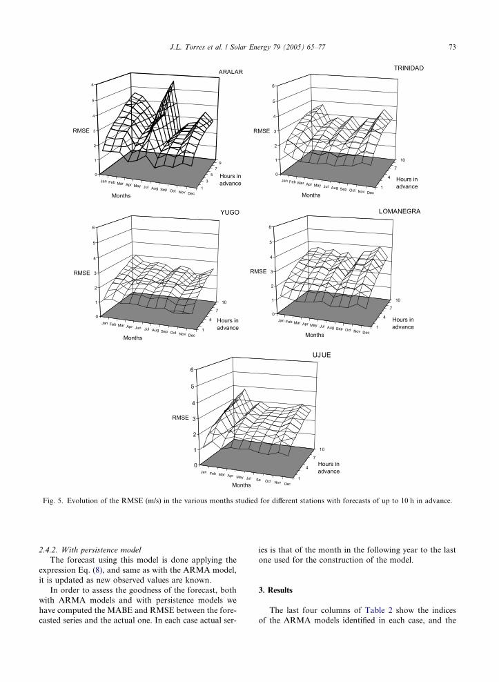
Fig. 5. Evolution of the RMSE (m/s) in the various months studied for different stations with forecasts of up to 10 h in advance.


2.4.2. With persistence model

The forecast using this model is done applying the

expression Eq. (8), and same as with the ARMA model,

it is updated as new observed values are known.

In order to assess the goodness of the forecast, both

with ARMA models and with persistence models we

have computed the MABE and RMSE between the fore-

casted series and the actual one. In each case actual ser-

ies is that of the month in the following year to the last

one used for the construction of the model.

3. Results

The last four columns of Table 2 show the indices

of the ARMA models identified in each case, and the


values of the computed coefficients for each one of

them. In six of the sixty series analyzed it was impos-

sible to find an ARMA model that represented them

and satisfied the Box–Pierce criterion at a level of sig-

nificance of 0.1, as recommended by Box and Jenkins

(1976).

There are up to ten different ARMA models among

those identified, being the most frequent: (1,2) in 37%

of the cases; (1,1) in 29.6% and (1,3) and (1,4) in

9.26% of the cases each, with two cases in which the indi-

ces of the model, and therefore the number of parame-

ters needed, is very high: (1,7) and (1,8).

As indicated, the study was at first applied to a larger

number of stations, for which the same analysis has been

carried out, showing a certain tendency in those stations

with higher average wind speed (Trinidad, Aralar,

Lomanegra, Ujue and Yugo) and consequently of higher

interest for the production of energy, to develop models

with a higher number of parameters, although we have

to point out that it is also in these stations where the

amount of available data was higher. In any case the

02468

101214161820

1 2 3 4 5 6 7

Hours in advance

% im

prov

emen

ts

Fig. 6. Percentage of improvement of the RMSE (averaged over all

opposed to the persistence model.

Table 3

Significant values of the RMSE, by station

Aralar Trinidad

RMSE min m/s 0.97 1.05

Month August March

Av(RMSE 1h) m/s 1.41 1.24

Desv(RMSE 1h) 0.26 0.19

RMSE max m/s 5.56 3.77

Month July November

Av(RMSE 10h) m/s 3.42 3.02

Desv(RMSE 10h) 0.98 0.46

Av(RMSE 5h) m/s 2.83 2.50

DESV(RMSE 5h) 0.66 0.35

most frequent models in all stations are those with

(1,2) and (1,1) orders.

Regarding the forecasts, we include Fig. 4, which dis-

plays the evolution of the RMSE and the MABE when

the forecast is done 1–10 h in advance, both with the ad-

justed ARMAmodel and with the persistence model, and

for the month and station indicated. The behaviour ob-

served in this particular case is repeated in the vast

majority of the other cases, i.e. the errors obtained with

the forecasts done with the ARMA models are always

smaller than the ones obtained with the persistence mod-

els, as only in four cases, and all of them for predictions

1 h in advance, the persistence model is better than the

ARMA model. This result differs from that obtained

by Geerts (1984) who came to the conclusion that the

RMSE with the persistence model for forecasts 1 or 1 h

in advance, were always smaller than those obtained with

the ARMA models. In contrast, results are similar to

those obtained byMilligan et al. (2003) who also indicate

that ARMA models provide significant improvements

over persistence models even for short forecast periods.

8 9 10

Aralar

Trinidad

Lomanegra

Yugo

Ujue

the months) of the forecast when the ARMA model is used, as

Lomanegra Yugo Ujue

1.05 0.90 1.18

August October January

1.19 1.09 1.43

0.11 0.12 0.24

4.00 3.00 3.81

November January February

3.40 2.42 2.89

0.32 0.28 0.34

2.55 2.06 2.47

0.25 0.21 0.29

8

RMSE

normalized

1 6.1-5.5

2 5.5-4.9

3 4.9-4.4

4 4.4-3.8

5 3.8-3.3

6 3.3-2.7

7 2.7-2.2

8 2.2-1.6

9 1.6-1.1

10 1 1 0 5

(a) (b)

RMSE

normalized

1 6.4-5.8

2 5.8-5.2

3 5.2-4.7

4 4.7-4.1

5 4.1-3.5

6 3.5-2.9

7 2.9-2.3

8 2.3-1.7

9 1.7-1.1

10 1.1-0.5

11 1.5-0.0

5 10 15 20 25 30 35

2

4

6

8

10

ahea

d

ahea

d

9

8

10

5

4

11

9 7

6

02468

1012

0 5 10 15 20 25 30 35 0 5 10 15 20 25 30

% o

ccur

renc

e

% o

ccur

renc

e

% o

ccur

renc

e

% o

ccur

renc

e

% o

ccur

renc

e

5 10 15 20 25 30

2

4

6

8

10

9 9

8

7

4

3

1

10

11

6

2

02468

1012

5 10 15 20 25

2

4

6

8

10

SR

UO

HDA

EH

A

1

4

3

5

6

7

8

9 10

2 1

11

02468

101214

0 5 10 15 20 25

1 8.1-7.3

2 7.3-6.6

3 6.6-5.8

4 5.8-5.1

5 5.1-4.4

6 4.4-3.7

7 3.7-2.9

8 2.9-2.2

9 2.2-1.4

1.4-0.710

RMSE

normalized

1 8.4-7.6

2 7.6-6.9

3 6.9-6.1

4 6.1-5.3

5 5.3-4.6

6 4.6-3.8

7 3.8-3.0

8 3.0-2.3

9 2.3-1.5 10 1.5-0.711 0.7-0.0

1 6.6-6.0

2 6.0-5.4

3 5.4-4.8

4 4.8-4.2

5 4.2-3.6

6 3.6-3.0

7 3.0-2.4

8 2.4-1.8

9 1.8-1.2

1.2-0.6105 10 15 20 25

2

4

6

8

10

HO

UR

S AH

EAD

HO

UR

S A

HE

AD

2

3

4

6

7

8

9

1

5

10

11

02468

101214

0 5 10 15 20 25

5 10 15 20 25

2

4

6

8

10

2

36

8

9

10

11

1

4

5

7

02468

101214

0 5 10 15 20 25wind speed (m/s)

wind speed (m/s)

wind speed (m/s)wind speed (m/s)

wind speed (m/s)

wind speed

wind speed

wind speed wind speed

wind speed

(c) (d)

(e)

RMSE

normalized

RMSE

normalized

11 0.7-0.0

11 0.7-0.0

Fig. 7. Plotting of the yearly standardised RMSE values for each wind speed range and for the indicates hours in advance in Aralar (a),

Trinidad (b), Lomanegra (c), Yugo (d) and Ujue (e) stations. In the lower graph, the percentage of occurrence of the velocities for each

of the ranges is included.



In any case, as we expected, both the RMSE and the

MABE increase as the moment of the forecast moves

away from the last observed datum available. To that ef-

fect, Fig. 5 represents the evolution of the RMSE in the

various months studied for the different stations, when

the forecast goes from 1 to 10 h in advance, and Fig. 6

shows the improvement in percentage of the average

RMSE for each station and advance period of the fore-

cast when the ARMA model is used as opposed to the

persistence model. There is an improvement of 2–5%

for forecasts 1 h in advance, and 12–20% for 10 h in

advance.

In Table 3 we have included, for all the months stud-

ied at each station, the minimum value (and the respec-

tive month), the average value and the standard

deviation of the RMSE for forecasts 1 h in advance;

the maximum value (and the respective month), average

value and the standard deviation of the RMSE for fore-

casts 10 h in advance and the average value and the

standard deviation of the RMSE for forecasts 5 h in ad-

vance. As it can be noticed, the minimum values are in

the 1 m/s range, the maximum values in the 3 m/s range,

and for forecasts 5 h in advance, in the 2.5 m/s range, so

that normally, when doing a forecast more than a few

hours in advance, the RMSE are over 1.5 m/s, the limit

that Geerts considers acceptable.

From a wind energy generation point of view, the

errors made are more important at wind velocities at

which the wind turbines are working, so we have evalu-

ated the RMSE at wind speed intervals of 1 m/s, from

the minimum to the maximum observed in each actual

time series. In order to obtain summarized information

of each one of the five stations studied, we have normal-

ized the values obtained each month in the different

speed intervals and for each given time in advance with

respect to the highest value observed. Finally, we have

added up the normalized values of the different months

for each speed interval and advance period, resulting in

the charts shown in Fig. 7.

4. Conclusions

The process of transformation and standardization

of the hourly wind speed time series used provide the

necessary conditions to represent them using ARMA

models, as can be proved by the fact that in most cases

it was possible to identify and validate the appropriate

model.

The behaviour of the forecasts in the transformed

series is similar to that of the actual velocities, so we

can conclude that the use of the hourly mean and stand-

ard deviation values used on a monthly basis for the

standardization is accurate.

The deterioration of the accuracy of the forecast as

the forecasting period increases indicates that if the

RMSE is not to exceed the 1.5 m/s threshold, the meth-

od applied is only valid for very short-term forecasts.

The use of ARMA models improves significantly the

wind speed forecasts as compared to those obtained with

persistence models. In only very few cases the errors

with the latter are smaller than the ones obtained with

ARMA models, and always for forecasts 1 h in advance.

In fact, for forecasts 10 h in advance, the errors with

ARMA models are between 12% and 20% smaller than

with persistence models.

We have not found significant differences in the

behaviour of the models for the five locations, either

mountainous regions or flat areas, where the data were

collected by the weather stations.

The RMSE obtained separately for different wind

speed demonstrate differences depending on the wind

speed values, showing the following tendencies: Firstly,

for wind speeds within a range of 4–11 m/s (that gener-

ally correspond to the ascending part of the power

curve of the wind turbines, between the cut-in and

rated speeds), the errors have relatively low values

and are hardly affected by the extent of the forecast.

Secondly, the biggest relative errors tend to fall within

high wind speeds, higher than the rated speeds of most

wind turbines, and for which the power regulation

mechanisms of the wind turbines are usually activated.

Thirdly, the lowest obtained RMSEs correspond to the

highest observed wind speeds. In most cases, wind tur-

bines are stopped for safety reasons at this speed range.

This fact, together with the low percentage of occur-

rence of high wind speeds, makes conclusions in this

speed range to be of little significance. In addition,

the low value of the normalized RMSE is favoured

by this low occurrence which may distort the con-

clusion.

Acknowledgments

The present study was carried out under a research

project supported by the Department of Culture and

Education, Government of Navarre, Spain. Authors

would like to thank Eloisa Izco for her help with tables

and figures.

Appendix A

A.1. General equation of ARMA model

ð1� /1 � B� /2 � B2 � � � � � /p � BpÞ � V �n;y

¼ ð1� h1 � B� h2 � B2 � � � � � hq � BqÞ � an;y : ðA:1Þ


A.2. Algorithm for ARMA models applicability

Appendix B

Mathematical expressions for Durbins relations:

uðn; nÞ ¼r1 l ¼ 1;

rðlÞ�Pl�1

j¼1ul�1;j �rl�j

1�Pl�1

j¼1ul�1;j �rj

l ¼ 2; 3; . . . ; L;

8><>:

ui;j ¼ ul�1;j � ul;l � ul�1;l�j i ¼ 1; 2; . . . ; L� 1:

ðB:2Þ

References

Balouktsis, A., Tsanakas, D., Vachtsevanos, G., 1986. Stoch-

astic simulation of hourly and daily average wind speed

sequences. Wind Engineering 10 (1), 1–11.

Beguin, J.M., Gourieroux, Ch., Monfort, A., 1980. Identifica-

tion of a mixed autoregressive-moving average process: the

corner method. In: Anderson, O.D. (Ed.), Time Series.

North-Holland, pp. 423–436.

Box, J.E.P., Jenkins, G.M., 1976. Times Series Analysis,

Forecasting and Control. Holden-Day, San Francisco.

Brown, B.G., Katz, R.W., Murphy, A.H., 1984. Time series

models to simulate and forecast wind speed and wind

power. Journal of Climate and Applied Meteorology 23,

1184–1195.

Chou, K.C., Corotis, R.B., 1981. Simulation of hourly wind

speed and array wind power. Solar Energy 26 (3), 199–

212.

Daniel, A.R., Chen, A.A., 1991. Stochastic simulation and

forecasting of hourly average wind speed sequences in

Jamaica. Solar Energy 46 (1), 1–11.

Dubey, S.D., 1967. Normal and Weibull distributions. Naval

Research Logistics Quarterly 14, 69–79.

Garcıa, A., Torres, J.L., Prieto, E., De Francisco, A., 1998.

Fitting wind speed distributions: a case study. Solar Energy

62 (2), 139–144.

Geerts, H.M., 1984. Short range prediction of wind speeds: a

system-theoretic approach. In: Proceedings of European

Wind Energy Conference. Hamburg, Germany, pp. 594–

599.

Kamal, L., Jafri, Y.Z., 1997. Time series models to simulate and

forecast hourly averaged wind speed in Quetta, Pakistan.

Solar Energy 61 (1), 23–32.

Milligan, M., Schwartz, M., Wan, Y., 2003. Statistical wind

power forecasting for US wind farms. NREL/CP-500-

35087, November 2003.

Nfaoui, H., Buret, J., Saygh, A.A.M., 1996. Stochastic simu-

lation of hourly average wind speed sequences in Tangiers.

Solar Energy 56 (3), 301–314.

Sfestos, A., 2000. A comparison of various forecasting tech-

niques applied to mean hourly wind speed time series.

Renewable Energy 21, 23–35.

Tsay, R.S., Tiao, G.C., 1984. Consistent estimates of autore-

gressive parameters and extended sample autocorrelation

function for stationary and nonstatitionary ARMA models.

Journal of the American Statistical Association 79 (385),

84–96.

Torres, J.L., Garcıa, A., Prieto, E., De Francisco, A., 1999.

Characterization of wind speed data according to wind

direction. Solar Energy 66 (1), 57–64.

Forecast of hourly average wind speed with ARMA models in Navarre (Spain

Documents

Transcript of Forecast of hourly average wind speed with ARMA models in Navarre (Spain