A near-global, 2-hourly data set of atmospheric precipitable water

from ground-based GPS measurements

Junhong Wang,1 Liangying Zhang,1 Aiguo Dai,1 Teresa Van Hove,2 and Joel Van Baelen3

Received 18 May 2006; revised 2 March 2007; accepted 23 March 2007; published 6 June 2007.

[1] A 2-hourly data set of atmospheric precipitable water (PW) has been produced fromthe zenith path delay (ZPD) derived from ground-based Global Positioning System (GPS)measurements. The PW data are available every 2 hours from 80 to 268 InternationalGNSS Service (IGS, formally International GPS Service) ground stations from 1997 to2004. The accuracy of the IGS ZPD product is roughly 4 mm. An analysis technique isdeveloped to convert ZPD to PW on a global scale. Special efforts are made onderiving surface pressure (Ps) and water-vapor-weighted atmospheric mean temperature(Tm), which are two key parameters for converting ZPD to PW. Ps is derived from global,3-hourly surface synoptic observations with temporal, vertical and horizontaladjustments. Tm is calculated from NCEP/NCAR reanalysis with temporal, vertical andhorizontal interpolations. The derived Ps and Tm at the GPS location and height haveroot-mean-square (rms) errors of 1.65 hPa and 1.3 K, respectively. A theoretical erroranalysis concludes that typical PW error associated with the errors in ZPD, Tm and Ps is onthe order of 1.5 mm. The PW data set is compared with radiosonde, microwave radiometer(MWR) and satellite data. The GPS and radiosonde PW comparisons at 98 stationsaround the globe show a mean difference of 1.08 mm (drier for radiosonde data) with astandard deviation of differences of 2.68 mm, which corresponds to mean percentagedifference and standard deviation of 5.5% and 10.6%, respectively. The bias is primarilydue to known dry biases in the Vaisala radiosonde data. The RMS difference betweenGPS and radiosonde/MWR data ranges from 1.2 mm to 2.83 mm. The latitudinal andseasonal variations of PW derived from the GPS data agree well with that fromInternational Satellite Cloud Climatology Project (ISCCP) data if the ISCCP data aresampled only at grid boxes containing GPS stations. The large difference between GPSand ISCCP data in the subtropics is interesting, but is not easily explained. Thecomparisons did not reveal any systematic bias in GPS PW data and show that a RMSdifference of less than 3 mm between GPS-derived PW and other data sets is achieved.The comparison study also illustrates the value of GPS-estimated PW for examiningthe quality of other data sets, such as those from radiosondes and MWR. Preliminaryanalysis of this data set shows interesting and significant diurnal variations in PW in fourdifferent regions.

Citation: Wang, J., L. Zhang, A. Dai, T. Van Hove, and J. Van Baelen (2007), A near-global, 2-hourly data set of atmospheric

precipitable water from ground-based GPS measurements, J. Geophys. Res., 112, D11107, doi:10.1029/2006JD007529.

1. Introduction

[2] Atmospheric water vapor plays a crucial role inEarth’s energy and water cycles through absorbing solarand infrared radiation, releasing latent heat, transportingwater, and forming clouds and precipitation. Water vapor is

the most abundant and also the most important greenhousegas in the atmosphere, thus it plays an important role inglobal climate change. Precipitable water (PW), which isalso referred to as total column or integrated water vapor, isthe total water vapor contained in an air column from theEarth’s surface to the top of the atmosphere. About 45–65%of the PW is included in the surface-850 hPa layer [Rossand Elliott, 1996].[3] Traditionally, there have been two atmospheric water

vapor observing systems on a global scale: the radiosoundings and satellite observations with passive sensors.Atmospheric humidity observations from radiosondes havebeen used to study water vapor variability and trends [e.g.,Gaffen et al., 1991; Ross and Elliott, 1996, 2001; Zhai andEskridge, 1997; Wang et al., 2001]. Satellite observations

JOURNAL OF GEOPHYSICAL RESEARCH, VOL. 112, D11107, doi:10.1029/2006JD007529, 2007ClickHere

for

FullArticle

1National Center for Atmospheric Research, Boulder, Colorado, USA.2University Corporation for Atmospheric Research, Boulder, Colorado,

USA.3Laboratoire de Meteorologie Physique, Observatoire de Physique du

Globe de Clermont-Ferrand, CNRS-Universite Blaise Pascal, Aubiere,France.

Copyright 2007 by the American Geophysical Union.0148-0227/07/2006JD007529$09.00

D11107 1 of 17

from either infrared sounders or microwave radiometers[e.g., Rossow and Schiffer, 1999; Gao et al., 2004], aloneor blended with radiosonde data, such as the NASA WaterVapor Project (NVAP) data set [Randel et al., 1996], havealso been used to quantify water vapor variability andchanges [e.g., Trenberth et al., 2005]. Many studies haveevaluated these data sets [e.g., Simpson et al., 2001; Amenuand Kumar, 2005; Sudradjat et al., 2005; Trenberth et al.,2005], but two main issues remain unsolved: a lack of high-temporal-resolution observations to resolve high-frequency(e.g., diurnal) variations and the poor quality of radiosondehumidity data for climate change studies.[4] Since the early 1990s, considerable efforts have been

devoted to derive PW using ground-based Global Position-ing System (GPS) measurements [e.g., Bevis et al., 1992,1994; Businger et al., 1996; Rocken et al., 1993, 1997;Tregoning et al., 1998] at high temporal resolution (5 min to2 hours). The advantages of the GPS-derived PW datainclude continuous measurements, availability under allweather conditions, high accuracy (<2 mm in PW), long-term stability and low cost [Ware et al., 2000]. The GPS-derived PW has broad applications, including validatingradiosonde, satellite and reanalysis data [e.g., Yang et al.,1999; Haase et al., 2003; Guerova et al., 2003; Hagemannet al., 2003; Li et al., 2003; Dietrich et al., 2004; VanBaelen et al., 2005], improving numerical weather predic-tion [e.g., Kuo et al., 1993; Vedel and Huang, 2004; Vedel etal., 2004; Gutman et al., 2004a; Gendt et al., 2004],studying diurnal variations of PW [Dai et al., 2002; Wu etal., 2003], and monitoring climate change [e.g.,Gradinarskyet al., 2002]. Although there have been many regionalapplications of ground-based GPS data [see Dai et al.,2002], there have been only a couple of studies to takeadvantage of the growing network of the International GNSSService (IGS) stations around the globe [Beutler et al., 1999;Hagemann et al., 2003; Deblonde et al., 2005]. This studyrepresents the first attempt to use GPS-derived zenith pathdelay (ZPD) at the existing and expanding IGS stations toderive a long-term PW data set on a global scale for climateand weather applications. This new GPS PW data set, whichwill be updated continuously, adds a new source of PW datafor global weather and climate analyses. Among manyscientific objectives of creating such data set, two arehighlighted below.[5] Global radiosonde data represent an increasingly

valuable resource for studies of climate change. Unfortu-nately, the usefulness of radiosonde data for long-termclimate monitoring is limited by errors and biases associatedwith instrument and data processing procedures and byradiosonde changes among stations and with time. One ofthe scientific objectives of creating a global PW data setfrom GPS measurements is to take advantage of theincreasing volume and maturity of GPS data and moreimportantly its long-term stability, and use it to monitorthe quality of global radiosonde data and potentially im-prove the long-term radiosonde climate records.[6] There exist substantial diurnal variations in atmo-

spheric water vapor, both column-integrated values (i.e.,PW) and vertical profiles [e.g., Dai et al., 2002;Wang et al.,2002a]. The water vapor diurnal variations affect surfaceand atmospheric longwave radiation and atmospheric ab-sorption of solar radiation. They are closely related to many

other processes, such as diurnal variations in moist convec-tion and precipitation [Dai et al., 1999], surface windconvergence [Dai and Deser, 1999] and surface evapotrans-piration. The diurnal cycle of water vapor also provides atest bed for many aspects of the physical parameterizationsin weather and climate models. Unfortunately, there is alack of data with high temporal resolution for studying thediurnal cycle of water vapor on the global scale. Thereforeone of scientific objectives for creating a global water vapordata set using high-temporal-resolution GPS measurementsis to analyze the data to document and understand watervapor diurnal variations, and to validate the representationof the water vapor diurnal cycle in climate and weathermodels.[7] The goal of this study is to (1) develop an analysis

technique to derive PW using the ZPD derived from theexisting ground-based GPS measurements on a global scale;(2) apply this technique to produce a near-global, 2-hourlyPW data set; (3) compare the PW data set with othermeasurements, such as those from radiosondes, microwaveradiometers (MWR), and satellites; and (4) use the PW datafor various scientific applications, including documentingPW diurnal variations and quantifying time- and space-dependent biases in global radiosonde humidity records.This paper describes the procedure to create the GPS PWdata set, shows comparisons with other measurements, andpresents a few preliminary results of the scientific applica-tions of the derived PW data set. The various data sets usedin this study are described in section 2. In section 3, wedetail the analysis technique and the final GPS PW data setalong with an error analysis on PW. In section 4, wecompare the GPS-derived PW data set with other data setsand briefly mention the scientific applications of the dataset. Preliminary results on PW diurnal variations in fourregions are presented in section 5. Conclusions and futurework are summarized in section 6.

2. Data

2.1. Global GPS ZPD Data

[8] The GPS system is made of a constellation of30 operational satellites circling at 20,200 kilometers abovethe Earth. They are evenly distributed in six orbital planesinclined at 55 degrees and perform a full revolution roughlyevery 12 hours such that up to 12 satellites are visible fromanywhere on the globe at any time. The radio signalstransmitted to the ground-based GPS receivers by thesesatellites include information on timing, satellite navigationand system parameters which allow real-time high-accuracytimekeeping, positioning, and navigation. The current glob-al IGS network consists of 382 receivers (or stations) as of10 February 2006 (Figure 1), and provides continuous GPSorbit tracking, as well as other high-quality navigationproducts in near real time. It is to be noted that in Figure 1only IGS sites have been shown over the continental UnitedStates, while there exist much denser GPS networksincluding the SuomiNet, NOAA/FSL, and other sites toprovide real-time atmospheric sensing [Ware et al., 2003].Likewise, many European countries operate denser net-works for their own purposes but also have regrouped themwithin an European-wide project for meteorological appli-cations which was started under the EC COST-716 project

D11107 WANG ET AL.: GPS WATER VAPOR DATA SET

2 of 17

D11107

auspices (http://www.oso.chalmers.se/geo/cost716.html)[e.g., Haase et al., 2001; Huang et al., 2003; Gendt et al.,2004] and is now continued under the EUMETNET E-GVapproject (http://egvap.dmi.dk). The IGS network has been andis steadily growing from �100 stations in February 1997 to382 stations in February 2006.[9] When traveling from the GPS satellites to the ground-

based GPS receivers, the radio (microwave) signals aredelayed by the ionosphere and the neutral atmosphereusually referred to as the total atmospheric delay or tropo-spheric delay. The ionosphere delay is frequency-dependentand can be removed by the data from dual-frequency GPSreceivers. The atmosphere delays the microwave transmis-sions by slowing the wave propagation and bending theraypath. The delay in signal arrival time can be expressed asan equivalent increase in travel path length. This excesspath length, or total atmospheric delay, is given by [Bevis etal., 1992]

DL ¼Z

L

n sð Þds� G ¼ 10�6

Z

L

N sð Þdsþ S � Gð Þ; ð1Þ

where n(s) is the refractive index as a function of positions along the curved raypath L, G is the straight-linegeometrical path length through the atmosphere (the paththat would occur if the atmosphere was replaced by avacuum), S is the geometrical path length along L, andN(s) = 106(n(s)-1) is atmospheric refractivity. The totalatmospheric delay is computed from the observed traveltime between the location of the GPS receiver and the GPSsatellite using the GPS software (e.g., the GAMIT, GIPSY,and Bernese GPS softwares) and can be partitioned into twoparts – the hydrostatic delay, which is mainly a function ofthe surface pressure at the GPS receiver, and the wet delay,

which depends strongly on total amount of water vaporalong the wave trajectory and weakly on the atmospherictemperature [e.g., Davis et al., 1985]. At any given time aGPS receiver can receive signals from 6–12 GPS satellites.The signals follow slant paths depending on the azimuthand elevation of each satellite. Total delay along the zenith,called zenith path delay (ZPD), is estimated by mappingslant delays to zenith-equivalent values with mappingfunctions [e.g., Niell, 1996]. The ZPD is a sum of zenithhydrostatic delay (ZHD) and zenith wet delay (ZWD).The derivation of PW from ZPD is described in detail insection 3.[10] The ZPD is one of the IGS data products derived

from a subset of the IGS network of the ground-based GPSreceivers [Gendt, 1998]. The final IGS ZPD is obtained bycombining the ZPD solutions from seven IGS data analysiscenters (AC) and has a temporal resolution of 2 hours(Table 1) [Gendt, 1998]. The quality of the combinedZPD is represented by the internal consistency amongACs, and is at the level of 4–6 mm corresponding to�1 mm in PW [Gendt, 1998; Byun et al., 2005]. Each ACestimates their own solution of ZPD using its own subset ofIGS stations, its own strategy and its own final orbits. Twoimportant parameters for the calculation of ZPD are theelevation cutoff angle and the mapping function. Histori-cally, four ACs use an elevation cutoff angle of 15�, whilethe three others use cutoff angles of 7�, 10� or even 20�[Gendt, 1998]. Five ACs implement the Niell mappingfunction, while two ACs have applied the Lanyi and theSaastamoinen mapping function [Gendt, 1998]. Most ofACs use piecewise continuous model to estimate the2-hourly ZPD and take into account AC-dependent biasesin order not to get jumps from missing data. The combined2-hourly ZPD is the piecewise continuous weighted mean of

Figure 1. Geographic distribution of all IGS stations as of 10 February 2006 (circle) and the stationswith ZPD data (triangle) and with PW data (red dot) in 2004. Total number of stations is given in thelegend.

D11107 WANG ET AL.: GPS WATER VAPOR DATA SET

3 of 17

D11107

the ZPD values from all available ACs [Byun et al., 2005].More than 70% of the stations report ZPD solutions fromthree or more ACs, thus allowing good quality combinedZPD values. The standard deviation of ZPD in the finalproduct is the weighted combination of submitted standarddeviations of the AC solutions and serves as an indicator ofoverall agreement. In this study, we rejected ZPD data withstandard deviations greater than 15 mm. This simple crite-rion proved very efficient in removing most of the outliersin the ZPD data. Note that the data that have zero standarddeviations pass the test, but might not represent good ZPDvalues. The 2-hourly ZPD data are available from 1997 at�100 stations each month to 2004 at �335 stations eachmonth, are centered at odd UTC hours (0100, 0300, . . .,2100 UTC) (Figure 2), and can be downloaded online fromthree IGS data archive centers with about 2 � 4-week delayfrom real time.[11] Starting from October 2000, the 5-min ZPD data at

all IGS sites are also produced using the precise pointpositioning approach [Byun et al., 2005; Humphreys etal., 2005]. Note that we still use the 2-hourly legacy productfor the whole period and for all analyses conducted in thisstudy. The new GPS product is superior to the 2-hourlylegacy product with higher temporal resolution and morestations, and claims higher accuracy [Byun et al., 2005]. Thelimitation of the legacy ZPD product is summarized byByun et al. [2005]. For long-term climate applications, thereis a particular concern in the lack of consistency over timein the legacy product resulting from occasional changesmade by individual ACs in their GPS data handling (e.g.,different elevation cutoff angles, revised antenna phasemaps) and their ZPD estimation algorithms (e.g., newmapping functions, different constraint schemes on theanalysis parameters). To minimize the impacts of suchchanges upon the corresponding time series, we haveapplied quality controls on the final PW data (see detailsin section 3).

2.2. Auxiliary Data

[12] A series of auxiliary data (Table 1) are used forconverting ZPD to PW described in section 3 and compar-ing with the GPS-PW data in section 4.

[13] Three-hourly surface synoptic observations of sur-face air pressure (Ps), temperature (Ts) and other meteoro-logical variables are available from over 15,000 stationsaround the globe from 1997 to present [Dai and Wang,1999]. The Ps and Ts data are used to calculate the Ps at GPSstations with temporal, horizontal and vertical interpolations(see section 3). The synoptic data are screened using a rangecheck and an outlier check. The range limits are �80�C to50�C for Ts and 550 hPa to 1100 hPa for Ps. The rangecheck removes �0.012% of data points. The outlier checkremoves data points outside the range of annual mean plus/minus three standard deviations at each weather station,which excludes �0.6% of data points.[14] The National Centers for Environmental Prediction/

National Center for Atmospheric Research (NCEP/NCAR)global reanalysis products are available from 1948 topresent at 6 hour intervals and T62 (�1.875� � 1.875�)horizontal resolution with 28 hybrid vertical levels (Table 1)[Kalnay et al., 1996]. The 6-hourly geopotential height,temperature and relative humidity profiles from the NCEP/

Figure 2. Number of stations with ZPD (triangle) and PW(dot) data for each month from February 1997 to December2004.

Table 1. Characteristics of Data Sets Used in This Study

Name Variables Spatial Coverage Spatial Resolution Temporal Resolution Temporal Coverage Sources

Legacy GPSZPD

ZPD �100–335 stations point 2 hours Feb 1997–present ftp://cddis.gsfc.nasa.gov/gps/products/trop/

New GPS ZPD ZPD �180–290 stations point 5 min Oct 2000-present ftp://cddisa.gsfc.nasa.gov/gps/products/trop_new

Synopticobservations

Ps, Ts, etc. �15,000 stations point 3 hours 1975–present http://dss.ucar.edu/datasets/ds464.0/

NCEP/NCARReanalysis

�35 (surfaceand upper air)

gridded, globe 94 � 192,28 levels

6 hours 1948–present http://dss.ucar.edu/datasets/ds090.0/

IGRA P, T, RH,wind profiles

1538 stations point 1–4 dailyat 0000/0600/1200/1800 UTC

1938–present ftp://ftp.ncdc.noaa.gov/pub/data/igra

MWR at Darwin PW and others 12.42�S, 130.89�E,29.9 m

point �24–32 s Apr 2002–present http://www.archive.arm.gov

MWR at Toulouse PW and others 43.56�N, 1.48�E,211.6 m

point 7.5 min 22 Aug to21 Oct 2002

Van Baelen et al. [2005]

MWR at Onsala PW and others 57.395�N,11.925�E, 10 m

point �12 s 1993–present Elgered and Jarlemark[1998]

ISCCP PW and others globe 2.5� � 2.5� monthly 1983–2004 http://isccp.giss.nasa.gov/products/browsed2.html

D11107 WANG ET AL.: GPS WATER VAPOR DATA SET

4 of 17

D11107

NCAR reanalysis are used to calculate Tm with someadjustments (see section 3).[15] The Integrated Global Radiosonde Archive (IGRA)

is a newly released radiosonde data set from NOAA’sNational Climatic data Center (NCDC) (Table 1) [Durreet al., 2006]. The data set consists of 1–4 radiosondeobservations per day at more than 1,000 globally distributedstations for the period 1938 to present [Wang et al., 2005].The PW data from the GPS and radiosonde are compared atcolocated stations in section 4.[16] The GPS-derived PW data are also compared with

the PW from microwave radiometers (MWR) at Darwin,Australia, Toulouse, France, and Onsala, Sweden (seeTable 1 for details). The MWR PW data at Darwin werecollected at the Atmospheric Radiation Measurement(ARM) Darwin site, which is located about 53 km north-west of the Darwin GPS station (DARW). A two-channel(23.8 GHz and 31.4 GHz) MWR has been operating at theARM Darwin site since April of 2002. The 2-month(22 August to 21 October 2002) MWR data in Toulouse,France are from Van Baelen et al. [2005], where a Radio-metrics Co. 12-channel microwave radiometer profiler wasoperated. AMWR collocated with the GPS receiver at Onsalameasures the sky emission at 21.0 GHz and 31.4 GHz and hasbeen in operation in a continuous sky-scanning mode since1993 [Elgered and Jarlemark, 1998]. We obtained the equiv-alent zenith wet delay data from this MWR from G. Elgered(personal communication, 2005) and converted them to PWusing Emardson et al. [1998, equation (3)].[17] Eight-year (1997–2004) monthly mean PW data

from the International Satellite Cloud Climatology Project(ISCCP) [Rossow and Schiffer, 1999] were downloadedfrom http://isccp.giss.nasa.gov/products/browsed2.html.The ISCCP water vapor data set is produced from opera-tional TOVS (TIROS Operational Vertical Sounder) prod-ucts with relayering, regridding and filling with aclimatological PW data [Zhang et al., 2004]. Zhang et al.[2006] shows that global mean PW difference betweenISCCP and other data sets is less than 3 mm over landand up to 3.5 mm over ocean. The latitudinal and seasonalvariations of PW from GPS are compared with those fromthe ISCCP data set.

3. Analysis Technique and GPS PW Data Set

3.1. Analysis Technique

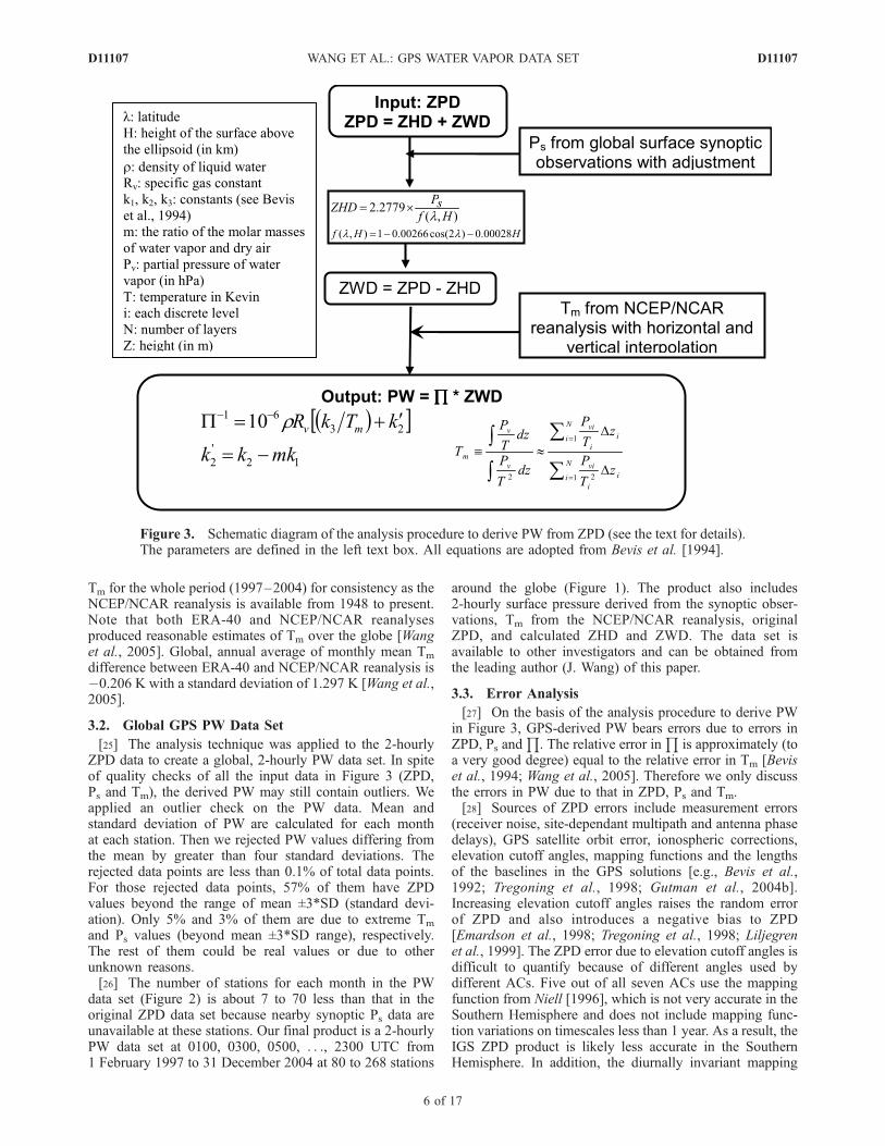
[18] The ZPD can be partitioned into two parts, the ZHDand ZWD. The ZHD can be estimated from the surfacepressure with good accuracy [Saastamoinen, 1972; Askneand Nordius, 1987; Elgered et al., 1991]. The ZWD can beobtained by subtracting ZHD from ZPD. Since the ZWD isa function of atmospheric water vapor and temperature, thisallows PW to be calculated if the water vapor pressure-weighted mean temperature of the atmosphere (Tm) can beestimated [Elgered et al., 1991; Bevis et al., 1992, 1994].We follow Bevis et al. [1992, 1994] for deriving PW fromZPD. In summary, Ps and Tm are required to convert ZPD toPW. The analysis technique is summarized in Figure 3. Psand Tm calculations are described in detail below.Gutman et al.[2003] presented a method to derive Ps from surface synopticobservations and Tm from a mesoscale numerical model

output, which is similar to a certain extent to our methodexplained below, but has some fundamental differences.[19] Only about 70 IGS stations provide surface meteo-

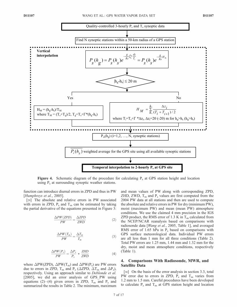
rological data including Ps. In addition, on the basis of ourevaluation, the GPS surface meteorological data are verynoisy and cannot be used without careful examination andquality control [Wang et al., 2006]. Therefore 2-hourly Ps atthe GPS station was derived from the 3-hourly surfacesynoptic observations through spatial and temporal interpo-lation. The steps for such calculation are listed in Figure 4and summarized below:[20] 1. For a given GPS station, a 50-km radius is drawn

to select nearby synoptic stations. Gutman et al. [2003]concluded that the synoptic stations within 50 km of a GPSstation can be used to derive Ps at the GPS site with about0.5 hPa bias.[21] 2. For each of these stations, the hydrostatic and ideal

gas equations are used to adjust Ps from the synoptic stationheight (hs), referred to as Ps(hs), to that at the GPS stationheight (hg), referred to as Ps(hg) in Figure 4. The temper-ature profile from hs to hg is constructed by assuming atypical lapse rate for moist adiabatic conditions, �6.5 K/km.As discussed byWang et al. [2005], the�6.5 K/km lapse rateis a good approximation of the tropospheric mean lapse rate.[22] 3. The Psi(hg) that is Ps(hg) at selected ith station is

averaged for all selected stations using the inverse of theirdistance to the GPS station as the weight to obtain the Ps at

the GPS station height and location (annotated as Ps hg� �

).(4) Ps hg

� �is linearly interpolated in time to the 2-hourly

resolution at 0100, 0300, 0500, . . ., 2300 UTC.[23] Among these steps, the vertical interpolation (step 2)

is the most important one. For example, Figure 5 shows thesize of the correction for Ps at the IGS station Graz, Austria(GRAZ) and a mountain station at Laguna Mountains,California (MONP) derived from two and one nearbysynoptic stations, respectively, when compared to thecorresponding GPS system surface meteorological data.At GRAZ, the scatter of the synoptic Ps from the two stationsis significantly reduced after adjustments. For the mountainstation, the synoptic station is 1072 m above the GPS station.After adjustments, the mean Ps difference between synopticand GPS met data is reduced to �0.93 hPa from 106.42 hPa.However, the adjusted values show a larger dispersionprimarily due to the fact that there can be temporarydepartures from the constant temperature lapse rate usedover such an altitude difference that can affect the adjustmentprocedure. The comparisons of Ps at 48 GPS sites derivedhere with that from the GPS surface meteorological datashow averaged RMS difference of 1.65 hPa.[24] The accuracy of GPS-estimated PW is directly related

to the accuracy of Tm and Ps [Bevis et al., 1994]. Tm can beeither calculated from temperature and humidity profiles orestimated from the surface temperature, Ts. Our evaluationsof various Tm estimates on a global scale show that, in theabsence of local temperature and humidity profile data, thebest option to estimate Tm is to calculate Tm using 6-hourlyERA-40 temperature and humidity profiles with adjustmentto GPS station heights and observation times [Wang et al.,2005]. However, ERA-40 data are currently available from1948 to 2002 only, and it is unclear whether and when thedata after 2002 will be available. Therefore we chose thenext best option, the NCEP/NCAR reanalysis, to calculate

D11107 WANG ET AL.: GPS WATER VAPOR DATA SET

5 of 17

D11107

Tm for the whole period (1997–2004) for consistency as theNCEP/NCAR reanalysis is available from 1948 to present.Note that both ERA-40 and NCEP/NCAR reanalysesproduced reasonable estimates of Tm over the globe [Wanget al., 2005]. Global, annual average of monthly mean Tm

difference between ERA-40 and NCEP/NCAR reanalysis is�0.206 K with a standard deviation of 1.297 K [Wang et al.,2005].

3.2. Global GPS PW Data Set

[25] The analysis technique was applied to the 2-hourlyZPD data to create a global, 2-hourly PW data set. In spiteof quality checks of all the input data in Figure 3 (ZPD,Ps and Tm), the derived PW may still contain outliers. Weapplied an outlier check on the PW data. Mean andstandard deviation of PW are calculated for each monthat each station. Then we rejected PW values differing fromthe mean by greater than four standard deviations. Therejected data points are less than 0.1% of total data points.For those rejected data points, 57% of them have ZPDvalues beyond the range of mean ±3*SD (standard devi-ation). Only 5% and 3% of them are due to extreme Tm

and Ps values (beyond mean ±3*SD range), respectively.The rest of them could be real values or due to otherunknown reasons.[26] The number of stations for each month in the PW

data set (Figure 2) is about 7 to 70 less than that in theoriginal ZPD data set because nearby synoptic Ps data areunavailable at these stations. Our final product is a 2-hourlyPW data set at 0100, 0300, 0500, . . ., 2300 UTC from1 February 1997 to 31 December 2004 at 80 to 268 stations

around the globe (Figure 1). The product also includes2-hourly surface pressure derived from the synoptic obser-vations, Tm from the NCEP/NCAR reanalysis, originalZPD, and calculated ZHD and ZWD. The data set isavailable to other investigators and can be obtained fromthe leading author (J. Wang) of this paper.

3.3. Error Analysis

[27] On the basis of the analysis procedure to derive PWin Figure 3, GPS-derived PW bears errors due to errors inZPD, Ps and

Q. The relative error in

Qis approximately (to

a very good degree) equal to the relative error in Tm [Beviset al., 1994; Wang et al., 2005]. Therefore we only discussthe errors in PW due to that in ZPD, Ps and Tm.[28] Sources of ZPD errors include measurement errors

(receiver noise, site-dependant multipath and antenna phasedelays), GPS satellite orbit error, ionospheric corrections,elevation cutoff angles, mapping functions and the lengthsof the baselines in the GPS solutions [e.g., Bevis et al.,1992; Tregoning et al., 1998; Gutman et al., 2004b].Increasing elevation cutoff angles raises the random errorof ZPD and also introduces a negative bias to ZPD[Emardson et al., 1998; Tregoning et al., 1998; Liljegrenet al., 1999]. The ZPD error due to elevation cutoff angles isdifficult to quantify because of different angles used bydifferent ACs. Five out of all seven ACs use the mappingfunction from Niell [1996], which is not very accurate in theSouthern Hemisphere and does not include mapping func-tion variations on timescales less than 1 year. As a result, theIGS ZPD product is likely less accurate in the SouthernHemisphere. In addition, the diurnally invariant mapping

Figure 3. Schematic diagram of the analysis procedure to derive PW from ZPD (see the text for details).The parameters are defined in the left text box. All equations are adopted from Bevis et al. [1994].

D11107 WANG ET AL.: GPS WATER VAPOR DATA SET

6 of 17

D11107

function can introduce diurnal errors in ZPD and thus in PW[Humphreys et al., 2005].[29] The absolute and relative errors in PW associated

with errors in ZPD, Ps and Tm can be estimated by takingthe partial derivative of the equations presented in Figure 3:

DPW ZPDð ÞPW

¼ DZPD

ZWDð2Þ

DPW Tmð ÞPW

¼ DTm

Tmð3Þ

DPW Psð ÞPW

¼ DPs

Ps*

ZHD

ZWDð4Þ

where DPW(ZPD), DPW(Tm) and DPW(Ps) are PW errorsdue to errors in ZPD, Tm and Ps (DZPD, DTm and DPs),respectively. Using an approach similar to Deblonde et al.[2005], we did an error analysis of GPS_PW usingequations (2)–(4) given errors in ZPD, Tm and Ps andsummarized the results in Table 2. The minimum, maximum

and mean values of PW along with corresponding ZPD,ZHD, ZWD, Tm and Ps values are first computed from the2004 PW data at all stations and then are used to computethe absolute and relative errors in PW for dry (minimum PW),moist (maximum PW) and mean (mean PW) atmosphereconditions. We use the claimed 4 mm precision in the IGSZPD product, the RMS error of 1.3 K in Tm calculated fromthe NCEP/NCAR reanalysis based on comparisons withradiosonde data [Wang et al., 2005, Table 1], and averagedRMS error of 1.65 hPa in Ps based on comparisons withGPS surface meteorological data. Individual PW errorsare all less than 1 mm for all three conditions (Table 2).Total PW errors are 1.25 mm, 1.44 mm and 1.32 mm for thedry, moist and mean atmosphere conditions, respectively(Table 1).

4. Comparisons With Radiosonde, MWR, andSatellite Data

[30] On the basis of the error analysis in section 3.3, totalPW error due to errors in ZPD, Ps and Tm varies from1.2 mm to 1.5 mm. Careful procedures have been developedto calculate Ps and Tm at GPS station height and location

Figure 4. Schematic diagram of the procedure for calculating Ps at GPS station height and locationusing Ps at surrounding synoptic weather stations.

D11107 WANG ET AL.: GPS WATER VAPOR DATA SET

7 of 17

D11107

(see section 3 and Wang et al. [2005]). Additional qualitychecks have been applied to ZPD, Ps and Tm. They all helpminimize the error in PW. In this section the 2-hourly GPS-derived PW data are evaluated through comparisons withthe PW data from a global radiosonde data set (IGRA),MWR measurements at three locations, and the ISCCPsatellite observations. It is always challenging to validateone product without a ground truth. The PW differencesbetween GPS and other data presented below will beexamined carefully and explained on the basis of the bestknowledge of known errors in all data sets. The disagree-ment between GPS and other data sets can originate fromerrors in either data set or both of them.

4.1. Comparisons With Radiosonde Data

[31] In the GPS PW and IGRA data sets for 2003 and2004, we found 102 stations where GPS and radiosondestations are located within 50 km and have elevation differ-

ences less than 100 m. The GPS PW values within an hourof radiosonde launch times are compared with those fromradiosondes at the 102 stations. Radiosonde temperatureand humidity profiles are required to reach at least 300 hPafor the calculation, and have data available at the surfaceand at least five (four) standard pressure levels above thesurface for stations below (above) 1000 hPa. The analysis ofhow sensitive PW is to missing data above the tropopause,300 hPa, 500 hPa and 700 hPa shows that missing dataabove 500 hPa and 300 hPa would introduce a dry bias of2.44% and 0.61% in PW, respectively. After enforcing therequirement on the radiosonde data, four stations have lessthan 50 pairs of matched data points and thus are removedfrom the comparisons. Figure 6 shows the mean andstandard deviation of the GPS – IGRA PW difference fromall the 98 stations, which are grouped and separated byradiosonde types. The mean difference is 1.08 mm (drier inthe radiosonde data), which results primarily from the drybiases at 76 stations launching Vaisala sondes [cf. Wang etal., 2002b]. MRZ/Mars (Russian) and IM-MK3 (Indian)radiosondes show systematic moist bias (Figure 6). All threesites launching IM-MK3 radiosondes have the largeststandard deviation of the difference (larger than 6.5 mm).The RMS difference computed from all data points at all98 stations is 2.83 mm, which is consistent with the 2–3 mmRMS error of GPS-derived PW by previous studies [e.g.,Gendt et al., 2004; Tregoning et al., 1998; Dietrich et al.,2004; Deblonde et al., 2005]. The RMS error of 2.83 mmbased on comparisons with radiosonde data is larger thanthat of <1.5 mm estimated from the theoretical calculationin section 4. This is not surprising because of uncertaintiesin radiosonde PW data, spatial and temporal separationsbetween GPS and radiosonde data and the fact that GPSobservations by viewing satellites in all directions sample adifferent volume of air than a radiosonde [Liou et al., 2001;Braun, 2004].[32] Figure 7 compares the GPS and radiosonde PWat six

individual stations. The GPS PW at HERT (U.K.) andNYA1 (Norway) agrees well with the radiosonde data(Figure 7). At the two Brazilian stations (Figure 7, middle)where Vaisala RS80-A radiosondes were launched, radio-sonde PW is systematically drier than GPS PW because ofknown dry bias in Vaisala radiosonde data [Wang et al.,2002b]. Radiosonde PW at a Russian station (KHAJ) issystematically larger than the GPS PW by 2.64 mm onaverage, which is possibly due to the slow response of theRussian radiosonde’s humidity sensor (goldbeater’s skin).The comparison at an India station (BAN2) has the largestscatters and shows wetter radiosonde data at PW <�30 mm.The dry and moist biases of upper tropospheric water vaporin capacitive and goldbeater’s skin humidity sensors,respectively, are also revealed by Soden and Lanzante[1996] in comparison to GOES satellite data. The applica-tion of using the GPS PW data to identify the errors/biasesin radiosonde humidity data will be explored further indetail in the future.

4.2. Comparisons With MWR Data

[33] For comparison with the 2-hourly GPS PW, the high-resolution MWR data (Table 1) were interpolated tothe median times of the GPS data (0100, 0300, 0500, . . .,2300 UTC). A second-order polynomial fit was applied to

Figure 5. Comparison of Ps from synoptic stations before(dark dots) and after (grey dots) the adjustments shown inFigure 4 with Ps from GPS surface met data at two GPSstations ((top) GRAZ and (bottom) MONP). Meandifference (synoptic-GPS_met), the standard deviation ofthe difference, and the correlation coefficient are given inthe legends and separated by slashes. The GPS elevationsare given in the title following the station names, and theelevations of synoptic stations are in parentheses.

D11107 WANG ET AL.: GPS WATER VAPOR DATA SET

8 of 17

D11107

all available MWR data points within the GPS 2-hour timewindow (e.g., 0000–0200 UTC for 0100 UTC) to estimatethe values at the times of the GPS data. All MWR measure-ments contaminated by rain were removed from the com-parison by using the wet window flag in the data.[34] The comparison between the GPS at the Darwin GPS

site and MWR PW at the ARM Darwin site for 2002–2004is shown in Figure 8. It can be seen that (1) MWR PW has asystematic positive bias (>20 mm) in 2002 (from July toSeptember), (2) there are some very large MWR PW values(>70 mm) in 2002 and 2003 (only two in 2004), and (3) the3-year data show that MWR PW is systematically higher by�3.17 mm after removing the outliers described in points 1and 2. Since the Darwin GPS site sits 95 m higher than theMWR site, the PW from the MWR site is expected to be

higher. MWR data are also compared with colocated radio-sonde data at the ARM Darwin site (not shown) and havethe same behaviors shown in Figure 8 but with smallerscatter. This suggests that the discrepancies between theGPS at the Darwin GPS site and MWR PW at the ARMDarwin site are mainly attributable to problems in the MWRdata, which are discussed in the ARM data quality reports(J. Liljegren, personal communications, 2005). The bias inMWR PW data from July to September in 2002 resultedfrom elevated sky brightness temperatures for an unknownreason and this was corrected later. The very large PWvalues in 2003 (also some in 2002) are a result of incorrectwet window flag during times of rain and should beremoved. Besides the location-related PW difference, thesystematic moist bias in the MWR data is also due to

Table 2. Maximum, Minimum, and Mean of PW Using 2004 Data at All Stations, Corresponding Values of ZPD, ZHD, ZWD, Tm and

Ps, GPS PWAbsolute and Relative Errors Computed From Equations (2), (3) and (4) as a Result of Given Errors in ZPD, Ps and Tm for

Dry (Minimum PW), Moist (Maximum PW) and Mean (Mean PW) Atmosphere Conditions, and Total PW Errors

Variable Minimum Maximum Mean Error

PW Errors, mm/%

Dry Moist Mean

PW, mm 4 42 18 – – – –ZPD, mm 2259 2471 2334 4 0.63/15% 0.64/1.5% 0.64/3.6%ZHD, mm 2232 2213 2221 – – – –ZWD, mm 26 259 113 – – – –Tm, K 267 281 274 1.30 0.02/0.5% 0.19/0.5% 0.08/0.5%Ps, hPa 980 971 975 1.65 0.60/14% 0.60/1.5% 0.60/3.3%Total PW error, mm/% – – – – 1.25/30% 1.44/3.5% 1.32/7.5%

Figure 6. GPS-IGRA mean PW differences (in 2003–2004) at 98 stations where IGRA and GPSinstruments are separated by less than 50 km horizontally and less than 100 m in elevation. Differentcolors represent different radiosonde types. Error bars represent the standard deviation of the difference.The legend in the top left corner includes the range and average of mean PW differences, the average ofstandard deviations at all stations, and the percentage of stations with mean differences less than 2 mm.

D11107 WANG ET AL.: GPS WATER VAPOR DATA SET

9 of 17

D11107

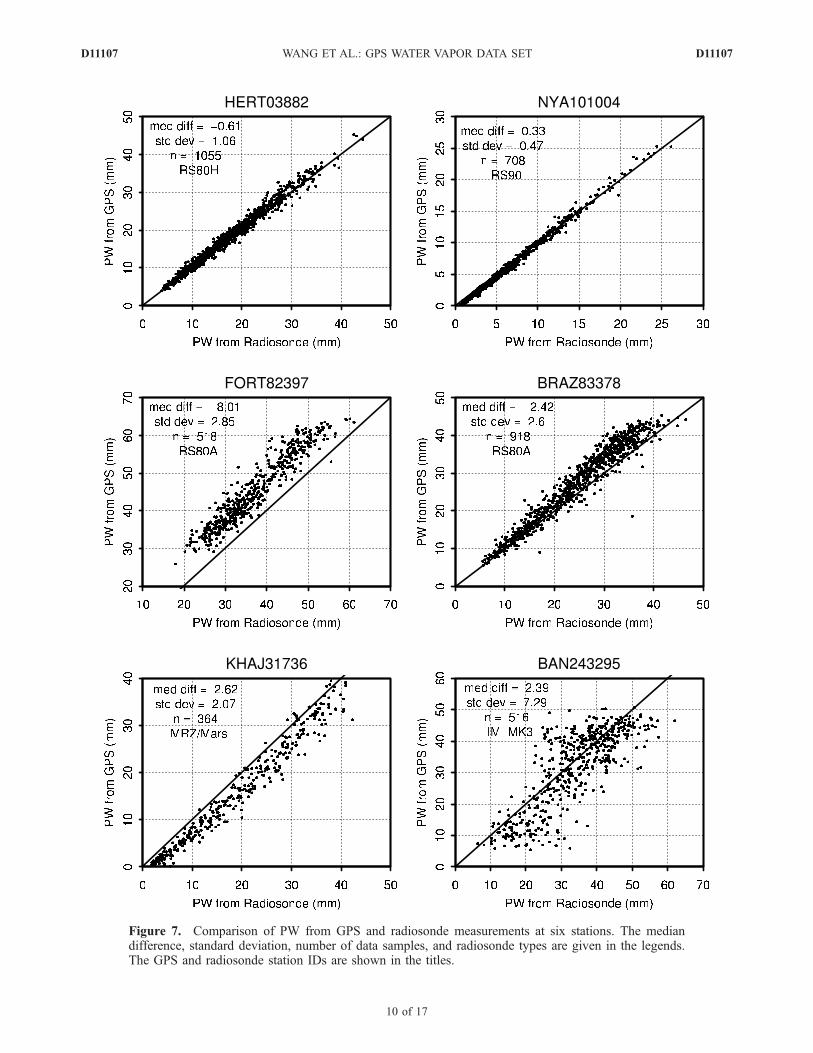
Figure 7. Comparison of PW from GPS and radiosonde measurements at six stations. The mediandifference, standard deviation, number of data samples, and radiosonde types are given in the legends.The GPS and radiosonde station IDs are shown in the titles.

D11107 WANG ET AL.: GPS WATER VAPOR DATA SET

10 of 17

D11107

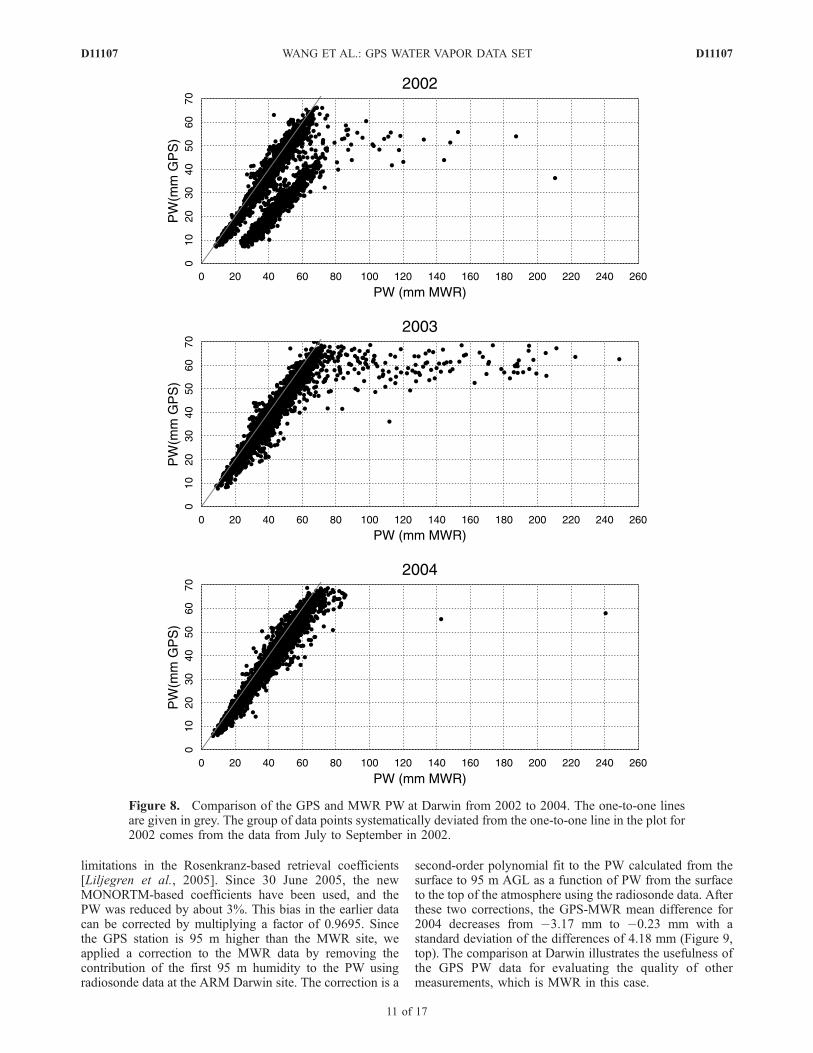
limitations in the Rosenkranz-based retrieval coefficients[Liljegren et al., 2005]. Since 30 June 2005, the newMONORTM-based coefficients have been used, and thePW was reduced by about 3%. This bias in the earlier datacan be corrected by multiplying a factor of 0.9695. Sincethe GPS station is 95 m higher than the MWR site, weapplied a correction to the MWR data by removing thecontribution of the first 95 m humidity to the PW usingradiosonde data at the ARM Darwin site. The correction is a

second-order polynomial fit to the PW calculated from thesurface to 95 m AGL as a function of PW from the surfaceto the top of the atmosphere using the radiosonde data. Afterthese two corrections, the GPS-MWR mean difference for2004 decreases from �3.17 mm to �0.23 mm with astandard deviation of the differences of 4.18 mm (Figure 9,top). The comparison at Darwin illustrates the usefulness ofthe GPS PW data for evaluating the quality of othermeasurements, which is MWR in this case.

Figure 8. Comparison of the GPS and MWR PW at Darwin from 2002 to 2004. The one-to-one linesare given in grey. The group of data points systematically deviated from the one-to-one line in the plot for2002 comes from the data from July to September in 2002.

D11107 WANG ET AL.: GPS WATER VAPOR DATA SET

11 of 17

D11107

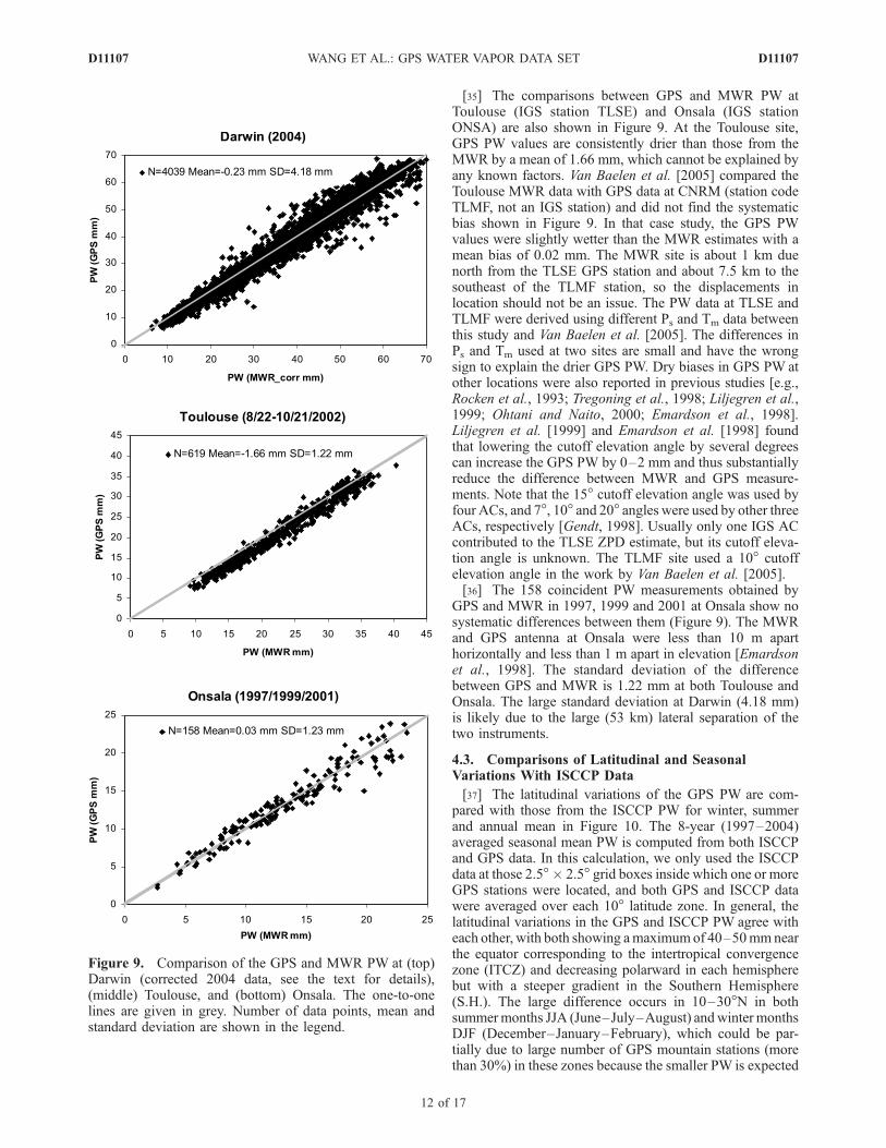
[35] The comparisons between GPS and MWR PW atToulouse (IGS station TLSE) and Onsala (IGS stationONSA) are also shown in Figure 9. At the Toulouse site,GPS PW values are consistently drier than those from theMWR by a mean of 1.66 mm, which cannot be explained byany known factors. Van Baelen et al. [2005] compared theToulouse MWR data with GPS data at CNRM (station codeTLMF, not an IGS station) and did not find the systematicbias shown in Figure 9. In that case study, the GPS PWvalues were slightly wetter than the MWR estimates with amean bias of 0.02 mm. The MWR site is about 1 km duenorth from the TLSE GPS station and about 7.5 km to thesoutheast of the TLMF station, so the displacements inlocation should not be an issue. The PW data at TLSE andTLMF were derived using different Ps and Tm data betweenthis study and Van Baelen et al. [2005]. The differences inPs and Tm used at two sites are small and have the wrongsign to explain the drier GPS PW. Dry biases in GPS PW atother locations were also reported in previous studies [e.g.,Rocken et al., 1993; Tregoning et al., 1998; Liljegren et al.,1999; Ohtani and Naito, 2000; Emardson et al., 1998].Liljegren et al. [1999] and Emardson et al. [1998] foundthat lowering the cutoff elevation angle by several degreescan increase the GPS PW by 0–2 mm and thus substantiallyreduce the difference between MWR and GPS measure-ments. Note that the 15� cutoff elevation angle was used byfour ACs, and 7�, 10� and 20� angles were used by other threeACs, respectively [Gendt, 1998]. Usually only one IGS ACcontributed to the TLSE ZPD estimate, but its cutoff eleva-tion angle is unknown. The TLMF site used a 10� cutoffelevation angle in the work by Van Baelen et al. [2005].[36] The 158 coincident PW measurements obtained by

GPS and MWR in 1997, 1999 and 2001 at Onsala show nosystematic differences between them (Figure 9). The MWRand GPS antenna at Onsala were less than 10 m aparthorizontally and less than 1 m apart in elevation [Emardsonet al., 1998]. The standard deviation of the differencebetween GPS and MWR is 1.22 mm at both Toulouse andOnsala. The large standard deviation at Darwin (4.18 mm)is likely due to the large (53 km) lateral separation of thetwo instruments.

4.3. Comparisons of Latitudinal and SeasonalVariations With ISCCP Data

[37] The latitudinal variations of the GPS PW are com-pared with those from the ISCCP PW for winter, summerand annual mean in Figure 10. The 8-year (1997–2004)averaged seasonal mean PW is computed from both ISCCPand GPS data. In this calculation, we only used the ISCCPdata at those 2.5�� 2.5� grid boxes inside which one or moreGPS stations were located, and both GPS and ISCCP datawere averaged over each 10� latitude zone. In general, thelatitudinal variations in the GPS and ISCCP PW agree witheach other, with both showing amaximumof 40–50mmnearthe equator corresponding to the intertropical convergencezone (ITCZ) and decreasing polarward in each hemispherebut with a steeper gradient in the Southern Hemisphere(S.H.). The large difference occurs in 10–30�N in bothsummermonths JJA (June–July–August) andwinter monthsDJF (December–January–February), which could be par-tially due to large number of GPS mountain stations (morethan 30%) in these zones because the smaller PW is expected

Figure 9. Comparison of the GPS and MWR PW at (top)Darwin (corrected 2004 data, see the text for details),(middle) Toulouse, and (bottom) Onsala. The one-to-onelines are given in grey. Number of data points, mean andstandard deviation are shown in the legend.

D11107 WANG ET AL.: GPS WATER VAPOR DATA SET

12 of 17

D11107

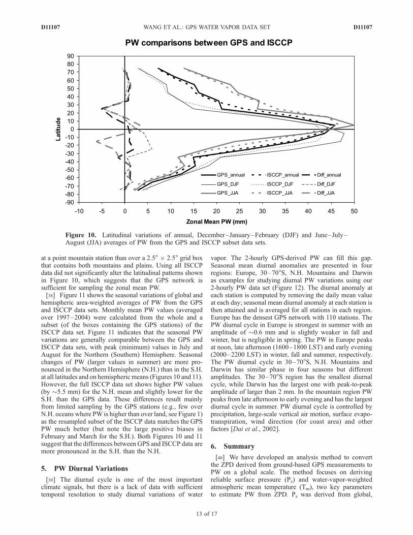
at a point mountain station than over a 2.5� � 2.5� grid boxthat contains both mountains and plains. Using all ISCCPdata did not significantly alter the latitudinal patterns shownin Figure 10, which suggests that the GPS network issufficient for sampling the zonal mean PW.[38] Figure 11 shows the seasonal variations of global and

hemispheric area-weighted averages of PW from the GPSand ISCCP data sets. Monthly mean PW values (averagedover 1997–2004) were calculated from the whole and asubset (of the boxes containing the GPS stations) of theISCCP data set. Figure 11 indicates that the seasonal PWvariations are generally comparable between the GPS andISCCP data sets, with peak (minimum) values in July andAugust for the Northern (Southern) Hemisphere. Seasonalchanges of PW (larger values in summer) are more pro-nounced in the Northern Hemisphere (N.H.) than in the S.H.at all latitudes and on hemispheric means (Figures 10 and 11).However, the full ISCCP data set shows higher PW values(by �5.5 mm) for the N.H. mean and slightly lower for theS.H. than the GPS data. These differences result mainlyfrom limited sampling by the GPS stations (e.g., few overN.H. oceans where PW is higher than over land, see Figure 1)as the resampled subset of the ISCCP data matches the GPSPW much better (but note the large positive biases inFebruary and March for the S.H.). Both Figures 10 and 11suggest that the differences between GPS and ISCCP data aremore pronounced in the S.H. than the N.H.

5. PW Diurnal Variations

[39] The diurnal cycle is one of the most importantclimate signals, but there is a lack of data with sufficienttemporal resolution to study diurnal variations of water

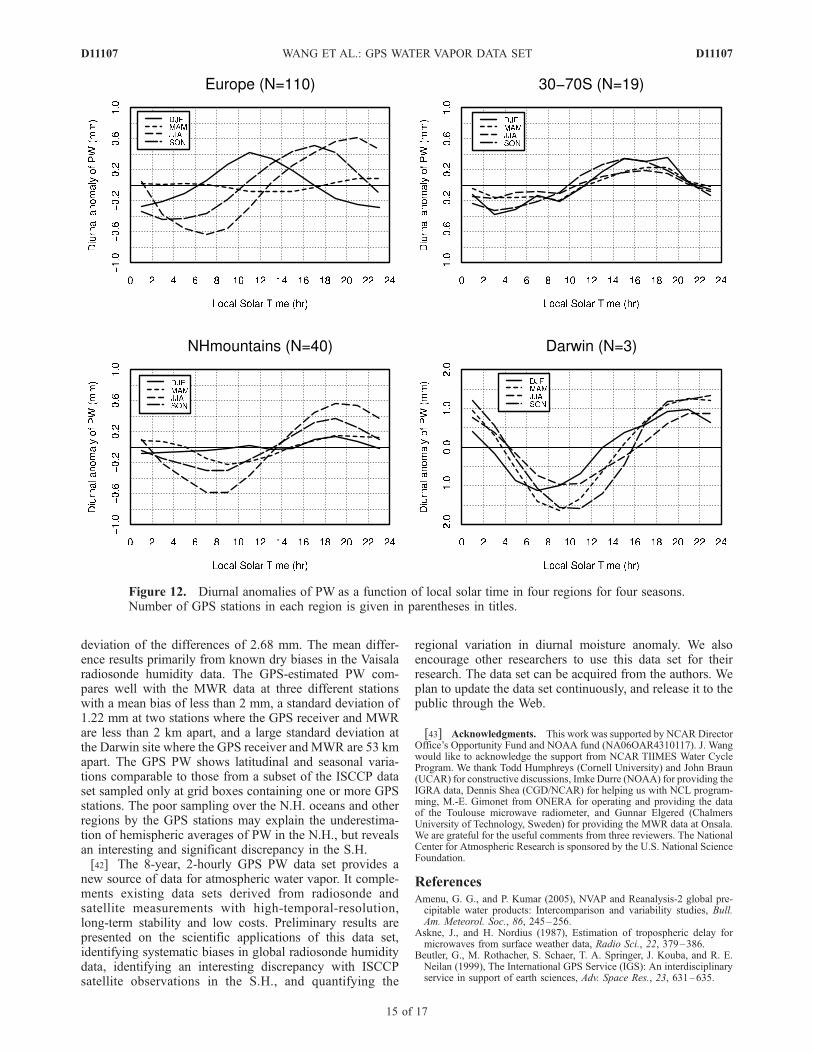
vapor. The 2-hourly GPS-derived PW can fill this gap.Seasonal mean diurnal anomalies are presented in fourregions: Europe, 30–70�S, N.H. Mountains and Darwinas examples for studying diurnal PW variations using our2-hourly PW data set (Figure 12). The diurnal anomaly ateach station is computed by removing the daily mean valueat each day; seasonal mean diurnal anomaly at each station isthen attained and is averaged for all stations in each region.Europe has the densest GPS network with 110 stations. ThePW diurnal cycle in Europe is strongest in summer with anamplitude of �0.6 mm and is slightly weaker in fall andwinter, but is negligible in spring. The PW in Europe peaksat noon, late afternoon (1600–1800 LST) and early evening(2000–2200 LST) in winter, fall and summer, respectively.The PW diurnal cycle in 30–70�S, N.H. Mountains andDarwin has similar phase in four seasons but differentamplitudes. The 30–70�S region has the smallest diurnalcycle, while Darwin has the largest one with peak-to-peakamplitude of larger than 2 mm. In the mountain region PWpeaks from late afternoon to early evening and has the largestdiurnal cycle in summer. PW diurnal cycle is controlled byprecipitation, large-scale vertical air motion, surface evapo-transpiration, wind direction (for coast area) and otherfactors [Dai et al., 2002].

6. Summary

[40] We have developed an analysis method to convertthe ZPD derived from ground-based GPS measurements toPW on a global scale. The method focuses on derivingreliable surface pressure (Ps) and water-vapor-weightedatmospheric mean temperature (Tm), two key parametersto estimate PW from ZPD. Ps was derived from global,

Figure 10. Latitudinal variations of annual, December–January–February (DJF) and June–July–August (JJA) averages of PW from the GPS and ISCCP subset data sets.

D11107 WANG ET AL.: GPS WATER VAPOR DATA SET

13 of 17

D11107

3-hourly surface weather observations with horizontal andvertical adjustments and temporal interpolation. Tm wascalculated from 6-hourly NCEP/NCAR reanalysis profileswith temporal, vertical and horizontal interpolations.[41] This method was applied to the global, 2-hourly ZPD

data product from the IGS data analysis centers to produce a2-hourly PW data set at the 80 to 268 IGS stations available

from February 1997 to December 2004. Total PW errorassociated with errors in ZPD (4 mm), Tm (1.3 K) and Ps(1.65 hPa) is less than 1.5 mm. The GPS-estimated PW wascompared to radiosonde, MWR and satellite PW data. Thecomparisons of PW at 98 colocated GPS and radiosondestations around the globe show a mean difference of1.08 mm (drier in the radiosonde data) and a standard

Figure 11. Monthly mean PW averaged over the globe, Northern and Southern Hemisphere and from1997 to 2004 using the GPS data (solid line), a subset of the ISCCP grid cells with GPS stations locatedinside them (ISCCP_GPS) (long-dashed line) and full ISCCP data (short-dashed line).

D11107 WANG ET AL.: GPS WATER VAPOR DATA SET

14 of 17

D11107

deviation of the differences of 2.68 mm. The mean differ-ence results primarily from known dry biases in the Vaisalaradiosonde humidity data. The GPS-estimated PW com-pares well with the MWR data at three different stationswith a mean bias of less than 2 mm, a standard deviation of1.22 mm at two stations where the GPS receiver and MWRare less than 2 km apart, and a large standard deviation atthe Darwin site where the GPS receiver and MWR are 53 kmapart. The GPS PW shows latitudinal and seasonal varia-tions comparable to those from a subset of the ISCCP dataset sampled only at grid boxes containing one or more GPSstations. The poor sampling over the N.H. oceans and otherregions by the GPS stations may explain the underestima-tion of hemispheric averages of PW in the N.H., but revealsan interesting and significant discrepancy in the S.H.[42] The 8-year, 2-hourly GPS PW data set provides a

new source of data for atmospheric water vapor. It comple-ments existing data sets derived from radiosonde andsatellite measurements with high-temporal-resolution,long-term stability and low costs. Preliminary results arepresented on the scientific applications of this data set,identifying systematic biases in global radiosonde humiditydata, identifying an interesting discrepancy with ISCCPsatellite observations in the S.H., and quantifying the

regional variation in diurnal moisture anomaly. We alsoencourage other researchers to use this data set for theirresearch. The data set can be acquired from the authors. Weplan to update the data set continuously, and release it to thepublic through the Web.

[43] Acknowledgments. This work was supported by NCAR DirectorOffice’s Opportunity Fund and NOAA fund (NA06OAR4310117). J. Wangwould like to acknowledge the support from NCAR TIIMES Water CycleProgram. We thank Todd Humphreys (Cornell University) and John Braun(UCAR) for constructive discussions, Imke Durre (NOAA) for providing theIGRA data, Dennis Shea (CGD/NCAR) for helping us with NCL program-ming, M.-E. Gimonet from ONERA for operating and providing the dataof the Toulouse microwave radiometer, and Gunnar Elgered (ChalmersUniversity of Technology, Sweden) for providing the MWR data at Onsala.We are grateful for the useful comments from three reviewers. The NationalCenter for Atmospheric Research is sponsored by the U.S. National ScienceFoundation.

ReferencesAmenu, G. G., and P. Kumar (2005), NVAP and Reanalysis-2 global pre-cipitable water products: Intercomparison and variability studies, Bull.Am. Meteorol. Soc., 86, 245–256.

Askne, J., and H. Nordius (1987), Estimation of tropospheric delay formicrowaves from surface weather data, Radio Sci., 22, 379–386.

Beutler, G., M. Rothacher, S. Schaer, T. A. Springer, J. Kouba, and R. E.Neilan (1999), The International GPS Service (IGS): An interdisciplinaryservice in support of earth sciences, Adv. Space Res., 23, 631–635.

Figure 12. Diurnal anomalies of PW as a function of local solar time in four regions for four seasons.Number of GPS stations in each region is given in parentheses in titles.

D11107 WANG ET AL.: GPS WATER VAPOR DATA SET

15 of 17

D11107

Bevis, M., S. Businger, T. A. Herring, C. Rocken, R. A. Anthes, and R. H.Ware (1992), GPS meteorology–Remote-sensing of atmospheric water-vapor using the Global Positioning System, J. Geophys. Res., 97(D14),15,787–15,801.

Bevis, M., S. Businger, S. Chiswell, T. A. Herring, R. A. Anthes, C. Rocken,and R. H. Ware (1994), GPS meteorology–Mapping zenith wet delaysonto precipitable water, J. Appl. Meteorol., 33, 379–386.

Braun, J. J. (2004), Remote sensing of atmospheric water vapor with theGlobal Positioning System, Ph.D. thesis, 137 pp., Univ. of Colorado,Boulder, Colo.

Businger, S., S. R. Chiswell, M. Bevis, J. Duan, R. A. Anthes, C. Rocken,R. H. Ware, M. Exner, T. Van Hove, and F. Solheim (1996), The promiseof GPS in atmospheric monitoring, Bull. Am. Meteorol. Soc., 77, 5–18.

Byun, S. H., Y. Bar-Serve, and G. Gendt (2005), The new troposphericproduct of the International GNSS Service, in Proceeding of 2005 IONGNSS Conference, Inst. of Navig., Long Beach, Calif.

Dai, A., and C. Deser (1999), Diurnal and semidiurnal variations in globalsurface wind and divergence fields, J. Geophys. Res., 104, 31,109–31,125.

Dai, A., and J. Wang (1999), Diurnal and semidiurnal tides in global surfacepressure fields, J. Atmos. Sci., 56, 3874–3891.

Dai, A., F. Giorgi, and K. E. Trenberth (1999), Observed and model simu-lated precipitation diurnal cycle over the contiguous United States,J. Geophys. Res., 104, 6377–6402.

Dai, A., J. Wang, R. H. Ware, and T. Van Hove (2002), Diurnal variation inwater vapor over North America and its implications for sampling errorsin radiosonde humidity, J. Geophys. Res., 107(D10), 4090, doi:10.1029/2001JD000642.

Davis, J. L., T. A. Herring, I. I. Shapiro, A. E. E. Rogers, and G. Elgered(1985), Geodesy by radio interferometry: Effects of atmospheric model-ing errors on estimates of baseline length, Radio Sci., 20, 1593–1607.

Deblonde, G., S. Macpherson, Y. Mireault, and P. Heroux (2005), Evalua-tion of GPS precipitable water over Canada and the IGS network, J. Appl.Meteorol., 44, 153–166.

Dietrich, S. V. R., K.-P. Johnsen, J. Miao, and G. Heygster (2004), Com-parison of tropospheric water vapour over Antarctica derived fromAMSU-B data, ground-based GPS data and the NCEP/NCAR reanalysis,J. Meteorol. Soc. Jpn., 82, 259–267.

Durre, I., R. S. Vose, and D. B. Wuertz (2006), Overview of the IntegratedGlobal Radiosonde Archive, J. Clim., 16, 53–68.

Elgered, G., and P. O. J. Jarlemark (1998), Ground-based microwave radio-metry and long-term observations of atmospheric water vapor, Radio Sci.,33, 707–717.

Elgered, G., J. L. Davis, T. A. Herring, and I. I. Shapiro (1991), Geodesy byradio interferometry: Water vapor radiometry of estimation of the wetdelay, J. Geophys. Res., 96, 6541–6555.

Emardson, T. R., G. Elgered, and J. M. Johansson (1998), Three months ofcontinuous monitoring of atmospheric water vapor with a network ofGlobal Positioning System receivers, J. Geophys. Res., 103, 1807–1820.

Gaffen, D. J., T. P. Barnett, and W. P. Elliott (1991), Space and time scalesof global tropospheric moisture, J. Clim., 4, 989–1008.

Gao, B.-C., P. K. Chan, and R.-R. Li (2004), A global water vapor data setobtained by merging the SSMI and MODIS data, Geophys. Res. Lett., 31,L18103, doi:10.1029/2004GL020656.

Gendt, G. (1998), IGS combination of tropospheric estimates –Thepilot experiment, IGS 1997 Technical Reports, edited by I. Mueller etal., pp 265–269, Jet Propul. Lab, Pasadena, Calif., Oct.

Gendt, G., G. Dick, C. Reigber, M. Tomassini, Y. Liu, and M. Ramatschi(2004), Near real time GPS water vapor monitoring for numerical weatherprediction in Germany, J. Meteorol. Soc. Jpn., 82, 361–370.

Gradinarsky, L. P., J. M. Johansson, H. R. Bouma, H.-G. Scherneck, andG. Elgered (2002), Climate monitoring using GPS, Phys. Chem. Earth,27, 335–340.

Guerova, G., E. Brockmann, J. Quiby, F. Schubiger, and C. Matzler (2003),Validation of NWP mesoscale models with Swiss GPS network AGNES,J. Appl. Meteorol., 42, 141–150.

Gutman, S. I., S. R. Sahm, J. Stewart, S. Benjamin, T. Smith, andB. Schwartz (2003), A new composite observing system strategy forground-based GPS meteorology, paper presented at the 12th Symposiumon Meteorological Observations and Instrumentation, Am. Meteorol.Soc., Boston, Mass.

Gutman, S. I., S. R. Sahm, S. G. Benjamin, B. E. Schwartz, K. L. Holub,J. Q. Stewart, and T. L. Smith (2004a), Rapid retrieval and assimilation ofground based GPS precipitable water observations at the NOAA forecastsystems laboratory: Impact on weather forecasts, J. Meteorol. Soc. Jpn.,82, 351–360.

Gutman, S. I., S. Sahm, S. Benjamin, and T. L. Smith (2004b), GPS watervapor observation errors, paper presented at the 8th Symposium onIntegrated Observing and Assimilation Systems for Atmosphere, Oceansand Land Surface, Am. Meteorol. Soc., Boston, Mass.

Haase, J., et al. (2001), The contributions of the MAGIC project to theCOST 716 objectives of assessing the operational potential of ground-based GPS meteorology on an international scale, Phys. Chem. EarthSolid Earth Geod., 26, 433–437.

Haase, J., M. Ge, H. Vedel, and E. Calais (2003), Accuracy and variabilityof GPS tropospheric delay measurements of water vapor in the westernMediterranean, J. Appl. Meteorol., 42, 1547–1568.

Hagemann, S., L. Bengtsson, and G. Gendt (2003), On the determination ofatmospheric water vapor from GPS measurements, J. Geophys. Res.,108(D21), 4678, doi:10.1029/2002JD003235.

Huang, X.-Y., et al. (2003), The TOUGH project (Targeting Optimal Use ofGPS Humidity Measurements in Meteorology), paper presented at theInternational Workshop on GPS Meteorology: Ground-Based and Space-Borne Applications, edited by T. Iwabuchi and Y. Shoji, Japan Meteorol.Agency, Tsukuba, Japan, Jan. 14–17.

Humphreys, T. E., M. C. Kelley, N. Huber, and P. M. Kintner Jr. (2005),The semidiurnal variation in GPS-derived zenith neutral delay, Geophys.Res. Lett., 32, L24801, doi:10.1029/2005GL024207.

Kalnay, E., et al. (1996), The NCEP-NCAR 40-year reanalysis project,Bull. Am. Meteorol. Soc., 77, 437–471.

Kuo, Y.-H., Y. R. Guo, and E. R. Westwater (1993), Assimilation of pre-cipitable water measurements into a mesoscale model, Mon. WeatherRev., 121, 1215–1238.

Li, Z., J.-P. Muller, and P. Cross (2003), Comparison of precipitable watervapor derived from radiosonde, GPS, and Moderate-Resolution ImagingSpectroradiometer measurements, J. Geophys. Res., 108(D20), 4651,doi:10.1029/2003JD003372.

Liljegren, J., B. Lesht, T. Van Hove, and C. Rocken (1999), A comparisonof integrated water vapor from microwave radiometer, balloon-bornesounding system and global positioning system, in Proceedings of NinthARM Science Team Meeting, U.S. Dep. of Energy, San Antonio,Texas, March 22–26. (Available at http://www.arm.gov/publications/proceedings/conf09/extended_abs/liljegren3_jc.pdf)

Liljegren, J., S.-A. Boukabara, K. Cady-Pereira, and S. A. Clough (2005),The effect of the half-width of the 22-GHz water vapor line on retrievalsof temperature and water vapor profiles with a twelve-channel microwaveradiometer, IEEE Trans, Geosci. Remote Sens., 43, 1102–1108.

Liou, Y.-A., Y.-T. Teng, T. Van Hove, and J. C. Liljegren (2001), Comparisonof precipitable water observations in the near tropics by GPS, microwaveradiometer, and radiosondes, J. Appl. Meteorol., 40, 5–15.

Niell, A. E. (1996), Global mapping functions for the atmosphere delay atradio wavelengths, J. Geophys. Res., 101, 3227–3246.

Ohtani, R., and I. Naito (2000), Comparison of GPS-derived precipitablewater vapors with radiosonde observations in Japan, J. Geophys. Res.,105, 26,917–26,929.

Randel, D. L., T. H. Vonder Haar, M. A. Ringerud, G. L. Stephens, T. J.Greenwald, and C. L. Combs (1996), A new global water vapor dataset,Bull. Am. Meteorol. Soc., 77, 1233–1246.

Rocken, C., R. H. Ware, T. Van Hove, F. Solheim, C. Alber, and J. Johnson(1993), Sensing atmospheric water vapor with the Global PositioningSystem, Geophys. Res. Lett., 20, 2631–2634.

Rocken, C., T. Van Hove, and R. H. Ware (1997), Near real-time GPSsensing of atmospheric water vapor, Geophys. Res. Lett., 24, 3221–3224.

Ross, R. J., and W. P. Elliott (1996), Tropospheric water vapor climatologyand trends over North America: 1973–1993, J. Clim., 9, 3562–3574.

Ross, R. J., and W. P. Elliott (2001), Radiosonde-based Northern Hemi-sphere tropospheric water vapor trends, J. Clim., 14, 1602–1611.

Rossow, W. B., and R. A. Schiffer (1999), Advances in understandingclouds from ISCCP, Bull. Am. Meteorol. Soc., 80, 2261–2287.

Saastamoinen, J. (1972), Atmospheric correction for the troposphere andstratosphere in radio ranging of satellites, in The Use of Artificial Satel-lites for Geodesy, Geophys. Monogr. Ser., 15, edited by S. W. Henriksenet al., pp. 247–251, AGU, Washington, D. C.

Simpson, J. J., J. S. Berg, C. J. Koblinsky, G. L. Hufford, and B. Beckley(2001), The NVAP global water vapor dataset: Independent cross-comparison and multiyear variability, Remote Sens. Environ., 76, 112–129.

Soden, B. J., and J. R. Lanzante (1996), An assessment of satellite andradiosonde climatologies of upper-tropospheric water vapor, J. Clim., 9,1235–1250.

Sudradjat, A., R. R. Ferraro, and M. Fiorino (2005), A comparison of totalprecipitable water between reanalyses and NVAP, J. Clim., 18, 1790–1807.

Tregoning, P., R. Boers, D. O’Brien, and M. Hendy (1998), Accuracy ofabsolute precipitable water vapor estimates from GPS observations,J. Geophys. Res., 103, 28,701–28,710.

Trenberth, K. E., J. Fasullo, and L. Smith (2005), Trends and variability incolumn-integrated atmospheric water vapor, Clim. Dyn., 24, 741–758.

Van Baelen, J., J.-P. Aubagnac, and A. Dabas (2005), Comparison of near-real time estimates of integrated water vapor derived with GPS, radio-

D11107 WANG ET AL.: GPS WATER VAPOR DATA SET

16 of 17

D11107

sondes, and microwave radiometer, J. Atmos. Oceanic Technol., 22,201–210.

Vedel, H., and X.-Y. Huang (2004), Impact of ground based GPS data onnumerical weather prediction, J. Meteorol. Soc. Jpn., 82, 459–472.

Vedel, H., X.-Y. Huang, J. Haase, M. Ge, and E. Calais (2004), Impact ofGPS Zenith Tropospheric Delay data on precipitation forecasts in Med-iterranean France and Spain, Geophys. Res. Lett., 31, L02102,doi:10.1029/2003GL017715.

Wang, J., H. L. Cole, and D. J. Carlson (2001), Water vapor variability inthe Tropical Western Pacific from a 20-year radiosonde data, Adv. Atmos.Sci., 18, 752–766.

Wang, J., A. Dai, D. J. Carlson, R. H. Ware, and J. C. Liljegren (2002a),Diurnal variation in water vapor and liquid water profiles from a newmicrowave radiometer profiler, in Sixth Symposium on IntegratedObserving Systems, pp. 198–201, Am. Meteorol. Soc., Orlando, Fl.,13–18 January.

Wang, J., H. L. Cole, D. J. Carlson, E. R. Miller, K. Beierle, A. Paukkunen,and T. K. Laine (2002b), Corrections of humidity measurement errorsfrom the Vaisala RS80 radiosonde–Application to TOGA COARE data,J. Atmos. Oceanic Technol., 19, 981–1002.

Wang, J., L. Zhang, and A. Dai (2005), Global estimates of water-vapor-weighted mean temperature of the atmosphere for GPS applications,J. Geophys. Res., 110, D21101, doi:10.1029/2005JD006215.

Wang, J., L. Zhang, and A. Dai (2006), A global, 2-hourly atmosphericprecipitable water dataset from IGS ground-based GPS measurements:Scientific applications and future needs, paper presented at the IGS work-shop 2006, Int. GNSS Serv., Darmstadt, Germany, May 8–11.

Ware, R. H., et al. (2000), SuomiNet: A real-time national GPS network foratmospheric research and education, Bull. Am. Meteorol. Soc., 81, 677–694.

Ware, R. H., et al. (2003), Real-time water vapor sensing with SuomiNet –Today and tomorrow, poster presented at the International GPS Meteor-ology Workshop, Japan Meteorol. Agency, Tsukuba, Japan, 14 –16 Jan.

Wu, P.-M., J.-I. Hamada, S. Mori, Y. I. Tauhid, M. D. Yamanaka, andF. Kimura (2003), Diurnal variation of precipitable water over a moun-tainous area of Sumatra Island, J. Appl. Meteorol., 42, 1107–1115.

Yang, X. H., B. H. Sass, G. Elgered, J. M. Johansson, and T. R. Emardson(1999), A comparison of precipitable water vapor estimates by an NWPsimulation and GPS observations, J. Appl. Meteorol., 38, 941–956.

Zhai, P., and R. E. Eskridge (1997), Atmospheric water vapor over China,J. Clim., 10, 2643–2652.

Zhang, Y., W. B. Rossow, A. A. Lacis, V. Oinas, and M. I. Mishchenko(2004), Calculation of radiative fluxes from the surface to top of atmo-sphere based on ISCCP and other global data sets: Refinements of theradiative transfer model and the input data, J. Geophys. Res., 109,D19105, doi:10.1029/2003JD004457.

Zhang, Y., W. B. Rossow, and P. W. Stackhouse Jr. (2006), Comparison ofdifferent global information sources used in surface radiative flux calcu-lation: Radiative properties of the near-surface atmosphere, J. Geophys.Res., 111, D13106, doi:10.1029/2005JD006873.

�����������������������A. Dai, J. Wang, and L. Zhang, National Center for Atmospheric

Research, P.O. Box 3000, Boulder, CO 80307, USA. (junhong@ucar.edu)J. Van Baelen, Laboratoire de Meteorologie Physique, Observatoire de

Physique du Globe de Clermont-Ferrand, 24 avenue des Landais, F-63177Aubiere, France.T. Van Hove, University Corporation for Atmospheric Research, Boulder,

CO 80305, USA.

D11107 WANG ET AL.: GPS WATER VAPOR DATA SET

17 of 17

D11107