WATER RESOURCES RESEARCH, VOL. 17, NO. 2, PAGES 399-409, APRIL 1981

A Stochastic Model for the Time Distribution

of Hourly Rainfall Depth

VAN-THANH=VAN NGUYEN AND JEAN ROUSSELLE

D•partement de G•nie Civil, Ecole Polytechnique, Montreal, Quebec, Canada

A probabilistic characterization of temporal strom patterns is presented wherein a storm is defined as an uninterrupted sequence of consecutive hourly rainfalls. A stochastic model is proposed to determine the probability distributions of rainfall accumulated at the end of each time unit within a total storm du- ration. An illustrative application of the model was made by using a 32-year hourly rainfall record at Dorval Airport on Montreal Island. The hourly rainfall depth was assumed to be an exponentially dis- tributed random variable. The probability of any given number of consecutive rainy hours was deter- mined by first- and second-order Markov chains. Statistical tests were performed to test the fit of the Markov model to the sequence of wet hours. The agreement between the observations and the proposed model is discussed. It is concluded that the methodology in this study is more flexible and more general than those that have been used in previous investigations. By using the stochastic model developed, a storm profile can be characterized in terms of the time of occurrence of a storm, the total storm depth, and the probability estimates of accumulated rainfalls at the end of each time unit within the total storm duration.

INTRODUCTION

Empirical procedures have been used in the design and planning of urban drainage systems wherein the systems have been treated as a linear or 'constant' system. Under such a simple assumption the statistical properties of runoff are ac- cepted as being identical to those of the input rainfall. In re- cent times, more realistic procedures have been developed to simulate rainfall-runoff behavior. Some analytical procedures now in use transform inputs nonlinearly into outputs. For ef- fective use of these newer procedures there is a need to char- acterize the temporal pattern or time distribution of storm rainfall for planning and design of urban drainage systems.

The difficulties involved in finding a suitable temporal pat- tern of rainfall for planning or design purposes have been confirmed by a large number of synthetic patterns proposed [e.g., Keifer and Chu, 1957; Pilgrim et al., 1969; Chien and Sari- kelle, 1976] and the various approaches that have been ad- vanced [e.g., Grace and Eagleson, 1966; Huff, 1967; Knisel and Snyder, 1975] to characterize the variations with time of rain- fall within each individual storm event. These approaches have been summarized by Nguyen [1979].

In practice, the most commonly used approach for deriving a synthetic storm pattern is to utilize intensity-duration-fre- quency curves developed for a particular place. These curves are derived by taking independently the largest rainfalls of given durations from different rainfall events, regardless of theft time of occurrence within each event, and then ranking each set of largest values separately for each duration. A storm synthesized from such data bears little resemblance to actual events. Thus for a given frequency curve the rainfall in- tensities corresponding to various durations generally repre- sent a series of unrelated values from a variety of rainfall events in a different time sequence than had actually oc- curred. In order to have a uniform set of numbers for dura-

tions of up to 2 hours or more, dummy values for shorter-du- ration events are arbitrarily included in the derivation of frequency curves. For these reasons, patterns derived from rainfall intensity-duration-frequency curves can be unrealis-

Copyright ¸ 1981 by the American Geophysical Union.

Paper number 80W 1356. 0043-1397/81/080W- 1356501.00

tic. Furthermore, under the assumption of a linear or constant system the estimated runoff flow is implied to have the same return period as that assigned to the rainfall element used.

In view of the lack of a generally acceptable procedure for the derivation of a synthetic temporal rainfall pattern it is the purpose of this study to provide basic information on the vari- ability of temporal patterns based on the probabilistic charac- teristics of an actual rainfall record. Information concerning the nature of the temporal distribution of rainfall within a storm is usually presented as a mass curve of accumulated depth as a function of time. The purpose here is to ascertain the probability distributions of rainfall accumulated at the end of each time unit within such a total storm representation. A general, theoretical methodology is proposed that has a greater potential flexibility for characterizing the temporal pattern of rainfall than previously available. This has been ac- complished by adapting some results from research in proba- bility theory, developed by others, in an attempt to improve knowledge on an important but complex practical problem.

APPROACH

In view of the objective stated in the previous section a storm in the present study is defined as an uninterrupted se- quence of consecutive hourly rainfalls. That is, a storm starts with the occurrence of a nonzero rainfall depth and ends when a zero value of rainfall recurs. With this definition of a

storm the probabilistic characterization of a temporal storm pattern can be achieved by finding the probability distribution function of accumulated rainfall amounts at the end of each

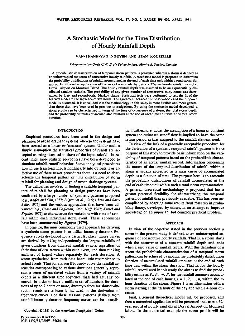
time unit within the storm duration. That is, for the hourly rainfall record used in this study the aim is to find the proba- bility estimates P•, P2, '", Pn for the rainfall amounts accumu- lated at the end of each hour t, t -- 1, 2, -.., n, within the n- hour duration of the storm. Figure 1 is an illustration with a storm starting at the ith hour of the day and with a 4-hour du- ration.

Fftst, a general theoretical model will be proposed, and then a numerical application will be presented that uses a 32- year record of hourly rainfalls at Dorval Airport on Montreal Island. In the numerical example the storm profile will be

399

400 NGUYEN AND ROUSSELLE: STOCHASTIC RAINFALL MODEL

.80

.4o -

.20 -

.IO --

o o

I n : 4 hours I

I I

I P4•,, I

' /i I I I I iPi

23 24,

TIME (HOUR

Fig. 1. Illustration of the approach to the problem of time distri- bution of rainfall depth. Pt is the probability estimate for accumulated rainfall at the end of each hour t, t = 1, 2, 3, 4.

characterized in terms of (1) the time of occurrence (at each hour of the day and in each month), (2) the total storm dura- tion, (3) the total storm depth, and (4) the probability esti- mates of accumulated rainfalls at the end of each hour within

the total storm duration.

A STOCHASTIC MODEL FOR HOURLY RAINFALL

The model to be described is an adaptation of the model developed by Todorovic and Woolhiser [1975], previously ap- plied to daily rainfall for an n-day period. Various modifica- tions were needed to use the model in this study of temporal storm pattern characterization. In Todorovic and Woolhiser's model the distribution function was found for the total

amount of precipitation during the n-day period regardless of the order of occurrences of rainy days within this period. However, according to the definition in this paper of a storm as an unbroken sequence of rainy hours the modified model will determine the probability distribution of accumulated amounts of consecutive rainfall during the n-hour period in which the first hour must be a rainy hour. In other words, we say no storm occurs in an n-hour period if the first hour of this particular period has zero rainfall or if there is no uninter- rupted sequence of rainy hours starting from the first hour in this n-hour period.

Because the number of consecutive rainy hours is random, the accumulated rainfall depth during any rainy period is in- deed the sum of a random number of random variables. The

challenge therefore is to find the distribution function of the sum of a random number of random variables. Properties of such sums have been treated by Wald [1944] and Renyi [1966] and, more extensively, by Todorovic [1970].

Definitions and Notations

Definition 1: Consider an interval of time which consists of n hours. With each hour j of this n-hour period we associate a random variable/b which is defined as

if jth hour is wet and

•=0

if jth hour is dry, where j -- 1, 2, ..., n. Definition 2: Let Mn be defined as the number of con-

secutive rainy hours starting from the first hour of the n-hour period. By this definition the random variable Mn can assume the values 0, 1, 2, -.., n. For example, for n -- 4 hours we have

{M4 = O) = {(0, O, O, 0), (0, ], O, 0), (0, O, l, 0), (0, O, O, ]), (0, l, l, 0), (0, l, O, 1), (0, l, l, 1), (0, O, l,

{M• = •) = {(], O, O, 0), (], O, ], 0), (], O, ], ]), (], O, O,

{Mn = 2} = {(1, l, O, 0), (1, l, O, 1)}

{M4 = 3} = {(1, l, l, 0)}

{Mn = 4} = {(1, l, l, 1)}

Definition 3: Let E• denote the hourly rainfall depth in the vth rainy hour of the n-hour period. The accumulated amount of rainfall $(n) during Mn consecutive rainy hours of this n- hour period can be defined as

M n

S(n) = • • •,•0

where •o -- 0, Mn = 1, 2, -.-, n. By this definition we have

P {S(n) -- 0} = P {M n m 0} •' P {•l •' 0}

and

P (S(n) > O) = 1 - P {S(n) = 0)

where P{ } denotes the probability.

Determination of the Distribution Function of the Process S(n)

The theoretical development in the following is very similar to that described by Todorovic and Woolhiser [1975]. How- ever, it should be noted that the meaning of Mn in this in- stance is the number of consecutive rainy hours in the n-hour period or, in other words, Mn can be interpreted as a rainfall duration and n as a total storm duration.

Let Fn (x) denote the distribution function of $(n), or Fn(x) = P {S(n) •< x}. We shah determine this distribution function under the two following assumptions: (1) •, •2, "', •n are inde- pendent, identically distributed random variables with H(x) = P{E• •< x}, and (2) •, •2, -.., •n are independent of Mn.

By definition 2, the sequence of events {Mn -- 0}, {Mn -- 1}, '", {Mn --' n} represents a finite partition of the sample space. Then the distribution function Fn(x) can be written as follows:

TABLE 1. Value of the X Parameter of the Fitted Exponential Distribution of Hourly Rainfall Depths for Each Month of the 32-

Year Period at Dorval Airport

Mean Hourly Rainfall Depth

Month m, in. Parameter X

Jan. 0.05068 19.73137 Feb. 0.03441 29.05835 March 0.04101 24.38234

April 0.03495 28.60858 May 0.03557 28.11484 June 0.05769 17.33342

July 0.06857 14.58467 Aug. 0.06789 14.72872 Sep. 0.05234 19.10635 Oct. 0.03759 26.60591 Nov. 0.03238 30.88235 Dec. 0.03609 27.70642

NGUYEN AND ROUSSELLE: STOCHASTIC RAINFALL MODEL 401

Fn(x ) __- p E ev •< X, M n -- (1) K-O •,--0

Under assumption 2 it follows that

Fn(x) -- • P {XK •< X} P {M n -- K} (2) K-o

in which Xo -- 0 and XK ---- Y•..0 • E• for K -- 0, 1, ..., n, or we can write

Fn(X ) = P {M n -- 0} + • P {XK • X} P {M n -- K} (3)

As was shown by Todorovic and Woolhiser [1974], the mean E {S(n)} and the variance D {S(n)} of the process S(n) are, re- spectively,

E {S(n)} = aE {Mn} (4)

D (S(n)} -- •Sf (Mn} + a:D (Mn} (5)

where a -- E {E•} and fl = D {E•} < oo. Then, by (3), to obtain the distribution function Fn(x) of the total amount of rainfall during Mn consecutive rainy hours in the n-hour period, it is necessary to compute the probabilities P {XK •< X} and P {Mn = K} for K = 1, 2, .-., n, as will be shown.

Computation of the Probability P {XK •< X}

AS in the works by Eagleson [1972] and Howard [1976], the hourly rainfall depth distribution in this study is assumed to

,.oo• /• •.••.--- •o• •

,om_// ,•o

. I• • •0 •0 •0 JO • gO .7• HOURLY RAINFALL DEPTH (JN )

•oo • ///•• .... 90

70 (B)

.30 ZO

I0

0 I I ! I 0 .I 0 .ZO .30 40 . 50 60 70

HOURLY RAINFALL DEPTH

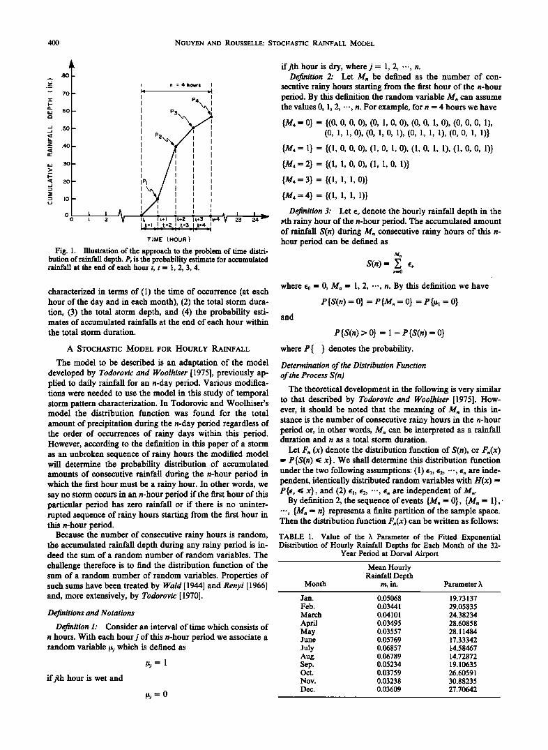
Fig. 2. Plots of fitted exponential distributions and observed fre- quencies of hourly rainfall depths for January (Figure 2a) and for April (Figure 2b).

1.00

9O

.80

•n 0 n • a. 30

2O

.10 • 0

0

JULY

(A)

Observed

----- F,tted

I I I I I

.10 .ZO .30 .40 .50

HOURLY RAINFALL DEPTH (IN )

I .

I00

80

m.- 6o

• .õo

o

.2o

OCTOBER

(B)

Observed

----- F,tted

0 I I I I I I I 0 .I 0 . zo 30 .,30 50 60 .70

HOURLY RAINFALL DEPTH {iN.

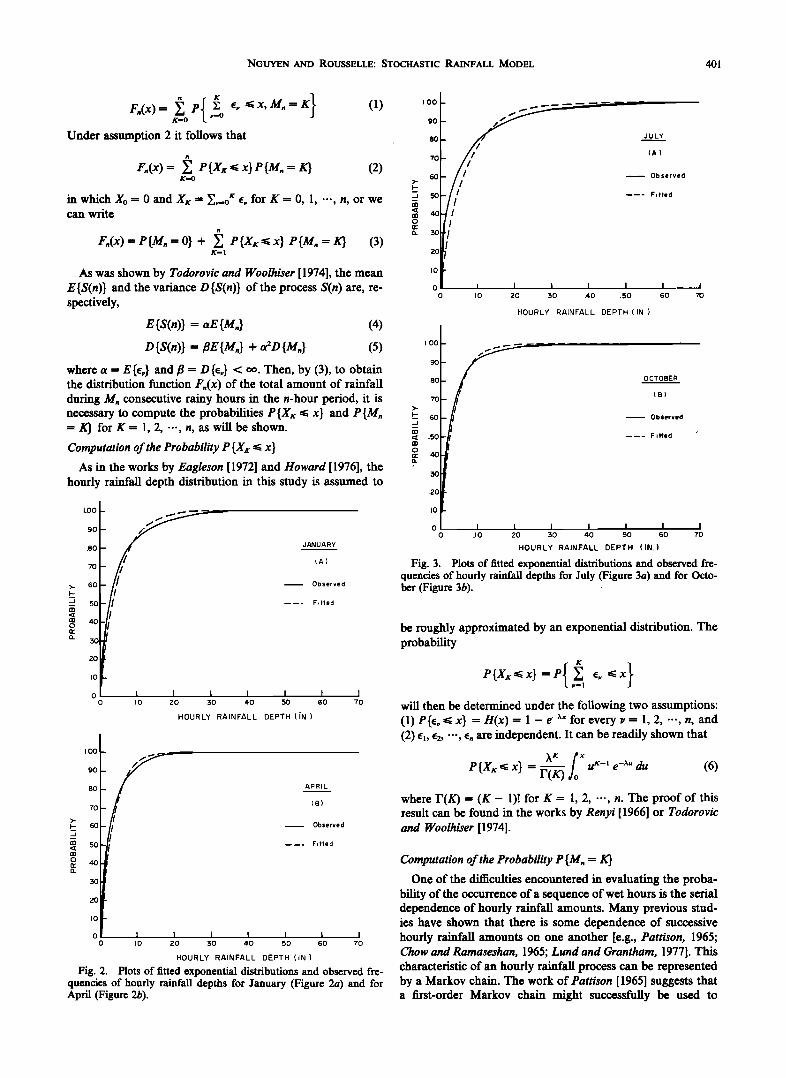
Fig. 3. Plots of fitted exponential distributions and observed fre- quencies of hourly rainfall depths for July (Figure 3a) and for Octo- ber (Figure 3b).

be roughly approximated by an exponential distribution. The probability

P = P{ will then be determined under the following two assumptions: (1) P {Ev •< x} -- H(x) = 1 - e -x• for every v = 1, 2, .-., n, and (2) El, E2, '", E n are independent. It can be readily shown that

•'• fo x P {XK •< X} ---- r-• u f-' e -x" du (6) where I•(K) = (K- 1)! for K = 1, 2, ..., n. The proof of this result can be found in the works by Renyi [1966] or Todorovic and Woolhiser [1974].

Computation of the Probability P {M n -- K}

One of the difficulties encountered in evaluating the proba- bility of the occurrence of a sequence of wet hours is the serial dependence of hourly rainfall amounts. Many previous stud- ies have shown that there is some dependence of successive hourly rainfall amounts on one another [e.g., Pattison, 1965; Chow and Ramaseshan, 1965; Lund and Grantham, 1977]. This characteristic of an hourly rainfall process can be represented by a Markov chain. The work of Pattison [1965] suggests that a first-order Markov chain might successfully be used to

402 NGUYEN AND ROUSSELLE: STOCHASTIC RAINFALL MODEL

O5

• o3

.o2

.ol -

oo o

JANUARY

i • i I i i I I I I i I

2 4 6 8 IO 12 14 16 18 20 22 24

TIME (HOUR), t,

.20 F,rst - Order JANUARY

---- Second-Order

i I I I I •2 I I I I ;2 I 2 4 6 8 I0 14 16 18 20 24

0

.•o D o

.40 --

0

6o [

o

80 u•

I OO

TIME (HOUR), t

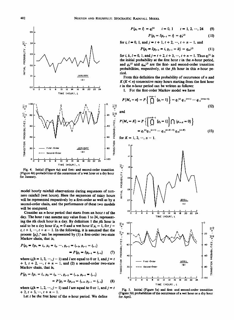
Fig. 4. Initial (Figure 4a) and first- and second-order transition (Figure 4b) probabilities of the occurrence of a wet hour or a dry hour for January.

model hourly rainfall observations during sequences of non- zero rainfall (wet hours). Here the sequences of rainy hours will be represented respectively by a first-order as well as by a second-order chain, and the performance of these two models will be compared.

Consider an n-hour period that starts from an hour t of the day. The hour t can assume any value from 1 to 24, represent- ing the tth clock hour in a day. By definition 1 the jth hour is said to be a dry hour if/•j -- 0 and a wet hour if/•j -- 1, for j -- t, t + 1, ..., t + n - 1. In the following, it is assumed that the process •j} i" can be represented by (1) a first-order two-state Markov chain, that is,

where in(h = 1, 2, ..., j - 1) and I are equal to 0 or 1, and j - t + 1, t + 2, ..., t + n - 1, and (2) a second-order two-state Markov chain, that is,

where ih(h -- 1, 2, ..., j - 1) and I are equal to 0 or 1, and j -- t +2, t+3,'...,t+n-1.

Let t be the first hour of the n-hour period. We define

P•,-- 0 -- q[') i-- 0, 1 t -- 1, 2, ..-, 24 (9)

P{.u.• = ll/•,-, = •} = q? (10)

fori, l--0, 1, and j--t+ 1, t+2,.,.,t+n- 1, and

P{laj = llt•j-2 = i, •_, = k} = q..? (11)

for i, k, 1 -- 0, 1, and j -- t + 2, t + 3, ..., t + n - 1. Thus qi (') is the initial probability at the first hour t in the n-hour period, and q,O) and q,,? are the first- and second-order transition probabilities, respectively, at the jth hour in this n-hour pe- riod.

From this d.efinition the probability of occurrence of n and K (K < n) consecutive rainy hours starting from the first hour t in the n-hour period can be written as follows:

1. For the first-order Markov model we have

{ ""l'nd I } (t+n-- 1) P [M. --' n} --- P •--- 1} -- q?) q,?+')..-

(12) and

P {M,-- K} -- P { {la• -- 1} f'• {l•t.4.K•---'O} ----' ql(t)qll (t+l) '" qll (t+K-l) qlo (t+10 (13)

forK-- 1,2,...,n- 1.

.12 -

.11 --

.IO --

09--

.08

O7

06 i i o

APRIL

i i i i I I I i i i

2 4 6 8 I0 12 14 16 18 20 22 24

TIME (HOUR), t.,

..

o

.4o -

F,rst -Order

20 .... Second-Order

0 • I I I I 0 2 4 6 8 i0

APRIL

(B)

I I I I I I I 12 14 16 18 20 22 24

0

40 •

6O 0

80 --

1.00

TIME ( HOUR), t

Fig. 5. Initial (Figure 5a) and first- and second-order transition (Figure 5b) probabilities of the occurrence of a wet hour or a dry hour for April.

NGUYEN AND ROUSSELLE: STOCHASTIC RAINFALL MODEL 403

2. For the second-order Markov model we have

t+n-- 1

-- ql(Oql l(t+l)ql I 1 (t+2) "' qll 1 (t+n--1) (14)

P {Mn- K } - P { {]•j- l} N -- l(t+2) 1) (t+• (15) -- q?) q•lO+D qll '" q•?+g- q•o

for K = 1, 2, ..., n - 1. For ex•ple, • n • 4 and t • 2 (i.e., the first hour of the 4-

hour period • at the second hour of the day), we have the fol- long:

1. For the first-order Markov model,

P{M4 = 4} = ql (2) q•(3) q•(4) qll(5)

and for K = 3,

P{M4 = 3} = q?)q•(3)q•o(4), etc. for K = 2, for K = 1

2. For the second-order Markov model,

P {M 4 = 4} = q•(2) q l?) q• 1(4) q•

and for K = 3,

.08

• -- .07

œ .o6

.0õ

ß ø" I .03 I o

JULY

(A)

I i

4 6 I i I I I I I I I 8 IO 12 14 16 18 20 22 24

TIME ( HOUR ) , t

1.00 -

_% 60

0

fl. .40

JULY

(B)

F,rst-Order

----- Second-Order

I I I 4 6 8 I0 0 I i 4 i I I i 1 0 ' 2 i 16 18 20 22 24

0 '-'o

.20 • o_

40 •

•o •o

.•o •

i.oo

TIME (HOUR), t,

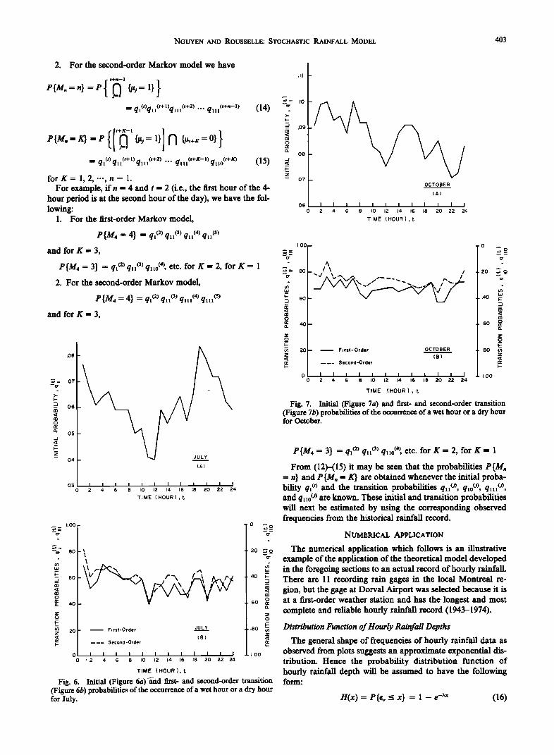
Fig. 6. Initial (Figure 6a)•d first- and second-order transition (Figure 6b) probabilities of the occurrence of a wet hour or a dry hour for July.

•D

0

.08

O?

.ll

0 2 4 6 8 IO 12 14 16 18 20 22 24

TIME ( HOUR ) , •,

60

40--

20--

0 0

First- Order

----- Second-Order

I i i I i I i

2 4 6 8 I0 12 14

OCTOBER

I I I I I

16 18 20 22 24

.2o • o_

.4o •

60 •

z

_(2

.80 • z

i.oo

TIME (HOUR), t,

Fig. 7. Initial (Figure 7a) and first- and second-order transition (Figure 7b) probabilities of the occurrence of a wet hour or a dry hour for October.

P{M4 -- 3} = ql a) qll (3) qllO (4), etc. for K = 2, for K = 1

From (12)-(15) it may be seen that the probabilities P{Mn = n} and P {M n -- K} are obtained whenever the initial proba- bility ql (t) and the transition probabilities qll ø), ql?, qlll ø), and q l lO t') are known. These initial and transition probabilities will next be estimated by using the corresponding observed frequencies from the historical rainfall record.

NUMERICAL APPLICATION

The numerical application which follows is an illustrative example of the application of the theoretical model developed in the foregoing sections to an actual record of hourly rainfall. There are 11 recording rain gages in the local Montreal re- gion, but the gage at Dorval Airport was selected because it is at a first-order weather station and has the longest and most complete and reliable hourly rainfall record (1943-1974).

Distribution Function of Hourly Rainfall Depths

The general shape of frequencies of hourly rainfall data as observed from plots suggests an approximate exponential dis- tribution. Hence the probability distribution function of hourly rainfall depth will be assumed to have the following form:

H(x) -- P {e,_< x} -- l - e -xx (16)

404 NGUYEN AND ROUSSELLE: STOCHASTIC RAINFALL MODEL

.10o0o

.05000

_ • •.•.ANUA RY \\\ ; : E mp•r•col

•-••x o--- -o Theoret•col (F•rst-Order) ß -----• Theoret•col (Second-Order)

.01000 i

--

¾ -

,.,, _

- n .00500 i

• -

n3 -- 0

.oo•oo i I I I I I I I i 0 I Z 3 4 5 6 7 8 9 I0

NUMBER OF CONSECUTIVE RAINY HOURS, K

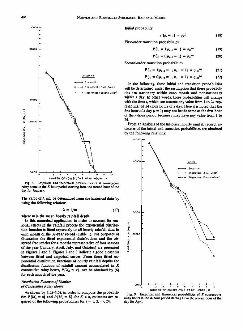
Fig. 8. Empirical and theoretical probabilities of K consecutive rainy hours in the K-hour period starting from the second hour of the day for January.

The value of h will be determined from the historical data by using the following relation:

X = 1/m (17)

where m is the mean hourly rainfall depth. In this numerical application, in order to account for sea-

sonal effects in the rainfall process the exponential distribu- tion function is fitted separately to all hourly rainfall data in each month of the 32-year record (Table 1). For purposes of illustration the fitted exponential distributions and the ob- served frequencies for 4 months representative of four seasons of the year (January, April, July, and October) are presented in Figures 2 and 3. Figures 2 and 3 indicate a good closeness between fitted and empirical curves. From these fitted ex- ponential distribution functions of hourly rainfall depths the distribution function of rainfall amount accumulated in K

consecutive rainy hours, P {X• <_ x}, can be obtained by (6) for each month of the year.

Distribution Function of Nurnber of Consecutive Rainy Hours

As shown by (12)-(15), in order to compute the probabili- ties P {M, -- n} and P {M, -- K} for K < n, estimates are re- quired of the following probabilities for t -- 1, 2, ..., 24:

Initial probability

P•, = 1} = ql (t) (18)

First-order transition probabilities

P•, = ll/•,_, = l} = qll (0 (19)

P•, = OI/•,_l = l} = qlo (t) (20)

Second-order transition probabilities

P•, = ll/•t_2 = 1, •t--, = l} = qlll (t) (21)

P{•tt t = OI/•t_2 = 1, j[•t-l = 1} = qllO (t) (22)

In the following, these initial and transition probabilities will be determined under the assumption that these probabili- ties are stationary within each month and nonstationary within a day. In other words, these probabilities will change with the time t, which can assume any value from 1 to 24 rep- resenting the 24 clock hours of a day. Here it is noted that the first hour of a day (t -- 1) may not be the same as the first hour of the n-hour period because t may have any value from 1 to 24.

From an analysis of the historical hourly rainfall record, es- timates of the initial and transition probabilities are obtained by the following relations:

I0000

0 I 2 3 4 5 6 7 8 9 I0

NUMBER OF CONSECUTIVE RAINY HOURS, K

Fig. 9. Empirical and theoretical probabilities of K consecutive rainy hours in the K-hour period starting from the second hour of the day for April.

NGUYEN AND ROUSSELLE: STOCHASTIC RAINFALL MODEL 405

•(,) _- Nw, (23)

where

c•(, ) _ N,•,_,,•, (24)

C•o(, ) _ N,•,_,t,, (25)

c•(,) _- N,•,_,,•,_,,•, (26) NWt--2Wt-- 1

c• •o(,) _- N,•,_,,•,_,z,, (27) NWt--2Wt-- 1

N•, number of days that hour t was wet; Nw,_,•, number of days that hours t - 1 and t were both

wet;

N•,_,D, number of days that hour t - 1 was wet and hour t was dry;

N•,_2•,_,w ' number of days that hours t - 2, t - 1, and t were wet;

N•,_2•,_,D, number of days that hours t - 2 and t - 1 were

I0000

.05000 JULY

; -_ Emp,rlcal

o---o Theorehcal (First-Order)

a,•--a, Theoret,cal (Second-Order)

ß I0000

.05000

.01000

00500

OOLOO o

- _OCTOBER

- \o•x• o-- -o Theoret,cal (F,rst-Order)

_ 'x\••. •------• Theorehcal (Second-Order)

- \

- •,

- \

0 _

I I i I I I i i i i I 2 3 4 5 6 7 8 9 i0

NUMBER OF CONSECUTIVE RAINY HOURS , K

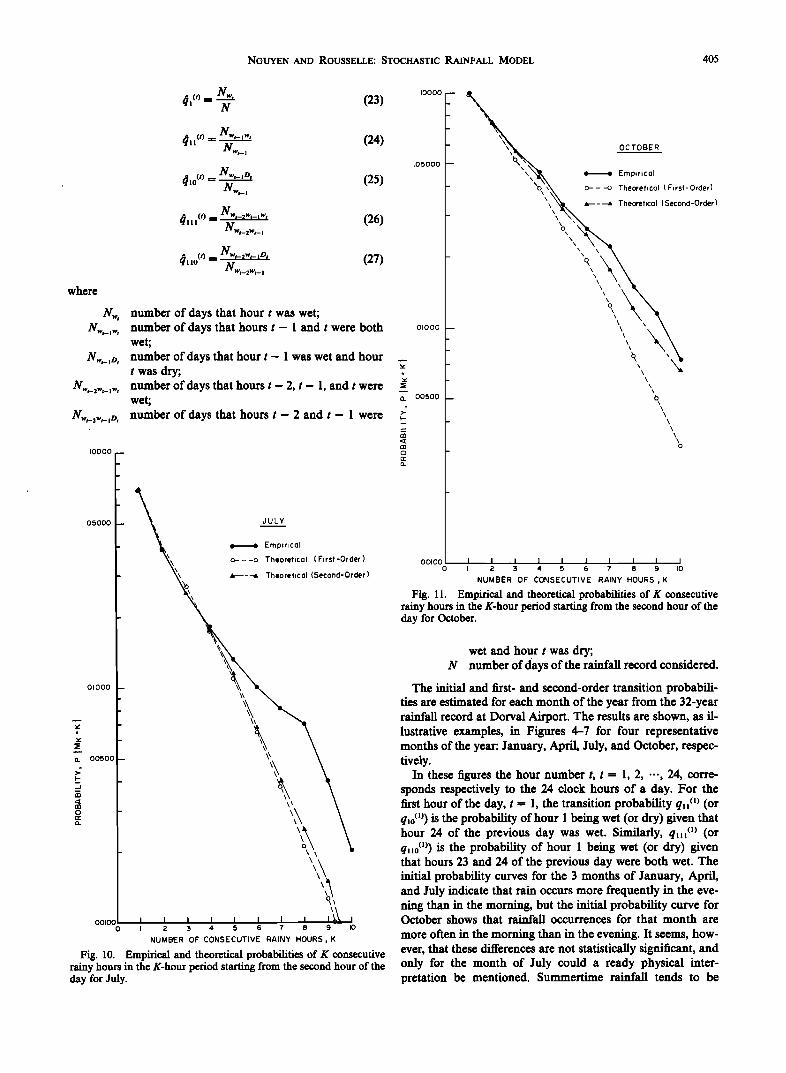
Fig. 11. Empirical and theoretical probabilities of K consecutive rainy hours in the K-hour period starting from the second hour of the day for October.

.01000

n .00500 \\

__J o

o

.ooloo I I I I I I i_•_ J 0 I 2 3 4 5 6 7 8 9 I0

NUMBER OF CONSECUTIVE RAINY HOURS, K

Fig. 10. Empirical and theoretical probabilities of K consecutive rainy hours in the K-hour period starting from the second hour of the day for July.

wet and hour t was dry; N number of days of the rainfall record considered.

The initial and first- and second-order transition probabili- ties are estimated for each month of the year from the 32-year rainfall record at Dorval Airport. The results are shown, as il- lustrative examples, in Figures 4-7 for four representative months of the year: January, April, July, and October, respec- tively.

In these figures the hour number t, t -- 1, 2, ..., 24, corre- sponds respectively to the 24 clock hours of a day. For the first hour of the day, t = 1, the transition probability q•(•) (or q•o (l)) is the probability of hour 1 being wet (or dry) given that hour 24 of the previous day was wet. Similarly, q•(•) (or q•o (•)) is the probability of hour 1 being wet (or dry) given that hours 23 and 24 of the previous day were both wet. The initial probability curves for the 3 months of January, April, and July indicate that rain occurs more frequently in the eve- ning than in the morning, but the initial probability curve for October shows that rainfall occurrences for that month are

more often in the morning than in the evening. It seems, how- ever, that these differences are not statistically significant, and only for the month of July could a ready physical inter- pretation be mentioned. Summertime rainfall tends to be

406 NGUYEN AND ROUSSELLE: STOCHASTIC RAINFALL MODEL

I.OC

0.80

o.6o

0,40

0.20

t mulated rainfall amount during Mn consecutive rainy hours in THEOR ETI CAL'xjN

'[ [Eq. 29• the n-hour period can be obtained by using (3). That is, = URS Fn(X) ---- P {Mn -- O} -I-- uK-'e -x" du P {Mn -- K}

K=I

(28)

where I'(K) -- (K- 1)!. Returning to (3), the distribution function Fn(x) applies to

all values of $(n), including zero values. In order to focus on

i I. oo •' o. oo • • the probability distribution function for nonzero values of 0.00 0.20 0.40 0.60 0.80 $(n), instead of using Fn(x) in (3) we introduce Fn*(X), as fol-

lows:

't Fn(X) -- P {Mn = 0}

[ THEORETICAL'• Fn*(X ) = - T•{-•n • ). ,.oo EL,. •3• ' ' 0.60

Or

1

•m 0.40 .•o

0.20

0.00 0.00 0.20 0.40 0.60 0.80 •.oo

CUMULATIVE RAINFALL (in.)

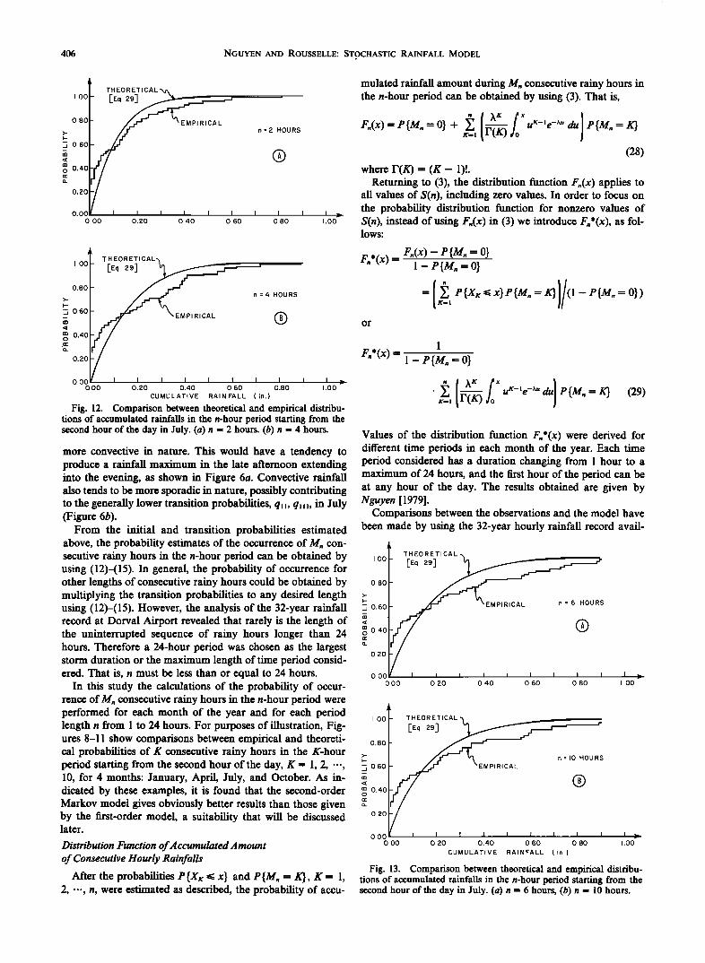
Fig. 12. Comparison between theoretical and empirical distribu- tions of accumulated rainfalls in the n-hour period starting from the second hour of the day in July. (a) n = 2 hours. (b) n = 4 hours.

more convective in nature. This would have a tendency to produce a rainfall maximum in the late afternoon extending into the evening, as shown in Figure 6a. Convective rainfall also tends to be more sporadic in nature, possibly contributing to the generally lower transition probabilities, q•, q•, in July (Figure 6b).

From the initial and transition probabilities estimated above, the probability estimates of the occurrence of Mn con- secutive rainy hours in the n-hour period can be obtained by using (12)-(15). In general, the probability of occurrence for other lengths of consecutive rainy hours could be obtained by multiplying the transition probabilities to any desired length using (12)-(15). However, the analysis of the 32-year rainfall record at Dorval Airport revealed that rarely is the length of the uninterrupted sequence of rainy hours longer than 24 hours. Therefore a 24-hour period was chosen as the largest storm duration or the maximum length of time period consid- ered. That is, n must be less than or equal to 24 hours.

In this study the calculations of the probability of occur- rence of Mn consecutive rainy hours in the n-hour period were performed for each month of the year and for each period length n from 1 to 24 hours. For purposes of illustration, Fig- ures 8-11 show comparisons between empirical and theoreti- cal probabilities of K consecutive rainy hours in the K-hour period starting from the second hour of the day, K-- 1, 2, ..., 10, for 4 months: January, April, July, and October. As in- dicated by these examples, it is found that the second-order Markov model gives obviously better results than those given by the first-order model, a suitability that will be discussed later.

Distribution Function of Accumulated Amount of Consecutive Hourly Rainfalls

After the probabilities P {X K • x} and P {Mn -- K}, K = 1, 2, -.., n, were estimated as described, the probability of accu-

( ) ß u •c-'e -x" du P {Mn: K} K• 1

(29)

Values of the distribution function Fn*(X) were derived for different time periods in each month of the year. Each time period considered has a duration changing from 1 hour to a maximum of 24 hours, and the first hour of the period can be at any hour of the day. The results obtained are given by Nguyen [1979].

Comparisons between the observations and the model have been made by using the 32-year hourly rainfall record avail-

• THEORETICAL x

•- 6 -i 0 60 EMPIRICAL n = HOU

(•040

0.20 I/ 0.00 I I I I I I I I

0.00 0.20 0.40 0.60 0.80

I

•_ ø'•ø I 0.60

0.40

0.20

THEORETICAL

EL, •]

EMPIRICAL

n = I0 HOU RS

Fig. 13. Comparison between theoretical and empirical distribu- tions of accumulated rainfalls in the n-hour period starting from the second hour of the day in July. (a) n = 6 hours, (b) n = 10 hours.

0.00 0.00 0.20 0.40 0.60 0.80 1.00

CUMULATIVE RAINFALL (in.)

NGUYEN AND ROUSSELLE'- STOCHASTIC RAINFALL MODEL 407

able at Dorval Airport in the region of Montreal. However, for purposes of illustration, F!gures 12 and 13 present the ob- served and computed distributions for the periods starting from the second hour of the day and consisting of n hours, n -- 2, 4, 6, 10, by using the hourly rainfall record for July. The re- suits will be discussed in the next section.

DISCUSSION AND CONCLUSIONS

In order to study the variability of temporal pattern of ac- cumulated amounts of consecutive rainfalls in the n-hour pe- riod a probabilistic model has been developed under the fol- lowing key assumptions: (1) the amounts of rainfall in every hour of the day are independent and identically exponentially distributed, (2) the accumulated amount of rainfall in K hours is independent of the duration K, and (3) there is some depen- dence between the rainfall occurrence in successive hours.

Furthermore, in applying the model to the historical rainfall record at Dorval Airport the effects of seasonal and diurnal variations of rainfall have been taken into account by assum- ing that (4) the exponential distribution of hourly rainfall depths for any given month is not identical to the distribution for the other months of the year, and (5) the initial and transi- tion probabilities in the first- and second-order Markov mod- els for the process Mn are nonstationary within a day but sta- tionary within each month of the year.

Figures 2 and 3 show a good closeness between fitted ex- ponential distribution and observed frequency curves of hourly rainfall depths. This supports assumption 1 above.

In practice, the assumption of independence between two random variables can not be justified except by physical in- tuition, and there is no precise means for evaluation of the ef- fects of this assumption on the performance of the model. There is no evidence to support this hypothesis except by vi- sual comparison of the theoretical and empirical results.

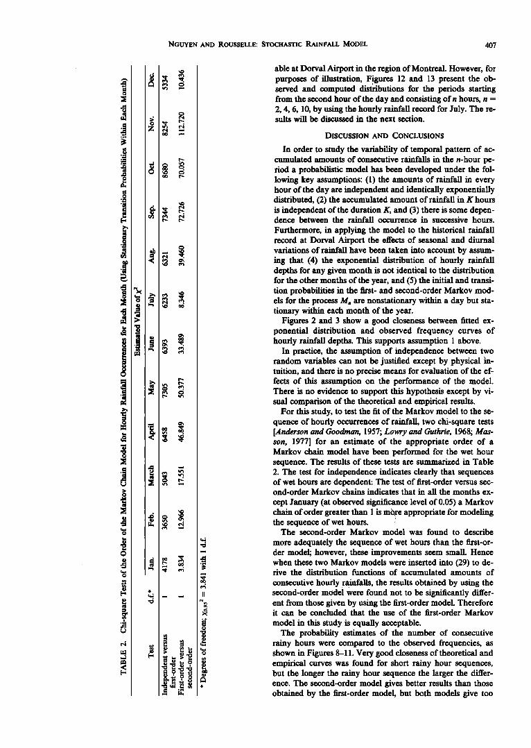
For this study, to test the fit of the Markov model to the se- quence of hourly occurrences of rainfall, two chi-square tests [Anderson and Goodman, 1957; Lowry and Guthrie, 1968; Mas- son, 1977] for an estimate of the appropriate order of a Markov chain model have been performed for the wet hour sequence. The results of these tests are summarized in Table 2. The test for independence indicates clearly that sequences of wet hours are dependent: The test of first-order versus sec- ond-order Markov chains indicates that in all the months ex-

cept January (at observed significance level of 0.05) a Markov

chain of order greater than 1 is m•re appropriate for modeling the sequence of wet hours. •

The second-order Markov model was found to describe

more adequately the sequence of wet hours than the first-or- der model; however, these improvements seem small. Hence when these two Markov models were inserted into (29) to de- rive the distribution functions of accumulated amounts of

consecutive hourly rainfa• '.: the results obtained by using the second-order mod•i Were found not to be significantly differ- ent from those given by using the first-order model. Therefore it can be concluded that the use of the first-order Markov

model in this study is equally acceptable. The probability estimates of the number of consecutive

rainy hours were compared to the observed frequencies, as shown in Figures 8-11. Very good closeness of theoretical and empirical curves was found for short rainy hour sequences, but the longer the rainy hour sequence the larger the differ- ence. The second-order model gives better results than those obtained by the first-order model, but both models give too

408 NGUYEN AND ROUSSELLE: STOCHASTIC RAINFALL MODEL

conservative probability estimates for long rainy hour periods as compared with the observed frequencies. The reason for these conservative estimates could be explained by the strong persistence inherent in the hourly rainfall process. The ,use of a higher-order Markov chain could improve the agreement of the theoretical probability estimates with the observed fre- quencies but requires additional computations using a more extensive rainfall data base to evaluate all the transition prob- abilities.

Table 1 shows the month-to-month variation of the param- eter h of the exponential distributions of hourly rainfall depths in each month. This supports assumption 4 above.

On the basis of an examination of the observed rainfall data

and by using physical intuition the initial and transition prob- abilities have been assumed to be nonstationary within a day. Figures 4a, 5a, 6a, and 7a indicate the hour-to-hour variation of the initial probabilities. Therefore this has supported the assumption of nonstationarity of initial probabilities.

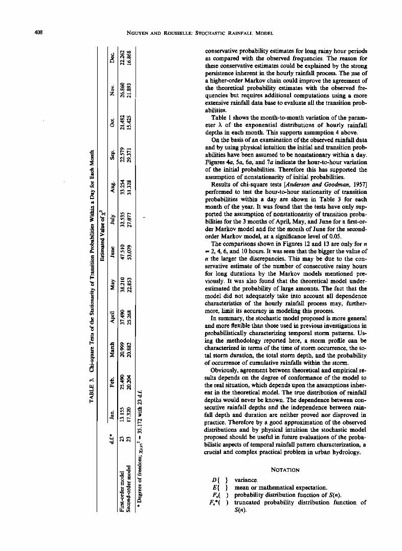
Results of chi-square tests [Anderson and Goodman, 1957] performed to test the hour-to-hour stationarity of transition probabilities within a day are shown in Table 3 for each month of the year. It was found that the tests have only sup- ported the assumption of nonstationarity of transition proba- bilities for the 3 months of April, May, and June for a first-or- der Markov model and for the month of June for the second-

order Markov model, at a significance level of 0.05. The comparisons shown in Figures 12 and 13 are only for n

= 2, 4, 6, and 10 hours. It was seen that the bigger the value of n the larger the discrepancies. This may be due to the con- servative estimate of the number of consecutive rainy hours for long durations by the Markov models mentioned pre- viously. It was also found that the theoretical model under- estimated the probability of large amounts. The fact that the model did not adequately take into account all dependence characteristics of the hourly rainfall process may, further- more, limit its accuracy in modeling this process.

In summary, the stochastic model proposed is more general and more flexible than those used in previous investigations in probabilistically characterizing temporal storm patterns. Us- ing the methodology reported here, a storm profile can be characterized in terms of the time of storm occurrence, the to- tal storm duration, the total storm depth, and the probability of occurrence of cumulative rainfalls within the storm.

Obviously, agreement between theoretical and empirical re- sults depends on the degree of conformance of the model to the real situation, which depends upon the assumptions infier- ent in the theoretical model. The true distribution of rainfall

depths would never be known. The dependence between con- secutive rainfall depths and the independence between rain- fall depth and duration are neither proved nor disproved in practice. Therefore by a good approximation of the observed distributions and by physical intuition the stochastic model proposed should be useful in future evaluations of the proba- bilistic aspects of temporal rainfall pattern characterization, a crucial and complex practical problem in urban hydrology.

NOTATION

O { } variance. E{ } mean or mathematical expectation. Fn( ) probability distribution function of S(n).

Fn*( ) truncated probability distribution function of S(n).

NGUYEN AND ROUSSELLE: STOCHASTIC RAINFALL MODEL 409

H( ) probability distribution function of K number of consecutive rainy hours. m mean hourly rainfall depth.

Mn number of consecutive rainy hours starting from the first hour of the n-hour period.

n total duration of a storm.

N number of days of the hourly rainfall record con- sidered.

Nw, number of days that hour t was wet. Nw,_,•, number of days that hours t - 1 and t were both

wet.

N•,_,D, number of days that hour t - 1 was wet and hour t was dry.

N,•,_2,•,_,D, number of days that hours t - 2 and t - 1 were both wet and hour t was dry.

N,•,_2,•,_,,•, number of days that hours t - 2, t - 1, and t were wet.

P { } probability. P{ I } conditional (or transition) probability.

P, probability estimate for accumulated rainfall amount at the end of each hour t.

q? probability of hour t being in state i (initial proba- bility).

q? probability of hour j being in state I given that hour j- 1 was in state i (first-order transition probability).

q•?) probability of hour j being in state I given that hour j- 2 was in state i and houyj- 1 was in state k (second-order transition probability).

S(n) accumulated amount of consecutive hourly rain- falls in the n-hour period.

t time.

X•c accumulated amount of rainfalls in K consecutive rainy hours.

a mean of the random variable ev. , • variance of the random variable e•. • hourly rainfall depth in the vth rainy hour of the

n-hour period. X parameter of the exponential distribution function

of hourly rainfall depth. /•i random variable associated either with rainy hour

j •i = 1) or with nonrainy hour j ½• -- 0). X 2 chi-square statistic. r3 intersection.

Acknowledgments. This research was supported by the Ministry of Education in Quebec (project CRP 356-75) and by the Natural Sci- ences and Engineering Research Council of Canada (project RD-812) and was part of the doctoral thesis of the first author. The extensive

critical review of the research and this paper by P. Todorovic is grate- fully acknowledged. We thank M. B. McPherson, who was coadvisor on the thesis, and G. Parry for their helpful reviews.

REFERENCES

Anderson, T. W., and L. A. Goodman, Statistical inference about Markov chains, Ann. Math. Star., 28, 89-110, 1957.

Chien, J., and S. Sarikelle, Synthetic design hyetograph and rational runoff coefficient, J. Irrig. Drain. Div. Am. Soc. Civ. Eng., 102(IR3), 307-315, 1976.

Chow, V. T., and S. Ramaseshan, Sequential generation of rainfall and runoff data, J. Hydraul. Div. Am. Soc. Civ. Eng., 91(HY4), 205- 223, 1965.

Eagleson, P.S., Dynamics of flood frequency, Water Resour. Res., 8(4), 878-898, 1972.

Grace, G. A., and P.S. Eagleson, The synthesis of short-time in- crement rainfall sequences, Rep. 91, Hydrodyn. Lab., Mass. Inst. of

' Technol., Cambridge, 1966. Howard, C. D. D., Theory of storage and treatment-plant overflows,

J. Environ. Eng. Div. Am. Soc. Civ. Eng., 102(EE4), 709-722, 1976. Huff, F. A., Time distribution of rainfall in heavy storms, Water Re-

sour. Res., 3(4), 1007-1019, 1967. Keifer, C. J., and H. H. Chu, Synthetic storm pattern for drainage de-

sign, J. Hydraul. Div. Am. Soc. Civ. Eng., 83(HY4), 25 pp., 1957. Knisel, W. G., Jr., and W. M. Snyder, Stochastic time distribution of

storm rainfall, Nord. Hydrol., 6, 242-262, 1975. Lowry, W. P., and D. Guthrie, Markov chains of order greater than

one, Mon. Weather Rev., 96(11), 798-801, 1968. Lund, I. A., and D. D. Grantham, Persistence, runs, and recurrence of

precipitation, J. Appl. Meteorol., 16(4), 346-358, 1977. Masson, J. M., Persistance des •tats pluvieux en fonction de leur

dur•e: Analyse de 52 an_n•es d'enregistrements pluviographiques/t Montpellier-Bel Air, Cah. ORSTOM Set. Hydrol., 14(2), 173-189, 1977.

Nguyen, V. T. V., Caract•risation hydrologique de la pluie pour le contr61e et la planification des syst•mes de drainage urbain, doc- toral thesis, 71 pp., Ecole Polytech., Montreal, Que., 1979.

Pattison, A., Synthesis of hourly rainfall data, Water Resour. Res., 1(4), 489-498, 1965.

Pilgrim, D. H., I. Cordery, and R. French, Temporal patterns of de- sign rainfall for Sydney, Civ. Eng. Trans. Inst. Eng. Aust., CEIl(I), 9-14, 1969.

Renyi, A., Calcul des Probabilit•s, 620 pp., Dunod, Parris, 1966. Todorovic, P., On some problems involving random number of ran-

dom variables, Ann. Math. Stat., 41(3), 1059-1063, 1970. Todorovic, P., and D. Woolhiser, Stochastic model of daily rainfall,

Proceedings of the Symposium on Statistical Hydrology, Tucson, Arizona, Aug. 31-Sept. 2, 1971, Misc. Publ. U.S. Dep. Agric., 1275, 232-246, 1974.

Todorovic, P., and D. Woolhiser, A stochastic model of n-day precipi- tation, J. Appl. Meteorol., 14(1), 17-24, 1975.

Wald, A., On cumulative sums of random variables, Ann. Math. Stat., 15(3), 283-296, 1944.

(Received March 5, 1980; revised July 16, 1980;

accepted September 18, 1980.)