GPS Signal Scattering from Sea Surface:Wind Speed Retrieval Using ExperimentalData and Theoretical Model

Attila Komjathy,* Valery U. Zavorotny,† Penina Axelrad,*George H. Born,* and James L. Garrison‡

Global Positioning System (GPS) signals reflected from applications. Recently, the sensitivity of this signal tothe ocean surface have potential use for various remote propagation effects was found to be useful for varioussensing purposes. Some possibilities are measurements of environmental remote sensing techniques. For example,surface roughness characteristics from which wave ionospheric and tropospheric delays of GPS signalsheight, wind speed, and direction could be determined. caused by variations of atmospheric refraction are knownFor this paper, GPS-reflected signal measurements col- to be a common error source affecting the use of thelected at aircraft altitudes of 2 km to 5 km with a delay- GPS for positioning and navigation. This phenomenon isDoppler mapping GPS receiver are used to explore the being successfully used for atmospheric remote sensingpossibility of determining wind speed. To interpret the purposes (Ware et al., 1996). Surface multipath is an-GPS data, a theoretical model has been developed that other error source affecting the GPS signal. However, itdescribes the power of the reflected GPS signals for dif- has only recently been recognized that multipath fromferent time delays and Doppler frequencies as a function the GPS signals reflecting off the sea surface could beof geometrical and environmental parameters. The results utilized as a new tool in oceanographic remote sensingindicate a good agreement between the measured and the

(Martı́n-Neira, 1993; Katzberg and Garrison, 1996, Gar-modeled normalized signal power waveforms duringrison et al., 1997; Garrison et al., 1998). In both cases,changing surface wind conditions. The estimated winda phenomenon that is usually regarded as an error sourcespeed using surface-reflected GPS data, obtained by com-to navigation was recognized to contain useful scientificparing actual and modeled waveforms, shows gooddata. Because the ocean surface roughness affects GPSagreement (within 2 m/s) with data obtained from asignal reflection, researchers can use the resultingnearby buoy and independent wind speed measurementsmultipath signal to determine factors such as wavederived from the TOPEX/Poseidon altimetric satellite.height, wind speed, and wind direction. The strength ofElsevier Science Inc., 2000the reflected signal is also a discriminator between wetand dry ground areas, and therefore could be applied tocoastal and wetland mapping.INTRODUCTION

Conventional monostatic radar remote sensing of theThe versatility and availability of signals from the Globaloceans requires dedicated transmitters and receivers withPositioning System (GPS) gave birth to many new GPSlarge directional antennae to achieve high resolution.GPS is, in fact, a bistatic radar system, which requires

* CCAR/University of Colorado at Boulder only a receiver, not a transmitter, because the GPS satel-† CIRES/University of Colorado at Boulder/NOAA/ETL

lites provide illumination for free. This bistatic geometry‡ NASA Goddard Space Flight Centerand the special structure of GPS signals can provideAddress correspondence to Attila Komjathy, Colorado Center for

Astrodynamics Research (CCAR), University of Colorado at Boulder, complementary information about ocean surface charac-Campus Box 431, Boulder, CO 80309-0431, USA. E-mail: komjathy@ teristics from a small patch of ocean surface without theGPS.colorado.edu

Accepted 18 January 2000. need for a directional antenna. All of this makes the re-

REMOTE SENS. ENVIRON. 73:162–174 (2000)Elsevier Science Inc., 2000 0034-4257/00/$–see front matter655 Avenue of the Americas, New York, NY 10010 PII S0034-4257(00)00091-2

GPS Wind Speed Retrieval 163

Figure 1. GPS scattering geometry.

flected GPS signals very attractive for use as a new earth receiver as the glistening zone. Away from the glisteningzone, the contribution from the specular reflections di-remote sensing tool.

Martı́n-Neira (1993) first proposed and described a minishes, and is replaced with significantly weaker Braggscattering caused by diffraction from a small-scale sur-bistatic ocean altimetry system utilizing the signal of

GPS. Subsequently, the accidental acquisition of surface- face component. Here we do not take into account thistype of scattering since it is too weak for our purposes.reflected GPS signals from aircraft was reported by

Auber et al., (1994). The potential of these reflected sig- This physical background allows us to use the so-calledgeometric optics limit of the Kirchhoff approximation fornals for oceanic and ionospheric remote sensing was rec-

ognized by Katzberg and Garrison (1996). They first the- theoretical modeling of the GPS-scattered signal.oretically predicted the change in GPS signal structurefollowing an ocean and land reflection, and then experi- THE DELAY-MAPPING GPS RECEIVERmentally demonstrated the intentional tracking of re-flected signals from aircraft using a left-hand circularly GPS satellites operate in nominally circular orbits in six

orbital planes (four satellites in each plane) with an or-polarized (LHCP) antenna and conventional surveyingGPS receivers (Garrison et al., 1997; Garrison et al., bital period of about 12 sidereal hours and inclination

angle of 558. The GPS constellation consists of 24 opera-1998).In this paper, we demonstrate wind speed retrieval tional satellites providing global coverage with four to

eight simultaneously visible satellites above 158 elevationfrom reflected signals obtained by a GPS receiver on-board an aircraft to provide evidence for the potential of angle at any time of the day. Highly accurate frequency

standards of the GPS satellites produce signals at twousing GPS for remote sensing applications. Before show-ing results, we discuss the background on radar remote L-band carrier frequencies, 1575.42 MHz (L1) and

1227.6 MHz (L2) with a coherence time up to 2 to 3sensing and elaborate on the theoretical model employed(Clifford et al., 1998; Zavorotny and Voronovich, 2000) hours. Each carrier is biphase-modulated by pseudoran-

dom noise (PRN) codes. Available for civilian use, theto interpret the GPS surface-reflected data. The theoret-ical model describes the power and correlation proper- L1 carrier is modulated by the Coarse/Acquisition (C/A)

code sequence taking values of {21, 11} on a time dura-ties of the reflected GPS signals as a function of scatter-ing geometry and environmental parameters of the tion sc of approximately 1 microsecond, further referred

to as a “code chip” (e.g., see Parkinson et al. , 1996;reflecting sea surface.The GPS scattering geometry is shown in Figure 1. Wells et al., 1987). Only this type of GPS signal is con-

sidered in this paper. A typical GPS receiver tracks theDisregarding the case of extreme grazing incidence, thescattering of LHCP signals toward the receiver is pro- PRN signals through the combination of a delay-lock-

loop (for code tracking) and a frequency or phase-lock-duced mostly by specular reflections from a statistical en-semble of large-scale (larger than several radio wave- loop for tracking the Doppler-shifted carrier. The

tracking loop is closed so as to achieve maximum cross-lengths) slopes of the surface. Therefore, the strongestscattered signal comes only from the limited area around correlation between the incoming code and a local rep-

lica of the PRN code.a nominal specular point on the mean sea surface. Forfurther convenience, we refer to the sea surface area Garrison and Katzberg (e.g., see Garrison et al.,

1998) developed a delay-mapping receiver for study ofcontributing to the random specular reflection toward a

164 Komjathy et al.

GPS surface reflections by modifying a software-confi- of the code, a(t), from the signal and its replica alwaysoccurs in a well-defined annulus zone on the surface duegurable GPS receiver to measure scattered power at dis-

crete time-delay steps. The new concept is, in some to the time-delay spread caused by the surface scattering.The position of such a zone can be calculated using thesense, the inverse of the GPS receiver designs because

it seeks to determine the power at specific code delays navigation information obtained from the upper chan-nels. Finally, the averaged power of the time-delayed sig-as opposed to determining the code delay that maximizes

the correlation power. The receiver includes two low- nal is obtained by squaring in-phase and in-quadraturecomponents of the signal and then averaging over the ac-gain L-band antennae: a zenith mounted right-hand cir-

cular polarized (RHCP) antenna and a nadir mounted cumulation time Ta [see Eq. (2)]:left-hand circular polarized (LHCP) antenna. It is as-

k|Y(s)|2l51Ta

#Ta

0

|Y(t0,s)|2dt0 (2)sumed that a downward-looking LHCP antenna inter-cepts only the scattered signal and is insensitive to thedirect signal. The key feature is that some of the 12 re- Thus, the delay-mapping GPS receiver can determine aceiver channels (usually four to six) are operated in nor- waveform of scattered signal (i.e., the signal power re-mal closed-loop configuration using an upward-looking flected by the surface for a series of sequential annuliRHCP antenna. The remainder of the channels are run centered on the specular point). The delay for the specu-open loop using a downward-looking LHCP, to measure lar point can be calculated as a function of the receiverthe code cross-correlation at a variety of delays, s, rela- height and the satellite elevation angle. Power receivedtive to the received signal u taken at the moment t0. for all other points within the glistening zone will be de-

Every channel includes an array of correlator pairs. layed relative to the specular point.Each of these will accumulate the results of the correla-tion between a locally generated PRN code replica, at

THEORETICAL MODELsome defined delay, and the in-phase and quadraturecomponents of a down-converted and digitized reflected In this research we are using a theoretical model devel-signal. Each of these pairs of correlators can be thought oped by Zavorotny and Voronovich (2000) to predict theof as range “bins” or “gates” in conventional radar sys- structure of GPS signals reflected by the ocean surfacetems. The postdetection power in each bin is computed and received by an airborne (or spaceborne) receiverfrom the sum of the squares of the in-phase and quadra- (see also Clifford et al., 1998). This model has been de-ture components (I 21Q 2). This then can be averaged to rived from the Kirchhoff approximation for the short-reduce the noise in the samples of the waveform. A de- wave, bistatic, rough-surface scattering problem (e.g., seetailed description of this system and its operation is given Beckmann and Spizzichino, 1963; Bass and Fuks, 1979;in Garrison et al. (1998). Rytov et al., 1988; Voronovich, 1999). The Kirchoff ap-

For every epoch t0 the code cross-correlation relative proximation implies that we use a “smooth” rough sur-to the received signal u taken at a variety of delays, s, face that can be approximated with a tangent plane atcan be expressed as the integral [see Eq. (1)]: any point on the surface.

The scattered GPS signal arriving at the receiver po-Y(t0,s)5#

Ti

0

a(t01t9)u(t01t91s)exp(2pifct9)dt9 (1) sition R→

r can be modeled by the integral taken over themean sea surface [see Eq. (3)]:

Here Ti is the integration time and a(t) is the replica ofthe PRN code sequence taking values of {21,11} on a u(R

→r,t)5#D(q→)a{t2[R0(t)1R(t)]/c}g(q→,t)d2q (3)

time duration sc. The oscillating factor containing fc isHere D(q→) is the initial footprint of the receiver antennaaimed to compensate for a possible Doppler shift of thein terms of an amplitude and a(t) is the PRN code func-signal u(t). The maximum correlation is achieved whention. Functions R0(t) and R(t) are distances from thethe Doppler shift is compensated and code sequencestransmitter and the receiver, respectively, to some pointfrom the signal and the receiver’s replica a are aligned[q→,z5f(q→, t)] on the “smoothed” rough sea surface withwith each other. If the received signal is a result of scat-an elevation of f(q→, t), fluctuating about the mean seatering from the surface, then the value u can be repre-level (Zavorotny and Voronovich, 2000). Earth’s curva-sented as a sum of partial waves traveling different paths,ture is neglected; q→5(x,y); the transmitter and receiverwhich experience different time delays and differentpositions are in the x50 plane, and z is a vertical axis.Doppler shifts. Only partial waves with equal time delaysA real rough sea surface is a multiscale surface, with ho-and equal Doppler shifts could be aligned successfully

with the code replica to produce maximum correlation rizontal spatial scales ranging from several millimeters upto several hundred meters. A contribution to scatteringaccording to Eq. (1). Note that equal time delays corre-

spond to elliptical annulus zones on the surface area from surface components (with spatial scales smallerthan several radio wavelengths) can be calculated sepa-within the glistening zone (i.e., that region that produces

significant reflection toward the receiver). The alignment rately using perturbation theory. This approach is called

GPS Wind Speed Retrieval 165

tained by substituting Eq. (5) into Eq. (2). Assuming thatintegration over the accumulation time Ta is equivalentto averaging over a statistical ensemble of surface eleva-tions and making some additional simplifications, we ar-rive at Eq. (8):

k|Y(s)|2l5T 21#D

2(q→)L2[s2(R01R)/c]|S[df(q→)]|2

4pR20R2

r0,b[q→(q→)]d2q

(8)

This type of equation is known as a bistatic-radarFigure 2. The L functionequation (Skolnik, 1990). Here R0 and R are distancesdefines the autocorrelation offrom the transmitter and the receiver, respectively, tothe satellite PRN code.some point on the mean sea surface. The quantity r0,b isthe normalized bistatic scattering cross-section of the

the two-scale model. It can be shown that for near-spec- ocean surface. An area over q→, where r0,b [q→(q→)] acquiresular directions the contribution from a small-scale rough- a significant value, determines a glistening zone, and theness to LHCP signal is insignificant compared to quasi- product D2L2|S|2 is the resulting footprint in terms ofspecular reflections from the large-scale, “smoothed” power.part of the surface. In some circumstances the resulting footprint func-

The function g describes propagation and scattering tion may occupy a much smaller area on the sea surfaceprocesses, as seen in Eq. (4): than any of the contributing factors; therefore it discrimi-

nates some specific portion of the glistening zone con-g(q→,t)52V(q→)q2 exp{ik[R0(t)1R(t)]}/4piR0Rqz (4)tributing to the received signal. This could allow the

where V is the Fresnel reflection coefficient; q→5k(n→2m→ ) mapping of the distribution of reflected power as a func-is the so-called scattering vector, where k52p/k is a radio tion of delay relative to the specular point and down-con-wave number; m→ is the unit vector of the incident wave; version (Doppler) frequency. Because an asymmetry ofand n→ is the unit vector of the scattered wave. Upon sub- this distribution is related to wind direction, this ap-stituting Eq. (4) into Eq. (3), and then into Eq. (1) and proach might be advantageous in the future for wind ve-making reasonable assumptions about time scales of sea locity retrieval.surface waves, the instantaneous signal can be presented In our case some simplifications can be made. Theas shown in Eq. (5) (Zavorotny and Voronovich, 2000): factor D2 can be taken out of the integral in Eq. (8) be-

cause of the low-gain antenna. If the difference df be-Y(t0,s)5Ti#D(q→)L[s2(R01R)/c]S[df(q→)]g(q→,t0)d2q (5) tween the Doppler shift fD and the compensation fre-

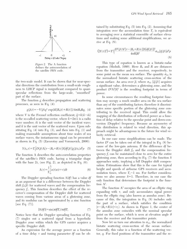
quency fc can be maintained close to zero for the entireThe function L describes the auto-correlation propertiesglistening zone, then according to Eq. (7) the function Sof the satellite’s PRN code, having a triangular shapeapproaches unity, implying a full Doppler shift compen-with the base 2sc (see Fig. 2), as depicted in Eq. (6):sation. Estimations show that this is the case for typicalheight and speeds of airborne GPS receivers and accu-L(s)5

1Ti

#Ti

0

a(t)a(t1s)dt (6)mulation times, where Ta,1 ms. For further considera-tions we also assume S51. Therefore, in our case theThe Doppler spreading function S(df) has a value dfonly function that determines the footprint is the func-as an argument that is a difference between the Dopplertion L2.shift fD(q→) for scattered waves and the compensation fre-

The function L2 occupies the area of an elliptic ringquency fc. This function describes the effect of the re-expanding with s, and only accumulates signal powerceiver’s compensation of the Doppler shift for scatteredfrom the elliptic ring (also known as annulus zone). Be-waves coming from various areas of a glistening zone,cause of this, the integration in Eq. (8) includes onlyand its modulus can be approximated by a sinc functionthe part of a surface, which satisfies the condition[see Eq. (7)]:|s2(R01R)/c|,sc). As shown in Figure 1, the center of|S(df)|5sin(pdfTi)/pdfTi (7) the annulus zone coincides with the nominal specularpoint on the surface, which is seen at elevation angle hNotice here that the Doppler spreading function of Eq.from the receiver and the transmitter points.(7) singles out a scattered signal from a hyperbolic

Now let us turn our attention to r0,b, the normalizedDoppler zone within which the GPS carrier acquires abistatic scattering cross-section of the ocean surface.specific Doppler shift.Generally, this value is a function of the scattering vec-An expression for the average power as a function

of a time delay s and tuning parameter df can be ob- tor, q. For fixed positions of the transmitter and the re-

166 Komjathy et al.

ceiver above a surface, this vector can be regarded as ponents. For a sea surface, the most probable orientationfunction of the coordinate q. Only in the case of back- of slopes is parallel to the plane z50. Then, the PDFscattering (m→ 52n→, q→52kn

→) the bistatic cross-section, r0,b has a maximum at s50, and the bistatic cross-section r0,b

becomes the conventional monostatic radar cross-section has a maximum at q→⊥50 (i.e., at nominal specular direc-of the sea surface, r0. The latter characteristics have tion with respect to the mean sea surface). Note that thebeen measured intensively in various radio wave bands width of r0,b in terms of q describes a glistening zonefor many years (Skolnik, 1990). Unfortunately, there is produced by quasispecular points on the sea surface.no analogous database for r0,b. However, r0,b can be mod- The effects of wind speed and direction appear ineled theoretically. Here, we limit ourselves to a regime the distribution of surface slopes. The stronger the wind,of so-called diffusive scattering from the sea surface (or the greater the variance of slopes and the wider the glis-large values of the Rayleigh parameter) requiring for any tening zone becomes. The direction along which the cor-part of a glistening zone that the typical wave height be responding slope variance (the size of the glisteningseveral times larger than the illumination wavelength di- zone) is maximal indicates the up/down wind direction.vided by the sine of an elevation angle h (both with re- To distinguish between up- and downwind, we need tospect to the transmitter and receiver). For our case of use the asymmetry between the PDF for negative andL-band radio waves (i.e., k50.19 m and elevation angles positive slopes. However, this issue is beyond the scopeh<458), this situation corresponds to well-developed seas of this paper. It is important to note that ultimately thedriven by winds greater than 3 m/s. The geometric optics a priori assumption about the surface spectrum modellimit of the Kirchhoff approximation, when calculating makes it possible to measure wind direction and speedr0,b, leads to the expression seen in Eq. (9) (Bass and using surface-reflected GPS signals.Fuks, 1979; Rytov et al., 1988): Statistics of the slopes are assumed here to be

Gaussian, with anisotropic surface slopes having wind-r0,b5p|V|2(q/qz)4W(2q⊥/qz) (9)dependent variances and correlations. There are some

The value of r0,b depends on a complex Fresnel coef- indications of a departure from Gaussianity at the tailsficient V(h), which in turn depends on a polarization of the PDF (Cox and Munk, 1954). In terms of the glis-state, a complex dielectric constant of seawater, e, and tening zone, it implies that this departure affects a pe-the local grazing angle, h. This is an important issue, be- riphery of the zone. This would translate into some dis-cause upon reflection from the sea surface, the signal at crepancy for the value of the waveform (|Y(s)|2) at timedifferent linear polarizations acquires different phase delays s where the signal itself is very low. Thus, in whatshifts that lead to a reversal of an initial right-hand circu- follows we do not rely on that part of a waveform in ourlar polarization to a predominantly left-hand circular po- retrieval attempts because of the low signal-to-noiselarization in the reflected wave. Only a small portion of ratio.the signal remains of the right-hand circular polarization. One advantage of a Gaussian distribution is that theBecause of this, in experiments with GPS reflections variance of slopes can be derived from a solely wave vec-from the sea surface the down-looking antenna is de- tor spectrum, W(j), of full surface elevations by integrat-signed to receive the left-hand circular-polarized radio ing it over wave numbers, j, which are smaller than awaves. dividing parameter, j*, of the two-scale model, where

Let us introduce a notation VAB for a local Fresnel j*52p/3k is usually considered a reasonable numbercoefficient, where subscripts A and B stand for an initial (see, for example, Zavorotny and Voronovich, 1998), asand final polarization state of radio waves, respectively. seen in Eq. (12) and Eq. (13):Then, Fresnel coefficients for circularly polarized waves,VRR and VRL, can be expressed through Fresnel coeffi- r2

sx,y5ks2x,yl5 ##

j<j*

j2x,yC(j→)d2j (12)

cients for linearly polarized waves, VVV and VHH, in man-ner shown in Eq. (10):

ks2x,yl5 ##

j<j*

jxjyC(j→)d2j (13)VRR5VLL5(VVV1VHH)/2

VRL5VLR5(VVV2VHH)/2 (10)To obtain the values in Eqs. (12) and (13) we utilize

where [see Eq. (11)] the surface spectrum for developed seas proposed byApel (1994). For example, for a wind blowing along aVVV5(e sinh2√e2cos2h)/(e sinh1√e2cos2h)y-axis (08 direction) and wind speed at 10 m height,

VHH5(sinh2√e2cos2h)/(sinh1√e2cos2h) (11) U10510 m/s; typical values for mean-square slope compo-nents are r2

sx50.0097 and r2Sy50.0137. Recently, anotherW(s→) in Eq. (9) is the probability density function

more advanced spectral model has been proposed by El-(PDF) of surface slopes s→5=⊥f(q→). Remember that thesefouhaily et al. (1997). This new model, among other nov-slopes characterize only the “smoothed” surface, which

according to the two-scale model lacks small-scale com- elties, describes diverse wave age (fetch) conditions and

GPS Wind Speed Retrieval 167

over the annulus zone. There is, however, another sourceof noise for the bottom channel, which is partially aver-aged by the annulus zone. This is a multiplicative Ray-leigh noise resulting from a random character of surfacescattering and having a different time scale. This obser-vation is supported by measurements showing that thereis no strong signal correlation between the top and bot-tom channels. It should be mentioned here that the Ray-leigh noise is more pronounced in the signal at bins cor-responding to the periphery of the glistening zone (thetail of the PDF) where the time averaging becomes in-

Figure 3. Mean-square slope as a function of wind sufficient.speed for two surface spectrum models. Therefore, the normalization of the bottom antenna

signal by the unstable top antenna signal is not reason-able. Instead, we normalize the bottom antenna signal by

agrees with in situ observations of Cox and Munk (1954), a more stable quantity, which is the integral value N de-whereas the model by Apel (1994) does not. rived again from the bottom antenna signal [see Eq. (14)]:

We should stress that the sensitivity of the mean-square slope to the choice of a spectral model depends N5#

T3

0

,|Y(s)|2.ds (14)on various specific factors, such as wind conditions, andthe value of the dividing parameter j*. In Figure 3, we This value is convenient for use as a normalization factorpresent results of computations for the mean-square because it can be shown that N practically does not de-slope, mss5r2

sx1r2sy, as a function of wind speed based on pend on surface statistics. Indeed, upon substituting Eq.

these two spectral models. It is seen that corresponding (8) into Eq. (14), one should notice that integration overcurves are relatively close to each other in the interval T3..sc produces a constant [see Eq. (15)]:of wind speed between 7 m/s and 18 m/s, where the dif-ference is less than about 10%. For lower and higher #

T3

0

L2[s2(R01R)/c]ds5A15const (15)winds, this difference increases. Next, we show how thisdifference in mean-square slopes translates into a differ- Under conditions of the experiment, an angularence between waveforms of the GPS surface-reflected width (from several to about 108) of the glistening zone,signal. as described by the function r0,b(q), is smaller than an

To compare the model predictions with the experi- angular width (more than 1008) of the low-gain antennamental results, the model was configured to predict the beam described by D, and also is smaller than othernormalized signal power as a function of code delay from characteristic angular scales of integrand functions in Eq.the predicted nominal specular point. There are various (8). This allows us to leave only r0,b under the integral,options to normalize the measured signals. We choose to taking other functions at the point of a nominal specularnormalize them by the integral power observed in delay reflection, as seen in Eq. (16):bins within the expected range of the glistening zone,

N5(T 2i A1BD2)/(4pR2

0R2) (16)rather than by the power of the direct signal. This is nec-essary because multipath from the airplane fuselage to- where [see Eq. (17)]gether with airplane random yaw, roll, and pitch createsa significant variation of the signal from the top antenna B5##r0,b(q→)d2q (17)on time scales of a few seconds. However, the signalfrom the bottom antenna is less affected by the fuselage If neglecting radiation losses in water (as expressed by

the Fresnel coefficient, V) from first principles [or di-multipath because it is suppressed by spatial averaging

Figure 4. Normalized maximum powerdependence on satellite elevation anglefor various wind speed at 10-km altitude.

168 Komjathy et al.

Figure 5. Normalized power dependence on timedelay for receiver height ranging from 10 km to100 km with 10-km increments for 8-m/s windspeed.

rectly from Eq.(9)], this value [Eq. (17)] should conserve formed numerical calculations of this power as a functionof s. For calculations, the surface spectral model by Apel(i.e., B is approximately a constant). Therefore, the value

N does not depend on surface statistics and indeed can (1994) has been used. For the sake of simplicity, we nor-malized this value by the power of the direct signalbe used as a normalization factor. Note also that for low-

gain antennae the ratio (|Y(s)|2)/N does not depend on D. rather than by the value N from Eq. (16).Qualitatively, the model predicts that the power ver-

sus delay curve will broaden (flatten out) and the nor-POSSIBILITY OF REMOTE SENSING malized maximum power will decrease with increasingOF WIND height of the receiver and increasing wind speed. This isillustrated in Figures 4 through 7. Thus, there are twoFor the specific conditions of GPS scattering observed

from an airborne platform, the radar equation of this regions of interest in the waveforms, which may provideinformation on surface conditions—namely, the maxi-model in Eq. (8) has been simplified based on two char-

acteristics of our experiment: (a) low-gain (wide-beam) mum (peak) and the tails. We display in Figure 4 thedependence of maximum normalized power on the windtransmitting and receiving antennae, and (b) aircraft

heights and speeds as well as integration times are short speed (08 wind direction) at 10-km receiver altitude as afunction of satellite elevation angle. It demonstrates anenough that the Doppler spreading across the entire glis-

tening surface is insignificant. obvious decrease in the normalized maximum powerwith an increase in wind speed. The sensitivity of theFrom Eq. (8) it follows that a factor that carries the

information about surface roughness or surface wind is maximum normalized power to the wind direction for allaltitudes is rather weak (i.e., about the 1–2-dB differencer0,b. Changes in wind conditions produce variations in

r0,b, and this affects the behavior of the waveform [i.e., between a signal obtained at up/downwind and cross-wind directions).(|Y(s)|2) as a function of time delay]. Therefore, by mea-

suring the time-delay dependence of (|Y(s)|2), one should As previously mentioned, the maximum reflectedsignal power also shows a sensitivity to the receiverbe able to draw a conclusion about the wind speed above

an ocean surface. From the theoretical analysis, it follows height. In Figure 5, we used an input wind speed of 8m/s, 08 wind direction, and 908 elevation angle. One canthat the optimal conditions for this type of observation

are when the widths of the annulus zones are signifi- clearly see in the presented waveforms that as the re-ceiver height increases, the normalized maximum powercantly smaller than the glistening zone, and at the same

time the range of the time delays s is large enough to decreases. Large separations between different receiverheights can be found in the tail end of the waveforms.cover the entire width of the glistening zone. To demon-

strate the dependence of the power of (|Y(s)|2) on wind Calculations show that at low receiver heights (less than1 km) and at wind speeds from 4 m/s to 10 m/s, thespeed and other parameters of the problem, we per-

Figure 6. Normalized power dependence ontime delay for different wind speeds at receiverheight of 10 km.

GPS Wind Speed Retrieval 169

Figure 7. Normalized power dependence on time de-lay for upwind and cross-wind directions at receiverheight of 5 km and 458 elevation angle.

shape of the waveforms do not significantly differ from estimate wind speed using normalized power measure-the shape of the direct signal. The influence of the sea ments at altitudes of 5 km to 10 km. The reason for thissurface roughness (and therefore, the wind) on the re- is that the sizes of the annulus and glistening zones beginflected signals begins at altitudes higher than 3 km. At equalizing at the 5-km to 10-km altitude range. Belowan altitude of about 10 km, wind speed has a significant that altitude, the glistening surface may be so small thateffect both on the normalized maximum power values the annulus zone cannot resolve it. Above the 5-km toand the tail end of the waveforms as shown in Figure 6 10-km altitude region, the glistening surface tends to get(for 908 elevation angle and 08 wind direction). Corre- as large as tens of kilometers, therefore significantly re-spondingly, for higher winds the sea surface roughness ducing the maximum reflected signal powers.begins to manifest itself at lower altitudes.

Sensitivity of the waveforms, especially their tailends, to the wind direction depends on the elevation REMOTE SENSING AIRCRAFTangle of the satellite. For elevations close to zenith this

For the receiver, a commercially available GPS-develop-sensitivity is minimal, because the footprint (the annulusment kit from GEC Plessey (1996) (now MITEL), in-zone) has a shape of a circular ring. Its angular symmetrycluding a 2021 correlator chip fed by two 2010 RF frontdoes not allow resolving an asymmetry of the glisteningends, was used. A zenith-oriented RHCP antennazone. However, at smaller elevation angles the footprintmounted on the top of the fuselage was utilized to re-acquires a stretched, oval shape along the incidenceceive the direct signal through one of the RF front ends,plane. Therefore, waveforms obtained for differentwhile a nadir-oriented LHCP antenna located on theangles between wind direction and the incidence planebottom of the fuselage was used to receive the reflectedwould have different behaviors, which is illustrated insignal through the other RF front end. Each front endFigure 7. This can be used to retrieve the wind direction.consists of an independent automatic gain control, suchIn the next section, we utilize this information to in-

fer wind speed using aircraft data. It appears possible to that the variance of the sampled data (which, before de-

Figure 8. Sixty-second average measuredand modeled waveforms for PRN21.

170 Komjathy et al.

Figure 9. Eighteen-minute average mea-sured and modeled waveforms for sat-ellite PRN21.

tection, is dominated by white noise) maintains a prede- both flights, an Ashtech Z-12 receiver was used to collectGPS data for precise aircraft position determination.termined average value.

This receiver has been used on aircraft remote sens- Data from the NOAA National Data Buoy Service andTOPEX overflight measurements were used for wind in-ing experiments since the summer of 1997. It has also

flown on a scientific balloon launched from Wallops Is- formation. We used a 150-s sliding average for each sat-ellite to smooth the raw reflected GPS measurementsland in which waveform data was collected up to an alti-

tude of 25 km. The existing receiver uses only one and applied the adaptive signal normalization based onEq. (16). The time delay is measured in half-chip bins,Doppler frequency corresponding to the direct signal

and generates a one-dimensional map of the waveform where one such bin equals approximately 0.5 ls in time,corresponding to 150 m in range. The satellites are iden-dependence on code delay.

In this paper, we present results of a comparison be- tified by their respective PRN numbers. To account fortween data sets obtained using a NASA Super King Air the noise floor of the reflected signal, we used the re-B-200 aircraft in November 1997 and a C-130 aircraft in flected signal between 16 and 32 half-chip delay bins andMay 1998 and the theoretical model described above. subtracted it from the reflected signal.The first data set using GEC Plessey delay-mapping GPSreceivers was obtained during flights out of the NASA

ANALYSIS OF RESULTSStennis Space Center in Mississippi at altitudes of ap-proximately 5 km. A second GPS surface-reflection data The comparison between the Stennis aircraft data and

modeled curves was performed for various GPS satellitesset was collected at NASA Wallops Flight Facility in Vir-ginia at an altitude of about 3 km. Simultaneously, for with different elevation and azimuth angles. In Figure 8,

Figure 10. Sixty-second average measuredand modeled waveforms for PRN01.

GPS Wind Speed Retrieval 171

Figure 11. Eighteen-minute averagemeasured and modeled waveforms forsatellite PRN01.

we show an example of the comparison for satellite variability of the measured wind speeds. In Figure 9, acomparison between an 18-min average, the length ofPRN21 between the modeled and measured waveforms.

The satellite has an average elevation of 458 and azimuth the observation session, and modeled waveforms revealsthat the average wind speed might have been between 8of 1368. We used 6-m/s, 8-m/s, 10-m/s, and 12-m/s wind

speeds and the surface spectral model by Apel (1994) for m/s and 10 m/s. As in Figure 8, reliable wind speed esti-mates can be obtained by taking a reading between 25well-developed seas to calculate the modeled waveforms.

For illustration, in Figure 8 we plotted representative dB and 220 dB on the trailing edge of the waveform.In Figure 9, 1r error bars are also indicated for everywaveforms averaged over 60 s for a period of 18 min.

The modeled waveforms for 6-m/s, 8-m/s, 10-m/s, and data point.Another example of 60-s waveforms of the Stennis12-m/s wind speeds are also displayed and are indicated

with smooth curves. The shapes of the measured wave- data set for PRN01 can be found in Figure 10. The satel-lite has an average elevation of 508 and azimuth of 408,forms show good agreement with the theoretical (mod-

eled) calculations. Note that good estimates for wind indicating a similar elevation angle but different azimuthangle compared to PRN21 described above. The com-speed can be obtained from the trailing edge that can be

characterized with a normalized power between 25 dB parison between the measured and modeled waveformsseems to indicate an estimated wind speed between 8and 220 dB. Below 220 dB, the noise contribution de-

teriorates the waveform. From Figure 8 we can see that m/s to 10 m/s. In Figure 11, the 18-min average wave-form seems to be supporting a 8-m/s to 10-m/s windthe 60-s waveforms between 25 dB and 220 dB fall

within the boundaries of wind speeds that can be charac- speed that we found in the case of PRN21. The errorbars (1r) indicate a 1-m/s level uncertainty in the mea-terized as 8 m/s and 10 m/s. The differences between

the 60-s waveforms can also be interpreted as spatial surements at 220-dB normalized power values. To pro-

Figure 12. Comparison betweenmeasured and modeled waveformsusing two different spectra for sat-ellite PRN21.

172 Komjathy et al.

Figure 13. TOPEX-measured wind speed.

vide independent assessment for the estimated wind to 8.7 m/s within about 40 km. In this investigation, wespeed, we found that a nearby buoy, maintained by were interested to find out whether the rapidly changingNOAA National Data Buoy Service, indicated an 8-m/s wind conditions could be detected in the GPS surface-wind speed. After comparing actual and modeled wave- reflection measurements. After processing the data andforms, we can conclude that the results indicate a 2-m/ matching the TOPEX-indicated geographic area with thes agreement between the measured and the modeled location of GPS measurements for PRN02, we obtainednormalized signal power waveforms. two different waveforms for 0.5-m/s and 8.7-m/s wind

As we mentioned before (see Fig. 3), there is a dif- speeds as indicated in Figure 14. We also displayed theference between mean-square slopes produced by two modeled values using the two different wind speeds. Asdifferent surface spectral models by Apel (1994) and by a matter of fact, our model, which is based on a diffusiveElfouhaily et al. (1997). In Figure 12 we present a com- scattering, should not work at such low wind speeds asparison between computed waveforms using these two 0.5 m/s because the Rayleigh criteria of diffuse scatteringmodels and measured data for PRN21 shown in Figure is violated, limiting the accuracy of modeled waveform9. Computations were made for 8-m/s to 10-m/s wind at lower than 2-m/s to 3-m/s wind speeds. However, for-speed and for a corresponding wind direction. For the

mally it predicts the shape of the waveform correctlyupper part of the trailing edge above the 220-dB level,with a shifted peak power. According to the predictedit is difficult to distinguish which modeled curve fits thevalues, the measured normalized power values display aexperimental points better. For the lower part of the trail-wider waveform for the higher 8.7-m/s wind speed com-ing edge, experimental points group along the 10-m/spared to that for 0.5-m/s wind speed. As predicted byApel’s curve, which overlaps with the 8-m/s Elfouhaily’sthe model, the normalized peak power decreases withcurve. However, because this difference is within the es-higher wind speed. Another example can be found fortimated 2-m/s error interval, the final conclusion cannotPRN07 in Figure 15. Note that agreement between mea-be made yet about the adequacy of these models. Tosured and modeled waveforms can be assessed on theovercome this problem we need to have measurementstrailing edge of the waveform between 25 dB and 220at lower or higher wind speeds with higher accuracy.dB as described earlier. The measured and modeledIn Figures 8 to 12, we presented results from thewind speeds show fair agreement both for PRN02 inStennis data set that can be characterized with a uniformFigure 14 and for PRN07 in Figure 15. The error bars8-m/s to 10-m/s wind speed. In the second (Wallops)indicate somewhat larger uncertainties in the measure-data set, the TOPEX-altimeter overflight indicated vary-ments due to the short (1-min) averaging used to processing wind speed conditions. As seen in Figure 13, TOPEX

data shows that wind speed had changed from 0.5 m/s this data. The satellites have similar azimuth angles,

Figure 14. Measured and modeledwaveforms with two different windspeeds for PRN02.

GPS Wind Speed Retrieval 173

Figure 15. Measured and modeledwaveforms with two different windspeeds for PRN07.

about 2808, but different average elevation angles (i.e., wind speeds. Furthermore, the figure indicates that windspeeds above 2 m/s to 3 m/s, estimated independentlyabout 528 and 338, respectively).

In Figures 14 and 15, the discrepancies between the using the two satellites, show fair agreement with theTOPEX-measured wind data.measured and modeled waveforms at and prior to the

trailing edge of the waveforms can be associated with theGPS receiver noise effects. These discrepancies can also CONCLUSIONSbe detected in the results corresponding to Figures 8through 11, but they are not displayed because the cor- We have demonstrated that GPS signals reflected from

the ocean surface and received at an aircraft altitude ofresponding normalized power values are below 230 dB.For every TOPEX observation, we estimated the 3 km to 5 km using a delay-mapping GPS receiver can

be used as a remote sensing tool to determine ocean sur-trailing edge slope using the GPS-measured waveformsbetween 25 dB and 220 dB and from the theoretical face wind speeds. The results indicate a good agreement

between the measured and the modeled normalized sig-model using various incremental wind speeds. The esti-mated wind speed was obtained by interpolating the nal power waveforms. The inferred wind speed, obtained

by comparing actual and modeled waveforms, showsmeasured slopes between the modeled ones. After pro-cessing the data, we matched the TOPEX-indicated geo- good agreement (within 2 m/s) with ground truth data

obtained from a nearby buoy and the TOPEX satellite.graphic area with the location of GPS measurements topermit a direct comparison between the two techniques. We also found that we were able to obtain fair agree-

ment between measured and modeled waveforms duringIn Fig. 16, we display both the TOPEX-measured windspeeds and our estimated ones using GPS data from two rapidly changing surface wind conditions within a 40-km

area. The results are encouraging and provide us withdifferent satellites, PRN02 and PRN07. We also displaythe 1r error bars on the measured wind speeds. Figure evidence that surface-reflected GPS signals received at

the 3-km to 5-km altitude region may be used to infer16 shows that the error bars are larger for higher windspeeds. This is due to the fact that for higher wind ocean surface wind conditions.

The surface-reflected GPS signals are expected tospeeds the separation between the two waveform slopes,corresponding to two separate wind speeds, are smaller find use in various other ocean remote sensing applica-

tions such as wave height, wind speed, wetland, salinity,than the separation between two wind speeds at smaller

Figure 16. Comparison between windspeed estimates using data from PRN02 andPRN07 and TOPEX satellite altimetry mea-surements.

174 Komjathy et al.

of the sea surface from photographs of the Sun’s glitter. J.and ionospheric total electron content determinationOpt. Soc. Am. 44:838–850.over oceans. The feasibility of making this measurement

Elfouhaily, T., Chapron, B, Katsaros, K, and Vandemark, D.from a satellite instrument is being studied at NASA-(1997), A unified directional spectrum for long and shortLangley, NASA-Goddard, NASA-JPL, NOAA/ETL, andwind-driven waves. J. Geophys. Res. 102:15781–15796.

the University of Colorado at Boulder. If similar results Garrison, J. L., Katzberg, S. J., and Hill, M. I. (1998), Effectcould be obtained from orbit, it will provide us with a of sea roughness on bistatically scattered range coded sig-unique opportunity to use GPS as a new remote sensing nals from the Global Positioning System. Geophys. Res.

Lett. 25:2257–2260.tool on a global scale to infer various geophysical param-Garrison, J. L., Katzberg, S. J., and Howell, C. T., (1997), De-eters. Surface-reflected GPS signals could soon become

tection of ocean reflected GPS signals: Theory and experi-a new source of data for scientists to obtain a better un-ment. Paper presented at The IEEE Southeastcon, Blacks-derstanding of effects such as global ocean current circu-burg, VA, USA.lation, global climate change, and global warming. GEC Plessey Semiconductors (1996), Global Positioning Prod-ucts Handbook.

Katzberg, S. J., and Garrison, J. L. Jr. (1996), Utilizing GPS toThe research was supported by NASA Langley Research Centerdetermine ionospheric delay over the ocean. NASA Tech.(LaRC) under grant no. NAG-1-1927. Part of the research was

also supported by Eric Lindstrom of NASA Headquarters un- Memo 4750.der the Physical Oceanography Program RTOP 622-47-55. The Martı́n-Neira, M. (1993), A passive reflectometry and interfer-continuous support of Stephen Katzberg of LaRC, who supplied ometry system (PARIS): Application to ocean altimetry. ESAthe GPS surface-reflected measurements, is gratefully acknowl- Journal 17:331–355.edged. We would like to thank Ed Walsh of NASA Goddard Parkinson, B. W., Spilker, J. J., Axelrad, P., and Enge, P., Eds.Space Flight Center for the many useful discussions. Many (1996), Global Positioning System: Theory and Applications,thanks goes to the reviewers who helped us with their com- Vol. 163, Progress in Astronautics and Aeronautics, Ameri-ments and suggestions that improved the final manuscript. can Institute of Aeronautics and Astronautics, Washington,

DC.Rytov, S. M., Kravtsov, Yu. A., and Tatarskii, V. I. (1988), Prin-

REFERENCES ciples of Statistical Radiophysics, Vols. 1–4, Springer-Ver-lag, Berlin.

Skolnik, M. I. (1990), Radar Handbook, 2d ed., McGraw-Hill,Apel, J. R. (1994), An improved model of the ocean surfaceNew York.wave vector spectrum and its effects on radar backscatter.

Voronovich, A. G. (1999), Wave Scattering from Rough Sur-J. Geophys. Res. 99:16269–16291.faces, 2d ed., Springer-Verlag, Berlin.Auber, J., Bibaut, A., and Rigal, J. (1994), Characterization of

Ware, R., Exner, M., Feng, D., Gorbunov, M., Hardy, K., Her-multipath on land and sea at GPS frequencies. In Proc. IONman, B., Kuo, Y., Meehan, T., Melbourne, W., Rocken, C.,GPS-94, the 7th International Technical Meeting of the Sat-Schreiner, W., Sokolovskiy, S., Solheim, F., Zou, X., Anthes,ellite Division of The Institute of Navigation, Salt Lake City,R., Businger, S., and Trenberth, K. (1996), GPS soundingUSA, pp. 1155–1171.of the atmosphere from low Earth orbit: Preliminary results.Bass, F. G., and Fuks, I. M. (1979), Wave Scattering from Sta-Bull. Amer. Meteor. Soc. 77:19–40.tistically Rough Surface, International Series in Natural Phi-

Wells, D. E., Beck, N., Delikaraoglou, D., Kleusberg, A., Krak-losophy, v.93, C. B. Vesecky and J. F. Vesecky (Eds.), Per- iwsky, E. J., Lachapelle, G., Langley, R. B., Nakiboglu, M.,gamon Press, Oxford. Schwarz, K. P., Tranquilla, J. M., and Vanic̆ek, P. (1987),

Beckmann, P., and Spizzichino, A. (1963), The Scattering of Guide to GPS Positioning, Canadian GPS Associates, Fred-Electromagnetic Waves from Rough Surfaces, Pergamon ericton, N.B., Canada.Press, New York. Zavorotny, V. U., and Voronovich, A. G. (1998), Two-scale

Clifford, S. F., Tatarskii, V. I., Voronovich, A. G., and Zavo- model and ocean radar Doppler spectra at moderate- androtny, V. U. (1998), GPS sounding of ocean surface waves: low-grazing angles. IEEE Trans. Antennas Propagat.Theoretical assessment. In Proc. Int. Geosci. and Remote 46:84–92.Sens. Symp. (IGARSS), Vol. IV, Seattle, USA, pp. Zavorotny, V. U., and Voronovich, A. G. (2000), Scattering of2005–2007. GPS signals from the ocean with wind remote sensing appli-

cation. IEEE Trans Geosci. Remote Sens., in press, Vol. 38.Cox, C., and Munk, W. (1954), Measurements of the roughness