Computing global and diffuse solar hourly irradiation on clear sky. Review and testing of 54 models

(This is a sample cover image for this issue. The actual cover is not yet available at this time.)

This article appeared in a journal published by Elsevier. The attachedcopy is furnished to the author for internal non-commercial researchand education use, including for instruction at the authors institution

and sharing with colleagues.

Other uses, including reproduction and distribution, or selling orlicensing copies, or posting to personal, institutional or third party

websites are prohibited.

In most cases authors are permitted to post their version of thearticle (e.g. in Word or Tex form) to their personal website orinstitutional repository. Authors requiring further information

regarding Elsevier’s archiving and manuscript policies areencouraged to visit:

http://www.elsevier.com/copyright

http://www.elsevier.com/copyright

Author's personal copy

Renewable and Sustainable Energy Reviews 16 (2012) 1636– 1656

Contents lists available at SciVerse ScienceDirect

Renewable and Sustainable Energy Reviews

j ourna l ho me pa ge: www.elsev ier .com/ locate / rse r

Computing global and diffuse solar hourly irradiation on clear sky. Review andtesting of 54 models

Viorel Badescua,∗, Christian A. Gueymardb, Sorin Chevalc, Cristian Opread, Madalina Baciud,Alexandru Dumitrescud,e, Flavius Iacobescua, Ioan Milosd, Costel Radad

a Candida Oancea Institute, Polytechnic University of Bucharest, Spl. Independentei 313, Bucharest 060042, Romaniab Solar Consulting Services, P.O. Box 392, Colebrook, NH 03576, USAc National Research and Development Institute for Environmental Protection, Splaiul Independentei nr. 294, Sect. 6, Bucuresti 060031, Romaniad National Meteorological Administration, 97 Sos. Bucuresti-Ploiesti, Bucharest 013686, Romaniae University of Bucharest, Faculty of Geography, Bucharest, Romania

a r t i c l e i n f o

Article history:Received 14 December 2011Accepted 18 December 2011

Keywords:Clear sky modelsGlobal solar radiationDiffuse solar radiationHourly irradiationRomania

a b s t r a c t

Fifty-four broad band models for computation of global and diffuse irradiance on horizontal surfaceare shortly presented and tested. The input data for these models consist of surface meteorological data,atmospheric column integrated data and data derived from satellite measurements. The testing procedureis performed for two meteorological stations in Romania (South-Eastern Europe). The testing procedureconsists of forty-two stages intended to provide information about the sensitivity of the models to varioussets of input data. There is no model to be ranked “the best” for all sets of input data. Very simple modelsas well as more complex models may belong to the category of “good models”. The best models for solarglobal radiation computation are, on equal-footing, ESRA3, Ineichen, METSTAT and REST2 (version 81).The second best models are, on equal-footing, Bird, CEM and Paulescu & Schlett. The best models for solardiffuse radiation computation are, on equal-footing, ASHRAE2005 and King. The second best model isMAC model. The best models for computation of both global and diffuse radiation are, on equal-footing,ASHRAE 1972, Biga, Ineichen and REST2 (version 81). The second best is Paulescu & Schlett model.

© 2011 Elsevier Ltd. All rights reserved.

Contents

1. Introduction . . . . . . . . . . . . . . . . . . . . . . . . . . . . . . . . . . . . . . . . . . . . . . . . . . . . . . . . . . . . . . . . . . . . . . . . . . . . . . . . . . . . . . . . . . . . . . . . . . . . . . . . . . . . . . . . . . . . . . . . . . . . . . . . . . . . . . . . . . 16372. Models . . . . . . . . . . . . . . . . . . . . . . . . . . . . . . . . . . . . . . . . . . . . . . . . . . . . . . . . . . . . . . . . . . . . . . . . . . . . . . . . . . . . . . . . . . . . . . . . . . . . . . . . . . . . . . . . . . . . . . . . . . . . . . . . . . . . . . . . . . . . . . . . 16373. Input data . . . . . . . . . . . . . . . . . . . . . . . . . . . . . . . . . . . . . . . . . . . . . . . . . . . . . . . . . . . . . . . . . . . . . . . . . . . . . . . . . . . . . . . . . . . . . . . . . . . . . . . . . . . . . . . . . . . . . . . . . . . . . . . . . . . . . . . . . . . . 1639

3.1. Solar radiation measurements . . . . . . . . . . . . . . . . . . . . . . . . . . . . . . . . . . . . . . . . . . . . . . . . . . . . . . . . . . . . . . . . . . . . . . . . . . . . . . . . . . . . . . . . . . . . . . . . . . . . . . . . . . . . . . . 16393.2. Surface meteorological data . . . . . . . . . . . . . . . . . . . . . . . . . . . . . . . . . . . . . . . . . . . . . . . . . . . . . . . . . . . . . . . . . . . . . . . . . . . . . . . . . . . . . . . . . . . . . . . . . . . . . . . . . . . . . . . . . . 16403.3. Column integrated data . . . . . . . . . . . . . . . . . . . . . . . . . . . . . . . . . . . . . . . . . . . . . . . . . . . . . . . . . . . . . . . . . . . . . . . . . . . . . . . . . . . . . . . . . . . . . . . . . . . . . . . . . . . . . . . . . . . . . . 1640

3.3.1. Ozone . . . . . . . . . . . . . . . . . . . . . . . . . . . . . . . . . . . . . . . . . . . . . . . . . . . . . . . . . . . . . . . . . . . . . . . . . . . . . . . . . . . . . . . . . . . . . . . . . . . . . . . . . . . . . . . . . . . . . . . . . . . . . . . 16403.3.2. Precipitable water . . . . . . . . . . . . . . . . . . . . . . . . . . . . . . . . . . . . . . . . . . . . . . . . . . . . . . . . . . . . . . . . . . . . . . . . . . . . . . . . . . . . . . . . . . . . . . . . . . . . . . . . . . . . . . . . . . 1640

3.4. Satellite derived data . . . . . . . . . . . . . . . . . . . . . . . . . . . . . . . . . . . . . . . . . . . . . . . . . . . . . . . . . . . . . . . . . . . . . . . . . . . . . . . . . . . . . . . . . . . . . . . . . . . . . . . . . . . . . . . . . . . . . . . . . 16403.4.1. Surface albedo . . . . . . . . . . . . . . . . . . . . . . . . . . . . . . . . . . . . . . . . . . . . . . . . . . . . . . . . . . . . . . . . . . . . . . . . . . . . . . . . . . . . . . . . . . . . . . . . . . . . . . . . . . . . . . . . . . . . . . 16403.4.2. Atmospheric turbidity data . . . . . . . . . . . . . . . . . . . . . . . . . . . . . . . . . . . . . . . . . . . . . . . . . . . . . . . . . . . . . . . . . . . . . . . . . . . . . . . . . . . . . . . . . . . . . . . . . . . . . . . . . 1640

3.5. Default values . . . . . . . . . . . . . . . . . . . . . . . . . . . . . . . . . . . . . . . . . . . . . . . . . . . . . . . . . . . . . . . . . . . . . . . . . . . . . . . . . . . . . . . . . . . . . . . . . . . . . . . . . . . . . . . . . . . . . . . . . . . . . . . . 16414. Testing procedure . . . . . . . . . . . . . . . . . . . . . . . . . . . . . . . . . . . . . . . . . . . . . . . . . . . . . . . . . . . . . . . . . . . . . . . . . . . . . . . . . . . . . . . . . . . . . . . . . . . . . . . . . . . . . . . . . . . . . . . . . . . . . . . . . . . . 1642

4.1. Compatibility between various input datasets . . . . . . . . . . . . . . . . . . . . . . . . . . . . . . . . . . . . . . . . . . . . . . . . . . . . . . . . . . . . . . . . . . . . . . . . . . . . . . . . . . . . . . . . . . . . . . 16424.1.1. Spatial compatibility of measurement datasets at Bucharest. . . . . . . . . . . . . . . . . . . . . . . . . . . . . . . . . . . . . . . . . . . . . . . . . . . . . . . . . . . . . . . . . . . . . . 16424.1.2. Time compatibility between measurements datasets . . . . . . . . . . . . . . . . . . . . . . . . . . . . . . . . . . . . . . . . . . . . . . . . . . . . . . . . . . . . . . . . . . . . . . . . . . . . . 16424.1.3. Compatibility between datasets . . . . . . . . . . . . . . . . . . . . . . . . . . . . . . . . . . . . . . . . . . . . . . . . . . . . . . . . . . . . . . . . . . . . . . . . . . . . . . . . . . . . . . . . . . . . . . . . . . . . 1642

∗ Corresponding author. Tel.: +40 21 402 9339; fax: +40 21 318 1019.E-mail addresses: [email protected] (V. Badescu), [email protected] (C.A. Gueymard), [email protected] (S. Cheval).

1364-0321/$ – see front matter © 2011 Elsevier Ltd. All rights reserved.doi:10.1016/j.rser.2011.12.010


V. Badescu et al. / Renewable and Sustainable Energy Reviews 16 (2012) 1636– 1656 1637

4.2. Computation of various quantities . . . . . . . . . . . . . . . . . . . . . . . . . . . . . . . . . . . . . . . . . . . . . . . . . . . . . . . . . . . . . . . . . . . . . . . . . . . . . . . . . . . . . . . . . . . . . . . . . . . . . . . . . . . 16424.2.1. Astronomical quantities . . . . . . . . . . . . . . . . . . . . . . . . . . . . . . . . . . . . . . . . . . . . . . . . . . . . . . . . . . . . . . . . . . . . . . . . . . . . . . . . . . . . . . . . . . . . . . . . . . . . . . . . . . . . 16424.2.2. Atmospheric turbidity parameters . . . . . . . . . . . . . . . . . . . . . . . . . . . . . . . . . . . . . . . . . . . . . . . . . . . . . . . . . . . . . . . . . . . . . . . . . . . . . . . . . . . . . . . . . . . . . . . . . 1642

4.3. Accuracy indicators . . . . . . . . . . . . . . . . . . . . . . . . . . . . . . . . . . . . . . . . . . . . . . . . . . . . . . . . . . . . . . . . . . . . . . . . . . . . . . . . . . . . . . . . . . . . . . . . . . . . . . . . . . . . . . . . . . . . . . . . . . . 16424.4. Broad criteria for model performance . . . . . . . . . . . . . . . . . . . . . . . . . . . . . . . . . . . . . . . . . . . . . . . . . . . . . . . . . . . . . . . . . . . . . . . . . . . . . . . . . . . . . . . . . . . . . . . . . . . . . . . 1642

5. Results and discussion . . . . . . . . . . . . . . . . . . . . . . . . . . . . . . . . . . . . . . . . . . . . . . . . . . . . . . . . . . . . . . . . . . . . . . . . . . . . . . . . . . . . . . . . . . . . . . . . . . . . . . . . . . . . . . . . . . . . . . . . . . . . . . . 16435.1. Analysis for Cluj-Napoca . . . . . . . . . . . . . . . . . . . . . . . . . . . . . . . . . . . . . . . . . . . . . . . . . . . . . . . . . . . . . . . . . . . . . . . . . . . . . . . . . . . . . . . . . . . . . . . . . . . . . . . . . . . . . . . . . . . . . 1643

5.1.1. Input data . . . . . . . . . . . . . . . . . . . . . . . . . . . . . . . . . . . . . . . . . . . . . . . . . . . . . . . . . . . . . . . . . . . . . . . . . . . . . . . . . . . . . . . . . . . . . . . . . . . . . . . . . . . . . . . . . . . . . . . . . . . 16435.1.2. Results . . . . . . . . . . . . . . . . . . . . . . . . . . . . . . . . . . . . . . . . . . . . . . . . . . . . . . . . . . . . . . . . . . . . . . . . . . . . . . . . . . . . . . . . . . . . . . . . . . . . . . . . . . . . . . . . . . . . . . . . . . . . . . 1644

5.2. Analysis for Bucharest . . . . . . . . . . . . . . . . . . . . . . . . . . . . . . . . . . . . . . . . . . . . . . . . . . . . . . . . . . . . . . . . . . . . . . . . . . . . . . . . . . . . . . . . . . . . . . . . . . . . . . . . . . . . . . . . . . . . . . . . 16465.2.1. Input data . . . . . . . . . . . . . . . . . . . . . . . . . . . . . . . . . . . . . . . . . . . . . . . . . . . . . . . . . . . . . . . . . . . . . . . . . . . . . . . . . . . . . . . . . . . . . . . . . . . . . . . . . . . . . . . . . . . . . . . . . . . 16465.2.2. Results . . . . . . . . . . . . . . . . . . . . . . . . . . . . . . . . . . . . . . . . . . . . . . . . . . . . . . . . . . . . . . . . . . . . . . . . . . . . . . . . . . . . . . . . . . . . . . . . . . . . . . . . . . . . . . . . . . . . . . . . . . . . . . 1651

5.3. Overall analysis for Cluj-Napoca and Bucharest . . . . . . . . . . . . . . . . . . . . . . . . . . . . . . . . . . . . . . . . . . . . . . . . . . . . . . . . . . . . . . . . . . . . . . . . . . . . . . . . . . . . . . . . . . . . . 16536. Conclusions . . . . . . . . . . . . . . . . . . . . . . . . . . . . . . . . . . . . . . . . . . . . . . . . . . . . . . . . . . . . . . . . . . . . . . . . . . . . . . . . . . . . . . . . . . . . . . . . . . . . . . . . . . . . . . . . . . . . . . . . . . . . . . . . . . . . . . . . . . 1654

Acknowledgments . . . . . . . . . . . . . . . . . . . . . . . . . . . . . . . . . . . . . . . . . . . . . . . . . . . . . . . . . . . . . . . . . . . . . . . . . . . . . . . . . . . . . . . . . . . . . . . . . . . . . . . . . . . . . . . . . . . . . . . . . . . . . . . . . . . 1654References . . . . . . . . . . . . . . . . . . . . . . . . . . . . . . . . . . . . . . . . . . . . . . . . . . . . . . . . . . . . . . . . . . . . . . . . . . . . . . . . . . . . . . . . . . . . . . . . . . . . . . . . . . . . . . . . . . . . . . . . . . . . . . . . . . . . . . . . . . . 1654

1. Introduction

The appropriate design of many solar energy devices requires adetailed knowledge of solar global and diffuse radiation availability.Although there are several world maps of solar radiation, they arenot detailed enough to be used for the determination of availablesolar energy on small areas. These circumstances have promptedthe development of calculation procedures to provide radiationestimates for areas where measurements are not carried out and forsituations when gaps in the measurement records occurred. Only aminority of these procedures has been validated by their authors,and usually under specific geographical or climatic circumstancesonly. To increase the confidence in modeled data accuracy there isa need for validation by independent groups and at a variety of testsites in many different climatic areas. Existing validation reports ofthe literature refer usually to a small number of models being inter-compared under specific climatic environments [1–10]. The correctvalidation and comparison of radiative models raise specific issues.For instance, different statistics may be used to evaluate the biasand random differences between the computed and measured data.Moreover, various ranking procedures can be used to compare theperformance of models, yielding different results (for more detaileddiscussions, see [9]).

One problem occurring during models utilization is the largevariety of input data that various users has at their disposal. It isquite usual that the user has access to databases which do not coverall the necessary input parameters of a specific model known tohave good performance. In this case the user has to choose anothermodel which fits the available input databases or, alternately, toprepare ad hoc input parameters for that specific model. This lastsolution sometimes involves data interpolation (or even extrap-olation) and lower overall performance is then expected due tounavoidable propagation of errors.

The present investigation considers 54 clear-sky global and dif-fuse solar radiation models, i.e. a much larger sample of what theliterature offers than in any previous study. Most of these modelshave been previously tested, under a few geographical conditions,during different time intervals and by using various testing proce-dures. How they compare in practice under specific and identicalconditions is still not known.

Reference radiometric measurements (used as “ground truth”)are provided here by two meteorological and radiometric stationsin South-Eastern Europe (Romania). These stations have providedgood-quality routine data over many years. These are not high-end research-class stations, however, which means that the presentstudy can be considered representative of what can be obtained athundreds of similar stations over the world, rather than at a fewspecialized sites, like in some previous studies (e.g. [9,10]). These

studies considered the ideal case when all the investigated models’inputs were measured locally at high frequency with high-qualityinstruments, so as to obtain the intrinsic performance of thesemodels by avoiding propagation of errors. In contrast, the presentinvestigation is much more pragmatic, since it uses “normal” radi-ation measurements and interpolated/extrapolated input data inboth space and time to evaluate the “real world” performance ofmodels under non-ideal conditions. Results have been presentedfor computation of global radiation [11] and diffuse radiation [12].

The objectives of this investigation are twofold. First, a reviewof models performance is made, by comparing their predictionsunder identical climate conditions and using a unique testing pro-cedure for computation of global and diffuse radiation. Second, thesensitivity of each model’s performance on the accuracy in theatmospheric databases used as inputs is reported for both typesof solar radiation.

2. Models

All the 54 models for computation of global and diffuse irradi-ance on horizontal surface are briefly described in what follows,using a call number (G001 to G054) for further reference. Some ofthese models were already tested in [9,10,13]. Fortran routines forall models may be found in [11,12]. The only input variable that iscommon to all models is the zenith angle, Z, which characterizesthe sun position. For those models that refer to the solar constant,a common value of 1366.1 W/m2 is used [14].

G001. ASHRAE 1972This is a historical model still widely used by engineers to cal-

culate solar heat gains and cooling loads in buildings, or insolationof simple solar systems. It is based on original empirical work con-ducted in the 1950s and 1960s [15]. For more details, see [3,10].

G002. ASHRAE 2005ASHRAE 2005 is similar to ASHRAE model of 1972, but with some

revised coefficients that appeared in [16].G003. BadescuThis model is based on MAC (entry G029 in this list), and was

proposed by Badescu [17].G004. BashahuThe composite model of Bashahu and Laplaze [18] is based on

the direct irradiance model of King and Buckius [19]; see entry G027below.

G005. BCLSMThis is the model originally proposed by Barbaro et al. [20] and

later modified in [1,4,21]. The original Barbaro equations are usedhere, with three modifications: (1) The units in Barbaro’s Eq. (10)are converted from cal/(cm2 min) to W/m2, using 1 cal = 4.184 J; (2)a multiplier of 0.1 that was apparently missing in the second part

https://www.researchgate.net/publication/236314578_Clear-sky_irradiance_predictions_for_solar_resource_mapping_and_large-scale_applications_Improved_validation_methodology_and_detailed_performance_analysis_of_18_broadband_radiative_models?el=1_x_8&enrichId=rgreq-6c4911f24b7fc1d54edbe32b2503a9e1-XXX&enrichSource=Y292ZXJQYWdlOzIzMzQxNjY3OTtBUzoxMDQ2ODc0MjAzMTM2MDZAMTQwMTk3MDgzNDk5NA==



https://www.researchgate.net/publication/236314624_Testing_52_models_of_clear_sky_solar_irradiance_computation_under_the_climate_of_Romania?el=1_x_8&enrichId=rgreq-6c4911f24b7fc1d54edbe32b2503a9e1-XXX&enrichSource=Y292ZXJQYWdlOzIzMzQxNjY3OTtBUzoxMDQ2ODc0MjAzMTM2MDZAMTQwMTk3MDgzNDk5NA==

https://www.researchgate.net/publication/222471635_Evaluation_of_selected_models_for_estimating_solar_radiation_on_horizontal_surfaces?el=1_x_8&enrichId=rgreq-6c4911f24b7fc1d54edbe32b2503a9e1-XXX&enrichSource=Y292ZXJQYWdlOzIzMzQxNjY3OTtBUzoxMDQ2ODc0MjAzMTM2MDZAMTQwMTk3MDgzNDk5NA==

https://www.researchgate.net/publication/226864563_Comparison_of_Cloudless_Sky_Parameterizations_of_Solar_Irradianceat_Various_Spanish_Midlatitude_Locations?el=1_x_8&enrichId=rgreq-6c4911f24b7fc1d54edbe32b2503a9e1-XXX&enrichSource=Y292ZXJQYWdlOzIzMzQxNjY3OTtBUzoxMDQ2ODc0MjAzMTM2MDZAMTQwMTk3MDgzNDk5NA==

https://www.researchgate.net/publication/228581201_Assessment_of_some_global_solar_radiation_parameterizations?el=1_x_8&enrichId=rgreq-6c4911f24b7fc1d54edbe32b2503a9e1-XXX&enrichSource=Y292ZXJQYWdlOzIzMzQxNjY3OTtBUzoxMDQ2ODc0MjAzMTM2MDZAMTQwMTk3MDgzNDk5NA==

https://www.researchgate.net/publication/223671960_Clear-sky_classification_procedures_and_models_using_a_world-wide_data-base?el=1_x_8&enrichId=rgreq-6c4911f24b7fc1d54edbe32b2503a9e1-XXX&enrichSource=Y292ZXJQYWdlOzIzMzQxNjY3OTtBUzoxMDQ2ODc0MjAzMTM2MDZAMTQwMTk3MDgzNDk5NA==

https://www.researchgate.net/publication/256325395_Direct_solar_transmittance_for_a_clear_sky?el=1_x_8&enrichId=rgreq-6c4911f24b7fc1d54edbe32b2503a9e1-XXX&enrichSource=Y292ZXJQYWdlOzIzMzQxNjY3OTtBUzoxMDQ2ODc0MjAzMTM2MDZAMTQwMTk3MDgzNDk5NA==

https://www.researchgate.net/publication/235276189_Accuracy_and_sensitivity_analysis_for_54_models_of_computing_hourly_diffuse_solar_irradiation_on_clear_sky?el=1_x_8&enrichId=rgreq-6c4911f24b7fc1d54edbe32b2503a9e1-XXX&enrichSource=Y292ZXJQYWdlOzIzMzQxNjY3OTtBUzoxMDQ2ODc0MjAzMTM2MDZAMTQwMTk3MDgzNDk5NA==


https://www.researchgate.net/publication/222694906_Comparison_of_eight_clear_sky_broadband_models_against_16_independent_data_banks?el=1_x_8&enrichId=rgreq-6c4911f24b7fc1d54edbe32b2503a9e1-XXX&enrichSource=Y292ZXJQYWdlOzIzMzQxNjY3OTtBUzoxMDQ2ODc0MjAzMTM2MDZAMTQwMTk3MDgzNDk5NA==

https://www.researchgate.net/publication/245188850_An_atmospheric_model_for_computing_solar_radiation?el=1_x_8&enrichId=rgreq-6c4911f24b7fc1d54edbe32b2503a9e1-XXX&enrichSource=Y292ZXJQYWdlOzIzMzQxNjY3OTtBUzoxMDQ2ODc0MjAzMTM2MDZAMTQwMTk3MDgzNDk5NA==

https://www.researchgate.net/publication/239365446_Verification_of_some_very_simple_clear_and_cloudy_sky_models_to_evaluate_global_solar_irradiance?el=1_x_8&enrichId=rgreq-6c4911f24b7fc1d54edbe32b2503a9e1-XXX&enrichSource=Y292ZXJQYWdlOzIzMzQxNjY3OTtBUzoxMDQ2ODc0MjAzMTM2MDZAMTQwMTk3MDgzNDk5NA==


https://www.researchgate.net/publication/236314644_Validation_and_Ranking_Methodologies_for_Solar_Radiation_Models?el=1_x_8&enrichId=rgreq-6c4911f24b7fc1d54edbe32b2503a9e1-XXX&enrichSource=Y292ZXJQYWdlOzIzMzQxNjY3OTtBUzoxMDQ2ODc0MjAzMTM2MDZAMTQwMTk3MDgzNDk5NA==




https://www.researchgate.net/publication/245168681_An_atmospheric_model_for_computing_direct_and_diffuse_solar_radiation?el=1_x_8&enrichId=rgreq-6c4911f24b7fc1d54edbe32b2503a9e1-XXX&enrichSource=Y292ZXJQYWdlOzIzMzQxNjY3OTtBUzoxMDQ2ODc0MjAzMTM2MDZAMTQwMTk3MDgzNDk5NA==

https://www.researchgate.net/publication/222440572_Critical_analysis_and_performance_assessment_of_clear_sky_solar_irradiance_models_using_theoretical_and_measured_data?el=1_x_8&enrichId=rgreq-6c4911f24b7fc1d54edbe32b2503a9e1-XXX&enrichSource=Y292ZXJQYWdlOzIzMzQxNjY3OTtBUzoxMDQ2ODc0MjAzMTM2MDZAMTQwMTk3MDgzNDk5NA==

https://www.researchgate.net/publication/285443868_Validation_of_models_for_estimating_solar_radiation_on_horizontal_surfaces?el=1_x_8&enrichId=rgreq-6c4911f24b7fc1d54edbe32b2503a9e1-XXX&enrichSource=Y292ZXJQYWdlOzIzMzQxNjY3OTtBUzoxMDQ2ODc0MjAzMTM2MDZAMTQwMTk3MDgzNDk5NA==


https://www.researchgate.net/publication/237683312_American_Society_of_Heating_Refrigerating_and_Air-Conditioning_Engineers_Inc_ASHRAE_New_York_NY1977?el=1_x_8&enrichId=rgreq-6c4911f24b7fc1d54edbe32b2503a9e1-XXX&enrichSource=Y292ZXJQYWdlOzIzMzQxNjY3OTtBUzoxMDQ2ODc0MjAzMTM2MDZAMTQwMTk3MDgzNDk5NA==


1638 V. Badescu et al. / Renewable and Sustainable Energy Reviews 16 (2012) 1636– 1656

of Eq. (10) has been added; and (3) Barbaro’s Eq. (11) has beencorrected for the missing cos Z term involving the zenith angle Z.

G006. BigaThis is the model proposed by Biga and Rosa [22].G007. Bird modelThis is the broadband transmittances and turbidity model

according to Bird and Hulstrom [23,24]. For more details, see[10,25].

G008. CEMThis is the broadband model proposed in Atwater and Ball

[26,27]. See details in [25].G009. ChandraIn this model proposed by Chandra [28], the Linke turbidity

coefficient, TL, was originally a necessary input. This coefficient isobtained here from an average of four linear relationships betweenAngstrom’s coefficient and TL, as proposed in [29–32]:

TL = 2.1331 + 19.0204ˇ. (1)

TL must be constrained to the range 2–5 to avoid divergencein Chandra’s model. Chandra reported his results as abso-lute irradiances in cal/(cm2 min), and used a solar constant of1.94 cal/(cm2 min) or 1353 W/m2. His results are therefore dividedhere by 1.94 to obtain transmittances. This empirical model is basedon measurements that certainly used the IPS56 radiometric scale,hence the multiplication by a correction factor of 1.022 [33] to com-ply with the current WRR scale (whose announcement by the WorldMeteorological Organization in 1978 is posterior to the historicaldata used for the model’s development).

G010. CLSThis is the Cloud Layer Sunshine model developed by Suckling

and Hay [34,35]. Note that precipitable water must be in cm, con-trarily to what is indicated in the original papers.

G011. CPCR2This is the original CPCR2 model by Gueymard [36] with revised

optical masses [3].G012. DogniauxThis combines the models that have been proposed by Dogniaux

for direct radiation [37] and for diffuse radiation [38]. The expres-sion for TL as a function of is taken here from [39]. See [25] fordetails.

G013. DPPThis is the Daneshyar–Paltridge–Proctor model tested in [4,40]

and also reviewed in [41]. The DPP acronym is from Badescu [4]. Thedirect irradiance at normal incidence is here from the original paperby Daneshyar [42] who used the model of Paltridge and Proctor[43], with corrected unit for Z. (It is actually degrees rather thanradians as Badescu or Daneshyar suggested.) Coefficients for diffuseirradiance are given by Daneshyar as 0.218 and 0.299 cal/(cm2 h)for the USA, as cited from [44]. Daneshyar also suggests 0.123 and0.181 for Iran. However, their Eq. (5a) suggests that Z is in radians,which is not correct. Goswami and Klett [40] used the USA values,which are used here too, after conversion from cal/(cm2 h) to W/m2.They used the correct unit for Z. Festa and Ratto [41] mention theIran values, but with Z in radians rather than degrees, due to theconfusion in the original papers. Badescu [4] also used radians, butwith considerably larger values for the coefficients. To avoid furtherconfusion, the modified equations as used here are provided below:

Ebn = 950[1 − exp(−0.075h)] (2)

Ed = 2.534 + 3.475h (3)

Here Ebn and Ed stand for direct normal irradiance and diffuse irradi-ance, respectively, both measured in W/m2. The sun altitude angleis given by h = 90 − Z where Z is in degrees.

G014. ESRA1

This is the model that was used to develop the European SolarRadiation Atlas, with the broadband transmittances and turbiditycomputed according to Rigollier et al. [45,46]. Here the Linke tur-bidity coefficient for an air mass of 2 is obtained from the newPage’s formula, Eq. (19) of [47]. This revision was suggested in [48].For more details, see [10].

G015. ESRA2This model is the same as ESRA1, except that TL is now obtained

using formulae proposed in [7,49].G016. ESRA3This model is similar to ESRA1 or ESRA2, but TL is obtained from

the empirical formula of [50] as a function of precipitable waterand Angstrom’s coefficient.

G017. ESRA4This model is again similar to ESRA1, but TL is obtained here

from Eq. (1).G018. HLJThis is the broadband model developed by Hottel [51] for direct

irradiance, and later modified in [52–56], who all added the diffusetransmittance formula of Liu and Jordan [57], based on Hottel’s ownrecommendation. The Hottel equations corresponding to a visibil-ity of 23 km are used here, which is consistent with the literaturecited. For more details, see [10].

G019. IderiahThis model is proposed in Ideriah [58] based on the direct irra-

diance model by King and Buckius (see entry G027 below).G020. IneichenThis model comes from Ineichen’s parameterization of the SOLIS

spectral model [59]. For more details, see [10].G021. Iqbal AThis is “model A” from Iqbal [33]. It is adapted from the McMas-

ter (MAC) model [60]. The original formulation for the Rayleightransmittance is used here, rather than Iqbal’s Eq. (7.4.8), whichcontains a typo. For more details, see Gueymard [3,10].

G022. Iqbal BThis is “model B” from Iqbal [33]. It is adapted from the Hoyt

model [61]. For more details, see [3,10].G023. Iqbal CThis is “model C” from Iqbal [33]. It is adapted from Bird’s model

(entry G005 above). For more details, see [3,10,25].G024. JosefssonThis is the model by Josefsson [62], as described, used and/or

modified in [1,2]. See [3] for details.G025. KASMThis is the modified Kasten model [63] according to [4].G026. KastenThis is another modification of the original Kasten model [63],

this time following [2,64]. TL is obtained from Eq. (1).G027. KingThis model uses the broadband transmittances and turbidity

functions according to King and Buckius [19] and Buckius and King[65]. The former reference provides and expression that can be usedto calculate direct irradiance [25]. In the latter reference, the diffuseirradiance is to be calculated from its Eq. (36), but two free param-eters remain, namely �L and a1. For this investigation, the function�L has been fitted to the numerical values provided in [65] for fivediscrete values of ˇ, such as

�L = 0.8336 + 0.17257 − 0.64595 exp(−7.4296ˇ1.5) (4)

Similarly, the value of coefficient a1 was only described as vary-ing between 0 and 1. The average value a1 = 0.5 is assumed here inthe absence of more specific indications.

G028. KZHWThis model was proposed by Krarti et al. [64] as a combina-

tion of those of Zhang and Huang [66] for global radiation and

https://www.researchgate.net/publication/222415296_A_broadband_simplified_version_of_the_Solis_clear_sky_model?el=1_x_8&enrichId=rgreq-6c4911f24b7fc1d54edbe32b2503a9e1-XXX&enrichSource=Y292ZXJQYWdlOzIzMzQxNjY3OTtBUzoxMDQ2ODc0MjAzMTM2MDZAMTQwMTk3MDgzNDk5NA==










https://www.researchgate.net/publication/223141576_The_Interrelationship_and_Characteristic_Distribution_of_Direct_Diffuse_and_Total_Solar_Radiation?el=1_x_8&enrichId=rgreq-6c4911f24b7fc1d54edbe32b2503a9e1-XXX&enrichSource=Y292ZXJQYWdlOzIzMzQxNjY3OTtBUzoxMDQ2ODc0MjAzMTM2MDZAMTQwMTk3MDgzNDk5NA==

https://www.researchgate.net/publication/222648151_Direct_solar_transmittance_and_irradiance_predictions_with_broadband_models_Part_I_Detailed_theoretical_performance_assessment?el=1_x_8&enrichId=rgreq-6c4911f24b7fc1d54edbe32b2503a9e1-XXX&enrichSource=Y292ZXJQYWdlOzIzMzQxNjY3OTtBUzoxMDQ2ODc0MjAzMTM2MDZAMTQwMTk3MDgzNDk5NA==





https://www.researchgate.net/publication/256325449_A_numerical_solar_radiation_model_based_on_standard_meteorological_observations?el=1_x_8&enrichId=rgreq-6c4911f24b7fc1d54edbe32b2503a9e1-XXX&enrichSource=Y292ZXJQYWdlOzIzMzQxNjY3OTtBUzoxMDQ2ODc0MjAzMTM2MDZAMTQwMTk3MDgzNDk5NA==

https://www.researchgate.net/publication/42358500_Worldwide_Linke_turbidity_information?el=1_x_8&enrichId=rgreq-6c4911f24b7fc1d54edbe32b2503a9e1-XXX&enrichSource=Y292ZXJQYWdlOzIzMzQxNjY3OTtBUzoxMDQ2ODc0MjAzMTM2MDZAMTQwMTk3MDgzNDk5NA==

https://www.researchgate.net/publication/223128029_A_model_for_calculating_direct_and_diffuse_solar_radiation?el=1_x_8&enrichId=rgreq-6c4911f24b7fc1d54edbe32b2503a9e1-XXX&enrichSource=Y292ZXJQYWdlOzIzMzQxNjY3OTtBUzoxMDQ2ODc0MjAzMTM2MDZAMTQwMTk3MDgzNDk5NA==

https://www.researchgate.net/publication/232873992_Modeling_direct_diffuse_and_total_solar_radiation_for_cloudless_days?el=1_x_8&enrichId=rgreq-6c4911f24b7fc1d54edbe32b2503a9e1-XXX&enrichSource=Y292ZXJQYWdlOzIzMzQxNjY3OTtBUzoxMDQ2ODc0MjAzMTM2MDZAMTQwMTk3MDgzNDk5NA==

https://www.researchgate.net/publication/223830173_Diffuse_solar_radiation_on_a_horizontal_surface_for_a_clear_sky?el=1_x_8&enrichId=rgreq-6c4911f24b7fc1d54edbe32b2503a9e1-XXX&enrichSource=Y292ZXJQYWdlOzIzMzQxNjY3OTtBUzoxMDQ2ODc0MjAzMTM2MDZAMTQwMTk3MDgzNDk5NA==


https://www.researchgate.net/publication/236562225_Solar_radiation_statistics_for_Iran?el=1_x_8&enrichId=rgreq-6c4911f24b7fc1d54edbe32b2503a9e1-XXX&enrichSource=Y292ZXJQYWdlOzIzMzQxNjY3OTtBUzoxMDQ2ODc0MjAzMTM2MDZAMTQwMTk3MDgzNDk5NA==

https://www.researchgate.net/publication/236482872_An_Introduction_to_Solar_Radiation?el=1_x_8&enrichId=rgreq-6c4911f24b7fc1d54edbe32b2503a9e1-XXX&enrichSource=Y292ZXJQYWdlOzIzMzQxNjY3OTtBUzoxMDQ2ODc0MjAzMTM2MDZAMTQwMTk3MDgzNDk5NA==




https://www.researchgate.net/publication/233370099_A_cloud_layer-sunshine_model_for_estimating_direct_diffuse_and_total_solar_radiation?el=1_x_8&enrichId=rgreq-6c4911f24b7fc1d54edbe32b2503a9e1-XXX&enrichSource=Y292ZXJQYWdlOzIzMzQxNjY3OTtBUzoxMDQ2ODc0MjAzMTM2MDZAMTQwMTk3MDgzNDk5NA==

https://www.researchgate.net/publication/252938628_Comparison_of_several_models_for_long_term_monthly_average_daily_insolation_on_horizontal_surfaces_and_the_estimation_of_horizontal_surface_insolation_for_16_U_S_locations?el=1_x_8&enrichId=rgreq-6c4911f24b7fc1d54edbe32b2503a9e1-XXX&enrichSource=Y292ZXJQYWdlOzIzMzQxNjY3OTtBUzoxMDQ2ODc0MjAzMTM2MDZAMTQwMTk3MDgzNDk5NA==


https://www.researchgate.net/publication/245169175_A_procedure_to_obtain_global_radiation_maps_from_sunshine_durations_at_isolated_stations_in_a_region_with_complex_orography?el=1_x_8&enrichId=rgreq-6c4911f24b7fc1d54edbe32b2503a9e1-XXX&enrichSource=Y292ZXJQYWdlOzIzMzQxNjY3OTtBUzoxMDQ2ODc0MjAzMTM2MDZAMTQwMTk3MDgzNDk5NA==

https://www.researchgate.net/publication/241330125_Development_of_typical_year_weather_data_for_Chinese_locations?el=1_x_8&enrichId=rgreq-6c4911f24b7fc1d54edbe32b2503a9e1-XXX&enrichSource=Y292ZXJQYWdlOzIzMzQxNjY3OTtBUzoxMDQ2ODc0MjAzMTM2MDZAMTQwMTk3MDgzNDk5NA==







https://www.researchgate.net/publication/223023259_A_two-band_model_for_the_calculation_of_clear-sky_solar_irradiance_illuminance_and_photosynthetically_active_radiation_at_the_Earth's_surface?el=1_x_8&enrichId=rgreq-6c4911f24b7fc1d54edbe32b2503a9e1-XXX&enrichSource=Y292ZXJQYWdlOzIzMzQxNjY3OTtBUzoxMDQ2ODc0MjAzMTM2MDZAMTQwMTk3MDgzNDk5NA==

https://www.researchgate.net/publication/256325440_Monthly_mean_solar_radiation_statistics_for_Australia?el=1_x_8&enrichId=rgreq-6c4911f24b7fc1d54edbe32b2503a9e1-XXX&enrichSource=Y292ZXJQYWdlOzIzMzQxNjY3OTtBUzoxMDQ2ODc0MjAzMTM2MDZAMTQwMTk3MDgzNDk5NA==

https://www.researchgate.net/publication/222523393_On_the_clear_sky_model_of_the_ESRA_-_European_Solar_Radiation_Atlas_-_With_respect_to_the_Heliosat_method?el=1_x_8&enrichId=rgreq-6c4911f24b7fc1d54edbe32b2503a9e1-XXX&enrichSource=Y292ZXJQYWdlOzIzMzQxNjY3OTtBUzoxMDQ2ODc0MjAzMTM2MDZAMTQwMTk3MDgzNDk5NA==

https://www.researchgate.net/publication/232356504_Solar_radiation_for_Shiraz_Iran?el=1_x_8&enrichId=rgreq-6c4911f24b7fc1d54edbe32b2503a9e1-XXX&enrichSource=Y292ZXJQYWdlOzIzMzQxNjY3OTtBUzoxMDQ2ODc0MjAzMTM2MDZAMTQwMTk3MDgzNDk5NA==






https://www.researchgate.net/publication/5549919_Equivalence_of_Pyrheliometric_and_Monochromatic_Aerosol_Optical_Depths_at_a_Single_Key_Wavelength?el=1_x_8&enrichId=rgreq-6c4911f24b7fc1d54edbe32b2503a9e1-XXX&enrichSource=Y292ZXJQYWdlOzIzMzQxNjY3OTtBUzoxMDQ2ODc0MjAzMTM2MDZAMTQwMTk3MDgzNDk5NA==

https://www.researchgate.net/publication/253811885_Review_Evaluation_and_Improvement_of_Direct_Irradiance_Models?el=1_x_8&enrichId=rgreq-6c4911f24b7fc1d54edbe32b2503a9e1-XXX&enrichSource=Y292ZXJQYWdlOzIzMzQxNjY3OTtBUzoxMDQ2ODc0MjAzMTM2MDZAMTQwMTk3MDgzNDk5NA==

https://www.researchgate.net/publication/284143747_Parametrisierung_der_Globalstrahlung_durch_Bedeckungsgrad_und_Trubungsfaktor?el=1_x_8&enrichId=rgreq-6c4911f24b7fc1d54edbe32b2503a9e1-XXX&enrichSource=Y292ZXJQYWdlOzIzMzQxNjY3OTtBUzoxMDQ2ODc0MjAzMTM2MDZAMTQwMTk3MDgzNDk5NA==


https://www.researchgate.net/publication/223649516_Simple_model_for_estimating_transmittance_of_direct_solar-radiation_through_clear_atmospheres?el=1_x_8&enrichId=rgreq-6c4911f24b7fc1d54edbe32b2503a9e1-XXX&enrichSource=Y292ZXJQYWdlOzIzMzQxNjY3OTtBUzoxMDQ2ODc0MjAzMTM2MDZAMTQwMTk3MDgzNDk5NA==


https://www.researchgate.net/publication/241362359_Dependence_of_solar_radiation_availability_on_atmospheric_turbidity?el=1_x_8&enrichId=rgreq-6c4911f24b7fc1d54edbe32b2503a9e1-XXX&enrichSource=Y292ZXJQYWdlOzIzMzQxNjY3OTtBUzoxMDQ2ODc0MjAzMTM2MDZAMTQwMTk3MDgzNDk5NA==



Watanabe et al. [67] for the direct/diffuse component separation.The empirical coefficients as modified in [64] are used here.

G029. MACThe McMaster model of Davies et al. [60] was later used

and/or modified in [1,2,68]. The formulation (particularly for theRayleigh and aerosol transmittances) used here is as described in[1]. A corrected Rayleigh transmittance expression is used heresince it was misprinted in the latter report. For more details, see[3,10].

G030. MachlerThis is the model proposed by Machler and Iqbal [69].G031. METSTATThis is a modified version of Bird’s model (entry G007 above)

according to Maxwell [70]. For more details, and how to evaluatethe Unsworth–Monteith turbidity coefficient it uses, see [3,10,25].

G032. MRM4This model is described by Muneer et al. [71] and Kambezidis

[72]. The numerical coefficients considered here are for the USAand southern Europe, as given in [73, p. 73]. For more details, anda discussion of this model’s shortcomings, see [25,74].

G033. MRM5More than a mere revision of MRM4 (entry G032 just above),

this is actually a completely different algorithm. It is adapted herefrom Fortran code, version 5, by Kambezidis and Psiloglou [75,76].Ozone, precipitable water, Angstrom’s coefficient and albedo arethe input variables here, as discussed in [10].

G034. NijegorodovThis model [77] uses the air mass formula from Nijegorodov

and Luhanga [78] and transmittance expressions from Bird’s model(entry G007 above). It is assumed here that the Earth radius is6367 km and that the effective atmosphere thickness is 29.7 km.

G035. NRCCThe original model by Belcher and DeGaetano [79,80] was

slightly modified according to personal communications withBelcher [81], as discussed in [10].

G036. PaltridgeThis is the empirical model of Paltridge and Platt [82].G037. PerrinThis is the broadband model of Perrin de Brichambaut and Vauge

[83], as discussed in [25].G038. PRA part of this model is described in Psiloglou et al. [84]. However,

the aerosol transmittance expression is here from the REST model[25] per Psiloglou’s request [85], with the purpose to improvethe model’s performance. The new acronym stands for “Psiloglou-REST”.

G039. PSIMThis model is described by Gueymard [74] and its performance

for direct irradiance predictions was discussed in [25,74].G040. REST250This is version 5.0 of the REST2 model, as described by Gueymard

[86].G041. RodgersThis model uses the Unsworth–Monteith turbidity coefficient.

It is described by Rodgers et al. [87]. See also [25].G042. RSCCarroll [88] combined earlier algorithms by Robinson [89] and

Sellers [90] to derive this model, hence its acronym.G043. SantamourisThis model is based on atmospheric transmittances from

Psiloglou et al. [84] (entry G029 above), following the advice of Dr.Santamouris [91]. A pressure correction was added where neededfor consistency, as also discussed in [25].

G044. SchulzeThis model was proposed by Schulze [92].G045. Sharma

This empirical model was proposed by Sharma and Pal [93]. Theyused a solar constant of 2 cal/(cm2 min), which is replaced here bythe more recent value of 1366.1 W/m2 [14].

G046. WattThis model was proposed by Watt [94], and its performance

was studied by Bird and Hulstrom [24]. These authors, however,seem to have misinterpreted some equations, due to Watt’s non-explicit use of the decimal logarithm. This can explain the subparperformance results of the Bird and Hulstrom study. The requiredextinction layer heights are derived here from the original author’sFig. 4.0.2. A fixed stratospheric turbidity of 0.02 is assumed.

G047. WeselyThis model by Wesely and Lipschutz [95,96] uses visibility,

which is derived here from Angstrom’s coefficient by using theformula of [19] in reverse mode.

G048. YangThe original model of Yang et al. [97] is used here with the cor-

rections described in [25], which were eventually included in a laterdescription of the model [98].

G049. ZhangThe model proposed by Zhang et al. [66,99] described

site-specific coefficients empirically derived from radiation mea-surements in China. For this study, the average of the coefficientstabulated for 24 sites [99] was rather used for improved universal-ity. The model’s Gompertz function that separates the direct anddiffuse components appeared to generate unphysical values, whichwas caused by its coefficient a4 being misprinted. The correct value(2.99) is used here [100].

G050. HSThis is a combination between the model by Haurwith [101,102]

to predict direct irradiance and the model by Schulze [92] to predictdiffuse irradiance.

G051. ABCGSThis is a combination between the model by

Adnot–Bourges–Campana–Gicquel [103] to predict directirradiance and the model by Schulze [92] to predict diffuseirradiance.

G052. Paulescu and SchlettIn this model by Paulescu and Schlett [104], the value � = 0.5 is

adopted here to approximate a Rayleigh atmosphere, based on thesuggestion by Paulescu [105].

G053. JanjaiThis model is based on publications by Janjai [106] and Janjai

and Sricharoen [107].G054. REST281This is version 8.1 of REST2 model, which contains a few

corrections compared to the entry G040 above and the originaldescription by Gueymard [86]. For more details on this model seeGueymard [10].

3. Input data

The input data depends on model. Table 1 shows the inputparameters needed by all models while Table 2 shows the entriesneeded by each model. The input data have been organized in sev-eral databases as described next.

3.1. Solar radiation measurements

The solar radiation database consists of global and diffusehourly irradiation measured by using Kipp & Zonen radiometersin Cluj-Napoca and Bucharest-Afumati (see Table 3 for geo-graphic coordinates). A Kipp & Zonen CM11 device is operatingat Bucharest-Afumati station while the Cluj-Napoca station is pro-vided with CM6B devices. The measurement uncertainty is ±3% for

https://www.researchgate.net/publication/245197014_Development_of_the_typical_meteorological_database_for_Chinese_locations?el=1_x_8&enrichId=rgreq-6c4911f24b7fc1d54edbe32b2503a9e1-XXX&enrichSource=Y292ZXJQYWdlOzIzMzQxNjY3OTtBUzoxMDQ2ODc0MjAzMTM2MDZAMTQwMTk3MDgzNDk5NA==


https://www.researchgate.net/publication/251574242_Semiempirical_models_for_the_estimation_of_clear_sky_solar_global_and_direct_normal_irradiances_in_the_tropics?el=1_x_8&enrichId=rgreq-6c4911f24b7fc1d54edbe32b2503a9e1-XXX&enrichSource=Y292ZXJQYWdlOzIzMzQxNjY3OTtBUzoxMDQ2ODc0MjAzMTM2MDZAMTQwMTk3MDgzNDk5NA==

https://www.researchgate.net/publication/234175640_A_method_for_estimating_hourly_averages_of_diffuse_and_direct_solar_radiation_under_a_layer_of_scattered_clouds?el=1_x_8&enrichId=rgreq-6c4911f24b7fc1d54edbe32b2503a9e1-XXX&enrichSource=Y292ZXJQYWdlOzIzMzQxNjY3OTtBUzoxMDQ2ODc0MjAzMTM2MDZAMTQwMTk3MDgzNDk5NA==

https://www.researchgate.net/publication/222317752_REST2_High-performance_solar_radiation_model_for_cloudless-sky_irradiance_illuminance_and_photosynthetically_active_radiation_-_Validation_with_a_benchmark_dataset?el=1_x_8&enrichId=rgreq-6c4911f24b7fc1d54edbe32b2503a9e1-XXX&enrichSource=Y292ZXJQYWdlOzIzMzQxNjY3OTtBUzoxMDQ2ODc0MjAzMTM2MDZAMTQwMTk3MDgzNDk5NA==


https://www.researchgate.net/publication/256106227_A_physically_based_method_of_estimating_solar_radiation_from_suncards?el=1_x_8&enrichId=rgreq-6c4911f24b7fc1d54edbe32b2503a9e1-XXX&enrichSource=Y292ZXJQYWdlOzIzMzQxNjY3OTtBUzoxMDQ2ODc0MjAzMTM2MDZAMTQwMTk3MDgzNDk5NA==



https://www.researchgate.net/publication/22145898_An_experimental_study_of_the_effects_of_aerosols_on_diffuse_and_direct_solar_radiation_received_during_the_summer_near_Chicago?el=1_x_8&enrichId=rgreq-6c4911f24b7fc1d54edbe32b2503a9e1-XXX&enrichSource=Y292ZXJQYWdlOzIzMzQxNjY3OTtBUzoxMDQ2ODc0MjAzMTM2MDZAMTQwMTk3MDgzNDk5NA==


https://www.researchgate.net/publication/222541243_Hybrid_model_for_estimating_global_solar_radiation?el=1_x_8&enrichId=rgreq-6c4911f24b7fc1d54edbe32b2503a9e1-XXX&enrichSource=Y292ZXJQYWdlOzIzMzQxNjY3OTtBUzoxMDQ2ODc0MjAzMTM2MDZAMTQwMTk3MDgzNDk5NA==

https://www.researchgate.net/publication/228350387_Improving_estimation_of_hourly_daily_and_monthly_solar_radiation_by_importing_global_data_sets?el=1_x_8&enrichId=rgreq-6c4911f24b7fc1d54edbe32b2503a9e1-XXX&enrichSource=Y292ZXJQYWdlOzIzMzQxNjY3OTtBUzoxMDQ2ODc0MjAzMTM2MDZAMTQwMTk3MDgzNDk5NA==

https://www.researchgate.net/publication/226985873_A_simplified_but_accurate_spectral_solar_irradiance_model?el=1_x_8&enrichId=rgreq-6c4911f24b7fc1d54edbe32b2503a9e1-XXX&enrichSource=Y292ZXJQYWdlOzIzMzQxNjY3OTtBUzoxMDQ2ODc0MjAzMTM2MDZAMTQwMTk3MDgzNDk5NA==

https://www.researchgate.net/publication/223047690_Interrelationships_between_total_direct_and_diffuse_solar_radiation_in_the_tropics?el=1_x_8&enrichId=rgreq-6c4911f24b7fc1d54edbe32b2503a9e1-XXX&enrichSource=Y292ZXJQYWdlOzIzMzQxNjY3OTtBUzoxMDQ2ODc0MjAzMTM2MDZAMTQwMTk3MDgzNDk5NA==




Table 1Input data for models used in this work.

Symbol Meaning

AstronomicalYear Number of yearMonth Number of the month in the year (1 to 12)Day Number of day in the month (1 to 31)h Hour (UTC)ı Sun declination (deg.)z Zenith angle (deg.)Esc Solar constant (W/m2)En0 Extraterrestrial irradiance (W/m2), corrected for the actual

sun-earth distancemK Kasten’s air massmKY Kasten & Young’s air massGeographical� Latitude (deg)ϕ Longitude (deg)hg Site’s elevation (meter)�g Ground albedoMeteorological (surface)p Surface air pressure (hPa)T Air temperature, dry-bulb (K)�T dry-bulb temperature T at time t, T(t), −T(t − 3 h)U Surface air relative humidity (%)W Wind speed (m/s)Meterological (column integrated)uo Reduced ozone vertical pathlength (atm-cm)uN Total NO2 vertical pathlength (atm-cm)w Precipitable water (cm)Quantities related to atmospheric turbidity˛ Angstrom wavelength exponentˇ Angstrom turbidity˛1 Angstrom wavelength exponent for <700 nm˛2 Angstrom wavelength exponent for >700 nm�1 Aerosol single-scattering albedo, <700 nm�2 Aerosol single-scattering albedo, >700 nmTL1 Linke turbidity estimated by using Page/Remund method

[47]TL2 Linke turbidity estimated by using Ineichen method [7]TL3 Linke turbidity estimated from the empirical formula of

Dogniaux [50] as a function of precipitable water andAngstrom’s beta coefficient

TL4 Linke turbidity estimated from the average of four linearrelationships between Angstrom’s beta coefficient andLinke turbidity by Hinzpeter [29], Katz et al. [30],Abdelrahman et al. [31] and Grenier et al. [32].

a Unsworth–Monteith broadband turbidity coefficient700 Aerosol optical depth at 700 nm, dimensionlessvis Visibility (km)

CM11 and ±5% for CM6B. The temperature dependence of sensi-tivity is ±1% for CM11 and ±2% for CM6B, on the interval −20 to+40 ◦C. On a monthly basis the bias for CM6B ranges between −2%and +0.9% [108]. The radiometers are checked twice per week andcleaned when necessary.

The measurement methodology is provided by standardprocedures prepared at the Romanian National MeteorologicalAdministration. Measurements are performed as follows. Solar irra-diance (units: W/m2) is measured at 1-min intervals. The series ofirradiance values are averaged over 10 min, 60 min and 1440 min,respectively. Irradiation values (units: J) for 10 min, 1 h and 24 h areobtained by multiplying the appropriate average irradiance valuesby the appropriate time duration. The integration interval starts ½hour before the time stamp in the files and ends ½ hour after thattime stamp. Central European Time is used in the files.

The radiometers are calibrated once per year throughshaded–unshaded measurements in clear sky days and throughdirect irradiance measurements on a horizontal surface with refer-ence to the Linke-Feussner etalon actinometer. The Linke-Feussneretalon is calibrated with reference to the national etalon, i.e.an Angstrom 702 pirheliometer with electric compensation. The

national etalon is calibrated once at five years with reference to theWorld Radiometric Reference at Davos (Swiss).

Partial sky obstructions or shading of the sensors by natural orartificial structures is low and is not considered. There are less than0.1% missing or suspicious data.

3.2. Surface meteorological data

Meteorological data measured in all stations of Table 3 are usedin this study. A few details follow. In case of Bucharest, some of themeteorological variables are measured at Bucharest-Baneasa sta-tion, whereas other parameters are measured at Bucharest-Afumatistation. Sunshine duration is calculated from solar radiation byusing the World Meteorological Organization sunshine criterion[109]. This stipulates that the “sun is shining” if the global solar irra-diance measured perpendicular on sun’s rays exceeds 120 W/m2.Sunshine data are recorded hourly. Daily totals are also computed.Measurements are reported in tens of an hour.

3.3. Column integrated data

3.3.1. OzoneLong-term measurements of column-integrated ozone are

performed in Romania once per day at a single station (Bucharest-Baneasa). Measurements are performed usually in the interval0900–1400 (Eastern European Time). There are missing days in therecordings (Saturdays, Sundays as well as other days). The WOUDCarchive provides data for Bucharest during 1980–2006. Ozone datameasured in 2009 are used here (see Fig. S1 of [11]).

3.3.2. Precipitable waterData for column-integrated precipitable water are available

from two stations. Radiosonde measurements are performed twicedaily at Bucharest-Baneasa (0000 and 1200 UTC) and once dailyat Cluj-Napoca (0000 UTC). Daily measurements for precipitablewater performed during 2009 at Cluj-Napoca and Bucharest-Baneasa (see Figs. S2 and S3 in [11]).

3.4. Satellite derived data

3.4.1. Surface albedoThe ground albedo is obtained for all stations from satellite

images on a monthly basis and 15-km spatial resolution. We haveused the Surface Albedo (SAL) product of the Satellite ApplicationsFacility on Climate Monitoring (CM-SAF) (http://www.cmsaf.eu),which is part of the EUMETSAT distributed ground segment. Theproduct line covers broadband albedo products from the SEVIRIinstrument aboard Meteosat-9 [110]. No information about topog-raphy or terrain roughness around the weather stations wasincluded in the input data files at this stage. Figs. S4 and S5 of [11]show monthly albedo information for Cluj-Napoca and Bucharest-Baneasa, respectively, as observed during 2009.

3.4.2. Atmospheric turbidity dataFor each station under scrutiny, the Ångström turbidity coeffi-

cients and ˇ, as well as the aerosol single-scattering albedo �, areobtained from world datasets [111]. These are climatological (long-term monthly average) values, whereas daily values would ideallybe necessary. These datasets actually provide the aerosol opticaldepth at 550 nm, a550, rather than ˇ. The latter must therefore becalculated from Ångström’s Law:

= a550 · 0.55˛ (5)

Data files containing values of ˛, a550 and � are the primarydatabases that are used here to evaluate aerosol extinction in thosemodels that take it into account. Data is gridded at 1 × 1◦ resolution,

https://www.researchgate.net/publication/222653867_Monthly_average_clear-sky_broadband_irradiance_database_for_worldwide_solar_heat_gain_and_building_cooling_load_calculations?el=1_x_8&enrichId=rgreq-6c4911f24b7fc1d54edbe32b2503a9e1-XXX&enrichSource=Y292ZXJQYWdlOzIzMzQxNjY3OTtBUzoxMDQ2ODc0MjAzMTM2MDZAMTQwMTk3MDgzNDk5NA==

https://www.researchgate.net/publication/267194085_Conference_Paper_Relative_Accuracy_of_1-Minute_and_Daily_Total_Solar_Radiation_Data_for_12_Global_and_4_Direct_Beam_Solar_Radiometers_Preprint?el=1_x_8&enrichId=rgreq-6c4911f24b7fc1d54edbe32b2503a9e1-XXX&enrichSource=Y292ZXJQYWdlOzIzMzQxNjY3OTtBUzoxMDQ2ODc0MjAzMTM2MDZAMTQwMTk3MDgzNDk5NA==



Table 2Input data for tested models.

Model number Model name z m �g p T U W vis w uo un a TL �

G001 ASHRAE72 XG002 ASHRAE05 XG003 Badescu X X X X XG004 Bashasu X X X X XG005 BCLSM X X XG006 Biga XG007 Bird X X X X X X X XG008 CEM X X X X XG009 Chandra X XG010 CLS X X X X XG011 CPCR2 X X X X X X X XG012 Dognio X X X XG013 DPPLT XG014 ESRA1 X X X XG015 ESRA2 X X X XG016 ESRA3 X X X XG017 ESRA4 X X X XG018 HLJ XG019 Ideria X X X X X XG020 Ineich X X X XG021 IqbalA X X X X X X X X XG022 IqbalB X X X X X X X XG023 IqbalC X X X X X X X X XG024 Josefs X X X X XG025 KASM X X X XG026 Kasten X X X XG027 King X X X X X XG028 KZHW X X X XG029 MAC X X X X XG030 Machler X X X XG031 METSTAT X X X X X X XG032 MRM4 X X X X XG033 MRM5 X X X X X X XG034 Nijego X X X X X X X XG035 NRCC X X X X XG036 Paltri XG037 Perrin X X X X X XG038 PR X X X X X X XG039 PSIM X X X X XG040 REST250 X X X X X X X X XG041 Rodger X X X XG042 RSC X X X X X XG043 Santa X X X X X XG044 Schulz XG045 Sharma XG046 Watt X X X X X X X XG047 WKB X X X XG048 Yang X X X X X XG049 Zhang X X XG050 HS XG051 ABCGS XG052 Paulescu X X X X X XG053 Janjai X X X X X X XG054 REST281 X X X X X X X X X

Table 3Meteorological stations involved in this study.

Geographic Code Station Latitude (deg N) Longitude (deg E) Altitude (m)

430613 Bucharest-Afumati 44.50 26.21 90430608 Bucharest-Baneasa 44.50 26.13 90647334 Cluj-Napoca 46.78 23.57 417

and no correction for elevation is considered. Ideally, a much finerspatial resolution (such as 10 km × 10 km) would be necessary forvalidation purposes, but this is currently not available. Figs. S4 andS5 in [11] show the monthly values of ˛, 550 and � at Cluj-Napocaand Bucharest-Baneasa, respectively. Since no information aboutthe inputs ˛1, ˛2, �1 and �2 in models G040 and G054 is available,the following approximations are used:

˛1 = ˛2 = (6)

�1 = �2 = � (7)

The monthly data were smoothed to derive daily data.

3.5. Default values

The column-integrated nitrogen dioxide content is not mea-sured. Constant values of 0.0002 atm cm over rural areas and



0.0005 atm cm over cities are assumed. The latter value is adoptedhere for both Bucharest and Cluj-Napoca.

4. Testing procedure

4.1. Compatibility between various input datasets

Since the input datasets come from various sources, it is impor-tant to check their compatibility.

4.1.1. Spatial compatibility of measurement datasets at BucharestBucharest has three main meteorological stations, two of them

being of importance here: Bucharest-Baneasa and Bucharest-Afumati. Most meteorological data used as input for testing themodels at Bucharest are measured at Bucharest-Baneasa. How-ever, the sunshine data come from Bucharest-Afumati. The twostations are 10.8 km away (see Fig. S6 of [11]). Although the rel-ative sunshine might be different at the two stations, the testingprocedure used here refers to clear days only. It is likely that thesky will be clear simultaneously at both stations, considering theshort distance and homogeneous terrain. The same should be truefor the meteorological variables measured at one station and usedto model solar radiation at the other. Therefore it is anticipated thatthe distance issue will not significantly affect the results.

4.1.2. Time compatibility between measurements datasetsMost meteorological datasets are prepared with reference to

UTC. Solar radiation datasets and relative sunshine are reported byusing Central European Time. Time compatibility has been ensuredbetween different datasets. We used different procedures to obtaintime integrations of various quantities (such as relative sunshineand solar irradiation). A preprocessing of the data was thereforeneeded before it could be used for this study. The quantities weregrouped according to their measurement time stamp and two ormore files with input data were prepared for the same station;each file contains those measured quantities associated to the samemeasurement time.

4.1.3. Compatibility between datasetsDisagreement may exist between the two quantities related to

the state of the sky: cloud cover amount C and relative sunshine (both quantities range between 0 and 1). Indeed, the cloud coveramount is an instantaneous quantity while the relative sunshineresults by time integration. The sky might be clear at the estima-tion moment (hence C = 0) while during the integration intervalthe sun may be covered by clouds from time to time, resulting a < 1 relative sunshine value. However, at Bucharest the disagree-ment between C and may be larger than usual because these twoquantities are measured in two different locations.

4.2. Computation of various quantities

4.2.1. Astronomical quantitiesIrradiance is a strong function of the solar zenith angle, Z. Most

models take the solar geometry into account through the relativeair mass, m, rather than Z. The specific relationship between m and Zrecommended by each model is used here. Computations were per-formed only for Z < 85◦ to avoid inaccuracies resulting from possiblehorizon shading or experimental cosine errors, for instance.

4.2.2. Atmospheric turbidity parametersA more elaborate value of the Angstrom turbidity coefficient ˇ

is used in computation. A first estimate of the Angstrom turbidity

(say ˆ ) is computed by using Eq. (5). Next, the modal value iscalculated from

=ˆ (0.83212 + 3.2104 ˆ )

1 + 5.852 ˆ 0.75(8)

Some models use a special value of that corresponds to an ˛value fixed at 1.3. It is calculated here by using Eq. (5) with =1.3. These various inputs used by different models to evaluate theeffects of aerosols are shown in Table 2. No elevation correction isneeded since all locations are low altitude.

The parameter ˇ2 for models G040 and G054 corresponds to ˛determined from spectral measurements of aerosol optical depth(AOD) for wavelengths between 700 and 1000 nm. Since no infor-mation about ˇ2 is available, the following approximation is used:

ˇ2 = (9)

A simplified way of characterizing the optical depth of aerosolsis through a broadband turbidity index. Well-known examples ofsuch are the Linke turbidity factor, TL, and the broadband aerosoloptical depth (BAOD), a, also known as the Unsworth–Monteithcoefficient. These indicators are input for some models as shown inTable 2.

4.3. Accuracy indicators

One considers n couples of measured and computed values,denoted mi and ci (i = 1, n), respectively. The mean values of thesemeasured and computed values are defined as:

m ≡ 1n

n∑i=1

mi (10)

c = 1n

n∑i=1

ci (11)

For the ith couple, the difference between the predicted and themeasured value is:

ei ≡ ci − mi (12)

Note that this difference ei has the same physical dimension asmi and ci. This difference would be an error if mi could be consideredthe truth, which is obviously not the case, since all measurementshave their own uncertainty.

The most common bulk performance statistics are the MeanBias Error (MBE) and the Root Mean Square Error (RMSE) whichare defined as

MBE = 1nm

n∑i=1

ei (13)

RMSE = 1m

√√√√1n

n∑i=1

e2i

(14)

Eqs. (13) and (14) provide dimensionless quantities since theirright hand side has been divided by the mean measured irradianceor irradiation. In what follows, they are expressed in percent forclarity.

4.4. Broad criteria for model performance

A model designed to compute hourly solar irradiation providesgood performance if the MBE and RMSE have as low values as pos-sible. The following quantitative recommendations are sometimesused [9]. For global irradiation, MBE within ±10% and RMSE < 20%indicate good fitting between model results and measurements.




For diffuse irradiation, a good fitting means MBE within ±20% andRMSE < 30%.

Here more stringent criteria for model performance are adopted.A model to compute solar global hourly irradiation provides “goodperformance” if:

• the model is well calibrated (i.e. −5% < MBE < +5%) and• the scatter in the results is such that RMSE < 15%.

A model to compute solar diffuse hourly irradiation provides“good performance” if:

• it is well calibrated (i.e. −10% < MBE < +10% and• the scatter in the results is such that RMSE < 30%).

5. Results and discussion

In the following we denote by the hourly relative sunshine(between 0 and 1) and by C the total cloud cover amount (between0 and 1 – instantaneous quantity).

The testing procedure is performed in several stages intended toprovide information about the sensitivity of the models to varioussets of input data. Separate analyses are performed for Cluj-Napocaand Bucharest. In both cases, details are first provided about theavailable input data while the results are reported next. Finally, anoverall conclusion about models’ performance is drawn.

5.1. Analysis for Cluj-Napoca

A first test (so called Stage 1) consisted of checking the proce-dure. A large number of subsequent tests have been performed forCluj-Napoca by using data from 2009. The most relevant steps arereported here.

5.1.1. Input dataStage 2This testing stage is associated to the best available input data.

Only data associated to C = 0 and = 1 were used. A total of 133hourly recordings were used in calculations.

Daily measurements for precipitable water performed once perday at 0.00 UTC at Cluj-Napoca were used. Daily measurementsfor ozone performed once per day at 12.00 UTC at Bucharest wereused for Cluj-Napoca. For intermediate hours, precipitable waterand ozone values were linearly interpolated between two consec-utive measured values. Satellite data were used to derive monthlyaveraged values for albedo, ˛, 550 and � for Cluj-Napoca. Eachvalue derived from satellite data was associated to the 15th day ina month. For intermediate days, values were linearly interpolated.A constant value is assumed during the day.

Stage 3This testing stage estimates models performance sensitivity to

input data related to visual (direct) estimation of the state of thesky. Therefore, only data associated to C = 0 were used while the val-ues of are free to vary. A few data points associated to C = 0 and = 0 exist. They may occur in clear days near the sunrise and sun-set, when the global radiation is small and the WMO “sun shining”criterion may not work. Other input data are similar to those forStage 2. A total of 166 hourly recordings were used in calculations.


input data related to (indirect) estimation of the state of the sky(i.e. by means of sunshine recordings). Indeed, the approximationC = 1 − is sometimes used in literature when data on cloud coveramount is missing. Only data associated to = 1 were used whilethe values of C are free to vary. Many of the cloud cover values

equal 0, as expected. However, positive values of C are also present.Such sort of situations may be imagined. Indeed, the sun may shinecontinuously for 1 h despite some parts of the sky being coveredby clouds. Other input data are similar to those used for Stage 2. Atotal of 775 hourly recordings were used in calculations.


input data related to ozone content in the atmosphere. A constantvalue uo = 0.3 atm cm was assumed all over the year. Other inputdata are similar to those of Stage 2. A total of 133 hourly recordingswere used in calculations.


input data related to precipitable water. The precipitable watercontent has been computed by using Leckner formula [112]. Otherinput data are similar to those used for Stage 2. A total of 133 hourlyrecordings were used in calculations.


input data related to ground albedo. A constant value 0.2 has beenused for the ground albedo all over the year. Other input data aresimilar to those used for Stage 2. A total of 133 hourly recordingswere used in calculations.


input data related to visual estimation of the state of the sky andozone. Only data for C = 0 were used (i.e. the values of the sunshinefraction are free to vary). Other input data are similar to those usedfor Stage 5 (where a constant ozone value has been used as input).A total of 166 hourly recordings were used in calculations.


input data related to visual estimation of the state of the sky andprecipitable water. Only data for C = 0 were used (i.e. the values ofthe sunshine fraction are free to vary). Other input data are similarto those used for Stage 6 (where the precipitable water has beencomputed by using Leckner’s formula [112]). A total of 166 hourlyrecordings were used in calculations.


input data related to visual estimation of the state of the sky andground albedo. Only data for C = 0 were used (i.e. the values of thesunshine fraction are free to vary). Other input data are similar tothose used for Stage 7 (when a fixed value of ground albedo has beenused). A total of 166 hourly recordings were used in calculations.

Stage 11This testing stage estimates models performance sensitivity

when measurements about ozone, precipitable water and groundalbedo are missing but surface measurement data are available. Aconstant ozone amount 0.3 atm cm has been assumed. Precipitablewater has been computed by using Leckner formula [112]. A con-stant ground albedo value (0.2) has been assumed. Other input dataare similar to those used for Stage 2. A total of 133 hourly recordingswere used in calculations.


when measurements about ozone, precipitable water and groundalbedo are missing and only visual information about the state ofthe sky exists. Only data for C = 0 were used (i.e. the values of thesunshine fraction are free to vary). Other input data are similar tothose used for Stage 11. A total of 166 hourly recordings were usedin calculations.

Stage 13This testing stage is associated to the best available input data

during the extended warm season (April–October). Only data asso-ciated to C = 0 and = 1 were used. Other input data are similar to

https://www.researchgate.net/publication/223795054_The_spectral_distribution_of_solar_radiation_at_the_earth's_surface_-_Elements_of_a_model?el=1_x_8&enrichId=rgreq-6c4911f24b7fc1d54edbe32b2503a9e1-XXX&enrichSource=Y292ZXJQYWdlOzIzMzQxNjY3OTtBUzoxMDQ2ODc0MjAzMTM2MDZAMTQwMTk3MDgzNDk5NA==





those used for Stage 2. A total of 129 hourly recordings were usedin calculations.

Stage 14This testing stage is associated to the best available input data

during the extended cold season (November–March). Only dataassociated to C = 0 and = 1 were used. Other input data are similarto those used for Stage 2. A total of 4 hourly recordings were used.Therefore, the results associated to this Stage should be taken withcaution due to the small number of recordings.


during the extended warm season (April–October) to input datarelated to visual estimation of the state of the sky. Therefore, onlydata associated to C = 0 were used while the values of are free tovary. Other input data are similar to those used for Stage 3. A totalof 161 hourly recordings were used.


during the extended cold season (November–March) to input datarelated to visual estimation of the state of the sky. Therefore, onlydata associated to C = 0 were used while the values of are free tovary. Other input data are similar to those used for Stage 3. A totalof 5 hourly recordings were used.


during the extended warm season (April–October) to input datarelated to indirect estimation of the state of the sky. Only dataassociated to = 1 were used in this stage while the valuesof C are free to vary. Other input data are similar to thoseused for Stage 4. A total of 695 hourly recordings were used incalculations.


during the extended cold season (November–March) to inputdata related to indirect estimation of the state of the sky. Onlydata associated to = 1 were used in this stage while the val-ues of C are free to vary. Other input data are similar to thoseused for Stage 4. A total of 65 hourly recordings were used incalculations.


when measurements about ozone, precipitable water and groundalbedo are missing but surface measurement data are available forthe extended warm season (April–October). Other input data aresimilar to those used for Stage 11. A total of 129 hourly recordingswere used in calculations.


when measurements about ozone, precipitable water and groundalbedo are missing but surface measurement data are available dur-ing the extended cold season (November–March). Other input dataare similar to those used for Stage 11. A total of 4 hourly recordingswere used in calculations.


during the extended warm season (April–October) when mea-surements about ozone, precipitable water and ground albedo aremissing but visual information about the state of the sky is avail-able. Only data for C = 0 were used (i.e. the values of the sunshinefraction are free to vary). Other input data are similar to thoseused for Stage 12. A total of 161 hourly recordings were used incalculations.


during the extended cold season (November–March) when mea-surements about ozone, precipitable water and ground albedo are

missing but visual information about the state of the sky is avail-able. Only data for C = 0 were used (i.e. the values of the sunshinefraction are free to vary). Other input data are similar to thoseused for Stage 12. A total of 5 hourly recordings were used incalculations.

5.1.2. ResultsTable 4 shows the models accuracy for computing global radia-

tion at Cluj-Napoca. MBE is used as the main accuracy indicator. Nomodel passed the testing stages 4, 17 and 18. This is not surprisingsince the catalogue contains clear sky models only and such sort ofmodels has no input parameter associated to the state of the sky.Despite the filter = 1 is imposed, the testing stages 4, 17 and 18allow input data from days with cloudy sky (i.e. C /= 0). Indeed, thesun may shine without intermittency for a whole hour, with someparts of the sky being covered by clouds.

Very simple clear sky models are defined as models which donot require meteorological data as input. Their input consists just ofastronomic data. These models are G001, G002, G006, G013, G018,GC36, GC44, G045, G050, and G051 (see Table 2). Table 4 shows thatvery simple models as well as more complex models may belongto the category of “good models”. This is in agreement with pre-vious knowledge about the performance of clear sky models tocomputing global irradiation [3,9,10].

Table 5 shows models stratification according to their accuracyfor computing global radiation at Cluj-Napoca. The best modelslisted there fulfill the performance criteria for both MBE and RMSE.However, MBE is used for ranking the models. No very simple modelis ranked among the first three best models in the stage testing. Asingle partial exception exists: model G006 is the second best inStage 18. But the RMSE criterion is not fulfilled for this Stage 18, asalready pointed out.

Most of the worst performing models have rather complex inputdata sets (GC47, GC19, GC30, G005, G028, G010, G049). Only twovery simple models are ranked among the worst three models perstage (G013 and G050).

Fig. 1 shows the number of testing stages per model with accu-racy criteria fulfilled for both MBE and RMSE indicators. This wayof classification stratified the models in several groups and the firsteleven best groups are shown in Fig. 1. Nine models belong to thefirst three best groups. One of these models (i.e. G001) is a verysimple model.

Table 6 shows the models accuracy for computing diffuse radi-ation at Cluj-Napoca. Again, MBE is used as the main accuracyindicator. No model passed the testing stages 4, 17 and 18. Thismimics the case of computing global radiation (Table 4). How-ever, the number of “good” models is smaller in case of computingdiffuse radiation than global radiation (compare Tables 6 and 4,respectively). Indeed, only fourteen models gave good performancewhen computing diffuse radiation. Model G029 performs the bestfor most testing stages.

Table 7 shows models stratification according to their accuracyfor computing diffuse radiation at Cluj-Napoca. The best modelslisted there fulfill the performance criteria for both MBE and RMSEbut MBE is used to rank the models. No single very simple model isranked the first in the stage testing. Among the very simple models,G006 is ranked in the first three best for several testing stages. Also,G002 is ranked the third best for two testing stages. All the worstperforming models have rather complex input data sets.

Fig. 2 shows the number of testing stages per model with accu-racy criteria fulfilled for both MBE and RMSE indicators. This wayof classification stratified the models in several groups and the firstnine best groups are shown in Fig. 2. Twelve models belong to thefirst three best groups. Three of these models (i.e. G001, G002 andG006) are very simple models.





Table 4Models’ accuracy for computing solar global radiation at Cluj-Napoca.

Color MeaningGood models (criteria for both MBE and RMSE are fulfilled)Best model according to MBE criterion; RMSE criterion is fulfilledBest model according to MBE criterion; RMSE criterion is not fulfilledWorst models according to MBE crit erion

StagesModel 2 3 4 5 6 7 8 9 10 11 12 13 14 15 16 17 18 19 20 21 22

G001G002G003G004G005G006G007G008G009G010G011G012G013G014G015G016G017G018G019G020G021G022G023G024G025G026G027G028G029G030G031G032G033G034G035G036G037G038G039G040G041G042G043G044G045G046G047G048G049G050G051G052G053G054



Table 5Models ranking according to their accuracy to compute global solar radiation at Cluj-Napoca. The best models fulfill the performance criteria for both MBE and RMSE exceptfor models whose number is underlined, which do not fulfill the RMSE criterion.

Stage Ranking – best models Ranking – worst models

1st 2nd 3rd 52nd 53rd 54th

2 53 52 35 13 47 193 32 53 3 5 47 194 28 49 43 50 13 195 52 35 53 13 47 196 53 52 35 13 47 197 53 52 35 13 47 198 32 45 52 5 47 199 32 53 3 5 47 19

10 32 53 3 5 47 1911 52 53 35 13 47 1912 32 3 53 5 47 1913 53 52 35 13 47 1914 14 15 54 30 19 4715 53 32 52 5 47 1916 12 40 41 28 49 4717 28 49 43 50 13 1918 42 6 35 10 19 4719 52 53 35 13 47 1920 14 15 24 49 30 4721 32 53 3 5 47 1922 11 41 12 28 49 47

5.2. Analysis for Bucharest

A large number of test stages have been performed for Bucharestby using 2009 data. The most relevant stages are reported here.

5.2.1. Input dataStage 32This testing stage is similar in most aspects to Stage 2. The dif-

ferences are as follows. The precipitable water has been measuredat Bucharest-Baneasa at 0.00 and 12.00 UTC. Daily measurementsfor ozone were performed at Bucharest at 12.00 UTC. Monthly aver-aged values for albedo, ˛, 550 and � for Bucharest have been used.A total of 324 hourly recordings were used during the analysis.

Stage 33This testing stage is similar in most aspects to Stage 3. Only data

associated to C = 0 were used while the values of are free to vary.

Other input data are similar to the input data used for Stage 32. Atotal of 391 hourly recordings were used in analysis.


associated to = 1 were used in this stage while the values of C arefree to vary. Other input data are similar to the input data used forStage 32. A total of 908 hourly recordings were used in computation.

Stage 35This testing stage is similar in most aspects to Stage 5. A constant

value uo = 0.3 atm cm was assumed all over the year. Other inputdata are similar to the input data used for Stage 32. A total of 324hourly recordings were used in computation.

Stage 36This testing stage is similar in most aspects to Stage 6. The

precipitable water content has been computed by using Leck-ner formula [112]. Other input data are similar to the input data

Fig. 1. Number of testing stages per model with accuracy criteria fulfilled for both MBE and RMSE indicators. The index ranking the accuracy groups of models is shown inordinate. Global solar radiation at Cluj-Napoca is considered. The maximum number of testing stages is twenty-one.




Table 6Models’ accuracy for computing solar diffuse radiation at Cluj-Napoca.

Color MeaningGood mo dels (cri teria for both MBE and RMSE are fulfill ed)Best model according to MBE crit erion; RMSE crit erion is fulfill edBest model according to MBE crit erion; RMSE crit erion is not fulfill edWorst models acc ording to MBE crit erion

modelStages

2 3 4 5 6 7 8 9 10 11 12 13 14 15 16 17 18 19 20 21 22G001G002G003G004G005G006G007G008G009G010G011G012G013G014G015G016G017G018G019G020G021G022G023G024G025G026G027G028G029G030G031G032G033G034G035G036G037G038G039G040G041G042G043G044G045G046G047G048G049G050G051G052G053G054

used for Stage 32. A total of 324 hourly recordings were used incomputation.

Stage 37This testing stage is similar in most aspects to Stage 7. A con-

stant value 0.2 this has been used for the ground albedo all overthe year. Other input data are similar to the input data used for

Stage 32. A total of 324 hourly recordings were used in computa-tion.


for C = 0 were used (i.e. the values of the sunshine fraction are freeto vary). Other input data are similar to the input data used for Stage



Table 7Models ranking according to their accuracy to compute diffuse solar radiation at Cluj-Napoca. The best models fulfill the performance criteria for both MBE and RMSE exceptfor models whose number is underlined, which do not fulfill the RMSE criterion.



2 29 6 46 30 32 193 29 6 5 30 32 194 34 3 43 22 32 195 29 6 46 30 32 196 29 6 52 30 32 197 29 6 46 30 32 198 29 6 5 30 32 199 29 6 54 30 32 19

10 29 6 5 30 32 1911 29 6 14 30 32 1912 29 6 52 30 32 1913 29 6 46 30 32 1914 21 27 2 42 53 3015 29 6 5 30 32 1916 25 21 27 30 42 5317 34 16 3 22 32 1918 9 43 28 37 42 5319 29 14 6 30 32 1920 21 27 2 32 42 3021 29 6 14 30 32 1922 25 21 27 32 30 42

35 (i.e. with a constant ozone value as input). A total of 391 hourlyrecordings were used in computation.


for C = 0 were used (i.e. the values of the sunshine fraction are free tovary). Other input data are similar to the input data used for Stage 36(i.e. with precipitable water computed by using Leckner’s formula[112]). A total of 391 hourly recordings were used in computation.

Stage 40This testing stage is similar in most aspects to Stage 10. Only

data for C = 0 were used (i.e. the values of the sunshine fraction arefree to vary). Other input data are similar to the input data usedfor Stage 37 (i.e. with fixed value of ground albedo). A total of 391hourly recordings were used in computation.

Stage 41This testing stage is similar in most aspects to Stage 11.

A constant ozone amount 0.3 atm cm has been assumed. Pre-cipitable water has been computed by using Leckner formula[112]. A constant ground albedo value (0.2) has been assumed.Other input data are similar to the input data used for Stage32. A total of 324 hourly recordings were used in computa-tion.


data for C = 0 were used (i.e. the values of the sunshine fractionare free to vary). Other input data are similar to the input dataused for Stage 41. A total of 391 hourly recordings were used incomputation.

Fig. 2. Same as Fig. 1, for diffuse solar radiation at Cluj-Napoca.





Table 8Models accuracy for computing solar global radiation at Bucharest.

Color Meanin gGood models (cr iteria for both MBE and RMSE are fulfill ed)Best model at that Stage acc ording to MBE c rit erion; RMSE c riterion is f ulfill edBest model at that Stage acc ording to MBE crit erion; RMSE criterion is not fulfill edWorst models at that Stage acc ording to MBE crit erion

modelStages

32 33 34 35 36 37 38 39 40 41 42 43 44 45 46 47 48 49 50 51 52G001G002G003G004G005G006G007G008G009G010G011G012G013G014G015G016G017G018G019G020G021G022G023G024G025G026G027G028G029G030G031G032G033G034G035G036G037G038G039G040G041G042G043G044G045G046G047G048G049G050G051G052G053G054


data associated to C = 0 and = 1 were used. Other input data aresimilar to the input data used for Stage 32. A total of 289 hourlyrecordings were used in computation.


data associated to C = 0 and = 1 were used. Other input data are

similar to the input data used for Stage 32. A total of 35 hourlyrecordings were used in computation.


data associated to C = 0 were used while the values of arefree to vary. Other input data are similar to the input data usedfor Stage 33. A total of 328 hourly recordings were used incomputation.



Table 9Models ranking according to their accuracy to compute global solar radiation at Bucharest. The best models fulfill the performance criteria for both MBE and RMSE exceptfor models whose number is underlined, which do not fulfill the RMSE criterion.



32 53 3 32 13 47 1933 8 54 45 5 19 4734 9 42 43 5 47 1935 32 3 16 13 47 1936 20 16 32 5 47 1937 53 3 32 13 47 1938 54 8 45 5 19 4739 31 33 45 5 19 4740 8 54 45 5 19 4741 20 16 32 5 47 1942 53 45 17 5 19 4743 16 3 30 13 47 1944 3 45 52 30 19 4745 54 33 17 5 47 1946 31 25 36 30 19 4747 43 42 18 5 13 1948 44 30 43 50 47 1949 53 30 8 5 47 1950 3 52 45 30 19 4751 33 31 38 5 47 1952 25 31 54 19 30 47


data associated to C = 0 were used while the values of are free tovary. Other input data are similar to the input data used for Stage33. A total of 63 hourly recordings were used in computation.


data associated to = 1 were used in this stage while the valuesof C are free to vary. Other input data are similar to the input dataused for Stage 34. A total of 874 hourly recordings were used incomputation.


associated to = 1 were used in this stage while the values of C are

free to vary. Other input data are similar to the input data used forStage 34. A total of 95 hourly recordings were used in computation.

Stage 49This testing stage is similar in most aspects to Stage 18. Other

input data are similar to the input data used for Stage 41. A total of289 hourly recordings were used in computation.

Stage 50This testing stage is similar in most aspects to Stage 19. Other

input data are similar to the input data used for Stage 41. A total of35 hourly recordings were used in computation.


data for C = 0 were used (i.e. the values of the sunshine fraction arefree to vary). Other input data are similar to the input data used for

Fig. 3. Same as Fig. 1 for global solar radiation at Bucharest.



Table 10Models accuracy for computing solar global radiation at Cluj-Napoca and Bucharest.

Color MeaningModels obeying both c riteria (MBE and RMSE) in both locali tiesModels which are simultaneously the best in both localities Models which are simultaneously the worst in both locali ties

modelStages ( Cluj-Napoca/Bucarest)

232

333

434

535

636

737

838

939

1040

1141

1242

1343

1444

1545

1646

1747

1848

1949

2050

2151

2252


Stage 42. A total of 328 hourly recordings were used in computa-tion.


data for C = 0 were used (i.e. the values of the sunshine fraction arefree to vary). Other input data are similar to the input data used forStage 52. A total of 63 hourly recordings were used in computation.

5.2.2. ResultsTable 8 shows the models accuracy for computing global radi-

ation at Bucharest. MBE is used as the main accuracy indicator.There is obvious similarity with the results obtained for Cluj-Napoca (compare Tables 8 and 4). First, no model passed thetesting stages 4, 17 and 18. Second, very simple models as wellas more complex models may belong to the category of “good



Fig. 4. Same as Fig. 1 for global solar radiation at Cluj-Napoca and Bucharest.

models”. Third, models G019 and G047 perform the worst in bothcases.

However, visual inspection shows that generally a given modelperforms better at Bucharest than at Cluj-Napoca (the number oftesting stages with accuracy criteria fulfilled is generally larger atBucharest than at Cluj-Napoca). Also, the category of best modelsper stage has generally different members in the two locations. Onlymodels G032 and G053 belong to this category in Cluj-Napoca andBucharest. The other members are G011, G012, G014 and G052 atCluj-Napoca and G003, G008, G016, G020, G025, G031, G033 andG054 at Bucharest.

Table 9 shows models stratification according to their accuracyfor computing global radiation at Bucharest. The best models listed

there fulfill the performance criteria for both MBE and RMSE indi-cators. However, MBE is used there to rank the models.

The very simple model G045 is ranked the second best in stage44 and the third best in several other stages. Also, the very simplemodel G036 is ranked the third best at stage 46. This is differentfrom Cluj-Napoca where no single very simple model is rankedamong the first three best in the stage testing (see Table 5). Sim-ilarly to Cluj-Napoca, the worst performing models are G019 andG047. Among other models ranked between positions 52 and 54one finds models with complex input dataset but also very simplemodels (G050 for instance).

Fig. 3 shows the number of testing stages per model with accu-racy criteria fulfilled for both MBE and RMSE indicators. This way

Fig. 5. Same as Fig. 1 for global solar radiation (at Cluj-Napoca and Bucharest) and diffuse solar radiation (at Cluj-Napoca).



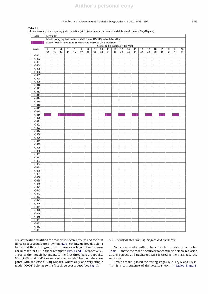
Table 11Models accuracy for computing global radiation (at Cluj-Napoca and Bucharest) and diffuse radiation (at Cluj-Napoca).

Color MeaningModels obeying both c riteria (MBE and RMSE) in both locali tiesModels which are simultaneously the worst in both locali ties

modelStages ( Cluj-Napoca/Bucarest)

232

333

434

535

636

737

838

939

1040

1141

1242

1343

1444

1545

1646

1747

1848

1949

2050

2151

2252


of classification stratified the models in several groups and the firstthirteen best groups are shown in Fig. 3. Seventeen models belongto the first three best groups. This number is larger than the sim-ilar number for Cluj-Napoca (compare Figs. 3 and 1, respectively).Three of the models belonging to the first three best groups (i.e.G001, G006 and G045) are very simple models. This has to be com-pared with the case of Cluj-Napoca, where only one very simplemodel (G001) belongs to the first three best groups (see Fig. 1).

5.3. Overall analysis for Cluj-Napoca and Bucharest

An overview of results obtained in both localities is useful.Table 10 shows the models accuracy for computing global radiationat Cluj-Napoca and Bucharest. MBE is used as the main accuracyindicator.

First, no model passed the testing stages 4/34, 17/47 and 18/48.This is a consequence of the results shown in Tables 4 and 8.



Second, four very simple models (i.e. G001, G006, G044 and G045)are good models for some particular stages. Third, models G019and G047 perform the worst for most stages in both localities. Justtwo models (G032 and G053) are the best in the two locations, forsimilar testing stages (i.e. Stages 5/35 for G032 and 2/32 and 7/37for G053).

Fig. 4 shows the number of testing stages per model with accu-racy criteria fulfilled for both MBE and RMSE indicators. This wayof classification stratified the models in several groups and the firsttwelve best groups are shown in Fig. 4. Sixteen models belong to thefirst three best groups. This number is between the similar numbersfor Cluj-Napoca (Fig. 1) and Bucharest (Fig. 3), respectively. How-ever, note that the best three groups in Figs. 1 and 3 refers to 18, 17and 16 testing stages passed by a given model, respectively, whilein Fig. 4 the best three groups refer to 16, 15 and 14 testing stagespassed by a given model, respectively. Three models belonging tothe first three best groups in Fig. 4 (i.e. G001, G006 and G045) arevery simple models.

Table 11 shows the models accuracy for computing global radi-ation (at Cluj-Napoca and Bucharest) and diffuse radiation (atCluj-Napoca). MBE is used as the main accuracy indicator. First, nomodel passed the testing stages 4, 17 and 18. This is a consequenceof the results shown in Tables 4 and 8. Second, some very simplemodels (i.e. G001, G006 and G045) are good models for some par-ticular stages. Third, model G019 perform the worst for most stagesin both localities.

There is no single model performing the best in computing bothglobal and diffuse radiation, in both localities, for similar testingstages.

Fig. 5 shows the number of testing stages per model with accu-racy criteria fulfilled for both MBE and RMSE indicators. This wayof classification stratified the models in several groups and the firstseven best groups are shown in Fig. 5. Six models belong to the firstthree best groups. Note that the best three groups in Fig. 5 refersto 14, 13 and 10 testing stages passed by a given model, respec-tively. These are considerably low numbers. Compare them withthe best three groups when computing global radiation in a singlelocation (i.e. 18, 17 and 16 testing stages passed by a given model;see Figs. 1 and 3). Or, compare them with the best three groupswhen computing diffuse radiation in a single location (i.e. 18, 16and 14 testing stages passed by a given model; see Figs. 2). Or,finally, compare them with the best three groups when computingglobal radiation in two locations (i.e. 16, 15 and 14 testing stagespassed by a given model; see Fig. 4).

Three models belonging to the first three best groups in Fig. 5(i.e. G001, G006 and G045) are very simple models.

6. Conclusions

Fifty-four broad band models for computation of global and dif-fuse irradiance on horizontal surface were selected. These modelswere tested by using input data from two meteorological sta-tions from Romania (South-Eastern Europe), i.e. Cluj-Napoca andBucharest. The input data consist of surface meteorological data,column integrated data and data derived from satellite measure-ments. The testing procedure is performed in forty-two stagesintended to provide information about the sensitivity of the modelsto various sets of input data.

Looking to the results for global radiation computation at Cluj-Napoca, one sees that nine models belong to the first three bestgroups. One of these models (i.e. G001) is a very simple model.However, no single very simple model is ranked among the firstthree best models in the stage testing. In case of computing diffuseradiation, the number of “good” models is smaller than when com-puting global radiation. Also, no very simple model is ranked the

first best model in a particular testing stage. However, three modelsof the first nine best groups (i.e. G001, G002 and G006) are very sim-ple models. Model G029 gives the best results to compute diffuseradiation for most testing stages. The best models for solar diffuseradiation computation are, on equal-footing, G002 and G027. Thesecond best model is G029.

Looking to the results for global radiation computation atBucharest, the models perform generally better than at Cluj-Napoca. Indeed, in Bucharest seventeen models belong to the firstthree best groups. But the category of best models per stage hasgenerally different members in the two locations. Three of the mod-els belonging to the first three best groups in Bucharest (i.e. G001,G006 and G045) are very simple models.

Looking to the combined results for global radiation computa-tion at Cluj-Napoca and Bucharest, one sees that sixteen modelsbelong to the first three best groups. Three models belonging to thefirst three best groups (i.e. G001, G006 and G045) are very simplemodels. Only two models (G032 and G053) are the best in both loca-tions, for one or two testing stages. The best models for solar globalradiation computation are, on equal-footing, G016, G020, G031 andG054. The second best models are, on equal-footing, G007, G008and G052.

Looking to the combined results for global and diffuse radiationcomputation at Cluj-Napoca and Bucharest, the following conclu-sions can be drawn. There is no single model performing the bestin computing both global and diffuse radiation, in both localities,for similar testing stages. Six models belong to the first three bestgroups. Three models belonging to the first three best groups inFig. 5 (i.e. G001, G006 and G045) are very simple models. The bestmodels for computation of both global and diffuse radiation are, onequal-footing, G001, G006, G020 and G054. The second best modelis G052.

We may conclude that models’ accuracy depends on the set ofinput data. There is no model to be ranked “the best” for all sets ofinput data. Very simple models as well as more complex modelsmay belong to the category of “good models” but generally the lastmodels perform better.

Detailed information about the performance of each model isprovided in [11,12].

Acknowledgments

This work was supported in part by a grant of the RomanianNational Authority for Scientific Research, CNCS – UEFISCDI, projectnumber PN-II-ID-PCE-2011-3-0089 and by the European Coopera-tion in Science and Technology project COST ES1002.

References

[1] Davies JA, McKay DC, Luciani G, Abdel-Wahab M. Validation of models forestimating solar radiation on horizontal surfaces. Downsview, Ontario: Atmo-spheric Environment Service; 1988. IEA Task IX Final Report.

[2] Davies JA, McKay DC. Evaluation of selected models for estimating solar radi-ation on horizontal surfaces. Solar Energy 1989;43:153–68.

[3] Gueymard C. Critical analysis and performance assessment of clear skysolar irradiance models using theoretical and measured data. Solar Energy1993;51:121–38.

[4] Badescu V. Verification of some very simple clear and cloudy sky models toevaluate global solar irradiance. Solar Energy 1997;61:251–64.

[5] Batlles FJ, Olmo FJ, Tovar J, Alados-Arboledas L. Comparison of cloudless skyparameterizations of solar irradiance at various Spanish midlatitude loca-tions. Theor Appl Climatol 2000;66:81–93.

[6] Iziomon MG, Mayer H. Assessment of some global solar radiation parameter-izations. J Atmos Solar Terr Phys 2002;64:1631–43.

[7] Ineichen P. Comparison of eight clear sky broadband models against 16 inde-pendent data banks. Solar Energy 2006;80:468–78.

[8] Younes S, Muneer T. Clear-sky classification procedures and models using aworld-wide data-base. Appl Energy 2007;84:623–45.

[9] Gueymard CA, Myers DR. Validation and ranking methodologies for solar radi-ation models. In: Badescu V, editor. Modeling solar radiation at the earthsurface. Berlin: Springer; 2008. p. 479–509 [chapter 20].


























[10] Gueymard CA, Clear-sky solar irradiance predictions for large-scale appli-cations using 18 radiative models: improved validation methodology anddetailed performance analysis, Solar Energy, in press.

[11] Badescu V, Gueymard CA, Cheval S, Oprea C, Baciu M, Dumitrescu A, et al.Accuracy and sensitivity analysis for 54 clear-sky solar radiation models usingroutine hourly global irradiance measurements in Romania, submitted forpublication.

[12] Badescu V, Gueymard CA, Cheval S, Oprea C, Baciu M, Dumitrescu A, et al.Accuracy and sensitivity analysis for fifty-four models of computing solardiffuse hourly irradiation on clear sky, submitted for publication.

[13] Badescu V, Cheval S, Gueymard C, Oprea C, Baciu M, Dumitrescu A, et al.Testing 52 models of clear sky solar irradiance computation under the cli-mate of Romania. In: The workshop solar energy at urban scale. 2010.p. 12–5.

[14] Gueymard CA, Kambezidis HD. Solar spectral radiation. In: Muneer T, editor.Solar radiation and daylight models. New York: Elsevier; 2004.

[15] ASHRAE. Handbook of fundamentals. Atlanta, GA: American Society of Heat-ing, Refrigerating and Air-Conditioning Engineers Inc.; 1972.

[16] ASHRAE. Handbook fundamentals. Atlanta, GA: American Society of Heating,Refrigerating and Air-Conditioning Engineers Inc.; 2005 [chapter 31].

[17] Badescu V. Use of sunshine number for solar irradiance time series generation.In: Badescu V, editor. Modeling solar radiation at the Earth surface. Berlin:Springer; 2008. p. 327–55 [chapter 13].

[18] Bashahu M, Laplaze D. An atmospheric model for computing solar radiation.Renew Energy 1994;4:455–8.

[19] King R, Buckius RO. Direct solar transmittance for a clear sky. Solar Energy1979;22:297–301.

[20] Barbaro S, Coppolino S, Leone C, Sinagra E. An atmospheric model for com-puting direct and diffuse solar radiation. Solar Energy 1979;22:225–8.

[21] Badescu V. Can the model proposed by Barbaro et al. be used to computeglobal solar radiation on the Romanian territory? Solar Energy 1987;38:247–54.

[22] Biga AJ, Rosa R. Contribution to the study of the solar radiation climate ofLisbon. Solar Energy 1979;23:61–7.

[23] Bird RE, Hulstrom RL, Direct insolation models, Solar Energy Research Insti-tute (now NREL), Golden CO, SERI/TR-335-344; 1980.

[24] Bird RE, Hulstrom RL. Review, evaluation, and improvement of direct irradi-ance models. Trans ASME, J Sol Engng 1981;103:182–92.

[25] Gueymard C. Direct solar transmittance and irradiance predictions withbroadband models. Part I: detailed theoretical performance assessment. SolarEnergy 2003;74:355–79.

[26] Atwater MA, Ball JT. A numerical solar radiation model based on standardmeteorological observations. Solar Energy 1978;21:163–70.

[27] Atwater MA, Ball JT. Erratum. Solar Energy 1979;23:275.[28] Chandra M. Dependence of solar radiation availability on atmospheric tur-

bidity. Proc ISES Conf 1978:430–4.[29] Hinzpeter H. Uber Trubungsbestimmungen in Potsdam in dem Jahren 1946

und 1947 m. Meteor 1950;4:1.[30] Katz M, Baille A, Mermier M. Atmospheric turbidity in a semi-rural site. Part

I: evaluation and comparison of different atmospheric turbidity coefficients.Solar Energy 1982;28:323–7.

[31] Abdelrahman MA, Said SAM, Shuaib AN. Comparison between atmo-spheric turbidity coefficients of desert and temperate climates. Solar Energy1988;40:219–25.

[32] Grenier JC, de la Casiniere A, Cabot T. A spectral model of Linke’s turbidityfactor and its experimental implications. Solar Energy 1994;52:303–14.

[33] Iqbal M. An Introduction to solar radiation. Toronto: Academic Press; 1983.[34] Suckling PW, Hay JE. Modeling direct, diffuse and total solar radiation for

cloudless days. Atmosphere 1976;14:298–308.[35] Suckling PW, Hay JE. A cloud layer-sunshine model for estimating direct,

diffuse and total solar radiation. Atmosphere 1977;15:194–207.[36] Gueymard C. A two-band model for the calculation of clear sky solar irra-

diance, illuminance, and photosynthetically active radiation at the earth’ssurface. Solar Energy 1989;43:253–65.

[37] Dogniaux B, Programme de calcul des eclairements solaires energetiques etlumineux de surfaces orientees et inclinees, Rep. 14, IRM, Brusels; 1976.

[38] Dogniaux B, Variations qualitatives et quantitatives des composantes du ray-onnement solaire sur une surface horizontale par ciel serein en fonction dutrouble atmospherique, Rep. B62, IRM, Brusels; 1970.

[39] Dogniaux B, Variations geographiques et climatiques des expositions ener-getiques solaires sur des surfaces receptrices horizontales et verticales, Rep.B38, IRM, Brusels; 1975.

[40] Goswami TK, Klett DE, Comparison of several models for long term monthlyaverage daily insolation on horizontal surfaces and the estimation of hori-zontal surface insolation for 16 U.S. locations, ASME paper 80-WA/Sol-28;1980.

[41] Festa R, Ratto CF, Solar radiation statistical properties, Rep. IEA-SCHP-9E-4,IEA Task IX, International Energy Agency; 1993.

[42] Daneshyar M. Solar radiation statistics for Iran. Solar Energy 1978;21:345–9.[43] Paltridge GW, Proctor D. Monthly mean solar radiation statistics for Australia.

Solar Energy 1976;18:235–43.[44] Kreith F, Kreider JF. Solar heating and cooling. Washington: Scripta Book Co.;

1975.[45] Rigollier C, Bauer O, Wald L. On the clear sky model of the ESRA—European

Solar Radiation Atlas—with respect to the Heliosat method. Solar Energy2000;68:33–48.

[46] ESRA, Helioclim, Lectures 2010 (http://www.helioclim.net/publications/index.html#esra).

[47] Remund J, Wald L, Lefevre M, Ranchin T, Page J. Worldwide Linke turbidityinformation. In: Proceedings of the ISES conference. 2003.

[48] Remund J, pers. commm.; 2006.[49] Molineaux B, Ineichen P, O’Neill N. Equivalence of pyrheliometric and

monochromatic aerosol optical depths at a single key wavelength. Appl Opt1998;37:7008–18.

[50] Dogniaux R. The estimation of atmospheric turbidity. In: Proc Advan Euro-pean Solar Radiation Climatol London UK, UK Int Sol Energy Soc. 1986.p. 3.1–4.

[51] Hottel HC. A simple model for estimating the transmittance of direct solarradiation through clear atmospheres. Solar Energy 1976;18:129–34.

[52] De Carli F, Groppi C, Festa R, Ratto CF. A procedure to obtain global radiationmaps from sunshine durations at isolated stations in a region with complexorography. Solar Energy 1986;37:91–108.

[53] Jafarpur K, Yaghoubi MA. Solar radiation for Shiraz, Iran. Solar Wind Technol1989;6:177–9.

[54] Aziz GMA. Estimation of hourly clear-sky solar radiation for P.D.R. Yemen.Solar Wind Technol 1990;7:255–60.

[55] Khalil A, Alnajjar A. Experimental and theoretical investigation of globaland dffuse solar radiation in the United Arab Emirates. Renew Energy1995;6:537–43.

[56] Togrul IT, Togrul H, Evin D. Estimation of global solar radiation under clearsky radiation in Turkey. Renew Energy 2000;21:271–87.

[57] Liu BYH, Jordan RC. The interrelationship and characteristic distribution ofdirect, diffuse and total solar radiation. Solar Energy 1960;4:1–12.

[58] Ideriah FJK. A model for calculating direct and diffuse solar radiation. SolarEnergy 1981;26:447–52.

[59] Ineichen P. A broadband simplified version of the Solis clear sky model. SolarEnergy 2008;82:758–62.

[60] Davies JA. Estimating global solar radiation. Bound Layer Meteor1975;9:33–52.

[61] Hoyt DV. A model for the calculation of global solar radiation. Solar Energy1978;21:27–35.

[62] Josefsson W, Modeling direct and global radiation from hourly synoptic obser-vations, unpublished manuscript; 1985.

[63] Kasten F. Parametrisierung der Globalstrahlung durch Bedeckungsgrad undTrübungsfaktor. Ann Met 1983;20:49–50.

[64] Krarti M, Huang J, Seo D, Dark J. Development of solar radiation models fortropical locations, final report for Research Project 1309-RP. Atlanta, GA:American Society of Heating, Refrigerating and Air-Conditioning EngineersInc.; 2006.

[65] Buckius RO, King R. Diffuse solar radiation on a horizontal surface for a clearsky. Solar Energy 1978;21:503–9.

[66] Zhang Q, Huang J, Lang S. Development of typical year weather data for Chi-nese locations. ASHRAE Trans 2002:108.

[67] Watanabe T, Urano Y, Hayashi H. Procedures for separating direct and dif-fuse insolation on a horizontal surface and prediction of insolation on tiltedsurface. Trans Architectural Inst Jpn 1983;330:96–108.

[68] Davies JA, Uboegbulam TC. Parameterization of surface incoming radiation intropical cloudy conditions. Atmos-Ocean 1979;17:14–23.

[69] Machler MA, Iqbal M. A modification of the ASHRAE clear sky irradiationmodel. ASHRAE Trans Part IA 1985;106–115.

[70] Maxwell EL. METSTAT—The solar radiation model used in the produc-tion of the National Solar Radiation Data Base (NSRDB). Solar Energy1998;62:263–79.

[71] Muneer T, Gul M, Kambezedis H. Evaluation of an all-sky meteorological radi-ation model against long-term measured hourly data. Energy Convers Mgmt1998;39:303–17.

[72] Kambezidis H, pers. comm.; 2002.[73] Muneer T. Solar radiation and daylight models. New York: Elsevier; 2004.[74] Gueymard CA. Direct solar transmittance and irradiance predictions with

broadband models. Part 2: validation with high-quality measurements.Solar Energy 2003;74:381–95. Corrigendum: Solar Energy 76 (2004)515.

[75] Kambezidis H, Psiloglou BE, pers. comm.; 2007.[76] Kambezidis H, Psiloglou BE. The Meteorological Radiation Model (MRM):

advancements and applications. In: Badescu V, editor. Modeling solar radia-tion at the Earth’s surface. Recent advances. Berlin: Springer; 2008. p. 357–92[chapter 14].

[77] Nijegorodov N, Adedoyin JA, Devan KRS. A new analytical-empirical modelfor the instantaneous diffuse radiation and experimental investigation of itsvalidity. Renew Energy 1997;11:341–50.

[78] Nijegorodov N, Luhanga PVC. Air mass: analytical and empirical treatment;an improved formula for air mass. Renew Energy 1996;7:57–65.

[79] Belcher BN, DeGaetano AT. Integration of ASOS weather data into model-derived solar radiation (1226-RP). ASHRAE Trans 2005;111(1):363–78.

[80] Belcher BN, DeGaetano AT. A revised empirical model to estimate solarradiation using automated surface weather observations. Solar Energy2007;81:329–45.

[81] Belcher B, pers. commun.; 2005.[82] Paltridge GM, Platt CMR. Radiative processes in meteorology and climatology.

New York: Elsevier; 1976.[83] Ch. Perrin de Brichambaut, Ch Vauge, Le gisement solaire, Evaluation de la

ressource énergétique, Lavoisier, Technique et Documentation, Paris; 1982.






https://www.researchgate.net/publication/245170073_A_revised_empirical_model_to_estimate_solar_radiation_using_automated_surface_weather_observations?el=1_x_8&enrichId=rgreq-6c4911f24b7fc1d54edbe32b2503a9e1-XXX&enrichSource=Y292ZXJQYWdlOzIzMzQxNjY3OTtBUzoxMDQ2ODc0MjAzMTM2MDZAMTQwMTk3MDgzNDk5NA==



https://www.researchgate.net/publication/223335326_METSTAT_-_the_solar_radiation_model_used_in_the_production_of_the_National_Solar_Radiation_Database_NSRDB?el=1_x_8&enrichId=rgreq-6c4911f24b7fc1d54edbe32b2503a9e1-XXX&enrichSource=Y292ZXJQYWdlOzIzMzQxNjY3OTtBUzoxMDQ2ODc0MjAzMTM2MDZAMTQwMTk3MDgzNDk5NA==



https://www.researchgate.net/publication/256325588_Comparison_between_atmospheric_turbidity_coefficients_of_desert_and_temperate_climates?el=1_x_8&enrichId=rgreq-6c4911f24b7fc1d54edbe32b2503a9e1-XXX&enrichSource=Y292ZXJQYWdlOzIzMzQxNjY3OTtBUzoxMDQ2ODc0MjAzMTM2MDZAMTQwMTk3MDgzNDk5NA==






















https://www.researchgate.net/publication/245168766_Atmospheric_turbidity_in_a_semi-rural_site-I_evaluation_and_comparison_of_different_atmospheric_turbidity_coefficients?el=1_x_8&enrichId=rgreq-6c4911f24b7fc1d54edbe32b2503a9e1-XXX&enrichSource=Y292ZXJQYWdlOzIzMzQxNjY3OTtBUzoxMDQ2ODc0MjAzMTM2MDZAMTQwMTk3MDgzNDk5NA==



https://www.researchgate.net/publication/236562225_Solar_radiation_statistics_for_Iran?el=1_x_8&enrichId=rgreq-6c4911f24b7fc1d54edbe32b2503a9e1-XXX&enrichSource=Y292ZXJQYWdlOzIzMzQxNjY3OTtBUzoxMDQ2ODc0MjAzMTM2MDZAMTQwMTk3MDgzNDk5NA==


https://www.researchgate.net/publication/267383752_Integration_of_ASOS_weather_data_into_model-derived_solar_radiation?el=1_x_8&enrichId=rgreq-6c4911f24b7fc1d54edbe32b2503a9e1-XXX&enrichSource=Y292ZXJQYWdlOzIzMzQxNjY3OTtBUzoxMDQ2ODc0MjAzMTM2MDZAMTQwMTk3MDgzNDk5NA==

https://www.researchgate.net/publication/267383752_Integration_of_ASOS_weather_data_into_model-derived_solar_radiation?el=1_x_8&enrichId=rgreq-6c4911f24b7fc1d54edbe32b2503a9e1-XXX&enrichSource=Y292ZXJQYWdlOzIzMzQxNjY3OTtBUzoxMDQ2ODc0MjAzMTM2MDZAMTQwMTk3MDgzNDk5NA==





https://www.researchgate.net/publication/256335051_A_spectral_model_of_Linke's_turbidity_factor_and_its_experimental_implications?el=1_x_8&enrichId=rgreq-6c4911f24b7fc1d54edbe32b2503a9e1-XXX&enrichSource=Y292ZXJQYWdlOzIzMzQxNjY3OTtBUzoxMDQ2ODc0MjAzMTM2MDZAMTQwMTk3MDgzNDk5NA==

https://www.researchgate.net/publication/256335051_A_spectral_model_of_Linke's_turbidity_factor_and_its_experimental_implications?el=1_x_8&enrichId=rgreq-6c4911f24b7fc1d54edbe32b2503a9e1-XXX&enrichSource=Y292ZXJQYWdlOzIzMzQxNjY3OTtBUzoxMDQ2ODc0MjAzMTM2MDZAMTQwMTk3MDgzNDk5NA==















https://www.researchgate.net/publication/233429809_Parameterization_of_surface_incoming_radiation_in_tropical_cloudy_conditions?el=1_x_8&enrichId=rgreq-6c4911f24b7fc1d54edbe32b2503a9e1-XXX&enrichSource=Y292ZXJQYWdlOzIzMzQxNjY3OTtBUzoxMDQ2ODc0MjAzMTM2MDZAMTQwMTk3MDgzNDk5NA==

https://www.researchgate.net/publication/233429809_Parameterization_of_surface_incoming_radiation_in_tropical_cloudy_conditions?el=1_x_8&enrichId=rgreq-6c4911f24b7fc1d54edbe32b2503a9e1-XXX&enrichSource=Y292ZXJQYWdlOzIzMzQxNjY3OTtBUzoxMDQ2ODc0MjAzMTM2MDZAMTQwMTk3MDgzNDk5NA==

https://www.researchgate.net/publication/229396121_Evaluation_of_an_all-sky_meteorological_radiation_model_against_long-term_measured_hourly_data?el=1_x_8&enrichId=rgreq-6c4911f24b7fc1d54edbe32b2503a9e1-XXX&enrichSource=Y292ZXJQYWdlOzIzMzQxNjY3OTtBUzoxMDQ2ODc0MjAzMTM2MDZAMTQwMTk3MDgzNDk5NA==



https://www.researchgate.net/publication/223366257_A_new_analytical-empirical_model_for_the_instantaneous_diffuse_radiation_and_experimental_investigation_of_its_validity?el=1_x_8&enrichId=rgreq-6c4911f24b7fc1d54edbe32b2503a9e1-XXX&enrichSource=Y292ZXJQYWdlOzIzMzQxNjY3OTtBUzoxMDQ2ODc0MjAzMTM2MDZAMTQwMTk3MDgzNDk5NA==








https://www.researchgate.net/publication/253497536_Use_of_Sunshine_Number_for_Solar_Irradiance_Time_Series_Generation?el=1_x_8&enrichId=rgreq-6c4911f24b7fc1d54edbe32b2503a9e1-XXX&enrichSource=Y292ZXJQYWdlOzIzMzQxNjY3OTtBUzoxMDQ2ODc0MjAzMTM2MDZAMTQwMTk3MDgzNDk5NA==










https://www.researchgate.net/publication/234178285_Radiative_Progress_in_Meteorology_and_Climatology?el=1_x_8&enrichId=rgreq-6c4911f24b7fc1d54edbe32b2503a9e1-XXX&enrichSource=Y292ZXJQYWdlOzIzMzQxNjY3OTtBUzoxMDQ2ODc0MjAzMTM2MDZAMTQwMTk3MDgzNDk5NA==

https://www.researchgate.net/publication/234178285_Radiative_Progress_in_Meteorology_and_Climatology?el=1_x_8&enrichId=rgreq-6c4911f24b7fc1d54edbe32b2503a9e1-XXX&enrichSource=Y292ZXJQYWdlOzIzMzQxNjY3OTtBUzoxMDQ2ODc0MjAzMTM2MDZAMTQwMTk3MDgzNDk5NA==








https://www.researchgate.net/publication/278712105_The_Meteorological_Radiation_Model_MRM_Advancements_and_Applications?el=1_x_8&enrichId=rgreq-6c4911f24b7fc1d54edbe32b2503a9e1-XXX&enrichSource=Y292ZXJQYWdlOzIzMzQxNjY3OTtBUzoxMDQ2ODc0MjAzMTM2MDZAMTQwMTk3MDgzNDk5NA==




https://www.researchgate.net/publication/297370611_Procedures_for_separating_direct_and_diffuse_insolation_on_a_horizontal_surface_and_prediction_of_insolation_on_tilted_surface?el=1_x_8&enrichId=rgreq-6c4911f24b7fc1d54edbe32b2503a9e1-XXX&enrichSource=Y292ZXJQYWdlOzIzMzQxNjY3OTtBUzoxMDQ2ODc0MjAzMTM2MDZAMTQwMTk3MDgzNDk5NA==





https://www.researchgate.net/publication/285916193_Direct_solar_transmittance_and_irradiance_predictions_with_broadband_models_Pt_2_validation_with_high-quality_measurements?el=1_x_8&enrichId=rgreq-6c4911f24b7fc1d54edbe32b2503a9e1-XXX&enrichSource=Y292ZXJQYWdlOzIzMzQxNjY3OTtBUzoxMDQ2ODc0MjAzMTM2MDZAMTQwMTk3MDgzNDk5NA==




https://www.researchgate.net/publication/44553900_Le_gisement_solaire_evaluation_de_la_ressource_energetique_Christian_Perrin_de_Brichambaut?el=1_x_8&enrichId=rgreq-6c4911f24b7fc1d54edbe32b2503a9e1-XXX&enrichSource=Y292ZXJQYWdlOzIzMzQxNjY3OTtBUzoxMDQ2ODc0MjAzMTM2MDZAMTQwMTk3MDgzNDk5NA==

https://www.researchgate.net/publication/44553900_Le_gisement_solaire_evaluation_de_la_ressource_energetique_Christian_Perrin_de_Brichambaut?el=1_x_8&enrichId=rgreq-6c4911f24b7fc1d54edbe32b2503a9e1-XXX&enrichSource=Y292ZXJQYWdlOzIzMzQxNjY3OTtBUzoxMDQ2ODc0MjAzMTM2MDZAMTQwMTk3MDgzNDk5NA==

https://www.researchgate.net/publication/279547193_A_modification_of_the_ASHRAE_clear_sky_model?el=1_x_8&enrichId=rgreq-6c4911f24b7fc1d54edbe32b2503a9e1-XXX&enrichSource=Y292ZXJQYWdlOzIzMzQxNjY3OTtBUzoxMDQ2ODc0MjAzMTM2MDZAMTQwMTk3MDgzNDk5NA==

https://www.researchgate.net/publication/279547193_A_modification_of_the_ASHRAE_clear_sky_model?el=1_x_8&enrichId=rgreq-6c4911f24b7fc1d54edbe32b2503a9e1-XXX&enrichSource=Y292ZXJQYWdlOzIzMzQxNjY3OTtBUzoxMDQ2ODc0MjAzMTM2MDZAMTQwMTk3MDgzNDk5NA==







[84] Psiloglou BE, Santamouris M, Asimakopoulos DN. Atmospheric broadbandmodel for computation of solar radiation at the Earth’s surface. Applicationto mediterranean climate. P Appl Geophys 2000;157:829–60.

[85] B.E. Psiloglou (pers. comm. 2006).[86] Gueymard CA. REST2: high performance solar radiation model for cloudless-

sky irradiance, illuminance and photosynthetically active radiation—validation with a benchmark dataset. Solar Energy 2008;82:272–85.

[87] Rodgers GG, Souster CG, Page KJ. The development of an interactive computerprogram SUN1 for the calculation of solar irradiances and daily irradi-ations on horizontal surfaces on cloudless days for given conditions ofsky clarity and atmospheric water content, Rep. BS28, Univ. of Sheffield;1978.

[88] Carroll JJ. Global transmissivity and diffuse fraction of solar radiation for clearand cloudy skies as measured and as predicted by bulk transmissivity models.Solar Energy 1985;35:105–18.

[89] Robinson N, editor. Solar radiation. Amsterdam: Elsevier; 1966.[90] Sellers WD. Physical climatology. Univ Chicago Press 1965.[91] Santamouris M, pers comm.; 2006.[92] Schulze RE. A physically based method of estimating solar radiation from

suncards. Agric Meteorol 1976;16:85–101.[93] Sharma MR, Pal RS. Interrelationships between total, direct, and diffuse solar

radiation in the tropics. Solar Energy 1965;9:183–92.[94] Watt D, On the nature and distribution of solar radiation, Report for U.S. DOE;

1978.[95] Wesely ML, Lipschutz RC. An experimental study of the effects of aerosols on

diffuse and direct solar radiation received during the summer near Chicago.Atmos Environ 1976;10:981–7.

[96] Wesely ML, Lipschutz RC. A method for estimating hourly averages of dif-fuse and direct solar radiation under a layer of scattered clouds. Solar Energy1976;18:467–73.

[97] Yang K, Huang GW, Tamai N. A hybrid model for estimating global solarradiation. Solar Energy 2001;70:13–22.

[98] Yang K, Koike T, Ye B. Improving estimation of hourly daily and monthlysolar radiation by importing global data sets. Agric Forest Meteorol2006;137:43–55.

[99] Zhang Q. Development of the typical meteorological database for Chineselocations. Energy Build 2006;38:1320–6.

[100] Zhang Q, pers. comm.; 2008.[101] Hourwitz B. Insolation in relation to cloudiness and cloud density. J Met

1945;2:154–6.[102] Hourwitz B. Insolation in relation to cloud type. J Met 1946;3:123–4.[103] Adnot J, Bourges B, Campana D, Gicquel R. Utilisation desc courbes de fre-

quence cumulees pour le calcul des installation solaire. In: Lestienne R, editor.Analyse statistique des processus meteorologiques appliquee a l’energiesolaire. Paris: CNRS; 1979. p. 9–40.

[104] Paulescu M, Schlett Z. A simplified but accurate spectral solar irradiancemodel. Theor Appl Climatol 2003;75:203–12.

[105] Paulescu M, pers. comm.; 2009.[106] Janjai S, Models for estimating direct normal and diffuse irradiances clear

sky condition, Technical report, Nakhonpathom, Thailand: Department ofPhysics, Silpakorn University; 2010.

[107] Janjai S, Sricharoen K, Pattarapanitchai S, Semi-empirical models for the esti-mation of clear sky solar global and direct normal irradiances in the tropics.Appl Energy (July 2011) doi:10.1016/j.apenergy.2011.06.021.

[108] Myers DR, Wilcox SM. Relative accuracy of 1-minute and daily total solarradiation data for 12 global and 4 direct beam solar radiometers. In: Americansolar energy society annual conference. 2009.

[109] WMO, Guide to meteorological instruments and methods of observation,WMO No. 8, 2008, Ch. 8–Measurement of sunshine duration, pp. I.8.1-1.8.11;<http://www.wmo.int/pages/prog/www/IMOP/publications/CIMO-Guide/CIMO Guide-7th Edition-2008.html>.

[110] Schulz J, Albert P, Behr H-D, Caprion D, Deneke H, Dewitte S, et al. Operationalclimate monitoring from space: the EUMETSAT Satellite Application Facil-ity on Climate Monitoring (CM-SAF). Atmos Chem Phys 2009;9:1687–709,http://www.atmos-chem-phys.org/9/1687/2009/acp-9-1687-2009.pdf.

[111] Gueymard CA, Thevenard D. Monthly average clear-sky broadband irradiancedatabase for worldwide solar heat gain and building cooling load calculations.Solar Energy 2009;83(11):1998–2018.

[112] Leckner B. The spectral distribution of solar radiation at the Earth’s surface –elements of a model. Solar Energy 1978;20:143–50.














https://www.researchgate.net/publication/256325566_Global_transmissivity_and_diffuse_fraction_of_solar_radiation_for_clear_and_cloudy_skies_as_measured_and_as_predicted_by_bulk_transmissivity_models?el=1_x_8&enrichId=rgreq-6c4911f24b7fc1d54edbe32b2503a9e1-XXX&enrichSource=Y292ZXJQYWdlOzIzMzQxNjY3OTtBUzoxMDQ2ODc0MjAzMTM2MDZAMTQwMTk3MDgzNDk5NA==














https://www.researchgate.net/publication/225533499_Atmospheric_Broadband_Model_for_Computation_of_Solar_Radiation_at_the_Earth's_Surface_Application_to_Mediterranean_Climate?el=1_x_8&enrichId=rgreq-6c4911f24b7fc1d54edbe32b2503a9e1-XXX&enrichSource=Y292ZXJQYWdlOzIzMzQxNjY3OTtBUzoxMDQ2ODc0MjAzMTM2MDZAMTQwMTk3MDgzNDk5NA==












Computing global and diffuse solar hourly irradiation on clear sky. Review and testing of 54 models

Documents

Transcript of Computing global and diffuse solar hourly irradiation on clear sky. Review and testing of 54 models