flood risk assessment of ofu river catchment in nigeria

i

FLOOD RISK ASSESSMENT OF OFU RIVER CATCHMENT IN NIGERIA

BY

Meshach IleanwaAlfa

B. Eng. (ABU, 2008), PGDE (UniMaid, 2009), M.Sc. (ABU, 2013)

P14EGWR9002

A THESIS SUBMITTED TO THE SCHOOL OF POSTGRADUATE STUDIES,

AHMADU BELLO UNIVERSITY, ZARIA NIGERIA

IN PARTIAL FULFILMENT OF THE REQUIRMENTS FOR THE AWARD

OF DOCTOR OF PHILOSOPHY DEGREE IN WATER RESOURCES AND

ENVIRONMENTAL ENGINEERING

DEPARTMENT OF WATER RESOURCES AND ENVIRONMENTAL

ENGINEERING,

AHMADU BELLO UNIVERSITY, ZARIA

NIGERIA

June, 2018

ii

DECLARATION

I declare that the work in the thesis entitled “Flood Risk Assessment of Ofu River

Catchment in Nigeria” has been carried out by me in the Department of Water Resources

and Environmental Engineering. The information derived from literature has been duly

acknowledged in the text and a list of references provided. No part of this thesis was

previously presented for another degree or diploma at this or any other Institution.

Meshach Ileanwa ALFA ____________________ _______________

Name of Student Signature Date

iii

CERTIFICATION

This Thesis entitled “Flood Risk Assessment of Ofu River Catchment in Nigeria” by

Meshach Ileanwa ALFA meets the regulations governing the award of the degree of

Doctor of Philosophy in Water Resources and Environmental Engineering of Ahmadu

Bello University, and is approved for its contribution to knowledge and literary

presentation.

Prof. D. B. Adie ____________________ _______________

Chairman, Supervisory Committee Signature Date

Dr. M. A. Ajibike ____________________ _______________

Member, Supervisory committee Signature Date

Prof. O. J. Mudiare ____________________ _______________

Member, Supervisory committee Signature Date

Prof. A. Ismail ____________________

_______________

Head of Department Signature Date

Prof. S. Z. Abubakar ____________________ _______________

Dean, School of Postgraduate Studies Signature Date

iv

DEDICATION

To the loving memory of my mother, Madam Mary Alfa and my mother-in-law, Mrs

Grace Mayomi Jegede who joined the cloud of witnesses just before this became a

reality.

v

ACKNOWLEDGMENTS

My greatest gratitude goes to the Almighty God, who has demonstrated again that He is

my Glory and the ‘Lifter up’ of my head. Once again I reaffirm my eternal allegiance to

You and my commitment to see Your Kingdom come and Your Will be done on earth

as it is in heaven.

I humbly acknowledge and sincerely appreciate my supervisory committee-the trio of

Prof. D. B. Adie, Dr. M. A. Ajibike and Professor O. J. Mudiare for their thoroughness,

dedication, flexibility yet very firm supervision of this work as well as the moral support

they provided during this study.

I wish to express my gratitude and appreciation to Apostle Joshua Selman Nimmak for

the spiritual covering I enjoyed throughout this study. You have indeed been a great

father, mentor, pastor and friend. I love, honour and greatly celebrate you sir. I want to

also specially appreciate Professor and Mrs Emmy Unuja Idegu who have been of great

support and inspiration to me throughout this study.

My special appreciation goes to the Vice Chancellor of the University of Jos for the

approval and sponsorship of this study. I also appreciate the Dean of the Faculty of

Engineering, University of Jos, Prof. Stephen J. Mallo for his consistent and tireless

motivation throughout this work and all the staff of the Department of Civil

Engineering, University Jos for the support I enjoyed throughout this study.

I also thank my Head of Department (Professor Abubakar Ismail), Professor C. A.

Okuofu, Professor J. A. Otun for their in-time academic support, encouragement,

patience, understanding and push I received during this study. I am grateful to Dr

vi

Sunday Bamidele Igboro for the significant contributions and academic support in all

ramifications towards the successful completion of this study. I also acknowledge the

immense support and encouragement of Engr. Sani Ismail, Dr. Babatude Adeogun, Dr.

(Mrs.) F. B. Ibrahim and all the members of staff of the Department of Water Resources

and Environmental Engineering.

Now my words have failed me to appreciate my priceless Jewel, my treasure of

inestimable value-Annie Opeyemi Meshach-Alfa for standing by me. I will need to write

an entire thesis to attempt to appreciate your sacrifice, love, support and prayers for the

success of this study. You are indeed the best thing that happened to me after Christ. I

love you eternally. I specially appreciate my dear sons, Jedidiah Ojimaojo Meshach-

Alfa and David Omokorede Meshach-Alfa for their sacrifice to see that Daddy

completes this study.

I specially appreciate my research assistants - Achema Alfa and Maneju Wada and my

Enumerators – Enemali Alfa, Richardson Edimeh, Hope Enemakwu, Iye Okekwu and

Isah Chubiyojo for all their effort on the field to make this work a reality. Finally, I will

like to appreciate Engr. Ashara, Mr Paul and Mr Aliyu for the GIS tutorials and others

too numerous to mention that contributed in one way or the other towards the success

of this work, I thank you all.

vii

ABSTRACT

The aim of this study was to carry out a flood risk assessment for Ofu River Catchment

in Nigeria. Shuttle Radar Topographic Mission Digital Elevation Model (SRTM DEM)

and River Map of Africa were used to delineate the catchment boundaries in ArcGIS

10.2.2 coupled with ArcHydro and HEC-GeoHMS extensions while the stream ordering

was done using the spatial analyst hydrology tool in ArcGIS 10.2.2. Stage and discharge

measured from February, 2016 to January, 2017 were used to develop the rating curve

at Oforachi Hydrometric Station. Key Informant Interviews and household surveys were

carried out to ascertain the opinion of the people on flood occurrence and their perceived

causes. Assessment of the rainfall characteristics of the catchment was also carried out

using the 35 years radar data corrected with data obtained from the Nigeria

Meteorological Agency (NiMet). The soil map of the study area was extracted from the

digital soil map of the world while Atterberg limits, sieve analysis and infiltration tests

were carried out at Oforachi as a confirmatory test. The percentage loss in volume and

surface area and loss in flow depth of Ofu River at Oforachi between 2000 and 2011

were also carried out using GIS tools in ArcGIS 10.2.2 while the loss rate was used to

estimate the flow depth for 2016. The annual sediment load of Ofu River at Oforachi

Hydrometric Station was also estimated. The terrain elevation, slope and proximity were

also measured via field measurement and GIS analysis. The landuse/ landcover (LULC)

changes between 1987 and 2016 were also examined using the LULC map for 1987,

2001 and 2016. The runoff curve numbers for these years were also estimated. Synthetic

stream flow for 1974 to 2016 was generated using the modified Thomas-Fierring’s

model. Peak discharge for the catchment was also estimated using the Natural Resource

Conservation Services Curve Number method and the rational method. The average

values for the three were compared with that from field measurement. Flood frequency

viii

analysis was carried out on the 62 years synthetic discharge values (1955-2016) and

peak discharge values for 2, 5, 10, 25, 50, 100 and 200 years return periods were

estimated. The extent of flood inundation was estimated first by Multi-criteria

evaluation in ArcGIS and secondly by hydraulic modelling in HEC-RAS and HEC-

GeoRAS/ArcGIS using hydrologically generated stream flow. Flood Hazard,

vulnerability and risk analysis were carried out in ArcGIS 10.2.2. The resulted show

that Ofu River Catchment covers a total drainage area of 1604.56 km2 covering 27.02

% of Dekina, 23.48 % of Ofu, 14.06 % of Igalamela/Odolu, 9.25 % of Idah and 14.04

% of Ibaji Local Government Areas in Kogi State and 0.80 % of Uzo-Uwani Local

Government Area in Enugu State, Nigeria. A rating curve equation, 𝑄 =

15.54096(𝐻 − 55.43192)0.69051was developed. Ofu River has lost 6.90 m of its flow

depth at Oforachi between 2000 and 2016 at a rate of 0.431 m per year which is the

major cause of flood within the catchment. The annual sediment load of the river at

Oforachi station is 66,824.73 x 103 kg. The runoff curve numbers for 1987, 2001 and

2016 were 61.8, 63.3 and 62.8, respectively showing no significant change. The

modified Thomas-Fierring Model was effectively used to generate 12 months synthtic

stream flow data for Ofu river from 1974 to 2016. The peak discharge values for 2, 5,

10, 25, 50, 100 and 200 years return periods were 444.57 m3/s, 499.23 m3/s, 530.35

m3/s, 565.61 m3/s, 589.59 m3/s, 611.96 m3/s and 633.25 m3/s, respectively while the

peak discharge values for 1995 and 2000 flood scenarios were 448.89 m3/s and 446.46

m3/s, respectively. Three hazard, vulnerability and risk zones-High, moderate and low

were identified which have put several elements at varying degrees of risk in 1995 and

2000 flood scenarios and other flood events of 100 years and 200-year return periods.

An assessment of the open defecation status of Oforachi, the most developed of the

communities within Ofu River Floodplain shows that 50.81 % of the population still

ix

defecate in the open field which will pose a serious health risk to the populace in the

event of flood, since Ofu River is a major source of household drinking water in the

community. The study demonstrated that Modified Thomas-Fierring’s model, Remote

Sensing, Geographic Information System, HEC-RAS and HEC-GeoRAS could be

effective tools for flood risk assessment. Efforts should be made by the government to

urgently dredge Ofu River to provide more discharge-carrying capacity.

x

TABLE OF CONTENTS

Title page - - - - - - - - - i

Declaration - - - - - - - - - ii

Certification - - - - - - - - - iii

Dedication - - - - - - - - - iv

Acknowledgement - - - - - - - - v

Abstract - - - - - - - - - vii

Table of Contents - - - - - - - - x

List of Tables - - - - - - - - xv

List of Figures - - - - - - - - xix

List of Plates - - - - - - - - xxiii

List of Appendices - - - - - - - - xxiv

CHAPTER ONE: INTRODUCTION

1.1 Background of the Study - - - - - - 1

1.2 Statement of the Research Problem - - - - - 5

1.3 Justification of the Study - - - - - - 7

1.4 Aim and Objectives - - - - - - - 8

1.5 Scope of Research - - - - - - - 8

1.6 Limitations of the Research - - - - - - 9

1.7 Description of Study Area - - - - - - 10

1.7.1 Location - - - - - - - - 10

1.7.2 Climate - - - - - - - - 10

1.7.3 Geology - - - - - - - - 12

1.7.4 Topography - - - - - - - - 12

1.7.5 Hydrology - - - - - - - - 12

xi

1.7.6 Agriculture - - - - - - - - 13

CHAPTER TWO: CONCEPTUAL AND THEORETICAL FRAMEWORK AND

LITERATURE REVIEW

2.1 Introduction - - - - - - - - 14

2.2 Conceptual Framework - - - - - - 14

2.2.1 Concept of Flood - - - - - - - 14

2.2.2 Concept of Runoff - - - - - - - 25

2.3 Morphologic Characteristics of a River Basin - - - 29

2.3.1 Delineation of watershed boundaries - - - - - 31

2.3.2 Determination of the morphological characteristics of a watershed - 36

2.4 Stream Gauging and Development of Rating Curve - - - 45

2.4.1 Stage Measurement - - - - - - - 46

2.4.2 Discharge Measurement - - - - - - 47

2.4.3 Development, Fitting and Extension of Rating Curve - - 50

2.5 Determination of Soil Characteristics - - - - - 53

2.5.1 Remotely Sensed Soil Data - - - - - - 53

2.5.2 Field Determination of Soil Characteristics - - - - 54

2.6 Evaluation of Landuse/Landcover Characteristics - - - 58

2.6.1 Image Classification - - - - - - - 58

2.6.2 Land Cover Indices - - - - - - - 60

2.7 Runoff Estimation - - - - - - - 62

2.7.1 Extension of Runoff Records using Thomas-Fiering’s Model - 62

2.7.2 Rainfall-Runoff Modelling for Unguaged Catchment using

Remote Sensing and GIS - - - - - - 64

2.8 Rainfall Data - - - - - - - - 73

2.8.1 Measurement of Rainfall - - - - - - 73

xii

2.8.2 Rainfall Interpolation - - - - - - - 74

2.8.3 Catchment Mean Aerial Rainfall Estimation - - - - 77

2.8.4 Presentation of Rainfall Data - - - - - - 78

2.9 Flood Frequency Analysis - - - - - - 78

2.10 Field Survey and Statistical Analysis - - - - - 80

2.10.1 Descriptive and Inferential Statistics - - - - 80

2.10.2 Population and Sample - - - - - - 81

2.10.3 Sampling Techniques - - - - - - 81

2.11 The Concept of Disaster - - - - - - 83

2.11.1 Flood Hazard and Flood Hazard Assessment - - - 83

2.11.2 Flood Vulnerability and Flood Vulnerability Assessment - - 84

2.11.3 Flood Risk and Flood Risk Assessment - - - - 86

2.11.4 Disaster Risk Management and Disaster Risk Reduction - - 87

2.11.5 Flood Risk Mapping - - - - - - - 88

2.12 Multi Criteria Evaluation in Risk Assessment - - - 90

2.13 Population Estimation - - - - - - - 93

2.14 Application of Remote Sensing and Geographic Information System

in Flood Risk Studies - - - - - - 94

2.14.1 Digital Elevation Models used for Flood risk Mapping - - 96

2.14.2 Satellite Images used for Flood Inundation Mapping - - 99

2.15 Software used in Flood Inundation Modelling - - - 101

2.15.1 Hydraulic models used for Flood Inundation Mapping - - 103

2.15.2 Description of Selected Models used in this Study - - - 104

CHAPTER THREE: MATERIALS AND METHODS

3.1 Materials - - - - - - - - 114

3.1.1 Types and Sources of Data - - - - - - 114

xiii

3.1.2 Hardware and Software - - - - - - 117

3.2 Methods - - - - - - - - 119

3.2.1 Determination of Morphologic Characteristics of Ofu River Catchment 119

3.2.2 Development of Stage-Discharge Rating Curve for Ofu River - 133

3.2.3 Methods of Identification of Flood Causative Factors in

Ofu River Catchment - - - - - - 143

3.2.4 Method of Flood Frequency Analysis- - - - - 170

3.2.5 Production of Flood Inundation Extent and Hazard Map - - 182

3.2.6 Method of Flood Risk Analysis - - - - - 199

CHAPTER FOUR: RESULTS AND DISCUSSION

4.1 Morphologic Analysis of Ofu River Catchment - - - 211

4.1.1 Delineation of Ofu River Catchment Boundaries - - - 211

4.1.2 Morphologic characteristics of Ofu River Catchment - - 211

4.2 Stage-Discharge Rating Curve for Ofu River - - - - 221

4.2.1 Results of the Observation of Ofu River Stage at

Oforachi Hydrometric Station - - - - - 221

4.2.2 Ofu River Discharge Measurement Values at

Oforachi Hydrometric station - - - - - 221

4.2.3 Results of the Development, fitting and Extension of

Ofu River Rating Curve at Oforachi Hydrometric Station - - 223

4.3 Flood Causative Factors - - - - - - 227

4.3.1 Knowledge of Flood Causes within the Catchment Communities - 227

4.3.2 Rainfall Characteristics of Oforachi Catchment (Meteorological Factors) 232

4.3.3 Geomorphologic Flood Causative Factors - - - - 235

4.3.4 Land use/Settlement Causative Factors - - - - 250

4.3.5 Respective Associations of Elevation, Proximity and

Slope with Flood Occurrence - - - - - 258

4.4 Flood Frequency Analysis - - - - - - 259

xiv

4.4.1 Peak Runoff - - - - - - - 259

4.4.2 Peak Discharge forecast using Log-Pearson Type III Distribution - 264

4.5 Flood Inundation Extent and Hazard Map - - - - 266

4.5.1 Flood Hazard Map by Thematic Integration of Causative Factors

(Multi-Criteria Evaluation) in ArcGIS - - - - 266

4.5.2 Hydraulic Modelling for Development of

Flood Inundation and Hazard Maps - - - - - 280

4.5.3 Results of the Comparison of Extent of Flood

Inundation from both Methods - - - - - 287

4.6 Flood Risk Analysis - - - - - - - 288

4.6.1 Flood Hazard Assessment - - - - - - 288

4.6.2 Flood Vulnerability Assessment - - - - - 292

4.6.3 Derivation of Population Vulnerability Weights - - - 297

4.6.4 Flood Risk Assessment - - - - - - 305

4.7 Strategic Plan for Ofu River Catchment Flood Management - - 328

CHAPTER FIVE: SUMMARY, CONCLUSION AND RECOMMENDATIONS

5.1 Summary - - - - - - - - 330

5.2 Conclusion - - - - - - - - 333

5.3 Recommendations - - - - - - - 335

REFERENCES - - - - - - - - 337

APPENDICES - - - - - - - - 356

xv

LIST OF TABLES

Table 2.1: Chronicles of Historical Flood Events in Nigeria between

1953 and 2012 - - - - - - - 16

Table 2.2: Guidelines for deciding Number of sub-sections of

River for Discharge Measurement - - - - 49

Table 2.3: Band Characteristics for Landsat 5, 7 and 8 Imageries - - 59

Table 2.4: Categories of Antecedent Moisture Content - - - 66

Table 2.5: Classification of Hydrological Soil Groups - - - 67

Table 2.6: Comparison of Spatial Interpolation Techniques - - 76

Table 2.7: Correlation between risk, hazard and vulnerability - - 87

Table 3.1: Properties of the Topographic Maps Used in the Study - - 114

Table 3.2: Historical Mean Annual Rainfall Data for Ofu River Catchment

Neighbouring Stations - - - - - - 115

Table 3.3: Historical Mean Discharge Record for Ofu River at Oforachi - 116

Table 3.4: Properties of Satellite Data and Relevance - - - 116

Table 3.5: Methods of Estimation of Derived Areal Morphologic Characteristics 130

Table 3.6: Methods of Estimation of Linear Morphologic Characteristics - 132

Table 3.7: Methods of Estimation of Relief Morphologic Characteristics - 133

Table 3.8: Characteristics of Soil within Ofu River Catchment - - 157

Table 3.9: Band Characteristics for NDVI and NDBI

Calculation for Ofu River Catchment - - - - 162

Table 3.10: Logarithm of Stream flow, Monthly Mean,

Standard Deviation and Correlation coefficient for T-F Model - 174

Table 3.11: Stream flow Estimation for Model Calibration and Validation 175

Table 3.12: Model Validation Parameters - - - - - 175

Table 3.13: Flood Hazard Classification Based on Flood Depths - - 200

Table 3.14: Estimated Population Growth Rates - - - - 202

Table 3.15: Estimation of Percentage of Population with Disability - 203

xvi

Table 3.16: Estimation of Percentage Distribution of Population by Age - 203

Table 3.17: Estimation of Percentage Distribution of Population by Gender 205

Table 3.18: Estimation of Ofu River Catchment Population by LGAs - 205

Table 3.19: Flood Vulnerability Classification - - - - 207

Table 3.20: Flood Risk Classification - - - - - 208

Table 4.1: Morphologic Characteristics of Ofu River Catchment (Areal Aspects) 213

Table 4.2: Morphologic Characteristics of Ofu River Catchment (Linear Aspects)216

Table 4.3: Morphologic Characteristics of Ofu River Catchment (Relief Aspects)220

Table 4.4: Estimation of Rating Curve Calibration Coefficients (h, m and K) 223

Table 4.5: Comparison of Monthly Discharge with Historical Discharge - 227

Table 4.6: Socio-demographic Characteristics of Respondents- - - 228

Table 4.7: Flood Experience and Characteristics - - - - 229

Table 4.8: Knowledge of Flood Causes in the Community - - - 231

Table 4.9: Summary Results of Channel Bed Elevations

(2000 and 2011), Bed Elevation Loss, Loss Rate and T-test - 240

Table 4.10: Monthly and Annual Sediment Loads of Ofu River at

Oforachi Hydrometric Station - - - - - 244

Table 4.11: Soil Classification based on Results of

Atterberg Limits Tests Conducted - - - - 246

Table 4.12: Soil Classification based on the Sieve Analysis Results - 246

Table 4.13: Soil Classification based on Saturated Hydraulic Conductivity 247

Table 4.14: Chi Square Results for Association of Elevation,

Proximity and Slope with Flood Experience - - - 258

Table 4.15a: Unbiased Statistics of the gauged (1955-1973) and

Synthetic (1955-2016) stream flow data - - - - 260

Table 4.15b: Coefficients of Determination, P-value, Critical F-value and

Reliability Index - - - - - - - 260

Table 4.16: Runoff Coefficient for Ofu River Catchment - - - 263

xvii

Table 4.17: Rainfall Intensity and Peak Discharge by Rational Method - 263

Table 4.18: Comparison of Average Peak Discharge from the

Respective Methods - - - - - - 264

Table 4.19: Results of the Flood Frequency Calculations using log-Pearson

Type III Distribution with Annual Maximum Discharge

Values (1955-2016) - - - - - - 265

Table 4.20: Discharge Values for Steady Flow Analysis in HEC-RAS - 266

Table 4.21: Criterion Weight for Elevation - - - - - 271

Table 4.22: Criterion Weight for Slope - - - - - 272

Table 4.23 Criterion Weight for Soil - - - - - 272

Table 4.24: Criterion Weight for Corridor - - - - - 273

Table 4.25: Criterion Weight for Causative Factors - - - 278

Table 4.26: Area, Depth and Velocity of Flood Inundated Water - - 282

Table 4.27: Comparison of Flood Inundation Extents by both Methods - 287

Table 4.28: Flood Hazard Zones/extent for 1995, 2000, 100 year and

200 year Floods - - - - - - - 292

Table 4.29: Population at Risk for 1995 and 2000 Flood Scenarios - 292

Table 4.30: Population at Risk for 100-year and 200-year Return Periods - 293

Table 4.31: Population at Risk by Age groups, Poverty level and

Gender for 1995 Flood Scenario - - - - - 294

Table 4.32: Population at Risk by Age groups, Poverty level and Gender for

2000 Flood Scenario - - - - - - 294


100 Year Flood - - - - - - - 296


200 Year Flood - - - - - - - 296

Table 4.35: Vulnerability Weights for all Population Categories for

1995 Flood Scenario - - - - - - 298


2000 Flood Scenario - - - - - - 298

xviii


100 Year Flood - - - - - - - 299


200 Year Flood - - - - - - - 299

Table 4.39: Overall Weights for All Vulnerability Maps derived by AHP - 300

Table 4.40: Flood Vulnerability Zones/extent for 1995, 2000, 100 year

and 200 year Floods - - - - - - 305

Table 4.41: Elements at Risk of 1995 Flood Scenario - - - 310

Table 4.42: Elements at Risk of 2000 Flood Scenario - - - 312

Table 4.43: Elements at Risk of 100 Year Flood - - - - 314

Table 4.47: Elements at Risk of 200 Year Flood - - - - 316

Table 4.45: Inter Profile Characteristics of Soil within the Risk Zones - 320

Table 4.46: Distribution of Household Populations by Toilet Facilities - 326

Table 4.47: Alternative Place of Defecation for those without Toilet Facilities 326

Table 4.48: Distribution of Household Populations by Sources of Drinking Water327

Table 4.49: Strategic Plan for Ofu River Catchment Flood Management - 329

xix

LIST OF FIGURES

Fig. 1.1: Map of Study Area - - - - - - - 11

Fig. 2.1: Schema of Double Ring Infiltrometer - - - - 57

Fig. 2.2: Process Flow diagram for Image Classification Methods - - 61

Fig. 2.3: Flood risk as a combination of Hazard and vulnerability - - 87

Fig. 2.4: Diagram showing the Terms in the Energy Equation - - 107

Fig. 2.5: HEC-RAS Conveyance Sub-division Method - - - 108

Fig. 2.6: Mean Energy Head Calculation - - - - - 109

Fig. 3.1: Project Point and Project Area for Ofu River Catchment Delineation 125

Fig. 3.2: Schematic Flowchart of the Morphometric Analysis Methodology 134

Fig. 3.3: Ofu River catchment showing location of gage stations - - 137

Fig. 3.4: Schema of the River Cross-section during one of the

Discharge Measurements- - - - - - - 138

Fig. 3.5: Schematic Flowchart of the Rating Curve Development Methodology 143

Fig. 3.6a: Triangulated Irregular Network (TIN) surface for 2000 - - 151

Fig. 3.6b: Triangulated Irregular Network (TIN) surface for 2011 - - 152

Fig. 3.7: Location of sections for Ofu River Volume estimation at Oforachi 153

Fig. 3.8: Location of Soil Sample Collection points at Oforachi - - 158

Fig. 3.9a: Normalized Difference Vegetation Index of Ofu River

Catchment for 1987 - - - - - - 163

Fig. 3.9b: Normalized Difference Vegetation Index of Ofu River

Catchment for 2001 - - - - - 164

Fig. 3.9c: Normalized Difference Vegetation Index of Ofu River

Catchment for 2016 - - - - - 165

Fig. 3.10a: Normalized Difference Built-up Index of Ofu River

Catchment for 1987 - - - - - 166

Fig. 3.10b: Normalized Difference Built-up Index of Ofu River

Catchment for 2001 - - - - - 167

xx

Fig. 3.10c: Normalized Difference Built-up Index of Ofu River

Catchment for 2016 - - - - - 168

Fig. 3.11: Screenshot of the RAS Layers created - - - - 191

Fig. 3.12: View of the Geometric data imported from ArcGIS to HEC-RAS 193

Fig. 3.13: Assigning of Manning’s n Values in HEC-RAS - - - 194

Fig. 3.14: One of the Cross-sections in HEC-RAS - - - - 195

Fig. 3.15: Akpagidigbo Bridge data showing deck/roadway editor and

bridge design editor - - - - - - 196

Fig. 3.16: Oforachi Bridge data showing deck/roadway editor and

bridge design editor - - - - - - 196

Fig. 3.17: Steady Flow Data and Boundary Conditions Input in HEC-RAS 197

Fig. 3.18: Exporting HEC-RAS Results to ArcGIS - - - - 198

Fig. 3.19: Schematic Flowchart of the Food Risk Assessment Methodology 210

Fig. 4.1: Areal Morphologic Characteristics of Ofu River Catchment - 212

Fig. 4.2: Strahler’s Stream Order of Ofu River Basin - - - 215

Fig. 4.3: Logarithm of Stream Number (Nu) versus Stream Order (U) - 216

Fig. 4.4: Logarithm of Stream Length (Lu) versus Stream Order (U) - 217

Fig. 4.5: Logarithm of Mean Stream Length (Lum) versus Stream Order (U) 217

Fig. 4.6: Digital Elevation Model (DEM) of Ofu River Catchment - 219

Fig. 4.7: Daily Stage Hydrograph of Ofu River at Oforachi Hydrometric Station 222

Fig. 4.8: Fitted Rating Curve for Ofu River at Oforachi Hydrometric station 225

Fig. 4.9: Discharge Hydrograph for Ofu River using fitted Rating Curve - 226

Fig. 4.10: Average Annual Rainfall Characteristics of Ofu River Catchment 232

Fig. 4.11: Annual Rainfall, 5-yr Moving Average and Trend Analysis Plot 233

Fig. 4.12: Annual Maximum Daily Rainfall Depths of Ofu River Catchment- 234

Fig. 4.13: Average Monthly Rainfall Characteristics of Ofu River Catchment 234

xxi

Fig. 4.14: Average Annual Rainfall Characteristics of Ofu River

Catchment and Neighbours. - - - - - 235

Fig. 4.15: Elevations of Households obtained during the field work

at Oforachi - - - - - - - - 236

Fig. 4.16: Slope of Households obtained during the field work at Oforachi 238

Fig. 4.17: Percentage Loss in Ofu River Channel Volume between 2000 and 2011-239

Fig. 4.18: Percentage Loss in River Surface Area between 2000 and 2011 -239

Fig. 4.19: Loss in Ofu River Channel depth between 2000, 2011 and

2016 (estimated) - - - - - - - 241

Fig. 4.20: Ofu River Channel Bed profile for 2000, 2011 and 2016 - 242

Fig. 4.21a: Plot of Suspended Sediment Concentration vs Ofu River

Discharge at Oforachi Station - - - - - 242

Fig. 4.21b: Plot of Unmeasured Sediment Discharge vs Ofu River

Discharge at Oforachi Station - - - - - 243

Fig. 4.22: Maximum Infiltration Rate, Average Infiltration Rate and

Antecedent Moisture Content - - - - - 245

Fig. 4.23: Comparison of Soil Analyses Results with the Digital Soil

Map of the World - - - - - - - 249

Fig. 4.24: Proximity of Households to Ofu River - - - - 251

Fig. 4.25a: Ofu River Catchment Landuse/Landcover classifications for

1987 - - - - - - - - 252

Fig. 4.25b: Ofu River Catchment Landuse/Landcover classifications for

2001 - - - - - - - - 253

Fig. 4.25c: Ofu River Catchment Landuse/Landcover classifications for

2016 - - - - - - - - 254

Fig. 4.26a: Area of each Land cover class (km2) - - - - 255

Fig. 4.26b: Area of each Land cover class (%) - - - - 255

Fig. 4.27: Ofu River Catchment LULC changes from 1987 to 2016- - 256

Fig. 4.28: Ofu River Catchment Runoff Curve Number for 1987, 2001 and 2016 257

xxii

Fig. 4.29: Flood Frequency Analysis for Ofu River at Oforachi using

Log-Pearson Type III Distribution with Annual Maximum

Discharge Values (1955-2016) - - - - - 265

Fig. 4.30: Elevation Layer for Multi-Criteria Evaluation - - - 267

Fig. 4.31: Slope Layer for Multi-Criteria Evaluation - - - 268

Fig. 4.32: Soil Layer for Multi-Criteria Evaluation - - - - 269

Fig. 4.33: Corridor Layer for Multi-Criteria Analysis - - - 270

Fig. 4.34: Reclassified Elevation Layer for Multi-Criteria Evaluation - 274

Fig. 4.35: Reclassified Slope Layer for Multi-Criteria Evaluation - - 275

Fig. 4.36: Reclassified Soil Layer for Multi-Criteria Evaluation - - 276

Fig. 4.37: Reclassified Corridor Layer for Multi-Criteria Evaluation - 277

Fig. 4.38: Flood Hazard Map by Multi-Criteria Evaluation Method - 279

Fig. 4.39: Processed DEM and Bounding Polygon Using HEC-GeoRAS - 280

Fig. 4.40: Water Surface TIN, Water Surface Grid and Velocity Grid - 281

Fig. 4.41a: 1995 Flood Inundation Extent - - - - - 283

Fig. 4.41b: 2000 Flood Inundation Extent - - - - - 284

Fig. 4.41c: 100-Year Flood Inundation Extent - - - - 285

Fig. 4.41d: 200-Year Flood Inundation Extent - - - - 286

Fig. 4.42a: 1995 Flood Hazard Map - - - - - - 288

Fig. 4.42b: 2000 Flood Hazard Map - - - - - 289

Fig. 4.42c: 100 Year Flood Hazard Map - - - - - 290

Fig. 4.42d: 200 Year Flood Hazard Map - - - - - 291

Fig. 4.43a: 1995 Flood Vulnerability Map - - - - - 301

Fig. 4.43b: 2000 Flood Vulnerability Map - - - - - 302

Fig. 4.43c: 100 Year Flood Vulnerability Map - - - - 303

Fig. 4.43d: 200 Year Flood Vulnerability Map - - - - 304

xxiii

Fig. 4.44a: 1995 Flood Risk Map - - - - - - 306

Fig. 4.44b: 2000 Flood Risk Map - - - - - - 307

Fig. 4.44c: 100 Year Flood Risk Map - - - - - 308

Fig. 4.44d: 200 Year Flood Risk Map - - - - - 309

Fig. 4.45a: Area Covered by the Soil Types within the respective

Risk Zones in km2 - - - - - - - 318

Fig. 4.45b: Percentage Area Covered by the Soil Types within the

respective Risk Zones - - - - - - 319

Fig. 4.46: Distribution of Respondents by Experience of 1995/2000 Flood Event 321

Fig. 4.47: Distribution of Respondents by Various Effects of 1995 Flood Event 323

Fig. 4.48: Distribution of Respondents by Various Effects of 2000 Flood Event 324

Fig. 4.49: Distribution of Households by type of Toilet Facility - - 325

Fig. 4.50: Extent of Open Defecation in Oforachi Community - - 326

Fig. 4.51: Distribution of Households by Sources of Drinking Water - 327

xxiv

LIST OF PLATES

Plate I: Location of the TBM at Oforachi Bridge Hydrometric station - 135

Plate II: Re-establishment of Staff gage at Oforachi Bridge Hydrometric station 136

Plate III: Stream flow Measurement at Oforachi Bridge Hydrometric station 138

Plate IV: Key Informant Interview with the Information Officer of

Igalamela/Odolu LGA - - - - - - 146

Plate V: Key Informant Interview with the Oforachi District Head - 147

Plate VI: Key Informant Interview with the Oforachi Village Head - 147

Plate VII: Researcher and Field Assistants Conducting Household Survey 148

Plate VIII: Researcher Carrying out Soil Analysis in the Laboratory - 159

Plate IX: Researcher conducting in situ infiltration test at Oforachi - 159

xxv

LIST OF APPENDICES

Appendix I: Topographic Maps of the Study Area - - - - 356

Appendix II: Rainfall Data - - - - - - - 359

Appendix III: Gauged Stream Flow Data - - - - - 361

Appendix IV: Sample Size Estimator - - - - - 362

Appendix V: Data Collection Instruments - - - - - 363

Appendix VI: Stream Discharge Measurements and Calculations - - 366

Appendix VII: Observed Daily Stage for Ofu River at Oforachi - - 377

Appendix VIII: Soil Classification - - - - - - 389

Appendix IX: SCS Runoff Curve Numbers - - - - 392

Appendix X: Normally Distributed Random Numbers - - - 396

Appendix XI: Runoff Computation by Rational Method - - - 398

Appendix XII: Analytical Hierarchical Process Tables - - - 401

Appendix XIII: Results of Soil Analyses - - - - - 402

Appendix XIV: Curve Number Estimation - - - - - 430

Appendix XV: Synthetic Stream Flow Results - - - - 432

Appendix XVI: Results of NRCS-CN Rainfall-Runoff Modelling - - 434

Appendix XVII: Estimation of Runoff Coefficient - - - - 435

Appendix XVIII: Flood Frequency Analysis Results - - - 436

Appendix XIX: Estimation of Flood Vulnerable Population - - 438

Appendix XX: Elements at Risk - - - - - - 442

1

CHAPTER ONE

INTRODUCTION

1.1 BACKGROUND OF STUDY

The issues relating to hydrological hazards such as flood have increasingly been a major

disturbing concern world over. These hydrological trends have been attributed to global

warming and climate change occasioned by anthropogenic activities (NHSA, 2015).

Flood is the flow of water above the carrying capacity of a channel (Nwafor, 2006;

Olajuyigbe et al., 2012). It refers to a general temporal condition of partial or total

inundation of normally dry areas as a result of the overflow of inland or tidal waters or

from an unusual and rapid accumulation of runoff (Jeb and Aggarwal, 2008). This

accumulation of runoff could be as a result of heavy rainfall.

Among the most widespread natural disasters globally, flood is the one which is caused

principally by heavy rainfall and damages human life and social developments (Sarma,

2013; Kandilioti and Makropoulos, 2012). Flood accounts for about 31 % of economic

losses globally (Jeb, 2014).

Excessive rainfall and its devastating consequences as a result of increasing climate

change remain unforgettable in the lives of many people and the environment as it has

resulted in flooding over the years which has claimed lives and properties (Alkema, 2004;

Kafle et al., 2004; Daffi, 2013; Komolafe et al., 2015). These experiences among others

have hindered the developmental drive of many nations of the world. As the world’s

population increases at an alarming rate with increase in infrastructural development on

the rise, more lives and properties are becoming vulnerable to the risk of flood hazards

2

whenever extreme events occur (Few, 2003; Gaillard, 2010). The United Nation

International Strategies for Disaster Reduction (UNISDR, 2005) reported a 35% increase

in flood economic risks, driven by the increasing exposure of people and economic assets

experienced in the last decades.

Nigeria as a nation is left out of these global hydrological manifestations and scenarios.

According to Aderogba (2012) flood is the highest occurring natural hazard in Nigeria

with great and devastating consequences on lives and properties. It is fast becoming an

annual occurrence in many regions occurring in the form of coastal flood, river flood,

flash floods and urban flood (Komolafe et al., 2015).

The encroachment into floodplains in Nigeria is not new. Obansa (2012) and Jeb (2014)

in separate studies reported that there was serious encroachment into the floodplains of

Kaduna River within Kaduna Metropolis. Daffi (2013) also reported encroachment into

the floodplains of the Dep River in North-Central, Nigeria. This encroachment into

floodplains is not unconnected with the fact that floodplains are very fertile lands

principally due to the alluvial deposits which attract agricultural activities. This usually

progresses from mere agricultural to developmental activities within the floodplains

(Alkema, 2007). As these activities increase within floodplains and the entire catchment

of the River, chances are that the dynamics of the River as well as its hydrologic behaviour

could be greatly influenced and modified. For instance, tilling of the soil for cultivation

of crops and removal of natural vegetative covers could increase the erodibility of the soil

and makes the land susceptible to flooding of varying magnitude (Stabel and Löffler,

2003; Daffi, 2013). It therefore becomes pertinent to carry out flood inundation extent

mapping to provide warning for those who stand the risk of being submerged in the event

of floods.

3

Nigeria was hit by the worst flood event in recent history (the worst in the last 40 years)

that affected about 35 out of the 37 states (including the Federal Capital Territory) across

the geopolitical zones. This flood event which lasted from July to October 2012 resulted

in serious damages both to lives and properties with Kogi, Plateau, Taraba, Benue, Edo,

Kwara, Delta and Bayelsa as the most affected (UNOCHA, 2012). According to the

report, the flood which was caused by heavy rainfall between July and September 2012

and water released from dams, notably the Lagdo dam in Cameroon, affected a population

of 7,705,378 persons, 3,870 communities, leaving 363 persons dead.

There is a yearly occurrence of floods of different severity within the Ofu River Basin

covering parts of Dekina, Ofu, Igalamela/Odolu, Idah and Ibaji Local Government Areas

in Kogi State and parts of Uzo-Uwani LGA in Enugu State. These have resulted in loss

of valuable properties, destruction of infrastructure, livestock and crops. Flood depth and

velocity affect agricultural activities within the Ofu floodplain including harvest and

transportation of crops within the area. During the rainy season, the farms become

submerged in floodwater which can be over one meter in depth, sometimes taking several

days to recede and resulting in destruction of submerged crops.

In addition, the increased runoff as a result of flooding within the Ofu River Basin has

resulted in major gullies across the entire Basin. Some of these gullies have resulted in

the relocation of inhabitants of the locations. While efforts are underway to control and

correct the challenge of gully erosion within the Basin, a proper assessment of the flood

pattern and potential hazard would provide sound footing for a proper erosion control

strategy. Though conventional traditional methods can be used for flood hazard

assessment, the use of remote sensing and geographic information system techniques

have been suggested to provide quick, efficient and effective results as investigated and

4

documented by Balabanova and Vassilev (2010), Damayanti (2011), Kafle et al. (2006),

Salimi et al. (2008), Ahmad et al. (2010) amongst others.

The study of flood frequency and magnitude is highly dependent on the availability of

both hydro-meteorological data as well as history of flood events themselves. These data

are usually insufficient or nonexistent in most cases in a developing economy like

Nigeria. These data scarcity have been a major clog in the wheel of flood related studies

as buttressed by Mazvimavi (2003). The case of Ofu River catchment in Kogi State,

Nigeria is a direct reflection of this scenario.

According to Eleuterio (2012), all kinds of flood risk management processes expect the

reduction of negative consequences of floods by controlling the hazard and/or by reducing

the vulnerability of the assets exposed to flood events. It therefore implies that preventive

approach to flood risk management is greatly essential in reducing the vulnerability of

assets to the events. It is therefore, necessary and possible to prepare for any flood event

by carrying out basin-wide flood risk assessment for rivers to determine the extent to

which water will overflow stream and river banks as a result of floods of different

magnitudes. This assessment will be instrumental in decision making in planning flood

disaster management at all stages.

Floodplain mapping has been (and being) carried out in the past via traditional/manual

methods. This is very tedious, time consuming and relatively expensive requiring

considerable field work and maintenance of long-term river and stream records, which

are not readily available for catchments (mostly ungauged) in a large developing country

such as Nigeria (Daffi, 2013). The aforementioned challenges to the use of traditional

methods could be solved with the use of Remotely Sensed data and Geographic

Information System. This method is less tedious and faster, more effective, more efficient,

5

more reliable and makes immediate assessment of natural resources possible and more

accurate although remotely sensed data could be expensive. Since remotely sensed data

covers large areas in one synoptic view, its use with GIS techniques can be instrumental

at various stages of flood forecasting as well as the flood risk assessment especially in

data-scarce areas (Khan et al., 2011) such as Ofu River Catchment.

1.2 STATEMENT OF THE RESEARCH PROBLEM

Flood has been widely considered by researchers to be one of the most devastating and

frequently occurring natural hazards in the world (Coto, 2012; Ajin et al., 2013; Obeta,

2014; Komolafe et al., 2015). The case in Nigeria is not any different as flooding is

viewed as the most frequent and most widespread natural hazard responsible for more

than 30% of all geophysical related hazards, adversely affecting more people than any

other natural hazard (Galy and Sanders, 2000; Adebayo and Oruonye, 2013; Obeta,

2014). This pronounced flood scenarios extensively recorded in Nigeria is not

unconnected with the overtopping of the natural boundaries of rivers together with the

submergence of the low-lying coastal areas (Sarma, 2013; Daffi et al., 2014; Komolafe

et al., 2015).

Notwithstanding the various solutions and recommendations developed over the years to

curb the far reaching impact of flood in Nigeria, it seems to have become an annual

occurrence with increasing frequency and magnitude of occurrence (Adebayo and

Oruonye, 2013; Aderoju et al., 2014). This has been the case with Ofu River Catchment

in Kogi and Enugu States, Nigeria. The settlements towards the downstream side of the

Ofu River especially Oforachi in Kogi State have been bedevilled with flood disasters on

annual basis. This disaster has caused colossal loss of properties, farmlands, submerged

6

routes and highways as well as divers degrees of injuries to a lot of people, yet no

investigation has been carried out on the menace beside the routine investigation for the

distribution of relief materials. In an interview with the Information Officer of

Igalamela/Odolu Local Government Area in Kogi State, the District Head of Oforachi

District and the Village head of Oforachi Community, there was a consensus of opinion

that the flood disaster of varying severity has been an annual occurrence at Oforachi, a

settlement along the Ofu River course with the flood events of 1995 and 2000 being the

most severe ones. It was gathered via the interview that some buildings 400 meters away

from the river had flood water rising to about 3 meters above the ground submerging

many of the buildings. This inundation was accompanied by varying degrees of damages

to properties and means of livelihood, although no loss of life was recorded.

Besides this menace at Oforachi in Kogi State, the flooding of some coastal communities

in Anambra State by the Anambra River is no longer a hidden news. For instance, it was

reported in the national dailies (Vanguard and This Day) on 8th September, 2016, that

about six (6) communities in Anambra state were submerged by flood resulting from the

Anambra River and were trapped by water hyacinth (www.vanguardngr.com;

www.thisdaylive.com). In as much as various stakeholders are making efforts to tackle

the problem of the Anambra River flood, neglecting the Ofu River will amount to serious

progress in the wrong direction. This is because Ofu River is one of the three (3) major

rivers draining into the Anambra River thus a contributor to the flood situation. It is for

these reasons that researches such as this one need to be carried out to provide information

on flood causes, scenario and possible mitigation, control and management strategies.

http://www.vanguardngr.com/

http://www.thisdaylive.com/

7

1.3 JUSTIFICATION OF THE STUDY

Disasters of all kinds happen when hazards seriously affect communities and households,

destroying the livelihood security of their members temporarily or for many years. The

United Nations Department of Humanitarian Affair (UNDHA, 1992), stated that adequate

assessment entails a survey of a real and/or potential disaster to estimate the actual or

expected damage in order to make adequate recommendations for prevention,

preparedness and response. There is therefore, a need to prevent avoidable disasters which

have resulted in colossal destruction of properties as a result of flood disasters. Rainfall

cannot be stopped but hazards of flooding, depending on the type can be contained. There

is a need to embark on preventive and mitigation measures that would ensure free flow

of runoff into the drainages. With adequate information and proper management

strategies, man can still enjoy the benefits that the floodplain provides and yet avoid the

hazards that come with such floods. This is achievable once the flood-prone areas for

different recurrence intervals have been identified.

In response to the Nigerian President’s request in 2010, the Nigeria Erosion and

Watershed Management Project (NEWMAP) was established by the World Bank in

collaboration with the Federal Government of Nigeria to reduce vulnerability to soil

erosion in targeted sub-catchments (www.newmap.gov.ng). According to the information

on the NEWMAP website, the Project focuses on watershed management in targeted

areas in Kogi State apart from the gully control (http://newmap.gov.ng/partner-

states/kogi-state/).

The findings of this study especially the catchment wide morphometric analysis will be

very instrumental to the attainment of the NEWMAP objective in Kogi state as it will

provide the basis for the desired watershed management flagged off by the Nigerian

8

Minister of State for Environment on 1st August, 2016 (www.newmap.gov.ng).

Furthermore, the results of this study on Ofu River Catchment will provide some vital

information for the adequate analysis and management of the Anambra River Watershed

where flooding has become a national concern in recent times.

1.4 AIM AND OBJECTIVES OF THE STUDY

This study was aimed at assessing flood risk assessment of Ofu River catchment in

Nigeria.

The specific objectives of this research include to:

i. determine the morphologic characteristics of Ofu River Catchment.

ii. develop a stage-discharge relationship or rating curve for Ofu River.

iii. identify flood causative factors within Ofu River Catchment.

iv. analyze flood frequencies and determine the return periods of extreme flood events

in the study area.

v. estimate the extent of flood inundation for respective return periods of extreme

flood events in the study area.

vi. assess flood risk in the study area.

1.5 SCOPE OF THE RESEARCH

This study was restricted to the Ofu River Catchment spanning across parts of Kogi and

Enugu States, Nigeria and the flood hazard, vulnerability and risk assessment was

restricted to only the flood prone areas within the flat river valley of the watershed with

respect to infrastructure and land uses that were affected. Flash floods within the

http://www.newmap.gov.ng/

9

catchment were not considered. The study assessed flood hazard, vulnerability and flood

risk assessments within the floodplain of the study area. The flood events of 1995 and

2000 respectively were considered in this study as well as floods of different probabilities

or return periods between 2 to 200 years were used.

1.6 LIMITATIONS OF THE RESEARCH

This research has the following limitations:

i. Cost: The cost of acquiring high resolution satellite imageries is high which

made the researcher to resort to the freely sourced archived satellite imageries

made available by the United States Geological Services (USGS). The choice of

satellite imageries, digital elevation data and software were also influenced by

cost constraints.

ii. Satellite Data availability and Quality: Most of the available satellite data for the

dates when the floods occur had challenges of high cloud cover which would

make their interpretation difficult. Therefore, available satellites imageries (with

minimal cloud cover) of the closest dates to the time of flood occurrence were

adopted and used in this study.

iii. Insufficient Hydrological Data: Lack of sufficient hydrological data for the Ofu

River Basin necessitated the use of synthetic methods to generate data required

for this study and only one year stream discharge data was used to establish a

rating curve.

10

1.7 DESCRIPTION OF STUDY AREA

1.7.1 Location

The Ofu River sub-basin lies between latitudes 6o 46ˈ 48.38ˈˈ N and 7o 38ˈ 31.2ˈˈ N and

longitudes 6o 42ˈ 43.56ˈˈ E and 7o 20ˈ 54.6ˈˈ E covering parts of Dekina, Ofu,

Igalamela/Odolu, Idah and Ibaji Local Government Areas in Kogi State and Uzo-Uwani

Local Government Area in Enugu State, Nigeria, within the humid tropical rain forest of

Nigeria. It is bounded to the north by Bassa and Omala LGAs in Kogi State, to the east

by Ankpa and Olamaboro LGAs in Kogi State and Nsukka, Igbo Eti and Igbo-Eze North

and South in Enugu State, to the south by Ezeagu and Udi LGAs in Enugu State and

Anambra West and Ayamelum LGAs in Anambra State and to the south by Ajaokuta

LGA in Kogi State, Etsako East and Central, and Esan South LGAs in Edo State. It falls

within the Lower Benue River Basin Development Authority in North Central Nigeria.

Fig. 1.1 shows the map of the study area within Kogi and Enugu States.

1.7.2 Climate

Climatologically, the study area falls within the tropical continental north region. It is

characterized by a tropical sub-humid climate with a fairly wide seasonal/ diurnal range

of temperature. Rainfall within the catchment is concentrated in one season lasting from

April/May to September/October. The overall climatic characteristics of the area are

generally determined by the Inter Tropical Convergence Zone (ITCZ) and air mass

movements (AR-AR, 2004).

11

Fig. 1.1: Map of Study Area

Source: Adapted from the Administrative Map of Nigeria, LOC (n.d);

http://www.nationsonline.org

12

1.7.3 Geology

Ofu River catchment is underlain by cretaceous sediments. Basement complex rocks,

mainly granites and granitic gneisses are found at the upstream of the river, the outcrops

of which appear to be scarce or absent (AR-AR, 2004).

1.7.4 Topography

The area is nearly level to undulating with dominant slopes between 0 to 2% clay plains

which are largely subject to seasonal water logging owing to impeded drainage. Rock

outcrops of sandstone and volcanic cones occur on the high grounds of the plains (AR-

AR, 2004).

1.7.5 Hydrology

The main river within the sub-basin (Ofu River) is perennial and parallel in pattern to

Imabolo and Okura Rivers which are close to the study area. Ofu River took its source

from Ojofu, in Dekina Local Government Area in Kogi State and flows in the eastward

direction with a catchment area amounting to about 1,604 km2 most of which is covered

by dense forest. Okura River joined Imabolo River in Egabada (Kogi State) and further

flow southwards before joining the Ofu River and the ‘three-in-one’ river empties into

the famous Anambra River in Anambra State (Gideon et al., 2013). According to the

Oforachi Irrigation Project Report by AR-AR (2004), the river is controlled by direct

rainfall into the stream channel, surface runoff from the fields around and close to the

main rivers and from ground water discharge. The peak flow is obtained during the wet

season in the month of September which causes flooding of nearby fields. The report also

stated that the catchment is characterized of dry season of about 5 months (November to

March) during which the flow in the River Ofu is maintained by ground water outflow.

The peak of rainy season (June to October) accounts for 96 % of the total annual flow.

13

1.7.6 Agriculture

The land within the study area is predominantly used for agriculture. This is becauseOfu

River has long been recognized as an extremely valuable water resource in North Central

Nigeria, where it is one of very few perennial rivers. Basin wide studies carried out by

the Lower Benue River Basin Development Authority have identified the Ofu-Imabolo

area as a potential for irrigated agriculture. As a result an irrigation project promoted by

the Lower Benue River Basin Development Authority is currently ongoing at Oforachi

town along the Idah-Nsukka highway (between longitude 6o 49ˈ E and 6o 57ˈ E and

latitude 7o 06ˈ N and 7o 09ˈ N) in Igalamela/Odolu Local Government Area.

14

CHAPTER TWO

CONCEPTUAL AND THEORETICAL FRAME WORK AND LITERATURE

REVIEW

2.1 INTRODUCTION

The review presented herein covers conceptual, theoretical and state-of-the art

information on Flood (definition, types, history, the situation in Ofu River Catchment and

causes), morphometric analysis of a river basin (boundary delineation and estimation of

morphologic characteristics), runoff (definition, factors affecting runoff and methods of

estimation) as well as the concept of stream gauging and development of rating curve.

Also covered in this review are concepts of rainfall-runoff modelling, generation of

synthetic stream flow data, flood frequency analysis, Flood hazard, vulnerability and risk

analysis.

2.2 CONCEPTUAL FRAMWORK

2.2.1 Concept of Flood

A flood is an unusual high stage of a river that overflows the natural or man-made banks

spreading water to its floodplains that are usually thickly populated due to the obvious

advantages of water supply, fertile soil and irrigation (Patra, 2008). Buttressing this,

Mustafa and Yusuf (2012) stated that a flood is said to occur when there is an unusual

high stage of a stream or river due to runoff from precipitations in quantities too large to

be confined in the normal water surface elevations of the streams or river which may

result from unusual combination of meteorological factors. Simply put, Nwafor (2006)

and Olajuyigbe et al. (2012) defined it as the flow of water above the carrying capacity

of a channel. Similarly, Chow (1956) defined flood as a relatively high flow which over-

15

taxes the natural channel provided for it while Ward (1978) sees it as a body of water

which rises to overflow land that is not normally submerged.

Generally, flood refers to a temporal condition of partial or total inundation of normally

dry areas as a result of the overflow of inland or tidal waters or from unusual and rapid

accumulation of runoff (Jeb and Aggarwal, 2008). Similarly, Walesh (1989) defined

flooding as temporary inundation of all or part of the floodplain or temporary localized

inundation occurring when surface water runoff moves through surface flow, drainages

and sewers.

Furthermore, Rossi et al. (2012) defined flood from two different perspectives. They first

described flood as a condition where an extremely high flow or level of river water

inundates floodplains or terrains outside of the water-confined in the major river channels

and secondly as a situation when water levels of lakes, ponds, reservoirs, aquifers and

estuaries exceed some critical values and inundate the adjacent land, or when the sea

surges on coastal lands much above the average sea level.

From the foregoing, it can be seen that different authors have defined flood from different

points of view. While some authors defined it in relation to rivers and other water bodies

(Chow, 1956; Ward, 1978; Rossi et al., 2012; Patra, 2008; Mustafa and Yusuf, 2012;

Nwafor, 2006 and Olajuyigbe et al,. 2012), others defined it in relation to general

inundation of originally dry land irrespective of the cause (Jeb and Aggarwal, 2008;

Walesh, 1989).

2.2.1.1 Historical perspective of flooding in Nigeria

Flood in history have wrought great havocs on humans, destroying settlements, properties

and inflicting great sufferings and even death in some cases. As discussed earlier floods

are natural occurrences caused by a combination of changes in climatic and

16

geomorphologic factors, channel characteristics of rivers, and human factors. Some parts

of Nigeria have experienced flood on a regular and perennial basis as a result of the

interplay of these factors. Akintola and Ikwuyatum (2006) stated that about one-third of

the land in Nigeria is at an elevation of less than eight meters above the mean sea level

which implies that about 30 percent of the country is often covered with flood water.

The major areas usually affected by flooding in Nigeria include the low-lying areas of

southern Nigeria such as the Niger Delta, the floodplains of the large rivers such as Benue,

Niger, Gongola, Sokoto, Hadejia, Tedseram, Katsina-Ala, Donga, Taraba, Cross River,

Imo, Anambra, Ogun, Kanupe, Gusao, Mada, Shemanker, and the flat and low-lying areas

to the south of Lake Chad, which may be flooded during the rainy season usually up to a

few weeks later. The Niger Delta area is the largest single area that have experienced the

highest number of flooding annually (Akintola and Ikwuyatum, 2006). A brief chronicle

of historical flood events with their causes and attendant damages is presented in Table

2.1.

Table 2.1: Chronicles of Historical Flood Events in Nigeria (1953 and 2012) S/No Location Date Cause Damage

1. Ibadan, Oyo State Sept.3, 1953 Heavy Rainfall Houses destroyed and Thousands of

people rendered homeless 2. 1956 Urban induced

3. 1960 Urban Induced

4. 1963 Collapse of Eleye

water works







11. Edo State July, 1980 Ojirami dam failure

due to heavy rainfall

218 persons rendered homeless; N2.2

million worth of properties destroyed

12. Borno State 1988 Heavy rainfall in

Gadaka town

Killed nine persons and destroyed 50

houses

13. Imo State 1988 Gully erosion 10,000 persons rendered homeless

14. Kano, Kano State August, 1988 Bagauda dam failure 206,376 families rendered homeless;

31,147 houses and 14,000 farmlands

destroyed

15. Lagos, Lagos State June, 1988 Heavy rainfall 3,000 people rendered homeless

16. Akure, Ondo State 1988 Heavy rainfall Properties worth millions of naira

destroyed

17

Table 2.1: Chronicles of Historical Flood Events in Nigeria (1953 and 2012) continues S/No Location Date Cause Damage

17. Rivers State 1988 Heavy rainfall in

Port-Harcourt

Rendered 6,000 persons homeless and

properties worth millions of naira

destroyed

18. Kwara State 1988 Heavy rainfall, dam

failure

100 villages destroyed; 10,000

families displaced, 440 hectares of

sugarcane plantation destroyed; 72km

of farmland destroyed.

19. Sokoto State 1988 Heavy rainfall 74 villages affected by the flood

20. Niger State 1988 Kainji lake flooded

due to the release of

excess water

Affected communities along Jebba to

Pategi; 100,000 people displaced;

N300 million worth of sugarcane

destroyed

21. Lagos, Lagos State July, 1990 Heavy rainfall Left many dead and thousands of

people were rendered homeless

22. 1991 Heavy Rainfall Flooded houses, washed off fences and

roads

23. Kano State Oct, 1992 Tiga dam failure 15 houses destroyed; 162 rendered

homeless; 6 hectares of farmland

destroyed

24. Niger State Sept., 1994 Heavy rainfall; Niger

river overflowing

banks

50 hectares of farmland destroyed plus

15 deaths

25. Jos, Plateau State Aug., 1995 Lamingo dam, heavy

rainfall

24 people killed; 50 houses washed

away; N2 million worth of properties

washed away

26. Osun State Aug., 1998 Erinle reservoir

overfilled due to

heavy rainfall

Destroyed farms and roads

27. Borno State Nov. 1998 Maga dam. Heavy

rainfall

46 houses destroyed; N1.5 million

worth of farmland destroyed.

28. Imo State 1999 Heavy rainfall 50 lives lost; submerged farmland and

oil installations destroyed

29. Kogi State 1999 Heavy rainfall, spill

over from Shiroro

dam

Thousands of people rendered

homeless

30. Niger 1999 Shiroro dam failure

due to heavy rainfall

16 people killed; thousands of people

rendered homeless

31. Cross River State 2000 Heavy rainfall 200 houses submerged; damaged and

cut off the highway linking Cross

River State and Eastern States

32 35 out of 37 states 2012 Heavy rainfall, water

release from dams,

notably Lagdo dam

in Cameroun, Jebba,

Kainji and Shiroro

dams along the River

Niger, increase in

water at the Niger

and Benue

confluence

Affected 7,705.378 persons, 3,879

communities, internally displaced

387,153 persons, left 363 persons

dead, damaged 597,476 houses as well

as other public infrastructures such as

schools, health centers, roads and

bridges that were completely

destroyed.

Source: Akintola and Ikwuyatum (2006); UNOCHA (2012)

18

2.2.1.2 Flooding situation in Ofu River Catchment

Flood has been an annual occurrence within Ofu River floodplain especially in Oforachi

since 1991 though little or no report exists on the menace. In an interview with the Village

head of Oforachi community, Chief Isah Atawodi (Agenyi Atta Igala) on 8th October,

2016, the first flood event in the community happened in 1991 which according to him

was the anger of the gods. He stated that, the corpse of a child who drowned in Ofu River

was taken away for burial in another village contrary to the demands of the ‘gods’. So, in

anger that the demand of the gods was violated, the river flooded a major part of the

community. This implied that the community generally regarded this flood occurrence as

a spiritual phenomenon which would later change with time. He further stated that the

next flood after the 1991 event happened in 1995 in a magnitude that was far beyond that

of 1991 attributed to the removal of sharp sand from the shores of the river after which

the flood has become an annual occurrence. In another interview with the information

officer of Igalamela/Odolu Local Government Area (LGA), Mr. Joel Idris Alfa on

Monday, 10th October, 2016, the most severe flood within the community happened in

2000, destroying properties and displacing many. He stated that attempt was made to

recommend relocation to higher ground for the inhabitants but was met with strong

oppositions so that the best they were able to do in conjunction with the State Emergency

Management Agency (SEMA) was to distribute relief materials after much oppositions

as well. The village head also stated that the flood situation is not only from the river but

that some areas of the community, his house being an example, are being flooded by

groundwater outflow. This has been so severe that it has destroyed their houses including

his palace several times.

19

2.2.1.3 Types of flood

Broadly speaking, flood has been classified based on the location by some authors while

others have classified it based on duration and speed of occurrence (Jeb, 2014).

(A) Classification of flood based on location

Scholars have classified flood based on location into four types. They are Coastal

flooding, River (or fluvial) flooding, Groundwater flooding, Arroyos flooding and Pluvial

flooding (Jeb, 2014; Nicholas, 2014).

a. Coastal flood:

This type of flood occurs in low-lying coastal areas such as, but not restricted to deltas

and estuaries when the land is inundated by brackish or saline water. The flood occurs

when the river water spills over the embankment along the coastal reaches. The increase

in the high-tide levels in the sea above the normal level by storm surge conditions can

greatly intensify this flooding situation (Smith and Ward, 1998). This type of flood occurs

in the coastal regions of Nigeria especially in cities such as Calabar, Port Harcourt, Warri,

Lagos and other smaller rural communities along the coast.

b. River or Fluvial flood:

This type of flood occurs mostly on floodplains of rivers as a result of flow exceeding the

discharge carrying-capacity of the stream channels thereby over spilling the banks. Most

river floods result directly or indirectly from climatological factors such as heavy and/or

prolonged rainfall (Smith and Ward, 1998; Nicholas, 2014).

20

c. Groundwater flood:

Macdonald et al. (2012) defined groundwater flooding as the emergence of groundwater

at the ground surface away from perennial river channels and can also include the rising

of groundwater into man-made ground, including basements and other subsurface

infrastructure. The British Geological Survey (BGS, nd.) stated that periods of

abnormally high rainfall can result in groundwater flooding of basements and the

emergence of groundwater at the ground surface, causing damage to property and

infrastructure. The challenges of high groundwater levels mainly occur in floodplains or

low-lying areas (Nicholas, 2014). Damage due to high groundwater levels occurs if there

is a considerable change in the groundwater levels whether sudden, gradual or prolonged.

These changes can be attributable to high rate of infiltration into the aquifer either as a

result of flooding or heavy rainfall, or reduced abstraction of groundwater (Kreibich and

Thieken, 2008).

d. Arroyos Flood:

Jeb (2014) described an arroyo as a river which is usually dry but forms fast moving river

along the gullies when there are storms approaching these areas. This can cause severe

damages. This type of flood occurs in the northern semi-arid regions of Nigeria such as

Sokoto, Katsina, Borno and Jigawa states.

e. Pluvial flood:

Pluvial flood is a type of flood that arises from high intensity extreme rainfall and is

typified by overland flow and ponding before the runoff reaches a watercourse or drainage

system (www.floodresiliencity.eu; Falconeret al., 2009; Maksimović et al., 2009;

Douglas et al., 2010; Chen et al., 2010). Sometimes, the runoff may not be able to enter

the stream or drainage channels which probably must have been filled to capacity as a

http://www.floodresiliencity.eu/

21

result of the rain. This type of flood is usually associated with high intensity rainfall with

short duration. Depending on the percentage of imperviousness, it can also occur with

prolonged lower intensity rainfall (Nicholas, 2014). Pluvial flooding can occur anywhere,

even areas at a high elevation well above the river or coastal floodplain, and often in areas

which are never expected to have a risk of flooding. This was the case in the summer

2007 floods in England when around two thirds of damage estimated at over 3 billion

euro was thought to be due to this type of flooding - much in areas where no flood risk

had been identified (www.floodresiliencity.eu). Furthermore, this type of flood is highly

influenced by the hydraulic conductivity of the soil and the degree of imperviousness.

Soils with low hydraulic conductivity such as saturated surface soils and paved surfaces

will increase the flood extent (Cobby et al., 2009).

The hazard associated with pluvial flooding can arise from rapid and sometimes deep

ponding or high velocity flows along roads and streets especially those with steep slopes

(Douglas et al., 2010). This is aggravated by the fact that it often occurs unexpectedly in

locations not obviously prone to flooding and with minimal warning. Since it is not well

understood by the general public, it is often termed “invisible hazard” (Houston et al.,

2011).

Pluvial flood is more likely to occur in urban areas than in rural because of the increase

in paved surfaces and built up areas due to urbanisation without adequate drainage

systems to handle the resultant runoff (Chen et al., 2010). Urban floods in Nigeria result

from human activities such as unplanned urbanization, poor refuse disposal, blocked

drainages and siltation of waterways (Jeb, 2014).

http://www.floodresiliencity.eu/

22

(B) Classification of flood based on duration and speed of occurrence

a. Flash Floods

Flash Floods usually occur within minutes or a few hours after a heavy rainfall, tropical

storm, failure of dams or levees or releases of ice jams. This usually results in the greatest

damages to society. Most Pluvial floods occur as flash floods especially in unplanned

urban areas. A recent example of such occurrences in Nigeria is the 2012 flood event in

Maraba Gurku in Nasarawa state, near Abuja as a result of prolonged heavy rainfall. In

addition, dam failures could also lead to flash floods with fatal consequences. This was

the case of Bagauda in Kano state and the Goronyo Dam failure in Sokoto state in 2011

which led to serious flash floods that washed away farmlands and led to loss of several

lives (Jeb, 2014)

b. Slow-Onset Floods

Slow-Onset floods usually last for a relatively longer period than the flash flood. It could

last for weeks or even months. The damage caused by this kind of flood is gradual but

with great magnitude. It could lead to loss of stock, damage to agricultural products, roads

and railway lines.

c. Rapid-Onset Floods

Rapid-Onset Floods last for a relatively shorter period than the slow-onset floods but

usually longer period than the flash floods. They could last for one or two days only.

Although this kind of flood lasts for a shorter period, it can cause more damages and pose

a greater risk to life and property as people usually have less time to take preventative

action during rapid-onset floods.

23

2.2.1.4 Causes of flood

Causes of flood tend to vary from one place to another depending on the available

protection and management processes (Akintola and Ikwuyatum, 2006). Urbanization

and/or the concentration of settlements have continued to increase the flood damage

potentials, as human settlements continue to encroach on flood prone areas. In some

places, over-reliance on available safety provided by existing flood control infrastructure,

such as dikes, levies and reservoirs can also result in flood disaster more severe than the

natural ones. For instance, dykes can collapse and cause immense destruction when flood

is on a large scale although it was a flood protective structure on a small scale. Losses in

this case could and usually exceed those in natural ones. Furthermore, human actions can

also cause floods. The insatiable affinity for more fertile lands has usually led to the

encroachment on floodplains. Increase in the percentage imperviousness, deforestation

and channel interference can also cause floods. Coto (2002) broadly summarized the

causes of flood into three factors. These factors are meteorological, geomorphologic and

land use/urbanization factors.

(A) Meteorological factors

The meteorological factors refer to the climatic characteristics of the catchment such as

rainfall, temperature, relative humidity amongst others. For instance, the meteorological

conditions in the Turrialba in Costa Rica induced torrential rainfall caused by the humid

winds coming from the Caribbean Sea (Coto, 2002).

(B) Geomorphologic factors

These factors relate with the terrain characteristics such as elevation, soil and drainage

characteristics, and slope amongst others.

24

(C) Land use/urbanization factors

Garba (2015) noted that the type of land use largely affects the surface runoff within the

catchment. Land use/Land cover (LULC) changes have been linked with flood occurrence

by various researchers (Ndabula, 2006; Nicholas, 2014; Garba, 2015). This is because the

land cover type determines the runoff curve number or runoff coefficient which in turn

determines the amount of runoff that could be generated from the catchment (Patra, 2008).

2.2.2 Concept of Runoff

Runoff refers to that part of precipitation which is drained from land after all losses such

as groundwater and evaporation and makes its way towards the river, stream or ocean

(Patra, 2008; Suresh, 2008; Mustafa and Yusuf, 2012).

Rainfall is the primary source of water for runoff generation over the land surface. As

rain falls over the earth’s surface, a part of it is intercepted by vegetation, buildings and

other objects, preventing that part from reaching the ground surface (interception) while

another part is stored in surface depressions and may not immediately contribute to the

runoff to the stream (depression storage), though this part may eventually infiltrate into

the soil or evaporate. When these losses are removed from the total precipitation, the

excess is what ends up as runoff to the stream or river (Suresh, 2008; Patra, 2008; Mustafa

and Yusuf, 2012).

An adequate knowledge of the runoff volume characteristics of a catchment over a period

of time at a particular site is very important for the appropriate and effective planning and

management of any water resource project. Patra (2008) emphatically stated that the

availability of a long-term runoff data covering a minimum of 30 years is required for

appropriate study of the economics of the project and to establish the pattern of demand

25

from that project. As a result of the foregoing, reliable methods of generating the runoff

(stream flow) data should be used to handle complex rainfall-runoff processes which

should effectively combine all the loss variables to provide a net output at the desired

location in the watershed.

2.2.2.1 Factors affecting runoff

The factors affecting runoff of a basin are broadly classified into three categories-climatic,

morphologic and Human (Patra, 2008; Suresh, 2008; Mustafa and Yusuf, 2012). These

factors are discussed as follows:

a. Climatic factors:

The principal climatic factors affecting runoff are the precipitation characteristics which

include the type, intensity, duration and aerial distribution in addition to other climatic

factors.

i. Type of Precipitation:

Precipitation may occur in the form of rainfall, snow, sleet or hail. The type of

precipitation has a great effect on the runoff. For instance, while runoff may start

immediately for precipitation which occurs as rainfall depending on its intensity and

magnitude, snow or hail will not result in runoff immediately as they have to melt first

before runoff takes place.

ii. Rainfall intensity:

The intensity of rainfall is directly proportional to the resultant runoff to the stream or

river. Rainfall at high intensity causes immediate rise in the discharge of the stream. If

rainfall intensity is greater than infiltration rate of the soil, the surface runoff takes place

26

very shortly while the reverse is the case for intensity less than infiltration rate. Prolonged

rainfall therefore will infiltrate and raise the surface of saturation to the ground surface

thereby reducing the infiltration capacity to zero and cause sudden increase in surface

runoff.

iii. Rainfall duration:

This also has a direct effect on the volume of runoff from a basin. Rainfall of given

intensity occurring for longer duration will result to more runoff from a catchment.

Keeping the intensity constant, the storm of longer duration will result in gradual rise in

the peak discharge of the stream until a maximum and remaining there as the storm lasts.

This is due primarily to the mean areal travel of a drop of water in the basin or watershed.

iv. Aerial distribution of Rainfall:

The aerial distribution of the rainfall also affects the runoff of a stream both in magnitude

and temporal distribution. Maximum runoff occurs when rainfall from the entire area of

a basin contribute to the runoff. A storm moving from upstream to downstream of a

catchment at a rate equal to the movement of water in the stream channel will result to a

maximum flood peak at the outlet.

v. Other climatic factors:

Other factors such as temperature, wind velocity, relative humidity amongst others will

affect the water losses from the watershed area significantly which in turn will affect the

runoff within the catchment. The lower the losses, the more the runoff will be.

27

b. Human factors:

The human factors refer to such effects that result from urbanization, agricultural

practices and engineering structures. Urbanization resulting in the construction of roads,

pavements, airfields amongst others increases the percentage of imperviousness which

often leads to significant increase in the runoff volume. Urbanization is also often

accompanied by construction works such as buildings and roads, which can increase the

erodibility of the soil. In addition, agricultural practices can also result in a sudden change

in catchment characteristics. Activities such as ploughing have been found to reduce

runoff by as much as 45% (Mustafa and Yusuf, 2012).

c. Geomorphologic factors:

The morphologic or physiographic factors of a watershed consist of both the

characteristics of the catchment and the channel itself such as size, shape, slope and

orientation of the catchment, soil characteristics, and land use, amongst others.

i. Size of the catchment

The volume of runoff from a cathment depends on its size amongst other factors.

According to Mustafa and Yusuf (2012), runoff increases with the catchment area. The

size of the catchment determines to a great extent the extent of the spatial heterogeneity

of its hydrological processes. It is expected that large catchments are more heterogeneous

than smaller ones. According a report by the Tamil Nadu University of Agriculture,

catchment sizes can be broadly classified as follows (http://www.agritech.tnau.ac.in):

1. Small catchment (< 250 km2)

a. Mini watersheds (0.01 - 1 km2)

b. Micro watersheds (1 - 10 km2)

28

c. Milli watersheds (10 - 100 km2)

d. Sub watersheds (100 - 250 km2)

2. Medium catchment (250 – 2,500 km2)

3. Large catchment (> 2,500 km2)

ii. Shape of the catchment

The runoff peak and duration can be affected by the shape of the catchment (Patra, 2008;

Mustafa and Yusuf, 2012). Catchments may have several shapes like square triangular

rectangular, oval, palm, and fern leaf shape amongst others. An elongated catchment has

lesser peak and longer runoff duration than a fern-shaped catchment of the same area.

iii. Soil characteristics

There is a relationship between the characteristics of soil, runoff and flood occurrence

(Vaezi et al., 2010). The soil receives water at the surface after rain, stores it for plant use

or slowly releases it for ground water recharge through gravitational flow (Magdolf and

Van Es, 2010). The ease with which the soil can do this is dependent on its infiltration

capacity. The infiltration capacity of the soil is influenced by the soil type, structure and

moisture content at the start of rain (Magdolf and Van Es, 2010). A high infiltration rate

will therefore result in lower runoff volumes. This is because runoff is produced when

rainfall exceeds a soil’s infiltration capacity. An understanding of the soil characteristics

is therefore an important pre-requisite to understanding the runoff characteristics and

flood risk in a catchment.

iv. Land use/land cover

Land use/ Land cover changes is one of the factors responsible for the non-stationarity in

runoff regime. Land use degradation can significantly affect infiltration and surface

roughness which could lead to higher flood discharges (Saghafian et al., 2008). In as

29

much as weather and climate are the major determinants of flood, land cover changes can

also influence the occurrence and frequency of floods by changing the responsiveness of

river flows to rainfall (Solín et al., 2011). The assessment of land use/ land cover changes

is therefore very important in catchment flood studies.

2.3 MORPHOLOGIC CHARACTERISTICS OF A RIVER BASIN

The morphologic characteristics of a river basin are very important factors in watershed

hydrology. They reflect the hydrological behaviour of the river basin and are useful in

evaluating the hydrologic response of the basin. Morphologic analysis of a river basin

refers to the measurement and mathematical evaluation of the surface, shape and

dimension of its landform (Agarwal 1998; Obi et al., 2002; Kulkarni, 2015). There are

relationships between river basin morphologic parameters and flood potential. For

instance, higher drainage density indicates a faster runoff and a more significant degree

of channel abrasion for a given quantity of rainfall (Withanage et al., 2014).

According to Horton (1945), rivers and fluvial processes are the most dominant

geomorphic systems of earth’s surface responsible for morphometric changes in drainage

basin or the watershed. According to Sapkale (2013), the geological nature of basin and

its landform generally controls the river, influence the channel slope and reveals

possibilities of erosion and depositions of the river.

Quantitative morphologic analysis of a river basin facilitates an understanding of the

drainage characteristics and development, surface runoff generation, infiltration capacity

of the ground as well as groundwater potential (Ibrampurkar, 2012). Raj and Azeez (2012)

further stated that baseline morphologic information at a sub basin level is very crucial

30

for the development of appropriate strategy for sustainable, socially acceptable,

ecologically friendly and economically viable development of a river basin. Furthermore,

it provides quantitative expression of drainage basins, and is regarded as one important

tool in hydraulic analysis that would provide simple and accurate measures to describe

the drainage systems (Angillieri, 2008). These factors make the analysis very attractive

as it brings out the basic characteristics on the geometrical and mechanical aspects of the

river basin which in turn would be helpful in understanding the hydrology, sediment

characteristics and landscape evolution of basins.

The morphologic characteristics of the river basins describe the hydrological and

geomorphic response of processes such as but not restricted to runoff, variations in river

flow, river sedimentation, floods, soil erosion, flow characteristics of the drainage lines

and the performance and sustainability of the associated hydraulic structures within the

basin (Withanage et al., 2014; Garde, 2005).

River basins are considered as an open system and the basic steps involved in

morphologic analysis are defining, measuring and analyzing the quantitative indices

related to flow plain geometry and profile, and bed form of river basins (Raj and Azeez,

2012). The morphologic analysis examines the linear, relief and areal aspects of the

drainage networks (Waikar and Nilawar, 2014).

Documenting basin characteristics using morphometric techniques became very

necessary since the early nineteenth century because of the threat to the world’s fresh

water flow regime as a result of several anthropogenic pressures and global climate

variations. The studies by Horton (1932), Horton (1945), Strahler (1957), Strahler (1964)

and Schumm (1956) are considered as pioneers in the field.

31

2.3.1 Delineation of watershed boundaries

Hydrological modelling of any kind begins with the first step of delineating streams and

watersheds (Merwade, 2012a). In other words, the delineation of the catchment

boundaries is the first step in the morphometric analysis of a river basin to determine the

areal parameters of the basin which are necessary for climate interpolation, runoff

calculation as well as other analyses. Basic watershed properties such as area, perimeter,

slope, flow length, stream network density, amongst others are also derived in the process.

The drainage basin watershed or catchment of river refers to the part of the earth’s surface

which is drained by the main stream and its tributaries (Martins and Gadiga, 2015). It is

the area of land that drains to a particular point along a stream. Patra (2008) defined it as

the area bounded by the highest contour, called ridge line, from where precipitated water

is collected by surface and subsurface flows and drains out through the natural river. The

ridge line or watershed divide forms a natural barrier dividing one basin or watershed

from another. Thus, any drop of water falling outside of the boundary will drain to another

watershed. The main element that characterizes the watershed divide is topography

(Daffi, 2013).

The process of identifying the drainage area of a point or a set of points on a stream or

river network is referred to as watershed delineation. Traditionally, watershed or

catchment delineation was and is still being carried out manually using

topographic/contour maps (Merwade, 2012a; Daffi, 2013). For instance, Ismail (1989)

delineated the catchments of the Kubani and Galma rivers respectively by observing the

contour lines on the topographic map of the area. This method was very tedious, time

consuming and subject to a high level of human error. These obvious limitations of

32

manual delineation from topographic map necessitated the shift in recent years to the use

of Remote Sensing and Geographic Information System (GIS). This has made the task of

catchment delineation faster, less tedious and more efficient depending on the availability

of data. According to Merwade (2012a), the availability of Digital Elevation Models

(DEM) and GIS tools makes it possible for watershed properties to be extracted by using

automated procedures. Daffi (2013) and Jeb (2014) used the Shuttle Radar Topographic

Mission Digital Elevation Model (SRTM DEM) to delineate the catchment of Dep River

Basin in North-Central Nigeria and 500 meters corridor of River Kaduna in Kaduna

Metropolis respectively. Both of them utilized the Integrated Land and Water Information

System (ILWIS) GIS software for the delineation.

Watershed delineation can be carried out using various GIS software such as ILWIS 3.7

(Daffi, 2013), Spatial Analyst Hydrology tool in ArcGIS 10 (Merwade, 2012a), HEC

GeoHMS extension in ArcGIS 10 (Merwade, 2012b) and ArcHydro Extension in ArcGIS

10 (Merwade, 2012). The processes of watershed delineation using any of the

aforementioned software are basically similar. The little variations that may exist may

only be a manufacturer’s preferences. The basic steps in watershed delineation in GIS

include the following, details of which can be obtained from the help menu of the

software:

i. Filling Sinks:

This fill sink function as the name implies, fills the sinks in a grid. This is important

because if higher elevation cells surround a cell, water will be trapped in that cell and will

not be able to flow. The Fill Sinks function modifies the elevation value of that particular

cell to eliminate this problem. In other words, the fill sink operation is used to clean up

the DEM before carrying out Flow Direction Operations. The Fill Sinks Operation

33

removes both depressions that consist of a single pixel as well as those that consist of

multiple pixels

ii. Flow Direction Operation:

This operation computes the flow direction for a given grid. It creates a raster of flow

direction from each cell to its steepest down slope neighbour. The value in any given cell

of the flow direction grid indicates the direction of the steepest descent from that cell to

one of its neighbouring cells using the eight direction pour point (D8) method. It utilizes

the output map of the fill sink operation.

iii. Flow Accumulation Operation:

This function uses the flow direction grid to compute the accumulated number of cells

that are draining to any particular cell in the DEM. It creates a raster of accumulated flow

into each cell.The flow accumulation process represents the amount of water that would

flow into each cell assuming all the water became runoff and there was no loss in the form

of interception, evapotranspiration or loss to groundwater. Flow Accumulation grid

contains a running total of all cells contributing to a given cell. The operation can be used

to find the drainage pattern of a terrain.

iv. Stream Network Extraction:

As stated earlier, flow accumulation gives the number of cells (or area) that drain to a

particular cell. It can therefore be used to define a stream in the watershed. It is assumed

that a stream is formed when a certain area (threshold) drains to a point. This threshold

can be defined by using the number of cells in the flow accumulation grid. The stream

Network operation extracts a basic drainage network, using the input from the Flow

Accumulation Operation. The output raster map will show the basic drainage as pixels

with value ‘True’, while other pixels have value ‘False’. A user sets a user-defined

threshold value, that is, a value for the minimum number of pixels that are supposed to

34

drain into a pixel to let this pixel remain as a drainage in the output map. The larger the

value chosen, the fewer drainages will remain in the output map.The user also sets a user-

defined threshold raster map that contains variable threshold values. A threshold map

can for instance be based on geological units, on height values, or on an internal relief

map, amongst others.

v. Stream Link Operation:

This tool assigns a unique number to each link (or segment) in the stream raster. It

examines all drainage lines in the Stream network map from the Stream Network

Extraction Operation, finds the nodes where two or more streams meet, and assigns a

unique ID to each stream in between these nodes, as well as to the streams that only have

a single node. An attribute table is also created where information on the drainage network

can be obtained.

vi. Stream Order:

This tool creates stream order for the stream network.

vii. Catchment Extraction Operation:

This operation uses the Stream Raster obtained from the Stream Network extraction

process and the Flow direction raster obtained from the flow direction operation to

construct catchment for each stream extracted in the former. As output a raster map, a

polygon map and an attribute table are produced.

viii. Catchment Merge Operation:

The Catchment merge operation merges adjacent catchments found from the Catchment

Extraction Operation. Catchments can be merged in two ways. The first method is carried

out by specifying a point map that contains locations of stream outlets within a catchment

so that all adjacent catchments that drain into such outlets will be merged while the second

method is by simply specifying an ordering value (either Strahler or Shreve) so that all

javascript:__ilwisapp__popup__drainage_network_extraction_popup.Click()

javascript:__ilwisapp__popup__drainage_network_extraction_popup.Click()

javascript:__ilwisapp__popup__catchment_extraction_popup.Click()

javascript:__ilwisapp__popup__catchment_extraction_popup.Click()

35

adjacent catchments that have this or lower order value and which drain into a common

catchment will be merged. Either method will produce a new catchment raster map,

polygon map and attribute table as output.

While there is a fast growing interest in the use of remote sensing data and GIS

techniques, the type of data used as well as the type of software remain the distinguishing

factors from one study to the other. There are different sources of digital elevation models

used for watershed delineation. As earlier mentioned, Daffi (2013) delineated the Dep

River watershed in North-Central Nigeria using Shuttle Radar Topographic Missions

Digital Elevation Model (SRTM DEM) with ILWIS 3.7 software. Jeb (2014) used a

combination of a DEM generated from topographic map and SRTM DEM to delineate

500 meters corridor of the Kaduna River within Kaduna Metropolis in ILWIS 3.8. Quan

(2006) used SRTM data to extract the DEM of the Can Le Catchment in Vietnam after

which it was combined with the existing drainage network digitized from the topographic

maps to generate a final DEM of the catchment. The Can Le catchment was then

delineated from the combined DEM. He noted that the combination of the SRTM DEM

with the digitized drainage network optimized the DEM for further hydrological analysis.

Similarly, Islam (2004) used two approaches to carry out watershed delineation. The first

approach utilized two different types of DEM, one prepared by Australian National

University (ANU) model and the other from traditional stereo images. GIS tools in HEC-

GeoHMS extension in ArcGIS were used for the delineation. This tool assumes a

watershed as a line whose flow accumulation value is zero. The second approach involved

hand delineation carried out by observing contour lines and slope where a catchment

divide line was indicated with arrows showing opposite directions. After comparing the

outcome of both approaches, he noted that differences were observed between them. He

36

further noted that the ANU DEM provided more accurate delineation than the traditional

stereo images. The delineated watersheds were used to simulate rainfall-runoff

hydrographs by HEC-HMS using SCS Curve Number method for three small watersheds

in the region. This was done to validate the accuracy of the DEM. He observed that the

computed and actual hydrographs were quite similar and the computed and observed

outflows also matched appreciably. He concluded that although hand delineation was

more cumbersome, it was observed not to be less accurate than computer generated

delineation.

2.3.2 Determination of the morphologic characteristics of a watershed

The systematic description of the geometry of a river basin and its stream channel requires

the measurement of linear aspects of the drainage network, areal aspects of the drainage

basin, and relief or gradient aspects of the channel network and contributing ground

slopes (Strahler, 1964; Withanage et al., 2014). The various aspects considered in the

morphologic description of the river basin are briefly discussed (Horton, 1932; Horton,

1945; Miller, 1953; Schumm, 1956; Melton, 1957; Strahler, 1957; Strahler, 1964; Patra,

2008; Mustafa and Yusuf, 2012; Suresh, 2008; Withanage et al., 2014).

2.3.2.1 Areal aspects

The areal aspects of the river basin are:

i. Basin area (A): The area of the basin is defined as the total area projected upon

a horizontal plane. Determining the Area of the drainage basin is important because, the

size of the basin affect the total volume of rainwater received which in turn determines

the total runoff produced and thus the stream discharge. It is measured in km2.

37

ii. Basin Perimeter (P): Perimeter is the length of the boundary of the basin. In

other words, basin perimeter is the length of the watershed boundary that encloses the

catchment area. It is measured along the divide between watersheds and may be used as

an indicator of watershed size and shape. The basin parameter is used in conjunction with

the basin area to give a measure of the departure of the basin from a true circle and in

conjunction with relief to give a measure of the general steepness of the basin. It is

measured in km.

iii. Basin Length (Lb): The length of drainage basin has been defined in different

ways by different scientists. While Horton (1932) defined it as the straight-line distance

from a basin mouth to the point on the water divide intersected by the projection of the

direction of the line through the source of the main stream, Schumm (1956) defined it as

the longest dimension of the basin parallel to the principal drainage line. Simply put, the

length of the drainage basin is the aerial distance between the watershed outlet and the

farthest point on the perimeter of the watershed (Gardiner et al.,, 1977). It is measured in

km.

iv. Longest flow path (Lfp): This is the distance between the outlet of the watershed

and the remotest part of the watershed along the course of the main stream. It reflects the

maximum distance any drop of rain will have to travel to get to the outlet. It is measured

in km.

v. Main Stream Length (SL): This is the length of the main stream with maximum

length measured along the stream course. The time of concentration is always maximum

along the main stream. It is measured in km.

vi. Basin Centroid (Cb): This represents the location of the point of weighted center

of the watershed. The distance between the centroid and the outlet of the watershed is

38

approximately half of the basin length (Patra, 2008). This parameter is important when

using Snyder’s method to synthesize unit hydrograph for an ungauged basin.

vii. Basin Centroid Longest Flow Path (Lcfp): This is the distance between the

watershed outlet and the basin centroid along the course of the main stream. It is measured

in km.

viii. Elongation Ratio (Re): Schumm (1956) defined elongation ratio as the ratio of

the diameter of a circle of the same area as the basin area to the maximum length of the

basin. The value varies between 0.25 and 1.00 over a wide variety of geologic formations.

The elongation ratio is equal to 1 for a circular basin and approaches 0 for a straight line.

Values in the range of 0.6-0.8 are generally associated with strong relief and steep

grounds. The values around 1.00 are typical of regions of very low relief. Elongated

basins with high bifurcation ratio yield a low but extended peak flow while circular basins

with low bifurcation ratio produce a sharp peak flow.

ix. Circularity Ratio (Rc): Miller (1953) defined circulatory ratio as the ratio of the

basin area (A) to the area of a circle of perimeter equal to the basin perimeter (P). It is the

measure of the degree of circularity of the given basin. A high value of circularity ratio

indicates old stage topography. Rc approaching 1 indicates circular shape of the basin

and old stage topography. Circularity and elongation ratios are very vital practical

parameters useful in predicting certain hydrological characteristics of a drainage basin.

x. Form Factor (Ff): Horton (1932) expressed form factor as the ratio of the basin

area (A) to the square of the maximum length of the basin (Lb). It varies from 0 to 1. Low

form factor indicates elongated basin. Basins with low form factor have flatter peak flow

for longer duration while the basins with high form factor have higher peak flows for a

shorter duration.

39

xi. Compactness Coefficient (Cc): Strahler (1964) defined compactness coefficient

as the ratio of perimeter of the basin (P) to the circumference of circle with area equal to

the basin area. The value is 1 for perfect circle and increases as the basin length increases.

The compactness coefficient therefore, is a direct indicator of the elongated nature of the

basin.

xii. Shape Factor (Bs): Shape factor of a watershed was proposed by the United

States Army Corps of Engineers in 1945 (Patra, 2008). They proposed that the shape

factor of a watershed is the ratio of the square of the watershed length to the watershed

area. The shape factor of a watershed is often greater than 1.

xiii. Stream Frequency (F): According to Horton (1945), stream frequency is the

number of stream segments of all orders per unit area of the basin. Stream frequency is a

reflection of the distribution of stream network on the watershed. High stream frequency

is favoured in regions of impermeable subsoil and steep gradients. The higher the stream

frequency, the faster is the surface runoff and therefore less time for infiltration.

xiv. Drainage Density (Dd): This is the ratio of the total length of all streams of the

catchment to the drainage basin area. It indicates the drainage efficiency of the basin

(Patra, 2008). Drainage density was introduced by Horton (1932) as an important

indicator of the linear scale of landform elements in stream eroded topography

(Withanage et al., 2014). It indicates the closeness of spacing of channels, thus providing

a quantitative measure of the average length of stream channels for the whole basin

(Horton, 1932). It has been observed from Dd measurements made over a wide range of

geologic and climatic types that a low Dd is more likely to occur in regions of highly

permeable subsoil material under dense vegetative cover and where relief is low. A high

Dd is the resultant of weak or impermeable subsurface material, sparse vegetation and

mountainous relief. Low Dd leads to coarse drainage texture while high Dd leads to fine

40

drainage texture (Strahler, 1964). It is expressed in km/km2. Drainage density is a useful

numerical measure of land dissection and runoff potential (Ibrampurkar, 2013). A study

by Krishnamurthy et al. (1996) classified drainage density <2 as very coarse, between 2

to 4 as coarse, 4 to 6 as moderate, 6 to 8 as fine and drainage density >8 as very fine.

xv. Drainage Texture (T): This is one of the important parameters of

geomorphology which describes the relative spacing of drainage lines. It is a factor

underlying lithology, infiltration capacity and relief aspect of the terrain. According to

Horton (1945), Drainage Texture is the total number of stream segments of all orders per

perimeter of the basin. The value of T depends upon a number of natural factors such as

climate, rainfall, vegetation, rock and soil type, infiltration capacity, relief and stage of

development (Smith, 1950). Similar to the drainage density, drainage texture can be

classified into very coarse (<2), coarse (2 to 4), moderate (4 to 6), fine (6 to 8) and very

fine (>8) (Smith, 1950).

xvi. Drainage Intensity (Id): Drainage intensity refers to the ratio of the stream

frequency to the drainage density (Faniran, 1968). The value of Id reveals the extent of

the effect of stream frequency and drainage density on the extent to which the soil surface

has been eroded by agents of soil erosion.

xvii. Constant of Channel Maintenance (Cm): The constant of channel maintenance

(Cm) refers to the area of the basin surface needed to sustain a unit length of stream

channel (Horton, 1945; Schumm, 1956). The constant of channel maintenance is a

function of ground hydraulic conductivity.

xviii. Length of Overland Flow (Lo): According to Horton (1945), the length of

overland flow refers to the length of flow of the rain water over the ground surface before

it gets concentrated in definite stream channels. In other words, it is the length of the

runoff of the rain water. It is measured as the length of non-channel flow path from a

41

point on the watershed divide to a point on the adjacent stream channel and is computed

as one half of the reciprocal of drainage density. The length of overland flow of a drainage

basin is an important measure of erodibility affecting hydrologic response and

physiographic development of watershed (Horton, 1945). In other words, the smaller the

value of length of overland flow, the quicker the surface runoff and lesser erosion and

vice-versa.

xix. Channel Sinuosity (Sc): Sinuosity is a quantitative index of stream meandering

and a distinctive property of channel pattern which is related to the morphological,

sedimentological and hydraulic characteristics of stream channels. According to Brice

(1984), channel sinuosity is calculated as the ratio of total stream length to valley length

(Longest flow path of the basin). A channel sinuosity value of 1 indicates a straight course

of the streams, 1 -1.5 indicates a sinuous course and values greater than 1.5 indicate

meandering course (Langbein and Leopold, 1964).

xx. Time of Concentration (Tc): This is the time required to move the surface runoff

from the remotest point of the basin to its outlet. High value of time of concentration will

produce low runoff rate.

xxi. Time from Peak to Recession (N): This is the time required for the flood

hydrograph to return from peak to minimum. It is estimated as a function of the basin area

(Mustafa and Yusuf, 2012).

2.3.2.2 Linear aspects

The Linear aspect of the drainage basin is characterized by the stream links and nodes

(Withanage et al., 2015). The Linear aspects of the river basin are briefly described as

follows:

42

i. Stream Order (U): Stream order according to Strahler (1964) is defined as a

measure of the position of a stream in the hierarchy of tributaries. Furthermore, it is the

relative position or rank of a stream channel segment in a drainage network. According

to Strahler (1964), the smallest unbranched stream, that is, finger tip stream with no

tributaries are designated as the 1st order stream, the one formed by the merging of two

such 1st order segments is the 2nd order stream and so on. He further stated that Stream

order is a useful indicator of stream size, drainage area and discharge. Furthermore,

stream order is inversely proportional to stream frequency.

ii. Stream Number (Nu): Stream number refers to the count of stream channels in a

given order. Stream numbering follows Horton’s law which states the number of streams

of different orders in a given basin tends closely to approximate as inverse geometric

series of which the first term is unity and the ratio is the bifurcation ratio (Horton, 1932).

Stream number is directly proportional to the size of contributing basin and the channel

dimension. The higher the stream number the lower the hydraulic conductivity and

infiltration.

iii. Stream Length (Lu): Stream length is the total length of stream segment of each

of the consecutive order in the basin (Horton, 1945). It is the quantification of

hydrological characteristics of bedrock and the drainage extent. When bedrock is of

permeable character then only small number of relatively longer streams is formed in a

well drained basin area. On the other hand, when the bed rock is less permeable then large

number of smaller lengths of streams in the basin is produced (Kulkarni, 2015).

iv. Mean Stream Length (Lum): Stream length of an order divided by its stream

number gives the mean stream length of that order. Mean stream length reveals the size

of components of drainage network and its contributing surface. It is directly proportional

to the size and topography of the drainage basin (Kulkarni, 2015).

43

v. Bifurcation Ratio (Rb): The ratio of number of streams of any given order (Nu)

to the number of streams in the next higher order (Nu+1) is called bifurcation ratio (Horton,

1932; Schumm, 1956). It generally ranges between 3 and 5 for natural drainage basins

without differential geological controls and only reaches higher values where geological

controls favour the development of elongated narrow basins (Strahler, 1964). Elongated

basin with high bifurcation ratio yields a low but extended peak flow while a circular

basin with low bifurcation ratio produces a sharp peak flow.

vi. Stream Length Ratio (RL): Horton’s law of stream lengths states that, there

exists a geometric relationship between the average length of streams of a given order

and the corresponding order, U. The parameter of this relationship is the Stream Length

Ratio, RL. The stream length ratio is a very important parameter in the study of surface

runoff and erosion in a basin (Horton, 1945; Schumm, 1956).

2.3.2.3 Relief aspects

The relief aspects of a drainage basin refer to to the three dimensional features of the

basin involving area, volume and altitude of vertical dimension of landforms wherein

different morphometric methods are used to analyze terrain characteristics. The basin

relief, relief ratio, relative relief and Basin slope are commonly evaluating relief aspects

(Horton, 1945; Melton, 1957; Miller, 1953; Schumm, 1956; Strahler, 1964) and are

briefly described as follows.

i. Basin Relief (H): The basin relief (H) of the watershed is defined as the difference

in the elevation between the highest point (Z) and the lowest point (z) on the valley floor

(Strahler, 1957).

ii. Relief Ratio (Rh): The Relief ratio (Rh) of a watershed can be obtained by

dividing the basin relief (H) by the maximum basin length (Lb). Relief ratio is a

44

dimensionless ratio which is equal to the tangent of the angle formed by two planes

intersecting at the mouth of the basin (Schumm, 1956). He further stated that it is a

measure of the overall steepness of a river basin and it is an indicator of the intensity of

the erosion process operating on the slope of the basin. Furthermore, relief ratio is an

indicator of the potential energy available to move water and sediments down the slope.

Therefore, high value of relief ratio indicates quick runoff of water resulting in large

peaked and steep limbed runoff hydrograph. Low relief ratio is indicative of gentle

topography while high relief ratio is characteristic of steep slopes.

iii. Relative Relief (Rhp): The relative relief (Rhp) is an important morphometric

variable used for the overall assessment of morphological characteristics of the terrain.

According to Melton (1957), relative relief (Rhp) is the ratio of the basin relief (H) to its

perimeter (P).

iv. Ruggedness Number (RN): It is defined as the product of the Basin relief (H)

and the drainage density (Dd). It gives an idea of the overall roughness of a watershed.

v. Basin Slope (S): The Basin slope is expressed as the difference in elevation

between two points divided by the horizontal difference between them. The slope of the

basin affects the velocity of flow in the stream channel as well as the runoff velocity in

the entire watershed. This affects the flow carrying capacity at any given location on the

stream course or at the outlet (Patra, 2008).

Waikar and Nilawar (2014) carried out morphometric analysis for the drainage basin in

Charthana, located in Parbhani district of Maharashtra state in India, to extract linear,

areal and relief aspects of the basin characteristics. The parameters estimated include

stream length, bifurcation ratio, drainage density, stream frequency, texture ratio,

elongation ratio, circularity ratio and form factor ratio amongst others. Similarly, Raj and

Azeez (2012) carried out morphometric analysis for Barathapuzha River in Southern

45

India. Remote sensing and GIS tools were used to study the morphometric characteristics

of the basin. They also determined the linear, areal and relief aspects of the watershed

characteristics. They noted that the Barathapuzha River, the second longest river in the

state of Kerala was a seventh order river formed by several lower order streams resulting

to a dentritic flow pattern. Similarly, Withanage et al. (2014) carried out morphometric

analysis of the Gal Oya River Basin in Sri Lanka to assess its hydrological characteristics

and flood potentials based on the morphological characteristics. They utilized spatial data

obtained from Geographical Information Systems (GIS) to estimate the linear, areal and

relief aspects of the basin characteristics. They noted that the Gal Oya River was a 6th

order river network following the Strahler’s classification with a dendritic drainage

pattern and moderate drainage texture. Martins and Gadiga (2015) also carried out

morphometric analysis of upper Yedzaram catchment of Mubi in Adamawa State, Nigeria

using Geographic Information System (GIS). The study focused on the hydrological and

geometrical analysis with emphasis on the linear and areal morphometric characteristics

of the catchment.

2.4 STREAM GAUGING AND DEVELOPMENT OF RATING CURVE

Measurement of surface water flow is an important aspect of hydrology related project

such as water quality monitoring, flooding, geomorphology, and aquatic life support

amongst others (Meals and Dressing, 2008). Accurate measurement of discharge of a

basin therefore is the first and most essential requirement for planning and management

of any water resource project including flood forecasting (Patra, 2008; Daffi, 2013).

Discharge measurements are usually done once in a day during normal periods and on an

hourly basis during floods. This continuous measurement is usually impractical and very

expensive, especially in less developed and developing countries such as Nigeria, where

46

the cost of establishing and maintaining a network of stream gauges is prohibitive (Patra,

2008; WMO, 2010). The rating curve is a most frequently used methodology to overcome

this difficulty (Leonard et al., 2000; Patra, 2008) reducing the problem to a simple reading

of river stage and then finding the corresponding discharge either from stage-discharge

graph or equation established at the site (Meals and Dressing, 2008; Patra, 2008;

Sadeghian et al., 2016).

2.4.1 Stage Measurement

The stage of a stream or lake is the height or elevation of the water surface above an

established datum plane (Sauer and Turnipseed, 2010). Stream stage is an important

parameter of stream flow measurement. While stage itself may be of interest in some

cases, such as flood management or the design of structures, it can also be a surrogate for

stream cross-sectional area if the stream channel has been surveyed and a component of

a stage-discharge relationship used to calculate flow (Meals and Dressing, 2008).

Mustafa and Yusuf (2012) listed the following methods for measuring stage height.

i. Visually observing staff gauges

ii. Manually operated weight or electrical sensors

iii. Float operated stage gauges and

iv. Depth sensor using either electrical resistance or capacitance-resistance or pressure

principles.

The further noted that the commonest of them is the float type which moves with the

falling or rising of water surface.

47

2.4.2 Discharge Measurement

Direct stream gauging is the most reliable method of determining surface runoff because

it is an accurate and continual study of water flows through rivers and streams over a

period of years by actual gauged discharge measurements. The most common methods

that could be employed as obtained from Patra (2008), Mustafa and Yusuf (2012) and

Mays (2005) are discharge measuring structures, approximate slope-area method,

radiotracer method, dilution or dye method, electromagnetic induction method and

velocity-area method. The method used for this study is the velocity-area method because

it is the most commonly used method for estimating river discharge globally (Herschy

1993).

2.4.2.1 Discharge measurement by Velocity-Area method

This method is based on the continuity equation. It involves the measurement of velocity

at the gauging site and the corresponding area to obtain river discharge directly in the

field. It involves the measurement of velocity and area.

a. Measurement of velocity: The velocity of flowing stream can be measured by

using floats method, ultrasonic methods and current meter method (Patra, 2008). The

method used for measuring velocity in this study is the current meter method. It is a more

accurate method for the determination of velocity of flow (Patra, 2008). There are various

types of current meters. There is the vertical axis type or price current meter which

consists of a horizontal wheel carrying a series of conical cups around a vertical axis, the

tail vans to keep it along the direction of flow and the balancing weight at the bottom.

There is also the propeller or horizontal axis current meter which has propellers fixed to

one end of a horizontal shaft and the other end carrying a set of fins which help to stabilize

48

it against the velocity of flowing water. The last type of current meter is the optical type

which is used as surface floats during high floods. The speed of revolution of the current

meter is proportional to the velocity. The number of revolutions in a given time is counted

on a digital counter or by use of earphones. Recent current meters give the velocity

directly in m/s on the digital counter. Measurement can be done by wading in shallow

streams or from a bridge or overhead cableway for big rivers.

b. Measurement of Area: The velocity of water at any river section varies in all the

direction being zero at the river periphery and changes rapidly as one moves from the

channel bed. A single velocity-area measurement for the entire section will give highly

erroneous results. Therefore, the cross-section of river at the gauging site is divided into

a number of subsections by imaginary verticals. The number of such subsections for a

stream are decided from the following criteria:

i. Discharge carried by any subsection should be up to 10 % of the total discharge

of the entire section.

ii. The width of any subsection should be about 1/15 to 1/20 of the total width of the

river at the site.

iii. There should not be any large velocity difference between the adjacent

subsections

iv. The discharge variations between adjacent subsections should be between 5 and

10%.

The guidelines for the selecting number and width of subsections for different river

channel width are presented in Table 2.2.

49

Table 2.2: Guidelines for deciding Number of Subsections of River for Discharge

Measurement

River or Channel Width

(m)

Number of observation

sections

Maximum section width

(m)

Upto 15 15 1.5

Between 15-90 15 6

Between 90-180 15 15

Over 180 25 To be fixed suitably

Source: Patra (2008)

Computation of area and water depths at various subsections is carried out by any of the

following methods:

i. Wading or sounding rod

ii. Lead-line or cable arrangement

iii. Echo sounder

Selecting a measurement section with desirable qualities is the first step in making a

conventional current-meter measurement of discharge. The section should meet as many

of the following criteria as possible:

i. Cross section lies within a straight reach, and streamlines are parallel to each

other.

ii. Velocities are greater than 0.15m/s and depths are greater than 0.15m.

iii. Streambed is relatively uniform and free of numerous boulders and heavy aquatic

growth.

iv. Flow is relatively uniform and free of eddies, slack water, and excessive

turbulence.

v. Measurement section is relatively close to the gauging-station control to avoid the

effect of tributary inflow between the measurement section and control and to

50

avoid the effect of storage between the measurement section and control during

periods of rapidly changing stage.

2.4.3 Development, Fitting and Extension of Rating Curve

The empirical, or theoretical, relationship existing between the water-surface stage (that

is, the water level) and the simultaneous flow discharge in an open channel is known as

stage-discharge relation or rating curve (Braca, 2008). The rating curve is a very

important tool in surface hydrology because the reliability of discharge data values is

highly dependent on a satisfactory stage-discharge relationship at the gauging station. It

can be used to obtain an estimate of the discharge of a large flood where only the stage

data is available, by extension of the rating curve (Patra, 2008; Mustafa and Yusuf, 2012).

The preparation of rating curves is an essentially empirical task which requires a wide

theoretical background in order to create a reliable tool to transform measured water level

to discharge. The rating curve has been and is still an extensively used tool in hydrology

to estimate discharge in natural and/or artificial open channels. It has been a common

practice to measure the discharge of streams at suitable times, usually by a current meter

or other methods since the early 19th century (Rantz, 1982a; ISO 1100-2, 2010).

Meanwhile, the corresponding stage is also measured; a curve of discharge against stage

can then be built by fitting these data with a power curve. Thus, a traditional and simple

way to gather information on current discharge is to measure the water level with gauges

and to use the stage-discharge relationship to estimate the flow discharge.

The most commonly used stage-discharge relationship or rating curve treats the discharge

as a unique function of the stage which typically follows a power curve of the form

51

Q = K(H – h)m in which K, h and m are calibration coefficients (Rantz, 1982b; Herschy,

1995, Braca, 2008; Patra, 2008 and ISO 1100-2, 2010).

The gauging site could be a permanent control when the stage-discharge relationship

remains unchanged with time or a shifting control when it changes with time. The rating

curve is only valid for a permanent control (ISO 18365, 2013).

ISO 1100-2 (2010) stated that although completely automatic rating analysis using the

curve-fitting programmes normally available for computers is technically possible, it is

usually discouraged. The reason for this is the fact that computer programmes use least

squares fitting technique, but do not allow any judgment as to the quality of individual

measurements, especially outliers, and about the hydraulic factors that are related to bends

and/or breaks in rating curves. As a result, extrapolation of an automatically fitted curve

is generally unsatisfactory. Fitting an equation to a manually drawn curve by inputting

selected points from that curve rather than from the observed data to a fitting programme

avoids the problem and is advised wherever the equation format is needed. Meanwhile,

another way to avoid the problem is by fitting the rating curve by determination of the

calibration coefficients via linear regression analysis. The logarithm of both sides of the

curve is taken to transform the equation into a linear form.

Patra (2008) outlined the following methods for assessing the efficiency of the fitted

curve:

i. The standard error of estimate (Se): This is the measure of variation of

observations made around the computed regression line. It is used to check the accuracy

of predictions made with the regression line.

52

ii. The correlation coefficient (r): This is a measure of the strength and direction of

the linear relationship between two variables. It is defined as the covariance of the

variables divided by the product of their standard deviations. It is an indicator of how well

the regression equation truly represents the set of data.

iii. Coefficient of Determination (R2): This is a statistical measure of how well the

regression line approximates the real data points. It gives some information about the

goodness of fit of a model. It is interpreted as the proportion of the variance in the

dependent variable that is predictable from the independent variable. The coefficient of

determination ranges from 0 to 1. It is the square of the correlation (r) between x and y

scores. An R2 of zero means that the dependent variable cannot be predicted from the

independent variable while an R2 of one means the dependent variable can be predicted

without error from the independent variable. An R2 between 0 and 1 indicates the extent

to which the dependent variable is predictable (http://www.stattrek.com).

iv. The Efficiency (Ƞ): This is the overall efficiency of the fitting process as a

function of the standard error of estimate and the variance of the observed discharge. Patra

(2008) further noted that the closer the efficiency is to 100 % the more efficient the fitted

curve.

This approach for the development and fitting of rating curve was used by Maroof et al.

(2015) to develop a stage-discharge relationship or rating curve for the Ero-Omola falls

in Kwara State, Nigeria. They determined the calibration coefficients by method of least

square. The ease and efficiency reported by them motivated its adoption in this study.

53

2.5 DETERMINATION OF SOIL CHARACTERISTICS

Soil characteristics can either be remotely sensed or obtained via field measurement.

2.5.1 Remotely Sensed Soil Data

With the growing application of Remote Sensing and Geographic Information System in

various fields, there is a possibility of obtaining soil characteristics for any part of the

world without necessarily carrying out a field observation. In recognition of the urgent

necessity for improved soil and easily accessible global soil information especially in the

context of climate change, the Food and Agriculture Organization of the United Nations

(FAO) and the International Institute for Applied Systems Analysis (IIASA) took the

initiative of combining the recently collected vast volumes of regional and national

updates of soil information into a new comprehensive Harmonized World Soil Databas

(Nachtergaele et al., 2009). Consequently, the Harmonized Soil Database of the World

was produced as a result of collaboration between the the Food and Agriculture

Organization of the United Nations, the International Institute for Applied Systems

Analysis (IIASA), the International Soil Reference and Information Center (ISRIC),

Institute of Soil Science, Chinese Academy of Science (ISSCAS) and the Joint Research

Center of the European Union (JRC).

The Harmonized World Soil Database is a 30 arc-second raster database with over 15,000

different soil mapping units that combines existing regional and national updates of soil

information worldwide. The soil information obtained from the Soil Map of the World

and the Soil and Terrain, the European Soil Bureau Network and the Soil Geographical

Database for Europe, Soil Map of China and Soil parameter data based on the World

Inventory of Soil Emission Potential were combined with the information contained

54

within the 1:5,000,000 scale FAO-UNESCO Soil Map of the World (www.fao.org/soils-

portal). The raster database resulting from this collaboration consists of 21,600 rows and

43,200 columns, which are linked to harmonized soil property data. The use of a

standardized structure allows for the linkage of the attribute data with the raster map to

display or query the composition in terms of soil units and the characterization of selected

soil parameters.

2.5.2 Field Determination of Soil Characteristics

The second method of obtaining soil information is by conventional field measurement

either in situ or ex situ. Some of the soil properties related to runoff and flood studies as

well as their methods of determination are briefly described as follows:

2.5.2.1 Determination of soil index properties

Soil index properties refer to the properties of soil that form the bases for its identification

and classification. They include properties such as consistency limits, particle size

distribution, specific gravity, and moisture content, amongst others.

a. Consistency Limits

The Swedish soil scientist Albert Atterberg originally defined seven “limits of

consistency” to classify fine-grained soils. Recently, only two these limits (the liquid and

plastic limits) have been commonly used in recent engineering practices. The Atterberg

limits are based on the moisture content of the soil. The plastic limit is the moisture

content at which the soil changes from a semi-solid to a plastic (flexible) state. The liquid

limit on the other hand is the moisture content at which the soil changes from a plastic to

a viscous fluid state. Amongst other applications in geotechnical engineering, these

Atterberg limits are used to classify a fine-grained soil according to the American

http://www.fao.org/soils-portal

http://www.fao.org/soils-portal

55

Association of State Highway and Transportation Officials (AASHTO) and Unified Soil

Classification Systems (USCS) soil classification systems.

b. Particle size distribution (Sieve Analysis)

The distribution of different grain sizes affects the engineering properties of soil. Grain

size analysis provides the grain size distribution, and it is required in classifying the soil.

Sieve analysis is a simple and proven method of separating bulk soil materials into size

fractions and to ascertain the particle size distribution. This is done by weighing the single

fractions retained on respective sieves. Usually, sieving processes are carried out on dry

material. However, when dry sieving cannot produce an adequate degree of separation

between the individual fractions, wet sieving is adopted.

c. Specific Gravity

The specific gravity of a soil is the ratio of the mass of a given volume of the material at

particular temperature to the mass of an equal volume of water at the same temperature.

The specific gravity of a soil is used in relating a weight of soil to its volume and in

calculation of phase relationship, that is, the relative volume of solids to water and air in

a given volume soil. The specific gravity is also used in the computations of most of the

laboratory tests, and is needed in nearly all pressure, settlement, and stability problems in

soil engineering.

2.5.2.1 Determination of infiltration capacity and hydraulic conductivity

a. Infiltration Measurement

Water infiltration refers to the process of water movement from the ground surface into

the soil. It is an important component of the hydrological cycle (Gana, 2011; Haghiabi et

56

al., 2011). The infiltration capacity of soil is a determinant of the extent of surface runoff

and groundwater recharge (Chow et al., 1988).

Infiltration characteristics of soils can be estimated either by direct measurement on the

field and/or mathematically fitting field infiltration data to infiltration models (Oku and

Aiyelari, 2011). The hydraulic conductivity is of critical importance to infiltration rate

since it expresses how easily water flows through soil and is a measure of the soil’s

resistance to flow. In contrast to the unsaturated hydraulic conductivity, the saturated

hydraulic conductivity at full saturation is used as a parameter in many of the infiltration

equations, since it is easier to determine than either the unsaturated hydraulic conductivity

or the diffusivity.

Generally, Reddy (2008) outlined two approaches to the determination of infiltration rate.

One of these approaches estimates the infiltration rates by analyzing the observed rainfall

hyetograph and the runoff hydrograph from a small plot or a natural watershed while the

other approach uses infiltrometer. There are two types of infiltrometer: the flooding type

and the rainfall simulator. The focus of this review is the flooding type which was used

in this study.

The flooding type infiltrometer can either be single ring or double ring. In both cases,

water is applied in the form of a sheet usually with a constant depth of flooding. The rings

are used to delineate the sample area. The one ring type is known as a simple infiltrometer

or a tube infiltrometer while the two ring type is known as double ring infiltrometer.

The procedure for infiltration measurement by double-ring infiltrometer has been

described by Parr and Bertrand (1960) and Bouwer (1986). The double ring infiltrometer

consists of two concentric rings as shown in Fig. 2.1.

57

Fig. 2.1: Schema of Double Ring Infiltrometer

The infiltration rate is determined by the amount of water that infiltrates into the soils per

surface area per unit time. The purpose of the outer ring is to ensure a one – dimensional

flow of water from the inner ring. The two rings are usually made of materials of same

thickness and installed to a maximum depth of 15 cm using a hammer and a wood placed

across the rings. As a precaution, the installation is done carefully avoiding disturbance

of the soil surface as much as possible. The soil surface around the outer surfaces are

usually compacted a little to avoid seepage during infiltration test. A Jute bag is wrapped

around the surface before pouring water into the rings to avoid scouring of the soil within

the rings. The depth of water in the inner ring is usually taken into account immediately

marking the beginning of the infiltration measurement. Refilling is done when the water

level in the rings has gone down considerably. For every refill of the inner ring, the outer

ring is also refilled to the same level with the inner ring. The depth of water that infiltrated

into the soil at a given time is considered as the change in depth of the graduated float or

meter rule on the surface of water in the inner ring. In situ infiltration measurement such

as double infiltration test amongst others have been reported to provide an estimate of

infiltration rates that are generally representative of the actual site-specific infiltration rate

(Telis, 2001; Philips and Kitch, 2011; Ajayi, 2015).

58

b. Estimation of Saturated Hydraulic Conductivity

Philip (1957) developed an infinite-series solution to solve the non-linear partial

differential Richard’s (1931) equation, which describes transient fluid flow in a porous

medium for both vertical and horizontal infiltration. Philip’s rapidly converging series

solves the flow equation for a homogeneous deep soil with uniform initial water content

under ponded conditions. The value of saturated hydraulic conductivity, K can used to

classify the respective soils.

2.6 EVALUATION OF LAND USE/LAND COVER CHARACTERISTICS

The assessment of land use/ land cover changes is very important in catchment flood

studies. While imageries from various satellites such as Quickbird, Spot amongst others

exist and are very useful in the analysis of land use/land cover, the focus of this review is

narrowed to those from the Landsat Thematic Mapper ™ and the Enhanced Thematic

plus (ETM+) sensors which are the imageries utilized in this study. The band

characteristics of the Landsat 5, 7 and 8 are presented in Table 2.3.

2.6.1 Image Classification

The process of assigning land cover classes to pixels is refered to as Image classification

(http://gisgeography.com).

The three main image classification techniques in remote sensing are unsupervised,

supervised and object-oriented image classification techniques. Unsupervised and

supervised image classification techniques are the two most common approaches but in

recent time, the object-based classification has found wide application because of its

useful for high-resolution data.

http://gisgeography.com/

59

Table 2.3: Band characteristics for Landsat 5, 7 and 8 imageries

Band Description Wavelength (µm) Resolution (m)

Landsat 5 (TM Sensor)

1 Blue 0.450 – 0.520 30

2 Green 0.520 – 0.600 30

3 Red 0.630 – 0.690 30

4 Near Infra Red (NIR) 0.760 – 0.900 30

5 Short Wave Infra Red (SWIR)-1 1.550 – 1.750 30

6 Long Wave Infra Red (LWIR)-1 10.40 – 12.50 120


Landsat 7 (ETM+ Sensor)

1 Blue 0.450 – 0.515 30

2 Green 0.525 – 0.600 30

3 Red 0.630 – 0.980 30





8 Panchromatic (Pan) 0.500 -0.680 15

Landsat 8 (ETM+ Sensor)

1 Coastal/Aerosol 30

2 Blue 0.450 – 0.515 30

3 Green 0.525 – 0.600 30

4 Red 0.630 – 0.980 30




8 Panchromatic (Pan) 0.500 -0.680 15

9 Cirrus 1.360 – 1.390 30



Source: http://web.pdx.edu; NASA (2010)

In the unsupervised classification technique, the pixels are first grouped into “clusters”

based on their properties, using image clustering algorithms such as K-means and

ISODATA. The number of groups is specified after the cluster algorithm is selected. The

user then manually identifies each cluster with land cover classes and merges related

clusters where necessary. It is the most basic image classification technique. It is an easy

way to segment and understand an image (http://gisgeography.com). In supervised

classification on the other the user selects representative samples called ‘training site’ for

each land cover class. The software then uses these “training sites” and applies them to

the entire image. Supervised classification uses the spectral signature defined in the

http://web.pdx.edu/


60

training set. The common supervised classification algorithms are maximum likelihood

and minimum-distance classification.

The last image classification technique is the object-based (or object-oriented) image

analysis classification. This technique groups pixels into representative shapes and sizes.

This process is multi-resolution segmentation or segment mean shift which produces

homogenous image objects by grouping pixels. The classification processes are shown in

Fig. 2.2.

2.6.2 Land Cover Indices

Supervised and object-based image classification techniques have been reported to be

slowed down by the requirement of selecting training samples for all cover types to be

mapped. Therefore, considerable efforts have been made to simplify the process of

automatically mapping land covers with the development of indices (Zha et al., 2003).

Some of the commonly used indices are Normalized Difference Vegetation Index

(NDVI), Normalized Difference Built-up Index (NDBI), Normalized Difference Water

Index (NDWI), amongst others. These indices take advantage of the unique shape of the

reflectance curve of the respective land cover type such as vegetation. In as much as these

indices along cannot be relied upon as the sole land cover classification techniques they

can give significant guidance on the development of training sites for supervised

classifications.

61

Fig. 2.2: Process Flow diagram for Image Classification Methods

Source: Adapted from http://gisgeography.com

1

Generat

e

Iso

2

Classif

y

Iso

Unsupervised Classification

Supervised Classification

1

Create

Trainin

g Set

2

Develop

Signatur

e File

3

Classif

y

Image

2

Add

Featur

e

3

Select

Sampl

es

4

Assig

n

Class

1

Multi-

Resolution

Segmenta

Object-Based Classification


62

2.7 RUNOFF ESTIMATION

The relationship between rainfall and runoff for a catchment is a very complex one

because it is influenced by such factors as the pattern of storm, antecedent moisture

condition and basin characteristics (Mustafa and Yusuf, 2012). These complexities and

the data scarcity in many developing countries such as Nigeria have necessitated the

development of various techniques to estimate runoff from readily available data. It can

either be by methods of extension of existing runoff records (such as Thomas-Fiering

model (T-F), harmonic analysis model, correlation with adjoining stations, regression

techniques, Longbeins methods and flow duration curves), methods of estimation of

runoff from rainfall records (such as rainfall-runoff correlation, rainfall-runoff relation of

neighbouring sites, empirical relations, runoff equations and runoff simulation models)

or rainfall runoff modelling for ungauged catchments (Patra, 2008; Mustafa and Yusuf,

2012; Chow, 1956). The method of extension of existing runoff records by Thomas-

Fiering’s model and rainfall-runoff modelling for ungauged catchment by Soil

Conservation Services Curve Number (SCS-CN) and rational methods were applied and

compared in this study.

2.7.1 Extension of Runoff Records using Thomas-Fiering’s Model

This method can be used when a runoff series at the site of interest for a period of about

12 years or more is available (Patra, 2008). The Thomas-Fiering model is an

Autoregressive Markov model which has been applied successfully to generate

sequentially the monthly, 10-daily or weekly volume of discharge from a serially

dependent series. The model assumes that a monthly or 10-daily variable is dependent

only on the just recent one or two variables involving non-stationarity both in mean and

standard deviation.

63

Harms and Campbell (1967) applied the Thomas-Fierring Model to two representative

Pacific Northwest Rivers and concluded that the model provides an authentic

representation of stream flow. Stedinger and Taylor (1982) used a range of monthly

stream flow models including Thomas-Fiering Model to generate synthetic data for the

upper Delaware River basin in New York State. They demonstrated that the model was

able to reproduce the basic unbiased statistics of the historical data. More so, Lebbe

(1991) used the lognormal Markov model (a modification of the Thomas-Fierring model)

to generate synthetic flow data for five reservoirs in Afghanistan and was able to preserve

the statistical properties of the historical data used. Similarly, Maroof et al. (2015)

employed the Thomas-Fierring Model to extend the 12 months discharge data at Ero-

Omola falls as a basis to study its hydropower development potential. Celeste et al. (2004)

also utilized Thomas-Fiering stochastic model for synthetic stream flow generation to

determine monthly inflow scenarios for the watershed of the reservoir that supplies the

city of Matsuyama, Ehime Prefecture. The scenarios were to be used by a stochastic

programming model being developed for the optimal operation of the reservoir. The

reason for their choice of this model is that it allows for the non-stationarity of seasonal

data. They used 20 years of historical data for calibrating the model parameters and

generated a new 20-year synthetic series. They concluded that the model can preserve the

characteristics of the historical series and effectively incorporate them into the generated

data. Furthermore, Ahmad et al. (2001) used the Thomas-Fiering Model alongside

Autoregressive Integrated Moving Average (ARIMA) model and deseasonalised model

to forecast water quality of river Ganges in India based on the data collected from 1981

to 1990. Similarly, Kurunc et al. (2005) evaluated the forecasting performance of two

modeling approaches, ARIMA and Thomas–Fiering, for selected water quality

constituents and stream flow of the Yeşilırmak River at Durucasu monitoring station

64

using 13-year (1984–1996) monthly time series records to obtain the best model. They

used the two approaches to generate 5-year (1997–2001) data for the river. They

concluded based on the root mean square error and mean absolute error calculated for the

two approaches that Thomas–Fiering model presented more reliable forecasting of water

quality constituents and stream flow than ARIMA model.

2.7.2 Rainfall-Runoff Modelling for Ungauged Catchment using Remote Sensing

and GIS

Rainfall-runoff modelling refers to the use of rainfall data to generate runoff data.

Establishing a rainfall-runoff relationship is an important aspect of hydrological analysis

required to generate stream flow data for data scarce catchments which are ungauged

(Makungo et al., 2010; Mustafa and Yusuf, 2012).

Conventional models for prediction of river discharge may require considerable

hydrological and meteorological data which are expensive and difficult to collect. The

use of remotely sensed data and Geographic Information System, however, requires only

rainfall data and hydrological soil groups. Remote sensing technology can be used to

augment the conventional methods in rainfall-runoff modelling by interpreting satellite

data to derive thematic layers of land use, vegetation, drainage amongst others. These

combined with conventionally measured climatic parameters such as precipitation,

temperature and topographic parameters such as height, contours and slopes provide the

necessary inputs to the rainfall-runoff models (Nayak and Jaiswal, 2001).

2.7.2.1 Soil Conservation Service-Curve Number Method

The Soil Conservation Service – Curve Number (SCS-CN) method utilizes Remote

Sensing and Geographic Information System for rainfall – runoff modelling. It has been

65

tested and extensively used for different watersheds in America, where it originated, India

and other countries.

The Soil Conservation Services Curve Number (SCS-CN) method was developed by the

United States Department of Agricultural Soil Conservation in 1972. It is one of the most

popular methods used in computing surface runoff from rainfall by establishing a rainfall-

runoff relation for a watershed. It involves the use of simple formulae and easily

accessible tables and curves.

For a storm on a watershed, the depth of excess precipitation or direct runoff ‘Q’ is always

expected to be less than or equal to the depth of actual precipitation ‘P’. Also after runoff

begins the additional depth of water retained in the watershed ‘Fa’ is less than or equal to

the Potential Maximum Retention of the soil, S. Some amount of rainfall ‘Ia’ is abstracted

at the initial stage, before ponding, for which no runoff will occur. Therefore potential

runoff is ‘P – Ia‘. (Mays, 2005).

The method assumes that the ratios of the actual to the potential are equal as expressed

by Eq. (2.1).

𝐹𝑎

𝑆=

𝑄

𝑃 − 𝐼𝑎 (2.1)

From continuity, the expression for precipitation is given as:

𝑃 = 𝑄 + 𝐼𝑎 + 𝐹𝑎 (2.2)

Combining the two equations gives the basic equation for computing the depth of direct

runoff using the SCS-CN method, expressed by Eq. (2.3).

𝑄 = (𝑃 − 𝐼𝑎)2

{(𝑃 − 𝐼𝑎) + 𝑆)}(𝑃 ≥ 𝐼𝑎 𝑒𝑙𝑠𝑒 𝑄 = 0) (2.3)

The relationship between S and Ia developed from data collected from the study of various

small watersheds in U.S.A are as expressed by Eq. (2.4a) to (2.4c) respectively.

𝐼𝑎 = 0.3𝑆 𝑓𝑜𝑟 𝐴𝑀𝐶𝐼 (2.4𝑎)

66

𝐼𝑎 = 0.2𝑆 𝑓𝑜𝑟 𝐴𝑀𝐶𝐼𝐼 (2.4𝑏)

𝐼𝑎 = 0.1𝑆 𝑓𝑜𝑟 𝐴𝑀𝐶𝐼𝐼𝐼 (2.4𝑐)

The Antecedent Moisture Condition (AMC) is the index of the soil condition with respect

to runoff potential before rainfall. The three categories of the AMC are shown in Table

2.4:

Table 2.4: Categories of Antecedent Moisture Content

AMC

Class

AMC

(mm) Condition

I <35 Dry soil but not at the wilting point (Low Moisture)

II 35 – 52.5 Average conditions (Normally used for annual flood estimates)

III >52.5 Saturated soils; heavy rainfall or light rain over preceding few days

TR-55 (1986)

Empirical studies indicate that the ‘S’ value is derived from the Curve Number (CN) using

the formulae expressed by Eq. (2.5)

𝑆 = 25400

𝐶𝑁− 254 (2.5)

In which CN is a runoff curve number that is a function of watershed hydrologic land use

/ land cover, hydrologic soil groups and antecedent moisture conditions. It is a

dimensionless number defined such that 0≤CN≤100. CN<100 for natural surfaces except

for impervious and water surfaces where it is 100.

Curve Number (CN) can be estimated by combining the soil and land cover

characteristics.

The Curve Numbers for all the Hydrologic Soil Groups (HSG) A, B, C and D

corresponding to the various landcover classes were obtained from from standard tables

(Appendix IX).

The Hydrologic Soil Group classifications based on texture of the distributed soil are

described in Table 2.5.

67

Table 2.5: Classification of Hydrological Soil Groups

Group Infiltration Rate (mm/hr) Soil Texture

A HIGH >25 Deep sand, deep loess, aggregated silt

B MODERATE 12.5 – 25 Shallow loess, sandy loam

C LOW 2.5 – 12.5 Clay Loams, shallow sandy loam, soils low in

organic content, and soils usually high in clay

D VERY LOW <2.5 Soils that swell significantly when wet, heavy

plastic clays, and certain saline soils

TR-55 (1986)

CN values for AMC I and III can be obtained using the formulae expressed by Eqs. (2.6)

and (2.7).

𝐶𝑁𝐼 = (4.2 ∗ 𝐶𝑁𝐼𝐼)

(10 − 0.058 ∗ 𝐶𝑁𝐼𝐼) (2.6)

𝐶𝑁𝐼𝐼𝐼 = (23 ∗ 𝐶𝑁𝐼𝐼)

(10 + 0.13 ∗ 𝐶𝑁𝐼𝐼) (2.7)

SCS Dimensionless Unit Hydrograph: Another important empirical formula for

determining the quantity of runoff is the SCS dimensionless unit hydrograph. The time to

peak and the peak discharge are parameters that are required. The following assumptions

are made for the use of this method (de Brouwer, 1997):

i. The duration of excess rainfall is less or equal to 0.133 x the time of concentration

ii. The rainfall duration is not too long (D < 0.2 time to peak)

Hjelmfelt Jr (1991) investigated the curve number procedure of the Soil Conservation

Service and established that it is a logically consistent and experimentally verifiable

system. Ponce and Hawkins (1996), in a review of the runoff curve number method stated

that the method is widely used in the United States and other countries due to the

perceived advantages of its simplicity, predictability, stability, reliance on only one

68

parameter and its responsiveness to major runoff-producing watershed properties such

soil type, land use/treatment, surface condition, and antecedent condition. They however

pointed out the method’s perceived disadvantages of its marked sensitivity to curve

number, the absence of clear guidance on how to vary antecedent condition, varying

accuracy for different biomes, the absence of an explicit provision for spatial scale effects

and the fixing of the initial abstraction ratio at 0.2, pre-empting a regionalization based

on geologic and climatic setting. However, Nayak and Jaiswal (2001) carried out rainfall-

runoff modelling using Soil Conservation Services Curve number (SCS-CN) method to

estimate runoff volume for the Bebas River in Madhya Pradesh, India. They utilized

satellite data and GIS for the Bebas River Catchment, and compared the results with

actual discharges measured for the river. They calculated monthly correlation coefficients

for the estimated and measured runoff volume and found a seasonal correlation

coefficient varying between 0.92 and 0.94. Similarly, Pandey et al. (2003) carried out a

study to estimate runoff for Karso agricultural watershed which is a part of Damodar

Barakar Catchment in Hazaribagh District of Jharkhand State using SCS Curve Number

method and GIS tools in Arc Info. They estimated the direct runoff from the daily rainfall

data for the year 1993 using the SCS-CN method which was then validated by comparing

it with the four selected events of monsoon season. The maximum and minimum

deviations were observed to be 28.33 and 3.27 per cent respectively. Furthermore, Salau

and Daffi (2009) used the SCS-CN method for the rainfall-runoff modelling of Upper

River ‘Dep’ basin in Bokkos Local Government Area of Plateau State. The land use/land

cover map and soil map were processed and intersected in ILWIS 3.1 and a cross map

produced from which areas of different land use class and soil combinations were

obtained and used for the estimation of the runoff curve numbers. They estimated 21 years

monthly runoff depths for the watershed from the rainfall data in MS Excel. They

69

concluded that about 72.51% of total rainfall on the upper river ‘Dep’ catchment goes

into the streams as surface runoff because of the highly clayey nature of the soil and the

terrain while the remaining 27.49% is shared between evapotranspiration and infiltration.

The same approach was used by Daffi (2013) to estimate the runoff volume contributed

by the two major rivers (River Gwayaka and River Dep) that contribute to the Dep River

basin based on the rainfall data obtained for 2009. The results obtained showed that

without consideration of slope and time of concentration, River Gwayaka and River Dep

contributed 72 % and 25 %, respectively to the Dep Basin.

2.7.2.2 Rational Method

The Rational Method is a simplified method of relating the rainfall intensity and

catchment characteristics, to obtain an estimate of the design flood. The application of

this simplified method is to be limited to catchments up to 12 km2 (FMW, 2013). For

catchments of larger area, adjustments are applied to prevent over estimation of the design

flood. The method is widely used for estimation of the peak runoff of ungauged

catchments especially in most road drainage designs. For instance, it is the recommended

method of peak runoff estimation for drainage design in the Nigerian Highway Manual.

In this method the runoff is related to the rainfall intensity in the formula expressed by

Eq. (2.8) (Patra, 2008; Mustafa and Yusuf, 2012)

𝑄 = 0.278𝐶𝐼𝐴 (𝟐. 𝟖)

In which, C is the composite runoff coefficient of the catchment, I is the rainfall intensity

expressed in millimetres per hour for a certain time of concentration and A is the

catchment area in square kilometres.

The rational method is based on the following assumptions:

70

i. The peak rate of runoff at any point is a direct function of the average rainfall intensity

during the time of concentration to that point.

ii. The frequency of the peak discharge is the same as the frequency of the average

rainfall intensity.

iii. The time of concentration is the time required for the runoff to become established

and flow from the most remote part of the drainage area to the point under design.

iv. The coefficient of runoff is the same for all storms of all recurrence probabilities.

Although the basic principles of the rational method are applicable to large drainage areas,

reported practice generally limits its use to urban areas of up to 12 km2. For areas larger

than this, storage and subsurface drainage flows result in an attenuation of the runoff

hydrograph so that rates of flow tend to be overestimated by the rational formula method

unless these are taken into account.

For watersheds with an area greater than 12 km2 a correction factor can be applied. The

correction factor is a general approximation that does not take into account specific

catchment characteristics therefore, care should be exercised in using the rational formula

in such cases where the catchment area greater than 12 km2. An alternative to the area

correction factor is to divide the catchment into smaller sub-catchments of less than 12

km2 each and aggregate the peak flows from these catchments using hydrologic routing.

The runoff coefficient accounts for abstractions or losses between rainfall and runoff

which may vary for a given drainage area as influenced by differing topographical,

vegetation and climatological conditions. The estimation of the runoff coefficient is

conventionally the most subjective variable of the Rational Method. The selection of the

appropriate value of C for a particular catchment requires inspection of the site and should

be based upon experience and engineering judgement of the prevailing conditions in the

71

catchment area but with the introduction of GIS and remote sensing, the respective

proportions of the catchment required to determine the runoff coefficient can be

accurately determined just like the curve number for the SCS-CN method.

The last component of the rational equation is the rainfall intensity which is the rate of

rainfall, given in the unit mm/hr. Although rainfall intensity varies during precipitation

events, many procedures used to determine intensity assume a constant rainfall intensity

to derive peak flow rates.

The determination of rainfall intensity for hydraulic design depends on the following

factors (FMW, 2013):

i. Average frequency of occurrence (or return period),

ii. Intensity duration characteristics of rainfall for selected average frequency of

occurrence and

iii. Time of concentration of the catchment.

Rainfall intensity can be determined using any of the following methods described in

FMW (2013).

a. Intensity Duration Frequency Equation (1973)

b. IDF Curves for Cities

c. Oyebande’s Regional Method (IDF Rainfall Maps of Nigeria and Mathematical

method)

The mathematical regional method developed by Oyebande (1982) was used in this study.

72

Oyebande’s Regional Mathematical Method

The development of accurate methods for the estimation of design rainfall intensities for

a particular city, region or country requires on-going measurement of rainfall using

gauges that can measure the rate of rainfall or intensity. Oyebande (1982) developed a

method which allows for the calculation of the rainfall intensity at any location in Nigeria

for a range of durations and storm frequencies or return periods. He divided the whole

country into ten rainfall zones in order to obtain data for design floods of high return

period with a good level of confidence. He studied Rainfall intensity-duration-frequency

(IDF) using annual extreme rainfall series available for 35 meteorological stations

throughout Nigeria on the basis of which the division was done. The IDF estimates were

then used to generate curves for the ten different rainfall zones and for individual stations.

IDF isohyetal maps for Nigeria were also generated from graphical estimates based on

individual stations. The mathematical method is one of the two (2) he developed for

determining rainfall intensity. He derived two basic equations for the calculation of

rainfall intensity given the rainfall zone, return period and storm duration. They are

expressed by Eq. (2.9a and b):

𝑦 = ∝ (𝐼 − 𝛽) (𝟐. 𝟗𝒂)

𝑦 = ln(𝑇𝑟) −1

(2𝑇𝑟)−

1

(24𝑇𝑟2)

−1

(8𝑇𝑟3)

(𝟐. 𝟗𝒃)

In which y is a factor which depends on the scale and location parameters (α and β), I is

the rainfall intensity and Tr is the return period or frequency of occurrence.

The rational method has also been extensively used to determine the peak discharge of

ungauged catchments for various design purposes especially the design of highway

73

drainage structures amongst others. For instance, the recommended method by the

Nigerian Highway Manual for peak flow estimation in the absence of gauged data is the

rational method (FMW, 2013). Nash (1958) noted that although the origin of the method

seems obscure, it has been in use as far back as 1851. Hotchkiss and McCallum (1995)

analysed six peak flow methods for small watersheds in Nebraska among which are the

Statewide regression equations, the Fletcher method and the rational method. They

discovered that the peak flows were close for these three methods mentioned. Similarly,

Akan (2002) used the rational method to calculate the peak runoff for the sizing of

infiltration structures. Furthermore, Chen et al. (2007) applied the rational method to

estimate the maximum discharge of a landslide-induced debris flow in south-western

China.

2.8 RAINFALL DATA

2.8.1 Measurement of Rainfall

Measurement of rainfall can be carried using the following methods (Patra, 2008; Mustafa

and Yusuf, 2012):

i. Rain gauges (recording and non-recording)

ii. Totalizers

iii. Automatic or Radio system (radio signal and weather radar)

The rainfall data used for this study were those obtained by weather radar. The choice

was inform by its availability and wide application in meteorological studies.

Measurement of rainfall by weather radar is based on the principle that the amount of

power returned from hydrometeor (rain drops) target is related to the intensity of rainfall.

Impulses from radio-energy are generated by a transmitter and radiated by a narrow beam.

74

Patra (2008) outlined the advantages of the weather radar over other methods of

measurement amongst which are the ease of computation of areal rainfall and stream flow

as the data are received directly into the computer and the ability to detect dangerous

meteorological phenomena.

There is a growing interest in the use of weather radar-derived data in hydrologic

modelling community as a source of input data to hydrologic models. This is because

these dataset provide continuous spatial coverage, hence captures the rainfall variability

with less uncertainty than simple point data and its derivative interpolated surfaces (Earls

and Dixon, 2007). Such data on a global scale have been made available by Waterbase

founded by the Institute for Water, Environment and Health (INWEH) and the

International Institute for Software Technology both of the United Nations University

(UNU) in collaboration with Texas A & M Agrilife Research, Texas A & M University,

Cornell University, International Water Management Institute (IWMI), National Oceanic

and Atmospheric Administration (NOAA), International Center for Agricultural

Research in the Dry Areas (ICARDA) and Virginia Polytechnic Institute and State

University (Virginia Tech). This data from 1979 was made freely available on a dedicated

site, www.waterbase.org where intending users can specify the coordinate boundaries of

their location and the data would be made available by email.

2.8.2 Rainfall Interpolation

Assessment of the spatial variation of rainfall is a major requirement for water resource

management, hydrologic and ecologic modelling, groundwater recharge assessment, and

irrigation scheduling, amongst others (Hartkamp et al., 1999). The ability to accurately

describe variability in rainfall patterns requires a dense network of gauges (Mair and

http://www.waterbase.org/

75

Fares, 2010). The cost of installation and maintenance of such gauges is prohibitive

especially in developing economies such as Nigeria. As such, Hydrologists are often

required to estimate point rainfall at unrecorded locations from measurements at

surrounding sites using spatial interpolation techniques (Naoum and Tsanis, 2004). A

comparison of some of the commonly used rainfall interpolation methods is presented in

Table 2.6.

This review focuses on the Kringing interpolation technique that was applied in this study.

Wikipedia defines Kriging or Gaussian process regression as a method of interpolation

for which the interpolated values are modelled by a Gaussian process governed by prior

covariances. Kriging provides a means of interpolating values for points not physically

sampled using knowledge about the underlying spatial relationships in a data provided by

variograms. It is based on regionalized variable theory which provides an optimal

interpolation estimate for a given coordinate location, as well as a variance estimate for

the interpolation value. The method involves an interactive investigation of the spatial

behaviour of the phenomenon before generating the output surface. It is based on the

regionalized variable theory, which assumes that the spatial variation in the phenomenon

is statistically homogeneous throughout the surface. In other words, the pattern of

variation at all locations on the surface is the same.

The technique is not suitable for data sets known to have spikes or abrupt changes. Naoum

and Tsanis (2004) compared 12 interpolation techniques using GIS-based decision

support system (DSS) in ArcView GIS Platform. The techniques compared were the

Spline (regularized and tension), IDW, Kriging (linear, Gaussian, circular, spherical,

exponential, universal 1 and 2), 2nd order polynomial and Thiessen polygons.

https://en.wikipedia.org/wiki/Interpolation

https://en.wikipedia.org/wiki/Gaussian_process

https://en.wikipedia.org/wiki/Covariance

76

Table 2.6: Comparison of Spatial Interpolation Techniques

Method Deterministic/

Stochastic Local/global

Transitions

(abrupt/gradual)

Exact

interpolator? Limitations of the procedure Best for

Assumptions

of interpolation

model

Classification Deterministic

‘soft’

information

Global Abrupt if

used alone

No Delineation of areas and classes may be

subjective. Error assessment limited to within-

class standard derivations.

Quick assessments when data are sparse.

Removing systematic differences before

continuous interpolation from data points.

Homogeneity

within boundaries

Trend surfaces Essentially

deterministic

(empirical)

Global Gradual No Physical meaning of trend may be unclear.

Outliers and edge effects may distort surface.

Error assessment limited to goodness of fit

Quick assessment and removal of

spatial trends

Phenomenological

explanation of trend, normally

distributed data

Regression

Models

Essentially

deterministic

(empirical-

statistical)

Global with Local

Refinements

Gradual if

inputs have

gradual

variation

No Results depend on the fit of the regression

model and the quality and detail of the input

data surfaces. Error assessment possible if

input errors are known.

Simple numerical modelling of expensive data

when better methods are not available or

budgets are limited

Phenomenological explanation

of regression model

Thiessen

polygons

Deterministic Local Abrupt Yes No errors assessment, only one data point per

polygon. Tessellation pattern depends on

distribution of data.

Nominal data from point observations Best local predictor is

nearest data point

Linear

interpolation

Deterministic Local Gradual Yes No error assessments Interpolating from point data when data

densities are high, as in converting gridded

data from one project to another

Data densities are so large that

linear approximation is

no problem

Inverse

distance

weighting

Deterministic Local Gradual Not with

regular

smoothing

window,

but can be

forced

No error assessments. Results depend on size

of search window and choice of weighting

parameter. Poor choice of window can give

artifacts when used with high data densities

such as digitized contours

Quick interpolation from sparse data on

regular grid or irregularly spaced samples

Underlying surface is smooth

Thin plate

splines

Deterministic

with local

stochastic

component

Local Gradual Yes, within

smoothing

limits

Goodness of fit possible, but within the

assumption that the fitted surface is perfectly

smooth.

Quick interpolation (univariate or

multivariate) of digital elevation data and

related attributes to create DEMs from

moderately detailed data.

Underlying surface is smooth

Everywhere

Kriging Stochastic Local with local

variograms when

stratified. Local

with global trends

Gradual Yes Error assessment depends on variogram and

distribution of data points and size of

interpolated blocks. Requires care when

modelling spatial correlation structures.

When data are sufficient to compute

variograms, Kriging provides a good

interpolator for sparse data. Binary and

nominal data can be interpolated with

indicator Kriging. Soft information can also be

incorporated as trends or stratification.

Multivariate data can be interpolated with co-

Kriging.

Interpolated surface is smooth.

Statistical stationarity and the

intrinsic hypothesis.

Conditional

simulation

Stochastic Local with local

variograms when

stratified. Local

with global

trends.

Irregular No Understanding of underlying stochastic

process and models is necessary.

Provides an excellent estimate of the range of

possible values of an attribute at unsampled

locations that are necessary for Monte Carlo

analysis of numerical models, also for error

assessments that do not depend on distribution

of the data but on local values.

Statistical stationarity and the

intrinsic hypothesis

Source: Adapted from Hartkamp et al., 1999

77

They concluded that Kriging models especially the exponential and universal 1 showed

consistent performance and provided reliable estimates regardless of the number of

gauges or the cell sizes used in the interpolation. Similarly, Mair and Fares (2010) carried

out a comparison of rainfall interpolation methods in the mountainous leeward portion of

the island of Oʻahu, Hawaiʻi using data from a total of 21 gauges. They used traditional

and geo-statistical interpolation methods, including Thiessen polygon, inverse distance

weighting (IDW), linear regression, ordinary kriging (OK), and simple kriging with

varying local means (SKlm) to estimate wet and dry season rainfall. They observed that

while the Thiessen method produced the highest error, the Ordinary Kriging (OK)

produced the lowest error in all but one period. They further reported that OK method

produced more accurate predictions than the other methods compared.

2.8.3 Catchment Mean Aerial Rainfall Estimation

Patra (2008) outlined the following methods for estimation of mean aerial rainfall for a

catchment:

a. Arithmetic Mean Method

b. Thiessen Polygon Method

c. Isohyetal Method

d. Grid point method

e. Orographic method and

f. Isopercental Method.

The arithmetic mean method was applied in this study. This method is applied to a basin

where the gauges are uniformly distributed and the individual gauge catches do not vary

much from the mean (Patra, 2008). The method assumes that the basin is reasonably flat.

It assumes that all gauges weigh equally. The method gives fairly good results if the

78

topographic influences on precipitation and aerial representativeness are considered while

selecting the gauge site. It is the simplest form in which the average depth of precipitation

over the basin is obtained by taking simple arithmetic mean of all the gauged amounts

within the basin. This method gives a rough estimate of the average precipitation. It

however does not account for the topographic and other influences. For use of this

method, no gauge station located outside the boundary of the watershed should be

considered.

2.8.4 Presentation of Rainfall Data

Patra (2008) outlined the following methods of presentation of rainfall data.

a. Moving Average Curve

b. Mass Curve

c. Rainfall Hyetograph

d. Intensity-Duration-Frequency Curve

The moving average curve is more commonly used because of its simplicity (Patra, 2008).

In hydrologic studies, rainfall data are characteristically plotted chronologically between

time on x-axis and precipitation on the y-axis. A simple moving average of 3 or 5 is used

to overcome the randomness associated with rainfall events. It helps to isolate the trend

in the rainfall data.

2.9 FLOOD FREQUENCY ANALYSIS

Flood frequency analysis is a form of risk analysis used to extrapolate the return periods

of floods beyond the gauged record (Kidson and Richards, 2005; Daffi, 2013). The

analysis is based on historical events which are capable of supplying useful predictions

79

of future probabilities and risks. The primary objectives of flood frequency analysis are

to determine the return periods and estimate the magnitudes of events for design return

periods beyond the recorded range (Mustafa and Yusuf, 2012). The fitted distribution is

used in estimating event magnitudes corresponding to return periods less than or greater

than those of the recorded range.

Flood frequency analysis involves using observed annual peak discharges to calculate

statistical information such as mean, standard deviations, skewness, and recurrence

intervals which are in turn used to construct frequency distributions. Flood frequency

distributions are tables and graphs that give information on the likelihood of various

discharge values as a function of recurrence interval or exceedence probability (Mays,

2005; Mustafa and Yusuf, 2012).

The frequency distributions can take on different forms according to the equations used

to carry out the statistical analyses. Some of these distributions are:

i. Normal Distribution

ii. Log-Normal Distribution

iii. Gumbel Distribution

iv. Pearson Type III Distribution

v. Log-Pearson Type III Distribution

(Chow et al., 1988; Patra, 2008; Mustafa and Yusuf, 2012)

Various researchers have used different distributions to carry out flood frequency

analysis. For instance, Salimi et al. (2008) carried out flood frequency analysis using Log-

Normal, Pearson Type III, Log-Pearson Type III and Gumbel distributions for flow data

of 24 years in order to estimate peak flow for 2, 5, 10, 20, 50 and 100 years return periods,

respectively. They concluded that the Log-Pearson Type III is the best distribution to

80

estimate peak flow in different return periods as regards the differences between the

observed and estimated peak flows. More so, Daffi (2013) carried out flood frequency

analysis for the Dep River using Log-Pearson Type III and Gumbel distributions,

respectively for 30 years synthetic flow data to determine its peak discharge for 2, 5, 10,

20, 50, 100, 200, 500 and 1000 years return periods, respectively. She concluded that the

Log-Pearson Type III distribution was preferred over the Gumbel distribution reasons

being that the values of discharge for the respective return periods were slightly higher

for the Log-Pearson Type III and preferred in the prediction of extreme flood events.

Besides these, the Log-Pearson Type III distribution is recommended for flood frequency

analysis, according to the U.S. Geological Survey (Dalrymple, 1960; Faber, 2010;

England Jr., 2017). Patra (2008) also noted that the Log-Pearson Type III distribution is

widely used in United States, India and other countries as the standard distribution for

flood frequency analysis of annual maximum floods. Benson (1968) cited in Chow et al.

(1988) also buttressed that the Log-Pearson Type III distribution is the standard

distribution for frequency analysis of annual maximum floods in the United States.

2.10 FIELD SURVEY AND STATISTICAL ANALYSIS

2.10.1 Descriptive and Inferential Statistics

As the name implies, descriptive statistics are used to describe the basic characteristics of

the data in a survey. They provide simple summaries about the sample and the measures.

They form the basis of nearly all quantitative analysis of data. They can sometimes be

presented using simple graphics analysis (Liu et al., 1999; Grant et al., 2016; Spriensma

and Wijnstok, 2016). Inferential statistics on the other hand are used to make predictions

81

(inferences) about populations using data drawn from the population (Liu et al., 1999;

Spriensma and Wijnstok, 2016)

2.10.2 Population and Sample

According to Frank and Althoen (1995), the universe of potential observations about

which some general statement or inference is to be made is called study population or

parent population. Depending on the size and accessibility of the parent population, it

may be impossible to assess all members of the population. It therefore becomes

imperative to make inferences about the distribution in the study population based on a

collection of data that constitutes a relatively small fraction of the population called a

sample. The process of taking out a predetermined number of observations (sample) from

the parent population is refered to as sampling.

2.10.3 Sampling Techniques

There are various sampling techniques. While some set out the probabilities that different

subsets of the population may be selected as the sample others are judgmental and not

probabilistic. Some of these techniques are briefly described as follows:

i. Simple random sampling: This is the simplest form of probability sampling and

forms the foundation for nearly all the other sampling techniques. In this technique, every

observation in the population has equal probability of being selected. It is the most

appropriate technique in situations where little is known about the population being

studied (de Leeuw and Dillman, 2008).

ii. Stratified random sampling: This technique provides a means of ensuring that

the sample contains representation from population subgroups of interest. The population

is divided into groups called strata so that each population unit belongs to exactly one

82

stratum. Simple random sampling can then be applied to the individual groups within the

population. This is applicable when different characteristics within the population have

to be represented in the sample. The stratified design ensures that the sample will have

members from each stratum. In some cases where the sample is expected to reflect the

overall characteristics of the population, one can use a stratified design with proportional

allocation, in which the same proportion of population units is sampled in each stratum

(de Leeuw and Dillman, 2008).

iii. Cluster sampling: In this sampling technique, the population is divided into

groups called clusters following a clearly defined rule. Each cluster is then treated as a

sampling unit. Simple random sampling is applied to select the clusters. All members of

the selected clusters are then sampled (Smith et al., 1995; de Leeuw and Dillman, 2008).

iv. Multistage sampling: This is a probability sampling technique that involves

carrying out the sampling in several stages such that the sample size gets reduced at each

stage. Large populations are divided into stages to make the sampling process more

practical. The technique combines stratified sampling or cluster sampling with simple

random sampling in most cases. The sampling units are usually arranged hierarchically

in accordance with the number of stages in the multistage sampling design (Shimizu,

1998).

v. Purposive sampling: This is a non-probability sampling technique that is most

effective when one needs to study a certain characteristic domain with knowledgeable

experts within (Tongco, 2007). In other words, the samples are selected based on

characteristics of a population and the objective of the study. Purposive sampling is also

known as judgmental, selective, or subjective sampling.

83

2.11 THE CONCEPT OF DISASTER

A disaster is a serious disruption of the functioning of a community or a society causing

wide spread human, material, economic or environmental losses which exceed the ability

of the affected community or society to cope using its own resources (Baas et al., 2008;

ISDR, 2009).

A disaster is a function of the risk process. It results from the combination of hazards,

conditions of vulnerability and insufficient capacity or measures to reduce the potential

negative consequences of risk.

2.11.1 Flood Hazard and Flood Hazard Assessment

Baas et al. (2008) defined hazard as a potentially damaging physical event, phenomenon

or human activity that may cause the loss of life or injury, property damage, social and

economic disruption or environmental degradation. This can include latent conditions that

may represent future threats and can have different origins: natural (geological, hydro-

meteorological and biological) or induced by human processes (environmental

degradation and technological hazards). Hazards can be single, sequential or combined in

their origin and effects. Each hazard is characterized by its location, intensity, frequency

and probability.

Alkema and Westen (2005) defined flood hazard as ‘the chance that a flood event of a

certain magnitude will occur in a given area within a given period of time’. In their

opinion, flood hazard assessment seek answers to such questions as ‘where does the water

come from?’, ‘where will the water go?’ and ‘which areas will be inundated?’ This

implies that catchment flood hazard assessment considers how the different

characteristics of the catchment combine and interact to contribute to flooding within the

84

floodplains (Daffi, 2013). Flood hazard assessment is the identification, quantification

and communication of the hazards due to flooding seeking to identify areas subject to

particular hazards, such as deep or fast-flowing water, and to assess the likelihood of them

occurring both now and in the future (Jeb, 2014).

The South Carolina Emergency Preparedness Division (SCEPD) through Cutter et al.

(1997) stated that the assessment of any hazard including flood involves identification of

the hazard, acquisition of data and calculation of the frequency of occurrence. This

provides basis for the determination of the extent of inundation (in the case of flood)

either by the multi criteria evaluation method (Garba, 2015) or hydraulic modelling

(Daffi, 2013).

2.11.2 Flood Vulnerability and Flood Vulnerability Assessment

Vulnerability has been defined differently by various authors and researchers.

International Panel of Climate Change (IPCC) in 1992 defined vulnerability as the degree

of incapability to cope with the consequences of climate change and sea-level rise. The

panel through Watson et al. (1996) redefined it as the extent to which climate change may

damage or harm a system depending not only on a system’s sensitivity but also on its

ability to adapt to new climatic conditions. Meanwhile, Blaikie et al. (2014) described it

as a measure of a person or a group’s exposure to the effects of a natural hazard, including

the degree to which they can recover from the impact of that event. Veen & Logtmeijer

(2005) expanded the concept of vulnerability beyond just climatic susceptibility and

ability to cope to describe flood vulnerability from an economic point of view. The Food

and Agricultural Organisation (FAO) through Baas et al. (2008) defined vulnerability as

the conditions determined by physical, social, economic and environmental factors or

85

processes, which increase the susceptibility of a community to the impact of hazards.

Similarly, ISDR (2004, 2009) defined it as the characteristics and circumstances of a

community, system or asset that make it susceptible to the damaging effects of a hazard.

Messner and Meyer (2006) and Merz et al. (2007), summarized the definition of

vulnerability to include elements at risk, the damage potential described by their exposure

to the hazard and their degree of susceptibility to loss. Mitchell (2006) on the other hand

described vulnerability as a function of exposure, resilience and resistance. Balica et al.

(2009) considered vulnerability as the extent of harm, which can be expected under

certain conditions of exposure, susceptibility and resilience. Specifically, they described

flood vulnerability as the extent to which a system is susceptible to floods due to exposure,

a perturbation, in conjunction with its capacity/incapacity to be resilient, to cope, recover

or adapt.

The South Carolina Emergency Preparedness Division (SCEPD) through Cutter et al.

(1997) summarized the social descriptors which are most indicative of the population

characteristics that may place people at greater risk to include age, gender, income or

economic status, amongst others. They outlined the following steps for the determination

of the population’s vulnerability to any hazard at the county or Local Government Area

(LGA) level which makes it most applicable in the present research.

i. Identification of vulnerable population sub-group

The entire population within the hazard zone are sub-divided to know those dependent as

well as those with less capacity to cope with a disaster such as flood. The dependent

population include persons less than 15 years, persons above 65 years and those living

with disabilities (Balica et al., 2009). The economic status is also believed to play a key

role in the ability of the populace to cope. Thus, those living in poverty are seen to be

86

more vulnerable than those above poverty while it is also believed that females are more

susceptible than their male counterpart.

ii. Acquisition of population data

Once the vulnerable population subgroups have been identified, the population data is

then acquired from relevant agencies.

iii. Calculating social vulnerability scores/index for each LGA in each sub-group

The vulnerability score or index of each LGA for the respective sub-group is calculated

for each sub-group on a scale of 0 – 1 which is indicative of the level of vulnerability of

each LGA for that sub group.

iv. Calculating Vulnerability weight of each sub-group

The vulnerability weight of each sub-group is calculated as an indication of the

contribution of each sub-group to the overall vulnerability to the hazard.

2.11.3 Flood Risk and Flood Risk Assessment

Risk refers to the probability of harmful consequences, or expected losses (deaths,

injuries, property, livelihoods, economic activity disrupted or environment damaged)

resulting from interactions between natural or human-induced hazards and vulnerable

conditions (Baas et al., 2008). Conventionally risk is expressed by the notation Risk =

Hazards x Vulnerability (Fig. 2.3).

87

Fig. 2.3: Flood risk as a combination of Hazard and vulnerability (adapted from Eleuterio,

2012).

A correlation between risk, hazard and vulnerability is presented in Table 2.7.

Table 2.7: Correlation between risk, hazard and vulnerability

Risk = Hazard X System Vulnerability

The probability of harmful

consequences, or expected

losses (deaths, injuries,

property, livelihoods, economic

activity disrupted or

environment damaged)

resulting from interactions

between natural or human

induced hazards and vulnerable

conditions.

A potentially damaging

physical event,

phenomenon or human

activity that may cause

the loss of life or injury,

property damage, social

and economic disruption

or environmental

degradation.

The conditions

determined by physical,

social, economic and

environmental factors

or processes, which

increase the

susceptibility of a

community to the

impact of hazards.

Source: (Jeb, 2014)

2.11.4 Disaster Risk Management and Disaster Risk Reduction

Disaster risk management is the systematic process of using administrative decisions,

organization, operational skills and capacities to implement policies, strategies and

coping capacities of the society and communities to lessen the impacts of natural hazards

and related environmental and technological disasters. This includes all forms of

88

activities, including structural and non structural measures to avoid (prevention) or to

limit (mitigation and preparedness) adverse effects of hazards (Baas et al., 2008).

Disaster risk reduction on the other hand refers to the conceptual framework of elements

considered with the possibilities to minimize vulnerabilities and disaster risks throughout

a society, to avoid (prevention) or to limit (mitigation and preparedness) the adverse

impacts of hazards, within the broad context of sustainable development (Baas et al.,

2008). The disaster risk reduction framework is composed of the following fields of

actions:

i. Risk awareness and assessment including hazard analysis and

vulnerability/capacityanalysis;

ii. Knowledge development including education, training, research and information;

iii. Public commitment and institutional frameworks, including organizational, policy,

legislation and community action;

iv. Application of measures including environmental management, land-use and urban

planning, protection of critical facilities, application of science and technology,

partnership and networking, and financial instruments;

v. Early warning systems including forecasting, dissemination of warnings,

preparedness measures and reaction capacities.

2.11.5 Flood Risk Mapping

Flood, like many other natural disasters can neither be totally prevented nor eradicated

but the resultant damages can be minimized (Jeb, 2014). Several activities which could

be short-term, ameliorative, long-term and preventive are usually carried out to reduce

the losses from flooding. These activities include post flood relief and rehabilitation, as

well as pre-flood prediction, forecasting, warning, monitoring and regulation. More so,

89

flood control structures could be built in many countries and regions to prevent water

from overflowing its banks (James, 1967; Bird, 1980; e Costa et al., 2004). These efforts

are usually made because of the recognition of the inherent socio-economic consequences

of flooding. As a result, guidelines for development and utilization of floodplains

especially in flood prone areas are developed in form of Master Plans in an effort to reduce

significantly the menace of flooding. Information on the nature, extent and severity of the

flood problem are baseline information required to produce a flood risk zone map that

will give a spatial understanding of the challenge.

Islam et al. (2001) considers flood depth as the most important indicator of the intensity

of flood hazard. Flood risk maps are therefore prepared based principally on the estimated

extent of inundation (Bücheleet al. 2006).The estimation is commonly derived from

various hydrological and remotely sensed data (Sanyal and Lu, 2004).

A flood risk map may be defined as a special thematic map that represents the

characteristics of a hypothetical flood graphically from a synthesis of past flood events

(Jeb, 2014). With sufficient long term and accurate records, flood extents drawn from the

empirical results become very powerful prediction tools because the flood risk map is

often a map of more than one flood event, flood risk maps are therefore the basic tools

and starting point of regional flood intervention policy (Bhanumurthyet al., 2004). Flood

risk maps are very important tool for appropriate land use planning since they provide

easily read and readily accessible charts and maps that facilitate the identification and

prioritization ofmitigation efforts (Bapalu and Sinha, 2005). Some of the uses of flood

risk maps outlined by Bhanumurthy et al. (2004) are briefly summarized as follows:

i. Flood hazard maps are used to determine the areas susceptible to flooding when

discharge of a stream exceeds the bank-full stage.

ii. They provide basic initial information for land use planning.

90

iii. Allow correct development plans for new urban areas.

iv. Enable adequate evaluation of costs of flood and flood reduction benefits.

v. They help to identify the worst affected areas or otherwise due to flooding and

provide a guide for better planning and rescue operations and allocation of resources.

vi. They provide basis for evaluation of feasibility of non – structural flood control

measures such as flood proofing.

vii. They can form the basis of any insurance plan.

viii. They serve as a logical basis for investment planning and priority setting.

ix. They increase the overall public awareness on flood risk and hazards.

2.12 MULTI CRITERIA EVALUATION IN RISK ASSESSMENT

Malczewski (1999) defined multi-criteria evaluation (MCE) as a set of systematic

procedures for analyzing complex decision problems which involves dividing the

problem into smaller parts that are easily understood, analyzing each part, and integrating

the parts in a logical manner to yield a meaningful solution.

Multi-criteria evaluation involves the three major steps described briefly as follows:

i. Problem Definition

The first step in multi-criteria evaluation for decision-making is the identification and

definition of the problem. This represents the intelligence phase of decision-making

which involves searching the environment for conditions, obtaining, processing and

examining the basic information necessary for identification of the problems

(Malczewski, 1999).

91

ii. Evaluation Criteria

The second stage involves specifying a set of objectives that reflects all aspects of the

problem and measures for achieving those objectives. Keeney and Raiffa (1976) call them

attributes of the problem. Since the evaluation criteria are related to geographic entities

and the relationship between them, they are usually presented in the form of maps often

referred to as attribute maps (Malczewski, 1999).

iii. Criterion Weights

A criterion weight can be defined as a value assigned to an evaluation criterion which

indicates its importance relative to other criteria under consideration (Garba, 2015).

Assigning weights of importance to evaluation criteria accounts for the variation of each

evaluation criterion and the different relative importance attached to these ranges of

variations (Kirkwood, 1997). Commonly employed weighting methods include: Ranking

and Pair-wise Comparison (Garba, 2015).

a. The Ranking Method:

The Ranking method which is the simplest method for evaluating the importance of

weights involves the ranking of the criteria under consideration in the order of the decision

maker’s preference. The ranking can be done either inversely or straight on a scale of 1

to nth value where n is the total number of factors being compared. In the inverse ranking,

1 is the least important factor and n is the most important while the straight ranking has n

as the least important factor and 1 as the most important factor (Yalcin and Akyurek,

2004). The simplicity of the ranking method makes it very attractive but less appropriate

where there are number of criteria to be considered (Murtala, 2014; Garba, 2015).

92

b. Pair-wise Comparison Method:

The Pair-wise Comparison (PC) method unlike the ranking method allows the comparison

of only two criteria at once which often results in a ratio matrix. The PC method is capable

of converting subjective assessments of relative importance into a linear set of weights

(Heywood et al., 1995). It takes pair-wise comparison as inputs and produces relative

weights as outputs. The method was developed by Saaty (1980) in the context of a

decision-making process known as the Analytical Hierarchy Process (AHP). The method

involves development of pair-wise comparison using the Saaty’s scale of preference with

values ranging from 1 to 9, computation of the weights, and estimating the Consistency

Ratio (CR) which is a check to determine if the comparisons are consistent or not. A

consistency ratio of 0≤CR≤0.1 would be accepted as being consistent but a value greater

than 0.1 would require revisiting the comparison. This is a major advantage of the PC

method over the ranking method.

Although the multi-criteria evaluation technique is not exactly new, its application in

flood risk analysis is quite recent. The technique has found more use in site suitability

analysis, but its application in flood risk assessment is receiving fast-growing attention

(Meyer et al., 2009). Raaijmakers et al. (2008) applied the MCE techniques alongside the

quantifiable conventional approach to risk and the taxonomic analysis of perceived risk

to assess the flood risk of the ‘Ebro Delta’ in Spain as part of the European sixth

framework project ‘Floodsite’. The results of their analysis were applied to a set of

scenarios representing both sea-level rise and land subsidence for a time span of 50 years.

Wang et al. (2011) applied the MCE technique to assess the flood risk in Dungting lake region,

Hunan province in Central China. They used a semi-quantitative model and fuzzy analytic

hierarchy process in geographic information system (GIS). They used the flood risk index

93

obtained to classify the study area into very low, low, medium, high and very risks, respectively.

Garba (2015) applied the technique to carry vulnerability analysis for Jalingo metropolis using

ArcGIS 10.1. Building on the existing deliberative processes, Kenyon (2007) developed a new

participant-led multi-criteria method which was used to evaluate flood risk management

options in Scotland. The results show that participants preferred regeneration or planting

of native woodland to other flood management options, and least preferred building

floodwalls and embankments. Meyer et al. (2009) carried out flood risk mapping of

Mulde River in Germany using a GIS-based multi-criteria approach. Musungu et al.

(2012) carried out flood risk analysis in Graveyard pond, an informal settlement in South

Africa using multi-criteria evaluation and GIS.

2.13 POPULATION ESTIMATION

Population estimation is very importance in vulnerability analysis. Census is seldom

carried out on an annual basis. For instance, the last population census in Nigeria was

conducted in 2006 (NPC, 2010a; NPC, 2010b; NBS 2012). This makes the projection of

population for subsequent years very important. Population projection referes to a

computational method used for estimating population size and structure at a particular

time from population size and structure at another time with particular attention to the

rate of changes.

Lin (2007) outlined the following methods for population estimation:

i. Arithmetic growth rate method

ii. Geometric growth rate method

iii. Declining growth rate method and

iv. Logistic curve method

94

2.14 APPLICATION OF REMOTE SENSING AND GEOGRAPHIC

INFORMATION SYSTEM IN FLOOD RISK STUDIES

Flood disaster is a complex phenomenon that requires an integrated approach for the

assessment that may lead to the effective management and reduction of the menace. Time

dependent information such as latest information on floodplain characteristics, flood

occurrence and depth as well as flood duration in addition to intensive fieldwork are often

required to prepare flood risk maps using hydrological and hydraulic mathematical

formulae and stream geometry. This has traditionally been carried out via manual

methods which are often tedious and prone to more error (Daffi, 2013; Jeb, 2014).

Accurate delineation of flood depths and extents within the floodplain is a necessary

requirement for the appropriate management of the floodplain (Noman et al., 2003).

Conventional means of recording hydrological parameters of a flood event often fail to

record the extreme event which has made remote sensing technology and GIS an

attractive alternative for flood monitoring (Sanyal and Lu, 2004). Furthermore, Hoque et

al. (2011) were of the opinion that remote sensing could be the most practical method that

floodplain managers could effectively use to quantify and adequately map flood impacts

especially for large and often inaccessible areas such as major river valleys. In buttressing

this assertion, Amini (2007) stated that it is an economical alternative to traditional

hydrologic data collection. The growing availability of multi-temporal satellite data has

increased opportunities and the applicability of remote sensing in flood risk studies

(Smith, 1997; van der Sande et al., 2003).

Consequently, various researches have been carried out for flood inundation mapping

using different types of satellite images, digital elevation models and diverse kinds of

software for hydraulic modelling. Different methods have been used for flood simulation

in the GIS environment depending on the available materials used.

95

Van Western (2001) defined Geographic Information System as a combination of tools

and methods for the collection, storage and processing of geo-spatial data and for the

dissemination and use of these data and of services based on these data. The implication

of this is the development and application of concepts for spatial data modelling, for

extraction of information from image data, and for the processing, analysis,

dissemination, presentation and use of geo-spatial data on one hand and the development

and implementation of concepts for the structuring, organization and management of geo-

spatial production processes in an institutional setting on the other hand.

Wikipedia defined remote sensing as the acquisition of information about an object or

phenomenon without making physical contact with the object. It is applicable in

numerous fields, including geography, land surveying and most earth science disciplines

such as hydrology, ecology, oceanography, glaciology, geology amongst others. Remote

sensing also has military, intelligence, commercial, economic, planning, and

humanitarian applications.

The application of remote sensing and GIS in flood risk mapping has been receiving

increasing interest from researchers and stake holders globally (Jeb, 2014). This is

because remote sensing provides synoptic data of an area either in real-time or near real-

time in different spatial or temporal resolutions for different magnitude of flood so that

the flood extent can be related to the flood magnitude. Consequently, the duration and

recession of flood waters can be estimated using multiple imageries of the same area over

a few days. GIS on the other hand provides platform of storage of large volumes of

geospatial data, quick access, retrieval and manipulation. It also provides the environment

for the integration of remotely sensed data alongside other spatial datasets to delineate the

flood prone areas for different flood scenarios and magnitudes either resulting from

96

embankment breach or overtopping of unprotected rivers amongst others (Sanyal and Lu,

2004; Sharma, 2004; Forkuo, 2011). In addition, GIS provides the framework within

which spatially distributed data are collected and used to prepare model input files and

evaluate model results (Miller et al., 2007).

Remote sensing and GIS have played a key role in the field of hydrology and water

resources management over the past two decades. GIS has been extensively used to model

surface water and flood damage (Smith, 1997; Dewan et al., 2007; Merz et al., 2007).

GIS is fast emerging as a powerful tool for the assessment of risk and management of

natural hazards to delineate flood prone areas (Prahdan, 2010). Such information will

provide sound basis for planners and decision-makers to take positive and timely steps

with respect to disaster management.

There are various operational satellites which are common source of remotely sensed data

relevant to flood risk assessment. Some of these include MODIS Terra/Aqua,

RADARST, NOAA/AVHRR, ERS, Landsat TM and ETM+, IRS-1C, SPOT amongst

others. Data derived from these satellites are used for deriving inputs for preparation of

flood risk zone maps.

2.14.1 Digital Elevation Models used for Flood risk Mapping

A Digital Elevation Model (DEM) is a specialized database that represents the relief of a

surface between points of known elevation (www.caliper.com). It is a representation of

the elevation values of a surface that change with position It is a continuous grid of regular

intervals or sizes and has an elevation specified for each grid cell (Daffi, 2013). In as

much as the terms Digital Elevation Model (DEM), Digital Terrain Model

(DTM) and Digital Surface Model (DSM) have often been used interchangeably in

97

scientific literature, it is necessary to distinguish between them. In most cases,

DSM represents the earth's surface including all objects on it while the DTM represents

the bare ground surface excluding any objects like plants and buildings. DEM is often

used as a general term for DSMs and DTMs, only representing height information without

any further definition about the surface. A Triangulated Irregular Network (TIN) is a set

of adjacent, non-overlapping triangles computed from irregularly spaced points and break

lines and stores the topological relationship between triangles and their adjacent

neighbour.

A DEM can either be represented as a raster in the form of grids or as a TIN. They can be

built using remote sensing techniques or from land surveying. DSM may be useful for

landscape modelling, city modelling and visualization applications while a DTM is often

required for flood or drainage modelling, land-use studies, geological applications,

amongst others. DEMs can be generated using interferometric synthetic aperture radar:

two passes of a radar satellite (such as RADARSAT-1 or TerraSAR-X), or a single pass

if the satellite is equipped with two antennas as it is the case with the shuttle radar

topographic mission (SRTM).

Digital elevation models can be obtained from any of the following sources:

i. GTOPO30 (30 arcsecond resolution, approx. 1 km).

ii. Advanced Spaceborne Thermal Emission and Reflection Radiometer (ASTER)

instrument of the Terra satellite (at a 30 meter resolution).

iii. Shuttle Radar Topography Mission (SRTM) data available at high resolution for the

United States territory and about 90 meters resolution for the rest of the world

http://en.wikipedia.org/wiki/Interferometric_synthetic_aperture_radar

http://en.wikipedia.org/wiki/RADARSAT-1

http://en.wikipedia.org/wiki/TerraSAR-X

http://en.wikipedia.org/wiki/Shuttle_Radar_Topography_Mission

http://en.wikipedia.org/wiki/GTOPO30

http://en.wikipedia.org/wiki/Arcsecond

http://en.wikipedia.org/wiki/Angular_resolution

http://en.wikipedia.org/wiki/Km

http://en.wikipedia.org/wiki/Advanced_Spaceborne_Thermal_Emission_and_Reflection_Radiometer

http://en.wikipedia.org/wiki/Terra_satellite

http://en.wikipedia.org/wiki/Meter

http://en.wikipedia.org/wiki/Shuttle_Radar_Topography_Mission

http://en.wikipedia.org/wiki/United_States_territory

98

iv. Light Detection and Ranging (LIDAR), a system for gathering digital terrain data

using airborne laser systems flown aboard an aircraft equipped with GPS at a

resolution of 3m.

The use of digital elevation model in flood risk mapping has received great attention and

exploration by researchers. For instance, Webster et al. (2006) used the airborne light

detection and ranging (LIDAR) DEM to study the flood scenario for a large section of the

New Brunswick coast along Northumberland Strait in 2003 and 2004. They generated

maps of flood depth for all water levels which were used for socio-economic and

ecosystem impact assessment. Flood risk maps were also developed using standard

Geographical Information System (GIS) processing routines to determine the spatial

extent of inundation for a given water level. They concluded that the high resolution of

the LIDAR Digital Elevation Model (DEM) was able to capture embankments such as

raised roadbeds that could prevent flooding inland. Similarly, Demirkesen et al (2007)

carried out coastal flood risk analysis using Landsat-7 ETM+ imagery and SRTM DEM

in Izmir, Turkey. They determined the spatial distribution of the coastal inundation

hazards of Izmir region using both the land-use and land-cover (LULC) types derived

from the maximum likelihood classification of Landsat-7 ETM+ multi-spectral image and

the classification of the SRTM-DEM. They came to a conclusion that coastal areas with

elevations of 2 and 5 m above mean sea-level vulnerable to inundation covered 2.1 and

3.7% of the study area, respectively. Furthermore, Galy and Sanders (2000) developed a

large-scale flood risk assessment model for the River Thames. Zheng et al. (2007) also

made use of DEM, soil type, landuse, channel network and catchment boundary (spatial

data) and inflow discharge (non-spatial data) to develop a grid cell based simplified flood

inundation simulation model for large watersheds which was integrated with rainfall-

runoff processes in order to obtain temporal-spatial distribution of flood inundation

99

vulnerability. More so, Daffi (2013) used the SRTM DEM to carry out flood hazard

assessment for the Dep sub-basin in North-central Nigeria. The catchment boundaries

were delineated from the DEM while the TIN for hydraulic modelling in HEC-RAS was

also generated from the DEM. Jeb (2014) combined a DEM obtained from topographic

map and SRTM DEM to carry out flood hazard, vulnerability and risk assessment for 500

meter corridor of the river Kaduna within Kaduna metropolis.

2.14.2 Satellite Images used for Flood Inundation Mapping

Satellite imagery consists of photographs of e or other planets made by means of artificial

satellites (Wikipedia). A satellite is an object or vehicle manufactured and sent into space

to orbit the earth, moon or other celestial body for information gathering.

Satellite imageries in remote sensing have four types of resolution described by Campbell

and Wynne (2011) as follows:

i. Spatial resolution: This is defined as the pixel size of an image representing the

size of the surface area (in square meters) being measured on the ground, determined by

the sensors' instantaneous field of view (IFOV). For example Landsat image has a spatial

resolution of 30m, the commercial satellite image GeoEye-1 has a resolution of 0.41m in

the panchromatic or black and white mode and 1.65m for the multispectral or colour

imagery, Nigerian Sat-1 has 31m resolution, SPOT satellites (Spot 2, 4 and 5) have

resolutions ranging from 2.5 m to 1 km and so on while Quickbird has 0.3m resolution.

ii. Spectral resolution: This is defined by the wavelength interval size (discreet

segment of the Electromagnetic Spectrum) and number intervals that the sensor is

measuring.

iii. Temporal resolution: This is defined by the amount of time (i.e. days) that passes

between imagery collection periods. For example Landsat 7 has return period of 16 days.

http://en.wikipedia.org/wiki/Artificial_satellites

http://en.wikipedia.org/wiki/Artificial_satellites

http://en.wikipedia.org/wiki/SPOT_(satellites)

100

iv. Radiometric resolution: This is defined as the ability of an imaging system to

record many levels of brightness.

Satellite imageries have been effective and efficient tools for the determination of flood

inundation areas (Brivio et al., 2002; Islam et al., 2009; Khan et al., 2011). With the

rapidly increasing availability of multi-temporal satellite data, opportunities for

monitoring large rivers from space have increased tremendously (Smith, 1997). Right

from the early days of Landsat Multi Spectral Scanner (MSS) with 80 m resolution to

Landsat Thematic Mapper (TM) imageries with 30m resolution and then to later stages

SPOT multi spectral imageries, satellite images were used for flood delineation with the

similar assumption that water has very low reflectance in the near infrared portion of the

spectra (Sanyal and Lu, 2004).

Remote sensing data acquired in the visible, near infrared (IR) and short-wave infrared

(SWIR) regions have shown encouraging results in providing information on spatial

pattern of flood inundation. Where clouds, trees and floating vegetation do not obscure

the water surface, passive and active sensors operating in the visible and microwave range

can give information for estimating inundation area and delineate flood boundaries

(Smith, 1997). However, the use of satellite imagery for flood inundation mapping has

the following limitations:

i. Incomplete image coverage of historical flow conditions in satellite imagery

archives because of historical gaps in the satellite image coverage

ii. Resolution issues for smaller streams and rivers

iii. Problems of cloud cover which often obscures rivers during major flood events

iv. Excessive vegetation cover for small rivers which makes it difficult to isolate the

river during classification.

101

Satellite images during floods can be used to define the extent of the inundated areas and

course of the propagation and are very important for verification and validation of the

hydraulic models outputs (Balabanova and Vassilev, 2010). Satellite images can also be

used for floodplain delineation but are very difficult to process because of cloud cover

during rainy season especially because it is essential to capture the flooded areas during

a storm and flood. Islam and Sado (2000b) used the National Oceanographic and

Atmospheric Administration - Advanced Very High Resolution Radiometer (NOAA-

AVHRR) data, with ground resolution of 1.1km, for evaluation of flooded area and flood

hazard assessment in Bangladesh. It was used to analyse historical flood event of 1988

which was a hundred-year flood.

Islam and Sado (2000a) demonstrated a technique to develop a flood hazard map and a

land development priority map for countermeasure against flood damage. NOAA-

AVHRR data for flood events were incorporated in GIS data of physiography, geology,

land cover classification, elevation, drainage network, administrative districts and

population density. Flood–affected frequency was carried out to delineate the inundated

area into high, medium, low and non-hazard areas and flood depth categories of no-

flooding, shallow, medium and deep flooding were estimated using NOAA-AVHRR

images.

2.15 SOFTWARE USED IN FLOOD INUNDATION MODELLING

There are various types of software available for flood inundation modelling most of

which are from free and open sources. Extensive studies have been going on among

researchers globally for ways to effectively apply the software in GIS for flood risk

assessment and flood management. For instance, Kafle et al. (2007) carried out rainfall-

102

runoff modelling on the Bagmati Basin in Nepal using the hydrological model HEC-HMS

in a GIS environment. The GIS extension HEC-GeoHMS was used in combination with

the model to convert excess precipitation to overland flow and channel runoff. The

predicted hydrograph was calibrated against the observed one for good simulation. The

predicted peak discharge based on point gauge data was fairly accurate but an exact

agreement was not achieved for smaller discharges. The peak flow of the derived

hydrograph was used as input in HEC-RAS, a hydraulic model, for producing flood maps

showing inundation area extent and flood depths. Similarly, Salimi et al. (2008) carried

out a research by integrating hydraulic simulation model, HEC-RAS and GIS analysis for

delineation of flood inundation extents and depths within a selected reach of Zaremroud

River in Iran for different return periods. In the research, steady flow was simulated along

the 3km end of the river which resulted in the creation of zonation maps which reasonably

separated high hazard from low hazard areas within the floodplain. Their conclusion was

that the study which made use of GIS for hydraulic simulation has the potential to both

improve accuracy and save cost for floodplain and flood hazard mapping. Finally, Ahmad

et al. (2010) integrated hydrological models with GIS to estimate the flood zone of Nullah

Lai in Rawalpindi, Pakistan. The hydrological models, HEC-RAS and HEC-GeoRAS

were used to delineate the flood vulnerable areas at different discharge values. GIS

technique was also used to delineate the variation of topography and to find the inundation

depths at various locations in the study area. Output of the study using HEC-RAS showed

that inundated areas and inundation depths were in close approximation with survey based

inundation results obtained by Japan International Cooperation Agency (JICA). This

confirmed that the integrated modelling approach used in the study worked well to

delineate areas vulnerable to flood and also gave good estimation of inundation depths at

a specific discharge value.

103

2.15.1 Hydraulic models used for Flood Inundation Mapping

Flood mapping is a non-structural measure in flood management to reduce flood hazard

and improve preparedness and awareness of all people involved in flood situations. Flood

inundation maps present the area prone to flooding at one or more floods with given return

periods. Flood inundation maps are normally created to get knowledge on the areas that

will be flooded corresponding to floods with certain return periods. Estimation of flood

depths and extents is necessary to provide information on disaster to deal with

contingency and alleviating risk and loss of life and property (Chang et al., 2010). This is

used in proposing improved land use planning and emergency preparedness to reduce

flood damages.

Before flood inundation mapping can be carried out, hydrological analysis or modelling

is needed to calculate lateral inflows and hydraulic models to calculate water levels along

the river reach (Lerat et al., 2012) thus requiring flood frequency analysis for the

hydrometric station (Balabanova and Vassilev, 2010).

Detailed and complex hydraulic modelling tools available include unsteady flow models,

2D hydraulics models, and 1D gradually varied flow models such as HEC-RAS. Also

MIKE 11 hydraulic simulation programme calculates the water surface profiles by

running discharges corresponding to flows with different return periods for different

scenarios. The output data from hydraulic modelling is then integrated in GIS to convert

the water surface to flood map using DEM (Babalanova and Vassilev, 2010). The 2-

dimensional hydrodynamic models consider the variation of flow in both the longitudinal

and the transverse directions of a river channel and the underlying principle is the solution

to the vertically integrated Navier–Stokes equations, also referred to as shallow-water

equations (Tarekegn et al., 2010).

Some important factors considered in hydraulic calculations are:

104

Velocity: As water levels rise above the top of bank in the main channel, the mean

velocity will continue to rise in addition to the increased flow area, and the design

discharge can still be considerably higher than flow at top of bank stage.

Channel slope: Reasonable estimate of channel slope can be obtained from the profiles

derived from DEM data.

Roughness parameter: Traditionally the Manning’s coefficient is used for hydraulic

calculations.

Tarekegn et al. (2010) studied the flooding characteristics in the data scarce region of the

Lake Tana Basin at the source of the Blue Nile River. The study integrated remote

sensing, GIS with a two-dimensional (2D) module of the SOBEK flood model. SOBEK

1D2D was developed with the aim of combining a one-dimensional (1D) channel flow

model (Saint-Venant equations) with a two-dimensional (2D) shallow-water equation

solver. The model uses the shallow-water equations to simulate flood inundation flows

through the conservation of mass and momentum. Digital Elevation Model (DEM) was

generated from the Advanced Spaceborne Thermal Emission and Reflection Radiometer

(ASTER) image for use in the 2D hydrodynamic model. A GIS model was then developed

to reconstruct the river terrain and channel bathymetry.

2.15.2 Description of Selected Models used in this Study

The following were extracted from the software HELP menu of the different methods and

models used for the flood inundation modelling:

105

2.15.2.1 HEC-RAS

HEC-RAS (Hydrological Engineering Center – River Analysis System) is integrated

system of software, designed for interactive use in a multitasking, multi-user network

environment. The major capabilities of HEC-RAS are the graphical user interface, river

analysis components, data storage and management components, the graphics and

reporting components and RAS mapper. It performs one-dimensional hydraulic

calculations for a full network of natural and constructed channels for steady and unsteady

flow, sediment transport-mobile bed simulation and water temperature analysis.

Hydraulic Analysis Components: The HEC-RAS system contains four one-dimensional

river analysis components for:

a. Steady flow water surface profile computations

b. Unsteady flow simulation

c. Movable boundary sediment transport computations and

d. Water quality analysis.

All these four components use a common geometric data representation and common

geometric and hydraulic computation routines. Other hydraulic design features can be

initiated once the basic water surface profiles are computed.

Steady Flow Surface Profile: This component of the modelling system is used for

calculation of water surface profiles for steady gradually varied flow and it can handle a

single river reach, a dendritic system, or a full network of channels. It can model

subcritical, supercritical, and mixed flow regime water surface profiles. The basic

computational procedure is based on the solution of the one-dimensional energy equation.

106

Energy losses are evaluated by friction (Manning’s equation) and contraction/expansion

(coefficient multiplied by the change in velocity head). The momentum equation is

utilized in situations where the water surface profile is rapidly varied. The effects of

various obstructions such as bridges, culverts, weirs, and other structures in the flood

plain may be considered in the computations. The steady flow system is designed for

application in flood plain management and flood insurance studies to evaluate floodway

encroachments. Also, capabilities are available for assessing the change in water surface

profiles due to channel improvements, and levees.

Theoretical Basis for One-Dimensional Flow Calculation (HEC-RAS): In steady-state

modelling, the flows are prescribed by the user and the model calculates water levels at

discrete cross-sections. There is essentially one unknown variable (stage) and therefore it

uses the energy equation is needed. In unsteady modelling, two variables are calculated

(stage and flow), so two equations are needed. Unsteady modelling is also, concerned

with how these parameters change with time and distance downstream. This is reflected

in the partial differential terms in the equations.

Different fundamental equations used for HEC-RAS algorithm to compute water surface

elevations using the standard step method for steady flow analysis are:

Energy Equations: Water surface profiles are computed from one cross-section to the

next by solving the Energy Equation with an iterative procedure. Energy equation is based

on principle of conservation of energy and it is the sum of the kinetic energy and potential

energy at any other cross section plus or minus energy loss or gains between the sections.

The energy equation can be written as expressed in Eq. (2.10).

𝑍2 + 𝑌2 +𝛼2𝑉2

2

2𝑔= 𝑍1 + 𝑌1 +

𝛼1𝑉11

2𝑔+ ℎ𝑒 (2.10)

107

Where, 𝑍1, 𝑍2 = elevation of the main channel inverts

𝑌1, 𝑌2 = depth of water at cross sections

𝑉1, 𝑉2 = average velocities

𝛼1, 𝛼2 = velocity weighing coefficients

𝑔 = gravitational acceleration

ℎ𝑒 = energy head loss

The diagram showing the terms of the energy equation is shown in Fig. 2.4.

Fig. 2.4: Diagram showing the Terms in the Energy Equation

Source: Bruner (2010)

The energy head loss (ℎ𝑒) is expressed as shown in Eq. (2.11).

ℎ𝑒 = 𝐿𝑆𝑓 + 𝐶 |𝛼2𝑉2

2

2𝑔−

𝛼1𝑉12

2𝑔| (2.11)

Where: 𝐿 = distance weighted reach length

𝑆𝑓 = representation friction slope between two sections

C = expansion or contraction loss coefficient

The distance weighted reach length, L, is calculated using Eq. (2.12).

𝐿 =(𝐿𝑙𝑜𝑏𝑄𝑙𝑜𝑏 + 𝐿𝑐ℎ𝑄𝑐ℎ + 𝐿𝑟𝑜𝑏𝑄𝑟𝑜𝑏)

(𝑄𝑙𝑜𝑏 + 𝑄𝑐ℎ + 𝑄𝑟𝑜𝑏) (2.12)

Where:

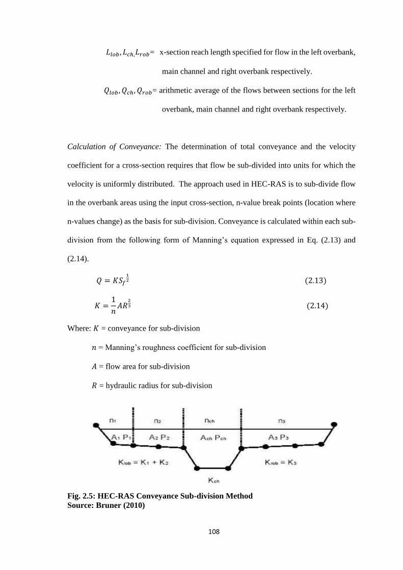
108

𝐿𝑙𝑜𝑏 , 𝐿𝑐ℎ,𝐿𝑟𝑜𝑏= x-section reach length specified for flow in the left overbank,

main channel and right overbank respectively.

𝑄𝑙𝑜𝑏, 𝑄𝑐ℎ, 𝑄𝑟𝑜𝑏= arithmetic average of the flows between sections for the left

overbank, main channel and right overbank respectively.

Calculation of Conveyance: The determination of total conveyance and the velocity

coefficient for a cross-section requires that flow be sub-divided into units for which the

velocity is uniformly distributed. The approach used in HEC-RAS is to sub-divide flow

in the overbank areas using the input cross-section, n-value break points (location where

n-values change) as the basis for sub-division. Conveyance is calculated within each sub-

division from the following form of Manning’s equation expressed in Eq. (2.13) and

(2.14).

𝑄 = 𝐾𝑆𝑓

12 (2.13)

𝐾 =1

𝑛𝐴𝑅

23 (2.14)

Where: 𝐾 = conveyance for sub-division

𝑛 = Manning’s roughness coefficient for sub-division

𝐴 = flow area for sub-division

𝑅 = hydraulic radius for sub-division

Fig. 2.5: HEC-RAS Conveyance Sub-division Method


109

All the incremental conveyances in the overbank are summed to obtain a conveyance for

the left and the right overbanks and the total conveyance for cross-section is obtained by

summing the three sub-division conveyances.

Calculation of Mean Kinetic Energy Head: Mean kinetic energy head for each cross-

section is obtained by computing the flow weighted kinetic energy heads for three sub-

sections of the cross-sections (Left Overbank, Channel, and Right Overbank). Figure 2.6

illustrates the mean kinetic energy calculation process for a cross-section with a main

channel and right overbank.

Fig. 2.6: Mean Energy Head Calculation


It is necessary to obtain the velocity head weighting coefficient α in order to compute the

mean kinetic energy. α can be calculated using Eq. (2.15).

𝛼 =(𝐴𝑡)2 [

𝐾𝑙𝑜𝑏3

𝐴𝑙𝑜𝑏2 +

𝐾𝑐ℎ3

𝐴𝑐ℎ2 +

𝐾𝑟𝑜𝑏3

𝐴𝑟𝑜𝑏2 ]

𝐾𝑡3 (2.15)

Where, 𝐴𝑡 = total flow area of cross-section

Alob, Ach, Arob = flow areas of left overbank, main channel and right overbank

𝐾𝑡 = total conveyance of cross-section

Klob, Kch, Krob = conveyance of left overbank, main channel and right over bank

110

Unsteady Flow Simulation: The component of the HEC-RAS modelling system is capable

of simulating one-dimensional unsteady flow through a full network of open channels.

The unsteady flow component was developed primarily for subcritical flow regime

calculations but the model can now perform mixed flow regime (subcritical, supercritical,

hydraulic jumps, and draw downs) calculations in the unsteady flow computations

module. Special features of the unsteady flow component include: Dam break analysis,

levee breaching and overtopping, Pumping stations, navigation dam operations and

pressurized pipe systems.

Sediment Transport/Movable Boundary Computations: This component of the modelling

system is intended for the simulation of one-dimensional sediment transport/movable

boundary calculations resulting from scour and deposition over moderate time periods

(typically years, although applications to single flood events are possible). This can be

used to evaluate deposition in reservoirs, design channel contractions required to maintain

navigation depths, predict the influence of dredging on the rate of deposition, estimate

maximum possible scour during large flood events, and evaluate sedimentation in fixed

channels.

Water Quality Analysis: This component of the modelling system is intended to allow the

user to perform riverine water quality analyses. An advection-dispersion module is

included in HEC–RAS, adding the capability to model water temperature. This new

module uses the QUICKEST-ULTIMATE explicit numerical scheme to solve the one-

dimensional advection-dispersion equation using a control volume approach with a fully

implemented heat energy budget.

111

Data Storage and Management: Data Storage is accomplished through the use of “flat”

files (ASCII and binary), as well as the HEC-DSS. User input data are stored in flow files

under separate categories of project, plan, geometry, steady flow, unsteady flow, and

sediment data. Output data is predominantly stored in separate binary files. Data can be

transferred between HEC-RAS and other programs by utilizing the HEC-DSS.

Graphics and Reporting: Graphics include X-Y plots of the river system schematic, cross-

sections, profiles, rating curves, hydrographs, and many other hydraulic variables. A

three-dimensional plot of multiple cross-sections is also provided. Tabular output is

available. Users can select from pre-defined tables or develop their own customized

tables. All graphical and tabular output can be displayed on the screen, sent directly to a

printer (or plotter), or passed through the Windows Clipboard to other software, such as

a word-processor or spreadsheet.

RAS Mapper: HEC-RAS has the capability to perform inundation mapping of water

surface profile results directly from HEC-RAS. Using the HEC-RAS geometry and

computed water surface profiles, inundation depth and floodplain boundary datasets are

created through the RAS Mapper. Additional geospatial data can be generated for analysis

of velocity, shear stress, stream power, ice thickness, and floodway encroachment data.

2.15.2.2 HEC- GeoRAS

HEC-Geo RAS is an ArcGIS extension specifically designed to process geo-spatial data

for use with the Hydrologic Engineering Center Rivers Analysis System (HEC-RAS).

The extension allows users to create an HEC-RAS import file containing geometric

attribute data from an existing Digital Elevation Model (DEM) and complementary data

112

sets. Water surface profile processed and exported from HEC-RAS to HEC-GeoRAS can

also be processed to visualize inundation depths and boundaries. HEC-GeoRAS extension

for ArcGIS used an interface method to provide a direct link to transfer information

between the ArcGIS and the HEC-RAS.

HEC-GeoRAS requires ArcGIS with 3D Analyst extensions. Although not a requirement,

the availability of the Spatial Analyst extension significantly speeds up post-processing.

In summary, HEC-GeoRAS extension provides the user with a set of procedures, tools

and utilities for the preparation of GIS data for import into HEC-RAS and generation of

GIS data from HEC-RAS output. These tasks are organized as pre-processing (preRAS)

and post-processing (postRAS) facilitated by menu and buttons.

Processing to Develop the RAS GIS import file: The RAS GIS Import File is created in

HEC-GeoRAS consisting of geometric attribute data necessary to perform hydraulic

computations in HEC-RAS. The cross-sectional geometric data is developed from DEM

(TIN) of the channel and surrounding land surface, while the cross-sectional attributes are

derived from points of intersection of the created RAS layers which include Stream

Centerlines, Flow Path Centerlines, Main Channel Banks, and Cross Section Cut Lines.

Additional RAS layers that may be created to extract additional geometric data for import

in HEC-RAS include Land Use, Levee Alignment, Ineffective Flow Areas, and Storage

Areas. Expansion/contraction coefficients, hydraulic structure data such as bridges and

culverts are not written to the RAS GIS Import File but are modelled through the RAS

interface.

Post – Processing to Generate GIS Data from HEC-RAS Results: Post-processing

facilitates the automated floodplain delineation based on the data contained in the RAS-

113

GIS output file and original terrain TIN. Based on the RAS-GIS export file, cross-sections

theme (with water levels for each modelled profile as attributes) and bounding polygon

of the likely floodplain can be generated. The water surface TIN is generated using these

cross-sections and bounding polygon themes. With the water surface TIN and the original

terrain TIN, inundated depth grids and floodplain polygons can be automatically

generated. Apart from this, HEC-GeoRAS can also generate the velocity TIN and grid.

2.15.2.3 ArcGIS 10.2.2

ArcGIS 10.2.2 was developed by Environmental Systems Research Institute (ESRI) Inc.

(1999 - 2014). It is a very important and easy to use tool that brings GIS to the desktop.

ArcGIS 10.2.2 is equipped with excellent graphical user interface (GUI). ArcGIS Desktop

includes a suite of integrated applications that allow GIS tasks to be performed, from

simple to advanced, including mapping, geographic analysis, data editing and

compilation, data management, visualization, and geo-processing.

ArcGIS 10.2.2 is also equipped with a number of extensions designed to perform various

tasks. They include spatial analyst which provides spatial analysis tools for use with raster

and feature data, 3D analyst which provides tools for surface modelling and 3D

visualization, geostatistical analyst which provides a complete set of spatial analytical

tools that range from techniques to explore the original data to post-processing, evaluation

of data and predictions uncertainties Arcscan which provides support for the creation of

vector features from a raster image amongst others. Some extensions, such as the ones

mentioned, are bundled with ArcGIS while others such as HEC-GeoHMS, HEC-GeoRAS

and ArcHydro are optional and can be added.

114

CHAPTER THREE

MATERIALS AND METHODS

3.1 MATERIALS

3.1.1 Types and sources of data

The data used in this study were obtained from both primary and secondary sources. The

following data were obtained and utilized for the achievement of the stated objectives:

i. Topographic Map:

The topographic maps used in this study are the Nigerian Survey Topographic Map Series

of Nigeria. They are Idah N.E. Sheet 267, Idah S. E. Sheet 267 and Ilushi N. E Sheet 286

all on a scale of 1:50,000 (Appendix Ia-c). The Idah N. E. and S. E. sheets were published

by the Office of the Surveyor General of the Federation while the Illushi N. E. was

published by the defunct Federal Surveys of Nigeria. The summary of the properties of

the topographic maps are presented in Table 3.1. They were obtained from the Kogi State

Ministry for Land and Urban Development Headquarters, Lokoja.

Table 3.1: Properties of the Topographic Maps Used in the Study

S/No Title Sheet No Coverage Year

Published Latitude Longitude

1 IDAH NE 267 NE 7o15’ - 7o30’ 6o45’ – 7o 2008

2 IDAH SE 267 SE 7o – 7o15’ 6o45’ – 7o 2008

3 ILLUSHI NE 286 NE 6o45’ – 7o 6o45’ – 7o 1964

Source: Kogi State Ministry of Land and Urban Development

The maps were scanned, georeferenced and digitized in ArcGIS 10.2.2 and used to

identify features for landuse/land cover classification as well as the flood vulnerability

assessment.

ii. Historical Rainfall Data of Neighbouring Towns

Historical rainfall data of towns surrounding the study area were obtained from project

reports available at the Library of the Lower Benue River Basin Development Authority

115

headquarters, Makurdi. The towns for which data were obtained from Literatures are Idah,

Onitsha, Nsukka, Adani and Enugu. In addition to these, meteorological data were also

obtained from the Nigerian Metrological Agency (NiMet), Tactical Air Command,

Makurdi-Airport (1980-2015). The summary of these historical rainfall data are presented

in Table 3.2. The details are presented in Appendix II (Table IIa).

iii. Historical Gauged Discharge Data of Ofu River at Oforachi

Discharge data of Ofu River at the Oforachi hydrometric station from 1955 to 1973 were

obtained from Kogi State Ministry of Water Resources and Rural Development. The

summary is presented in Table 3.3 while the details are presented in Appendix III (Table

III).

iv. Soil Map

The digital soil map of the world alongside the attributes was obtained from the Food and

Agricultural Organization (FAO)’s website via the following link.

(http://www.fao.org/geonetwork/srv/en/metadata.show?id=14116)

v. Satellite Data

Properties and relevance of the SRTM Digital Elevation Model and other satellite

imageries used in this study are presented in Table 3.4. The projection for all the data is

the Universal Transverse Mercator (UTM) zone 32 while the datum is WGS84.

Table 3.2: Historical Mean Annual Rainfall for Ofu River Catchment Neighbouring

Stations

Station Latitude

(0N)

No. of Years Mean Annual

Rainfall (mm)

Idah 7o06’ 32 1517.52

Onitsha 6o23’ 55 2243.52

Nsukka 7o52’ 21 1930.14

Adani 6o43’ 17 1995.00

Enugu 6o27’ 54 2163.72

Makurdi 7o41’ 30 1165.82

Source: Skoup and Motor Columbus (1980), NiMET (2016)

http://www.fao.org/geonetwork/srv/en/metadata.show?id=14116

116

Table 3.3: Historical Mean Discharge Record for Ofu River at Oforachi

Month Jan Feb Mar Apr May Jun Jul Aug Sep Oct Nov Dec Total

Ave

(m3/s) 3.86 2.85 2.14 13.31 15.95 44.02 132.45 403.79 432.02 83.01 5.8 3.93 1143.12

Source: Kogi State Ministry of Water Resources and Rural Development

Table 3.4: Properties of Satellite Data and Relevance

Data Type Resolution No of

Bands

Date of

Acquisition

Date of

Publication Source

SRTM DEM V3 30m 1 11/02/2000 26/07/2014 Earthexplorer.usgs.gov

ASTER GDEM2 30m 1 2011 October, 2011 Earthexplorer.usgs.gov

Landsat 8 Imagery of 2016 30m 12 15/03/2016 03/05/2016 Glovis.usgs.gov



River map of Africa NA NA NA NA www.waterbase.org

117

vi. Meteorological Data

The rainfall data used for this study were obtained from the radar data available on

http://www.waterbase.org/download_data.html. They consist of data from 41 stations

surrounding the study area. The data covered a 35 year period from January, 1979 to

December, 2013. The summary of this data is presented in Appendix II (Tables IIb and

IIc).

vii. Information on Previous Flood Occurrence

The information on previous flood experience was gathered with the aid of questionnaires

admistered during field survey.

3.1.2 Hardware and software

3.1.2.1 Hardware

i. A High speed memory Lenovo ideapad 100 Intel Pentium Laptop Computer.

ii. A Garmin hand-held Global Positioning System (GPS) receiver model GPSmap

78sc for marking of locations during fieldwork.

iii. An Impeller current meter, Valeport model 0012B Version 4.01

iv. Ring Infiltrometer (Fabricated)

v. Soil Classification Apparatus (Atterberg Limits apparatus, Sieve Analysis

Apparatus, Weighing balance and Oven)

3.1.2.2 Software

i. Google Earth Pro 4.2 was used for the identification and extraction of information

for landuse/landcover classification.

http://www.waterbase.org/download_data.html

118

ii. ArcGIS 10.2.2 is a commercial software developed by Environmental Systems

Research Institute (ESRI) that is essentially used for GIS analysis. It has the

capability of accepting compatible add-on extensions such as the ArcHydro, HEC-

GeoHMS and HEC-GeoRAS. The Spatial analyst and the 3D analyst tools have

capabilities that make easy data manipulation, analysis and management with

regards to floodplain simulation.

iii. HEC-GeoHMS10.2 is a free software developed by the Hydraulic Engineering

Centre (HEC) of the United States Army Corp of Engineers (USACE). It is an

extension installed in ArcGIS for GIS analysis with spatial data for catchment

delineation and hydrological modelling.

iv. HEC-GeoRAS10.2 is a free software developed by the Hydraulic Engineering

Centre (HEC) of the United States Army Corp of Engineers (USACE). It is an

extension installed in ArcGIS for GIS analysis with spatial data, flood inundation

and water depth simulation. It is normally used in conjunction with HEC-RAS.

v. HEC-RAS 4.1 is also a free software developed by the Hydraulic Engineering

Centre (HEC) of the United States Army Corp of Engineers (USACE) for one-

dimensional hydraulic modelling. The RAS mapper has the capability of flood

inundation mapping. It is normally used in conjunction with HEC-GeoRAS.

vi. Microsoft Office Excel 2007 for river discharge analysis, flood frequency analysis

and other statistical analysis and presentation.

vii. Minitab® Release 14.12.0 Statistical Software developed by Minitab Inc. was used

alongside Microsoft Excel for statistical analysis.

viii. Stata®/SEversion 13.1 special edition developed by Stata Corp Lp was used

alongside Microsoft Excel and Minitab for statistical/data analysis.

119

3.2 METHODS

3.2.1 Determination of Morphologic Characteristics of Ofu River Catchment

3.2.1.1 Delineation of Ofu River catchment boundaries

The terrain pre-processing of the DEM for the delineation of the catchment boundaries

was done using the ArcHydro terrain preprocessing tool in ArcHydro extension while

the actual delineation was done using the HEC GeoHMS.

(A) Terrain pre-processing using ArcHydro

a. Datasets Preparation

Two datasets were required for the Terrain pre-processing and watershed delineation. The

first dataset was the digital elevation model (DEM). The DEM used for this study was

obtained from the four tiles of the STRM DEM (Table 3.4). A single DEM was created

using the Mosaic tool in dataset Management Tool in ArcGIS 10.2.2 by clicking Dataset

management tool>Raster>Raster Dataset>Mosaic with the four DEMs as input and the

first tile chosen as the target raster. On clicking OK, the mosaic process was completed.

The other DEMs were removed leaving only the target raster as the raw DEM for the

analysis. The mosaicked DEM was projected by clicking Dataset management

tool>Projections and Transformations>Raster>Project Raster with the mosaicked DEM

as the input raster dataset. The output raster dataset was named ofu_dem and saved in the

working directory. The output coordinate system was defined to WGS1984 UTM Zone

32. On clicking Ok, the DEM was projected to the defined coordinate system. The

projected DEM was converted to grid using the raster to other formats conversion tool

by clicking Conversion>To Raster>Raster to other formats (multiple).

120

The second dataset was the streams shapefile. This is a shapefile containing stream

network for the study area. This was clipped from the river map of Africa extracted from

http://www.waterbase.org/download_data.html. The stream feature was also projected to the

same coordinate system as the DEM by clicking Dataset management tool>Projections and

Transformations>Project.

Both datasets were added to the new map document.

b. Terrain Pre-processing

Terrain Pre-processing in Arc Hydro follows a sequential order. Terrain pre-processing

is pre-requisite for the watershed processing and delineation itself thus must be completed

first. The processes carried out at this stage are described below:

i. DEM Reconditioning: DEM reconditioning was carried out to modify the

elevation data to be more consistent with the input vector stream network. This was done

on the assumption that the stream network data are more reliable than the DEM data thus

increasing the degree of agreement between stream networks delineated from the DEM

and the input vector stream networks.

The DEM reconditioning was carried out by selecting Terrain Preprocessing >DEM

Manipulation> DEM Reconditioning on ArcHydro Toolbar. The projected ofu_dem was

selected as input raw DEM while the clipped river of the study area was selected as the

input agree Stream feature. The Sharp drop/raise parameter was reduced from its default

1000 to 10 while other fields were left as they were. On clicking Ok, the AgreeDEM was

produced and added to the map document.


121

ii. Fill Sinks: The fill sink operation was carried out by selecting Terrain

Preprocessing>Data Manipulation>Fill Sinks on the ArcHydro toolbar with AgreeDEM

as input. The output Hydro DEM was named ofu_fil. The other fields were left unchanged.

On pressing Ok, the fill sink operation was completed and the ofu_fil layer was added to

the map document.

iii. Flow Direction: The flow direction operation was carried out by selecting Terrain

Preprocessing>Flow Direction on the ArcHydro toolbar with ofu_fil as the input Hydro

DEM. The output grid was named ofu_fdr. On pressing Ok, the flow direction operation

was completed and the ofu_fdr grid was added to the map document.

iv. Flow Accumulation: The flow accumulation operation was carried out by

selecting Terrain Preprocessing>Flow Accumulation on the ArcHydro toolbar with

ofu_fdr as the input Flow direction grid. The output grid was named ofu_fac. On pressing

Ok, the flow accumulation operation was completed and the ofu_fac grid was added to

the map document.

v. Stream Definition: The definition operation was carried out by selecting Terrain

Preprocessing>stream definition on the ArcHydro toolbar with ofu_fac as the input Flow

Accumulation grid. The output grid was named ofu_str. A threshold area of 25 km2 was

used in the stream definition. On pressing Ok, the stream definition operation was

completed and the ofu_str grid was added to the map document.

vi. Stream Segmentation: The segmentation operation was carried out by selecting

Terrain Preprocessing>Stream Segmentation on the ArcHydro toolbar with ofu_fdr and

ofu_str as the input for Flow direction and stream grids, respectively. The output grid was

122

named ofu_str_link. On pressing Ok, the stream segmentation operation was completed

and the ofu_str_lnk grid was added to the map document.

vii. Catchment Grid Delineation: The catchment grid delineation operation was

carried out by selecting Terrain Preprocessing>Catchment Grid Delineation on the

ArcHydro toolbar with ofu_fdr and ofu_str_lnk as the input for Flow direction and stream

link grids, respectively. The output Catchment Grid Layer was named ofu_cat. On

pressing Ok, the catchment grid delineation was completed and the ofu_cat grid was

added to the map document.

viii. Catchment Polygon Processing: The catchment Polygon processing operation

was done to convert the Catchment grid from raster to vector format. This was done by

selecting Terrain Preprocessing >Catchment Polygon Processing in ArcHydro toolbar

with ofu_cat as the input Catchment Grid. The output polygon was named catchment. On

pressing Ok, the catchment grid was converted into a catchment polygon feature class.

This was then added to the map document.

ix. Drainage Line Processing: The drainage line processing operation was done to

convert the input Stream Link grid into a Drainage Line feature class which would be

used for the delineation of the catchments. This was done by selecting Terrain

Preprocessing >Drainage Line Processing on the ArcHydro toolbar with ofu_str_lnk as

the input Stream Link and to ofu_fdr as the Flow Direction Grid. The default name for

the output Drainage Line was accepted as DrainageLine. On pressing Ok, the drainage

line processing operation was completed and the linear feature class ‘DrainageLine’ was


123

x. Adjoint Catchment Processing: The adjoint catchment processing operation was

done by selecting Terrain Preprocessing > Adjoint Catchment Processing with

DrainageLine and Catchment as inputs while default ouput name was accepted as

AdjointCatchment.

On pressing Ok, a polygon feature class named AdjointCatchment was added to the map

document.

(B) Ofu Watershed Processing and Delineation Using HEC GeoHMS

a. Datasets Management

The outputs of the terrain pre-processing in ArcHydro were the inputs for the Watershed

processing in HEC GeoHMS project set up. The Datasets were confirmed by clicking

HMS Project Setup>Data Management on the HEC-GeoHMS Main View toolbar. The

corresponding map layers were confirmed as follows:

i. Raw DEM: ofu_dem

ii. Hydro DEM: ofu_fil

iii. Flow Direction Grid: ofu_fdr

iv. Flow Accumulation Grid: ofu_fac

v. Stream Grid: ofu_str

vi. Stream Link Grid: ofu_str_lnk

vii. Catchment: ofu_cat

viii. Adjoint Catchment: AdjointCatchment

b. Creating Ofu River Project

The first step in catchment delineation in HEC GeoHMS is the Project creation. This

involved starting new project, defining the project point and Generating the Project.

124

i. Start New Project

This was done by clicking on Project Setup>Start New Project. The default ProjectArea

and ProjectPoint were accepted. Thus, the ProjectPoint and ProjectArea feature classes

were created. The process pops up another dialogue box for defining a new project. The

following links fields were required and provided as follows:

Project Name: OfuRiver

Description: HMS model for Ofu River

Extraction Method: Original Stream Definition

Project Data location: Outside mainview Geodatabase

Every other field was left as default. On pressing Ok, the process of creating the Ofu

River project was completed and the projectArea and ProjectPoint feature classes were

added to the map document. These feature classes were added to the same geodatabase

ofu.gdb

ii. Define Project Point

The Add Project Points tool on the HEC-GeoHMS toolbar was used to define the outlet

of Ofu River just before its confluence with Omabolo River downstream.

A new dialogue box “Project Point for OfuRiver” popped up. The defaults point Name

and description “outlet1” were accepted. Thus, the definition of project point was

completed and added to the map document.

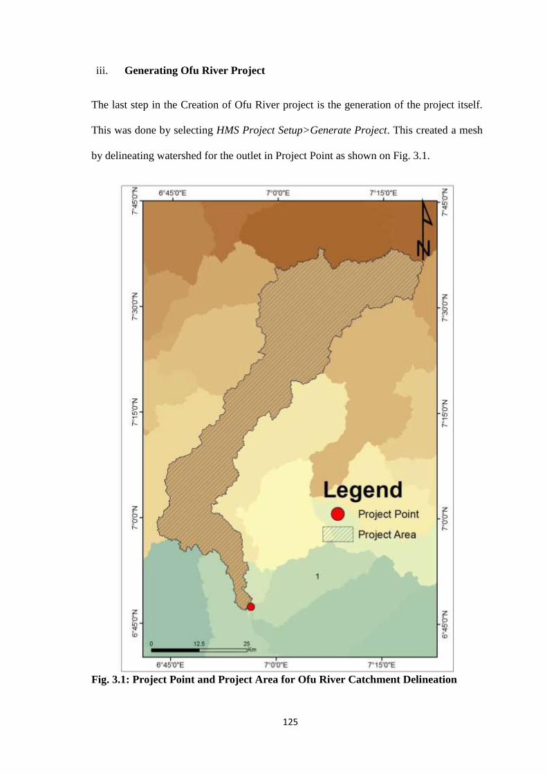
125

iii. Generating Ofu River Project

The last step in the Creation of Ofu River project is the generation of the project itself.

This was done by selecting HMS Project Setup>Generate Project. This created a mesh

by delineating watershed for the outlet in Project Point as shown on Fig. 3.1.

Fig. 3.1: Project Point and Project Area for Ofu River Catchment Delineation

126

The message box asking if you want to create a project for this hatched area was accepted

by clicking ‘Yes’ on the message box. The layer names for the new project was confirmed

while the default names for Subbasin, Project Point, River and BasinHeader were left as

they were (Subbasin 181, ProjectPoint181, River 181). On clicking Ok, a new folder was

created inside the working folder with the name ‘OfuRiver’ where all the relevant raster,

vector and tabular data were stored. The raster data were stored in a sub folder with the

project name (OfuRiver) inside OfuRiver folder while all vector and tabular data were

stored in OfuRiver.mdb. At the same time, a new data frame (OfuRiver) was added in the

map document containing the data for Ofu River.

c. River Profile

The River Profile tool in HEC GeoHMS main toolbar was used to display the profile of

selected Ofu river reach. It was observed that there was no significant change in the river

slope.

d. Extracting Basin Characteristics

The basin characteristics menu in the HEC-GeoHMS Project was used to extract the

physical characteristics of Ofu River (River181) and Ofu Catchment (Subbasin181) into

attribute tables.

The properties were extracted via the following methods.

i. River Length: The River length was computed by selecting

Characteristics>River Length on the HEC GeoHMS toolbar with River181 (Ofu River)

as input River. On pressing Ok, the RiverLen field in attribute table was filled with the

Length of the main stream.

127

ii. River Slope: The slope of the River segment was computed by selecting

Characteristics>River Slope on the HEC GeoHMS toolbar with River181 (Ofu River)

as input River. On pressing Ok, the Slp field in attribute table was filled with the slope

of the main stream.

iii. Basin Slope: A slope grid was created using Arc Hydro tools by selecting Terrain

Preprocessing > Slope with ofu_dem as input and percent_rise as slope type. A slope

grid with the default name WshSlopePct was produced and added to the map document.

This was used as input alongside the subbasin polygon for the computation of average

slope for Ofu river basin using HEC geoHMS.

The basin slope computation was done by selecting Characteristics>Basin Slope with the

Subbasin181 (Ofu River basin) and Slope Grid as input. The Subbasin1 for Ofu River

attribute table was instantly filled with the average basin slope of Ofu River watershed.

iv. Longest Flow Path: The longest flow path was computed by selecting

Characteristics>Longest Flow Path on the HEC GeoHMS toolbar with ofu_dem as the

input raw DEM, ofu_fdr as the input flow direction grid and Subbasin181 as the input

subbasin. On pressing Ok, a new feature class storing longest flow path for the basin

was created and added to the map document.

v. Basin Centroid: The Basin centroid was computed by selecting

Characteristics>basin Centroid on the HEC GeoHMS toolbar with Subbasin181 as the

input subbasin. The default center of gravity method was selected as the centroid

method. On pressing Ok, a point feature class showing centroid for each subbasin was


vi. Basin Centroid Elevation: The Basin Centroid Elevation was computed by

selecting Characteristics>Basin Centroid Elevation on the HEC GeoHMS toolbar with

128

ofu_dem as the input raw DEM Centroid181 as the input Centroid. On pressing Ok, the

elevation field of the centroid attribute table was populated.

vii. Centroidal Longest Flow Path: The Centroidal longest flow path was computed

by selecting Characteristics>Centroidal Longest Flow Path on the HEC GeoHMS

toolbar with subbasin181 as the input Subbasin, centroid181 as the input Centroid and

LongestFlowPath181 as the input Longest Flow Path. On pressing Ok, a new feature

class storing Centroidal longest flow path for each basin was created and added to the

map document.

3.2.1.2 Estimation of morphologic parameters of Ofu River catchment

The morphologic parameters determined for Ofu River catchment were broadly classified

into areal, linear and relief aspects, respectively. The following standard methods were

followed to determine the morphometric parameters.

(A) Areal Aspects

The basic areal morphologic characteristics of the river basin were determined via the

following methods:

i. Basin area (A): The basin area was calculated after the delineation of the

catchment boundaries. The Attribute table of the Sub-basin was opened in ArcGIS 10.2.2

and a new field was added and named Area. The Calculate Geometry tool was then used

to calculate the area of the catchment in km2 which was done automatically and the

required field populated.

ii. Basin Perimeter (P): The same procedure followed for the calculation of the

basin area was followed for the calculation of the basin perimeter. The Perimeter field

was then populated automatically with the perimeter values in km.

129

iii. Basin Length (Lb): The Schumm (1956) definition of basin length was adopted

in this study. The basin length was taken as the longest distance between the basin outlet

and the remotest part of the watershed divide parallel to the drainage line. This was done

using the measurement tool in ArcGIS 10.2.2

iv. Longest flow path (Lfp): This was extracted from the attribute table of the

Longest Flow Path feature class in km.

v. Main Stream Length (SL): This was extracted from the attribute table of the

River (River181) in km.

vi. Basin Centroid Longest Flow Path (Lcfp): This was extracted from the

Centroid181 feature class in km.

The methods for the estimation of the derived areal morphologic characteristics of the

Catchment are summarized in Table 3.5.

Where A is the Basin area (km2), Lb is the Basin length (km), P is Basin Perimeter (km),

ΣNu is number of streams of all orders, ΣLu is total length of streams of all orders (km),

Lfp is the longest flow path (km) and S is the Basin Slope.

130

Table 3.5: Methods of Estimation of Derived Areal Morphological Characteristics

S/N Parameters Symbol Equation

No. Reference

vii. Elongation ratio 𝑹𝒆 =𝟐√𝑨 𝝅⁄

𝑳𝒃⁄ 3.1

Schumm

(1956)

viii. Circularity ratio 𝑹𝒄 = 𝟒𝝅𝑨𝑷𝟐⁄ 3.2 Miller (1953)

ix. Form factor 𝑭𝒇 = 𝑨𝑳𝒃

𝟐⁄ 3.3 Horton (1932)

x. Compactness

coefficient 𝑪𝒄 = 𝟎. 𝟐𝟖𝟐𝟎𝟑𝟖𝑷

𝑨𝟎.𝟓⁄ 3.4 Horton (1945)

xi. Shape Factor 𝑩𝒔 =𝑳𝒃

𝟐

𝑨⁄ 3.5 Horton (1932)

xii. Stream frequency 𝑭 =∑ 𝑵𝒖

𝑨⁄ 3.6 Horton (1945)

xiii. Drainage Density 𝑫𝒅 =∑ 𝑳𝒖

𝑨⁄ 3.7

Horton (1932;

1945)

xiv. Drainage Texture 𝑫𝒕 =∑ 𝑵𝒖

𝑷⁄ 3.8 Horton (1945)

xv. Drainage Intensity 𝑰𝒅 = 𝑭𝑫𝒅

⁄ 3.9 Faniran (1968)

xvi. Constant of Channel

Maintenance 𝑪𝒎 = 𝟏

𝑫𝒅⁄ 3.10 Strahler (1952)

xvii. Length of Overland

Flow 𝑳𝒐 = 𝟏

𝟐𝑫𝒅⁄ 3.11

Langbein &

Leopold (1964)

xviii. Channel Sinuosity 𝑺𝒄 =∑ 𝑳𝒖

𝑳𝒇𝒑⁄ 3.12 Le Roux (1992)

xix. Time of

Concentration 𝑻𝒄 = 𝟎. 𝟎𝟎𝟎𝟑𝟐𝟑𝑳𝒇𝒑

𝟎.𝟕𝟕𝑺−𝟎.𝟑𝟖𝟓 3.13 Kirpich (1940)

xx. Time from Peak to

Recession 𝑵 = 𝟎. 𝟖𝟒𝑨𝟎.𝟐 3.14

Mustafa and

Yusuf (2012)

(B) Linear Aspects

The Linear aspects of the drainage basin derived in this study are stream order, stream

number, stream length, Mean stream length, bifurcation ratio and stream length ratio.

The stream order of Ofu River Catchment was derived using the spatial analyst hydrology

tools in ArcGIS 10.2.2. via the following steps using the Ofu River flow accumulation

and flow direction rasters obtained from the HEC GeoHMS catchment delineation

process as input.

131

i. Stream network definition: In order to extract the stream network, it was

assumed that a total of 25km2 is the required drainage threshold to form a stream

(Merwade, 2012). The pixel value of this threshold is calculated as follows:

𝑇ℎ𝑟𝑒𝑠ℎ𝑜𝑙𝑑 𝑝𝑖𝑥𝑒𝑙𝑠 = 25 × 106

90 × 90= 27,778 𝑝𝑖𝑥𝑒𝑙𝑠

The stream network definition was done by creating a raster from the ofu_fac such that

only cells that have pixel value greater than 27,778 was included. This was done using

the raster calculator by selecting Spatial Analyst Tools>Map Algebra>Raster calculator.

The “setnull” command was used to create a calculation raster where all the cells with

value greater than or equal to 27,778 in ofu_fac were assigned a value of 1, while all other

cells are set to zero. This was done by specifying the command

‘SetNull(“ofu_fac”<27778,1)’ in raster calculator. The output raster was named stream

and was added to the map document.

ii. Stream link definition: The stream link definition tool assigns a unique number

to each link (or segment) in the stream raster. This was done by double clicking on Stream

Link in spatial analyst hydrology tool providing stream as the input surface stream raster

and ofu_fdr as the flow direction raster. The output raster was named str_link.

iii. Stream order extraction: The stream order extraction tool was used to stream

order for the stream network. This was done by double clicking on stream order in the

spatial analyst hydrology tool providing stream as the input for stream raster and ofu_fdr

as the input for flow direction raster. The output raster was named str_order. Two

methods are available in ArcGIS 10.2.2 for estimating stream order. The Strahler’s

method was chosen and specified in the ‘method of stream ordering’ link. On clicking

Ok, the process of stream ordering for Ofu River catchment was completed and a new

str_order raster was added to the map document.

132

iv. Conversion of Stream network from raster to feature: The last step here was

the conversion of the stream raster to a polyline feature class (shapefile). This was done

by double clicking Stream to feature in the spatial analyst hydrology tool providing

stream as the input for stream raster and ofu_fdr as the input for the flow direction raster.

The output was saved as ofu_stream in the working directory. On clicking Ok, the process

of converting the stream raster to ployline feature class was completed and a shapefile

named ofu_stream was added to the map document. This same tool was used to convert

the str_order raster to a polyline feature class named Stream_oder using the str_order

raster instead of the stream raster.

The attribute table of the stream_order feature class is automatically populated with the

stream order (U) of all the defined streams, the number of streams (Nu) in each order and

the length of streams (Lu) in each order. These were used to calculate the mean stream

length, bifurcation ratio and the stream length ratio as presented in Table 3.6

Table 3.6: Methods of Estimation of Linear Morphological Characteristics


No. Reference

i. Mean Stream Length 𝑳𝒖𝒎 =𝑳𝒖

𝑵𝒖⁄ 3.16 Strahler (1964)

ii. Bifurcation Ratio 𝑹𝒃 =𝑵𝒖

𝑵𝒖+𝟏⁄ 3.17 Schumm (1956)

iii. Stream Length Ratio 𝑹𝑳 =𝑳𝒖

𝑳𝒖−𝟏⁄ 3.18 Horton (1945)

Where Lu is length of streams of order U, Nu is the number streams of order U, Nu+1 is the

number of streams of the next higher order U+1 and Lu-1 is the length of streams of the

next lower order U-1.

133

(C) Relief Aspects

The methods of estimation of the relief characteristics of Ofu River catchment are

presented in Table 3.7 except for the basin slope, S that was extracted from the sub basin

attribute table.

Table 3.7: Methods of Estimation of Relief Morphological Characteristics


No. Reference

i. Basin Relief 𝑯 = 𝒁 − 𝒛 3.18 Strahler (1957)

ii. Relief Ratio 𝑹𝒉 = 𝑯𝑳𝒃

⁄ 3.19 Schumm (1956)

iii. Relative Relief 𝑹𝒉𝒑 = 𝑯𝑷⁄ 3.20 Melton (1957)

iv. Ruggedness

Number 𝑹𝑵 = 𝑯 × 𝑫𝒅 3.21

Patton and Baker

(1976)

Where Z is the highest elevation (m above seal level), z is the lowest elevation (m above

sea level), Lb is Basin Length (m), P is the Basin Perimeter (m) and Dd is the drainage

density.

A schematic flowchart of the morphometric analysis methodology is presented in Fig.

3.2.

3.2.2 Development of Stage-Discharge Rating Curve for Ofu River

Hydrological data such as stream flow and water levels are necessary inputs for hydraulic

modelling of a river channel. These data were scarce or inexistent in the case of Ofu River

as it is for several ungauged catchments in developing nations thus necessitating field

work to generate these data. The detailed description of the methods adopted for the

measurement of water levels and discharge of Ofu River as well as the development of

the rating curve are presented as follows.

134

Fig. 3.2: Schematic Flowchart of the Morphometric Analysis Methodology

135

3.2.2.1 Ofu River stage gauge recalibration and water level measurement

It was observed during the reconnaissance survey that the original staff gauge of the Ofu

River at Oforachi Bridge hydrometric station has been washed off by successive flood

events that have taken place in the study area which necessitated a recalibration.

The temporary benchmark (TBM) of the area was located (Plate I) and transferred from

the bridge to the gauging points on the old Oforachi Bridge where the firm poles of the

previous staff gauges were located. This point is firm and satisfies all the criteria for

locating a gauging site (Meals and Dressing, 2008; Sauer and Turnipseed, 2010). This

was used as a reference for the recalibration of the staff gauge relative to mean sea level.

Plate I: Location of the TBM at Oforachi Bridge Hydrometric station

This transfer was done with the aid of a Total Station. The service of a professional

surveyor was employed from the Department of Survey and Geomatics, Federal

Polytechnic Idah, Kogi State (Plate II).

Three staff gauges were calibrated and labelled gauge 1, 2 and 3, respectively. These were

used to take the water level of Ofu River every morning and evening for twelve (12)

months beginning from the February 1, 2016 to January 31, 2017.

136

Plate II: Re-establishment of Staff gauge at Oforachi Bridge Hydrometric station

The location of the gauge point is shown in Fig. 3.3.

137

Fig. 3.3: Ofu River catchment showing location of gauge stations

138

3.2.2.2 Ofu River discharge measurement at Oforachi hydrometric station

The stream flow of Ofu River was measured for 12 months beginning from February 1,

2016 to January 31, 2017 in order to generate data for the development of the rating curve.

The discharge measurement carried out in this study adopted the Velocity-Area method

(mid section) using a Valeport Impeller current meter model 0012B Version 4.01 (Plate

III).

Ofu River is a perennial river whose year round flow depth does not go below 2 meters

at the deepest point thus making it difficult to apply the wading method. The bridge

suspension method was therefore adopted incorporating some wading techniques to fit

into the site peculiarities.

Plate III: Stream flow Measurement at Oforachi Bridge Hydrometric station

The schema of the river cross section is shown in Fig. 3.4.

Fig. 3.4: Schema of the River Cross-section during one of the discharge

measurements

139

The number of subsections for the observation was between 12 and 17 spaced 1 m apart

throughout the period of observation. The discharge measurement was carried out via the

following steps:

Step 1: The depth of water for each subsection was measured using the wading rod and

recorded as d.

Step 2: A uniform horizontal distance (width of subsections) w of 1 m was adopted (Table

2.2). The width was measured from the reference bank along the old bridge beam where

the measurement was taken.

Step 3: The area of each subsection was calculated using Eqs. (3.22a) and (3.22b) for the

end sections and intermediate sections respectively.

𝑎1 =𝑑1

2(

𝑤2

2+ 𝑤1) (3.22𝑎)

𝑎2 = 𝑑2 (𝑤2 + 𝑤3

2) (3.22𝑏)

Step 4: The velocity at the respective sections were measured using the current meter.

The one point measurement was done for depths less than 2 m while the two point

measurement was done for depths greater than 2 m but less than 3 m as recommended by

Mustafa and Yusuf (2012). For the one point measurement, the impeller of the current

meter was placed at 0.6d from the water surface. The velocity obtained was taken as the

average velocity of the section. For the two point measurement on the other hand, the

current meter impeller was placed at 0.2d and 0.8d from the water surface respectively.

The average velocity of the section was calculated using the relation expressed Eq.

(3.23b).

𝑉𝑖 = 0.5(𝑉0.2𝑑 + 𝑉0.8𝑑) (3.23)

140

Step 5: The sub-sectional discharge qi was calculated by multiplying the area of

subsection by the average velocity at the sub section. The total discharge of the section

was obtained by summing up the discharge for all the sub-sections. Thus the total

sectional discharge is calculated using Eq. (3.24) (Patra, 2008; Mustafa and Yusuf, 2012;

Daffi, 2013).

𝑄 = ∑ 𝑣𝑖𝑦𝑖∆𝑤𝑖

𝑛

𝑖=1

(3.24)

The measured discharge and water levels (stage) for Ofu River are shown in Appendices

VI and VII respectively.

3.2.2.3 Method of Development, fitting and extension of Ofu River rating curve at

Oforachi hydrometric station

The stage-discharge relationship in this study was treated as a power curve of the form

expressed by Eq. 3.25 (Braca, 2008)

𝑄 = 𝐾(𝐻 − ℎ)𝑚 (3.25)

Where:

Q = Discharge (m3/s)

H = Observed stage (m asl)

h = Gauge height of zero flow (m)

K = Discharge when effective depth of flow (H-h) is equal to 1

m = Slope of the rating curve on a logarithmic paper.

K, h and m are calibration coefficients for the rating curve.

141

The value of stage for zero flow, h was obtained by trial and error while the value of curve

coefficients, K and m where obtained by the method of least squares for the linear

equation obtained by taking logarithm of both sides of Eq. (3.25). The linear equation is

expressed by Eq. (3.26). The value of h with the lowest standard error of estimate (Se)

was chosen.

𝐿𝑜𝑔𝑄 = 𝑚𝑙𝑜𝑔(𝐻 − ℎ) + 𝑙𝑜𝑔𝐾 (3.26)

Which takes the form of a straight line equation, 𝑦 = 𝑚𝑥 + 𝑐 where y = logQ and

x = log(H-h) and c = logK.

The coefficient m and K were calculated using Eqs. (3.27) and (3.28), respectively (Patra,

2008).

𝑚 =𝑁(∑ 𝑥𝑦) − (∑ 𝑥)(∑ 𝑦)

𝑁(∑ 𝑥2) − (∑ 𝑥)2 (𝟑. 𝟐𝟕)

𝐾 = 𝑎𝑛𝑡𝑖𝑙𝑜𝑔𝑐 = 𝑎𝑛𝑡𝑖𝑙𝑜𝑔 ((∑ 𝑦 − 𝑚 ∑ 𝑥

𝑁) (𝟑. 𝟐𝟖)

The standard error of estimate, Se, correlation coefficient, r, coefficient of determination,

R2, and efficiency, Ƞ were respectively calculated using Eqs. (3.29), (3.30), (3.31) and

(3.32).

𝑆𝑒 = [1

𝑁∑(𝑄𝑜 − 𝑄𝑐)2]1/2 (𝟑. 𝟐𝟗)

In which Qo is observed discharge, Qc is calculated discharge and N is number of

observations.

𝑟 =[∑ 𝑥𝑦 − (∑ 𝑥 ∑ 𝑦)/𝑁]

[∑ 𝑥2 − (∑ 𝑥)2

/𝑁]1/2

[∑ 𝑦2 − (∑ 𝑦)2

/𝑁]1/2

(𝟑. 𝟑𝟎)

𝑅2 = {(

1

𝑁) × ∑[(𝑥 − �̅�)(𝑦 − �̅�)]

(𝜎𝑥𝜎𝑦)}2 (3.31)

In which σx and σy are the standard deviations of x and y respectively.

142

𝜂 =𝑉𝑎𝑟𝑖𝑎𝑛𝑐𝑒 𝑜𝑓 𝑜𝑏𝑠𝑒𝑟𝑣𝑒𝑑 𝑑𝑖𝑠𝑐ℎ𝑎𝑟𝑔𝑒 − 𝑆𝑒

2

𝑉𝑎𝑟𝑖𝑎𝑛𝑐𝑒 𝑜𝑓 𝑜𝑏𝑠𝑒𝑟𝑣𝑒𝑑 𝑑𝑖𝑠𝑐ℎ𝑎𝑟𝑔𝑒× 100 (3.32)

The variance used in Eq. (3.32) was calculated using Eq. (3.33).

𝑉𝑎𝑟 =∑(𝑄 − 𝜇)2

𝑁 (3.33)

In which µ is mean of observed discharge.

The computations were done using the analysis tool pack of Microsoft Excel 2007.

Thus, the rating curve of Ofu River at Oforachi was developed which followed a power

curve of the form expressed by Eq. (3.25).

The graph of the effective depth of flow (H-h) was plotted against the calculated discharge

as the final rating curve.

3.2.2.4 Estimation of twelve months daily discharge for Ofu River

The rating curve developed was used to estimate the corresponding discharge for the daily

stage values obtained from field measurement. The estimation was done for the days that

the discharge values were not measured.

The general methodology for the development of the rating curve is shown in Fig. 3.5.

143

Fig. 3.5: Schematic Flowchart of the Rating Curve Development Methodology

3.2.3 Methods of Identification of Flood Causative Factors in Ofu River

Catchment

The assessment of flood causative factors in Ofu River Catchment was carried out as

follows:

3.2.3.1 Assessment of knowledge of the causes of flood within Ofu River Catcment

communities

The assessment of the local knowledge of the causes of flood was carried out as described

in this section.

144

a. Study Population

The study population comprise of all heads of households or representatives who have

lived in Oforachi Community of Igalamela/Odolu Local Government Area (LGA) of

Kogi State for a minimum of ten years.

b. Study Design

The study was a cross-sectional study conducted among the household heads in Oforachi

Community between September and October, 2016 using quantitative methods of data

collection.

c. Inclusion and Exclusion Criteria

The study population included all household heads or the representatives who have been

resident within the community for a minimum of ten years and consented to participate

in the study. A household was defined as a group of people who live under the same roof

and eat from the same pot. All household heads or representative who declined consent

and scattered houses within the suburbs such as Fulani settlements were excluded from

the study.

d. Determination of sample size

The sample size was estimated using the sample size estimator developed by the Research

Advisors (2006) based on the method of Krejcie and Morgan (1970) as expressed by Eq.

(3.34).

𝑛 =𝑋2𝑁𝑃(1 − 𝑃)

𝑑2(𝑁 − 1) + 𝑋2𝑃(1 − 𝑃) (3.34)

145

Where:

n = Sample Size

X2 = the table value of chi-square for 1 degree of freedom

at thedesired confidence level.

N = the population size.

P = the population proportion.

d = the degree of accuracy expressed as a proportion.

The sample size estimator is presented in Appendix IV.

The total number of Households in Oforachi Community according to the records

available at the Primary Health Care (PHC) centre is 616. A sample size of 320 was

estimated at 99% level of confidence and 5% degree of accuracy. A minimum sample

size of 325 was used for ease of proportionate distribution among the nine human

settlements that make up Oforachi Community.

e. Sampling Technique

A multi-stage sampling technique was used in this study. The first stage was the purposive

selection of Oforachi community in Igalamela/Odolu LGA of Kogi State firstly due to its

history of being consistently flooded for over 20 years and secondly, on the basis of its

accessibility and organisation relative to a few other communities which are quite

dispersed, scattered and difficult to access. The number of households sampled from each

of the nine (9) human settlements within the community was determined using proportion

to size technique (number of households within settlement divided by total number of

settlements in the community multiplied by the sample size). This gave 116, 32, 7, 20,

52, 77, 7, 7 and 7 for Oforachi central, Okobu, Caterpillar, Atanegoma, Agwoko, Ojokuta,

146

Ojoyibo, Ojuwo and Camp respectively. Finally, household listing and enumeration was

done to a total of 222, 62, 12, 99, 148, 12, 12 and 12 respectively for Oforachi, Okobu,

Caterpillar, Atanegoma, Agwoko, Ojokuta, Ojoyibo, Ojuwo and Camp. Computer

generated list of random numbers from Minitab 14.12 statistical software was used to

select the respondents for each of the settlements in this study.

f. Data Collection

The first three (3) sections of a five (5) part semi structured interviewer administered

questionnaire were used for data collection in this segment of the study. The sections are;

socio-demographic characteristics of respondents, historical flood characteristics, and

opinions/knowledge of causes of flood. The last two sections were respectively used to

assess the specific impacts of the 1995 and 2000 flood scenarios and the open defecation

extent/ household sources of drinking water. Reconnaissance visits were paid to the

Information Officer of the LGA (Plate IV), the District Head (Plate V) and the Village

head of the Community (Plate VI) to intimate them on the research and solicit for their

support. They were respectively interviewed as key informants in this study (Appendix

Va).

Plate IV: Key Informant Interview with the Information Officer of Igalamela/Odolu LGA

147

Plate V: Key Informant Interview with the Oforachi District Head

Plate VI: Key Informant Interview with the Oforachi Village Head

A research team consisting of five (5) Field Assistants with the Researcher as the Team

Leader was raised for the household survey. The team was made up of two Community

Health Extension Workers (CHEW), two teachers with a minimum qualification of

National Certificate in Education (NCE) and one National Youth Service Corps (NYSC)

member. They were trained by the Researcher in the administration of household survey

instruments during the field enumeration (Plate VII). The data collection instruments

(Appendix Vb) were pretested in Idah LGA prior to the commencement of the study.

Ethical clearance was sought and obtained from the Postgraduate committee of the

Department of Water Resources and Environmental Engineering, Ahmadu Bello

University, Zaria. Verbal informed consent was obtained from all the respondents with

confidentiality and anonymity of their responses assured.

148

Plate VII: Researcher and Field Assistants Conducting Household Survey

g. Data Management and Analysis

In order to determine the level of knowledge of respondents on the causes of flood, seven

questions designed on the five point likert scale was used. The seven causative factors

were stated in the positive with the lowest score of 1 for ‘strongly disagree’ and the

highest score of 5 for ‘strongly agree’. Any average score less than the average value of

3 was regarded as ‘No Knowledge’, average scores between 3 to 3.75 as ‘Fair

Knowledge’, average scores between 3.75 to 4.5 as ‘Good Knowledge’ while average

scores greater from greater 4.5 were regarded as excellent knowledge.

3.2.3.2 Assessment of rainfall characteristics in Ofu River catchment (Meteorological

factors)

Total monthly rainfall data from the 41 stations for each year were plotted in ArcGIS

10.2.2 and interpolated using the Ordinary Kriging interpolation technique in spatial

analyst hydrology toolbox. The respective rainfall raster surfaces for the catchment were

extracted by mask from the interpolated raster surfaces. The average value for the

catchment was obtained from the raster statistical tool. The same procedure was carried

out with the average annual rainfall data for the 41 stations.

149

Correction of Radar Rainfall Data with Ground Truth Data

A correction factor was applied to the respective rainfall for the study area interpolated

from the rainfall of 41 surrounding stations obtained from radar source. This was

necessary because satellite derived rainfall data might not capture localised rainstorms

and the seasonality of the rainfall as accurate as the ground-measured data such as the

NiMeT rainfall stations would. The correction factor was derived by dividing the 34 years

(1980 – 2013) average annual total rainfall of Markurdi by 34 years (1980 – 2013) average

annual total rainfall of the study area obtained from radar source. The ground data of

Markurdi was used because it falls within the same rainfall Zone (IVa) with the study

area. This method was recommended by FMW (2013).

In addition, 5-year moving average and the linear trend were calculated for the annual

rainfall values in order to examine the catchment rainfall trend. The annual rainfall, 5-

year moving average and the linear trend were plotted on the same graph in Microsoft

Excel.

3.2.3.3 Assessment of geomorphologic factors

The geomorphologic factors refer to factors that relate with the earth characteristics such

as but not limited to elevation, slope, drainage density, soil type and the discharge

capacity of the river channel.

(A) Assessment of the terrain elevation of the flooded areas

In order to collect information of the elevation of the terrain and its relation to flooding,

the coordinates and elevations of 325 households surveyed in the course of the field work

in this study were taken using the handheld GPS. They were plotted in ArcGIS and used

150

for the assessment of the relationship between the household elevations and the flood

occurrence. This was done by comparing the field elevations with the Ofu River stage

(water level) observed for 12 months. The highest elevation obtained for the households

flooded by Ofu River with some allowance was set as the limit for highest flood risk class

on the elevation raster. These sets of information were used to classify the Shuttle Radar

Topographic Mission (SRTM) Digital Elevation Model (DEM) of the study area.

(B) Assessment of the terrain slope of the flooded areas

The slope of the entire catchment was obtained from the DEM of the study area in ArcGIS

10.2.2. The extract value to point Spatial analyst tool in ArcGIS 10.2.2 was used to

extract the slope for the respective households surveyed.

(C) Assessment of Ofu River channel discharge capacity at Oforachi

The assessment of the change in the carrying capacity of the Ofu River Channel was

carried out using the Digital Terrain Model (DTM) of 2000 and 2011. The change in

volume, surface area and Channel bed elevation for 29 sections of the river were

calculated using the 3D Analyst Tools in ArcGIS 10.2.2. Although the selection of the

sections was random, care was taken to ensure that they were spread around Oforachi

where the actual field work was carried out. The steps are described as follows:

Step 1: The DEMs of 2000 and 2011 were respectively converted to triangulated Irregular

Network (TIN) surfaces (Fig. 3.6 a and b) using the 3D Analyst Conversion Tool.

Step 2: Polygon shapefiles for the 29 sections along the river channel were created in

ArcCatalogue as shown in Fig. 3.7. They were respectively projected to the same

151

coordinate as the DTM (WGS_1984_UTM_Zone_32N). These were used as the

reference polygons.

Fig. 3.6a: Triangulated Irregular Network (TIN) surface for Year 2000

152

Fig. 3.6b: Triangulated Irregular Network (TIN) surface for Year 2011

153

Fig. 3.7: Location of sections for Ofu River Volume estimation at Oforachi

Step 3: The reference height for each of the reference polygons were specified in the

respective attribute tables of the reference polygons using the Editor Extension

tool.

Step 4: The Volume and Surface Area between the reference polygon for each section

and the TIN surfaces were calculated using the 3D Analyst Triangulated Surface

154

Polygon Volume Tool. The attribute tables of the respective reference polygons

were automatically populated with the volume and surface area results for the

respective section which were extracted for further analysis. This was carried out

for all sections.

Step 5: The process of volume calculation was repeated at different reference heights for

all sections until the highest elevation with zero volume and surface area was

obtained for that section. This elevation is the channel bed elevation above mean

sea level at that section. The average volume and surface area for each section

was calculated and recorded.

The steps were followed for both DTMs (2000 and 2011) and the percentage loss in

average volume and surface area at the 29 sections for the respective elevations were

calculated using Microsoft Office Excel 2007.

In order to calibrate the results obtained for the bed elevations, a relationship of the form

a relationship of the form D = mQn (where D is maximum depth of flow, Q is discharge

and m and n are constants) was developed between the maximum depth of flow and the

corresponding discharge obtained during the discharge measurement at Oforachi. The

methods described previously for the fitting of the rating curve were followed to estimate

the constants m and n. this relationship was used to estimate the maximum flow depth for

2011 based on the extended flow. The value of the maximum depth was respectively

added to the 2000 Bed elevation which was used to adjust the bed elevations obtained for

2011. The change in channel bed elevation between 2000 and 2011 (Loss in flow depth),

the average annual loss in flow depth as well as estimated bed elevation and loss in flow

depth for 2016 were also calculated using Microsoft Office Excel 2007.

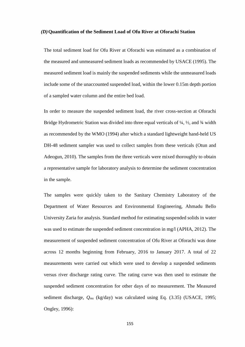
155

(D) Quantification of the Sediment Load of Ofu River at Oforachi Station

The total sediment load for Ofu River at Oforachi was estimated as a combination of

the measured and unmeasured sediment loads as recommended by USACE (1995). The

measured sediment load is mainly the suspended sediments while the unmeasured loads

include some of the unaccounted suspended load, within the lower 0.15m depth portion

of a sampled water column and the entire bed load.

In order to measure the suspended sediment load, the river cross-section at Oforachi

Bridge Hydrometric Station was divided into three equal verticals of ¼, ½, and ¾ width

as recommended by the WMO (1994) after which a standard lightweight hand-held US

DH-48 sediment sampler was used to collect samples from these verticals (Otun and

Adeogun, 2010). The samples from the three verticals were mixed thoroughly to obtain

a representative sample for laboratory analysis to determine the sediment concentration

in the sample.

The samples were quickly taken to the Sanitary Chemistry Laboratory of the

Department of Water Resources and Environmental Engineering, Ahmadu Bello

University Zaria for analysis. Standard method for estimating suspended solids in water

was used to estimate the suspended sediment concentration in mg/l (APHA, 2012). The

measurement of suspended sediment concentration of Ofu River at Oforachi was done

across 12 months beginning from February, 2016 to January 2017. A total of 22

measurements were carried out which were used to develop a suspended sediments

versus river discharge rating curve. The rating curve was then used to estimate the

suspended sediment concentration for other days of no measurement. The Measured

sediment discharge, Qms (kg/day) was calculated using Eq. (3.35) (USACE, 1995;

Ongley, 1996):

156

𝑄𝑚𝑠 = 𝐾𝑐𝑄 (3.35)

Where Qms is Measured sediment discharged (kg/day), c is sediment concentration

(mg/l), Q is River discharge (m3/s) and, K= 86.4. The value of c was obtained as the

concentration of the sampled sediments using a standard lightweight hand-held US DH-

48 sediment sampler, Q was obtained from the stage-discharge relationships for Ofu

River at Oforachi Bridge Hydrometric Station described in previuosly.

The Colby’s method for estimating unmeasured sediment load described in detail

previously by Otun and Adeogun (2010) was used in the study. As a result 22

unmeasured sediment discharges, Qus (tonnes/day) were measured and regressed on the

corresponding River discharge values to develop a relation which was used to estimate

unmeasured sediment load for the 12 months. The total sediment load Qtot was

calculated using Eq. (3.36):

𝑄𝑡𝑜𝑡 = 𝑄𝑚𝑠 + 𝑄𝑢𝑠 (3.36)

Where, Qtot is the total sediment load, Qms is the measured sediment load and Qus is the

unmeasured sediment load.

(E) Assessment of the Soil Characteristics of the flooded areas within the Catchment

The Digital soil map of the World (DSMW) obtained from the FAO’s website was added

to the map document. The spatial analyst extraction tool was used to extract the soil layer

for Ofu River catchment. Four soil layers with distinct characteristics were extracted. A

description of the soil types, the area covered and hydrological soil group (HSG) for curve

number (CN) generation is presented in Table 3.8

157

Table 3.8: Characteristics of Soil within Ofu River Catchment

SMU FAOSoil

Symbol

Area

(km2) Name Textured Class HSG

1021 Af13-1a 975.61 Ferric Acrisols Sandy loam A

1567 Nd5-1a 259.77 Dystric Nitosols Loam B

1193 G2-2/3a 366.61 Gleysols Clay Loam D

677 Jd3-2a 2.59 Calcaric Fluvisols Sandy Clay Loam C

Source: www.fao.org; Researcher’s GIS Analysis (2016)

In addition to the aforementioned, in situ and ex situ soil analysis for determination of

index properties and infiltration rates were conducted on soil samples collected from ten

(10) locations in Oforachi (Fig. 3.8). This was done to confirm the classifications based

on the Digital Soil Map of the world. The classifications were done using the charts and

Tables in Appendix VIII.

Apart from the infiltration test and part of the Antecedent Moisture content measurement

that were carried out in-situ, the samples were transported to the Geotechnical

Engineering Laboratory in The Department of Civil Engineering, Ahmadu Bello

University, Zaria for the determination of soil index properties. The tests carried out were

Moisture contents, Atterberg limits and Sieve analysis. The tests were carried out

according to standard methods for soil analysis and classified according to American

Association of State Highway and Transportation Officials (AASHTO) and Unified Soil

Classification Systems (USCS) soil classification systems (Appendix VIII).

The double ring infiltrometer method was used for the in-situ infiltration measurement.

The infiltrometer consisted of an outer ring of 35 cm diameter and inner ring of 20 cm

diameter. The height of both rings was 27 cm. The sizing of the infiltrometer followed

the design method described previously by Parr and Bertrand (1960). The fabrication of

the rings was made using 1mm mild steel sheets. Both rings were hammered 15 cm into

the soil with a plank to protect the surface of the ring from damage during hammering.

http://www.fao.org/

158

Fig. 3.8: Location of Soil Sample Collection points at Oforachi

159

Plate VIII: Researcher Carrying out Soil Analysis in the Laboratory

Plate IX: Researcher conducting in situ infiltration test at Oforachi

The test began by pouring water into the inner ring to an appropriate depth and at the

same time, adding water to the space between the two rings to the same depth as quickly

as possible. The time when the test began was recorded and the water level on the

calibration was noted. After two (2) minutes, the drop in water level in the inner ring was

160

recorded and water added to bring the level back to approximately the original level at

the start of the test. The water level outside the ring was maintained similar to the one

inside to prevent lateral flow. Each infiltration test lasted four (4) hours with cumulative

time intervals; 2, 5, 10, 20, 30, 45, 60, 90, 120, 150, 180, 210 and 240 minutes. The

cumulative infiltration depth at the elapsed time was recorded.

Estimation of Saturated Hydraulic Conductivity

The analysis of the field data was done based on Philip’s infiltration model expressed in

Eq. (3.37) (Philip, 1957).

𝑖(𝑡) = 𝑆𝑡1/2 + 𝐴𝑡 (2.37)

Where;

i(t) = Cumulative infiltration at cumulative time t (cm)

t = Time (s)

S = Sorptivity (cm/hr1/2)

A = Transmisivity or permeability coefficient

Values of cumulative infiltration, i(t) and time, t were obtained from field measurement

while the sorptivity, S and permeability coefficient, A were determined using the method

of least square between the field measured cumulative infiltration and the calculated

cumulative infiltration.

The saturated hydraulic conductivity, K (ms-1) as a function of the transmisivity or

permeability coefficient, A and a constant m (2/3) was calculated using Eq. (3.38).

161

𝐾 =𝐴

𝑚 (2.38)

The value of saturated hydraulic conductivity, K was used to classify the respective soils

based on the CSN 721020 classification table (Appendix VIII).

3.2.3.4 Assessment of Landuse/Settlement Factors

The two causative factors assessed in this category are the proximity of households to

Ofu River and the Landuse/Landcover changes. The methods of assessment are discussed

as follows:

(A) Assessment of Proximity of Flooded areas to the River channel

It was gathered in the course of the field survey that there were human settlements within

the catchment at elevations similar to those of the flooded areas that have never been

affected by flood implying that the proximity of the settlements to the river is also a factor

to be considered. The coordinates of the 325 surveyed households plotted in ArcGIS were

used for the estimation of their distance (corridor) from Ofu River. This was done using

the Near Proximity Analysis tool in ArcGIS 10.2.2.

(B) Assessment of Landuse/Landcover changes within Ofu River Catchment

The assessment of Landuse/Landcover (LULC) changes within the catchment was carried

out using the Landsat 5 Imagery of 1987, Landsat 7 Imagery of 2001 and Landsat 8

Imagery of 2016 (Table 3.4) in ArcGIS 10.2.2. The imageries were atmospherically

corrected since the spectral reflectance was the vital component for their classification.

The Band composites was created for the respective imageries using the image analysis

extension after which the extraction spatial analyst tool was used to subset the image to

162

the study area. The Normalized Difference Vegetative Index (NDVI) and the Normalized

Difference Built-up Index (NDBI) were respectively calculated for each year to show the

extent of vegetative covers and built-up areas. The NDVI and NDBI were both derived

using the Raster Calculator in Spatial Analyst Map Algebra toolbox in ArcGIS 10.2.2

using Eq. (3.39) and (3.40) respectively.

𝑁𝐷𝑉𝐼 =𝑁𝐼𝑅 − 𝑅

𝑁𝐼𝑅 + 𝑅 (3.39)

𝑁𝐷𝐵𝐼 =𝑆𝑊𝐼𝑅 − 𝑁𝐼𝑅

𝑆𝑊𝐼𝑅 + 𝑁𝐼𝑅 (3.40)

In which R, NIR, SWIR are the Red, Near Infrared and the Short wave Infrared bands

respectively.

The details of the bands used for generation of the indices are shown in Table 3.9. The

NDVI and NDBI for 1987, 2001 and 2016 are shown in Figs. 3.9 and 3.10.

Table 3.9: Band Characteristics for NDVI and NDBI Calculation for Ofu River

Catchment

Year Satellite Sensor Red NIR SWIR

1987 Landsat 5 TM Band 3 Band 4 Band 5

2001 Landsat 7 ETM+ Band 3 Band 4 Band 7

2016 Landsat 8 ETM+ Band 4 Band 5 Band 7

Source: Glovis.usgs.gov

163

Fig. 3.9a: Normalized Difference Vegetation Index of Ofu River Catchment for 1987

164

Fig. 3.9b: Normalized Difference Vegetation Index of Ofu River Catchment for 2001

165

Fig. 3.9c: Normalized Difference Vegetation Index of Ofu River Catchment for 2016

166

Fig. 3.10a: Normalized Difference Built-up Index of Ofu River Catchment for 1987

167

Fig. 3.10b: Normalized Difference Built-up Index of Ofu River Catchment for 2001

168

Fig. 3.10c: Normalized Difference Built-up Index of Ofu River Catchment for 2016

169

The generation of these indices helped in the creation of training signatures for the

Maximum likelihood supervised classification of the imageries. This served as an

accuracy check for the classified Landuse/Landcovers. In addition, an IsoCluster

unsupervised classification was performed in order to have an idea of the maximum

number of distinct classes and a general overview of the area which was followed by the

maximum likelihood supervised classification for the final land cover classes for 1987,

2001 and 2016.

Ground truthing was embarked upon after the classification of the imageries so as to

reaffirm the land use /land cover classes for the 2016 imagery. The area of each land cover

class for the respective years were used to evaluate the changes that have happened within

the period.

Estimation of Curve Number for Ofu River Catchment

The catchment Curve number for 1987, 2001 and 2016 were estimated using the soil and

landuse/Landcover data generated for the respective years. This was done to assess the

extent to which the land cover changes might have affected the surface runoff to the

streams within the catchment.

The Curve Numbers for all the Hydrologic Soil Groups (HSG) A, B, C and D

corresponding to the various landcover classes were obtained from the tables shown in

Appendix IX. The Composite Curve number for the respective hydrologic soil group, CNh

was calculated using Eq. (3.41).

𝐶𝑁ℎ =∑ 𝐴𝑖𝐶𝑁𝑖

𝑛𝑖=1

∑ 𝐴𝑖𝑛𝑖=1

(3.41)

170

In which Ai = Area of land cover class i, CNi = Curve number for landcover i and h =

HSG

The values of CN obtained for the respective HSG were used to compute the composite

CN for the catchment based on the soil classes and their corresponding HSG and CN. The

composite CN for the catchment was computed using Eq. (3.42).

𝐶𝑁 =∑ 𝐴𝑗𝐶𝑁𝑗

𝑛𝑗=1

∑ 𝐴𝑗𝑛𝑗=1

(3.42)

In which Aj = Area of soil class j, CNj = Curve number for HSG/Soil class j

3.2.3.5 Assessment of the respective measures of association of Elevation, Proximity and

Slope with flood occurrence

Statistical analysis was carried out to determine the respective measures of association of

the terrain elevation, household proximity to Ofu River and terrain slope with household

flood experience using the Pearson’s Chi square in Stata/SE version 13.1 statistical

software at 95% confidence level. The Pearson’s chi sqaure and the P-value were used to

determine whether association exist or not.

3.2.4 Method of Flood Frequency Analysis

The estimation of the stream flow for Ofu River was estimated using three methods.

3.2.4.1 Method of estimation of peak runoff

A comparison of three (3) methods for the determination of the peak runoff was made in

this section. The methods compared are the extension of stream flow data (Synthetic)

171

using Modified Thomas-Fiering model, Soil Conservation Services Curve Number (SCS-

CN) method and the Rational method.

(A) Generation of synthetic stream flow data

Synthetic stream flow data used in this study were generated from the 19 year gauged

stream flow data (Appendix III) using the Modified Thomas-Fierring (T-F) Model. The

modification was the incorporation of linear regression to adjust the extended flow data

to fit perfectly with the gauged data. The method of generating synthetic discharge values

using the T-F model described by Patra (2008) was adopted.

Identification and treatment of outliers was first carried out on the the historical stream

flow data for 1955-1973 using boxplot in Minitab 14.12.0 statistical software. The

outliers were treated as missing data to prevent excessive skewness of the data.

The logarithm transferred flows method was used to avoid negative flows in the synthetic

data. The following steps were followed for the generation of the synthetic stream flow

data.

Step 1: The first step was the calculation of the logarithm to base 10 of the gauged stream

flow data (1955 – 1973).

Step 2: The second step was the calculation of the mean and standard deviation for each

month.

Step 3: The third step was the calculation of the correlation coefficient between all the

successive months.

The logarithmic stream flow values, mean, standard deviation and correlation coefficients

are presented in Table 3.10.

172

Step 4: In the fourth step, two sets of normally distributed random numbers with zero

mean and unit standard deviation (Appendix X) were generated. The random numbers

were generated using the analysis tool park in Microsoft Excel 2007. The number of

variables were set as 12 (12 months) in both cases while the number of random numbers

were set as 18 and 43 for the respective sets (18 years for which gauged data exist and 43

years of synthetic data respectively).

Step 5: Synthetic stream flow values (logarithm to base 10) were generated using Eq.

(3.43).

𝑄𝑗+1 = 𝑄𝑎𝑣𝑗+1 + 𝑏𝑗,𝑗+1(𝑄𝑗 − 𝑄𝑎𝑣𝑗) + 𝑍𝑗𝑆𝑗+1√(1 − 𝑟𝑗+12) (3.43)

Where:

j+1 = month for which synthetic discharge is generated;

j = preceding month;

Qj+1 =Discharge during (j+1)th month;

Qj = Discharge during jth month;

Qavj+1 = mean monthly discharge during (j+1)th month;

Qavj = mean monthly discharge during jth month;

Sj+1 = Standard deviation for (j+1)th month;

Sj = Standard deviation for jth month;

rj,j+1 = The correlation coefficient between the months j and (j+1);

Zj = The random independent variable with zero mean and unit variance

while,

173

𝑏𝑗,𝑗+1 = 𝑟𝑗,𝑗+1 (𝑆𝑗+1

𝑆𝑗) (3.44)

Step 6: The synthetic discharge values for 1956-1973 were obtained by taking the

antilogarithm of extended logarithmic values. The values for 1956 – 1970 (15 years) were

used for calibration of the model since gauged data exist for these years. The remaining

three years (1971 – 1973) were used for model validation.

Linear regression analysis was carried out in Microsoft excel 2007 with the gauged data

(1956 -1970) as ‘y’ and the generated data (1956 -1970) as ‘x’ to obtain linear

relationships with slopes and intercepts for the respective months.

Thus 12 linear relationships developed for the 12 months were used to adjust the synthetic

discharge values generated for 1971-1973 (Table 3.11) for which gauged data already

exist as form of validation.

Step 6: Regression analysis and (student’s) paired t test (95% confidence interval) were

carried out on the gauged data and the adjusted synthetic data (1971 – 1973) using the

Analysis Tool Pack of Microsoft Office 2007 to assess the goodness of fit of both data

(Table 3.12).

The correlation coefficient (r) of 0.9515, coefficient of determination (R2) of 0.9026 and

P-value (P = 0.1801) obtained show that the adjusted synthetic discharge values fit well

with the gauged values thus validating the model which implies that the developed

equations could be used to adequately adjust the synthetic data generated for 1974 - 2016.

174

Table 3.10: Logarithm of Stream flow, Monthly Mean, Standard Deviation and Correlation coefficient for T-F Model

Year Logarithm of Discharge (m3/s)

Jan Feb Mar Apr May Jun Jul Aug Sep Oct Nov Dec

1955 0.591 0.462 0.322 1.057 0.903 1.270 1.898 2.602 2.359 2.186 0.398 0.122

1956 0.146 -0.046 -0.222 0.851 0.362 1.228 2.270 2.770 2.746 1.811 0.580 -0.222

1957 0.462 0.279 0.114 1.188 0.950 1.453 1.980 2.545 2.639 2.204 0.813 -0.097

1958 0.623 0.447 0.255 1.305 1.193 1.644 2.211 2.580 2.762 1.922 0.653 0.079

1959 0.041 -0.222 -0.222 0.839 1.021 1.272 1.898 2.558 2.559 1.678 0.505 -0.301

1960 0.322 0.176 0.000 0.903 1.068 1.318 2.031 2.513 2.517 1.721 0.568 0.122

1961 0.279 0.114 -0.097 1.340 0.568 1.782 2.352 2.707 2.744 1.932 0.699 -0.222

1962 0.498 0.362 -0.301 1.170 0.613 1.207 1.889 2.762 2.671 2.038 0.699 0.000

1963 0.498 0.400 0.258 1.281 0.950 1.204 1.881 2.464 2.509 2.053 0.857 0.122

1964 0.643 0.531 0.462 0.964 1.093 1.713 2.055 2.789 2.859 1.954 0.716 0.122

1965 0.531 0.342 0.204 1.072 0.690 1.937 2.176 2.687 2.608 1.674 0.690 0.176

1966 0.556 0.462 0.342 1.107 0.950 1.960 1.926 2.475 2.293 1.849 0.301 0.362

1967 -0.301 0.176 0.079 1.265 0.996 1.637 2.195 2.668 2.713 1.956 0.944 0.079

1968 0.724 0.613 0.544 0.602 0.950 1.583 2.094 2.309 2.524 1.619 0.279 0.122

1969 0.114 0.041 0.041 1.365 1.083 1.450 2.125 2.660 2.623 2.210 0.716 0.000

1970 0.519 0.643 0.230 1.049 0.959 1.436 1.833 2.677 2.697 1.714 0.724 0.230

1971 0.623 0.556 0.491 1.124 0.964 1.704 2.189 2.649 2.683 1.732 0.875 0.122

1972 0.724 0.613 0.544 1.033 1.127 1.684 2.119 2.382 2.503 1.601 0.820 0.122

1973 0.672 0.568 0.491 1.124 0.839 1.354 2.197 2.297 2.678 1.775 0.763 0.491

Mean 0.435 0.343 0.186 1.086 0.910 1.518 2.069 2.584 2.615 1.875 0.663 0.075

SD 0.271 0.245 0.268 0.195 0.212 0.243 0.152 0.148 0.141 0.197 0.186 0.192

R 0.534 0.817 0.827 -0.133 0.062 0.152 0.404 0.100 0.534 0.030 0.173 -0.021

175

Table 3.11: Stream flow Estimation for Model Calibration and Validation

Year Discharge (m3/s)

Jan Feb Mar Apr May Jun Jul Aug Sep Oct Nov Dec

1971 2.15 1.89 1.15 6.72 4.47 68.25 153.91 511.89 532.32 66.13 2.51 1.14

1972 1.55 2.18 1.82 22.20 11.01 67.33 67.79 330.13 472.22 98.39 3.85 1.66

1973 2.14 3.98 2.66 51.49 2.73 67.92 146.78 300.67 508.97 54.91 3.87 1.06

Table 3.12: Model Validation Parameters

Parameter Value

Correlation Coefficient, r 0.9515

Coeficient of Determination (Adjusted R2) 0.9026

P-value 0.1801

176

Step 7: The synthetic discharge values for 1974-2016 were obtained by taking the

antilogarithm of extended logarithmic values for the 1974-2016. The 12 linear equations

developed in the preceding steps were then used to adjust the synthetic discharge values

for 1974-2016 for the respective months. The mean and standard deviation are principally

the determinants of unbiased statistics but since stream flow is a serially dependent

phenomenon, the correlation between successive months needs to also be preserved for

the generated data to be reliable (Patra, 2008).

The mean, standard deviation and correlation coefficient for the gauged data of 1955-

1973 and the synthetic data of 1955-2016 (first, second and third runs) were calculated

using the aforementioned statistical software. The reliability assessment was then carried

out by comparing these estimates for both datasets using linear regression and One Way

Analysis of Variance (ANOVA). The coefficient of determination (R2), P-value,

calculated F and Critical F values at 5% level of significance were used to infer whether

there is statistically significant difference or not. P<0.05 was taken to be statistically

significant.

In order to estimate the reliability index, the average of the three coefficients of

determination (R2) was recorded as the score for R2, P-value greater than 0.05 was given

a score of 1 while, calculated F less than Critical F was given a score of 1. The reliability

index was calculated as the ratio of the total score obtained to the total obtainable score.

177

(B) Runoff Estimation by SCS Curve Number Method

i. Interpolation and extraction of Daily Rainfall layer for Ofu River Catchment

The annual maximum daily rainfall from the 41 stations surrounding the study area

obtained from radar source were plotted in ArcGIS 10.2.2 environment and interpolated

using the Ordinary Kriging method as discussed earlier. The annual maximum daily

rainfall raster surfaces for Ofu River Catchment were respectively extracted and the

average values for the catchment were obtained using simple arithmetic mean computed

using the raster statistical tool in ArcGIS 10.2.2.

ii. Correction of Radar Rainfall Data with Ground Truth Data

A correction factor was applied to the annual maximum daily rainfall for the study area

interpolated from the rainfall of 41 surrounding stations obtained from radar source.

This was necessary because satellite derived rainfall data might not capture localised

rainstorms and the seasonality of the rainfall as accurate as the ground measured data

such as the NiMeT rainfall stations would. The correction factor was derived by dividing

the 34 years (1980 – 2013) average annual total rainfall of Markurdi by 34 years (1980

– 2013) average annual total rainfall of the study area obtained from radar source. The

ground data of Markurdi was used because it falls within the same rainfall Zone (IVa)

with the study area. This method was recommended by FMW (2013).

iii. Estimation of Runoff Depth and Peak Runoff for Ofu River Catchment

The SCS Curve number method was used to estimate the daily runoff from the catchment.

The method of estimation of the Curve number for the catchment has been discussed

previously.

178

The method described in the TR-55 (1986) was adopted for the estimation of runoff depth

using the rainfall values. The runoff depth, Q (mm) was calculated using Eq. (3.45) while

Initial abstraction, Ia was calculated using Eq. (3.46) assuming AMC II condition for the

watershed.

𝑄 = (𝑃 − 𝐼𝑎)2

{(𝑃 − 𝐼𝑎) + 𝑆)}(𝑃 ≥ 𝐼𝑎𝑒𝑙𝑠𝑒𝑄 = 0) (3.45)

𝐼𝑎 = 0.2𝑆 (3.46)

In which P is rainfall depth (mm).

The Storage, S on the other hand was calculated using Eq. (3.47)

𝑆 = 25400

𝐶𝑁− 254 (3.47)

The daily peak runoff Qp was estimated using the methods described by de Brouwer

(1997). It was estimated using Eq. (3.48).

𝑄𝑝 = 2.8𝑄 × 𝐴

𝑡𝑝 (3.48)

Where: Qp = Peak runoff rate (m3/s)

Q = Storm runoff or excess rainfall volume (cm)

A = Watershed area (km2)

tp = Time to peak (hr)

= 𝐷

2+ 𝑡𝑙𝑎𝑔 (3.49)

D = Duration of excess rainfall (hr) = 0.133𝑡𝑐

tc = Time of concentration (hr)

179

tlag = The lag time of the watershed (hr) = 0.6𝑡𝑐

TR-55 (1986) stated clearly that the SCS-CN method was designed for small watershed

area. Since Ofu Catchment area falls within the medium size catchment, the area

reduction factor developed by FMW (2013) was used to correct the area. This was done

to avoid over-estimation.

The area reduction factor, fA was estimated using Eq. (3.50a) while the corrected area,

Acorrected was estimated using Eq. (3.50b).

𝑓𝐴 = 1 𝑒(1−12

𝐴)⁄ (3.50𝑎)

𝐴𝑐𝑜𝑟𝑟𝑒𝑐𝑡𝑒𝑑 = 𝐴 − (𝑓𝐴 × 𝐴) (3.50𝑏)

This corrected area was used in place of the original catchment area.

(C) Rational Method

The rational method described in the Drainage Design of the Highway Manual (FMW,

2013) was adopted in this study. The runoff is related to the rainfall intensity by Eq.

(3.51).

𝑄 = 0.278𝐶𝐼𝐴 (3.51)

In which, C is the composite runoff coefficient of the catchment, I is the rainfall intensity

expressed in millimetres per hour for a certain time of concentration and A is the

catchment area in square kilometres.

The steps followed are outlined as follows:

180

Step 1: The runoff coefficient was calculated based on the recommended guide in

Appendix XI (Table XIa and XIb) using Eq. (3.52).

𝐶 = 𝐶𝑠 + 𝐶𝑝 + 𝐶𝑣 (3.52)

Where:

C = Composite runoff coefficient for the catchment

Cs = Runoff coefficient based on surface slope

Cp = Runoff coefficient based on permeability (soil characteristics)

Cv = Runoff coefficient based on vegetation.

The method described earlier for computation of composite curve number was used to

estimate the respective components of the runoff coefficient using the area weighted

method.

Step 2: The rainfall intensity was estimated following the regional method developed by

Oyebande (1982). The study area falls within the Nigeria Rainfall zone IVa (Appendix

XI-Fig. XI). The rainfall intensity was calculated using Eq. (3.53).

𝐼 = 𝛽 + (1

𝛼) [ln(𝑇𝑟) −

1

(2𝑇𝑟)−

1

(24𝑇𝑟2)

−1

(8𝑇𝑟3)

] (3.53)

In which α and β are scale and location parameters, I is the rainfall intensity (mm/hr) and

Tr is the return period or frequency of occurrence (years).

The time of concentration-dependent parameters, β and α were derived using Table XId

(Appendix XI) for Rainfall zone VIa. The time of concentration has been estimated earlier

as part of the areal characteristics of Ofu River Catchment.

181

Step 3: The area of the catchment had been previously obtained as one of the areal

characteristics of Ofu River catchment. Since the area of the catchment is greater than 12

km2, area correction was carried out to avoid over estimation. The area correction was

done using Eqs. (3.50a and b)

Step 4: The last step was the calculation of the Discharge, Q using Eq. (3.51).

3.2.4.2 Flood frequency analysis using Log-Pearson Type III Distribution

The flood frequency analysis of synthetic stream flow records for Ofu River at Oforachi

Gauge station was carried out using the Log-Pearson Type III distribution (Dalrymple,

1960; Salimi et al., 2008; Daffi, 2013; England Jr., 2017).

The Log Pearson Type III distribution was used to obtain stream flow for 2, 5, 10, 25, 50,

100 and 200-year return periods respectively using the 62 years synthetic discharge data.

The method outlined in Patra (2008) and Mustapha and Yusuf (2012) were adopted as

follows.

The maximum discharge values for each year from 1955 to 2016 were arranged by year

after which they were sorted and ranked in decreasing order from 1 to 62 with 1 being the

highest ranked. The logarithm to base 10 of each ranked discharge was obtained and

recorded in the respective columns.

The general equation for the Log-Pearson Type III distribution is given by Eq. (3.54):

𝐿𝑜𝑔 𝑄 = 𝐿𝑜𝑔 𝑄̅̅ ̅̅ ̅̅ ̅̅ + 𝐾𝜎𝐿𝑜𝑔 𝑄 (3.54)

182

Where:

Q = Maximum discharge (m3/s)

𝐿𝑜𝑔 𝑄̅̅ ̅̅ ̅̅ ̅̅ = the average of the Logarithm of the maximum discharge values Q

K = frequency factor which is a function of the return period and the

Skewness Coefficient and obtained from the frequency factor table

σLog Q = standard deviation of the Logarithm of the maximum discharge, Q

The mean, variance, standard deviation and skewness coefficient of the data were

calculated using Eqs. (3.55), (3.56), (3.57) and (3.58) respectively:

𝐿𝑜𝑔 𝑄̅̅ ̅̅ ̅̅ ̅̅ =∑ 𝐿𝑜𝑔 𝑄

𝑁 (3.55)

𝑉𝑎𝑟𝑖𝑎𝑛𝑐𝑒 = ∑(log 𝑄 − 𝐿𝑜𝑔𝑄̅̅ ̅̅ ̅̅ ̅)2

𝑁 − 1 (3.56)

𝜎𝐿𝑜𝑔𝑄 = √Variance (3.57)

𝐶𝑠 = 𝑁 ∑(𝐿𝑜𝑔𝑄 − 𝐿𝑜𝑔𝑄̅̅ ̅̅ ̅̅ ̅)3

(𝑁 − 1)(𝑁 − 2)(𝜎𝐿𝑜𝑔𝑃)3 (3.58)

The maximum discharge for the respective return periods were obtained by taking the

antilog of the value obtained from Eq. (3.54).

3.2.5 Production of Flood Inundation Extent and Hazard Map

The production of flood hazard map for Ofu River catchment was carried out using the

Method of Thematic Integration of Causative Factors (Multi-Criteria Evaluation) in

ArcGIS and One-dimensional steady flow hydraulic modelling in HEC-RAS (using the

hydrologically generated stream flow as input) combined with HEC-GeoRAS extension

in ArcGIS. This was to enable a comparison between both methods.

183

3.2.5.1 Production of flood hazard map by thematic integration of causative factors

(Multi-Criteria Evaluation) in ArcGIS

The production of flood hazard map involved the generation of the thematic layers of four

causative factors (Elevation, Corridor, slope and soil), derivation of their criterion weight,

reclassification based on the derived weights and their final integration. The methods

followed are described in the succeeding sections.

(A) Generation of Thematic Layers of Flood Causative Factors

i. Generation of Elevation layer

The Elevation layer was generated using the SRTM DEM of the catchment. The elevation

information obtained from the field was compared with the maximum stage obtained for

Ofu River which served as a guide for the classification of the SRTM DEM. The DEM

was classified into five domain groups based on their respective elevations above sea

level (a.s.l.) in ArcGIS 10.2.2 as follows:

0 m a.s.l. – 70 m a.s.l. - Very High Risk (VHR)

70 m a.s.l. – 100 m a.s.l. - High Risk (HR)

100 m a.s.l. – 200 m a.s.l. - Moderate Risk (MR)

200 m a.s.l. - 350 m a.s.l. - Low Risk (LR)

> 350 m a.s.l. - No Risk (NR)

ii. Generation of Slope layer

The catchment slope was obtained in percentage from the sub-mapped SRTM DEM of

Ofu River Catchment subjected to spatial analysis by clicking on Spatial Analyst

Tools>Surface>Slope with ofu_dem as the input raster while the output raster was named

ofu_slope. The slope was then filtered using the filter operation in spatial analyst

184

Neighbourhood tools in ArcGIS 10.2.2 and classified into five domain groups based on

Daffi (2013) classification as follows:

0 % - 2 % - Flat (VHR)

2 % - 8 % - Undulating (HR)

8 % - 16 % - Rolling (MR)

16 % - 30 % - Hilly (LR)

> 30 % - Mountainous (NR)

iii. Generation of Soil layer

The soil layer for Ofu River catchment was extracted from the Digital soil map of the

World (DSMW) obtained from the FAO’s website using the spatial analyst extraction

tool in ArcGIS 10.2.2 and was added to the map document. Four soil layers with distinct

characteristics were extracted.

iv. Generation of Corridor layer

The DEM of Ofu River Catchment was first converted to point feature class by clicking

on Conversion Tools>From Raster>Raster To Points on the Arc Toolbox with ofu_dem

as the input raster while the output point feature class was named ofu_dem_point. On

clicking Ok, the study area DEM was converted to point feature class. Secondly, the

distance of all the points from the main stream (Ofu River) was calculated by clicking on

Analysis Tools>Proximity>Near on the Arc Toolbox with the point DEM as input and

River181 (Ofu River) as the Near feature accepting the default planar method. On clicking

185

Ok, the distance was calculated in meters and the attribute table of the point DEM was

populated accordingly. The corridor layer was classified into five domain groups based

on field observations as follows.

0 m – 500 m - Too close (VHR)

500 m – 1,500 m - Very close (HR)

1,500 m – 6,000 m - Close (MR)

6,000 m – 20,000 m - A bit close (LR)

> 20,000 m - Not close (NR)

(B) Derivation of Criterion Weights using the Analytical Hierarchical Process (AHP)

Multi-criteria evaluation (MCE) was carried out to establish a relationship between all

the thematic maps of flood causative factors. The relationships between these layers as

well as their respective attributes were derived using the Analytical Hierarchical Process

(AHP) developed by Saaty (1980).

As stated earlier, four (4) thematic maps were produced for four (4) causative factors

(Elevation, slope, soil and corridor). These thematic maps as well as their respective

classifications formed the network for the pair-wise comparison in the AHP. The next

step was the generation of the Pair-wise Comparison Matrices of the relative important

values. This was determined based on Saaty’s 1-9 scale shown in Appendix XII (Table

XIIa). The respective associations of elevation, proximity (corridor) and slope with flood

occurrence were used as a guide for the derivation of relative importance matrix.

186

The method of Eigenvector estimation was used to estimate respective weights of the

various criteria. The pair-wise comparison was checked using the Saaty’s Consistency

Ratio, CR. CR was calculated using Eq. (3.59a).

𝐶𝑅 =𝐶𝐼

𝑅𝐼 (3.59𝑎)

Where:

CI = Consistency Index which reflects the consistency of the judgment

RI = Random Inconsistency Index dependent on the sample size

The consistency Index, CI was calculated using Eq. (3.59b).

𝐶𝐼 =𝜆𝑚𝑎𝑥 − 𝑛

𝑛 − 1 (3.59𝑏)

Where, λ is the average of the value of the consistency vector (calculated factor

weight).

The Random Inconsistency Indices, RI for respective sample sizes are presented in

Appendix XII (Table XIIb).

The judgment would be accepted for 0 ≤ 𝐶𝑅 ≤ 0.1 with a value of zero (0) being the

most consistent. Any value outside this range would require re-visiting the assignment of

the criterion weight.

(C) Reclassification of Thematic Layers

The four (4) thematic layers produced (Elevation, Corridor, Slope and Soil) were

subsequently reclassified into appropriate classes based on the criteria weights derived

187

which in turn were based on the datasets perceived contribution to flood occurrence. This

perception was based on field experience and the assessment of their respective measures

of association with flood occurence.

(D) Integration of Thematic Layers and production of Hazard Map

All the weighted data sets were integrated in ArcGIS 10.2.2 to produce the flood Hazard

map by weighted overlay where each class individual’s weight was multiplied by the map

scores and the results added.

The flood hazard map produced via the previous operation was then reclassified into five

Hazard classes: ‘Very High Hazard,’ ‘High Hazard,’ ‘Moderate Hazard,’ ‘Low Hazard’

and ‘No Hazard. The Very High Hazard zone represents the extent of inundation of flood

water.

3.2.5.2 Hydraulic modelling for development of flood inundation and hazard maps

The hydraulic modelling for the development of Ofu River flood inundation and Hazard

maps was carried out using HEC-GeoRAS extension in ArcGIS 10.2.2 and HEC-RAS.

(A) Data Preparation

The digital elevation model of Ofu River Catchment was converted from raster format to

a Triangulated Irregular Network (TIN) surface using the 3D Analyst Conversion Tools

in the ArcToolbox of ArcGIS 10.2.2.

(B) Pre-processing of data in HEC-GeoRAS

The pre-processing was done using the HEC-GeoRAS extension in ArcGIS 10.2.2

following the methods described in Ackerman (2011), Daffi (2013) and Merwade (2016).

188

The process began with the addition of created TIN surface to the new map document as

the terrain data. The RAS Geometry>Create RAS Layers tool in HEC-GeoRAS was used

to create the required layers. The layers created are:

i. Stream Centreline

ii. Bank Lines

iii. Flow Path Centrelines

iv. XS Cut Lines

v. Bridges/Culverts

vi. Ineffective Flow Areas

A geo-database was created by HEC-GeoRAS in the working directory with the name of

the map document where all the created layers were stored.

The respective RAS layers were populated as follows:

i. Creating Stream Centreline: A single feature was digitized for the entire reach

of Ofu River by approximately following the centre of the river, aligning in the direction

of flow. The stream centreline was created using the Editor Tools. The Start Editing tool

was selected with Create New Feature as Task and River as the Target.

The assigning of the River and Reach name followed the creation of the River centreline

feature. This was done using the Assign RiverCode and ReachCode to River button.

Ofu River was supplied as the River name and Main Reach as the Reach name.

The remaining attributes (Topology, Lengths/Stations and Elevation) were populated by

clicking RAS Geometry>Stream Centerline Attributes>All. These were done to connect

the reach using the FromNode, ToNode, give the actual length of the reach in map units

(ArcLength) and from station to station details (FromSta, ToSta) as well as create the

River3D feature with the elevation values.

189

ii. Creating River Banks: The banks centre lines were created following the same

digitization process with the Banks layer as the task. The bank lines were digitized from

the upstream end to the downstream end beginning with the left bank looking

downstream.

iii. Creating Flow Path Centrelines: The flow path centre lines were created using

RAS Geometry>Create RAS Layers>Flow Path Centerlines. The stream centerline was

used to create the flowpath centreline and the left and right flow paths were digitized

using the sketch tools in the Editor toolbar. This was done by selecting Create New

Feature as the Task and Flowpaths as the Target feature. The left and right flowpaths

were digitized within the floodplain in the downstream direction by first digitizing the

left flowpath followed by the right flowpath for the entire reach looking in the

downstream direction.

The Assign LineType button on the HEC-GeoRAS toolbar was used to label the flow

paths as left, channel and right, respectively looking in the downstream direction

iv. XS Cut Lines: The cross-section cutlines were created by selecting the Create

New Feature in the Editor Toolbar as the Task, and XSCutlines as the Target. They were

digitized using the sketch tools, making sure that the cross-sections were wide enough to

cover the floodplain. The following guidelines were followed in creating cross-section

cutlines:

(a) They were digitized perpendicular to the direction of flow;

(b) They spanned over the entire flood extent to be modelled and

(c) They were digitized from left to right, looking in the downstream direction.

One cross-section was defined each on the upstream and downstream of the bridges across

Ofu River at Akpagidigbo and Oforachi, respectively.

190

After digitizing the cross-sections, the next step was to add HEC-RAS attributes to the

cutlines. The attributes added were the River/Reach Names, Stationing, Bank Stations,

Downstream Reach Lengths and Elevations. This was done by selecting RAS Geometry>

XS Cut Line Attributes>All and all these attributes were added automatically to the XS

cutline feature while a 3D XS cutline feature was created which contain the Z values.

v. Bridges/Culverts: Two Bridges were identified across the Ofu River at

Akpagidigbo and Oforachi. They were defined in the Bridges feature class by selecting

Create New Feature as the Task, and Bridges as the Target. The sketch tool on the editor

toolbar was used to digitize the bridge locations. River/Reach name, stationing and

elevations were assigned to the bridge feature by clicking RAS

Geometry>Bridge/Culverts>All. These attributes were added automatically and a 3D

Bridge feature was added which contain the Z values.

vi. Ineffective Flow Areas: Ineffective flow areas are used to identify non-

conveyance areas of the floodplain, that is, areas with water but no flow/zero velocity

such as areas behind bridge abutments. One ineffective area was defined at the Oforachi

Bridge by selecting Create New Feature as the Task, and IneffAreas as the Target in the

Editor Toolbar. It was then defined using the sketch tool.

The position and elevation at points where these ineffective areas intersect with cross-

sections were extracted using RAS Geometry>Ineffective Flow Areas>Position. The

attributes of the IneffectivePositions table was then opened to view the information stored.

IA2DID is the HydroID of the ineffective flow area, XS2DID is the HydroID of the

intersecting cross-section, BeginFrac and EndFrac are the relative positions of the first

and last intersecting points (looking downstream) of the ineffective area with the cross-

191

section. BegElev and EndElev are the elevations of the first and last intersecting points of

the ineffective area with the cross-section.

Fig. 3.11: Screenshot of the RAS Layers created

After all the aforementioned layers were created, the RAS Geometry>Layer Setup was

clicked and the layers in each tab were verified to check if all the layers created are the

ones to be exported. After this RAS Geometry>Export GIS Data was used to export the

RAS layers.

(C) One-Dimensional Hydraulic Modelling in HEC-RAS

The one-dimensional steady state hydraulic modelling was carried out using HEC-RAS

and HEC-GeoRAS extension in ArcGIS 10.2.2. HEC-GeoRAS is a GIS-based 2-

dimensional hydrodynamic model.

The HEC-RAS software was opened and a new project was created and saved with a new

name in the working folder. The Geometric data created in ArcGIS was imported by first

opening the Geometric Data editor from the edit menu after which the File>Import

Geometry Data>GIS Format was selected. Thus, the geometric section from HEC-

GeoRAS section was imported (Fig. 3.12) while the ArcMap document was left open.

192

The imported geometric data was saved and some quality checks carried out. Manning’s

n-values were assigned based on field observation by selecting Manning’s n or k value

from the Table tools. The Manning’s n values were assigned shown in Fig. 3.13.

193

Fig. 3.12: View of the Geometric data imported from ArcGIS to HEC-RAS

194

Fig. 3.13: Assigning of Manning’s n Values in HEC-RAS

The cross-section tool in Geometric data Editor window was then used to view the river

cross-section after which the Graphical Cross-section Editor selected from the Geometric

Editor tools was used to edit the cross-sections, The editor was used to adjust the Bank

Stations. One of the edited cross sections is shown in Fig. 3.14.

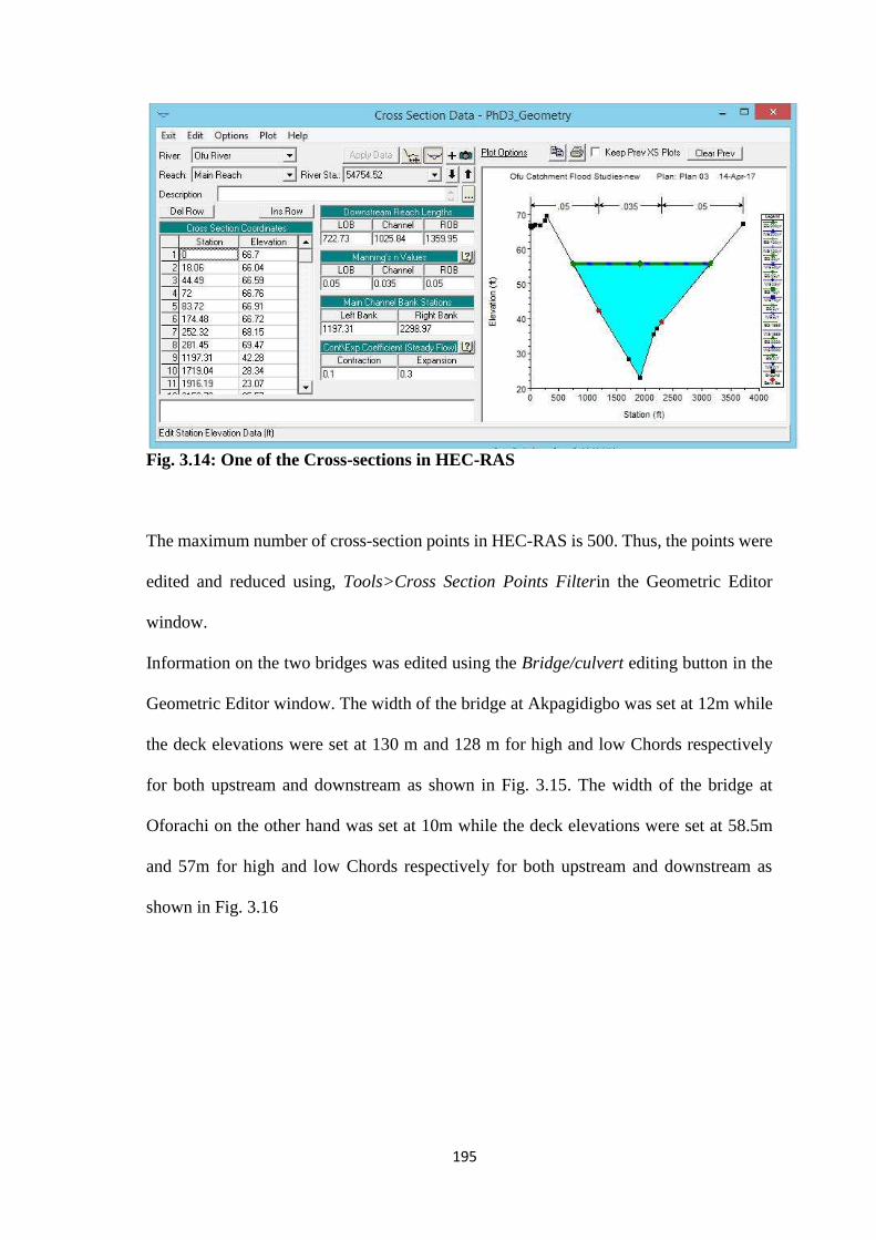
195

Fig. 3.14: One of the Cross-sections in HEC-RAS

The maximum number of cross-section points in HEC-RAS is 500. Thus, the points were

edited and reduced using, Tools>Cross Section Points Filterin the Geometric Editor

window.

Information on the two bridges was edited using the Bridge/culvert editing button in the

Geometric Editor window. The width of the bridge at Akpagidigbo was set at 12m while

the deck elevations were set at 130 m and 128 m for high and low Chords respectively

for both upstream and downstream as shown in Fig. 3.15. The width of the bridge at

Oforachi on the other hand was set at 10m while the deck elevations were set at 58.5m

and 57m for high and low Chords respectively for both upstream and downstream as

shown in Fig. 3.16

196

Fig. 3.15: Akpagidigbo Bridge data showing deck/roadway editor and bridge design

editor

Fig. 3.16: Oforachi Bridge data showing deck/roadway editor and bridge design

editor

40 cm diameter pile foundations on three rows (12 per row) were used for both bridges.

The pier information was thus edited based on the physical observation of the bridges.

While the Akpagidigbo piles were spaced 10 m apart across the bridge length, those of

Ofu were space 18 m apart. This information was obtained via a phone interview with

one of the Engineers with Setraco Nig Ltd who constructed the Oforachi Bridge and

confirmed during the field work. This data were entered in the Bridge Design editor as

197

shown above for the two bridges (Figs. 3.15 and 3.16). The geometric data was saved and

Geometric Editor window exited.

Steady flow information was entered by selecting Edit>Steady Flow Data from the HEC-

RAS main menu. Nine (9) profiles were created and the estimated flow discharge for Ofu

River entered for year 1995, year 2000, 2-yr, 5-yr, 10-yr, 25-yr, 50-yr, 100-yr and 200-yr

return periods. Normal Depth was selected and slope of 0.0001 specified as shown in Fig.

3.17.

Fig. 3.17: Steady Flow Data and Boundary Conditions Input in HEC-RAS

The flow data was saved and the Steady Flow Data editor exited.

The next step was to run the steady flow analysis. This was done by selecting Run>Steady

Flow Analysis in the HEC-RAS main window. The HEC-RAS results were then exported

to ArcGIS on successful simulation. This was done by selecting File>Export GIS Data

in the HEC-RAS main window. The results for Water surfaces, water surface extent and

velocity for the nine profiles were specified for export as shown in Fig. 3.18.

198

Fig. 3.18: Exporting HEC-RAS Results to ArcGIS

(D) Flood Inundation Mapping

i. Flood Depths, Inundation Area and Velocity Simulation in HEC-

GeoRAS/ArcGIS

The Import RAS SDF file button ( ) on the HEC-GeoRAS toolbar was selected to

convert the RAS output file exported earlier to GIS from the SDF file to XML file. A new

analysis layer for HEC-RAS post-processing was set up by selecting RAS

Mapping>Layer Setup and the required fields were filled. On pressing Ok, the terrain

TIN was converted to digital terrain model (DTM). The RAS Mapping>Import RAS Data

was selected afterwards and the bounding polygon which defines the analysis extent for

inundation mapping, by connecting the endpoints of XS Cut Lines, was created and added

199

to the map layer alongside bank points, velocities, water surface extent, River 2D and XS

Cut lines.

The inundation extent mapping was done in two (2) steps. Firstly, RAS

Mapping>Inundation Mapping>Water Surface Generation was selected on the HEC-

GeoRAS toolbar which created a water surface TIN. The second step involved the

conversion of the water surface TIN to a GRID and subtracting the DTM grid from the

water surface grid. This was done by selecting RAS Mapping>Inundation

Mapping>Floodplain Delineation on the HEC-GeoRAS toolbar. The area with positive

results implied that the water surface is higher than the terrain. These areas are the flood

areas which form the flood inundation polygon. HEC-GeoRAS interpolates and expresses

model results in two-dimensions on the landscape. Velocity modelling was also carried

out by selecting RAS Mapping>Velocity Mapping on the HEC-GeoRAS toolbar.

3.2.5.3 Comparison of Extent of Flood Inundation from both Methods

The extents of inundation obtained from the GIS integration of thematic layers and the

HEC-RAS hydraulic modelling were compared. The pattern and area extent of inundation

were the area of comparison.

3.2.6 Methods of Flood Risk Analysis

3.2.6.1 Method of Flood hazard assessment

Flood hazard analyses were carried out for floods of 1995 and 2000 flood scenarios as

well as the 100-year and 200-year flood events. The flood hazard classification was done

based on the depth of inundation water only. The velocity was not considered as the

average velocity was far less than 1 m/s which is the lowest hazard velocity limit for flood

inundation water. Besides, the major flood challenge within Ofu River floodplains has

200

been that of inundation which probably could be the reason why no loss of live has ever

been recorded. Thus the inundation raster maps for the respective events were reclassified

into ‘High,’ ‘Moderate’ and ‘Low’ based on Daffi (2013) as shown in Table 3.13.

Table 3.13: Flood Hazard Classification Based on Flood Depths

Flood Depth (m) Hazard Classification Indicators

0 – 1 Low Hazard Minor increase to existing flood levels.

1 – 2 Moderate Hazard Significant increase in flood levels with

respect to crops, roads and buildings.

> 2 High Hazard Major increase to existing flood levels

with respect to crops, roads and buildings.

Source: Daffi (2013)

This implies that the threshold for high hazard was set at 2m depth of flood inundation

water.

3.2.6.2 Method of Flood vulnerability assessment

The procedure for determining social vulnerability developed by Cutter et al. (1997) for

the South Carolina Emergency Preparedness Division was adopted in this study. The

method was developed for vulnerability assessment at County level which is equivalent

to the LGA system in Nigeria. This makes it suitable for the present study.

(A) Estimation of population within inundated area

i. Estimation of Population Growth Rates Population Figures and Densities

Population figures for 1991 and 2006 census (NPC, 2010a; NPC, 2010b; NBS 2012) were

obtained from the official websites of the National Populations Commissions and the

National Bureau of Statistics. The population growth rates for the respective local

201

governments were estimated using the geometric growth rate equation expressed by Eq.

(3.60).

𝑃𝐸 = 𝑃𝑜𝑒𝑟𝑛 (3.60)

Where:

PE = Expected population

Po = Population of previous year

e = Exponential

r = Growth rate

n = Number of years interval

The population figures of 1991 for each Local Government Area were used as Po while

those of 2006 were used as PE. The difference in years between 2006 and 1991 was used

as n for the estimation of the respective growth rates by LGAs. Igalamela/Odolu and Ibaji

LGAs were not created as at the 1991 census thus their population figures were part of

their mother LGA-Idah for 1991. The sum of the population figures for Idah,

Igalamela/Odolu and Ibaji LGAs was used as PE for Idah in 2006 for the estimation of

the population growth rate for Idah LGA. This growth was eventually used for the three

LGAs. The population growth rates estimated are presented in Table 3.14.

The population figures of the respective LGAs for 1995 and 2000 were estimated based

on 1991 census figures while those for 2055 (100-year flood) and 2155 (200-Year flood)

were estimated based on 2006 census figures. The growth rates estimated previously

(Table 2.14) were used for the population projection in both cases.

202

Table 3.14: Estimated Population Growth Rates

LGA 1991 2006 Growth Rate

Dekina 177513 260968 260968 0.026

Ofu 108095 191480 191480 0.038

Igalamela/Odolu 147048

Idah 224692 79755 354375 0.030

Ibaji 127572

Uzo-Uwani 88112 127150 127150 0.024

NBS (2012)

The land area covered by the respective LGAs was obtained from KGS (2012). The

population density of the respective LGAs for each year was estimated using Eq. (3.61).

𝑃𝑑 =𝑃2

𝐴 (3.61)

Where:

Pd = Population density (persons/km2)

P2 = Estimated Population for the year

A = Land Area for the LGA (km2).

ii. Estimation of Affected Population

The polygon of the inundation extent for 1995, 2000, 100-year and 200-year floods were

divided using the LGA boundaries so that the area of inundation for each LGA could be

extracted. Thus, the population affected for each LGA was estimated using Eq. (3.62).

𝑃𝐴 = 𝑃𝑑 × 𝐴𝑖 (3.62)

Where:

PA = Affected Population in the LGA

Pd = Population Density for the LGA

Ai = Inundated Area for the LGA

203

(B) Social Distribution of Affected Population

i. Age and Disability Status

The percentage of the total population for each LGA living with any form of disability

was estimated as shown in Table 3.15.

Table 3.15: Estimation of Percentage of Population with Disability

State LGA 2006 Disabled

Population %

Kogi

Dekina 260968 3825 1.47

Ofu 191480 2410 1.26

Igalamela/Odolu 147048 2197 1.49

Idah 79755 1323 1.66

Ibaji 127572 1794 1.41

Enugu Uzo-Uwani 127150 2470 1.94

NPC (2010b) <

In addition, the population for each LGA obtained from NPC (2010a) distributed by 5

years interval was divided into three categories. They are under 15 years, 15 – 65 years

and above 65 years.

The percentage of the total population for each age category was estimated as shown in

Table 3.16.

Table 3.16: Estimation of Percentage Distribution of Population by Age

State Total under 15 15 - 65 Above 65

Population % Population % Population %

Kogi 3314043 1507045 45.47 1715349 51.76 91833 2.77

Enugu 3267837 1163114 35.59 1958088 59.92 146672 4.49

NPC (2010a)

These percentages were used to distribute the affected populations into the three

categories (Under 15 years, 15 – 65 years and above 65 years). The population obtained

for each category was further divided into those with disabilities (WD) and those with no

disabilities (ND) using the percentages obtained in Table 3.14. Thus six (6) categories of

population distribution by age were obtained.

204

ii. Poverty Line

According to NBS (2012), 73.4 % and 69 % of rural population were living in poverty in

2003-04 and 2009-10 respectively. The proportion of affected population living in

poverty for 1995 and 2000 were estimated as 73.4 % of the affected population for each

LGA while those for the 100-year and 200-year events were estimated as 69 % of the

affected population.

iii. Gender

The affected population was distributed according to gender to determine their

vulnerability. The population figures for 1991 and 2006 census distributed by gender

were used to estimate the percentage for each category as shown in Table 3.17.

These percentages obtained were used to divide the affected population into male and

female categories. The percentages obtained for 1991 were used for the 1995 and 2000

scenarios while those for 2006 were used for the 100-year and 200-year events.

Finally, ten (10) social vulnerability groups were obtained and used for further analysis.

(C) Estimation of Vulnerability Weight

The method of estimation of vulnerability weight described previously Cutter et al.

(1997) for South Carolina Emergency Preparedness Division was adopted for the

estimation of vulnerability weight for each category. The population of the entire

catchment distributed by the component LGAs was estimated using the population

densities and the areas derived previously as shown in Table 3.18.

205

Table 3.17: Estimation of Percentage Distribution of Population by Gender

LGA 1991 2006

Total Male % Female % Total Male % Female %

Dekina 177513 85705 48.28 91808 51.72 260968 131394 50.35 129574 49.65

Ofu 108095 52254 48.34 55841 51.66 191480 96671 50.49 94809 49.51

Igalamela/Odolu - - - - - 147048 74489 50.66 72559 49.34

Idah 224692 108777 48.41 115915 51.59 79755 40141 50.33 39614 49.67

Ibaji - - - - - 127572 64423 50.50 63149 49.50

Uzo-Uwani 88112 41993 47.66 46119 52.34 127150 63759 50.14 63391 49.86

NBS (2012)

Table 3.18: Estimation of Ofu River Catchment Population by LGAs

LGA Area

Population within Catchment Portion

1995 2000 2055 2155

Pop

Density Population

Pop

Density Population

Pop

Density Population

Pop

Density Population

Dekina 672.12 79.18 53219.70 90.17 60608.11 375.07 252089.10 5049.78 3394061.65

Ofu 392.10 75.34 29541.38 91.11 35722.90 737.89 289329.10 32984.67 12933353.62

Igalamela/Odolu 316.50 66.49 21045.30 77.26 24451.15 284.14 89927.46 5707.01 1806241.25

Idah 3.68 66.49 244.62 77.26 284.21 8717.60 32069.95 175097.65 644142.23

Ibaji 213.35 66.49 14186.35 77.26 16482.19 365.20 77914.05 7335.28 1564945.46

Uzo-Uwani 6.82 163.70 1116.15 184.57 1258.46 482.04 3286.71 5313.58 36229.96

1604.56 119353.50 138807.01 744616.37 20378974.16

206

The derivation of vulnerability weights was carried out in two steps. The first step was

the derivation of the vulnerability proportion. This was done by dividing the population

for the vulnerability categories in each LGA by the total population within the catchment.

The second step was the estimation of the vulnerability weight. This was done by dividing

the vulnerability proportion for each LGA by the maximum vulnerability proportion for

that category. Thus, the vulnerability weights were calculated for each category with 1 as

the maximum in each case. These weights were multiplied by 100 for ease of

reclassification in ArcGIS.

Finally, Saaty’s Analytical Hierarchical Process (Saaty, 1980) was used to rank all the

vulnerability categories. This method has been previously described. Thus Vulnerability

weight was assigned to each category.

(D) Production of Vulnerability Map

i. Production of Vulnerability Maps

A table of estimated populations for the ten categories was produced in Microsoft Excel

2007 and saved in the CSV (Comma delimited) format recognized by ArcGIS. This table

was joined to the flood inundation polygon for each event using the Joins and Relates

tool in ArcGIS. The conversion tool was then used to produce raster maps of each

population vulnerability category.

ii. Reclassification of Vulnerability Maps

The Vulnerability weights estimated were used to reclassify the maps produced in the

previous process. This was done using the Reclassify Spatial Analyst Tool.

207

iii. Integration of Vulnerability Maps

The reclassified vulnerability maps were then integrated to produce the final flood

vulnerability Map for each event/scenario. This was done using the weighted Sum tool in

the Spatial Analyst Tools in ArcGIS 10.2.2. The weights derived for each category was

used at this point for the integration. The final Vulnerability Map was first converted to

float by dividing by the maximum value using the Raster Calculator in Spatial Analyst

(Map Algebra) tool. Thus the final Flood Vulnerability Map was produced with 1 as the

maximum value. This map was then reclassified into three vulnerability classes as shown

in Table 3.19.

Table 3.19: Flood Vulnerability Classification

Vulnerability Index Vulnerability Classification

0 – 0.1 Low Vulnerability

0.1 – 0.4 Moderate Vulnerability

0.4 – 1 High Vulnerability

Coto (2002)

3.2.6.3 Method of Flood Risk Assessment

(A) Production of Flood Risk Map

The flood Risk map, Rm was produced as a product of the Hazard map, Hm and the

Vulnerability map Vm. the multiplication was done using Raster calculator in Map

Algebra Spatial Analyst tool in ArcGIS 10.2.2.

Thus, the Flood Risk map for each event was produced and reclassified into three risk

zones (‘High,’ ‘Moderate’ and ‘Low’) using Natural breaks as shown in Table 3.20.

208

Table 3.20: Flood Risk Classification

Vulnerability Index Risk Classification

1 – 3 Low Risk

4 – 6 Moderate Risk

7 – 9 High Risk

Cutter et al. (1997)

(B) Identification of Elements at Risk

The final flood risk map was converted to polygon according the risk classes and used to

extract all the elements digitized from the topographic maps obtained for the study area.

These features were split into the three risk zones to determine their status.

(C) Assessment of Extent of Damage of the 1995 and 2000 Flood Scenarios

Section D of the household survey questionnaire (Appendix Vb) was used to assess the

impacts of the 1995 and 2000 flood events. The scores of the eleven questions were used

to assess these flood events which are the most severe in recent history of the community.

A total of 22 responses (11 positive and eleven negative) were used. The positive

responses were given a score of 1 while the negative ones were given a score of 0. A total

score of 0 was regarded as no impact, scores greater than 0 but less than or equal to 2.75

(25%) as low impact, scores greater than 2.75 (25%) but less than 5.5 (50%) as moderate

impact, score greater than 5.5 (50%) but less than or equal to 8.25 (75%) as high impact

while scores greater than 8.25 (75%) was regarded as very high impact.

(D) Assessment of Environmental Health Implication of Flood

Section E of the household survey questionnaire (Appendix Vb) was used to assess the

availability of toilet facilities at household level as well as the type of toilet for those who

have. This was done to assess the extent of open defecation within the community. The

209

assessment also covered the household’s source of drinking water. These assessments

were carried out to check how much faecal waste are probably washed by floodwater into

households and ultimately, Ofu River as well as the extent of dependence of the

community on Ofu River as the source of water for household consumption.

The general methodology for the flood risk assessment is shown in Fig. 3.19.

210

Fig. 3.19: Schematic Flowchart of the Flood Risk Assessment Methodology

211

CHAPTER FOUR

RESULTS AND DISCUSSION

4.1 MORPHOLOGIC CHARACTERISTICS OF OFU RIVER CATCHMENT

4.1.1 Delineation of Ofu River Catchment Boundaries

The delineation of Ofu River catchment boundaries was carried out using ArcHydro for

terrain pre-processing and HEC GeoHMS for the project generation. The physical

characteristics of the sub-basin and the Ofu River (main stream) extracted are River length

and slope, Basin slope, Longest flow path, Basin centroid, Basin centroid elevation and

Centroid longest flow path. The attribute tables of Ofu River and the Ofu River catchment

were populated with area, perimeter and average slope of the basin. These data were the

basic parameters for the estimation of the areal aspects of the morphometric parameters.

4.1.2 Morphologic Characteristics of Ofu River Catchment

The morphologic characteristics of Ofu River obtained from the morphometric analysis

are classified into three categories and presented as follows:

4.1.2.1 Areal characteristics of Ofu River Catchment

The basic areal characteristics of Ofu River Catchment analyzed in this study are shown

in Fig. 4.1. This shows the physical characteristics of the river and the catchment extracted

during the catchment delineation process.

212

Fig. 4.1: Areal Morphologic Characteristics of Ofu River Catchment

Furthermore, the results of the areal morphological characteristics of Ofu River

Catchment estimated are presented in Table 4.1.

213

Table 4.1: Morphologic Characteristics of Ofu River Catchment (Areal Aspects)

Parameters Symbol Unit Value

Basic Parameters

Area A km2 1604.56

Perimeter P km 556.98

Basin Length Lb km 100.93

Longest Flow Path Lfp km 159.14

Main Stream Length SL km 121.37

Basin Centroid Longest Flow Path Lcfp km 89.32

Derived Parameters

Elongation ratio Re - 0.45

Circularity ratio Rc - 0.07

Form factor Ff - 0.16

Compactness coefficient Cc - 3.92

Shape Factor Bs - 6.35

Stream frequency F km-2 0.11

Drainage Density Dd km/km2 0.26

Drainage Texture T km-1 0.31

Drainage Intensity Id km-1 0.42

Constant of Channel Maintenance Cm km2/km 3.90

Length of Overland Flow Lo km 1.95

Channel Sinuosity Sc - 2.59

Time of Concentration Tc Hrs 6.17

Time from peak to Recession N Days 3.68

Table 4.1 shows that Ofu River Catchment covers a total area of 1,604.56 km2 and is

bounded by a perimeter of 556.98 km. 41.89 % of this area falls in Dekina LGA, 24.4 %

in Ofu LGA, 19.72 % in Igalamela/Odolu LGA, 0.23 % in Idah LGA and 13.30 % in Ibaji

LGA all in Kogi State while 0.42 % falls in Uzo-Uwani LGA in Enugu State. In addition,

the percentage of each LGA land mass drained by Ofu River are 27.02 %, 23.48 %, 14.06

%, 9.25 %, 14.04 % and 0.80 % for Dekina, Ofu, Igalamela/Odolu, Idah, Ibaji and Uzo-

Uwani LGAs respectively. Based on this area, Ofu River Catchment can be classified as

medium (Sreedevi et al., 2013). Schumm’s basin length of Ofu River Catchment is 100.93

km. The longest flow path is 159.14 km while the length of main stream (Ofu River) is

121.37 km. the basin centroid longest flow path is 89.32 km.

214

Table 4.1 further shows that the catchment has an elongation ratio of 0.45, circularity

ratio of 0.07, form factor of 0.16, compactness coefficient of 3.92 and a shape factor of

6.35. More so, the stream frequency of the catchment is 0.11 km-1 while the drainage

density is 0.26 km/km2. The drainage texture is 0.31 km-1, the drainage intensity is 0.42

km-1, while the constant of channel maintenance is 3.90 km2/km. Finally, the length of

overland flow is 1.95 km, and the channel sinuosity is 2.59 while the time of concentration

and time from peak to recession were 6.17 hours and 3.68 days respectively. These imply

that while it will take a drop of water 6.17 hours to flow from the remotest part of the

catchment to get to the outlet, it will take approximately four days for flood water to

recede after peak.

The low value of Drainage density (Dd) of 0.26 km/km2 indicates that the catchment has

highly permeable subsoil and thick vegetative cover. In addition, the low Circularity ratio

(Rc) of 0.07 obtained also indicates that as the catchment is almost elongated in shape, it

has a low discharge rate of runoff and highly permeable subsoil conditions. More so, the

low elongation ration (Re) of 0.45 and Form factor (Ff) of 0.16 confirm that the basin is

elongated and thus the basin has a flatter peak with a longer duration. The lower values

of Stream frequency (Fs) and Drainage intensity (Id) values further confirm that the

surface runoff is not quickly removed from the river basin. The results reveal that the

basin is well capable of absorbing water into the soil and recharging groundwater while

reducing the risk of flooding. If such floods happen, they could be managed easily from

this type of elongated catchments than from circular basins. The results of the areal

morphologic characteristics show that Ofu River Catchment is inherently and

morphologically capable of reducing the flood risk but sustainable management plans

should be made in advance to cope with the potential floods that can occur due to high

rainfalls as has been the case with the low lying flood plains for years.

215

4.1.2.2 Linear characteristics of Ofu River Catchment

The analyzed drainage network of the Ofu River Catchment is presented in Fig. 4.2.

Fig. 4.2: Strahler’s Stream Order of Ofu River Basin

216

The linear aspects of the morphometric analysis conducted for the river network are

presented in Table 4.2.

Table 4.2: Morphologic Characteristics of Ofu River Catchment (Linear Aspects) Stream Order

(U)

Stream Number

(Nu)

Stream Length

(Lu)

Mean Stream

Length (Lum)

Bifurcation

Ratio (Rb)

Stream Length

Ratio (RL)

1 20 98.76 4.94 1.25

2 16 101.17 6.32 5.33 1.02

3 3 41.47 13.82 0.41

ΣNu = 39 ΣLu =241.40 - Av. Rb = 3.29 Av. RL = 0.72

The results in Table 4.2 reveal that a total of 39 streams are found in Ofu River catchment.

These streams are linked up to the 3rd order spreading over an area of 1,604.56 km² (Fig.

4.2). There are a total of 20, 16 and 3 streams of orders 1, 2 and 3, respectively with

stream lengths of 98.76 km, 101.17 km and 41.47 km in respective orders. This small

number of streams indicates mature topography in the catchment (Zaidi, 2011). The mean

stream lengths for order 1, 2 and 3 were, respectively 4.94 km, 6.32 km and 13.82 km. A

plot of the respective logarithm of stream number (Nu), stream length (Lu) and mean

stream length (Lum) versus stream order are presented in Figs. 4.3, 4.4 and 4.5. These

were used to describe the relationship between these parameters and the stream order.

Fig. 4.3: Logarithm of Stream Number (Nu) versus Stream Order (U)

217

Fig. 4.4: Logarithm of Stream Length (Lu) versus Stream Order (U)

Fig. 4.5: Logarithm of Mean Stream Length (Lum) versus Stream Order (U)

Figs. 4.3 and 4.4 show that there was a decrease in stream number and stream length,

respectively with increasing order which agrees with Horton (1945). In addition, the mean

stream length (Lum) showed an increase with increasing order (Fig. 4.5) as explained by

Strahler (1964). These results agree with those of previous studies carried out on other

similar catchments (Withanage et al., 2014; Waikar and Nilawar, 2014).

Dendritic drainage pattern can be observed in Ofu River basin (Fig. 4.2) which is probably

the most common drainage pattern identified in Nigerian river basins and the world at

large. This is a randomly developed, treelike pattern composed of branching tributaries

218

and a main stream characteristic of essentially flat-lying and/or relatively homogeneous

rocks and impervious soils (Zernitz, 1932). According to Withanage et al. (2014),

dendritic patterns develop on rocks of uniform resistance which indicate a complete lack

of structural control. It is more likely to be found on nearly horizontal sedimentary rocks

or on areas of massive igneous rocks and sometimes on complex metamorphosed rocks

(Garde, 2006). Ofu River shares similar geological characteristics with Ankpa which

according to Imasuen et al. (2011) falls within the Anambra Basin whose genesis has

been linked with the development of the Niger Delta Miogeosyncline and the opening of

the Benue Trough. According to them, the Benue Trough is underlain by the rocks of

Anambra Sedimentary Basin consisting of the Ajali and Mamu formations.

Furthermore, Table 4.2 shows that bifurcation ratios of 1.25 and 5.33 were obtained for

Ofu catchment while the average bifurcation ratio is 3.29. According to Horton (1945),

bifurcation ratio is an index of reliefs and dissections. The bifurcation ratios were not the

same from one order to the next which according to Strahler, (1964) and Withanage et al.

(2014) is attributable to the geological and lithological development of the drainage basin.

Strahler (1964) and Nag (1998) stated that lower values of bifurcation ratios are

characteristics of watersheds which have suffered less structural disturbances. The higher

bifurcation ratio of 5.33 obtained for order 2 streams in this study indicates that strong

structural disturbances have occurred in the basin when the underlying geological

structure underwent transformations.

In addition to the forgoing, Chorley et al. (1957) noted that bifurcation ratio could be an

index of flood risk level. He stated that the lower the bifurcation ratio, the higher the risk

of flooding, particularly of parts and not the entire basin. This explains why the flooding

within the Ofu River catchments affects only a part of the basin amongst other factors.

The values of bifurcation ratio (Rb) obtained in this study (1.25 and 5.33), the high

219

average of 3.29 together with the elongated shape of Ofu River basin would result in a

lower and extended peak flow, which will reduce the risk of flooding within the basin.

4.1.2.3 Relief characteristics of Ofu River Catchment

The Digital Elevation Model (DEM) of Ofu River catchment is shown in Fig. 4.6.

Fig. 4.6: Digital Elevation Model (DEM) of Ofu River Catchment

220

The relief characteristics of Ofu River Catchment derived using the elevation data

obtained from the DEM are presented in Table 4.3.

Table 4.3: Morphologic Characteristics of Ofu River Catchment (Relief Aspects)

Parameters Symbol Unit Value

Highest Elevation Z m asl. 436

Lowest Elevation Z m asl. 11

Basin Relief H M 425

Relief Ratio Rh - 0.0042

Relative Relief Rhp - 0.0008

Ruggedness Number RN - 0.109

Basin Slope S - 0.19

The relief aspects of a drainage basin relates to the three dimensional features of the basin

involving area, volume and altitude of vertical dimension of landforms wherein different

morphometric methods are used to analyze terrain characteristics (Withanage et al.,

2014). The results presented in Table 4.3 reveal that the highest and lowest elevations of

Ofu River basin are 436 and 11 m above mean sea level (m asl.), respectively. The Basin

relief (H), Relief ratio (Rh) and Relative relief (Rhp) are 425 m, 0.0042 and 0.0008,

respectively while the Ruggedness number and Basin slope are respectively 0.109 and

0.19.

The Relief ratio according to Schumm (1956) is equal to the tangent of the angle formed

by two planes intersecting at the mouth of the basin. It is also a measure of the overall

steepness of a river basin which is an indicator of the intensity of erosion process

operating on the slope of the basin. The Rh value of 0.0042 obtained for Ofu River Basin

reveals that the basin is morphometrically less susceptible to severe erosion. From the

reconnaissance survey conducted, it was observed that the catchment is not affected by

serious erosion characteristic of a major part of Kogi East Senatorial district. The relief

221

ratio (Rhp) is an important morphometric variable used for the overall assessment of

morphological characteristics of terrain.

4.2 STAGE-DISCHARGE RATING CURVE OF OFU RIVER

4.2.1 Results of the observation of Ofu River stage at Oforachi Hydrometric

Station

The results of the daily stage of Ofu River observed for a period of twelve months at the

Oforachi Bridge hydrometric station are presented in Appendix VI. The Daily stage

hydrograph developed is shown in Fig. 4.7.

The results show that there are variations in the water levels of Ofu River from morning

to evening during the rainy season. This is because the level rises immediately after

rainfall and begins to drop gradually. For times of heavy down pour over the night, it is

expected that the water level would rise significantly but may not be as high as it was in

the morning in the evening as losses are encountered in the process.

The maximum water level observed was 56.39 m above mean sea level (asl) while the

minimum value was 55.432 m asl.

4.2.2 Ofu River Discharge Measurement Values at Oforachi Hydrometric Station

The results of the Ofu River discharge measurement at Oforachi hydrometric station are

presented in Appendix VII.

222

Fig. 4.7: Daily Stage Hydrograph of Ofu River at Oforachi Hydrometric Station

223

4.2.3 Results of the Development, Fitting and Extension of Ofu River Rating Curve

at Oforachi Hydrometric Station

4.2.3.1 Development of stage-discharge rating curve of Ofu River

The result of the stage and discharge measurement from the field observation was used

to develop a relationship between the stage and discharge.

The curve follows a power series as a result of the existence of a single permanent control

(the Oforachi Bridge).

4.2.3.2 Results of the fitting and extension of stage-discharge rating curve for Ofu River

The results of the linear regression analysis carried out to estimate the calibration

coefficients of the rating curve are presented in Table 4.4 with a final trial value of h =

55.43192 m.

Table 4.4: Estimation of Rating Curve Calibration Coefficients (h, m and K)

S/No. H

(m asl) Qo (m

3/s) H-h X

(log(H-h))

Y

(log Qo) X2 Y2 XY Qc = K(H-h)m (Qo-Qc)

2

1 55.432 0.158293 8E-05 -4.09691 -0.80054 16.78467 0.640862 3.279736 0.023042 0.018293

2 55.462 0.268754 0.03008 -1.52172 -0.57065 2.315638 0.325637 0.868364 1.382656 1.240779

3 55.521 4.24297 0.08908 -1.05022 0.62767 1.102962 0.39397 -0.65919 2.926113 1.734112

4 55.523 4.218715 0.09108 -1.04058 0.62518 1.0828 0.39085 -0.65055 2.971321 1.555992

5 55.528 4.38527 0.09608 -1.01737 0.641996 1.035036 0.412159 -0.65315 3.083019 1.695857

6 55.520 4.80537 0.08808 -1.05512 0.681727 1.113284 0.464751 -0.71931 2.903391 3.617522

7 55.556 5.385345 0.12358 -0.90805 0.731214 0.824558 0.534673 -0.66398 3.668254 2.9484

8 55.552 6.651085 0.119747 -0.92174 0.822892 0.849598 0.677152 -0.75849 3.589302 9.374515

9 55.542 6.631095 0.110247 -0.95763 0.821585 0.917064 0.675002 -0.78678 3.390175 10.50356

10 55.663 7.90556 0.23108 -0.63624 0.897933 0.404798 0.806283 -0.5713 5.651318 5.081607

11 55.651 8.64072 0.218747 -0.66006 0.93655 0.435677 0.877126 -0.61818 5.441281 10.23641

12 55.601 6.69484 0.169247 -0.77148 0.82574 0.595181 0.681847 -0.63704 4.557888 4.566562

13 55.597 7.421615 0.164913 -0.78274 0.870498 0.612689 0.757768 -0.68138 4.476984 8.670852

14 56.310 13.43526 0.878267 -0.05637 1.128246 0.003178 1.272939 -0.0636 14.20861 0.598078

15 56.302 13.308 0.869949 -0.06051 1.124113 0.003661 1.26363 -0.06802 14.11555 0.652142

16 56.387 14.61335 0.955272 -0.01987 1.16475 0.000395 1.356642 -0.02315 15.05759 0.197357

17 56.363 14.23846 0.930768 -0.03116 1.153463 0.000971 1.330477 -0.03594 14.78981 0.303993

18 55.653 7.674735 0.220663 -0.65627 0.885063 0.43069 0.783337 -0.58084 5.474158 4.842539

19 55.446 0.209928 0.013802 -1.86006 -0.67793 3.459841 0.45959 1.260995 0.807394 0.356966

20 55.453 0.315042 0.020673 -1.68461 -0.50163 2.837899 0.251634 0.845052 1.067188 0.565724

21 55.444 0.178058 0.011719 -1.93112 -0.74944 3.729238 0.56166 1.447261 0.721138 0.294937

22 55.443 0.168299 0.011081 -1.95543 -0.77392 3.823708 0.59895 1.513344 0.6938 0.276152

Σ -23.6753 9.864515 42.36354 15.51694 1.04387 69.33235

224

The coefficient m

=𝑁(∑ 𝑥𝑦) − (∑ 𝑥)(∑ 𝑦)

𝑁(∑ 𝑥2) − (∑ 𝑥)2

=22 × (1.04387) − (−23.6753) × 9.864515

22 × 42.36354 − (−23.6753)2= 0.69051

The coefficient K

= 𝑎𝑛𝑡𝑖𝑙𝑜𝑔𝑐 = 𝑎𝑛𝑡𝑖𝑙𝑜𝑔 ((∑ 𝑦 − 𝑚 ∑ 𝑥

𝑁)

= 𝑎𝑛𝑡𝑖𝑙𝑜𝑔 (9.864515 − 0.69051 × (−23.6753)

22) = 15.54096

The standard error of estimate, Se

= [1

𝑁∑(𝑄𝑜 − 𝑄𝑐)2]1/2

= [1

22× (69.33235)]1/2 = 1.775238

The correlation coefficient, r

=[∑ 𝑥𝑦 − (∑ 𝑥 ∑ 𝑦)/𝑁]

[∑ 𝑥2 − (∑ 𝑥)2

/𝑁]1/2

[∑ 𝑦2 − (∑ 𝑦)2

/𝑁]1/2

=[(1.04387) − (−23.6753 × 9.864515)/22

[42.36354 − (−23.6753)2/22]1/2[15.51694 − 9.8645152/221/2= 0.851894

The Variance of observed discharge = 22.80335

Thus, the Efficiency, Ƞ

=𝑉𝑎𝑟𝑖𝑎𝑛𝑐𝑒 𝑜𝑓 𝑜𝑏𝑠𝑒𝑟𝑣𝑒𝑑 𝑑𝑖𝑠𝑐ℎ𝑎𝑟𝑔𝑒 − 𝑆𝑒

2

𝑉𝑎𝑟𝑖𝑎𝑛𝑐𝑒 𝑜𝑓 𝑜𝑏𝑠𝑒𝑟𝑣𝑒𝑑 𝑑𝑖𝑠𝑐ℎ𝑎𝑟𝑔𝑒× 100

=22.80335 − 1.7752382

22.80335× 100 = 86.17979 ≅ 86.18%

225

According to Patra (2008), the value of 86.18% obtained shows a good efficiency of the

fitted curve. Moreover, the curve shows a very good correlation between the stage and

discharge with a coefficient of determination (R2) of 0.900167 (adjusted R2 = 0.895175).

Thus the Final fitted rating curve for Ofu River at Oforachi bridge hydrometric station is

𝑄 = 15.54096(𝐻 − 55.43192)0.69051 (𝟒. 𝟏)

The plot of Effective depth of flow against the calculated discharge using the fitted rating

curve is shown in Fig. 4.8

Fig. 4.8: Fitted Rating Curve for Ofu River at Oforachi Hydrometric station

4.2.3.3 Results of the estimation of twelve months daily discharge for Ofu River

The discharge hydrograph obtained is shown in Fig. 4.9.

226

Fig. 4.9: Discharge Hydrograph for Ofu River using fitted Rating Curve

227

Furthermore, Table 4.5 shows a comparison of total monthly discharge values for

2016/2017 obtained from field measurement and the developed rating curve with the

average monthly discharge for 1955 – 1973.

Table 4.5: Comparison of Monthly Discharge with Historical Discharge

Monthly Discharge (m3/s)

Feb Mar Apr May Jun Jul Aug Sep Oct Nov Dec Jan

2016/2017 21.44 56.66 106.59 138.73 159.88 155.61 410.76 405.60 205.06 123.20 27.93 20.98

Average

1955-1973 2.85 2.14 13.31 15.95 44.02 132.45 403.79 432.02 83.01 5.80 3.93 3.86

The results show that the maximum monthly discharge for Ofu River between February

2016 and January, 2017 is 410.76 m3/s (August, 2016) contrary to the historical data

where a maximum discharge of 432.02 m3/s was obtained in the month of September.

That notwithstanding, the discharge values for August and September for both 2016/2017

and 1955 to 1973 fall within the same range. The closeness of the measured discharge to

the historical discharge points to the fact that the flood situation in Ofu River catchment

may not be caused by the river discharge alone but by possible inter play of other factors

as will be discussed subsequently.

4.3 FLOOD CAUSATIVE FACTORS

4.3.1 Knowledge of Flood Causes within the Catchment Communities

4.3.1.1 Socio-demographic characteristics of respondents

The socio-demographic characteristics of the respondents are presented in Table 4.6.

Majority of respondents in this study 175 (53.85%) were from Oforachi Ward I while the

remaining 150 (46.15%) were from Oforachi Ward II. A majority 234 (72%) were males

while 91 (28%) were females. This could probably be a factor that could greatly influence

the vulnerability of these households to flood disasters (Cutter et al., 1997). The age

228

distribution shows that 6 respondents (1.85%) were between 26-30 years, 19 (5.85%)

between 31-35 years, 54 (16.62%) between 36-40 years while a majority 246 (75.69%)

were above 40 years. Furthermore, 279 (85.85%) respondents were married while 7

(2.15%) and 39 (12%) respondents were divorced and widowed respectively.

Table 4.6: Socio-demographic characteristics of respondents Characteristics Frequency Percentage

Ward

Oforachi I 175 53.85

Oforachi II 150 46.15

Total 325 100.00

Gender

Male 234 72.00

Female 91 28.00

Total 325 100.00

Age (Years)

26-30 6 1.85

31-35 19 5.85

36-40 54 16.62

Above 40 246 75.69

Total 325 100.00

Marital Status

Married 279 85.85

Divorced 7 2.15

Widowed 39 12.00

Total 325 100.00

Highest Education

Primary 90 27.69

Secondary 86 26.46

Tertiary 59 18.15

Adult Education 90 27.69

Total 325 100.00

Occupation

Farming 206 63.38

Trading 40 12.31

Civil Servant 58 17.85

Craftsman 14 4.31

Others 7 2.15

Total 325 100.00

Length of Stay in Community (Years)

11-20 34 10.46

21-30 60 18.46

31-40 125 38.46

Above 40 106 32.62

Total 325 100.00

Household Size Minimum Maximum Mean±SD

1 30 13±8

SD = Standard Deviation

An equal number of respondents of 90 (27.69%) had primary and adult education

respectively, closely followed by secondary education held by 86 (26.46%) respondents

229

while only 59 (18.15%) respondents proceeded to a tertiary institution. With respect to

the occupation of respondents, a majority 206 (63.38%) were farmers, 58 (17.85%) were

civil servants, 40 (12.31%) were traders, 14 (4.31%) were craftsmen while a minority 7

(2.15%) were involved in other occupations not listed in the options. More so, a majority

125 (38.46%) respondents had spent between 31-40 years in the community, 106

(32.62%) for more than 40 years, 60 (18.46%) between 21-30 years while 34 (10.46%)

had spent 11-20 years. Finally, the minimum household size was one while the maximum

and mean sizes were 30 and 13±8.

4.3.1.2 History of flood occurrence

The historical charateristics of flood occurrence for the community surveyed are


The results show that 197 (60.62%) respondents have ever experienced flood in their

households while 128 (39.38%) have never experienced flood in their households.

Out of the 197 (60.62%) respondents that have experienced flood, 104 (52.79%) had their

first experience in 1991, 69 (35.03%) in 1995, 5 (2.54%) in 1997, 4 (2.03%) in 1999 while

15 (7.06%) had theirs in 2000. This is implies that the households have been flooded for

a minimum of 16 years to a maximum of 22 years with an average of 20.08±2.58 years.

The results on Table 4.7 also show that the maximum depth of flood water at the

households ranged from 0.2 m to 3.0 m with an average of 1.158±0.72 m. Furthermore,

the Table 4.7 also show that the flood water lasted for a minimum of 1 day to a maximum

of 7days with an average of 4.00±1.67 days. This average confirms the time to recession

from peak of 3.68 days calculated for Ofu River catchment during the morphometric

analysis.

230

Table 4.7: Flood Experience and Characteristics Characteristics Frequency Percentage

Have you ever experienced flood

Yes 197 60.62

No 128 39.38

Total 325 100.00

Year of first experience

1991 104 52.79

1995 69 35.03

1997 5 2.54

1999 4 2.03

2000 15 7.61

Total 197 100.00

How many times have you been flooded? (Years)

16 55 27.92

21 49 24.87

22 93 47.21

Total 197 100.00

Mean±Standard deviation 20.076±2.58

Maximum Depth of flood water (m)

0.2 13 6.60

0.5 47 23.86

1.0 70 35.53

1.5 34 17.26

2.0 18 9.14

3.0 15 7.61

Total 197 100.00


Duration of flood (days)

1 6 3.05

2 35 17.77

3 60 30.46

4 7 3.55

5 44 22.34

6 31 15.74

7 14 7.11

Total 197 100.00


The results of the respondents’ knowledge of flood causes are presented in Table 4.8. The

results further shows the association between the knowledge level and flood experience,

ward, education, gender, age, marital status and occupation of respondents respectively.

The results show that 26 (8.00%) had fair knowledge, 263 (80.92%) had good knowledge while,

36 (11.08%) had excellent knowledge of the causes of flood. The results showed that there was

no association between the knowledge level and gender (Pearson’s chi2 = 3.15; P = 0.207).

Meanwhile the factors that influenced the knowledge level of the respondents in decreasing order

of associations are Age (Pearson’s chi2 = 44.46; P = 0.000), Education (Pearson’s chi2 = 44.39; P

= 0.000), Occupation (Pearson’s chi2 = 18.52; P = 0.018), Flood experience (Pearson’s chi2 =

231

17.87; P = 0.000), Marital Status (Pearson’s chi2 = 9.81; P = 0.044) and Ward (Pearson’s chi2 =

9.68; P = 0.008). The closeness of the P-value of the marital status to 0.05 showed that the

association between the knowledge level and marital status is actually very weak. The difference

in knowledge level between the two wards may not be unconnected to the fact that majority of

those affected by flood (69.04%) were from Oforach ward II, while only 30.96 % were from

Oforachi ward I. The knowledge of these associating factors will be very instrumental for the

development of effective early warning signals and non-structural flood control measures.

Table 4.8: Knowledge of flood causes in the community

Parameter Knowledge Level

Total Pearson’s

chi2 P-Value

Fair Good Excellent

Experienced Flood? No 20 92 16 128

17.87 0.000 Yes 6 171 20 197

Total 26 263 36 325

Ward

Oforachi I 20 131 24 175

9.676 0.008 Oforachi II 6 132 12 150

Total 26 263 36 325

Education

Primary 0 68 22 90

42.3862 0.000

Secondary 14 64 8 86

Tertiary 6 47 6 59

Adult Education 6 84 0 90

Total 26 263 36 325

Gender

Male 20 184 30 234

3.1481 0.207 Female 6 79 6 81

Total 26 263 36 325

Age

26-30 0 6 0 6

44.457 0.000

31-35 0 19 0 19

36-40 13 27 14 54

Above 40 13 211 22 246

Total 26 263 36 325

Marital Status

Married 20 223 36 279

9.8097 0.044 Divorced 0 7 0 7

Widowed 6 33 0 39

Total 26 263 36 325

Occupation

Farming 20 156 30 206

18.5246 0.000

Trading 0 40 0 40

Civil Servant 6 46 6 58

Craftsman 0 14 0 14

Others 0 7 0 7

Total 26 263 36 325

232

4.3.2 Rainfall Characteristics of Oforachi Catchment (Meteorological Factors)

The results of the assessment of the Ofu River Catchment’s rainfall characteristics are

presented in this section. The average annual rainfall map of the catchment is shown in

Fig. 4.10.

Fig. 4.10: Average Annual Rainfall Depths of Ofu River Catchment

233

Fig. 4.10 show that the average annual rainfall within the Ofu River catchment ranged

from a minimum of 1024.75 mm to a maximum of 1291.27 mm. Meanwhile, the total

rainfall for each year, 5-year moving average and the rainfall trend from 1979 to 2013 are

presented in Fig. 4.11.

Fig. 4.11: Annual Rainfall, 5-yr Moving Average and Trend Analysis Plot

The results in Fig. 4.11 reveal that the annual rainfall for Ofu River catchment showed a

downward trend with 1982 and 2000 recording the highest and lowest annual rainfall of

2298.32 mm and 628.72 mm, respectively. More so, the annual maximum daily rainfall

depth for the study area is presented in Fig. 4.12. Figure 4.12 shows that 1985 recorded

the highest annual maximum daily rainfall depth of 116.65 mm which closely followed

by 2008 with an annual maximum daily rainfall depth of 114.06 mm. the lowest annual

maximum daily rainfall depth was recorded in 2000 (20.93 mm) which was closely

followed by 2001 with an annual maximum daily rainfall depth of 34.89 mm. The case

of year 2000 is very ironical as that year recorded one of the most sever flood events

within the catchment in recent history thus implying that rainfall may not be the major

factor responsible for flood within Ofu River Catchment.

234

Fig. 4.12: AAnnual Maximum Daily Rainfall Depths of Ofu River Catchment

Furthermore, the average monthly rainfall values (35 year average) for Ofu River

Catchment are shown in Fig. 4.13.

Fig. 4.13: Average Monthly Rainfall Depths of Ofu River Catchment

The results show that September has the highest average monthly rainfall of 312.16 mm

which is closely followed by August with an average monthly rainfall of 235.63 mm.

Information obtained from the field survey show that the floods experienced by

communities within the floodplain often occur between the month of August and

September annually. January has the least rainfall of 4.70 mm followed by December

with 5.29 mm. The average monthly rainfall for February, March, April, May, June, July,

October and November are 12.59 mm, 41.49 mm, 96.93 mm, 183.17 mm, 181.92 mm,

220.54 mm, 167.52 mm and 20.56 mm, respectively. Finally, the average annual Rainfall

235

for Ofu River Catchment was compared with average annual rainfall of other neighbours

with the Rainfall Zone IVa as shown in Fig. 4.14.

Fig. 4.14: Average Annual Rainfall Characteristics of Ofu River Catchment and

Neighbours. Source: Skoup and Motor Columbus (1980); FMW (2013); NiMeT (2016)

Fig. 4.14 reveals that the average rainfall of Ofu River Catchment is in agreement with

the Rainfall pattern of the Nigeria Rainfall Zone IVa where the catchment falls.

4.3.3 Geomorphologic Flood Causative Factors

4.3.3.1 Terrain elevation of the flooded communities

The elevations of households obtained in the course of the field are shown in Fig. 4.15.

These elevation data were used for the assessment of the terrain elevations.

236

Fig. 4.15: Elevations of Households obtained during the field work at Oforachi

237

The elevations ranged from 46 m to 67 m above mean sea level for households affected

by Ofu River flood, 65 m to 77 m above mean sea level for households affected by

groundwater flood and 57 m to 77 m for the households that never experiemced flood. It

can be observed that the elevations of some non-flooded households are actually lower

than the maximum for the flooded households yet they were not flooded. This could

probably be attributed to other factors such as but not limited to their distance from the

river.

4.3.3.2 Terrain slope of the flooded communities

The slopes of the surveyed households are shown in Fig. 4.16. The slope ranged from

0.02 % to 8.52% for households affected by Ofu River surface flood, 1.27 % to 1.78 %

for households affected by groundwater flood and 0.89 % to 3.89 % for the households

that never experiemced flood. The variation of slope with flood occurrence indicates that

the contribution of the terrain slope to the occurrence of flood is largely dependent on the

elevation and probably the proximity to the river.

238

Fig. 4.16: Slope of Households obtained during the field work at Oforachi

239

4.3.3.3 Ofu River Channel discharge capacity at Oforachi

The results of the percentage loss in volume of Ofu River channel for all sections are

presented in Fig. 4.17.

Fig. 4.17: Percentage Loss in Ofu River channel Volume between 2000 and 2011

The percentage loss in volume ranged from a minimum of 36.3 % at section 26 to a

maximum of 96.4 % at section 6 with an average of 62±18.9 %. More so, the percentage

loss in surface area of Ofu River for the respective sections is presented in Fig. 4.18.

Fig. 4.18: Percentage Loss in River Surface Area between 2000 and 2011

240

Unlike the volume, the surface area between 2000 and 2011 decreased marginally for 15

sections and significantly for two sections (1 and 6) while marginal increase were

observed for 12 sections. The average loss in surface area was 2.55% with a standard

deviation of 10.1%. Two outliers were observed at sections 1 and 6 which implies that

the percentage loss in surface area for the 29 sections probably did not follow a normal

distribution thus could not be adequately described by the means and standard deviation.

The skewness of 3.94 calculated also buttresses this assertion. Thus the loss in surface

area was better described using the median and interquartile range (0.06% and 1.498%

respectively).

The summary of the channel bed elevations for 2000 and 2011, losses and the loss per

annum are presented in Table 4.9. The results in Table 4.9 also show the P-value and 95%

confidence interval obtained from the paired t-test carried out to compare the channel bed

elevations for 2000 and 2011.

Table 4.9: Summary Results of Channel Bed Elevations (2000 and 2011), Bed

Elevation Loss, Loss Rate and T-test

Mean ± SD Minimum Maximum Median IQR P-Value&

95% CI

2000 Bed Elevation (m asl.) 30.248±4.031 21.270 37.240 31.110 7.095 0.000;

2.804, 6.686 2011 Bed Elevation (m asl.) 34.992±3.302 29.427 40.469 34.604 5.679

Loss (m) 4.745±3.988 -0.297 13.887 4.317 7.391

Loss/Annum (m/year) 0.431±0.363 -0.027 1.262 0.393 0.672

SD=Standard deviation; IQR=Inter quartile range; CI=Confidence Interval

The P-value and the 95% confidence interval obtained confirm that the difference

between the channel bed elevations for 2000 and 2011 were statistically significant at 95

% confidence level. This confirms there is an actual loss in the flow depth of the river

over this period. These losses are indicative of possible sedimentation occurring along

the river course which could be attributable to the landuse pattern and other anthropogenic

activities capable of increasing the erodibility of the soils.

241

Furthermore, the average bed elevations for 2000 and 2011, bed elevation loss as well as

estimated bed elevation and loss for 2016 are presented in Fig. 4.19.

Fig. 4.19: Loss in Ofu River Channel depth between 2000, 2011 and 2016

(estimated).

The Ofu River average bed elevation in 2000 and 2011 were 30.25 m and 34.99 m above

mean sea level, respectively. This implied that an average loss in flow depth of 4.74 m

had occurred between 2000 and 2011. Based on this, it is projected that the bed elevation

would have risen to 37.15 m above mean sea level implying a loss in flow depth of 6.90

m between 2000 and 2016. The Village head confirmed that this extent of loss could

actually be true. As stated earlier, this loss in flow depth is indicative of possible

sedimention in the river and could be a major factor contributing to the flood situation

within the catchment.

The Ofu River channel bed profile for 2000, 2011 and 2016 are presented in Fig. 4.20.

242

Fig. 4.20: Ofu River Channel Bed profile for 2000, 2011 and 2016

4.3.3.4 Sediment load of Ofu River at Oforachi Station

The respective relationships of the suspended sediment concentrations and unmeasured

sediment loads with the river discharges presented in Figs. 4.21a and b follow a power

curve in agreement with previous studies (Otun and Adeogun, 2010; Warrick, 2015).

Fig. 4.21a: Plot of Suspended Sediment Concentration vs Ofu River Discharge at

Oforachi Station

C = 44.02Q0.987

R² = 1

1

10

100

1000

0.1 1 10 100

Susp

en

de

d S

ed

ime

nt

Co

nce

ntr

atio

n,

C

(mg/

l)

River Discharge, Q (m3/s)

243

Fig. 4.21b: Plot of Unmeasured Sediment Discharge vs Ofu River Discharge at

Oforachi Station

More so, the sediment loads of Ofu River at Oforachi hydrometric station are presented

in Table 4.10. Measured sediment loads for Ofu River is 56,747,260 kg/year while the

unmeasured sediment loads is 10,077,470 kg/year. While this trend is similar to the

results of Otun and Adeogun (2010), the values obtained herein are far higher than the

14,944,000 kg/year and 1,125,000 kg/year obtained respectively for Samaru River.

Table 4.10 further shows that January has the lowest total sediment load of 3,030

kg/month while the highest total sediment load of 24,596,840 kg/month was recorded

in the month of August. As noted by USACE (1995), the unmeasured sediment loads

comprise of the bed load and suspended materials within 0.15 m from the river bed.

Thus this unmeasured sediment accounts for the loss in flow depth recorded in this

study. However, the annual sediment load of Ofu River at Oforachi bridge hydrometric

station was 66,824,730 kg which further confirms not just the loss in flow depth but the

fact that it will continue to increase.

The high values of the suspended sediment concentration are indicative of the significant

disturbances of nearby fields used for Agricultural activities.

Qus = 0.200Q2.492

R² = 0.997

0.001

0.01

0.1

1

10

100

0.1 1 10 100

Un

me

asu

red

Se

dim

en

t D

isch

arge

, Q

us

(To

nn

es/

day

)

River Discharge, Q (m3/s)

244

Table 4.10: Monthly and Annual Sediment Loads of Ofu River at Oforachi Hydrometric Station

Month Measured Sediment

Load (x 103 kg/Month)

Unmeasured Sediment

Load (x 103 kg/Month)

Total

(x 103 kg/Month)

January 2.97 0.06 3.03

February 5.06 0.12 5.19

March 493.38 43.73 537.11

April 1,473.27 152.64 1,625.91

May 2,413.80 280.83 2,694.64

June 3,357.49 434.42 3,791.91

July 2,963.78 358.72 3,322.50

August 20,534.27 4,062.57 24,596.84

September 20,405.29 4,041.63 24,446.92

October 5,088.56 702.50 5,791.06

November 5.87 0.15 6.02

December 3.52 0.08 3.60

Total

(x103 kg/Annum) 56,747.26 10,077.47 66,824.73

245

4.3.3.5 Soil and drainage characteristics of the flooded areas within the catchment

The results of the Atterberg-limits tests and sieve analyses as well as their corresponding

soil classifications are presented in Tables 4.11 and 4.12, respectively.

Furthermore, a comparison of the infiltration capacities of the soils with their respective

antecedent moisture contents (AMC) is presented in Fig. 4.22.

Fig. 4.22: Maximum Infiltration Rate, Average Infiltration Rate and Antecedent Moisture

Content

Figure 4.22 shows that OF-03 has the lowest antecedent moisture content of 22.51 (%)

while OF-06 has the highest AMC of 42.48 %. This probably explains the low infiltration

rates obtained for all the samples. Furthermore, the saturated hydraulic conductivity as

well as corresponding classifications is presented in Table 4.13.

246

Table 4.11: Soil Classification based on Results of Atterberg Limits Tests Conducted

Sample Atterberg Limits

Liquid Limit Plastic Limit Plasticity Index Class

OF-01 28.86 23.87 4.99 ML-Silt

OF-02 26.96 25.14 1.82 ML-Silt

OF-03 31.4 14.07 17.33 CL-Lean Clay

OF-04 Non Liquid Non Plastic Non Plastic -

OF-05 18.54 15.63 2.91 ML-Silt

OF-06 49.84 33.86 15.98 ML-MH (Silt to Elastic silt)

OF-07 Non Liquid Non Plastic Non Plastic -

OF-08 31.52 27.18 4.34 ML-Silt

OF-09 24.82 17.36 7.46 CL-ML-Silty clay

OF-10 27.45 20.16 7.29 CL-ML-Silty clay

Table 4.12: Soil Classification based on the Sieve Analysis Results

Sample

Sieve Analysis Results Classification

Cu Cc

% Fine

(Passing

#200)

Fine sand Medium sand %

Coarse

Sand

%

Sand

(Total)

USCS AASHTO %

passing

#40

% Fine

sand

%

passing

#10

%

Medium

sand

OF-01 5.6 0.86 41.85 86.9 45.05 97.9 11 2.1 58.15 SM - Silty Sand A-2-4 (Silty sand)

OF-02 31.11 1.07 50.55 84.1 33.55 97 12.9 3 49.45 ML - Sandy silt A-2-4 (Silty sand)

OF-03 13.08 1.37 37.35 94 56.65 99.6 5.6 0.4 62.65 SC-Clayey Sand A-2-6 (Clayey sand)

OF-04 11.08 1.66 25 78.5 53.5 98.5 20 1.5 75 SW - Well Graded Sand A-3 (fine sand)

OF-05 4.59 0.78 32.45 85.2 52.75 99.1 13.9 0.9 67.55 SM-Silty sand A-2-4 (Silty sand)

OF-06 135 2.67 42.2 71.4 29.2 83 11.6 17 57.8 SM - Silty Sand A-2-7 (Clayey sand)

OF-07 8.06 1.38 22.4 65.1 42.7 79.5 14.4 20.5 77.6 SW - Well Graded Sand A-3 (fine sand)

OF-08 25.33 0.63 32.5 71 38.5 96.1 25.1 3.9 67.5 SM-Silty sand A-2-4 (Silty sand)

OF-09 44.55 7.42 21.55 55.1 33.55 97.2 42.1 2.8 78.45 SC-SM-Silty or clayey sand A-2-4 (Silty sand)

OF-10 171.43 0.67 44.2 80 35.8 98.2 18.2 1.8 55.8 SC-SM-Silty or clayey sand A-2-4 (Silty sand)

247

Table 4.13: Soil Classification based on Saturated Hydraulic Conductivity

Sample K (m/s) Description Classification

OF-01 -2.01136 x 10-06 Highly Impermeable Low plasticity soil with Clay characteristics



OF-04 -3.53072 x 10-06 Highly Impermeable Non plastic soil with Clay characteristics

OF-05 6.68813 x 10-07 Lowly (poorly)

Permeable

Low plasticity soil with characteristics of sandy loams,

loamy sands or clayey sands


OF-07 -2.69122 x 10-06 Highly Impermeable Non plastic soil with Clay characteristics




248

Based on the three classifications shown in Tables 4.11 to 4.13, it can be seen that the

soils tested combines silt and clay characteristics. This probably confirms the digital soil

map of the world’s (DSMW) classification of the soil within the sample locations as sandy

loam. The plotted sample locations were overlaid on the DSMW as shown in Fig. 4.23.

This shows that the classification based on the DSMW actually reflect the soil

characteristics of Ofu River Catchment.

249

Fig. 4.23: Comparison of Soil Analyses Results with the Digital Soil Map of the World

250

4.3.4 Landuse/Settlement Causative Factors

4.3.4.1 Proximity of households to Ofu River

The proximity of households to Ofu River obtained in the course of the field are shown

in Fig. 4.24. The proximity ranged from 9.08 m to 495.73 m for households affected by

Ofu River surface flood, 900.80 m to 1170.57 m for households affected by groundwater

flood and 183.51 m to 1466.89 m for the households that never experiemced flood. From

the forgoing, it can be deduced that the occurrence of flood within the study area is not

exclusively dependent on a single factor but a combination multiple factors. In order

words, neither elevation, proximity nor slope can stand alone as a factor that determines

whether a household would be flooded or not but a combination of all.

4.3.4.2 Landuse/landcover changes within Ofu River Catchment

The results of the Land use/ Land cover classifications for 1987, 2001 and 2016 are

presented in Figs. 4.25 (a – c). The study area is a rural community. They were classified

into three classes: Built Up, Vegetation and Bare Surfaces. Furthermore, the areas of the

respective land cover for each year as well as their percentage are presented in Fig. 4.26

(a and b) while percentage changes in land use/ land cover is presented in Fig. 4.27.

The results show that vegetation covered a land area of 711.23 km2 (44.33 %), 651.99

km2 (40.64 %) and 869.10 km2 (54.17 %) in 1987, 2001 and 2016, respectively.

Meanwhile, the bare surface area was 415.12 km2 (25.87 %), 402.22 km2 (25.07 %) and

122.84 km2 (7.66 %) in 1987, 2001 and 2016, respectively. Finally, the built up areas

were 478.15 km2 (29.80 %), 550.29 km2 (34.30 %) and 612.56 km2 (38.18 %) in 1987,

2001 and 2016, respectively.

251

Fig. 4.24: Proximity of Households from Ofu River

252

Fig. 4.25a: Ofu River Catchment Land use/Land cover classifications for 1987

253

Fig. 4.25b: Ofu River Catchment Land use/Land cover classifications for 2001

254

Fig. 4.25c: Ofu River Catchment Land use/Land cover classifications for 2016

255

Fig. 4.26a: Area of each Land cover class (km2)

Fig. 4.26b: Area of each Land cover class (%)

Further more, the land use/Land cover changes for Ofu River catcment are presented in

Fig. 4.27.

256

Fig. 4.27: Ofu River Catchment LULC Changes from 1987 to 2016

Figure 4.27 shows that the land area covered by vegetation reduced by 8.3 % between

1987 and 2001 but suddenly increased by 33.3 % between 2001 and 2016. This probably

could be a function of the date of acquisitions of the respective satellite imageries. The

Imageries for 1987 and 2001 were acquired in January while that of 2016 was acquired

in March. The imageries used for the respective years were the ones with minimal cloud

cover to allow for easy classification. The monthly rainfall characteristics of the

catchment shown in Fig. 4.13 reveal that January is actually the lowest rainfall month

with an average monthly rainfall of 3.98 mm while March has slightly higher average

monthly rainfall of 35.14 mm which is usually the beginning of the rainy season. This

implies that a part of the vegetations in 1987 and 2001 will be so dry and unhealthy that

the maximum likelihood may interpret them as bare surfaces while that of 2016 obtained

at the onset of the rainy season would appear healthy and rightly interpreted as vegetation.

This probably explains the vegetation trend mentioned earlier. Meanwhile the change in

vegetation between 1987 and 2016 was found to be 22.2 %. The change in bare surface

area showed a downward trend. There was a 3.1 % reduction from 1987 to 2001 and 69.5

% reduction from 2001 to 2016. The change in bare surface area from 1987 to 2016 was

257

70.4 %. This confirms the explanation given earlier for the vegetation trend. The built up

areas on the other hand increased continuously between 1987 and 2016 in agreement with

urbanization trend.

4.3.4.3 Runoff curve number for Ofu River Catchment

The runoff curve numbers estimated for 1987, 2001 and 2006 are presented in Fig. 4.28.

The details of the calculations are presented in Appendix XIV.

Fig. 4.28: Ofu River Catchment Runoff Curve Number for 1987, 2001 and 2016

The results show there was no major change in the value of the curve numbers for the

respective years. This shows that although changes in land covers have happened over

the period, the change has not significantly affected the runoff that would be generated

from the catchment. This is not excusing other activities that probably have increased the

erodibility of the soils.

258

4.3.5 Respective Associations of Elevation, Proximity and Slope with Flood

Occurrence

The results of the Pearson’s chi square test carried out to assess the respective association

of terrain elevation, proximity of houses to Ofu River and the terrain slope with household

flood experience are presented in Table 4.14.

Table 4.14: Chi Square result for Association of Elevation, Proximity and Slope with

Household flood experience

Parameter

Flood Experience

Total

[Freq.

(%)]

Pearson

’s Chi2

P-

Value

Affected

[Freq.

(%)]

Never

Affected

[Freq.

(%)]

Elevation (m asl)

> 67 7(3.55) 65(50.78) 72(22.15)

100.35 0.000 < 67 190(96.45

) 63(49.22) 253(77.85)

Total 197 (100) 128(100) 325(100)

Proximity (m)

> 495.73 22(11.17) 75(58.59) 97(29.85)

83.35 0.000 < 495.73 175(89.83

) 53(41.41) 228(70.15)

Total 197(100) 128(100) 325(100)

Slope (%)

Flat (0 – 2) 14(7.11) 0(0) 14(4.31)

21.73 0.000

Undulating (2 - 8) 26(13.20) 39(30.47) 65(20.00)

Rolling (8 – 30) 157(79.70

) 89(69.53) 246(75.69)

Total 197(100) 128(100) 325(100)

The P-value of 0.000 obtained in all cases demonstrates that terrain elevations, proximity of

households to the river and the terrain slope had varying measures of association with the

household experience of flood which implies that they are actually flood causative factors.

Meanwhile, Elevation had strongest association with flood occurrence (chi2 = 100.35) followed

by proximity (chi2 = 83.35) with slope having the least association (chi2 = 21.73).

259

4.4 FLOOD FREQUENCY ANALYSIS

4.4.1: Peak Runoff

The results of the estimation of peak runoff by the three methods (Modified Thomas-

Fierring Model, SCS Curve Number Method and the Rational Method) are presented and

discussed in this section.

4.4.1.1 Generation of synthetic stream flow data using Modified Thomas-Fierring Model

The results of the extension of gauged stream flow data for Ofu River are presented in

Appendix XV. The generated synthetic data are presented in Table XVa (Appendix XV)

while the adjusted results are presented in Table XV (Appendix XV). Meanwhile, the

unbiased statistics of the gauged and synthetic stream flow data are presented in Table

4.15a. Furthermore, the coefficients of determination, P-value, F-value, Crtitical F-value

and Reliability Index are presented in Table 4.15b. The coefficients of determination for

the comparison of mean and standard deviation were very close to unity which is

indicative of a very good fit which agrees with the findings of Dashora et al. (2015) who

concluded that Thomas-Fiering’s model performed very well in the prediction of high

stream flows for the Narmada River Basin given by the high coefficient of determination

and the Root Mean Square Error. The coefficient of determination for the comparison of

correlation coefficient on the other hand is very low (0.677) which shows that only about

67% of the correlation coefficients of the gauged data were preserved in the synthetic

data. The P-values obtained for the mean, standard deviation and correlation coefficient

were all greater that 0.05 which shows that the difference between these parameters were

not statistically significant. This was further buttressed by the calculated F-value which

was less than the critical F-value for the three parameters compared.

260

Table 4.15a: Unbiased Statistics of the gauged (1955-1973) and synthetic (1955-2016) stream flow data

Year Mean (m3/s) Standard Deviation (m3/s) Correlation Coefficient

Gauged Synthetic Gauged Synthetic Gauged Synthetic

January 3.15 3.15 1.43 0.80 0.52 0.43

February 2.51 2.41 1.17 0.66 0.89 0.79

March 1.81 1.75 1.00 0.55 0.85 0.84

April 13.31 13.36 5.34 2.92 -0.28 -0.28

May 8.92 8.91 3.44 1.91 0.09 0.08

June 38.32 37.43 22.60 13.15 0.01 0.01

July 124.31 126.25 43.40 24.70 0.30 0.27

August 403.79 402.81 125.73 73.33 0.20 0.15

September 432.02 444.86 129.61 72.11 0.64 0.59

October 83.01 74.29 39.97 26.98 -0.03 -0.09

November 4.98 5.14 1.87 1.03 0.13 0.07

December 1.30 1.24 0.60 0.38 -0.02 0.00

Table 4.15b: Coefficients of Determination, P-value, F-value, Crtitical F-value and Reliability Index

Parameter Mean (m3/s)

Standard Deviation

(m3/s)

Correlation

Coefficient

Value Score Value Score Value Score

R2 0.998 0.998 0.956 0.956 0.677 0.677

P-Value 1.000 1 0.879 1 0.905 1

F 0.001 1

0.224 1

0.187 1

F-Critical 2.816 2.816 2.817

Total Score 2.998 2.956 2.677

Reliability

Index 0.9590

261

The above results are indicative of the fact that the unbiased statistics of the gauged data

especially mean and standard deviation were sufficiently preserved in the synthetic data

(Stedinger and Taylor, 1982; Lebbe, 1991). Related studies by other researchers

(Teymouri and Fathzadeh, 2015; Dashora et al., 2015; Cui et al, 2017; Sathish and Babu,

2017) agree with the findings in this present study in the aspect of the unbiased statistics

of the gauged data being preserved in the synthetic data but most concluded that in

comparison with other models such as the Autoregressive Intigrated Moving Average

(ARIMA) model, the Thomas-Fiering’s model has the tendency of over-estimating the

stream flow especially for months of low flow. Kurunc et al. (2005) however was of a

contrary opinion that the Thomas-Fiering’s Model is more reliable in stream flow

prediction than the ARIMA model.

The overall reliability index obtained was 0.959. This implies that the synthetic stream

flow data generated using the modified Thomas Fierring’s model is 95.9% reliable.

4.4.1.2 SCS Curve Number method of runoff estimation

The Storage, S

= 25400

𝐶𝑁− 254

Curve number for 2016, CN = 62.79

Therefore, Storage, S

= 25400

62.79− 254 = 150.53 𝑚𝑚

Initial Abstraction, Ia

= 0.2𝑆

= 0.2 × 150.53 = 30.11 𝑚𝑚

Depth of Runoff, Q

262

𝑄 = (𝑃 − 𝐼𝑎)2

{(𝑃 − 𝐼𝑎) + 𝑆)}(𝑃 ≥ 𝐼𝑎𝑒𝑙𝑠𝑒𝑄 = 0)

Duration of excess rainfall, D

= 0.133𝑡𝑐

Where time of concentration, tc = 6.17 hr

Therefore, duration of excess rainfall, D

= 0.133 × 6.17 = 0.82𝐻𝑟

The lag time of the watershed, tlag

= 0.6𝑡𝑐

= 0.6 × 6.17 = 3.70𝐻𝑟

Time to peak, tp

=𝐷

2+ 𝑡𝑙𝑎𝑔

=0.82

2+ 3.70 = 4.11 𝐻𝑟

Area reduction factor, fA

= 1/𝑒(1−12

𝐴)

Area of catchment, A = 1604.56 km2

Therefore, fA

= 1/𝑒(1−12

1604.56) = 0.371

Thus, corrected Area, Acorrected

= 𝐴 − (𝑓𝐴 × 𝐴)

= 1604.56 − (0.371 × 1604.56) = 1,009.84 𝑘𝑚2

Finally, the peak runoff, Qp

= 2.8𝑄 × 𝐴𝑐𝑜𝑟𝑟𝑒𝑐𝑡𝑒𝑑

𝑡𝑝

The peak runoff values calculated from the corrected annual maximum daily rainfall for

Ofu River Catchment are presented in Table XVIa (Appendix XVI).

263

4.4.1.3 Rational method of estimation of peak runoff

Estimation of Runoff Coefficient

The results of the estimation of runoff coefficient for Ofu River catchment is summarized

in Table 4.16. The details of the calculations are presented in Appendix XVII.

Table 4.16: Runoff Coefficient for Ofu River Catchment

Component Runoff Coefficient

Surface Slope (Cs) 0.08

Permeability (Cp) 0.14

Vegetation (Cv) 0.15

Composite C 0.38

The results in Table 4.16 show that the composite runoff coefficient for Ofu River

Catchment is 0.38. Furthermore, the rainfall intensity parameters (1/α and β) for the time

of concentration of 6.17 hours, rainfall intensity and peak discharge are presented in Table

4.17.

Table 4.17: Rainfall Intensity and Peak Discharge by Rational Method

1/α β Rainfall Intensity

(mm/hr)

Peak Discharge

(m3/s)

3.00 10.42 8.42 898.34

The results show that the rainfall intensity is 8.42 mm/hr while the peak discharge is

898.34 m3/s.

264

4.4.1.4 Comparison of the results from the three methods

A comparison of the peak discharge obtained using Modified Thomas-Fierring’s (T-F)

model, SCS-CN method and the rational method with the field measured discharge is


Table 4.18: Comparison of Average Peak Discharge from the Respective Methods

Synthetic (T-FM) SCS-CN Rational Field Measurement

(Rating Curve)

Average Peak Discharge

(m3/s) 448.66 825.95 898.34 410.79

Table 4.18 shows that the average peak discharge for the synthetic stream flow obtained

using the Modified Thomas-Fierring’s Model was 448.66 m3/s, while those for the SCS-

CN and the rational methods were respectively, 825.95 m3/s and 898.34 m3/s. Peak

discharge obtained from the twelve month discharge (February, 2016 to January, 2017)

derived using the rating curve on the other hand is 410.79 m3/s. It can be seen that the

synthetic data (T-FM) reflects the current discharge characteristics much more than the

other methods. Meanwhile, the synthetic discharge values covers a period of 62 years

compared to the 35 years of the SCS-CN discharge values. As a result of these factors,

the synthetic discharge values were used for the flood frequency analysis.

4.4.2 Peak Discharge Forcast using Log-Pearson Type III Distribution

The results of the flood frequency Analysis using Log-Pearson Type III distribution are


265

Table 4.19: Results of the Flood Frequency Calculations using log-Pearson Type III

Analysis with Average Annual Maximum Discharge Values (1955-2016)

Return Period

(years)

Skew Coefficient

K(-0.0104)

Discharge, Q

(m3/s)

2 0.00 444.57

5 0.84 499.23

10 1.28 530.35

25 1.75 565.61

50 2.05 589.59

100 2.32 611.96

200 2.57 633.25

Table 4.19 shows that discharge values of 444.57 m3/s, 499.23 m3/s, 530.35 m3/s, 565.61

m3/s, 589.59 m3/s, 611.96 m3/s and 633.25 m3/s, respectively were obtained for 2, 5, 10,

25, 50, 100 and 200 years return periods. Flood frequency curve for the respective return

periods is shown in Fig. 4.29.

Fig. 4.29: Forecasted Discharge of Ofu River at Oforachi using Log-Pearson Type

III Distribution with Annual Maximum Discharge Values (1955-2016).

266

Furthermore, the discharge values for the 1995 and 2000 flood scenarios as well as for

the respective return periods that were used for the Steady flow modelling in HEC-RAS

are presented in Table 4.20.

Table 4.20: Discharge Values for Steady Flow Analysis in HEC-RAS

Flood Events Return Periods

1995 2000 2 5 10 25 50 100 200

Discharg

e (m3/s)

448.8

9

446.4

6

444.5

7

499.2

3

530.3

5

565.6

1 589.59 611.96 633.25

4.5 FLOOD INUNDATION EXTENT AND HAZARD MAP

4.5.1 Flood Hazard Map by Thematic Integration of Causative Factors (Multi-

Criteria Evaluation) in ArcGIS

The results of the production of flood hazard map by thematic integration of causative

factor maps in ArcGIS are presented in this section. The results cover the generation of

the thematic layers of four causative factors (Elevation, Corridor, slope and soil),

derivation of their criterion weight, reclassification and final integration.

4.5.1.1 Thematic maps of flood causative factors in Ofu River Catchment

(A) Elevation

The elevation layer of the study area was obtained from the DEM of the study area

extracted from the SRTM DEM (Table 3.4). The output Elevation layer is shown in Fig.

4.30.

267

Fig. 4.30: Elevation Layer for Multi-Criteria Evaluation

The elevation was classified into five classes based of field experience. Elevations less

than 70 m above mean sea level were categorised as very high risk (VHR). This elevation

range characterise the south western part of the catchment towards its outlet. The other

ranges are 70 – 100 m, 100 – 200 m, 200 – 300 m and greater than 300 m above sea level

which were respectively categorised as high risk (HR), moderate risk (MR), low risk (LR)

and no risk (NR).

268

(B) Slope

The output slope layer is shown in Fig.4.31.

Fig. 4.31: Slope Layer for Multi-Criteria Evaluation

Figure 4.31 shows that the Ofu River Catchment could be said to be predominantly flat

to undulating terrain. Similar to the elevation layer, the south western part towards the

catchment outlet are relatively flat terrain. While a major part of the catchment northward

are relatively undulating which very small portion of rolling, hilly and mountainous

terrain.

269

(C) Soil

The output soil layer for the study area extracted from the digital soil map of the world

(DSMW) is shown in Fig.4.32

Fig. 4.32: Soil Layer for Multi-Criteria Evaluation

Figure 4.32 shows that the catchment is composed of four distinct types of soil. At the

catchment outlet are found Calcaric Fluvisols (Sandy Clay Loam), while Gleysols (Clay

loam) are found just before this at the South western part of the catchment. The north

270

eastern part of the catchment consists of Dysteric Nitosols (Loam) while the extreme

north towards the central part of the catchment is composed principally of Ferric Acrisols

(Sandy Loam).

(D) Corridor

The corridor layer shows the distance of respective points on the catchment from Ofu

River. The output corridor layer is shown in Fig. 4.33.

Fig. 4.33: Corridor Layer for Multi-Criteria Analysis

271

Fig. 4.45 shows that locations with distance less than 500 m from the river was

categorised as being too close and constitutes a very high risk of inundation. The other

categories are 500 – 1,500 m, 1,500 – 6,000 m, 6,000 – 20, 000 m and greater than 20,000

m categorised as ‘Very close’, ‘Close’, ‘A bit close’ and ‘Not close,’ respectively.

4.5.1.2 Criterion Weights and Reclassification of Thematic Maps of Causative Factors

(A) Elevation Layer

The results of the pair-wise comparison for elevation carried out using AHP are presented

in Table 4.21.

Table 4.21: Criterion Weight for Elevation

VHR HR MR LR NR Weight Weight*100

VHR 1 9/8 9/5 9/3 9 0.35 35

HR 8/9 1 8/5 8/3 8 0.31 31

MR 5/9 5/8 1 5/3 5 0.19 19

LR 1/3 3/8 3/5 1 3 0.12 12

NR 1/9 1/8 1/5 1/3 1 0.04 4

1.00 100

CR = 0.00

The VHR class which is the most susceptible to flood had a weight of 35 while the HR,

MR, LR and NR classes had weights of 31, 19, 12 and 4, respectively. The consistency

ratio of 0.00 obtained shows the accuracy of the process. The elevation layer was

reclassified based on these weights (Fig. 4.34).

(B) Slope Layer

The results of the pair-wise comparison of the slope carried out using the AHP are


272

Table 4.22: Criterion Weight for Slope

Flat Undulating Rolling Hilly Mountainous Weight Weight*100

Flat 1 9/7 9/5 9/3 9 0.36 36

Undulating 7/9 1 7/5 7/3 7 0.28 28

Rolling 5/9 5/7 1 5/3 5 0.20 20

Hilly 1/3 3/7 3/5 1 3 0.12 12

Mountainous 1/9 1/7 1/5 1/3 1 0.04 4

1.00 100

CR = 0.00

The results of the pair-wise comparison on slope (Table 4.22) show that flat terrain has

the highest weight of 36 which is followed by the undulating terrain with a weight of 28.

The rolling, hilly and mountainous terrains respectively have weights of 20, 12 and 4.

The consistency ration of 0.00 obtained show that the results can be accepted. The slope

layer was reclassified using the derived weights (Fig. 4.35).

Lindsay-Walters (n.d) stated that the slope of the terrain can significantly affect the rate

of runoff. He noted that the greater and steeper the angle, the faster the runoff and the

lower the tendency for flooding and vice versa (Daffi, 2013; Garba, 2015).

(C) Soil Layer

The results of the pair-wise comparison for the soil layer are presented in Table 4.23.

Table 4.23 Criterion Weight for Soil

Clay

Loam

Sandy Clay

Loam Loam Sandy Loam Weight Weight*100

Clay Loam 1 9/7 9/5 9/3 0.38 38

Sandy Clay Loam 7/9 1 7/5 7/3 0.29 29

Loam 5/9 5/7 1 5/3 0.21 21

Sandy Loam 1/3 3/7 3/5 1 0.13 13

1.00 100

CR = 0.00

273

The ranking was done based on the ability of the soil class to allow water to infiltrate into

the ground thereby reducing surface runoff (Garba, 2015). Based on the aforementioned

reason, Clay loam with least infiltration rate ranked highest with a weight of 38 while

Sandy Clay loam, Loam and Sandy Loam had weights of 29, 21 and 13 respectively. The

soil layer was reclassified based on these weights (Fig. 4.36).

(D) Corridor Layer

The results of the pair-wise comparison for corridor layer are presented in Table 4.24.

Table 4.24: Criterion Weight for Corridor

Too close Very close Close A bit close Not close Weight Weight*100

Too close 1 9/7 9/4 9/2 9 0.39 39

Very close 7/9 1 7/4 7/2 7 0.30 30

Close 4/9 4/7 1 2 4 0.17 17

A bit close 2/9 2/7 ½ 1 2 0.09 9

Not close 1/9 1/7 ¼ ½ 1 0.04 4

1.00 100

CR = 0.00

The ranking was done based on the field experience. Some household with elevations

similar to those of the flooded households were not flooded because of their distance from

the River. Thus the areas with 500 meters from the river were designated too close and

ranked the highest with a weight of 39 while the very close, close, A bit close and Not

close categories had weights of 30, 17, 9 and 4 respectively. The consistency ratio of 0.00

obtained shows that the decision was correct. These weights derived were used to

reclassify the corridor layer (Fig. 4.37).

274

Fig. 4.34: Reclassified Elevation Layer for Multi-Criteria Evaluation

275

Fig. 4.35: Reclassified Slope Layer for Multi-Criteria Evaluation

276

Fig. 4.36: Reclassified Soil Layer for Multi-Criteria Evaluation

277

Fig. 4.37: Reclassified Corridor Layer for Multi-Criteria Evaluation

278

4.5.1.3 Criterion weights of flood causative factors and integration of thematic maps

The results of the comparison of the four flood causative factors using the Analytical

Hierarchical Process (AHP) are presented in Table 4.25.

Table 4.25: Criterion Weight for Causative Factors

Elevation Corridor Slope Soil Weight Weight*100

Elevation 1 1 9/8 9/5 0.29 29

Corridor 1 1 9/8 9/5 0.29 29

Slope 8/9 8/9 1 8/5 0.26 26

Soil 5/9 5/9 5/8 1 0.16 16

1 100

CR = 0.00

Elevation and corridor ranked equally first with a weight of 29 each followed closely by

slope with a weight of 26 while soil ranked least with a weight of 16. A consistency ratio

of 0.00 was obtained for the pair-wise comparison which implies that the decision is

correct. The thematic maps of flood causative factors were integrated using the criterion

weights derived. The output Hazard map is classified as shown in Fig. 4.38.

The output map (Fig. 4.38) was classified into ‘High Hazard’, ‘Moderate Hazard’ and

‘Low Hazard’. The high hazard class represents the extent of inundation by flood water.

279

Fig. 4.38: Flood Hazard Map by Multi-Criteria Evaluation Method

280

4.5.2 Hydraulic Modelling for Development of Flood Inundation and Hazard

Maps

4.5.2.1 Flood inundation simulation in HEC-GeoRAS/ArcGIS

The bounding polygon which defines the analysis extent for flood inundation mapping

and the digital elevation model (DEM) converted from the terrain triangulated irregular

network surface (TIN) are shown in the Fig. 4.39.

Fig. 4.39: Processed DEM and Bounding Polygon Using HEC-GeoRAS

More so, the water surface TIN, water surface GRID and velocity GRID are shown in

Fig. 4.40.

281

Fig. 4.40: Water Surface TIN, Water Surface Grid and Velocity Grid

The TIN created represent the water surface elevation which includes all the outer points

of the bounding polygon. This implies that the TIN takes into account all areas that are

within the possible flood inundation extent. The water surface GRID on the other hand is

a result of water surface TIN conversion. It is the digital elevation model of the water

surface.

The flood inundation depth and extent are determined by subtracting the terrain DEM

from the water surface GRID in the Flood delineation process. This process results in the

creation of the flood area map. The flood inundation process produced flood maps for the

1995 and 2000 flood events as well as the floods of the inputted return periods of 2, 5,

10, 25, 50, 100 and 200 years.

The flood depths, flood inundation extents and flood velocities obtained from flood

inundation mapping in HEC-GoeRAS/ArcGIS are shown in Table 4.26.

282

Table 4.26: Area, Depth and Velocity of Flood Inundated Water

Return

Period/Scenario

Area

(km2)

Depth (m) Velocity (m/s)

Range Average Range Average

200 267.37 0.000092 - 11.76 8.28 0 - 2.75 0.46

100 266.84 0.000015 - 11.70 8.12 0 - 2.62 0.46

50 265.96 0.000023 - 11.63 8.00 0 - 2.60 0.45

25 262.34 0.000008 - 11.56 7.93 0 - 2.57 0.45

10 258.17 0.000034 - 11.01 7.78 0 - 2.53 0.44

5 256.34 0.000011 - 10.91 7.59 0 - 2.50 0.42

2 252.63 0.000004 - 10.72 7.28 0 - 2.42 0.40

2000 251.80 0.000027 - 10.72 7.29 0 - 2.42 0.40

1995 251.98 0.000019 - 10.73 7.30 0 - 2.43 0.40

Table 4.26 shows that average velocity of flood water is less than 1 m/s for the scenarios

analysed which implies that the challenge of flood within Ofu River catchment is not

actually a function of the velocity but just the inundation. This explains why no death or

injury has ever been recorded.

The flood inundation extents for 1995, 2000, 100-year and 200-year floods are shown in

Fig. 4.41a –d

283

Fig. 4.41a: 1995 Flood Inundation Extent

284

Fig. 4.41b: 2000 Flood Inundation Extent

285

Fig. 4.41c: 100-Year Flood Inundation Extent

286

Fig. 4.41d: 200-Year Flood Inundation Extent

287

4.5.3 Results of the Comparison of Extent of Flood Inundation from both Methods

Table 4.27 shows a comparison between the extents of flood inundation obtained by the

method of thematic integration of causative factor maps (multi-criteria evaluation) and

the one-dimensional steady flow modelling in HEC-RAS/HEC-GeoRAS.

Table 4.27: Comparison of Flood Inundation Extents by both Methods

Method Scenario/Return

Period

Inundation Area

(km2)

Integration of Thematic Maps NA 257.49

HEC-RAS Modelling

Year 1995 251.98

Year 2000 251.80

2 Years 252.63

5 Years 256.34

10 Years 258.17

25 Years 262.34

50 Years 265.96

100 Years 266.84

200 Years 267.37

Table 4.27 shows that the inundation extent for the thematic integration method (multi-

criteria evaluation) is 257.49 km2 while those for the HEC-RAS modelling ranged from

251.80 km2 (year 2000 flood event) to 267.37 km2 (200 year flood). The inundation extent

obtained through the thematic integration is a bit similar to the 5 years return period

(256.34 km2) and 10 years return period (258.17 km2) flood inundation extents obtained

via HEC-RAS modelling. Since the HEC-RAS model allows for easy use of

hydrologically generated stream flow for different flood scenarios and different return

periods, the results obtained via the one-dimensional steady flow modelling in HEC-

RAS/HEC-GeoRAS was used for the flood hazard, vulnerability and risk analysis.

288

4.6 FLOOD RISK ANALYSIS

4.6.1 Flood Hazard Assessment

The flood hazard maps for 1995 and 2000 flood events are shown in Fig. 4.42a and b.

Fig. 4.42a: 1995 Flood Hazard Map

289

Fig. 4.42b: 2000 Flood Hazard Map

The flood hazard maps for 100 and 200 years return periods are shown in Fig. 4.42c and

d.

290

Fig. 4.42c: 100 Year Flood Hazard Map

291

Fig. 4.42d: 200 Year Flood Hazard Map

292

Details of the classifications and the extent of each class for 1995 and 2000 flood events

as well as the 100 and 200 years return periods are presented in Table 4.28.

Table 4.28: Flood Hazard Zones/extent for Year 1995, Year 2000, 100 years and 200

years Return Periods Floods

Scenario/Return Period Hazard Zone

Total High Moderate Low

Year 1995 218.232 20.250 14.481 252.963

Year 2000 217.832 20.331 14.630 252.793

100 Years 242.366 12.711 12.756 267.833

200 Years 244.939 11.496 11.937 268.372

Table 4.28 shows that the High hazard zone covered an area of 218.232 km2, 217.832

km2, 242.366 km2 and 244.939 km2 for year 1995, year 2000, 100 years and 200 years

return periods floods, respectively. The moderate hazard category covered 20.250 km2,

20.331 km2, 12.711 km2 and 11.496 km2, respectively while the low hazard category

covered 14.481 km2, 14.630 km2, 12.756 km2 and 11.937 km2, respectively.

4.6.2 Flood vulnerability assessment

4.6.2.1 Estimation of population at risk

The total population affected by the 1995, 2000, 100-year and 200-year flood inundations are

presented in Table 4.29 and 4.30. Details of the calculations are presented in Table XIXa and b

(Appendix XIX).

Table 4.29: Population at Risk for 1995 and 2000 Flood Scenarios

State LGA Persons affected

1995 2000

Kogi

Dekina 161 183

Ofu 481 581

Igalamela/Odolu 5245 6085

Idah 0 0

Ibaji 10889 12648

Enugu Uzo-Uwani 156 176

16932 19673

293

The results in Table 4.29 show that a total of 16, 932 and 19,673 persons were affected

by the year 1995 and 2000 flood events, respectively.

Table 4.30: Population at Risk for 100-years and 200-years Return Periods


100 Years 200 Years

Kogi

Dekina 828 11269

Ofu 5147 232184

Igalamela/Odolu 26120 527132

Idah 0 0

Ibaji 60179 1208741

Enugu Uzo-Uwani 459 5051

92733 1984377

The results in Table 4.30 on the other hand show that a total of 92,733 and 1,984,377

persons will be affected by the 100-years and 200-years flood events, respectively.

The affected population for year 1995 flood scenario distributed by age, disability status,

poverty level and gender are presented in Table 4.31.

Table 4.31 shows that a total of 111 persons under 15 years with disabilities were affected

by the 1995 flood while those under 15 years with no disabilities were 7576 persons. Six

(6) persons above 65 years with disabilities were affected while those above 65 years with

no disabilities were 469 persons. Furthermore, 126 persons between 15 – 65 years with

disabilities were affected while those with no disabilities (15 – 65 years) were 8,644

persons. The results also show that a total of 12,429 persons were in poverty while 4,503

persons were above poverty level. Finally, a total of 8,196 and 8,736 persons were male

and female, respectively.

More so, the affected population for the 2000 flood scenario distributed by age, disability

status, poverty level and gender are presented in Table 4.32.

294

Table 4.31: Population at Risk by Age groups, Poverty level and Gender for year 1995 Flood Scenario

State LGA

Population within Inundated Area (Persons)

Under 15 Years Above 65 Years 15 - 65 Years Poverty Gender

WD ND WD ND WD ND In Poverty Above Poverty Male Female

Kogi

Dekina 1 73 0 5 1 81 118 43 78 83

Ofu 3 216 0 14 3 245 353 128 233 248

Igalamela/Odolu 36 2350 2 144 41 2672 3850 1395 2539 2706

Ibaji 70 4882 4 298 79 5556 7993 2896 5272 5617

Enugu Uzo-Uwani 1 55 0 8 2 90 115 41 74 82

Total 111 7576 6 469 126 8644 12429 4503 8196 8736

WD (With Disability); ND (No Disability)

Table 4.32: Population at Risk by Age groups, Poverty level and Gender for 2000 Flood Scenario

State LGA




Kogi

Dekina 1 83 0 6 1 92 134 49 88 95

Ofu 3 262 0 17 4 295 426 155 281 300

Igalamela/Odolu 41 2727 3 166 47 3101 4466 1619 2946 3139

Ibaji 81 5671 5 346 92 6453 9284 3364 6123 6525

Enugu Uzo-Uwani 1 62 0 8 2 103 129 47 84 92

Total 128 8804 7 543 146 10044 14440 5233 9522 10151


295

The results in Table 4.32 show that a total of 128 persons under 15 years with disabilities

and 8,804 persons with no disabilities were affected by the 2000 flood, while, seven (7)

persons above 65 years with disabilities and 543 persons with no disabilities were

affected. Furthermore, population of affected persons between 15 – 65 years were 146

persons with disabilities and 10,044 persons with no disabilities. The results further reveal

that a total of 14,440 persons and 5,233 were in poverty and above poverty level,

respectively while, a total of 9,522 and 10,151 persons were male and female,

respectively.

Furthermore, the affected population for the 100-year flood distributed by age, disability

status, poverty level and gender are presented in Table 4.33.

The results in Table 4.33 show that a total of 600 persons under 15 years with disabilities

and 41,527 persons with no disabilities would be affected by the 100-year flood, while,

37 persons above 65 years with disabilities and 2,542 persons with no disabilities would

be affected. More so, population of persons between 15 – 65 years that would be affected

are 685 persons with disabilities and 47,342 persons with no disabilities. The results

further reveal that a total of 63,986 persons and 28,747 are in poverty and above poverty

level, respectively while, a total of 46.867 and 45,866 persons were male and female,

respectively.

The affected population for the 200-year flood distributed by age, disability status,

poverty level and gender are presented in Table 4.34.

The results in Table 4.34 show that a total of 12,735 persons under 15 years with

disabilities and 888,154 persons with no disabilities would be affected by the 200-year

flood, while, 779 persons above 65 years with disabilities and 54,297 persons with no

disabilities would be affected.

296

Table 4.33: Population at Risk by Age groups, Poverty level and Gender for 100 Year Flood

State LGA



WD ND WD ND WD ND In

Poverty Above Poverty Male Female

Kogi

Dekina 6 371 0 23 6 422 571 257 417 411

Ofu 29 2312 2 141 34 2629 3551 1596 2599 2548

Igalamela/Odolu 177 11701 11 713 202 13316 18023 8097 13231 12889

Ibaji 385 26982 23 1645 438 30706 41524 18655 30390 29789

Enugu Uzo-Uwani 3 161 0 21 5 269 317 142 230 229

Total 600 41527 37 2542 685 47342 63986 28747 46867 45866


Table 4.34: Population at Risk by Age groups, Poverty level and Gender for 200 Year Flood

State LGA



WD ND WD ND WD ND In

Poverty Above Poverty Male Female

Kogi

Dekina 75 5050 5 308 85 5746 7776 3493 5674 5595

Ofu 1329 104256 81 6353 1512 118653 160207 71977 117221 114963

Igalamela/Odolu 3567 235144 218 14389 4091 269723 363721 163411 267025 260107

Ibaji 7730 541940 471 33024 8797 616779 834031 374710 610406 598335

Enugu Uzo-Uwani 35 1763 4 223 59 2967 3485 1566 2533 2518

Total 12735 888154 779 54297 14545 1013867 1369220 615157 1002859 981518


297

Furthermore, population of persons between 15 – 65 years that would be affected are

14,545 persons with disabilities and 1,013,867 persons with no disabilities. The results

further reveal that a total of 1,369,220 persons and 615,157 are in poverty and above

poverty level, respectively while, a total of 1,002,859 and 981,518 persons are male and

female, respectively.

Thus, a total of ten (10) vulnerability groups were created for each flood event. The

vulnerability classes are WD15 (under 15 years with disabilities), ND15 (under 15 years

with no disabilities, WD65 (above 65 years with disabilities), ND65 (above 65 years with

no disabilities), WD15_65 (between 15 - 65 years with disabilities), ND15_65 (between

15 – 65 years with no disabilities), InPov (In poverty), AbPov (Above Poverty level),

Male and Female.

Further detailed calculations are presented in Table XIXc-h (Appendix XIX).

4.6.3 Derivation of Population Vulnerability Weights

The weights derived for each LGA under each of the vulnerability classes for 1995 and

2000 flood scenarios as well as 100-year and 200-year flood events are presented in

Tables 4.35 - 4.38.

The results in Table 4.39 shows that WD15 and WD65 ranked highest with a weight of

13 each followed by ND15 with a weight of 12, ND65 with weight of 11, while

WD15_65, InPov and Female had a weight of 10 respectively. ND15_65, AbPov and

Male ranked least with a weight of 7 each. The weights represent the level of vulnerability

of each class to flood disaster. The consistency ratio of 0.00 obtained show that the pair-

wise comparison is correct and the decision can be accepted. Furthermore, the weights of

each vulnerability class in the overall vulnerability analysis are presented in Table 4.39.

298

Table 4.35: Vulnerability Weights for all Population Categories for 1995 Flood Scenario

State LGA

Vulnerability Weight *100



Kogi

Dekina 1 1 0 2 1 1 1 1 1 1

Ofu 4 4 0 5 4 4 4 4 4 4

Igalamela/Odolu 51 48 50 48 52 48 48 48 48 48

Ibaji 100 100 100 100 100 100 100 100 100 100

Enugu Uzo-Uwani 1 1 0 3 3 2 1 1 1 1


Table 4.36: Vulnerability Weights for all Population Categories for 2000 Flood Scenario

State LGA




Kogi

Dekina 2 1 0 2 1 1 1 1 1 1

Ofu 4 5 0 5 4 5 5 5 5 5

Igalamela/Odolu 51 48 51 48 51 48 48 48 48 48

Ibaji 100 100 100 100 100 100 100 100 100 100

Enugu Uzo-Uwani 2 1 0 2 2 2 1 1 1 1


299

Table 4.37: Vulnerability Weights for all Population Categories for 100 Year Flood

State LGA




Kogi

Dekina 1 1 1 1 1 1 1 1 1 1

Ofu 8 9 8 9 8 9 9 9 9 9

Igalamela/Odolu 46 43 46 43 46 43 43 43 44 43

Ibaji 100 100 100 100 100 100 100 100 100 100

Enugu Uzo-Uwani 1 1 2 1 1 1 1 1 1 1


Table 4.38: Vulnerability Weights for all Population Categories for 200 Year Flood

State LGA


Under 15 Years Above 65

Years 15 - 65 Years Poverty Gender


Kogi

Dekina 1 1 1 1 1 1 1 1 1 1

Ofu 17 19 17 19 17 19 19 19 19 19

Igalamela/Odolu 46 43 46 44 47 44 44 44 44 43

Ibaji 100 100 100 100 100 100 100 100 100 100

Enugu Uzo-Uwani 0 0 1 1 1 0 0 0 0 0


300

Table 4.39: Overall Weights for All Vulnerability Maps derived by AHP

WD15 ND15 WD65 ND65 WD15_65 ND15_65 Inpov Abpov Male Female Weight Weight*100

WD15 1 9/8 1 9/8 9/7 9/5 9/7 9/5 9/5 9/7 0.13 13

ND15 8/9 1 8/9 1 8/7 8/5 8/7 8/5 8/5 8/7 0.12 12

WD65 1 9/8 1 9/8 9/7 9/5 9/7 9/5 9/5 9/7 0.13 13

ND65 8/9 1 8/9 1 8/7 8/5 8/7 8/5 8/5 8/7 0.11 11

WD15_65 7/9 7/8 7/9 7/8 1 7/5 1 7/5 7/5 1 0.10 10

ND15_65 5/9 5/8 5/9 5/8 5/7 1 5/7 1 1 5/7 0.07 7

Inpov 7/9 7/8 7/9 7/8 1 7/5 1 7/5 7/5 1 0.10 10

Abpov 5/9 5/8 5/9 5/8 5/7 1 5/7 1 1 5/7 0.07 7

Male 5/9 5/8 5/9 5/8 5/7 1 5/7 1 1 5/7 0.07 7

Female 7/9 7/8 7/9 7/8 1 7/5 1 7/5 7/5 1 0.10 10

1.00 100

CR = 0.00


301

The resulting flood vulnerability maps for 1995, 2000, 100-year and 200-year floods are

presented in Fig. 4.43a-d.

Fig. 4.43a: 1995 Flood Vulnerability Map

302

Fig. 4.43b: 2000 Flood Vulnerability Map

303

Fig. 4.43c: 100 Year Flood Vulnerability Map

304

Fig. 4.43d: 200 Year Flood Vulnerability Map

305

Details of the vulnerability classifications and the extent of each class for 1995 and 2000

flood events as well as the 100 and 200 years return periods are presented in Table 4.40.

Table 4.40: Flood Vulnerability Zones/extent for 1995, 2000, 100 year and 200 year Floods

Scenario/Return Period Vulnerability Zone


Year 1995 242.413 0.000 9.055 251.468

Year 2000 242.537 0.000 9.009 251.546

100 Years 256.501 0.000 10.164 266.665

200 Years 256.819 6.818 3.361 266.998

Table 4.40 shows that the High vulnerability zone covered an area of 242.413 km2,

242.537 km2, 256.501 km2 and 256.819 km2 for 1995, 2000, 100 year and 200 year floods,

respectively. There was no moderate vulnerability zone for the 1995, 2000 and 100-year

floods but covered an area of 6.818 km2 for the 200-year flood. Lastly, the low

vulnerability category covered 9.055 km2, 9.009 km2, 10.164 km2 and 3.361 km2,

respectively.

4.6.4 Flood Risk Assessment

4.6.3.1 Flood risk maps of Ofu River Catchment

The flood risk maps produced as a product of hazard and vulnerability are presented in

Fig. 4.44a-d

306

Fig. 4.44a: 1995 Flood Risk Map

307

Fig. 4.44b: 2000 Flood Risk Map

308

Fig. 4.44c: 100 Year Flood Risk Map

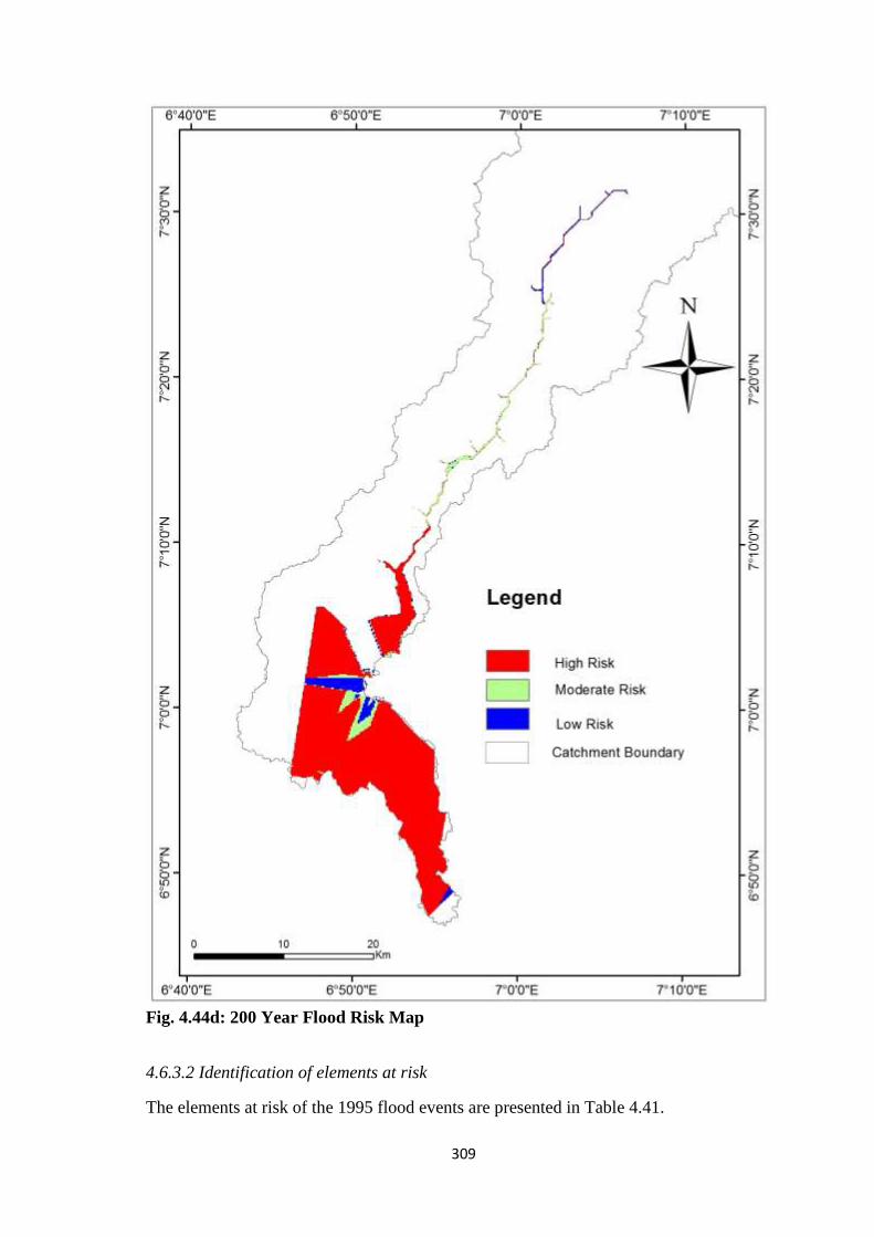
309

Fig. 4.44d: 200 Year Flood Risk Map

4.6.3.2 Identification of elements at risk

The elements at risk of the 1995 flood events are presented in Table 4.41.

310

Table 4.41: Elements at Risk of 1995 Flood Scenario

Elements Risk Zone


Land Surface (km2) 208.647 19.712 22.457 250.816

Road

Main Road (km) 1.522 0.039 1.646 3.207

Minor Road (km) 23.170 0.615 0.384 24.169

Main Path (km) 98.155 9.474 3.398 111.027

Human Settlements

Built Areas (no) 6 0 1 7

Built Areas (ha) 30.563 0 37.251 67.814

Scattered (no) 8 8

Agricultural Forest Reserve (ha) 687.040 27.690 26.220 740.95

Oil Palm Plantation (ha) 0.132 0 0 0.1324

Others

Church (no) 1 0 0 1

Mosque (no) 1 0 0 1

Police Station (no) 1 0 0 1

PHC (no) 1 0 0 1

Market (no) 1 0 0 1

311

Table 4.41 shows that a total land surface of 250.816 km2 was at risk of the 1995 flood

out of which 208.647 km2, 19.712 km2 and 22.457 km2 were in the High, Moderate and

Low risk zones, respectively. In addition to this, 3.207 km of main road out of which

1.522 km, 0.039 km and 1.646 km fell in the High, Moderate and Low risk zones,

respectively. More so, 24.169 km of minor road (23.170 km, 0.615 km and 0.384 km in

High, Moderate and Low risk zones, respectively) was at risk while, 111.027 km of main

path (98.155 km, 9.474 km and 3.398 km in High, Moderate and Low risk zones,

respectively) was at risk of the 1995 flood. Furthermore, six (6) built areas (30.563 ha)

were in the High risk zone while one (1) built area (37.251 ha) was in the Low risk zone

making a total of seven (7) built areas (67.814 ha) at risk of the 1995 flood. Closely related

to this, eight scattered settlements were at risk of the 1995 flood scattered across the three

risk zones. Also at risk is 687.040 ha (High), 27.690 ha (Moderate) and 26.220 ha (Low)

of forest reserve comprising principally of Teak and Melina making a total of 740.95 ha

of forest reserve. More so, 0.132 ha of oil palm plantation was also identified within the

high risk zone. Finally, a church, a mosque, a police station, a Primary Health Care centre

and a small village market were also identified within the high risk zones of the 1995

flood event. The flood risk map showing the elements at risk of the 1995 flood scenario

is shown in Fig. XXa (Appendix XX).

The elements at risk of the 2000 flood events are presented in Table 4.42.

312

Table 4.42: Elements at Risk of 2000 Flood Scenario

Elements Risk Zone


Land Surface (km2) 208.415 19.725 22.547 250.687

Road

Main Road (km) 1.522 0.039 1.644 3.205

Minor Road (km) 23.170 0.615 0.384 24.169

Main Path (km) 98.173 9.463 3.390 111.026

Human Settlements


Built Areas (ha) 30.551 0 37.242 67.793

Scattered (no) 8 8



Others

Church (no) 1 0 0 1

Mosque (no) 1 0 0 1

School (no) 1 0 0 1


PHC (no) 1 0 0 1

Market (no) 1 0 0 1

313

The results in Table 4.42 shows that a total of 250.687 km2 of land surface (208.415 km2

within High, 19.725 km2 within Moderate and 22.547 km2 with Low risk zones) was at

risk of the 2000 flood event. 3.025 km of main asphalt overlaid road (1.522 km within

High, 0.039 km within Moderate and 1.644 km within Low risk zones) was at risk of the

2000 flood while 24.169 km of minor road (23.170 km within High, 0.615 km within

Moderate and 0.384 km within Low risk zones) was at risk. Furthermore, 111.026 km of

main path (98.173 km within High, 9.463 km within Moderate, 3.390 km within Low risk

zones) was at risk. In addition to these, six (6) built areas (30.551 ha) were in the High

risk zone while one (1) built area (37.242 ha) was in the Low risk zone making a total of

seven (7) built areas (67.793 ha) at risk of the 2000 flood. Similarly, eight scattered

settlements were at risk of the 2000 flood scattered across the three risk zones. Also at

risk is 687.041 ha (High), 27.690 ha (Moderate) and 26.136 ha (Low) of forest reserve

comprising principally of Teak and Melina making a total of 740.867 ha of forest reserve.

More so, 0.132 ha of oil palm plantation was also identified within the high risk zone.

Finally, a primary school, a church, a mosque, a police station, a Primary Health Care

centre and a small village market were also identified within the high risk zones of the

2000 flood event. The flood risk map showing the elements at risk of the 2000 flood

scenario is shown in Fig. XXb (Appendix XX).

The elements at risk of the 100-year flood events are presented in Table 4.43.

314

Table 4.43: Elements at Risk of 100 Year Flood

Elements Risk Zone


Land Surface (km2) 231.645 12.164 21.627 265.436

Road

Main Road (km) 1.575 1.417 1.760 4.752

Minor Road (km) 23.539 0.300 0.477 24.316

Main Path (km) 108.138 1.418 2.167 111.723

Human Settlements


Built Areas (ha) 30.548 0 41.535 72.083

Scattered (no) 8 8

Agricultural

Forest Reserve (ha) 699.336 37.238 15.711 752.285

Oil Palm Plantation

(ha) 0.132 0 0 0.1324

Others

Church (no) 1 0 0 1

Mosque (no) 1 0 0 1

School (no) 1 0 0 1


PHC (no) 1 0 0 1

Market (no) 1 0 0 1

Wireless Mast (no) 1 0 0 1

315

At risk of the 100-year flood are 265.436 km2 of land surface (231.645 km2, 12.164 km2

and 21.627 km2 within High, Moderate and Low risk zones, respectively), 4.752 km of

main asphalt overlaid road (1.575 km, 1.417 km and 1.760 km within the High, Moderate

and Low risk zones, respectively), 24.316 km of minor road (23.539 km, 0.3 km and

0.477 km within High, Moderate and Low risk zones respectively) and 111.723 km of

main path (108.138 km, 1.418 km, 2.167 km within High, Moderate and Low risk zones,

respectively). Also at risk of the 100-year flood are seven (7) built areas (72.083 ha). Six

(6) of these built areas (30.548 ha) are within the High risk zone while one (1) built area

(37.238 ha) is in the Low risk zone. Similarly, eight scattered settlements are at risk of

the 100-year flood scattered across the three risk zones. In addition to these, 699.336 ha

(High), 37.238 ha (Moderate) and 15.711 ha (Low) of Teak and Melina forest reserve (A

total of 752.285 ha of forest reserve) are at risk of the 100-year flood. Furthermore, 0.132

ha of oil palm plantation was also identified within the high risk zone. Finally, a primary

school, a church, a mosque, a police station, a Primary Health Care centre, a small village

market and a wireless mast are also at high risk of the 100-year flood event. The flood

risk map showing the elements at risk of the 100-year flood scenario is shown in Fig.

XXc (Appendix XX).

The elements at risk of the 200-year flood events are presented in Table 4.44.

316

Table 4.44: Elements at Risk of 200 Year Flood

Elements Risk Zone


Land Surface (km2) 234.189 17.021 14.706 265.916

Road

Main Road (km) 1.578 1.555 0.214 3.347

Minor Road (km) 23.534 0.670 0.101 24.305

Main Path (km) 108.761 2.024 1.019 111.804

Human Settlements

Built Areas (no) 7 7

Built Areas (ha) 30.557 38.338 2.954 71.849

Scattered (no) 8 8



Others

Church (no) 1 0 0 1

Mosque (no) 1 0 0 1

School (no) 1 0 0 1


PHC (no) 1 0 0 1

Market (no) 1 0 0 1

Wireless Mast (no) 1 0 0 1

317

At risk of the 200-year flood are 265.916 km2 of land surface (234.189 km2, 17.021 km2

and 14.706 km2 within High, Moderate and Low risk zones, respectively), 3.347 km of

main asphalt overlaid road (1.578 km, 1.555 km and 0.214 km within the High, Moderate

and Low risk zones, respectively), 24.305 km of minor road (23.534 km, 0.670 km and

0.101 km within High, Moderate and Low risk zones respectively) and 111.804 km of

main path (108.761 km, 2.024 km, 1.019 km within High, Moderate and Low risk zones,

respectively). Also at risk of the 200-year flood are seven (7) built areas covering an area

of 71.849 ha (30.557 ha within the High risk zone, 38.338 ha within the Moderate risk

zone while 2.954 ha are within the Low risk zone). Similarly, eight scattered settlements

are at risk of the 200-year flood scattered across the three risk zones. In addition to these,

706.197 ha (High), 31.627 ha (Moderate) and 15.238 ha (Low) of Teak and Melina forest

reserve (A total of 753.062 ha of forest reserve) are at risk of the 200-year flood. More

so, 0.132 ha of oil palm plantation was also identified within the high risk zone. Finally,

a primary school, a church, a mosque, a police station, a Primary Health Care centre, a

small village market and a wireless mast are also at high risk of the 200-year flood event.

The flood risk map showing the elements at risk of the 200-year flood (2155) scenario is

shown in Fig. XXd (Appendix XX).

Furher more, the soil types within the respective risk zones are presented in Figs. 4.45a

and b while the inter profile soil characteristics for the respective soil types are presented

in Table 4.45.

318

Fig. 4.45a: Area Covered by the Soil Types within the respective Risk Zones in km2.

319

Fig. 4.45b: Percentage Area Covered by the Soil Types within the respective Risk Zones.

320

Table 4.45: Inter Profile Characteristics of Soil within the Risk Zones

SMU Name

Share in

SMU

(%)

Sand

Fraction

(%)

Silt

Fraction

(%)

Clay

Fraction

(%)

Silt+Clay

Fraction

(%)

Texture

Gravel

Content

(%)

1021

Top Soil (0 - 30 cm)

Ferric Acrisols (DS) 60 78 12 10 22 sandy loam 4

Lithosols (ASI) 20 43 34 23 57 loam 26

Plinthic Acrisols (ASI) 20 47 30 23 53 loam 35

Average

56 25 19 44

22

Sub Soil (30 - 100 cm)

Ferric Acrisols (DS) 60 65 12 23 35 sandy clay loam 10

Lithosols (ASI) 20 - - - - - -

Plinthic Acrisols (ASI) 20 36 27 37 64 clay loam 19

Average 51 20 30 50 15

1193


Gleysols (DS) 35 38 40 22 62 loam 4

Gleysols (ASI) 35 16 31 53 84 clay (light) 7

Fluvisols (ASI) 30 39 41 20 61 loam 4

Average

31 37 32 69

5


Gleysols (DS) 35 37 35 28 63 clay loam 5

Gleysols (ASI) 35 21 27 52 79 clay (light) 1

Fluvisols (ASI) 30 41 39 20 59 loam 8

Average 33 34 33 67 5

1567


Dystric Nitosols (DS) 60 76 13 11 24 sandy loam 4

Lithosols (ASI) 20 43 34 23 57 loam 26

Orthic Acrisols (ASI) 20 49 27 24 51 sandy clay loam 10

Average

56 25 19 44

13


Dystric Nitosols (DS) 60 62 13 25 38 sandy clay loam 4

Lithosols (ASI) 20 - - - - - -

Orthic Acrisols (ASI) 20 40 24 36 60 clay loam 10

Average 51 19 31 49 7

677


Calcaric Fluvisols

(DS) 60 49 32 19 51 loam 4

Dystric Nitosols (ASI) 20 44 33 23 56 loam 11

Plinthic Gleysols

(ASI) 20 42 37 21 58 loam 7

Average

45 34 21 55

7


Calcaric Fluvisols

(DS) 60 52 28 20 48 loam 8

Dystric Nitosols (ASI) 20 35 24 41 65 clay (light) 26

Plinthic Gleysols

(ASI) 20 36 30 34 64 clay loam 10

Average 41 27 32 59 15

SMU-Soil Mapping Unit; DS-Dorminant soils; ASI-Associated soils with inclusions Source: Extracted from Harmonised World Soil Database

321

It can be observed from Fig. 4.45a that the predominant soil type within the high risk zone

is Gleysols (Clay loam) covering areas of 182.36 km2, 182.13 km2, 204.81 km2 and

207.24 km2 for year 1995, year 2000, 100 years return period and 200 years return period

respectively. These areas represent 72.93 %, 72.87%, 77. 40 % and 78.18 % of the total

flood risk extent for year 1995, year 2000, 100 years return period and 200 years return

period respectively (Fig. 4.45b). The inter profile characteristics presented in Table 4.45

shows that the combined fractions of silt and clay in Gleysols are 69 % and 67 % for the

top soil and the sub soil respectively. This high clay-silt content explains why the flood

risk within that zone is high. It means that the ability of the soil to permit infiltration is

low thus resulting in runoff and consequently, flooding.

4.6.3.3 Extent of damage of the 1995 and 2000 flood scenarios

The results of the assessment of the extent of damages of the 1995 and 2000 flood

scenarios at Oforachi are presented and discussed in this section. The distribution of

households by experience of the 1995/2000 flood events are presented in Fig. 4.46.

Fig. 4.46: Distribution of Respondents by Experience of 1995/2000 Flood Event

322

The results in Fig. 4.46 show that out of the 61.23 % households that have experienced

flood, 55.38 % experienced either the 1995 flood, 2000 flood or both while 5.85 % did

not experience the 1995/2000 flood event.

More so, Fig. 4.47 shows the households’ responses on damages/disasters as a result of

the 1995 flood event. Figure 4.47 shows that no death or injury was recorded as a result

of the 1995 flood event. Although the houses of all those affected by the flood were

submerged, the houses of 59 % collapsed. Meanwhile, 81 % had to be evacuated implying

that even some households whose building did not collapse had to evacuate their houses

because of the depth of floodwater. The crops of 92 % of those affected were destroyed

while 48 % lost some goods that were to be sold either in shops or market. As a result of

complete inundation of access road, all the students of the affected households and the

community at large could not go to school. Furthermore, 41 % of the households lost

various livestock ranging from chicken, goats, and sheep, amongst others. Finally, 33 %

of affected households experienced outbreak of diseases that could be linked directly to

the flood.

Figure 4.48 shows the households’ responses on damages/disasters as a result of the 2000

flood event.

323

Fig. 4.47: Distribution of Respondents by Various Effects of 1995 Flood Event

324

Fig. 4.48: Distribution of Respondents by Various Effects of 2000 Flood Event

325

The effects of the 2000 flood event seem to be similar to those of 1995 viewing from the

response of the respondents. The results in Fig. 4.48 show that no death or injury was

recorded as a result of the 1995 flood event, while 100 % of the houses of those affected

were submerged. Meanwhile, the houses of 67 % of those affected collapsed while 89 %

were evacuated either because of building collapse of because of high floodwater. The

results further show that 92 % of respondents lost crops in the farm while 63 % lost some

goods either in shops or market. Students of the 100 % of affected households were unable

to go to school due to complete inundation of the access roads as well as the challenge of

having to manage the flood crisis. More so, 67 % of the households lost various livestock

ranging from chicken, goats, and sheep, amongst others. Finally, 56 % of affected

households experienced outbreak of diseases that could be linked directly to the flood

implying that there were more outbreak of flood related diseases during the 2000 flood

event than the 1995 flood event.

4.6.3.4 Environmental health implication of flood

(A) Open Defecation Extent

The results of the assessment of availability of toilet facilities in households as well as

the type are presented in Fig. 4.49.

Fig. 4.49: Distribution of Households by type of Toilet Facility

326

Figure 4.49 shows that 51 % of the households do not have any toilet facility in their

households while 27 %, 6 % and 16 % have pit latrine, VIP latrine and water closet,

respectively. Furthermore, a projection of the total population represented by the

aforementioned percentages is presented in Table 4.46.

Table 4.46: Distribution of Household Populations by Toilet Facilities

Toilet Type Percentage

(%)

Number of

Households Population

No Toilet 51.08 315 4095

Pit Latrine 26.46 163 2119

VIP Latrine 6.15 38 494

Water Closet 16.31 100 1300

Table 4.46 shows that a total of 4,095 persons in Oforachi Community do not have a toilet

facility in their houses. On the other hand, 2,119 persons, 494 persons and 1,300 persons

have pit latrine, VIP latrine and water closet, respectively in their houses. A further

analysis to find out the 4,095 persons without a toilet facility in their houses defecate was

carried out. The results are presented in Fig. 4.50 and Table 4.47.

Fig. 4.50: Extent of Open Defecation in Oforachi Community

Table 4.47: Alternative Place of Defecation for those without Toilet Facilities

Point of Defecation % Number of


Open Fields 99.34 313 4069

Neighbour's toilet 0.66 2 26

327

The results in Fig. 4.50 and Table 4.47 reveal that only 26 persons representing 0.66% of

those without toilet use the facilities in neighbouring households while 4,069 persons

representing 99.34 % resort to open defecation in nearby fields. This implies that 4,069

persons representing 50.81 % of the entire community defecate in the open field. The

implication of this is that these faeces find their way to the river especially in the event of

flood and could possibly lead to an epidemic since a large percentage of the community

use the river as their source of drinking water.

(B) Sources of Drinking Water

The community’s sources of drinking water and the estimated populations depending on

each source are represented in Fig. 4.51 and Table 4.48.

Fig. 4.51: Distribution of Households by Sources of Drinking Water

Table 4.48: Distribution of Household Populations by Sources of Drinking Water

Source of Drinking

Water

Percentage

(%)

Number of


Ofu River 44.92 277 3601

Borehole 55.08 339 4407

The results in Fig. 4.52 and Table 4.48 show that 277 households (3,601 persons)

representing 44.92 % of the community depend on Ofu River as their source of drinking

water while 339 households (4,407 persons) representing 55.08 % of the community

328

depend on borehole for their drinking water. The implication is that 3,601 persons are at

risk of contacting water borne disease as a result of open defecation and flooding. Since

the point of consumption and the point of contamination are the same, there will be

insufficient distance for the river to self purify. This probably explains the 33 % and 67

% disease outbreaks during the 1995 and 2000 floods, respectively at Oforachi.

4.7 STRATEGIC PLAN FOR OFU RIVER CATCHMENT FLOOD

MANAGEMENT

The foregoing results have clearly shown that Ofu River flood disaster will increase in

intensity and the extent of damages to properties of people within the flood plain. In order

the effectively manage and prevent the occurrence of flood as well as minimize its impact

upon the people, a strategic plan has been developed for sustainable use, maintenance and

maximization the benefits of the floodplains. Most flood hazard mitigation measures have

shifted from structural approach to non-structural because of the disadvantages associated

with the sense of safety the structural measures give to floodplain users. The priority will

be given to non-structural measures in this flood management plan. The proposed

strategic plan is presented in Table 4.49.

329

Table 4.49: Strategic Plan for Ofu River Catchment Flood Management

S/N PLAN ACTION RESPONSIBILITY

1. Ofu River catchment

management team

Set up a management team

comprising of a representative of

LBRBDA, at least one official from

each of the component LGAs, the

counsellor of component wards and

the village heads of communities

along the river course or their

representatives

LBRBDA, Government,

NEWMAP

2. Channelization of Ofu

River to accommodate

more flood waters

Dredging and widening of the Ofu

River channel

State Government with support

from the Federal Government

through LBRBDA Headquarters

Makurdi

3. Clearing of Ofu River to

accommodate more

flood waters

Periodic clearing of excessive

vegetative cover on the Ofu River

water course

Ofu River catchment

Management Team

4. Increase public

awareness of flooding

Public enlightenment campaigns,

town hall meetings and stakeholders

forum

Information Office of the

Respective LGAs in

collaboration with the State

Ministry responsible for water

resources and rural development

and Ofu River catchment

management team.

5. Set up an early warning

and emergency

preparedness scheme

Design and implement emergency

and early warning scheme that will

involve the community leadership,

paying particular attention to ease of

understanding of the communities

LBRBDA Headquarters Makurdi

State Government, Ofu River

Catchment Management Team

and the community Leadership

6. Set up a flood plain

management

programme

Engage floodplain managers to train

people to meet up with current and

growing challenges in floodplain

management.

LBRBDA Headquarters Makurdi

and Ofu River Catchment

management team

330

CHAPTER FIVE

SUMMARY, CONCLUSION AND RECOMMENDATIONS

This chapter highlights the summary of the findings of this work, conclusion drawn

from the results of this study and the recommendations made.

5.1 SUMMARY

Flood disaster has become an annual occurrence in the floodplain of Ofu River since 1991

causing varying degree of damages to properties and disrupting the socio-economic live

of the residents, yet, no study (to the best of my knowledge) seem to have been carried

out to assess the cause and damage extent of this phenomenon that would provide a basis

for its mitigation. This is the reason why this study was carried out with the aim of

conducting a flood risk assessment for Ofu River Catchment.

The study set out six specific objectives. The first was to determine the morphologic

characteristics of Ofu River Catchment, the second was to develop a Stage-Discharge

relationship or rating curve for Ofu River, the third was to identify flood causative factors

within Ofu River Catchment, the fourth was to analyze flood frequencies and determine

the return periods of extreme flood events in the study area, the fifth was to derive the

flood hazard maps and determine the extent of inundation for respective return periods of

extreme flood events in the study area while the last objective was to carry out a flood

risk analysis in the study area.

The major findings of this study are summarized as follows:

1. Ofu River Catchment covers a total drainage area of 1604.56 km2 covering 27.02 %

of Dekina, 23.48 % of Ofu, 14.06 % of Igalamela/Odolu, 9.25 % of Idah and 14.04 %

331

of Ibaji Local Government Areas in Kogi State and 0.80 % of Uzo-Uwani Local

Government Area in Enugu State, Nigeria. The time of concentration for the

catchment was 6.17 hours while the time from peak to recession 3.68 days.

2. The rating curve equation (relating discharge Q in m3/s and stage H in m above mean

sea level) for Ofu River at Oforachi Bridge Hydrometric Station is 𝑄 =

15.54096(𝐻 − 55.43192)0.69051 which can be used for the transformation of

available stage data into discharge.

3. 8.00% household heads had fair knowledge, 80.92% had good knowledge while,

11.08% had excellent knowledge of the causes of flood. Their knowledge level was

influenced by the following factors in decreasing order of associations:Age (Pearson’s

chi2 = 44.46; P = 0.000), Education (Pearson’s chi2 = 44.39; P = 0.000), Occupation

(Pearson’s chi2 = 18.52; P = 0.018), Flood experience (Pearson’s chi2 = 17.87; P =

0.000), Marital Status (Pearson’s chi2 = 9.81; P = 0.044) and Ward (Pearson’s chi2 =

9.68; P = 0.008).

4. Ofu River has lost an average of 6.90 m of its flow depth at Oforachi between 2000

and 2016 at an average rate of 0.431 m per year which is the major cause of flood as

the river overflows its banks with any prolonged rainfall. In addition to this, the Land

use/ Land cover changes within Ofu River catchment between 1987 and 2016 has not

significantly affected the amount of runoff given by the almost equal runoff curve

numbers of 61.8, 63.3 and 62.8 for 1987, 2001 and 2016, respectively.

5. The modified Thomas-Fierring Model was effectively used to generate 12 months

synthtic stream flow data for Ofu River from 1974 to 2016 using the gauged data of

1955 to 1973 making the stream flow data cover a total of 62 years (1955 – 2016).

6. The peak discharge values for 2, 5, 10, 25, 50, 100 and 200 years return periods are

444.57 m3/s, 499.23 m3/s, 530.35 m3/s, 565.61 m3/s, 589.59 m3/s, 611.96 m3/s and

332

633.25 m3/s, respectively. More so, the peak discharge values for 1995 and 2000 flood

scenarios were 448.89 m3/s and 446.46 m3/s, respectively.

7. The extent of flood inundation obtain using thematic integration of factor maps

(multi-criteria analysis) was 257.49 km2 while those for the HEC-RAS modelling

were 251.98 km2 and 251.80 km2 for the 1995 and 2000 flood scenarios, respectively

and 252.63 km2, 256.34 km2, 258.17 km2, 262.34 km2, 266.84 km2 and 267.37 km2

for 2, 5, 10, 25, 50, 100 and 200 years return periods, respectively.

8. The high flood hazard zone covered an area of 218.232 km2, 217.832 km2, 242.366

km2 and 244.939 km2 for year 1995, year 2000, 100 year and 200 year floods,

respectively. The moderate flood hazard category covered 20.250 km2, 20.331 km2,

12.711 km2 and 11.496 km2, respectively while the low hazard category covered

14.481 km2, 14.630 km2, 12.756 km2 and 11.937 km2, respectively.

9. A total of 242.413 km2, 242.537 km2, 256.501 km2 and 256.819 km2 were highly

vulnerable to year 1995, year 2000, 100 year and 200 year floods, respectively. There

was no moderate vulnerability zone for the 1995, 2000 and 100-year floods but

covered an area of 6.818 km2 for the 200-year flood. Lastly, the low vulnerability

category covered 9.055 km2, 9.009 km2, 10.164 km2 and 3.361 km2, respectively.

10. The year 1995 flood event put 250.816 km2 land area and 16,932 persons at risk while

the year 2000 flood event put 250.687 km2 and 19,673 persons at risk. The 100-year

flood will put 265.436 km2 and 92,733 persons at risk while, the 200-year flood will

put 265.916 km2 and 1,984,377 persons at risk in addition to roads, built and scattered

settlements, forest reserve, oil palm plantation, church, mosque, school, police station,

primary health clinic, market and wireless mast that will be at risk.

11. The predominant soil type within the high risk zone is Clay loam which could be one

of the reasons for the high flood risk.

333

12. An assessment of the open defecation status of Oforachi, the most developed of the

communities within Ofu River floodplain shows that 50.81 % of the population still

defecate in the open field. This poses a risk for contamination and outbreak of diseases

during flood events.

5.2 CONCLUSION

From the results of the study conducted, the following conclusions were drawn:

1. Ofu River Catchment covers a total drainage area of 1604.56 km2 covering 27.02 %

of Dekina, 23.48 % of Ofu, 14.06 % of Igalamela/Odolu, 9.25 % of Idah and 14.04 %

of Ibaji Local Government Areas in Kogi State and 0.80 % of Uzo-Uwani Local

Government Area in Enugu State, Nigeria. The time of concentration of 6.17 hours

obtained for the catchment implies that it will take a drop of rain approximately 6

hours 10 minutes to flow from the remotest part of the catchment to its outlet, while

the time from peak to recession of 3.68 days imply that it would take any flood water

an average of approximatley four days to completely recede from the ground surface.

The catchment consists of 39 streams up to the third order. It is made up of 20 first

order streams of 98.76 km length (4.94 km mean length), 16 second order streams of

101.17 km length (6.32 km mean length) and three (3) third order streams of 41.47

km length (13.82 km mean length).

2. A rating curve equation, 𝑄 = 15.5410(𝐻 − 55.4319)0.6905 (where Q = discharge in

m3/s and H = stage in m above mean sea level) was developed for Ofu River at

Oforachi Bridge Hydrometric Station which can be used for the transformation of

available stage data into discharge and can therefore serve as a monitoring station for

early warning to the inhabitants.

334

3. The inhabitant’s level of knowledge of flood causes was influenced by age (Pearson’s

chi2 = 44.46; P = 0.000), education (Pearson’s chi2 = 44.39; P = 0.000), occupation

(Pearson’s chi2 = 18.52; P = 0.018), flood experience (Pearson’s chi2 = 17.87; P =

0.000), marital status (Pearson’s chi2 = 9.81; P = 0.044) and ward (Pearson’s chi2 =

9.68; P = 0.008), thus should be considered in the development of early warning

schemes. More so, Ofu River has lost an average of 6.90 m of its flow depth at

Oforachi between 2000 and 2016 at an average annual rate of 0.431 m due to sediment

load accumulation estimated at 66,824.73 x 103 kg/annum which makes it overflow

its banks with any prolonged rainfall.

4. Ofu River stream flow data for 1955 – 1955 was effectively extended to 2016 using

the modified Thomas-Fierring Model coupled with linear regression. Ofu River

stream flow values for 2, 5, 10, 25, 50, 100 and 200 years return periods estimated

based on these synthetic data were 444.57 m3/s, 499.23 m3/s, 530.35 m3/s, 565.61

m3/s, 589.59 m3/s, 611.96 m3/s and 633.25 m3/s.

5. Multi-criteria analysis (MCA) via thematic integration of flood causative factor maps

in ArcGIS can be effectively used to determine the extent of flood inundation in the

absence of stream flow data. More so, HEC-RAS with HEC-Geo-RAS extension in

ArcGIS are effective tools for flood inundation mapping using hydrologically

generated stream flow which can clearly determine inundation extents, depths and

velocity. The flood inundation extent obtained via thematic integration of flood

causative factors is 257.49 km2. The flood inundation extents for year 1995 and year

2000 flood events obtained via steady flow analysis in HEC-RAS/GeoRAS were

251.98 km2 and 251.80 km2 respectively while those for floods of 2, 5, 10, 25, 50,

100 and 200 years return periods were respectively 252.63 km2, 256.34 km2, 258.17

km2, 262.34 km2, 265.96 km2, 266.84 km2, 267.37 km2.

335

6. The year 1995 flood event put 250.816 km2 and 16,932 persons at risk while the year

2000 flood event put 250.687 km2 and 19,673 persons at risk. The 100-year flood will

put 265.436 km2 and 92,733 persons at risk while, the 200-year flood will put 265.916

km2 and 1,984,377 persons at risk in addition to roads, built and scattered settlements,

forest reserve, oil palm plantation, church, mosque, school, police station, Primary

Health Clinic, market and wireless mast that will be at risk. The fact that more than

50 % of the community still defecate in the open field makes them at a high risk of an

epidemic outbreak in the event of flood disaster since Ofu River is a major source of

drinking water for the community.

5.3 RECOMMENDATIONS

The following recommendations are made from the study:

1. The Federal Government of Nigeria should consider dredging Ofu River as a matter

of urgency.

2. The State Government in collaboration with the Lower Benue River Basin

Development Authority (LBRBDA) and NEWMAP should set up a management

team for Ofu River Catchment. The team should comprise of a representative of

LBRBDA, one official from each of the component LGAs, the counsellor of

component wards and the village heads of communities along the river course or their

representatives.

3. The catchment management team should ensure periodic clearing of excessive

vegetative cover on the Ofu River water course to provide more discharge capacity

for the river.

336

4. An emergency and early warning scheme should be designed and implemented by the

Lower Benue River Basin Development Authority (LBRBDA), involving the

community stakeholders for effective implementation.

5. A well planned strategic awareness creation should be made by the management team

in the communities within the floodplain, on the danger of living in those places with

plans for possible evacuation and resettlement in safer locations.

6. Factors such as age, level of education, occupation and marital status, should be

considered by the National Emergency Management Agency (NEMA) in the

development of an effective early warning and public enlightenment systems.

7. A monitoring station for early warning be established at Oforachi Bridge

Hydrometric Station by the National Emergency Management Agency (NEMA).

337

REFERENCES

Ackerman C. T. (2011). HEC-GeoRAS GIS Tools for Support of HEC-RAS using

ArcGIS® User’s Manual, US Army Corps of Engineers Hydrologic Engineering Center.

Davis CA.

Adebayo, A. A., and Oruonye, E. D. (2013). An Assessment of the effects of the 2012

Floods in Taraba State, Nigeria. Paper presented at the Annual National Conference,

organized by the Association Hydrological Science University of Agriculture, Abeokuta,

Ogun, state, Nigeria.

Aderogba, K. A. (2012). Global warming and challenges of floods in Lagos metropolis,

Nigeria. Academic Research International, 2(1), 448-468.

Aderoju, O. M., Jantiku, J., Fagbemiro, O. A., Aliyu, I., Nwadike, B. K., Ajonye, S. E.,

and Salman, K. S. (2014). Geospatial assessment of 2012 flood disaster in Kogi State,

Nigeria. J. Environ. Sci. Toxicol. Food Technol, 8, 74-84.

Agarwal, C. S. (1998). Study of drainage pattern through aerial data in Naugarh area of

Varanasi district, UP. Journal of the Indian Society of Remote Sensing, 26(4), 169-175.

Ahmad, B., Muhammad, S. K., Butt, M. J., and Dahri, Z. H. (2010). Hydrological

modelling and flood hazard mapping of Nullah Lai. Proc Pak Acad Sci, 47(4), 215-226.

Ahmad, S., Khan, I. H., and Parida, B. P. (2001). Performance of stochastic approaches

for forecasting river water quality. Water research, 35(18), 4261-4266.

Ajayi, S. A. (2015). Performance of Selected Water Infiltration Models in Organic-

Amended Soils. Unpublished MSc. Dissertation in the Department of Agricultural

Engineering, Ahmadu Bello University, Zaria.

Ajin, R., Krishnamurthy, R., Jayaprakash, M., and Vinod, P. (2013). Flood hazard

assessment of Vamanapuram River Basin, Kerala, India: An approach using Remote

Sensing & GIS techniques. Adv Appl Sci Res, 4, 263-274.

Akan, A. O. (2002). Modified rational method for sizing infiltration structures. Canadian

Journal of Civil Engineering, 29(4), 539-542.

Akintola F. O. and Ikwuyatum G. O. (2006). Sustainable Issues in Flood Management in

Nigeria in: Ivbijaro M. F. A., Akintola F. and Okechukwu R. U. (Eds) 2006. Sustainable

Environmental Management in Nigeria Ibadan, Mattivi Production.

Alkema, D and Westen, C. (2005). Flood Hazard and Risk Assessment. Refresher Course

on Geo-Information for natural Disaster Reduction in Easter Africa. Makerere

University, 12 – 23 September 2005.

Alkema, D. (2004). Remote Sensing and GIS Applications in Flood Forecasting. National

workshop on Flood Disaster Management – Space Inputs, 3-4 June, 2004. NRSA,

Hyderabad. India.http://www.itc.nl/library/Papers_2004/n_p_conf/alkema.pdf

http://www.itc.nl/library/Papers_2004/n_p_conf/alkema.pdf

338

Alkema, D. (2007). Simulating floods: On the application of a 2D-hydraulic model for

flood hazard and risk assessment. ITC dissertation number 147. The Netherlands.

American Public Health Association (2012). Standard Methods for the Examination of

Water and Wastewater, 20th ed. Jointly published by American Public Health Association

(APHA), American Water Works Association (AWWA) and Water Environment

Federation (WEF), Washington, USA.

Amini, J. (2007). Generating floodplain maps using Ikonos image and DTM. Proceedings

of the 4th International Conference on Recent Problems in Geodesy and Related Fields

with International Importance. Sofia, Bulgeria.

Angillieri, M. Y. E. (2008). Morphometric analysis of Colangüil river basin and flash

flood hazard, San Juan, Argentina. Environmental geology, 55(1), 107-111.

AR-AR Partnership (2004). Oforachi Irrigation Project Contract Documents Volume III:

Main Report Prepared for Lower Benue River Basin Development Authority, Federal

Republic of Nigeria (Unpublished).

Baas, S., Ramasamy, S., DePryck, J. D., and Battista, F. (2008). Disaster risk

management systems analysis: A guide book (Vol. 3). Food and Agriculture Organization

of the United Nations.

Balabanova, S., and Vassilev, V. (2010). Creation of flood hazard maps. Water

Observation and Information System for Balkan Countries (BALWOIS).Ohrid, Republic

of Macedonia.

Balica, S. F., Douben, N., and Wright, N. G. (2009). Flood vulnerability indices at varying

spatial scales. Water science and technology, 60(10), 2571-2580.

Bapalu, G. V and Sinha, R. (2005). “GIS in Flood Hazard Mapping: A Case Study of

Kosi RiverBasin, India”. GIS Development Weekly, 1(13), pp 1-3. Accessed

fromhttp://www.gisdevelopment.net/application/natural_hazards/floods on 12th March

2009.

Bhanumurthy, V., Manjusree P. and Rao G. S., (2004). Managing Floods: A remote

Sensing Approach. ISG Newsletter Vol. 10 No. 1 & 2, March/June, 2004, pp 46-53

Bird, J. F. (1980). Geomorphological implications of flood control measures, Lang Lang

River, Victoria. Australian Geographical Studies, 18(2), 169-183.

Blaikie, P., Cannon, T., Davis, I., and Wisner, B. (2014). At risk: natural hazards,

people's vulnerability and disasters. Abingdon (UK). Routledge.

Bouwer, H. (1986). Intake rate: cylinder infiltrometer. Pp. 825-844 in Klute A (Ed.).

Methods of Soil Analysis, Part 1: Physical and Mineralogical Methods, 2nd Ed.

Madison: American Society of Agronomy and Soil Science Society of America. 1188

p. ISBN 0-89118-088-5.

339

Braca, G. (2008). Stage-discharge relationships in open channels: Practices and

problems. Univ. degliStudi di Trento, Dipartimento di IngegneriaCivile e Ambientale.

Brice, J. C. (1984). Planform properties of meandering rivers. In River meandering (p.

15). ASCE available on cedb.asce.org

British Geological Survey (BGS) (nd). Groundwater Flooding.

http://www.bgs.ac.uk/research/groundwater/flooding/home.html accessed on 27th

March, 2017.

Brivio, P. A., Colombo, R., Maggi, M., and Tomasoni, R. (2002). Integration of remote

sensing data and GIS for accurate mapping of flooded areas. International Journal of

Remote Sensing, 23(3), 429-441.

Büchele, B., Kreibich, H., Kron, A., Thieken, A., Ihringer, J., Oberle, P., ... and

Nestmann, F. (2006). Flood-risk mapping: contributions towards an enhanced assessment

of extreme events and associated risks. Natural Hazards and Earth System Sciences, 6(4),

485-503.

Bruner G. W. (2010). HEC-RAS, River Analysis System Hydraulic Reference Manual,

US Army Corps of Engineers Hydrologic engineering Center. Davis CA.

Campbell, J. B., & Wynne, R. H. (2011). Introduction to remote sensing. New York.

Guilford Press.

Celeste, A. B., Suzuki, K., Kadota, A., and de Farias, C. A. (2004). Stochastic Generation

of Inflow Scenarios to be used by Optimal Reservoir Operation Models. Annual Journal

of Hydraulic Engineering, 48, 451-456.

Chang, L. C., Shen, H. Y., Wang, Y. F., Huang, J. Y., and Lin, Y. T. (2010). Clustering-

based hybrid inundation model for forecasting flood inundation depths. Journal of

hydrology, 385(1), 257-268.

Chen, A. S., Djordjević, S., Leandro, J., and Savić, D. A. (2010). An analysis of the

combined consequences of pluvial and fluvial flooding. Water Science and Technology,

62(7), 1491-1498.

Chen, N. S., Yue, Z. Q., Cui, P., and Li, Z. L. (2007). A rational method for estimating

maximum discharge of a landslide-induced debris flow: A case study from southwestern

China. Geomorphology, 84(1), 44-58.

Chorley, R. J., Malm, D. E., & Pogorzelski, H. A. (1957). A new standard for estimating

drainage basin shape. American Journal of Science, 255(2), 138-141.

Chow, V.T., Maidment, D.R. and Mays, L.W. (1988). Applied Hydrology. McGraw-Hill

Series in Water Resources and Environmental Engineering. McGraw-Hill: New York.

ISBN 0-07-010810-2. xiii, 572 pp.

Chow, V. T. (1956). Hydrologic studies of floods in the United States. International

Association of Hydrological Sciences, 42, 134-170.

http://www.bgs.ac.uk/research/groundwater/flooding/home.html

340

Cobby, D., Falconer, R., Forbes, G., Smyth, P., Widgery, N., Astle, G., ...and Golding,

B. (2009). Potential warning services for groundwater and pluvial flooding.

Coto, E. B. (2002). Flood hazard, vulnerability and risk assessment in the city of

Turrialba, Costa Rica. International Institute for Geo-information Science and Earth

Observation (ITC), 1-102

Cui, Q., Wang, X., Li, C., Cai, Y., and Liang, P. (2016). Improved Thomas–Fiering and

wavelet neural network models for cumulative errors reduction in reservoir inflow

forecast. Journal of hydro-environment research, 13, 134-143.

Cutter S. L., Mitchell T. T. and Scott M. S. (1997). Handbook for Conducting a GIS-

Based Hazard Assessment at the County Level. Prepared for South Carolina Emergency

Preparedness Division, Office of the Adjutant General. Accessed 25/01/2016 from

https://www.researchgate.net/publication/257343365_Handbook_for_conducting_a_GI

S-based_hazards_assessment_at_a_county_level

Daffi R. E. (2013). Flood Hazard Assessment for River Dep Catchment Using Remote

Sensing and Geographic Information System Techniques Unpublished PhD Thesis in The

Department of Water Resources and Environmental Engineering Ahmadu Bello

University, Zaria.

Daffi, R. E., Otun, J. A., & Ismail, A. (2014). Flood hazard assessment of River Dep

floodplains in North-Central Nigeria. Int. J. Water Resour. Environ. Engr, 6(2), 67-72.

Dalrymple, T. (1960). Flood-frequency analyses, Manual of Hydrology: Part 3 Water

Supply Paper (- ed.). A publication of the United State Geological Survey available at

https://pubs.er.usgs.gov/publication/wsp1543A (accessed 26/05/2017).

Damayanti, F. (2011). Hydrodynamic Modeling for Flood Hazard Assessment

inTelemoyo Catchment Central Java, Indonesia. Unpublished M.Sc Thesis Gadjah Mada

University and Faculty of Geo-Information Science and Earth Observation University of

Twente.

Dashora, I., Singal, S. K., & Srivastav, D. K. (2015). Software Application for Data

Driven Prediction Models for Intermittent Streamflow for Narmada River Basin.

International Journal of Computer Applications, 113(10), 9 - 17.

de Brouwer (1997). Determination of Peak Runoffrate in: ILWIS Application Guide,

ILWIS Department, International Institute for Aerospace Survey and Earth Sciences,

Enschede, The Netherlands.

de Leeuw, E. D., and Dillman, D. A. (Eds.). (2008). International handbook of survey

methodology. Taylor & Francis.

Demirkesen, A. C., Evrendilek, F., Berberoglu, S., and Kilic, S. (2007). Coastal flood risk

analysis using Landsat-7 ETM+ imagery and SRTM DEM: A case study of Izmir,

Turkey. Environmental monitoring and assessment, 131(1), 293-300.

https://www.researchgate.net/publication/257343365_Handbook_for_conducting_a_GIS-based_hazards_assessment_at_a_county_level

https://www.researchgate.net/publication/257343365_Handbook_for_conducting_a_GIS-based_hazards_assessment_at_a_county_level

https://pubs.er.usgs.gov/publication/wsp1543A

341

Dewan, A. M., Islam, M. M., Kumamoto, T., and Nishigaki, M. (2007). Evaluating flood

hazard for land-use planning in Greater Dhaka of Bangladesh using remote sensing and

GIS techniques. Water Resources Management, 21(9), 1601.

Douglas, I., Garvin, S., Lawson, N., Richards, J., Tippett, J., and White, I. (2010). Urban

pluvial flooding: a qualitative case study of cause, effect and nonstructural mitigation.

Journal of Flood Risk Management, 3(2), 112-125.

Earls, J., and Dixon, B. (2007). Spatial interpolation of rainfall data using ArcGIS: A

comparative study. In ESRI User Conference June 2007.

e Costa, C. A. B., Da Silva, P. A., and Correia, F. N. (2004). Multicriteria evaluation of

flood control measures: The case of Ribeira do Livramento. Water Resources

Management, 18(3), 263-283.

Eleuterio J. (2012). Flood Risk Analysis: Impact of uncertainty in hazard modelling and

vulnerability assessments on damage estimations. PhD thesis at the Augustin Cournot

Doctoral School, Water Science and Environmental Economics, Department of Civil

Engineering, the University of Strasbourg.

England Jr J. F., Timothy A. Cohn, Beth A. Faber, Jery R. Stedinger, Wilbert O. Thomas

Jr., Andrea G., Veilleux, Julie E. Kiang, and Robert R. Mason (2017). Guidelines for

Determining Flood FlowFrequencyBulletin17C: Techniques andMethods 4–

BXXhttps://acwi.gov/hydrology/Frequency/b17c/Bulletin17C-draft-for-USGS-

EditorialReview-10Apr2017.pdf (26/5/2017)

Faber B. (2010). Current Methods for Flood Frequency Analysis. Being a paper presented

at the Workshop on Non-Stationarity, Hydrologic Frequency Analysis, and Water

Management organized by the Hydraulic Engineering Center of the United States Army

Corps of Engineers, January 13, 2010.

Falconer, R. H., Cobby, D., Smyth, P., Astle, G., Dent, J., and Golding, B. (2009). Pluvial

flooding: new approaches in flood warning, mapping and risk management. Journal of

Flood Risk Management, 2(3), 198-208

Faniran, A. (1968). The index of drainage intensity-A provisional new drainage factor.

Australian Journal of Science, 31, 328-330.

Federal Ministry of Works (2013). Highway Manual Part I-Design Volume IV: Drainage

Design. Abuja. Author

Few, R. (2003). Flooding, vulnerability and coping strategies: local responses to a global

threat. Progress in Development Studies, 3(1), 43-58.

Forkuo, E. K. (2011). Flood hazard mapping using Aster image data with GIS.

International journal of Geomatics and Geosciences, 1(4), 932-950.

Frank H. and Althoen S. C. (1995). Statistics: Concepts and Applications. Cambridge

University Press.

https://acwi.gov/hydrology/Frequency/b17c/Bulletin17C-draft-for-USGS-EditorialReview-10Apr2017.pdf

https://acwi.gov/hydrology/Frequency/b17c/Bulletin17C-draft-for-USGS-EditorialReview-10Apr2017.pdf

342

Gaillard, J. C. (2010). Vulnerability, capacity and resilience: perspectives for climate and

development policy. Journal of International Development, 22(2), 218-232.

Galy, H. M., & Sanders, R. A. (2000). Using SAR imagery for flood modeling.

Englewood, CO. http://www. intermap. ca/PDF/rgs_paper. pdf (22 February 2000).

Gana, A. K. (2011). Cow dung: soil amendment agent for the sandy upland sugarcane

ecology in Nigeria. Journal of Agricultural Technology 2011 Vol. 7(2): 497-505

Garba, H. A (2015): Flood Vulnerability Assessment in Jalingo Metropolis, Taraba State,

Nigeria. Unpublished M.Sc. Dissertation in the Department of Geography, Ahmadu Bello

University, Zaria.

Garde, R.J. (2006). River Morphology, New Age International (Pvt) Ltd. Publishers, New

Delhi.

Gardiner, V., Gregory, K. J., and Walling, D. E. (1977). Further notes on the drainage

density-basin area relationship. Area, 117-121.

Gideon, Y. B., Fatoye, F. B., and Omada, J. I. (2013). Quality Assessment of Physico-

Chemical Characteristics of Okura River, Kogi State, Nigeria. International Journal of

Science and Technology, 2(12), 891-899.

Grant, A., Ries, R., and Thompson, C. (2016). Quantitative approaches in life cycle

assessment—part 1—descriptive statistics and factor analysis. The International Journal

of Life Cycle Assessment, 21(6), 903-911.

Haghiabi, A. H., Heidarpourand M. and Habili, J. (2011). A new method for estimating

the parameters of Kostiakov and modified Kostiakov infiltration equations. World

Applied Sciences Journal. 15(1): 129 –135.

Harms, A. A., and Campbell, T. H. (1967). An extension to the Thomas‐Fiering Model

for the sequential generation of streamflow. Water Resources Research, 3(3), 653-661.

Hartkamp, A. D., De Beurs, K., Stein, A., and White, J. W. (1999). Interpolation

techniques for climate variables.NRG-GIS Series 99-01. Mexico, D.F.: CIMMYT

Herschy, R. (1993). The velocity-area method. Flow measurement and instrumentation,

4(1), 7-10.

Herschy R. W. (1995). Stream flow Measurement, Chapman & Hall, Second Edition.

Heywood, I., Oliver, J., and Tomlinson, S. (1995). Building an exploratory multi-criteria

modelling environment for spatial decision support. Innovations in GIS, 2, 127-136.

Hjelmfelt Jr, A. T. (1991). Investigation of curve number procedure. Journal of Hydraulic

Engineering, 117(6), 725-737.

343

Hoque, R., Nakayama, D., Matsuyama, H., and Matsumoto, J. (2011). Flood monitoring,

mapping and assessing capabilities using RADARSAT remote sensing, GIS and ground

data for Bangladesh. Natural Hazards, 57(2), 525-548.

Horton, R. E. (1932). Drainage‐basin characteristics. Eos, Transactions American

Geophysical Union, 13(1), 350-361.

Horton, R. E. (1945). Erosional development of streams and their drainage basins;

hydrophysical approach to quantitative morphology. Geological society of America

bulletin, 56(3), 275-370.

Hotchkiss, R. H., and McCallum, B. E. (1995). Peak discharge for small agricultural

watersheds. Journal of Hydraulic Engineering, 121(1), 36-48.

Houston, D., Werritty, A., Bassett, D., Geddes, A., Hoolachan, A., and McMillan, M.

(2011). Pluvial (rain-related) flooding in urban areas: the invisible hazard. Joseph

Rowntree Foundation.

http://www.agritech.tnau.ac.in/agriculture/agri_majorareas_watershed_watershedmgt.ht

ml

http://www.caliper.com/glossary/what-is-a-digital-elevation-model-dem.htm

http://www.fao.org/soils-portal/soil-survey/soil-maps-and-databases/harmonized-world-

soil-database-v12/en/

http://www.floodresiliencity.eu/frc-output/153/t/3-understanding-pluvial-flooding

http://gisgeography.com/image-classification-techniques-remote-sensing/ http://www.nationsonline.org/oneworld/map/nigeria-administrative-map.htm

http://newmap.gov.ng/partner-states/kogi-state/

http://www.stattrek.com/statistics/dictionary.aspx?definition=coefficient_of_determinati

on.

https://www.thisdaylive.com/index.php/2016/09/08/five-communities-in-anambra-

submerged-by-flood/


http://web.pdx.edu/~emch/ip1/bandcombinations.html

http://www.vanguardngr.com/2016/09/flood-water-hyacinth-traps-6-communities-

anambra/

Ibrampurkar, M. M. (2012). Hydrological and hydrogeological evaluation of Mhadei

river watershed-in Goa and Karnataka (Doctoral dissertation, Goa University).

http://www.caliper.com/glossary/what-is-a-digital-elevation-model-dem.htm

http://www.floodresiliencity.eu/frc-output/153/t/3-understanding-pluvial-flooding

http://gisgeography.com/image-classification-techniques-remote-sensing/

http://www.nationsonline.org/oneworld/map/nigeria-administrative-map.htm

http://newmap.gov.ng/partner-states/kogi-state/

https://www.thisdaylive.com/index.php/2016/09/08/five-communities-in-anambra-submerged-by-flood/

https://www.thisdaylive.com/index.php/2016/09/08/five-communities-in-anambra-submerged-by-flood/

http://web.pdx.edu/~emch/ip1/bandcombinations.html

http://www.vanguardngr.com/2016/09/flood-water-hyacinth-traps-6-communities-anambra/

http://www.vanguardngr.com/2016/09/flood-water-hyacinth-traps-6-communities-anambra/

344

Imasuen, O., Omali, A., and Ibrahim, I. (2011). Assessment of environmental impacts

and remedies for gully erosion in Ankpa Metropolis and environs, Kogi State, Nigeria.

Adv. Applied Sci. Res, 2, 372-384.

International Strategy for Disaster Reduction (2004), Living with Risk. UNISDR, UN,

Geneva (http://www.unisdr.org/eng/about_isdr/bd-lwr-2004-eng.htm)

International Strategy for Disaster Reduction (2009).United Nations International

Strategy for Disaster Risk Reduction (UNISDR) Terminology on Disaster Risk

Reduction. UNISDR, UN, Geneva

Islam, A. S., Bala, S. K.and Haque, A. (2009). Flood Inundation Map Of Bangladesh

Using Modis Surface Reflectance Data. Proc. Of 2nd International Conference on Water

& Flood Management.

Islam, M. R. (2004). A review on watershed delineation using GIS tools. Dept. of Civil

Engineering, University of Manitoba, Winnipeg from http://www. wrrc. dpri. kyoto-u. ac.

jp.

Islam, M. M., and Sado, K. (2000a). Development of flood hazard maps of Bangladesh

using NOAA-AVHRR images with GIS. Hydrological Sciences Journal, 45(3), 337-355.

Islam, M. M, and Sado, K. (2000b). Flood hazard assessment in Bangladesh using NOAA

AVHRR data with geographical information system. Hydrological Processes, 14(3), 605-

620.

Islam, M. M., Sado, K. I. M. I. T. E. R. U., Owe, M., Brubaker, K., Ritchie, J., and Rango,

A. (2001). Flood damage and management modelling using satellite remote sensing data

with GIS: case study of Bangladesh. IAHS PUBLICATION, 455-457.

Ismail A. (1989). Basin Characteristics of Galma and Kubanni Catchments. A Final year

Undergraduate project in the Department of Water Resources and Environmental

Engineering, Ahmadu Bello University, Zaria.

ISO 18365: (2013). Hydrometry -- Selection, establishment and operation of a gauging

station. https://www.iso.org/standard/62267.html

ISO 1100-2: (2010). Hydrometry -- Measurement of liquid flow in open channels -- Part

2: Determination of the stage-discharge relationship. A publication of the International

Organization for standardization. Geva. Available online at

https://www.iso.org/standard/42207.html

James, L. D. (1967). Economic analysis of alternative flood control measures. Water

Resources Research, 3(2), 333-343.

Jeb, D. N and Aggarwal, S.P (2008), “Flood inundation hazard modeling of the River

Kaduna using Remote Sensing and Geographic Information Systems”, Journal of

Applied Sciences Research, 4 (12). 1822-1833

https://www.iso.org/standard/42207.html

345

Jeb D. N. (2014). Flood Risk Analysis in Kaduna Metropolis, Kaduna State, Nigeria

Using Geo-Information Science. Unpublished PhD Thesis in the Department of

Geography, Ahmadu Bello University, Zaria.

Kafle,T. P., Hazarika, M. K., Shrestha, K. G., Prathumchai, K. and Samarakoon, L.

(2006). Integration of remote sensing and Gis with flood simulation model for flood

hazard mapping in the Bagmati River, Nepal. New Technologies for Urban Safety of

Mega Cities in Asia. 257 – 267.

Kafle, T. P., Hazarika, M. K., Karki, S., Shrestha, R. M., Sharma, S., and Samarakoon,

L. (2007). Basin scale rainfall-runoff modelling for flood forecasts. In Proceedings of the

5th Annual Mekong Flood Forum, Ho Chi Minh City, Vietnam (pp. 17-18).

Kandilioti, G. and Makropoulos, C. (2012). Preliminary Flood Risk Assessment: The

Case of Athens. Natural Hazards, 61, 441-468

Keeney, R.L. and Raiffa, H. (1976). Decision with Multicriteria Objectives: Preferences

and Value Tradeoffs. New York.Wiley.

Kenyon, W. (2007). Evaluating flood risk management options in Scotland: A

participant-led multi-criteria approach. Ecological Economics, 64(1), 70-81.

Khan, S. I., Hong, Y., Wang, J., Yilmaz, K. K., Gourley, J. J., Adler, R. F., ... and Irwin,

D. (2011). Satellite remote sensing and hydrologic modeling for flood inundation

mapping in Lake Victoria basin: Implications for hydrologic prediction in ungauged

basins. IEEE Transactions on Geoscience and Remote Sensing, 49(1), 85-95.

Kirkwood, C. W. (1997). Strategic Decision Making: Multi-objective Decision Making

with Spreadsheets. Belmont, Duxbury Press.

Kidson, R., and Richards, K. S. (2005). Flood frequency analysis: assumptions and

alternatives. Progress in Physical Geography, 29(3), 392-410.

Kirpich, Z. P. (1940). Time of concentration of small agricultural watersheds. Civil

Engineering, 10(6), 362.

Kogi State Government (2012). Blueprint for the Transformation of Kogi State (2012 – 2016)

Volume I.

Komolafe, A. A., Adegboyega, S. A.-A., and Akinluyi, F. O. (2015). A Review of Flood

Risk Analysis in Nigeria. American Journal of Environmental Sciences, 11(3), 157-166.

Kreibich, H., and Thieken, A. H. (2008). Assessment of damage caused by high

groundwater inundation. Water Resources Research, 44(9).

Krejcie R. V. and Morgan D. W (1970) “Determining Sample Size for Research

Activities”. Educational and Psychological Measurement, #30, pp. 607-610

Krishnamurthy, J., Venkatesa Kumar, N., Jayaraman, V., and Manivel, M. (1996). An

approach to demarcate ground water potential zones through remote sensing and a

346

geographical information system. International Journal of Remote Sensing, 17(10), 1867-

1884.

Kulkarni, M. D. (2015) The Basic Concept to Study Morphometric Analysis of River

Drainage Basin: A Review.International Journal of Science and Research, 4(7), 2277-

2280.

Kurunç, A., Yürekli, K., and Çevik, O. (2005). Performance of two stochastic approaches

for forecasting water quality and streamflow data from Yeşilιrmak River, Turkey.

Environmental Modelling & Software, 20(9), 1195-1200.

Langbein, W. B., and Leopold, L. B. (1964). Quasi-equilibrium states in channel

morphology. American Journal of Science, 262(6), 782-794.

Lebbe, J. M. E. (1991). Reliability Studies of Multi-Reservoir System Using Stochastic

Approach. An M.Sc. Civil Engineering at King Fahd University of Petroleum & Minerals,

Dhahran, Saudi Arabia.

Léonard, J., Mietton, M., Najib, H., and Gourbesville, P. (2000). Rating curve modelling

with Manning's equation to manage instability and improve extrapolation. Hydrological

Sciences Journal, 45(5), 739-750.

Lerat, J., Perrin, C., Andréassian, V., Loumagne, C., and Ribstein, P. (2012). Towards

robust methods to couple lumped rainfall–runoff models and hydraulic models: A

sensitivity analysis on the Illinois River.Journal of Hydrology, 418, 123-135.

Le Roux, J. P. (1992). Determining the channel sinuosity of ancient fluvial systems from

paleocurrent data. Journal of Sedimentary Research, 62(2) 283-29

Library of Congress (n.d). Administrative Map of Nigeria. Available at

https://www.loc.gov/item/2010592721/. Accessed 08/06/2017)

Lindsay-Walters, A. (n.d). The chances of a river flooding after a period of rain are

determined by natural factors. Available online on

http://www.markedbyteachers.com/international-baccalaureate/geography/the-chances-

of-a-river-flooding-after-a-period-of-rain-are-determined-by-natural-factors-do-you-

agree.html. Accessed 5th May, 2016

Lin S. D. (2007). Water and Wastewater Calculations Manual, 2nd Ed. New York.

McGraw-Hill

Liu, R. Y., Parelius, J. M., and Singh, K. (1999). Multivariate analysis by data depth:

descriptive statistics, graphics and inference,(with discussion and a rejoinder by Liu and

Singh). The annals of statistics, 27(3), 783-858.

Macdonald, D., Dixon, A., Newell, A., and Hallaways, A. (2012). Groundwater flooding

within an urbanised flood plain. Journal of Flood Risk Management, 5(1), 68-80.

Magdoff, F., and Van Es, H. (2000). Building soils for better crops (No. 631.584/M188b).

Beltsville: Sustainable Agriculture Research and Education (SARE). Available online at

https://www.loc.gov/item/2010592721/

http://www.markedbyteachers.com/international-baccalaureate/geography/the-chances-of-a-river-flooding-after-a-period-of-rain-are-determined-by-natural-factors-do-you-agree.html



347

http://www.sare.org/Learning-Center/Books/Building-Soils-for-Better-Crops-3rd-

Edition/Text-Version (29/11/2017)

Mair, A., and Fares, A. (2010). Comparison of rainfall interpolation methods in a

mountainous region of a tropical island. Journal of Hydrologic Engineering, 16(4), 371-

383.

Maksimović, Č., Prodanović, D., Boonya-Aroonnet, S., Leitão, J. P., Djordjević, S., and

Allitt, R. (2009). Overland flow and pathway analysis for modelling of urban pluvial

flooding. Journal of Hydraulic Research, 47(4), 512-523.

Makungo, R., Odiyo, J. O., Ndiritu, J. G. and Mwaka, B. (2010). Rainfall-runoff modeling

approach for ungauged catchments: A case study of Nzhelele River sub-quaternary

catchment. Physics and Chemistry of the Earth. 35; 596 – 607

MalczewskI, J. (1999). GIS and Multicriteria Decision Analysis. New York: JohnWiley.

Maroof, L. K., Sule, B. F., and Ogunlela, O. A. (2015). Economic Sustainability of

Integrated Hydropower Development of Ero-Omola Falls, Kwara State, Nigeria. In

Decision Making and Knowledge Decision Support Systems (pp. 143-164). Springer

International Publishing.

Martins, A. K., and Gadiga, B. L. (2015). Hydrological and Morphometric Analysis of

Upper Yedzaram Catchment of Mubi in Adamawa State, Nigeria. Using Geographic

Information System (GIS). World Environment, 5(2), 63-69.

Mays, L. W. (2005). Water Resources Engineering. John Wiley & Sons Inc. NewJersey.

Mazvimavi, D. (2003). Estimation of Flow Characteristics of Ungauged Catchments:

Case Study in Zimbabwe. Unpublished PhD Thesis. Wageningen University, The

Netherlands.

Meals D. W. and Dressing S. A. (2008). Surface water flow measurement for water

quality monitoring projects, Tech Notes 3, March 2008. Developed for U.S.

Environmental Protection Agency by Tetra Tech, Inc., Fairfax, VA, 16 p. Available

online at www.bae.ncsu.edu/programs/extension/wqg/319monitoring/tech_notes.htm.

Melton, M. A. (1957). An analysis of the relations among elements of climate, surface

properties, and geomorphology (No. CU-TR-11). COLUMBIA UNIV NEW YORK.

Merwade, V. (2012a). Stream network and watershed delineation using spatial analyst

hydrology tools. School of Civil Engineering, Purdue University available at

ics.purdue.edu

Merwade, V. (2012b). Terrain Processing and HMS-Model Development using

GeoHMS. Lafayette, Indiana.

Merwade, V. (2016). Tutorial on using HEC-GeoRAS with ArcGIS 10 and HECRAS

Modeling. School of Civil Engineering, Purdue University, Indiana.

http://www.sare.org/Learning-Center/Books/Building-Soils-for-Better-Crops-3rd-Edition/Text-Version

http://www.sare.org/Learning-Center/Books/Building-Soils-for-Better-Crops-3rd-Edition/Text-Version

http://www.bae.ncsu.edu/programs/extension/wqg/319monitoring/tech_notes.htm

348

Merz, B., Thieken, A. H., and Gocht, M. (2007). Flood risk mapping at the local scale:

concepts and challenges. In Flood risk management in Europe (pp. 231-251). Springer

Netherlands.

Messner, F., and Meyer, V. (2006). Flood damage, vulnerability and risk perception–

challenges for flood damage research. Flood risk management: hazards, vulnerability and

mitigation measures, 149-167.

Meyer, V., Scheuer, S., and Haase, D. (2009). A multicriteria approach for flood risk

mapping exemplified at the Mulde river, Germany. Natural hazards, 48(1), 17-39.

Miller, S. N., Semmens, D. J., Goodrich, D. C., Hernandez, M., Miller, R. C., Kepner, W.

G., and Guertin, D. P. (2007). The automated geospatial watershed assessment tool.

Environmental Modelling & Software, 22(3), 365-377.

Miller, V. C. (1953). A quantitative geomorphic study of drainage basin characteristics

in the clinch mountain area virginia and tennessee (No. CU-TR-3). Columbia University

New York.

Mitchell, J. K. (2006). Urban disasters as indicators of global environmental change:

assessing functional varieties of vulnerability. In Earth System Science in the

Anthropocene (pp. 135-152). Springer Berlin Heidelberg.

Murtala, H. A. (2014).The use of Gegraphic Information System in Landfill sites

Selection in Jos North, Plateau State Nigeria. Unpublished M.Sc. Dissertation in the

Department of Geography, Ahmadu Bello University, Zaria.

Mustafa S. and Yusuf M. I. (2012). A Textbook of Hydrology and Water Resources,

Revised Edition. Abuja. Topsmerit Page Publishing Company.

Musungu, K., Motala, S., and Smit, J. (2012). Using multi-criteria evaluation and GIS for

flood risk analysis in informal settlements of Cape Town: the case of Graveyard Pond.

South African Journal of Geomatics, 1(1), 92-108.

Nachtergaele, F., van Velthuizen, H., Verelst, L., Batjes, N., Dijkshoorn, K., van Engelen,

V., ... and Prieler, S. (2009). Harmonized world soil database. Wageningen: ISRIC.

Nag, S. K. (1998). Morphometric analysis using remote sensing techniques in the Chaka

sub-basin, Purulia district, West Bengal. Journal of the Indian society of remote sensing,

26(1), 69-76.

Naoum, S., and Tsanis, I. K. (2004). Ranking spatial interpolation techniques using a

GIS-based DSS. Global Nest, 6(1), 1-20.

NASA (2010). Landsat Data Continuity Brochure. Available online at

landsat.gsfc.nasa.gov/pdf_archive/20101119_LDCMbrochure.pdf Accessed 29/11/2017.

Nash, J. E. (1958). Determining run-off from rainfall. Institution of Civil Engineers.

349

National Population Commission (2010b). 2006 Population and Housing Census Priority

Table Volume XI: Population Distribution by Age, Sex and Disability Status (State &

Local Government Area) available at www.population.gov.ng. Accessed 28/3/2017

National Population Commission (2010a). 2006 Population and Housing Census Priority

Table Volume IV: Population Distribution by Age & Sex (State & Local Government

Area) available at www.population.gov.ng. Accessed 28/3/2017

National Bureau of Statistics (2012). Annual Abstract of Statistics, 2012. Available at

www.nigerianstat.gov.ng. accessed 17/4/2017

Nayak, T. R and Jaiswal, R. K. (2001). Rainfall-Runoff modeling using satellite data and

GIS for Bebas River in Madhya Pradesh.

Ndabalu C. (2006): Assessment of landuse/landcover changes in Kaduna metropolitan

area using remote sensing and geographic information system techniques . Unpublished

M.Sc. Dissertation in the Department of Geography, Ahmadu Bello University, Zaria

Nicholas J. E. (2014). Assessment of the 2012 flooding in Mararabakaru Local

Government Area of Nasarawa state, Nigeria. Unpublished M.Sc. Dissertation in the

Department of Geography, Ahmadu Bello University, Zaria.

Nigeria Hydrological Services Agency (2015). Annual Flood Outlook. Abuja. Nigeria

Hydrological Services Agency.

Migeria Meteorological Agency (2016). Daily Rainfall Data for Makurdi from 1980 –

2015 (unpublished)

Noman, N. S., Nelson, E. J., and Zundel, A. K. (2003). Improved process for floodplain

delineation from digital terrain models. Journal of water resources planning and

management, 129(5), 427-436.

Nwafor, J. C. (2006). Environmental impact assessment for sustainable development: the

Nigerian perspective. Environment and Development Policy Centre for Africa (EDPCA).

Obansa Y. M. (2012). Temporal Changes in Floodplains of River Kaduna, Nigeria.

Unpublished PhD Thesis in the Department of Geography, Bayero University, Kano

Obeta, M. C. (2014). Institutional Approach to Flood Disaster Management in Nigeria:

Need for a Preparedness Plan. British Journal of Applied Science & Technology, 4(33),

4575-4590.

Obi Reddy, G. E., Maji, A. K., and Gajbhiye, K. S. (2002). GIS for morphometric analysis

of drainage basins. GIS lndia, 11(4), 9-14

Oku, E. and Aiyelari, A. (2011). Predictability of Philip and Kostiakov infiltration model

under inceptisols in the Humid Forest Zone, Nigeria. Kasetsart Journal (Natural

Science), 45: 594 -602.

http://www.population.gov.ng/

http://www.population.gov.ng/

http://www.nigerianstat.gov.ng/

350

Olajuyigbe, A. E., Rotowa, O. O., and Durojaye, E. (2012). An assessment of flood hazard

in Nigeria: The case of mile 12, Lagos. Mediterranean Journal of Social Sciences, 3(2),

367-375.

Ongley, E. (1996). Sediment Measurement in Water Monitoring- A Practical Guide to

the Design and Implementation of Freshwater Quality Studies and Monitoring

Programmes Ed. Jamie B. & Richard B. United Nation Environment Programme and The

World Health Organisation.

Otun, J. A., and Adeogun, B. K. (2010). Analysis of Fluvial Sediment Discharges into

Kubanni Reservoir. Nigerian Journal of Technology, 29(2), 64-75.

Oyebande, L. (1982). Deriving rainfall intensity-duration-frequency relationships and

estimates for regions with inadequate data. Hydrological Sciences Journal, 27(3), 353-

367.

Pandey, A., Chowdary, V. M., Mal, B. C., and Dabral, P. P. (2003). Estimation of runoff

for agricultural watershed using SCS Curve Number and Geographic Information

System. Map India. Online. URL: http://www. gisdevelopment.

net/application/agriculture/soil/pdf/48. pdf (Issue: March 2007).

Parr, J.R. and Bertrand, A.R. (1960) Water infiltration into soils. Advances in Agronomy,

12, 311-363.

Patra, K. C. (2008). Hydrology and Water Resources Engineering, Second Edition. New

Delhi. Narosa Publishing House.

Patton, P. C., and Baker, V. R. (1976). Morphometry and floods in small drainage basins

subject to diverse hydrogeomorphic controls. Water Resources Research, 12(5), 941-952

Philips, C.E. and Kitch, W. A. (2011). A review of methods for characterization of site

infiltration with design recommendation.Proceedings 43rd Symposium on Engineering

Geology and Geotechnical Engineering (University of Las Vegas, Nevada) pg 130 – 140.

Philip, J. R. (1957). The theory of infiltration: 4. Sorptivity and algebraic infiltration

equations. Soil science, 84(3), 257-264.

Ponce, V. M., and Hawkins, R. H. (1996). Runoff curve number: Has it reached

maturity?.Journal of hydrologic engineering, 1(1), 11-19.

Pradhan, B. (2010). Flood susceptible mapping and risk area delineation using logistic

regression, GIS and remote sensing. Journal of Spatial Hydrology, 9(2).

Quan, N. H. (2006). Rainfall-Runoff Modelling in the Ungauged Can Le Catchment,

Saigon Basin, an Unpublished M.Sc. Thesis at the International Institute for Geo-

Information Science and Earth Observation, Enschede, The Netherlands.

Raaijmakers, R., Krywkow, J., and van der Veen, A. (2008). Flood risk perceptions and

spatial multi-criteria analysis: an exploratory research for hazard mitigation. Natural

hazards, 46(3), 307-322.

351

Raj, P. N., and Azeez, P. A. (2012). Morphometric analysis of a tropical medium river

system: a case from Bharathapuzha River southern India.Open Journal of Modern

Hydrology, 2, 91-98.

Rantz S.E. (1982a). Measurement and computation of streamflow, Volume1

Measurement of Stage and Discharge U.S. Geological Survey Water Supply Paper2175

Rantz S.E. (1982b). Measurement and computation of streamflow, Volume2

Computation of Discharge, U.S.Geological Survey Water Supply Paper2175

Reddy, P. J. R. (2008). A textbook of hydrology. University Science Press Publishers

Bangalore India.

Research Advisors (2006): Sample Size Table. http://research-advisors.com

Richards, L. A. (1931). Capillary conduction through porous mediums. Physics 1: 313-

318.

Rossi, G., Harmancioglu, N. B., and Yevjevich, V. (Eds.). (2012). Coping with floods

(Vol. 257). Springer Science & Business Media.

Saaty, T.(1980). The Analytical Hierachy Process.New York. McGraw Hill.

Sadeghian, M. S., Salarijazi, M., Ahmadianfar, I., and Heydari, M. (2016). Stage-

Discharge Relationship in Tidal Rivers for Tidal Flood Condition. Feb-Fresenius

Environmental Bulletin, 25(10). 4111-4117.

Saghafian, B., Farazjoo, H., Bozorgy, B., and Yazdandoost, F. (2008). Flood

intensification due to changes in land use. Water resources management, 22(8), 1051-

1067.

Salau, O.B.E. and Daffi, R.E. (2009). Rainfall-Runoff Modelling using remote sensing

and geographic information system. Nigerian Journal of Engineering Management.

10(2). 42–51.

Salimi, S., Ghanbarpour, M. R., Solaimani, K. and Ahmadi, M. Z. (2008). Floodplain

mapping using hydraulic simulation model in GIS. Journal of Applied Sciences 8 (4).

660-665.

Sanyal, J., and Lu, X. X. (2004). Application of remote sensing in flood management with

special reference to monsoon Asia: a review. Natural Hazards, 33(2), 283-301.

Sapkale, J. B. (2013). Cross Sectional and Morphological Changes after a Flood in

Bhogawati Channel of Kolhapur, Maharashtra. Indian Geographical Quest, 2, 68-78.

Sarma, D. (2013). Rural Risk Assessment due to Flooding and Riverbank Erosion in

Majuli, Assam, India. Master’s thesis, in the Faculty of Geo-Information Science and

Earth Observation, University of Twente.

http://research-advisors.com/

352

Sathish, S. and Babu, S. K. (2017, November). Stochastic time series analysis of

hydrology data for water resources. In IOP Conference Series: Materials Science and

Engineering, 263(4), p. 042140). IOP Publishing.

Sauer, V.B., and Turnipseed, D.P. (2010). Stage measurement at gaging stations: U.S.

Geological Survey Techniques and Methods book 3, chap. A7, 45 p. (Also available at

http://pubs.usgs.gov/tm/tm3-a7/.)

Schumm, S. A. (1956). Evolution of drainage systems and slopes in badlands at Perth

Amboy, New Jersey. Geological society of America bulletin, 67(5), 597-646.

Sharma, P. (2004) Flood risk zone mapping of Dikrong Sub-Basin in Assam. A paper

presented at the Map Asia Conference, 2004 at Beijing International Convention Centre,

Beijing, China.

Shimizu, I. (1998). Multistage Sampling. Wiley StatsRef: Statistics Reference Online.

Skoup and Co. Ltd and Motor Columbus Inc. Switzerland (1980). Ayangba Project Area

Feasibility Study Volume II: Project Report, prepared for the Anambra-Imo River Basin

Development Authority, Federal Republic of Nigeria.

Smith, D. R., Conroy, M. J., and Brakhage, D. H. (1995). Efficiency of adaptive cluster

sampling for estimating density of wintering waterfowl. Biometrics, 777-788.

Smith, K., and Ward, R. (1998). Floods: physical processes and human impacts. West-

Sussex. John Wiley and Sons Ltd.

Smith, K. G. (1950). Standards for grading texture of erosional topography. American

Journal of Science, 248(9), 655-668.

Smith, L. C. (1997). Satellite remote sensing of river inundation area, stage, and

discharge: A review. Hydrological processes, 11(10), 1427-1439.

Solín, Ľ., Feranec, J., and Nováček, J. (2011). Land cover changes in small catchments

in Slovakia during 1990–2006 and their effects on frequency of flood events. Natural

hazards, 56(1), 195-214.

Spriensma, A., and Wijnstok, N. (2016). Randomized controlled trials: how to describe

your study population. Journal of Endourology, 30(1), 1-4. DOI:

10.1089/end.2015.29007.cro

Sreedevi, P. D., Sreekanth, P. D., Khan, H. H., and Ahmed, S. (2013). Drainage

morphometry and its influence on hydrology in a semi arid region: using SRTM data and

GIS. Environmental earth sciences, 70(2), 839-848.

Stabel, E. and Löffler, E. (2003). Optimised Mapping Of Flood Extent And Floodplain

Structures By Radar Eo-Methods. Proc. of FRINGE 2003 Workshop, Frascati, Italy.

Stedinger, J. R., and Taylor, M. R. (1982). Synthetic streamflow generation: 1. Model

verification and validation. Water Resources Research, 18(4), 909-918.

http://pubs.usgs.gov/tm/tm3-a7/

https://doi.org/10.1089/end.2015.29007.cro

353

Strahler, A. N. (1952). Hypsometric (area-altitude) analysis of erosional topography.

Geological Society of America Bulletin, 63(11), 1117-1142.

Strahler, A. N. (1957). Quantitative analysis of watershed geomorphology. Eos,

Transactions American Geophysical Union, 38(6), 913-920.

Strahler, A. N. (1964). Quantitative geomorphology of drainage basin and channel

networks. Handbook of applied hydrology, Ed. Ven TeChow, 04, 9 - 76.

Suresh R. (2008). Land and Water Management Principles. Delhi. Standard Publishers

Distributors.

Tarekegn, T. H., Haile, A. T., Rientjes, T., Reggiani, P., and Alkema, D. (2010).

Assessment of an ASTER-generated DEM for 2D hydrodynamic flood modeling.

International Journal of Applied Earth Observation and Geoinformation, 12(6), 457-465.

Telis, P. A. (2001). Estimation of infiltration rates of saturated soils at selected sites in

the Caloosahatchee River basin, southwestern Florida (No. USGS-OFR-01-65).

GEOLOGICAL SURVEY RESTON VA.

Teymouri, M., and Fathzadeh, A. (2015). Stochastic modeling of monthly river flow

forecasting (Case study: Atrak River Basin, Iran). Journal of Selçuk University Natural

and Applied Science, 4(2), 38-48.

Tongco, M. D. C. (2007). Purposive sampling as a tool for informant selection.

Ethnobotany Research and Applications, 5, 147-158.

TR-55 (1986). Urban Hydrology for Small Watersheds, Technical Release 55. United

States Department of Agriculture, Natural Resources Conservation Services and

Conservative Engineering Division.

United Nations Department of Humanitarian Affair (UNDHA) (1992). Internationally

agreed glossary of basic terms related in disaster management, Geneva

United Nations International Strategy for Disaster Risk Reduction (UNISDR) (2005).

Hyogo Framework for 2005-2015: Building the Resilience of Nations and Communities

to Disasters. Available at http://www.unisdr.org/wcdr/intergover/official-

doc/Ldocs/Hyogo-framework-foraction-english.pdf.

United Nations Office for the Coordination of Humanitarian affairs (2012). Nigeria:

Humanitarian Dashboard - Floods (as of 26 Nov. 2012) available at

http://reliefweb.int/report/nigeria/nigeria-humanitarian-dashboard-floods-26-nov-2012

(accessed 17/02/2017)

U.S. Army Corps of Engineers (1995). Sediment Measurement Techniques (Em 1110-2-

4000; Ch 8). www.usace army.mil

Vaezi, A. R., Bahrami, H. A., Sadeghi, S. H. R., and Mahdian, M. H. (2010). Modeling

relationship between runoff and soil properties in dry-farming lands, NW Iran. Hydrology

and Earth System Sciences Discussions, 7(2), 2577-2607.

http://www.unisdr.org/wcdr/intergover/official-doc/Ldocs/Hyogo-framework-foraction-english.pdf

http://www.unisdr.org/wcdr/intergover/official-doc/Ldocs/Hyogo-framework-foraction-english.pdf

http://reliefweb.int/report/nigeria/nigeria-humanitarian-dashboard-floods-26-nov-2012

354

van der Sande, C. J., De Jong, S. M., and De Roo, A. P. J. (2003). A segmentation and

classification approach of IKONOS-2 imagery for land cover mapping to assist flood risk

and flood damage assessment. International Journal of applied earth observation and

geoinformation, 4(3), 217-229.

VanWesten, C., (2001). Geoinformation Science and Earth Observation for municipal

risk management : The SLARIM project. In: I. International Instititute for

Geoinformation Science and Earth Observation (Editor), Risk management. ITC,

Enschede. Accessed 02-02-2009

Veen, A. V. D., and Logtmeijer, C. (2005). Economic hotspots: visualizing vulnerability

to flooding. Natural Hazards, 36(1), 65-80.

Waikar, M. L., and Nilawar, A. P. (2014). Morphometric analysis of a drainage basin

using geographical information system: a case study. Int J Multidiscip Curr Res, 2, 179-

184

Walesh, S. G. (1989). Urban surface water management. John Wiley & Sons.

Wang, Y., Li, Z., Tang, Z., and Zeng, G. (2011). A GIS-based spatial multi-criteria

approach for flood risk assessment in the Dongting Lake Region, Hunan, Central China.

Water resources management, 25(13), 3465-3484.

Ward, R.C. (1978). Floods – A Geographical Perspective. London (UK). Macmillan.

Warrick, J. A. (2015). Trend analyses with river sediment rating curves. Hydrological

processes, 29(6), 936-949.

Watson, R. T., Zinyowera, M. C., and Moss, R. H. (1996). Climate Change 1995 impacts,

adaptations and mitigation of climate change: Scientific-technical analysis. Cambridge

University Press.

Webster, T. L., Forbes, D. L., MacKinnon, E., & Roberts, D. (2006). Flood-risk mapping

for storm-surge events and sea-level rise using lidar for southeast New Brunswick.

Canadian Journal of Remote Sensing, 32(2), 194-211.

Withanage, N. S., Dayawansa, N. D. K., and De Silva, R. P. (2014). Morphometric

analysis of the Gal Oya River basin using spatial data derived from GIS. Tropical

Agricultural Research, 26(1), 175-188

World Meteorological Organisation (1994). Guide to Hydrological Practices. Fifth

Edition, WMO-No. 168, Geneva.

World Meteorological Organization (2010). Manual on Stream Gauging.

wmo.int/pages/prog/hwrp/publications/stream_gauging/1044_vol_II_en.pdf

Yalcin, G. and Akyurek, Z. (2004). Analyzing Flood Vulnerable Areas with Multi-criteria

Evaluation. 20th ISPRS Congress, Istanbul, Turkey.

355

Zaidi, F. K. (2011). Drainage basin morphometry for identifying zones for artificial

recharge: A case study from the Gagas River Basin, India. Journal of the Geological

Society of India, 77(2), 160-166.

Zernitz, E. R. (1932). Drainage patterns and their significance. The Journal of Geology,

498-521.

Zha, Y., Gao, J., and Ni, S. (2003). Use of normalized difference built-up index in

automatically mapping urban areas from TM imagery. International Journal of Remote

Sensing, 24(3), 583-594.

Zheng, N., Tachikawa, Y. and Takara, K. (2007). Simplified flood inundation model

integrating with rainfall-runoff processes. Annals of Disaster Prevention Research

Institute. Kyoto University. № 50B. Pp75-78.

356

APPENDIX I: TOPOGRAPHIC MAPS OF THE STUDY AREA

Fig Ia: Topographic Map of Idah sheet 267 NE

357

Fig Ib: Topographic Map of Idah sheet 267 SE

358

Fig Ic: Topographic Map of Illushi sheet 286 NE

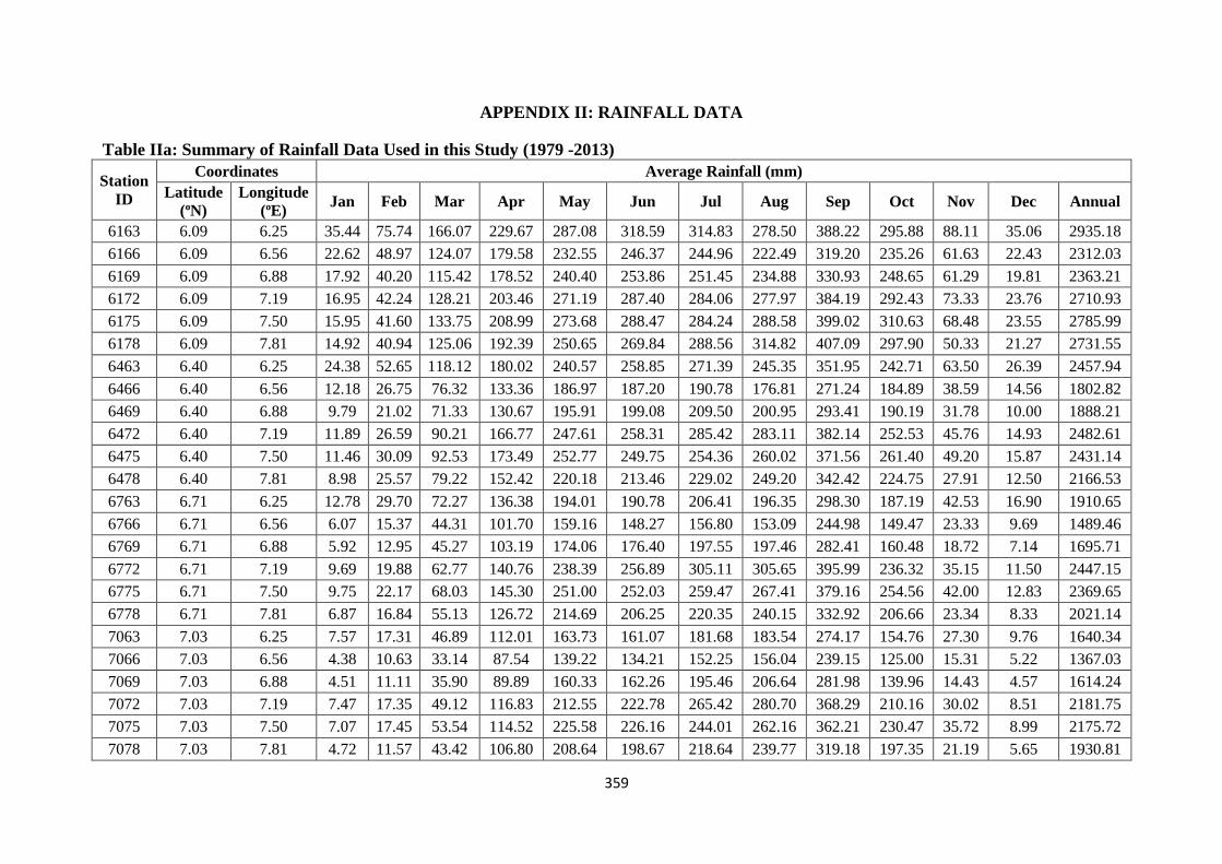
359

APPENDIX II: RAINFALL DATA

Table IIa: Summary of Rainfall Data Used in this Study (1979 -2013)

Station

ID

Coordinates Average Rainfall (mm)

Latitude

(oN)

Longitude

(oE) Jan Feb Mar Apr May Jun Jul Aug Sep Oct Nov Dec Annual

6163 6.09 6.25 35.44 75.74 166.07 229.67 287.08 318.59 314.83 278.50 388.22 295.88 88.11 35.06 2935.18

6166 6.09 6.56 22.62 48.97 124.07 179.58 232.55 246.37 244.96 222.49 319.20 235.26 61.63 22.43 2312.03

6169 6.09 6.88 17.92 40.20 115.42 178.52 240.40 253.86 251.45 234.88 330.93 248.65 61.29 19.81 2363.21

6172 6.09 7.19 16.95 42.24 128.21 203.46 271.19 287.40 284.06 277.97 384.19 292.43 73.33 23.76 2710.93

6175 6.09 7.50 15.95 41.60 133.75 208.99 273.68 288.47 284.24 288.58 399.02 310.63 68.48 23.55 2785.99

6178 6.09 7.81 14.92 40.94 125.06 192.39 250.65 269.84 288.56 314.82 407.09 297.90 50.33 21.27 2731.55

6463 6.40 6.25 24.38 52.65 118.12 180.02 240.57 258.85 271.39 245.35 351.95 242.71 63.50 26.39 2457.94

6466 6.40 6.56 12.18 26.75 76.32 133.36 186.97 187.20 190.78 176.81 271.24 184.89 38.59 14.56 1802.82

6469 6.40 6.88 9.79 21.02 71.33 130.67 195.91 199.08 209.50 200.95 293.41 190.19 31.78 10.00 1888.21

6472 6.40 7.19 11.89 26.59 90.21 166.77 247.61 258.31 285.42 283.11 382.14 252.53 45.76 14.93 2482.61

6475 6.40 7.50 11.46 30.09 92.53 173.49 252.77 249.75 254.36 260.02 371.56 261.40 49.20 15.87 2431.14

6478 6.40 7.81 8.98 25.57 79.22 152.42 220.18 213.46 229.02 249.20 342.42 224.75 27.91 12.50 2166.53

6763 6.71 6.25 12.78 29.70 72.27 136.38 194.01 190.78 206.41 196.35 298.30 187.19 42.53 16.90 1910.65

6766 6.71 6.56 6.07 15.37 44.31 101.70 159.16 148.27 156.80 153.09 244.98 149.47 23.33 9.69 1489.46

6769 6.71 6.88 5.92 12.95 45.27 103.19 174.06 176.40 197.55 197.46 282.41 160.48 18.72 7.14 1695.71

6772 6.71 7.19 9.69 19.88 62.77 140.76 238.39 256.89 305.11 305.65 395.99 236.32 35.15 11.50 2447.15

6775 6.71 7.50 9.75 22.17 68.03 145.30 251.00 252.03 259.47 267.41 379.16 254.56 42.00 12.83 2369.65

6778 6.71 7.81 6.87 16.84 55.13 126.72 214.69 206.25 220.35 240.15 332.92 206.66 23.34 8.33 2021.14

7063 7.03 6.25 7.57 17.31 46.89 112.01 163.73 161.07 181.68 183.54 274.17 154.76 27.30 9.76 1640.34

7066 7.03 6.56 4.38 10.63 33.14 87.54 139.22 134.21 152.25 156.04 239.15 125.00 15.31 5.22 1367.03

7069 7.03 6.88 4.51 11.11 35.90 89.89 160.33 162.26 195.46 206.64 281.98 139.96 14.43 4.57 1614.24

7072 7.03 7.19 7.47 17.35 49.12 116.83 212.55 222.78 265.42 280.70 368.29 210.16 30.02 8.51 2181.75

7075 7.03 7.50 7.07 17.45 53.54 114.52 225.58 226.16 244.01 262.16 362.21 230.47 35.72 8.99 2175.72

7078 7.03 7.81 4.72 11.57 43.42 106.80 208.64 198.67 218.64 239.77 319.18 197.35 21.19 5.65 1930.81

360

7363 7.34 6.25 6.87 13.74 40.99 113.05 168.35 169.08 198.03 207.65 293.88 151.16 22.94 6.82 1711.77

7366 7.34 6.56 3.77 8.00 29.27 87.51 140.76 138.58 170.11 180.84 251.30 116.12 12.00 3.26 1421.52

7369 7.34 6.88 4.08 9.69 33.97 86.13 155.88 160.09 206.18 219.57 286.58 127.47 13.48 3.52 1623.84

7372 7.34 7.19 4.59 12.79 42.02 94.15 181.26 185.99 218.63 237.87 318.93 164.75 21.20 4.93 1832.83

7375 7.34 7.50 3.75 11.74 40.32 87.76 176.74 171.61 195.51 218.88 298.70 166.17 19.93 4.30 1719.73

7378 7.34 7.81 2.53 7.69 31.25 79.96 172.49 158.71 189.44 213.88 278.22 149.76 14.25 2.95 1617.42

7663 7.65 6.25 4.23 10.60 37.85 127.68 191.77 190.75 224.10 245.57 310.34 154.05 19.79 3.71 1860.23

7666 7.65 6.56 2.80 6.23 28.51 97.00 152.79 146.71 197.66 217.85 258.10 108.70 10.00 2.65 1520.21

7669 7.65 6.88 3.13 7.77 31.80 92.21 158.28 155.62 225.17 243.16 280.00 114.74 9.82 2.85 1644.99

7672 7.65 7.19 3.59 9.44 37.45 92.29 173.91 162.50 215.12 228.92 291.56 137.74 13.66 3.32 1693.40

7675 7.65 7.50 2.33 8.23 33.25 79.62 153.33 135.17 176.47 193.52 256.44 126.59 10.83 2.92 1467.91

8063 7.96 6.25 1.89 6.15 28.25 130.61 199.57 197.82 245.57 272.44 302.56 136.71 11.20 1.45 1885.93

8066 7.96 6.56 1.67 4.71 24.41 105.74 161.46 155.37 213.69 245.64 252.57 100.44 6.50 1.07 1581.16

8069 7.96 6.88 2.56 5.29 31.00 105.33 165.20 165.72 246.95 275.81 278.69 110.74 7.58 1.93 1739.53

8072 7.96 7.19 3.44 6.95 35.82 105.03 181.61 177.30 245.46 264.15 303.59 138.76 10.87 2.71 1822.63

8075 7.96 7.50 2.74 7.23 33.28 95.90 169.07 153.39 210.79 227.02 275.87 129.10 9.45 2.54 1634.83

8078 7.96 7.81 2.32 6.78 31.24 90.47 168.22 160.10 235.60 253.67 291.14 124.23 8.07 2.42 1719.39

Table IIb: Detailed Historical Rainfall Data for some Towns within Hydrological Zone IVa

Stations Latitude

(N) Duration Jan Feb Mar Apr May Jun Jul Aug Sep Oct Nov Dec Total

Idah 7o06’ 32 8.60 14.00 36.50 112.90 153.60 185.90 177.60 168.80 227.90 148.50 26.40 3.90 1264.60

Onitsha 6o23’ 55 18.10 28.10 72.20 155.90 206.10 248.20 282.40 228.90 322.00 241.70 51.00 15.00 1869.60

Nsukka 7o52’ 21 14.00 20.15 75.65 144.15 187.40 178.75 231.10 173.60 307.00 213.65 47.65 15.35 1608.45

Adani 6o43’ 17 14.30 16.70 65.30 141.50 186.40 246.50 275.30 197.10 293.80 177.60 31.20 16.80 1662.50

Enugu 6o27’ 54 21.50 24.00 75.80 149.00 253.20 288.60 204.80 178.40 317.90 233.70 43.60 12.60 1803.10

Makurdi 7o41’ 30 3.70 3.65 18.75 81.83 135.36 169.20 186.53 234.13 205.88 118.39 7.25 1.14 1165.82

361

APPENDIX III: GAUGED STREAM FLOW DATA

Table III: Detailed Historical Discharge Record for Ofu River at Oforachi

Year Jan Feb Mar Apr May Jun Jul Aug Sep Oct Nov Dec

1955 3.90 2.90 2.10 11.40 8.00 18.60 79.00 399.90 228.60 153.60 2.50 3.90

1956 1.40 0.90 0.60 7.10 2.30 16.90 186.20 588.40 557.30 64.70 3.80 0.60

1957 2.9 1.90 1.30 15.40 36.80 28.40 95.60 350.80 435.50 160.10 6.50 0.80

1958 4.2 2.80 1.80 20.20 15.60 44.10 162.50 380.40 578.70 83.60 4.50 1.20

1959 1.1 0.60 0.60 6.90 10.50 18.70 79.00 361.20 362.10 47.60 3.20 0.50

1960 2.10 1.50 1.00 8.00 11.70 20.80 107.40 326.20 328.50 52.60 3.70 3.30

1961 1.90 1.30 0.80 21.90 3.70 60.60 225.10 508.80 555.10 85.50 13.40 0.60

1962 9.30 2.30 0.50 14.80 4.10 16.10 77.50 578.10 469.00 109.20 12.20 1.00

1963 10.50 9.00 8.10 19.10 43.20 16.00 76.00 290.90 322.90 113.10 7.20 17.20

1964 4.40 3.40 2.90 9.20 12.40 51.60 113.50 615.70 723.30 90.00 5.20 9.10

1965 3.40 2.20 1.60 11.80 4.90 86.50 150.10 486.00 405.70 47.20 4.90 1.50

1966 3.60 2.90 2.20 12.80 54.80 91.10 84.30 298.80 196.50 70.70 2.00 2.30

1967 0.50 1.50 1.20 18.40 9.90 43.40 156.70 466.00 516.90 90.40 8.80 1.20

1968 5.30 4.10 3.50 4.00 34.50 146.50 279.00 203.70 334.10 41.60 1.90 6.80

1969 1.30 1.10 1.10 23.20 12.10 28.20 133.30 457.30 419.60 162.00 5.20 1.00

1970 3.30 4.40 1.70 11.20 9.10 27.30 68.10 474.90 498.10 51.80 5.30 1.70

1971 4.20 3.60 3.10 13.30 9.20 50.60 154.50 445.90 482.00 54.00 7.50 4.70

1972 5.30 4.10 3.50 10.80 13.40 48.30 131.40 241.10 318.20 39.90 6.60 14.10

1973 4.70 3.70 3.10 13.30 6.90 22.60 157.30 198.00 476.30 59.50 5.80 3.10

Source: Kogi State Ministry of Water Resources and Rural Development

362

APPENDIX IV: SAMPLE SIZE ESTIMATOR

Source: The Research Advisors (2006)

363

APPENDIX V: DATA COLLECTION INSTRUMENTS

Appendix Va: Key Informants Interview (KII)

KEY INFORMANTS INTERVIEW QUESTIONNAIRE

1. Name of Community: ____________________________ 2. Ward:

________________________________

3. LGA: __________________________________ 4. Constituency: ________________________________

Respondent’s Personal Information

5. Name:__________________________ 6. Position: ___________7. Sex: Male [ ] Female [ ]

8. Age: 20-25 [ ] 26-30 [ ] 31-35 [ ] 36-40 [ ] above 40 [ ]

9. Marital Status: Single [ ] Married [ ] Divorced [ ] Separated [ ] Widowed [ ]

10. Highest Educational Level: Primary [ ] Secondary [ ] Tertiary [ ] Others (specify)______

11. Occupation_______________________________ 12. Family size_________________________

13. How long have you lived in the Community? __________________________ years

Flood History

14. What year did you start experiencing flood in this community? ________________________________

15. Was there any change in the magnitude? Yes [ ] No [ ]

16. If yes what year did you observe this change? Yes [ ] No [ ]

17. What year was the Idah-Nsukka highway constructed? _____________________________________

18. What year was the new Oforachi bridge constructed? ____________________________________

19. Do you think there is a relationship between the construction and the flood? Yes [ ] No [ ]

20. What do you think are the causes of flood in this community (Probe for all possible causes)?

21. Have you had any loss of live as a result of flood? Yes [ ] No [ ]

22. Has there been any case of injuries? Yes [ ] No [ ]

Has any of the following happened as a result of flood?

23. Building submerged? Yes [ ] No [ ]

24. Building collapsed? Yes [ ] No [ ]

25. Crops destroyed? Yes [ ] No [ ]

26. Goods in shop/market affected? Yes [ ] No [ ]

27. Access road submerged? Yes [ ] No [ ]

28. Children unable to go to school? Yes [ ] No [ ]

29. Loss of livestock? Yes [ ] No [ ]

30. Sickness (Epidemic outbreak)? Yes [ ] No [ ]

31. Did you have to evacuate people from their houses? Yes [ ] No [ ]

_____________________ ______________________

Name of Enumerator Signature & Date

FLOOD HAZARD VULNERABILITY AND RISK ASSESSMENT FOR OFU RIVER FLOOD PLAIN IN KOGI

STATE, NORTHCENTRAL NIGERIA

Being a Ph.D Research Survey

ID:

___________

364

Appendix Vb: Household Survey

HOUSEHOLD QUESTIONNAIRE

1. Name of Community: ____________________________ 2. Ward: ___________________

3. LGA: __________________________________

Section A: Respondent’s Personal Information

4. Name:__________________________________ 5. Position:___________________

6. Sex: Male [ ] Female [ ]

7. Age: 20-25 [ ] 26-30 [ ] 31-35 [ ] 36-40 [ ] above 40 [ ]

8. Marital Status: Single [ ] Married [ ] Divorced [ ] Separated [ ] Widowed [ ]

9. Educational Level: Primary [ ] Secondary [ ] Tertiary [ ] Adult Education [ ] Others specify)___

10. Occupation: Farming [ ] Trading [ ] Civil Servant [ ] Craftsman [ ] Others [ ]

11. Family size_________________________

12. How long have you lived in the Community? 1-10 [ ] 11-20 [ ] 21-30 [ ] 31-40 [ ] above 40[ ]

Section B: Respondent’s opinion on Flood occurrence

13. Have you ever experienced flood in your house? Yes [ ] No [ ]

14. If yes, what year did you start experiencing flood? ________________________________

15. How often is your house flooded?

Max. Depth How often Maximum Duration (days)

Ankle

Knee

Waist

Breast

First floor

Section C: Respondent’s opinion on causes of Flood (For Respondents who answered yes to 13)

(Tick any of the options as it applies to your opinion on causes of flood at Oforachi)

Strongl

y Agree Agree Indifferent Disagree

Strongly

Disagree

16. The Construction of the Idah-Nsukka highway is

one of the factors responsible for flood

17. Prolonged rainfall is one of the causes of flood

18. Heavy rainfall upstream sometimes result in flood at

Oforachi

19. Embankment breach by individuals contributes to

the flood

20. There is a significant loss in the flow depth of Ofu

river at Oforachi

FLOOD HAZARD VULNERABILITY AND RISK ASSESSMENT FOR OFU RIVER FLOOD

PLAIN IN KOGI STATE, NORTHCENTRAL NIGERIA

Being a Ph.D Research Survey

ID:

___________

365

Section D: Respondents’ opinion on the Impact of 1995 and 2000 Flood Event

(For Respondents who answered yes to 13)

1995 2000

34. Where you affected by the 1995 and/or 2000 flood? Yes [ ] No [ ] Yes [ ] No [ ]

Did you experience any of the following as a result of the 1995 and/or 2000 flood event? Tick appropriately

35. Loss of lives? Yes [ ] No [ ] Yes [ ] No [ ]

36. Injuries to members of your household? Yes [ ] No [ ] Yes [ ] No [ ]

37. Building submerged? Yes [ ] No [ ] Yes [ ] No [ ]

38. Building collapsed? Yes [ ] No [ ] Yes [ ] No [ ]

39. Crops destroyed? Yes [ ] No [ ] Yes [ ] No [ ]

40. Goods in shop/market affected? Yes [ ] No [ ] Yes [ ] No [ ]

41. Access road submerged? Yes [ ] No [ ] Yes [ ] No [ ]

42. Children unable to go to school? Yes [ ] No [ ] Yes [ ] No [ ]

43. Loss of livestock? Yes [ ] No [ ] Yes [ ] No [ ]

44. Sickness (Epidemic outbreak)? Yes [ ] No [ ] Yes [ ] No [ ]

45. Were you evacuated from your house? Yes [ ] No [ ] Yes [ ] No [ ]

Section E: Respondents’ opinion on the Availability of Toilet Facility and Household source of drinking water

46. Do you have a toilet facility in your house? Yes [ ] No [ ]

47. If yes to 47, what type? Pit Latrine [ ] VIP Latrine [ ] Water closet [ ]

48. If No to 47, where do you defecate? Open Field [ ] Neighbour’s house [ ] Others_______

49. Where do you get drinking water from? Ofu River [ ] Borehole [ ]

_____________________ ______________________

Name of Enumerator Signature & Date

366

APPENDIX VI: STREAM DISCHARGE MEASUREMENTS AND

CALCULATIONS

Distance from

Origin (m)

Width

(m)

Ave Depth

(m)

Sectional

Area (m2)

Time (s)Av. Vel

(m/s)

Sectional

Discharge

(m3/s)0.2d 0.6d 0.8d 0.2d 0.8d

1 1 1.192 1.986 1.986 20 0.006 0.011916

2 1 0.4572 1.8288 2.286 2.286 20 0.007 0.005 0.006 0.013716

3 1 0.4752 1.9008 2.376 2.376 20 0.011 0.0091 0.01005 0.0238788

4 1 0.4652 1.8608 2.326 2.326 20 0.012 0.01 0.011 0.025586

5 1 1.18 1.966 1.966 20 0.016 0.031456

6 1 0.966 1.61 1.61 20 0.015 0.02415

7 1 0.924 1.54 1.54 20 0.006 0.00924

8 1 0.804 1.34 1.34 20 0.004 0.00536

9 1 0.648 1.08 1.08 20 0.0035 0.00378

10 1 0.72 1.2 1.2 20 0.003 0.0036

11 1 0.684 1.14 1.14 20 0.003 0.00342

12 1 0.657 1.095 1.095 20 0.002 0.00219

0.1582928

RIVER DISCHARGE MEASUREMENT

Depth of Observation (m)

End Time: 15:39

Velocity (m/s)

River: Ofu

River Basin: Ofu-Imabolo

Location/Station: Oforachi Coordinates:

Gage Height: 55.432 Date: 13-02-2016 Start Time: 13:48

Distance from

Origin (m)

Width

(m)

Ave Depth

(m)

Sectional

Area (m2)

Time (s)Av. Vel

(m/s)

Sectional

Discharge

(m3/s)

0.2d 0.6d 0.8d 0.2d 0.8d

1 1 1.068 1.78 1.78 20 0.003 0.001 0.002 0.00356

2 1 0.4632 1.8528 2.316 2.316 20 0.033 0.024 0.0285 0.066006

3 1 0.4812 1.9248 2.406 2.406 20 0.028 0.011 0.0195 0.046917

4 1 0.4714 1.8856 2.357 2.357 20 0.012 0.011 0.0115 0.0271055

5 1 1.198 1.996 1.996 20 0.021 0.041916

6 1 1.064 1.774 1.774 20 0.012 0.021288

7 1 0.98 1.634 1.634 20 0.011 0.017974

8 1 0.928 1.546 1.546 20 0.01 0.01546

9 1 0.881 1.469 1.469 20 0.009 0.013221

10 1 0.868 1.446 1.446 20 0.005 0.00723

11 1 0.841 1.402 1.402 20 0.004 0.005608

12 1 0.74 1.234 1.234 20 0.002 0.002468

0.2687535


River: Ofu Gage Height: 55.462 Start Time: 16:42

Depth of Observation (m) Velocity (m/s)

Date: 14-02-2016

River Basin: Ofu-Imabolo

Coordinates:

End Time: 18:14

Location/Station: Oforachi

367

Distance

from Origin

(m)

Width (m)Ave Depth

(m)

Sectional

Area (m2)

Time (s)Av. Vel

(m/s)

Sectional

Discharge

(m3/s)

0.2d 0.6d 0.8d 0.2d 0.8d

1 1 0.414 1.656 2.07 2.07 20 0.247 0.223 0.235 0.48645

2 1 0.47 1.88 2.35 2.35 20 0.3255 0.3197 0.3226 0.75811

3 1 0.512 2.048 2.56 2.56 20 0.3611 0.36 0.36055 0.923008

4 1 0.496 1.984 2.48 2.48 20 0.2812 0.2801 0.28065 0.696012

5 1 0.414 1.656 2.07 2.07 20 0.234 0.48438

6 1 0.996 1.66 1.66 20 0.221 0.36686

7 1 0.984 1.64 1.64 20 0.061 0.10004

8 1 0.954 1.59 1.59 20 0.059 0.09381

9 1 0.936 1.56 1.56 20 0.055 0.0858

10 1 0.876 1.46 1.46 20 0.051 0.07446

11 1 0.852 1.42 1.42 20 0.046 0.06532

12 1 0.84 1.4 1.4 20 0.042 0.0588

13 1 0.768 1.28 1.28 20 0.039 0.04992

4.24297

River Basin: Ofu-Imabolo End Time: 09:25


River: Ofu Gage Height: 55.521 Date: 26-03-2016 Start Time: 07:00



Distance

from Origin

(m)

Width (m)Ave Depth

(m)

Sectional

Area (m2)

Time (s)Av. Vel

(m/s)

Sectional

Discharge

(m3/s)

0.2d 0.6d 0.8d 0.2d 0.8d

1 1 0.412 1.648 2.06 2.06 20 0.212 0.208 0.21 0.4326

2 1 0.472 1.888 2.36 2.36 20 0.297 0.295 0.296 0.69856

3 1 0.49 1.96 2.45 2.45 20 0.322 0.319 0.3205 0.785225

4 1 0.48 1.92 2.4 2.4 20 0.255 0.253 0.254 0.6096

5 1 0.408 1.632 2.04 2.04 20 0.298 0.60792

6 1 1.014 1.69 1.69 20 0.287 0.48503

7 1 0.99 1.65 1.65 20 0.069 0.11385

8 1 0.954 1.59 1.59 20 0.062 0.09858

9 1 0.93 1.55 1.55 20 0.059 0.09145

10 1 0.882 1.47 1.47 20 0.055 0.08085

11 1 0.876 1.46 1.46 20 0.053 0.07738

12 1 0.876 1.46 1.46 20 0.051 0.07446

13 1 0.774 1.29 1.29 20 0.049 0.06321

4.218715






368

Distance

from Origin

(m)

Width (m)Ave Depth

(m)

Sectional

Area (m2)

Time (s)Av. Vel

(m/s)

Sectional

Discharge

(m3/s)

0.2d 0.6d 0.8d 0.2d 0.8d

1 1 0.428 1.712 2.14 2.14 20 0.227 0.172 0.1995 0.42693

2 1 0.426 1.704 2.13 2.13 20 0.277 0.222 0.2495 0.531435

3 1 0.492 1.968 2.46 2.46 20 0.31 0.294 0.302 0.74292

4 1 0.462 1.848 2.31 2.31 20 0.305 0.32 0.3125 0.721875

5 1 1.182 1.97 1.97 20 0.388 0.76436

6 1 1.026 1.71 1.71 20 0.294 0.50274

7 1 1.008 1.68 1.68 20 0.071 0.11928

8 1 0.972 1.62 1.62 20 0.069 0.11178

9 1 0.954 1.59 1.59 20 0.066 0.10494

10 1 0.918 1.53 1.53 20 0.064 0.09792

11 1 0.894 1.49 1.49 20 0.062 0.09238

12 1 0.876 1.46 1.46 20 0.061 0.08906

13 1 0.81 1.35 1.35 20 0.059 0.07965

4.38527






Distance

from Origin

(m)

Width (m)Ave Depth

(m)

Sectional

Area (m2)

Time (s)Av. Vel

(m/s)

Sectional

Discharge

(m3/s)

0.2d 0.6d 0.8d 0.2d 0.8d

1 1 1.122 1.87 1.87 20 0.222 0.41514

2 1 0.434 1.736 2.17 2.17 20 0.337 0.231 0.284 0.61628

3 1 0.486 1.944 2.43 2.43 20 0.351 0.241 0.296 0.71928

4 1 0.464 1.856 2.32 2.32 20 0.358 0.245 0.3015 0.69948

5 1 0.426 1.704 2.13 2.13 20 0.365 0.251 0.308 0.65604

6 1 1.068 1.78 1.78 20 0.305 0.5429

7 1 0.864 1.44 1.44 20 0.273 0.39312

8 1 1.032 1.72 1.72 20 0.132 0.22704

9 1 0.954 1.59 1.59 20 0.114 0.18126

10 1 0.96 1.6 1.6 20 0.064 0.1024

11 1 0.846 1.41 1.41 20 0.062 0.08742

12 1 0.828 1.38 1.38 20 0.061 0.08418

13 1 0.822 1.37 1.37 20 0.059 0.08083

4.80537






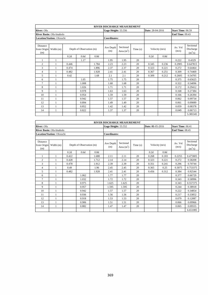
369

Distance

from Origin

(m)

Width (m)Ave Depth

(m)

Sectional

Area (m2)

Time (s)Av. Vel

(m/s)

Sectional

Discharge

(m3/s)

0.2d 0.6d 0.8d 0.2d 0.8d

1 1 1.17 1.95 1.95 20 0.222 0.4329

2 1 0.446 1.784 2.23 2.23 20 0.345 0.236 0.2905 0.647815

3 1 0.474 1.896 2.37 2.37 20 0.323 0.221 0.272 0.64464

4 1 0.482 1.928 2.41 2.41 20 0.367 0.251 0.309 0.74469

5 1 0.42 1.68 2.1 2.1 20 0.309 0.212 0.2605 0.54705

6 1 1.05 1.75 1.75 20 0.375 0.65625

7 1 1.008 1.68 1.68 20 0.322 0.54096

8 1 1.026 1.71 1.71 20 0.172 0.29412

9 1 0.978 1.63 1.63 20 0.168 0.27384

10 1 0.954 1.59 1.59 20 0.166 0.26394

11 1 0.942 1.57 1.57 20 0.062 0.09734

12 1 0.894 1.49 1.49 20 0.061 0.09089

13 1 0.852 1.42 1.42 20 0.059 0.08378

14 1 0.822 1.37 1.37 20 0.049 0.06713

5.385345






Distance

from Origin

(m)

Width (m)Ave Depth

(m)

Sectional

Area (m2)

Time (s)Av. Vel

(m/s)

Sectional

Discharge

(m3/s)

0.2d 0.6d 0.8d 0.2d 0.8d

1 1 0.422 1.688 2.11 2.11 20 0.268 0.183 0.2255 0.475805

2 1 0.428 1.712 2.14 2.14 20 0.323 0.221 0.272 0.58208

3 1 0.478 1.912 2.39 2.39 20 0.351 0.241 0.296 0.70744

4 1 0.49 1.96 2.45 2.45 20 0.365 0.25 0.3075 0.753375

5 1 0.482 1.928 2.41 2.41 20 0.456 0.312 0.384 0.92544

6 1 1.062 1.77 1.77 20 0.377 0.66729

7 1 1.032 1.72 1.72 20 0.343 0.58996

8 1 0.975 1.625 1.625 20 0.343 0.557375

9 1 0.957 1.595 1.595 20 0.244 0.38918

10 1 0.942 1.57 1.57 20 0.222 0.34854

11 1 0.936 1.56 1.56 20 0.217 0.33852

12 1 0.918 1.53 1.53 20 0.079 0.12087

13 1 0.906 1.51 1.51 20 0.066 0.09966

14 1 0.882 1.47 1.47 20 0.065 0.09555

6.651085






370

Distance

from Origin

(m)

Width (m)Ave Depth

(m)

Sectional

Area (m2)

Time (s)Av. Vel

(m/s)

Sectional

Discharge

(m3/s)

0.2d 0.6d 0.8d 0.2d 0.8d

1 1 0.428 1.712 2.14 2.14 20 0.282 0.193 0.2375 0.50825

2 1 0.434 1.736 2.17 2.17 20 0.337 0.231 0.284 0.61628

3 1 0.468 1.872 2.34 2.34 20 0.317 0.217 0.267 0.62478

4 1 0.482 1.928 2.41 2.41 20 0.365 0.25 0.3075 0.741075

5 1 0.418 1.672 2.09 2.09 20 0.47 0.322 0.396 0.82764

6 1 1.056 1.76 1.76 20 0.332 0.58432

7 1 0.996 1.66 1.66 20 0.343 0.56938

8 1 0.924 1.54 1.54 20 0.332 0.51128

9 1 0.984 1.64 1.64 20 0.299 0.49036

10 1 1.128 1.88 1.88 20 0.25 0.47

11 1 0.942 1.57 1.57 20 0.221 0.34697

12 1 0.924 1.54 1.54 20 0.081 0.12474

13 1 0.906 1.51 1.51 20 0.073 0.11023

14 1 0.894 1.49 1.49 20 0.071 0.10579

6.631095






Distance

from Origin

(m)

Width (m)Ave Depth

(m)

Sectional

Area (m2)

Time (s)Av. Vel

(m/s)

Sectional

Discharge

(m3/s)

0.2d 0.6d 0.8d 0.2d 0.8d

1 1 1.068 1.78 1.78 20 0.198 0.35244

2 1 0.464 1.856 2.32 2.32 20 0.227 0.187 0.207 0.48024

3 1 0.498 1.992 2.49 2.49 20 0.277 0.213 0.245 0.61005

4 1 0.5 2 2.5 2.5 20 0.366 0.301 0.3335 0.83375

5 1 0.458 1.832 2.29 2.29 20 0.343 0.279 0.311 0.71219

6 1 1.068 1.78 1.78 20 0.349 0.62122

7 1 1.08 1.8 1.8 20 0.371 0.6678

8 1 1.068 1.78 1.78 20 0.338 0.60164

9 1 1.05 1.75 1.75 20 0.294 0.5145

10 1 1.032 1.72 1.72 20 0.251 0.43172

11 1 1.038 1.73 1.73 20 0.232 0.40136

12 1 0.984 1.64 1.64 20 0.104 0.17056

13 1 0.972 1.62 1.62 20 0.091 0.14742

14 1 0.942 1.57 1.57 20 0.082 0.12874

15 1 0.93 1.55 1.55 20 0.74 1.147

16 1 0.894 1.49 1.49 20 0.057 0.08493

7.90556






371

Distance

from Origin

(m)

Width (m)Ave Depth

(m)

Sectional

Area (m2)

Time (s)Av. Vel

(m/s)

Sectional

Discharge

(m3/s)

0.2d 0.6d 0.8d 0.2d 0.8d

1 1 1.068 1.78 1.78 20 0.223 0.39694

2 1 0.464 1.856 2.32 2.32 20 0.249 0.224 0.2365 0.54868

3 1 0.498 1.992 2.49 2.49 20 0.293 0.268 0.2805 0.698445

4 1 0.5 2 2.5 2.5 20 0.3755 0.3505 0.363 0.9075

5 1 0.458 1.832 2.29 2.29 20 0.345 0.32 0.3325 0.761425

6 1 1.068 1.78 1.78 20 0.372 0.66216

7 1 1.08 1.8 1.8 20 0.395 0.711

8 1 1.068 1.78 1.78 20 0.36 0.6408

9 1 1.05 1.75 1.75 20 0.316 0.553

10 1 1.032 1.72 1.72 20 0.273 0.46956

11 1 1.038 1.73 1.73 20 0.254 0.43942

12 1 0.984 1.64 1.64 20 0.126 0.20664

13 1 0.972 1.62 1.62 20 0.113 0.18306

14 1 0.942 1.57 1.57 20 0.104 0.16328

15 1 0.93 1.55 1.55 20 0.762 1.1811

16 1 0.894 1.49 1.49 20 0.079 0.11771

8.64072






Distance

from Origin

(m)

Width (m)Ave Depth

(m)

Sectional

Area (m2)

Time (s)Av. Vel

(m/s)

Sectional

Discharge

(m3/s)

0.2d 0.6d 0.8d 0.2d 0.8d

1 1 1.176 1.96 1.96 20 0.198 0.38808

2 1 0.43 1.72 2.15 2.15 20 0.227 0.187 0.207 0.44505

3 1 0.51 2.04 2.55 2.55 20 0.272 0.213 0.2425 0.618375

4 1 0.5 2 2.5 2.5 20 0.31 0.301 0.3055 0.76375

5 1 0.442 1.768 2.21 2.21 20 0.366 0.279 0.3225 0.712725

6 1 1.14 1.9 1.9 20 0.299 0.5681

7 1 1.134 1.89 1.89 20 0.36 0.6804

8 1 0.99 1.65 1.65 20 0.288 0.4752

9 1 1.008 1.68 1.68 20 0.291 0.48888

10 1 0.972 1.62 1.62 20 0.277 0.44874

11 1 0.966 1.61 1.61 20 0.252 0.40572

12 1 0.978 1.63 1.63 20 0.179 0.29177

13 1 0.966 1.61 1.61 20 0.088 0.14168

14 1 0.93 1.55 1.55 20 0.064 0.0992

15 1 0.906 1.51 1.51 20 0.061 0.09211

16 1 0.834 1.39 1.39 20 0.054 0.07506

6.69484






372

Distance

from Origin

(m)

Width (m)Ave Depth

(m)

Sectional

Area (m2)

Time (s)Av. Vel

(m/s)

Sectional

Discharge

(m3/s)

0.2d 0.6d 0.8d 0.2d 0.8d

1 1 1.176 1.96 1.96 20 0.223 0.43708

2 1 0.43 1.72 2.15 2.15 20 0.249 0.224 0.2365 0.508475

3 1 0.51 2.04 2.55 2.55 20 0.2905 0.2655 0.278 0.7089

4 1 0.5 2 2.5 2.5 20 0.3475 0.3225 0.335 0.8375

5 1 0.442 1.768 2.21 2.21 20 0.3565 0.3315 0.344 0.76024

6 1 1.14 1.9 1.9 20 0.322 0.6118

7 1 1.134 1.89 1.89 20 0.384 0.72576

8 1 0.99 1.65 1.65 20 0.31 0.5115

9 1 1.008 1.68 1.68 20 0.313 0.52584

10 1 0.972 1.62 1.62 20 0.299 0.48438

11 1 0.966 1.61 1.61 20 0.274 0.44114

12 1 0.978 1.63 1.63 20 0.201 0.32763

13 1 0.966 1.61 1.61 20 0.11 0.1771

14 1 0.93 1.55 1.55 20 0.086 0.1333

15 1 0.906 1.51 1.51 20 0.083 0.12533

16 1 0.834 1.39 1.39 20 0.076 0.10564

7.421615






Distance

from Origin

(m)

Width (m)Ave Depth

(m)

Sectional

Area (m2)

Time (s)Av. Vel

(m/s)

Sectional

Discharge

(m3/s)

0.2d 0.6d 0.8d 0.2d 0.8d

1 1 0.49 1.96 2.45 2.45 20 0.266 0.241 0.2535 0.621075

2 1 0.642 2.568 3.21 3.21 20 0.283 0.259 0.271 0.86991

3 1 0.68 2.72 3.4 3.4 20 0.502 0.479 0.4905 1.6677

4 1 0.664 2.656 3.32 3.32 20 0.339 0.314 0.3265 1.08398

5 1 0.62 2.48 3.1 3.1 20 0.369 0.344 0.3565 1.10515

6 1 0.56 2.24 2.8 2.8 20 0.519 0.494 0.5065 1.4182

7 1 0.54 2.16 2.7 2.7 20 0.468 0.444 0.456 1.2312

8 1 0.48 1.92 2.4 2.4 20 0.453 0.428 0.4405 1.0572

9 1 0.408 1.632 2.04 2.04 20 0.457 0.432 0.4445 0.90678

10 1 1.188 1.98 1.98 20 0.408 0.80784

11 1 1.182 1.97 1.97 20 0.389 0.76633

12 1 1.194 1.99 1.99 20 0.357 0.71043

13 1 1.182 1.97 1.97 20 0.262 0.51614

14 1 1.146 1.91 1.91 20 0.143 0.27313

15 1 1.122 1.87 1.87 20 0.112 0.20944

16 1 1.05 1.75 1.75 20 0.109 0.19075

13.435255






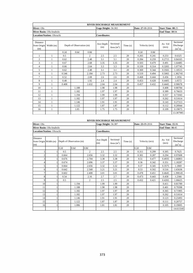
373

Distance

from Origin

(m)

Width (m)Ave Depth

(m)

Sectional

Area (m2)

Time (s)Av. Vel

(m/s)

Sectional

Discharge

(m3/s)

0.2d 0.6d 0.8d 0.2d 0.8d

1 1 0.5 2 2.5 2.5 20 0.265 0.241 0.253 0.6325

2 1 0.62 2.48 3.1 3.1 20 0.284 0.259 0.2715 0.84165

3 1 0.67 2.68 3.35 3.35 20 0.503 0.479 0.491 1.64485

4 1 0.66 2.64 3.3 3.3 20 0.339 0.314 0.3265 1.07745

5 1 0.62 2.48 3.1 3.1 20 0.369 0.344 0.3565 1.10515

6 1 0.546 2.184 2.73 2.73 20 0.519 0.494 0.5065 1.382745

7 1 0.52 2.08 2.6 2.6 20 0.468 0.444 0.456 1.1856

8 1 0.48 1.92 2.4 2.4 20 0.453 0.428 0.4405 1.0572

9 1 0.408 1.632 2.04 2.04 20 0.457 0.432 0.4445 0.90678

10 1 1.188 1.98 1.98 20 0.408 0.80784

11 1 1.182 1.97 1.97 20 0.389 0.76633

12 1 1.194 1.99 1.99 20 0.357 0.71043

13 1 1.182 1.97 1.97 20 0.262 0.51614

14 1 1.146 1.91 1.91 20 0.143 0.27313

15 1 1.122 1.87 1.87 20 0.112 0.20944

16 1 1.05 1.75 1.75 20 0.109 0.19075

13.307985






Distance

from Origin

(m)

Width (m)Ave Depth

(m)

Sectional

Area (m2)

Time (s)Av. Vel

(m/s)

Sectional

Discharge

(m3/s)

0.2d 0.6d 0.8d 0.2d 0.8d

1 1 0.5 2 2.5 2.5 20 0.311 0.299 0.305 0.7625

2 1 0.664 2.656 3.32 3.32 20 0.301 0.287 0.294 0.97608

3 1 0.676 2.704 3.38 3.38 20 0.51 0.477 0.4935 1.66803

4 1 0.674 2.696 3.37 3.37 20 0.36 0.342 0.351 1.18287

5 1 0.664 2.656 3.32 3.32 20 0.37 0.345 0.3575 1.1869

6 1 0.642 2.568 3.21 3.21 20 0.53 0.502 0.516 1.65636

7 1 0.602 2.408 3.01 3.01 20 0.478 0.451 0.4645 1.398145

8 1 0.54 2.16 2.7 2.7 20 0.473 0.443 0.458 1.2366

9 1 0.5 2 2.5 2.5 20 0.432 0.421 0.4265 1.06625

10 1 1.194 1.99 1.99 20 0.411 0.81789

11 1 1.188 1.98 1.98 20 0.401 0.79398

12 1 1.182 1.97 1.97 20 0.365 0.71905

13 1 1.182 1.97 1.97 20 0.262 0.51614

14 1 1.146 1.91 1.91 20 0.123 0.23493

15 1 1.122 1.87 1.87 20 0.111 0.20757

16 1 1.086 1.81 1.81 20 0.105 0.19005

14.613345






374

Distance

from Origin

(m)

Width (m)Ave Depth

(m)

Sectional

Area (m2)

Time (s)Av. Vel

(m/s)

Sectional

Discharge

(m3/s)

0.2d 0.6d 0.8d 0.2d 0.8d

1 1 0.502 2.008 2.51 2.51 20 0.301 0.278 0.2895 0.726645

2 1 0.644 2.576 3.22 3.22 20 0.29 0.26 0.275 0.8855

3 1 0.686 2.744 3.43 3.43 20 0.51 0.481 0.4955 1.699565

4 1 0.67 2.68 3.35 3.35 20 0.361 0.332 0.3465 1.160775

5 1 0.66 2.64 3.3 3.3 20 0.37 0.345 0.3575 1.17975

6 1 0.6 2.4 3 3 20 0.53 0.5 0.515 1.545

7 1 0.58 2.32 2.9 2.9 20 0.48 0.451 0.4655 1.34995

8 1 0.52 2.08 2.6 2.6 20 0.473 0.443 0.458 1.1908

9 1 0.46 1.84 2.3 2.3 20 0.445 0.439 0.442 1.0166

10 1 1.188 1.98 1.98 20 0.408 0.80784

11 1 1.182 1.97 1.97 20 0.389 0.76633

12 1 1.194 1.99 1.99 20 0.357 0.71043

13 1 1.182 1.97 1.97 20 0.262 0.51614

14 1 1.146 1.91 1.91 20 0.143 0.27313

15 1 1.122 1.87 1.87 20 0.112 0.20944

16 1 1.104 1.84 1.84 20 0.109 0.20056

14.238455






Distance

from Origin

(m)

Width (m)Ave Depth

(m)

Sectional

Area (m2)

Time (s)Av. Vel

(m/s)

Sectional

Discharge

(m3/s)

0.2d 0.6d 0.8d 0.2d 0.8d

1 1 0.43 1.72 2.15 2.15 20 0.213 0.188 0.2005 0.431075

2 1 0.466 1.864 2.33 2.33 20 0.246 0.221 0.2335 0.544055

3 1 0.49 1.96 2.45 2.45 20 0.251 0.226 0.2385 0.584325

4 1 0.52 2.08 2.6 2.6 20 0.323 0.298 0.3105 0.8073

5 1 0.42 1.68 2.1 2.1 20 0.368 0.343 0.3555 0.74655

6 1 0.4 1.6 2 2 20 0.362 0.337 0.3495 0.699

7 1 1.14 1.9 1.9 20 0.388 0.7372

8 1 1.17 1.95 1.95 20 0.355 0.69225

9 1 1.074 1.79 1.79 20 0.304 0.54416

10 1 1.032 1.72 1.72 20 0.296 0.50912

11 1 1.026 1.71 1.71 20 0.199 0.34029

12 1 1.044 1.74 1.74 20 0.198 0.34452

13 1 1.038 1.73 1.73 20 0.151 0.26123

14 1 1.002 1.67 1.67 20 0.097 0.16199

15 1 0.978 1.63 1.63 20 0.087 0.14181

16 1 0.906 1.51 1.51 20 0.086 0.12986

7.674735






375

Distance

from Origin

(m)

Width (m)Ave Depth

(m)

Sectional

Area (m2)

Time (s)Av. Vel

(m/s)

Sectional

Discharge

(m3/s)

0.2d 0.6d 0.8d 0.2d 0.8d

1 1 0.416 1.664 2.08 2.08 20 0.008 0.0059 0.00695 0.014456

2 1 0.43 1.72 2.15 2.15 20 0.0085 0.006 0.00725 0.0155875

3 1 0.474 1.896 2.37 2.37 20 0.012 0.01 0.011 0.02607

4 1 0.5 2 2.5 2.5 20 0.02 0.011 0.0155 0.03875

5 1 0.446 1.784 2.23 2.23 20 0.011 0.008 0.0095 0.021185

6 1 0.4 1.6 2 2 20 0.007 0.005 0.006 0.012

7 1 1.116 1.86 1.86 20 0.008 0.01488

8 1 0.99 1.65 1.65 20 0.011 0.01815

9 1 0.96 1.6 1.6 20 0.009 0.0144

10 1 0.936 1.56 1.56 20 0.0079 0.012324

11 1 0.93 1.55 1.55 20 0.0054 0.00837

12 1 0.912 1.52 1.52 20 0.0033 0.005016

13 1 0.9 1.5 1.5 20 0.0025 0.00375

14 1 0.894 1.49 1.49 20 0.0023 0.003427

15 1 0.852 1.42 1.42 20 0.0011 0.001562

0.2099275






Distance

from Origin

(m)

Width (m)Ave Depth

(m)

Sectional

Area (m2)

Time (s)Av. Vel

(m/s)

Sectional

Discharge

(m3/s)

0.2d 0.6d 0.8d 0.2d 0.8d

1 1 0.418 1.672 2.09 2.09 20 0.008 0.006 0.007 0.01463

2 1 0.436 1.744 2.18 2.18 20 0.009 0.007 0.008 0.01744

3 1 0.478 1.912 2.39 2.39 20 0.012 0.091 0.0515 0.123085

4 1 0.504 2.016 2.52 2.52 20 0.023 0.012 0.0175 0.0441

5 1 0.45 1.8 2.25 2.25 20 0.011 0.007 0.009 0.02025

6 1 0.404 1.616 2.02 2.02 20 0.008 0.005 0.0065 0.01313

7 1 1.134 1.89 1.89 20 0.008 0.01512

8 1 1.002 1.67 1.67 20 0.011 0.01837

9 1 0.966 1.61 1.61 20 0.009 0.01449

10 1 0.936 1.56 1.56 20 0.0079 0.012324

11 1 0.93 1.55 1.55 20 0.0054 0.00837

12 1 0.906 1.51 1.51 20 0.0033 0.004983

13 1 0.9 1.5 1.5 20 0.0025 0.00375

14 1 0.894 1.49 1.49 20 0.0023 0.003427

15 1 0.858 1.43 1.43 20 0.0011 0.001573

0.315042






376

Distance

from Origin

(m) Width (m)

Ave Depth

(m)

Sectional

Area (m2)

Time (s)Av. Vel

(m/s)

Sectional

Discharge

(m3/s)

0.2d 0.6d 0.8d 0.2d 0.8d

1 1 0.406 1.624 2.03 2.03 20 0.007 0.005 0.006 0.01218

2 1 0.442 1.768 2.21 2.21 20 0.009 0.008 0.0085 0.018785

3 1 0.472 1.888 2.36 2.36 20 0.013 0.009 0.011 0.02596

4 1 0.47 1.88 2.35 2.35 20 0.015 0.0095 0.01225 0.0287875

5 1 0.432 1.728 2.16 2.16 20 0.009 0.008 0.0085 0.01836

6 1 1.104 1.84 1.84 20 0.006 0.01104

7 1 1.074 1.79 1.79 20 0.009 0.01611

8 1 0.966 1.61 1.61 20 0.0095 0.015295

9 1 0.93 1.55 1.55 20 0.009 0.01395

10 1 0.87 1.45 1.45 20 0.0052 0.00754

11 1 0.84 1.4 1.4 20 0.0028 0.00392

12 1 0.828 1.38 1.38 20 0.0025 0.00345

13 1 0.81 1.35 1.35 20 0.001 0.00135

14 1 0.798 1.33 1.33 20 0.001 0.00133

0.1780575






Distance

from Origin

(m)

Width (m)Ave Depth

(m)

Sectional

Area (m2)

Time (s)Av. Vel

(m/s)

Sectional

Discharge

(m3/s)

0.2d 0.6d 0.8d 0.2d 0.8d

1 1 0.404 1.616 2.02 2.02 20 0.007 0.005 0.006 0.01212

2 1 0.448 1.792 2.24 2.24 20 0.008 0.006 0.007 0.01568

3 1 0.466 1.864 2.33 2.33 20 0.009 0.005 0.007 0.01631

4 1 0.48 1.92 2.4 2.4 20 0.013 0.009 0.011 0.0264

5 1 0.458 1.832 2.29 2.29 20 0.009 0.007 0.008 0.01832

6 1 0.41 1.64 2.05 2.05 20 0.007 0.005 0.006 0.0123

7 1 1.044 1.74 1.74 20 0.006 0.01044

8 1 0.99 1.65 1.65 20 0.009 0.01485

9 1 0.93 1.55 1.55 20 0.0091 0.014105

10 1 0.876 1.46 1.46 20 0.008 0.01168

11 1 0.84 1.4 1.4 20 0.005 0.007

12 1 0.822 1.37 1.37 20 0.003 0.00411

13 1 0.816 1.36 1.36 20 0.0025 0.0034

14 1 0.792 1.32 1.32 20 0.0012 0.001584

0.168299






377

APPENDIX VII: OBSERVED DAILY STAGE FOR OFU RIVER AT

OFORACHI

Gage1:

Gage2: Gage3:

Gage1 Gage2 Gage3

Average

(m) Gage1 Gage2 Gage3

Average

(m)

01/02/16 55.432 55.432 55.432 55.432 55.432 55.432 55.432 55.432 55.432

02/02/16 55.432 55.432 55.432 55.432 55.432 55.432 55.432 55.432 55.432

03/02/16 55.432 55.432 55.432 55.432 55.432 55.432 55.432 55.432 55.432

04/02/16 55.432 55.432 55.432 55.432 55.432 55.432 55.432 55.432 55.432

05/02/16 55.432 55.432 55.432 55.432 55.432 55.432 55.432 55.432 55.432

06/02/16 55.432 55.432 55.432 55.432 55.432 55.432 55.432 55.432 55.432

07/02/16 55.432 55.432 55.432 55.432 55.432 55.432 55.432 55.432 55.432

08/02/16 55.432 55.432 55.432 55.432 55.432 55.432 55.432 55.432 55.432

09/02/16 55.432 55.432 55.432 55.432 55.432 55.432 55.432 55.432 55.432

10/02/16 55.432 55.432 55.432 55.432 55.432 55.432 55.432 55.432 55.432

11/02/16 55.432 55.432 55.432 55.432 55.432 55.432 55.432 55.432 55.432

12/02/16 55.432 55.432 55.432 55.432 55.432 55.432 55.432 55.432 55.432

13/02/16 55.432 55.432 55.432 55.432 55.432 55.432 55.432 55.432 55.432

14/02/16 55.462 55.462 55.462 55.462 55.462 55.462 55.462 55.462 55.462

15/02/16 55.462 55.462 55.462 55.462 55.462 55.462 55.462 55.462 55.462

16/02/16 55.462 55.462 55.462 55.462 55.462 55.462 55.462 55.462 55.462

17/02/16 55.462 55.462 55.462 55.462 55.462 55.462 55.462 55.462 55.462

18/02/16 55.462 55.462 55.462 55.462 55.462 55.462 55.462 55.462 55.462

19/02/16 55.462 55.462 55.462 55.462 55.462 55.462 55.462 55.462 55.462

20/02/16 55.462 55.462 55.462 55.462 55.462 55.462 55.462 55.462 55.462

21/02/16 55.462 55.462 55.462 55.462 55.462 55.462 55.462 55.462 55.462

22/02/16 55.462 55.462 55.462 55.462 55.462 55.462 55.462 55.462 55.462

23/02/16 55.462 55.462 55.462 55.462 55.462 55.462 55.462 55.462 55.462

24/02/16 55.462 55.462 55.462 55.462 55.462 55.462 55.462 55.462 55.462

25/02/16 55.462 55.462 55.462 55.462 55.462 55.462 55.462 55.462 55.462

26/02/16 55.462 55.462 55.462 55.462 55.462 55.462 55.462 55.462 55.462

27/02/16 55.462 55.462 55.462 55.462 55.462 55.462 55.462 55.462 55.462

28/02/16 55.462 55.462 55.462 55.462 55.462 55.462 55.462 55.462 55.462

29/02/16 55.462 55.462 55.462 55.462 55.462 55.462 55.462 55.462 55.462

DAILY STAGE MEASUREMENT FOR OFU RIVER

DateStage (m)

asl

Location: Oforachi Bridge

Morning Evening

Gage Locations:

378

Gage1:

Gage2: Gage3:

Gage1 Gage2 Gage3Average

(m)Gage1 Gage2 Gage3

Average

(m)

01/03/16 55.462 55.462 55.462 55.462 55.462 55.462 55.462 55.462 55.462

02/03/16 55.462 55.462 55.462 55.462 55.462 55.462 55.462 55.462 55.462

03/03/16 55.462 55.462 55.462 55.462 55.462 55.462 55.462 55.462 55.462

04/03/16 55.462 55.462 55.462 55.462 55.462 55.462 55.462 55.462 55.462

05/03/16 55.462 55.462 55.462 55.462 55.462 55.462 55.462 55.462 55.462

06/03/16 55.462 55.462 55.462 55.462 55.462 55.462 55.462 55.462 55.462

07/03/16 55.462 55.462 55.462 55.462 55.462 55.462 55.462 55.462 55.462

08/03/16 55.462 55.462 55.462 55.462 55.462 55.462 55.462 55.462 55.462

09/03/16 55.462 55.462 55.462 55.462 55.462 55.462 55.462 55.462 55.462

10/03/16 55.462 55.462 55.462 55.462 55.462 55.462 55.462 55.462 55.462

11/03/16 55.462 55.462 55.462 55.462 55.462 55.462 55.462 55.462 55.462

12/03/16 55.462 55.462 55.462 55.462 55.462 55.462 55.462 55.462 55.462

13/03/16 55.462 55.462 55.462 55.462 55.462 55.462 55.462 55.462 55.462

14/03/16 55.462 55.462 55.462 55.462 55.462 55.462 55.462 55.462 55.462

15/03/16 55.462 55.462 55.462 55.462 55.462 55.462 55.462 55.462 55.462

16/03/16 55.462 55.462 55.462 55.462 55.462 55.462 55.462 55.462 55.462

17/03/16 55.462 55.462 55.462 55.462 55.462 55.462 55.462 55.462 55.462

18/03/16 55.462 55.462 55.462 55.462 55.462 55.462 55.462 55.462 55.462

19/03/16 55.462 55.462 55.462 55.462 55.462 55.462 55.462 55.462 55.462

20/03/16 55.462 55.462 55.462 55.462 55.462 55.462 55.462 55.462 55.462

21/03/16 55.462 55.462 55.462 55.462 55.462 55.462 55.462 55.462 55.462

22/03/16 55.462 55.462 55.462 55.462 55.462 55.462 55.462 55.462 55.462

23/03/16 55.462 55.462 55.462 55.462 55.462 55.462 55.462 55.462 55.462

24/03/16 55.462 55.462 55.462 55.462 55.462 55.462 55.462 55.462 55.462

25/03/16 55.462 55.462 55.462 55.462 55.462 55.462 55.462 55.462 55.462

26/03/16 55.521 55.521 55.521 55.521 55.521 55.521 55.521 55.521 55.521

27/03/16 55.523 55.523 55.523 55.523 55.523 55.523 55.523 55.523 55.523

28/03/16 55.528 55.528 55.528 55.528 55.528 55.528 55.528 55.528 55.528

29/03/16 55.528 55.528 55.528 55.528 55.528 55.528 55.528 55.528 55.528

30/03/16 55.528 55.528 55.528 55.528 55.528 55.528 55.528 55.528 55.528

31/03/16 55.528 55.528 55.528 55.528 55.528 55.528 55.528 55.528 55.528

EveningStage (m)

asl

Location: Oforachi Bridge


Date

Morning

Gage Locations:

379

Gage1:

Gage2: Gage3:



Average

(m)

01/04/16 55.528 55.528 55.528 55.528 55.528 55.528 55.528 55.528 55.528

02/04/16 55.528 55.528 55.528 55.528 55.528 55.528 55.528 55.528 55.528

03/04/16 55.528 55.528 55.528 55.528 55.528 55.528 55.528 55.528 55.528

04/04/16 55.528 55.528 55.528 55.528 55.528 55.528 55.528 55.528 55.528

05/04/16 55.528 55.528 55.528 55.528 55.528 55.528 55.528 55.528 55.528

06/04/16 55.528 55.528 55.528 55.528 55.528 55.528 55.528 55.528 55.528

07/04/16 55.528 55.528 55.528 55.528 55.528 55.528 55.528 55.528 55.528

08/04/16 55.528 55.528 55.528 55.528 55.528 55.528 55.528 55.528 55.528

09/04/16 55.528 55.528 55.528 55.528 55.528 55.528 55.528 55.528 55.528

10/04/16 55.539 55.550 55.539 55.543 55.539 55.550 55.539 55.543 55.543

11/04/16 55.539 55.550 55.539 55.543 55.539 55.550 55.539 55.543 55.543

12/04/16 55.539 55.550 55.539 55.543 55.539 55.550 55.539 55.543 55.543

13/04/16 55.539 55.550 55.539 55.543 55.539 55.550 55.539 55.543 55.543

14/04/16 55.539 55.550 55.539 55.543 55.539 55.550 55.539 55.543 55.543

15/04/16 55.565 55.553 55.576 55.565 55.565 55.553 55.576 55.565 55.565

16/04/16 55.568 55.558 55.646 55.591 55.578 55.581 55.656 55.605 55.598

17/04/16 55.574 55.568 55.706 55.616 55.577 55.629 55.726 55.644 55.630

18/04/16 55.585 55.623 55.626 55.611 55.585 55.633 55.626 55.615 55.613

19/04/16 55.590 55.633 55.626 55.616 55.590 55.633 55.626 55.616 55.616

20/04/16 55.540 55.543 55.556 55.546 55.540 55.543 55.556 55.546 55.546

21/04/16 55.540 55.533 55.540 55.538 55.540 55.533 55.540 55.538 55.538

22/04/16 55.520 55.523 55.520 55.521 55.520 55.523 55.520 55.521 55.521

23/04/16 55.520 55.523 55.526 55.523 55.530 55.523 55.530 55.528 55.525

24/04/16 55.530 55.523 55.530 55.528 55.520 55.513 55.526 55.520 55.524

25/04/16 55.530 55.513 55.536 55.526 55.520 55.513 55.526 55.520 55.523

26/04/16 55.520 55.513 55.536 55.523 55.520 55.513 55.536 55.523 55.523

27/04/16 55.515 55.509 55.536 55.520 55.515 55.509 55.536 55.520 55.520

28/04/16 55.545 55.543 55.566 55.551 55.550 55.553 55.576 55.560 55.556

29/04/16 55.540 55.553 55.566 55.553 55.540 55.553 55.566 55.553 55.553

30/04/16 55.540 55.513 55.566 55.540 55.540 55.513 55.566 55.540 55.540


Date

Morning EveningStage (m)

asl

Location: Oforachi Bridge Gage Locations:

380

Gage1:

Gage2: Gage3:



Average

(m)

01/05/16 55.540 55.535 55.576 55.550 55.540 55.543 55.576 55.553 55.552

02/05/16 55.535 55.533 55.566 55.545 55.525 55.528 55.566 55.540 55.542

03/05/16 55.530 55.523 55.556 55.536 55.530 55.523 55.556 55.536 55.536

04/05/16 55.540 55.543 55.566 55.550 55.540 55.543 55.566 55.550 55.550

05/05/16 55.530 55.523 55.556 55.536 55.520 55.513 55.546 55.526 55.531

06/05/16 55.510 55.503 55.536 55.516 55.510 55.503 55.536 55.516 55.516

07/05/16 55.520 55.513 55.546 55.526 55.520 55.513 55.546 55.526 55.526

08/05/16 55.525 55.523 55.556 55.535 55.530 55.523 55.556 55.536 55.536

09/05/16 55.530 55.533 55.566 55.543 55.530 55.523 55.556 55.536 55.540

10/05/16 55.560 55.573 55.616 55.583 55.570 55.583 55.636 55.596 55.590

11/05/16 55.610 55.613 55.656 55.626 55.605 55.603 55.646 55.618 55.622

12/05/16 55.600 55.603 55.636 55.613 55.600 55.603 55.636 55.613 55.613

13/05/16 55.590 55.593 55.626 55.603 55.580 55.593 55.636 55.603 55.603

14/05/16 55.580 55.573 55.616 55.590 55.600 55.603 55.646 55.616 55.603

15/05/16 55.600 55.613 55.656 55.623 55.600 55.613 55.656 55.623 55.623

16/05/16 55.620 55.623 55.676 55.640 55.608 55.603 55.656 55.622 55.631

17/05/16 55.605 55.603 55.626 55.611 55.603 55.601 55.636 55.613 55.612

18/05/16 55.600 55.593 55.616 55.603 55.600 55.593 55.616 55.603 55.603

19/05/16 55.590 55.583 55.590 55.588 55.540 55.543 55.540 55.541 55.564

20/05/16 55.580 55.578 55.586 55.581 55.580 55.578 55.586 55.581 55.581

21/05/16 55.585 55.633 55.656 55.625 55.090 55.633 55.656 55.460 55.542

22/05/16 55.585 55.633 55.656 55.625 55.600 55.643 55.666 55.636 55.631

23/05/16 55.580 55.563 55.586 55.576 55.586 55.603 55.646 55.612 55.594

24/05/16 55.600 55.613 55.626 55.613 55.600 55.613 55.626 55.613 55.613

25/05/16 55.605 55.633 55.656 55.631 55.640 55.648 55.696 55.661 55.646

26/05/16 55.640 55.643 55.676 55.653 55.640 55.643 55.664 55.649 55.651

27/05/16 55.620 55.613 55.656 55.630 55.610 55.613 55.646 55.623 55.626

28/05/16 55.620 55.603 55.636 55.620 55.610 55.603 55.636 55.616 55.618

29/05/16 55.610 55.593 55.626 55.610 55.610 55.603 55.626 55.613 55.611

30/05/16 55.610 55.593 55.626 55.610 55.610 55.603 55.626 55.613 55.611

31/05/16 55.605 55.583 55.616 55.601 55.600 55.573 55.606 55.593 55.597


Date


asl


381

Gage1:

Gage2: Gage3:



Average

(m)

01/06/16 55.600 55.593 55.616 55.603 55.600 55.593 55.616 55.603 55.603

02/06/16 55.643 55.643 55.643 55.643 55.640 55.643 55.640 55.641 55.642

03/06/16 55.620 55.623 55.626 55.623 55.615 55.633 55.626 55.625 55.624

04/06/16 55.590 55.633 55.616 55.613 55.585 55.543 55.586 55.571 55.592

05/06/16 55.600 55.593 55.600 55.598 55.590 55.583 55.590 55.588 55.593

06/06/16 55.580 55.573 55.616 55.590 55.580 55.573 55.616 55.590 55.590

07/06/16 55.580 55.573 55.616 55.590 55.575 55.593 55.626 55.598 55.594

08/06/16 55.580 55.593 55.626 55.600 55.570 55.583 55.626 55.593 55.596

09/06/16 55.590 55.583 55.636 55.603 55.590 55.583 55.636 55.603 55.603

10/06/16 55.600 55.613 55.656 55.623 55.600 55.603 55.646 55.616 55.620

11/06/16 55.550 55.533 55.596 55.560 55.550 55.533 55.596 55.560 55.560

12/06/16 55.550 55.543 55.606 55.566 55.555 55.553 55.601 55.570 55.568

13/06/16 55.580 55.593 55.636 55.603 55.580 55.593 55.636 55.603 55.603

14/06/16 55.643 55.643 55.666 55.651 55.643 55.643 55.666 55.651 55.651

15/06/16 55.625 55.613 55.641 55.626 55.620 55.608 55.636 55.621 55.624

16/06/16 55.643 55.643 55.666 55.651 55.643 55.643 55.666 55.651 55.651

17/06/16 55.620 55.613 55.656 55.630 55.620 55.613 55.656 55.630 55.630

18/06/16 55.610 55.608 55.646 55.621 55.610 55.606 55.646 55.621 55.621

19/06/16 55.600 55.603 55.656 55.620 55.600 55.603 55.636 55.613 55.616

20/06/16 55.590 55.583 55.626 55.600 55.590 55.573 55.626 55.596 55.598

21/06/16 55.620 55.603 55.656 55.626 55.620 55.603 55.656 55.626 55.626

22/06/16 55.610 55.598 55.651 55.620 55.610 55.603 55.646 55.620 55.620

23/06/16 55.783 55.783 55.946 55.837 55.783 55.783 55.946 55.837 55.837

24/06/16 55.803 55.803 55.876 55.827 55.803 55.803 55.946 55.851 55.839

25/06/16 55.743 55.743 55.746 55.744 55.723 55.723 55.726 55.724 55.734

26/06/16 55.683 55.683 55.706 55.691 55.673 55.673 55.673 55.673 55.682

27/06/16 55.663 55.663 55.663 55.663 55.663 55.663 55.663 55.663 55.663

28/06/16 55.643 55.643 55.666 55.651 55.643 55.643 55.666 55.651 55.651

29/06/16 55.628 55.623 55.656 55.636 55.623 55.623 55.656 55.634 55.635

30/06/16 55.620 55.618 55.646 55.628 55.618 55.613 55.636 55.622 55.625


Date


asl


382

Gage1:

Gage2: Gage3:



Average

(m)

01/07/16 55.610 55.603 55.636 55.616 55.595 55.573 55.631 55.600 55.608

02/07/16 55.610 55.593 55.611 55.605 55.600 55.593 55.600 55.598 55.601

03/06/16 55.600 55.588 55.600 55.596 55.600 55.593 55.600 55.598 55.597

04/07/16 55.600 55.593 55.600 55.598 55.600 55.593 55.600 55.598 55.598

05/07/16 55.640 55.633 55.640 55.637 55.635 55.623 55.635 55.631 55.634

06/07/16 55.630 55.623 55.630 55.628 55.620 55.613 55.620 55.618 55.623

07/07/16 55.600 55.613 55.600 55.604 55.600 55.613 55.600 55.604 55.604

08/07/16 55.590 55.583 55.590 55.588 55.580 55.578 55.580 55.579 55.584

09/07/16 55.595 55.583 55.595 55.591 55.595 55.583 55.595 55.591 55.591

10/07/16 55.610 55.593 55.610 55.604 55.615 55.603 55.646 55.621 55.613

11/07/16 55.610 55.593 55.610 55.604 55.610 55.593 55.610 55.604 55.604

12/07/16 55.600 55.583 55.600 55.594 55.620 55.633 55.620 55.624 55.609

13/07/16 55.643 55.643 55.646 55.645 55.653 55.653 55.653 55.653 55.649

14/07/16 55.653 55.653 55.653 55.653 55.653 55.653 55.653 55.653 55.653

15/07/16 55.643 55.643 55.643 55.643 55.643 55.643 55.643 55.643 55.643

16/07/16 55.620 55.603 55.656 55.626 55.615 55.593 55.656 55.621 55.624

17/07/16 55.630 55.613 55.630 55.624 55.620 55.623 55.646 55.630 55.627

18/07/16 55.620 55.623 55.646 55.630 55.620 55.623 55.646 55.630 55.630

19/07/16 55.610 55.593 55.636 55.613 55.608 55.583 55.626 55.606 55.609

20/07/16 55.602 55.573 55.621 55.599 55.600 55.563 55.616 55.593 55.596

21/07/16 55.600 55.563 55.616 55.593 55.600 55.563 55.616 55.593 55.593

22/07/16 55.600 55.563 55.616 55.593 55.610 55.573 55.616 55.600 55.596

23/07/16 55.673 55.673 55.673 55.673 55.673 55.673 55.673 55.673 55.673

24/07/16 55.683 55.683 55.683 55.683 55.683 55.683 55.683 55.683 55.683

25/07/16 55.653 55.653 55.656 55.655 55.653 55.653 55.656 55.655 55.655

26/07/16 55.620 55.623 55.626 55.623 55.620 55.623 55.626 55.623 55.623

27/07/16 55.615 55.623 55.626 55.621 55.610 55.623 55.626 55.620 55.621

28/07/16 55.610 55.623 55.626 55.620 55.600 55.613 55.600 55.604 55.612

29/07/16 55.610 55.593 55.610 55.604 55.610 55.593 55.610 55.604 55.604

30/07/16 55.590 55.593 55.590 55.591 55.590 55.593 55.590 55.591 55.591

31/07/16 55.610 55.603 55.611 55.608 55.610 55.603 55.610 55.608 55.608

Date


asl



383

Gage1:

Gage2: Gage3:



Average

(m)

01/08/16 55.743 55.743 55.743 55.743 55.743 55.743 55.743 55.743 55.743

02/08/16 55.743 55.743 55.743 55.743 55.743 55.743 55.743 55.743 55.743

03/08/16 55.743 55.743 55.743 55.743 55.743 55.743 55.743 55.743 55.743

04/08/16 56.265 56.265 56.265 56.265 56.265 56.265 56.265 56.265 56.265

05/08/16 56.308 56.308 56.308 56.308 56.308 56.308 56.308 56.308 56.308

06/08/16 56.308 56.308 56.308 56.308 56.308 56.308 56.308 56.308 56.308

07/08/16 56.308 56.308 56.308 56.308 56.308 56.308 56.308 56.308 56.308

08/08/16 56.308 56.308 56.308 56.308 56.308 56.308 56.308 56.308 56.308

09/08/16 56.304 56.304 56.304 56.304 56.304 56.304 56.304 56.304 56.304

10/08/16 56.304 56.304 56.304 56.304 56.304 56.304 56.304 56.304 56.304

11/08/16 56.304 56.304 56.304 56.304 56.304 56.304 56.304 56.304 56.304

12/08/16 56.304 56.304 56.304 56.304 56.304 56.304 56.304 56.304 56.304

13/08/16 56.304 56.304 56.304 56.304 56.304 56.304 56.304 56.304 56.304

14/08/16 56.304 56.304 56.304 56.304 56.304 56.304 56.304 56.304 56.304

15/08/16 56.305 56.305 56.305 56.305 56.305 56.305 56.305 56.305 56.305

16/08/16 56.121 56.121 56.121 56.121 56.121 56.121 56.121 56.121 56.121

17/08/16 56.201 56.201 56.201 56.201 56.201 56.201 56.201 56.201 56.201

18/08/16 56.201 56.201 56.201 56.201 56.201 56.201 56.201 56.201 56.201

19/08/16 56.308 56.308 56.308 56.308 56.308 56.308 56.308 56.308 56.308

20/08/16 56.308 56.308 56.308 56.308 56.308 56.308 56.308 56.308 56.308

21/08/16 56.308 56.308 56.308 56.308 56.308 56.308 56.308 56.308 56.308

22/08/16 56.308 56.308 56.308 56.308 56.308 56.308 56.308 56.308 56.308

23/08/16 56.308 56.308 56.308 56.308 56.308 56.308 56.308 56.308 56.308

24/08/16 56.308 56.308 56.308 56.308 56.308 56.308 56.308 56.308 56.308

25/08/16 56.308 56.308 56.308 56.308 56.308 56.308 56.308 56.308 56.308

26/08/16 56.310 56.310 56.310 56.310 56.310 56.310 56.310 56.310 56.310

27/08/16 56.302 56.302 56.302 56.302 56.302 56.302 56.302 56.302 56.302

28/08/16 56.303 56.303 56.303 56.303 56.303 56.303 56.303 56.303 56.303

29/08/16 56.301 56.301 56.301 56.301 56.301 56.301 56.301 56.301 56.301

30/08/16 56.302 56.302 56.302 56.302 56.302 56.302 56.302 56.302 56.302

31/08/16 56.302 56.302 56.302 56.302 56.302 56.302 56.302 56.302 56.302

Date


asl



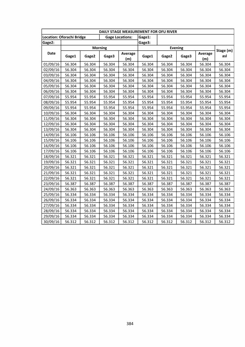
384

Gage1:

Gage2: Gage3:



Average

(m)

01/09/16 56.304 56.304 56.304 56.304 56.304 56.304 56.304 56.304 56.304

02/09/16 56.304 56.304 56.304 56.304 56.304 56.304 56.304 56.304 56.304

03/09/16 56.304 56.304 56.304 56.304 56.304 56.304 56.304 56.304 56.304

04/09/16 56.304 56.304 56.304 56.304 56.304 56.304 56.304 56.304 56.304

05/09/16 56.304 56.304 56.304 56.304 56.304 56.304 56.304 56.304 56.304

06/09/16 56.304 56.304 56.304 56.304 56.304 56.304 56.304 56.304 56.304

07/09/16 55.954 55.954 55.954 55.954 55.954 55.954 55.954 55.954 55.954

08/09/16 55.954 55.954 55.954 55.954 55.954 55.954 55.954 55.954 55.954

09/09/16 55.954 55.954 55.954 55.954 55.954 55.954 55.954 55.954 55.954

10/09/16 56.304 56.304 56.304 56.304 56.304 56.304 56.304 56.304 56.304

11/09/16 56.304 56.304 56.304 56.304 56.304 56.304 56.304 56.304 56.304

12/09/16 56.304 56.304 56.304 56.304 56.304 56.304 56.304 56.304 56.304

13/09/16 56.304 56.304 56.304 56.304 56.304 56.304 56.304 56.304 56.304

14/09/16 56.106 56.106 56.106 56.106 56.106 56.106 56.106 56.106 56.106

15/09/16 56.106 56.106 56.106 56.106 56.106 56.106 56.106 56.106 56.106

16/09/16 56.106 56.106 56.106 56.106 56.106 56.106 56.106 56.106 56.106

17/09/16 56.106 56.106 56.106 56.106 56.106 56.106 56.106 56.106 56.106

18/09/16 56.321 56.321 56.321 56.321 56.321 56.321 56.321 56.321 56.321

19/09/16 56.321 56.321 56.321 56.321 56.321 56.321 56.321 56.321 56.321

20/09/16 56.321 56.321 56.321 56.321 56.321 56.321 56.321 56.321 56.321

21/09/16 56.321 56.321 56.321 56.321 56.321 56.321 56.321 56.321 56.321

22/09/16 56.321 56.321 56.321 56.321 56.321 56.321 56.321 56.321 56.321

23/09/16 56.387 56.387 56.387 56.387 56.387 56.387 56.387 56.387 56.387

24/09/16 56.363 56.363 56.363 56.363 56.363 56.363 56.363 56.363 56.363

25/09/16 56.334 56.334 56.334 56.334 56.334 56.334 56.334 56.334 56.334

26/09/16 56.334 56.334 56.334 56.334 56.334 56.334 56.334 56.334 56.334

27/09/16 56.334 56.334 56.334 56.334 56.334 56.334 56.334 56.334 56.334

28/09/16 56.334 56.334 56.334 56.334 56.334 56.334 56.334 56.334 56.334

29/09/16 56.334 56.334 56.334 56.334 56.334 56.334 56.334 56.334 56.334

30/09/16 56.312 56.312 56.312 56.312 56.312 56.312 56.312 56.312 56.312

Date


asl



385

Gage1:

Gage2: Gage3:



Average

(m)

01/10/16 55.743 55.743 55.743 55.743 55.743 55.743 55.743 55.743 55.743

02/10/16 55.743 55.743 55.743 55.743 55.723 55.723 55.726 55.724 55.734

03/10/16 55.723 55.723 55.726 55.725 55.723 55.723 55.726 55.724 55.724

04/10/16 55.733 55.733 55.746 55.740 55.733 55.733 55.746 55.737 55.738

05/10/16 55.713 55.713 55.716 55.715 55.703 55.703 55.711 55.706 55.710

06/10/16 55.683 55.683 55.706 55.695 55.683 55.683 55.706 55.691 55.693

07/10/16 55.663 55.663 55.696 55.680 55.683 55.683 55.701 55.689 55.684

08/10/16 55.673 55.673 55.706 55.690 55.663 55.663 55.696 55.674 55.682

09/10/16 55.663 55.663 55.696 55.680 55.663 55.663 55.696 55.674 55.677

10/10/16 55.683 55.683 55.706 55.695 55.703 55.703 55.703 55.703 55.699

11/10/16 55.703 55.703 55.726 55.715 55.703 55.703 55.726 55.711 55.713

12/10/16 55.703 55.703 55.726 55.715 55.703 55.703 55.726 55.711 55.713

13/10/16 55.703 55.703 55.726 55.715 55.683 55.683 55.706 55.691 55.703

14/10/16 55.673 55.673 55.696 55.685 55.678 55.678 55.706 55.687 55.686

15/10/16 55.693 55.693 55.716 55.705 55.693 55.693 55.716 55.701 55.703

16/10/16 55.883 55.883 55.896 55.890 55.793 55.793 55.836 55.807 55.848

17/10/16 55.753 55.753 55.796 55.775 55.743 55.743 55.743 55.743 55.759

18/10/16 55.733 55.733 55.733 55.733 55.733 55.733 55.733 55.733 55.733

19/10/16 55.733 55.733 55.733 55.733 55.735 55.735 55.735 55.735 55.734

20/10/16 55.743 55.743 55.743 55.743 55.734 55.734 55.734 55.734 55.739

21/10/16 55.733 55.733 55.733 55.733 55.753 55.753 55.796 55.767 55.750

22/10/16 55.763 55.763 55.763 55.763 55.753 55.753 55.796 55.767 55.765

23/10/16 55.755 55.755 55.755 55.755 55.743 55.743 55.743 55.743 55.749

24/10/16 55.703 55.703 55.726 55.715 55.703 55.703 55.726 55.711 55.713

25/10/16 55.673 55.673 55.696 55.685 55.673 55.673 55.696 55.681 55.683

26/10/16 55.673 55.673 55.696 55.685 55.663 55.663 55.691 55.672 55.678

27/10/16 55.643 55.643 55.666 55.655 55.643 55.643 55.666 55.651 55.653

28/10/16 55.663 55.663 55.666 55.665 55.663 55.663 55.666 55.664 55.664

29/10/16 55.668 55.668 55.696 55.682 55.668 55.668 56.696 56.011 55.846

30/10/16 55.673 55.673 55.696 55.685 55.673 55.673 55.696 55.681 55.683

31/10/16 55.673 55.673 55.696 55.685 55.673 55.673 55.696 55.681 55.683

Date


asl



386

Gage1:

Gage2: Gage3:



Average

(m)

01/11/16 55.673 55.673 55.676 55.674 55.668 55.668 55.676 55.671 55.672

02/11/16 55.663 55.663 55.671 55.666 55.663 55.663 55.676 55.667 55.667

03/11/16 55.663 55.663 55.676 55.667 55.663 55.663 55.676 55.667 55.667

04/11/16 55.663 55.663 55.676 55.667 55.637 55.637 55.676 55.650 55.659

05/11/16 55.643 55.643 55.656 55.647 55.643 55.643 55.676 55.654 55.651

06/11/16 55.643 55.643 55.656 55.647 55.640 55.633 55.640 55.638 55.643

07/11/16 55.640 55.623 55.640 55.634 55.640 55.623 55.640 55.634 55.634

08/11/16 55.640 55.623 55.640 55.634 55.640 55.623 55.640 55.634 55.634

09/11/16 55.640 55.623 55.640 55.634 55.640 55.623 55.640 55.634 55.634

10/11/16 55.640 55.623 55.640 55.634 55.640 55.623 55.640 55.634 55.634

11/11/16 55.640 55.623 55.640 55.634 55.640 55.623 55.640 55.634 55.634

12/11/16 55.640 55.623 55.640 55.634 55.640 55.623 55.640 55.634 55.634

13/11/16 55.630 55.623 55.630 55.628 55.624 55.623 55.624 55.624 55.626

14/11/16 55.630 55.613 55.630 55.624 55.620 55.613 55.620 55.618 55.621

15/11/16 55.620 55.613 55.620 55.618 55.620 55.603 55.636 55.620 55.619

16/11/16 55.610 55.603 55.636 55.616 55.620 55.603 55.636 55.620 55.618

17/11/16 55.620 55.603 55.636 55.620 55.620 55.603 55.636 55.620 55.620

18/11/16 55.620 55.603 55.636 55.620 55.620 55.603 55.636 55.620 55.620

19/11/16 55.614 55.603 55.636 55.618 55.613 55.603 55.636 55.617 55.618

20/11/16 55.610 55.593 55.610 55.604 55.600 55.593 55.600 55.598 55.601

21/11/16 55.610 55.593 55.610 55.604 55.610 55.603 55.610 55.608 55.606

22/11/16 55.610 55.603 55.610 55.608 55.610 55.598 55.610 55.606 55.607

23/11/16 55.610 55.598 55.610 55.606 55.610 55.598 55.610 55.606 55.606

24/11/16 55.446 55.446 55.446 55.446 55.446 55.446 55.446 55.446 55.446

25/11/16 55.453 55.453 55.453 55.453 55.453 55.453 55.453 55.453 55.453

26/11/16 55.453 55.453 55.453 55.453 55.453 55.453 55.453 55.453 55.453

27/11/16 55.453 55.453 55.453 55.453 55.453 55.453 55.453 55.453 55.453

28/11/16 55.453 55.453 55.453 55.453 55.453 55.453 55.453 55.453 55.453

29/11/16 55.453 55.453 55.453 55.453 55.453 55.453 55.453 55.453 55.453

30/11/16 55.453 55.453 55.453 55.453 55.453 55.453 55.453 55.453 55.453

Date


asl



387

Gage1:

Gage2: Gage3:



Average

(m)

01/12/16 55.453 55.453 55.453 55.453 55.453 55.453 55.453 55.453 55.453

02/12/16 55.453 55.453 55.453 55.453 55.453 55.453 55.453 55.453 55.453

03/12/16 55.453 55.453 55.453 55.453 55.453 55.453 55.453 55.453 55.453

04/12/16 55.453 55.453 55.453 55.453 55.453 55.453 55.453 55.453 55.453

05/12/16 55.453 55.453 55.453 55.453 55.453 55.453 55.453 55.453 55.453

06/12/16 55.453 55.453 55.453 55.453 55.453 55.453 55.453 55.453 55.453

07/12/16 55.451 55.451 55.451 55.451 55.451 55.451 55.451 55.451 55.451

08/12/16 55.451 55.451 55.451 55.451 55.451 55.451 55.451 55.451 55.451

09/12/16 55.451 55.451 55.451 55.451 55.451 55.451 55.451 55.451 55.451

10/12/16 55.451 55.451 55.451 55.451 55.451 55.451 55.451 55.451 55.451

11/12/16 55.451 55.451 55.451 55.451 55.451 55.451 55.451 55.451 55.451

12/12/16 55.451 55.451 55.451 55.451 55.451 55.451 55.451 55.451 55.451

13/12/16 55.451 55.451 55.451 55.451 55.451 55.451 55.451 55.451 55.451

14/12/16 55.451 55.451 55.451 55.451 55.451 55.451 55.451 55.451 55.451

15/12/16 55.451 55.451 55.451 55.451 55.451 55.451 55.451 55.451 55.451

16/12/16 55.451 55.451 55.451 55.451 55.451 55.451 55.451 55.451 55.451

17/12/16 55.451 55.451 55.451 55.451 55.451 55.451 55.451 55.451 55.451

18/12/16 55.451 55.451 55.451 55.451 55.451 55.451 55.451 55.451 55.451

19/12/16 55.451 55.451 55.451 55.451 55.451 55.451 55.451 55.451 55.451

20/12/16 55.445 55.445 55.445 55.445 55.445 55.445 55.445 55.445 55.445

21/12/16 55.445 55.445 55.445 55.445 55.445 55.445 55.445 55.445 55.445

22/12/16 55.445 55.445 55.445 55.445 55.445 55.445 55.445 55.445 55.445

23/12/16 55.444 55.444 55.444 55.444 55.444 55.444 55.444 55.444 55.444

24/12/16 55.444 55.444 55.444 55.444 55.444 55.444 55.444 55.444 55.444

25/12/16 55.444 55.444 55.444 55.444 55.444 55.444 55.444 55.444 55.444

26/12/16 55.444 55.444 55.444 55.444 55.444 55.444 55.444 55.444 55.444

27/12/16 55.444 55.444 55.444 55.444 55.444 55.444 55.444 55.444 55.444

28/12/16 55.444 55.444 55.444 55.444 55.444 55.444 55.444 55.444 55.444

29/12/16 55.444 55.444 55.444 55.444 55.444 55.444 55.444 55.444 55.444

30/12/16 55.444 55.444 55.444 55.444 55.444 55.444 55.444 55.444 55.444

31/12/16 55.444 55.444 55.444 55.444 55.444 55.444 55.444 55.444 55.444

Date


asl



388

Gage1:

Gage2: Gage3:



Average

(m)

01/01/17 55.443 55.443 55.443 55.443 55.443 55.443 55.443 55.443 55.443

02/01/17 55.443 55.443 55.443 55.443 55.443 55.443 55.443 55.443 55.443

03/01/17 55.443 55.443 55.443 55.443 55.443 55.443 55.443 55.443 55.443

04/01/17 55.443 55.443 55.443 55.443 55.443 55.443 55.443 55.443 55.443

05/01/17 55.443 55.443 55.443 55.443 55.443 55.443 55.443 55.443 55.443

06/01/17 55.443 55.443 55.443 55.443 55.443 55.443 55.443 55.443 55.443

07/01/17 55.443 55.443 55.443 55.443 55.443 55.443 55.443 55.443 55.443

08/01/17 55.443 55.443 55.443 55.443 55.443 55.443 55.443 55.443 55.443

09/01/17 55.443 55.443 55.443 55.443 55.443 55.443 55.443 55.443 55.443

10/01/17 55.443 55.443 55.443 55.443 55.443 55.443 55.443 55.443 55.443

11/01/17 55.443 55.443 55.443 55.443 55.443 55.443 55.443 55.443 55.443

12/01/17 55.443 55.443 55.443 55.443 55.443 55.443 55.443 55.443 55.443

13/01/17 55.443 55.443 55.443 55.443 55.443 55.443 55.443 55.443 55.443

14/01/17 55.443 55.443 55.443 55.443 55.443 55.443 55.443 55.443 55.443

15/01/17 55.443 55.443 55.443 55.443 55.443 55.443 55.443 55.443 55.443

16/01/17 55.443 55.443 55.443 55.443 55.443 55.443 55.443 55.443 55.443

17/01/17 55.443 55.443 55.443 55.443 55.443 55.443 55.443 55.443 55.443

18/01/17 55.443 55.443 55.443 55.443 55.443 55.443 55.443 55.443 55.443

19/01/17 55.443 55.443 55.443 55.443 55.443 55.443 55.443 55.443 55.443

20/01/17 55.443 55.443 55.443 55.443 55.443 55.443 55.443 55.443 55.443

21/01/17 55.443 55.443 55.443 55.443 55.443 55.443 55.443 55.443 55.443

22/01/17 55.443 55.443 55.443 55.443 55.443 55.443 55.443 55.443 55.443

23/01/17 55.443 55.443 55.443 55.443 55.443 55.443 55.443 55.443 55.443

24/01/17 55.443 55.443 55.443 55.443 55.443 55.443 55.443 55.443 55.443

25/01/17 55.443 55.443 55.443 55.443 55.443 55.443 55.443 55.443 55.443

26/01/17 55.443 55.443 55.443 55.443 55.443 55.443 55.443 55.443 55.443

27/01/17 55.443 55.443 55.443 55.443 55.443 55.443 55.443 55.443 55.443

28/01/17 55.443 55.443 55.443 55.443 55.443 55.443 55.443 55.443 55.443

29/01/17 55.443 55.443 55.443 55.443 55.443 55.443 55.443 55.443 55.443

30/01/17 55.443 55.443 55.443 55.443 55.443 55.443 55.443 55.443 55.443

31/01/17 55.443 55.443 55.443 55.443 55.443 55.443 55.443 55.443 55.443

Date


asl



389

APPENDIX VIII: SOIL CLASSIFICATION

391

Table VIII: Soil classification table based on values of saturated hydraulic conductivity K (according to the Czech

standard)

Soil

(according the relative

permeability)

Approximate range of

saturated hydraulic

conductivity (m s-1)

Examples of soil types

Highly impermeable < 10-10

clays with low and medium plasticity,

clays with high and extremely high

plasticity

Impermeable from 10-8 to 10-10

gravel loams, gravel clays and sandy

clays, loams with low and medium

plasticity

Lowly (poorly) permeable from 10-6 to 10-8 sandy loams, loamy sands and clayey

sands, loamy gravels and clayey gravels

Permeable from 10-4 to 10-6 sands and gravels , containing fine-

grained fraction(5 – 15 %)

Highly permeable > 10-4 sands and gravels without or with very

low fine grained fraction (<5%)

Source: CSN 721020 (n.d)

392

APPENDIX IX: SCS RUNOFF CURVE NUMBERS

Table IXa: Runoff curve numbers for urban areas

Source: TR-55 (1986)

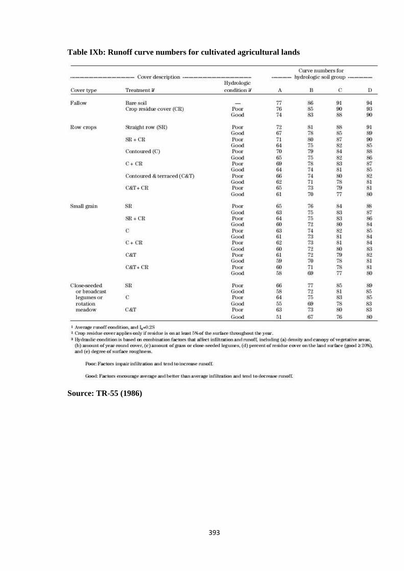
393

Table IXb: Runoff curve numbers for cultivated agricultural lands


394

Table IXc: Runoff curve numbers for other agricultural lands


395

Table IXd: Runoff curve numbers for arid and semiarid rangelands


Source: TR-55; US. Department of Agricultural Soil Conservation Service (1986)

396

APPENDIX X: NORMALLY DISTRIBUTED RANDOM NUMBERS

Table Xa: Random Numbers Generated for the Thomas-Fiering Model

1 2 3 4 5 6 7 8 9 10 11 12

1 -0.112 1.375 0.262 1.043 -1.149 1.212 -0.142 1.929 -1.229 -1.552 -1.989 0.001

2 -1.827 1.025 0.652 0.922 -0.076 0.947 -0.062 1.964 0.935 0.548 0.919 0.038

3 1.151 -0.394 -1.067 -1.942 -0.402 0.360 -1.705 -0.471 -0.151 0.106 -0.154 0.995

4 0.682 2.378 1.160 -0.450 -0.209 -1.656 -0.596 -0.732 1.694 -2.623 0.569 1.810

5 0.490 0.661 -0.105 -0.100 -1.043 -0.954 1.003 -1.165 -0.325 1.375 -0.819 0.434

6 -0.002 -0.852 0.027 1.292 0.177 -1.895 0.830 1.661 1.582 0.279 -1.030 -2.906

7 -0.765 -1.004 -0.432 -1.649 -1.219 1.909 0.534 0.579 -1.282 -2.489 0.361 0.414

8 -0.301 0.621 -1.467 0.190 1.395 0.189 -0.560 -0.296 -1.617 0.527 0.547 0.194

9 0.188 -0.143 0.603 -0.566 0.380 -1.072 -0.464 -1.358 0.024 0.467 0.166 -1.327

10 -0.420 0.000 0.544 -0.426 -0.846 -0.306 1.794 -2.618 -0.023 0.667 0.533 0.104

11 0.720 0.924 -1.046 -1.082 -0.374 -0.371 -0.597 0.452 0.558 -0.652 -1.554 0.249

12 1.029 1.236 0.588 0.943 0.829 -0.482 -1.146 -1.015 -0.010 -0.689 -2.530 -0.763

13 -2.346 -1.730 -1.043 0.192 -0.068 -0.068 -0.795 1.007 0.501 0.149 -0.443 0.150

14 0.781 -0.613 -1.109 0.471 0.746 -0.384 -0.228 -0.519 0.144 -1.469 1.861 0.311

15 -1.122 -0.959 1.610 0.495 -0.039 0.742 -0.986 1.613 -1.355 0.189 0.521 -1.193

16 -0.366 -1.455 -0.361 -0.105 -2.163 -1.309 -1.018 1.426 0.674 -0.099 -0.035 -0.708

17 -1.423 -2.404 -0.956 -0.088 0.911 0.831 1.754 -1.893 -1.327 0.685 0.646 0.854

18 -0.743 0.114 -2.075 -0.748 0.052 1.848 1.277 -2.025 -0.831 0.301 -0.920 0.057

19 0.201 -1.057 0.611 -0.971 0.520 1.036 0.901 -1.041 -0.050 1.419 0.035 0.888

20 0.550 -1.321 1.153 0.711 0.810 2.213 -2.586 -0.642 0.490 1.587 0.526 1.570

21 1.453 0.292 0.896 -0.400 -1.275 -1.368 2.404 -0.447 0.709 0.956 1.549 1.173

22 -1.267 -0.626 1.217 -0.346 -0.346 -0.878 -0.253 0.601 -0.430 1.227 -0.937 0.490

23 1.123 -0.867 -2.166 -0.048 1.040 -0.681 0.286 -1.156 -0.111 -0.476 -0.545 0.824

24 -0.936 -0.363 -0.255 -0.468 -0.083 0.463 -0.121 -0.487 -0.083 -0.144 0.671 2.922

25 0.374 -0.478 0.163 -0.699 0.960 -1.990 0.249 0.973 0.000 -1.262 0.952 0.103

26 0.638 0.373 -0.148 1.791 0.801 -0.576 1.769 0.637 0.193 -0.755 -0.573 -1.259

27 -1.099 0.314 0.569 -0.330 -0.444 -2.018 0.599 -0.475 0.740 -0.803 0.068 -1.598

28 -0.329 -0.721 -0.953 -0.296 -0.286 1.058 -0.562 -0.939 -0.246 -0.737 -1.015 0.863

29 -1.094 -1.158 -0.738 -0.858 -0.021 -0.299 0.866 -0.152 0.638 -2.606 1.743 0.288

30 -0.662 0.126 -0.186 0.663 0.572 -0.874 0.221 0.036 -1.022 -0.933 -0.863 0.447

31 0.730 2.347 -2.409 0.732 1.454 -2.720 -2.745 -1.020 -0.691 1.083 -0.555 1.016

397

Table Xb: Random Numbers Generated for the Thomas-Fiering Model (Continues)

1 2 3 4 5 6 7 8 9 10 11 12

32 -1.097 -0.173 -0.216 -0.696 0.755 0.174 -0.859 -0.650 1.007 -0.047 0.648 1.105

33 2.426 2.040 0.940 0.321 -0.228 -0.259 -0.659 -0.855 -0.237 -0.101 -0.269 -0.335

34 -0.187 1.127 0.040 0.428 -0.288 1.404 -1.218 -2.019 0.699 1.175 0.964 0.220

35 -0.588 -0.077 -0.790 -0.925 0.600 -0.936 1.005 -0.225 0.356 0.539 -1.242 -1.623

36 -0.245 -0.348 -0.774 0.266 0.260 0.301 0.327 0.460 -1.697 0.369 0.013 -1.012

37 -0.336 -1.112 -0.127 0.569 0.344 -1.067 -1.493 0.524 0.887 -0.630 0.233 1.293

38 0.158 1.260 -0.911 -0.594 -0.747 1.300 -1.453 -1.215 -0.181 -0.147 -0.723 0.541

39 -0.894 -0.745 0.453 -1.629 1.764 -1.712 -1.519 0.242 0.068 0.641 0.983 0.184

40 -1.431 0.102 -0.232 1.836 -0.070 1.397 0.471 0.298 -1.668 0.907 -0.021 0.024

41 1.084 0.040 -1.039 0.774 0.877 1.303 0.615 -0.096 0.040 -0.106 -0.588 0.014

42 -0.298 0.508 0.169 -1.217 0.616 -0.298 0.230 1.265 -0.191 -0.525 -0.191 1.470

43 1.193 0.857 0.302 -0.975 1.303 -2.097 0.801 -0.476 -0.942 1.231 0.107 0.491

44 1.309 1.481 -0.210 2.429 -0.036 1.180 1.826 0.550 0.125 -1.137 0.439 2.268

45 -0.305 -1.199 0.870 0.378 -1.638 0.135 1.826 -0.570 -0.827 0.519 -0.464 -1.714

46 1.207 -0.046 -0.338 -1.554 -0.441 0.780 -0.707 -1.163 -1.276 0.276 -0.569 0.185

47 0.043 -0.053 -1.687 2.280 0.619 0.777 -0.502 0.425 -0.239 -0.270 -0.344 -0.153

48 -0.361 -0.408 -0.971 1.207 -1.160 0.788 -0.031 -0.235 0.778 -1.287 0.867 -0.655

49 -1.934 -0.384 -2.325 -1.923 0.908 1.477 0.272 0.348 0.165 0.355 0.270 -0.448

50 -0.732 3.401 0.526 0.633 -0.616 -1.399 1.428 0.112 0.788 0.276 -0.159 0.659

51 1.079 0.395 0.248 -1.495 -0.234 0.434 1.814 0.201 -0.020 -0.985 -0.244 -2.844

52 0.015 0.819 1.540 0.737 -1.196 -1.022 0.047 -0.349 -0.297 -1.846 -0.395 1.712

53 1.797 -0.132 1.422 1.231 0.817 -0.816 -0.065 -1.938 -0.972 -0.521 1.357 -0.023

54 0.286 1.233 2.090 1.084 -0.037 -0.877 0.678 -0.514 0.376 -2.635 -1.212 0.575

55 -0.896 -0.765 -0.166 -0.273 0.126 -1.795 -1.940 -0.729 -2.172 -0.957 0.213 -1.533

56 1.183 1.255 -0.666 -1.615 -0.460 -1.125 -0.065 0.845 -0.591 -0.309 -0.589 -1.366

57 -0.537 0.893 -0.971 1.009 0.683 -0.604 -0.682 -0.305 -0.463 -0.123 0.789 -0.343

58 -1.136 -1.446 0.848 0.333 -0.055 -0.444 1.358 -0.523 0.199 -0.421 -1.873 -0.512

59 -1.055 1.640 -1.249 0.763 -0.488 0.376 0.141 -0.258 0.661 0.910 0.104 -0.875

60 -0.335 -0.781 0.644 0.899 0.265 1.046 0.793 1.233 0.111 -1.202 -2.141 -0.332

61 1.561 -0.217 0.500 0.002 -0.139 -1.268 -0.398 -0.216 2.031 1.946 -0.221 1.059

398

APPENDIX XI: RUNOFF COMPUTATION BY RATIONAL METHOD

Table XIa: Recommended Guide on the Value of Runoff Coefficient in Rural Areas

Table XIb: Guidance on Permeability of Catchment based on soil type

Source: FMW (2013)

399

Fig. XI: Map showing the Rainfall Zones of Nigeria (FMW, 2013)

Table XIc: Ranges of characteristics of some Rainfall zones

Source: FMW (2013)

400

Table XId: Estimates of parameters β and 1/α for calculation of Rainfall Intensity

401

APPENDIX XII: ANALYTICAL HIERARCHICAL PROCESS TABLES

Table XIIa: Fundamental Scale for Pair wise Comparison

Intensity of Importance Definition Explanation

1 Equal importance

Two elements contribute equally to the

objective

3 Moderate importance Experience and judgment slightly favor

one element over another

5 Strong importance Experience and judgment strongly favor

one element over another

7 Very Strong

importance

One element is favored very strongly

over another; its dominance is

demonstrated in practice

9 Extreme importance

The evidence favoring one element over

another is of the highest possible order

of affirmation

2,4,6, and 8 are intermediate values

Source: Saaty (1980)

Table XIIb: Random Inconsistency Indices (RI) for N-10

N 1 2 3 4 5 6 7 8 9 10

RI 0 0 0.58 0.89 1.12 1.24 1.32 1.41 1.45 1.49

Source: Saaty (1980)

402

APPENDIX XIII: RESULTS OF SOIL ANALYSES

Date:

Date:

Boring No: Depth

Coordinate

Var. Units

N blows 47 36 28 17 13

--- --- OF1 OF2 OF3 OF4 OF5 OF6 OF7 OF8 OF8

MC (g) 8.80 8.80 8.80 8.80 9.40 9.40 8.20 8.90 8.90

MCMS (g) 11.40 11.10 10.60 11.03 21.90 24.50 26.40 27.50 27.90

MCDS (g) 10.90 10.60 10.30 10.60 18.90 21.00 23.20 23.20 23.40

MS (g) 2.10 1.80 1.50 1.80 9.50 11.60 15.00 14.30 14.50

MW (g) 0.50 0.50 0.30 0.43 3.00 3.50 3.20 4.30 4.50

w (%) 23.8 27.8 20.0 23.9 31.6 30.2 21.3 30.1 31.0

LL PI

4 4

25.5 4

115.89 70

0 0

70 70

7 7

29.6 7

50 0

50 70

15.8 7

85.778 70

25 0

25 10

25 20

25 30

25 40

25 60

Location: Oforachi Checked By:

4

USCS Soil Classification: ML

TEST

2 31

LIQUID LIMITPLASTIC LIMIT

53 4

Procedure B One-

Point

Wet Preperation

Multipoint

XDry Preperation

Multipoint

Procedure A

Multipoint

PROCEDURE USED

Liquid Limit (LL or w L ) (%): 28.86

PI at "A" Line = 0.73(LL-20)

One Point Liquid Limit Calculation:

LL = w n (N/25)0.12

Plasticity Index (PI) (%): 4.99

USCS Classification: ML

Mass of Empty Can

Mass Can & Soil (Wet)

Mass Can & Soil (Dry)

Plastic Limit (PL or w P ) (%): 23.87

Mass of Soil

Mass of Water

Water Content

Can Number

VariableNO

1 2

Number of Blows

D.B. Adie

Project Name:

Atterberg Limits Data SheetASTM D4318-10

PhD Research Tested By: M.I. Alfa 18/5/2016

12-24 inches

30/5/2016

OF 01 Test Number: 1

Elevation:

y = -0.48ln(x) + 30.41R² = 0.003

20

22

24

26

28

30

32

10 100

Wate

r C

on

ten

t (%

)

Number of Blows (N)

0

10

20

30

40

50

60

0 10 20 30 40 50 60 70 80 90 100

Pla

sti

cit

y I

nd

ex (

PI)

Liquid Limit (LL or wL)

MHCL

CL-ML

A LineU Line

ML

CH

403

Date:

Date:

Boring No: Depth

Coordinate

Var. Units

N blows 48 37 29 19 11


MC (g) 8.80 8.80 9.40 9.00 8.20 8.40 8.90 8.40 9.00

MCMS (g) 10.70 11.10 12.60 11.47 22.10 20.20 23.20 27.10 30.50

MCDS (g) 10.40 10.50 12.10 10.93 19.40 17.90 20.10 23.10 25.40

MS (g) 1.60 1.70 2.70 1.93 11.20 9.50 11.20 14.70 16.40

MW (g) 0.30 0.60 0.50 0.54 2.70 2.30 3.10 4.00 5.10

w (%) 18.7 35.3 18.5 28.0 24.1 24.2 27.7 27.2 31.1

LL PI

4 4

25.5 4

115.89 70

0 0

70 70

7 7

29.6 7

50 0

50 70

15.8 7

85.778 70

25 0

25 10

25 20

25 30

25 40

25 60

D.B. Adie

Project Name:



12-24 inches

30/5/2016


Elevation:

Can Number

VariableNO

1 2

Number of Blows

Mass of Empty Can




Mass of Soil

Mass of Water

Water Content

PROCEDURE USED


PI at "A" Line = 0.73(LL-20)


LL = w n (N/25)0.12



Procedure B One-

Point

Wet Preperation

Multipoint

XDry Preperation

Multipoint

Procedure A

Multipoint


4


TEST

2 31


53 4

y = -4.66ln(x) + 41.96R² = 0.879

20

22

24

26

28

30

32

10 100

Wate

r C

on

ten

t (%

)

Number of Blows (N)

0

10

20

30

40

50

60

0 10 20 30 40 50 60 70 80 90 100

Pla

sti

cit

y I

nd

ex (

PI)


MHCL

CL-ML

A LineU Line

ML

CH

404

Date:

Date:

Boring No: Depth

Coordinate

Var. Units

N blows 48 37 28 18 13


MC (g) 10.20 14.40 14.50 13.03 8.70 8.60 14.70 14.00 14.00

MCMS (g) 12.20 16.50 16.90 15.20 20.50 22.60 24.60 35.00 31.10

MCDS (g) 12.00 16.20 16.60 14.93 18.40 19.90 20.80 31.00 27.60

MS (g) 1.80 1.80 2.10 1.90 9.70 11.30 6.10 17.00 13.60

MW (g) 0.20 0.30 0.30 0.27 2.10 2.70 3.80 4.00 3.50

w (%) 11.1 16.7 14.3 14.2 21.6 23.9 62.3 23.5 25.7

LL PI

4 4

25.5 4

115.89 70

0 0

70 70

7 7

29.6 7

50 0

50 70

15.8 7

85.778 70

25 0

25 10

25 20

25 30

25 40

25 60

D.B. Adie

Project Name:



12-24 inches

30/5/2016


Elevation:

Can Number

VariableNO

1 2

Number of Blows

Mass of Empty Can




Mass of Soil

Mass of Water

Water Content

PROCEDURE USED


PI at "A" Line = 0.73(LL-20)


LL = w n (N/25)0.12


USCS Classification: CL

Procedure B One-

Point

Wet Preperation

Multipoint

XDry Preperation

Multipoint

Procedure A

Multipoint


4

USCS Soil Classification: CL

TEST

2 31


53 4

y = 0.431ln(x) + 30.01R² = 0.000

20

25

30

35

40

45

50

55

60

65

10 100

Wate

r C

on

ten

t (%

)

Number of Blows (N)

0

10

20

30

40

50

60

0 10 20 30 40 50 60 70 80 90 100

Pla

sti

cit

y I

nd

ex (

PI)


MHCL

CL-ML

A LineU Line

ML

CH

405

Date:

Date:

Boring No: Depth

Coordinate

Var. Units

N blows

--- ---

MC (g)

MCMS (g)

MCDS (g)

MS (g)

MW (g)

w (%)


Mass of Soil

Mass of Water

Liquid Limit (LL or w L ) (%): Nil

Plastic Limit (PL or w P ) (%): Nil

Plasticity Index (PI) (%):

4 53 4

Nil

Water Content

Mass of Empty Can



USCS Soil Classification: Nil

TEST

Can Number

VariableNO

1 2 2 31

LIQUID LIMIT

Number of Blows

PLASTIC LIMIT

D.B. Adie

Project Name:



12-24 inches

30/5/2016


Elevation:

406

Date:

Date:

Boring No: Depth

Coordinate

Var. Units

N blows 47 37 28 17 13


MC (g) 14.20 13.70 15.60 14.50 14.60 11.30 15.00 13.70 13.80

MCMS (g) 15.90 15.70 17.20 16.27 27.10 25.50 31.00 32.40 32.40

MCDS (g) 15.60 15.50 17.00 16.03 25.10 23.20 28.20 29.10 30.40

MS (g) 1.40 1.80 1.40 1.53 10.50 11.90 13.20 15.40 16.60

MW (g) 0.30 0.20 0.20 0.24 2.00 2.30 2.80 3.30 2.00

w (%) 21.4 11.1 14.3 15.7 19.0 19.3 21.2 21.4 12.0

LL PI

4 4

25.5 4

115.89 70

0 0

70 70

7 7

29.6 7

50 0

50 70

15.8 7

85.778 70

25 0

25 10

25 20

25 30

25 40

25 60


4


TEST

2 31


53 4

Procedure B One-

Point

Wet Preperation

Multipoint

XDry Preperation

Multipoint

Procedure A

Multipoint

PROCEDURE USED


PI at "A" Line = 0.73(LL-20)


LL = w n (N/25)0.12



Mass of Empty Can




Mass of Soil

Mass of Water

Water Content

Can Number

VariableNO

1 2

Number of Blows

D.B. Adie

Project Name:

ASTM D4318-10


12-24 inches

30/5/2016


Elevation:

y = 3.559ln(x) + 7.086R² = 0.246

10

12

14

16

18

20

22

10 100

Wate

r C

on

ten

t (%

)

Number of Blows (N)

0

10

20

30

40

50

60

0 10 20 30 40 50 60 70 80 90 100

Pla

sti

cit

y I

nd

ex (

PI)


MHCL

CL-ML

A LineU Line

ML

CH

407

Date:

Date:

Boring No: Depth

Coordinate

Var. Units

N blows 47 36 28 17 13


MC (g) 8.90 8.90 8.90 8.90 8.90 8.60 8.70 9.50 9.00

MCMS (g) 11.10 11.50 11.20 11.27 21.50 20.70 24.50 28.60 26.70

MCDS (g) 10.60 10.80 10.60 10.67 17.50 16.50 19.40 22.20 20.70

MS (g) 1.70 1.90 1.70 1.77 8.60 7.90 10.70 12.70 11.70

MW (g) 0.50 0.70 0.60 0.60 4.00 4.20 5.10 6.40 6.00

w (%) 29.4 36.8 35.3 33.9 46.5 53.2 47.7 50.4 51.3

LL PI

4 4

25.5 4

115.89 70

0 0

70 70

7 7

29.6 7

50 0

50 70

15.8 7

85.778 70

25 0

25 10

25 20

25 30

25 40

25 60


4

USCS Soil Classification: ML-MH

TEST

2 31


53 4

Procedure B One-

Point

Wet Preperation

Multipoint

XDry Preperation

Multipoint

Procedure A

Multipoint

PROCEDURE USED


PI at "A" Line = 0.73(LL-20)


LL = w n (N/25)0.12


USCS Classification: ML-MH

Mass of Empty Can




Mass of Soil

Mass of Water

Water Content

Can Number

VariableNO

1 2

Number of Blows

D.B. Adie

Project Name:



12-24 inches

30/5/2016


Elevation:

y = -2.04ln(x) + 56.41R² = 0.160

20

25

30

35

40

45

50

55

10 100

Wate

r C

on

ten

t (%

)

Number of Blows (N)

0

10

20

30

40

50

60

0 10 20 30 40 50 60 70 80 90 100

Pla

sti

cit

y I

nd

ex (

PI)


MHCL

CL-ML

A LineU Line

ML

CH

408

Date:

Date:

Boring No: Depth

Coordinate

Var. Units

N blows

--- ---

MC (g)

MCMS (g)

MCDS (g)

MS (g)

MW (g)

w (%)


Mass of Soil

Mass of Water

Liquid Limit (LL or w L ) (%): Nil

Plastic Limit (PL or w P ) (%): Nil

Plasticity Index (PI) (%):

4 53 4

Nil

Water Content

Mass of Empty Can



USCS Soil Classification: Nil

TEST

Can Number

VariableNO

1 2 2 31

LIQUID LIMIT

Number of Blows

PLASTIC LIMIT

D.B. Adie

Project Name:



12-24 inches

30/5/2016


Elevation:

409

Date:

Date:

Boring No: Depth

Coordinate

Var. Units

N blows 48 37 26 15 12


MC (g) 8.40 8.70 8.90 8.67 8.50 9.10 8.50 8.80 9.10

MCMS (g) 10.40 10.70 11.00 10.70 19.20 24.50 26.70 31.30 31.40

MCDS (g) 9.90 10.30 10.60 10.27 16.80 20.90 22.30 25.60 25.90

MS (g) 1.50 1.60 1.70 1.60 8.30 11.80 13.80 16.80 16.80

MW (g) 0.50 0.40 0.40 0.43 2.40 3.60 4.40 5.70 5.50

w (%) 33.3 25.0 23.5 26.9 28.9 30.5 31.9 33.9 32.7

LL PI

4 4

25.5 4

115.89 70

0 0

70 70

7 7

29.6 7

50 0

50 70

15.8 7

85.778 70

25 0

25 10

25 20

25 30

25 40

25 60


4


TEST

2 31


53 4

Procedure B One-

Point

Wet Preperation

Multipoint

XDry Preperation

Multipoint

Procedure A

Multipoint

PROCEDURE USED


PI at "A" Line = 0.73(LL-20)


LL = w n (N/25)0.12



Mass of Empty Can




Mass of Soil

Mass of Water

Water Content

Can Number

VariableNO

1 2

Number of Blows

D.B. Adie

Project Name:



12-24 inches

30/5/2016


Elevation:

y = -3.04ln(x) + 41.31R² = 0.841

20

22

24

26

28

30

32

34

10 100

Wate

r C

on

ten

t (%

)

Number of Blows (N)

0

10

20

30

40

50

60

0 10 20 30 40 50 60 70 80 90 100

Pla

sti

cit

y I

nd

ex (

PI)


MHCL

CL-ML

A LineU Line

ML

CH

410

Date:

Date:

Boring No: Depth

Coordinate

Var. Units

N blows 48 37 27 19 12


MC (g) 8.90 8.50 8.30 8.57 8.60 8.60 8.40 8.90 9.10

MCMS (g) 10.40 10.50 10.20 10.37 24.20 22.60 23.70 27.40 34.00

MCDS (g) 10.20 10.20 9.90 10.10 21.20 19.80 20.70 23.70 28.90

MS (g) 1.30 1.70 1.60 1.53 12.60 11.20 12.30 14.80 19.80

MW (g) 0.20 0.30 0.30 0.27 3.00 2.80 3.00 3.70 5.10

w (%) 15.4 17.6 18.7 17.6 23.8 25.0 24.4 25.0 25.8

LL PI

4 4

25.5 4

115.89 70

0 0

70 70

7 7

29.6 7

50 0

50 70

15.8 7

85.778 70

25 0

25 10

25 20

25 30

25 40

25 60

D.B. Adie

Project Name:



12-24 inches

30/5/2016


Elevation:

Can Number

VariableNO

1 2

Number of Blows

Mass of Empty Can




Mass of Soil

Mass of Water

Water Content

PROCEDURE USED


PI at "A" Line = 0.73(LL-20)


LL = w n (N/25)0.12


USCS Classification: CL-ML

Procedure B One-

Point

Wet Preperation

Multipoint

XDry Preperation

Multipoint

Procedure A

Multipoint


4

USCS Soil Classification: CL-ML

TEST

2 31


53 4

y = -1.13ln(x) + 28.46R² = 0.716

20

21

22

23

24

25

26

10 100

Wate

r C

on

ten

t (%

)

Number of Blows (N)

0

10

20

30

40

50

60

0 10 20 30 40 50 60 70 80 90 100

Pla

sti

cit

y I

nd

ex (

PI)


MHCL

CL-ML

A LineU Line

ML

CH

411

Date:

Date:

Boring No: Depth

Coordinate

Var. Units

N blows 48 37 26 18 13


MC (g) 8.40 8.70 9.00 8.70 8.50 9.10 9.00 9.20 8.90

MCMS (g) 10.60 11.30 10.80 10.90 22.60 27.70 28.60 25.90 27.10

MCDS (g) 10.20 10.90 10.50 10.53 19.70 23.80 24.40 22.20 23.00

MS (g) 1.80 2.20 1.50 1.83 11.20 14.70 15.40 13.00 14.10

MW (g) 0.40 0.40 0.30 0.37 2.90 3.90 4.20 3.70 4.10

w (%) 22.2 18.2 20.0 20.2 25.9 26.5 27.3 28.5 29.1

LL PI

4 4

25.5 4

115.89 70

0 0

70 70

7 7

29.6 7

50 0

50 70

15.8 7

85.778 70

25 0

25 10

25 20

25 30

25 40

25 60

D.B. Adie

Project Name:



12-24 inches

30/5/2016


Elevation:

Can Number

VariableNO

1 2

Number of Blows

Mass of Empty Can




Mass of Soil

Mass of Water

Water Content

PROCEDURE USED


PI at "A" Line = 0.73(LL-20)


LL = w n (N/25)0.12


USCS Classification: CL-ML

Procedure B One-

Point

Wet Preperation

Multipoint

XDry Preperation

Multipoint

Procedure A

Multipoint


4

USCS Soil Classification: CL-ML

TEST

2 31


53 4

y = -2.49ln(x) + 35.52R² = 0.994

20

21

22

23

24

25

26

27

28

29

30

10 100

Wate

r C

on

ten

t (%

)

Number of Blows (N)

0

10

20

30

40

50

60

0 10 20 30 40 50 60 70 80 90 100

Pla

sti

cit

y I

nd

ex (

PI)


MHCL

CL-ML

A LineU Line

ML

CH

412

Project Name: Tested By: M.I. Alfa Date: 18/5/2016

Location: Checked By: D.B. Adie Date: 30/5/2016

Boring No: OF 01 Test Number: 1

Sample Depth: 12-24 inches Elevation:

USCS Soil Classification:

AASHTO Soil Classification:

Sieve NumberDiameter

(mm)

Mass of Sieve

(g)

Mass of Sieve

& Soil (g)

Soil Retained

(g)

Soil Retained

(%)

Soil Passing

(%)

#7 2.80 512.38 516.18 3.8 1.9 98.1

#14 1.40 464.38 465.08 0.7 0.3 97.8

#25 0.71 411.99 423.49 11.5 5.8 92.0

#36 0.43 368.57 377.77 9.2 4.6 87.4

#52 0.36 528.66 540.06 11.4 5.7 81.7

#72 0.21 340.89 359.99 19.1 9.6 72.2

#100 0.15 347.23 368.13 20.9 10.5 61.7

#200 0.075 378.07 417.77 39.7 19.9 41.9

Pan 0 374.07 457.77 83.7 41.9 0.0

TOTAL: 200 100.0

% Gravel: 0.00 D10: 0.025 Cu: 5.60

% Sand: 58.15 D30: 0.055 Cc: 0.86

% Fines: 41.85 D60: 0.14

Grain Size Distribution Curve Results:

Sieve Analysis Data SheetASTM D422-63(2007)

PhD Research

Oforachi

0.0

10.0

20.0

30.0

40.0

50.0

60.0

70.0

80.0

90.0

100.0

0.010.101.0010.00

% P

assi

ng

Particle Size (mm)

413








(mm)

Mass of Sieve

(g)

Mass of Sieve

& Soil (g)

Soil Retained

(g)

Soil Retained

(%)

Soil Passing

(%)

#7 2.80 512.38 517.58 5.2 2.6 97.4

#14 1.40 464.38 464.88 0.5 0.3 97.2

#25 0.71 411.99 424.99 13.0 6.5 90.7

#36 0.43 368.57 379.07 10.5 5.3 85.4

#52 0.36 528.66 543.06 14.4 7.2 78.2

#72 0.21 340.89 360.09 19.2 9.6 68.6

#100 0.15 347.23 360.33 13.1 6.6 62.1

#200 0.075 378.07 401.07 23.0 11.5 50.6

Pan 374.07 475.17 101.1 50.6 0.0

TOTAL: 200 100.0

% Gravel: 0.00 D10: 0.0045 Cu: 31.11

% Sand: 49.45 D30: 0.026 Cc: 1.07

% Fines: 50.55 D60: 0.14



PhD Research

Oforachi

0.0

10.0

20.0

30.0

40.0

50.0

60.0

70.0

80.0

90.0

100.0

0.010.101.0010.00

% P

assi

ng

Particle Size (mm)

414








(mm)

Mass of Sieve

(g)

Mass of Sieve

& Soil (g)

Soil Retained

(g)

Soil Retained

(%)

Soil Passing

(%)

#7 2.80 512.38 513.08 0.7 0.3 99.7

#14 1.40 464.38 464.78 0.4 0.2 99.5

#25 0.71 411.99 418.29 6.3 3.1 96.3

#36 0.43 368.57 374.57 6.0 3.0 93.3

#52 0.36 528.66 540.16 11.5 5.7 87.6

#72 0.21 340.89 366.69 25.8 12.9 74.7

#100 0.15 347.23 388.33 41.1 20.5 54.2

#200 0.075 378.07 411.97 33.9 16.9 37.3

Pan 374.07 448.77 74.7 37.3 0.0

TOTAL: 200.4 100.0

% Gravel: 0.00 D10: 0.013 Cu: 13.08

% Sand: 62.72 D30: 0.055 Cc: 1.37

% Fines: 37.28 D60: 0.17



PhD Research

Oforachi

0.0

10.0

20.0

30.0

40.0

50.0

60.0

70.0

80.0

90.0

100.0

0.010.101.0010.00

% P

assi

ng

Particle Size (mm)

415








(mm)

Mass of Sieve

(g)

Mass of Sieve

& Soil (g)

Soil Retained

(g)

Soil Retained

(%)

Soil Passing

(%)

#7 2.80 512.38 515.08 2.7 1.4 98.7

#14 1.40 464.38 465.08 0.7 0.3 98.3

#25 0.71 411.99 434.89 22.9 11.5 86.9

#36 0.43 368.57 384.57 16.0 8.0 78.9

#52 0.36 528.66 554.96 26.3 13.2 65.7

#72 0.21 340.89 372.69 31.8 15.9 49.8

#100 0.15 347.23 372.33 25.1 12.6 37.3

#200 0.075 378.07 402.57 24.5 12.3 25.0

Pan 374.07 424.07 50.0 25.0 0.0

TOTAL: 200 100.0

% Gravel: 0.00 D10: 0.028 Cu: 11.07

% Sand: 75.00 D30: 0.12 Cc: 1.66

% Fines: 25.00 D60: 0.31



PhD Research

Oforachi

SP - Poorly Graded Sand

A-3 (Fine Sand)

0.0

10.0

20.0

30.0

40.0

50.0

60.0

70.0

80.0

90.0

100.0

0.010.101.0010.00

% P

assi

ng

Particle Size (mm)

416








(mm)

Mass of Sieve

(g)

Mass of Sieve

& Soil (g)

Soil Retained

(g)

Soil Retained

(%)

Soil Passing

(%)

#7 2.80 512.38 514.18 1.8 0.9 99.1

#14 1.40 464.38 464.38 0.0 0.0 99.1

#25 0.71 411.99 421.99 10.0 5.0 94.1

#36 0.43 368.57 377.97 9.4 4.7 89.4

#52 0.36 528.66 543.56 14.9 7.4 82.0

#72 0.21 340.89 367.19 26.3 13.2 68.8

#100 0.15 347.23 375.23 28.0 14.0 54.8

#200 0.075 378.07 422.77 44.7 22.4 32.5

Pan 374.07 438.97 64.9 32.5 0.0

TOTAL: 200 100.0

% Gravel: 0.00 D10: 0.037 Cu: 4.59

% Sand: 67.55 D30: 0.07 Cc: 0.78

% Fines: 32.45 D60: 0.17



PhD Research

Oforachi

0.0

10.0

20.0

30.0

40.0

50.0

60.0

70.0

80.0

90.0

100.0

0.010.101.0010.00

% P

assi

ng

Particle Size (mm)

417








(mm)

Mass of Sieve

(g)

Mass of Sieve

& Soil (g)

Soil Retained

(g)

Soil Retained

(%)

Soil Passing

(%)

#7 2.80 512.38 545.38 33.0 16.5 83.5

#14 1.40 464.38 466.18 1.8 0.9 82.6

#25 0.71 411.99 427.39 15.4 7.7 74.9

#36 0.43 368.57 375.47 6.9 3.4 71.5

#52 0.36 528.66 539.86 11.2 5.6 65.9

#72 0.21 340.89 359.19 18.3 9.2 56.7

#100 0.15 347.23 359.33 12.1 6.1 50.7

#200 0.075 378.07 394.97 16.9 8.4 42.2

Pan 374.07 458.47 84.4 42.2 0.0

TOTAL: 200 100.0

% Gravel: 0.00 D10: 0.002 Cu: 135.00

% Sand: 57.80 D30: 0.038 Cc: 2.67

% Fines: 42.20 D60: 0.27



PhD Research

Oforachi

0.0

10.0

20.0

30.0

40.0

50.0

60.0

70.0

80.0

90.0

100.0

0.010.101.0010.00

% P

assi

ng

Particle Size (mm)

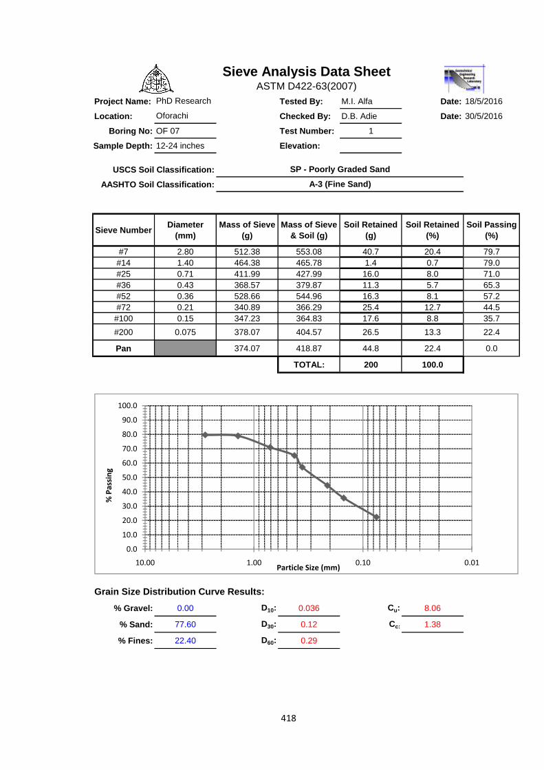
418








(mm)

Mass of Sieve

(g)

Mass of Sieve

& Soil (g)

Soil Retained

(g)

Soil Retained

(%)

Soil Passing

(%)

#7 2.80 512.38 553.08 40.7 20.4 79.7

#14 1.40 464.38 465.78 1.4 0.7 79.0

#25 0.71 411.99 427.99 16.0 8.0 71.0

#36 0.43 368.57 379.87 11.3 5.7 65.3

#52 0.36 528.66 544.96 16.3 8.1 57.2

#72 0.21 340.89 366.29 25.4 12.7 44.5

#100 0.15 347.23 364.83 17.6 8.8 35.7

#200 0.075 378.07 404.57 26.5 13.3 22.4

Pan 374.07 418.87 44.8 22.4 0.0

TOTAL: 200 100.0

% Gravel: 0.00 D10: 0.036 Cu: 8.06

% Sand: 77.60 D30: 0.12 Cc: 1.38

% Fines: 22.40 D60: 0.29



PhD Research

Oforachi

SP - Poorly Graded Sand

A-3 (Fine Sand)

0.0

10.0

20.0

30.0

40.0

50.0

60.0

70.0

80.0

90.0

100.0

0.010.101.0010.00

% P

assi

ng

Particle Size (mm)

419








(mm)

Mass of Sieve

(g)

Mass of Sieve

& Soil (g)

Soil Retained

(g)

Soil Retained

(%)

Soil Passing

(%)

#7 2.80 512.38 519.48 7.1 3.6 96.5

#14 1.40 464.38 465.58 1.2 0.6 95.9

#25 0.71 411.99 443.29 31.3 15.7 80.2

#36 0.43 368.57 386.77 18.2 9.1 71.1

#52 0.36 528.66 552.86 24.2 12.1 59.0

#72 0.21 340.89 360.99 20.1 10.1 49.0

#100 0.15 347.23 361.63 14.4 7.2 41.8

#200 0.075 378.07 396.57 18.5 9.3 32.5

Pan 374.07 439.07 65.0 32.5 0.0

TOTAL: 200 100.0

% Gravel: 0.00 D10: 0.015 Cu: 25.33

% Sand: 67.50 D30: 0.06 Cc: 0.63

% Fines: 32.50 D60: 0.38



PhD Research

Oforachi

0.0

10.0

20.0

30.0

40.0

50.0

60.0

70.0

80.0

90.0

100.0

110.0

0.010.101.0010.00

% P

assi

ng

Particle Size (mm)

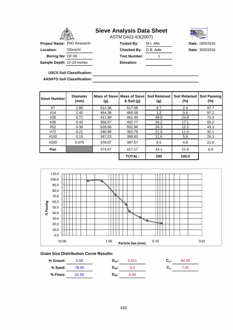
420








(mm)

Mass of Sieve

(g)

Mass of Sieve

& Soil (g)

Soil Retained

(g)

Soil Retained

(%)

Soil Passing

(%)

#7 2.80 512.38 517.08 4.7 2.4 97.7

#14 1.40 464.38 465.58 1.2 0.6 97.1

#25 0.71 411.99 461.49 49.5 24.8 72.3

#36 0.43 368.57 402.77 34.2 17.1 55.2

#52 0.36 528.66 552.96 24.3 12.2 43.1

#72 0.21 340.89 362.79 21.9 11.0 32.1

#100 0.15 347.23 358.83 11.6 5.8 26.3

#200 0.075 378.07 387.57 9.5 4.8 21.6

Pan 374.07 417.17 43.1 21.6 0.0

TOTAL: 200 100.0

% Gravel: 0.00 D10: 0.011 Cu: 44.55

% Sand: 78.45 D30: 0.2 Cc: 7.42

% Fines: 21.55 D60: 0.49



PhD Research

Oforachi

0.0

10.0

20.0

30.0

40.0

50.0

60.0

70.0

80.0

90.0

100.0

110.0

0.010.101.0010.00

% P

assi

ng

Particle Size (mm)

421








(mm)

Mass of Sieve

(g)

Mass of Sieve

& Soil (g)

Soil Retained

(g)

Soil Retained

(%)

Soil Passing

(%)

#7 2.80 512.38 515.68 3.3 1.6 98.4

#14 1.40 464.38 464.98 0.6 0.3 98.1

#25 0.71 411.99 432.49 20.5 10.3 87.8

#36 0.43 368.57 383.77 15.2 7.6 80.2

#52 0.36 528.66 546.96 18.3 9.1 71.1

#72 0.21 340.89 368.79 27.9 14.0 57.1

#100 0.15 347.23 361.53 14.3 7.2 50.0

#200 0.075 378.07 389.57 11.5 5.8 44.2

Pan 374.07 462.47 88.4 44.2 0.0

TOTAL: 200 100.0

% Gravel: 0.00 D10: 0.0014 Cu: 171.43

% Sand: 55.80 D30: 0.015 Cc: 0.67

% Fines: 44.20 D60: 0.24



PhD Research

Oforachi

0.0

10.0

20.0

30.0

40.0

50.0

60.0

70.0

80.0

90.0

100.0

110.0

0.010.101.0010.00

% P

assi

ng

Particle Size (mm)

422

M.I. Alfa Date: 9/10/16

D.B. Adie Date:

Coordinate 1

Boring No:

Initial Water level: 2.00 cm Start Time: 8:34 End Time: 12:34

Infiltration (cm)Infiltration

(cm)

Measured (cm/min) (cm/hr) Calculated

1 8:34 0 0 2.00 0.00 0.00 0 0

2 8:36 2 2 2.20 0.20 0.10 6.00 0.20 0.21037762 0.000108

3 8:39 3 5 2.20 0.20 0.07 4.00 0.40 0.31785096 0.013889

4 8:44 5 10 2.30 0.30 0.06 3.60 0.70 0.42594464 0.015862

5 8:54 10 20 2.50 0.50 0.05 3.00 1.20 0.55524767 0.003052

6 9:04 10 30 2.50 0.50 0.05 3.00 1.70 0.63574584 0.018427

7 9:19 15 45 2.70 0.70 0.05 2.80 2.40 0.71219012 0.000149

8 9:34 15 60 2.60 0.60 0.04 2.40 3.00 0.75769336 0.024867

9 10:04 30 90 3.10 1.10 0.04 2.20 4.10 0.79510837 0.092959

10 10:34 30 120 3.00 1.00 0.03 2.00 5.10 0.78876614 0.04462

11 11:04 30 150 2.90 0.90 0.03 1.80 6.00 0.75446062 0.021182

12 11:34 30 180 2.60 0.60 0.02 1.20 6.60 0.70029192 0.010058

13 12:04 30 210 2.50 0.50 0.02 1.00 7.10 0.63107186 0.01718

14 12:34 30 240 2.50 0.50 0.02 1.00 7.60 0.54993562 0.002494

S A 0.264846

0.02067365 -0.00013409 K = -0.0002011 cm/s

-0.0120681 cm/min

-2.011E-06 m/s

SSEInfiltration Rate Cum.

Infiltration

(cm)

S/NoClock

Reading

Time elapse

(min)

Cum. Time

(min)

Water level

(cm)

Test Number:

Soil TypeOF01

Infiltration Test

Project Name: PhD Research Tested By:Location: Oforachi (Okobu) Checked By:


D.B. Adie Date:

Coordinate 1

Boring No:


Infiltration

(cm)

Infiltration

(cm)


1 12:40 0 0 2.00 0.00 0 0

2 12:42 2 2 2.20 0.20 0.10 6.00 0.20 0.253166922 0.002827

3 12:45 3 5 2.20 0.20 0.07 4.00 0.40 0.382954128 0.033472

4 12:50 5 10 2.20 0.20 0.04 2.40 0.60 0.513946018 0.098562

5 13:00 10 20 2.60 0.60 0.06 3.60 1.20 0.671563625 0.005121

6 13:10 10 30 2.50 0.50 0.05 3.00 1.70 0.770556418 0.073201

7 13:25 15 45 2.80 0.80 0.05 3.20 2.50 0.865828491 0.004333

8 13:40 15 60 2.70 0.70 0.05 2.80 3.20 0.923933922 0.050146

9 14:10 30 90 3.50 1.50 0.05 3.00 4.70 0.975770271 0.274817

10 14:40 30 120 3.40 1.40 0.05 2.80 6.10 0.975045052 0.180587

11 15:10 30 150 3.30 1.30 0.04 2.60 7.40 0.940730094 0.129075

12 15:40 30 180 2.60 0.60 0.02 1.20 8.00 0.882555306 0.079838

13 16:10 30 210 2.60 0.60 0.02 1.20 8.60 0.8063007 0.04256

14 16:40 30 240 2.60 0.60 0.02 1.20 9.20 0.715732276 0.013394

S A 0.987933

0.02483336 -0.00015724 K = -0.00023586 cm/s

-0.01415169 cm/min

-2.3586E-06 m/s

SSEInfiltration Rate

S/NoClock

Reading

Time elapse

(min)

Cum. Time

(min)

Water level

(cm)

Cum.

Infiltration

(cm)

Test Number:

Soil TypeOF02

Infiltration Test

Project Name: PhD Research Tested By:Location: Oforachi (Okobu) Checked By:

423


D.B. Adie Date:

Coordinate 1

Boring No:


Infiltration

(cm)

Infiltration

(cm)


1 8:30 0 0 2.00 0.00 0 0

2 8:32 2 2 2.30 0.30 0.15 9.00 0.30 0.3215404 0.000464

3 8:35 3 5 2.40 0.40 0.13 8.00 0.70 0.48413609 0.007079

4 8:40 5 10 2.70 0.70 0.14 8.40 1.40 0.64600037 0.002916

5 8:50 10 20 2.90 0.90 0.09 5.40 2.30 0.83623958 0.004065

6 9:00 10 30 2.90 0.90 0.09 5.40 3.20 0.95149483 0.002652

7 9:15 15 45 3.00 1.00 0.07 4.00 4.20 1.05631046 0.003171

8 9:30 15 60 2.90 0.90 0.06 3.60 5.10 1.11358817 0.04562

9 10:00 30 90 3.40 1.40 0.05 2.80 6.50 1.14580549 0.064615

10 10:30 30 120 3.20 1.20 0.04 2.40 7.70 1.11079403 0.007958

11 11:00 30 150 3.20 1.20 0.04 2.40 8.90 1.03281968 0.027949

12 11:30 30 180 2.60 0.60 0.02 1.20 9.50 0.92432747 0.105188

13 12:00 30 210 2.80 0.80 0.03 1.60 10.30 0.7927103 5.31E-05

14 12:30 30 240 2.70 0.70 0.02 1.40 11.00 0.64278507 0.003274

S A 0.275004

0.03176306 -0.00022005 K = -0.00033008 cm/s

-0.01980489 cm/min

-3.3008E-06 m/s

SSE

Cum.

Infiltration

(cm)

Infiltration RateS/No

Clock

Reading

Time elapse

(min)

Cum. Time

(min)

Water level

(cm)

Test Number:

Soil TypeOF03

Infiltration Test

Project Name: PhD Research Tested By:Location: Oforachi Checked By:


D.B. Adie Date:

Coordinate 1

Boring No:


Infiltration

(cm)

Infiltration

(cm)SSE


1 12:40 0 0 2.00 0.00 0 0

2 12:42 2 2 2.40 0.40 0.20 12.00 0.40 0.35845111 0.001726

3 12:45 3 5 2.40 0.40 0.13 8.00 0.80 0.54080702 0.019827

4 12:50 5 10 2.60 0.60 0.12 7.20 1.40 0.72345166 0.01524

5 13:00 10 20 3.10 1.10 0.11 6.60 2.50 0.9403852 0.025477

6 13:10 10 30 3.00 1.00 0.10 6.00 3.50 1.07398403 0.005474

7 13:25 15 45 3.40 1.40 0.09 5.60 4.90 1.19873453 0.040508

8 13:40 15 60 3.30 1.30 0.09 5.20 6.20 1.27065295 0.000861

9 14:10 30 90 3.40 1.40 0.05 2.80 7.60 1.3229819 0.005932

10 14:40 30 120 3.20 1.20 0.04 2.40 8.80 1.30059498 0.010119

11 15:10 30 150 3.10 1.10 0.04 2.20 9.90 1.2304605 0.01702

12 15:40 30 180 3.00 1.00 0.03 2.00 10.90 1.12640946 0.015979

13 16:10 30 210 3.00 1.00 0.03 2.00 11.90 0.99665809 1.12E-05

14 16:40 30 240 3.00 1.00 0.03 2.00 12.90 0.84655974 0.023544

S A 0.181718

0.03530043 -0.00023538 K = -0.0003531 cm/s

-0.0211843 cm/min

-3.531E-06 m/s

Infiltration Rate Cum.

Infiltration

(cm)

S/NoClock

Reading

Time elapse

(min)

Cum. Time

(min)

Water level

(cm)

Infiltration Test


Test Number:

Soil TypeOF04

424


D.B. Adie Date:

Coordinate 1

Boring No:


Infiltration

(cm)

Infiltration

(cm)


1 8:35 0 0 2.00 0.00 0 0

2 8:37 2 2 2.20 0.20 0.10 6.00 0.20 0.07372925 0.015944

3 8:40 3 5 2.20 0.20 0.07 4.00 0.40 0.12149254 0.006163

4 8:45 5 10 2.30 0.30 0.06 3.60 0.70 0.17965203 0.014484

5 8:55 10 20 2.10 0.10 0.01 0.60 0.80 0.26973759 0.028811

6 9:05 10 30 2.20 0.20 0.02 1.20 1.00 0.34508726 0.02105

7 9:20 15 45 2.50 0.50 0.03 2.00 1.50 0.44473515 0.003054

8 9:35 15 60 2.60 0.60 0.04 2.40 2.10 0.53504085 0.00422

9 10:04 30 90 2.50 0.50 0.02 1.00 2.60 0.69947113 0.039789

10 10:35 30 120 2.90 0.90 0.03 1.80 3.50 0.85068957 0.002432

11 11:05 30 150 3.20 1.20 0.04 2.40 4.70 0.99346491 0.042657

12 11:35 30 180 3.10 1.10 0.04 2.20 5.80 1.13024286 0.000915

13 12:05 30 210 3.30 1.30 0.04 2.60 7.10 1.26247629 0.001408

14 12:35 30 240 3.30 1.30 0.04 2.60 8.40 1.3911118 0.008301

S A 0.189227

0.0062421 4.45875E-05 K = 6.6881E-05 cm/s

0.00401288 cm/min

6.6881E-07 m/s

Time elapse

(min)

Clock

ReadingS/No

Infiltration RateCum.

Infiltration

(cm)

SSEWater level

(cm)

Cum. Time

(min)

Infiltration Test


Test Number:

Soil TypeOF05


D.B. Adie Date:

Coordinate 1

Boring No:


Infiltration

(cm)

Infiltration

(cm)


1 12:40 0 0 2.00 0.00 0 0

2 12:42 2 2 2.30 0.30 0.15 9.00 0.30 0.14749347 0.023258

3 12:45 3 5 2.30 0.30 0.10 6.00 0.60 0.22233835 0.006031

4 12:50 5 10 2.40 0.40 0.08 4.80 1.00 0.29711059 0.010586

5 13:00 10 20 2.60 0.60 0.06 3.60 1.60 0.38553118 0.045997

6 13:10 10 30 2.50 0.50 0.05 3.00 2.10 0.43961712 0.003646

7 13:25 15 45 2.40 0.40 0.03 1.60 2.50 0.48957849 0.008024

8 13:40 15 60 2.30 0.30 0.02 1.20 2.80 0.51777256 0.047425

9 14:10 30 90 2.40 0.40 0.01 0.80 3.20 0.53645864 0.018621

10 14:40 30 120 2.60 0.60 0.02 1.20 3.80 0.52436112 0.005721

11 15:10 30 150 2.50 0.50 0.02 1.00 4.30 0.49259117 5.49E-05

12 15:40 30 180 2.40 0.40 0.01 0.80 4.70 0.44684729 0.002195

13 16:10 30 210 2.40 0.40 0.01 0.80 5.10 0.39051465 9E-05

14 16:40 30 240 2.40 0.40 0.01 0.80 5.50 0.32579887 0.005506

S A 0.177156

0.01454409 -9.8576E-05 K = -0.00014786 cm/s

-0.00887183 cm/min

-1.4786E-06 m/s

Infiltration Rate Cum.

Infiltration

(cm)

SSES/NoClock

Reading

Time elapse

(min)

Cum. Time

(min)

Water level

(cm)

Infiltration Test


Test Number:

Soil TypeOF06

425


D.B. Adie Date:

Coordinate 1

Boring No:


Infiltration

(cm)

Infiltration

(cm)


1 8:34 0 0 2.00 0.00 0 0

2 8:36 2 2 2.50 0.50 0.25 15.00 0.50 0.27896955 0.048854

3 8:39 3 5 2.50 0.50 0.17 10.00 1.00 0.42130677 0.006193

4 8:44 5 10 2.50 0.50 0.10 6.00 1.50 0.5642882 0.004133

5 8:54 10 20 2.80 0.80 0.08 4.80 2.30 0.73496494 0.00423

6 9:04 10 30 2.70 0.70 0.07 4.20 3.00 0.84088288 0.019848

7 9:19 15 45 2.80 0.80 0.05 3.20 3.80 0.94097451 0.019874

8 9:34 15 60 2.70 0.70 0.05 2.80 4.50 1.0000107 0.090006

9 10:04 30 90 3.20 1.20 0.04 2.40 5.70 1.046973 0.023417

10 10:34 30 120 3.30 1.30 0.04 2.60 7.00 1.03587415 0.069762

11 11:04 30 150 3.30 1.30 0.04 2.60 8.30 0.98767103 0.097549

12 11:34 30 180 2.70 0.70 0.02 1.40 9.00 0.9131116 0.045417

13 12:04 30 210 2.70 0.70 0.02 1.40 9.70 0.81858063 0.014061

14 12:34 30 240 2.70 0.70 0.02 1.40 10.40 0.70823818 6.79E-05

S A 0.443413

0.02743171 -0.00017941 K = -0.0002691 cm/s

-0.0161473 cm/min

-2.691E-06 m/s


Infiltration

(cm)

SSES/NoClock

Reading

Time elapse

(min)

Cum. Time

(min)

Water level

(cm)

Infiltration Test


Test Number:

Soil TypeOF07


D.B. Adie Date:

Coordinate 1

Boring No:


Infiltration

(cm)

Infiltration

(cm)


1 12:40 0 0 2.00 0.00 0 0

2 12:42 2 2 2.20 0.20 0.10 6.00 0.20 0.231799083 0.001011

3 12:45 3 5 2.20 0.20 0.07 4.00 0.40 0.350577561 0.022674

4 12:50 5 10 2.30 0.30 0.06 3.60 0.70 0.470404207 0.029038

5 13:00 10 20 2.50 0.50 0.05 3.00 1.20 0.614477339 0.013105

6 13:10 10 30 2.50 0.50 0.05 3.00 1.70 0.704860961 0.041968

7 13:25 15 45 2.80 0.80 0.05 3.20 2.50 0.791699333 6.89E-05

8 13:40 15 60 2.70 0.70 0.05 2.80 3.20 0.84449992 0.02088

9 14:10 30 90 3.30 1.30 0.04 2.60 4.50 0.891145919 0.167162

10 14:40 30 120 3.20 1.20 0.04 2.40 5.70 0.88965522 0.096314

11 15:10 30 150 3.00 1.00 0.03 2.00 6.70 0.857402518 0.020334

12 15:40 30 180 2.60 0.60 0.02 1.20 7.30 0.803298614 0.04133

13 16:10 30 210 2.60 0.60 0.02 1.20 7.90 0.732636934 0.017593

14 16:40 30 240 2.60 0.60 0.02 1.20 8.50 0.648866437 0.002388

S A 0.473865

0.02274278 -0.00014446 K = -0.000216694 cm/s

-0.013001668 cm/min

-2.16694E-06 m/s

Test Number:

Soil TypeOF08

Infiltration Test


Cum.

Infiltration

(cm)


S/NoClock

Reading

Time elapse

(min)

Cum. Time

(min)

Water level

(cm)

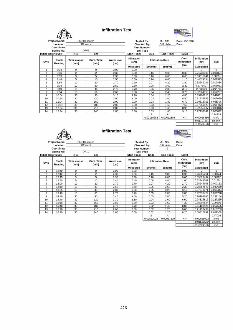
426


D.B. Adie Date:

Coordinate 1

Boring No:


Infiltration

(cm)

Infiltration

(cm)


1 8:34 0 0 2.00 0.00 0 0

2 8:36 2 2 2.30 0.30 0.15 9.00 0.30 0.21739108 0.006824

3 8:39 3 5 2.30 0.30 0.10 6.00 0.60 0.33015841 0.00091

4 8:44 5 10 2.50 0.50 0.10 6.00 1.10 0.44529154 0.002993

5 8:54 10 20 2.70 0.70 0.07 4.20 1.80 0.58649141 0.012884

6 9:04 10 30 2.60 0.60 0.06 3.60 2.40 0.6776607 0.006031

7 9:19 15 45 2.70 0.70 0.05 2.80 3.10 0.768999 0.004761

8 9:34 15 60 2.60 0.60 0.04 2.40 3.70 0.82861918 0.052267

9 10:04 30 90 3.10 1.10 0.04 2.20 4.80 0.89292215 0.042881

10 10:34 30 120 3.00 1.00 0.03 2.00 5.80 0.91236893 0.007679

11 11:04 30 150 2.90 0.90 0.03 1.80 6.70 0.90315013 9.92E-06

12 11:34 30 180 2.80 0.80 0.03 1.60 7.50 0.87356929 0.005412

13 12:04 30 210 2.80 0.80 0.03 1.60 8.30 0.82855907 0.000816

14 12:34 30 240 2.80 0.80 0.03 1.60 9.10 0.77133341 0.000822

S A 0.14429

0.02119286 -0.00012304 K = -0.00018456 cm/s

-0.01107381 cm/min

-1.8456E-06 m/s

Cum.

Infiltration

(cm)


S/NoClock

Reading

Time elapse

(min)

Cum. Time

(min)

Water level

(cm)

Infiltration Test


Test Number:

Soil TypeOF09

M.I. Alfa Date:

D.B. Adie Date:

Coordinate 1

Boring No:


Infiltration

(cm)

Infiltration

(cm)


1 12:40 0 0 2.00 0.00 0.00 0 0

2 12:42 2 2 2.30 0.30 0.15 9.00 0.30 0.26205261 0.00144

3 12:45 3 5 2.30 0.30 0.10 6.00 0.60 0.39523437 0.00907

4 12:50 5 10 2.40 0.40 0.08 4.80 1.00 0.52849307 0.01651

5 13:00 10 20 2.70 0.70 0.07 4.20 1.70 0.68649661 0.000182

6 13:10 10 30 2.60 0.60 0.06 3.60 2.30 0.78354547 0.033689

7 13:25 15 45 2.80 0.80 0.05 3.20 3.10 0.87378671 0.005444

8 13:40 15 60 2.70 0.70 0.05 2.80 3.80 0.92538424 0.050798

9 14:10 30 90 3.40 1.40 0.05 2.80 5.20 0.96164643 0.192154

10 14:40 30 120 3.30 1.30 0.04 2.60 6.50 0.94325816 0.127265

11 15:10 30 150 2.80 0.80 0.03 1.60 7.30 0.88994524 0.00809

12 15:40 30 180 2.70 0.70 0.02 1.40 8.00 0.81182425 0.012505

13 16:10 30 210 2.60 0.60 0.02 1.20 8.60 0.71490492 0.013203

14 16:40 30 240 2.60 0.60 0.02 1.20 9.20 0.60310292 9.63E-06

S A 0.47036

0.02582028 -0.00017329 K = -0.00025993 cm/s

-0.01559582 cm/min

-2.5993E-06 m/s

Time elapse

(min)

Clock

ReadingS/No


Infiltration

(cm)

SSEWater level

(cm)

Cum. Time

(min)

Infiltration Test


Test Number:

Soil TypeOF10

427

Tested By: M.I. Alfa Date: 09-10-16

Checked By: D.B. Adie Date:

Boring No: Depth 12-24 inches

Coordinate Elevation:

Sample

No.

Can

No.

Mass of

Can (g)

Mass of Can

+ Wet Soil (g)

Mass of Can

+ Dry Soil (g)

Mass of

Dry Soil

(g)

Mass of

Water

(g)

Moisture

Content

(%)

Average

Moisture

Content (%)

1 OF01 8.30 42.11 33.30 25.00 8.81 35.24

2 OF02 9.30 44.58 35.80 26.50 8.78 33.1334.19

Project Name:

Location:

Moisture Contents

PhD Research

Oforachi

OF 01





Sample

No.

Can

No.

Mass of

Can (g)

Mass of Can

+ Wet Soil (g)

Mass of Can

+ Dry Soil (g)

Mass of

Dry Soil

(g)

Mass of

Water

(g)

Moisture

Content

(%)

Average

Moisture

Content (%)

1 OF03 8.90 39.40 32.45 23.55 6.95 29.51

2 OF04 9.10 44.80 36.60 27.50 8.20 29.8229.66

Project Name:

Location:

Moisture Contents

PhD Research

Oforachi

OF 02





Sample

No.

Can

No.

Mass of

Can (g)

Mass of Can

+ Wet Soil (g)

Mass of Can

+ Dry Soil (g)

Mass of

Dry Soil

(g)

Mass of

Water

(g)

Moisture

Content

(%)

Average

Moisture

Content (%)

1 OF05 8.50 37.80 32.45 23.95 5.35 22.34

2 OF06 9.10 44.80 38.20 29.10 6.60 22.6822.51

Project Name:

Location:

Moisture Contents

PhD Research

Oforachi

OF 03





Sample

No.

Can

No.

Mass of

Can (g)

Mass of Can

+ Wet Soil (g)

Mass of Can

+ Dry Soil (g)

Mass of

Dry Soil

(g)

Mass of

Water

(g)

Moisture

Content

(%)

Average

Moisture

Content (%)

1 OF07 9.00 39.00 34.10 25.10 4.90 19.52

2 OF08 9.00 41.00 35.70 26.70 5.30 19.8519.69

Project Name:

Location:

Moisture Contents

PhD Research

Oforachi

OF 04

428





Sample

No.

Can

No.

Mass of

Can (g)

Mass of Can

+ Wet Soil (g)

Mass of Can

+ Dry Soil (g)

Mass of

Dry Soil

(g)

Mass of

Water

(g)

Moisture

Content

(%)

Average

Moisture

Content (%)

1 OF09 8.60 52.30 39.70 31.10 12.60 40.51

2 OF10 9.00 45.20 34.70 25.70 10.50 40.8640.69

Project Name:

Location:

Moisture Contents

PhD Research

Oforachi

OF 05





Sample

No.

Can

No.

Mass of

Can (g)

Mass of Can

+ Wet Soil (g)

Mass of Can

+ Dry Soil (g)

Mass of

Dry Soil

(g)

Mass of

Water

(g)

Moisture

Content

(%)

Average

Moisture

Content (%)

1 OF11 9.10 35.20 27.40 18.30 7.80 42.62

2 OF12 9.30 28.80 23.00 13.70 5.80 42.3442.48

Project Name:

Location:

Moisture Contents

PhD Research

Oforachi

OF 06





Sample

No.

Can

No.

Mass of

Can (g)

Mass of Can

+ Wet Soil (g)

Mass of Can

+ Dry Soil (g)

Mass of

Dry Soil

(g)

Mass of

Water

(g)

Moisture

Content

(%)

Average

Moisture

Content (%)

1 OF13 9.00 38.40 32.75 23.75 5.65 23.79

2 OF14 8.80 34.20 29.30 20.50 4.90 23.9023.85

Project Name:

Location:

Moisture Contents

PhD Research

Oforachi

OF 07





Sample

No.

Can

No.

Mass of

Can (g)

Mass of Can

+ Wet Soil (g)

Mass of Can

+ Dry Soil (g)

Mass of

Dry Soil

(g)

Mass of

Water

(g)

Moisture

Content

(%)

Average

Moisture

Content (%)

1 OF15 9.10 40.40 32.90 23.80 7.50 31.51

2 OF16 9.00 43.90 35.50 26.50 8.40 31.7031.61

Project Name:

Location:

Moisture Contents

PhD Research

Oforachi

OF 08

429





Sample

No.

Can

No.

Mass of

Can (g)

Mass of Can

+ Wet Soil (g)

Mass of Can

+ Dry Soil (g)

Mass of

Dry Soil

(g)

Mass of

Water

(g)

Moisture

Content

(%)

Average

Moisture

Content (%)

1 OF17 8.90 44.00 36.20 27.30 7.80 28.57

2 OF18 8.40 44.01 36.00 27.60 8.01 29.0228.80

Project Name:

Location:

Moisture Contents

PhD Research

Oforachi

OF 09


Checked By: D.B. Adie Date: 30/5/2016



Sample

No.

Can

No.

Mass of

Can (g)

Mass of Can

+ Wet Soil (g)

Mass of Can

+ Dry Soil (g)

Mass of

Dry Soil

(g)

Mass of

Water

(g)

Moisture

Content

(%)

Average

Moisture

Content (%)

1 OF19 9.20 39.50 32.90 23.70 6.60 27.85

2 OF20 8.90 44.70 37.00 28.10 7.70 27.4027.63

Project Name:

Location:

Moisture Contents

PhD Research

Oforachi

OF 10

430

APPENDIX XIV: CURVE NUMBER ESTIMATION

Table XIVa: 1987 Curve Number Estimation for all HSGs by landcover type

Landcover Area, A

(km2)

CN

A B C D

CN A*CN CN A*CN CN A*CN CN A*CN

Vegetation 711.23 33 23470.63 56 39828.95 70 49786.19 77 54764.81

Bare Surface/light

Grassland 415.12 55.5 23039.29 70.5 29266.12 80 33209.78 84.5 35077.83

Built up Areas 478.15 77 36817.43 85 40642.61 90 43033.36 92 43989.65

Total 1604.50 83327.35 109737.69 126029.33 133832.30

51.93 68.39 78.55 83.41

Table XIVb: 1987 Composite Curve Number Estimation for Ofu River Catchment

SMU FAOSOIL

Symbol Name

Textured

Class

Area, A

(km2) HSG CN A*CN

1021 Af13-1a Ferric Acrisols Sandy loam 975.61 A 51.93 50666.73

1567 Nd5-1a Dystric Nitosols Loam 259.77 B 68.39 17766.63

1193 G2-2/3a Gleysols Clay Loam 366.61 D 83.41 30579.41

677 Jd3-2a Calcaric

Fluvisols

Sandy Clay

Loam 2.59 C 78.55 203.13

1604.58 99215.90

Catchment Composite CN 61.83

Table XIVc: 2001 Curve Number Estimation for all HSGs by landcover type

Landcover Area, A

(km2)

CN

A B C D

CN A*CN CN A*CN C

N A*CN CN A*CN

Vegetation 651.994

2 33

21515.8

1 56 36511.68 70 45639.59 77 50203.55

Bare

Surface/light

Grassland

402.216

3

55.

5

22323.0

0

70.

5 28356.25 80 32177.30

84.

5 33987.28

Built up Areas 550.291

5 77

42372.4

5 85 46774.78 90 49526.24 92 50626.82

Total 1604.50 86211.2

6

111642.7

0

127343.1

3

134817.6

5

53.73 69.58 79.37 84.02

431

Table XIVd: 2001 Composite Curve Number Estimation for Ofu River Catchment

SMU FAOSOIL

Symbol Name

Textured

Class

Area, A

(km2) HSG CN A*CN


1567 Nd5-1a Dystric Nitosols Loam 259.77 B 69.58 18075.05


677 Jd3-2a Calcaric

Fluvisols

Sandy Clay

Loam 2.59 C 79.37 205.25

1604.58 101505.13


Table XIVe: 2016 Curve Number Estimation for all HSGs by landcover type

Landcover Area, A

(km2)

CN

A B C D

CN A*CN CN A*CN CN A*CN CN A*CN

Vegetation 869.10 33 28680.28 56 48669.57 70 60836.96 77 66920.65

Bare Surface 122.84 76 9335.92 85 10441.49 90 11055.69 92 11301.37

Built up

Areas 612.56 77 47167.24 85 52067.74 90 55130.54 92 56355.67

Total 1604.50 85183.44 111178.79 127023.19 134577.69

53.09 69.29 79.17 83.88

Table XIVf: 2016 Composite Curve Number Estimation for Ofu River Catchment

SMU FAOSOIL

Symbol Name

Textured

Class

Area, A

(km2) HSG CN A*CN


1567 Nd5-1a Dystric

Nitosols Loam 259.77 B 69.29 17999.94


677 Jd3-2a Calcaric

Fluvisols

Sandy Clay

Loam 2.59 C 79.17 204.73

1604.58 100749.72


432

APPENDIX XV: SYNTHETIC STREAM FLOW RESULTS

Table XVa: Generated Synthetic Stream flow Data (1974-2016) for Ofu River at Oforachi Using T-

F Model

Jan Feb Mar Apr May Jun Jul Aug Sep Oct Nov Dec Total

1974 3.52 1.67 2.48 8.95 17.49 67.97 147.34 219.71 404.76 91.96 5.31 4.02 975.18

1975 4.00 1.61 1.79 17.47 22.41 139.80 66.09 231.15 499.89 178.00 6.89 13.69 1182.78

1976 6.00 3.79 3.48 15.20 3.79 15.26 235.06 448.35 492.03 132.09 11.62 11.57 1378.25

1977 1.23 1.13 1.33 9.27 8.36 20.49 101.93 431.06 361.53 118.68 3.17 2.96 1061.14

1978 5.77 2.35 0.77 7.87 27.19 22.77 124.40 261.70 417.86 61.09 3.80 4.61 940.18

1979 1.64 1.46 0.99 7.48 10.45 47.30 123.93 327.37 410.44 70.06 7.19 59.12 1067.43

1980 2.75 1.84 1.41 8.16 25.41 10.04 105.99 497.86 400.09 41.40 8.17 3.11 1106.24

1981 4.32 3.28 2.11 31.07 22.26 24.38 206.93 608.77 412.23 53.29 3.73 0.49 1372.86

1982 1.87 2.04 1.79 10.96 7.69 10.05 119.15 322.67 515.37 61.59 5.23 0.41 1058.82

1983 3.00 1.75 0.91 7.72 8.79 68.82 114.43 270.71 401.07 52.63 2.96 4.25 937.05

1984 1.51 1.02 0.61 4.82 11.01 29.32 158.14 411.07 487.26 26.07 12.13 4.59 1147.55

1985 1.93 1.93 1.30 14.42 18.28 20.30 119.24 383.46 311.44 39.87 3.17 2.82 918.18

1986 4.60 7.38 1.94 18.45 38.78 6.32 35.78 152.45 379.22 115.23 3.87 5.71 769.72

1987 1.46 1.48 1.02 6.85 21.33 39.04 93.51 271.39 565.70 93.03 7.18 8.50 1110.48

1988 11.16 10.52 8.78 34.58 9.27 30.15 95.43 255.65 404.74 70.70 4.41 1.44 936.83

1989 2.87 3.54 2.42 18.11 8.79 85.46 95.55 172.74 547.50 158.02 8.62 3.61 1107.26

1990 2.07 1.85 1.01 6.16 18.69 19.52 153.90 395.98 452.89 102.77 2.69 0.29 1157.81

1991 3.27 2.13 1.15 11.28 14.01 42.54 141.26 479.27 252.20 61.47 5.08 0.75 1014.41

1992 2.81 1.45 1.03 12.18 15.05 18.04 65.79 341.83 532.94 68.30 5.72 9.30 1074.44

1993 2.92 3.76 1.82 9.81 5.94 80.59 87.39 217.27 418.78 71.02 3.48 3.27 906.06

1994 1.75 1.30 1.15 4.81 50.33 11.83 60.42 298.58 432.30 103.99 8.58 3.47 978.49

1995 1.27 1.52 1.04 21.61 10.59 84.86 167.93 492.14 253.44 78.74 5.04 2.26 1120.43

1996 5.80 3.37 1.58 16.79 23.71 79.01 173.95 438.12 410.56 71.28 3.74 1.93 1229.83

1997 2.61 2.64 1.95 7.70 18.96 29.11 127.68 599.68 371.62 54.74 4.55 10.04 1231.28

1998 5.32 4.43 3.24 11.29 34.07 9.34 125.82 330.96 323.78 109.53 5.45 3.85 967.09

1999 6.27 6.19 3.64 55.47 10.93 74.04 257.80 655.65 401.13 43.89 6.27 27.51 1548.79

2000 1.99 1.16 1.21 12.19 2.78 39.31 229.91 425.71 324.66 79.46 4.00 0.32 1122.70

2001 7.60 3.77 2.23 7.12 7.70 57.95 105.68 241.80 306.29 68.13 3.77 2.32 814.36

2002 3.14 2.33 0.90 24.47 19.05 57.05 112.87 426.17 381.45 62.64 4.22 1.71 1096.01

2003 2.55 1.82 0.93 15.37 4.18 58.78 132.86 368.30 512.82 49.27 7.87 1.36 1156.11

2004 1.03 1.13 0.38 2.31 24.24 88.09 158.18 486.72 419.72 89.34 5.89 1.47 1278.51

2005 2.08 7.29 5.47 30.82 6.66 14.84 168.75 463.22 500.85 98.36 4.73 4.30 1307.38

2006 5.41 3.73 2.73 8.15 9.19 46.53 236.08 559.08 392.66 46.29 4.40 0.10 1314.35

2007 4.24 3.87 4.46 28.95 4.06 18.93 111.09 325.71 387.24 31.00 4.01 12.22 935.79

2008 7.43 3.60 4.01 34.13 22.56 20.98 109.01 188.89 342.45 51.58 10.17 3.02 797.84

2009 3.52 4.12 5.74 38.76 10.90 20.43 139.12 342.47 463.08 24.78 2.60 2.94 1058.46

2010 1.76 1.29 0.92 7.84 12.49 11.47 52.20 200.84 244.62 32.94 5.52 0.45 572.34

2011 7.23 6.12 3.06 8.21 7.59 17.58 105.57 475.92 341.93 56.74 3.70 0.44 1034.09

2012 2.64 3.09 1.49 18.13 20.10 24.00 90.86 300.83 373.35 65.92 7.63 1.87 909.92

2013 1.60 0.94 0.99 10.73 10.72 26.80 183.42 388.83 434.75 64.49 1.91 0.79 1125.97

2014 1.83 3.41 1.48 16.13 7.41 45.02 134.09 367.03 496.89 130.32 5.47 0.90 1209.98

2015 2.76 1.64 1.51 17.36 14.09 67.81 179.61 696.47 396.83 42.28 1.63 0.89 1422.88

2016 8.43 3.72 2.98 16.73 9.99 16.01 92.87 313.17 737.07 279.86 4.75 6.61 1492.18

Average 3.65 2.99 2.12 15.72 15.29 39.95 131.33 374.11 416.68 79.14 5.36 5.47 1091.80

YearDischarge (m

3/s)

433

TableXVb: Adjusted Synthetic Stream flow Data (1974-2016) for Ofu River at Oforachi Using T-F

Model

Jan Feb Mar Apr May Jun Jul Aug Sep Oct Nov Dec Total

1974 3.55 3.28 1.84 13.30 19.07 36.56 135.26 370.79 443.72 76.42 5.98 3.89 1113.67

1975 3.24 3.31 2.16 13.55 21.65 9.98 135.96 372.80 440.47 63.72 5.95 3.39 1076.17

1976 1.92 2.28 1.36 13.48 11.88 56.08 134.51 411.02 440.73 70.50 5.86 3.50 1153.12

1977 5.04 3.54 2.38 13.31 14.28 54.14 135.65 407.98 445.20 72.48 6.03 3.95 1163.96

1978 2.07 2.96 2.64 13.27 24.17 53.30 135.46 378.17 443.27 80.98 6.01 3.86 1146.18

1979 4.77 3.38 2.54 13.26 15.37 44.22 135.46 389.73 443.52 79.66 5.95 1.03 1138.90

1980 4.05 3.21 2.34 13.28 23.23 58.01 135.61 419.73 443.88 83.89 5.93 3.94 1197.10

1981 3.02 2.52 2.01 13.93 21.58 52.70 134.75 439.25 443.46 82.13 6.02 4.08 1205.45

1982 4.63 3.11 2.16 13.36 13.93 58.01 135.50 388.90 439.94 80.91 5.98 4.08 1150.50

1983 3.89 3.25 2.58 13.27 14.50 36.25 135.54 379.76 443.84 82.23 6.03 3.88 1125.02

1984 4.86 3.59 2.72 13.19 15.67 50.87 135.17 404.46 440.90 86.15 5.84 3.86 1167.29

1985 4.59 3.16 2.39 13.46 19.49 54.21 135.50 399.60 446.91 84.11 6.03 3.96 1173.40

1986 2.84 0.58 2.09 13.57 30.25 59.39 136.22 358.95 444.59 72.99 6.01 3.81 1131.29

1987 4.89 3.38 2.53 13.24 21.09 47.27 135.72 379.88 438.22 76.26 5.95 3.66 1132.09

1988 0.00 0.00 0.00 14.03 14.76 50.57 135.70 377.11 443.72 79.56 6.00 4.03 1125.48

1989 3.97 2.40 1.86 13.57 14.51 30.09 135.70 362.52 438.84 66.67 5.92 3.91 1079.95

1990 4.50 3.20 2.53 13.23 19.70 54.50 135.20 401.80 442.07 74.83 6.04 4.09 1161.68

1991 3.71 3.07 2.46 13.37 17.25 45.98 135.31 416.46 448.93 80.93 5.99 4.06 1177.52

1992 4.01 3.39 2.52 13.40 17.79 55.05 135.96 392.27 439.34 79.92 5.97 3.62 1153.23

1993 3.94 2.29 2.15 13.33 13.01 31.89 135.77 370.36 443.24 79.52 6.02 3.93 1105.45

1994 4.71 3.46 2.46 13.19 36.32 57.35 136.01 384.66 442.78 74.65 5.92 3.92 1165.41

1995 5.02 3.35 2.52 13.66 15.45 30.31 135.08 418.72 448.89 78.38 5.99 3.99 1161.37

1996 2.06 2.48 2.26 13.53 22.34 32.48 135.03 409.22 443.52 79.48 6.02 4.00 1152.41

1997 4.14 2.83 2.09 13.27 19.84 50.95 135.43 437.65 444.85 81.92 6.00 3.58 1202.54

1998 2.37 1.98 1.48 13.37 27.78 58.27 135.44 390.36 446.49 73.83 5.98 3.90 1161.24

1999 1.75 1.14 1.29 14.63 15.62 34.32 134.31 447.50 443.84 83.52 5.96 2.67 1186.56

2000 4.55 3.52 2.43 13.40 11.35 47.17 134.55 407.04 446.46 78.27 6.01 4.09 1158.83

2001 0.88 2.29 1.95 13.25 13.93 40.27 135.62 374.67 447.08 79.94 6.01 3.98 1119.89

2002 3.80 2.97 2.58 13.75 19.89 40.61 135.56 407.11 444.51 80.75 6.01 4.01 1161.55

2003 4.18 3.22 2.57 13.49 12.08 39.97 135.38 396.93 440.02 82.73 5.93 4.03 1140.53

2004 5.17 3.54 2.83 13.12 22.62 29.12 135.17 417.77 443.21 76.81 5.97 4.03 1159.34

2005 4.49 0.62 0.43 13.93 13.38 56.23 135.08 413.64 440.43 75.48 6.00 3.88 1163.58

2006 2.31 2.31 1.72 13.28 14.71 44.50 134.50 430.50 444.13 83.17 6.00 4.10 1181.23

2007 3.08 2.24 0.90 13.87 12.02 54.72 135.57 389.44 444.32 85.42 6.01 3.47 1151.06

2008 0.99 2.37 1.12 14.02 21.73 53.96 135.59 365.36 445.85 82.39 5.88 3.95 1133.20

2009 3.55 2.12 0.30 14.15 15.61 54.16 135.33 392.39 441.72 86.34 6.04 3.95 1155.67

2010 4.70 3.46 2.57 13.27 16.44 57.48 136.08 367.47 449.19 85.14 5.98 4.08 1145.86

2011 1.12 1.18 1.56 13.28 13.87 55.22 135.62 415.87 445.87 81.62 6.02 4.08 1175.31

2012 4.13 2.61 2.30 13.57 20.44 52.84 135.74 385.06 444.79 80.27 5.94 4.01 1151.70

2013 4.80 3.63 2.54 13.36 15.51 51.81 134.95 400.54 442.69 80.48 6.05 4.06 1160.43

2014 4.65 2.46 2.31 13.51 13.78 45.06 135.37 396.71 440.57 70.76 5.98 4.06 1135.22

2015 4.04 3.30 2.29 13.54 17.29 36.62 134.98 454.68 443.99 83.76 6.06 4.06 1204.61

2016 0.33 2.31 1.60 13.53 15.13 55.80 135.73 387.23 432.36 48.68 5.99 3.76 1102.45

Average 3.50 2.68 2.03 13.50 17.91 46.94 135.40 397.95 443.31 78.32 5.98 3.82 1151.34

YearDischarge (m

3/s)

434

APPENDIX XVI: RESULTS OF NRCS-CN RAINFALL-RUNOFF MODELLING

Table XVI: Annual Daily Peak Runoff (m3/s)

Year P(mm) P-Ia (P-Ia)2 (P-Ia)+S Q (mm) Q(m3s)

1979 99.54 69.43 4820.45 219.96 21.92 1506.56

1980 99.48 69.37 4812.56 219.90 21.88 1504.49

1981 47.71 17.61 310.05 168.14 1.84 126.77

1982 79.52 49.41 2441.35 199.94 12.21 839.41

1983 98.72 68.62 4708.05 219.15 21.48 1476.90

1984 85.58 55.48 3077.79 206.01 14.94 1027.06

1985 116.65 86.55 7490.60 237.08 31.60 2172.04

1986 63.38 33.27 1107.11 183.80 6.02 414.08

1987 61.21 31.10 967.50 181.63 5.33 366.18

1988 74.92 44.81 2007.95 195.34 10.28 706.65

1989 70.75 40.64 1651.58 191.17 8.64 593.91

1990 82.81 52.70 2777.43 203.23 13.67 939.50

1991 95.19 65.09 4236.55 215.62 19.65 1350.73

1992 49.66 19.55 382.25 170.08 2.25 154.50

1993 92.64 62.53 3910.14 213.06 18.35 1261.63

1994 57.99 27.88 777.28 178.41 4.36 299.50

1995 95.78 65.68 4313.41 216.21 19.95 1371.50

1996 71.53 41.42 1715.79 191.95 8.94 614.49

1997 60.88 30.77 946.97 181.30 5.22 359.07

1998 76.42 46.31 2144.70 196.84 10.90 749.02

1999 89.18 59.08 3490.14 209.61 16.65 1144.67

2000 20.93 -9.18 84.27 141.35 0.00 0.00

2001 34.89 4.78 22.85 155.31 0.15 10.11

2002 90.84 60.73 3688.36 211.26 17.46 1200.20

2003 77.96 47.85 2289.64 198.38 11.54 793.44

2004 90.08 59.97 3596.32 210.50 17.08 1174.49

2005 40.31 10.21 104.15 160.74 0.65 44.54

2006 53.82 23.71 562.32 174.24 3.23 221.85

2007 95.90 65.79 4328.93 216.32 20.01 1375.68

2008 114.06 83.96 7048.68 234.49 30.06 2066.49

2009 107.51 77.40 5991.50 227.93 26.29 1807.04

2010 47.44 17.34 300.63 167.87 1.79 123.11

2011 51.50 21.40 457.91 171.93 2.66 183.09

2012 70.30 40.19 1615.37 190.72 8.47 582.26

2013 60.28 30.18 910.72 180.71 5.04 346.46

435

APPENDIX XVII: ESTIMATION OF RUNOFF COEFFICIENT

Slope Class Area, A

(km2)

Runoff Coefficient

(C) A*C

<3% 850.31 0.05 42.52

3-10% 675.86 0.11 74.34

10-30% 60.18 0.20 12.04

>30% 17.96 0.30 5.39

1604.31 134.28

Cs 0.08

Name Textured Class Permeability Area, A

(km2)

Runoff

Coefficient

(C)

A*C

Ferric Acrisols Sandy loam Permeable 975.61 0.10 97.56

Dystric Nitosols Loam Semi-permeable 259.77 0.20 51.95

Gleysols Clay Loam Semi-permeable 366.61 0.20 73.32

Calcaric Fluvisols Sandy Clay Loam Semi-permeable 2.59 0.20 0.52

1604.58 223.35

Cp 0.14

Landcover Area RC A*RC

Vegetation 869.10 0.05 43.45

Bare Surface 122.84 0.15 18.43

Built up Areas 612.56 0.30 183.77

1604.50 245.65

Cv 0.15

436

APPENDIX XVIII: FLOOD FREQUENCY ANALYSIS RESULTS

Table XVIIIa: Flood Frequency Calculations using log-Pearson Type III Analysis

Rank Year Qmax (m3/s) logQ (log Q -avg(logQ))^2 (log Q -avg(logQ))^3

Return Period, Tr =

[(n+1)/m]

Exceedence Probability

(1/Tr)

1 1964 723.30 2.859 0.045 0.009459 63.00 0.0159

2 1956 588.40 2.770 0.015 0.001809 31.50 0.0317

3 1958 578.70 2.762 0.013 0.001506 21.00 0.0476

4 1962 578.10 2.762 0.013 0.001488 15.75 0.0635

5 1961 555.10 2.744 0.009 0.000900 12.60 0.0794

6 1967 516.90 2.713 0.004 0.000282 10.50 0.0952

7 1970 498.10 2.697 0.002 0.000121 9.00 0.1111

8 1965 486.00 2.687 0.002 0.000058 7.88 0.1270

9 1971 482.00 2.683 0.001 0.000044 7.00 0.1429

10 1973 476.30 2.678 0.001 0.000027 6.30 0.1587

11 1969 457.30 2.660 0.000 0.000002 5.73 0.1746

12 2015 454.68 2.658 0.000 0.000001 5.25 0.1905

13 2010 449.19 2.652 0.000 0.000000 4.85 0.2063

14 1991 448.93 2.652 0.000 0.000000 4.50 0.2222

15 1995 448.89 2.652 0.000 0.000000 4.20 0.2381

16 1999 447.50 2.651 0.000 0.000000 3.94 0.2540

17 2001 447.08 2.650 0.000 0.000000 3.71 0.2698

18 1985 446.91 2.650 0.000 0.000000 3.50 0.2857

19 1998 446.49 2.650 0.000 0.000000 3.32 0.3016

20 2000 446.46 2.650 0.000 0.000000 3.15 0.3175

21 2011 445.87 2.649 0.000 0.000000 3.00 0.3333

22 2008 445.85 2.649 0.000 0.000000 2.86 0.3492

23 1977 445.20 2.649 0.000 0.000000 2.74 0.3651

24 1997 444.85 2.648 0.000 0.000000 2.63 0.3810

25 2012 444.79 2.648 0.000 0.000000 2.52 0.3968

26 1986 444.59 2.648 0.000 0.000000 2.42 0.4127

27 2002 444.51 2.648 0.000 0.000000 2.33 0.4286

28 2007 444.32 2.648 0.000 0.000000 2.25 0.4444

29 2006 444.13 2.648 0.000 0.000000 2.17 0.4603

30 1980 443.88 2.647 0.000 0.000000 2.10 0.4762

31 1983 443.84 2.647 0.000 0.000000 2.03 0.4921

32 1988 443.72 2.647 0.000 0.000000 1.97 0.5079

33 1974 443.72 2.647 0.000 0.000000 1.91 0.5238

34 1979 443.52 2.647 0.000 0.000000 1.85 0.5397

35 1996 443.52 2.647 0.000 0.000000 1.80 0.5556

36 1981 443.46 2.647 0.000 0.000000 1.75 0.5714

37 1978 443.27 2.647 0.000 0.000000 1.70 0.5873

38 1993 443.24 2.647 0.000 0.000000 1.66 0.6032

39 2004 443.21 2.647 0.000 0.000000 1.62 0.6190

40 1994 442.78 2.646 0.000 0.000000 1.58 0.6349

41 2013 442.69 2.646 0.000 0.000000 1.54 0.6508

42 1990 442.07 2.645 0.000 0.000000 1.50 0.6667

43 2009 441.72 2.645 0.000 0.000000 1.47 0.6825

44 1984 440.90 2.644 0.000 0.000000 1.43 0.6984

45 1976 440.73 2.644 0.000 0.000000 1.40 0.7143

46 2014 440.57 2.644 0.000 0.000000 1.37 0.7302

47 1975 440.47 2.644 0.000 0.000000 1.34 0.7460

48 2005 440.43 2.644 0.000 0.000000 1.31 0.7619

49 2003 440.02 2.643 0.000 0.000000 1.29 0.7778

50 1982 439.94 2.643 0.000 0.000000 1.26 0.7937

51 1992 439.34 2.643 0.000 0.000000 1.24 0.8095

52 1989 438.84 2.642 0.000 0.000000 1.21 0.8254

53 1987 438.22 2.642 0.000 0.000000 1.19 0.8413

54 1957 435.50 2.639 0.000 -0.000001 1.17 0.8571

55 2016 432.36 2.636 0.000 -0.000002 1.15 0.8730

56 1955 399.90 2.602 0.002 -0.000097 1.13 0.8889

57 1959 362.10 2.559 0.008 -0.000705 1.11 0.9048

58 1968 334.10 2.524 0.015 -0.001905 1.09 0.9206

59 1960 328.50 2.517 0.017 -0.002263 1.07 0.9365

60 1963 322.90 2.509 0.019 -0.002672 1.05 0.9524

61 1972 318.20 2.503 0.021 -0.003057 1.03 0.9683

62 1966 298.80 2.475 0.030 -0.005128 1.02 0.9841

Sum 27817 164.165 0.219 0.000

Average 449 2.648 0.004 -0.0000021

437

Table XVIIIb: Estimated Discharge Values using log-Pearson Type III Analysis Variance 0.0036

standard deviation 0.0599

skew coefficient -0.0104

Tr K(-0.1) K(0) slope K(-0.0104) Q (m3/s)

2 0.017 0.000 -0.17 0.002 444.57

5 0.846 0.842 -0.04 0.842 499.23

10 1.270 1.282 0.12 1.281 530.35

25 1.716 1.751 0.35 1.747 565.61

50 2.000 2.054 0.54 2.048 589.59

100 2.252 2.326 0.74 2.318 611.96

200 2.482 2.576 0.94 2.566 633.25

1000 2.950 3.090 1.4 3.075 679.33

438

APPENDIX XIX: ESTIMATION OF FLOOD VULNERABLE POPULATION

Table XIXa: Population at Risk for 1995 and 2000 Flood Scenarios

State LGA Population (Persons)

Area (km2) Population density Area inundated Persons affected

1991 1995 2000 1995 2000 1995 2000 1995 2000

Kogi

Dekina 177513 196969 224313 2487.55 79.18 90.17 2.03 2.02 161 183

Ofu 108095 125840 152172 1670.27 75.34 91.11 6.38 6.37 481 581

Igalamela/Odolu 78.88 78.75 5245 6085

Idah 224692 253340 294339 3809.91 66.49 77.26 0.00 0.00 0 0

Ibaji 163.75 163.71 10889 12648

Enugu Uzo-Uwani 127150 139962 157806 855.00 163.70 184.57 0.95 0.95 156 176

637450 716109 828630 8822.73 251.98 251.80 16932 19673

Table XIXb: Population at Risk for 100-year and 200-year Return Periods

State LGA Population (Persons) Area (km2) Population density

(persons/km2) Area inundated (km2) Persons affected

2006 100 Years 200 Years 100 Years 200 Years 100 Years 200 Years 100 Years 200 Years 100 Years

Kogi

Dekina 260968 932993 12561575 2487.55 375.07 5049.78 2.21 2.23 828 11269

Ofu 191480 1232480 55093299 1670.27 737.89 32984.67 6.97 7.04 5147 232184

Igalamela/Odolu 147048 639546 12845631 2250.85 284.14 5707.01 91.93 92.37 26120 527132

Idah 79755 346873 6967135 39.79 8717.60 175097.65 0.00 0.00 0 0

Ibaji 127572 554841 11144272 1519.27 365.20 7335.28 164.78 164.78 60179 1208741

Enugu Uzo-Uwani 127150 412142 4543112 855.00 482.04 5313.58 0.95 0.95 459 5051

933973 4118875 103155024 8822.73 266.84 267.37 92733 1984377

439

Table XIXc: Age Distribution of Population for 1995 and 2000


Under 15 Years Above 65 Years 15 - 65 Years

1995 2000 1995 2000 1995 2000

1995 2000 WD ND WD ND WD ND WD ND WD ND WD ND

Kogi

Dekina 161 183 1 73 1 83 0 5 0 6 1 81 1 92

Ofu 481 581 3 216 3 262 0 14 0 17 3 245 4 295

Idah

5245 6085 36 2350 41 2727 2 144 3 166 41 2672 47 3101

0 0 0 0 0 0 0 0 0 0 0 0 0 0

10889 12648 70 4882 81 5671 4 298 5 346 79 5556 92 6453

Enugu Uzo-Uwani 156 176 1 55 1 62 0 8 0 8 2 90 2 103

16932 19673 110 7577 128 8804 7 468 8 543 126 8644 146 10044

*WD-With disability, ND-No disability

Table XIXd: Age Distribution of Population for 100 years and 200 years Return Periods


Under 15 Years Above 65 Years 15 - 65 Years

100 Years 200 Years 100 Years 200 Years 100 Years 200 Years

2055 2155 WD ND WD ND WD ND WD ND WD ND WD ND

Kogi

Dekina 828 11269 6 371 75 5050 0 23 5 308 6 422 85 5746

Ofu 5147 232184 29 2312 1329 104256 2 141 81 6353 34 2629 1512 118653

Igalamela/Odolu 26120 527132 177 11701 3567 235144 11 713 218 14389 202 13316 4091 269723

Idah 0 0 0 0 0 0 0 0 0 0 0 0 0 0

Ibaji 60179 1208741 385 26982 7730 541940 23 1645 471 33024 438 30706 8797 616779

Enugu Uzo-Uwani 459 5051 3 161 35 1763 0 21 4 223 5 269 59 2967

92733 1984377 600 41527 12735 888154 37 2542 779 54297 685 47342 14545 1013867

*WD-With disability, ND-No disability

440

Table XIXe: 1995 and 2000 Affected Population Distributed by Poverty Line

State LGA

Persons affected Poverty

1995 2000

1995 2000

In

poverty

Above

poverty

In

poverty

Above

poverty

Kogi

Dekina 161 183 118 43 134 49

Ofu 481 581 353 128 426 155

Igalamela/Odolu 5245 6085 3850 1395 4466 1619

Idah 0 0 0 0 0 0

Ibaji 10889 12648 7993 2896 9284 3364

Enugu Uzo-Uwani 156 176 115 41 129 47

16932 19673 12428 4504 14440 5233

Table XIXf: Affected Population Distributed by Poverty Line for 100-Years and 200-Years

Return Periods

State LGA

Persons affected Poverty

100

Years

200

Years

100 Years 200 Years

In

poverty

Above

poverty

In

poverty

Above

poverty

Kogi

Dekina 828 11269 571 257 7776 3493

Ofu 5147 232184 3551 1596 160207 71977

Igalamela/Odolu 26120 527132 18023 8097 363721 163411

Idah 0 0 0 0 0 0

Ibaji 60179 1208741 41524 18655 834031 374710

Enugu Uzo-Uwani 459 5051 317 142 3485 1566

92733 1984377 63986 28747 1369220 615157

Table XIXg: 1995 and 2000 Affected Population Distributed by Gender

State LGA

Persons affected Gender

1995 2000 1995 2000

Male Female Male Female

Kogi

Dekina 161 183 78 83 88 95

Ofu 481 581 233 248 281 300

Igalamela/Odolu 5245 6085 2539 2706 2946 3139

Idah 0 0 0 0 0 0

Ibaji 10889 12648 5272 5617 6123 6525

Enugu Uzo-Uwani 156 176 74 82 84 92

16932 19673 8195 8737 9522 10151

441

Table XIXh: Affected Population Distributed by Gender for 100-Years and 200-Years

Return Periods

State LGA

Persons affected Gender

100

Years

200

Years

100 Years 200 Years

Male Female Male Female

Kogi

Dekina 828 11269 417 411 5674 5595

Ofu 5147 232184 2599 2548 117221 114963

Igalamela/Odolu 26120 527132 13231 12889 267025 260107

Idah 0 0 0 0 0 0

Ibaji 60179 1208741 30390 29789 610406 598335

Enugu Uzo-Uwani 459 5051 230 229 2533 2518

92733 1984377 46867 45866 1002859 981518

442

APPENDIX XX: ELEMENTS AT RISK

Fig. XXa: Elements at Risk of the 1995 Flood

443

Fig. XXb: Elements at Risk of the 2000 Flood

444

Fig. XXc: Elements at Risk of the 100-Year Flood

445

Fig. XXd: Elements at Risk of the 200-Year Flood

flood risk assessment of ofu river catchment in nigeria

Documents

Transcript of flood risk assessment of ofu river catchment in nigeria