FLOOD HAZARD ASSESSMENT IN A FLOOD PRONE URBAN ...
87
FLOOD HAZARD ASSESSMENT IN A FLOOD PRONE URBAN AREA USING HYDRODYNAMIC MODELS AND GIS TECHNIQUES Case of study in Pergamino, Argentina Silvia Roxana Mattos Gutierrez April, 2010
-
Upload
khangminh22 -
Category
Documents
-
view
1 -
download
0
Transcript of FLOOD HAZARD ASSESSMENT IN A FLOOD PRONE URBAN ...

FLOOD HAZARD ASSESSMENT IN A FLOOD
PRONE URBAN AREA USING HYDRODYNAMIC
MODELS AND GIS TECHNIQUES Case of study
in Pergamino, Argentina
Silvia Roxana Mattos Gutierrez
April, 2010

FLOOD HAZARD ASSESSMENT IN A FLOOD PRONE URBAN AREA USING HYDRODYNAMIC MODELS
AND GIS TECHNIQUES Case of Study in Pergamino, Argentina
by
Silvia Roxana Mattos Gutierrez
Thesis submitted to the International Institute for Geo-information Science and Earth Observation in partial fulfilment of the requirements for the degree of Master of Science in Geo-information Science
and Earth Observation, Specialisation: Integrating Watershed Modelling and Management Surface
Water Hydrology
Thesis Assessment Board
Chairperson Prof. Dr. V.G. Jetten (ESA department, ITC Enschede)
External Examiner Dr. Ir. M.J. Booij (UT Twente University, Enschede)
First supervisor MSc. Ir. G.N. Parodi (WRS department, ITC Enschede)
Second supervisor Dr. D. Alkema (ESA department, ITC Enschede)
Advisor MSc. Ir. F. Damiano (INTA, Buenos Aires, Argentina)
INTERNATIONAL INSTITUTE FOR GEO-INFORMATION SCIENCE AND EARTH OBSERVATION
ENSCHEDE, THE NETHERLANDS

Disclaimer
This document describes work undertaken as part of a programme of study at the International
Institute for Geo-information Science and Earth Observation. All views and opinions expressed
therein remain the sole responsibility of the author, and do not necessarily represent those of
the institute.

To my parents Jorge and Carmen

i
Abstract
The use of hydrodynamic models to assess flood events and levels has been applied all over the world
for already many years. However, in developing countries flood hazard assessments has to overcome
limitations of the information and lack of technical assessment. This work focuses on the flood hazard
assessment in a flat area of Pergamino (Argentina) using two hydrodynamic models with the support
of GIS techniques. The research attempts the evaluation of flood characteristics of the river using 1D
model HecRas and the assessment of the flood propagation in the urban area using model Flo-2D. The
work is based on data collected from previous studies and validation values taken during fieldwork.
HecRas model allowed the calibration and validation of the rating curve for the only city liminimeter
(Florencio Sanchez). The wave celerity and the travel time of the wave were also calculated. The
limnigraph stations Alfonzo y Urquiza located upstream and downstream of the urban area were
evaluated as source of data for the modelling process, however, a backwater effect found in the area
of Alfonzo plus the scarcity of topographic information were determinant to restrict their application.
A DTM generated from points measured during a topographic survey was used as main data. Major
attention is place in the construction of the DTM and advices exposed. The three origin of flood
events were simulated: a) Heavy rainfall, b) Overflow from the channel (riverine event) and c) the
combination of both events for 10 years of return period. During the simulations the volume
conservation and numerical stability were evaluated, and a process considering changes in the
numerical stability criterion was performed. Furthermore a comparison between the maximum
simulated flow depth for a past event and the values recorded locally was attempt.
The results showed a properly performance of Hec Ras model for the river channel in steady flow
conditions, a hazard map with the water depths under the levees have failure problems was presented.
Furthermore, the simulations with Flo-2D allowed the generation of flood hazard maps as first
approach or draft for the city. In the case of scenario a), the three hours total rainfall did not generate
high level of flood hazard, a medium hazard level was predominant in the case of scenario b) and c).
The comparison between the simulated maximum flow depth for a past event and the values recorded
in Pergamino showed the need to improve the data collection with instrumentation in a systematic
manner to allow further validations.
Key words: Flood hazard, hydrodynamic models, Hec Ras, Flo-2D, Pergamino city.

ii
Acknowledgements
First, I would like to thank to God for his presence and mercy.
I owe my deep and most sincere gratitude to my first supervisor MSc Ing. Gabriel Parodi for his
guidance throughout this research, for his patience and trust. “Gracias Gabriel por todas tus
enseñanzas, tu siempre disponibilidad y buen animo”. I am also grateful to my second supervisor Dr.
Dinand Alkema for his constructive comments in the improvement of this research. I would like also
express my grateful to MSc. Francisco Damiano for his valuable assistance during fieldwork, his help
to access the collection of data and his availability to support this work.
I would like to express also my grateful to MSc Byron Quan Luna for his values suggestions and for
share his knowledge about Flo-2D model. Also, my thanks go to Dr. Alemseged Tamiru for his
spontaneous and valuable assistance.
I would to express my grateful to the people in Pergamino city from the Municipality and
CO.S.S.O.PER for their availability to offer me the information and their help during fieldwork.
I also want to say thank you to Karen O´Brien from Flo-2D technical support office, for her
suggestions during the modelling process.
I owe to say “Betam Amesegnalehu” to Ayele Almaw, Ashebir Sewale Belay, Ambasager Tetemke
and “Terima kasih banyak” to Kristina Dewi and Erwinda Ds for their sincere friendship offered and
the memorable moments shared. Thank you my friends, you made me felt that my home was not far.
I want to say thank you to my classmates and friends from WREM for all the nice moments shared in
the cluster.
I like to express my gratitude to Edson Villagomez for the support and friendship offered to me during
these years, and also to Salvador Alvarado for the unforgettable coincidence and for all the help
provided in this research.
Last but not least, my heartily thanks to my beloved family: my parents Jorge and Carmen, my sisters
Carmen and Patricia and my brother Jorge for their unwavering support, prayers and love throughout
my life.

iii
Table of contents
1. INTRODUCTION............................................................................................................................9
1.1. Background.............................................................................................................................9
1.2. Problem statement.................................................................................................................10
1.2.1. Main objective..................................................................................................................11
1.2.2. Research questions ...........................................................................................................11
1.3. Thesis outline........................................................................................................................11
1.4. Literature review...................................................................................................................12
1.4.1. Modelling flood events.....................................................................................................12
1.4.2. River and Flood routing....................................................................................................13
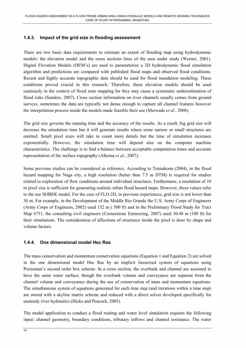
1.4.3. Impact of the grid size in flooding assessment.................................................................14
1.4.4. One dimensional model Hec Ras .....................................................................................14
1.4.5. Two dimensional model Flo2D........................................................................................15
1.4.6. Flood warning system proposed for Pergamino city........................................................16
2. STUDY AREA...............................................................................................................................18
2.1. Main Characteristics .............................................................................................................18
2.1.1. Location............................................................................................................................18
2.1.2. Climate .............................................................................................................................18
2.1.3. Relation between historical rainfall and flood events ......................................................19
2.1.4. Recurrence Period for Precipitation in Pergamino...........................................................19
2.2. Data availability....................................................................................................................20
2.2.1. Topography data available ...............................................................................................21
2.2.2. Hydrological data .............................................................................................................22
2.2.3. Remote sensing and other GIS data..................................................................................24
3. METHODOLOGY.........................................................................................................................25
3.1. Hec Ras model ......................................................................................................................25
3.1.1. River System schematic....................................................................................................25
3.1.2. Steady flow assessment ....................................................................................................26
3.1.3. Unsteady flow assessment................................................................................................27
3.2. Flo- 2D model .......................................................................................................................29
3.2.1. Input data description .......................................................................................................29
3.2.2. Trial simulations...............................................................................................................34
3.2.3. Model performance ..........................................................................................................37
3.3. Flood hazard assessment.......................................................................................................38
4. RESULTS AND DISCUSSION.....................................................................................................40
4.1. Hec Ras performance............................................................................................................40
Steady flow assessment..................................................................................................................40
4.1.1. Model calibration .............................................................................................................40
4.1.2. Roughness coefficient ......................................................................................................42
4.1.3. Levees exceeded hazard ...................................................................................................42
Unsteady flow assessment..............................................................................................................45
4.1.4. Flood celerity analysis......................................................................................................45
4.1.5. Limnigraphs analysis........................................................................................................46
iv
4.1.6. Improving in the existing Flood warning system ............................................................ 48
4.2. Flo2D model performance ................................................................................................... 49
4.2.1. Grid Size constrain .......................................................................................................... 49
4.2.2. Failed simulation ............................................................................................................. 50
4.2.3. Roughness coefficient calibration ................................................................................... 51
4.2.4. Flood patterns .................................................................................................................. 56
4.2.5. Scenario B........................................................................................................................ 58
4.2.6. Scenario C........................................................................................................................ 59
4.2.7. Flood propagation............................................................................................................ 60
4.2.8. Applicability of the results .............................................................................................. 61
4.3. Flood hazard assessment...................................................................................................... 63
5. CONCLUSIONS AND RECOMMENDATIONS ........................................................................ 67
5.1. Conclusions.......................................................................................................................... 67
5.2. Recommendations................................................................................................................ 68
REFERENCE ........................................................................................................................................ 71
APPENDICES....................................................................................................................................... 73
Appendix A ........................................................................................................................................... 73
FIELDWORK.................................................................................................................................... 73
A1. Discharges determination ........................................................................................................... 73
A2. Measurements of water level values: ......................................................................................... 74
A3. Inspection of the catchment upstream and dowstream of the river. ........................................... 75
A4. Inspection of the river located in the urban area. ....................................................................... 75
A5. Collection of data from the Pergamino Municipality and CO.S.O.PPER.................................. 75
Appendix B............................................................................................................................................ 76
B1. Alfonzo Station simulation......................................................................................................... 76
B2.Steady flow assessment ............................................................................................................... 76
B3.Detail of the flood hazard assesed in every cross section ........................................................... 77
B4.Results from sensitivy analysis performed by Hec Ras............................................................... 79
B5.Determination of the rainfall percentage (Input data for Flo2D simulations)............................. 79
B6.Pergamino Street map with the location of the bridges............................................................... 80
B7.Comparison between the results obtained with Flo-2D model.................................................... 80
B8. Flooding propagation scenario C................................................................................................ 82
B9. Flood hazard map by FEMA ...................................................................................................... 83
v
List of figures
Figure 1 Recent flooding in San Antonio de Areco (December 2009). Pergamino dikes resisted with less than 90
cm of overtopping. ........................................................................................................................................ 10
Figure 2 Work schematic of each grid ................................................................................................................... 15
Figure 3 Location of the study area ....................................................................................................................... 18
Figure 4 Flood events in Pergamino ...................................................................................................................... 19
Figure 5 Gumbel probability for the precipitation record in Pergamino (1967 – 2007) ........................................ 20
Figure 6 Location of the areas assessed during the study ...................................................................................... 21
Figure 7 Cross Section example ............................................................................................................................ 22
Figure 8 Plan example ........................................................................................................................................... 22
Figure 9 Rating curve Discharge- High curve at F. Sanchez Bridge ..................................................................... 22
Figure 10 Linmimeter in F Sanchez Bridge ........................................................................................................... 22
Figure 11 Income hydrographs to the Pergamino city ........................................................................................... 23
Figure 12 Hyetograph of 3 hours storm, recurrence period 10 years..................................................................... 24
Figure 13 River system schematic ......................................................................................................................... 25
Figure 14 Input cross section data ......................................................................................................................... 25
Figure 15 Cross Section schematic ........................................................................................................................ 25
Figure 16 Scheme of roughness coefficient measured in field............................................................................... 27
Figure 17 Geometry Data Alfonzo Station ............................................................................................................ 28
Figure 18 Bridge located downstream of Alfonso Station ..................................................................................... 28
Figure 19 Simulation with Normal Depth boundary condition. This would reproduce the condition without back
water ............................................................................................................................................................. 28
Figure 20 Simulation with W.S. Known boundary condition. This reproduces the effect with backwater. This was
the real situation at Alfonzo. ......................................................................................................................... 28
Figure 21 Distance and Elevation measurement in the Cross Sections.................................................................. 30
Figure 22 Location of the new points and new contours lines interpolated ........................................................... 30
Figure 23 Contour map modified........................................................................................................................... 30
Figure 24 First Digital Model Terrain. Pixel size 2.5 m........................................................................................ 30
Figure 25 Some mistakes found in the contours map interval 0.5 m ..................................................................... 31
Figure 26 Parameters used to Kriging Interpolation .............................................................................................. 31
Figure 27 Points set modified ................................................................................................................................ 31
Figure 28 Final Digital Terrain Model .................................................................................................................. 31
Figure 29 Topography sheet. Contours interval 2.5 m........................................................................................... 32
Figure 30 Digital Terrain Model from topography sheet source............................................................................ 32
Figure 31 Inflow input, upstream condition........................................................................................................... 33
Figure 32 Outflow input, downstream condition ................................................................................................... 33
Figure 33 Scheme of channel input........................................................................................................................ 33
Figure 34 Steps in the process of the channel input............................................................................................... 33
Figure 35 Simulation process ................................................................................................................................ 36
Figure 36 Example of the summary table reported by the Model after finishing the simulation ........................... 37
Figure 37 Flood hazard zones................................................................................................................................ 39
Figure 38 Comparison between water depths generated by Hec Ras model and values determined by the rating
curve F. Sanchez. .......................................................................................................................................... 40
Figure 39 Rating curve adjusted from the calibrated model .................................................................................. 41
Figure 40 Roughness coefficient sensitivity analysis............................................................................................. 42
Figure 41 Cross sections under overflow hazard for water depths in the ranges from 2.0 m to 2.9 m................... 43
Figure 42 Cross sections under overflow hazard for water depths in the ranges from 3.0 m to 3.9 m................... 43

vi
Figure 43 Cross sections under overflow hazard for water depths in the ranges from 4.0 m to 5.0 m................... 44
Figure 44 Water depths to generate flood hazard to the bridges............................................................................ 44
Figure 45. Wave time for 10 years recurrence period............................................................................................ 46
Figure 46 Comparison between values from limnigraphs stations......................................................................... 47
Figure 47 Comparison between peak values from the limnigraphs station, February 2009................................... 47
Figure 48: Upstream view over Alfonzo bridge during a low risk flood (February 2010). It shows the limnigraph
station, the backwater effect that had been foreseen by HECRAS and the large inundation plain the will be
inundated in case of extreme flooding. Reducing the peak to Pergamino ..................................................... 48
Figure 49: Downstream Alfonzo bridge................................................................................................................. 48
Figure 50 Lagoon Del Pescado location, between the Alfonzo Station and Pergamino City................................. 49
Figure 51 Constrain at the moment to introduce the inflow data ........................................................................... 49
Figure 52 Example of constrain in the identification of the features ..................................................................... 50
Figure 53 Roughness coefficients introduced as input for the simulation considering Scenario A........................ 52
Figure 54 Difference between the roughness coefficients introduced as input and the roughness coefficients
adjusted by the model during each simulation Scenario A............................................................................ 53
Figure 55 Example of grid with high velocity........................................................................................................ 53
Figure 56 Difference between the roughness coefficients introduced as input and the roughness coefficients
adjusted by the model during each simulation Scenario B............................................................................ 54
Figure 57 Roughness coefficients used during the assessment in Scenario B........................................................ 54
Figure 58 Roughness coefficients used during the assessment in Scenario C........................................................ 55
Figure 59 Difference between the roughness coefficients introduced as input and the roughness coefficients
adjusted by the model during each simulation Scenario C............................................................................ 56
Figure 60 Inundation Area for the Scenario A....................................................................................................... 57
Figure 61 a) Maximum Flow depth b) Maximum Flow velocity ........................................................................... 57
Figure 62 Location of the areas affected................................................................................................................ 58
Figure 63 Inundation Area for the Scenario B ....................................................................................................... 59
Figure 64 Maximum flow depth Scenario B .......................................................................................................... 59
Figure 65 Inundation Area for Scenario C............................................................................................................. 60
Figure 66 Maximum flow depth in Scenario C...................................................................................................... 60
Figure 67 Flooding propagation for Scenario C .................................................................................................... 61
Figure 68 Street selected for the depth and velocity assessment............................................................................ 62
Figure 69 Maximum flow depth simulated in the Scenario A in Dr. Alem Street.................................................. 62
Figure 70 Maximum Flow depth simulated in the Scenario B and C for Alem Street ........................................... 63
Figure 71 Flood Hazard map in the case of Scenario A : Rainfall event ............................................................... 63
Figure 72 Flood Hazard map in the case of Scenario B: Overflow in the channel ................................................ 64
Figure 73 Flood Hazard map for Scenario C: Rainfall and Overflow in the channel ............................................ 64
Figure 74 Flood Hazard map for Scenario A (According FEMA classification)................................................... 65
Figure 75 Flood Hazard map for Scenario B (According FEMA classification) ................................................... 65
Figure 76 Flood Hazard map for Scenario C (According FEMA classification) ................................................... 66

vii
List of tables
Table 1 Maximum Discharges for several recurrences .......................................................................................... 23
Table 2 Flow data input for the Steady flow assessment ....................................................................................... 26
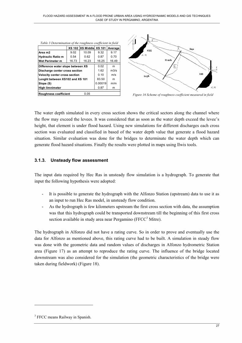
Table 3 Determination of the roughness coefficient in field.................................................................................. 27
Table 4 Grid size selection .................................................................................................................................... 32
Table 5 Roughness coefficient............................................................................................................................... 34
Table 6 Summary simulations................................................................................................................................ 37
Table 7 Flood hazard level used by Flo-2D model................................................................................................ 38
Table 8 Results from simulation in Steady flow conditions................................................................................... 40
Table 9 Wave celerity for different recurrence periods ......................................................................................... 46
Table 10 Trials performed for scenario A ............................................................................................................. 51
Table 11 Trials performed for the scenario B........................................................................................................ 53
Table 12 Example of the difference n-values (Final n – originl n) calculated from the output results .................. 53
Table 13 Trials performed in Scenario C............................................................................................................... 55
Table 14 Districts affected Scenario A .................................................................................................................. 57
Table 15 Comparison between the water depth reported by CO.S.S.O.PER and the values simulated by the model
...................................................................................................................................................................... 58
Table 16 Districts affected Scenario B .................................................................................................................. 59
Table 17 Districts affected in Scenario C .............................................................................................................. 60
Table 18 Areas according to Hazard zone identified............................................................................................. 66

FLOOD HAZARD ASSESSMENT IN A FLOOD PRONE URBAN AREA USING HYDRODYNAMIC MODELS AND GIS TECHNIQUES
CASE OF STUDY IN PERGAMINO, ARGENTINA
9
1. INTRODUCTION
1.1. Background
Flood, is defined as an overflowing of water onto land that is normally dry. Flood events have existed
and will continue to exist around the world. They are considered one of the most recurrent natural
hazards in urban and rural areas and although efforts continue, nowadays the number of people
affected by this phenomenon does not decrease. Only between 1900 and 2005 around 17 million
people were killed by floods and droughts and more than 5 billion were affected in the world (Cooley
et al., 2006).
At the moment of assessing flood events, the attention focuses in regions where human presence and
prone land areas combine. The developing of urban cities implies the change in the land use that
generally results in more runoff. According to the CEOS (CEOS, 2003) the runoff in an urban area
increases from two to six times when compared with the natural terrain. Moreover, the
geomorphology of the area will strongly influence the flood characteristics and the way to approach
its assessment. For example, in flat areas where the water tends to stay long, flood duration and water
depth are the main responsible for the damage; whilst in mountain regions water velocity and erosive
power of discharge are the main factors.
The traditional approach to simulate flow in river channels is done with one-dimensional (1D)
hydrodynamic modeling. However, in cases when speed and localized forces have to be known more
accurately in other 2D or 3D hydrodynamic models are being use (Merwade et al., 2008). In these
cases, the principal constraint is the input data availability.
Therefore, the compilation of the available data and the post processing analysis of the modeling
results might be supported by the use of GIS techniques. Besides that, from the experience in previous
researches, a GIS–based flood assessment allows the compensation of the data scarcity and assist in
the validation of the modelling results (Peters, 2008).
This study focuses on the assessment in one of these developing flood prone areas, Pergamino
(Argentina). This region was affected for several flood events throughout its history. Between 1912
and 2002, there were 113 floods of different degrees of severity. Of these, 35 resulted in water levels
reaching heights that demanded the partial evacuation of the local population (Herzer, 2006). One of
the greatest flood events that caused major damage to Pergamino happened in 1995. After two days of
rainfall medium intensity, a storm of 6 hours duration, struck with over 300 mm of rainfall, a case
with no precedents in the history of the region. This caused overflow of streams, and urban flooding
which was aggravated by the backwater from the Pergamino river into the drainage system of the city.
As a result, four people died and the city suffered significant economic losses (IATASA and ABS,
2008).

FLOOD HAZARD ASSESSMENT IN A FLOOD PRONE URBAN AREA USING HYDRAULIC MODELS AND REMOTE SENSING TECHNIQUES
CASE OF STUDY IN PERGAMINO, ARGENTINA
10
The flood events in Pergamino city happen from three sources: the first one related to the river
overflow as the flow from the upstream subcatchments produces the rise of the water level in the
channel and the water exceeds the banks. The second one is caused by heavy local rainfalls; the rain
and the insufficient hydraulic capacity of the sewage system combines produce the flood. The last one
is the combination of the overflowing in the river and the heavy rainfall in the city.
Furthermore, the assessment of the flood hazard in
Pergamino is not an isolated issue. Other
surrounding cities with similar characteristics in
terms of topography and hydrologic suffer similar
flood problems. For example, in December 2009,
Arrecifes and San Antonio de Areco (located
downstream of Pergamino) had a flood event
without precedents (Cornejo, 2009).
In this context, several efforts to understand the
floods and prevent more damage in Pergamino
have been made by the Municipality,
Neighborhoods Association (CO.S.S.O.PER) and the Province Government through institutions as the
Water National Institute (INA); this research intends to contribute with that from a modeling approach
and the assessment of results in terms of flood hazard.
1.2. Problem statement
In developing countries, the flood hazard assessment has not been evaluated in full magnitude yet.
When a flood event happens in a region, in most of cases, the attention is focused only in the
humanity help to the affected after the event. However, the data collection and correct compilation,
during and after the event (e.g. water levels signs, peak discharges, duration of the flood, etc), are not
done properly for the authorities. This inaction reduces the chances of accessing vital information.
The lack of the technical assessment in flood events can be overcame using hydrodynamic models and
GIS techniques; however, the limitation on the information available will limit the accuracy of the
results. Understanding what is possible to achieve during flood assessments under data scarcity
constraints helps to propose strategies to face the problem. One and two dimensional hydrodynamic
models are proposed to asses flood events. The knowledge of the model requirements and its
performance are crucial before deciding on its used for a specific area.
As discussed in the background section, Pergamino region faced several flood events in its history.
The topographic characteristics (rolling, local name: “pampa ondulada”) makes the region prone to
suffer flood events. The authorities are developing a project to construct two dams upstream the city
(IATASA and ABS, 2008), but a combination between political and economic problems are
postponing the execution. This project will also be considered in this thesis and the results will
contribute to some extra information for decision makers. The flat character of the area suggests the
used of two dimensional models to asses the flood events; however, the acquisition cost and the lack
of experience in the applications of these models become a constraint. The evaluation of the model
performance, in this case with FLO – 2D, will give reference to the level of analysis that it is possible
Figure 1 Recent flooding in San Antonio de Areco (December
2009). Pergamino dikes resisted with less than 90 cm of
overtopping.

FLOOD HAZARD ASSESSMENT IN A FLOOD PRONE URBAN AREA USING HYDRODYNAMIC MODELS AND GIS TECHNIQUES
CASE OF STUDY IN PERGAMINO, ARGENTINA
11
to achieve with the available data. Furthermore, the use of Hec Ras, can also contribute in the
evaluation of the flood problem considering the attention only in the river channel and next-to-river
floodplain areas. The premise of this study is to demonstrate the level of assessment that can be
achieved with the combination of both models.
1.2.1. Main objective
The main objective in this study is to assess the flood hazard in the urban area of Pergamino using
hydrodynamic models supported by ground information, and GIS techniques.
In order to achieve the main objective, the following specific objectives are formulated:
1. To asses the flood characteristics in Pergamino River using 1D model Hec Ras.
2. To study the flood propagation in Pergamino city using 2D model Flo-2D.
3. To compare the models results with the information provided in the area.
4. To generate a flood hazard map for the Pergamino city.
1.2.2. Research questions
1. What are the main characteristics of the Pergamino stream in terms of water depth and other
water dynamics?
2. What is the flood propagation produced in the urban area of Pergamino for the studied event?
3. What is the difference between the models results and the information provided in the area?
4. What is the flood hazard in Pergamino city?
1.3. Thesis outline
The research begins with the Introduction Chapter, which presents the problem background as a
description of the historical and current situation. Furthermore, describes the problem statement with
the objectives and the research questions. An overview about the bibliography is presented at the end
of this chapter.
Chapter 2 has two parts, the first one related to the description of the study area, location, climate and
relation between historical rainfall and flood events. The second one focuses in the description of the
available data like topography and hydrologic.
The methodology applied in the research is developed in Chapter 3. Both models, Hec Ras and Flo-2D
are described in individual section, focusing in the introduction of the input data and the assessment
during the processes.
Chapter 4 presents the results. The main results of the simulations are discussed and the comparison
with information provided in the area is also done.
The conclusions and recommendations are presented in Chapter 5.
An appendix chapter is added with the fieldwork information and a memory that includes some
process.

FLOOD HAZARD ASSESSMENT IN A FLOOD PRONE URBAN AREA USING HYDRAULIC MODELS AND REMOTE SENSING TECHNIQUES
CASE OF STUDY IN PERGAMINO, ARGENTINA
12
1.4. Literature review
Water is essential for the development of any civilization. Since the beginning of the history, human
beings settled their cities and developed their activities near water sources. For centuries, several
flood events have showed the power of this resource, flooding has been one of the most devastating
disasters both in terms of property damage and human casualties (Mujumdar, 2001). Flooding as a
natural phenomenon does not mean death and destruction, that kind of disaster event happen when
human lives or property values are affected (Dworak and Hansen, 2003). A hazard is defined as a
phenomenon that may cause disruption to humans or their property and infrastructure. The hazard
assessment determining the type of hazardous phenomena that may affect the area, their frequency
and magnitude, and representing on a map which areas are likely to be affected (Van Westen, 2000).
However, the flood assessment will depend on the kind of event because all floods are not alike. A
flood travels along a river as a wave, with velocity and depth continuously changing with time and
distance(Mujumdar, 2001). Some floods develop slowly, sometimes over a period of days; in this case
the attention will be focus in the duration and depth of the water more than the velocity. But flash
floods can develop quickly, sometimes in just a few minutes and without any visible signs of rain, in
this cases the velocity will be the factor to cause more damage (Fema, 2005).
Many urban areas are developed close to the rivers. However, the flood risk will depend on the
vulnerability of the city to the hazard event. (Imperviousness due to asphalts on streets decreases the
soil infiltration capability and the surface runoff increases)
1.4.1. Modelling flood events
The representation of hazard phenomenon in the real world is possible using models; their
performance will help to understand it and to raise mitigation strategies. For the case of inundation in
urban areas, modelling enables to calculate the magnitude of the event in terms of water depth and
velocity. However, the complexity in the urban environment and the lack of high resolution
topographic and hydrologic data compromise the implementation of those models in developing
countries (Chen et al., 2009).
Many approaches have been developed in order to understand and forecast the hydrodynamic
response of the rivers. Conventionally, the flood damage assessments have been doing through the use
of one dimensional (1D) models. This kind of models are very useful to asses the response of the river
(Alkema et al., 2007). They do not fully consider the effect of cross section shape changes, bends, and
other two-dimensional and three-dimensional aspects of flow. All flow is parallel to the direction of
the main channel (Tennakoon, 2004). Although this assumption is not theoretically correct, it is
suitable for most open channel hydraulic work (Dyhouse et al., 2003). These models are usually
applied to study flood levels and discharges in river systems, and have been applied successfully in
modelling flood routing at river reach scales from tens to hundreds of kilometers (Werner, 2004).
One dimensional models are capable of calculating flood levels and discharges quite accurately in
applications where the flow path is mainly “linear”. However, in urban areas two dimensional (2D)
models have more sounding theoretical basis for flooding simulations. These models require

FLOOD HAZARD ASSESSMENT IN A FLOOD PRONE URBAN AREA USING HYDRODYNAMIC MODELS AND GIS TECHNIQUES
CASE OF STUDY IN PERGAMINO, ARGENTINA
13
dedicated and continuous representation of terrain topography (mainly the preservation of narrow
water containing structures degradable during DEM generation) and provide information about: flood
water depth, velocity and spatial distribution, variation of extent and duration over a user defined time
frame (Peters, 2008). The output produced by them can be easily transferred to decision makers as
they match maps and GIS, However, their application, most of the time, requires considerable cost
and time for data collection.
1.4.2. River and Flood routing
Flood routing or stream routing is solved using mathematical procedures. Nowadays, is approached by
the use of numerical techniques (Brutsaert, 2005). During a flood event, depth and velocity are
assessed. Both flow properties change with the time, so the flood flow is considered unsteady and
gradually varied. The principles which governs the wave movement are the Saint Venant equations:
Continuity (Conservation of mass) (Equation 1) and Momentum (Newton`s second law of motion)
equation (Equation 2).
0=−∂∂
+∂∂
qt
A
x
Q Equation 1
0)(11 2
=−−∂∂
+∂
∂
+∂∂
fo SSg
x
ygx
A
Q
At
Q
A
Equation 2
Where ‘Q’ is the discharge (m3/s), ‘A’ is the area, ‘q’ is the lateral flow per unit length of the channel
(m3/s/m), ‘x’ is the distance along the channel, ‘y’ is the depth of flow, ‘g’ the Earth gravity, ‘So’, the
bed slope of the channel and ‘Sf’ is the friction slope. Some flow routing equations are generated by
using the Equation 1 and neglecting some terms of the Equation 2, this is according to the accuracy
level desired or simplifications that can be done after analyzing the flow type (Mujumdar, 2001).
As it is not possible to solve the above equations analytically (except in some very simplified cases),
numerical solutions are possible to obtain the variation of discharge and depth with time, along the
length of the water body. The numerical methods start at time= 0 with an initial condition and
boundary conditions. The boundary conditions describe the exchange of water mass between the study
area an the rest of the universe during the model run (Alkema et al., 2007). Upstream boundary
conditions are specified commonly as discharge hydrograph, on the other side, downstream conditions
might be specified as stage or discharge hydrograph, stage-discharge relationship, or hydraulic fall
(Tamiru, 2005).
Local
Acceleration
term
Convective
Acceleration
term
Pressure
Force
term
Gravity
Force
term
Friction
Force
term
Kinematic wave
Diffusion wave
Dynamic wave
FLOOD HAZARD ASSESSMENT IN A FLOOD PRONE URBAN AREA USING HYDRAULIC MODELS AND REMOTE SENSING TECHNIQUES
CASE OF STUDY IN PERGAMINO, ARGENTINA
14
1.4.3. Impact of the grid size in flooding assessment
There are two basic data requirements to estimate an extent of flooding map using hydrodynamic
models: the elevation model and the cross sections lines of the area under study (Werner, 2001).
Digital Elevation Models (DEM’s) are used to parameterize a 2D hydrodynamic flood simulation
algorithm and predictions are compared with published flood maps and observed flood conditions.
Recent and highly accurate topographic data should be used for flood inundation modeling. These
conditions proved crucial in this research. Therefore, these elevation models should be used
cautiously in the context of flood zone mapping for they may cause a systematic underestimation of
flood risks (Sanders, 2007). Cross section information on river channels usually comes from ground
surveys, sometimes the data are typically not dense enough to capture all channel features however
the interpolation process inside the models made feasible their use (Merwade et al., 2008).
The grid size governs the running time and the accuracy of the results. As a result, big grid size will
decrease the simulation time but it will generate results where some narrow or small structures are
omitted. Small pixel sizes will take in count more details but the time of simulation increases
exponentially. However, the simulation time will depend also on the computer machine
characteristics. The challenge is to find a balance between acceptable computation times and accurate
representation of the surface topography (Alkema et al., 2007).
Some previous studies can be considered as reference. According to Tennakoon (2004), in the flood
hazard mapping for Naga city, a high resolution (better than 7.5 m DTM) is required for studies
related to exploration of flow conditions around individual structures. Furthermore, a resolution of 10
m pixel size is sufficient for generating realistic urban flood hazard maps. However, these values refer
to the use SOBEK model. For the case of FLO-2D, in previous experiences, grid size is not lower than
30 m. For example, in the Development of the Middle Rio Grande the U.S. Army Corps of Engineers
(Army Corps of Engineers, 2002) used 152 m ( 500 ft) and in the Preliminary Flood Study for Tract
Map 6731, the consulting civil engineers (Cornerstone Enineering, 2007) used 30.48 m (100 ft) for
their simulations. The consideration of affections of structures inside the pixel is done by shape and
volume factors.
1.4.4. One dimensional model Hec Ras
The mass conservation and momentum conservation equations (Equation 1 and Equation 2) are solved
in the one dimensional model Hec Ras by an implicit linearized system of equations using
Preissman’s second order box scheme. In a cross section, the overbank and channel are assumed to
have the same water surface, though the overbank volume and conveyance are separate from the
channel volume and conveyance during the use of conservation of mass and momentum equations.
The simultaneous system of equations generated for each time step (and iterations within a time step)
are stored with a skyline matrix scheme and reduced with a direct solver developed specifically for
unsteady river hydraulics (Hicks and Peacock, 2005).
The model application to conduct a flood routing and water level simulation requires the following
input: channel geometry, boundary conditions, tributary inflows and channel resistance. The water

FLOOD HAZARD ASSESSMENT IN A FLOOD PRONE URBAN AREA USING HYDRODYNAMIC MODELS AND GIS TECHNIQUES
CASE OF STUDY IN PERGAMINO, ARGENTINA
15
level output in every cross section shows the performance of the model in terms of flooding events
(Brussel, 2008). Even though the model does not work by itself in a spatial distribution, the results
allow an accurate interpretation of the real flood situation. Furthermore, interfaces with GIS tools
improve the use of these model (Knebl et al., 2005).
1.4.5. Two dimensional model Flo2D
FLO-2D is a grid-based physical process model which routes precipitation-runoff and flood
hydrographs over unconfined surfaces and channels using either a kinematic, diffusive or dynamic
wave approximation to the momentum equation (Equation 2) (Hübl and Steinwendtner, 2001). During
the simulation, the model routes flows in eight directions (Figure 2). The spatial and temporal
resolution is dependent on the size of the grid elements and rate of rise in the hydrograph (O'Brien et
al., 2009).
The Flo-2D flood routing scheme follow , in a brief summarize, the follow steps: (For more detail
refers to Flo-2D Manual (O'Brien et al., 2009)) :
1. The average flow geometry, roughness and slope between
two grid elements are computed.
2. The flow depth for computing the velocity across a grid
boundary for the next timestep is estimated from the
previous timestep.
3. The first estimate of the velocity is computed using the
diffusive wave equation. (Equation 2).
4. The predicted diffusive wave velocity for the current
timestep is used to solve the full dynamic wave equation
for the solution velocity.
5. The discharge across the boundary is computed by multiplying the velocity by the cross
sectional flow area.
6. The incremental discharge for the timestep across the eight boundaries is summed and the
change in volume is distributed over the available storage area to determine an incremental
increase in the flow depth.
7. The numerical stability criteria are then checked for the new grid element flow depth. If any
of the stability criteria are exceeded, the simulation time is reset to the previous simulation
time, the timestep increment is reduced, and all the previous timestep computations are
discarded and the velocity computations begin again.
8. The simulation progresses with increasing timesteps until the stability criteria are exceeded.
In this computation sequence, the grid system inflow discharge and rainfall is computed first, then the
channel flow is computed, next the overland flow in 8- directions is determined (Figure 2). The model
verified three stability criteria to avoid volume conservation problems (error allowed lower than
0.001%). These criteria are checked by the model in a sequence of steps:
1. First, the percentage change in depth (the value suggested by the manual is equal to 0.2).
Figure 2 Work schematic of each grid

FLOOD HAZARD ASSESSMENT IN A FLOOD PRONE URBAN AREA USING HYDRAULIC MODELS AND REMOTE SENSING TECHNIQUES
CASE OF STUDY IN PERGAMINO, ARGENTINA
16
2. Then, Courant-Friedrich-Lewy (CFL) criterion, which relates the floodwave celerity to the
model time and spatial increments. The physical interpretation of this criterion is that a
particle of fluid should not travel more than one spatial increment ∆x in one timestep ∆t:
∆t=C∆x/(βV+c) Equation 3
Where ‘C’ is the Courant number (the model works with a value equal to 1.0 and it does not allow to
the user to change it), ‘∆x’ is the square grid element width, ‘V’ is the computed average cross section
velocity, ‘β’is a coefficient (5/3 for a wide channel) and ‘c’ is the computed wave celerity (O'Brien et
al., 2009).
3. Finally the Dynamic wave stability criteria governed which is an extension of the Courant
Criteria.
∆t<ξSo∆x2/qo
Equation 4
Where ‘∆x’ is the grid width, ‘qo’ is the discharge, ‘So’ is the bed slope and ‘ξ’ is the dynamic
stability coefficient “Wavemax”. The model verifies the numerical stability criteria in every grid
element at each timestep to ensure that the solution is stable. The model by default used 1.0 for
Wavemax, however, it is possible and sometimes necessary to modified the value (O'Brien et al.,
2009). The understanding of the stability procedure is essential to run FLO-2D, at it might save days
of processing.
- Wavemax = 0.1 to 1.0 (typical value = 0.25): Dynamic wave stability criteria increments and
decrements the computational timestep when Wavemax is exceeded, the model runs more
slowly but is stable.
- Wavemax = -0.1 to -1.0 (typical value = -0.25): the model does not consider the third criterion
and the increment or decrement of the timestep is according to the two first criteria. The
floodplain roughness values are incremented when the stability criteria exceed, but the
timestep is not decreased.
- Wavemax >100 (typical value = 100.25): the timestep are incremented or decremented only
by the two first criteria, but in this case, there is no n-value adjusted.
Flo-2D starts with a minimum timestep equal to 1 second and increases it until one of the three
numerical stability condition is exceeded, and then the timestep is decreased. If the stability criteria
continue to be exceeded, the timestep is decreases until a minimum timestep is reached. If the
minimum timestep is not small enough to conserve volume or maintain numerical stability, then the
minimum timestep can be reduced, the numerical stability coefficients can be adjusted or the input
data can be modified. The timesteps are a function of the discharge flux for a given grid element and
its size.
1.4.6. Flood warning system proposed for Pergamino city
The project “Defense works and storm drains in the Pergamino city”((IATASA and ABS, 2008)
formulates, some strategies to manage the flood events in the urban area. The proposal considers as
strategic to control the flood through the construction of two regulation dams upstream of the city.
FLOOD HAZARD ASSESSMENT IN A FLOOD PRONE URBAN AREA USING HYDRODYNAMIC MODELS AND GIS TECHNIQUES
CASE OF STUDY IN PERGAMINO, ARGENTINA
17
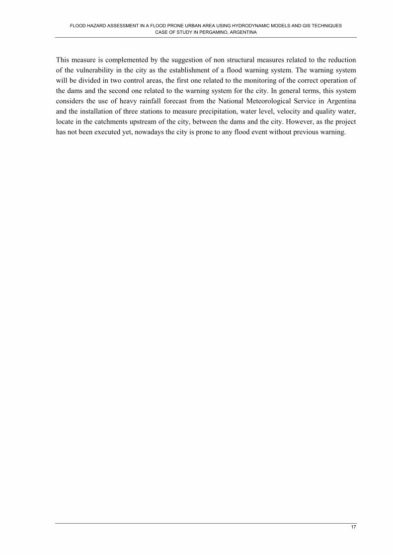
This measure is complemented by the suggestion of non structural measures related to the reduction
of the vulnerability in the city as the establishment of a flood warning system. The warning system
will be divided in two control areas, the first one related to the monitoring of the correct operation of
the dams and the second one related to the warning system for the city. In general terms, this system
considers the use of heavy rainfall forecast from the National Meteorological Service in Argentina
and the installation of three stations to measure precipitation, water level, velocity and quality water,
locate in the catchments upstream of the city, between the dams and the city. However, as the project
has not been executed yet, nowadays the city is prone to any flood event without previous warning.
FLOOD HAZARD ASSESSMENT IN A FLOOD PRONE URBAN AREA USING HYDRAULIC MODELS AND REMOTE SENSING TECHNIQUES
CASE OF STUDY IN PERGAMINO, ARGENTINA
18
2. STUDY AREA
2.1. Main Characteristics
2.1.1. Location
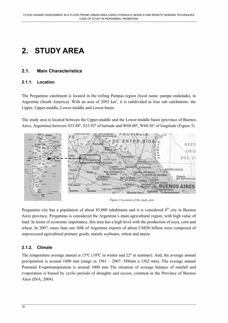
The Pergamino catchment is located in the rolling Pampas region (local name: pampa ondulada), in
Argentina (South America). With an area of 2092 km2, it is subdivided in four sub catchments: the
Upper, Upper-middle, Lower-middle and Lower basin.
The study area is located between the Upper-middle and the Lower-middle basin (province of Buenos
Aires, Argentina) between S33.88º, S33.92º of latitude and W60.60º, W60.56º of longitude (Figure 3).
Pergamino city has a population of about 85,000 inhabitants and it is considered 8th city in Buenos
Aires province. Pergamino is considered the Argentina’s main agricultural region, with high value of
land. In terms of economic importance, this area has a high level with the production of soya, corn and
wheat. In 2007, more than one fifth of Argentine exports of about US$56 billion were composed of
unprocessed agricultural primary goods, mainly soybeans, wheat and maize.
2.1.2. Climate
The temperature average annual is 15ºC (10ºC in winter and 22º in summer). And, the average annual
precipitation is around 1000 mm (range in 1961 – 2007: 588mm a 1562 mm). The average annual
Potential Evapotranspiration is around 1000 mm The situation of average balance of rainfall and
evaporation is biased by cyclic periods of droughts and excess, common in the Province of Buenos
Aires (INA, 2004).
Figure 3 Location of the study area

FLOOD HAZARD ASSESSMENT IN A FLOOD PRONE URBAN AREA USING HYDRODYNAMIC MODELS AND GIS TECHNIQUES
CASE OF STUDY IN PERGAMINO, ARGENTINA
19
2.1.3. Relation between historical rainfall and flood events
As it was mention in background section, Pergamino city has a long record of flood events during its
history. In the Figure 4 the flood events from 1933 until 2000 are presented. Each event was classified
according to the level of impact:
� Slight level means that flooding happened in specific areas caused by rainfall without overflow of
the river.
� Moderate level means flooding of extend areas in the city without evacuation of the population.
� High level means flooding with evacuation.
� Very high level means big impact in the population in terms of duration and water extend.
This classification was done after newspaper reports and because the information was not always
accurate or complete, these categories are relatively subjective (Centro, 2000).
0
50
100
150
200
250
300
350
1905
1910
1915
1920
1925
1930
1935
1940
1945
1950
1955
1960
1965
1970
1975
1980
1985
1990
1995
2000
2005
Year
Ra
infa
ll/2
4 h
ou
rs (
mm
)
Slight event Moderate event High event Very High event
Figure 4 Flood events in Pergamino
Source: Centro estudios sociales y ambientales,2000
Slight events was caused by similar precipitation (range around 50 mm and 100 mm), however in the
same range of rainfall, some moderate and high events happened, which means that similar rainfall
events can produce different impact in the same area. Moreover, the records show that there is no
similar recurrence between events with the same class, e.g. in the first years of the records (1915 to
1925) there were not events categorized as High level, then the next years (1925 to 1944) those kind
of events appear, later on, (1945 to 1960) not floods with that category were recorded but during the
last period (1980 to 1995) the high events occurred more frequently than before.
2.1.4. Recurrence Period for Precipitation in Pergamino
The Figure 5 present below was generated from the Maximum Precipitation in 24 hours record
measured in INTA Station, Pergamino. According to that, for 10 years of return period the Maximum
Precipitation is around 150 mm. However, this study considers for the modelling process a total
precipitation in three hours calculated by IATASA as part of the project “Defense works and drainage
for Pergamino city”.

FLOOD HAZARD ASSESSMENT IN A FLOOD PRONE URBAN AREA USING HYDRAULIC MODELS AND REMOTE SENSING TECHNIQUES
CASE OF STUDY IN PERGAMINO, ARGENTINA
20
Figure 5 Gumbel probability for the precipitation record in Pergamino (1967 – 2007)
Source: INTA, 2009
2.2. Data availability
Pergamino River, has a historic past related with flooding problems, because of that, several studies
were made by different organizations in the last years. From these studies some of the data were
available and collected. Part of that information was available and assessed during the pre – fieldwork
and the rest was completed during the fieldwork.
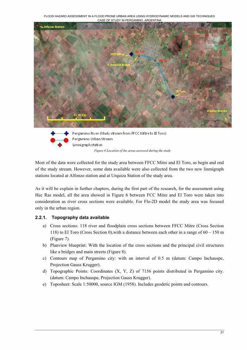
The Figure 6 presents the areas where were collected the data. The figure is quiet important for the
understanding of this thesis as the areas with different level of data availability are defined as the
geographical position with respect to Pergamino. Alfonzo Station is upstream and Urquiza station
downstream of the Thesis area.
FLOOD HAZARD ASSESSMENT IN A FLOOD PRONE URBAN AREA USING HYDRODYNAMIC MODELS AND GIS TECHNIQUES
CASE OF STUDY IN PERGAMINO, ARGENTINA
21
Most of the data were collected for the study area between FFCC Mitre and El Toro, as begin and end
of the study stream. However, some data available were also collected from the two new linmigraph
stations located at Alfonzo station and at Urquiza Station of the study area.
As it will be explain in further chapters, during the first part of the research, for the assessment using
Hec Ras model, all the area showed in Figure 6 between FCC Mitre and El Toro were taken into
consideration as river cross sections were available. For Flo-2D model the study area was focused
only in the urban region.
2.2.1. Topography data available
a) Cross sections: 118 river and floodplain cross sections between FFCC Mitre (Cross Section
118) to El Toro (Cross Section 0),with a distance between each other in a range of 60 – 150 m
(Figure 7).
b) Planview blueprint: With the location of the cross sections and the principal civil structures
like a bridges and main streets (Figure 8).
c) Contours map of Pergamino city: with an interval of 0.5 m (datum: Campo Inchauspe,
Projection Gauss Krugger).
d) Topographic Points: Coordinates (X, Y, Z) of 7156 points distributed in Pergamino city.
(datum: Campo Inchauspe, Projection Gauss Krugger).
e) Toposheet: Scale 1:50000, source IGM (1958). Includes geodetic points and contours.
Figure 6 Location of the areas assessed during the study

FLOOD HAZARD ASSESSMENT IN A FLOOD PRONE URBAN AREA USING HYDRAULIC MODELS AND REMOTE SENSING TECHNIQUES
CASE OF STUDY IN PERGAMINO, ARGENTINA
22
Figure 7 Cross Section example
Figure 8 Plan example
f) Cross Sections at the Limnigraphs stations areas: 8 for Alfonzo Station and 3 for Urquiza
Station.
g) Bridges characteristics: dimensions of the bridges located in the study stream and in Alfonzo
Station.
2.2.2. Hydrological data
a) Rating curve at F. Sanchez bridge [H= F(Q)]: The rating curve was built after individual and
isolated points measured for several discharges since 1967 to 2004 at the limnimeter located in F.
Sanchez Bridge (urban area, close to the cross section 102). No points are available during
moderate to high river levels (See Figure 9).
-0.5
0
0.5
1
1.5
2
2.5
3
0 20 40 60 80 100
Discharge [m3/s]
High [m]
Figure 9 Rating curve Discharge- High curve at F. Sanchez Bridge
Figure 10 Linmimeter in F Sanchez Bridge
These values were measured systematically, therefore a frequency analysis is not possible to achieve,
more over, the extreme flood events occurred in the urban area of Pergamino were not recorded
through this limnimeter.
The best-adjusted just curve is presented below:
0.4895915H2.784557-H13.63949 Q 2 +∗∗=
Source: INA, 2004
Equation 5

FLOOD HAZARD ASSESSMENT IN A FLOOD PRONE URBAN AREA USING HYDRODYNAMIC MODELS AND GIS TECHNIQUES
CASE OF STUDY IN PERGAMINO, ARGENTINA
23
Where Q is discharge in m3/s and H is water depth in ‘m’ (value read in the limnimeter).
During fieldwork the water depth value in the limnimeter was measured. It will be later used as
calibration point.
b) Water level values from the two limnigraph stations at Alfonzo and Urquiza: because of the
stations were established in 2008, the record is only available for that period.
c) Hydrographs: according to the objectives formulated, the hydrologic study of the area is not part
of this research, mainly due to limited resources. However, a hydrograph to run a hydrodynamic
model is necessary as an input. In a previous study “Study of defense projects and flood control
Pergamino stream” the follow design hydrographs to the Pergamino city were determined for
different return periods.
0
100
200
300
400
500
600
700
800
900
1000
0 20 40 60 80 100 120 140 160
Time (hrs)
Dis
ch
arg
e (
m3/s
)
R=10 R=50 R=100
Figure 11 Income hydrographs to the Pergamino city
Source: INA, 2004
d) Discharges values: during fieldwork three values of discharge were measured. One close to F.
Sanchez Bridge (cross section 102), the second in Alfonzo Station and the last one at Urquiza
Station.( The detail of the measurements and calculations are presented in Appendix A1).
Furthermore, in the same hydrologic study, after a recurrence assessment, INA1 determined the
follow peak discharges at the begin of the urban stream (FFCC Mitre Bridge). Table 1 Maximum Discharges for several recurrences
Recurrence
(years)
Peak discharge
(m3/s)
2 66
5 163
10 317
20 487
50 682
75 696
100 847
Source: INA, 2004
1 INA: (Instituto Nacional de Agua) is the official water board at national level in the country

FLOOD HAZARD ASSESSMENT IN A FLOOD PRONE URBAN AREA USING HYDRAULIC MODELS AND REMOTE SENSING TECHNIQUES
CASE OF STUDY IN PERGAMINO, ARGENTINA
24
e) Rainfall data: a hyetograph of 3 hours of duration and 10 years return period from the “Study of
defense projects and flood control Pergamino stream” (INA, 2004). From the hyetograph was
determined a Total Precipitation equal to 76.41 mm. (See Appendix B2). This is a design
hyetogram proposed by the methods of alternating blocks after the IDF curves. As such this
rainfall does not represent any real past event.
0
20
40
60
80
100
120
140
160
180
200
00.17
0.33 0.
50.67
0.83 1
1.17
1.33 1.
51.67
1.83 2
2.17
2.33 2.
52.67
2.83 3
Time (min)
Inte
nsit
y (
mm
/h)
Figure 12 Hyetograph of 3 hours storm, recurrence period 10 years
Source: INA, 2004
f) Historical record of past events: in 2001 the Pergamino neighbors association (CO.S.S.O.PER.)
made, on their own initiative, a quantitative record of the water level reached in previous rainfall
events. They selected five heavy rainfall events; the closest at the moment of the evaluation, and after
several meetings, the neighbors recalled each event and filled a form where they indicated the water
levels reached in the streets closer to their houses. Although this form was sent to all the districts in
the city, unfortunately not all the district reply it, however, the information collected was sent to INA,
who compiled and presented the data in Autocad format. From that information, it was selected for
this research the rainfall event occurred in February 9, 2001, with a total precipitation of 113.7 mm in
three hours, because according to the study made by IATASA, that kind of value corresponds to 10
years return period (IATASA and ABS, 2008). This precipitation was used to simulate a past event in
Flo-2D.
2.2.3. Remote sensing and other GIS data
a) QuickBird image of the study area: This image was taken from Google Earth Pro (2009), after
that a georeferenced process was done in Ilwis in based of control points obtained from the
Google Earth and the Topography sheet.
b) Cadastral map of the Pergamino city at block level (Source: Pergamino Municipality, 2007,
Autocad format)
c) Streets and main routes in Pergamino city map (Source: Pergamino Municipality, 2009,
Autocad format)

FLOOD HAZARD ASSESSMENT IN A FLOOD PRONE URBAN AREA USING HYDRODYNAMIC MODELS AND GIS TECHNIQUES
CASE OF STUDY IN PERGAMINO, ARGENTINA
25
3. METHODOLOGY
In this section a description of the methods and data collected during fieldwork will be introduced.
Hypothesis, calculations and restrictions that influence the model setting are discussed. The analysis
of results is done in the next chapter.
3.1. Hec Ras model
The analysis of the flood characteristics in the Pergamino river, between Mitre and El Toro, using the
1D model Hec Ras was done in two parts. The first one is to the steady simulation of the channel in
order to calibrate the current rating curve generated by INA. Then, a sensitivity analysis of roughness
coefficients was also done. Finally, with the results of the simulation, potential sectors along the
channel with overflow hazard were identified. Furthermore, in the second part, after the assessment
and simulation of the data from the limnigraphs stations, an unsteady simulation was performed to
determine the wave celerity.
3.1.1. River System schematic
The river system schematic was introduced to the Hec Ras model for the study area between FFCC
Mitre to El Toro (Figure 6). As a first step in Hec Ras, a QuickBird image was imported to visualize
the features and to support the introduction of the geometric data. Then, the river scheme was
digitalized and the cross sections were introduced one by one in the model. Moreover, the location of
the banks and levees were also introduced for every cross section and finally, a verification of the
cross sections width and the location of the banks was done using as reference the image imported. As
major improvement, the geometric characteristics of five bridges, were also introduced.
Figure 13 River system schematic
Figure 14 Input cross section data
Figure 15 Cross Section schematic

FLOOD HAZARD ASSESSMENT IN A FLOOD PRONE URBAN AREA USING HYDRAULIC MODELS AND REMOTE SENSING TECHNIQUES
CASE OF STUDY IN PERGAMINO, ARGENTINA
26
3.1.2. Steady flow assessment
As was explained in the previous chapter, the current rating curve F. Sanchez was generated from
field measurements where the maximum water depth value recorded was 2.5 m (water elevation 55.78
m) corresponding to a discharge of 78.41 m3/s, this can be consider a limitation at the moment to
assess extreme flow events in the urban area. Therefore, in order to improve that constrain, a steady
flow assessment described below was done to obtain a calibrated rating.
To generate a set of adequate steady flow data, the current rating curve F. Sanchez was used as
source. Thirteen water depths from 0.25 to 5.0 m were assumed as possible scenarios from low flow
to overflow in the channel; those values were introduced to the rating curve to obtain the discharges
values for the simulations (Table 2). The table shows the values of the discharge calculated from the
available rating curve. Values above 70 m3/s were interpolations. HECRAS requires values of
discharge in steady flow. From these values, the water height is calculated by the model.
Table 2 Flow data input for the Steady flow assessment
Scenario 2name
0.25m 0.8 m 1.0 m 1.5m 2.0 m 2.5 m 3.0 m 3.5 m 4.0 m 4.5 m 4.6 m 4.8 m 5.0 m
Discharge
(m3/s) 0.65 6.99 11.34 27 49.48 78.78 114.89 157.83 207.58 264.16 276.29 301.38 327.55
The river hydraulics was simulated in steady flow considering the discharges values calculated in
Table 2 as upstream boundary condition and the normal depth (0.0003845 m/m) as downstream
boundary condition. The assessment of the results was made in the cross section 102 (closest to
limnimeter F. Sanchez). The comparison between the results generated by the model and the values
calculated directly from the rating curve equation, in terms of water depth brought in first instance the
evaluation of the model performance. Moreover, based on the results obtained from the simulation, a
new rating curve was formulated for the F. Sanchez gauge. Finally, the rating curve proposed was
validated using the values obtained in fieldwork.
Furthermore, with the model calibrated a simple roughness sensitivity analysis was done. The
previous simulation was performed using a roughness coefficient equal to 0.03, value suggested by
the literature for natural stream channel, clean and straight (Brussel, 2008). Moreover, three more
simulations were performed, for roughness in the channel changed to 0.025, 0.04 and 0.05. The last
value was calculated from measures made during fieldwork (Table 3).
Based on Manning Equation
n = 1/Q * R2/3*S1/2
Equation 6
Where ‘Q’ is discharge in m3/s, ‘A’ is area in m2, ‘P’ is wet perimeter in m, ‘S’ slope in m/m and ‘n’
is the roughness coefficient.
2 The high values presented in the table are just an indication of the scenario (profile) name in a Hec Ras run and
they do not refer to the exact water level.
FLOOD HAZARD ASSESSMENT IN A FLOOD PRONE URBAN AREA USING HYDRODYNAMIC MODELS AND GIS TECHNIQUES
CASE OF STUDY IN PERGAMINO, ARGENTINA
27
Table 3 Determination of the roughness coefficient in field
XS 102 XS Middle XS 101 Average
Area m2 9.02 10.09 9.32 9.17
Hydraulic Ratio m 0.54 0.62 0.87 0.70
Wet Perimeter m 16.73 16.23 16.25 16.49
Difference water slope between XS 0.02 m
Discharge center cross section 1.62 m3/s
Velocity center cross section 0.10 m/s
Lenght between XS102 and XS 101 83.50 m
Slope (S) 0.00019 m/m
High limnimeter 0.87 m
Roughness coefficient 0.05
Figure 16 Scheme of roughness coefficient measured in field
The water depth simulated in every cross section shows the critical sectors along the channel where
the flow may exceed the levees. It was considered that as soon as the water depth exceed the levee’s
height, that element is under flood hazard. Using new simulations for different discharges each cross
section was evaluated and classified in based of the water depth value that generate a flood hazard
situation. Similar evaluation was done for the bridges to determinate the water depth which can
generate flood hazard situations. Finally the results were plotted in maps using Ilwis tools.
3.1.3. Unsteady flow assessment
The input data required by Hec Ras in unsteady flow simulation is a hydrograph. To generate that
input the following hypothesis were adopted:
- It is possible to generate the hydrograph with the Alfonzo Station (upstream) data to use it as
an input to run Hec Ras model, in unsteady flow condition.
- As the hydrograph is few kilometers upstream the first cross section with data, the assumption
was that this hydrograph could be transported downstream till the beginning of this first cross
section available in study area near Pergamino (FFCC3 Mitre).
The hydrograph in Alfonzo did not have a rating curve. So in order to prove and eventually use the
data for Alfonzo as mentioned above, this rating curve had to be built. A simulation in steady flow
was done with the geometric data and random values of discharges in Alfonzo hydrometric Station
area (Figure 17) as an attempt to reproduce the rating curve. The influence of the bridge located
downstream was also considered for the simulation (the geometric characteristics of the bridge were
taken during fieldwork) (Figure 18).
3 FFCC means Railway in Spanish.
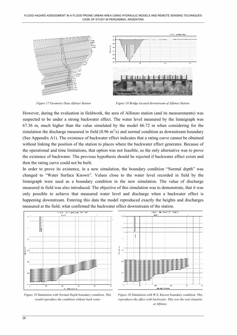
FLOOD HAZARD ASSESSMENT IN A FLOOD PRONE URBAN AREA USING HYDRAULIC MODELS AND REMOTE SENSING TECHNIQUES
CASE OF STUDY IN PERGAMINO, ARGENTINA
28
Figure 17 Geometry Data Alfonzo Station
Figure 18 Bridge located downstream of Alfonso Station
However, during the evaluation in fieldwork, the area of Alfonzo station (and its measurements) was
suspected to be under a strong backwater effect. The water level measured by the limnigraph was
67.36 m, much higher than the value simulated by the model 66.72 m when considering for the
simulation the discharge measured in field (0.96 m3/s) and normal condition as downstream boundary
(See Appendix A1). The existence of backwater effect indicates that a rating curve cannot be obtained
without linking the position of the station to places where the backwater effect generates. Because of
the operational and time limitations, that option was not feasible, so the only alternative was to prove
the existence of backwater. The previous hypothesis should be rejected if backwater effect exists and
then the rating curve could not be built.
In order to prove its existence, in a new simulation, the boundary condition “Normal depth” was
changed to “Water Surface Known”. Values close to the water level recorded in field by the
limnigraph were used as a boundary condition in the new simulation. The value of discharge
measured in field was also introduced. The objective of this simulation was to demonstrate, that it was
only possible to achieve that measured water level and discharge when a backwater effect is
happening downstream. Entering this data the model reproduced exactly the heights and discharges
measured at the field, what confirmed the backwater effect downstream of the station.
Figure 19 Simulation with Normal Depth boundary condition. This
would reproduce the condition without back water
Figure 20 Simulation with W.S. Known boundary condition. This
reproduces the effect with backwater. This was the real situation
at Alfonzo.

FLOOD HAZARD ASSESSMENT IN A FLOOD PRONE URBAN AREA USING HYDRODYNAMIC MODELS AND GIS TECHNIQUES
CASE OF STUDY IN PERGAMINO, ARGENTINA
29
This backwater effect is caused by the topographic characteristics downstream of the bridge, which
makes possible an unusual rising of the water level upstream (Figure 20). Although HecRas can model
this kind of situation, the scarcity of the cross sections data downstream the bridge made impossible to
handle it for the period of this research.
Concluded the analysis, the hypothesis formulated to generated the hydrograph from the Alfonzo
station was rejected. However, the geometric data for the study area (FFCC Mitre – El Toro) was
validated in the steady flow simulation. Then, to achieve the wave celerity analysis in unsteady flow
condition the hydrographs determined by INA (Figure 11) were introduced in the model. The
simulations were done for each period of recurrence and the hydrographs results from the first and the
last cross section were assessed.
In spite of the situation found during the analysis in Alfonzo Station, a simulation in steady flow was
made also for the area of Urquiza Station to generate a rating curve. However, the scarcity in the
number of cross section used (only three) did not allow to continue with the assessment. Obtaining
more section was limited by accessibility and high risk during fieldwork.
3.2. Flo- 2D model
The flood hazard assessment with Flo 2D was only focused in Pergamino urban area. The analysis is
presented in two sections. The first section relates effort in data input as it was the most time
consuming task of the model, and the one proven more sensitive: the generation of the digital terrain
model, grid size assessment and roughness coefficient. The second part describes the flood run
performed, the problems faced during the process and the improvements made until achieve the final
simulation.
3.2.1. Input data description
a) Digital terrain model generation
The most influential input to simulate a flood event using a 2-D model is without any doubt the DTM.
The time spent in the design of an FLO-2D-compatible DTM will certainly save hundreds of hours of
erroneous calculations. This is one of the main conclusions of this research in terms of data input.
In some developing areas the possibility to work with accurate DTM’s from LIDAR data is low as it is
very costly. There is one company in Argentina able to flight LIDAR, but the airplanes and equipment
need to be transported from Brazil, and the cost can only be covered in well funded projects. In most
cases, the sources to generate a DTM must come from topography surveys. In any case, the quality of
that data will (extremely) condition the results. In the Pergamino case, the DTM was generated from
the topography survey made in 2007, as it was considered the most up-to-date and sensible
information. (See subtitle 2.2.1). However the goal of that survey was not to develop a model for
Flood Hazard, and soon this became clear after the first analysis. The development of a DTM-for-
flood model is a methodology by itself that requires the survey of structures that affect water flow
rather than a standard striped-pattern survey for cadastral or road planning.

FLOOD HAZARD ASSESSMENT IN A FLOOD PRONE URBAN AREA USING HYDRAULIC MODELS AND REMOTE SENSING TECHNIQUES
CASE OF STUDY IN PERGAMINO, ARGENTINA
30
The first approach was developing a DTM from contours with an interval of 0.5 m provided by the
Pergamino Municipality. After importing from Autocad format, the first DTM was generated using
the spatial interpolation tool in Ilwis. However, some erroneous features were generated and found in
the results. An unreal embankment shape off the river channel was created as the contours delineation
confused the upper cord (pavement) of the bridges as part of the natural terrain. To improve that, the
only solution possible was to neglect those problematic contours.
The following procedure was selected for the river area:
1. Digitalization of the river stream using as a base the QuickBird image (georeferenced high
resolution Google Earth image (dry period))
2. Measurement of the distance from the main river axis to every elevation point in the cross
sections available after the field survey (Figure 21).
3. Those points were plotted in the available contours map (Figure 22). Then, the new points
were used to produce an interpolation and, as a result, new contours were built (Figure 23).
4. With the contour map improved, a new DTM was generated using the spatial interpolation
tool in Ilwis.
5. The optimized DTM process was executed in Ilwis using the hydroprocessing tools available.
The optimization process requires the values of buffer distance, smooth drop and sharp drop,
to introduce those values as best representation of the river, this was considered in four
segments (Figure 24).
Figure 21 Distance and Elevation measurement in the Cross
Sections
Figure 22 Location of the new points and new contours lines
interpolated
Figure 23 Contour map modified
Figure 24 First Digital Model Terrain. Pixel size 2.5 m
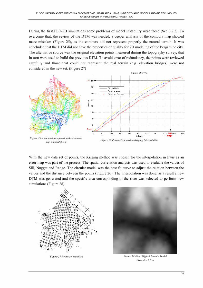
FLOOD HAZARD ASSESSMENT IN A FLOOD PRONE URBAN AREA USING HYDRODYNAMIC MODELS AND GIS TECHNIQUES
CASE OF STUDY IN PERGAMINO, ARGENTINA
31
During the first FLO-2D simulations some problems of model instability were faced (See 3.2.2). To
overcome that, the review of the DTM was needed, a deeper analysis of the contours map showed
more mistakes (Figure 25), as the contours did not represent properly the natural terrain. It was
concluded that the DTM did not have the properties or quality for 2D modeling of the Pergamino city.
The alternative source was the original elevation points measured during the topography survey, that
in turn were used to build the previous DTM. To avoid error of redundancy, the points were reviewed
carefully and those that could not represent the real terrain (e.g. elevation bridges) were not
considered in the new set. (Figure 27)
Figure 25 Some mistakes found in the contours
map interval 0.5 m
Figure 26 Parameters used to Kriging Interpolation
With the new data set of points, the Kriging method was chosen for the interpolation in Ilwis as an
error map was part of the process. The spatial correlation analysis was used to evaluate the values of
Sill, Nugget and Range. The circular model was the best fit curve to adjust the relation between the
values and the distance between the points (Figure 26). The interpolation was done; as a result a new
DTM was generated and the specific area corresponding to the river was selected to perform new
simulations (Figure 28).
Figure 27 Points set modified
Figure 28 Final Digital Terrain Model
Pixel size 2.5 m

FLOOD HAZARD ASSESSMENT IN A FLOOD PRONE URBAN AREA USING HYDRAULIC MODELS AND REMOTE SENSING TECHNIQUES
CASE OF STUDY IN PERGAMINO, ARGENTINA
32
Finally, as the standard source of topographic information in developing countries is the contours of
the toposheets, a third Digital Terrain Model was generated in Ilwis from the digitalized contours
(Figure 29) and (Figure 30). The comparison between Figure 28 and Figure 30 clearly shows the
unavoidable error of the different DTM’s generated from different sources.
Figure 29 Topography sheet. Contours interval 2.5 m
Figure 30 Digital Terrain Model from topography sheet source
Pixel size 2.5 m
b) Grid Size and Boundary conditions for the flood routing simulation
When the DTM is introduced as input data in the model, the grid size must be simultaneously defined.
Every next step is handled by the model through each grid, after the grid size is defined. An
interpolation process is done by the model in order to assign an elevation value to every grid element
or cell, understanding that the grid size is coarser than the pixel size. The following relation (O'Brien
et al., 2009) was carefully considered at the moment of selecting the grid size:
Equation 7
Table 4 Grid size selection
Q Grid Grid Q/A
m3/s size m Area m
2
317 20 400 0.79
317 35 1225 0.26
317 50 2500 0.13 Where Q is the discharge expressed in m3/ s and A is the grid area expressed in m2.
Considering the peak discharge equal to 317 m3/s from the hydrograph of 10 years recurrence period
(Figure 11), according to the Equation 7 the minimum grid size value should be 35 m to guarantee a
properly computational time. The first simulations were ran with that value; however, that grid size
was inadequate when considering the river width. Due to the river channel performance plays an
important role during the flood simulation, a 20 m grid size was selected as a final value for the rest of
the simulations.
A QuickBird image (from Google Earth) was used to visualize and to introduce the main elements
(e.g. channel River, upstream node, etc). The hydrograph for 10 years of recurrence was input as a
boundary condition in one node upstream of the channel river (Figure 31). All the grid-cells located in
2
3
2
3
3.003.0ms
m
A
Q
ms
m
−<<
−

FLOOD HAZARD ASSESSMENT IN A FLOOD PRONE URBAN AREA USING HYDRODYNAMIC MODELS AND GIS TECHNIQUES
CASE OF STUDY IN PERGAMINO, ARGENTINA
33
the downstream boundary were considered as outflow plain, which means that the flow is allowed to
pass out of the system through those grids (Figure 32). This is standard procedure in Flo-2D (O'Brien
et al., 2009).
Figure 31 Inflow input, upstream condition
Figure 32 Outflow input, downstream condition
c) River channel
The river channel in the model is defined by the cross section data. First, the channel was digitalized
in the model using as a base the city image that was imported. During the digitalization each point,
which represented the channel, matched with the center of each cell, however, as the cell does not
contain perfectly the river, some reaches are not properly represented. The river cross sections from
the urban area were imported from the HEC RAS model using the proper FLO-2D options, then each
cross section was located and linked with its respective grid taken the left bank as a reference. After
that, the model established the localization of the right banks based on the cross section width.
Finally, as every grid-cell of the channel must have a defined cross section; an interpolation process
available in the model was selected. (Figure 33) (Figure 34)
Figure 33 Scheme of channel input
Figure 34 Steps in the process of the channel input
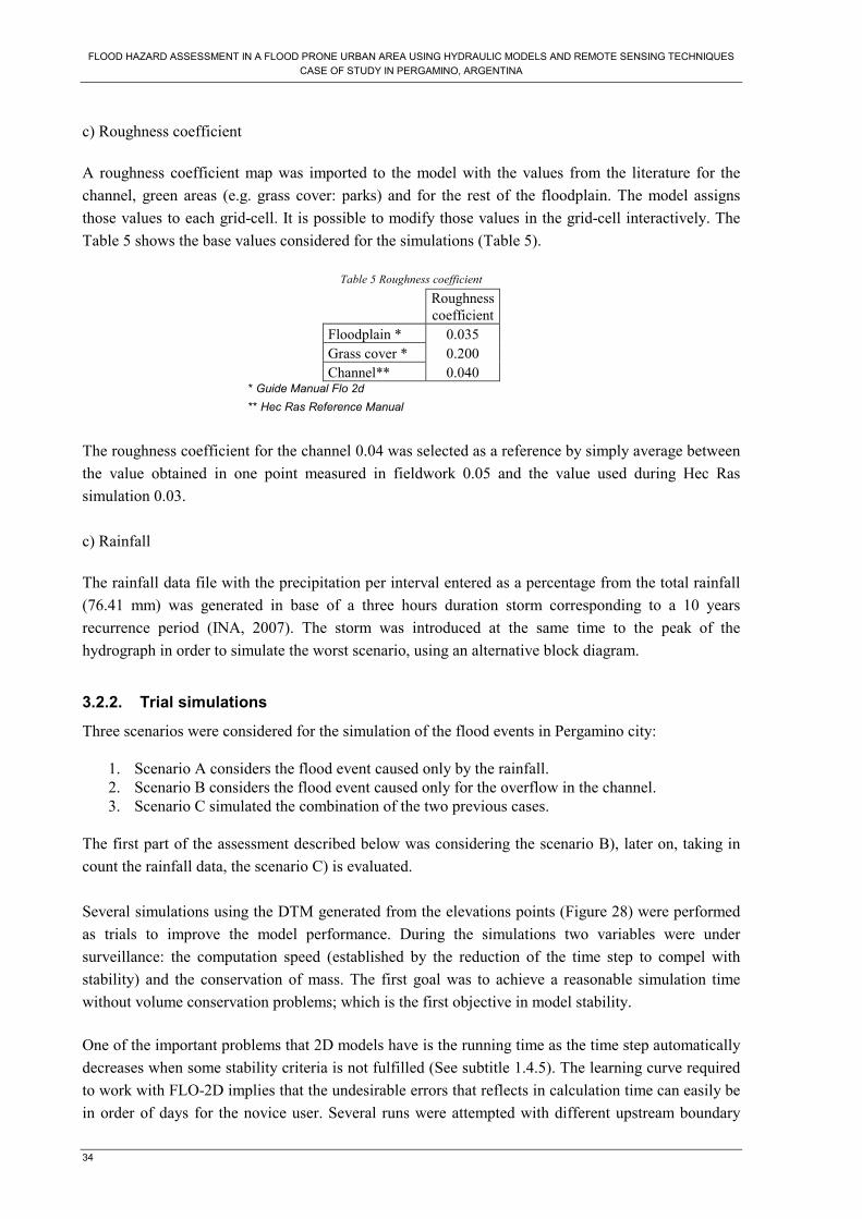
FLOOD HAZARD ASSESSMENT IN A FLOOD PRONE URBAN AREA USING HYDRAULIC MODELS AND REMOTE SENSING TECHNIQUES
CASE OF STUDY IN PERGAMINO, ARGENTINA
34
c) Roughness coefficient
A roughness coefficient map was imported to the model with the values from the literature for the
channel, green areas (e.g. grass cover: parks) and for the rest of the floodplain. The model assigns
those values to each grid-cell. It is possible to modify those values in the grid-cell interactively. The
Table 5 shows the base values considered for the simulations (Table 5).
Table 5 Roughness coefficient
Roughness
coefficient
Floodplain * 0.035
Grass cover * 0.200
Channel** 0.040 * Guide Manual Flo 2d
** Hec Ras Reference Manual
The roughness coefficient for the channel 0.04 was selected as a reference by simply average between
the value obtained in one point measured in fieldwork 0.05 and the value used during Hec Ras
simulation 0.03.
c) Rainfall
The rainfall data file with the precipitation per interval entered as a percentage from the total rainfall
(76.41 mm) was generated in base of a three hours duration storm corresponding to a 10 years
recurrence period (INA, 2007). The storm was introduced at the same time to the peak of the
hydrograph in order to simulate the worst scenario, using an alternative block diagram.
3.2.2. Trial simulations
Three scenarios were considered for the simulation of the flood events in Pergamino city:
1. Scenario A considers the flood event caused only by the rainfall.
2. Scenario B considers the flood event caused only for the overflow in the channel.
3. Scenario C simulated the combination of the two previous cases.
The first part of the assessment described below was considering the scenario B), later on, taking in
count the rainfall data, the scenario C) is evaluated.
Several simulations using the DTM generated from the elevations points (Figure 28) were performed
as trials to improve the model performance. During the simulations two variables were under
surveillance: the computation speed (established by the reduction of the time step to compel with
stability) and the conservation of mass. The first goal was to achieve a reasonable simulation time
without volume conservation problems; which is the first objective in model stability.
One of the important problems that 2D models have is the running time as the time step automatically
decreases when some stability criteria is not fulfilled (See subtitle 1.4.5). The learning curve required
to work with FLO-2D implies that the undesirable errors that reflects in calculation time can easily be
in order of days for the novice user. Several runs were attempted with different upstream boundary
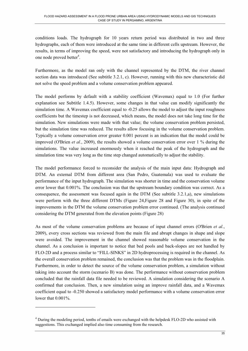
FLOOD HAZARD ASSESSMENT IN A FLOOD PRONE URBAN AREA USING HYDRODYNAMIC MODELS AND GIS TECHNIQUES
CASE OF STUDY IN PERGAMINO, ARGENTINA
35
conditions loads. The hydrograph for 10 years return period was distributed in two and three
hydrographs, each of them were introduced at the same time in different cells upstream. However, the
results, in terms of improving the speed, were not satisfactory and introducing the hydrograph only in
one node proved better4.
Furthermore, as the model ran only with the channel represented by the DTM, the river channel
section data was introduced (See subtitle 3.2.1, c). However, running with this new characteristic did
not solve the speed problem and a volume conservation problem appeared.
The model performs by default with a stability coefficient (Wavemax) equal to 1.0 (For further
explanation see Subtitle 1.4.5). However, some changes in that value can modify significantly the
simulation time. A Wavemax coefficient equal to -0.25 allows the model to adjust the input roughness
coefficients but the timestep is not decreased, which means, the model does not take long time for the
simulation. New simulations were made with that value; the volume conservation problem persisted,
but the simulation time was reduced. The results allow focusing in the volume conservation problem.
Typically a volume conservation error greater 0.001 percent is an indication that the model could be
improved (O'Brien et al., 2009), the results showed a volume conservation error over 1 % during the
simulations. The value increased enormously when it reached the peak of the hydrograph and the
simulation time was very long as the time step changed automatically to adjust the stability.
The model performance forced to reconsider the analysis of the main input data: Hydrograph and
DTM. An external DTM from different area (San Pedro, Guatemala) was used to evaluate the
performance of the input hydrograph. The simulation was shorter in time and the conservation volume
error lower that 0.001%. The conclusion was that the upstream boundary condition was correct. As a
consequence, the assessment was focused again in the DTM (See subtitle 3.2.1,a), new simulations
were perform with the three different DTMs (Figure 24,Figure 28 and Figure 30), in spite of the
improvements in the DTM the volume conservation problem error continued. (The analysis continued
considering the DTM generated from the elevation points (Figure 28)
As most of the volume conservation problems are because of input channel errors (O'Brien et al.,
2009), every cross sections was reviewed from the main file and abrupt changes in shape and slope
were avoided. The improvement in the channel showed reasonable volume conservation in the
channel. As a conclusion is important to notice that bed pools and back-slopes are not handled by
FLO-2D and a process similar to “FILL-SINKS” in 2D hydroprocessing is required in the channel. As
the overall conservation problem remained, the conclusion was that the problem was in the floodplain.
Furthermore, in order to detect the source of the volume conservation problem, a simulation without
taking into account the storm (scenario B) was done. The performance without conservation problem
concluded that the rainfall data file needed to be reviewed. A simulation considering the scenario A
confirmed that conclusion. Then, a new simulation using an improve rainfall data, and a Wavemax
coefficient equal to -0.250 showed a satisfactory model performance with a volume conservation error
lower that 0.001%.
4 During the modeling period, tenths of emails were exchanged with the helpdesk FLO-2D who assisted with
suggestions. This exchanged implied also time consuming from the research.

FLOOD HAZARD ASSESSMENT IN A FLOOD PRONE URBAN AREA USING HYDRAULIC MODELS AND REMOTE SENSING TECHNIQUES
CASE OF STUDY IN PERGAMINO, ARGENTINA
36
As the volume conservation problem was overcame for that Wavemax coefficient, the next step was to
calibrate the roughness coefficient adjusted by the model. This was done in a series of simulations.
The scheme presents in Figure 35 shows the steps followed in the next simulations.
Figure 35 Simulation process
Considering as Wavemax5 -0.250 and as limiting Froude number6 0.9, for the floodplain and the
channel, the first trial was done. During the simulation, the model adjusted the roughness coefficient
in those cells where the limiting Froude number was exceeded; as a result, a new set of roughness
coefficients were generated as outputs. Then the maximum velocities happening in few unstable grid-
cells were carefully reviewed, the grids with unusual high velocity values were identified, in those
cases, the roughness values for the vicinity grids of those nodes were increased, and the rest of the
adjusted roughness values were accepted. In the next trial the roughness set improved was used as
new input and the steps described above were repeated in several trials until only few incremental
roughness values appeared in the results. A last trial was performed with a Wavemax 100.25 to speed
up the model and to check in the results any possible high velocity (O'Brien et al., 2009). Finally, with
the roughness coefficients calibrated and considering Wavemax7 0.250, the Final trial was done. In all
these scenarios the conservation mass was observed within the recommended values.
The sequence described above was repeated for the three scenarios. For the case of the scenario A,
after the final trial, a new simulation was performed considering the rainfall event similar to the one
occurred in Pergamino city on February 9, 2001, in this case, the value of total precipitation registered
by INTA station 113.7 mm (IATASA,2007) was introduced to the model considering the same
hyetograph shape used in the previous simulations (Return period 10 years). As it was the only source
of comparison available, the results of the model, in terms of maximum flow depth were compared
with the areas where the neighbours gave values after the event (See subtitle 2.2.2. f).
5 Assign WAVEMAX=-0.250 increase the roughness values for those elements that are numerically unstable
resulting in unreasonable velocities. (O’Brien,2009) 6 Assign Limiting Froude number has the purpose to make sure that the computed velocities are reasonable.
(O’Brien,2009) The simulation made with HEC RAS gave as a result Froude number lower than 1 (subcritical
flow), in based of that a limiting value of 0.9 was selected for the case of Flo-2D simulations. 7 Wavemax = 0.250 Dynamic wave stability criteria increments and decrements the computational timestep when
Wavemax is exceeded. Model runs more slowly but is stable. (O’Brien,2009)

FLOOD HAZARD ASSESSMENT IN A FLOOD PRONE URBAN AREA USING HYDRODYNAMIC MODELS AND GIS TECHNIQUES
CASE OF STUDY IN PERGAMINO, ARGENTINA
37
d) Summary of the simulations
During the flood assessment using Flo-2D model, as it is explained above, several simulations (trials)
were performed. Different alternatives of inputs for the model were tested and experience gained. The
Table 6 presents only the final runs for which their results will be part of the assessment in the
corresponding analysis chapter (See Chapter 4).
Table 6 Summary simulations
Scenari
o
Trial name Scenario Description
A) Final_rain 3 hours Storm, Recurrence period of 10 years
Final_Cossoper Rainfall event February 9, 2001, Recurrence period of 10 years
B) Final_flow Flow in the channel
C) Final_both 3 hours Storm and Flow in the channel at the same time.
General characteristics Grid size: 20 m; hydrograph input: one node; Return period
Rainfall and Flow: 10 years; DTM: generated from the point map
3.2.3. Model performance
Flo2D allows following the performance process during the simulation time, the user can select the
option to follow the simulation by graph display or by text screen. In both cases the conservation
volume error is presented for each output interval chose. Besides that, when the graph display is
selected, it is possible to visualize the simulation time, the process along the hydrograph and the depth
for that simulation time. The graph display option was selected during the simulations of the scenario
B and C; in the case of scenario A, as there is not hydrograph as data, the model only displays the
process through the text screen.
When the model finishes the simulation, a result simulation summary shows the overall performance
on volume conservation, channel volume conservation, numerical stability, maximum velocities
(floodplain and channel) and variation in n-values. This screen gives a first perception of the
performance and it was used as guide to review the output files.
Figure 36 Example of the summary table reported by the Model after finishing the simulation
Flo-2D model gives the output in several files, which can be read in *.txt format, at the same time, the
results can be visualized using the post-processor program MAPPER (that is incorporated into Flo-2D
model) which brings the map results of inundation area, maximum flow depth, maximum flow
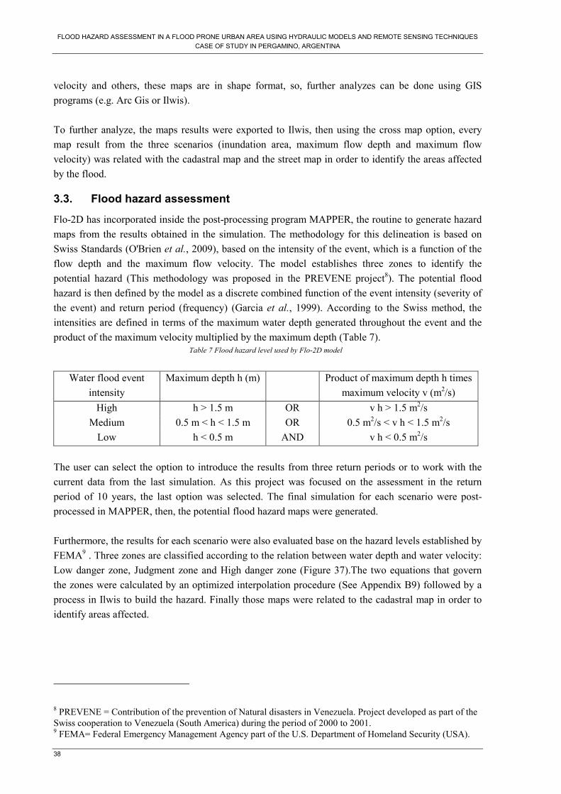
FLOOD HAZARD ASSESSMENT IN A FLOOD PRONE URBAN AREA USING HYDRAULIC MODELS AND REMOTE SENSING TECHNIQUES
CASE OF STUDY IN PERGAMINO, ARGENTINA
38
velocity and others, these maps are in shape format, so, further analyzes can be done using GIS
programs (e.g. Arc Gis or Ilwis).
To further analyze, the maps results were exported to Ilwis, then using the cross map option, every
map result from the three scenarios (inundation area, maximum flow depth and maximum flow
velocity) was related with the cadastral map and the street map in order to identify the areas affected
by the flood.
3.3. Flood hazard assessment
Flo-2D has incorporated inside the post-processing program MAPPER, the routine to generate hazard
maps from the results obtained in the simulation. The methodology for this delineation is based on
Swiss Standards (O'Brien et al., 2009), based on the intensity of the event, which is a function of the
flow depth and the maximum flow velocity. The model establishes three zones to identify the
potential hazard (This methodology was proposed in the PREVENE project8). The potential flood
hazard is then defined by the model as a discrete combined function of the event intensity (severity of
the event) and return period (frequency) (Garcia et al., 1999). According to the Swiss method, the
intensities are defined in terms of the maximum water depth generated throughout the event and the
product of the maximum velocity multiplied by the maximum depth (Table 7). Table 7 Flood hazard level used by Flo-2D model
Water flood event
intensity
Maximum depth h (m) Product of maximum depth h times
maximum velocity v (m2/s)
High h > 1.5 m OR v h > 1.5 m2/s
Medium 0.5 m < h < 1.5 m OR 0.5 m2/s < v h < 1.5 m2/s
Low h < 0.5 m AND v h < 0.5 m2/s
The user can select the option to introduce the results from three return periods or to work with the
current data from the last simulation. As this project was focused on the assessment in the return
period of 10 years, the last option was selected. The final simulation for each scenario were post-
processed in MAPPER, then, the potential flood hazard maps were generated.
Furthermore, the results for each scenario were also evaluated base on the hazard levels established by
FEMA9 . Three zones are classified according to the relation between water depth and water velocity:
Low danger zone, Judgment zone and High danger zone (Figure 37).The two equations that govern
the zones were calculated by an optimized interpolation procedure (See Appendix B9) followed by a
process in Ilwis to build the hazard. Finally those maps were related to the cadastral map in order to
identify areas affected.
8 PREVENE = Contribution of the prevention of Natural disasters in Venezuela. Project developed as part of the
Swiss cooperation to Venezuela (South America) during the period of 2000 to 2001. 9 FEMA= Federal Emergency Management Agency part of the U.S. Department of Homeland Security (USA).

FLOOD HAZARD ASSESSMENT IN A FLOOD PRONE URBAN AREA USING HYDRODYNAMIC MODELS AND GIS TECHNIQUES
CASE OF STUDY IN PERGAMINO, ARGENTINA
39
Figure 37 Flood hazard zones
Source: FEMA, 2009

FLOOD HAZARD ASSESSMENT IN A FLOOD PRONE URBAN AREA USING HYDRAULIC MODELS AND REMOTE SENSING TECHNIQUES
CASE OF STUDY IN PERGAMINO, ARGENTINA
40
4. RESULTS AND DISCUSSION
This chapter summarizes the results found of the scenarios and attempts explained in the previous
chapter.
4.1. Hec Ras performance
Steady flow assessment
4.1.1. Model calibration
The results from the first simulations before fieldwork showed that the geometric data obtained from
third party survey provides a good representation of the real river situation.
The final simulation allowed a comparison between water depths simulated and estimated from the
current rating curve respectively (Figure 38). This comparison was made in the cross section closest
to the limnigraph F. Sanchez Bridge (number 102) (Table 8)
Table 8 Results from simulation in Steady flow conditions
F. Sanchez gauge
(1) (2) (3) (4)
Water Surface
Discharge Hec Ras Hec Ras F. Sanchez
m3/s m m m
0.65 53.48 0.73 0.78
6.99 54.05 1.30 1.33
11.34 54.26 1.51 1.53
27.00 54.78 2.03 2.03
49.48 55.33 2.58 2.53
78.78 55.85 3.10 3.03
114.89 56.34 3.59 3.53
157.83 56.89 4.14 4.03
207.58 57.55 4.80 4.53
264.16 58.46 5.71 5.03
276.29 58.68 5.93 5.13
301.38 58.79 6.04 5.33
327.55 58.88 6.13 5.53
Water depth
Where:
(1) Discharge introduced as input in the model.
(2) Results of the Hec Ras simulation
(3) Water depth values calculated from the results of the
model.
(4) Water depth values calculated with the rating curve
F. Sanchez. Note the current rating curve was
obtained with a maximum measured value of 78.4
m3/s. Other values are extrapolation from the
original equation
(To see an example of the calculation steps refers to Appendix B2)
0.50
1.50
2.50
3.50
4.50
5.50
6.50
0.00 50.00 100.00 150.00 200.00 250.00 300.00 350.00
Q ( m3/s)
H (
m)
Equation from Field measurements Hec Ras Results
Figure 38 Comparison between water depths generated by Hec Ras
model and values determined by the rating curve F. Sanchez.

FLOOD HAZARD ASSESSMENT IN A FLOOD PRONE URBAN AREA USING HYDRODYNAMIC MODELS AND GIS TECHNIQUES
CASE OF STUDY IN PERGAMINO, ARGENTINA
41
Hec Ras gave as result of the simulation Water Surface values (column 2, Table 8). The difference
between those values and the lowest elevation point in the river bed cross section assessed
(corresponding to F. Sanchez Bridge) gave the water depth (column 2) to compare with the values
calculated directly from the rating curve (Equation 5). The deviation between the two curves is for the
effect of the bridge structure as water approaches the upper cord Figure 38 This effect is not
considered by the original rating curve, as data for the rating curve were obtained for values well
below from those reaching the bridge crone.
The performance of the model was following the original rating curve till water depths lower than 4.0
m. (Figure 38). Water depths higher than that value showed an increase in the difference. The
Florencio Sanchez Bridge was simulated with 5.0 m of height (elevation 57.75 m). As soon as the
water level past that value, that bridge begins to work under pressure conditions, as a result the
hydraulic conditions change downstream. Because of that, the calibration of the model fits
satisfactorily the measured ranting curve only until the threshold 4.0 m. Therefore, from the results
assessed the best curve adjusted for that range is presented below for F. Sanchez limnimeter:
Equation 8
Where ‘Q’ is the discharge in m3/s and ‘H’ is water depth in m.
Note in the Equation 8 the discharge value is expressed as a function of the water depth, because this
parameter measures direct from the limnimeter. However, to expresses the results of the curve in
Water levels all the values must be refer to 52.75 m as the lowest point elevation of the cross section.
(e.g. Water depth of 1.0 m is equal to water level 53.75 m)
Although the improved rating curve
generated needs more than one point
value to be validated, the comparison
between the only discharge calculated
from measurement during fieldwork and
the value obtained using curve adjusted
(Equation 8) shows a good agreement:
Water depth measured in the
limnimeter= 0.87 m
Field discharge = 1.62 m3/s
(See Appendix A1)
Calculated discharge = 1.52 m3/s
The presented rating curve is a better
estimation of the values for depth water
compared to a mere extrapolation of the
measured rating curve. Furthermore, the
use of Hec Ras allows seeing the effect of the bridge in the flow, condition that happened in the past
but it was not measured.
Figure 39 Rating curve adjusted from the calibrated model
8.4*6.14*5.12 2 +−= HHQ

FLOOD HAZARD ASSESSMENT IN A FLOOD PRONE URBAN AREA USING HYDRAULIC MODELS AND REMOTE SENSING TECHNIQUES
CASE OF STUDY IN PERGAMINO, ARGENTINA
42
4.1.2. Roughness coefficient
In order to assess the model performance as a function of the roughness coefficient used, the results in
terms of water depth were evaluated in the cross section located near to F. Sanchez Bridge for the
fourth simulations performed (Figure 40).
The roughness coefficient suggested by the
literature for the kind of riverbed (0.03) gave
the best results to the water depths matching
the F. Sanchez rating curve. The value
determined in the field 0.05 (one point
measurement, using the slope-area method)
did not allow good performance of the
model, the difference is bigger. The
roughness coefficient is a parameter with an
important sensitivity for the Hec Ras
performance, the incorrect use of it can
generate unrealistic results. Therefore, for
the case of Hec Ras model, the simulation
with the coefficient 0.03 for the river bed
was accepted as the best one and used in
subsequent analysis for long term analysis,
understanding that the roughness condition
of the channels changes with time. The value
measured in field will be considered during the assessment with Flo-2D model.
4.1.3. Levees exceeded hazard
As it was explained in chapter 3, the flood hazard was assessed for water levels exceeding the levee
height. The lowest water depth simulated before the water pass over the dike was identified in each
cross section10. As a result, flood hazard maps considering the overflow in the channel were generated
(Figure 41, Figure 42, Figure 43 and Figure 44). These maps can be considered as useful information
to prevent and mitigate possible failures in the levees along the channel.
Considering the river bottom as reference, lower depth values, between 2.0 m and 3.0 m generated
critical situations in the sectors located upstream and downstream of the city (Figure 41) where the
levee is less maintained. This is also supported because in that sector the channel shape is natural
(with minor or without modifications). In the range upper than 3.0 m the hazard increases downstream
(Figure 42). However, it is only since the water depth achieves values above 4.0 m that the hazard
appears in the urban area. (Figure 43)
10 A database with the information in terms of cross section geographic location, street affect, water level which
causes the flood hazard and dike side affected was generated. (See Appendix B3)
0.50
1.50
2.50
3.50
4.50
5.50
6.50
0.00 50.00 100.00 150.00 200.00 250.00 300.00 350.00
Q ( m3/s)
H (
m)
Using F. Sanchez Curve n=0.03 n=0.025 n=0.04 n=0.05
F. Sanchez Bridge height
4.00
Figure 40 Roughness coefficient sensitivity analysis

FLOOD HAZARD ASSESSMENT IN A FLOOD PRONE URBAN AREA USING HYDRODYNAMIC MODELS AND GIS TECHNIQUES
CASE OF STUDY IN PERGAMINO, ARGENTINA
43
Figure 41 Cross sections under overflow hazard for water depths in the ranges from 2.0 m to 2.9 m
Figure 42 Cross sections under overflow hazard for water depths in the ranges from 3.0 m to 3.9 m
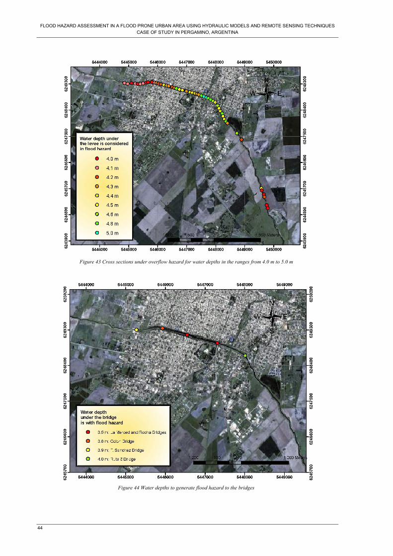
FLOOD HAZARD ASSESSMENT IN A FLOOD PRONE URBAN AREA USING HYDRAULIC MODELS AND REMOTE SENSING TECHNIQUES
CASE OF STUDY IN PERGAMINO, ARGENTINA
44
Figure 43 Cross sections under overflow hazard for water depths in the ranges from 4.0 m to 5.0 m
Figure 44 Water depths to generate flood hazard to the bridges

FLOOD HAZARD ASSESSMENT IN A FLOOD PRONE URBAN AREA USING HYDRODYNAMIC MODELS AND GIS TECHNIQUES
CASE OF STUDY IN PERGAMINO, ARGENTINA
45
The first kilometers of the city (from 2+270 to 3+638 m11) (See Appendix B3) has the highest hazard
to suffer the overflow with water levels between 4.0 m and 4.3 m. The path between the Rocha and
Ruta 8 Bridges (from 3+480 to 4+068) presented lower hazard with water levels between 4.4 m and
4.6 m. (See water levels in Appendix B3).
The overtop danger in the dikes is not in all the cases for both sides of the cross sections. Some times
one bank is affected first. This could be calculated from HECRAS but these results were not
presented in the figures above. The determination of that along with the location of the cross section
and the streets affected is presented in Appendix B3.
La Merced and Rocha Bridges (Figure 44) are under hazard when the water depths arises 3.5 m (water
levels 55.8 m. and 54.8 m respectively). At this height, the bridges work under pressure.
According to the assessment, the streets more threatened are Matheu, Rivadavia and 9 de Julio with a
water depths of 4.2 m (water levels 56.9 m 56.7 m respectively).
Unsteady flow assessment
4.1.4. Flood celerity analysis
The backwater effect downstream Alfonzo station was demonstrated using the Hec Ras model. In this
context the measured water level values cannot be used to elaborate a rating curve which in turns
prevents to generate the wave celerity assessment using the hydrograph generated.
However, the model showed properly performance in steady flow conditions for the main (central)
study stream longitudinal profile. A simulation using the design hydrograph calculated by INA 2007
(Figure 11) was done. In order to evaluate the celerity of the flood wave the results hydrographs from
the first (FFCC Mitre) and the last cross section (El Toro) were evaluated (See Figure 45). For this
section there is confidence on the cross sections and longitudinal profile.
The time of travel the flood wave through the reach is the time between the centroids of the inflow
and outflow hydrographs. (Brutsaert, 2005) The time that the flood wave needs from the beginning
(FFCC Mitre) to the end (El Toro) of the study stream is about 3 hours (Figure 45). As the longitude
of the river in the study area is 11.5 Km the celerity wave is 1.06m/s. A time of three hours does not
leave much room for warning. In this regards, is by far insufficient and the idea of building the
temporal storage reservoirs upstream Pergamino is then supported.
11 Nomenclature which expresses the location of the cross section in terms of length, e.g. 3+480 means 3.48 km as from Mitre
station.
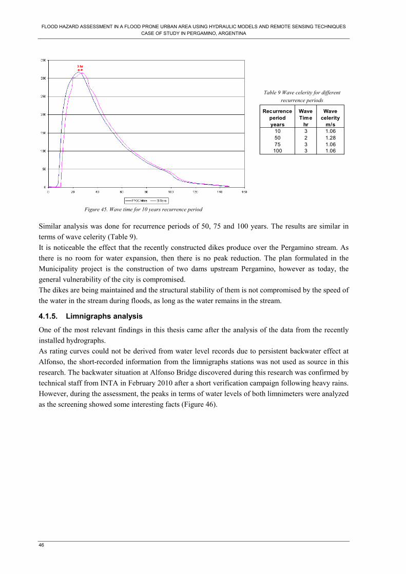
FLOOD HAZARD ASSESSMENT IN A FLOOD PRONE URBAN AREA USING HYDRAULIC MODELS AND REMOTE SENSING TECHNIQUES
CASE OF STUDY IN PERGAMINO, ARGENTINA
46
Figure 45. Wave time for 10 years recurrence period
Table 9 Wave celerity for different
recurrence periods
Recurrence
period
Wave
Time
Wave
celerity
years hr m/s
10 3 1.06
50 2 1.28
75 3 1.06
100 3 1.06
Similar analysis was done for recurrence periods of 50, 75 and 100 years. The results are similar in
terms of wave celerity (Table 9).
It is noticeable the effect that the recently constructed dikes produce over the Pergamino stream. As
there is no room for water expansion, then there is no peak reduction. The plan formulated in the
Municipality project is the construction of two dams upstream Pergamino, however as today, the
general vulnerability of the city is compromised.
The dikes are being maintained and the structural stability of them is not compromised by the speed of
the water in the stream during floods, as long as the water remains in the stream.
4.1.5. Limnigraphs analysis
One of the most relevant findings in this thesis came after the analysis of the data from the recently
installed hydrographs.
As rating curves could not be derived from water level records due to persistent backwater effect at
Alfonso, the short-recorded information from the limnigraphs stations was not used as source in this
research. The backwater situation at Alfonso Bridge discovered during this research was confirmed by
technical staff from INTA in February 2010 after a short verification campaign following heavy rains.
However, during the assessment, the peaks in terms of water levels of both limnimeters were analyzed
as the screening showed some interesting facts (Figure 46).

FLOOD HAZARD ASSESSMENT IN A FLOOD PRONE URBAN AREA USING HYDRODYNAMIC MODELS AND GIS TECHNIQUES
CASE OF STUDY IN PERGAMINO, ARGENTINA
47
The peak at Urquiza
Station (downstream)
appears before the one
at Alfonzo Station
(upstream), this
situation it is not
usual. That can be
observed clearly in
February and it has
been repeated in
several showers (
Figure 47). This
singularity can only be
explained considering
the contributions of
water discharges from
small subcatchments
downstream Alfonzo and close to the city and from the city itself. Those contributions make it to
Urquiza faster than the upstream water from Alfonzo does.
0
500
1000
1500
2000
2500
3000
27/01/20
09 00:00
01/02/20
09 00:00
06/02/20
09 00:00
11/02/20
09 00:00
16/02/20
09 00:00
21/02/20
09 00:00
26/02/20
09 00:00
03/03/20
09 00:00
Date
Wate
r L
evel (m
m)
Alfonzo Station Urquiza Station
Figure 47 Comparison between peak values from the limnigraphs station, February 2009
The Alfonzo limnigraph is located upstream of an embankment bridge that is acting as linear reservoir
in case of a flood. The influence of this small elevated road was not in the safety plans for Pergamino
but the effect is not negligible. As such a study should be carried out to account for the storage and
the beneficial effect of Alfonzo bridge to the downstream city.
0
500
1000
1500
2000
2500
3000
18/12/2008
00:00
06/02/2009
00:00
28/03/2009
00:00
17/05/2009
00:00
06/07/2009
00:00
25/08/2009
00:00
14/10/2009
00:00
03/12/2009
00:00
22/01/2010
00:00
Date
Wa
ter
lev
el
(mm
)
Urquiza M.Alfonzo
Figure 46 Comparison between values from limnigraphs stations

FLOOD HAZARD ASSESSMENT IN A FLOOD PRONE URBAN AREA USING HYDRAULIC MODELS AND REMOTE SENSING TECHNIQUES
CASE OF STUDY IN PERGAMINO, ARGENTINA
48
Figure 48: Upstream view over Alfonzo bridge during a low risk
flood (February 2010). It shows the limnigraph station, the
backwater effect that had been foreseen by HECRAS and the large
inundation plain the will be inundated in case of extreme flooding.
Reducing the peak to Pergamino
Figure 49: Downstream Alfonzo bridge.
4.1.6. Improving in the existing Flood warning system
The results obtained in this research, showed two influential terrain feature aspects that were not
analyzed in the project mentioned above. The situation is graphically depicted in Figure 50. The
future location of the two dams is upstream Alfonzo station, close to Del Pescado lagoon. The
limnigraph readings at Alfonso (upstream Pergamino) show that the peak of discharge appears
systematically later than the peak at Urquiza station (downstream Pergamino city).
Second, the bridge at Alfonzo station builds a considerable retention in the storage area produces by
the road embankment (Figure 50) and the second large storage happens at the location of Pescado
lagoon immediately downstream Alfonzo, where the dam are planned. The combination of these two
effects is considerable. This effect was discovered and tested after a HECRAS analysis over the
limnigraph curve from Alfonzo Station. A simulated backwater effect and bridge damming was
reproducing the measurements at Alfonso, proving this effect. As a consequence the peak at Alfonso
is independent from the peak at Urquiza which supports the hypothesis that a review study of the dam
projects could be consider the existence of a damping effect in Alfonzo station area, that could be
eventually end up by reducing the projected height design of the dam (the current project consider a
9.0 m high (Figure 50)).
The quick peaks at the hydrograph in Urquiza do not come mainly from Alfonzo as it was supposed in
the warning system design, but more locally from the subbasins surrounding Pergamino that are out of
this present study. The conclusion is that a more adequate hydrological model calibrated for the
damping effects now not considered should end in a cheaper solution (using the favorable effects of
Alfonzo and Del Pescado that allows reducing the dam specifications) and more attention should be
given to local flows from Pergamino vicinity.

FLOOD HAZARD ASSESSMENT IN A FLOOD PRONE URBAN AREA USING HYDRODYNAMIC MODELS AND GIS TECHNIQUES
CASE OF STUDY IN PERGAMINO, ARGENTINA
49
Figure 50 Lagoon Del Pescado location, between the Alfonzo Station and Pergamino City
4.2. Flo2D model performance
4.2.1. Grid Size constrain
As it was explained in the chapter 3, the spatial and temporal resolution of the FLO-2D model
depends on the size of the grid elements and the rate of rise in the hydrograph (discharge) (Equation
7). With that relation, the highest grid size suggested to run the model was 35 m, however,
considering some important features to be assessed, it was decided the attempt with 20 m grid-cell
accepting that the model will run slowly. The main considerations were the average width of the
channel (around 30 m) and the average width of the streets (around 8 m).
Due to stability constraints, to perform the model with this higher resolution the peak discharge value
must be lower, some tries to reduce the value dividing the peak in two or three hydrographs was done,
however, the constrain in the size grid at the input cell nodes was notorious.
Two grids-cell (40 m) apparently could
represent the width of the channel (around
35 m), however, the grids locations over the
georeference image did not coincide exactly
to represent the channel. As a result, the
model did not consider the second
hydrograph as part of the channel. In base on
that analysis the introduction of the inflow
data in two or even three nodes to achieve
the stability the discharge was rejected.
During the introduction of the parameters in
a flood simulation, the trend is to have as
Figure 51 Constrain at the moment to introduce the inflow data

FLOOD HAZARD ASSESSMENT IN A FLOOD PRONE URBAN AREA USING HYDRAULIC MODELS AND REMOTE SENSING TECHNIQUES
CASE OF STUDY IN PERGAMINO, ARGENTINA
50
higher level of detail as possible; however, the grid size limits becomes a constrain. The ideal scenario
for the flood modelling in an urban area would be with the introduction of roughness coefficients for
each specific feature, considering the differentiation between the gardens, the material of the street
(asphalt, soil, etc), and the houses. However, in this specific study, it was not possible to introduce the
information with that level of detail, because the grid size and lack of information. Therefore, as first
approach, all the simulations were performed considering only three types of areas for the
introduction of the roughness coefficient: floodplain, channel, and parks or green areas. For the same
reasons, the representation of the buildings was not achieved in this study.
Flo-2D deals with storage and conveyance at cell level by assigning the percentage of the area that
cannot be occupied by surface flows (e.g. impervious buildings) and the percentage of flow width lost
due to obstruction, meaning the direction where the flow will not pass, using the Area Reduction
Factor and the Width Reduction Factor respectively (O'Brien et al., 2009)) . The assignment of these
factors will modified the performance of
the model, as the flow does not calculate
for the 8 directions and for the total grid
area, so it would be give different results.
Even when the attempt to use this options
was done, the higher resolution of the
image and the grid size did not allow
completing successfully for the final
simulations (different features inside the
same grid, e.g. in the same grid there were
buildings, gardens and street) The
difficulties found to achieve model
stability constrained the original
expectation in the research, but the experience proved valid to establish a clear criterion on what
spend time and effort before running the model.
Furthermore, at the moment to analyze the model results by grid, the grid size influence was
notorious. e.g. some streets catalogued with potential flood problems did not fit exactly in the width of
some grids. As a result the street belongs to partial grids at the same time (Figure 52).
4.2.2. Failed simulation
Most of the problems in the first simulations were focus in the way to introduce the input data, even
thought the model offers a tutorial, moving away to a real case with limited data proved an issue. The
data set had to be verified, therefore, more simulations were done, as the use of the DTM was
evaluated from threes sources, the first one from the contours map offered by the Municipality faced
several problems of numerical stability criteria, the computation time were in these simulations
several days without results. The third DTM generated from the topography sheet (scale 1:50000,
interval 2.5m, source 1958) did not offer improvement at the moment to solve the volume
conservation problems, the computation, the computer run time was similar than the previous
simulations. As a result the second DTM generated from the points map provided by survey
topography was chose to do next simulations.
Figure 52 Example of constrain in the identification of the features

FLOOD HAZARD ASSESSMENT IN A FLOOD PRONE URBAN AREA USING HYDRODYNAMIC MODELS AND GIS TECHNIQUES
CASE OF STUDY IN PERGAMINO, ARGENTINA
51
4.2.3. Roughness coefficient calibration
Scenario A
From the scheme process described in previous chapter (Figure 35) , four trials were performed until
achieve the final simulation.(Table 10). After each simulation concluded, the maximum floodplain
velocity and the roughness coefficient adjusted for each grid were analyzed from the output files. To
assess the maximum flow velocities reported by the model, a threshold equal to 2.5 m/s was
established, this value was selected base on the assumption that flat areas (average slope 0.045%) will
not report higher values in terms of velocity, furthermore, former flood modeling studies in other
regions reported velocities lower than the threshold, e.g. in Ocotopeque, Honduras, the mean
maximum velocity is reported in the range of 2.0 to 3.0 m/s (Ahti, 2007); in Tegucigalpa, Honduras,
the mean maximum velocity was 2.21 m/s, considering for the modelling a DTM with resolution 2.5
m (Tamiru, 2005); and in Naga, Philippines the range of maximum velocities was reported lower than
1.0 m/s.
In the following we show the results after the recommended procedure to run FLO-2D in an
interactive manner to detect unstable cells producing high speeds. Table 10 Trials performed for scenario A
Trial Wavemax
coefficient
Maximum Flow
Velocity
Number of grid
adjusted
Rain -0.250 < 2.5 m/s 2691
Rainv2 -0.250 < 2.5 m/s 2397
Rainv3 -0.250 < 2.5 m/s 1962
Rainv4 100.25 < 2.5 m/s 0
The first trial did not report maximum flow velocities higher than 2.5 m/s, from that results, according
to the sequence process (Figure 35), it would be possible to run the model setting the Wavemax
coefficient equal to 100.25 for the final verification of the velocities, however, in order to see the
performance in the number of n-values adjustments, two more trials were done (Trial 2 and Trial 3) as
a previous step with the same Wavemax coefficient.
In terms of roughness coefficient, Figure 53 shows the values introduced as input in each simulation,
in Trial 1 graph the values correspond to the literature (Table 5), the Trial 2 graph shows the values
adjusted by the model during the simulation of trial 1, the range between the values (0.030 to 0.234)
represent the floodplain area, the model kept the roughness value for the channel in 0.040. The Trial 3
graph shows that during the simulation in Trial 2 the values were increased in some cells until 0.237,
even though the change looks not significant, the number of cells adjusted was reduced (Table 10). No
more increased in roughness values were done by the model during the simulation in Trial 3, only the
number of cells adjusted was reduced. The Trial 4 graph presents the roughness values used for the
final simulations.

FLOOD HAZARD ASSESSMENT IN A FLOOD PRONE URBAN AREA USING HYDRAULIC MODELS AND REMOTE SENSING TECHNIQUES
CASE OF STUDY IN PERGAMINO, ARGENTINA
52
Figure 53 Roughness coefficients introduced as input for the simulation considering Scenario A
Furthermore, one parameter which affects the adjustment of the roughness coefficient during the
simulations is the Limiting Froude Number. Despite that the model presents by default a value equal
to 0 (representing Froude can vary freely) previous simulations using that value showed a high
increase in the roughness values during the adjustment (it was recorded as the highest value 0.918).
The same indications were reported by the authors of FLO-2D who indicated that those values did not
correspond to characteristics of the area. The literature presented n-values lower than 0.5 (O'Brien et
al., 2009). A Limiting Froude Number equal to 0.9 (sub-critical conditions) was considered
acceptable for the trials presented in Figure 53.
The results presented in the Figure 53 were assessed considering the difference between the original
roughness coefficients (introduced as input in the simulation) and the final roughness values (adjusted
by the model during the simulation and reported in the output files. The difference values (Figure 54)
represent the grids where the model identified potential stability problems (the dynamic wave stability
criteria were exceeded) and defaulted to an increase the roughness values. If that difference was
significant, a new simulation was required to reduce it. During the simulation of the Trial 1, the
difference values were in the range between 0.00 to 0.199, the grids with zero difference shows no
need of adjustments, in the Trial 2 the range between 0 to 0.109 which meant better performance of
the model, finally as the Trial 3 gave the range between 0 to 0.072, the roughness values adjusted
were accepted to continue the process (Figure 35). The next simulation (Trial 4) did not report any
higher velocity that could be responsible of any possible instability problems, as a result the
roughness values were considered as calibrated for the final simulation.
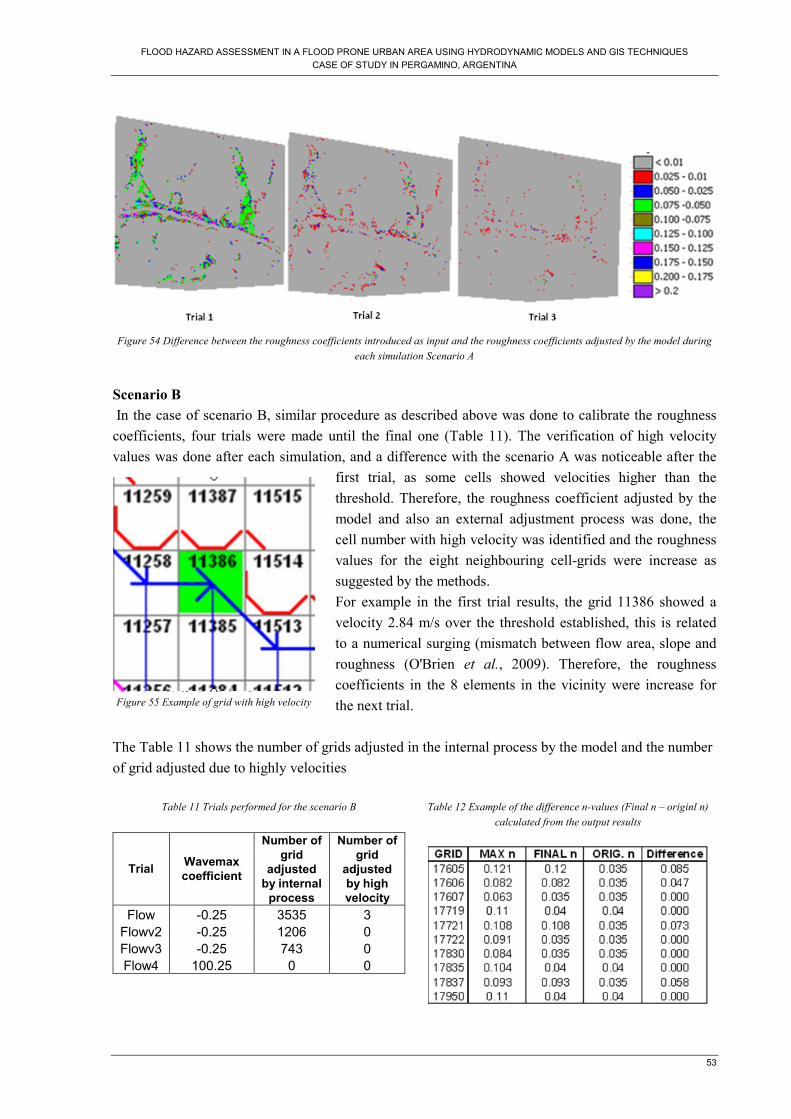
FLOOD HAZARD ASSESSMENT IN A FLOOD PRONE URBAN AREA USING HYDRODYNAMIC MODELS AND GIS TECHNIQUES
CASE OF STUDY IN PERGAMINO, ARGENTINA
53
Figure 54 Difference between the roughness coefficients introduced as input and the roughness coefficients adjusted by the model during
each simulation Scenario A
Scenario B
In the case of scenario B, similar procedure as described above was done to calibrate the roughness
coefficients, four trials were made until the final one (Table 11). The verification of high velocity
values was done after each simulation, and a difference with the scenario A was noticeable after the
first trial, as some cells showed velocities higher than the
threshold. Therefore, the roughness coefficient adjusted by the
model and also an external adjustment process was done, the
cell number with high velocity was identified and the roughness
values for the eight neighbouring cell-grids were increase as
suggested by the methods.
For example in the first trial results, the grid 11386 showed a
velocity 2.84 m/s over the threshold established, this is related
to a numerical surging (mismatch between flow area, slope and
roughness (O'Brien et al., 2009). Therefore, the roughness
coefficients in the 8 elements in the vicinity were increase for
the next trial.
The Table 11 shows the number of grids adjusted in the internal process by the model and the number
of grid adjusted due to highly velocities
Table 11 Trials performed for the scenario B
Trial Wavemax
coefficient
Number of
grid
adjusted
by internal
process
Number of
grid
adjusted
by high
velocity
Flow -0.25 3535 3
Flowv2 -0.25 1206 0
Flowv3 -0.25 743 0
Flow4 100.25 0 0
Table 12 Example of the difference n-values (Final n – originl n)
calculated from the output results
Figure 55 Example of grid with high velocity

FLOOD HAZARD ASSESSMENT IN A FLOOD PRONE URBAN AREA USING HYDRAULIC MODELS AND REMOTE SENSING TECHNIQUES
CASE OF STUDY IN PERGAMINO, ARGENTINA
54
As for the scenario A, the internal adjustment process was also evaluated calculating the difference
between the roughness values introduced and final values presented by the model at the end of each
simulation. (See e.g. Table 12). The first trial present increments in the values in the range of 0 to
0.270, the grids changed are surrounding the channel where the flood happens. In the next trial, the
range of increasing from 0 to 0.163 and finally in the third trial performed the difference decrease
until the range of 0 to 0.105. Therefore, the roughness values adjusted in the trial 3 were considered
acceptable for the next step that is, the verification of high velocities using Wavemax coefficient
equal to 100.25 (Figure 35)
Figure 56 Difference between the roughness coefficients introduced as input and the roughness coefficients adjusted by the model during
each simulation Scenario B
Figure 57 Roughness coefficients used during the assessment in Scenario B

FLOOD HAZARD ASSESSMENT IN A FLOOD PRONE URBAN AREA USING HYDRODYNAMIC MODELS AND GIS TECHNIQUES
CASE OF STUDY IN PERGAMINO, ARGENTINA
55
The roughness coefficient used during the different trials (Figure 57) are in the range from 0.030 to
0.305, the adjustments correspond to the floodplain areas most of the time, even though it was
detected some channel grids to be adjusted, at the end of the simulations all the roughness values for
the channel were kept by the model in the original value 0.04, those values are in the range suggested
by the literature, more over, the green areas near to the channel where also adjusted by the model
increasing the values from 0.2 to 0.305.
Scenario C
Scenario C is the most compromised, similar process was followed in this scenario, four trials were
done to obtain the adjusted roughness coefficients set for the final simulation. In all the trials was
necessary to increase the roughness coefficient in the vicinity grids of those with high velocities (>
2.5 m/s) (Table 13). Table 13 Trials performed in Scenario C
Trial Wavemax
coefficient
Number of
grid adjusted
by internal
process
Number of
grid adjusted
by high
velocity
Both -0.25 4130 7 Bothv2 -0.25 2027 5 Bothv3 -0.25 1133 3 Bothv4 100.25 0 4
Figure 58 Roughness coefficients used during the assessment in Scenario C
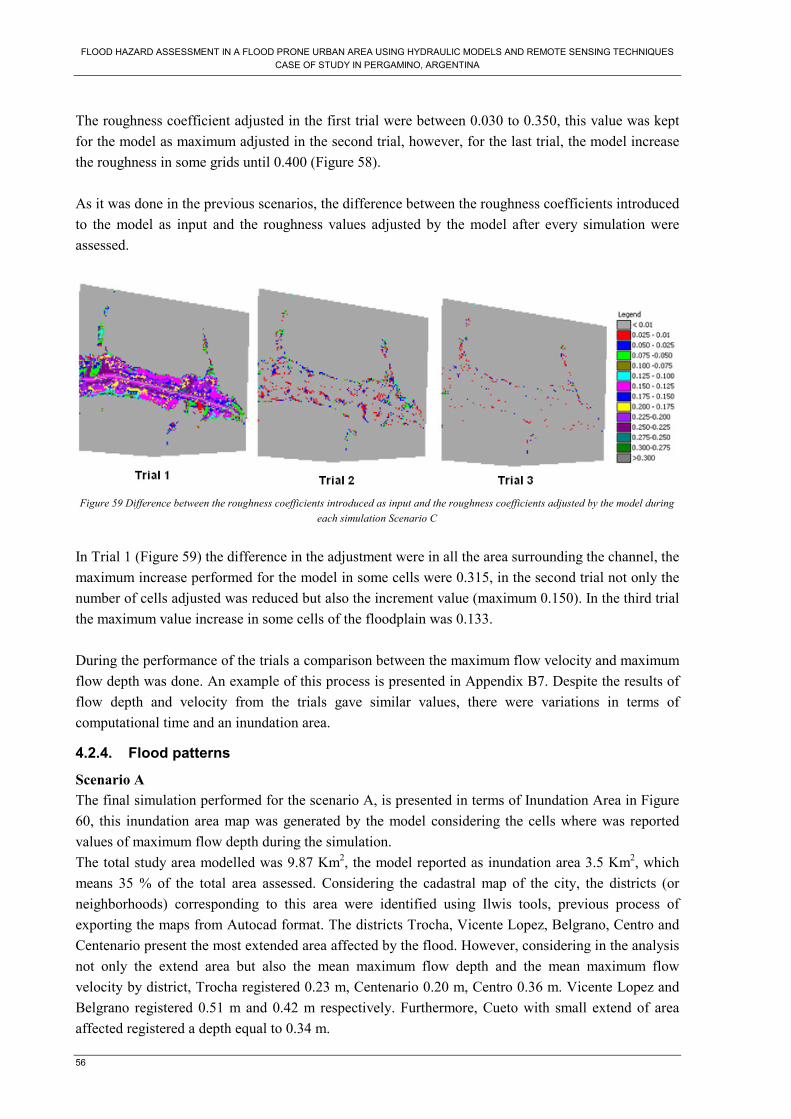
FLOOD HAZARD ASSESSMENT IN A FLOOD PRONE URBAN AREA USING HYDRAULIC MODELS AND REMOTE SENSING TECHNIQUES
CASE OF STUDY IN PERGAMINO, ARGENTINA
56
The roughness coefficient adjusted in the first trial were between 0.030 to 0.350, this value was kept
for the model as maximum adjusted in the second trial, however, for the last trial, the model increase
the roughness in some grids until 0.400 (Figure 58).
As it was done in the previous scenarios, the difference between the roughness coefficients introduced
to the model as input and the roughness values adjusted by the model after every simulation were
assessed.
Figure 59 Difference between the roughness coefficients introduced as input and the roughness coefficients adjusted by the model during
each simulation Scenario C
In Trial 1 (Figure 59) the difference in the adjustment were in all the area surrounding the channel, the
maximum increase performed for the model in some cells were 0.315, in the second trial not only the
number of cells adjusted was reduced but also the increment value (maximum 0.150). In the third trial
the maximum value increase in some cells of the floodplain was 0.133.
During the performance of the trials a comparison between the maximum flow velocity and maximum
flow depth was done. An example of this process is presented in Appendix B7. Despite the results of
flow depth and velocity from the trials gave similar values, there were variations in terms of
computational time and an inundation area.
4.2.4. Flood patterns
Scenario A
The final simulation performed for the scenario A, is presented in terms of Inundation Area in Figure
60, this inundation area map was generated by the model considering the cells where was reported
values of maximum flow depth during the simulation.
The total study area modelled was 9.87 Km2, the model reported as inundation area 3.5 Km2, which
means 35 % of the total area assessed. Considering the cadastral map of the city, the districts (or
neighborhoods) corresponding to this area were identified using Ilwis tools, previous process of
exporting the maps from Autocad format. The districts Trocha, Vicente Lopez, Belgrano, Centro and
Centenario present the most extended area affected by the flood. However, considering in the analysis
not only the extend area but also the mean maximum flow depth and the mean maximum flow
velocity by district, Trocha registered 0.23 m, Centenario 0.20 m, Centro 0.36 m. Vicente Lopez and
Belgrano registered 0.51 m and 0.42 m respectively. Furthermore, Cueto with small extend of area
affected registered a depth equal to 0.34 m.
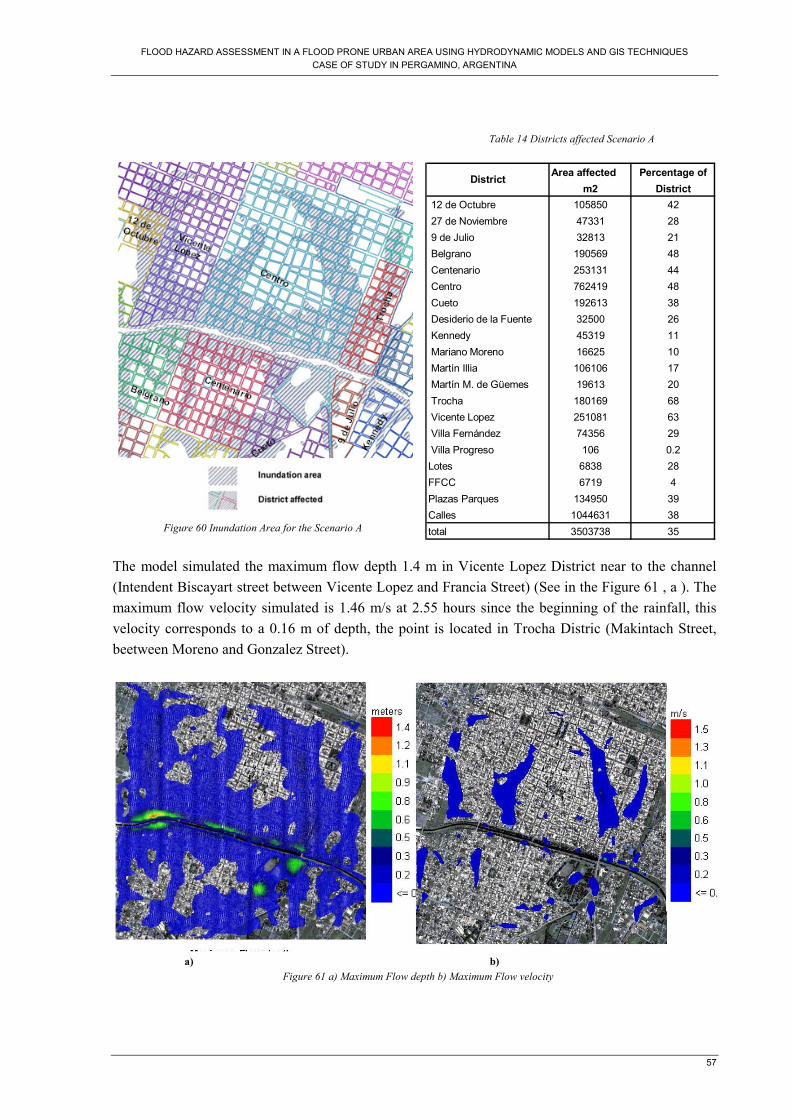
FLOOD HAZARD ASSESSMENT IN A FLOOD PRONE URBAN AREA USING HYDRODYNAMIC MODELS AND GIS TECHNIQUES
CASE OF STUDY IN PERGAMINO, ARGENTINA
57
Figure 60 Inundation Area for the Scenario A
Table 14 Districts affected Scenario A
The model simulated the maximum flow depth 1.4 m in Vicente Lopez District near to the channel
(Intendent Biscayart street between Vicente Lopez and Francia Street) (See in the Figure 61 , a ). The
maximum flow velocity simulated is 1.46 m/s at 2.55 hours since the beginning of the rainfall, this
velocity corresponds to a 0.16 m of depth, the point is located in Trocha Distric (Makintach Street,
beetween Moreno and Gonzalez Street).
a) b)
Figure 61 a) Maximum Flow depth b) Maximum Flow velocity
Area affected Percentage of
m2 District
12 de Octubre 105850 42
27 de Noviembre 47331 28
9 de Julio 32813 21
Belgrano 190569 48
Centenario 253131 44
Centro 762419 48
Cueto 192613 38
Desiderio de la Fuente 32500 26
Kennedy 45319 11
Mariano Moreno 16625 10
Martín Illia 106106 17
Martín M. de Güemes 19613 20
Trocha 180169 68
Vicente Lopez 251081 63
Villa Fernández 74356 29
Villa Progreso 106 0.2
Lotes 6838 28
FFCC 6719 4
Plazas Parques 134950 39
Calles 1044631 38
total 3503738 35
District

FLOOD HAZARD ASSESSMENT IN A FLOOD PRONE URBAN AREA USING HYDRAULIC MODELS AND REMOTE SENSING TECHNIQUES
CASE OF STUDY IN PERGAMINO, ARGENTINA
58
Historical Rainfall: February 9, 2001
The areas where CO.S.S.O.PER12 supplied information from the rainfall event occurred in February 9,
2001, were identified in the grid system used by the model for the simulation. The values recorded for
the neighbours were compared with the maximum flow depth simulated by the model (Table 15).
Table 15 Comparison between the water depth reported by CO.S.S.O.PER and the values simulated by the model
CO.S.S.O.PER
Flow
depth Time
Grid
Selected hr
0 Jauretche Street 0.30 0.41 0.32 2.34 0.32 0.10
1 Villegas e/ Jauretche and Lavalle Street 0.45 0.33 0.43 2.08 0.77 0.14
2 25 de Mayo e/ Magallanes and Balboa Street 0.30 0.13 0.21 1.42 0.21 0.10
3 Magallanes e/ 25 de Mayo and Villegas Street 0.30 0.28 0.30 1.63 0.37 0.18
4 Int Biscayar, 3 de Febrero and Castelli e/ Rocha and Azcuenaga. 0.25 0.36 0.25 2.13 0.41 0.25
5 Int Biscayar, 3 de Febrero and Castelli e/ Rocha and Azcuenaga 0.25 0.39 0.27 1.86 0.47 0.27
6 Solis e/ 25 de Mayo and Jauretche 0.20 0.12 0.17 1.89 0.17 0.07
Flow
depth
Max (m)
Flow
depth
Min (m)
FLO-2D
LocationAreaFlow depth
(m)
Flow
depth
average
(m)
The values reported by the neighbours were not taking in direct
measures during the event, the source of these values is from
unsupervised meetings where the neighbours recalled the event
and filled a form with theirs memories about it (See e.g.
Appendix A5). During fieldwork some marks in the doors or
walls were search to support those values, unfortunately
without any results. Therefore, the values reported by
CO.S.S.O.PER have to be considered only as reference to
evaluate the model performance.
The comparison between the mean maximum depth and the
CO.S.S.O.PER values (Table 15) shows an apparently
variation in the model performance. However, as the maximum depth in every grid is simulated at
different times of the event, the average value is not a right representation of the area. Therefore, from
all the grids inside the affected area, it was selected the one which have similar value to the one
reported by CO.S.SO.PER. The time where those values were simulated is presented in the Table 15,
also as reference are presented the maximum and minimum value simulated considering all the grids
inside the affected area.
In short all the values should be seen as a reference that depends on the event considered, but the
model showed a consistency in the area affected.
4.2.5. Scenario B
In the case of the Scenario B, the model simulated 1.70 Km2 as inundation area (Table 16). The
districts with more extend area affected are Vicente Lopez and Belgrano, Although Martin M de
12 They are o group of good-will neighbors who decided to take some records during the flood and locate them in
maps. Despite that the data was quantitatively doubtful this association is the only resource of records in the area.
Figure 62 Location of the areas affected
Source: CO.S.S.O.PER,2009

FLOOD HAZARD ASSESSMENT IN A FLOOD PRONE URBAN AREA USING HYDRODYNAMIC MODELS AND GIS TECHNIQUES
CASE OF STUDY IN PERGAMINO, ARGENTINA
59
Guemes has almost 50% of area affected, the value is not considered as reference as its total surface is
not inside the boundaries of the study area.
Figure 63 Inundation Area for the Scenario B
Table 16 Districts affected Scenario B
The maximum flow velocities were
simulated in the areas surrounding
the channel (maximum value 1.70
m/s near to the upstream boundary).
The maximum flow depth
predominant in the floodplain is
0.030 m, however, near to the
channel higher values were simulated
as 2.8m or 3.15m, the maximum flow
depth average is 1.8 m,
4.2.6. Scenario C
The final simulation for the scenario C, combined the effect of the rainfall event and the overflow in
the channel, gave the largest flood area equal to 1.9 Km2 (Figure 65).
Figure 64 Maximum flow depth Scenario B
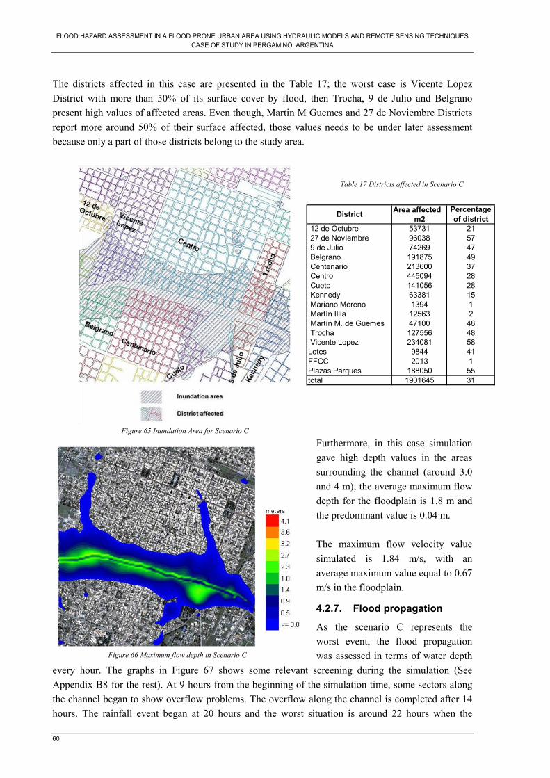
FLOOD HAZARD ASSESSMENT IN A FLOOD PRONE URBAN AREA USING HYDRAULIC MODELS AND REMOTE SENSING TECHNIQUES
CASE OF STUDY IN PERGAMINO, ARGENTINA
60
The districts affected in this case are presented in the Table 17; the worst case is Vicente Lopez
District with more than 50% of its surface cover by flood, then Trocha, 9 de Julio and Belgrano
present high values of affected areas. Even though, Martin M Guemes and 27 de Noviembre Districts
report more around 50% of their surface affected, those values needs to be under later assessment
because only a part of those districts belong to the study area.
Furthermore, in this case simulation
gave high depth values in the areas
surrounding the channel (around 3.0
and 4 m), the average maximum flow
depth for the floodplain is 1.8 m and
the predominant value is 0.04 m.
The maximum flow velocity value
simulated is 1.84 m/s, with an
average maximum value equal to 0.67
m/s in the floodplain.
4.2.7. Flood propagation
As the scenario C represents the
worst event, the flood propagation
was assessed in terms of water depth
every hour. The graphs in Figure 67 shows some relevant screening during the simulation (See
Appendix B8 for the rest). At 9 hours from the beginning of the simulation time, some sectors along
the channel began to show overflow problems. The overflow along the channel is completed after 14
hours. The rainfall event began at 20 hours and the worst situation is around 22 hours when the
Figure 65 Inundation Area for Scenario C
Table 17 Districts affected in Scenario C
Area affected
m2
12 de Octubre 53731 21
27 de Noviembre 96038 57
9 de Julio 74269 47
Belgrano 191875 49
Centenario 213600 37
Centro 445094 28
Cueto 141056 28
Kennedy 63381 15
Mariano Moreno 1394 1
Martín Illia 12563 2
Martín M. de Güemes 47100 48
Trocha 127556 48
Vicente Lopez 234081 58
Lotes 9844 41
FFCC 2013 1
Plazas Parques 188050 55
total 1901645 31
DistrictPercentage
of district
Figure 66 Maximum flow depth in Scenario C

FLOOD HAZARD ASSESSMENT IN A FLOOD PRONE URBAN AREA USING HYDRODYNAMIC MODELS AND GIS TECHNIQUES
CASE OF STUDY IN PERGAMINO, ARGENTINA
61
combination of rainfall and overflow in the channel acted together. After that peak, the inundation
area is defined by the model and the rest of the hours the area affected become to decrease.
Figure 67 Flooding propagation for Scenario C
4.2.8. Applicability of the results
During the flood assessment the maximum flow depth in a specific area and the time when that value
happened was considered. The results that Flo-2D model offers at the end of the simulation enable to
assess those values in specific areas or cells. To show the assessment that is possible to achieve with
the results, only one sector was chosen as example: Dr. Leandro N. Alem Street, located in the Centro
District between Biscayart Street and Trincavelli Street. The grids inside the area were identified in
the system scheme generated by the model. Since the grid size did not match exactly with the shape
and width of the street. (Figure 68) in this analysis were considered those cells with at least 50% of
the area inside the study surface. (Number grids selected: 12152, 12280, 12281, 12282, 12283, 12410
and 12411)

FLOOD HAZARD ASSESSMENT IN A FLOOD PRONE URBAN AREA USING HYDRAULIC MODELS AND REMOTE SENSING TECHNIQUES
CASE OF STUDY IN PERGAMINO, ARGENTINA
62
Figure 68 Street selected for the depth and velocity assessment
The values simulated by the model for those cells were plotted for each scenario. In (Figure 69) is
presented the maximum flow depth and the time when those values were simulated, more over, the
velocity on that grid for that specific time. The biggest depth values in the street, are between 0.21m
to 0.43 m, and were simulated at the end of the rainfall event; however, at the middle of the rainfall
event (1.5 hr) the maximum depth was simulated in the north part of the street.
Figure 69 Maximum flow depth simulated in the Scenario A in Dr. Alem Street
The maximum flow depth increased more than 1.0 m when was considered the scenario B and C in
comparison with the scenario A, (Figure 70). In the case of the specific street assessed, the velocities
values for those water depths are quite similar for both scenarios. In scenario C the time when the
maximum depth is simulated is shorter than in scenario B, this is because a more water volume of
water (combination of rainfall and overflow) is presented in the first one. The comparison with the
scenario A (Figure 69) apparently shows a higher influence of the flow in the channel than the rainfall
over the city.

FLOOD HAZARD ASSESSMENT IN A FLOOD PRONE URBAN AREA USING HYDRODYNAMIC MODELS AND GIS TECHNIQUES
CASE OF STUDY IN PERGAMINO, ARGENTINA
63
Figure 70 Maximum Flow depth simulated in the Scenario B and C for Alem Street
4.3. Flood hazard assessment
Despite some difficulties in the model run, the simulation with Flo-2D model, is presented as first
approach to a potential flood hazard maps for Pergamino city with 10 years return period.
Figure 71 Flood Hazard map in the case of Scenario A : Rainfall event

FLOOD HAZARD ASSESSMENT IN A FLOOD PRONE URBAN AREA USING HYDRAULIC MODELS AND REMOTE SENSING TECHNIQUES
CASE OF STUDY IN PERGAMINO, ARGENTINA
64
Figure 72 Flood Hazard map in the case of Scenario B: Overflow in the channel
Figure 73 Flood Hazard map for Scenario C: Rainfall and Overflow in the channel

FLOOD HAZARD ASSESSMENT IN A FLOOD PRONE URBAN AREA USING HYDRODYNAMIC MODELS AND GIS TECHNIQUES
CASE OF STUDY IN PERGAMINO, ARGENTINA
65
According to the hazard delineation performed by the model a High Hazard Level (red colour in the
maps) means “Persons are in danger both inside and outside their houses. Buildings are in danger of
being destroyed”, then, a Medium Hazard Level (orange colour in the maps) means “Persons are in
danger outside their houses. Buildings may suffer damage and possible destruction depending on
construction characteristics”. Finally Low Hazard Level (yellow colour in the maps) means “Danger
to persons is low or non-existent. Buildings may suffer little damages, but flooding may affect houses
interiors” (O'Brien et al., 2009).
Despite that the flood propagation in scenario A represents a bigger area in comparison with the other
two scenarios, the hazard level identified is low almost everywhere, only near the channel the flood
hazard increases to medium level. In the scenario B, a medium hazard level is presented in most of the
inundation area and the high level appears surrounding the channel and in the area corresponding to
the Municipality Park. Furthermore, even when the inundation area in scenario C was bigger (Figure
60), the hazard map generated by Flo-2D represents smaller area (Figure 73), this is because the
threshold used by the model (Table 7)
Furthermore, according to the danger zone classification made by FEMA (Figure 37), three maps were
generated (Figure 74, Figure 75 and Figure 76). The zones identified with this methodology are
different in comparison with the hazard maps generated by Flo-2D. For example the medium hazard
level, (analogue to judgment zone) presents more extension in area for the maps generated by Flo-2D.
This is because the criterion used related velocity and depth is different. However, in each scenario,
both maps can be useful for the decision makers as this raise the concern that a local criteria needs to
be built.
Figure 74 Flood Hazard map for Scenario A (According FEMA
classification)
Figure 75 Flood Hazard map for Scenario B (According FEMA
classification)
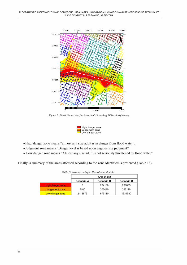
FLOOD HAZARD ASSESSMENT IN A FLOOD PRONE URBAN AREA USING HYDRAULIC MODELS AND REMOTE SENSING TECHNIQUES
CASE OF STUDY IN PERGAMINO, ARGENTINA
66
Figure 76 Flood Hazard map for Scenario C (According FEMA classification)
• High danger zone means “almost any size adult is in danger from flood water”,
• Judgment zone means “Danger level is based upon engineering judgment”
• Low danger zone means “Almost any size adult is not seriously threatened by flood water”
Finally, a summary of the areas affected according to the zone identified is presented (Table 18).
Table 18 Areas according to Hazard zone identified
Area in m2
Scenario A Scenario B Scenario C
High danger zone 0 204130 231835
Judgement zone 5480 306440 326120
Low danger zone 2418875 675110 1331530

FLOOD HAZARD ASSESSMENT IN A FLOOD PRONE URBAN AREA USING HYDRODYNAMIC MODELS AND GIS TECHNIQUES
CASE OF STUDY IN PERGAMINO, ARGENTINA
67
5. CONCLUSIONS AND RECOMMENDATIONS
5.1. Conclusions
Developing countries need to improve the flood assessment using technical tools as hydrodynamic
models, however, the available data is the main constrain when they are applied. The research was
done based on the available data in terms of terrain representation and hydrologic features to evaluate
the level of flood hazard assessment of Pergamino city as was possible. The conclusions that can be
drawn from this study are:
1. Flood characteristics in the Pergamino River using 1D model Hec Ras
What are the main characteristics of the Pergamino stream in terms of water depth and other
water dynamics?
The simulations made using Hec Ras model solved satisfactorily the steady flow conditions for
Pergamino River. The results in terms of water depth enabled to improve the rating curve
(Discharge – High) for the limnimeter at F. Sanchez located in the urban area. This will allow the
determination of calibrated discharges values for further assessments in the channel instead of
using directly extrapolation from the measured values.
The unsteady flow assessment showed a wave celerity in the river of 1.1 m/s, with travel time
equal to 3 hours (between FFCC Mitre Bridge and El Toro). This time is short for an immediate
answer from the urban area. The results support the criterion formulated by the municipality
project to control the flow volume upstream of the city. Furthermore, an independency of the
hydrographs peaks between the limnigraphs stations was found; therefore, further assessments
need to consider the independent systems for the analysis. One related to the area upstream from
the city and the other one relate to the urban area itself. This might lead to more in-deep
hydrological modeling.
2. Flood propagation in Pergamino city using 2D model Flo-2D
What is the flood propagation produced in the urban area of Pergamino for the studied event?
The flood propagation assessment in Pergamino urban area using Flo-2D model considering 10
years as return period gave the extend area affected for three scenarios: 3.5 Km2 , 1.1 Km2 and 1.9
Km2 (flood caused by Rainfall, Overflow in the channel and the combination of the previous ones
respectively). The performance of the Flo-2D model presented during the simulations problems
related to numerical instability and volume conservation that were overcome through the
adjustment of the roughness coefficient in several simulations.

FLOOD HAZARD ASSESSMENT IN A FLOOD PRONE URBAN AREA USING HYDRAULIC MODELS AND REMOTE SENSING TECHNIQUES
CASE OF STUDY IN PERGAMINO, ARGENTINA
68
3. Comparison of the model results with information provided in the area
What is the difference between the models results and the information provided in the area?
The comparison between the maximum flow depth results simulated by the model for a past
rainfall event (February 9, 2001) and the values recorded by the neighborhood association
(CO.S.S.O.PER) showed agreement when the assessment was not considering the average of grid-
cells inside the study area but the selection of them in a specific time of the event. However, when
the comparison is related to the maximum or minimum value simulated (between cells) the model
overestimated and underestimated the depth value.
4. Flood hazard maps in Pergamino city
What is the flood hazard in Pergamino city?
Three flood hazard maps were generated from the simulations results using Flo-2D model, in the
case of scenario A, the three hours total rainfall does not generate high level of flood hazard in the
city. However, for the case of scenario B and C, the medium level of flood hazard is predominant
in the inundation area; high levels of flood hazard are presented in the areas close to the channel
and in the Municipality Park.
5.2. Recommendations
The applicability of hydrodynamic models to assess hazard flood in developing areas was
accomplished throughout the overcome of several constrains. The flood hazard maps are
generated as first approach for the city. Furthermore, from the experience gained during this
research some recommendations are formulated below.
Recommendation for the data input in FLO-2D
- All the input data are introduced to Flo-2D using the preprocessor program GDS, however,
the consuming time to introduce all the information (e.g. Rainfall, levees, channel data, Cross
Section, hydrograph data) become a limitation at the moment to do the adjustments and
improvements for next simulations. Therefore, the GDS program is recommended in the first
simulation, but then at the moment to do the adjustments, it is better to work directly with the
ASCII files and a text editor.
- In Flo-2D, when the simulation represent a combined event of rainfall and discharge with
different times of occurrence (e.g. rainfall time shorter than hydrograph time), the model
works with a total precipitation expressed in percentage. The rainfall data must be kept in 1.0
until the end of the discharge event; otherwise a volume conservation problem will be faced.
- Before the import process of the cross section from Hec Ras to Flo-2D, all the levees in every
cross section must be deleted; because those elements must be introduce to Flo-2D as
FLOOD HAZARD ASSESSMENT IN A FLOOD PRONE URBAN AREA USING HYDRODYNAMIC MODELS AND GIS TECHNIQUES
CASE OF STUDY IN PERGAMINO, ARGENTINA
69
independent process. The abrupt changes of shape and slope between cross section must be
reviewed carefully in order to avoid possible stability problems.
Recommendation for the model validation
- The information collected by CO.S.S.O.PER was useful as first approach and it should be
maintained, supported and augmented as an important social service. However, as it was not
come from a direct measure the accuracy of the model results could not be demonstrated.
Therefore, the validation of the results obtained by Flo-2D model needs to be completed. This
requires a systematic and technical system of data collection in terms of water depth and
duration of the event need to be carried out by the Municipality under the support of
CO.S.S.O.PER.
Recommendation for future studies and continuation of the research
- The lack of cross section data did not allow the use of the data from the limnigraphs stations
to generate the hydrographs, then a bathymetry and a topographic survey must be done in the
area located between the Alfonzo Station and FF.CC Mitre. Besides that, it is necessary to
evaluate the location of both stations in terms of elevation because during fieldwork it was
observed the vulnerability of the instruments for water level increase.
- The DTM generated in this research needs to be improved throughout a specific topography
survey that consider not only the urban area but also the upstream area. Despite that extending
the study area upstream could required more computational time, it would counteract some
undesirable effects closer to the area of interest. In this way the instability and inaccuracies
are kept away of the modeled area. Negative slopes due to pits or depressions should be
strictly avoided in the channel.
- During the simulations performed with Flo-2D, the numerical stability problem was overcome
with the modification of the Wavemax coefficient related to the third stability criterion.
However, a sensitivity analysis about the first stability criterion Percentage change in flow
depth (this study kept the default value in 0.2) can give a second option to evaluate numerical
instability problems.
- As next step in the simulations with Flo-2D, the use of Reduction Area and Reduction Width
factors must be evaluated. The comparison between the results obtained in this research and
new results using those factors can prove or reject their use as alternative to avoid roughness
coefficient adjustments throughout the modification of Wavemax coefficient. The use of these
alternatives requires a multidisciplinary project to evaluate the influence of the actual
structures and buildings in the model.
- As the levees along the channel were introduced as independent element in this study,
changes in their grid-cell location and elevation values must be tested in order to evaluate
their influence in the channel volume conservation.

FLOOD HAZARD ASSESSMENT IN A FLOOD PRONE URBAN AREA USING HYDRAULIC MODELS AND REMOTE SENSING TECHNIQUES
CASE OF STUDY IN PERGAMINO, ARGENTINA
70
Recommendation for Pergamino Municipality
- After this research and the effort of INTA, INA and the Municipality rating curve in F.
Sanchez bridge is one of the most reliable information in the system. As such it is strongly
suggested that a full hydrometric station is place there. This station would be valuable to
understand all the flow mechanism on the Pergamino Stream.
- The existence of a damping effect in Alfonzo station and Del Pescado lagoon area must be
considered in the review study of the dams project formulated by the Municipality, in order to
take in count the favorable effect in the height design of the dams.

FLOOD HAZARD ASSESSMENT IN A FLOOD PRONE URBAN AREA USING HYDRODYNAMIC MODELS AND GIS TECHNIQUES
CASE OF STUDY IN PERGAMINO, ARGENTINA
71
REFERENCE
Ahti, K., 2007. Devastacion de Ciudad Ocotepeque en 1934. 5th IWHA Conference "Pasts and
Futures of Water", Tampere, Finland.
Alkema, D., Nieuwenhuis, J.D.p., de Jong, S.M.p., 2007. Simulating floods : on the application of a
2D hydraulic model for flood hazard and risk assessment. ITC Dissertation;147. ITC,
Enschede, p. 198.
Army Corps of Engineers, U.S., 2002. Development of the Middle Rio GrandeFlo-2D Flood Routing
Model cochiti Dam to Elephant Butte Reservoir.
Brussel, G., 2008. HEC-RAS, River Analysis System Hydraulic Reference Manual. US Army Corps
of Engineers.
Brutsaert, W., 2005. Hydrology An Introduction. Cambridge.
CEOS, 2003. The Use of Earth Observing Satellites for Hazard Support: Assessments & Scenarios.
National Oceanic & Atmospheric Administration, Department of Commerce United States of
America.
Cooley, H., Katz, D., Lee, E., Morrison, J., Palaniappan, M., Samulon, A., Wolff, G., 2006. The
World's Water. The Biennial Report on Freshwater Resources 2006 -2007. In: Acid (Ed.).
Pacific Institute for Studies in Development, Environment, and Security.
Cornejo, J., 2009. Grave inundacion y polemica en Areco. La Nacion, Buenos Aires.
Cornerstone Enineering, I., 2007. Preliminary Flood Study for Tract Map 6731.
Chen, J., Hill, A.A., Urbano, L.D., 2009. A GIS-based model for urban flood inundation. Journal of
Hydrology 373, 184-192.
Dworak, T., Hansen, W., 2003. The European Flood Approach. Towars natural flood reduction
strategies, Warsaw, p. 6.
Dyhouse, G., Benn, J., Hatchett, J., 2003. Floodplain modeling using HEC - RAS : Haestad methods.
Haestad, Waterbury.
Fema, 2005. Floodplain management plan.
Garcia, R., López, J.L., Noya, M., Bello, M.E., Gonzales, N., 1999. Hazard mapping for debris flow
events in the alluvial fans of northern Venezuela.
Herzer, H., 2006. Flooding: Between the Ordinary and the Extraordinary: Deconstructing Risk in the
Argentine City of Pergamino. Milenio Ambiental, Vancouver.
Hicks, F.E., Peacock, T., 2005. Suitability of HEC-RAS for Flood Forecasting. Canadian Water
Resources Journal 30(2), 16.
Hübl, J., Steinwendtner, H., 2001. Two-dimensional simulation of two viscous debris flows in
Austria. Physics and Chemistry of the Earth, Part C: Solar, Terrestrial & Planetary Science
26, 639-644.

FLOOD HAZARD ASSESSMENT IN A FLOOD PRONE URBAN AREA USING HYDRAULIC MODELS AND REMOTE SENSING TECHNIQUES
CASE OF STUDY IN PERGAMINO, ARGENTINA
72
IATASA, U., ABS, 2008. Obras de Defensa y Desagues pluviales de la ciudad de Pergamino.
Pergamino Municality, Pergamino.
INA, 2004. Estudio de Obras de Defensa y Control de Inundaciones del Arroyo Pergamino. Instituto
Nacional del Agua, Pergamino.
Knebl, M.R., Yang, Z.L., Hutchison, K., Maidment, D.R., 2005. Regional scale flood modeling using
NEXRAD rainfall, GIS, and HEC-HMS/RAS: a case study for the San Antonio River Basin
Summer 2002 storm event. Journal of Environmental Management 75, 325-336.
Merwade, V., Cook, A., Coonrod, J., 2008. GIS techniques for creating river terrain models for
hydrodynamic modeling and flood inundation mapping. Environmental Modelling & Software
23, 1300-1311.
Mujumdar, P., 2001. Flood Wave Propagation The Saint Venant Equations. Resonance.
O'Brien, J., Jorgensen, C., Garcia, R., 2009. Flo-2D Manuals. USA.
Peters, G., 2008. Integrating local knowledge into GIS-based flood risk asessment. International
Institute for Geo-Information Science and Earth Observation, Enschede, p. 352.
Sanders, B.F., 2007. Evaluation of on-line DEMs for flood inundation modeling. Advances in Water
Resources 30, 1831-1843.
Tamiru, A., 2005. Integrating Hydrodynamic Models and Hig Resolution DEM (LIDAR) for Flood
Modelling. ITC. Twente, Enschede.
Tennakoon, K., 2004. Parameterisation of 2D Hydrodynamic Models and Flood Hazard Mapping for
Naga city, Philippines. Water Resources. International Institute for Geo-Information Science
and Earth Observation Enschede, p. 102.
Van Westen, C.J., 2000. Remote sensing and Geographic Information Systems for Natural Disaster
Management. International Journal of Applied Earth Observation and Geoinformation.
Werner, M.G.F., 2001. Impact of grid size in GIS based flood extent mapping using a 1D flow model.
Physics and Chemistry of the Earth, Part B: Hydrology, Oceans and Atmosphere 26, 517-522.
Werner, M.G.F., 2004. Spatial Flood extent modelling a performance-based comparison. Civil
Engineer Delft, Delft.

FLOOD HAZARD ASSESSMENT IN A FLOOD PRONE URBAN AREA USING HYDRODYNAMIC MODELS AND GIS TECHNIQUES
CASE OF STUDY IN PERGAMINO, ARGENTINA
73
APPENDICES
Appendix A
FIELDWORK
A1. Discharges determination
• Were done three points of the river: Alfonzo Limnigraph Station, Limnimeter F. Sanchez. and
Urquiza Limnigraph Station. Furthermore, the water levels were read at the same moment of each
measure.
a) Discharge in Alfonzo Limnigraph station
Vertical Distance Width Depth Veloc. Area Discharge Average Time n
Number from base depth Velocity
[cm] [cm] [cm] [cm/s] [cm2] [m3/s] [cm/s] [s]
1.0 0.0 150.0 0.0 0.0 1125.0 0.0 0.0 0.0 0.0
2.0 300.0 250.0 30.0 7.6 7500.0 0.1 7.6 704.0 0.1
3.0 500.0 200.0 60.0 17.3 12000.0 0.2 17.3 256.0 0.4
4.0 700.0 200.0 62.0 20.0 12400.0 0.2 20.0 217.0 0.5
5.0 900.0 200.0 55.0 19.4 11000.0 0.2 19.4 225.0 0.4
6.0 1100.0 200.0 50.0 13.8 10000.0 0.1 13.8 334.0 0.3
7.0 1300.0 300.0 25.0 13.2 7500.0 0.1 13.2 352.0 0.3
8.0 1700.0 200.0 0.0 0.0 1250.0 0.0 0.0 0.0 0.0
Q = 0.962 m3/s
0.0
10.0
20.0
30.0
40.0
50.0
60.0
70.0
0.0 500.0 1000.0 1500.0 2000.0
Distance
(cm)
Wa
ter
De
pth
(c
m)
b) Discharge in F. Sanchez Limnimeter
Vertical Distance Width Depth Veloc. Area Discharge Average Time n
Number from base depth Velocity
[cm] [cm] [cm] [cm/s] [cm2] [m3/s] [cm/s] [s]
1.0 0.0 50.0 0.0 0.0 625.0 0.0 0.0 0.0 0.0
2.0 100.0 150.0 50.0 15.0 7500 0.1 15.0 453.0 0.3
3.0 300.0 200.0 68.0 15.7 13600 0.2 15.7 428.0 0.4
4.0 500.0 200.0 75.0 16.1 15000 0.2 16.1 418.0 0.4
5.0 700.0 200.0 74.0 15.8 14800 0.2 15.8 425.0 0.4
6.0 900.0 200.0 85.0 15.7 17000 0.3 15.7 428.0 0.4
7.0 1100.0 200.0 68.0 18.6 13600 0.3 18.6 353.0 0.4
8.0 1300.0 200.0 66.0 15.6 13200 0.2 15.6 432.0 0.3
9.0 1500.0 150.0 41.0 15.0 6150 0.1 15.0 453.0 0.3
10.0 1600.0 50.0 0.0 0.0 513 0.0 0.0 0.0 0.0
Q = 1.620 m3/s
0.0
10.0
20.0
30.0
40.0
50.0
60.0
70.0
80.0
90.0
0.0 500.0 1000.0 1500.0 2000.0
Dimension
(cm)
Wate
r D
ep
th (
cm
)

FLOOD HAZARD ASSESSMENT IN A FLOOD PRONE URBAN AREA USING HYDRAULIC MODELS AND REMOTE SENSING TECHNIQUES
CASE OF STUDY IN PERGAMINO, ARGENTINA
74
c) Discharge in Urquiza Limnigraph station
Vertical Distance Width Depth Veloc. Area Discharge Average Time n
Number from base depth Velocity
[cm] [cm] [cm] [cm/s] [cm2] [m3/s] [cm/s] [s]
1.0 0.0 100.0 0.0 0.0 975.0 0.0 0.0 0.0 0.0
2.0 200.0 200.0 39.0 11.6 7800.0 0.1 11.6 408.0 0.2
3.0 400.0 200.0 33.0 18.4 6600.0 0.1 18.4 239.0 0.4
4.0 600.0 200.0 30.0 31.5 6000.0 0.2 31.5 132.0 0.8
5.0 800.0 200.0 60.0 34.7 12000.0 0.4 34.7 119.0 0.8
6.0 1000.0 200.0 22.0 36.2 4400.0 0.2 36.2 114.0 0.9
7.0 1200.0 200.0 25.0 33.4 5000.0 0.2 33.4 124.0 0.8
8.0 1400.0 200.0 20.0 31.1 4000.0 0.1 31.1 134.0 0.7
9.0 1600.0 100.0 0.0 0.0 500.0 0.0 0.0 0.0 0.0
Q = 1.267 m3/s
0.0
10.0
20.0
30.0
40.0
50.0
60.0
70.0
0.0 500.0 1000.0 1500.0 2000.0
Distance
(cm)
Dep
th w
ate
r (c
m)
Velocimetry
Cross section measurements
Slope measurement
Three cross section were considered for the determination of the roughness coefficient in the area
located downstream of the F. Sanchez limnimeter.
A2. Measurements of water level values:
Water level measured by the Alfonzo limnigraph = 0.916 m
Water level measured at the F. Sanchez limnimeter = 0.870 m
Water level measured by the Urquiza limnigraph = 0.636 m
Limnigraph equipment
Record from the limnigraph
Alfonzo Station
During the fieldwork there was evidenced that the Alfonzo Station location were suspect to be under
backwater effect. Furthermore, the Urquiza Station location was not working at the moment of the

FLOOD HAZARD ASSESSMENT IN A FLOOD PRONE URBAN AREA USING HYDRODYNAMIC MODELS AND GIS TECHNIQUES
CASE OF STUDY IN PERGAMINO, ARGENTINA
75
visit because in previous days the water overpass it, as a result all the equipment was affected. To
measure the water level in that point was momentarily moved the equipment from Alfonzo Station.
A3. Inspection of the catchment upstream and dowstream of the river.
The basin is large and wide. Upstream of the stream under study, the catchment is a typical lowland-
flat prone area with non defined network drainage. The Pergamino rivers is excavated and marked at
the urban area. All the channel of the urban area was altered by human activities.
Downstream of the urban area, the catchment changes, even though the river bed is lower, the network
drainage is more incised in a natural channel until Urquiza Station. This difference between
downstream and upstream is attributing to the Pedalogy (soil study).
A4. Inspection of the river located in the urban area.
The stream corresponding to the urban area was visited; the dimension values of the bridges
introduced in Hec Ras model before fieldwork were checked.
A5. Collection of data from the Pergamino Municipality and CO.S.O.PPER.
Two meetings were made with authorities of the Pergamino Municipality and CO.S.O.PPER, to
obtain information about historical floods and to complete the data for the simulations.
Floods historical records
Gps measurements
Meeting with CO.S.O.PPER
Furthermore, direct interviews with formers citizen affected for the flooding events in 1995 and 2001
helped to understand not only the technical magnitude but also the social impact in the population.

FLOOD HAZARD ASSESSMENT IN A FLOOD PRONE URBAN AREA USING HYDRAULIC MODELS AND REMOTE SENSING TECHNIQUES
CASE OF STUDY IN PERGAMINO, ARGENTINA
76
Appendix B
B1. Alfonzo Station simulation
Q Water Surface H
m3/s m m
0.1 66.39 0.23
0.25 66.49 0.33
0.5 66.59 0.43
0.75 66.67 0.51
0.962 66.72 0.56
1 66.73 0.57
5 67.11 0.95
25 67.79 1.63
50 68.44 2.28
100 69.48 3.32
150 69.64 3.48
200 69.78 3.62
250 69.91 3.75
300 70.21 4.05
350 70.74 4.58
Low point Cross section 1 = 66.20 m
Discharge measured in fieldwork= 0.962 m3/s
Results of the simulation with that discharge:
H=0.56 m
Therefore:
Elevation water simulated= 66.72 m <67.36 m =
Elevation water field
B2.Steady flow assessment
The example of the calculations steps for the table Table 8 is presented below:
The water depth assumed to obtain the discharge value was 0.25 m. Replacing that value in the
current rating curve F. Sanchez
0.4895915H2.784557-H13.63949 Q 2 +∗∗=
Q = 0.65 m3/s
This value was simulated by the model and the result obtained, in terms of water surface, for the cross
section corresponding to F. Sanchez Bridge is = 53.48 m
As the lowest elevation point in that cross section is 52.75 m (bottom of the river), the water height (
53.48 m – 52.75 m) is 0.73 m.
Before the comparison between the depth values obtained by the model and the values calculated from
the rating curve was necessary to consider the limnimeter level. The instrument was not installed in
the level 52.75m (bottom of the river) but in 53.48 m, which means that the depth value measured
from the limnimeter must be adjusted with a delta height equal to 0.53 m. Therefore, the depth water
value considered for the comparison must be 0.78 m (0.25 m + 0.53 m).
Finally both values 0.73 m from the simulation and 0.78 m were plotted to assess the model
performance.
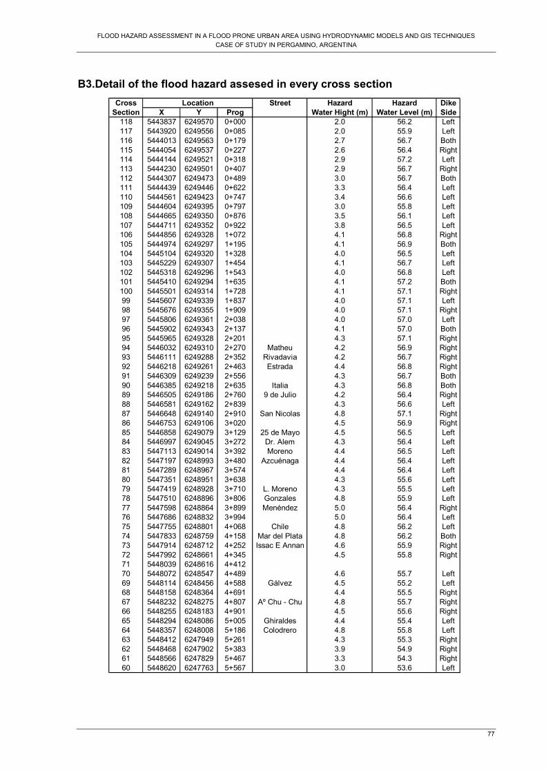
FLOOD HAZARD ASSESSMENT IN A FLOOD PRONE URBAN AREA USING HYDRODYNAMIC MODELS AND GIS TECHNIQUES
CASE OF STUDY IN PERGAMINO, ARGENTINA
77
B3.Detail of the flood hazard assesed in every cross section
Cross Street Hazard Hazard Dike
Section X Y Prog Water Hight (m) Water Level (m) Side
118 5443837 6249570 0+000 2.0 56.2 Left
117 5443920 6249556 0+085 2.0 55.9 Left
116 5444013 6249563 0+179 2.7 56.7 Both
115 5444054 6249537 0+227 2.6 56.4 Right
114 5444144 6249521 0+318 2.9 57.2 Left
113 5444230 6249501 0+407 2.9 56.7 Right
112 5444307 6249473 0+489 3.0 56.7 Both
111 5444439 6249446 0+622 3.3 56.4 Left
110 5444561 6249423 0+747 3.4 56.6 Left
109 5444604 6249395 0+797 3.0 55.8 Left
108 5444665 6249350 0+876 3.5 56.1 Left
107 5444711 6249352 0+922 3.8 56.5 Left
106 5444856 6249328 1+072 4.1 56.8 Right
105 5444974 6249297 1+195 4.1 56.9 Both
104 5445104 6249320 1+328 4.0 56.5 Left
103 5445229 6249307 1+454 4.1 56.7 Left
102 5445318 6249296 1+543 4.0 56.8 Left
101 5445410 6249294 1+635 4.1 57.2 Both
100 5445501 6249314 1+728 4.1 57.1 Right
99 5445607 6249339 1+837 4.0 57.1 Left
98 5445676 6249355 1+909 4.0 57.1 Right
97 5445806 6249361 2+038 4.0 57.0 Left
96 5445902 6249343 2+137 4.1 57.0 Both
95 5445965 6249328 2+201 4.3 57.1 Right
94 5446032 6249310 2+270 Matheu 4.2 56.9 Right
93 5446111 6249288 2+352 Rivadavia 4.2 56.7 Right
92 5446218 6249261 2+463 Estrada 4.4 56.8 Right
91 5446309 6249239 2+556 4.3 56.7 Both
90 5446385 6249218 2+635 Italia 4.3 56.8 Both
89 5446505 6249186 2+760 9 de Julio 4.2 56.4 Right
88 5446581 6249162 2+839 4.3 56.6 Left
87 5446648 6249140 2+910 San Nicolas 4.8 57.1 Right
86 5446753 6249106 3+020 4.5 56.9 Right
85 5446858 6249079 3+129 25 de Mayo 4.5 56.5 Left
84 5446997 6249045 3+272 Dr. Alem 4.3 56.4 Left
83 5447113 6249014 3+392 Moreno 4.4 56.5 Left
82 5447197 6248993 3+480 Azcuénaga 4.4 56.4 Left
81 5447289 6248967 3+574 4.4 56.4 Left
80 5447351 6248951 3+638 4.3 55.6 Left
79 5447419 6248928 3+710 L. Moreno 4.3 55.5 Left
78 5447510 6248896 3+806 Gonzales 4.8 55.9 Left
77 5447598 6248864 3+899 Menéndez 5.0 56.4 Right
76 5447686 6248832 3+994 5.0 56.4 Left
75 5447755 6248801 4+068 Chile 4.8 56.2 Left
74 5447833 6248759 4+158 Mar del Plata 4.8 56.2 Both
73 5447914 6248712 4+252 Issac E Annan 4.6 55.9 Right
72 5447992 6248661 4+345 4.5 55.8 Right
71 5448039 6248616 4+412
70 5448072 6248547 4+489 4.6 55.7 Left
69 5448114 6248456 4+588 Gálvez 4.5 55.2 Left
68 5448158 6248364 4+691 4.4 55.5 Right
67 5448232 6248275 4+807 Aº Chu - Chu 4.8 55.7 Right
66 5448255 6248183 4+901 4.5 55.6 Right
65 5448294 6248086 5+005 Ghiraldes 4.4 55.4 Left
64 5448357 6248008 5+186 Colodrero 4.8 55.8 Left
63 5448412 6247949 5+261 4.3 55.3 Right
62 5448468 6247902 5+383 3.9 54.9 Right
61 5448566 6247829 5+467 3.3 54.3 Right
60 5448620 6247763 5+567 3.0 53.6 Left
Location

FLOOD HAZARD ASSESSMENT IN A FLOOD PRONE URBAN AREA USING HYDRAULIC MODELS AND REMOTE SENSING TECHNIQUES
CASE OF STUDY IN PERGAMINO, ARGENTINA
78
Cross Hazard Hazard Dike
Section X Y Prog Water Level (m) Water Level (m) Side
59 5448677 6247681 5+667 3.4 54.2 Right
58 5448736 6247601 5+768 4.6 55.3 Right
57 5448803 6247526 5+868 3.8 54.5 Right
56 5448865 6247447 5+938 3.7 54.4 Right
55 5448893 6247382 6+010 4.2 54.9 Right
54 5448904 6247313 6+094 2.5 53.0 Left
52 5448928 6247231 6+094 2.6 53.7 Left
51 5449018 6247124 6+233 3.5 53.9 Left
50 5449086 6247052 6+333 3.2 53.5 Left
49 5449144 6246970 6+435 2.5 52.7 Left
48 5449174 6246826 6+580 3.6 53.3 Right
47 5449205 6246766 6+646 3.6 53.4 Both
46 5449256 6246679 6+747 2.6 52.3 Left
45 5449286 6246593 6+839 3.1 52.8 Left
44 5449312 6246501 6+935 3.0 52.7 Left
43 5449356 6246393 7+051 2.7 52.2 Left
42 5449386 6246299 7+149 3.8 53.3 Left
41 5449395 6246167 7+282 2.9 52.3 Left
40 5449492 6246014 7+465 2.9 52.3 Left
39 5449503 6245924 7+555
38 5449553 6245842 7+652 3.3 52.7 Left
37 5449579 6245706 7+790 4.5 54.0 Left
36 5449592 6245634 7+864 4.0 53.5 Right
35 5449666 6245499 8+017 4.0 53.4 Left
34 5449680 6245414 8+103 4.2 53.5 Right
33 5449692 6245325 8+194
32 5449741 6245221 8+307 3.0 52.3 Right
31 5449766 6245125 8+407 4.0 53.4 Both
30 5449795 6245024 8+511 4.0 53.4 Left
29 5449809 6244875 8+661 3.5 52.7 Left
28 5449867 6244752 8+798 2.9 52.0 Left
27 5449943 6244690 8+896 3.0 52.1 Left
26 5450016 6244605 9+007 3.3 52.4 Left
25 5450031 6244508 9+108 3.5 52.4 Left
24 5450059 6244392 9+227 2.8 51.8 Right
23 5450101 6244307 9+321 2.5 51.3 Right
22 5450153 6244261 9+390 2.5 51.2 Both
21 5450198 6244150 9+512 2.5 51.3 Both
20 5450242 6244058 9+612 2.5 51.3 Left
19 5450290 6243973 9+710 3.4 52.2 Left
18 5450353 6243864 9+836 3.6 52.3 Left
17 5450352 6243713 9+989 2.5 51.1 Left
16 5450421 6243610 10+112 3.4 51.9 Left
15 5450501 6243489 10+257 3.4 51.8 Left
14 5450551 6243406 10+355 3.4 52.0 Left
13 5450605 6243313 10+460 3.8 52.4 Both
12 5450653 6243240 10+548 3.6 52.2 Right
11 5450705 6243154 10+649 3.3 51.7 Right
10 5450790 6243104 10+747 2.7 51.2 Left
9 5450826 6243047 10+813 3.3 51.9 Right
8 5450874 6242980 10+895 3.5 51.9 Right
7 5450939 6242895 11+005 3.1 51.4 Right
6 5450995 6242806 11+108 2.7 51.0 Right
5 5451091 6242691 11+257 3.2 51.3 Right
4 5451159 6242599 11+373 2.5 50.3 Right
3 5451259 6242488 11+523 2.5 49.9 Right
2 5451321 6242397 11+632 2.6 50.5 Right
1 5451386 6242333 11+724 2.5 50.3 Right
0 5451434 6242285 11+792 2.5 50.3 Right
Location
Water level that caused flood hazard in the bridges
Water depth Water level
Bridge m m
F. Sanchez 3.9 56.7
Colon 3.8 56.6
La Merced 3.5 55.8
Rocha 3.5 54.8
Ruta 8 4.0 55.3
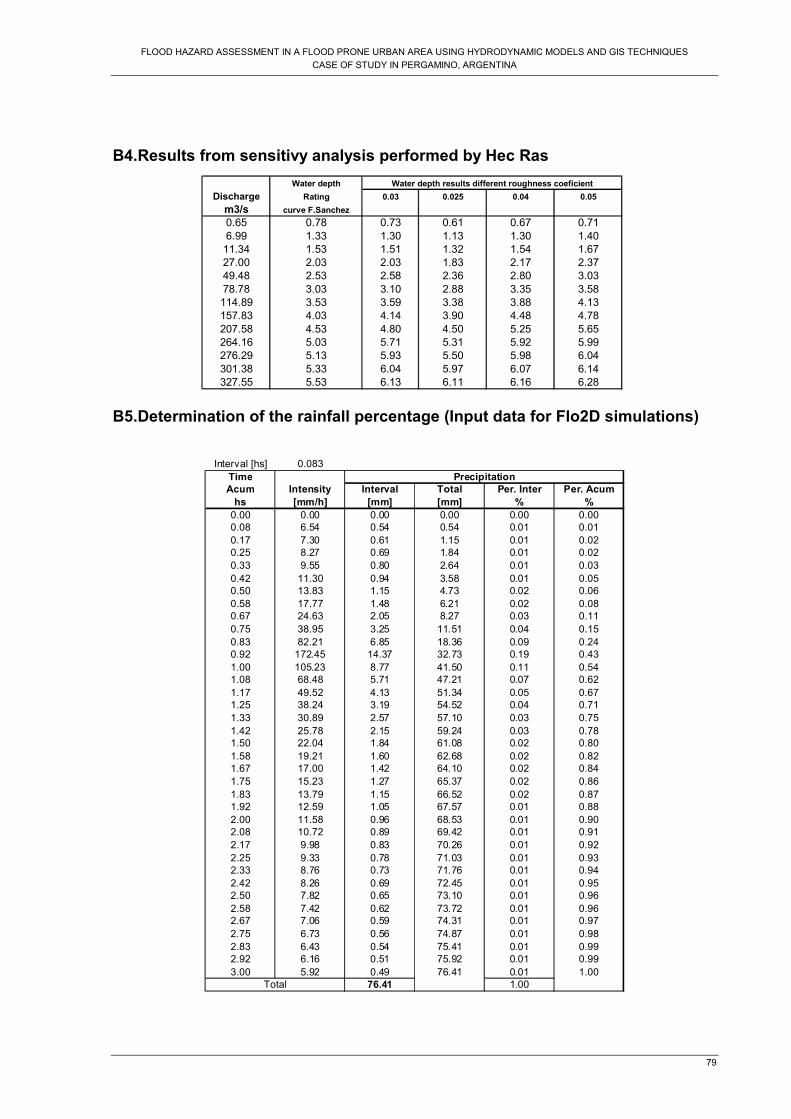
FLOOD HAZARD ASSESSMENT IN A FLOOD PRONE URBAN AREA USING HYDRODYNAMIC MODELS AND GIS TECHNIQUES
CASE OF STUDY IN PERGAMINO, ARGENTINA
79
B4.Results from sensitivy analysis performed by Hec Ras
Water depth
Discharge Rating 0.03 0.025 0.04 0.05
m3/s curve F.Sanchez
0.65 0.78 0.73 0.61 0.67 0.71
6.99 1.33 1.30 1.13 1.30 1.40
11.34 1.53 1.51 1.32 1.54 1.67
27.00 2.03 2.03 1.83 2.17 2.37
49.48 2.53 2.58 2.36 2.80 3.03
78.78 3.03 3.10 2.88 3.35 3.58
114.89 3.53 3.59 3.38 3.88 4.13
157.83 4.03 4.14 3.90 4.48 4.78
207.58 4.53 4.80 4.50 5.25 5.65
264.16 5.03 5.71 5.31 5.92 5.99
276.29 5.13 5.93 5.50 5.98 6.04
301.38 5.33 6.04 5.97 6.07 6.14
327.55 5.53 6.13 6.11 6.16 6.28
Water depth results different roughness coeficient
B5.Determination of the rainfall percentage (Input data for Flo2D simulations)
Interval [hs] 0.083
Time
Acum Intensity Interval Total Per. Inter Per. Acum
hs [mm/h] [mm] [mm] % %
0.00 0.00 0.00 0.00 0.00 0.00
0.08 6.54 0.54 0.54 0.01 0.01
0.17 7.30 0.61 1.15 0.01 0.02
0.25 8.27 0.69 1.84 0.01 0.02
0.33 9.55 0.80 2.64 0.01 0.03
0.42 11.30 0.94 3.58 0.01 0.05
0.50 13.83 1.15 4.73 0.02 0.06
0.58 17.77 1.48 6.21 0.02 0.08
0.67 24.63 2.05 8.27 0.03 0.11
0.75 38.95 3.25 11.51 0.04 0.15
0.83 82.21 6.85 18.36 0.09 0.24
0.92 172.45 14.37 32.73 0.19 0.43
1.00 105.23 8.77 41.50 0.11 0.54
1.08 68.48 5.71 47.21 0.07 0.62
1.17 49.52 4.13 51.34 0.05 0.67
1.25 38.24 3.19 54.52 0.04 0.71
1.33 30.89 2.57 57.10 0.03 0.75
1.42 25.78 2.15 59.24 0.03 0.78
1.50 22.04 1.84 61.08 0.02 0.80
1.58 19.21 1.60 62.68 0.02 0.82
1.67 17.00 1.42 64.10 0.02 0.84
1.75 15.23 1.27 65.37 0.02 0.86
1.83 13.79 1.15 66.52 0.02 0.87
1.92 12.59 1.05 67.57 0.01 0.88
2.00 11.58 0.96 68.53 0.01 0.90
2.08 10.72 0.89 69.42 0.01 0.91
2.17 9.98 0.83 70.26 0.01 0.92
2.25 9.33 0.78 71.03 0.01 0.93
2.33 8.76 0.73 71.76 0.01 0.94
2.42 8.26 0.69 72.45 0.01 0.95
2.50 7.82 0.65 73.10 0.01 0.96
2.58 7.42 0.62 73.72 0.01 0.96
2.67 7.06 0.59 74.31 0.01 0.97
2.75 6.73 0.56 74.87 0.01 0.98
2.83 6.43 0.54 75.41 0.01 0.99
2.92 6.16 0.51 75.92 0.01 0.99
3.00 5.92 0.49 76.41 0.01 1.00
76.41 1.00
Precipitation
Total

FLOOD HAZARD ASSESSMENT IN A FLOOD PRONE URBAN AREA USING HYDRAULIC MODELS AND REMOTE SENSING TECHNIQUES
CASE OF STUDY IN PERGAMINO, ARGENTINA
80
B6.Pergamino Street map with the location of the bridges
º Source: Pergamino Munipality,2009
B7.Comparison between the results obtained with Flo-2D model
In order to see the influence in the adjustments of the roughness coefficient during the trials
simulations, the maximum flow velocity and maximum flow depth for the Scenario A were exported
into Ilwis. Then the average, maximum, minimum and predominant values were calculated. The
comparison of those results, for the scenario A, are presented:

FLOOD HAZARD ASSESSMENT IN A FLOOD PRONE URBAN AREA USING HYDRODYNAMIC MODELS AND GIS TECHNIQUES
CASE OF STUDY IN PERGAMINO, ARGENTINA
81
Comparison between Maximum Flow Depth in the floodplain obtained from the trials simulated in Scenario A
Comparison between Maximum Flow Velocity in the floodplain obtained from the trials simulated in Scenario A
In both cases the minimum value did not change through the simulations, in the three first trials
performed with the Wavemax -0.250 was observed a decrease in the values, however, as soon as the
model performed with a positive Wavemax coefficient (100.25 and 0.25 respectively) the values
increase. The figures above apparently show that the final simulation gave similar to the first trial,
however, the adjustment influence is observed in the variation of the run time and the inundation area:
Comparison between the results from the trials in scenario A
Name
Run time
(hr)
Inundation area
(m2)
Rain 0.049 3503976
Rainv2 0.049 3503744
Rainv3 0.048 3503899
Rainv4 0.045 3503721
Rainv5 3.952 3503738

FLOOD HAZARD ASSESSMENT IN A FLOOD PRONE URBAN AREA USING HYDRAULIC MODELS AND REMOTE SENSING TECHNIQUES
CASE OF STUDY IN PERGAMINO, ARGENTINA
82
B8. Flooding propagation scenario C

FLOOD HAZARD ASSESSMENT IN A FLOOD PRONE URBAN AREA USING HYDRODYNAMIC MODELS AND GIS TECHNIQUES
CASE OF STUDY IN PERGAMINO, ARGENTINA
83
B9. Flood hazard map by FEMA
The follow equations were calculated in base on the graph presented by FEMA (Figure 37)
Low danger zone under this curve:
Depth = 3.2677*0.3048*e-0.36377685*V/0.3048
Judgment zone under this curve:
Depth = 0.3048/(0.21943529+0.079357487*(V/0.3048)^2.480132)
Then the follow relation was used in Ilwis process to generate the maps:
Flood_hazard: iff(d1<depth1,"Low danger zone",iff(d1<depth2,"Judgement zone","High danger
zone"))
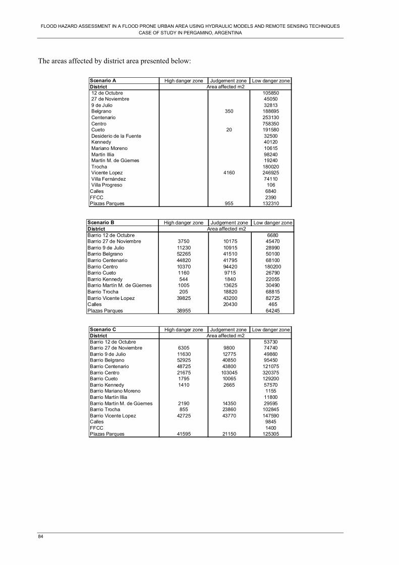
FLOOD HAZARD ASSESSMENT IN A FLOOD PRONE URBAN AREA USING HYDRAULIC MODELS AND REMOTE SENSING TECHNIQUES
CASE OF STUDY IN PERGAMINO, ARGENTINA
84
The areas affected by district area presented below:
Scenario A High danger zone Judgement zone Low danger zone
District
12 de Octubre 105850
27 de Noviembre 45050
9 de Julio 32813
Belgrano 350 188695
Centenario 253130
Centro 758350
Cueto 20 191580
Desiderio de la Fuente 32500
Kennedy 40120
Mariano Moreno 10615
Martín Illia 98240
Martín M. de Güemes 19240
Trocha 180020
Vicente Lopez 4160 246925
Villa Fernández 74110
Villa Progreso 106
Calles 6840
FFCC 2390
Plazas Parques 955 132310
Area affected m2
Scenario B High danger zone Judgement zone Low danger zone
District
Barrio 12 de Octubre 6680
Barrio 27 de Noviembre 3750 10175 45470
Barrio 9 de Julio 11230 10915 28990
Barrio Belgrano 52265 41510 50100
Barrio Centenario 44820 41795 68100
Barrio Centro 10370 94420 180200
Barrio Cueto 1160 9715 26790
Barrio Kennedy 544 1840 22055
Barrio Martín M. de Güemes 1005 13625 30490
Barrio Trocha 205 18820 68815
Barrio Vicente Lopez 39825 43200 82725
Calles 20430 465
Plazas Parques 38955 64245
Area affected m2
Scenario C High danger zone Judgement zone Low danger zone
District
Barrio 12 de Octubre 53730
Barrio 27 de Noviembre 6305 9800 74740
Barrio 9 de Julio 11630 12775 49860
Barrio Belgrano 52925 40850 95450
Barrio Centenario 48725 43800 121075
Barrio Centro 21675 103045 320375
Barrio Cueto 1795 10065 129200
Barrio Kennedy 1410 2665 57570
Barrio Mariano Moreno 1155
Barrio Martín Illia 11800
Barrio Martín M. de Güemes 2190 14350 29595
Barrio Trocha 855 23860 102845
Barrio Vicente Lopez 42725 43770 147590
Calles 9845
FFCC 1400
Plazas Parques 41595 21150 125305
Area affected m2