FINAL TECHNICAL

REPORT

Asia Pacific Research Initiative for

Sustainable Energy Systems

Office of Naval Research

Grant Award Number N00014-13-1-0463

March 1, 2013 to September 30, 2018

December 2018

Table of Contents

EXECUTIVE SUMMARY .................................................................................................................1

TASK 1: PROGRAM MANAGEMENT AND OUTREACH .........................................................4

TASK 2: ELECTROCHEMICAL POWER SYSTEMS..................................................................4

2.1 Fuel Cell Development and Battery Testing ......................................................................... 5

2.2. Contaminant Mitigation and Field Testing ........................................................................ 41

TASK 3: ALTERNATIVE FUELS .................................................................................................52

3.1 Methane Hydrates ............................................................................................................... 52

3.2 Technology for Synthetic Fuels Production ........................................................................ 65

3.3 Low-Cost Material for Solar Fuels Production ................................................................. 119

3.4 Hydrogen Refueling Support ............................................................................................ 123

TASK 4: OCEAN ENERGY ...........................................................................................................142

4.1 Ocean Thermal Energy Conversion (OTEC) .................................................................... 143

4.2 Wave Energy Testing ........................................................................................................ 167

4.3 Seawater Air Conditioning (SWAC)................................................................................. 169

TASK 5: GEOTHERMAL RESOURCE ASSESSMENT ...........................................................175

TASK 6: MICROGRIDS/GRID INTEGRATION ......................................................................175

6.1 Solar Monitoring ............................................................................................................... 175

6.2 Secure Micro-grids ............................................................................................................ 190

6.3 Grid Technology Performance Assessments..................................................................... 216

TASK 7: ENERGY EFFICIENCY ...............................................................................................221

1

Final Technical Report

Asia Pacific Research Initiative for Sustainable Energy Systems

Grant Award Number N00014-13-1-0463

March 1, 2013 to September 30, 2018

EXECUTIVE SUMMARY

This report summarizes work conducted under Grant Award Number N00014-13-1-0463 the Asia

Pacific Research Initiative for Sustainable Energy Systems 2012 (APRISES12), funded by the

Office of Naval Research (ONR) to the Hawaii Natural Energy Institute (HNEI) of the University

of Hawaii at Manoa (UH). The overall objective of APRISES12 was to develop, test, and evaluate

distributed energy systems, emerging technologies and power grid integration using Hawaii as a

model for applicability throughout the Pacific Region. APRISES12 encompassed fuel cell

research, contaminant mitigation and evaluation; battery testing; seafloor methane hydrates

extraction and stability; synthetic fuels processing and production to accelerate the use of biofuels

for Navy needs; alternative energy systems for electric power generation and integration into smart

microgrids, and energy efficient building platforms. Testing and evaluation of alternative energy

systems included Ocean Thermal Energy Conversion (OTEC), grid-scale battery energy storage,

and development of several microgrid test projects.

Under Task 1, Program Management and Outreach, HNEI provided overall program management

and coordination, developed and monitored partner and subcontract agreements, and developed

outreach materials for both technical and non-technical audiences. Additionally, HNEI continued

to collaborate closely with ONR and NRL to identify high-priority areas requiring further detailed

evaluation and analysis.

Under Task 2, Fuel Cell Systems, HNEI conducted testing and evaluation of single cells, stacks

and balance of plant components to support NRL efforts to develop fuel cells for unmanned aerial

vehicles (UAVs), identified contaminant mechanisms and developed mitigation techniques for

organic contaminants present in air and hydrogen, validated a method to measure and separate

mass transfer coefficients suitable for the design of low cost and high power density fuel cells, and

evaluated the potential of anion exchange membrane fuel cells. Development and laboratory

testing continued on fuel cell air purification materials and novel sensor devices. HNEI also

developed and advanced battery diagnosis techniques and investigated key performance aspects

of battery modules.

Efforts under Task 3, Alternative Fuels, focused on the development, testing and evaluation of

alternative fuels and technologies, and included activities in the areas of Methane Hydrates,

2

Technology for Synthetic Fuels Production, Low-cost Material for Solar Fuels Production, and

Hydrogen Fueling Support. Methane hydrate destabilization was examined using ionic salt

compounds found in seawater, and calorimetric investigation focused on hydrate formation and

dissociation in sand matrices. Hydrate desalinization and removal of biological contaminants was

also examined. Synthetic fuels processing focused on hydrogen production for fuel cell

applications, second generation biofuel properties impacted by petroleum aromatics, solvent based

extraction of fermentable sugars from biomass, development of a novel bioreactor for liquid fuels

from synthesis gas, bio-contamination of blended fuels and biodiesel degradation, biofuel

corrosion in diesel/renewable diesel/seawater mixtures, constant volume carbonization processing

variables to convert waste biomass, and enhanced performance of hybrid biochar supports for high

rate anaerobic digestion. For solar fuels production an environmentally friendly potentially low-

cost thin film printing process was refined to fabricate copper-zinc-tin-sulfo-selenide solar cells

with double the efficiency achieved during APRISES11. Hydrogen refueling support involved

commissioning hydrogen production and compression equipment, procurement of a Power Export

Unit for emergency backup power from a fuel cell electric bus, and the design of a hydrogen

dispensing system.

Task 4, Ocean Energy included development of advanced heat exchangers for Ocean Thermal

Energy Conversion (OTEC), Wave Energy Testing, and baseline water monitoring for Seawater

Air Conditioning. To advance OTEC heat exchanger development, a subaward was made to

Makai Ocean Engineering. Makai designed, built, and tested six configurations of Epoxy-Bonded

Heat Exchangers. A new 100-kW test station was designed and constructed to support this testing.

Results were promising and led to the design and fabrication of the Foil Fin Heat Exchanger. An

autonomous control system for the OTEC test facility was also developed, and long term corrosion

testing was continued. In support of the Navy’s Wave Energy Test Site (WETS) off Marine Corps

Base Hawaii, and in collaboration with NAVFAC, HNEI subcontracted with Sea Engineering, Inc.

to conduct a selection process, deploy and commission a remotely operated vehicle (ROV). This

adds a critically important capability to support wave energy conversion device and mooring

inspections, particularly for the deep-water sites at WETS. Seawater Air Conditioning (SWAC)

pre-impact conditions were characterized with further deployments of long-term oceanographic

mooring, water column profiling and sampling to assess the environmental impact of this new

system on the ocean ecosystem near Honolulu.

Funding for the Geothermal Resource Assessment planned for task 5 was reallocated to other areas

of the program as approved by ONR.

Task 6, Microgrids/Grid Integration included a range of projects to develop, test and integrate

secure microgrid technology including distributed energy resources. An empirical model to

characterize the DC performance of PV modules was expanded to evaluate AC performance of

PV systems and power conditioning units, as well as the impact of shading. Development of a

3

low-cost, real-time power monitor with wireless communications for distribution system

operations was continued. Advanced, real-time data analysis and controls were added to the power

monitor system hardware and software, leading to a second provisional patent being filed,

"Enabling Ubiquitous Distribution Grid Modeling for Enhanced Visibility and Controls".

Hardware-in-the-loop equipment was purchased and initial setup completed in order to test

distributed energy resources and devices in real-world grid operation scenarios. Additionally, the

Conservation Voltage Reduction prototype was advanced towards being more cost effective by

utilizing a small DC power supply to emulate a solar module and power an inverter. Initial tests

were successfully conducted at the UH Marine Center. The Battery Energy Storage System

(BESS) on Molokai was modified for faster response, enabling the BESS to respond to

contingency events on the grid. Work continued on the Coconut Island DC microgrid including

procurement of an electric boat (E-boat) and electric utility vehicle, along with a swappable battery

system. HNEI completed the conversion of the E-boat to an all-electric vehicle, and installed the

battery charging station for the swappable battery system in the Boat House on Coconut Island.

To increase the amount of distributed PV that can be connected and utilized by the microgrid on

the Island of Molokai, the impact of a Load Bank was analyzed and found to be an effective

solution. Development was continued on solar forecasting methods and systems, including testing

and evaluation in an operational framework, and validating the predictions generated using ground

observations. Work continued on the Coconut Island DC microgrid including procurement of an

electric boat (E-boat) and electric utility vehicle, along with a swappable battery system. HNEI

completed the conversion of the E-boat to an all-electric vehicle, and installed the battery charging

station for the swappable battery system in the Boat House on Coconut Island. The Maui College

project integrated an additional 500 kW of PV and a 500 kW/500 kWh battery, and performance

was assessed on the campus microgrid, along with charging of electric vehicles from renewable

energy. Additionally, agreements executed with the utility for Power Purchase, Energy

Performance, and Fast Demand Response. The Kauai College project assessed, procured,

deployed and analyzed the performance and impact of Demand Side Management Load Controller

technologies and protocols on the campus microgrid.

Under Task 7, Energy Efficiency, areas of focus included modeling air flows in naturally ventilated

spaces, monitoring and performance comparison of building research platforms, the installation

and analysis of small, vertical axis wind turbines, and support of the utility’s demand response

demonstration projects.

This report describes the work that has been accomplished under each of these tasks, along with

summaries of task efforts that are detailed in journal and other publications, including reports,

conference proceedings, presentations and patent applications. Publications produced through

these efforts are listed and available, or linked, on HNEI’s website at

https://www.hnei.hawaii.edu/publications/project-reports#APRISES12.

4

TASK 1: PROGRAM MANAGEMENT AND OUTREACH

This program-wide task provided management and coordination of all research, test, development

and evaluation efforts under APRISES12. Partner and subcontract agreements were developed

and monitored, and outreach materials for both technical and non-technical audiences were

developed. In close collaboration with ONR, high-priority needs requiring further detailed

evaluation and analysis were identified for application of emerging energy technologies, with a

focus on Hawaii and the Asia-Pacific region. Task-specific information and more detail are

provided below for partner, subcontract and outreach activities.

TASK 2: ELECTROCHEMICAL POWER SYSTEMS

Under Task 2, fuel cell testing and evaluation was conducted on single cells, stacks and balance of

plant components to support NRL efforts to develop fuel cell powered autonomous vehicles; to

support development of mitigation techniques for organic contaminants present in air and

hydrogen; to validate a method to measure and separate mass transfer coefficients suitable for the

design of low cost and high power density fuel cells, and to evaluate the potential of anion

exchange membrane fuel cells using commercial materials and mass production manufacturing

methods.

Battery research under this task focused on automation of battery diagnosis to allow online

monitoring and forecasting, investigation of the performance and durability of battery technology

under large-scale grid support operations, and impact of vehicle to grid (V2G) usage on electric

vehicle (EV) type batteries.

Contaminant Mitigation focused on development of advanced fuel cell air purification materials

and novel sensor devices to allow the use of fuel cells to be expanded into harsh environmental

conditions. These sorbent materials and devices were tested in controlled laboratory conditions

under this effort.

5

2.1 Fuel Cell Development and Battery Testing

2.1a Fuel Cell Development

Testing and evaluation was conducted on single fuel cells, stacks and balance of plant components

to support NRL efforts to develop fuel cell powered unmanned aerial vehicles (UAVs), develop

contaminant mechanisms and mitigation techniques for organic contaminants present in air and

hydrogen, validate a method to measure and separate mass transfer coefficients suitable for the

design of low cost and high power density fuel cells, and evaluate the real potential of anion

exchange membrane fuel cells using commercial materials and mass production manufacturing

methods. HNEI also tested battery packs to support the development of the NRL battery state of

health diagnostic.

Key accomplishments included characterization and design recommendations to NRL related to

their fuel cell stack design based on metallic bipolar plates. Two HNEI developed hydrogen

recovery units were sent to NRL which were integrated into a breadboard system and successfully

operated and validated. The applicability range of the NRL battery pack state of health diagnostic

was tested and extended to 0°C from 25°C. Recovery strategies were validated for fuel cells

contaminated with acetylene (a welding fuel) and bromomethane (a product of biological activity

in oceans). The use of the segmented cell was demonstrated as a diagnostic tool revealing different

signatures for fuel cell contamination mechanisms. The impact of two fuel cell system

contaminants on the oxygen reduction and hydrogen oxidation reaction mechanisms were

established. Several impedance spectroscopy models for data interpretation and parameter

extraction were developed and validated to validate results obtained with the HNEI method to

measure and separate reactant mass transfer coefficients. The realistic performance of anion

exchange membrane fuel cells were established using commercially available and mass production

manufacturing methods.

Details of the work conducted in each of these areas are described below, and in the publications

and presentations referenced at the end of this section.

Support to NRL

Under APRISES11 and 13, HNEI supported NRL by providing extensive diagnostic data for NRL

stacks based on 3D printed bipolar plates to establish the limits and benefits of that manufacturing

technology, co-developed with NRL a hydrogen recovery sub-system to increase efficiency, and

extended a NRL battery state of health diagnostic based on impedance from a single cell to a short

stack. Under APRISES12, these activities were continued with test data for NRL stacks based on

metallic bipolar plates to verify their quality and improve their design, by providing advice for the

6

integration of the hydrogen recovery sub-system to the UAV breadboard system, and by verifying

the applicability of the NRL battery state of health diagnostic to a wider temperature range.

Fuel cell for UAV systems

Under APRISES 12, HNEI continued to support NRL efforts to develop fuel cell powered

unmanned aerial vehicles (UAVs). Work conducted under this activity focused on the issues

associated with fuel cell stack manufacturing and balance of plant development. Particular

attention was given to the tradeoff between weight, volume, and performance to meet flight

requirements and the manufacturability of system components. The potential of stamped metal

bipolar plates was explored as these components can be significantly thinner than those made of

composites or by 3D printing, as previously determined by NRL and HNEI, resulting in a lower

volume and a lighter weight per cell. Corrosion resistant metals are typically used in the production

of metal bipolar plates to prevent degradation under fuel cell conditions. Metals such as stainless

steel have protective layers that prevent degradation. However, these layers also exhibit a high

resistivity leading to unacceptable voltage losses. Specialized coating layers are thus applied to the

plates, post-formation, to alleviate the high resistance and increase conduction without sacrificing

the protective benefits. Manufacturing of metallic bipolar plates can be summarized into four

general steps; boss formation, removal of excess material, plate bonding or welding, and coating

application. A high dimensional accuracy is necessary in the final manufactured product to achieve

uniform distribution of reactants from plate to plate in the stack and channel to channel within each

cell. A low dimensional accuracy can result in issues such as gas leakage, reactant starvation, and

uneven plate compression leading to localized excessive stresses or hot spots. Engineers and

scientists at HNEI continue to consult with NRL on a weekly basis to address issues such as those

mentioned above in the design of NRL’s in-house developed stamped metal plate fuel cell system

and provide testing and evaluation services leveraging the full suite of advanced stack diagnostics

developed at HNEI.

In the reporting period for APRISES 2012, multiple fuel cell stacks built by NRL with metal

bipolar plates were tested and evaluated at HNEI for design conformity and performance

uniformity. Build issues, such as gas leakage due to improper sealing or plate to plate performance

non-uniformity, were identified and communicated to NRL for correction in subsequent builds.

Optimal operating conditions, stack orientation with respect to the aerial vehicle chassis, and

reactant configurations were determined and incorporated by NRL into their system designs. As

part of the balance of plant development, integration and validation of the HNEI developed

hydrogen recovery unit, reported under APRISES 2013, was performed and two units were sent

to NRL for breadboard system integration. Test results were disseminated to NRL through weekly

update meeting presentations and data files were transmitted to NRL using the ARMDEC Safe

Access File Exchange system. Intellectual property developed in this project has been submitted

for a full, non-provisional patent under Patent Application 15/932,050.1 For more information and

7

specific details of the UAV fuel cell development program at NRL, contact Karen Swider-Lyons

(karen.lyons@nrl.navy.mil).

Li-ion state of health monitoring

The utility of a single-point impedance-based technique to monitor the state-of-health of a pack of

four 18650 lithium-ion cells wired in series was completed under APRISES11 funds.2 The single-

point state-of-health frequency is unique to each type of cell chemistry, manufacturer and form

factor, and nearly invariant with state-of-charge making it an ideal probe for continuous online

monitoring. The work reported here under APRISES12 funding broadens the applicability of the

single-point monitoring technique to identify temperature induced faults within packs at a lower

temperature of 0 °C. Under such operating conditions, lithium-ion cells are prone to performance

loss and a number of safety concerns. During cycling at a low temperature, impedance differences

between cells in series can cause weaker cells to overcharge and overdischarge while the pack still

maintains a perceived acceptable voltage within the normal operational boundaries.

The present study utilized commercial 18650 cylindrical lithium-ion cells of 2.6 Ampere-hour

nominal capacity. Single cells and packs were tested in a thermal chamber at 25 or 0 °C. Discharge

cycling in the serial pack configuration used two different modes of lower voltage cutoff: (i) when

the first cell in the pack reached 2.75 V or (ii) when the pack voltage reached 11.0 V. Observations

from the single-point impedance monitoring technique at 316 Hertz were validated against an

exhaustive analysis of different cells degradation mechanisms using electrochemical voltage

spectroscopy (incremental capacity analysis).

Data were utilized to develop a state of health map (Figure 2.1a.1), which shows the average

impedance response of uncycled cells at 25 and 0 °C (yellow circles). The dashed line represents

an empirical relationship established between impedance response and temperature. As

temperature decreases, the acceptable impedance response shifts toward higher real and imaginary

impedance due to slow kinetics for both cell reactions. The free form shapes represent arbitrary

risk indexes where green envelopes 3x the impedance variance across 0 to 100 % state of charge,

orange is 4x and red is 5x the impedance variance at the identified temperatures. The boundaries

for the risk indexes are developed arbitrarily, but can be informed with future safety testing of cells

cycled under the abusive low temperature condition. The small black dots indicate the actual

impedance response of the pack when cycled at 25 °C for 1, 10, 30 and 50 cycles. There is little

change in the impedance response over 50 charge/discharge cycles at this temperature. The pack

level impedance response is much different for packs cycled at 0 °C. The pack level impedance is

shown for the pack with a 2.75 V cell cutoff (light blue circles) and 11.0 V pack cutoff (dark blue

circles) where the number inside the circle indicates the number of completed cycles prior to

diagnostic testing. The low temperature cycling condition is abusive to the pack, particularly the

pack discharged to pack voltage cutoff of 11.0 V, with a progressive translation outside of the

8

healthy zone. More details are provided in the published manuscript (item 1 in the Publications

and Presentations Resulting from these Efforts section).

Figure 2.1a.1. State of health map generated from single-point impedance responses at 316 Hertz

after 1, 10, 30, and 50 discharge cycles, where the cycle number is denoted inside the circles. The

acceptable impedance variance range (<3x) is shown in green, 4x in orange and 5x in red. The

empirical relationship between impedance response and temperature at 316 Hertz is shown by the

black dashed line.

PEM fuel cell contamination

The effects of different contaminants on proton exchange membrane fuel cell operation was

investigated using prior APRISES and other federal funds to ultimately identify and develop more

effective prevention and mitigation strategies. Specifically with APRISES11 and 13 funds, the

effects of air and fuel contaminants on incumbent platinum catalysts and platinum metal group

free catalysts were characterized using different analytical techniques to support the development

of mechanisms and recovery strategies. Activities also targeted aspects relevant to field operation

(contaminant effects on stacks, contaminant mixtures, and long term exposure to contaminants).

Under APRISES12 funds, these activities were continued for several organic contaminants in air

and hydrogen. Acetylene (welding fuel), benzene (chemical intermediate, combustion product),

naphthalene (chemical intermediate, fumigant) and bromomethane (fumigant, product of

biological activity in oceans) are present in air. Caprolactam is released by polymer components

of the fuel cell system and ethylene glycol is the preferred automotive coolant.

9

Acetylene in air

Acetylene, widely used as a welding fuel and as a precursor for chemical syntheses is, among

airborne contaminants, a representative alkyne. Acetylene in the atmosphere originates almost

exclusively from anthropogenic sources, including manufacturing and end-use plant emissions,

fossil and biofuel/biomass combustion. Acetylene concentrations up to 5.5 (1 h average) and 3 (24

h average) ppm by volume near an acetylene plant were predicted with a diffusion model.

Acetylene adsorption as well as catalytic and electrochemical reactions on platinum (Pt) were

extensively studied. Stable surface species were reported for acetylene chemically adsorbed (low

coverage) on Pt surfaces under an ultra-high vacuum. Adsorbed acetylene species are

electrochemically reduced to ethylene and ethane when the adsorption voltage is lower than 0.2 V

versus a hydrogen electrode reference, or are electrochemically oxidized to carbon dioxide at a

potential higher than 0.35 V versus a hydrogen reference. However, under specific operating

conditions, the adsorption rate of acetylene is larger than the oxidation rate which favors acetylene

accumulation and inhibits oxygen adsorption on the Pt surface. Initial accelerated tests with 300

ppm by volume acetylene led to an 88 % cell performance loss.3 Ex situ rotating ring/disk electrode

tests confirmed that acetylene adsorption severely inhibits the oxygen reduction reaction (ORR)

and shifts the ORR mechanism in favor of a hydrogen peroxide product (rather than water),4 a

strong oxidant that can damage the membrane. A more detailed study was needed to better

understand acetylene contamination mechanisms to design mitigation measures. More

specifically, intermediates and products resulting from acetylene exposed to an operating fuel cell

environment have not previously been identified.

Generally, contaminant reactions in the cathode of an operating fuel cell include not only catalytic

reactions but also electrochemical reactions. Under APRISES12 work, the catalytic and

electrochemical acetylene reactions were characterized by using conditions that either suppress

electrochemical reactions or not. Furthermore, reaction intermediates and products were identified

by gas chromatography. These tests were supplemented by two electroanalytical techniques

(chronoamperometry, cyclic voltammetry) to facilitate and confirm species assignments.

Acetylene reactions and products in an operating proton exchange membrane fuel cell are

summarized in Figure 2.1a.2. It is surmised that catalytic reactions predominantly occur on the

bare Pt surface whereas electrochemical reactions occur on the ionomer-covered Pt surface

because the latter reactions require the transport of ions. Carbon dioxide is produced by the

electrochemical oxidation of acetylene at cathode potentials above 0.5 V versus a hydrogen

electrode and the catalytic oxidation of acetylene by the oxygen in air. Above 0.65 V versus a

hydrogen electrode, the acetylene adsorbates are rapidly oxidized into carbon dioxide by platinum

oxides. The carbon dioxide product readily desorbs from the Pt surface and is entrained by the air

flow. On the other hand, below 0.3 V versus a hydrogen electrode acetylene adsorbates are reduced

to ethane, ethylene and methane electrochemically and catalytically by the hydrogen crossing over

10

from the anode through the membrane. All these reduction products also readily desorb and are

entrained by the air flow. Reduction and oxidation processes mentioned so far lead to a rapid cell

performance recovery after the acetylene exposure is interrupted. However, the reduction

intermediates vinylidene and ethylidyne formed between 0.3 and 0.5 V versus a hydrogen

electrode are electrochemically stable even at potentials up to 0.83 V versus a hydrogen electrode.

Additionally, the carbon monoxide oxidation intermediate (or a related oxygenated species)

formed above 0.5 V versus a hydrogen electrode is also electrochemically stable below 0.69 V

versus a hydrogen electrode. Therefore, a cell exposed to acetylene is particularly vulnerable when

the cell is operated at cathode potentials within the 0.3 to 0.69 V versus a hydrogen electrode.

These observations were useful to formulate an effective recovery strategy.5 If a fuel cell is

poisoned and result in a cathode potential below 0.5 V versus a hydrogen electrode, an increase in

current density to reach a cathode potential below 0.3 V versus a hydrogen electrode promotes a

rapid cell performance recovery. Alternatively, if the fuel cell is poisoned above 0.5 V versus a

hydrogen electrode, operation with a cathode potential higher than 0.69 V versus a hydrogen

electrode accelerates the performance recovery. More details are provided in the published

manuscript (item 6 in the Publications and Presentations Resulting from these Efforts section).

Figure 2.1a.2. Acetylene conversion rate and product distribution in proton exchange membrane

fuel cells at different voltages (left). Acetylene reactions at different electrode potentials. PZC:

potential of zero charge. Adsorbates with a subscript “ad” refer to catalytic reactions.

11

Aromatic hydrocarbons in air

Benzene is present in crude oil and gas wells. Benzene is a commodity chemical used to

manufacture other organic compounds and polymers. Naphthalene is produced to manufacture

chemical precursors, intermediates and chemicals. Benzene and naphthalene are released in air by

several mechanisms including evaporation during processing operations and product use and as a

combustion residue. It is known that benzene and naphthalene adsorb on platinum due to an

interest in electrochemical syntheses and effluent treatment, resulting in a partially blocked active

surface and leading to a poorer cell voltage (equivalent to a larger effective current density).

However, only a few reports relate to benzene and/or naphthalene effects on proton exchange

membrane fuel cell operation. None of these reports considered the relative importance of the

successive contaminant processes (transport, adsorption/desorption, reaction, product

adsorption/desorption) on cell behavior.

Contamination processes are contaminant concentration dependent and therefore expected to

depend on the distance from the air inlet port because progressive adsorption and consumption by

surface reactions locally decrease the flow channel concentration. Therefore and under

APRISES12, a segmented cell was used to record the local cell performance. As already mentioned

for acetylene, the contaminant concentration was higher than in atmospheric air to enhance and

accelerate effects, thus limiting test durations to an acceptable level.

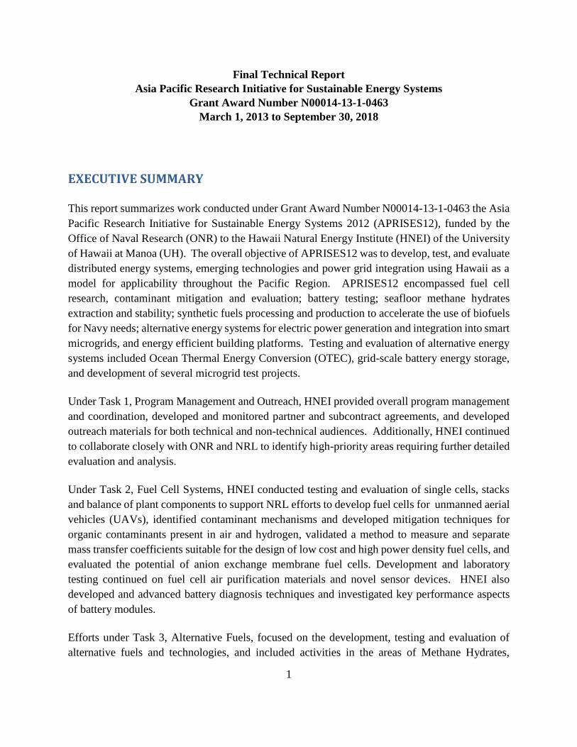
The observed performance drop with benzene was accompanied by a relatively rapid and small

dimensionless current density redistribution of 8 to 9 % (Figure 2.1a.3, left). It is surmised that

the relatively low adsorption energy of benzene on the platinum catalyst surface only consumes a

small fraction of the benzene inventory contained in the air stream (the contaminant concentration

is relatively constant across the cell). Furthermore, the segments near the cell outlet (those close

to segment 10) are more largely impacted (the dimensionless local current is less than 1). It was

not possible to identify a reasonable explanation for this observation. In contrast, the dimensionless

current distribution resulting from naphthalene contamination (Figure 2.1a.3, right) is larger

varying from 14 to 25 %, which is explained by a higher adsorption energy on platinum (higher

coverage). The current distribution is also time dependent and correlates with the cell voltage drop.

The cell voltage decreases due to the accumulation of naphthalene on the catalyst surface

(naphthalene oxidation does not take at these cell voltages), which increases the current density

redistribution. However, at a cell voltage of 0.26 to 0.28 V, the current density trend reverses

because naphthalene is desorbed and/or reduced to less strongly adsorbed products such as decalin

(an alkane). As a result, the cell voltage reaches a steady state near a cell voltage of 0.1 V with a

small effect on current distribution because most of the naphthalene is reduced to a benign form.

12

These results indicate that the current distribution could be used as a signature to identify specific

contamination mechanisms. More details are provided in the published manuscript (item 10 in the

Publications and Presentations Resulting from these Efforts section).

Figure 2.1a.3. Segments’ voltage (top) and normalized current densities (bottom) for an exposure

to 2 ppm benzene (left) and 2.3 ppm naphthalene (right).

Bromomethane in air

Bromomethane was used as a biocide in agriculture, fumigant, chemical intermediate and fire

extinguishing agent. Bromomethane is also naturally formed by algae and kelp in ocean. Trace

amounts of bromomethane have been detected in most places. Industrial areas, fumigated homes

and fields have higher levels (ranging up to 1.2 ppb). The literature indicates that bromomethane

and bromide ions are a threat to proton exchange membrane fuel cells. However, little information

exists in relation to bromomethane adsorption and reactions on Pt either in contact with a gas phase

or aqueous acidic environments. Fortunately, the adsorption and reactions of a related species, the

bromide anion (Br), on a Pt electrode was extensively studied in aqueous electrolyte.

Bromomethane slowly hydrolyses in water, yielding methanol and bromide ions. Methanol is

readily oxidized to carbon dioxide in the air compartment, which easily desorbs from the Pt surface

as indicated above in relation to acetylene contamination. The adsorption of bromide ion on a Pt

surface occurs between 0.135 and 1.19 V versus a hydrogen electrode, which almost entirely

covers the fuel cell accessible electrode potential range. Rotating ring/disk electrode results

demonstrated that strongly adsorbed bromide ions suppress the adsorption of oxygen and hydrogen

by blocking catalyst sites and altering the oxygen reduction path by promoting the formation of

the hydrogen peroxide intermediate.

13

Under APRISES12 work, bromomethane contamination of proton exchange membrane fuel cells

was investigated using both single cells and segmented cells. In addition to the usual

characterization methods (impedance spectroscopy, cyclic voltammetry, linear scanning

voltammetry, polarization), other analytical techniques were employed either in situ or ex situ

(scanning electron microscopy, transmission electron microscopy, X-ray absorption spectroscopy,

X-ray photoelectron spectroscopy) to gain additional structural and chemical information

considering that a cell voltage loss persisted after contaminant exposure. X-ray spectroscopies

were completed in collaboration with NRL, the Brookhaven National Laboratory and the

University of New Mexico.

Experimental results indicated that trace amounts of bromomethane in the air stream caused a

slowly evolving, significant and locally variable cell performance loss. As illustrated in Figure

2.1a.4, left, bromomethane is hydrolyzed to a bromide ion, which accumulates at the catalyst layer

interface because its negative charge prevents it from entering the ionomer (Donnan exclusion)

and inhibits both kinetic and mass transport processes. Methanol oxidation at high electrode

potentials facilitates the hydrolyzation of bromomethane (Le Chatelier principle). The Pt catalyst

surface is eventually covered with the bromide ions, which cannot be removed solely by changing

the cell voltage. Also, the formation of stable complex ions [PtBr4]2 and [PtBr6]

2 favors Pt

dissolution and re-deposition resulting in larger Pt particles, a smaller catalyst surface and a

permanent cell performance loss. The transport of these complex ions is favored by the presence

of liquid water. Hence, segmented cell data show that the current density increases during

contamination near the sub-saturated inlet. This observation was supported by spectroscopic

analyses that showed a more deteriorated catalyst near the cell outlet. However, it was also found

that less bromide was present on the catalyst in the same region. This inconsistency will require

additional tests to resolve and improve the contamination mechanism.

A low electrode potential applied during operation (near the limiting current for example) induces

bromide desorption from Pt sites (Figure 2.1a.4, right). The simultaneous presence of liquid water

would favor the removal of desorbed bromide ions from the cell and restore its performance.

However, the recovery is incomplete owing to the irreversible damage associated with Pt

dissolution and re-deposition (up to 94 % in a single cell). More details are provided in the

published manuscripts (items 7 and 9 in the Publications and Presentations Resulting from these

Efforts section).

14

Figure 2.1a.4. Proposed bromomethane contamination mechanism (left) and electrode potential

range for bromomethane adsorption on the Pt catalyst (right). PZC: point of zero charge, SHE:

standard hydrogen electrode.

Caprolactam and ethylene glycol in air and hydrogen

Ethylene glycol is a relevant contaminant because it is widely used as a coolant, antifreeze agent,

and de-icing solution.6 De-icing of airport runways and airplanes is the primary source of ethylene

glycol in the environment. Ethylene glycol is also dispersed in the environment by the disposal of

products that contain it. Caprolactam, which is an important monomer for Nylon 6 production, is

another potential contaminant that the proton exchange membrane fuel cell system materials

commonly release as a result of either degradation or leaching.7 These two contaminants may

adsorb on the Pt catalyst, compete with the main reactions, or penetrate into the ionomer and

membrane, which would increase cell voltage losses attributed to reaction kinetics, and ionic

conductivity of the catalyst layer and membrane. However, the effects of ethylene glycol and

caprolactam on the hydrogen peroxide production during oxygen reduction and on the hydrogen

oxidation were not previously investigated. As mentioned above, hydrogen peroxide slowly

damages the catalyst layer ionomer and membrane.

Under APRISES12 work, the ex situ rotating ring/disk electrode method was used to separate the

kinetic effect from ohmic and mass transfer contributions, which is facilitated by a small electrode

active surface, controlled hydrodynamics and a simple ohmic loss measurement and correction. In

contrast, ohmic and mass transfer contributions are more difficult to compensate in a single fuel

cell owing to a much larger active area and dependence on location along the flow (inlet to outlet).

Both anode and cathode reactions were investigated because system contaminants can reach both

reactant compartments and their different electrode potentials are expected to yield different results

and tolerance limits. Furthermore, contaminant concentrations were varied to gain insight into the

levels that would lead to measurable effects. This information is important for the design of

mitigation strategies.

15

The activity of the platinum catalyst decreased for both oxygen reduction and hydrogen oxidation

with the increase in ethylene glycol and caprolactam concentration (Figure 2.1a.5, left,

concentration effect not shown). This observation is to a significant extent due to a large Pt surface

coverage as confirmed by cyclic voltammetry. Furthermore, the oxygen reduction side reaction

product hydrogen peroxide is also formed at a higher rate with the increase in ethylene glycol and

caprolactam concentration (Figure 2.1a.5, right, concentration effect not shown). A decrease in Pt

active surface area leads to a smaller number of contiguous Pt sites, which favors oxygen

adsorption in an end-on configuration, decreases the likeliness of an oxygen-oxygen bond

breakage and increases the hydrogen peroxide yield (H2O2) rather than water (H2O). For both

contaminants a low concentration of 0.001 mole per liter is sufficient to observe a significant effect

on oxygen reduction. The concentration increases to 0.01 mole per liter for hydrogen oxidation,

which expectedly indicates that the anode reaction is less sensitive to contamination because the

reaction is more facile. These concentrations need to be translated for use with fuel cells (gas phase

rather than liquid phase concentrations) to mitigate negative impacts on cell performance with the

use of filters. More details are provided in the published manuscript (item 8 in the Publications

and Presentations Resulting from these Efforts section).

Figure 2.1a.5. Polarization curves for oxygen reduction in the presence of ethylene glycol (EG)

and caprolactam (left). Hydrogen peroxide (H2O2) yields with background correction during the

oxygen reduction (right). I: current density, E: electrode potential versus a hydrogen electrode.

Mass transfer analysis

Fuel cells are still too expensive for mass commercialization. Material costs are reduced by

increasing current densities, effectively decreasing stack size. Under these conditions, reactant

mass transfer becomes significant. HNEI is currently developing a method to measure and separate

mass transfer coefficients into elementary contributions to facilitate design optimization. However,

the method needs to be validated by another method. HNEI is currently developing impedance

spectroscopy models to meet this objective and this activity is conducted in collaboration with the

16

Institute of Energy and Climate Research, Jülich, Germany. This activity leverages other federal

funds provided by the Army Research Office. Under APRISES11, an impedance model based on

a physical representation of processes was validated using data obtained with oxygen (rather than

air); a high stoichiometry and a low current density to minimize concentration gradients and match

the 1D model (through the membrane/electrode assembly plane). Under APRISES 13, the model

was extended for more practically relevant operating conditions leading to concentration gradients

along the flow field channel thereby relaxing stoichiometry and current density limitations. For

APRISES 2012, efforts were focused on aspects related to the catalyst layer design and data

processing: ionomer loading uniformity in the catalyst layer, catalyst loading level, and a novel

approach to analyze impedance spectra.

Ionomer uniformity analysis

Near the open circuit voltage and at high load signal frequencies, only cathode catalyst layer

processes in a proton exchange membrane fuel cell are relevant. Under these conditions,

impedance data form a straight line with a 45 degrees angle in a Nyquist representation from which

the catalyst layer ionomer conductivity is obtained. However, the linear behavior is not always

observed which was attributed to non-linear ionomer properties. Therefore, a more accurate

interpretation of impedance data requires a model that includes these non-uniform ionomer

properties.

Under APRISES12, impedance spectra were measured using a segmented fuel cell, for improved

parameter statistics, and a power supply/load bank combined unit, considering measurements are

completed at the open circuit potential. The excitation signal amplitude superimposed to the open

circuit potential means that power is intermittently generated and consumed. The impedance model

was derived with the objective to obtain an analytical solution and by assuming that the ionomer

proton conductivity is an exponential function of the distance through the catalyst layer thickness.

Experimental data showed a good fit to the model (Figure 2.1a.6), which confirmed the hypothesis

of a non-uniform ionomer proton conductivity. The proton conductivity at the membrane interface

varies in the range from 0.09 to 0.23 ohm1 cm1. The mean proton conductivity is 0.13 ohm1

cm1, which agrees well with the value for humidified Nafion at the measurement temperature of

60 °C. This impedance model modification is integrated below to a more comprehensive version

used to obtain parameters for validation of the HNEI method to measure mass transfer coefficients.

More details are provided in the published manuscript (item 5 in the Publications and Presentations

Resulting from these Efforts section).

17

Figure 2.1a.6. Experimental (points) and fitted model impedance (dashed lines) for the whole cell

and for segments 1 to 3. The left panels show the Nyquist spectra in the coordinates with equal

scales along the real and imaginary axis. The right panels show the same spectra with the stretched

real coordinate, to represent the details. Arrows in the frame (a) indicate frequencies in Hertz.

Im(Z): imaginary impedance, Re(Z): real impedance.

18

Cathode catalyst loading

A decrease in platinum loading to commercially relevant levels below 0.1 mg cm2 causes a

significant increase in mass transport losses. This observation is especially relevant for the

development of the HNEI mass transfer coefficient measurement method and the concurrent

development of impedance models for validation. However, characterization of such low loaded

electrode with impedance spectroscopy has seldom been attempted. Furthermore, existing models

have not been fitted to experimental data owing to a need for significant computational resources

to avoid a slow convergence toward a solution.

Under APRISES12, a segmented cell was used to acquire impedance spectra for

membrane/electrode assemblies with two different platinum loadings (0.1 and 0.4 mg cm2 for

both anode and cathode). High stoichiometries were used to minimize concentration gradients

along the flow field length and fit overall cell spectra because local oxygen concentrations were

unknown. The impedance model was derived by combining previous versions that includes the

non-uniform conductivity of the catalyst layer ionomer (previous section) and the non-uniform

concentration gradient along the flow field channel with the objective to use as many analytical

solutions as possible to minimize computational resources to fit experimental data.

A good agreement was found between experimental and model impedance spectra (not shown).

Mass transfer coefficients in the gas diffusion and cathode catalyst layers are given in Figure

2.1a.7). The smaller mass transfer coefficient in the catalyst layer for a lower catalyst loading is

ascribed to a limiting oxygen adsorption on the catalyst surface. The linear increase of the mass

transfer coefficient in the catalyst layer with current density is unclear and warrants further

analysis. Additionally, the cathode catalyst layer mass transfer coefficient obtained by impedance

spectroscopy is smaller by an order of magnitude in comparison to those derived using the HNEI

method. This is due to the difference in operating conditions and a larger amount of liquid water

for the present measurements with air rather than with diluted oxygen streams for the HNEI

method. In contrast, the gas diffusion layer mass transfer coefficient is almost independent of

current density, is different for both membrane/electrode assemblies (attributed to a

membrane/electrode assembly preparation variation) and is much larger than for the cathode

catalyst layer. Furthermore, the gas diffusion layer mass transfer coefficient for the high loaded

membrane/electrode assembly is in agreement with the value measured with the HNEI method.

Again, this impedance model modification is integrated below to a more comprehensive version

used to obtain parameters for validation of the HNEI method to measure mass transfer coefficients.

More details are provided in the published manuscript (item 4 in the Publications and Presentations

Resulting from these Efforts section).

19

Figure 2.1a.7. Fitting parameters for the low platinum (open circles) and high platinum (filled

circles) loaded cells. Mass transfer coefficient in the cathode catalyst layer (CCL, left) and in the

gas diffusion layer (GDL, right).

Novel analysis for impedance spectra

Water management is important to optimize fuel cell performance. For example, the membrane

requires water to maintain its ionic conductivity. However, if product water accumulates in the gas

diffusion electrodes, oxygen transport is impeded. The water distribution is not uniform across the

active area of a fuel cell because the air stoichiometry is generally low to minimize the energy

required by a blower or compressor. For instance, an air stoichiometry of two leads to a 50 %

decrease in oxygen concentration along the flow field length between the cell inlet and outlet with

associated changes in local current density and transport parameters. Impedance spectra collected

with a fuel cell contain this localized information. However, an impedance model derived on the

basis of locally non-uniform parameters has not previously been available for data analysis.

Under APRISES12, an impedance model was first derived by separating the active area into a

fixed number of virtual segments, each having a distinct set of five kinetic and transport

parameters. All segments were interconnected via an oxygen mass balance in the flow field

channel and represented by the latest impedance model (previous two sections). Subsequently, the

overall impedance spectrum for a segmented cell operated at a low and practical air stoichiometry

of two was used to fit the impedance model which contains 50 (10 virtual segments) or 100 (20

virtual segments) parameters.

The impedance model showed a good agreement with experimental impedance spectra (Figure

2.1a.8, left). The oxygen diffusivity in the cathode catalyst layer was not uniform across the cell

active area and decreased from the inlet to the outlet for low current densities (Figure 2.1a.8, right).

For current densities larger than 0.2 A cm2, the non-uniformity disappeared. This behavior is

presumed to be due to the accumulation of product liquid water downstream of the flow field

channel. However, with a constant air stoichiometry, the reactant stream flow velocity

proportionally increases with the current density, which facilitates liquid water removal from the

porous electrode layers. Also, the oxygen diffusivity near the cell inlet increased with current

density. This observation is consistent with Figure 2.1a.7 data obtained with a higher air

20

stoichiometry. The development of the novel analysis approach is ongoing with a focus on its

applicability to a set of local impedance spectra. More details are provided in the published

manuscript (item 2 in the Publications and Presentations Resulting from these Efforts section).

Figure 2.1a.8. Experimental (filled points) and fitted model (open symbols) spectrum of the proton

exchange membrane fuel cell (left) for 10 virtual segments. Experimental and fitted points are

shown for the same frequencies. Oxygen diffusion coefficient in the cathode catalyst layer (CCL)

along the air channel for a current density of 0.2 A cm2 (right). Im(Z): imaginary impedance,

Re(Z): real impedance.

Anion exchange membrane fuel cells

The development of stable and highly ionically conductive anion exchange materials (membranes

and ionomers) has attracted significant attention for application in fuel cells. The conductivity of

these materials is due to hydroxyl anions rather than protons. The change in chemical environment

enables the use of less costly catalysts than those based on platinum group metals for both fuel

oxidation and oxygen reduction. The performance of anion exchange membrane fuel cells operated

with oxygen (rather than air) and platinum catalysts is still significantly lower than for proton

exchange membrane fuel cells. This situation was ascribed to slow reaction kinetics and ionic and

mass transport limitations. The real potential of anion exchange membrane fuel cells is currently

unknown because commercial materials and mass production manufacturing methods have not yet

been used.

Under APRISES12 work, commercially available Pt catalysts, ionomer and membranes, and gas

diffusion layers were used to assemble membrane/electrode assemblies. Catalyst loadings were

also commercially relevant and close to the Department of Energy targets. Catalyst coated

membranes were prepared using digital printing, a method consistent with mass production, which

improves reproducibility. Key operating parameters, gas stream relative humidity and oxygen

concentration, were also varied to identify relevant areas for future design iterations. The project

was completed in collaboration with Pajarito Powder LLC and EWII Fuel Cell LLC.

21

The maximum power density was reproducible and reasonably high at approximately 260-280

mW cm2 with saturated gas streams and oxygen (Figure 2.1a.9, left). Under these conditions,

impedance spectra showed two capacitive loops at high and intermediate frequencies, which were

respectively attributed to hydrogen oxidation and oxygen reduction (not shown). The presence of

these loops suggest that both reactions are slow and would benefit from improved catalysts.

Changes in reactant streams’ humidification revealed that the best performance was observed with

a 50 % relative humidity leading to a peak power density of 330 mW cm2. This observation

suggests that water management can be improved by optimizing the hydrophobicity of anode and

cathode gas diffusion layers. Operation with air led to a lower performance which was attributed

to electrolyte poisoning by carbon dioxide with the creation of carbonate anions that exchange

hydroxyl anions decreasing ionomer and membrane conductivities, and mass transfer losses at the

cathode owing to the diluted stream (Figure 2.1a.9, right). Impedance spectra showed an additional

inductive behavior at low frequencies (not shown). It is presumed that this feature originates from

the oxygen reduction side reaction (2-electron pathway leading to hydrogen peroxide followed by

its disproportionation), which occurs in parallel with the main reaction (4-electron pathway leading

to water). This statement supports the need for improved cathode catalysts with a higher

selectivity. More details are provided in the published manuscript (item 3 in the Publications and

Presentations Resulting from these Efforts section).

Figure 2.1a.9. Polarization curves obtained with oxygen for three membrane/electrode assembly

(MEA) samples (left). Polarization curves obtained with oxygen and air (right). HFR: high

frequency resistance, iR: ohmic voltage loss.

22

Publications and Presentations

Peer Reviewed Publications

1. C. T. Love, M. Dubarry, T. Reshetenko, A. Devie, N. Spinner, K. E. Swider-Lyons, R.

Rocheleau, ‘Lithium-Ion Cell Fault Detection by Single-Point Impedance Diagnostic and

Degradation Mechanism Validation for Series-Wired Batteries Cycled at 0 °C’, Energies, 11

(2018) article number 834.

2. T. Reshetenko, A. Kulikovsky, ‘A Model for Extraction of Spatially Resolved Data from

Impedance Spectrum of a PEM Fuel Cell’, J. Electrochem. Soc., 165 (2018) F291.

3. T. Reshetenko, M. Odgaard, D. Schlueter, A. Serov, ‘Analysis of Alkaline Exchange

Membrane Fuel Cells Performance at Different Operating Conditions Using DC and AC

Methods’, J. Power Sources, 375 (2018) 185.

4. T. Reshetenko, A. Kulikovsky, ‘Impedance Spectroscopy Characterization of Oxygen

Transport in Low– and High–Pt Loaded PEM Fuel Cells’, J. Electrochem. Soc., 164 (2017)

F1633.

5. T. Reshetenko, A. Kulikovsky, ‘Impedance Spectroscopy Study of the PEM Fuel Cell Cathode

with Nonuniform Nafion Loading’, J. Electrochem. Soc., 164 (2017) E3016.

6. Y. Zhai, J. St-Pierre, ‘Acetylene Contamination Mechanisms in the Cathode of Proton

Exchange Membrane Fuel Cells’, ChemElectroChem, 4 (2017) 655.

7. T. V. Reshetenko, K. Artyushkova, J. St-Pierre, ‘Spatial Proton Exchange Membrane Fuel Cell

Performance Under Bromomethane Poisoning’, J. Power Sources, 342 (2017) 135.

8. J. Qi, Y. Zhai, J. St-Pierre, ‘Effects of Ethylene Glycol and Caprolactam on the ORR and HOR

Performances of Pt/C Catalysts’, J. Electrochem. Soc., 163 (2016) F1618.

9. Y. Zhai, O. Baturina, D. Ramaker, E. Farquhar, J. St-Pierre, K. Swider-Lyons, ‘Bromomethane

Contamination in the Cathode of Proton Exchange Membrane Fuel Cells’, Electrochim. Acta,

213 (2016) 482.

10. T. V. Reshetenko, J. St-Pierre, ‘Study of the Aromatic Hydrocarbons Poisoning of Platinum

Cathodes on Proton Exchange Membrane Fuel Cell Spatial Performance Using a Segmented

Cell System’, J. Power Sources, 333 (2016) 237.

23

Conference Proceedings

11. J. Qi, Y. Zhai, J. St-Pierre, ‘RRDE Analysis of Ethylene Glycol and Caprolactam Effects on

the ORR’, Electrochem. Soc. Trans., 75 (14) (2016) 317.

Contributed Presentations

12. T. Reshetenko, J. St-Pierre, ‘Influence of Aromatic Hydrocarbons in Air on Spatial PEMFC

Performance’, in Meeting Abstracts, Electrochemical Society volume 2016-2, The

Electrochemical Society, Pennington, NJ, 2016, abstract 2716.

13. T. Reshetenko, K. Artyushkova, J. St-Pierre, ‘Comprehensive Studies of Spatial PEMFC

Performance Under CH3Br Poisoning of Cathode’, in Meeting Abstracts, Electrochemical

Society volume 2016-2, The Electrochemical Society, Pennington, NJ, 2016, abstract 2701.

14. J. Qi, Y. Zhai, J. St-Pierre, ‘RRDE Analysis of Ethylene Glycol and Caprolactam

Contaminants on the ORR and HOR’, in Meeting Abstracts, Electrochemical Society volume

2016-2, The Electrochemical Society, Pennington, NJ, 2016, abstract 2523.

15. Y. Zhai, O. Baturina, D. Ramaker, J. St-Pierre, K. Swider-Lyons, ‘The Effect of Airborne

Bromomethane Contamination on PEMFC Performance’, in Meeting Abstracts,

Electrochemical Society volume 2016-2, The Electrochemical Society, Pennington, NJ, 2016,

abstract 2520.

References

1. B. Gould, M. Schuette, J. Rogers, R. Ramamurti, K. Swider-Lyons, K. Bethune, ‘Hydrogen

Fuel Cell Power Source with Metal Bipolar Plates’, United States Patent Application number

15/932,050, filed November 20, 2017.

2. C. T. Love, M. B.V. Virji, R. E. Rocheleau, K. E. Swider-Lyons, ‘State-of-Health Monitoring

of 18650 4S Packs with a Single-Point Impedance Diagnostic’, J. Power Sources, 266 (2014)

512.

3. Y. Zhai, J. St-Pierre, ‘Proton Exchange Membrane Fuel Cell Cathode Contamination -

Acetylene’, J. Power Sources, 279 (2015) 165.

4. J. Ge, J. St-Pierre, Y. Zhai, ‘PEMFC Cathode Catalyst Contamination Evaluation with a RRDE

- Acetylene’, Electrochim. Acta, 133 (2014) 65.

24

5. Y. Zhai, J. St-Pierre, ‘Tolerance and Mitigation Strategies of Proton Exchange Membrane Fuel

Cells Subject to Acetylene Contamination’, Int. J. Hydrogen Energy, 43 (2018) 17475.

6. Y. Garsany, S. Dutta, K. E. Swider-Lyons, ‘Effect of Glycol-Based Coolants on the

Suppression and Recovery of Platinum Fuel Cell Electrocatalysts’, J. Power Sources, 216

(2012) 515.

7. H. Wang, C. Macomber, J. Christ, G. Bender, B. Pivovar, H. N. Dinh, ‘Evaluating the Influence

of PEMFC System Contaminants on the Performance of Pt Catalyst via Cyclic Voltammetry’,

Electrocatalysis, 5 (2014) 62.

2.1b Battery Testing

APRISES12 battery research was focused on three areas; the automation of battery diagnosis to

allow online monitoring and forecasting [1-6];the investigation of the performance and durability

of battery technology under large-scale grid support operations; and the impact of vehicle to grid

(V2G) usage on electric vehicle (EV) type batteries.

In the area of battery diagnosis, we developed new strategies that are allowing increased

understanding of Li-ion battery degradation automatically or semi- automatically. Significant

progress was made in the understanding of how environmental and usage aspects affect batteries.

Of particular interest was the investigation of intrinsic variabilities in battery packs made of

thousands of single cells. We found that the pack capacity will be increasingly limited by the cell

that degrades the fastest, and not necessarily by the cell with the lowest initial capacity. The journal

publication for this study was selected as the cover article for the monthly issue of the peer

reviewed open access journal Energies.

In the area of grid operations, focus was set on the lithium ion titanate batteries used in grid-scale

deployed systems monitored by HNEI under other APRISES tasks and efforts [7-9]. We found

that Lithium titanium oxide (LTO)-based Battery Energy Storage Systems (BESS) could be better

suited than graphite-based batteries for reserve applications because of the limited capacity loss at

high SOC. We also used the gathered knowledge to estimate the impact of different energy/power

strategies. For these batteries, we found that increasing power at the expense of energy could

possibly reduce capacity loss by 50%.

In the area of vehicle to grid, focus was set on the understanding of the additional degradation

induced by V2G to assess the potential for grid storage [7, 10-13]. We clearly established a

detrimental impact of V2G under aggressive conditions but we also established that, under certain

25

conditions, V2G could help increase the longevity of the battery pack by delaying the typical

accelerated degradation at end of life. In practice however, such results will only be obtained with

intelligent control algorithms that would require a coordinated policy effort.

All the battery testing was done in the battery-testing laboratory at HiSERF that was developed

under APRISES13. All the results of APRISES12 research have been published in peer reviewed

scientific literature [1-13], and are discussed in more detail below.

Li-ion battery degradation

In APRISES12 we focused on the automation of the analysis to allow online monitoring and

forecasting. HNEI introduces the concept of features of interest (FOI) which correspond to small

sections of the voltage curves that varied significantly only for one type of degradation and not for

the others. FOIs can be selected on any representation of the cell electrochemical behavior. In this

work, IC curves were chosen but, among others, voltage vs. capacity or differential voltage curves

would have been equally viable choices. For IC curves, a FOI can be voltage based (peak position,

front/back tail voltage, peak half-width, voltage variation, resistance increase …), intensity based

(peak/arch intensity, intensity at front/back tail, intensity variation …), capacity based (area under

IC curves) and derivative based (slope of peak/arch) as shown in Figure 2.1b.1.

Figure 2.1b.1 Example of Features of Interest (FOI).

The FOI technique for semi-automated analysis of battery cycling data (i.e. with human

intervention to limit the number of cases to consider) was first tried on graphite intercalation

compound (GIC) / Lithium iron phosphate (LFP) batteries [4, 6] cycled under fast charging and

dynamic driving conditions, Figure 2.1b.2. For these studies, the chosen FOI were area based and

26

they allowed identifying and forecasting the ongoing aging modes acting on the cell in-operando,

to detect and quantify the reversible and irreversible part of lithium plating, and to provide a unique

tool towards early lithium plating detection. More detail can be found in [4, 6].

The technique was also validated on two other popular Li-ion battery chemistries, GIC/ Lithium

Nickel Manganese Cobalt Oxide (NMC) [5] and GIC/ Lithium Nickel Cobalt Aluminum Oxide

(NCA) [2] with FOIs based on voltage, area and IC intensity. In the latter study, we applied these

techniques to investigate cell-to-cell variations at the initial stage and after aging and found no

correlation between the two. A critical aspect of this study was that degradation between cells was

identical but the pace at which the degradation took place varied from cell to cell. It highlighted

that lithium-ion cells’ degradation exhibits a non-trivial amount of intrinsic variability. The

practical consequence of this intrinsic variability in a battery pack is that the overall capacity will

be increasingly limited by the cell degrading the fastest and not necessarily by the cell with the

lowest initial capacity. This study was selected as the cover article for the monthly issue of the

peer reviewed open access journal Energies. Finally, we also compared the results of our approach

to a new impedance based technique [1] for low temperature cycling of battery packs. This was

done in collaboration with Navy Research Laboratory.

Figure 2.1b.2: Diagnosis and prognosis of a graphite/LiFePO4 battery using HNEI techniques.

27

With the viability of the FOI approach demonstrated, we next focused on the complete automation

of the analysis without the need for human intervention [3, 5]. A sensibility analysis showed that,

without human input or complex pattern recognition techniques, no automated diagnosis is

possible as no FOI is solely influenced by one degradation mechanism. To circumvent this issue,

we developed a new multi-step approach where a final multidimensional look-up table is to be

embedded in the automated process to enable a low computing but robust diagnosis of the battery

degradation. The originality of this approach resides in the consideration of the variations of all

FOIs concurrently by using detection in an n-D space for n-FOIs. This enables having accurate

prediction even when each FOI taken separately cannot provide a conclusive diagnosis.

The methodology first consists in emulating the cell that is to be monitored from its half-cell data.

This emulation approach creates a virtual representation of the cell from its individual electrode

data. The virtual cell can then be degraded under different degradation modes to highlight the

changes in voltage response. Battery degradation can be summarized in seven degradation modes,

loss of lithium inventory (LLI), loss of active material (LAM) on the positive electrode (PE) and

on the negative electrode (NE), lithiated (li) or not (de), and the kinetics limitations (RDF) of the

PE and NE. Once the emulation is completed, FOIs can be identified from the voltage response of

the cell and their sensibility towards capacity loss and degradation modes can be established.

Finally, the variation of the most sensible FOIs upon different degradation paths can be compiled

into a multidimensional look-up table. Only the final look-up table is to be embedded in to the

battery management system (BMS), which renders this method appealing. The SOH diagnosis is

performed by comparing the measured FOI values to the values stored in the look-up table.

Out of 5000 possible validation degradation scenarios, the average diagnosis error for the model

was 1.3% for a GIC/LFP cell with up to 30% capacity loss, Figure 2.1b.3. Throughout the range

of capacity loss, 90% of the diagnoses have an error of less than 4.0%, 6.0%, and 1.0% for LLI,

LAMPE and LAMNE, respectively. The maximum error rose to 9.0%, 9.0%, and 4.5% for LLI,

LAMPE and LAMNE, respectively when 95% of the data was considered. For a LTO//NMC cell,

(the cell chemistry used in BESS monitored under APRISES projects), the average diagnosis error

was below 0.1%. Considering 90% of the data, the error on LLI and LAMPE estimation was small,

less than 1%, but the error for LAMNE was increasing from 1% to 12% at 30% capacity loss. The

errors increased up to 3.5%, 2.5% and 16% when 95% of the data are considered. The automated

diagnosis was concluded to be accurate for at least 90% of the test data and the diagnosis errors

were also found to be localized and thus easily manageable.

28

Figure 2.1b.3: Average diagnoses error for (a) the GIC//LFP cell and (b) the LTO//NMC. For each

capacity loss, the left bar represents percentage of LLI, the middle bar the percentage of LAMPE

and the right bar the percentage of LAMNE. The error bars represents the maximum diagnosis

error. The error bars are enriched with quantile information: The spread between , , , and

accounts for 50%, 90%, 95%, and 99% of the data respectively

BESS system cell durability

The purpose of this APRISES project is to understand aging of commercial cells used in large

scale BESS based on single cell laboratory testing. The project had two objectives: First to test

individual single cells in a laboratory setting to understand the cell aging patterns, reproduce the

aging observed in real life and accelerate this degradation to enable the end of life prognosis of the

installed BESS. Second, to monitor, quantify and analyze the battery degradation observed in the

BESS systems installed on the power grid (under other APRISES efforts).

To reach the first objective, we investigated the cell degradation as a function of different aging

conditions with both calendar and cycle aging. The calendar aging study used a design of

experiment methodology to assess the effect of SOC and temperature on calendar degradation in

eight experiments. The cycling aging study focused on understanding the degradation introduced

by the BESS field usage throughout the three years of testing. This knowledge was used to test 3

29

single cells under nominal and harsher conditions. This approach is summarized in Figure 2.1b.4

and comprises three distinct steps: usage analysis, laboratory test and HNEI custom analysis. In

the first step, we used three years’ worth of collected real-world BESS data to quantify the average

usage of the system and defined representative metrics. In the second step, we generated a design

of experiment that allowed us to test the impact of each of the selected metrics of degradation.

Step 1 and 2 were completed under APRISES12. In the last step, we are planning to use HNEI’s

unique battery degradation analysis capabilities such as incremental capacity analysis with FOIs

and pack modeling to analyze cell degradation and diagnose the impact of the selected metrics

individually. This will be conducted under APRISES16 funding and reported at a later time.

Figure 2.1b.4: Schematic test plan of the laboratory testing for the BESS single cells.

The results of the first and second steps are summarized in Figure 2.1b.5. First, we investigated

the usage over three years of a BESS operating at the distribution level of the Hawaii Island grid.

The BESS was in use for more than 90% of the time and stored 1.5 GWh of energy, which amounts

to close to 2 MWh per day for a system rated at 250 kWh. This implies an intensive usage of the

cells with an average of 5 equivalent full cycles per day (>5000 total cycles in 3 years). Our study

of the maintenance cycles showcased that these 5000 equivalent cycles induced an estimated 5-

10% degradation on the single cells. Our analysis of the duty cycle suggests that the usage of the

cells can be described by five parameters: The representative usage consists of several 9 s,

alternating C/2 charge and discharge pulses causing 5% SOC swings with a 0.75% SOC/min ramp

rate at 35 ºC. However, extreme values with currents up to more than 4 C, 100% SOC swings and

temperatures above 50 ºC were also observed.

Second, we investigated the battery degradation associated with the representative usage of the

BESS. The research entailed the impact of different stress factors such as the C-rate, the

temperature, and the SOC swing range on the battery degradation. The results showed that the

accelerated laboratory testing forecasted a capacity loss similar to the values observed in the field.

Temperature increase and C-rate increases were found to have a detrimental effect on capacity

30

retention. In addition, it was found that capacity faded faster when smaller SOC swings were

applied. Moreover, no significant compounding interactions were identified between the three

stress factors. Initial modeling showcased that the modules are not all losing capacity at the same

pace because of slight temperature gradients. The forecast for up to 10 years indicates capacity

loss for the hottest cells in the order of 30% vs. 15% for the coolest cells. In this work, we assumed

a perfect battery pack with identical perfectly balanced modules fading at the same pace. This

assumption might not be verified in the field and might explain the larger observed spread of

fading. Therefore, more comprehensive modeling taking into account cell-to-cell variations,

inhomogeneous aging conditions will be performed under APRISES16 to improve the accuracy of

the simulations.

Regarding calendar aging, the cells did not degrade significantly when kept below 35 °C, but

deteriorated from exposure to temperatures above 45 °C especially if left at low SOC. This result

was counterintuitive based on common understanding of the calendar aging of Li-ion cells that

suggests more degradation at high temperature and high SOCs. This was likely induced by the

presence of a titanate NE in lieu of the graphite NE. Calendar aging is well known to be associated

with loss of lithium inventory induced by the growth of a passivation layer. This parasitic reaction

is fueled by the voltage of the battery, above 4V, that is enough to decompose the electrolyte. In

LTO-based cells, this is inhibited because the voltage is lower, 2.5V, and thus the electrolyte stable.

In order to compare our calendar aging results and the behavior of these titanate cells to the state

of the art, we performed a literature review [7] on the topic and found that LTO based cells are

indeed less affected than graphite cells. Losing little capacity from calendar aging could be a

significant advantage for BESS reserve applications. Such systems must spend most of their time

resting at high SOCs to be ready to be used at any time. Therefore, LTO-based BESS could be

better suited than graphite-based BESS for this application. Moreover, the limited loss at room

temperature or below allows for easy and prolonged storage of cells without performance fade.

Although it cannot be concluded yet that the testing acceleration protocol simulated actual long-

term battery usage, this dataset elucidated the influence of certain factors such as the impact of

cooling and of sizing on the BESS longevity. There was an undeniable deleterious effect of

temperature on the cells. Temperatures above ambient need to be avoided both during usage and

during idling and offline periods, especially if the BESS is at low SOC. When identifying an

adequate sizing of the BESS, this study can be used to roughly estimate the impact of different

energy/power strategies. The SOC swing range is a proxy for the BESS energy. Decreasing the

SOC swing is equivalent to deploying a BESS with higher capacity performing the same task. The

C-rate corresponds to the power rating. Since power is voltage multiplied by the current,

decreasing current emulates a BESS that is required to deliver more power given the same voltage

31

and energy. Table 2.1b.1 compiles the difference in capacity loss associated with dividing or

multiplying the available energy or power by a factor of two while performing the same usage. In

this case, since small SOC swings induced more capacity loss and low currents induced less loss,

it was most advantageous to increase power (−48% capacity loss) at the expense of energy. More

work is needed to investigate sizing issues further, but the proposed test matrix shows great

promise. The gathering of information in 6 months of testing should enable the determination of

which topology is most efficient based on the predicted usage.

Further detail can be found in [8, 9] .

Figure 2.1b.5: Graphical summary of the laboratory experiments performed on the LTO/Lithium

Cobalt Nickel Aluminum Oxide Altairnano Generation 1cells.

32

Table 2.1b.1: Impact of different Power-to-Energy combinations on capacity loss after the same

overall usage (lower is better).

V2G impact assessment

Battery degradation is extremely important to EV technologies and is a function of several factors,

such as electrode chemistries, operating temperatures, and usage profiles (i.e. driving vs. driving

+ vehicle-to-grid applications). The goal of this research was to assess such impact. The battery

test plan used two separate experiments: a cycling experiment to assess the impact of both V2G

and grid-to-vehicle (G2V) charging strategies and a calendar aging experiment to assess the impact

of temperature and SOC, Figure 2.1b.6.

The effect of constant power V2G and G2V protocols on single cells was investigated. Since V2G

and G2V protocols might have a combined effect with other variables such as the charging

schedule, and the charging level, it was essential to study a matrix of tests encompassing the

different combinations. Four different duty cycles were selected to occur during @Home and

@Work periods: A V2G discharge followed by a charge and rest (DCR), a charge then a rest (CR,

standard usage), a rest then a charge (RC, G2V delayed charging), and just a rest (R). The pace of

calendar aging is known to be dependent on the cells' SOC and on the environmental temperature

[7]. For EV applications, the SOC could be anywhere from 100% to 0% and the temperature,

dependent on the location and climate (from -27°C to 55°C in this study). Since calendar aging on

GIC//NCA cells occurs for the most part at high temperature and SOC, the density of measurement

was increased in this area. More detail on the experimental protocol can be found in the full

publication [12].

For this study, 100 GIC/NCA cells were purchased. They are representative of the cells used by

Tesla in their EVs. Preliminary testing, Figure 2.1b.7, consisted in assessing the cell-to-cell

variations and in the emulation of the cell enabling a sensibility analysis and proper FOI selection.

More detail can be found in [13]. The cell-to-cell variation analysis revealed that the test cells were

of high quality with similar thermodynamic properties as well as less than 0.5% variation in rate

capability and maximum capacity, and less than 3% variation in resistance. Thus, the selected cells

33

were found suited for long term studies of cells tested under a range of aging scenarios such as

V2G and G2V. As a result, 36 cells were selected for the cycle aging experiment and 16 cells for

the calendar aging experiment.

Figure 2.1b.6: Test plan for the V2G/G2V study.

34

Figure 2.1b.7: Graphical summary of preliminary testing.

With 52 cells in testing, and to accelerate the analysis of the degradation data and perform

advanced diagnosis without resorting to post-mortem analysis, the FOI approach was used. In

order to select the most appropriate FOIs, a sensibility analysis was performed from an emulated

version of the cells. The impact of the degradation modes is different enough to enable accurate

diagnosis of cell degradation and permit comparison of cells following different degradation paths.

Selected FOIs were the intensity of the peak at 4.1V and the intensity and position of the minimum

in voltage between 3.7 and 3.9V.

Next, the effect of V2G and G2V on battery durability was investigated. In addition, the effects of

calendar aging on capacity loss, resistance increase, and rate capability were identified. Results

were reported in [12] and are summarized in Figure 2.1b.8.

This study focused on testing the impact of V2G discharging the battery twice a day to the power

grid for a total of 2 hours per day at the maximum possible power to maximize potential electricity

savings or revenues for the EV owner. Results showed that such a V2G step twice a day increased

the capacity loss by 75% and the resistance by 10%. Reducing the V2G usage by half (to one

discharge cycle lasting 1 hour per day) degraded the cell less but the result was still found to

35

accelerate the capacity loss by 33% and the resistance increase by 5% over no V2G at all. Thus, a

detrimental impact of V2G under these aggressive conditions was clearly established for these

cells. Translating these results to the entire life of the cells using the model developed for this

project showed that participating in V2G programs could decrease the lifetime of the battery packs

below 4 years because of a capacity loss of more than 20%. In contrast, delaying the G2V charge

rather than charging immediately after driving (to help the grid to spread the load) had no

significant effect (<1%) on capacity retention and was found to limit the resistance growth (5%

less increase). It was noted that this experiment was performed at room temperature where the

SOC exercised very little influence on calendar aging.

The calendar aging experiment showed that the storage SOC has a much higher impact at higher

temperature. This suggests that delayed G2V should induce less degradation and be beneficial in

warmer climates. Looking more closely at calendar aging, aging was found to influence the cells

and that, at room temperature, charging the cells twice a day instead of once lowered the rate of

capacity loss by 5%. However, since the capacity loss increases with temperature and SOC, this

will not be the case in warmer climates. The capacity loss associated with time, temperature and

SOC was modeled with a double-quadratic equation. This modeling allowed for the prediction of

the capacity loss induced by time, temperature and SOC. Looking at the individual effect analysis,

storage temperature was found to have the biggest impact on capacity loss and rate capability.

However, the SOC had more influence on the resistance increase.

36

Figure 2.1b.8: Graphical summary of both the cycle and calendar aging studies.

From the analysis of the FOI, published in [11] and summarized in Figure 2.1b.9, the modes

causing the degradation of these commercial graphite//NCA cells subjected to 20 different duty

cycles, including cycle and calendar aging, were investigated. It was found that, in general, the

cells did not degrade in the same way, and that the degradation was path dependent. Cycle aging,

with or without an extra discharge step to determine the effect of V2G strategies on battery life,

resulted in greater loss of active material and more kinetic limitations on the negative electrode

than calendar aging. Temperature induced additional loss of lithium inventory and loss of active

material at the positive electrode. SOC, on top of catalyzing the temperature effect, caused kinetic

limitations and loss of negative electrode material. Most noteworthy, the loss of active material at

the negative electrode was faster than the loss of lithium inventory in the cycle-aging experiment.

This finding was a clear sign that the cycled cells will enter a stage of advanced aging characterized

by the onset of lithium plating. This result led to a revision of the lifetime prognosis for the usage

of these cells for EV application. However, the manifestation of the second stage could be delayed

or suppressed with intelligent control algorithms.

37

Figure 2.1b.9: Graphical summary of the FOI analysis of the cycle and calendar aging studies.

Following up on the concept of intelligent control algorithms to reduce the impact of V2G on the

cells, we teamed up with the University of Warwick [16] for a collaborative publication on the

policy impact of our respective findings [10]. We concluded that the simplistic approach adopted

by current V2G pilot studies, namely that an EV is discharged and charged without consideration

of battery degradation is not economically viable because of the impact additional V2G cycling

has on battery life. However, a smart control algorithm with an objective of maximizing battery

longevity can reverse this. In such an approach, the control algorithm only allows access to the

battery's stored energy if there are no adverse effects on battery longevity; therefore, the worst case

is that a battery degrades as if there was no V2G. This approach relies upon the development of

accurate battery prognostic models and further advances in understanding the causes, mechanisms

and impacts of battery degradation.

From a policy perspective, anticipated EV growth offers great potential for V2G to play a

significant role as a grid service. When coupled with jurisdictions that have committed to

renewable energy, V2G can be an enabler for carbon reduction. Installing the grid improvements

and platform is an essential first step, but establishing the appropriate compensation model will be

challenging and necessary for V2G to expand. Ultimately, establishing a new, free market to

aggregate and trade grid services combined with the methodology envisioned by us and others

could lead to unbridled growth of V2G as a future grid service.

38

In summary, much was accomplished under APRISES12 battery efforts. Significant progress was

made in the understanding of how different key environmental and usage aspects affect the single

cells and how these cells can be characterized. These studies pave the way to develop a complete

BESS model under APRISES16 funding.

Publications and Presentations

Peer Reviewed Publications

1. “Durability and Reliability of Electric Vehicle Batteries under Electric Utility Grid

Operations. Part 1: Cell-to-Cell Variations and Preliminary Testing “, A. Devie, M.

Dubarry, Batteries, 2(3) (2016) 28.

2. “Online state of health estimation on NMC cells based on predictive analytics“, M.

Berecibar, F. Devriendt, M. Dubarry, I. Villarreal, N. Omar, W. Verbeke, J. Van Mierlo,

J. Power Sources, 320(2016) 239-250.

3. “Fast charging technique for high power LiFePO4 batteries: A mechanistic analysis of

aging”, D. Anseán, M. Dubarry, A. Devie, B.Y. Liaw, V.M. García, J.C. Viera, M.

González, J. Power Sources, 321(2016) 201-209.

4. “Operando lithium plating quantification and early detection of a commercial LiFePO 4

cell cycled under dynamic driving schedule”, D. Anseán, M. Dubarry, A. Devie, B.Y.

Liaw, V.M. García, J.C. Viera, M. González, J. Power Sources, 356(2017) 36-46.

5. “Durability and reliability of electric vehicle batteries under electric utility grid

operations: Bidirectional charging impact analysis “, M. Dubarry, A. Devie, K.

McKenzie, J. Power Sources, 358(2017) 39-49.

6. “State of health battery estimator enabling degradation diagnosis: Model and algorithm

description”, M. Dubarry, M. Berecibar, A. Devie, D. Anseán, N. Omar, I. Villarreal, J.

Power Sources, 360(2017) 59-69.

7. “Battery Energy Storage System battery durability and reliability under electric utility

grid operations: Analysis of 3 years of real usage”, M. Dubarry, A. Devie, K. Stein, M.

Tun, M. Matsuura, R. Rocheleau, J. Power Sources, 338(2017) 65-73.

8. “Lithium-Ion Cell Fault Detection by Single-Point Impedance Diagnostic and

Degradation Mechanism Validation for Series-Wired Batteries Cycled at 0 °C”, C. Love,

M. Dubarry, T. Reshetenko, A. Devie, N. Spinner, K. Swider-Lyons, R. Rocheleau,

Energies, 11(4) (2018).

9. “The viability of vehicle-to-grid operations from a battery technology and policy

perspective”, K. Uddin, M. Dubarry, M. Glick, Energy Policy, 113(2018) 342-347.

39

10. “Durability and Reliability of EV Batteries under Electric Utility Grid Operations: Path

Dependence of Battery Degradation”, M. Dubarry, G. Baure, A. Devie, J. Electrochem.

Soc., 165(5) (2018) A773-A783.

11. ”Intrinsic Variability in the Degradation of a Batch of Commercial 18650 Lithium-Ion

Cells”, A. Devie, G. Baure, M. Dubarry, Energies, 11(5) (2018).

12. “Battery durability and reliability under electric utility grid operations: Representative

usage aging and calendar aging”, M. Dubarry, A. Devie, Journal of Energy Storage,

18(2018) 185-195.

13. “Calendar aging of commercial Li-ion cells of different chemistries – A review”, M.

Dubarry, N. Qin, P. Brooker, Current Opinion in Electrochemistry, 9 (2018) 106-113.

Contributed Presentations and Posters

1. Li Plating Quantification in Commercial Graphite‖LiFePO4 cells, D. Anseán, M. Dubarry,

A. Devie, B.Y. Liaw, V.M. García, J.C. Viera, M. González, 230th Meeting of the

Electrochemical Society, Honolulu, HI, USA, October 2016.

2. Path Dependence in Lithium-Ion Batteries Degradation - a Comparison of Cycle and

Calendar Aging, M. Dubarry, A. Devie, 230th Meeting of the Electrochemical Society,

Honolulu, HI, USA, October 2016.

3. EV cell degradation under electric utility grid operations: Impact of calendar aging &

vehicle to grid strategies, A. Devie and M. Dubarry, EV Summit and Transportation

Summit, Cocoa Beach, FL, USA, October 2016. (Poster)

4. Cycle and Calendar Aging Study of Lithium-Ion Batteries in the Context of Grid-Scale

Energy Storage Systems, A. Devie and M. Dubarry, 230th Meeting of the Electrochemical

Society, Honolulu, HI, USA, October 2016. (Poster)

5. Laboratory testing of Lithium Titanate based cells for BESS applications, A. Devie and M.

Dubarry, EV Summit and Transportation Summit, Cocoa Beach, FL, USA, October 2016.

(Poster)

6. Cycle and Calendar Aging Study of Lithium-Ion Batteries Under Various Vehicle-to-Grid

Scenarios, A. Devie and M. Dubarry, 230th Meeting of the Electrochemical Society,

Honolulu, HI, USA, October 2016. (Poster)

7. Hawai‘i Energy Storage Overview, Jay Griffin, Marc Matsuura, Matthieu Dubarry and

Richard Rocheleau, Hawaii Public Utility Commission Briefing, Honolulu, HI, December

2016.

8. Non-intrusive operando battery diagnosis and prognosis, M. Dubarry, 12th Pacific Rim

Conference on Ceramic and Glass Technology, Waikoloa, HI, USA, May 2017.

40

9. Durability and Reliability of EV Batteries under Electric Utility Grid Operations:

Bidirectional Charging Impact Analysis, A. Devie, G. Baure, and M. Dubarry, 232th

Electrochemical Society Meeting, National Harbor, MD, USA, Oct. 2017.

10. State of Health Battery Estimator Enabling Degradation Diagnosis, M. Dubarry, M.

Berecibar, G. Baure, N. Omar and I. Villarreal, 232th Electrochemical Society Meeting,

National Harbor, MD, USA, Oct. 2017. (Poster)

11. State of Health Battery Estimator Enabling Degradation Diagnosis, M. Dubarry, M.

Berecibar, G. Baure, N. Omar and I. Villarreal, 8th annual Battery Safety, Arlington, VA,

USA, November 2017. (Poster)

12. Hawaii Energy and the Role for Storage, M. Dubarry and K. McKenzie, American

Chemical Society Hawaii Local Section Election Luncheon, Honolulu, HI, USA,

November 2017

13. State of Health Battery Estimator Enabling Degradation Diagnosis, M. Dubarry, M.

Berecibar, G. Baure, N. Omar and I. Villarreal, Gordon Research Conference, Batteries,

Ventura, CA, March 2018. (Poster)

14. Durability and Reliability of EV Batteries under Electric Utility Grid Operations:

Bidirectional Charging Impact Analysis, G. Baure and M. Dubarry, Advanced Automotive

Batteries Conference, San Diego, CA, June 2018. (Poster)

References

[1] C. Love, M. Dubarry, T. Reshetenko, A. Devie, N. Spinner, K. Swider-Lyons, R. Rocheleau,

Energies, 11(4) (2018).

[2] A. Devie, G. Baure, M. Dubarry, Energies, 11(5) (2018).

[3] M. Dubarry, M. Berecibar, A. Devie, D. Anseán, N. Omar, I. Villarreal, J. Power Sources,

360(2017) 59-69.

[4] D. Anseán, M. Dubarry, A. Devie, B.Y. Liaw, V.M. García, J.C. Viera, M. González, J. Power

Sources, 356(2017) 36-46.

[5] M. Berecibar, F. Devriendt, M. Dubarry, I. Villarreal, N. Omar, W. Verbeke, J. Van Mierlo, J.

Power Sources, 320(2016) 239-250.

[6] D. Anseán, M. Dubarry, A. Devie, B.Y. Liaw, V.M. García, J.C. Viera, M. González, J. Power

Sources, 321(2016) 201-209.

41

[7] M. Dubarry, N. Qin, P. Brooker, Current Opinion in Electrochemistry, 9(2018) 106-113.

[8] M. Dubarry, A. Devie, Journal of Energy Storage, 18(2018) 185-195.

[9] M. Dubarry, A. Devie, K. Stein, M. Tun, M. Matsuura, R. Rocheleau, J. Power Sources,

338(2017) 65-73.

[10] K. Uddin, M. Dubarry, M. Glick, Energy Policy, 113(2018) 342-347.

[11] M. Dubarry, G. Baure, A. Devie, J. Electrochem. Soc., 165(5) (2018) A773-A783.

[12] M. Dubarry, A. Devie, K. McKenzie, J. Power Sources, 358(2017) 39-49.

[13] A. Devie, M. Dubarry, Batteries, 2(3) (2016) 28.

[14] M. Dubarry, A. Devie, B.Y. Liaw, Journal of Energy and Power Sources, 1(5) (2014) 242-

249.

[15] M. Dubarry, C. Truchot, B.Y. Liaw, J. Power Sources, 219(2012) 204-216.

[16] K. Uddin, T. Jackson, W.D. Widanage, G. Chouchelamane, P.A. Jennings, J. Marco, Energy,

133(2017) 710-722.

2.2. Contaminant Mitigation and Field Testing

Task 2.2 focused on the development of advanced fuel cell air purification materials and novel

sensor devices to allow the use of fuel cells to be expanded into harsh environmental conditions.

These sorbent materials and devices were tested in controlled laboratory conditions under this

effort. Under other APRISES funding, field testing is planned onboard a fuel cell electric bus in

Hawaii Volcanoes National Park (HAVO), where the environment contains detrimental gas

contaminants such as the acidic gases SO2, NO2 and H2S.

The key accomplishments of this APRISES12 subtask were as follows: comparative studies of

low concentration SO2 and NO2 sorption by activated carbon supported 1-ethyl-3-

methylimidazolium acetate and potassium hydroxide sorbents, quantum chemical modeling of gas

contaminant (SO2 and NO2) and 1-ethyl-3-methylimidazolium acetate sorbent binding

interactions; fabrication and installation of a small scale test stand for testing HNEI synthesized

materials; preliminary testing of a novel sensor system and refinement of operational protocols

which are designed to expand operational capability of fuel cell vehicles; the characterization of

42

commercially available air filtration materials under HAVO conditions to predict field

performance and lifetime; the renovation of HNEI’s HIG 412 laboratory on the UH Manoa campus

to allow future materials development work to be performed.

Air Filtration: Materials Development

Under APRISES12 we expanded our experimental investigations of activated carbon supported

ionic liquid sorbents as advanced high performance sorbent materials for air purification to include

simultaneous acid gas (SO2 and NO2) contaminant sorption. Furthermore, theoretical modelling

studies of gas contaminants (SO2, SO3, CO2 and NO2) and ionic liquid binding interactions were

performed to gain an understanding of the thermodynamic properties and the favored binding

interactions occurring during SO2 and NO2 sorption. Ionic liquids are a class of “green

compounds” which have recently received considerable attention in numerous applications due to

their negligible volatility, large liquidus range, and tunable chemical properties [1-8]. Ionic liquids

have recently been shown to be capable to partially regeneratively absorb a variety of contaminants

through physisorption and chemisorption processes [9].

In APRISES 12 we evaluated single and mixed acid gas contaminant sorption performance of

activated carbon supported 1-ethyl-3-methylimidazolium acetate and activated carbon supported

potassium hydroxide (KOH) sorbents under simulated atmospheric conditions containing 2-10

ppm SO2 and NO2 in air at 25°C and 50% relative humidity. In order to mitigate the effects of high

viscosity of the ionic liquids, we prepared activated carbon sorbents loaded with 10 and 30 wt%

1-ethyl-3-methylimidazolium acetate ionic liquid using methods developed under APRISES 13.

Thus thin films of the ionic liquid were supported on a coconut based granulated activated carbon.

We focused on activated carbon supported 1-ethyl-3-methylimidazolium acetate ([C2mim][Ac]

sorbent) as it was previously determined to have superior performance compared to other activated

carbon supported ionic liquid sorbents, under practical conditions [8].

The single contaminant studies showed that the [C2mim][Ac] sorbent, has superior sorption

performance for SO2, with breakthrough times greater than pure activated carbon, pelletized KOH

activated carbon and granulated KOH activated carbon. The granulated KOH activated carbon and

pure activated carbon had highest NO2 break through times compared to the ionic liquid sorbents.

Generally, the pelletized KOH activated carbon had the lowest SO2 or NO2 absorption

performance indicating pelletized sorbents may not be ideal for use in high flow rate applications

such as fuel cells.

The mixed gas contaminant sorption behavior was studied at 5 ppm SO2 and 5 ppm NO2, 25 oC,

and 50 % RH with a flow rate of 30 LPM. The 30 wt% [C2mim][Ac] sorbent maintained its

superior performance in SO2 capture even in the presence of NO2, Figure 2.2.1. The trend in SO2

or NO2 uptake in the mixed gas contaminant studies was similar to that of the single gas

43

contaminants. Overall, the breakthrough times were lower than in the single gas contaminant

sorption testing suggesting no cooperative sorption effects in mixed gas contaminants.

Figure 2.2.1. Simultaneous sorption of SO2 and NO2 at 5 ppm and 30 LPM for sorbents, (a) pure

activated carbon, GCN30; (b) 10 wt % KOH impregnated activated carbon, (c) 30 wt%

[C2mim][Ac] sorbent and (d) 10 wt % [C2mim][Ac] sorbent.

The mixed gas contaminant sorption behavior of 30 wt% [C2mim][Ac] sorbent is shown in Figure

2.2.1c. The greater SO2 selectivity of the 30 wt% [C2mim][Ac] sorbent and its ability to displace

absorbed NO2 suggest potential use of the sorbent in the separation of SO2 and NO2 in mixtures.

The high SO2 selectivity exhibited by 30 wt% [C2mim][Ac] sorbent is preferable in fuel cell

applications, where SO2 has the greater detrimental impact compared to NO2. This supported ionic

liquid sorbent has potential for use in integrated filtration systems composed of multiple segments

in which each sorbent segment is optimized for the effective selective removal of

individual/multiple gas pollutants. The superior performance of the 30 wt% [C2mim][Ac] sorbent

suggests that impregnation of ionic liquid onto nanoporous support has the potential to

significantly enhance their use as practical sorbents for low concentration gas contaminant capture

due to the increased gas diffusion through the ionic liquid thin films compared to sorption in pure

bulky ionic liquids. Furthermore, the high viscosity of ionic liquids which is an impediment in gas

sorption in bulky ionic liquids, has beneficial effects in supported ionic liquids as it reduces the

forward flow and stripping of the ionic liquids from the support due to the continuous flow of the

challenge gas.

Fig. 1a Fig. 1b

44

Theoretical Density Functional Theory (DFT) calculations using dispersion corrected B3LYPd

functional [11-14] and a 6-311(d,p) basis set [15, 16] were performed with the GAMESS [10]

software package to gain insight into the types of interactions taking place between a single

contaminant XO2 (X = N, S), SO2 and NO2, and the 1-ethyl-3-methylimidazolium acetate ionic

liquid.

The experimentally observed greater selectivity for SO2 than NO2 using the [C2mim][Ac] sorbent

was confirmed by DFT calculations which indicated larger binding energies for SO2 compared to

NO2 by the ionic liquid. The studies indicated that the gas contaminants preferentially interact with

the oxygen atoms of the acetate anion of the ionic liquid compared to the imidazole cation, Figure

2.2.2.

Figure 2.2.2. Lowest energy [C2mim][Ac]ˑXO2ˑYO2 structures where XO2ˑYO2 is (a) NO2ˑNO2,

(b) NO2ˑSO2, (c) SO2ˑNO2, and (d) SO2ˑSO2. The atom colors are: black (C), blue (N), red (O),

yellow (S) and white (H).

45

For detailed information on Methods, Results and Discussion of work performed under the air

filtration materials development effort, see the paper listed below under Publications Resulting

from these Efforts, “Severa, G., Head, J., Bethune, K., Higgins, S., Fujise, A., Comparative studies

of low concentration SO2 and NO2 sorption by activated carbon supported [C2mim][Ac] and KOH

sorbents. Journal of Environmental Chemical Engineering, 2018, 6 (1), 718-727.

Furthermore, under APRISES12, an air filtration test stand was fabricated and installed for testing

small sized samples of HNEI synthesized materials. General laboratory equipment associated with

syntheses and characterization of gas contaminant sorbent materials was set up in the lab.

Under APRISES14 syntheses and characterization of metallo ionic liquids for SO2 mitigation will

be begun. This effort will be guided by theoretical calculations and our previous experimental

findings.

FCEV Operation in Contaminated Air Environments

HNEI has continued previous APRISES13 efforts to develop the Environmental Sensor System

(ESS) to allow fuel cell vehicles to operate safely and reliably in environments with contaminated

air. The addition of the ESS turns a fuel cell vehicle into a ‘smart’ vehicle capable of sensing and

reacting to the environment in which it is operating in order to protect the fuel cell from air

contaminants. The development of the ESS included device design, fabrication, installation and

troubleshooting along with programming the interface with the vehicle control system to allow

communication.

Under APRISES 12 funding, the ESS was tested onboard a fuel cell electric bus and integrated

into the vehicle control software. The control software integration allows the user to set the air

contaminant thresholds at which the ESS performs the protection protocols. These protection

protocols consist of shutting down the fuel cell and relying on the battery power should a threshold

of any monitored air contaminant be met, either in the environment or after the air filter. The result

of the ESS installation and testing can be seen in Figure 2.2.3, where a simulated high air

contaminant environment is repeatedly introduced to the ESS and the resulting reaction from the

vehicle can be seen protecting the fuel cell by shutting it down.

46

Figure 2.2.3. Fuel cell current response to simulated high air contaminant environments displaying

the ability of the ESS to control the fuel cell for protecting from high air contamination (Box B

represents one half of the ESS unit)

For more detail, see the paper “Environmental Sensor System for Expanded Capability of PEM

Fuel Cell Use in High Air Contaminant Conditions” that was submitted to the International Journal

of Hydrogen and is listed below and available on the HNEI website. This work is currently under

review at the US Patent and Trademark office for a full utility patent. HNEI is currently in

discussions with several fuel cell companies who are interested in licensing the technology.

In support of the HAVO bus project, two of the major fuel cell air filters manufactures were tested

at HNEI’s air filtration test stand in preparation for use at HAVO. Both company’s filters were

tested under simulated HAVO conditions and compared for performance, see Table 2.2.1.

0

50

100

150

200

250

300

350

400

450

0

0.1

0.2

0.3

0.4

0.5

0.6

0.7

0.8

0.9

1

1320 1340 1360 1380 1400 1420 1440

Curr

ent

(am

ps)

Conta

min

ant

Conce

ntr

atio

n (

ppm

)

Time (seconds)

Box B nitrogen dioxide Box B nitric oxide

Box B hydrogen sulfide Box B sulfur dioxide

Box B volatile organic compound Fuel cell current

47

Table 2.2.1 Detailed breakthrough times showing performance characteristics of two commercial

air filter suppliers

Filter Manufacturer Breakthrough

(hrs)

SO2 Captured by

filter (mg)

Areal

Density

(mg/cm2)

A 137.3 14806.5 8.9

A 134.0 14449.5 8.6

A 50.0 8021.2 4.8

A 50.0 8021.2 4.8

A 29.8 6297.5 3.8

A 29.8 6298.5 3.8

B 179.2 4653.5 10.6

B 8.0 797.2 1.8

B 8.0 798.2 1.8

B 0.7 122.9 0.3

The characterization of commercially available air filtration materials in the HNEI air filtration

test stand allows a commercial filter to be chosen for use in HAVO, and performance can be

predicted and incorporated into the ESS control software. This is an integral part of the technology

which will allow the control software to accurately predict filter lifetime in the conditions tested.

Further, the development of the protocols for testing can be applied to any environment ONR

intends to use fuel cells in to accurately predict performance in that environment. The above data

is proprietary and therefore not published or disclosed.

Under this task, HNEI has renovated a laboratory on the UH Manoa campus (HIG 412). The

renovated laboratory will be utilized for materials development work related fuel cells and fuel

cell performance and be available to HNEI staff for other projects requiring a materials lab.

Publications and Presentations

Peer Reviewed Publications

1. Severa, G., Head, J., Bethune, K., Higgins, S., Fujise, A., Comparative studies of low

concentration SO2 and NO2 sorption by activated carbon supported [C2mim][Ac] and

KOH sorbents. Journal of Environmental Chemical Engineering, 2018, 6 (1), 718-727.

2. Higgins, S, Ewan, J., St-Pierre, J., Severa G, Davies, K., Bethune, K, Goodarzi, A.,

Rocheleau, R, Environmental Sensor System for Expanded Capability of PEM Fuel Cell

48

Use in High Air Contaminant Conditions, International Journal of Hydrogen Energy,

Submitted April 29, 2018 Ms. Ref. No.: HE-D-18-01864

Contributed Presentations

1. Higgins, S, Ewan, J., St-Pierre, J., Severa G, Davies, K., Bethune, K, Goodarzi, A.,

Rocheleau, R, Environmental Sensor System for Expanded Capability of PEM Fuel Cell Use

in High Air Contaminant Conditions. European Fuel Cell Conference, Naples, Italy, Nov.

2017

2. Higgins, S, Ewan, J., St-Pierre, J., Severa G, Davies, K., Bethune, K, Goodarzi, A.,

Rocheleau, R, Environmental Sensor System for Expanded Capability of PEM Fuel Cell Use

in High Air Contaminant Conditions, Fuel Cell Seminar, Los Angeles California, Dec. 2017

3. Godwin Severa, John Head, Keith Bethune Scott Higgins and Richard Rocheleau, Ionic

Liquid Based Sorbents for Acidic Gas Capture. American Filtration and Separations Society

Conference, Filtcon, Minnesota, USA April 23–25, 2018

Patents

U.S. Patent Application No.: 15/269,390, Title: ENVIRONMENTAL SENSOR ARRAY

FOR FUEL CELL AIR FILTRATION SYSTEMS, Filed: September 19, 2016,

Inventor: Scott Robert Higgins and James Ewan

References

[1] C. Berger, Handbook of fuel cell technology, Prentice-Hall, Englewood Cliffs, N.J.,, 1968.

[2] A.J.L. Verhage, J.F. Coolegem, M.J.J. Mulder, M.H. Yildirim, F.A. de Bruijn, 30,000 h

operation of a 70 kW stationary PEM fuel cell system using hydrogen from a chlorine factory,

International Journal of Hydrogen Energy 38(11) (2013) 4714-4724.

[3] T. Fletcher, R. Thring, M. Watkinson, An Energy Management Strategy to concurrently

optimise fuel consumption &amp; PEM fuel cell lifetime in a hybrid vehicle, International

Journal of Hydrogen Energy 41(46) (2016) 21503-21515.

[4] M. Masiol, S. Squizzato, G. Formenton, R.M. Harrison, C. Agostinelli, Air quality across a

European hotspot: Spatial gradients, seasonality, diurnal cycles and trends in the Veneto

region, NE Italy, Science of The Total Environment 576 (2017) 210-224.

49

[5] L. Huang, J. Hu, M. Chen, H. Zhang, Impacts of power generation on air quality in China—

part I: An overview, Resources, Conservation and Recycling 121 (2017) 103-114.

[6] J.M. Moore, P.L. Adcock, J.B. Lakeman, G.O. Mepsted, The effects of battlefield contaminants

on PEMFC performance, Journal of Power Sources 85(2) (2000) 254-260.

[7] P.A. Nadeau, C.A. Werner, G.P. Waite, S.A. Carn, I.D. Brewer, T. Elias, A.J. Sutton, C. Kern,

Using SO2 camera imagery and seismicity to examine degassing and gas accumulation at

Kīlauea Volcano, May 2010, Journal of Volcanology and Geothermal Research 300 (2015)

70-80.

[8] K. AlRafea, A. Elkamel, S.A. Abdul-Wahab, Cost-analysis of health impacts associated with

emissions from combined cycle power plant, Journal of Cleaner Production 139 (2016) 1408-

1424.

[9] J. Gallus, U. Kirchner, R. Vogt, T. Benter, Impact of driving style and road grade on gaseous

exhaust emissions of passenger vehicles measured by a Portable Emission Measurement

System (PEMS), Transportation Research Part D: Transport and Environment 52, Part A

(2017) 215-226.

[10] J. St-Pierre, Proton exchange membrane fuel cell contamination model: Competitive

adsorption followed by a surface segregated electrochemical reaction leading to an irreversibly

adsorbed product, Journal of Power Sources 195(19) (2010) 6379-6388.

[11] J. St-Pierre, M. Angelo, K. Bethune, J. Ge, S. Higgins, T.V. Reshetenko, M.B.V. Virji, Y.

Zhai, PEMFC Contamination - Fundamentals and Outlook, ECS Transactions 61(23) (2014)

1-14.

[12] D.M. Kennedy, D.R. Cahela, W.H. Zhu, K.C. Westrom, R.M. Nelms, B.J. Tatarchuk, Fuel

cell cathode air filters: Methodologies for design and optimization, Journal of Power Sources

168(2) (2007) 391-399.

[13] J. St-Pierre, D.P. Wilkinson, Fuel cells: A new, efficient and cleaner power source, AIChE

Journal 47(7) (2001) 1482-1486.

[14] Y.Z. J. St-Pierre, J. Ge, M. Angelo, T. Reshetenko, T. Molter, L. Bonville, U. Pasaogullari,

W. Collins, S. Wessel, The Effect of Airborne Contaminants on Fuel Cell Performance and

Durability, DOE Hydrogen and Fuel Cells Program - 2013 Annual Progress Report, United

States Department of Energy, DOE/GO-102013-4260 V-1-V-6

50

[15] B.K. Kakati, A.R.J. Kucernak, K.F. Fahy, Using corrosion-like processes to remove poisons

from electrocatalysts: a viable strategy to chemically regenerate irreversibly poisoned polymer

electrolyte fuel cells, Electrochimica Acta 222 (2016) 888-897.

[16] B.K. Kakati, A. Unnikrishnan, N. Rajalakshmi, R.I. Jafri, K.S. Dhathathreyan, A.R.J.

Kucernak, Recovery of Polymer Electrolyte Fuel Cell exposed to sulphur dioxide, International

Journal of Hydrogen Energy 41(12) (2016) 5598-5604.

[17] R. Baron, J. Saffell, Amperometric Gas Sensors as a Low Cost Emerging Technology

Platform for Air Quality Monitoring Applications: A Review, ACS Sensors 2(11) (2017) 1553-

1566.

[18] D.R. MacFarlane, N. Tachikawa, M. Forsyth, J.M. Pringle, P.C. Howlett, G.D. Elliott, J.H.

Davis, M. Watanabe, P. Simon, C.A. Angell, Energy applications of ionic liquids, Energy &

Environmental Science 7(1) (2014) 232-250.

[19] B. Kirchner, Topics in current chemistry, in: B. Kirchner (Ed.) Ionic liquids, Springer-Verlag

new york, 2009, p. 40.

[20] P. Wasserscheid, T. Welton, Ionic liquids in synthesis, Wiley-VCH Verlag, Weinheim, 2003.

[21] J. Palomar, J. Lemus, M.A. Gilarranz, J.J. Rodriguez, Adsorption of ionic liquids from

aqueous effluents by activated carbon, Carbon 47(7) (2009) 1846-1856.

[22] G. Severa, G. Kumar, M. Troung, G. Young, M.J. Cooney, Simultaneous extraction and

separation of phorbol esters and bio-oil from Jatropha biomass using ionic liquid–methanol

co-solvents, Separation and Purification Technology 116(0) (2013) 265-270.

[23] J.L. Anderson, J.K. Dixon, J.F. Brennecke, Solubility of CO2, CH4, C2H6, C2H4, O2, and

N2 in 1-Hexyl-3-methylpyridinium Bis(trifluoromethylsulfonyl)imide: Comparison to Other

Ionic Liquids, Accounts of Chemical Research 40(11) (2007) 1208-1216.

[24] Y. Shang, H. Li, S. Zhang, H. Xu, Z. Wang, L. Zhang, J. Zhang, Guanidinium-based ionic

liquids for sulfur dioxide sorption, Chemical Engineering Journal 175(0) (2011) 324-329.

[25] G. Severa, K. Bethune, R. Rocheleau, S. Higgins, SO2 sorption by activated carbon supported

ionic liquids under simulated atmospheric conditions, Chemical Engineering Journal 265

(2015) 249-258.

51

[26] W. Wu, B. Han, H. Gao, Z. Liu, T. Jiang, J. Huang, Desulfurization of Flue Gas: SO2

Absorption by an Ionic Liquid, Angewandte Chemie International Edition 43(18) (2004) 2415-

2417.

[27] M.W. Schmidt, K.K. Baldridge, J.A. Boatz, S.T. Elbert, M.S. Gordon, J.H. Jensen, S. Koseki,

N. Matsunaga, K.A. Nguyen, S. Su, T.L. Windus, M. Dupuis, J.A. Montgomery, General

atomic and molecular electronic structure system, Journal of Computational Chemistry 14(11)

(1993) 1347-1363.

[28] A.D. Becke, Density-functional exchange-energy approximation with correct asymptotic

behavior, Physical Review A 38(6) (1988) 3098-3100.

[29] C. Lee, W. Yang, R.G. Parr, Development of the Colle-Salvetti correlation-energy formula

into a functional of the electron density, Physical Review B 37(2) (1988) 785-789.

[30] A.D. Becke, Density‐functional thermochemistry. III. The role of exact exchange, The Journal

of chemical physics 98(7) (1993) 5648-5652.

[31] S. Grimme, J. Antony, S. Ehrlich, H. Krieg, A consistent and accurate ab initio

parametrization of density functional dispersion correction (DFT-D) for the 94 elements H-Pu,

The Journal of chemical physics 132(15) (2010) 154104.

[32] R. Krishnan, J.S. Binkley, R. Seeger, J.A. Pople, Self‐consistent molecular orbital methods.

XX. A basis set for correlated wave functions, The Journal of chemical physics 72(1) (1980)

650-654.

[33] M.J. Frisch, J.A. Pople, J.S. Binkley, Self‐consistent molecular orbital methods 25.

Supplementary functions for Gaussian basis sets, The Journal of chemical physics 80(7) (1984)

3265-3269.

[34] Y. Yuan, J. Zhang, H. Li, Y. Li, Y. Zhao, C. Zheng, Simultaneous removal of SO2, NO and

mercury using TiO2-aluminum silicate fiber by photocatalysis, Chem Eng J 192(0) (2012) 21-

28.

[35] N. Serpone, P. Maruthamuthu, P. Pichat, E. Pelizzetti, H. Hidaka, Exploiting the interparticle

electron transfer process in the photocatalysed oxidation of phenol, 2-chlorophenol and

pentachlorophenol: chemical evidence for electron and hole transfer between coupled

semiconductors, Journal of Photochemistry and Photobiology A: Chemistry 85(3) (1995) 247-

255.

52

[36] G. Jiang, Z. Lin, C. Chen, L. Zhu, Q. Chang, N. Wang, W. Wei, H. Tang, TiO2 nanoparticles

assembled on graphene oxide nanosheets with high photocatalytic activity for removal of

pollutants, Carbon 49(8) (2011) 2693-2701.

[37] D. Chatterjee, S. Dasgupta, Visible light induced photocatalytic degradation of organic

pollutants, Journal of Photochemistry and Photobiology C: Photochemistry Reviews 6(2–3)

(2005) 186-205.

[38] M. Yamagishi, S. Kuriki, P.K. Song, Y. Shigesato, Thin film TiO2 photocatalyst deposited

by reactive magnetron sputtering, Thin Solid Films 442(1–2) (2003) 227-231.

[39] F. Fresno, M.D. Hernández-Alonso, D. Tudela, J.M. Coronado, J. Soria, Photocatalytic

degradation of toluene over doped and coupled (Ti,M)O2 (M&#xa0;=&#xa0;Sn or Zr)

nanocrystalline oxides: Influence of the heteroatom distribution on deactivation, Applied

Catalysis B: Environmental 84(3–4) (2008) 598-606.

[40] S. Moradi, P. Aberoomand-Azar, S. Raeis-Farshid, S. Abedini-Khorrami, M.H. Givianrad,

The effect of different molar ratios of ZnO on characterization and photocatalytic activity of

TiO2/ZnO nanocomposite, Journal of Saudi Chemical Society (0).

TASK 3: ALTERNATIVE FUELS

This effort focused on the development, testing and evaluation of alternative fuels and

technologies, and included activities in the areas: Methane Hydrates Technology for Synthetic

Fuels Production including Hydrogen Production for Fuel Cell Applications, Evaluation of Second

Generation Biofuels, Novel Solvent Based Extraction from Biomass, Liquid fuels from Synthesis

Gas, Bio-contamination of Fuels, Biofuel Corrosion Control, Waste Management, and High Rate

Anaerobic Digestion, and Low-cost Material for Solar Fuels Production, and Hydrogen Refueling

Support.”

3.1 Methane Hydrates

The APRISES12 Methane Hydrates activities comprised four areas of focus: Hydrate Energy,

Environmental Impacts of Methane Release from Hydrates, Hydrate Engineering Applications,

and International Collaborative R&D.

53

National R&D programs on methane hydrates were initiated in Japan and India in the mid-1990’s

with the goal of commercial gas production within a 20 year time horizon. The U.S. established

its own program in May 2000. The Methane Hydrate Research and Development Act of 2000

(Public Law 106-193) included seven technical areas of focus: (1) identification, exploration,

assessment, and development of methane hydrate as a source of energy; (2) technology

development for efficient and environmentally sound recovery of methane from hydrates; (3)

transport and storage of methane produced from methane hydrates; (4) education and training

related to methane hydrate resource R&D; (5) assessment and mitigation of environmental impacts

of natural and purposeful hydrate degassing; (6) development of technologies to reduce the risks

of drilling through methane hydrates; and (7) support of exploratory drilling projects. The

objectives of the Methane Hydrates Task of the APRISES initiative reflect most of the priorities

of P.L. 106-193, but emphasize those areas of particular relevance to the ONR and which are

consistent with the overall goals of APRISES. Specifically, the development of hydrates and

related sources of seafloor methane as logistical fuels for Naval applications, and related marine

environmental issues, have been the principal areas of interest; exploratory drilling projects and

seafloor stability/safety have received limited attention. Work also was performed to explore

engineering applications of hydrates such as hydrogen fuel storage. Task objectives were devised

to leverage fully the hydrate R&D expertise and infrastructure that had been developed at HNEI

during previous research programs on CO2 ocean sequestration and deep oil spills.

During the present reporting period, the goals of the APRISES Methane Hydrates Task were to:

Pursue development of methods to recover methane gas from hydrates.

Investigate environmental impacts of methane hydrates on the marine environment.

Explore engineering applications for hydrates such as desalination and biofiltration.

Promote international collaborative research on methane hydrates.

Specific technical initiatives that were pursued to attain the above goals included:

Continue laboratory experiments on hydrate destabilization by chemical inhibitors,

focusing on ferric chloride (FeCl3) and related ionic salt compounds found in seawater.

Complete an experimental calorimetric investigation on hydrate formation and

dissociation in sand matrices.

Collect and analyze samples from methane hydrate reservoirs on the Chatham Rise

offshore of New Zealand to investigate the mechanisms of microbial methane

metabolism in ocean sediment.

Mentor and provide technical support to an undergraduate student conducting

experiments to assess the feasibility of utilizing hydrates for desalination and

biofiltration.

Organize the 9th International Workshop of Methane Hydrate R&D.

54

Work on the Methane Hydrates Task focused on the four primary areas and is described below.

Hydrate Energy

Practicable and environmentally acceptable methods to destabilize hydrate reservoirs in seafloor

sediments and arctic permafrost must be developed in order to release and collect the methane gas

for energy applications. Hydrate destabilization strategies also are of critical importance to the

operation of natural gas transport pipelines, which are vulnerable to blockage by solid hydrate

plugs. Under prior ONR awards, significant progress was made by HNEI in elucidating the

mechanisms by which various chemical reagents destabilize pure methane hydrate.

For APRISES12, we continued our experimental studies of hydrate destabilization by reagent

injection, focusing on FeCl3 and related transition metal salt compounds present in seawater.

Based on our prior preliminary calorimetry results, FeCl3 appears consistently and significantly to

outperform alcohols currently employed by the natural gas industry for pipeline flow assurance

(i.e., to prevent the formation of hydrate plugs). Consequently, a series of experiments were

conducted to clarify the mechanism of action by which FeCl3 destabilizes methane hydrate and to

explore other inhibitors with similar chemical features.

There is general consensus that seafloor hydrate reservoirs that occur in sandy sediments are the

low-hanging fruit that will be the first to be developed commercially. In consideration of this, we

previously initiated experiments to investigate hydrate formation and dissociation in sand matrices.

For APRISES12, these experiments were completed and the results constitute the basis of the M.S.

thesis of a graduate student in ocean engineering.

The primary accomplishments under this activity were: (1) completed an experimental study to

determine the effectiveness and mechanism of action by which FeCl3 and other transition metal

salts destabilize methane hydrate and published these results in a peer review journal; and (2)

completed a study on the effects of porous media (sand) on phase equilibrium of methane hydrate.

Destabilization by Transition Metal Salts

Clathrate hydrates can be induced to dissociate (melt) or prevented from forming by application

of thermodynamic inhibitors such as alcohols and salts. These inhibitors shift the equilibrium

between the three phases, hydrate (H), liquid water (Lw), and guest molecular vapor (V) to lower

temperature or higher pressure (Sloan & Koh, 2008). It has been posited that dissolved inhibitors

tie up water molecules needed for hydrate formation via hydrogen bonding, as in the case of

alcohols and glycols (Nihous et al., 2009), or via Coulombic forces, as in the case of salt ions

(Sloan & Koh, 2008).

The behavior of clathrate hydrates in the presence of transition metal salts was investigated using

a Differential Scanning Calorimeter (DSC). Specifically, a DSC was employed to determine the

onset temperature for methane hydrate decomposition in the presence of ferric chloride

55

hexahydrate, [FeCl2(H2O)4]Cl∙2H2O, anhydrous ferric chloride, FeCl3, MnSO4, FeSO4, CuSO4,

and AgNO3, and to compare the inhibiting properties of these transition metal salts with NaCl and

CaCl2, two well-known salt inhibitors.

Most of the transition metal salts investigated in the present study inhibited methane hydrate

formation at high concentrations but none to the extent of sodium chloride except for FeCl3. FeSO4

and CuSO4 at concentrations up to 2 mol % were observed to have minimal impact on hydrate

stability. At lower concentrations (0.5 mol %), some of the salts (FeCl3, FeSO4, and MnSO4),

appeared to promote hydrate formation, i.e., dissociation temperature increased slightly as

indicated by negative ΔT (defined as the reduction in dissociation temperature induced by the

inhibitor) in Table 3.1.1. This effect has not been observed with other chloride salts, but has been

observed with other water soluble compounds such as alcohols (Abay and Svartaas, 2010).

The present results appear to confirm Sabil et al.’s (2010) assertion that the inhibitor effect

increases with increasing charge on the cation. The chloride salt of the higher charged Fe3+ exhibits

greater inhibition of methane hydrate formation in comparison to Na+; but the iron salt of the larger

polyatomic anion, sulfate, exhibits less inhibition than the FeCl3 salt. One possible explanation

for the behavior observed in this and previous studies is that, when salts dissolve, the ions interact

with the dipoles of the water molecules. The stronger interaction between water with salt ions

(versus hydrate guest molecules) interferes with the organization of the water lattice around the

clathrate hydrate guest molecule, and thus inhibits hydrate formation. The strength of the salt ion-

dipole bond between the metal ion and water molecules may correlate with the degree of inhibition

of hydrate formation. The strength of the ion-dipole bond in the primary solvation shell is expected

to increase with the electrical charge, z, on the metal ion and decrease as its radius, r, increases

(Petrucci et al., 2007). Therefore, higher charged metal ions, such as Ca2+ and Fe3+ would be

expected to have a greater attraction to the water molecules and thus more effectively impede

hydrate formation. Furthermore, larger polyatomic anions, such as SO42- would have a weaker

attraction to the water molecules and would be less effective inhibitors. Table 3.1.2 summarizes

the ionic radii for the monoatomic cations and anions for the salts included in this study.

56

Table 3.1.1. Temperature of Dissociation of Methane Hydrate in the Presence of Metal Salts.

CH4 Pressure

(MPa) 5.51 6.89 8.27 9.65

Inhibitor Inhibitor (mol%) Tdiss

(K) ΔT

Tdiss

(K) ΔT

Tdiss

(K) ΔT

Tdiss

(K) ΔT

None 0 280.7 - 282.6 - 284.3 - 286 -

NaCl 0.5 279.8 0.9 282.2 0.4 283.7 0.6 285 1

1 279.1 1.6 281.4 1.2 283.2 0.9 284.5 1.5

2 277 3.7 279.4 3.2 281.2 3.2 282.6 3.8

3.94 275.8 4.9 276.8 5.8 278.6 5.7 - -

FeCl3 0.5 - - 281.9 0.7 283.5 0.8 284.8 1.2

1 277.3 3.4 279 3.6 281.1 3.2 283.4 3.9

2 273.1 7.6 273.1 9.5 275.1 9.3 275.4 10.6

3.94 - - - - - - - -

MnSO4 0.5 281.0 -0.3 283.0 -0.4 284.5 -0.2 286.2 -0.2

1 280.2 0.5 282.3 0.3 283.6 0.7 285.3 0.7

2 279.2 1.5 281.5 1.1 283.2 1.1 284.1 1.9

FeSO4 0.5 281.2 -0.5 283.3 -0.7 285.2 -0.9 286.0 0.0

1 280.4 0.3 282.6 0 284.5 -0.2 285.5 0.5

2 280.3 0.4 282.2 0.4 284.3 0 285.3 0.7

CuSO4 0.5 280.7 0 283.4 -0.8 285.0 -0.7 286.5 -0.5

1 280.7 0 282.8 -0.2 284.6 -0.3 286.0 0

2 280.4 0.3 282.5 0.1 284.2 0.1 285.4 0.6

CaCl2 0.5 280.6 0.1 283 -0.4 284.6 -0.3 - -

1 279.5 1.2 281.9 0.7 283.6 0.7 - -

2 279.3 1.4 281.6 1 283.3 1 - -

AgNO3 0.5 279.9 0.8 283.1 -0.5 284.7 -0.3 286.0 0

1 279.2 1.4 282.6 0 284.4 -0.1 285.7 0.3

2 279.3 1.3 281.5 1.1 283.0 1.3 284.5 1.5

57

The degree of methane hydrate inhibition induced by the salts that were studied (as indicated by

the reduction in dissociation temperature at a given pressure), when compared between mixtures

with the same mole percentages of the salt, increases in the following order: FeSO4 ≈ CuSO4 <

MnSO4 ≈ AgNO3 ≈ CaCl2 < NaCl < FeCl3. A smaller decrease in the dissociation temperature

was observed with salts that contained the larger sulfate anion when compared to salts that

contained the smaller chloride anion. A smaller decrease in the dissociation temperature was

observed with salts that contained smaller cations like Fe2+ when compared to salts that contained

larger cations such as Ag+ and Mn2+. Therefore, consideration of the charge and size

characteristics of the anion and cation components of the tested salts appears to support the

mechanism based on the ion-dipole interaction between the ions and water posited above to explain

this behavior (Table 3.1.2). Several other water soluble metal salts are available and additional

inhibitor activity on methane hydrates provided by these salts should be investigated to confirm

this trend.

Table 3.1.2. Ionic Radii.

Ion Ionic radii (Ǻ)

Na+ 1.02

Mg2+ 0.72

Ca2+ 1.0

Cu2+ 0.73

Mn2+ 0.83

Fe2+ 0.63

Fe3+ 0.49

Ag+ 1.15

Cl- 1.81

Complete details can be found in a publication by Sylva et al. (2016) which is posted on the HNEI

website.

Phase Equilibrium of Methane Hydrates in Porous Media

Calorimetric experiments were performed to test the hypothesis that the pressure-temperature

phase boundaries of methane hydrate change when formation and dissociation occur in porous

media. Two “standard” sands (designated as Toyoura and Ottawa) selected by the national

methane hydrate R&D programs in Japan and the U.S. were employed in these experiments. The

data suggest that a small shift in the phase boundary of hydrates might occur in porous media. The

measured change is of the order of scatter in the experimental data but is consistent. Figure 3.1.1

shows an example of the measured change in the dissociation temperature of methane hydrate in

Toyoura sand. For both tested sands, and over a range of pressures relevant to deep ocean

58

sediments, the phase boundary for a simple water-methane binary system tends to over-predict

hydrate melting temperature.

Figure 3.1.1. Measured dissociation temperatures (DT) of methane hydrate formed in a Toyoura

sand matrix. The blue solid line represents the phase boundary of pure methane hydrate (no sand).

Lower melting temperatures imply that natural hydrate deposits in seafloor sediment are more

vulnerable to purposeful or inadvertent increases in temperature. While this can be advantageous

for certain methane recovery strategies, it raises concerns about outgassing and seafloor stability

in a warming climate. Additional experiments appear to be warranted to confirm this phenomenon

for a broader range of porous media properties and to more definitively quantify the shift in the

phase boundary and to understand the underlying mechanism.

Complete details of these experiments can be found in the M.S. Plan B thesis report by Miyakita

(2014) which is posted on the HNEI website.

59

Environmental Impacts of Methane Release from Hydrates

The goal of this focus area is to elucidate the mechanisms by which microbes control free methane

gas levels in, and methane leakage from, the seafloor sediment and arctic permafrost; and generate

and produce methane in the water column. While this goal is directly relevant to methane fuel

production from naturally-occurring accumulations of hydrates, the results are also important to

assessments of the environmental impacts of deep ocean oil spills--like the 2010 Deepwater

Horizon incident--and marine and terrestrial waste disposal (e.g., near-shore organic runoff and

deposition; dumping of dredged material; landfills).

In cooperation with the marine biogeochemistry group at NRL, we have collected sediment, pore

water, and water column samples during research cruises in the Gulf of Mexico, off the North

Slope of Alaska, and New Zealand. Molecular biology analyses have characterized the microbial

assemblages in these samples and correlated these populations with methane levels and fluxes but,

to date, isolation, incubation and culturing of the key benthic organisms (i.e., methanogens and

methanotrophs) have been very difficult. As an alternative, a novel approach was devised to

investigate critical microbial metabolic pathways using single cell techniques that comprise the

following steps: first, identify Archaea within methane hydrate sediment samples collected during

past research cruises using fluorescence and/or confocal microscopy. Using a laser tweezers,

single cells are isolated for DNA amplification. Analysis of an ensemble of experiments could

yield populations and metabolic mechanisms. Unfortunately, sediment pore water samples from

previous oceanographic expeditions were not viable for this approach, so fresh samples were

collected during a research cruise by NRL to the Chatham Rise offshore New Zealand.

Technical accomplishments included collecting microbiological samples from the Chatham Rise

offshore New Zealand, and testing a novel approach to investigate the critical microbial metabolic

pathways of methane production and consumption in the ocean sediment using single cell DNA

amplification techniques.

Molecular biology analyses have characterized the microbial assemblages collected during

previous oceanographic research cruises with NRL to various offshore sites, and correlated these

populations with methane levels and fluxes. To date, however, isolation, incubation and culturing

of the key benthic organisms (i.e., methanogens and methanotrophs) have been very difficult. As

an alternative, we pursued a novel approach to investigate the critical microbial metabolic

pathways using single cell DNA amplification techniques that comprises the following steps: first,

Archaea was identified within methane hydrate sediment samples collected during past research

cruises using fluorescence and/or confocal microscopy. Next, using laser tweezers, single cells

are isolated for DNA amplification.

Analysis of the samples collected from the Chatham Rise exploration offshore New Zealand did

not yield biologically rich sediments (Naval Research Laboratory, 2013). It was initially

speculated that a previously massive release of methane had caused a benthic depression resulting

60

in a bathymetric “pockmark.” Sixteen samples that had been collected from this exploration were

analyzed at the University of Hawaii Biological Electron Microscopy Facility

(http://www5.pbrc.hawaii.edu/bemf/) using SEM and EDS. From this analysis, it was determined

that the majority of the samples had a mostly inorganic composition with little to no carbon as seen

in Figure 3.1.2.

A limitation of the single cell isolation technique is that random cells are selected, and

identification can only occur after sequencing is performed. To determine if the targeted

microorganisms are minimally present within the samples, Fluorescent In-Situ Hybridization

(FISH) was attempted. As a control, nearshore brackish water sediments was used with a Marker

Gene Technologies Cy3 fluorescent in-situ hybridization kit and Archaea and methanotroph

specific oligonucleotide probes applied (Bourne et al. 2000; Jupraputttasri et al. 2005). An

Olympus BX-43 microscope with fluorescence capability having Cy3 filters was used for

visualization. Weak fluorescence was observed using this methodology, suggesting its utility prior

to single cell isolation. An observed limitation that was the presence of background fluorescence

due to non-specific adsorption onto micrometer sized sediment.

Although the sediments had a low organic composition, single cell isolation was performed using

a Zeiss PALM laser and optical tweezer system. Many cells were isolated and amplified using

16rDNA targets or Archaea primers, dependent upon the depth of the sediment sample, and an

illustra Single Cell GenomiPhi DNA Amplification Kit. Target microorganisms that include

Archaea and methanotrophic bacteria were not identified.

61

Figure 3.1.2. SEM (a) and EDS (b) analysis of a Chatham Rise sample; piston core #9, sample

496, 175cm below sea floor surface. Replicate analysis across the sample yields either an absence

or low carbon presence.

Hydrate Engineering Applications

Numerous attempts to develop practicable hydrate desalination systems have been pursued in the

past with limited success. Hydrate desalination takes advantage of the exclusion of dissolved salts

during the crystallization process. This same property can be exploited to selectively filter

mixtures of gases (comprising both hydrate formers and non-formers) or to remove chemical and

biological contaminants from aqueous solutions. As part of an undergraduate research project, we

have provided mentoring, technical support, and access to our facilities to a student investigating

hydrate desalination. An additional component of his study is to assess the degree of removal of

biological contaminants from a water sample. For APRISES FY12, we completed this ongoing

study and the results constitute the basis of the student’s senior Honors Thesis in Global

Environmental Science.

Numerous attempts to develop practicable hydrate desalination systems have been pursued in the

past with limited success (McCormack & Anderson, 1995; Karamoddin & Varaminian, 2014).

Hydrate desalination takes advantage of the exclusion of dissolved salts during the crystallization

process. This same property can be exploited to selectively filter mixtures of gases (comprising

both hydrate formers and non-formers) or to remove chemical and biological contaminants from

aqueous solutions.

As part of an undergraduate research project, we provided mentoring, technical support, and access

(a) (b)

62

to our facilities to a student investigating hydrate desalination. An additional component of his

study was to assess the degree of removal of biological contaminants from a water sample.

Experiments were performed to assess the feasibility and effectiveness of using hydrates as a

method to purify water. While these experiments demonstrated that hydrates will remove a portion

of the dissolved salts in seawater and, to a much lesser extent, certain biocontaminants from fresh

water, the effectiveness of the process could not be accurately quantified due to a lack of

repeatability in the measured data.

Key accomplishments and conclusions of the student’s research included:

An experimental facility and test protocols were developed to investigate hydrate

desalinization and removal of biological contaminants.

Hydrates were successfully formed from water contaminated with salt and bovine serum

albumin (which was used as a benign proxy for biological pathogens).

Hydrates were more effective at purifying a saline solution than a solution that contained

albumin.

Trapping of contaminants within the non-uniform, collected hydrate samples significantly

impacts the effectiveness of using hydrates to purify the solution.

Based on the demonstrated potential for hydrates to reduce the level of salt in a solution,

hydrates could be used as a first step process for integrated desalinization systems based

on reverse osmosis or multi-stage flash distillation. This will allow the subsequent steps

to reduce their energy requirements.

Suggested future work includes an investigation which clarifies why the hydrate was more

effective at purifying the saline solution than the solution that contained albumin. This

may help to determine if hydrates can be used to purify biologically-contaminated water.

Another experiment to consider is whether the temperature and pressure conditions affect

the rate of hydrate formation, and consequently, the amount of contaminants included in

the hydrate lattice.

Complete details of these experiments can be found in the Senior Honors Thesis in Global

Environmental Science at the University of Hawaii by Chinaka (2013). A copy of this thesis is

posted on the HNEI website. (See Theses Resulting from these Efforts at the end of this subtask.)

International Collaborative Research and Development

Pursuant to the goal of promoting international R&D cooperation on methane hydrates, that was a

cornerstone of the methane hydrate task of the previous HEET program proposal, HNEI provided

support for and served as a member of the International Organizing Committee of the 9th

63

International Fiery Ice Workshop on methane hydrates in 2014. The 9th International Workshop

on Methane Hydrate R&D was held in Hyderabad, India on 9-12 November 2014. HNEI served

on the organizing committee and as a sponsor for this (and previous) workshops. The 9th

Workshop was attended by 106 scientists, engineers, and other stakeholders. The workshop

comprised two keynote lectures, 10 national reports, six breakout sessions and 46 individual

research presentations consisting of 16 oral and 30 poster presentations. The Final Workshop

Report is available online at http://www.igu.in/19-3/12report.pdf and is also posted on the HNEI

website.

Publications and Presentations

1. Sylva, T.Y., Kinoshita, C.K., and Masutani. S.M. 2016. Inhibiting effects of transition metal

salts on methane hydrate stability. Chem. Eng. Sci. 155 doi: 10.1016/j.ces.2016.06.028.

2. Coffin, R.B, Rose, P.S, Yoza, B., Millholland, L.C., Downer, R. and Woods, S. 2013.

Geochemical cruise report 0226/2 RV Sonne Chatham Rise expedition. Naval Research

Laboratory http://www.dtic.mil/dtic/tr/fulltext/u2/a587416.pdf.

Theses Resulting from these Efforts

1. Chinaka, B.M. 2014. Desalination and bio-purification using hydrates. B.S. Senior Honors

thesis. University of Hawaii, Honolulu, Hawaii.

2. Miyakita, S. 2014. Effect of the properties of porous media on hydrate stability. M.S. Plan B

thesis. University of Hawaii, Honolulu, Hawaii

References

1. Abay, H.K. and Svartaas, T.M. 2010. Effect of ultralow concentration of methanol on methane

hydrate formation. Energy & Fuels, 24, 752-757.

2. Bourne, D.G., Holmes, A.J., Iverson, N. and Murrell, C.J. 2000. Fluorescent oligonucleotide

rDNA probes for specific detection of methane oxidizing bacteria. FEMS Micro. Ecol. 31; 29-

38.

3. Chinaka, B.M. 2014. Desalination and bio-purification using hydrates. B.S. Senior Honors

thesis. University of Hawaii, Honolulu, Hawaii.

4. Coffin, R.B, Rose, P.S, Yoza, B., Millholland, L.C., Downer, R. and Woods, S. 2013.

Geochemical cruise report 0226/2 RV Sonne Chatham Rise expedition. Naval Research

Laboratory http://www.dtic.mil/dtic/tr/fulltext/u2/a587416.pdf.

5. Jupraputtasri, W., Boonapatcharoen, N., Cheevadhanarak, S., Chaiprasert, P., Tanticharoen,

M. et al. 2005. Use of an alternative Archaea-specific probe for methanogen detection. J

64

Microbiol Methods 61: 95-104. doi: https://doi.org/10.1016/j.mimet.2004.11.017. PubMed:

15676200.

6. Karamoddin, M. and Varaminian, F. 2014. Water desalination using R141b gas hydrate

formation. Desal. Water Treat. 52(13-15), 2450-2456. doi:

https://doi.org/10.1080/19443994.2013.798840.

7. McCormack, R. and Anderson, R. 1995. Clathrate Desalination Plant Preliminary Research

Study. San Diego: U.S. Bureau of Reclamation Water Treatment Technology Program Report

No. 5.

8. Miyakita, S. 2014. Effect of the properties of porous media on hydrate stability. M.S. Plan B

thesis. University of Hawaii, Honolulu, Hawaii.

9. Naval Research Laboratory. 2013. NRL geochemistry survey at Chatham Rise reveals absence

of modern day greenhouse gas emissions. https://phys.org/news/2013-05-nrl-geochemistry-

survey-chatham-reveals.html Accessed Aug. 2018.

10. Nihous, G.C., C.K. Kinoshita, and S.M. Masutani. 2009. A determination of the activity of

water-alcohol mixtures using mobile order thermodynamics. Chem. Eng. Sci. 64(11): 2767-

2771.

11. Petrucci, R. H., F.G. Herring, J.D. Madura, and C. Bissonnette. 2007. General Chemistry:

Principles and Modern Applications. Upper Saddle River, NJ: Prentice Hall.

12. Sabil, K.M., Roman, V.R., Witkamp, G-J., Peters, C.J., 2010. Experimental observations on

the competing effect of tetrahydrofuran and an electrolyte and the strength of hydrate inhibition

among metal halides in mixed CO2 hydrate equilibria, J. Chem. Thermodynamics., 42, 400-

408.

13. Sloan, E.D., Koh, C.A., 2008. Clathrate hydrates of natural gases, 3rd edition, Taylor & Francis,

CRC Press, Boca Raton, Fl.

14. Sylva, T.Y., Kinoshita, C.K., and Masutani. S.M. 2016. Inhibiting effects of transition metal

salts on methane hydrate stability. Chem. Eng. Sci. 155 doi: 10.1016/j.ces.2016.06.028.

65

3.2 Technology for Synthetic Fuels Production

Technology for Synthetic Fuels Production includes Hydrogen Production for Fuel Cell

Applications, Evaluation of Second Generation Biofuels, Novel Solvent Based Extraction from

Biomass, Liquid fuels from Synthesis Gas, Bio-contamination of Fuels, Biofuel Corrosion

Control, Waste Management, and High Rate Anaerobic Digestion.

3.2a Hydrogen Production for Fuel Cell Applications

Under previous phases of APRISES, waste materials representative of streams generated at

contingency bases were characterized for reactivity in steam and inert environments to inform

design of appropriate-scale, hydrogen production systems [1]. These data reflect the reactivity of

the organic fraction of the waste stream, but the inorganic fraction (i.e. ash) may play an important

role in determining maintenance requirements and associated costs. Under the current phase,

components of the contingency base waste streams with high ash contents as identified in Table 5

of Cui and Turn [1] were prepared and analyzed for elemental composition using x-ray

fluorescence. These components included cardboard, white paper, food trays, food waste (dog

food), high density polyethylene, polyvinyl chloride, low density polyethylene, wood, rubber, and

textiles. Results of the analysis are reported. Under other funding, future analysis will report the

potential impacts of the composite ash fraction under temperatures typical of hydrogen production

systems.

Samples of the materials identified in Tables 3.2a.1 and 3.2a.2 were air dried to <10 wt% moisture

and ground until the entire sample passed through a 200 µm sieve. Two particle size reduction

techniques were used. A Retsch Ultra Centrifugal Mill ZM200 was used for materials with

structural integrity and resistance to moderate heating. For materials that were heat sensitive or

lacked structural integrity, a Retsch Cryogenic mill was employed. Pellets were made using 8.0 g

(±0.1 g) of sample mixed with 2.0 g (±0.1 g) of Hoechst Wax C powder (Bruker AXS, bis-stearoyl-

ethylendiamin, C38H76N2O2, grain size approximately <10 μm) as binder. The mixture was pressed

in a 40 mm bore steel die in a manually operated hydraulic press (Herzog, TP20). Pressure was

applied until the reading was stable at 20 ton, and then held for 10 s. At least two pellets were

made from each sample for analysis by x-ray fluorescence (XRF). Each pellet was analyzed twice,

once on each side.

During previous studies of the XRF instrument it was found that for routine analysis of biomass it

is sufficient to analyze each sample twice (once on each side of the pellet) [2, 3]. This approach

typically results in relative systematic error (bias or trueness) less than ±20% for elements in the

range 25 to 100 ppm, less than ±15% for the range 100 to 1000 ppm and less than ±10% for

66

concentrations above 1000 ppm. The relative precision (measured as the relative standard error)

was often less than ±5%, typically ±1−2% for concentrations >25 ppm.

The XRF analysis was done on a wavelength-dispersive (WD) XRF spectrometer (S8 Tiger from

Bruker AXS) with a 4 kW water-cooled X-ray tube with Rh anode, 75 μm Be window, and 60 kV

maximum acceleration voltage. Spectrum recording and evaluation was performed with the

precalibrated / standardless software Quant-Express (Bruker AXS, delivered with the XRF

instrument) intended for analysis of approximately 70 elements from F to U. The instrument and

method have been described in detail elsewhere [2, 3]. Blank runs of pellets produced of 10 g

Hoechst Wax C showed the following concentrations: Cl, 81 ppm; Ru, 34 ppm; Cu, 9 ppm; Fe,

Zn, 6 ppm; and Ni, 5 ppm.

XRF detection and quantification limits vary by element [2, 3], and values are provided in the

results section. Elements present at concentration of less than 25 ppm can have significant bias

when examined by XRF as shown previously [2, 3]. For example, Cu is known to be overestimated

by ~9 ppm or as CuO by ~12 ppm, whereas chlorine is typically underestimated by ~30%. In

general, results for elements with concentrations less than 25 ppm (or ~40 ppm as oxides), or levels

which are close to the detection limit, should be interpreted with caution.

In this study, quantitative results are reported for: Na, Mg, Al, Si, P, S, Cl, K, Ca, Ti, Mn, Fe, Cu,

Zn, and Sr. These elements can be measured quantitatively via XRF as demonstrated in previous

calibration studies [2, 3]. The results presented herein also include Zr, Mo, Ru, Pd, and Ag,

however, it has not been demonstrated that these elements can be reliably quantified by XRF due

to a lack of certified values for these element in the CSRM's used in our previous studies [2, 3].

The method used to analyze the pellets automatically corrects for the 20% wax binder present.

However, the composition of the organic part of the sample is not calculated in the iterative

process. Instead, the method requires that the empirical chemical formula (CxHyOzNq) of the

organic matrix is specified by the user based on estimates or actual data from organic elemental

analysis of the sample. The specified fixed formula for the organic matrix is incorporated, and the

mass fraction of the organic matrix is then calculated in the iterative process. As demonstrated

elsewhere, pure cellulose (C6H10O5) can be used as the default composition of the organic matrix

for biomass which gives results essentially indifferent from using the empirical formula of the

actual biomass samples [2, 3].

Results of the analysis of contingency base waste samples are presented in Tables 3.2a.1 and

3.2a.2. Elements present at concentrations greater than 0.1% in at least one of the parent materials

include Ca, Ti, Mg, Si, Al, S, Na, P, Cl, and K. The inorganic elemental analysis presented here

coupled with the composition of C, H, O, and N in the organic matrix reported by Cui and Turn

[1] and the waste stream recipes described by Margolin et al. [4] and Ruppert et al. [5] will provide

67

the data necessary to conduct thermochemical equilibrium analysis of contingency base waste

across a range of operating conditions representative of hydrogen production systems. These

analyses will inform system design and waste sorting strategies to improve system performance.

Results of the thermochemical equilibrium analysis of contingency base waste will be conducted

under future phases of APRISES.

68

Table 3.2a.1. X-ray fluorescence (XRF) analysis of plastics. Labeling corresponds to Table 3 in Hong and Cui [1], polyvinyl chloride

(PVC), high density polyethylene (HDPE), low density polyethylene (LDPE), polystyrene (PS), and other (compact disc).

Properties # 4-3 PVC # 4-2 HDPE #4-4 LDPE #4-6-1 PS #4-7 Other

Mg (12) /ppm 28.2 ± 69.0 0.0 ± 0.0 1,250.0 ± 67.8 0.0 ± 0.0 396.0 ± 69.5

Al (13) /ppm 54.5 ± 59.8 0.0 ± 0.0 310.8 ± 49.5 14.0 ± 28.0 7.3 ± 17.8

Si (14) /ppm 104.3 ± 51.2 84.1 ± 67.3 1,740.0 ± 61.6 7.4 ± 14.7 536.5 ± 85.3

S (16) /ppm 891.67 ± 42.38 0.0 ± 0.0 225.0 ± 8.83 10.5 ± 7.1 25.3 ± 13.1

Cl (17) /ppm N/A a 0.0 ± 0.0 113.3 ± 76.7 11.4 ± 22.8 0.0 ± 0.0

K (19) /ppm 0.0 ± 0.0 0.0 ± 0.0 105.1 ± 13.4 0.0 ± 0.0 0.0 ± 0.0

Ca (20) /ppm 24,916.7 ± 1,130.3 14.0 ± 16.9 65,650.0 ± 1,396.4 948.5 ± 45.6 317.7 ± 30.9

Ti (22) /ppm 7,121.7 ± 278.4 0.0 ± 0.0 2,585.0 ± 44.4 2,050.0 ± 87.2 0.0 ± 0.0

Fe (26) /ppm 391.5 ± 55.8 20.8 ± 4.8 179.8 ± 8.6 22.3 ± 2.6 36.2 ± 2.7

Zn (30) /ppm 0.0 ± 0.0 0.0 ± 0.0 154.5 ± 1.3 84.1 ± 2.1 1.6 ± 3.9

Ru (44) /ppm 0.0 ± 0.0 88.8 ± 8.9 60.4 ± 40.8 24.3 ± 17.0 30.3 ± 33.6

Ag (47) /ppm 0.0 ± 0.0 0.0 ± 0.0 0.0 ± 0.0 0.0 ± 0.0 98.8 ± 50.0

XRF Ash% wt 4.95 ± 0.27 0.04 ± 0.02 10.69 ± 0.29 0.50 ± 0.04 0.15 ± 0.04

Ash % wt (Ref [1]) 8.7 0.9 13.4 0.3 0.0

Note: a. PVC matrix used is C2H3Cl and the element in the table doesn’t include chlorine

69

Table 3.2a.2. XRF analysis of other waste materials.

Properties White paper Food tray Cardboard Dog food Wood Textile

Na (11) /ppm 755.3 ± 54.5 326.2 ± 87.3 960.5 ± 97.9 2,035.0 ± 241.6 0.0 ± 0.0 381.8 ± 73.6

Mg (12) /ppm 1,258.3 ± 46.2 194.2 ± 17.2 753.0 ± 69.3 725.3 ± 56.6 124.0 ± 20.1 58.9 ± 40.9

Al (13) /ppm 219.2 ± 31.9 820.7 ± 75.5 4,075.0 ± 176.0 25.7 ± 41.8 0.0 ± 0.0 0.0 ± 0.0

Si (14) /ppm 1426.7 ± 52.8 901.3 ± 139.0 4,785.0 ± 177.5 260.5 ± 41.3 10.3 ± 20.1 100.5 ± 67.0

P (15) /ppm 38.18 ± 21.78 61.5 ± 13.7 69.4 ± 47.1 3,486.7 ± 100.5 85.5 ± 6.0 0.0 ± 0.0

S (16) /ppm 166.7 ± 16.5 96.3 ± 9.0 1,277.5 ± 32.0 1,500.0 ± 71.6 42.7 ± 5.5 14.7 ± 17.0

Cl (17) /ppm 1,181.7 ± 41.7 733.2 ± 31.3 310.5 ± 55.1 5,646.7 ± 97.3 48.6 ± 56.5 129.8 ± 18.5

K (19) /ppm 0.0 ± 0.0 10.5 ± 16.2 193.3 ± 10.8 7,220.0 ± 100.6 940.3 ± 42.2 163.0 ± 14.3

Ca (20) /ppm 59,266.7 ± 1,838.1 7,481.7 ± 53.1 10,375.0 ± 150.0 3,930.0 ± 122.0 440.5 ± 18.1 172.0 ± 10.5

Ti (22) /ppm 0.0 ± 0.0 0.0 ± 0.0 389.5 ± 37.5 0.0 ± 0.0 0.0 ± 0.0 0.0 ± 0.0

Mn (25) /ppm 0.0 ± 0.0 0.0 ± 0.0 36.9 ± 3.1 73.93 ± 4.45 48.0 ± 2.5 0.0 ± 0.0

Fe (26) /ppm 119.8 ± 7.2 41.4 ± 2.8 521.8 ± 113.6 222.2 ± 79.1 13.9 ± 9.3 37.5 ± 2.4

Cu (29) /ppm 0.0 ± 0.0 11.6 ± 1.6 21.5 ± 3.8 28.8 ± 1.9 4.1 ± 4.8 0.0 ± 0.0

Zn (30) /ppm 0.0 ± 0.0 2.8 ± 4.3 31.5 ± 2.9 136.0 ± 4.9 3.9 ± 4.5 4.6 ± 5.4

Sr (38) /ppm 41.1 ± 1.8 3.9 ± 4.3 15.3 ± 2.6 3.50 ± 3.85 0.0 ± 0.0 0.0 ± 0.0

Zr (40) /ppm 0.0 ± 0.0 0.0 ± 0.0 3.2 ± 3.7 0.0 ± 0.0 0.0 ± 0.0 0.0 ± 0.0

Mo (42) /ppm 0.0 ± 0.0 7.7 ± 11.9 11.1 ± 13.0 3.6 ± 8.8 0.0 ± 0.0 0.0 ± 0.0

Ru (44) /ppm 34.78 ± 19.9 39.2 ± 20.2 56.4 ± 4.1 24.0 ± 26.4 53.7 ± 12.9 15.2 ± 17.5

Pd (46) /ppm 0.0 ± 0.0 21.5 ± 34.7 13.5 ± 27.1 38.6 ± 30.4 18.5 ± 37.1 12.2 ± 24.3

XRF Ash% wt 6.44 ± 0.22 1.60 ± 0.08 4.07 ± 0.17 3.74 ± 0.15 0.25 ± 0.03 0.15 ± 0.04

Ash % wt (Ref [1]) 11.0 3.7 4.7 7.2 0.3 2.2

70

References

[1] Cui, H. and S. Turn. 2018. Fuel properties and steam reactivity of solid waste from

contingency bases. Waste Management. 78. pp 16-30.

[2] Andersen, L. K.; Morgan, T. J.; Boulamanti, A. K.; Alvarez, P.; Vassilev, S. V.; Baxter, D.

2013. Quantitative x-ray fluorescence analysis of biomass: objective evaluation of a typical

commercial multi-element method on a WD-XRF spectrometer. Energy & Fuels. 27 (12),

7439−7454.

[3] Morgan, T. J.; George, A.; Boulamanti, A. K.; Alvarez, P.; Adanouj, I.; Dean, C.; Vassilev, S.

V.; Baxter, D.; Andersen, L. K. 2015. Quantitative x-ray fluorescence analysis of biomass

(switchgrass, corn stover, eucalyptus, beech, and pine wood) with a typical commercial multi-

element method on a WD-XRF spectrometer. Energy & Fuels. 29 (3), 1669−1685.

[4] Margolin, J.A., Marrone, P.A., Randel, M.A., Allmon, W.R., McLean, R.B., Bozoian, P.M.,

2015. Test Standards for Contingency Base Waste-to-Energy Technologies. US Army Research

Laboratory.

[5] Ruppert, W.H., Bush, T.A., Verdonik, D.P., Geiman, J.A., Harrison, M.A., 2004. Force

Provider Solid Waste Characterization Study. U.S. Army Research, Development and Engineering

Command Natick Soldier Center.

3.2b Evaluation of Second Generation Biofuels

Hydroprocessed renewable diesel (HRD-76) and synthesized isoparaffin (SIP-76) have been

produced in sufficient quantity for testing by the US Navy, and demonstrated as compatible

replacements or blend stock with marine diesel (NATO F-76). Operational limitations with respect

to the lubricity, seal swell and cold-flow properties, however, need to be addressed before

operational use of 100% HRD-76 or SIP-76. Aromatics are known to improve seal swell and low-

temperature characteristics. In this study, three commercial aromatic fluids (Aromatic 100, 150

and 200) produced from petroleum refining were added to HRD-76 and SIP-76 at various

concentrations to investigate their impacts on the properties of the biofuel blend. The composition,

hydrogen content and physicochemical properties of these aromatic fluids were determined

according to ASTM methods and compared with that of HRD-76, SIP-76, and F-76. The seal-

swell capability of the aromatic fluids and biofuel blends was investigated using nitrile O-rings,

while the effects of aromatic fluids on fuel low-temperature quality were evaluated using

differential scanning calorimetry. In addition, ASTM D5304 and D2274 tests were conducted to

71

investigate the impacts of adding aromatics to biofuels on long-term storage and oxidative

stabilities. Although the composition and characteristics of these three aromatics fluids varied, all

were capable of inducing o-ring seal swell and adjusting the density of biofuels without

significantly affecting the biofuels’ stabilities. HRD-76 and aromatic fluid blends also exhibited

liquid to solid phase transitions at lower temperatures and greater hydrophilicity than neat HRD-

76.

Complete details can be found in the publication listed below.

Publications

Effects of aromatic fluids on properties and stability of alternative marine diesels, Jinxia Fu, Scott

Q. Turn, Fuel, 2018, Vol 216, pp 171-180, https://doi.org/10.1016/j.fuel.2017.12.019

3.2c Novel Solvent Based Extraction from Biomass

Under this subtask, HNEI completed an assessment of a bio-oil derived from a yeast process that

utilizes sugar rich yeast extract to significantly improve the energy balance.

Growth on the recycled mixed glucose/xylose carbon substrate was successfully demonstrated

with glucose consumed before xylose and overall cell mass to lipid yields (YP/X) between 57%

and 61% was achieved (w/w relative to whole dried cell mass). Enzymatic hydrolysis of the

delipified carbohydrate fraction recovered approximately 9%–11% (w/w) of the whole dried cell

mass as fermentable sugars, which were successfully recycled as carbon sources without further

purification. In total, up to 70% (w/w) of the whole dried cell mass was recovered as lipids and

fermentable sugars, and the substrate to lipid yields (YP/S) was increased from 0.12 to 0.16 g

lipid/g carbohydrate consumed.

In a prior funding year it was demonstrated that the application of ionic liquid based co-solvents

to simultaneously extract lipids and pretreat the carbohydrate fraction of oil seed biomass (jatropha

and safflower seeds) also successfully pretreated the biomass for further enzymatic hydrolysis of

the carbohydrate fraction to fermentable sugars (Severa et al, 2014). As the spent (i.e. delipified)

yeast cell mass contains glucose, mannose and other sugars that have been previously shown to be

efficiently utilized by oleaginous yeast, the extraction system of Severa et al (2014) was applied

to the lipid bearing red yeast R. toruloides to investigate whether fermentable sugars could be

recovered and recycled. If successful the process could be used to reduce the total amount of

fermentable sugars required for each new fermentation, thus creating an indirect route to increase

the substrate to lipid yield (YP/S). The general concept is provided below in Figure 3.2c.1. The

72

use of recovered sugars should improve the yield of bio-oil recovered per amount of substrate

(sugars) required to support growth. This has the effect of increasing the energy yield (i.e. energy

out versus energy in).

Figure 3.2c.1. Pathways for the recovery of waste carbohydrate (A) and recycled fermentable

sugars (B).

Since the growth media for batch two was dissolved in the recycled hydrolysis solution plus

“make-up” deionized water, it was unclear if there were any background chemicals in the

hydrolysis solution that would inhibit cell growth. To test this batch, fermentations were executed

wherein recycle was and was not used. Figure 3.2c.2 below presents the biomass production and

carbohydrate consumption by R. toruloides in two such batch fermentation studies. In batch one

no recycle was used and the culture was grown entirely on defined media containing carbon in the

form of glucose and xylose at a carbon to nitrogen ratio of 108. In batch two, the same defined

media was used except that the sugars recovered from the delipified biomass (after bio-oil had

been extracted using the novel extraction system) were used as a supplement to the defined media.

Batch one (without recycle) reached a maximum cell mass density of approximately 9.1 (±0.2)

gdw/L, a value comparable to previous reports performed under similar conditions using simple

carbohydrate feeds such as glucose. As expected, R. toruloides consumed xylose only after glucose

depletion, Figure 3.2c.1. The substrate to lipid yield (YP/S) for batch one was 0.12 ±0.07 (g lipid/g

fermentable sugars consumed), Table 3.2c.1. This value is similar to those obtained for the growth

of the oleaginous yeast Lipomyces starkeyi grown on glucose and mannose. Batch two produced

qualitatively similar results. Both batch one (no recycle) and batch two (with recycle) achieved

similar final cell mass densities (9.1 (±0.2) gdw/L for batch one versus 9.4 (±0.2) gdw/L for batch

two) that are in line with previous reports. The biomass to lipid yields (YP/X) for batch one and two

were also similar at approximately 60.5 (±1.5) and 57.4 (±0.3) % (% w/w, whole dried cell mass),

respectively, and equivalent to those reported by others. For batch culture under similar conditions

(~ 56 % w/w, whole yeast), indicating that the batch culture conditions were appropriate for lipid

Carbon

Feedstock

Carbohydrate

Waste (Path A) Hydrolysis Fermentation Extraction

Lipid

Recycle Fermentable Sugars (Path B)

73

production. The substrate to lipid yield (YP/S) in batch two significantly improved to 0.16 ± 0.07

(g lipid/g fermentable sugars consumed), verifying the use of delipified yeast hydrolysate as a

source of recycled carbon to increase the substrate to lipid yield (YP/S).

Figure 3.2c.2. Biomass production and carbohydrate consumption by R. toruloides: batch one

(open symbols) and batch two (closed symbols). Circles: xylose; Squares: glucose; triangles:

cell mass.

Estimating the cost savings associated with recycling is challenging given that bulk pricing for

fermentable sugars (mixtures of glucose and xylose) derived from woody biomass are not currently

available. Alternatively, the potential cost savings was approximated using glucose as the sole

carbon source, Figure 3.2c.2. For a process producing 10,000 kg of lipids, 83,333 kg are consumed

0

2

4

6

8

10

12

0

5

10

15

20

25

30

35

0 50 100 150 200 250

Bio

mass

(gd

w/L

)

Su

gars

(g/L

)

Time (h)

Table 3.2c.1: Batch fermentation data.

Batch Cell mass

Cell mass

fermentable sugars

Cell mass to lipid yield

(Y P/X )

Substrate to lipid yield

(Y P/S )

(gdw/L) Glucose

% (w/w) 1

Mannose

% (w/w) 1

% (w/w) 1 (g/g)

1 9.1

(±0.2) 8 .6

(±0.2) 0.9 (±0.1)

60.5 (±1.5)

0.1 2 (±0.07)

2 9.4

(±0.2) 9.8 (±0.2)

1.4 (±0.1) 57.4

(±0.3) 0.16

(±0.07 ) 2

1 Fermentable sugars are those recovered from hydrolysis reaction. Weight percent values are relative to freeze dried whole yeast .

2 The calculation of grams carbohydrate (i.e. fermentable sugars) consumed was made using the total amount of make - up sugars added as the starting concentration.

74

without recycle (YP/S = 0.12 g/g, Table 3.2c.1). With recycle (YP/S = 0.16 g/g, Table 3.2c.1) only

62,500 kg are consumed. Using a bulk price of glucose between $1,100-1,200 per metric ton

yields a feedstock cost savings of $25,000 (or $2.50 per kg of lipid). Clearly, the benefit of these

savings must be levied against costs to process the carbohydrate fraction into fermentable sugars

using ionic liquid pretreatment followed by enzymatic hydrolysis. While these costs are

significant, one potential scenario is to integrate this into a production process that already applies

ionic liquids to pretreat woody biomass to recover fermentable sugars. In this scenario the

technology to treat and recover fermentable sugars from high cell density cultures of lipid bearing

microorganisms would already be in place.

Results were published as listed below, and are available on the HNEI website.

Publications and Presentations

Peer Reviewed Publications

2017 Severa, G., Edwards, M., and M. J. Cooney. Bio-oil extraction of Jatropha curcas with

ionic liquid co-solvent: Fate of biomass protein. Biotechnology Progress. 226:255-261.

2016 Cooney, M. J., and K. Benjamin. Ionic Liquids in Lipid Extraction and Recovery. In (Zu,

X., Guo, Z., and L.-Z. Cheon, Editors) Ionic Liquids in Lipid Processing and Analysis:

Opportunities and Challenges. Elsevier AOCS Press, New York. ISBN: 978-1-63067-047-4.

Table 2: Scale up analysis using recycle of carbohydrate fermentable sugars.

Mass

feed

carbohydrate

X

Volume

Lipid

Yield

Mass

biomass

produced

Mass

lipid

recovered

Mass

carbohydrate

recovered

Mass

carbohydrate

in makeup

Savings

(kg) (gdw/L)1 (L) (g/g) 2 (kg) (kg) (kg)3 (kg) ($)

Fed-Batch

w/o recycle

2,145 80 10,000 0.22 800 472 0 2,145 $0

Fed-Batch

with recycle

2,145 80 10,000 0.24, 800 472 192 1,953 $1,6324

1Optimized biomass density and lipid to carbohydrate consumed yield on from the literature were used [3]. 2 Lipid Yield (g lipid/ g carbohydrate consumed) of fed batch w/o recycle was taken from literature and the yield of fed batch with recycle was calculated based on

the amount of carbohydrate in make-up. 3 The R. toruloides yeast was assumed to be composed of 60 % lipids, 24 % carbohydrates, 3 % ash and 14 % proteins. 4 The savings are calculated based on difference in quantity of processed carbohydrate used in fed batch w/o recycle and fed batch with recycle multiplied by the

cost of processed carbohydrates. The cost of processed carbohydrates (glucose or mannose) was assumed to be $8.50/ kg based on market price for 25 kg of

glucose.

Table 3.2c.2: Scale up analysis using recycle of carbohydrate fermentable sugars.

75

2014 Severa, G., G. Kumar, and M. J. Cooney. Co-Recovery of lipids and fermentable sugars

from Rhodosporidium toruloides using ionic liquid co-solvents: Application of recycle in batch

fermentation. Journal of Biotechnology Progress. 30(5):1239-1242.

Presentations

2015 Cooney, M. J. Co-Recovery of Lipids, Fermentable Sugars, and Protein from Bio-Oil

Bearing Biomass Using Ionic Liquid co-Solvents. 2015 meeting of the AICHE, Salt Lake City

Utah, November 8-13th.

3.2d Liquid Fuels from Synthesis Gas

The aim of this task was to develop a new technology to produce liquid fuels from syngas (H2,

CO, and CO2). The process consists of two steps: (1) formation of polyhydroxybutyrate (PHB) by

a chemoautotrophic bacterium from the gas substrates, and (2) conversion of PHB into liquid fuels.

Because of very low solubility of the gas substrates in an aqueous mineral solution, the microbial

cell density and productivity of gas fermentation depend on the gas mass transfer rate. In this work,

a novel bioreactor was designed, built and operated for gas fermentation enhancement under a

raised gas pressure. In previous research, a liquid oil was formed via PHB methanolysis, but the

energy content was relatively low because of a high oxygen content of the oil. In this work,

catalytic deoxygenation of PHB was investigated to make a hydrocarbon oil of low oxygen

content.

The novel bioreactor was built with a stainless steel vessel (10 cm diameter, 4 liters, 20 atm work

pressure) as shown in Figure 3.2d.1. An external liquid circulation loop was connected with

stainless steel tubing, including a stainless steel magnetic drive pump (13.8 atm maximum

pressure) and an in-line pH probe (10 atm maximum pressure). The parts were purchased from

Cole Parmer (Vernon Hills, IL).

76

An aqueous mineral solution was circulated via the loop and sprayed into full cone plumes (90o)

through three nozzles (BETE Fog Nozzle, Greenfield, MA) with a total open area of 0.1 cm2. The

mineral solution composition and other experimental conditions can be found in reference [1]. At

a circulation rate of 3 L min-1, the liquid in the bioreactor was mixed very well and the tiny liquid

droplets provided good gas/liquid contact. The gas volumetric mass transfer coefficient reached

ca. 250 h-1. The water droplets also prevented the gas mixture from possible ignition when the gas

composition was in the flammable range of H2. The solution pH was controlled by an integrated

pH controller (Etatron DLX/B series, 15 atm, Cole-Parmer, IL) with a base solution (5 wt%

ammonium). The fermentation was conducted in an air-conditioned room (ca. 25 oC). The flow

rates of individual gases from the cylinders were controlled with mass flow meters at

predetermined standard cm-3 min-1 (sccm at 0 oC, 1 atm), from which the total gas flow rate and

inlet gas composition were determined. The operation pressure in the bioreactor was kept at a

predetermined level by using a backpressure regulator (BPR) that was controlled with nitrogen

pressure. When the gas pressure in the bioreactor was higher than the preset (nitrogen) pressure,

BPR

Pressure set

Gas

O2 CO2 H2

F F F

p p p

N2

p

SD

P

Vent

SFM

pH

Air

p

L

G

Figure 3.2d.1. Schematic diagram of a pressured bioreactor setup consisting of a stainless steel

vessel, gas cylinders, gas mass flow meters (F), in-line pH probe (pH), safety disk (SD), pressure

gauge (P) and soap film meter (SFM). An aqueous mineral solution (L) was circulated by a

magnetic pump and sprayed through nozzles into gas phase (G). The gas pressure in the bioreactor

was controlled by a backpressure regulator (BPR) that in turn was set with a nitrogen gas pressure.

77

gas was discharged and the exhaust gas was sampled with a plastic bag for composition analysis.

The discharged gas flow rate was measured with a soap film meter under ambient conditions (ca.

25 oC, 1 atm). The H2-rich exhaust gas went to fume hood through vent tubing and was

immediately diluted below its lower flammable level (4 % vol). The tightness of the bioreactor

system was tested by using air up to 6 atm and the gas fermentation was conducted below 5 atm

absolute.

A gas fermentation was started by adding an inoculum of Cupriavidus necator into 1.5 L mineral

solution. Figure 3.2d.2 is the time courses of cell density (dry cell mass concentration) under 1 atm

absolute pressure (Run A) and 4 atm absolute pressure (Run B), respectively. The specific growth

rates were calculated by using a linear correlation of natural logarithm of cell density versus time

and listed in Table 3.2d.1. Specifically, two growth stages and rates were observed during

fermentation as indicated by a critical cell density (Xcr). Under 1 atm gas pressure, the critical cell

density was ca. 4.5 g L-1, where the specific growth rate dropped from 0.094 h-1 to 0.011 h-1. Under

4 atm gas pressure, the critical cell density was ca. 6.3 g L-1, where the specific growth rate declined

from 0.12 h-1 to 0.01 h-1. The linear correlations in each stage exhibited quite high coefficients of

determination (R2) as shown in Table 3.2d.1. The two growth stages can be recognized easily

under 4 atm (Figure 3.2d.2). In about 100 hours, the dry cell mass concentration under 4 atm

reached 18 g L-1 and started to decline, probably because of depletion of growth nutrients. This

was confirmed by Run C in which the cell mass at the end of Run B was recovered with

centrifugation and re-suspended in a fresh medium solution containing doubled amounts of ferric

ammonium citrate (0.2 g L-1) and MgSO4·7H2O (1 g L-1). As shown in Figure 3.2d.2, the cell

density was 11.7 g L-1 at the beginning and increased almost linearly with time. Because of the

high initial cell density, only one low growth rate (0.0074 h-1) was observed throughout the gas

fermentation (Table 3.2d.1, Run C).

The high operation pressure in the bioreactor significantly enhanced gas fermentation. The growth

rate was increased from 0.094 h−1 to 0.12 h−1 when the operation pressure was raised from 1 atm

to 4 atm. The numbers imply that the chemolithotrophic growth under 1 atm was to some extent

restricted by gas substrates. When the cell density reached a critical level (Xcr 4.5 g L−1), the

dissolved concentration of one gas such as O2 first declined below a critical level and the gas

became the limiting substrate. After that, the cell growth rate was reduced to and maintained at a

quite low level (0.01 h−1) because of the limitation of the gas substrate. Under a high pressure (4

atm), the solubility of gas was increased to support a higher critical cell density (Xcr 6.3 g L−1).

The result shows that about 40% more cell mass was formed under the conditions of sufficient gas

substrates because of the raised pressure. Once the critical cell density was reached, however, the

specific growth rates dropped to the same low level (0.01 h−1). The slow chemolithotrophic growth

was attributed to gas limitation as well as the energy consumption for cell maintenance. This was

confirmed by using an inoculum of very high cell density under which the gas became limited

right at the beginning and no high growth rate was observed throughout the gas fermentation.

78

Table 3.2d.1. Effect of gas pressure on cell growth rate.

Run P a

(atm)

FeMg b

X0 c

(g L-1)

Xcr d

(g L−1)

High rate Low rate

µ e

(h−1)

R2

(-)

µ e

(h−1)

R2

(-)

A 1 1 0.5 4.5 0.094 0.960 0.011 0.975

B 4 1 0.45 6.3 0.12 0.976 0.010 0.954

C 4 2 11.7 None - - 0.0074 0.969

a. The absolute gas pressure in bioreactor; b. Concentrations of Fe and Mg: (1) ferric ammonium

citrate 0.1 g L−1, MgSO4·7H2O 0.5 g L−1, and (2) ferric ammonium citrate 0.2 g L−1, MgSO4·7H2O

1 g L−1; c. The initial cell density or dry cell mass concentration; d. A critical cell density between a

high growth stage and a slow growth stage; e. The specific growth rate µ is the slope of linear

correlation: Ln (X/X0)=µt. R2 value is a statistical measure of how close the data are to the regression

model.

Figure 3.2d.2. Chemolithotrophic growth of Cupriavidus necator on a gas mixture of H2, CO2

and O2 under two operation pressures (1 atm and 4 atm). See Table 3.2d.1 for the fermentation

conditions and concentrations of Fe and Mg. The amounts of Fe and Mg were doubled in one

fermentation (4atm_FeMg).

0

5

10

15

20

25

30

0 20 40 60 80 100 120 140

Dry

cel

l mas

s (g

/L)

Time (hr)

1atm

4atm

4atm_FeMg

79

In the gas fermentations above (Table 3.2d.1), 1.5 L of mineral solution was gassed by a constant

gas stream at 140 sccm or 0.093 vvm (gas volume per liquid volume per min). In contrast to a high

gassing rate (1-2 vvm) used in conventional bioreactors, a low gassing rate (<0.1 vvm) resulted in

a low gas discharge rate, and hence low H2 waste. The exhaust gas flow rate was measured under

room conditions (25 oC, 1 atm) and converted into sccm under the standard conditions (0 oC, 1

atm). Figure 3.2d.3 shows the gas uptake rates, i.e. the difference between the inlet and outlet gas

flow rates, by the microbes in 1 L medium solution. Under 1 atm gas pressure, the gas uptake rate

increased with time (i.e. cell density), and reached a plateau around 50 sccm L-1. The number

indicates that about 54 vol% of the inlet gas was absorbed and utilized by the microbes. Under 4

atm gas pressure, the gas uptake rate increased with time much faster, approaching a higher plateau

around 70 sccm L-1. The number indicates that about 75 vol% of the inlet gas was absorbed and

utilized by the microbes. With an inoculum of very high cell density, the gas uptake rate under 4

atm gas pressure started at ca. 55 sccm L-1 and increased to a plateau around 80 sccm L-1. It

indicates that about 86 vol% of the inlet gas was absorbed and utilized by the microbes. Table

3.2d.2 gives the gas uptake rates and gas compositions at the end of fermentations, from which the

uptake rates of individual gases at the quasi steady state are calculated.

Figure 3.2d.3. Gas uptake rates by C. necator under different gas pressures (1atm and 4 atm).

See Table 3.2d.1 for the fermentation conditions and the concentrations of Fe and Mg. The

amounts of Fe and Mg were doubled in one fermentation (4atm_FeMg).

0

10

20

30

40

50

60

70

80

90

-10 40 90 140

Gas

up

take

rat

e (s

ccm

/L_l

iq)

Time (h)

1atm4atm4atm_FeMg

80

Table 3.2d.2. The inlet and outlet gas flow rates and gas compositions at the end of fermentations.

Run a

Inlet Gas Outlet Gas Uptake Rate

(sccm)

Fin b

(sccm)

H2 (v

%)

O2

(v %)

CO2

(v %)

Fout b

(sccm)

H2 (v

%)

O2 (v

%)

CO2

(v %) H2 O2

CO

2

A 140 60 20 20 67.8 60.3 15.4 24.3 43.1 17.6 11.

5

B 140 70 20 10 29.3 83.0 9.8 7.2 73.7 25.1 11.

9

C 140 70 20 10 29.3 78.0 13.0 9.0 75.1 24.2 11.

4 a. See Table 3.2d.1 for the operation conditions; b. Gas flow rate (cm3 min−1) under

standard conditions (273 K, 1 atm) and gas composition in volume % (= mole %).

Obviously, the microbial gas uptake rate was increased under the high pressure because of the

enhanced gas mass transfer rate. At the end of gas fermentations, ca. 80 vol % of inlet gas was

taken up by microbes under 4 atm while about 50% of the inlet gas was consumed under 1 atm

(Table 3.2d.2). Interestingly, the same CO2 uptake rate (11.4–11.9 sccm or ca. 0.5 mmole min−1)

was observed at the quasi-steady state under both low and high pressures. This was in line with

the same low specific growth rate under the gas limitation as shown above.

Crotonic acid is a possible key intermediate in the catalytic deoxygenation of PHB. In one

experiment, 0.5 g PHB or crotonic acid and 10 mL of H3PO4 solution were put into a 20 mL

polytetrafluoroethylene (PTFE) reactor (Par Instrument, IL). The reactor was purged with N2 gas

and then heated in a thermostat oven that was preheated and maintained at 220 oC. After a

predetermined time, the reactor was quickly cooled down in tap water. The reaction solution

consisted of a top layer of oily products and a bottom layer of aqueous phosphoric acid solution.

The oil was recovered by extraction with methylene chloride and the water moisture of solvent

solution was removed with anhydrous magnesium sulfate. After evaporation of methylene chloride

at 40 oC, the oil was weighted to calculate the yield based on the initial amount of PHB or crotonic

acid. More information on materials and methods can be found in reference [2]. The oils produced

under typical reaction conditions (100 wt% H3PO4, 220 oC, 3 hours) were analyzed with 13C-NMR

(Figure 3.2d.4), FTIR (Figure 3.2d.5) and GC-MS (Figures 3.2d.6, 3.2d.7), respectively. The

results show that almost same oil products were produced from crotonic acid or PHB.

81

Figure 3.2d.4. (A) 13C-NMR spectra of PHB (black) and PHB-derived oil (blue), and (B) 13C-

NMR spectra of crotonic acid (black) and crotonic acid-derived oil (blue). The structural formula

of PHB and crotonic acid are also presented.

82

Figure 3.2d.6. GC-MS chromatograms of PHB-derived oil (A) and crotonic acid-derived oil (B).

Figure 3.2d.5. FTIR spectra of crotonic acid (black), PHB (red), crotonic

acid-derived oil (blue) and PHB derived oil (pink).

83

The chemical formula of PHB and crotonic acid are [-OCH(CH3)CH2CO-]n and

CH3CH=CHCOOH, respectively. The carbonyl (C=O) and carboxyl (COO) groups are the major

oxygen-containing groups. Comparing the 13C-NMR spectra of PHB and crotonic acid with the

spectra of the oil products reveals that the oxygen-containing groups were almost completely

removed (Figure 3.2d.4), and aromatic, alkene and alkane groups were formed in the oily

compounds. This was confirmed with FTIR analysis (Figure 3.2d.5). The huge absorption peak of

carbonyl group (C=O) at 1700 cm-1 of crotonic acid and 1720 cm-1 of PHB disappeared in the oil

products. The absorption peaks (3100 to 2800 cm-1, 1458 cm-1, 1380 cm-1, and 870 cm-1) of oil

compounds indicate the presence of methyl, methylene, and aromatic groups as the major groups.

Similar composition of the oils was also confirmed with GC-MS analysis (Figure 3.2d.6). All the

facts above indicate that crotonic acid is the key intermediate formed in the first step of PHB

deoxygenation. The reaction routes and mechanisms will be further investigated under

11.775 19.596

850 738 927

23.668 24.401

936 944

24.862 24.934

922

25.231

928

25.373

906

25.722

929

26.233

889

26.289

888

26.429

951

26.679

923

26.825

942

27.012

955 952

27.169 27.274

945

27.474

871

27.538

918

28.061

931

O

28.318

880 867

28.522 28.717

887

28.772

892

28.963

903

29.392

912857

29.240

29.549

873 891

29.683 29.863

888 827

30.225 30.614

827

30.825

874

O

30.933

878

31.065

788

31.157

824

31.284

918

31.444

814

31.547

843

31.757

893

31.804

872

32.344

929

32.520

789

32.831

789

33.138

821

33.245 33.307

851

O

33.710

778

34.025

840

34.371

758

775

29.044

O

35.363

819

35.619

35.665

866

37.652

884

37.923

891

39.138

828

40.26840.123

885875

40.773

851

O

40.909

890

41.113

813

813

Red numbers: Ret.time (min); blue number: R. match (‰)

861

Figure 3.2d.7. Possible chemical structures of oil compounds identified with GC-MS analysis.

The red numbers are the retention times in the chromatograms (Figure 3.2d.6) and the blue

numbers are the matching score (per thousand) with the GC-MS mass spectral library.

84

APRISES14. The chemical compounds in the oils were identified with a NIST11 mass spectral

data library as shown in Figure 3.2d.7. In addition to the main compounds of alkenes and

aromatics, a few aldehydes and ketones (retention times of 28.318, 30.614, 33.245, 33.710 and

40.909 in Figure 3.2d.7) were also detected by GC-MS analysis. All the analytical results

consistently indicate that PHB was deoxygenated at a low temperature (220 oC) to form a

hydrocarbon oil in one pot reaction.

In addition to the liquid oil, byproducts in the gas phase were also investigated. In one experiment,

3.6 g of PHB or crotonic acid and 72 mL of H3PO4 solution in a glass beaker was put in a 600 mL

reactor (Parr Instrument, IL). The reactor was then purged with nitrogen to remove air (using at

least ten times the reactor volume’s worth of nitrogen). The reactor was heated to a pre-determined

temperature. After the reaction, the reactor was cooled down in ambient conditions and gas

samples were taken with a FT-IR gas cell for qualitative analysis. The quantitative determination

of gas byproducts was performed by using gas chromatography equipped with a thermal

conductivity detector (GC-TCD, Varian Bruker 450-GC, FL) [2]. Figure 3.2d.8 is the FTIR

spectra of gas products formed from crotonic acid and PHB, respectively. By comparing with the

spectra of pure CO2, CO and propylene C3H6, we found that the major gaseous product was CO2

followed by propylene, with a negligible amount of CO. Therefore, PHB was deoxygenated

primarily via decarboxylation (formation of CO2), instead of decarbonylation (formation of CO).

It should be pointed out that more oxygen was removed through decarboxylation than

decarbonylation at the expense of one carbon. Decarboxylation has a higher efficiency than

decarbonylation for PHB deoxygenation.

85

According to the complete decarboxylation of a PHB monomer or crotonic acid (C4H6O2 → C3H6

+ CO2), the theoretical yield of CO2 is 51.2 wt% of initial PHB. The detected CO2 in gas phase

accounted for 35.3 wt%, or 68.9 % of maximum yield. It implies that at least 68.9 % of oxygen in

PHB was removed by decarboxylation. Some oxygen in PHB might also be removed by formation

of water [2]. With crotonic acid, 70.8 wt% of oxygen was removed as CO2 via decarboxylation.

In deoxygenation of PHB or crotonic acid, propylene C3H6 was the major gaseous hydrocarbon

[2]. As shown in Figure 3.2d.8, almost the same gas byproducts were produced from crotonic acid

and PHA, respectively, providing additional evidence that crotonic acid is the key intermediate

formed in the first step of PHB deoxygenation.

Figure 3.2d.8. FTIR spectra of gas byproducts formed from crotonic acid (black) and

PHB (red).

86

Phosphoric acid was the catalyst in PHB decarboxylation, and its concentration had a significant

effect on oil yield under typical reaction conditions (220 oC, 3 hours) as shown in Figure 3.2d.9.

In a solution of 50 wt% H3PO4, oil yield was only 5.4 wt% of PHB and crotonic acid was a major

product [2]. With increase of H3PO4 concentration, the residual crotonic acid content decreased,

and little crotonic acid was left in the 100 wt% H3PO4 or polyphosphoric acid. The PHB-derived

oil yield increased from 5.4 wt% to 37.3 wt% corresponding to the increase of H3PO4 concentration

from 50 wt% to 100 wt%. Little char (<2 wt%) was formed in these H3PO4 solutions. In

polyphosphoric acid solution (115 wt% H3PO4), however, a substantial amount of char (55.5 wt%)

was formed, and the oil yield declined to 5.2 wt% of initial PHB. Carbonization of PHB became

the predominant reaction in polyphosphoric acid solution. A similar effect of phosphoric acid on

crotonic acid was also observed (Figure 3.2d.9). We suspect that PHB carbonization occurred after

its thermal degradation into crotonic acid based on our previous observation that crotonic acid was

the key intermediate of PHB deoxygenation.

The concentration of H3PO4 also affected the composition of the PHB-derived oils as revealed by

GC-MS analysis. Table 3.2d.3 gives the relative peak area (%) of the compounds identified by

GC-MS analysis (Figures 3.2d.6 and 3.2d.7). Specifically, aromatics (benzene and naphthalene

derivatives) were the main oil compounds in 100 wt% H3PO4, probably formed via ring

condensation [3]. They became predominate in polyphosphoric acid solution. Formation of high

C/H ratio hydrocarbons in high concentration of phosphoric acid was in agreement with our

Figure 3.2d.9. Hydrocarbon oil yield of PHB and crotonic acid under reactions of 220 oC,

3 hours.

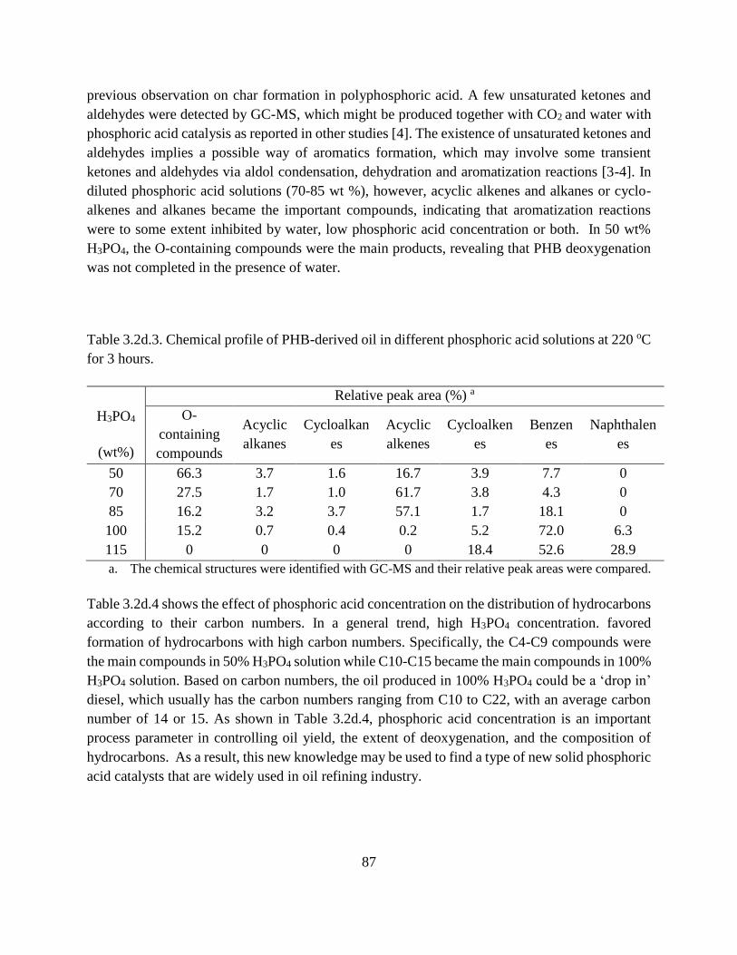
87

previous observation on char formation in polyphosphoric acid. A few unsaturated ketones and

aldehydes were detected by GC-MS, which might be produced together with CO2 and water with

phosphoric acid catalysis as reported in other studies [4]. The existence of unsaturated ketones and

aldehydes implies a possible way of aromatics formation, which may involve some transient

ketones and aldehydes via aldol condensation, dehydration and aromatization reactions [3-4]. In

diluted phosphoric acid solutions (70-85 wt %), however, acyclic alkenes and alkanes or cyclo-

alkenes and alkanes became the important compounds, indicating that aromatization reactions

were to some extent inhibited by water, low phosphoric acid concentration or both. In 50 wt%

H3PO4, the O-containing compounds were the main products, revealing that PHB deoxygenation

was not completed in the presence of water.

Table 3.2d.3. Chemical profile of PHB-derived oil in different phosphoric acid solutions at 220 oC

for 3 hours.

Relative peak area (%) a

H3PO4

(wt%)

O-

containing

compounds

Acyclic

alkanes

Cycloalkan

es

Acyclic

alkenes

Cycloalken

es

Benzen

es

Naphthalen

es

50 66.3 3.7 1.6 16.7 3.9 7.7 0

70 27.5 1.7 1.0 61.7 3.8 4.3 0

85 16.2 3.2 3.7 57.1 1.7 18.1 0

100 15.2 0.7 0.4 0.2 5.2 72.0 6.3

115 0 0 0 0 18.4 52.6 28.9

a. The chemical structures were identified with GC-MS and their relative peak areas were compared.

Table 3.2d.4 shows the effect of phosphoric acid concentration on the distribution of hydrocarbons

according to their carbon numbers. In a general trend, high H3PO4 concentration. favored

formation of hydrocarbons with high carbon numbers. Specifically, the C4-C9 compounds were

the main compounds in 50% H3PO4 solution while C10-C15 became the main compounds in 100%

H3PO4 solution. Based on carbon numbers, the oil produced in 100% H3PO4 could be a ‘drop in’

diesel, which usually has the carbon numbers ranging from C10 to C22, with an average carbon

number of 14 or 15. As shown in Table 3.2d.4, phosphoric acid concentration is an important

process parameter in controlling oil yield, the extent of deoxygenation, and the composition of

hydrocarbons. As a result, this new knowledge may be used to find a type of new solid phosphoric

acid catalysts that are widely used in oil refining industry.

88

Table 3.2d.4. Carbon distribution of PHB-derived oil in different phosphoric acid solutions at 220 oC for 3 hours.

H3PO4

(wt%)

Relative peak area (%) a

C4 C

5 C6 C7

C

8 C9

C1

0

C1

1

C1

2

C1

3

C1

4

C1

5

C1

6

50 12.

1

4.

6 5.3

31.

2

5.

9

24.

3 2.6 0.6 4.6 8.8 0 0 0

70 5.5 0 3.1 20 2.

7

59.

6 4.9 0 0.3 3.6 0.3 0 0

85 0.8 0 0.7 4.5 5.

1

34.

2

21.

2 6.8 8.8

13.

6 1.8 2.5 0

100 0 0 0.4 0 0.

2 1.1 8.5 5.3

13.

1

40.

5

24.

7 6.2 0

115 0 0 18.

4 0 0 0.2

13.

6 8 10

20.

9 6.2

18.

0 4.7

a. The carbon numbers were identified with GC-MS analysis and their relative peak areas were

compared.

More detail on the study can be found in the publications listed below, including those partially

supported by the APRISES12 program. These publications are available on the HNEI website.

89

Publications and Presentations

Peer Reviewed Publications

J. Yu, P. Munasinghe. Gas fermentation enhancement for chemolithotrophic growth of

Cupriavidus necator on carbon dioxide, Fermentation, 2018, 4, 63-77.

DOI:10.3390/fermentation4030063.

S. Kang, J. Yu. One-pot production of hydrocarbon oil from poly(3-hydroxybutyrate), RSC

Advances, 2014, 4, 14320-14327. DOI:10.1039/c4ra00892h.

Contributed Presentations

Pradeep Munasinghe, Shimin Kang, Jian Yu (2014). Renewable hydrocarbon oils and chemicals

from solar energy and carbon dioxide. Asia Pacific Clean Energy Summit and Expo, September

15-17, Honolulu, Hawaii.

Patents and Technology Licensing

A Novel Bioreactor for High Efficiency Gas Utilization by Microbes

Inventor: P. Munasinghe and J. Yu

Invention disclosure UH ID No. 00958, October 23, 2013

US Provisional patent 62433748, December 13, 2016

University of Hawaii IP license to Bio-on S.p.A. Italy, January, 2017.

PCT application 107502, December 2017.

References

[1] J. Yu, P. Munasinghe. Gas fermentation enhancement for chemolithotrophic growth of

Cupriavidus necator on carbon dioxide, Fermentation, 2018, 4, 63-77.

DOI:10.3390/fermentation4030063.

[2] S. Kang, J. Yu. One-pot production of hydrocarbon oil from poly(3-hydroxybutyrate), RSC

Advances, 2014, 4, 14320-14327. DOI:10.1039/c4ra00892h.

90

[3] C. K. Bradsher. Formation of six-membered aromatic rings by cyclialkylation of some

aldehydes and ketones. Chem. Rev., 1987, 87, 1277-1297.

[4] M.A. Alotaibi, E.F. Kozhevnikova, I. V. Kozhevnikov, Deoxygenation of propionic acid on

heteropoly acid and bifunctional metal-loaded heteropoly acid catalysts: Reaction pathways and

turnover rates, Applied Catalysis A: General, 2012, 447–448, 32–40.

3.2e Bio-contamination of Fuels

Metabolic processes and interactions that can be limited to decrease the impacts of bio-

contamination in blended fuels were investigated, using a genomic and proteomic approach.

Blended diesel fuels contain trace amounts of glycerol, an undesirable byproduct associated with

biodiesel production, and also sulfur compounds typically found in diesel. During APRISES 2011,

it was determined that a Burkholderia sp., in the presence of glycerol can enhance the metabolism

of dibenzothiophene (DBT), a stable organosulfur compound found in diesel. This co-metabolic

activity results in the favorable reduction of undesirable chemical components that are typically

found within blended diesel. It was also observed that along with the enhanced metabolism the

secretion of a rhamnolipid (RL), a biosurfactant, was significantly increased. The literature

suggests that RL could be involved in cell transport and may increase the biodegradation of

hydrophobic chemicals (Bai et al. 1997) such as petroleum or biodiesels.

During APRISES 2012 the role that the secreted RL have on DBT metabolism was further

investigated. This information could provide insights into what metabolic processes can be limited

to decrease the impacts from bio-contamination.

Burkholderia sp. C3 grown using glycerol and DBT was found to cometabolically degrade DBT,

and also exhibited higher growth rates when compared with glycerol alone. The cometabolism

results show up to an 18-fold increase in DBT biodegradation and a tripling in RL secretion.

Inhibiting RL biosynthesis using 2-Bromohexanoic Acid (HEX) or 2-Bromooctanoic Acid (OC)

significantly reduced both the growth rate of C3 and also the biodegradation of DBT, up to 8 times.

A multifactorial analysis showed RLs are a statistically significant factor (p-value < 0.01) for DBT

degradation. Addition of RLs into cultures grown after removing glycerol resulted in a 1.8-fold

increase of DBT biodegradation.

Due to their amphipathic chemistry, biosurfactants can interact with polycyclic aromatic

hydrocarbons and at water-oil interfaces. By inhibiting metabolic processes that influence cellular

uptake mechanisms, bio-inhibition methods could be developed for application with blended

91

biofuels. In conclusion, it is clear that RLs have an important influence on the metabolic functions

involved with the cellular uptake of polycyclic aromatic hydrocarbons during co-metabolism with

glycerol

Moniliella wahieum Y12 genome sequencing and investigation of proteins that are expressed

duing biodiesel degradation was investigated. Determination of the metabolic pathways that are

involved with biodiesel degradation is necessary for the development of inhibitors. The

degradation of fatty acids in yeast is a complex pathway requiring an assortment of β-oxidation

enzyme activities (Hiltunen et al. 2006). During APRISES 2012 a genomic and proteomic

approach using the biodiesel contaminant, Moniliella wahieum Y12, is used for these

investigations.

For elucidation of the genes involved with fatty acid metabolism, a shot-gun sequencing approach

was applied. The genome coverage from the sequence analysis was analyzed using BlastX for the

determination of potential genes related with fatty acid metabolism. The limited annotation

performed have already revealed numerous enzymatic esterase and lipase orthologs that are

associated with β-oxidation.

A comparative proteomic investigation was also performed for the determination of gene

expression associated with the metabolism of biodiesel. When compared with M. wahieum Y12

grown on glucose 150 proteins were uniquely expressed. Under other funding, further

investigations that show the relationship between genetic composition and the proteomic

expression results will be performed, after more comprehensive genomic data is obtained. This

will allow for a better understanding of the metabolic processes involved with the degradation of

biodiesel. In conclusion, M. wahieum Y12 was found to express 150 unique proteins when grown

on biodiesel as the sole carbon source.

References

Bai G, Brusseau ML, Miller RM. 1997. Influence of a RL biosurfactant on the transport of bacteria

through a sandy soil. Appl Environ. Microbiol. 63:1866–1873.

Ching T.H., Yoza B.A.*, Wang R., Masutani S., Donachie S., Hihara L. and Li Q. 2016.

Biodegradation of biodiesel and microbiologically induced corrosion by Moniliella sp. Y12.

Intern. Biodeter. Biodegrad. 108: 122-126

Hiltunen JK, Mursula AM, Rottensteiner H., Wierenga RK, Kastaniotis AJ, Gurvitz A. 2006. The

biochemistry of peroxisomal B-oxidation in the yeast Saccharomyces cerevisiae. FEMS Micro

Rev https://doi.org/10.1016/S0168-6445(03)00017-2

92

Seo J.S., Keum Y.S., Hu Y., Lee S.E., Li Q.X. 2007. Degradation of phenanthrene by Burkholderia

sp C3: initial 1,2- and 3,4-dioxygenation and meta and ortho cleavage of naphthalene-1,2-diol.

Biodegradation. 18(1): 123-31

3.2f Biofuel Corrosion Control

The US Navy successfully [1] demonstrated the use of a 50 vol. % - 50 vol. % blend (50v:50v

blend) of a traditional, petroleum-based F-76 diesel and an algae-derived hydrotreated renewable

diesel (algal HRD-76) in warships. Renewable biodiesel is an alternative fuel produced from

renewable resources, such as vegetable oils and animal fats. The conventional biodiesel is

produced using a transesterification process and consists of fatty acid methyl esters (FAME), while

the HRD is chemically not esters but consists mainly of paraffins, a composition similar to the

conventional petroleum diesel.[2] The HRD has advantages over the FAME biodiesel in three

major aspects. First, HRD has been hydrotreated to remove oxygen and is free of aromatics,

leaving predominantly linear and branched chain hydrocarbons in the fuel. Second, the

hydroprocessing includes desulphurization reactions which result in a low-sulfur fuel

(< 10 ppm wt) with very low greenhouse gas emissions.[3] Third, the hydroprocessing technology

produces no byproducts and can be used in existing refineries without any new investments.[4]

One difference, however, is that the HRD-76 has a higher diffusion coefficient for oxygen than

F-76 due to a lower dynamic viscosity.[5] The ranking from the highest to lowest diffusion

coefficient for oxygen is HRD-76, HRD-76/F-76 (50v:50v blend), and F-76. During the operation

of the warships, seawater is drawn into the carbon-steel fuel tanks to maintain balance as the fuel

is consumed. Therefore, there is interest to determine if the HRD-76 fuel and its blends can cause

unexpected corrosion damage in fuel-seawater mixtures. APRISES 11 focused on the

measurement of corrosion rates and the identification of microbiological species in the

seawater/fuel mixtures. APRISES 12 (this work) focuses on the identification of corrosion

products formed on the corrosion coupons exposed in the seawater/fuel mixtures. APRISES 13

focused on the utilization of corrosion inhibitors to attenuate corrosion.

In the present work (APRISES12), an in-depth analyses was conducted on the identification of

corrosion products that formed on plain-carbon 1018 steel (UNS G10180) exposed in natural

seawater/fuel mixtures of HRD-76, HRD-76/F-76 50v:50v blend, and F-76 for various time

durations (i.e., 3 days, 10 days, 1 month, 6 months, and 1 year). The 1018 coupons were immersed

in bottles with the bottom half of the sample in the seawater layer and the top half in the fuel layer.

The 1018 steel has a composition which is within specifications for steels typically used for

pipelines and storage vessels and tanks. Energy dispersive X-ray analyses (EDXA), X-ray

diffraction (XRD), Raman spectroscopy, and FTIR spectroscopy were used to identify the

corrosion products. To differentiate between abiotic electrochemical corrosion and

93

microbiologically influenced corrosion (MIC), various permutations of filtered and unfiltered fuel

and seawater combinations were used as exposure medium. A 0.22 micron filter was used to filter

the seawater and fuel. Both aerobic and anaerobic conditions were examined. There were two

aerobic conditions: Filtered aerobic where a 0.22 micron filter prevented larger air-borne

contaminates into the test bottles, and an open aerobic where airborne contaminants were allowed

to enter the test bottles. The seawater was either natural, off-shore, surface water or synthetic

according to ASTM International (ASTM) specifications. Hence, the test conditions were filtered-

aerobic, aerobic, or anaerobic of the following seawater-fuel mixtures: 1) filtered seawater/filtered

fuel, 2) filtered seawater/non-filtered fuel, 3) non-filtered seawater/filtered fuel, and 4) non-

filtered seawater/non-filtered fuel conditions. The results on molecular identification of bacteria

and fungi performed via 16S ribosomal ribonucleic acid (rRNA) and 18S rRNA sequencing was

reported in APRISES 11.

Also reported in APRISES 11 was that corrosion rates of 1018 carbon steel were primarily driven

by oxygen reduction and were highest in HRD-76, followed by the HRD-76/F-76 50v:50v blend,

and then F-76, which corresponded to the similar ranking of oxygen diffusion coefficients (from

highest to lowest):HRD-76, HRD-76/F-76 50v:50v blend, and F-76. On the 1018 corrosion

coupons, the region of steel in the seawater layer was most severely corroded due to the high

corrosivity induced by chlorides. The corrosion-rate results showed that abiotic corrosion

dominated the corrosion damage and overshadowed any effects of MIC. In the fuel/water interface

and water zones, rust formation showed an inner layer (black) identified as magnetite and an outer

layer (red/yellow) identified as lepidocrocite and goethite. The amount of magnetite in the inner

layer increased with increasing content of HRD-76 in the fuels. Hence, the highest amount of

magnetite was observed for the coupons exposed in HRD-76 followed by those in the

HRD-76/F-76 50v:50v blend and least in the F-76. White precipitates identified as Mg(OH)2

(magnesium hydroxide), MgO (magnesium oxide), Na2CO3 (sodium carbonate), Na2CO3.H2O

(thermonatrite), Na3H(CO3)2(H2O)2 (trona), CaCO3 (calcite and aragonite) formed in the fuel zone

and were shown to be a consistent visual indicator for a high corrosion rate of steel. Precipitation

was likely induced by a high amount of oxygen reduction (in the fuel layer) that generated OH-,

which precipitated the carbonates and hydroxides. The presence of the white precipitates was most

abundant on the coupons exposed to the HRD-76 and to a lesser degree on those exposed to the

HRD-76/F-76 50v:50v blend, which is consistent with higher rates of oxygen diffusion and hence

corrosion in the HRD-76 fuel.

Hence, higher rates of corrosion and the precipitation of carbonates and hydroxides are likely to

be expected with the utilization of algal HRD-76 fuel as a replacement for traditional petroleum-

based F-76. For more information, see the conference paper listed below, (which also includes

results from APRISES13).

94

Publications and Presentations

S. Li, J. Kealoha, L. H. Hihara, “Corrosion of Low-Carbon Steel in Seawater/Biodiesel Mixtures

– a Study Related to the Corrosion of Fuel Tanks in Ships”, NACE International Corrosion 2015

Conference and Expo, (location, date), Paper No. 6095.

References

1) R. Turgeon, S. Williams, R. Kamin, R. Leung, G. Eldridge, "Overview of U.S. Navy's Ship

Renewable Fuels Evaluation," International Association for Stability, Handling and Use of

Liquid Fuels: Atlanta, GA (2011): pp. manoharan1/1-manoharan1/26.

2) G. Knothe, "Biodiesel and renewable diesel: A comparison," Progress in Energy and

Combustion Science 36, 3 (2010): pp. 364-373.

3) P. Šimáček, D. Kubička, G. Šebor, M. Pospíšil, "Fuel properties of hydroprocessed

rapeseed oil," Fuel 89, 3 (2010): pp. 611-615.

4) S. Bezergianni, A. Dimitriadis, "Comparison between different types of renewable diesel,"

Renewable and Sustainable Energy Reviews 21, (2013): pp. 110-116.

5) J. Fu, S.Q. Turn, "Characteristics and Stability of Neat and Blended Hydroprocessed

Renewable Diesel," Energy & Fuels 28, 6 (2014): pp. 3899-3907.

3.2g Waste Management

Research under other phases of APRISES developed constant volume carbonization (CVC)

techniques to convert biomass materials into carbon-rich materials. With the ultimate goal of

manufacturing charcoals with physical and chemical properties tailored to their end use, the

present study provides a deeper understanding of the CVC process by elucidating the effect of

various processing variables on char yields and properties.

In recent work under earlier phases of APRISES, constant volume carbonization product yields

were determined together with charcoal proximate analysis and in some instances with higher

heating values (HHV) and elemental analyses [1,2,3]. CVC experiments consistently approached

theoretical fixed-carbon yields across a variety of processing conditions [1,2,3]. Although

charcoals maintained fixed-carbon yields near theoretical values, chars suffered a more intense

devolatilization and therefore presented improved fixed-carbon contents from (1) higher heat

treatment temperatures (HTTs) (in a 300-400°C range) [2,3], (2) prolonged soaking times at

carbonization temperature (from less than 30 minutes to almost 3 hours) [3], (3) smaller particle

sizes (from <2 mm to <0.2 mm in tests at HTT of 300°C) [3] or (4) higher mass loadings (from

95

129 to 165 g/L in spruce CVC tests at 300°C) [3]. Among these factors, char devolatilization was

especially sensitive to the carbonization temperature, while the mass loading had a lesser effect.

An intriguing phenomenon was also observed on the char morphology when testing charcoals

produced at higher temperatures and pressures. As conditions became more severe in the CVC

reactor, the charcoal solid structure transformed from a particulate solid retaining the original

biomass morphology to a coke-looking piece that had undergone a transient plastic phase (TPP)

and had adopted the shape of the reaction vessel [2,3].

Additionally, a single charcoal derived from a pyrolysis experiment in a reactor with a valve

slightly opened to the atmosphere was also produced for comparison to the charcoals manufactured

in the constant-volume reactor. Results from proximate, elemental, and bomb calorimetry analysis

of the chars are also presented.

A detailed description for the reactor—named the Wall Heated Tubing Bomb (WHTB)—and the

experimental procedure employed for the CVC experiments is given elsewhere [3]. Different

versions of the WHTB reactor are presented in reference [3] going from its original version to an

upgraded version with roughly double the loading capacity of the original. All reactor designs

conserved the fundamentals of the CVC process permitting carbonization in a sealed reactor at

elevated temperatures and pressures. Evolution of the reactor design mainly relied on

improvements in loading capacities, in safety equipment and in data measuring techniques. The

present study made use of the original reactor for the earlier runs on oak pyrolysis (see reference

[3] for reactor details) plus an upgraded (current) reactor for the later experiments on birch

pyrolysis. The current WHTB design has an internal volume of ~0.22 L and permits CVC of ~30

g of spruce grains sized below 2 mm. The amount of biomass loaded in the reactor can be further

increased by the use of feedstocks with higher packing density, for example ~50 g could be loaded

when using the same-sized birch grains (<2 mm), or by the use of finer powder.

The current WHTB introduced slight modifications to the safety system compared to the one

presented in reference [3]. One of the safety apparatus, the burst diaphragm, was replaced for a

lighter and smaller model (LaMot) with a superior pressure rating of 21.3 MPa at 22 °C (vs. 16.20

MPa at 22°C) [3] which allowed the testing of more severe experimental conditions. The new burst

diaphragm is within the allowable working pressure of the weakest part of the WHTB reactor, i.e.

the reactor body rated at 16.24 MPa at 537°C, [3] plus pressure allowances permitted by the ASME

B31.3 piping code. Under certain conditions, one is allowed to operate at 33% over the allowable

working pressure for events that are not longer than 10 hours at any one time, nor more than 100

hours per year [4]. In a couple of experiments that tested the influence of the biomass loading, the

WHTB was additionally modified by extending the amount of dead-volume in the reactor tubing

–i.e. additional tubing was added to the top part of the reactor system.

96

The biomass feedstocks pyrolyzed in the present study consisted of oak, spruce, birch and

cellulose. Each biomass specimen was subject to the following characterization in HNEI

laboratories: moisture and proximate analysis by standards ASTM E872-82(2013) [5] and ASTM

E830-87(1996) [6] on three samples per specimen, ultimate analysis by ASTM E777-17 [7], E775-

15 [8] and E778-15 [9] on two samples per specimen and bomb calorimetry on one sample per

specimen. See reference [3] for a detailed study on the uncertainties of each analytical technique.

Table 3.2g.1 displays the data collected from the HNEI characterization (moisture content,

proximate analysis, ultimate analysis, and higher heating value) of the biomass feedstocks along

with compositional data (cellulose, hemicellulose and lignin) taken from literature [10].

97

Table 3.2g.1. Moisture content, ultimate and proximate analysis, higher heating value, and

structural composition (cellulose, hemicellulose and lignin) of spruce, birch, cellulose and oak

feedstocks. Spruce and birch analytical results are replicated from reference [3].

Spruce Birch Cellulose Oak

Moisture content

[wt.%, wet basis] 7.8 7.9 5.9 7.5

Ultimate Analysisa

[wt.%, dry basis]

C 46.93±0.05 47.4 ±0.3 41.9 ±0.1 45.4 ±0.1

H 6.26±0.02 6.32±0.03 6.3±0.1 6.1±0.1

Od 46.3 45.43 51.7 47.1

N 0.20±0.02 0.20±0.02 0.08±0.04 0.215±0.002

S 0.011±0.001 0.0158±0.001. 0.00 0.017±0.001

Ashe 0.36±0.17 0.67±0.02 0.00 1.18±0.05

Proximate

analysisb [wt.%,

dry basis]

fCCf 14.8±0.1 13.1±0.2 6.0±0.2 14.0±0.7

VMg 84.9±0.1 86.2±0.2 94.0±0.2 84.8±0.8

Ash 0.36±0.17 0.67±0.02 0.0±0.0 1.18±0.05

Higher heating

value [MJ/kg] 18.00 18.50 16.15 17.67

Contents of

structural

components[wt.%,

dry-ash free

basis]c

Cellulose 43.6, 47 50.2, 49.1 100 58.4

Hemicellulose 27.4, 25.3 32.8, 31.6 0.0 31.4

Lignin 29.0, 27.7 17.0, 19.3 0.0 10.2

Extractives 1.8, 2.5 3.0 0.0 NAh

a Average of two analysis, uncertainty indicates range of values. Elemental analysis of cellulose closely resembles

C 44.4%, H 6.2% and O 49.4% given by its formula (C6H10O5)n. b Average of three analyses, uncertainty indicates standard deviation. c Composition of structural components taken from [10]. d Oxygen by difference. e Ash content determined by proximate analysis. f Fixed-carbon content (fCC). g Volatile matter content (VM). hNot Available (NA).

Regarding characterization of the final pyrolytic products, non-condensable gases were subject to

gas chromatography and volume evaluation. Solid charcoals were subject to ultimate and

proximate analysis, SEM, bomb calorimetry and weight measurement. Details of the standards

followed for each measuring technique are given presented elsewhere [3]. Additionally, gaseous,

liquid and solid yields were subjected to a mass balance.

After the CVC tests on oak, the proximate analysis method for the characterization of the solid

char was modified from a method that followed ASTM -D1762-84 [11] to a method that followed

98

ASTMs E872-82(2013) [5] and E830-87(1996) [6] for respective determination of volatile matter

and ash content. The accuracies of both proximate analysis methods were evaluated as follows:

proximate analysis of cellulose samples following both methods (three samples per method) were

deliberately interrupted after the volatile matter removal step. Since cellulose contains negligible

ash, the remaining product would be fixed-carbon. The carbon purity of this fixed-carbon fraction

can be used as an indicator of the accuracy of the reported values. The original proximate analysis

technique revealed a “fixed-carbon” of just 94.54 wt% carbon with the balance comprising O and

H in decreasing amounts, whereas the updated technique showed an improved “fixed-carbon”

composed of 95.5 wt% carbon. The results indicated that the measured experimental fixed-carbon

contents are likely to represent slight overestimates of the actual values.

A reproducibility study of the CVC process revealed good repeatability of char and gas yields

(<±1.5 wt% absolute), and of the fractions determined by char proximate analysis (<±2 wt%

absolute), and poor repeatability of the measured liquid yields [3]. The greater uncertainties of the

liquid yields were a result of the difficulty recovering the final products from the reactor system.

To gain a better understanding of the carbon fate, carbon mass balances revealed that >97 wt% of

the elemental carbon present in the virgin biomass was recovered in the form of solid charcoal and

in the form of gas, mainly as CO2 and CO. The results confirmed that negligible free-tars were

produced in the CVC process and that the final liquid product mainly represented water evolved

during the carbonization process plus moisture inherent to the original feedstock.

This section presents experimental CVC conditions and results. The CVC results and trends at

distinct processing conditions are evaluated against trends reported in literature from other

carbonization processes and against theoretical trends predicted by thermodynamics.

Table 3.2g.2 displays the experimental conditions and results from the 23 experiments conducted

in this study. A single carbonization experiment was performed in a reactor with one of the valves

slightly opened to the atmosphere (experiment # 1). The final char was analyzed and compared to

a char derived from CVC, i.e. performed in a sealed reactor, under analogous experimental

conditions (temperature, pressure, particle size…). In the additional 22 experiments, CVC was

performed and the influences of a number of processing conditions on product yields and

properties were investigated.

99

Table 3.2g.2. Conditions and results for Wall Heated Tubing Bomb experiments. Superscripts

are defined in footnotes at the bottom of the table.

Experiment Number 1g 2 3 4 5 6 7 8

Date (yymmdd) 151201 151125 150121 141210 150115 160120 150909 160126

Conditions

Reactor Type Original Original Original Original Original Original Original Original

Feedstock Oak Oak Oak Oak Oak Oak Oak Oak

Heat Treatment Temperature[°C] 300 300 300 300 300 300-350 300-370 300-400

Pretest Nitrogen Pressure [MPa] 0.1 0.1 1.48 2.69 4.79 4.79 4.79 4.79

Immersion Time [min] a 34 134 24 38 21 37 181 63

Mass Loading [g biomass/Lreactor] ~100 ~100 ~120 ~160 ~120 ~145 ~145 ~155

Particle size[mm] 0.149-

0.425

0.149-

0.425

0.149-

0.425

0.149-

0.425

0.149-

0.425

0.149-

0.425

0.149-

0.425

0.149-

0.425

Reactants

Moist Mass [g] 12.77 13.63 11.44 16.92 12.22 13.47 13.26 14.38

Moisture Content [%, wb]b 7.68 7.65 7.62 7.49 7.73 7.58 7.70 7.60

Pyrolysis Reaction

Axis Peak Temperature [°C] 304h 233h 294h 311h 309h 347h 352h 356h

Wall Peak Temperature [°C] 304 311 292 293 294 352 364 384

Peak Pressure [MPa] 0.1 NAi 5.18 7.62 10.60 13.19 13.06 14.36

Solid Products

Char Moist Mass [g] 8.42 10.15 8.38 11.40 9.61 9.72 8.98 11.68

Char Moisture Content [%, wb]b, e 3.34 28.53 30.84 15.50 29.26 25.87 32.66 41.96

Volatile Matter Content [%, db]c 63.1 40.9 49.3 50.8 49.3 33.3 28.2 25.9

Ash Content [%, db]c 1.9 3.6 1.0 0.9 1.3 2.9 2.9 2.6

Fixed Carbon Content [%, db]c 34.4 55.5 49.7 48.3 49.3 63.8 68.8 71.5

Fixed Carbon Yield [%, db]c 23.99 32.52 28.40 30.88 30.79 38.35 35.81 36.46

Higher Heating Value [MJ/kg] NAi NAi NAi NAi NAi NAi NAi NAi

Gas Products

Final Gas in VBomb[mol]d NAi 0.054 0.104 0.170 0.142 0.260 0.279 0.226

Nitrogen [mol %] NAi 12.04 69.84 69.48 85.91 81.01 80.02 77.90

Oxygen [mol %] NAi 1.55 0.06 0.00 1.38 0.26 1.11 0.00

Hydrogen [mg/g (Dry Feed)] NAi NAk 0.093 0.061 0.071 0.142 0.23 0.181

Methane [mg/g (Dry Feed)] NAi NAk 0.031 0.024 0.053 0.00 0.78 0.00

Carbon Monoxide [mg/g (Dry Feed)] NAi NAk 190 180 170 19 180 20

Carbon Dioxide [mg/g (Dry Feed)] NAi NAk 100 120 110 150 170 170

Mass Balance NAi

Gas Products [%, db]c NAi NAk 12.37 14.06 12.62 17.12 18.58 18.66

Char Yield [%, db]c 69.80 58.59 56.90 63.61 62.09 60.10 52.03 51.02

Liquid [%, db]c NAi 15.86 26.02 16.67 24.34 23.43 30.73 28.66

Solid not recovered [%, db]c, f

Total [%, db]c NAi NAi 95.82 94.35 99.05 100.65 101.34 98.34

Carbon Balance Total [%, db]c NAi NAi NAi NAi NAi NAi NAi NAi

100

Experiment Number 9 10 11 12 13

Date (yymmdd) 170822 180106 170817 180126 170802

Conditions

Reactor Type Dual-

intermediate

Dual-current Dual-

intermediate

Dual-current Dual-

intermediate

Feedstock Birch Birch Birch Birch Birch

Heat Treatment Temperature[°C] 300 400 500 550 300

Pretest Nitrogen Pressure [MPa] 2.17 2.17 0.1 0.1 0.1

Immersion Time [min] a 190 190 190 190 190

Mass Loading [g biomass/Lreactor] ~130 ~130 ~130 ~130 ~130

Particle size[mm] <2 <2 <2 <2 <0.2

Reactants R1j R2k R1j R2k R1j R2k R1j R2k R1j R2k

Moist Mass [g] 14.44 14.81 14.20 14.25 14.12 14.48 14.03 14.07 14.30 14.38

Moisture Content [%, wb]b 7.83 7.98 7.83 7.99 7.27

Pyrolysis Reaction

Axis Peak Temperature [°C] 340 320 405 405 496 505 556 553 299h 300h

Wall Peak Temperature [°C] 291 296 401 405 486 509 546 NAi 310 299

Peak Pressure [MPa] 11.05 17.48 14.50 17.87 5.01

Solid Products

Char Moist Mass [g] 11.64 12.02 10.29 10.18 7.58 7.44 6.42 6.84 9.30 10.43

Char Moisture Content [%, wb]b, e 39.38 39.82 46.28 45.62 26.64 34.48 32.68 34.12 22.83 31.41

Volatile Matter Content [%, db]c 40.3 22.8 11.1 8.7 39.1

Ash Content [%, db]c 2.1 2.1 2.4 2.0 3.7

Fixed Carbon Content [%, db]c 57.6 75.2 86.5 89.3 57.2

Fixed Carbon Yield [%, db]c 30.51 31.77 34.23 30.51 30.84

Higher Heating Value [MJ/kg] 31.29 33.30 34.52 33.64 29.68

Gas Products

Final Gas in VBomb[mol]d 0.335 NAi 0.329 NAi 0.135

Nitrogen [mol %] 62.64 NAi 5.20 NAi 8.94

Oxygen [mol %] 1.17 NAi 0.13 NAi 0.00

Hydrogen [mg/g (Dry Feed)] 0.241 NAi 1.386 NAi 0.363

Methane [mg/g (Dry Feed)] 0.00 NAi 0.01 NAi 0.00

Carbon Monoxide [mg/g (Dry Feed)] 14.37 NAi 35.76 NAi 28.21

Carbon Dioxide [mg/g (Dry Feed)] 179.74 NAi 318.33 NAi 161.92

Mass Balance

Gas Products [%, db]c 19.44 NAi 35.55 NAi 19.05

Char Yield [%, db]c 53.01 42.26 39.59 34.15 53.88

Liquid [%, db]c 26.31 27.39 9.35 10.33 14.38

Solid not recovered [%, db]c, f 1.46 5.04 1.63 11.72 4.50

Total [%, db]c 100.21 NAi 86.12 NAi 91.82

Carbon Balance Total [%, db]c 97.21 NAi 97.10 NAi 94.69

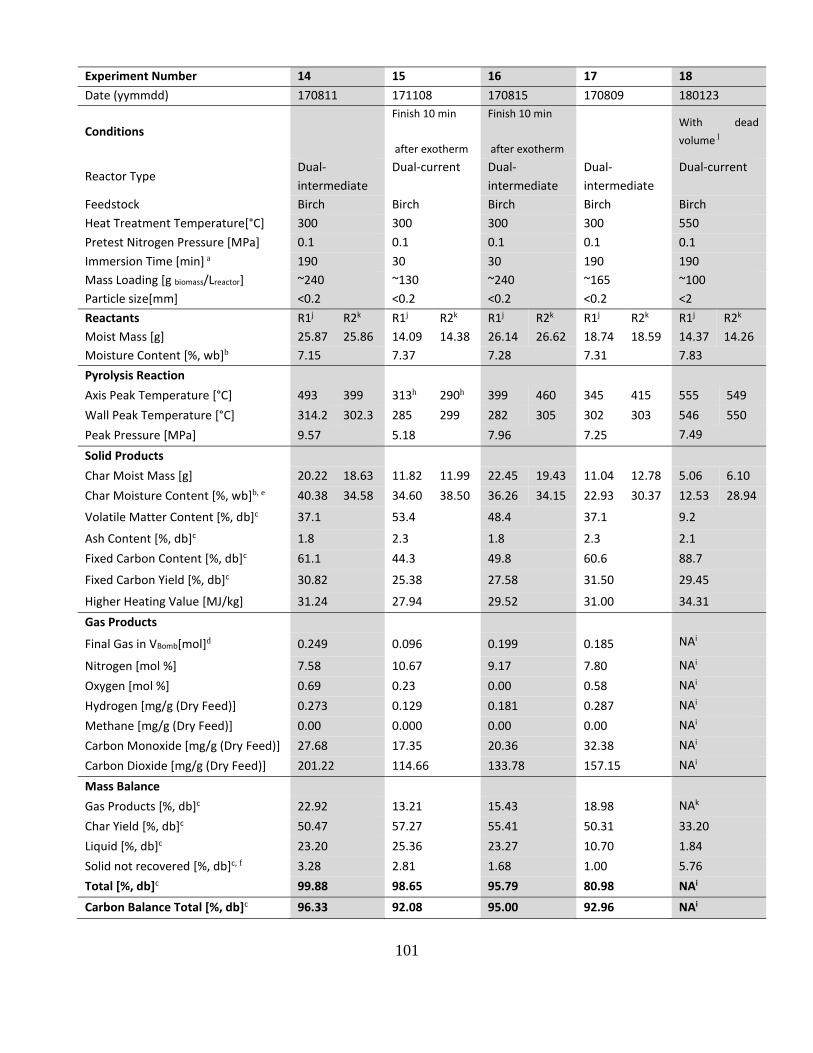
101

Experiment Number 14 15 16 17 18

Date (yymmdd) 170811 171108 170815 170809 180123

Conditions

Finish 10 min

after exotherm

Finish 10 min

after exotherm

With dead

volume l

Reactor Type Dual-

intermediate

Dual-current Dual-

intermediate

Dual-

intermediate

Dual-current

Feedstock Birch Birch Birch Birch Birch

Heat Treatment Temperature[°C] 300 300 300 300 550

Pretest Nitrogen Pressure [MPa] 0.1 0.1 0.1 0.1 0.1

Immersion Time [min] a 190 30 30 190 190

Mass Loading [g biomass/Lreactor] ~240 ~130 ~240 ~165 ~100

Particle size[mm] <0.2 <0.2 <0.2 <0.2 <2

Reactants R1j R2k R1j R2k R1j R2k R1j R2k R1j R2k

Moist Mass [g] 25.87 25.86 14.09 14.38 26.14 26.62 18.74 18.59 14.37 14.26

Moisture Content [%, wb]b 7.15 7.37 7.28 7.31 7.83

Pyrolysis Reaction

Axis Peak Temperature [°C] 493 399 313h 290h 399 460 345 415 555 549

Wall Peak Temperature [°C] 314.2 302.3 285 299 282 305 302 303 546 550

Peak Pressure [MPa] 9.57 5.18 7.96 7.25 7.49

Solid Products

Char Moist Mass [g] 20.22 18.63 11.82 11.99 22.45 19.43 11.04 12.78 5.06 6.10

Char Moisture Content [%, wb]b, e 40.38 34.58 34.60 38.50 36.26 34.15 22.93 30.37 12.53 28.94

Volatile Matter Content [%, db]c 37.1 53.4 48.4 37.1 9.2

Ash Content [%, db]c 1.8 2.3 1.8 2.3 2.1

Fixed Carbon Content [%, db]c 61.1 44.3 49.8 60.6 88.7

Fixed Carbon Yield [%, db]c 30.82 25.38 27.58 31.50 29.45

Higher Heating Value [MJ/kg] 31.24 27.94 29.52 31.00 34.31

Gas Products

Final Gas in VBomb[mol]d 0.249 0.096 0.199 0.185 NAi

Nitrogen [mol %] 7.58 10.67 9.17 7.80 NAi

Oxygen [mol %] 0.69 0.23 0.00 0.58 NAi

Hydrogen [mg/g (Dry Feed)] 0.273 0.129 0.181 0.287 NAi

Methane [mg/g (Dry Feed)] 0.00 0.000 0.00 0.00 NAi

Carbon Monoxide [mg/g (Dry Feed)] 27.68 17.35 20.36 32.38 NAi

Carbon Dioxide [mg/g (Dry Feed)] 201.22 114.66 133.78 157.15 NAi

Mass Balance

Gas Products [%, db]c 22.92 13.21 15.43 18.98 NAk

Char Yield [%, db]c 50.47 57.27 55.41 50.31 33.20

Liquid [%, db]c 23.20 25.36 23.27 10.70 1.84

Solid not recovered [%, db]c, f 3.28 2.81 1.68 1.00 5.76

Total [%, db]c 99.88 98.65 95.79 80.98 NAi

Carbon Balance Total [%, db]c 96.33 92.08 95.00 92.96 NAi

102

Experiment Number 19 20 21 22 23

Date (yymmdd) 171227 180102 180104 180111 180108

Conditions

Low Heating

Rate

No soaking time

Low heating

rate,

180 min soaking

time

Low heating

rate,

0 min soaking

time

Low heating

rate,

120 min soaking

time

Reactor Type Dual-current Dual-current Dual-current Dual-current Dual-current

Feedstock Spruce Birch Birch Birch Birch

Heat Treatment Temperature[°C] 300 300 300 500 500

Pretest Nitrogen Pressure [MPa] 0.1 0.1 0.1 0.1 0.1

Immersion Time [min] a 300 53 232 200 350

Mass Loading [g biomass/Lreactor] ~130 ~130 ~130 ~130 ~130

Particle size[mm] <2 <2 <2 <2 <2

Reactants R1j R2k R1j R2k R1j R2k R1j R2k R1j R2k

Moist Mass [g] 13.26 13.87 14.13 14.36 14.57 14.29 13.98 14.15 13.96 14.07

Moisture Content [%, wb]b 8.00 8.07 7.95 8.02 8.07

Pyrolysis Reaction

Axis Peak Temperature [°C] 330 334 306 301 310 322 493 494 505 505

Wall Peak Temperature [°C] 308 307 294 292 306 309 489 490 506 506

Peak Pressure [MPa] 6.38 3.84 5.84 10.95 15.10

Solid Products

Char Moist Mass [g] 10.18 12.28 12.28 13.94 12.11 12.12 9.20 10.22 7.54 9.03

Char Moisture Content [%, wb]b, e 32.42 40.51 32.07 37.31 40.77 42.23 40.90 49.00 34.42 45.69

Volatile Matter Content [%, db]c 42.6 61.9 42.4 17.8 12.2

Ash Content [%, db]c 2.0 1.5 1.8 1.8 2.1

Fixed Carbon Content [%, db]c 55.4 36.6 55.8 80.4 85.8

Fixed Carbon Yield [%, db]c 31.47 23.90 29.80 33.10 32.78

Higher Heating Value [MJ/kg] 29.83 24.93 29.86 33.74 34.47

Gas Products

Final Gas in VBomb[mol]d NAi NAi NAi NAi NAi

Nitrogen [mol %] NAi NAi NAi NAi NAi

Oxygen [mol %] NAi NAi NAi NAi NAi

Hydrogen [mg/g (Dry Feed)] NAi NAi NAi NAi NAi

Methane [mg/g (Dry Feed)] NAi NAi NAi NAi NAi

Carbon Monoxide [mg/g (Dry Feed)] NAi NAi NAi NAi NAi

Carbon Dioxide [mg/g (Dry Feed)] NAi NAi NAi NAi NAi

Mass Balance

Gas Products [%, db]c NAi NAi NAi NAi NAi

Char Yield [%, db]c 56.84 65.21 53.36 41.16 38.22

Liquid [%, db]c 24.56 26.33 29.98 25.43 17.54

Solid not recovered [%, db]c, f 0.24 2.14 1.92 1.82 3.22

103

Total [%, db]c NAi NAi NAi NAi NAi

Carbon Balance Total [%, db]c NAi NAi NAi NAi NAi a Long duration experiments ended 190 minutes after the WHTB was submerged into the hot sand bath. Short experiments ended

10 minutes after the end of the exotherm, i.e. the exotherm was considered to end once the pressure rise considerably slowed. b Reported on a wet basis (wb). c Reported on a dry basis (db). d Final gas moles were calculated using the ideal gas law at conditions after cooldown. Final gas volume was measured with the

Water Displacement Vessel [13]. e Weight loss of char product from drying in a vacuum oven at 105°C. f Amount of solid adhered on the walls was calculated as the difference between initial and final masses of the empty reactors. g Experiment with reactor open to the atmosphere. h Temperature measurement cannot be compared to other experiments due to either a non-reliable temperature measurement

technique (oak tests) or due to the thermocouple not being in contact with the biomass (birch tests with small particle sizes and

low mass loadings) i Not Available (NA) j Data for reactor body 1 (R1) of the dual reactor. k Data for reactor body 2 (R2) of the dual reactor. l Reactor with extended dead volume was employed.

In line with previous observations, [3] the tabulated results from the total mass balance showed

that a considerable amount of the final products (around 20 wt%) was sometimes not recovered

from the CVC experiments. The carbon mass balance of the CVC experiments revealed that nearly

all the carbon present in the original feedstock (>92 wt%) was recovered in the final products in

the form of solid or gas. The results confirmed the near absence of free-tars in CVC and supported

the conjecture that liquid moisture was the main unrecovered product.

Experimental fixed-carbon yields were calculated on a dry basis as: yfC = ychar · %fC/100.

Literature values of fixed-carbon yields are typically calculated on a dry ash-free basis and

ensuring common base units are important for valid comparison. In case of pyrolyzing feedstocks

with minor ash contents such as the ones employed in this study, the required adjustments are

nearly unnoticeable. A dry basis, rather than a dry-ash free basis, for the fixed-carbon yields was

intentionally selected in this work with the goal of depicting experimental fixed-carbon yields

along with yields of products (solid, gas, liquid), all given on a dry basis. Theoretical values were

also calculated on a dry basis. The accuracy of the experimental fixed-carbon yields relied on the

accuracy of the proximate analysis method.

Theoretical fixed-carbon yields were predicted by FactSage 5.4.1 [12] via Gibbs energy

minimization modules that simulated a state of chemical equilibrium. Possible components of the

products were selected from a large thermodynamic database based on the elements present in the

reactants. "Solution" databases can also be selected based on the inorganic elements present in the

reactants but were not included. A parity plot (Figure 3.2g.1) compares the theoretical values

against experimental data. In consideration of the fact that theoretical fixed-carbon yields represent

the limiting maximum values attainable by a carbonization process, the figure, in agreement with

104

earlier publications, [2,3] reconfirmed that CVC was able to approach its maximum possible

efficiency, especially when higher temperatures (400-500°C) were used. The parity plot only

displays results from CVC experiments that pyrolyzed birch feedstock.

Figure 3.2g.1. Parity plot displaying the experimental fixed-carbon yields from birch CVC vs

theoretical fixed-carbon yields. Colors represent heat treatment temperature:300°C, 400°C,

500°C,550°C. Symbol size represents immersion time: small symbols represent short

experiments (~30 min) and the rest of the symbols represent long experiments (190 min). Symbol

fillings represent special experimental conditions: ◧ small biomass particles, ◒ use of volume

compensation, ◓ under initial nitrogen pressure, low heating rate, star symbol on top of a

symbol indicates high loading.

Figure 3.2g.2 compares experimental data of fixed-carbon, volatile matter and ash yields derived

from different carbonization methods: CVC, carbonization in a conventional furnace,

hydrothermal carbonization and flash carbonization. The highest efficiency was reported by the

CVC of birch at a HTT of 500°C which attained an experimental fixed-carbon yield of 34.2 wt%,

with a remarkable fixed-carbon content of 86.5 wt%.

105

Figure 3.2g.2. Comparison of product yields from different carbonization techniques. CVC: Data

from constant volume carbonization experiments at an initial (pretest) pressure of 0.1 MPa. FC:

Data calculated from Flash Carbonization experiments [14]. FAO: Data calculated from the Food

and Agriculture Organization (FAO) [21]. FAO provided theoretical reference values, but method

and biomass species were not specified. Fuwape: Data calculated from carbonization in a

conventional furnace [22]. HTC: Data calculated from hydrothermal carbonization [23].

In addition to approaching maximum efficiency, CVC is a simple process that requires minimal

technical equipment and can be easily controlled. The main issue faced when considering the CVC

scale up is the elevated pressures experienced by the reactor and consequently the need for costly

high-pressure equipment. This will be further explored in future work under other funding.

In comparison, the flash carbonization process, developed and patented by Dr. Antal, presents a

higher complexity [13]. In this process, a fire is ignited at the bottom of a deep packed bed of

biomass in a pressurized reactor (~1-2 MPa). A continuous air flow is introduced from the top of

the carbonizer and the pyrolysis gas is evacuated from the bottom. An inlet and outlet valve serve

to regulate the gas flow to keep the reactor at constant pressure. A pyrolyzing reaction zone moves

from the bottom to the top of the bed countercurrent to the downward air flow as the biomass is

106

thermochemically converted into a solid charcoal. The process revealed high efficiencies, and also

achieved near-theoretical fixed-carbon yields.

Note that flash carbonization fixed-carbon yields in Figure 3.2g.2 were transformed from values

on a dry-ash free basis given in reference [13] to values on a dry basis for consistency. Charcoal

from one flash carbonization test on birch in Figure 3.2g.2 showed an almost complete volatile

extraction. The char was characterized by a fixed-carbon content value of 91.4 wt% and a fixed-

carbon yield of 21.8 wt%. As observed from carbonization processes in “open” reactors, the

profound devolatilization was accompanied by a loss in process efficiency.

Compared to CVC, flash carbonization requires regulating the reactor pressure, recovering and

handling of condensed tarry vapors and the handling of the continuous and variable composition

exhaust gas to comply with environmental regulations. Additionally, flash carbonization processes

require equipment capable of withstanding elevated pressures and temperatures. Temperatures as

high as ~900°C and working pressures of around 1-2 MPa have been reported [14]. The

temperatures are considerably higher than the ones reported in CVC processes.

The pressures in flash carbonization are not autogenerated as in CVC but are maintained by a back

pressure regulator at a process setpoint, and a pressure relief valve avoids exceeding the maximum

allowable working pressure of the reactor. Typically, flash carbonization operates at a pressure

below those achieved in CVC processes. Nonetheless, recent CVC tests have successfully reduced

CVC peak pressures while maintaining final fixed-carbon yields and fixed-carbon contents of the

charcoals. Thus, pressures required in CVC processes could also change.

Sealed batch reactors are typical of both hydrothermal carbonization (HTC) and CVC processes

(there are HTC processes that operate in continuous mode [15] but they are exceptions, the vast

majority operate in batch mode). The main difference between HTC and CVC is the pyrolyzing

medium. In HTC, the biomass is submerged in a liquid medium while in CVC, biomass is

pyrolyzed in a low humidity gas atmosphere. As temperature increases, so does the pressure.

Above a critical temperature value, HTC operating pressure is expected to dramatically surpass

that of CVC due to the exponential pressure rise of saturated water with temperature. This critical

temperature value is estimated to be ~200-250°C but could considerably change depending on the

mass loading employed. Due to these high pressures, typical HTC operating temperatures are

limited to a lower range of 180-250°C. The lower temperatures of HTC processes restrict the

profound char devolatilization achieved by the pyrolytic processes in dry atmospheres.

Consequently, HTC processes become impractical for the manufacture of charcoals intended for

metallurgical applications. Hydrochars (chars from HTC), nonetheless, can be valuable products

for soil amending and novel research has given hope to applications such as adsorption, [16,17]

catalysis, ion-exchange or energy storage [18-20]. Notice that Figure 3.2g.2 presents HTC yields

107

for a run that operated at a high temperature for a HTC process (280°C) which resulted in higher

fixed-carbon yields and lower volatiles than typical, lower temperature HTC.

Finally, carbonization in a conventional furnace presented the lowest efficiencies (see Fuwape in

Figure 3.2g.2). The Food and Agriculture Organization (FAO) of the United Nations also provided

rough values for carbonization processes at various temperatures [21]. The values indicate high

efficiencies and at a temperature of 500°C, intense devolatilization. Details about the carbonization

process (other than the temperature) and biomass species were not specified.

Plastic behavior of chars from CVC

Under certain CVC conditions, the char morphology appeared to undergo a transient plastic phase

that converted the original grainy biomass structure into a single piece that took on the shape of

the reactor vessel interior and with the appearance of coke. Figure 3.2g.3 shows the contrasting

appearances of some CVC charcoals with panels (b), (c), and (d) exhibiting characteristics

associated with a transient plastic phase.

Figure 3.2g.3. (a) Birch charcoal produced in a CVC test under a HTT of 550°C, an initial nitrogen

pressure of 0.1 MPa, biomass particle size <2 mm, biomass loading of 130 g/L and an immersion

time of 190 minutes. (b) Birch charcoal produced in a CVC test under a HTT of 300°C, an initial

nitrogen pressure of 0.1 MPa, particle size <0.2 mm, biomass loading of 240 g/L and an immersion

time of 190 minutes. (c) Oak charcoal produced in a CVC test under a HTT of 300-400°C, an

initial nitrogen pressure of 2.69 MPa, a coarse particle size, biomass loading of ~120 g/ L and an

immersion time of 55 minutes. (d) Cellulose charcoal produced in a CVC test under a HTT of 300-

400°C, an initial nitrogen pressure of 2.4 MPa, a particle size of 50-180 µm, biomass loading of

~200 g/ L and an immersion time of 85 minutes.

108

Signs of a molten phase were evident in chars derived from CVC of birch particles of size <2 mm

at a pretest pressure of 0.1 MPa N2, a HTT of 400 °C and a heating rate of ~1°C/s [3], and in chars

from the CVC of cellulose grains in a size range from 0.050-0.18 mm, at a pretest pressure of 2.40

MPa N2 , a HTT of 260 °C and a similar heating rate [2]. To our knowledge, this is the first time

molten charcoals have been observed in pyrolysis processes operating at moderate conditions of

temperature and slow heating rates.

These temperatures and heating rates contrast with those reported in “open” reactor configurations.

In “open” reactors, the morphological transformation of the char into a plastic state have been

studied by a limited number of authors using fast pyrolysis processes operating at temperatures

>550°C [24-26], heating rates of ~500°C/s [24] to ~104°C/s [24,25,27], small particles and small

amounts of sample. If the heating rates typical of slow pyrolysis (or carbonization) processes were

employed, the transient plastic phase vanished and the structure of the charcoals resembled

skeletons of the virgin biomasses [25].

In conclusion, it appears that volatiles act as plastifying agents. CVC processes foster the

prolonged retention of a high concentration of volatiles within the char matrix. The result is the

shift of the char softening point to lower temperatures and heating rates. Conditions employed in

the CVC process such as temperature, pressure, heating rate, particle size or biomass loading

played key roles in the evolution of the char morphology. Details of the influence of each variable

are given in the following sections.

Figures 3.2g.4 and 3.2g.5 illustrate the effect of sealing the WHTB reactor on the product

yields and proximate analysis of chars from oak pyrolysis at a HTT of 300°C and an initial pretest

pressure of 0.1 MPa N2(Experiments # 1 and 2 in Table 3.2g.2). Notice that proximate analysis

values in Figure 3.2g.5 represents the normalization to 100% of the solid fractions from Figure

3.2g.4. Carbonization in the sealed WHTB (i.e. CVC) and carbonization in a reactor slightly

opened to the atmosphere resulted in charcoal yields of 58.6 wt% and 69.8 wt%, respectively but

the CVC char product was characterized by a dramatically improved fixed-carbon content (55 vs

34 wt%, respectively) and fixed-carbon yield. Yields of free tars constituted a considerable fraction

(not quantified) of the final products of the pyrolysis in the open reactor but became a negligible

fraction in the CVC process. The liquid yield of the CVC test shown in Figure 3.2g.4 represents

the char moisture content. Notice that the prolonged immersion time employed with the closed

reactor (134 min) versus the “open” reactor (34 min) can partially account for the differences in

the final products from both processes. Nonetheless, the higher extent of secondary char formation

observed in the CVC process is mainly explained by the retention of volatiles in the reaction zone

and consequent prevention of carbon losses in the outflow of gases and tars. In the CVC process,

released volatiles are in contact with the solid at a higher partial pressure and for longer periods of

time than in the “open” reactor. These effects promote secondary reactions between volatiles and

109

the solid char that produce secondary char and lead to higher fixed-carbon contents and fixed-

carbon yields.

Figure 3.2g.4. Effect of sealing the reactor on the yields of char, condensate and gas from oak

carbonization at a HTT of 300°C, initial atmospheric pressure, feedstock particle size of 0.149-

0.425 mm and mass loading of ~100 g/L. Negligible free tars are recovered from the closed reactor

experiments (CVC). Liquid yield mainly represents water content of the final moist charcoal.

Figure 3.2g.5. Effect of sealing the WHTB reactor on the proximate analysis of chars from oak

carbonization at a HTT of 300°C, initial atmospheric pressure, feedstock particle size of 0.149-

0.425 mm and mass loading of ~100 g/L.

110

In conclusion, the results demonstrate that the CVC process and appropriate processing conditions

can produce charcoals with properties tailored for their end use. For example, lower rank charcoals

can be produced at moderate temperature (300°C) and short reaction time (<60 mins) in greater

yield (50-60 wt%) than any other known process; these charcoals are suitable for combustion

applications. At the other end of the spectrum, high rank and value biocarbons with low volatiles

and high fixed carbon content (>85 wt%) can be produced by using higher temperature (500-

550°C) and longer soaking times at carbonization temperature (~3 hours). This opens up the

opportunity for the production of metallurgical grade chars in a single step process, which is of

great interest to this industry.

In addition, the morphological characteristics of charcoals can also be tuned. Higher HTT, pretest

pressures, heating rates and possibly smaller particle sizes resulted in a change from a particulate

charcoal that retained the structure of the virgin feedstock to a solidified single piece of coke-like

material that had undergone a TPP transition and formed to the shape of the reactor vessel interior.

The main findings from the research are listed below:

1. Experimental fixed-carbon yields provide meaningful measurements of the

carbonization efficiencies. Efficiencies obtained in the CVC process compare

favorably with other carbonization processes such as flash carbonization, conventional

carbonization or HTC. Confirming previous findings [2,3], CVC was able to

consistently approach the maximum theoretical efficiencies predicted by

thermodynamic equilibrium calculations, and produce negligible free tars and a

gaseous product mainly composed of CO2. CVC products consequently present

minimum disposal issues and environmental impacts (i.e. due to the lack of tar

products).

2. When the carbonization reactor was left slightly open to permit a constant atmospheric-

pressure and provide an escape path for the released volatiles, the gaseous residence

time and partial pressure were reduced. Under these conditions, volatiles have fewer

opportunities for secondary char-forming reactions. Consequently, in comparison to

chars derived from CVC, carbonization in the open reactor generates a notable fraction

of free tar and a char with a lower fixed-carbon content and a lower fixed-carbon yield.

3. Based on CVC tests performed with different feedstocks, it appears that smaller particle

sizes favor the formation of the TPP. Nonetheless, robust conclusions regarding the

effect of particle size, as well as the mass loading, on char morphologies cannot be

stated based on the CVC experiments presented herein. Increasing the particle size or

mass loading can have opposing effects. Higher mass loadings or larger particles may

raise intraparticle volatile pressure which would favor the TPP development.

Conversely, both can slow down the intraparticle heat transfer which may prevent the

TPP from occurring.

111

References

[1] S. Williams, C. Higashi, P. Phothisantikul, S. Van Wesenbeeck, M.J.A. Jr, The

fundamentals of biocarbon formation at elevated pressure: From 1851 to the 21st century. J. Anal.

Appl. Pyrolysis. (2015) 113, pp 225-230.

[2] S. Van Wesenbeeck, C. Higashi, M. Legarra, L. Wang, M.J. Antal, Biomass Pyrolysis in

Sealed Vessels. Fixed-Carbon Yields from Avicel Cellulose That Realize the Theoretical Limit.

Energy and Fuels. (2016) 30 (1), pp 480-491. doi:10.1021/acs.energyfuels.5b02628.

[3] M. Legarra, T. Morgan, S. Turn, L. Wang, Ø. Skreiberg, M.J. Antal, Carbonization of

Biomass in Constant-Volume Reactors. Energy and Fuels. (2018) 32(1), pp 475-489.

[4] Charles Becht IV, PROCESS PIPING. The complete guide to ASME B31.3 (Charles Becht

IV), 2002.

[5] M. Grønli, Industrial production of charcoal, PyNe Newsl. (2000).

[6] ASTM E830-87(1996), Standard Test Method for Ash in the Analysis Sample of Refuse-

Derived Fuel , (1996). doi:10.1520/E0830-87R04.

[7] ASTM E777-17, Standard Test Method for Carbon and Hydrogen in the Analysis Sample

of Refuse-Derived Fuel, (2017). doi:10.1520/E0777-17.

[8] ASTM E775-15, Standard Test Methods for Total Sulfur in the Analysis Sample of Refuse-

Derived Fuel, (2015). doi:10.1520/E0775-15.

[9] ASTM E778-15, Standard Test Methods for Nitrogen in Refuse-Derived Fuel Analysis

Samples, (2015). doi:10.1520/E0778-15.

[10] S. V. Vassilev, D. Baxter, L.K. Andersen, C.G. Vassileva, T.J. Morgan, An overview of

the organic and inorganic phase composition of biomass, Fuel. 94 (2012) 1–33.

doi:10.1016/J.FUEL.2011.09.030.

[11] ASTM D1762-84, Standard Test Method for Chemical Analysis of Wood Charcoal,

(2013).

[12] C.W. Bale, P. Chartrand, S.A. Degterov, G. Eriksson, K. Hack, R. Ben Mahfoud, J.

Melançon, A.D. Pelton, S. Petersen, FactSage thermochemical software and databases, Calphad.

26 (2002) 189–228. doi:10.1016/S0364-5916(02)00035-4.

[13] M.J. Antal, Process for flash carbonization of biomass, US6790317B2, 2001.

https://patents.google.com/patent/US6790317/en:Method (accessed July 13, 2018).

[14] S. Van Wesenbeeck, L. Wang, F. Ronsse, W. Prins, Ø. Skreiberg, M.J. Antal, Charcoal

“Mines” in the Norwegian Woods, Energy & Fuels. 30 (2016) 30, pp. 7959–7970.

[15] M.T. Reza, C. Coronella, S. Sullivan, R. Shekarriz, Design and Operation of a Bench scale

Continuous Reactor for Hydrothermal Carbonization, 2015 AIChE Natl. Meet. (2015).

[16] R. Demir-Cakan, N. Baccile, M. Antonietti, M.-M. Titirici, Carboxylate-Rich

Carbonaceous Materials via One-Step Hydrothermal Carbonization of Glucose in the Presence of

Acrylic Acid, Chem. Mater. 21 (2009) pp. 484–490. http://dx.doi.org/10.1021/cm802141h.

[17] Z. Liu, F.-S. Zhang, J. Wu, Characterization and application of chars produced from

pinewood pyrolysis and hydrothermal treatment, Fuel. 89 (2010) 510–514.

112

[18] X Cui, M. Antonietti, S.-H. Yu, Structural Effects of Iron Oxide Nanoparticles and Iron

Ions on the Hydrothermal Carbonization of Starch and Rice Carbohydrates, Small. (2006) , 2(6),

pp 756–759.

[19] S.H. Yu, X.J. Cui, L.L. Li, K. Li, B. Yu, M. Antonietti, H. Cölfen, From Starch to

Metal/Carbon Hybrid Nanostructures: Hydrothermal Metal-Catalyzed Carbonization, Advanced

Materials. (2004) 16, pp. 1636–1640. doi:10.1002/adma.200400522.

[20] H.S. Qian, S.H. Yu, L.B. Luo, J.Y. Gong, L.F. Fei, X.M. Liu. Synthesis of Uniform

Te@Carbon-Rich Composite Nanocables with Photoluminescence Properties and Carbonaceous

Nanofibers by the Hydrothermal Carbonization of Glucose, Chemistry of Materials. (2006) 18(8),

pp. 2102–2108.

[21] Food and Agriculture Organization of the United Nations. FAO Forestry Department,

Simple Technologies of Charcoal Making. Pap. 41. (1987). viewed at

http://www.fao.org/docrep/X5328E/X5328E00.htm

[22] Fuwape J.A. Carbonisation of Five Short Rotation Tropical Tree Species. In: Bridgwater

A.V., Boocock D.G.B. (eds) Developments in Thermochemical Biomass Conversion. (1997)

Springer, Dordrecht

[23] D. Kim, K. Yoshikawa, K.Y. Park, Characteristics of Biochar Obtained by Hydrothermal

Carbonization of Cellulose for Renewable Energy, Energies. (2015) 8, pp 12412.

http://www.mdpi.com/1996-1073/8/12/12412.

[24] E. Cetin, R. Gupta, B. Moghtaderi. Effect of pyrolysis pressure and heating rate on radiata

pine char structure and apparent gasification reactivity, Fuel. (2005) 84, pp 1328–1334.

doi:https://doi.org/10.1016/j.fuel.2004.07.016.

[25] G. Newalkar, K. Iisa, A.D. D’Amico, C. Sievers, P. Agrawal. Effect of Temperature,

Pressure, and Residence Time on Pyrolysis of Pine in an Entrained Flow Reactor. Energy & Fuels.

(2014) 28. pp 5144–5157. doi:10.1021/ef5009715.

[26] M.W. Jarvis, T.J. Haas, B.S. Donohoe, J.W. Daily, K.R. Gaston, W.J. Frederick, M.R.

Nimlos. Elucidation of biomass pyrolysis products using a laminar entrained flow reactor and char

particle imaging. Energy & Fuels. (2010) 25, pp 324–336.

[27] E. Biagini, M. Simone, L. Tognotti, Characterization of high heating rate chars of biomass

fuels, Proc. Combust. Inst. (2009) 32, pp 2043–2050.

doi:https://doi.org/10.1016/j.proci.2008.06.076.

113

3.2h High Rate Anaerobic Digestion

An extensive amount of work was executed to develop biofilm supports that would cultivate

growth of thin film biofilms possessing active methanogenic microbial communities. Specifically,

biochar-based supports that stimulated the formation of island microbial communities in thin-film

biofilms were envisioned and fabricated. Such biofilm supports were postulated to possess surface

properties that would limit growth of biofilms to thin-films possessing highly efficient populations

of active methanogenic microbial communities. Our approach under this effort was to entrap

evenly distributed biochar granules within thin films of deacylated chitosan that can be molded/cut

into preferred geometries (see, for example Figure 3.2h.1). Deacylated chitosan is a model

polymer with surface functional groups (amines) that have been postulated to limit growth of

biofilms. Biochar, by contrast, is a material shown (in this lab) to support growth of thick active

methanogenic biofilm communities1. Figure 3.2h.1 shows a representative example of this

concept.

The casting process of these hybrid materials was the subject of long trials of various formulations

and curing techniques, all of which were dedicated to finding the best and industrially relevant

methods to systematically entrap biochar surfaces, equally distant from each other, within chitosan

thin films. Factors such as starting deacylated chitosan concentration, the degree of deacylation,

if and the degree to which plasticizers should be added, how to prepare and pour the deacylated

chitosan film into molds, how to cure the film such that the biochar pieces were firmly held in

place, as well as methods to restrict the biochar movement within the film during the drying

process, were all exhaustively considered.

Ultimately, a process methodology was settled upon. Specifically, deacetylated chitosan (>85%

degree of deacetylation) and sorbitol (plasticizer) were dissolved in 0.2 M acetic acid to final

concentrations of 2.34 and 1.43 wt%, respectively. The stock solution was mixed using a stand-

up mixer (Cole Parmer, 50006-01) at 200 rpm for 20 minutes before being left to stand until all

entrained bubbles were fully dissipate. The stock deacylated chitosan solution was then kept well

Figure 3.2h.1. Biochar granules in deacylated chitosan thin film.

114

mixed under magnetic stirring until use. When ready for use, 9.31 ml of 0.05 vol% glutaraldehyde

(GTA crosslinker) solution was added to each 100 ml of stock deacylated chitosan solution. After

the addition of GTA, the solution was stirred for 30 to 60 minutes to permit the crosslinking

reaction to occur. The solution was then heated by microwave (Panasonic NN-5560A or

equivalent on low setting) until a solution viscosity resembling a thick hydrogel (20000 ≥ μ ≥

70000 cP) was achieved. The microwaving process was periodically interrupted to permit stirring

to prevent the formation of a surface skin.

Portions (approximately 26.31 ± 2.35 g of the resulting viscous hydrogel) were poured into molds

with anti-stick coatings and allowed to settle undisturbed for a period of 1 hour until a level film

approximately 5 mm thick was achieved. A desired mesh of sifted biochar (Charcoal Green Pure

Black, Charcoal House) was then hand pressed into the viscous hydrogel to form the desired

pattern (see, for example, Figure 3.2h.2). The biochar impregnated hydrogel was then dried in a

convection oven at 50°C for 4 hours prior to being left overnight at room temperature. The dried

film was then immersed in a 10 wt% sodium hydroxide (NaOH) bath for 20 minutes followed by

1 minute submersion in deionized water. The water rinse was repeated five additional times until

the film dried to a constant weight at 50°C in a convection oven. These films were then stored at

room temperature for an additional 2 days before being heat treated (cured) at 110°C for 2 hours

in a convection oven (Figure 3.2h.3). In an industrial setting, these features could easily be

accomplished on rolling beds and standing convection ovens through which the films are rolled.

All aspects of this manufacturing approach could be accommodated with existing equipment in

food or plastic film processing plants.

To test durability upon resuspension, the dried films were re-suspended in deionized water for a

minimum of 6 weeks at room temperature, after which they were visually inspected for signs of

disintegration. Although the fabricated films formed strong, hard disks when dried (Figure

3.2h.2B) they softened and greatly swelled upon re-submersion in aqueous solution (Figure

3.2h.2C). The biochar pieces remained well attached and within the original pattern through

multiple shrink/swell cycles of the hybrid support material. Although the swelling process

introduced water molecules that ultimately could have contributed to the dissolution of the internal

hydrogen bonds of the chitosan polymer strands, the use of an internal crosslinking agent and post

processing application of NaOH rinses afforded, as hypothesized, long film lifetimes (one to two

years) at room temperature in standing water. Results also showed only minor fractions of the

chitosan dissolved while the great majority of the core film remained intact (Figure 3.2h.2C).

Small fragments of biochar would occasionally break off with handling but this is also a function

of the source material from which the biochar is made. Some wood derived biochar are splintery

while others are much harder and durable. Also, wood biochar, for example, is likely to break or

chip than biochar derived from coal. Finally, preferred results were found with chitosan films that

were smaller rather than thicker.

115

The biofilm supports were then tested continuously in anaerobic reactors for a period of six months

followed by visual inspection of material integrity (Figure 3.2h.3). The reactor system comprised

an initial mixing tank followed by anaerobic column reactors filled with either the hybrid chitosan-

biochar support material or bulk biochar. The operating conditions were equivalent for both

biofilm supports to permit cross comparison of performance. The feed wastewater was comprised

of grease trap waste (GTW) wastewater collected from a local GTW processing facility possessing

a chemical oxygen demand (COD) of approximately 18 to 20 g COD/L. The biochar packed

reactors were inoculated with 250 mL of anaerobic sludge collected from a local wastewater

treatment plant. Immediately following inoculation, the system HRT was set to 10.5 days (organic

loading rate (OLR) of ~ 1.98 kg/m3/d). After the start-up period, the HRT was lowered to 6.94

days (OLR was raised to 2.64 kg/m3/d) and measurements started after steady state (as identified

by steady gas production rates) was achieved. All other operating variables (temperature, pH

control…etc.) were kept equivalent between the two systems. All monitored values were recorded

daily. Liquid phase samples were collected every 1-2 days from reactors and analyzed for pH and

dissolved oxygen (DO), when applicable. Weekly COD measurements were used to gauge

performance.

Figure 3.2h.2. (A) Embodiment of spacing of stimulatory surface (black

clumped biochar pieces) within an otherwise inhibitory surface (deacylated

chitosan film). (B) Chitosan - biochar film after drying. (C) Chitosan – biochar

film after resuspension in aqueous solution.

A B C

116

Figure 3.2h.3. Legend: (1) Wastewater Feed; (2) Hydrolysis Reactor; (3,7), Solids Recycle; (4)

Anaerobic Reactors; (5) Hybrid Packing Material (see all inserts); (6) Internal Recycle Loops; (7)

Aerobic Recycle; (8) Biogas; (9) Effluent.

The performance of the hybrid chitosan-biochar supports exceeded those achieved with bulk

biochar in nearly all categories. Specifically, the reactors filled with bulk biochar achieved COD

reductions of 94%, total suspended solids (TSS) reductions of 72%, and total biogas production of

343.5 l/kg COD degraded and 66% methane composition in the headspace biogas. By contrast, at

equivalent organic loading rates (OLRs), the hybrid chitosan-biochar supports yielded a higher

COD reduction of 95.8%, TSS reduction of 86% and total biogas production rates of 367.12 l/kg

COD degraded with approximately 62.61% methane composition in the reactor headspace gas.

Similar to the bulk biochar system, more than 98% of the total volatile organic compounds

(TVOAs) were consumed in the reactor with the hybrid supports. More importantly, bulk biochar

provided a COD reduction of 0.87% per gram biochar, while the biochar of the hybrid support

material provided a COD reduction of 4.6% per gram biochar, equivalent to a greater than 5-fold

increase in performance on a biochar weight basis. Table 3.2h.1 presents a comparison of key

parameters for both systems.

117

Table 3.2h.1. Key performance parameters for the bulk biochar packed system and hybrid support

packed system.

Bulk biochar Hybrid support

COD reduction (%) 94 95.8

Specific COD reduction (%/g biochar) 0.87 4.6

TSS reduction (%) 72 86

Biogas production rate (L/kg COD degraded) 343.5 367.1

Headspace methane composition (%) 66 62.61

Methane production rate (L/kg COD degraded) 226.7 219.61

% maximum theoretical CH4 production rate 64.7 63.75

TN reduction (%) 52 32

TP reduction (%) 29 42

There was one category where the hybrid supports performed non-optimally and no better than the

bulk biochar. Specifically, methane production yields remained well below the theoretical

maximums. The methane production yield for the hybrid system reached 219.61 l/kg COD

degraded which is 65.7% of the theoretical maximum methane production (350 L/kg COD

degraded1). Comparatively, the bulk biochar system similarly produced 63.75% of the theoretical

maximum methane. The non-optimal methane production yields in both systems were attributed

to uneven gas production rates at low organic loading rates due to gas hold-up, an outcome

resulting from both the bulk biochar and swelled chitosan-biochar hybrid materials tending to

blocking gas up-flow. This outcome will be addressed in future funding periods.

A randomly selected piece of the chitosan-biochar hybrid support material was removed and fixed

for imaging by scanning electron microscopy (SEM). Specifically, a single disc was removed

from the anaerobic reactor and immediately submerged within a solution of 0.1 M sodium

cacodylate buffer containing paraformaldehyde (2 % v/v) and glutaraldehyde (2.5 v/v %) for 1-2

hours at room temperature. The disc was then cut into ~ 1 cm samples, preferably while immersed

(underwater) to avoid excessive exposure to the air-water interphase which causes drying and/or

lysing of the cells. The smaller ~1cm samples were then transferred to 0.1M sodium cacodylate

buffer for 10 minutes, with a change of fresh solution after the first 5 minutes. They were then

post-fixed with 1% v/v osmium tetroxide in 0.1 M sodium cacodylate solution for 1 hour, followed

by dehydration in a graded ethanol series of 30%, 50%, 70%, 85%, and 95% v/v for 5 minutes,

and 2 changes of solution each. For the last dehydration step with 100% ethanol, 3 changes were

required for 10 minutes each. Thereafter, the samples were dried by a critical point drier with

carbon dioxide, mounted, and sputter coated.

1 The average gas production rate was used to calculate/estimate this value.

118

SEM images revealed that thick layers of dense microbial biofilms formed on biochar surfaces

(Figure 3.2h.4, lower right hand corner) while sparsely populated monolayer biofilms covered the

chitosan surface (Figure 3.2h.4, upper left hand corner).

Publications

Lopez, R., Higgins, S., Pagaling, E., Yan, T., and M. J. Cooney. High rate anaerobic digestion of

wastewater separated from grease trap waste. Journal of Renewable Energy, 62:234-242. (2014)

Cooney, M. J., D. Harris, K. Lewis, and Tao Yan. Biochar as a packing material in anaerobic

digesters for rapid start up at demonstration scale. Journal of Water Process Engineering. 9:e7-

e13. (2016)

Lamichhane, K, Lewis, K., Rong, K., Babcock, R., and M. J. Cooney. Treatment of high strength

acidic wastewater using passive pH control. Journal of Water Process Engineering. 18:198-201.

(2017)

Cooney, M. J., Lamichhane, K. and K. Rong. Cross comparative analysis of liquid phase

anaerobic digesters. Journal of Water Research. Submitted to Journal of Water Process

Engineering. (2018)

References

1. Lopez, R., Higgins, S., Pagaling, E., Yan, T., and M. J. Cooney. High rate anaerobic digestion

of wastewater separated from grease trap waste. Journal of Renewable Energy, 62:234-242

(2014).

Figure 3.2h.4: SEM image of selected sample of hybrid Chitosan-biochar support.

119

3.3 Low-Cost Material for Solar Fuels Production

Methods were advanced to produce high-efficiency, low-cost photovoltaics (PV) based on the use

of Earth-abundant materials. To improve the morphology, microstructure and photo-conversion

efficiency of copper-zinc-tin-sulfo-selenide (CZTSSe) thin film solar absorbers, the post

deposition annealing process as well as the printing process were further developed. Thin films

obtained with this new method were integrated as solar cells, and test results indicated a doubling

of efficiencies achieved during the APRISES 11 research phase.

Among all possible thermodynamic pathways to produce energy from sustainable sources, direct

solar-to-electron conversion is considered one of the most efficient routes. However, location and

time of PV operation requires storage and transport of produced electricity, both of which incur

energetic losses. Storing solar power in the form of chemical bonds is an elegant way to address

both energy storage and transport issues. So-called “Solar Fuels” can take various forms (e.g. H2,

CH4, C2H4) and be converted on demand into mechanical or electrical power. Amongst all possible

technologies, PV-electrolysis is arguably the most straightforward approach to produce Solar

Fuels. HNEI is focused on the PV component of PV-electrolysis to develop low cost methods to

produce high-efficiency, low-cost PV based on the use of CZTSSe. This is an Earth-abundant

material that has already demonstrated efficiencies of nearly 10%. This work leverages HNEI’s

experience in low-cost/high-throughput multi-elemental compound synthesis, thin-film solar cell

fabrication, and solar fuel synthesis.

Under APRISES 11, HNEI developed a unique process to synthesis CZTSSe solar cells with

inexpensive and scalable methods. This process includes three key steps. In step 1, printable CZTS

nano-crystalline inks are synthesized via a “hot injection technique” (Figure 3.3.1a), using precise

amounts of metal chlorides (CuCl2, ZnCl2 and SnCl) dissolved in ethylene glycol (EG). This

solution is then transferred into a 3-neck flask, purged with nitrogen and heated at 250oC. After

this step, a second EG solution containing sulfur is injected in the hot CZT/EG mixture, leading to

the spontaneous formation of mono-dispersed CZTS nanoparticles, approximately 10 nm in

diameter (Figure 3.3.1b). In step 2, ink containing CZTS nanocrystals “building blocks” is printed

onto conductive substrates (molybdenum coated glass) using spray techniques. Finally, in step 3,

CZTS-coated substrates are placed into a furnace with a few milligrams of elemental selenium and

heated at 500oC for 30 minutes. During this crystallization step, the selenium reacts with the CZTS

nanoparticles to form large CZTSSe crystals. Finally, the CZTSSe thin films are integrated as solar

cells using a standard architecture for thin film-based absorbers (Mo/CZTSSe/CdS/ZnO/ITO). So

far, HNEI’s best CZTSSe solar cell can generate short-circuit photocurrent density, open circuit

voltage and efficiency of 19 mA/cm2, 375 mV and 2.3%, respectively (Figure 3.3.1c).

120

Figure 3.3.1. (a) Schematic of the “hot injection” process, (b) transmission electron micrograph of

CZTS nanoparticles, and (c) current vs. voltage characteristic of a CZTSSe-based solar cell. All

results obtained during APRISES 11 research phase.

During the APRISES 12 research period, the HNEI team worked extensively on the post deposition

annealing process (crystallization, step 3) to improve the morphology, microstructure and photo-

conversion efficiency of CTZSSe thin film solar absorbers. First, X-ray diffraction and Raman

spectroscopic measurements were performed on CZTS nanoparticles before and after the

crystallization step to better understand the mechanism responsible for the formation of thin films.

These analyses demonstrate that the crystallographic ordering of CZTS nanoparticles (Wurtzite)

differs from that of CZTSSe thin films (Kesterite), as depicted in Figure 3.3.2a and b. Such

differences appear to play an important role in the synthesis of CZTSSe thin films, since the

crystallographic phase in which CZTS nanoparticles grow (Wurtzite) is known to be unstable. At

this stage of the research, we speculate that unstable CZTS nanoparticles partially decompose

during the crystallization process and locally coalesce to form a thin film.

Mo

Glass

MoS2

CZTSSe

Voltage (V)

(a) (b) (c)(a) (b)

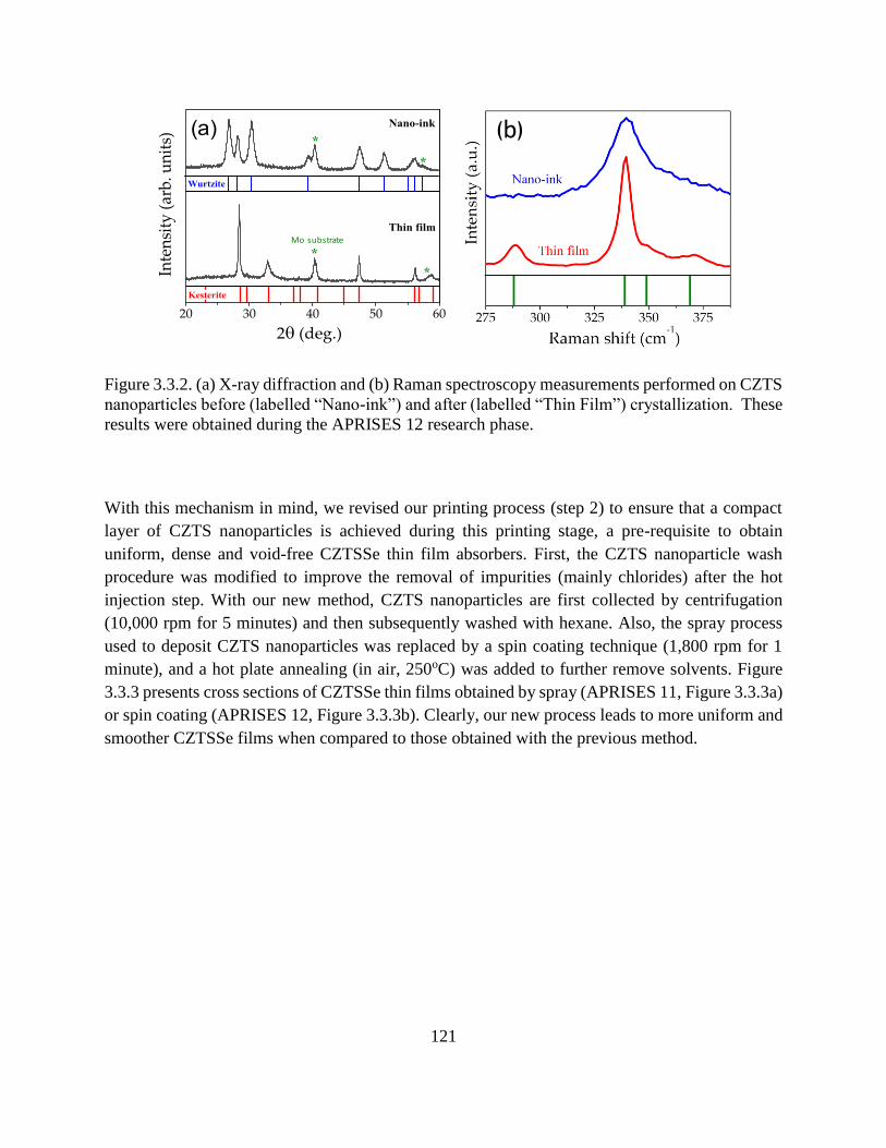
121

Figure 3.3.2. (a) X-ray diffraction and (b) Raman spectroscopy measurements performed on CZTS

nanoparticles before (labelled “Nano-ink”) and after (labelled “Thin Film”) crystallization. These

results were obtained during the APRISES 12 research phase.

With this mechanism in mind, we revised our printing process (step 2) to ensure that a compact

layer of CZTS nanoparticles is achieved during this printing stage, a pre-requisite to obtain

uniform, dense and void-free CZTSSe thin film absorbers. First, the CZTS nanoparticle wash

procedure was modified to improve the removal of impurities (mainly chlorides) after the hot

injection step. With our new method, CZTS nanoparticles are first collected by centrifugation

(10,000 rpm for 5 minutes) and then subsequently washed with hexane. Also, the spray process

used to deposit CZTS nanoparticles was replaced by a spin coating technique (1,800 rpm for 1

minute), and a hot plate annealing (in air, 250oC) was added to further remove solvents. Figure

3.3.3 presents cross sections of CZTSSe thin films obtained by spray (APRISES 11, Figure 3.3.3a)

or spin coating (APRISES 12, Figure 3.3.3b). Clearly, our new process leads to more uniform and

smoother CZTSSe films when compared to those obtained with the previous method.

122

Figure 3.3.3. Scanning electron micrograph of CZTSSe thin films obtained with synthesis recipes

developed during (a) APRISES 11 and (b) APRISES 12.

Finally, CZTSSe thin films obtained with our new method were integrated as solar cells, using 100

nm thick CdS buffers and 100nm/500nm ZnO/ITO transparent conductive oxide layers. The

electrical properties measured on 7 cells under simulated AM1.5G illumination (1,000W/m2) at

25oC are presented in Table 3.3.1. The highest efficiency achieved was 4.48%, a value double that

achieved during the APRISES 11 research phase. On average, the short-circuit photocurrent

density, open circuit voltage and efficiency were 24.7 mA/cm2, 389 mV and 3.84%, respectively.

For comparison, the highest efficiency of state-of-the-art CZTSSe synthesized via vacuum-based

process during the APRISES 12 reporting period is 9.15% (I. Repins, Sol. Energy Mater. Sol.

Cells, 2012, 101, 154–159).

Table 3.3.1. Electrical properties of printed CZTSSe solar cells.

Voc(DMM)

[mV]Cell# Voc

[mV]

Jsc

[mA/cm 2 ]

FF

[%]

Eff

[%]

Rs

[Ω-cm 2 ]

Rsh

[Ω-cm 2 ]

419 1 414 20.7 29.30 2.44 2.5 88.5

424 2 423 25.4 29.72 3.05 1.4 116

421 3 419 23.2 34.66 3.37 1.93 196

407 4 417 27.4 39.37 4.48 1.48 202

280 5 372 21.9 44.46 3.62 3.03 68.4

dead 6 288 29.5 35.49 3.03 2.7 24.1

391 7 392 30.8 31.84 3.84 2.16 55.8

Average 389.3 24.7 35.5 3.3 2.2 115.8

Std.dev. 48.2 3.4 5.8 0.7 0.7 71.1

Mo

Glass

CZTSSeCZTSSe

Mo

(a) (b)

5 � m

123

3.4 Hydrogen Refueling Support

The APRISES 2012 activities were focused on two locations: the hydrogen production and fueling

station located at the Natural Energy Laboratory Hawaii Authority (NELHA) in Kailua-Kona, and

the hydrogen fueling dispenser station located at Hawaii Volcanoes National Park (HAVO), both

on the Island of Hawaii. APRISES 12 funding supported the commissioning of hydrogen

production and compression equipment at the NELHA site, the procurement of a Power Export

Unit to enable a fuel cell electric bus to provide 110/240 VAC power for emergency backup power

in support of civil defense operations, and the design of a hydrogen dispensing system and

procurement of hydrogen dispensing equipment at HAVO. Funding also supported the

development of a grid-connected electrolyzer model operated in support of grid frequency

management ancillary services.

Figure 3.4.1 Central Site Production/Distributed Dispensing

As illustrated in Figure 3.4.1, the overall hydrogen fueling concept is to produce hydrogen at a

central site and deliver it to distributed dispenser stations using a fleet of hydrogen transport trailers

(HTT). This concept provides for optimizing capital utilization for hydrogen production while

utilizing distributed dispensing sites with minimum complexity and infrastructure to reduce fuel

distribution costs. Central hydrogen production “at scale” leverages the utilization of larger

124

electrolyzers that in addition to producing hydrogen for transportation, can be used to provide grid

support ancillary services that can be monetized to provide additional revenue streams to the

hydrogen production company. This in turn offsets the production cost of hydrogen.

It has been demonstrated that an electrolyzer has the potential to be used as a variable controllable

load that can be reduced or increased in order to maintain the total load balance and frequency

stability of the grid. The high-level objectives of this project are to validate the performance,

durability, and cost benefits of grid integrated hydrogen systems by:

Demonstrating the dynamic operation of electrolyzers to mitigate impacts of intermittent

renewable energy sources on the grid – do they respond fast enough?

Investigating the durability of the electrolyzer over a long duration when used in a dynamic

operating mode;

Developing models that characterize the performance of electrolyzers in the grid support

operational mode;

Demonstrating the potential for multiple revenue streams from the monetization of

ancillary services while producing hydrogen;

Supporting the development of regulatory structures for the permitting and installation of

hydrogen systems in Hawaii;

Supporting the operation of hydrogen equipment at NELHA;

Supporting the procurement of equipment for the HAVO hydrogen dispensing system;

Supporting fuel cell bus operations by supplying hydrogen to shuttle buses operated by

County of Hawaii Mass Transit Agency (MTA) and Hawaii Volcanoes National Park

(HAVO);

The NELHA site design is illustrated in Figure 3.4.2. It is comprised of a 40 ft ISO container that

houses 1) a Proton Onsite Model C30 proton exchange membrane electrolyzers that produces 65

kg of hydrogen over a 24-hour period at a pressure of 450 psi, 2) a HydroPac compressor that is

capable of compressing 120 kg of hydrogen per day, and 3) an electrical distribution room. The

hydrogen is compressed into hydrogen transport trailers shown in the bottom left of the diagram.

The trailers supply 450 bar hydrogen to the hydrogen dispenser shown in the upper right of the

diagram which then dispenses hydrogen to the County of Hawaii bus (Figure 3.4.3).

125

Figure 3.4.2 NELHA Hydrogen Production and Dispensing Site Design

Figure 3.4.3 County of Hawaii FCEB

126

Figure 3.4.4 Entrance to NELHA Hydrogen Production and Dispensing Site Design

Figure 3.4.5 NELHA 350 Bar Hydrogen Dispenser

APRISES 12 funding supported the commissioning and maintenance of the electrolyzer (Figure

3.4.6) and the compressor (Figure 3.4.7) systems by technicians from Proton Onsite and Powertech

respectively to ensure that the equipment and their balance of plant systems were properly installed

and functional. This included operation of their respective chiller units and the electrolyzer

deionized water supply.

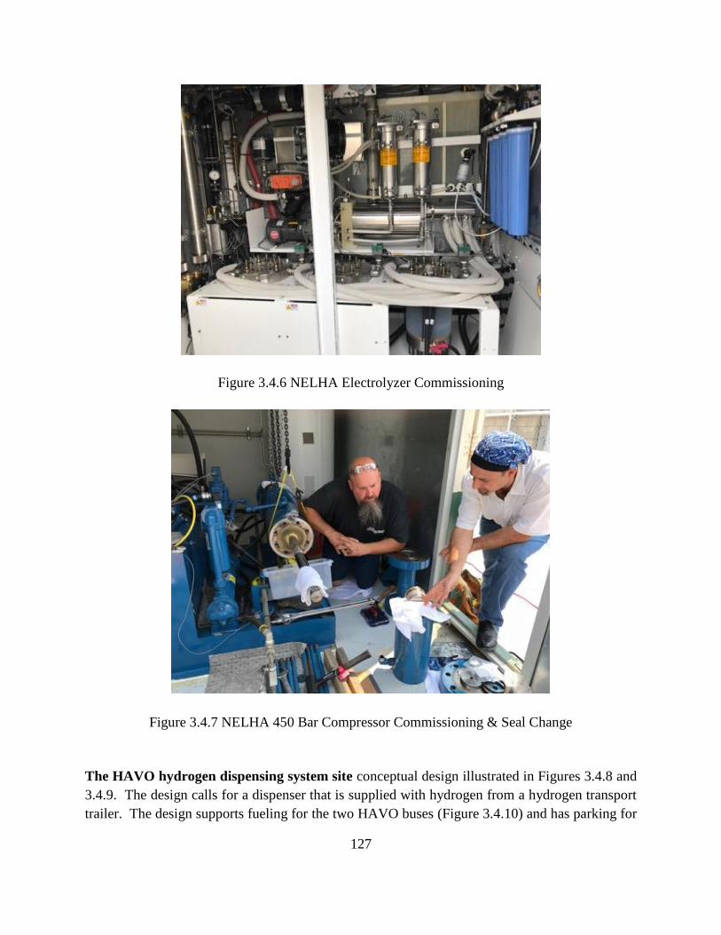
127

Figure 3.4.6 NELHA Electrolyzer Commissioning

Figure 3.4.7 NELHA 450 Bar Compressor Commissioning & Seal Change

The HAVO hydrogen dispensing system site conceptual design illustrated in Figures 3.4.8 and

3.4.9. The design calls for a dispenser that is supplied with hydrogen from a hydrogen transport

trailer. The design supports fueling for the two HAVO buses (Figure 3.4.10) and has parking for

128

two hydrogen transport tube trailers. A firewall with a 2-hour fire rating separates the hydrogen

fueling pad from existing gasoline and diesel tanks in accordance with NFPA-2 setback codes and

standards requirements. A small 10 ft ISO container is used to house various balance of plant

equipment and the electrical distribution system. The dispenser is weather protected with a

canopy. There is also a provision to charge the buses’ onboard batteries using an EV charging

station.

A contract for an architectural and engineering design suitable for bidding on the installation of

the site infrastructure (using other budgets) was prepared and a contractor was selected. However,

the Kilauea eruption began on May 3, 2018 and all activities associated with installing the site

infrastructure were halted. The eruption and severe earthquakes have caused extensive damage to

the park’s infrastructure and it is uncertain when the park will be ready to receive a hydrogen

dispensing station. Other options are being evaluated.

Figure 3.4.8 HAVO 350 Bar Dispensing Station Conceptual Design

129

Figure 3.4.9 HAVO 350 Bar Dispensing Station Rendering

Figure 3.4.10 HAVO Fuel Cell Electric Bus

A novel automated fueling system for the HAVO buses was developed utilizing a “cascade” filling

process - a high-pressure system which is used for the refilling of lower pressure compressed gas

cylinders. The cascade system allows cylinders to be filled without a compressor. When gas

contained in a cylinder at high pressure is allowed to flow into another cylinder that contains gas

130

at a lower pressure, the pressures will equalize to a value somewhere between the two initial

pressures. In a cascade storage system, several large cylinders are used to bring a small cylinder

up to a desired pressure, by always using the supply cylinder with the lowest useable pressure first,

then the cylinder with the next lowest pressure, and so on. The problem is that it is only possible

to extract about 50% of the hydrogen from the trailer if the bus is to be filled to its full 350 bar

capacity. The trailer must then be returned to NELHA for refilling with half of the hydrogen

remaining onboard. This essentially doubles the cost of delivering hydrogen and was deemed

unsatisfactory.

HNEI tasked Powertech to design and build a hydrogen boost compressor system that will be used

to extract the majority of the hydrogen from the hydrogen transport trailers. This will significantly

reduce the amount of hydrogen that is back-hauled, and in turn, reduce the number and cost of

delivery trips by approximately 50%. Figure 3.4.11 is illustrates the new connection post that

contains a small boost compressor. The Hydrogen Transport Trailers were also modified to allow

their valves to be operated by the automated control system in the correct sequence required to

optimize the dispensing process.

Figure 3.4.11 HAVO Boost Compressor System

APRISES 12 funding was also used to procure and develop the non-recurring engineering to

integrate a 10kW Export Power Unit (EPU) into the County of Hawaii bus (Figure 3.4.12).

The EPU (Figure 3.4. 13) allows the bus to power critical loads in a civil defense emergency

131

such as a hurricane. The EPU can convert input 320-450VDC voltages to an output of

110/220VAC, 10kW, 60/50 Hz. This will allow the MTA bus to provide up to 32 hours of

backup power at 10 kW. The bus can then fill its hydrogen tanks in 15 minutes and provide

another 30 hours of critical load power. The bus thus becomes a mobile power source. This

capability is being very well received by the County of Hawaii.

Figure 3.4.12 MTA Bus Undergoing Conversion

Figure 3.4.13 Export Power Unit, 10kW, Installed on MTA Bus

132

Under this subtask, a Hydrogen Energy System (HES) simulation tool was developed to evaluate

and characterize the performance of an electrolyzer system for grid management applications

under realistic island grid load profiles. The simulation tool was developed in the Matlab-Simulink

environment to analyze the use of an electrolyzer as a potential grid management tool for a small

electrical grid. The HES simulation tool consists of a PEM electrolyzer system model, island

electrical grid model, and input sources of power, load and grid frequency signals to drive the

simulation. Figure 3.4.14 shows the HES simulation tool in the Matlab-Simulink environment.

Figure 3.4.14 HES Simulation Tool in the Matlab-Simulink environment

Figure 3.4.15 is a schematic of the main components of the NELHA hydrogen fueling station. The

system consists of a Proton Onsite C30 electrolyzer unit with two cooling chillers to produce

hydrogen at 30 bar at a rate of 65 kg/day. The 30 bar hydrogen is stored in a small buffer tank and

is further compressed to 450 bar by the compressor system at a maximum rate of 120 kg/day. The

450 bar compressed hydrogen is stored in 12 tanks inside a hydrogen transport trailer (HTT) that

is connected to a fueling post for onsite dispensing.

133

Figure 3.4.15: Main Components of the NELHA hydrogen fueling station

The hydrogen generator is a Proton Exchange Membrane (PEM) electrolyzer system configured

with three PEM stacks each operating at maximum current of 410 Amps to produce 30 Nm3/h. of

hydrogen. The unit has a deionized-water (di-water) production and circulating system to supply

di-water to the stacks for producing pressurized hydrogen and oxygen and also removing waste

heat. The oxygen is safely vented out to the atmosphere while the hydrogen is separated from water

and dried to deliver high purity (99.999%) pressurized product gas. The unit has two liquid cooling

systems to maintain stack and power supply temperatures of 50°C and 40°C respectively.

Supervisory controls enable safe performance and automatic operation of the electrolyzer unit.

The C30 Proton electrolyzer is a fully automated system that regulates the hydrogen production

rate to maintain a set buffer tank pressure. This electrolyzer unit also has a mass flow controller to

govern its operation externally via a 4-20 mA output port. This enables the electrolyzer to run in

dynamic mode and its hydrogen production to be controlled by a grid management algorithm.

The product hydrogen is stored in a buffer tank before it’s compressed to 450 bar by the

compressor system. The compressor only operates when the HTT is connected to the fueling post

and the tanks are empty. The compressor starts automatically when the buffer tank pressure is

greater than 29.5 bar and runs until the buffer tank pressure drops below 16.8 bar. One compressor

cycle takes about 20 minutes. The operation of compressor and the monitoring of all critical

pressures and temperature of the system are done by the main PLC controller. The PLC controller

is also responsible for the smooth and safe operation of all the main and ancillary components of

134

the fueling station which includes the hydrogen generator, compressor, three chillers, fueling post,

HTT storage, and the hydrogen dispenser.

The dynamic operation of the electrolyzer via a 4-20mA control port is implemented in the PLC

controller and is available through the Human Machine Interface (HMI). Normally the hydrogen

energy system is operated at a constant maximum production rate from the HMI to generate

hydrogen on demand to refill the storage capacity of the fueling station. One of the objectives of

this project is to operate the electrolyzer in a dynamic mode using a grid management control

algorithm in order evaluate the ability of the electrolyzer to stabilize grid frequency fluctuations

caused by fluctuating renewable energy power sources such as wind and solar.

A feasibility study was done to understand the level of grid management the current size of the

electrolyzer of the HES would be capable of achieving and what optimal electrolyzer size would

be required to achieve the maximum level of grid frequency stability. The impact of operating the

electrolyzer in dynamic mode on the production of the hydrogen for the fueling station was also

analyzed. A dynamic model of the electrolyzer system and an Island of Hawaii grid model have

been developed to be used in an HES Simulation Tool for this feasibility study under different

operational strategies and renewable power profile.

The electrolyzer model (Figure 3.4.16) models the PEM stack current and temperature for the

production of hydrogen gas, the hydrogen pressure within the electrolyzer (system pressure), and

the hydrogen pressure in the buffer tank (product pressure). The electrolyzer system model was

developed based on a validated PEM fuel cell model and integrates the control and dynamic

characteristics of the Proton C30 electrolyzer system during the startup (powering up) process,

safety check and venting procedure, and normal operational process. The thermal, current, and

pressure controllers and time constants were designed and tuned to simulate the dynamic ramping

characteristics of the electrolyzer.

135

Figure 3.4.16: PEM Electrolyzer System Model in the Matlab-Simulink Environment

The model determines, for a given supply current, the voltage of each cell which is then multiplied

by the total number of the cells to evaluate the over-all DC power consumed by the three

electrolyzer hydrogen production stacks. The pressurized wet hydrogen produced at the cathode

side increases the system pressure in the pipes and small volumes in the electrolyzer unit and is

then fed into a pressure-swing dryer unit. The dry hydrogen is then supplied as product gas to the

buffer tank.

The system pressure is used to control the electrolyzer current. A mechanical back pressure

regulator (BPR) maintains constant system pressure and also physically separates the system and

product pressures. When the buffer gets full and the product pressure increases above the BPR

setpoint, the system pressure increases too, and the controller throttles the stack current and, hence,

the hydrogen production.

The Proportional-Integral-Derivative (PID) controller2 and time constants were implemented into

the PEM electrolyzer system model. These were tuned to have very similar initial, transient and

steady state operational characteristics as the Proton C30 electrolyzer system during the startup

and at normal operation. Controller parameters and the time constants were tuned using measured

2 Proportional-Integral-Derivative controller automatically applies accurate and responsive correction to a

control function

136

data from the electrolyzer ramping up/down cycle tests during commissioning at Powertech in

March 2015.

The buffer tank block in Figure 3.4.17 has the buffer tank model to estimate the pressure of the

tank from the flowrate of the dry hydrogen supplied from the electrolyzer. The pressure builds up

in the tank until the upper limit is reached after which either the compressor is switched on to

consume the stored hydrogen, or the hydrogen production is stopped. The hydrogen compressor is

modeled by an algorithm which allows the compressor to switch ON and OFF when the buffer

tank is full and empty respectively. The compressor switches ON when the buffer pressure is over

29.5 bar and runs until the buffer tank pressure drops below 16.8 bar. These upper and lower buffer

tank pressure limits give a hydrogen compressing time of about 20 minutes, as measured in the

actual HES system.

The PEM Electrolyzer system model was validated with measured data obtained during

performance tests at Powertech. The electrolyzer system model was setup to run in the same way

as the actual Proton C30 Electrolyzer unit from the “Power-up and Prestart State” where all the

safety checks are done, the “Generate and Venting State” where the stack operation and hydrogen

quality are verified, and the “Normal Pressurized Operation State” for generating the hydrogen as

product gas. Figure 3.4.18 shows the simulated results compared to the measured data for the H2

flowrate, system and product pressures, and a single stack current during the different operational

states. The simulated results show that the control parameters and the time constants in the model

are well-tuned to accurately estimate the operational characteristics of the actual Proton C30

electrolyzer system operation.

137

Figure 3.4.17: Simulated results for different operating states compared with measured data

from the Proton C30 Electrolyzer.

138

Figure 3.4.18: Simulated results of H2 production and compression cycles compared with

measured data from actual HES

The performance of the HES which is the combined operation of the electrolyzer and the

compressor was also simulated, and the results were compared to the measured data from the

combined system. The simulated results for nearly three complete hydrogen production and

compression cycles from the HES model were compared to measured data as shown in Figure

3.4.18. The electrolyzer operates at maximum current to support the hydrogen production for the

compressor cycles.

To analyze the effects of the hydrogen electrolyzer system on the electrical grid, models of the

Island of Hawaii electrical grid and an electrolyzer grid interface were developed. The

139

conventional model of grid frequency dynamics based on the swing equation3 was modified to

estimate the Island of Hawaii grid model shown in Figure 3.4.19. The grid model includes a system

inertia algorithm which characterizes the rotational inertia of the generators and frequency

dependent loads while the “governor” transfer function represents the turbine generators in the

Island of Hawaii power plant. The model parameters of the system inertia (M, D) and governor

(Kp, Ki, time constants) algorithm specifically for the Island of Hawaii grid were obtained from

the Hawaii Natural Energy Institute (HNEI) study of a grid-scale battery energy storage system

(BESS) on the Island of Hawaii. This study developed these algorithms and validated them with a

fast-acting 1 MW Lithium-ion BESS on the Hawaii Island grid system.

The Island of Hawaii grid model determines the grid frequency depending on the total load on the

grid such as daily residential, industrial or/and electrolyzer demand, compared to the total power

generated on the grid from either fossil fuel turbines, battery energy storage systems, and

renewable power sources such as solar, wind or geothermal, available on the Island of Hawaii and

connected to the grid.

3 The swing equation is the relationship between the power and frequency for generators. It is used to determine

the change in average system frequency and is defined as the “center of inertia of the system”. This algorithm

is valid for reasonable frequency deviations due to imbalances between the instantaneous generation and

consumption of electric power which has an accelerating or decelerating effect on the synchronous machines.

BESS Project HNEI reference can be accessed at the following link:

https://www.hnei.hawaii.edu/sites/www.hnei.hawaii.edu/files/Development%20of%20Real-time%20Closed-

loop%20Control%20Algorithms%20for%20Grid-scale%20BESS.pdf

140

Figure 3.4.19: Island of Hawaii grid model in the Matlab-Simulink Environment

An electrolyzer grid controller algorithm was developed to ramp the electrolyzer system between

80% and 100% of its hydrogen production capacity as a function of grid frequency. The

electrolyzer normally operates at 90% of its production rate to generate hydrogen for fueling

stations while consuming power from the grid. The electrolyzer grid controller ramps up the

electrolyzer from 90% to 100% when grid frequency is greater than 60 Hz and ramps down to 80%

when the frequency is less than 60 Hz. Figure 3.4.16 shows the electrolyzer grid controller

implemented in the PEM Electrolyzer System block in the Matlab-Simulink-Environment. The

regulating frequency, c, of the electrolyzer grid controller determines how sensitive the grid

controller is, in regulating the electrolyzer up or down. When c is set to a very narrow window

around 60 Hz, then the smallest deviations between grid frequency (grid) and regulating (c)

frequency, i.e. [(grid-c) Hz], would cause the electrolyzer to ramp up or down more often,

causing high-dynamic operation of the electrolyzer. Hence, for a particular grid system, an optimal

window value of the c has to be determined to allow smooth and safe grid management operation

of the electrolyzer.

The functionality of the electrolyzer grid controller (Figure 3.4.16) algorithm was tested with a

grid frequency profile measured on the Island of Hawaii during the BESS system analysis. The

deviation of the grid frequency from the nominal grid frequency of 60 Hz was used to regulate the

electrolyzer between 80%-100% of its production rate for the grid management application.

141

During the grid management operations, after the startup period of 200 seconds, the electrolyzer

operates at an average of 90% and ramps between 80 to 100% depending on the grid condition.

When there is surplus power (grid frequency > 60.00 Hz) available on the grid, e.g. from the

renewable energy sources, the controller ramps up the hydrogen production rate towards 100%

and when there are increases in power demand (grid frequency < 60.00 Hz) or generation shortage,

the controller ramps down the hydrogen production rate towards 80% thereby decreasing the

electrolyzer power demand on the grid.

Figure 3.4.20 shows the performance of the Proton C30 electrolyzer system under the measured

Island of Hawaii grid frequency variability. Due to inherent time constants and time delays of the

standard off-the-shelf commercial electrolyzer control system, the electrolyzer does not respond

to faster transients seen in the measured grid frequency plot and therefore electrolyzer ramps are

much smoother compared to the very rapid nature of the grid frequency.

Figure 3.4.20: Performance of the Proton C30 electrolyzer under a measured grid frequency of

the Island of Hawaii.

142

The future objectives of the HES Simulation tool will be to:

Analyze the effects of renewable solar and wind power on the variability of the grid

frequency of the Island of Hawaii electrical grid and identify the level of grid management

that can be achieved by different sizes of electrolyzers.

Determine the optimal electrolyzer size to minimize grid frequency variability that is

generated by a particular size of renewable power sources such as wind and solar when

connected to the Island of Hawaii electrical grid.

Perform a trade-off study to determine the optimal proportion of the HES that can be

reserved for grid management application while generating adequate quantities of

hydrogen for commercial applications.

Presentations

1. Ewan M., US DOE Webinar, “Supporting a Hawaii Hydrogen Economy”, July 29, 2014.

2. Ewan M., Rocheleau, R., Oral presentation at H2 Fuel Cell and Battery EV Stakeholder

Charrette, “Hydrogen Technology Status for Hawaii”, Honolulu, HI, January 13, 2015.

3. Ewan M., Rocheleau, R., Oral presentation at US DOE Annual Merit Review, “Hydrogen

Energy Systems as a Grid Management Tool”, Washington, DC, June 9, 2016

4. Ewan, M., Rocheleau, R., Hydrogen Presentation to Hawaiian Electric Company senior

management team January 23, 2017.

5. Ewan, M., Presentation to NELHA Board of Directors March 21, 2017.

6. Ewan, M., “HNEI Hydrogen Projects”. Presentation to ONR Global, October 16, 2017.

7. Ewan, M., “Non Lithium-Ion Storage Options – Hydrogen”, EUCI Workshop, November

29, 2017

8. Ewan M., Rocheleau, R., Oral presentation at US DOE Annual Merit Review, “Hydrogen

Energy Systems as a Grid Management Tool”, Washington, DC, June 14, 2018

9. Ewan, M., “Supporting a Hawaii Hydrogen Economy”, Oral presentation at First

International Hydrogen Forum, San Jose, Cost Rica, August 13, 2018.

TASK 4: OCEAN ENERGY

Ocean Energy work included development of Ocean Thermal Energy Conversion (OTEC), Wave

Energy Testing and Seawater Air Conditioning. Under a subaward to Makai Ocean Engineering,

development of OTEC for both US Navy and commercial applications continued, focused on heat

143

exchanger design, development, and testing, system operational experience, and corrosion testing.

For wave energy testing, HNEI subcontracted with Sea Engineering, Inc. to conduct a market

study, procure an ROV, and utilize the ROV for various functions at Navy’s Wave Energy Test

Site (WETS). Oceanographic monitoring continued to assess Seawater air conditioning (SWAC)

impacts.

4.1 Ocean Thermal Energy Conversion (OTEC)

HNEI subcontracted with Makai Ocean Engineering Inc. to conduct research in support of

continued development of Ocean Thermal Energy Conversion (OTEC) for both US Navy and

commercial applications. This research has been focused on three major areas: 1) heat exchanger

design, development, and testing, 2) OTEC system operational experience, 3) and corrosion

testing. Makai’s OTEC work is conducted at the Ocean Energy Research Center (OERC), located

within the Natural Energy Lab of Hawaii Authority (NELHA) in Kailua Kona, Hawaii.

Under APRISES12 and in support of OTEC heat exchanger development, Makai designed, built,

and tested six configurations of Epoxy-Bonded Heat Exchangers (EBHX). Variations in fin pitch

and fin width were tested. The heat exchangers were tested at the 100-kW station, which was

designed and constructed to support EBHX testing. Results were promising and encouraged

design and fabrication of the Foil Fin Heat Exchanger (FFHX). Design revisions to the 100-kW

station are underway to support FFHX testing. APRISES13 built on this APRISES12 work, and

focused on new OTEC heat exchanger fabrication methods and designs, and corrosion testing.

This report summarizes the APRISES12 work, which was performed between January 2014 and

October 2016 specifically pertaining to:

100-kW station design and construction,

EBHX design, fabrication, and testing,

Turbine design, installation, and operational testing,

OTEC Control System autonomous controls, and

Corrosion testing from October 2013 to September 2014

To advance OTEC system operational experience under APRISES 12, Makai installed and

commissioned a 105-kW turbine generator – the first grid connected OTEC turbine in the U.S. –

at the OERC in June 2015. Several iterations of loadbank and grid-connected turbine testing

followed commissioning activities. Testing and operational knowledge was incorporated into a

new version of the OTEC Control System program which now includes the ability to start up and

operate the OTEC system autonomously.

144

To support corrosion testing, Makai has continued to test treatments and improve analysis

techniques that were initiated under previous APRISES contracts. As of October 30, 2016, the

remaining box beam samples have been tested for over 6 years. Corrosion testing also continues

with samples in the multi-column imaging racks (MCIR) and representative heat exchanger

samples.

EBHX Design, Development, and Testing

The EBHX was a prototype for Makai’s FFHX, which Makai believes to be a solution for OTEC

heat exchangers. The most important considerations for an OTEC heat exchanger are: low cost

per unit area, low volume, seawater corrosion resistant (for 30+ years), and the ability to withstand

high working fluid (ammonia) pressures. Makai’s approach to heat exchanger design was to

eliminate as much material as possible, simplify the fabrication process, and only use materials

compatible with the working environment. The EBHX/FFHX design points that specifically

address Makai’s approach are:

1) The seawater passages are constructed with titanium, so the life expectancy of the

heat exchanger will not be limited by corrosion.

2) Titanium is the most expensive component in the heat exchanger by weight, the

FFHX design (compared to a traditional plate-and-frame heat exchanger) reduces

the amount of titanium used by over 95%, representing a significant savings in heat

exchanger cost.

3) The titanium sheets are internally supported, eliminating the need for heavy, steel

structures to support the pressure, as in the case of plate-frame or shell & tube heat

exchangers.

4) The FFHX incorporates densely packed aluminum fins on the ammonia side, which

yields a compact and efficient heat exchanger.

5) The design of the heat exchanger allows for low cost, high-volume manufacturing

in the future. Makai envisions a fabrication method in which raw materials are fed

into one side of a machine while heat transfer plates are ejected from the other.

These foil-fin plates are then stacked into a complete heat exchanger with minimal

construction effort and minimal cost.

6) The design of the heat exchanger allows for infinite customization of fluid paths

and inlet/outlet nozzles. The heat exchanger is stacked layer by layer and fluid paths

can be separated during assembly.

The basic component of the EBHX is the Heat Transfer Plate (HTP), which is essentially

corrugated aluminum fins with a thin titanium sheet (foil) overlain on both ends. Epoxy is spread

over the surface of the foil and the foil is then pressed onto the aluminum fins. In the process,

most of the epoxy is expelled from the fin crest, leaving only a thin layer, where most of the heat

145

transfer is expected to occur. In the FFHX, foil is joined to the fins using laser welding. Multiple

HTPs are stacked together to form an EBHX/FFHX.

Titanium foil thickness was chosen to withstand pressure and to provide sufficient contact length

between the foil and the fin crests. Thicker foil will distribute heat more evenly across the foil

surface from fin crest but is also less pliable, resulting in reduced contact length at the fin crest.

Makai believes contact length to be critical to performance and thinner foil is also more

economical.

The aluminum fin height is based on a trade-off between heat transfer effectiveness and ammonia

head losses. Thermal analysis predicts the middle section of the current fin has the same

temperature as the surrounding ammonia and therefore is not transferring heat. A shorter fin would

reduce this dead zone but also reduces the ammonia flow area and increases the head losses.

Because ammonia is saturated, increased head losses diminish LMTD and lowers heat exchanger

performance.

EBHX fabrication equipment was custom designed and built by Makai. The major components

are summarized in Table 4.1.1.

Table 4.1.1. EBHX Fabrication Equipment

Component Purpose

Epoxy Roller Table

Holds foil in tension for surface prep and epoxy application

Applies epoxy at specified thickness on foil

Passes foil to Plate Template after epoxy is applied

Plate Template

Contains razor guides for foil edge trimming

Aligns foil for fin plates and edge bar attachment

Holds the plate together until epoxy is set

Clamping Plate and

Frame

Used to stack HTPs together and ensure clamping pressure is

distributed evenly

A 100-kW station was designed to test the Makai-designed EBHXs with a nominal duty of 100

kW. For the EBHXs, the working fluid is propane because ammonia is incompatible with epoxy.

146

The 100-kW station is capable of seawater flow rates up to 650 gpm and propane mass flow rates

up to 0.35 kg/s.

The 100-kW station has slots for two EBHX’s (an evaporator and a condenser). An APV titanium

plate-and-frame heat exchanger is installed as the accompanying heat exchanger for use during

EBHX performance testing. The APV plate and frame heat exchanger functions as an evaporator

during EBHX condenser testing and as a condenser for EBHX evaporator testing. An established

heat exchanger was used to ensure performance of the tested heat exchanger would not be limited

by an untested accompanying heat exchanger.

Figure 4.1.1. Epoxy-Bonded Heat Exchanger (EBHX) condenser and evaporator at the 100-kW

test station. The APV companion heat exchanger is the vertical blue component in the background.

On the working fluid side, when propane is boiled in the evaporator, saturated propane enters the

separator tank. Propane vapor exits the separator vapor outlet and is condensed in the condenser.

From the condenser, liquid propane drains into the buffer tank. The feed pump pumps liquid

propane out of the buffer tank into the recirc pump intake line. Liquid propane from the separator

liquid outlet is also piped into the recirc pump intake line. The recirc pump pumps liquid propane

back into the evaporator. A vapor Coriolis flow meter at the separator vapor outlet measures the

propane vapor flow. Pressure and temperature sensors are located at the inlet and outlet of the

EBHXs but not in the other portions of working fluid piping.

On the seawater side, seawater flow is measured on a section of the discharge piping that is

common to EBHXs but not the accompanying APV heat exchanger. Seawater pressure and

temperature sensors are located at the inlet and outlet of the EBHXs but not on the accompanying

heat exchanger. The accompanying seawater flow is not measured.

Installation and shakedown testing was completed in November 2014.

147

The 100-kW station met its designed purpose for testing EBHXs but several areas could be

improved with modifications. A check valve between the feed and recirc pump would improve

recirc pump operational stability. Horizontal pipes should be angled so propane can be more easily

drained and additional valves would make the process of changing out heat exchangers more

efficient. More sensors could provide insight into the working fluid state throughout the system.

These lessons learned will be incorporated in upcoming modifications to the 100-kW station to

support testing of Makai’s FFHXs using ammonia as the working fluid.

Six EBHXs – two evaporators and four condensers – were tested at the 100-kW station. Each

heat exchanger had six plates but the fin pitch (in fins per inch, FPI) and thickness, foil material

and thickness, and epoxy thickness were varied between the heat exchangers. Regardless of

configuration, each heat exchanger was 1.5 m in length and the total heat transfer area was 5.04

m2. The configurations and properties are summarized in Table 4.1.2.

The condensers were tested at cold seawater flow rates from 200-600 gpm and at duties from 40-

100 kW. The evaporators were tested at warm seawater flow rates from 200-500 gpm and at duties

from 40-80 kW.

The seawater channel widths between the plates were the same for each heat exchanger but we

attempted to preferentially divert seawater flow away from the channels on the end (because there

is no heat transfer on one side) by restricting the end channel widths using epoxy. For the

condenser, the epoxy detached from the header during the first test. The epoxy restriction

remained intact for the evaporator. Seawater pressure drop (SW dP) is plotted versus seawater

flow velocity in Figure 4.1.2 to remove the effects of different seawater flow cross sectional areas.

For EBHX-4 and -5, a small adjustment was also made to account for the Al foil being thicker

than the Ti foil. Except for EBHX-4 and -5, the SW dPs agreed to within 5 kPa.

148

Table 4.1.2. Summary of EBHX configurations.

Type Specifications Epoxy Nominal

Thickness (mm)

EBHX-1 Condenser 5 plates of 26 FPI and 1 plate of 51 FPI, all

with Ti foil 0.381

EBHX-2 Condenser 5 plates of 39 FPI and 1 plate of 51 FPI, all

with Ti foil 0.381

EBHX-3 Condenser 6 plates of 51 FPI, all with Ti foil 0.381

EBHX-4 Condenser 4 plates of 17 FPI with Ti foil and 2 plates of

17 FPI with Al foil 0.381

EBHX-5 Evaporator 6 plates of 17 FPI, all with Al foil 0.762

EBHX-6 Evaporator 6 plates of 51 FPI, all with Ti foil 0.381

Figure 4.1.2. Seawater pressure drop (SW dP) vs Flow Velocity for all six EBHXs

0

5

10

15

20

25

30

35

0 0.5 1 1.5 2 2.5 3 3.5

SW d

P [

kPa]

SW Velocity [m/s]

SW dP vs Flow Velocity

EBHX-4 (17 FPI - COND) EBHX-5 (17 FPI - EVAP)

EBHX-1 (26 FPI - COND) EBHX-2 (39 FPI - COND)

EBHX-3 (51 FPI - COND) EBHX-6 (51 FPI - EVAP)

149

Some of the discrepancy in SW dP may be due to inaccuracies in the width of the outermost

seawater channels. Agreement is poor for EBHX-4 and EBHX-5; both were 17 FPI and contained

Al foil. It is possible that the lower fin density allowed for slightly deeper ripples in the foil which

increased resistance in the seawater flow channel and resulted in higher pressure drop. However,

it is unclear why EBHX-3 differed from EBHX-6; the same plates which were initially used in

EBHX-3 were re-used for EBHX-6.

The U-values for the heat exchangers must also be carefully interpreted. There was no significant

difference in U-value between the two evaporators tested. For the condensers, EBHX-3 and

EBHX-4 had highest and second highest U-values, respectively. Several factors make the results

difficult to interpret.

First, for the condensers, EBHX-1 and -2 had 5 plates of the same fin pitch and 1 plate of 51 FPI.

It is unlikely that working fluid flow was uniform between all 6 plates and it is unclear how

performance may have been affected. For example, it is conceivable that most of the heat transfer

occurred in the 5 plates and little propane vapor entered the 51 FPI plate due to increased pressure

drops associated with the smaller cross sectional area.

Another confounding factor that is applicable to both the evaporators and condensers and specific

to the EBHX design, is the effective heat transfer area. Heat transfer from propane to seawater

occurs mostly in the fin crest region, where epoxy is thinnest. Epoxy is thicker on other parts

where the fin and foil are joined. A layer of epoxy also covers the exposed foil between the fins,

acting as an insulator and reducing any heat transfer directly through the foil. According to

computer models, the contact area is greatest for 17 FPI, followed by 39 FPI, 26 FPI, and 51 FPI;

there is ~11% less contact area for 51 FPI compared to 17 FPI. Of course, some variation during

assembly is expected. Greater effective heat transfer area should equate to better performance.

Finally, we must also consider difference in thermal conductivity between Al and Ti foils. For the

evaporator, EBHX-5 had aluminum foil and EBHX-6 had titanium foil. For the condenser, EBHX-

3 had two plates with Al foil while the remaining condensers all used Ti foil. Although the

aluminum foil is thicker, the thermal conductivity of aluminum is almost ten times that of titanium.

150

Figure 4.1.3. Comparison of evaporator U-value vs seawater flow at 40 kW and 60 kW. There is

no significant difference between the two evaporators.

0

0.5

1

1.5

2

2.5

0 0.5 1 1.5 2 2.5 3 3.5

U [

kW/m

2-K

]

WSW Velocity [m/s]

Evaporator U vs WSW Flow

EBHX-6 (51 FPI) - 60 kW

EBHX-5 (17 FPI) - 60 kW

EBHX-6 (51 FPI) - 40 kW

EBHX-5 (17 FPI) - 40 kW

151

Figure 4.1.4. Comparison of U vs seawater flow at 60 kW and 80 kW (top and bottom graphs

respectively). EBHX-3, with 6 plates of 51 FPI and Ti foil, had the highest U-value. The EBHX-

4 had the second highest U-value.

0

0.5

1

1.5

2

2.5

3

3.5

4

4.5

0 0.5 1 1.5 2 2.5 3 3.5

U [

kW/m

2-K

]

CSW Velocity [m/s]

Condenser U vs CSW Flow at Duty = 80 kW

EBHX-4 (17FPI)EBHX-1 (26FPI)EBHX-2 (26FPI)

0

0.5

1

1.5

2

2.5

3

3.5

4

4.5

0 0.5 1 1.5 2 2.5 3 3.5

U [

kW/m

2-K

]

CSW Velocity [m/s]

Condenser U vs CSW Flow at Duty = 60 kW

EBHX-4 (17FPI)EBHX-1 (26FPI)EBHX-2 (39FPI)

152

It is difficult to draw conclusions from the EBHX testing results because there were often several

variations between the different heat exchangers. Both evaporators had comparable performance

in terms of U-value and working fluid dP. Seawater dP for the EBHX-5 was the highest of all heat

exchangers tested. EBHX-3 was the best performing condenser. However, it is unclear whether

the degree of improved performance was due to the higher fin density or whether non-uniform

working fluid distribution suppressed U-values for the EBHX-1 and -2 low. EBHX-4 performed

nearly as well as EBHX-3; the reasons are most likely a combination of the larger contact foil-to-

fin contact area at the fin crests, the addition of Al foil for two plates, and improved seawater side

convection due to deeper corrugations in the foil.

The turbine generator, including all the structural, mechanical, and electrical systems was

successfully installed at the OERC in May 2015. The structural modifications to the testing tower

included the addition of a fourth floor for the turbine generator skid. The turbine, gearbox,

generator, lube oil system, and electrical / instrumentation panels are mounted on the turbine

generator skid. A compressed air system for the turbine control inlet valve (TCIV) and a cooling

water system for the lube oil system were also installed. The ammonia vapor piping from the

separator outlet to the condenser inlet was modified to include a branch for turbine operations.

Figure 4.1.5. Layout of turbine deck on the fourth floor of the Ocean Energy Research Center

(OERC).

The electrical system consists of the generator, switchgear, loadbank, battery bank, the overspeed

resistors, and all the instrumentation and control system. Most of the instrumentation and control

starts (or ends) at the Generator Control Cabinet (GCC) located in the Makai office. The GCC

also houses Woodward ATLAS II governor (TCIV controller), Schweitzer SEL-700G0 (monitor

for the grid tie breaker), Marathon DVR 2000E+ (voltage regulator), HMI 5070L (touchscreen

interface for ATLAS), and various meters and switches for manual operation.

153

Turbine commissioning took place in May and June 2015. A month-long break was necessary to

complete modifications to the electrical system. During commissioning, turbine control and safety

features were verified. ATLAS control constants were also tuned to ensure a smooth startup.

Although the turbine was aligned, high vibrations and noise were observed during initial

operations. One source of the vibration was the permanent magnet generator (PMG), which was

not securely mounted on the generator shaft.

When vibrations and noise were still observed after the PMG was correctly mounted, further

investigation identified an interference issue with the turbine shroud. The turbine design included

a shroud that was fitted onto the turbine blade ring to improve efficiency by reducing the tip

clearance (and leakage rate). The shroud was designed to rotate with turbine blades. Sometime

during commissioning or operational testing, the shroud slipped about halfway (axially) down the

turbine blade ring and was rubbing against the housing. The turbine was removed from the OERC

and sent back to the manufacturer to correct the problem. A new shroud was fabricated, this time

press fit into the stationary housing instead of onto the rotating blade ring. This new design

resulted in a larger tip clearance and was predicted to reduce efficiency by 1% according to the

manufacturer.

A separate issue with the gearbox oil was identified during the vibration troubleshooting. Gearbox

oil was observed to be very dark colored, indicative of overheating. The gearbox was returned to

the manufacturer for inspection. No bearing damage was identified and a faulty oil heater was the

most likely cause of the burnt oil. The heater elements were replaced and the gearbox was

reassembled without modification.

Makai also replaced the low-speed coupling. Initial vibration measurements on the turbine and

gearbox were high when coupled with the generator but within specification when uncoupled from

the generator. We suspected misalignment introduced through the coupling may have contributed

to the high vibrations. The original set-screw mount low-speed coupling was replaced with a taper

lock low-speed coupling.

At the same time, the generator was also removed from the OERC and sent out for re-balancing

as a preventative measure in case the vibration issues adversely affected the generator.

Finally, modifications were also made to stiffen the turbine skid by adding a new W8x31 beam

between the existing W12x40 beams to reduce flexing of the skid (Figure 4.1.6). Alignment and

vibration monitoring was performed again when all components were re-installed. No further

issues were identified.

154

Figure 4.1.6. Turbine skid stiffening modifications.

New beam

155

Turbine performance can be characterized by looking at pressure drop and flow across the turbine

and isentropic efficiency. Turbine pressure drop is calculated from the inlet and outlet pressure

sensors. The highest pressure drop recorded during testing (using two evaporators and three

condensers) was ~ 301.5 kPa and that corresponded to an electrical power output of almost 88.3

kW. Based on estimates from collected data, 325 kPa is required to produce 100 kW. Turbine

flow cannot be directly measured and is calculated using the liquid ammonia flow sensors and tank

and separator-receiver line levels. Based on collected data, approximately 3.5 kg/s of ammonia

vapor flow is required to produce 100 kW. The dP vs Power curve predicts the power to within

10% of the manufacturer’s targeted data points provided in the design document (CDR). The

turbine flow vs power curve is up to 20% off, but inaccuracies associated with calculating turbine

flow likely contribute to the error.

Figure 4.1.7. Turbine power vs dP and ammonia flow. Turbine flow is calculated using a

combination of flow sensors and integrated level sensors, so more variability is expected. Based

on the projected curve fit, to produce 100 kW, dP needs to be ~ 325 kPa and ammonia vapor flow

needs to be ~3.5 kg/s. Manufacturer provided points are marked by ‘X’s.

Calculating turbine efficiency is more complex. During heat exchanger testing, ammonia vapor

from the expansion valve outlet to the condenser inlet is slightly superheated; thermodynamic

properties can be calculated using pressure and temperature. During turbine operations, depending

on the seawater flow rates, temperatures, and turbine power output, ammonia at the turbine exit

and condenser inlet may be saturated with unknown quality. Without quality, the enthalpy at the

turbine outlet is unknown, and therefore, the isentropic efficiency and turbine work is unknown.

0

10

20

30

40

50

60

70

80

90

100

0 50 100 150 200 250 300 350

Gen

erat

or

Ou

tpu

t [k

We]

Turbine dP (TIPS-TOPS) [kPa]

Power vs dP

Data

CDR

0

10

20

30

40

50

60

70

80

90

100

0 1 2 3 4

Gen

erat

or

Ou

tpu

t [k

We]

Turbine Flow Rate [kg/s]

Power vs Flow

Data

CDR

156

The work required to spin the turbine and gearbox (decoupled from the generator) at 1800 rpm

should be constant. For certain combinations of seawater flow rates, when the generator is

decoupled and but the turbine and gearbox are spinning at 1800 rpm, ammonia vapor can exit the

turbine in a superheated state. By testing several seawater flow combinations and using only data

when turbine outlet conditions are superheated, the work required to spin the turbine and gearbox

can be found. The resulting averaged gearbox work is 5.75 kW (Figure 4.1.8). Gearbox work can

be added to power produced (after taking into account generator efficiency) to find the total work

done by ammonia. The total work can then be used to solve for turbine outlet conditions and

isentropic efficiency.

Turbine outlet enthalpy in saturated conditions can be calculated using:

hturbine outlet = hturbine inlet −Total Work

mammonia

where Total Work = Gearbox Work + Generator Electrical Output

Generator Efficiency. Because TCIV was 100% open

during operational testing, turbine inlet enthalpy was calculated using the temperature and pressure

sensors at the turbine inlet vice the separator outlet. Quality was calculated using the turbine outlet

pressure and the turbine outlet enthalpy. The turbine design document predicted “2.4% wet at the

nozzle discharge”, or a quality of 97.6%. In our data, for the observed turbine inlet and outlet

conditions, if isentropic efficiency were 100%, the quality would be no less than 98%. The

calculated quality was always greater than 98.4% and decreased with increasing power.

157

Figure 4.1.8. The work required to spin the turbine and gearbox averages to be 5.75 kW.

Ammonia vapor flow is likely non-uniform when turbine control inlet valve (TCIV) is less at 48%

open. Enthalpy at the separator vapor outlet (h2b) was used instead of enthalpy at the turbine inlet

(h3).

158

Figure 4.1.9. Turbine outlet quality and isentropic efficiency were calculated using gearbox work

= 5.75 kW. The manufacturer target for turbine isentropic efficiency is 68% and predicted 97.6%

quality at the turbine outlet. Generator efficiency was calculated by interpolating based on power

and power factor from manufacturer provided curves.

Isentropic efficiency is calculated using:

Isentropic Efficiency = hturbine inlet−hturbine outlet

hturbine inlet−hturbine outlet, isentropic.

Isentropic efficiency is dependent on the power output and approaches 70%. The design

specifications targeted 68% at full-load. Again, because turbine outlet enthalpy is calculated using

turbine ammonia flow, the instability in flow is most likely the cause of the data scatter at high

power.

Overall, turbine performance is in agreement with the manufacturer provided data. There is

significant room for improvement in turbine efficiency. However, as efficiency changes with

power output, it may be more important to design for maximum power output, taking into

consideration the seasonal variations in seawater temperature rather than maximizing efficiency

for a single operating condition.

Part of turbine testing was performed on the loadbank. The loadbank is a series of resistors that

can be configured to provide from 0 to 105-kW resistive load in 1 kW increments. The turbine

generator output is connected to the loadbank via the loadbank breaker on the GCC. One safety

feature is that the loadbank breaker cannot be shut if the grid tie breaker is shut. When the loadbank

98.4%

98.6%

98.8%

99.0%

99.2%

99.4%

99.6%

99.8%

100.0%

0 10 20 30 40 50 60 70 80 90 100

Qu

alit

y [%

]

Generator Output [kWe]

Turbine Outlet Quality

0%

10%

20%

30%

40%

50%

60%

70%

80%

90%

100%

0 10 20 30 40 50 60 70 80 90 100

Effi

cien

cy [

%]

Generator Output [kWe]

Turbine Efficiencies

Isentropic

Generator

159

breaker is shut, there is a small load because the loadbank blower is powered from the generator

output. Digital output signals, controlled from the OTEC Control System, are used to add resistive

load. When a load is applied, the generator slows and ATLAS opens the TCIV to speed the

generator back up to 1800 rpm. Likewise, when a load is removed, the generator speeds up and

ATLAS responds by closing the TCIV to maintain speed at 1800 rpm. Load shedding at 1

kW/second resulted in the generator tripping on overspeed; load changes on the loadbank should

be limited to 1 kW/5 seconds. Loadbank testing is not reflective of load changes during grid

testing. During grid testing, generator speed is locked in to the grid frequency so load changes can

happen as quickly as ATLAS can move the TCIV.

OTEC System Testing

Different heat exchanger combinations were used in OTEC system testing. Each heat exchanger

had best practice operating conditions, for example, maintaining the APV evaporator at least 50%

full of liquid ammonia improved performance, whereas this was not necessary for the CHART

evaporator.

The OTEC system was less stable at high power using two (APV and CHART) evaporators and

all three condensers. Steady state operations were difficult because it was difficult to control

ammonia flow. Proportioning ammonia flow on the evaporator side required trial and error to find

the right balance. Bottling in the condensers complicated our ability to maintain stable ammonia

flow. At various times, although the buffer tank was nearly empty, liquid ammonia could be seen

in the ETHX sight glass (higher elevation than the buffer tank inlet) even when there was little to

no difference between condenser and buffer tank pressure. In addition, trying to keep SRLS level

between 15-85% made it difficult to keep consistent liquid ammonia flow into the evaporators.

The pressure difference between the receiver tank and the evaporator was at times too high for the

recirc pump. Instabilities in ammonia liquid flow carry over because turbine ammonia flow is

calculated from flow sensors and changes in tank and separator receiver line levels. The increased

scatter in Turbine Power vs Flow at higher flow rates and power are most likely due to inaccuracies

in flow calculation.

For a fixed heat exchanger configuration, power production is affected by variations in seawater

flow rates and seawater temperatures. For an offshore OTEC plant, seawater flow rates may vary

due to platform motion. In order to simulate open ocean wave conditions, warm and cold seawater

control valves were moved cyclically to produce a sinusoidal flow rate (Figure 4.1.10). Without

ATLAS intervention, power fluctuated +/- 1.7 kW with cold seawater variations of 75 gpm

amplitude and 20-second period. With ATLAS trying to maintain a set power, the same seawater

fluctuations produced +/- 1.5 kW fluctuations in power. ATLAS gains were not tuned to

effectively maintain power under the seawater fluctuation condition that we tested. It is most likely

160

that the gains have to be adjusted higher to allow for quicker response if required to hold a fixed

power.

Under warm seawater fluctuations of 150 gpm in amplitude and 20-seconds in period, gross power

only fluctuated +/- 1 kW. At first, it appears that changes in cold seawater have a greater effect

on power; however, we must consider that the test was performed using the APV condenser and

the average cold seawater flow rate was 1250 gpm, which is at the lower limit of flow for power

production. It follows that small fluctuations at the lower extreme has greater impact on the

system. This test should be repeated at higher power and higher flows prior to changing the gains

in ATLAS.

161

Figure 4.1.10. Comparison of fluctuations in gross power under 1) no seawater fluctuations, 2) warm seawater fluctuation of 150 gpm with 20-second

period, 3) cold seawater fluctuation of 75 gpm with 20-second period, and 4) cold seawater fluctuation of 75 gpm with 20-second period and ATLAS

attempting to maintain gross power at 10 kW. ATLAS could not respond quickly enough to maintain a significant improvement in power fluctuation

over the case where TCIV remained fixed at 100%. However, the low flow condition for cold seawater may be the lower flow limit for the APV

condenser. Future testing conducted at higher flow rates may not reveal as large fluctuations in power and the TCIV may perform better at maintaining

a fixed power.

162

Makai completed major revisions to the OTEC Control System, the user-interface to remotely

operate the OTEC system. The revisions include:

Autonomous controls mode

Long-term heat exchanger performance monitoring

Updated to feed pump controls logic

In situ sensor checks

Streamlining of data collection

Autonomous controls help streamline operations at the OERC by performing testing and

operations according to a test plan, which reduces the need for human intervention. Autonomous

controls can be used to start up the OTEC system or to transition the OTEC system to a specific

operating condition from any state. Autonomous controls also has the added advantage of being

able to efficiently monitor trends and take actions to prevent failures or provide notifications of

anomalies. In order to preserve the flexibility of the OTEC system as a testing facility and to

provide operational experience in OTEC power production, the OTEC Control System has three

modes of operation when in autonomous mode: 1) Power Plant Operations, 2) OTEC System

Testing, and 3) Heat Exchanger (HX) Testing. In Power Plant Operations, the OTEC Control

System can either operate at the maximum net power or hold a fixed net power. In OTEC System

Testing and HX Testing, the OTEC Control System follows a user-specified test plan.

There are three layers of controls in the OTEC Control System. In the first layer of controls,

control valves and pumps can be directly manipulated by setting the position of the control valve,

the pump frequency, or turning the pump on or off. Pump frequency and pump power changes

almost instantaneously. The rate of adjustment for control valves is only restricted by the time it

takes for the control valve to move. The second layer of controls utilizes local control systems.

Local control systems are a grouping of control valves and/or pumps that work together to control

a parameter. For example, the warm seawater flow local control system consists of an 18” and a

4” control valve and both are used to control warm seawater flow. When activated, the local

control system adjusts valves and/or pumps so the controlled parameter gets to and remains at the

target setpoint. Finally, the third layer of controls is autonomous controls. Autonomous controls

can directly manipulate valves and pumps, turn pumps on and off, activate/deactivate local control

systems, and manipulate setpoints for local control systems.

One of the lessons learned in developing the OTEC Controls System logic was that in a saturated

system, small changes can propagate throughout the system. For example, when ATLAS moves

the TCIV, evaporator and condenser pressure is affected, which affects ammonia flow, and

ultimately evaporator duty. To better stabilize the system and prevent oscillations, the controls

utilize a modified proportional-differential (PD) controller which is based on matching the rate of

change of the current value (slope, continuously calculated using data from the previous 10

163

seconds) to a target slope. The error (the difference between the setpoint and the current value) is

used to find the target slope from a pre-established look-up table. In other words, the controls are

based on affecting the rate of change of the current value towards the setpoint instead of the

absolute error.

A secondary advantage to the modified PD controller is the same set of gains can be used for all

the operating conditions. The OTEC system is designed to accommodate a wide range of duties,

flows, temperatures, and pressures for testing. In a traditional PD controller, each set of conditions

would require a unique set gains; tuning of gains can be an extensive, time intensive task.

The controlled parameter can also affect OTEC system stability. For example, when the feed

control system is controlling buffer tank level, feed flow into the receiver tank may not be steady.

These pulses of cold ammonia from the buffer tank lowers receiver tank pressure, which changes

the dP of the recirc pump, which results in oscillations in ammonia flow into the evaporator.

Evaporator duty and power also oscillate. The oscillations in ammonia flow can lead to unsteady

flow from the condenser into the buffer tank, thereby continuing the cycle of pulses of cold

ammonia into the receiver tank. This situation can be resolved by controlling feed flow instead of

buffer tank level, which results in a steady, stable condition.

The key takeaways are that stability and slow changes are more important for an OTEC Control

System than trying to quickly get to a setpoint.

Long-term monitoring and in situ sensor checks were also included in the revised OTEC Control

System. Pressure sensors are calibrated prior to a testing effort but ammonia pressure sensors in

the vapor piping are now also checked against each other during stable, no-flow periods. By

performing this check immediately after calibration and then periodically during testing, sensors

that deviate significantly from the average or begin to drift are identified. Seawater pressure

sensors at the heat exchanger inlet and outlet can also be checked in a similar manner. With the

heat exchanger primed but under no flow, the difference between the inlet and outlet pressure

sensor, i.e., static head, is recorded. Static head is rechecked any time there is a no flow condition.

An accurate static head measurement is important because it is used to calculate heat exchanger

seawater side losses, which is a component of heat exchanger performance. Sudden changes in

dP vs flow could be indicative of a pressure sensor failure, a flow sensor failure, or an issue with

the heat exchanger. If static head matches the historical data, pressure sensor failure may be

eliminated. Finally, the pressure and temperature sensor at the evaporator outlet during operations

should indicate saturated conditions (within sensor accuracy). Gross deviations may indicate

sensor failure or a physical anomaly that requires further investigation. The addition of these

operational sensor checks makes the OTEC Control System and data collection more robust.

164

Autonomous can be more effective at identifying trends and intervening to correct potential

problems, thereby improving OTEC system reliability and stability while minimizing human

intervention. Autonomous controls can be more efficient in power plant operations where an

OTEC power plant can be directed to produce the maximum net power possible or operate as

dispatchable power source. Instead of relying on a human operator to manually optimize flow

rates and determine the required operating conditions, Makai has developed the logic for the

autonomous controls to perform OTEC system optimization to provide maximum net power or

operate in dispatchable power mode; this logic can be applied to future dedicated OTEC power

plants.

Corrosion Testing

Corrosion testing continues work conducted under previous APRISES programs. This section

summarizes Makai’s corrosion-related findings under APRISES12, from October 2013 to

September 2014 only.

In September 2014 corrosion testing included box samples, flat coupons in 3-point racks,

representative heat exchanger samples, flat samples in the Multi-Column Imaging Rack (MCIR),

and tubular samples in the biofouling rack.

Four-year box samples were removed and processed in May 2014. Samples performed well in

warm seawater, mixed in cold seawater, and poorly in deep seawater. In WSW, two (one of Alloy

1100 and one of Alloy LA83I) of the 24 samples had a pit; no pits were found on the remaining

22 samples. Alloy 3003 was the best performer in warm seawater, with a maximum pit depth of

< 0.1 mm on one sample. In CSW, Alloys 1100 and 6063 were severely pitted. Both Alloy 6063

samples had deep extrusion defects that were likely pit initiation sites. Both Alloy 1100 samples

exhibited severe crevice corrosion. A few pits were identified on the remaining samples but pitting

was not severe. Most pits identified by the profilometer were less than 0.1mm deep and could not

be found under microscope examination. Alloy 3003 and LA83I were the best performers but

each alloy had some severely pitted samples that were removed previously. For Alloy 3003, the

pitted sample also had extrusion defects. In DSW, all samples had severe pitting. Although Alloy

3003 performed the best with pits up to 0.5 mm deep. Warm seawater pre-treatment samples

performed better than untreated CSW samples. Although Alloys 1100 and 6063 had large pits,

pits on the remaining alloys were small and few.

Flat samples were still being tested in September 2014. No pits were observed on the WSW

samples. The WSW samples that were still tested were: 1) Alloy 3003 virgin, heat-treated,

machined, tee, and welded samples; 2) FSW samples; 3) untreated Alloy 3003, 5052, and 6063

samples; and 4) Alloy 5052 and 6063 electropolished samples. All flat samples in CSW had pits.

165

The only flat samples remaining were the Alloy 3003 virgin, heat-treated, and welded samples.

All other flat samples in CSW were severely corroded and removed earlier.

Representative heat exchanger samples were also being tested. No pits were observed in WSW

samples. CSW samples were susceptible to crevice corrosion at the gasket interface, indicating

low flow areas should be minimized in heat exchanger design or treated to prevent crevice

corrosion.

Four pit mitigation treatments – warm seawater pre-treatment, sulfamic acid, citric acid, and ozone

– were being tested in the MCIR in WSW and CSW. In WSW, samples had been tested for 1.3

years and neither the control nor any of the treated samples had pits. In CSW, the control sample

had been tested for almost 2 years. The treatment samples were started at different times; exposure

times ranged from 0.65 to 1.1 years. Pits were observed on the control sample after 125 days. The

warm seawater pre-treatment sample did not have any pits after 1.1 years. Acid treatments were

performed either every 2 months or when OCP rose above -800 mV. In the sulfamic acid 2-month

interval sample, corrosion product was observed on the trailing edge of the sample after two

months. No pits were identified on the sulfamic acid OCP-based interval sample. Pits were

observed after eight months on the citric acid 2-month interval sample while no pits were found

on the citric acid OCP-based interval sample. The ozone treated sample in CSW had pits 45 days

after testing had started. Warm seawater pre-treatment and sulfamic-acid treatments on OCP-

based intervals were the most effective at preventing pits.

A biofouling control experiment was also conducted to determine if there was a better treatment

than hypochlorination (bleach). Ozone and iodine treatments were tested but hypochlorination

was still the best treatment. The iodine system was complex and had multiple equipment

malfunctions that most likely resulted in ineffective treatment. Monthly ozone treatment was

ineffective in preventing biofouling, there was little difference between the ozone and control

samples.

Conclusions

Makai tested six configurations (four condensers and two evaporators) of Epoxy-Bonded Heat

Exchangers (EBHXs) at the 100-kW testing station with propane as the working fluid. Both

evaporators had similar performance. The condenser with the highest fin density – 51 FPI – had

higher U-values compared to the other condensers. Conclusions were difficult to draw from

EBHX testing because several variables were changed between configurations. Overall, Makai

believes that the fin-foil contact area (fin density x contact length) and material thermal

conductivity are most important in determining the overall heat transfer coefficient.

166

Seawater dP should have been comparable for all condensers and all evaporators but both 17 FPI

EBHXs had higher dPs than the other EBHXs. Surprisingly, the 51 FPI condenser also had a

higher dP even though the same plates were used in the 51 FPI evaporator. Differences in foil

ripple depth are most likely the contributing factor to differences in seawater pressure losses.

With EBHX testing, Makai demonstrated the viability of a fin-foil type heat exchanger. Laser-

welded FFHXs are expected to have improved performance because there is no epoxy layer

insulating the working fluid side of the foil. Also, because there is no epoxy, ammonia can be

used as the working fluid. Improvements to the 100-kW testing station were completed under

APRISES13 in 2018 and were followed by FFHX testing.

As part of OTEC system testing, Makai performed turbine characterization tests. Turbine

operations complicate ammonia system measurements in two ways: 1) ammonia vapor flow cannot

be directly measured as the vapor Coriolis flow meter is bypassed and 2) ammonia exits the turbine

in a saturated state of unknown quality. Ammonia vapor flow is calculated using the other

ammonia flow sensors and level sensors in the system. A series of tests were set up to find the

gearbox work, which, along with a manufacturer provided generator efficiency curve, was used to

calculate turbine quality and turbine isentropic efficiency. At higher power setpoints, the turbine

is performing to within 10% of the isentropic efficiency specified in the design document. For

turbine pressure drop vs generator output, the turbine is performing within 10% of the points

provided in the turbine design document.

After the installation of the turbine generator, Makai gained OTEC operational experience that

was used to revise the OTEC Control System, which now includes an autonomous controls mode.

Autonomous mode is capable of starting up the OTEC system or transitioning the OTEC system

to a specified operating condition from any starting condition. Heat exchanger and OTEC system

testing can be performed autonomously according to a test plan. Another significant advantage of

the autonomous mode is the ability to efficiently perform operational sensor checks and identify

sensor malfunctions. This function was included because the autonomous mode relies on accurate

instrument readings to determine operating conditions and send appropriate control outputs.

Finally, autonomous mode also monitors trends in the OTEC system and performs actions to

mitigate potential failures and/or sends notifications about potential problems. The autonomous

mode makes the OTEC Control System more reliable and robust and provides a logic basis

transferrable to future OTEC power plants.

Corrosion testing has focused on aluminum alloys because of their cost-effectiveness and

flexibility of fabrication methods. Testing exposes samples to warm surface seawater (WSW) or

cold seawater from a depth of 674 m (CSW) or 915 m (DSW). With the expected lifetime of a

heat exchanger in mind, Makai determined that the uniform corrosion rates of the aluminum alloys

tested were acceptable. However, after two years of testing, localized corrosion – pitting, crevice

167

corrosion, or a combination of both – began to appear. Box coupons have been tested for over

four years. To date, samples exposed to WSW have been performing well; only a few samples

have small, shallow pits. Alloy 3003 has been performing the best in WSW, with a maximum pit

depth of 0.1 mm identified on a 3-year sample. The worst performer in WSW was Alloy 1100

with a maximum pit depth of 0.5 mm. In CSW and DSW, all alloys have been susceptible to

pitting and/or crevice corrosion. Alloys 3003 and LA83I were the best performing alloys in CSW;

yet each alloy had severely pitted samples. For Alloy 3003 in CSW, the two-year sample with

extrusion defects was the only severely pitted sample. For Alloy LA83I in CSW, three severely

pitted 21-month samples were removed. Alloys 1100 and 6063 were the worst performers in CSW;

samples from both alloys had pits greater than 1 mm deep. In DSW, Alloy 3003 was the best

performer but still had pits up to 0.5 mm deep. Samples from all other alloys had deeper pits and

greater pit coverage area.

Untreated aluminum alloys may not be suitable choices for condensers. The representative heat

exchanger samples tested in CSW began to show crevice corrosion at the gasket interface within

2 months. Makai’s research indicates pre-treatment using warm seawater exposure has led to some

protection against pitting. OCP-based treatment with sulfamic and citric acid has also produced

promising results.

Finally, both WSW and CSW samples have experienced some degree of biofouling. With

improvements in the chlorine delivery system, darkening of test rooms, and shielding of seawater

supply pipes, the severe biofouling issues have been resolved. An iodine infusion system was

tested but equipment failures prevented reliable assessment. Ozone treatments at the

concentrations and intervals tested were inadequate as biofouling control, but more significantly,

ozone treatments enhanced pitting in CSW samples. Ozone treatment is not being pursued at this

time. Hypochlorination, when performed daily, has been effective in controlling biofouling.

4.2 Wave Energy Testing

In support of the Navy’s evolving needs at the Wave Energy Test Site (WETS) off Marine Corps

Base Hawaii, HNEI subcontracted with Sea Engineering, Inc. to conduct a market study, procure

an ROV, utilize the ROV for various functions at WETS, and provide a final report on the selection

process and initial assessment of ROV utility in support of wave energy testing. This was done in

consultation with HNEI and NAVFAC.

The original APRISES12 SOW in this area had focused on two areas of support to WETS;

enhanced wave resource characterization through the deployment of two Waverider wave buoys

to feed wave forecast and hindcast modeling tools, and testing of prototype/scaled devices at UH’s

168

Makai Research Pier. As WETS research support priorities evolved over time, funds were

redirected from these tasks. Specifically, Waverider buoys were ultimately procured with US

Department of Energy funds, and with separate other ONR funds not under APRISES 12. DOE

and NAVFAC funds have adequately supported our research to develop a wave forecast tool with

high-resolution wind forecasting, as well as a multi-decadal wave climatology to support

operations and wave energy converter (WEC) deployment planning and device design.

Further, the idea of testing WEC prototypes at Makai Research Pier has not materialized. While

it was envisioned that such a facility would be useful to WEC developers as a step in the direction

of larger-scale testing at the open-ocean WETS facility, developers to date have not utilized this

facility. Rather, most developers are employing a build-test-build approach that utilizes wave tank

facilities and/or local waters near their location of development. This generally proves more cost

effective for them than doing scaled testing in Hawaii. While it remains possible that future WEC

developers may desire such a test location as Makai, particularly for a Hawaii-based

company/development, it was determined that these funds were better utilized in other ways.

However, an emerging need in support of WETS was that of a more robust ROV than the small

inspection class ROV that is available through HNEI’s marine services contractor, Sea

Engineering. This inspection class ROV is limited in its ability to conduct inspection in currents,

has fairly low-resolution video capability, and cannot support tools, such as cutting tools and

calipers, that are useful when conducting inspections and minor maintenance on WEC moorings

and/or WECs themselves. For this reason, Sea Engineering, in consultation with HNEI and

NAVFAC selected, procured, and assessed an ROV, the Sub-Atlantic Forum Super Mohawk

(Figure 4.2.1).

Figure 4.2.1 Forum Energy Technologies Sub-Atlantic Super Mohawk remotely operated vehicle

(ROV) selected for use at WETS.

169

The ROV has been delivered to Hawaii, integrated with the WETS site-dedicated support vessel,

and put through initial trials and operations. The full final report prepared by Sea Engineering,

including appendices for requirements development, market analysis, procedural analysis, ROV

purchase documentation, installation aboard the site-dedicated vessel, and operational

assessments, is listed below in Reports Resulting from these Efforts, and is available on the HNEI

website.

This ROV adds a critically important capability to HNEI’s support to the Navy WETS. With

numerous WEC deployments coming to WETS in the 2018-2022 timeframe, the Super Mohawk

will be put to use on a regular basis to conduct inspections of mooring hardware and WEC systems

(under other funding). Additionally, the deep berth mooring systems at WETS have experienced

unexpected wear and failures in the four years since initial deployment in September 2014. As a

result, mooring repairs are planned in the coming months under other funding, along with an

increased awareness of the critical nature of regular ROV-based inspections of these systems. The

new ROV will allow careful inspection of various mooring components known, through numerical

analysis, to be potential “hot spots”, or fatigue points, such as joining links, padeyes, shackles/pins,

etc. Calipers and high-resolution video will allow assessment of corrosion relative to numerical

assumptions, which is particularly important for elements of the systems that will remain in place

after the repairs are conducted. In summary, the robust inspection capability afforded to WETS

through the purchase of this larger, more powerful ROV, as well as its ability to conduct many

light work functions, detailed in the report listed below, will inevitably enhance achievement of

Navy test objectives in support of advancing wave energy for potential application to Navy shore

infrastructure and offshore energy needs.

More detail is available in the following report on the HNEI website.

Wave Energy Testing ROV Final Report, prepared by Sea Engineering Inc. for Hawaii Natural

Energy Institute, University of Hawaii, June 2018.

4.3 Seawater Air Conditioning (SWAC)

To understand the environmental impacts of novel marine renewable energy developments, a

comprehensive and long-term oceanographic monitoring program continued under APRISES12 at

the proposed seawater air conditioning (SWAC) site. A from District-scale SWAC has been

proposed for downtown Honolulu, Hawaii. Under previous APRISES funding, an oceanographic

monitoring program was initiated and continued to be maintained under APRISES 12 to assess the

environmental impact of this new system on the ocean ecosystem near Honolulu. The proposed

SWAC system, to be built by Honolulu Seawater Air Conditioning Inc., will use cold, deep

170

seawater to air condition buildings via a land-based heat exchanger. The system will upwell water

from 500 m, heat the water, and release it back into the coastal ocean via a 20-port diffuser system

spanning 100-140 m depth along the benthos (Figure 4.3.1a)

This monitoring program allows the investigation of novel questions regarding the impact of the

SWAC system and the artificial deep water upwelling it will create, and a thorough understanding

of the pre-existing oceanographic conditions at the future site of the diffuser plume provides

essential baseline information for the assessment of changes in the oceanographic environment.

APRISES 12 supported oceanographic monitoring at the proposed SWAC site from 03/01/2013-

09/30/2015 using 1) long term moored oceanographic instrumentation at the proposed diffuser

site, and 2) conductivity-temperature-depth (CTD) profiles and water sampling from both the

proposed intake and proposed diffuser sites (Figure 4.3.1b).

Figure 4.3.1a) Diagram showing the proposed seawater air conditioning (SWAC) system. b) Map

showing proposed locations of the diffuser and intake for SWAC, and locations for water profiling

and long-term moored instruments.

During the period funded by APRISES 12, seven deployments of the long-term oceanographic

mooring were completed, and 13 CTD profiling and water sampling cruises were completed. The

oceanographic mooring was deployed near-continuously at the proposed SWAC site, and

instruments recorded time-series measurements of currents, temperature, salinity, pressure,

dissolved oxygen, backscatter, turbidity, chlorophyll, nitrate, and estimated backscatter. The water

column profiler took measurements throughout the water column for salinity, temperature,

pressure, chlorophyll, turbidity, oxygen, and photosynthetically active radiation (PAR). Bottle

samples were taken for oxygen, dissolved inorganic carbon, methane, nitrous oxide, chlorophyll,

nutrients, and flow cytometry.

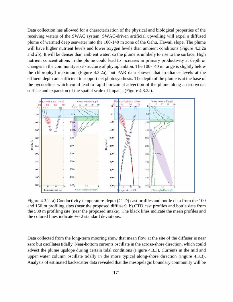
171

Data collection has allowed for a characterization of the physical and biological properties of the

receiving waters of the SWAC system. SWAC-driven artificial upwelling will expel a diffused

plume of warmed deep seawater into the 100-140 m zone of the Oahu, Hawaii slope. The plume

will have higher nutrient levels and lower oxygen levels than ambient conditions (Figure 4.3.2a

and 2b). It will be denser than ambient water, so the plume is unlikely to rise to the surface. High

nutrient concentrations in the plume could lead to increases in primary productivity at depth or

changes in the community size structure of phytoplankton. The 100-140 m range is slightly below

the chlorophyll maximum (Figure 4.3.2a), but PAR data showed that irradiance levels at the

effluent depth are sufficient to support net photosynthesis. The depth of the plume is at the base of

the pycnocline, which could lead to rapid horizontal advection of the plume along an isopycnal

surface and expansion of the spatial scale of impacts (Figure 4.3.2a).

Figure 4.3.2. a) Conductivity-temperature-depth (CTD) cast profiles and bottle data from the 100

and 150 m profiling sites (near the proposed diffuser). b) CTD cast profiles and bottle data from

the 500 m profiling site (near the proposed intake). The black lines indicate the mean profiles and

the colored lines indicate +/- 2 standard deviations.

Data collected from the long-term mooring show that mean flow at the site of the diffuser is near

zero but oscillates tidally. Near-bottom currents oscillate in the across-shore direction, which could

advect the plume upslope during certain tidal conditions (Figure 4.3.3). Currents in the mid and

upper water column oscillate tidally in the more typical along-shore direction (Figure 4.3.3).

Analysis of estimated backscatter data revealed that the mesopelagic boundary community will be

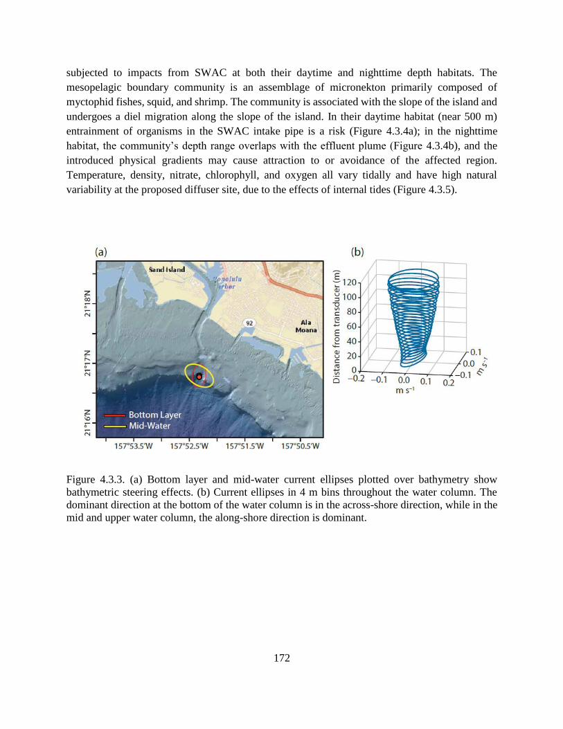
172

subjected to impacts from SWAC at both their daytime and nighttime depth habitats. The

mesopelagic boundary community is an assemblage of micronekton primarily composed of

myctophid fishes, squid, and shrimp. The community is associated with the slope of the island and

undergoes a diel migration along the slope of the island. In their daytime habitat (near 500 m)

entrainment of organisms in the SWAC intake pipe is a risk (Figure 4.3.4a); in the nighttime

habitat, the community’s depth range overlaps with the effluent plume (Figure 4.3.4b), and the

introduced physical gradients may cause attraction to or avoidance of the affected region.

Temperature, density, nitrate, chlorophyll, and oxygen all vary tidally and have high natural

variability at the proposed diffuser site, due to the effects of internal tides (Figure 4.3.5).

Figure 4.3.3. (a) Bottom layer and mid-water current ellipses plotted over bathymetry show

bathymetric steering effects. (b) Current ellipses in 4 m bins throughout the water column. The

dominant direction at the bottom of the water column is in the across-shore direction, while in the

mid and upper water column, the along-shore direction is dominant.

173

Figure 4.3.4. Contour plots of normalized estimated backscatter (Sv) (scale: 0–1) for a sample 10-

day period. (A) Deployment at bottom depth 120 m, where estimated backscatter was generally

higher at night. (B) Deployment at bottom depth 517 m, where estimated backscatter was generally

higher during the day. (C) Close-up of the bottom layer for two days highlights the diel patterns

(upper panel is from the diffuser monitoring area; lower panel is from the deep intake site).

174

Figure 4.3.5. Temperature-salinity plots showing the variability in density, nitrate, salinity, and

fluorescence observed at the bottom mooring location. Trends are visible in these data, particularly

that nitrate is higher in cooler, fresher water and oxygen and fluorescence are higher in warmer,

higher-salinity water.

Overall, these baseline data provide an understanding of pre-impact conditions at the future SWAC

site. More detail can be found in the publications listed below. Data from the CTD cast cruises is

available at an open-access database

(http://hahana.soest.hawaii.edu/cmoreswac/cmoreswac.html). The deployments of the long-term

oceanographic mooring, water column profiling, and bottle sampling were also partially supported

by APRISES 13 funding (with more information available in publications and the final report on

the HNEI website). Water column profiling and bottle sampling efforts were partially supported

by other funding (NSF, Gordon and Betty Moore Foundation).

Publications and Presentations

Peer Reviewed Publications

Comfort, C. M., McManus, M. A., Clark, S. J., Karl, D. M., & Ostrander, C. E. (2015).

Environmental properties of coastal waters in Mamala bay, Oahu, Hawaii, at the future site of a

seawater air conditioning outfall. Oceanography, 28(2), 230-239.

175

Contributed Presentations and Posters

Comfort, C.M., Ostrander, C.E., McManus, M.A., Karl, D.M., Luther, D., Vega, L (2013).

Observing ocean changes at the nation’s first SWAC system. OTEC Symposium, Honolulu, HI

Comfort, C.M., Ostrander, C.E., McManus, M.A., Karl, D.M., Luther, D (2014). Monitoring ocean

changes in response to seawater air conditioning in Honolulu, HI. Ocean Sciences, Honolulu, HI

Comfort, C.M., Ostrander, C.E., McManus, M.A., Karl, D.M. (2016). Understanding the impact

of coastal renewable energy technology on the marine environment. MARES Conference, Olhão,

Portugal.

Comfort, C.M., McManus, M.A., Karl, D.K., Merrifield, M., Ostrander, C.E. (2017). Changes in

potential environmental impacts of seawater air conditioning under future climate scenarios.

ASLO, Honolulu, HI.

Smith, K.A., Comfort, C.M., McManus, M.A., Neuheimer, A.B., Sevadjian, J., Ostrander, C.

(2017). Observations of the mesopelagic micronekton boundary community’s diel migration at

Oʻahu, Hawaiʻi based on backscatter data. ASLO, Honolulu, HI. (Poster)

TASK 5: GEOTHERMAL RESOURCE ASSESSMENT

Funding for this task 5 was reallocated to other areas of the program as approved by ONR, as a

result of the unforeseen loss of key geothermal faculty.

TASK 6: MICROGRIDS/GRID INTEGRATION

6.1 Solar Monitoring

PV performance testing and analysis conducted under APRISES11 and 13 were expanded under

APRISES12 with the further development of an empirical model to characterize the impact of

irradiation, ambient temperature, wind speed, soiling, shading, and aging. While previous efforts

focused on the DC performance of individual PV modules, APRISES12 provides an analysis of

176

the AC performance of PV systems using various PV technologies, system configurations, and

power conditioning units (PCUs). This report also describes work done to finalize another analysis

tool developed to characterize the impact of shading at cell level, and provides results on the

shading tolerance of PV systems and modules.

Results of this work indicate that the most important factor in PV energy production is module

technology, with up to a 10% difference between the tested technologies and manufacturers.

Shading was found to be the next most important parameter, followed by aging and system

configuration, then soiling, and lastly the environmental conditions as tested.

The existing HNEI PV test beds were used, primarily the test bed at Maui Economic Development

Board (MEDB), that was commissioned in February 2016 in Kihei, Maui (under previous

funding). This test platform consists of 15 grid-connected PV systems using 10 types of PV

modules and 3 system architectures using either microinverters, string inverters, or optimizers. The

tested PV technologies include 4 standard p-type crystalline (1 mono and 3 polycrystalline), 3 high

efficiency n-type monocrystalline (1 with a heterojunction intrinsic thin layer, 1 with rear contacts,

and 1 bifacial), and 3 thin-films (2 Copper Indium Gallium Selenide (CIGS), and 1 Cadmium

Telluride (CdTe)). All modules are mounted on a carport with 20o tilt and 197oN azimuth. The

PCUs in test at MEDB include a 2 kW high frequency string inverters, a 3 kW string inverter

especially designed to operate with optimizers, microinverters from 2 different manufacturers, and

add-on optimizers i.e. designed to operate with regular string inverters.

Numerous sensors were installed on the MEDB test platform to monitor environmental parameters

and PV performance including a reference (secondary standard) thermopile pyranometer, a

weather station, and an AC power meter. The equipment was recalibrated once a year, with the

latest calibration completed in early June 2018. Testing, hardware, and DC analysis are described

under previous reports (including final technical reports for APRISES11 and APRISES13, as well

as USDOE Hawaii Distributed Energy Resource Technologies for Energy Security (DE-FC26-

06NT42847, DE-EE0003507).

Daily performance is commonly evaluated using the performance ratio (PR), defined by the

International Electrotechnical Commission (IEC) 61724 [1]. PR is the operating performance of a

PV system corresponding to the daily average efficiency relative to the datasheet specifications

defined at standard test conditions (STC). In the following, the AC performance is analyzed using

PRAC (Equation 1).

Equation 1

𝑃𝑅𝐴𝐶 =∫ 𝑃𝐴𝐶⋅𝑑𝑡

𝛥𝑡

𝑃𝑀𝑃,𝑆𝑇𝐶×

𝐺𝑆𝑇𝐶

∫ 𝐺⋅𝑑𝑡𝛥𝑡

,

177

where PAC is the AC power of the PV system [W]; GSTC is the STC irradiance [=1 kWm-2]; Δt is

the period of analysis [hour]; PMP,STC is the power [W] of the maximum power point at STC.

An empirical model, introduced in APRISES13, was developed to estimate the impact of the

parameters including irradiation (IRR), ambient temperature (AT), and soiling. Soiling impact was

correlated to the number of cumulative days without rainfall that is called in the following, duration

of dry period (DDP). The present model (Equation 2) was improved and takes into account

additional parameters: wind speed (WS), and aging or degradation.

Equation 2

𝑃𝑅𝐴𝐶 = 𝑃𝑅𝐴𝐶,𝑂 + 𝑘𝐼𝑅𝑅 × 𝐼𝑅𝑅 + 𝑘𝐴𝑇 × 𝐴𝑇 + 𝑘𝑊𝑆 × 𝑊𝑆 + 𝑘𝐷𝐷𝑃 × 𝐷𝐷𝑃 + 𝑘𝐴𝐺𝐸 × 𝐴𝐺𝐸

where 𝑃𝑅𝐴𝐶,𝑂 is the constant term in the fit; 𝑘𝐼𝑅𝑅, 𝑘𝐴𝑇, 𝑘𝑊𝑆, 𝑘𝐷𝐷𝑃, and 𝑘𝐴𝐺𝐸 are the weight or

impact of each parameter on the performance.

Due to new structures built on the neighboring property that shade a portion of the PV system,

periods of operation with shading were removed from the dataset before determining the model

coefficients with least-square linear regression. (Shading impacts are further addressed later in

this report, under the Cell-Level Shadow Detection Tool.) The dataset was also adjusted to include

only the days with irradiation above 2 kWhm-2 due to significant changes in performance in

overcast conditions. In such environmental conditions, the PV module performance increases

slightly [2], [3], and the inverter efficiency drastically decreases due to operation at a low power

ratio. Overcast days with IRR below 2 kWhm-2 account for 5% of the total number of analyzed

days (791 days) but only 1% of the total solar energy.

Figure 6.1.1 shows the daily values of the main parameters of PRAC including IRR, AT, WS, and

DDP during the full period of recording from April 4th, 2016 to September 5th, 2018. (Data is

missing in March-May 2018 due to issues with data recording and internet connection loss.) The

daily irradiation averaged 5.5±1.2 kWhm-2. Daytime temperature averaged 27.8±2.2oC with highs

in September and lows in January-February. Wind speed averaged is 2.5±0.9 ms-1. Dry periods

were usually less than 30 days in length, with exceptions up to a 77-day dry period from September

to December 2016.

178

Figure 6.1.1: Daily average values of the main PV parameters from April 2016 to early September

2018 at MEDB: irradiation (IRR), ambient temperature (AT), wind speed (WS) and duration of

dry period (DDP).

The daily performance of 11 PV systems during the 29 months of operation is shown in Figure

6.1.2. Four of the 15 PV systems in test at MEDB consist of 2 modules each, grid-connected with

microinverters. No AC measurement was collected on these systems. For all PV systems, PRAC is

estimated between 0.8 and 0.95 in April 2016, and generally decreases overtime with values

between 0.74 and 0.86 in early September 2018. Systems were off during summer 2017. Despite

a relatively constant variation during the 29 months of operation, PRAC exhibits important drops

during winter with lowest values around solstices. This is the effect of shading that, as mentioned

earlier, started affecting the PV platform in January 2017. The drop of performance in December

2016 is related to an overcast period.

179

Figure 6.1.2: AC PV performance ratio (PRAC) of 11 PV systems tested at MEDB during 29

months. The legend shows the acronym for each PV system, starting with a letter indicating the

PV technology (C for the CIGS thin-film, D for the CdTe thin-film, H for the high efficiency

crystalline, S for standard crystalline), followed by a digit to differentiate the manufacturers, and

last a letter indicating the system configuration (S for string inverter, O for string inverter with

optimizers, M for microinverter).

Figure 6.1.3 shows PRAC as a function of IRR plotting only the days without significant shading

(so January to March 2017, and September 2017 to March 2018 were removed). As mentioned

above, the performance of the systems decreases for IRR below 2 kWhm-2 except for the

microinverter system S3M. Thin film C1S system exhibits lower performance than the other

systems for IRR below 4 kWhm-2. Lower performance of C1S is related to lower performance of

the PV modules at low IRR compared to other modules [4]. It is also due to the low inverter loading

ratio with only 1.4 kW PV for a 2 kW inverter.

180

Figure 6.1.3: PRAC of 11 PV systems as a function of IRR (dataset from April 2016 to early

September 2018 excluding periods of shading).

Figure 6.1.4 compares the measured and estimated PRAC for a PV system (H1S). The data and

model are correlated except during the winter when the system performance drops due to shading.

The mean relative error (MRE) between data and model results is between 1.0% and 1.6% for

most systems, and 2.2% for C1S. In comparison, the few previous models for daily energy [5], [6]

obtained MRE below 5%. As indicated in the textbox of Figure 6.1.4, the average daily energy

production during the 29 months is measured at 4.3 kWhm-2 while the model estimated 4.6

kWhm-2. The difference between measured and estimated energy production is allocated to the

impact of shading. For this system, energy loss due to shading is estimated at 5% of the actual PV

production.

181

Figure 6.1.4: Measured and modelled PRAC of the PV system H1S during 29 months of operation.

Figure 6.1.5 presents the average performance of the PV systems including the measured and

simulated values, the latter providing an estimated PRAC without the impact of shading. PRAC is

measured between 78% and 85%. Without shading, the system performance would be between

79% and 89%. Different system configurations were tested on the crystalline systems. For both

data and model results, the microinverter systems are most efficient at the site followed by the

string inverters and then, the string inverters with optimizers.

182

Figure 6.1.5: Average PRAC of the 11 PV systems at MEDB from April 2016 to early September

2018.

Figure 6.1.6 shows the estimated PRAC as a function of irradiation for the 11 PV systems at the

beginning of the analyzed period (April 4th, 2016) operating at mean values of the environmental

conditions (AT, WS) and without soiling.

Table 6.1.1 describes the model coefficients providing the impact of the parameters. The following

was observed:

IRR has low impact on the performance of most systems except for C1S exhibiting an

increase of PRAC with increasing IRR, and for S3M with much higher performance in

overcast conditions than on sunny days (as already seen in Figure 6.1.3). C2S and D1S

exhibit the highest PRAC at all IRR level. The next best system is H1S with constant PRAC

as a function of IRR except below 3 kWhm-2 when S3M has a higher PRAC.

AT impact is mostly negative, meaning higher performance in cooler conditions. Positive

impact on D1S could be related to the spectral energy increasing in summer similarly to

AT. High coefficient for C1S is arguable and is allocated for now to the distribution of the

dataset for this system leading to a less accurate model as seen on the MRE.

WS has a cooling effect on the PV systems leading improved performance in windy

conditions. The difference in coefficients between systems is attributed to the location of

the system on the carport i.e. distance from the wind sensor and from a nearby building.

Soiling impact varies between 0.03% and 0.11% per day. Difference between PV systems

could also be related to the system location. Systems more sensitive to WS are also more

sensitive to soiling. These systems are located on the east side of the carport near a dusty

field. The nearby building that obstructs the Trade wind would reduce the impact of soiling

and wind speed on the high efficiency PV systems located on the west side of the platform.

183

Aging is estimated between 1.4% and 3.4% per year which is above of the typically

warrantied degradation of ~1% per year. Microinverter systems exhibit lower degradation

than string and optimizer ones.

Figure 6.1.6: PRAC as a function of IRR for 11 PV systems at the beginning of the analyzed period

(April 4th, 2016) operating at mean values of the environmental conditions (AT, WS), and without

soiling. Empirical model presented in equation (2) fitted to the first 29 months of operation

excluding the periods of shading.

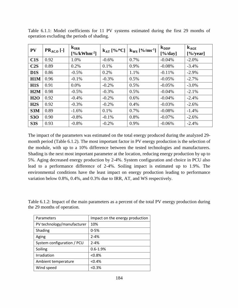
184

Table 6.1.1: Model coefficients for 11 PV systems estimated during the first 29 months of

operation excluding the periods of shading.

PV 𝐏𝐑𝐀𝐂,𝐎 [-] 𝐤𝐈𝐑𝐑

[%/kWhm-2] 𝐤𝐀𝐓 [%/oC] 𝐤𝐖𝐒 [%/ms-1]

𝐤𝐃𝐃𝐏

[%/day]

𝐤𝐀𝐆𝐄

[%/year]

C1S 0.92 1.0% -0.6% 0.7% -0.04% -2.0%

C2S 0.89 0.2% 0.1% 0.9% -0.08% -3.4%

D1S 0.86 -0.5% 0.2% 1.1% -0.11% -2.9%

H1M 0.96 -0.1% -0.3% 0.5% -0.05% -2.7%

H1S 0.91 0.0% -0.2% 0.5% -0.05% -3.0%

H2M 0.98 -0.5% -0.3% 0.5% -0.04% -2.1%

H2O 0.92 -0.4% -0.2% 0.6% -0.04% -2.4%

H2S 0.92 -0.3% -0.2% 0.4% -0.03% -2.6%

S3M 0.89 -1.6% 0.1% 0.7% -0.08% -1.4%

S3O 0.90 -0.8% -0.1% 0.8% -0.07% -2.6%

S3S 0.93 -0.8% -0.2% 0.9% -0.06% -2.4%

The impact of the parameters was estimated on the total energy produced during the analyzed 29-

month period (Table 6.1.2). The most important factor in PV energy production is the selection of

the module, with up to a 10% difference between the tested technologies and manufacturers.

Shading is the next most important parameter at the location, reducing energy production by up to

5%. Aging decreased energy production by 2-4%. System configuration and choice in PCU also

lead to a performance difference of 2-4%. Soiling impact is estimated up to 1.9%. The

environmental conditions have the least impact on energy production leading to performance

variation below 0.8%, 0.4%, and 0.3% due to IRR, AT, and WS respectively.

Table 6.1.2: Impact of the main parameters as a percent of the total PV energy production during

the 29 months of operation.

Parameters Impact on the energy production

PV technology/manufacturer 10%

Shading 0-5%

Aging 2-4%

System configuration / PCU 2-4%

Soiling 0.6-1.9%

Irradiation <0.8%

Ambient temperature <0.4%

Wind speed <0.3%

185

Conclusions

An empirical model was developed to predict the daily PV energy production (by

modelling PRAC) with an error below 2.2%. The model accounts for the effect of

irradiation, AT, WS, soiling, and aging. Shading is estimated by comparing the data and

model results.

Using the model fit to the data collected during 29 months of operation, the following is

concluded:

The main parameters are, in decreasing order of importance, the PV

technology/manufacturer, shading, aging, system configuration/PCU, and

soiling. The environmental conditions IRR, AT, and WS lead to minimal

variability of the PV energy production.

The system configuration and the type of PCU have an impact on the

average PV performance as well as on the degradation. Results suggest that

microinverters provide the best system configuration. One type of

microinverter improved the performance in overcast conditions,

recommending it for overcast locations.

Long term assessment at MEDB is essential to evaluate if the high estimated degradation

(1.4%-3.4% per year) is related to the early stage of the PV system operation.

Shadow Analysis

As mentioned earlier, shading is an important performance parameter of the PV systems at MEDB.

To understand the impact of shading on the performance of the PV modules and systems, the

shadow shape needs to be characterized at module and cell level. Different solutions to characterize

shadow shape were identified and described in the APRISES13 final report. Image-based shadow

detection was chosen for APRISES12 work because of spatial resolution, cost, and development

time. Three wireless cameras were installed February 2018 on the structures that shade the PV

platform. Shadow detection algorithms were finalized under this subtask using Matlab software.

The algorithms and collected photographs were used to evaluate the number of cells shaded per

module and the percentage area of shadow on each cell. The goal was to evaluate the relationship

between the shadow coverage and the performance of the PV modules and systems. Preliminary

results are presented following a short description of the necessary steps for shading analysis.

The method employed included image processing, shadow detection and characterization, and is

outlined as follows.

Image processing: The pictures from the 3 cameras taken at a 1-minute sample rate were corrected

for lens distortion and perspective, and then stitched together in order to provide an overhead view

of the PV carport as seen in Figure 6.1.7.

186

Two images were created to identify each module and cell on the overhead view. The first image

(Module ID Mask) identifies the general area of the modules, including the frame. The second

image (Cell ID Mask) locates the cells within each module. Cell identification was ineffective for

all 3 types of thin film modules due to their plain dark appearance as visible in Figure 6.1.7d).

a) b) c)

⇩

d)

Figure 6.1.7: Converting the 3 raw camera images (a, b, c) to an d) overhead image.

Shadow Detection: A shadow mask (Figure 6.1.8) was created by first thresholding on a black-

and-white image created from the Red-Green-Blue (RGB) overhead image. After thresholding,

erosion and dilation was applied to fill in the gaps and remove noise from the image.

187

Figure 6.1.8: Shadow mask image created from the overhead image.

Shadow Characterization: The final step was to create a table containing the estimated ratio of

the area covered by shaded cells. The columns represent the module ID, cell ID, and ratio of area

covered in that cell (0-1). To accelerate calculation of the cell shadow ratio, selected cells were

analyzed. The shadow mask was first intersected with the module ID mask to find modules with

shadows on them. Any module that has more than 0.05% of its area covered with shadow is then

analyzed at the cell level.

Important information will be provided with the Cell-Level Shadow Analysis tool as soon as more

data are available. Since the cameras were installed at the end of February 2018, only a few days

suffered from shading affecting the platform from September to March (as seen in Figure 6.1.2).

The following presents preliminary results obtained using the Shadow Detection Tool. Starting

with an analysis at system level, the second part compares the shading tolerance between

individual PV modules.

Figure 6.1.9 and Figure 6.1.10 show the correlation between the Shadow Ratio and PRAC

comparing 2 systems with different system configurations (H1M and H1S) on February 27th, 2018.

Figure 6.1.9 displays PRAC, the Shadow Ratio (% of shaded area per system), and the Shadow

Module Ratio (% of shaded modules per system). Maximum shading occurs around 4:20PM as

seen on the Shadow Ratio similar for both PV systems. Despite a relatively low Shadow Ratio (<

0.1), only one or 2 modules per system are shaded as indicated by the Shadow Module ratio (with

8 modules total per system). This is detrimental for H1S performance, which exhibits an important

drop in PRAC as soon as the Shadow Ratio becomes significant, which occurs around 3:40PM.

PRAC of H1M however barely shows any impact of shading. Figure 6.1.10 shows PRAC as a

function of the Shadow Ratio. The correlation between PRAC and Shadow Ratio is exponential for

the string configuration and linear for the microinverter system.

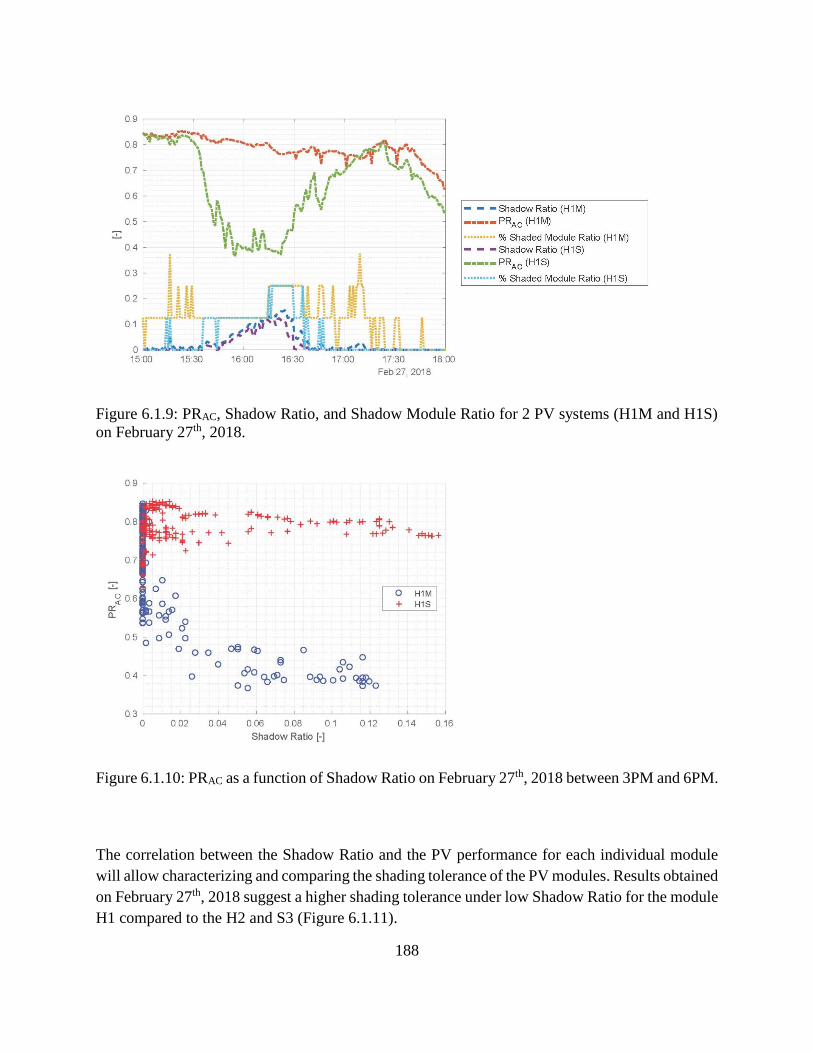
188

Figure 6.1.9: PRAC, Shadow Ratio, and Shadow Module Ratio for 2 PV systems (H1M and H1S)

on February 27th, 2018.

Figure 6.1.10: PRAC as a function of Shadow Ratio on February 27th, 2018 between 3PM and 6PM.

The correlation between the Shadow Ratio and the PV performance for each individual module

will allow characterizing and comparing the shading tolerance of the PV modules. Results obtained

on February 27th, 2018 suggest a higher shading tolerance under low Shadow Ratio for the module

H1 compared to the H2 and S3 (Figure 6.1.11).

189

Figure 6.1.11: PRDC of the modules H1, H2, and S3 as a function of Shadow Ratio on February

27th, 2018 between 3PM and 6PM.

Conclusions

A Cell-Level Shadow Detection Tool was developed to characterize the modules and cells affected

by shading using an inexpensive monitoring system (web cameras) and a Matlab analysis tool.

Further analysis will provide a better understanding of the impact of shading on the PV

performance by determining the shading tolerance of the PV modules and systems. Under other

funding, development and analysis will be continued to further characterize the PV performance

and the impact of all parameters including shading. Plans include completing and submitting 4

journal papers drafted under APRISES12 to peer reviewed Energy and Measurement journals.

References

[1] “IEC 61724-1 - Photovoltaic system performance – Part 1: Monitoring IEC,” IEC Stand.,

no. 1.0, 2017.

[2] HNEI Report, “Final Technical Report of the Office of Naval Research Asia Pacific

Research Initiative for Sustainable Energy Systems (N00014-12-1-0496), Subtask 6.1.

Solar Hydrogen at Marine Corps Base Hawai`i,” 2017.

[3] S. Busquet and J. Kobayashi, “Modelling daily PV performance as a function of irradiation,

ambient temperature, soiling, wind speed, and aging – Applied to PV modules operating in

Maui.,” in 7th World Conference on Photovoltaic Energy Conversion, 2018.

[4] S. Busquet, J. Kobayashi, and R. E. Rocheleau, “Daily Performance Comparison of PV

190

modules Operating in Maui,” in 33rd European Photovoltaic Solar Energy Conference and

Exhibition, 2017, pp. 2311–2315.

[5] E. L. Meyer and E. Ernest van Dyk, “The effect of reduced shunt resistance and shading on

photovoltaic module performance,” Conf. Rec. Thirty-first IEEE Photovolt. Spec. Conf.

2005., pp. 1331–1334.

[6] C. Cañete, J. Carretero, and M. Sidrach-de-Cardona, “Energy performance of different

photovoltaic module technologies under outdoor conditions,” Energy, vol. 65, pp. 295–302,

2014.

6.2 Secure Micro-grids

6.2a Molokai Load Bank

An analysis was conducted to estimate the impact of connecting a Load Bank to the Molokai Island

microgrid, in order to overcome the grid constraint and increase the amount of Distributed PV

generation (DG PV) that can be connected and utilized by the grid. An agreement was executed

with the utility, Maui Electric Co., to collaborate on the integration of the Load Bank, including

algorithm and control development, and data sharing.

Molokai Island has approximately 2,144 kW of DG PV on the Molokai grid, and there is 133 kW

of DG PV approved for interconnection, as well as a 100 kW hydro project that is also approved

for interconnection. In addition, there is another 665 kW of DG PV in an interconnection queue

pending an increase in the hosting capacity of the grid. In total, there is 3,042 kW of DG installed,

approved or nearly approved or in the queue on the Molokai system which has a minimum daytime

load of approximately 3,700 kW. In March 2015, Maui Electric Co. started informing customers

that the Molokai grid was nearing system-level constraints to further interconnection of DG, and

since that time most interconnection requests have been delayed pending near-term solutions to

address the grid constraint.

Figure 6.2a.1 illustrates the primary near-term system-level constraint of energy oversupply during

periods of low demand and high PV output. If the net load (load – DG PV) falls below the

minimum generation level of 1,300 kW, the system will not meet its downward regulating reserve

requirement to deal with sudden load losses due to system faults. The dark brown line in Figure

6.2a.1 shows that the net load in 2015 was close to the minimum generation for the system and as

such, the system was not able to accept more PV capacity unless the PV system has the ability to

reduce its output if the net load falls below 1,300 kW, i.e. unless the PV system is “curtailable”.

191

Figure 6.2a.1: Projected System-Level Hosting Capacity on Molokai Source: E3 Interconnection

Potential Analysis – Molokai, October 8, 2015.

Under future funding, a Load Bank will be used to analyze its performance and effectiveness as

an energy safety valve to provide a near-term solution for interconnection and a longer-term grid

management asset for a small (microgrid scale) grid. In this application, the Load Bank adds load

to the Molokai system, using secure communications within the power plant, when needed as a

near-term solution to balance the grid during infrequent periods of excess energy supplied to the

grid. While this excess energy would be literally burned off as heat, it would enable the

interconnection of all 665 kW of DG PV in the queue which would result in a significant increase

overall in renewable energy on the grid, and a relatively small amount of excess energy burned off

per year.

Figure 6.2a.2 shows an analysis using hourly system load data from 2009 for Molokai. In 2009

there was only a negligible amount of DG PV on the system, and since then the system load has

not experienced much growth. The calculated 2,942 kW of DG PV (2,144 kW installed, 133 kW

of DG PV approved for installation and 665 kW in the queue) and 100KW of hydro production

was subtracted from the 2009 load data to generate the net load profile vs. the minimum generation

limit in Figure 6.2a.2. This analysis shows that with the additional DG PV generation, an

additional 1,106 MWh of energy can be utilized from the 665kW of DG PV while only passing

approximately 4 MWh of excess energy through the Load Bank.

192

Figure 6.2a.2: Molokai Generation Profile.

Figure 6.2a.3 shows a bar chart that provides a graphical representation of the additional energy

that would be utilized by the grid and the excess energy produced if the 665 kW of DG PV in the

queue were added to the grid given the 2009 load profile.

193

Figure 6.2a.3: Additional renewable energy (RE) from Distributed PV generation (DG PV) in the

Queue – 2009 load data.

The ASCO 4800 750KVA resistive Load Bank and step up transformer, shown in Figure 6.2a.4,

were installed and commissioned by the utility at the Palaau Power Station on Molokai. The Load

Bank, that is owned by the utility, is currently manually controlled by the System Operator through

the SCADA network at the power station.

194

Figure 6.2a.4: Installed Load Bank and step-up transformer.

Using APRISES 14, HNEI will work in collaboration with the utility to design and test automated

algorithms and controls to automate the Load Bank’s primary use case of managing excess DG

PV energy on the grid. HNEI will also instigate additional system benefits that the Load Bank can

support beyond the management of excess DG PV energy by developing additional uses cases and

test plans. Once the uses cases are finalized with the utility, HNEI will develop a control and

monitoring system for the Load Bank that will automate the use case functions with the goal of

improving the efficiency of the system as compared to its current manual operation.

6.2b Coconut Island DC Microgrid

The objective of this project is to demonstrate the performance and resilience of a DC microgrid

designed to serve the loads within two buildings on Coconut Island, off the Island of Oahu, and to

provide the island with clean electrified transportation options primarily powered by the sun.

Following the planning, data gathering, energy modeling, component sizing and procurement of

the swappable battery system and electric E-car and E-boat under APRISES11 and 13, the

procurement and implementation phase of the project was continued under APRISES 12. Under

APRISES 12, HNEI completed the conversion of the E-boat to an all-electric vehicle that works

with the swappable battery system, and installed the battery charging station for the swappable

battery system in the Boat House on Coconut Island.

195

When complete, the Coconut Island DC Microgrid Project will integrate a DC distribution system

into two buildings on the island, the Marine Mammal Research Project (MMRP) building and the

Boat House (See Figure 6.2b.1). These two buildings are currently served by one of the utility

owned transformers on the island. This project is made possible by funding from previous

APRISES awards (APRISES11 and 13), the current APRISES12, and future APRISES14 funding.

Coconut Island (Moku O Loe) is a 28-acre (113,000 m²) island in Kaneohe Bay off the island of

Oahu that is home to the Hawaii Institute of Marine Biology (HIMB) of the University of Hawaii.

It is an ideal site for a technology-based test bed since it is representative of a tropical marine

environment in an isolated location with critical power needs, and one of the goals established for

the island is to become a model for sustainable living systems. The island is exposed to persistent

trade winds and salt spray resulting in a highly corrosive environment for material and technology

testing in micro-climates representative of those that would potentially be encountered by coastal

installations.

(a) (b)

Figure 6.2b.1: a) Coconut Island, b) DC/AC microgrid project site.

The objective of this project is to demonstrate the performance and resilience of a DC microgrid

designed to serve the loads within two buildings on Coconut Island and provide the island with

clean electrified transportation options primarily powered by the sun. The project has the

following goals:

196

Demonstrate innovative new clean energy technologies

Economically minimize the energy purchased from the utility

Provide a research platform to study DC microgrid resources and loads, e.g. energy

storage and supporting technology and DC power appliances, in a tropical coastal

environment

Increase the energy sustainability of the island

Provide solar electric powered transportation for HIMB

The proposed DC microgrid design described in the APRISES 13 final report utilized a 380V DC

bus as the backbone of the DC microgrid. Following the filing of that report, HNEI issued two

requests for proposals, one to install the PV and battery energy storage system (BESS) and another

to integrate those resources with the fully functioning microgrid.

Unfortunately, the single bid received for the PV and BESS systems was unreasonably high and

there were no bids received for the microgrid implementation and integration work. The issue is

that 380V DC systems are not common in Hawaii and the uncertainty risk is causing high prices

or no bids on requests for proposals. As a result, the HNEI project team decided to revise the

scope of the project to utilize a more common 48V bus that would allow the use of 48V equipment

and control systems that are more widely available and implemented locally. The system is not as

expandable as with the 380V bus, but while expandability is desirable it is not critical to the meet

the goals of the project.

Some of the key components of the system for the revised project scope include components shown

in Figure 6.2b.2 and described below:

1) PV modules installed on MMRP roof as the primary source of energy for the microgrid.

The PV size is approximately 20 kW DC which is the maximum capacity allowed by the

roof space of the MMRP.

2) A Stationary BESS (between at 24 kWh and 32 kWh of usable energy with minimum 12

kW power) used to store excess PV energy and export that energy to minimize the use of

grid power by the DC microgrid during normal operation, and to keep the DC microgrid

system operational during utility grid outages.

3) A unidirectional 30 kW rectifier that provides power to the 48 Vdc bus from the grid (3

phase, 120V/208V GrdY) when there is insufficient energy available within the microgrid,

and to prevent back feeding power to the grid.

4) Power Monitor Unit (PMU) that can be used to control the microgrid components as

needed and produce operational information including local dashboards displaying DC

microgrid information and performance.

197

5) Inverter(s) with a capacity appropriate to supply the AC loads (Computers and Wi-Fi

network) within the MMRP buildings to be powered by the DC microgrid.

6) DC lighting and controls in the MMRP buildings that meet applicable office lighting

standards.

7) DC powered air conditioning to take the place of all but one of the existing AC powered

air conditioning units. (The existing AC powered units will remain in place for possible

future use.) The remaining existing air conditioner in the standalone office will be used as

a point of comparison with the DC air conditioners.

8) Swappable battery system, designed and manufactured by PUES Corporation in Okinawa

Japan (“PUES”), will charge the swappable batteries used in the electric vehicles (E-boat

and E-car) and portable power “suitcase battery” system. This station is capable of charging

twelve (12) batteries through the DC Bus with a capacity of 1.4 KW and 1.4 KWh each.

9) A 48 Vdc bus that transmits power between energy resources (PV, BESS, Rectifier) and

loads (Lighting, Air conditioning, Inverters for AC loads, and Swappable Battery System)

within the microgrid.

Figure 6.2b.2: DC microgrid description.

198

HNEI purchased two vehicles, along with the components of an associated charging station,

swappable batteries and two portable suit case battery enclosures, under APRISES 13. The

vehicles included a pontoon boat (the E-boat) and an electric powered John Deere Gator (the E-

car) modified to utilize the swappable batteries. As noted above, the battery charging station

installed in the Boat House during APRISES12 is currently powered from the grid until the PV

system and stationary battery are installed.

The Okinawa Institute of Science and Technology (OIST) and PUES, who are partners on this

project and part of the Hawaii-Okinawa Clean Energy Partnership between the U.S. Department

of Energy and the Ministry of Economy Trade and Industry of Japan, developed the swappable

battery system. PUES and OIST used funds from the Government of Japan to develop and test the

first version of the swappable battery system and vehicle. Photographs of this initial design are

shown in Figure 6.2b.3. Under APRISES 13, PUES and OIST consulted with HNEI to improve

this initial design and develop the next version of the system to be tested at OIST, and on Coconut

Island by HNEI.

Figure 6.2b.3: Version 1 of the PUES Swappable Battery System at Okinawa Institute of Science

and Technology (OIST).

The swappable battery charging station that was installed consists of two parts, 1) the battery

charging control system and 2) twelve battery receptacles. A schematic of the swappable battery

charging station is shown in Figure 6.2b.4 where the control system is shown in blue and the

receptacles are shown in green. The completed installation of the charging station in the Boat

House is shown in Figure 6.2b.5.

199

Figure 6.2b.4: Schematic of Battery Charging Station.

200

Figure 6.2b.5: Battery Charging Station: Battery receptacles on the left (in the grey enclosure) with

the portable suitcase battery shown in front of the receptacles, and the battery charging control

system on the right.

As noted above, the E-boat gas powered system was replaced with an all-electric battery powered

system. These modifications included replacing the gas engine of the boat with a Torqeedo electric

motor, adding two sets of four swappable batteries along with their receptacles and adding a control

system to manage the charging of the batteries from four PV panels installed on the boat canopy.

Under APRISES 12, the electric power system was installed, tested, and made operational. The E-

boat with the Torqeedo motor and charging control system are shown in Figure 6.2b.6. Under

APRISES 14, the E-boat is undergoing final preparations and will soon be ready for delivery to

the project site for testing.

201

Figure 6.2b.6: E-boat with Torqeedo Electric motor and charging control system.

With the installation of the charging station, the E-car is now operational and being used by HIMB

on Coconut Island. The E-car used an electric John Deere Gator that was modified to utilize a

swappable battery system to power the car and along with a state of charge (SOC) monitor for the

swappable batteries. Figure 6.2b.7 shows added battery receptacles and SOC monitor.

Figure 6.2b.7: Modified John Deere Gator E-car, with battery receptacles (left) and SOC monitor

(right).

202

Implementation of the detailed design and DC microgrid, along with demonstration, testing and

evaluation of the DC microgrid and electric vehicles will be completed using APRISES 14

funding. Additionally, HNEI is revising and simplifying the scope of work for this ongoing

APRISES project, and will issue a new request for proposals for the installation of the 48V DC

microgrid. Under future funding awards, HNEI will test and evaluate the efficiency and resiliency

of the DC microgrid and characterize its benefits and limitations.

6.2c Grid Scale Energy Storage

Analyses were conducted on a grid-connected Battery Energy Storage System (BESS) on the

Hawaiian Island of Molokai, to better understand the BESS response to faults and other significant

events on the grid. Additionally, a control algorithm was developed to better understand the

interactions between the BESS response and the conventional generation, and to enable analysis

of the impact of the BESS.

The procurement, installation and commissioning of a 2MW, 397kW-Hr BESS on Molokai was

completed under previous HEET and APRISES awards. Analysis work on the Molokai BESS was

continued under APRISES 12. This included analyses of faults and other significant events on the

grid. The BESS consistently responded appropriately to most grid contingencies but responded

unpredictably for short periods (1-2 cycles) during faults (short circuits) on the grid. An example

of this is shown in Figure 6.2c.1.

203

Figure 6.2c.1 (A) BESS response to a fault: full view of synchrophasor data. Blue line indicates

grid frequency and is aligned with the left axis. Green line indicates simultaneous BESS response

and is aligned with the axis on the right. (B) This expansion includes an approximate ideal BESS

response as a black dashed line.

Figure 6.2c.1 (A) shows the grid frequency and the BESS response (limited to 500kW) for 80

seconds of time. Figure 6.2c.1 (B) is an expansion near 9.8 seconds after the start of the data

capture window where the frequency is under 60Hz due to a fault. The black dash in the bottom

plot of Figure 6.2c.1 (B) approximates the ideal BESS response to an under-frequency event. The

green trace shows that the BESS was (1) muted during the fault and (2) swung rapidly up and

down away from the ideal response. It is possible that the meter feeding the BESS inverter is

calculating frequency incorrectly because the grid voltages are unstable during faults.

204

Outside of APRISES 12, discussions are currently underway to address these problems (e.g., by

incorporating a rate limiter within the inverter logic). Discussions are also underway about

increasing the BESS authority from the current level of 500kW to 750kW. It was previously

determined (under APRISES 13) that increasing the authority also increases the amplitude of the

rapid power swings. However, since the swings are short-lived and generally in the right direction

(exporting during under voltage periods), they are not expected to worsen the contingencies. That

is, the instantaneous BESS power swings can cause instantaneous frequency changes for 1-2

cycles. However, that is not enough time to trip even the east Molokai circuit, which requires 10

cycles of a large frequency spike.

During APRISES 12, HNEI developed a PSCAD version of the existing Molokai BESS control

algorithm. The motivation for this effort was to take advantage of a currently available Molokai

dynamic grid model, also in PSCAD (developed by HECO) to better understand the interactions

between the BESS response and the conventional generation on the grid. The combination of the

algorithm and the grid model will enable analysis of the impact of the BESS. For example, it

cannot currently be concluded that the BESS has arrested significant grid contingencies. Grid

models (such as load flow) that were previously developed under multiple APRISES awards were

done in simulation environments that run on course time scales. The PSCAD model is capable of

micro-second time steps. Because the BESS is a fast-acting device, this is the type of model that

is needed to understand how it interacts with the Molokai grid.

Future work will require the combination of the control algorithm and the grid model. Aside from

the motivation indicated above, the combination will be required by the utility company to

incorporate future grid enhancements such as:

Addition of a 750kW load bank.

Potential addition of a large battery for a PV farm.

Potential addition of synchronous condenser.

Without the model, the utility company would have required the BESS to deactivate the current

fast-response control algorithm in favor of a more conventional droop-type frequency response

that would require a large dead-band to maintain system stability.

6.2d Power Grid Monitoring and Controls

The overall objective of this multi-year APRISES project was to develop a low-cost real-time

power monitor with wireless communications for distribution system operations, controls, and

analysis. During APRISES12, the power monitor system was enhanced by adding the capability

205

for advanced real-time data analysis and controls. Our approach leverages advances in wireless

communications, smart meter integrated circuits, and open source software to create a fully

integrated device for this application. The device is intended to support HNEI's research and field

demonstrations on the distribution grid as well as to provide a solution that could be

commercialized to help solve grid operational issues with high penetrations of distributed energy

resources (DER) such as photovoltaics (PV). This work on the system led to a second provisional

patent being filed.

Further background on the project is given in the APRISES 11 and 13 reports. Under APRISES

11 funding, we built initial prototypes, established a power monitor test lab with basic tools for

120V AC (alternating current) testing, and offered a junior-level undergraduate engineering

project course. Under APRISES 13, we began prototyping a weatherized version of the device and

offered a senior-level engineering project course focused on software development.

The objective for the project under APRISES 12 funding was to continue developing and refining

the hardware and software of the power monitor system, focusing on adding the capability for

advanced real-time data analysis and controls. Previous versions of the device streamed data of

root mean square (RMS) current, RMS voltage, active and reactive power, and frequency to a

server for archival and post-processing. To provide additional flexibility and support for grid

resiliency, it is desirable to implement an edge computing framework where each device can

perform onboard analytics and controls in a semi-autonomous manner. Thus operation can

continue when communications or the server is compromised, and each device can take actions to

restore normal operations. Towards this end, we replaced the microcontroller in the device with a

field programmable gate array (FPGA) that has significantly more computing power and

flexibility. The FPGA implements logic modules and a soft-core processor that can be completely

reconfigured—both at a software and hardware level—to provide the ultimate platform for

research and development in real-time grid analytics and controls.

Built-in communications was previously limited to 2.4 GHz WiFi and 900 MHz mesh networking.

Under APRISES 12 funding, we identified and integrated a Long Term Evolution (LTE) system-

on-package (SOP) that can offer high-speed commercial data communications over AT&T when

deployed to pole-top locations. This platform will enable many features in the future including

near real-time reporting of raw voltage and current waveforms.

We significantly enhanced the web interface for the device, offering numerous real-time and

historical plots. The website is available at argems.soest.hawaii.edu, with a password provided by

HNEI upon request. Several screenshots of the website are shown in Figure 6.2d.1. We continued

our long-term testing and maintenance of an initial device installed at the Frog 1 net zero energy

building on the UH Manoa campus. This led to numerous reliability enhancements.

206

Figure 6.2d.1: Selected screenshots from power monitor website.

207

HNEI leveraged the power monitoring platform for additional proposals and funding. We

submitted an ARPA-E OPEN 2018 proposal that would utilize the device for applied research in

grid parameter identification and real-time and predictive distributed modeling. We have

responded to reviewer comments and are expecting a decision in October 2018. The device has

also been included in an ONR Department of Defense University Research-to-Adoption (DURA)

project led by Arizona State University (ASU). One device is now operational at ASU, and nine

others will be delivered over the course of the project. The devices will be connected to real-time

controllers to perform conservation voltage reduction (CVR) and provide enhanced microgrid

resiliency.

HNEI filed a second provisional patent on the system June 29, 2018 entitled "Enabling Ubiquitous

Distribution Grid Modeling for Enhanced Visibility and Controls" (#62/692,613). A utility patent

application is expected in November 2018. HNEI conducted meetings with potential research and

commercial partners.

Patents

Provisional Patent #62/692,613, "Enabling Ubiquitous Distribution Grid Modeling for Enhanced

Visibility and Controls", filed on June 29, 2018.

6.2e Conservation Voltage Reduction

Initially funded under APRISES 11, this Conservation Voltage Reduction project led to the

invention of a new patent-pending technology, and we worked closely with Hitachi and IKS to

develop an initial prototype. The prototype performed well during testing, however, the cost and

physical size of the device limited our ability to perform a feeder level field demonstration.

The objective of this project under APRISES 12 was to take this technology to a commercially

feasible prototype. The design approach taken by IKS required large capacitors which are

expensive. Under APRISES 11, we tested the dynamic voltage compensation algorithm using

commercially available inverters. In order for PV inverters to operate, they require DC power

which is typically solar modules. A small DC power supply can emulate a solar module so that

the inverter is able to operate and is not dependent on time of day. Thus, under APRISES12 HNEI

searched the market for a small DC power supply that is capable of “waking up” the inverter. We

acquired the Delta ES 0300-0.45 150W programmable DC power supply.

208

The inverter and DC power supply have been installed at the University of Hawaii Marine Center

based on the electrical diagram as shown in Figure 6.2e.1.

Figure 6.2e.1: Electrical Wiring Schematic.

Initial tests proved that this relatively small DC power supply is able to power the inverter and

thus the technology based on this combination of equipment can be used to produce a cost effective

prototype. Under APRISES14 funding, we are continuing to explore industry partners with the

right expertise to develop a commercially viable prototype.

6.2f Hardware-in-the-loop (HIL) Testing

HNEI acquired and began to set up hardware-in-the-loop (HIL) equipment to test distributed

energy resources (DER) and associated devices. The equipment, shown in Figure 6.2f.1, consists

of an OPAL-RT real-time simulator with high-speed analog interfaces to control a three-phase bi-

directional power amplifier. This setup allows HNEI to mimic real-world grid operation and fault

scenarios in a controlled research setting, bringing a new level of flexibility to our testing and

increasing our confidence in new technology before it is deployed to the grid.

209

Figure 6.2f.1: Real-time grid simulator (left) and power amplifier (right).

This platform can be used in many configurations such as those shown in Figure 6.2f.2. HNEI will

use Configuration 2, (Real-time Simulation with Real and Forecasted PV) to demonstrate

applications of HNEI’s PV forecasting system under DOE funding through the UI-ASSIST project

led by Washington State University (WSU). The Distribution Energy Management System will be

developed and hosted at WSU, while the virtual grid and PV monitoring and forecasting is at

HNEI. HNEI will use Configurations 3 (Controller HIL), 4 (Power HIL), and/or 5 (Power HIL

with System-Controlled DER) to test and validate HNEI’s CVR algorithms and devices.

Configuration 4 will be used with a test profile (instead of a virtual grid) of various voltages, real

and reactive power, and frequencies to validate HNEI’s power monitor.

Under other funding, HNEI is converting detailed models of the Maui Meadows distribution circuit

to run on the simulator, which will enable testing under accurate, realistic scenarios. (More

information on the Maui Meadows project can be found in APRISES11 and 13 final reports.)

HNEI expects that the real-time simulation and HIL equipment will lead to valuable and

productive new projects and collaborations. Under DOE UI-ASSIST funding, HNEI will explore

the possibility of connecting the HIL equipment into Idaho National Laboratory’s Real-time

210

SuperLab4. HNEI has proposed to use the equipment on an ARPA-E Open 2018 proposal that is

currently under review by DOE.

Figure 6.2f.2: Various use cases and configurations for the real-time simulation and hardware-in-

the-loop (HIL) equipment.

4 M. Mohanpurkar and R. Hovsapian, “Real-time SuperLab,” Fourth International Grid Simulator Testing Workshop

at National Renewable Energy Laboratory, April 25, 2017. Available at

https://www.nrel.gov/grid/assets/pdfs/20170425-mohanpurkar-super-lab.pdf.

211

6.2g Solar Forecasting

Building on previous APRISES-funded work, under this subtask HNEI continued to develop new

solar forecasting methods and systems, employ those systems in an operational framework, and

calibrate and validate the predictions generated using ground observations.

The high penetration of distributed, behind-the-meter, photovoltaic (PV) systems in Hawaii can

create operational and power quality issues due to seemingly random, short-timescale variations

in power output. Problems are exacerbated for the relatively small, isolated, island electric grids,

where resources for grid stabilization are limited. Under previous funding, HNEI began

development of an advanced solar forecasting system intended to generate operational solar

irradiance and PV power predictions over a wide range of time-scales for the state of Hawaii. This

system combines three separate components, allowing for the system to generate forecasts from

minutes to days ahead:

1) Day-ahead forecasts (DA): A Numerical weather prediction (NWP) component is used to

generate hours to days ahead forecasts, providing information useful for planning unit

commitment.

2) Hour-ahead forecasts (HA): A satellite image based component is used to generate minutes

to hours ahead forecasts, providing information used for unit dispatch and operational

reserve management.

3) Minute-ahead (MA) forecasts: A sky image based component is used to generate solar

irradiance nowcasts and seconds to minutes ahead forecasts, providing information useful

for grid stabilization and fast ramp events.

In the following, we discuss the continued work to develop and test solar forecasting system under

APRISES 12, including: (i) maintaining, evaluating, and improving an operational forecasting

system using the DA and HA components, (ii) performing an extensive evaluation of the HA

component following an extensive redesign; (iii) continuing to develop, build, and test a new

ground-based forecasting instrument, the Affordable High Resolution Irradiance Prediction

System (AHRIPS); and (iv) developing a solar irradiance dataset for Oahu, Hawaii.

Under this funding, we completed a redesign of the HA forecasting component that was initiated

in late 2017, under APRISES 13 funding. The main goals of the redesign were: to increase the

computational efficiency of the system, to develop new methods so that power forecasts could be

quickly generated for large numbers of distributed PV systems anywhere in the state, with varying

orientations, and to add functionality to the cloud tracking and advection procedures to deal with

multi-layer cloud motion. Under APRISES 13 funding, we demonstrated the reduced forecasting

latency, added functionality, and increased accuracy, using a short time-series of forecasts, of the

redesigned HA forecasting component. Under APRISES 12 funding, we have added these changes

to the operational system and initiated a comprehensive evaluation of the HA forecasting

212

component using over 6 years of archived satellite imagery. Initial results from 1 year of data are

presented below.

In the following, HA forecasts are compared against PV power output and irradiance data from

two HNEI PV test beds, located at: the UH Manoa campus, on the island of Oahu, built as part of

the Green Holmes Hall Initiative (GHHI), and in the city of Kihei, on the island of Maui, built at

the Maui Economic Development Board (MEDB). To evaluate the accuracy and precision of the

forecasts, plane-of-array irradiance and power production estimates are quantitatively compared

against ground-based observations and measurements using four statistical performance metrics:

1) Root Mean Square (RMS) difference - gives a measure of the imperfection of the fit of the

estimator to the data in the units of the estimate.

2) Mean Absolute Bias (MAD) - gives the statistical dispersion or mean difference in units of

the estimate.

3) Correlation Coefficient (CC) - gives the strength and the direction of the linear relationship.

4) Mean Absolute Percent Error (MAPE) - measures the prediction accuracy, given as a

percentage.

We first show HA forecasts for a group of example days from late March 2018 (Figure 6.2g.1). In

this set, a clear day (3/28/2018), a cloudy day (3/23/2018), and variable day (3/19/2018) are shown.

Irradiance and power forecasts for the MEDB and GHHI sites are shown in Figure 6.2g.1, along

with statistical metrics from 1 hour and 2 hour ahead forecasts. The clear sky day shows the level

of best agreement for the forecasts, with RMS values of 55.7 and 39.0 W/m2 for the 1-hour and 2-

hour ahead forecasts. The cloudy day presented also shows low forecasting error, with RMS

values of 61.9 and 92.6 W/m2. As expected, the forecasting errors are higher for the variable day

(RMS of 194 and 193 W/m2), however, the forecasts did capture the changes through the day.

The forecasting metrics for power output show similar levels of agreement to the irradiance

forecasts. This is expected as irradiance is the main source of variability in PV power.

213

Figure 6.2g.1: Example irradiance (left column) and power (right column) forecasts from three

days in late March 2018 at the Green Holmes Hall Initiative (GHHI) and Maui Economic

Development Board (MEDB) test sites. Forecasts are indicated by solid dots, with the 1-hour

ahead forecasts highlighted in red. Clearsky irradiance (grey thin line - left), pyranometer

observations (black thick line - left), power output data (black thick line - right) and daily

agreement statistics (1 hour ahead - left side; 2 hour ahead - right side) are also given.

214

Figure 6.2g.2 shows the statistical results from 1 year of HA forecasts (May 2017 to June 2018).

The statistics are computed from data binned with respect to time and forecasting time. The

RMS and MAD forecasting metrics increase with forecasting time and vary with diurnal clear

sky irradiance. However, the CC and MAPE metrics show little diurnal variability, changing

primarily with forecasting time. MAPE and CC for nowcasts and short term forecasts ( < 1 hour

ahead) show strong agreement (CC > 0.8), with low errors (MAPE < 20%). At 2 hours ahead

correlations are above 0.5 and MAPE values are less than 40%. These initial results are

promising and demonstrate that the redesign of the HA forecasting component is working

correctly. Under APRISES 14 funding, the work will be expanded to a 6-year comparison using

pyranometer and PV power data from all four of the main Hawaiian islands.

215

Figure 6.2g.2: Statistical comparison results from 1 year of Hour-ahead forecasts

(HA) forecasts compared against pyranometers at the GHHI and MEDB test sites.

216

Under this funding, we have also continued hardware development for a new ground-based sky

imager and solar forecasting instrument, the Affordable High Resolution Irradiance Prediction

System (AHRIPS). The design of the third generation of the instrument was completed and

construction of five instruments intended for deployment on the island of Molokai was initiated.

Under this funding and in collaboration with researchers from the Department of Atmospheric

Sciences at UH Manoa, a long term irradiance database was developed for Oahu, Hawaii. The

irradiance database was created using imagery from the GOES-West satellite. This database was

then calibrated and validated against irradiance observations from pyranometers located at a

variety of locations around the island. A manuscript describing this work was published in the

journal Renewable Energy in May 2018, listed below.

Publications

Sarah Williamson, Steven Businger, Dax Matthews, Development of a solar irradiance dataset

for Oahu, Hawai'i, Renewable Energy, Volume 128, Part A, 2018, Pages 432-443, ISSN 0960-

1481, https://doi.org/10.1016/j.renene.2018.05.082.

6.3 Grid Technology Performance Assessments

An array of promising green grid technologies and control systems were analyzed, tested, and

evaluated for their performance when grid-connected to a small island utility.

6.3a Distributed Energy Resources (MC) Maui CC

The purpose of this project was to demonstrate the performance and integration of certain

promising green grid technologies and control systems through implementation and evaluation on

the Maui College campus electical grid. These technologies included integrated PV and on-site

storage, renewable energy charging of electric vehicles (EVs), and display of certain results via

energy and CO2 dashboards. The work accomplished in this effort developed from the grid

integration tasks initiated under APRISES 11 funding. The goal of demonstrating integrated PV

and on site storage was furthered through a number of developments.

An additional 500 kW of rooftop PV and a 500 kW/500 kWh battery were installed. A Power

Purchase Agreement (PPA) for the PV and storage, along with an Energy Performance Contract

(EPC) for efficiency measures were entered into for longer term support, (beyond the end of this

APRISES funding).

217

A PPA for an additional 1.6 MW of PV and 3MW/12+MWh of battery storage along with an EPC

for substantial energy efficiency improvements were executed. Combined with existing systems,

the Maui College campus is projected to offset 100% of its electrical usage with renewables within

a year.

An important objective of the demonstration project was to effectively integrate the Maui College

campus grid with the Maui Electric Co. (MECO) utility grid. Towards that end, an agreement was

made to participate in the MECO Fast Demand Response program. This enables MECO to reduce

their peak demand by calling on a response from Maui College at certain periods during the month.

Maui College responds by reducing its demand on the utility through the discharge of its battery

storage system. This is accomplished automatically through coordination of utility-side controls

and the campus energy management system.

The goal of developing renewable energy charging of EVs has transformed over the research

period. Since DC-DC Level 3 fast charging poses a challenge with renewable energy use, because

of the higher voltages, more power, and substantial cost, alternatives were sought.

The solution adopted in this project aimed to take advantage of longer duration stays on the part

of staff and students needing to charge their EVs while on campus. This allows the use of lower

voltage, lower cost, Level 2 charging. The effort in this phase of the research was to increase the

adoption of EVs and to ensure that a greater amount of the electricity would be offset by campus-

generated renewable energy resources.

Important lessons were learned through this strategy. When first installed, EV charging was

provided free to users. Through most of the day, charging stations were fully utilized. The most

pressing challenge was to notify users that their car was fully charged and that they needed to

vacate to make room for others. A number of methods were employed to successfully alleviate

this problem including campus email to notify charging station users, and campus security to

monitor charging station availability.

At a later time campus administration decided to stop subsidizing EV charging. A fee based on

usage was determined to be the fairest method for recovering costs. After these fees were

implemented, use of the charging stations dropped dramatically as users opted for alternative

methods for charging their vehicles. Until existing charging stations are more fully utilized, no

plans exist to provide additional EV chargers on campus.

As the utility is highly motivated to increase the adoption of EVs, and also to increase the overall

diminishing daytime load on the grid, working closely with HECO/MECO and Hawaii Energy

leadership to support managed workplace charging on campus, possibly through some form of

cost sharing, is an important strategy. Conversations toward this end have begun.

218

Meetings with Maui County Department of Transportation were held to explore the use of Maui

College campus renewable energy facilities for the charging of public EV shuttles and buses. Both

the County and Utility leadership were enthusiastic. In addition, if funds were available, this would

be an excellent opportunity to pilot a high power DC-DC fast charger utilizing renewable energy

resources.

The goal of demonstrating the use of energy and CO2 dashboards had mixed results.

Although use of the energy and CO2 dashboard kiosks at Maui College campus has diminished,

submetering of individual buildings providing their underlying data has proven useful. Data from

eGauge Energy Metering Systems is collected by the campus-wide Metasys Building Automation

System and used for crucial energy management tasks such as reduction in campus peak demand

and the MECO utility demand response program.

Additionally, British Thermal Unit (BTU) meters are being installed which will provide better

assessment of individual building air-conditioning loads. As a result of the campus central chiller

plant architecture this information is unavailable to the eGauge building load center metering.

Analysis and use of the BTU meter data will be valuable in optimizing overall campus energy

management strategies. Further integration of campus assets into a functioning microgrid are

planned through the existing EPC and PPA contracts with developer Johnson Controls Inc.

without support from APRISES grant funds.

With substantial clean energy generation and storage, as well as a campus-wide energy

management system, Maui College is well positioned to participate in both present and future

utility grid integration programs. The installation and commissioning of the scheduled large PV

array and storage system, will be completed under funding from HEI subsidiary, Pacific

Currents.

Currently, energy management strategies are focused on (a) reducing campus peak demand, and

(b) participating in the utility FastDR program, designed to reduce the utility peak. Regrettably,

these peak demands are not synchronized. Campus peaks can occur mid-day with high-

occupancy, when utility loads are small. Reducing campus demand at these times works against

utility needs. When utility demand is peaking, typically, between 6 and 8 pm at night, campus

load is small. The utility FastDR program is limited to campus minimum load with no export

from campus storage systems. As campus generation and storage assets increase, more

innovative utility programs involving storage system export should be developed in a potential

collaboration between the University, Utility, and Public Utilities Commission.

An area that is ripe to innovate in grid-integration management is the electrification of

transportation. Both managed workplace charging, and a pilot, solar-generated, EV-charging

219

public transportation project can be implemented on the Maui College campus. These strategies

could be crucial in addressing the small and decreasing daytime loads experienced by the utility.

An important additional goal, especially in light of recent catastrophic hurricanes, is the plan to

increase the resiliency of the Maui College electric grid. Given the potential for 100% offset of

day and nighttime loads with campus generation and storage, provision should be made to

develop, under other funding, a full microgrid with capacity to either island or interact with the

connected utility grid. Plans for additional design and equipment necessary to implement this are

underway. The value of a functioning campus microgrid with workshops, labs, food and medical

equipment, and other facilites should be realized. In addition, the possibility of being able to

export electricity to neighbors would provide additional value to both the utility and community

in times of some catastrophic events.

6.3b Demand Side Management (KCC)

The Kauai Community College (KCC) is addressing the challenges of integrating intermittent

renewable energy resources into its campus microgrid to help offset rising electricity costs and

contribute to grid stabilization. The objective of this subtask was to assess, procure, deploy and

analyze the performance and impact of Demand Side Management (DSM) Load Controller

technologies and protocols on this microgrid. The KCC intermittent renewable energy

technologies, PV and wind turbines, are rated at approximately 800 kW in total, equivalent to

approximately 100% of KCC’s peak load. The procurement and deployment of the PV and wind

turbine technology was conducted under other funding.

The first phase of this project involved research and benchmarking Load Controller technologies

and protocols. Results indicated that distributed lighting controls in each of the classrooms, offices

and common areas would address KCC’s needs significantly less expensively than single central

building control units. Furthermore, distributed controllers require less extensive training and less

operational staff time, reducing the burden on maintenance supervision.

The conceptual design of the system was developed in the second phase of the project, as well as

the scope of work, and procurement of the electrical contracting services. To begin the conceptual

design, student interns created AutoCAD building plans and system layouts for 25 of the 27

buildings. Douglas Engineering was contracted to finish and review the conceptual design.

The design includes standalone occupancy sensors with ultrasound and infra-red detectors, as well

as segmented control relay panels where large areas were previously connected on a single relay

220

such as the KCC Library. This allows zoning of the area, so that a single occupant has overhead

lighting, with the majority of the library remaining lightly illuminated or not at all.

KCC worked closely with RCUH Financial Services as well as UH Facilities and Environmental

Health during the bidding process, resulting in a contract with Kauai-based Ron’s Electric to

procure and install the equipment.

The third and final phase of the project involved execution of the contracted scope of work, rollout

and implementation. This phase included planning, coordination, communication with users,

administration of building and office access, as well as finalization of lighting zone layouts and

configuration of the respective motion sensors.

Installation of the equipment progressed on schedule and was completed May 23, 2014, with the

scope of work fulfilled with no change orders. An independent engineer from Douglas Engineering

administered the review, approval and stamping of the final, as built drawings. A follow-up review

of the operating status of the equipment by the college’s maintenance staff was conducted on

August 26, 2014 and found no complaints or operational issues. Given no change orders were

needed, additional motion sensor equipment procurement and installation was made possible.

Learning results included benchmarking international DSM solutions, applying what was learned,

and hiring three student interns in the conceptual design, and an additional student intern in the

implementation phase.

Motion sensors were installed throughout two of the campus buildings, the One Stop Center and

the Learning Resource Center, targeted by the independent electrical engineer as having the most

energy cost savings to gain.

The installed sensors deliver a combination of three technologies:

1) Traditional infra-red motion sensing

2) Progressive ultrasound motion sensing, as well as

3) Light receptors, which automatically fade the lights as external outside light shines in.

Findings from this project indicate that distributed lighting controls were significantly less

expensive than single central building control units. Standalone occupancy sensors as well as

control relay panels allow zoning of the illuminated area, expected to result in a significant

decrease in electricity usage and cost.

221

TASK 7: ENERGY EFFICIENCY

Four projects relating to energy efficiency in buildings were undertaken in collaboration with

various consultants, contractors and collaborators: 1) computational fluid dynamic (CFD) methods

to assess air movement between internal and external building spaces in naturally ventilated

spaces, with consultant Sustainable Design and Consulting; 2) continued monitoring of the Project

FROG zero net energy building research platforms with contractor MKThink; 3) the second phase

of installing and monitoring the performance of small, vertical axis wind turbines at Crissy Field,

in collaboration with the Golden Gate National Parks Conservancy; 4) support of demand response

(DR) integration for grid reliability in collaboration with the Hawaiian Electric Company,

(HECO).

7.1 CFD Modeling for Naturally Ventilated Spaces

This work was completed in February of 2016 and all of the reports resulting from this study have

been posted on the HNEI website. The following is a brief summary of the project.

The project endeavored and successfully delivered on the following objectives:

Developed a CFD analysis methodology and integrate building ventilation models of the

exterior and interior of the buildings. Exterior and interior CFD modeling have a common

theoretical basis and similar analysis procedures, but specific applications are different.

Verified external and internal CFD prediction models of airflow and pressure distribution

around and on building envelope and interior spaces.

Used CFD methods to predict occupant comport level in naturally ventilated spaces, with

and without comfort enhancing technologies.

Tested prototype installations of naturally ventilated spaces with and without comfort

enhancing technologies and assessed the perceived occupant comfort so that actual test

data can be correlated with the CFD predictions.

External CFD Investigations: The work involved modeling and validation of wind patterns around

the exterior of buildings. Natural ventilation inside buildings is maintained by wind pressures on

the building, and external wind conditions are the driving forces for internal air movement. The

impact of temperature difference between outdoors and indoors was also investigated. For the

research work, only wind induced ventilation (“cross ventilation”) was considered. For effective

cross ventilation, a pressure difference between external openings in the building envelope is

222

required as a driving force to convey air through interior spaces. The most effective of these

external openings are on the windward and leeward sides of the building.

The investigations of wind patterns around buildings included assessments of how wind patterns

are affected by the building structure under different wind approach conditions. CFD simulations

were carried out to predict the wind patterns.

Internal CFD Investigations: Part 2 investigated air movement through interior spaces. The main

objective was to identify how internal air movement was affected by external wind conditions and

internal pathways. Internal pathways affect the amount of air flow rates through interior spaces.

Given the same wind induced external driving forces, internal air flow pathways with the lowest

pressure losses cause the highest air flow rates.

Occupant Comfort in Naturally Ventilated Spaces: The basic premise of the investigations into

occupant comfort was the performance of so-called “comfort islands”, a term used by the project

team. These comfort islands are spaces inside non-conditioned spaces where equipment is installed

to provide localized comfort improvements. The value proposition of comfort islands is that by

avoiding conditioning the entire space and only providing comfort enhancement measure on a

limited localized scale, significant energy can be saved.

External CFD Investigations: The results confirmed that building designers can obtain important

insights in the wind patterns and pressure distributions around buildings through the use of

advanced CFD simulations, and specifically:

A naturally ventilated building needs sufficient pressure differentials between external

openings to provide the required driving forces for air movements through the buildings.

Based on results of external CFD simulation the designer can conclude whether the

placement and shape of the building can provide good natural ventilation effectiveness.

Placement and shape of the building includes building orientation relative to primary

wind approach direction, wind interactions with adjacent structures and placement and

size of external openings.

While the wind tunnel used to be the preferred method of identifying good wind designs

of buildings, CFD simulations are becoming more and more important. The project

develops design framework for CFD simulations to predict wind patterns around the

buildings.

Internal CFD Investigations: The results showed that CFD simulations can successfully predict air

movements in naturally ventilated buildings, and specifically.

223

The precise prediction of air flow through buildings is necessary to assess the amount of

air changes per time period. Such an assessment determines whether or not the naturally

ventilated spaces provide code-conformant ventilation rates.

The work culminated in a proposed procedure to predict long-term natural ventilation

performance of the building based on CFD simulations combined with long-term wind

records.

The outcome is a prediction of the probability that a certain air change in the building can

be accomplished by natural ventilation alone, or if additional mechanical assist

ventilation would be required.

This application of CFD simulation can be an important design tool for energy saving

buildings which rely primarily on natural ventilation.

Occupant Comfort in Naturally Ventilated Spaces: The results confirmed that occupant comfort

can be attained in naturally ventilated spaces at any time if comfort enhancement measures, or

“comfort islands”, are added to the spaces.

Typically, naturally ventilated spaces provide insufficient occupant comfort during times

of insufficient wind and hot outdoor climate. The research work identified that ceiling

fans and combinations of ceiling fans with actively cooled surfaces can provide

significant comfort enhancement in naturally ventilated spaces.

The comfort enhancement through comfort islands can render natural ventilation as a

viable alternative to mechanical space cooling and ventilation.

The investigation also concluded that comfort simulations can successfully predict the

level of comfort improvements.

Recommendations for future research and development of comfort islands: Follow-up research

into the effectiveness of comfort islands may benefit from the following:

Using a larger test space. Follow-up tests should use radiant barriers to shield test

participants from high radiant temperatures of the surrounding walls and ceiling to

improve the effectiveness of radiant surfaces installed around the test subject.

A dedicated thermal comfort software product should be used in lieu of the generic CFD

program that was used during all three parts of the Research Project.

Validation of the comfort simulations could greatly benefit from the use of instrumented

manikins.

Reports produced through these efforts are listed below and available on HNEI’s website.

224

Reports

Zapka, M., Tran, T., Peppard, E., Maskrey, A., Meder, S., “Modeling and Validating Thermal

Comfort in Naturally Ventilated Spaces: Project Summary Report and Presentation for Phase

7.C, Vol. 15”, project report to HNEI. February 2016

References

Zapka, M., Tran, T., Peppard, E., Maskrey, A., Meder, S., Modeling and Validating Thermal

Comfort in Naturally Ventilated Spaces, Phases 1, 2 and 3, Volumes 1-14, December 2013-

December 2017. (Funded under previous APPRISES grants.)

7.2 Project FROG Monitoring

The Project FROG energy and environmental monitoring work is an extension of the data

collection process begun under previous APRISES grants for the original three Project FROG

platforms in Ewa Beach and Kauai, as well as the new platforms installed at the University of

Hawaii, all constructed under previous APRISES funding. The period covered under this

APRISES12 award extends from 2012 through June 2018.

The three first generation FROG platforms were monitored by contractor MKThink for a period

of 3 years, and reported in HEET10 and APRISES11. This monitoring work was suspended from

late 2015 through mid-2017, at which time MKThink was contracted to recommission the data

acquisition system and begin collecting data that HNEI could use to gauge persistence in

performance, as well as establish a more current baseline for which to compare future behavior-

related interventions such as education and awareness initiatives and a real-time dashboard to

provide feedback to the users. The monitoring typology has been described in detail in past reports,

and can be referenced on the HNEI website.

Data was collected from July 2017 through August of 2018, with specific detailed analysis

conducted from August through December of 2017, and for February through August 2018.

MKThink’s scope for this project included: configuration and implementation; system

functionality testing; analysis & visualization support: monthly maintenance of data, including

verification, transformation, error removal and data storage.

During the configuration and implementation stage, MKThink tested and refurbished the on-site

controllers and sensors, after which data was successfully transmitted to the data server. During

functionality testing, MKThink applied a two-step data quality test to determine if sensors were

delivering data within acceptable ranges. Step 1 included examining a week’s worth of data (May

225

20-27, 2017) to see if the results were within an anticipated range. Each type of sensor and

corresponding dataset had different minimum and maximum parameters identifying an acceptable

range. Please refer to Table 7.2.1 for the sensor error ranges. The first data quality test binned the

failed datasets into the following groups: outliers; consistent high single value; pattern exists, but

data are too high; data incorrect.

For each sensor at a given timestamp, the following qualitative results were also produced in

addition to the quantitative value:

good - if the value is not flagged by any of the following:

missing - no value was received

bad - there was an error converting the raw value

too_high - the value is above the expected maximum value

too_low - the value is below the expected minimum value

226

Table 7.2.1 Ranges of sensor error for data validation.

The second step utilized graphic aids, which were then employed to visually inspect dataset

patterns and to report on whether or not test range criteria was met. Figure 7.2.1 shows sample

data for two of the sensors, Room Illuminance (west wall) and Supply Air Temperature, both in

range as is indicated in upper right. Figure 7.2.2 shows a visualization that indicates data is out of

range for the Room Illuminance Sensor (ceiling).

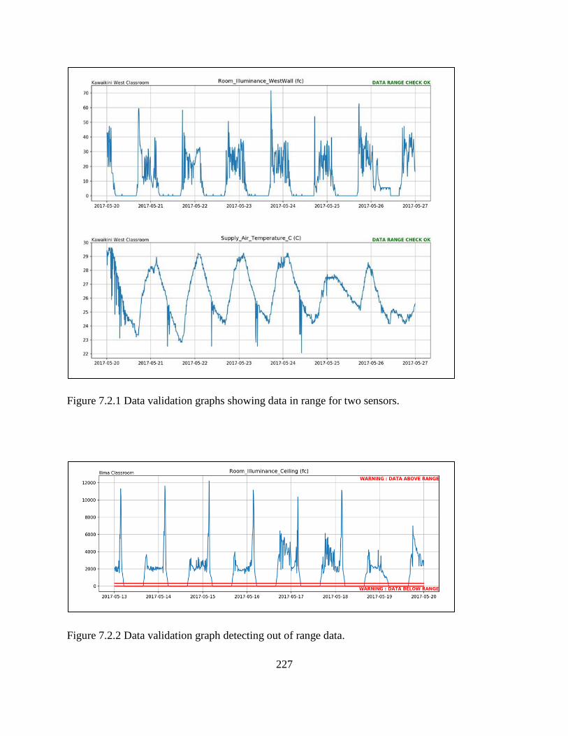
227

Figure 7.2.1 Data validation graphs showing data in range for two sensors.

Figure 7.2.2 Data validation graph detecting out of range data.

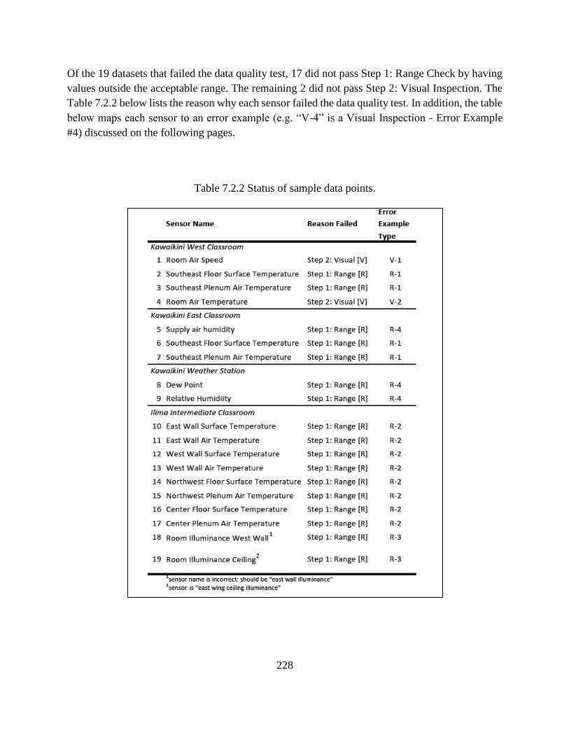
228

Of the 19 datasets that failed the data quality test, 17 did not pass Step 1: Range Check by having

values outside the acceptable range. The remaining 2 did not pass Step 2: Visual Inspection. The

Table 7.2.2 below lists the reason why each sensor failed the data quality test. In addition, the table

below maps each sensor to an error example (e.g. “V-4” is a Visual Inspection - Error Example

#4) discussed on the following pages.

Table 7.2.2 Status of sample data points.

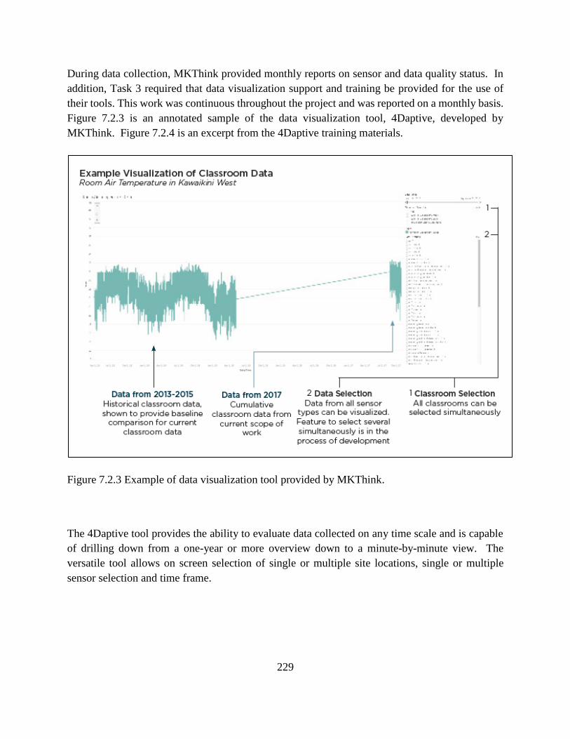
229

During data collection, MKThink provided monthly reports on sensor and data quality status. In

addition, Task 3 required that data visualization support and training be provided for the use of

their tools. This work was continuous throughout the project and was reported on a monthly basis.

Figure 7.2.3 is an annotated sample of the data visualization tool, 4Daptive, developed by

MKThink. Figure 7.2.4 is an excerpt from the 4Daptive training materials.

Figure 7.2.3 Example of data visualization tool provided by MKThink.

The 4Daptive tool provides the ability to evaluate data collected on any time scale and is capable

of drilling down from a one-year or more overview down to a minute-by-minute view. The

versatile tool allows on screen selection of single or multiple site locations, single or multiple

sensor selection and time frame.

230

Figure 7.2.4 Sample from user guide provided to HNEI by MKThink for use of 4Daptive

visualization tool.

The objective was to gather the one year baseline data for additional HNEI research to compare

the first generation to the second generation FROG. MKThink was not tasked with data analysis.

Construction of the two second generation of the Project FROG zero net energy, component-built

platforms was completed in late 2016 and initial performance was reported in APRISES13. This

section summarizes analysis developed partially under APRISES13, and completed under

APRISES12. In addition to being used as classrooms for high school and university students, the

structures are being used by HNEI as research platforms to: 1) test efficient building technologies

such as energy storage, advanced occupancy sensing, advanced fan control and 2) gather data on

actual interior conditions and perceived indoor comfort. The energy performance and

environmental conditions are currently being monitored by HNEI with support from the UH

School of Architecture’s Environmental Research and Design Laboratory (ERDL).

The energy performance of the two FROG classrooms has on average improved on the first-

generation zero net energy FROG designs by up to 47%. The two new mixed-mode FROG

classrooms built on the UH Manoa (UHM) campus demonstrate advanced lighting and HVAC

231

control schemes as well as the impacts of user education and awareness. HNEI monitored energy

consumption and generation at circuit-level, and recorded internal environmental conditions to

determine the relationship between comfort, environmental factors, energy demand and user

response to new controls. A dashboard in each classroom delivers real-time visual feedback to

users.

The actual energy performance exceeded both the predictive building simulation models as well

as the first-generation all-electric zero net energy structures also built for HNEI, realizing energy

use intensity (EUIs) of 8.11 to 10.37 kBtu/sf/yr, excluding solar. This is in part attributed to

improved lighting and daylighting controls, and especially a unique, On-Demand approach to

controlling the HVAC use. The On-Demand control reduced energy consumption 84% beyond a

conventional thermostat scheduled for 7 a.m. to 7 p.m. operation. The On-Demand control is

particularly effective in classroom environments where schedules and staffing vary daily and

hourly over the week.

This comparison of the five buildings demonstrates that efficiency, advanced controls, user

training and real-time feedback are key elements in the FROG’s successful performance. This

section compares the performance of the two generations of zero net energy structures (Figure

7.2.5), the performance of innovative energy saving control strategies, and the influence of user

preference and behavior on energy consumption.

Figure 7.2.5 First-generation FROG (left) with locations in Ewa Beach, Oahu and Lihue, Kauai.

Second-generation FROG (right) located on the University of Hawaii at Manoa campus.

Both generations of the Project FROG structures are component-based and assembled on site. The

envelope design integrates basic energy efficient concepts: due north and south orientation to

minimize solar gain; overhangs further shield the high performance, low-e glazing from solar gain;

and the walls and roofs are well insulated.

The second-generation FROG benefit from more sophisticated lighting and HVAC controls than

the first generation. They utilize LED lighting with daylight harvesting controls that optimize

lighting levels according to the amount of daylighting available within the space while the first

232

generation uses T-8 fluorescents with daylight sensors. The second generation HVAC design is

fine tuned for mixed-mode performance, delivering slightly higher temperature supply air in order

to avoid condensation at the supply registers due to higher room humidity levels. On-Demand

controls require users to make a conscious decision to turn the AC ON (i.e. a user preference),

which allows the unit to run for one hour only. When the conditions require that it be restarted, the

override button is once again pressed. In classroom situations where there may be long intervals

between classes, and where users may have different room condition preferences, this feature

results in significant savings if the button is not pressed again. As research platforms, the UHM

FROG classrooms incorporate a real-time dashboard that displays current and past operating

conditions, including indoor comfort indicators, as well as the energy used by different end-uses.

Intended as an educational tool, the dashboard and supplemental training for instructors aimed to

foster more conscious energy efficient behavior by allowing the building occupants to visualize

their energy usage and PV generation.

A comparison of the energy features of both generations of FROG are listed in Table 7.2.3. They

share common features such as envelope insulation and glazing, however the lighting, HVAC and

approach to natural ventilation are different.

Table 7.2.3 Energy features of two generations of FROG buildings.

Energy Features 1st Generation FROG (1,280 sf) Energy Features 2nd Generation FROG (1,440 sf)

R-24 walls; R-30 roof decks.

Operable louvers at the base of the solid

wall panels for natural ventilation.

High and low operable windows for natural

ventilation.

Low-e, PPG Solarban 70XL glazing

(SHGC=0.27; U=0.24; VLT=64%).

Roof mounted exhaust fan at high point of

the roof for fan induced ventilation.

Direct/Indirect fluorescent T8 lighting with

photosensor daylight control.

Nine speed, variable speed ceiling fans.

High efficiency split system fan coil and

condensing unit (EER 11.0).

North-South orientation

PV systems: 5.24 kW per structure.

All electric, no natural gas on site

R-24 walls; R-30 roof decks.

High and low operable windows for natural

ventilation.

Low-e, PPG Solarban 70XL glazing

(SHGC=0.27; U=0.24; VLT=64%).

External shade structure on south glazing.

Direct/Indirect LED lighting with daylight

control.

Six speed, variable speed ceiling fans.

High efficiency split system fan coil and

condensing unit (EER: 11.8).

North-South orientation.

PV systems: 8.0 kW per structure.

All electric, no natural gas on site

233

The first generation FROGs were instrumented and monitored for three years, ending in 2016 and

recommissioned mid-2017. The second generation FROGs were instrumented and monitored from

September 2016. Table 7.2.4 summarizes the sensing points for both generations.

Table 7.2.4. The sensing points for the environmental and energy data

Electrical circuits Indoor Weather

HVAC condenser

HVAC fan coil

Lighting (internal and

external)

Ceiling fans

Solar PV

Exhaust fan (1st Gen. only)

Panel feed

Room air temperature

Wall surface temperature

Supply and return air temp.

Relative humidity (room,

supply and return duct)

CO2 concentration

Illumination

Air speed (1st Gen. only)

Ambient temperature

Relative humidity

Solar radiation

Wind speed

Wind direction

When comparing EUI between the first and second generation FROGs, on average the second

generation uses approximately 47% less energy per square foot than the first generation (Table

7.2.5). Consumption data for the second generation is from the calendar year 2017, but calculated

rather than actual PV data was used since it was installed in late 2017. Consumption data for the

first generation are from August 1, 2017 through January 31, 2018 (six months) and doubled for a

one-year estimate. Since the PV generation was lower for these months and not representative of

a full year, the 2014-2015 school year PV data was used.

Table 7.2.5. Source energy use intensity (EUI) for 2017

1st Generation FROG 2nd Generation FROG

Kawaikini

East

Kawaikini

West

Ilima UHM

FROG 1

UHM

FROG 2

Total annual

electricity energy

(kWh/yr)

5,549 2,165 11,942 4,376 3,421

Actual EUI

(kBtu/sf/yr)

14.79

5.77 31.83 10.37 8.11

Energy disaggregation of all five FROGs can be seen in Figure 7.2.6. On average, less energy is

used for both lighting and HVAC systems in the second generation than the first generation.

Ceiling fans make up a larger proportion of the energy consumed in the second generation by

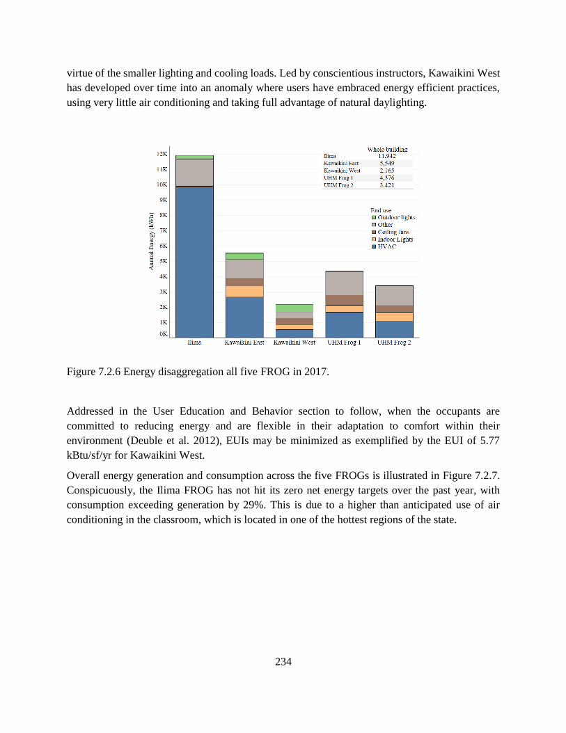
234

virtue of the smaller lighting and cooling loads. Led by conscientious instructors, Kawaikini West

has developed over time into an anomaly where users have embraced energy efficient practices,

using very little air conditioning and taking full advantage of natural daylighting.

Figure 7.2.6 Energy disaggregation all five FROG in 2017.

Addressed in the User Education and Behavior section to follow, when the occupants are

committed to reducing energy and are flexible in their adaptation to comfort within their

environment (Deuble et al. 2012), EUIs may be minimized as exemplified by the EUI of 5.77

kBtu/sf/yr for Kawaikini West.

Overall energy generation and consumption across the five FROGs is illustrated in Figure 7.2.7.

Conspicuously, the Ilima FROG has not hit its zero net energy targets over the past year, with

consumption exceeding generation by 29%. This is due to a higher than anticipated use of air

conditioning in the classroom, which is located in one of the hottest regions of the state.

235

Figure 7.2.7 Overall energy generation and consumption comparison of five FROGs in 2017.

All of the other FROGs are hitting their zero net energy goals. The PV systems for the UHM

FROGs are oversized relative to their current consumption. The operating hours assumed in the

design phase are greater than the current operating schedule, but as the buildings’ utilization

increases, the loads are expected to grow.

The UHM FROGs are multi-purpose classrooms whose schedules vary daily throughout the week.

The mornings are used consistently by a UH-based charter K-12 school, while the afternoons are

used by the UH College of Education, with one or two classes conducted through the afternoon

and evenings. Classes may be held from 5 to 10 hours per day over a 12-hour period. The schedules

are dynamic in that they change every semester, and to date they are currently operating at an

average of 71% of capacity, non-inclusive of extracurricular weekend activity.

These mixed mode buildings are designed to actively engage users while utilizing some degree of

automated controls. The lighting utilizes daylight harvesting sensors to reduce lighting energy,

although users are encouraged to manually turn the lights completely off when the daylight is

adequate to meet class-specific needs. HVAC utilizes an On-Demand control that requires user

engagement to activate, but automatically shuts off after one hour. Ceiling fan operation is 100%

manual, utilizing a variable speed wall switch. The impact of this hybrid approach to engage the

user is discussed later in the Results portion of the report.

236

Data analyzed for this report are from the fall 2017 semester (August 20-December 16, 2017; 119

days), after instrumentation commissioning was complete and regular classroom scheduling was

implemented (previous semester trial schedules were irregular). The period includes 81 school

days and 38 non-school days (weekends + holidays). The building schedules differ slightly as

shown in Table 7.2.6, with FROG 1 having approximately 10% greater classroom occupancy hours

than FROG 2.

Table 7.2.6 UHM FROG 2017 fall semester schedule.

Energy consumption is distributed among five primary end-uses: HVAC, lighting, ceiling fans and

other that includes telecommunications, fire alarm, multi-media, and misc. plug loads, see Table

7.2.7 below:

Table 7.2.7 Energy summary by disaggregated loads (August 20 – December 16, 2017).

Air conditioning

(kWh)

Ceiling fans

(kWh)

Indoor lights

(kWh)

Other loads*

(kWh)

Whole

building (kWh)

Fall 2017 Semester (24h/7days)

UHM

FROG 1

866 283 212 577 1,938

UHM

FROG 2

576 229 222 500 1,528

Fall 2017 Semester for Scheduled Occupied Hours

UHM

FROG 1

632 147 132 219 1,130

UHM

FROG 2

409 149 103 197 858

237

*Other loads=Plug loads + Telecommunications + Multi-Media + Fire alarm

Due to the user engagement required to optimize the utilization of the UHM FROGs, education

and training are essential. Currently, brief training sessions are held for the instructors using the

rooms. In addition, an engaging poster with cues on basic building operation were placed in each

classroom. Finally, a dashboard is mounted in each room providing real-time feedback on daily

and year-to-date energy generation, daily energy consumption by end-use, and comparative results

to the other FROGs.

Lighting energy in the UHM FROGs is controlled by two types of wireless sensors and a control

module. Two wireless Lutron Pico occupancy sensors per classroom activate the lights when

entering the room. A Lutron QSM daylight sensor mounted on the ceiling automatically sets the

light levels according to ambient conditions. A Lutron Energy Saver Node Module interfaces with

the daylight and occupancy sensors to manage the lighting operation according to user-

programmed criteria. In the main room, four rows of Lutron Lantana LED fixtures are controlled

by one occupancy sensor and one daylight sensor. In the entry zone, 2 rows of fixtures have

identical controls. The rows are pre-programmed to operate at light levels determined by their

distance from the windows. On a typical sunny day, approximately 30 seconds after the lights are

activated by the occupancy sensor, the fixtures will dim to the minimum Illuminating Engineers

Society (IES) standards required for the space, with the perimeter row dimming to about 10%, the

center row to about 25% and the interior row to about 40%. The fourth bank located in the rear of

the room, is also at about 40%. On overcast days and evenings, the fixtures will ramp up output

accordingly.

The impact of this control configuration is illustrated in Figure 7.2.8a. Various sensor

configurations are compared for a hypothetical day with a full schedule. No controls would use

the lights at full brightness (0.47 kW) from 7 a.m. to 7 p.m. The occupancy sensor (OS) would

turn off lights during the breaks between sessions, saving 13%. The daylight harvesting (DH) in

addition to OS is estimated to save 35%.

Considering a full semester, if there were no controls and lights used at full brightness from 7 a.m.

to 7 p.m., 457 kWh would have been used (Figure 7.2.8b). However, the schedule was only filled

74% and 68% of capacity (see Table 7.2.8 but percentages account for hours users did not occupy

the buildings at their scheduled time), resulting in a reduction to 340 kWh and 309 kWh from the

OS (26% and 32% savings). The users manually turned the lights off 43% to 48% of the time they

occupied the buildings, reducing the energy to 192 kWh and 160 kWh, leaving less need for

daylight harvesting which reduced the energy to 139 kWh and 113 kWh.

As will be discussed in the User Education and Behavior section, the most effective intervention

is manual, where the user turns the fixtures off completely, using only daylighting to deliver

slightly less than IES standards. In these FROGs, natural daylight can provide adequate light most

of the daytime hours.

238

Figure 7.2.8(a) Average daily energy consumption and percentage savings of lighting

control intervention options for a hypothetical day with a full schedule; (b) Actual energy

used and percent savings for the full semester for school days.

Classrooms in a university setting have dynamic schedules that may vary significantly by day over

the course of a week. The UHM FROGs were outfitted with an On-Demand control for the HVAC

system to reduce run time when there are no occupants in the building. In addition, the On-Demand

control requires user engagement and decision-making (called technological or environmental

adjustment in Azizi et al. 2015), increasing the awareness of building operation.

The On-Demand system integrates the functionality of a vacancy sensor and a timer. In order to

run the HVAC, the user must consciously decide that cooling is required, then engage an override

switch that turns the system on for an hour. After the system turns OFF, the user must decide

whether the interior conditions warrant a second hour of cooling.

To illustrate, Figure 7.2.9 presents two energy profiles for one day, one with a conventional

thermostat, and one with an On-Demand thermostat. Based on five-minute averages of the

occupied periods over the entire semester, the On-Demand control shows an 84% reduction in

energy consumption over the daily energy that would have been used absent controls to limit its

operating time.

Another design modification was incorporated into the UHM FROGs, specifically to address

issues that can face mixed-mode buildings. Mixed-mode buildings utilize both natural ventilation

systems and mechanical systems, frequently on the same day. In humid regions, bringing in air

through operable windows also introduces moisture to the space. In the FROG design, the design

supply air temperature was elevated to 65ºF rather than conventional 55ºF supply air temperature,

in order to avoid condensation at the supply air registers that could result from the elevated

humidity.

239

The setpoint for the On-Demand controller is 77ºF. While the indoor air temperature does not

always reach the setpoint, the variable speed ceiling fans provide air motion whose comfort

perception is equivalent to approximately 3-6 ºF reduction of air temperature.

Figure 7.2.9 Comparison of Conventional vs On-Demand HVAC control (5 minute

average data).

User behavior and response to a building’s condition can impact energy end-use even more than

automated controls.

The UHM FROGs were designed to rely heavily on natural daylighting and daylighting controls.

When comparing occupancy sensing controls, daylight harvesting sensors and the human factor of

choice (to turn off the lights), the user initiated response saved the greatest amount of energy

(Figure 7.8b). If the schedule utilization increased from the current 74% and 68% to 100%, the

user choice will represent the largest energy savings by far.

Figure 7.2.10 indicates that different user preferences will impact the decision to switch the lights

ON or OFF. A noticeable difference in lighting energy use is seen between the two FROGs,

indicating that one classroom is more energy conscious; or the classes require more lighting to

reach their educational mission (e.g. art may require greater visual acuity); or a pattern due to

habituation to turning lights on has developed over time. The illustration shows that user-choice

significantly impacts energy use in otherwise identical classrooms.

240

Figure 7.2.10 Weekly average lighting power for afternoon class session for occupied

hours.

A mixed mode building is also dependent on user response to the interior conditions. While the

intention is to minimize use of mechanical cooling and rely primarily on natural ventilation

through open windows as well as ceiling fans, user preference and/or operational awareness (again

technological or environmental adjustment, Azizi et al. 2015) can impact their response. One type

of user prefers the fresh air and wishes to save energy. Another user may activate the air

conditioning without regard to energy; while yet another is indeed responsive when properly

informed of the intent and features of a special zero net energy building, and is willing to physically

open and close the windows as necessary.

User behavior in these two buildings can be observed in several dimensions. As suggested in

Figure 7.2.11, after a training session was offered during the first week of classes, HVAC

consumption dropped whereas consumption in FROG 1 increased. The pattern reflects

conscientiousness over HVAC energy system use in the FROG 2 classroom that is not reflected in

FROG 1. While this was not a target of rigorous evaluation in this study, anecdotal input from the

instructors indicates that training and awareness of how the systems operate affect behavior and

overall consumption. The impact of reduced HVAC operation is of course, higher temperature.

But as it has been observed by previous researchers (Deuble et al. 2012), occupants with a higher

level of environmental concern were more forgiving of their building and prepared to overlook

less-than-ideal conditions as compared to less environmentally-conscious occupants. The

temperature differential for the two mixed-mode buildings over the entire semester averaged

1.34ºF: FROG 1 averaged 79.47ºF and FROG 2 averaged 80.81ºF.

241

Figure 7.2.11 Weekly average of HVAC power for morning class session for occupied hours.

The second dimension to decision-making and behavior relates to decision mid-session. Once a

decision has been made to turn on the On-Demand HVAC, a secondary decision will be when the

one-hour ON time period is over. The user must answer the question, “Are we comfortable enough

to not need a second hour?” With ceiling fans running, the interior conditions must be assessed

against the current comfort levels. If conditions are currently acceptable, a conscious decision can

be made to not run the HVAC for a second hour.

A third level of decision-making relies on the awareness of how the building operates, and a

commitment to the proper operation of a zero net energy building, primarily dependent upon

education and training. We have observed that even though there were only 10-15 minutes left of

class, the one-hour override switch was pushed, leaving at least 45 minutes of cooling an

unoccupied space. With a conscientious approach, a user might elect to forego HVAC for few

remaining minutes of a class with the knowledge that much of it will be wasted. Alternatively,

they can turn the system ON, but as aware users, manually turn it OFF when leaving the classroom.

These situations require insight into how the controls operate as well as philosophical “buy-in”

into the design intent of the facility. This insight is gained though comprehensive and effective

training of the users.

Another factor to consider when operating a mixed-mode building is that of air quality, specifically

CO2 concentration. In the UHM FROGs, a CO2 build-up was noticed when the HVAC was

running, and presumably the windows were not open (Figure 7.2.12). The CO2 concentration

increased even more after the HVAC turns off, presumably because they still occupy the building

but have not opened the windows. Conversely, when running in a naturally ventilation state, the

windows were open and CO2 levels remained low. Over the course of the semester and during

occupied hours, the FROG 1 consistently ran the HVAC system more than the FROG 2 (Table

7.2.7). Table 7.2.6 shows consistently higher CO2 concentrations in FROG 1 in the morning

242

session while the building used HVAC more (Figure 7.2.11). Figure 7.2.13 shows an increase in

CO2 concentration in FROG 1 over the semester, suggesting that the habit of not opening the

windows continued even though the need for HVAC was less as the outdoor temperatures

decreased over the fall. This reduction in HVAC use can be seen by trend line in Figure 7.2.11.

Figure 7.2.12 Example of CO2 concentration increasing as users remained in building after HVAC

turned off (assuming the windows were still closed).

Table 7.2.6 Average CO2 concentrations (ppm) for the morning session for the fall 2017 semester

Figure 7.2.13 Hourly average CO2 concentrations for the morning session during occupied hours.

243

The following preliminary data analysis covers the period January 1-August 10, 2018 and

considers both university and high school occupancy of the UHM FROGs, including the second

semester of the high school calendar (January 8-May 31, 2018) and two UH semesters, Spring

2018 (January 8-May 12, 2018) and Summer sessions 2018 (1st session: May 21-June 29, 2018;

2nd session: July 2, August 10, 2018). For details please refer to Table 7.2.8.

Table 7.2.8 High school and UH classroom utilization calendars

Both interior and exterior conditions were monitored during the considered period. UHM FROG

buildings are equipped with 8kW PV systems which were installed at the end of 2017 and

commissioned in January 22, 2018. The weather station installed at the same time as the PV is

located on the roof of FROG 1, providing temperature, relative humidity, solar radiation, wind

speed and wind direction.

The energy consumption of the building was evaluated using data collected at 5 min average data

WebCNTRL instrumentation. The two classrooms were used according to different schedules

(morning, afternoon, evening sessions) and hours per month (Figure 7.2.14).

High school calendar

2nd

semester

UH calendar

Spring 2018

UH calendar

Summer sessions 2018

1st session 2

nd session

First day of instructions

Jan. 8, 2018

Last day of instructions

May 31, 2018

First day of instructions

Jan. 8, 2018

Last day of instructions

May 12, 2018

First day of instructions

May 21, 2018

Last day of instructions

Jun. 29, 2018

First day of instructions

Jul. 2, 2018

Last day of instructions

Aug. 10, 2018

School days 90 School days 68 School days 22 School days 29

Holidays 14 Holidays 4 Holidays 2 Holidays 1

Weekend days 40 Weekend days 35 Weekend days 10 Weekend days 10

Non-school days (holidays+weekend

days)

54 Non-school days

(holidays+weekend

days

39 Non-school days

(holidays+weekend

days

12 Non-school days

(holidays+weekend

days

11

Total number of

analyzed days 144

Total number of

analyzed days 107

Total number of

analyzed days 34

Total number of

analyzed days 40

Holidays: Jan. 15 (Dr. Martin Luther King. Jr.); Feb. 12 Institute Day; Feb. 19

(Presidents’ Day); Mar. 19-23 Spring Break; Mar. 26 (Kuhio Day); Mar. 30

(Good Friday); May 28 (Memorial Day)

Holidays: Jan. 15 (Dr. Martin Luther King. Jr.); Feb. 19 (Presidents’ Day);

Mar. 26 (Kuhio Day); Mar. 30 (Good Friday)

Holidays: May 28 (Memorial Day); Jun.

11 (Kamehameha Day) Holidays: Jul. 4 (Independence Day)

244

Figure 7.2.14: Number of scheduled hours UHM FROG

Figure 7.2.15 shows the weekly energy consumption of both UHM FROG buildings. The first four

weeks of the year 2018 (January 1-30, 2018) have not been included in the analysis due to technical

problems with the data acquisition system. Thus, the analysis of the energy consumption covers

February 1 to August 10, 2018.

245

Figure 7.2.15: UHM FROG 2018 weekly energy consumption, February – August 2018

FROG 1 has a higher weekly energy use than FROG 2 due to the higher scheduled usage in the

first three months (interesting, FROG 2 has a higher scheduled usage in April but not a higher

energy consumption). The first drop of energy consumption (week 12) corresponds to the ULS

spring break (March 19-23, 2018). After that, the consumptions increased again but then, the

weekly energy usage decreased significantly for both buildings starting from week 20 which

corresponds to the end of the Spring semester for UHM students and the end of the second semester

for ULS students.

On January 22, two 8kW PV systems were turned on. The electricity production during the

investigated period of analysis is shown in Figure 7.2.16.

246

Figure 7.2.16 UHM FROG weekly electricity production.

Table 7.2.9 shows the energy used by appliance for the entire period of analysis (Feb. 1-Aug. 10,

2018). For detailed monthly usage values, please refer to Figure 7.2.17.

Table 7.2.9 Energy summary (disaggregated loads) – February 1-August 10, 2018

UH FROG

Air conditioning

(kWh)

Ceiling fans

(kWh)

Indoor lights (kWh)

Other loads* (kWh)

Whole building (kWh)

PV production

(kWh)

Whole building

net (kWh)

FROG 1 607 153 204 895 1,859 6,330 4,471

FROG 2 520 184 218 807 1,728 6,383 4,655

*Other loads = Plug loads + Telecommunication + Window actuators + Fire alarm

247

Figure 7.2.17 UHM FROG monthly energy consumption by appliance.

FROG 1 used more HVAC and indoor lights during the first months of the year (February-April),

then the usage started to decrease and in the last analyzed months (June-August), the building was

using more ceiling fans. FROG 2 shows a lower usage of HVAC in the first months (February-

March), then the consumption increased up to May and then decreased again. Differently from the

other building, HVAC was used in July.

During the analyzed period of time (February 1-August 10) the scheduled occupancy of both

building was different and equal to: FROG 1 = 991.25 hours; FROG 2 = 911 hours. By dividing

the energy and the scheduled occupancy (occupied hours) the following Table 7.2.10 and Figure

7.2.18 are obtained. Thus, even if FROG 2 was theoretical used for a less amount of time, it shows

a higher energy consumption due to the use of more ceiling fans and indoor lights.

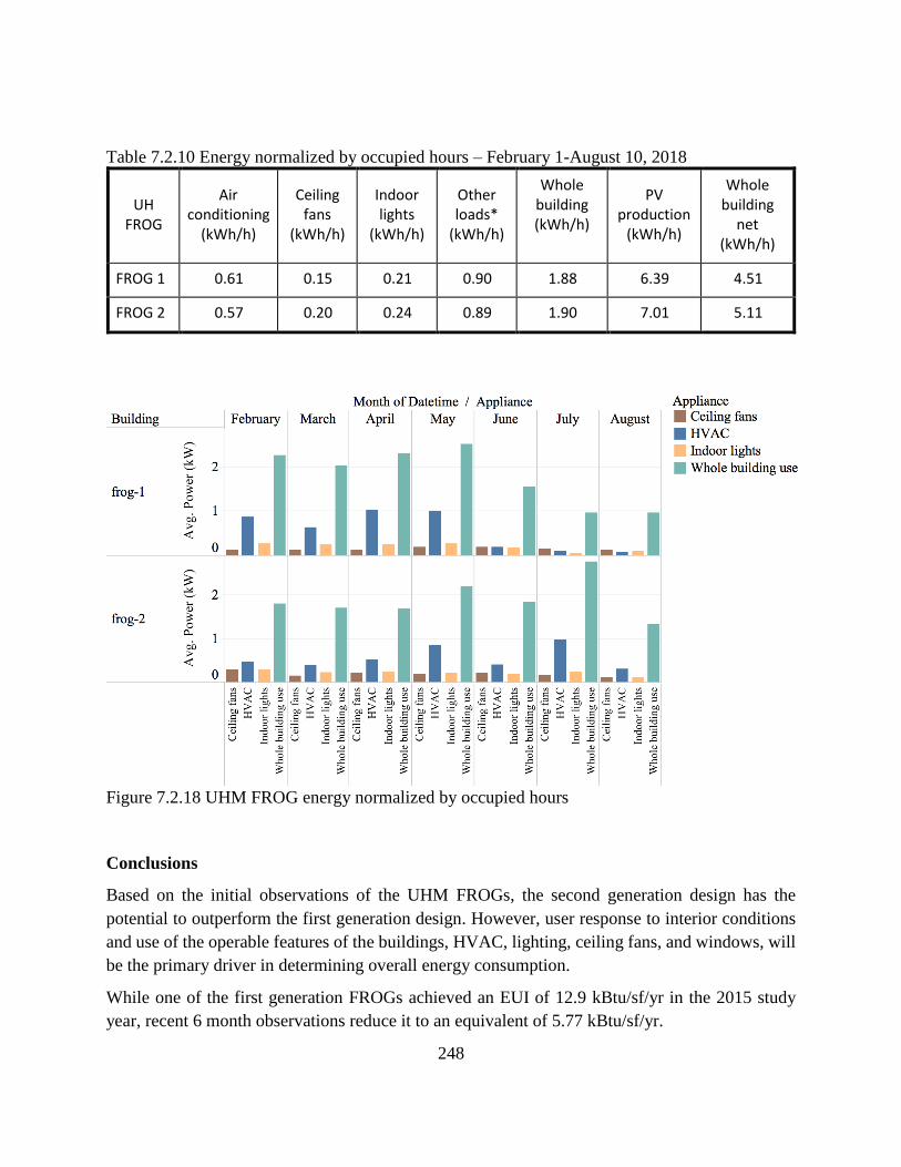
248

Table 7.2.10 Energy normalized by occupied hours – February 1-August 10, 2018

UH FROG

Air conditioning

(kWh/h)

Ceiling fans

(kWh/h)

Indoor lights

(kWh/h)

Other loads*

(kWh/h)

Whole building (kWh/h)

PV production

(kWh/h)

Whole building

net (kWh/h)

FROG 1 0.61 0.15 0.21 0.90 1.88 6.39 4.51

FROG 2 0.57 0.20 0.24 0.89 1.90 7.01 5.11

Figure 7.2.18 UHM FROG energy normalized by occupied hours

Conclusions

Based on the initial observations of the UHM FROGs, the second generation design has the

potential to outperform the first generation design. However, user response to interior conditions

and use of the operable features of the buildings, HVAC, lighting, ceiling fans, and windows, will

be the primary driver in determining overall energy consumption.

While one of the first generation FROGs achieved an EUI of 12.9 kBtu/sf/yr in the 2015 study

year, recent 6 month observations reduce it to an equivalent of 5.77 kBtu/sf/yr.

249

The second generation lighting system controls, i.e., occupancy sensor and daylight harvesting,

contribute at least 35% savings, but considering user behavior of choosing to turn lights off total

savings of up to 75% resulted.

Limiting the duration of HVAC operation by using an On-Demand thermostat, savings of up to

84% were observed. These reductions are due to the HVAC system operating only when users are

present as well user opportunity to consider natural ventilation options. The On-Demand

thermostat is a mechanical equivalent to a vacancy sensor as it must be manually activated, and

will automatically shut off.

During this project, HNEI identified future interventions that will improve overall performance of

zero net energy buildings, including:

Provide comprehensive education and training to all users, not simply the instructors, but

classroom users (students) as well. This can be done with online mini-training; in-person;

or through a “train the trainers (instructors)” approach.

Reprogram the lighting controls to vacancy sensing, requiring the lights to be manually

turned ON between the hours of 8 p.m. and 5 p.m., rather than automatically turned on with

an occupancy sensor. Natural daylight may be adequate for classroom purposes.

Install actuators on manually operated windows will overcome one barrier to natural

ventilation: the time-consuming task of opening a multi-window banks of windows.

Install occupancy sensors for fans.

Reports and Presentations

MKThink. 2016. "Net Zero Energy Test Platform Performance Comprehensive Analysis".

Maskrey, A.J., S. Cerri, E. Peppard, M. 2018. "Second Generation ZNE: Inheriting the Good

Genes" In Proceedings of the 2018 ACEEE Summer Study on Energy Efficiency in Buildings

10:1-14. Pacific Grove, CA: ACEEE.

http://aceee.org/files/proceedings/2018/index.html#/paper/event-data/p309

References

MKThink. 2016. "Net Zero Energy Test Platform Performance Comprehensive Analysis".

Maskrey, A.J., S. Cerri, E. Peppard, M. 2018. "Second Generation ZNE: Inheriting the Good

Genes" In Proceedings of the 2018 ACEEE Summer Study on Energy Efficiency in Buildings 10:1-

14. Pacific Grove, CA: ACEEE. http://aceee.org/files/proceedings/2018/index.html#/paper/event-

data/p309

250

Maskrey, A.J., S. Cerri, E. Peppard, M. Miller, and S. Uddenberg. 2016. "Positively Net Zero:

Case Study of Performance Simulation and Hitting the Targets." In Proceedings of the 2016

ACEEE Summer Study on Energy Efficiency in Buildings 10:1-14. Pacific Grove, CA: ACEEE.

http://aceee.org/files/proceedings/2016/data/index.htm

Deuble, M.P., and R. de Dear. 2012. "Green occupants for green buildings: The missing link?".

Building and Environment 6: 21-27.

Azizi, N.S.M., S. Wilkinson, and E. Fassman. "An analysis of occupants response to thermal

discomfort in green and conventional buildings in New Zealand". Energy and Buildings 104:

191-198.

7.3 Small, Vertical Axis Wind Turbines at Crissy Field Center

This is the second phase study of small, vertical axis wind turbines, which were installed at Crissy

Field in San Francisco Figure 7.3.1 in collaboration with the Golden Gate National Parks

Conservancy. The first phase, with five (different) wind turbines, was funded under HEET09,

N00014-10-1-1310 and was completed in December 2015.

Figure 7.3.1 Crissy Field Education Center, San Francisco, CA. UGE turbines 1st and 4th from

the left. Omniflow turbines 2nd and 3rd from the left.

251

This phase of the project provided for the installation and performance monitoring of four vertical

axis turbines -- two UGE VisionAire3 systems and two Omniflow1.2 systems, see Figure 7.3.2.

These were installed at the site of the previous five wind turbines. The UGE turbine is a Darrieus

type design similar to three in the first study but by a different manufacturer, while the Omniflow

turbines are of a unique design that combines a Venturi effect with integrated PV cells. A data

acquisition system collected wind and power data in one second intervals, with enough resolution

to determine response lag. In addition to turbine performance, the project sought to determine the

impact of land based, urban obstructions such as vehicles, trees, shrubs and ground surface

variations on unobstructed wind.

The objective of the second phase of research was to evaluate and test selected wind turbine

technologies to determine the relative effectiveness of differing turbine design technologies; the

impact of urban wind conditions (environment-induced turbulence) relative to idealized (laminar)

wind conditions under which turbines are tested and rated; and integration with the test platform

systems toward the achievement of energy neutrality and/or net positive energy within the test

site.”

The Crissy Field site provides an ideal location to conduct wind technology research, as the site is

subject to urban wind conditions and is immediately adjacent to the unobstructed area of the San

Francisco Bay. The wind regime at the Crissy Field site is quite different than when measured

from the unobstructed reference wind site, Anita Rock from which design data was originally

taken. Trees and buildings surrounding a site create an “urban wind” effect that reflects diminished

velocity and power of the wind, while creating turbulence that may also impact the ability to

translate wind into power across a turbine blade.

The subawardee, Golden Gate National Parks Conservancy, contracted with Luminalt Energy

Corporation for the design, maintenance and installation of the turbines. Luminalt was also the

contractor for the installation of phase I. Consultant Loisos + Ubbelohde were also contracted for

the design and installation of the data acquisition systems, including power and wind sensing

devices. Weatherflow provided wind data for the Anita Rock wind monitoring site offshore of

Crissy Field.

252

Figure 7.3.2 Specification sheets for UGE VisionAire3 (l) and Omniflow 1.2 (r)

Turbine Components and Installation.

The design team for phase II was tasked with making use of the existing infrastructure from

phase I to the greatest extent possible. Existing footings, conduit and conductors were re-

used, and in the case of the Omniflow units, the towers from the Phase I Venco units were

retrofitted to accept the new turbines. Existing footings were evaluated for by structural

engineers, Plump Engineering, to confirm structural adequacy for the new turbines and to

design adapter plates to match the new bolt patterns.

The majority of the components for the project were purchased by the project prime contractor,

Luminalt Energy Corporation. Luminalt purchased the two UGE Vision AIR 3 turbines, 7 meter

towers, associated electronics and adaptor plates (and required engineering) from Castle Energy

LLC. Castle Energy is a registered distributor for UGE products. Figures 7.3.3 through 7.3.6

highlight various phases of the installation process.

253

Figure 7.3.3 UGE Turbines and Towers delivered to Crissy Field.

Figure 7.3.4 UGE Turbines unpacked and stored for installation at site.

254

Figure 7.3.5 Preparation of assembled UGE turbine for mounting.

Figure 7.3.6 Installation of UGE turbine.

The Parks Conservancy contracted directly with Omniflow to purchase two turbines and

associated electronics. The Omniflow is configured as a hub with fan blades that spin on a vertical

axis. A flange mounted to the bottom perimeter of the hub features 2 rows of photovoltaic silicon

cells, as shown in Figure. 7.3.7.

255

Figure 7.3.8 Omniflow controller unpacked.

Figure 7.3.7 Omniflow photovoltaic cowling before assembly (l). Omniflow turbine prior to

installation of photovoltaic flanges (r).

Figure 7.3.9 Fully assembled Omniflow in

preparation to raise.

256

Figure 7.3.10 Completed Omniflow (left) and UGE (right) turbines.

257

\

Figure 7.3.11 Omniflow and UGE Inverter and controller installation.

All components and equipment for upgrading the data acquisition system (DAS) system for Phase

II were sourced by project sub-consultants Loisos + Ubbelohde, who were responsible for the

design and installation of the system as well as for developing and implementing the data

monitoring protocols.

For the new DAS design, the team at Loisos + Ubbelohde sought to both enhance the earlier

system’s data collection capacity and correct for the correlation issues identified in Phase I. The

design team was able to reuse most of the installed infrastructure from the Phase I DAS system,

but the requirements for Phase II necessitated additions/modifications to both the physical

hardware and the data collection design.

In Phase I, wind speed and turbine power output were sampled at different time intervals. The

former measured instantaneous samples and the latter recorded sixty second averages. For Phase

II, a new data collection protocol was developed – the sampling rate was standardized to 1 second

for wind speed, direction and turbine power output. This enables a more precise analysis of

correlations between data sets allowing for instance, analysis of the turbines’ responses to changes

in wind direction and speed.

In order to meet the new experimental requirements in Phase II, additional monitoring equipment

needed to be designed and installed (Figure 7.3.12). To enable the investigation of on-site wind

patterns associated with an “urban” wind regime, anemometers were added to each wind turbine

tower.

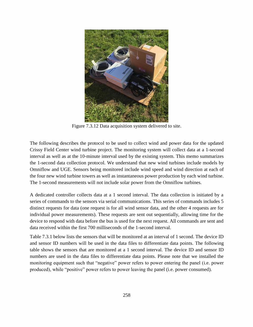
258

Figure 7.3.12 Data acquisition system delivered to site.

The following describes the protocol to be used to collect wind and power data for the updated

Crissy Field Center wind turbine project. The monitoring system will collect data at a 1-second

interval as well as at the 10-minute interval used by the existing system. This memo summarizes

the 1-second data collection protocol. We understand that new wind turbines include models by

Omniflow and UGE. Sensors being monitored include wind speed and wind direction at each of

the four new wind turbine towers as well as instantaneous power production by each wind turbine.

The 1-second measurements will not include solar power from the Omniflow turbines.

A dedicated controller collects data at a 1 second interval. The data collection is initiated by a

series of commands to the sensors via serial communications. This series of commands includes 5

distinct requests for data (one request is for all wind sensor data, and the other 4 requests are for

individual power measurements). These requests are sent out sequentially, allowing time for the

device to respond with data before the bus is used for the next request. All commands are sent and

data received within the first 700 milliseconds of the 1-second interval.

Table 7.3.1 below lists the sensors that will be monitored at an interval of 1 second. The device ID

and sensor ID numbers will be used in the data files to differentiate data points. The following

table shows the sensors that are monitored at a 1 second interval. The device ID and sensor ID

numbers are used in the data files to differentiate data points. Please note that we installed the

monitoring equipment such that “negative” power refers to power entering the panel (i.e. power

produced), while “positive” power refers to power leaving the panel (i.e. power consumed).

259

Table 7.3.1 Sensor architecture within data acquisition system.

Data files will contain rows as follows, where values include integer values as well as

converted 32-bit floating point values:

Timestamp is given as 'YYYY/MM/DD hh:mm:ss'. Data files are saved with measured data

at a 1-hour interval; the identifier will be approximately the first timestamp measured, as a

Unix timestamp.

To facilitate the revised data protocol, Loisos and Ubbelohde developed a design and

specifications for new equipment, as shown in the installation schematics below (Figures 7.3.13 -

7.3.15):

<timestamp>,<deviceID>,<sensorID>,<value>

260

Figure 7.3.14 Data acquisition system architecture.

Figure 7.3.13 Monitoring equipment locations at Crissy Field Center.

261

Figure 7.3.15 Data path from turbines to Crissy Field Center

Data files are first saved locally on the controller. A cloud-based server was developed to

retrieve, convert, and transfer data files. This server is implemented as a Flask server running

on Heroku. Since FTP access to the controller and HNEI servers required whitelisting of the

server IP address, a service was added to the Heroku server to provide a static IP address via

a proxy server. The Heroku server and the proxy server incur a monthly cost, which we will

include with our monthly maintenance budget. The controller was programmed to save data

hourly and to contact the server after a new data file has been saved. The server then retrieves

any data files from the controller, converts the data to engineering units as described above,

transfers both the raw and converted data to the UHM HNEI FTP server located at

crissy.soest.hawaii.edu, and finally deletes the original files from the controller. The data

transfer server has been deployed, and the data transfer process is operational.

A .csv data file was downloaded and checked for potential errors. Wind speed, wind direction,

and power were plotted for each wind turbine, using a 2-second average to enhance

readability. At the time of this initial check, the UGE wind turbines had not yet been fully

commissioned. A second data file was downloaded to examine UGE data. The data check of

each of these files showed data range and variation consistent with expectations (see Figure

7.3.16). In particular, we note:

Wind speed and direction vary, but patterns are consistent across sensors.

Power monitoring of the Omniflow turbines shows increases that seem to correspond

to increasing PV output.

262

Wind speed resolution is somewhat coarse – this is unavoidable since the execution

interval of data collection is so small. The sensor uses a pulse signal with each full

rotation of the anemometer, so there is no way to measure a fraction of a rotation.

UGE North turbine and wind data for wind speed and power generated show very

similar patterns of variation.

UGE North turbine shows high frequency variation in performance that is different

from the UGE South turbine.

Figure 7.3.16 Data check for key metrics power, wind direction and wind speed

In the process of commissioning the UGE power monitoring, L+U discovered an unexpected and

unusual issue. The UGE inverters are connected to the electrical panel using 2-pole breakers.

During lower levels (<280W) of power output, the direction of current in each wire is opposite,

and the total power produced or used is the difference between the readings. This required a change

to explicitly monitor net positive power and net negative power. The original method measured

total power – or the sum of the absolute values for power on each phase. This showed a near

constant 300 W of power produced, even though the totals were much lower. For example, L+U

performed a test on site where the UGE North turbine was switched from power production to

“free spin” mode, and then back to power production mode (see Figure 7.3.17). This shows the

variation in power logged in each wire (L2 and L3), in the calculated Net Power, and in the

263

calculated Total (absolute) Power. This graph further demonstrates why Net Power needs to be

calculated rather than using the Total Power.

Luminalt and Loisos + Ubbelohde researched the issue and discussed these observations with

Ginlong, the turbine manufacturer, and with Dent Instruments, the manufacturer of the Powerscout

meters. The team identified low power factors as a likely cause of these observations, as described

in more detail in this document, posted by Continental Control Systems, another power meter

manufacturer: https://ctlsys.com/support/inverter-power-factor/

While this issue presents further monitoring challenges for the dashboard data collection (see

below), for purposes of the high frequency monitoring, it confirms that our monitoring of net

power will accurately capture total power production or use at any given moment in time.

Figure 7.3.17 Annotated results from UGE data acquisition testing

The issue described above regarding the need for logging of Net Power is an issue for the

existing monitoring system, because the existing Powerscout 18 is not capable of logging Net

Power. It logs Total Power, or the sum of power from each phase. As a result, it will over-

estimate power production any time Net Power production is less than around 280W.

L+U identified three potential solutions to monitor the power production of these UGE units:

1. The Powerscout 18 unit can be replaced with a Powerscout 24 unit that is capable

of sensing the direction of current flow and can track Net Power.

264

2. Due to the observed behavior of the current flowing from the inverter, it appears

that a calculation could be applied to estimate power produced by the UGE

turbines. In the graph above, note that L3 power is always positive, and that L2

power switches to positive when L3 power is above approximately 280W

(although this limit is inconsistent). In order to infer the sign of L2 power, we can

test to see if L3 power is above or below 280W, and assign a negative number to

L2 if L3 is below 280W.

The document provided by Continental Control Systems (see link above) provides a method

for calculating total power by monitoring apparent power and power factor for a single phase.

This calculation could be performed for data from a single CT using the Powerscout 18, thus

allowing us to calculate corrected total power from one CT.

L+U further investigated the second and third solutions by recording detailed data for each

UGE turbine using the Powerscout 24 to both simulate data collected by the Powerscout 18

and to measure net power. We were thus able to test each potential calculation method. We

found that calculating total power using the 280W threshold was slightly more accurate than

calculating the total using data from a single CT, and it was also easier. Based on our test of

using the 280W threshold, we found this would produce accurate results for small or large

power values, and an occasional error up to ±50% when total power is around 280W. We

found that this error was larger for the UGE North turbine, which exhibits a high frequency

pattern of variation in its output, than for the UGE South turbine. See figures below for the

percent error vs measured power for each turbine. We also plotted the measured and calculated

values over time, and we note that when taken as a whole, the calculated values tend to show

a similar overall pattern (i.e., when measured power is high, calculated power tends to be high

as well).

The Omniflow turbines have several features that required additional analysis and engineering by

Loisos and Ubbelohde. First, the units produce power from both a wind driven generator and

photovoltaic panels. Second, the units are equipped with a battery that is charged by the wind/PV

sources and is used to power the system’s inverter and controller.

Simple measurement of the unit’s output using a currency transformer will yield aggregated,

undifferentiated information from all three of these sources. Loisos and Ubbelohde summarize

their recommendations for collecting disaggregated data specific to the turbine:

The objective of the power monitoring in the project is to establish a relationship between

variations in wind speed and direction and variations in power produced by wind turbines. Data

will be collected at a 1-second interval in order to study this relationship at a fine resolution. The

electrical design of the Omniflow generator includes a source of solar power and a set of batteries;

these components add complexity to the monitoring plan since wind power needs to be

265

disaggregated from the total. To disaggregate wind data, we recommend using data collected at

night to eliminate solar power data, and short- term supplemental monitoring to understand the

behavior of the battery.

Based on documentation provided by Omniflow and a phone conversation with Pedro Ruão, the

founder and CEO of the company, the Omniflow system will function in different modes

depending on the voltage charge in the battery. When the battery is below 24V, all power generated

is directed to charge the battery (Figure 7.3.18a). When the battery charge is between 24V and

26.7V, the inverter is switched on, and power is directed to the grid as well as to charging the

battery (Figure 7.3.18b). When the battery is at 26.7V, it is fully charged, and all power is directed

towards the grid (Figure 7.3.18c). When voltage from power production drops, the battery

discharges to feed the controller and inverter (Figure 7.3.18d)

Figure 7.3.18a: Battery Charging Mode. Grid connection shows 0 Amps, which is less than

what the turbine is actually producing.

266

Figure 7.3.18b: Battery Charging and Inverter Mode. Grid connection may show more or less

than the power produced by the wind turbine.

Figure 7.3.18c: Inverter Only Mode. Grid connection will show more than the power produced

by the wind turbine.

267

Figure 7.3.18d: Battery Discharging and Inverter Mode. Grid connection will show more than

the power produced by the wind turbine.

The planned monitoring system includes monitoring of the electricity produced by the system

as it is being transferred to the electrical panel. This measurement will be affected by system

operating mode, showing less power produced whenever the battery is being charged and

potentially more power when the battery is discharged. This measurement will also include

any solar energy being produced.

The controller in the Omniflow system has data points available via serial connection that

include battery voltage and current, although the accuracy of these measurements is

questionable and the data connection to the device has not been tested. Furthermore, the

monitoring system was not designed for additional serial devices and may not have the

capacity for additional data collection.

In order isolate wind energy produced directly, either the energy being produced by the wind

turbine must be measured directly, or the aggregate data will need to be processed to isolate

times when the system is feeding exclusively wind energy directly to the grid. Direct

measurement of wind energy would either involve relying upon inaccurate current

measurements taken by the controller, or identifying monitoring equipment capable of

measuring variable AC power. These direct measurement options are problematic due to

potential accuracy issues and/or project budget constraints.

268

Alternatively, the recommended approach included isolating wind turbine energy by studying

night hours (to eliminate PV power production) and when the battery is fully charged (Figure

7.3.18e). By studying these times, the team should be able to eliminate any potential

contribution of solar power or battery buffering. However, this approach includes risks, such

as:

The time period of buffering is unknown. If a partially filled battery charges quickly

and stays charged for long periods of time, then it will be easier to disaggregate the

contribution of the battery from the data. However, if battery charges and discharges

frequently, then it may be difficult go disaggregate the effect.

Diurnal wind patterns will not be captured since daytime wind data cannot be

disaggregated from solar.

Figure 7.3.18e: Night Inverter Only Mode. Grid connection will show isolated wind power

production.

In order to understand the contribution of the battery, the team should consider short- term

high resolution monitoring of battery performance to assess battery behavior and identify any

further steps needed to isolate the behavior of the battery. Using the controller as a source of

battery voltage data is untested. We know that data is available from the controller, but it is

likely going to be difficult to integrate these data points with the specified data collection

system. Rather, it may be fairly straightforward to temporarily monitor voltage using data

loggers such as those from Onset (e.g. a HOBO U12-013, 0-24V input sensor and a voltage

divider for an effective input range of 0-48V).

269

Detailed analyses are underway under other funding, and should be complete by year end 2018,

with findings presented in future reports.

Reports

Golden Gate National Parks Conservancy, “Crissy Field: Wind Power Study, Phase II, Report

1”, May-June 2018.

Golden Gate National Parks Conservancy, “Crissy Field: Wind Power Study, Phase II, Report

2.1: Stored Materials and Major Component Inventory”, June 2018.

Golden Gate National Parks Conservancy, “Crissy Field: Wind Power Study, Phase II, Reports

2.2: Wind Turbine and Data Acquisition System Installation”, June 2018.

Golden Gate National Parks Conservancy, “Crissy Field: Wind Power Study, Phase II, Reports

3: Commissioning of the Wind Turbines and Data Acquisition System”, July 2018.

Golden Gate National Parks Conservancy, “Crissy Field: Wind Power Study, Phase II, Reports

4.1- 4.3: Interim Operating Reports”, July 2018.

References

Loisos + Ubbelohde, “Crissy Monitoring Installation Report”, internal correspondence to

Golden Gate National Parks Conservancy, May 24, 2017

Loisos + Ubbelohde, “Crissy Monitoring Software Update and Commissioning Report”, internal

correspondence to Golden Gate National Parks Conservancy, June 21, 2017

7.4 Demand Response Portfolio Plan Assistance to HECO

HNEI provided financial support, data and project evaluation for several HECO demand response

(DR) demonstration projects developed under the first phase of its implementation of its Demand

Response Portfolio Plan. The projects were meant to demonstrate how different combinations of

customer-sited energy resources could deliver the following grid services: capacity and load

shifting, fast frequency response, and regulating reserves. HECO selected vendors through a

competitive solicitation process. The selected projects represented an array of end-use

technologies installed at different types of customer facilities that could provide information on

270

technology and operational performance of DR technologies and market acceptance by customers

and vendors. The projects were also intended to inform and refine the implementation of HECO’s

future DR program portfolio.

Five projects were implemented:

1. Regulating Reserves – Web-based solution configured to support and interface with

automatic generation control, remote terminal units and a “virtual power plant”, that

aggregated resources to present a single forecasted DR capability to HECO.

2. Fast Frequency Response, Regulating Reserves, Capacity – Enlisted existing residential

customers with PV and battery storage and EV chargers to determine the capability of

systems to follow regulating signals.

3. Fast Frequency Response, Regulating Reserves, Capacity – Enlisted a commercial

customer with battery energy storage systems (BESS) to determine the capability of

systems to follow regulating signals.

4. Regulating Reserves – Aggregated two commercial BESS to determine the capability of

systems to follow regulating signals.

5. Capacity – Remotely controlled the thermostat of five small business customers to test the

customer acceptability to internal space temperature changes, and track the reduction in

electricity use.

HECO considered the projects to be successful based on the results of each project where each

vendor met expectations to provide reliable, repeated responses to demand response events. In

addition, HECO stated it learned several lessons including that FFR requires accurate forecasting

to ensure an accurate response, policy and technical issues must be resolved before 2-way EV

charging response can be used in practice, and that aggregators must find ways to balance customer

needs with utility grid service availability needs.

Conclusions

Excerpt from HECO Final Report to PUC:

“In reflecting on these projects and the subsequent analysis and assessment of them, the

Companies have identified several key takeaways worth noting. These observations have

or will have a direct bearing on the evolution and maturation of the Grid Services market

and the Companies’ ability to deliver Grid Services through third party vendors utilizing

271

customer resources. Specifically,

Optimizing the balance between customer needs and grid needs: While this seems

apparent, it is much more difficult to achieve in practice. When a customer purchases

resources to serve their needs, e.g. demand reduction or resiliency, that need typically

comes first before grid or DR needs. Vendor algorithms that maximize or optimize the

amount of the resource available to the grid are very complex, require tuning, and active

post-installation monitoring. A majority of the resources utilized for these demonstration

projects were employed primarily to serve customer needs rather than DR. For example,

some battery energy storage systems were utilized primarily to reduce the peak demand

charge of commercial customer sites. The customer and vendor partnership is based

primarily on the peak demand charge reduction, and secondarily participation in demand

response. This balance needs to be managed by the vendor to ensure both utility

requirements and customer requirements are met. As a result, careful assessment by

vendors must be performed to determine management of the customer’s resources to fulfill

these competing needs. These determinations will ultimately culminate in valuing Grid

Service delivery during GSPA contracting and operation.

Customer acceptance and concerns: During outreach to customers, many customers were

skeptical of the opportunities offered by the Demonstration Vendors, which resulted in

numerous calls to the Companies. As a result, co-branding with the Companies was added

to the GSPA to help reassure customers of the legitimacy of the DR opportunities presented

to them.

Assessment of Regulating Reserve delivery: The regulation signal that was used for the

Regulating Reserve projects reflected several real-world operating examples based on

actual grid performance, i.e., “good” and “bad” renewable generation production. These

real-world examples included a highly variable regulation signal that existing, established

assessment tools do not fully address, as discussed in section V.A.2.d. For future

assessments of Regulating Reserve, the time window will be shortened to better capture

the fast and highly variable nature of the Companies’ regulation signal.

Application of value Grid Service delivery: The Grid Service Value table was included in

the draft GSPA, as a result of discussions with Demonstration Vendors around the

relationship between maximizing value, forecasting accuracy, and targeting customers for

demonstration project participation. The Grid Service Value table reflects the hours of the

day in which the delivery of Grid Services is the most beneficial to the Grid. Using the

Grid Services Value table, Grid Service Suppliers can target customers who would be the

most effective and productive during the most valuable hours. This in turn helps to ensure

the delivery of Grid Services to the Companies is reliable and dependable.

Assessment of market and technical readiness: DR control technology that was layered

onto installed homogenous populations of resources was enabled significantly faster than

272

those that required new resource installation or interconnection. Enabling resources

already “in the ground” is key to quick enrollment, and having similar or identical installed

resources enabled efficient installation processes. New equipment installations must pass

through the predefined Hawaiian Electric interconnection process, which may also require

inverter manufacturers to qualify their inverters and formally certify to UL 1741

Supplement A, using the Company’s applicable Source Requirements, especially for new

inverter models. Some vendors faced delays with regards to interconnection, while others

that did not install new equipment moved far more quickly through the demonstration

phase. During the contracting process, it will be critical to assess each vendor’s enablement

plan in terms of acquisition schedule and installed resources to ensure the targets are

achievable.

Specific technologies have a role: While many demand-side resources can be enabled to

deliver Grid Services, certain technologies and resources are more adaptable to deliver Grid

Services than others. For example, FFR, which is deployed in response to a contingency

event on the grid, requires accurate forecasting and accurate delivery to ensure grid

reliability. Through the Demonstration Phase, it became apparent that the most reliable

way to deliver this Grid Service was to employ a battery energy storage device and reserve

a portion of the battery for FFR at all times to ensure availability. All Demonstration

Vendors chose this method to deliver FFR. Other demand-side resources can accurately

delivery Grid Services, but it is accomplished by forecasting or committing significantly

less Grid Service than is available so as not to under or over deliver. During GSPA

contracting process, vendors will need to demonstrate (if they haven’t already done so)

their ability to comply with FFR delivery requirements.

Capacity Grid Service continues to evolve: During the Demonstration Phase, Capacity

Load Shift tests consisted of participant systems following the utility TOU rate, which

applied to all 24 hours of the day. Specifically for Project 2 participants, the TOU rate

implementation changed participants’ daily load profile by building load or charging

energy storage during daytime hours and reducing load or discharging energy storage

during the evening hours. While a standard feature of participant’s systems, the load shift

demonstrated was a static and constant weekday shift. As implemented, the system was

not able to perform Load Shift “on demand” or be dispatched to address grid conditions.

However, this additional “on-demand” flexibility would allow dispatch of Capacity Build

on a high solar production day or Capacity Reduction to address a capacity shortfall which

is a much more utilizable resource. Independent dispatch of Capacity also allows

respondents to the Grid Services RFP to include a greater variety of end-use resources since

Capacity Build and Reduction are not required to be symmetrical as they would be under

Capacity Load Shift. The Companies anticipate that Capacity Grid Service will continue

to be refined as the Grid Service is implemented.

273

EVs offer Grid Services delivery opportunities: Utilizing 2-way EV charging as a DR

resource was a proof of concept during the Demonstration Phase; while successful, there

are still policy and technical issues with this end-use resource that need to be addressed

before 2-way EV charging can be used in practice at scale. EV participants were generally

interconnected under the Net Energy Metering (“NEM”) interconnection agreement, which

explicitly allows for export of customer-generated renewable energy to the grid. There is

no process in place to verify that the stored energy in an EV battery was generated by a

renewable resource (e.g., not charging from a non-renewable resource: workplace

charging, chargers installed at shopping centers, Hawaiian Electric DC fast chargers, etc.).

That being said, there is however meaningful potential for 1-way charging to deliver Grid

Services, as there are no interconnection requirements for 1-way chargers since there is no

potential for customer back-feed to the grid.

Participant resources do have limitations: Each participant’s technology and situation

impacts the availability and reliability of their resources to deliver Grid Services. While

the Internet of Things (IoT) is anticipated to offer the level of coordination, interoperability,

reliability, and security required to enable a resource to deliver Grid Services, it remains

an evolving sector. Demonstration Vendors relied on customer Wi-Fi or cellular data, or

both from the Demonstration Vendor’s head-end system down to the customer end-device.

Cellular was implemented as a backup in cases, where the participant’s Wi-Fi was not

always available, either due to participant behavior or location. There is considerable

expense involved in adding and maintaining this backup communications path at scale.

But, establishing reliable communications is very important so that the resource can

reliably deliver Grid Services. Further, a customer’s existing infrastructure greatly

influences their ability to provide Grid Services. For example, reliance on customer HVAC

systems for load reduction requires a properly sized HVAC system, which was not always

the case amongst the Companies’ existing customers in practice. Utilizing HVAC for

demand response will also definitely compromise customer comfort, so it is up to the

aggregator vendor to properly compensate the customer for their participation. As a result,

vendors may incur additional expense to ensure reliable delivery of Grid Services, which

would likely be reflected in their costs to the Companies.” (HECO, 2018).

Additional details can be found in HECO’s final report to HNEI, “Demand Response

Demonstration Phase: Final Report (June 2018) ”, posted on the HNEI website as well as the

their August 31, 2018 Final Report submitted to the Hawaii Public Utilities Commission in support

of Docket 2015-0412, (both referenced below).

274

References

Hawaiian Electric Company, “Demand Response Demonstration Phase: Final Report”, Submitted

for Docket 2015-0412. August 31, 2018

Hawaiian Electric Company, “Demand Response Demonstration Phase: Final Report”, Submitted

for HNEI. June 12, 2018