Final Report - CiteSeerX

Final Report

DEVELOPMENT OF A FIELD PERMEABILITY APPARATUS the Vertical and Horizontal Insitu Permeameter (VAHIP)

BD-545, RPWO # 15

UF Project 00030900 (4554023-12)

Submitted by:

David Bloomquist Adrian Albert Viala

Mike Gartner

Department of Civil and Coastal Engineering University of Florida

Gainesville, Florida 32611

Developed for the

David Horhota, Ph.D., P.E., Project Manager

ii

July, 2007

Disclaimer The opinions, findings, and conclusions expressed in this publication are those of the author and not necessarily those of the State of Florida Department of Transportation.

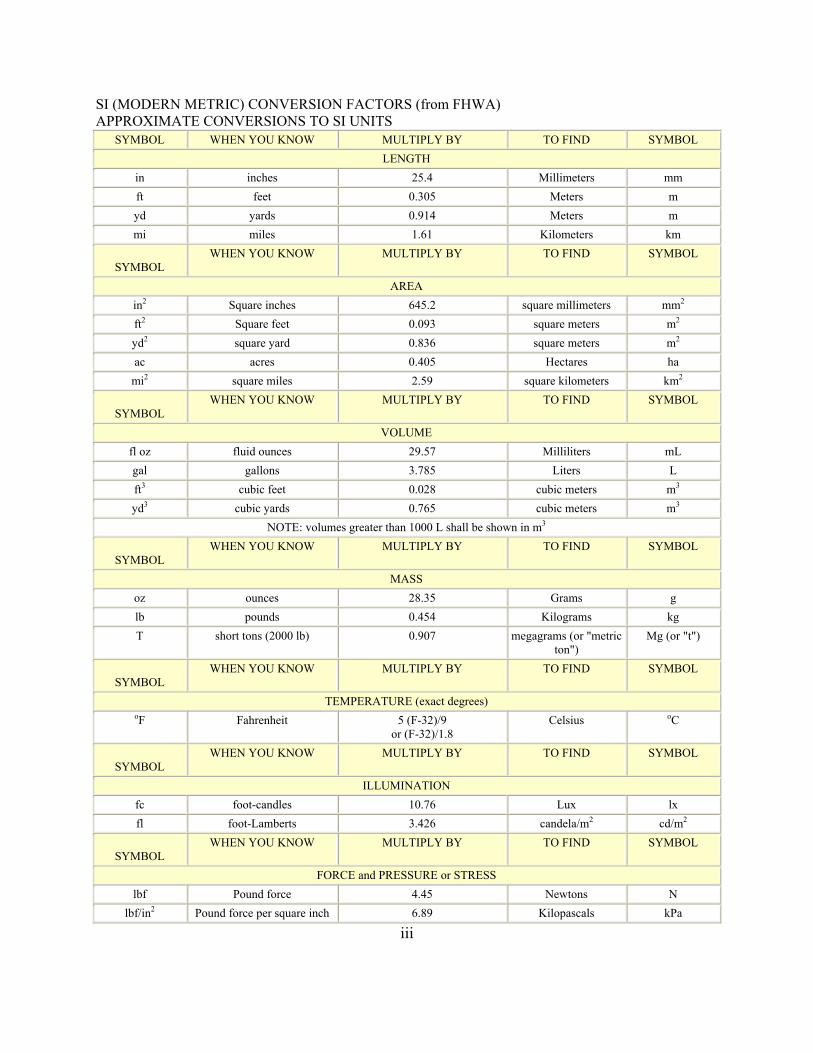
SI (MODERN METRIC) CONVERSION FACTORS (from FHWA) APPROXIMATE CONVERSIONS TO SI UNITS

SYMBOL WHEN YOU KNOW MULTIPLY BY TO FIND SYMBOL LENGTH

in inches 25.4 Millimeters mm ft feet 0.305 Meters m yd yards 0.914 Meters m mi miles 1.61 Kilometers km

SYMBOL

WHEN YOU KNOW MULTIPLY BY TO FIND SYMBOL

AREA in2 Square inches 645.2 square millimeters mm2 ft2 Square feet 0.093 square meters m2 yd2 square yard 0.836 square meters m2 ac acres 0.405 Hectares ha

mi2 square miles 2.59 square kilometers km2

SYMBOL WHEN YOU KNOW MULTIPLY BY TO FIND SYMBOL

VOLUME fl oz fluid ounces 29.57 Milliliters mL gal gallons 3.785 Liters L ft3 cubic feet 0.028 cubic meters m3 yd3 cubic yards 0.765 cubic meters m3

NOTE: volumes greater than 1000 L shall be shown in m3


MASS oz ounces 28.35 Grams g lb pounds 0.454 Kilograms kg T short tons (2000 lb) 0.907 megagrams (or "metric

ton") Mg (or "t")

SYMBOL


TEMPERATURE (exact degrees) oF Fahrenheit 5 (F-32)/9

or (F-32)/1.8 Celsius oC

SYMBOL


ILLUMINATION fc foot-candles 10.76 Lux lx fl foot-Lamberts 3.426 candela/m2 cd/m2


FORCE and PRESSURE or STRESS lbf Pound force 4.45 Newtons N

lbf/in2 Pound force per square inch 6.89 Kilopascals kPa

iii

APPROXIMATE CONVERSIONS TO ENGLISH UNITS SYMBOL WHEN YOU KNOW MULTIPLY BY TO FIND SYMBOL

LENGTH mm millimeters 0.039 Inches in m meters 3.28 Feet ft m meters 1.09 Yards yd

km kilometers 0.621 Miles mi


AREA mm2 square millimeters 0.0016 square inches in2 m2 square meters 10.764 square feet ft2 m2 square meters 1.195 square yards yd2 ha hectares 2.47 Acres ac

km2 square kilometers 0.386 square miles mi2


VOLUME mL milliliters 0.034 fluid ounces fl oz L liters 0.264 Gallons gal m3 cubic meters 35.314 cubic feet ft3 m3 cubic meters 1.307 cubic yards yd3

SYMBOL WHEN YOU KNOW MULTIPLY BY TO FIND SYMBOL MASS

g grams 0.035 Ounces oz kg kilograms 2.202 Pounds lb

Mg (or "t") megagrams (or "metric ton") 1.103 short tons (2000 lb) T


TEMPERATURE (exact degrees) oC Celsius 1.8C+32 Fahrenheit oF


ILLUMINATION lx lux 0.0929 foot-candles fc

cd/m2 candela/m2 0.2919 foot-Lamberts fl


FORCE and PRESSURE or STRESS N newtons 0.225 Pound force lbf

kPa kilopascals 0.145 Pound force per square inch

lbf/in2

*SI is the symbol for the International System of Units. Appropriate rounding should be made to comply with Section 4 of ASTM E380. (Revised March 2003)

iii (cont.)

Technical Report Documentation Page

1. Report No.

2. Government Accession No. 3. Recipient's Catalog No.

4. Title and Subtitle

Vertical and Horizontal Insitu Permeameter (VAHIP)

(DEVELOPMENT OF A NEW PERMEABILITY DEVICE TO MEASURE INSITU VERTICAL AND HORIZONTAL PERMEABILITY AT DIFFERENT

DEPTHS)

BD-545, RPWO # 3 UF Project 00030890 (4554013-12)

5. Report Date April 2007

6. Performing Organization Code

7. Author(s) David Bloomquist, Adrian Viala , Mike Gartner

8. Performing Organization Report No.

9. Performing Organization Name and Address Department of Civil and Coastal Engineering

365 Weil Hall University of Florida

Gainesville, Florida 32611

10. Work Unit No. (TRAIS)

11. Contract or Grant No. BC-545, RPWO #3

12. Sponsoring Agency Name and Address

Florida Department of Transportation 605 Suwannee Street, MS 30

Tallahassee, FL 32399

13. Type of Report and Period Covered

Final Report 8/2003 – 10/2006

14. Sponsoring Agency Code 15. Supplementary Notes

16. Abstract A new device has been designed to measure the insitu vertical and horizontal permeability at

multiple depths within a soil layer. Preliminary field testing of the device indicates that permeability results obtained are in agreement with that obtained from other conventional tests.

17. Key Word Permeability, field testing, probe

18. Distribution Statement No restrictions.

19. Security Classif. (of this report)

Unclassified.

20. Security Classif. (of this page)

Unclassified.

21. No. of Pages 137

22. Price NA

iv

1

TABLE OF CONTENTS page

LIST OF TABLES ...........................................................................................................................4

LIST OF FIGURES .........................................................................................................................5

Executive Summary ..................................................................................................................7

INTRODUCTION ...........................................................................................................................8

1.1 Background .........................................................................................................................8 1.2 Scope ...................................................................................................................................9

REVIEW OF LITERATURE ........................................................................................................11

2.1 Hydraulic Conductivity ....................................................................................................11 2.1.1 Hydraulic Conductivity in Sands ............................................................................13 2.1.2 Hydraulic Conductivity in Clays ............................................................................13 2.1.3 Typical Range of Hydraulic Conductivity for Various Soils .................................14

2.2 Vertical and Horizontal Permeability ...............................................................................15 2.21 Mean Coefficient of Permeability ...........................................................................16

2.3 Retention Ponds ................................................................................................................18 2.3.1 Infiltration in Retention Ponds ...............................................................................18 2.3.2 Vertical Unsaturated Flow Analysis .......................................................................19 2.3.3 Lateral Saturated Flow ...........................................................................................20

2.4 Determination of Hydraulic Conductivity ........................................................................21 2.4.1 Laboratory Methods ...............................................................................................21

2.4.1.1 Constant Head Method .................................................................................22 2.4.1.2 Falling Head Method ....................................................................................23

2.4.1.3 Flexible Walled Permeability Device ..................................................................25 2.4.1.4 Limitations of Laboratory Methods .............................................................26

2.4.2 Empirical Methods .................................................................................................26 2.4.2.1 Hansen’s Empirical Formula (1892) ............................................................27 2.4.2.2 Kozeny-Carman Formula .............................................................................27 2.4.2.3 Hagen – Poiseuille Formula .........................................................................29 2.4.2.4 Limitations and Assumptions of Empirical Methods ...................................29

2.4.3 Indirect Testing Methods ........................................................................................30 2.4.3.1 CRS Test Permeability Theory ....................................................................30 2.4.3.2 CRS Test Limitations and Assumptions ......................................................31

2.4.4 Insitu Methods ........................................................................................................32 2.4.4.1 Infiltrometers ................................................................................................32 2.4.4.1.1 Open single ring ........................................................................................33 2.4.4.1.2 Closed single ring ......................................................................................33 2.4.4.1.3 Open double ring .......................................................................................33 2.4.4.1.4 Closed double ring ....................................................................................34

2

2.4.4.1.5 Cylinder permeameter ...............................................................................34 2.4.4.1.6 Other Infiltrometers ...................................................................................35 2.4.4.1.7 Limitations ................................................................................................35 2.4.4.2 Tracer Dilution Tests ....................................................................................35 2.4.4.3 Slug Test .......................................................................................................35 2.4.4.3.1 Procedure ...................................................................................................36 2.4.4.3.2 Slug test analysis .......................................................................................36 2.4.4.3.3 Slug test theory ..........................................................................................38 2.4.4.3.4 Strengths and limitations ...........................................................................40 2.4.4.4 Well tests ......................................................................................................40 2.4.4.4.1 General procedure .....................................................................................41 2.4.4.4.2 Theory .......................................................................................................42

CHAPTER 3 ..................................................................................................................................46

DEVELOPMENT OF THE VAHIP ..............................................................................................46

3.1 Description of Prototype ...................................................................................................46 3.1.1 Basic Design ...........................................................................................................46 3.1.2 Assembly ................................................................................................................47

3.2 Complications with Design ...............................................................................................50 3.2.1 Full Flow Condition ...............................................................................................50 3.2.2 Area Correction ......................................................................................................50 3.2.3 Equation Limitations ..............................................................................................50 3.2.4 Mechanical Complications .....................................................................................50

3.2.4.1 Sand intrusion ...............................................................................................51 3.2.4.2 Piezotube connection ....................................................................................51 3.2.4.3 Assembling and disassembling ....................................................................51

3.2.5 Rigidity ...................................................................................................................52 3.3 Description of 2005 VAHIP Probe ...................................................................................52 3.4 Field Testing of 2005 VAHIP Probe ................................................................................56 3.5 Description of 2006 VAHIP Probe ...................................................................................59

3.4.1 Assembling and Operation Methodology ...............................................................61 3.5 Description of Plexiglas Standpipe ...................................................................................64 3.6 Description of Control Panel ............................................................................................65

3.6.1 Available Water Supply .........................................................................................66

PROCEDURE FOR FIELD USE OF VAHIP AND DATA REDUCTION .................................68

4.1 Outlined Field Test Procedure ..........................................................................................68 4.1.1 Pre-field Preparation ...............................................................................................68 4.1.2 Probe Assembly ......................................................................................................68 4.1.3 VAHIP Flow Measurement Assembly ...................................................................68 4.1.4 Test Procedure ........................................................................................................69 4.1.5 Test Types ..............................................................................................................69

4.1.5.1 Constant head ...............................................................................................70 4.1.5.2 Falling head ..................................................................................................70

3

4.2 Alternative Testing Procedure ..........................................................................................70 4.3 VAHIP Maintenance ........................................................................................................71 4.4 Data Reduction .................................................................................................................71

4.4.1 Hvorslev’s Theory ..................................................................................................72 4.4.2 F Factor or Shape Factors for Probe .......................................................................74

4.4.2.1 Determination of F Factor ............................................................................75 4.4.2.2 F Factor (Fourier expansions with Bessel Function coefficients) ................80

4.4.3 VAHIP Data Reduction - Constant Head Tests .....................................................87 4.4.3.1 Horizontal flow ............................................................................................87 4.4.3.2 Vertical flow .................................................................................................88

4.4.4 VAHIP Data Reduction -Falling Head Tests .........................................................88 4.4.4.1 Horizontal flow ............................................................................................88 4.4.4.2 Vertical flow .................................................................................................89

TEST RESULTS ............................................................................................................................90

5.1 Test Results .......................................................................................................................90 5.1.1 Probe Permeability Tests ........................................................................................90 5.1.2 Sand Barrel Tests ....................................................................................................91 5.1.3 Pseudo Field Tests ..................................................................................................93 5.1.4 Field Tests ..............................................................................................................95 5.1.5 Further Enhancement of the Probe .......................................................................100 5.5.6 Field Testing of the Enhanced Probe ....................................................................101

CONCLUSIONS AND RECOMMENDATIONS ......................................................................104

6.1 Overview .........................................................................................................................104 6.2 Results and Conclusions .................................................................................................104 6.3 Recommendations ...........................................................................................................106

VAHIP EQUIPMENT CHECKLIST ..........................................................................................109

PROBE AND PLEXIGLAS FMD PROPERTIES ......................................................................110

SPREADSHEETS FOR VAHIP PERMEABILITY TESTS ......................................................111

TYPICAL PERMEABILITY TEST RESULTS SPREADSHEETS ..........................................113

USER’S MANUAL .....................................................................................................................118

LIST OF REFERENCES .............................................................................................................131

4

LIST OF TABLES

Table page Table 1-1. Advantages and disadvantages of laboratory and insitu testing techniques* ..............10

Table 2-1. Hydraulic conductivity of some soils (from Casagrande and Fadum, 1939, as cited in Lambe and Whitman, 1969) .............................................................................14

Table 2-2. Classification of soils according to their coefficients of permeability (Terzaghi and Peck, as cited in Lambe and Whitman, 1969) .............................................................14

Table 2-3. Ranges of hydraulic conductivities for unconsolidated sediments (from Fetter, 2001 as cited in Murthy, 2003) ..........................................................................................14

Table 2-4. Typical values of permeability for sands (Leonards, 1962) .........................................15

Table 2-4. Typical slug test analysis methods (Butler 1998) .........................................................37

Table 2-5. Advantages and Disadvantages of the slug test ............................................................40

Table 2-6. Typical pump test measurement recording frequency ..................................................42

Table 3.1 2005 Probe Field Test Results ......................................................................................58

Table 5-1. Probe Permeability Test Results ...................................................................................91

Table 5-2 Summary of Barrel Test Results (fine sand) .................................................................92

Table 5-3 Summary of Pseudo-Field Tests Results (Brown Fine Sand) .......................................94

Table 5-5 Field Test Results ..........................................................................................................96

Table 5-6 Field Test Results for the modified Probe ...................................................................103

5

LIST OF FIGURES

Figure page Figure 2-1. Infiltration Stages in Retention Ponds .........................................................................19

Figure 2-4. (A) Short circuiting of water flow along fixed wall permeability testing device. (B) Flexible walled permeability testing device reduces chances of short circuiting. .......26

Figure 2-5. Ring Infiltrometers Profile View (a) open single ring (b) closed single ring (c) open double ring (d) closed double ring ............................................................................34

Figure 2-6. Slug Test Schematic ....................................................................................................38

Figure 2-7. Pump Test Schematic ..................................................................................................45

Figure 3-1. VAHIP Probe (2004). A) Stage I (Vertical Permeability) B) Stage II (Horizontal Permeability) ......................................................................................................................48

Figure 3-6 Potentially clogged flow ports (2005 probe) ................................................................58

Figure 3-6 Schematic representation of 2006 probe with tip closed for horizontal flow and opened for vertical flow. ....................................................................................................60

Figure 3-7 Dismantled 2006 VAHIP Probe Showing Components ..............................................62

Figure 3-8 Probe tip opened for vertical flow ................................................................................63

Figure 3-9 Probe tip closed for horizontal flow .............................................................................63

Figure 3-10. Picture of Flow Measurement Device (FMD) ..........................................................65

Figure 3-11. Picture of Control Panel ............................................................................................66

Figure 3-12. Graph of tank pressure vs. fill time for the Buell Compressor and 7gallon air tank. ....................................................................................................................................67

Figure 4-4. Variable definitions for time lag derivation. ...............................................................72

Figure 4-5. Inflow and Shape Factors from Hvorslev (1951) ........................................................77

Figure 4-6. Formulas for Determining Permeability (Hvorslev, 1951) .........................................77

Figure 4-1. Boundary conditions for axisymmetric flow domain of single injection screen. .......82

Figure 4-2. Example of successive approximation and extrapolation to obtain exact F ...............85

Figure 4-3. Example of resulting flow field properties for injection/extraction with close-by vertically confining layers. .................................................................................................86

6

Figure 5-2 Setup for Sand Barrel Test ...........................................................................................92

Figure 5-4 Summary of Barrel Test Results ..................................................................................93

Figure 5-5 Pseudo – Field test behind the Reed Lab. ....................................................................93

Figure 5-7 Laboratory permeability test on sample .......................................................................94

Figure 5-6 Summary of Pseudo-Field test Results ........................................................................94

Figure 5-9 Field testing ..................................................................................................................97

Figure 5.10 Summary of Field testing ...........................................................................................98

Figure 5.10 Summary of Field testing continued ...........................................................................98



Figure 6.1 Modified Probe with tip closed ..................................................................................100

Figure 6.2 Modified Probe with tip opened .................................................................................101

Figure 6.3 Summary of Field Testing of Modified Probe ...........................................................103

7

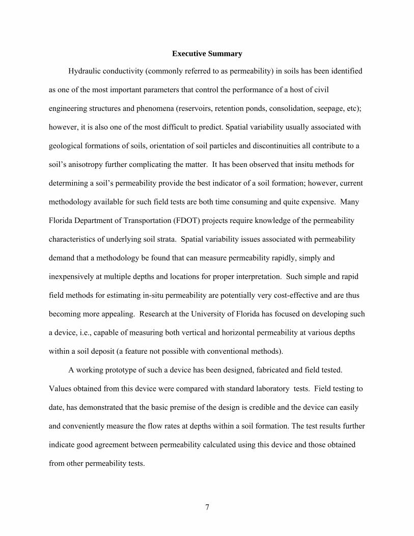
Executive Summary

Hydraulic conductivity (commonly referred to as permeability) in soils has been identified

as one of the most important parameters that control the performance of a host of civil

engineering structures and phenomena (reservoirs, retention ponds, consolidation, seepage, etc);

however, it is also one of the most difficult to predict. Spatial variability usually associated with

geological formations of soils, orientation of soil particles and discontinuities all contribute to a

soil’s anisotropy further complicating the matter. It has been observed that insitu methods for

determining a soil’s permeability provide the best indicator of a soil formation; however, current

methodology available for such field tests are both time consuming and quite expensive. Many

Florida Department of Transportation (FDOT) projects require knowledge of the permeability

characteristics of underlying soil strata. Spatial variability issues associated with permeability

demand that a methodology be found that can measure permeability rapidly, simply and

inexpensively at multiple depths and locations for proper interpretation. Such simple and rapid

field methods for estimating in-situ permeability are potentially very cost-effective and are thus

becoming more appealing. Research at the University of Florida has focused on developing such

a device, i.e., capable of measuring both vertical and horizontal permeability at various depths

within a soil deposit (a feature not possible with conventional methods).

A working prototype of such a device has been designed, fabricated and field tested.

Values obtained from this device were compared with standard laboratory tests. Field testing to

date, has demonstrated that the basic premise of the design is credible and the device can easily

and conveniently measure the flow rates at depths within a soil formation. The test results further

indicate good agreement between permeability calculated using this device and those obtained

from other permeability tests.

8

CHAPTER 1 INTRODUCTION

Permeability is basically a measure of the ability of a material or porous media to transmit

fluid through it. Materials such as rocks, concrete, soils, etc are permeable as a result of the void

spaces within them. Permeability thus is a property of the porous media and depends basically on

the volume and interconnectedness of void spaces within the porous media. With regards to the

flow or transmission of water in these materials, permeability is typically referred to as the

hydraulic conductivity. Hydraulic conductivity is a property of the soil or rock that describes the

ease with which water flows through the pore spaces. The design of most systems in civil

engineering is influenced by the rate at which water flows through the system or in the strata on

which they are founded. Knowledge of the hydraulic conductivity of soils is therefore essential

and required in the design of earth dams, retention ponds, dewatering systems, hydraulic

structures, wells, landfills and a host of other geotechnical engineering analyses. The accurate

determination of the hydraulic conductivity is often essential and plays a pivotal role in

determining the economy and efficacy of a particular design.

1.1 Background

The measurement of hydraulic conductivity in soils is difficult largely due to the lack of

homogeneity and spatial variability. Consequently, hydraulic conductivity values generally tend

to show variations throughout a soil formation thus making a generalized prediction of the

overall permeability difficult to quantify. Again, because of the usually stratified nature of

sedimentary soil materials, such soils are usually anisotropic even when homogenous. Within an

anisotropic formation, the vertical component of the saturated hydraulic conductivity is usually

lower (by one or more orders of magnitude) than the horizontal component. More often than not,

the method and procedure used in measuring hydraulic conductivity directly impinges on the

9

results obtained. Generally two techniques are normally employed - laboratory and insitu

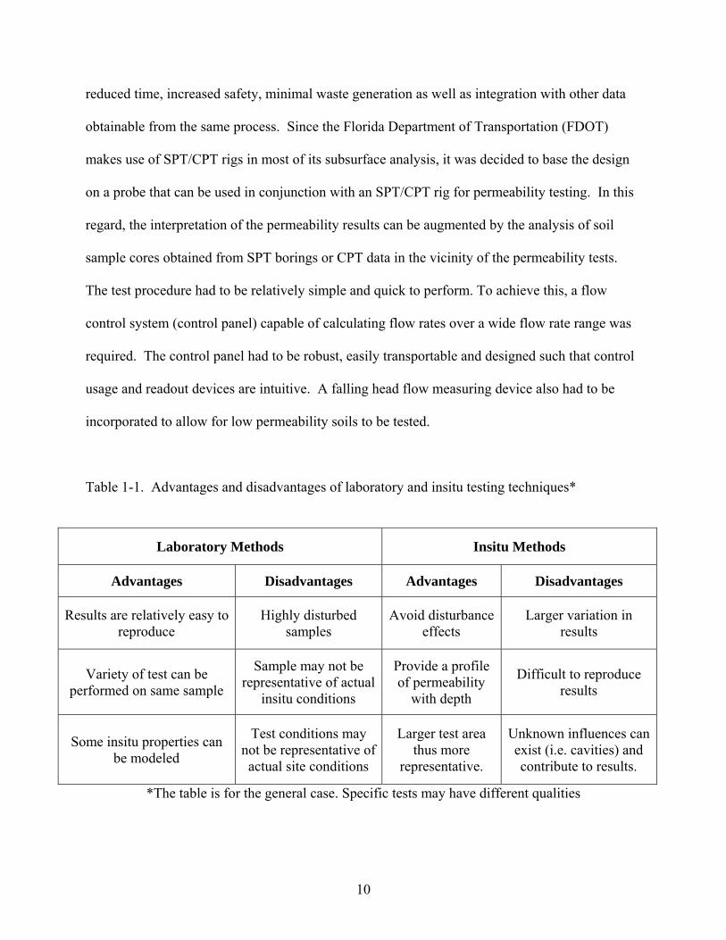
techniques; each with its own attendant strengths and weaknesses as outlined in Table 1-1.

Generally for most design purposes, field generated data provide a better representation of actual

insitu conditions compared with laboratory methods. Lab tests are usually employed when actual

representation of field conditions is not of fundamental importance in a particular design. Field

methods, however, are usually more expensive.

The FDOT conducts on-site permeability testing for a variety of projects. Undertaking

field permeability testing on such a variety of sites using conventional methodologies has proven

to be an expensive and time consuming undertaking. It has been recognized that simple and

rapid field methods for estimating in-situ permeability would not only be appealing from a

timing standpoint, but would be potentially cost-effective as well. In addition, for an effective

design, it is advantageous if coefficients of hydraulic conductivity in both the vertical and

horizontal directions can be measured. This is particularly important in retention pond design,

where the exiting of water from a pond can be accomplished in two stages; an initial stage which

is entirely due to vertical percolation, followed by a second stage consisting of predominantly

horizontal flow.

1.2 Scope

The overriding goal of this research was to develop a device which can effectively measure

the insitu vertical and horizontal saturated hydraulic conductivity at variable depths within a soil

formation. The primary objective was to create, based on sound theoretical constraints, a device

that would be relatively quick to use, and to verify that the results obtained using the device were

consistent with values obtained from other methods. The permeameter needed to be designed to

be robust and quickly assembled and disassembled in the field. A direct push technique was

identified as one possible methodology which when used for permeability tests would lead to

10

reduced time, increased safety, minimal waste generation as well as integration with other data

obtainable from the same process. Since the Florida Department of Transportation (FDOT)

makes use of SPT/CPT rigs in most of its subsurface analysis, it was decided to base the design

on a probe that can be used in conjunction with an SPT/CPT rig for permeability testing. In this

regard, the interpretation of the permeability results can be augmented by the analysis of soil

sample cores obtained from SPT borings or CPT data in the vicinity of the permeability tests.

The test procedure had to be relatively simple and quick to perform. To achieve this, a flow

control system (control panel) capable of calculating flow rates over a wide flow rate range was

required. The control panel had to be robust, easily transportable and designed such that control

usage and readout devices are intuitive. A falling head flow measuring device also had to be

incorporated to allow for low permeability soils to be tested.

Table 1-1. Advantages and disadvantages of laboratory and insitu testing techniques*

Laboratory Methods Insitu Methods

Advantages Disadvantages Advantages Disadvantages

Results are relatively easy to reproduce

Highly disturbed samples

Avoid disturbance effects

Larger variation in results

Variety of test can be performed on same sample

Sample may not be representative of actual

insitu conditions

Provide a profile of permeability

with depth

Difficult to reproduce results

Some insitu properties can be modeled

Test conditions may not be representative of actual site conditions

Larger test area thus more

representative.

Unknown influences can exist (i.e. cavities) and contribute to results.

*The table is for the general case. Specific tests may have different qualities

11

CHAPTER 2 REVIEW OF LITERATURE

As stated earlier, permeability is basically a measure of the ability of a material or porous

media to transmit fluid through it. The permeability of a material is best described by the

permeability coefficient, k, which may be defined as the discharge velocity of a fluid through a

unit area driven by a unit hydraulic gradient within the material.

2.1 Hydraulic Conductivity

With regards to the flow or transmission of water in materials, permeability is referred to

as the hydraulic conductivity. Hydraulic conductivity is a property of the soil or rock that

describes the ease with which water flows through its pore spaces. In the area of soil mechanics,

permeability and hydraulic conductivity can be used interchangeably. Knowledge of the

hydraulic conductivity of soils is important and required in a variety of geotechnical engineering

analyses. For design, the desired soil permeability is a function of the project’s objectives. In a

landfill, it is desired that permeability of the liner be low such that contaminants are restrained

from entering the ground water supply. In a retention pond, the opposite is true; high soil

permeability is desired such that the storage areas do not fail due to overloading.

In general, water flowing through a saturated soil mass experiences a resistance to its flow

as a result of the presence of solid soil matter in accordance with the laws of fluid mechanics.

Darcy (1856) derived an empirical formula for the behavior of flow through saturated soils under

steady state conditions. He concluded that the quantity of water per second (q) flowing through a

cross-sectional area (A) of soil normal to the direction of flow under hydraulic gradient (i) can be

expressed by the formula,

(2. 1) kiAq =

Where: k is termed the hydraulic conductivity of the soil.

12

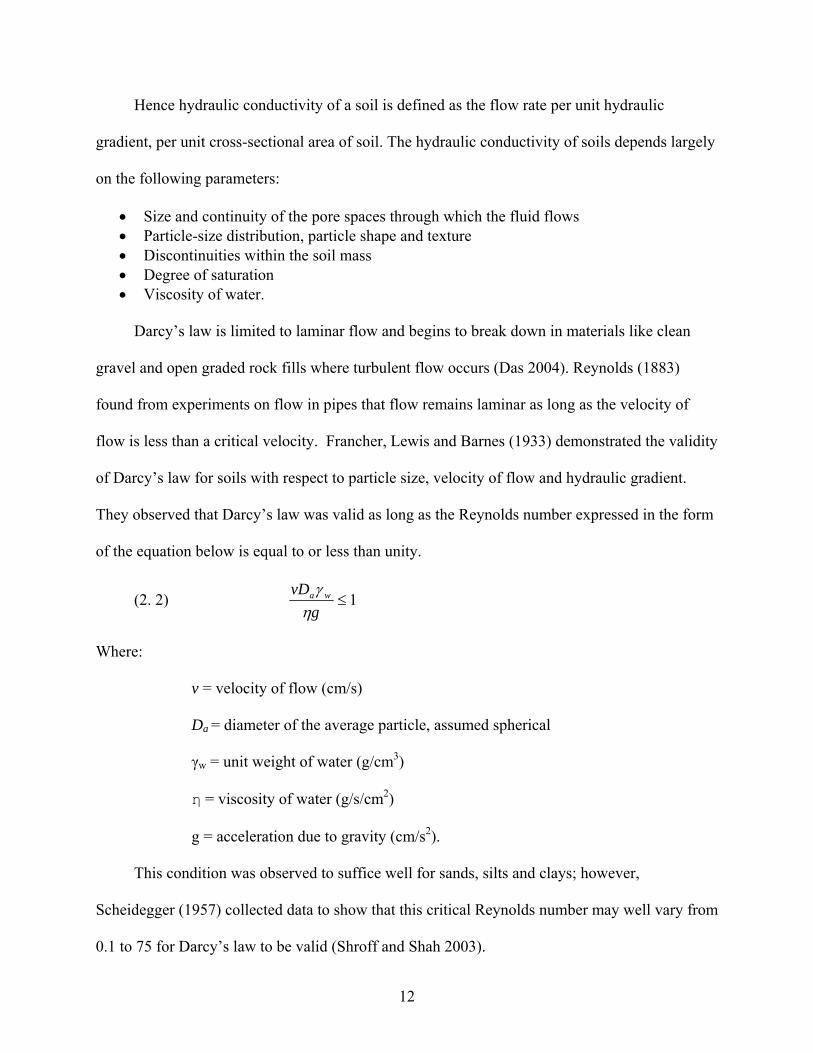
Hence hydraulic conductivity of a soil is defined as the flow rate per unit hydraulic

gradient, per unit cross-sectional area of soil. The hydraulic conductivity of soils depends largely

on the following parameters:

• Size and continuity of the pore spaces through which the fluid flows • Particle-size distribution, particle shape and texture • Discontinuities within the soil mass • Degree of saturation • Viscosity of water.

Darcy’s law is limited to laminar flow and begins to break down in materials like clean

gravel and open graded rock fills where turbulent flow occurs (Das 2004). Reynolds (1883)

found from experiments on flow in pipes that flow remains laminar as long as the velocity of

flow is less than a critical velocity. Francher, Lewis and Barnes (1933) demonstrated the validity

of Darcy’s law for soils with respect to particle size, velocity of flow and hydraulic gradient.

They observed that Darcy’s law was valid as long as the Reynolds number expressed in the form

of the equation below is equal to or less than unity.

(2. 2) 1≤g

vD wa

ηγ

Where:

v = velocity of flow (cm/s)

Da = diameter of the average particle, assumed spherical

γw = unit weight of water (g/cm3)

η = viscosity of water (g/s/cm2)

g = acceleration due to gravity (cm/s2).

This condition was observed to suffice well for sands, silts and clays; however,

Scheidegger (1957) collected data to show that this critical Reynolds number may well vary from

0.1 to 75 for Darcy’s law to be valid (Shroff and Shah 2003).

13

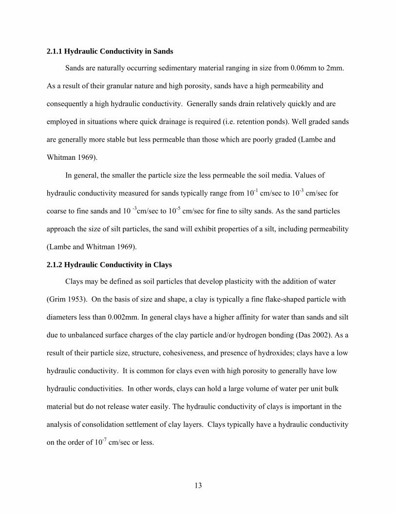
2.1.1 Hydraulic Conductivity in Sands

Sands are naturally occurring sedimentary material ranging in size from 0.06mm to 2mm.

As a result of their granular nature and high porosity, sands have a high permeability and

consequently a high hydraulic conductivity. Generally sands drain relatively quickly and are

employed in situations where quick drainage is required (i.e. retention ponds). Well graded sands

are generally more stable but less permeable than those which are poorly graded (Lambe and

Whitman 1969).

In general, the smaller the particle size the less permeable the soil media. Values of

hydraulic conductivity measured for sands typically range from 10-1 cm/sec to 10-3 cm/sec for

coarse to fine sands and 10 -3cm/sec to 10-5 cm/sec for fine to silty sands. As the sand particles

approach the size of silt particles, the sand will exhibit properties of a silt, including permeability

(Lambe and Whitman 1969).

2.1.2 Hydraulic Conductivity in Clays

Clays may be defined as soil particles that develop plasticity with the addition of water

(Grim 1953). On the basis of size and shape, a clay is typically a fine flake-shaped particle with

diameters less than 0.002mm. In general clays have a higher affinity for water than sands and silt

due to unbalanced surface charges of the clay particle and/or hydrogen bonding (Das 2002). As a

result of their particle size, structure, cohesiveness, and presence of hydroxides; clays have a low

hydraulic conductivity. It is common for clays even with high porosity to generally have low

hydraulic conductivities. In other words, clays can hold a large volume of water per unit bulk

material but do not release water easily. The hydraulic conductivity of clays is important in the

analysis of consolidation settlement of clay layers. Clays typically have a hydraulic conductivity

on the order of 10-7 cm/sec or less.

14

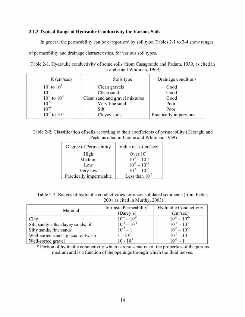
2.1.3 Typical Range of Hydraulic Conductivity for Various Soils

In general the permeability can be categorized by soil type. Tables 2-1 to 2-4 show ranges

of permeability and drainage characteristics, for various soil types.

Table 2-1. Hydraulic conductivity of some soils (from Casagrande and Fadum, 1939, as cited in Lambe and Whitman, 1969)

K (cm/sec) Soils type Drainage conditions 101 to 102 101 10-1 to 10-4 10-5 10-6 10-7 to 10-9

Clean gravels Clean sand

Clean sand and gravel mixtures Very fine sand Silt Clayey soils

Good Good Good Poor Poor

Practically impervious

Table 2-2. Classification of soils according to their coefficients of permeability (Terzaghi and

Peck, as cited in Lambe and Whitman, 1969)

Table 2-3. Ranges of hydraulic conductivities for unconsolidated sediments (from Fetter, 2001 as cited in Murthy, 2003)

Material Intrinsic Permeability* (Darcy’s)

Hydraulic Conductivity (cm/sec)

Clay Silt, sandy silts, clayey sands, till Silty sands, fine sands Well-sorted sands, glacial outwash Well-sorted gravel

10-6 – 10-3 10-3 – 10-1 10-2 – 1 1 - 102 10 - 103

10-9 – 10-6 10-6 – 10-4 10-5 – 10-3 10-3 – 10-1 10-2 – 1

* Portion of hydraulic conductivity which is representative of the properties of the porous medium and is a function of the openings through which the fluid moves.

Degree of Permeability Value of k (cm/sec) High

Medium Low

Very low Practically impermeable

Over 10-1 10-1 – 10-3 10-3 – 10-5 10-5 – 10-7

Less than 10-7

15

Table 2-4. Typical values of permeability for sands (Leonards, 1962)

Type of sand (U.S. Army Engineer classification)

Value of k x 10-4 (cm/sec)

Very fine sand Fine sand

Fine to medium sand Medium sand

Medium to coarse sand Gravel and coarse sand

50 200 500 1000 1500 3000

2.2 Vertical and Horizontal Permeability

As already indicated, natural soil deposits and mechanically compacted embankments are

almost always stratified to some degree and rarely isotropic. Soil stratification and

discontinuities provide flow channels within the soil mass which are less resistive to flow. Also

under field conditions, both vertical and horizontal hydraulic gradients exist to compel flow

either in the vertical or horizontal direction.

The culminating effect of these factors means that soil masses usually possess anisotropic

permeability, with differing permeability in the vertical and horizontal directions. The natural

orientation of particles in soils which have been consolidated vertically and discontinuities on

stratum bedding planes ensures that the average permeability parallel to the planes of

stratification is greater than the permeability perpendicular to these planes. The inclusion of thin

horizontal layers of coarse-grained soil in a mass of fine-grained soil may dramatically increase

the horizontal permeability while having little effect on the vertical permeability. Also, it is

possible to increase the drainage rate of a soil layer without changing the permeability of the

bulk of the soil by introducing layer drains (sand wicks) or fracturing the soil. These examples

reveal that soil permeability in the horizontal and vertical directions are greatly affected by the

sizes and orientation of soil particles as well as any discontinuities present. Thus it can be

16

inferred that the coefficient of permeability in horizontal and vertical directions in soil would not

always be the same, with the horizontal values almost always being larger than the vertical.

Soil permeability is an important soil parameter for any project where flow of water

through soil or rock is a matter of concern. For effective design, it is expected that the

coefficients of soil permeability in both the vertical and horizontal directions can be determined

and also easily measurable. As earlier stated, this is particularly important in retention pond

design where exiting of water from the pond can be achieved in two stages; an initial stage which

is entirely due to vertical percolation followed by a second stage of horizontal flow. During

vertical infiltration in a retention pond, the water percolates through the unsaturated soil between

the basin and the ground water table and fills the empty void spaces. This portion of soil thus

becomes saturated with time and limits further downward water movement. A second stage then

commences whereby the water infiltrates horizontally through the side slopes. This fills the voids

of the unsaturated soil on the slope above the bottom of the basin. In such a scenario, knowledge

of the vertical and horizontal coefficient of permeability of the soil material underlying the pond

would yield a more cost effective and better design.

2.21 Mean Coefficient of Permeability

Generally in seepage analysis for most soils, it is required that a value of permeability is

determined which best gives an indication of the average rate of water movement through the

soil mass, irrespective of direction. In order to obtain such an isotropic representative value of

the coefficient of permeability, it is usually common to transform and express the overall average

coefficient of permeability of a soil mass and the degree of anisotropy as:

(2. 3) hvm KKK = and h

v

KK

m =

Where:

17

Km is the mean coefficient of permeability for the soil mass

Kv is the coefficient of permeability in the vertical direction

Kh is the coefficient of permeability in the horizontal direction

m is the degree of anisotropy.

The mathematical basis of this transformation is outlined as follows.

Plane flow in an anisotropic material having a horizontal permeability, Kh , and a vertical

permeability, kv , is governed by the equation:

(2. 4) 02

2

2

2

=+z

hkx

hk vh ∂∂

∂∂

Introducing a new variable and let xmx = and zz = the seepage equation then becomes:

(2. 5) 02

2

2

2

2 =+z

hx

hkm

k

v

h

∂∂

∂∂

If we substitute v

h

kk

m =

Equation (2.4), which represents flow in an anisotropic medium, converts to a relationship for

isotropic conditions given by:

(2. 6) ∂∂

∂∂

2

2

2

2 0hx

hz

+ =

18

Now considering an element of soil in the x direction, having a length, l, and cross-sectional

area, A, under a hydraulic head, hΔ , the flow rate in the untransformed state is given by:

(2. 7) lhAkq vv

Δ=

Substituting the coefficient of permeability in the transformed state by hvm kkk = , then in the

transformed state:

(2. 8) =Δ

=

v

hmv

kk

l

hAkq vv

v

hhv q

lhAk

kk

l

hAKK =Δ

=Δ

Hence a mean coefficient of permeability hvm kkk = can then be introduced under this

transformed isotropic condition for seepage analysis.

2.3 Retention Ponds

Retention ponds are used to store storm water run-off and allow it to percolate through the

permeable soil layer into the underlying aquifer. It is essential that the soil in the retention pond

has the desired permeability properties to allow efficient water flow through the medium. A high

permeability and favorable ground water table are preferred.

2.3.1 Infiltration in Retention Ponds

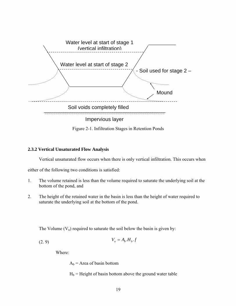
The process by which water exits a retention pond takes place in two stages. In the first

stage, only vertical infiltration through the bottom of the pond (unsaturated flow) occurs. In the

second, the water immigrates horizontally through the side slopes. This fills the voids of the

unsaturated soil on the slope above the bottom of the basin.

19

Figure 2-1. Infiltration Stages in Retention Ponds

2.3.2 Vertical Unsaturated Flow Analysis

Vertical unsaturated flow occurs when there is only vertical infiltration. This occurs when

either of the following two conditions is satisfied:

1. The volume retained is less than the volume required to saturate the underlying soil at the bottom of the pond, and

2. The height of the retained water in the basin is less than the height of water required to

saturate the underlying soil at the bottom of the pond.

The Volume (Vu) required to saturate the soil below the basin is given by:

(2. 9) fHAV bbu ..=

Where:

Ab = Area of basin bottom

Hb = Height of basin bottom above the ground water table

Impervious layer

Water level at start of stage 1 (vertical infiltration)

Water level at start of stage 2

Mound

Soil voids completely filled

- Soil used for stage 2 –

20

f = Fillable porosity

For unsaturated vertical flow, the recovery time Tsat is given by

(2. 10) d

bsat I

HfT

.=

Where: Id = design infiltration rate

According to the modified Green and Ampt infiltration equation:

(2. 11) FSK

I vd =

Where: Kv is the unsaturated vertical hydraulic conductivity and FS is the factor

of safety which is introduced to account for flow losses due to basin bottom silting or clogging

and is usually given a recommended value of two (2).

2.3.3 Lateral Saturated Flow

When the volume of storm water retained in the basin is such that does not completely

percolate through the unsaturated soil underneath the basin, lateral flow occurs when the

underlying soils become saturated. The rate of lateral flow depends on the horizontal

permeability of the soil on the side slopes of the retention pond.

Andreyev and Wiseman (1989) proposed a methodology to calculate the recovery time of a

pond under lateral saturated flow using the following dimensionless parameters:

(2. 12) 5.02

...4 ⎥⎦

⎤⎢⎣

⎡=

tDKWF

Hx

(2. 13) T

cy H

hF =

21

Where:

Fx= Dimensionless parameter representing the physical and hydraulic

characteristics of the retention basin and effective aquifer system

Fy= Dimensionless parameter representing the percent of water level

decline below a maximum level

W =Average width of the pond midway between basin bottom and water

level at time t

KH = Average horizontal hydraulic conductivity (ft/day)

D=Average thickness of aquifer (ft) given by 2chHD +=

hc =Height of water (ft) in the basin above the initial ground water table

time t

H=Initial saturation thickness of the aquifer (ft)

t =Cumulative time space (days) since the saturated lateral (stage two)

flow started

HT = Height of water (ft) in the basin above the initial ground water table

at the start of the saturated flow (stage two) given by 2hHH bT +=

h2 = Height of water (ft) in the basin above the basin bottom at the start of

saturated lateral flow (stage two).

2.4 Determination of Hydraulic Conductivity

Determination of hydraulic conductivity is usually carried out by methods which can be

classified as laboratory or field methods, empirical correlations, or indirect methods. Some of

these methodologies are discussed below.

2.4.1 Laboratory Methods

One of the main advantages of laboratory methods is the capability of reproducing results. In a

laboratory, conditions can be better monitored and easily controlled (i.e. hydraulic head);

however, it is very difficult to obtain an undisturbed sample. Since it is almost impossible to

22

obtain undisturbed samples of cohesionless soils and highly pre-consolidated clays, laboratory

tests on these materials are typically conducted on samples which are reconstructed or remolded

to best simulate field conditions of the soil.

The test method usually involves a cylindrical soil specimen with a length (L) and surface

area (A) being placed into the testing device. A difference in head between the top and bottom of

the specimen is created resulting in a hydraulic gradient, i, which in turn forces the water to flow

though the specimen. The hydraulic conductivity during steady state conditions is then calculated

using Darcy’s law.

Three types of laboratory methods generally used to determine the hydraulic conductivity

of soils are discussed below.

2.4.1.1 Constant Head Method

This test is particularly suited for granular soils with a coefficient of permeability on the

order of 10-3 or greater (Terzaghi & Peck). This method may not be well suited for low

permeability soils because of the length of time required for a sufficient quantity of water to flow

through the sample, and the possibility of evaporation losses of this water (Davidson 2002).

The apparatus, depicted in Figure 2-2, consists of a vertical cylindrical tube containing the

soil specimen. The sample of length (L) and cross-sectional area (A) is subjected to a constant

head (H) of water flow. This total head is held constant throughout the test by using overflow

reservoirs to maintain the headwater and tailwater levels. Under steady state and fully saturated

conditions, the volume of water (Q) collected in a given time (t) is measured. The value of the

permeability coefficient can then be determined directly from Darcy’s law as expressed below.

23

(2.14) HAtQLk

Δ=

Figure 2-2. Constant Head Test Laboratory Setup.

2.4.1.2 Falling Head Method

Terzaghi and Peck (1969) suggest using this method for soils that have a permeability

coefficient less than 1 cm/s. However, if the permeability of a soil is too high (e.g. coarsed

grained sands), accurate timing measurement of the falling water column may be too difficult

(Davidson 2002). This method is well suited for fine grained soils such as silts and clays with

low hydraulic conductivities.

24

Figure 2-3. Falling Head Laboratory test set up.

Figure 2-3 shows a schematic of the falling head permeability apparatus. The soil sample is

placed in a vertical cylinder with a cross-sectional area, A. A transparent standpipe of cross-

sectional area, a, is attached to the test cylinder. During the test, the tailwater is held consent by

an overflow reservoir while the elevation of the headwater is allowed to change. Under steady

state and fully saturated condition, the change in head (Hi – Hf) with respect to time (t) is

measured.

The flowrate, q, through the specimen can be computed by

(2.15) dt

dHaALHkq −==

where q = flowrate [L3/T] and a = area of standpipe [L2]. Rearranging (2.15) to solve for dt gives

(2.16) ⎟⎠⎞

⎜⎝⎛−=

HdH

AkaLdt

Integrating both sides yields

(2.17) ∫ ∫ −=t H

H

f

i HdH

AkaLdt

0

25

(2.18) f

i

HH

AkaLt ln=

Solving for k produces following equation

(2.19) f

i

HH

AtaLk ln=

2.4.1.3 Flexible Walled Permeability Device

For a rigid wall permeability test apparatus, the interface between the soil specimen and

fixed wall can act as a flow channel and hence bypass the specimen. This phenomenon which is

termed flow short circuiting occurs because water flows along the path of least resistance. Short

circuiting mostly occurs in soils with a low permeability where the specimen exhibits a high

resistance to flow within the soil relative to the resistance along the interface.

To hinder flow short circuiting, a flexible walled permeability apparatus may be employed.

In a flexible walled device, the rigid cylinder containing the specimen is replaced by a rubber

membrane. The specimen in then placed into the chamber where the pressure can be adjusted.

Thus by increasing the pressure, the flexible membrane takes the shape of the soil specimen and

hinders the development of flow boundaries on the specimen as shown in Figure 2-4(B).Other

advantages derived from the use of this device for permeability testing are:

1) Used for testing very low permeability soils ( k < 1 x 10-4 cm/sec)

2) Hydraulic gradient is easily varied

3) Confining pressure can also be varied

4) Back pressure causes adequate saturation

26

A B

Figure 2-4. (A) Short circuiting of water flow along fixed wall permeability testing device. (B) Flexible walled permeability testing device reduces chances of short circuiting.

2.4.1.4 Limitations of Laboratory Methods

One of the main advantages of laboratory methods is the capability of reproducing results.

In a lab, conditions can be better monitored and easily controlled (i.e. specimen dimensions,

applied head). Even though these testing methods are relatively simple to perform, it is very

difficult to simulate actual field conditions. Some limitations of laboratory methods are:

• Disturbance. It is not possible to obtain a truly undisturbed sample. Samples are always disturbed to some degree. Careful sampling may reduce the disturbance but cannot eliminate it completely. Disturbances that affect the permeability include anisotropy, confining pressures, particle orientation, and void ratio.

• Sample size. The soil sample size obtained for a given site is very small relative to the site itself. Thus the samples may not reflect the effects of nonhomogeneity that may exist on the site.

• Test Duration. During long testing hours, water losses due to evaporation may result in errors in the calculated total head.

2.4.2 Empirical Methods

It has been observed that some of the soil parameters that affect permeability are

interrelated. Soil properties such as void ratio and grain size distribution can be used to estimate

27

permeability. Smaller soil grain sizes results in smaller voids or flow channels, subsequently

lowering the material’s permeability.

Various empirical correlations have been obtained between such properties and the

hydraulic conductivities of soils. Some empirical correlations are discussed below.

2.4.2.1 Hansen’s Empirical Formula (1892)

Extensive investigations by Hansen on fine uniform sand with effective sizes varying from

0.1 to 3 mm and uniformity coefficients less than 5 resulted in the correlation:

(2.19) 2eCDk =

The term De (cm) is the characteristic effective grain size which was determined to be

equal to D10.

Where:

D10 corresponds to the grain size at which 10-percent of the particles are

finer.

k is the coefficient of permeability (cm/s)

C is a constant; ~ 100. The magnitude of C however varies and is

based upon soil type. Published values for C may range from 1 to 1,000

(Carrier 2003).

2.4.2.2 Kozeny-Carman Formula

A more accurate equation in estimating permeability is by utilizing the Kozeny-Carman

Formula. The formula is a semi-empirical / semi-theoretical prediction of permeability in porous

media. It is defined below for water

(2.20) [ ])1()/1)(/1)(/( 320 eeSCk CKww += −μγ

28

Where:

wγ = unit weight of water.

wμ = viscosity of water.

CK-C = Kozeny-Carman empirical coefficient

S0 = specific surface area per unit volume of particles.

e = void ratio.

The coefficient CK-C is generally taken to be five (5) for uniform spheres (sands). The specific

storage can be calculated by

(2.21) effDS /60 =

Where:

(2.22) [ ]avgiieff DfD /

%100∑=

Where:

fi = ratio of particles larger and smaller than two (2) sieve sizes.

Davg = average particle size between the two sieves.

The Kozeny-Carman formula is a better predictor of permeability for clean sands when

compared to the Hansen counterpart. However, more computations are required and may be why

the method is not as popular as Hansen’s. With advances in computer technology since the

development of the Kozeny-Carman equation in the 1950’s, applying this equation is now just as

easy to use as Hansen’s.

29

2.4.2.3 Hagen – Poiseuille Formula

Analysis of hydraulic conductivity, k, of granular soils, based on Hagen-Poiseuille’s

equation leads to correlations between k and void ratio, e. The hydraulic conductivity of a

granular soil can be expressed as

(2.23) )(eFkk ′=

where k’ is a soil constant depending on temperature and void ratio. The term F(e) is an

empirical function of the void ratio. For experimental data, F(e) is determined to be:

(2.24) e

eeF+

=12)(

3

2.4.2.4 Limitations and Assumptions of Empirical Methods

The empirical formulas discussed above have been derived by performing various

experiments which may not be fully representative of insitu conditions. Empirical methods have

been derived for only an approximate permeability. The above formulas for predicting

permeability have the following assumptions and/or constraints:

1. Assumes no ionic attraction between water and soil particles. Therefore this method should not be used for clayey material.

2. Assumes laminar flow. Large particles that have large void spaces will allow greater pore velocities. If void channels become too large and allow high pore velocities, the laminar flow assumption would not be valid.

3. Assumes soil particles are compact (round). Plate shaped particles (i.e. clay, mica, etc.) would make the assumption invalid.

4. Assumes soil is isotropic. 5. Formulas not valid for soils with long, flat soil distribution curves.

In general, the above methods are only applicable for uniform sands. Due to the variability

of permeability predictions, empirical methods should not be relied upon for permeability

dependent design.

30

2.4.3 Indirect Testing Methods

Indirect testing methods are usually performed to provide an approximation of the

coefficient of hydraulic conductivity that can be used for preliminary analysis or estimations.

The most common indirect method makes use of an extension of the one-dimensional

consolidation test.

2.4.3.1 CRS Test Permeability Theory

This test determines the coefficient of permeability indirectly from the constant rate of

strain (CRS) test for clays using a method developed by Yoshikuni, Moriwaki, Ikegami, and Xo

(1995).

The model proposed by Yoshikuni et al assumes the compressibility and permeability

properties of clay are nonlinear, flow is one dimensional, the solids and fluids are

incompressible, and the soil homogenous.

By applying Darcy’s Law, the basic consolidation equation is

(2.25) te

etuk

w ∂∂

+=

∂∂

112

γ

The volumetric strain ratio can be computed by

(2.26) VV

tV

VtH

Htee

te

e

•

Δ=

ΔΔ

=Δ

Δ=

Δ+Δ

=∂∂

+111

111

(2.27) VV

tuk

w

•

Δ=

∂∂2

γ

Where:

V = volume

e = void ratio

H = height of specimen

u = pore pressure

31

•

ΔV = volumetric strain rate.

Assuming the following boundary conditions:

Top drainage: u(0,t) = 0

Impervious base: ),( tHtu

∂∂ = 0

Integrating twice using the above boundary conditions and solving for k yields

(2.28) 2

21 H

VV

uk

b

w

•

Δ−=

γ

(2.29) ( )2

21 H

tHH

uk

b

w

Δ⋅Δ

−=γ

Where:

(2.30) ratestrain ==Δ

Δ •

εt

H

Therefore:

(2.31) Hu

kb

w•

−= εγ21

Since the strain rate is constant for the CRS test, Equation 2-31 is easily solved.

2.4.3.2 CRS Test Limitations and Assumptions

The above theory requires several important simplifying assumptions:

1. Homogenous Material 2. Incompressible Fluids and Solids 3. One-Dimensional Flow 4. Darcy’s Law Applies (i.e. laminar flow)

32

The CRS test is only valid for clays and silts. The permeability constant is a function of

specimen void ratio. Therefore, as the test progresses, the permeability decreases. The

permeability is calculated for a wide range of void ratios; therefore it is important for the

engineer to know the insitu soil conditions in order to choose the applicable k value.

Rate of consolidation is a function of excess pore pressure to applied vertical stress. This

ratio must remain between 3 and 30 percent (ASTM D 4786). Anything greater may cause

particle migration and/or invalidate Darcy’s Law’s ssumptions.

2.4.4 Insitu Methods

Accurate and reliable information on hydraulic conductivity of soils may be obtained by

conducting insitu tests. The advantages are that the soil is tested in place thus reducing

disturbance effects and the “specimen” size is substantially larger yielding results that are more

representative of the site. Various types of insitu tests have been developed and are discussed

below.

2.4.4.1 Infiltrometers

Infiltrometers are devices used to measure the infiltration rate of water through soils. If

additional parameters are identified/determined, permeability can be calculated. The procedure

usually involves placing water in the infiltrometer and allowing it to percolate into the soil. A

measured quantity of water is added to maintain a constant head. Infiltrometers are an

economical way to determine the infiltration rate of a localized surface layer of soil. There is a

wide variety available. The type of infiltrometer setup and test method is determined by:

1. Soil type 2. Required accuracy of results 3. Expected conditions which will be modeled 4. Direction of flow (vertical or horizontal) 5. Ground water table (GTW) location The most common types of infiltrometer are discussed below.

33

2.4.4.1.1 Open single ring

An open single ring infiltrometer is the simplest of the infiltrometers. It consists of a steel

ring approximately 8-inches in diameter. The test is run by embedding the infiltrometer into the

soil and sealing it; usually with a bentonite based grout. The ring is filled with water which is

maintained at a constant measured height and the flowrate monitored. With the use of the Green-

Ampt model for unsaturated soil flow and measured flowrate, the vertical hydraulic conductivity

can be calculated.

2.4.4.1.2 Closed single ring

This works in the same fashion as the open single ring infiltrometer previously discussed.

The advantage with using a closed ring is that evaporation effects become negligible. This

system is better suited for soils with low permeability in which test times are long. However,

only a limited head can be applied, rendering the closed single ring infiltrometer ineffective for

very permeable materials.

2.4.4.1.3 Open double ring

The open double ring infiltrometer is similar to the open single ring infiltrometer with the

addition of a second inner ring. The equipment consists of two concentric rings and driving plate,

with handles for both the inner and outer rings. The outer ring is 24" in diameter and the inner

ring 12". The two rings are driven into the ground and partially filled with water. The double ring

design helps prevent divergent flow in layered soils. The outer ring acts as a barrier to encourage

only vertical flow from the inner ring.

The water level is maintained for a specific period of time, depending on the type of soil

and permeability level. The volume of water needed to maintain a specified level and the time

factors are recorded from which the permeability can then be calculated.

34

2.4.4.1.4 Closed double ring

The closed double ring infiltrometer is similar to the open double ring infiltrometer with

the inner ring sealed to prevent evaporation. Like the closed single ring type, the closed double

ring is used primarily for soils with a low permeability (e.g. clay). It was designed primarily to

calculate the vertical permeability in a clay liner.

2.4.4.1.5 Cylinder permeameter

The cylinder permeameter method was developed by Boersma in 1965 and improved by

Moulton and Seals in 1979. This method is available for applications above the ground water

table. To perform the test, a large diameter borehole is drilled and a cylindrical sleeve is place in

the center (Birgisson and Solseng, 1996). The bottom of the sleeve is made to penetrate the soil

at the bottom of the borehole. Water is then pumped into the borehole and casing to maintain an

equal and constant head. Only the flow into the casing is measured. A tensiometer is placed at

the bottom of the casing to measure pressure. When the tensiometer indicates a zero tension

reading, saturation is assumed and the vertical hydraulic conductivity may be calculated.

Figure 2-5. Ring Infiltrometers Profile View (a) open single ring (b) closed single ring (c) open

double ring (d) closed double ring

35

2.4.4.1.6 Other Infiltrometers

Other infiltrometers available but not discussed include:

• Gradient intake • Seepage meter • Technical University of Munich infiltration test • Australian Road research board permeameter • Midslab constant head permeability test • Midslab falling head permeability test • Edge of slab constant head permeability test

2.4.4.1.7 Limitations

Infiltrometers are economical and are relatively easy to use to determine permeability of

surface soils. However, this method is limited to shallow soils above the groundwater table

(GWT). An estimate of soil moisture content from the wetting front suction head, lateral

spreading, and evaporation may be required depending on the test method (Birgisson et al,

1996). Testing time and disturbances (usually medium to high) are also a function of soil type

and test method.

2.4.4.2 Tracer Dilution Tests

A tracer dilution test is a method of determining the permeability of soil around a borehole

by measuring the concentration of a tracer with time. The tracer (e.g. salt, bromide) is mixed in

the water present in a borehole until a uniform mixture is made. An initial concentration reading

is taken followed by additional readings to measure the change in concentration with time.

Readings may be taken with ion-specific electrode probes placed vertically in the borehole. The

decline in the measured concentrations with time can be correlated to determine seepage

velocities in the vicinity of the borehole.

2.4.4.3 Slug Test

A slug test is an insitu method commonly used to measure the permeability of soils. In this

test, an element of known volume (slug) is added to or removed from a well. The recovery of

36

head verses time is then measured. The response of head in the well can then be used to estimate

soil permeability parameters.

2.4.4.3.1 Procedure

To perform this test a borehole must be drilled to the desired depth and a well developed.

The procedure and care at which a well is developed will determine the effectiveness of

collecting accurate data (Butler 1998). A virtually instantaneous change in head is applied to the

borehole by the addition or withdrawal of a measured quantity. The recovery time (time it takes

water to return to its static state) is measured and can be correlated to the permeability of

surrounding soils. An observation well within the proximity of the borehole may also be

monitored in certain instances to make additional measurements and verify results. The slug test

design, performance, and analysis are detailed by Butler (1998).

The test procedures for a slug test depend on the properties of the aquifer, especially the

transmissivity, which is a measure of how much water can be transmitted horizontally to a

pumping well. If the surrounding soil has low trasmissivity, then a bail down method (removing

a measured volume) works well. However, in soils where transmisivity is high, it may be more

accurate to add a measured volume (slug). The use of a pressure transducer is recommended such

that accurate measurements are made and recorded by data acquisition equipment.

2.4.4.3.2 Slug test analysis

The analysis of a slug test is highly dependent on the site conditions which exist. The value

of the data collected is largely determined by the detail of the procedures followed in the design,

performance, and analysis phases of the test program (Butler 1998). Butler stresses the

importance of well development, test design, and appropriate analysis procedures to produce

accurate results.

Selecting the proper analysis model requires the following (Butler 1998):

37

• If the normalized data coincide • Relative permeability • Confined or unconfined aquifer • Fully or partially penetrating well • Reproducible dependence on H0 • Dependence on flow direction • Implausibility on dimensionless storage parameter (α) • Noise in data.

Commonly accepted analysis methods are shown in Table 2-1. The proper method is

dependent upon conditions listed above.

Table 2-1. Typical slug test analysis methods (Butler 1998)

Method Permeability Equation General Use Conditions

Cooper et al 0.1

2

BtrK c

r =

1. CA, PPW, FPW 2. UCA, plausible a 3. Low conductivity

4. Multi well w/ packer

Peres et al Approximate Deconvolution ~

2

4

30.2

sB

rK cr

Δ= CA, PPW

KGS model 0.1

2

btrK c

r =

1. CA, PPW 2. UCA, below WT 3. Low conductivity

4. Multi well w/ packer

Bourwer and Rice ( )0

2/12

2

ln

BTKKr

RrK rzw

cc

r

⎟⎟⎠

⎞⎜⎜⎝

⎛

=UCA, no skin effects

Dagan ( )

0

2

21bT

PrK cr =

where P = dimensionless parameter

UCA, no skin effects

Chu and Grader 22

2

0

2

0.1

wD

cow

r rBr

rHH

K⎟⎟⎠

⎞⎜⎜⎝

⎛

=FPW, CA, Multi well tests

Hvorslev 0

2

2)ln(

BTrRrK wcc

r =

where T = 0.368

FPW,CA, no skin effects

Note: Some of the above equations rely on the use of curves not presented in this report. Other factors such as noise in the data, skin effects, and the plausibility α, may influence which method should be used.

Key: FPW: Fully penetrating well, PPW: partially penetrating well, CA: confined aquifer, UCA: unconfined aquifer

38

2.4.4.3.3 Slug test theory

Using Horslev’s Theory, the permeability from a slug test may be determined. For a

cased, uncased, or perforated extension into an aquifer of finite thickness for L>8r , the empirical

F-factor is given as

(2.32) ⎟⎠⎞

⎜⎝⎛

=

rLLF

ln

2π

Where:

L = length of the intake

r = radius of the borehole.

Substituting into Hvorslev’s Equations

(2. 33) 2

1

1

0

2

012 lnlnln

HH

FkA

HH

HH

Ttt =⎟⎟⎠

⎞⎜⎜⎝

⎛−=−

Yields

(2.34) ( ) ( )( )21

212 ln

2ln

ttHH

LrLrk

−=

Figure 2-6. Slug Test Schematic

39

The field data in Hvorslev’s method is plotted on a semi-log plot; h/h0 verses t, where h/h0

is on the log scale (Domenico and Schwartz 1990). Using a straight line to fit the data and taking

the value of T0 as h/h0 = 0.368, the permeability coefficient can be calculated by

(2.35) ( )0

2

2lnLT

rLrk =

For confined aquifers with fully penetrating wells, the Cooper et al method is valid in most

cases. It is based of the mathematical model for radial flow as follows:

(2.36) th

KS

rh

rrh

r

S

∂∂

=∂∂

∂∂ 1

2

2

By applying the following conditions

No drawdown in well at t = 0 0)0,( =rh Instantaneous change in head at t = 0 0)0( HH = No drawdown effects at an infinite distance from well ( ) 0, =∞ th Drawdown is equal to head difference in well screen ( ) ( )tHtrh w =,

The differential becomes

(2.37) dt

tdHrr

trhBKr c

wrw

)(),(2 2ππ =

∂∂

By matching the data to type-curves, an estimate of permeability may be calculated by

(2.38) 0.1

2

btr

K cr =

40

The KGS model assumptions are the same as that used in the Cooper et al model.

However, the KGS model allows the well to be partially penetrating and the possibility of a

vertical flow component. The set of type-curves for the KGS model is different than that of the

Cooper et al model. However, the curves converge to the Cooper et al type curve at large α

values.

2.4.4.3.4 Strengths and limitations

Butler (1998) outlined the advantages and disadvantages of the slug test. These are

presented in Table 2-5. It is important to note that the advantages and disadvantages listed are

based on the comparison between the slug test and the well test (discussed in the section 2.4.4.3).

Table 2-2. Advantages and Disadvantages of the slug test

2.4.4.4 Well tests

In a pump test, water is extracted at a constant rate for a specified time. By measuring the

drawdown in wells and flowrate, the transmissivity and specific yield can be extrapolated. With

these parameters, the permeability can then be estimated. Pump tests may be performed in a well

which already exists.

Advantages Disadvantages

Manpower and equipment requirements result in low costs

Poor field procedures and/or improperly developed observation wells may cause accuracy

errors

Procedure is simple Only a relatively small volume of aquifer is

tested Test can be performed relatively quickly Useful for low permeability formations

Use of a solid slug precludes pumping and contaminated waste disposal

Values of k may reflect the presence of the gravel pack around well screen and/or drilling mud

left in borehole Large number of large scale tests may characterize spatial variability

41

2.4.4.4.1 General procedure

For accuracy it is important that the well screen be fully submerged below the water table

so that proper measurements and calculation assumptions can be made.

For testing accuracy, it is recommended that controllable activities which may affect the

aquifer (i.e. pumping, drilling, etc.) should be halted at least 48 hours prior to the test. Diurnal

fluctuations due to tidal influences should be noted to be compared to water level readings after

the test(s). The static fluctuations should be measured until a trend is established. Typically the

length of a pumping test is 72 hours for a non-confined aquifer and 24 hours for a confined. The

testing time may be reduced for low-capacity tests.

Data collection should be completed at all available points including points outside the

radius of influence. It is recommended that observation wells be placed as uniform as practical

around the pumped well. Accuracy of information will increase with the increase in number of

observation wells. A minimum of 3 wells is recommended for a pump test. The diameter of the

observation well is dependent on the type of measuring equipment to be used. The pumping well

should be equipped with a flowrate recording device and a flowrate regulator. This will ensure

proper control and measurement when the test is underway. Recovery measurements may be

recorded at the end of the test or in the event of pump failure.

Fluids pumped from the well should not be discharged were it will affect the

measurements. It should be noted that water typically pumped may be considered hazardous and

must be pumped into holding facilities to await proper disposal. The frequency of measurements

recorded are shown in Table 2-6. It is required that measurements be recorded more frequently

at the beginning of the test due to rapid changes that occur upon commencement of the test.

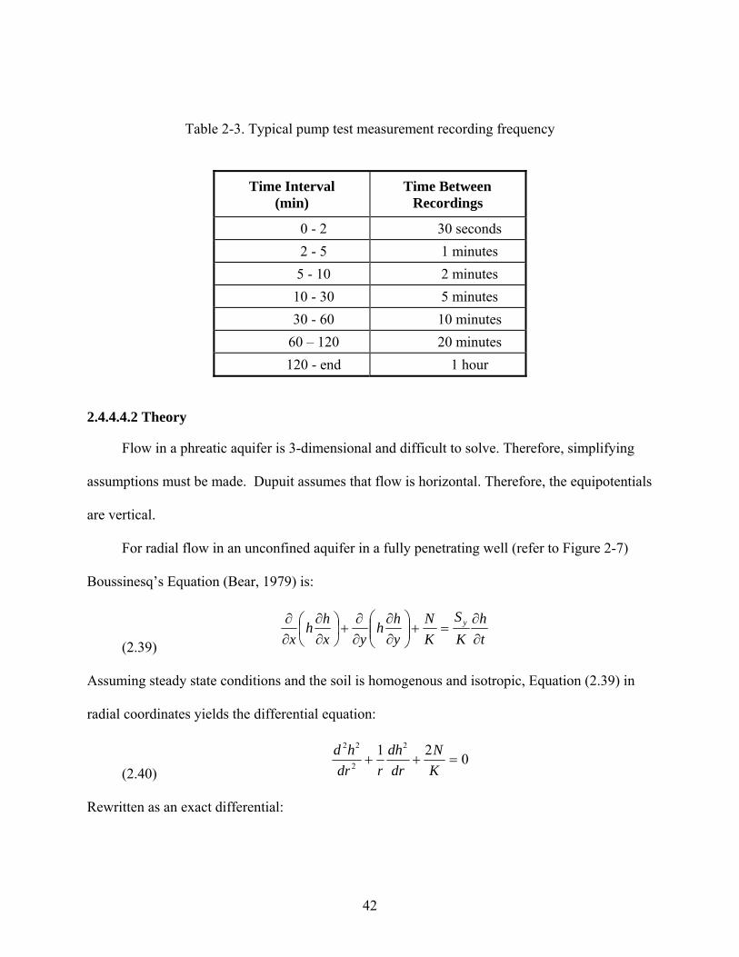
42

Table 2-3. Typical pump test measurement recording frequency

Time Interval (min)

Time Between Recordings

0 - 2 30 seconds 2 - 5 1 minutes 5 - 10 2 minutes 10 - 30 5 minutes 30 - 60 10 minutes

60 – 120 20 minutes 120 - end 1 hour

2.4.4.4.2 Theory

Flow in a phreatic aquifer is 3-dimensional and difficult to solve. Therefore, simplifying

assumptions must be made. Dupuit assumes that flow is horizontal. Therefore, the equipotentials

are vertical.

For radial flow in an unconfined aquifer in a fully penetrating well (refer to Figure 2-7)

Boussinesq’s Equation (Bear, 1979) is:

(2.39) th

KS

KN

yhh

yxhh

xy

∂∂

=+⎟⎟⎠

⎞⎜⎜⎝

⎛∂∂

∂∂

+⎟⎠⎞

⎜⎝⎛

∂∂

∂∂

Assuming steady state conditions and the soil is homogenous and isotropic, Equation (2.39) in

radial coordinates yields the differential equation:

(2.40) 021 2

2

22

=++KN

drdh

rdrhd

Rewritten as an exact differential:

43

(2. 41) 021 2

=+⎟⎟⎠

⎞⎜⎜⎝

⎛KN

drdhr

drd

r

where r = the radial distance from well. Two boundary conditions exist: h = hw at r = rw

and h = H0 at r = R.

Integrating twice, applying the boundary conditions, and applying Darcy’s equation gives

(2.42)

( )[ ]⎟⎠⎞⎜

⎝⎛

+−+−=

w

w

rR

NRhHKNrQln2

2 22202 ππ

If there is no recharge (N=0) then equation (2.42) reduces to the Dupuit-Forcheimer well

discharge equation as

(2.43)

( )⎟⎠⎞⎜

⎝⎛

−=

w

w

rR

hHKQln

220π

Solving for the coefficient of permeability for N≠0 and N=0 yields Equations (2.44) and

(2.45), respectively:

(2.44)

( )( )22

0

22ln

w

w

hH

NRNrQrR

K−

−+⎟⎠⎞⎜

⎝⎛

=π

π

(2.45) ( )220

ln

w

w

hHr

RQK

−

⎟⎠⎞⎜

⎝⎛⋅

=π

The variable R is the effective radius of influence. Dimensionally constant equations (Bear,

1979) include:

44

Lembke (1886)

(2.46) NKHR

2=

Weber (Schultze 1924)

(2.47) e

HKtRη

45.2=

Kusakin (Aravin and Numerov 1953)

(2.48) e

HKtRη

9.1=

where he is dimensionless.

Empirical equations for R include:

Siechardt (Chertousov 1962)

(2.49) 2/13000 KsR w=

Kusakin (Chertousov 1949)

(2.50) ( ) 2/1575 HKsR w=

where H, R and Sw are expressed in meters and K is expressed in m/s.

In a pump test, monitoring wells are placed at various locations around the pumping well.

Equation (2.45) can be transposed to account for monitoring wells placed at radial distances (ri)

from the pumping well and having a head of hi. The new equation yields:

(2. 51) ( )21

22

2

1ln

hhr

rQK

−

⎟⎠⎞⎜

⎝⎛⋅

=π

45

For the pump test described above, steady state conditions must be established within

reasonable boundaries. This may require pumping times ranging between hours and day. It is

largely dependent on permeability. The advantage of the pump test lies in the fact that it accounts

for relatively large areas and may include effects of channeling. However, the costs of installing

wells are high and the time required to run a single test is highly dependent on soil permeability.

Figure 2-7. Pump Test Schematic

46

CHAPTER 3

DEVELOPMENT OF THE VAHIP

The scope of this project is to develop an insitu permeability device which could measure

the vertical and horizontal component of soil permeability independently. A Vertical and

Horizontal Insitu Permeameter (VAHIP) prototype was developed and preliminary testing of the

permeameter was performed by Julian Sandoval in the summer of 2004. The purpose of the tests

was to determine:

• A proper procedure for field tests • If the VAHIP functioned according to the intended design • If testing data could be replicated • If permeability results using the VAHIP were similar to those from other

conventional tests

This chapter will discuss the necessary modifications made as a result of information

obtained in the preliminary testing of the probe.

3.1 Description of Prototype

The 2004 prototype is depicted in Figure 3-1 and is the preliminary design implemented in

2004.

3.1.1 Basic Design

The VAHIP was designed as a probe that could be connected to a Standard PenetrationTest

(SPT) rig. It is to be advanced to the desired depth within a soil formation by the SPT rig and

measure vertical and horizontal permeability in two stages. In stage I, it is expected that water

will flow vertically down from the tip of the probe to measure the permeability in the vertical

direction. Once stage I testing is complete, the stage II test may commence in which water is

directed to flow through a horizontal screen to measure horizontal permeability. An O-ring

inside the tip directs the water to either flow through the tip to measure vertical permeability

(stage I) or through the screen to measure horizontal permeability (stage II). To toggle between

47

stages, the periphery parts need to move along the shaft by mechanical means. As seen in Figure

3-1 the compressed position and extended position is Stage I and Stage II, respectively. In the

field using an SPT rig, Stage I would be achieved by pushing on the rod and stage II achieved by

pulling up on the rod.

3.1.2 Assembly

The basic configuration of the 2004 VAHIP prototype is illustrated in Figure 3-2. The

probe consists primarily of the core and periphery members (collar, well screen, shoulder stops,

and tip).

Core. The VAHIP probe consists of a steel core, threaded to fit an AWJ rod; the AWJ rod

is normally used on SPT rigs. The core is hollow and allows water to pass through the probe and

exit horizontally or at the tip via flow ports. The core also secures the 1/16 inch tubing used to

estimate the hydrostatic pressure within the soil.

Screen. The screen used to flow water horizontally, was made from a 1-1/4 inch PVC well

screen. It has a total open area of 12.5 in2 per foot of screen. The screen was backed with non-

woven filter paper to prevent soil particles from entering the interior of the probe. A total of eight

machine screws attached the screen to the collar and tip (4 each).

Tip. The leading edge of the probe consisted of a steel 45° cone tip. Eight ¼ inch diameter

flow ports were drilled symmetrically about its axis. Sintered steel, with a 1/16-inch diameter

hole was placed inside each flow port. Four machine screws fasten the cone tip to the probe. The

tip is allowed to slide along the core. Within the tip is an o-ring which directs flow for stage I or

II measurements. The position of the o-ring with respect to the flow ports in the core determines

flow direction depending upon the stage.

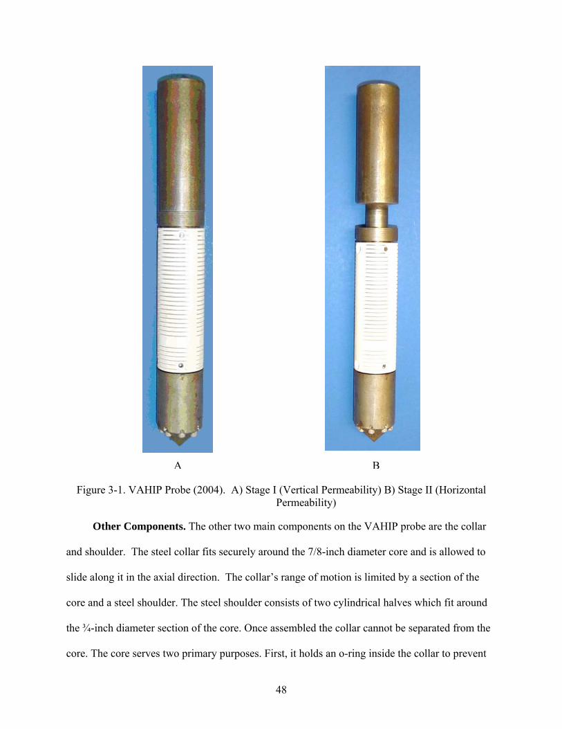
48

Figure 3-1. VAHIP Probe (2004). A) Stage I (Vertical Permeability) B) Stage II (Horizontal Permeability)

Other Components. The other two main components on the VAHIP probe are the collar

and shoulder. The steel collar fits securely around the 7/8-inch diameter core and is allowed to

slide along it in the axial direction. The collar’s range of motion is limited by a section of the

core and a steel shoulder. The steel shoulder consists of two cylindrical halves which fit around

the ¾-inch diameter section of the core. Once assembled the collar cannot be separated from the

core. The core serves two primary purposes. First, it holds an o-ring inside the collar to prevent

A B

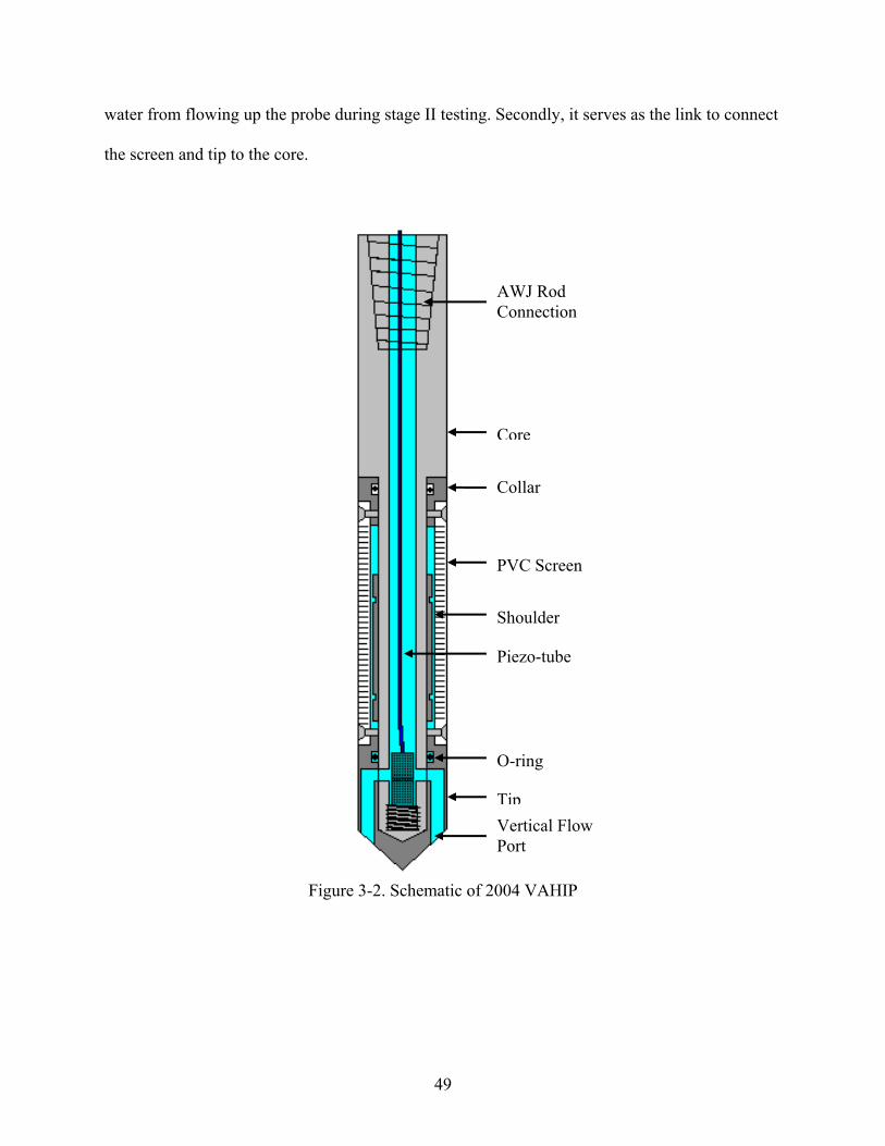
49

water from flowing up the probe during stage II testing. Secondly, it serves as the link to connect

the screen and tip to the core.

Figure 3-2. Schematic of 2004 VAHIP

AWJ Rod Connection

Core

PVC Screen

Collar

TipVertical Flow Port

O-ring

Piezo-tube

Shoulder

50

3.2 Complications with Design

The preliminary testing of the probe in the laboratory and in the field presented advantages

over other accepted methods. However, some complications were evident. These are outlined

below.

3.2.1 Full Flow Condition

When measuring stage II (horizontal) permeability, the equations assume water is flowing

out of the entire screen area, referred to as a full flow condition (FFC). The FFC could not be

achieved when gradients were low. To correct this, a reduction in screen area was recommended.

This would allow for a FFC with a lower applied head.

3.2.2 Area Correction

A correction to account for the fact that water does not flow through the entire screened

section of the probe needed to be made. This in turn would reduce the calculated permeability

except in the falling head test for lateral flow where an ASTM equation is used which is not

sensitive to actual flow area of the screen.

3.2.3 Equation Limitations

Several theoretical permeability equations used to reduce the data had limitations in its use.

The USBR equation (k=V*ln( Leff/R)) used to calculate permeability in the constant head lateral

flow test had the tendency to fail since the effective length of the horizontal flow area was

typically less than the radius of the probe. Thus Leff/R would most likely be less than one and the

natural log term in the equation will produce a negative number and therefore a negative

permeability.

3.2.4 Mechanical Complications

Some complications experienced were due to the limitations of the probe and the test

media. These are outlined below.

51

3.2.4.1 Sand intrusion

Stage I testing of the VAHIP involved pushing on the rod thus forcing the probe into a

compressed state. To switch to stage II testing the rod would be pulled to extend the probe.

Confining stresses around probe would hold the periphery segments in place as the core is

shifted up. When in the stage II position there is a gap between the collar and core section.

During stage II testing, material spilled into this gap and sometimes prevented the VAHIP from

returning to the stage I position.

Each time the probe toggles between stages, there is the likelihood of sand entering the

probe. This intrusion of sand caused a build up in friction between internal parts and hindered the

ability of the probe to switch between stages. With the eventual increase in friction it was

doubtful that the confining pressure would be great enough to overcome the internal frictional

resistance.

3.2.4.2 Piezotube connection

The 1/16- inch tube used to measure the head was attached to the core using a quick

connect. The results from the piezotube were suitable; however the connection hindered the

water from exiting the core. In highly permeable soils, a large enough flowrate could not be

generated. The lack of flow rate would have impacted the stage II measurements the most

because a FFC could not be established.

3.2.4.3 Assembling and disassembling

The 2004 VAHIP probe prototype was assembled using machine screws to attach the

screen to the tip and collar. This arrangement functioned as intended, but it would not be

practical when performing multiple tests in multiple locations.

Due to the unavoidable sand infiltration during testing, the probe must be disassembled,

cleaned, and reassembled between each borehole. The small screws could be easily lost during

52

this process. The overall process would be time consuming and may become complicated by

factors such as cross-threading and/or thread wear.

3.2.5 Rigidity

The screen of the 2004 VAHIP was made from a 1-1/4- inch diameter PVC well screen.

The advantage of using the PVC well screen is that it is easily replaceable and it was successful

in the preliminary testing phase. Conversely, it could be foreseen that PVC would not be a

suitable material for the screen in the final design.

The screen is the link between the collar and the tip. Though the screen is easily

replaceable the tip is not. If the screen were to fail structurally during field testing the tip would

be lost. Failure would most likely be due to stress concentrations occurring at fastening screw

locations when the probe is pulled in tension.

3.3 Description of 2005 VAHIP Probe

By observing the wear after preliminary testing and reviewing the compilations previously

discussed, a list of modifications were made. The modifications made to the 2004 VAHIP were

intended to allow easier for assembly, improve the workability, and increase the probe’s rigidity.

The obstacles and modifications are listed below:

1. A threaded steel plug was screwed into the tip of the core. The purpose of the plug is to secure the piezotube inside the core. The extent of the threads inside the core would not allow the plug to be fully inserted. This caused the plug to become deformed by the tip while advancing the VAHIP into the ground. The threads were extended in the core to allow the plug to screw entirely into the core.

2. The quick connect used to hold the piezotube to the plug at the bottom of the core hindered the flow of water out the exit ports. The location of the exit ports could not be changed due to complications that would be created; rather, the connection had to be shortened. This was done by replacing the piezotube quick connect assembly with a shorter “C”-hold set up. This setup consisted of a tube cap attached to the 1/16inch piezotube. A 1/16inch hole was drilled into the cap to allow the tube to function. The threaded steel plug was machined to secure the cap to the plug preventing the piezotube

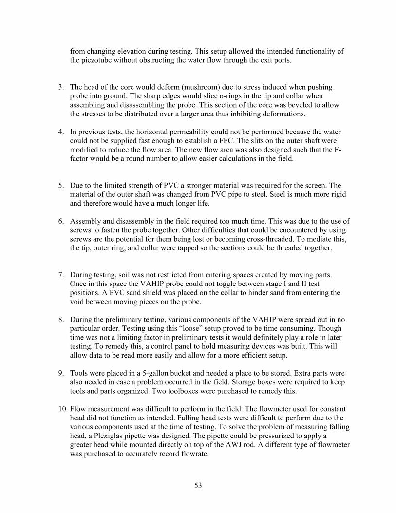
53

from changing elevation during testing. This setup allowed the intended functionality of the piezotube without obstructing the water flow through the exit ports.

3. The head of the core would deform (mushroom) due to stress induced when pushing probe into ground. The sharp edges would slice o-rings in the tip and collar when assembling and disassembling the probe. This section of the core was beveled to allow the stresses to be distributed over a larger area thus inhibiting deformations.

4. In previous tests, the horizontal permeability could not be performed because the water

could not be supplied fast enough to establish a FFC. The slits on the outer shaft were modified to reduce the flow area. The new flow area was also designed such that the F-factor would be a round number to allow easier calculations in the field.

5. Due to the limited strength of PVC a stronger material was required for the screen. The material of the outer shaft was changed from PVC pipe to steel. Steel is much more rigid and therefore would have a much longer life.

6. Assembly and disassembly in the field required too much time. This was due to the use of screws to fasten the probe together. Other difficulties that could be encountered by using screws are the potential for them being lost or becoming cross-threaded. To mediate this, the tip, outer ring, and collar were tapped so the sections could be threaded together.

7. During testing, soil was not restricted from entering spaces created by moving parts.

Once in this space the VAHIP probe could not toggle between stage I and II test positions. A PVC sand shield was placed on the collar to hinder sand from entering the void between moving pieces on the probe.

8. During the preliminary testing, various components of the VAHIP were spread out in no particular order. Testing using this “loose” setup proved to be time consuming. Though time was not a limiting factor in preliminary tests it would definitely play a role in later testing. To remedy this, a control panel to hold measuring devices was built. This will allow data to be read more easily and allow for a more efficient setup.

9. Tools were placed in a 5-gallon bucket and needed a place to be stored. Extra parts were also needed in case a problem occurred in the field. Storage boxes were required to keep tools and parts organized. Two toolboxes were purchased to remedy this.

10. Flow measurement was difficult to perform in the field. The flowmeter used for constant head did not function as intended. Falling head tests were difficult to perform due to the various components used at the time of testing. To solve the problem of measuring falling head, a Plexiglas pipette was designed. The pipette could be pressurized to apply a greater head while mounted directly on top of the AWJ rod. A different type of flowmeter was purchased to accurately record flowrate.

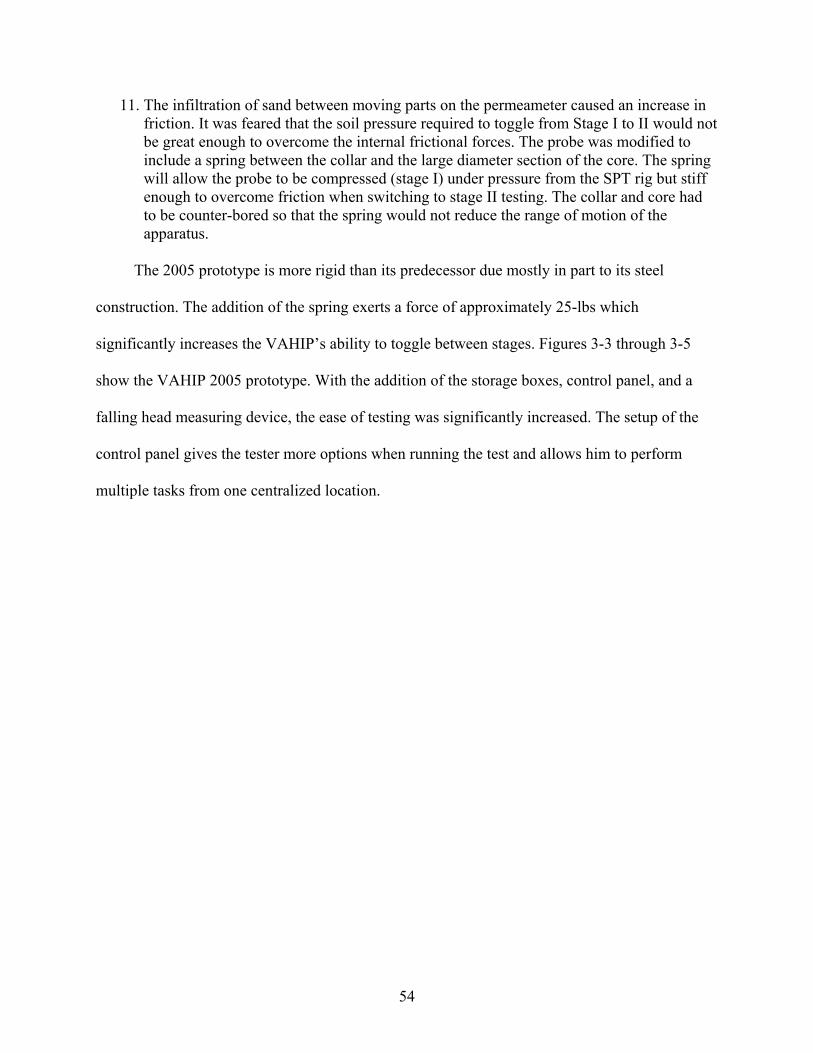
54

11. The infiltration of sand between moving parts on the permeameter caused an increase in friction. It was feared that the soil pressure required to toggle from Stage I to II would not be great enough to overcome the internal frictional forces. The probe was modified to include a spring between the collar and the large diameter section of the core. The spring will allow the probe to be compressed (stage I) under pressure from the SPT rig but stiff enough to overcome friction when switching to stage II testing. The collar and core had to be counter-bored so that the spring would not reduce the range of motion of the apparatus.

The 2005 prototype is more rigid than its predecessor due mostly in part to its steel

construction. The addition of the spring exerts a force of approximately 25-lbs which

significantly increases the VAHIP’s ability to toggle between stages. Figures 3-3 through 3-5

show the VAHIP 2005 prototype. With the addition of the storage boxes, control panel, and a

falling head measuring device, the ease of testing was significantly increased. The setup of the

control panel gives the tester more options when running the test and allows him to perform

multiple tasks from one centralized location.

55

Figure 3-3. 2005 VAHIP Prototype

Figure 3-4. VAHIP probe tip.

56

Figure 3-5. 2005 disassembled VAHIP

3.4 Field Testing of 2005 VAHIP Probe

Field tests using the 2005 VAHIP were performed at two test sites; Hawthorn and

Newberry. The Hawthorn site was a location where a FDOT retention pond was proposed. The

site in Newberry is a 5-acre FDOT retention pond.

At the Hawthorn site, the VAHIP was advanced 7 feet into the soil via an automatic

hammer on a SPT rig. Hand auger borings reveled that the soil tested was fine sand. Vertical and

horizontal tests were performed and data collected. The constant head test for the vertical

direction could not be performed due to the tremendously low flowrate. A borehole test was

57

performed at the site by the FDOT technician so that the result could be compared with that of

the VAHIP.

The testing performed at the Newberry site was performed in conjunction with another

UF/FDOT project. Testing at this site occurred at one physical location because the SPT rig was

owned and operated by a private engineering firm that charged a setup fee when the rig was

moved. For this reason the VAHIP was tested in the same hole the SPT boring was to be

performed. Two depths were tested at the Newberry site. The soil tested was sand. Two soil

samples were obtained at the Newberry site. These samples were extracted using a hand auger.

Borehole permeability tests were performed on these samples to compare to the VAHIP results.

The results of these tests are presented in Tables 3.1.

During this field testing of the 2005 probe, the main problem encountered was the clogging

of the tiny vertical flow ports at the tip of the probe during driving. Consequently it became

necessary again to redesign the probe to address this problem. Figure 3-6 reveals the flow ports

that are potentially clogged after retrieval from a test.

58

Figure 3-6 Potentially clogged flow ports (2005 probe)

Table 3.1 2005 Probe Field Test Results

Test Location Depth Soil Type

VAHIP Field Permeability Results (cm/s) Borehole Permeability Results (cm/s)

Constant Head Falling Head

Horizontal Vertical Horizontal Vertical Constant Head

Falling Head

Hawthorn

7 ft Fine Sand

1.47E-05

N/A

6.90E-04

1.03E-02

1.67E-05

N/A

Newberry

3 ft

Grey Fine Sand

N/A

N/A

8.47E-05

4.52E-05

5.47E-05

N/A

6 ft

Grey Fine Sand

N/A

N/A

1.16E-03

6.88E-04

9.63E-04

N/A

59

3.5 Description of 2006 VAHIP Probe

The 2005 probe had to be redesigned to address the issue of clogging of the flow ports

during driving. The main design feature of the new probe was the development of a new tip

which invariably resulted in the modification of other components of the probe to be compatible

with the new tip, as well as a change in the testing procedure. Overall, the mechanical basis of

the 2005 design was not altered. The eight small flow ports of the 2005 prototype were replaced

by one large vertical flow port. The total area of the 8 flow ports was approximately 0.025in2.

The single flow port designed for the new probe had a diameter of 0.75 inch, which was ideal for

generating the needed flow rates. Since the potential for clogging is only a concern during the

driving process, it was required that this vertical flow port is closed off during the driving

process and opened prior to the vertical permeability testing. In the 2005 prototype design, the

vertical test position and the driving position are the same (i.e. the flow ports are open when the

probe is driven). To test the horizontal permeability in this case, the SPT rod is retracted and the

VAHIP is lengthened. This mechanical toggling directs flow to the horizontally oriented screen.

The new design however ensures that the vertical flow port is closed during the driving process

while the horizontal slots remain open. Thus instead of the probe toggling from vertical to

horizontal tests by lifting the SPT rod, it rather toggles from horizontal flow position to vertical

in the new design (it is reversed from the 2005 design).

To close off the vertical flow ports during the driving process, the 2006 prototype was

designed to have a core (central shaft) with a pointed end that extends through the 0.75 inch

opening at the tip and is flush with the tip when pushed, thereby closing it or moving out of the

tip to keep it opened when retracted. This core is fixed to the SPT union connector on the probe

to which an SPT rod can be attached. Thus it retracts as the SPT rod is retracted while the

periphery parts of the probe remain in place and the water is then able to flow through the tip.

60

This new design necessitated changes in the test procedure so that at the desired depth, the

horizontal test would have to be performed before the vertical. A schematic depiction of the

probe is shown in Figure 3-6 in which the various components can be seen.

Figure 3-6 Schematic representation of 2006 probe with tip closed for horizontal flow and

opened for vertical flow.

61

3.4.1 Assembling and Operation Methodology

The probe consists primarily of the inner core with tip and periphery members (collar, well

screen, shoulder, and tip). The inner core is hollow and is threaded at one end with an exit flow

port near its mid-portion to facilitate an outward horizontal flow of water and another at the tip to

facilitate vertical flow through the tip. The threaded end of the hollow core connects to an AWJ

union rod which is normally used on SPT rigs, thus facilitating connection to an SPT rig drive

head. The tip of the probe’s inner core is cone shaped at the end. This cone-shaped end is

designed to fit flush onto the outer tip which is a threaded cone-shaped plug with a 0.75 inch

hole. The well screen is a hollow cylindrical tube with horizontal slots to allow water to exit

through the probe horizontally while the upper hollow cylindrical collar, which is made of PVC,

facilitates the toggling of the probe from the vertical to the horizontal test position. A double-

end threaded screw connector connects these two together. The shoulder which is also a hollow

cylindrical tube connects the outer tip to the well screen via another double-end screw. This

connection of collar, well screen and shoulder portion of the probe thus forms an enveloping

outer periphery around the inner core and tip of the probe. The main premise for such an

arrangement and design was to ensure that during driving of the probe into the ground, the outer

tip would be closed to prevent soil intrusion and therefore clogging. Once at the required depth, a

horizontal permeability test can be performed since water would only be able to exit the probe

horizontally. After horizontal testing at this depth is completed, the inner tip of the probe is

retracted by pulling on the AWJ rod via the SPT drive head thus opening the tip flow port to

allow water to exit vertically through the outer tip opening while closing the horizontal flow port

on the core thus preventing horizontal water flow.

Figures 3-8 and 3-9 shows the 2006 probe with the tip opened for vertical flow and the tip

closed for horizontal flow.

62

Figure 3-7 Dismantled 2006 VAHIP Probe Showing Components

The probe components shown in Figure 3-7 are as listed below:

1. Outer tip with 0.75 inch diameter tip opening 2. Hollow cylindrical shoulder 3. Double-end threaded connection screw 4. Hollow cylindrical screen with horizontal slots 5. PVC collar connected to a double-end threaded screw 6. Hollow inner core with tip 7. AWJ connector rod.

In the 2005 prototype, the piezotube was intended to monitor groundwater levels, but it did

not function as expected and was interfering with the toggling of the probe. The piezotube was

omitted in the new 2006 probe design; however, groundwater levels need to be determined

through independent means.

6

1

12

3

4

5

6

7

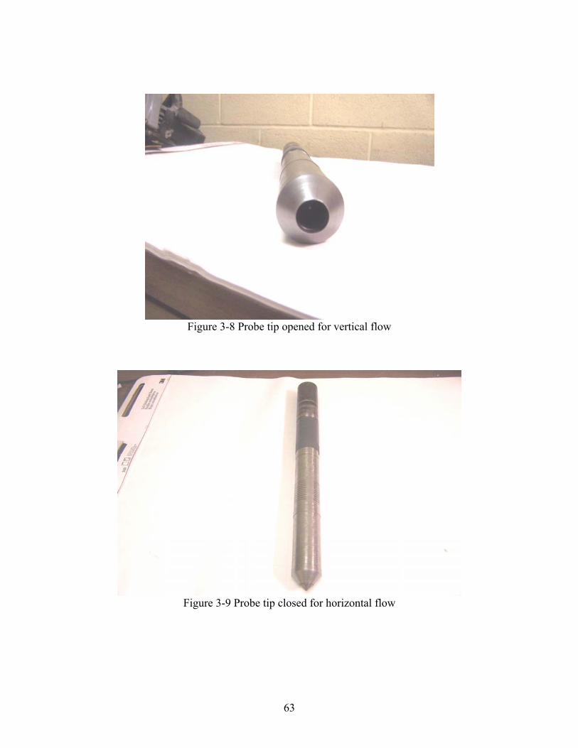
63

Figure 3-8 Probe tip opened for vertical flow

Figure 3-9 Probe tip closed for horizontal flow

64

3.5 Description of Plexiglas Standpipe

The Plexiglas standpipe was designed for of monitoring the water head, flow rate and

changes in water level required during testing for permeability calculation. It consists of a 1.5-

inch diameter (1.13”I.D.) Plexiglas tube mounted on top of a 4-inch diameter (3.55”I.D.)

Plexiglas tube. Water is introduced through an open male quick connect which is threaded to the

top of the 4 inch tube. Water level or head readings can be taken on either the bigger or smaller

pipe as appropriate during testing. It is expected that during testing of soils with low

permeability, the smaller standpipe would be utilized in monitoring water level drops and vice-

versa.

A smaller, open, male quick connect is threaded into the top of the 1.5inch (smaller) tube

and is used to apply an additional pressure head when testing if necessary. An AWJ male thread

welded to a 4 inch diameter steel plate forms the base of the Plexiglas stand pipe thus making the

assembly easily compatible to an SPT rod.

This device depicted in Figure 3-10 is ideal for use in combination with the probe as a

result of the following design attributes:

• Changes in water levels are easy to read • It can be easily attached to an SPT rod • It is easily filled with water • It is capable of being pressurized to increase head.

65

Figure 3-10. Picture of Flow Measurement Device (FMD)

3.6 Description of Control Panel

A control panel was deemed necessary to allow the operator to easily control the test from

one location. The control panel is as depicted in Figure 3-11. It serves as the source for

regulating the flow of water into the Plexiglas Flow Measuring Device (FMD), introducing

pressure into the Plexiglas FMD to increase flow, as well as measuring the flow rate for constant

head tests. A pressure tank within the panel is used to force water into the FMD and also

pressurize the FMD when a greater head is required. Valves on the panel control the flowrates

and gauges mounted on the panel monitor the necessary pressures. The flow rates are measured

with a micro-flow sensor which can be connected to two connector ports installed on the panel.

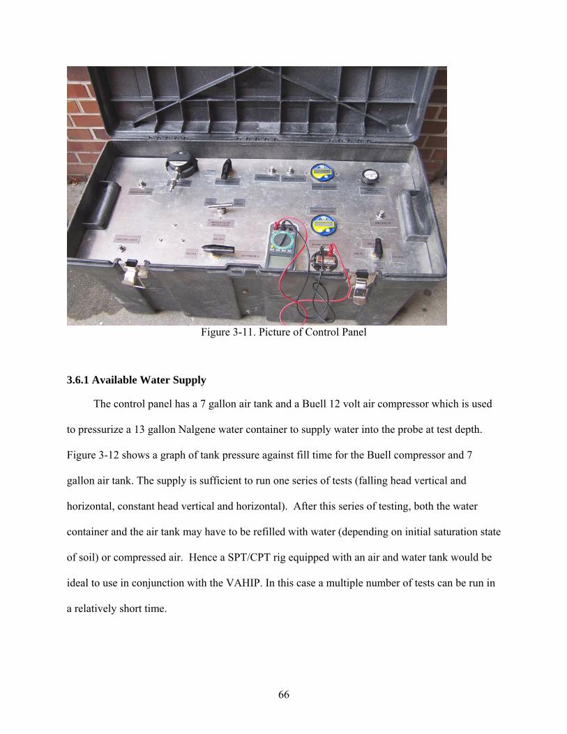
66

Figure 3-11. Picture of Control Panel

3.6.1 Available Water Supply

The control panel has a 7 gallon air tank and a Buell 12 volt air compressor which is used

to pressurize a 13 gallon Nalgene water container to supply water into the probe at test depth.

Figure 3-12 shows a graph of tank pressure against fill time for the Buell compressor and 7

gallon air tank. The supply is sufficient to run one series of tests (falling head vertical and

horizontal, constant head vertical and horizontal). After this series of testing, both the water

container and the air tank may have to be refilled with water (depending on initial saturation state

of soil) or compressed air. Hence a SPT/CPT rig equipped with an air and water tank would be

ideal to use in conjunction with the VAHIP. In this case a multiple number of tests can be run in

a relatively short time.

67

Tank Pressure vs. Time

P = -0.0723t2 + 5.0203t

0

20

40

60

80

100

0 5 10 15 20 25 30 35

Time (min)

Pres

sure

(psi

)

Figure 3-12. Graph of tank pressure vs. fill time for the Buell Compressor and 7gallon air tank.

68

CHAPTER 4 PROCEDURE FOR FIELD USE OF VAHIP AND DATA REDUCTION

4.1 Outlined Field Test Procedure

The following field permeability testing procedure is recommended when using the

VAHIP and a SPT rig for driving purposes to determine the vertical and horizontal permeability

of a soil formation at various depths. Soil above the water table should be adequately saturated

prior to testing.

4.1.1 Pre-field Preparation

1. The VAHIP must be clean and rid of any foreign material that would hinder water flow. 2. Prepare all materials and tools listed in the equipment check list in the appendix. 3. Fill up the nalgene tank with clean water and the air tank in the control panel with air

using a compressor. Be sure not to exceed the limiting pressure of 90 psi in the air tank. 4.1.2 Probe Assembly

1. Attach the upper threaded part of the inner core into the base of the AWJ union connector rod by pushing the core through the hole in the screw at the base of the PVC collar and screwing such that the AWJ connector sits in the collar. Try sliding the inner core within the hole by pulling up and down on the AWJ connector while holding onto the PVC collar. Make sure the assembled unit is sliding smooth.

2. Attach the upper part of the hollow cylindrical well screen to the end of collar by screwing onto its threaded end.

3. Attach one threaded portion of the double-end screw to the lower part of the well screen. 4. Attach the upper part of the hollow cylindrical shoulder to the threaded portion of the

double-end screw. 5. Pull up completely on the AWJ connector to retract the inner tip of the core and attach

the outer tip to the lower end of the shoulder by screwing onto it. 6. Push down on the AWJ connector to get the inner tip flush within the hole in the outer

tip. 7. Pull up and down on the AWJ rod to retract and push in the inner tip. Make sure this

motion is easy and flexible. 4.1.3 VAHIP Flow Measurement Assembly

1. Connect the appropriate 3/8 inch hose tubing fitting from the outlet of the nalgene water tank to the water in connection on the control panel.

2. Connect the appropriate 3/8 inch hose tubing fitting from the water – out connection on the control panel to the open male quick connect which is threaded to the top of the 4inch tube on the Plexiglas stand pipe. Open and close water flow pin valve on control panel as necessary to fill Plexiglas pipe with water.

69

3. Connect the appropriate 3/8 inch hose tubing fitting from the airline-out connection on the control panel to the open male quick connect which is threaded to the top cover of the nalgene tank. Close the top cover tightly and use the air flow pin valve on the control panel to add air pressure in the nalgene water tank to increase flow when necessary.

4. Connect the appropriate hose tubing from the alternate airline-out on the control panel to the smaller, open male quick connect threaded into the top of the 1.5 inch (smaller) tube of the Plexiglas stand pipe. This is used to apply an additional pressure head when testing and also to flush out soil particles from the probe if necessary.

4.1.4 Test Procedure

1. Fully assemble the probe and push down the tip so that the tip hole is blocked and the probe is in driving and horizontal (stage I) testing position. Make sure all connections are tight.

2. Connect desired AWJ rods to the probe via the AWJ-AW union connector on the probe. Provide an o-ring between each section to prevent water leakage during testing.

3. Connect the probe assembly to an SPT rig equipped with an AWJ drive head. Advance the probe to the desired depth. Disconnect the drive head from the rod and connect the Plexiglas standpipe. Connect all tubing to control panel and perform stage I (horizontal) tests by performing constant head, falling head or both tests, as applicable, as outlined under test types.

4. After stage I testing at the depth is performed, stage II (vertical) testing may commence. To get the probe in the stage II position, use the SPT rig to pull the rod about 1.5inches out of ground. Attach Plexiglass standpipe to AWJ rod, complete required connections, and perform stage II tests by performing constant head, falling head or both tests, as applicable, as, outlined under test types.

5. Disconnect the Plexiglas standpipe and reconnect the AWJ rod to the SPT drive head. Advance the probe to the next desired text depth thus getting the probe back in stage I (horizontal) test position.

6. Make all the necessary connections and carry out stage I tests. Again after stage I testing at this depth, perform stage II testing by pulling on the SPT rod about 1.5-inches from the ground as already described.

7. Continue with steps 3-6 until the maximum test depth is reached and the last stage II test is completed.

8. Extract the probe from the ground. Note the condition of the probe (e.g. clogged ports, deformations, etc). Flush probe with water and remove any foreign material within the probe. Brush off all dirt on the probe threads with a wire brush. Wash all rod connections clean.

9. Move to next test location and perform steps 1-7 until tests are completed.

4.1.5 Test Types

Two main types of tests, constant head and falling head, can be performed when using the

VAHIP. Test details and procedures are outlined below. Attach all necessary connections from

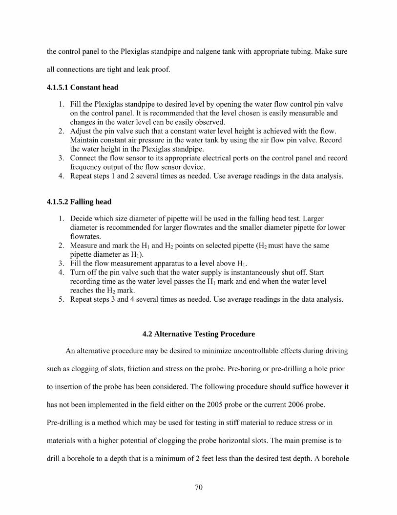
70

the control panel to the Plexiglas standpipe and nalgene tank with appropriate tubing. Make sure

all connections are tight and leak proof.

4.1.5.1 Constant head

1. Fill the Plexiglas standpipe to desired level by opening the water flow control pin valve on the control panel. It is recommended that the level chosen is easily measurable and changes in the water level can be easily observed.

2. Adjust the pin valve such that a constant water level height is achieved with the flow. Maintain constant air pressure in the water tank by using the air flow pin valve. Record the water height in the Plexiglas standpipe.

3. Connect the flow sensor to its appropriate electrical ports on the control panel and record frequency output of the flow sensor device.

4. Repeat steps 1 and 2 several times as needed. Use average readings in the data analysis.

4.1.5.2 Falling head

1. Decide which size diameter of pipette will be used in the falling head test. Larger diameter is recommended for larger flowrates and the smaller diameter pipette for lower flowrates.

2. Measure and mark the H1 and H2 points on selected pipette (H2 must have the same pipette diameter as H1).

3. Fill the flow measurement apparatus to a level above H1. 4. Turn off the pin valve such that the water supply is instantaneously shut off. Start

recording time as the water level passes the H1 mark and end when the water level reaches the H2 mark.

5. Repeat steps 3 and 4 several times as needed. Use average readings in the data analysis.

4.2 Alternative Testing Procedure

An alternative procedure may be desired to minimize uncontrollable effects during driving

such as clogging of slots, friction and stress on the probe. Pre-boring or pre-drilling a hole prior

to insertion of the probe has been considered. The following procedure should suffice however it

has not been implemented in the field either on the 2005 probe or the current 2006 probe.

Pre-drilling is a method which may be used for testing in stiff material to reduce stress or in

materials with a higher potential of clogging the probe horizontal slots. The main premise is to

drill a borehole to a depth that is a minimum of 2 feet less than the desired test depth. A borehole

71

of lesser diameter than the probe can be drilled at the last two feet if material is very stiff. The

VAHIP probe can then be advanced in the pre-drilled hole and testing performed as previously

described.

4.3 VAHIP Maintenance

Cleanup. Disassemble probe by first pulling up on AWJ connector and unscrewing the

outer tip. Unscrew other parts, wash probe with clean water and wire brush removing all soil

particles from flow ports and connecting parts. Prior to placing into storage, use a lubricant to

hinder oxidation and reduce friction. Note: Due to possible environmental concerns, the lubricant

may be required to be non-toxic.

Routine Inspections. The probe should be inspected after each cleanup for deformed

and/or worn parts. Note deformities and replace parts as needed. Lines in the control panel

should be inspected periodically for leaks.

Storage. The VAHIP, control panel, and standpipe should be stored in cool dry place to

prevent oxidation to steel components. The pressure tank should have a maximum of 10-psi and

the water from the nalgene tank emptied. Remove the battery from the flow meter.

4.4 Data Reduction

Data should be collected in the field using data sheets provided in Appendix C. The

spreadsheet template (provided) may be used to calculate permeability from field test data.

Properties such as probe dimensions and predetermined water levels during tests have been

preloaded into spreadsheet. However these can be changed if future modifications are made to

the probe or when different predetermined water levels are used.

Currently the data is reduced using borehole permeability (Hvorslev’s) theory which is

discussed in the next section. The vertical permeability is akin to flow from an open-ended,

72

cased borehole and the horizontal flow akin to a borehole packer test. The theory has been

slightly modified to account for geometry differences.

4.4.1 Hvorslev’s Theory

The permeability from a slug test can be calculated using several different methods.

Hvorslev (1951) derived an equation based on the differential equation for radial flow from a

well. Figure 4-4 is a schematic representation of Hvorslev’s basic hydrostatic time lag

definitions.

Figure 4-4. Variable definitions for time lag derivation.

Assumptions. The derivation of the basic differential equation for the determination of the

hydrostatic time lag and influence were based on the following assumptions:

• Darcy’s Law is valid • The fluids and solids are incompressible • Pressure equalization does not cause drawdown in the ground water (GW) level • Friction losses within the pipe are negligible.

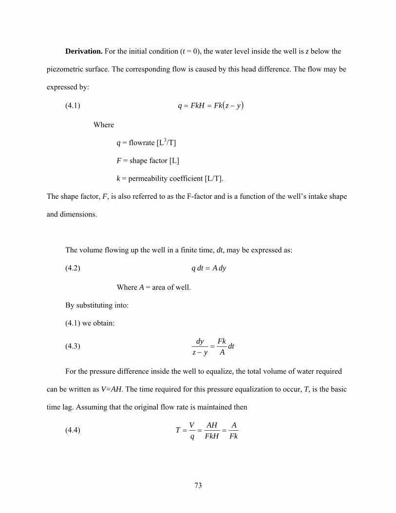
73

Derivation. For the initial condition (t = 0), the water level inside the well is z below the

piezometric surface. The corresponding flow is caused by this head difference. The flow may be

expressed by:

(4.1) ( )yzFkFkHq −==

Where

q = flowrate [L3/T]

F = shape factor [L]

k = permeability coefficient [L/T].

The shape factor, F, is also referred to as the F-factor and is a function of the well’s intake shape

and dimensions.

The volume flowing up the well in a finite time, dt, may be expressed as:

(4.2) dyAdtq =

Where A = area of well.

By substituting into:

(4.1) we obtain:

(4.3) dtA

Fkyz

dy=

−

For the pressure difference inside the well to equalize, the total volume of water required

can be written as V=AH. The time required for this pressure equalization to occur, T, is the basic

time lag. Assuming that the original flow rate is maintained then

(4.4) FkA

FkHAH

qVT ===

74

Therefore (4.2) becomes

(4.5) Tdt

yzdy

=−

For a static piezometric surface z = H0. By integrating (4.4) with y = 0 at t = 0 as the

boundary conditions, the solution is

(4.6) HH

yHH

Tt 0

0

0 lnln =−

=

For a variable head in the borehole and a constant GW piezometric head, the following

expression can be derived

(4.7) 2

1

1

0

2

012 lnlnln

HH

FkA

HH

HH

Ttt =⎟⎟⎠

⎞⎜⎜⎝

⎛−=−

Hence k is determined by the following equation, which is similar to the falling head

laboratory test:

(4.8) ( ) ⎟⎟⎠

⎞⎜⎜⎝

⎛−

=2

1

21

lnHH

ttFAk

4.4.2 F Factor or Shape Factors for Probe

When field permeability testing, a variation to the basic Darcy equation is required to make

the data reduction take into account field conditions and test method.

From Darcy’s law,

(4.9) ⎟⎠⎞

⎜⎝⎛

==A

Lh

qAi

q

*

* k =

⎟⎠⎞

⎜⎝⎛

LAh

q

*

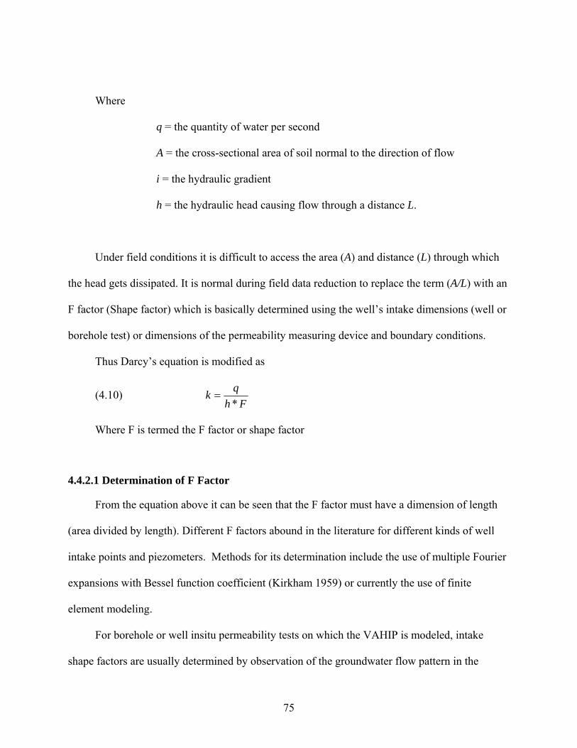
75

Where

q = the quantity of water per second

A = the cross-sectional area of soil normal to the direction of flow

i = the hydraulic gradient

h = the hydraulic head causing flow through a distance L.

Under field conditions it is difficult to access the area (A) and distance (L) through which

the head gets dissipated. It is normal during field data reduction to replace the term (A/L) with an

F factor (Shape factor) which is basically determined using the well’s intake dimensions (well or

borehole test) or dimensions of the permeability measuring device and boundary conditions.

Thus Darcy’s equation is modified as

(4.10) Fh

qk*

=

Where F is termed the F factor or shape factor

4.4.2.1 Determination of F Factor

From the equation above it can be seen that the F factor must have a dimension of length

(area divided by length). Different F factors abound in the literature for different kinds of well

intake points and piezometers. Methods for its determination include the use of multiple Fourier

expansions with Bessel function coefficient (Kirkham 1959) or currently the use of finite

element modeling.

For borehole or well insitu permeability tests on which the VAHIP is modeled, intake

shape factors are usually determined by observation of the groundwater flow pattern in the

76

vicinity of the entry region. For a hydraulically isotropic porous medium, only the geometrical

feature of the surface through which water leaves or enters the borehole characterizes the shape

factor. The analysis for determining the shape factor usually involves solving the potential

equation that governs Darcy’s law for flow in porous media. Hvorslev (1951) presents a detailed

list of shape factors that is applicable to borehole entry points in hydraulically isotropic soil

media. Figures 4-5 and 4-6 shows Hvorslev’s charts for shape factors and borehole permeability

formulas.

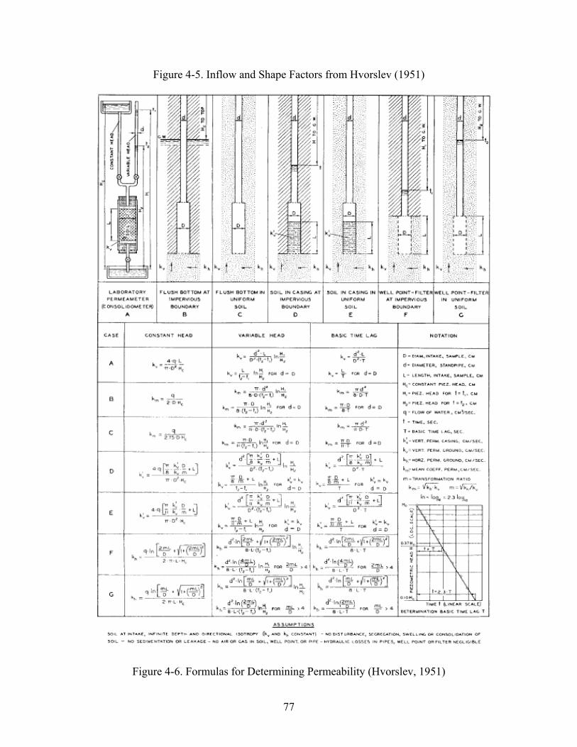
77

Figure 4-5. Inflow and Shape Factors from Hvorslev (1951)

Figure 4-6. Formulas for Determining Permeability (Hvorslev, 1951)

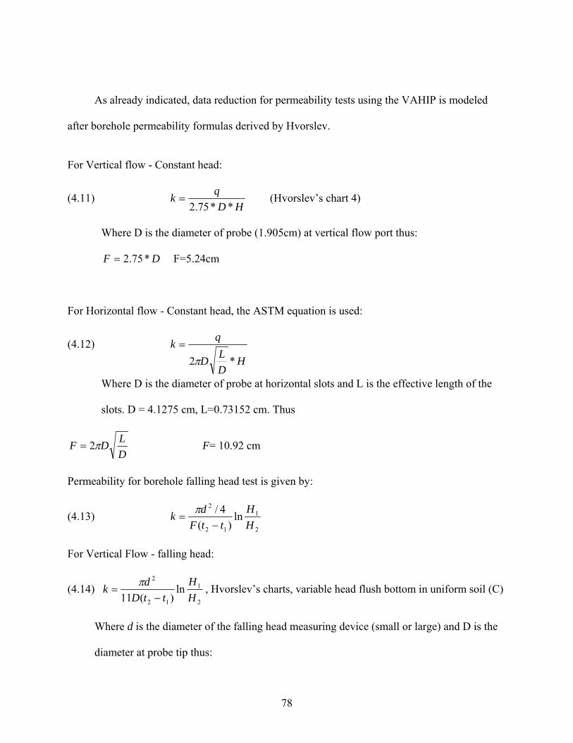
78

As already indicated, data reduction for permeability tests using the VAHIP is modeled

after borehole permeability formulas derived by Hvorslev.

For Vertical flow - Constant head:

(4.11) HD

qk**75.2

= (Hvorslev’s chart 4)

Where D is the diameter of probe (1.905cm) at vertical flow port thus:

DF *75.2= F=5.24cm

For Horizontal flow - Constant head, the ASTM equation is used:

(4.12) H

DLD

qk*2π

=

Where D is the diameter of probe at horizontal slots and L is the effective length of the

slots. D = 4.1275 cm, L=0.73152 cm. Thus

DLDF π2= F= 10.92 cm

Permeability for borehole falling head test is given by:

(4.13) 2

1

12

2

ln)(

4/HH

ttFdk

−=

π

For Vertical Flow - falling head:

(4.14) 2

1

12

2

ln)(11 H

HttD

dk−

=π , Hvorslev’s charts, variable head flush bottom in uniform soil (C)

Where d is the diameter of the falling head measuring device (small or large) and D is the

diameter at probe tip thus:

79

F=11*D/4 = 5.24 cm

For Horizontal flow - Falling head:

The F factor is determined by subtracting the flowrate equation from Hvorslev’s chart (4)

from that of chart (8). Chart (8) gives an equation for a cased borehole with an extended well

point or hole typically giving permeability sensitive to both vertical and horizontal flow. Chart

(4) gives an equation for a cased borehole typically giving permeability more sensitive to vertical

flow as already shown.

Subtracting chart (4) from chart (8) and rearranging gives a shape factor applicable to flow

sensitive to horizontal flow given as follows:

(4.15)

⎟⎟

⎠

⎞

⎜⎜

⎝

⎛⎟⎠⎞

⎜⎝⎛++

=2

8

1ln

*2

DL

DL

kHLq π chart (8)

(4.16) kHDq *75.24 = chart (4)

(4.17) =−= 48 qqq kHD

DL

DL

L *75.2

1ln(

22

⎟⎟⎟⎟⎟

⎠

⎞

⎜⎜⎜⎜⎜

⎝

⎛

−

⎟⎠⎞

⎜⎝⎛++

π

Since kHFq *= , then:

(4.18) D

DL

DL

LF 75.2

1ln

22

−

⎟⎟

⎠

⎞

⎜⎜

⎝

⎛⎟⎠⎞

⎜⎝⎛++

=π

For D = 4.1275 cm and L=0.73152 cm, F=14.5 cm

80

As stated earlier, finite element methods and multiple Fourier expansions are also currently

in use for the determination of shape factors. Such analyses model the physical presence of the

probe in the soil as well as the right boundary conditions. It also has the added advantage of

versatility during modeling since the input factors can be changed and their effect on the shape

factor observed. A Fourier expansion analysis was performed on the probe for the lateral flow

conditions and is presented below.

4.4.2.2 F Factor (Fourier expansions with Bessel Function coefficients)

A conceptualized physical configuration of a single screen injection test configuration is

depicted in Figure 4-1. It consists of a fully penetrating impermeable cylindrical device of radius,

a [L], between (in a first approach) two horizontal impermeable boundaries of separation d [L].

The device possesses an injection screen positioned between h1 [L] and h2 [L]. The system is

seen to be axisymmetric around the z-axis and with boundary conditions I through VI in an axial

plane. Boundary condition I defines a constant known potential at a radial distance, b [L], from

the center of the device. Boundary conditions II and III are the no-flow conditions for the

confining layers while conditions IV and VI correspond to the no-flow conditions along the

impermeable portions of the device. Boundary condition V represents the constant injection head

over the screened (permeable) portion of the device. Introducing the hydrodynamic potential Φ,

the Laplace equation governing potential flow in axisymmetric cylindrical coordinates (Lamb,

1932; Smythe, 1950) is

(4.19) 012

2

2

2

=Φ

+Φ

+Φ

zrrr δδ

δδ

δδ

and a general solution of Equation 4.19 is given by Zaslavsky and Kirkham (1964) as

81

(4.20) [ ][ ][ ][ ]

LKzarJarIzmrHmrGmzFmzE

nrDnrCnzBnzAzr

++++++++

+++=Φ

)/ln()/ln( )(Y)(J)cosh()sinh(

)(K)(I)cos()sin(),(

00

00

where A through L, a, m and n are arbitrary real constants and I0, K0, J0 and Y0 are Bessel

functions of order zero (Dwight, 1947). By superposing solutions of Equation 4.20 with different

sets of constants, specific boundary conditions can be met. For an injection head, φ1 [L], the

boundary conditions of Figure 4-1 can be formulated as

(4.21) dzbrI ≤≤==Φ 0for at 0

(4.22) bradz

zII ≤≤==

Φ for at 0 δδ

(4.23) braz

zIII ≤≤==

Φ for 0at 0 δδ

(4.24) 10for at 0 hz ar

rIV ≤≤==

Φδδ

(4.25) 211 for at hzharV ≤≤==Φ ϕ

(4.26) dzhar

rVI ≤≤==

Φ2for at 0

δδ

82

Figure 4-1. Boundary conditions for axisymmetric flow domain of single injection screen.

By slightly modifying the potential function used by Kirkham (1959) the constants in

Equation 4.20 are chosen such that, after superposition,

(4.27) ∑=

+=ΦN

nn dzndrnrB

abrbBzr

,...2,100 )/cos()/(

)/ln()/ln(),( ππ

with

(4.28) )/()/(

)/()/(

)/()/(

)/()/(

)/(

0

0

0

0

0

0

0

0

0

dbnIdanI

dbnKdanK

dbnIdrnI

dbnKdrnK

drnr

ππ

ππ

ππ

ππ

π−

−=

Inspection of Equation 4.27 demonstrates that boundary conditions I, II and III are inherently

satisfied, since sin(0) = sin(nπ) = 0 and r0(nπb/d) = 0, whereas conditions IV, V and VI are still

to be met by defining the constants B0 and Bn. Substituting Equation 4.27 into Equations 4.24,

d

Impermeable Casing

Injection Screen

h1

2a

h2

I

II

III

IV

VI

V

z

r

b

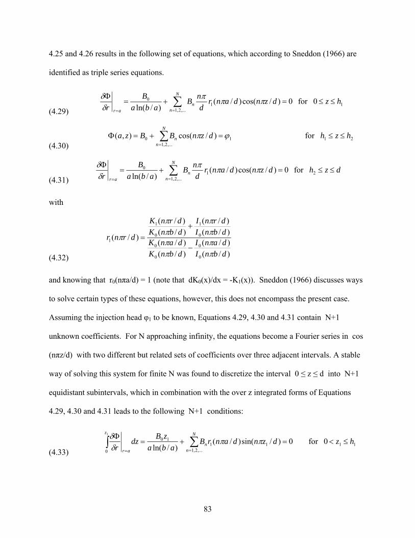
83

4.25 and 4.26 results in the following set of equations, which according to Sneddon (1966) are

identified as triple series equations.

(4.29) 1

,...2,11

0 0for 0)/cos()/()/ln(

hzdzndanrd

nBaba

Br

N

nn

ar

≤≤=+=Φ ∑

==

πππδδ

(4.30) 211

,...2,10 for )/cos(),( hzhdznBBza

N

nn ≤≤=+=Φ ∑

=

ϕπ

(4.31) dzhdzndanr

dnB

abaB

r

N

nn

ar

≤≤=+=Φ ∑

==2

,...2,11

0 for 0)/cos()/()/ln(

πππδδ

with

(4.32) )/()/(

)/()/(

)/()/(

)/()/(

)/(

0

0

0

0

0

1

0

1

1

dbnIdanI

dbnKdanK

dbnIdrnI

dbnKdrnK

drnr

ππ

ππ

ππ

ππ

π−

+=

and knowing that r0(nπa/d) = 1 (note that dK0(x)/dx = -K1(x)). Sneddon (1966) discusses ways

to solve certain types of these equations, however, this does not encompass the present case.

Assuming the injection head φ1 to be known, Equations 4.29, 4.30 and 4.31 contain N+1

unknown coefficients. For N approaching infinity, the equations become a Fourier series in cos

(nπz/d) with two different but related sets of coefficients over three adjacent intervals. A stable

way of solving this system for finite N was found to discretize the interval 0 ≤ z ≤ d into N+1

equidistant subintervals, which in combination with the over z integrated forms of Equations

4.29, 4.30 and 4.31 leads to the following N+1 conditions:

(4.33) 11

,...2,111

10

0

0for 0)/sin()/()/ln(

1

hzdzndanrBaba

zBdzr

N

nn

z

ar

≤<=+=Φ ∑∫

==

ππδδ

84

(4.34)

( ) [ ] ( )

221

121,...2,1

12120

for

)/sin()/sin(),(2

1

hzh

hzdhndznndBhzBdzza

N

nn

z

h

≤<

−=−+−=Φ ∑∫=

ϕπππ

(4.35)

( ) [ ]

dzh

dhndzndanrBabahzBdz

r

N

nn

z

h ar

≤<

=−+−

=Φ ∑∫

==

32

,...2,1231

230

for

0)/sin()/sin()/()/ln(

3

2

πππδδ

where z1, z2 and z3 represent the in total N+1 limits of the equidistant discretization intervals in

the respective ranges indicated in Equations 4.33 through 4.35. In other words, Equations 4.33

and 4.35 assure that total flow across each discretization interval within the no flow boundaries is

zero, while Equation 4.34 imposes that the integrated head in each discretization interval is equal

to a prescribed value. Solving the linear system of Equations 4.33 through 4.35 (e.g., using

Matlab) results in the required coefficients B0 and Bn of Equation 4.27 where the Bn converge to

zero as n approaches N and N increases.

The total flow, Q [L3/T], leaving the injection screen is then obtained from:

(4.36) 00 ln

22 B

ab

dkdzr

rkQ fs

d

fs πδδπ =Φ

= ∫

which becomes independent of r and where kfs [L/T] is the hydraulic permeability of the test

medium. B0 (such as all Bn) can be shown to be proportional to φ1 by inspection of Equations

4.33 through 4.35. Hence, by defining B0,u = B0/φ1 [-] as a normalized B0 for a unit injection

head, the “geometric conductance” or shape factor F [L] of the system becomes

(4.37)

uB

abdF ,0

ln

2π=

85

and the saturated permeability, kfs [L/T] of a test medium results from an injection test as:

(4.38) F

Qk fs1ϕ

=

Note that F has the dimension of length, which means that it is not only determined by the

shape of the well screen (e.g. the ratio diameter over length) but also by the absolute size of the

well screen (e.g. diameter). Figure 4-2 illustrates that the convergence of B0 for N → ∞ (exact

solution) is hyperbolic, resulting in a linear plot of F(1/N) that can be extrapolated to find the

exact F at 1/N = 0.

For the probe’s lateral flowtest using this analysis, F is obtained as 11.8 cm which does

compare well to 10.92 cm and 14.5 cm obtained from the prior analysis for constant and falling

head lateral flows. Figure 4-3 gives an example of a possible flow field where artifacts of a finite

N approximation can be seen at the singularities of the radial flux distribution along the probe.

F [c

m]

10

8

12

roughbetterEXACT Approximation

1/N [-]0.010

F [c

m]

10

8

12

roughbetterEXACT Approximation

1/N [-]0.010

Figure 4-2. Example of successive approximation and extrapolation to obtain exact F.

86

Radial Distance From Probe

Ver

tical

Dis

tanc

e A

long

Pro

beScreen

Casing

Casing

Head Radial Flux

0 0

(along probe)Hydraulic Head Field

Radial Distance From Probe

Ver

tical

Dis

tanc

e A

long

Pro

beScreen

Casing

Casing

Head Radial Flux

0 0

(along probe)Hydraulic Head Field

Figure 4-3. Example of resulting flow field properties for injection/extraction with close-by

vertically confining layers.

Another scenario may be where the top and bottom confining (Newman) boundaries in

Figure 4-1 become artesian (Dirichlet) boundaries. This results in a modification of the boundary

conditions II and III in the following way:

(4.39) bradzJzIIa ≤≤==Φ for at

(4.40) brazIIIa ≤≤==Φ for 0at 0

where J [-] is a vertical hydraulic gradient that may be present between the boundaries. In order

to comply with boundary conditions I, IIa and IIIa the potential function of Equation 4.27 is

substituted by a function similar to the one used by Boast and Kirkham (1971), for which the

same solution algorithm has been found to be useful.

(4.41) ∑=

+=ΦN

nn dzndrnrBJzzr

,...2,10 )/sin()/(),( ππ

Furthermore, still applying the same solution algorithm, it is straightforward to include

more that one screen interval (or, in general, arbitrary head and flux conditions along r = a) in

the solution of Equations 4.27 and 4.41. Known vertical anisotropies in kfs can be taken into

87

account by previously scaling one axis of the physical flow domain (e.g., Figure 4-1). According

to Hvorslev (1951), for cases with a horizontal permeability, kr [L/T], and a vertical

permeability, kz [L/T], a scaling of rz kkrr =' and z’ = z while using kr as an effective

permeability allows for treating the resulting flow domain as isotropic.

4.4.3 VAHIP Data Reduction - Constant Head Tests

The vertical permeability for a constant head test is calculated using Hvorslev’s theory

described in Chapter 2 in which the flow is expressed by

(4.19) ( )yzFkFkHq −==

Therefore:

(4.10) FHqk =

Where: q = flowrate and F= Shape Factor

4.4.3.1 Horizontal flow

The permeability measured in the horizontal plane given a constant head is:

(4.21) ASTM 2 DLDH

qkπ

=

Where:

q= flowrate,

D=Internal diameter of the probe

H= Total head,

L= effective length of horizontal flow area.

88

4.4.3.2 Vertical flow

For vertical flow at constant head, applying Hvorslev’s equation:

(4.22) ( ) 1951 Hvorslev, 75.2 DH

QK =

Where:

Q = flowrate

D = diameter of vertical flow port

H = Total Head.

4.4.4 VAHIP Data Reduction -Falling Head Tests

The falling head test is outlined in section 4.1.3.2. The time required for the level of water

in the pipette to drop from an initial level of H1 to a final level of H2 within a time range, Δt is

recorded for each test performed. Employing Hvorslev’s equation derived based on the

differential equation for radial flow from a well as described above, the following equations are

obtained.

4.4.4.1 Horizontal flow

For Horizontal flow, the permeability is determined using the equation:

(4.11) ⎟⎟⎠

⎞⎜⎜⎝

⎛Δ

=2

12

ln4 H

HtF

dk π

F is the shape factor which for the device used is given by:

(4.12)

D

DL

DL

LF 8.2

1ln

22

−

⎟⎟⎟

⎠

⎞

⎜⎜⎜

⎝

⎛

⎟⎟

⎠

⎞

⎜⎜

⎝

⎛⎟⎠⎞

⎜⎝⎛++

=π

89

Where:

d = pipette diameter used,

L= effective length of probe

D = diameter of probe.

4.4.4.2 Vertical flow

The vertical flow during the falling head test is calculated using the equation:

(4. 13) ⎟⎟⎠

⎞⎜⎜⎝

⎛Δ

=2

12

ln11 H

HtD

dk π

Where:

d = pipette diameter used

D = diameter of vertical flow port

H1, H2 = final and initial levels of water in time Δt.

90

CHAPTER 5 TEST RESULTS

5.1 Test Results

The process of testing of the 2006 VAHIP was divided into various systematic test

categories with each getting a step nearer to the ultimate goal of performing actual field tests

using an STP rig as required by the design concept. This ensured that the performance of the

probe was evaluated consistently with each test category as testing progressed.

These test categories are as follows:

• Probe Permeability Tests • Sand Barrel Tests • Pseudo Field Tests • Actual Field Tests.

5.1.1 Probe Permeability Tests

These tests were performed to determine the permeability of the probe itself and were

achieved by the probe hanging in mid-air and not experiencing any resistance to flow. They

provided the value of the maximum permeability the VAHIP can be used to measure. This was

necessary since permeability through poorly graded sands and gravels can be very high relative

to other types of soils and if voided areas within the soil mass are greater than the area of the

VAHIP’s flow ports, the flow ports may be unable to deliver enough volume of water to measure

the permeability accurately. The resistance to flow in the soil would be less than the resistance

of the probe, and hence the data collected would reflect the permeability of the probe rather than

that of the soil.

A summary of average results of the tests are listed in Table 5-1. These represent the

maximum permeability the VAHIP can measure and permeability testing results obtained with

the VAHIP which are close to these results may be in error and may be actually higher.

91

Table 5-1. Probe Permeability Test Results

Constant Head Test Falling Head Test Horizontal Vertical (cm/s) Horizontal (cm/s) Vertical (cm/s) 4.72E-02 8.96E-02 3.81E-02 8.63E-02

Probe Permeability

0.00E+00

2.00E-02

4.00E-02

6.00E-02

8.00E-02

1.00E-01


Perm

eabi

lity(

cm/s

)

Horizontal PermeabilityVertical Permeability

Figure 5-1 Probe Permeability Test Results

5.1.2 Sand Barrel Tests

These tests were performed to ensure that the VAHIP works as intended and to produce

preliminary test results which can be compared to conventional laboratory test methods. It

involved driving the probe by hand into clean white fine sand placed in a 55-gallon barrel, and

performing both horizontal and vertical permeability tests. It provided an opportunity to observe

how well the probe toggles from the horizontal test position to the vertical position when

embedded in soil. A typical test set up is shown in Figure 5-2 as well as a summary of the

average results obtained in Table 5-2 and Figure 5-4. The probe was placed in the middle of the

sand to minimize boundary effects and also short circuiting of flow along the barrel edges.

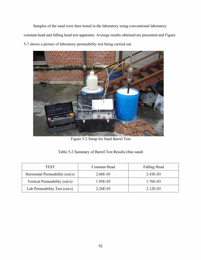
92

Samples of the sand were then tested in the laboratory using conventional laboratory

constant head and falling head test apparatus. Average results obtained are presented and Figure

5-7 shows a picture of laboratory permeability test being carried out.

Figure 5-2 Setup for Sand Barrel Test

Table 5-2 Summary of Barrel Test Results (fine sand)

TEST Constant Head Falling Head

Horizontal Permeability (cm/s) 2.06E-03 2.43E-03

Vertical Permeability (cm/s) 1.95E-03 1.76E-03

Lab Permeability Test (cm/s) 2.26E-03 2.12E-03

93

Barrel Test Results

0.00E+00

5.00E-04

1.00E-03

1.50E-03

2.00E-03

2.50E-03

3.00E-03


Per

mea

bilit

y(cm

/s)

VAHIP HorizontalVAHIP Vertical Stadard Lab Test

Figure 5-4 Summary of Barrel Test Results

5.1.3 Pseudo Field Tests

These were test to simulate actual field conditions. It involved the probe being manually

driven into the ground to a shallow depth within a soil layer. The soil deposit chosen was fill

material on the University of Florida campus behind the Reed Laboratory. Figure 5.5 shows a

picture of the test being performed. A sample of the soil taken to the laboratory for analysis

revealed it was brown fine sand. Laboratory permeability tests were performed on the sample

and results are presented along with the probe test results in Table 5.3 and Figure 5-6. Due to

low flow rates during vertical flow which were outside the range of the flow meter on the control

panel, the vertical permeability at constant head could not be computed during the test.

Figure 5-5 Pseudo – Field test behind Reed Lab.

94

Figure 5-7 Laboratory permeability test on sample

Table 5-3 Summary of Pseudo-Field Tests Results (Brown Fine Sand)

TEST Constant Head Falling Head

Horizontal Permeability (cm/s) 2.09E-03 1.80E-03

Vertical Permeability (cm/s) N/A 8.19E-04

Standard Lab Permeability Test 9.59E-04 9.11E-04

Pseudo-Field Test Results

0.00E+00

5.00E-04

1.00E-03

1.50E-03

2.00E-03

2.50E-03


Per

mea

bilit

y(cm

/s)

VAHIP HorizontalVAHIP VerticalStandard Lab Test

Figure 5-6 Summary of Pseudo-Field test Results

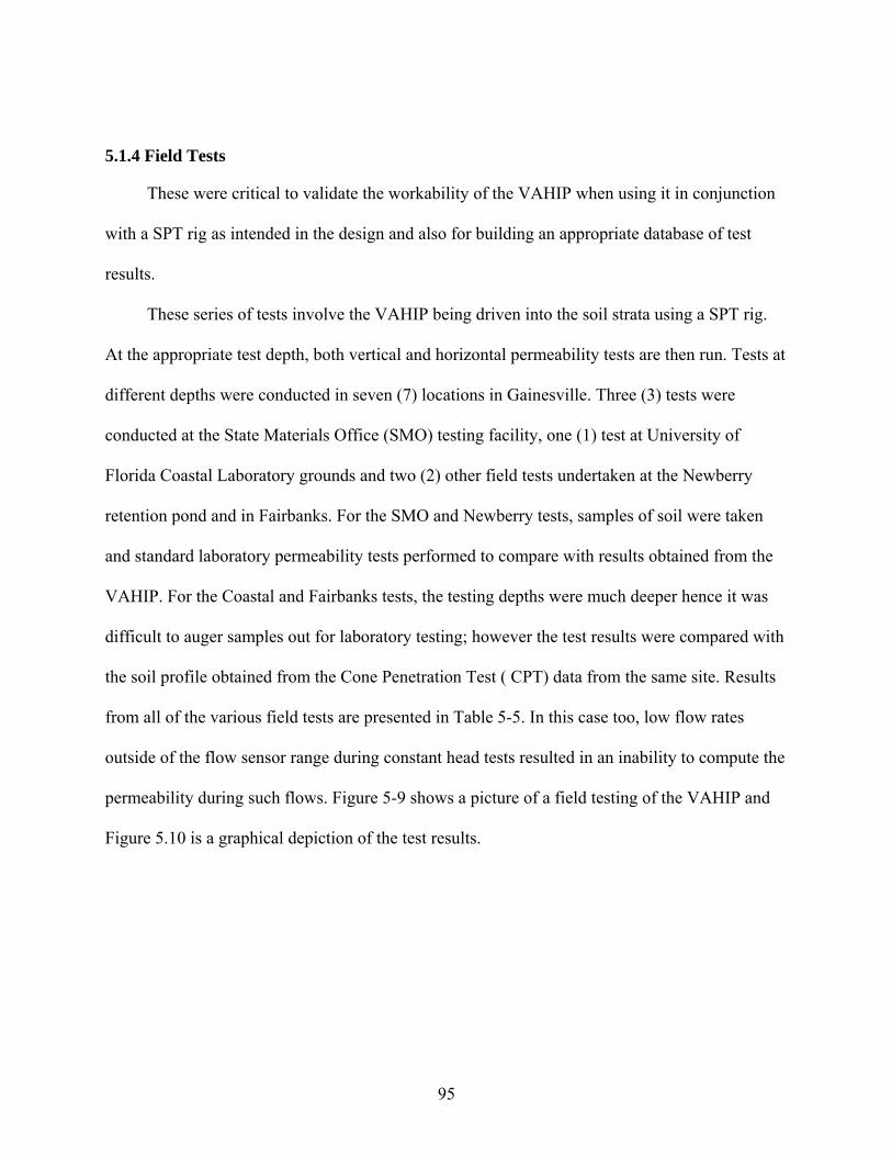
95

5.1.4 Field Tests

These were critical to validate the workability of the VAHIP when using it in conjunction

with a SPT rig as intended in the design and also for building an appropriate database of test

results.

These series of tests involve the VAHIP being driven into the soil strata using a SPT rig.

At the appropriate test depth, both vertical and horizontal permeability tests are then run. Tests at

different depths were conducted in seven (7) locations in Gainesville. Three (3) tests were

conducted at the State Materials Office (SMO) testing facility, one (1) test at University of

Florida Coastal Laboratory grounds and two (2) other field tests undertaken at the Newberry

retention pond and in Fairbanks. For the SMO and Newberry tests, samples of soil were taken

and standard laboratory permeability tests performed to compare with results obtained from the

VAHIP. For the Coastal and Fairbanks tests, the testing depths were much deeper hence it was

difficult to auger samples out for laboratory testing; however the test results were compared with

the soil profile obtained from the Cone Penetration Test ( CPT) data from the same site. Results

from all of the various field tests are presented in Table 5-5. In this case too, low flow rates

outside of the flow sensor range during constant head tests resulted in an inability to compute the

permeability during such flows. Figure 5-9 shows a picture of a field testing of the VAHIP and

Figure 5.10 is a graphical depiction of the test results.

96

Table 5-5 Field Test Results


VAHIP Field Permeability Results (cm/s) Standard Lab. Permeability Results (cm/s)



Falling Head

FDOT Site 1

3 ft

Grey Fine Sand

8.50E-04

5.78E-04

9.68E-04

5.54E-04

6.93E-04

7.06E-04

FDOT Site 2

3 ft

Grey Fine Sand

3.70E-03

3.49E-03

4.11E-03

3.84E-03

2.50E-03

2.88E-03

5 ft Grey Fine Sand

2.47E-03

2.24E-03

2.67E-03

2.42E-03

FDOT Site 3

7 ft

Clayey Sand

N/A

N/A

1.13E-05

4.02E-05

4.16E-04

4.34E-04

8 ft Clayey Sand

N/A

N/A

1.38E-05

3.05E-05

Newberry Pond

7ft

Brown Fine Sand

7.29E-04

7.15E-03

7.05E-04

8.54E-03

3.13E-03

3.31E-03

9ft Brown Fine Sand

3.69E-04

1.64E-03

3.53E-04

2.67E-03

FDOT Site 4

11ft

Clayey Sand

N/A

N/A

7.09E-05

1.60E-04

N/A

N/A

Coastal Lab(1)

8.5ft

Clay

N/A

N/A

1.59E-07

4.83E-07

N/A

N/A

16ft

Clay

N/A

N/A

1.46E-07

4.58E-07

N/A

N/A

Coastal Lab(2)

8ft

Silty Sand

N/A

N/A

5.98E-05

1.48E-04

N/A

N/A

15.5ft

Silty Sand

N/A

N/A

4.02E-05

2.75E-05

N/A

N/A

Fairbanks

7ft

Stiff Sand

2.34E-03

8.41E-03

3.89E-03

8.50E-03

N/A

N/A

9ft

1.82E-03

6.47E-03

4.36E-03

7.29E-03

N/A

N/A

97

Figure 5-9 Field testing

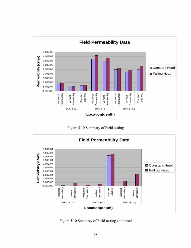
98

Field Permeability Data

0.00E+00

5.00E-04

1.00E-03

1.50E-03

2.00E-03

2.50E-03

3.00E-03

3.50E-03

4.00E-03

4.50E-03

Hor

izon

tal

Perm

eabi

lity

Verti

cal

Perm

eabi

lity

Stan

dard

Lab

test

Hor

izon

tal

Perm

eabi

lity

Verti

cal

Perm

eabi

lity

Hor

izon

tal

Perm

eabi

lity

Verti

cal

Perm

eabi

lity

Stan

dard

Lab

test

SMO 1 (3' ) SMO 2 (3') SMO 2 (5' )

Location(depth)

Perm

eabi

lity

(cm

/s)

Constant Head

Falling Head

Figure 5.10 Summary of Field testing


0.00E+005.00E-051.00E-041.50E-042.00E-042.50E-043.00E-043.50E-044.00E-044.50E-045.00E-04

Hor

izon

tal

Perm

eabi

lity

Verti

cal

Perm

eabi

lity

Hor

izon

tal

Perm

eabi

lity

Verti

cal

Perm

eabi

lity

Stan

dard

Lab

test

Hor

izon

tal

Perm

eabi

lity

Verti

cal

Perm

eabi

lity

SMO 3 (7' ) SMO 3 (8' ) SMO 4(11' )

Location(depth)

Perm

eabi

lity

(Cm

/s)

Constant HeadFalling Head

Figure 5.10 Summary of Field testing continued

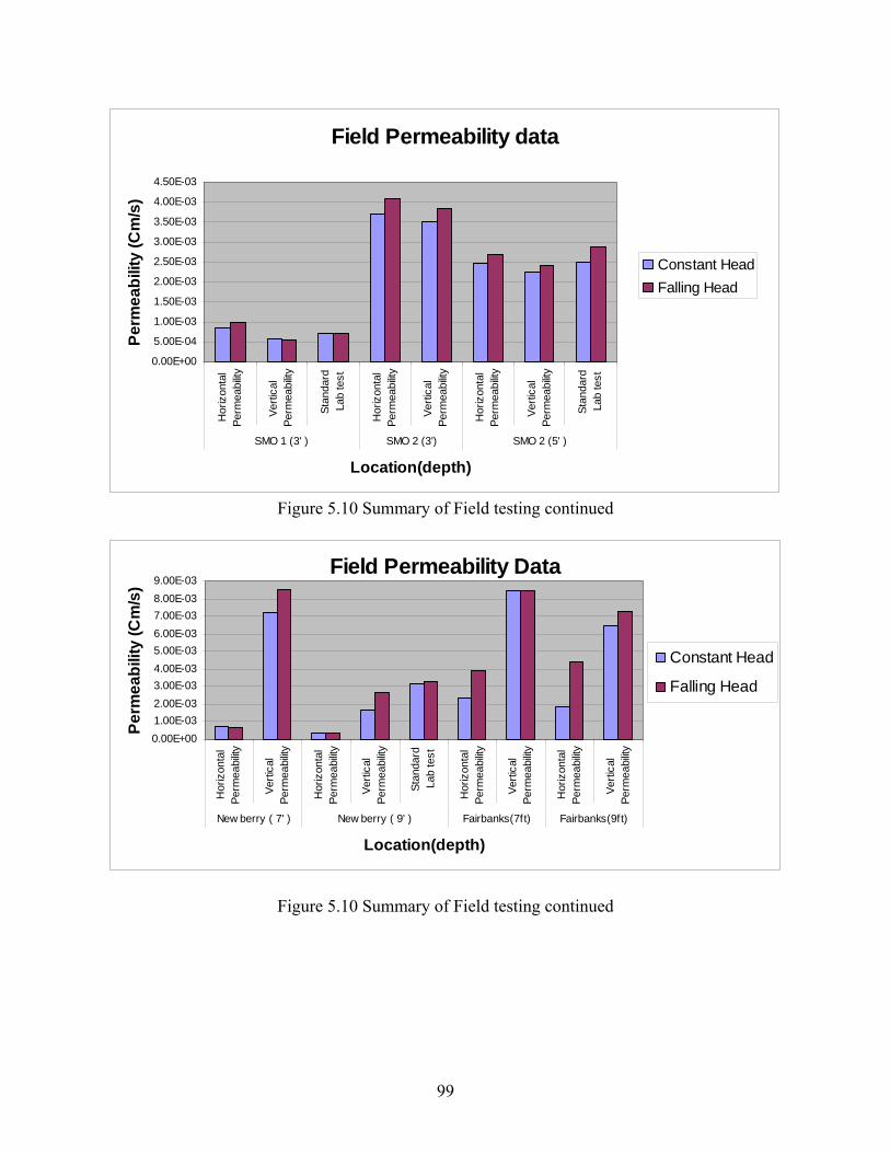
99

Field Permeability data

0.00E+00

5.00E-04

1.00E-03

1.50E-03

2.00E-03

2.50E-03

3.00E-03

3.50E-03

4.00E-03

4.50E-03

Hor

izon

tal

Perm

eabi

lity

Verti

cal

Perm

eabi

lity

Stan

dard

Lab

test

Hor

izon

tal

Perm

eabi

lity

Verti

cal

Perm

eabi

lity

Hor

izon

tal

Perm

eabi

lity

Verti

cal

Perm

eabi

lity

Stan

dard

Lab

test

SMO 1 (3' ) SMO 2 (3') SMO 2 (5' )

Location(depth)

Perm

eabi

lity

(Cm

/s)




0.00E+001.00E-032.00E-033.00E-034.00E-035.00E-036.00E-037.00E-038.00E-039.00E-03

Hor

izon

tal

Perm

eabi

lity

Verti

cal

Perm

eabi

lity

Hor

izon

tal

Perm

eabi

lity

Verti

cal

Perm

eabi

lity

Stan

dard

Lab

test

Hor

izon

tal

Perm

eabi

lity

Verti

cal

Perm

eabi

lity

Hor

izon

tal

Perm

eabi

lity

Verti

cal

Perm

eabi

lity

New berry ( 7' ) New berry ( 9' ) Fairbanks(7ft) Fairbanks(9ft)

Location(depth)

Perm

eabi

lity

(Cm

/s)

Constant Head

Falling Head


100

5.1.5 Further Enhancement of the Probe

In general the probe did not function quite well during testing in stiff clayey and sandy

material. During driving in such material, stresses on the inner rod on the probe tend to be

excessive resulting in bending of the inner rod at the sleeve portion of the probe resulting in the

sleeve itself which is made of PVC sometimes being mangled. A more robust inner rod and

sleeve set-up was thus considered to allow testing in stiff material. Modifications were thus made

on the probe. Basically the modification involved strengthening the inner rod by increasing the

thickness as well as replacing the PVC collar with a stainless steel one. All other aspects of the

original design remained the same. Figure 6.1 and 6.2 shows a picture of the modified probe with

tip closed and opened respectively.

Figure 6.1 Modified Probe with tip closed

101

Figure 6.2 Modified Probe with tip opened

5.5.6 Field Testing of the Enhanced Probe

The enhanced probe was field tested and the results are presented in Table 5-6. Testing of

the probe involved driving it into the ground. Even though the preferred driving method was to

use the FDOT hydraulic rig to hydraulically push the probe into the ground so as to minimize the

stresses, an FDOT hydraulic rig was not available within the time frame so a conventional

hammer type SPT rig was utilized for the driving. The maximum driving depth was limited to

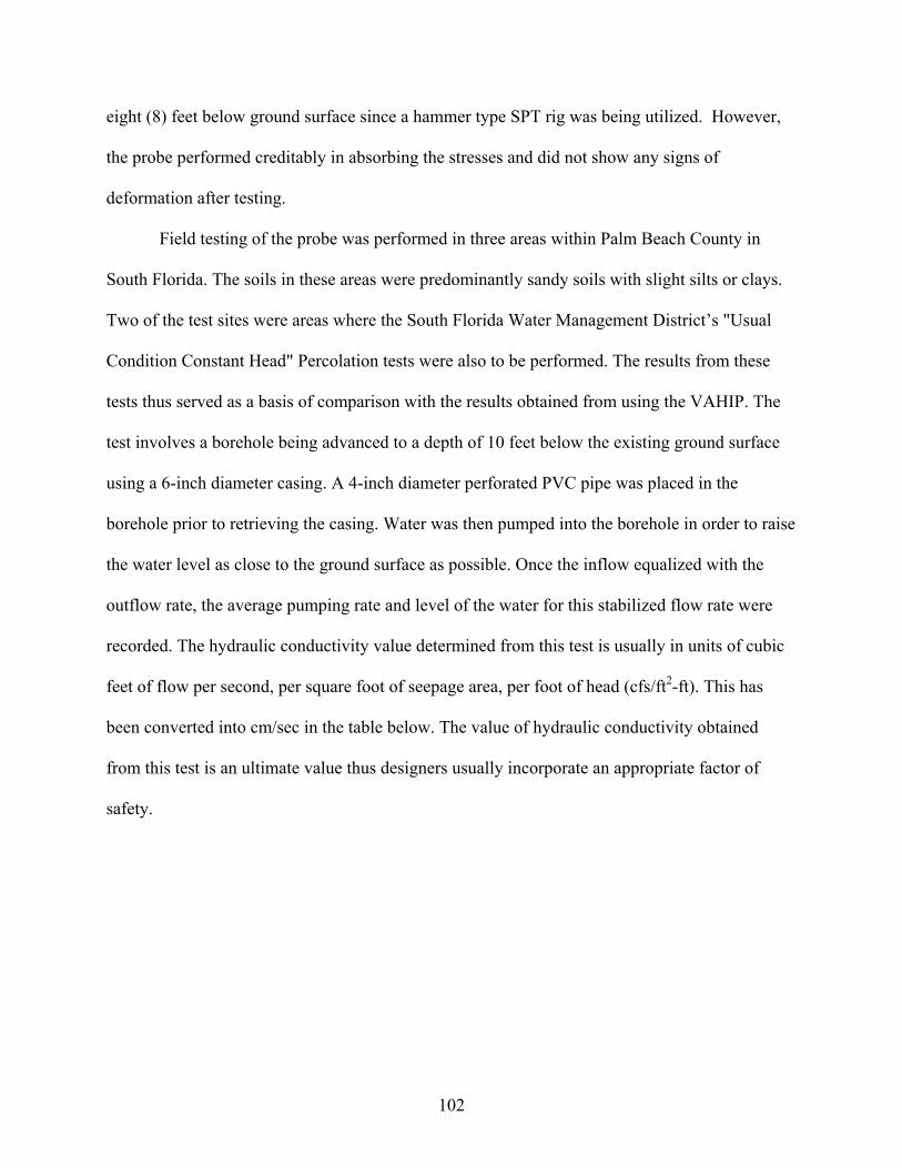
102

eight (8) feet below ground surface since a hammer type SPT rig was being utilized. However,

the probe performed creditably in absorbing the stresses and did not show any signs of

deformation after testing.

Field testing of the probe was performed in three areas within Palm Beach County in

South Florida. The soils in these areas were predominantly sandy soils with slight silts or clays.

Two of the test sites were areas where the South Florida Water Management District’s "Usual

Condition Constant Head" Percolation tests were also to be performed. The results from these

tests thus served as a basis of comparison with the results obtained from using the VAHIP. The

test involves a borehole being advanced to a depth of 10 feet below the existing ground surface

using a 6-inch diameter casing. A 4-inch diameter perforated PVC pipe was placed in the

borehole prior to retrieving the casing. Water was then pumped into the borehole in order to raise

the water level as close to the ground surface as possible. Once the inflow equalized with the

outflow rate, the average pumping rate and level of the water for this stabilized flow rate were

recorded. The hydraulic conductivity value determined from this test is usually in units of cubic

feet of flow per second, per square foot of seepage area, per foot of head (cfs/ft2-ft). This has

been converted into cm/sec in the table below. The value of hydraulic conductivity obtained

from this test is an ultimate value thus designers usually incorporate an appropriate factor of

safety.

103

Table 5-6 Field Test Results for the modified Probe


0.00E+00

5.00E-03

1.00E-02

1.50E-02

2.00E-02

2.50E-02

3.00E-02

3.50E-02

4.00E-02

4.50E-02

Hor

izon

tal

Per

mea

bilit

yV

ertic

alP

erm

eabi

lity

Hor

izon

tal

Per

mea

bilit

yV

ertic

alP

erm

eabi

lity

Usu

al O

pen

Hol

eH

oriz

onta

lP

erm

eabi

lity

Ver

tical

Per

mea

bilit

yH

oriz

onta

lP

erm

eabi

lity

Ver

tical

Per

mea

bilit

yU

sual

Ope

nH

ole

Hor

izon

tal

Per

mea

bilit

yV

ertic

alP

erm

eabi

lity

Hor

izon

tal

Per

mea

bilit

yV

ertic

alP

erm

eabi

lity

Usu

al O

pen

Hol

e

Indrio ( 5' ) Indrio ( 8' ) Jog ( 6' ) Jog ( 8' ) Palm ( 7' ) Palm ( 8' )

Location

Perm

eabi

lity

(Cm

/s)


Figure 6.3 Summary of Field Testing of Modified Probe


VAHIP Field Permeability Results (cm/s) Usual Open Hole Permeability Results (cm/s)



Indrio Road Site

5 ft

Grey Fine Sand 3.52E-03 4.50E-03 2.08E-03 2.14E-03

N/A

8 ft Grey Fine

Sand 3.20E-03 3.67E-03 2.98E-03 2.42E-03

Jog Road

Site

6 ft

Brown Fine Sand 2.64E-03 3.02E-03 1.08E-03 2.02E-03

4.23E-02

8 ft Brown

Fine Sand 2.34E-03 2.98E-03 1.32E-03 2.06E-03

Palm Beach

Medical Center

Site

7ft

Brown Fine Sand 2.41E-03 3.18E-03 4.32E-03 6.54E-03

4.10E-02

9ft Brown

Fine Sand 3.08E-03 3.64E-03 4.53E-03 5.67E-03

104

CHAPTER 6 CONCLUSIONS AND RECOMMENDATIONS

6.1 Overview

The main purpose of this project was to develop a field permeability device for the FDOT

that would be capable of measuring both the horizontal and vertical permeability at any

particular depth within a soil formation. Major tasks in the project involved:

1. Development of a probe that could be driven into the ground via a CPT/SPT rig to measure permeability.

2. Development of appropriate auxiliary devices to enable water to be introduced into the probe at depth and to measure the flow rate.

3. Identify existing theoretical relationships that can be used to convert the measured steady state flow rates into the field saturated permeability at any depth.

4. Undertake adequate tests to ensure workability of the device and obtain data consistent with laboratory permeability results.

5. Preparation of a User’s Manual for Field use of the device.

6.2 Results and Conclusions

Currently the database of field permeability results obtained from the VAHIP tests is quite

small. This is mainly due to the fact that the design of the probe had to go through a number of

changes as the project progressed and also it was quite difficult to get a SPT/CPT rig to perform

a large number of tests within the time frame. However, information from the available data

generally shows that some VAHIP test results obtained in sandy material compares well with

standard laboratory test results from samples taken. These permeability obtained were of the

same order. For tests performed in sandy material, horizontal and vertical permeability results

were also of same order however; in the case of test results obtained from the Newberry retention

pond, the vertical permeability was an order of magnitude greater than the horizontal

permeability. This may well be attributed to the presence of voids in the rock/soil since there is

evidence of sink hole activity at the pond. Test results obtained from field testing in clayey

materials were one exponential order of magnitude less than that obtained from the

105

corresponding standard laboratory test. Vertical permeabilities were greater than the horizontal

permeabilities.

Permeability results obtained using the modified probe was one exponential order of

magnitude less than that calculated from the “Usual Open Hole Constant Head” percolation test.

However it must be noted that the “Usual Open Hole” test result is an ultimate value and also the

prior disturbing of the soil through augering of the test hole as opposed to the VAHIP test

method may be contributing to this difference.

Generally the constant and falling head test results were similar. The difference in

permeability values may be attributed to the difference in test methods. Constant head tests could

not be performed in clayey material because of the low flow rates (which were out of the range

of the flow sensor). Flow rates below 18.9 ml/s are difficult to measure with the Omega FP-

5063 Micro-Flow Sensor. In such situations, falling head tests are more appropriate. During the

constant head test, flow is adjusted using the fine valve adjustment such that a constant level is

maintained in the Plexiglas flow measurement device. Because it is easier to see volume

fluctuations better in the smaller tube, the flow must be balanced using the smaller Plexiglas

tube. Flow adjustments should be made until the fluctuations at the predetermined constant

height in the small Plexiglas tube do not exceed 1mm in a 30-second period. Falling head tests

was preferred over constant head tests due to difficulties in fine tuning the control panel valve to

adequately achieve a stable constant head.

For testing of the probe in fairly stiff material, it would be preferred that holes are pre-

bored to depth before inserting the probe. It is recommended that the probe should be pushed

into the ground with an SPT/CPT rig which is hydraulically operated as opposed to the hammer

106

type rig to minimize the stresses on the probe during driving and also to better align the probe’s

descent into the ground in a plumb manner.

It must be noted that permeability results from the VAHIP field tests at any particular

depth corresponds to the soil within the vicinity of the vertical and horizontal flow ports of the

probe, as appropriate. Consequently, any anomalies or discontinuities in the soil in these areas

are more likely to influence the test results. As a result of spatial variability issues associated

with permeability, it is recommended that adequate discretion be used in determining the number

and locations of field tests that would be required when using the VAHIP to access the

permeability characteristics of a soil formation within an area. Prior information from other

insitu tests (e.g. SPT/CPT) can help determine how testing with the VAHIP can be effectively

done to optimize the testing program to establish the permeability characteristics of the soil

formation. This is where the versatility of the VAHIP and its ease of use is advantageous. Such

prior information (SPT/CPT) can also help such that very stiff materials can be avoided so as not

to damage the probe. In the event that a stiff upper material has to be penetrated to reach a less

stiff material whose permeability is desired, pre-bored holes can be identified early and planned

to be used.

From tests performed to date it has been realized that the basic premise of the design of the

VAHIP is credible and the VAHIP can measure the vertical and horizontal flow rate at any

particular depth and consequently, the permeability in both flow directions determined using the

appropriate theoretical equations.

6.3 Recommendations

Availability of water and compressed air were critical factors on the number of test that

could be performed. Above the ground water table, water is required to bring the surrounding

soil to a saturated state and compressed air is typically required to get the water into the probe

107

from the water tank. Thus a SPT rig equipped with water and compressed air tanks is needed in

conjunction with the VAHIP for field tests.

The groundwater depth gauge that was incorporated in the 2005 prototype probe did not

work as intended, hindering the flow of water through the vertical flow ports of the probe and

interfering with the probe’s ability to toggle between vertical and horizontal flow positions. The

gauge was completely removed in the 2006 prototype and groundwater levels during testing

ascertained by other means now (dropping of plumb bob, nearby test boreholes, water level

records, etc). It is recommended that a way be found to incorporate a groundwater level gauge in

the current set up to ensure an easier and quicker determination of the water table depth and thus

faster data reduction. However, performing VAHIP permeability tests in conjunction with other

insitu tests such as SPT/CPT would eliminate the need for this since both tests include

groundwater measurements.

During driving of the probe into the ground, there exists the possibility of the densification

or compaction of the surrounding soil immediately around the periphery of the probe especially

when driving in loose sands. Hence, measured flow rates would be less than what must ideally be

expected. It is further recommended that the effects of such densification on the measured

permeability be analyzed and if required some correction factors be introduced to account for

that. There is also the possibility of some short-circuiting of flow for horizontal permeability

particularly when testing in stiff clay layers. However the current results do not give a strong

indication of this happening. Therefore, the use of the current probe in stiff clayey material is not

recommended.

To be able to make a more meaningful assessment and evaluation of permeability results

from the VAHIP, a larger database of test results in differing soil conditions is recommended.

108

It is expected that the current VAHIP would be adequately field tested to provide the necessary

database of results. Another area worth looking at is the theoretical equations used in the data

reduction for converting the field measured flow rates into permeability. Currently, the equations

are based on borehole permeability tests under saturated conditions. Efforts should be made to

find alternative equations that would be based more on the probe flow and boundary conditions

and also able to convert flow rates in both unsaturated and saturated conditions into respective

permeability.

Based on results and experiences to be gathered from further field testing over time, the

alternative probe design as presented by Harrald Klammler (GRIP Conference 2006 –

Development of Field Permeability Apparatus) can also be looked at. This alternate design

would eliminate some of the problems encountered in field testing which have been already

enumerated.

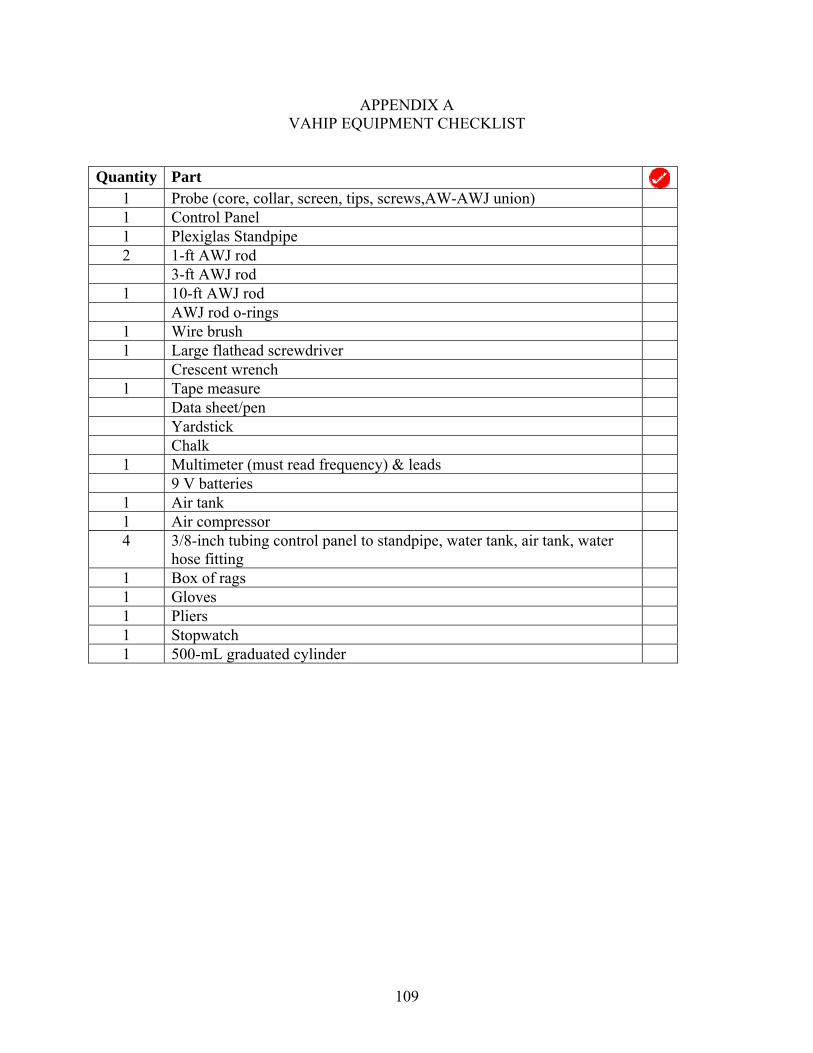
109

APPENDIX A VAHIP EQUIPMENT CHECKLIST

Quantity Part

1 Probe (core, collar, screen, tips, screws,AW-AWJ union) 1 Control Panel 1 Plexiglas Standpipe 2 1-ft AWJ rod 3-ft AWJ rod 1 10-ft AWJ rod AWJ rod o-rings 1 Wire brush 1 Large flathead screwdriver Crescent wrench 1 Tape measure Data sheet/pen Yardstick Chalk 1 Multimeter (must read frequency) & leads 9 V batteries 1 Air tank 1 Air compressor 4 3/8-inch tubing control panel to standpipe, water tank, air tank, water

hose fitting

1 Box of rags 1 Gloves 1 Pliers 1 Stopwatch 1 500-mL graduated cylinder

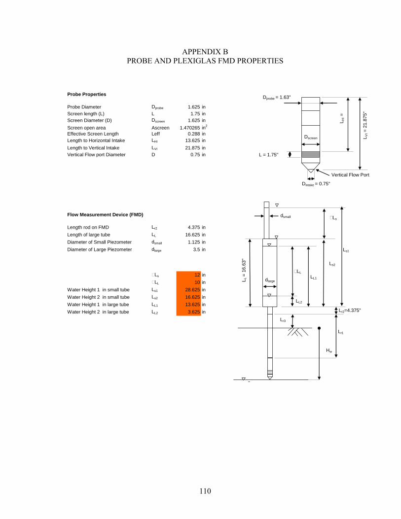
110

APPENDIX B PROBE AND PLEXIGLAS FMD PROPERTIES

Probe Properties

Probe Diameter Dprobe 1.625 inScreen length (L) L 1.75 inScreen Diameter (D) Dscreen 1.625 inScreen open area Ascreen 1.470265 in2

Effective Screen Length Leff 0.288 inLength to Horizontal Intake LHI 13.625 inLength to Vertical Intake LVI 21.875 inVertical Flow port Diameter D 0.75 in

Flow Measurement Device (FMD)

Length rod on FMD Lr2 4.375 inLength of large tube LL 16.625 inDiameter of Small Piezometer dsmall 1.125 inDiameter of Large Piezometer dlarge 3.5 in

Ls 12 inLL 10 in

Water Height 1 in small tube Ls1 28.625 inWater Height 2 in small tube Ls2 16.625 inWater Height 1 in large tube LL1 13.625 inWater Height 2 in large tube LL2 3.625 in

Lr1

Hw

Lr2=4.375"

Ls

Dintake = 0.75"

L = 1.75"

Dscreen

Dprobe = 1.63"

LL

L HI =

L VI =

21.

875"

LL2

LL1

Ls1

Ls2

L L =

16.

63"

dsmall

dlarge

Lr3

Vertical Flow Port

111

APPENDIX C SPREADSHEETS FOR VAHIP PERMEABILITY TESTS

Testing of a Vertical and Horizontal Insitu Permeameter (Soil above GWT)

Date of test:

Location:

Soil Type:

Performed by:

Notes:

Constant Head Vertical

Test No.

Total Length of Rod

Length of rod above Ground

Height of water in FMD

WT Height

Total Head Volume Flowrate Flowrate Flowrate Flowrate

Lr1 Lr3 L1L Hw HT V t Q Q Q Qin in in in in mL mm: ss s cm^3/s in^3/s Hz in^3/s

Constant Head Horizontal

Test No.

Total Length of Rod

Lengtrh of Rod above Ground

Heigh of water in FMD

WT Height

Total Head

Volume Filled Flowrate Flowrate Flowrate Flowrate

Lr1 Lr3 L1L Hw HT V t Q Q Q Qin in in in in mL mm: ss s ccps in^3/s Hz in^3/s

Falling Head Vertical

Test No.Small or large tube

Total Length of Rod


WT Height

Initial Head

Final Head H1/H2 Time 1 time 2

S or L Lr1 Lr3 Hw H1 H2 t1 t2 t2-t1in in in in mm: ss s mm: ss s

Falling Head Horizontal


Total Length of Rod


WT Height

Initial Head



time

time

LviLhi

Lr1

Hw

L1SL2S

L1L

L2L

H1S

H2L

H1L

H2S

Lr3

Lr2=4.375"

112

Testing of a Vertical and Horizontal Insitu Permeameter(Soil below GWT)

Date of test:

Location:

Soil Type:

Performed by:

Notes:


Test No.

Total Length of Rod


Height of water in FMD

WT Height




Test No.

Total Length of Rod


Heigh of water in FMD

WT Height

Total Head





Total Length of Rod


WT Height

Initial Head





Total Length of Rod


WT Height

Initial Head



time

time

LviLhi

Lr1Hw

L1SL2S

L1L

L2L

H1S

H2L

H1L

H2S

Lr3

Lr2=4.375"

113

APPENDIX D TYPICAL PERMEABILITY TEST RESULTS SPREADSHEETS

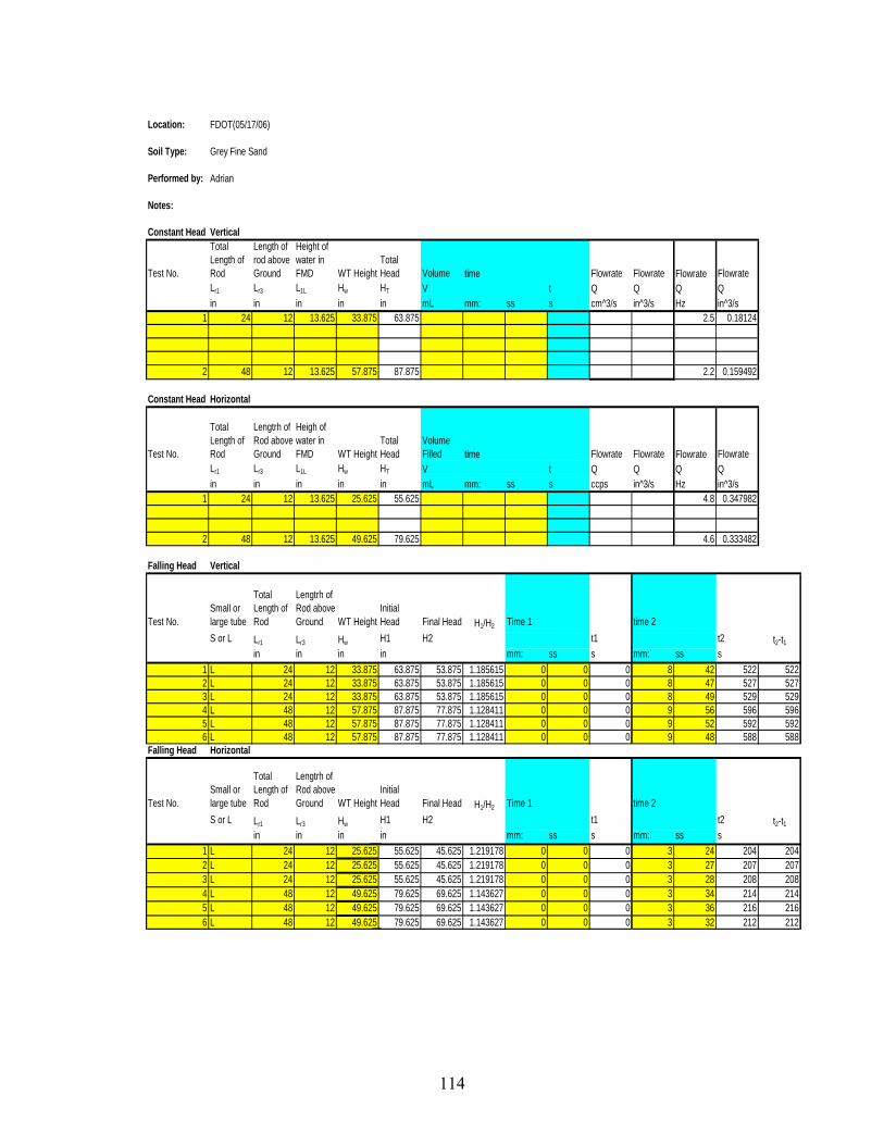
114

Location: FDOT(05/17/06)

Soil Type: Grey Fine Sand

Performed by: Adrian

Notes:


Test No.

Total Length of Rod


Height of water in FMD WT Height



1 24 12 13.625 33.875 63.875 2.5 0.18124

2 48 12 13.625 57.875 87.875 2.2 0.159492


Test No.

Total Length of Rod


Heigh of water in FMD WT Height

Total Head



1 24 12 13.625 25.625 55.625 4.8 0.347982

2 48 12 13.625 49.625 79.625 4.6 0.333482



Total Length of Rod

Lengtrh of Rod above Ground WT Height

Initial Head Final Head H1/H2 Time 1 time 2


1 L 24 12 33.875 63.875 53.875 1.185615 0 0 0 8 42 522 5222 L 24 12 33.875 63.875 53.875 1.185615 0 0 0 8 47 527 5273 L 24 12 33.875 63.875 53.875 1.185615 0 0 0 8 49 529 5294 L 48 12 57.875 87.875 77.875 1.128411 0 0 0 9 56 596 5965 L 48 12 57.875 87.875 77.875 1.128411 0 0 0 9 52 592 5926 L 48 12 57.875 87.875 77.875 1.128411 0 0 0 9 48 588 588



Total Length of Rod

Lengtrh of Rod above Ground WT Height

Initial Head Final Head H1/H2 Time 1 time 2


1 L 24 12 25.625 55.625 45.625 1.219178 0 0 0 3 24 204 2042 L 24 12 25.625 55.625 45.625 1.219178 0 0 0 3 27 207 2073 L 24 12 25.625 55.625 45.625 1.219178 0 0 0 3 28 208 2084 L 48 12 49.625 79.625 69.625 1.143627 0 0 0 3 34 214 2145 L 48 12 49.625 79.625 69.625 1.143627 0 0 0 3 36 216 2166 L 48 12 49.625 79.625 69.625 1.143627 0 0 0 3 32 212 212

time

time

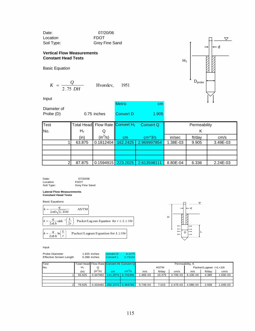
115

Date: 07/20/06Location FDOTSoil Type: Grey Fine Sand

Vertical Flow MeasurementsConstant Head Tests

Basic Equation

InputMetric cm

Diameter of Probe (D) 0.75 inches Convert D 1.905

Test Total Head Flow Rate Convert HT Convert QNo. HT Q

(in) (in3/s) cm cm^3/s in/sec ft/day cm/s1 63.875 0.1812404 162.2425 2.969997854 1.38E-03 9.905 3.49E-03

2 87.875 0.1594915 223.2025 2.613598111 8.80E-04 6.336 2.24E-03

PermeabilityK

1951 Hvorslev, 75.2 DH

QK =Dprobe

d

HT

Date: 07/20/06Location FDOTSoil Type: Grey Fine Sand

Lateral Flow MeasurementsConstant Head Tests

Basic Equations

Input

Probe Diameter 1.625 inches convert D 4.1275Effective Screen Length 0.288 inches Convert L 0.73152

Test Total Head Flow Rate Convert Ht Convert QNo. HT Q

(in) (in3/s) cm cm3/s in/s ft/day cm/s in/s ft/day cm/s1 55.625 0.347982 141.2875 5.702396 1.46E-03 10.479 3.70E-03 6.10E-04 4.389 1.55E-03

2 79.625 0.333482 202.2475 5.464796 9.74E-04 7.015 2.47E-03 4.08E-04 2.938 1.04E-03

ASTMPermeability, K

Packer/Lugean r<L<10r

rLrr

LLhqk 10for Equation ean Packer/Lug

2sinh

21 ≤≤⎟

⎠⎞

⎜⎝⎛= −

π

rLrL

Lhqk 10for Equation ean Packer/Lug ln

2≥=

⎟⎟⎟

⎠

⎞

⎜⎜⎜

⎝

⎛

πLD

d

H

ASTM 2 HDLD

qkπ

=

116

Date: 07/20/06Location FDOTSoil Type: Grey fine Sand

Vertical Flow MeasurementsFalling Head Tests

Basic Equation

Input

Effective Diameter: 0.75 inches

Test TimeDiameter of Peizometer H1/H2

No. t2-t1 d d

(Seconds) in cm in/s ft/day cm/s1 522 L 3.5 1.1856148 8.89 1.52E-03 1.10E+01 3.86E-032 527 L 3.5 1.1856148 8.89 1.51E-03 1.09E+01 3.83E-033 529 L 3.5 1.1856148 8.89 1.50E-03 1.08E+01 3.81E-034 596 L 3.5 1.1284109 8.89 9.46E-04 6.81E+00 2.40E-035 592 L 3.5 1.1284109 8.89 9.52E-04 6.85E+00 2.42E-036 588 L 3.5 1.1284109 8.89 9.58E-04 6.90E+00 2.43E-03

Lr1 in/s ft/day cm/s24 1.51E-03 1.09E+01 3.84E-0348 9.52E-04 6.85E+00 2.42E-03

Average Permeability kv

Large or Small FMD kv

Permeability

D

d

H1H2

( ) ⎟⎟⎠

⎞⎜⎜⎝

⎛−

=2

1

12

2

1 ln11 H

HttD

dk π

117

Date: 07/20/06Location FDOT

Soil Type: Grey Fine Sand

Basic Equation

Input

Probe Diameter 1.625 inches D (cm) 4.1275Screen Length 0.288 inches L (cm) 0.73152F-Factor 5.713159493 inches F-Factor (cm) 14.51142511

Test No. Time Pipette Diameter

Pipette Diameter

t2-t1 H1/H2 d d(Seconds) L or S (in.) in cm in/s ft/day cm/s

1 204 L 1.21917808 3.5 8.89 1.64E-03 1.18E+01 4.16E-032 207 L 1.21917808 3.5 8.89 1.61E-03 1.16E+01 4.10E-033 208 L 1.21917808 3.5 8.89 1.60E-03 1.16E+01 4.08E-034 214 L 1.14362657 3.5 8.89 1.06E-03 7.60E+00 2.68E-035 216 L 1.14362657 3.5 8.89 1.05E-03 7.53E+00 2.66E-036 212 L 1.14362657 3.5 8.89 1.07E-03 7.68E+00 2.71E-03

Lr1 in/s ft/day cm/s24 1.62E-03 1.16E+01 4.11E-0348 1.05E-03 7.57E+00 2.67E-03

Lateral Flow Measurements (Pseudo Field Tests)Falling Head Tests

Large or Small FMD

Average Permeability Kh

Permeability

Kh

D

d

H1H2⎟⎟⎠

⎞⎜⎜⎝

⎛−

=2

1

12

2

ln)(

4/HH

ttFdk π

D

DL

DL

LF 8.2

1ln

22

−

⎟⎟

⎠

⎞

⎜⎜

⎝

⎛⎟⎠⎞

⎜⎝⎛++

=π

118

APPENDIX E USER’S MANUAL

USER’S MANUAL FOR THE 2006 VAHIP

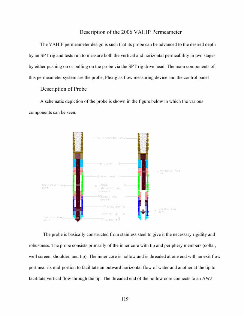
119

Description of the 2006 VAHIP Permeameter

The VAHIP permeameter design is such that its probe can be advanced to the desired depth

by an SPT rig and tests run to measure both the vertical and horizontal permeability in two stages

by either pushing on or pulling on the probe via the SPT rig drive head. The main components of

this permeameter system are the probe, Plexiglas flow measuring device and the control panel

Description of Probe

A schematic depiction of the probe is shown in the figure below in which the various

components can be seen.

The probe is basically constructed from stainless steel to give it the necessary rigidity and

robustness. The probe consists primarily of the inner core with tip and periphery members (collar,

well screen, shoulder, and tip). The inner core is hollow and is threaded at one end with an exit flow

port near its mid-portion to facilitate an outward horizontal flow of water and another at the tip to

facilitate vertical flow through the tip. The threaded end of the hollow core connects to an AWJ

120

union rod which is normally used on SPT rigs, thus facilitating connection to an SPT rig drive head.

The tip of the probe inner core is cone shaped at the end. This cone shaped end is designed to flush

fit perfectly into the outer tip which is a threaded cone shaped plug with a 0.75in tip hole. The well

screen is a hollow cylindrical tube with horizontal slots to allow water to exit through the probe

horizontally whiles the upper hollow cylindrical collar which is made of PVC facilitates the

toggling of the probe from the vertical to the horizontal test position. A double end threaded screw

connector connects these two together. The shoulder which is also a hollow cylindrical tube

connects the outer tip to the well screen via another double ended screw. This connection of collar,

well screen and shoulder portion of the probe thus forms an enveloping outer periphery around the

inner core and tip of the probe. The probe components are listed below.

1. Outer tip with 0.75in diameter tip opening

2. Hollow cylindrical shoulder

3. Double end threaded connection screw

4. Hollow cylindrical screen with horizontal slots

5. Stainless Steel collar connected to a double end threaded screw

6. Hollow inner core

7. AWJ connector rod

121

Pictures of the modified Probe

122

Description of Plexiglas Flow Measuring Device

The Plexiglas standpipe was a device designed for purposes of monitoring the water head,

flow rate and changes in water level required during testing for permeability calculation. It consists

of a 1.5-inch diameter (1.13”-I.D.) Plexiglas tube mounted on top of a 4-inch diameter (3.55”-I.D.)

Plexiglas tube. Water is introduced through an open male quick connect which is threaded to the

top of the 4-inch tube. Water level or head readings can therefore be taken on either the bigger or

smaller pipe as appropriate during testing. It is expected that during testing of soils of low

permeability, the smaller standpipe would be utilized in monitoring water level drops and vice-

versa.

A smaller, open, male quick connect is threaded into the top of the 1.5-inch (smaller) tube and

is used to apply an additional pressure head if necessary when testing. An AWJ male thread welded

to a 4-inch diameter steel plate forms the base of the Plexiglas stand pipe thus making the assembly

easily connectable to an SPT rod.

This device depicted in the figure below is ideal for use in combination with the probe as a

result of the following design attributes.

• Changes in water levels are easy to read. • It can be easily attached to an SPT rod. • It is easily filled with water. • It is capable of being pressurized to increase head.

123

Plexiglas Flow Measurement Device (FMD)

Description of Control Panel

A control panel was deemed necessary to allow the operator to easily control the test from

one location. The control panel is as depicted in the figure below. It was designed to be the center

of the test equipment and serve as the source for regulating the flow of water into the Plexiglas

FMD, introducing pressure in the Plexiglas FMD to increase flow as well as measuring the flow

rate for constant head tests. A pressure tank within the panel is used to drive water into the FMD

and also pressurize the FMD when a greater driving head is required. Valves on the panel control

the flowrates and gauges mounted on the panel monitor the necessary pressures. The flow rates are

measured with a micro-flow sensor which can be connected to two connector ports installed on the

panel.

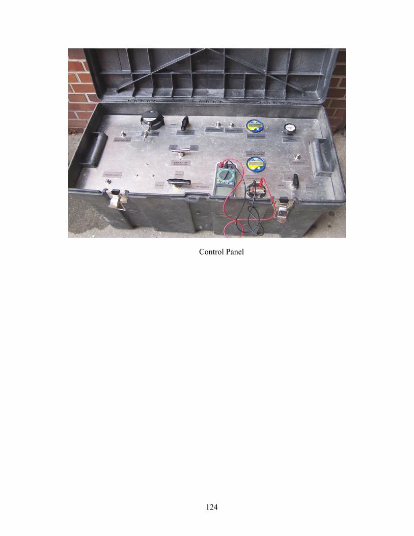
124

Control Panel

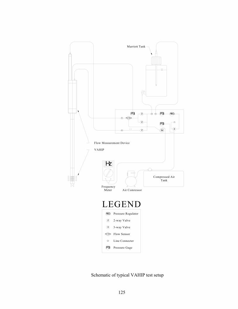
125

PSI

PSI

PSI

2

2

2

3

REG

Compressed AirTank

Flow Sensor

9V

Hz

LEGEND

PSI

2

3

REG

Flow Sensor

Pressure Regulator

2-way Valve

3-way Valve

Flow Sensor

Line Connecter

Pressure Gage

Air ComressorFrequency Meter

Marriott Tank

Flow Measurement Device

VAHIP

Schematic of typical VAHIP test setup

126

Recommended Procedure for Field use of VAHIP

This field permeability testing procedure is recommended when using the VAHIP and an SPT

rig for driving purposes to determine the vertical and horizontal permeability of a soil formation at

various depths. Soil above the water table should be adequately saturated prior to testing.

Probe Assembly

1. Screw up the upper threaded part of the inner core into the base of the AWJ union connector rod by pushing the inner core through the hole in the collar and screwing such that the AWJ connector sits in the collar. Try sliding the inner core within the hole by pulling up and down on the AWJ connector while holding onto the PVC collar. Make sure sliding is smooth.

2. Attach the upper part of the hollow cylindrical well screen to the end of collar by screwing onto its threaded end.

3. Attach one threaded portion of the double end screw to the lower part of the well screen. 4. Attach the upper part of the hollow cylindrical shoulder with horizontal slots to the threaded

portion of the double end screw. 5. Pull up completely on the AWJ connector to retract the inner tip of the core and attach the

outer tip to the lower end of the shoulder by screwing onto it. 6. Push down on the AWJ connector to get the inner tip flush within the hole in the outer tip. 7. Pull up and down on the AWJ rod to retract and push in the inner tip. Make sure this motion is

easy and flexible.

Pre-field Preparation

1. The VAHIP must be clean and rid of any foreign material that would hinder water flow. Prepare all materials and tools listed in the equipment check list in appendix A.

2. Fill up the nalgene tank with clean water and the air tank in the control panel with air using a compressor. Be sure not to exceed the limiting pressure of 90 psi in the air tank.

i. Fill up the nalgene tank by removing the top cover and dropping a hose to deliver the water. Make sure the outlet hose is well connected to the tank outlet to prevent the water from flowing out.

ii. Fill up the air tank by connecting the appropriate hose fitting to the air inlet on the control panel. Turn the air flow pin valve 1 to air - in position and couple the hose to air source (compressor). Monitor the tank pressure from the pressure gauge on the control panel. When maximum pressure is attained turn off pin valve to neutral (no flow) position.

127

Test Procedure

1. Fully assemble the probe and push down the tip so that the tip hole is blocked and the probe is in driving and horizontal (stage I) testing position. Make sure all connections are tight.

2. Connect desired AWJ rods to the probe via the AWJ-AW union connector on the probe. Provide an o-ring between each section to prevent water leakage during testing.

3. Connect the probe assembly to an SPT rig equipped with an AWJ drive head. Advance the probe to the desired depth. Disconnect the drive head from the rod and connect the Plexiglas standpipe. Connect all tubing to control panel and perform stage I (horizontal) tests by performing constant head, falling head or both tests as applicable as outlined under test types.

4. After stage I testing at the depth is performed, stage II(vertical) testing may commence. To get probe in the stage II position, use the SPT rig to pull the rod a about 1.5 -inches out of ground. Attach Plexiglas standpipe to AWJ rod, complete required connections, and perform stage II tests by performing constant head, falling head or both tests as applicable as outlined under test types.

5. Disconnect Plexiglas standpipe and reconnect the AWJ rod to the SPT drive head. Advance the probe to the next desired text depth thus getting the probe back in stage I (horizontal) test position.

6. Make all the necessary connections and carry out stage I tests. Again after stage I testing at this depth, perform stage II testing by pulling on the SPT rod about 1.5-inches from the ground as already described.

7. Continue with steps 3-6 until the maximum test depth is reached and the last stage II test is completed.

8. Extract the probe from the ground. Note the condition of probe (e.g. clogged ports, deformations, etc). Flush probe with water and remove any foreign material within the probe. Brush off all dirt on the probe threads with a wire brush. Wash all rod connections clean.

9. Move to next test location and perform steps 1-7 until tests are completed.

Test Types

Two main types of tests, constant head and falling head tests can be performed when using

the VAHIP. Test details and procedures are as outlined below. To begin, perform all necessary

connections from the control panel to the Plexiglas standpipe and nalgene tank with appropriate

tubing. Make sure all connections are tight and leak proof.

128

VAHIP Flow Measurement Assembly

1. Connect the appropriate 3/8-inch hose tubing fitting from the outlet of the nalgene water tank to the waterline – in connection on the control panel.

2. Connect the appropriate 3/8-inch hose tubing fitting from the waterline – out connection on the control panel to the open male quick connect which is threaded to the top of the 4-inch tube on the Plexiglas stand pipe. Open and close water flow pin valve on control panel as necessary to fill Plexiglas with water.

3. Connect the appropriate 3/8-inch hose tubing fitting from the airline- out 1 connection on the control panel to the open male quick connect which is threaded to the top cover of the nalgene tank. Close the top cover tightly over tank and use the air flow pin valve 1 on the control panel to add air pressure in the nalgene water tank to increase flow when necessary by turning it to the air-out position. Turn to neutral (no flow) to stop air flow.

4. Connect the appropriate hose tubing from the alternate airline-out on the left side of control panel to the smaller, open, male quick connect threaded into the top of the 1.5-inch (smaller) tube of the Plexiglas stand pipe. This is used to apply an additional pressure head when testing and also to flush off soil particles from the probe if necessary by using the airflow valve 2.

Constant Head

1. Fill Plexiglas standpipe to desired level by opening the water flow control pin valve on the control panel. It is recommended that the level chosen is easily measurable and changes in water level can be easily observed.

2. Adjust pin valve such that a constant water level height is achieved. Record water height in Plexiglas standpipe. If flow is slow, use the air flow pin valve on the control panel to add air pressure.

3. Connect the flow sensor to its appropriate electrical ports on the control panel and record frequency output of the flow sensor device.

Repeat steps 1 and 2 several times as needed. Use average readings in data analysis

Falling Head

1. Decide which size diameter of pipette will be used in the falling head test. Larger diameter is recommended for larger flowrates and the smaller diameter pipette for lower flowrates.

2. Measure and mark the H1 and H2 points on selected pipette (H2 must have the same pipette diameter as H1).

129

3. Fill flow measurement apparatus to a level above H1.

4. Turn off pin valve such that water supply is instantaneously shut off. Start recording time as

water level passes the H1 mark and end when the water level reaches the H2 mark.

5. Repeat steps 3 and 4 several times as needed. Use average readings in data analysis.

VAHIP Maintenance

Cleanup. Disassemble probe by first pulling up on AWJ connector and unscrewing the outer

tip. Unscrew other parts, wash probe with clean water and wire brush removing all soil particles

from flow ports and connecting parts. Prior to placing into storage use a lubricant to hinder

oxidation and reduce friction. Note: Due to possible environmental concerns, the lubricant may be

required to be non-toxic.

Routine Inspections. The probe should be inspected after each cleanup for deformed and/or

worn parts. Note deformities and replace parts as needed. Lines in the control panel should be

inspected periodically for leaks.

Storage. The VAHIP, control panel, and standpipe should be stored in cool dry place to

prevent oxidation to steel components. The pressure tank should have a maximum of 10-psi and the

water from the nalgene tank emptied. Remove the battery from flow meter set up.

Data Reduction Spreadsheets

Two SpreadSheets (Appendix C) are provided for reducing the data obtained from field tests.

One is used for tests below the water table while the other is for tests above the water table.

Properties of the Probe and some predetermined water levels have already been inputted in the

spreadsheets however these can be easily changed when the need arises. The main difference

130

between tests below the water table and above is the head difference used in calculating

permeability. For the former case, the water table depth will have to be inputted directly in the

spread sheet info page whiles for the later case it is calculated directly from the probe dimensions

and extension rods that have been added.

Inputs Required for Spreadsheet Properties and Info. Page

Below is a summary of the measurements required to be taken during testing and inputted in

the spreadsheet Info. and Properties sheets. Typically the Info. and Properties sheets would have to

be printed out and filled up as testing progresses in the field.

Constant Head Testing (Vertical and Lateral)

• The total length of AWJ Extension Rods added onto probe to get it to depth - Lr1 • The length of AWJ Extension Rod sticking out above the ground surface when probe

is at depth – Lr3 • The constant height of water that would be maintained in the Plexiglas measuring

device during testing – L1L • Water table depth if testing below the water table. • The flow rate in Hz from the flowmeter or cm^3/s using a measuring cylinder and

stop watch if flow meter does not function.

Falling Head Testing (Vertical and Lateral)

• Identify and input whether the small cylinder (S) or larger cylinder (L) of the Plexiglas device would be used for testing.

• The total length of AWJ Extension Rods added onto the probe to get it to depth - Lr1 • The length of AWJ Extension Rod sticking out above the ground surface when probe

is at depth – Lr3 • Determine and input the change in water level (ΔLs or ΔLL) to be used in the test as

well as initial and final water levels (LS1 LS2, LL1 LL2) on the properties sheet. (These have been already preloaded in the spreadsheet but can be changed).

• Input water table depth if testing below the water table. • The time for the water to drop from the initial to the final level.

131

LIST OF REFERENCES

ASTM Standards: D 4186-89 (Reapproved 1998) Standard Test Method for One-Dimensional Consolidation Properties of Soils Using Controlled-Strain Loading. D 4044-96 Standard Test Method (Field Procedure) for Instantaneous Change in Head (Slug) Test for Determining Hydraulic Properties of Aquifers. Ayan et al. (1994) Measuring Permeability Anisotropy: The Latest Approach. Schlumberger. Huston, TX. Arvind VS, Dhananjay LS (2003) Soil Mechanics and Geotechnical Engineering. A.A. Balkema Publishers, India. Bear J (1972) Dynamics of Fluids in porous Media. Dover, New York Boast CW, Kirkman D (1971) Auger hole seepage theory. Soil Science Society of America Proceedings, 35(3), 365-373 Bouwer H (1978) Groundwater Hydrology. McGraw-Hill, New York Butler JJ Jr (1998) The Design, Performance, and Analysis of Slug Tests, Lewis Publishers, New York, 252p. Carpenter GW, Stephenson RW (1996) Permeability Testing in a Triaxial Cell. Geotechnical Testing Journal. GTJODJ, Vol. 9, No. 4, pp 3-9. Daniel D (1989) In situ hydraulic conductivity tests for compacted clays. J Geotech.Engr ASCE 115(9):1205–1227 Darcy H (1856) The Public Fountains of the City of Dijon: Appendix – Note D. Paris, France. Translated by Brown G and Cateni B. 1999. Das BM (2002) Principles of Geotechnical Engineering 5th Edition Wadsworth Group. Pacific Grove, CA. Das BM (2004) Principles of Foundation Engineering 5th Edition Brooks/Cole. Pacific Grove, CA. Daniel DE (1989) A note on Falling Headwater and Rising Tailwater Permeability Tests Geotechnical Testing Journal. GTJODJ, Vol. 12, No. 4. pp 308-310 Daniel DE (1989) In Situ Hydraulic Conductivity Tests for Compacted Clay. Journal of Geotechnical Engineering. ASCE, Vol. 115, No. 9 pp1205-1225. Davidson JL (2002) Soil Mechanics Laboratory Manual. University of Florida. Gainesville, FL.

132

Gartner M (2005) Improvement of a new permeameter (VAHIP). Masters report. University of Florida. Grim R.E., Clay Mineralogy, 1953; McGraw-Hill Book Company, Inc., New York Hay C (1995) Development of a Field Permeability Device. Masters thesis, University of Florida. Hvorslev MJ (1951) Time lag and soil permeability in groundwater observations. Bulletin No. 36. U.S. Army Engineer Waterways Experiment Station, Vicksburg, MS. Kirkham D (1959) Exact theory of flow into a partially penetrating well. Journal of Geophysical Research, 64(9), 1317-1327. Lambe TS, Whitman R (1969) Soil Mechanics. John Wiley & Sons, Inc. New York Liu C, Evett J (2004) Soils and Foundations 6th Edition. Pearson Education.Upper Saddle River, NJ. Moriwaki T, Umehara K (2003) Method for Determining the Coefficient of Permeability of Clays. Geotechnical Testing Journal. ASTM International, Vol. 26, No. 1 pp 47-56. Murthy VNS (2003) Geotechnical Engineering Principles and Practices of Soil Mechanics and Foundation Engineering. Marcel Dekker, Inc. New York. Sneddon IN (1966) Mixed boundary value problems in potential theory. Amsterdam: North –Holland Publishing Company.

Final Report - CiteSeerX

Documents

Transcript of Final Report - CiteSeerX