Exploring New Models for Population Prediction inDetecting Demographic Phase Change

for Sparse Census Data

Arindam Gupta∗, Sabyasachi Bhattacharya∗∗

andAsis Kumar Chattyopadhyay∗,Ψ

∗Department of StatisticsUniversity of Calcutta

∗∗Agricultural and Ecological Research UnitΨ Population Studies Unit

Indian Statistical Institute, Kolkata

Abstract

Logistic model has long history regarding it’s usefulness in popula-tion predictions. But the model has some limitations when applying forthe sparse census data sets, typically available for developing countries.In such situation the relative growth rates (RGR) exhibit some un-usual trend (increasing, primary increasing and then decreasing) whichis different from the common decreasing trend of logistic law. To tacklethose complicated demographic situations we have successfully exploreda simplified version of Tsoularis and Wallace model (TWM) which canexplain all of these feasible monotonic structures of RGR. In additionto this we have also proposed another model (PM) by assuming RGRas a direct function of time covariate but not the size. The model hassome key advantages than the simplified TWM (STWM). It can detectthe demographic phase change point at which the developing countryswitches over towards developed one. We performed RGR modelling(as a function of time) but not the size as neither TWM nor STWMis analytically solvable and the underlying population model is betteridentifiable in the former case but not in the later. The less number ofparameters involve in both the STWM and PM ensure a better chanceof convergence under non-linear least square estimation than the orig-inal TWM with more parameters.

Keywords and phrases: Population prediction, relative growthrate, Tsoularis-Wallace model, demographic phase change.

AMS Subject Classification: 62P25

1

1 Introduction

The problem of population prediction is concerned with the predictionof the size and composition of the future population on the basis of thesize and composition of current population. Usually elaborate predic-tions are made of the population size at each age group and separatelyfor male and female. Gradually different methods have been developedby the population scientists for this purpose. Among these, cohort com-ponent method is a very familiar one where predictions are first madeseparately for the three components viz. survivorship, migration andbirth and then these three components are combined to predict the netsize and composition of the future population.

In projecting population for small areas such as a city, state etc. theavailable techniques are very few in numbers. The cohort componentmethod often fails due to the difficulties of prediction of the flow ofmigrants in and out of these areas. The estimates are often found tobe unrealistic .

In the case of estimating Indian population or population of it’ssub-regions, it is revealed that logistic model grossly underestimatestrue population. Additionally the logistic model has some limitationswhen applying for the scanty sparse census data set, typically availablefor developing countries. In such situations the relative growth rates(RGR) exhibit some unusual trend (increasing, primary increasing andthen decreasing) which is different from the common decreasing trendof logistic law.

In population prediction problem, rate modeling may often be morepowerful than the usual size modeling where rate is define as the rel-ative change of size with respect to time. Sometime it is not easy orrather misleading for the experimenter to identify the proper underly-ing model by studying the shape of the growth profile curves among theplenty available growth curves. But in comparison if we plot the em-pirical estimate of RGR against time or size we can at least guess andidentify the proper family of growth curves which is appropriate for thegiven data based on the monotonic structure of RGR. So eliminationof improper model is comparatively easy from RGR profile than thesize profile curves. This is particularly important when growth profilecurves similar to common and existing growth curves though the RGRis not monotonically decreasing with time (Gompertz) / size (logistic,Richards, von-Bertallanfy etc.) or constant (exponential) - which isthe basic property of the standard population growth curves. Corre-sponding to different census figures we observed different growth rates

2

though growth profiles look alike (see Figure 1). The simulated Figure2 (bell shaped) also illustrates the same property by showing the sizeprofile, S-shaped Sigmoidal, whereas the RGR profile is not decreasingbut primarily increasing then decreasing with size. So the underlyingpopulation model is better identifiable in the former case but not in thelater. Finally, the most important point in favouring RGR modelling isthat sometimes it is really impossible to solve the growth law analyti-cally, by just integrating the rate differential equation. Basically thesetwo shortcomings motivates us to introduce RGR modelling but not thesize. We try to explore this by introducing Tsoullaris-Wallace model(2002) (TWM) which has the property to exhibit various uncommonstructures of RGR. Tosoularis-Wallace model (2002) altogether consistsof five unknown parameters to be estimated from the population censusfigures. Although for developed countries population figures are ade-quate to estimate all the parameters but it is not true for developingcountries where population census figures are available only for 8-10periods. The presence of less number of parameters in any standardmodel ensure a better chance of convergence in the non-linear leastsquare estimates. So for the later case reduction of number of para-meters is needed for using TWM without sacrificing it’s advantages inrepresenting all feasible monotonic structures of RGR. In the Section3.2 we have discussed this model (STWM) elaborately.

In the spirit of TWM we also proposed a similar model, based onRGR as a function of time. This proposed model (PM) is simple andflexible enough to represent all type of feasible monotonic structures ofRGR. The proposed model is more tractable than the TWM althoughboth shares the property of having different monotonic structures ofRGR (see Figure 2 and 3). In addition to this PM has some key ad-vantages over the TWM and STWM which may be listed as: a) it canbe solved analytically, b) it can detect the demographic phase changepoint at which the developing country switches over towards developedone. This phase change occurs at the time point at which RGR ismaximized. The PM is discussed in Section 3.3.

The “Dynamic Logistic Model” (DLM) (Bhat (1999)) (describedin Section 3.4) suffers from a serious drawback that it can not coverthe situation when the population size ultimately explodes but notstabilizes after a specified time period. In comparison the STWM andthe PM stabilizes ultimately which is one of the desired and expectedproperty of the population growth curve model. The upper ceilingpoint of DLM is not constant but varies with time. So selection of theproper form of ceiling point is really difficult and arbitrary. The fitting

3

of parameters of the model and ultimately the prediction of populationsize is largely dependent on the proper choice of this model althoughthere does not exist any standard procedures so that we can choose acorrect one. We prefer such a model which provides the fitting, at leastas good as the DLM, but does not suffer from the above drawbacks.With a view to meet these purposes we have tried to explore STWMand PM.

The stochastic formulation of the STWM and PM is done by addingdelta correlated and auto correlated errors with the deterministic counterpart of the models. The estimates of different parameters are obtainedby minimizing errors sum of squares and using non-linear least squaretheory. The empirical estimates of RGR (Fisher (1921)) is used asresponse variable which is basically a discretised version of the rateequation. The solution of the formulated stochastic differential equa-tion (SDE) is also obtained using Statonovich calculus.

2 The Data

Census data

We have used the census data of West Bengal (from 1901 to 1981;9 timepoints), India (from 1901 to 1991;10 time points) and China (from 1949to 1999; 50 time points). The nature of data are illustrated in figure 1.From Figure 1 corresponding to China (size is measured per billion) itmay be observed that there is an increasing trend at the initial stagebut a decreasing trend after reaching a maximum . At the initial stagea sharp decline is reflected at a particular time point(probably dueto Government policy regarding family welfare). So an approximatebell shaped trend is expected if the sudden decline case is treated asan exceptional situation of the entire data frame. On the other handfor India (size is measured per billion) and one of it’s province (state)West Bengal (size is measured per million) an overall increasing trendis observed although a slight decreasing tendency is reflected towardsthe end of the studied census time points.

Simulated data

Along with the census data we have also used the simulated data. Toconstruct simulated data from Tsoularis and Wallace (2002)model weadopted the following algorithm.

4

Time

Siz

e

0 10 20 30 40 50

68

10

12

Time

RG

R

0 10 20 30 40 50

-0.0

10

.01

0.0

3

Size

RG

R6 8 10 12

-0.0

10

.01

0.0

3

Time

Siz

e

2 4 6 8

34

56

7

Time

RG

R

2 4 6 8

0.0

0.1

00

.20

Size

RG

R

3 4 5 6 7

0.0

0.1

00

.20

Time

Siz

e

2 4 6 8

20

30

40

50

Time

RG

R

2 4 6 8

0.0

50

.15

0.2

5

Size

RG

R

20 30 40 50

0.0

50

.15

0.2

5

China

India

West Bengal

Figure 1: Size and RGR profile curves for census data of China, Indiaand West Bengal

5

We can choose any real number sequence for x values. But from thedemographic population the RGR is generally bounded and in rare sit-uation it may exceed 1. So from practical point of view we have startedwith a sequence of feasible length (0.14 to 1.0). One may construct anyother sequence based on the particular problem under consideration.Assuming this sequence as x values we evaluated the functional valuesof

Γ(m + n)

(Γ(m)Γ(n))xm−1

(1−

(x

k

))n−1

(1)

for different values of x. Considering these functional values asRGR, population size P (t) are generated through either of the fol-lowing recursive relationships of RGR and “ Average Relative GrowthRate”(ARGR) (Fisher(1921)).

P (t + 1) = P (t) exp (R(t)) (2)

P (t + 1) = P (t)(1 + R(t)). (3)

Equations 2 and 3 are derived from discrete and continuous approxi-mation of the term 1

P (t)dP (t)

dt. For discrete approximation 1

P (t)dP (t)

dt=

R(t) = P (t+1)−P (t)P (t)

(RGR) leads to equation 3 and for continuous ap-

proximation R(t) =∫ t+1t

(1

P (s)dP (s)

ds

)ds(ARGR) leads to equation 2.

Then using these P (t) values different sets of RGR values with dif-ferent monotonic structures are generated by choosing different sets ofparameter values of the Tsoularis and Wallace (2002)model given by

R(t) = rP (t)a(1− (P (t)/k))c

The choices of different sets of parameters considered are (r = 0.12, a =0.6, k = 14, c = 0.01) , (r = 0.12, a = 0.01, k = 328, c = 1) and (r =0.2, a = 0.8, k = 600, c = 20) and initial values are chosen to be (3.4,2.4 and 3.4) for increasing, decreasing and bell shaped trend of RGRrespectively. The trends are exhibited in Figure 2. The size profileslook alike in bare eye for increasing and decreasing trend whereas theARGR profiles showing completely reverse trend. It may also be notedfrom the last figure that although the size profile is similar to commongrowth law, ARGR profile is bell shaped.

3 The Model

To understand the taxonomy of the proposed model let us start withthe exponential growth law. The exponential growth of multiplying

6

Time

Siz

e

5 10 15 20

46

81

01

4

Size

AR

GR

4 6 8 10 12 14

0.2

50

.40

0.5

5

Time

Siz

e

5 10 15 20

01

00

20

03

00

Size

AR

GR

0 50 100 150 200 250 300

0.0

0.0

40

.10

Time

Siz

e

5 10 15 20

04

08

01

20

Size

AR

GR

0 20 40 60 80 100 120

0.2

0.6

1.0

increasing trend

decreasing trend

bell shaped trend

Figure 2: Figure showing growth and RGR profiles with size for simu-lated data under reduced TWM

7

Time

Siz

e

2 4 6 8 10 12

01

23

Time

AR

GR

2 4 6 8 10

0.0

0.4

0.8

Time

Siz

e

2 4 6 8 10 12

0.0

1.0

Time

AR

GR

2 4 6 8 10

0.0

0.4

0.8

1.2

Time

Siz

e

2 4 6 8 10 12

0.2

0.6

Time

AR

GR

2 4 6 8 10

0.0

0.4

0.8

increasing trend

decreasing trend

bell shaped trend

Figure 3: Figure showing growth and RGR profiles with time for sim-ulated data under proposed model

8

organism is represented by a simple and widely used model that in-creases without bounds or limits as Figure 4(a) - illustrates. So, inmathematical terminology growth rate is proportional to populationsize (i.e. RGR is constant through out the whole growth process) andthat leads to the exponential growth law represented by the followingdifferential equation

dP (t)

dt= r P (t). (4)

The familiar solution to (4) is

P (t) = m er t, (5)

where r is the growth rate and m is the initial population P (0).Although many population grow exponentially for a limited time pe-riod,no bounded system sustain exponential growth indefinitely, unlessthe parameters or boundaries of the system are changed. Because onlya few, if any, systems are permanently unbounded and sustain expo-nential growth, equation (5) must be modified to have a limit or acarrying capacity that makes it more realistic sigmoidal shaped as il-lustrated in Figure 4(b). The most widely used modification of theexponential growth rate is the logistic growth rate. It was introducedby Verhulst(1838) but popularized by Lotka(1925), as Kingsland (1985)wrote in her comprehensive history of such models in Population ecol-ogy.

The logistic equation begins with P (t) and r of the exponential

curve but adds a “negative feedback” term(1− P (t)

k

)that reduces the

growth rate of a population as the limit k is approached :

dP (t)

dt= rP (t)

[1− P (t)

k

]. (6)

Note that the “negative feedback” term is closed to 1 when P (t) ¿ kand approaches to 0 as P (t) → k. Thus, the growth rate begins ex-ponentially then decreases to 0 as the population P (t) approaches tothe limit k, and producing an S-shaped (sigmoidal) growth trajectory.The term r P (t) can be treated as a “positive feedback” term. So, inlogistic law both the “positive and negative feedback” terms are linearin nature. In some of the practical scenario due to various environmen-tal and demographical fluctuations these feedback terms might not belinear but a polynomial of suitable degree. That modifies the “positive

and negative feedback” terms as r P (t)a and(1−

(P (t)

k

)b)c

and leads to

9

the TWM which is described elaborately in the next sub section. SinceTsoularis and Wallace (2002) derived the model only from mathemati-cal tractability view point they have not well-described interpretationsof different parameters.

3.1 Tsoularis-Wallace Model

Tsoularis-Wallace modified Neldar (1961) and Richards’ (1969) equa-tions to generalize logistic law.

Their proposed model generalized the logistic equation which canincorporate most of the previously reported laws as special cases.

The Tsoularis-Wallace model with full set of parameters is charac-terized by the equation

10

1

P (t)

dP (t)

dt= rP (t)a

1−

(P (t)

k

)b

c

(7)

where r, a, b, c and k are positive real numbers.

3.2 Simplified TWM

From the TWM it is difficult to estimate the five parameters as thechance of convergence of the nonlinear least square estimates is verylow due the singularity problem in the gradient matrix.

It will be best if we can reduce the number of parameters of theTWM without loosing the representations of different shapes of RGRfunctions. In this paper we have introduced more simple form of TWMwith reduced set of parameters which can still exhibit the differenttrends of RGR. STWM is more powerful in avoiding singularity problemwhich ensures the better chance of convergence than the original TWM.

We can propose the reduced form (b = 1) of the TWM defined asSTWM as described below

1

P (t)

dP (t)

dt= rP (t)a

[1− P (t)

k

]c

(8)

The other form of STWM we use in this paper are respectively givenby the following two equations where we have assumed a = 1 and c = 1respectively

1

P (t)

dP (t)

dt= rP (t)

[1− P (t)

k

]c

(9)

1

P (t)

dP (t)

dt= rP (t)a

[1− P (t)

k

]. (10)

3.3 Proposed Model

As P (t) is not analytically solvable for STWM as defined in (8), itis very difficult to find the time point (tmax) at which RGR attainsits maximum value. In some particular demographic situations RGRdecreases with time after reaching its maximum value which clearly in-dicates that with limited source of environmental resources populationis going to change it’s phase from less developed to better one. So, itis quite reasonable to identify this change point as to explain that par-ticular demographic phenomenon. This motivates us to develop such a

11

model by which we can analytically find the time point (tmax) at whichthe RGR is maximized. To achieve this we proposed PM where RGR isexplained through time covariate but not size. The PM is representedby

1

P (t)

dP (t)

dt= r ta

[1− t

d

]c

, 0 ≤ t ≤ d (11)

= 0, t > d

It is to be noted that for both STWM and PM a and c are thekey parameters which can efficiently tune the monotonicity of RGR.Different uncommon structures (increasing, primarily increasing thendecreasing etc.) of the RGR are visible for small sparse data set avail-able from census and that needs to tune the usual monotonicity ofRGR. The unusual shape of RGR indicates serious environmental anddemographic fluctuations. The key or in other words the tunning para-meters a and c for both the STWM and PM play a vital role to explainthese unusual shapes. So, these parameters can be interpreted as theenvironmental and demographic surrogates.

For reasonably large value of d population approaches to the upperceiling point (say, P (d)) when t → d. So basically d is the upperceiling point of time but not the population. It is to be noted thatRGR (see equation (11)) is zero at both t = 0 & d. So P (t) stabilizesat t = d and this obviously implies that P (t) can be represented as aS-Shaped sigmoidal carve. In other words we try to transform the timeframe within which P (t) stabilizes, from (0,∞) to (0, d) which is morerealistic from practical point of view. Also, the PM can also sharesall feasible monotonic structures of RGR similar to STWM(see Figure2-3). Moreover it has one additional key advantage in expressing P (t)analytically as a function of t.

In the following section we are going to discuss some main featuresof the proposed model.

The analytic solution of the proposed model (11) is given by

P (t) = P (0)exp

(r t(1+a)Hypergeometric2F1[1 + a,−c, 2 + a, t

d]

(1 + a)

)

(12)

where, Hypergeometric2F1[m,n, p, q] =∞∑

r=0

(m)r(n)r

(p)r

qr

r!and P (0) is the

population size at first census.

12

The three main features of the PM are

1. The RGR of the PM attains maximum at t = a da+c

2. The point of inflections of the curve (12) can be obtained as asolution of the equation (13) given by

a (t− d) + t(c− r (d− t) ta

(1− t

d

)c)= 0 (13)

3. The points of inflections of the RGR curve given by the equation(11)are

a2 d+a d (c−1)−√a d√

c√

a+c−1a2+(c−1) c+a (2 c−1)

and a2 d+a d (c−1)+√

a d√

c√

a+c−1a2+(c−1) c+a (2 c−1)

4. At tmax the magnitude of RGR is

r

(a d

a + c

)a (d c

a + c

)c

(14)

If any one of the parameters of (14) tends to 0, the RGR ap-proaches 0.

For simulated data trends are exhibited in Figure 3 . It is to be notedthat in the first figure the size profile is similar to existing growth lawbut ARGR profile is showing increasing trend which is not very com-mon. For the last two figures both the size profiles are exhibiting thecommon S-shaped curve but ARGR profiles are not same. One showsdecreasing but another shows bell shaped trend which is an exceptionalphenomenon.

3.4 Dynamic Logistic Model

The traditional logistic curve provides a poor fit to past populationtrends mainely because of the underlying assumptions that the ceilingof the population size is time invariant. Owing to various reasons, thecapacity of the same land to accommodate people may rise with timeand thus explain the reason behind increasing or stationary growthrates seen in the population. The DLM (Bhat, 1999) based on the timedependent ceiling point, is characterized by the equation

1

P (t)

dP (t)

dt= b[k(t)− P (t)] (15)

13

For estimating population size we can assume different functionalforms of k(t). In this paper we have assumed the simplest form ofk(t) that is linear. The further complicated form requires a relativelystraightforward extension of this theory, although actual computationof the population size is much messier.

Then we can predict the population sizes at different censuses byusing the nonlinear least square estimates in the following recursiverelation.

P (t + 1) = exp[ln P (t) + b ˆk(0) + bkt− bP (t)] (16)

The initial condition figure is obtained from the first census.

4 Parameter Estimation

In population dynamics the parameters are usually estimated from de-terministic solution of the population differential equation. It is quitereasonable to insert the random component in the deterministic modeldue to the various demographic fluctuations . The correlated structureof ARGR / RGR between different time points are completely unknownin population dynamics. Even if sometimes the existence of this depen-dency is a big question. For some of the earlier problems Rao (1952,1987) assumed independent structure but without any proper expla-nation. Hence for the parameter estimation it is better to assume amore general structure of errors so that the response variable ARGR/ RGR are either correlated or uncorrelated when the errors are autocorrelated or uncorrelated accordingly.

Consider the model described by the stochastic differential equationas follows

1

P (t)

dP (t)

dt=

d lnP (t)

dt= R(t) = h(P (t); θ) + σ(t; η)ε(t) (17)

and1

P (t)

dP (t)

dt=

d lnP (t)

dt= R(t) = h(t; θ) + σ(t; η)ε(t), (18)

where, ε(t) is a stationary “Gaussian Random Process” withV ar(ε(t)) = 1 and σ(t; η) is included to allow the variance of the errorsto change over time (heteroscedastic). Note that the model (17) is ofthe form (7) and (8) but the model (11) is the special case of the generalmodel (18). Now let us consider two following cases.

14

(a) Delta Correlated Process : The error process ε(t) is calleddelta correlated if Cov(ε(ti), ε(tj)) = 0 for all ti 6= tj. That is ε(t)

follows iid N(0, σ2) if σ(t; η) = σ2 (homoscedastic). Then 1P (t)

dP (t)dt

follows independently N(h(P (t); θ), σ2).(b) Auto Correlated Process : The process is called auto corre-

lated if ε(t) has stationary auto correlation function i.e., Corr(ε(ti), ε(tj) =ρ(|ti− tj|). Then the problem is not a simple nonlinear regression prob-lem even if we don’t allow the heteroscedasticity in the process.

Now, the RGR for any size variable at a time point t is defined asthe relative rate of change of size; this is mathematically defined as

1P (t)

dP (t)dt

where P (t) is the size at time point t. If we consider a time

interval (t1, t2), t1 < t2, rather than a specific time point, then the RGRcan be approximated by

ln(P (t2))− ln(P (t1))

t2 − t1

(Fisher, 1921), where ∆t = t2 − t1 is the length of the time interval.This is basically the ARGR over the interval ∆t. Levenbach and Reuter(1976), Sandland and Gilchrist (1979), Seber and Wild (1984), amongothers, used the same empirical estimate of RGR in their studies ofgrowth curve analysis.

In our case population data are discrete and available for equispacedtime points so without loss of generality we can replace t2 by (t + 1)and t1 by t and that leads ∆t = 1.

If P (t) is the population size at time point t then we can use ARGRas the estimate of RGR and is given by

ln(P (t + 1))− ln(P (t)) (19)

In this paper we replace the left hand side of (17) and (18) by thisempirical estimate of RGR.

The estimated value of θ can be obtained through “nonlinear leastsquare” due to Marquardt (1963) principle by minimizing the error sumof squares.

Under auto-correlated error structure the parameters are estimatedthrough “iterated non-linear least square” technique (Seber and Wild(1989)). Correlation structure is estimated by Prais-Winsten(1954)method.

It may be noted that this nonlinear least square estimates are alsoMLE estimates under the Guassian errors.

15

It is really difficult to estimate the parameters of STWM or PMfrom scanty and sparse census data. Singularity of the gradient matrixcreates the problem in estimating the parameters of the model throughnonlinear least square for this scanty census data set. So it is reasonableto study the existence and the consistency properties of the nonlinearleast square estimates although it follows from the general results of thetheory of estimating equations. For PM the existence and consistencyproperty of least square estimates hold. These asymptotic propertiesare studied elaborately in the appendix (Section 10.1 - 10.2).

5 Solution of stochastic differential equa-

tion

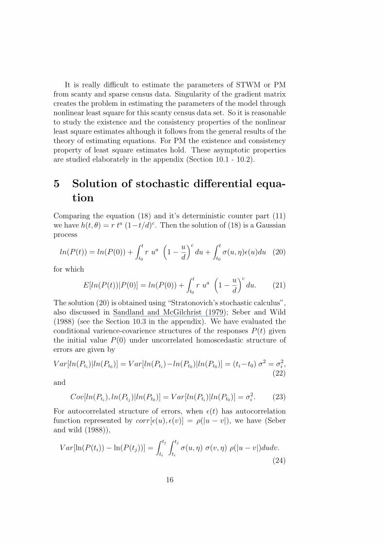
Comparing the equation (18) and it’s deterministic counter part (11)we have h(t, θ) = r ta (1−t/d)c. Then the solution of (18) is a Gaussianprocess

ln(P (t)) = ln(P (0)) +∫ t

t0r ua

(1− u

d

)c

du +∫ t

t0σ(u, η)ε(u)du (20)

for which

E[ln(P (t))|P (0)] = ln(P (0)) +∫ t

t0r ua

(1− u

d

)c

du. (21)

The solution (20) is obtained using “Stratonovich’s stochastic calculus”,also discussed in Sandland and McGilchrist (1979); Seber and Wild(1988) (see the Section 10.3 in the appendix). We have evaluated theconditional varience-covarience structures of the responses P (t) giventhe initial value P (0) under uncorrelated homoscedastic structure oferrors are given by

V ar[ln(Pti)|ln(Pt0)] = V ar[ln(Pti)−ln(Pt0)|ln(Pt0)] = (ti−t0) σ2 = σ2i ,

(22)and

Cov[ln(Pti), ln(Ptj)|ln(Pt0)] = V ar[ln(Pti)|ln(Pt0)] = σ2i . (23)

For autocorrelated structure of errors, when ε(t) has autocorrelationfunction represented by corr[ε(u), ε(v)] = ρ(|u − v|), we have (Seberand wild (1988)),

V ar[ln(P (ti))− ln(P (tj))] =∫ tj

ti

∫ tj

tiσ(u, η) σ(v, η) ρ(|u− v|)dudv.

(24)

16

Also, for any two non overlapping time intervals [t2, t1] and [t4, t3],

Cov[ln(P (t2))− ln(P (t1)), ln(P (t4))− ln(P (t3))]

=∫ t2

t1

∫ t4

t3σ(u, η) σ(v, η) ρ(|u− v|)du dv. (25)

For special case, when ρ has some specific structure, the derived expres-sions for (22,23) are available in the appendix. As the census figuresare available for equispaced time points, without loss of generality thetime frame can be transformed in such a way so that the increment isunity. It converts the weighted least square estimation procedure toa more simple ordinary least square to estimate the model parameters(see the Section 10.3 in the appendix)

6 Advantage of PM over STWM in de-

tecting demographic phase change

With a limited source of environmental resource a population going tochange it’s phase from developing to developed one when RGR switchesover it’s patteren from increasing to decreasing trend. It will happenwhen RGR is bell shaped. The two distinct phases are separated atthe key time point where the RGR is maximized. So RGR is one ofthe vital tools in reflecting this phase change although there are alsoother responsible demographic parameters which can distinguish thosephases in different ways.

This key time point varies from one population to another whichclearly indicates that the occurrence of demographic phase change de-layed in one of the two populations. The identification of demographiccause for this delay might be one of the very promising social problemsof interest. So it is quite reasonable to frame and test the hypothesiswhether the time points where RGR attains its’ maximum value aresame for the two populations against one is greater than other. Thetest can be constructed only when the census data are available at thesame time periods for two populations.

The two point of inflexions of the RGR curve also have some de-mographic interpretations. When RGR is increasing with time initiallythe slope is flat but suddenly it grows up and the slope become steeper.But when RGR is decreasing the nature of the curve behaves reverselythat is primarily the slope is steeper but then it is gradually decreasingin a slow rate. So the time points indicating a sharp change in terms of

17

the slope of the RGR might have immense practical values for both thecases. More specifically these time points provide some caution to thedeveloping countries in terms of the demographic change. In the firstcase when the slope of the RGR grows up, it indicates that the devel-oping country gradually loosing it’s status and is approaching towardsan worse condition which would lead the population ultimately towardsexplosion. So some caution should be taken. Similarly for the secondcase when the decreasing rate of RGR slows down it would provide anegative feedback in the shifting process forcing a developing countrytowards a developed one. Under this scenario it is also important toidentify some social and demographic factors so that some preventivemeasures can be taken. These changes might not be occurred at thesame time and so one can think to construct a hypothesis whether thetime points where the point of inflexions occurs for RGR curve are samefor the two populations or not.

As STWM (or TWM) is not analytically solvable, it is not possibleto evaluate the time points where the RGR is maximized or the pointof inflexions of the RGR curve in terms of model parameters. So this isone of the major shortcomings of the STWM model. But in comparisonwe can easily evaluate a closed and simple analytical form of these timepoints from PM. So the related tests can also be constructed for thePM and which is the key advantage of the model.

Test for phase change and point of inflexions

Let us denote the theoretical solutions of the time points at which theRGR is maximized respectively by t1 and t2 for the two populations.Similarly, the theoretical points of inflexions of the RGR curves forboth the two populations are respectively denoted by(t1inf , t

∗1inf ) and

(t2inf , t∗2inf ). From the feature (1) of the proposed model as described in

Section 3.3, the magnitude of t1 and t2 are respectively a1d1

a1+c1and a2d2

a2+c2.

Where, the model parameters for the first and second populations arerespectively (a1, d1, c1) and (a2, d2, c2). Similarly the evaluated expres-sion (see feature 3) for (t1inf , t

∗1inf ) and (t2inf , t

∗2inf ) are

(a21 d1+a1 d1 (c1−1)−√a1 d1

√c1√

a1+c1−1

a21+(c1−1) c1+a1 (2 c1−1)

,a21 d1+a1 d1 (c1−1)+

√a1 d1

√c1√

a1+c1−1

a21+(c1−1) c1+a1 (2 c1−1)

)

and(

a22 d2+a2 d2 (c2−1)−√a2 d2

√c2√

a2+c2−1

a22+(c2−1) c2+a2 (2 c2−1)

,a22 d2+a2 d2 (c2−1)+

√a2 d2

√c2√

a2+c2−1

a22+(c2−1) c2+a2 (2 c2−1)

)

respectively.In mathematical notation, the hypotheses based on the time point

where RGR is maximized and points of inflexion of the RGR curve are

18

stated as follows.

H10 : a1d1

a1+c1= a2d2

a2+c2ag H11 : not H10,

H20 :a21 d1+a1 d1 (c1−1)−√a1 d1

√c1√

a1+c1−1

a21+(c1−1) c1+a1 (2 c1−1)

=a22 d2+a2 d2 (c2−1)−√a2 d2

√c2√

a2+c2−1

a22+(c2−1) c2+a2 (2 c2−1)

ag H21 : not H20,

H30 :a21 d1+a1 d1 (c1−1)+

√a1 d1

√c1√

a1+c1−1

a21+(c1−1) c1+a1 (2 c1−1)

=a22 d2+a2 d2 (c2−1)+

√a2 d2

√c2√

a2+c2−1

a22+(c2−1) c2+a2 (2 c2−1)

ag H31 : not H30.

If we assume errors distribution to be N(0, σ2) then the nonlinearleast square estimates (NLSE) and MLE are equivalent (Seber & Wild,1989).

Simulation for the verification of the asymptoticnormality of NLSE

It is really questionable whether the asymptotic normality of the non-linear least square estimates really holds good for the scanty, sparsecensus data set. Extensive simulation is needed to verify it in a moreprecise way. In this context we can also think for the profile likelihoodwhich is not symmetric but strongly skewed. Although the estima-tion through profile-likelihood may be an alternative approach but it istypically applicable in the situation where the number of nuisance para-meters is significant. But in our situation the only nuisance parameteris r and this approach may not improve the estimation procedure. Sowe stick to asymptotic normality. For illustration we use the sparseand scanty census data of India and West Bengal which are availablefor the same time periods. Now let us denote the MLE (NLSE) of(a1, d1, c1, a2, d2, c2) by (a1, d1, c1, a2, d2, c2). Since t1 and t2 are one toone function of the parameters (a1, d1, c1, a2, d2, c2) the ML estimates

of t1 and t2 are t1, t2 respectively with t1 = a1d1

a1+c1and t2 = a2d2

a2+c2. For

simplicity we have taken the parameter a to be known with magnitude1.

At first using the census data the model parameters are estimatedthrough non-linear least square (Marquandt, 1963). The response vari-able ARGR is normally distributed which holds from the normality as-sumption of the error terms. We can approximate the mean of ARGRby putting the estimated values of the parameters of non-linear func-tion. Since the raw census data set of West Bengal consists of only eight

19

observations, to identify the asymptotic behavior of the estimated pa-rameters, we have drawn 1000 random samples each of size eight. Asthe parameters are very sensitive and some of them are very small inmagnitude, the variance of errors or ARGR is to be chosen suitablysmall. For each of the 1000 sets of random samples two parameters dand c are estimated 1000 times. The histograms are shown in Figure5 for the parameters d and c respectively. The simulated histogramsare quite close to normal density. The p-values for goodness of fit testare 0.80941,0.93898 for the parameters d and c respectively. So, theassumption of normality for NLSE is quite reasonable.

0.512 0.514 0.516 0.518 0.520 0.522 0.524

050

100

150

c

9.70 9.72 9.74 9.76 9.78

050

100

150

200

250

300

dFigure5: Histograms of the distribution of parameters "c" and "d"

Test Statistics

From the simulation results asymptotically we have,θi ∼ N(θi, var(θi)), i = 1(1)3, where (θ1, θ2, θ3) = (a, c, d) ⇒ tk ∼N(tk, var(tk)), k = 1, 2, and (tk,tk)are the one to one function of the(θi, θi) .

The test statistics and critical regions for H10, H20 and H30 arerespectively

T1 =(t1 − t2)− (t1 − t2)√

ˆV ar(t1) + ˆV ar(t2)(26)

T2 =( t1inf − t2inf )− (t1inf − t2inf )√

ˆV ar( t1inf ) + ˆV ar( t2inf )(27)

20

T3 =( t∗1inf − t∗2inf )− (t∗1inf − t∗2inf )√

ˆV ar( t∗1inf ) + ˆV ar( t∗2inf )(28)

Under H01, H02 and H03 all T1, T2 and T3 ∼ N(0, 1). So H01, H02

and H03 are rejected at α% level of significance if

|T1| > τα/2, |T2| > τα/2 and |T3| > τα/2

where the variances can be estimated from the general results ofasymptotic theory (Rao (1987)).

7 Data Analysis

Here the pattern of change of population trend as well as ARGR do notmatch with any standard growth curve models for our scanty and sparsecensus data sets. The famous logistic and other sigmoidal growth curvemodels often used in demographic problems are not applicable for thissituation as the ARGR is not decreasing with time or size but ratherincreasing at some time points. Basically that motivates us to exploreSTWM and PM for our data.

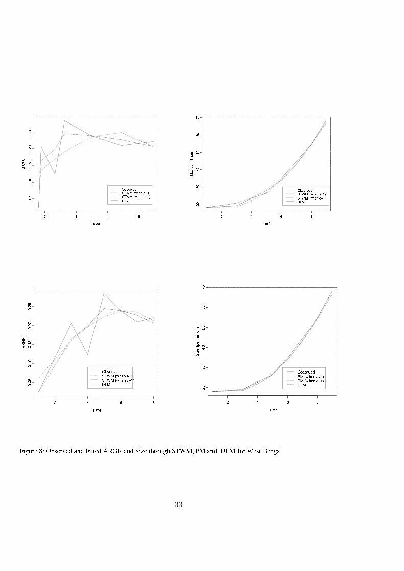
On the hand we expect that the DLM will give a better predictionfor any data set if we can choose the proper function for the upperceiling point which is no doubt a hard job as it is purely arbitrary.The estimates of upper ceiling points for different census figures arecompletely impossible for DLM where as STWM and PM do not sufferfrom those drawbacks. Assuming linearity of the upper ceiling point inthe DLM we have fitted DLM, STWM and PM for China (Figure 6),India (Figure 7) and West Bengal (Figure 8)data. Although STWMand PM smooth out the trend in comparison with the DLM but interms of “ Residual Sum of Squares” (RSS) of over all fitting, thedifferences are negligible in magnitude. For example if we considerthe China data the RSS values of ARGR fittings are (0.002572744,0.002631723) and (0.00180148, 0.00181418) for STWM and PM underuncorrelated and auto correlated error structures respectively. On theother hand the RSS value for DLM is 0.002528938. It has been observedthat the RSS values of STWM and PM are pretty closed with that ofDLM even if with auto correlated error structure it is less than DLM.The estimated upper ceiling point under STWM with uncorrelated andautocorrelated errors are approximately 30 and 21 (measured in billion)respectively where as for proposed model the upper ceiling point of

21

population are observed at time points 54 (year 2003) and 55 (year2004) under uncorrelated and autocorrelated errors respectively. Theestimated population figures for these time points are respectively 32and 28 (approximately)(measured in billion) as obtained from equation14.

The asymptotic test for detecting the demographic phase changewhere the RGR is maximized, is carried out for the scanty censusdata set of India and West Bengal. The estimated values of the phasechange for West Bengal and India occurred approximately at the 6th(year 1951) and 9th (year 1981)time point of the census data set. Theasymptotic normality for the NLSE is verified through extensive sim-ulations. The observed value of the test statistic (26) is 6.45 and thetest is rejected at 1 % level of significance. It indicates that the phasechanges occurred for West Bengal and India are not at the same timepoint for the census data. So this implies the initiation of developmentof one province does not necessarily mean the development process ofthe whole country has been started.

8 Concluding Remarks

In the present work we have tried to explain the phenomenon of pop-ulation change through different types of growth curves. The previousmodels suffered from the difficulties that they could not explain andpredict properly some special situations where the population changesoccurred in some exceptional ways. In addition it is also an attemptto represent the relative growth rate as a function of time only whichenabled us to estimate the parameters of the models in closed formswhich is not possible in STWM model.

We hope that the present study will help the population scientiststo rediscover different critical nature of population growth in severaldeveloped and developing countries which will emerge due to differentfamily welfare programmes and changing nature of the conjugal lifethroughout the world.

Another important contribution of the present work is the identifi-cation of demographic phase change point for a particular region. Thisfeature will help us to take proper actions beforehand so that ultimatelythe present world with severe inequalities will be a homogeneous one.

When the shape of the RGR curve is bimodal or multimodal, theprediction problem can be extended in a straight forward way, repre-senting RGR as a weighted mixture of the proposed model. The weights

22

are determined by treating it as the additional parameters for the non-linear least square.

Acknowledgment

The work of first author was supported by a research fellowship fromCouncil of Scientific and Industrial Research (Sanction No. 9/28(611)/2003-EMR-I),India.

9 References

Amemiya, T(1983): Non-linear regression models. In Z. Grilichesand M. D. Intriligator (Eds.), Handbook of Econometrics, North-Holland : Amsterdam.

Bankas,R.B.(1994): Growth and Diffusion Phenomena: MathematicalFrameworks and Applications,Berlin,Springer-Verleg

Bhat,P.N. Mari(1999): Population Projections for Delhi: DynamicLogistic Model Versus Cohort-Component Method.DemographyIndia,28,No. 2

Bhattacharya, S. (2003): Growth Curve Analysis incorporating Chrono-biological and Directional Issues for an Indian Major CarpCirrhinus Mrigala. Ph.D. dissertation, Jadavpur University, Kolkata,India.

Fisher,R.A.(1921): Some remarks on the methods formulated in a re-cent article on ”The quantative analysis of plant growth”, Annalsof Applied Biology,7,367-372

Gallant, A. R.(1975): The power of the likelihood ratio test of locationin nonlinear regression models. J. Am. Statist. Assoc., 70 198-203.

Garcia O. (1983): A stochastic differential equation for Height, growthof Forest stands. Biometrics, 39, 1059-1072

Jennrich, R. I.(1969): Asymptotic properties of nonlinear least squaresestimators. Ann. Math. Statist., 40, 633-643.

Kingsland S.E.(1985): Modeling Nature: Episodes in the History ofPopulation ecology. University of Chicago Press, Chicago.

23

Levendach, H. and Reuter, B. E. (1976): Forecasting trending timeseries with relative growth rate models. Technometrics, 18, 261–272.

Lotka A.J.(1925): Elements of Physical Biology. Willams and Wilkins,Baltimore,MD, . (republished as Elements of Mathematical Biol-ogy, Dover, New York,1956).

Malinvaud, E.(1970a): The consistency of nonlinear regression. Ann.Math. Statist., 41, 956-969.

Malinvaud, E.(1970b): Statistical Methods of Econometrics, trans-lated by A. Silvey. North-Holland : Amsterdam.

Marquardt, D. W.(1963): An algorithm for least-squares estimationof nonlinear parameters. SIAM J. Appl. Math., 11, 431-441.

Nelder, F.J.(1961): The fitting of generalization of logistic curve Bio-metrics, 17, 89-110.

Prais, S. J. and Winsten, C. B. (1954):Trend estimators and serialcorrelation, Unpublished Cowles Commission discussion paper :Stat. No. 383, Chicago.

Rao, C. R. (1952):Advanced Statistical Methods in Biometric Research.John Wiley & Sons, New York.

Rao, C. R. (1987): Prediction of future observations in growth curvemodels. Statistical Science, 2, 434–447.

Richards, F.J.(1969): The quantitative analysis of growth, Chapter 1,Vol VA, Plant Physiology : Analysis of growth : Behaviour ofplants and their organs. Accademic Press :New York, 3-76.

Sandland, R. L. and McGilchrist, C. A. (1979): Stochastic growthcurve analysis. Biometrics, 35, 255–271.

Seber, G. A. F. and Wild, C. J. (1989): Nonlinear Regression. JohnWiley & Sons, New York.

Tsoularis A., Wallace J.(2002): Analysis of Logistic growth mod-els.Mathematical Biosciences,179,21-55

Verhulst, P.F.(1838):Notice sur la loi que la population suit dans sonaccroissement, Curr. Math. Phys,10,113

24

Wu, C. F.(1981): Asymptotic theory of nonlinear least squares esti-mation. Ann. Statist., 9, 501-513.

10 Appendix

10.1 Existence of the nonlinear least squareestimator

TWM and proposed model ((4) and (6)) under SDE set up (equa-tions (12) and (13)) with uncorrelated and homoscedastic errorprocess can be written as

R(t) = rP (t)a

[1− P (t)

k

]c

+ ε(t) (29)

or

R(t) = b ta[1− t

d

]c

+ ε(t) (30)

Here both the equations (24) and (25) can be written as

y = f(θ, x) + ε (31)

where, f(θ, x) = rxa[1− x

d

]c.

Now θ is chosen to be the nonlinear -least-square estimator of theparameter θ if it minimizes the following function.

Sn(θ) =∑

i

(y(i)− f(θ, x(i))2 =∑

(y − f(θ, x))2 (32)

where θ = (r, a, d, c)′.

In case of equation (27) we have the following restrictions

(1) ε’s are iid with mean zero and variance σ2 (σ2 > 0).

(2) Now for each nonzero x, f(θ, x) is definitely a continuousfunction of θ defined in Θ. WLG we can take x as nonzero becauseif it is zero then the axis can be transformed in such a way so thatit is nonzero.

(3) Θ is closed, bounded (i.e. compact) subset of <4.

With the above restrictions which are obviously true for the model(24) and (25) and by following the same technique of Jennrich(1969)

25

it can be proved that the nonlinear-least-square estimators existfor both the two regression models.

The boundedness of Θ as described above is not a serious restric-tion, as most parameters are bounded by the physical constraintsof the system being modelled.

10.2 Consistency of the nonlinear least squareestimate for the PM

To sketch the the proof we have considered heavily the worksof Jennrich (1969), Malinvaud (1970a, b) and Wu (1981), andthe helpful review papers of Gallant (1975) and Amemiya (1983).Henceforth we will consider only the equation (25) written in theform (26).

Let θ∗∗ is the true value of the 4 dimensional vector θ. Then toproof the consistency of the nonlinear least square estimator θthe first step is to prove that θ∗∗ uniquely minimizes plimSn(θ).In that case, if n is sufficiently large so that n−1Sn(θ) is close toplimSn(θ), then θ which minimizes the former, will be close toθ∗∗, which minimizes the latter. This gives the weak consistency.Now let us consider the equation (27), then

n−1Sn(θ) = n−1∑

(y − f(θ, x)2

= n−1∑

(y − f(θ∗∗, x) + f(θ∗∗, x)− f(θ, x))2

= n−1∑

(ε + f(θ∗∗, x)− f(θ, x))2

= n−1∑

ε2+2n−1∑

ε(f(θ∗∗, x)−f(θ, x))+n−1∑

(f(θ∗∗, x)−f(θ, x))2

= C1 + C2 + C3

By law of large numbers, plimC1 = σ2. Secondly, for fixed θ∗∗

and θ, plimC2 follows from the convergence of

n−1∑

(f(θ∗∗, x)− f(θ, x))2

by Chebyshev’s inequality :

P (n−1∑

(f(θ∗∗, x)− f(θ, x))ε > η2) <σ2

η2n2

∑(f(θ∗∗, x)−f(θ, x))2

(33)

26

Since the uniform convergence of C2 follows from the uniformconvergence of the right-hand side of (28), it suffices to assume

1

n

∑f(θ1, x)f(θ2, x) converges uniformly in θ1, θ2 ∈ Θ.

Hence plimSn(θ) will have a unique minimum at θ∗∗ if limC3

has a unique minimum at θ∗∗. Weak consistency would then beproved.

With this idea in mind, we have defined

Bn(θ1, θ2) =∑

f(θ1, x)f(θ2, x),

Dn(θ1, θ2) =∑

(f(θ1, x)− f(θ2, x))2, (34)

and made the following assumption with the three restrictionsalready defined above :

(4).(a) n−1Bn(θ1, θ2) converges uniformly for all θ1, θ2 in Θ tofunction B(θ1, θ2).

This implies, by expanding (29), that n−1Dn(θ1, θ2) convergesuniformly to D(θ1, θ2) = B(θ1, θ1) + B(θ2, θ2)− 2B(θ1, θ2).

(4).(b) It is now further assume that D(θ, θ∗∗) = 0 if and only ifθ = θ∗∗ (i.e. D(θ, θ∗∗) is “positive definite”.

Now for the model (26)

Bn(θ1, θ2) =∑

r1r2xa1

(1− x

d1

)c1

xa2

(1− x

d2

)c2

(35)

The function f(θ, x) in the model (26) is uniquely maximized atx = a d

a+cfor all positive values of the parameters.

So, Bn(θ1, θ2) <∑ (

a1 d1

a1 + c1

) (a2 d2

a2 + c2

).

⇒ n−1Bn(θ1, θ2) <(

a1 d1

a1+c1

) (a2 d2

a2+c2

)= B(θ1, θ2). ⇒ Bn(θ1, θ2)

converges uniformly to B(θ1, θ2). Hence the consistent estimatorof θ exists.

27

10.3 Detail solution and estimation procedure ofthe SDE

The detail derivation of the solution of SDE (already described in Sec-tion 5) under two headings uncorrelated and autocorrelated errors aregiven below

Uncorrelated Error Process

If ε(t) is “ white noise” (technically, the “ derivative” of a Wienerprocess), then ln(P(t)) has independent increments. In particular, set-ting zti = ln(Pti+i

)− ln(Pti) [where ln(Pti) = ln(P (ti)] for i=1,2,...,(n-1), the zti ’s are mutually independent. From (20) with ti+1 and tiinstead of t and t0, and E[ε(t)]=0, we have

E[zti ] =∫ ti+1

tir ua

(1− u

d

)c

du, (36)

Since V ar[ε(t)] = 1, we also have

V ar[zti ] =∫ ti+1

tiσ2(u, η)du (37)

= (ti+1 − ti)σ2 if σ2(u, η) = σ2.

Hence, from (20),

zti =∫ ti+1

tir ua

(1− u

d

)c

du + ε(ti) (i = 1, 2, . . . , (n− 1)), (38)

where the ε(ti) are independently distributed [ since ε(t) has indepen-dently increments], and (32) can be fitted by weighted least squaresusing weights from (31).

It is also useful to have varience-covarience matrix of the originalresponses ln(P (ti)). Conditional on ln(P (tt0)), the size at some chosentime origin, we have from Seber and Wild (1989)

V ar[ln(Pti)|ln(Pt0)] = V ar[ln(Pti)−ln(Pt0)|ln(Pt0)] =∫ ti

t0σ2(u, η)du = σ2

i ,

(39)say. Since

ln(Ptr)− ln(Pt0) = z0 + z1 + z2 + . . . + zr−1,

it follows that for ti ≤ tj,

28

Cov[ln(Pti), ln(Ptj)|ln(Pt0)] = Cov[ln(Pti)−ln(Pt0), ln(Ptj)−ln(Pt0)|ln(Pt0)]

= V ar[ln(Pti)− ln(Pt0)|ln(Pt0)]

= V ar[ln(Pti)|ln(Pt0)]. (40)

The error structure considered in (18) introduces variation in the size ofthe growth increment due to stochastic variations in the environment.Garcia[1983] considered an additional source of error, namely errors inthe measurement of ln(Pti). We measure ln(Pti)

∗ given by

ln(Pti)∗ = ln(Pti) + τi, (41)

where, τ1,τ2,. . . ,τn are i.i.d. N(0, σ2τ ) independently of the ln(P (ti)).

Thus E[ln(P (ti))]∗ = E[ln(P (ti))] and,

for ln(P (ti))∗ = (ln(P (t1))

∗, ln(P (t2))∗, . . . , ln(P (tn))∗)′

D[ln(P )∗] = D[ln(P )] + σ2τIn (42)

The model can then be fitted using maximum likelihood or gener-alized least squares.

Autocorrelated Error Processes

When ε(t) has autocorrelation function Corr[ε(u), ε(v)] = ρ(|u − v|),we have from Seber and wild (1988),

V ar[ln(P (ti))− ln(P (tj))] =∫ tj

ti

∫ tj

tiσ(u, η) σ(v, η) ρ(|u− v|)dudv.

(43)Also, for any two non overlapping time intervals [t1, t2] and [t4, t3],

Cov[ln(P (t2))− ln(P (t1)), ln(P (t4))− ln(P (t3))]

=∫ t2

t1

∫ t4

t3σ(u, η) σ(v, η) ρ(|u− v|)dudv. (44)

Consider our case in which σ(u, η) = σ and ρ(|u − v|) = exp−λ |u−v|

with λ > 0. Evaluating (38) when t1 < t2 < t3 < t4, we have

Cov[ln(P (t2))− ln(P (t1)), ln(P (t4))− ln(P (t3))]

=∫ t2

t1

(∫ t4

t3σ2 exp−λ (u−v) du

)dv. =

σ2

λ2

(eλ t2 − eλ t1

) (eλ t3 − eλ t4

)

(45)

29

From (37) and symmetry considerations,

V ar[ln(P (t2))− ln(P (t1))] = 2∫ t2

t1

∫ t2

t1σ2 ρv−ududv

= 2σ2

λ2

[λ(t2 − t1) + eλ(t1−t2) − 1

]= σ2

∗, (46)

say. Suppose ti+1−ti = ∆(i = 0, 1, 2, . . . , n−1), and let zti = ln(Pti+i)−

ln(Pti) as before. Then provided ∆ is not too large, we would expectfrom (22) and (23) that Corr[zti , ztj ] ≈ e−λ∆|i−j| which is of the form

ρ|i−j|. Hence we would expect the error structure of the Zti to beapproximately AR(1).

If we devide (38) by ∆t then R(ti) =zti

∆tis the ARGR and empirical

fitted model is represented by

R(ti) =1

∆t

∫ ti+1

tirua

(1− u

d

)d

du + ε(ti) (47)

where ε(ti) are possibly autocorrelated errors. The trend relationshipfor R(ti) may be transformed to remove the heteroscedasticity beforefitting a model with additive errors. As

∫ ti+1

tirua

(1− u

d

)d

du = rtai

(1− ti

d

)d

∆t (48)

implies R(ti) ≈ h(ti; θ). Different parameters are estimated through(48) which we already discussed in Section 4.

30

31

32

33