INTEGRATED DEMOGRAPHIC MODELING AND ... - GETD

INTEGRATED DEMOGRAPHIC MODELING AND ESTIMATION OF THE CENTRAL

GEORGIA, USA, BLACK BEAR POPULATION

by

JAMIE L. SKVARLA SANDERLIN

(Under the Direction of Michael J. Conroy)

ABSTRACT

The central Georgia population (CGP) of black bears is considered to inhabit mostly

forested land in and around 186 km2, and potentially an area of 1,200 km2, associated with the

Ocmulgee River drainage system, and likely a core area of contiguous forest in the Oaky Woods

and Ocmulgee Wildlife Management Areas (WMAs). We document the density, survival and

reproduction, as well as genetic structure, of the CGP under the sampling protocol, over the

duration of the study from 2003 to 2008. We describe a joint model of population abundance

with three data structures (DNA hair snares, camera traps, and radiotelemetry) that incorporates

genetic error from replicate genetic samples and a calibration sample of known individuals. The

hierarchical joint Bayesian model incorporates Markov-Chain Monte Carlo (MCMC) methods

with Gibbs, Metropolis-Hastings, and reversible jump Metropolis-Hastings sampling algorithms

of posterior distributions. Median posterior abundance estimates within the WMA land over five

seasons from 2004 to 2006 were: 2004 summer 213 (95% BCI: 144-354), 2004 fall 106 (95%

BCI: 72-179), 2005 summer 184 (95% BCI: 137-266), 2005 fall 131 (95% BCI: 91-207), 2006

summer 192 (95% BCI: 143-280). Adult annual survival estimates were 0.861 (95% CI: 0.746-

0.976) for females and 0.845 (95% CI: 0.754-0.937) for males. Reproduction rates were

simulated from bootstrap simulations using mean birth interval and average number of cubs per

female litter. Reproduction rates from the CGP only and the CGP combined with eastern black

bear populations were 0.845 (95% CI; 0.843-0.847) and 1.139 (95% CI: 1.137-1.141),

respectively. Population viability analyses using demographic parameters from the CGP and

eastern black bear populations suggest that population growth is decreasing. The joint Bayesian

hierarchical model also suggests that population growth is decreasing, since the Bayesian

credible intervals of λ, the finite rate of population increase, included values above and below

one. The λ from abundance models overlapped confidence intervals with λ from the population

viability analyses, which suggest that conclusions based on increased harvest and population

status are consistent with different data sources. Additional effort for the CGP should be focused

on estimates of cub and sub-adult survival and reproduction.

INDEX WORDS: population modeling, Ursus americanus, Ursus, genetic error, population

viability analysis, hierarchical modeling, MCMC, survival, reproduction, joint data structures



by


B.S., Purdue University, 2002

M.S., University of Georgia, 2009

A Dissertation Submitted to the Graduate Faculty of The University of Georgia in Partial

Fulfillment of the Requirements for the Degree

DOCTOR OF PHILOSOPHY

ATHENS, GEORGIA

2009

© 2009

Jamie L. Skvarla Sanderlin

All Rights Reserved



by


Major Professor: Michael J. Conroy

Committee: John P. Carroll Nicole Lazar Joseph Nairn Lynne Seymour

Electronic Version Approved: Maureen Grasso Dean of the Graduate School The University of Georgia August 2009

iv

ACKNOWLEDGEMENTS

I would first like to thank my major advisor, Dr. Michael Conroy, for all of his help with

the various model components throughout this project, and all of his support and encouragement.

I am also thankful for my committee members, Drs. John Carroll, Nicole Lazar, Joeseph Nairn,

and Lynne Seymour, for their unique insights to different aspects of this research. Research

support was provided jointly by the Georgia Department of Natural Resources and through

teaching assistantships through Warnell School of Forestry and Natural Resources. I would like

to thank the GA DNR for assistance with collection of blood, tissue, and hair samples from the

known bears and collection of radiotelemetry and bear reproduction data. I am grateful to Drs.

Nairn and Carroll for providing laboratory space and equipment for all of the genetic analyses.

Genetic lab assistance with bear hair extractions is greatly appreciated from S. h. Eo, L. Wilson,

Dr. Conroy, and J. R. Sanderlin. B. Faircloth and other members of the Wildlife Genetics Lab

deserve special recognition for my initial training in the lab and for the many discussions

regarding laboratory techniques. K. Cook was extremely helpful in discussions about bear habitat

use and telemetry. I would also like to thank all the field technicians and volunteers, since much

of this work would not be possible without them: B. Alexandro, E. Ball, J. Betsch, J. Chu, E.

Crandall, K. Giano, C. Hayes, S. Hilgher, M. Hughes, S. Hunter, M. Kane, S. Kirk, E. Nixon, A.

Ross, J. R. Sanderlin, R. Sempler, B. Smith, T. Thein, and C. Wampler. I would especially like

to thank my family and friends for their support and encouragement during the years in graduate

school and always. Lastly, I could never fully express my gratitude towards my husband and

thank him for joining me on this life adventure.

v

TABLE OF CONTENTS

Page

ACKNOWLEDGEMENTS........................................................................................................iv

LIST OF TABLES.................................................................................................................. viii

LIST OF FIGURES ..................................................................................................................xv

CHAPTER

1 INTRODUCTION AND LITERATURE REVIEW ...................................................1

INTRODUCTION.................................................................................................1

LITERATURE REVIEW ......................................................................................2

OBJECTIVES .....................................................................................................17

LITERATURE CITED........................................................................................18

2 DENSITY ESTIMATION USING JOINT DATA STRUCTURES FROM

CAMERAS, DNA HAIR TRAPS, AND TELEMETRY......................................40

INTRODUCTION...............................................................................................41

METHODS .........................................................................................................44

STATISTICAL MODEL.....................................................................................59

RESULTS ...........................................................................................................71

DISCUSSION .....................................................................................................77

LITERATURE CITED........................................................................................84

3 ESTIMATION OF SURVIVAL AND REPRODUCTION DEMOGRAPHIC

PARAMETERS FOR CENTRAL GEORGIA BEARS......................................148

INTRODUCTION.............................................................................................149

vi

FIELD METHODS ...........................................................................................152

STATISTICAL ANALYSIS AND MODELING...............................................155

RESULTS .........................................................................................................162

DISCUSSION ...................................................................................................169

LITERATURE CITED......................................................................................175

4 MANAGEMENT IMPLICATIONS AND CONCLUSIONS.................................223

MANAGEMENT IMPLICATIONS..................................................................223

FUTURE WORK ..............................................................................................225

CONCLUSIONS...............................................................................................227

LITERATURE CITED......................................................................................229

APPENDICES ........................................................................................................................230

A SIMULATION ANALYSIS OF JOINT DATA MODEL INCORPORATING

THREE DATA STRUCURES OF DNA HAIR SNARES, CAMERAS, AND

TELEMETRY FOR AMERICAN BLACK BEAR CENTRAL GEORGIA

POPULATION DATA......................................................................................230

B METROPOLIS ALGORITHM FOR UPDATING ABUNDANCE AND

INDIVIDUAL CAPTURE PROBABILITY FROM CAMERA PARAMETERS

FROM THE JOINT MODEL INCORPORATING THE THREE DATA

STRUCTURES OF DNA HAIR SNARES, TELEMETRY, AND CAMERA

TRAPS FOR CENTRAL GEORGIA POPULATION AMERICAN BLACK

BEAR DATA....................................................................................................244

vii

C METHODS OF UPDATING TRUE GENOTYPES, TRUE CAPTURE HISTORIES,

AND GENOTYPE FREQUENCIES FROM WRIGHT ET AL. (2009) FOR THE

JOINT MODEL INCORPORATING THE THREE DATA STRUCTURES OF

DNA HAIR SNARES, TELEMETRY, AND CAMERA TRAPS FOR CENTRAL

GEORGIA POPULATION AMERICAN BLACK BEAR DATA.....................248

D CENTRAL GEORGIA AMERICAN BLACK BEAR POPULATION CLOSED

POPULATION MODEL RESULTS WITH PROGRAM MARK USING DNA

HAIR SNARES FROM 2004 TO 2006 .............................................................253

E PYTHON CODE FOR THE JOINT MODEL INCORPORATING THE THREE

DATA STRUCTURES OF DNA HAIR SNARES, TELEMETRY, AND

CAMERA TRAPS FOR CENTRAL GEORGIA POPULATION AMERICAN

BLACK BEAR DATA......................................................................................261

viii

LIST OF TABLES

Page

Table 1.1: Density estimates for American black bear populations in the southeastern US.........31

Table 1.2: Home range estimates for American black bear populations in the southeastern US..35

Table 1.3: Median band-sharing values for genetic similarities within American black bear

populations in the southeastern United States from Miller (1995). .............................36

Table 1.4: Median band-sharing values for genetic similarities between American black bear

populations in the southeastern United States from Miller (1995). .............................37

Table 2.1: Percent of vegetation type for each web for the American black bear central Georgia

population from 2004 to 2006 based on 30m x 30m resolution. .................................93

Table 2.2: Slope summary statistics (range, mean, standard deviation) for each web for the

American black bear central Georgia population from 2004 to 2006..........................94

Table 2.3: DEM (digital elevation model) in meters above sea level for each web for the

American black bear central Georgia population from 2004 to 2006 summary statistics

(range, mean, standard deviation) ..............................................................................95

Table 2.4: Summary of web area, rings, spacing between rings, average number of snares per

web for years 2004 to 2006 for the American black bear central Georgia population,

and average density of snares per web .......................................................................96

Table 2.5: Summary of webs for the American black bear central Georgia population from 2004

to 2006 used for telemetry error calculations. ............................................................97

ix

Table 2.6: Notation and definitions for terms in the Bayesian density model incorporating three

data structures (camera, hair snares, telemetry) for the American black bear central

Georgia population from 2004 to 2006 ......................................................................98

Table 2.7: Hair snare data summary for the American black bear central Georgia population from

2003 to 2006 .............................................................................................................99

Table 2.8: American black bear central Georgia population genetic data for assessment of genetic

error from allelic

dropout……………………………………………………………………………….100

Table 2.9: Camera data summary for the American black bear central Georgia population from

2003 to 2006 ...........................................................................................................101

Table 2.10: Live-captures, recaptures, and recoveries of American black bears with the central

Georgia population from 2003 to 2008 ....................................................................102

Table 2.11: Number of alleles (A), individuals analyzed at each locus (N), number of

heterozygotes (Nhet), and homozygotes (Nhom), observed heterozygosity (HO), expected

heterozygosity (HE), and p-value for Hardy-Weinberg Equilibrium (HWE) test for the

American black bear central Georgia population with known individuals (n=83)

collected from samples from 2003 to 2006 with the Paetkau markers ......................103

Table 2.12: Observed alleles for each locus with more than one allele for known individuals,

number of alleles observed (n), and frequency of alleles from the American black bear

central Georgia population from samples collected from 2003 to 2006 with the

Paetkau markers ......................................................................................................104

x




American black bear central Georgia population with individuals (n=84) from known

tissue samples from 2003 to 2006 with the Sanderlin et al. (2009) tetranucleotide

markers ...................................................................................................................105

Table 2.14: Observed alleles for each locus, number of alleles observed (n), and frequency of

alleles from the American black bear central Georgia population with known

individuals (n=84) from tissue and blood samples collected from 2003 to 2006 with

the Sanderlin et al. (2009) tetranucleotide markers ..................................................106

Table 2.15: Number of hair snare genetic samples with data at all 8 loci for the American black

bear central Georgia population from 2003 to 2006…………………….…………..108

Table 2.16: Number of unique individuals detected with genetic hair samples at all 8 loci for the

American black bear central Georgia population from 2003 to 2006………….....…109

Table 2.17: Minimum known alive in the American black bear central Georgia population from

2003 to 2007 ...........................................................................................................110




American black bear central Georgia population with individuals (n=184 unique

individuals) from observed hair samples collected at hair snares from 2003 to 2006

with the Sanderlin et al. (2009) tetranucleotide markers...........................................111

xi

Table 2.19: Observed alleles for each locus and allele frequencies from the American black bear

central Georgia population with unique individuals (n=184) from observed hair

samples collected at hair snares from 2003-2006 with the Sanderlin et al. (2009)

tetranucleotide markers ...........................................................................................112

Table 2.20: Parameter median, lower and upper 95% BCI for summer 2004 of the American

black bear central Georgia population......................................................................115

Table 2.21: Parameter median, lower and upper 95% BCI for fall 2004 of the American black

bear central Georgia population...............................................................................118



Table 2.23: Parameter median, lower and upper 95% BCI for fall 2005 of the American black

bear central Georgia population...............................................................................122



Table 3.1: Survival estimates reported from American black bear populations in the eastern

United States ......................................................................................................... ..180

Table 3.2: Reproduction estimates of eastern American black bear populations.......................182

Table 3.3: Live captures, recaptures and recoveries from American black bears in central

Georgia………………………………………………………………………………184

Table 3.4: Dead recovery bears from the American black bear central Georgia population (15

M:11 F) included in the age distribution analysis.....................................................185

Table 3.5: Central Georgia population den observation data of American black bears from 2004

to 2007....................................................................................................................186

xii

Table 3.6: Reproduction estimates of American black bear populations in the eastern United

States used in the analysis from multiple studies of mean litter size……………….187

Table 3.7: Reproduction estimates of American black bear populations in the eastern United

States used in the analysis from multiple studies of mean interbirth interval ............189

Table 3.8: Annual survival estimates, variance, standard error (SE), and 95% confidence

intervals for males and female American black bears from the central Georgia

population using the Kaplan-Meier approach with the staggered entry design for years

2003 to 2008 ...........................................................................................................190

Table 3.9: Sources of mortality for radiocollared bears in the central Georgia American black

bear study............................................................................................................... 191

Table 3.10: Studies with estimates of American black bear cub survival used in the central

Georgia population population viability analysis ....................................................192

Table 3.11: Studies with estimates of sub-adult American black bear survival used in the

population viability analyses for the central Georgia population ..............................193

Table 3.12: Studies with estimates of adult American black bear survival used in the population

viability analyses for the central Georgia population................................................194

Table 3.13: Demographic parameter estimates primarily from the central Georgia population of

American black bears used in the population viability analyses ...............................195

Table 3.14: Demographic parameter estimates primarily from eastern American black bear

studies, including the central Georgia population, used in population viability

analyses...................................................................................................................196

xiii

Table 3.15: Increased harvest rate scenarios with stochastic simulations (n=10,000) of λs using

reproduction data from the American black bear central Georgia population only and

from eastern American black bear populations ........................................................197

Table 3.16: Sex ratio of American black bears in research projects from the southeastern United

States ......................................................................................................................198

Table 3.17: Age structure of southeastern United States American black bear populations ......199

Table A.1: Parameter values for simulation combinations of the joint data model incorporating

DNA hair snares, cameras, and telemetry for American black bear central Georgia

population data........................................................................................................239

Table A.2: 95% Bayesian credible interval (BCI) percent coverage for parameters Ntot, r, θ, p, λ,

and pw, for all 10 webs for the joint data model incorporating DNA hair snares,

cameras, and telemetry for American black bear central Georgia population data....240

Table A.3: Mean 95% Bayesian credible interval (BCI) length for parameters Ntot, r, θ, p, λ, and

pw, for all 10 webs for the joint data model incorporating DNA hair snares, cameras,

and telemetry for American black bear central Georgia population data...................241

Table A.4: Relative bias (RBIAS) for parameters Ntot, r, θ, p, λ, and pw, for all 10 webs for the

joint data model incorporating DNA hair snares, cameras, and telemetry for American

black bear central Georgia population data ..............................................................242

Table A.5: Relative root mean square error (RRMSE) for parameters Ntot, r, θ, p, λ, and pw, for

all 10 webs for the joint data model incorporating DNA hair snares, cameras, and

telemetry for American black bear central Georgia population data .........................243

Table D.1: Closed population MARK models from CMR hair snare data collected in Summer

2004 for the American black bear central Georgia population..................................256

xiv

Table D.2: Closed population MARK models from CMR hair snare data collected in Fall 2004

for the American black bear central Georgia population. .........................................257



Table D.4: Closed population MARK models from CMR hair snare data collected in Fall 2005

for the American black bear central Georgia population. .........................................259



xv

LIST OF FIGURES

Page

Figure 1.1: Present distribution of the black bear, based on survey responses from provinces and

states and research projects in Mexico and reported occupied habitat of black bears in

Georgia .....................................................................................................................38

Figure 1.2: Main research objectives with the central Georgia population (CGP) of American

black bears ................................................................................................................39

Figure 2.1: Hair snare locations for the American black bear central Georgia population during

year 2003 ................................................................................................................126


year 2004 ................................................................................................................127


year 2005 ................................................................................................................128


year 2006 ................................................................................................................129

Figure 2.5: Web locations with 2004 boundaries fro the American black bear central Georgia

population with Gap data.........................................................................................130

Figure 2.6: Web locations for the American black bear central Georgia population with DEM

data (meters above sea level), 2004 boundaries........................................................131

Figure 2.7: Web locations with 2003 boundaries from the American black bear central Georgia

population ...............................................................................................................132

xvi

Figure 2.8: Trapping web with 27 hair snares (located at the intersection of a circle and line) with

three snares at the center covering an area of 7 or 15 km2, depending on the location in

the WMAs for the American black bear central Georgia population during the years

2003 to 2006 ...........................................................................................................133

Figure 2.9: Barbed wire strands were placed 25 cm and 50 cm from the ground and baited with

corn in a plastic bottle with anise oil to collect hair snare samples from the American

black bear central Georgia population during the years 2003 to 2006.......................134

Figure 2.10: Histogram of the von Mises distribution with parameters θ=0, and κ=30.5

(n=10,000 samples) .................................................................................................135

Figure 2.11: Diagram of the hierarchical model incorporating the three data structures: camera,

telemetry, and hair snare..........................................................................................136

Figure 2.12: Initial and recapture coordinates for American central Georgia population black

bears from 2003 ......................................................................................................137


bears from 2004 ......................................................................................................138


bears from 2005 ......................................................................................................139


bears from 2006 ......................................................................................................140

Figure 2.16: Capture coordinates for years 2003-2006 of initial and recaptured American central

Georgia population black bears ...............................................................................141

Figure 2.17: Telemetry error for 10 observers for the central Georgia population American black

bear study from years 2003-2006 (n=360 stations) ..................................................142

xvii

Figure 2.18: Posterior distribution of total abundance (a) and trace (b) in year 2004, summer

season, for the American black bear central Georgia population from 2 chains of

50,000 MCMC iterations (25,000 burn-in period for each chain).............................143

Figure 2.19: Posterior distribution of total abundance (a) and trace (b) in year 2004, fall season,

for the American black bear central Georgia population from 2 chains of 50,000

MCMC iterations (25,000 burn-in period for each chain)……………………….….144




Figure 2.21: Posterior distribution of total abundance (a) and trace (b) in year 2005, fall season,

for the American black bear central Georgia population from 2 chains of 50,000

MCMC iterations (25,000 burn-in period for each chain) ........................................146




Figure 3.1: Age frequency of female American black bears at initial capture in Middle Georgia,

2003-2006.. .............................................................................................................201

Figure 3.2: Age frequency of male American black bears at initial capture in Middle Georgia,

2003-2006…. ..........................................................................................................202

Figure 3.3: Body mass (kg) of female American black bears at initial capture from Middle

Georgia, 2003-2006.................................................................................................203

Figure 3.4: Body mass (kg) of male American black bears at initial capture from Middle

Georgia, 2003-2006.................................................................................................204

xviii

Figure 3.5: Age frequency of American black bears at initial capture in Middle Georgia in

2003........................................................................................................................205


2004 ........................................................................................................................206


2005 ........................................................................................................................207


2006........................................................................................................................208

Figure 3.9: Age frequency of American black bears at initial capture in Middle Georgia from

2003 to 2006 with a) all years combined, and b) separated by year .........................209

Figure 3.10: Age frequency of dead recovery female American black bears in Middle Georgia,

2003-2006.. .............................................................................................................210

Figure 3.11: Age frequency of dead recovery male American black bears in Middle Georgia,

2001-2007.. .............................................................................................................211

Figure 3.12: Number of cubs per litter from den observations of American black bears in Middle

Georgia from 2003 to 2007 (n=12 bears).. ...............................................................212

Figure 3.13: Simulated distribution of reproduction rate for the central Georgia American black

bear population using data from 2003 to 2007. ........................................................213

Figure 3.14: Simulated distribution of reproduction rate from eastern American black bear

populations (n=22 studies).......................................................................................214

Figure 3.15: Kaplan-Meier survival estimates for male American black bears by week for the

central Georgia population from 2003 to 2008.........................................................215

xix

Figure 3.16: Kaplan-Meier survival estimates for female American black bears by week for the

central Georgia population from 2003 to 2008.........................................................216

Figure 3.17: Stochastic simulations (n=10,000) of mean λs and 95% CI lines over 50 years with

reproduction and survival data from the central Georgia population and no

harvest.....................................................................................................................217

Figure 3.18: Stochastic simulations (n=10,000) of American black bear abundance (N) over 50

years with reproduction and survival data from the central Georgia population and no

harvest.....................................................................................................................218

Figure 3.19: Stochastic simulations (n=10,000) of mean λs and 95% CI lines over 50 years with

reproduction and survival data with reproduction and survival data from the eastern

American black bear populations and no harvest .....................................................219

Figure 3.20: Stochastic simulations (n=10,000) of American black bear abundance (N) over 50

years with reproduction and survival data from eastern American black bear

populations and no harvest ......................................................................................220

Figure 3.21: American black bear distribution of λ from 2 chains of 50,000 iterations (25,000

burn-in period) from the three data structure joint model for total abundance, for the

time period from summer 2004 to summer of 2005 in central Georgia.....................221

Figure 3.22: American black bear distribution of λ from 2 chains of 50,000 iterations (25,000

burn-in period) from the three data structure joint model for total abundance, for the

time period from summer 2005 to summer 2006 in central Georgia.........................222

Figure E.1: Flowchart of the MCMC steps from the joint model incorporating the three data

structures of DNA hair snares, telemetry, and camera traps for central Georgia

population black bear data.......................................................................................308

1

CHAPTER 1

INTRODUCTION AND LITERATURE REVIEW

Introduction

Less than 10% of the original range of the American black bear (Ursus americanus) in

the eastern United States is believed to support bear populations (Pelton 1982, Maehr 1984), with

most bears surviving on scattered publicly-owned lands (Pelton 1985). Pelton (1990) describes at

least 30 distinct populations in thirteen southeastern states. There are three populations of black

bears consisting of two subspecies, with an unknown amount of connectivity, in Georgia. The

northern population (U. a. americanus) is associated with the Appalachian Mountains of the

northeast and north central area of Georgia. The central population (U. a. americanus) (CGP) is

associated with the Ocmulgee River drainage system, south of Macon, while the southeastern

population of black bears (U. a. floridanus) is associated with the Okefenokee Swamp (Figure

1.1). The central Georgia population (CGP) of black bears is considered to inhabit mostly

forested land in and around 186 km2 (and potentially upwards of 1,200 km2) associated with the

Ocmulgee River drainage system, and likely a core area of contiguous forest in the Oaky Woods

and Ocmulgee Wildlife Management Areas (WMAs).

There are few studies that examine the demographics of a bear population before the

potential of development and infrastructure. We document the density, survival and

reproduction, as well as genetic structure, of a bear population under our sampling protocol. In

the course of the study, the majority of the land (~145 km2) of the wildlife management areas

2

was sold to private individuals, timber companies, and real estate agencies. The state owns a

small portion of the land within the CGP, therefore much of the area has an unpredictable

landuse future.

Population viability models can be constructed from the combination of abundance and

demographic parameters (i.e., survival and reproduction). A sampling protocol for abundance,

survival, and reproduction estimation relies on knowledge of several biological characteristics

(e.g., habitat use, dispersal and movement patterns). Influences on capture probability and the

genetic structure of a population are also integral to an optimal sampling design. Here I review

the population biology, population genetics, conservation issues, and sampling and estimation

techniques for black bear populations in the southeastern United States. I also review Bayesian

hierarchical models, capture mark-recapture (CMR) models, and genetic markers.

Literature review

Bear abundance

Knowledge of abundance or density of black bear populations is important for the

management of populations. Abundance, survival, reproduction, and movement estimates, are

typical components of population viability models. Estimated densities for Eastern black bear

populations, specifically southeastern populations, vary by location, habitat, and statistical

procedures utilized (Table 1.1). Each density estimate also has associated errors with the

estimate, as well as known biases in the study, discussed below.

3

Sampling methods for bear abundance

Field methods for estimating bear density or abundance include: physical captures

(Smith 1985, McLean and Pelton 1994, Hellgren and Vaughn 1989b), camera detections

(Grogan and Lindzey 1999, Martorello 1998, Beausoleil 1999, Mace et al. 1994), tetracycline

markers and resighting with harvested bears (Garshelis and Visser 1997), DNA hair snares

(Woods et al. 1999, Mowat and Strobeck 2000, Kendall et al. 2008, Kendall et al. 2009), aerial

radiotelemetry and mark-resights (Miller et al. 1997), mark-recapture with dogs (Akenson et al.

2001), density based on bear-sign (Garshelis et al. 1999), and occupancy studies (Boulanger et

al. 2008b). Some field methods are associated with more rigorous statistical estimation models

than others. Methods also vary in the degree of handling of the animal from invasive to

noninvasive.

Capture-mark-recapture models (CMR), for both open (Jolly-Seber) and closed

populations, are used with physical captures, DNA hair snares, and mark-recapture with dogs.

These methods require substantial sample sizes and physical effort to cover the population area

where bears occur. Therefore, these methods are rare in large-scale and long-term bear studies.

Less expensive and more practical methods include camera detections and mark-resighting from

telemetry and tetracycline markers, where physical recaptures of animals are not necessary.

Lastly, methods focused on bear presence or occupancy (MacKenzie et al. 2006), such as bear-

sign (e.g., scats, bear tracks, scratching posts, or presence of bear hair), not necessarily

abundance, are least expensive, but provide less information about abundance.

4

Detection probability considerations for bears

Capture variability can be classified into three main types: 1) heterogeneity, where each

individual animal has a different probability of capture, or measurable individual attributes (e.g,

group or individual covariates) that predict capture probability 2) behavior, where animals

captured have different probabilities of capture than animals not captured, either trap-happy or

trap-shy, and 3) time, where capture probability can vary over trapping sessions (White et al.

1982). The probability that a given black bear will be detected is influenced by several

behavioral traits. Male black bears have a greater chance of encountering bait stations or being

sited due to increased travel distances and large home ranges; and as a result, a greater chance of

being captured than female black bears (Hellgren and Vaughan 1989b). Depending on the

capture method used, detection also may depend on age, with juveniles and cubs being less likely

to be captured than adults. Family groups, consisting of parent-offspring and siblings traveling

together, are also a large source of nonindependent movement in bear populations (Kendall et al.

2009). However, simulation studies indicate that this movement will cause minimal bias in

population estimates (Miller et al. 1997, Boulanger et al. 2004). Individual heterogeneity is

considered a problem with animals sampled with mark-recapture techniques and other encounter

techniques.

Black bears have large home ranges and are highly mobile, with males more mobile than

females. Therefore, temporary emigration, or when an animal is temporarily unavailable for

capture due to movement off of the sample area, is a concern in the sampling procedure.

Individuals that temporarily emigrate are not available for detection and unique identification

during a given period (Kendall and Nichols 1995, Kendall et al. 1995). The Robust Design

(Pollock 1982) is a possible solution to temporary emigration. This design assumes primary

5

periods are open to births, deaths and movement, and secondary periods, or short intervals within

a primary period, are assumed closed (Pollock 1982, Kendall and Nichols 1995, Kendall et al.

1995, Kendall et al. 1997).

The most common trap configuration for bears is a grid system. For example, the

systematic grid design described in Mowat and Strobeck (2000) is based on female grizzly bear

home range size in similar ecosystems of British Columbia. In a grid system, traps are evenly or

randomly spaced on boxed grids over a study area. Density is calculated in a grid system by

estimating the population size and dividing that value by the area of the trapping grid.

Geographic closure under this design is difficult to meet because animals at the edge of the

trapping grid may have only part of their home range in the study, thus the effective trapping

area is actually larger than what is used in the density equation (White and Shenk 2001). Edge

animals may move in and out of the sampling area during a sampling period, and may bias

estimates of density and abundance. Alternate approaches include estimating density from

explicit trapping arrays (Anderson et al. 1983) or trapping arrays of arbitrary geometry (Gardner

et al. 2009, Efford 2004, Royle and Young 2008).

Noninvasive sampling techniques

Animals that occur at low densities or have elusive behavior are difficult to sample for

population inference, and this often leads to low sample sizes with physical captures.

Noninvasive sampling techniques, or techniques that do not require physical capture of animals,

allow many populations of animal species to be monitored with greater detail. Noninvasive

methods for sampling bear density include DNA hair snares and the use of remote cameras.

Camera trapping is a technique that uses capture-resight data, much like radio telemetry.

6

Animals only need to be handled once at initial capture to mark, while resighting of those

individuals are obtained through photography. At this point, focus will be on the biases

associated with camera resighting, and genetic hair snare traps, since these two methods were

utilized in the CGP study.

There are problems that may occur with camera detections. Marked bears may be less

attracted to baits or flashes that occur in low-light situations. Those bears would be less likely to

be photographed, and thus detected, than unmarked bears because of capture experience. This

may lead to bears avoiding baits or reducing their movement patterns so not to encounter baits

and not be captured or resighted (Grogan and Lindzey 1999). This is commonly referred to as a

behavioral response. Under this scenario, selection of the closed capture model, Mb, can reduce

bias in population estimates. Another problem with camera trapping is that unmarked bears may

revisit a camera site within the same sampling period, which does not allow for individual

identification. Capture-resight methods rely on the ability to distinguish individuals. Occupancy

models (MacKenzie et al. 2006) would be better suited for these scenarios. Camera data is also

less expensive than physical capture-recapture data.

Advances within the fields of molecular and genetic biology have increased the ability to

use genetic analyses in wildlife studies. Genetic samples (e.g., shed hairs, feathers, feces, shed

skin), collected noninvasively in the field, are often small and contain degraded DNA. The

ability to create multiple copies of DNA from these samples with PCR (polymerase chain

reaction) has advanced noninvasive genetic sampling techniques (Waits 1999). There are three

types of genetic markers that can be used in DNA analysis: mitochondrial DNA (mtDNA)

markers, Y chromosome markers, and nuclear DNA markers. Mitochondrial DNA, located in

the mitochondria of mammalian cells, is maternally inherited and is used to study female

7

evolutionary history, gene flow, and genetic diversity. Nuclear DNA, located in the nucleus of

mammalian cells, is inherited by both parents and can be used to study maternal and paternal

evolutionary history, gene flow, genetic diversity and relatedness. The Y chromosome (i.e., sex

chromosome) is inherited from father to son and can be used to study paternal evolutionary

history, gene flow, and genetic diversity (Waits 1999). In most capture-recapture studies,

nuclear DNA from microsatellite loci are used to determine individuals for bear identification

(Waits 1999). Microsatellite loci are short tandem repeats of 1-5 bases. Noninvasive genetic

samples are currently utilized with bear species globally for problems of demographics (Taberlet

et al. 1997, Mowat and Strobeck 2000, Boulanger et al. 2002, Bellemain et al. 2005, Triant et al.

2004, Kendall et al. 2008), habitat relationships (Apps et al. 2004), and dispersal and/or

effectiveness of corridors (Dixon et al. 2006, Schwartz et al. 2006, Dixon et al. 2007, Proctor et

al. 2004).

Possible benefits of noninvasive genetic sampling are: 1) field methods that may be less

expensive, and less harmful to the animal than physical captures, and 2) the mark, or genetic

identity, is visible, read clearly, and permanent (Foran et al. 1997, Woods et al. 1999). These

assumptions are adopted in many noninvasive studies, although they warrant further

investigation. There remains doubt in the clarity of genetic identity (Taberlet et al. 1999, Bonin

et al. 2004) and cost-effectiveness of noninvasive techniques. The presence of genetic error

(allelic dropout or false alleles) is a key factor with accuracy measures for genetic noninvasive

techniques. Allelic dropout is caused by PCR inhibitors, and sampling stochasticity in the

laboratory from amplification and pipetting of small amounts of low quality DNA (Goossens et

al. 1998, Taberlet et al 1999, Woods et al. 1999). False alleles can be a result of amplification

artifacts from PCR (Goossens et al. 1998, Taberlet et al 1999, Woods et al. 1999).

8

Genetic errors can occur at various steps in a genetic study (e.g., sampling, DNA

extraction, molecular analysis, scoring, data analysis) and be caused by human or technical error,

or biological processes (Bonin et al. 2004). Technical error can include amplification artifacts

(Rodriguez et al. 2001), biochemical anomalies (Smith et al. 1995), electrophoresis (Fernando et

al. 2001), temperature variation in the laboratory (Davison and Chiba 2003), method of

electrophoresis (Delmotte et al. 2001), and quality and type of DNA used (Goosens et al. 1998).

With improvements in laboratory and field sampling techniques, population monitoring

with noninvasive samples has increased substantially since the methods were first available.

However, there are limited analytical and statistical methods that incorporate multiple

noninvasive sampling field methods (such as hair snags and bear rub trees: Boulanger et al.

2008a), particularly with the incorporation of genetic error into abundance estimates (but see

Wright et al. 2009). If genetic error is ignored, population sizes estimates can be sensitive to

genetic error and biased (Creel et al. 2003, Waits and Leberg 2000). Current methods of

incorporating genetic error in noninvasive sampling mark-recapture models use maximum-

likelihood methods (Lukacs and Burnham 2005, Kalinowski et al. 2006), Bayesian methods

(Wright et al. 2009, Petit and Valière 2006), and ad hoc approaches (Paetkau 2003, McKelvey

and Schwartz 2004). Many approaches also require multiple PCR attempts to assess error (i.e.,

multiple-tubes approach Taberlet et al. 1996), which increases the cost per sample.

Hierarchical modeling and Bayesian estimation

Hierarchical state-space models, provide a way of linking observations from data, such as

capture-mark-recapture (CMR) or occupancy samples, to the underlying ecological or state

processes (Royle and Dorazio 2008). Often, it is not possible to observe ecological processes

9

directly, and samples from a population or groups of populations are used to make inference on

the processes. Hierarchical models can incorporate all components of variance (statistical from

sampling and inherent biological), incorporate different scales of observation, and provide a way

of combining multiple sources of data with common parameters. One of the main goals of this

study is to estimate abundance of black bears in central Georgia using a combination of several

sources of data. The common parameter of inference between the data sources is abundance,

which cannot be directly observed. Species abundance is influenced by many biological

processes, including habitat relationships, within population processes (e.g., density-

dependence), and species interactions (e.g., Lotka-Volterra models of predator-prey

relationships, species competition, mutualisms, and co-evolution).

Hierarchical models are often complex and difficult to make inferences on population

parameters with classical methods of statistics, like maximum likelihood methods (MLE).

Bayesian approaches do not rely on asymptotic properties of estimators, which are often difficult

to achieve with biological sampling methods, or repeated samples. In the Bayesian paradigm,

model parameters are treated as random variables with associated probability distributions. The

Bayesian approach incorporates prior information along with observations of data, to achieve

posterior inference on a parameter or parameters of interest. The fundamental basis of a

Bayesian approach is with a rule of probability, proposed by the Reverend Thomas Bayes

(1763), commonly referred to as Bayes’ Rule. To make probability statements on the parameter

θ, given the data y, the joint probability distribution for θ and y, is a combination of the prior

distribution p(θ) and the sampling distribution, or likelihood function, p(y|θ), or:

p(θ,y)= p(θ)p(y|θ)

10

Further, by conditioning on the known data, since this is observed, the posterior density of the

parameter given data is as follows:

!

p(" | y) =p(",y)

p(y)=p(")p(y |")

p(y)

The unnormalized posterior density omits the fixed data y, which is as a constant with respect to

the parameter. Therefore an equivalent form of Bayes’ Rule, is:

!

p(" | y)# p(")p(y |")

Black bear biology

The black bear, an omnivore and generalist, is a highly adaptable large mammal that

inhabits many diverse forested areas in North America (Pelton 1985). Black bears live in varied

habitats, such as the arid desert forests in the Southwest, the Northern Boreal forests, Florida

subtropical forests, and temperate rain forests in the Appalachian Mountains (Powell et al. 1997).

The basic needs of bears can be classified into categories of food, cover, and protection and,

specifically, thick understory with plentiful hard and soft mast and limited road access with large

home range areas (Pelton 1985). However, with increased urban sprawl, logging, and human

population growth, forest habitat for the black bear is decreasing, but this does not always lead to

decreased population growth for black bears. Some black bear populations are large and can

sustain harvest, while other black bear populations are small and fragmented and hence, cannot

sustain harvesting. Black bears usually exist in low densities, and often in dense vegetation due

to their cryptic behavior. Bears also move large distances and inhabit wide-ranging areas, further

increasing the difficulty in estimating demographic parameters.

11

Bear habitat use and home range size

Home range can be defined as the geographic area where an animal forages, mates, and

reproduces (Burt 1943). Home range size can differ temporally, as well as by sex and age.

Home range size of black bears also varies with population location in North America. Habitat

models for the central Georgia population (CGP) indicate bear presence with annual home

ranges in areas with low road density and possible effects from habitat diversity (Cook 2007). In

the CGP, the mean 95% fixed kernel annual home range for adult female bears was 14.7 km2

(95% CI: 9.8-19.6 km2) and 195.3 km2 (95% CI: 49.51-352.02 km2) for adult male bears

between May 2003 and August 2004 (Cook 2007). Male home range sizes for all seasons were

larger than females for the CGP. These home range sizes are consistent with other populations

in the southeastern US (Table 1.2). Smith and Pelton (1990) found summer ranges of adult black

bear males to be significantly larger than spring home ranges, and solitary adult females had

larger ranges in summer than spring or fall-winter. They also observed that female black bears

with newborn cubs had smaller spring ranges than solitary adults or females with yearlings. The

degree of overlap between individual animal home ranges will affect the density of a population.

Smith and Pelton (1990) discovered adult male home ranges overlapped the most in the summer,

rather than spring, fall, or winter seasons. On a larger scale, female black bears are known to

defend and not overlap territories when food resources are less abundant and are more tolerant of

other females when resources are abundant, as is the case in most Southeastern populations

(Rogers 1987a).

Black bear habitat suitability models in Mississippi predict that soft mast basal area, hard

mast canopy cover, and hard mast basal acre of mature trees are the best indicators of presence

(Bowman 1999). Other important habitat indicators of presence in the Southeast include canopy

12

closure, horizontal cover, and den availability (Landers et al. 1979, Hamilton and Marchinton

1980, Smith 1986, Hellgren and Vaughan 1989a, Oli et al. 1997, Dobey et al. 2002).

Bear dispersal and movement

The dispersal and movement patterns of a species will contribute to either additions or

deletions of individuals from a population. Dispersal and other types of movement maintain

genetic diversity and supplement populations that may be experiencing low population numbers.

Therefore it is important to understand why and how bears make movements and are distributed

in space. Black bear movement is often dependent on food availability and distribution (Amstrup

and Beecham 1976). Garshelis et al. (1981) determined that diurnal rates of travel of black bears

in the Southern Appalachians were higher than nocturnal rates during spring and summer, but

fall travel rates were slightly higher among females than males in their study. Males also

traveled further per hour than females diurnally and nocturnally. Male black bears move more

often and further, on average, than females. Black bears can disperse far distances from their

natal home ranges (Rogers 1987b, Lee and Vaughan 2003).

Bear survival

Survival, the probability that an animal survives from time t to time t+1, in black bears

can vary by space, time, sex, and age. The highest reported free-ranging female black bear

longevity values are between 27 and 30+ years, and bears are self-sufficient at 1.5 years of age

(range 0.5-2.5 years) (Bunnell and Tait 1985). Subadult bears are more prone to dispersal from a

population, and may encounter lower survival rates than adults. Reported mortality rates vary

between 15 to 35% annually (Bunnell and Tait 1985). Several studies have attributed causes of

13

adult mortality to legal harvest, illegal kills, vehicle collisions, nuisance mortalities, cannibalism,

natural causes, and research handling. Cub survival at one year of age has been documented as

59%, and 39% by 2.5 years (Elowe and Dodge 1989). Causes of mortality attributed to bear cubs

include: abandonment in dens, natural accidents, disease, mother died, vehicle collisions,

hunting, research handling of cubs (Elowe and Dodge 1989), and unique to the Southeast,

drowning in tree dens and complications from flooding habitats (Smith 1985).

Bear reproduction

Reproduction rate, or the number of young produced per female adult, determines the

number of new individuals entering the population via in situ recruitment. Individuals also may

be recruited into the population via immigration of juvenile or adult individuals, and it is

important to distinguish these two types of recruitment in demographic analysis. Reproduction

rate in bears is a difficult parameter to estimate due to their elusive behavior. Age of first

reproduction, litter size, and breeding interval appear to be driven by nutritional condition within

the genus Ursus in a density-independent way (Bunnell and Tait 1985). It is also hypothesized

that body weight and age influence reproductive parameters (Rogers 1987a, Alt 1989, Elowe and

Dodge 1989, Stringham 1990). Studies have shown that litter order is an important variable in

determining litter size, with first litters being smaller (McDonald and Fuller 2001). The mating

system is considered promiscuous and females have induced ovulation and delayed implantation

(Bunnell and Tait 1985). These characteristics enhance the probability of successful matings and

maximize reproductive success.

14

Bear conservation issues in the southeastern United States

Larger mammalian carnivores are known to be sensitive to habitat loss and fragmentation

(Crooks 2002). With increased fragmentation in the southeastern US, habitat conservation and

reduction of barriers to movement are of special concern. Fragmentation can lead to smaller

populations with genetic consequences. Loss of genetic variability in small populations due to

inbreeding and genetic drift increases the population probability of extinction (Gilpin and Soule

1986). Fragmentation essentially limits the amount of gene flow between populations.

Roads are often barriers to movement and genetic exchange for bears or other large

mammals with wide home ranges (Thompson et al. 2005, Dixon et al. 2006). In the Southeast,

secondary and primary roads are considered major fragmenting sources for black bear habitat

(Hellgren and Maehr 1992, Brandenburg 1996, Brody and Pelton 1989, Beringer et al. 1990).

Primary roads increase the chances of vehicular mortality and fragment contiguous forest types,

displacing bears from quality habitat, while secondary roads provide increased access to habitats

and lead to exposure to anthropogenic forms of mortality, such as poaching (McLellan 1990).

Vander Heyden (1997) determined that female bears were negatively associated with roads and

avoided crossing them. However, Brandenburg (1996) found that secondary roads did not

appear to inhibit bear movement in coastal North Carolina, and some bears even used secondary

roads as nocturnal travel corridors. Bears from the CGP were documented to cross high-traffic

highways mainly during activity center shifts that occur during the fall (Cook 2007).

15

Georgia black bears

Georgia bear distribution

Research projects from the 1970s report densities in northern Georgia ranging from 1

bear per 1013 hectares to 1 bear per 202 hectares, and an increasing population estimate between

900 and 1100 animals (Carlock et al. 1999). Black bears in the northern Georgia population are

associated with large areas of forested land and minimal human disturbance, found in 12

counties (Dawson, Fannin, Gilmer, Habersham, Lumpkin, Murray, Pickens, Rabun, Stephens,

Towns, Union, and White) of about 657,132 hectares total (Carlock et al. 1999). Bear densities

tend to be highest in areas with limited road access. Carlock et al. (1999) also reports densities

of approximately 1 bear per 405-809 hectares on the Dixon Memorial State Forest, the

Okefenokee Refuge, and privately-owned tracts on the swamp perimeter in Southeast Georgia.

This is approximately equal to a range of 610-763 bears. It is speculated that the population

declines as increasing distance from the swamp perimeter, based on scent post indices from

Abler (1985). Black bears in Southeast Georgia are also associated with forested land and

minimal human disturbance, found in Brantley, Charlton, Clinch, Echols, and Ware counties of

about 614,133 hectares total (Carlock et al. 1999). Dobey et al. (2005) conducted an additional

project in the Okefenokee Swamp using a combination of physical captures and DNA from hair

snares. Their estimate was 0.12 bears per km2 over an area of 593 km2. Grahl (1985) reported a

population estimate of 64 (sd=18) bears using the Lincoln Index method for the CGP, which

corresponded to a density of 0.323 bears per km2.

Comparisons from black bear studies across the southeastern United States, including the

Georgia populations, may be limited due to a variety of methodologies from sampling and

population estimate model assumptions. Specifically, the area and spatial extent inhabited by the

16

estimated population varies considerably. Interpretation and methods for calculating the area

inhabited by the populations varies, and large differences in sample sizes from studies also make

comparisons difficult.

Genetic structure of central Georgia population

Bears tend to have low levels of genetic variation because of low population densities and

low effective population sizes (Paetkau and Strobeck 1994). These conditions may increase the

difficulty of identifying individuals in capture-recapture studies. The southeastern black bear

populations tend to be more fragmented than other populations in the United States. Miller

(1995) conducted a multilocus DNA fingerprinting study of eight individual populations of U. a.

americanus (sampled populations from Virginia, Tennessee, South Carolina, Arkansas,

Minnesota) and additional populations of U. a. floridanus and U.a.luteolus. Miller (1995)

reported the Ocmulgee River, central GA population (n=9 bears from physical captures), had the

highest median genetic similarity of 0.82 within the eight sampled populations (Table 1.3). The

median band-sharing similarity value between the CGP and Sumter National Forest in South

Carolina was 0.45, with Okefenokee National Wildlife Refuge in Georgia was 0.485, and with

Apalachicola National Forest in Florida was 0.29 (Table 1.4). This indicates the CGP is more

related to itself than other nearby black bear populations. The Georgia population from the

Okefenokee National Wildlife Refuge had the lowest within-population genetic similarity, which

means it had the greatest genetic diversity within U. a. floridanus (Miller 1995).

The genetic status of the CGP is also of conservation interest. Miller (1995) suggested

the CGP warranted further genetic investigation, since it lies on the interface between U.a.

americanus and U.a. floridanus. Miller (1995) also suggests that the CGP ‘may warrant

17

protection as a distinct population due to low population size and a high degree of within-

population similarity’. Similar protections have been documented for populations of the Florida

black bear subspecies, and Louisiana black bear subspecies (Warrilow et al. 2001).

Objectives

The main research objective for the study was to estimate bear abundance in an efficient

and accurate manner. An additional objective was to estimate demographic parameters,

specifically survival and reproduction, and use these estimates in demographic models to

forecast the impact of harvest and project population viability for CGP black bears in Chapter 3

(Figure 1.2). To obtain efficient estimates of abundance within our first objective, we developed

hierarchical Bayesian statistical models incorporating three data structures (DNA hair snares,

camera traps, and radiotelemetry). The use of DNA hair snares introduces an additional source

of error from genetic laboratory error, thus a model incorporating the three data structures and

genetic error was developed in Chapter 2.

18

Literature Cited

Abler, W. A. 1985. Bear population dynamics on a study area in southeast Georgia. Georgia

Department of Natural Resources, Final Rep., Fed. Aid Proj. W-47R, Study LII, Atlanta.

91 pp.

Akenson J. J., M. G. Henjum, T. L. Wertz, and T. J. Craddock. 2001. Use of dogs and mark-

recapture techniques to estimate American black bear density in northeastern Oregon.

Ursus 12: 203-210.

Allen, T.G. 1999. Black bear population size and habitat use on the Alligator River National

Wildlife Refuge, North Carolina. Thesis, University of Tennessee, Knoxville.

Alt, G.L. 1989. Reproductive biology of female black bears and early growth and development

of cubs in northeastern Pennsylvania. Dissertation, University of West Virginia,

Morgantown.

Amstrup, S. C., and J. Beecham. 1976. Activity patterns of radio-collared black bears in Idaho.

Journal of Wildlife Management 40: 340-348.

Anderson, D.R., K.P. Burnham, G.C. White, and D.L. Otis. 1983. Density estimation of small-

mammal populations using a trapping web and distance sampling methods. Ecology

64:674-680.

Apps, C. D., B. N. McLellan, J. G. Woods, and M. F. Proctor. 2004. Estimating grizzly bear

distribution and abundance relative to habitat and human influence. Journal of Wildlife

Management 68: 138-152.

19

Beausoleil, R.A. 1999. Population and spatial ecology of the Louisiana black bear in a

fragmented bottomland hardwood forest. Thesis, University of Tennessee, Knoxville.

Bellemain, E., J.E. Swenson, D. Tallmon, S. Brunberg, and P. Taberlet. 2005. Estimating

population size of elusive animals with DNA from hunter-collected feces: four methods

for brown bears. Conservation Biology 19: 150-161.

Beringer, S., G. Seibert, and M. R. Pelton. 1990. Incidence of road crossing by black bears on

Pisgah National Forest, North Carolina. International Conference in Bear Research and


Boersen, M. R. 2001. Abundance and density of Louisiana black bears on the Tensas River

National Wildlife Refuge. M.S. thesis, University of Tennessee, Knoxville.

Bonin, A., E. Bellemain, P. Bronken Eidesen, F. Pompanon, C. Brochmann, and P. Taberlet.

2004. How to track and assess genotyping errors in population genetics studies.

Molecular Ecology 13:3261-3273.

Boulanger, J., G. C. White, B. N. McLellan, J. Woods, M. Proctor, and S. Himmer. 2002. A

meta-analysis of grizzly bear DNA mark-recapture projects in British Columbia, Canada.

Ursus 13: 137-152.

Boulanger, J., B. N. McLellan, J. G. Woods, M. F. Proctor, and C. Strobeck. 2004. Sampling

design and bias in DNA-based capture-mark-recapture population and density estimates

of grizzly bears. Journal of Wildlife Management 68: 457-469.

Boulanger, J., K.C. Kendall, J. B. Stetz, D. A. Roon, L. P. Waits, and D. Paetkau. 2008a. Use of

multiple data sources to improve DNA-based mark-recapture population estimates of

grizzly bears. Ecological Applications 18: 577-589.

20

Boulanger, J., G. C. White, M. Proctor, G. Stenhouse, G. MacHutchon, and S. Himmer. 2008b.

Use of occupancy models to estimate the influence of past live captures on detection

probabilities of grizzly bears using DNA hair snagging methods. Journal of Wildlife


Bowman, J. L. 1999. An assessment of habitat suitability and human attitudes for black bear

restoration in Mississippi. Dissertation. Mississippi State University, Starkvill,

Mississippi, USA.

Brandenburg, D.M. 1996. Effects of roads on behavior and survival of black bears in coastal

North Carolina. Thesis, University of Tennessee, Knoxville.

Brody, A. J. and M. R. Pelton. 1989. Effects of roads on black bear movements in western North

Carolina. Wildlife Society Bulletin 17: 5-10.

Butfiloski, J.W. 1996. Home range, movements and habitat utilization of female black bears in

the mountains of South Carolina. M.S. Thesis, Clemson University.

Bunnell, F.L. and D.E.N. Tait. 1985. Population dynamics of Bears- implications in T.D. Smith

and C. Fowler, eds. Dynamics of large mammal populations. John Wiley and Sons, Inc.

New York, NY. Pp.75-98.

Burt, W. H. 1943. Territoriality and home range concepts as applied to mammals. Journal of

Mammalogy 24: 346-352.

Carlock, D.M., R.H. Conley, J.M. Collins, P.E. Hale, K.G. Johnson, A.S. Johnson, and M.R.

Pelton. 1983. Tri-state black bear study. Tennessee Wildlife Resources Agency Technical

Report 83-9, Nashville. 286 pp.

21

Carlock, D., J. Ezell, G. Balkcom, W. Abler, P. Dupree, and D. Forster. 1999. Black bear

management plan for Georgia. Georgia Department of Natural Resources, Wildlife

Resources Division, Game Management Section, 39 pp.

Clark, J.D. 1991. Ecology of two black bear (Ursus americanus) populations in the Interior

Highlands of Arkansas. Dissertation, University of Arkansas, Fayetteville.

Cook, K. L. 2007. Space use and predictive habitat models for American black bears (Ursus

americanus) in central Georgia, USA. Thesis. University of Georgia, Athens, GA, USA.

Creel, Scott, G. Spong, J.L. Sands et al. 2003. Population size estimation in Yellowstone wolves

with error-prone noninvasive microsatellite genotypes. Molecular Ecology 12: 2003-

2009.

Crooks, K. R. 2002. Relative sensitivities of mammalian carnivores to habitat fragmentation.

Conservation Biology 16: 488-502.

Davison, A., and S, Chiba. 2003. Laboratory temperature variation is a previously unrecognized

source of genotyping error during capillary electrophoresis. Molecular Ecology Notes 3:

321-323.

Delmotte, F., N. Leterme, and J.C. Simon. 2001. Microsatellite allele sizing: difference between

automated capillary electrophoresis and manual technique. Biotechniques 31: 810,814-

816,818.

Dixon, J.D., M.O. Oli, M.C. Wooten, T.H. Eason, J.W. McCown, and D. Paetkau. 2006.

Effectiveness of a regional corridor in connecting two Florida black bear populations.

Conservation Biology 20: 155-162.

22

Dixon, J. D., M. K. Oli, M. C. Wooten, T. H. Eason, J. W. McCown, and M. W. Cunningham.

2007. Genetic consequences of habitat fragmentation and loss: the case of the Florida

black bear (Ursus americanus floridanus). Conservation Genetics 8: 455-464.

Dobey, S. T. , D. V. Masters, B. K. Scheick, J. D. Clark, M. R. Pelton and M. Sunquist. 2002.

Population ecology of black bears in the Okefenokee-Osceola ecosystem. Final Report,

Southern Appalachian Field Lab, US Geological Survey, Knoxville, Tennessee, USA.

Dobey, S., D. V. Masters, B. K. Scheik, J. D. Clark, M. R. Pelton, and M. E. Sunquist. 2005.

Ecology of Florida black bears in the Okefenokee-Osceola Ecosystem. Wildlife

Monographs 158: 1-41.

Efford, M. G. 2004. Density estimation in live-trapping studies. Oikos 106: 598-610.

Elowe, K.D. and W.E. Dodge. 1989. Factors affecting black bear reproductive success and cub

survival. Jouranl of Wildlife Management 53: 962-968.

Fernando, P, B.J. Evans, J.C. Morales, and D.J. Melnick. 2001. Elecrophoresis artifacts- a

previously unrecognized cause of error in microsatellite analysis. Molecular Ecology

Notes 1: 325-328.

Foran, D.R., S.C. Minta, and K.S. Heinemeyer. 1997. DNA-based analysis of hair to identify

species and individuals for population research and monitoring. Wildlife Society Bulletin

25:840-847.

Gardner, B., J. A. Royle and M. T. Wegan. 2009. Hierarchical models for estimating density

from DNA mark-recapture studies. Ecology 90: 1106-1115.

Garshelis, D. L. and M. R. Pelton. 1981. Movements of black bears in the Great Smokey

Mountains National Park. Journal of Wildlife Management 45: 912-925.

23

Garshelis, D. L., and L. G. Visser. 1997. Enumerating megapopulations of wild bears with an

ingested biomarker. Journal of Wildlife Management 61: 466-480.

Garshelis, D. L., A. R. Joshi, J. L. D. Smith, and C. G. Rice. 1999. Sloth bear conservation

action plan (Melursus ursinus). Pages 225-240 in C. Servheen, S. Herrero, and B. Peyton,

compilers. Bears. Status survey and conservation action plan. IUCN/SSC Bear and Polar

Bear Specialist Groups, IUCN- The World Conservation Union, Gland, Switzerland.

Gilpin, M. E. and M. E. Soule. 1986. Minimum viable populations: processes of species

extinction. Pages 19-34 in M. E. Soule, ed. Conservation biology- the science of scarcity

and diversity. Sinauer Assoc., Sunderland, Mass.

Goossens, B., L.P. Waits, and P. Taberlet. 1998. Plucked hair samples as a source of DNA:

reliability of dinuccleotide microsatellite genotyping. Molecular Ecology 7: 1237-1241.

Grahl, D.K., Jr. 1985. Preliminary investigation of Ocmulgee River drainage black bear

population. Georgia Department of Natural Resources. Final Report, Fed Aid Proj. W-

37-R, Study B-2, Atlanta, Georgia, USA. 15 pp.

Grogan, R. G. and F. G. Lindzey. 1999. Estimating population size of a low-density black bear

population using capture-resight. Ursus 11: 117-122.

Hamilton, R.J. 1978. Ecology of the black bear in southeastern North Carolina. M.S. thesis,

University of Georgia, Athens. 214 pp.

Hamilton, R. J. and R. L. Marchinton. 1980. Denning and related activities of black bears in the

coastal plain of North Carolina. International Conference on Bear Research and


Hardy, D. M. 1974. Habitat requirements of the black bear in Dare County, North Carolina. M.

S. thesis, Virginia Polytechnic Institute and State University, Blacksburg. 121 pp.

24

Harter, H.W. 2001. Biology of the black bear in the Northern Coastal Plain of South Carolina.

M.S. thesis, Clemson University.

Hellgren, E. C., and D. S. Maehr. 1993. Habitat fragmentation and black bears in the eastern

United States. In: Orff EP, ed., Eastern black bear workshop for research and

management. Waterville Valley, New Hampshire, pp. 154-165.

Hellgren, E. C. and M. R. Vaughn. 1989a. Denning ecology of black bears in a southeastern

wetland. Journal of Wildlife Management 53: 347-353.

Hellgren, E. C. and M. R. Vaughn. 1989b. Demographic analysis of a black bear population in

the Great Dismal Swamp. Journal of Wildlife Management 53: 969-977.

Kalinowski, S.T., M.L. Taper, and S. Creel. 2006. Using DNA from non-invasive samples to

identify individuals and census populations: and evidential approach tolerant of

genotyping errors. Conservation Genetics 7: 319-329.

Kendall, K.C., J.B. Stetz, D. A. Roon, L. P. Waits, J. B. Boulanger. and D. Paetkau. 2008.

Grizzly bear density in Glacier National Park, Montana. Journal of Wildlife Management

72: 1693-1705.

Kendall, K. C., J. B. Stetz, J. Boulanger, A. C. Macleod, D. Paetkau, and G. C. White. 2009.

Demography and genetic structure of a recovering grizzly bear population. Journal of

Wildlife Management 73: 3-17.

Kendall, W. L., and J. D. Nichols. 1995. On the use of secondary capture-recapture samples to

estimate temporary emigration and breeding proportions. Journal of Applied Statistics 22:

751-762.

25

Kendall, W. L., K. H. Pollock, and C. Brownie. 1995. A likelihood-based approach to capture-

recapture estimation of demographic parameters under the robust design. Biometrics 51:

293-308.

Kendall, W. L., J. D. Nichols, and J. E. Hines. 1997. Estimating temporary emigration using

capture-recapture data with Pollock’s robust design. Ecology 78: 563-578.

Landers, J. L., R. J. Hamilton, A. S. Johnson, and R. L. Marchinton. 1979. Foods and habitat of

black bears in southeastern North Carolina. Journal of Wildlife Management 43: 143-

153.

Lee, D. J. and M. R. Vaughn. 2003. Dispersal movements by subadult American black bears in

Virginia. Ursus 12: 162-170.

Lukacs, P. M. and K.P. Burnham. 2005. Estimating population size from DNA-based closed

capture-recapture data incorporating genotyping error. Journal of Wildlife Management

68: 439-448.

Mace, R. D., S. C. Minta, T. L. Manley, and K. E. Aune. 1994. Estimating grizzly bear

population size using camera sightings. Wildlife Society Bulletin 22: 74-83.

Maehr, D. S. 1984. Distribution of black bears in eastern North America. Page 74 in D. S.

Maehr and J. R. Brady, eds. Proc. 7th eastern workshop on black bear management and

research. Florida Game and Fresh Water Fish Comm. Gainesville, FL.

MacKenzie, D. I., J. D. Nichols, J. A. Royle, K. H. Pollock, and J. E. Hines. 2006. Occupancy

estimation and modeling. Elsevier, Inc., Academic Press, Boston.

Martorello, D.A. 1998. Ecology of black bears in coastal North Carolina. Thesis, University of

Tennessee, Knoxville.

26

McDonald, J. E. and T.K. Fuller. 2001. Prediction of litter size in American black bears. Ursus

12: 93-102.

McKelvey, K. and M. Schwartz. 2004. Genetic errors associated with population estimation

using noninvasive molecular tagging: problems and new solutions. Journal of Wildlife


McLean, P. K. and M. R. Pelton. 1994. Estimates of population density and growth of black

bears in the Smoky Mountains. International Conference on Bear Research and


McLellan, B. N. 1990. Relationships between industrial activity and grizzly bears. International

Conference on Bear Research and Management 8: 57-64.

Miller, D. A. 1995. Systematic classification of black bears in the Southeastern United States.

Thesis, Virginia Polytechnic Institute and State University, Blacksburg.

Miller, D. S., G. C. White, R. A. Sellers, H. V. Reynolds, J. W. Schoen, K. Titus, V. G. Barnes,

Jr., R. B. Smith, R. R. Nelson, W. B. Ballard, and C. C. Swartz. 1997. Brown and black

bear density estimation in Alaska using radio telemetry and replicated mark-resight

techniques. Wildlife Monographs 133.

Mowat, G. and C. Strobeck. 2000. Estimating population size of grizzly bears using hair

capture, DNA profiling, and mark-recapture analysis. Journal of Wildlife Management

64: 183-193.

Oli, M. K., H. A. Jacobson, and B. D. Leopold. 1997. Denning ecology of black bears in the

White River National Wildlife Refuge. Arkansas. Journal of Wildlife Management 61:

700-706.

27

Paetkau, D. 2003. An empirical exploration of data quality in DNA-based population inventories.


Paetkau, D. and C. Strobeck. 1994. Microsatellite analysis of genetic variation in black bear

populations. Molecular Ecology 3: 489-495.

Pelton, M. R. 1982. Black bear. Pages 504-514 in J. A. Chapman and G. A. Feldhamer, eds.

Wild mammals of North America: biology, management, and economics. John Hopkins

University Press, Baltimore, MD.

Pelton, M. R. 1985. “Habitat needs of black bears in the East” in Wilderness and Natural Areas

in the Eastern United States: A management challenge. Center for Applied Studies,

School of Forestry, S.F. Austin University, Nacogdoches. Eds. D.L. Kulhavy and R. N.

Conner.

Pelton, M. R. 1990. Black bears in the Southeast: to list or not to list. Eastern Workshop on

Black Bear Research and Management 10: 155-161.

Petit, E. and N. Valière. 2006. Estimating population size with noninvasive capture-mark-

recapture data. Conservation Biology 20: 1062-1073.

Pollock, K. H. 1982. A capture-recapture design robust to unequal probability of capture.


Powell, R. A., J. W. Zimmerman, and D. E. Seaman. 1997. Ecology and behavior of North

American black bears: home ranges, habitat and social organization. Chapman and hall,

London, UK.

Proctor, M.F., B.N. McLellan, C. Strobeck, and R.M.R. Barclay. 2004. Gender-specific

dispersal distances of grizzly bears estimated by genetic analysis. Canadian Journal of

Zoology 82: 1108-1118.

28

Rodriguez, S., G. Visedo, and C. Zapata. 2001. Detection of errors in dinucleotide repeat typing

by nondenaturing electrophoresis. Electrophoresis 22: 2656-2664.

Rogers, L. L. 1987a. Effects of food supply and kinship on social behavior, movements, and

population growth of black bears in northeastern Minnesota. Wildlife Monographs 97.

Rogers, L. L. 1987b. Factors influencing dispersal in the black bear. Pages 75-84 in B. D.

Chepko-Sade and Z. T. Halpin, editors. Mammalian dispersal patterns: the effects of

social structure on population genetics. University of Chicago Press, Chicago.

Royle, J. A. and K. Young. 2008. A hierarchical model for spatial capture-recapture data.

Ecology.

Royle, J. A. and R. M. Dorazio. 2008.Hierarchical modeling and inference in ecology. Elsevier

Ltd., Boston.

Schwartz, M.K., S. A. Cushman, K. S. McKelvey, J. Hayden, and C. Engkjer. 2006. Detecting

genotyping errors and describing American black bear movement in northern Idaho.

Ursus 17: 138-148.

Smith, T. R. 1985. Ecology of black bears in a bottomland hardwood forest in Arkansas. Ph.D.

dissertation, University of Tennessee, Knoxville. 209 pp.

Smith, T. R. 1986. Activity and behavior of denned black bears in the Lower Mississippi River

Valley. International Conference on Bear Research and Management 6: 137-143.

Smith, T. R. and M. R. Pelton. 1990. Home ranges and movements of black bears in a

bottomland hardwoods forest in Arkansas. International Conference on Bear Research

and Management 8: 213-218.

29

Smith, J.R., J.D. Carpten, M.J. Brownstein et al. 1995. Approach to genotyping errors caused by

nontemplated nucleotide addition by Taq DNA-polymerase. Genome Research 5: 312-

317.

Stringham, S.F. 1990. Black bear reproductive rate relative to body weight in hunted

populations. International Conference on Bear Research and Management 8:425-432.

Taberlet, P. ,S. Griffen, B. Goossens, S. Questiau, V. Manceau, N. Escaravage, L. P. Waits and J.

Bouvet. 1996. Reliable genotyping of samples with very low DNA quantities using PCR.

Nucleic Acids Research 24: 3189-3194.

Taberlet, P., J. Camarra, S. Griffin, E. Uhres, O. Hanotte, L.P. Waits, C. Dubois-Paganon, T.

Burke, and J. Bouvet. 1997. Noninvasive genetic tracking of the endangered Pyrenean

brown bear population. Molecular Ecology 6: 869-876.

Taberlet, P., L.P. Waits, G. Luikart. 1999. Noninvasive genetic sampling: look before you leap.

Trends in Ecology and Evolution 14:323-327.

Thompson, L.M., F.T. van Manen, and T. L. King. 2005. Geostatistical analysis of allele

presence patterns among American black bears in eastern North Carolina. Ursus 16: 59-

69.

Triant, D. A. , R. M. Pace, III, and M. Stine. 2004. Abundance, genetic diversity and

conservation of Louisiana black bears (Ursus americanus luteolus) as detected through

noninvasive sampling. Conservation Genetics 5: 647-659.

Vander Heyden, M. 1997. Female black bear habitat selection and home range ecology in the

central Oregon Cascades. Thesis, Oregon State University, Corvallis, Oregon, USA.

Waits, L.P. 1999. Molecular genetic applications for bear research. Ursus 11:253-260.

30

Waits, J. L. and P. L. Leberg. 2000. Biases associated with population estimation using

molecular tagging. Animal Conservation 3:191-199.

Warrillow, J., M. Culver, E. Hallerman, and M. Vaughn. 2001. Subspecific affinity of black

bears in the White River national Wildlife Refuge. Journal of Heredity 92: 226-233.

White, G. C., D. R. Anderson, K. P. Burnham, and D. L. Otis. 1982. Capture-recapture removal

methods for sampling closed populations. Los Alamos National Laboratory Publication.

LA-8787-NERP. Los Alamos, NM.

White, G. C. and T. M. Shenk. 2001. Population estimation with radio-marked animals in Radio

Tracking and Animal Populations, Academic Press.

Wright, J. A., R. J. Barker, M. R. Schofield, A. C. Frantz, A. E. Byrom, and D. M. Gleeson.

2009. Incorporating genotype uncertainty into mark-recapture-type models for

estimating abundance using DNA samples. Biometrics. DOI: 10.1111/j.1541-

0420.2008.01167.

Woods, J.G., D. Paetkau, D. Lewis, B.N. McLellan, M. Proctor, and C. Strobeck. 1999. Genetic

tagging of free-ranging black and brown bears. Wildlife Society Bulletin 27:616-627.

31

Table 1.1. Density estimates for American black bear populations in the Southeastern US. Habitat types include: FW (forested

wetland), TRF (temperate rainforest), BHW (bottomland hardwood), UHW (upland hardwood), P (pine), M (mixed), S

(swamp), W (open water), F (flatwoods). Data types include: PC (physical captures), C (camera), and DNA (hair snares).

Estimation methods include: LP (Lincoln-Petersen), JS (Jolly-Seber), BB (Bailey’s binomial), MM (Minta-Mangel), BE

(Bowden’s estimator), and C (Closed models with program CAPTURE).

Location (Source) State Habitat

Study

area size

(km2)

Data

type

Sampling

method (s)

Estimation

method (s) N

Density estimate

bears/km2

White River NWR (Smith

1985) AK BHW 212 PC LP, BB 51 0.29 (0.17-0.42)

White Rock (Clark 1991) AK UHW, P,

BHW 413.7 LP, JS 43 0.08

Dry Creek (Clark 1991) AK P, M 517.7 LP, JS 65 0.09

Osceola National Forest

(Dobey et al. 2005) FL FW, S, F, 309

PC,

DNA

1 trap/3.3

km2 C, JS

78 PC,

37 DNA 0.14

32

Table 1.1 (continued)

Location (Source) State(s) Habitat

Study area

size

(km2)

Data type Sampling

method (s)

Estimation

method (s) N

Density

estimate

bears/km2

Ocmulgee River (Grahl 1985) GA P, FW 205 PC LP 22 0.323

Tensas River Tract (Boersen 2001) LA FW,

BHW 329 PC, DNA

sampling

grid (1

trap/2.70

km2)

LP, C, JS

42 PC,

58

DNA

0.35

Deltic, Tesas River Basin

(Beausoleil 1999) LA FW PC, C

>0.8 km

apart with

cameras

JS, BB,

MM BE

24 PC,

193 C 1.43

Bladen County, Southeastern NC

(Hamilton 1978) NC 0.115

33



Study

area size

(km2)

Data

type

Sampling

method (s)

Estimation

method (s) N

Density

estimate

bears/km2

Bladen County, Southeastern

NC (Hamilton 1978) NC 0.115

Dare County, Northeastern NC

(Hardy 1974) NC 0.063

Pisgah National Forest

(McLean and Pelton 1994) NC TRF 114 PC JS 60 0.211

Alligator River NWR (Allen

1999) NC 0.86

Gum Swamp (Martorello

1998) NC

P, HW,

M, S 119 PC, C

systematic

placement

JS, LP, BB,

MM 136 PC,

35 C 1.35

Big Pocosin (Martorello 1998) NC P, HW,

M, S 149 PC, C

systematic

placement JS LP, BB, MM 77 PC,

29 C 0.53

34



Study

area size

(km2)

Data

type

Sampling

method

(s)

Estimation

method (s) N

Density

estimate

bears/km2

Camp Lejeune MCB

(Brandenburg 1996) NC

P, HW, beach,

wetland,

pocosin

250 PC LP 16 (0.005-0.033)

Great Smoky Mountains National

Park (McLean and Pelton 1994) TN TRF 506 PC JS 605 0.292

Cherokee National Forest

(McLean and Pelton 1994) TN TRF 760 PC JS 81 0.35

Great Dismal Swamp (Hellgren

and Vaughn 1989b)

VA,

NC FW 555 PC

LP,

Schnabel,

JS, C

101 (0.47-0.68)

35

Table 1.2. Home range estimates for American black bear populations in the Southeastern United States. Home range estimation

methods include: MCP (mimimum convex polygon), MA (maximum area method), HM (harmonic mean), K (95% fixed

kernel), AK (adaptive kernel)

Study (citation) Estimation

method Nf Nm

Mean annual home

range (M) (km2)

Mean annual home

range (F) (km2)

White River NWR, AR (Smith 1985) MCP, MA 9 9 128 (39-266) 11 (7-22)

Deltic, Tesas River Basin (Beausoleil 1999) MCP,AK,HM 12 5 7,7.1,4.8 4.2, 12.6, 8.1

SC Pickens County (Butfiloski 1996) MCP 15 7 44.1 (29.7) 16.1 (4.2),16.6 (2.2)

Northern Coastal Plain (Harter 2001) MCP 10 8

Central GA (Cook 2007) K 9 15 195.3 (49.51-352.02) 14.7 (9.8-19.6)

Smoky Mountain National Park (Garshelis & Pelton 1981) MCP 8 21 21 (13-28) 8 (2-23)

Pisgah Bear Sanctuary, NC (Powell et al. 1997) K 38 43 44.1 (27.6) 16.9 (11.7)

North GA mountains (Carlock et al. 1983) MCP 38 20 75 12

White River NWR, AR (Smith & Pelton 1989) MCP 6 6 116 (39-266) 12 (7-22)

Okefenokee NWR (GA) (Dobey et al. 2005) K 69 7 336.7 (95.6) 55.9 (6.96)

Osceola NF (FL) (Dobey et al. 2005) K 53 30.3 (4.0)

36

Table 1.3. Median band-sharing values for genetic similarities within American black bear

populations in the southeastern United States from Miller (1995).

Population Bear subspecies n Median band-sharing

Ocmulgee River, GA U. a. americanus 9 0.82

Shenandoah National Park, VA U. a. americanus 16 0.74

Great Smoky Mountains National Park, TN U. a. americanus 7 0.7

Myrtle Beach, SC U. a. americanus 6 0.69

Sumter National Forest, SC U. a. americanus 6 0.67

Ouachita National Forest, AR U. a. americanus 8 0.635

Ozark National Forest, AR U. a. americanus 8 0.63

Cook County, MN U. a. americanus 31 0.57

Mobile River, AL and MS U. a. floridanus 13 0.86

Big Cypress National Park, FL U. a. floridanus 13 0.74

Apalachicola National Forest, FL U. a. floridanus 39 0.73

Ocala National Forest, FL U. a. floridanus 21 0.7

Okefenokee National Wildlife Refuge, GA U. a. floridanus 20 0.69

White River National Wildlife Refuge, AR U. a. luteolus 17 0.81

Tensas River National Wildlife Refuge, LA U. a. luteolus 16 0.78

Lower Atchafalaya River Basin, LA U. a. luteolus 12 0.78

Upper Atchafalaya River Basin, LA U. a. luteolus 11 0.67

37

Table 1.4. Median band-sharing values for genetic similarities between American black bear populations in the southeastern United

States from Miller (1995).

Population 1 Population 2 Bear subspecies n Median

Shenandoah National Park, VA Great Smoky Mountains National Park, TN U. a. americanus 14 0.540

Sumter National Forest, SC Ocmulgee River, GA U. a. americanus 12 0.450

Cook County, MN Ozark National Forest, AR U. a. americanus 18 0.300

Ozark National Forest, AR Ouachita National Forest, AR U. a. americanus 16 0.430

Cook County, MN Ouachita National Forest, AR U. a. americanus 18 0.230

Apalachicola National Forest, FL Ocala National Forest, FL U. a. floridanus 15 0.600

Apalachicola National Forest, FL Mobile River, AL and MS U. a. floridanus 14 0.430

Ocala National Forest, FL Big Cypress National Park, FL U. a. floridanus 14 0.640

Ocala National Forest, FL Okefenokee National Wildlife Refuge, GA U. a. floridanus 14 0.490

Apalachicola National Forest, FL Big Cypress National Park, FL U. a. floridanus 13 0.605

White River National Wildlife Refuge, AR Tensas River National Wildlife Refuge, LA U. a. luteolus 13 0.700

Tensas River National Wildlife Refuge, LA Upper Atchafalaya River Basin, LA U. a. luteolus 13 0.560

Upper Atchafalaya River Basin, LA Lower Atchafalaya River Basin, LA U. a. luteolus 18 0.500

38

Figure 1.1. Present distribution of the black bear, based on survey responses from provinces and

states (left, from Pelton 1994) and research projects in Mexico (D. Doan, Texas A & I

University, personal communication) and reported occupied habitat of black bears in Georgia

(right, from Carlock et al. 1999).

(Pelton 1994) (Carlock et al. 1999)

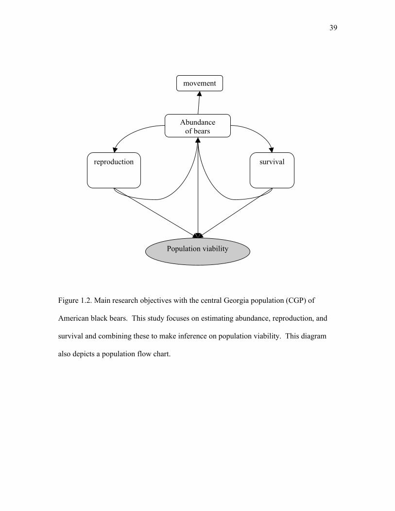
39

Figure 1.2. Main research objectives with the central Georgia population (CGP) of

American black bears. This study focuses on estimating abundance, reproduction, and

survival and combining these to make inference on population viability. This diagram

also depicts a population flow chart.

Abundance of bears

survival reproduction

movement

Population viability

CHAPTER 2

DENSITY ESTIMATION USING JOINT DATA STRUCTURES FROM CAMERAS, DNA

HAIR TRAPS, AND TELEMETRY1

1 Sanderlin, J. S., M. J. Conroy, et al. To be submitted to Ecology.

41

Introduction

Estimating demographic parameters of cryptic species, like the black bear, is difficult

because of their elusive nature and low densities. Non-invasive sampling methods may be

valuable for wildlife studies with consideration of incomplete detection. Often, it is not possible

to observe ecological processes directly, and samples from a population or groups of populations

are used to make inference on the processes. Hierarchical state-space models provide a way of

linking observations from data, such as capture-mark-recapture (CMR) or occupancy samples, to

the underlying ecological or state processes (Royle and Dorazio 2008). Hierarchical models can

incorporate all components of variance (sampling and biological), incorporate different scales of

observation, and provide a way of combining multiple sources of data with common parameters.

One of the main goals of this study is to estimate abundance of American black bears (Ursus

americanus) in central Georgia, USA, using several sources of data. The common parameter of

inference between the data sources is abundance in the central Georgia population (CGP) of

black bears, which cannot be directly observed. Species abundance is influenced by many

biological processes, including habitat relationships, within population processes (e.g., density-

dependence), and species interactions (e.g., Lotka-Volterra models of predator-prey

relationships, species competition, mutualisms, and co-evolution).

Field methods for estimating bear density or abundance include: physical captures

(Smith 1985, McLean and Pelton 1994, Hellgren and Vaughn 1989), camera detections (Grogan

and Lindzey 1999, Martorello 1998, Beausoleil 1999, Mace et al. 1994), tetracycline markers

and resighting with harvested bears (Garshelis and Visser 1997), DNA hair snares (Woods et al.

1999, Mowat and Strobeck 2000, Kendall et al. 2008, Kendall et al. 2009), aerial radiotelemetry

and mark-resights (Miller et al. 1997), mark-recapture with dogs (Akenson et al. 2001), density

42

based on bear-sign (Garshelis et al. 1999), and occupancy studies (Boulanger et al. 2008b). Field

methods vary in the degree of handling of the animal from invasive to noninvasive and some

methods have more rigorous statistical estimation models than others.

Noninvasive methods for sampling bear density include DNA hair snares and the use of

remote cameras. Camera trapping is a technique that uses passive encounter data, much like

radio telemetry. Animals only need to be handled once at initial capture to mark, while

reencounters of those individuals are obtained through photography. With this method, several

unmarked bears may revisit a camera site within the same sampling period, which does not allow

for individual identification. Because abundance estimation generally requires the ability to

individually distinguish individuals, occupancy models (MacKenzie et al. 2006) may be more

appropriate when individual encounter histories cannot be distinguished.

Advances within the fields of molecular and genetic biology have increased the ability to

use genetic analyses in wildlife studies (Waits 1999). However, the genetic identity obtained

with noninvasive genetic techniques may not be as clear (Taberlet et al. 1999, Bonin et al. 2004)

and cost-effective as expected. The presence of genetic error (allelic dropout or false alleles)

reduces the accuracy of genetic noninvasive techniques. Genetic errors can occur at various steps

in a genetic study, e.g., sampling, DNA extraction, molecular analysis, scoring, data analysis,

and caused by human or technical error, or biological processes (Bonin et al. 2004). Sampling

stochasticity with small amounts of low quality DNA in the laboratory leads to allelic dropout

(Goossens et al. 1998, Taberlet et al 1999, Woods et al. 1999). False alleles can occur with

amplification artifacts from PCR (Goossens et al. 1998, Taberlet et al 1999, Woods et al. 1999).

With improvements in laboratory and field sampling techniques, the use of noninvasive

genetic sampling for population monitoring has increased substantially since the methods were

43

first available. However, there are limited analytical and statistical methods that incorporate

multiple noninvasive sampling field methods (such as hair snags and bear rub trees: Boulanger et

al. 2008a). Additionally, few statistical methods incorporate genetic error into abundance

estimates (but see Wright et al. 2009). If genetic error is ignored, population sizes estimates can

be sensitive to genetic error and biased (Creel et al. 2003, Waits and Leberg 2000). Current

methods of incorporating genetic error in noninvasive sampling mark-recapture models use

maximum-likelihood methods (Lukacs and Burnham 2005, Kalinowski et al. 2006), Bayesian

methods (Wright et al. 2009, Petit and Valière 2006), and ad hoc approaches (Paetkau 2003,

McKelvey and Schwartz 2004). Some approaches also require multiple PCR attempts to assess

error (i.e., multiple-tubes approach Taberlet et al. 1996), which increases the cost per sample.

In general, black bears are associated with large areas of forested land in Georgia with

densities highest in areas with limited road access (Carlock et al. 1999). There are three

populations of black bears in Georgia; one in the northern Georgia mountains, the CGP along the

Ocmulgee River, and one in southeastern Georgia. In a preliminary study of the CGP, Grahl

(1985) reported a population estimate of 64 (sd=18) bears using the Lincoln Index, which

corresponds to a density of 0.323 bears per km2. Thus, a current abundance estimate does not

exist for the CGP.

We formulate hierarchical Bayesian statistical models incorporating multiple data

structures (e.g., DNA hair snares, camera detections, telemetry), which also account for genetic

laboratory error. Estimates from the abundance model will assist with evaluating population

viability and harvest impact of the black bear CGP. Therefore, our objective was to estimate bear

abundance in an efficient and accurate manner.

44

Methods

Study Area

The approximate CGP range, estimated by bear sightings and captures, encompasses an

area southeast of Macon, Georgia along the Ocmulgee River (~1,200 km2) falling between the

Piedmont and the Upper Coastal Plain physiographic regions. The study area encompassed

Ocmulgee and Oaky Woods Wildlife Management Areas (WMAs) in Bleckley, Bibb, Houston,

Pulaski, and Twigg Counties, located in central Georgia. The average total annual precipitation

is 119.1 cm (estimated from 1966-2003), and the average minimum and maximum temperature

is 11.4 °C and 24.8 °C for this region (Georgia Automated Environmental Network 2006). The

WMAs consist of a variety of habitat types (pine stands, bottomland hardwood, mixed forest,

upland hardwood, black-belt prairie, clearcuts, thinned pine stands, and cypress-gum swamps).

Hair snares were placed within the boundaries of Ocmulgee and Oaky Woods WMAs between

2003 and 2006 (Figure 2.1, Figure 2.2, Figure 2.3, Figure 2.4, Figure 2.5, Figure 2.6, Figure 2.7).

Descriptive statistics, such as vegetation associations, slope, and elevation, can be used as

habitat covariates with future spatial models of bear density. Therefore, we present a descriptive

summary of the sampled web areas. Descriptive statistics were summarized for each web by

creating boundaries with a radius distance from the center point of each web to the maximum

distance of a hair snare in the outermost ring of each web using BUFFER and MERGE

procedures in ArcView® .

Vegetation associations were based on a digital map layer (30- x 30-m resolution;

Georgia Gap Project) in ArcView®: vegetation associations were open water, transportation,

utility swaths, clearcut/sparse vegetation, deciduous forest, evergreen forest, mixed forest,

pasture/hay, row crop, and forested wetland. The webs were summarized by the number of

45

30x30 m cells classified in each vegetation association out of the total number of cells for each

web, to obtain a percent vegetation type for each web (Table 2.1). Webs A, B, C, E, F, H, and I

have evergreen forest as the dominant vegetation type. Web D has forested wetland as the

dominant vegetation type and web G has mixed forest as the dominant vegetation type. Webs A,

B, C, and I have evergreen forest as the dominant vegetation type and forested wetland as second

dominant vegetation type. Similarly, webs E, F, and H can be grouped together for the two

dominant vegetation types. In summary, webs on Oaky Woods WMA (A, B, I) are very similar

in vegetation classification, while webs on Ocmulgee WMA (C, D, E, F, G, H) are more diverse.

Web D is less like the other webs according to vegetation classification.

The slope, or maximum rate of change in elevation, from each cell to its neighbors in

each web was calculated from the topographic map data. The output slope grid theme in

ArcView® represents the degree of slope (e.g., 3 degree slope) for each cell location. Summary

statistics for the slope of the webs were calculated (Table 2.2). The Digital elevation model

(DEM) measured in meters above sea level was also used to describe the webs. Summary

statistics for the DEM of webs were calculated (Table 2.3). The following arbitrary groupings

can be made based on mean slope: group 1 (A and I), group 2 (B, C, E), group 3 (D, F, H).

Webs A and D had the highest range in slope (indicating more variation in topography), while E

and H had the lowest range in slope. The following arbitrary categorical groupings can be made

based on mean elevation above sea level (meters): group 1 (A, E, I), group 2 (B, G, H), group 3

(C, F), and group 4 (D). Webs A, G, and I had the highest range in elevation (indicating more

variation in meters above sea level), while H had the lowest range in elevation.

46

Field methods

Bears were captured and immobilized with a 2:1 mixture of ketamine hydrochloride

(Ketaset) and xylazine hydrochloride (Rompun) at a dosage of 4.4 mg/kg of Ketaset and 2.2

mg/kg of Rompun, for estimated body weights by Georgia Department of Natural Resources

personnel. Bears were captured in the study area using Fremont foot trap snares (Fremont 1986)

in each of four trapping seasons, which extend from May through August each year. Culvert

traps were used to trap nuisance bears and release the bears on Oaky Woods WMA. An upper

pre-molar tooth for age estimation by cementum annuli analysis (Willey 1974), blood samples,

and hair follicles were collected from each captured bear. Sectioning, staining, and aging of

teeth were conducted by Matson Laboratories (Milltown, Montana). All bears were uniquely

marked using a combination of collars, lip tattoos, and ear tags/streamers. Pertinent

physiological data were recorded for each captured bear. Most bears were fitted with Advanced

Telemetry Systems (Isanti, MN) radio transmitter collars (VHF, very high frequency) equipped

with mortality signal sensors and motion sensors and four male bears received radio collars that

contained Global Positioning technology and a mortality switch. All collars fitted to bears during

the project were equipped with either a mechanical timer release (GPS) or a degradable release

tab (VHF).

Barbed wire enclosures designed to obtain hair samples from individual bears entering

the devices (Woods et al. 1999) were placed on Oaky Woods and Ocmulgee WMAs using

trapping web arrays. A trapping web consists of lines with regularly spaced traps, which radiate

from a central point, and has higher densities of traps or hair snares in the center (Anderson et al.

1983) (Figure 2.8). Nine trapping webs were placed in randomly selected locations covering

most of the WMAs. Each trapping web consisted of 27 hair snares with three snares at the

47

center, and eight spokes, three rings, covering an area of ~ 7 or 16 km2, depending on the

location in the WMAs (Table 2.4). Web size was based on average female home range size in the

CGP and average daily movement of bears (Cook 2007). Some webs had fewer snares if the web

extended to private residences, or if the area was actively logged, burned, or flooded (so that the

realized numbers of snares per web ranged from 22 to 35). In some cases, hair snares were

placed outside but near web perimeters to monitor movement of individuals into the trapping

web. Actual snare locations were recorded with Universal Transverse Mercator (UTM)

coordinates (North American Datum 1987, Zone 17) using global positioning system (GPS)

receivers using Garmin GPS units (Garmin International, Inc., Olathe, KS).

Hair snares in the trapping webs were monitored at least one primary period, and maximum

of two primary periods from May to December, which consisted of three secondary sessions at 6-

9 day intervals, with two to three simultaneously active webs considered to be independent from

the other active webs. Some webs were monitored for two primary periods each year (2004,

2005, 2006). Within a primary period, the population is closed to births, deaths, immigration and

emigration. The population from 1 April to 1 September (Summer), or from 1 September to 10

December (Fall) for each year is closed from births, deaths, immigration, and emigration. This

summer primary period corresponds to the main trapping period the DNR used to capture and fit

radiocollars to bears. The Robust Design (Pollock 1982) was used to allow for future analysis of

combined estimated of abundance from closed periods and survival between open periods for the

population. The Robust Design assumes the time period between primary periods is open to

births, deaths and movement, and secondary periods, or short intervals within a primary period

are assumed closed (Pollock 1982). Secondary periods from 6-9 days are replicated samples

within the closed primary periods of each season. The Robust Design has the advantage of

48

sampling at two different temporal scales, which lead to more robust estimation of parameters,

especially capture probability (Pollock 1982).

Barbed wire (4 point, 15.5 gauge) strands were placed 25 cm and 50 cm from the ground

around 3-5 trees (10-30 m2) and baited with corn in a perforated plastic bottle sprayed with anise

oil (Figure 2.9). Irregularities in terrain, leading to high or low wire, were adjusted with debris

on the ground. Each tree was flagged with brightly colored tape for public safety. Hair samples

were removed from barbed wire with tweezers and placed into manila coin envelopes. Date,

location, sample number, and strand (top or bottom) were recorded on each envelope. For the

season of Summer 2005 and thereafter, area (defined as a group of hair samples in an area big

enough for one bear to pass through) was also recorded as additional stratification of hair

samples. The barbed wire and tweezers were sterilized between samples using a lighter for one

to two seconds or until visible hairs were removed. A hair sample consisted of a sample on one

barb on either the top or bottom strand, or two adjacent barbs on a strand. In cases of three

adjacent barbs with hair, two samples were collected in arbitrary order (one barb in one sample,

two adjacent barbs in the other). If there were no samples with more than 10 hairs, hair samples

(one to nine hairs) with visible roots were collected. Hair samples from other species were also

noted during each session.

Digital cameras utilizing a passive infra-red trigger system were used to monitor bait

stations for marked or unmarked bears. Fifteen cameras were randomly placed among active

webs at snare locations with a higher density of cameras at the center of a web, or near web

perimeters. Cameras were secured to trees that are 3-5 m from the hair snare and aimed at the

hair snare or 100 m from the web perimeter. Pictures from each camera were stored on digital

memory cards and downloaded for analysis. Memory cards also stored the date and time of each

49

picture. Cameras in or near the trapping webs were monitored for three sessions at six to nine-

day intervals, with charged batteries and memory cards replaced every session. The number of

bear pictures and other species' pictures were recorded for each session. Pictures of unmarked

bears taken two minutes between each picture were considered to be the same individual if

physical characteristics are similar. Marked bears were individually identified if marks could be

read.

Any time at least one hair snare within a web was baited the web was considered an

active web. Active webs were monitored at least once a day, weather permitting, for bears with

radiocollars. Pre-determined road routes that encircle and bisect the web were used to scan for

all signals with a receiver and a whip antenna (Advanced Telemetry Systems, Isanti, MN) from

vehicles during daylight and some night hours. The routes were selected to ensure that an

observer would be able to detect a bear if the bear was in or near the web at least once during the

route. A three-element yagi antenna (Advanced Telemetry Systems, Isanti, MN) was used to

determine the direction of the collar in the field. If there was uncertainty whether the bear was in

or out of the web, telemetry locations were estimated by the line that bisects the angle between

two directions where the signal can just be heard (Kenward 1987). The azimuths were between

60º and 120º apart and collected within 20 minutes to increase accuracy of azimuth

measurements. The azimuth range is best for triangulation purposes (White and Garrott 1990)

and the short time period reduces the chance of large bear movements. If an observer was on the

edge or outside of the web, and the direction of the bear was opposite the web, only one azimuth

was obtained. If a bear were in the web, an observer would often be able to detect its frequency

more than once during the web scan route. Locations of observers were recorded in Universal

50

Transverse Mercator (UTM) coordinates using global positioning system (GPS) receivers from

Garmin GPS units (Garmin International, Inc., Olathe, KS).

Telemetry error was estimated using test collars placed throughout the webs in the study

area. Webs were chosen to represent common topographic and vegetation conditions from the

entire study area (see Tables 2.1, 2.2, 2.3 for vegetation data, elevation, and slope representation

of each web). In all cases, locations of test collars were unknown to the observer. Web

telemetry error was calculated for 10 observers (three from fall 2004, three from summer 2005,

one from fall 2005, three from summer 2006). A separate telemetry data set was analyzed using

two observers from summer 2004 from Cook (2007). One collar was placed in two to six webs

in Oaky Woods and Ocmulgee WMAs during 2004-2006 (Table 2.5). Azimuths were obtained at

five pre-selected stations at varied distances from the collars (0.2-2 km). Azimuth stations were

repeated three times on separate days with summer and fall 2005, 2006 observers. Telemetry

error was calculated as difference in the observed from the true azimuth based on observer

location at a station and the known location of the test collar. Telemetry error, with telemetry

observations of bears, will be used to determine if a bear is present in a web during the time

periods when hair snares are baited.

Laboratory Methods

At least one hair sample per hair snare, web, session, season, and year occasion was

selected for analysis, based on visual inspection of quality (i.e., visible roots with skin cells) and

quantity (10 hairs). Additional samples were randomly selected, with more weight given to hair

snares with more hair samples, to increase the chances of identifying additional unique bears. If

possible, other areas or sections of the hair snare were selected than the original sample for the

51

additional samples. This follows the assumptions that: 1) more hair samples at a hair snare

might lead to more individual bears, and 2) individual bears may leave hair samples in different

locations at a hair snare. The sub-sampling technique aims to capture more unique individuals in

the population. If only high-quality samples were selected, some hair snare, web, session,

season, and year occasions would not be selected, which may bias population estimates (i.e.,

some bears may consistently leave lower quality samples than others). Budget and time

constraints also precluded analyzing all hair samples.

After field collection, hair samples were stored in silica desiccant then transferred to

a -20° C freezer. Prior to extraction and after field collection, blood and tissue samples were also

stored in a -20° C freezer. Extraction of DNA from Georgia tissue samples was done with the

DNeasy Kit (QIAGEN) and with one captured bear blood sample using the GenomicPrep DNA

isolation kit (GE Healthcare). DNA from hair samples were extracted with Chelex100 (10%

solution) (Promega), along with proteinase K (Phenix Research Products, QIAGEN) used for

protein digestion that may inhibit PCR reactions (modified from Boersen 2001). The root portion

(1 cm) from a maximum of 10 hairs per sample were cut and placed into 150 µl of Chelex 100

(10% solution) (Promega). The number of hairs and quality of sample were recorded. If the

number of hairs was less than 10, the entire strand of hair was used in the sample. Low quality

samples had little or no visible roots, and usually consisted of under-fur (thin) hairs. Medium

quality samples were classified as samples with half of the hairs with roots visible and some

guard hairs. High quality samples were classified by a majority of the hairs as guard hairs with

most or all of the roots visible, and including visible skin cells. After roots were placed in the

10% solution Chelex 100 (Promega), 10 µl proteinase-K was added to digest excess protein. The

hair samples were incubated at 65° C overnight (~8 hours). Samples were vortexed, and then

52

boiled at 100° C for 10 minutes. After removal, the samples were centrifuged at 10,000-12,000

rpm for 3 minutes. The supernatant was pulled off and placed into a clean tube, and stored at

-20° C until PCR analysis.

PCR amplifications were performed in 10 µL volumes using Bio-Rad MyCycler thermal

cyclers for both tissue and hair samples with 8 tetranucletide loci (UA-BM3-P1F04, UA-BM4-

P1H06, UA-BM4-P2B06, UA-BM4-P2C10, UA-BM3-P1D05, UA-BM4-P2A06, UA-BM4-

P2B08, and BM4-P2C02, hereafter named Bear 10Y, Bear 12Y, Bear 17G, Bear 19Y, Bear 30B,

Bear 33B, Bear 35G, and Bear 36, respectively) previously described in Sanderlin et al. (2009).

Loci Bear 10Y, Bear 12Y, Bear 17G, Bear19Y, Bear 30B, Bear 33B, and Bear 35G were directly

labeled primers with the dyes NED (Y), HEX (G), and FAM (B). For comparison with known

individuals from the CGP, eight microsatellite markers developed by Paetkau and Strobeck

(1994) and Paetkau et al. (1995) were initially used for individual identification: G1A, G1D,

G10B, G10C, G10L, G10M, G10P, and G10X. Final concentrations for optimizing reactions

with unlabelled primers were 10 mM Tris pH 8.4, 50 mM KCl, 0.5 µM “pigtailed” primer

(Brownstein 1996), 0.05 µM CAG or M13-reverse tagged primer (CAG or M13-reverse +

primer), 0.45 µM dye labeled tag (HEX or FAM + CAG or M13-reverse), 1.5 mM MgCl2, 0.5

mM dNTPs, 0.5 U AmpliTaq Gold DNA Polymerase (Applied Biosystems), and 50 ng DNA.

Final concentrations for optimizing reactions with directly labeled primers were 10 mM Tris pH

8.4, 50 mM KCl, 0.5 µM upper directly labeled primer, 0.5 µM lower directly labeled primer,

1.5 mM MgCl2, 0.5 mM dNTPs, 0.5 U AmpliTaq Gold DNA Polymerase (Applied Biosystems),

and 50 ng DNA. We ran reactions using one touchdown thermal cycling program (Don et al.

1991), encompassing a 10.5 oC span of annealing temperatures (range: 60-49.5 oC).

53

For tissue samples, cycling parameters were: 21 cycles of 96o C for 20 s; highest

annealing temperature for 30 s minus 0.5o C per annealing cycle; and 72o C for 1 min 30 s

followed by 14 cycles of 96o C for 20 s; 50o C, for 30 s; 72o C for 1 min 30 s; and a final

extension period of 10 min. at 72o C. For hair samples, cycling parameters were: 20 cycles of

96o C for 20 s; highest annealing temperature for 30 s minus 0.5o C per annealing cycle; and

72o C for 1 min 30 s followed by 30 cycles of 96o C for 20 s; 50o C, for 30 s; 72o C for

1 min 30 s; and a final extension period of 10 min. at 72o C. We checked PCR products for

amplification and sized fragments using a 3730xl DNA sequencer (Applied Biosystems) with

GENESCAN Rox500 fluorescent size standard (PE Applied Biosystems). Results were analyzed

using GENEMAPPER software (Applied Biosystems) using the local Southern size-calling

method.

Statistical methods

Observed and expected heterozygosity were calculated for each locus from the observed

unique individual genotypes collected from hair snares using Cervus 2.0 (Marshall et al. 1998).

GENEPOP 3.4 (Raymond and Rousset 1995) was used to test for genotypic linkage

disequilibrium with a posteriori sequential Bonferroni correction to correct for multiple

comparisons of markers (Rice 1989). The α level of significance is divided by the number of

comparisons between markers to reduce pseudoreplication. The probability of identity (PID), or

the probability that 2 randomly chosen individuals in a population will have identical genotypes

(Paetkau and Strobeck 1994) was calculated over all loci with the observed unique individual

genotypes collected from hair snares using the following formula:

24 )2(j

i ij

i

i

ippp !!!

>

+

(Equation 2.1)

54

where pi and pj are the frequencies of the ith and jth alleles. The more conservative estimate with

PIDsib , or the probability of identity among siblings (Evett and Weir 1998), was also calculated

using the following formula:

)25.0(])(5.0[)5.0(25.0 4222 !!! "++iiippp

(Equation 2.2)

where pi is the frequency of the ith allele. The inbreeding coefficient, or within population

heterozygote deficit (Fis ), for the Paetkau and Strobeck (1994) and Paetkau et al. (1995) markers

and Sanderlin et al. (2009) markers of known individuals was calculated using program FSTAT

(Version 2.9.3) (Goudet 1995).

A minimum number of bears for each year (2003-2007) was calculated from known bears

with radiocollars, and other captures of bears that were not marked. The unmarked bears from

dead recoveries were also included. This information can be combined with the number of bears

with radiocollars to obtain a minimum known number of bears per year (alive+dead).

We use a condensed version of telemetry data for model simplification in the full

Bayesian model, described in the next section. Raw telemetry data consist of observations from

radiocollared bears detected during vehicular travel with radio-equipped vehicles. Pre-

determined routes encompassed, bisected, and were near the webs during sampling sessions.

When a bear was detected during the vehicular scan, ground telemetry observations, including

azimuths (angle from observer to bear), elevation above sea level, and level of gain, were

conducted. Observer sampling error with telemetry may influence and bias conclusions of

presence or absence of bears within a web with raw telemetry data, therefore this error should be

included within the modeling procedure. The probability of presence in a web for each bear

55

observation was simulated from the combination of: 1) observer location points, and 2) estimates

of azimuth error from spatial distributions of telemetry sampling error. The number of simulated

locations in the web out of total number of simulated locations (n=10,000) was used as an

estimate of the probability of the bear in the web for each bear and day observation in a

secondary period. If this probability exceeded 0.50, the bear was classified as present (‘1’, and

‘0’ otherwise) for that observation. Data were collapsed to a period of three weeks, with the

assumption that the population was closed during the three-week sampling period for each web.

Therefore, if a bear was detected at least once in a web over the three-week period, it was

classified as a detection on that web.

The predicted true azimuth direction was simulated as the sum of the observed angle plus

one draw from the von Mises distribution to simulate error in observer azimuth direction. The

von Mises distribution is often used with circular data, like azimuth directions with possible

values encompassing 360° (for example, see Figure 2.10). The probability density function of the

von Mises distribution takes the following form:

!

"(#) = [2$%0(&)]'1e& cos(# 'µ0 )

(Equation 2.3)

where the angles θ and µ0 are between -π and π, and standard deviation κ is greater than zero,

and I0(κ) is the modified Bessel function of the first kind and order. The predicted azimuth

direction is:

(Equation 2.4)

!

) " = "

obs+ vonMises("

error,s2)

56

The predicted distance from the observer to the bear was modeled from known distances to

collars and recorded gain levels.

!

) d = "

0+ "

1* gain + error

(Equation 2.5)

The full Bayesian Markov-Chain Monte Carlo (MCMC) models of the joint data

structures were implemented using a combination of Gibbs and Metropolis sampling algorithms.

Monte Carlo refers to estimation by simulation. Markov chains are a special type of stochastic

process, where the future depends on the current state, but not past states. This is known as the

‘Metropolis algorithm’ first described by Metropolis and Ulam (1949) and Metropolis et al.

(1953). Markov chains have the following properties of homogeneity, irreducibility, recurrence,

stationarity, and ergodicity. Homogeneity is when the transition probabilities are independent of

time. Irreducibility refers to a non-zero probability of reaching a state from any other state in the

chain. States can be repeatedly selected with the property of recurrence. The marginal

distribution is produced when multiplied by the transition kernel with stationarity. Ergodicity

means that after many steps the marginal distribution of a Markov chain is the same at one step

as all other steps.

The Metropolis algorithm was later generalized by Hastings (1970), and labeled as the

Metropolis-Hastings algorithm. This special case of the Metropolis algorithm generates

candidate state transitions from an alternative distribution, and uses an acceptance/rejection rule

to converge to the specified distribution. The Metropolis algorithm uses a symmetric jumping

distribution, while the Metropolis-Hastings algorithm is not limited to symmetry with the

jumping distribution. The algorithm steps are listed below, following notation and summary of

algorithm steps from Gelman et al. (2004).

57

1. First, select a starting point for parameter, θ0, from either a starting distribution or

reasonable initial values.

2. For t=1,… :

a) Sample a proposed value of the parameter, θ*, from a jumping distribution at time t.

b) Calculate the ratio of densities or likelihoods of the parameter given y data as follows,

!

r =p("* | y)

p(" t#1| y) (Equation 2.6)

c) Generate a uniform random variable, and accept the proposed value, θ*, with probability

min(r,1), and the previous value, θ t-1, otherwise

Convergence to the target distribution with the Metropolis algorithm occurs because the

sequence is a Markov chain with a unique stationary distribution and the stationary distribution

equals the target distribution (Gelman et al. 2004). The Metropolis algorithm is useful for

models that are not conditionally conjugate, i.e., the full conditional distribution kernels are not

known distributions. However, the Metropolis algorithm can be slow. The Gibbs sampling

algorithm offers a relatively fast alternative and is only appropriate for full conditionals that are

kernels of known distributions.

Gibbs sampling, first named by Geman and Geman (1984), utilizes conditional

distributions, where each parameter is conditioned on current values of the other k-1 parameters.

By cycling through each parameter, conditioned on the current values of the other parameters,

samples from the posterior distribution are generated.

To illustrate the scenarios in which Gibbs sampling would be useful, versus Metropolis-

Hastings, here are two examples. First, consider a scenario where the likelihood the data given

58

the parameter is a binomial distribution, and the prior on p, the probability of success, is a beta

distribution. The full conditional distribution of p is below:

!

[p |•]"n

#

$

% & '

( ) p

#(1* p)n*# p+*1(1* p), *1

" p# ++*1

(1* p)n*# +, *1

(Equation 2.7)

This is the kernel of a Beta distribution with parameters θ+α and n-θ+β. This is an example of

when Gibbs sampling would make sense, since the posterior can be directly sampled. However,

consider the same binomial likelihood, but that p is constrained to the following form:

!

p =1" (1" r)a (Equation 2.8)

So, the full conditional distribution of p is now:

!

[p |•]"n

#

$

% & '

( ) (1* (1* r)

a)#(1* (1* (1* r)a ))n*# (Equation 2.9)

This does not have a known distributional form, thus Metropolis sampling from the posterior is

the only option.

Reversible jump MCMC (RJMCMC) was also used for posterior simulation of

parameters in the joint data structure model. Reversible jump MCMC was first introduced by

Green (1995), and is useful when the dimension of the parameter space has a possibility of

changing from one iteration to the next. The Markov chain samplers can jump between

parameter subspaces of differing dimensionality in RJMCMC (Green 1995).

For each model, two chains of 50,000 iterations each and a burn-in period of 25,000

iterations were run with Python, version 2.5.2 (Python Software Foundation, http://python.org).

No thinning interval was used. Each chain was selected from different combinations of initial

parameter values to evaluate parameter convergence. The posterior iterations after the burn-in

period from each chain were combined for output statistics and figures. The output for each

59

model included the median, 95% Bayesian credible interval (BCI), and histograms and traces of

the posterior distributions. A full simulation study was conducted to assess model performance

(Appendix A).

Statistical model

State-space models include both measurement and process error (Royle and Dorazio

2008). This is useful when multiple data sets are collected for inference on abundance, such as

the following model incorporating three data structures of camera, telemetry and DNA hair snare

data (refer to Table 2.6 for complete description of model notation, Figure 2.11). The biological

motivation, assumptions for statistical distributions, and updating of parameters for the

individual data components are described below, followed by the full Bayesian statistical model.

Spatial parameters of local abundance, Ni

We assume the true abundance distribution in the superpopulation follows a Poisson-

Gamma process, where λ, the Poisson parameter, is the local density of bears and α and β, the

Gamma parameters, control the amount of variability in abundance across the landscape. Due to

low local abundance, and perhaps low sample size, the Poisson model may be more relevant to

the study, thus efforts were focused on this less complex, null, model. However, we present the

more complex model first, followed by the model used for this analysis. The Poisson distribution

is often used to model count data, such as abundance, and allows for extra-Poisson variation in

abundance, or overdispersion. The Poisson-Gamma process is used to control for local

heterogeneity in abundance. Heterogeneity in local abundance can be a function of habitat

covariates, environmental factors, or other unknown sources. The Poisson-Gamma process,

60

reparameterized as a negative binomial, has been used in ecological studies (Royle and Nichols

2003, Conroy et al. 2008).

The mixture of Poisson distributions that follow the gamma distribution results in a

marginal distribution for Ni following a negative binomial distribution with parameters α and β

(Gelman et al. 2004). Consider the vector of abundance {Ni}, i=1,…m, and the local density,

{λi,} i=1,…m. The spatial joint distribution of the data {Ni}, and the parameters λi, α, β is:

[{Ni},λi, α, β]= [[{Ni}|λi ][ λi |α, β][α][ β] (Equation 2.10)

These are, respectively, Poisson, Gamma, and Gamma hyperprior distributions for α and β. Also,

ν and ω are the parameters of the Gamma hyperprior distribution for α and δ and η are the

parameters for the Gamma hyperprior distribution for β. Putting this together we get:

!

[{Ni},"

i,#,$] = [{Ni} | "

i]

i=1

m

% ["i|#,$]&

"i

Ni e

'"i

Ni!

( ) *

+ , -

$#

.(#)"i

#'1e'$"

i/0

.(0)i=1

m

%i=1

m

%i=1

m

% #0'1e'/# 12

.(2)$2 '1e'1$

(Equation 2.11)

To sample directly from the posterior distribution using Gibbs sampling, we must first derive the

full conditional distributions. The full conditional distributions for the spatial parameters are:

!

["i|•]#

"i

Ni e

$"i

Ni!

%&

'(&)"i

&$1e$%"

i =%&

Ni!*'(&)

"i

Ni+&$1

e$%"

i$"

i

#"i

(Ni+& )$1

e$"

i(% +1)

(Equation 2.12)

This is the kernel of the known Gamma distribution with parameters Ni+α and β+1, so the

61

posterior distribution can be sampled directly using Gibbs sampling. For the parameter α, the

full conditional is:

!

[" |•]#$"

%(")i=1

m

& 'i

"(1e($'

i)*

%(*)"* (1

e(*"

#$"

%(")

+

, -

.

/ 0

m

'i

"(1

i=1

m

&+

, -

.

/ 0 e

(m)"($ 'i

i=1

m

1"*(1

(Equation 2.13)

This is not a known distribution, and requires the Metropolis-Hastings algorithm to sample from

the posterior distribution. For the parameter β, the full conditional is:

!

[" |•]#"$

%($)i=1

m

& 'i

$(1e("'

i)*

%(*)"* (1e()"

#"m$+m* (me

(m)"(" 'i

i

m

+

#" (m$+m* (m+1)(1e

(" (m) + 'i)

i

m

+

(Equation 2.14)

This is a kernel of the known Gamma distribution with parameters (mα+mδ-m+1) and

(mη+

!

"i

i=1

m

# ), so the posterior distribution can be sampled directly using Gibbs sampling.

If we assume local abundance is determined by only one density parameter, λ, the

process is reduced to a Poisson process. The conjugate prior density for a Poisson process is the

Gamma distribution (Gelman et al. 2004). Following Gelman et al. (2004), the posterior

distribution for density, λ, is a Gamma distribution, which can be directly sampled from using

Gibbs sampling:

!

[" |•] ~ Gamma(# + Ni

i=1

m

$ ,% + m) , (Equation 2.15)

where α and β are the parameters from the Gamma prior distribution, and m is the number of

total possible webs. We chose a diffuse prior, a Gamma(0.001, 0.001), for the distribution.

62

Telemetry parameter

Telemetry data provides inference on the presence of a bear in a web, commonly referred

to as occupancy, ψ, or the probability that a patch or sampling unit is occupied (MacKenzie et al.

2006). We are not directly estimating the probability of a patch occupied, but rather the number

of bears in a patch. This can be used to indirectly estimate occupancy, where Ni>0 means the

probability that a patch is occupied is one. The telemetry component consists of:

!

[{Vik} | pwi,V ][{Ni} | pwi

][pwi], (Equation 2.16)

where V is the telemetry data consisting of the number of total bears collared during the year and

season over all three sessions or occasions, and the individual bears detected on each web i

(described below). The likelihood of the number of true bears on a web, Ni, given the total bears

in a population, Ntot, and the probability of a bear on a web, pwi, can be classified as a binomial

distribution, or a series of independent Bernoulli trials where each trial is a bear with probability

pwi of being on the web. Similarly, the number of bears with collars on a web, ncollared,i , given the

total number of bears with collars on during the sampling period, Ncollared, can also be classified

as a binomial distribution, with each bear with a collar having probability pwi of being present on

a web. This assumes that bears with and without collars have the same probability of being on a

web. The conjugate prior for binomial distributions is a beta prior on the probability of a bear on

a web. The full conditional distribution of the probability of a bear on a web, pwi, includes the

product of two binomial distributions and a Beta(1,1) prior on the probability of a bear on a web:

!

[pwi|•]"

Ncollared

ncollared ,i

#

$ %

&

' ( pwi

ncollared,i(1) pwi

)Ncollared )ncollared,i

Ntot

Ni

#

$ %

&

' ( pwi

Ni

(1) pwi)Ntot )Ni pwi

*)1(1) pwi

)+ )1

" pwi

ncollared,i +Ni +*)1(1) pwi

)Ncollared )ncollared,i +Ntot )Ni ++ )1

,

(Equation 2.17)

63

where ncollared,i is the number of bears with collars on web i, Ncollared is the total number of bears

with collars on during the sampling period, Ni is the number of true bears on web i, Ntot is the

total bears the population, and α and β are the parameters for the beta prior on pw,i. This is a

kernel of a Beta distribution with parameters: ncollared,i+Ni+α and Ncollared-ncollared,i+Ntot-Ni+β.

Posterior prediction of pw on webs not sampled is conducted by using a Beta (Nj+α, Ntot-Nj+β).

Camera parameters

We used a model that links abundance and heterogeneous detection probabilities, known

as the Royle-Nichols model (Royle and Nichols 2003) with the camera data. The probability of

detecting occupancy di with the camera samples is a transformation of the individual probability

of camera detection, r, and Ni, the abundance of bears on web i:

!

[di] =1" (1" r)

Ni (Equation 2.18)

The probability of individual detection from cameras is assumed constant among bears and

among webs. The conditional distribution of camera detections, Yi, on web i, given the

probability of detection, di, follows a binomial sampling model, where each camera is an

independent Bernoulli trial of bear detection:

!

[Yi | di] =j

yi

"

# $

%

& ' di

Yi (1( di)j(Yi , (Equation 2.19)

where j is the total number of cameras or sites on web i. Additionally, we assume that detection

does not vary by occasion k, so j is condensed data consisting of the number of camera by

occasion replicates in web i, and yi is the number of bear detections over all cameras*occasions

in web i in one season.

64

The conditional probability of occupancy, di, is a deterministic function of the stochastic r and Ni

parameters. The full conditional distribution of r is:

!

[r |•]"j

Yi

#

$ % &

' ( (1) (1) r)

Ni )Yi (1) r)Ni ( j)Yi )

i=1

w

* (Equation 2.20)

This does not factor into a known distribution, and requires the Metropolis-Hastings algorithm

for updating r from the posterior distribution (See Appendix B for details of algorithm).

Genetic data parameters

This component of the joint data structure model is based on the genetic error model with

allelic dropout originally in Wright et al. (2009), with the exception of the calibration sample

component. The calibration sample data consists of genotypes of tissue and/or blood, and hair

samples from known individuals from the bear CGP, as originally described in Sanderlin (2009).

The tissue samples are of higher quality with a lower probability of error than the hair samples,

and can be used in conjunction with replicated hair samples from unknown individuals.

Dropout error probability, p

For true heterozygotes (

!

Ail1" A

il2), where A is the allele at locus l for individual i, the

probability of observing a true heterozygote is 1-p, while the probability of observing a

homozygote is 0.5*p, since there are 2 ways that an allele can drop out. Following Wright et al.

(2009), therefore, the probability of an observed genotype given the true genotype is as follows:

!

Pr(Gjlr

obs| G jl ) =

1" pl Ail1r

obs # Ail2r

obs

0.5pl Ail1r

obs= Ail2r

obs

$ % &

(Equation 2.21)

Since we are only considering allelic dropout, the probability of observing a homozygous

individual at locus l, replicate r, given that the true individual at locus l is homozygous, is 1.

65

We assume that the calibration sample (t=1,…T, for tissue and blood samples and

h=1,…H, for hair samples) is independent of the replicated hair samples from unknown

individuals and that the allelic dropout probability is the same within the calibration samples and

the replicated hair samples. Using the conjugate beta prior for allelic dropout of a binomial

distribution, the error likelihood is the product of the two binomial likelihoods and beta prior.

Following notation from Wright et al. (2009):

!

[Gobs,C

obs|G,C,N, p] = I(Gjl1 "Gjl2)

p

2

#

$ % &

' (

r=1

R

)l=1

L

)j=1

S

)I (G jl1r

obs=G jl1r

obs)

(1* p)I (G jl1r

obs "G jl1robs

)

I(C jl1 " C jl2)l=1

L

)t=1

T

) p

2

#

$ % &

' (

h=1

H

)I (C jl1r

obs=C jl1r

obs)

(1* p)I (C jl1r

obs "C jl1robs

)p+(1* p), *1

(Equation 2.22)

This reduces to a Beta(α +w+wc, β+W+Wc) distribution, where w and wc are the number of times

the heterozygous loci originally seen in tissue/blood samples of the calibration sample or the

samples, were genotyped as homozygous in any of R replicates. W and Wc are the total number

of heterozygous loci across all n individuals that appeared in one of the S samples. Since this is a

kernel of a known distribution, the posterior distribution of allelic dropout can be sampled using

Gibbs updates.

True genotype matrix, G, and true sample histories, X

The true genotype matrix and true capture histories are updated using direct sampling,

following Wright et al. (2009) (See Appendix C for a full description of how these matrices are

updated). The true genotypes are updated by a combination of the error likelihood described

above, and the probability of observing the specific genotype, given the true genotype

frequencies in the population. The true sample histories are updated with the capture-history

likelihood of proposed capture histories of compatible individual genotypes and the probability

66

of observing the observed genotype given the true genotype and error probability. Both

sequences of updating require inserting proposed values of either the genotype at a specific locus

and individual (genotype matrix), or proposed values of capture histories (capture history matrix)

and evaluating the likelihood of the proposed values compared to other possible values.

Genotype frequencies, γ

Following Wright et al. (2009), the genotype frequencies are the kernel of the joint

distribution of L independent Dirichlet random variables with parameters {ykj+αkj} of dimension

lj. Using uninformative priors, αkj, of 1, the full conditional distribution of vector γ is:

!

[" |•] = " kjykj +#kj $1

k=1

l j

%j=1

L

% (Equation 2.23)

For a complete description of how these parameters are updated and derived, see Appendix C.

Capture probability from DNA hair snares, θ

Capture variation in closed mark-recapture models can be classified into three main

categories: 1) heterogeneity (Mh), where each individual animal has a different probability of

capture, or measurable individual attributes (e.g, group or individual covariates) 2) behavior

(Mb), where animals captured have different probabilities of capture than animals not captured,

either trap-happy or trap-shy, and 3) time (Mt), where capture probability can vary over trapping

sessions (Pollock 1974, Otis et al. 1978, White et al. 1982). For the models presented in this

chapter, the constant capture probability (M0) over time, behavior and heterogeneity, and web

was selected to reduce model complexity. However, there is evidence of behavior and time in

67

capture heterogeneity from closed capture models that assume no genetic error (see Appendix D

for this analysis). Therefore, future models will include more complexity.

To update the constant capture probability after the genotype and capture history matrices

are updated, the sufficient statistics of u., or the unique number of individuals captured with

DNA hair snares, and n., the total number of times these individuals were captured over the three

trapping occasions with DNA hair snares, are used. Capture mark-recapture (CMR) data

consists of a series of independent Bernoulli trials, or animals, with probability of capture, θ. The

full conditional likelihood of constant capture probability, using the conjugate Beta(1,1) prior for

a binomial distribution is:

!

[" |•]#N

w!

(Nw$ u.)!

"n.(1$")k(Nw

)$n."%$1(1$")& $1

#" n.+% $1(1$")kNw

$n.+& $1

, (Equation 2.24)

where

!

n.= ni

k=1

3

"i=1

w

" , or the total number of captures over the webs sampled for all three

occasions, Nw is the true abundance of bears with webs sampled, k is the number of trapping

occasions, and κ and υ are the capture probability priors. This is the kernel of a Beta distribution

with parameters n.+ κ and kNw- n.+υ, thus the posterior distribution of θ can be sampled directly

using Gibbs sampling.

Abundance of sampled areas (Ni)

The full conditional distribution of abundance on sampled areas (Ni) is the joint

distribution of the three data structures and the spatial model of N. The full conditional likelihood

is a combination of one Poisson from the spatial component, and two binomials from the camera

and telemetry components, respectively, and a negative binomial from the genetic CMR data.

68

We also use a discrete uniform prior on Ni, with a lower limit of max(u.i, ncollared,i, ‘1’ if Yi>0),

and upper limit is the total number of genotype combinations of individuals over all loci. The

full conditional likelihood is:

!

[{Ni} |•] = [{Yijk} | r,Ni][{Ni} | pwi][{Ni} | "i]

i=1

m

# [G | Ni,$][Xik |Ni,%ik ][{Ni}]

!

"#iNi e

$#i

Ni!

% & '

( ) * i=1

w

+j

Yi

,

- . /

0 1 (1$ (1$ r)

Ni )Yi (1$ r)Ni ( j$Yi )

Ntot

Ni

,

- .

/

0 1 (pwi

)Ni (1$ pwi

)Ntot $N i

Ni!

(Ni $ u.i)!2 n.i (1$2)k(Ni )$n.i

"#iNi e

$#i

Ni!

% & '

( ) * i=1

w

+j

Yi

,

- . /

0 1 (1$ (1$ r)


Ntot

Ni

,

- .

/

0 1 (pwi

)Ni (1$ pwi

)Ntot $N i

Ni!

(Ni $ u.i)!(3

0)Ni $u.i

(Equation 2.25)

where π0 is the probability of not being captured at least once over the three occasions (i.e.,

!

"0

= (1#$)3). A sequential update of Ni was used, where Ntot of the current accepted Ni s were

used in Ntot from the telemetry portion, or probability of a bear on a web. The Poisson

distribution with the current value of λ was used for posterior prediction of abundance for webs

not sampled with the less complex spatial model. However, a negative binomial with updated

spatial parameters of α and β (described in equations 2.9 and 2.10), would be used for posterior

prediction of abundance on webs not sampled with the Poisson-gamma spatial model.

Based on the dimension of a proposed value of N*, the genotype matrix G and the

capture-history matrix are augmented (Tanner and Wong 1987) by N*- N rows. Following

Wright et al. (2009), the genotype matrix is augmented by sampling genotypes directly from

multinomial distributions [G|γ], with the constraint that the sampled genotype is not present in the

population currently. The capture-history matrix is augmented with rows of zeros. If N*<N,

values must be deleted from the genotype and capture-history matrix. These individuals cannot

appear in any of the observed samples. This joint full conditional for N is not a known

69

distribution and could potentially change matrix dimensions. Therefore, a reversible jump

Metropolis-Hastings step is needed to update N (see Appendix B for details of the Metropolis-

Hastings algorithm).

Unconditional population estimate of abundance

We want the unconditional estimate of abundance of bears in the target population of

inference in central Georgia. The target population of inference encompasses the total area in

which webs were sampled (see Figure 2.7). The minimal inference population is the WMA land

(186 km2), which includes both Ocmulgee and Oaky Woods, while the maximal inference

population is the estimated range of black bears in central Georgia (~1200 km2, Cook 2007). For

this chapter, we will focus on the minimal inference population of the WMA land. This can be

labeled the ‘superpopulation’.

We have sample observations related to Ni under our sampling protocol, not Ntot, where i

is the individual web and tot is the superpopulation. Therefore, we must obtain posterior

predictions of abundance from unsampled areas within the inference population from the

heterogeneity parameters of abundance on sampled areas. One may assume random selection of

webs, however, this is not entirely correct due to limitations of land ownership and other

attributes of the WMA boundaries (rivers, roads, highways) that do not permit placement of web

arrays. Our sample is part of the total set of possible web-sized areas in the inference population,

or more formally:

!

Ni=1,...w UN

i=w+1,...m,

where w is the total number of webs sampled and m is the total number of possible webs in the

population area. The unconditional abundance of the superpopulation over all possible webs,

70

Ntot, is the sum of abundance over all sampled webs plus the predicted abundance from posterior

simulation for unsampled webs using the Poisson-Gamma spatial model (described above) in the

population range.

!

[Ntot |•] ~ Ni

i=1

w

" + N j

j=w+1

m

" , (Equation 2.26)

where w is the total number of webs sampled, m is the total number of possible webs in the

population area, and tot refers to the superpopulation.

Full Bayesian model of joint camera, telemetry, and DNA hair snare data structures

The joint distribution of camera detection data {Yijk}, capture histories at hair snares

{Xik}, telemetry data {Vik}, observed genotypes from DNA hair snares

!

{Gikr

obs}, and genetic

calibration sample data {C, Cobs} is:

!

[{Yijk},{Vik},{Gikr

obs},{C},{C

obs},{Xik},{Ni},di,r, pwi

, p,Gikr,G,",#,$,%,&] =

[{Yijk} | di][di | r,Ni][{Vik} | pwi,V ][pwi

|{Ni},N][{Ni} | $i][$i |%,&][Cobs | p,C][Gobs,ikr |Gikr, p]i=1

m

'

!

[G | Ntot ,"][Xik |Ni,#][r][p][$][%]["][#][Ni] (Equation 2.27)

where i is the individual web, k is the number of sessions or occasions, and m is the total number

of web areas. Bayes theorem allows us to obtain the probability of abundance on web i, given

the bear is on web i, from the probability that the bear is on web i, given the true number of bears

on web i:

!

[pwi|{Ni}] =

[{Ni} | pwi][pwi

]

[{Ni}]"[{Ni} | pwi

][pwi]

(Equation 2.28)

71

This leads to the joint distribution, where the only difference between Equation 2.28 and

Equation 2.29 is the double underlined portion from the Equation 2.28 reverse conditioning:

!

[{Yijk},{Vik},{Gikr

obs},{C},{C

obs},{Xik},{Ni},di,r, pwi

, p,Gikr,G,",#,$,%,&] =

[{Yijk} | di][di | r,Ni][{Vik} | pwi,V ][{Ni} | pw

i][pw

i][{Ni} | $i][$i |%,&][Cobs | p,C][Gobs,ikr |Gikr, p]

i=1

m

'

!

[G | Ntot ,"][Xik |Ni,#][r][p][$][%]["][#][Ni] (Equation 2.29)

The Python code for the full model can be found in Appendix E.

Results

Data summary

Over 6 seasons from years 2003 to 2006, a total of 32 ‘webs’ (note: webs were sampled

more than once, since there were 9 actual webs), or 830 hair snares were actively checked. A

total of 4,180 hair samples over 2516 snare sessions (dates which a snare was ‘active’) were

collected (Table 2.7). The number of snares with at least one hair sample was 1113. Some of

these samples could contain feral hog hair, but not all samples were analyzed in the genetics

laboratory. Some snares were not sampled for all three sessions due to river flooding or

controlled burns, therefore the number of snares multiplied by three does not always equal the

number of snare sessions

The total number of hair samples selected for genetic analysis was 1,487. These hair

samples were collected at hair snares from 2003-2006, over six sample seasons. Of the 1487 hair

samples selected, 1041 samples (70.0 %) had positive amplification for at least one locus. Of the

1041 samples with positive amplification for at least one locus, 42.7 % amplified at all 8 loci

72

selected for genetic identification (n=445). The samples that amplified at 7 loci (n=57) and 6 loci

(n=66) could plausibly be used in further capture-recapture models. Models presented in this

chapter only include samples with amplification at 8 loci. The samples with 6 and 7 loci with

positive amplification have different probabilities of identity, and may match multiple samples

that have information at all 8 loci.

Hair samples (n=203, or 19.5% of the total 1041 samples) were randomly selected from

the hair samples that positively amplified for at least one locus to assess the genetic error in the

DNA extraction, PCR, genotyping, scoring/binning of alleles, and database storage process.

This process involved the selection of different hairs (but from the same physical sample as the

initial sample) for DNA extraction, and may assess any mixed-sample errors. Samples were

given a new genetic tag and treated as new hair samples in the whole process from extraction to

scoring and database storage. Of the 203 hair samples selected for this assessment of genetic

error, 180 samples (88.7 %) positively amplified for at least one locus. Additional samples

(n=23, or 5.2% of the total 445 samples) were randomly selected to assess the PCR and re-

genotyping error (not DNA extraction) from the samples that amplified at all 8 loci. This also

involves scoring/binning of alleles and database storage of Genemapper data. There were six

allelic dropout (ADO) events detected over all eight loci with the calibration data set, originally

described in Sanderlin (2009) from known individuals (n=84) (Table 2.8). For the heterozygous

samples from the first replicates with hair snare samples, the number of samples classified as

homozygous with the second replicates varied over the following years and seasons: 2004

summer (n=16 samples), 2004 fall (n=9 samples), 2005 summer (n=29), 2005 fall (n=5), 2006

summer (n=5) (Table 2.8).

73

During 2003-2006, the number of camera samples of bear detections was 181 (note:

individual cameras were used multiple times since there were only 15 physical cameras, and not

all webs were monitored at the same time) with 530 camera sessions, or number of weeks in

which the cameras were active and able to take photographs. There were 180 cameras with at

least one picture of a bear (Table 2.9). Some cameras were not operational for all 3 sessions due

to equipment failure, camera availability, or bear damage; therefore, the number of cameras

multiplied by three does not always equal the number of camera sessions.

A total of 84 bears (53 M: 31F) were physically captured from 2003 to 2006. There were

16 recaptures (10 M: 6 F) from 2003 to 2006. There were a total of 14 recoveries of captured

bears (12 M: 2 F). This summary includes the Sandersville male and North Carolina female

bears, three untagged male bears (2003, 2004), one untagged female bear (2006), and two

capture mortalities (one initial in 2004, one recapture in 2004) (2.10). Capture coordinates for

initial and recaptured bears for 2003, 2004, 2005, and 2006 were spread out over the WMAs and

surrounding land (Figures 2.12, 2.13, 2.14, 2.15, 2.16).

Telemetry error

The mean absolute value of telemetry error over all webs, observers, and years was 18.9

degrees, based on 360 stations from 10 observers (Figure 2.17). An analysis of variance

(ANOVA) indicated no difference among azimuth error between years (df=1, p=0.929),

observers (df=8, p=0.101), and webs (df=5, p=0.443) with an α significance level of 0.05.

74

Genetics

Tissue and blood samples from 83 bears (81 captured bears from 2003-2006, one capture

mortality and one unmarked bear from a vehicle collision) were analyzed to determine if markers

were adequate. The summaries reported here do not include the translocated female from North

Carolina, known to be a non-resident of the central Georgia population. Seven of the eight loci

amplified in at least one individual with the Paetkau markers. One locus, G10C, did not amplify

well with any sample, so it was excluded from further genetic analyses. The observed number of

alleles, number of heterozygotes and homozygotes are summarized, along with allele frequency

distribution (Table 2.11) and the mean number of alleles observed per locus for the individuals

that amplified was 2.25.

The North Carolina bear had unique alleles at the following Paetkau loci: G1A, G1D,

G10L, G10P, G10X. Loci G1D and G10P were fixed in the central Georgia population with a

sample of 82 and 78 known bears, respectively. Linkage disequilibrium tests with the Paetkau

markers indicated that in central Georgia one loci pair (G1A vs. G10X, p=0.0004) had

probability values smaller than the sequential significance level of 0.000476. Only one locus

(G10M) had evidence of nonrandom mating (α=0.05) for the bears in central Georgia with the

Hardy-Weinberg equilibrium test (refer to the p-values in Table 2.12). The overall probability of

identity for all loci that amplified at 83 known bears from the central Georgia population was

0.00157, or 1 chance in 600 of randomly sampling 2 bears possessing identical genotypes. The

probability of identity among siblings, or the more conservative estimate, was 0.051, or 1 in 20

chance of encountering matching genotypes in central Georgia among siblings.

There were 38 bears with unique genotypes, and 45 bears with overlapping genotypes, or

matching genotypes with the loci that amplified with the 7 Paetkau loci. This does not

75

necessarily mean those 45 bears have matching genotypes, since not all loci amplified. There

were no bears that had identical genotypes with the new Sanderlin et al. (2009) markers with the

sample of 84 known bears from this analysis, which is a substantial proportion of the population

for any specific year.

The overall inbreeding coefficient (Fis) was 0.165 for the CGP known individuals (n=83)

using all of the Paekau markers, indicating an excess of heterozygotes with these markers.

The overall Fis value for the CGP with all of the new markers and known individuals (n=84) was

-0.019, compared to an overall Fis value of 0.010 with the CGP hair samples from hair snares

(n=184 unique individuals), which show a small deficit and excess of heterozygotes,

respectively.

For known individuals (n=84) with the new Sanderlin et al. (2009) markers, the observed

number of alleles, number of heterozygotes and homozygotes are summarized, along with allele

frequency distribution (Table 2.13) and the mean number of alleles observed per locus for the

individuals that amplified was 3.75. Linkage disequilibrium tests with the Sanderlin et al. (2009)

markers with known individuals indicated that in central Georgia no loci pairs had probability

values smaller than the sequential significance level of 0.000435. No loci had evidence of

nonrandom mating (α=0.05) for the bears in central Georgia with the Hardy-Weinberg

equilibrium test (refer to the p-values in Table 2.14). The overall probability of identity for all

loci that amplified at 84 known bears from the central Georgia population was 1.38x10-5, or 1

chance in 72,500 of randomly sampling 2 bears possessing identical genotypes. The probability

of identity among siblings, or the more conservative estimate, was 0.00547, or 1 in 200 chance of

encountering matching genotypes in central Georgia among siblings.

76

Over all years from 2003 to 2006, a total of 184 unique individuals were identified from

the observed genetic data from hair snares from the samples with data for all 8 loci (Table 2.15,

Table 2.16). The observed number of alleles, number of heterozygotes and homozygotes are

summarized, along with allele frequency distribution (Table 2.18) and the mean number of

alleles observed per locus for the individuals that amplified was 5.38. Three loci (Bear17G,

Bear36, Bear30B) had evidence of nonrandom mating (α=0.05) for the bears in central Georgia

with the Hardy-Weinberg equilibrium test after Bonferroni correction (refer to the p-values in

Table 2.19). The overall probability of identity for all loci that amplified with hair samples from

central Georgia population was 1.31x10-5, or 1 chance in 76,500 of randomly sampling 2 bears

possessing identical genotypes. The probability of identity among siblings, or the more

conservative estimate, was 0.00555, or 1 in 200 chance of encountering matching genotypes in

central Georgia among siblings with these hair samples.

Error rates from joint model

The allelic dropout rates varied from season and year. In general, the allelic dropout rate

decreased with newer samples and was greater in the summer than fall seasons. Summer 2004

had a median posterior estimate of allelic dropout rate over all loci of 0.052 (95% BCI: 0.034-

0.076). Fall 2004 had a median posterior estimate of allelic dropout rate over all loci of 0.039

(95% BCI: 0.023-0.062). Summer 2005 samples had a median posterior estimate of allelic

dropout rate over all loci of 0.076 (95% BCI: 0.054-0.102). Fall 2005 samples had a median

posterior estimate of allelic dropout rate over all loci of 0.030 (95% BCI: 0.016-0.050). Summer

2006 had a median posterior estimate of allelic dropout rate over all loci of 0.027 (95% BCI:

0.014-0.045).

77

Population Size

The minimum number of bears known to be alive was calculated from bears with

telemetry collars (Table 2.17). Using data from unmarked, but known-fate bears and live-

captures of unmarked bears, the total known number of bears in the population per year, alive or

dead, was also summarized (Table 2.17).

The median posterior abundance estimates of black bears from the WMAs for the CGP

were higher in the summer compared to the fall seasons between 2004 and 2006 (Table 2.20,

2.21, 2.22, 2.23, 2.24). Summer 2004 had the highest median posterior abundance estimate of

black bears out of all the seasons sampled with an estimate of 213 (95% BCI: 144-354) (Figure

2.18); however, all seasons had Bayesian credible intervals that covered all other Bayesian

credible intervals. The lowest median posterior estimate of abundance of black bears out of all

the seasons was in the Fall 2004 with an estimate of 106 (95% BCI: 72-179) (Figure 2.19). The

other seasons had median posterior estimates of abundance of 184 (95% BCI: 137-266) (Figure

2.20), 131 (95% BCI: 91-207) (Figure 2.21), and 192 (95% BCI: 143-280) (Figure 2.22) for

Summer 2005, Fall 2005 and Summer 2006, respectively.

In general, the constant CMR capture probabilities from DNA hair snares were low over

all seasons (Tables 2.20, 2.21, 2.22, 2.23, 2.24), although the last two seasons had higher capture

probabilities than the other seasons. The individual animal detection probabilities from camera

data were consistently high over all seasons and years (Tables 2.20, 2.21, 2.22, 2.23, 2.24).

Discussion

Suitability of genetic markers

In general, bears tend to have low levels of genetic variation because of low population

densities and effective population sizes (Paetkau and Strobeck 1994). These conditions may

78

increase the difficulty of uniquely identifying individuals in genetic capture-recapture studies.

The Paetkau bear markers used in many other bear research studies were evaluated for the

central Georgia population. These markers are known to be polymorphic in many bear

populations, ranging from the southeastern U.S. to the northeastern and western United States,

and even in other species, such as Brown bears (Ursus arctos) and polar bears (Ursus

maritimus). Seven of the eight loci amplified, with only five of seven polymorphic. Thus the

genotype at those two loci was identical for all bears sampled and varied at the remaining five

loci. However, not all bears could be evaluated at all seven loci, due to low amounts of DNA in

the samples or other laboratory inconsistencies. The number of bears, 84 from central Georgia,

is a substantial sample of the population, thus similar genotypes are likely not due to a low

sample size. Sampled bears from successive years, however, may be related, which could

decrease the diversity seen in these samples.

The North Carolina bear had unique alleles at five out of the seven loci with the Paetkau

markers and three of the eight loci with the Sanderlin et al. (2009) markers, which indicates there

is a difference between residents and non-residents of the central Georgia population. This may

also mean that the central Georgia bear population has low genetic diversity with these loci. The

mean number of alleles observed, 2.25, is much lower than other bears in the southeastern U.S.

using the same bear markers (Okefenokee Swamp ranged from 5-8 alleles per locus, Dobey et al.

2005, Tensas River National Wildlife Refuge, LA from Warrillow et al. 2001, mean=3.75). This

supports the possibility of a population bottleneck in central Georgia. However, the new

tetranucleotide markers had a higher average number of alleles per locus of 5.38 compared with

the Paetkau markers. This number is comparable to other bear populations in the southeastern

U.S.

79

There is evidence of linkage disequilibrium, even after sequential Bonferonni correction

for one locus pair with the Paetkau markers but none with known individuals using the Sanderlin

et al. (2009) tetranucleotide markers. The p-value (0.0004) is close to the predetermined

significance level of 0.000476, so this should not be a big concern. There also was no evidence

of non-random mating for this population with the tetranucleotide loci used in the current

analysis. Of particular concern were the calculations of the overall probability of identity and

probability of identity among siblings. That is, 1 chance in 500 of randomly sampling two bears

possessing identical genotypes, and 1 in 18 chance of encountering matching genotypes in

central Georgia among siblings with the five polymorphic loci with the Paetkau markers. These

estimates of PID were inadequate for sampling a population with noninvasive techniques, since

the ability of distinguishing individuals was so poor. Estimates of PID are theoretical in nature,

thus, are not always accurate estimates of true PID(Waits et al. 2001). Waits et al. (2001) found

that observed values of PID were much higher than the calculated theoretical values of PID. This

happens if there is population substructure, non-random mating, many related individuals in the

sample, or past events that disrupt Hardy-Weinberg equilibrium. Often, if these scenarios are

present with a population, one is unable to detect it until a large number of samples are collected.

These results provided impetus behind developing new markers for the bear population. The

new tetranucleotide markers had 1 chance in 76,500 of randomly sampling two bears possessing

identical genotypes, and 1 in 200 chance of encountering matching genotypes in central Georgia

among siblings with the eight polymorphic loci used for the hair snare analysis.

None of the known individuals had identical genotypes with the new tetranucleotide

markers, compared to only 38 bears with unique genotypes using the Paetkau markers. Since 84

known bears is a large sample, and likely a high percentage of the total number of individuals in

80

the population at any one time, the higher PID,sib for the new tetranucleotide markers may not be a

problem for the CGP. This provides evidence that noninvasive genetic methods were a valid

sampling method for the CGP using the new tetranucleotide markers, despite lower genetic

variability and allele counts.

Genetic error

There was an increase in genetic error from allelic dropout with older samples. Older

samples tend to have more error and/or less DNA amplification success. Therefore, minimizing

delays (<six months) between collection and DNA extraction maximizes amplification efforts

(Roon et al. 2003). The DNA extraction of older samples occurred at the same time as newer

samples, which increased the time between collection and extraction of older samples (>six

months of between collection and extraction). DNA tends to degrade with time, and in particular

with exposure to moisture or UV light (Lindahl 1993, Piggot 2004). Genetic error was also

greater in summer than fall. Central Georgia experience hot and humid conditions in the summer,

much more than the fall. Some noninvasive genetic studies document that warmer seasons have

increased genetic error or reliability (Lucchini et al. 2002, Piggot and Taylor 2003). For

example, wolf samples that were collected in the winter had higher-quality DNA than samples

collected in the summer, or older samples (Lucchini et al. 2002).

Capture probability with DNA hair snares

The probability of detection for a black bear is influenced by several behavioral traits.

Male black bears have a greater chance of encountering bait stations or being sited due to

increased travel distances and large home ranges; and as a result, a greater chance of being

81

captured than female black bears (Hellgren and Vaughan 1989). However, we cannot distinguish

between male and female bears in our sampling scheme. Noninvasive methods aim to reduce

bias in capture rates with female and young age classes of bears. Depending on the capture

method used, detection also may depend on age, with juveniles and cubs being less likely to be

captured than adults. But, Kendall et al. (2009) document a substantial proportion of cubs and

yearlings known to be present near DNA hair snares for Brown bears. Family groups, consisting

of parent-offspring and siblings traveling together, are also a large source of nonindependent

movement in bear populations (Kendall et al. 2009). Although, simulation studies indicate that

this will cause minimal bias in population estimates (Miller et al. 1997, Boulanger et al. 2004).

The current model also does not explicitly account for time, behavioral, or heterogeneity effects

that may be present. There may indeed be time and behavioral capture effects with this

population (Appendix D), which warrant further models.

Population estimates

Fall abundance estimates were lower than summer abundance estimates. This pattern is

consistent with the cub mortality period, post-reproduction. The abundance estimates

incorporate all age classes, although specific age classes cannot be determined through DNA hair

traps. Telemetry data only captures presence of adult bears on webs. We can approximate the

proportion of cubs in samples with hair and camera traps at the same location with camera

occupancy data, which may warrant future development. The minimum estimates of abundance

are well below the estimates of abundance from the joint data structure model, which should be

expected. The abundance estimates presented in this chapter are for the WMA land only, and not

for the entire region of central Georgia. Future models should include more information on the

82

spatial relationship to habitat (i.e., CAR models) and bear abundance, for posterior prediction of

abundance on unsampled areas. These preliminary estimates should be used as initial estimates

of abundance in population viability models and harvest decisions and additional management

decisions.

Future models

The trapping web sampling design used in this study of the CGP is an extension of point

transects and allows density to be directly estimated using Distance sampling methods (Anderson

et al. 1983). Future models can incorporate Distance sampling methods in the joint full Bayesian

model incorporating three data structures. The trapping web design also allows us to obtain

estimates of capture-mark-recapture (CMR) data, as well as density estimates, which may

improve estimates. The current model does not allow for bear movement among webs, which

may occur within sampling periods. Thus, a movement model for individual bears from one

sampling occasion to the next (i.e. random walk, average movement rates for females/males)

could improve the probability of being on a web and telemetry portion of the model. Camera

data do have additional information that could provide inference on abundance, rather than

occupancy, such as the identity of individuals with collars, sex and/or age of unmarked

individuals, and the minimum and maximum number of marked and unmarked bears.

Models that exclude areas that are predicted as unlikely to be occupied based on habitat

models (Cook 2007) would improve estimates as well. The current model only includes WMA

land. The current spatial Poisson model can be classified as a ‘null’ model for the CGP, where

there is simply random variation of abundance, from one Poisson distribution, across the

landscape. The next step would be to include the Poisson-Gamma process, which allows for

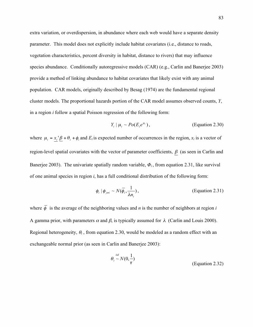
83

extra variation, or overdispersion, in abundance where each web would have a separate density

parameter. This model does not explicitly include habitat covariates (i.e., distance to roads,

vegetation characteristics, percent diversity in habitat, distance to rivers) that may influence

species abundance. Conditionally autoregressive models (CAR) (e.g., Carlin and Banerjee 2003)

provide a method of linking abundance to habitat covariates that likely exist with any animal

population. CAR models, originally described by Besag (1974) are the fundamental regional

cluster models. The proportional hazards portion of the CAR model assumes observed counts, Y,

in a region i follow a spatial Poisson regression of the following form:

)(~| ieEPoYiii

µµ , (Equation 2.30)

where iiii

x !"#µ ++= ' and Ei is expected number of occurrences in the region, xi is a vector of

region-level spatial covariates with the vector of parameter coefficients, ! (as seen in Carlin and

Banerjee 2003). The univariate spatially random variable, Φi , from equation 2.31, like survival

of one animal species in region i, has a full conditional distribution of the following form:

)1

,(~|i

iijin

N!

""" #, (Equation 2.31)

where ! is the average of the neighboring values and n is the number of neighbors at region i

A gamma prior, with parameters α and β, is typically assumed for ! (Carlin and Louis 2000).

Regional heterogeneity, θi , from equation 2.30, would be modeled as a random effect with an

exchangeable normal prior (as seen in Carlin and Banerjee 2003):

)1,0(~!

" N

iid

i

(Equation 2.32)

84

Literature Cited



91 pp.

Akenson J. J., M. G. Henjum, T. L. Wertz, and T. J. Craddock. 2001. Use of dogs and mark-

recapture techniques to estimate American black bear density in northeastern Oregon.

Ursus 12: 203-210.

Anderson, D.R., K.P. Burnham, G.C. White, and D.L. Otis. 1983. Density estimation of small-

mammal populations using a trapping web and distance sampling methods. Ecology

64:674-680.

Beausoleil, R.A. 1999. Population and spatial ecology of the Louisiana black bear in a

fragmented bottomland hardwood forest. Thesis, University of Tennessee, Knoxville.

Besag, J. 1974. Spatial interaction and the statistical analysis of lattice systems (with discussion).

Journal of the Royal Statistical Society, Series B 36: 192- 236.

Best, D. J. and N. I. Fisher. 1979. Efficient simulation of the von Mises distribution. Applied

Statistics 28: 152-157.

Boersen, M. R. 2001. Abundance and density of Louisiana black bears on the Tensas River

National Wildlife Refuge. M. S. thesis, University of Tennessee, Knoxville.

Bonin, A., E. Bellemain, P. Bronken Eidesen, F. Pompanon, C. Brochmann, and P. Taberlet.

2004. How to track and assess genotyping errors in population genetics studies.


85

Boulanger, J., B. N. McLellan, J. G. Woods, M. F. Proctor, and C. Strobeck. 2004. Sampling

design and bias in DNA-based capture-mark-recapture population and density estimates

of grizzly bears. Journal of Wildlife Management 68: 457-469.

Boulanger, J., K.C. Kendall, J. B. Stetz, D. A. Roon, L. P. Waits, and D. Paetkau. 2008a. Use of

multiple data sources to improve DNA-based mark-recapture population estimates of

grizzly bears. Ecological Applications 18: 577-589.

Boulanger, J., G. C. White, M. Proctor, G. Stenhouse, G. MacHutchon, and S. Himmer. 2008b.

Use of occupancy models to estimate the influence of past live captures on detection

probabilities of grizzly bears using DNA hair snagging methods. Journal of Wildlife


Brownstein, M., J. Carpten, and J. Smith. 1996. Modulation of non-templated nucleotide addition

by Taq DNA polymerase: primer modifications that facilitate genotyping. Biotechniques

20: 1004-1010.

Carlin, B. and S. Banerjee. 2003. Hierarchical multivariate CAR models for spatio temporally

correlated survival data. Bayesian Statistics 7: 1-18.

Carlin, B. and T. Louis. 2000. Bayes and empirical Bayes methods for data analysis. Chapman

& Hall, Florida.

Carlock, D., J. Ezell, G. Balkcom, W. Abler, P. Dupree, and D. Forster. 1999. Black bear

management plan for Georgia. Georgia Department of Natural Resources, Wildlife

Resources Division, Game Management Section, 39 pp.

Conroy, M. J., J. P. Runge, R. J. Barker, M. R. Schofield, and C. J. Fonnesbeck. 2008. Efficient

estimation of abundance for patchily distributed populations via two-phase, adaptive

sampling. Ecology 89: 3362-3370.

86

Cook, K. L. 2007. Space use and predictive habitat models for American black bears (Ursus

americanus) in central Georgia, USA. Thesis. University of Georgia, Athens, GA, USA.

Creel, Scott, G. Spong, J.L. Sands et al. 2003. Population size estimation in Yellowstone wolves

with error-prone noninvasive microsatellite genotypes. Molecular Ecology 12: 2003-

2009.

Dobey, S., D. V. Masters, B. K. Scheik, J. D. Clark, M. R. Pelton, and M. E. Sunquist. 2005.

Ecology of Florida black bears in the Okefenokee-Osceola Ecosystem. Wildlife


Don. R.H., P. T. Cox, B. J. Wainwright, K. Baker, and J. S. Mattick. 1991. ‘Touchdown’ PCR to

circumvent spurious priming during gene amplification. Nucleic Acids Research 19:

4008.

Evett, I. W., and B. S. Weir. 1998. Interpreting DNA evidence: Statistical Genetics for Forensic

Scientists. Sinauer Associates, Sunderland, MA.

Fremont, A. D. and G. J. Steil. 1986. Foot snare live trap. Patent No. 4581843. USA.

Garshelis, D. L., and L. G. Visser. 1997. Enumerating megapopulations of wild bears with an

ingested biomarker. Journal of Wildlife Management 61: 466-480.

Garshelis, D. L., A. R. Joshi, J. L. D. Smith, and C. G. Rice. 1999. Sloth bear conservation

action plan (Melursus ursinus). Pages 225-240 in C. Servheen, S. Herrero, and B. Peyton,

compilers. Bears. Status survey and conservation action plan. IUCN/SSC Bear and Polar

Bear Specialist Groups, IUCN- The World Conservation Union, Gland, Switzerland.

Gelman, A., J. B. Carlin, H. S. Stern, and D. B. Rubin. 2004. Bayesian data analysis, 2nd edition.

Chapman & Hall, New York.

87

Geman, S. and D. Geman. 1984. Stochastic relaxation, Gibbs distributions, and the Bayesian

restoration of images. IEEE Transactions on Pattern Analysis and Machine Intelligence 6:

721-741.

Goossens, B., L.P. Waits, and P. Taberlet. 1998. Plucked hair samples as a source of DNA:

reliability of dinuccleotide microsatellite genotyping. Molecular Ecology 7: 1237-1241.

Goudet, J. 1995. FSTAT (version 1.2): a computer program to calculate F-statistics. Journal of

Heredity 86: 6.




Green, P. J. 1995. Reversible jump Markov chain Monte Carlo computation and Bayesian model

determination. Biometrika 82: 711-732.

Grogan, R. G. and F. G. Lindzey. 1999. Estimating population size of a low-density black bear

population using capture-resight. Ursus 11: 117-122.

Hastings, W. K. 1970. Monte Carlo sampling methods using Markov chains and their

applications. Biometrika 57: 97-109.

Hellgren, E. C. and M. R. Vaughn. 1989. Demographic analysis of a black bear population in


Kalinowski, S.T., M.L. Taper, and S. Creel. 2006. Using DNA from non-invasive samples to

identify individuals and census populations: and evidential approach tolerant of

genotyping errors. Conservation Genetics 7: 319-329.

88

Kendall, K.C., J.B. Stetz, D. A. Roon, L. P. Waits, J. B. Boulanger. and D. Paetkau. 2008.

Grizzly bear density in Glacier National Park, Montana. Journal of Wildlife Management

72: 1693-1705.

Kendall, K. C., J. B. Stetz, J. Boulanger, A. C. Macleod, D. Paetkau, and G. C. White. 2009.

Demography and genetic structure of a recovering grizzly bear population. Journal of

Wildlife Management 73: 3-17.

Kenward, R. 1987. Wildlife Radio Tagging: equipment, field techniques, and data analysis.

Academic Press, New York.

Lindahl, T. 1993. Instability and decay of the primary structure of DNA. Nature 362: 709-715.

Lucchini, V., E. Gabbri, F. Marucco, S. Ricci, L. Biotani, and E. Randi. 2002. Noninvasive

molecular tracking of colonizing wolf (Canis lupus) packs in the western Italian Alps.

Molecular Ecology 11: 857-868.

Lukacs, P. M. and K.P. Burnham. 2005. Estimating population size from DNA-based closed

capture-recapture data incorporating genotyping error. Journal of Wildlife Management

68: 439-448.

Mace, R. D., S. C. Minta, T. L. Manley, and K. E. Aune. 1994. Estimating grizzly bear

population size using camera sightings. Wildlife Society Bulletin 22: 74-83.

MacKenzie, D. I., J. D. Nichols, J. A. Royle, K. H. Pollock, L. L. Bailey, and J. E. Hines. 2006.

Occupancy estimation and modeling, inferring patterns and dynamics of species

occurrence. Elsevier Inc., New York.

Marshall, T. C., J. Slate, L.E.B. Kruuk, and J. M. Pemberton. 1998. Statistical confidence for

likelihood-based paternity inference in natural populations. Molecular Ecology 7: 639-

655.

89



McKelvey, K. and M. Schwartz. 2004. Genetic errors associated with population estimation

using noninvasive molecular tagging: problems and new solutions. Journal of Wildlife


McLean, P. K. and M. R. Pelton. 1994. Estimates of population density and growth of black

bears in the Smoky Mountains. International Conference on Bear Research and


Metropolis, N., A. W. Rosenbluth, M. N. Rosenbluth, A. H. Teller, and E. Teller. 1953.

Equation of state calculations by fast computing machines. Journal of Chemical Physics

21: 1087-1092.

Metropolis, N. and S. Ulam. 1949. The Monte Carlo method. Journal of the American Statistical

Association 44: 335-341.

Miller, D. S., G. C. White, R. A. Sellers, H. V. Reynolds, J. W. Schoen, K. Titus, V. G. Barnes,

Jr., R. B. Smith, R. R. Nelson, W. B. Ballard, and C. C. Swartz. 1997. Brown and black

bear density estimation in Alaska using radio telemetry and replicated mark-resight

techniques. Wildlife Monographs 133.

Mowat, G. and C. Strobeck. 2000. Estimating population size of grizzly bears using hair

capture, DNA profiling, and mark-recapture analysis. Journal of Wildlife Management

64: 183-193.

Otis, D. L., K. P. Burnham, G. C. White, and D. R. Anderson. 1978. Statistical inference from

capture data on closed animal populations. Wildlife Monographs 62: 1-135.

90

Paetkau, D., W. Calvert, I. Stirling, and C. Strobeck. 1995. Microsatellite analysis of population

structure in Canadian polar bears. Molecular Ecology 4: 347-354.

Paetkau, D. 2003. An empirical exploration of data quality in DNA-based population inventories.




Petit, E. and N. Valière. 2006. Estimating population size with noninvasive capture-mark-

recapture data. Conservation Biology 20: 1062-1073.

Piggott, M. P. and A. C. Taylor. 2003. Remote collection of animal DNA and its applications in

conservation management and understanding the population biology of rare and cryptic

species. Wildlife Research 30: 1-13.

Piggott, M. P. 2004. Effect of sample age and season of collection on the reliability of

microsatellite genotyping of faecal DNA. Wildlife Research 31: 485-493.

Pollock, K. H. 1974. The assumption of equal catchability of animals in tag-recapture

experiments. Ph.D. Thesis, Cornell University, Ithaca, NY.

Pollock, K. H. 1982. A capture-recapture design robust to unequal probability of capture.


Raymond, M. and F. Rousset. 1995. GENEPOP (version 1.2): population genetics software for

exact tests and ecumenisism. Journal of Heredity 86: 248-249.

Rice, W. R. 1989. Analyzing tables of statistical tests. Evolution 43: 223-225.

Roon, D. A., L. P. Waits, and K. C. Kendall. 2003. A quantitative evaluation of two methods for

preserving hair samples. Molecular Ecology Notes 3: 163-166.

91

Royle, J. A. and R. M. Dorazio. 2008. Hierarchical modeling and inference in ecology. Elsevier

Ltd., Boston.

Royle, J. A. And J. D. Nichols. 2003. Estimating abundance from repeated presence-absence

data or point counts. Ecology 84: 777-790.

Sanderlin, J. Skvarla, B. Faircloth, B. Shamblin, and M. Conroy. 2009. Tetranucleotide

microsatellite loci from the black bear (Ursus americanus). Molecular Ecology

Resources 9: 288-291.

Sanderlin, J. S. 2009. Misidentification error in non-invasive genetic mark-recapture sampling:

case study with the central Georgia black bear population. Thesis. University of

Georgia, Athens, GA, USA.



Taberlet, P. ,S. Griffen, B. Goossens, S. Questiau, V. Manceau, N. Escaravage, L. P. Waits and J.

Bouvet. 1996. Reliable genotyping of samples with very low DNA quantities using PCR.

Nucleic Acids Research 24: 3189-3194.

Taberlet, P., L.P. Waits, G. Luikart. 1999. Noninvasive genetic sampling: look before you leap.

Trends in Ecology and Evolution 14:323-327.

Tanner, M. A. and W. H. Wong. 1987. The calculation of posterior distributions by data

augmentation. Journal of the American Statistical Association 82: 528-540.

Waits, L.P. 1999. Molecular genetic applications for bear research. Ursus 11:253-260.

Waits, J. L. and P. L. Leberg. 2000. Biases associated with population estimation using

molecular tagging. Animal Conservation 3:191-199.

92

Waits, L. P., G. Luikart, and P. Taberlet. 2001. Estimating the probability of identity among

genotypes in natural populations: cautions and guidelines. Molecular Ecology 10: 249-

256.

Warrillow, J., M. Culver, E. Hallerman, and M. Vaughan. 2001. Subspecific affinity of black

bears in the White River National Wildlife Refuge. The Journal of Heredity 92: 226-233.

White, G. C., D. R. Anderson, K. P. Burnham, and D. L. Otis. 1982. Capture-recapture removal

methods for sampling closed populations. Los Alamos Natl. Lab. Publ. LA-8787-NERP.

Los Alamos, NM.

White, G. C. and R. A. Garrott. 1990. Analysis of wildlife radio-tracking data. Academic Press,

San Diego, California.

Willey, C. H. 1974. Aging black bears from first premolar tooth sections. Journal of Wildlife


Woods, J.G., D. Paetkau, D. Lewis, B.N. McLellan, M. Proctor, and C. Strobeck. 1999. Genetic

tagging of free-ranging black and brown bears. Wildlife Society Bulletin 27:616-627.

Wright, J. A., R. J. Barker, M. R. Schofield, A. C. Frantz, A. E. Byrom and D. M. Gleeson. 2009.

Incorporating genotype uncertainity into mark-recapture-type models for estimating

abundance using DNA samples. Biometrics. DOI: 10.1111/j.1541-0420.2008.01167.

93

Table 2.1. Percent of vegetation type for each web for the American black bear central Georgia population from 2004 to 2006 based

on 30m x 30m resolution.

* indicates dominant vegetation type, ** indicates second dominant vegetation type, # indicates third dominant vegetation type

Web A B C D E F G H I

Open water 0.0008 0.000109 0.009818 0.00248 0.004416 0.002243 0.004386 0.013868 0.000117

Transportation 0.0844 0.068481 0.061705 0.047919 0.026865 0.067476 0.066199 0.066842 0.058934

Utility swaths 0.0023 0 0 0.018007 0 0.017347 0.012147 0.028983 0.013915

Clearcut #0.1530 #0.127398 0.061979 #0.113349 0.035083 0.105204 0.112153 0.065178 #0.080917

Deciduous 0.1216 0.081926 0.02545 0.053723 0.056428 0.066882 0.082327 0.057412 0.040926

Evergreen *0.4025 *0.45543 *0.427326 **0.287465 *0.499387 *0.430051 **0.28315 *0.387602 *0.657858

Mixed forest 0.0537 0.122588 #0.083041 0.021082 **0.171001 **0.239958 *0.312639 **0.259603 0.041394

Pasture/hay 0 0 0 0 0.004416 0.006992 0.005398 0.001387 0

Row crop 0.0005 0.000492 0.069493 0.006945 0.096663 0.063848 0.121601 #0.119124 0.00152

Forested

Wetland **0.1809 **0.14292 **0.261079 *0.44903 #0.105741 #0.158565 #0.256967 0.06601 **0.10442

94

Table 2.2. Slope summary statistics (range, mean, standard deviation) for each web for the

American black bear central Georgia population from 2004 to 2006.


Range 13.5613 10.5547 10.9184 14.4636 8.2430 12.3128 11.6261 7.3924 10.0887

Mean 3.8165 2.4685 2.3323 1.7850 2.1287 2.8475 3.1347 1.7651 3.3189

sd 2.0783 1.5919 1.4755 2.2143 1.7253 1.8387 2.2211 1.1838 1.8901

95

Table 2.3. DEM (digital elevation model) in meters above sea level for each web for the

American black bear central Georgia population from 2004 to 2006 summary statistics (range,

mean, standard deviation).


Range 70.9454 56.4680 52.6306 52.6458 55.8992 54.6838 66.7063 42.0025 67.2368

Mean 119.2861 96.6152 91.6718 77.7615 119.9789 93.0943 99.7679 100.7098 113.5859

sd 16.6140 10.9320 13.0387 12.7276 12.0218 11.4467 16.1277 8.0271 17.5940

96

Table 2.4. Summary of web area, rings, spacing between rings, average number of snares per

web for years 2004 to 2006 for the American black bear central Georgia population, and average

approximate density of snares per web.

Web

Area

(km2) Rings

Spacing between

rings (m)

Average number of

snares/web

Average density of snares

(snares/km2

A 12.6 4 500 35 2.778

B 15.9 3 750 26.4 1.66

C 15.9 3 750 23.3 1.46

D 15.9 3 750 25.3 1.59

E 7.1 3 500 24 3.38

F 15.9 3 750 22.5 1.42

G 15.9 3 750 25.5 1.6

H 7.1 3 500 22 3.1

I 7.1 3 500 26 3.66

97

Table 2.5. Summary of webs for the American black bear central Georgia population from 2004

to 2006 used for telemetry error calculations. Each cell represents the number of observers for

each web and year combination. Cells marked with ‘*’ indicated web and year combinations in

which telemetry error calculations for observers were not conducted.

Web 2004 2005 2006

A * 4 3

B 3 4 3

C * 3 3

D * 3 3

E 3 * *

F 3 3 3

G * * *

H * * *

I * 4 3

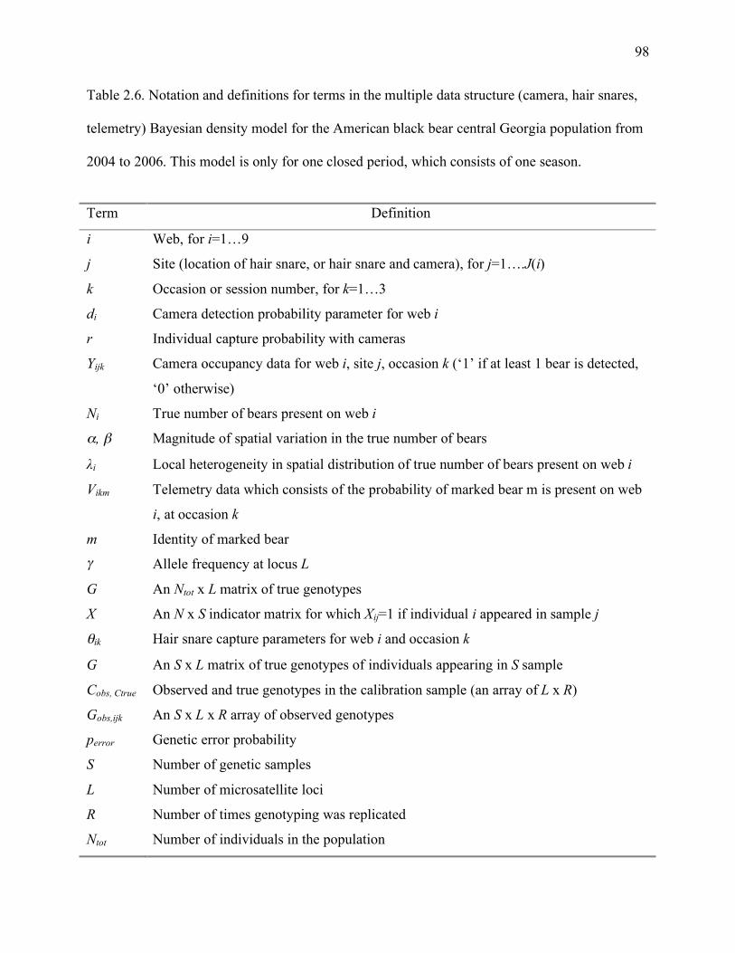
98

Table 2.6. Notation and definitions for terms in the multiple data structure (camera, hair snares,

telemetry) Bayesian density model for the American black bear central Georgia population from

2004 to 2006. This model is only for one closed period, which consists of one season.

Term Definition

i Web, for i=1…9

j Site (location of hair snare, or hair snare and camera), for j=1….J(i)

k Occasion or session number, for k=1…3

di Camera detection probability parameter for web i

r Individual capture probability with cameras

Yijk Camera occupancy data for web i, site j, occasion k (‘1’ if at least 1 bear is detected,

‘0’ otherwise)

Ni True number of bears present on web i

α, β Magnitude of spatial variation in the true number of bears

λi Local heterogeneity in spatial distribution of true number of bears present on web i

Vikm Telemetry data which consists of the probability of marked bear m is present on web

i, at occasion k

m Identity of marked bear γ Allele frequency at locus L

G An Ntot x L matrix of true genotypes

X An N x S indicator matrix for which Xij=1 if individual i appeared in sample j

θik Hair snare capture parameters for web i and occasion k

G An S x L matrix of true genotypes of individuals appearing in S sample

Cobs, Ctrue Observed and true genotypes in the calibration sample (an array of L x R)

Gobs,ijk An S x L x R array of observed genotypes

perror Genetic error probability

S Number of genetic samples

L Number of microsatellite loci

R Number of times genotyping was replicated

Ntot Number of individuals in the population

99

Table 2.7. Hair snare data summary for the American black bear central Georgia population from

2003 to 2006.

Year Seasons Webs Snares Hair

Samples1

No.of snare

sessions2

Snares w/ hair

detected

2003 1 (F/W) 1 27 134 121 48

2004 2 (S, F) 11 282 927 837 246

2005 2 (S, F) 14 362 1929 1081 561

2006 1 (S) 6 159 1190 477 258

TOTAL 6 32 830 4180 2516 1113

1 Some samples may contain feral hog hair, thus bear hair samples may be fewer. Not all

samples were analyzed within the laboratory.

2 Some snares were not able to be sampled for all 3 sessions due to river flooding or

controlled burns, therefore the number of snares x 3 does not always equal the number of

snare sessions

100

Table 2.8. American black bear central Georgia population genetic data for assessment of genetic error from allelic dropout. Samples

were collected from 2003 to 2006. Tissue and hair samples from known individuals (n=85) from the calibration sample data set were

used to supplement replicate hair snare samples for each year by season combination, originally in described in Sanderlin (2009).

Heterozygous samples with the first replicate and numbers of homozygous samples with the second replicate were used as a sample of

allelic dropout from unknown hair samples.

Number of heterozygous samples Number of homozygous samples

Locus Bear

10Y

Bear

12Y

Bear

17G

Bear

19Y

Bear

30B

Bear

33B

Bear

35G

Bear

36

Bear

10Y

Bear

12Y

Bear

17G

Bear

19Y

Bear

30B

Bear

33B

Bear

35G

Bear

36

Calibration

samples 35 36 51 42 46 46 42 37 1 0 1 0 1 2 1 0

2004 Summer 3 7 12 14 8 10 13 9 1 2 1 0 2 2 4 4

2004 Fall 4 4 6 6 6 7 10 3 1 2 1 2 0 1 1 1

2005 Summer 12 10 17 11 9 12 16 13 2 3 2 6 1 4 2 9

2005 Fall 2 4 8 6 4 7 7 7 0 0 1 0 0 1 0 3

2006 Summer 9 7 13 12 13 11 12 9 0 0 0 0 0 2 0 3

Total 65 68 107 91 86 93 100 78 5 7 6 8 4 12 8 20

101

Table 2.9. Camera data summary for the American black bear central Georgia population from

2003 to 2006.

Year Cameras on webs No. of Camera Sessions1 Cameras w/detections

2003 14 42 6

2004 59 176 23

2005 78 224 115

2006 30 88 36

TOTAL 181 530 180

1 Some cameras were not operational for all 3 sessions due to equipment failure, camera

availability, or bear damage; therefore, the number of cameras x 3 does not always equal the

number of camera sessions

102

Table 2.10. Live captures, recaptures and recoveries of American black bears with the central Georgia population from 2003 to 2008.

Note: this summary includes the Sandersville male (2005) and North Carolina female (2003), 3 untagged male bears (2003, 2004), 1

untagged female bear (2006), and 2 capture mortalities (1 initial capture in 2004, 1 recapture in 2004).

Year Number of Live Captures

Number of Recaptures Number of Recoveries

2003 initial capture 2004 initial capture 2005 initial capture 2006 initial capture

Total Male Female Total Male Female Male Female Male Female Male Female Total Male Female

2003 30 18 12 2 1 1 0 0 0 0 0 0 1 1 0

2004 19 13 6 7 3 2 1 1 0 0 0 0 2 2 0

2005 15 7 8 5 1 2 2 0 0 0 0 0 6 5 1

2006 20 15 5 2 0 0 1 0 1 0 0 0 2 2 0

2007 0 0 0 0 0 0 0 0 0 0 0 0 2 2 0

2008 0 0 0 0 0 0 0 0 0 0 0 0 1 0 1

TOTAL 84 53 31 16 5 5 4 1 1 0 0 0 14 12 2

103

Table 2.11. Number of alleles (A), individuals analyzed at each locus (N), number of

heterozygotes (Nhet) and homozygotes (Nhom), observed heterozygosity (HO), expected

heterozygosity (HE), and p-value for Hardy-Weinberg Equilibrium (HWE) test for the American

black bear central Georgia population with known individuals (n=83) collected from samples

from 2003 to 2006 with the Paetkau markers. Locus G10C did not amplify with any individuals,

so data from this locus are not included in the table. A p-value for HWE cannot be calculated

with monomorphic loci (G1D and G10P), marked with ‘NA’.

Locus A N Nhet Nhom HO HE

HWE p-value

G1A 4 82 57 25 0.695 0.676 0.623

G1D 1 82 0 82 0 0 NA

G10B 3 81 38 43 0.469 0.393 0.188

G10L 3 82 41 41 0.500 0.570 0.423

G10M 3 24 4 20 0.167 0.542 0.0001*

G10P 1 78 0 78 0 0 NA

G10X 3 68 29 39 0.426 0.514 0.023

* indicates significance after Bonferroni correction

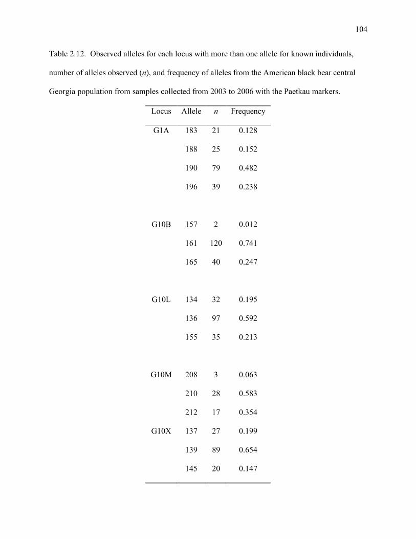
104

Table 2.12. Observed alleles for each locus with more than one allele for known individuals,

number of alleles observed (n), and frequency of alleles from the American black bear central

Georgia population from samples collected from 2003 to 2006 with the Paetkau markers.

Locus Allele n Frequency

G1A 183 21 0.128

188 25 0.152

190 79 0.482

196 39 0.238

G10B 157 2 0.012

161 120 0.741

165 40 0.247

G10L 134 32 0.195

136 97 0.592

155 35 0.213

G10M 208 3 0.063

210 28 0.583

212 17 0.354

G10X 137 27 0.199

139 89 0.654

145 20 0.147

105

Table 2.13. Number of alleles (A), number of individuals analyzed (N), number of heterozygotes

(Nhet) and homozygotes (Nhom) for the American black bear central Georgia population with

individuals (n=84) from known tissue samples from 2003 to 2006 with the Sanderlin et al.

(2009) tetranucleotide markers.


HWE p-value

Bear10Y 5 84 41 43 0.488 0.454 0.871

Bear12Y 3 84 48 36 0571 0.603 0.221

Bear17G 4 81 58 23 0.716 0.672 0.748

Bear19Y 4 80 48 32 0.600 0.658 0.225

Bear30B 4 84 53 31 0.631 0.612 0.924

Bear33B 4 82 52 30 0.634 0.631 0.795

Bear35G 4 83 47 36 0.566 0.532 0.462

Bear36 2 84 46 38 0.548 0.503 0.513

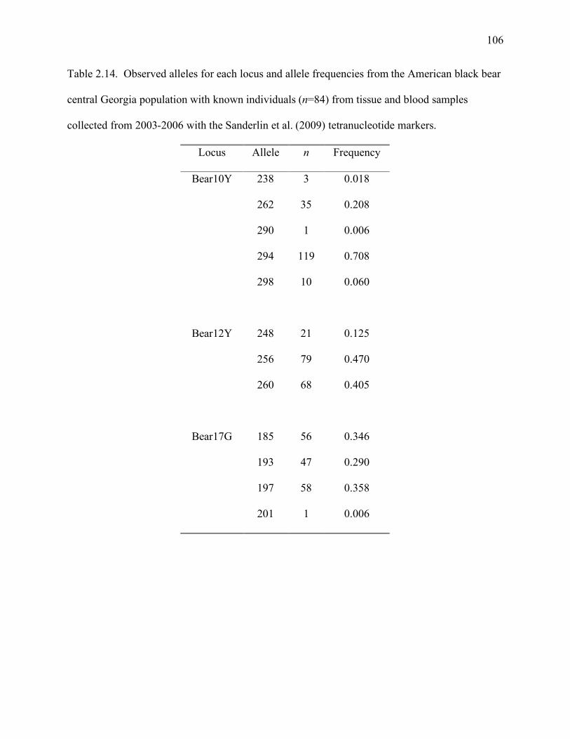
106

Table 2.14. Observed alleles for each locus and allele frequencies from the American black bear

central Georgia population with known individuals (n=84) from tissue and blood samples

collected from 2003-2006 with the Sanderlin et al. (2009) tetranucleotide markers.


Bear10Y 238 3 0.018

262 35 0.208

290 1 0.006

294 119 0.708

298 10 0.060

Bear12Y 248 21 0.125

256 79 0.470

260 68 0.405

Bear17G 185 56 0.346

193 47 0.290

197 58 0.358

201 1 0.006

107



Bear19Y 356 34 0.213

359 2 0.013

371 65 0.406

375 58 0.369

Bear 30B 439 47 0.280

443 27 0.161

447 90 0.536

451 4 0.024

Bear 33B 272 83 0.506

286 51 0.311

292 22 0.134

302 8 0.049

Bear 35G 216 1 0.006

220 30 0.181

224 106 0.639

228 29 0.175

Bear 36 198 82 0.488

207 86 0.512

108

Table 2.15. Number of hair snare genetic samples with data at all 8 loci for the America black

bear central Georgia population from 2003 to 2006.

Web1

Year/Season A B C D E F G H I Total

2003 Fall 17 - - - - - - - - 17

2004 Summer 33 5 - - 7 - 19 - 6 70

2004 Fall - 7 1 7 0 20 - 3 - 38

2005 Summer 28 10 3 4 - 16 9 11 20 101

2005 Fall 16 9 1 14 - 13 - - 21 74

2006 Summer 42 35 1 7 - 32 - - 28 145

Total 136 66 6 32 7 81 28 14 75 445

1 Webs that were not sampled during the year and season combination are marked with a ‘-‘.

109

Table 2.16. Number of unique individuals detected with genetic hair samples at all 8 loci for the

American black bear central Georgia population from 2003 to 2006.

Web1

Year/Season A B C D E F G H I Total

2003 Fall 14 - - - - - - - - 14

2004 Summer 21 5 - - 6 - 8 - 5 45

2004 Fall - 5 1 5 0 11 - 2 - 24

2005 Summer 14 8 3 4 - 14 8 5 10 66

2005 Fall 11 6 1 4 - 9 - - 9 40

2006 Summer 18 12 1 5 - 20 - - 9 65

Total 78 36 6 18 6 54 16 7 33 254

1 Webs that were not sampled during the year and season combination are marked with a ‘-‘.

110

Table 2.17. Minimum Known Alive in the American black bear central Georgia population from

2003 to 2007.

Year (date) Number

radiocollared

1

Number

censored1,2

Mortalities1,2 Total Other3 Total

Known

(alive+dead)

Minimum

Known

Alive

2003 (9/1) 25 3 0 5 30 26

2004 (9/1) 31 10 3 1 35 32

2005 (9/1) 26 17 5 9 40 26

2006 (9/1) 29 16 1 4 34 29

2007 (5/15) 21 5 2 2 25 21

1 This summary includes the Sandersville male nuisance mortality, Altanta female and 2 capture

mortalities (1 initial capture, 1 recapture)

2 Number of censored and mortalities of bears with radiocollars indicates the number of bears

censored from collar drops or lost collar and/or any mortality since the previous date and year (or

the start of the study for the first record)

3 Unmarked, but known-fate bears from capture mortalities, vehicle collisions, illegal harvest,

and legal harvest. There are 2 captures of bears that were unmarked, but alive included in this

column: a male bear in 2003 (9/1) (B-00) and a male bear in 2004 (9/1) (B-30).

111

Table 2.18. Number of alleles (A), number of individuals analyzed (N), number of heterozygotes

(Nhet) and homozygotes (Nhom) for the American black bear central Georgia population with

individuals (n=184 unique individuals) from observed hair samples collected at hair snares from

2003 to 2006 with the Sanderlin et al. (2009) tetranucleotide markers.


HWE p-value

Bear10Y 8 184 85 99 0.462 0.434 0.092

Bear12Y 4 184 113 71 0.614 0.607 0.104

Bear17G 8 184 122 62 0.663 0.684 0.004*

Bear19Y 4 184 113 71 0.614 0.659 0.059

Bear30B 4 184 104 80 0.565 0.594 0.522

Bear33B 7 184 100 84 0.543 0.616 <0.001*

Bear35G 4 184 112 72 0.609 0.532 0.084

Bear36 4 184 93 91 0.505 0.496 <0.001*

• indicates significance after Bonferroni correction

112

Table 2.19. Observed alleles for each locus and allele frequencies from the American black bear

central Georgia population with unique individuals (n=184) from observed hair samples

collected at hair snares from 2003-2006 with the Sanderlin et al. (2009) tetranucleotide markers.


Bear10Y 217 2 0.0054

238 11 0.0299

262 64 0.1739

270 2 0.0054

286 1 0.0027

290 5 0.0136

294 269 0.7310

298 14 0.0380

Bear12Y 248 48 0.1304

252 4 0.0109

256 133 0.3614

260 183 0.4973

Bear17G 181 2 0.0054

185 122 0.3315

189 1 0.0027

193 121 0.3288

197 116 0.3152

201 3 0.0082

113

Table 2.19. (continued)


Bear 17G 205 1 0.0027

213 2 0.0054

Bear19Y 356 91 0.2473

359 2 0.0054

371 149 0.4049

375 126 0.3424

Bear30B 439 112 0.3043

443 55 0.1495

447 199 0.5408

451 2 0.0054

Bear33B 268 4 0.0109

270 7 0.0190

272 201 0.5462

274 3 0.0082

286 97 0.2636

292 47 0.1277

302 9 0.0245

114



Bear35G 216 2 0.0054

220 82 0.2228

224 233 0.6332

228 51 0.1386

Bear 36 191 8 0.0054

198 215 0.5842

202 2 0.0054

207 149 0.4049

115

Table 2.20. Parameter median, lower and upper 95% BCI for summer 2004 of the American

black bear central Georgia population.

Parameter Median 95% Lower BCI 95% Upper BCI

p 0.052 0.034 0.076

Ntot 213 144 354

r 0.009 0.004 0.019

θ 0.224 0.128 0.337

λ 15.255 9.895 25.382

N1 27 21 39

N2 9 5 19

N3 15 7 29

N4 15 7 29

N5 10 4 21

N6 15 7 29

N7 17 12 30

N8 15 7 29

N9 12 6 24

N10 15 7 29

N11 15 7 29

N12 15 7 29

N13 15 7 29

N14 15 7 29

116

Table 2.20. (continued) Parameter median, lower and upper 95% BCI for summer 2004 of the

American black bear central Georgia population.


d0 0.228 0.118 0.379

d1 0.084 0.038 0.162

d4 0.089 0.038 0.175

d6 0.156 0.078 0.269

d8 0.107 0.047 0.207

pw,1 0.132 0.085 0.197

pw,2 0.046 0.020 0.085

pw,3 0.073 0.032 0.129

pw,4 0.073 0.031 0.129

pw,5 0.049 0.020 0.090

pw,6 0.073 0.031 0.129

pw,7 0.126 0.081 0.190

pw,8 0.073 0.032 0.130

pw,9 0.065 0.032 0.112

pw,10 0.073 0.032 0.130

pw,11 0.073 0.032 0.130

pw,12 0.073 0.031 0.130

pw,13 0.073 0.032 0.129

pw,14 0.073 0.032 0.129

117

Table 2.21. Parameter median, lower and upper 95% BCI for fall 2004 of the American black

bear central Georgia population.


p 0.039 0.023 0.062

Ntot 106 72 179

r 0.015 0.007 0.029

θ 0.213 0.119 0.324

λ 7.590 4.823 13.064

N1 8 2 16

N2 10 7 17

N3 4 2 10

N4 9 7 16

N5 2 0 8

N6 13 10 20

N7 7 2 16

N8 6 4 12

N9 8 2 16

N10 8 2 16

N11 8 2 16

N12 8 2 16

N13 7 2 16

N14 8 2 16

118

Table 2.21. (continued) Parameter median, lower and upper 95% BCI for fall 2004 of the



d2 0.141 0.069 0.255

d3 0.063 0.024 0.136

d4 0.136 0.067 0.243

d5 0.030 0.000 0.101

d6 0.175 0.089 0.302

d8 0.090 0.041 0.180

pw,1 0.075 0.021 0.158

pw,2 0.130 0.075 0.209

pw,3 0.045 0.014 0.098

pw,4 0.127 0.072 0.206

pw,5 0.021 0.002 0.068

pw,6 0.128 0.073 0.205

pw,7 0.075 0.021 0.159

pw,8 0.081 0.039 0.146

pw,9 0.075 0.021 0.158

pw,10 0.075 0.021 0.159

pw,11 0.075 0.020 0.157

pw,12 0.075 0.021 0.158

pw,13 0.075 0.021 0.157

pw,14 0.075 0.021 0.158

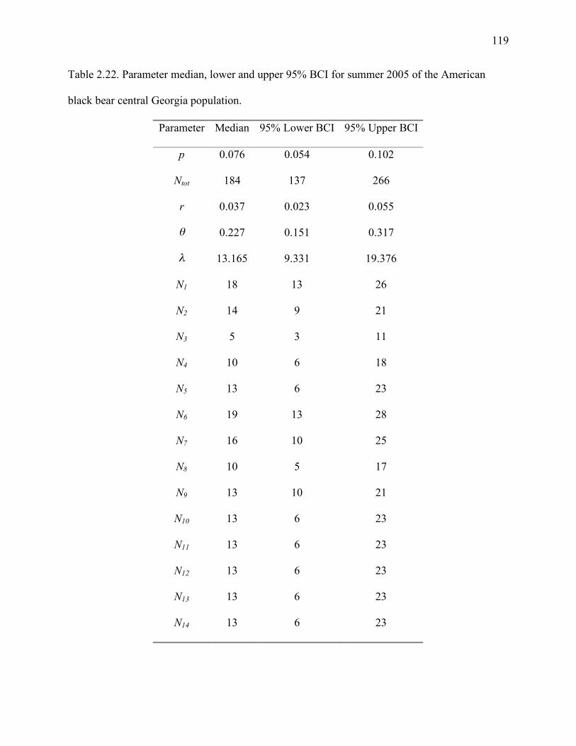
119




p 0.076 0.054 0.102

Ntot 184 137 266

r 0.037 0.023 0.055

θ 0.227 0.151 0.317

λ 13.165 9.331 19.376

N1 18 13 26

N2 14 9 21

N3 5 3 11

N4 10 6 18

N5 13 6 23

N6 19 13 28

N7 16 10 25

N8 10 5 17

N9 13 10 21

N10 13 6 23

N11 13 6 23

N12 13 6 23

N13 13 6 23

N14 13 6 23

120




d0 0.492 0.373 0.617

d1 0.396 0.277 0.532

d2 0.186 0.106 0.309

d3 0.307 0.201 0.449

d5 0.508 0.368 0.657

d6 0.443 0.312 0.592

d7 0.297 0.171 0.454

d8 0.395 0.274 0.545

pw,1 0.141 0.093 0.204

pw,2 0.101 0.060 0.154

pw,3 0.030 0.010 0.065

pw,4 0.079 0.044 0.128

pw,5 0.073 0.030 0.134

pw,6 0.122 0.076 0.182

pw,7 0.116 0.071 0.174

pw,8 0.058 0.027 0.104

pw,9 0.115 0.071 0.174

pw,10 0.074 0.029 0.134

pw,11 0.074 0.029 0.134

121




pw,12 0.074 0.029 0.134

pw,13 0.074 0.029 0.134

pw,14 0.073 0.030 0.134

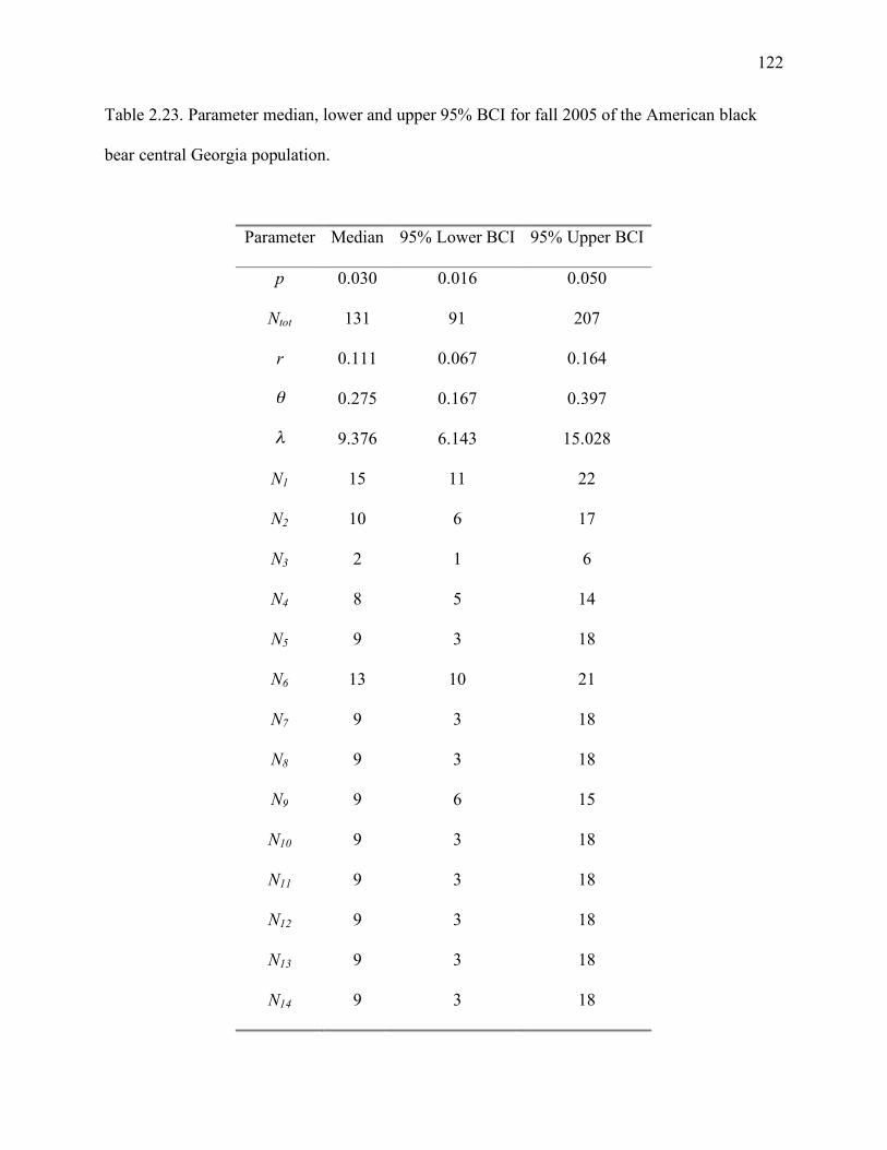
122

Table 2.23. Parameter median, lower and upper 95% BCI for fall 2005 of the American black

bear central Georgia population.


p 0.030 0.016 0.050

Ntot 131 91 207

r 0.111 0.067 0.164

θ 0.275 0.167 0.397

λ 9.376 6.143 15.028

N1 15 11 22

N2 10 6 17

N3 2 1 6

N4 8 5 14

N5 9 3 18

N6 13 10 21

N7 9 3 18

N8 9 3 18

N9 9 6 15

N10 9 3 18

N11 9 3 18

N12 9 3 18

N13 9 3 18

N14 9 3 18

123

Table 2.23. (continued) Parameter median, lower and upper 95% BCI for fall 2005 of the



d0 0.821 0.694 0.914

d1 0.684 0.526 0.822

d2 0.231 0.101 0.425

d3 0.588 0.417 0.754

d5 0.786 0.638 0.901

d8 0.637 0.496 0.773

pw,1 0.163 0.103 0.246

pw,2 0.094 0.051 0.157

pw,3 0.026 0.007 0.063

pw,4 0.073 0.035 0.130

pw,5 0.075 0.024 0.147

pw,6 0.122 0.071 0.193

pw,7 0.074 0.024 0.147

pw,8 0.074 0.024 0.148

pw,9 0.080 0.040 0.139

pw,10 0.075 0.024 0.148

pw,11 0.074 0.024 0.148

pw,12 0.074 0.024 0.148

pw,13 0.075 0.025 0.148

pw,14 0.074 0.024 0.148

124




p 0.027 0.014 0.045

Ntot 192 143 280

r 0.040 0.024 0.060

θ 0.308 0.206 0.413

λ 13.729 9.782 20.413

N1 21 17 30

N2 15 11 23

N3 3 1 8

N4 9 6 16

N5 14 6 24

N6 20 16 28

N7 14 6 24

N8 14 6 24

N9 13 8 22

N10 14 6 24

N11 14 6 24

N12 14 6 24

N13 14 6 24

N14 14 6 24

125




d0 0.583 0.434 0.727

d1 0.470 0.336 0.611

d2 0.111 0.038 0.246

d3 0.302 0.194 0.440

d5 0.563 0.415 0.706

d8 0.410 0.259 0.585

pw,1 0.175 0.119 0.247

pw,2 0.097 0.059 0.151

pw,3 0.017 0.003 0.047

pw,4 0.067 0.035 0.112

pw,5 0.074 0.030 0.133

pw,6 0.137 0.088 0.202

pw,7 0.073 0.031 0.133

pw,8 0.074 0.030 0.132

pw,9 0.095 0.055 0.149

pw,10 0.074 0.030 0.133

pw,11 0.073 0.030 0.133

pw,12 0.074 0.030 0.133

pw,13 0.074 0.030 0.132

pw,14 0.073 0.030 0.133

126

Figure 2.1. Hair snare locations for the American black bear central Georgia population during year 2003.

127


128


129


130

Figure 2.5. Web locations with 2004 boundaries for the American black bear central Georgia population with Gap data.

131

Figure 2.6. Web locations for the American black bear central Georgia population with DEM data (meters above sea level), 2004

boundaries.

132

Figure 2.7. Web locations with 2003 boundaries from the American black bear central Georgia

population.

A

B

C

D

E F

G

H

I

A

133

Figure 2.8. Trapping web with of 27 hair snares (located at the intersection of a circle and line)

with 3 snares at the center covering an area of 7 or 15 km2, depending on the location in the

WMAs for the American black bear central Georgia population during the years 2003 to 2006.

134

Figure 2.9. Barbed wire strands were placed 25 cm and 50 cm from the ground and baited with

corn in a plastic bottle and anise oil to collect hair snare samples from the American

black bear central Georgia population during the years 2003 to 2006.

Bait

Barbed wire

3 meters

3 meters

25 cm above ground

50 cm above ground

135

Figure 2.10. Histogram of the von Mises distribution with parameters θ=0, and κ=30.5

(n=10,000 samples). The distribution was simulated using Python, version 2.5.2 (Python

Software Foundation, http://python.org) and an algorithm for the von Mises distribution (Best

and Fisher 1979).

136

Figure 2.11. Diagram of the hierarchical model incorporating the three data structures: camera,

telemetry, and hair snare. This model is for population abundance of American black bears in the

central Georgia population for the years 2004 to 2006.

137

Figure 2.12. Initial and recapture coordinates for American central Georgia population black

bears from 2003.

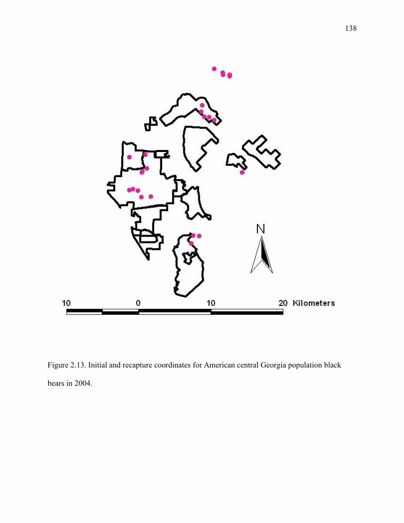
138

Figure 2.13. Initial and recapture coordinates for American central Georgia population black

bears in 2004.

139

Figure 2.14. Initial and recapture coordinates for central Georgia population American black

bears in 2005

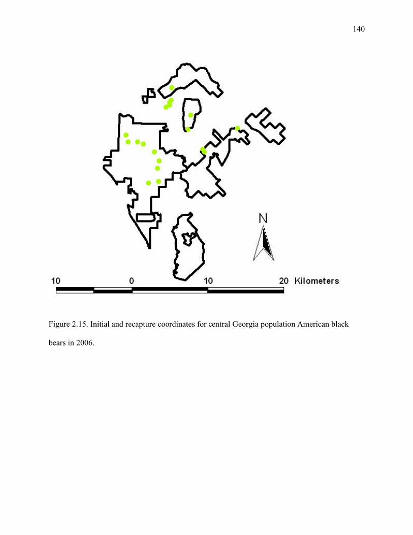
140

Figure 2.15. Initial and recapture coordinates for central Georgia population American black

bears in 2006.

141

Figure 2.16. Capture coordinates for years 2003-2006 of initial and recaptured American central Georgia population black bears.

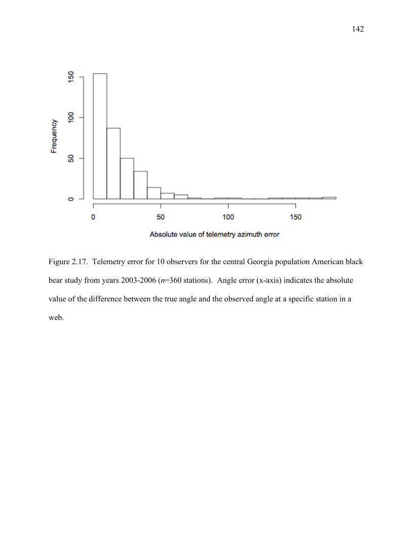
142

Figure 2.17. Telemetry error for 10 observers for the central Georgia population American black

bear study from years 2003-2006 (n=360 stations). Angle error (x-axis) indicates the absolute

value of the difference between the true angle and the observed angle at a specific station in a

web.

143

Figure 2.18. Posterior distribution of total abundance (a) and trace (b) in year 2004, summer

season for the American black bear central Georgia population from 2 chains of 50,000 MCMC

iterations (25,000 burn-in period for each chain).

a)

b)

144

Figure 2.19. Posterior distribution of total abundance (a) and trace (b) in year 2004, fall season,

for the American black bear central Georgia population from 2 chains of 50,000 MCMC


a)

b)

145


season for the American black bear central Georgia population from 2 chains of 50,000 MCMC


a)

b)

146

Figure 2.21. Posterior distribution of total abundance (a) and trace (b) in year 2005, fall season,

for the American black bear central Georgia population from 2 chains of 50,000 MCMC


a)

b)

147


season, for the American black bear central Georgia population from 2 chains of 50,000 MCMC


a)

b)

CHAPTER 3

ESTIMATION OF SURVIVAL AND REPRODUCTION DEMOGRAPHIC PARAMETERS

FOR CENTRAL GEORGIA BLACK BEARS 1

1 Sanderlin, J. S., M. J. Conroy, et al. Submit to Journal of Wildlife Management.

149

Introduction

Population viability models require information on survival and reproduction in a

population. These components provide information on the numbers of individuals that are added

or deleted from a population. The age and sex ratio of a population are also integral parts of a

population viability model. The current age distribution at the current time t, along with survival

and reproduction, predicts the future population size at time t+1. For example, consider two

populations of equal total population size and with the same survival and reproductive rates in all

age classes. One population has a higher proportion of young age classes than the other

population. The first population will have a future population size that is larger, and a larger rate

of population growth than the second population with a higher proportion of older age classes.

Age stability and stationarity analyses can be conducted, but several assumptions are necessary

(e.g., sampling probabilities are constant over time, sex, and age classes), and the data to

construct these models are often difficult to collect (Williams et al. 2002). Unbalanced sex ratios

in populations may have genetic implications based on effective population size (Caballero 1994,

Woodworth et al. 1994) and population growth (Brook et al. 2000), or be indicators of

competition for resources (Hamilton 1967, Clark 1978).

Survival

Survival estimates reported from black bear populations in the eastern United States,

specifically southeastern populations, tend to be high, with higher survival estimates in females

than males (Table 3.1). Reported causes of adult mortality include: legal harvest, illegal harvest,

vehicle collisions, nuisance mortalities, cannibalism, natural causes, research handling, and

unknown sources. Eastern black bear populations have cub survival estimates ranging between

150

62 and 75% (Wathen 1983, Smith 1985, McLean 1991). Causes of mortality for bear cubs

include: abandonment in dens, natural accidents, disease, death of the mother, vehicle collisions,

hunting, research handling of cubs (Elowe and Dodge 1989), and unique to the southeast,

drowning in tree dens and other complications from flooded habitats (Smith 1985). Of the

possible causes of cub mortality listed previously, most cases are commonly attributed to food

abundance and the nutrition of parturient females (Wathen 1983), which could cause cub

abandonment in dens, disease, and mortality of the mother. Subadult bears are more likely to

disperse from a population, and may have lower survival rates than adults. Reported mortality

rates for subadults vary between 15 to 35% annually (Bunnell and Tait 1985). In conclusion,

there are three main age classes for bears: cub, subadult, and adult. As a result of the reported

differences in mortality, for predictive population modeling, it is important to consider these

three stages of survival.

Reproduction

In the eastern part of North America, black bears often live in habitats consisting of

deciduous or mixed forests, which provide energy and nutrient-rich foods, such as berries and

mast (Bunnell and Tait 1985). The average litter sizes per study, not necessarily per year, range

from 2.15 to 2.74 from several studies, with an average of 2.42 among all the summarized

studies (reported in Bunnell and Tait 1985). In the eastern United States, specifically

southeastern populations, mean litter sizes per study range from 1.4 to 2.98 (Table 3.2). Growth

rates in the eastern United States are generally faster than western populations, ages of first

reproduction are younger, and breeding interval is about 2 years (Bunnell and Tait 1985).

151

Reported ages of first reproduction in the eastern United States, specifically southeastern

populations, range from 3 to 5.2, with mean birth intervals ranging from 2 to 2.4 (Table 3.2).

Most female bears in North Georgia do not produce litters until age 4, and average about

2.59 cubs per female every other year (Carlock et al. 1983). The female bears in the other two

populations from Georgia tend to reach an earlier age of maturity than the northern Georgia

bears. Female bears in Southeast Georgia, based on examination of reproductive tracts, have the

capability to breed at 2.5 years (Abler 1985), and litter sizes range from 1-4 cubs per sow

(

!

x =2.1) (Dobey et al. 2005).

A population viability model can be constructed from survival and reproduction estimates

with both deterministic and stochastic population models. Deterministic models require

assumptions of constant survival and reproduction over time, no environmental or demographic

stochasticity, and equal sampling probabilities over time, sex, and age classes. Demographic and

environmental stochasticity are often important components of population viability models,

because populations rarely meet all the assumptions of deterministic models. Previous chapters

have focused on abundance estimation for the central Georgia population. The population

abundance is an important component in a population viability model. However, these quantities

alone do not necessarily provide information on the viability of a population. The finite rate of

population growth per-capita λ over one year indicates if a population is increasing (λ>1),

decreasing (λ<1), or is constant (λ=1). Without additional information on other vital rates, the

reasons for the population increasing, decreasing, or remaining constant are unknown. For

example, a population may have a high abundance, but decreasing survival and low

reproduction, which may lead to an unsustainable population. Conversely, populations of

smaller population size may have high rates of survival and high reproductive output, leading to

152

a sustainable population. To properly manage populations with conservation applications or

harvest management, all vital rates should be assessed in a population viability model. The goal

of this chapter is to assess the demographic rates of survival and reproduction in the central

Georgia population, and include them in a population viability model. Given the demographic

rates and population viability analysis, an additional goal is assess the feasibility of an increase in

harvest for the black bear CGP.

Field Methods

Physical Capture

Bears were captured in the study area using Fremont foot trap snares (Fremont 1986) for

four trapping seasons (May-August). Bears were immobilized with a 2:1 mixture of ketamine

hydrochloride (Ketaset) and xylazine hydrochloride (Rompun) at a dosage for estimated body

weights by Georgia Department of Natural Resources personnel. Culvert traps were used to trap

and release nuisance bears to Oaky Woods WMA. An upper pre-molar tooth for age estimation

by cementum annuli analysis (Willey 1974), blood samples, hair follicles, and physiological data

were collected from each captured bear. Sectioning, staining, and aging of teeth were conducted

by Matson Laboratories (Milltown, Montana). All bears were uniquely marked using a

combination of collars, lip tattoos, and ear tags/streamers. Most bears were fitted with Advanced

Telemetry Systems (Isanti, MN) radio transmitter collars (VHF, very high frequency) equipped

with mortality signal sensors and motion sensors and four male bears received radio collars that

contained Global Positioning technology and a mortality switch. All collars fitted to bears during

the project were equipped with either a mechanical timer release (GPS) or a degradable release

tab (VHF).

153

Telemetry observations

Telemetry bear signals were obtained by scanning all signals with the receiver and a whip

antenna (Advanced Telemetry Systems, Isanti, MN) from vehicles. Department of Natural

Resources personnel monitored radiocollared bears at least once per week to determine the status

of bears (alive, dead, or dropped collar) from the motion and mortality sensors equipped with the

radio transmitter collars. Any radio collar with a mortality signal was located within 1-2 days

using first a whip antenna (Advanced Telemetry Systems, Isanti, MN) from vehicles to locate the

general area of the collar, and then a 3-element yagi antenna (Advance Telemetry Systems,

Isanti, MN) to determine the specific location of the collar in the field. Once the collar was

located, and a death had occurred, the cause of death was determined from visual inspection or

via necropsy. If the cause of death could not be determined, the cause was classified as

‘unknown’. The location of either the dropped collar or bear mortality was recorded with a

Garmin GPS unit (Garmin International, Inc., Olathe, KS) using Universal Transverse Mercator

(UTM) coordinates.

Dead recoveries of unmarked bears

Physiological data (e.g., age, weight, sex), when possible, were collected within 1 day

(usually immediately) of reporting for dead recovery bears from legal kills and vehicle collisions

by Georgia Department of Natural Resources personnel. Dead recoveries also included illegal

kills detected by Georgia DNR. If the fate of a bear could not be classified, the cause of death

was considered as ‘unknown’.

154

Reproduction and den observations

One method of obtaining estimates of reproduction is with female den observations.

Other methods include field counts of cubs, examining the corpora lutea or taking note of

placental scars. Georgia DNR personnel monitored female bears during the winter months for

den activity with radiotelemetry by first scanning telemetry from all radioed bears with a receiver

and whip antenna (Advanced Telemetry Systems, Isanti, MN) from vehicles, and then taking

locations with a 3-element yagi antenna (Advanced Telemetry Systems, Isanti, MN). From

February to March, visual inspection of dens was conducted by first locating the den with a whip

antenna (Advanced Telemetry Systems, Isanti, MN) from vehicles, and then a three-element yagi

antenna (Advance Telemetry Systems, Isanti, MN) was used to locate the specific location of the

den. To minimize the risk of den abandonment, personnel approached dens as quietly as

possible. Reproductive status was determined by visual observation or listening for young at den

sites.

Additional estimates of reproduction were based on data from cementum layers in the

teeth extracted from physical capture, or known-fate at encounter bears. A thinner layer, or

reduced deposition, in the tooth section is an indicator of a year during which a female black bear

successfully reared a cub(s). This has been documented for female black bears in northern

Minnesota (Rogers 1975) and central Arizona (Carrel 1980). Cementum characteristics vary

greatly among black bear populations and individuals, therefore, not all teeth can be

reconstructed for reproductive history (Matson Laboratories, Milltown, MT).

155

Statistical Analysis and Modeling

Age and Sex Ratios

Two separate medians and 95% CI and distributions of ages for females and males were

calculated from: 1) physically captured bears (including capture mortalities), and 2) known-fate

at encounter bears (i.e. illegal kills, legal kill, vehicle collisions). To determine whether the sex

ratio differed from 1:1, the z-test for comparing binomial proportions was used. Differences in

age by sex and age by weight for both sexes were tested with the nonparametric Kruskal-Wallis

test (Gottfried 1971) using the program R (R Development Core Team 2008). The median

weight and 95% CI for females and males was also calculated. The median and 95% CI and

distribution of ages for both sexes for all years (2003-2006) of physical captures were also

calculated to show any changes in age distribution within the study period. All graphics were

produced in program R (R Development Core Team 2008).

Reproduction

The median and 95% CI of the breeding interval and age of first reproduction were

calculated from cementum layers in the teeth extracted from physical captured or unmarked dead

recovery bears. The natality rate or reproduction rate (b), or the number of cubs per adult female

per year, was calculated by dividing the average litter size by the mean interval between

reproduction events, or the interbirth interval (Stringham 1980, Bunnell and Tait 1985). Since

this quantity is composed of two independent means with respective variances, the variance of

the reproduction rate with mean values can be approximated. An empirical variance was

obtained through bootstrap simulation using 500,000 iterations in a Python program, version

156

2.5.2 (Python Software Foundation, http://python.org) of litter size from a Poisson distribution

with the mean from central Georgia bears and a weighted mean from other eastern black bear

studies. A Poisson distribution is commonly used to simulate reproduction events or other forms

of count data. Next, an interval between reproduction events was simulated from a log-normal

distribution with mean and coefficient of variation (CV) from the central Georgia bears and the

weighted mean from other eastern black bear studies. A log-normal distribution ensures the

interval values will be positive, since negative intervals are impossible. We also assume a

normal distribution of intervals between reproduction events. Finally, the litter size was divided

by the interval between reproduction events. The variance of the distribution of values over the

500,000 iterations was the approximate variance used in further modeling. The weighted means

were weighted with normalized weights of sample size of the specific studies, wi, (i.e.,

!

wi

i=1

n

" =1),

calculated by:

!

x = wix

i

i=1

n

" ,

with sample standard deviation,

!

"(x ) = wi

2"i

2

i=1

n

#

Survival estimation from radiotelemetry data

Annual survival for both sexes was estimated using the Kaplan-Meier product-limit

model, allowing staggered entry and censoring (Pollock et al. 1989) with weekly time intervals.

The estimated survival function was calculated as:

157

!<

""

#

$

%%

&

'(=

taj j

j

jr

dtS

|

1)(ˆ ,

S is the probability of survival, dj is the number of deaths at time aj, rj is the number of animals

at risk at time aj, aj is a particular time of death, and t is the week after the initiation of the study

period each year (Pollock et al. 1989). Estimates of variance were calculated as:

!

var) S (t)[ ] =

) S (t)

2[ ] 1") S (t)[ ]

r(t).

Then, 95% confidence intervals were calculated from the estimated probability of survival and

its respective variance. The Kaplan-Meier estimator is based on the following assumptions: 1)

all animals were sampled randomly, 2) survival times were independent for individual animals,

3) capturing or radiocollaring animals did not influence future survival, 4) censoring mechanisms

were random, and 5) survival functions for newly marked animals were the same as for

previously marked animals (Pollock et al. 1989). The log-rank test (Pollock et al. 1989) was

used to compare overall survival rates by sex. The overall annual survival rates were calculated

using the geometric mean over all years, where

!

) S (t) is the weekly survival estimate for all weeks

in the study, and years is the total number of years for the study:

!

) S year =

) S (t)

1/ years

Survival estimation from age-structure data

Survival can also be estimated from age distribution data, either from age-specific

(horizontal life tables) or from time-specific (vertical life tables). If the population is at a stable

age distribution and stationary (or λ is known for each year of observation), vertical life tables

can be used to calculate age-specific survival rates. Additionally, sampling probability is

158

assumed constant over time and among age classes. The age structure data from initial physical

captures and stochastic estimates of λ (see next section for calculation) were used to calculate a

combined survival estimate for both sexes of sub-adults (age two) and adults (age three and

over). A sub-adult survival rate was not calculated for age one individuals because sampling

bias may occur with this age group (i.e., leg snares are more likely to catch larger, and thus older

bears). The approach of Udevitz and Ballachey (1998) was used to calculate maximum

likelihood estimates (MLE) of age-specific survival from age-structure data. They show that the

MLE of survival at age i is:

!

) S

i=

xi+1(t)"

xi(t)

,

where x is the number of individuals in the specific age class i, and λ is the known population

growth rate. Udevitz and Ballachey (1998) show that the variance of survival estimate can be

derived from the delta method, with the additional variance of λ, if λ is independently estimated:

!

) v ar(

) S

i) = [

) S

i

2/n(t)][1/

) c

i(t) +1/

) c

i+1(t)] + (

) S

i/) " )2

var() " ) ,

where n(t) is the sum of all individuals in each age class, and c(t) is the estimate of age class

proportion.

Population viability analysis

The survival and reproduction estimates, age ratio, and sex ratio from the central Georgia

population were the main components of the population viability model. When necessary,

values from other bear populations in the Eastern United States, specifically cub and subadult

survival and reproduction estimates, were pooled together to use in the overall population

viability model. Projections of population growth, or the finite range of population growth (λ),

were calculated using matrix models and stochastic simulations.

159

A population projection matrix is a matrix consisting of age-specific survival (Si) for age

class i, and reproduction (Fi), where F represents the fecundity or number of young produced by

survivors that were in cohort i at time t. This matrix can be used, along with current abundances

at each age class to project the future population size of each age class. The population

projection matrix we use has the standard form for the three age classes of cubs (age 0),

subadults (ages 1 and 2), and adults (ages 3 and over). Under this scenario, the fecundity and

survival of the one and two year sub-adult age classes are equal (i.e., F1=F2 and S1=S2 ). The

standard form of the post-breeding model for the CGP bear population is:

!

N0(t +1)

N1(t +1)

N2(t +1)

N3(t +1)

"

#

$ $ $ $

%

&

' ' ' '

=

F0

F1

F2

F3

S0

0 0 0

0 S1

0 0

0 0 S2

S3

"

#

$ $ $ $

%

&

' ' ' '

N0(t)

N1(t)

N2(t)

N3(t)

"

#

$ $ $ $

%

&

' ' ' '

,

where i indicates the age-specific class in years, Si represents age-specific survival, Ni represents

the number of individuals in an age class, and Fi represents the number of young produced by

survivors in the specific age class at time t. Fecundity (Fi ) is calculated by multiplying the

reproduction rate (bi) described above by the age-specific survival (Si) and the proportion of

females in the age class (sex ratio).

The stable age distribution and λ were calculated for the CGP bear population using the

population projection matrix. The dominant eigenvalue represents λ and the eigenvector

associated with the dominant eigenvalue represents the stable age distribution (Caswell 2001).

The stable age distribution is when individuals in all age-classes expand exponentially at the

same per capita rate of growth (Caswell 2001). Values of λ greater than one indicate population

growth; while λ values less than one indicate population decline. Values of λ equal to one after

160

the stable age distribution is attained indicate the population size is not changing. A population

would require λ values greater than one to sustain harvest.

Stochastic simulations of population growth for the bear CGP included as many

parameter estimates from data collected in the CGP as possible. Random survival rates were

generated from a beta distribution, with parameters α and β (described below), to constrain the

random variables on the interval between zero and one and to allow modeling of heterogeneity.

The survival rates were generated using the first two moments with survival mean and

coefficient of variation (CV) estimates. The survival mean (

!

x ) and sample variance (v), where

v=(CV

!

x )2, can be used to approximate a prior Beta distribution with the first two method-of-

moments estimates. The two parameters (α, β) for the Beta distribution are approximated by the

following: 1)

!

" = x x (1# x )

v#1

$

% &

'

( ) , and 2)

!

" = (1# x )x (1# x )

v#1

$

% &

'

( ) . Sex-specific survival rates and

sex-ratios were used for each age class. Random recruitment was generated using a log-normal

distribution, given mean estimates of reproduction rate and CV. The log-normal distribution

restricts random values to be positive and still maintain a normal distribution. Two scenarios

were used, one including reproductive values from bootstrap simulations and survival estimates

from the CGP only and one with reproductive values from bootstrap simulations of derived

parameters and survival estimates from multiple eastern black bear population studies. Initial

population size of both sexes was generated from the sample of radio-tagged bears from the CGP

pooled across all years, as a representative sample of the population age and sex ratio.

Population growth was monitored for 50 years, using 10,000 replications of the stochastic

simulation process. The number of times that the population went extinct for 50 years out of the

total 10,000 replications was calculated as percent extinction probability.

161

Harvest analysis

We assume a constant additive mortality hypothesis of harvest for models (Anderson and

Burnham 1976). The additive mortality hypothesis assumes as harvest mortality increases, the

total annual mortality increases proportionately. Annual survival probability (S(t)) would be

modified by the harvest rate (h(t)) in the following manner:

S(t)=S0[1-h(t)]

A few scenarios of increased harvest (1%, 2%, 3%) were selected for analysis. These absolute

percentage increases in harvest are equivalent to harvest of 1-2 additional bears per harvest

percentage. The current harvest of bears in the CGP is about one bear every year to two years.

We also assume harvest would be targeted towards adults, so only adult survival probabilities

were modified. Stochastic simulations, described above, of population growth with the extra

parameter of harvest rate were used to determine if the harvest rate is sustainable (i.e., average λ

over all replications is equal to or greater than one after a reduction in survival from harvest

occurs). The extinction probability over 50 years was also calculated for the increased harvest

scenarios.

Comparison with abundance data

To assess the validity of demographic parameters used in the population viability

analyses, the values of λ from the PVA were compared to apparent rates of change based on the

yearly estimates of abundance of the WMA properties from the DNA hair snare, camera, and

telemetry model of abundance. Two λ values were calculated from one summer (mid-May-

August) to the next summer (mid-May-August) in 2004 to 2005 and 2005 to 2006. This

corresponds to the post-reproduction period for each year. The values of λ were calculated from

162

the MCMC posterior distributions from chapter 2 of total abundance for years 2004, 2005, and

2006. Distributions, median values, and 95% Bayesian Credible Intervals (BCI) of λ were

calculated using Python, version 2.5.2 (http://www.python.org).

Results

Data summary of physical captures

From 2003 to 2006, 84 bears (53M: 31F) were captured (Table 3.3). There were 16

recaptures (10M: 6 F) from 2003 to 2006. There were a total of 14 recoveries, or known-fate

from the captured bears (12 M: 2 F) from 2003 to 2008. This summary includes the Sandersville

male (2005) and North Carolina female (2003), 3 untagged male bears (2003, 2004), 1 untagged

female bear (2006), and 2 capture mortalities (1 initial capture in 2004, 1 recapture in 2004).

There were a total of 31 bears in the dead recovery data set for age and weight distribution

analyses (Table 3.4). Successful den observations for 3 female bears in 2004, 3 females in 2005,

3 females in 2006, and 3 females in 2007 were made (Table 3.5).

Age and sex ratio

The North Carolina female and Sandersville male were removed from this analysis. The

initial capture data set included all live-capture bears with radiocollars (50 M: 30 F), live-

captures without collars (1 M: 2 F), cub captures with live-capture bears (1 M: 2 F), and capture

mortalities (2 M: 1 F). Age and/or weight measurements were not available for all individuals

from this data set; hence the discrepancies between total sample sizes reported below. The bear

sex ratio from initial captures was 1.56 M: 1 F (n=89) and differed from 1:1 (z=2.014, p=0.044).

The age distribution of females (n=34) differed from males (n=54) (

!

"05

2= 7.168 , df=1,

163

p=0.007). The median age of females (n=34) from initial captures was 6.0 years (95% CI: 4.4-

6.7), ranging from 0.5 to 14 years, and the median age of males (n=54) from initial captures was

3.0 (95% CI: 0.6- 6.7) years, ranging from 0.5 to 11 years (Figure 3.1, Figure 3.2). The median

initial capture body mass of females (n=33) was 55.6 kg (95% CI: 50.8-59.8) and for males

(n=51) was 81.6 kg (95% CI: 80.4-106.5) (Figure 3.3, Figure 3.4). The distribution for female

age by weight for initial captures had less variation as age increased than males (Figure 3.3,

Figure 3.4).

The median age for both sexes (n=31) from 2003 initial captures was 5.0 years (95% CI:

4.5- 6.6), ranging from 1 to 14 years (Figure 3.5). The median age for both sexes (n=19) from

2004 initial captures was 2.0 years (95% CI: 2.6- 5.1), ranging from 1 to 10 years (Figure 3.6).

The median age for both sexes (n=15) from 2005 initial captures was 5.0 years (95% CI: 3.5-

6.1), ranging from 1 to 11 years (Figure 3.7). The median age for both sexes (n=23) from 2006

initial captures was 2.0 years (95% CI: 2.0- 4.0), ranging from 0.5 to 10.5 years (Figure 3.8).

The age distribution from 2003 to 2006 did not differ much from year to year (Figure 3.9).

The data set for dead recovery bears included illegal kills (0 M: 2 F), legal harvest (0 M:

1 F), and bears from vehicle collisions (13 M: 7 F). Again, age and/or weight measurements

were not conducted on some individuals in the data set; hence the discrepancy below in total

sample sizes. The median age of females (n=8) from known-fates was 4.5 years (95% CI: 1.6-

11.4), ranging from 0.5 to 18 years, and the median age of males (n=12) from known-fates was

4.0 years (95% CI: 0.6- 8.6), ranging from 0.5 to 12 years (Figure 3.10, Figure 3.11). The median

known-fate at encounter body mass of females (n=3) was 68.5 kg (95% CI: 49.2-96.2) and for

males (n=5) was 117.9 kg (95% CI: 47.7- 142.2).

164

Reproduction

The total number of female bears age 3 or older is 30, however, only 15 bears age 3 or

older had reproduction data (50 %). The mean age of first reproduction based on data from

cementum annuli was 4.3 years (n=15, 95% CI: 4.0-4.7). The mean breeding interval per

female, based on data from cementum annuli, was 2.1 (n=8, 95% CI: 1.9-2.4). There were 12

successful observations of dens out of 20 total observations in central Georgia for years 2004-

2007. The average number of cubs per female litter observed was 1.8 (n=12, 95% CI: 1.1-2.4)

(Figure 3.12). This was used to calculate reproduction rate pooled over all years of den

observations and age classes. Due to small sample size and inconsistent effort, alternative

approaches were also used to estimate reproduction rate.

Two values of natality rate or reproduction rate (b), or number of cubs per adult female

per year, were calculated. The first estimate of reproduction rate was calculated from the mean

estimate of litter size from den observations and the mean interbirth interval from the cementum

annuli from bears in central Georgia from this study. Reproduction rate was determined directly

through simulation using these two means, but we also report the means and distributions of litter

size and interbirth interval for comparison to other eastern black bear populations.

The first estimate of reproduction rate from this study is 0.845 cubs per adult female per

year (95% CI: 0.843-0.847) (Figure 3.13). The second estimate of reproduction rate was

calculated from an analysis of 22 studies (including the CGP) of weighted mean litter size

(

!

x wt=2.45, CV=0.003), weighted by the normalized weights of study litter sample size, and 7

studies (including the CGP) of weighted mean interbirth interval (

!

x wt =2.15, CV=0.003),

165

weighted by the normalized weights of study sample sizes (Table 3.6, Table 3.7, Figure 3.14).

The second estimate of reproduction rate is 1.139 cubs per adult female per year (95% CI: 1.137-

1.141).

Survival estimation from telemetry data

Survival was estimated using the non-parametric Kaplan-Meier approach with a

staggered entry design on marked bears (n=81, M=51, F= 30) starting 31 March 2003 and ending

23 June 2008 (273 weeks) for females and ending 5 November 2007 (240 weeks) for males, in

weekly time intervals. The ending weeks for males and females differed because there were no

more male bears with collars after 5 November 2007 due to censoring or mortalities, but a few

female bears still had collars. The North Carolina bear (female) and Sandersville bear (male),

and 1 unmarked male bear were not included in the survival analysis. The North Carolina and

Sandersville bears were not considered residents of the central Georgia population. The overall

annual survival estimate was 0.845 (95% CI: 0.754-0.937) for males and 0.861 (95% CI: 0.746-

0.976) for females (Figure 3.15, Figure 3.16). Annual survival rates varied from 0.754 to 1.000

for males between the years of 2003 to 2007, and from 0.237 to 1.000 for females between the

years of 2003 to 2008 (Table 3.8). The difference between female and male survival functions

was statistically significant using the log-rank test of significance (χ2 1df =5.70, p=0.017). The

main source of mortality for bears with radiocollars was vehicle collision (Table 3.9).

Survival estimation from age-structure data

Under the assumption of age stability during the period of 2003 to 2006, an adult (ages 3

and older) and sub-adult (age 2) survival estimate was calculated from the vertical table of initial

166

physical capture age structure data (n=88). The mean sub-adult survival estimate was 0.622

(95% CI: 0.568-0.676) and the adult survival estimate was 0.610 (95% CI: 0.565- 0.654), under

the assumption of λs from mainly CGP data equal to 0.788 (see next section for calculation of

λs). The mean juvenile sub-adult estimate was 0.879 (95% CI: 0.830 -0.929) and the adult

survival estimate was 0.862 (95% CI: 0.837- 0.887), under the assumption of λs from eastern

black bear populations equal to 1.114 (see next section for calculation of λs).

Population viability analysis

Estimates of cub survival rate were calculated from an analysis of three eastern bear

population studies (

!

x =0.632, CV=0.034) (Table 3.10). Both sexes were pooled in this age class

due to low sample size. Estimates of sub-adult survival rate were calculated from an analysis of

four eastern bear population studies, specifically, a study conducted on a population in Florida

and Georgia (Dobey et al. 2005) (

!

x females=0.863, CVfemales=0.019,

!

x males

=0.543, CVmales=0.124)

(Table 3.11). Additional estimates of adult survival rate, weighted by normalized weights of

study sample sizes, were calculated from an analysis of five eastern bear population studies,

including the CGP (

!

x wt, females =0.909, CVfemales=0.002,

!

x wt,males

=0.767, CVmales=0.009) (Table

3.12). Demographic parameter estimates for the population viability analysis included estimates

mainly from the CGP (Table 3.13) and estimates pooled from eastern black bear populations

(Table 3.14).

Projections of population growth, or λ, were calculated using matrix models and

stochastic simulations. The stable age distribution and the deterministic population growth (λd)

were calculated for the CGP bear population using the population projection matrix. Both sexes

167

were pooled for all age classes, so average estimates of survival were used in the projection

matrix. Two projection matrices were used:

1) with reproduction values from the CGP only,

A1=

!

0 0 0 0.845

0.632 0 0 0

0 0.700 0 0

0 0 0.700 0.853

"

#

$ $ $ $

%

&

' ' ' '

2) with reproduction values from the analysis from eastern black bear populations,

A2=

!

0 0 0 1.139

0.632 0 0 0

0 0.700 0 0

0 0 0.700 0.838

"

#

$ $ $ $

%

&

' ' ' '

The first projection matrix had a λd of 1.047, with a stable age distribution of 0.289 cubs, 0.174

sub-adults (age class 1), 0.117 sub-adults (age class 2), and 0.420 adults. The second projection

matrix had a λd of 1.076, with a stable age distribution of 0.323 cubs, 0.190 sub-adults (age class

1), 0.123 sub-adults (age class 2), and 0.364 adults.

Stochastic simulations of population growth (λs) for the bear CGP included as many

parameter estimates from the CGP as possible. Two scenarios were used, one including

reproductive values from bootstrap simulations and adult survival estimates of the CGP only

(Table 3.13) and one with reproductive values from bootstrap simulations of derived parameters

and adult survival estimates from eastern black bear populations (Table 3.14). The λs for the

first scenario was 0.788 (95% CI: 0.783-0.793) over 10,000 replications of 50 years each (Figure

3.17). The mean final population size was 71 (95% CI: 0- 448) with 54.1 % of the replications

resulting in extinction after 50 years (Figure 3.18). The λs for the second scenario was 1.114

(95% CI: 1.114- 1.115) over 10,000 replications of 50 years each (Figure 3.19). The mean final

168

population size was 6,006 (95% CI: 1,059-15,092) with 0.0001 % of the replications resulting in

extinction after 50 years (Figure 3.20).

Harvest analysis

Stochastic simulations of population growth for the bear CGP included as many

parameter estimates from the CGP as possible. A few scenarios of increased harvest (0%, 1%,

2%, 3%) were selected as possible scenarios. Two sets of parameter estimates were used, one

including reproductive values and adult survival estimates from the CGP only and one with

reproductive values and adult survival estimates from eastern black bear populations. The λs for

the CGP only had values between 0.544 and 0.788 (Table 3.15). Harvest cannot be sustained

with the CGP mean lambda of 0.788 (95% CI: 0.783-0.793) over 10,000 replications of 50 years

each (Figure 3.17). All values of increased harvest had λs less than one, which indicates

increased harvest is unsustainable under this scenario.

The λs for the analysis derived from estimates from eastern black bear populations had

values between 1.090 and 1.114 (Table 3.15). The parameters that differed from this set and the

CGP only data set were adult survival and reproductive values, which may indicate key

parameters for population viability analyses since harvest sustainability was very different under

the two parameter sets. All scenarios of increased harvest rate had confidence intervals with a

lower limit above one, which indicates increased harvest is sustainable up to 3% with these

parameter values. However, with a 7 % increase in harvest, under these parameter values, the

mean λs was 0.999 (95% CI: 0.996-1.002) with 14.1 % of the replications resulting in extinction

after 50 years. This indicates that a 7 % percentage of increase in harvest would be

unsustainable.

169

Comparison with abundance data

Two values of λ from apparent rates of change were calculated, one from summer 2004

to summer 2005, and the other from summer 2005 to summer 2006. From summer 2004 to

summer 2005, the median value of λ was 0.861 (95% BCI: 0.484-1.478) (Figure 3.21). From

summer 2005 to summer 2006, the median value of λ was 1.043 (95% BCI: 0.641-1.677) (Figure

3.22). The BCI coverage overlapped the values calculated in the population viability analysis.

Discussion

Age and Sex Ratio

The sex ratio of captured bears and unmarked, but known-fate bears differed from 1:1,

with more males than females captured or detected. This is common in bear studies, and has

been documented in other eastern U.S. black bear populations (Table 3.16). Male black bears

have a greater chance of encountering bait stations or being sighted due to increased travel

distances and large home ranges; and as a result, a greater chance of being captured than female

black bears (Hellgren and Vaughan 1989). Male bears typically have larger home ranges

(Garshelis and Pelton 1981, Rogers 1987), and disperse further than females for a variety of

reasons, such as aggression (Pelton 1982), food shortage (Rogers 1987), and avoidance of

inbreeding (Rogers 1987). Therefore, an apparent sex ratio difference from this study does not

necessarily indicate a true sex ratio difference, only that a sex ratio difference exists in the

sample of bears, which primarily consist of captured bears. Biases may exist in the dead

recovery bears as well. Sampling efforts and study design should attempt to mitigate these

differences if one of the main goals is to estimate the true sex ratio. Techniques, such as sex-

identification (Taberlet et al. 1993) with DNA from hair snares placed within the size of a bear

170

female home range, increase the capture probability of female bears and provide a more reliable

view of the population sex ratio. Sex-identification with genetic data does have associated errors

(Bradley et al. 2001).

Male bear behavior also leads to lower survival probabilities, thus leading to an age

structure in males that is younger than females. The bears in central Georgia had a significant

difference between the female age distribution and the male age distribution, with females

having a larger mean age at first capture. The variation in female age was much larger than

males, with the oldest female detected at 18 years of age. The distribution of age frequencies did

not vary much from year to year (mean age range over all years: 3.0-5.6), suggesting that the

population may be at a stable age structure. Hellgren (1988) suggests that exploited bear

populations have mean ages of less than 4 years of age and are less than 55% adults, and

unexploited bear populations have mean ages greater than 6 years and greater than 60% adults.

With a limited hunting season (1 day per year) in central Georgia, one might a priori classify the

population as unexploited. The Georgia DNR documented four cases of illegal kills during the

course of the study (one marked male bear, two unmarked female bears, one unmarked and

unknown sex bear) of the central Georgia bear population. This number is likely an

underestimate for the total number of illegal kills, due to low detection rates. The overall mean

age of bears initially captured was 4.4, which means the bear CGP can neither be classified as an

exploited or unexploited bear population using Hellgren’s rule (1988) described above. The

overall mean age for both sexes of the bears initially captured is similar to other populations in

the southeastern U.S. (Table 3.17).

171

Reproduction

Reproduction estimates (i.e. age of first reproduction, breeding interval, and ages at

which female reared cubs) were based on data from female teeth. These estimates were based on

the assumption that information reported from Mattson’s Laboratory was accurate. However,

eight of the fifteen individual female bears with ages at which cubs were recorded as

successfully reared were classified as "layer thinning for this year cannot be determined with

certainty". Also, 7 out of 15 individual female bears had layer thinning for years in which years

could not be judged because "criteria were absent, indistinct, or ambiguous". This means that

possible breeding intervals for these ages were not evaluated. Carrel (1992) reported a few cases

in which no light staining cementum was visible for very old females, leading to a source of error

in aging old females. However, unlike den observations, reconstruction of reproduction data

from females indicates successful cub rearing and accounts for cub mortality (a female’s

resources would not be allocated to cub rearing if the cub dies, thus the ring for that year would

not be thin or indicate a ‘cub year’), so it is an approximation of reproduction (Carrel 1992).

The mean age of first reproduction and mean breeding interval for central Georgia, based

on the bears sampled, were similar to other estimates of these parameters in the southeastern

region of the U. S. (Table 3.2). The mean number of cubs per litter observed during den visits

was low compared to other populations in the southeastern U.S. (Table 3.2). It is important to

note that most of the sample sizes for the other research studies in the table were much higher, so

this difference may be due to a higher degree of variation in small sample sizes. However, if this

estimate is representative of the population, it is evidence of a low reproduction rate, an

important parameter for predicting population viability models.

172

Survival

Behavioral traits of male bears, such as increased rates of dispersal and large home

ranges, may be responsible for observed lower rates of survival, as outlined in the discussion

section on age and sex ratio. Similarly, the female annual survival rate was significantly higher

than the male annual survival rate with the radiocollared bears in central Georgia. The combined

sex annual survival rate is similar to other populations in the southeastern U. S. (Table 3.1). All

causes of mortality observed in other studies, were also observed in central Georgia, including a

possible case of cannibalism. The highest sources of mortality with known bears from this

population were anthropogenic in nature (vehicle collisions and illegal kills).

The adult survival rate from age-structure data with the λs from eastern black bear

populations was similar to the adult survival rate of both sexes calculated from radiotelemetry

data. If the assumption of a stable age structure is true for this analysis, this suggests that the

population may have a λ closer to the eastern black bear population estimate, than the one with

mainly CGP data. The age-structure data analysis of survival also suggests little difference

between adult and sub-adult estimates, however, only age class two individuals were included in

this analysis due to inconsistent sampling effort of the younger age class. It is likely that the

estimate is lower since sub-adults tend to have lower survival rates.

Population viability and harvest analysis

We did not have data for two main components (cub and sub-adult survival estimates) of

the population viability analysis. Therefore, these estimates were based on studies of other

populations of black bears in the eastern United States. These reproduction data have limited

value, due to low sample sizes and the associated biases of the types of data. The sensitivity to

173

population growth and harvest analysis was evaluated with demographic estimates primarily

from the CGP, as well as estimates from bear populations in the eastern United States. The CGP

demographic estimates of reproductive rate were lower than estimates from other populations,

which may just be a reflection of small sample size from reproduction data or, alternatively, it

could be evidence of an area of concern for this population. Also, the CGP sample size from

radiotelemetry data of adult female survival was not too low (n=30), and was about 5% lower

than the weighted female survival mean from black bear populations in the eastern United States.

This could also indicate an area of concern for this population compared to other populations in

the eastern United States. Both scenarios of demographic parameters led to deterministic

population growth estimates that were increasing, but just by a small amount. This indicates that

reproduction and adult female survival estimates are an integral component of the health of the

population, and future sampling efforts should focus on obtaining a better estimate of the

reproduction demographic rate.

All values of increased harvest for the CGP produced λs < 1.0, which indicated increased

harvest at any level with reproduction and adult survival estimates based on the CGP data would

be unsustainable. The λs for the analysis derived from estimates from eastern black bear

populations had values greater than one. All scenarios of increased harvest rate (below an

increased harvest of 7%) had confidence intervals with a lower limit above one, which indicates

increased harvest is sustainable with these parameter values. The conclusions from the two data

sets are very different, which may indicate that the CGP is sensitive to the parameters that differ

between the two data sets. The parameter values that differed from the two data sets were adult

survival, particularly adult female survival, and reproductive values. Future sampling efforts in

the CGP should focus on estimating reproduction and cub and sub-adult survival rates to reduce

174

uncertainty in the population viability analysis. Additional monitoring of female adult survival

would also be ideal. Since there is uncertainty in these key parameter values, the most

conservative and recommended course of action is not to increase harvest in the CGP.

The BCI coverage from apparent rates of change, calculated from the posterior

distributions of total abundance from chapter 2, overlapped the values calculated in the

population viability analysis. This indicates that the values used in the population viability

analysis are reasonable and are consistent with the apparent rates of change in abundance.

Therefore, the conclusions based on increased harvest rates will also be consistent with the

values of apparent rate of change from abundance models. In conclusion, future sampling efforts

in the CGP should focus on estimating reproduction and cub and sub-adult survival rates and

abundance to reduce uncertainty in the population viability analysis and apparent rate of change

from abundance models (see Chapter 2 discussion regarding abundance of age class models).

175

Literature Cited



91 pp.

Alt, G.L. 1989. Reproductive biology of female black bears and early growth and development

of cubs in northeastern Pennsylvania. Dissertation, University of West Virginia,

Morgantown.

Anderson, D. R. and K. P. Burnham. 1976. Population ecology of the mallard. VI. The effect of

exploitation on survival. U. S. Fish and Wildlife Serv. Resour. Publ. 128.

Bradley, B.J., K.E. Chambers, and L. Vigilant. 2001. Accurate DNA-based sex identification of

apes using non-invasive samples. Conservation Genetics 2: 179-181.

Brandenburg, D.M. 1996. Effects of roads on behavior and survival of black bears in coastal

North Carolina. Thesis, University of Tennessee, Knoxville.

Brook, B.W., M.A. Burgman, R. Frankham. 2000. Differences and congruencies between PVA

packages: the importance of sex ratio for predictions of extinction risk. Conservation

Ecology 4: 6.

Bunnell, F.L. and D.E.N. Tait. 1985. Population dynamics of Bears- implications in T.D. Smith

and C. Fowler, eds. Dynamics of large mammal populations. John Wiley and Sons, Inc.

New York, NY. Pp.75-98.

Caballero, A. 1994. Developments in the prediction of effective population size. Heredity 73:

657-679.

176

Carlock, D.M., R.H. Conley, J.M. Collins, P.E. Hale, K.G. Johnson, A.S. Johnson, and M.R.

Pelton. 1983. Tri-state black bear study. Tennessee Wildlife Resources Agency Technical

Report 83-9, Nashville. 286 pp.

Carney, D.W. 1985. Population dynamics and denning ecology of black bears in Shenandoah

National Park, Virginia. Thesis, Virginia Polytechnic Institute and State University,

Blacksburg.

Carrel, W.K. 1980. Aging game animals by annuli in dental cementum. Arizona Game Fish

Dep. Fed. Aid Final Report W-78-R, Phoeniz. 7 pp.

Carrel, W.K. 1992. Reproductive history of female black bears from dental cementum. Ninth

International Conference on Bear Research and Management (1): 205-212.

Caswell, H. 2001. Matrix population models: construction, analysis, and interpretation, 2nd

edition. Sinauer Associates, Sunderland, MA.

Clark, A. B. 1978. Sex ratio and local resource competition in a prosimian primate. Science 201:

163-165.

Clark, J.D. 1991. Ecology of two black bear (Ursus americanus) populations in the Interior

Highlands of Arkansas. Dissertation, University of Arkansas, Fayetteville.

Collins, J. M. 1973. Some aspects of reproduction and age structures in the black bear in North

Carolina. Proceedings of the Annual Conference of the Southeastern Association of

Game and Fish Comm. 27: 163-170.

Dobey, S., D.V. Masters, B.K. Scheick, J.D. Clark, M.R. Pelton, and M.E. Sunquist. 2005.

Ecology of Florida black bears in the Okefenokee-Osceola ecosystem. Wildlife


177

Eiler, J., W. G. Wathen, and M. R. Pelton. 1989. Reproduction in black bears in the Southern

Appalachian Mountains. Journal of Wildlife Management 53: 353-360.

Elowe, K.D. and W.E. Dodge. 1989. Factors affecting black bear reproductive success and cub

survival. Journal of Wildlife Management 53: 962-968.

Fremont, A. D. and G. J. Steil. 1986. Foot snare live trap. Patent No. 4581843. USA.

Garshelis, D. L. and M. R. Pelton. Movements of black bears in the Great Smoky Mountains

National Park. Journal of Wildlife Management 45: 912-925.

Gottfried, N. 1971. Introduction to statistics, a nonparametric approach, 2nd edition. Houghton

Mifflin Company, Boston.




Hamilton, W. D. 1967. Extraordinary sex ratios. Science 156: 477-488.

Hamilton, R.J. 1978. Ecology of the black bear in southeastern North Carolina. M.S. thesis,

University of Georgia, Athens. 214 pp.

Harlow, R. F. 1961. Characteristics and status of Florida black bear. Trans. North American

Wildlife and Natural Resources Conference 26: 481-495.

Hellgren, E. C. 1988. Ecology and physiology of a black bear (Ursus americanus) population in

the Great Dismal Swamp and Reproductive Physiology in the Captive Female Black

Bear. Dissertation. Virginia Polytechnic Institute and State University, Blacksburg,

Virginia.

Hellgren, E. C. and M. R. Vaughan. 1989. Demographic analysis of a black bear population in


178

Kasbohm, J.W. 1994. Response of black bears to gypsy moth infestation in Shenandoah

National Park, Virginia. Dissertation, Virginia Polytechnic Institute and State University,

Blacksburg.



McDonald, J. E. and T.K. Fuller. 2001. Prediction of litter size in American black bears. Ursus

12: 93-102.

McLean, P.K. 1991. The demographic and morphological characteristics of black bears in the

Smoky Mountains. Dissertation, University of Tennessee, Knoxville.

Pelton, M. R. 1982. Black bear. Pages 504-514 in J. A. Chapman and G. A. Feldhamer, eds.

Wild mammals of North America: biology, management, and economics. John Hopkins

University Press, Baltimore, MD.

Pollock, K.H., S.R. Winterstein, C.M. Bunck, and P.D. Curtis. 1989. Survival analysis in

telemetry studies: staggered entry design. Journal of Wildlife Management 53: 7-15.

R Development Core Team. 2008. R: A language and environment for statistical computing,

reference index version 2.7.2. R Foundation for Statistical Computing, Vienna, Austria.

ISBN 3-900051-07-0, URL http://www.R-project.org.

Rogers, L. L. 1975. The use of dental annuli as an index to reproductive success. Page 62 in

Abstracts of technical papers presented at the 55th annual meeting of the Am. Soc.

Mammal. Univ. of Montana, Missoula.

Rogers, L.L. 1987. Effects of food supply and kinship on social behavior, movements, and

population growth of black bears in northeastern Minnesota. Wildlife Monographs 97.

179



Stickley, A. R. 1961. A black bear tagging study in Virginia. Proceedings of the Annual

Conference of the Southeastern Association Game Fish Comm. 15: 43-54.

Stringham, S. F. 1980. Possible impacts of hunting on the grizzly/brown bear, a threatened

species. International Conference on Bear Research and Management 4: 337-349.

Taberlet, P., H. Mattock, C. Dubois-Paganon and J. Bouvet. 1993. Sexing free-ranging brown

bears Ursus arctos using hairs found in the field. Molecular Ecology 2: 399-403.

Udevitz, M. S. and B. E. Ballachey. 1998. Estimating survival rates with age-structure data.


Wathen, W. G. 1983. Reproduction and denning of black bears in the Great Smoky Mountains.

M.S. thesis, University of Tennessee, Knoxville.

White, G.C. and K. P. Burnham. 1999. Program MARK: Survival estimation from populations

of marked animals. Bird Study 46 Supplement, 120-138.

Willey, C. H. 1974. Aging black bears from first premolar tooth sections. Journal of Wildlife


Williams, B. K., J. D. Nichols, and M. J. Conroy. 2002. Analysis and management of animal

populations. Academic Press.

Woodworth, L.M, M.E. Montgomery, R.K. Nurthen, D.A. Briscoe, and R. Frankham. 1994.

Modelling problems in conservation genetics using Drosophila: consequences of

fluctuating population sizes. Molecular Ecology 4: 393-399.

180

Table 3.1. Survival estimates reported from American black bear populations in the eastern US.

a physical capture and telemetry , b physical capture, c apparent annual mortality rate, d roadkill

and illegal kill

* indicates subadult mortality rate

LK= legal harvest, IK= illegal harvest, C= cannibalism, NAT= natural causes, N= nuisance, V=

vehicle collision, R= research handling, U= unknown

Location and Source

Sample

size

Adult (>1 yr)

annual survival

rate Sources of mortality

Great Dismal Swamp, E. Virginia and

N.E.. North Carolina (Hellgren and

Vaughn 1989) a 46 0.59 M, 0.87

LK,C, V, IK

(suspected),N, R

White River NWR, Arkansas (Smith

1985) a 26 0.95 LK, U

Gum Swamp (Martorello 1998) a 29 0.83 (0.70-0.96) LK, U

Big Pocosin (Martorello 1998) a 23 1.00 (0.88-1.00) none

Camp Lejeune MCB, NC (Brandenburg

1996) a 16 0.71 (0.56-0.87) V, LK, IK, NAT

White Rock, Dry Creek (Clark 1991) a 31 0.977 NAT, V, IK, LK, N

181


Location and Source Sample size

Adult (>1 yr) annual

survival rate

Sources of

mortality

GSMNP (McLean 1991) b 0.78

LK, IK, C, V,

R,NAT,U

Cherokee and Pisgah National

Forest (Mclean 1991) b 0.7 LK, IK, V, R

Southeastern GA (Abler 1985) c 43 0.82 M, 0.68 F

Southeastern NC (Hamilton 1978) c 66 0.72 M, 0.84 F

Okefenokee Swamp, GA (Dobey et

al. 2005) a

68,10F*,

6M * 0.89 (0.83-0.95

LK, IK, NAT, V,

N

Ocmulgee River, central GA (Grahl

1985) d 39 0.95 V, IK

Osceola National Forest, FL (Dobey

et al. 2005) a 21 , 9 * 0.97 (0.92-1.00)

LK, IK, NAT, V,

N

a physical capture and telemetry , b physical capture, c apparent annual mortality rate, d roadkill

and illegal kill

* indicates subadult mortality rate

LK= legal harvest, IK= illegal harvest, C= cannibalism, NAT= natural causes, N= nuisance, V=

vehicle collision, R= research handling, U= unknown

182

Table 3.2. Reproduction estimates of eastern American black bear populations. Litter size

methods are: D (den observations), FC (field count), CL (corpora lutea), and P (placental scars)

Location and Source State Litter size

method

N litters Mean

Litter

size

Age of first

breeding

Mean

interbirth

interval

White River NWR

(Smith 1985)

AK D 10 2.3 4 2.4

Dry Creek (Clark

1991)

AK D 20 2.25

(0.22)

White River (Clark

1991)

AK D 17 1.41

(0.12)

Florida (Harlow 1961) FL FC 10 2.2

Osceola National

Forest, FL (Dobey et

al. 2005)

FL D 22 (32

bears)

2.08

(0.14)

Southeastern GA

(Abler 1985)

GA CL 5 2

Okefenokee Swamp,

GA (Dobey et al.

2005)

GA D 34 (72

bears

2.1

(0.11)

Ocmulgee River,

central GA (Grahl

1985)

GA FC 5

females

2

183


Southeastern NC (Hamilton

1978) NC CL, P 11 2.4

North Carolina (Collins 1973) NC CL 30 1.8 4.2 2

Camp Lejeune MCB

(Brandenburg 1996) NC D 4 2.5

Northeast Pennsylvania (Alt

1989) PA 211 2.98

GSMNP, CNF_Cherokee

National Forest (Wathen 1983) TN, NC D 19 2.58 5.2 (n=6) 2.15

GSMNP (McLean 1991) TN, NC D

81 *,

23**

1.96 *,

1.96 **

4.82

(n=11) 2.39 (n=18)

Cherokee and Pisgah National

Forest (Mclean 1991) TN, NC D

32 *,

11**

2.25 *,

1.91 **

3.6

(n=10) 2.2 (n=5)

Virginia (Stickley 1961) VA D 19 2.63

Shenandoah NP (Carney 1985) VA 21 2 2.3

Shenandoah NP (Kasbohm

1994) VA 26 2.31


and Vaughn 1989)

VA,

NC D,CL 12 2.1 3 2

West Virginia (Alt 1989) WV 41 2.73

* cubs, ** yearlings

184

Table 3.3. Live captures, recaptures and recoveries from American black bears in central

Georgia. Note: this summary includes the Sandersville male (2005) and North Carolina female

(2003), 3 untagged male bears (2003, 2004), 1 untagged female bear (2006), and 2 capture

mortalities (1 initial capture in 2004, 1 recapture in 2004).

Number of Recaptures

Year

Number of

Live Captures 2003 2004 2005 2006

Number of

Recoveries

Total M F Total M F M F M F M F Total M F

2003 30 18 12 2 1 1 0 0 0 0 0 0 1 1 0

2004 19 13 6 7 3 2 1 1 0 0 0 0 2 2 0

2005 15 7 8 5 1 2 2 0 0 0 0 0 6 5 1

2006 20 15 5 2 0 0 1 0 1 0 0 0 2 2 0

2007 0 0 0 0 0 0 0 0 0 0 0 0 2 2 0

2008 0 0 0 0 0 0 0 0 0 0 0 0 1 0 1

TOTAL 84 53 31 16 5 5 4 1 1 0 0 0 14 12 2

185

Table 3.4. Dead recovery bears from the American black bear central Georgia population (15

M: 11 F) included in the age distribution analysis. Additional unmarked bears were also

included (2 M: 3F). The bears are summarized below by mortality cause or unmarked/no

mortality and year of tooth extraction or estimated age.

Year 2001 2002 2003 2004 2005 2006 2007

Mortality Cause or

Unmarked live capture M F M F M F M F M F M F M F

TOTAL

Capture mortality 2 1 3

Vehicle collision 1 1 2 2 1 3 4 4 2 20

Illegal kill 1 1 2

Legal harvest 1 1

Unmarked live capture 1 1 1 2 5

TOTAL 1 0 1 0 5 3 0 2 3 7 5 2 2 0 31

186

Table 3.5. central Georgia population den observation data of American black bears from 2004

to 2007. An ‘*’ indicates the bear ran away before the resting location could be determined, and

a ‘+’ indicates the estimate was based on the number of cubs heard making noise.

Year Location Bear Observed Cubs cub age Cub weight (kg.)

2004 20 1 4 6 weeks

2004 25 1 2 6 weeks

2004 26 1 2 6 weeks

2005 27 1 0

2005 37 1 2

2005 43 1 2

2005 44 * 0

2005 48 * 0

2006 OW 13 1 3 (1M, 2F) 6 weeks 1.36-1.7

2006 Perry 18 1 0

2006 Twiggs 62 1 1-2 +

2007 25 * 0

2007 75 * 0

2007 OC 16 1 1 yearling

2007 N. of 96 65 1 2 6 weeks

2007 78 * 0

2007 84 * 0

2007 OW 76 1 2 (2F) 4 weeks 0.91-1.13

2007 58 0

2007 61 0

187

Table 3.6. Reproduction estimates of American black bear populations in the eastern United

States used in analysis from multiple studies of mean litter size. The litter size methods include:

D (den observations), FC (field count), CL (corpora lutea), P (placental scars).

Study State

Litter size

method

N (Litters unless

marked F)

Mean litter

size

Central GA (this study) GA D 12 1.8

White River NWR (Smith 1985) AK D 10 2.3

Dry Creek (Clark 1991) AK D 13 2.38

White River (Clark 1991) AK D 14 1.36

Florida (Harlow 1961) FL FC 10 2.2

Osceola National Forest, FL (Dobey et al.

2005) FL D 22 L, 104 F 2.1

Southeastern GA (Abler 1985) GA CL 5 2

Okefenokee Swamp, GA (Dobey et al. 2005) GA D 34 L, 72 F 2.1

Ocmulgee River, central GA (Grahl 1985) GA FC 5 F 2

Southeastern NC (Hamilton 1978) NC CL, P 11 2.4

North Carolina (Collins 1973) NC CL 30 1.8

Camp Lejeune MCB (Brandenburg 1996) NC D 4 2.5

Northeast Pennsylvania (Alt 1989) PA 211 2.98

GSMNP, CNF_Cherokee National Forest

(Wathen 1983) TN, NC D 19 2.58

188

Study State

Litter size

method

N (Litters unless

marked F)

Mean litter

size

GSMNP (McLean 1991) TN,NC D 83 1.99

Cherokee and Pisgah National Forest (Mclean

1991) TN,NC D 34 2.24

Virginia (Stickley 1961) VA D 19 2.63

Shenandoah NP (Carney 1985) VA 21 2

Shenandoah NP (Kasbohm 1994) VA 26 2.31

Great Dismal Swamp (Hellgren and Vaughn

1989) VA, NC D,CL 12 2.1

West Virginia (Alt 1989) WV 41 2.73

GSMNP (Eiler et al. 1989) TN, NC D 22 2.59

189

Table 3.7. Reproduction estimates of American black bear populations in the Eastern United

States used in analysis from multiple studies of mean interbirth interval. The litter size

methods include: D (den observations), FC (field count), CL (corpora lutea), P (placental

scars).

Study State

Litter

size

method N (Litters)

Mean

interbirth

interval

Central GA (this study) GA D 12 2.1

White River NWR (Smith 1985) AK D 10 2.4

North Carolina (Collins 1973) NC CL 30 2

GSMNP, CNF_Cherokee National Forest

(Wathen 1983) TN, NC D 19 2.15

GSMNP (McLean 1991) TN,NC D 83 2.39

Shenandoah NP (Carney 1985) VA 21 2.3


1989)

VA,

NC D,CL 12 2

190

Table 3.8. Annual survival estimates, variance, standard error (SE), and 95% confidence

intervals for male and female American black bears from the central Georgia population using

the Kaplan-Meier approach with the staggered entry design for years 2003 to 2008.

Males Females

Year

Survival

estimate

Survival

variance

Survival

SE

Survival 95%

CI

Survival

estimate

Survival

variance

Survival

SE

Survival 95%

CI

2003 0.908 0.004 0.067 (0.777-1.000) 1.000 0.000 0.000 (1.000-1.000)

2004 1.000 0.000 0.000 (1.000-1.000) 1.000 0.000 0.000 (1.000-1.000)

2005 0.851 0.005 0.072 (0.711-0.992) 0.909 0.004 0.060 (0.792-1.000)

2006 0.875 0.004 0.065 (0.749-1.000) 1.000 0.000 0.000 (1.000-1.000)

2007 0.754 0.010 0.100 (0.558-0.950) 1.000 0.000 0.000 (1.000-1.000)

2008 N/A N/A N/A N/A 0.237 0.011 0.103 (0.034-0.439)

Overall 0.845 0.002 0.047 (0.754-0.937) 0.861 0.003 0.059 (0.746-0.976)

191

Table 3.9. Sources of mortality for radiocollared bears in the central Georgia American black

bear study. Other sources of mortality include: 2 capture mortalities (censored from analysis

at capture mortality), 1 nuisance bear (removed from analysis entirely), 1 illegal kill, 1

possible case of cannibalism and 2 unknown causes of death.

Year

Number of

mortalities

Number of

vehicle collisions

Number of male

mortalities

Number of female

mortalities

2003 1 0 1 0

2004 2 0 2 0

2005 6 5 5 1

2006 2 1 2 0

2007 2 1 2 0

2008 1 0 0 1

TOTAL 14 7 12 2

192

Table 3.10. Studies with estimates of American black bear cub survival used in the central

Georgia population population viability analyses.

Location and Source Data type N Survival rate

MA (Elowe & Dodge 1989) Direct observation 41 (21M, 20F) 0.38 M, 0.8 F

Bunnell and Tait (1985) Literature review 0.70-0.75

GSMNP (Eiler et al. 1989) Direct observation 29 0.621

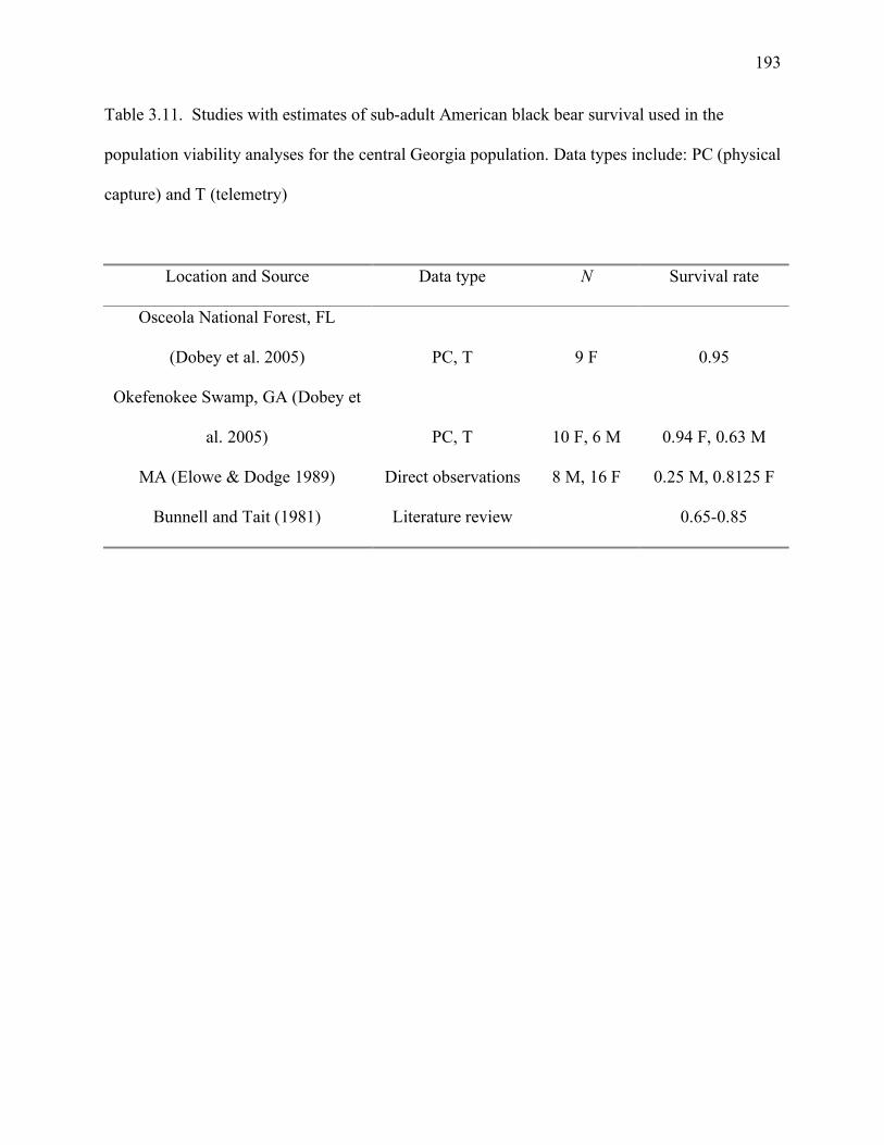
193

Table 3.11. Studies with estimates of sub-adult American black bear survival used in the

population viability analyses for the central Georgia population. Data types include: PC (physical

capture) and T (telemetry)

Location and Source Data type N Survival rate

Osceola National Forest, FL

(Dobey et al. 2005) PC, T 9 F 0.95

Okefenokee Swamp, GA (Dobey et

al. 2005) PC, T 10 F, 6 M 0.94 F, 0.63 M

MA (Elowe & Dodge 1989) Direct observations 8 M, 16 F 0.25 M, 0.8125 F

Bunnell and Tait (1981) Literature review 0.65-0.85

194

Table 3.12. Studies with estimates of adult American black bear survival used in the population

viability analyses for the central Georgia population. All study data types were from physical

captures and telemetry. Dashed lines indicate survival estimates for males were not available for

that particular study.

Location and Source Nf

Female survival

rate (95%CI) Nm

Male annual survival

rate (95%CI)

Great Dismal Swamp, VA,

NC (Hellgren and Vaughn

1989) 24 0.87 22 0.59

White Rock, Dry Creek, AK

(Clark 1991) 31 0.977 - -

Okefenokee Swamp, GA

(Dobey et al. 2005) 41 0.88 (0.81-0.95) 11 0.76 (0.57-0.96)

Osceola National Forest, FL

(Dobey et al. 2005) 21 0.98 (0.94-1.00) - -

CGP (this study) 30

0.861 (0.746-

0.976) 51 0.845 (0.754-0.937)

195

Table 3.13. Demographic parameter estimates primarily from the central Georgia population of American black bears used in

population viability analyses. The initial population sizes were pooled over all years of physical captures of the central Georgia

population. An equal sex-ratio was used in all analyses.

Age class Age

Class N Nm Nf

Male survival2,3,4,

Sm (CV)

Female survival2,3,4,

Sf (CV)

Reproduction

Rate1, b

Mean

litter

size1

Mean

breeding

interval1 (CV)

Cubs 0 3 1 2 0.632 (0.034) 0.632 (0.034) 0 0 0

Sub-adults 1 7 6 1 0.543 (0.124) 0.863 (0.019) 0 0 0

Sub-adults 2 19 13 6 0.543 (0.124) 0.863 (0.019) 0 0 0

Adults 3 59 34 25 0.845 (0.055) 0.861 (0.068) 0.845 1.79 2.1 (0.06)

1 Estimates were calculated from central Georgia population data (n=12 observations of litters, n=8 females’ breeding intervals)

2 Cub estimate was calculated from eastern black bear studies (n=3 studies)

3 Sub-adult estimates were calculated from eastern black bear studies (n=4 studies)

4 Adult survival was calculated from central Georgia population Kaplan-Meier estimates from telemetry data (n=81 bears)

196

Table 3.14. Demographic parameter estimates primarily from eastern American black bear studies, including the central Georgia

population, used in population viability analyses. The initial population sizes were pooled over all years of physical captures of the

central Georgia population. An equal sex-ratio was used in all analyses.

Age class Age

Class N Nm Nf

Male survival2,3,4,

Sm (CV)

Female survival2,3,4,

Sf (CV)

Reproduction

Rate1, b

Mean

litter

size1

Mean

breeding

interval1 (CV)

Cubs 0 3 1 2 0.632 (0.034) 0.632 (0.034) 0 0 0

Sub-adults 1 7 6 1 0.543 (0.124) 0.863 (0.019) 0 0 0

Sub-adults 2 19 13 6 0.543 (0.124) 0.863 (0.019) 0 0 0

Adults 3 59 34 25 0.767 (0.009) 0.909 (0.002) 1.137 2.45 2.15 (0.003)

1 Estimates were calculated from a collection of eastern black bear populations (n=22 studies of mean litter size, n=7 studies of

breeding intervals)

2 Cub estimate was calculated from eastern black bear studies (n=3 studies)

3 Sub-adult estimates were calculated from eastern black bear studies (n=4 studies)

4 Adult estimates were calculated from eastern black bear studies (n=5 studies)

197

Table 3.15. Increased harvest rate scenarios with stochastic simulations (n=10,000 replications)

of λs using reproduction data from the American black bear central Georgia population only and

from eastern American black bear populations.

Increase in

harvest rate

λs (95 % CI) for

CGP only

% extinct for

CGP only

λs (95% CI) from

eastern black bear

populations

% extinct from

eastern black bear

populations

0% 0.788 (0.783-0.793) 0.542 1.114 (1.114-1.115) 0.0001

1% 0.704 (0.699-0.710) 0.683 1.107 (0.107-1.108) 0.0003

2% 0.615 (0.610-0.620) 0.814 1.100 (1.099-1.100) 0.0011

3% 0.544 (0.540-0.549) 0.892 1.090 (1.089-1.090) 0.0034

198

Table 3.16. Sex ratio of American black bears in research projects from the eastern United

States. The data types include: physical captures (PC) and harvest data (H).

Location and Source State(s)

Data

type

Sample

size

Sex ratio

(M:100 F)


1989) VA, NC PC 101 237

White River NWR (Smith 1985) AR PC 64 156

White Rock, Dry Creek (Clark 1991) AR PC 113 88

Osceola National Forest (Dobey et al. 2005) FL PC 78 160

Southeastern GA (Abler 1985) GA PC, H 43 72

Okefenokee Swamp (Dobey et al. 2005) GA PC 127 149

Ocmulgee River (Grahl 1985) GA PC 22 340

Southeastern NC (Hamilton 1978) NC PC, H 66 194

Gum Swamp (Martorello 1998) NC PC 136 116

Big Pocosin (Martorello 1998) NC PC 77 88

GSMNP (McLean 1991) TN, NC PC 312 92

Pisgah National Forest (Mclean 1991) TN, NC PC 26 133

Cherokee National Forest (McLean 1991) TN, NC PC 43 96

199

Table 3.17. Age structure of eastern United States American black bear populations. All data

types are from physical captures, unless specifically noted.

Location and Source State Sample size

!

x total

(sd)

!

x f

(sd)

!

x m

(sd)


and Vaughn 1989)

VA,

NC 100 (30F:70M) 4.2 (0.3) 4 4.2

Big & Montgomery Islands

(White 1996) AR 12 (4F:8M) 8.5 4.5

White Rock, Dry Creek (Clark

1991) AR 113 (53M:60F)

4.68

(0.44)

4.58

(0.57)

Osceola National Forest (Dobey

et al. 2005) FL 78 (30F:48M) 3.3 (0.28) 3.4 (0.45) 3.2 (0.36)

Ocala NF (McCown et al. 2004) FL 126 (40F:86M) 4.8 4.4

Okefenokee Swamp (Dobey et al.

2005) GA 127 (51F:76M) 3.8 (0.21) 4.5 (0.33) 3.3 (0.25)

Ocmulgee River (Grahl 1985) 1 GA 39 (6F:33M) 6.1 4.8

Camp Lejeune MCB

(Brandenburg 1996) NC 15 (12F:3M) 5.7 (1.45)

5.9

(1.17)

9.875

(10)

Gum Swamp, Big Pocosin

(Martorello 1998) NC 123 4.2 (0.22)

GSMNP (McLean 1991)

TN,

NC

437

(254M:183F)

4.52

(2.704)

5.28

(3.224) 3.92 (2.1)

200

Pisgah National Forest (Mclean

1991)

TN,

NC 56 (30M:26F)

3.86

(2.631)

4.46

(3.256)

3.33

(1.84)

Cherokee National Forest

(McLean 1991)

TN,

NC 66 (39M:27F)

3.74

(2.037)

3.28

(1.761)

4.06

(2.171)

1 Data from vehicle collisions and illegal kills were also included into these reported means

201

Figure 3.1. Age frequency of female American black bears at initial capture in Middle Georgia,

2003-2006.

202

Figure 3.2. Age frequency of male American black bears at initial capture in Middle Georgia,

2003-2006.

203

Figure 3.3. Body mass (kg) of female American black bears at initial capture from Middle

Georgia, 2003-2006.

204

Figure 3.4. Body mass (kg) of male American black bears at initial capture from Middle

Georgia, 2003-2006.

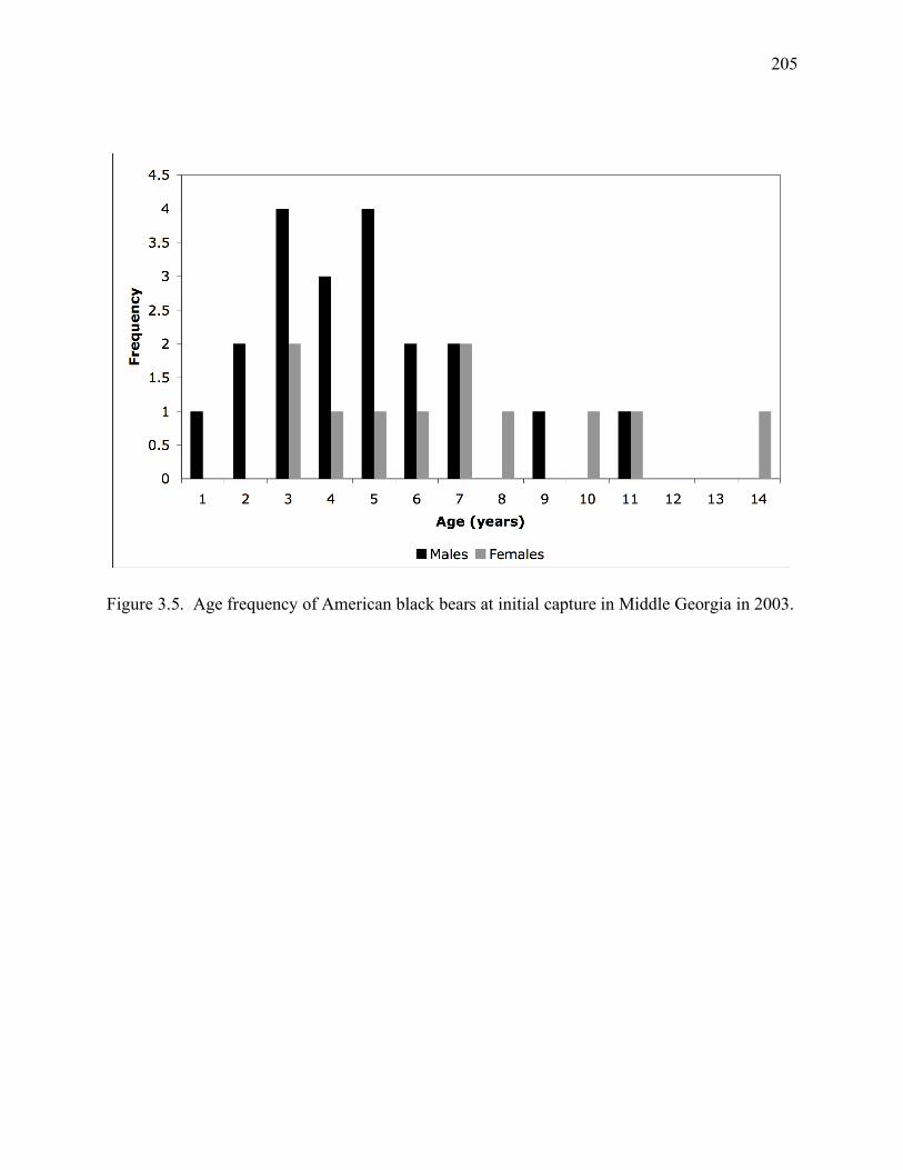
205

Figure 3.5. Age frequency of American black bears at initial capture in Middle Georgia in 2003.

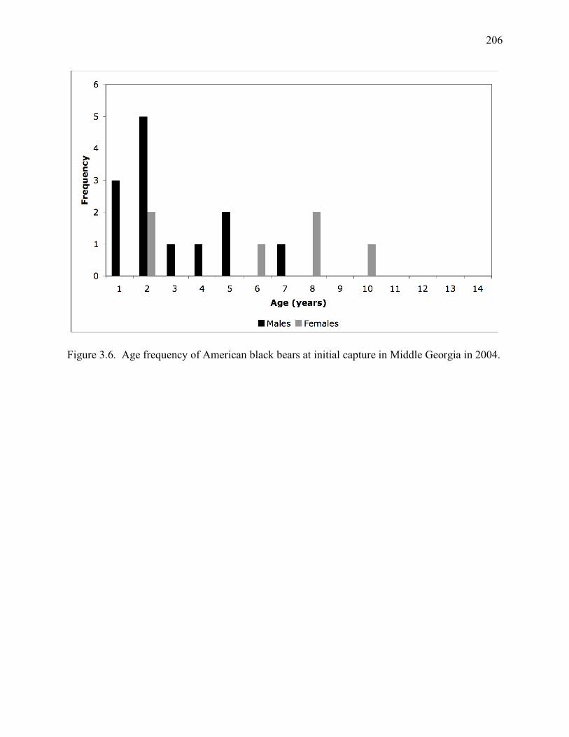
206


207


208


209

Figure 3.9. Age frequency of all American black bears at initial capture in Middle Georgia from

2003 to 2006 with a) all years combined, and b) separated by year.

a)

b)

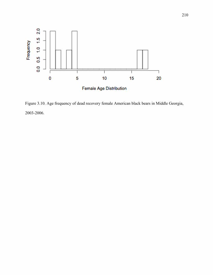
210

Figure 3.10. Age frequency of dead recovery female American black bears in Middle Georgia,

2003-2006.

211

Figure 3.11 Age frequency of dead recovery male American black bears in Middle Georgia,

2001-2007.

212

Figure 3.12. Number of cubs per litter from den observations of American black bears in Middle

Georgia from 2003 to 2007 (n=12 bears).

213

Figure 3.13. Simulated distribution of reproduction rate for the central Georgia American black

bear population using data from 2003 to 2007.

214

Figure 3.14. Simulated distribution of reproduction rate from eastern American black bear

populations (n=22 studies).

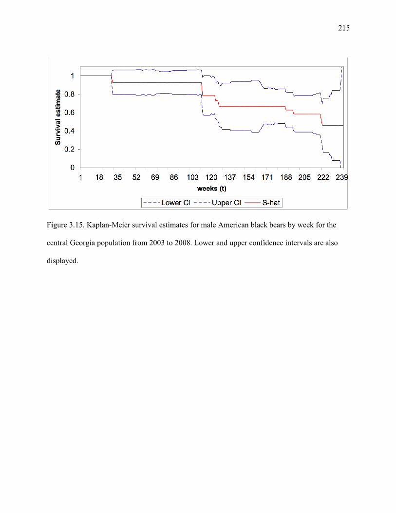
215

Figure 3.15. Kaplan-Meier survival estimates for male American black bears by week for the

central Georgia population from 2003 to 2008. Lower and upper confidence intervals are also

displayed.

216

Figure 3.16. Kaplan-Meier survival estimates for female American black bears by week for the

central Georgia population from 2003 to 2008. Lower and upper confidence intervals are also

displayed.

217

Figure 3.17. Stochastic simulations (n=10,000) of mean λs and 95 % CI lines over 50 years with

reproduction and survival data from the central Georgia American black bear population and no

harvest.

218

Figure 3.18. Stochastic simulations (n=10,000) of American black bear abundance (N) and 95 %

CI lines over 50 years with reproduction and survival data from the central Georgia population

and no harvest.

219

Figure 3.19. Stochastic simulations (n=10,000) of mean λs and 95 % CI lines over 50 years with

reproduction and survival data from eastern American black bear populations and no harvest.

220

Figure 3.20. Stochastic simulations (n=10,000) of black bear abundance (N) and 95 % CI lines

over 50 years with reproduction and survival data eastern American black bear populations and

no harvest.

221

Figure 3.21. American black bear distribution of λ from 2 chains of 50,000 MCMC iterations

(25,000 burn-in period) from the three data structure joint model for total abundance, for the time

period from summer 2004 to summer of 2005 in central Georgia.

222

Figure 3.22. American black bear distribution of λ from 2 chains of 50,000 MCMC iterations

(25,000 burn-in period) from the three data structure joint model for total abundance, for the time

period from summer 2005 to summer 2006 in central Georgia.

223

CHAPTER 4

MANAGEMENT IMPLICATIONS AND CONCLUSIONS

Management implications

Bear management is often considered an exercise in ‘people management’. Since bears

are a wide-ranging species, they are more likely to have competing resources with humans. With

the increase in human population growth in central Georgia and Georgia in general, the increase

in human-bear conflicts is inevitable. Efforts to minimize human-bear conflicts include: public

education and setting aside protected areas for bears. The highest source of mortality observed

with marked bears from this study was from vehicle collisions. To reduce vehicle kills, least

costly methods include reducing traffic speeds in areas prone to vehicle mortality. More costly

strategies include building tunnels, building longer elevated road bridges over streams and rivers

to allow continuity of a broad riparian vegetation, elevating highways in selected areas to create

broad underpasses, and bridges over known locations where bears cross roads.

Our results indicate that there may be evidence of a low reproduction rate with the CGP

and low female survival rate, according to the population viability analyses. These are important

parameters in population viability models of the CGP. Future efforts should focus on obtaining

more observations of litter size per female, and other methods of assessing reproduction in the

CGP. Cub and sub-adult survival are also important aspects of a population viability model, and

should be monitored for more accurate population viability analyses. Since we did not have data

for cub and sub-adult survival estimates, we are relying on the assumption that the CGP has

similar survival estimates in the eastern United States. The age-structure data analysis of

224

sub-adults indicated that the sub-adult survival rate from eastern black bear populations was

similar, so this assumption may be warranted. Cub survival may not differ much from other

populations in the Southeast. Adult females are exposed to similar habitats in the southeastern

United States, which leads to similar diets and nutrition, a key component of cub survival

(Wathen 1983).

Reproduction and survival estimates from mainly CGP data in the population viability

analyses, indicated population growth estimates were decreasing. Therefore, increases in harvest

rate, with these estimates of survival and reproduction, would not be sustainable. However,

reproduction and survival estimates from eastern black bear populations in population viability

analyses indicated the population was increasing, and could sustain an increase in harvest up to

7%. Since there is uncertainty in key values (e.g., cub and sub-adult survival, and reproduction),

the most conservative and recommended course of action is not to increase harvest in the CGP.

Preliminary estimates presented in Chapter 2 should be used as initial estimates of the

WMA property in central Georgia for population viability models and harvest decisions. Of

particular interest is the population size for the central Georgia region, although our current

efforts were focused on the WMA land. The spatial relationship of density with respect to

habitat may be quite different not on WMA land, which is why future models should incorporate

a spatial-abundance relationship with explicit formulation of habitat covariates. Currently,

management decisions should only be focused on the WMA land, not the entire proposed

expanse (~1200 km2) of the black bear range in central Georgia.

225

Future work

The classification of the CGP regarding subspecies to either Ursus americanus

americanus or Ursus americanus floridanus is not known. Miller (1995) classifies the

population as U. a. americanus, but there has not been a study since then to explore this

assumption. To investigate this assumption, multiple samples from other populations are needed

to compare within and between population genetic variability. We had tissue samples from only

one of the three populations of black bears in Georgia. The subspecies classification of the

population may have management implications if the population is more closely related to the

Florida black bear subspecies. Future studies in Georgia should be focused on a larger scale

encompassing the whole state of Georgia, with respective genetic samples from the other two

populations. Apparent rates of migration from the genetic studies would also be of interest. One

could infer the degree of genetic exchange among the populations, if there is any. Similarly,

there does not exist a statewide study exploring the black bear distribution. Occupancy samples

on a county-by-county basis would be helpful for delineating populations or possible avenues of

migration and genetic exchange.

One avenue for populations with reduced genetic variability and/or population numbers is

reintroduction. Bear reintroductions have been successful in the southeastern U.S. (Smith and

Clark 1994, Eastridge and Clark 2001). A preliminary study by Miller (1995) suggests that the

Ocmulgee River population in central Georgia ‘may warrant protection as a distinct population

due to low population size and a high degree of within-population similarity’. We also found

that the old Paetkau markers had low diversity, compared to other black bear populations in the

Southeast. However the tetranucleotide markers used in this study were not consistent with this

pattern, since allelic diversity was similar to other southeastern black bear populations.

226

Optimal sampling designs under the joint data structure model would have applications to

other bear and wildlife populations with similar sampling protocols. An optimal sampling design

for demographic parameter estimation, which we define as the design that maximizes the ratio of

accuracy to cost, is important with limited resources. The sampling design is influenced by the

spatial and behavioral ecology of the study species, the amount of resources available, and the

desired accuracy for the parameter of interest. There is a trade-off between increasing effort to

obtain increased sample observations, which likely increase accuracy of estimates, and costs

(e.g., time and money) required to obtain the estimates. An optimal sampling design with

noninvasive sampling techniques, such as DNA hair traps, includes a laboratory component with

the field component. Study objectives should guide where resources are allocated in a sample

design, especially with future Georgia DNR resources for management of the CGP.

One component of future abundance models of this population should explore ways of

approximating the age class distribution from the abundance joint data structure model. All age

classes have the opportunity of being sampled with DNA hair snares, and camera trapping,

however, it is not possible to distinguish age with DNA samples, unless the bear is a known

captured bear. The camera traps could be used as an approximation. Another source of

heterogeneity not accounted for is the difference between sexes in capture rate with the DNA

hair snares or cameras. The use of sex-ID markers in the genetic analysis should be considered

in future efforts with this population to account for any sex biases, if they exist.

The current joint data structure model assumes a constant capture probability with respect

to time, behavior, and heterogeneity. Future models should incorporate this flexibility in a

model-selection framework. Also, a joint model of density and CMR samples with the trapping

web design and Distance sampling methods would be of interest. The current model also

227

includes limited information about the spatial relationship of bear density and habitat, thus future

models could incorporate this relationship more explicitly (e.g., CAR models) described

previously in chapter 2.

Conclusions

Estimating demographic parameters of cryptic species, like the black bear, is difficult

because of their elusive nature. Non-invasive sampling methods may be valuable for wildlife

studies with consideration of incomplete detection, although there are biases associated with

non-invasive methods that should be accounted for in statistical models. Bears tend to have low

levels of genetic variation because of low population densities and low effective population sizes

(Paetkau and Strobeck 1994). These conditions may increase the difficulty of identifying

individuals in capture-recapture studies. The southeastern black bear populations tend to be more

fragmented than other populations in the United States.

Grahl (1985) reported a population estimate of 64 (sd=18) bears using the Lincoln Index

method for Ocmulgee River population in Georgia, which corresponded to a density of 0.323

bears per km2. Our results suggest a population size that is three times the preliminary estimate

for the WMA land only, not all of Middle Georgia. This could indicate population growth since

1985. However, comparisons between this preliminary estimate from 1985 and now may be

weak, due to differences in population estimation techniques, scale of population inference, and

the time that has elapsed since the first study in 1985.

Hierarchical state-space models provide a way of linking observations from data, such as

capture-mark-recapture (CMR) or occupancy samples, to the underlying ecological or state

processes (Royle and Dorazio 2008). Often, it is not possible to observe ecological processes

228

directly, and samples from a population or groups of populations are used to make inference on

the processes. One of the main goals of this study was to estimate abundance of black bears in

central Georgia using a combination of several sources of data. The common parameter of

inference between the data sources was abundance, which could not be directly observed. This

joint data structure model can be applied to other bear populations and other wildlife

populations, especially those with noninvasive sampling techniques.

The main objectives for this study were to estimate bear abundance in an efficient and

accurate manner, in addition to other demographic parameters, specifically survival and

reproduction of the CGP. We used various sampling techniques for abundance, including

noninvasive genetic sampling. Since statistical models incorporating the three data structures

(DNA hair snares, camera traps, and radiotelemetry) used to estimate abundance did not exist,

we formulated hierarchical Bayesian statistical models incorporating the three data structures.

The use of DNA hair snares introduces an additional source of error from genetic laboratory

error, thus a model incorporating the three data structures and genetic error was developed. This

model has wide scale use for other bear populations and other wildlife species with multiple

sampling techniques.

229

Literature Cited

Eastridge, R. and J. D. Clark. 2001. Evaluation of 2 soft-release techniques to reintroduce black

bears. Wildlife Society Bulletin 29: 1163-1174.




Miller, D. A. 1995. Systematic classification of black bears in the Southeastern United States.

Thesis, Virginia Polytechnic Institute and State University, Blacksburg.



Royle, J. A. and R. M. Dorazio. 2008. Hierarchical modeling and inference in ecology. Elsevier

Ltd., Boston.

Smith, K. G. and J. D. Clark. 1994. Black bears in Arkansas: characteristics of a successful

translocation. Journal of Mammalogy 75: 309-320.

Wathen, W. G. 1983. Reproduction and denning of black bears in the Great Smoky Mountains.

M. S. thesis, University of Tennessee, Knoxville.

230

APPENDIX A.

SIMULATION ANALYSIS OF JOINT DATA MODEL INCORPORATING THREE DATA

STRUCTURES OF DNA HAIR SNARES, CAMERAS, AND TELEMETRY FOR

AMERICAN BLACK BEAR CGP DATA

A simulation analysis was conducted to evaluate model performance using the Python,

version 2.5.2 (Python Software Foundation, http://python.org) programming language. A few

parameter levels (Table A.1) of simulated data from the three data structures were selected.

Specifically, the percentage of webs sampled, the influence of different individual capture

probabilities for camera data, and the presence of genetic error was evaluated. A smaller sample

size of total abundance was selected to increase the processing time of the simulations. Since the

simulated data was mainly from a small population size, a larger population size was selected for

one simulation combination to evaluate an increase in sample size. To evaluate if camera data

assists with estimation of total abundance, one simulation combination included no camera data.

Methods

Data were simulated for each scenario using the parameter values from each simulation

combination. True abundance was simulated for 10 webs using the same Poisson distribution for

each web. The true genotypes were simulated using an even distribution of allelic frequencies

for each locus for each individual. True captures were simulated using a series of Bernoulli trials

231

for each individual in the population with the given capture probability for hair snares. Observed

captures were modified from the true captures by permuting each individual and locus with the

amount of genetic error given. If the individual at a specific locus was a true homozygote, the

true genotype was not modified. If the individual at a specific locus was a true heterozygote, one

of the alleles was modified using the probability of genetic error from equation 2.21 in Chapter 2

with equal probability of selection of another allele if it was chosen to have error. The observed

capture histories were then modified based on the number of times the observed unique

individuals were captured. All simulation combinations used 30% of the samples for genetic

replication samples, also permuted through the genetic error process with equation 2.21 for true

heterozygotes. All simulation combinations used 25 samples as calibration samples, also

permuted through the genetic error process with equation 2.21 for true heterozygotes. Detection

probability for cameras was calculated using the known r parameter and using equation 2.18

from Chapter 2. Camera detections were simulated on each sampled web using a binomial

distribution with number of trials as the number of cameras and the detection probability

calculated from equation 2.18. All combinations included 50% of the true bears with collars.

The true probability of being on a web (pw) was calculated as the true number of bears on the

specific web divided by the total number of true bears in the population. The number of bears

with collars on each sampled web was simulated from a binomial distribution with the number of

trials as the total number of bears with collars in the population, and the probability of being on a

web. The total number of bears with collars was modified with sampling without replacement for

each successive web sampled.

For each scenario, 100 replications of the simulation-MCMC estimation algorithm were

processed in Python, version 2.5.2 (Python Software Foundation, http://python.org). The

232

frequentist properties of Bayesian credible interval (BCI) percent coverage, BCI length, relative

mean squared error (RMSE), and relative bias (RBIAS) were used to evaluate the following

parameters: Ntot, r, θ, p, λ, and pw. Each replication of the simulation-MCMC process included

10,000 iterations with a burn-in period of 5,000 iterations, a tuning period of 4,000 iterations and

no thinning.

The 95% Bayesian credible interval (BCI) coverage is the sum of the number of

replications where the true parameters were contained in the BCI, divided by the total number of

replications. The BCI interval is the distance between the lower and upper 95% credible interval

values. Relative root mean-squared error (RMSE) with r being the total number of replicates, i

the individual replicate,

!

) " i , the estimated parameter at replicate i, θi the true value of parameter

at replicate i, and θ the mean of the true parameter values over all replicates, is:

Relative bias (RBIAS), following the same notation as above, is:

!

RBIAS =

1/r () " i#"

i)

i

n

$

"

!

RMSE =

1/r () " i#"

i)2

i

n

$

"

233

Results

BCI coverage

In general, an increase in the number of webs increased the BCI coverage for total

abundance, individual capture probability for cameras and density (Table A.2). The BCI

coverage did not change with increased number of webs for CMR capture probability, genetic

error, and the probability of being in the web parameters (Table A.2). An increase in individual

capture probability for cameras had an increase in coverage for individual capture probability for

cameras and a slight increase in coverage with total abundance (Table A.2). The BCI coverage

did not change with increased individual camera capture probability for CMR capture

probability, genetic error, density, and the probability of being in the web parameters (Table

A.2). The only consistent pattern with an increase in the true genetic error for all parameters was

an increase in coverage for the genetic error probability (Table A.2).

The simulation combination with no cameras had lower BCI coverage for total

abundance, CMR capture probability, and density (Table A.2). The simulation combination with

larger population size had lower BCI coverage for total abundance, CMR capture probability,

and density, but higher BCI coverage for camera individual capture probability and genetic error

(Table A.2).

BCI length

An increase in the number of webs increased the BCI length for total abundance, CMR

capture probability, and density (Table A.3). The BCI length did not change with increased

number of webs for individual capture probability for cameras, genetic error, and the probability

of being in the web parameters (Table A.3). An increase in individual capture probability for

234

cameras had an increase in interval length for individual capture probability for cameras (Table

A.3). The BCI length did not change with increased individual camera capture probability for

CMR capture probability, genetic error, density, total abundance and the probability of being in

the web parameters (Table A.3). The only consistent pattern with an increase in the true genetic

error for all parameters was an increase in BCI length for the genetic error probability (Table

A.3).

The simulation combination with no cameras had the same BCI length for all parameters

(Table A.3). The simulation combination with larger population size had lower BCI length for

CMR capture probability, genetic error, density, and probability of being in a web, but higher

BCI length for total abundance, camera and individual capture probability (Table A.3).

Relative bias

An increase in the number of webs decreased the positive relative bias for total

abundance and density, and decreased the negative relative bias in capture probability (Table

A.4). The RBIAS did not change the negative values of individual capture probability for

cameras, CMR capture probability, genetic error, and the probability of being in the web

parameters (Table A.4). An increase in individual capture probability for cameras had no

consistent pattern for RBIAS over all parameters (Table A.4). The only consistent pattern with

an increase in the true genetic error for all parameters was a decrease in RBIAS for the genetic

error probability parameter (Table A.4).

The simulation combination with no cameras had increased RBIAS for total abundance

and density, but decreased RBIAS for CMR capture probability and probability of being in a web

parameters (Table A.4). The simulation combination with larger population size had lower

235

RBIAS for individual capture probability and genetic error probability, but higher RBIAS for

total abundance and density (Table A.4).

Relative root mean square error

An increase in the number of webs increased accuracy (decreased RRMSE) for total

abundance, CMR capture probability, individual capture probability for cameras, and density

(Table A.5). The RRMSE did not change with increased number of webs for individual capture

probability for cameras, genetic error and the probability of being in the web parameters (Table

A.5). An increase in individual capture probability for cameras had an increase in accuracy

(decrease in RRMSE) for individual capture probability for cameras (Table A.5). The RRMSE

did not change with increased individual camera capture probability for CMR capture

probability, genetic error, density, total abundance and the probability of being in the web

parameters (Table A.5). The only consistent pattern with an increase in the true genetic error for

all parameters was an increase in accuracy (decrease RRMSE) for the genetic error probability

(Table A.5).

The simulation combination with no cameras had the same level of accuracy (RRMSE)

for all parameters (Table A.5). The simulation combination with larger population size had

increased accuracy with total abundance, individual capture probability with cameras, CMR

capture probability, genetic error, and density, but lower accuracy for probability of being in a

web (Table A.5).

236

Discussion

Number of webs sampled

With an increase in sample size, or an increase in the number of webs sampled, BCI

coverage and accuracy increased, and bias decreased for total abundance and density. This

should be expected with samples size differences. There are implications for study design, where

an increase in samples may increase coverage and decrease bias with an associated cost for each

additional web sampled.

Genetic error

An increase in genetic error increased BCI coverage and BCI length, decreased relative

bias, and increased accuracy of the genetic error parameter. This could be a result of a low

ability to detect genetic error with a small population size and small genetic error rate. Changes

in genetic error did not influence the rest of the model parameters with BCI coverage, interval

length, RBIAS and RRMSE.

Individual capture probability for cameras

An increase in individual capture probability for cameras increased BCI coverage for

individual capture probability for cameras and a slightly increased coverage with total

abundance. There was also an increase in interval length and increase in accuracy for individual

capture probability for cameras. There was no consistent pattern for bias over all parameters.

These results may also reflect a sample size difference where increases in individual capture

probability for cameras increases the amount of camera data available to estimate that capture

237

probably in a model. Since there are a low number of replicates (12), this may have implications

for estimating true individual capture probability for cameras.

Joint data model with no camera data

The simulation combination with no cameras compared to the simulation combination

with camera data had lower BCI coverage for total abundance, CMR capture probability, and

density. The simulation combination with no cameras also had increased RBIAS for total

abundance and density, but decreased RBIAS for CMR capture probability and probability of

being in a web parameters. These results provide evidence that the joint model with all three

data structures leads to less bias and increased coverage for total abundance, the main parameter

of interest in for the black bear CGP, compared to the joint model with just DNA hair snare data

and telemetry.

Large true population size

The simulation combination with larger population size had lower BCI coverage for total

abundance, CMR capture probability, and density, but higher BCI coverage for camera

individual capture probability and genetic error. Higher coverage and lower bias would be

expected with individual capture probability and genetic error since the sample size for genetic

samples is higher (more individuals lead to more errors) and there are more individuals that can

be detected with cameras. The reduced coverage in total abundance, and CMR capture

probability may indicate some bias in the model (e.g., positive bias was also increased with

higher population size). However, 0.87 and 0.90 coverage for abundance and CMR capture

probability, respectively, is still relatively high. The simulation combination with larger

238

population size had lower BCI length for CMR capture probability, genetic error, density, and

probability of being in a web, which is probably due to the difference in sample size. Finally, the

simulation combination with larger population size had increased accuracy with total abundance,

individual capture probability with cameras, CMR capture probability, genetic error, and density,

but lower accuracy for probability of being in a web. This result for accuracy is expected with

increases in sample size.

In conclusion, these simulation results indicate that the joint model for three data

structures used in the abundance models for the black bear CGP is valid for small and large

population sizes, and robust to differences in individual capture probability for cameras and

genetic error. The inclusion of camera data with the joint model both increases parameter

coverage and decreases bias with respect to total abundance, the most important parameter for

black bear CGP abundance models. Finally, the simulation results of varied effort in sampling (3

versus 5 webs sampled) have implications for study design, where an increase in sampling effort

increases coverage and decreases bias. However, there is an associated cost for each additional

web sampled. This warrants future exploration for sampling effort with the different components

(DNA hair snares, telemetry, camera replicates) versus cost for study designs under the joint data

structure model for abundance.

239

Table A.1. Parameter values for simulation combinations of the joint data model incorporating

DNA hair snares, cameras, and telemetry for American black bear CGP data.

Parameter Simulation levels

Webs sampled 3, 5

Camera replicates 12

Individual capture probability, r 0.01, 0.005

Density, λ 5

CMR capture probability, θ 0.40

Collared bears (% of Ntot) 0.50

Genetic error, p 0.01, 0.05

Total combinations 8

240

Table A.2. 95% Bayesian credible interval (BCI) percent coverage for parameters Ntot, r, θ, p, λ, and pw, for all 10 webs for the joint

data model incorporating DNA hair snares, cameras, and telemetry for American black bear CGP data. Each simulation combination

included 100 replications of the combination. All combinations included 12 camera replicates, true λ of 5, CMR capture probability

of 0.4, and 50% of the true bears with telemetry collars. ‘NC’ indicates no cameras and ‘LP’ indicates large population size.

___True___ ______________________________BCI Coverage_______________________________

Level Webs r p Ntot r θ p λ pw1 pw2 pw3 pw4 pw5 pw6 pw7 pw8 pw9 pw10

1 5 0.01 0.01 0.95 0.91 0.94 0.94 0.95 0.97 0.97 0.96 0.98 1.00 0.97 0.98 0.99 0.98 1.00

2 3 0.01 0.01 0.92 0.84 0.93 0.96 0.93 0.99 0.99 1.00 0.99 0.99 0.98 0.96 0.97 0.96 0.98

3 5 0.01 0.05 0.95 0.94 0.95 1.00 0.95 0.99 0.99 0.97 0.99 0.97 0.98 0.98 0.98 0.98 0.95

4 3 0.01 0.05 0.94 0.82 0.95 0.97 0.93 1.00 0.99 0.98 0.96 0.99 0.95 0.94 0.98 0.98 0.99

5 5 0.005 0.01 0.93 0.79 0.93 0.94 0.95 0.99 0.98 0.98 1.00 1.00 0.99 1.00 0.98 0.96 0.98

6 3 0.005 0.01 0.93 0.61 0.96 0.94 0.91 0.97 0.99 1.00 0.97 0.97 0.95 0.97 0.94 0.97 0.98

7 5 0.005 0.05 0.92 0.80 0.95 0.97 0.92 0.99 0.98 0.99 0.99 0.97 0.98 0.94 0.95 0.96 0.98

8 3 0.005 0.05 0.90 0.61 0.94 0.95 0.96 0.99 0.98 0.99 0.98 0.98 0.95 0.97 0.98 0.97 0.99

NC 5 0.01 0.01 0.92 - 0.92 0.96 0.92 0.99 0.98 0.98 1.00 0.99 0.98 0.97 0.95 0.99 0.98

LP 10 0.01 0.01 0.87 0.99 0.9 0.96 0.85 0.98 0.98 0.98 0.98 0.94 0.97 0.95 0.98 0.98 0.96

241

Table A.3. Mean 95% Bayesian credible interval (BCI) length for parameters Ntot, r, θ, p, λ, and pw, for all 10 webs for the joint data

model incorporating DNA hair snares, cameras, and telemetry for American black bear CGP data. Each simulation combination

included 100 replications of the combination. All combinations included 12 camera replicates, true λ of 5, CMR capture probability

of 0.4, and 50% of the true bears with telemetry collars. ‘NC’ indicates no cameras and ‘LP’ indicates large population size.

___True___ _________________________________BCI length____________________________________


1 5 0.01 0.01 48.53 0.04 0.27 0.04 5.73 0.15 0.14 0.15 0.14 0.13 0.22 0.22 0.22 0.21 0.22

2 3 0.01 0.01 78.97 0.02 0.35 0.04 8.55 0.15 0.15 0.15 0.22 0.22 0.22 0.22 0.22 0.22 0.22

3 5 0.01 0.05 48.82 0.02 0.28 0.07 5.74 0.14 0.14 0.14 0.15 0.14 0.22 0.22 0.22 0.22 0.22

4 3 0.01 0.05 75.59 0.06 0.35 0.07 8.20 0.15 0.15 0.15 0.22 0.22 0.22 0.22 0.22 0.22 0.22

5 5 0.005 0.01 48.94 0.01 0.27 0.04 5.76 0.14 0.14 0.14 0.14 0.14 0.21 0.21 0.21 0.21 0.21

6 3 0.005 0.01 73.80 0.01 0.35 0.04 8.01 0.15 0.15 0.15 0.22 0.22 0.22 0.22 0.22 0.22 0.22

7 5 0.005 0.05 47.09 0.01 0.28 0.07 5.60 0.14 0.15 0.14 0.14 0.14 0.22 0.22 0.22 0.22 0.22

8 3 0.005 0.05 79.32 0.01 0.35 0.08 8.55 0.15 0.14 0.15 0.22 0.22 0.22 0.22 0.22 0.22 0.22

NC 5 0.01 0.01 48.22 - 0.27 0.04 5.73 0.14 0.14 0.14 0.14 0.14 0.21 0.21 0.21 0.21 0.21

LP 10 0.01 0.01 65.37 0.11 0.19 0.03 3.91 0.07 0.07 0.11 0.11 0.11 0.11 0.11 0.11 0.11 0.11

242

Table A.4. Relative bias (RBIAS) for parameters Ntot, r, θ, p, λ, and pw, for all 10 webs for the joint data model incorporating DNA

hair snares, cameras, and telemetry for American black bear CGP data. Each simulation combination included 100 replications of the

combination. All combinations included 12 camera replicates, true λ of 5, CMR capture probability of 0.4, and 50% of the true bears

with telemetry collars. ‘NC’ indicates no cameras and ‘LP’ indicates large population size.

___True___ __________________________________RBIAS_________________________________________


1 5 0.01 0.01 0.12 -0.21 -0.12 0.48 0.15 0.08 0.04 0.03 -0.04 -0.03 0.07 0.05 0.04 0.04 0.05

2 3 0.01 0.01 0.18 -0.20 -0.13 0.37 0.19 0.03 0.04 -0.02 0.09 0.05 -0.05 0.10 0.22 0.03 0.11

3 5 0.01 0.05 0.11 -0.11 -0.11 0.08 0.14 0.02 0.04 0.05 0.02 -0.05 0.05 0.01 0.05 0.12 0.05

4 3 0.01 0.05 0.16 -0.22 -0.08 0.07 0.19 0.05 0.00 -0.01 0.09 0.06 0.12 0.06 0.05 0.00 0.13

5 5 0.005 0.01 0.12 -0.10 -0.09 0.43 0.17 0.04 0.03 0.06 -0.02 -0.01 0.09 0.01 0.02 0.07 0.06

6 3 0.005 0.01 0.25 -0.21 -0.09 0.50 0.28 0.03 0.03 0.03 0.10 0.10 0.03 0.08 0.12 0.00 0.04

7 5 0.005 0.05 0.11 -0.17 -0.09 0.01 0.14 0.08 0.05 0.01 -0.03 -0.04 0.06 0.03 0.03 0.12 0.08

8 3 0.005 0.05 0.18 -0.32 -0.12 0.12 0.21 0.06 0.02 0.02 0.04 0.12 0.09 0.08 0.00 0.08 0.07

NC 5 0.01 0.01 0.15 - -0.10 0.48 0.19 0.05 0.00 0.00 -0.03 -0.06 0.09 0.08 0.05 0.09 0.11

LP 10 0.01 0.01 0.15 0.03 -0.12 0.31 0.17 0.04 0.07 0.10 0.02 0.11 0.15 0.08 0.04 0.08 0.04

243

Table A.5. Relative root mean square error (RRMSE) for parameters Ntot, r, θ, p, λ, and pw, for all 10 webs for the joint data model

incorporating DNA hair snares, cameras, and telemetry for American black bear CGP data. Each simulation combination included

100 replications of the combination. All combinations included 12 camera replicates, true λ of 5, CMR capture probability of 0.4, and

50% of the true bears with telemetry collars. ‘NC’ indicates no cameras and ‘LP’ indicates large population size.

___True___ ____________________________________RRMSE___________________________________


1 5 0.01 0.01 0.25 0.57 0.21 0.92 0.29 0.26 0.29 0.29 0.27 0.27 0.38 0.44 0.38 0.43 0.37

2 3 0.01 0.01 0.37 0.70 0.24 0.86 0.39 0.26 0.28 0.24 0.46 0.41 0.44 0.49 0.49 0.45 0.44

3 5 0.01 0.05 0.21 0.58 0.20 0.27 0.26 0.24 0.23 0.35 0.22 0.27 0.43 0.42 0.44 0.51 0.42

4 3 0.01 0.05 0.37 0.74 0.26 0.35 0.42 0.28 0.30 0.30 0.51 0.37 0.44 0.41 0.36 0.41 0.40

5 5 0.005 0.01 0.25 0.82 0.21 0.86 0.30 0.27 0.26 0.24 0.26 0.26 0.37 0.39 0.41 0.43 0.42

6 3 0.005 0.01 1.43 0.95 0.25 0.93 1.46 0.30 0.28 0.27 0.44 0.44 0.45 0.45 0.50 0.37 0.37

7 5 0.005 0.05 0.24 0.77 0.20 0.31 0.28 0.28 0.28 0.26 0.26 0.28 0.42 0.45 0.46 0.47 0.43

8 3 0.005 0.05 0.41 0.91 0.25 0.40 0.42 0.26 0.29 0.28 0.37 0.40 0.47 0.43 0.38 0.43 0.39

NC 5 0.01 0.01 0.25 - 0.20 0.91 0.32 0.27 0.25 0.27 0.23 0.26 0.38 0.45 0.45 0.44 0.41

LP 10 0.01 0.01 0.21 0.33 0.16 0.78 0.24 0.28 0.28 0.45 0.44 0.48 0.48 0.43 0.44 0.44 0.41

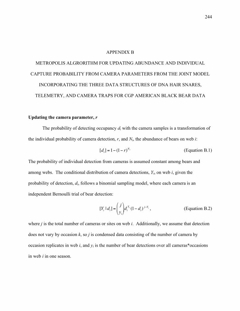
244

APPENDIX B

METROPOLIS ALGRORITHM FOR UPDATING ABUNDANCE AND INDIVIDUAL

CAPTURE PROBABILITY FROM CAMERA PARAMETERS FROM THE JOINT MODEL

INCORPORATING THE THREE DATA STRUCTURES OF DNA HAIR SNARES,

TELEMETRY, AND CAMERA TRAPS FOR CGP AMERICAN BLACK BEAR DATA

Updating the camera parameter, r

The probability of detecting occupancy di with the camera samples is a transformation of

the individual probability of camera detection, r, and Ni, the abundance of bears on web i:

!

[di] =1" (1" r)

Ni (Equation B.1)

The probability of individual detection from cameras is assumed constant among bears and

among webs. The conditional distribution of camera detections, Yi, on web i, given the

probability of detection, di, follows a binomial sampling model, where each camera is an

independent Bernoulli trial of bear detection:

!

[Yi | di] =j

yi

"

# $

%

& ' di

Yi (1( di)j(Yi , (Equation B.2)

where j is the total number of cameras or sites on web i. Additionally, we assume that detection

does not vary by occasion k, so j is condensed data consisting of the number of camera by

occasion replicates in web i, and yi is the number of bear detections over all cameras*occasions

in web i in one season.

245

A reasonable value of r was selected as the starting value with the Metropolis algorithm.

The new proposed value of the parameter, r*, was generated from a normal distribution with

mean log(r), to keep the value positive, and tuning parameter τr. The tuning parameter was

adapted based on whether the previous proposed r was accepted or rejected. Then, the ratio of

binomial likelihoods (Equation B.1, B.2) of r given the camera data was calculated as follows,

!

rr =p(r* | y)

p(r | y) (Equation B. 3)

A uniform random variable was generated, and the proposed value, r*, was accepted with

probability min(rr,1), and the previous value, r t-1, otherwise.

Updating the abundance of sampled areas, Ni

The full conditional distribution of abundance on sampled areas (Ni) is the joint

distribution of the three data structures and the spatial model of N. The full conditional

likelihood is:

!

[{Ni} |•] = [{Yijk} | r,Ni][{Ni} | pwi][{Ni} | "i]

i=1

m

# [G | Ni,$][Xik |Ni,%ik ][{Ni}]

!

"#iNi e

$#i

Ni!

% & '

( ) * i=1

w

+j

Yi

,

- . /

0 1 (1$ (1$ r)


Ntot

Ni

,

- .

/

0 1 (pwi

)Ni (1$ pwi

)Ntot $N i

Ni!

(Ni $ u.i)!2 n.i (1$2)k(Ni )$n.i

"#iNi e

$#i

Ni!

% & '

( ) * i=1

w

+j

Yi

,

- . /

0 1 (1$ (1$ r)


Ntot

Ni

,

- .

/

0 1 (pwi

)Ni (1$ pwi

)Ntot $N i

Ni!

(Ni $ u.i)!(3

0)Ni $u.i

(Equation B.4)

where π0 is the probability of not being captured at least once over the three occasions (i.e.,

!

"0

= (1#$)3). A sequential update of Ni was used, where Ntot of the current accepted Ni s were

used in Ntot from the telemetry portion, or probability of a bear on a web.

246

For each Ni, a reasonable value of Ni was selected as the starting value with the

Metropolis algorithm. The new proposed value of the parameter, Ni *, was generated from a

discrete uniform jumping distribution from the current value of Ni, and tuning parameter, τN ,

which controls how big the proposed jump will be. The tuning parameter was adapted based on

whether the previous proposed N was accepted or rejected. Then, the ratio abundance

likelihoods (Equation B.4) of Ni given the DNA hair snare, telemetry, and camera data was

calculated as follows,

!

rN=p(Ni* | y)

p(Ni | y) (Equation B. 3)

A uniform random variable was generated, and the proposed value, Ni *, was accepted with

probability min(rN,1), and the previous value, Ni t-1, otherwise.

Based on the dimension of a proposed value of N*, the genotype matrix G and the

capture-history matrix are augmented (Tanner and Wong 1987) by N*- N rows. Therefore, N

could potentially change matrix dimensions if the proposed value, N*, is greater than N and is

accepted, which utilizes this reversible jump Metropolis step, as in Wright et al. (2009).

247

Literature cited

Tanner, M. A. and W. H. Wong. 1987. The calculation of posterior distributions by data

augmentation. Journal of the American Statistical Association 82: 528-540.

Wright, J. A., R. J. Barker, M. R. Schofield, A. C. Frantz, A. E. Byrom and D. M. Gleeson.



0420.2008.01167.

248

APPENDIX C.

METHODS OF UPDATING TRUE GENOTYPES, TRUE CAPTURE HISTORIES, AND

GENOTYPE FREQUENCIES FROM WRIGHT ET AL. (2009) FOR THE JOINT MODEL

INCORPORATING THE THREE DATA STRUCTURES OF DNA HAIR SNARES,

TELEMETRY, AND CAMERA TRAPS FOR CGP AMERICAN BLACK BEAR DATA

The following description of updates of matrices and parameters follows directly from Wright et

al. (2009), both with equations and notation.

Updating true genotype matrix, G

The true genotypes for each individual i and locus l are updated through direct sampling.

The first step involves updating individuals that appeared in the observed samples. For those

individuals, we consider all values for G il that are compatible with observed genotypes in all

replicated samples where the individual appeared and do not result in an individual genotype, G i

, that is the same for any other individual in the population. Consider ki compatible genotypes

with the kth one denoted as

!

Gil

(k ). The contribution

!

"il

(k ) made by individual i at locus l to the joint

probability is:

!

"il(k )

= Xij Pr(Gjlr

obs| Gil

(k ))

r=1

R

#j=1

S

#$ % &

' &

( ) &

* & xPr(Gil

(k )| +)

249

Where G (k) is the matrix G with element G il replaced by the proposed value of

!

Gil

(k ) and

!

Pr(Gjlr

obs| Gil

(k )) is given here and in Chapter 2. For true heterozygotes (

!

Ail1" A

il2), the probability

of observing a true heterozygote is 1-p, while the probability of observing a homozygote is

0.5*p, since there are 2 ways that an allele can drop out:

!

Pr(Gjlr

obs| G jl ) =

1" pl Ail1r

obs # Ail2r

obs

0.5pl Ail1r

obs= Ail2r

obs

$ % &

Since we are only considering allelic dropout, the probability of observing a homozygous

individual at locus l, replicate r, given that the true individual at locus l is homozygous is 1.

Most

!

"il

(k ) are zero, except when a sample is observed. Finally, considering all candidate values of

G ij one is selected with probability for the kth one by:

!

"il

(k )

"il

(h )

h=1

Ki

#

For animals not in the samples, a value for G il is drawn directly from the multinomial

distribution of genotype frequencies, so that the resulting genotype (across all loci) does not

correspond to a genotype of any other animal in the population.

Updating the true capture history matrix, X

This step is also accomplished using direct sampling. It directly follows that a vector G

(SxL) of true genotypes that appeared in the samples is the combination of X and G. The capture

history for one out of the three sessions for each sample i, is updated by swapping the capture

history of all other individuals in the population that have compatible genotypes over all loci and

then computing the contribution made by this switch, similar to the updating of true genotypes.

Let X(j) denote the X-matrix associated with the jth switch and

250

!

"ij = Pr(X( j )|N)Pr(Gi

obs| Gi

( j ), p)

From the set of candidate G-matrices one is selected with probability

!

"ij

"ijh=1

N

# and the new value

of X in the matrix X(j) associated with this choice and replaces the old value.

Updating the genotype frequencies, γ

Consider a parameter array γ comprised of L vectors γj, each of length lj=mj(mj+1)/2;

these are the number of distinct genotypes gkj, at locus j. A Dirichlet prior on vector γj (j=1,…,L)

results in:

!

["j] =

#( $kj )k=1

l j

%#($kj )j

&" kj$kj '1

k=1

l j

&

and

!

[G | ",N] = " kjI (Gij = gkj )

k=1

l j

#j=1

L

#i=1

N

#

= " kjykj

k=1

l j

#j=1

L

#

where ykj is the number of the N individuals with genotype gkj at locus j.

Therefore, we can obtain the full conditional distribution of the γ parameter:

!

[" |•] = " kjykj +#kj $1

k=1

l j

%j=1

L

%

This is the kernel of the joint distribution of L independent Dirichlet random variables, where the

jth component has parameter vector {ykj+αkj} (k=1,….,lj) of dimension lj. To simulate a draw

from a Dirichlet distribution with parameters α1,…, αlj, we sample lj values from gamma

251

Ga(αk,1) distributions, where k=1,…,nj. Using the notation of yk for these gamma random

variables, then a vector (x1,…,xlj) is a vector of Dirichlet random variables, where

!

xk =yk

yhh

".

252

Literature Cited

Wright, J. A., R. J. Barker, M. R. Schofield, A. C. Frantz, A. E. Byrom and D. M. Gleeson.



0420.2008.01167.

253

APPENDIX D

CENTRAL GEORGIA AMERICAN BLACK BEAR POPULATION CLOSED POPULATION

MODEL RESULTS WITH PROGRAM MARK USING DNA HAIR SNARES FROM 2004 TO

2006

Closed population models from Program MARK (White and Burnham 1999) were used

to assess capture heterogeneity with DNA hair snare data from the bear CGP. The option ‘full

closed captures with heterogeneity’ was selected in Program MARK (White and Burnham 1999).

Each season was analyzed separately. Behavior effects (Mb), time (Mt), individual heterogeneity

(Mh) and web group effects (Mg), and combinations of the above were used to assess capture

heterogeneity.

Comparisons of competing models can be done in a model selection framework using the

corrected version of Akaike’s Information Criterion (AICc) (Sugiura 1978), a modification of

AIC (Akaike 1973) for small sample size, described below:

!

AICc = "2log(L() # )) + 2K

n

n "K "1

$

% &

'

( ) ,

where

!

L() " ) is the likelihood of the estimated model parameters given the data, K is the number

of parameters, and n is the effective sampling size. The low AICc model is classified as the most

likely model in a candidate model set.

254

All seasons had the Mbt model as the low AICc model, indicating that there is evidence of

behavior and time heterogeneity in the DNA hair snare data, when genetic error is ignored

(Tables D.1, D.2, D.3, D.4, D.5). The group ‘web’ effect models, or the models where capture

probability is different for each web, had no model weight for all seasons. Therefore, this model

was not selected as a potential model in Chapter 2. The null model (M0) had some model weight,

albeit a small amount, for most seasons. This is the simplest model to implement in the joint

model of DNA hair snares, cameras, and telemetry, and was selected for models in Chapter 2.

Future work will incorporate behavior and time effects. There also is some evidence of

individual heterogeneity, according to the models presented here.

255

Literature Cited

Akaike, H. 1973. Information theory as an extension of the maximum likelihood principle.

Pages 267-281 in B. N. Petrov, and F. Csaki, (eds.) Second International Symposium on

Information Theory. Akademiai Kiado, Budapest.

Sugiura, N. 1978. Further analysis of the data by Akaike’s information criterion and the finite

corrections. Communications in Statistics, Theory and Methods A7: 13-26.

White, G. C. and K. P. Burnham. 1999. Program MARK: survival estimation from populations

of marked animals. Bird Study 46 Supplement, 120-138.

256

Table D. 1. Closed population MARK models from CMR hair snare data collected in Summer

2004 for the American black bear CGP. The model, AICc, Δ AICc, AICc model weight, model

likelihood, number of parameters (np), and model deviance are included.

Model AICc Δ AICc AICc Weights Model Likelihood np Deviance

Mbt 18.48 0.00 0.94 1.00 10 29.16

Mbth 26.07 7.59 0.02 0.02 16 21.92

M0 27.00 8.51 0.01 0.01 6 46.79

Mb 28.96 10.48 0.01 0.01 7 46.53

Mh 29.22 10.74 0.00 0.00 7 46.79

Mg 29.29 10.81 0.00 0.00 10 39.97

Mt 30.59 12.11 0.00 0.00 8 45.90

Mbg 30.91 12.43 0.00 0.00 15 29.33

Mbh 31.22 12.74 0.00 0.00 8 46.53

Mgh 31.66 13.18 0.00 0.00 11 39.97

Mbgh 33.49 15.01 0.00 0.00 16 29.34

Mht 36.88 18.40 0.00 0.00 12 42.78

Mgt 38.67 20.19 0.00 0.00 20 23.76

Mbgt 51.72 33.24 0.00 0.00 30 6.29

Mtgh 84.27 65.79 0.00 0.00 36 17.54

Mtbgh 161.39 142.91 0.00 0.00 56 0.00

257

Table D. 2. Closed population MARK models from CMR hair snare data collected in Fall 2004

for the American black bear CGP. The model, AICc, Δ AICc, AICc model weight, model


Model AICc Δ AICc

AICc

Weights

Model

Likelihood np Deviance

Mbt 52.98 0.00 0.83 1.00 11 24.58

Mth 57.68 4.70 0.08 0.10 13 23.50

M0 59.34 6.35 0.03 0.04 7 41.45

Mt 59.86 6.88 0.03 0.03 9 36.88

Mb 61.62 8.64 0.01 0.01 8 41.22

Mh 61.85 8.86 0.01 0.01 8 41.45

Mbh 64.21 11.22 0.00 0.00 9 41.22

Mbth 67.48 14.50 0.00 0.00 17 20.53

Mg 70.02 17.03 0.00 0.00 12 38.77

Mgh 72.95 19.97 0.00 0.00 13 38.77

Mbg 83.80 30.82 0.00 0.00 18 33.37

Mbgh 87.40 34.42 0.00 0.00 19 33.37

Mgt 96.94 43.95 0.00 0.00 24 22.72

Mbgt 151.42 98.43 0.00 0.00 36 7.10

Mght 210.87 157.89 0.00 0.00 43 0.59

Mbght 1437.93 1384.95 0.00 0.00 67 0.00

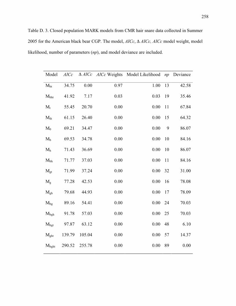
258





Mbt 34.75 0.00 0.97 1.00 13 42.58

Mbht 41.92 7.17 0.03 0.03 19 35.46

Mt 55.45 20.70 0.00 0.00 11 67.84

Mth 61.15 26.40 0.00 0.00 15 64.32

M0 69.21 34.47 0.00 0.00 9 86.07

Mb 69.53 34.78 0.00 0.00 10 84.16

Mh 71.43 36.69 0.00 0.00 10 86.07

Mbh 71.77 37.03 0.00 0.00 11 84.16

Mgt 71.99 37.24 0.00 0.00 32 31.00

Mg 77.28 42.53 0.00 0.00 16 78.08

Mgh 79.68 44.93 0.00 0.00 17 78.09

Mbg 89.16 54.41 0.00 0.00 24 70.03

Mbgh 91.78 57.03 0.00 0.00 25 70.03

Mbgt 97.87 63.12 0.00 0.00 48 6.10

Mght 139.79 105.04 0.00 0.00 57 14.37

Mbght 290.52 255.78 0.00 0.00 89 0.00

259

Table D. 4. Closed population MARK models from CMR hair snare data collected in Fall 2005

for the American black bear CGP. The model, AICc, Δ AICc, AICc model weight, model



Mbt 49.86 0.00 0.99 1.00 11 34.85

M0 60.31 10.45 0.01 0.01 7 54.74

Mt 62.30 12.44 0.00 0.00 9 52.10

Mb 62.32 12.46 0.00 0.00 8 54.46

Mh 62.61 12.75 0.00 0.00 8 54.74

Mhbt 63.76 13.90 0.00 0.00 17 33.19

Mbh 64.66 14.80 0.00 0.00 9 54.46

Mht 67.38 17.51 0.00 0.00 13 47.38

Mg 67.62 17.76 0.00 0.00 12 50.14

Mhg 70.14 20.28 0.00 0.00 13 50.14

Mbg 71.49 21.63 0.00 0.00 18 38.15

Mhbg 74.32 24.46 0.00 0.00 19 38.15

Mgt 82.85 32.99 0.00 0.00 24 31.65

Mbgt 103.16 53.29 0.00 0.00 36 8.49

Mhgt 142.21 92.35 0.00 0.00 43 15.85

Mhbgt 299.80 249.93 0.00 0.00 67 0.00

260





Mbt 19.97 0.00 0.94 1.00 11 28.05

Mb 26.60 6.63 0.03 0.04 8 41.36

Mbh 28.79 8.82 0.01 0.01 9 41.35

M0 30.39 10.43 0.01 0.01 7 47.33

Mhbt 30.79 10.82 0.00 0.00 17 24.82

Mt 32.57 12.60 0.00 0.00 9 45.13

Mh 32.57 12.60 0.00 0.00 8 47.33

Mg 34.20 14.23 0.00 0.00 12 40.00

Mbg 34.94 14.97 0.00 0.00 18 26.53

Mhg 36.50 16.53 0.00 0.00 13 40.00

Mhbg 37.41 17.44 0.00 0.00 19 26.53

Mht 37.53 17.56 0.00 0.00 13 41.03

Mgt 49.52 29.55 0.00 0.00 24 25.88

Mbgt 66.79 46.82 0.00 0.00 36 9.15

Mhgt 100.01 80.04 0.00 0.00 43 19.99

Mhbgt 175.94 155.97 0.00 0.00 67 0.00

261

APPENDIX E

PYTHON CODE FOR THE JOINT MODEL INCORPORATING THE THREE DATA

STRUCTURES OF DNA HAIR SNARES, TELEMETRY, AND CAMERA TRAPS FOR CGP

AMERICAN BLACK BEAR DATA

The Python code is a collection of posterior parameter updates using Gibbs, Metropolis

and reversible jump Metropolis-Hastings algorithms from the joint model for data from Fall

2005 season. There are also with references to equations from Chapter 2 presented with the code.

The Python modules are separated by the sections from the MCMC steps (Figure E.1).

1) Input data, and 16) output parameter traces

def

run(nwebs=14,alleles=[8,4,8,4,4,7,4,4],occasions=3,collars=22.,rinit=0.04,Ninit=10,tune_r=0.5,t

une_N=30,iterations=50000,burn=25000,tuner=15000,reps=1,if_print=10,if_output=1000,estima

te=True,plotting=True):

#data

#total cameras

kcam=[18,16,15,12,'NA',12,'NA','NA',31,'NA','NA','NA','NA','NA']

#notes: k is number of cameras at each site

#camera detections

camera=[15,12,1,7,'NA',10,'NA','NA',20,'NA','NA','NA','NA','NA']

#telemetry detections

telem=[10,4,1,3,'NA',5,'NA','NA',3,'NA','NA','NA','NA','NA']

262

loci=len(alleles)

it=[x for x in range(iterations+1)]

#import observed genetic samples and create dictionary

data=csv.reader(open('gobs_5Fweb.csv','U'),dialect='excel')

obssamp={}

for line in data:

temp=string.join((line[1],line[2],line[3],line[4],line[5],line[6],line[7],line[8]),",")

obssamp[int(line[0])]=[eval(temp),int(line[9]),int(line[10])]

#obs capture ids and capture history

obsCap=sum_samples_webs(obssamp,occasions)

#import replicate samples and create dictionary

data2=csv.reader(open('rep_5F.csv','U'),dialect='excel')

repsamp2={}

for line in data2:

temp=string.join((line[1],line[2],line[3],line[4],line[5],line[6],line[7],line[8]),",")

repsamp2[int(line[0])]=[eval(temp)]

#obs summary stats

udot_obs,ndot_obs=sum_stats_web(obssamp,occasions,nwebs)

print 'obs u,n dot',udot_obs,ndot_obs

if estimate:

captrace,N_trace,errortrace,Ntottrace,denstrace,acceptancer,rtrace,dtrace,pwebtrace,acceptanceN

=MCMC_sampler(nwebs,udot_obs,ndot_obs,obsCap,obssamp,repsamp2,alleles,occasions,iterati

ons,tuner,if_print,if_output,Ninit,rinit,camera,kcam,collars,telem,tune_r,tune_N)

if plotting:

263

varnames=['Ntot','p_error','r','density','pcapt']

vartraces=[Ntottrace,errortrace,rtrace,denstrace,captrace]

plotnum=1

for i in range(len(varnames)):

plotnum=plot_tracepost(varnames[i],vartraces[i],plotnum)

print 'r acceptance rate',acceptancer

print 'N acceptance rate',acceptanceN

print ''

for i in range(len(varnames)):

output_stats(varnames[i],vartraces[i])

if __name__ == '__main__':

run()

2) Initialize parameters modules

def initial_parms(nwebs,alleles,sampobsinit,oc,initialN,perrinit):

"""generate initial matrices, parameters"""

#genetic error init

proberr_init=perrinit

#prior alphas for gamma, genotype frequency, priors are all 1's

alpha_init=[]

for i in alleles:

cat=i*(i+1)/2

alpha_init.append([1]*cat)

#create initial genotype frequencies (all equal)

gam_init=geno_freq(alleles)

264

gen_cat=gen_categories(alleles)

#permute initial true sample ids

sampletrue=copy.deepcopy(sampobsinit)

#expected samples with at least one error

experr=np.ceil(len(sampobsinit)*((1.-(1.-proberr_init)**len(alleles))))

generr=random_sample(experr,len(sampobsinit))

for samp in sampletrue:

if generr[samp]:

newgenid=[]

for j in range(len(alleles)):

compat=compat_gen(sampletrue[samp][0][j],gen_cat[j],proberr_init)

probcompat=[1./(len(compat)) for i in range(len(compat))]

newG=compat[mult(probcompat)]

newgenid.append(newG)

sampletrue[samp][0]=tuple(newgenid)

#generate initial true script G matrix of true IDs and capture history

Nmatrixinittemp,truewebdict=sum_samples_webs(sampletrue,oc)

webNinit=sum_web(truewebdict,nwebs)

#initial N is greater than the current value of N, add new rows

for i in range(nwebs):

if i==0:

if initialN>webNinit[i]:

webNinit[i]=initialN

Nmatrixinit1,truewebdictinit1=gen_rows(initialN,webNinit[i],Nmatrixinittemp,gam_init,alleles,i

,truewebdict)

265

else:

Nmatrixinit1=copy.copy(Nmatrixinittemp)

truewebdictinit1=copy.copy(truewebdict)

else:

if initialN>webNinit[i]:

webNinit[i]=initialN

Nmatrixinit,truewebdictinit=gen_rows(initialN,webNinit[i],Nmatrixinit1,gam_init,alleles,i,truew

ebdictinit1)

Nmatrixinit1=copy.copy(Nmatrixinit)

truewebdictinit1=copy.copy(truewebdictinit)

return alpha_init,gam_init,sampletrue,Nmatrixinit1,truewebdictinit1,webNinit

def random_sample(m,M):

"""take a random sample m out of M possible items"""

#first element of each tuple is sample label

#second element is indicator for sampled (1) or not (0)

x=np.arange(M)

random.shuffle(x)

y=[(x[i],(i<m)*1) for i in range(M)]

y.sort()

z=[w[1] for w in y]

return z

3), 14), 15) Main MCMC sampler

266

def

MCMC_sampler(nwebs,udot_init,ndot_init,Gobsmatrix,obssamples,repsamples,alleles,occasions

,iterations,tuner,if_print,if_output,Ninit,rinit,xdetect,ncameras,totcollars,collars,tune_r,tuneN):

"""main program for MCMC sampler of genetic CMR data, camera data, telemetry data,

spatial process"""

#static observation matrix

G_obs=copy.copy(Gobsmatrix)

#static obs samples,reps,calibration true and calibration obs samples

sample_obs=obssamples.copy()

sample_rep=repsamples.copy()

samples=0

accept_r=0

accept_N=0

d_=[]

r_=[rinit]

pweb_=[]

dens_=[]

sd_r=tune_r

sd_N=tuneN

#priors and initial parameter values

#initial value of capture probability

cap_p=[0.3]

#initial value of genetic error probability

error_p=[0.05]

#prior alpha, initial gamma, initial true samples, initial Nmatrix, initial true web dictionary

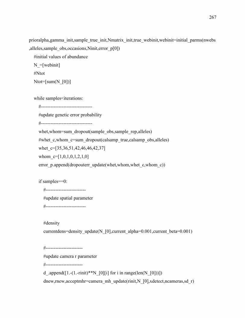
267

prioralpha,gamma_init,sample_true_init,Nmatrix_init,true_webinit,webinit=initial_parms(nwebs

,alleles,sample_obs,occasions,Ninit,error_p[0])

#initial values of abundance

N_=[webinit]

#Ntot

Ntot=[sum(N_[0])]

while samples<iterations:

#--------------------------------

#update genetic error probability

#--------------------------------

whet,whom=sum_dropout(sample_obs,sample_rep,alleles)

#whet_c,whom_c=sum_dropout(calsamp_true,calsamp_obs,alleles)

whet_c=[35,36,51,42,46,46,42,37]

whom_c=[1,0,1,0,1,2,1,0]

error_p.append(dropouterr_update(whet,whom,whet_c,whom_c))

if samples==0:

#-------------------------

#update spatial parameter

#-------------------------

#density

currentdens=density_update(N_[0],current_alpha=0.001,current_beta=0.001)

#-----------------------

#update camera r parameter

#-----------------------

d_.append([1.-(1.-rinit)**N_[0][i] for i in range(len(N_[0]))])

dnew,rnew,acceptmhr=camera_mh_update(rinit,N_[0],xdetect,ncameras,sd_r)

268

accept_r=accept_r+acceptmhr

#-----------------------------

#update telemetry p_w parameter

#------------------------------

pwnew=pw_update(collars,N_[0],totcollars)

#---------------------

#update true genotypes

#---------------------

Nmatrix_new,samp_truenew,trueweb_new=truegen_update(nwebs,true_webinit,Nmatrix_init,ga

mma_init,alleles,error_p[0],sample_obs,sample_rep,sample_true_init,occasions)

#-------------------------------------------------

#update true capture histories,and Gtrue of size(S)

#-------------------------------------------------

Nmatrix_new2,Gtrue_new,Gtrue_web=truehist_update(nwebs,trueweb_new,Nmatrix_new,gam

ma_init,alleles,error_p[0],cap_p[0],occasions,samp_truenew,sample_obs,ncameras)

#-------------

#update gamma

#-------------

gamma_new=genfreq_update(Nmatrix_new2,prioralpha,alleles)

#-----------------------

#update pcapture (theta)

#------------------------

#obtain new udot and ndot

udot_new,ndot_new=sum_stats_web(Gtrue_new,occasions,nwebs)

currentpcapture=pcapture_update(udot_new,ndot_new,N_[0],occasions,cap_p[0],ncameras)

269

#-----------------------------

#update N

#-----------------------------

currentN,acceptN=spatN_update(currentdens,N_[0],currentpcapture,udot_new,ndot_new,sd_N,x

detect,ncameras,occasions,pwnew,rnew,collars)

accept_N=accept_N+acceptN

else:

#-------------------------

#update spatial parameter

#-------------------------

#density

currentdens=density_update(Nold,current_alpha=0.001,current_beta=0.001)

#-----------------------

#update camera r parameter

#-----------------------

dnew,rnew,acceptmhr=camera_mh_update(rold,Nold,xdetect,ncameras,sd_r)

accept_r=accept_r+acceptmhr

#-----------------------------

#update telemetry p_w parameter

#------------------------------

pwnew=pw_update(collars,Nold,totcollars)

#---------------------

#update true genotypes

#---------------------

Nmatrix_new,samp_truenew,trueweb_new=truegen_update(nwebs,web_finalnew,Nmatrix_final

new,gamma_new,alleles,error_p[samples],sample_obs,sample_rep,Gtrue_new,occasions)

#-------------------------------------------------

270

#update true capture histories,and Gtrue of size(S)

#-------------------------------------------------

Nmatrix_new2,Gtrue_new,Gtrue_web=truehist_update(nwebs,trueweb_new,Nmatrix_new,gam

ma_new,alleles,error_p[samples],cap_p[samples],occasions,samp_truenew,sample_obs,ncamera

s)

#-------------

#update gamma

#-------------

gamma_new=genfreq_update(Nmatrix_new2,prioralpha,alleles)

#-----------------------

#update pcapture (theta)

#------------------------

#obtain new udot and ndot

udot_new,ndot_new=sum_stats_web(Gtrue_new,occasions,nwebs)

currentpcapture=pcapture_update(udot_new,ndot_new,Nold,occasions,pcaptureold,ncameras)

#-----------------------------

#update N

#-----------------------------

currentN,acceptN=spatN_update(currentdens,Nold,currentpcapture,udot_new,ndot_new,sd_N,xd

etect,ncameras,occasions,pwnew,rnew,collars)

accept_N=accept_N+acceptN

#augment N (add or delete rows) Reversible-jump M-H

Nmatrix_finalnew,web_finalnew=n_update(nwebs,Nmatrix_new2,currentN,gamma_new,alleles,

Gtrue_web,Gtrue_new)

271

densold=copy.copy(currentdens)

dens_.append(currentdens)

rold=copy.copy(rnew)

r_.append(rnew)

d_.append(dnew)

Nold=copy.copy(currentN)

N_.append(currentN)

Ntot.append(sum(currentN))

pcaptureold=copy.copy(currentpcapture)

cap_p.append(currentpcapture)

pweb_.append(pwnew)

samples+=1

acceptance_r=float(accept_r)/float(samples)

acceptance_N=float(accept_N)/float(samples*6)

if samples<tuner:

if acceptN==1:

sd_N=np.min(sd_N+1,5)

else:

sd_N=np.max(1,sd_N-1)

if acceptmhr==1:

sd_r=sd_r*0.999

else:

sd_r=sd_r*1.001

if (np.mod(samples,if_print)==0):

print 'iter, N',samples,sum(currentN)

print 'N accept',acceptance_N

272

print 'r accept',acceptance_r

if (np.mod(samples,if_output)==0):

MCMC_output(samples,nwebs,ncameras,cap_p,error_p,Ntot,r_,N_,dens_,d_,pweb_,Nmatrix_fin

alnew,gamma_new,Gtrue_new,web_finalnew)

return cap_p,N_,error_p,Ntot,dens_,acceptance_r,r_,d_,pweb_,acceptance_N

def

MCMC_output(iteration,nwebs,kcam,captrace,errortrace,Ntottrace,rtrace,N_trace,denstrace,dtrac

e,pwebtrace,currentNmatrix,currentgamma,currentGtrue,currentwebdict):

coda_out=[]

coda_out.extend(errortrace)

coda_out.extend(Ntottrace)

coda_out.extend(rtrace)

coda_out.extend(captrace)

coda_out.extend(denstrace)

Nall_trace=[]

for j in range(nwebs):

tempN=[]

for k in range((len(N_trace))):

tempN.append(N_trace[k][j])

Nall_trace.append(tempN)

coda_out.extend(tempN)

dall_trace=[]


tempd=[]

if kcam[j]!='NA':

for k in range((len(dtrace))):

273

tempd.append(dtrace[k][j])

dall_trace.append(tempd)

coda_out.extend(tempd)

pweball_trace=[]


temppweb=[]

for k in range((len(pwebtrace))):

temppweb.append(pwebtrace[k][j])

pweball_trace.append(temppweb)

coda_out.extend(temppweb)

sumfile=open('iter'+str(iteration)+'_fall5.txt','w')

for i in range(len(coda_out)):

alldat=[]

dat=str(coda_out[i])

alldat.append(dat)

alldat.append("\n")

sumfile.writelines(alldat)

sumfile.close()

sumfile2=open('iter'+str(iteration)+'_nmatrix_fall5.txt','w')

for i in currentNmatrix:

alldat=[]

dat=str(i)+str(':')+str(currentNmatrix[i])

alldat.append(dat)

alldat.append("\n")

sumfile2.writelines(alldat)

sumfile2.close()

sumfile3=open('iter'+str(iteration)+'_gamma_fall5.txt','w')

274

for i in range(len(currentgamma)):

alldat=[]

dat=str(currentgamma[i])

alldat.append(dat)

alldat.append("\n")


sumfile3.close()

sumfile4=open('iter'+str(iteration)+'_Gtrue_fall5.txt','w')

for i in currentGtrue:

alldat=[]

dat=str(i)+str(":")+str(currentGtrue[i])

alldat.append(dat)

alldat.append("\n")


sumfile4.close()

sumfile5=open('iter'+str(iteration)+'_webdict_fall5.txt','w')

for i in currentwebdict:

alldat=[]

dat=str(i)+str(":")+str(currentwebdict[i])

alldat.append(dat)

alldat.append("\n")


sumfile5.close()

return

4) Genetic error update modules

Equation 2.22

def dropouterr_update(whet,whom,whet_c,whom_c ):

275

"""update genetic error probability using Gibbs step"""

#for now assume ado is constant across all loci

tot_whet=sum(whet)

tot_whom=sum(whom)

tot_whetc=sum(whet_c)

tot_whomc=sum(whom_c)

#assume alpha=1 and beta=1 for priors

a=1.

b=1.

newerr=pm.rbeta(2*a+tot_whom+tot_whomc-1, 2*b+tot_whet+tot_whetc-1)

return newerr

def sum_dropout(obssamp,repsamp,alleles):

"""summarize dropout from observed and replicated genetic samples"""

loci=len(alleles)

w_het=[0]*loci

w_hom=[0]*loci

for obs in obssamp:

for rep in repsamp:

if obs==rep:

for j in range(loci):

if isHom(obssamp[obs][0][j])==False:

if repsamp[rep][0][j]!='nn':

w_het[j]+=1

if isHom(str(repsamp[rep][0][j]))==True:

w_hom[j]+=1

276

return w_het,w_hom

5) Spatial parameter update module

Equation 2.15

def density_update(current_N,current_alpha,current_beta):

"""update lambda using Gibbs sampling"""

nextlambda=pm.rgamma(np.mean(current_N)*len(current_N)+current_alpha,len(current_N)+cu

rrent_beta)

return nextlambda

6) Camera parameter update module

Equations 2.18, 2.19, 2.20

def camera_mh_update(current_r,current_N,x_detect,n_cam,tune_r):

"""Metropolis-Hastings step of updating detection probability at camera under Royle-Nichols

model"""

taur=tune_r

#single animal detection probability r

#detection probability

d_current=[1.-(1.-current_r)**current_N[i] for i in range(len(current_N))]

#proposal distribution

x_prop=pm.rnormal(logit(current_r),taur)

r_prop=expit(x_prop)

d_prop=[1.-(1.-r_prop)**current_N[i] for i in range(len(current_N))]

f=0.

f_prop=0.

for i in range(len(x_detect)):

if x_detect[i]!='NA':

277

#likelihood of current value

f+=pm.binomial_like(x_detect[i],n_cam[i],d_current[i])

#likelihood of proposed value

f_prop+=pm.binomial_like(x_detect[i],n_cam[i],d_prop[i])

#acceptance ratio

r= np.exp(f_prop-f)

if random.rand()<r:

nextd=d_prop

nextr=r_prop

accept=1

else:

nextd=d_current

nextr=current_r

accept=0

return nextd,nextr,accept

7) Telemetry parameter update module

Equation 2.17

def pw_update(ncollared,currentN,totcollars):

"""update probability of bear on web detected with collar using Gibbs sampling"""

Ntot=sum(currentN)

pwnew=[]

for i in range(len(currentN)):

if ncollared[i]!='NA':

pwnew.append(pm.rbeta(ncollared[i]+currentN[i]+1.,totcollars-ncollared[i]+Ntot-

currentN[i]+1.))

else:

#posterior prediction onto webs not sampled

278

pwnew.append(pm.rbeta(currentN[i]+1,Ntot-currentN[i]+1))

return pwnew

8) Modules associated with genetic CMR parameters and matrices

def n_update(nwebs,Nmatrix,Nstar_,gammanew,alleles,truewebdict,truesampgen):

Nmatrix_copy=Nmatrix.copy()

N_=sum_web(truewebdict,nwebs)

for i in range(len(N_)):

if i==0:

#proposed N is greater than the current value of N, add new rows

if Nstar_[i]>N_[i]:

Nmatrixnew,truewebdictnew=gen_rows(Nstar_[i],N_[i],Nmatrix_copy,gammanew,alleles,i,true

webdict)

#proposed N is less than the current value of N, delete rows

else:

Nmatrixnew=Nmatrix_copy.copy()

truewebdictnew=truewebdict.copy()

del_row=N_[i]-Nstar_[i]

k=0

for j in Nmatrix_copy:

if tuple(j) not in truesampgen:

if k<del_row:

#can only delete individuals not observed

if Nmatrix_copy[tuple(j)]=='000':

if truewebdict[tuple(j)]==i:

del Nmatrixnew[tuple(j)]

del truewebdictnew[tuple(j)]

279

k+=1

else:

#proposed N is greater than the current value of N, add new rows

if Nstar_[i]>N_[i]:

Nmatrixnew1,truewebdictnew1=gen_rows(Nstar_[i],N_[i],Nmatrixnew,gammanew,alleles,i,true

webdictnew)

#proposed N is less than the current value of N, delete rows

else:

Nmatrixnew1=copy.copy(Nmatrixnew)

truewebdictnew1=copy.copy(truewebdictnew)

del_row=N_[i]-Nstar_[i]

k=0

for j in Nmatrix_copy:

if tuple(j) not in truesampgen:

if k<del_row:

#can only delete individuals not observed

if Nmatrix_copy[tuple(j)]=='000':

if truewebdict[tuple(j)]==i:

del Nmatrixnew1[tuple(j)]

del truewebdictnew1[tuple(j)]

k+=1

return Nmatrixnew1,truewebdictnew1

def gen_rows(Nstar_,webmatrix,Nmatrix,gammanew,alleles,web,webdict):

"""simulates the true genotypes given number of alleles

per locus and adds rows to genotypes. This does NOT require Hardy-Weinberg

Equilibrium"""


280

nloc=len(alleles)

gamman=gammanew

webdictnew=webdict.copy()

webm=copy.copy(webmatrix)

while webm<Nstar_:

g=[mult(gamman[i]) for i in range(nloc)]

x=[gen_diction(y,z) for y,z in zip(g,alleles)]

#check for identical genoptypes, if proposed value identical, redraw for new individual

if tuple(x) not in Nmatrix_copy:

Nmatrix_copy[tuple(x)]='000'

webdictnew[tuple(x)]=web

webm+=1

return Nmatrix_copy,webdictnew

def geno_freq(loc):

"""returns the constant genotype frequency for each locus"""

freq=[]

for i in loc:

cat=i*(i+1)/2

freq.append([float(1./cat)]*cat)

return freq

def mult(genprobs):

"""returns index value for multinomial rv"""

gg=pm.rmultinomial(1,genprobs)

for i in range(len(gg)):

if gg[i]:

return i

281

def gen_diction(genIndex,nallele):

"""creates genotype dictionary based on genotype index"""

categories=(nallele*(nallele+1))/2

allgen=list()

m=0

for i in range(nallele):

for j in range(m,nallele):

allgen.append(str(i)+str(j))

m+=1

genId={}

for k in range(categories):

genId[k]=allgen[k]

gen=genId[genIndex]

return gen

def prob_het(pgenerr):

"""computes prob of observing a genotype given the true heterozygous genotype

with p the probability of one allele dropping out"""

prob=[0.0]*3

#obs het=true het

prob[0]=1.-pgenerr

#obs hom, dropout of first allele occured

prob[1]=0.5*pgenerr

#obs hom, dropout of second allele occured

prob[2]=1.-sum(prob[0:2])

282

return prob

def obs_trueHet(trueGen,obsIndex):

"""this function creates actual observed genotype, not index of observed genotype"""

if obsIndex==0:

#observed heterozygote (no ADO)

actual=trueGen

if obsIndex==1:

#observed homozygote (first allele drops out)

actual=string.replace(trueGen,trueGen[0],trueGen[1])

if obsIndex==2:

#observed homozygote (second allele drops out)

actual=string.replace(trueGen,trueGen[1],trueGen[0])

return actual

def isHom(string):

"""function returns true if genotype is homozygous, false otherwise"""

intString=[int(ch) for ch in string]

if intString[0]==intString[1]:

return True

else:

return False

def gen_categories(alleles):

"""returns all genotype categories, given the number of

alleles for each locus"""

283

allgen=[]

for k in range(len(alleles)):

hold=[]

m=0

for i in range(alleles[k]):

for j in range(m,alleles[k]):

hold.append(str(i)+str(j))

m+=1

allgen.append(hold)

return allgen

def sum_web(webdict,nwebs):

"""number of individuals in each web"""

webN=[0]*nwebs

for id in webdict:

for j in range(len(webN)):

if webdict[id]==j:

webN[j]+=1

return webN

def init_gen(initialN,gammapriors,alleles):

"""creates an initial true N matrix of genotypes given number of alleles

per locus. This does NOT require Hardy-Weinberg Equilibrium"""

initialNmatrix=[]

nloc=len(alleles)

gamman=copy.copy(gammapriors)

while len(initialNmatrix)<initialN:

g=[mult(gamman[i]) for i in range(nloc)]

284



if tuple(x) not in initialNmatrix:

initialNmatrix.append(tuple(x))

return initialNmatrix

#factorial function

def fact(x): return (1 if x==0 else x * fact(x-1))

def x_like(Ntot,udot_,ndot_,pcapt,occasions,webcameras):

"""returns likelihood of X matrix, given N and p capture"""

like=0.

for i in range(len(Ntot)):

if webcameras[i]!='NA':

first=pm.gammaln(float(Ntot[i]+1.))-pm.gammaln(float(Ntot[i]-udot_[i]+1.))

like+=(first+ndot_[i]*np.log(pcapt)+(occasions*Ntot[i]-ndot_[i])*np.log(1.-pcapt))

return like

def geno_like(genlist,gammaprob):

"""returns likelihood of individual genotype at a locus, given allele freqencies at that given

locus"""

cat=len(genlist)

liketemp=0.

for j in range(cat):

liketemp+=pm.gammaln(float(genlist[j]))

285

liketemp2=pm.gammaln(float(sum(genlist)+1.))-liketemp

for i in range(cat):

liketemp2+=genlist[i]*np.log(gammaprob[i])

like=np.exp(liketemp2)

return like

def genloc_compat(nmatrixkeys,loc):

"""compatible genotypes at locus"""

loc_compat=[]

for i in range(len(nmatrixkeys)):

if nmatrixkeys[i][loc] not in loc_compat:

loc_compat.append(nmatrixkeys[i][loc])

return loc_compat

def listloop(list1,list2):

"""appends list in a loop"""

all=[]

for i in range(len(list2)):

newlist=copy.copy(list1)

newlist.append(list2[i])

all.append(newlist)

return all

def gen_diction_reverse(genIndex,allgen):

"""creates genotype dictionary based on genotype identity and

returns genotype index"""

286

categories=len(allgen)

genId={}

for k in range(categories):

genId[allgen[k]]=k

gen=genId[genIndex]

return gen

def sum_genfreq(alleles,truepop):

"""this function computes the genotype frequencies over all loci"""


true_freq=[]


allgen=gen_cat[k] #genotypes in each category

sumid=[]

#sum up all individuals with genotypes in each category at locus

for cat in allgen:

count=0

for id in range(len(truepop)):

if truepop[id][k]==cat:

count+=1

sumid.append(count)

hold=[float(sumid[i])/sum(sumid) for i in range(len(sumid))]

true_freq.append(hold)

287

return true_freq

def sum_genotypes(alleles,genlist):

"""this funciton computes the number of genotypes over all loci"""


genlist_keys=genlist.keys()

true_sums=[]


allgen=gen_cat[k] #genotypes in each category

sumid=[]


for cat in allgen:

count=0

for id in range(len(genlist_keys)):

if genlist_keys[id][k]==cat:

count+=1

sumid.append(count)

true_sums.append(sumid)

return true_sums

def sum_stats_true(captures,nwebs,capturewebs):

"""calculates summary statistics for captured individuals and

outputs udot,ndot"""

captures_copy=captures.copy()

udot_=[0]*nwebs

288

ndot_=[0]*nwebs

for id in captures:

for idweb in capturewebs:

if id==idweb:

hist=list(captures[id])

hist=[int(hist[x]) for x in range(len(hist))]

ndot_[capturewebs[idweb]]+=sum(hist)

if sum(hist)>0:

udot_[capturewebs[idweb]]+=1

return udot_,ndot_

def sum_samples_webs(samplelist,occasions):

"""this function summarizes the capture histories for each web, and outputs the web

dictionary"""

samples=samplelist.copy()

captures={}

samplewebs={}

for samp in samples:

id=samples[samp][0]

if samples[samp][1]=='NA':

captures[tuple(id)]='0'*occasions

samplewebs[tuple(id)]=samples[samp][2]

else:

capt=int(samples[samp][1])

if tuple(id) in captures:

289

hold=list(captures[tuple(id)])

hold[capt]='1'

captures[tuple(id)]=''.join(hold)

else:

hist=['0']*occasions

hist[capt]='1'

captures[tuple(id)]=''.join(hist)

samplewebs[tuple(id)]=samples[samp][2]

return captures,samplewebs

def sum_stats_web(samplelist,occasions,nwebs):

"""calculates summary statistics for captured individuals and

outputs udot,ndot"""

captures,capturewebs=sum_samples_webs(samplelist,occasions)

udot_=[0]*nwebs

ndot_=[0]*nwebs

for id in captures:

for idweb in capturewebs:

if id==idweb:

hist=list(captures[id])

hist=[int(hist[x]) for x in range(len(hist))]

ndot_[capturewebs[idweb]]+=sum(hist)

if sum(hist)>0:

udot_[capturewebs[idweb]]+=1

return udot_,ndot_

290

def c_sum(samplelist,ident):

"""computes number of times an individual was observed in the genetic CMR data set"""

samples=samplelist.copy()

c_=0

for samp in samplelist:

if samplelist[samp][0]==tuple(ident):

c_+=1

return c_

def compat_gen(obsgen,gencat,perr):

"""creates a list of all compatible genotypes, given the observed genotype

and number of alleles at a given locus"""

compatible=[]

if perr==0.0:

compatible.append(obsgen)

return compatible

if isHom(str(obsgen))==False:

compatible.append(obsgen)

return compatible

else:

for id in gencat:

if string.find(str(id),str(obsgen[0]))>-1:

compatible.append(id)

return compatible

def prob_obs(obsgen,truegen,perr):

291

"""returns the probability of an observed genotype, given the true genotype"""

if perr==0:

prob_=1.0

else:

if isHom(truegen)==True:

if truegen==obsgen:

prob_=1.0

else:

prob_=0.0

else:

prob=prob_het(perr)

if isHom(obsgen)==True:

prob_=prob[1]

else:

prob_=prob[0]

return prob_

9) True genotype matrix update module

Appendix C

def

truegen_update(nwebs,true_webdict,Nmatrix,gamma_new,alleles,p_err,obssamples,repsamples,t

ruesamples,occasions):

"""returns the updated true genotpes given the observed genotypes,

the number of times each genotype was observed (both in the samples S

and the replicates R), , and the current genotypes in the true N matrix"""

true_webcopy=true_webdict.copy()

292


Nmatrix_keys=Nmatrix_copy.keys()


loci=len(alleles)

samples_obs=obssamples.copy() #initial samples

obs_keys=samples_obs.keys()

samples_rep=repsamples.copy()

rep_keys=samples_rep.keys()

samples_true=truesamples.copy() #true samples

samples_truenew=copy.copy(truesamples)

gtrue,gtruewebs=sum_samples_webs(samples_true,occasions)

#compatible genotypes for each locus

loc_compat=[]

for i in range(loci):

loc_compat.append(genloc_compat(Nmatrix_keys,i))

Nmatrix_new={}

true_webnew={}

#true genotypes not in samples

addgen={}

for genid in Nmatrix_copy:

if genid not in gtrue:

addgen[genid]=Nmatrix_copy[genid]


if genid in gtrue:

293

#number of times that individual was in true samples

c=c_sum(samples_true,genid)

for samp in range(len(samples_true)):

newgenid=[]

if samples_true[samp][0]==genid:


#generate compatible genotypes for each inidividual by locus and replicate

compatible=[]

if c==1:

if samp in rep_keys:

compattemp=compat_gen(samples_obs[samp][0][j],gen_cat[j],p_err)

if samples_rep[samp][0][j]!='nn':

morecompat=compat_gen(samples_rep[samp][0][j],gen_cat[j],p_err)

for m in morecompat:

if m in compattemp:

compatible.append(m)

else:

compatible=compat_gen(samples_obs[samp][0][j],gen_cat[j],p_err)

else:

#these are all the compatible genotypes from all c_i rep samples

sampid=[]

for s in samples_true:

if samples_true[s][0]==samples_true[samp][0]:

sampid.append(s)

294

compatible=[]

compattemp=compat_gen(samples_obs[samp][0][j],gen_cat[j],p_err)

for sid in sampid:

if sid in rep_keys:

if samples_rep[sid][0][j]!='nn':

morecompat=compat_gen(samples_rep[sid][0][j],gen_cat[j],p_err)

for m in morecompat:

if m in compattemp:

compatible.append(m)

else:

compatible=compattemp

#check that the compatible genotype at il does not result in any individual

#in population, if it does, eliminate it from compatible list

Gtrue_compat=[]

m=0

for i in compatible:

test=copy.copy(samples_true[samp][0])

test=list(test)

test[j]=i

if c==1:

if tuple(test)==samples_true[samp][0]:

Gtrue_compat.append(i)

else:

if tuple(test) not in Nmatrix_copy:


else:

for sid in sampid:

if tuple(test)==samples_true[sid][0]:

295

if i not in Gtrue_compat:


else:

if tuple(test) not in Nmatrix_copy:

if i not in Gtrue_compat:


if len(Gtrue_compat)>0:

prob=[]

prob_gen=[]

for i in Gtrue_compat:

#prob(g_obs|G proposed)**(c_i**replicates)

if c==1:

probtemp=prob_obs(samples_obs[samp][0][j],i,p_err)

if samp in rep_keys:

if samples_rep[samp][0][j]!='nn':

probtemp2=prob_obs(samples_rep[samp][0][j],i,p_err)

else:

probtemp2=1.

else:

probtemp2=1.

prob.append(probtemp*probtemp2)

#replace genotype matrix with proposed genotype at specific locus

genmatrix=copy.copy(samples_truenew)

temp=list(genmatrix[samp][0])

temp[j]=i

genmatrix[samp][0]=tuple(temp)

296

totalgenmatrix,matrixwebs=sum_samples_webs(genmatrix,occasions)

totalgenmatrix.update(addgen)

genout=sum_genotypes(alleles,totalgenmatrix)

#calculate likelihood with this replacement

prob_gen.append(geno_like(genout[j],gamma_new[j]))

else:

probhold=1.

for s in sampid:

probhold*=prob_obs(samples_obs[s][0][j],i,p_err)

if s in rep_keys:

if samples_rep[s][0][j]!='nn':

probhold*=prob_obs(samples_rep[s][0][j],i,p_err)

prob.append(probhold)

#replace genotype matrix with proposed genotype at specific locus

genmatrix=copy.copy(samples_truenew)

for s in sampid:

temp=list(genmatrix[s][0])

temp[j]=i

genmatrix[s][0]=tuple(temp)

totalgenmatrix,matrixweb=sum_samples_webs(genmatrix,occasions)

totalgenmatrix.update(addgen)

genout=sum_genotypes(alleles,totalgenmatrix)

#calculate likelihood of replacement

prob_gen.append(geno_like(genout[j],gamma_new[j]))

#calculate lambda contributions for all compatible genotypes

297

lambda_k=[prob[i]*prob_gen[i] for i in range(len(Gtrue_compat))]

#calculate probability of lambda

prob_lambda=[lambda_k[i]/sum(lambda_k) for i in range(len(lambda_k))]

#selecte one of the lambdas (i.e. replaced genotypes) based on the probability

newG=Gtrue_compat[mult(prob_lambda)]

newgenid.append(newG)

else:

newgenid.append(samples_true[samp][0][j])

if c==1:

samples_truenew[samp][0]=tuple(newgenid)

else:

for sid in sampid:

samples_truenew[sid][0]=tuple(newgenid)

Nmatrix_new,true_webnew=sum_samples_webs(samples_truenew,occasions)

udot_temp,ndot_temp=sum_stats_web(samples_truenew,occasions,nwebs)

#for all individuals not sampled, select new genotypes conditioned on current gamma

probabilities



g=[mult(gamma_new[i]) for i in range(loci)]



if tuple(x) not in Nmatrix_new:

Nmatrix_new[tuple(x)]='0'*occasions

true_webnew[tuple(x)]=true_webdict[genid]

298

return Nmatrix_new,samples_truenew,true_webnew

10) True capture history matrix update module

Appendix C

def

truehist_update(nwebs,trueweb,Nmatrix,gamma_new,alleles,p_err,captureprob,occasions,samptr

ue,sampobs,wcams):

"""update true capture history matrix of genetic CMR samples, given capture probability, and

true genotypes"""


currentNweb=sum_web(trueweb,nwebs)


loci=len(alleles)

pcapt=copy.copy(captureprob)

true_samp=copy.copy(samptrue)

true_keys=samptrue.keys()

true_sampnew=copy.copy(samptrue) #true genotypes in samples

gobs_samp=sampobs.copy()

gobs_keys=sampobs.keys()

gtrue,gtruewebs=sum_samples_webs(true_samp,occasions)

addgen={}

addgenwebs={}



addgen[genid]=Nmatrix_copy[genid]

addgenwebs[genid]=trueweb[genid]

for ident in gobs_keys:

299

#create list of all compatible individual genotypes with observed genotype


compat=compat_gen(gobs_samp[ident][0][j],gen_cat[j],p_err)

if j>0:

new=[]

for i in range(len(compatible)):

new.extend((listloop(compatible[i],compat)))

del compatible

compatible=copy.copy(new)

else:

compatible=[]

for k in compat:

compatible.append([k])

#find all compatible genotypes in Gtrue matrix, and eliminate all not in matrix

Gtrue_compat=[]

compat_hist=[]

for i in compatible:

if tuple(i) in Nmatrix_copy:

if tuple(i) not in gtrue:

Gtrue_compat.append(tuple(i))

compat_hist.append('NA')

else:

place=copy.copy(gobs_samp[ident][1])

compat_hist.append(place)

Gtrue_compat.append(tuple(i))

300

if len(Gtrue_compat)>0:

#update true sample histories

probgobs=[]

for i in Gtrue_compat:

prob=1.

#prob(g_obs individual|G proposed individual) over all loci


prob*=(prob_obs(gobs_samp[ident][0][j],i,p_err))

probgobs.append(prob)

#likelihood of X(j) matrix given N and p

probX=[]

for i in range(len(Gtrue_compat)):

xmatrix=copy.copy(true_sampnew)

xmatrix[ident][1]=compat_hist[i]

udottemp,ndottemp=sum_stats_web(xmatrix,occasions,nwebs)

probX.append(x_like(currentNweb,udottemp,ndottemp,pcapt,occasions,wcams))

lambda_X=[probgobs[i]*probX[i] for i in range(len(probgobs))]

prob_lambdaX=[lambda_X[i]/sum(lambda_X) for i in range(len(lambda_X))]

#new X matrix associated with new G matrix

newX=copy.copy(compat_hist[mult(prob_lambdaX)])

true_sampnew[ident][1]=newX

Gtrue_new,Gtruewebs=sum_samples_webs(true_sampnew,occasions)

obsu,obsn=sum_stats_web(true_sampnew,occasions,nwebs)

Gtrue_new.update(addgen)

301

Gtruewebs.update(addgenwebs)

return Gtrue_new,true_sampnew,Gtruewebs

11) True genotype frequency update module

Equation 2.23

def genfreq_update(genotypes,priorgenfreq,alleles):

"""returns the new genotype frequencies, or gamma, given the number of

alleles at all loci, current number of individuals with each genotype and

priors for alphas with Gibbs sampling step"""

gen1=genotypes.copy()

gen=gen1.keys()


gamma_new=[]


allgen=gen_cat[k] #genotype categories

sumid=[]


for cat in allgen:

count=0

for id in gen:

if id[k]==cat:

count+=1

sumid.append(count)

prior=priorgenfreq[k]

302

#this simulates a draw from Dirichlet distribution

alphagammas=[pm.rgamma(i+j,1) for i,j in zip(sumid,prior)]

gammanew=[float(alphagammas[i])/(sum(alphagammas)) for i in range(len(alphagammas))]

gamma_new.append(gammanew)

return gamma_new

12) Capture probability update module

Equation 2.24

def pcapture_update(udotnew,ndotnew,N_current,occasions,prevpcapt,numbcameras):

"""update capture probability parameters for genetic CMR data using Gibbs"""

#constant time and web (but not estimate webs not sampled)

ncurrent=0

ndotnew_=0

for i in range(len(numbcameras)):

if numbcameras[i]!='NA':

ncurrent+=N_current[i]

ndotnew_+=ndotnew[i]

b=ncurrent*occasions-ndotnew_+1.

a=ndotnew_+1.

try:

temp=pm.rbeta(a,b)

except:

temp=prevpcapt

return temp

13) True abundance update modules

Equation 2.25

303

def

N_like(currentdensity,allN,currentpcapt,currentudot,currentndot,occasions,x_detect,n_cam,curre

ntr,currentpw):

"""joint 3 data and spatial likelihood of N using Metropolis step"""

like1=0.

like2=0.

like3=0.

like4=0.

like=0.

badvalue=False

for i in range(len(x_detect)):

if x_detect[i]!='NA':

like1+=pm.poisson_like(allN[i],currentdensity) #spatial like

like2+=pm.binomial_like(x_detect[i],n_cam[i],(1.-(1.-currentr)**allN[i])) #camera

like

like3+=pm.binomial_like(allN[i],sum(allN),currentpw[i]) #telemetry

like

#calculate pi0, probability of capture at least once

pi0=1.-(1.-currentpcapt)**occasions

genalpha=currentudot[i]+1.

genmu=genalpha*(1.-pi0)/pi0

like4+=pm.negative_binomial_like(allN[i]-currentudot[i],genmu,genalpha)

#genetic CMR like

like=like1+like2+like3+like4

return like

304

def

spatN_update(currentdensity,curN,currentpcapt,currentudot,currentndot,tune_n,xdetect,ncameras

,occasions,currentpw,current_r,brcollars):

"""update N using M-H with joint 3 data model"""

currentN_=copy.copy(curN)

tempN=copy.copy(curN)

nextN=copy.copy(curN)

taun=tune_n

accept=0

for i in range(len(curN)):

if xdetect[i]!='NA':

fpropbadvalue=True

while fpropbadvalue==True:

Njump=int(np.ceil(randu()*taun))

u=bern(0.50)

Ni_prop=u*(currentN_[i]+Njump)+(1-u)*(currentN_[i]-Njump)

#constrain to nonnegative values

if Ni_prop<0:

fpropbadvalue=True

else:

#constraint based on genetic CMR data

if Ni_prop<currentudot[i]:

fpropbadvalue=True

else:

#constraint based on telemetry data

if Ni_prop<brcollars[i]:

305

fpropbadvalue=True

else:

#constraint based on camera data

if xdetect[i]>0:

if Ni_prop==0:

fpropbadvalue=True

else:

fpropbadvalue=False

else:

fpropbadvalue=False

nextN[i]=copy.copy(Ni_prop)

#likelihood of proposed value

f_prop=N_like(currentdensity,nextN,currentpcapt,currentudot,currentndot,occasions,xdetect,nca

meras,current_r,currentpw)

#likelihood of current value

f=N_like(currentdensity,currentN_,currentpcapt,currentudot,currentndot,occasions,xdetect,ncam

eras,current_r,currentpw)

#ratio of likelihoods

ratio_N= np.exp(f_prop-f)

#generate r.v. and accept or reject based on if less than r

if random.rand()<ratio_N:

nextN[i]=copy.copy(Ni_prop)

accept+=1

else:

nextN[i]=copy.copy(currentN_[i])

else:

306

#posterior prediction onto webs not sampled using marginal negative binomial

distribution

nextN[i]=pm.rpoisson(currentdensity)

return nextN,accept

Additional modules

def bern(x):

u=randu()

if u<x:

out=0

else:

out=1

return out

def plot_tracepost(var,vartrace,plotnum):

"""plot the posterior traces and histograms"""

it=np.arange(0,len(vartrace))

figure(plotnum)

plot(it,vartrace)

savefig(var+'trace')

close()

figure(plotnum+1)

hist(vartrace,bins=50)

savefig(var+'posterior')

close()

nextplotnum=plotnum+2

return nextplotnum

307

def output_stats(varname,vartrace):

"""print to screen all output statistics"""

samples=len(vartrace)

vartrace.sort()

lower=int(samples*.025)

upper=int(samples*.975)

print varname

print 'lower',vartrace[lower]

print 'upper',vartrace[upper]

print 'median',np.median(vartrace)

print 'mean',np.mean(vartrace)

print ''

return

def logit(p):

"""compute logit of a value"""

x=np.log(p/(1.-p))

return x

def expit(x):

"""compute expit of a value"""

p=1./(1.+np.exp(-x))

return p

308

Figure E.1. Flowchart of the MCMC steps from the joint model incorporating the three data

structures of DNA hair snares, telemetry, and camera traps for CGP black bear data.

INTEGRATED DEMOGRAPHIC MODELING AND ... - GETD

Documents

Transcript of INTEGRATED DEMOGRAPHIC MODELING AND ... - GETD