Demographic correlates of language diversity

Part IV

Interfaces

M26_RH of Historical Linguistics_Chap26.indd 555M26_RH of Historical Linguistics_Chap26.indd 555 3/26/2014 1:11:53 PM3/26/2014 1:11:53 PM

557

26

Demographic correlates of language diversity

Simon J. Greenhill

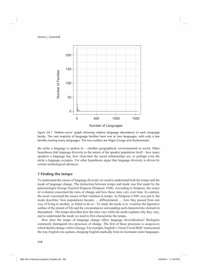
Why do some languages change at a different rate to others?1 What causes one language to change faster than another? Why do some language families have many languages and why do some families only have a few? According to the latest version of the Ethnologue (Lewis 2013), there are 7,547 languages in the world divided into at least 289 language families (including isolates).2 However, there is substantial variation in the number of languages – what I will call diversity3 – in each family. The Niger-Congo and Austronesian language families contain 1,543 and 1,255 languages respectively – about 37 per cent of the total alone. At the other end of the scale, 160 language families have only one surviving language.

Plotting the number of languages in each family gives a language abundance distribution (Figure 26.1) that follows a common distribution called the ‘hollow curve’ fi rst identifi ed in biology (Willis and Yule 1922). The hollow curve distribution shows that there are only a few large language families (e.g. Niger-Congo, Austronesian), and a handful of moderately sized families (e.g. Indo-European, Pama-Nyungan, Trans-New Guinea). The vast majority of language families, however, are very small.

What could be causing the substantial variation in the number of languages, i.e. language diversity? Diversity is the outcome of differences in the birth-rate and the death-rate of languages. For example, there are 31 Mayan languages and 1,235 Malayo-Polynesian languages (Lewis 2013). Both groups have only diverged in the last 4,500 years (Atkinson et al. in press; Gray et al. 2009). Therefore, in those 4,500 years, the ancestral Proto-Malayo-Polynesian language was almost 40 times more prolifi c than Mayan: there was one Mayan language born every 145 years on average while Malayo-Polynesian spawned one language every 44 months.

The pattern of diversity tells us much about the important processes in human prehistory and the factors that have shaped our current global pattern of languages and cultures. Understanding this diversity is so important that it has generated many prominent hypotheses. Some of these hypotheses are more helpful than others for explaining the global pattern of diversity. The fall of Rome, for example, might explain why there are now 42 Romance languages, but does not explain why New Guinea has 477 Trans-New Guinea languages and only four Eastern Trans-Fly languages. What general explanations can we draw about the global causes of language diversity? In this chapter I will review just some of the proposed hypotheses, focusing on those that are large scale and applicable to many languages. Some of these proposed explanations link language diversity to the age of the language family, or


Simon J. Greenhill

558

0

0

50

100

150

200

500 1000 1500

Number of Languages

Num

ber

of F

amili

es

Figure 26.1 ‘Hollow-curve’ graph showing relative language abundance in each language family. The vast majority of language families have one or two languages, with only a few families having many languages. The two outliers are Niger-Congo and Austronesian.

the niche a language is spoken in – whether geographical, environmental or social. Other hypotheses link language diversity to the nature of the speaker population itself – how many speakers a language has, how close-knit the social relationships are, or perhaps even the niche a language occupies. Yet other hypotheses argue that language diversity is driven by certain technological advances.

1 Finding the tempo

To understand the causes of language diversity we need to understand both the tempo and the mode of language change. The distinction between tempo and mode was fi rst made by the paleontologist George Gaylord Simpson (Simpson 1944). According to Simpson, the tempo of evolution concerned the rates of change and how these rates vary over time. In contrast, the mode concerned the causes of that variation in tempo. As Simpson (1944: xxx) put it, the mode describes ‘how populations became … differentiated, … how they passed from one way of living to another, or failed to do so’. To study the mode is to ‘examine the fi gurative outline of the stream of life and the circumstances surrounding each characteristic element in that pattern’. The tempo describes how the rates vary while the mode explains why they vary, and to understand the mode we need to fi rst characterise the tempo.

How does the tempo of language change affect language diversifi cation? Biologists commonly distinguish two processes of change. The fi rst of these processes is anagenesis which details change within a lineage. For example, English’s ‘Great Vowel Shift’ restructured the way English was spoken, changing English markedly from its Germanic sister languages.



559

However, this anagenetic change did not cause new languages to be born. The second process is cladogenesis, which details lineage splitting events – e.g. the birth of new languages. Linguistics tends to confl ate these two different processes. The theories I will discuss below often assume that any increase in anagenesis leads to cladogenesis. These theories assume that increasing the tempo of change, or providing more opportunities for anagenetic changes to occur will increase the rate of language diversifi cation. This assumption makes sense if we think of language as primarily a communication tool, and that ultimately a new language is formed when two groups of people can no longer communicate (cf. Labov 2007). Therefore while the tempo of change may not directly determine the formation of new languages, it is strongly linked to the formation of new languages.

1.1 Lexicostatistics and glottochronology

In linguistics the fi rst major investigation into the tempo of language change occurred primarily through the linked approaches of lexicostatistics and glottochronology. In a series of articles Swadesh (1950, 1952, 1955) proposed that language relationships could be inferred statistically by the number of cognates each language shared on a short wordlist of ‘basic’ or ‘core’ vocabulary. The more cognates shared by two languages the more closely related they were. This approach became known as lexicostatistics. Swadesh extended this hypothesis into glottochronology, a system for inferring the ages of language divergences which assumed that languages lost their shared cognates at a constant rate. Swadesh (1952: 459) described the logic as such:

A language is a highly complex system of symbols serving a vital communicative function in society. The symbols are subject to change by the infl uence of many circumstances, yet they cannot change too fast without destroying the intelligibility of language. If the factors leading to change are great enough, they will keep the rate of change up to the maximum permitted by the communicative function of language. We have, as it were, a powerful motor kept in check by a speed regulating mechanism.

Swadesh (1950) fi rst applied his method to the Salishan languages spoken in the Pacifi c Northwest (see Thomason, this volume). First, he calculated the number of cognates each language shared with each other, then converted these estimates to time using the following equation:

t = logC2logr

Where t is time and C is the number of shared cognates. Swadesh’s r is the retention rate – the rate at which cognates were replaced in the basic vocabulary. In this paper he assumed a retention rate of 0.85 per 1,000 years based on the differences documented between Old and Modern English over a 1,000-year period on a 165 item wordlist. Thus two languages would share 85 per cent of their basic vocabulary after 1,000 years, 72 per cent after 2,000 years, 61 per cent after 3,000 years, and so on.

Support for glottochronology came from a study by Lees (1953) who calculated the retention rates of 13 languages with a documented history of over 1,000 years. For example, Lees found a retention rate of 0.77 in the 1,000 years between Old and Modern English, and 0.85 in the 1,100 years separating Old High German from Modern German. In the 13


Simon J. Greenhill

560

languages studied by Lees the average retention rate was 0.81 ± 0.018 every 1,000 years. The variation in this rate between languages was so small – just 2 per cent – that he argued that this rate was universal with 90 per cent of the world’s languages having a retention rate between 0.79 and 0.82.

Therefore, according to glottochronology, the tempo of language change is largely constant and varies little over time. If this were the case then the primary driver of language diversity would be the age of the family. However, critics were quick to note that there was marked variation in tempo both between and within languages. Bergsland and Vogt (1962) pointed out that there were major discrepancies between known ages and the retention rates proposed by lexicostatistics. Rather than a very tightly constrained rate around 0.81 every 1,000 years, they found that the rate varied substantially. For example, Old Norse and Icelandic diverged around 1,000 years ago, but glottochronology estimated their divergence at less than 200 years. More recently, Blust (2000) showed that only 26.5 per cent of 230 Austronesian languages had retention rates near the proposed 81 per cent.

While lexicostatistics did eventually develop tools to recognise some variability in tempo (e.g. Sankoff 1973; van der Merwe 1966), it fell out of favour in mainstream linguistics (Greenhill and Gray 2009). Instead, the tempo of language change came to be seen as primarily the outcome of the social history of the speakers of a language (Thomason and Kaufman 1988: chapter 3), rather than as some inherent rate of linguistic change (e.g. Swadesh’s ‘engine’). According to this viewpoint, the rate of language change was largely governed by idiosyncrasies of the physical environment, social environment, inter-group contact, bi- or multi-lingualism, prestige factors, and other rate-affecting mechanisms (Nettle 1999a). Taken to the extreme, one could possibly argue, like Dixon (1997: 9) that ‘[t]he rate at which language changes is not constant and is not predictable’. Under this viewpoint the tempo varies wildly and the driver of language diversity can be anything.

1.2 Modern methods

Linguistics has therefore largely swung between two extremes when trying to characterise the tempo. The fi rst extreme assumes that there is a relatively constant tempo of language change across all languages. The second assumes that language change is purely idiosyncratic and at the whim of history. The truth, of course, is somewhere in between Swadesh’s universally regulated ‘engine’ and Dixon’s ‘unpredictability’. The assumption that languages that are more closely related will be more similar, and that languages change at a relatively constant rate in the absence of extenuating factors is a sensible null hypothesis (see section 2.1). What we need therefore are methods that can quantify rates of change and identify signifi cant changes in rates.

The last decade has seen the development of a range of new approaches that attempt to quantify the tempo and make inferences about the mode of language change. There are three approaches mentioned here that are all heavily data-driven and quantitative. The fi rst set of approaches are traditional statistical methods – especially generalised linear models. Generalised linear models are a class of methods that are designed to model the relationship between a set of independent variables and a dependent variable (Nelder and Wedderburn 1972). They aim to discover how well the independent variables predict the dependent variable. Of the three approaches, these statistical methods are often the easiest to use with many off-the-shelf packages existing to set up quite complex analyses. However, one key concern with these approaches is that languages share similarity due to descent and are therefore not statistically independent. This is known as Galton’s Problem. Therefore great



561

care must be taken to factor out the effects of this shared similarity before any inferences can be drawn (Eff 2001).

The second tool used to investigate language diversity is simulations. Here, the researcher makes assumptions about the important factors in language change and then simulates data under these assumptions. The researcher can then manipulate these assumptions and investigate how the output changes. For example, Nettle (1999d) was concerned with investigating the effect of population size on the tempo of language change. He simulated the spread of two competing variants through a population of speakers. Each speaker chose from the two variants according to the relative prevalence of the variants in the population (i.e. the more popular variants got chosen more often). Nettle (1999d) was then able to modify the population size and thus infer the effects of population size on the diffusion of innovations. Simulation methods like this can be elegant and avoid the complexity in real data (Peck 2004). But it is critical that simulations are designed carefully to factor in the relevant aspects of language change. And for simulation approaches to be really effective we need a good theoretical understanding of what factors might be important.

Finally, the third set of approaches are phylogenetic methods (see also Dunn, this volume). Phylogenetic methods take a sample of data from a set of languages and infer their family tree (i.e. the phylogeny). These phylogenies can then be used to make inferences about the processes that shaped that tree. These tools are very powerful and are currently one of the most effective methods for quantitatively testing hypotheses about languages (Greenhill and Gray 2009). One major advantage of phylogenetic methods is to directly quantify the amount of similarity between languages due to descent, leaving the remainder as evidence for the process that is being investigated (Felsenstein 1985). In fact, the ability to side-step Galton’s problem means that phylogenetic methods have higher power when testing hypotheses (Purvis et al. 1994). However, to be most effective these methods require substantial data from many languages within a family and suffi cient data to get a good estimate of the family tree of the relevant languages. Unfortunately good data and good trees are only available for a few language families. Therefore while these phylogenetic methods are exceptionally powerful they are hampered by a lack of good data and have low statistical power when investigating small language families.

2 The mode of language diversity

Armed with these tools to study language tempo we can begin to investigate the mode, i.e. the ‘way, manner, and pattern of evolution’ (Simpson 1944: xxx). What has caused the languages we see around us today and what has driven their diversity? There are many hypotheses about the potential drivers of diversity. All of these hypotheses place the emphasis on different aspects of human prehistory, from the time since divergence, to the size of the speaker population, to technological innovations (especially agriculture), to the geographical and ecological factors and the social and political processes involved in shaping diversity.

2.1 Age

The simplest explanation for why language families differ in size is age (McPeek and Brown 2007; Rabosky et al. 2012). If languages diversify at a relatively constant rate then – all things being equal – older language families will have more languages. A language family like Austro-Asiatic with 169 languages must be roughly about ten times older than a family like Mixe-Zoquean with 17 languages. Following the fall of glottochronology most linguists


Simon J. Greenhill

562

would object strongly to that reasoning. However, the assumption that family age is the primary determinant of family size is often still used implicitly in arguments about time-depth, e.g. the diversity of a given region is inconsistent with a recent settlement date (e.g. Nichols 1990 on the settlement of the Americas).

Despite the strong rejection of glottochronological reasoning, the assumption that family age predicts language diversity is a very good null hypothesis for the size of language families. If a language family has more languages than we would expect given its age, then we should look for potential reasons for this excess diversity. If, however, a language family has fewer languages than we would expect, we might ask what factors could have decreased the diversity.

So how many languages do we expect there to be after a given time? Unfortunately there have been very few good comparative studies of family age and language diversity. The lessons from the glottochronology debate is that there is substantial variation in language birth and death rates. This strongly suggests that family age is not the major predictor. Testing the effect of family age, however, will require more quantifi cation of language diversity rates. Evolutionary biologists have developed a series of birth–death models for estimating the expected diversity in species after a given amount of time and a birth rate (Magallón and Sanderson 2001; Nee et al. 1994). To date these methods have only been applied in linguistics to estimate the total number of languages (> 500,000) ever spoken (Pagel 2000), and not to estimate the birth and death rates within language families. These birth–death models could be very promising in detecting when diversity is unusual. However, these methods need well-dated language trees – a prospect hinted at by the increasing availability of robust phylogenetic dating methods (Gray et al. 2011).

2.2 Population size

Population size is often thought to be one of the main factors determining rates of change (Simpson 1944; Thurston 1987). However, the effect of population size on rates of change is complicated and researchers are divided on just how population size affects rates.

One suggestion is that smaller populations can change faster. In biological populations the success of a new mutation is not only contingent on how useful it is but the size of the population it must spread through (Kimura 1962; Wright 1931). This process is perhaps similar to how a new innovation in a language spreads through a speaker population (Labov 2007; Nettle 1999d). In a linguistic context new innovations (e.g. a new word, or a new phoneme) arise in a population at some specifi c rate. These innovations spread across the members of the community as new people acquire and decide to use this innovation.

Nettle (1999a) argues that in smaller populations new innovations can rapidly diffuse through the population until all members use that form. In larger populations, however, it will take longer for the new innovation to fi lter through all speakers, and the chance is higher that the new innovation does not spread through the entire population. We would expect, therefore, that smaller populations should have a higher tempo of change, which would in turn increase their rate of diversifi cation.

To investigate the effect of population size on rates of change, Nettle (1999a, d) simulated the spread of new innovations through a speech community. In this simulation a given population of speakers decide whether to adopt one of two competing variants. The likelihood that a variant got adopted was based on the proportion of the population with that particular variant (i.e. the more people who have a variant the more likely a speaker is to acquire it). By varying the size of the speaker population, Nettle was able to infer the speed at which



563

innovations diffuse between people. His simulations showed that, as he predicted, the smaller a population the more rapidly innovations spread through it.

The effect of population size on language diversity is perhaps nowhere more evident than in the New World. There is a long-standing debate about when the Americas were fi rst settled. Much of the genetic and archaeological evidence suggests that humans entered North America via a land bridge across the Bering Strait around 15,000 years ago (Kitchen et al. 2008; O’Rourke and Raff 2010). However, the linguistic diversity of the Americas is much higher than many other regions of the globe (with the main exception being New Guinea). Nichols (1990) argued that the sheer number of language families – 69 in North America alone – was incongruent with a 15,000 year time-depth. Instead, she argued that this amount of diversity was about the same as that found in Australia and New Guinea, settled around 50,000 years before present. If true, this diversity would suggest that the Americas were settled much earlier than 15,000 years ago – perhaps even as early as 35,000 years ago.

Nettle (1999c), however, argued that differences in population size explained the supposed mismatch between the linguistic diversity and the genetic and archaeological dates. The languages of the New World were spoken by much smaller populations on average: the New World languages had median population sizes of 385 speakers, while the languages in the Old World had a median population size of 16,778 speakers. While these estimates were contemporary estimates of population size, and not prehistoric estimates, Nettle (1999c) argued that it was likely that this relative difference in population sizes between the New and Old worlds also existed in prehistoric times and was not the result of post-colonial disruption. Therefore, according to Nettle, rather than the high diversity in the Americas refl ecting a deep chronology, the diversity could also be the outcome of a shorter chronology with faster rates of change in smaller populations.

Despite Nettle’s simulation results, empirical evidence that population size is linked to diversifi cation rates is lacking (Wichmann and Holman 2009). The reason why this evidence is lacking is that the effect of population size is not clear. While everyone is clear that population size affects rates of change, researchers are divided on just what this effect might be. Other researchers have suggested that smaller populations have denser social networks (Trudgill 2011) which would slow down the spread of innovations (Granovetter 1973). Indeed, small populations are often conservatising (Bowern 2010) which would allow them to better maintain linguistic and cultural norms.

To resolve these competing theories about population size we need a better understanding of how linguistic innovations spread through the population, and the factors underlying this spread. One way forward here is to incorporate empirical evidence about how innovations diffuse through languages into simulation studies (Labov 2007; Nerbonne 2010). Rather than simply accounting for population size, these simulations would also need to model how innovations spread through different types of social networks (Ross 1997).

Just as importantly there are major problems with how population size is quantifi ed. The database most commonly used for population size estimates, the Ethnologue (Lewis 2013) has only partial information about population size, and this information varies in accuracy and the time it was recorded (1922–2012). Recent estimates of population size are problematic as many populations have undergone substantial increases or decreases in the last few decades especially after contact with European colonists. More importantly populations are not constant – a single estimate of population size at some point in time is rarely suffi cient as populations grow and contract. Fluctuations in population size need to be accounted for. One way to do this would be to apply insights from Coalescent Theory (Kingman 1982). Coalescent models can infer past population dynamics (Drummond et al. 2005) by estimating


Simon J. Greenhill

564

ancestral population sizes under different scenarios of population growth (e.g. exponential increase, or a constant population size over time). These methods could be extended to incorporate information about known population sizes in different time periods and model the unknown population sizes over time.

2.3 Technology

Another possible driver of language diversity is technology. One of the world’s largest language families is Austronesian with 1,255 languages spoken throughout the Pacifi c. The Austronesian peoples originated in Taiwan around 5,200 years ago – and stayed there for another thousand years. Around 4,500–4,000 years ago a rapid expansion pulse swept through the Philippines into Island South East Asia before reaching Western Polynesia around 3,000 years ago (Gray et al. 2009).

What might have caused the 1,000-year long pause before the Austronesians entered the Philippines? Strikingly, the pattern of Austronesian expansion can be strongly linked to advances in canoe technology (Pawley and Pawley 1994). Taiwan and the Philippines are separated by the 350km wide Bashi Channel. The invention of the outrigger canoe and its sail may have enabled the Austronesians to cross the rough water in this channel into the Philippines. Indeed, the terms for outrigger canoes can only be reconstructed to Proto-Malayo-Polynesian – the ancestor of all the Austronesian languages outside Taiwan (Pawley and Pawley 1994). The absence of cognate canoe terms in the languages of Taiwan suggests that they did not have outrigger canoes.

After reaching Western Polynesia there was another long settlement pause of more than 1,000 years before the fi nal expansion into Eastern Polynesia (Pawley 2002). It seems that technological advances are also linked to this fi nal expansion pulse. While in Western Polynesia these peoples developed the double-hulled canoe, which had much greater stability and carrying capacity. Not only did the incipient Polynesians develop better canoes, they combined this with better navigation techniques and social strategies for dealing with greater levels of isolation found in Eastern Polynesia (Irwin 1998). It appears that these technological advances substantially helped the Austronesians to expand into and settle the Pacifi c. Thus technological items can help increase the rate of diversifi cation by opening up new niches for a population to expand into, or by providing the means to out-compete their neighbours, or by enabling the speakers of a language to survive better.

2.3.1 Farming

One technological innovation in particular might have spurred language diversity – farming. The advent of agriculture has been suggested as the major driver of language diversity (Diamond and Bellwood 2003). Agriculture was invented many times around the globe: the ‘Fertile Crescent’ in Mesopotamia 11,000 years ago, the Yangzi and Yellow River basins 9,000 years ago, the New Guinea Highlands 9,000–6,000 years ago, and in Central Mexico 5,000–4,000 years ago (Diamond and Bellwood 2003). Farming populations could generate more food from an area of land and could therefore grow to larger sizes than existing hunter-gatherer populations. Agriculture allowed societies to accumulate and store surplus food. This surplus would both protect them from ecological risk, and act as a precursor to the rise of more complex technologies, social stratifi cation, centralised states and professional armies (Diamond and Bellwood 2003). These key advantages enabled farming populations – and their languages – to grow faster and expand quicker to out-compete hunter-gatherer populations almost globally.



565

Diamond and Bellwood (2003) argue that farming drove or facilitated the expansion of many of the big language families: Afro-Asiatic (376 languages), Arawakan (60), Austro-Asiatic (171), Austronesian (1,255), Aymaran (3), the Bantu subgroup of Niger-Congo (526), Cariban (32), Chibchan (20), Dravidian (85), Indo-European (444), Iroquoian (9), Japonic (12), Mayan (31), Nilo-Saharan (205), Oto-Manguean (177), Quechuan (46), Sino-Tibetan (461), Siouan (14), Tai-Kadai (95), Trans-New Guinea (479), Tupian (75), the Turkic subgroup of Altaic (40), and Uto-Aztecan (61). In short, according to Diamond and Bellwood, 4,677 of the world’s 7,547 languages – 62 per cent – belong to language families that spread with the invention of agriculture.

This Farming Language Dispersal hypothesis is very tempting. First, the advent of agriculture did enable farming populations to rapidly expand in size. Coalescent modelling of genetic data show that farming populations increased in size much faster (approximately fi ve times faster!) than non-farming populations (Gignoux et al. 2011). Second, the dispersal of many of the major language families is coincident with the advent of farming in their home ranges, and agricultural vocabulary can be reconstructed to many of their proto-languages (e.g. Bellwood and Renfrew 2002). Third, many of the biggest language families are primarily spoken by agriculturalist populations. Hammarström (2010) demonstrates that language families which are primarily agricultural have a mean size of 34.9 languages while hunter-gatherer language families have a mean size of just 4.4. In fact, the largest hunter-gatherer language family, Pama-Nyungan, is an order of magnitude smaller with 285 languages than the largest agricultural families like Niger-Congo and Austronesian (1,543 and 1,255 languages respectively).

There might appear to be overwhelming support for the Farming Language Dispersal Hypothesis but there are still some unresolved issues and some sceptics. How, for example, is dispersal linked to diversity? The simplistic view is that the more a language disperses, the more likely it is to diversify into daughter languages. However, farming could just enable populations to grow in size and be more stable over time. Campbell and Poser (2008) argue that agriculture does not always cause expansions but ‘can provide a people with the stability just to stay put, in relative self-suffi ciency’ (p. 338). In fact, as Campbell and Poser (2008) point out, there are prominent exceptions to the hypothesis. Some language families like Mixe-Zoquean, Mayan, Munda and Nakh-Daghestanian are spoken by agriculturalists but have not expanded substantially. In other cases, larger language families like Pama-Nyungan, Uralic and Athabaskan have spread substantially without agriculture.

To answer the question of whether farming caused language dispersals we need much more evidence about the infl uence of subsistence style on populations and their rates of growth and diversifi cation. Why did some ‘farming’ families like Mayan not expand and why did ‘non-farming’ families like Pama-Nyungan expand? One way to answer these questions would be to take a more nuanced approach focusing on the primary subsistence style used by the speakers of those languages (rather than language families). We could then quantify the different food sources used by a population and link that with their population sizes and rates. Perhaps the best way to model these interrelated factors is through some form of aggregate measure of ‘expansion potential’ that quantifi es the likelihood that a language will disperse, given the population size, the environmental carrying capacity, and any other factors. These variables could then be correlated to rates of language change and diversifi cation (e.g. Maddison et al. 2007).


Simon J. Greenhill

566

2.4 Geography and ecology

Unsurprisingly, geography and ecology shape human linguistic and cultural diversity. The effects of geography and ecology can be felt at a regional level by infl uencing resource availability, creating barriers to human contact, and constraining the area inhabited by languages. At a more global scale, geographical effects can be seen in how languages spread across continents and how languages cluster towards the equator.

2.4.1 Resource availability

One major factor shaping language diversity is resource availability. Languages tend to spread out from high-resource areas such as coastlines, rivers, or the forested regions of Europe and North America into low-resource areas. Languages and societies in mountainous areas have tended to expand from lowland regions into highland regions. These local effects are presumably because the better resources in the more fertile regions allow societies to dominate their neighbours. Nichols (1997) has argued that the outcome of these local expansions is that they tend to cause ‘accretion zones’ in resource-poor areas where unrelated languages tend to accrete or accumulate as they are forced out by the more dominant expanding languages. Nichols claims that examples of accretion zones include the Amazon, California and the Pacifi c Northwest, the Caucasus, the Himalayas, New Guinea, North Australia, the northern Rift Valley and Ethiopian highlands.

However, despite Nichols’ theory being relatively prominent, there are some problems. A major issue is that some of the cases that she discusses do not show the expected accretion pattern. In New Guinea, for example, the many subgroups of the large Trans-New Guinea language family – Asmat, Awyu-Dumat, Marind, Kiwai in the south and Madang in the north – appear to have expanded out of the relatively resource-poor highlands, down into the richer lowlands (Pawley 2005). Therefore rather than accreting languages, resource-poor areas might be more prone to being abandoned and then recolonised. In which case, rather than high linguistic diversity in resource-poor areas, we might expect to see fewer languages.

2.4.2 Barriers to human contact

Geography affects language diversity by acting as a barrier to human contact. The less contact people have the less likely they are to share a common language. These barriers can be literal, such as mountain or river or an ocean. One suggestion why New Guinea has so many languages is because of the rough terrain coupled with impassable ‘crocodile-infested rivers’ kept people apart from each other increasing the proliferation of languages (Thurston 1987). In other cases, rivers acted instead as conduits to population expansions and contact between societies while the relatively impenetrable jungle barred human access (Diller 2008). Other barriers are less obvious – the initial settlement of Taiwan lead to the formation of the Austronesian Formosan languages. Sagart (2004) suggests that the Formosan languages spread around the island in a counter-clockwise manner to avoid the ‘possibly malarial’ swamp in the Taipei Basin.

One major important barrier is distance: people fi nd it harder to communicate with people further away. Referring to the great Austronesian expansion, Pawley and Green (1973), argue that it is inevitable that a language spread across multiple islands will diversify if it is separated by enough distance (they suggest about 450km). Marck (1986) noticed a similar pattern in Micronesia (again, part of the Austronesian diaspora) where a major determinant



567

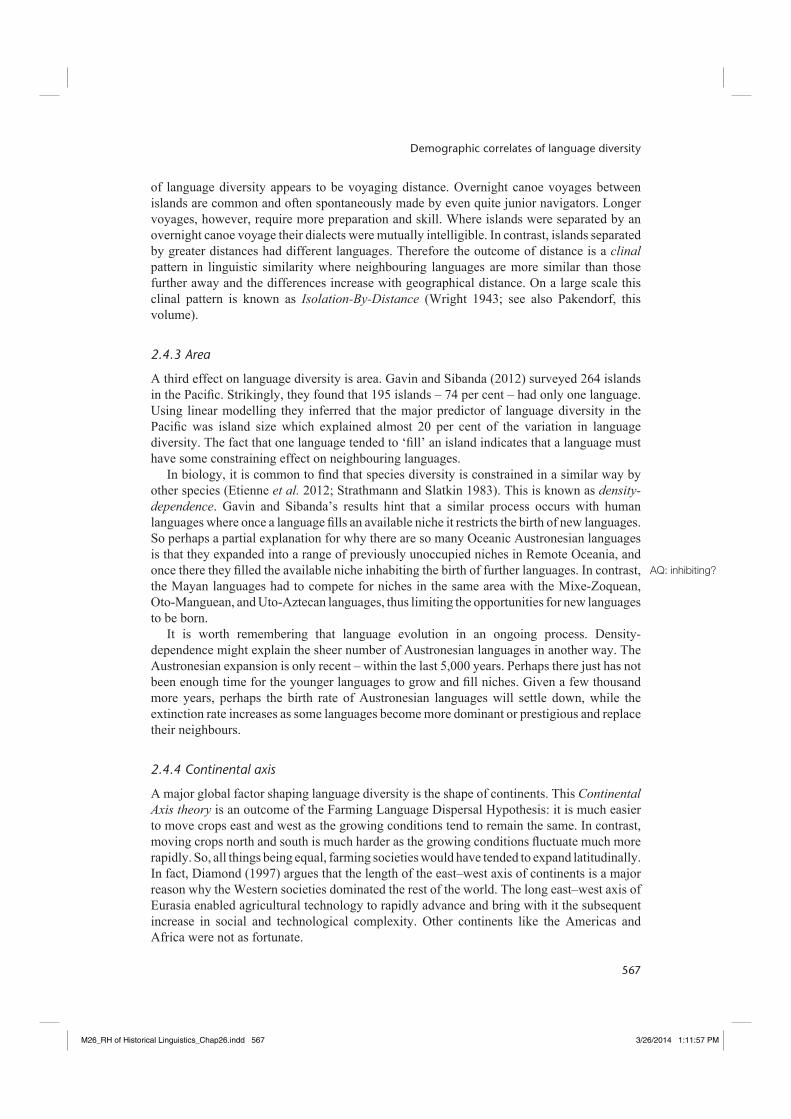
of language diversity appears to be voyaging distance. Overnight canoe voyages between islands are common and often spontaneously made by even quite junior navigators. Longer voyages, however, require more preparation and skill. Where islands were separated by an overnight canoe voyage their dialects were mutually intelligible. In contrast, islands separated by greater distances had different languages. Therefore the outcome of distance is a clinal pattern in linguistic similarity where neighbouring languages are more similar than those further away and the differences increase with geographical distance. On a large scale this clinal pattern is known as Isolation-By-Distance (Wright 1943; see also Pakendorf, this volume).

2.4.3 Area

A third effect on language diversity is area. Gavin and Sibanda (2012) surveyed 264 islands in the Pacifi c. Strikingly, they found that 195 islands – 74 per cent – had only one language. Using linear modelling they inferred that the major predictor of language diversity in the Pacifi c was island size which explained almost 20 per cent of the variation in language diversity. The fact that one language tended to ‘fi ll’ an island indicates that a language must have some constraining effect on neighbouring languages.

In biology, it is common to fi nd that species diversity is constrained in a similar way by other species (Etienne et al. 2012; Strathmann and Slatkin 1983). This is known as density-dependence. Gavin and Sibanda’s results hint that a similar process occurs with human languages where once a language fi lls an available niche it restricts the birth of new languages. So perhaps a partial explanation for why there are so many Oceanic Austronesian languages is that they expanded into a range of previously unoccupied niches in Remote Oceania, and once there they fi lled the available niche inhabiting the birth of further languages. In contrast, the Mayan languages had to compete for niches in the same area with the Mixe-Zoquean, Oto-Manguean, and Uto-Aztecan languages, thus limiting the opportunities for new languages to be born.

It is worth remembering that language evolution in an ongoing process. Density- dependence might explain the sheer number of Austronesian languages in another way. The Austronesian expansion is only recent – within the last 5,000 years. Perhaps there just has not been enough time for the younger languages to grow and fi ll niches. Given a few thousand more years, perhaps the birth rate of Austronesian languages will settle down, while the extinction rate increases as some languages become more dominant or prestigious and replace their neighbours.

2.4.4 Continental axis

A major global factor shaping language diversity is the shape of continents. This Continental Axis theory is an outcome of the Farming Language Dispersal Hypothesis: it is much easier to move crops east and west as the growing conditions tend to remain the same. In contrast, moving crops north and south is much harder as the growing conditions fl uctuate much more rapidly. So, all things being equal, farming societies would have tended to expand latitudinally. In fact, Diamond (1997) argues that the length of the east–west axis of continents is a major reason why the Western societies dominated the rest of the world. The long east–west axis of Eurasia enabled agricultural technology to rapidly advance and bring with it the subsequent increase in social and technological complexity. Other continents like the Americas and Africa were not as fortunate.

AQ: inhibiting?


Simon J. Greenhill

568

Using multivariate linear regression Laitin et al. (2012) estimate the effect of north–south and east–west axes within countries on cultural persistence – the number of historically attested languages that have maintained a language community. They show that the more north–south oriented a country is the longer its languages persist. This result would suggest that the shape of continents and countries shapes language diversity. These results would suggest that countries with longer east–west axes should have more languages, due to the lower cultural persistence and the greater ability for languages and cultures to diffuse latitudinally. In contrast, countries with north–south axes should have fewer, more stable societies and languages.

2.4.5 Latitudinal gradient

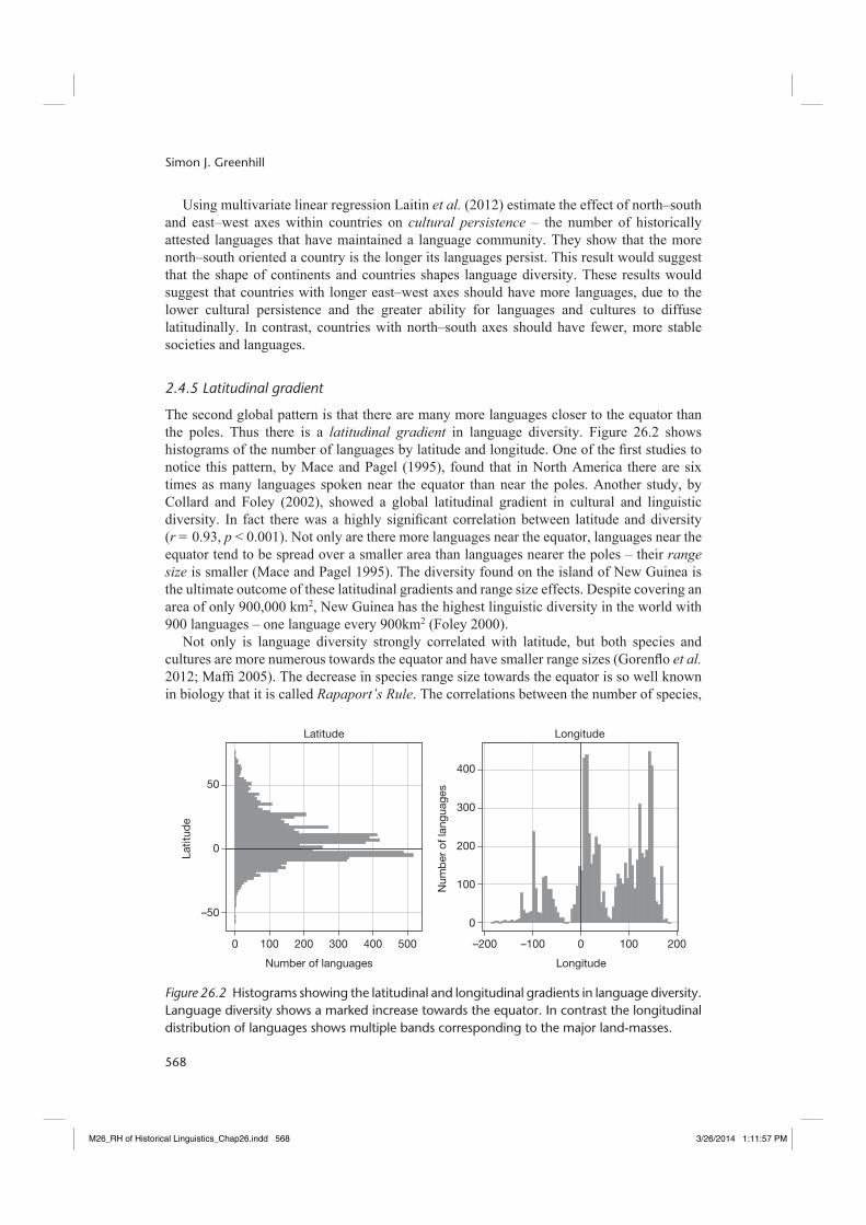
The second global pattern is that there are many more languages closer to the equator than the poles. Thus there is a latitudinal gradient in language diversity. Figure 26.2 shows histograms of the number of languages by latitude and longitude. One of the fi rst studies to notice this pattern, by Mace and Pagel (1995), found that in North America there are six times as many languages spoken near the equator than near the poles. Another study, by Collard and Foley (2002), showed a global latitudinal gradient in cultural and linguistic diversity. In fact there was a highly signifi cant correlation between latitude and diversity (r = 0.93, p < 0.001). Not only are there more languages near the equator, languages near the equator tend to be spread over a smaller area than languages nearer the poles – their range size is smaller (Mace and Pagel 1995). The diversity found on the island of New Guinea is the ultimate outcome of these latitudinal gradients and range size effects. Despite covering an area of only 900,000 km2, New Guinea has the highest linguistic diversity in the world with 900 languages – one language every 900km2 (Foley 2000).

Not only is language diversity strongly correlated with latitude, but both species and cultures are more numerous towards the equator and have smaller range sizes (Gorenfl o et al. 2012; Maffi 2005). The decrease in species range size towards the equator is so well known in biology that it is called Rapaport’s Rule. The correlations between the number of species,

0 0

0

100

200

300

400

–100 100 200–200

–50

0

50

100 200

Number of languages

Latit

ude

Longitude

Num

ber

of l

angu

ages

300 400 500

Latitude Longitude

Figure 26.2 Histograms showing the latitudinal and longitudinal gradients in language diversity. Language diversity shows a marked increase towards the equator. In contrast the longitudinal distribution of languages shows multiple bands corresponding to the major land-masses.



569

languages and cultures in an area suggest that there is some common underlying factor driving this biocultural diversity (Maffi 2005). Strikingly, despite the strength of this gradient little is known about the causes of it (Moore et al. 2002). One possible cause is hinted at by the differences in resource-availability mentioned earlier. Regions near the equator are much more fertile and productive than regions nearer the poles. This theory fi ts with the decrease in range size: more productive environments allow languages, cultures and species to get the resources they need from a smaller area. Alternatively, perhaps the higher latitudes were settled later because it required specialised cultural knowledge for people to survive and thrive in those environments.

The hypothesis that environmental productivity underlies diversity makes intuitive sense for species – more fertile land and better growing conditions means that there can be more species. But how can environmental productivity increase language diversity? Nettle (1998) suggested that the root cause is that different ecologies favour different types of social networks, which leads to differences in language group size. In areas with high seasonal and inter-year variation in food production there is a high level of ecological risk. The higher risk of a shortfall in food forces people to form a large number of social bonds across wider areas so that they can obtain food and resources when they are scarce. In contrast, more productive areas nearer the equator have lower ecological risk and smaller social groups are therefore able to provide everything a society needs. Since a common language is one of the best ways of maintaining social networks, the number of speakers of a language is strongly conditioned by the ecological risk in the environment.

If this ecological risk hypothesis is true, then the languages where ecological risk is higher should have more speakers and be spread across a larger area. Nettle (1998) used regression analysis to compare the mean growing season (i.e. the proportion of the year that food could be produced – a proxy for ecological risk) to the number of languages and speakers in a country. His results showed that this was indeed the case: the longer the growing season was, the more languages there were, even when accounting for population size and land area. This is a very tempting hypothesis for why there are more languages nearer the equator. However, not everyone is convinced. Campbell and Poser (2008: chapter 2) argue that speaking the same language is not necessary for economic links. In many cases these same links can be obtained by lingua francas or trade languages. In fact, many smaller languages in areas like New Guinea have social networks that are defi ned by clan boundaries and not language boundaries (e.g. Foley 2000).

2.4.6 Testing these hypotheses

There are therefore many hypotheses about how geography and ecology interact with language diversity. However, it is only the longitudinal gradient and east–west spreads hypotheses that have really been tested. For the other hypotheses many of the arguments are largely ad hoc or developed on a case-by-case basis. To really test these hypotheses we need two things – good estimates of distances and good estimates of language spread rates.

The fi rst component needed is good estimates of distance. Often a simple measure of the distance between two points (‘as the crow fl ies’) is not appropriate. Instead, the real human distance between two places is a function of the ease of travel between them. One step towards a better distance measure has been made by Haynie (2012) investigating the Eastern Miwok languages of Central Sierra Nevada. Haynie used cost distance modelling to adjust travel costs by incorporating environmental parameters (e.g. elevation, terrain, etc) into a ‘hitch-hiking’ model that describes how fast people travel on foot over different slopes.


Simon J. Greenhill

570

The second component needed to test these geographic hypotheses are good estimates of the rates of language spread. One study by Nichols (2008) calculates the language spread rates of North American languages from the distance they covered in a given timeframe. However, this method depends on crude glottochronological estimates of time-depth and only calculates a point rate for each language family (rather than allowing for variation in expansion rates). More recently a new set of phylogeographical methods has been applied to Indo-European languages by Bouckaert et al. (2012). Phylogeographic methods combine phylogenetic approaches with geographical modelling to infer the phylogeny of these languages, while simultaneously estimating the geographic location of proto-languages and their homelands. The results showed that the Indo-European language family expanded at a mean rate of 0.48 kilometres per year – with much variation between languages. The model of Bouckaert et al. provides a really powerful tool for quantifying language spread rates at a far better resolution than that provided by Nichols (2008). However, the Bouckaert et al. model only incorporates information about coastal boundaries and is ripe for extension.

Combining these two components – real distance measures and phylogeography – into a combined model of language diffusion would lead to a nuanced understanding of how languages spread across different landscapes. These tools could directly model the effect of different terrains e.g. speeding up along coastlines, or slowing down through mountainous areas, and infer how the rates of change vary across space and time. This combination is very promising, raising the exciting prospect of answering these questions about how geography and ecology infl uence language expansions and language diversity.

2.5 Social factors

Social factors play a major role in affecting language diversity in many different ways (see also Michael, this volume). Most of these social factors tend to affect the tempo of change. For example, some languages re-organise themselves due to the effects of language contact (Ross 1996), while others import many or few items from other languages (Blust 1996), yet others ratchet up the tempo by practices such as word tabooing (Elmendorf 1970). Other factors prejudice speakers for or against a language (e.g. perceived prestige biases, religious practices, or stigmatisation), thus increasing the rate at which some languages grow and causing others to die out. Following the theme of this chapter I will only discuss in detail three prominent large-scale hypotheses that seek to explain global language diversity: emblematic function, the linguistic niche hypothesis and political complexity.

2.5.1 Emblematic function

One function of language is to provide distinctive ‘emblems’ for social groups (Grace 1975; Ross 1996). For example, François (2011) discusses the strikingly high levels of linguistic diversity in Vanuatu – more than 100 languages spoken on a series of islands settled only 3,000 years ago. François argues that this extreme linguistic diversity has been caused by a social bias that indulges cultural differentiation. When innovations arise they are typically seized upon as a linguistic shibboleth designed to differentiate one group from another. The result of this process is that each community will have a substantially different lexicon to its neighbours. Foley (2000) has suggested that this sort of process is one of the major causes of language diversity in New Guinea.

Thus, perhaps one of the factors causing language diversity is the formation of new languages themselves – as languages are born, people elaborate differences to make linguistic



571

emblems. We would see a pattern of punctuated equilibrium (Eldredge and Gould 1972) where for most of the time there would be little change – an equilibrium – but this equilibrium would be punctuated by bursts of change caused by the newly developed social groups forming a new language. If this hypothesis is true, the amount of change in a language should be correlated with the number of ancestral language stages it passed through. Atkinson et al. (2008) used phylogenetic methods to test whether languages experience just such a burst of change. To do this, they inferred phylogenetic trees from the basic vocabulary of three large language families – Austronesian, Bantu, and Indo-European. Their results show that a substantial proportion of the total amount of lexical change arose as a result of language splitting events: 31 per cent in Bantu, 21 per cent in Indo-European, and 9.5 per cent in Austronesian. The Central Pacifi c subfamily of Austronesian in Polynesia showed the highest rates of punctuational change at 33 per cent. Atkinson et al. argue that these results show that punctuated equilibrium – presumably as a result of emblematicity – is the prevailing mode of language change.

The results from Atkinson et al. are intriguing but much more work is needed. One issue is that we would not necessarily expect linguistic emblems in the basic vocabulary data used by Atkinson et al. (2008). Testing for this effect in the wider lexicon would be more appropriate. Another concern is that there may be methodological artefacts in their analysis that could overestimate the strength of punctuational effects. Rabosky (2012) argues that a better test would be to simultaneously estimate the covariance between the rate of diversifi cation and the rate of change.

2.5.2 Esoterogeny and exoterogeny

An extension of the idea that languages have an emblematic function is that we can differentiate languages based on how often people tend to communicate with insiders or outsiders. Thurston (1987) distinguishes between two different types of languages. Esoteric languages are languages that are spoken by small and tightly-knit groups – picture the stereotypical language spoken in one village. These esoteric languages are primarily learnt by children within the same community. In contrast, exoteric languages are spoken by large numbers of people across social boundaries e.g. English. Rather than native speakers, exoteric languages are primarily spoken by second-language speakers and are learnt during adulthood. Since adults have a much harder time learning language, they tend to not learn complex morphological and syntactical rules. Thus, we would perhaps expect that, over time, exoteric languages would become less morphologically and syntactically complex. Smaller languages, in contrast, can accumulate more irregularities in their morphology.

These two different types of languages fi ll different social niches. If this linguistic niche hypothesis is true then we would expect there to be a linkage between social structure and language complexity. That is, languages should decrease in complexity as the speaker population increases, and vice versa. Lupyan and Dale (2010) tested this hypothesis using a general linear model. They show that, as predicted, languages with more speakers tended to be less morphologically complex and used lexical strategies to encode semantic and syntactic distinctions. Therefore, as languages expand over larger areas they become increasingly affected by constraints on learnability and the limitations of second-language learners. This bias causes irregularities and complexities to be lost making the language easier to learn. Lupyan and Dale’s results provide some tantalising evidence that social and demographic factors infl uence the tempo of change within languages. How might this affect the mode of language diversity? We might predict that as languages increase in speakers, they would become easier to learn and gain more speakers. This inference, however, needs to be tested further.


Simon J. Greenhill

572

2.5.3 Political complexity

The ways that people organise themselves into societies also infl uences language diversity. One aspect of social organisation linked to language diversity is political complexity. Within the last 10,000 years human societies have grown in size. As societies have grown they have faced increasing demands to organise themselves in a way to enhance co-ordination between large groups of people. One way of dealing with this increase in size is to increase political complexity by creating hierarchical levels of control in a society. Currie and Mace (2009) use a linear mixed model to demonstrate that the area that languages cover is predicted by the degree of political complexity in the society that uses that language – presumably because more complex societies tend to expand to replace or incorporate other societies.

Currie and Mace (2009) argue that their results show that political complexity enables languages to expand over larger areas. The alternative is that the possession of a common language in a large population enables complex societies to arise. Currie and Mace (2009) propose that the fi rst alternative is more likely. Historical evidence shows that people tend to give up their languages for those spoken by politically dominant societies (e.g. Latin) – people fl ock to the dominant and complex societies. One way to resolve these two competing hypotheses would be to use phylogenetic comparative methods to infer whether political complexity tended to arise before the birth of languages belonging to politically complex societies or after.

3 Outstanding problems

Understanding the causes of language diversity is vital to understanding the patterns and processes of human prehistory. I have presented only a very partial catalogue of these causes above and many more have not been mentioned. Often linguists explain diversity by invoking a laundry list of possible causes rather than attempting to pinpoint the most prominent causes. On the other hand when general causes are proposed they are written off because of counter-examples. It is true that counter-examples matter, and the causes of diversity are manifold. However, what matters is the relative strength of these causes in shaping language diversity. To understand this we must be careful to quantify diversity and to statistically test the hypothesised drivers. As the biologist John Maynard-Smith put it, when referring to species diversity (Maynard-Smith 1989: 6):

it is fatally easy to read a pattern into stochastically generated data. The fi rst task, then, is to provide convincing evidence that a pattern really exists. This is not easy.

To avoid reading spurious patterns from language diversity we need to gain a far better understanding of both the tempo and the mode. To better understand the tempo we need much more quantitative information about language change within languages, between languages and over time. Unfortunately, most of the work on the tempo of language change has either been highly specifi c – focusing on a small number of changes in one or a few languages – or impressionistic (Johnson 1976), or simply concerned with fi nding stable features (Parkvall 2008) rather than exploring variation. Instead, what we need are large-scale comparative studies of how various features of language vary in tempo. One way to do this would be to use phylogenetic methods to quantify the rate of change in language features. There have been some preliminary studies quantifying the rates of change in basic vocabulary (Pagel et al. 2007), and in structural features (Dediu 2010; Greenhill et al. 2010), however



573

these need to be extended to more languages and wider sets of data for us to fully understand the tempo.

To better understand the mode of language change we need much more empirical work testing the causes of diversity. In the sections above I have outlined specifi cs about how I think this could be done. In general, however, I think the way forward is through a fuller methodological cross-fertilisation with evolutionary biology. Evolutionary biologists are concerned with many of the same things that historical linguists are (Greenhill and Gray 2009). Biologists have long been fascinated by species diversity and there has been a major research undertaking to understand the patterns of diversity in species since the 1970s (Raup et al. 1973). As a result there have been a number of powerful methods developed to answer questions about biological diversity (Ricklefs 2007). One approach is to quantify the shape of family trees and make insights about whether the birth rates are unequal in different parts of the tree (Aldous 2001). The distribution of subgroups over time can be used to infer whether speciation sped up or slowed down (Pybus and Harvey 2000). Another approach is to infer birth rates and extinction rates from observed distributions of species diversity (Nee 2006; Nee et al. 1994). Other methods can calculate the link between certain features and the rate of diversifi cation (Maddison et al. 2007). All of these approaches provide a way of answering some of the questions about proposed drivers of language diversity.

It is not only empirical studies that are lacking, but the theoretical background of proposed language drivers is often weak. As one example, often the models of language that underlie the proposed drivers are unclear or confl icting. The hypotheses about population size and geographical factors assume that language divergence is a passive and entropic process (Grace 1975) where languages simply diverge as similarity is lost. This model places the locus of change at the level of the language and minimises the role of the speaker. However, the other hypotheses about social factors assume that language diversifi cation is the active outcome of goal directed actions by language speakers. Here the locus of change is directly on the speakers. These two different models of language change are very different (Bradshaw 1995). How do we resolve these competing models? Ultimately we need to develop a full theoretical model of how languages change, how they are carried in a speech community, and how speech communities break up as their speakers disperse across the world. Some initial forays have been made (Milroy and Milroy 1985; Ross 1997; see also François, this volume) but there is much work to be done.

One fi nal outstanding problem is that all these proposed drivers are often treated as single causes. Often this is a necessity for operationalising research questions to test them. However, many of the proposed drivers are suggested to be the primary cause of diversity. Reality is much more complex. Explanations of why New Guinea is the most linguistically diverse island in the world requires at least three factors – the large amount of time since settlement (~ 50,000 years), the rough terrain causing populations to be small and fragmented, and the social attitudes of the speakers to multilingualism (Foley 2000). To move forwards we need a more nuanced picture of how drivers are related and interact. For example, the invention of farming requires fertile land with suffi cient area. Fertile land increases population size and decreases the risk of running out of food. Population size in turn enables the rise of political and technological complexity (Kline and Boyd 2010). Language diversity is the complex outcome of all these interlocking causes that feed back onto each other in complex ways. Truly understanding language diversity will require us to understand how all these proposed drivers of diversity interact.


Simon J. Greenhill

574

4 Conclusion

Our understanding of the demographic causes and correlates of language change are still preliminary. The stakes are high – what factors have shaped the modern-day distribution of languages and what factors are important in causing new languages? However, we know strikingly little about all of the factors involved. One of the most complete studies incorporates information about most of the proposed drivers discussed into an analysis of Pacifi c island languages (Gavin and Sibanda 2012). This study only manages to explain half of the variation in language diversity in the Pacifi c. What are we missing?

Notes

1 Thank you to Claire Bowern, Beth Evans, Nick Evans, Andrew Pawley and Annik van Toledo for commenting on the manuscript, and to Hannah Haynie for discussing her work with Miwok.

2 All counts of languages, language families and populations are taken from Lewis (2013).3 There are many uses of the term ‘diversity’ in linguistics ranging from the number of families to

the magnitude of differences between each language (i.e. disparity). In this chapter I will use it to simply refer to the number of languages in each family.

Further reading

Campbell, Lyle and William J. Poser. 2008. Language classifi cation: history and method. Cambridge: Cambridge University Press.

Gavin, Michael C., Carlos A. Botero, Claire Bowern, Robert K. Colwell, Michael Dunn, Robert R. Dunn, Russell D. Gray, Kathryn R. Kirby, Joe McCarter, Adam Powell, Thiago F. Rangel, John R. Stepp, Michelle Trautwein, Jennifer L. Verdolin and Gregor Yanega. 2013. Toward a mechanistic understanding of linguistic diversity. BioScience 63(7): 524–535.

Greenhill, Simon J., Quentin D. Atkinson, Andrew Meade and Russell D. Gray. 2010. The shape and tempo of language evolution. Proceedings of the Royal Society B: Biological Sciences 277(1693): 2443–2450.

Nettle, Daniel. 1999. Linguistic diversity. Oxford: Oxford University Press.Ross, Malcolm. 1997. Social networks and kinds of speech-community event. In Roger Blench and

Matthew Spriggs (eds) Archaeology and language I: theoretical and methodological orientations. London/New York: Routledge, 209–261.

References

Aldous, David J. 2001. Stochastic models and descriptive statistics for phylogenetic trees, from Yule to today. Statistical Science 16(1): 23–34.

Atkinson, Quentin D., Andrew Meade, Chris Venditti, Simon J. Greenhill and Mark Pagel. 2008. Languages evolve in punctuational bursts. Science 319(5863): 588.

Atkinson, Quentin D., Simon J. Greenhill and Russell D. Gray. in press. Bayesian phylogenetic analyses of Mayan languages.

Bellwood, Peter and Colin Renfrew. 2002. Examining the farming/language dispersal hypothesis. Cambridge: McDonald Institute for Archaeological Research, Cambridge University Press.

Bergsland, Knut and Hans Vogt. 1962. On the validity of glottochronology. Current Anthropology 3(2): 115–153.

Blust, Robert. 1996. Some remarks on the linguistic position of Thao. Oceanic Linguistics 35(2): 272–294.——2000. Why lexicostatistics doesn’t work: the ‘universal constant’ hypothesis and the Austronesian

languages. In Colin Renfrew, April McMahon and Larry Trask (eds) Time depth in historical linguistics. Cambridge: McDonald Institute for Archaeological Research, 311–331.



575

Bouckaert, Remco R., Philippe Lemey, Michael Dunn, Simon J. Greenhill, Alexander V. Alekseyenko, Alexei J. Drummond, Russell D. Gray, Mark A. Suchard and Quentin D. Atkinson. 2012. Mapping the origins and expansion of the Indo-European language family. Science 337(6097): 957–960.

Bowern, Claire. 2010. Correlates of language change in hunter-gatherer and other ‘small’ languages. Language and Linguistics Compass 4(8): 665–679.

Bradshaw, Joel. 1995. How and why do people change their languages? Oceanic Linguistics 34(1): 191–201.

Campbell, Lyle and William J. Poser. 2008. Language classifi cation: history and method. Cambridge: Cambridge University Press.

Collard, Ian F. and Robert A. Foley. 2002. Latitudinal patterns and environmental determinants of recent human cultural diversity: do humans follow biogeographical rules? Evolutionary Ecology Research 4: 371–383.

Currie, Thomas E. and Ruth Mace. 2009. Political complexity predicts the spread of ethno-linguistic groups. Proceedings of the National Academy of Sciences of the United States of America 106(18): 7339–7344.

Dediu, Dan. 2010. A Bayesian phylogenetic approach to estimating the stability of linguistic features and the genetic biasing of tone. Proceedings of the Royal Society B: Biological Sciences 278(1704): 474–479.

Diamond, Jared. 1997. Guns, germs, and steel. New York: W. W. Norton.Diamond, Jared and Peter Bellwood. 2003. Farmers and their languages: the fi rst expansions. Science

300(5619): 597–603.Diller, Anthony. 2008. Mountains, rivers or seas? Ecology and language history in Southeast Asia. In

Wilaiwan Khanittanan and Paul Sidwell (eds) SEALSXIV: Papers from the 14th meeting of the Southeast Asian Linguistics Society (2004): Volume 1. Canberra: Pacifi c Linguistics.

Dixon, R. M. W. 1997. The rise and fall of languages. Cambridge: Cambridge University Press.Drummond, A. J., A. Rambaut, B. Shapiro and O. G. Pybus. 2005. Bayesian coalescent inference of

past population dynamics from molecular sequences. Molecular Biology and Evolution 22(5): 1185–1192.

Eff, E. Anthon. 2001. Does Mr. Galton still have a problem?: autocorrelation in the Standard Cross-Cultural Sample. World Cultures 15: 153–170.

Eldredge, Niles and Stephen J. Gould. 1972. Punctuated Equilibria: an alternative to phyletic gradualism. In Thomas J. M. Schopf (ed.) Models in paleobiology. San Francisco: Freeman Cooper, 193–223.

Elmendorf, W. W. 1970. Word tabu and change rates: tests of a hypothesis. In Earl H. Swanson (ed.) Languages and cultures of western North America. Pocatello: Idaho State University Press, 74–85.

Etienne, Rampal S., Bart Haegeman, Tanja Stadler, Tracy Aze, Paul N. Pearson, Andy Purvis and Albert B. Phillimore. 2012. Diversity-dependence brings molecular phylogenies closer to agreement with the fossil record. Proceedings of the Royal Society B: Biological Sciences 279(1732): 1300–1309.

Felsenstein, Joseph. 1985. Phylogenies and the Comparative Method. The American Naturalist 125(1): 1–15.

Foley, William A. 2000. The Languages of New Guinea. Annual Review of Anthropology 29: 357–404.François, Alexandre. 2011. Where *R they all? The geography and history of *R-loss in Southern

Oceanic languages. Oceanic Linguistics 50(1): 140–197.Gavin, Michael C. and Nokuthaba Sibanda. 2012. The island biogeography of languages. Global

Ecology and Biogeography 10(1): 958–967.Gavin, Michael C., Carlos A. Botero, Claire Bowern, Robert K. Colwell, Michael Dunn, Robert R.

Dunn, Russell D. Gray, Kathryn R. Kirby, Joe McCarter, Adam Powell, Thiago F. Rangel, John R. Stepp, Michelle Trautwein, Jennifer L. Verdolin and Gregor Yanega. 2013. Toward a mechanistic understanding of linguistic diversity. BioScience 63(7): 524–535.

Gignoux, Christopher R., Brenna M. Henn and Joanna L. Mountain. 2011. Rapid, global demographic expansions after the origins of agriculture. Proceedings of the National Academy of Sciences of the United States of America 108(15): 6044–6049.


Simon J. Greenhill

576

Gorenfl o, L. J., Suzanne Romaine, Russell A. Mittermeier and Kristen Walker-Painemilla. 2012. Co-occurrence of linguistic and biological diversity in biodiversity hotspots and high biodiversity wilderness areas. Proceedings of the National Academy of Sciences of the United States of America 109(21): 8032–8037.

Grace, George W. 1975. Linguistic diversity in the Pacifi c: on the sources of diversity. University of Hawai’i Working Papers in Linguistics 7(3): 1–7.

Granovetter, Mark S. 1973. The strength of weak ties. American Journal of Sociology 78(6): 1360–1380.

Gray, Russell D., Alexei J. Drummond and Simon J. Greenhill. 2009. Language phylogenies reveal expansion pulses and pauses in Pacifi c settlement. Science 323(5913): 479–483.

Gray, Russell D., Quentin D. Atkinson and Simon J. Greenhill. 2011. Language evolution and human history: what a difference a date makes. Philosophical Transactions of the Royal Society B: Biological Sciences 366(1567): 1090–1100.

Greenhill, Simon J. and Russell D. Gray. 2009. Austronesian language phylogenies: myths and misconceptions about Bayesian computational methods. In Alexander K. Adelaar and Andrew Pawley (eds) Austronesian historical linguistics and culture history: a festschrift for Robert Blust. Canberra: Pacifi c Linguistics, 375–397.

Greenhill, Simon J., Quentin D. Atkinson, Andrew Meade and Russell D. Gray. 2010. The shape and tempo of language evolution. Proceedings of the Royal Society B: Biological Sciences 277(1693): 2443–2450.

Hammarström, Harald. 2010. A full-scale test of the language farming dispersal hypothesis. Diachronica 27(2): 197–213.

Haynie, Hannah J. 2012. Topics in the history and geography of California languages. Ph.D. Dissertation, University of California (Berkeley).

Irwin, Geoffrey. 1998. The colonisation of the Pacifi c Plate: chronological, navigational and social issues. Journal of the Polynesian Society 107: 111–145.

Johnson, Lawrence. 1976. A rate of change index for language. Language in Society 5: 165–172.Kimura, Motoo. 1962. On the probability of fi xation of mutant genes in a population. Genetics 57:

713–719.Kingman, J. F. C. 1982. The coalescent. Stochastic Processes and their Applications 13(3): 639–248.Kitchen, Andrew, Michael M. Miyamoto and Connie J. Mulligan. 2008. A three-stage colonization

model for the peopling of the Americas. PloS One 3(2): e1596.Kline, Michelle A. and Robert Boyd. 2010. Population size predicts technological complexity in

Oceania. Proceedings of the Royal Society B: Biological Sciences 277(1693): 2559–2564.Labov, William. 2007. Transmission and diffusion. Language 83: 344–387.Laitin, David D., Joachim Moortgat and Amanda Lea Robinson. 2012. Geographic axes and the

persistence of cultural diversity. Proceedings of the National Academy of Sciences of the United States of America 109(26): 10263–10268.

Lees, R. B. 1953. The basis of Glottochronology. Language 29(2): 113–127. Lewis, Paul M. (ed.). 2013. Ethnologue: languages of the world. 17th Edition. Dallas, Texas: SIL

International.Lupyan, Gary and Rick Dale. 2010. Language structure is partly determined by social structure. PloS

One 5(1): e8559.Mace, Ruth and Mark Pagel. 1995. A latitudinal gradient in the density of human languages in North

America. Proceedings of the Royal Society B: Biological Sciences 261(1360): 117–121.Maddison, Wayne P., Peter E. Midford and Sarah P. Otto. 2007. Estimating a binary character’s effect

on speciation and extinction. Systematic Biology 56(5): 701–710.Maffi , Luisa. 2005. Linguistic, cultural, and biological diversity. Annual Review of Anthropology 34(1):

599–617.Magallón, Susana and Michael J. Sanderson. 2001. Absolute diversifi cation rates in angiosperm clades.

Evolution 55(9): 1762–1780.

AQ: check

folio pls



577

Marck, Jeffrey C. 1986. Micronesian dialects and the overnight voyage. Journal of the Polynesian Society 95(2): 253–258.

Maynard-Smith, J. 1989. The causes of extinction. Philosophical Transactions of the Royal Society of London. Series B: Biological Sciences, 325(1228): 241–252.

McPeek, Mark A. and Jonathan M. Brown. 2007. Clade age and not diversifi cation rate explains species richness among animal taxa. The American Naturalist 169(4): e97–106.

Milroy, James and Lesley Milroy. 1985. Linguistic change, social network and speaker innovation. Journal of Linguistics 21(2): 339–384.

Moore, Joslin L., Lisa Manne, Thomas Brooks, Niel D. Burgess, Robert Davies, Carsten Rahbek, Paul Williams and Andrew Balmford. 2002. The distribution of cultural and biological diversity in Africa. Proceedings of the Royal Society B: Biological Sciences 269(1501): 1645–1653.

Nee, Sean. 2006. Birth-death models in macroevolution. Annual Review of Ecology, Evolution, and Systematics 37: 1–17.

Nee, Sean, Robert M. May and Paul H. Harvey. 1994. The reconstructed evolutionary process. Philosophical Transactions of the Royal Society B: Biological Sciences 344: 305–311.

Nelder, J. A. and R. W. M. Wedderburn. 1972. Generalized Linear Models. Journal of the Royal Statistical Society A. 135: 370–384.

Nerbonne, John. 2010. Measuring the diffusion of linguistic change. Philosophical Transactions of the Royal Society of London. Series B: Biological Sciences 365(1559): 3821–3828.

Nettle, Daniel. 1998. Explaining global patterns of language diversity. Journal of Anthropological Archaeology 17: 354–374.

——1999a. Is the rate of linguistic change constant? Lingua 108(2–3): 119–136.——1999b. Linguistic diversity. Oxford: Oxford University Press.——1999c. Linguistic diversity of the Americas can be reconciled with a recent colonization.

Proceedings of the National Academy of Sciences 96(6): 3325–3329.——1999d. Using Social Impact Theory to simulate language change. Lingua 108(2–3): 95–117.Nichols, Johanna. 1990. Linguistic diversity and the fi rst settlement of the New World. Language

66(3): 475–521.——1997. Modeling ancient population structures and movement in linguistics. Annual Review of

Anthropology 26: 359–384.——2008. Language spread rates and prehistoric American migration rates. Current Anthropology

49(6): 1109–1117.O’Rourke, Dennis H. and Jennifer A. Raff. 2010. The human genetic history of the Americas: the fi nal

frontier. Current Biology 20(4): R202–R207.Pagel, Mark. 2000. The history, rate and pattern of world linguistic evolution. In Chris Knight, Michael

Studdert-Kennedy and James Hurford (eds) The evolutionary emergence of language. Social function and the origins of linguistic form. Cambridge: Cambridge University Press, 391–416.

Pagel, Mark, Quentin D. Atkinson and Andrew Meade. 2007. Frequency of word-use predicts rates of lexical evolution throughout Indo-European history. Nature 449(7163): 717–720.

Parkvall, M. 2008. Which parts of language are the most stable? STUF-Language Typology and Universals 61(3): 234–250.

Pawley, Andrew. 2002. The Austronesian dispersal: languages, technologies and people. In Peter Bellwood and Colin Renfrew (eds) Examining the farming/language dispersal hypothesis. Cambridge: McDonald Institute for Archaeological Research, 251–273.

——2005. Trans New Guinea hypothesis: recent research and its implications. In Andrew Pawley, Robert Attenborough, Jack Golson and Robin Hide (eds) Papuan Pasts: cultural, linguistic and biological histories of Papuan-speaking peoples. Canberra: Pacifi c Linguistics, 251–273.

Pawley, Andrew and Roger C. Green. 1973. Dating the dispersal of the Oceanic languages. Oceanic Linguistics 12(1): 1–67.

Pawley, Andrew and Medina Pawley. 1994. Early Austronesian terms for canoe parts and seafaring. In Andrew Pawley and Malcolm D. Ross (eds) Austronesian terminologies: continuity and change. Canberra: Pacifi c Linguistics, 329–361.


Simon J. Greenhill

578

Peck, Steven L. 2004. Simulation as experiment: a philosophical reassessment for biological modeling. Trends in Ecology and Evolution 19(10): 530–534.

Purvis, Andy, John L. Gittleman and H. K. Luh. 1994. Truth or consequences: effects of phylogenetic accuracy on comparative methods. Journal of Theoretical Biology 167(3): 293–300.

Pybus, Oliver G. and Paul H. Harvey. 2000. Testing macro-evolutionary models using incomplete molecular phylogenies. Proceedings of the Royal Society B: Biological Sciences 267(1459): 2267–2272.

Rabosky, Daniel L. 2012. Positive correlation between diversifi cation rates and phenotypic evolvability can mimic punctuated equilibrium on molecular phylogenies. Evolution 66: 2622–2627.

Rabosky, Daniel L., Graham J. Slater and Michael E. Alfaro. 2012. Clade age and species richness are decoupled across the eukaryotic tree of life. PLoS Biology 10(8): e1001381.

Raup, David M., Stephen Jay Gould, Thomas J. M. Schopf and Daniel S. Simberloff. 1973. Stochastic models of phylogeny and the evolution of diversity. Journal of Geology 81(5): 525–542.

Ricklefs, Robert E. 2007. Estimating diversifi cation rates from phylogenetic information. Trends in Ecology and Evolution 22(11): 601–610.

Ross, Malcolm. 1996. Contact-induced change and the comparative method: cases from Papua New Guinea. In Mark Durie and Malcolm Ross (eds) The Comparative Method reviewed: regularity and irregularity in language change. Oxford: Oxford University Press, 180–217.

——1997. Social networks and kinds of speech-community event. In Roger Blench and Matthew Spriggs (eds) Archaeology and language I: theoretical and methodological orientations. London/New York: Routledge, 209–261.

Sagart, Laurent. 2004. The higher phylogeny of Austronesian and the position of Tai-Kadai. Oceanic Linguistics 43(2): 411–444.

Sankoff, David. 1973. Mathematical developments in lexicostatistic theory. Current Trends in Linguistics 11: 93–113.

Simpson, George G. 1944. Tempo and mode in evolution. New York: Columbia University Press.Strathmann, Richard R. and Montgomery Slatkin. 1983. The improbability of animal phyla with few

species. Paleobiology 9(2): 97–106.Swadesh, Morris. 1950. Salish internal relationships. International Journal of American Linguistics

16(4): 157–167.——1952. Lexico-statistic dating of prehistoric ethnic contacts. With special reference to North

American Indians and Eskimos. Proceedings of the American Philosophical Society 96(4): 452–463.

——1955. Towards greater accuracy in lexicostatistic dating. International Journal of American Linguistics 21(2): 121–137.

Thomason, Sarah Grey and Terence Kaufman. 1988. Language contact, creolization, and genetic linguistics. California: University of California Press.

Thurston, William R. 1987. Processes of change in the languages of North-Western New Britain. Canberra: Pacifi c Linguistics.

Trudgill, Peter. 2011. Sociolinguistic typology: social determinants of linguistic complexity. Oxford: Oxford University Press.

van der Merwe, N. J. 1966. New mathematics for glottochronology. Current Anthropology 7: 485–500.Wichmann, Søren and Eric W. Holman. 2009. Population size and rates of language change. Human

Biology 81: 259–274.Willis, J. C. and G. Undy Yule. 1922. Some statistics of evolution and geographical distribution in

plants and animals, and their signifi cance. Nature 109: 177–179.Wright, Sewall. 1931. Evolution in Mendelian populations. Genetics 16(2): 97–159.——1943. Isolation by distance. Genetics 28: 114–138.


Demographic correlates of language diversity

Documents

Transcript of Demographic correlates of language diversity