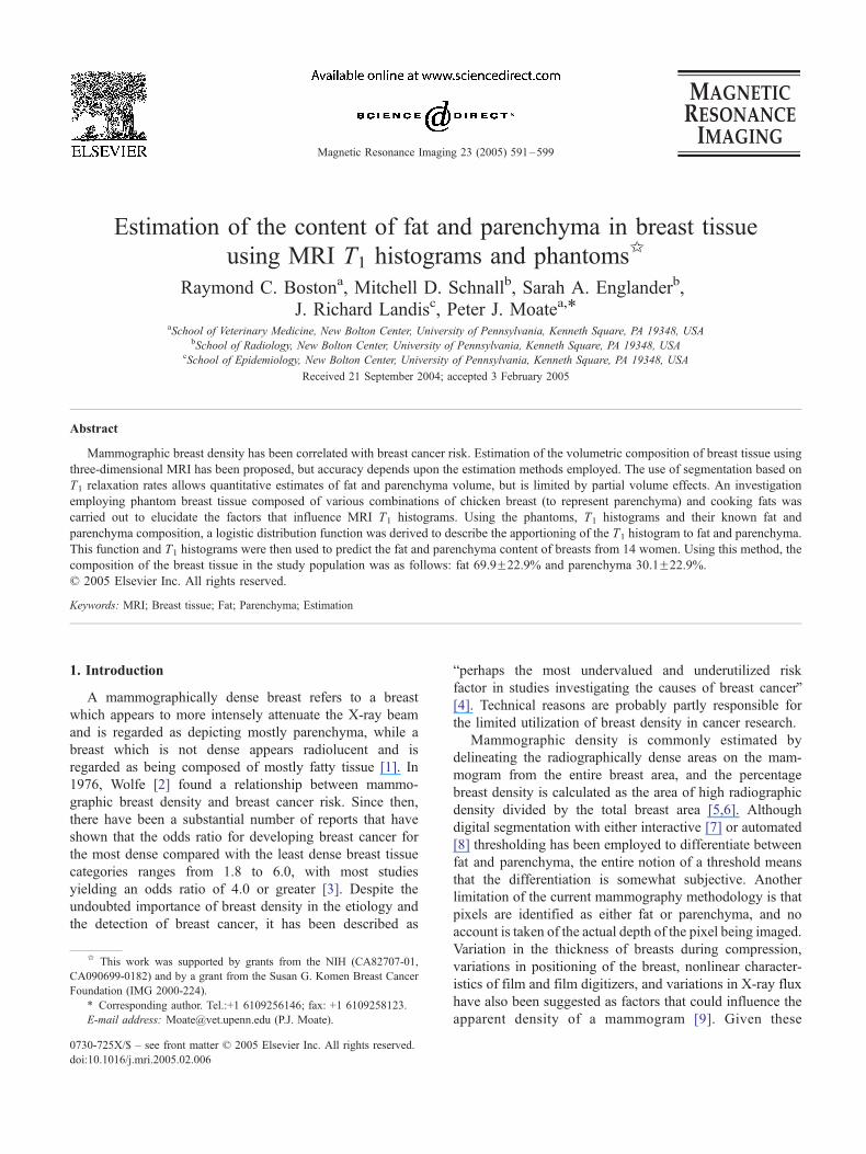
Magnetic Resonance Im

Estimation of the content of fat and parenchyma in breast tissue

using MRI T1 histograms and phantomsB

Raymond C. Bostona, Mitchell D. Schnallb, Sarah A. Englanderb,

J. Richard Landisc, Peter J. Moatea,TaSchool of Veterinary Medicine, New Bolton Center, University of Pennsylvania, Kenneth Square, PA 19348, USA

bSchool of Radiology, New Bolton Center, University of Pennsylvania, Kenneth Square, PA 19348, USAcSchool of Epidemiology, New Bolton Center, University of Pennsylvania, Kenneth Square, PA 19348, USA

Received 21 September 2004; accepted 3 February 2005

Abstract

Mammographic breast density has been correlated with breast cancer risk. Estimation of the volumetric composition of breast tissue using

three-dimensional MRI has been proposed, but accuracy depends upon the estimation methods employed. The use of segmentation based on

T1 relaxation rates allows quantitative estimates of fat and parenchyma volume, but is limited by partial volume effects. An investigation

employing phantom breast tissue composed of various combinations of chicken breast (to represent parenchyma) and cooking fats was

carried out to elucidate the factors that influence MRI T1 histograms. Using the phantoms, T1 histograms and their known fat and

parenchyma composition, a logistic distribution function was derived to describe the apportioning of the T1 histogram to fat and parenchyma.

This function and T1 histograms were then used to predict the fat and parenchyma content of breasts from 14 women. Using this method, the

composition of the breast tissue in the study population was as follows: fat 69.9F22.9% and parenchyma 30.1F22.9%.

D 2005 Elsevier Inc. All rights reserved.

Keywords: MRI; Breast tissue; Fat; Parenchyma; Estimation

1. Introduction

A mammographically dense breast refers to a breast

which appears to more intensely attenuate the X-ray beam

and is regarded as depicting mostly parenchyma, while a

breast which is not dense appears radiolucent and is

regarded as being composed of mostly fatty tissue [1]. In

1976, Wolfe [2] found a relationship between mammo-

graphic breast density and breast cancer risk. Since then,

there have been a substantial number of reports that have

shown that the odds ratio for developing breast cancer for

the most dense compared with the least dense breast tissue

categories ranges from 1.8 to 6.0, with most studies

yielding an odds ratio of 4.0 or greater [3]. Despite the

undoubted importance of breast density in the etiology and

the detection of breast cancer, it has been described as

0730-725X/$ – see front matter D 2005 Elsevier Inc. All rights reserved.

doi:10.1016/j.mri.2005.02.006

B This work was supported by grants from the NIH (CA82707-01,

CA090699-0182) and by a grant from the Susan G. Komen Breast Cancer

Foundation (IMG 2000-224).

T Corresponding author. Tel.:+1 6109256146; fax: +1 6109258123.

E-mail address: Moate@vet.upenn.edu (P.J. Moate).

bperhaps the most undervalued and underutilized risk

factor in studies investigating the causes of breast cancerQ[4]. Technical reasons are probably partly responsible for

the limited utilization of breast density in cancer research.

Mammographic density is commonly estimated by

delineating the radiographically dense areas on the mam-

mogram from the entire breast area, and the percentage

breast density is calculated as the area of high radiographic

density divided by the total breast area [5,6]. Although

digital segmentation with either interactive [7] or automated

[8] thresholding has been employed to differentiate between

fat and parenchyma, the entire notion of a threshold means

that the differentiation is somewhat subjective. Another

limitation of the current mammography methodology is that

pixels are identified as either fat or parenchyma, and no

account is taken of the actual depth of the pixel being imaged.

Variation in the thickness of breasts during compression,

variations in positioning of the breast, nonlinear character-

istics of film and film digitizers, and variations in X-ray flux

have also been suggested as factors that could influence the

apparent density of a mammogram [9]. Given these

aging 23 (2005) 591–599

R.C. Boston et al. / Magnetic Resonance Imaging 23 (2005) 591–599592

confounding factors, it is not surprising that recent research

has demonstrated the high degree of inaccuracy of mam-

mography for estimating the fat and parenchyma content of

breasts [10]. Despite these problems, there is now evidence

that there is large variation in the parenchyma/fat tissue in

women [11] and that this ratio declines with age [1,12] and

can be expected to decline as the compressed thickness of the

breast increases [13]. Breast composition also undergoes

cyclic changes during the menstrual cycle [14] and may be

influenced by diet (intakes of polyunsaturated fat, vitamins C,

E and B12, and by intake of alcohol) [15] and by hormone

replacement therapy [16].

Despite the importance of breast composition to the

etiology and diagnosis of breast cancer, there have been only

a few studies that have made direct chemical measurements

of parenchyma and fat in breast tissue, and these involved

only a small number of fresh mastectomy specimens [17,18].

An alternative modality for estimating the fat and

parenchyma content of tissues in animals and humans

involves MRI [19-21]. Moreover, a significant correlation

has already been shown between X-ray mammography

percent density and two MRI parameters: mean T2 relaxation

time and relative water content [22]. A number of different

methods have been used to estimate fat and parenchyma

content of tissues from MRI data. Kover et al. [19], when

estimating the fat content of live chickens, used a mouse to

manually draw around areas of adipose tissue and thus

f

f

A

C

f

D

0

1000

2000

3000

4000

5000

0 500 1000 1500 2000

Time (ms)

f

0

10000

20000

30000

40000

50000

0 500 1000 1500 2000

Time (ms)

f

Fig. 1. T1 histograms of individual breasts from four subjects (A, B, C and

segment theMR image into fat and parenchyma. Baulain [20]

used both gray value distribution (histogram) of the pixels

and also cluster analysis methods to estimate body compo-

sition of live pigs and sheep. In human breast tissue, fat is

often diffusely dispersed throughout parenchymal tissue, and

it may not necessarily be practical or possible to manually

outline in a MR image distinct regions of adipose tissue.

Therefore, a variety of methods have been used to segment

MR images and to classify the tissue in the different segments

[23]. There are two distinct approaches that rely on unique

NMR properties of fat relative to the fibroglandular tissues:

chemical shift and T1. Although chemical shift techniques

may be more specific in identifying fat, T1-based techniques

are easier to implement over a wide variety of scanner

platforms and field strengths. This is a technique currently

being employed in a study at the University of Pennsylvania.

T1-based techniques take advantage of the fact that

inversion recovery images with different T1 times, or T1

weighted images with different TR values, will have a gray

scale such that the signal in each voxel is related to the T1

relaxation time of the voxel (or cube of tissue) that the pixel

depicts. A T1 image or map can be calculated from a series

of images produced using an inversion recovery pulse

sequence. The gray scale of a specific pixel is related to the

T1 relaxation time of the voxel (or cube of tissue) which that

pixel depicts. T1 histograms depict the number of voxels

that have specific T1 relaxation times. Fig. 1A–D depicts a

0 500 1000 1500 2000

Time (ms)

f

0

2000

4000

6000

8000

10000

0 500 1000 1500 2000

Time (ms)

0

300

600

900

1200

1500

f

B

D). f is the frequency or number of pixels that have a value of T1.

able 1

escription and composition of phantoms

hantom

o.

Cooking

fat (ml)

Canola

oil (ml)

Chicken

(ml)

Fat (%) Chicken

(%)

1 25 0 0 100 0

2 0 50 0 100 0

3 0 0 50 0 100

4 25 0 12 66.6 33.4

5 0 25 25 50 50

6 20 0 11.5 63.5 36.5

7 20 0 16.5 54.8 45.2

8 40 0 0 100 0

9 20 0 16.5 54.8 45.2

10 12.5 0 34.5 26.6 73.4

11 10 0 0 100 0

12 0 0 10 0 100

13 25 0 0 100 0

14 0 0 25.5 0 100

15 0 0 41.5 0 100

R.C. Boston et al. / Magnetic Resonance Imaging 23 (2005) 591–599 593

variety of commonly observed T1 histograms of women’s

breasts, calculated from an inversion recovery experiment

with T1=1600, 800, 400, 200 and 100 ms. Fig. 1A shows a

T1 histogram obtained from the left breast of a woman. The

Gaussian-type curve centered on a T1 time of approximately

280 ms corresponds to the signal obtained from adipose

dominant tissue. This histogram is typical of that observed

in many older women with large, fatty or bglandularQbreasts. The T1 histogram shown in Fig. 1B comes from a

breast containing small amounts of both adipose and

parenchymal tissue. The Gaussian-type curve center cen-

tered on approximately 940 ms corresponds to the signal

obtained from parenchyma dominant tissue. The bridging

area between the two peaks is thought to represent tissue

that contains both adipose and parenchymal tissue. This

type of histogram is typically obtained from young women

athletes who have small, bmuscularQ breasts. Fig. 1C shows

a T1 histogram with a substantial bfatQ peak, but in the

region of the histogram normally associated with parenchy-

ma, the T1 curve is so flat that it is not possible to accurately

determine the time of the parenchyma peak. This type of

histogram is typical of histograms obtained from many

young women. In Fig. 1D, there is only one substantially

skewed peak and in the region of the T1 histogram normally

associated with parenchyma, the histogram declines mono-

tonically. This histogram is very unusual and, by visual

inspection of the MR image, resulted from a breast

containing a substantial quantity of parenchyma finely

dispersed throughout the adipose tissue.

Some researchers have analyzed T1 histograms by fitting

data to a sum of exponentials [24]. However, in our

experience, the diversity of T1 histograms as demonstrated

in Fig. 1A–D makes this approach problematic. Segmenta-

tion of the type of histogram shown in Fig. 1B–D to provide

an estimate of the fat and parenchyma content of a breast is

bedeviled by the problem of partial voluming. This

phenomenon arises since volumes of breast tissue, even

those as small as a voxel, can contain mixtures of fat and

parenchyma. In the past, many researchers have examined

each voxel in each slice of a histogram and, on the basis of a

threshold T1 value, have designated each voxel as being

either fat or parenchyma and then aggregated these specific

voxel types to obtain an overall estimate of the total content

of fat and parenchyma [19,25]. A primary difficulty with this

approach is determining the value of the threshold [23]. A

second problem with this approach is that it denies the fact

that many voxels are composed of combinations of tissue

types (partial volume effects). In an example of the types of

problems that arise from the use of threshold algorithms,

Laidlaw et al. [26] presented a brain MR image in which both

stair step artifacts and layers of misclassified voxels are

clearly evident. In 1996, Graham et al. [22], in an attempt to

improve the estimation of breast composition, correlated the

mean T2 value of a MRI histogram (calculated as the first

moment of the estimated continuous T2 distribution) with the

relative volumetric water content of breasts (also estimated

by MRI). This approach may allow a global estimation of fat

and parenchymal content but may not be appropriate for

small regions of interest or individual voxels.

Another approach to overcome the difficulties caused by

the partial volume phenomenon is the use of Bayesian

probability theory to estimate the highest probability combi-

nation of materials within each voxel-sized region [26]. The

possible tissue types within each voxel are identified, and

continuous bbasisQ functions p(x) are assumed/developed to

represent the probability that a particular voxel contains a

particular tissue type. Linear combinations of these functions

are fitted to each voxel, and the most likely combination of

materials is chosen probabilistically.

This contribution describes the use of breast phantoms to

elucidate the effect of various combinations of fat and

parenchyma on the pattern of T1 histograms, the nature of

the p(x) basis functions and the use of basis functions to

predict the percentage of fat and parenchyma in breasts from

the whole-breast T1 histogram.

2. Methods

2.1. Phantoms

The phantoms were made of a plastic-capped, 50-ml

polyethylene (1-mm-thick) sampling tube containing vari-

ous quantities and proportions of ground lean chicken breast

(representing parenchyma) and cooking fat (Crisco) or

canola oil representing adipose tissue (see Table 1). The

volume of chicken breast added to each phantom was

determined by water displacement, while the volumes for

liquefied cooking fat or canola oil were measured. In order

to simulate the heterogeneity of fat and parenchyma that

occurs within breasts, the fat and chicken within each

phantom were mixed thoroughly by means of a glass rod.

The label on the cooking fat listed the long-chain fatty acid

(LCFA) composition as: saturated 30%, monounsaturated

40% and polyunsaturated 30%, while the LCFA composi-

T

D

P

n

P

P

P

P

P

P

P

P

P

P

P

P

P

P

P

R.C. Boston et al. / Magnetic Resonance Imaging 23 (2005) 591–599594

tion of the canola oil was as follows: saturated 7.8%,

monounsaturated 55.3% and polyunsaturated 32.4%. The

USDA National Nutrient Database (http://www.nal.usda.

gov/fnic/cgi-bin/nut_search.pl) lists lean chicken breast

without skin as containing 1.24% fat and the LCFA

composition (as % of total LCFA) as: saturated 36.3%,

monounsaturated 33.0% and polyunsaturated 30.7%.

2.2. Human subjects

Magnetic resonance imaging was performed on both left

and right breasts of 14 Caucasian women patients as part of

standard procedures for the investigation of possible breast

cancer. The meanFstandard deviation and range for their

ages (years) were 48.1F8.6 and 38–70, and for body-

weights (kg) were 65.9F15.6 and 46.4–104.1. Approval

from our institutional review board was obtained prior to

the start of this study.

2.3. Instrumentation and imaging protocol

MR imaging was performed on a 1.5-T Signa scanner

(General Electric Medical Systems, Milwaukee, WI). After

informed consent, patients were placed in the scanner in the

prone position. Total imaging time for both breasts was

approximately 20 min. Briefly, the MRI protocol employed

was as follows: the field of view (FOV) was generally

180 to 240 mm, and sagittal slice thickness ranged from 2.2

to 3.5 mm depending on the size of particular breasts. The

number of data points (D), i.e., pixels per FOV on the

computer screen used in this investigation, was 250. With

FOV=180 mm, S=2.2 mm and D=250, a voxel will have

the following dimensions: height=180/250=0.72 mm,

width=0.72 mm, thickness=2.2 mm.

Three-dimensional bilateral slab interleaved spoiled

gradient echo inversion recovery sequence was used to

acquire data (TR/TE 17.6/1.4 ms, flip angle=558, F64 kHz

sampling bandwidth, 64 slices). Five data sets were obtained

using a nonselective inversion pulse at 1600, 800, 400,

200 and 100 ms prior to the start of the imaging sequence.

The total acquisition time for the data acquired for each

patient exam was 20 min; however, more recent implemen-

tation of SENSE encoding has reduced this to 10 min. These

inversion recovery data were used to calculate T1 maps of

each slice [27]. The protocol for imaging the phantoms was

similar to that used for the patients except that the phantoms

were imaged at room temperature (258C), sagittal slice

thickness was 3.5 mm (to reproduce the worst case scenario

in terms of partial volume effects), and 14 slices/phantom

were made.

2.4. Analysis of MR imaging data

Images were masked by hand to remove the chest wall.

Breast tissue was identified visually by qualified person-

nel. Breast tissue could clearly be distinguished from the

chest wall and the axilla. We used a graphical user

interface (GUI)-based program — written in-house.

Functionality of this GUI-based program included adding

or removing area, dilating or eroding, and selecting a

cutoff threshold. T1 maps were constructed by fitting the

data acquired using five inversion times with a function

derived from the solution of the Bloch equations for the

MR pulse sequence. Histograms of the masked images

were produced. Calculations were performed on the T1

histogram data using a Microsoft Excel spreadsheet.

STATA software was used to estimate spline functions

and their derivatives, and to perform regressions and

statistical analyses [28]. In the studies described here, the

mean T1 value (T̂1) of each histogram was calculated from

the first moment of the T1 distribution:

T̂T 1 ¼

Pi¼1

i¼n

fi 4 T1i

n 4 f̂f ið1Þ

where fi is the frequency or signal count that has a value

of T1i, f̂ i is the average count or frequency for the

histogram, i is the bin number centered on time T1i, n is

the number of bins used for the histogram and, in all the

histograms in this investigation, n was set at 200 and the

bin width was 10 ms.

Using the phantom T1 histograms, a linear regression

equation was determined as a calibration equation to relate

parenchyma percentage in the phantoms to T̂1 (Eq. (2)):

P% ¼ � 33:1F7:3þ 0:153F0:0127 4 T̂T 1;

R2 ¼ 0:91 ð2Þ

Although Eq. (2) has a high R2 value, from a practical

point of view, the fact that the T̂1 values for pure fat and

pure chicken breast (parenchyma) may not closely match

the times of the corresponding peaks in T1 histograms of

breast tissue in vivo makes the use of this specific equation

for predicting breast composition somewhat problematic.

However, since in phantoms there is a high degree of

concordance with respect to T̂1 and the peak times of both

pure fat (P1, ms) and pure parenchyma (P2, ms) (this

finding presented in the Results section), it is likely that this

concordance would also occur in breast tissue in vivo. We

therefore surmised that the parenchyma % (P%) of a breast

could be approximately estimated from the total T1

histogram by:

P% ¼ � P1 4 100

P2� P1

� �þ 100

P2� P1

� �4 T̂T 1 ð3Þ

where in this case, P1 refers to the population mean time of

the fat peak (P1, ms) and P2 refers to the population mean

time of the parenchyma peak (P2, ms) of breast tissue.

Unfortunately, when using this equation to predict breast

composition, if a particular breast were to have a T̂1 less

than the mean P1 value or greater than the mean P2 value,

then infeasible predictions of P% (i.e., P%b0 or P%N100)

0

10

20

30

40

50

60

0 10 20 30 40 50 60

Measured tissue volume (ml)

Pre

dic

ted

tis

sue

volu

me

(ml)

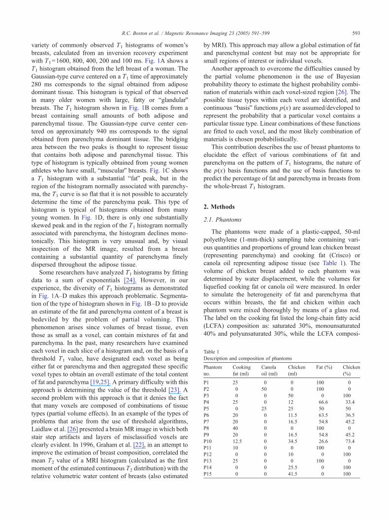
Fig. 2. The standard curve derived from phantoms used to predict the

volumes (ml) of fat (empty squares) and parenchyma (solid triangles) in

breast histograms. The solid line is the line of identity.

Time (ms)

1.

Fat

or

par

ench

yma

pro

po

rtio

n i

n T

1 si

gn

al

1

0

0.2

0.4

0.6

0.8

2

0 500 1000 1500 2000

Fig. 3. The logistic functions (thick line for parenchyma, thin line for fat)

used to segment breast T1 histograms. The vertical dotted lines (at T1

times 457.85, 565.43, 654.57 and 762.36 ms) segment the histogram

into quintiles.

R.C. Boston et al. / Magnetic Resonance Imaging 23 (2005) 591–599 595

could occur. This problem was circumvented by introducing

the modifications shown in Eq. (4):

P% ¼ 0 if T̂T 1VP1

P% ¼ � P1 4 100

P2� P1

� �þ 100

P2� P1

� �4 T̂T 1 for P1V T̂T1VP2

P% ¼ 100 if T̂T 1zP2 ð4Þ

In order to utilize Eq. (4) to predict the parenchyma

content of breasts, the population mean estimates of P1 and

P2 were estimated from our sample of subjects. First, ten-

knot quadratic spline functions were used to obtain smooth,

continuous-distribution functions to describe the T1 histo-

grams of each breast. The first derivative of the spline

functions was used to identify the times of the fat and

parenchyma peaks.

2.5. Prediction of breast composition using a logistic

equation

A logistic function [29] was used to describe the

proportion (Pxp(i)) of the T1 signal that originates from

voxels composed of parenchyma. Alternatively, Pxp(i)) can

be thought of as a function that approximates the probability

that a particular voxel will contain parenchyma.

Pxp ið Þ ¼ 1

1þ exp � P3 4 T1 �P1þ P2

2

� �� �� �� � ð5Þ

where T1 is the relaxation time of a specific voxel, P1 is the

mean T1 time of the fat peak, P2 is the mean T1 time of the

parenchyma peak and P3 is the maximum slope of the

logistic curve. We chose a logistic function as this type of

curve has the desired shape attributes and good parameter

estimability due to their intrinsic dimensionality and domain

of influence [30]. Since we assume that breast tissue

contains only fat and parenchyma, the function used to

describe the proportion of fat in a specific voxel (Pxf) is

described by Eq. (6):

Pxf ið Þ ¼ 1� Pxp ið Þ ð6Þ

It follows that the total amount of parenchyma (TP, ml)

that caused the T1 histogram can be described by:

TP ¼Xnl

FOV 4 FOV 4 S 4 fi 4 Pxp ðiÞD 4D 4 1000

ð7Þ

where FOV is the field of view in millimeters, S is

the slice thickness in millimeters and D represents the

number of pixels per FOV. Similarly, the total amount

of fat (ml) responsible for the T1 histogram can be

described by:

TF ¼Xnl

FOV 4 FOV 4 S 4 fi 4 Pxf ðiÞD * D * 1000

ð8Þ

In the case of phantoms, P1 and P2 were taken to be

the mean peak times of the phantoms composed of pure

fat and pure chicken breast, respectively.

In order to estimate parameter P3 in Eq. (5), Eqs. (7)

and (8) were coded into an Excel spreadsheet so as to

predict the amount of fat and parenchyma in each phantom.

By utilizing the bsolverQ optimizer available in Excel to

minimize the sum of squares of the differences between

the predicted quantities of fat and parenchyma with the

measured quantities of fat and parenchyma in each

phantom, P3 was estimated to be 0.009102 ms�1. The

calibration line resulting from this optimization procedure

and which relates the known and predicted volumes of fat

and parenchyma is shown in Fig. 2. Eqs. (7) and (8) were

also used to estimate the volumes of fat and parenchyma

present in breasts. The value of parameter P3 determined

using phantoms was assumed to apply to breasts, but the

mean P1 and P2 values of breasts per se were employed.

The logistic equations used to estimate the proportions of

parenchyma and fat in breasts are shown in Fig. 3.

R.C. Boston et al. / Magnetic Resonance Imaging 23 (2005) 591–599596

3. Results and discussion

3.1. Phantom histograms

T1 histograms of cooking fat, canola oil, chicken breast

and mixtures of chicken breast and fat are shown in

Fig. 4A–D. The histogram of cooking fat was Gaussian in

form and closely resembled the fat peak that occurs in

typical breast T1 histograms (compare with Fig. 1A). The

histogram from the canola oil had a much smaller peak and

was more platykurtotic than the histogram obtained from the

cooking fat. The histograms produced from phantoms

containing mixtures of fat and chicken had reduced peak

heights for both fat and chicken relative to histogram peak

heights obtained from phantoms containing either pure fat

or chicken (compare Fig. 4A with B and C). Phantoms that

contained mixtures of fat and chicken had T1 histograms

with substantial bbridgingQ between the fat and parenchyma

peak (Fig. 4B and C). We interpret this observation as

evidence of the bpartial volumeQ phenomenon.

3.2. Comparison of phantom T1 histograms with breast T1

histograms

The five phantoms that were 100% fat had (meanFS.D.)

T̂1 of 228F12.4 ms and their peak times (P1) occurred at

208F25.7 ms. In contrast to fat or adipose tissue, the four

phantoms that were composed of 100% chicken had T̂1 of

818F102.9ms and peak times (P2) occurred at 810F95.0ms.

A

0

500

1000

1500

2000

2500

0 200 400 600 800 1000

f

B

f

C

0

100

200

300

400

500

0 200 400 600 800 1000

f

DTime (ms)

Time (ms)

f

Fig. 4. T1 histograms of phantoms: (A) fats: solid dots represent cooking fat (25

chicken breast (25 ml). (C) Solid dots represent a mixture of cooking fat (25 ml) a

and chicken (25 ml). Note that in each case the frequency axis has been rescaled

The slight discrepancies between the T̂1 values and the time

of the corresponding peak result from the fact that the

histograms of these bpureQ phantoms cannot be described by

pure Gaussian-type equations and reflect the fact that the

histograms are slightly skewed. The P1 values for fat in

phantoms are less than the P1 values (280F14 ms) that we

have observed in T1 histograms of in vivo breasts (Table 2)

and slightly less than the 230F10 ms mean value for ex vivo

breasts reported by Graham et al. [31]. In addition, the peak

time for parenchyma in phantoms (810F95.0 ms) is smaller

than the peak times we have observed for parenchymal

breast tissue in vivo 945F108 (ms) (see Table 2) and

substantially smaller than the value of 1330F240 ms

reported for parenchymal breast tissue ex vivo [31].

There are a number of factors that could account for these

apparent discrepancies between the observed times of fat

and parenchyma peak heights for phantoms and the

observed times of peak heights for corresponding peaks in

breast tissue. Firstly, the phantoms were at room tempera-

ture when the MRI was conducted, and this would have

caused a substantial shortening of the T1 relaxation times,

especially that of parenchyma [32]. Secondly, in vivo, both

adipose and parenchymal breast tissue are highly vascular-

ized and contain approximately 5–8% blood by weight.

Thus, it can be expected that in the phantoms, the absence of

the water (in blood) would tend to slightly decrease the T1

relaxation times of both the adipose and the parenchymal

0

200

400

600

800

1000

0 200 400 600 800 1000

Time (ms)

0

200

400

600

800

1000

0 200 400 600 800 1000

Time (ms)

ml); hollow circles represent canola oil (50 ml). (B) Solid dots represent

nd chicken (12 ml). (D) Solid dots represent a mixture of canola oil (25 ml)

for display purposes.

Table 2

Characteristics of T1 histograms of breasts and estimated fat and

parenchyma content of breasts of 14 Caucasian women

Parameter Left breast Right breast Breasts

Number 14 14 28

Total area under the

curve*106 (counts ms)

1.76F0.96 1.70F0.85 1.73F0.90

Time of fat peak (P1) (ms) 276F12 282F15 279F14

Time of parenchyma peak

(P2) (ms)

910F114 972F114 941F110

T̂1 (ms) 443F155 480F198 461F176

Fat (%) by T̂1 69.5F29.4 64.8F32.7 67.1F30.6

Parenchyma (%) by T̂1 30.5F29.4 35.2F32.7 32.9F30.6

Fat (%) by logistic equation 71.3F22.4 68.6F24.1 69.9F22.9

Parenchyma (%) by

logistic equation

28.7F22.4 31.4F24.1 30.1F22.9

Breast volume (ml) by

logistic equation

472F381 449F352 460F360

Fat volume (ml) by

logistic equation

394F378 369F358 381F362

Parenchyma volume (ml) by

logistic equation

78F50 80F49 79F49

R.C. Boston et al. / Magnetic Resonance Imaging 23 (2005) 591–599 597

peaks in our phantoms. Thirdly, as shown in Fig. 4A, the

degree of saturation of fat can influence the time of the fat

peak. In breast cancer patients, the breast LCFA composi-

tion has been reported to be as follows: saturated 33.3F3.9,

monounsaturated 48.0F2.2 and polyunsaturated 16.6F3.7

A B

C D

0

1000

2000

3000

4000

0 500 1000 1500 2000

Time (ms)

ff

0

10000

20000

30000

40000

50000

0 500 1000 1500 2000

f

Time (ms)

f

2

4

6

8

f

Fig. 5. Segmentation of four breast T1 histograms using the logistic function. The g

the parenchyma signal. (A) 93.3% fat; (B) 22.8% fat; (C) 60.9% fat; (D) 67.6%

[33]. In comparison, the LCFA composition of canola oil

was as follows: saturated 7.8%, monounsaturated 55.3%

and polyunsaturated 32.4%, while for the LCFA composi-

tion of the cooking fat was saturated 30%, monounsaturated

40% and polyunsaturated 30%. Clearly, these differences in

LCFA composition could contribute towards the discrepan-

cy between phantoms and breasts in the mean times for the

fat peak.

3.3. Prediction of breast composition based on the T1

histogram

The mean fat and P% of breasts as predicted by Eq. (4)

are shown in Table 2. It should be noted that for some

individual breasts, the use of Eq. (4) resulted in a prediction

of 0% parenchyma. Since breasts are likely to contain at

least some parenchyma, this extreme type of prediction is

likely to have some error and this type of prediction could

lead to discontinuities and step artifacts in imaging.

As can be seen in Fig. 5, the use of Eqs. (7) and (8) to

predict parenchyma and fat in breast tissue resulted in

distribution curves without discontinuities. Indeed, all fat

and parenchyma distribution curves calculated using this

function appeared plausible in that they generally showed

strong symmetry typical of the Gaussian-type curves ob-

tained from phantoms of bpureQ fat and bpureQ parenchyma.

1500

Time (ms)

0

300

600

900

1200

0 500 1000 1500 2000

0

000

000

000

000

0 500 1000 1500 2000

Time (ms)

ray line depicts the histogram, the long dash the fat signal and the short dash

fat.

R.C. Boston et al. / Magnetic Resonance Imaging 23 (2005) 591–599598

Furthermore, in contrast to the moments approach, when

using the logistic approach (Eqs. (7) and (8)), we did not

obtain any implausible predictions of the composition of

individual breasts (i.e., none with zero parenchyma). More

importantly, the strong concordance of the known and

predicted volumes of fat and parenchyma in the phantoms

(Fig. 4) gives us reason to have confidence in the same

logistic equation approach for predicting the composition of

breasts. The mean percentages of fat and parenchyma in

breasts as estimated by the logistic equation are similar to

the corresponding values as estimated by the moments

approach. Both methods may be useful for predicting the fat

and P% of breasts, but the logistic approach more readily

lends itself to imaging since the logistic curve enables the

imager to identify a number of ranges, e.g., quintiles (see

Fig. 3), which could allow an MR image to be segmented

into a limited number of gray scales representing defined

composition ranges of fat and parenchyma.

In this investigation, a number of experimental issues

could have introduced some error into this empirical

calibration approach. Firstly, the phantoms were of much

smaller volume than breasts. Since we employed phantoms

that ranged in volume from only 10.0 to 50 ml, this

necessarily introduced some errors. The determination of fat

and chicken volume by displacement probably involved an

error of up to 10% for the determination of individual

phantom volumes. Furthermore, in small phantoms, the ratio

of edge effects to binternalQ voxels is greater than in larger-

size breasts, and it is problematic to consider that bedgeQvoxels that contain some fat, chicken and air may or may

not be detected by MRI. The relatively large slice thickness

(3.5 mm), which was chosen to match the slice thickness

employed for the majority of breast MRI, probably resulted

in inappropriate resolution for the small volumes of the

phantoms. For these reasons, we concur with Clarke et al.

[23] who have said bFor a true indication of the maximum

accuracy of the segmentation methods, the phantom

volumes should be comparable to the anatomical or

pathologic structures of interest.QWe surmise that spatial scale of the phantom mixture

may greatly impact on the type of histogram obtained. We

speculate that for a phantom composed of both fat and

chicken, if the lumps of chicken breast were very much

larger than the voxel size, bimodal histograms would likely

result. However, even when the lumps of chicken breast are

larger than the voxel size, due to edge effects (chicken

abutting fat), there would still be voxels that contain both fat

and chicken, and bridge effects (like those seen in Fig. 4C

and D) would result. Experimental difficulties also impinge

on the type of histograms we obtain. We have found that

even when chicken is chopped and ground to a fine

consistency, it will naturally tend to clump, especially when

mixed with oil. These difficulties acknowledged, with

phantoms composed of fat and ground chicken breast, we

were nevertheless able to obtain a diverse range of histo-

grams that mimicked the types of histograms obtained from

breasts in vivo. This suggests that we had indeed replicated

the spatial scale of the fat/parenchyma distribution that

occurs in vivo.

As mentioned earlier, the phantoms were imaged at room

temperature instead of body temperature. As also discussed

earlier, cooking fat, and especially canola oil, may not

necessarily be the best simulacra to human body fat. Indeed

it could be expected that pork fat would more closely

chemically resemble human fat, and there is experimental

precedent for using pork fat as phantoms in MRI inves-

tigations [34]. Furthermore, the fat and oil used in these

phantoms may have contained some moisture, and the

chicken breast almost certainly contained some fat. For

these reasons, the work presented here must be regarded as

preliminary in nature. Nevertheless, although the estimated

volumes of fat and parenchyma in breasts in this investi-

gation may not be absolutely correct, their relative ranking

would still be useful for quantifying the effects of

experimental drugs or investigating the time course changes

in breast composition. Graham et al. [22], working with a

population of asymptomatic patients, have shown associa-

tions between relative water content of breasts (as measured

by MRI) and socio-demographic and anthropometric risk

factors for breast cancer. The possibility that the empirical

approach to the estimation of parenchyma and fat content of

breasts as described here could provide a more direct and

perhaps enhanced measure of risk could have important

implications for epidemiological studies of breast cancer

and for models that predict risk of breast cancer [35].

4. Conclusion

The empirical logistic model presented here has the

flexibility to accurately and plausibly segment all of the

MRI T1 histograms that we have encountered.

References

[1] Stomper P, D’Souza D, DiNitto P, Arredondo M. Analysis of

parenchymal density on mammograms in 1353 women 25–79 years

old. AJR Am J Roentgenol 1996;167(5):1261–5.

[2] Wolfe JN. Breast patterns as an index of risk for developing breast

cancer. AJR Am J Roentgenol 1976;126:1130–9.

[3] Harvey JA, Bovbjerg VE. Quantitative assessment of mammographic

breast density: relationship with breast cancer risk. Radiology

2004;230(1):29–41.

[4] Byrne C. Studying mammographic density: implications for under-

standing breast cancer. J Natl Cancer Inst 1997;89(8):531–3.

[5] Shepherd JA, Kerlikowske KM, Smith-Bindman R, Genant HK,

Cummings SR. Measurement of breast density with dual X-ray

absorptiometry: feasibility. Radiology 2002;223(2):554–7.

[6] Ursin G, Parisky YR, Pike MC, Spicer DV. Mammographic density

changes during the menstrual cycle. Cancer Epidemiol Biomark Prev

2001;10(2):141–2.

[7] Byng JW, Yaffe MJ, Jong RA, Shumak RS, Lockwood GA, Tritchler

DL, et al. Analysis of mammographic density and breast cancer risk

from digitized mammograms. Radiographics 1998;18(6):1587–98.

[8] Sivaramakrishna R, Obuchowski NA, Chilcote WA, Powell KA.

Automatic segmentation of mammographic density. Acad Radiol

2001;8(3):250–6.

R.C. Boston et al. / Magnetic Resonance Imaging 23 (2005) 591–599 599

[9] Wang XH, Good WF, Chapman BE, Chang YH, Poller WR, Chang

TS, et al. Automated assessment of the composition of breast tissue

revealed on tissue-thickness-corrected mammography. AJR Am J

Roentgenol 2003;180(1):257–62.

[10] Lee NA, Rusinek H, Weinreb J, Chandra R, Toth H, Singer C, et al.

Fatty and fibroglandular tissue volumes in the breasts of women

20–83 years old: comparison of X-ray mammography and computer-

assisted MR imaging. AJR Am J Roentgenol 1997;168(2):501–6.

[11] Costanza ME. Breast cancer screening in older women. Cancer Suppl

1992;69(7):1925–31.

[12] Byrne C, Schairer C, Wolfe J, Parekh N, Salane M, Brinton L, et al.

Mammographic features and breast cancer risk: effects with time, age,

and menopause status. J Natl Cancer Inst 1995;87(21):1622–9.

[13] Gentry JR, DeWerd LA. The measurement of in vivo mammographic

exposures and the calculated mean glandular dose across the United

States. Med Phys 1996;23(6):899–903.

[14] Soderqvist G, Isaksson E, von Schoultz B, Carlstrom K, Tani E, Skoog

L. Proliferation of breast epithelial cells in healthy women during the

menstrual cycle. Am J Obstet Gynecol 1997;176(1 Pt 1):123–8.

[15] Vachon CM, Kushi LH, Cerhan JR, Kuni CC, Sellers TA. Association

of diet andmammographic breast density in theMinnesota breast cancer

family cohort. Cancer Epidemiol Biomark Prev 2000;9(2):151–60.

[16] Rutter CM, Mandelson MT, Laya MB, Seger DJ, Taplin S. Changes in

breast density associated with initiation, discontinuation, and con-

tinuing use of hormone replacement therapy [see comment]. JAMA

2001;285(2):171–6.

[17] Hammerstein G, Miller D, White D, Masterson M, Woodard H,

Laughlin J. Absorbed radiation dose in mammography. Radiology

1979;130(2):485–91.

[18] Woodard H, White D. The composition of body tissues. Br J Radiol

1986;59(708):1209–18.

[19] Kover G, Romvari R, Horn P, Berenyi E, Jensen JF, Sorensen P. In

vivo assessment of breast muscle, abdominal fat and total fat volume

in meat-type chickens by magnetic resonance imaging. Acta Vet Hung

1998;46(2):135–44.

[20] Baulain U. Magnetic resonance imaging for the in vivo determination

of body composition in animal science. Comput Electron Agric

1997;17(2):189–203.

[21] Poon CS, Bronskill MJ, Henkelman RM, Boyd NF. Quantitative

magnetic resonance imaging parameters and their relationship to

mammographic pattern. J Natl Cancer Inst 1992;84(10):777–81.

[22] Graham SJ, Bronskill MJ, Byng JW, Yaffe MJ, Boyd NF. Quantitative

correlation of breast tissue parameters using magnetic resonance and

X-ray mammography. Br J Cancer 1996;73(2):162–8.

[23] Clarke LP, Velthuizen RP, Camacho MA, Heine JJ, Vaidyanathan M,

Hall LO, et al. MRI segmentation: methods and applications. Magn

Reson Imaging 1995;13(3):343–68.

[24] Kroeker RM, Stewart CA, Bronskill MJ, Henkelman RM. Continuous

distributions of NMR relaxation times applied to tumors before and

after therapy with X-rays and cyclophosphamide. Magn Reson Med

1988;6(1):24–36.

[25] Graham SJ, Stanchev PL, Lloyd-Smith JO, Bronskill MJ, Plewes DB.

Changes in fibroglandular volume and water content of breast tissue

during the menstrual cycle observed by MR imaging at 1.5 T. J Magn

Reson Imaging 1995;5(6):695–701.

[26] Laidlaw DH, Fleischer KW, Barr AH. Partial-volume Bayesian

classification of material mixtures in MR volume data using voxel

histograms. IEEE Trans Med Imaging 1998;17(1):74–86.

[27] Englander SA, Quing Yuan Schnall M. A 3D technique to determine

global contrast pharmacokinetics and parenchyma volume in breasts

[Abstract]. Glasgow (Scotland)7 International Society of Magnetic

Resonance in Medicine; 2001 [April 23–27].

[28] Stata. Stata statistical software. Release 7.0 ed. College Station (Tex)7

Stata Corporation; 2001.

[29] Hill AV, Lupton H. Muscular exercise, lactic acid, and the supply and

utilization of oxygen. Q J Med 1923;16:135–71.

[30] Moate PJ, Dougherty L, Schnall MD, Landis RJ, Boston RC. A

modified logistic model to describe gadolinium kinetics in breast

tumors. Magn Reson Imaging 2004;22(4):467–73.

[31] Graham SJ, Ness S, Hamilton BS, Bronskill MJ. Magnetic resonance

properties of ex vivo breast tissue at 1.5 T. Magn Reson Med

1997;38(4):669–77.

[32] Bohris C, Schreiber WG, Jenne J, Simiantonakis I, Rastert R,

Zabel HJ, et al. Quantitative MR temperature monitoring of high-

intensity focused ultrasound therapy. Magn Reson Imaging 1999;

17(4):603–10.

[33] Chajes V, Niyongabo T, Lanson M, Fignon A, Couet C, Bougnoux P.

Fatty-acid composition of breast and iliac adipose tissue in breast-

cancer patients. Int J Cancer 1992;50(3):405–8.

[34] Poon CS, Szumowski J, Plewes DB, Ashby P, Henkelman RM. Fat/

water quantitation and differential relaxation time measurement using

chemical shift imaging technique. Magn Reson Imaging 1989;7(4):

369–82.

[35] Gail MH, Costantino JP. Validating and improving models for

projecting the absolute risk of breast cancer. J Nat Cancer Inst

2001;93(5):334–5.