Multifractal diffusion entropy analysis: Optimal bin width of probability histograms

$: Multifractal diffusion entropy analysis: Optimal bin width of probability histograms$
arX

iv:1

401.

3316

v1 [

q-fin

.ST

] 14

Jan

201

4

Physica A 00 (2014) 1–18

Physica A

Multifractal Diffusion Entropy Analysis: Optimal Bin Width ofProbability Histograms

Petr Jizbaa,b, Jan Korbela,c

aFaculty of Nuclear Sciences and Physical Engineering, Czech Technical University in Prague, Brehova 7, 11519, Prague, Czech RepublicbInstitute of Theoretical Physics, Freie Universitat in Berlin, Arnimallee 14, 14195 Berlin, Germany

cMax Planck Institute for the History of Science, Boltzmannstrasse 22, 14195 Berlin, Germany

Abstract

In the framework of Multifractal Diffusion Entropy Analysis we propose a method for choosing an optimal bin-width in histogramsgenerated from underlying probability distributions of interest. This presented method uses techniques of Renyi’s entropy and themean square error analysis to discuss the conditions under which the error in Renyi’s entropy estimation is minimal. Weillustratethe utility of our method by focusing on a scaling behavior offinancial time series. In particular, we analyze the S&P500 stockindex as sampled at a daily rate in the time period 1950-2013.In order to demonstrate a strength of the optimality of the bin-width we compare theδ-spectrum for various bin-widths. Implications for the multifractal δ-spectrum as a function of Renyi’sqparameter are also discussed and graphically represented.

c© 2013 Published by Elsevier Ltd.

Keywords: Multifractals, Renyi entropy, Time seriesPACS:89.65.Gh, 05.45.Tp

1. Introduction

The evolution of many complex systems in natural, economical, medical and biological sciences is usually pre-sented in the form of time data-sequences. A global massification of computers together with their improved ability tocollect and process large data-sets have brought about the need for novel analyzing methods. A considerable amountof literature has been recently devoted to developing and using new data-analyzing paradigms. These studies includesuch concepts as fractals and multifractals [1], fractional dynamics [2, 3], complexity [4, 5], entropy densities [5] ortransfer entropies [6, 7, 8]. Particularly in the connection with financial time series there has been rapid developmentof techniques for measuring and managing the fractal and multifractal scaling behavior from empirical high-frequencydata sequences. Such a non-trivial scaling behavior in a time data-set represents a typical signature of a multi-timescale cooperative behavior in much the same way as the non-trivial scaling behavior in second-order phase transitionsreflects the underlying long-range (or multi-scale) cooperative interactions. The usefulness of the scaling approachis manifest, for instance, in quantifying critical or closeto critical scaling which typically signalizes onset of finan-cial crises, including stock market crashes, currency crises or sovereign default [9]. A multifractal scaling is alsoinstrumental in identifying the relevant scales that are involved in both temporal and inter-asset correlations [8]. Inpassing one can mention that apart from financial data sequences the similar (multi)fractal scaling patterns are also

Email addresses:[email protected] (Petr Jizba),[email protected] (Jan Korbel)

1

http://arxiv.org/abs/1401.3316v1

P. Jizba and J. Korbel/ Physica A 00 (2014) 1–18 2

observed, for instance, in time data-sets of heart rate dynamics [10, 11], DNA sequences [12, 13], long-time weatherrecords [14] or in electrical power loads [15].

In order to identify fractal and multifractal scaling in time data-sequences, several tools have been developedover the course of time. To the most prominent ones belong Detrended Fluctuation Analysis [12, 16], Wavelets [17]or Generalized Hurst Exponents [18]. The purpose of the present paper is to give a brief account of yet anotherpertinent method, namely the Multifractal Diffusion Entropy Analysis (MF-DEA) and to stress the key role thatRenyi’s entropy (RE) plays in this context. To this end, we employ two approaches for the estimation of the scalingexponents that can be directly phrased in terms of RE, namely, the monofractal approach of Scafettaet al. [19] andthe multifractal approach of Huanget al. [20]. The most obvious upshot that emerges from our study is the proposalfor the optimal bin-width in empirical histograms. The latter ensures that the error in the RE evaluation, when theunderlying probability density function (PDF) is replacedby its empirical histograms, is minimal in the sense ofRenyi’s information divergence and ensuingL1-distance. Such an optimal bin-width permits the characterization ofthe hierarchy of multifractal scaling exponentsδ(q) in a fully quantitative fashion.

This paper is structured as follows: In Section 2 we briefly review foundations of the multifractal analysis thatwill be needed in following sections. In particular, we introduce such concepts as Lipschitz–Holder’s singularityexponent, multifractal spectral function and their Legendre conjugates. In Section 3 we state some fundamentals ofthe MF-DEA and highlight the role of Renyi’s entropy. After this preparatory material we turn in Section 4 to thequestion of the optimal bin-width choice that should be employed in empirical histograms. In particular, we analyzethe bin-with that is needed to minimalize error in the RE evaluation. In Section 5, we demonstrate the usefulness andformal consistency of the proposed error estimate by analyzing time series from S&P500 market index sampled at adaily (end of trading day) rate basis in the period from January 1950 to March 2013 (roughly 16000 data points). InSection 5 we apply the symbolic coding computation with the open source software R to illustrate the strength of ouroptimal bin-width choice. In particular, we graphically compare the multifractalδ-spectrum for various bin-widths.Our numerical results imply that the proposed bin with is indeed optimal. Implications for theδ(q)-spectrum as afunction of Renyi’sq parameter are also discussed and graphically represented.Conclusions and further discussionsare relegated to the concluding section. For the reader’s convenience, we present in Appendix A the source code inthe language R that can be directly employed for efficient estimation of theδ(q)-spectrum (and ensuing generalizeddimensionD(q)) of long-term data-sequences.

2. Multifractal analysis

Let us have a discrete time series{x j}Nj=1 ⊂ RD, wherex j are obtained from measurements at timest j with an

equidistant time lags. We divide the whole domain of definition ofx j ’s into distinct regionsKi and define theprobability of each region as

pi ≡ limN→∞

Ni

N= lim

N→∞

card{ j ∈ {1, . . . ,N}|x j ∈ Ki}N

, (1)

where “card” denotes thecardinality, i.e., the number of elements contained in a set. For every region, we considerthat the probability scales aspi(s) ∝ sαi , whereαi are scaling exponents also known as the Lipschitz–Holder (orsingularity) exponents. The key assumption in the multifractal analysis is that in the small-s limit we can assume thatthe probability distribution dependssmoothlyonα and thus the probability that some arbitrary region has the scalingexponent in the interval (α, α + dα) can be considered in the form

dρ(s, α) = limN→∞

card{pi ∝ sα′ |α′ ∈ (α, α + dα)}

N= c(α)s− f (α)dα . (2)

The corresponding scaling exponentf (α) is known as themultifractal spectrumand by its very definition it representsthe (box-counting) fractal dimension of the subset that carries PDF’s with the scaling exponentα.

A convenient way how to keep track with variouspi ’s is to examine the scaling of the correspondent moments. Tothis end one can define a “partition function”

Z(q, s) =∑

i

pqi ∝ sτ(q) . (3)

2


Here we have introduced thescaling functionτ(q) which is (modulo a multiplicator) an analogue of thermodynamicalfree energy [21, 22]. In its essence is the partition function (3) nothing but the expected value of (q− 1)-th power ofthe probability distribution1, i.e.,Z(q, s) = 〈Pq−1(s)〉. It is sometimes convenient to introduce the generalized mean ofthe random variableX = {xi} as

〈X〉 f = f −1

∑

i

f (xi)pi

. (4)

The functionf is also known as the Kolmogorov–Nagumo function [21]. For the choicef (x) = xq−1 one obtains theso-calledq-mean which is typically denoted as〈· · · 〉q. It is then customary to introduce the scaling exponentD(q) oftheq-mean as

〈P(s)〉q = q−1√

〈Pq−1(s)〉 ∝ sD(q) . (5)

SuchD(q) is called ageneralized dimensionand from (3) it is connected withτ(q) via the relation;D(q) = τ(q)/(q− 1).In some specific situations, the generalized dimension can be identified with other well known fractal dimensions, e.g.,for q = 0 we have the usualbox-counting fractal dimension, for q→ 1 we have theinformational dimensionand forq = 2 it corresponds to thecorrelation dimension. The generalized dimension itself is obtainable from the relation

D(q) = lims→0

1q− 1

ln Z(q, s)ln s

, (6)

which motivates the introduction of Renyi’s entropy2

Hq(s) =1

1− qln Z(q, s) . (7)

This, in turn, implies that for smalls one hasHq(s) ∼ −D(q) ln s+ Cq whereCq is the term independent ofs (cf.Ref. [21]). The multifractal spectrumf (α) and scaling functionτ(q) are not independent. The relation between themcan be found from the expression for the partition function which can be, with the help of (1) and (2), equivalentlywritten as

Z(q, s) =∫

dαc(α)s− f (α)sqα . (8)

By taking the the steepest descent approximation one finds that

τ(q) = qα(q) − f (α(q)) . (9)

Hereα(q) is such a value of the singularity exponent, that maximizesqα − f (α) for given q. Together with theassumption of differentiability, one finds thatα(q) = dτ(q)/dq, and hence Eq. (9) is nothing but the Legendre transformbetween two conjugate pairs (α, f (α)) and (q, τ(q)). The Legendre transformf (α) of the functionτ(q) contains thesame information asτ(q), and is the characteristic customarily studied when dealing with multifractals [17, 20, 21, 22].

3. Multifractal diffusion entropy analysis

In the literature one can find a number of approaches allowingto extract above multifractal scaling exponentsfrom empirical data sequences. To these belong, for instance, Detrended Fluctuation Analysis [12, 16], Wavelets [17],Generalized Hurst Exponents [18], etc. In the following we will employ two approaches for the estimation of scalingexponents that are directly based on the use of RE, namely, the monofractal approach of Scafettaet al. [19] and themultifractal approach of Huanget al.[20]. Discussion along the lines of Huanget al. was also undertaken in Ref. [23].The reason for choosing these approaches is that unlike other methods in use, RE can deal very efficiently with heavy-tailed distributions that occur quite often in complex datasequences such as, e.g., financial time series [8]. Moreover,

1Pq−1 is a random variable with probabilitiespi and values equal topq−1i .

2Here and throughout we use the natural logarithm, thought from the information point of view it is more natural to phrase RE via the logarithmto the base two. RE thus defined is then measured in natural units — nats, rather than bits.

3


as we have already seen, RE is instrumental in uncovering a self-similarity present in the underlying distribution [24].To better appreciate the role of RE in a complex data analysis and to develop a general analysis further, it is helpful toexamine some simple model situation. To this end, let us begin to assume that the PDFp(x, t) has the self-similarityencoded via the scaling rule

p(x, t)dx =1tδ

F( xtδ

)

dx . (10)

Such a scaling is known to hold, for instance, in Gaussian distribution, exponential distribution or more generallyfor (Levy) stable distribution. One way how to operationally extract the exponentδ is to employ the differential (orcontinuous) Shannon entropy

H1(t) = −∫

dx p(x, t) ln[p(x, t)] , (11)

because in such a caseH1(t) = A+ δ ln t (A is at-independent constant). Soδ can be decoded from lin-log plot in the(t,H1) plane. Note that for the Brownian motion this givesδ = 1/2 which implies the well-known Brownian scaling,and for (Levy) stable distribution is theδ-exponent related with the Levyα parameter via relationδ = 1/α.

Although the above single-scale models capture much of the essential dynamics involved, e.g., in financial mar-kets, they neglect the phenomenon of temporal correlation that in turn leads to both long- and short-range hetero-geneities encountered in empirical time sequences. Such correlated time series do not obey the central limit theoremand consequently cannot be described in terms of a single-scaling exponent. As a rule, in realistic time series thescaling exponents differ at different time scales, i.e., for each time window of sizes (within some fixed time horizont) exponentsδ(s) have generally different values for differents. One can further assume that for each fixed time scales the underlying processes are statistically independent and so the total PDF for the time horizont can be written as aconvolution of respective PDF’s, i.e.

p(x, s, t) =∫

d⌊t/s⌋z δ

x−⌊t/s⌋∑

i=1

zi

⌊t/s⌋∏

j=1

1sδ(s)

F( zi

sδ(s)

)

, (12)

where⌊x⌋ denotes the floor function ofx (i.e., the largest integer not greater thanx). Assumption of independencyAnalogously as in the single-scale case, we can identify a concrete scaling by looking an the dependence of the

differential entropy on the time scales. Instead of the Shannon differential entropy we should now use the whole classof differential RE, defined as

Hq(s, t) =1

1− qln

∫

dx pq(x, s, t) . (13)

The reason why RE’s are more pertinent in this case is becausea particular choice ofq highlights only certain timescales and hence allows to identify the corresponding scaling exponentδ(s). So one can writeδ(s) = δ(s(q)) ≡ δ(q)(cf. Ref. [21]). It is also easy to check that from (13) directly follows a simple relation

Hq(s, t) = Aq(t) + δ(q) ln s, (14)

whereAq is a s-independent constant. It should be stressed that in contrast to the discrete case (7), differential RE’sHq(s, t) are not(!) generally positive. In particular, a distribution which is more confined than a unit volume hasless Renyi’s entropy than the corresponding entropy of a uniform distribution over a unit volume and hence yields anegativeHq(t) (see, e.g., Ref. [21]). Note that after comparing (14) withthe general discussion in the previous sectionwe can setδ(q) = D(q).

Of course, the question is, if we are able to calculate RE for distributions and parameters of interest. For instance,for negativeq’s the situation is notoriously problematic, because for PDF’s with unbounded support the integral ofpq(x) does not converge. Of course, we co assume a truncated (or regulated) model, where we would specifyminimalandmaximalvalue of the support. This helps formally with the integral convergence, nevertheless, regarding thetime dependence of the PDF, it will be very problematic to define such time-dependent bounds properly, and whatmore, this most certainly will affect the scaling behavior. In fact, from the information theoretical ground, one shouldrefrain from using Renyi’s entropy with negativeq’s. This is because reliability of a signal decoding (or informationextraction) is corrupted for negativeq’s (see, e.g., Ref. [21]). In the following we will confine ourattention mostly onpositive valuedq’s.

4


3.1. Fluctuation collection algorithm

In order to be able to utilize RE for extracting scaling exponents, we need to correctly estimate probability dis-tribution from given empirical data sequence. The method that is particularly useful in this respect is the so-calledfluctuation collection algorithm[19] which is motivated by a particle fluctuating in a stochastic environment. To un-derstand what is involved, let us assume that{x j}Nj=1 is a stationary series (sampled history) representing fluctuationsof a particle position at different times, and let the typical time lag between two samplings iss0. If we wish to identifythe probability distribution of the particle after the times = n · s0, wheren ∈ N, we sum up all the fluctuations afterthe times. To this end we define

σs(t) =s

∑

j=0

x j+t. (15)

All obtained values are divided into regionsKi of lengthh and the probability is estimated from the (normalized)equidistant histogram, i.e.

pi(s) ≡card{t|σs(t) ∈ Ki}

N − s+ 1. (16)

In case of multidimensional data series, i.e., when{x j}Nj=1 ⊂ RD, we estimateD-dimensional histogram with hyper-

cubical bins of the elementary volumehD. Eventually, Renyi’s entropy is estimated as

Hq(s) =1

1− qln

∑

i

[ pi(s)]q , (17)

and the exponentδ(q) can be read off from the linear regression ofHq(s) ∼ [δ(q) ln s].

4. Probability estimation and its error

As we have seen in the previous section, when trying to estimate the scaling exponentδ(q), one needs to specifythe underlying probability distributionp(x, t) in the form of a histogram for each fixedt. The formation of thehistogram fromp(x, t) should be, however, done with care because in the RE-based analysis one needs not only allpi(t)’s, but also their powers, i.e., ˆpi(t)q’s for different values ofq. In this section we evaluate the error whenp(x, t) isreplaced by its histogram and outline what choice of the bin-sizeh is optimal in order to minimize the error in the REestimation. Let assume that from the underlying PDFp(x, t) we generate (e.g., via sampling) a histogram ˆp(x, t) withsome inherent bin widthh, i.e.

p(x) 7→ p(x) =nB∑

i=1

pi(t)hχi(x) =

1Nh

nB∑

i=1

νi(t)χi(x) , (18)

whereχi(x) is a characteristic function of the intervalIi = [xmin + (i − 1)h, xmin + ih], nB is the number of bins andpi(t) are the actual sampling values at timet andνi(t) are sampled counts, so thatpi(t) = νi(t)/N. There is a simplerelationship between bin-widthh and number of binsnB, namely

nB =

⌈ xmax − xmin

h

⌉

, (19)

where⌈x⌉ denotes the ceiling function (i.e., the smallest integer not less thanx). In the following we omit the timeargument in the PDF and denote∆(x) = p(x) − p(x), wherep(x) is the underlying PDF of the process from whichthe series{x j}Nj=1 is sampled. For simplicity we will confine ourselves to one-dimensional case. Higher-dimensionalsituation can be obtained via straightforward extension ofthe following reasoning.

In statistical estimation problems there exits a number of measures between probability distributions, amongthese Hellinger coefficient, Jeffreys distance, Chernoff coefficient, Akaike’s criterion, directed divergence, and itssymmetrizationJ-divergence provide examples. In the context of the RE-based analysis the most natural measure isthe Renyi information divergence of ˆp from p. This is defined as [25]

Dq(p||p) =1

q− 1ln

∫

R

dx p1−q(x)pq(x) . (20)

5


0 5000 10000 15000

−0.

200.

00

1950−2013

Index

0 50 100 150 200 250

−0.

050.

05

2008

Index

0 10 20 30 40

−0.

080.

00

Fluctuation collection for s = 8 over Jan and Feb 2008

index

0 2 4 6 8

Histogram

0 50 100 150 200 250

−0.

5−

0.2

0.1

Fluctuation collection for s = 64 over 2008

0 20 40 60

Histogram

Figure 1. Illustration of fluctuation collection algorithm. From above: a) Time series of financial index S&P500 from January 1950 to March2013, containing approx. 16000 entries. b) A subset of S&P500 for the year 2008 alone. c) Fluctuation collection algorithm for the first twomonths of 2008 ands = 8. The series is partially integrated, i.e., fluctuation sumsσ8(t) (defined in Eq. (15)) are collected into the histogram onthe right-hand-side. d) Fluctuation collection algorithmfor the whole year 2008 fors = 64. This histogram was estimated independently of thefirst histogram, and therefore estimated bin- widths for both histogram differ. This is a problem for RE estimation, so it is necessary to find somecommon bin-width for all scales.

Fluctuation collection algorithm for time series S&P 500

a)

b)

c)

d)

From information theory it is known (see, e.g., Ref. [8, 21, 25]) that the Renyi information divergence represents ameasure of the information lost when ˆp(x) is used to approximatep(x). Note that in the limitq→ 1 one recovers theusual Shannon entropy-based Kullback–Leibler divergence. By using Jensen’s inequality for the logarithm

1− 1z≤ ln z ≤ z− 1 , (21)

(valid for anyz> 0), we obtain that

|Dq(p||p)| ≤cq

|q− 1|

∫

R

dx |pq(x) − pq(x)| , (22)

where

cq = max

1,

(∫

R

dx p1−q(x)pq(x)

)−1

. (23)

Note that forq ≥ 1 we havecq = 1. This is because forq ≥ 1 we can write

∫

R

dx p1−q(x)pq(x) =∑

k

1n

p1−q(xk)pq(xk) =

∑

k

p1−qk

pqk=

∑

k

pk

(

pk

pk

)q

≥

∑

k

pk

q

= 1 , (24)

6


where the integrated probabilities are defined as

pk =

∫ (k+1)/n

k/ndx p(x) ≈ 1

np(xk) , pk =

∫ (k+1)/n

k/ndx p(x) ≈ 1

np(xk) . (25)

The last inequality in (24) results from Jensen’s inequality for convex functions.The situation withq ∈ [0, 1) is less trivial because

∫

R

dx p1−q(x)pq(x) < 1 , (26)

due to concavity of(

pk/pk

)q. A simple majorization ofcq can be found by using∫

R

dx p1−q(x)pq(x) =∑

k

p1−qk

pqk≥

∑

k

p1−qk

pk ≥ min(p1−qi

) = [min(pi )]1−q , (27)

and hencecq ≤ [min(pi )]q−1. The correspondingL1-distance between functionpq(x) and pq(x) appearing in (22) can

be further conveniently rewritten as

‖pq − pq‖L1 =

∫

R

dx

∣

∣

∣

∣

∣

∣

∣

pq(x) − 1hq

nB∑

i=1

pqi χi(x)

∣

∣

∣

∣

∣

∣

∣

=

∫ xmin

−∞dx pq(x) +

nB∑

i=1

∫

Ii

dx

∣

∣

∣

∣

∣

∣

pq(x) −[

pi

h

]q∣∣

∣

∣

∣

∣

+

∫ ∞

xmax

dx pq(x) . (28)

Assuming that the error∆(x) for everyx is sufficiently small, we may approximatepq(x) as

p(x)q =

[

pi

h

]q

+

(

q1

) [

pi

h

]q−1

∆(x) + O(

∆2(x))

, (29)

and thereforenB∑

i=1

∫

Ii

dx

∣

∣

∣

∣

∣

∣

pq(x) −[

pi

h

]q∣∣

∣

∣

∣

∣

O(∆2)≈ qnB∑

i=1

[

pi

h

](q−1)

∆i (30)

where∆i ≡∫

Iidx |∆(x)|. Denoting

∆q0 ≡

∫ xmin

−∞dx pq(x) and ∆

qnB+1 ≡

∫ ∞

xmax

dx pq(x) , (31)

the total distance can be approximately expressed as

‖pq − pq‖L1 ≈ ∆q0 + q

nB∑

i=1

[

pi

h

]q

∆i + ∆qnB+1 ≡ ∆

q0 +Sq + ∆

qnB+1 . (32)

In the following we will confine the discussion only to the middle sumSq. This is becauseSq depends only onthe choice of the histogram and hence on the value ofh. Expressions∆q

0 and∆qnB+1 depend more on the underlying

distribution itself. We shall only note that with increasing N, it is more probable thatxmin andxmax get closer to therespective borders of support ofp(x). A reasonable assumption is that for sufficiently largeN, outer errors can beomitted, therefore, we approximate the total error only bySq.

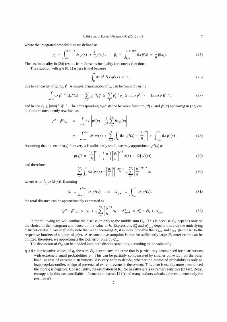
The discussion ofSq can be divided into three distinct situations, according tothe value ofq:

q < 0 : for negative values ofq, the sumSq accentuates the error that is particularly pronounced for distributionswith extremely small probabilitiespi . This can be partially compensated by smaller bin-width, onthe otherhand, in case of extreme distributions, it is very hard to decide, whether the estimated probability is only aninappropriate outlier, or sign of presence of extreme events in the system. This error is usually more pronouncedthe moreq is negative. Consequently, the estimation of RE for negativeq’s is extremely sensitive (in fact, Renyientropy is in this case unreliable information measure [21]) and many authors calculate the exponents only forpositiveq’s.

7


0 < q < 1 : For these values, the exponentq− 1 is larger than−1, even though the errors from small probabilities areaccentuated (because ofpq

i ), the error is bounded, becausepqi ≤ 1 for q ∈ (0, 1), so the error is not as dramatic

as in the first case.

q > 1 : in this case is the error diminished, because the factorpq−1i suppresses the error exponentially withq. The pre-

factorq does not grow as fast, and therefore in this case the error is reduced. Indeed, the against the suppressiongoes factorh1−q, which increases the error for smallh, and therefore it is generally better for this case not toover-fit the histogram too much.

All things together, we have seen, that even minimization ofthe local absolute errors|p(x)− p(x)|, resp. integratedabsolute errors

∫

Ik|p(x) − p(x)|dx does not necessarily mean minimization of errors of|pq(x) − pq(x)|. In such case,

we have to create histograms with different bin-width, which minimizes not the distance between histogramp(x) andunderlying PDFp(x), but theirq-th powers .

4.1. Optimal width of the histogram bin

As discussed above, the proper histogram formation from theunderlying distribution is a crucial step in the REestimation. In order to approximate the underlying probability via the equidistant-bin histogram, as in our case, it isnecessary to determine either a number of bins, or width of the bin. Now, the issue at stake is to find the optimal bin-width h∗ that minimizes the error in (32) and hence it provides the least biased empirical value of RE. There are severalapproaches for optimal width definition. In this connectionwe can mention, e.g.,Sturges rule[26], that estimates thenumber of bins of the histogram asnB = 1 + log2 N, which is motivated by the histogram of binomial distributions.This rule is very useful when visualizing data, but in case ofprobability density approximation, one can find moreeffective relations. From this point of view, particularly pertinent is the classicmean square error(MSE) method (seee.g., Ref. [27]) which allows to measure the difference between ˆpq(x) and a power of an underlying PDFpq(x). In theprevious section, we have been measured the error between a histogram and its underlying distribution byL1 distance.The connection to the MSE method is following: the estimatedhistogram is actually a random variable dependent onthe realizations{xi}Ni=1 of the underlying PDF. Hence, locally, we can measure the error betweenq-histogram3 pq(x)andpq(x) as an expectation value of the error of theq-histogram which is defined as follows

E[|pq(x) − pq(x)|]. (33)

The squared mean error is because of Jensen’s inequality forexpectation values smaller than mean squared error (cf.e.g., Feller [28]), so

E[|pq(x) − pq(x)|]2 ≤ E[(pq(x) − pq(x))2]. (34)

The motivation of working withL2-distance for calculation of errors instead ofL1-distance is mainly computational,because dealing withL2-norm is easier in calculations [29]. Connections to approaches based on different measures(mainly L1) are listed and discussed e.g., in Refs. [30, 31]. Naturally, different approaches can generally lead todifferent results, nevertheless, discussions in Refs. [29, 30,31, 32] and elsewhere predicate that in case of histogram,which can be regarded as 1-parameter class of step functions, one can reasonably assume that optimal bin-widthobtained from different approaches will not drastically differ from each other. Such argument can be supported by agraphical visualization of histograms created from time series of daily returns of S&P 500 financial index for differentbin widths (Fig. 2). Histograms for too small, or too large bin-widths do not represent the underlying distribution wellat all. Indeed, the resultant entropy fits (Fig. 3) do not perform a good linear behavior, which is also accentuated bydifferent values ofq.

The histogram error measured by squaredL2-distance is defined as follows:

E[(pq(x) − p(x)q)2] = E[(pq(x) − E[ pq(x)])2] + E[

(E[pq(x)] − pq(x))2]

= Var(pq(x)) +[

Bias(pq(x))]2, (35)

so the first term represents variance of the estimator and thesecond term represents squared bias of the histogram,i.e. Bias(pq(x)) = E[E[pq(x)] − pq(x)]. In our case, this quantity represents a local deviation of the q-histogram fromtheoretical (or underlying)q-th power of PDF.

3abbreviation forq-th power of histogram

8


Figure 2. Un-normalized (or frequency) histograms of fluctuation sumsσs, for s = 8, 64 and 512 and bar widthsh = 100, 10, 1,0.1 and 0.01,measured in unitsu = 3× 10−4 for better visualization. The optimal width is listed in thetable on Figure 6. We can see that far from the optimalvalue, the shape of histogram is not appropriately approximating the theoretical probability distribution, i.e. we observe under-fitted or over-fittedhistograms.

h = 100

h = 10

h = 1

h = 0.1

h = 0.01

Beginning with computation of variance, we find that ˆpq(x) =vq

kNqhq , wherek is the label of corresponding bin,

whereχk(x) = 1. Naturally,νk is binomially distributed,νk ∼ B(N, pk), wherepk is a theoretical probability ofk-th

bin, sopk =∫

Ikp(x)dx and indeed ˆpk

N→∞→ pk. Thus,

Var(pq(x)) = Var

νqk

Nqhq

=1

N2qh2q

(

E[ν2qk ] − E[(νk)

q]2)

. (36)

This leads to calculation of fractional moments of binomialdistribution, which is generally intractable, unlessq isnatural. When we have enough statistics (a broad discussionand some practical rules are in Ref. [33]), we canapproximate the distribution by normal distributionB(N, p) ∼ N(Np,Np(1− p)), so

E[νqk] ≈∫

R

dx|x|q 12πNpk(1− pk)

exp

(

− (x− (Npk)2)2

2Npk(1− pk)

)

. (37)

Moment E[xq] was replaced by the absolute moment E[|x|q], because the latter value is real, while the first may not.The integral can be performed in the following way:

E[νqk] ≈ 1√π

(2Npk(1− pK))q/2 Γ

(

1+ q2

)

e−npk

2(1−pk)1F1

(

1+ q2,12

;Npk

2(1− pk)

)

, (38)

9


2 3 4 5 6

12

34

5

width of bin = 100

2 3 4 5 6

34

56

7

width of bin = 10

2 3 4 5 6

5.0

6.0

7.0

8.0

width of bin = 1

2 3 4 5 67.

07.

58.

08.

59.

0

width of bin = 0.1

2 3 4 5 6

8.8

9.0

9.2

9.4

9.6

width of bin = 0.01

−1 0 1 2 3 4

Symbols for diffrent values of q

Figure 3. Linear fits of estimated RE vs logarithm of time lag for h = 100, 10, 1, 0.1, 0.01 . Note, in particular, that the error is distributed also tothe regression of the scaling exponents, also depending onq, which means that universal choice ofh∗ for all q’s leads to improper results and onehas to findh∗q depending onq.

Sq(s)

Sq(s)

Sq(s)

Sq(s)

Sq(s)

ln(s)

ln(s)

ln(s)

ln(s)

ln(s)

where1F1(α, β; z) aconfluent hypergeometric functiondefined as

1F1(α, β; z) = 1+α

β · 1!z+α(α + 1)β(β + 1)2!

z2 + · · · =∞∑

j=0

(α) j

(β j) j!zj . (39)

Symbol (α)k = α(α + 1) . . . (α + k) is calledPochhammer symbol. According to Lebedev and Silverman [34], theconfluent hypergeometric function can be asymptotically expanded as

1F1(α, β; z) =Γ(β)Γ(α)

ezz−(β−α)(

1+ (β − α)(1− α)z−1 + O(z−2))

(40)

for sufficiently largez. Inserted into Eq.(38) we have that

E[νqk] = Nqpqk

(

1+12

q(q− 1)(1− pk)

Npk+ O(N−2)

)

. (41)

Consequently, the variance is in leading order ofN equal to

Var(pq(x)) =1

N2qh2qN2qp2q

k

[

q21− pk

Npk+ O(N−2)

]

=q2p2q−1

k (1− pk)

h2qN+ O(N−2) ≤

q2p2q−1k

h2qN+ O(N−2) . (42)

Trying to calculate the bias, we have that

Bias(pq(x)) =E[νqk]

Nqhq− pq(x) =

( pk

h

)q− pq(x) + O(N−1) . (43)

10


When we want to calculate the total error for all points of histogram, we should simply integrate over all errorsand obtainmean integrated square error(MISE), which is equal to integrated variance plus integrated squared bias.

MISE(pq) ≡∫

R

Var(pq(x))dx +∫

R

[

Bias(pq(x))]2 dx . (44)

Naturally, we will be dealing only with leading terms of bothquantities, which gives us expression for the integratedvariance

∫

R

Var(pq(x))dx =∞∑

k=−∞

∫

Ik

Var(pq(x))dx ≈nB+1∑

k=0

q2p2q−1k

h2q−1N, (45)

By applying the mean value theorem forpk

pk =

∫

Ik

p(x)dx = hp(ξk) (46)

we obtain that

∫

R

Var(pq(x))dx ≈∞∑

k=−∞

q2p2q−1k

h2q−1N=

q2

Nh

∞∑

k=−∞p2q−1(ξk)h ≈

q2

Nh

∫

R

p2q−1(x)dx. (47)

Calculating the integrated squared bias similarly as a sum of integrated squared biases overk-th bin

∫

R

[

Bias(pq(x))]2 dx =

∞∑

k=−∞

∫

Ik

[

Bias(pq(x))]2 dx , (48)

we look firstly at such bin, which lies between 0 andh; we approximate the corresponding probabilityp[0,h] =∫ h

0p(t)dt

as

p[0,h] =

∫ h

0p(t)dt =

∫ h

0

(

p(x) + (t − x)dpdx

(x) + . . .

)

dt = hp(x) + h

(

h2− x

)

dp(x)dx+ O(h3) . (49)

We note that becausex ∈ (0, h), the second term iso(h2). Theq-th power can be therefore approximated as

pq[0,h] = hqpq(x) + qhq−1pq−1(x)h

(

h2− x

)

dpdx

(x) + O(hq+2) , (50)

and the bias of that bin is equal to (again, with help of mean value theorem)

∫ h

0

(

h2− x

)2 (

qdpdx

(x)pq−1(x)

)2

=

∫ h

0

((

h2− x

)

dpq

dx(x)

)2

dx =

(

dpq

dx(ξ0)

)2 ∫ h

0

(

h2− x

)2

dx =h3

12

(

dpq

dx(ξ0)

)2

. (51)

The bias for other bins can be calculated similarly, so we have that

∫

R

[

Bias(pq(x))]2 dx ≈ h2

12

∞∑

k=−∞

(

dpq

dx(ξk)

)2

h ≈ h2

12

∫

R

(

dpq

dx(x)

)2

. (52)

Combining Eqs. (47) and (52), we get that the asymptotic4 mean integrated squared error (AMISE) is equal to

AMISE(pq) ≡ E∫

R

[|pq(x) − pq(x)|] =∫

RE[|pq(x) − pq(x)|] = q2

Nh

∫

R

p2q−1(x)dx+h2

12

∫

R

(

dpq(x)dx

)2

. (53)

4The wordasymptoticdenotes the fact that the error is approximated by its leading order

11


Note that forq = 1 we recover the classic error discussed e.g., in Ref. [29]. Minimizing the error gives us the relationfor optimalh∗q

h∗q =3

√

6q2

NNq, (54)

whereNq is equal to

Nq =

∫

Rp2q−1(x)dx

∫

R

(

dpq

dx (x))2

dx. (55)

Similarly to Scott [29] we assume that underlying distribution is the normal distributionN(µ, σ2). In such a case isNq for q > 1

2 equal to

Nq =4√πσ3

√

q(2q− 1), (56)

which gives us the error as

AMISE(pq) =q2(2π)1−q(σ2)1−q

Nh√

2q− 1+

h2

12√

q2−(1+q)π−(1/2+q)σ−(1+2q) , (57)

and optimalh∗q as

h∗q = σN−1/3 3

√

24√π

q1/2

6√

2q− 1= h∗1ρq , (58)

whereρq =q1/2

6√

2q−1is theq-dependent part andh∗1 is the optimal bin-width, whenq = 1 (corresponding to classic

results from histogram theory, see e.g., [29, 32]). In practical estimation, theoretical standard deviation is replaced bythe empirical one, and one has the rule for bin-width:

hS cq = 3.5σN−1/3ρq , (59)

whereσ is estimated standard deviation of the series. On the other hand, Freedman and Diaconis (FD) (see Ref. [35])proposed more robust rule, in which the estimated standard deviation is replaced 3.5σ by 2 · IQR, where IQR is theinterquartile range IQR= x0.75 − x0.25; Nevertheless, this estimation is not precise, because

IQR(N(µ, σ)) = 2√

2 · erfc(−1) (1/2)σ ≈ 1.349σ. (60)

Function erfc(−1)(z) is inverse complementary error function. Contrary to original Freedman-Diaconis theory, we haveto care more about over-fitting of histogram because the multiplication constant is accentuated for small and largeq’s.When we replace ˆσ by IQR more precisely, the resulting rule has the following form:

hFDq = 2.6(IQR)N−1/3ρq . (61)

In our method, we have to estimate simultaneously more probability distributionspqs for more time lags5 {s1, s2, . . . , sm},

all with the same bin width. This can by done by minimizing thesum of all errors from all histograms and find suchh∗q that minimizes thetotal asymptotic mean square error (TAMISE), which is defined as

TAMISE({pqs1, . . . , pq

sm}) ≡

m∑

i=1

AMISE(pqsi) =

m∑

i=1

q2(2π)1−qσ2(1−q)si

Nsi h√

2q− 1+

h2

12√

q2−(1+q)π−(1/2+q)σ−(1+2q)si

(62)

5according to the introductory definition in Section 2, it corresponds to the situation, when varying typical time lag, which is usually conveyedby taking multiples of time lags0, on which was the experiment measured (e.g., for the investigated series S&P 500 is the basic time lags0 = 1 day)

12


2 4 6 8 10

1

2

3

4

2 4 6 8 10

1.5

2.0

2.5

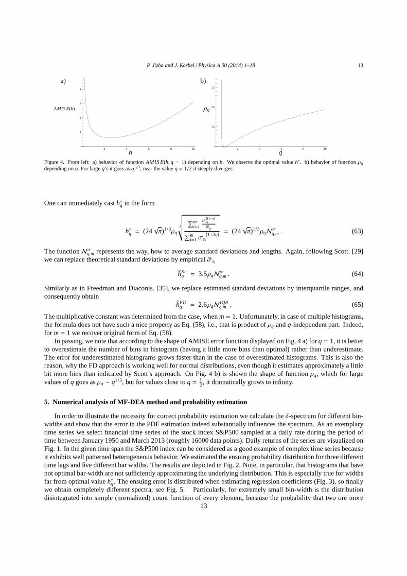
Figure 4. From left: a) behavior of functionAMIS E(h, q = 1) depending onh. We observe the optimal valueh∗. b) behavior of functionρq

depending onq. For largeq’s it goes asq1/3, near the valueq = 1/2 it steeply diverges.

a) b)

AMIS E(h) ρq

h q

One can immediately casth∗q in the form

h∗q = (24√π)1/3ρq

3

√

√

√

√

√∑m

i=1σ

2(1−q)si

Nsi∑m

i=1σ−(1+2q)si

= (24√π)1/3ρqNσq,m . (63)

The functionNσq,m represents the way, how to average standard deviations and lengths. Again, following Scott. [29]we can replace theoretical standard deviations by empirical σsi

hS cq = 3.5ρqN σq,m . (64)

Similarly as in Freedman and Diaconis. [35], we replace estimated standard deviations by interquartile ranges, andconsequently obtain

hFDq = 2.6ρqN IQR

q,m . (65)

The multiplicative constant was determined from the case, whenm= 1. Unfortunately, in case of multiple histograms,the formula does not have such a nice property as Eq. (58), i.e., that is product ofρq andq-independent part. Indeed,for m= 1 we recover original form of Eq. (58).

In passing, we note that according to the shape of AMISE errorfunction displayed on Fig. 4 a) forq = 1, it is betterto overestimate the number of bins in histogram (having a little more bins than optimal) rather than underestimate.The error for underestimated histograms grows faster than in the case of overestimated histograms. This is also thereason, why the FD approach is working well for normal distributions, even though it estimates approximately a littlebit more bins than indicated by Scott’s approach. On Fig. 4 b)is shown the shape of functionρq, which for largevalues ofq goes asρq ∼ q1/3, but for values close toq = 1

2, it dramatically grows to infinity.

5. Numerical analysis of MF-DEA method and probability estimation

In order to illustrate the necessity for correct probability estimation we calculate theδ-spectrum for different bin-widths and show that the error in the PDF estimation indeed substantially influences the spectrum. As an exemplarytime series we select financial time series of the stock indexS&P500 sampled at a daily rate during the period oftime between January 1950 and March 2013 (roughly 16000 datapoints). Daily returns of the series are visualized onFig. 1. In the given time span the S&P500 index can be considered as a good example of complex time series becauseit exhibits well patterned heterogeneous behavior. We estimated the ensuing probability distribution for three differenttime lags and five different bar widths. The results are depicted in Fig. 2. Note, inparticular, that histograms that havenot optimal bar-width are not sufficiently approximating the underlying distribution. This is especially true for widthsfar from optimal valueh∗q. The ensuing error is distributed when estimating regression coefficients (Fig. 3), so finallywe obtain completely different spectra, see Fig. 5. Particularly, for extremely small bin-width is the distributiondisintegrated into simple (normalized) count function of every element, because the probability that two ore more

13


−

−

− − − −

−1 0 1 2 3 4

−0.1

0.00.1

0.20.3

0.40.5

−

−

−

−

−−

−

−

−

−

−

−

−

−

− − − −

−1 0 1 2 3 4

−0.1

0.00.1

0.20.3

0.40.5

−

−

−−

−−

−−

−−

−−

−

−

− − − −

−1 0 1 2 3 4

−0.1

0.00.1

0.20.3

0.40.5

−−

−−−−

−−

−−

−−

−−

− − − −

−1 0 1 2 3 4

−0.1

0.00.1

0.20.3

0.40.5

−

− −

−−

−

−

−

−

−

−

−

− − −−

−

−

−1 0 1 2 3 4

−0.1

0.00.1

0.20.3

0.40.5

−−

−−

−

−−

−−

−

−

−

Figure 5. Estimatedδ-spectra (middle point) and 99% confidence intervals (within upper and lower point) for different values of bin-widthh. Forbin-width far from the optimal width the spectrum is diminished and confidence intervals get wider. Particularly, for under-fitted histograms theerror is most dramatic for smallq’s, for over-fitted histograms the error is most visible for large values ofq’s.

h = 100 h = 10 h = 1 h = 0.1 h = 0.01

values fall into the same bin withh → 0 is going to zero for given constant lengthN. Let us note that the right binestimation is important also for monofractal version of DEA, introduced by Scafettaat al. in Ref. [19]. Of course, ifwe estimate the spectrum within a small range of fluctuation times, when typicallysi ≪ N for all si , soN ∼ Nsi andthe variance grows with an exponentσ ∼ sV, whereV is typically around 0.5 (let us remind the connection with theHurst exponent [36]), then we can estimate the optimal bin width for the first histogram, and use it for other histogramsas well. Nevertheless, for estimation across many scales orif we need to estimate the spectrum for sensitive values ofq, the choice of properh∗ becomes more and more important.

5.1. Comparison ofδ-spectrum from different bin-width estimation methods

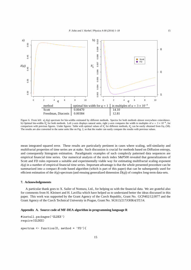
For every method discussed in Section 4.1 we estimated the probability distribution width, the bin-width and thespectrum. Results obtained are presented in Fig. 6 togetherwith the table with the calculated optimal widths. Thefigure implies that the different spectrum for the two aforementioned two approaches. We can observe that eventhough the optimal bin-widths for Scott and FD method are different, the corresponding spectra can coalesce togetherfor some cases. This can be caused by the fact, that financial data are traded not for arbitrary price, which couldbe any real number, but prices are always in dollars and cents(at the U.S. stocks) and the number expressed indollars have maximally two digits after decimal point. Thiscauses that the data are grouped at these price surfaces,so different histograms can look completely the same, if these price surfaces fall into the same regions. In case ofinfinite precision of the data (or if we could trade assets forany real-valued price), the spectra would be generallydifferent. Which method will be more efficient depends on a concrete data-set but, as we already know from ourprevious discussion, it is generally better to overestimate the number of bins, than to underestimate it. Hence fromthis standpoint is the FD method more robust.

6. Conclusions

This paper has investigated the issue of the optimal bin-width choice for empirical probability histograms thattypically appear in the framework of Monofractal and Multifractal Diffusion Entropy Analysis. Our investigationrevealed that in order to obtain a reliable differential Renyi’s entropy and the ensuing scaling exponents δ(q), thebin-width must be chosen with care. We have argued that errors caused by estimation of the bin-width can be wellquantified by the Renyi information divergence (which is aq-generalization of the Kullback–Leibler divergence)and the resultingL1-distance. One significant finding that emerged from this study is that classic bin-width rules(e.g., Scott or FD rules), familiar from theory of histograms and based onL2-distance (which gives similar resultsasL1, but is easier to deal with), can be straightforwardly generalized for multiple histograms with the same bin-width and different values ofq. In this case the resultant bin-width is derived from minimizing of total asymptotic

14


0 2 4 6 8 10

0.30

0.35

0.40

0.45

0.50

0 2 4 6 8 100.

003

0.00

40.

005

0.00

60.

007

0.00

80.

009

0.01

0

1020

30

ScottFD

method optimal bin width forq = 1 in multiples ofu = 3× 10−4

Scott 0.00470 14.10Freedman, Diaconis 0.00384 12.81

Figure 6. From left: a)δ(q) spectrum for bin-widths estimated by different methods. Spectra for both methods almost everywhere coincidence.b) Optimal bin-widthsh∗q for both methods. Left y-axis displays natural units, righty-axis compares the width to multiples ofu = 3 × 10−4, forcomparison with previous figures. Under figures: Table with optimal values ofh∗1 for different methods,h∗q can be easily obtained from Eq. (58).The results are also converted to the same units like on Fig. 2, so that the reader can easily compare the results with previous values.

q

δ(q)

q

h∗q

a) b)

mean integrated squared error. These results are particularly pertinent in cases where scaling, self-similarity andmultifractal properties of time series are at stake. Such discussion is crucial for methods based on Diffusion entropy,and consequently histogram estimation. Paradigmatic examples of such complexly patterned data sequences areempirical financial time series. Our numerical analysis of the stock index S&P500 revealed that generalizations ofScott and FD rules represent a suitable and experimentally viable way for estimating multifractal scaling exponentδ(q) in a number of empirical financial time series. Important advantage is that the whole presented procedure can besummarized into a compactR-code based algorithm (which is part of this paper) that can be subsequently used forefficient estimation of theδ(q)-spectrum (and ensuing generalized dimensionD(q)) of complex long-term data-sets.

7. Acknowledgements

A particular thank goes to X. Sailer of Nomura, Ltd., for helping us with the financial data. We are grateful alsofor comments from H. Kleinert and H. Lavicka which have helped us to understand better the ideas discussed in thispaper. This work was supported by the Grant Agency of the Czech Republic, Grant No. GCP402/12/J077 and theGrant Agency of the Czech Technical University in Prague, Grant No. SGS13/217/OHK4/3T/14.

Appendix A. Source code of MF-DEA algorithm in programming language R

#install.packages(’GLDEX’)

require(GLDEX)

spectrum <- function(X, method = ’FD’){

15


############################

# Input parameters

############################

scale <- c(4,8,16,32,64,128,256,512) #set of time lags

q <- seq(0,10, by= 0.1) #set of q’s

#############################

# Fluctuation collection

#############################

fluctuation <- matrix(ncol=length(X), nrow=length(scale))

for(t in 1:length(scale)){

for(s in 1:(length(X)-scale[[t]])){

fluctuation[t,s] <- sum(X[s:(s+scale[[t]]-1)])

}

}

#############################

# Estimation of hstar

#############################

sigmaL <- array(dim = length(scale))

for(i in 1:length(scale)){

sigmaL[[i]] <- sd(na.omit(fluctuation[i,]))

}

sigma <<- sigmaL

IQRangeL <- array(dim = length(scale))


IQRangeL[[i]] <- IQR(na.omit(fluctuation[i,]))

}

IQRange<<- IQRangeL

lengthsL <- array(dim = length(scale))


lengthsL[[i]] <- length(na.omit(fluctuation[i,]))

}

lengths<<- lengthsL

rho <- function(q){

if(q>1){

return(q^(1/2)/(2*q-1)^(1/6))}

else{

return(1)}

}

######### Scott hstar ###########

hstarS <- function(q){

return(rho(q)*3.5*(sum ( sigma^(2*(1-q)) /lengths ) / sum( 1/ (sigma^(1+2*q)) ))^(1/3))

16


}

###### Freedman-Diaconis hstar ####

hstarF <- function(q){

return(rho(q)*2.6*(sum ( IQRange^(2*(1-q)) /lengths ) / sum( 1/ (IQRange^(1+2*q)) ))^(1/3))

}

######### Choice of method #######

if(method == ’Scott’){

hstar <- hstarS}

else{

hstar <- hstarF

}

#############################

# Estimation of histogram

#############################

Sq <- matrix(nrow = length(q),ncol = length(scale))

tauq <- matrix(nrow = length(q), ncol = 2)

for(n in 1:(length(scale))){

for(i in 1:length(q)){

p <- na.omit(fluctuation[n,])

h <-hist(p, breaks = floor((max(p)-min(p))/hstar(q[[i]]))+1, plot = FALSE)

pr <-fun.zero.omit(h$counts/length(p))

#############################

# Estimation of Renyi entropy

#############################

if(q[i] == 1){

Sq[i,n] <- -sum(pr*log(pr))}

else{

Sq[i,n] <- 1/(1-q[i])*log(sum(pr^q[i]))

}

}

}

for(i in 1:length(q)){

fit <- as.vector(na.omit(Sq[i,]))

model <- lm(fit ~ log(scale))

tauq[i,] <- coefficients(model)

}

tq <- tauq[,2]

ret <- data.frame(q,tq)

return(ret)

17


} #end of function

References

[1] K. Kim, S.-M. Diaconis, Multifractal features of financial markets, Physica A 344 (2) (2004) 272.[2] J. Machado, F. Duarte, G. M. Duarte, Fractional dynamicsin financial indices, Int. J. Bifurcation Chaos 22 (10) (2012) 1250249.[3] B. West, D. West, Fractional dynamics of allometry, Int.J. Theor. and Appl. 15 (1) (2012) 70.[4] J. Park, J. Lee, J.-S. Yang, H.-H. Jo, H.-T. Moon, Complexity analysis of the stock market, Physica A 379 (1) (2007) 179.[5] J. W. Lee, J. B. Park, H.-H. Jo, J.-S. Yang, H.-T. Moon, Minimum entropy density method for the time series analy-

sis,arXiv:physics/0607282 .[6] T. Schreiber, Measuring information transfer, Phys. Rev. Lett. 85 (2) (2000) 461.[7] R. Marschinski, H. Kantz, Analysing the information flowbetween financial time series, Eur. Phys. J. B 30 (2) (2002) 275.[8] P. Jizba, H. Kleinert, M. Shefaat, Renyi information transfer between financial time series, Physica A 391 (10) (2012) 2971.[9] H. Kleinert, Path Integrals in Quantum Mechanics, Statistics, Polymer Physics and Financial Markets, 4th edn, World Scientific, 2009.

[10] C.-K. Peng, S. Havlin, H. Stanley, A. Goldberger, Quantification of scaling exponents and crossover phenomena in nonstationary heartbeattime series, Chaos 5 (1) (1995) 82.

[11] J. Voit, The Statistical Mechanics of Financial Merkets, Springer, 2003.[12] C.-K. Peng, S. Buldyrev, S. Havlin, M. Simons, H. Stanley, A. Goldberger, Mosaic organization of dna nucleotides, Phys. Rev. E 49 (2)

(1994) 1685.[13] R. Mantegna, H. Stanley, An introduction to econphysics: cirrelations and complexity in finance, Cambridge University Press, 2000.[14] P. Talker, R. Weber, Power spectrum and detrended fluctuation analysis: Application to daily temperatures, Phys. Rev. E 62 (1) (2000) 150.[15] M. Bozic, M. Stojanovic, Z. Stajic, N. Floranovic, Mutual information-based inputs selection for electric load time series forecasting, Entropy

15 (2) (2013) 926.[16] W. Kantelhardt, S. Zschiegner, E. Koscielny-Bunde, S.Havlin, A. Bunde, H. Stanley, Multifractal detrended fluctuation analysis of nonsta-

tionary time series, Physica A 316 (2002) 87 – 114.[17] J. F. Muzy, E. Bacry, A. Arneodo, Multifractal formalism for fractal signals: The structure-function approach versus the wavelet-transform

modulus-maxima method, Phys. Rev. E 47 (2) (1993) 875.[18] R. Morales, T. D. Matteo, R. Gramatica, T. Aste, Dynamical generalized hurst exponent as a tool to monitor unstable periods in financial time

series, Physica A 391 (11) (2012) 3180.[19] N. Scafetta, P. Grigolini, Scaling detection in time series: diffusion entropy analysis, Phys. Rev. E 66 (3) (2002) 036130.[20] J. Huang, et al., Multifractal diffusion entropy analysis on stock volatility in financial markets, Physica A 391 (22) (2012) 5739.[21] P. Jizba, T. Arimitsu, The world according to Renyi: thermodynamics of multifractal systems, Annals of Physics 312 (1) (2004) 17.[22] H. Stanley, P. Meakin, Multifractal phenomena in physics and chemistry, Nature 335 (29) (1988) 405.[23] A. Y. Morozov, Comment on ’multifractal diffusion entropy analysis on stock volatility in financial markets’ [Physica A 391 (2012) 5739-

5745], Physica A 392 (10) (2013) 2442 – 2446.[24] C. Beck, F. Schlogl, Thermodynamics of Chaotic Systems: An Introduction, Cambridge University Press, 1995.[25] A. Renyi, Selected Papers of Alfred Renyi,vol.2, Akademia Kiado, 1976.[26] H. Sturges, The choice of a class-interval, J. Amer. Statist. Assoc. 21 (1926) 65.[27] E. Lehmann, G. Casella, Theory of Point Estimation (2nded.), Springer, 1998.[28] W. Feller, An Introduction to Probability theory and its Applications, 2nd Edition, Vol. 2, Wiley, 1970.[29] D. Scott, Multivariate density estimation: Theory, practice and visualisation, John Willey and Sons, Inc., 1992.[30] P. Hall, M. P. Wand, Minimizing{L1} distance in nonparametric density estimation, Journal of Multivariate Analysis 26 (1) (1988) 59 – 88.[31] D. W. Scott, Feasibility of multivariate density estimates, Biometrika 78 (1) (1991) 197–205.[32] B. W. Silverman, Density Estimation for Statistics andData Analysis, Chapman & Hall, London, 1986.[33] G. Box, J. Hunter, W. Hunter, Statistics for experimenters: design, innovation, and discovery, Wiley series in probability and statistics,

Wiley-Interscience, 2005.[34] N. Lebedev, R. Silverman, Special Functions and Their Applications, Dover Books on Mathematics Series, Dover Publications, 1972.[35] D. Freedman, P. Diaconis, On the histogram as a density estimator, Zeitschrift fur Wahrscheinlichkeitstheorie und Verwandte Gebiete 57 (4)

(1981) 453.[36] H. Hurst, R. Black, Y. Simaika, Long-term storage : an experimental study, Constable, London, 1965.

18

http://arxiv.org/abs/physics/0607282

Multifractal diffusion entropy analysis: Optimal bin width of probability histograms

Documents

Transcript of Multifractal diffusion entropy analysis: Optimal bin width of probability histograms