Determining the effective width of composite beams with ...

Structural Engineering and Mechanics, Vol. 21, No. 3 (2005) 295-313 295

Determining the effective width of composite beams with precast hollowcore slabs

Ehab El-Lobody†

Department of Structural Engineering, Faculty of Engineering, Tanta University, Tanta, Egypt

Dennis Lam‡

School of Civil Engineering, University of Leeds, Leeds, LS2 9JT, U.K.

(Received October 8, 2004, Accepted July 7, 2005)

Abstract. This paper evaluates the effective width of composite steel beams with precast hollowcoreslabs numerically using the finite element method. A parametric study, carried out on 27 beams withdifferent steel cross sections, hollowcore unit depths and spans, is presented. The effective width of theslab is predicted for both the elastic and plastic ranges. 8-node three-dimensional solid elements are usedto model the composite beam components. The material non-linearity of all the components is taken intoconsideration. The non-linear load-slip characteristics of the headed shear stud connectors are included inthe analysis. The moment-deflection behaviour of the composite beams, the ultimate moment capacity andthe modes of failure are also presented. Finally, the ultimate moment capacity of the beams evaluatedusing the present FE analysis was compared with the results calculated using the rigid – plastic method.

Key words: effective width; precast; hollowcore slabs; finite element; modelling; composite design;steel; concrete.

1. Introduction

Composite construction using precast hollowcore units (hcu) is relatively new. For this type of

composite beam, mechanical shear connectors pre-welded on to the top flange of the steel beam are

used to connect the steel beam with the precast hcu floor. The present knowledge concerning the

behaviour of stud connectors within precast hollow core slabs and designing of composite beams

with precast hcu slabs is limited (Lam et al. 2000a, b). Detailed finite element (FE) analysis of the

behaviour of headed stud shear connectors in this form of construction is previously investigated by

El-Lobody and Lam (2002) to establish the load-slip behaviour of the headed shear connectors.

In composite design, determination of the effective width (beff) is traditionally treated by an

approximate method. T-section is formed by assuming the steel beam act compositely with an

effective width of the concrete slab; usually related to the span of the beam so that simple beam

theory can be applied for the analysis. The effective width is typically prescribed in codes of

† Lecturer‡ Senior Lecturer, Corresponding author, E-mail: [email protected]

DOI: http://dx.doi.org/10.12989/sem.2005.21.3.295

296 Ehab El-Lobody and Dennis Lam

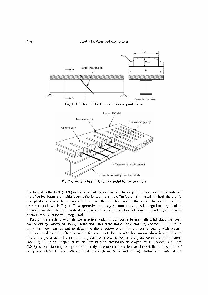
practice likes the EC4 (1994) as the lesser of the distances between parallel beams or one quarter of

the effective beam span whichever is the lesser, the same effective width is used for both the elastic

and plastic analysis. It is assumed that over the effective width, the strain distribution is kept

constant as shown in Fig. 1. This approximation may be true in the elastic stage but may lead to

overestimate the effective width at the plastic stage since the effect of concrete cracking and plastic

behaviour of steel beam is neglected.

Previous research to evaluate the effective width in composite beams with solid slabs has been

carried out by Ansourian (1975), Heins and Fan (1976) and Amadio and Fragiacomo (2002), but no

work has been carried out to determine the effective width for composite beams with precast

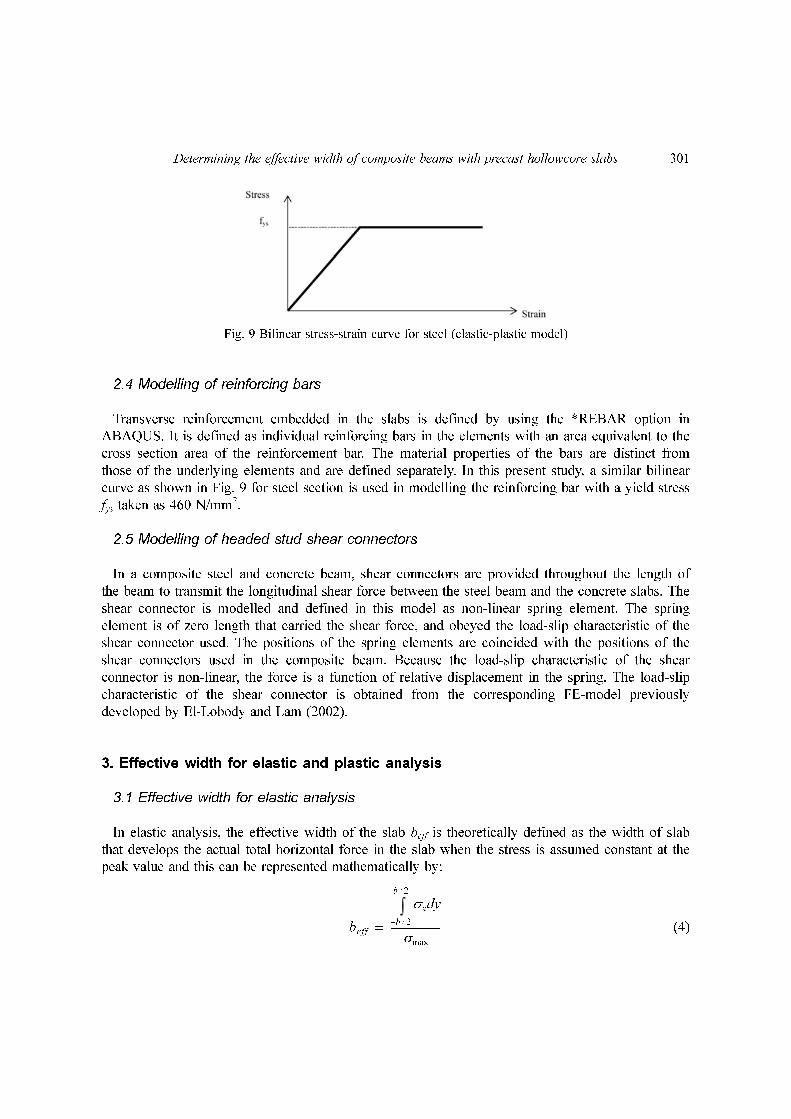
hollowcore slabs. The effective width for composite beams with hollowcore slabs is complicated

due to the presence of the in-situ and precast concrete, as well as the presence of the hollow cores

(see Fig. 2). In this paper, finite element method previously developed by El-Lobody and Lam

(2003) is used to carry out parametric study to establish the effective slab width for this form of

composite slabs. Beams with different spans (6 m, 9 m and 12 m), hollowcore units’ depth

Fig. 1 Definition of effective width for composite beam

Fig. 2 Composite beam with square-ended hollow core slabs

Determining the effective width of composite beams with precast hollowcore slabs 297

(150 mm, 200 mm and 250 mm) and steel sections (UB 356, UB 406 and UB 457) were used for

this study. The material non-linearity of precast concrete, in-situ concrete and the steel beams are

taken into account. The load-slip characteristic of the shear connectors are taken from the previous

finite element analyses by El-Lobody and Lam (2002).

2. Modelling of composite beams with precast hollowcore slabs

The composite beams modelled in this research, consists of steel beam, pre-welded headed stud

shear connectors, prestressed hcu’s and cast in-situ concrete. The hcus’ are rested directly on the top

flange of the steel beam, with an in-situ gap ‘g’ in the longitudinal direction as shown in Fig. 2.

The alternative cores of each hcu were left open for a length of 500 mm to allow for placing of the

transverse reinforcement. Fig. 3 shows a standard 1200 mm width × 150 mm depth precast hollow

core unit. Reinforcing bar is placed on site into the open cores and filled with a minimum grade

C25 in-situ concrete. Fig. 4 shows the section of the precast / in-situ joint of the composite beam

with hollowcore slabs. The longitudinal and transverse joints between the hcus’ are filled with in-

situ concrete so that horizontal compressive forces can be transferred through the slabs.

Fig. 4 Details of the precast-in-situ joint of composite beam with square-end hollowcore slabs

Fig. 3 Details of a typical 1200 mm length hollow core unit


2.1 Finite element mesh and boundary conditions

The three-dimensional FE solid elements are used to model the composite beams. Each precast

unit is modelled with 114 elements. The in-situ concrete infill is modelled with 160 elements for the

6 m span beam; 240 elements for the 9 m span beam and 320 elements for the 12 m span beam.

The in-situ infill which contained the reinforcing bar is modelled with 1 element in the x-direction,

2 elements in the y-direction and 1 element in the z-direction. Fig. 5 shows the 3-D FE model of the

composite beams used in this study. For the boundary conditions, all nodes of precast concrete

units, in-situ concrete and the steel beam in the symmetry surface passing through the middle of

Fig. 5 FE mesh of composite beams with precast hollowcore slabs

Fig. 6 Boundary conditions for the composite beam


beams are restricted to move in the x- and y-directions as shown in Fig. 6. The support is allowed

to move in the x-direction but prevented to move in the y- and z-directions. The load is applied as

uniformly distributed load using the RIKS method available from the ABAQUS (1998).

2.2 Concrete material model

Modelling of the concrete elements is the most important part of this study. Concrete is assumed

to be an isotropic material prior to cracking. The presence of cracks affects the stress and material

stiffness of the elements.

2.2.1 Concrete cracking

Concrete cracking is the most important aspect in modelling the concrete elements and

representation of cracks and post-cracking behaviour dominates the accuracy of the model. Cracking

is occurred when the stress reached a failure surface, which is called “crack detection surface”. This

failure surface is a linear relationship between the equivalent pressure stress, p and the Von Mises

equivalent stress, q. Once a crack has been detected, its orientation is stored and subsequent

cracking at the same point is assumed to be orthogonal to this direction. The post failure behaviour

of direct straining across cracks is modelled with the *TENSION STIFFENING option in

ABAQUS (1998).

2.2.2 Tensile and compressive behaviour

Concrete in tension is considered as linear-elastic material until the uni-axial tensile stress, ft. A

linear softening model is assumed to represent the post-failure behaviour in tension by tension

stiffening, this allows for the effects of interaction between reinforcement and concrete. Concrete in

compression is considered to be a linear-elastic / plastic material. When the principal stress

components are dominantly compressive, the response of concrete is modelled by elastic-plastic

Fig. 7 Uni-axial behaviour of plain concrete


theory using a simple form of yield surface. This surface is written in terms of the equivalent

pressure stress, p, and the Von Mises equivalent stress, q. The cracking and compressive responses

of concrete that are incorporated in the model are illustrated by the uni-axial behaviour shown in

Fig. 7. When concrete is loaded in compression, it initially exhibits elastic response. As the stress is

increased, some inelastic straining occurs and the response of the material softens. When ultimate

stress ‘fuc’ is reached, the material start to lose the strength until it can no longer carry any stress. In

multi-axial stress states these observations are generalised through the concept of surfaces of failure

and flow in stress space. These surfaces are fitted to experimental data as shown in Fig. 8.

Following the BS8110 (1997), average values of ultimate strain at failure ‘εu’, the ultimate

compression stress of concrete ‘fuc’, the initial Young’s modulus ‘Eco’ can be calculated from the

following relations:

(1)

(2)

(3)

2.3 Steel material model

The steel material in this study is treated as elastic – plastic material, i.e., it behaves linear

elastically up to the yield stress of steel, fys, see Fig. 9. After this stage it becomes fully plastic. In

the present study, Es is taken as 200000 N/mm2 and fys is taken as 275 N/mm2.

εu 0.00024 fcu=

fuc 0.67fcu=

Eco 5500 fcu=

Fig. 8 Yield and failure surface for in-plane stresses


2.4 Modelling of reinforcing bars

Transverse reinforcement embedded in the slabs is defined by using the *REBAR option in

ABAQUS. It is defined as individual reinforcing bars in the elements with an area equivalent to the

cross section area of the reinforcement bar. The material properties of the bars are distinct from

those of the underlying elements and are defined separately. In this present study, a similar bilinear

curve as shown in Fig. 9 for steel section is used in modelling the reinforcing bar with a yield stress

fys taken as 460 N/mm2.

2.5 Modelling of headed stud shear connectors

In a composite steel and concrete beam, shear connectors are provided throughout the length of

the beam to transmit the longitudinal shear force between the steel beam and the concrete slabs. The

shear connector is modelled and defined in this model as non-linear spring element. The spring

element is of zero length that carried the shear force, and obeyed the load-slip characteristic of the

shear connector used. The positions of the spring elements are coincided with the positions of the

shear connectors used in the composite beam. Because the load-slip characteristic of the shear

connector is non-linear, the force is a function of relative displacement in the spring. The load-slip

characteristic of the shear connector is obtained from the corresponding FE-model previously

developed by El-Lobody and Lam (2002).

3. Effective width for elastic and plastic analysis

3.1 Effective width for elastic analysis

In elastic analysis, the effective width of the slab beff is theoretically defined as the width of slab

that develops the actual total horizontal force in the slab when the stress is assumed constant at the

peak value and this can be represented mathematically by:

(4)beff

σx yd

b 2⁄–

b 2⁄

∫

σmax

--------------------=

Fig. 9 Bilinear stress-strain curve for steel (elastic-plastic model)


In a non-linear step-by-step incremental load procedure, the stresses and strains at the end of the

first increment are obtained based on elastic material properties. So, by integrating the longitudinal

axial stresses over the width ‘b’ at the end of the first increment and dividing the result by the peak

value of the longitudinal stress, the elastic effective width can be calculated easily. This approach is

used in this present parametric study to evaluate the elastic effective width of composite beams with

precast hollowcore slabs.

3.2 Effective width for plastic analysis

The elasto-plastic analysis of composite beams was accomplished by a step-by-step load

incremental procedure. Initially, the composite beam is solved by an elastic analysis and the stresses

at the end of the first increment are calculated. The minimum value of the load that will cause any

point in the structure to yield is determined. The elastic equations are then modified so that the

equations at the yield points obeyed the plastic condition. Loads are then applied to the structure in

increments to form additional yield points. For each load increment, it is necessary to solve the

equilibrium equations and to find the distribution of incremental stresses in equilibrium with the

increments of loads. Therefore, at any load stage, the internal stress field will always satisfy the

equations of equilibrium and the yield condition, together with the boundary conditions. The

procedure is repeated until the yielding has spread to a stage when equilibrium may no longer be

maintained or convergence during the iteration procedure can no longer be obtained. Von Mises’

yield criteria govern the equilibrium at the plastic stage of the composite beams.

When the slabs in the composite beams reached plasticity, normal stress became uniform along

the width of the cross section. The theoretical effective width, calculated from Eq. (4), will cover

the part that has uniform normal stress (maximum uni-axial compressive stress), in addition to the

parts that represent the transfer of stresses from the yielded section to the non-yielded section, see

Fig. 10. Due to cracking of the concrete, the transfer of stresses from the cracked sections to the un-

cracked sections can not be guaranteed. So, for design safety, the plastic effective width in this

Fig. 10 Definition of the plastic effective width of the composite beam


study will be considered as the width that has uniform maximum longitudinal axial stress over the

width of the cross section at failure. Unlike the elastic effective width, the plastic effective width is

dependent to the material properties of the composite beam’s components.

4. Parametric study of the effective width

Twenty-seven composite beams with precast hollowcore slabs were analysed in the parametric

study as shown in Table 1. The FE model used is previously validated against the experimental data

and presented in El-Lobody and Lam (2003). The beams are loaded with uniformly distributed load

up to failure and the distribution of longitudinal axial stresses is plotted on the top surface of the

concrete slab at failure. All beams are classified into 9 main groups depending on the steel beam

Table 1 Summary of the beams in the parametric study

Group Beam Steel Beam Sizes HCU Depth (mm) Span (m)

G1

S1 UB 356 × 171 × 51 150 6

S2 UB 356 × 171 × 51 150 9

S3 UB 356 × 171 × 51 150 12

G2

S4 UB 406 × 178 × 60 150 6

S5 UB 406 × 178 × 60 150 9

S6 UB 406 × 178 × 60 150 12

G3

S7 UB 457 × 191 × 67 150 6

S8 UB 457 × 191 × 67 150 9

S9 UB 457 × 191 × 67 150 12

G4

S10 UB 356 × 171 × 51 200 6

S11 UB 356 × 171 × 51 200 9

S12 UB 356 × 171 × 51 200 12

G5

S13 UB 406 × 178 × 60 200 6

S14 UB 406 × 178 × 60 200 9

S15 UB 406 × 178 × 60 200 12

G6

S16 UB 457 × 191 × 67 200 6

S17 UB 457 × 191 × 67 200 9

S18 UB 457 × 191 × 67 200 12

G7

S19 UB 356 × 171 × 51 250 6

S20 UB 356 × 171 × 51 250 9

S21 UB 356 × 171 × 51 250 12

G8

S22 UB 406 × 178 × 60 250 6

S23 UB 406 × 178 × 60 250 9

S24 UB 406 × 178 × 60 250 12

G9

S25 UB 457 × 191 × 67 250 6

S26 UB 457 × 191 × 67 250 9

S27 UB 457 × 191 × 67 250 12


cross section and the precast hollowcore unit used. Each group contains three different beam spans

of 6, 9 and 12 m and has the same steel cross section and the same hcu’s depth. The width of the

concrete slab is chosen so that the ratio of the slab width ‘b’ to the beam span ‘L’ remains constant.

The b/L ratio is chosen to be approximately equal to 0.3 and the effect to the ratio on the

calculation of the effective width will be discussed later. The width of the concrete slab is taken as

2065 mm (1000 mm hcu’s width each side + 65 mm gap width between hcus) for the 6 m span

beams, 3065 mm (1500 mm hcu’s width each side + 65 mm gap width between hcus) for the 9 m

span beams and 4065 mm (2000 mm hcu’s width each side + 65 mm gap width between hcus) for

the 12 m span beams.

The hcu has characteristic cube strength of 50 N/mm2 while the cast in-situ concrete has a

concrete strength of 26 N/mm2. The steel beam has a yield stress of 275 N/mm2. 10 mm transverse

reinforcing bars are used for all the 27 beams. The load-slip characteristic of the 19 mm diameter ×

100 mm height used with hcu concrete slab; 26 N/mm2 cast in-situ concrete and 10 mm transverse

reinforcement is taken from the previous FE study by El-Lobody and Lam (2002).

The approach adopted to evaluate the elastic effective width (the effective width calculated base

on elastic material properties) and the plastic effective width (the effective width calculated base on

elastic-plastic material properties) is as previously discussed. The procedures are explained here for

group G1 and applied for the other eight groups carried out in this parametric study.

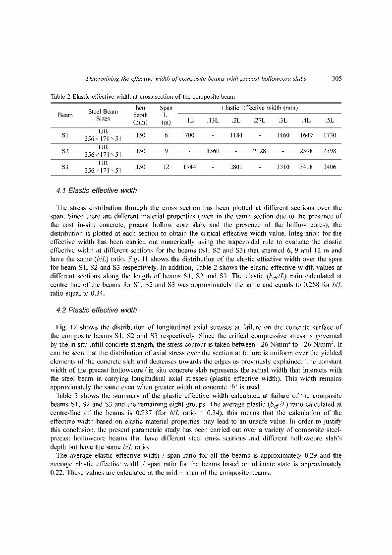
Fig. 11 Distribution of the elastic effective breadth


4.1 Elastic effective width

The stress distribution through the cross section has been plotted at different sections over the

span. Since there are different material properties (even in the same section due to the presence of

the cast in-situ concrete, precast hollow core slab, and the presence of the hollow cores), the

distribution is plotted at each section to obtain the critical effective width value. Integration for the

effective width has been carried out numerically using the trapezoidal rule to evaluate the elastic

effective width at different sections for the beams (S1, S2 and S3) that spanned 6, 9 and 12 m and

have the same (b/L) ratio. Fig. 11 shows the distribution of the elastic effective width over the span

for beam S1, S2 and S3 respectively. In addition, Table 2 shows the elastic effective width values at

different sections along the length of beams S1, S2 and S3. The elastic (beff /L) ratio calculated at

centre line of the beams for S1, S2 and S3 was approximately the same and equals to 0.288 for b/L

ratio equal to 0.34.

4.2 Plastic effective width

Fig. 12 shows the distribution of longitudinal axial stresses at failure on the concrete surface of

the composite beams S1, S2 and S3 respectively. Since the critical compressive stress is governed

by the in-situ infill concrete strength, the stress contour is taken between −26 N/mm2 to +26 N/mm2. It

can be seen that the distribution of axial stress over the section at failure is uniform over the yielded

elements of the concrete slab and decreases towards the edges as previously explained. The constant

width of the precast hollowcore / in situ concrete slab represents the actual width that interacts with

the steel beam in carrying longitudinal axial stresses (plastic effective width). This width remains

approximately the same even when greater width of concrete ‘b’ is used.

Table 3 shows the summary of the plastic effective width calculated at failure of the composite

beams S1, S2 and S3 and the remaining eight groups. The average plastic (beff /L) ratio calculated at

centre-line of the beams is 0.237 (for b/L ratio = 0.34), this means that the calculation of the

effective width based on elastic material properties may lead to an unsafe value. In order to justify

this conclusion, the present parametric study has been carried out over a variety of composite steel-

precast hollowcore beams that have different steel cross sections and different hollowcore slab’s

depth but have the same b/L ratio.

The average elastic effective width / span ratio for all the beams is approximately 0.29 and the

average plastic effective width / span ratio for the beams based on ultimate state is approximately

0.22. These values are calculated at the mid – span of the composite beams.

Table 2 Elastic effective width at cross section of the composite beam

BeamSteel Beam

Sizes

hcu depth(mm)

Span L

(m)

Elastic Effective width (mm)

.1L .13L .2L .27L .3L .4L .5L

S1UB

356 × 171 × 51150 6 700 - 1184 - 1460 1649 1730

S2UB

356 × 171 × 51150 9 - 1560 - 2228 - 2598 2598

S3UB

356 × 171 × 51150 12 1944 - 2801 - 3310 3418 3406


Fig. 12 Stress contour for Group 1 (356 × 171 × 51 UB, 150 mm deep slabs)

Table 3 Summary of the plastic effective width / span ratio

Group BeamBeam span, L

(mm)beff

(mm)beff /L(mm)

G1

S1 6000 1692 0.282

S2 9000 2008 0.223

S3 12000 2465 0.205

G2

S4 6000 1591 0.265

S5 9000 2065 0.229

S6 12000 2465 0.205

G3

S7 6000 1557 0.259

S8 9000 2065 0.229

S9 12000 2465 0.205

G4

S10 6000 1557 0.259

S11 9000 1800 0.200

S12 12000 2258 0.188

G5

S13 6000 1502 0.25

S14 9000 2065 0.229

S15 12000 2465 0.205


4.3 Effect of ‘b/L’ ratio on the calculation of effective width

The parametric study on a variety of composite beams with hollowcore slabs has shown that, for

a ‘b/L’ ratio equals to 0.34, the effective width calculated based on elastic material properties is

greater than that one calculated based on elastic-plastic material properties. To investigate the

effect of ‘b/L’ ratio on the effective width, parametric study has been extended to calculate the

elastic and plastic effective widths at different b/L ratios. The 9 m span beam ‘S2’ is analysed

using the same procedures used but with different b/L ratios. Fig. 13 shows the relationship

between ‘beff /L’ and ‘b/L’ ratios. It can be seen that both the elastic effective width and the plastic

Fig. 13 Effective width of composite steel-precast HC slab girders

Table 3 Continued

Group BeamBeam span, L

(mm)beff

(mm)beff /L(mm)

G6

S16 6000 1620 0.27

S17 9000 1964 0.218

S18 12000 2465 0.205

G7

S19 6000 1490 0.248

S20 9000 1792 0.199

S21 12000 1516 0.126

G8

S22 6000 1475 0.246

S23 9000 2028 0.225

S24 12000 2098 0.175

G9

S25 6000 1452 0.242

S26 9000 1950 0.217

S27 12000 2064 0.172


effective width are increased with the increase of the slab width until the plastic effective width

reaches a constant value. The average value of the effective width is equal to 0.22L for all of the

beams that has b ≥ 0.26L. This value is calculated at the mid – span and decreases towards the

support as shown in Fig. 11.

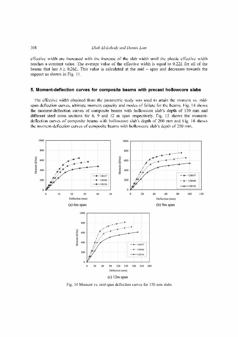
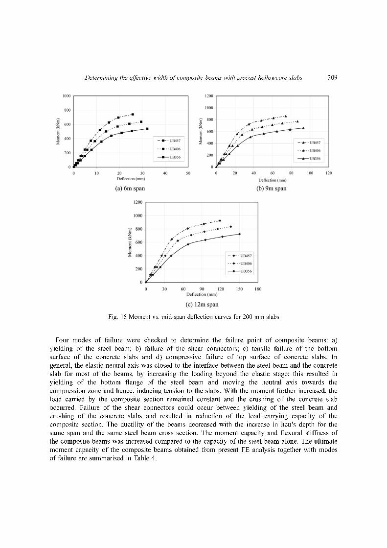
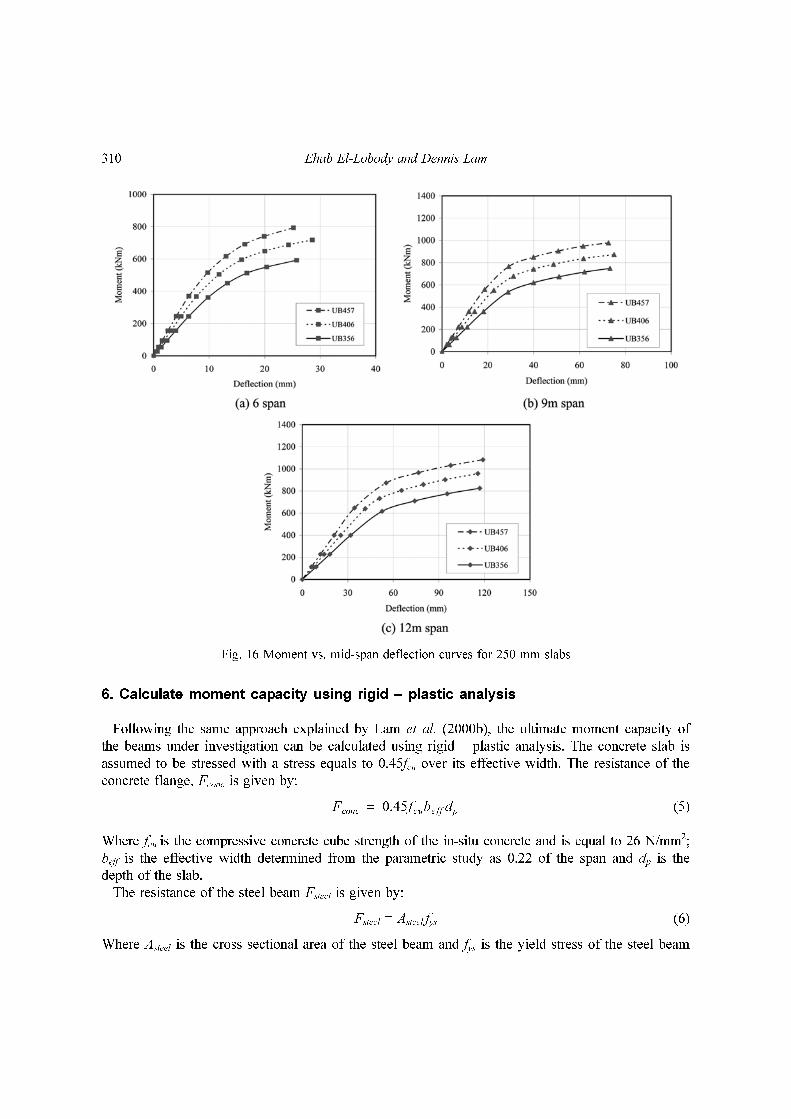
5. Moment-deflection curves for composite beams with precast hollowcore slabs

The effective width obtained from the parametric study was used to attain the moment vs. mid-

span deflection curves, ultimate moment capacity and modes of failure for the beams. Fig. 14 shows

the moment-deflection curves of composite beams with hollowcore slab’s depth of 150 mm and

different steel cross sections for 6, 9 and 12 m span respectively. Fig. 15 shows the moment-

deflection curves of composite beams with hollowcore slab’s depth of 200 mm and Fig. 16 shows

the moment-deflection curves of composite beams with hollowcore slab’s depth of 250 mm.

Fig. 14 Moment vs. mid-span deflection curves for 150 mm slabs


Four modes of failure were checked to determine the failure point of composite beams: a)

yielding of the steel beam; b) failure of the shear connectors; c) tensile failure of the bottom

surface of the concrete slabs and d) compressive failure of top surface of concrete slabs. In

general, the elastic neutral axis was closed to the interface between the steel beam and the concrete

slab for most of the beams, by increasing the loading beyond the elastic stage; this resulted in

yielding of the bottom flange of the steel beam and moving the neutral axis towards the

compression zone and hence, inducing tension to the slabs. With the moment further increased, the

load carried by the composite section remained constant and the crushing of the concrete slab

occurred. Failure of the shear connectors could occur between yielding of the steel beam and

crushing of the concrete slabs and resulted in reduction of the load carrying capacity of the

composite section. The ductility of the beams decreased with the increase in hcu’s depth for the

same span and the same steel beam cross section. The moment capacity and flexural stiffness of

the composite beams was increased compared to the capacity of the steel beam alone. The ultimate

moment capacity of the composite beams obtained from present FE analysis together with modes

of failure are summarised in Table 4.



6. Calculate moment capacity using rigid – plastic analysis

Following the same approach explained by Lam et al. (2000b), the ultimate moment capacity of

the beams under investigation can be calculated using rigid – plastic analysis. The concrete slab is

assumed to be stressed with a stress equals to 0.45fcu over its effective width. The resistance of the

concrete flange, Fconc is given by:

(5)

Where fcu is the compressive concrete cube strength of the in-situ concrete and is equal to 26 N/mm2;

beff is the effective width determined from the parametric study as 0.22 of the span and dp is the

depth of the slab.

The resistance of the steel beam Fsteel is given by:

Fsteel = Asteel fys (6)

Where Asteel is the cross sectional area of the steel beam and fys is the yield stress of the steel beam

Fconc 0.45fcubeff dp=


Determining the effective width of composite beams with precast hollowcore slabs

3

11

Table 4 Summary of the ultimate moment capacity

Group Beam UBbeff dp As D Tflange Bflange Zpl Ms Fflange Fconc Fsteel Fcon Failure

Mode

Mcomp cal. Mcomp FE Mcomp cal.

(mm) (mm) (cm2) (mm) (mm) (mm) (cm3) (kN.mm) (kN) (kN) (kN) (kN) (kN.m) (kN.m) Mcomp FE

S1 356×171×51 1320 150 64.9 355 11.5 171.5 896 246400 542.4 2316.6 1784.75 1470 Concrete 396 478 0.83

G1 S2 356×171×51 1980 150 64.9 355 11.5 171.5 896 246400 542.4 3474.9 1784.75 2170 Concrete 516 546 0.95

S3 356×171×51 2640 150 64.9 355 11.5 171.5 896 246400 542.4 4633.2 1784.75 2870 Concrete 533 612 0.87

S4 406×178×60 1320 150 76.5 406.4 12.8 177.9 1199 329725 626.2 2316.6 2103.75 1470 Steel beam 478 570 0.84

G2 S5 406×178×60 1980 150 76.5 406.4 12.8 177.9 1199 329725 626.2 3474.9 2103.75 2170 Steel beam 648 660 0.98

S6 406×178×60 2640 150 76.5 406.4 12.8 177.9 1199 329725 626.2 4633.2 2103.75 2870 Steel beam 671 720 0.93

S7 457×191×67 1320 150 85.5 453.4 12.7 189.9 1471 404525 663.2 2316.6 2351.25 1470 Steel beam 551 644 0.86

G3 S8 457×191×67 1980 150 85.5 453.4 12.7 189.9 1471 404525 663.2 3474.9 2351.25 2170 Steel beam 628 763 0.82

S9 457×191×67 2640 150 85.5 453.4 12.7 189.9 1471 404525 663.2 4633.2 2351.25 2870 Steel beam 796 814 0.98

S10 356×171×51 1320 200 64.9 355 11.5 171.5 896 246400 542.4 3088.8 1784.75 1470 Concrete 469 538 0.87

G4 S11 356×171×51 1980 200 64.9 355 11.5 171.5 896 246400 542.4 4633.2 1784.75 2170 Concrete 605 658 0.92

S12 356×171×51 2640 200 64.9 355 11.5 171.5 896 246400 542.4 6177.6 1784.75 2870 Concrete 622 724 0.86

S13 406×178×60 1320 200 76.5 406.4 12.8 177.9 1199 329725 626.2 3088.8 2103.75 1470 Steel beam 552 636 0.87

G5 S14 406×178×60 1980 200 76.5 406.4 12.8 177.9 1199 329725 626.2 4633.2 2103.75 2170 Steel beam 753 770 0.98

S15 406×178×60 2640 200 76.5 406.4 12.8 177.9 1199 329725 626.2 6177.6 2103.75 2870 Steel beam 777 835 0.93

S16 457×191×67 1320 200 85.5 453.4 12.7 189.9 1471 404525 663.2 3088.8 2351.25 1470 Stud 625 740 0.84

G6 S17 457×191×67 1980 200 85.5 453.4 12.7 189.9 1471 404525 663.2 4633.2 2351.25 2170 Stud 737 859 0.86

S18 457×191×67 2640 200 85.5 453.4 12.7 189.9 1471 404525 663.2 6177.6 2351.25 2870 Stud 914 925 0.99

S19 356×171×51 1320 250 64.9 355 11.5 171.5 896 246400 542.4 3861 1784.75 1470 Concrete 543 592 0.92

G7 S20 356×171×51 1980 250 64.9 355 11.5 171.5 896 246400 542.4 5791.5 1784.75 2170 Concrete 694 748 0.93

S21 356×171×51 2640 250 64.9 355 11.5 171.5 896 246400 542.4 7722 1784.75 2870 Concrete 711 825 0.86

S22 406×178×60 1320 250 76.5 406.4 12.8 177.9 1199 329725 626.2 3861 2103.75 1470 Steel beam 625 718 0.87

G8 S23 406×178×60 1980 250 76.5 406.4 12.8 177.9 1199 329725 626.2 5791.5 2103.75 2170 Steel beam 858 872 0.98

S24 406×178×60 2640 250 76.5 406.4 12.8 177.9 1199 329725 626.2 7722 2103.75 2870 Steel beam 882 958 0.92

S25 457×191×67 1320 250 85.5 453.4 12.7 189.9 1471 404525 663.2 3861 2351.25 1470 Stud 698 793 0.88

G9 S26 457×191×67 1980 250 85.5 453.4 12.7 189.9 1471 404525 663.2 5791.5 2351.25 2170 Stud 845 978 0.86

S27 457×191×67 2640 250 85.5 453.4 12.7 189.9 1471 404525 663.2 7722 2351.25 2870 Stud 1031 1083 0.95


and is equal to 275 N/mm2 for structural steel grade S275.

For composite beam with full shear interaction (i.e., sufficient number of shear connectors is used

to transfer the longitudinal shear forces at the steel-concrete interface), Fcon (the resistance force of

the shear connectors) is greater than the smaller of Fconc or Fsteel. Fcon is given by:

Fcon = nPR (7)

Where n is the number of shear connectors spaced at S in a half span L/2 (n = L/2S + 1) and PR is

the resistance of the shear connector obtained from previous FE analysis by El-Lobody and Lam

(2002) and equals to 70 kN for the 19 mm diameter × 100 mm height headed stud in push-off test

with hollowcore slab with in-situ concrete strength of 26 N/mm2 and transverse reinforcing bars of

10 mm in diameter.

For a plastic neutral axis in the concrete flange (Fconc > Fsteel), the calculated ultimate moment

capacity of the composite beam is given by:

(8)

For a plastic neutral axis in the steel section (Fsteel > Fconc), the calculated ultimate moment

capacity of the composite beam is given by:

(9)

For composite beam with partial shear interaction, Fcon is less than the smaller of Fconc or Fsteel.

The calculated ultimate moment capacity of the composite beam is given by:

(10)

Table 4 shows the ultimate moment capacity obtained from rigid - plastic analyse and compared

with the results obtained from the present FE solution. Results showed good agreement between the

FE solution and the rigid – plastic analysis using the effective width obtained from the FE models.

7. Conclusions

This paper presents a numerical study to determine the effective width of composite beams with

precast hollowcore slabs. The model takes into account the non-linear load-slip characteristics of

headed stud shear connector and all the other materials non-linearity.

From the parametric study carried out on the effective width of composite beams with hollowcore

slabs, it is found that:

1. The effective width is equal to 0.22 L for slab width/span ratio greater or equal to 0.26.

2. For b/L less than 0.26, the effective width can be obtained from Fig. 13.

Moment vs. mid-span deflection curves were plotted using the predicted effective width and the

ultimate moment capacity; the modes of failure were also evaluated. Predictions of the ultimate

moment capacity obtained from present FE analysis were compared with that of the rigid - plastic

analysis. The comparison shows good agreement between both FE solution and the theoretical

calculations.

Mcomp FsteelD

2---- dp

Fsteel

Fconc

-----------dp

2-----–+⎝ ⎠

⎛ ⎞=

Mcomp FsteelD

2---- Fconc

dp

2-----

Fsteel Fconc–( )2

Fflange

-----------------------------------T

4---–+=

Mcomp Ms Fconx+ dp

Fcon

Fconc

-----------dp

2-----–⎝ ⎠

⎛ ⎞×Fsteel Fcon–( )2

Fflange

---------------------------------T

4---–=


Acknowledgements

The authors would like to acknowledge the support provided by the Egyptian Government, Bison

Concrete Products Ltd., Severfield-Reeve Plc. and the skilled assistance provided by the technical

staff in the School of Civil Engineering at the University of Leeds.

References

ABAQUS (1998), User’s Manual, Ver. 5.8, Hibbitt, Karlson and Sorensen, Inc.Amadio, C. and Fragiacomo, M. (2002), “Effective width evaluation for steel-concrete composite beams”, J.

Constructional Steel Research, 58, 373-388.Ansourian, P. (1975), “An application of the method of finite elements to the analysis of composite floor

systems”, Proc. Insn. Civ. Engrs., Part 2, Issue 59, 699-726.BS 8110 (1997): Parts 1,2, Structural Use of Concrete, “Code of Practice for Design and Construction”, British

Standards Institution, London.EC4 (1994), DD ENV 1994-1-1, “Design of Composite Steel and Concrete Structures. Part 1.1, General Rules

and Rules for Buildings (with U.K National Application Document)”, British Standards Institution, London.El-Lobody, E. and Lam, D. (2002), “Modelling of headed stud in steel - precast composite beams”, Steel and

Composite Structures, 2(5), 355-378.El-Lobody, E. and Lam, D. (2003), “Finite element analysis of steel-concrete composite girders”, Advances in

Struct. Eng. – An Int. J., 6(4), 267-281.Heins, C.P. and Fan, H.M. (1976), “Effective composite beam width at ultimate load”, J. Struct. Div., ASCE,102(ST11), 12538-2179.

Lam, D., Elliott, K.S. and Nethercot, D.A. (2000a), “Experiments on composite steel beams with precastconcrete hollow core floor slabs”, Proc. of the Institution of Civil Engineers, Structures and Buildings, 140,127-138.

Lam, D., Elliott, K.S. and Nethercot, D.A. (2000b), “Designing composite steel beams with precast concrete-hollow core slabs”, Proc. of the Institution of Civil Engineers, Structures and Buildings, 140, 139-149.

Determining the effective width of composite beams with ...

Documents

Transcript of Determining the effective width of composite beams with ...