Music Performers Classification by Using Multifractal Features

$: Music Performers Classification by Using Multifractal Features$
ARCHIVES OF ACOUSTICS

Vol. 42, No. 2, pp. 223–233 (2017)

Copyright c© 2017 by PAN – IPPT

DOI: 10.1515/aoa-2017-0025

Music Performers Classification by Using Multifractal Features:A Case Study

Natasa RELJIN(1), David POKRAJAC(2)

(1)University of Connecticut260 Glenbrook Road, Unit 3247, Storrs, CT 06269, USA; e-mail: [email protected]

(2)Delaware State University1200 North DuPont Hwy, Dover, DE 19901, USA

(received September 27, 2015; accepted February 28, 2017)

In this paper, we investigated the possibility to classify different performers playing the same melodiesat the same manner being subjectively quite similar and very difficult to distinguish even for musicallyskilled persons. For resolving this problem we propose the use of multifractal (MF) analysis, which isproven as an efficient method for describing and quantifying complex natural structures, phenomena orsignals. We found experimentally that parameters associated to some characteristic points within the MFspectrum can be used as music descriptors, thus permitting accurate discrimination of music performers.Our approach is tested on the dataset containing the same songs performed by music group ABBA and byactors in the movieMamma Mia. As a classifier we used the support vector machines and the classificationperformance was evaluated by using the four-fold cross-validation. The results of proposed method werecompared with those obtained using mel-frequency cepstral coefficients (MFCCs) as descriptors. For theconsidered two-class problem, the overall accuracy and F-measure higher than 98% are obtained withthe MF descriptors, which was considerably better than by using the MFCC descriptors when the bestresults were less than 77%.

Keywords: music classification; multifractal analysis; support vector machines; cross-validation; mel-frequency cepstral coefficients.

Notations

F – first point in multifractal spectrum,FM – first point and point of maximum in multifractal

spectrum,FML – first point, point of maximum and last point in multi-

fractal spectrum,FN – false negative,FP – false positive,FV – feature vector,L – last point in multifractal spectrum,M – point of maximum in multifractal spectrum,ML – point of maximum and last point in multifractal

spectrum,MF – multifractal,

MFCC – mel-frequency cepstral coefficients,OA – overall accuracy,RBF – radial basis function,SVM – support vector machines,TN – true negative,TP – true positive.

1. Introduction

Explosive growth of inexpensive but highly power-ful multimedia devices enables the production of ex-

tremely huge collection of various audio-visual data.Indexing and browsing such data, searching for desiredfiles, and classifying existing material, have becomevery difficult tasks. Many efforts have been made to re-solve these problems. Except for images and video, sig-nificant attention was devoted to the automatic analy-sis and classification of music content and audio infor-mation, having numerous potential applications, suchas genre classification, musical instrument classifica-tion, indexing of audio databases, etc., which are usu-ally referred as music information retrieval (MIR), asreported in (Wold et al., 1996; Li et al., 2001;Tzane-takis, Cook, 2002; Guo, Li, 2003; Kostek, 2004;Barbedo, Lopes, 2007; Feng et al., 2008; Lee et al.,2009; Jensen et al., 2009).Humans, especially those who are musically edu-

cated and/or gifted, are capable of making accuratedistinctions between different music pieces and sepa-rating sounds originated from different sources. Recog-nition and classification of sounds is performed spon-taneously by means of subjective auditory sensationgenerated in human brain. Regarding machine process-

224 Archives of Acoustics – Volume 42, Number 2, 2017

ing, description and classification of sounds are veryhard and challenging tasks, because a device (or analgorithm) needs appropriate descriptions of percep-tual features. The main problem in automatic clas-sification of sounds is to find suitable objective de-scriptors in good correspondence to subjective sensa-tion of sounds. Usually, descriptors are expressed asnumerals and are arranged in the form of an appro-priate feature vector (FV). By comparing FVs of dif-ferent sounds their similarity/dissimilarity can be eva-luated.Standard approach for describing audio content

uses temporal and/or spectral features (Tzanetakis,Cook, 2002; Guo, Li, 2003; McKinney, Bree-baart, 2003; Rein, Reisslein, 2006; Chudy, 2008).Among various spectral features, the most frequentlyused are mel-frequency cepstral coefficients (MFCCs),which are perceptually motivated and well suited tothe human auditory system. The Mel scale1 was intro-duced by (Stevens et al., 1937) as a scale of pitcheswhich are subjectively equal in distance from one an-other. The MFCCs were proven as an efficient tool forspeaker identification (Davis, Mermelstein, 1980)and have widely been used in different systems for au-tomatic speech recognition and speaker classification,for instance (Huang et al., 2001; Muda et al., 2010).Later, the use of MFCC was extended to music analysisand classification (Logan, 2000; Berenzweig et al.,2002; Tsai, Wang, 2006; Feng et al., 2008). Basicaudio descriptors are even standardized and embeddedinto the MPEG-7 standard (Kostek, 2004; Lyndsay,2011; Gomez, 2013;). Note that for the two challeng-ing problems in MIR: recognition of music genres andrecognition of instruments playing together in a givenmusic sample, the data mining contest was organizedin 2011, in conjunction with the 19th Int. Symposiumon Methodologies for Intelligent Systems, ISMIS 2011(Kryszkiewicz et al., 2011). In this contest, competi-tors were requested to use feature vectors with a de-fined number of 171 descriptors from which the first147 were ‘standard’ descriptors: MPEG-7 (127 descrip-tors), and MFCC (20), while additional 24 were relatedto time domain and have been a free choice of competi-tors being their original contribution (Kostek, 2011).In the paper by (Schedl et al., 2013) very interestingstudy regarding system-based and user-centric MIRwas derived. The authors pointed out the problemswith subjective judgment of similarity of songs/musicand hence difficulties at user-centric evaluation in fieldsrelated to MIR.In (Mandelbrot, 1967) Mandelbrot introduced

a new kind of geometry, called the fractal geometry,which has been proven as an efficient way for describ-ing the complexity of structures, objects, systems, or

1The word mel comes from the word melody, indicating tothe pitch comparison.

phenomena. The fractal concept is one of the most im-portant developments in mathematics in the secondhalf of the 20th century. Fractals are central to un-derstanding and quantitatively evaluating a wide va-riety of complex structures (for instance, the shapeof clouds, structure of a tree or a snowflake, etc.)as well as chaotic, non-stationary and nonlinear sys-tems, in cases when Euclidean geometry falls down.Such structures and systems can be described quan-titatively by a fractal dimension (FD) which is usu-ally a non-integer number (thus Mandelbrot coinedthe term fractal, meaning fractional or broken). Byusing the FD, objective description, characterization,comparison and classification of complex and irregularstructures is enabled. This concept was very successfulin describing events, signals, structures or phenomena,characterized by a fundamental feature known and re-ferred to as self-similarity. This property means thatby observing the structure of the object in differentscales, for instance by zooming part of the structure,(almost) the same shape arises, i.e., it seems that thestructure is composed of smaller versions of itself. Arti-ficially generated self-similar objects by applying somepredefined rules, for instance, the Cantor set, the vonKoch’s curve and snowflake, the Sierpinski carpet, etc.(Peitgen et al., 2004), have exactly the same FD inall scales. Such objects are characterized by an uniqueFD and are known as monofractals. Conversely, a largescale of (mainly natural) objects, for instance, a coast-line, structure of a tree, venous, arterial or nervoussystem, some vegetables (cauliflower, broccoli), eventrends in economy, structure of vocal sounds, music,etc., exhibit some kind of self-similarity, but not instrict sense, meaning these objects have different FDat different scales. Such objects cannot be describedby an unique FD. Instead, the distribution of FDs overdifferent scales is used to provide even deeper insightinto the structure. This is a simple explanation of mul-tifractal concept, as an extension of fractal geometry(Mandelbrot, 1982). Since FDs of such objects dif-fer at various scales, these objects are known as mul-tifractals. The distribution of FDs can be expressed inthe form of so-called multifractal spectrum, which willbe described in Sec. 2.The interdisciplinary nature of fractal geometry

and multifractals has found a broad spectrum of ap-plications, for instance, in the classification of natu-ral objects (Mandelbrot, 1982; Stanley, Meakin,1988), in the analysis of nonlinear and chaotic physicalphenomena (Grassberger, 1983; Hentschel, Pro-caccia, 1983), in the description of biology structures(Buldyrey et al., 1994; Iannaccone, Khokha,1996), in medicine (Sedivy, Mader, 1997; Vasilje-vic et al., 2012; Reljin et al., 2015), in economics(Falconer, 2003), even in arts (Bovill, 1996; Peit-gen et al., 2004). Moreover, these techniques foundsignificant applications in signal and image analyses

N. Reljin, D. Pokrajac – Music Performers Classification by Using Multifractal Features: A Case Study 225

and processing: the reader can find many examples,for instance, in (Vehel, Mignot, 1994; Vehel, 1996;1998; Reljin et al., 2000).Regarding the audio, fractal and multifractal anal-

yses were also used, mainly for speech analysis andrecognition, but also for music analysis and classifica-tion. For instance, the paper (Sabanal, Nakagawa,1996) considered fractal properties of vocal soundsand results were applied to the speech recognitionmodel. Further, the authors of (Maragos, Potami-anos, 1999; Pitsikalis, Maragos, 2009) applied thefractal dimension of speech signals to their automaticrecognition and classification. The Higuchi fractal di-mension (Higuchi, 1988), in combination with MFCC,was used in (Ezeiza et al., 2011) in order to improvethe correct word rate for automatic speech recogni-tion. The authors of (Krajewski et al., 2012) evalu-ated fractal features, among other nonlinear dynamicsfeatures, for speech based sleepiness detection, whilethe authors of (Gonzales et al., 2012) explored thefractal and multrifractal nature of speech signals fromtwo different Portuguese speech databases and foundthat, in general, all analyzed signals revealed multi-fractal behavior under a time frame analysis rangingfrom 50 ms to 100 ms.In (Hsu, Hsu, 1990), the authors suggested the

methodology for describing and characterizing mu-sic pieces using fractal dimension. Their initial re-sults were derived from some Bach’s and Mozart’smusic pieces and Swiss children’s songs. In the study(Bigerelle, Iost, 2000) was shown that fractal di-mension can be used to discriminate different mu-sic genres. In the papers (Su, Wu, 2006; 2007) au-thors found that sequences of musical notes exhibitfractal nature, and demonstrated the applicability ofMF analysis to distinguish between different stylesof music. Music search and playlist generation basedon fractal dimensions of music were presented in thepaper (Hughes, Manaris, 2012). Also, the authors of(Zlatintsi, Maragos 2013) proposed the use of mul-tiscale fractal dimension for recognizing musical instru-ments.The main benefit of using MF in signal processing

is that this concept enables both local and global anal-yses of an observed signal. Hence, using MF analysisit is possible to find and extract details from the sig-nal under consideration, which carries some hidden andsubtle information thus enabling the recognition, selec-tion and classification of complex signals. For instance,MF was applied to find clicks in heart sounds char-acterizing pathological syndrome so-called the MVP(mitral valve prolapse, or click-murmure syndrome),as reported in (Gavrovska et al., 2013). Moreover,it was shown that some MF parameters can be usedas characteristic features for discriminating malignantfrom benign cases from appropriate medical signals, asshown in (Reljin et al., 2008), or for identifying the

primary cancer from biopsy images of bone metastases(Vasiljevic et al., 2012).In music/sound analysis and classification partic-

ular attention should be addressed to the problemof distinguishing and classifying performers (or musicgroups) playing the same music piece(s) in the samemanner, using the same types of instruments, similarvocals, and under the same arrangements. In this case,performed music pieces are subjectively similar thusmaking their recognition and classification very diffi-cult even for musically skilled persons. This problem,which may be of interest in forensic and/or copyrightissues, is the goal of our research. Since the MF anal-ysis has been proven as an efficient tool for describingsignals and finding fine details and characteristic partswithin signals, we investigated the use of MF for re-solving this problem. Although the MF analysis wasapplied to some of audio related problems, to the bestof our knowledge this approach was not used for giventask of music performers classification. We found thatonly a few MF parameters, which correspond to thecharacteristic points within the MF spectrum, couldbe used as features, thus enabling successful classifi-cation of music performers. As a classification tool weused support vector machines (SVM), while four-foldcross-validation was used to determine optimal valuesof the SVM hyperparameters and to evaluate the ac-curacy of the proposed classifier.The paper is organized as follows. Section 2 consid-

ers the basics of multifractal analysis. In Sec. 3 a con-cept of proposed classifier based on MF parametersas relevant features is presented. Section 4 describesexperimental setup for music performer classificationbased on MF features and presents classification re-sults derived on the dataset containing the same songsperformed by music group ABBA and by actors in themovie Mamma Mia. Results are compared with thosederived on the same dataset by applying MFCC ascharacteristic features and using the same SVM classi-fiers with linear, polynomial and RBF kernel functions.Concluding remarks are given in Sec. 5.

2. Basics of the multifractal analysis

Multifractal spectrum can be derived in severalways, as reported in literature (Harte, 2001; Peit-gen et al., 2004). The histogram method is very pop-ular due to its simplicity and possibility to determineMF spectrum directly from measured data (Chhabra,Jensen, 1989; Vehel, 1998). Main steps for derivingthe MF spectrum using this method will be briefly ex-plained as follows.Signal is covered by non-overlapping boxes Bi of

side width ε. Within the box, a signal is characterizedby some attribute, called a measure, µ(Bi) (Vehel,Mignot, 1994). Different measures may be used, forinstance, the maximum of the signal’s intensity, the


minimum value, the sum of intensities, etc. (Vehel,1998). It is common to assume normalized space, i.e.,ε, µ ∈ [0, 1].For audio signals, which are considered in this pa-

per, signal is time-dependent and boxes are representedby time intervals (windows) of width ε. Among differ-ent measures that can be used, we found that measuremaximum provided the best results for considered clas-sification problem. For a particular time interval Bi

the coarse Holder exponent αi is calculated as (Vehel,Mignot, 1994):

αi =log (µ(Bi))

log ε. (1)

By using a sequence of time intervals B(k)i , with de-

scending widths ε(k), k = 1, 2, . . ., i.e., ε(k) > ε(k+1),andB(k)

i ⊃ B(k+1)i , the corresponding values of param-

eter αi will differ, but will approach to limit value α,known as the Holder exponent (Vehel, 1998). Due topractical reasons, the value of α is usually estimated asa slope of linear regression line in the log-log diagram:log(µ(Bi)) vs. log(ε), for several values of ε (Su, Wu,2006).After estimating Holder exponents for all signal

samples the α-representation of the signal is obtained– each signal sample is characterized by its α value.Since α is calculated from the measure µ around a par-ticular sample of the signal, this parameter describeslocal singularity (regularity) of the signal. For sampleswhere the signal is smooth (slow varying with respectto neighbor samples) the value of α is small, while sam-ples within regions with sudden changes are character-ized by high values of α (Vehel, 1998). The Holderexponent has finite limits αmin and αmax. In the wholesignal, many samples can have the same value of α,i.e., they can have the same local regularity. After es-timating the Holder exponents of all samples withinthe observed signal, we find their distribution. All ob-tained values of Holder exponents can be consideredas the α-space. The continuous α-space is divided intoR values as follows:

αr = αmin + (r − 1)∆α, r = 1, 2, . . . , R, (2)

∆α = (αmax − αmin)/R, (3)

and the histogram of αr values is calculated: if the ac-tual value of α falls within the subrange [αr, αr+1),this value is replaced by αr. The number of subrangesR has to be determined empirically. Small value of Rbehaves as low-frequency filtering: MF spectrum willbe smooth but with small resolution, which reducesdiscriminative capabilities. As opposed to when usinghigh R value, more details can be extracted but spec-trum becomes irregular (saw-toothed). A compromisesolution could be to choose R between 50 and 100.In the next step, the α-space is covered by boxes

of width δ (δ < 1) and the number of boxes, Nδ(α),

containing given value of Holder exponent, α = αr,is counted. Furthermore, the Hausdorff dimension ofthe distribution of α, also known as the multifractalsingularity spectrum (or simply, the MF spectrum), isdetermined as (Vehel, 1998):

f(α) = − limδ→0

log(Nδ(α))

log δ. (4)

In practice, similar to determining Holder exponents,the values of f(α) are estimated by a linear regressionin (log(δ), log(Nδ)) for several box sizes δ. The plot ofMF spectrum is usually parabola shaped, as shown inFig. 1, with finite values, αmin; αmax; fmin(α); fmax(α).

Fig. 1. Typical shape of MF spectrum.

Values of f(α) describe global regularity of the sig-nal. Small values of f(α) correspond to rare events,meaning that a small number of points in the origi-nal space (amplitude-time space) is characterized bythis particular value of α. The opposite is true for highvalues of f(α). By combining the pair (α, f(α)), bothlocal regularity (via α) and global behavior (via f(α))can be described, thus permitting fine analysis andclassification of signals, both images (Vehel, 1998;Reljin et al., 2000) and music (Su, Wu, 2006; 2007).

3. Music performer classifier based

on MF features

3.1. Creation of audio database

For given problem, distinguishing and classifyingmusic performers playing the same melodies in quitesimilar manner, our initial assumption was that ir-respective of subjective similarity, each performer ormusic group has some characteristic (individual) fea-tures. Since the MF analysis has been proven as a pow-erful method for finding subtle details within signals(Gavrovska et al., 2013) and for characterizing anddistinguishing different signals (Reljin et al., 2008;Vasiljevic et al., 2012) we investigated the MF ap-proach for resolving given problem. As examples we


will observe the same 14 songs, listed in Table 1, per-formed by famous Swedish group ABBA, producingmega hits from 1974 to 1982 (Sheridan, 2012), andby actors in the movieMamma Mia (released in 2008).These songs are denoted here as ABBA and MOVIE.These melodies were composed by the same composersand arrangers (Benny Anderson and Bjorn Ulvaeus)and were performed in a very similar way, being dif-ficult for distinguishing even for musically educatedpersons. We have created a database as follows.

Table 1. Songs considered for classification.

Pieces ABBA Title of the song Pieces MOVIE

1, 2 Dancing Queen 29, 30

3, 4 Does Your Mother Know 31, 32

5, 6 Gimme Gimme Gimme 33, 34

7, 8 I Have a Dream 35, 36

9, 10 Lay All Your Love on Me 37, 38

11, 12 Mamma Mia 39, 40

13, 14 Money Money Money 41, 42

15, 16 SOS 43, 44

17, 18 Super Trouper 45, 46

19, 20 Take a Chance on Me 47, 48

21, 22 Thank You for the Music 49, 50

23, 24 The Name of the Game 51, 52

25, 26 The Winner Takes It All 53, 54

27, 28 Voulez Vous 55, 56

Prior to further processing and classification, all thesongs are preprocessed. First, recordings are convertedfrom stereo to mono, and downsampled to 8 kHz, withthe Audacity software (Audacity, 2015). Although mu-sic is characterized by wide bandwidth, and nowadaysthe sampling frequency is usually 44.1 kHz, the reasonfor using 8 kHz is based on several facts. In the paper(Rein, Reisslein, 2006) was shown that sampling fre-quency of 8 kHz is sufficient to identify classical mu-sic compositions, although such music is characterizedby spectra rich in harmonics. Further, the authors of(Jensen et al., 2009) derived deep quantitative anal-ysis of a MFCC, as a common audio similarity mea-sure. The authors have shown that if all songs havethe same sampling frequency of 8 kHz, the classifica-tion accuracy decreased only by few percents comparedto when higher sampling frequency is used. Certainly,extracting MFCCs from downsampled songs is compu-tationally easier and cheaper, and since classificationaccuracy is not noticeably degraded, authors suggestedthe use of homogeneous music collection downsampledto 8 kHz. This is of particular interest in cases whensongs in actual database do not have the same sam-pling rate.After downsampling, songs were normalized with

respect to their amplitudes. Each song from the con-

sidered audio collection has parts that repeat; partswith the same melody but different lyrics – verses, andparts with the same melody and the same lyrics – cho-ruses. Hence, by selecting just these parts of the songs,we obtain parts that are subjectively similar and haveall the necessary information for representing the ba-sic music characteristics of the song (melodic line andharmony), as well as characteristics of performers. Byfollowing this assumption, we constructed two musicsequences per song (in the text we will call these se-quences pieces): the first verse and chorus (denoted byodd numbers 1–27 for ABBA and 29–55 for MOVIE),and the second verse and chorus (denoted by evennumbers 2–28 and 30–56 for ABBA and MOVIE, re-spectively). Each piece lasts about 40 seconds. Thisway we constructed the music dataset with 28 piecesper performer (music group ABBA and MOVIE), i.e.,56 pieces in the whole dataset, as indicated by ordinalnumbers 1 to 56 in Table 1.Next step in signal preprocessing is to divide each

music piece into short overlapping blocks called framesas is common in audio analysis (Logan, 2000; Beren-zweig et al., 2002;Barbedo, Lopez, 2007; Zlatinsi,Maragos, 2013). The reason for using short se-quences, of length 20–50 ms, is to assure the station-arity of the signal. Namely, as shown in (Rabiner,Juang, 1993, p. 17), speech signal is almost station-ary over a sufficiently short period of time (between 5and 100 ms), and similar conclusion is derived for mu-sic instruments (Zlatintsi, Maragos, 2013). In ourstudy, we used frames of 32 ms of length overlappedby 50%. In order to reduce the discontinuities at theedges of the frames, and thus to reduce the spectralleakage, the Hamming tapered window is applied.

3.2. MF feature extraction

For each particular frame within our dataset, we es-timated its MF spectrum using custom developed soft-ware based on histogram method (Reljin et al., 2000).Then we determined the MF spectra for every musicpiece (28 of ABBA and 28 of MOVIE) as a mean of MFspectra of their frames. The two illustrative examplesare depicted in Figs. 2–5. Figures 2 and 3 respectivelyrelate to first and second pieces of song Dancing Queen(pieces denoted by numerals 1 and 2 for ABBA, andby 29 and 30 for MOVIE, according to Table 1), whileFigs. 4 and 5 relate to song Does Your Mother Know(pieces 3 and 4 for ABBA, and 31 and 32 for MOVIE).Characteristic points within MF spectra plots: the firstpoint (F), the last point (L), and the point of maxi-mum (M), are denoted, and corresponding values ofα and f(α) are inserted into Figs. 2–5. Although MFspectra are visually similar, the three significant con-clusions may be derived:

1. For the same music group playing the same song,for instance Dancing Queen, Figs. 2 and 3, the first


Fig. 2. MF spectra of the first pieces of the song DancingQueen: 1 (ABBA) and 29 (MOVIE).

Fig. 3. MF spectra of the second pieces of the song DancingQueen: 2 (ABBA) and 30 (MOVIE).

Fig. 4. MF spectra of the first pieces of song Does YourMother Know: 3 (ABBA) and 31 (MOVIE).

Fig. 5. MF spectra of second pieces of song Does YourMother Know: 4 (ABBA) and 32 (MOVIE).

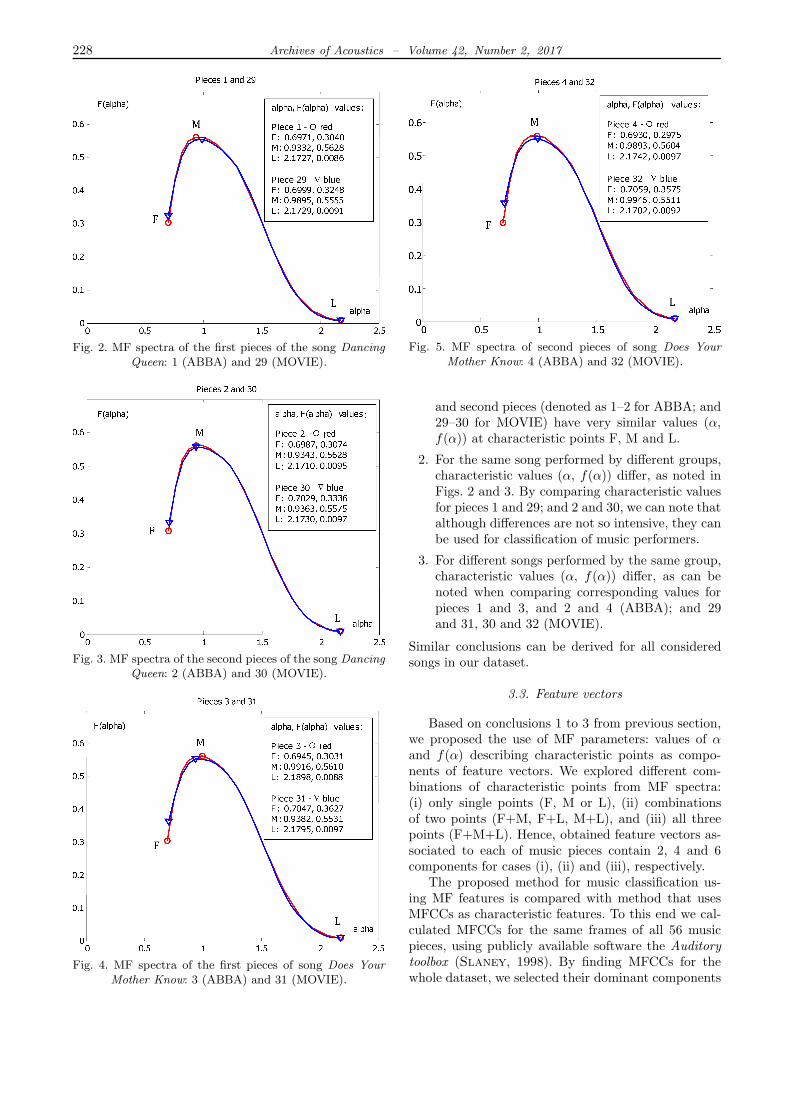
and second pieces (denoted as 1–2 for ABBA; and29–30 for MOVIE) have very similar values (α,f(α)) at characteristic points F, M and L.

2. For the same song performed by different groups,characteristic values (α, f(α)) differ, as noted inFigs. 2 and 3. By comparing characteristic valuesfor pieces 1 and 29; and 2 and 30, we can note thatalthough differences are not so intensive, they canbe used for classification of music performers.

3. For different songs performed by the same group,characteristic values (α, f(α)) differ, as can benoted when comparing corresponding values forpieces 1 and 3, and 2 and 4 (ABBA); and 29and 31, 30 and 32 (MOVIE).

Similar conclusions can be derived for all consideredsongs in our dataset.

3.3. Feature vectors

Based on conclusions 1 to 3 from previous section,we proposed the use of MF parameters: values of αand f(α) describing characteristic points as compo-nents of feature vectors. We explored different com-binations of characteristic points from MF spectra:(i) only single points (F, M or L), (ii) combinationsof two points (F+M, F+L, M+L), and (iii) all threepoints (F+M+L). Hence, obtained feature vectors as-sociated to each of music pieces contain 2, 4 and 6components for cases (i), (ii) and (iii), respectively.The proposed method for music classification us-

ing MF features is compared with method that usesMFCCs as characteristic features. To this end we cal-culated MFCCs for the same frames of all 56 musicpieces, using publicly available software the Auditorytoolbox (Slaney, 1998). By finding MFCCs for thewhole dataset, we selected their dominant components


supporting more than 98% of signal energy (in our casewe selected first 13 components).

3.4. Classification and performance evaluation

In this study we used support vector machines asa classifier. This method was originally developed forbinary (two-class) problem (Vapnik, 1998) and laterwas extended to multiclass problems as well (Hsu, Lin,2002). The SVMs are widely and successfully used inmany classification problems, including the music in-formation retrieval. Moreover, as noted in (Rosneret al., 2014), the SVM algorithm is even better choicefor music genre classification than, for instance, a verypopular k-nearest neighbor (k-NN) method. The goalof SVMs is to construct a hyperplane in the space oftransformed input vectors, which will separate observa-tions from different classes such that the minimal dis-tance between observations and the separation hyper-plane is maximized (Kecman, 2001; Bishop, 2006).We used SVMs with different kernels: linear, polyno-mial and radial basis function (RBF) (Kecman, 2001;Chang, Lin, 2011).The performance of the classification model can be

measured in several ways. The confusion matrix is fre-quently used, and for the two-class problem has theform as given in Table 2 (Tan et al., 2005). Classes aredenoted as +1 and −1: in our case classes correspondto music pieces ABBA and MOVIE. The entries of theconfusion matrix have the following meaning: the truepositive (TP) value denotes the number of music piecesbelonging to the class +1 which are correctly classifiedas+1, while false negative (FN) is the number of piecesfrom class +1 which are incorrectly predicted as class−1. Similarly, false positive (FP) represents the num-ber of pieces from the class −1 which are incorrectlyclassified, and true negative (TN) is the number of cor-rectly classified pieces from the class −1.

Table 2. Confusion matrix for our two-class problem.

Predictedclass +1

Predictedclass −1

True class +1

(ABBA)True Positive (TP) False Negative (FN)

True class −1

(MOVIE)False Positive (FP) True Negative (TN)

By combining entries from the confusion matrix,several performance measures can be derived (Tanet al., 2005). These measures are Overall Accuracy(OA) and F-measure (Tan et al., 2005), which are de-fined as:

OA =TP + TN

TP + TN + FP + FN, (5)

F -measure =2 · TP

2 · TP + FP + FN. (6)

These two measures are compact, describing classifier’sperformance with only one value, thus being of highpractical use.To determine the optimal values of the SVM hyper-

parameters as well as to evaluate the classifier’s perfor-mance, we utilized a four-fold cross validation method(Bishop, 2006), recommended for small data sets.

4. Experimental results and discussion

Based on previous considerations we developed ex-perimental setup for music performer classification, asdepicted in Fig. 6. For every music piece from ourdataset we created two groups of feature vectors: basedon MF parameters and on MFCC. Feature vectors aredetermined from MF spectra using custom developedsoftware based on histogram method (Reljin et al.,2000), while MFCCs are calculated following the pro-cedure in (Slaney, 1998).

Fig. 6. Block scheme of experimental setup used for musicperformer classification.

As already noted, feature vectors created from MFanalysis consist of pairs (α, f(α)) from characteristicpoints in MF spectra, F, M, L and their combinationswith two points (F+M, M+L, or F+L), and all threepoints (F+M+L). This way MF feature vectors arevery low-dimensional, containing n = 2, 4 and 6 com-ponents, for single points, combination of two points,and all three points, respectively. In Fig. 7, plots ofpairs (α, f(α)) associated to characteristic points: F,M and L of MF spectra, for the whole dataset of 56music pieces (28 ABBA and 28 MOVIE), are depicted.Points related to ABBA are presented by circles, whiletriangles are related to MOVIE pieces.Using feature vectors based on the described MF

and MFCC features, the classification of music groups


Fig. 7. Plots of characteristic points (α, f(α)) of MF spectrafor the music dataset with 56 pieces: 28 pieces denoted asABBA and 28 denoted as MOVIE in Table 1. Characteristicpoints: the first point (F), points of maxima (M), and thelast point (L), are depicted in upper, middle and lower

plots, respectively.

from our dataset was performed by applying the sup-port vector machines algorithms embedded in an in-tegrated software LIBSVM (Chang, Lin, 2011). Weused linear SVMs and SVMs with polynomial and RBFkernel functions (Kecman, 2001; Bishop, 2006). Toassure fair classification and comparison, the four-foldcross-validation was applied, enabling also the determi-nation of optimal values of relevant SVM parametersfor the best possible classification.Classification results, expressed by Overall Accu-

racy and F-measure (given by Eqs. (5) and (6)), arepresented in Table 3. Note that the MF feature vec-tors, labelled in Table 3 as MF type-n, are low-dimensional, containing only n = 2, 4 or 6 compo-nents, respectively, where type relates to character-istic point(s): single point (F, M, or L), combination

Table 3. Classification results for different feature vectors and different SVMs.

Feature vectorLinear SVMs Polynomial SVMs RBF SVMs

OA [%] F-meas [%] OA [%] F-meas [%] OA [%] F-meas [%]

MF F-2 73.21 71.96 76.79 79.57 69.64 74.32

MF M-2 55.36 59.36 53.57 65.64 55.36 61.19

MF L-2 91.07 92.07 96.43 97.13 94.64 94.92

MF FM-4 91.07 92.59 92.86 93.10 92.86 91.59

MF ML-4 92.86 93.90 96.43 97.13 96.43 96.48

MF FL-4 98.21 97.87 98.21 97.87 98.21 98.41

MF FLM-6 98.21 97.87 98.21 98.46 98.21 98.18

MFCC-13 71.43 73.56 71.43 76.28 71.43 76.50

of two points (FM, ML, or FL), and all three points(FML). Since MFCC method is widely used and welldescribed in literature we only note here that first 13dominant components, supporting more than 98% ofsignal energy, are used for feature vectors, denoted inTable 3 as MFCC-13.As can be noted from results presented in Table 3,

our general observation is that MF features providebetter classification than MFCC. The best classifica-tion result is obtained with MF-FLM feature vectorwith polynomial SVM (row 7 in Table 3): obtained re-sults for OA and F-measure were 98.21% and 98.46%,respectively, and very close were results for the MF-FL (row 6). On the other hand, the best results withMFCCs were 71.43% and 76.50%, respectively for theOA and F-measure (last row, for RBF SVM).Note that the single point L (corresponding to high

local changes), having only 2 components in FVs, ex-hibits (in general) the most relevant discriminative ca-pabilities with F-measure and Overall Accuracy in therange between 91.07% and 97.13%, depending on theSVM used, as shown in third row in Table 3. The Fpoint (first row) achieves the second best result, whilethe M point (second row) is the worst case. By com-bining the two characteristic MF points, classificationresults are improved. For instance, even M with F pro-duces slightly better results than those of L point alone(row 4, case with linear SVM), while combining M withL (row 5, for all three SVMs) classification capabilitiesare improved significantly, being even better in com-parison to only L point.These results can be explained by observing plots

of (α, f(α)) pairs of characteristic points, as depictedin Fig. 7. As evident from plots in Fig. 7, points char-acterizing music pieces ABBA and MOVIE are clus-tered in some way, thus permitting their distinctionand classification. The best discriminative behavior isthat of last points (lowest plot in Fig. 7) – the overlap-ping of classes is minimal for the case of L points forABBA and MOVIE, while for the M points (middleplot) classes ABBA and MOVIE are very interweavedthus being difficult to separate.


5. Conclusions

In this paper the use of MF features for music per-formers classification is proposed. Our study indicatesthat features obtained from characteristic points ofmultifractal spectra may be promising for audio classif-cation tasks, and are more suitable for the classificationof different music performers playing the same songsthan well-adopted mel-frequency cepstral coeffcients.By considering the same songs performed by differentmusic groups (14 songs from the music group ABBAand the same songs performed by the cast of the movieMamma Mia) in quite similar way, the F-measure andthe Overal Accuracy were about 98% (or slightly bet-ter, depending on the SVM used) with MF-based fea-tures, which were notably better than the best resultwith MFCC features (less than 77%). Moreover, byusing low-dimensional feature vectors with only twocomponents (containing values of α and f(α) from lastpoints in MF spectra), very good classification was ob-tained: Fmeasure and Overall Accuracy were between91% and 97% (depending on the SVM used). Theseresults could be explained by the fact that multifrac-tal analysis captures both local regularity and globalbehavior of the observed signal, permitting better dis-tinguishing of subtle details within signals.The proposed methodology was evaluated on a lim-

ited dataset with 28 songs. A part of our work inprogress is the validation of the proposed method us-ing MF features on larger audio datasets. In addition,we plan to compute the MF spectra over shorter mu-sic pieces (for instance, 5 to 10 seconds, instead of thecurrently used 40 second pieces), and explore if perfor-mance could be further improved. While the principalaim of the study is music performer classification, itcan be used as a case study for a much broader prob-lem of utilizing features based on multifractal analysisfor various kinds of music (or audio in general) classi-fication tasks.

Competing interests

The authors do not have any competing interests.

Acknowledgment

The authors would like to thank Dr. Tia L. Vance,University of Maryland Eastern Shore, for her valuablecomments.This work was supported in part by the Delaware

IDeA Network of Biomedical Research Excellencegrant, US Department of Defense funded “Cen-ter for Advanced Algorithms” grant (W911NF-11-2-0046), the US Department of Defense Breast Can-cer Research Program (HBCU Partnership Train-ing Award #BC083639), the US National ScienceFoundation (CREST grant #HRD-1242067), and the

US Department of Defense/Department of Army(#54412-CI-ISP).

References

1. Audacity software, http://audacityteam.org/, Retrie-ved Feb. 09, 2017.

2. Barbedo J.G.A., Lopes A. (2007), Automatic genreclassification of musical signals, EURASIP Journal ofAdvances in Signal Processing, Article ID 64960.

3. Berenzweig A.L., Ellis D.P.W., Lawrence S.(2002), Using voice segments to improve artist classifi-cation of music, Proceedings of the Audio EngineeringSociety (AES) 22nd International Conference on Vir-tual, Synthetic and Entertainment Audio, pp. 119–122,Espoo, Finland.

4. Bigerelle M., Iost A. (2000), Fractal dimension andclassification of music, Chaos, Solitons and Fractals,11, 14, 2179–2192.

5. Bishop C.M. (2006), Pattern recognition and machinelearning, Springer, New York.

6. Bovill C. (1996), Fractal geometry in architecture anddesign, Springer Science & Business Media, Boston:Birkhauser.

7. Buldyrev S., Goldberger A., Havlin S., Peng C.,Stanley H. (1994), Fractals in biology and medicine:From DNA to heartbeat, [in:] Fractals in science,Bunde A., Havlin S. [Eds.], pp. 49–87, Berlin: Springer-Verlag.

8. Chang C.-C., Lin C.-J. (2011), LIBSVM: A libraryfor support vector machines, ACM Transactions onIntelligent Systems and Technology, 2, 3, 27:1–27:27,http://www.csie.ntu.edu.tw/∼cjlin/libsvm, RetrievedFeb. 09, 2017.

9. Chhabra A., Jensen R.V. (1989), Direct determina-tion of the f(α) singularity spectrum, Physical ReviewLetters, 62, 12, 1327–1330.

10. Chudy M. (2008), Automatic identification of musicperformer using the linear prediction cepstral coeffi-cients method, Archives of Acoustics, 33, 1, 27–33.

11. Davis S., Mermelstein P. (1980), Comparisonof parametric representations for monosyllabic wordrecognition in continuously spoken sentences, IEEETransactions on Acoustics, Speech, and Signal Process-ing, 28, 4, 357–366.

12. Ezeiza A., de Ipina K.L., Hernandez C., Bar-roso N. (2011), Combining mel frequency cepstral co-efficients and fractal dimensions for automatic speechrecognition, Advances in Nonlinear Speech Processing(NOLISP 2011), Lecture Notes in Computer Science(LNAI), 7015, pp. 183-189, Las Palmas de Gran Ca-naria, Spain.

13. Falconer K. (2003), Fractal geometry: Mathematicalfoundations and application. 2nd ed., John Wiley &Sons, Ltd.

14. Feng L., Nielsen A.B., Hansen L.K. (2008), Vocalsegment classification in popular music, Proceedings


of 9th International Symposium on Music InformationRetrieval (ISMIR08), pp. 121–126, Philadelphia, PA,USA, 2008.

15. Gavrovska A., Zajic G., Reljin I., Reljin B.(2013), Classification of prolapsed mitral valve versushealthy heart from phonocardiograms by multifractalanalysis, Computational and Mathematical Methodsin Medicine, Article ID 376152.

16. Gomez E., Gouyon F., Herrera P., Amatrian X.(2013), MPEG-7 for content-based music processing,Digital Media Processing for Multimedia InteractiveServices: Proceedings of the 4th European Workshopon Image Analysis for Multimedia Interactive Services:Queen Mary, University of London.

17. Gonzalez D.C., Ling L.L., Violaro F. (2012),Analysis of the multifractal nature of speech signals,Progress in Pattern Recognition, Image Analysis, Com-puter Vision, and Applications, Lecture Notes in Com-puter Science, 7441, 740–748.

18. Grassberger P. (1983), Generalized dimensions ofstrange attractors, Physics Letters A, 97, 6, 227–230.

19. Guo G., Li S.Z. (2003), Content-based audio classifi-cation and retrieval by support vector machines, IEEETransactions on Neural Networks, 14, 1, 209–215.

20. Harte D. (2001), Multifractals: Theory and applica-tions, Chapman and Hall.

21. Hentschel H.G.E, Procaccia I. (1983), The infi-nite number of generalized dimensions of fractals andstrange attractors, Physica D: Nonlinear Phenomena,8, 3, 435-444.

22. Higuchi T. (1988), Approach to an irregular time se-ries on the basis of the fractal theory, Physica D, 31,277–283.

23. Huang X., Acero A., Hon H. (2001), Spoken lan-guage processing – A guide to theory, algorithm, andsystem development, Prentice Hall PTR, New Jersey.

24. Hsu K.J., Hsu A.J. (1990), Fractal geometry of music,Proceedings of the National Academy of Sciences of theUSA, 87, 3, 938–341.

25. Hsu C.-W., Lin C.-J. (2002), A comparison of meth-ods for multiclass support vector machines, IEEETransactions on Neural Networks, 13, 2, 415–425.

26. Hughes D., Manaris B. (2012), Fractal dimensions ofmusic and automatic playlist generation, Proceedingsof the Eighth International Conference on IntelligentInformation Hiding and Multimedia Signal Processing,pp. 436–440, Piraues, Greece.

27. Iannaccone P.M., Khokha M.K. (1996), Fractal ge-ometry in biological systems, CRC Press, Boca Raton,FL.

28. Jensen J.H., Christensen M.G., Ellis D.P.W.,Jensen S.H. (2009), Quantitative analysis of a com-mon audio similarity measure, IEEE Transactions onAudio, Speech, and Language Processing, 17, 4, 693–703.

29. Kecman V. (2001), Learning and soft computing: Sup-port vector machines, neural networks, and fuzzy logicmodels, The MIT Press, Cambridge, MA, USA.

30. Kostek B. (2004), Musical instrument classifica-tion and duet analysis employing music informationretrieval techniques (Invited Paper), Proceedings ofIEEE, 92, 4, 712–729.

31. Kostek B. (2011), Report of the ISMIS 2011 contest:Music information retrieva, Proceedings of 19th In-ternational Symposium ISMIS, pp. 715–724, Warsaw,Poland.

32. Krajewski J., Schnieder S., Sommer D., Batli-ner A., Schuller B. (2012), Applying multiple clas-sifiers and non-linear dynamics features for detectingsleepiness from speech, Neurocomputing, 84, 65–75.

33. Kryszkiewicz M., Rybinski H., Skowron A.,Raś Z.W. [Eds.] (2011), Foundations of IntelligentSystems – 19th International Symposium, ISMIS 2011,Warsaw, Poland, June 28–30, Proceedings, Springer se-ries: Lectures Notes in Artificial Intelligence, Vol. 6804,ISBN 978-3-642-21915-3.

34. Lee C.-H., Shih J.-L., Yu K.-M., Lin H.-S. (2009),Automatic music genre classification based on modu-lation spectral analysis of spectral analysis of spectraland cepstral features, IEEE Transactions on Multime-dia, 11, 4, 670–682.

35. Li D., Sethi I.K., Dimitrova N., McGee T. (2001),Classification of general audio data for content-basedretrieval, Pattern Recognition Letters, 22, 5, 533–544.

36. Lindsay A., Herre J. (2011), MPEG-7 and MPEG-7audio – An overview, AES Journal, 49, 7–8, 589–594.

37. Logan B. (2000), Mel frequency cepstral coeffi-cients for music modeling, Proceedings of 1st Inter-national Symposium on Music Information Retrieval(ISMIR00), pp. 5–11, Plymouth, MA, USA.

38. Mandelbrot B.B. (1967), How long is the coast ofBritain? Statistical self-similarity and fractional di-mension, Science, 156, 636–638.

39. Mandelbrot B.B. (1982), The fractal geometry of na-ture, W.H. Freeman, Oxford.

40. Maragos P., Potamianos A. (1999), Fractal dimen-sions of speech sounds: Computation and applicationto automatic speech recognition, Journal of AcousticalSociety of America, 105, 3, 1925–1932.

41. McKinney M.F., Breebaart J. (2003), Featuresfor audio and music classification, Proceedings of 4thInternational Symposium on Music Information Re-trieval (ISMIR03), pp. 151–158, Baltimore, MD, USA.

42. Muda L., Begam M., Elamvazuthi I. (2010), Voicerecognition algorithms using mel frequency cepstral co-efficient (MFCC) and dynamic time warping (DTW)techniques, Journal of Computing, 2, 3, 138–143.

43. Peitgen H.-O., Juergens H., Saupe D. (2004),Chaos and fractals, 2nd Ed, Springer.

44. Pitsikalis V., Maragos P. (2009), Analysis and clas-sification of speech signals by generalized fractal dimen-sion features, Speech Communication, 51, 12, 1206–1223.

45. Rabiner L., Juang B-H. (1993), Fundamentals ofSpeech Recognition, Prentice-Hall.


46. Rein S., Reisslein M. (2006), Identifying the classi-cal music composition of an unknown performance withwavelet dispersion vector and neural nets, Elsevier-Information Sciences, 176, 12, 1629–1655.

47. Reljin I., Reljin B., Pavlović I., Rakocević I.(2000), Multifractal analysis of gray-scale images, Pro-ceedings of 10th IEEE Mediterranean ElectrotechnicalConference (MELECON-2000), pp. 490–493, Lemesos,Cyprus.

48. Reljin I., Reljin B., Avramov-Ivic M., Jovano-vic D., Plavec G., Petrovic S., Bogdanovic G.(2008), Multifractal analysis of the UV/VIS spectra ofmalignant ascites: Confirmation of the diagnostic va-lidity of a clinically evaluated spectral analysis, PhysicaA: Statistical Mechanics and its Applications, 387, 14,3563–3573.

49. Reljin N., Reyes B.A., Chon K.H. (2015), Tidalvolume estimation using the blanket fractal dimensionof the tracheal sounds acquired by smartphone, Sensors,15, 5, 9773–9790.

50. Rosner A., Schuller B., Kostek B. (2014), Classi-fication of music genres based on music separation intoharmonic and drum components, Archives of Acous-tics, 39, 4, 629–638.

51. Sabanal S., Nakagawa M. (1996), The fractal prop-erties of vocal sounds and their application in thespeech recognition model, Chaos, Solitons and Fractals,7, 11, 1825–1843.

52. Sedivy R., Mader R. (1997), Fractals, chaos and can-cer: Do they coincide?, Cancer Investigation, 15, 6,601–607.

53. Schedl M., Flexer A., Urbano J. (2013), The ne-glected user in music information retrieval research,Journal of Intelligent Information Systems, 41, 523–539.

54. Sheridan S. (2012), The complete ABBA, 2nd Ed, Ti-tan Books, London, UK.

55. Slaney M. (1998), Auditory toolbox, version 2, Tech-nical report 1998-010, Interval Research Corporation.

56. Stanley H.E., Meakin P. (1988), Multifractal phe-nomena in physics and chemistry, Nature, 335, 405–409.

57. Stevens S.S., Volkmann J., Newman E.B. (1937),A scale for the measurement of the psychological ma-

gnitude pitch, Journal of the Acoustical Society ofAmerica, 8, 3, 185–190.

58. Su Z.-Y., Wu T. (2006), Multifractal analyses of mu-sic sequences, Physica D: Nonlinear Phenomena, 221,2, 188–194.

59. Su Z.-Y., Wu T. (2007), Music walk, fractal geome-try in music, Physica A: Statistical Mechanics and itsApplications, 380, 418–428.

60. Tan P.-N., Steinbach M., Kumar V. (2005), Intro-duction to data mining, Addison-Wesley, Upper SaddleRiver, NJ, USA.

61. Tsai W.-H., Wang H.-M. (2006), Automatic singerrecognition of popular music recordings via estimationand modeling of solo vocal signals, IEEE Transactionson Audio, Speech, and Language Processing, 14, 1,330–341.

62. Tzanetakis G., Cook P. (2002), Musical genreclassification of audio signals, IEEE Transactions onSpeech and Audio Processing, 10, 5, 293–302.

63. Vapnik V.N. (1998), Statistical learning theory, JohnWiley & Sons, New York.

64. Vasiljevic J., Reljin B., Sopta J., Mijucic V.,Tulic G., Reljin I. (2012), Application of multifractalanalysis on microscopic images in the classification ofmetastatic bone disease, Biomedical Microdevices, 14,3, 541–548.

65. Vehel J.L., Mignot P. (1994), Multifractal segmen-tation of images, Fractals, 2, 3, 379-382.

66. Vehel J.L. (1996), Fractal approaches in signal pro-cessing, [in:] Fractal geometry and analysis: The Man-delbrot festschrift, Evertsz C.J.G., Peitgen H.-O., VossR.F. [Eds.], World Scientific.

67. Vehel J.L. (1998), Introduction to the multifractalanalysis of images, Fractal Image Encoding and Ana-lysis, 159, 299–341.

68. Wold E., Blum T., Keislar D., Wheaton J.(1996), Content-based classification, search, and re-trieval of audio, IEEE Multimedia, 3, 3, 27–36.

69. Zlatintsi A., Maragos P. (2013), Multiscale fractalanalysis of musical instrument signals with applicationto recognition, IEEE Transactions on Audio, Speech,and Language Processing, 21, 4, 737–748.

Music Performers Classification by Using Multifractal Features

Documents

Transcript of Music Performers Classification by Using Multifractal Features