Machine Vision and ApplicationsDOI 10.1007/s00138-007-0086-y

ORIGINAL PAPER

Automated insect identification through concatenated histogramsof local appearance features: feature vector generationand region detection for deformable objects

Natalia Larios · Hongli Deng · Wei Zhang · Matt Sarpola · Jenny Yuen ·Robert Paasch · Andrew Moldenke · David A. Lytle · Salvador Ruiz Correa ·Eric N. Mortensen · Linda G. Shapiro · Thomas G. Dietterich

Received: 17 October 2006 / Accepted: 17 March 2007© Springer-Verlag 2007

Abstract This paper describes a computer visionapproach to automated rapid-throughput taxonomic identi-fication of stonefly larvae. The long-term objective of thisresearch is to develop a cost-effective method for environ-mental monitoring based on automated identification of indi-cator species. Recognition of stonefly larvae is challengingbecause they are highly articulated, they exhibit a high degreeof intraspecies variation in size and color, and some spe-cies are difficult to distinguish visually, despite prominentdorsal patterning. The stoneflies are imaged via an appa-ratus that manipulates the specimens into the field of viewof a microscope so that images are obtained under highlyrepeatable conditions. The images are then classified through

N. Larios (B)Department of Electrical Engineering,University of Washington, Seattle, WA, USAe-mail: nlarios@u.washington.edu

H. Deng · W. Zhang · E. N. Mortensen · T. G. DietterichSchool of Electrical Engineering and Computer Science,Oregon State University,Corvallis, OR, USAe-mail: deng@eecs.oregonstate.edu

W. Zhange-mail: zhangwe@eecs.oregonstate.edu

E. N. Mortensene-mail: enm@eecs.oregonstate.edu

T. G. Dietteriche-mail: tgd@eecs.oregonstate.edu

M. Sarpola · R. PaaschDepartment of Mechanical Engineering,Oregon State University,Corvallis, OR, USAe-mail: matts@videx.com

R. Paasche-mail: paasch@engr.orst.edu

a process that involves (a) identification of regions of interest,(b) representation of those regions as SIFT vectors (Lowe,in Int J Comput Vis 60(2):91–110, 2004) (c) classificationof the SIFT vectors into learned “features” to form a histo-gram of detected features, and (d) classification of the featurehistogram via state-of-the-art ensemble classification algo-rithms. The steps (a) to (c) compose the concatenated featurehistogram (CFH) method. We apply three region detectorsfor part (a) above, including a newly developed principalcurvature-based region (PCBR) detector. This detector findsstable regions of high curvature via a watershed segmentationalgorithm. We compute a separate dictionary of learnedfeatures for each region detector, and then concatenate the

A. MoldenkeDepartment of Botany and Plant Pathology,Oregon State University, Corvallis, OR, USAe-mail: moldenka@science.oregonstate.edu

D. A. LytleDepartment of Zoology, Oregon State University,Corvallis, OR, USAe-mail: lytleda@science.oregonstate.edu

J. YuenComputer Science and AI Laboratory,Massachusetts Institute of Technology, Cambridge, MA, USAe-mail: jenny@csail.mit.edu

S. Ruiz CorreaDepartment of Diagnostic Imaging and Radiology,Children’s National Medical Center,Washington, DC, USAe-mail: SRCorrea@cnmc.org

L. G. ShapiroDepartment of Computer Science and Engineering,University of Washington, Seattle, WA, USAe-mail: shapiro@cs.washington.edu

123

N. Larios et al.

histograms prior to the final classification step. We evaluatethis classification methodology on a task of discriminatingamong four stonefly taxa, two of which, Calineuria andDoroneuria, are difficult even for experts to discriminate. Theresults show that the combination of all three detectors givesfour-class accuracy of 82% and three-class accuracy (poolingCalineuria and Doro-neuria) of 95%. Each region detectormakes a valuable contribution. In particular, our new PCBRdetector is able to discriminate Calineuria and Doroneuriamuch better than the other detectors.

Keywords Classification · Object recognition ·Interest operators · Region detectors · SIFT descriptor

1 Introduction

There are many environmental science applications that couldbenefit from inexpensive computer vision methods forautomated population counting of insects and other smallarthropods. At present, only a handful of projects can jus-tify the expense of having expert entomologists manuallyclassify field-collected specimens to obtain measurements ofarthropod populations. The goal of our research is to developgeneral-purpose computer vision methods, and associatedmechanical hardware, for rapid-throughput image capture,classification, and sorting of small arthropod specimens. Ifsuch methods can be made sufficiently accurate and inex-pensive, they could have a positive impact on environmentalmonitoring and ecological science [9,15,18].

The focus of our initial effort is the automated recogni-tion of stonefly (Plecoptera) larvae for the biomonitoringof freshwater stream health. Stream quality measurementcould be significantly advanced if an economically practi-cal method were available for monitoring insect populationsin stream substrates. Population counts of stonefly larvaeand other aquatic insects inhabiting stream substrates areknown to be a sensitive and robust indicator of stream healthand water quality [17]. Because these animals live in thestream, they integrate water quality over time. Hence, theyprovide a more reliable measure of stream health than single-time-point chemical measurements. Aquatic insects are espe-cially useful as biomonitors because (a) they are found innearly all running-water habitats, (b) their large species diver-sity offers a wide range of responses to water quality change,(c) the taxonomy of most groups is well known and iden-tification keys are available, (d) responses of many speciesto different types of pollution have been established, and(e) data analysis methods for aquatic insect communities areavailable [6]. Because of these advantages, biomonitoringusing aquatic insects has been employed by federal, state,local, tribal, and private resource managers to track changesin river and stream health and to establish baseline criteria for

water quality standards. Collection of aquatic insect samplesfor biomonitoring is inexpensive and requires relatively lit-tle technical training. However, the sorting and identificationof insect specimens can be extremely time consuming andrequires substantial technical expertise. Thus, aquatic insectidentification is a major technical bottleneck for large-scaleimplementation of biomonitoring.

Larval stoneflies are especially important for biomonitor-ing because they are sensitive to reductions in water qualitycaused by thermal pollution, eutrophication, sedimentation,and chemical pollution. On a scale of organic pollutiontolerance from 0 to 10, with 10 being the most tolerant,most stonefly taxa have a value of 0, 1, or 2 [17]. Becauseof their low tolerance to pollution, change in stonefly abun-dance or taxonomic composition is often the first indicationof water quality degradation. Most biomonitoring programsidentify stoneflies to the taxonomic resolution of family,although when expertise is available genus-level (andoccasionally species-level) identification is possible.Unfortunately, because of constraints on time, budgets, andavailability of expertise, some biomonitoring programs failto resolve stoneflies (as well as other taxa) below the levelof order. This results in a considerable loss of informationand, potentially, in the failure to detect changes in waterquality.

Besides its practical importance, the automated identifica-tion of stoneflies raises many fundamental computervision challenges. Stonefly larvae are highly articulatedobjects with many sub-parts (legs, antennae, tails, wing pads,etc.) and many degrees of freedom. Some taxa exhibit inter-esting patterns on their dorsal sides, but others are not pat-terned. Some taxa are distinctive; others are very difficult toidentify. Finally, as the larvae repeatedly molt, their size andcolor change. Immediately after molting, they are light col-ored, and then they gradually darken. This variation in size,color, and pose means that simple computer vision methodsthat rely on placing all objects in a standard pose cannotbe applied here. Instead, we need methods that can handlesignificant variation in pose, size, and coloration.

To address these challenges, we have adopted the bag-of-features approach [8,10,32]. This approach extracts a bagof region-based “features” from the image without regardto their relative spatial arrangement. These features are thensummarized as a feature vector and classified via state-of-the-art machine learning methods. The primary advantageof this approach is that it is invariant to changes in pose andscale as long as the features can be reliably detected. Further-more, with an appropriate choice of classifier, not all featuresneed to be detected in order to achieve high classificationaccuracy. Hence, even if some features are occluded or failto be detected, the method can still succeed. An additionaladvantage is that only weak supervision (at the level of entireimages) is necessary during training.

123

Automated insect identification through concatenated histograms of local appearance features

A potential drawback of this approach is that it ignoressome parts of the image, and hence loses some potentiallyuseful information. In addition, it does not capture the spatialrelationships among the detected regions. We believe that thisloss of spatial information is unimportant in this applicationbecause all stoneflies share the same body plan and, hence,the spatial layout of the detected features provides very littlediscriminative information.

The bag-of-features approach involves five phases:(a) region detection, (b) region description, (c) region clas-sification into features, (d) combination of detected featuresinto a feature vector, and (e) final classification of the fea-ture vector. For region detection, we employ three differentinterest operators: (a) the Hessian-affine detector [29], (b) theKadir entropy detector [21], and (c) a new detector that wehave developed called the principal curvature-based regiondetector (PCBR). The combination of these three detectorsgives better performance than any single detector or pair ofdetectors. The combination was critical to achieving goodclassification rates.

All detected regions are described using Lowe’s SIFTrepresentation [25]. At training time, a Gaussian mixturemodel (GMM) is fit to the set of SIFT vectors, and eachmixture component is taken to define a feature. The GMMcan be interpreted as a classifier that, given a new SIFTvector, can compute the mixture component most likely tohave generated that vector. Hence, at classification time, eachSIFT vector is assigned to the most likely feature (i.e., mix-ture component). A histogram consisting of the number ofSIFT vectors assigned to each feature is formed. A separateGMM, set of features, and feature vector is created for eachof the three region detectors and each of the stonefly taxa.These feature vectors are then concatenated prior to classi-fication. The steps mentioned above form the concatenatedfeature histogram (CFH) method, which allows the use ofgeneral classifiers from the machine learning literature. Thefinal labeling of the specimens is performed by an ensem-ble of logistic model trees [23], where each tree has onevote.

The rest of the paper is organized as follows. Section 2 dis-cusses existing systems for insect recognition as well as rel-evant work in generic object recognition in computer vision.Section 3 introduces our PCBR detector and its underlyingalgorithms. In Sect. 4, we describe our insect recognitionsystem including the apparatus for manipulating and photo-graphing the specimens and the algorithms for feature extrac-tion, learning, and classification. Section 5 presents a seriesof experiments to evaluate the effectiveness of our classifi-cation system and discusses the results of those experiments.Finally, Sect. 6 draws some conclusions about the overallperformance of our system and the prospects for rapid-throughput insect population counting.

2 Related work

We divide our discussion of related work into two parts.First, we review related work in insect identification systems.Then we discuss work in generic object recognition.

2.1 Automated insect identification systems

A few other research groups have developed systems thatapply computer vision methods to discriminate among adefined set of insect species.

2.1.1 Automated bee identification system

The Automated bee identification system (ABIS) [1] per-forms identification of bees from forewings features. Eachbee is manually positioned and a photograph of its forewing isobtained in a standard pose. From this image, the wing vena-tion is identified, and a set of key wing cells (areas betweenveins) are determined. These are used to align and scale theimages. Then geometric features (lengths, angles, and areas)are computed. In addition, appearance features are computedfrom small image patches that have been normalized andsmoothed. Classification is performed using support vectormachines and kernel discriminant analysis.

This project has obtained very good results, even when dis-criminating between bee species that are known to be hard toclassify. It has also overcome its initial requirement of expertinteraction with the image for feature extraction; although itstill has the restriction of complex user interaction to manip-ulate the specimen for the capture of the wing image. TheABIS feature extraction algorithm incorporates prior expertknowledge about wing venation. This facilitates the bee clas-sification task; but makes it very specialized. This specializa-tion precludes a straightforward application to other insectidentification tasks.

2.1.2 Digital automated identification system

Digital automated identification system (DAISY) [31] is ageneral-purpose identification system that has been appliedto several arthropod identification tasks including mosqui-toes (Culex p. molestus vs. Culex p. pipiens), palaearticceratopogonid biting midges, ophionines (parasites oflepidoptera), parasitic wasps in the genus Enicospilus, andhawk-moths (Sphingidae) of the genus Xylophanes. Unlikeour system, DAISY requires user interaction for image cap-ture and segmentation, because specimens must be alignedin the images. This might hamper DAISY’s throughput andmake its application infeasible in some monitoring taskswhere the identification of large samples is required.

123

N. Larios et al.

In its first version, DAISY built on the progress made inhuman face detection and recognition via eigen-images [41].Identification proceeded by determining how well a specimencorrelated with an optimal linear combination of the princi-pal components of each class. This approach was shown tobe too computationally expensive and error-prone.

In its second version, the core classification engine isbased on a random n-tuple classifier (NNC) [26] and plas-tic self-organizing maps (PSOM). It employs a pattern topattern correlation algorithm called the normalized vectordifference (NVD) algorithm. DAISY is capable of handlinghundreds of taxa and delivering the identifications in sec-onds. It also makes possible the addition of new specieswith only a small computational cost. On the other hand,the use of NNC imposes the requirement of adding enoughinstances of each species. Species with high intra-class var-iability require many training instances to cover their wholeappearance range.

2.1.3 Species identification, automated and web accessible

Species identification, automated and web accessible(SPIDA)-web [9] is an automated species identification sys-tem that applies neural networks to wavelet encoded images.The SPIDA-web prototype has been tested on the spider fam-ily Trochanteriidae (119 species in 15 genera) using imagesof the external genitalia.

SPIDA-web’s feature vector is built from a subset of thecomponents of the wavelet transform using the Daubechines4 function. The spider specimen has to be manipulated byhand, and the image capture, preprocessing and region selec-tion also require direct user interaction. The images are ori-ented, normalized, and scaled into a 128 × 128 square priorto analysis. The specimens are classified in a hierarchicalmanner, first to genus and then to species. The classifica-tion engine is composed of a trained neural network for eachspecies in the group. Preliminary results for females indi-cate that SPIDA is able to classify images to genus level with95–100% accuracy. The results of species-level classificationstill have room for improvement; most likely due to the lackof enough training samples.

2.1.4 Summary of previous insect identification work

This brief review shows that existing approaches rely on man-ual manipulation and image capture of each specimen. Somesystems also require the user to manually identify key imagefeatures. To our knowledge, no system exists that identifiesinsects in a completely automated way, from the manipu-lation of the specimens to the final labeling. The objectiveof our research is to achieve full rapid-throughput automa-tion, which we believe is essential to supporting routine bio-monitoring activities. One key to doing this is to exploit

recent developments in generic object recognition, which wenow discuss.

2.2 Generic object recognition

The past decade has seen the emergence of new approachesto object-class recognition based on region detectors, localfeatures, and machine learning. Current methods are ableto perform object recognition tasks in images taken in non-controlled environments with variability in the position andorientation of the objects, with cluttered backgrounds, andwith some degree of occlusion. Furthermore, these methodsonly require supervision at the level of whole images—theposition and orientation of the object in each training imagedoes not need to be specified. These approaches comparefavorably with previous global-feature approaches, for exam-ple [34,40].

The local feature approaches begin by applying an inter-est operator to identify “interesting regions”. These regionsmust be reliably detected in the sense that the same regioncan be found in images taken under different lighting condi-tions, viewing angles, and object poses. Further, for genericobject recognition, these detected regions must be robust tovariation from one object to another within the same genericclass. Additionally, the regions must be informative—thatis, they must capture properties that allow objects in differ-ent object classes to discriminate from one another. Specialeffort has been put into the development of affine-invariantregion detectors to achieve robustness to moderate changes inviewing angle. Current affine-invariant region detectors canbe divided into two categories: intensity-based detectors andstructure-based detectors. The intensity-based region detec-tors include the Harris-corner detector [16], the Hessian-affine detector [28,29], the maximally stable extremal regiondetector (MSER) [27], the intensity extrema-based regiondetector (IBR) [42], and the entropy-based region detector[21]. Structure-based detectors include the edge-based regiondetector (EBR) [43] and the scale-invariant shape feature(SISF) detector [19].

Upon detection, each region must then be characterizedas a vector of features. Several methods have been employedfor this purpose, but by far the most widely-used regionrepresentation is David Lowe’s 128-dimensional SIFTdescriptor [25], which is based on histograms of local inten-sity gradients. Other region descriptors can be computedincluding image patches (possibly after smoothing and down-sampling), photometric invariants, and various intensity sta-tistics (mean, variance, skewness, and kurtosis).

Once the image has been converted into a collection ofvectors—where each vector is associated with a particu-lar region in the image—two general classes of methodshave been developed for predicting the object class fromthis information. The first approach is known as the “bag

123

Automated insect identification through concatenated histograms of local appearance features

of features” approach, because it disregards the spatialrelationships among the SIFT vectors and treats them as anun-ordered bag of feature vectors. The second approach isknown as the “constellation method”, because it attemptsto capture and exploit the spatial relationships among thedetected regions. (Strictly speaking, the term constellationmodel refers to the series of models developed by Burl, Weberand Perona [5].)

In the bag-of-features approach, the standard method is totake all of the SIFT vectors from the training data and clusterthem (possibly preceded by a dimensionality-reduction stepsuch as PCA). Each resulting cluster is taken to define a “key-word”, and these keywords are collected into a codebook ordictionary [7,11,20]. The dictionary can then be applied tomap each SIFT vector into a keyword, and therefore, to mapthe bag of SIFT features into a bag of keywords.

The final step of our approach is to train a classifier toassign the correct class label to the bag of keywords. Themost direct way to do this is to convert the bag into a featurevector and apply standard machine learning methods such asAdaBoost [13]. One simple method is to compute a histo-gram where the i-th element corresponds to the number ofoccurrences in the image of the i-th keyword.

Another classification strategy is to employ distance-basedlearning algorithms such as the nearest-neighbor method.This involves defining a distance measure between two bagsof keywords such as the minimum distance between all key-words from one bag and all keywords from the other bag.

Given a new image to classify, the process of finding inter-esting regions, representing them as SIFT vectors, mappingthose to keywords, and classifying the resulting bags of key-words is repeated.

In the constellation method, several techniques have beenapplied for exploiting the spatial layout of the detectedregions. The star-shaped model [24,37] is a common choice,because it is easy to train and evaluate. Fergus et al. [12]employ a generative model of the (x, y) distribution of theregions as a two-dimensional Gaussian distribution. Morecomplex methods apply discriminative graphical models tocapture the relations between the detected regions [2,22,35].

3 Principal curvature-based region detector

Before describing our stonefly recognition system, we firstintroduce our new principal curvature-based region (PCBR)detector. This detector is of independent interest and we havedemonstrated elsewhere that it can be applied to a wide rangeof object recognition problems [45].

The PCBR detector grew out of earlier experiments thatapply Steger’s “curvilinear” detector [39] to the stoneflyimages. The curvilinear detector finds line structures (eithercurved or straight) such as roads in aerial or satellite imagesor blood vessels in medical scans. When applied to stonefly

images, the detector provides a kind of sketch of the char-acteristic patterning that appears on the insects’ dorsal side.Further, these curvilinear structures can be detected over arange of viewpoints, scales, and illumination changes.

However, in order to produce features that readily map toimage regions, which can then be used to build a descrip-tor (such as SIFT), our PCBR detector ultimately uses onlythe first steps of Steger’s curvilinear detector process—thatof computing the principal eigenvalue of the Hessian matrixat each pixel. We note that since both the Hessian matrixand the related second moment matrix quantify a pixel’slocal image geometry, they have also been applied in severalother interest operators such as the Harris [16], Harris-affine[30], and Hessian-affine [29] detectors to find image posi-tions where the local image geometry is changing in morethan one direction. Likewise, Lowe’s maximal difference-of-Gaussian (DoG) detector [25] also uses components of theHessian matrix (or at least approximates the sum of the diag-onal elements) to find points of interest. However, we alsonote that our PCBR detector is quite different from these othermethods. Rather than finding interest “points”, our methodapplies a watershed segmentation to the principal curvatureimage to find “regions” that are robust to various image trans-formations. As such, our PCBR detector combines differen-tial geometry—as used by the Harris—and Hessian-affineinterest point detectors with concepts found in region-basedstructure detectors such as EBR [43] or SISF [19].

3.1 A curvature-based region detector

Given an input image (Fig. 1a), our PCBR region detectorcan be summarized as follows:

1. Compute the Hessian matrix image describing eachpixel’s local image curvature.

2. Form the principal curvature image by extracting thelargest positive eigenvalue from each pixel’s Hessianmatrix (Fig. 1b).

3. Apply a gray scale morphological closing on the princi-pal curvature image to remove noise and threshold theresulting image to obtain a “clean” binary principal cur-vature image (Fig. 1c).

4. Segment the clean image into regions using the water-shed transform (Figs. 1d, e).

5. Fit an ellipse to each watershed regions to produce thedetected interest regions (Fig. 1f).

Each of these steps is detailed in the following.

3.2 Principal curvature image

There are two types of structures that have high curvaturein one direction: edges and curvilinear structures. Viewing

123

N. Larios et al.

Fig. 1 Regions defined byprincipal curvature. a Theoriginal, b principal curvature,and c cleaned binary images.The resulting d boundaries ande regions that result by applyingthe watershed transform to c.f The final detected regionscreated by fitting an ellipse toeach region

an image as an intensity surface, the curvilinear structuredetector looks for ridges and valleys of this surface. Thesecorrespond to white lines on black backgrounds or black lineson white backgrounds. The width of the detected line is deter-mined by the Gaussian scale used to smooth the image (seeEq. 1 below). Ridges and valleys have large curvature in onedirection, edges have high curvature in one direction andlow curvature in the orthogonal direction, and corners (orhighly curved ridges and valleys) have high curvature in twodirections. The shape characteristics of the surface can bedescribed by the Hessian matrix, which is given by

H(x, σD) =[

Ixx (x, σD) Ixy(x, σD)

Ixy(x, σD) Iyy(x, σD)

](1)

where Ixx , Ixy and Iyy are the second-order partial derivativesof the image and σD is the Gaussian scale at which the sec-ond partial derivatives of the image are computed. The inter-est point detectors mentioned previously [16,29,30] applythe Harris measure (or a similar metric [25]) to determine apoint’s saliency. The Harris measure is given by

det(A) − k · tr2(A) > threshold (2)

where det is the determinant, tr is the trace, and the matrixA is either the Hessian matrix, H, (for the Hessian-affinedetector) or the second moment matrix,

M =[

I 2x Ix Iy

Ix Iy I 2y

], (3)

for the Harris or Harris-affine detectors. The constant k istypically between 0.03 and 0.06 with 0.04 being very com-mon. The Harris measure penalizes (i.e., produces low valuesfor) “long” structures for which the first or second derivativein one particular orientation is very small. One advantage ofthe Harris metric is that it does not require explicit computa-tion of the eigenvalue or eigenvectors. However, computingthe eigenvalues and eigenvectors for a 2 × 2 matrix requiresonly a single Jacobi rotation to eliminate the off-diagonalterm, Ixy , as noted by Steger [39].

Our PCBR detector complements the previous interestpoint detectors. We abandon the Harris measure and exploitthose very long structures as detection cues. The principalcurvature image is given by either

P(x) = max(λ1(x), 0) (4)

or

P(x) = min(λ2(x), 0) (5)

where λ1(x) and λ2(x) are the maximum and minimumeigenvalues, respectively, of H at x. Equation 4 providesa high response only for dark lines on a light background (oron the dark side of edges) while Eq. 5 is used to detect lightlines against a darker background. We do not take the largestabsolute eigenvalue since that would produce two responsesfor each edge. For our stonefly project, we have found that thepatterning on the stonefly dorsal side is better characterizedby the dark lines and as such we apply Eq. 4. Figure 1b showsan eigenvalue image that results from applying Eq. 4 to thegrayscale image derived from Fig. 1a. We utilize the princi-ple curvature image to find the stable regions via watershedsegmentation [44].

3.3 Watershed segmentation

Our detector depends on a robust watershed segmentation.A main problem with segmentation via the watershed trans-form is its sensitivity to noise and image variations. Figure 2ashows the result of applying the watershed algorithm directly

Fig. 2 a Watershed segmentation of original eigenvalue image(Fig. 1b). b Detection results using the “clean” principal curvature image(Fig. 1c)

123

Automated insect identification through concatenated histograms of local appearance features

to the eigenvalue image (shown in Fig. 1b). Many of the smallregions are due to noise or other small, unstable image varia-tions. To achieve a more stable watershed segmentation, wefirst apply a grayscale morphological closing followed byhysteresis thresholding. The grayscale morphological clos-ing operation is defined as

f • b = ( f ⊕ b) � b (6)

where f is the image (P from Eq. 4 for our application),b is a disk-shaped structuring element, and ⊕ and � arethe grayscale dilation and erosion, respectively. The clos-ing operation removes the small “potholes” in the principalcurvature terrain, thus eliminating many local minima thatresult from noise and would otherwise produce watershedcatchment basins.

However, beyond the small (in terms of area of influence)local minima, there are other minima that have larger zones ofinfluence and are not reclaimed by the morphological closing.Some of these minima should indeed be minima since theyhave a very low principal curvature response. However, otherminima have a high response but are surrounded by evenhigher peaks in the principle curvature terrain. A primarycause for these high “dips” between ridges is that the Gauss-ian scale used to compute the Hessian matrix is not largeenough to match the thickness of the line structure; hence,the second derivative operator produces principal curvatureresponses that tend toward the center of the thick line butdon’t quite meet up. One solution to this problem is to usea multiscale approach and try to estimate the best scale toapply at each pixel. Unfortunately, this would require thatthe Hessian be applied at many scales to find the single char-acteristic scale for each pixel. Instead, we choose to computethe Hessian at just a few scales (σD = 1, 2, 4) and then useeigenvector-flow hysteresis thresholding to fill in the gapsbetween scales.

For eigenvalue-flow hysteresis thresholding we have ahigh and a low threshold—just as in traditional hysteresisthresholding. For this application, we have set the high thresh-old at 0.04 to indicate strong principal curvature response.Pixels with a strong response act as seeds that expand outto include connected pixels that are above the low threshold.Unlike traditional hysteresis thresholding, our low thresholdis a function of the support each pixel’s major eigenvectorreceives from neighboring pixels. Of course, we want thelow pixel to be high enough to avoid over-segmentation andlow enough to prevent ridge lines from fracturing. As such,we choose our low threshold on a per-pixel basis by compar-ing the direction of the major (or minor) eigenvector to thedirection of the adjacent pixels’ major (or minor) eigenvec-tors. This can be done by simply taking the absolute value ofthe inner (or dot) product of a pixel’s normalized eigenvectorwith that of each neighbor. The inner product is 1 for vectors

Fig. 3 Illustration of how the eigenvector flow is used to support weakprincipal curvature response

pointing in the same direction and 0 for orthogonal vectors. Ifthe average dot product over all neighbors is high enough, weset the low to high threshold ratio to 0.2 (giving an absolutethreshold of 0.04 × 0.2 = 0.008); otherwise the low to highratio is 0.7 (for an absolute low threshold of 0.028). Theseratios were chosen based on experiments with hundreds ofstonefly images.

Figure 3 illustrates how the eigenvector flow supports anotherwise weak region. The small white arrows represent themajor eigenvectors To improve visibility, we draw them atevery four pixels. At the point indicated by the large whitearrow, we see that the eigenvalue magnitudes are small andthe ridge there is almost invisible. Nonetheless, the directionof the eigenvectors are quite uniform. This eigenvector-basedactive thresholding process yields better performance inbuilding continuous ridges and in filling in scale gaps betweenridges, which results in more stable regions (Fig. 2b).

The final step is to perform the watershed transform on theclean binary image. Since the image is binary, all black (or0-valued) pixels become catchment basins and the midline ofthe thresholded white ridge pixels potentially become water-shed lines if it separates two distinct catchment basins. Afterperforming the watershed transform, the resulting segmentedregions are fit with ellipses, via PCA, that have the samesecond-moment as these watershed regions. These ellipsesthen define the final interest regions of the PCBR detector(Fig. 1f).

4 Stonefly identification system

The objective of our work is to provide a rapid-throughputsystem for classifying stonefly larvae to the species level.To achieve this, we have developed a system that combinesa mechanical apparatus for manipulating and photograph-ing the specimens with a software system for processing andclassifying the resulting images. We now describe each ofthese components in turn.

123

N. Larios et al.

Fig. 4 a Prototype mirror andtransportation apparatus.b Entire stonefly transportationand imaging setup (with amicroscope and an attacheddigital camera, light boxes, andcomputer controlled pumps fortransporting and rotating thespecimen

4.1 Semi-automated mechanical manipulation and imagingof stonefly larvae

The purpose of the hardware system is to speed up the imagecapture process in order to make bio-monitoring viable andto reduce variability during image capture. To achieve con-sistent, repeatable image capture, we have designed and con-structed a software-controlled mechanical stonefly larvaltransport and imaging apparatus that positions specimensunder a microscope, rotates them to obtain a dorsal view,and photographs them with a high-resolution digital camera.

Figure 4 shows the mechanical apparatus. The stonefliesare kept in alcohol (70% ethanol) at all times, and there-fore, the apparatus consists of two alcohol reservoirsconnected by an alcohol-filled tube (having a diamond cross-section). To photograph a specimen, it is manually insertedinto the arcylic well shown at the right edge of the figureand then pumped through the tube. Infrared detectors posi-tioned part way along the tube detect the passage of thespecimen and cut off the pumps. Then a side fluid jet “cap-tures” the specimen in the field of view of the microscope.When power to this jet is cut off, the specimen settles tothe bottom of the tube where it can be photographed. Theside jet can be activated repeatedly to spin the specimento obtain different views. Once a suitable image has beenobtained (a decision currently made by the human operator),the specimen is then pumped out of the tube and into theplexiglass well at the left edge of the figure. For this project,a “suitable image” is one that gives a good back (dorsal side)view of the specimen. In future work, we plan to constructa “dorsal view detector” to automatically determine whena good dorsal image has been obtained. In addition, futureversions of the apparatus will physically sort each specimeninto an appropriate bin based on the output of the recog-nizer.

Figure 4b shows the apparatus in place under the micro-scope. Each photograph taken by the camera captures two

images at a 90◦ separation via a set of mirrors. The origi-nal purpose of this was to support 3D reconstruction of thespecimens, but for the work described in this paper, it dou-bles the probability of obtaining a good dorsal view in eachshot.

All images are captured using a QImaging MicroPub-lisher 5.0 RTV 5 megapixel color digital camera. The dig-ital camera is attached to a Leica MZ9.5 high-performancestereo microscope at 0.63× magnification. We use a 0.32objective on the microscope to increase the field of view,depth of field, and working distance. Illumination is pro-vided by gooseneck light guides powered by Volpi V-Lux1000 cold light sources. Diffusers installed on the guidesreduce glare, specular reflections, and hard shadows. Carewas taken in the design of the apparatus to minimize the cre-ation of bubbles in the alcohol, as these could confuse therecognizer.

With this apparatus, we can image a few tens of specimensper hour. Figure 6 shows some example images obtainedusing this stonefly imaging assembly.

4.2 Training and classification

Our approach to classification of stonefly larvae followsclosely the “bag of features” approach but with several mod-ifications and extensions. Figure 5 gives an overall picture ofthe data flow during training and classification, andTables 1, 2, and 3 provide pseudo-code for our method. Wenow provide a detailed description.

The training process requires two sets of images, one fordefining the dictionaries and one for training the classifier. Inaddition, to assess the accuracy of the learned classifier, weneed a holdout test data set. Therefore, we begin by partition-ing the data at random into three subsets: clustering, training,and testing.

123

Automated insect identification through concatenated histograms of local appearance features

Fig. 5 Object recognition system overview. Feature generation andclassification components

Table 1 Dictionary construction; D is the number of region detectors(3 in our case), and K is the number of stonefly taxa to be recognized(4 in our case)

Dictionary construction

For each detector d = 1, . . . , DFor each class k = 1, . . . , K

Let Sd,k be the set of SIFT vectors that resultsfrom applying detector d to all cluster images fromclass k

Fit a Gaussian mixture model to Sd,k to obtain aset of mixture components {Cd,k,�}, � = 1, . . . , L

The GMM estimates the probability of each SIFTvector s ∈ Sd,k as

P(s) =L∑

�=1

Cd,k,�(s | µd,k,�, �d,k,�)P(�)

where Cd,k,� is a multi-variate Gaussiandistribution with mean µd,k,� and diagonal covariancematrix �d,k,�

Define the keyword mapping functionkeyd,k(s) = argmax� Cd,k,�(s | µd,k,�, �d,k,�)

As mentioned previously, we apply three region detectorsto each image: (a) the Hessian-affine detector [29], (b) theKadir Entropy detector [21], and (c) our PCBR detector.

Table 2 Feature vector construction

Feature vector construction

To construct a feature vector for an image:For each detector d = 1, . . . , D

For each class k = 1, . . . , KLet Hd,k be the keyword histogram for detector d

and class kInitialize Hd,k [�] = 0 for � = 1, . . . , LFor each SIFT vector s detected by detector d

increment Hd,k [keyd,k(s)]Let H be the concatenation of the Hd,k histograms

for all d and k

Table 3 Training and classification; B is the number of bootstrap iter-ations (i.e., the size of the classifier ensemble)

Training

Let T = {(Hi , yi )}, i = 1, . . . , N be the set of N trainingexamples where Hi is the concatenated histogram fortraining image i and yi is the corresponding classlabel (i.e., stonefly species)

For bootstrap replicate b = 1, . . . , BConstruct training set Tb by sampling N training

examples randomly with replacement from TLet L MTb be the logistic model tree fitted to Tb

Classification

Given a test image, let H be the concatenated histogramresulting from feature vector construction

Let votes[k] = 0 be the number of votes for class kFor b = 1, . . . , B

Let yb be the class predicted by L MTb applied to HIncrement votes[yb].

Let y = argmaxk votes[k] be the class with the most votesPredict y

We use the Hessian-affine detector implementation avail-able from Mikolajczyk1 with a detection threshold of 1,000.For the Kadir entrophy detector, we use the binary codemade available by the author2 and set the scale search rangebetween 25–45 pixels with the saliency threshold at 58. Allthe parameters for the two detectors mentioned above areobtained empirically by modifying the default values in orderto obtain reasonable regions. For the PCBR detector, wedetect in three scales with σD = 1, 2, 4. The higher value inhysteresis thresholding is 0.04. The two ratios applied to getthe lower thresholds are 0.2 and 0.7—producing low thresh-olds of 0.008 and 0.028, respectively. Each detected regionis represented by a SIFT vector using Mikolajczyk’s modifi-cation to the binary code distributed by David Lowe [25].

We then construct a separate dictionary for each regiondetector d and each class k. Let Sd,k be the SIFT descriptorsfor the regions found by detector d in all cluster-set images

1 www.robots.ox.ac.uk/˜vgg/research/affine/.2 www.robots.ox.ac.uk/˜timork/salscale.html.

123

N. Larios et al.

from class k. We fit a Gaussian mixture model (GMM) to Sd,k

via the expectation-maximization (EM) algorithm. A GMMwith L components has the form

p(s) =L∑

�=1

Cd,k,�(s | µd,k,�, �d,k,�)P(�) (7)

where s denotes a SIFT vector and the component probabilitydistribution Cd,k,� is a multivariate Gaussian density functionwith mean µd,k,� and covariance matrix �d,k,� (constrainedto be diagonal). Each fitted component of the GMM definesone of L keywords. Given a new SIFT vector s, we computethe corresponding keyword � = keyd,k(s) by finding the �

that maximizes p(s | µd,k,�, �d,k,�). Note that we disregardthe mixture probabilities P(�). This is equivalent to map-ping s to the nearest cluster center µ� under the Mahalobisdistance defined by ��.

We initialize EM by fitting each GMM component to eachcluster obtained by the k-means algorithm. The k-meansalgorithm is initialized by picking random elements. TheEM algorithm iterates until the change in the fitted GMMerror from the previous iteration is less than 0.05% or untila defined number of iterations is reached. In practice, learn-ing of the mixture almost always reaches the first stoppingcriterion (the change in error is less that 0.05%).

After building the keyword dictionaries, we next constructa set of training examples by applying the three region detec-tors to each training image. We characterize each regionfound by detector d with a SIFT descriptor and then mapthe SIFT vector to the nearest keyword (as describe above)for each class k using keyd,s . We accumulate the keywordsto form a histogram Hd,k and concatenate these histogramsto produce the final feature vector. With D detectors, K clas-ses, and L mixture components, the number of attributes Ain the final feature vector (i.e., the concatenated histogram)is D · K · L .

Upon constructing the set of training examples, we nextlearn the classifier. We employ a state-of-the-art ensembleclassification method: bagged logistic model trees. Bagging[3] is a general method for constructing an ensemble of clas-sifiers. Given a set T of labeled training examples and adesired ensemble size B, it constructs B bootstrap replicatetraining sets Tb, b = 1, . . . , B. Each bootstrap replicate isa training set of size |T | constructed by sampling uniformlywith replacement from T . The learning algorithm is thenapplied to each of these replicate training sets Tb to producea classifier L MTb. To predict the class of a new image, eachL MTb is applied to the new image and the predictions vote todetermine the overall classification. The ensemble of LMTsclassifier only interacts with the feature vectors generated bythe CFH method.

Our chosen learning algorithm is the logistic model tree(LMT) method of Landwehr et al. [23]. An LMT has the

structure of a decision tree where each leaf node containsa logistic regression classifier. Each internal node tests thevalue of one chosen feature from the feature vector against athreshold and branches to the left child if the value is less thanthe threshold and to the right child if the value is greater thanor equal to the threshold. LMTs are fit by the standard top-down divide-and-conquer method employed by CART [4]and C4.5 [36]. At each node in the decision tree, the algo-rithm must decide whether to introduce a split at that pointor make the node into a leaf (and fit a logistic regressionmodel). This choice is made by a one-step lookahead searchin which all possible features and thresholds are evaluatedto see which one will result in the best improvement in thefit to the training data. In standard decision trees, efficientpurity measures such as the GINI index or the informationgain can be employed to predict the quality of the split. InLMTs, it is instead necessary to fit a logistic regression modelto the training examples that belong to each branch of theproposed split. This is computationally expensive, althoughthe expense is substantially reduced via a clever incrementalalgorithm based on logit-boost [14]. Thorough benchmark-ing experiments show that LMTs give robust state-of-the-artperformance [23].

5 Experiments and results

We now describe the series of experiments carried out toevaluate our system. We first discuss the data set and showsome example images to demonstrate the difficulty of thetask. Then we present the series of experiments and discussthe results.

5.1 Stonefly dataset

We collected 263 specimens of four stonefly taxa from fresh-water streams in the mid-Willamette Valley and CascadeRange of Oregon: the species Calineuria californica (Banks),the species Doroneuria baumanni Stark & Baumann, the spe-cies Hesperoperla pacifica (Banks), and the genus Yoraperla.Each specimen was independently classified by two experts,and only specimens that were classified identically by bothexperts were considered in the study. Each specimen wasplaced in its own vial with an assigned control number andthen photographed using the apparatus described in Sect. 4.Approximately, ten photos were obtained of each specimen,which yields 20 individual images. These were then manu-ally examined, and all images that gave a dorsal view within30◦ of vertical were selected for analysis. Table 4 summarizesthe number of specimens and dorsal images obtained.

A potential flaw in our procedure is that the specimenvials tended to be grouped together by taxon (i.e., severalCalineurias together, then several Doroneurias, etc.), so that

123

Automated insect identification through concatenated histograms of local appearance features

Table 4 Specimens and images employed in the study

Taxon Specimens Images

Calineuria 85 400

Doroneuria 91 463

Hesperoperla 58 253

Yoraperla 29 124

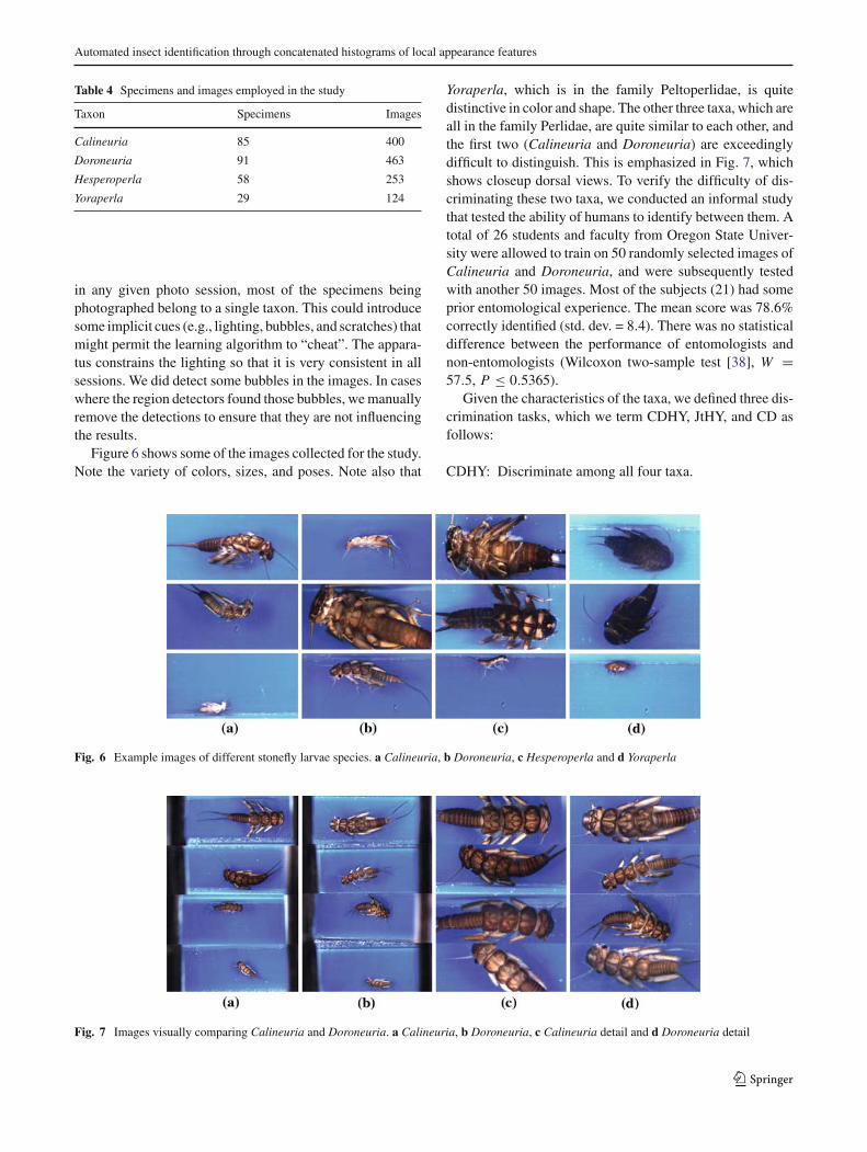
in any given photo session, most of the specimens beingphotographed belong to a single taxon. This could introducesome implicit cues (e.g., lighting, bubbles, and scratches) thatmight permit the learning algorithm to “cheat”. The appara-tus constrains the lighting so that it is very consistent in allsessions. We did detect some bubbles in the images. In caseswhere the region detectors found those bubbles, we manuallyremove the detections to ensure that they are not influencingthe results.

Figure 6 shows some of the images collected for the study.Note the variety of colors, sizes, and poses. Note also that

Yoraperla, which is in the family Peltoperlidae, is quitedistinctive in color and shape. The other three taxa, which areall in the family Perlidae, are quite similar to each other, andthe first two (Calineuria and Doroneuria) are exceedinglydifficult to distinguish. This is emphasized in Fig. 7, whichshows closeup dorsal views. To verify the difficulty of dis-criminating these two taxa, we conducted an informal studythat tested the ability of humans to identify between them. Atotal of 26 students and faculty from Oregon State Univer-sity were allowed to train on 50 randomly selected images ofCalineuria and Doroneuria, and were subsequently testedwith another 50 images. Most of the subjects (21) had someprior entomological experience. The mean score was 78.6%correctly identified (std. dev. = 8.4). There was no statisticaldifference between the performance of entomologists andnon-entomologists (Wilcoxon two-sample test [38], W =57.5, P ≤ 0.5365).

Given the characteristics of the taxa, we defined three dis-crimination tasks, which we term CDHY, JtHY, and CD asfollows:

CDHY: Discriminate among all four taxa.

Fig. 6 Example images of different stonefly larvae species. a Calineuria, b Doroneuria, c Hesperoperla and d Yoraperla

Fig. 7 Images visually comparing Calineuria and Doroneuria. a Calineuria, b Doroneuria, c Calineuria detail and d Doroneuria detail

123

N. Larios et al.

Table 5 Partitions for 3-fold cross-validation

Partition # Specimens # Images

1 87 413

2 97 411

3 79 416

JtHY: Merge Calineuria and Doroneuria to define a singleclass, and then discriminate among the resulting threeclasses.

CD: Focus on discriminating only between Calineuria andDoroneuria.

The CDHY task assesses the overall performance of the sys-tem. The JtHY task is most relevant to biomonitoring, sinceCalineuria and Doroneuria have identical pollution tolerancelevels. Hence, discriminating between them is not critical forour application. Finally, the CD task presents a very challeng-ing objective recognition problem, so it is interesting to seehow well our method can do when it focuses only on thistwo-class problem.

Performance on all three tasks is evaluated via three-foldcross-validation. The images are randomly partitioned intothree equal-sized sets under the constraint that all images ofany given specimen were required to be placed in the samepartition. In addition, to the extent possible, the partitions arestratified so that the class frequencies are the same across thethree partitions. Table 5 gives the number of specimens andimages in each partition.

In each “fold” of the cross-validation, one partition servesas the clustering data set for defining the dictionaries, a sec-ond partition serves as the training data set, and the thirdpartition serves as the test set.

Our approach requires specification of the followingparameters:

– the number L of mixture components in the Gaussianmixture model for each dictionary,

– the number B of bootstrap replicates for bagging,– the minimum number M of training examples in the

leaves of the logistic model trees, and– the number I of iterations of logit boost employed for

training the logistic model trees.

These parameters are set as follows. L is determined for eachspecies through a series of EM fitting procedures. We incre-ment the number of mixture components until the GMM iscapable of modeling the data distribution—when the GMMachieves a relative fitting error below 5% in less than 100EM iterations. The resulting values of L are 90, 90, 85 and65 for Calineuria, Doroneuria, Hesperoperla, and Yoraper-la, respectively. Likewise, B is determined by evaluating a

Table 6 Number of bagging iterations for each experiments

Experiment Bagging iterations B

4-species: CDHY 20

3-species: JtHY 20

2-species: CD 18

series of bagging ensembles with different numbers of clas-sifiers on the same training set. The number of classifiersin each ensemble is incremented by two until the trainingerror starts to increase, at which point B is simply assignedto be five less than that number. The reason we assign B tobe 5 less than the number that causes the training error toincrease—rather than simply assign it to the largest numberthat produces the lowest error—is that the smaller number ofboostrap replicates helps to avoid overfitting. Table 6 showsthe value of B for each of the three tasks. The minimum num-ber M of instances that each leaf in the LMT requires to avoidpruning is set to 15, which is the default value for the LMTimplementation recommended by the authors. The numberof logit boost iterations I is set by internal cross-validationwithin the training set while the LMT is being induced.

5.2 Results

We designed our experiments to achieve two objectives. First,we wanted to see how well the CFH method (with three regiondetectors) coupled with an ensemble of LMTs performs onthe three recognition tasks. To establish a basis for evalua-tion, we also apply the method of Opelt et al. [33], which iscurrently one of the best object recognition systems. Second,we wanted to evaluate how each of the three region detectorsaffects the performance of the system. To achieve this secondobjective, we train our system using seven different configu-rations corresponding to training with all three detectors, allpairs of detectors, and all individual detectors.

5.2.1 Overall results

Table 7 shows the classification rates achieved by the CFHmethod on the three discrimination tasks. Tables 8, 9, and10 show the confusion matrices for the three tasks. On the

Table 7 Percentage of images correctly classified by our system withall three region detectors along using a 95% confidence interval

Task Accuracy %

CDHY 82.42 ± 2.12

JtHY 95.40 ± 1.16

CD 79.37 ± 2.70

123

Automated insect identification through concatenated histograms of local appearance features

Table 8 CDHY confusion matrix of the combined Kadir, Hessian-affine and PCBR detectors

Predicted as ⇒ Cal. Dor. Hes. Yor.

Calineuria 315 79 6 0

Doroneuria 80 381 2 0

Hesperoperla 24 22 203 4

Yoraperla 1 0 0 123

Table 9 JtHY confusion matrix of the combined Kadir, Hessian-affineand PCBR detectors

Predicted as ⇒ Joint CD Hes. Yor.

Joint CD 857 5 1

Hesperoperla 46 203 4

Yoraperla 0 1 123

Table 10 CD confusion matrix of the combined Kadir, Hessian-affineand PCBR detectors

Predicted as ⇒ Calineuria Doroneuria

Calineuria 304 96

Doroneuria 82 381

CDHY task, our system achieves 82% correct classifications.The confusion matrix shows that it achieves near perfect rec-ognition of Yoraperla. It also recognizes Hesperoperla verywell with only a few images misclassified as Calineuria orDoroneuria. As expected, the main difficulty is to discrim-inate Calineuria and Doroneuria. When these two classesare pooled in the JtHY task, performance reaches 95% cor-rect, which is excellent. It is interesting to note that if wehad applied the four-way classifier and then pooled the pre-dictions of the classifiers, the three-class performance wouldhave been slightly better (95.48% vs. 95.08%). The differ-ence is that in the JtHY task, we learn a combined dictio-nary for the merged Calineuria and Doroneuria (CD) class,whereas in the four-class task, each taxon has its own dictio-naries.

A similar phenomenon occurs in the two-class CD task.Our method attains 79% of correct classification rate whentrained on only these two tasks. If instead, we applied theCDHY classifiers and treated predictions for Hesperoperlaand Yoraperla as errors, the performance would be slightlybetter (79.61% vs. 79.37%). These differences are notstatistically significant, but they do suggest that in futurework it might be useful to build separate dictionariesand classifiers for groups within each taxon (e.g., first clus-ter by size and color) and then map the resulting predictionsback to the four-class task. On this binary classificationtask, our method attains 79% correct classification, which is

approximately equal to the mean for human subjects withsome prior experience.

Our system is capable of giving a confidence measureto each of the existing categories. We performed a seriesof experiments where the species assignment is thresholdedby the difference between the two highest confidence mea-sures. In this series, we vary the threshold from 0 to 1. If thedifference is higher than the defined threshold, the label ofthe highest is assigned otherwise the specimen is declaredas “uncertain”. Figure 8 shows the plotting of the accuracyagainst the rejection rate. The curves show us that if we rejectaround 30% of the specimens, all the tasks will reach an accu-racy higher than 90%, even the CD task.

We also evaluate the performance of our classificationmethodology relative to a competing method [33] on themost difficult CD task using the same image features. Opelt’smethod is similar to our method in that it is also based onensemble learning principles (AdaBoost), and it is also capa-ble of combining multiple feature types for classification. Weadapted Opelt’s Matlab implementation to our features andused the default parameter settings given in the paper. TheEuclidean distance metric was used for the SIFT features andnumber of iterations I was set to 100. Table 11 summarizesthe classification rates. Our system provides 8–12% betteraccuracy than Opelt’s method for all four combinations ofdetectors. In addition, training Opelt’s classifier is more com-putationally expensive than is training our system. In partic-ular, the complexity of computing Opelt’s feature-to-imagedistance matrix is O(T 2 R2 D), where T is the number oftraining images, R is the maximum number of detected imageregions in a single image, and D = 128 is the SIFT vectordimension. The total number of detected training regions,T · R, is easily greater than 20,000) in this application. Onthe other hand, training our system is much faster. The com-plexity of building the LMT ensemble classifier (which dom-inates the training computation) is O(T · A · I ), where A isthe number of histogram attributes and I is the number ofLMT induction iterations (typically in the hundreds).

5.2.2 Results for multiple region detectors

Table 12 summarizes the results of applying all combinationsof one, two, and three detectors to the CDHY, JtHY, and CDtasks. The first three lines show that each detector has uniquestrengths when applied alone. The Hessian-affine detectorworks best on the 4-class CDHY task; the Kadir detector isbest on the three-class JtHY task, and the PCBR detectorgives the best two-class CD results. On the pairwise experi-ments it appears that the Hessian-affine and PCBR comple-ment each other well. The best pairwise results for the JtHYtask is obtained by the Kadir–Hessian pair; which appearsto be better for tasks that require an overall assessment of

123

N. Larios et al.

Fig. 8 Accuracy/rejectioncurves for the three experimentswith all the detectors combinedwhile changing theconfidence-difference threshold

0 10 20 30 40 50 60 70 80 9075

80

85

90

95

100Accuracy/Rejection Curve

Rejected [%]

Cor

rect

ly C

lass

ified

[%]

0 10 20 30 40 50 60 70 8082

84

86

88

90

92

94

96

98

100Accuracy/Rejection Curve

Rejected [%]

0 5 10 15 20 25 30 35 40 4595

95.5

96

96.5

97

97.5

98

98.5

99

99.5Accuracy/Rejection Curve

Rejected [%]

CD

JtHY

CDHY

Cor

rect

ly C

lass

ified

[%]

Cor

rect

ly C

lass

ified

[%]

Table 11 Comparison of CD classification rates using Opelt’s methodand our system with different combinations of detectors. A

√indicates

the detector(s) used

Hessian affine Kadir entropy PCBR Accuracy (%)

Opelt [33] Ours

√60.59 70.10√62.63 70.34√67.86 79.03√ √ √70.10 79.37

shape. Finally, the combination of all three detectors givesthe best results on each task.

To understand the region detector results, it is helpful tolook at their behaviors. Figures 9 and 10 show the regionsfound by each detector on selected Calineuria and Doroneu-ria specimens. The detectors behave in quite different ways.The PCBR detector is very stable, although it does not alwaysidentify all of the relevant regions. The Kadir detector is alsostable, but it finds a very large number of regions, most ofwhich are not relevant. The Hessian-affine detector finds verygood small-scale regions, but its larger-scale detections are

Table 12 Classification rates using our system with different combi-nations of detectors. A

√indicates the detector(s) used

Hessian affine Kadir entropy PCBR Accuracy (%)

CDHY JtHY CD

√73.14 90.32 70.10√70.64 90.56 70.34√71.69 86.21 79.03√ √78.14 94.19 74.16√ √80.48 93.79 78.68√ √78.31 92.09 68.83√ √ √82.42 95.40 79.37

not useful for classification. The PCBR detector focuses onthe interior of the specimens, whereas the other detectors(especially Kadir) tend to find points on the edges betweenthe specimens and the background. In addition to concentrat-ing on the interior, the regions found by the PCBR detectorare more “meaningful” in that they correspond better to bodyparts. This may explain why the PCBR detector did a betterjob on the CD task.

123

Automated insect identification through concatenated histograms of local appearance features

Fig. 9 Visual Comparison of the regions output by the three detectors on three Calineuria specimens. a Hessian-affine, b Kadir entropy, c PCBR

Fig. 10 Visual Comparison of the regions output by the three detectors on four Doroneuria specimens. a Hessian-affine, b Kadir entropy, c PCBR

6 Conclusions and future work

This paper has presented a combined hardware-software sys-tem for rapid-throughput classification of stonefly larvae. Thegoal of the system is to perform cost-effective bio-monitoringof freshwater streams. To this end, the mechanical appara-tus is capable of nearly unassisted manipulation and imagingof stonefly specimens while also obtaining consistently highquality images. The generic object recognition algorithmsattain classification accuracy that is sufficiently good (82%for four-classes; 95% for three-classes) to support the appli-cation. By rejecting for manual classification the specimens

in which the confidence level is not high enough; only a rea-sonable 30% of the samples would require further processingwhile the remaining identified specimens can reach an accu-racy above 90% on all the defined tasks.

We compared our CFH method to Opelt’s related state-of-art method on the most difficult task, discrimating Caline-uria from Doroneuria. The CFH method always achievedbetter performance. It is also worth noticing that human sub-jects with some prior experience and using the same imagesreached an accuracy equal to our method. Finally, we des-cribed a new region detector, the principal curvature-basedregion (PCBR) detector. Our experiments demonstrated

123

N. Larios et al.

that PCBR is particularly useful for discriminating betweenthe two visually similar species, and, as such provides animportant contribution in attaining greater accuracy.

There are a few details that must be addressed before thesystem is ready for field testing. First, the mechanical appa-ratus must be modified to include mechanisms for sortingthe specimens into bins after they have been photographedand classified. Second, we need to develop an algorithm fordetermining whether a good dorsal image of the specimenhas been obtained. We are currently exploring several meth-ods for this including training the classifier described in thispaper for the task. Third, we need to evaluate the perfor-mance of the system on a broader range of taxa. A practicalbio-monitoring system for the Willamette Valley will needto be able to recognize around 8 stonefly taxa. Finally, weneed to develop methods for dealing with specimens that arenot stoneflies or that do not belong to any of the taxa that thesystem is trained to recognize. We are studying SIFT-baseddensity estimation techniques for this purpose.

Beyond freshwater stream bio-monitoring, there are manyother potential applications for rapid-throughput arthropodrecognition systems. One area that we are studying involvesautomated population counts of soil mesofauna for soil biodi-versity studies. Soil mesofauna are small arthropods (mites,spiders, pseudo-scorpions, etc.) that live in soils. There areupwards of 2,000 species, and the study of their interactionsand population dynamics is critical for understanding soilecology and soil responses to different land uses. In our futurework, we will test the hypothesis that the methods describedin this paper, when combined with additional techniques forshape analysis and classification, will be sufficient to build auseful system for classifying soil mesofauna.

Acknowledgments We wish to thank Andreas Opelt for providing theMatlab code of his PAMI’06 method for the comparison experiment.We also wish to thank Asako Yamamuro and Justin Miles for theirassistance with the dataset stonefly identification.

References

1. Arbuckle, T., Schroder, S., Steinhage, V., Wittmann, D.:Biodiversity informatics in action: identification and monitoringof bee species using ABIS. In: Proceedings of the 15th Inter-national Symposium Informatics for Environmental Protection,vol. 1, pp. 425–430. Zurich (2001)

2. Bouchard, G., Triggs, B.: Hierarchical part-based visual objectcategorization. In: IEEE Conference on Computer Vision andPattern Recognition, pp. I 710–715 (2005). http://lear.inrial-pes.fr/pubs/2005/BT05

3. Breiman, L.: Bagging predictors. Mach. Learn. 24(2), 123–140(1996). http://citeseer.ist.psu.edu/breiman96bagging.html

4. Breiman, L., Friedman, J., Olshen, R., Stone, C.: Classificationand Regression Trees. Chapman and Hall, New York (1984)

5. Burl, M., Weber, M., Perona, P.: A probabilistic approach to objectrecognition using local photometry and global geometry. In: Pro-ceedings of the ECCV, pp. 628–641 (1998)

6. Carter, J., Resh, V., Hannaford, M., Myers, M.: Macroinverte-brates as biotic indicators of env. qual. In: Hauer, F., Lamberti,G. (eds.) Methods in Stream Ecology. Academic, San Diego(2006)

7. Csurka, G., Dance, C., Fan, L., Williamowski, J., Bray, C.: Visualcategorization with bags of keypoints. ECCV’04 workshop onStatistical Learning in Computer Vision, pp. 59–74 (2004)

8. Csurka, G., Bray, C., Fan, C.L.: Visual categorization with bagsof keypoints. ECCV workshop (2004)

9. Do, M., Harp, J., Norris, K.: A test of a pattern recognition sys-tem for identification of spiders. Bull. Entomol. Res. 89(3), 217–224 (1999)

10. Dorko, G., Schmid, C.: Object class recognition using discrim-inative local features. INRIA—Rhone-Alpes, RR-5497, Feb-ruary, 2005, Rapport de recherche. http://lear.inrialpes.fr/pubs/2005/DS05a

11. Dorkó, G., Schmid, C.: Object class recognition using discrimina-tive local features (2005). http://lear.inrialpes.fr/pubs/2005/DS05.Accepted under major revisions to IEEE Trans. Pattern Anal.Mach. Intell. (updated 13 September)

12. Fergus, R., Perona, P., Zisserman, A.: Object class recognitionby unsupervised scale-invariant learning. In: Proceedings of theIEEE Conference on Computer Vision and Pattern Recognition,vol. 2, pp. 264–271. Madison, Wisconsin (2003)

13. Freund, Y., Schapire, R.E.: Experiments with a new boostingalgorithm. In: International Conference on Machine Learning,pp. 148–156 (1996). http://citeseer.ist.psu.edu/freund96experi-ments.html

14. Friedman, J., Hastie, T., Tibshirani, R.: Additive logistic regres-sion: a statistical view of boosting (1998). http://citeseer.ist.psu.edu/friedman98additive.html

15. Gaston, K.J., O’Neill, M.A.: Automated species identification:why not? Philosophical Trans. R. Soc. B: Biol. Sci. 359(1444),655–667 (2004)

16. Harris, C., Stephens, M.: A combined corner and edge detector.Alvey Vision Conference, pp. 147–151 (1988)

17. Hilsenhoff, W.L.: Rapid field assessment of organic pollution witha family level biotic index. J. North Am. Benthol. Soc. 7, 65–68(1988)

18. Hopkins, G.W., Freckleton, R.P.: Declines in the numbers ofamateur and professional taxonomists: implications for conser-vation. Anim. Conserv. 5(3), 245–249 (2002)

19. Jurie, F., Schmid, C.: Scale-invariant shape features for recogni-tion of object categories. CVPR 2, 90–96 (2004)

20. Jurie, F., Triggs, B.: Creating efficient codebooks for visual rec-ognition. In: ICCV ’05: Proceedings of the 10th IEEE Interna-tional Conference on Computer Vision (ICCV’05), vol. 1, pp.604–610. IEEE Computer Society, Washington, DC, USA (2005).DOI http://dx.doi.org/10.1109/ICCV.2005.66

21. Kadir, T., Zisserman, A., Brady, M.: An affine invariant salientregion detector. In: European Conference on Computer Vision(ECCV04), pp. 228–241 (2004)

22. Kumar, S., August, J., Hebert, M.: Exploiting inference forapproximate parameter learning in discriminative fields: an empir-ical study. In: 5th International Workshop, EMMCVPR 2005, pp.153–168. Springer, St. Augustine (2005)

23. Landwehr, N., Hall, M., Frank, E.: Logistic model trees. Mach.Learn. 59(1–2), 161–205 (2005). DOI 10.1007/s10994-005-0466-3

24. Leibe, B., Seemann, E., Schiele, B.: Pedestrian detection incrowded scenes. In: CVPR ’05: Proceedings of the 2005IEEE Computer Society Conference on Computer Visionand Pattern Recognition (CVPR’05), vol. 1, pp. 878–885.

123

Automated insect identification through concatenated histograms of local appearance features

IEEE Computer Society, Washington, DC, USA (2005). DOIhttp://dx.doi.org/10.1109/CVPR.2005.272

25. Lowe, D.G.: Distinctive image features from scale-invariantkeypoints. Int. J. Comput. Vis. 60(2), 91–110 (2004). DOI10.1023/B:VISI.0000029664.99615.94

26. Lucas, S.: Face recognition with continuous n-tuple classifier. In:Proceedings of the British Machine Vision Conference, pp. 222–231. Essex (1997)

27. Matas, J., Chum, O., Urban, M., Pajdla, T.: Robust wide-baseline stereo from maximally stable extremal regions. ImageVis. Comput. 22(10), 761–767 (2004)

28. Mikolajczyk, K., Schmid, C.: An affine invariant interest pointdetector. ECCV 1(1), 128–142 (2002)

29. Mikolajczyk, K., Schmid, C.: Scale and affine invariant interestpoint detectors. IJCV 60(1), 63–86 (2004)

30. Mikolajczyk, K., Tuytelaars, T., Schmid, C., Zisserman, A.,Matas, J., Schaffalitzky, F., Kadir, T., Gool, L.V.: A compar-ison of affine region detectors. IJCV 65(1/2), 43–72 (2005).http://lear.inrialpes.fr/pubs/2005/MTSZMSKG05

31. O’Neill, M.A., Gauld, I.D., Gaston, K.J., Weeks, P.: Daisy: anautomated invertebrate identification system using holistic visiontechniques. In: Proceedings of the Inaugural Meeting BioNET-INTERNATIONAL Group for Computer-Aided Taxonomy (BIG-CAT), pp. 13–22. Egham (2000)

32. Opelt, A., Fussenegger, M., Pinz, A., Auer, P.: Weak hypothe-ses and boosting for generic object detection and recognition. In:8th European Conference on Computer Vision, vol. 2, pp. 71–84.Prague, Czech Republic (2004)

33. Opelt, A., Pinz, A., Fussenegger, M., Auer, P.: Generic objectrecognition with boosting. IEEE Trans. Pattern Anal. Mach. In-tell. 28(3), 416–431 (2006)

34. Papageorgiou, C., Poggio, T.: A trainable system for object detec-tion. Int. J. Comput. Vis. 38(1), 15–33 (2000)

35. Quattoni, A., Collins, M., Darrell, T.: Conditional random fieldsfor object recognition. In: Proceedings of the NIPS 2004. MITPress, Cambridge (2005)

36. Quinlan, J.R.: C4.5: programs for machine learning. MorganKaufmann, San Francisco (1993)

37. Shotton, J., Blake, A., Cipolla, R.: Contour-based learningfor object detection. In: ICCV ’05: Proceedings of the 10thIEEE International Conference on Computer Vision (ICCV’05),vol. 1, pp. 503–510. IEEE Computer Society, Washington, DC,USA (2005). DOI http://dx.doi.org/10.1109/ICCV.2005.63

38. Sokal, R.R., Rohlf, F.J.: Biometry, 3rd edn. W. H. Freeman,Gordonsville (1995)

39. Steger, C.: An unbiased detector of curvilinear struc-tures. PAMI 20(2), 113–125 (1998)

40. Sung, K.K., Poggio, T.: Example-based learning for view-basedhuman face detection. IEEE Trans. Pattern Anal. Mach. In-tell. 20(1), 39–51 (1998)

41. Turk, M.A., Pentland, A.P.: Face recognition using eigenfaces. In:Proceedings of IEEE Conference on Computer Vision and PatternRecognition, pp. 586–591 (1991)

42. Tuytelaars, T., Gool, L.V.: Wide baseline stereo matching basedon local, affinely invariant regions. BMVC, pp. 412–425 (2000)

43. Tuytelaars, T., Gool, L.V.: Matching widely separated views basedon affine invariant regions. IJCV 59(1), 61–85 (2004)

44. Vincent, L., Soille, P.: Watersheds in digital spaces: an efficientalgorithm based on immersion simulations. PAMI 13(6), 583–598 (1991)

45. Zhang, W., Deng, H., Dietterich, T.G., Mortensen, E.N.: A hier-archical object recognition system based on multi-scale principalcurvature regions. International Conference of Pattern Recogni-tion, pp. 1475–1490 (2006)

Author biographies

Natalia Larios received the BSin Computer Engineering from theUniversidad Nacional Autonomade Mexico in 2003. She is currentlya graduate student and researchassistant in the Electrical Engineer-ing Department at the Universityof Washington. Her research inter-ests include computer vison, objectrecognition and image retrievalemploying machine learning andprobabilistic modeling.

Hongli Deng received a BE degreein 1992 from Wuhan University oftechnology and ME degree in 1999from Sichuan University in China.He is a PhD candidate in Electri-cal Engineering and Computer Sci-ence department of Oregon StateUniversity. His research interestsare local image feature detection,description and registration.

Wei Zhang received the BS andMS degrees from Xi’an JiaotongUniversity, China, in 2001 and2004. Currently, he is a PhD candi-date and research assistant at Ore-gon State University. His researchinterests include machine learning,computer vision and object recog-nition.

123

N. Larios et al.

Matt Sarpola graduated fromOregon State University with hisMS in mechanical engineering in2005 and currently does new productresearch and development for Videxin Corvallis, OR.

Jenny Yuen is currently a grad-uate student at the MassachusettsInstitute of Technology ComputerScience and Artificial IntelligenceLaboratory, where she is workingon computer vision for event recog-nition and detection. She has a BSin Computer Science from the Uni-versity of Washington.

Robert Paasch is an Associ-ate Professor in the Departmentof Mechanical Engineering at Ore-gon State University, and currentlyholds the Boeing Professorship inMechanical Design. He received hisPh.D. in Mechanical Engineeringfrom the University of Californiaat Berkeley in 1990. His researchinterests include automated moni-toring and diagnosis, probabilisticand robust design, and design the-ory and methodology.

Andrew R. Moldenke is an ecol-ogist in the Department of Bot-any and Plant Pathology at Ore-gon State University. His researchinterests center on the interactionsbetween arthropods and plants, inparticular pollination and nutri-ent recycling. He is especiallyconcerned about the inability ofscientists to develop appropriateprotocols for measuring criticalchanges in biodiversity as the cli-mate changes due to the sheer num-bers of arthropod species and thelimited number of trained taxono-mists.

Dave A. Lytle is currently an Assis-tant Professor of Zoology at Ore-gon State University. He receivedhis PhD in Ecology and Evolution-ary Biology from Cornell Univer-sity in 2000. He has been a D.H.Smith Postdoctoral Fellow and aPostdoctoral Associate in the Uni-versity of Chicago. His researchinterests include the use of evolu-tionary ecology to understand howaquatic organisms are shaped.

Salvador Ruiz Correa was bornin Mexico City, Mexico, 1966. Hereceived the B.S. and M.S. degreesin Electrical Engineering from theUniversidad Nacional Autonomade Mexico, in 1990 and 1994,respectively, and the Ph.D. degreein Electrical Engineering from theUniversity of Washington, Seattle,in 2004. He has worked as a post-doctoral fellow in imaging infor-matics at Children’s Hospital andRegional Medical Center in Seattle,WA, and Children’s National Med-ical Center in Washington, D.C.,

from 2004 to present. Currently, he is the director of the Pediatric Imag-ing Research Laboratory at CNMC. His research interests include com-puter vision, biomedical image processing, pattern recognition, roboticsand imaging informatics. Dr. Ruiz is an associate member of the IEEEand reviewer for IEEE PAMI, the International Journal of ComputerVision and Pattern Recognition and IEEE Transactions on Multimedia.

Eric N. Mortensen is an Assis-tant Professor in the Schoolof Electrical Engineering andComputer Science at OregonState University. He receivedhis Ph.D. in Computer Sciencefrom Brigham Young Univer-sity in 2000. His research inter-ests include interactive vision,image and video segmentation andediting, feature detection/descrip-tion/matching, object recognition,and image-based modeling. He isa member of the Institute of Elec-trical and Electronics Engineers(IEEE) and the Association for

Computing Machinery (ACM).

123

Automated insect identification through concatenated histograms of local appearance features

Linda G. Shapiro is a Professorof Computer Science and Engineer-ing and of Electrical Engineering atthe University of Washington. Herresearch interests include computervision, image database systems,artificial intelligence, pattern recog-nition, and robotics. She is a Fellowof the IEEE, a Fellow of the IAPR,and a past Chair of the IEEE Com-puter Society Technical Committeeon Pattern Analysis and MachineIntelligence. She has served asEditor-in-Chief of CVGIP: ImageUnderstanding, Associate Editor of

IEEE Transactions on Pattern Analysis and Machine Intelligence, andChair or Program Chair of numerous computer vision conferences. Shehas co-authored three textbooks, one on data structures and two oncomputer vision.

Thomas G. Dietterich isProfessor and Director of Intel-ligent Systems in the School ofElectrical Engineering and Com-puter Science at Oregon State Uni-versity, where he joined as thefaculty in 1985. In 1987, he wasnamed a Presidential Young Inves-tigator for the NSF. In 1990, hepublished, with Dr. Jude Shav-lik, the book entitled Readings inMachine Learning, and he alsoserved as the Technical ProgramCo-Chair of the National Con-ference on Artificial Intelligence(AAAI-90). From 1992 to 1998 he

held the position of Executive Editor of the journal Machine Learning.He is a Fellow of the American Association for Artificial Intelligence(1994) and of the Association for Computing Machinery (2003). In2000, he co-founded a new, free electronic journal: The Journal ofMachine Learning Research. He served as Technical Program Chair ofthe Neural Information Processing Systems (NIPS) conference in 2000and General Chair in 2001. He is currently President of the InternationalMachine Learning Society, and he also serves on the Board of Trusteesof the NIPS Foundation.

123