A Review of Mixture Theory for Deformable Porous Media and ...
Upload
khangminh22Category
view
3download
0
HAL Id: tel-02534996https://tel.archives-ouvertes.fr/tel-02534996
Submitted on 7 Apr 2020
HAL is a multi-disciplinary open accessarchive for the deposit and dissemination of sci-entific research documents, whether they are pub-lished or not. The documents may come fromteaching and research institutions in France orabroad, or from public or private research centers.
L’archive ouverte pluridisciplinaire HAL, estdestinée au dépôt et à la diffusion de documentsscientifiques de niveau recherche, publiés ou non,émanant des établissements d’enseignement et derecherche français ou étrangers, des laboratoirespublics ou privés.
Visual servoing on deformable objects : an application totether shape controlMatheus Laranjeira Moreira
To cite this version:Matheus Laranjeira Moreira. Visual servoing on deformable objects : an application to tether shapecontrol. Automatic. Université de Toulon, 2019. English. NNT : 2019TOUL0007. tel-02534996


Acknowledgements
First of all, I would like to thank each member of my jury for giving me the honor ofassessing my work. Thanks to Yvan Petillot, professor at the Heriot-Watt University,for chairing my jury. Thanks to Luc Jaulin, professor at ENSTA Bretagne, and toFrancois Chaumette, Inria senior research scientist, for the time they spent analyzingthis thesis and for all the remarks and high-quality feedbacks given in their reports.Thanks to Viviane Cadenat, associate professor at Universite de Toulouse III, to Vin-cent Creuze, associate professor at Universite de Montpelier, and to Andrea Cherubini,associate professor at Universite de Montpelier, for accepting to be members of thejury and for their interest in my work. Thanks to the invited members of my jury,David Navarro-Alarcon, assistant professor at The Hong Kong Polytechnic University,Yves Chardard, CEO of the Subsea Tech company, Jan Opderbecke, head of unit forunderwater systems at Ifremer, and Lorenzo Brignone, head of the underwater roboticslaboratory at Ifremer, for their useful comments.
I also thank the French Sud region and the Subsea Tech company for their financialsupport.
I would like to thank my supervisor, Vincent Hugel, and advisor, Claire Dune. Theyintroduced me to the scientific and academic world. Their advices and criticism allowedme to advance during the thesis. I thank them for their availability and support.Thanks to all the members of the laboratory for all the discussions and interestingfeedbacks. Thanks to Sabine Seillier and Cedric Anthierens for their assistance duringthe experimental phase of this thesis.
I thank my former colleagues at the office: Minh, Jerome, Nicolas, Ornella, Jean-Baptiste, Hoang Anh... The pleasant working environment and good mood helped mea lot to keep my optimism even in harder times. Thanks to Minh for his supportduring my first experiments in the summer of 2016. Thank you Anh for your kindnessand providential help during the experiments with underwater robots. Thanks for thecayenne peppers. It will be amazing to see them grow and have fresh peppers thissummer. Thank you Jean-Baptiste for presenting me this wonderful region that is theProvence and the Mediterranean coast and for the interesting discussions about thelatin languages. Thanks for the Slivovica. It will be nice to appreciate it next winter.
I would also like to thank my family. My father, Agnaldo, my sister, Paloma, andmy bother, Saulo, for all the good times we spent together and their support, evenat a distance. A special thanks to my mother, Magali, for being present at some keymoments in this thesis.
Thanks to Salima and Edmond for the restoring weekends and for being present inmy thesis defense. Thanks to Marisa for all the support during the last months.
I have to enormously thank Dorothea, my partner and great love. Thank you foralways listening to me and providing endless support and encouragement. Thanks alsofor accepting to be the official graphic designer of this thesis. Your work significantlyimproved the aesthetic quality of this manuscript. For all your help in everyday life, Ido not know how to thank you. I believe you will have to do a thesis as well. But I askthe good Lord not to.

Contents
Contents 1
Glossary 4
Introduction 7
1 State of the Art on Tether Management 11
1.1 The Underwater Environment . . . . . . . . . . . . . . . . . . . . . . . . 12
1.2 Underwater Robots . . . . . . . . . . . . . . . . . . . . . . . . . . . . . . 13
1.2.1 Autonomous Underwater Vehicles . . . . . . . . . . . . . . . . . 13
1.2.2 Remotely Operated Vehicles . . . . . . . . . . . . . . . . . . . . . 14
1.3 Tethers . . . . . . . . . . . . . . . . . . . . . . . . . . . . . . . . . . . . 16
1.3.1 Utility . . . . . . . . . . . . . . . . . . . . . . . . . . . . . . . . . 16
1.3.2 Buoyancy . . . . . . . . . . . . . . . . . . . . . . . . . . . . . . . 17
1.3.3 Cross-section . . . . . . . . . . . . . . . . . . . . . . . . . . . . . 17
1.3.4 Models . . . . . . . . . . . . . . . . . . . . . . . . . . . . . . . . 20
1.4 Tethers and Deformable Objects Management . . . . . . . . . . . . . . 21
1.4.1 Underwater Applications . . . . . . . . . . . . . . . . . . . . . . 21
1.4.2 Terrestrial and Aerial Applications . . . . . . . . . . . . . . . . . 23
1.4.3 Synthesis of Existing Cable Management Strategies . . . . . . . . 26
1.4.3.1 Passive and Active Cable Management Strategies . . . 26
1.4.3.2 Classification according to Cable Perception and Mod-eling techniques . . . . . . . . . . . . . . . . . . . . . . 28
1.5 Our Scientific Focus: Vision Servoing of a Pair of Robots in a Chain ofMini-ROVs . . . . . . . . . . . . . . . . . . . . . . . . . . . . . . . . . . 30
2 System Modeling 33
2.1 Tether Model . . . . . . . . . . . . . . . . . . . . . . . . . . . . . . . . . 33
2.1.1 Catenary Equation . . . . . . . . . . . . . . . . . . . . . . . . . . 33
2.1.2 Catenary Parameter . . . . . . . . . . . . . . . . . . . . . . . . . 35
2.1.3 Catenary Parameter Constraints . . . . . . . . . . . . . . . . . . 37
2.2 Robots Model and Configuration . . . . . . . . . . . . . . . . . . . . . . 38
2.2.1 Thruster Configuration and Allocation Matrix . . . . . . . . . . 39
2.2.2 Kinematic Model of a mini-ROV . . . . . . . . . . . . . . . . . . 46
1

2 Contents
2.3 Pair of Robots Connected by a Tether . . . . . . . . . . . . . . . . . . . 49
2.3.1 Catenary Model Applied for Tethered Robots . . . . . . . . . . . 49
2.3.2 Tether Attachment Points and Robots Kinematics . . . . . . . . 52
2.4 Conclusions . . . . . . . . . . . . . . . . . . . . . . . . . . . . . . . . . . 56
3 Underwater Perception of the Tether 57
3.1 Camera Configurations and Assumptions . . . . . . . . . . . . . . . . . 57
3.2 Camera Modeling . . . . . . . . . . . . . . . . . . . . . . . . . . . . . . . 60
3.2.1 Image Formation . . . . . . . . . . . . . . . . . . . . . . . . . . . 60
3.2.2 Camera Exposure and White Balance . . . . . . . . . . . . . . . 60
3.2.3 The Pinhole Camera Model . . . . . . . . . . . . . . . . . . . . . 62
3.2.4 Intrinsic Parameters . . . . . . . . . . . . . . . . . . . . . . . . . 63
3.3 Tether Detection . . . . . . . . . . . . . . . . . . . . . . . . . . . . . . . 65
3.4 Catenary Features Estimation . . . . . . . . . . . . . . . . . . . . . . . 67
3.4.1 Catenary Equation in the Camera Frame . . . . . . . . . . . . . 67
3.4.2 Catenary Projection on the Image Plane . . . . . . . . . . . . . . 69
3.4.3 Catenary Curve Fitting . . . . . . . . . . . . . . . . . . . . . . . 70
3.4.3.1 Gauss-Newton Algorithm . . . . . . . . . . . . . . . . . 71
3.4.3.2 Study of the Gauss-Newton Jacobian Singularities . . . 72
3.4.3.3 Particular Case of Remote Points . . . . . . . . . . . . 74
3.4.3.4 Gauss-Newton Improved Algorithm . . . . . . . . . . . 75
3.4.3.5 Initial Guess of Catenary Shape for Gauss-Newton . . . 84
3.5 Results . . . . . . . . . . . . . . . . . . . . . . . . . . . . . . . . . . . . . 92
3.5.1 Focus on Feature Vector Estimation Error . . . . . . . . . . . . 92
3.5.2 Study Cases in a Simulated Environment . . . . . . . . . . . . . 97
3.5.3 Discussion . . . . . . . . . . . . . . . . . . . . . . . . . . . . . . . 106
3.6 Conclusions . . . . . . . . . . . . . . . . . . . . . . . . . . . . . . . . . . 108
4 Tether Shape Control 109
4.1 State of the Art on Vision-Based Control . . . . . . . . . . . . . . . . . 110
4.1.1 Rigid Objects . . . . . . . . . . . . . . . . . . . . . . . . . . . . . 110
4.1.2 Deformable Objects . . . . . . . . . . . . . . . . . . . . . . . . . 112
4.2 General Control Scheme . . . . . . . . . . . . . . . . . . . . . . . . . . . 115
4.3 Catenary-Based Interaction Matrices . . . . . . . . . . . . . . . . . . . . 117
4.4 Follower Robot Control using Tether Visual Feedback . . . . . . . . . . 125
4.4.1 Preliminary Results with Terrestrial Robots . . . . . . . . . . . . 126
4.4.1.1 Catenary-Based Visual Servoing for Terrestrial Robots 126
4.4.1.2 Comparison of Catenary-Based Control with Image-BasedVisual Servoing . . . . . . . . . . . . . . . . . . . . . . 130
4.4.2 Underwater Tether Shape Regulation while Leader Robot is Mo-tionless . . . . . . . . . . . . . . . . . . . . . . . . . . . . . . . . 138
4.4.2.1 Visual Servoing Control with 3× 4 Interaction Matrix . 139
4.4.2.2 Sum of Controllers . . . . . . . . . . . . . . . . . . . . . 141
4.4.2.3 Hierarchical Task Control . . . . . . . . . . . . . . . . . 143
Contents 3
4.4.2.4 Comparing Follower Robot Trajectories . . . . . . . . . 1474.4.3 Underwater Tether Shape Regulation while Leader Robot Moves 148
4.4.3.1 Neglecting the Leader Velocity on the Follower RobotCommand . . . . . . . . . . . . . . . . . . . . . . . . . 149
4.4.3.2 Including the Leader Velocity on the Follower RobotCommand . . . . . . . . . . . . . . . . . . . . . . . . . 154
4.5 Follower Robot Control using Tether Visual Feedback from Both Cam-eras - Underwater Case . . . . . . . . . . . . . . . . . . . . . . . . . . . 156
4.6 Discussion . . . . . . . . . . . . . . . . . . . . . . . . . . . . . . . . . . . 1614.7 Conclusions . . . . . . . . . . . . . . . . . . . . . . . . . . . . . . . . . . 163
5 Conclusions 165
5.1 Summary . . . . . . . . . . . . . . . . . . . . . . . . . . . . . . . . . . . 1655.2 Perspectives . . . . . . . . . . . . . . . . . . . . . . . . . . . . . . . . . . 166
A Position and Orientation Representation 169
B Expression of the catenary parameter C 171
C Kinematic Equations with Twist Matrix: General Case 177
D Catenary Derivatives 179
E Preliminary Results with Terrestrial Robots 181
F Interaction Matrix Test Protocol 195
G Scientific publications, Workshop Participations and Scientific Popu-
larization Activities 201
H Resume en francais 203
Bibliography 223
Table des figures 225

4 Contents
Glossary
General rules
a a scalar in the image plane is represented by a lowercase letter
A a scalar in E3 is represented by an uppercase letter
a a vector is represented by a bold lowercase letter
A a matrix is represented by a bold uppercase letter
Mathematics
En Euclidean space with n dimensions
Fa a generic Euclidean reference frame Fa(Pa, ia, ja,ka) consists of anorigin Pa and an orthogonal basis (ia, ja,ka)
p the bold lowercase letter p is reserved to represent a vector containingthe normalized coordinates of an image point. For example, pa =[xa ya 1]T represents an image point a in the camera frame
Pa a generic point in the Euclidean space E3 is noted Pa, where the
subscript a identifies the point
PbPa a vector defined by starting point Pb and end point PabPa the overlined bold uppercase letter P is reserved to represent a vector
containing the Cartesian coordinates of a 3-D point. b PbPa =bPa = [bXa
bYabZa]
T represents the 3-D point Pa in frame Fb
a
dP2P1
dt
Fb
the derivative of vector P2P1 with respect to frame Fb and expressed
in frame Fa˙bPa the derivative of vector PbPa with respect to frame Fb and expressed
in frame FbbPa the bold uppercase letter P is reserved to represent a vector contain-
ing the homogeneous coordinates of a 3-D point. bPa = [bPa 1]T
represents a 3-D point Pa in frame FbbRa a 3-D rotation matrix from frame Fa to frame FbbMa an homogeneous transformation matrix from frame Fa to frame Fbbva the velocity screw vector bva = [bνa,
bωa]
T of point Pa expressed inthe coordinate frame Fb.
bνa and b
ωa are, respectively, the linearand angular components of the velocity vector
va the generic velocity screw vector va = [νa,ωa]T of point Pa not
projected in any coordinate frame. The linear velocity of Pa is noted
5

6 Glossary
νa and the angular velocity of frame Fa with respect to the worldframe FW is noted ωa.
Introduction
Unmanned mobile robots are well suited to explore environments considered too costly,time consuming, and hazardous for human inspection. They execute a wide varietyof tasks such as gathering samples or monitoring and maintenance of structures ininaccessible sites. In some cases, when the explored environment is well structured,these robots can operate in autonomy, without any human intervention, being mostlyemployed in survey applications. However, autonomous navigation in unknown spacesand autonomous manipulation requiring physical contacts with unstructured environ-ments without human supervision represent technical and technological challenges thatremain to be addressed.
Many robotic tasks require continuous human intervention to be carried out. Insuch cases, the decision-making and intelligence of operation is the human responsi-bility, while the robot is limited to execute the low level tasks. Teleoperation systemsare required to allow human operators to control the robots with the aid of visual andother sensory feedback. Teleoperation systems can be divided into two main categories:wired and wireless communication. Wireless teleoperation is preferable in some roboticapplications, since it offers the robot more freedom of motion and flexibility in naviga-tion. Nevertheless, a wireless link may be subject to interference and signal loss thatdegrade the reliability of data exchange with the robot. Therefore, the use of tethershas advantages in applications where robust data communication is a priority and itsinterruption can lead to the loss of the robot and mission failure.
Applications where the use of tethers is preferable instead of wireless communica-tion include, for example, urban search and rescue operations (Fukushima et al., 2000;Perrin et al., 2004), planetary geologic survey (Tsai et al., 2013), underwater missions(McKerrow and Ratner, 2007) and sewerage (Reverte et al., 2011). Specifically in thecase of underwater operations, wireless communication is even more complicated, sinceelectromagnetic waves are strongly attenuated in water and acoustic subsea commu-nications have a very low bandwidth and significant time delay, which represents aconsiderable obstacle to robust teleoperation (Marani et al., 2009).
The main advantage of using tethers is the provision of a fast and stable commu-nication link. In addition, tethers can transfer power, which makes it possible to carryout longer operations with energy consuming payload and enable vehicle downsizingthanks to the absence of batteries. Another advantage of tethers is that they can beused as a mechanical support for robots exploring hard-to-reach areas as cliffs, caves,crevices and other steep terrains (McGarey et al., 2016b). Nevertheless, tethering also
7
8 Introduction
have important shortcomings. Tethers are known to limit the robot workspace andthey may become entangled with obstacles or with other fellow robots, leading to im-mobilization. The energy transfer by wire may also represent a constraint to largerobot displacements since a very long cable increases the losses by Joule heating. Acompromise must be found between the power demanded by the robot and the size ofthe cable: for a better power flow, thicker cables are needed. However, the thicker thecable, the more rigid it is and greater torsion efforts it applies on the robot, which willrequire more power to compensate them.
In this thesis, we are interested in the use of small tethered underwater robots, alsocalled mini remotely operated vehicles (mini-ROVs), in the context of exploration ofshallow waters, with less than 10 meters of depth. The ROVs are linked to a surfacevessel by a tether (also called umbilical) that ensures energy supply and data transfer.Typical ROVs generally weigh some hundred kilograms and are powerful electrome-chanical machines that require significant human and material resources to be deployed.They have a working depth between 1,000 and 6,000 meters and can move away severaltenths of kilometers from their base. The logistical difficulties of deploying large un-derwater robots led to the development of mini-ROVs, that weigh a few kilograms andare low-power demanding. They are able to explore shallow waters, caves and somewrecks that are not accessible to typical ROVs. However, these light-weight and lesspowerful vehicles are much more sensitive to the disturbances engendered by a longtether, which can cause unbalance and make them difficult to maneuver. Mini-ROVsare thus limited to displacements around the surface vessel, which consequently limitsthe exploration of shallow waters, since the vessel cannot get too close to the coast.
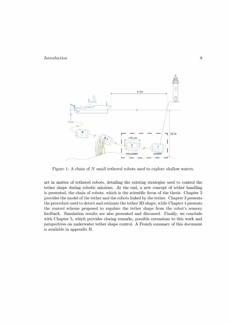
The Cosmer Laboratory and the SUBSEA-TECH company, a partner and co-funderof this thesis, came together in reflections and discussions on the possible strategies ofunderwater robotic teleoperation in coastal areas. Thereby, the idea of using mini-ROVs serially linked with a tether arose: a group of small-size identical robots aredistributed all along the tether (see Figure 1). All robots forming the fleet have the samearchitecture, the same set of sensors and actuators, hence the same motion capability.Together, the small robots can compensate the disturbances of a long tether and allowthe leader robot to behave as if it were in the vicinity of the base. Moreover, thischain of robots can work as a sensor network that have a distributed perception of theunderwater environment. Mapping of currents and seabed can be achieved with thisfleet of robots that can collect data and share informations in real time thanks to thewired connection. Depending on the situation, the fleet could also be organized in waysother than serial, as triangular or square grids, in order to enlarge the covered area.
The objective of this PhD thesis is to investigate how to control the shape of asection of tether linking a pair of robots, a leader and a follower, as it is illustrated byFigure 1. The general idea is that the leader robot freely explores its surrounding, asif it was not attached to anything, while the follower robot is expected to manage thetether shape from its embedded sensors feedback so that the tether does not hamperthe leader movements. We propose to use only standard sensors commonly embeddedin the mini-ROVs while the tether itself will not be modified nor instrumented.
The thesis is structured as follows. Chapter 1 is dedicated to the state-of-the-

10 Introduction

Chapter 1
State of the Art on Tether
Management
There are two types of unmanned underwater vehicles: remotely operated vehicles(ROVs) and autonomous underwater vehicles (AUVs). ROVs communicate continu-ously with a surface vessel thanks to a physical link called umbilical or tether, dueto the low-bandwidth of underwater wireless communication. AUVs are completelyautonomous and previously programmed to execute specific mission with very littlecommunication with the surface vessel.
Despite the recent development of techniques of autonomous navigation and taskexecution, a large number of underwater robotic missions are still carried out by tele-operation. The tether provides a reliable communication link and power supply thatenables the fulfillment of long-term missions. There are different types of tethers, de-pending on the type of mission and deployed robot. Heavy, thick and rigid tethers areused to transfer data and huge amounts of energy to work-class ROVs that operate indeep sea. Thinner and more flexible tethers are used to provide data exchange to largeROVs that have embedded batteries, or also to provide energy to low power-consumingROVs. Tethers are thus an important element in underwater robotics operations, anda large number of missions that require continuous human intervention could not beachieved without them. Tethers, however, also bring with them additional problemsto robotics operation, since they limit the robot workspace and can be entangled withobjects in the environment, leading to robot immobilization and, consequently, missionabort.
Tether management is one of the most challenging issues in operations using teth-ered robots. In this Chapter we address the current strategies that deal with the controlof umbilicals. We start by describing the underwater coastal environment where oursystem will be deployed. Then, we continue by defining the different types of robotsand tethers that are used in underwater operation. Next, we give some details aboutthe existing strategies of tether and deformable objects handling in the context of un-derwater application, which can be also extended to others domains of application.Finally, we present our strategy of tether management for mini-ROVs that operate in
11
12 State of the Art on Tether Management
underwater cluttered coastal zones (less than 10 meters deep) while being as far aspossible from the surface vessel.
1.1 The Underwater Environment
Coastal areas are the boundaries between the marine and continental domains. Theseare important areas in terms of both marine and terrestrial biodiversity as well as interms of convergence of oceanic and continental processes that play a major role in thedetermination of geomorphological, geochemical and climatic changes. The coasts arevery attractive, as evidenced by the strong anthropomorphization of the littoral zone.It is estimated that currently more than 60% of the world’s population (3.8 billionpeople) live in coastal area (less than 150km from the coast). This high concentrationof population is due to a considerable economic activity, particularly in the fisheriessector, aquaculture, trade and energy, but also due to the booming touristic sector.
With respect to the underwater environment, the abundance of light in the firstmeters of depth makes the environment the home of a large range of species. It isalso an important area of reproduction, as it is, for example, the case of estuaries andcoral reefs. The coastal marine environment shelters fragile ecosystems that should beconstantly monitored with the aim of preserving their balance. This surveillance is allthe more important since coastal ecosystems are often affected by pollutants generatedby ship traffic and liquid waste emission of cities.
Seawater can be characterized by thermophysical properties as density, temperatureand salinity. The density of surface seawater ranges from about 1020 to 1029kg/m3,depending on the temperature and salinity. At a temperature of 25C, salinity of 35g/kgand pressure of 1atm, the density of seawater is 1023.6kg/m3 (Nayar et al., 2016). Deepin the ocean, under high pressure, seawater can reach a density of 1050kg/m3 or higher.In the Mediterranean sea, the surface temperature ranges from 13C to 25C annually.Salinity varies between 38.4 and 41.2g/kg and its density is around 1027kg/m3. Waterdensity slightly varies with depth and can be considered constant in the first 30 meters.
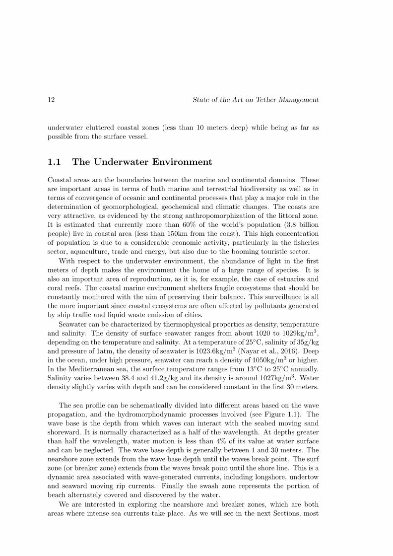
The sea profile can be schematically divided into different areas based on the wavepropagation, and the hydromorphodynamic processes involved (see Figure 1.1). Thewave base is the depth from which waves can interact with the seabed moving sandshoreward. It is normally characterized as a half of the wavelength. At depths greaterthan half the wavelength, water motion is less than 4% of its value at water surfaceand can be neglected. The wave base depth is generally between 1 and 30 meters. Thenearshore zone extends from the wave base depth until the waves break point. The surfzone (or breaker zone) extends from the waves break point until the shore line. This is adynamic area associated with wave-generated currents, including longshore, undertowand seaward moving rip currents. Finally the swash zone represents the portion ofbeach alternately covered and discovered by the water.
We are interested in exploring the nearshore and breaker zones, which are bothareas where intense sea currents take place. As we will see in the next Sections, most
Underwater Robots 13
Figure 1.1: Profile or cross-section of a typical wave-dominated beach showing the near-shore zone, the surf zone, and finally the swash zone. Courtesy of Short and Woodroffe(2009).
of the time, unmanned underwater vehicles are equipped with proprioceptive and exte-roceptive sensors, such as inertial measurement units (IMU), sonars, cameras, dopplervelocity-log (DVL), pressure gauge, etc. In coastal environments, inertial measure-ments become noisier due to accelerations produced by the currents on the robot. Thisleads to a gradual drift of position estimation in inertial navigation systems. The imagefeedback of the cameras are also affected by the presence of current, since they put theseabed sediments in suspension, rendering the water more turbid. Camera visibility isalready limited to some tenths of meters in clear waters due to light absorption (allcolors are absorbed, except blue). In turbid waters, the presence of sediments can fur-ther degrade the image quality of cameras. The following Sections deal with a surveyof existing solutions in order to design a relevant robotic system that could be used toexplore such challenging environments.
1.2 Underwater Robots
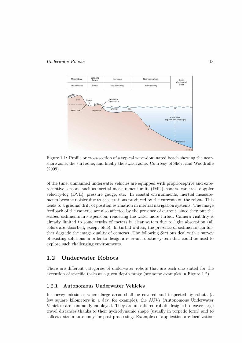
There are different categories of underwater robots that are each one suited for theexecution of specific tasks at a given depth range (see some examples in Figure 1.2).
1.2.1 Autonomous Underwater Vehicles
In survey missions, where large areas shall be covered and inspected by robots (afew square kilometers in a day, for example), the AUVs (Autonomous UnderwaterVehicles) are commonly employed. They are untethered robots designed to cover largetravel distances thanks to their hydrodynamic shape (usually in torpedo form) and tocollect data in autonomy for post processing. Examples of application are localization
14 State of the Art on Tether Management
missions of wreckages of missing airplanes or detailed mosaicking of the seafloor forthe oil and gas industries (Wynn et al., 2014). An important subclass of AUVs arethe underwater gliders, that use small changes in their buoyancy in order to move upand down in the ocean. This vertical displacement generates a forward motion thanksto the use of flying wings and to the control of the vehicle pitch by movable internalballast (usually battery packs). Vehicle steering is accomplished either with a rudderor by moving internal ballast to control roll. They are generally used in oceanographyresearch to collect chemical and physical measurements of seawater in ocean samplingmissions that range from hours to weeks or months, with up to hundreds of kilometersof range (Inzartsev and Alexander Pavin, 2009, chap. 26). Since they are deployed formissions of long duration (up to several months) and large displacement (hundreds ofkilometers), their localization is less accurate than other AUVs during the cyclic divingperiod.
(a) (b)
(c) (d)
Figure 1.2: Some examples of French underwater robots. (a) the AUV A9 from ECArobotics. (b) the AUV glider Sea-Explorer from Alseamar. (c) Victor 6000, an Ifre-mer work-class ROV dedicated to scientific ocean research in deep waters. (d) theobservation-class mini-ROV observer from Subseatech.
1.2.2 Remotely Operated Vehicles
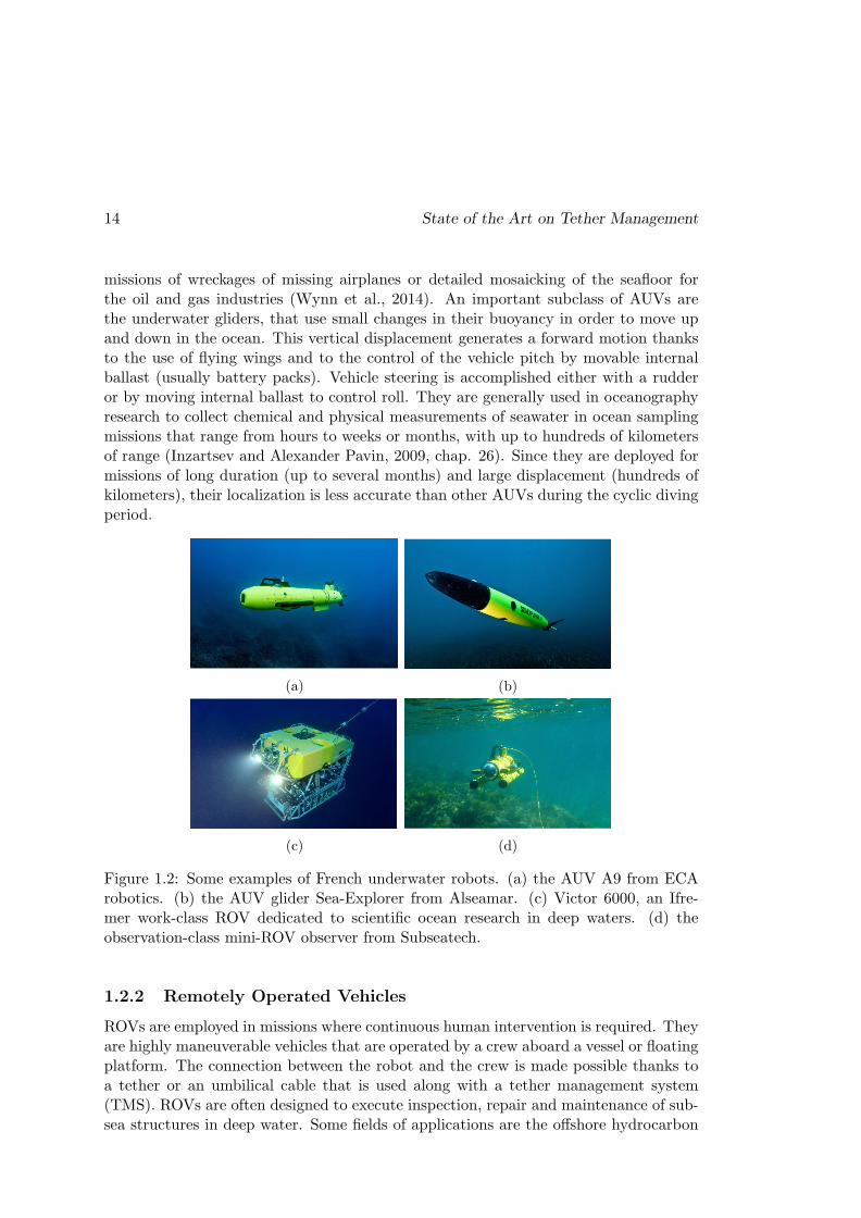
ROVs are employed in missions where continuous human intervention is required. Theyare highly maneuverable vehicles that are operated by a crew aboard a vessel or floatingplatform. The connection between the robot and the crew is made possible thanks toa tether or an umbilical cable that is used along with a tether management system(TMS). ROVs are often designed to execute inspection, repair and maintenance of sub-sea structures in deep water. Some fields of applications are the offshore hydrocarbon
Underwater Robots 15
extraction and the scientific research studying deep sea ecosystems and archaeolog-ical sites. There are three main categories of ROVs, based on the vehicle size andcapabilities (Christ and Wernli Sr, 2013):
1. Work class ROVs: Vehicles in this category are generally heavy electrome-chanical machines (over 1000 kg). These robots are used to execute maintenanceand construction tasks of huge underwater structures, typically in the oil and gasindustry or in the heavy civil engineering. Due to the necessity of large amountsof force, the vehicle propellers and manipulators are hydraulically powered. Theyare designed to be deployed in waters deeper than 3000 meters. This deep depthcan be achieved thanks to bulky pressure housings that protect the whole systemfrom high pressure. The size and weight of the vehicle implies that they have tobe deployed from large surface vessels with a specific launch and recovery system(LARS) that looks like a crane. In such operations, the amount of exposed cableis so important that a dedicated tether management system (TMS) is requiredto reduce the disturbances generated by the cable on the robot.
2. Mid-sized ROVs: These vehicles weigh from 100 kg up to 1000 kg. They aredesigned to operate in intermediate depths around 1000 meters, being thus morecompact than the work-class ROVs. They are also generally all-electric vehicles(powering locomotion and sensors) with some hydraulic power for the operationof manipulators. Their missions are similar to work-class ROVs, but operatingat lower depths. They also need to be deployed by a LARS and depending ontheir weight and size, smaller surface vessel and fewer crew members are needed,reducing the operation costs.
3. Observation class ROVs: These robots go from the smallest vehicles to thosewighting 100 kg. They are employed in depths lower than 300 meters. Theyare completely electric machines, DC-powered and much less expensive than theother class of ROVs. They are mainly used for observation missions, for inspectionin offshore industry or for oceanographic and archaeological research. Some ofthem are equipped with electrical manipulator arms to perform dexterous tasks(as biological sampling or archaeological excavation). The arm is equipped withspecific tools such as vacuum gripper, brushes or pliers. The lighter vehicles withinthis class are typically hand launched, and can move freely from the surface withmanual handling of the tether.
In this thesis we focus on the use of mini-ROVs, a sub-category of the observationclass. Usually, mini-ROVs are used in places such as a sewer, pipeline, small cavities,very shallow waters and other cluttered spaces. One person can carry the completeROV system (robot and tether) up to a small boat, deploy it and complete the jobwithout outside help. A remarkable advantage of using mini-ROVs is the low cost ofthe operation (Wernli and Christ, 2009). Actually, the reduction of the operating costsis a main goal in underwater robotics research, since the mobilization of huge structures(host ship and crew) represents an important part of the mission charges. In the cases
16 State of the Art on Tether Management
of survey or light manipulation missions, mini-ROVs can be used in cooperation withUSVs (unmanned surface vessels), as described in Shimono et al. (2015); Conte et al.(2018). This kind of system eliminates the need of an on-board crew, that can inreturn operate onshore via a radio-link. The reduced costs facilitate the access tounderwater intervention for safety and security operations in civil structures such asports, channels and dams (Molchan, 2005), as well as for many other scientific domains,such as oceanography (Smolowitz et al., 2015) and archaeological (L’Hour and Creuze,2016) research. Normally, in such fields, the tasks of surveying and sampling are madeby a professional diver. However, the operating complexity, medical problems, highcosts and limited time of diving have led to the development of alternative roboticsolutions in which the use of mini-ROVs plays a relevant role. These robots are operatedup to some hundreds of meters away from the surface vessel.
At these distances, important dragging forces are applied to the tether which con-siderably disturbs the motion of the mini-ROV. Therefore, even for these small robots,a system that could manage the tether is required. Besides, this system should be ableto detect or prevent tether entanglement. This necessity is even more important if themini-ROV is deployed in confined or cluttered environments. In order to achieve afunctional tether management for mini-ROV we must have some knwoledge about thetether properties. Another objective is to minimize the forces that the tether applieson the ROV. In the next section we focus on the different types of tether and theirphysical properties.
1.3 Tethers
In order to understand the forces that a tether applies on a mini-ROV, the interactionbetween the robot motion and the cable shape should be modeled. First we will givesome definitions about ROV usual tethers. Secondly we will investigate the influenceof the tether cross-sectional area on the system design and then present some existingcable models.
1.3.1 Utility
ROVs require an electromechanical cable that provides mechanical support, power sup-ply and data exchange with the surface vessel. In work-class and middle-class ROVs,a tether management system (TMS) is needed to regulate the thousands of meters ofcable deployed and disturbances caused by the surface vessel motion. The cable linkingthe surface to TMS is termed the umbilical, while the cable from the TMS to thesubmersible is termed the tether. The umbilical cable is used to reach the operationaldepth while the tether cable allows the ROV to make excursions at that depth for adistance of around a few hundred meters away from the TMS. ROVs of various sizesand categories can use a TMS, with the constraint of having a crane on board the shipthat can move the whole system (robot and TMS) from the deck to the splash zone.
In the case of mini-ROVs, since their operational depth is limited to some hundredsof meters, no TMS is needed and the robot remains in the vicinity of the surface vessel.
Tethers 17
Thus, we will always use the term tether when making reference to a cable linking amini-ROV to a surface vessel, base station or fellow robot. The diameter of the cable isthe dominant factor in overall vehicle drag. Therefore, minimizing cable diameter is animportant part of ROV design and operation. Some advanced ROVs carry their ownpower sources and only require a communication link to the surface vessel through anexpendable fiber-optic cable (Brignone et al., 2015). The umbilical cable is generallysteel jacketed, while the tether cable uses synthetic fibers to maintain the requiredbuoyancy (neutral, slightly negative or positive).
1.3.2 Buoyancy
The tether buoyancy in water is also an important aspect to consider. There are threebuoyancies to consider:
• Positive: when the tether has a lower density than water and therefore rises.
• Neutral: when the tether has the same density than water and therefore remainsin suspension in the water column.
• Negative: when the tether has a higher density than water and sinks.
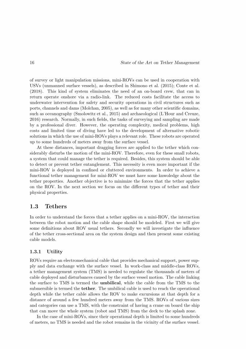
Some examples of tethers are depicted in Figure 1.3 and their physical properties canbe found in Table 1.1.
Which tether to choose depends on the application. For example if the ROV is tooperate on the sea floor it would be preferable to use a neutral or positive tether to keepit from dragging along the sea floor and potentially becoming entangled with objects.A negatively buoyant tether has fewer applications and are commonly employed in deepwater environments, or areas with snagging hazards near the surface of the water, suchas under-ice teleoperations (Bowen et al., 2012; Katlein et al., 2017).
Tether diam. (m) lin. density (kg/m) buoyancy
Fathom 7.6× 10⁻³ 4.3× 10⁻² neutral
Novasub 7.4× 10⁻³ 5.4× 10⁻² negative
µlinx 8.0× 10⁻⁴ 7.0× 10⁻⁴ negative
Table 1.1: Tethers physical properties shown in Figure 1.3: diameter, linear densityand buoyancy in fresh water.
1.3.3 Cross-section
Work class ROVs have power provided in alternating current (AC), which is transmittedthrough the umbilical from the surface vessel to the cage and then from the cage to theROV through the tether. When it reaches the robot, the electrical power is convertedto direct current (DC) to power the electronics. Video and data are often transmittedthrough optical fibers in order to reduce the electromagnetic disturbances caused bythe AC power transmission.
18 State of the Art on Tether Management
outer jacket
Vectranfiber braidstrengthmember
a pair oftwisted shielded
cables2x24 AWG
powerconductors2x0.5 mm2
(a)
outer jacket
Kevlarstrengthfibers
Polyethyleneinner jackets
26 AWGstrandedtwisted pairs
Dacronfiller fiber
(b)
outer jacket
aramid yarn
acrylatecoating
silica clad
silica core
0.8 mm
(c)
Figure 1.3: Some examples of tethers used by mini-ROVs. (a) the tether model DLR-1P20-2C50 from Novasub for power supply and data transfer. (b) the Fathom tetherfrom BlueRobotics that carries four pairs of 26 AWG wire for data exchange. (c) theµlinx 50 OM3 tether from OFS optics is composed of a multimode 50 µm optical fiberfor data transfer.
While mid-sized and work class ROVs use AC current for power transmissionthrough the umbilical and then a combination (AC and DC) along the tether, mostobservation class ROV systems use exclusively DC current for power transmission. Thedelivered power should be sufficient to operate all the electronics and thrusters. Thepropulsion of the vehicle must be powerful enough to overcome its own drag force butalso that of the tether. Therefore, the tether length may be critical in determining theavailable power for vehicle displacement. A too long tether can generate too much dragforce that would lead to the vehicle immobilization. In addition, long cables also de-creases the available power due to losses caused by Joule effect. The maximum tetherlength for a given power requirement is a function of the voltage, the size and theresistance of the conductor:
P =U2A
ρL(1.1)
where P is the delivered power, U is the voltage, A is the cross-sectional area of theconductor, ρ is its electrical resistivity and L is the tether length. The maximum rangeof the robot is hence limited by a maximum tether length above which the most partof the delivered power is dissipated in heat through the cables (see Figure 1.4). In the

Tethers 19
case of mini-ROVs, this limitation is even more restrictive due to the low voltage of theembedded electronic devices and thrusters (about 12 volts).
Figure 1.4: The maximum tether length for a given voltage V and a given cable cross-sectional area A. Extracted from Christ and Wernli Sr (2013).
The ROV’s tether is typically the highest drag item on the ROV system. The dragproduced by the ROV is based upon the following formula (Christ and Wernli Sr, 2013):
Dtether =σAtLtV
2t Cdt
2(1.2)
where σ is the ratio between the density of water and the gravitational acceleration;Cd is the non-dimensional drag coefficient, ranging from 0.8 to 1 based on the cross-sectional area of the tether profile (A); L is the tether length; V is the tether relativevelocity with respect to water and AL is the characteristic area on which Cd is applied.The robot drag is calculated in the same way and the system total drag is then:
Dtotal =σAtLtV
2t Cdt
2+σAvLvV
2v Cdv
2(1.3)
The total drag increases proportionally with the tether length for a given cross-section (see Figure 1.5).

20 State of the Art on Tether Management
Figure 1.5: Tether drag versus tether length. Extracted from Christ and Wernli Sr(2013).
The demanded power needed to compensate the total drag is calculated as follows:
PD = DvVv +DtVt. (1.4)
It is linearly proportional to the tether length and to the cube of the velocity, whichmeans that for a given maximum velocity, the longest the cable, the highest the powerneeded to displace the vehicle and tether. From equation 1.1, in order to increase theavailable power, for a given length, we have to increase the cable cross-sectional area,which directly impacts the power needed to compensate the dragging force. Then, atrade-off has to be found between the maximum velocity and maximum reach of thesystem with reasonable power requirements.
1.3.4 Models
In order to be able to manage the motion of a cable that is freely deployed in seawaterin presence of currents, tides and waves, we need to estimate the tether shape. To doso, there are two solutions. The first one is to add sensors at the attachment points andall along the cable, as is the case of Smart Tethers (Frank et al., 2013). These tethersare designed to offer a real-time GPS location of the ROV using non-acoustic tethershape measurements. Several nodes are embedded along the tether cable to providelocal orientation and depth. This information is used to estimate the current tethershape and ROV heading and position with a 10-30 Hz refresh rate. Similarly, opticalfiber may also be used to give visual feedback of the tether shape (Childers et al., 2010).
The second solution, if we consider a non-equipped tether, is to use a parametrizedmodel of the cable. A cable can be physically described by its attachment points, across-sectional area, length, linear density and axial, flexural and torsional rigidities.Cable modeling is useful to help to understand cabled structure statics and dynamics aswell as to design carrying cables for suspension bridges, intercontinental communicationcables, cable-driven robots, and to design umbilicals and tethers providing power supplyand data transfer for teleoperated robots.
The most complete cable model in the air relies on the Irvine equation (Irvine,1981) that takes into account both the elasticity and the deformation of the cable due

Tethers and Deformable Objects Management 21
to its own mass and has been shown to be very realistic (Merlet, 2018c). This modelassumes that the cable lies in a vertical plane, the cable plane, and is therefore a 2Dmodel. However, this model is complex to use in a kinematic analysis (Merlet, 2018c).In Howell (1992), the problem of low-tension cables is investigated for underwater ap-plications and several models that consider or ignore the cables elasticity are studied.The equations of motion for a cable are nonlinear and strongly coupled for completecable models. Other numerical models of underwater umbilicals and tether were ad-dressed in Buckham (2003); Buckham et al. (2003), where a tether lumped mass modelis addressed. If we consider inextensible (nonelastic), perfectly flexible and subjected toa uniformly distributed load, a widely spread cable model is the catenary curve (Irvine,1981). Analytic solutions are difficult to obtain for complete models, and numericalapproximation techniques are often necessary. In the simplified case of a catenary,analytic solutions are available.
In the next section we will see that other simplified models were used for tetherand deformable objects shape control strategies such as parabolas, splines and circlearcs. For real-time robotic control these approximated parametric models have thegreat advantage of speeding up the computational time of the control loop, althoughbeing limited to some environmental and operational assumptions.
1.4 Tethers and Deformable Objects Management
This section focuses on existing strategies of tether management for underwater andmobile robots in general. Since the tether can also be seen as a deformable object, thissection will also address some techniques of deformable objects handling that could beapplied to tether management.
1.4.1 Underwater Applications
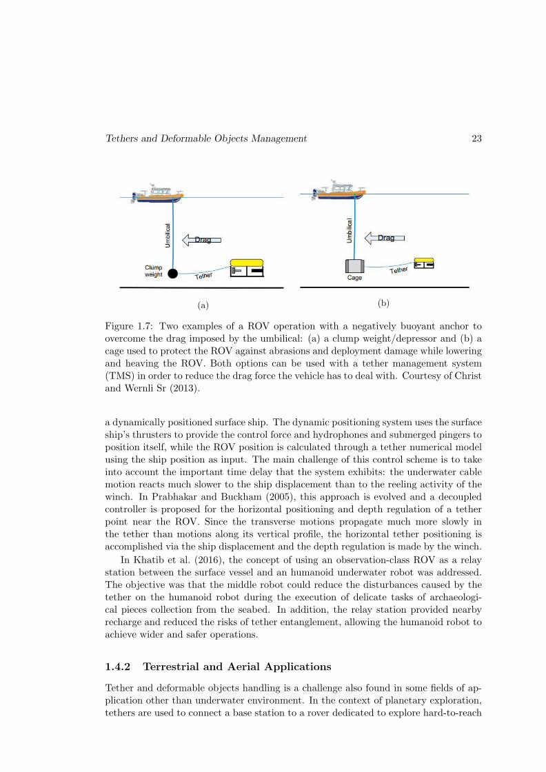
This subsection deals with tether management systems (TMS) that are typically usedfor work-class and middle-class robots. As depicted in Figure 1.6, the TMS is placed atthe junction between the end of the umbilical and the beginning of the tether (Hawkesand Jeffrey, 1987; Abel, 1994). This junction is made by a simple clump/depressorweight or by a vehicle handling system (a protection cage or a top hat mechanism), asit is shown in Figure 1.7.
The use of a clump weight is prevalent in the observation-class category. Theclump weight absorbs the cross-section drag of the current in a passive way, relievingthe submersible of the umbilical drag from the surface to the working depth. Therefore,the ROV only needs to drag a portion of the tether length between the clump weightand the vehicle. Similarly to clump weights, cages also function as a negatively buoyantanchor to overcome the drag imposed by the umbilical, and additionally, they are usedto protect the vehicle against abrasions and deployment damage due to the instabilityof most surface vessels. Clump weights and cages can be used without a TMS forreasons of simplicity. The addition of a TMS is considered by operators as a similarcomplexity of having a second ROV concurrently in the water.

22 State of the Art on Tether Management
LARS
TMSROV
Figure 1.6: Main components for teleoperation in underwater robotics. A remotelyoperated vehicle (ROV), a tether management system (TMS) and a launch and recoverysystem (LARS). Adapted from (Salgado-Jimenez et al., 2010).
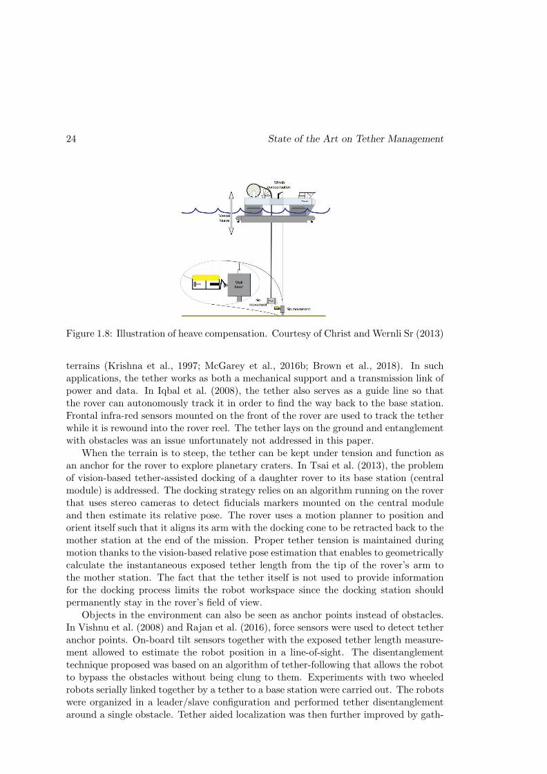
The TMS aims to control the amount of unwound tether between the ROV and acage housing or clump weight. With respect to the umbilical, the amount of unwoundcable can be controlled by a heave compensator system (see Figure 1.8). The objectiveis to reduce the umbilical slackness by reeling in the cable or to unwind additionalcable as the sea dynamics dictates. If these heave dynamics are not compensated forthen the vehicle at the end of the umbilical will not be stable and/or the umbilical canbecome overstressed and damaged. Heave compensation systems can be active (Yanget al., 2008) or passive (Driscoll et al., 2000). With active heave compensation (AHC),motion sensors measure vessel movement along the vessel’s vertical axis and direct theAHC unit to reel in or reel out the cable. With passive heave compensation (PHC),a system of sheaves is used for shortening or lengthening the exposed cable length inconcert with the vessel’s motion. AHC is much more accurate for achieving a constantload position as it works on a position reference frame (rather than weight which hasno direct reference to motion).
In most offshore applications, the ROV umbilical will be handled by a winch systemthat can have a heave compensator embedded to wind/unwind the umbilical followingthe ocean dynamics. The tether connecting the ROV to the cage is handled by the TMS,which increases or decreases the tether length according to the operator’s commands.
Another strategy for tether management more rarely addressed in the literatureis the use of the surface vessel for the dynamic positioning of a control point on thetether in order to reduce the disturbance force exerted on the ROV. In Triantafyllou andGrosenbaugh (1991), a control scheme is proposed to manage an underwater tether from
Tethers and Deformable Objects Management 23
(a) (b)
Figure 1.7: Two examples of a ROV operation with a negatively buoyant anchor toovercome the drag imposed by the umbilical: (a) a clump weight/depressor and (b) acage used to protect the ROV against abrasions and deployment damage while loweringand heaving the ROV. Both options can be used with a tether management system(TMS) in order to reduce the drag force the vehicle has to deal with. Courtesy of Christand Wernli Sr (2013).
a dynamically positioned surface ship. The dynamic positioning system uses the surfaceship’s thrusters to provide the control force and hydrophones and submerged pingers toposition itself, while the ROV position is calculated through a tether numerical modelusing the ship position as input. The main challenge of this control scheme is to takeinto account the important time delay that the system exhibits: the underwater cablemotion reacts much slower to the ship displacement than to the reeling activity of thewinch. In Prabhakar and Buckham (2005), this approach is evolved and a decoupledcontroller is proposed for the horizontal positioning and depth regulation of a tetherpoint near the ROV. Since the transverse motions propagate much more slowly inthe tether than motions along its vertical profile, the horizontal tether positioning isaccomplished via the ship displacement and the depth regulation is made by the winch.
In Khatib et al. (2016), the concept of using an observation-class ROV as a relaystation between the surface vessel and an humanoid underwater robot was addressed.The objective was that the middle robot could reduce the disturbances caused by thetether on the humanoid robot during the execution of delicate tasks of archaeologi-cal pieces collection from the seabed. In addition, the relay station provided nearbyrecharge and reduced the risks of tether entanglement, allowing the humanoid robot toachieve wider and safer operations.
1.4.2 Terrestrial and Aerial Applications
Tether and deformable objects handling is a challenge also found in some fields of ap-plication other than underwater environment. In the context of planetary exploration,tethers are used to connect a base station to a rover dedicated to explore hard-to-reach
24 State of the Art on Tether Management
Figure 1.8: Illustration of heave compensation. Courtesy of Christ and Wernli Sr (2013)
terrains (Krishna et al., 1997; McGarey et al., 2016b; Brown et al., 2018). In suchapplications, the tether works as both a mechanical support and a transmission link ofpower and data. In Iqbal et al. (2008), the tether also serves as a guide line so thatthe rover can autonomously track it in order to find the way back to the base station.Frontal infra-red sensors mounted on the front of the rover are used to track the tetherwhile it is rewound into the rover reel. The tether lays on the ground and entanglementwith obstacles was an issue unfortunately not addressed in this paper.
When the terrain is to steep, the tether can be kept under tension and function asan anchor for the rover to explore planetary craters. In Tsai et al. (2013), the problemof vision-based tether-assisted docking of a daughter rover to its base station (centralmodule) is addressed. The docking strategy relies on an algorithm running on the roverthat uses stereo cameras to detect fiducials markers mounted on the central moduleand then estimate its relative pose. The rover uses a motion planner to position andorient itself such that it aligns its arm with the docking cone to be retracted back to themother station at the end of the mission. Proper tether tension is maintained duringmotion thanks to the vision-based relative pose estimation that enables to geometricallycalculate the instantaneous exposed tether length from the tip of the rover’s arm tothe mother station. The fact that the tether itself is not used to provide informationfor the docking process limits the robot workspace since the docking station shouldpermanently stay in the rover’s field of view.
Objects in the environment can also be seen as anchor points instead of obstacles.In Vishnu et al. (2008) and Rajan et al. (2016), force sensors were used to detect tetheranchor points. On-board tilt sensors together with the exposed tether length measure-ment allowed to estimate the robot position in a line-of-sight. The disentanglementtechnique proposed was based on an algorithm of tether-following that allows the robotto bypass the obstacles without being clung to them. Experiments with two wheeledrobots serially linked together by a tether to a base station were carried out. The robotswere organized in a leader/slave configuration and performed tether disentanglementaround a single obstacle. Tether aided localization was then further improved by gath-
Tethers and Deformable Objects Management 25
ering multiple sensory feedback. In Murtra and Tur (2013), wheel odometry, tetherlength measurements, and an IMU (inertial measurement unit) were used to localizea pipe-inspection robot, where tether length was used to limit uncertainty about thedistance traveled in a pipe. This work was only concerned with localization of the robotand no attempt was made to detect and map tether contact points (i.e., the anchorpoint) within the pipe. In McGarey et al. (2016a) and McGarey et al. (2017), the poseof a tethered robot and the positions of the intermediate tether anchor points wereestimated using tether length, bearing-to-anchor angle, and odometry gathered alongthe trajectory. The objective of this work was the formulation of a tethered simultane-ous localization and mapping (TSLAM) problem whose solution would allow the robotto safely return to its base along an outgoing trajectory while avoiding tether entan-glement. The motivation was to use TSLAM as a building block to aid conventional,camera and laser-based approaches to SLAM, which tend to fail in dark and or dustyenvironments.
Multiple mobile robots can be used for cooperative transportation of large objects,that can be rigid (Huntsberger et al., 2004) or flexible. In Echegoyen et al. (2010), threeterrestrial robots were used to transport a flexible hose modeled by Geometrically ExactDynamic Splines (GEDS). A camera with a global view of the scene was used to detectthe robots and the hose by color segmentation. The leader robot pursued a predefinedtrajectory while the follower-robots’ command velocities were computed from a fuzzy-heuristic local controller. The curvature of the hose segment in front of each robot wasused as a visual feature by the controller that was regulated in order to avoid the hoseof being taut.
Aerial robots were also used in the transportation of flexible cables (Estevez andGrana, 2015; Estevez et al., 2015). The criteria for the transportation was that all therobots should carry the same load. Thus, the hose was modeled by a catenary and theIMU of the robots were used to estimate their relative height, which was regulated bya PID controller with the aim of evenly distribute the hose weight among the robots.
Tethers are used by unmanned aerial vehicles (UAV) for long-term missions withhigh-speed communication between the operator and the robot in an wide range ofapplications, such as robot-assisted search and rescue (Pratt et al., 2008) and coastaland environmental remote sensing (Klemas, 2015). Most published work in the fieldof tethered flight are restricted to the taut tether case. In these systems no tethermanagement is employed while the UAV maintains tension. Otherwise, a winch mech-anism placed in a fixed or mobile base station continuously reels in any slack tetherlength (Nicotra et al., 2017). The dynamics and control of a quadrotor unmannedaerial vehicle connected to a fixed point on the ground via a tether was addressedin Lee (2015). The tether was considered as a collection of an arbitrary number ofrigid links that are serially interconnected via ideal ball joints. The motion equationsof the system (robot and tether) were obtained from Hamilton’s principle. A controllaw based on inertial sensing was designed through feedback linearizion and used theUAV pose with the aim of maintaining a desired tether state (orientation and tension).This control law was evaluated in two numerical examples of station keeping and pre-defined path tracking. A reactive tether management approach, where the tension and

26 State of the Art on Tether Management
departure angle are measured at the winch, showed moderate winch controller resultsthat can be further improved by incorporating knowledge of the UAV position (Zikouet al., 2015). Another work used the measured tether length, tension, and departureangle as a means for non-GPS position estimation of the UAV based on a catenarycable model (Kiribayashi et al., 2017). In Talke et al. (2018), the quasi-static catenarycurve of a hanging tether between an essentially stationary UAV and a small unmannedsurface vehicle (USV) is investigated and characterized. The objective is to develop ina near future a winch controller that could maintain the tether slack and compensatethe USV heave in order to minimize the tether traction and the risk of being in contactwith the water surface. A multi-agent extension of the tethered aerial robot problemwas investigated through numerical simulations in Tognon and Franchi (2015), wherea chain of two flying robots was considered. The goal was to independently control theelevation angles of the two tether segments as well as their internal stress.
Cable management is also an important issue in cable-driven parallel robots (CDPR)domain. In Dallej et al. (2011) and Dallej et al. (2012), a vision-based controller wasintroduced and validated on simulation. The cable model relied on a simplified modelof an inextensible hefty cable in which the profile was considered to be a paraboliccurve. A multi-camera setup allowed to measure the direction of the cable tangents aswell as the pose of a visual target attached to the robot’s mobile platform, whose posewas then controlled through visual servoing. Recently, a novel method for workspaceplanning for a cable-control robot in cluttered environments was introduced (Wang andBhattacharya, 2018). More complex cable models were also considered and their usewas proved to enlarge the workspace border of CDPR (Merlet, 2018a).
1.4.3 Synthesis of Existing Cable Management Strategies
In this Section we will present a short summary of the cable perception and handlingstrategies previously addressed. We will conclude by analyzing which solutions wouldbe adapted to operations with mini-ROVs navigating in the underwater coastal envi-ronment.
1.4.3.1 Passive and Active Cable Management Strategies
The ROV systems are composed of a surface vessel, a linking cable and a teleoperatedrobot. The solutions for tethers and cables management presented in Sections 1.4.1and 1.4.2 are grouped in the following list:
A. Passive management
A1. add an intermediate clump weight: the heave motion of the sur-face vessel is absorbed by a submerged massive body placed at the junctionbetween the umbilical cable and the ROV tether (Christ and Wernli Sr, 2013,chap. 9).
A2. add a passive heave compensator: shock absorbers, drill stringcompensators or more sophisticated hydraulic and mechanical systems of
Tethers and Deformable Objects Management 27
winches (Huster et al., 2009) are used to absorb and dissipate the energygenerated by the ship heave motion.
B. Active management
B1. actuate the tether extremities: winches are used in underwatermissions to compensate heave motion of the vessel and manage the amountof tether between the clump weight and the robot. The winch mechanismcan be placed on the ship (Yang et al., 2008), on the robot (Brignone et al.,2015) or inside the TMS cage (Hawkes and Jeffrey, 1987; Abel, 1994). Theyare also used by cable-driven parallel robots (Dallej et al., 2011, 2012), ter-restrial rovers (Tsai et al., 2013; Vishnu et al., 2008; Rajan et al., 2016) andunmanned aerial robots (Lee, 2015; Talke et al., 2018) to regulate the lengthof exposed cable.
B2. actuate the surface vessel: regulate the ship-robot relative positionin order to reduce the amount of tether deployed to allow the ROV hori-zontal displacement (Triantafyllou and Grosenbaugh, 1991; Prabhakar andBuckham, 2005).
B3. actuate the tether: add an intermediate robot that works as arelay station and is commanded by an onboard operator (Khatib et al.,2016) or use a team of robots that transport together deformable ob-jects (Echegoyen et al., 2010; Estevez et al., 2015; Rajan et al., 2016).
The most simple strategy to reduce the disturbances generated by the cable on therobot is to use a clump weight that absorbs the cable oscillations caused by the heavemotion of the ship (item A1 of the list). This is a passive tether management solutionwhere neither the ship nor the cable are instrumented. This option is commonly used bywork-class and middle-class ROVs that operate in mostly wide and empty environmentsand is therefore not adapted to the type of mission we focus on that use mini-ROVs toexplore coastal underwater environments.
The cable oscillations can be compensated by equipping its extremities with in-telligent winch mechanisms that can either be aboard the surface vessel, embeddedin the robot or submerged at the depth of operation (item B1). When the exposedtether length is controlled aboard the ship it is called heave compensator. When thesystem is submerged and it is commanded by an onboard operator it is called tethermanagement system (TMS). Heave compensator could be an interesting solution fortether management of mini-ROVs. However, a shortcoming of this solution is that themini-ROVs would be limited to explore a zone in the vicinity of the ship since theycannot pull a large amount of cable (over 300 meters). On the other hand, the choice ofadding submerged winch mechanisms is not adapted to coastal zones due to the shal-low depth and to the presence of obstacles in the marine relief such as stones and coralreefs. Finally, equipping the ROV with winches increases its weight, making it bulkier.Moreover, the reeling activity generates non-negligible variation of the mini-ROV massrepartition, affecting its buoyancy and whole dynamics.
28 State of the Art on Tether Management
Other studies proposed to use a combined control scheme that regulates both theship positioning and the amount of deployed tether by the surface winch (item B2 itemof the list). However, the mini-ROVs would remain limited to the exploration aroundthe surface vessel, which is also constrained itself not to get too close to the coast.
1.4.3.2 Classification according to Cable Perception and Modeling tech-
niques
In the case of active tether management, an estimation of the tether state must be com-puted to determine the action the system has to take: reel in/out the tether or move itsextremities, for example. The models used to represent the cable shape vary dependingon the physical properties of the cable and the hypothesis of operation. The sensorsused to perceive the cable and to provide input information for the model computationalso vary depending on the type of robot used and the domain of application.
The list here below summarizes cable handling strategies with respect to the absenceor presence of cable models:
A. Without tether model: the tether shape can be regulated without con-sidering any cable model. This can be done by a human operator, by a passivemechanical system or by an active compensator based on sensory feedback. Unlessotherwise noted, the three subclasses below are related to underwater operations.
A1. teleoperation: human operators can command a tether managementsystems (TMS) reeling in/out the tether based on visual information or onROV-ship relative position estimation (Abel, 1994). Another alternative isto add an intermediate robot that works as a relay station near the mainROV. It was the case of the operations of the underwater humanoid robotOcean One (Khatib et al., 2016).
A2. passive regulation: shock absorbers, string compensators or moresophisticated hydraulic and mechanical winch system can be used to pas-sively absorb the heave motion of the ship and thus reduce the disturbancesgenerated on the umbilical (Huster et al., 2009).
A3. active regulation: the disturbances caused by the ship heave motionon the umbilical can also be compensated by a control unit that managesthe speed of a hydraulic winch from information provided by an inertialmeasurement unit (IMU) (Yang et al., 2008). In the context of planetaryexploration, the exposed tether length was also regulated through activewinches mounted on rovers (Tsai et al., 2013). The tether connected therover to a base station and it was maintained taut during the entire opera-tion. Fiducial markers mounted on the front of the base station allowed therover to estimate its relative pose and then maintain the tether taut duringthe entire operation.
B. With geometric tether models: cables and deformable objects can berepresented by geometric models that may offer regulation parameters to be used
Tethers and Deformable Objects Management 29
in a control loop.
B1. Parabolic curves were used to model the cable profile for cable-drivenparallel robots. In Dallej et al. (2012), a set of cameras was used to estimatethe relative position of the robotic platform and the control winches in orderto regulate the cable length deployed.
B2. Spline curves were used to model a flexible hose that is transportedby a team of terrestrial robots (Echegoyen et al., 2010). A camera observingthe global scene was used to return to the vehicles velocity controllers therobots position and the spline curvature (that represented the hose 1-Ddeformation).
B3. Catenaries were used to model tethers and flexible wires in the contextof unmanned aerial vehicles (UAV) operations. In Estevez and Grana (2015),the relative pose of three simulated quadrotors was regulated so that the hosebeing carried has its weight equally distributed among the robots. In Lee(2015), a control scheme was proposed to manage the shape of a simulatedtether linking an UAV to a grounded anchor point. No winch system wasused and the tether shape was managed through the UAV-anchor relativeposition. In Talke et al. (2018), a tether with known length and attachmentpoints relative position was modeled by catenary curve. The tether waslinking UAV and USV (unmanned surface vessel) prototypes. The catenarymodel was useful to investigate the system robustness to the USV heavemotion in order to minimize the risks of the tether touching the water surface.
C. With tether lumped mass models: more complex numeric schemes arealso used to represent the tether shape in underwater applications (Prabhakarand Buckham, 2005; Triantafyllou and Grosenbaugh, 1991). These approachesare often grounded in the knowledge of the relative position between ship andROV, which implies the use of external acoustic positioning systems. In Eidsvikand Schjølberg (2016), the cable was modeled by finite-elements methods usingBeam equations.
The amount and type of information given by the sensory feedback determines thecable model that will be used. For example, force and angle sensors can be used toregulate the tension and orientation of a cable without necessarily having to resort toan accurate model. Otherwise, vision sensors are preferably used to return informationthat can be easily applied to geometric models of the object in the observed scene.Positioning systems are used in the case of more precise models where the physicalproperties of cables are well-known.
The sensory payload available in a mini-ROV is very restrictive because of its smallsize and its low propulsive power. These robots are mainly used for observation tasksand are, therefore, often equipped with cameras that give visual feedback to the opera-tor, and with an IMU that gives feedback about the robot orientation and that can beused to get a rough location estimation. Since visual sensors are available, representing

30 State of the Art on Tether Management
the cable by parametrized geometric curves sounds a natural choice. That is actuallypart of the solution we investigate in this thesis with the aim of proving the feasibilityof a tether management strategy that allows mini-ROVs to be deployed far away fromthe surface vessel without being limited by an important drag force of a long tether.This will be discussed in the following Section.
1.5 Our Scientific Focus: Vision Servoing of a Pair of
Robots in a Chain of Mini-ROVs
The long term objective of this project is to design an active tether man-
agement solution for mini-ROV missions of long range displacements within
cluttered environments and shallow waters.
We choose to control the tether shape by adding several robots linked togetherall along it. We call this concept the chain of mini-ROVs (see Figure 1.9). Therobots play the role of actuators and change the whole tether shape depending on thesituation at hand. Our strategy is to avoid any contact with obstacles. If the depthis too narrow, it would be better to maintain the tether more taut in order to preventit from dragging on the seabed. Otherwise, if the environment is more spacious, thetether can be more slack in order to give more freedom of motion to the robots.
The robots that compose the chain are compact, lightweight and with a limitedsensory payload. Thus, we choose to investigate the use of the onboard camera toperceive and estimate a parameterized geometric model of the cable. The main focusof this thesis is to manage the tether linking two robots through visual feedback. Theserobots are named leader, for the front vehicle, and follower, for the rear vehicle. Thethesis objective can be therefore summarized by the following question:
How can we manage a tether link between two successive robots, a
leader and a follower, within the chain through visual sensory feed-
back?
The proposed chain of mini-ROVs will operate under the set of assumptions listedbelow:
A.1.1 the maximum distance between robots is about 10 meters;
A.1.2 the robots can navigate at slightly different depths (difference less than 5 meters,depending on the tether length);
A.1.3 the roll and pitch motion of the robots are mechanically stabilized or regulatedat low level to keep the vehicle horizontal;

Our Scientific Focus: Vision Servoing of a Pair of Robots in a Chain of Mini-ROVs 31
A.1.4 the robots are equipped with a frontal and/or a rear camera that films the tether;
A.1.5 each robot within the chain must manage the tether segment preceding it;
A.1.6 the leader robot should not manage any portion of the tether, being free to exploreits surroundings and execute other tasks;
A.1.7 the leader robot may be outside the follower camera field of view, but a portionof the tether is always visible.
A.1.8 the tether is detectable in the camera image flow;
A.1.9 the tether linking both robots is negatively buoyant and the tether plane remainsin the vertical. The tether lowest point is always situated between both robots;
10 m
0.70 m
Follower Leader
FOCUS OF THE THESIS
2000 m
Figure 1.9: A chain of N compact tethered robots used to explore shallow waters.The thesis focuses on the shape control of the tether link between the first two robots,namely the leader and its immediate follower. The robots that compose the chain arelight-weight mini-ROVs equipped with a frontal and rear cameras and an IMU.
32 State of the Art on Tether Management
The maximum distance between the robots is limited because the modeling errorswould be propagated over a too long length of tether and then affect our managementstrategy. A camera mounted on the front of the robot will be used to give real-timeinformations about the current tether shape. The camera is supposed to be near thetether attachment point on the robot so that at least a portion of the tether can becaptured all along the mission. This also gives more freedom of motion to the leaderrobot that is not required to be in the field of view of the follower.
As depicted in Figure 1.10, the tether management strategy we proposed can bedecomposed into three main steps. First, the tether is detected in the camera image.Secondly, the detected points are used to estimate a parametrized geometric modelthat fits the tether observed shape. Third, the current tether parameters are entered ina control loop that will displace the tether attachment points so that a desired shapeof the tether is reached. Actually, the tether desired shape is obtained through theregulation of robots relative pose. Both robots could enter in the control loop, butwe took the choice of leaving the leader robot free to move in the environment andexecute other tasks. The follower robot, in turn, will be in charge of moving itself inorder to regulate the tether shape. Each step mentioned above will be developed in thefollowing three Chapters of this document, as presented in right side of Figure 1.10.
Chapter 2:system modeling
the tether and robot models
are introduced
detect thetether
tetherdesiredshape
calculate variationof tether-shape
features
estimate thecurrent shape of
the tether
move followerrobot to reachdesired shape
Chapter 3 Chapter 4
START
Chapter 3:tether perception
the proposed method for
tether perception and shape
estimation is introduced
Chapter 4:tether shape control
the proposed method for
tether shape control is
developed
Chapter 5:Conclusions
concluding remarks are
given and work perspectives
are analyzed
Figure 1.10: Left: simplified algorithm chart flow of the proposed vision-based tethershape control scheme. Right: short presentation of the following Chapters content.
Chapter 2
System Modeling
This Chapter presents the model of the tether used and the robotic system composed oftwo underwater robots linked together by the tether, which is under study in this thesis.This set is the initial portion of the chain of tethered robots presented in the previousChapter. The robots do not have the same task in this system: one is the leader, andhas as main task the exploration of its surroundings; the other is the follower, behindthe leader, whose main task is the control of the tether shape in order not to hamperthe leader movements. The follower robot should manage the tether shape primarilyusing its own sensory feedback. In this thesis, the objective is to use the tether as itis, and not considering additional sensors that could equip the tether to obtain sensoryfeedback on its current shape. The Chapter is organized in three parts. The first partdeals with the catenary equations, the second part presents the model of the robots andthe last part gives the relation between the kinematics of the robots and the kinematicsof the attachment points.
2.1 Tether Model
The underwater tether we use in this work is slightly negative buoyant, which is fre-quently the case of tethers and umbilicals that transfer power. They are used in main-tenance, survey (see Section 1.3.2) and archaeological missions (Khatib et al., 2016).We assume that our tether is a perfectly inextensible and flexible cable with a constanttransversal section and constant linear density. From these assumptions, we choose tomodel the tether as a catenary.
2.1.1 Catenary Equation
The catenary curve is the shape of a perfectly flexible, inextensible hanging cablethat is subject to uniform load distribution along itself and that is supported at itsextremities (Johnston et al., 2009).
Figure 2.1 presents a scheme of a hanging cable attached at points P1 and P2.The cable lowest point, P0, is supposed to be at the center of the coordinate frame
33
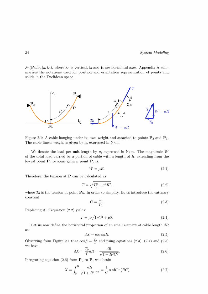
34 System Modeling
F0(P0, i0, j0,k0), where k0 is vertical, i0 and j0 are horizontal axes. Appendix A sum-marizes the notations used for position and orientation representation of points andsolids in the Euclidean space.
T
W = µR
T0
W = µRT
P1
P0
P P
R
dZ
βdR
T0
dX
R
P2
k0
i0
F0
Figure 2.1: A cable hanging under its own weight and attached to points P2 and P1.The cable linear weight is given by µ, expressed in N/m.
We denote the load per unit length by µ, expressed in N/m. The magnitude Wof the total load carried by a portion of cable with a length of R, extending from thelowest point P0 to some generic point P, is:
W = µR. (2.1)
Therefore, the tension at P can be calculated as
T =√T 20 + µ2R2, (2.2)
where T0 is the tension at point P0. In order to simplify, let us introduce the catenaryconstant
C =µ
T0. (2.3)
Replacing it in equation (2.2) yields:
T = µ√1/C2 +R2. (2.4)
Let us now define the horizontal projection of an small element of cable length dRas:
dX = cosβdR. (2.5)
Observing from Figure 2.1 that cosβ = T0
Tand using equations (2.3), (2.4) and (2.5)
we have
dX =T0TdR =
dR√1 +R2C2
. (2.6)
Integrating equation (2.6) from P0 to P, we obtain
X =
∫ R
0
dR√1 +R2C2
=1
Csinh−1 (RC) (2.7)

Tether Model 35
that can be rewritten as
R =1
Csinh (CX) , (2.8)
which is the geometric expression of the catenary cable half-length.
We can now write that:
dZ = tanβdX. (2.9)
Observing from Figure 2.1 that tanβ = WT0
and using equations (2.1), (2.3), (2.8) and(2.9), we have:
dZ = sinh (CX) dX. (2.10)
Integrating from P0 to P we obtain
Z =
∫ X
0sinh (CX) dX, (2.11)
which reduces to the equation of the catenary cable in the coordinate frame F0 centeredat the lowest point of the catenary, namely P0:
Z =1
C[cosh (CX)− 1] . (2.12)
2.1.2 Catenary Parameter
The catenary parameter C depends on the height difference between attachment points∆H, the cable slackness H and the cable total length L. Figure 2.2 depicts the notationused for the catenary model.

36 System Modeling
H +∆H
∆H
H
P0
k0
i0
D D ∆D
R R
F0
P1
P2
(a)
H +∆H
∆H
H
P0
k0
i0
D D ∆D
R R
F0
P1
P2
(b)
Figure 2.2: Illustration of a catenary with attachment points P2 and P1, and lowestpoint P0. (a) an example of catenary with ∆H > 0. (b) an example of catenary with∆H < 0.
In order to calculate the catenary parameter C as a function of the H, ∆H and Lwe express that the attachment points belong to the catenary and that the total lengthof the catenary is constant. Knowing that the coordinates of the attachment points inframe F0 are 0P2 = [−D, 0, H]T and 0P1 = [D+∆D, 0, H+∆H], we obtain, thanksto equation (2.12), that:
H =1
C[cosh(CD)− 1] and (2.13)
H +∆H =1
C[cosh(C(D +∆D)− 1] . (2.14)
Using equation (2.8) we can calculate the total length of the catenary:
L =1
C[sinh(C(D +∆D)) + sinh(CD)] . (2.15)
The analytical solving of this equation leads to a second order equation for C. Oneof the solutions is a catenary where the lowest point is between the cable attachmentpoints and therefore belongs to the cable. The other solution is a catenary where thelowest point does not belong the cable.

Tether Model 37
Appendix B gives the details of the calculation of the catenary parameter C, whoseexpression related to the lowest point belonging to the catenary is:
C =2
L2 − (2H +∆H)2
(2H +∆H + 2L
√H
H +∆H
L2 −∆H2
)(2.16)
which can be rewritten as:
C = 2Cn
Cd
= 22H +∆H + 2L
√H H+∆H
L2−∆H2
L2 − (2H +∆H)2(2.17)
In the case where the attachment points are at the same height, ∆H = 0, and weobtain the following expression for C:
C =2H
R2 −H2, (2.18)
where R is the catenary half-length.
2.1.3 Catenary Parameter Constraints
The conditions of study of the catenary relative to cable length L, slackness H anddifference of attachment points height ∆H are:
H > 0 (2.19)
H +∆H > 0 (2.20)
2H +∆H < L. (2.21)
These inequalities ensure the validity of equation (2.17), where the term below thesquare root must be positive, as well as the denominator.
Equations (2.19) and (2.20) state that the catenary lowest point is between theattachment points. If ∆H is positive (see Figure 2.2a), the cable should be long enoughto cumulate twice the slackness length H and the difference of height ∆H. The limitcase, H = 0, is when the attachment point P2 is the lowest point of the catenary. If∆H is negative (see Figure 2.2b), the slackness H should be greater than the differenceof height so that the catenary lowest point still remains between the attachment points.The limit case, H + ∆H = 0, is when the attachment point P1 is the lowest point ofthe catenary.
The inequalities (2.21) ensures that parameter C remains positive which means thatthe catenary is not degenerated. The degenerated case, L = 2H + ∆H, occurs whenboth attachment points and the lowest point are on the same vertical.
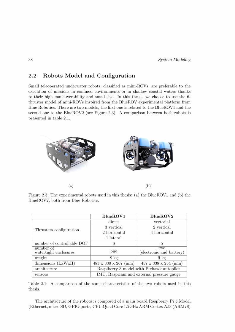
38 System Modeling
2.2 Robots Model and Configuration
Small teleoperated underwater robots, classified as mini-ROVs, are preferable to theexecution of missions in confined environments or in shallow coastal waters thanksto their high maneuverability and small size. In this thesis, we choose to use the 6-thruster model of mini-ROVs inspired from the BlueROV experimental platform fromBlue Robotics. There are two models, the first one is related to the BlueROV1 and thesecond one to the BlueROV2 (see Figure 2.3). A comparison between both robots ispresented in table 2.1.
(a) (b)
Figure 2.3: The experimental robots used in this thesis: (a) the BlueROV1 and (b) theBlueROV2, both from Blue Robotics.
BlueROV1 BlueROV2
Thrusters configuration
direct vectorial3 vertical 2 vertical
2 horizontal 4 horizontal1 lateral
number of controllable DOF 6 5number ofwatertight enclosures one
two(electronic and battery)
weight 8 kg 9 kg
dimensions (LxWxH) 483 x 330 x 267 (mm) 457 x 338 x 254 (mm)
architecture Raspiberry 3 model with Pixhawk autopilot
sensors IMU, Raspicam and external pressure gauge
Table 2.1: A comparison of the some characteristics of the two robots used in thisthesis.
The architecture of the robots is composed of a main board Raspberry Pi 3 Model(Ethernet, micro SD, GPIO ports, CPU Quad Core 1.2GHz ARMCortex A53 (ARMv8)

Robots Model and Configuration 39
Broadcom BCM2837 64bit, 1GB of RAM), which is connected via USB to a generalpurpose microcontroller, namely a Pixhawk autopilot microcontroller that was designedfor aerial drones. The microcontroller has the following internal sensors: a 3-axisaccelerometer and gyroscope (Invensense MPU6000), a 3-axis gyroscope (ST MicroL3GD20H), a 3D e-compass (ST Micro LSM303D) and a barometer (MEAS MS5611).
Both robots are equipped with an external pressure sensor (the Bar30 model fromBlueRobotics) that is connected to the Pixhawk and used to measure water pressure.The Pixhawk controls the six ESCs (electronic speed controllers) that manage the powerand rotation velocity commands sent to the thrusters. Each robot is also equippedwith a Raspberry Pi Camera. The onboard computer communicates with a remoteworkstation via a Fathom-X Tether Interface that provides robust high-speed Ether-net connection. The tether attached to the robot only provides data exchange withthe workstation. The power is delivered by an embedded battery (a LiPo 3S 11.1V5000mAh) that ensures an average autonomy of 1 hour. A schematic overview of therobot components is presented in Figure 2.4.
powerdata
Legend:
control/sensorsmessages
workstationonboardcomputer
micro-controller
electronicspeed
controller(ESC)
camerapressuresensor
thrusters
power
networkinterface
watertight enclosure
Figure 2.4: A scheme presenting the components of the BlueROVs. The watertightzone is delimited by the dashed rectangle.
2.2.1 Thruster Configuration and Allocation Matrix
The main difference between the two models is the thruster configuration: the BlueROV1has a direct thrusters configuration and the BlueROV2 has a vectored thrusters con-figuration.
Figure 2.5 presents, for both robots, a scheme containing the camera and thrusterspositions and orientations. We note Fr(Pr, ir, jr,kr) the coordinate frame linked torobot r. Pr is the center of the robot, ir, jr, kr are respectively the robot’s longitudinal,lateral and vertical axes. For the BlueROV1, Pr is at the middle of the segment linking
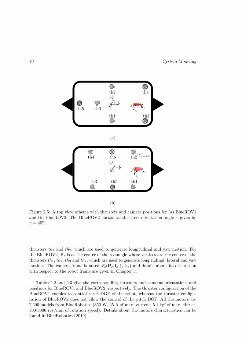
40 System Modeling
th4
th3th1
th6
th2
th5
Fr
jr
irFc
ickckr
jc
(a)
th1th3 th5
th4 th6
kc
ic
Fc
Fr
jrir
krjc
th2 γ = 45
(b)
Figure 2.5: A top view scheme with thrusters and camera positions for (a) BlueROV1and (b) BlueROV2. The BlueROV2 horizontal thrusters orientation angle is given byγ = 45.
thrusters th1 and th2, which are used to generate longitudinal and yaw motion. Forthe BlueROV2, Pr is at the center of the rectangle whose vertices are the center of thethrusters th1, th2, th3 and th4, which are used to generate longitudinal, lateral and yawmotion. The camera frame is noted Fc(Pc, ic, jc,kc) and details about its orientationwith respect to the robot frame are given in Chapter 3.
Tables 2.2 and 2.3 give the corresponding thrusters and cameras orientations andpositions for BlueROV1 and BlueROV2, respectively. The thruster configuration of theBlueROV1 enables to control the 6 DOF of the robot, whereas the thruster configu-ration of BlueROV2 does not allow the control of the pitch DOF. All the motors areT200 models from BlueRobotics (350 W, 25 A of max. current, 5.1 kgf of max. thrust,300-3800 rev/min of rotation speed). Details about the motors characteristics can befound in BlueRobotics (2019).
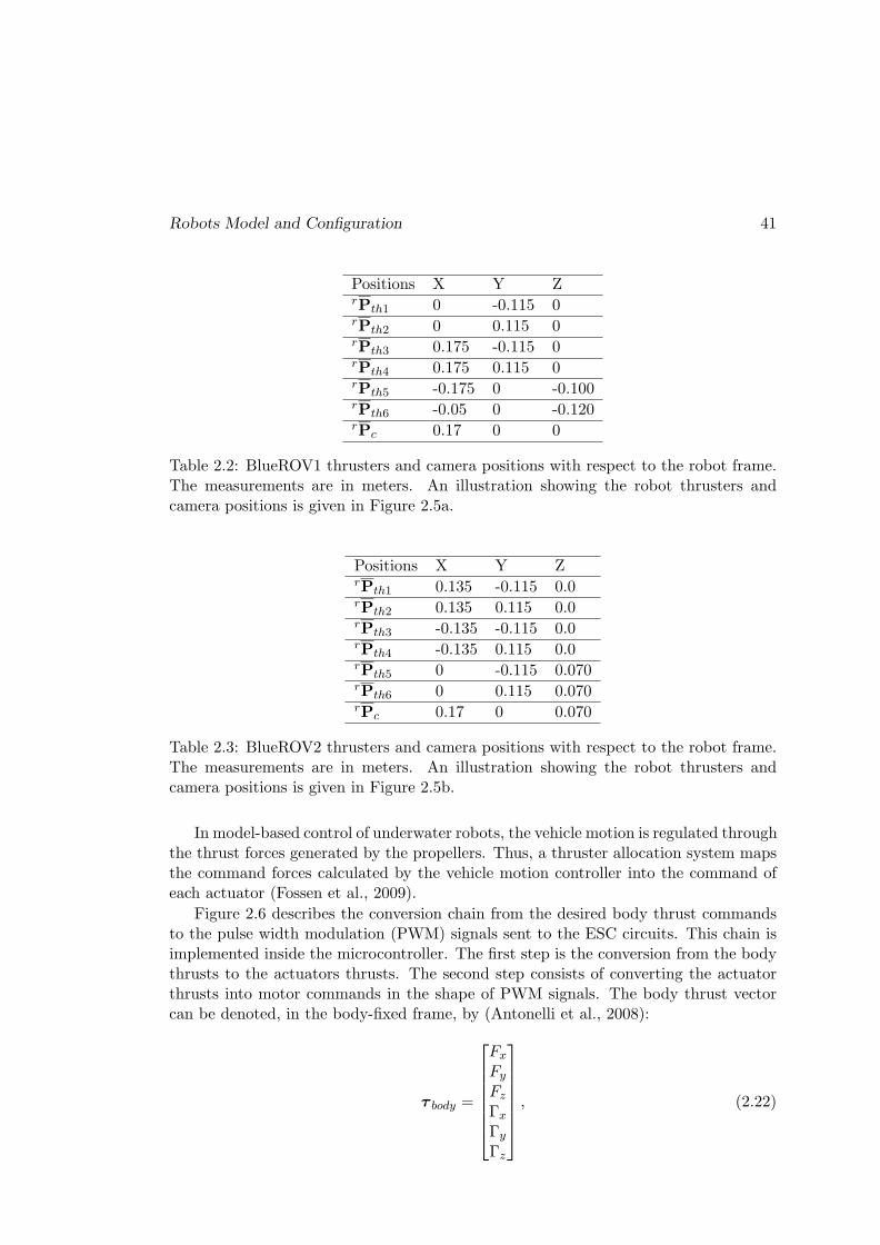
Robots Model and Configuration 41
Positions X Y ZrPth1 0 -0.115 0rPth2 0 0.115 0rPth3 0.175 -0.115 0rPth4 0.175 0.115 0rPth5 -0.175 0 -0.100rPth6 -0.05 0 -0.120rPc 0.17 0 0
Table 2.2: BlueROV1 thrusters and camera positions with respect to the robot frame.The measurements are in meters. An illustration showing the robot thrusters andcamera positions is given in Figure 2.5a.
Positions X Y ZrPth1 0.135 -0.115 0.0rPth2 0.135 0.115 0.0rPth3 -0.135 -0.115 0.0rPth4 -0.135 0.115 0.0rPth5 0 -0.115 0.070rPth6 0 0.115 0.070rPc 0.17 0 0.070
Table 2.3: BlueROV2 thrusters and camera positions with respect to the robot frame.The measurements are in meters. An illustration showing the robot thrusters andcamera positions is given in Figure 2.5b.
In model-based control of underwater robots, the vehicle motion is regulated throughthe thrust forces generated by the propellers. Thus, a thruster allocation system mapsthe command forces calculated by the vehicle motion controller into the command ofeach actuator (Fossen et al., 2009).
Figure 2.6 describes the conversion chain from the desired body thrust commandsto the pulse width modulation (PWM) signals sent to the ESC circuits. This chain isimplemented inside the microcontroller. The first step is the conversion from the bodythrusts to the actuators thrusts. The second step consists of converting the actuatorthrusts into motor commands in the shape of PWM signals. The body thrust vectorcan be denoted, in the body-fixed frame, by (Antonelli et al., 2008):
τ body =
Fx
Fy
Fz
Γx
Γy
Γz
, (2.22)

42 System Modeling
where (Fx, Fy, Fz) and (Γx,Γy,Γz) are, respectively, the components of the resultantforces and moments acting on the center of the vehicle, namely Pr. The actuator thrustvector can be denoted by:
τ actuators =
Fth1
Fth2
Fth3
Fth4
Fth5
Fth6
, (2.23)
where Fthiis the thrust force generated by the thruster thi.
thrusterallocationmatrixinversion
bodythrust
conversion fromactuator thrusts
to motorscommandvelocity
actuatorthrust
ESC
motorscommands(PWM)
motorsmicrocontroller
Figure 2.6: A block diagram illustrating the low level thrust conversion from the vehicledesired body thrust to the PWM commands sent to the motors. The steps implementedin the robot micro-controller are surrounded by a black dashed line.
The relation between τ body and τ actuators can be expressed as (Creuze, 2014):
τ body = TWτ actuators, (2.24)
where T is called the thruster allocation matrix and W is a weighting matrix thattakes into account the thrusters specificities. As the thrusters are all the same for theBlueROVs, we have W = I6×6.
The thruster allocation matrix is given by:
T =
[u1 · · · ui · · · un
rPth1× u1 · · · rPthi
× ui · · · rPthn× un
](2.25)
where rPthiis the thruster thi position with respect to the robot center, and ui is the
unit vector giving the thrust direction of thruster thi. The total number of thrustersis n.
For the BlueROV1 the allocation matrix is given by
TBR1 =
1 1 0 0 0 00 0 0 0 0 −10 0 1 1 1 00 0 −dY dY 0 −dZ6
0 0 −dX −dX dX 0dY −dY 0 0 0 dX6
, (2.26)

Robots Model and Configuration 43
where dX = 0.175m, dY = 0.115m, dX6= 0.050m and dZ6
= 0.175m (see table 2.2).The inverse matrix is given by:
T−1BR1 =
0.5dX6
2dY0 0 0 1
2dY
0.5 −dX6
2dY0 0 0 − 1
2dY
0dZ6
2dY0.25 − 1
2dY− 1
4dX0
0 − dZ6
2dY0.25 1
2dY− 1
4dX0
0 0 0.5 0 12dX
0
0 −1 0 0 0 0
. (2.27)
The motors configuration of the BlueROV1 allocates only one motor – thruster 6 –for the lateral motion. As a consequence, the single lateral thrust will also generateroll and yaw motion, since the motor is not positioned at center of the robot. Incase the positioning of the motor is not accurate, it can generate disturbing roll andyaw motion. Moreover, the single lateral thruster is also responsible for a disturbingpitch motion because the propeller rotation exerts a torque on the robot body frame,according to the action/reaction principle. These disturbances could be compensatedby adding counteracting roll/pitch/yaw thrust terms that depend on the lateral thrust.The compensation matrix that could be applied after the TBR1 matrix is:
CBR1 =
1 0 0 0 0 00 1 0 0 0 00 0 1 0 0 00 δx 0 1 0 00 δy 0 0 1 00 δz 0 0 0 1
, (2.28)
where δx, δy and δz have to be determined empirically. The equation (2.24) can behence rewritten as:
τ body = CBR1TBR1τ actuators. (2.29)
If we want to control the actuator, we need to inverse the previous equation to get:
τ actuators = (CBR1TBR1)−1
τ body, (2.30)
where
(CBR1TBR1)−1 =
0.5−δz+dX6
2dY0 0 0 1
2dY
0.5 −−δz+dX6
2dY0 0 0 −1
2dY
0δy4dX− −δx−dZ6
2dY0.25 −1
2dY−14dX
0
0δy4dX
+−δx−dZ6
2dY0.25 1
2dY−14dX
0
0−δy2dX
0.5 0 12dX
0
0 −1 0 0 0 0
. (2.31)

44 System Modeling
The values of δx and δz are used to compensate the inaccuracies of measurements ofdX6
and dZ6, while δy is mainly used to compensate the disturbing pitch motion due
to the propeller rotation of thruster 6.
For the BlueROV2 the allocation matrix is given by:
TBR2 =
cos γ cos γ − cos γ − cos γ 0 0sin γ − sin γ sin γ − sin γ 0 00 0 0 0 1 10 0 0 0 −dY dYd⊥ −d⊥ −d⊥ d⊥ 0 0
, (2.32)
where γ is the angle between ir and the thruster direction axis, d⊥ = dXsγ + dY cγ,dX = 0.135m, dY = 0.115m, sγ = sin γ and cγ = cos γ (see table 2.3). The body thrustvector is now given by:
τ body =
Fx
Fy
Fz
Γx
Γz
, (2.33)
since the pitch motion is not controllable. The allocation matrix can be decoupled intotwo submatrices, one that deals with longitudinal, lateral and yaw motion, and theother one that deals with vertical and roll motion:
Fx
Fy
Γz
=
cos γ cos γ − cos γ − cos γsin γ − sin γ sin γ − sin γd⊥ −d⊥ −d⊥ d⊥
Fth1
Fth2
Fth3
Fth4
= M
Fth1
Fth2
Fth3
Fth4
(2.34)
[Fz
Γx
]=
[1 1−dY dY
] [Fth5
Fth6
](2.35)
The equation (2.35) can be directly inverted to get
[Fth5
Fth6
]=
[0.5 −0.5/dY0.5 0.5/dY
] [Fz
Γx
]. (2.36)
The matrix M is not square. However, since γ = 45, matrix MMT is invertible and wecan use the Moore-Penrose pseudo-inverse to express the actuator vector as a functionof the desired body thrust vector:
Fth1
Fth2
Fth3
Fth4
= M+
Fx
Fy
Γz
(2.37)
with M+ = MT (MMT )−1.
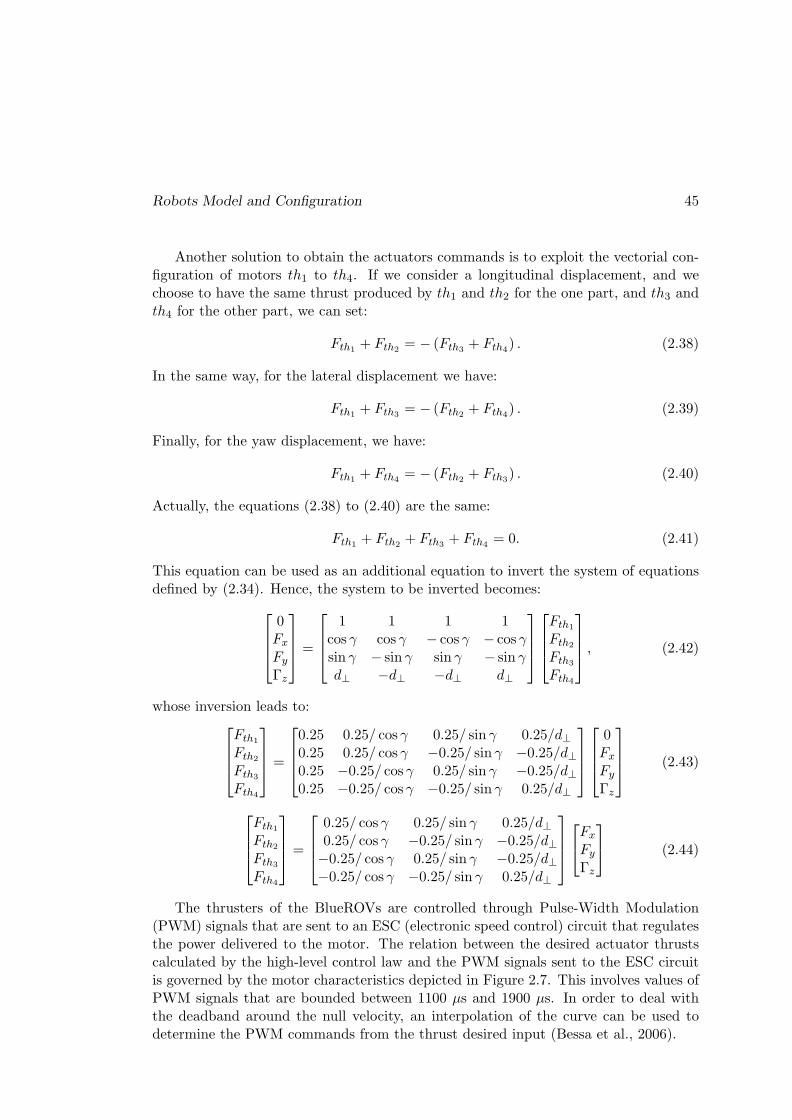
Robots Model and Configuration 45
Another solution to obtain the actuators commands is to exploit the vectorial con-figuration of motors th1 to th4. If we consider a longitudinal displacement, and wechoose to have the same thrust produced by th1 and th2 for the one part, and th3 andth4 for the other part, we can set:
Fth1+ Fth2
= − (Fth3+ Fth4
) . (2.38)
In the same way, for the lateral displacement we have:
Fth1+ Fth3
= − (Fth2+ Fth4
) . (2.39)
Finally, for the yaw displacement, we have:
Fth1+ Fth4
= − (Fth2+ Fth3
) . (2.40)
Actually, the equations (2.38) to (2.40) are the same:
Fth1+ Fth2
+ Fth3+ Fth4
= 0. (2.41)
This equation can be used as an additional equation to invert the system of equationsdefined by (2.34). Hence, the system to be inverted becomes:
0Fx
Fy
Γz
=
1 1 1 1cos γ cos γ − cos γ − cos γsin γ − sin γ sin γ − sin γd⊥ −d⊥ −d⊥ d⊥
Fth1
Fth2
Fth3
Fth4
, (2.42)
whose inversion leads to:
Fth1
Fth2
Fth3
Fth4
=
0.25 0.25/ cos γ 0.25/ sin γ 0.25/d⊥0.25 0.25/ cos γ −0.25/ sin γ −0.25/d⊥0.25 −0.25/ cos γ 0.25/ sin γ −0.25/d⊥0.25 −0.25/ cos γ −0.25/ sin γ 0.25/d⊥
0Fx
Fy
Γz
(2.43)
Fth1
Fth2
Fth3
Fth4
=
0.25/ cos γ 0.25/ sin γ 0.25/d⊥0.25/ cos γ −0.25/ sin γ −0.25/d⊥−0.25/ cos γ 0.25/ sin γ −0.25/d⊥−0.25/ cos γ −0.25/ sin γ 0.25/d⊥
Fx
Fy
Γz
(2.44)
The thrusters of the BlueROVs are controlled through Pulse-Width Modulation(PWM) signals that are sent to an ESC (electronic speed control) circuit that regulatesthe power delivered to the motor. The relation between the desired actuator thrustscalculated by the high-level control law and the PWM signals sent to the ESC circuitis governed by the motor characteristics depicted in Figure 2.7. This involves values ofPWM signals that are bounded between 1100 µs and 1900 µs. In order to deal withthe deadband around the null velocity, an interpolation of the curve can be used todetermine the PWM commands from the thrust desired input (Bessa et al., 2006).
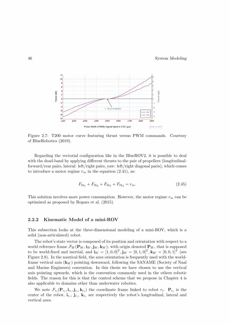
46 System Modeling
Figure 2.7: T200 motor curve featuring thrust versus PWM commands. Courtesyof BlueRobotics (2019).
Regarding the vectorial configuration like in the BlueROV2, it is possible to dealwith the dead-band by applying different thrusts to the pair of propellers (longitudinal:forward/rear pairs, lateral: left/right pairs, yaw: left/right diagonal paris), which comesto introduce a motor regime rm in the equation (2.41), as:
Fth1+ Fth2
+ Fth3+ Fth4
= rm. (2.45)
This solution involves more power consumption. However, the motor regime rm can beoptimized as proposed by Ropars et al. (2015).
2.2.2 Kinematic Model of a mini-ROV
This subsection looks at the three-dimensional modeling of a mini-ROV, which is asolid (non-articulated) robot.
The robot’s state vector is composed of its position and orientation with respect to aworld reference frame FW (PW , iW , jW ,kW ), with origin denoted PW , that is supposedto be world-fixed and inertial, and iW = [1, 0, 0]T , jW = [0, 1, 0]T ,kW = [0, 0, 1]T (seeFigure 2.8). In the nautical field, the axes orientation is frequently used with the world-frame vertical axis (kW ) pointing downward, following the SANAME (Society of Naaland Marine Engineers) convention. In this thesis we have chosen to use the verticalaxis pointing upwards, which is the convention commonly used in the others roboticfields. The reason for this is that the control scheme that we propose in Chapter 4 isalso applicable to domains other than underwater robotics.
We note Fri(Pri , iri , jri ,kri) the coordinate frame linked to robot ri. Pri is thecenter of the robot, iri , jri , kri are respectively the robot’s longitudinal, lateral andvertical axes.

Robots Model and Configuration 47
water surface
Fr
kr
ir
jr
Pr
FW
kW
iW
jW
PW
Figure 2.8: The world-fixed and robot-fixed coordinate frames: FW and Fr, respec-tively.
Kinematic Equations in the World Frame Let us define
WPr =
WXrWYrWZr
, (2.46)
the vector containing the position coordinates of center of the robot expressed in theworld-fixed reference frame FW , and
WΩr =
φθψ
, (2.47)
the vector containing the Euler angle coordinates in FW .The time derivative of the robot position vector expressed in the world-fixed frame
is ˙WPr. If we define
rνr =
νxνyνz
(2.48)
as the linear velocity vector of the robot-fixed frame Fr(Pr, ir, jr,kr) with respect tothe world-fixed frame FW , expressed in the robot-fixed frame, the following relationbetween the defined linear velocities holds
˙WPr =WRr
rνr, (2.49)
where WRr ∈ SO(3) is the rotation matrix expressing the transformation from therobot-fixed frame to the world frame.
The time derivative of the orientation vector expressed in the world frame is ˙WΩr.Let us define
rωr =
ωx
ωy
ωz
(2.50)
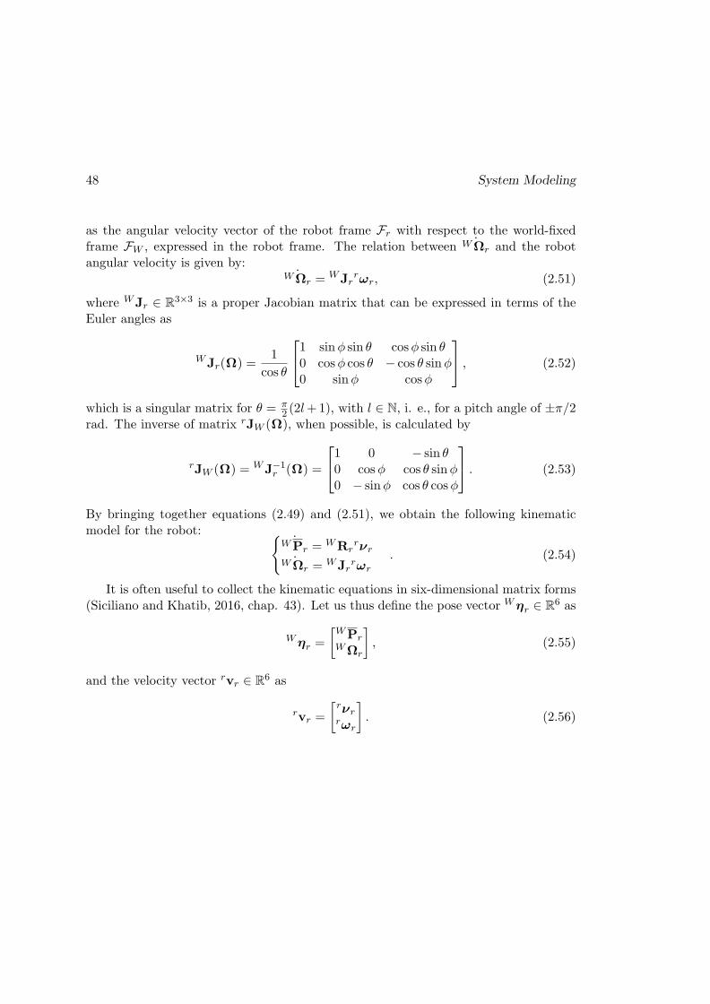
48 System Modeling
as the angular velocity vector of the robot frame Fr with respect to the world-fixedframe FW , expressed in the robot frame. The relation between ˙WΩr and the robotangular velocity is given by:
˙WΩr =WJr
rωr, (2.51)
where WJr ∈ R3×3 is a proper Jacobian matrix that can be expressed in terms of the
Euler angles as
WJr(Ω) =1
cos θ
1 sinφ sin θ cosφ sin θ0 cosφ cos θ − cos θ sinφ0 sinφ cosφ
, (2.52)
which is a singular matrix for θ = π2 (2l+1), with l ∈ N, i. e., for a pitch angle of ±π/2
rad. The inverse of matrix rJW (Ω), when possible, is calculated by
rJW (Ω) = WJ−1r (Ω) =
1 0 − sin θ0 cosφ cos θ sinφ0 − sinφ cos θ cosφ
. (2.53)
By bringing together equations (2.49) and (2.51), we obtain the following kinematicmodel for the robot:
˙WPr =WRr
rνr
˙WΩr =WJr
rωr
. (2.54)
It is often useful to collect the kinematic equations in six-dimensional matrix forms(Siciliano and Khatib, 2016, chap. 43). Let us thus define the pose vector W
ηr ∈ R6 as
Wηr =
[WPrWΩr
], (2.55)
and the velocity vector rvr ∈ R6 as
rvr =
[rνr
rωr
]. (2.56)

Pair of Robots Connected by a Tether 49
2.3 Pair of Robots Connected by a Tether
In this Section, the physical system under study is modeled. It is composed of twomini-ROVs linked together by a sagging tether, which corresponds to the first pair ofrobots that composes the chain of robots described in the previous Chapter. First,the geometric model of a hanging tether linking both robots is introduced. Then, theequation relating the robot velocity with the tether attachment point relative positionvariation is given.
Figure 2.9 presents the generic nomenclature pattern of coordinate frames inside thechain of robots. The index i ∈ [0, n] is the robot index inside the chain composed of nrobots. The robot’s front and rear camera frames are named Fci,1 and Fci,2 . Similarly,the tether attachment point frames in the robots are named Fi,1 and Fi,2, respectivelyfor front and rear attachment. This is a generic nomenclature. The detailed descriptionof our system composed of the first pair of robots and the tether segment linking themis given in the following.
FW
kW
iW
Fr2
kr2
ir2
F2,1 i2,1
k2,1
F1,2
k1,2
i1,2toward thesurface vessel
jc2,2
kc2,2
Fc2,2
jc2,1
kc2,1
Fc2,1
Fn,1 in,1
kn,1
jcn,1
Frn
krn
irnjcn,2
kcn,2
Fcn,2
kcn,1
Fcn,1
F2,2
i2,2
k2,2
Fr1
kr1
ir1jc1,2
kc1,2
Fc1,2
jc1,1
kc1,1
Fc1,1
Figure 2.9: An illustration presenting the generic nomenclature pattern of coordinateframes inside the chain of robots.
2.3.1 Catenary Model Applied for Tethered Robots
The catenary model of a tether is suitable for quasi-static analyses (Milutinovic et al.,2014). This means that the system has a slow dynamic behavior and the tether attach-ment points move at a low relative velocity (lower than 0.5 m/s). In such conditions,we can assume that the tether is in static equilibrium at successive instants of timewhile the robots, and consequently the attachment points, move.
We consider the case of the first two robots of the chain linked by a sagging tethercatenary (see Figure 2.10). The robots are named r1 and r2, respectively for leader andfollower. The tether attachment points frames are named F1 and F2, respectively forattachment on the leader and on the follower robot. The coordinate frame named F0
is at the tether lowest point.

50 System Modeling
α1
Fr2
jr2ir2
Fr1
jr1
ir1
α2F2
j2i2
F0
j0
i0
F1
j1
i1
FW
jW
iW
(a)
FW
kW
iW
Fr2
kr2
ir2
F2 i2
k2 ∆H2
H2
F0
F1
k0
i0
k1
i1
Fr1
kr1
ir1
D2 D2 ∆D2
(b)
Figure 2.10: Two illustrations presenting the (a) top view and (b) side view of thefirst pair of robots composing the chain of robots. The tether linking the robots ismodeled by a catenary whose slackness is noted H2. The difference of height betweenthe attachment points from P2 is ∆H2. The H2-slack catenary half-span is noted D2
and ∆D2 is the supplementary span due to the height difference. The tether orientationangles with respect to its attachment point frames are noted α1 and α2, respectivelyfor leader and follower attachment points.
The tether attachment point coordinate frames are noted Fi(Pi, ii, ji,ki), with i =1, 2, and are defined as follows:
ii =jri × kW
‖jri × kW ‖(2.57)
ki = kW (2.58)
ji = ki × ii. (2.59)
This means that ki is vertical, ii is the intersection of the sagittal plane of the robot riwith the horizontal plane, and ji is horizontal and orthogonal to ii.
The coordinate frame F1(P1, i1, j1,k1) is at the tether attachment point on theleader robot r1. The axis k1 is vertical, i1 is parallel to the longitudinal axis of the

Pair of Robots Connected by a Tether 51
robot (ir1) and points backwards. Axis j1 is horizontal and orthogonal to i1. Theoriented angle from i1 to i0 is named α1.
The coordinate frame F2(P2, i2, j2,k2) is at the tether attachment point on thefollower robot r2. The axis k2 is vertical, i2 is parallel to the longitudinal axis of therobot (ir2) and points forwards. Axis j2 is horizontal and orthogonal to i2. The orientedangle from i2 to i0 is named α2.
The coordinate frame F0(P0, i0, j0,k0) is attached to the catenary lowest point (seeSection 2.1.1). The axis k0 is vertical and i0 is horizontal inside the vertical planewhere the catenary is included. The axis j0 is horizontal and orthogonal to i0.
The catenary equation can be expressed in the lowest point frame F0 or in theattachment point frames F1 and F2. Since we are interested in this work to estimate andcontrol the tether shape evolution due to the robots motion, we choose to express thecatenary equation in the attachment point frames. Actually, F1 and F2 are symmetric,and the catenary slackness and half-span presented in Figure 2.10 with respect to F2
can also be defined with respect to F1. Figure 2.11 presents the symmetry of thecatenary features according to the frame of reference (F1 or F2).
FW
kW
iW
F2
i2
k2
∆H2
H2
P0
F1
k0
i0,2
k1
i1
D2 D2 ∆D2
F0
P1
P2
D1 D1∆D1
∆H1
H1
i0,1
Figure 2.11: An illustration presenting the symmetry of the catenary features accordingto the reference frame chosen (F1 or F2). The catenary slackness are H1 = 0Z1 andH2 =
0Z2. The attachment points difference of height is ∆H1 =1Z2 andH2 =
2Z1. Thecatenary parameter C(H1,∆H1) = C(H2,∆H2) is invariant whatever the point Pi wechoose for the starting attachment point of the cable. Thanks to the symmetry we have:∆H1 = −∆H2, H1 = H2 + ∆H2, H2 = H1 + ∆H1, ∆D1 = −∆D2, D1 = D2 + ∆D2,D2 = D1 +∆D1. As a reminder: Hi > 0, Hi +∆Hi > 0, Di > 0 and Di +∆Di > 0.
Here below we develop the catenary equation in F2, centered at the follower robotattachment point. The same procedure could be applied to express this equation in F1.
From equation (2.12), a generic point with homogeneous coordinates 0P =[0X,
0Y, 0Z, 1]T

52 System Modeling
defined in frame F0, belongs to the catenary if its coordinates are:
0P =
0X0
1C
[cosh(C 0X)− 1
]
1
. (2.60)
We can write the same equation in frame F2 though the following homogeneous trans-formation:
2P = 2M00P, (2.61)
where
2M0 =
cosα2 − sinα2 0 D2 cosα2
sinα2 cosα2 0 D2 sinα2
0 0 1 −H2
0 0 0 1
(2.62)
is the homogeneous transformation matrix from F0 to F2. Developing equation 2.61,we obtain the following equations:
2X = cosα2
(0X +D2
)(2.63)
2Y = sinα2(0X +D2) (2.64)
2Z =1
C
[cosh(C 0X)− 1
]−H2. (2.65)
From equations (2.63) and (2.64) we obtain
2X = cotα22Y,
and from equations (2.64) and (2.65) we obtain
2Z =1
C
[cosh
(C
(2Y
sinα2−D2
))− 1
]−H2.
Both equations form the catenary equation in frame F2 that is given by:
2P =
cotα22Y
2Y1C
[cosh
(C(
2Ysinα2
−D2
))− 1]−H2
1
. (2.66)
2.3.2 Tether Attachment Points and Robots Kinematics
In this section we focus on the tether attachment point kinematics in relationship withrobots kinematics. In order to design the robot motion control (Chapter 4), we willneed to take into account the kinematics of the tether attachment points with respectto the robot.
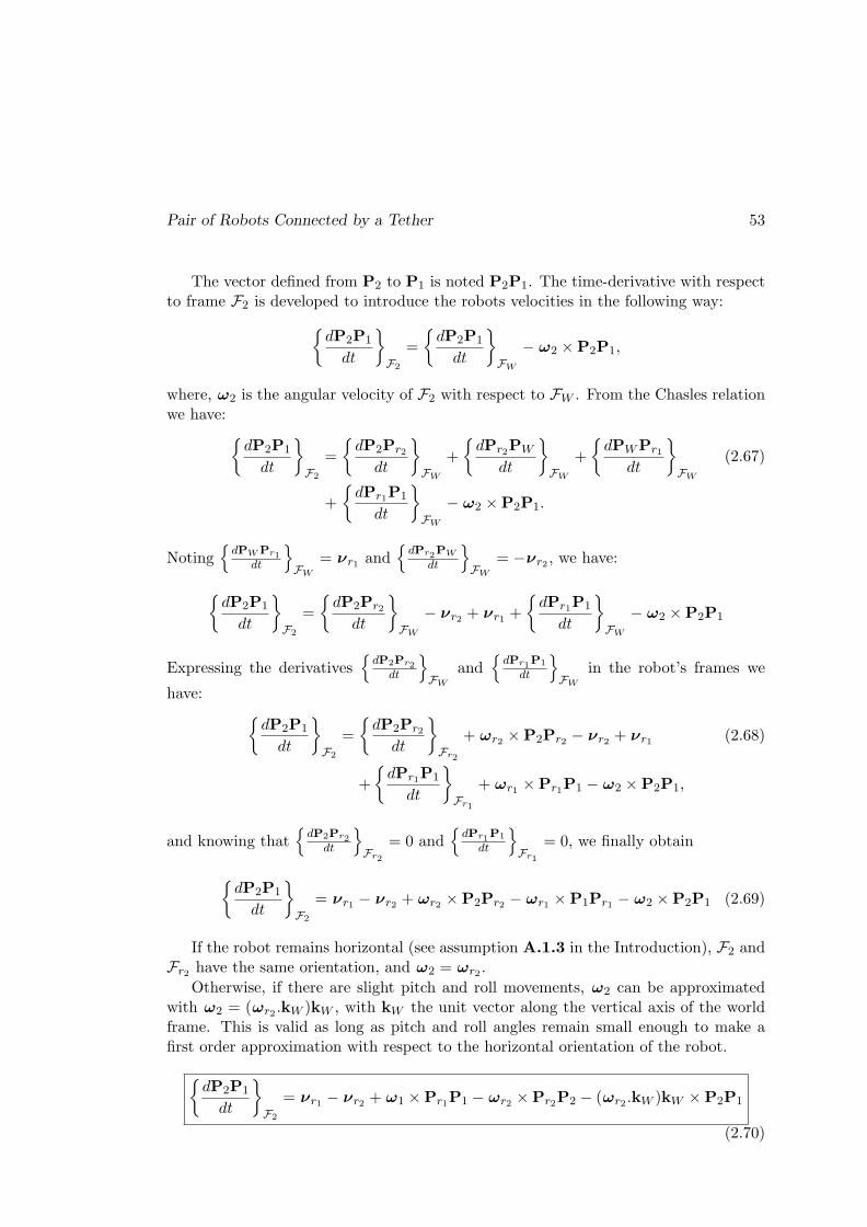
Pair of Robots Connected by a Tether 53
The vector defined from P2 to P1 is noted P2P1. The time-derivative with respectto frame F2 is developed to introduce the robots velocities in the following way:
dP2P1
dt
F2
=
dP2P1
dt
FW
− ω2 ×P2P1,
where, ω2 is the angular velocity of F2 with respect to FW . From the Chasles relationwe have:
dP2P1
dt
F2
=
dP2Pr2
dt
FW
+
dPr2PW
dt
FW
+
dPWPr1
dt
FW
(2.67)
+
dPr1P1
dt
FW
− ω2 ×P2P1.
Noting
dPWPr1
dt
FW
= νr1 and
dPr2PW
dt
FW
= −νr2 , we have:
dP2P1
dt
F2
=
dP2Pr2
dt
FW
− νr2 + νr1 +
dPr1P1
dt
FW
− ω2 ×P2P1
Expressing the derivatives
dP2Pr2
dt
FW
and
dPr1P1
dt
FW
in the robot’s frames we
have:dP2P1
dt
F2
=
dP2Pr2
dt
Fr2
+ ωr2 ×P2Pr2 − νr2 + νr1 (2.68)
+
dPr1P1
dt
Fr1
+ ωr1 ×Pr1P1 − ω2 ×P2P1,
and knowing that
dP2Pr2
dt
Fr2
= 0 and
dPr1P1
dt
Fr1
= 0, we finally obtain
dP2P1
dt
F2
= νr1 − νr2 + ωr2 ×P2Pr2 − ωr1 ×P1Pr1 − ω2 ×P2P1 (2.69)
If the robot remains horizontal (see assumption A.1.3 in the Introduction), F2 andFr2 have the same orientation, and ω2 = ωr2 .
Otherwise, if there are slight pitch and roll movements, ω2 can be approximatedwith ω2 = (ωr2 .kW )kW , with kW the unit vector along the vertical axis of the worldframe. This is valid as long as pitch and roll angles remain small enough to make afirst order approximation with respect to the horizontal orientation of the robot.
dP2P1
dt
F2
= νr1 − νr2 + ω1 ×Pr1P1 − ωr2 ×Pr2P2 − (ωr2 .kW )kW ×P2P1
(2.70)

54 System Modeling
If the leader robot is considered motionless,
dP2P1
dt
F2
= −νr2 − ωr2 ×Pr2P2 − (ωr2 .kW )kW ×P2P1 (2.71)
The inertial measurement unit (IMU) of the robot can give the quaternion of orien-tation of the robot and therefore the world coordinates of the robot axes, hence WRr2 .Then, the orientation of F2 in FW can be calculated thanks to equations (2.57) to(2.59), and therefore the rotation matrix between F2 and Fr2 , noted
2Rr2 .
We assume we also have WRr1 thanks to the IMU of the leader robot, which allowsto get 1Rr1 , thanks to equations (2.57) to (2.59). The relative orientation between therobots is given by r2Rr1 = WRT
r2WRr1 .
If pitch and roll angles are considered as zero (see assumption A.1.3 in the Intro-duction),
2Rr2 = I (2.72)1Rr1 = I (2.73)
r2Rr1 =
− cos(α2 − α1) sin(α2 − α1) 0− sin(α2 − α1) − cos(α2 − α1) 0
0 0 1
(2.74)
Then,
2ν2 =
2Rr2r2ν2 (2.75)
2ν1 =
2Rr2r2Rr1
r1ν1 (2.76)2ω2 =
2Rr2r2ω2 (2.77)
2ω1 =
2Rr2r1ω1 (2.78)
2 Pr2P2 = 2Rr2r2P2 (2.79)
2 Pr1P1 = 2Rr2r2Rr1
r1P1 (2.80)2 P2P1 = 2P1 (2.81)2 Pr2P1 = 2 Pr2P2+ 2 P2P1 (2.82)
= 2Rr2r2P2 +
2P1 (2.83)
We note ˙2P1 the velocity of P1 with respect to frame F2 expressed in F2:
˙2P1 =2
dP2P1
dt
F2
(2.84)
We also note rivri = [riνri ,riωri ]
T , the velocity vector defined at Pri, center of therobot ri, and expressed in frame Fri . In order to simplify the writing, we note for nowon this ego-centered velocity as:

Pair of Robots Connected by a Tether 55
riv = [riν , riω ]T (2.85)
We can rewrite Eq. (2.70) in matrix form:
˙2P1 =[2Rr2
r2Rr1 , −[2Rr2r2Rr1
r1P1]×2Rr2
r2Rr1
]r1v
−
2Rr2 , −[2Rr2
r2P2]×2Rr2 − [2P1]
×
0 0 00 0 00 0 1
2Rr2
r2v, (2.86)
where [X]× is the skew matrix defined from vector X.We note Tr1,2 and Tr2,2 and rewrite equation (2.86) such that:
˙2P1 = Tr1,2r1v +Tr2,2
r2v. (2.87)
Symmetrically, we can write
˙1P2 = Tr1,1r1v +Tr2,1
r2v. (2.88)
Equations (2.87) and (2.88) link the kinematics of the tether attachment points Pi withrespect to the kinematics of both robots. These kinematic equations will be used forthe control scheme described in Chapter 4.
If we assume that the robots remain horizontal (r2R2 = I), we can write:
Tr2,2 = −[I3×3, −
[r2P2]
× − [2P1]×] = −
[I3×3, −[r2P1]
×] (2.89)
Tr1,2 =[r2Rr1 , −[r2Rr1
r1P1]×r2Rr1
]
Otherwise we can extract the robot attitude angle from the IMU sensors. The framesFr2 and F2 have the same azimuthal orientation. Therefore, the rotation matrix r2R2
is a function of only roll (φ) and pitch (θ) angles of robot r2, as follows:
r2R2 =
cos θ sin θ sinφ sin θ cosφ0 cosφ − sinφ
− sin θ cos θ sinφ cos θ cosφ
. (2.90)
In addition, Tr1,2 can be expressed as a function of Tr2,2. Indeed we have:
Tr1,2 = −Tr2,2r2Vr1 (2.91)
wherer2Vr1 =
[r2Rr1 , [r2Pr1 ]
×r2Rr1
0 r2Rr1
](2.92)
is the velocity twist matrix that allows to get the velocity of the center of anothercoordinate frame (Fr1), while making the frame transformation from Fr1 to Fr2 (seeappendix C). We need the coordinates of the previous frame center, Pr1 , expressed inthe new frame (Fr2).
56 System Modeling
Using the twist matrix, we can rewrite the equation (2.87) as:
˙2P1 = Tr2,2 (−r2Vr1r1v + r2v) . (2.93)
Finally, if we assume that the robot is horizontal and that the leader robot isstationary (r1v = 0), the equation that links the kinematics of attachment point P1 tothe kinematics of the follower robot is reduced to:
˙2P1 = Tr2,2r2v =
[−I3×3, [r2P1]
×][r2ν
r2ω
](2.94)
˙2P1 = −r2ν − r2ω × r2P1 (2.95)
2.4 Conclusions
In this Chapter we focused on the model description of the first pair of robots ofthe chain. The pair is connected by a tether segment and it is composed of a leaderrobot, that should freely explore its surroundings, and a follower, that is expected tocontrol the tether shape in order not ot hamper the leader movements. Two differenttypes of robots are used in this work: one with vectored thrusters configuration andanother with direct configuration. Both types of robots are described, a kinematicmodel is developed and details about their architecture, embedded sensors and thrustersallocation are given. A model of the tether linking the leader and the follower robotsis also introduced. The tether is supposed to be slightly negative buoyant, perfectlyflexible and inextensible, being, therefore, modeled by a catenary cable. The catenarymodel of the tether is developed in order to express the tether equations in the followerrobot attachment frame. The complete system composed of both robots (leader andfollower) and the linking tether is also modeled.
The next Chapter addresses the strategies of perception of the tether, explaininghow it is detected in the image and how its shape is estimated from the camera feed-back.
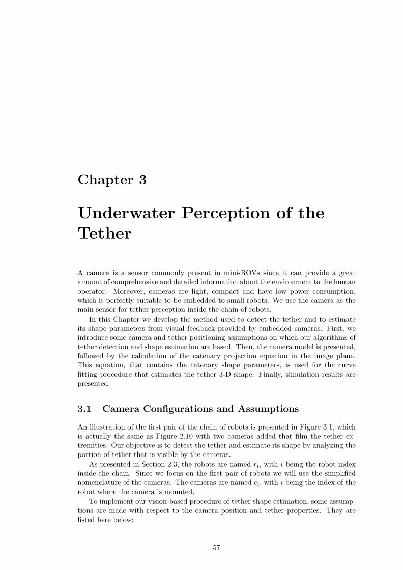
Chapter 3
Underwater Perception of the
Tether
A camera is a sensor commonly present in mini-ROVs since it can provide a greatamount of comprehensive and detailed information about the environment to the humanoperator. Moreover, cameras are light, compact and have low power consumption,which is perfectly suitable to be embedded to small robots. We use the camera as themain sensor for tether perception inside the chain of robots.
In this Chapter we develop the method used to detect the tether and to estimateits shape parameters from visual feedback provided by embedded cameras. First, weintroduce some camera and tether positioning assumptions on which our algorithms oftether detection and shape estimation are based. Then, the camera model is presented,followed by the calculation of the catenary projection equation in the image plane.This equation, that contains the catenary shape parameters, is used for the curvefitting procedure that estimates the tether 3-D shape. Finally, simulation results arepresented.
3.1 Camera Configurations and Assumptions
An illustration of the first pair of the chain of robots is presented in Figure 3.1, whichis actually the same as Figure 2.10 with two cameras added that film the tether ex-tremities. Our objective is to detect the tether and estimate its shape by analyzing theportion of tether that is visible by the cameras.
As presented in Section 2.3, the robots are named ri, with i being the robot indexinside the chain. Since we focus on the first pair of robots we will use the simplifiednomenclature of the cameras. The cameras are named ci, with i being the index of therobot where the camera is mounted.
To implement our vision-based procedure of tether shape estimation, some assump-tions are made with respect to the camera position and tether properties. They arelisted here below:
57

58 Underwater Perception of the Tether
FOLL
OWER
LEADERFr2
jr2ir2
Fr1
jr1
ir1
Fc2kc2
ic2
α2F2
j2i2
F0
j0
i0
F1
j1
i1
FW
jW
iW
α1 Fc1
kc1
ic1
(a)
FOLLOWER
LEADER
D D ∆D2FW
kW
iW
ir2
F2 i2
k2 ∆H2
H2
F0
F1
k0
i0
k1
i1
Fr1
kr1
ir1
Fr2
kr2 Fc2
jc2
kc2
jc1
kc1
Fc1
(b)
Figure 3.1: Illustration of a pair of tethered robots where the field of view of the camerasis highlighted by red dashed lines. (a) top view and (b) side view.
A.3.1 The cameras have a fixed and known pose with respect to the robot frame, whichcan be expressed as the following homogeneous matrix: riMci . We assume thatthe camera optical axis (kci) is aligned with the robot longitudinal axis (iri). Theoptical axis points forwards for frontal camera and backwards for rear camera.The camera vertical axis (jci) points downwards and it is aligned with the robotvertical axis (kri). In other words, we have: kci ‖ iri and jci ‖ kri ;
A.3.2 The tether attachment points have a fixed and known positions with respect tothe robots. This means that r2P2 and r1P1 are constant and known. The tetherattachment point is above the camera in the robot frame. For a robot ri andattachment point riPi we have: riZi >
riZci ;
A.3.3 The difference of height between the tether attachment points can be estimatedthrough pressure sensors embedded on the robots. ∆Hi is thus directly measured.
A.3.4 The tether has a known length;
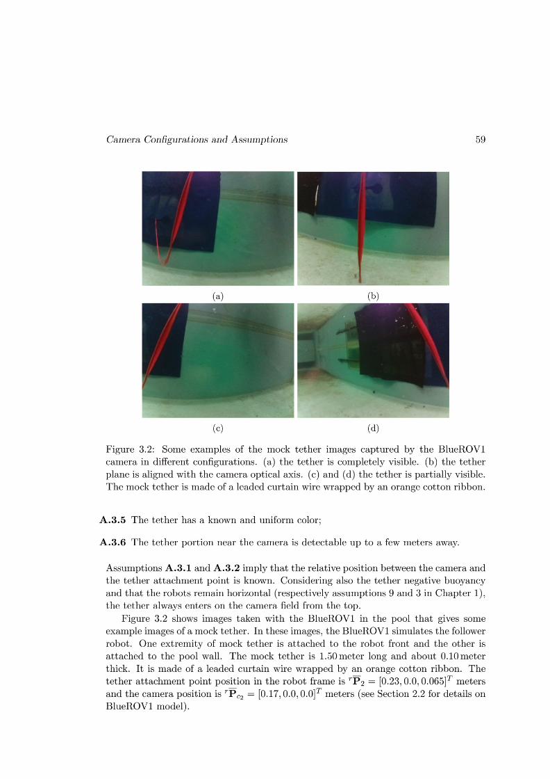
60 Underwater Perception of the Tether
Considering assumption A.3.3, there are only two parameters left to be
estimated through camera feedback: the tether slacknesses Hi and the ori-
entation angles αi.
3.2 Camera Modeling
In this section we will introduce the pinhole camera model, which is a standard cameramodel used in computer vision applications.
3.2.1 Image Formation
A camera is a device composed of a set of lenses used to direct the light on a sensitivesurface in order to form an image of the observed scene. Digital cameras are equippedwith a light sensitive surface composed of metal-oxide-semiconductors (MOS) capaci-tors that allows the conversion of incoming photons into electron charges that are readby a charge-coupled device (CCD) to form the image. In order to have a quality image,some camera parameters related to the photometry must be set. Among these settings,we will highlight, in the next subsection, the adjustment of the camera exposure andthe white balance, which are the precondition for image sharpness and color fidelity.
An image is a two-dimensional brightness array. Mathematically, an image is afunction I, defined on a compact region S of a two-dimensional surface, taking valuesin the positive real numbers(Ma et al., 2012):
I : S ∈ R2 → R
+; (x, y) 7→ I(x, y), (3.1)
for a single channel or grayscale image. Images capture two kinds of information:photometric, which are related to intensity and color of images, and geometric, whichare related to positions, lines and curves of the objects in the scene.
If the image is colored, it is actually composed of three arrays also called chan-nels (Ma et al., 2012). The RGB (red, green, blue) model is a widely used color modelin which these basic colors are added to form a colored image. An alternative repre-sentation is the HSV (hue, saturation, value) model, which is widely used in computervision algorithms to perform color detection of objects since the color can be directlyfiltered by the hue channel. In this thesis we will consider the hue channel to segmentthe tether.
3.2.2 Camera Exposure and White Balance
Camera exposure determines the amount of light entering in the device, that is to say,how dark or light the image will appear when it is captured by the camera. The cameraexposure is defined by three camera parameters that compose the exposure triangle:the aperture, the ISO setting and the shutter speed. Each parameter controls theexposure differently.
The aperture controls the area over which light can enter in the camera and it isusually specified in terms of a f-number N , which is given by the ratio of focal length
Camera Modeling 61
to effective aperture diameter.
N =f
d
where f is the focal length and d is the diameter of the entrance pupil (effective aper-ture).
The shutter speed (or exposure time) determines when the camera sensor will beopen or closed to incoming light from the camera lens. It is measured in seconds andrange from 1/400 to 30 seconds.
The ISO setting determines how sensitive the camera’s sensor is to incoming light,which is measured on a numerical scale defined by the ISO standard.
Many combinations of the above three settings can be used to achieve the sameexposure. The key, however, is knowing which trade-offs to make, since each settingalso influences other image properties. For example, shutter speed affects motion blur,ISO setting affects image noise and aperture affects depth of field (the range of dis-tance that objects in the image appear acceptably sharp). Most digital cameras havestandardized exposure modes that automatically control the aperture, ISO setting andshutter speed. For robotic applications, this means that the camera does not have aconstant configuration and its exposure can change during the operation. Such behav-ior is mostly undesirable. Therefore, in this thesis, the camera exposure is manuallyset by the operator.
White balance (WB) is the process of removing unrealistic color casts, so that ob-jects which appear white in the scene are rendered white in the photo. The humaneyes are very good at judging what is white under different light sources, but digitalcameras often have great difficulty with automatic white balance (AWB) and can createunsightly blue, orange, or even green color casts. Such changes can cause disturbancesin the execution of robotic tasks that uses image feedback for the detection or recog-nition of objects. Many algorithms relay on the objects hue information to performdetection, classification and recognition in the computer vision. Therefore, an incor-rect adjustment of white balance or an AWB that incorrectly compensate to changeof lighting can degrade the performance of vision-based detection algorithms, once thehue of objects will change in the image. In some robotic tasks, AWB is avoided and,in this thesis, the white balance of the camera is manually set by the human operator.
The camera exposure and the white balance determine the brightness, sharpnessand colors (hue) of objects in the image. These parameters have to be set carefully toobtain an accurate and robust color detection of the tether.
In the next subsection we will address the geometric aspects of image formationin order to obtain the relationship between the position of objects in the scene andits correspondence in the image. In computer vision, the most used geometric cameramodel is the pinhole model, since it allows a simple and linear modeling of imageformation in homogeneous coordinates.

62 Underwater Perception of the Tether
3.2.3 The Pinhole Camera Model
The pinhole model considers that the reflection and diffraction effects can be neglectedduring light propagation in the camera’s lens system, and only light refraction is con-sidered (Ma et al., 2012). The model also assumes that the light enters in the camerathrough a minimal aperture so that all rays are undeflected from the emitting sourcetowards the optical center. Moreover, the intensity measured at a pixel is identical tothe amount of energy radiated at the corresponding point in space, i.e., a Lambertiansurface (Ma et al., 2012). Under these conditions, the image formation process can bereduced to an ideal perspective projection, which is a good geometric approximationof a well-focused system.
The pinhole model (Figure 3.3) is composed of a frame Fc(Pc, ic, jc,kc), whoseorigin Pc is the center of projection. The projection plane or image plane πi is parallelto the plane (ic, jc) and it is placed at a distance f (the focal length) from the origin.The axis kc is called the optical axis and its intersection with the image plane is calledthe principal point pc.
A point a in the space is defined in the camera frame Fc by the vector cPa =[cXa
cYacZa 1]T in metric coordinates. It is projected on the image plane πi as a point
with coordinates pa = [xa, ya, 1]T , that are calculated using the Thales theorem:
pa =f
cZa
cXacYacZa
, (3.2)
where cZa 6= 0. This equation can be rewritten in matrix form:
pa =1
cZa
f 0 0 00 f 0 00 0 1 0
cPa. (3.3)
If the focal length is known, it can be normalized to 1 and the equation (3.3) becomes:
pa =1
cZaAcPa, (3.4)
where
A =
1 0 0 00 1 0 00 0 1 0
(3.5)
is called the standard (or canonical) projection matrix.
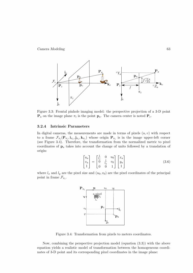
Camera Modeling 63
Fc
Pc
jc
ic
pc
pa
Pa
kc
Pa
pa
jc
kcPc
fcY acZa
cZa
cYa
Figure 3.3: Frontal pinhole imaging model: the perspective projection of a 3-D pointPa on the image plane πi is the point pa. The camera center is noted Pc.
3.2.4 Intrinsic Parameters
In digital cameras, the measurements are made in terms of pixels (u, v) with respectto a frame Fπi
(Pπi, iπi
, jπi,kπi
) whose origin Pπiis in the image upper-left corner
(see Figure 3.4). Therefore, the transformation from the normalized metric to pixelcoordinates of pa takes into account the change of units followed by a translation oforigin:
uava1
=
1lx
0 u00 1
lyv0
0 0 1
xaya1
(3.6)
where lx and ly are the pixel size and (u0, v0) are the pixel coordinates of the principalpoint in frame Fπi
.
a pixel
uPπi
v
cpa
jc
icpc
Figure 3.4: Transformation from pixels to meters coordinates.
Now, combining the perspective projection model (equation (3.3)) with the aboveequation yields a realistic model of transformation between the homogeneous coordi-nates of 3-D point and its corresponding pixel coordinates in the image plane:
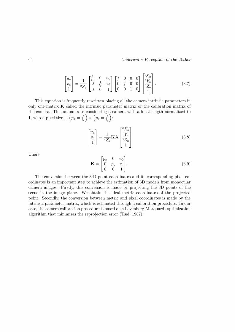
64 Underwater Perception of the Tether
uava1
=
1cZa
1lx
0 u00 1
lyv0
0 0 1
f 0 0 00 f 0 00 0 1 0
cXacYacZa
1
. (3.7)
This equation is frequently rewritten placing all the camera intrinsic parameters inonly one matrix K called the intrinsic parameter matrix or the calibration matrix ofthe camera. This amounts to considering a camera with a focal length normalized to
1, whose pixel size is(px = f
lx
)×(py = f
ly
):
uava1
=
1cZa
KA
cXacYacZa
1
(3.8)
where
K =
px 0 u00 py v00 0 1
. (3.9)
The conversion between the 3-D point coordinates and its corresponding pixel co-ordinates is an important step to achieve the estimation of 3D models from monocularcamera images. Firstly, this conversion is made by projecting the 3D points of thescene in the image plane. We obtain the ideal metric coordinates of the projectedpoint. Secondly, the conversion between metric and pixel coordinates is made by theintrinsic parameter matrix, which is estimated through a calibration procedure. In ourcase, the camera calibration procedure is based on a Levenberg-Marquardt optimizationalgorithm that minimizes the reprojection error (Tsai, 1987).
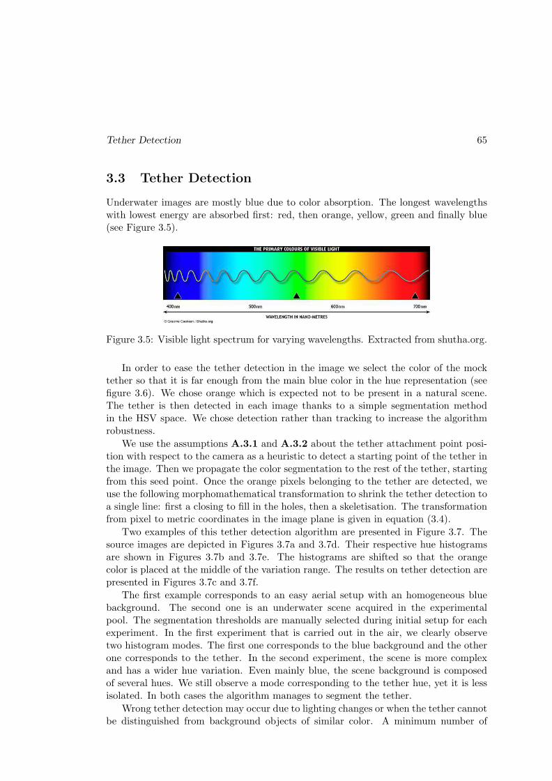
Tether Detection 65
3.3 Tether Detection
Underwater images are mostly blue due to color absorption. The longest wavelengthswith lowest energy are absorbed first: red, then orange, yellow, green and finally blue(see Figure 3.5).
Figure 3.5: Visible light spectrum for varying wavelengths. Extracted from shutha.org.
In order to ease the tether detection in the image we select the color of the mocktether so that it is far enough from the main blue color in the hue representation (seefigure 3.6). We chose orange which is expected not to be present in a natural scene.The tether is then detected in each image thanks to a simple segmentation methodin the HSV space. We chose detection rather than tracking to increase the algorithmrobustness.
We use the assumptions A.3.1 and A.3.2 about the tether attachment point posi-tion with respect to the camera as a heuristic to detect a starting point of the tether inthe image. Then we propagate the color segmentation to the rest of the tether, startingfrom this seed point. Once the orange pixels belonging to the tether are detected, weuse the following morphomathematical transformation to shrink the tether detection toa single line: first a closing to fill in the holes, then a skeletisation. The transformationfrom pixel to metric coordinates in the image plane is given in equation (3.4).
Two examples of this tether detection algorithm are presented in Figure 3.7. Thesource images are depicted in Figures 3.7a and 3.7d. Their respective hue histogramsare shown in Figures 3.7b and 3.7e. The histograms are shifted so that the orangecolor is placed at the middle of the variation range. The results on tether detection arepresented in Figures 3.7c and 3.7f.
The first example corresponds to an easy aerial setup with an homogeneous bluebackground. The second one is an underwater scene acquired in the experimentalpool. The segmentation thresholds are manually selected during initial setup for eachexperiment. In the first experiment that is carried out in the air, we clearly observetwo histogram modes. The first one corresponds to the blue background and the otherone corresponds to the tether. In the second experiment, the scene is more complexand has a wider hue variation. Even mainly blue, the scene background is composedof several hues. We still observe a mode corresponding to the tether hue, yet it is lessisolated. In both cases the algorithm manages to segment the tether.
Wrong tether detection may occur due to lighting changes or when the tether cannotbe distinguished from background objects of similar color. A minimum number of
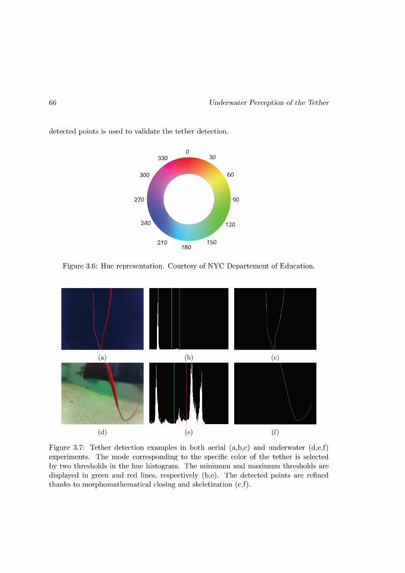
Catenary Features Estimation 67
3.4 Catenary Features Estimation
Once the 2D points that belong to the tether are detected in the image, we can use themto estimate the tether features that are related to its 3D shape: H and α. First, we haveto express the 3D equation of the catenary in the camera frame. Then, its perspectiveprojection in the image plane can be expressed using the pinhole model described inSection 3.2. Finally, the 3D catenary features can be estimated by matching the 2Dprojection to the detected points through a curve fitting algorithm.
3.4.1 Catenary Equation in the Camera Frame
The expression of the tether catenary in frame F2 was given by equation (2.66), in theprevious Chapter, as follows:
2P =
cotα22Y
2Y1C
[cosh
(C(
2Ysinα2
−D2
))− 1]−H2
1
. (3.10)
The transformation between F2 and the robot centered frame Fr2 is then made by
r2P = r2M22P, (3.11)
where r2M2 the homogeneous matrix expressing the pose of F2 in Fr2 :
r2M2 =
[r2R2
r2P2
0T3×1 1
]. (3.12)
As presented in Section 2.3.1, the frames Fr2 and F2 have the same azimuthal orien-tation. Therefore, the rotation matrix r2R2 is a function of only roll (φ) and pitch (θ)angles of robot r2, as follows:
r2R2 =
cos θ sin θ sinφ sin θ cosφ0 cosφ − sinφ
− sin θ cos θ sinφ cos θ cosφ
. (3.13)
If we suppose that the robot r2 is mechanically stabilized in roll and pitch by floaters,we have that r2R2 = I and the previous homogeneous transformation becomes a simpletranslation:
r2M2 =
1 0 0 r2X2
0 1 0 r2Y20 0 1 r2Z2
0 0 0 1
. (3.14)
The catenary equation transformation between the follower robot camera frame Fc2
and the robot frame Fr2 then made as follows:
c2P = c2Mr2r2M2
2P. (3.15)

68 Underwater Perception of the Tether
If we consider the frontal camera is fixed to the robot body, c2Mr2 = r2M−1c2
is constant.Considering the alignment between the camera and robot frame axes given by theassumptions A.3.1 and A.3.2 in the previous section (and also depicted in Figure 3.1)we have that
c2Mr2 =
0 −1 0 r2Yc20 0 −1 r2Zc2
1 0 0 −r2Xc2
0 0 0 1
. (3.16)
Replacing equations (3.16) and (3.14) in (3.15) we obtain:
c2P =
0 −1 0 r2Yc20 0 −1 r2Zc2
1 0 0 −r2Xc2
0 0 0 1
1 0 0 r2X2
0 1 0 r2Y20 0 1 r2Z2
0 0 0 1
2P, (3.17)
that yields
c2P =
0 −1 0 −r2Y2 +r2Yc2
0 0 −1 −r2Z2 +r2Zc2
1 0 0 r2X2 − r2Xc2
0 0 0 1
2P. (3.18)
The position of the tether attachment point P2 in the camera frame Fc2 is given by:
c2P2 =c2Mr2
r2P2. (3.19)
Using equation (3.16) in (3.19) we obtain
c2P2 =
c2X2c2Y2c2Z2
1
=
−r2Y2 +r2Yc2
−r2Z2 +r2Zc2
r2X2 − r2Xc2
1
, (3.20)
and replacing equation (3.20) in (3.18) yields:
c2P =
0 −1 0 c2X2
0 0 −1 c2Y21 0 0 c2Z2
0 0 0 1
2P. (3.21)
Finally, replacing equation (3.10) in (3.21) we obtain:
c2P =
−2Y + c2X2
− 1C
[cosh
(C(
2Ysinα2
−D2
))− 1]+H2 +
c2Y2
cotα22Y + c2Z2
1
. (3.22)
Catenary Features Estimation 69
From the first line of equation (3.22) we have the following relationship:
2Y = −c2X + c2X2. (3.23)
Hence, we can rewrite equation (3.22) as:
c2P =
c2X
− 1C
[cosh
(C(−c2X+c2X2
sinα2−D2
))− 1]+H2 +
c2Y2
cotα2 (−c2X + c2X2) +c2Z2
1
. (3.24)
Symmetrically, the equation of the tether catenary can also be written in frames F1
and Fc1 . This leads to an equation similar to (3.24), but with parameters H1, ∆H1, D1
and ∆D1 (see Section 2.3.2 and Figure 2.11). From now on, we develop the catenaryprojection equation in the camera frame Fc2 . The frame Fc2 is noted Fc, the angle α2
is noted α, the catenary half-span and slackness are respectively noted D and H, andthe tether attachment points difference of height is noted ∆H. Hence, the notation ofequation (3.24) is simplified to:
cP =
cX
− 1C
[cosh
(C(−cX+cX2
sinα−D
))− 1]+H + cY2
cotα (−cX + cX2) +cZ2
1
. (3.25)
3.4.2 Catenary Projection on the Image Plane
A generic 3-D point belonging to the catenary with homogeneous coordinates cP in Fc,is projected on the image plane as a 2-D point with coordinates p = [x y 1]T usingequation (3.4):
p =1cZ
1 0 0 00 1 0 00 0 1 0
cP (3.26)
that yields
x =cXcZ
y =cYcZ
(3.27a)
(3.27b)
From the second line of the matrix of equation (3.25), let us define that
ζ =−cX + cX2
sinα, (3.28)
and from the third line of the same equation we have that
cZ = cotα (−cX + cX2) +cZ2. (3.29)

70 Underwater Perception of the Tether
Then, replacing equation (3.29) in (3.27a) yields:
cX =x (cX2 cotα+ cZ2)
1 + x cotα, (3.30)
that replaced back in equations (3.28) and (3.29) gives, respectively:
ζ =cX2 − xcZ2
sinα+ x cosα(3.31)
andcZ =
cotαcX2 +cZ2
1 + x cotα. (3.32)
Finally, from equations (3.31) and (3.32), and replacing the second line of equa-tion (3.25) in (3.27b) we obtain the catenary projection equation on the image planey = f(x,H,∆H,α), knowing that C and D depend on H and ∆H (see equations (2.14)and (2.17)):
y =1cZ
[−cosh (Cζ − CD)− 1
C+H + cY2
](3.33)
where ζ and cZ are defined by equations (3.31) and (3.32), respectively.
3.4.3 Catenary Curve Fitting
The catenary 3D shape is estimated through a nonlinear least-square fitting procedurebased on a Guass-Newton algorithm: the catenary projection model (equation (3.33))is fitted to the tether points detected in the camera image. The algorithm of tetherdetection was addressed in Section 3.3. In this current Section we focus on the fittingprocedure, assuming that the tether is detectable.
The catenary shape is described by the following parameters:
a =H
Hmax(3.34a)
b = sinα (3.34b)
∆H = 2Z1 (3.34c)
with Hmax being a maximum acceptable tether slackness. We assume that the differ-ence of height between the tether attachments points (∆H) is estimated through therobot’s external pressure sensors (see assumption A.3.3). Therefore, only the first twoparameters of equation (3.34) are estimated through curve fitting. These parametersform a feature vector s defined as:
s =
[ab
]. (3.35)
The parameters a and b are respectively related to the tether slackness and orienta-tion with respect to the follower robot. Since 0 < H < Hmax, the a-parameter rangesin the interval ]0, 1[.
Catenary Features Estimation 71
For the b-parameter, we will consider that it ranges in the same interval ]0, 1[.Therefore, we always consider the case α > 0. When α < 0, we will use the mirrorimage in order to comply with these boundaries.
The tether is completely taut when a = 0 and it reaches the maximum acceptableslackness Hmax when a = 1. When b = 0 the tether belongs to the plane π (P2, i2,k2)and when b = 1 it belongs to the plane π (P2, j2,k2).
Rewriting equation (3.33) with these new parameters yields:
y (s, x) =1cZ
[−cosh (Cζ − CD)− 1
C+ aHmax +
cY2
], (3.36)
where
ζ =cX2 − xcZ2
b+ x√1− b2
(3.37)
and
cZ =
√1− b2cX2 + bcZ2
b+√1− b2x
. (3.38)
3.4.3.1 Gauss-Newton Algorithm
The Gauss-Newton algorithm is a modification of the Newton’s method for solvingnonlinear least squares problems of continuous and differentiable functions. The Gauss-Newton algorithm has the advantage of not requiring second derivatives, therefore, itis commonly used in curve fitting problems, where a sum of squared functions calledresiduals is minimized.
A residual can be defined as the distance between a point in the curve we want tofit and its correspondent in the curve issued from the current parameters estimation.In our case, we computed the residuals as follows:
ri (s) = yi − y(s, xi) (3.39)
where(xi, yi) are the metric coordinates of the i-th detected point of the tether in theimage and y(s, xi) is the tether model given by equation (3.36).
The sum of residuals is commonly called the cost function and our objective is tominimize it. Here below is the cost function we designed for the catenary fitting:
Γ(s) =1
M
M∑
i=1
r2i (s), (3.40)
where M ∈ N is the total number of detected points.
The minimum of the cost function Γ(s) is found through an iterative process thatis usually initialized at a starting point in the middle of variation range of the featurevector. In our case, since a ∈]0; 1[ and b ∈]0; 1[, we use
s0 = [0.5, 0.5]T (3.41)

72 Underwater Perception of the Tether
as starting point (in Section 3.4.3.5 a procedure of initial guess is presented). Thefeature vector is iterated as follows:
sk+1 = sk − λJ+r r(sk), (3.42)
where k ∈ 1, ..., N is the iteration index with N ∈ N, λ ∈ R+, r
(sk)is a column
vector that stacks the residuals ri(sk)and J+
r is the Moore-Penrose pseudo-inverse ofthe Jacobian matrix Jr. Since the catenary is continuous and differentiable, so is thecost function Γ(s). The Jacobian matrix Jr of the residuals vector is thus given by
Jr =1
M
dr
ds, (3.43)
whose i-th row has the following form:
Jr (i) =1
M
[−∂y(xi,s)
∂a−∂y(xi,s)
∂b
], (3.44)
where
∂y(xi, s)
∂a=
1
Z
[−∂
(1C
)
∂a[cosh (Cζ − CD)− 1]
− sinh (Cζ − CD)
C(A1 +A2 +A3) +Hmax
] (3.45)
and
∂y(xi, s)
∂b=− 1
C
∂ 1Z
∂b[cosh (Cζ − CD)− 1− C (H + cY 2)]
− 1
Z
∂ζ
∂bsinh (Cζ − CD) ,
(3.46)
with A1 = ζ ∂C∂a
, A2 = −D ∂C∂a
and A3 = −C ∂D∂a
. The calculation details of the Jacobianderivatives are presented in appendix D.
3.4.3.2 Study of the Gauss-Newton Jacobian Singularities
A singular matrix is a matrix whose determinant is zero and it is hence non-invertible.This occurs when the matrix is not full ranked or when there are elements in the matrixthat tend to infinity. We will study the singularities of the Jacobian matrix defined inequation (3.43) with respect to parameters a and b.
Firstly, let us focus on the partial derivative with respect to the a-parameter, whichis given by equation (3.45). We note that this equation is singular in the following case:
2H +∆H = L. (3.47)
However, this corresponds to the degenerated case and it is excluded as defined in theconditions of existence of the catenary presented in Section 2.1.3. Therefore, such a
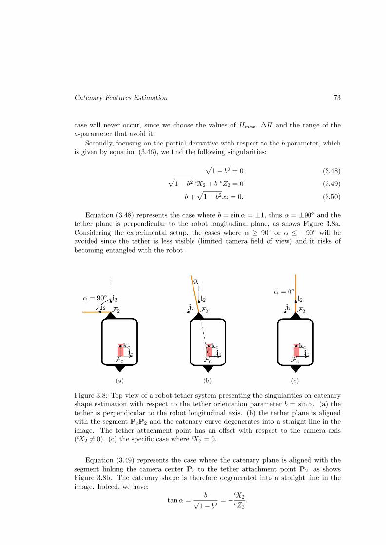
Catenary Features Estimation 73
case will never occur, since we choose the values of Hmax, ∆H and the range of thea-parameter that avoid it.
Secondly, focusing on the partial derivative with respect to the b-parameter, whichis given by equation (3.46), we find the following singularities:
√1− b2 = 0 (3.48)
√1− b2 cX2 + b cZ2 = 0 (3.49)
b+√1− b2xi = 0. (3.50)
Equation (3.48) represents the case where b = sinα = ±1, thus α = ±90 and thetether plane is perpendicular to the robot longitudinal plane, as shows Figure 3.8a.Considering the experimental setup, the cases where α ≥ 90 or α ≤ −90 will beavoided since the tether is less visible (limited camera field of view) and it risks ofbecoming entangled with the robot.
α = 90
Fc
kcic
F2j2
i2
(a)
Fc
kcic
F2j2
i2
α
(b)
Fc
kcic
F2j2
i2α = 0
(c)
Figure 3.8: Top view of a robot-tether system presenting the singularities on catenaryshape estimation with respect to the tether orientation parameter b = sinα. (a) thetether is perpendicular to the robot longitudinal axis. (b) the tether plane is alignedwith the segment PcP2 and the catenary curve degenerates into a straight line in theimage. The tether attachment point has an offset with respect to the camera axis(cX2 6= 0). (c) the specific case where cX2 = 0.
Equation (3.49) represents the case where the catenary plane is aligned with thesegment linking the camera center Pc to the tether attachment point P2, as showsFigure 3.8b. The catenary shape is therefore degenerated into a straight line in theimage. Indeed, we have:
tanα =b√
1− b2= −
cX2
cZ2.

74 Underwater Perception of the Tether
If cX2 = 0, this situation occurs when the catenary plane is also aligned with the robotlongitudinal axis and thus b = 0 (see Figure 3.8c).
Equation (3.50) leads to:
b√1− b2
= −xi
and from the perspective projection given by equation (3.4), we obtain:
tanα = −cXi
cZi.
Regarding Figure 3.9b and from the definition of tanα, we obtain
cXi − cX2
cZi − cZ2=
cXi
cZi.
which simplifies to (assuming cZi 6= 0):
xi =cX2
cZ2= x2.
This means that the points Pi and P2 have the same abscissa in the image plane.Therefore, this occurs when the catenary projection degenerates into a vertical line inthe image. This is the generalization of equation (3.49). These cases are depicted inFigures 3.8b and 3.8c.
3.4.3.3 Particular Case of Remote Points
The more remote the catenary points from the image plane, the more tightened thex-coordinates of their projection in the image plane. This is illustrated in Figure 3.9 bythe left part of the curves that tend to be more and more vertical as the 3-D points getfurther away from the image plane. As a consequence, derivatives can take very highvalues, which can lead to numerical issues such as ill-conditioning of the Gauss-NewtonJacobian matrix. Another issue is occurrence of high residuals in the cost function.
In order to cope with these problems, a filter that selects only bounded residualsis used. This filter and other improvements added to the standard Gauss-Newtonalgorithm are described in the following Section.
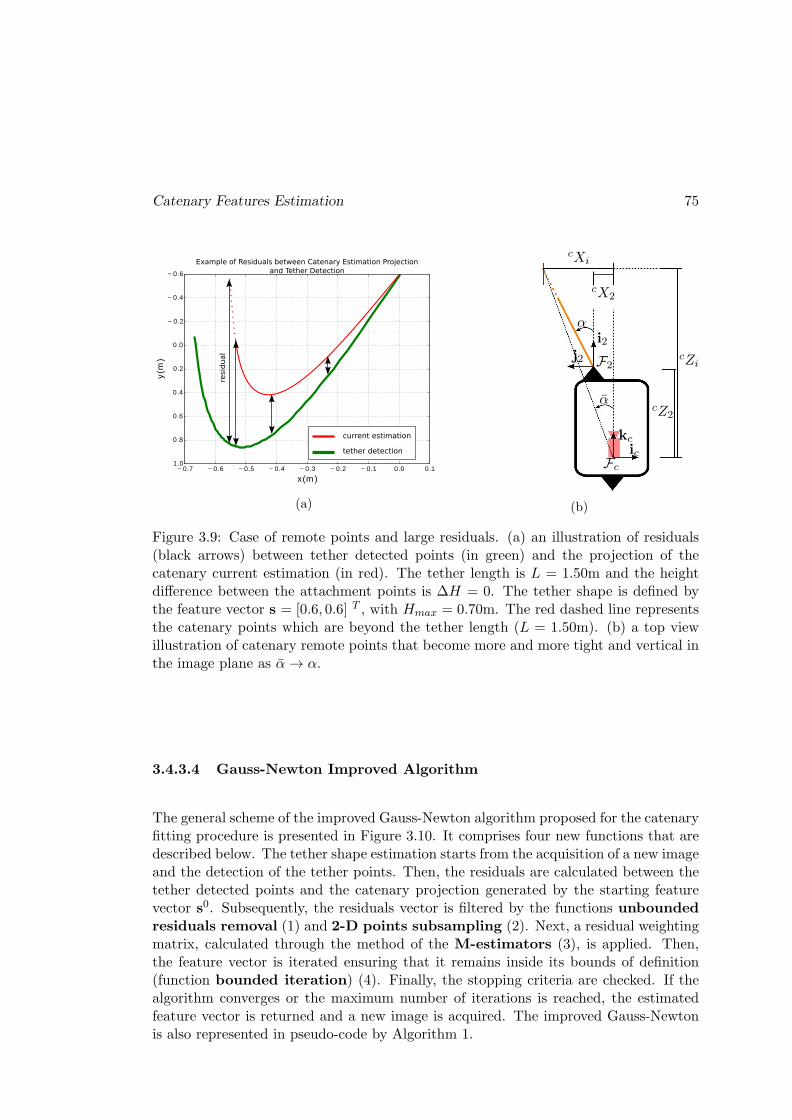
Catenary Features Estimation 75
− 0.7 − 0.6 − 0.5 − 0.4 − 0.3 − 0.2 − 0.1 0.0 0.1
x(m )
− 0.6
− 0.4
− 0.2
0.0
0.2
0.4
0.6
0.8
1.0
y(m
)
Catenary Project ion
resid
ual
tether detection
current estimation
Example of Residuals between Catenary Estimation Projection
and Tether Detection
(a)
Fc
kcic
F2j2
i2
α
cZ2
cX2
cXi
cZi
α
(b)
Figure 3.9: Case of remote points and large residuals. (a) an illustration of residuals(black arrows) between tether detected points (in green) and the projection of thecatenary current estimation (in red). The tether length is L = 1.50m and the heightdifference between the attachment points is ∆H = 0. The tether shape is defined bythe feature vector s = [0.6, 0.6] T , with Hmax = 0.70m. The red dashed line representsthe catenary points which are beyond the tether length (L = 1.50m). (b) a top viewillustration of catenary remote points that become more and more tight and vertical inthe image plane as α→ α.
3.4.3.4 Gauss-Newton Improved Algorithm
The general scheme of the improved Gauss-Newton algorithm proposed for the catenaryfitting procedure is presented in Figure 3.10. It comprises four new functions that aredescribed below. The tether shape estimation starts from the acquisition of a new imageand the detection of the tether points. Then, the residuals are calculated between thetether detected points and the catenary projection generated by the starting featurevector s0. Subsequently, the residuals vector is filtered by the functions unbounded
residuals removal (1) and 2-D points subsampling (2). Next, a residual weightingmatrix, calculated through the method of the M-estimators (3), is applied. Then,the feature vector is iterated ensuring that it remains inside its bounds of definition(function bounded iteration) (4). Finally, the stopping criteria are checked. If thealgorithm converges or the maximum number of iterations is reached, the estimatedfeature vector is returned and a new image is acquired. The improved Gauss-Newtonis also represented in pseudo-code by Algorithm 1.

76 Underwater Perception of the Tether
tether pointsdetection
calculate residuals
unbounded residualsremoval
M-estimators
boundediteration
check stoppingcriteria
new imageacquisition
improved
Gauss-Newton
2-D pointssubsampling
1.
2.
3.
4.
give starting points0 = [0.5, 0.5]T
return estimatedfeature vector s
continue iteration
stop iteration
calculateinitial guess
or
Figure 3.10: Chart flow of the improved Gauss-Newton algorithm. The four new func-tions added to the algorithm flow are numbered and highlighted by a pink background.
Algorithm 1 improved Gauss-Newton Algorithm
1: procedure GNA(Tin, s0, kmax)
2: k ← 03: sk ← s0
4: while k ≤ kmax do
5: T← Tin ⊲ retrieve tether points6: r← calculateResiduals(T, sk)7: r,T← unboundedResidualsRemoval(T, sk, r)8: r,T← 2DPointsSubsampling(T, r)9: D← robustEstimation(r)
10: J← calculateJacobian(T, sk)11: sk+1 ← boundedIteration(B,J,D, r, sk)12: if Γ
(sk+1
)− Γ
(sk)< 0 and
∣∣Γ(sk+1
)− Γ
(sk)∣∣ < ǫ then
13: return sk+1 ⊲ precision threshold reached14: else if Γ
(sk+1
)− Γ
(sk)> 0 then
15: return sk ⊲ cost function increased
16: sk ← sk+1
17: return sk+1 ⊲ max. number of steps exceeded
The first two functions are illustrated with the tether detected points obtainedfrom the simulated image shown in Figure 3.11. In this simulation the feature vectoris s = [0.6, 0.6]T , Hmax = 0.70meter and ∆H = 0meter. All the steps of detectionand fitting are run. Thus, it includes noise due to image segmentation and pixel/meterconversion.
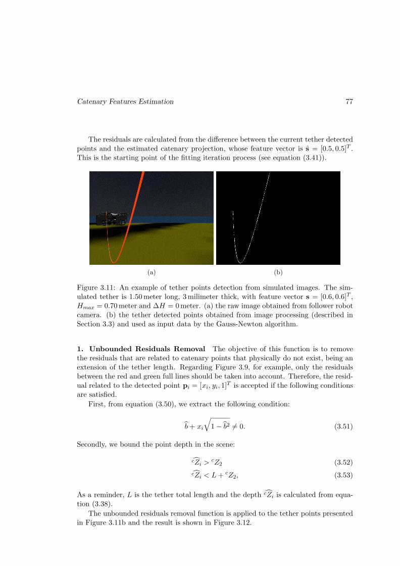
Catenary Features Estimation 77
The residuals are calculated from the difference between the current tether detectedpoints and the estimated catenary projection, whose feature vector is s = [0.5, 0.5]T .This is the starting point of the fitting iteration process (see equation (3.41)).
(a) (b)
Figure 3.11: An example of tether points detection from simulated images. The sim-ulated tether is 1.50meter long, 3milimeter thick, with feature vector s = [0.6, 0.6]T ,Hmax = 0.70meter and ∆H = 0meter. (a) the raw image obtained from follower robotcamera. (b) the tether detected points obtained from image processing (described inSection 3.3) and used as input data by the Gauss-Newton algorithm.
1. Unbounded Residuals Removal The objective of this function is to removethe residuals that are related to catenary points that physically do not exist, being anextension of the tether length. Regarding Figure 3.9, for example, only the residualsbetween the red and green full lines should be taken into account. Therefore, the resid-ual related to the detected point pi = [xi, yi, 1]
T is accepted if the following conditionsare satisfied.
First, from equation (3.50), we extract the following condition:
b+ xi
√1− b2 6= 0. (3.51)
Secondly, we bound the point depth in the scene:
cZi >cZ2 (3.52)
cZi < L+ cZ2, (3.53)
As a reminder, L is the tether total length and the depth cZi is calculated from equa-tion (3.38).
The unbounded residuals removal function is applied to the tether points presentedin Figure 3.11b and the result is shown in Figure 3.12.
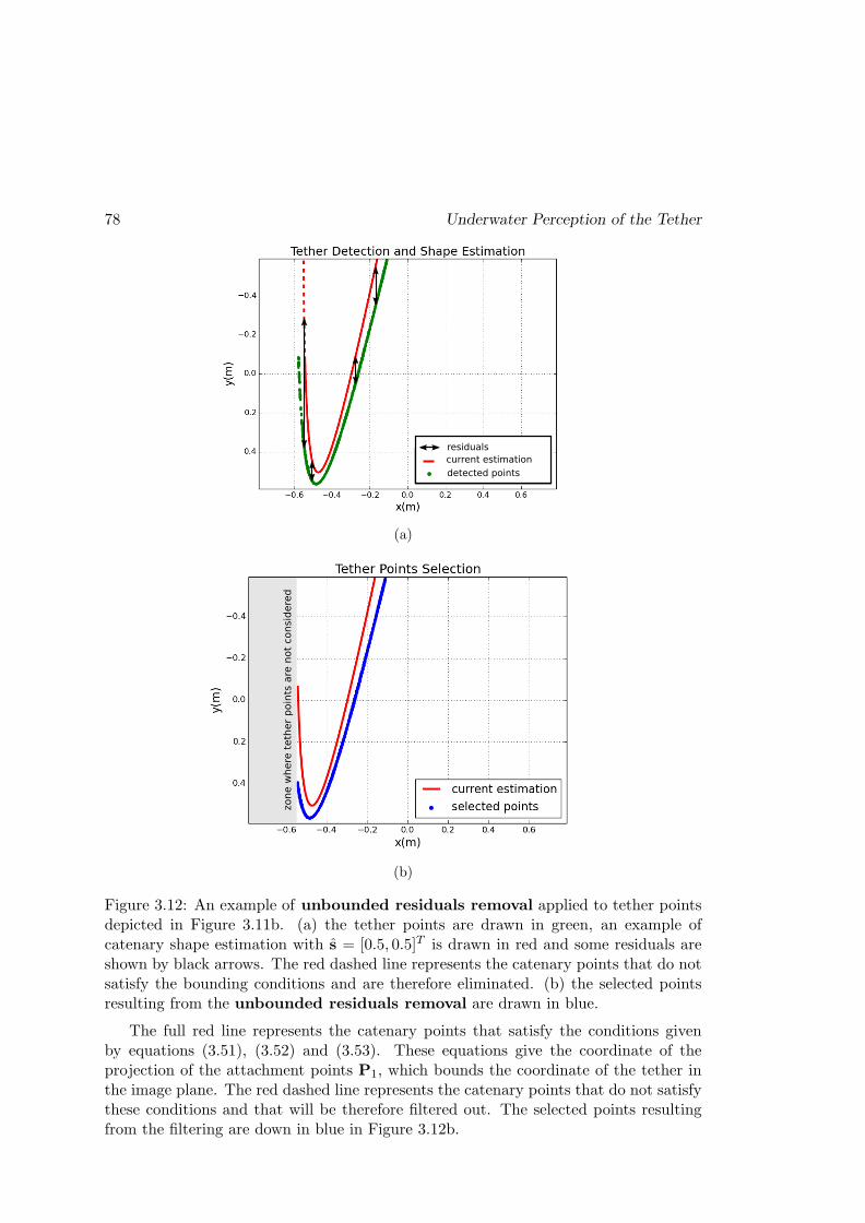
78 Underwater Perception of the Tether
current estimation
detected points
residuals
(a)
zone w
here
teth
er
poin
ts a
re n
ot
consid
ere
d
(b)
Figure 3.12: An example of unbounded residuals removal applied to tether pointsdepicted in Figure 3.11b. (a) the tether points are drawn in green, an example ofcatenary shape estimation with s = [0.5, 0.5]T is drawn in red and some residuals areshown by black arrows. The red dashed line represents the catenary points that do notsatisfy the bounding conditions and are therefore eliminated. (b) the selected pointsresulting from the unbounded residuals removal are drawn in blue.
The full red line represents the catenary points that satisfy the conditions givenby equations (3.51), (3.52) and (3.53). These equations give the coordinate of theprojection of the attachment points P1, which bounds the coordinate of the tether inthe image plane. The red dashed line represents the catenary points that do not satisfythese conditions and that will be therefore filtered out. The selected points resultingfrom the filtering are down in blue in Figure 3.12b.
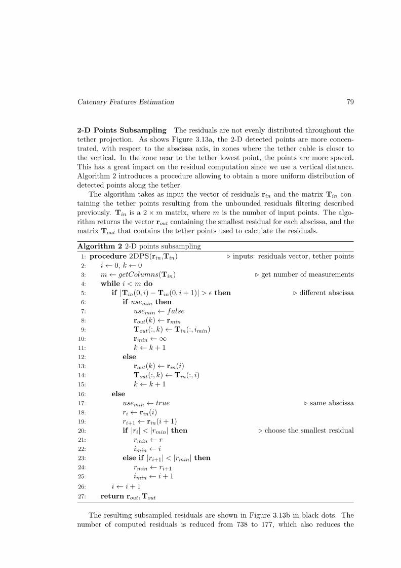
Catenary Features Estimation 79
2-D Points Subsampling The residuals are not evenly distributed throughout thetether projection. As shows Figure 3.13a, the 2-D detected points are more concen-trated, with respect to the abscissa axis, in zones where the tether cable is closer tothe vertical. In the zone near to the tether lowest point, the points are more spaced.This has a great impact on the residual computation since we use a vertical distance.Algorithm 2 introduces a procedure allowing to obtain a more uniform distribution ofdetected points along the tether.
The algorithm takes as input the vector of residuals rin and the matrix Tin con-taining the tether points resulting from the unbounded residuals filtering describedpreviously. Tin is a 2 ×m matrix, where m is the number of input points. The algo-rithm returns the vector rout containing the smallest residual for each abscissa, and thematrix Tout that contains the tether points used to calculate the residuals.
Algorithm 2 2-D points subsampling
1: procedure 2DPS(rin,Tin) ⊲ inputs: residuals vector, tether points2: i← 0, k ← 03: m← getColumns(Tin) ⊲ get number of measurements4: while i < m do
5: if |Tin(0, i)−Tin(0, i+ 1)| > ǫ then ⊲ different abscissa6: if usemin then
7: usemin ← false8: rout(k)← rmin
9: Tout(:, k)← Tin(:, imin)10: rmin ←∞11: k ← k + 112: else
13: rout(k)← rin(i)14: Tout(:, k)← Tin(:, i)15: k ← k + 1
16: else
17: usemin ← true ⊲ same abscissa18: ri ← rin(i)19: ri+1 ← rin(i+ 1)20: if |ri| < |rmin| then ⊲ choose the smallest residual21: rmin ← r22: imin ← i23: else if |ri+1| < |rmin| then24: rmin ← ri+1
25: imin ← i+ 1
26: i← i+ 1
27: return rout,Tout
The resulting subsampled residuals are shown in Figure 3.13b in black dots. Thenumber of computed residuals is reduced from 738 to 177, which also reduces the

80 Underwater Perception of the Tether
Jacobian matrix size and allows a faster computation of the Gauss-Newton iterations.
− 0.6 − 0.4 − 0.2 0.0 0.2 0.4 0.6
x(m )
− 0.4
− 0.2
0.0
0.2
0.4
y(m
)
Tether Points Subsam pling
current est im at ion
input points
zoom
around 4-7 point
per abscissa
zoom
around 2-4 point
per abscissa
(a)
− 0.6 − 0.4 − 0.2 0.0 0.2 0.4 0.6
x(m )
− 0.4
− 0.2
0.0
0.2
0.4
y(m
)
Tether Points Subsam pling - Result
current est im at ion
selected points
zoom
1 point per
abscissa
zoom
1 point per
abscissa
(b)
Figure 3.13: An example of 2-D points subsampling applied to tether points thatwere already filtered by the unbounded residuals removal function, as presented inFigure 3.12b. (a) the input points are drawn in blue and the current catenary shapeestimation (s = [0.5, 0.5]T ) is drawn in red. The unevenly tether points distribution isdemonstrated by two zoomed regions. (b) the selected points resulting from the 2-Dpoints subsampling are drawn in black. Only one tether point per abscissa is selected(the one with the smallest residual).
Catenary Features Estimation 81
Robust Estimation Following the residuals subsampling, we apply a procedure ofresiduals weighting called M-estimators (Pressigout, 2006, chap. 3). This procedureaims to make the tether shape estimation more robust to detection noise (color seg-mentation and pixel/meter conversion). The general idea is to give a higher weight tosmaller residuals, which are associated to a more reliable measure. The new residualsvector is thus weighted by the diagonal matrix D as follows:
rM = Dr (3.54)
where
D =
w1 · · · 0
. . .
0 · · · wM
. (3.55)
The weights wi, with i ∈ 1, ...,M and M being the number of residuals, range in theinterval [0, 1]. They are calculated according to Huber (1981), as follows:
wi =fM (ri)
ri, (3.56)
where fM (ri) is the weighting function defined as (Marchand et al., 2005):
fM (ri, S) =
ri(r
2i − S2)2 if |ri| < S
0 else(3.57)
where S = 4.7σ and σ = 1.48Medi(|ri −Medi(ri)|) is the median absolute deviation.Once we added a new weight matrix D, the feature vector iteration rule defined by
equation (3.42) should be updated as follows:
sk+1 = sk − λ (DJr)+Dr(sk). (3.58)
Bounded Iteration The feature vector, as defined by equation (3.35), is bounded:s ∈]0, 1[×]0, 1[. Feature vectors outside these bounds are associated to catenary pro-jections that do not exist. Therefore, we have to ensure that the feature vector remainsinside this bounded zone throughout the iteration process.
In order to manage the boundedness of the feature vector, the function describedby Algorithm 3 is applied to each iteration step. This function takes as input theJacobian matrix J, the weighting matrix D, the residual vector r, the feature vectorat the current iteration sk and the matrix B that contains the bounds of the featurevector.
The general idea of the algorithm is to reduce the gains inside matrix Λ correspond-ing to features that are out of bounds. These gains are reduced until the feature returnto the bounds. Matrix Λ is diagonal and it is defined as follows:
Λ =
λ1 · · · 0
. . .
0 · · · λN
, (3.59)

82 Underwater Perception of the Tether
where N is the size of the feature vector.
Algorithm 3 Bounded Iteration Algorithm
1: procedure BI(J,D, r, sk,B)2: sk+1 = sk −Λ (DJr)
+Dr(sk)
3: while isOutofBounds(sk+1,B) do ⊲ if vector is out of bounds4: i← 05: while i < size(sk+1) do ⊲ find feature that is out of bounds6: if isOutofBounds(sk+1(i),B(i, :)) then7: Λ(i, i) = 0.1Λ(i, i) ⊲ reduce the corresponding gain
8: i← i+ 1
9: sk+1 = sk −Λ (DJr)+Dr(sk)
⊲ re-iterate
10: return sk+1
Iteration Stopping Criteria The stopping criteria for the iteration process wechoose are related to the evolution of the cost function. They are enumerated herebelow.
1. If the cost function decrement is positive and smaller than the precision thresholdǫ:
Γ(sk+1
)− Γ
(sk)< 0
and∣∣∣Γ(sk+1
)− Γ
(sk)∣∣∣ < ǫ.
The found solution that minimizes the cost function is:
s = sk+1.
2. If the cost function decrement is positive, the iteration process is stopped:
Γ(sk+1
)− Γ
(sk)> 0.
The found solution that minimizes the cost function is:
s = sk.
3. If the number of iterations exceed a maximum threshold kmax:
k ≥ kmax,
where k is the number of the current iteration.
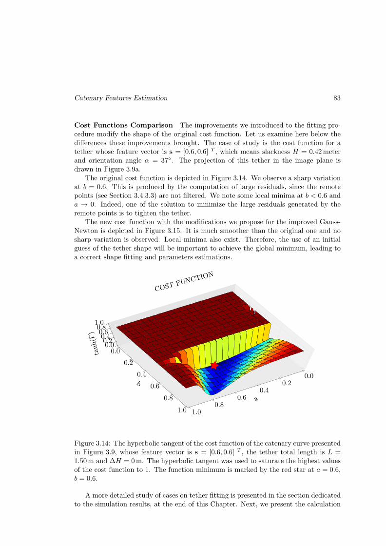
Catenary Features Estimation 83
Cost Functions Comparison The improvements we introduced to the fitting pro-cedure modify the shape of the original cost function. Let us examine here below thedifferences these improvements brought. The case of study is the cost function for atether whose feature vector is s = [0.6, 0.6] T , which means slackness H = 0.42meterand orientation angle α = 37. The projection of this tether in the image plane isdrawn in Figure 3.9a.
The original cost function is depicted in Figure 3.14. We observe a sharp variationat b = 0.6. This is produced by the computation of large residuals, since the remotepoints (see Section 3.4.3.3) are not filtered. We note some local minima at b < 0.6 anda → 0. Indeed, one of the solution to minimize the large residuals generated by theremote points is to tighten the tether.
The new cost function with the modifications we propose for the improved Gauss-Newton is depicted in Figure 3.15. It is much smoother than the original one and nosharp variation is observed. Local minima also exist. Therefore, the use of an initialguess of the tether shape will be important to achieve the global minimum, leading toa correct shape fitting and parameters estimations.
a
0.00.2
0.40.6
0.81.0
b
0.0
0.2
0.4
0.6
0.8
1.0
0.00.20.40.60.81.0
tanh(Γ)
COST FUNCTIO
N
Figure 3.14: The hyperbolic tangent of the cost function of the catenary curve presentedin Figure 3.9, whose feature vector is s = [0.6, 0.6] T , the tether total length is L =1.50m and ∆H = 0m. The hyperbolic tangent was used to saturate the highest valuesof the cost function to 1. The function minimum is marked by the red star at a = 0.6,b = 0.6.
A more detailed study of cases on tether fitting is presented in the section dedicatedto the simulation results, at the end of this Chapter. Next, we present the calculation

84 Underwater Perception of the Tether
a
0.0
0.2
0.4
0.6
0.8
1.0
b
0.0
0.2
0.4
0.6
0.8
1.0
0.00.20.40.60.81.0
COST
FUNC
TION
tanh(Γ)
Figure 3.15: The hyperbolic tangent of the improved Gauss-Newton cost function of thecatenary curve presented in Figure 3.9. The hyperbolic tangent was used to saturatethe highest values of the cost function to 1. The function minimum at a = 0.6, b = 0.6,marked by the red star.
procedure of the tether shape initial guess.
3.4.3.5 Initial Guess of Catenary Shape for Gauss-Newton
The Gauss-Newton algorithm proposed in the previous Section is always initializedat the starting point s0 = [0.5, 0.5]T , which is not necessarily near the solution thatminimizes the cost function. Since global convergence is not assured by the Gauss-Newton algorithm, local minima may be found. This would lead to the algorithmconvergence but to wrong parameters estimation. In order to avoid these local minima,an initial guess near the global minimum should be used as starting point of the Gauss-Newton algorithm.
In the case of catenary fitting, we propose to use an initial guess based on thefollowing approximation (see Figure 3.16):
The projection p0 of the tether 3D lowest point P0 is approximated with the tetherlowest point detected in the image pB.
Our objective is to calculate an initial estimation, an initial guess, of the tethershape. This is achieved by calculating a catenary projection that passes through thetether lowest point in the image considering the approximation mentioned here above(pB ≈ p0).
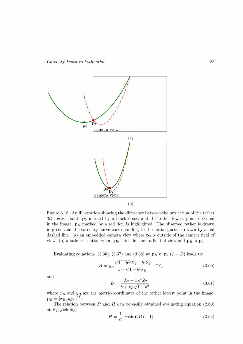
Catenary Features Estimation 85
pBp0camera view
(a)
camera viewpB
p0
(b)
Figure 3.16: An illustration showing the difference between the projection of the tether3D lowest point, p0 marked by a black cross, and the tether lowest point detectedin the image, pB marked by a red dot, is highlighted. The observed tether is drawnin green and the catenary curve corresponding to the initial guess is drawn by a reddashed line. (a) an embedded camera view where p0 is outside of the camera field ofview. (b) another situation where p0 is inside camera field of view and pB ≈ p0.
Evaluating equations (3.36), (3.37) and (3.38) at pB ≈ p0 (ζ = D) leads to:
H = yB
√1− b2cX2 + bcZ2
b+√1− b2xB
− cY2 (3.60)
and
D =cX2 − xBcZ2
b+ xB√1− b2
, (3.61)
where xB and yB are the metric-coordinates of the tether lowest point in the image:pB = [xB, yB, 1]
T .The relation between D and H can be easily obtained evaluating equation (2.60)
at P2, yielding:
H =1
C[cosh(CD)− 1] (3.62)
86 Underwater Perception of the Tether
In order to facilitate writing, let us redefine equations (3.60) and (3.61) as
H =G2
G3(3.63)
and
D =G1
G3. (3.64)
where
G1 =cX2 − cZ2xB
G2 = yB
(√1− b2cX2 + bcZ2
)− cY2G3
G3 = b+ xB√1− b2
Then, replacing equations (3.63) and (3.64) in (3.62) we obtain the new function
g (b) =CG2
G3− cosh
(CG1
G3
)+ 1 = 0. (3.65)
Replacing H = G2/G3 in the expression of the catenary parameter C in equation (2.17)we obtain:
C = 22G2
G3+∆H + 2L
√G2
G3
G2
G3+∆H
L2−∆H2
L2 −(2G2
G3+∆H
)2 (3.66)
C = 2G3
2G2 +G3∆H + 2L√G2
G2+G3∆HL2−∆H2
G23L
2 − (2G2 +G3∆H)2. (3.67)
Replacing equation (3.67) in (3.65) yields:
g (b) = CG2 − cosh(CG1
)+ 1 = 0, (3.68)
where
C = 22G2 +G3∆H + 2L
√G2
G2+G3∆HL2−∆H2
G23L
2 − (2G2 +G3∆H)2.
The equation (3.68) can be used to find a root value binit for the initial estimation ofthe orientation parameter (b) that corresponds to a catenary that passes through pB.The calculation of the slackness parameter (a) is obtained replacing equation (3.60) inEq. (3.34a):
a =G2
G3Hmax. (3.69)
In order to search for the root value of equation (3.68), we must use a numericalmethod. Among the possible numerical solving algorithms, we use the bisection (or
Catenary Features Estimation 87
dichotomy) algorithm. We could have used other methods like an interval analysismethod. However this method requires to find bounds of the function derivative, whichis more complicated to implement. In all these methods the functions must be contin-uous in order to avoid numerical drift generated by function derivatives that tend toinfinity.
Bounds for initial guess The root of equation (3.65) should be explored by thedichotomy algorithm within a bounded interval b ∈ [blow, bupp] that ensures the existenceof the catenary. This interval is given by the following constraints:
1. The tether lowest point pB is in front of the robot, which means that D > 0;
2. The tether lowest point pB is below the attachment points which means H > 0and H +∆H > 0. The constraint is H > max(0,−∆H);
3. The tether lowest point pB is between the attachment points and the catenaryshape is not degenerated, which requires that L > 2H+∆H. Taking into accountH < Hmax, the constraint is H < min(Hmax,
L−∆H2 ).
The first constraint imposes that the catenary half-span between the tether attach-ment points is a positive quantity: D > 0. Knowing that the tether lowest point pB
is considered on the left of the tether attachment point cP2 for the study (b > 0), wehave:
xB < x2 (3.70)
xB <cX2
cZ2, (3.71)
which yieldscX2 − cZ2xB > 0
and, from equation (3.64), we have:
G1 > 0.
In order to have D > 0, since G1 > 0, we get, from the denominator of equation (3.64):
G3 > 0
b+ xB√
1− b2 > 0
Knowing that
tanα =b√
1− b2,
we finally obtain:
tanα > −xB.

88 Underwater Perception of the Tether
The first bound is thus given by:
αL1 = tan−1(−xB) (3.72)
The second constraint imposes H > 0 and H > −∆H. Let us write the slacknesslower bound inequality from equation (3.63):
H > max(0,−∆H) (3.73)
G2
G3> max(0,−∆H) (3.74)
yB
(√1− b2cX2 + bcZ2
)
b+ xB√1− b2
− cY2 > max(0,−∆H) (3.75)
Let us introduce the tether slackness lower bound as:
ξmax = max(0,−∆H).
Replacing it in equation (3.75) we obtain:
E(ξmax) tanα > F (ξmax) (3.76)
where
F = −yBcX2 + xB(ξmax +cY2)
E = yBcZ2 − (ξmax +
cY2)
If E > 0, equation (3.76) yields a lower bound for α:
αL2 = tan−1
(F (ξmax)
E(ξmax)
). (3.77)
Otherwise, if E < 0, it yields an upper bound:
αU2 = tan−1
(F (ξmax)
E(ξmax)
). (3.78)
The third constraint imposes H < L−∆H2 and H < Hmax. From equation (3.63),
let us write the inequality that gives the tether slackness upper bound:
H < min
(Hmax,
L−∆H
2
)(3.79)
yB
(√1− b2cX2 + bcZ2
)
b+ xB√1− b2
− cY2 < min
(Hmax,
L−∆H
2
)(3.80)
Let us introduce the tether slackness upper bound as:
ξmin = min
(Hmax,
L−∆H
2
).

Catenary Features Estimation 89
Similarly to equation (3.76), we obtain the bounds for α as:
E(ξmin) tanα < F (ξmin) (3.81)
If E > 0, equation (3.81) yields an upper bound:
αU3 = tan−1
(F (ξmin)
E(ξmin)
)(3.82)
Otherwise, if E < 0, it yields a lower bound:
αL3 = tan−1
(F (ξmin)
E(ξmin)
). (3.83)
The procedure that gives the upper and lower bounds for α is described by Algo-rithm 4, which finally yields:
blow = sin (αlow) (3.84)
and
bupp = sin (αupp) . (3.85)
The definition of the bounds ensures that the root searching algorithm will find asolution for the initial guess of the catenary shape that meets the conditions of existenceof the catenary. These conditions were discussed in Section 2.1.3 and state, in summary,that the tether lowest point remains between the attachment points. The uniquenessof the solution was not established but we are only interested in getting one solutionfor the initial guess.
An example of the initial guess function g(b), defined by equation (3.68), is drawnin Figure 3.17. This function was generated by a catenary curve with feature vectors = [0.6, 0.6]T . The root of g(b) is searched inside the bounds blow = 0.54 and bupp = 1.0,which are marked by green vertical lines. For this case, the initial guess of the catenaryshape is given by s = [0.66, 0.57]T .
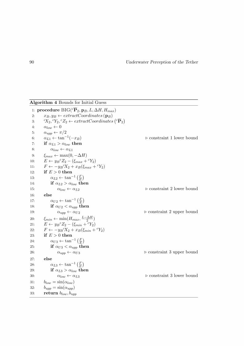
90 Underwater Perception of the Tether
Algorithm 4 Bounds for Initial Guess
1: procedure BIG(cP2, pB, L,∆H,Hmax)2: xB, yB ← extractCoordinates (pB)3: cX2,
cY2,cZ2 ← extractCoordinates
(cP2
)
4: αlow ← 05: αupp ← π/26: αL1 ← tan−1(−xB) ⊲ constraint 1 lower bound7: if αL1 > αlow then
8: αlow ← αL1
9: ξmax ← max(0,−∆H)10: E ← yB
cZ2 − (ξmax +cY2)
11: F ← −yBcX2 + xB(ξmax +cY2)
12: if E > 0 then
13: αL2 ← tan−1(FE
)
14: if αL2 > αlow then
15: αlow ← αL2 ⊲ constraint 2 lower bound
16: else
17: αU2 ← tan−1(FE
)
18: if αU2 < αupp then
19: αupp ← αU2 ⊲ constraint 2 upper bound
20: ξmin ← min(Hmax,L−∆H
2 )21: E ← yB
cZ2 − (ξmin + cY2)22: F ← −yBcX2 + xB(ξmin + cY2)23: if E > 0 then
24: αU3 ← tan−1(FE
)
25: if αU3 < αupp then
26: αupp ← αU3 ⊲ constraint 3 upper bound
27: else
28: αL3 ← tan−1(FE
)
29: if αL3 > αlow then
30: αlow ← αL3 ⊲ constraint 3 lower bound
31: blow = sin(αlow)32: bupp = sin(αupp)33: return blow, bupp
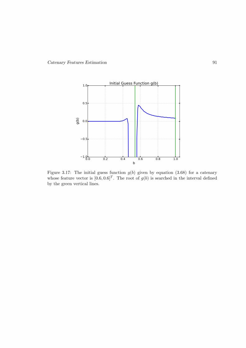
Catenary Features Estimation 91
0.0 0.2 0.4 0.6 0.8 1.0b
−1.0
−0.5
0.0
0.5
1.0
g(b)
Initial Guess Function g(b)
Figure 3.17: The initial guess function g(b) given by equation (3.68) for a catenarywhose feature vector is [0.6, 0.6]T . The root of g(b) is searched in the interval definedby the green vertical lines.
92 Underwater Perception of the Tether
3.5 Results
We present in this Section the simulation results we obtained for tether shape es-timation. Three methods of catenary fitting are tested: the standard Gauss-Newtonalgorithm (GN), the improved Gauss-Newton without initial guess (IGN) and improvedGauss-Newton with initial guess (IGN + IG).
First, the estimation error of the feature vector is evaluated in the entire range ofdefinition (s ∈]0, 1[×]0, 1[), considering non-noisy data and an infinite camera field ofview, which means that the 2-D points are generated from the theoretical projectionequation of the catenary into the image (see equation (3.36)), and that all points of thetether are taken into account.
Next, these methods are tested in a simulation environment comprising all aspectsof tether shape estimation, from detection to fitting procedure. Two study cases wherethe camera is static are presented to demonstrate the improvements our modificationsbrought to catenary curve fitting and, consequently, to tether shape estimation. Inaddition, to evaluate the fitting robustness, the feature vector is estimated all along apredefined path of the camera.
3.5.1 Focus on Feature Vector Estimation Error
In this study, image tether points are generated through the catenary projection equa-tion. The tether detection is not simulated and the camera field of view is assumed asinfinite. Then, these points are used as input for the studied fitting procedures, whoseaccuracy is compared through the following error measurement:
e = |ssim − s|
where ssim is the feature vector used to simulate the tether points, s is the estimationprovided by the fitting procedure, and |.| is the Euclidean norm. Since the input data isnot noisy, this study allows to check the estimation error arising from the optimizationprocedure itself.
The simulated tether is composed of 1000 points, which is a constant value. Thetether is 1.50meter long, the height difference between the attachment points is zero(∆H = 0) and the maximum authorized slackness is Hmax = 0.70meter. The fittingalgorithm gain is set to λ = 0.5 (see equation (3.42)).
Figure 3.18 presents the feature vector estimation error and the exit status forthe standard Gauss-Newton (GN). This algorithm produces accurate results when thesolution is near the starting point s0 = [0.5, 0.5]T . Around b = 0.5, we observe that theshape estimation is more accurate for low values of a-parameter and worse for largevalues. This occurs because, for a same orientation angle, the slacker the tether is (a→1), the tighter it becomes in the image. Both tether portions near the attachment pointsget closer and more vertical in the image and the catenary shape is less characterized.
Analyzing Figure 3.18a, we could incorrectly conclude that the GN algorithm es-timation error is moderately low for most of cases, particularly in the zone arounds = [0.5, 0.5]T . However, the algorithm does not converge towards the solution and

Results 93
remains stuck near the departing point, which is in the middle of the feature vectorvariation range. The iteration process is interrupted at the beginning due to an increasein the cost function or singular Jacobian computation, as shows Figure 3.18b. This be-havior is expected because, as seen at the end of Section 3.4.3.4, the existence of largeresiduals produces sharp variations in the cost function of the standard Gauss-Newton.Moreover, the feature vector is not bounded and it may be evaluated in regions whereour catenary model is not defined.
Figure 3.19a presents the estimation error for the improved Gauss-Newton withoutinitial guess (IGN). This algorithm may reach the solution when 0.4 < b < 0.8. Weobserve that the error increases for low values of the b-parameter. In such cases, thecable is very tight in the image and catenary shape is not well characterized. If thea-parameter approaches zero, the estimation accuracy becomes even worse since thetether cable is taut. The catenary is thus degenerated into a straight line in the image.
The exit status for the IGN algorithm is depicted in Figure 3.19b. Globally, thealgorithm converges when the solution is near the starting point s0 = [0.5, 0.5]T , spe-cially with respect to the b-parameter. The reason is that the b-parameter has a directinfluence on the amount of points to be removed due to large residuals computation(see Section 3.4.3.3). If too many points are filtered, the iteration process cannot becontinued and the algorithm stops. These cases are signalized by the red squares inthe legend and typically occur for tight tether projections in the image (low values ofb-parameter).
Figure 3.20a presents the estimation error for the improved Gauss-Newton withinitial guess (IGN + IG). The error is kept close to zero throughout the whole planea, b, except for low values of a and b parameters. In these few cases, the tether is taut(a → 0) and its projection in the image is tight (b → 0). The catenary shape in theimage plane is thus degenerated into a straight line and the fitting procedure is notable to improve the shape estimation given by the initial guess.
Since the camera field of view is assumed to be infinite, the projection of the tetherlowest point is always present in the image plane. As a result, the approximation used tocalculate the initial guess on the tether shape and initialize the IGN + IG algorithm isalways near the solution. This greatly enhances the probability of the global minimumto be reached. That is the reason why the IGN +IG has such a better accuracy incomparison with the IGN (see Figures 3.19a and 3.20a).
Regarding the exit status for the IGN + IG (Figure 3.20b), the algorithm convergesin the vast majority of cases. This does not occur for some few cases of low values ofa and b parameters, as expected. There is no exit due to excessive points removal (redsquares), since the starting point is always close to the solution.
In the next Section we will study the whole fitting chain including image processingand pixel/meter conversion. Taking into account a limited camera field of view, 3-Dprojection of the tether lowest point will not always be inside the image. In these cases,we expect the initial guess to be less accurate, nonetheless ensuring the convergence.Moreover, we may find additional error due to image processing.
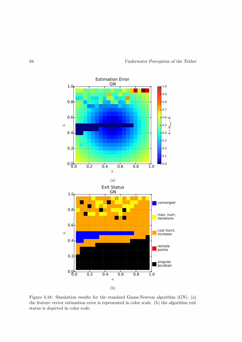
94 Underwater Perception of the Tether
0.0 0.2 0.4 0.6 0.8 1.0a
0.0
0.2
0.4
0.6
0.8
1.0
b
Estimation ErrorGN
0.0
0.1
0.2
0.3
0.4
0.5
0.6
0.7
0.8
0.9
1.0
e=|s s
im−s
|
(a)
0.0 0.2 0.4 0.6 0.8 1.0a
0.0
0.2
0.4
0.6
0.8
1.0
b
Exit StatusGN
converged
max. num.iterations
cost funct.increase
remotepoints
singularJacobian
(b)
Figure 3.18: Simulation results for the standard Gauss-Newton algorithm (GN). (a)the feature vector estimation error is represented in color scale. (b) the algorithm exitstatus is depicted in color code.

Results 95
0.0 0.2 0.4 0.6 0.8 1.0a
0.0
0.2
0.4
0.6
0.8
1.0b
Estimation ErrorIGN
0.0
0.1
0.2
0.3
0.4
0.5
0.6
0.7
0.8
0.9
1.0
e=|s s
im−s
|(a)
0.0 0.2 0.4 0.6 0.8 1.0a
0.0
0.2
0.4
0.6
0.8
1.0
b
Exit StatusIGN
converged
max. num.iterations
cost funct.increase
remotepoints
singularJacobian
(b)
Figure 3.19: Simulation results for the improved Gauss-Newton algorithm withoutinitial guess (IGN). (a) the feature vector estimation error is represented in color scale.(b) the algorithm exit status is depicted in color code.

96 Underwater Perception of the Tether
0.0 0.2 0.4 0.6 0.8 1.0a
0.0
0.2
0.4
0.6
0.8
1.0
b
Estimation ErrorIGN + IG
0.0
0.1
0.2
0.3
0.4
0.5
0.6
0.7
0.8
0.9
1.0
e=|s s
im−s
|
(a)
0.0 0.2 0.4 0.6 0.8 1.0a
0.0
0.2
0.4
0.6
0.8
1.0
b
Exit StatusIGN + IG
converged
max. num.iterations
cost funct.increase
remotepoints
singularJacobian
(b)
Figure 3.20: Simulation results for the improved Gauss-Newton algorithm withoutinitial guess (IGN + IG). (a) the feature vector estimation error is represented in colorscale. (b) the algorithm exit status is depicted in color code.
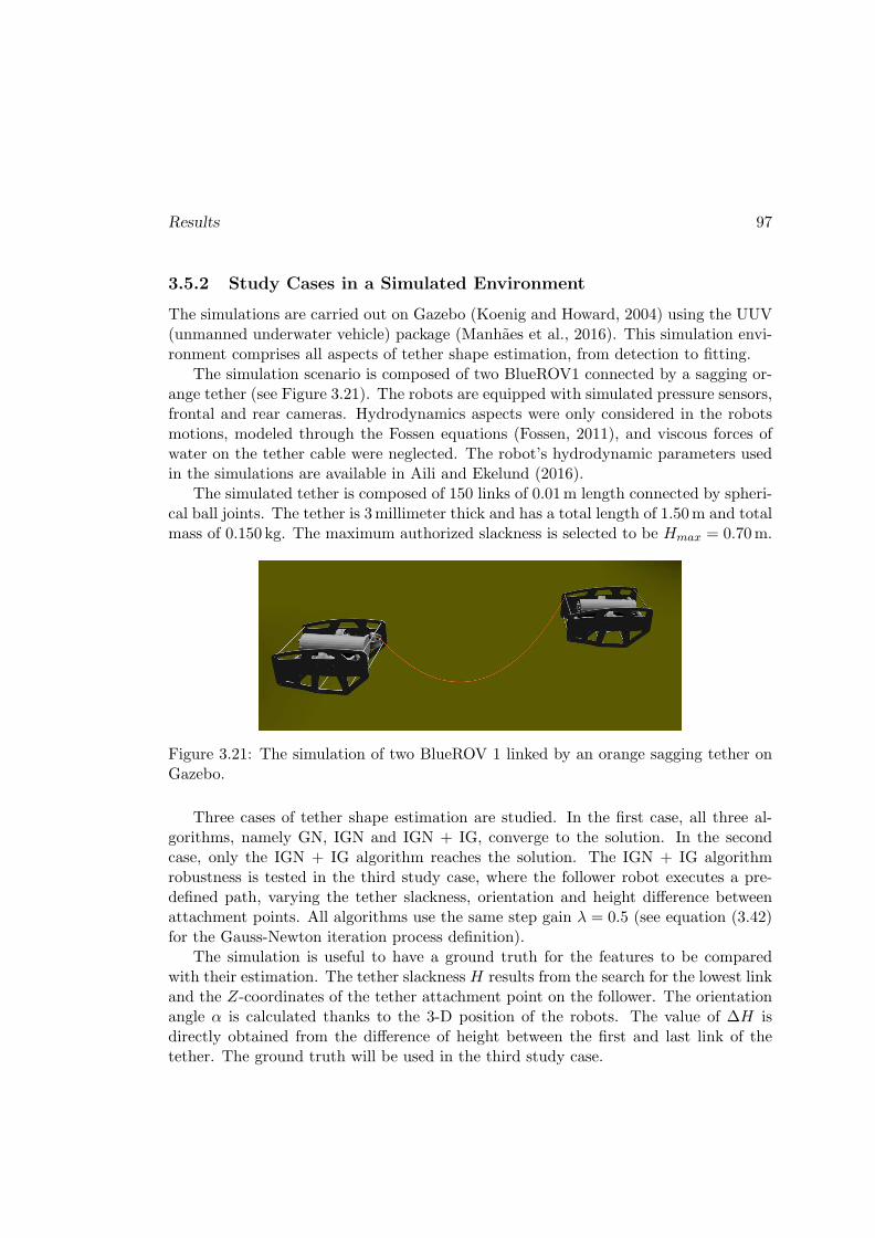
Results 97
3.5.2 Study Cases in a Simulated Environment
The simulations are carried out on Gazebo (Koenig and Howard, 2004) using the UUV(unmanned underwater vehicle) package (Manhaes et al., 2016). This simulation envi-ronment comprises all aspects of tether shape estimation, from detection to fitting.
The simulation scenario is composed of two BlueROV1 connected by a sagging or-ange tether (see Figure 3.21). The robots are equipped with simulated pressure sensors,frontal and rear cameras. Hydrodynamics aspects were only considered in the robotsmotions, modeled through the Fossen equations (Fossen, 2011), and viscous forces ofwater on the tether cable were neglected. The robot’s hydrodynamic parameters usedin the simulations are available in Aili and Ekelund (2016).
The simulated tether is composed of 150 links of 0.01m length connected by spheri-cal ball joints. The tether is 3millimeter thick and has a total length of 1.50m and totalmass of 0.150 kg. The maximum authorized slackness is selected to be Hmax = 0.70m.
Figure 3.21: The simulation of two BlueROV 1 linked by an orange sagging tether onGazebo.
Three cases of tether shape estimation are studied. In the first case, all three al-gorithms, namely GN, IGN and IGN + IG, converge to the solution. In the secondcase, only the IGN + IG algorithm reaches the solution. The IGN + IG algorithmrobustness is tested in the third study case, where the follower robot executes a pre-defined path, varying the tether slackness, orientation and height difference betweenattachment points. All algorithms use the same step gain λ = 0.5 (see equation (3.42)for the Gauss-Newton iteration process definition).
The simulation is useful to have a ground truth for the features to be comparedwith their estimation. The tether slackness H results from the search for the lowest linkand the Z-coordinates of the tether attachment point on the follower. The orientationangle α is calculated thanks to the 3-D position of the robots. The value of ∆H isdirectly obtained from the difference of height between the first and last link of thetether. The ground truth will be used in the third study case.

98 Underwater Perception of the Tether
Case 1 The image source and tether detected points of case 1 are presented in Fig-ure 3.22. The tether is entirely visible in the image and its shape given by the featurevector s = [0.40, 0.45]T , which is the solution of our minimization problem. This fea-ture vector corresponds to a tether with slackness H = 0.28meter and orientation angleα = 27.
(a) (b)
Figure 3.22: The (a) source image and (b) tether detected points of study case 1.The tether shape is given by the feature vector s[0.40, 0.45]T , which corresponds to aslackness H = 0.28meter and orientation angle α = 27.
The cost function and the steps of the standard Gauss-Newton (GN) are drawn inFigure 3.23. As we can observe, the algorithm starting point is in the blue zone, wherethe cost function values are lowest. This allows to converge quickly to the solution,after 8 iterations. The cost function, however, is not smooth everywhere. We observea sharp variation around b = 0.45 due to the presence of large residuals, as previouslyexplained in Section 3.4.3.3.
Both IGN and IGN + IG algorithms converge to the solution, as expected. The costfunction and steps of both optimization algorithms are drawn in Figure 3.24. The costfunction is much smoother than that of the standard Gauss-Newton. No sharp variationis observed, thanks to the function of large residuals removal (see Section 3.4.3.4). Bothstarting points are near the solution (blue zone). The IGN and IGN + IG algorithmsconverge after 7 and 8 iterations, respectively. Comparing IGN and GN optimizations,we observe that both realize a large first step. Otherwise, the convergence of IGN +IG is more gradual since the departure point is closer to the solution.
The initial and final tether shape estimation for the three studied procedures aredepicted in Figure 3.25. As expected, the estimated catenary fits the tether detectedpoints using any of the three methods. Notably, the tether shape initial guess is veryclose to the solution.

Results 99
0.2 0.3 0.4 0.5 0.6 0.7 0.8a
0.2
0.3
0.4
0.5
0.6
0.7
0.8b
GN Descent
0.06
0.12
0.18
0.24
0.30
0.36
0.42
0.48
Cost Fun
ction
Γ(s) in m
2
Figure 3.23: The descent of the GN algorithm marked by black dots. The startingpoint is at s0 = [0.5, 0.5]T and the solution is at s = [0.40, 0.45]T , marked by a red star.The cost function values are plotted in the background using the color scale depictedon the right.
0.2 0.3 0.4 0.5 0.6 0.7 0.8a
0.2
0.3
0.4
0.5
0.6
0.7
0.8
b
IGN and IGN + IG Descents
6.0×10⁻⁶
1.2×10⁻⁵
1.8×10⁻⁵
2.4×10⁻⁵
3.0×10⁻⁵
3.6×10⁻⁵
4.2×10⁻⁵
4.8×10⁻⁵
Cost Fun
ction Γ(s) in m
2
Figure 3.24: Comparison of the descent of IGN (white dots) and IGN + IG (blackdots) algorithms. The solution is at s = [0.40, 0.45]T , marked by a red star. The costfunction values are plotted in the background using the color scale depicted on theright.
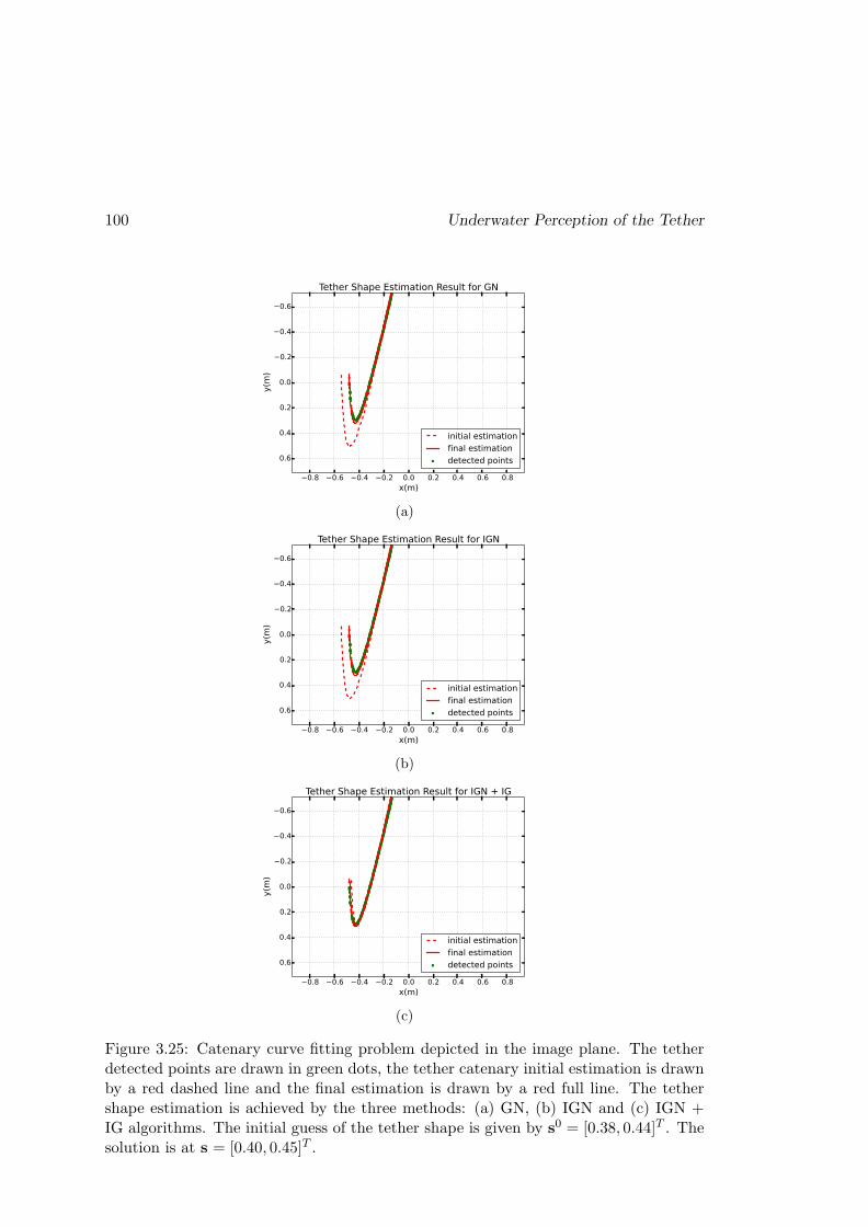
100 Underwater Perception of the Tether
−0.8 −0.6 −0.4 −0.2 0.0 0.2 0.4 0.6 0.8x(m)
−0.6
−0.4
−0.2
0.0
0.2
0.4
0.6
y(m)
Tether Shape Estimation Result for GN
initial estimationfinal estimationdetected points
(a)
−0.8 −0.6 −0.4 −0.2 0.0 0.2 0.4 0.6 0.8x(m)
−0.6
−0.4
−0.2
0.0
0.2
0.4
0.6
y(m)
Tether Shape Estimation Result for IGN
initial estimationfinal estimationdetected points
(b)
−0.8 −0.6 −0.4 −0.2 0.0 0.2 0.4 0.6 0.8x(m)
−0.6
−0.4
−0.2
0.0
0.2
0.4
0.6
y(m
)
Tether Shape Estimation Result for IGN + IG
initial estimationfinal estimationdetected points
(c)
Figure 3.25: Catenary curve fitting problem depicted in the image plane. The tetherdetected points are drawn in green dots, the tether catenary initial estimation is drawnby a red dashed line and the final estimation is drawn by a red full line. The tethershape estimation is achieved by the three methods: (a) GN, (b) IGN and (c) IGN +IG algorithms. The initial guess of the tether shape is given by s0 = [0.38, 0.44]T . Thesolution is at s = [0.40, 0.45]T .
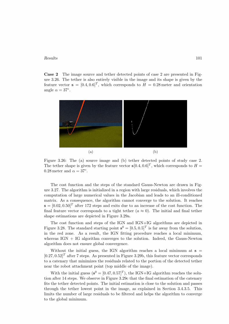
Results 101
Case 2 The image source and tether detected points of case 2 are presented in Fig-ure 3.26. The tether is also entirely visible in the image and its shape is given by thefeature vector s = [0.4, 0.6]T , which corresponds to H = 0.28meter and orientationangle α = 37.
(a) (b)
Figure 3.26: The (a) source image and (b) tether detected points of study case 2.The tether shape is given by the feature vector s[0.4, 0.6]T , which corresponds to H =0.28meter and α = 37.
The cost function and the steps of the standard Gauss-Newton are drawn in Fig-ure 3.27. The algorithm is initialized in a region with large residuals, which involves thecomputation of large numerical values in the Jacobian and leads to an ill-conditionedmatrix. As a consequence, the algorithm cannot converge to the solution. It reachess = [0.02, 0.50]T after 172 steps and exits due to an increase of the cost function. Thefinal feature vector corresponds to a tight tether (a ≈ 0). The initial and final tethershape estimations are depicted in Figure 3.29a.
The cost function and steps of the IGN and IGN+IG algorithms are depicted inFigure 3.28. The standard starting point s0 = [0.5, 0.5]T is far away from the solution,in the red zone. As a result, the IGN fitting procedure reaches a local minimum,whereas IGN + IG algorithm converges to the solution. Indeed, the Gauss-Newtonalgorithm does not ensure global convergence.
Without the initial guess, the IGN algorithm reaches a local minimum at s =[0.27, 0.52]T after 7 steps. As presented in Figure 3.29b, this feature vector correspondsto a catenary that minimizes the residuals related to the portion of the detected tethernear the robot attachment point (top middle of the image).
With the initial guess (s0 = [0.47, 0.57]T ), the IGN+IG algorithm reaches the solu-tion after 14 steps. We observe in Figure 3.29c that the final estimation of the catenaryfits the tether detected points. The initial estimation is close to the solution and passesthrough the tether lowest point in the image, as explained in Section 3.4.3.5. Thislimits the number of large residuals to be filtered and helps the algorithm to convergeto the global minimum.

102 Underwater Perception of the Tether
0.2 0.3 0.4 0.5 0.6 0.7 0.8a
0.2
0.3
0.4
0.5
0.6
0.7
0.8
b
GN Descent
0.06
0.12
0.18
0.24
0.30
0.36
0.42
0.48
Cost Fun
ction
Γ(s) in m
2
Figure 3.27: The descent of a standard Gauss-Newton algorithm marked by black dots.The starting point is at s0 = [0.5, 0.5]T and the solution is at s = [0.4, 0.6]T , markedby a red star. The cost function values are plotted in the background using the colorscale depicted on the right. The algorithm does not reach the solution.
0.2 0.3 0.4 0.5 0.6 0.7 0.8a
0.2
0.3
0.4
0.5
0.6
0.7
0.8
b
IGN and IGN + IG Descents
6.0×10⁻⁶
1.2×10⁻⁵
1.8×10⁻⁵
2.4×10⁻⁵
3.0×10⁻⁵
3.6×10⁻⁵
4.2×10⁻⁵
4.8×10⁻⁵
Cost Fun
ction Γ(s) in m
2
Figure 3.28: Comparison of the descent of the IGN (white dots) and IGN+IG (blackdots) algorithms. The solution is at s = [0.4, 0.6]T , marked by a red star. The costfunction values are plotted in the background using the color scale depicted on theright. The solution is only reached if an initial guess (s0 = [0.47, 0.57]T ) of the tethershape is given.

Results 103
−0.8 −0.6 −0.4 −0.2 0.0 0.2 0.4 0.6 0.8x(m)
−0.6
−0.4
−0.2
0.0
0.2
0.4
0.6
y(m)
Tether Shape Estimation Result for GN
initial estimationfinal estimationdetected points
(a)
−0.8 −0.6 −0.4 −0.2 0.0 0.2 0.4 0.6 0.8x(m)
−0.6
−0.4
−0.2
0.0
0.2
0.4
0.6
y(m)
Tether Shape Estimation Result for IGN
initial estimationfinal estimationdetected points
(b)
−0.8 −0.6 −0.4 −0.2 0.0 0.2 0.4 0.6 0.8x(m)
−0.6
−0.4
−0.2
0.0
0.2
0.4
0.6
y(m
)
Tether Shape Estimation Result for IGN + IG
initial estimationfinal estimationdetected points
(c)
Figure 3.29: Catenary curve fitting problem depicted in the image plane for the threemethods studied: (a) GN, (b) IGN and (c) IGN+IG. The tether detected points aredrawn in green, the initial estimation is drawn by a red dashed line and the finalestimation is drawn by a red full line. The correct tether shape estimation is onlyachieved by the improved Gauss-Newton with initial guess (IGN+IG).

104 Underwater Perception of the Tether
A summary with the number of computed steps and exit status of study cases1 and 2 is given on Table 3.1 for all the three algorithms under study. The exitcode 0 corresponds to algorithm convergence and the code −1 corresponds to iterationinterrupted due to increase in cost function.
GN IGN IGN+IG
steps exit steps exit steps exitcase1
s = [0.40, 0.45]T 8 0 7 0 8 0case2
s = [0.40, 0.60]T 172 -1 8 -1 14 0
Table 3.1: A summary of study cases 1 and 2. The exit code 0 corresponds to algorithmconvergence and the code −1 corresponds to iteration interrupted due to increase incost function.
Case 3 The tether shape estimation is tested in a case where the follower robotexecutes a predefined path, while the three features, namely H, α and ∆H, are madevariable. Moreover, during the motion, the robot will have to cross the singularity b = 0.At the beginning (0 − 17s), α = −45 and ∆H = 0.26m, the follower robot executesa lateral motion in order to pass through the singularity α = 0. Then (17− 24s), therobot goes downwards and stops when ∆H = −0.23m. At the end (24 − 35s), onemore lateral motion is executed until α = 52 so that the tether lowest point is outsidethe camera field of view.
The value of ∆H is estimated from pressure sensors mounted on the robots, whilethe tether parameters H and α are estimated through the curve fitting procedure wepropose. The evolution of the estimated and real values of these variables throughoutthe executed path are depicted in Figure 3.30.
We observe that the tether shape estimation procedure yields accurate results allalong the path, except around the singularity b = 0. Some oscillations are noted in theestimated values of H and α. This is due to the natural motion of the tether when itis displaced by the robot. In the simulation the cable is not subject to the dampingeffect of the water. Back-and-forth movements on the cable add some noise to theestimation of H, while the swinging motion of the tether plane around the vertical isresponsible for the oscillations on α. Actually, the catenary model assumes a staticcable. Therefore, the tether shape variations caused by the cable motion are not takeninto account in our fitting procedure. The tether cable does not behave as a perfectcatenary all the time, which generates slight inaccuracies in the shape estimation.
The crossing of the singularity α = 0 occurs around 8 s, when we observe a poorestimation of H and α (see Figure 3.30a). In such cases, the tether is very tight inthe image, which can be noted by examining the standard deviation of the detectedpoints abscissa. In such cases, instead of launching the fitting procedure, the previouslyestimated values of the tether parameters can be maintained (see Figure 3.30b). Thus,the estimated curves of H and α are flat around the singularity, instead of being

Results 105
unstable. Furthermore, the tether shape control law, that will be presented in thenext Chapter, can be used to predict the shape features evolution from the robotmotion (Laranjeira et al., 2017). This prediction can help to cross the singularity.
−0.4
−0.2
0.0
0.2
0.4
0.6
Ha
nd∆H
(m)
Estimation
0 5 10 15 20 25 30 35
Time (s)
−0.4
−0.2
0.0
0.2
0.4
0.6
Ha
nd∆H
(m)
Real Values
−80−60−40−200
20
40
60
80
α(d
eg)
H ∆H α
−80−60−40−200
20
40
60
80
α(d
eg)
Tether Shape Evolution
(a)
−0.4
−0.2
0.0
0.2
0.4
0.6
Ha
nd∆H
(m)
Estimation
0 5 10 15 20 25 30 35
Time (s)
−0.4
−0.2
0.0
0.2
0.4
0.6
Ha
nd∆H
(m)
Real Values
−80−60−40−200
20
40
60
80
α(d
eg)
H ∆H α
−80−60−40−200
20
40
60
80
α(d
eg)
Tether Shape Evolution
(b)
Figure 3.30: Estimation and real values of the tether shape during the execution ofa path by the follower robot. (a) the fitting procedure is used during the whole pathexecution. (b) during the singularity crossing (around 8 second), the fitting procedureis stopped and the previously estimated values of the tether shape are maintained.
106 Underwater Perception of the Tether
3.5.3 Discussion
The improved Gauss-Newton with an initial (IGN+IG) guess has been demonstrated toyield accurate results in tether shape estimation. The modifications proposed make thecost function much smoother, avoiding singularities in the Jacobian computation andallowing the algorithm to reach the solution. Moreover, the feature vector is bounded,which ensures that the catenary projection equation is always evaluated within thedefinition range of the shape parameters a and b. As soon as the initial guess providesa fine first approximation of the tether shape, the algorithm converges to the solutionand local minima are avoided. This occurs when the tether lowest point is inside thecamera field of view.
Some enhancements on the proposed procedure of tether shape estimated can bediscussed. They are addressed here below.
Detection Improvements The catenary projection equation may be used to imple-ment a model tracker (Marchand and Chaumette, 2005). The nonlinear minimizationprocess would thus start from the estimated tether shape resulting from the previousimage. This would lead to a faster computation of the estimation loop. However, thedrawback of such tracking methods is the loss of robustness in environments where thereare objects the tether can be confused with. A strategy of tracking reinitialization, witha new the tether detection, should thus be additionally implemented.
Choice of Residual Distance Function We use a vertical distance between pointsto compute the residuals. This distance is not very discriminating in terms of shapevariation when the tether is tightened in the image and its projection is similar totwo vertical line segments connected. An alternative would be to use a horizontaldistance, but the same problem would be faced in cases where the tether is taut andits projection in the image plane approaches a horizontal line. The orthogonal distancebetween the curves could be also computed. However, this increases the complexity(and thus computing time) of the fitting procedure, since another minimization problemincluded inside the estimation loop in order to find the orthogonal distance.
Optimization Algorithm Other optimization algorithms could be investigated. Forexample, the feature vector boundaries could be dealt with a barrier function, as isdone in interior points methods. Moreover, inequality constraints could be added tothe problem. The information provided by the tether lowest point in the image could bethus further explored, in addition to the initialization step. The minimizing catenarywould be constrained to pass near the detected tether lowest point in order to leadthe fitting procedure to reach the global minimum. This would be interesting in caseswhere the tether lowest point projection is outside the camera field of view and theinitial guess is not close to the solution.
Tether Attachment Point Influence The first points of the detected tether couldbe used to online refine the measured position of the tether attachment point cP2. This
Results 107
point has a non-negligible influence on the fitting, since it defines the departing pointof the tether in the image. It is assumed to be a constant, but, in fact, variationson its actual position may occur. A solution would be to estimate it as an additionalparameter of the curve fitting. However, this would lead to three more derivatives andto additional local minima in the cost function.
Additional Sensors The catenary model may be degenerated into a vertical line inthe image when the tether plane is aligned with the camera optical axis. This singularitycould be avoided through the addition of another camera that films the tether fromanother point of view. Hence, this degenerated case will never occur simultaneously inboth images, and the fusion of such complementary visual information would lead toan accurate tether shape estimation in an wider workspace.
Other sensors, such as 3-D accelerometers could be added to the tether ends andprovide additional information about its shape. The cable plane vertical orientationand its departure angles could be estimated from the accelerometers inclination withrespect to the gravitational field. This additional data can be used together withthe visual feedback in order to produce a more robust shape estimation, namely incomplex scenes where tether detection may be less accurate. In this thesis, we assumedthat the tether is not instrumented, as it is the case with most of the tethers foundin the market. However, new products have been recently introduced where inertialmeasurements units are distributed throughout the cable (Frank et al., 2013), whichare promising.
Model Improvements The cable model studied is the catenary curve, which isadapted for sagging cable modeling. Negatively buoyant tethers are sagging cables,and the catenary curve was used to estimate their 3-D shape from curve fitting. Thefeatures issued from the catenary model, the slackness and orientation parameters, givea physical and intelligible notion of the cable shape. In this thesis, the tether planeis assumed to remain in the vertical. This degree of freedom can be integrated to thetether model in future works. Moreover, the physical interaction between tether, robotsand surrounding water can be studied in an hydrodynamic modeling of the system.Other models could also be investigated, such as parabolas and splines, although theirparameters reflect a less physical notion of the cable shape. Finite element models havebeen recently proposed a system composed of a ROV and a cable. The main advantageof the catenary model is the reduced number of parameters, which allows a fast andanalytical computation of the cable shape and its projection in the image. As longas the disturbances in water are limited, the catenary model is sufficient to design alocal vision-based estimator and controller of the tether shape and regulate the relativepositions of robots inside a chain.
108 Underwater Perception of the Tether
3.6 Conclusions
In this Chapter, the procedure of tether 3-D shape estimation from camera feedbackwas presented. First, the pinhole camera model and the procedure of tether pointsdetection in the image were introduced. Then, the catenary 3-D equation of the tethercable was developed in the camera frame, and its projection in the image plane wascalculated. The tether 3-D shape is given by a feature vector that expresses the tetherslackness and orientation with respect to the robot. The objective is to estimate thefeature vector, and consequently the tether 3-D shape, from the detected points in theimage through a curve fitting process. Therefore, a Gauss-Newton-like algorithm wasused to fit the catenary projection to the tether detected points and thus estimate its3-D shape.
Four new functions were added to the standard Gauss-Newton algorithm in orderto improve the fitting procedure performance. Three residual filtering functions wereintroduced and used to avoid singularities in the Gauss-Newton Jacobian, speed up itscomputation, and to enhance the algorithm robustness to detection noise. The fourthfunction aims to bound the feature vector throughout the iteration process. Moreover,an initialization heuristic was introduced in order to obtain a starting point closer tothe solution and hence avoid local minima.
The tether shape estimation procedure was validated in simulations and it has beenshown to produce accurate results. The advantage of the simulation is to provide aground truth to check the validity of the algorithm. Experimental results on real imageswere carried out with terrestrial robots in Laranjeira et al. (2017). These experimentshave shown the robustness of the algorithm in presence of light change and detectionnoise. The proposed improvement functions added to the standard Gauss-Newtonalgorithm (GN) make the cost function much smoother, avoiding singularities in theJacobian computation. The algorithm initialization heuristic has been shown to ensurethe global minimum is reached as soon as the tether lowest point projection is visible inthe image. Possible improvements in tether detection and shape estimation procedureswere also addressed and the use of alternative methods and sensors were discussed.
Chapter 4
Tether Shape Control
In this Chapter the control scheme used to regulate the tether shape from visual feed-back is introduced. We propose a new visual servoing scheme for parametric deformableobjects. This new vision based control is innovative in two ways: firstly because it dealswith deformable objects, secondly because the object is linked to the robot and its de-formation is directly induced by the robot motion itself.
We will see in the literature survey why only a few research work on visual servoingdeals with deformable objects, whereas the literature dealing with rigid objects is veryextensive. We will especially point out the differences between the control of rigidobjects and deformable objects shape. Furthermore, only a few works envision thecase where the objects are directly attached to the robot and modified by the robot’smotion.
Next, the general control scheme is presented: a low level controller based on IMU(inertial measurement unit) data is dedicated to high speed control of the pitch androll and a high level controller is designed for the positioning of the follower robot withregards to tether shape.
We will show how the standard visual servoing scheme, proposed by Chaumette andHutchinson (2006, 2007), can be adapted to control a robot relatively to deformableobjects linked with it. Hence we will develop the equations of our visual servoingcontrol scheme based on the catenary model of the tether and the motion of the tetherattachment points.
Firstly, an interaction matrix related to the follower robot motion with regardsto the catenary features variation is established. Preliminary results on tether shapecontrol obtained with terrestrial robots are presented.
Secondly, keeping in mind that both leader and follower are equipped with visionsensors, it follows another symmetrically built interaction matrix related to the leaderpoint of view. We will show that the fusion of both controllers allows to fully constrainthe pair of robots. The catenary-based interaction matrices are then used to builddifferent proportional control laws: simple stack of matrices and hierarchical controlschemes. These controllers are tested in simulation.
Finally, the results are discussed and concluding remarks are given.
109
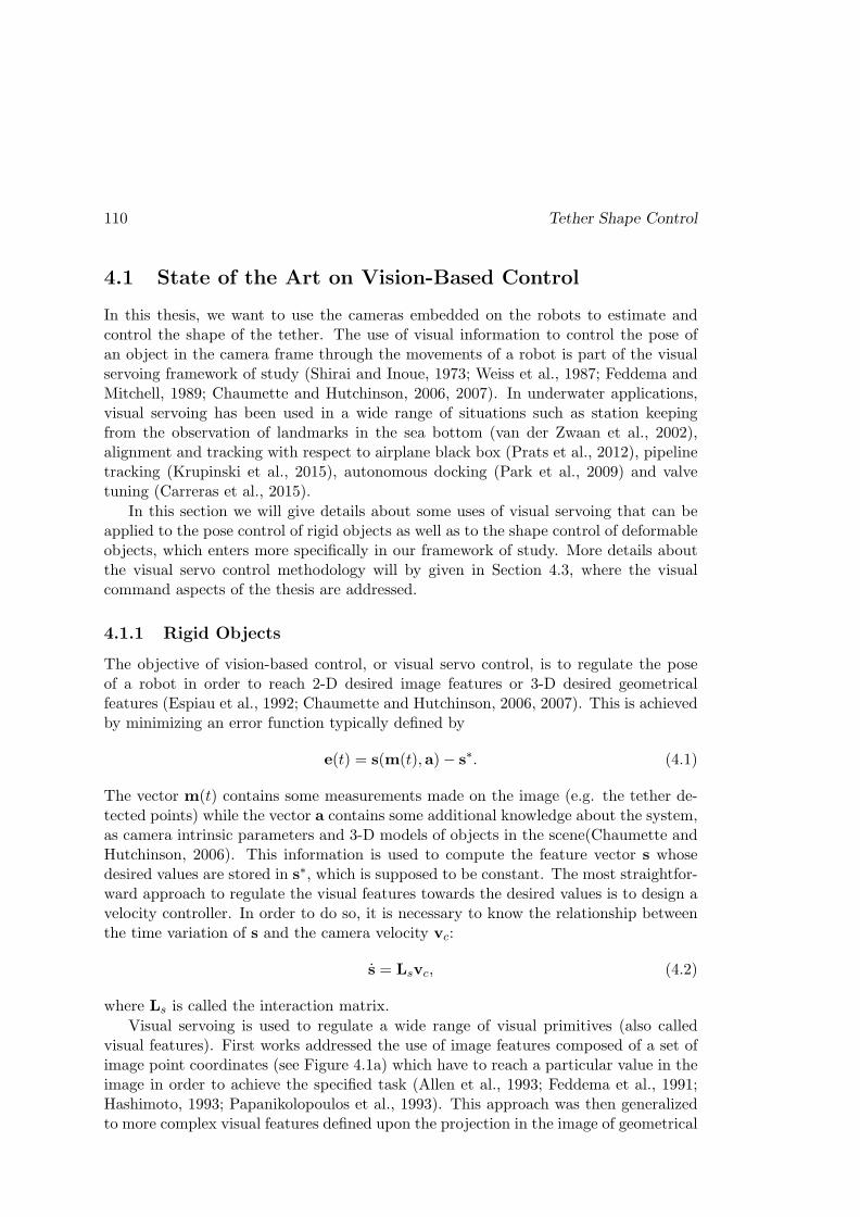
110 Tether Shape Control
4.1 State of the Art on Vision-Based Control
In this thesis, we want to use the cameras embedded on the robots to estimate andcontrol the shape of the tether. The use of visual information to control the pose ofan object in the camera frame through the movements of a robot is part of the visualservoing framework of study (Shirai and Inoue, 1973; Weiss et al., 1987; Feddema andMitchell, 1989; Chaumette and Hutchinson, 2006, 2007). In underwater applications,visual servoing has been used in a wide range of situations such as station keepingfrom the observation of landmarks in the sea bottom (van der Zwaan et al., 2002),alignment and tracking with respect to airplane black box (Prats et al., 2012), pipelinetracking (Krupinski et al., 2015), autonomous docking (Park et al., 2009) and valvetuning (Carreras et al., 2015).
In this section we will give details about some uses of visual servoing that can beapplied to the pose control of rigid objects as well as to the shape control of deformableobjects, which enters more specifically in our framework of study. More details aboutthe visual servo control methodology will by given in Section 4.3, where the visualcommand aspects of the thesis are addressed.
4.1.1 Rigid Objects
The objective of vision-based control, or visual servo control, is to regulate the poseof a robot in order to reach 2-D desired image features or 3-D desired geometricalfeatures (Espiau et al., 1992; Chaumette and Hutchinson, 2006, 2007). This is achievedby minimizing an error function typically defined by
e(t) = s(m(t),a)− s∗. (4.1)
The vector m(t) contains some measurements made on the image (e.g. the tether de-tected points) while the vector a contains some additional knowledge about the system,as camera intrinsic parameters and 3-D models of objects in the scene(Chaumette andHutchinson, 2006). This information is used to compute the feature vector s whosedesired values are stored in s∗, which is supposed to be constant. The most straightfor-ward approach to regulate the visual features towards the desired values is to design avelocity controller. In order to do so, it is necessary to know the relationship betweenthe time variation of s and the camera velocity vc:
s = Lsvc, (4.2)
where Ls is called the interaction matrix.
Visual servoing is used to regulate a wide range of visual primitives (also calledvisual features). First works addressed the use of image features composed of a set ofimage point coordinates (see Figure 4.1a) which have to reach a particular value in theimage in order to achieve the specified task (Allen et al., 1993; Feddema et al., 1991;Hashimoto, 1993; Papanikolopoulos et al., 1993). This approach was then generalizedto more complex visual features defined upon the projection in the image of geometrical

State of the Art on Vision-Based Control 111
primitives such as lines, spheres and cylinders (Chaumette, 1994). These works wereconcerned with known and simple objects. They assumed that the objects in the scenecan be expressed with simple geometrical features (points, straight lines, ellipses etc.).The group of objects that these methods can be applied to is thus limited.
(a) (b) (c)
(d) (e)
Figure 4.1: Example of visual servo control on rigid and articulated objects. (a) anexperiment of positioning in front of a square extracted from Espiau et al. (1992).Detected feature points in large dots and their desired positions are drawn in smallwhite dots. (b) an example of an amorphous planar shape used to validate the use ofimage moments in visual servoing; extracted from Tahri and Chaumette (2003). (c)an example of shape alignment using a technique of contour fitting to estimate objectfeature points to be used in visual servoing (extracted from Yazicioglu et al. (2009)).The feature points trajectories are drawn in green and blue lines. (d) an example ofvisual servoing used to regulate the robot’s pose with respect to a rigid object whoseCAD model is known (from Comport et al. (2004)). (e) another similar example butapplied to articulated objects (from Comport et al. (2007)).
Positioning tasks through 2-D visual servoing with respect to objects of unknownshape was achieved in Collewet and Chaumette (2002) and Dune (2009). In Collewetand Chaumette (2002), the object was assumed to be planar and motionless and the
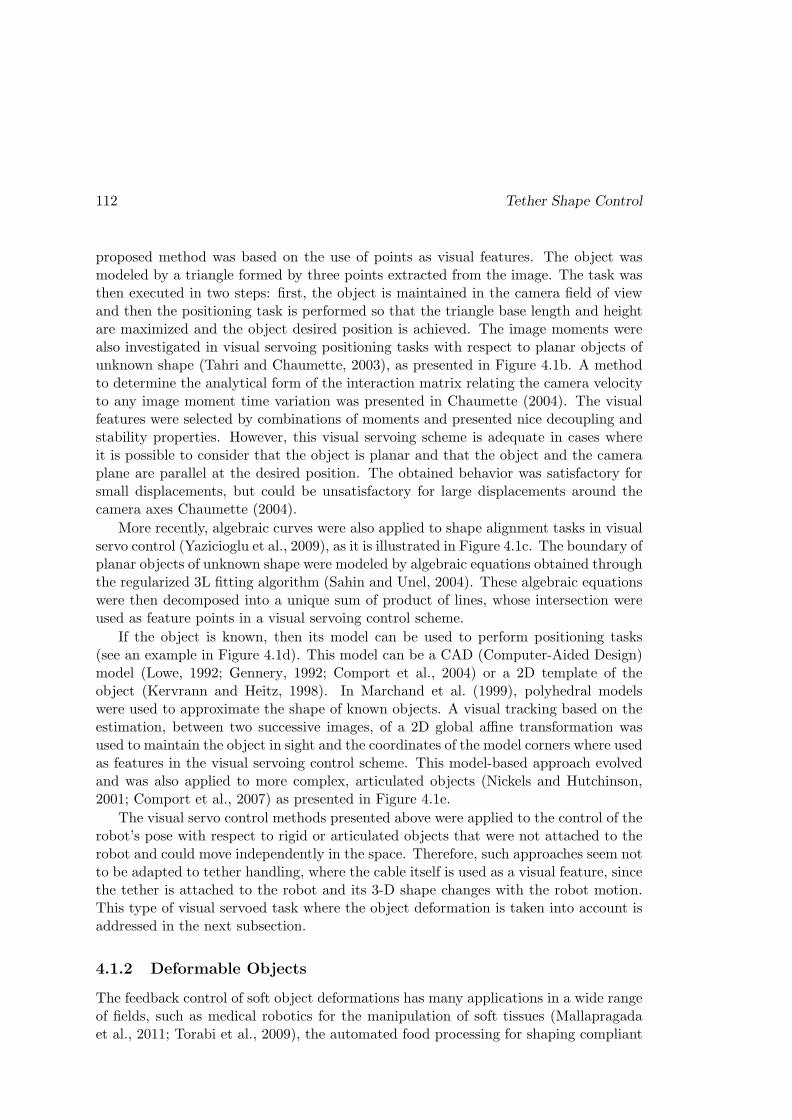
112 Tether Shape Control
proposed method was based on the use of points as visual features. The object wasmodeled by a triangle formed by three points extracted from the image. The task wasthen executed in two steps: first, the object is maintained in the camera field of viewand then the positioning task is performed so that the triangle base length and heightare maximized and the object desired position is achieved. The image moments werealso investigated in visual servoing positioning tasks with respect to planar objects ofunknown shape (Tahri and Chaumette, 2003), as presented in Figure 4.1b. A methodto determine the analytical form of the interaction matrix relating the camera velocityto any image moment time variation was presented in Chaumette (2004). The visualfeatures were selected by combinations of moments and presented nice decoupling andstability properties. However, this visual servoing scheme is adequate in cases whereit is possible to consider that the object is planar and that the object and the cameraplane are parallel at the desired position. The obtained behavior was satisfactory forsmall displacements, but could be unsatisfactory for large displacements around thecamera axes Chaumette (2004).
More recently, algebraic curves were also applied to shape alignment tasks in visualservo control (Yazicioglu et al., 2009), as it is illustrated in Figure 4.1c. The boundary ofplanar objects of unknown shape were modeled by algebraic equations obtained throughthe regularized 3L fitting algorithm (Sahin and Unel, 2004). These algebraic equationswere then decomposed into a unique sum of product of lines, whose intersection wereused as feature points in a visual servoing control scheme.
If the object is known, then its model can be used to perform positioning tasks(see an example in Figure 4.1d). This model can be a CAD (Computer-Aided Design)model (Lowe, 1992; Gennery, 1992; Comport et al., 2004) or a 2D template of theobject (Kervrann and Heitz, 1998). In Marchand et al. (1999), polyhedral modelswere used to approximate the shape of known objects. A visual tracking based on theestimation, between two successive images, of a 2D global affine transformation wasused to maintain the object in sight and the coordinates of the model corners where usedas features in the visual servoing control scheme. This model-based approach evolvedand was also applied to more complex, articulated objects (Nickels and Hutchinson,2001; Comport et al., 2007) as presented in Figure 4.1e.
The visual servo control methods presented above were applied to the control of therobot’s pose with respect to rigid or articulated objects that were not attached to therobot and could move independently in the space. Therefore, such approaches seem notto be adapted to tether handling, where the cable itself is used as a visual feature, sincethe tether is attached to the robot and its 3-D shape changes with the robot motion.This type of visual servoed task where the object deformation is taken into account isaddressed in the next subsection.
4.1.2 Deformable Objects
The feedback control of soft object deformations has many applications in a wide rangeof fields, such as medical robotics for the manipulation of soft tissues (Mallapragadaet al., 2011; Torabi et al., 2009), the automated food processing for shaping compliant
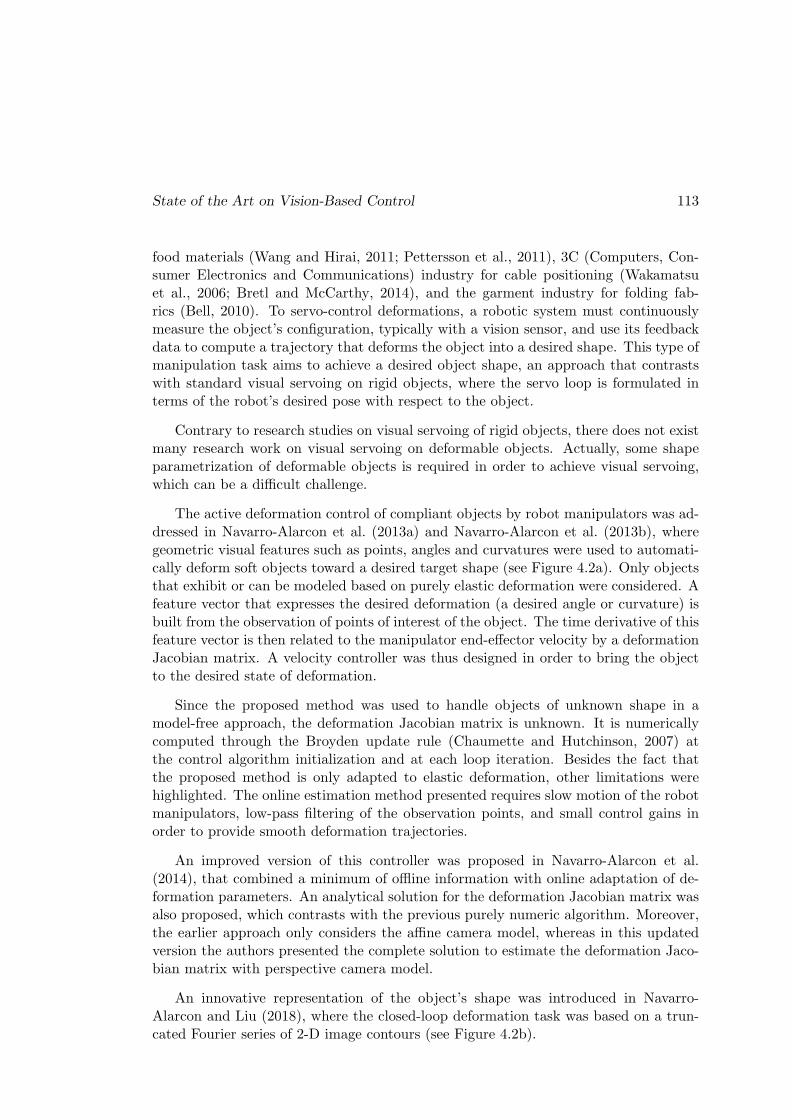
State of the Art on Vision-Based Control 113
food materials (Wang and Hirai, 2011; Pettersson et al., 2011), 3C (Computers, Con-sumer Electronics and Communications) industry for cable positioning (Wakamatsuet al., 2006; Bretl and McCarthy, 2014), and the garment industry for folding fab-rics (Bell, 2010). To servo-control deformations, a robotic system must continuouslymeasure the object’s configuration, typically with a vision sensor, and use its feedbackdata to compute a trajectory that deforms the object into a desired shape. This type ofmanipulation task aims to achieve a desired object shape, an approach that contrastswith standard visual servoing on rigid objects, where the servo loop is formulated interms of the robot’s desired pose with respect to the object.
Contrary to research studies on visual servoing of rigid objects, there does not existmany research work on visual servoing on deformable objects. Actually, some shapeparametrization of deformable objects is required in order to achieve visual servoing,which can be a difficult challenge.
The active deformation control of compliant objects by robot manipulators was ad-dressed in Navarro-Alarcon et al. (2013a) and Navarro-Alarcon et al. (2013b), wheregeometric visual features such as points, angles and curvatures were used to automati-cally deform soft objects toward a desired target shape (see Figure 4.2a). Only objectsthat exhibit or can be modeled based on purely elastic deformation were considered. Afeature vector that expresses the desired deformation (a desired angle or curvature) isbuilt from the observation of points of interest of the object. The time derivative of thisfeature vector is then related to the manipulator end-effector velocity by a deformationJacobian matrix. A velocity controller was thus designed in order to bring the objectto the desired state of deformation.
Since the proposed method was used to handle objects of unknown shape in amodel-free approach, the deformation Jacobian matrix is unknown. It is numericallycomputed through the Broyden update rule (Chaumette and Hutchinson, 2007) atthe control algorithm initialization and at each loop iteration. Besides the fact thatthe proposed method is only adapted to elastic deformation, other limitations werehighlighted. The online estimation method presented requires slow motion of the robotmanipulators, low-pass filtering of the observation points, and small control gains inorder to provide smooth deformation trajectories.
An improved version of this controller was proposed in Navarro-Alarcon et al.(2014), that combined a minimum of offline information with online adaptation of de-formation parameters. An analytical solution for the deformation Jacobian matrix wasalso proposed, which contrasts with the previous purely numeric algorithm. Moreover,the earlier approach only considers the affine camera model, whereas in this updatedversion the authors presented the complete solution to estimate the deformation Jaco-bian matrix with perspective camera model.
An innovative representation of the object’s shape was introduced in Navarro-Alarcon and Liu (2018), where the closed-loop deformation task was based on a trun-cated Fourier series of 2-D image contours (see Figure 4.2b).

114 Tether Shape Control
(a)
(b)
(c)
Figure 4.2: Some examples of visual servoing on deformable objects. (a) shape controlof a sponge with current and desired shape feature drawn in red and green, respectively.Initial shape on the left-hand side and final shape on the right-hand side. Extractedfrom Navarro-Alarcon et al. (2013b). (b) manipulation of an uterus model thoughvisual feedback where the object contour is modeled by a truncated Fourier series. Thedesired contour is drawn in red and the figure was extracted from Navarro-Alarcon andLiu (2018). (c) the same technique of shape modeling through Fourier series appliedto 1-D objects. Image extracted from Zhu et al. (2018).
This approach contrasts with previous methods that typically use the displacementsof feature points to define the deformation task (reach a desired angle or curvature).The controller design relied on an explicit shape servo loop by feeding back a vector ofFourier coefficients. This design provided more flexibility for the description of the feed-back shape and its target configuration (the desired contour can be roughly sketchedon a screen), and allowed the manipulation of soft objects with unstructured surfaceswithout special fiducial markers. To avoid the full parametric identification of the ob-ject’s model, an online algorithm that approximates the deformation properties was
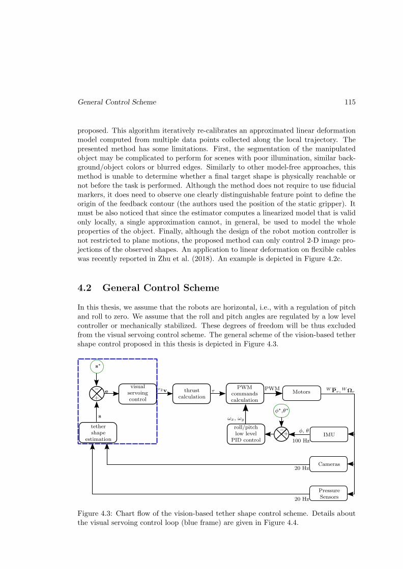
General Control Scheme 115
proposed. This algorithm iteratively re-calibrates an approximated linear deformationmodel computed from multiple data points collected along the local trajectory. Thepresented method has some limitations. First, the segmentation of the manipulatedobject may be complicated to perform for scenes with poor illumination, similar back-ground/object colors or blurred edges. Similarly to other model-free approaches, thismethod is unable to determine whether a final target shape is physically reachable ornot before the task is performed. Although the method does not require to use fiducialmarkers, it does need to observe one clearly distinguishable feature point to define theorigin of the feedback contour (the authors used the position of the static gripper). Itmust be also noticed that since the estimator computes a linearized model that is validonly locally, a single approximation cannot, in general, be used to model the wholeproperties of the object. Finally, although the design of the robot motion controller isnot restricted to plane motions, the proposed method can only control 2-D image pro-jections of the observed shapes. An application to linear deformation on flexible cableswas recently reported in Zhu et al. (2018). An example is depicted in Figure 4.2c.
4.2 General Control Scheme
In this thesis, we assume that the robots are horizontal, i.e., with a regulation of pitchand roll to zero. We assume that the roll and pitch angles are regulated by a low levelcontroller or mechanically stabilized. These degrees of freedom will be thus excludedfrom the visual servoing control scheme. The general scheme of the vision-based tethershape control proposed in this thesis is depicted in Figure 4.3.
tethershape
estimation
s∗
+
−
s
evisual
servoingcontrol
roll/pitchlow level
PID control
thrustcalculation
IMU
Cameras
PressureSensors
r2v τPWM
commandscalculation
MotorsPWM
100 Hz
20 Hz
20 Hz
ωx, ωy
φ∗,θ∗
φ, θ+
−
WPr,WΩr
Figure 4.3: Chart flow of the vision-based tether shape control scheme. Details aboutthe visual servoing control loop (blue frame) are given in Figure 4.4.


Catenary-Based Interaction Matrices 117
a catenary fitting algorithm. Then, the cost function value is used to calculate afitting quality index. If the shape estimation is not accurate, the tether features arepredicted from the previous command velocities and interaction matrix evaluation. Ifthe shape estimation is enough accurate, the error vector between current and desiredfeatures are computed. Next, the interaction matrix and the new command velocitiesare calculated before sending them to the embedded micro-controller. The calculationof the interaction matrix is detailed in the following Section.
4.3 Catenary-Based Interaction Matrices
The objective of this Section is to express the velocities of the follower robot as afunction of features extracted from the catenary model of the tether, i.e., its slackness,orientation, and height difference between attachment points. As explained in previousSection, the tether slackness and orientation are estimated thanks to image fittingtechniques whereas the attachment points height difference is calculated from depthsensors feedback.
FOLL
OWER
LEADERFr2
jr2ir2
Fr1
jr1
ir1
Fc2kc2
ic2
α2F2
j2i2
F0
j0
i0
F1
j1
i1
FW
jW
iW
α1 Fc1
kc1
ic1
(a)
FOLLOWER
LEADER
D D ∆D2FW
kW
iW
ir2
F2 i2
k2 ∆H2
H2
F0
F1
k0
i0
k1
i1
Fr1
kr1
ir1
Fr2
kr2 Fc2
jc2
kc2
jc1
kc1
Fc1
(b)
Figure 4.5: Figure 3.1 is reproduced to remind the features definition. (a) top viewand (b) side view.

118 Tether Shape Control
The catenary features (see Figure 4.5) from the follower robot side, as introducedin Chapter 3 in equations (3.34a) and (3.34b), are noted
a2 =H2
Hmax(4.3)
b2 = sinα2, (4.4)
and range in the interval ]0, 1[. In addition to these features, we add a third one relatedto ∆H2:
d2 =∆H2 +∆Hmax
2∆Hmax(4.5)
This new feature is also normalized and ranges in the interval ]0, 1[. If P1 is above P2,then d2 ∈ [0.5, 1] else d2 ∈ [0, 0.5], which means that ∆H2 ∈ [−∆Hmax,∆Hmax].
We then define the feature vector as:
s2 =
a2b2d2
. (4.6)
Similarly, from the leader robot side, we can set the feature vector as:
s1 =
a1b1d1
, (4.7)
where a1 =H1
Hmax, b1 = sinα1 and d1 =
∆H1+∆Hmax
2∆Hmax.
From equations (2.87) and (2.88) in Chapter 2, we have the relation between therobots velocities and the variation of the tether attachment points relative position:
˙2P1 =
˙2X1˙2Y1˙2Z1
= Tr1,2
r1v +Tr2,2r2v (4.8)
˙1P2 =
˙1X2˙1Y2˙1Z2
= Tr1,1
r1v +Tr2,1r2v.
Now, we need to find the relationship between the feature vector time derivative andthe coordinates of the attachment points time derivative. We will conduct the calcu-
lation from the follower side using s2 =[a2, b2, d2
]Tand ˙2P1 =
[˙2X1, ˙2Y1, ˙2Z1
]T. The
expression regarding the leader robot side will be obtained symmetrically.We start the calculation with
2P1 =
2X12Y12Z1
=
(2D2 +∆D2) cosα2
(2D2 +∆D2) sinα2
∆H2
F2
=
(2D2 +∆D2)
√1− b22
(2D2 +∆D2)b22d2∆Hmax −∆Hmax
F2
. (4.9)
Catenary-Based Interaction Matrices 119
We know from Figure 2.10 that:
sinα2 = b2 =2Y1
2D2 +∆D2(4.10)
cosα2 =√1− b22 =
2X1
2D2 +∆D2. (4.11)
The values of a2 and b2 are obtained from the vision system, and d2 from the depthsensors. The value of D2 is obtained thanks to the following equation:
D2 =1
Ccosh−1 (Ca2Hmax + 1) , (4.12)
which states that P2 belongs to the catenary, as introduced by equation (2.13) inSection 2.1.2.
The value of D2 +∆D2 is obtained thanks to the equation:
D2 +∆D2 =1
Ccosh−1 (C (a2Hmax + 2d2∆Hmax −∆Hmax) + 1) , (4.13)
which states that P1 belongs to the catenary, as introduced by equation (2.14).Let us differentiate equation 4.9:
˙2P1 =
[D2 + (D2 + ∆D2)
]√1− b22 − (2D2 +∆D2)
b2b2√1−b2
2[D2 + (D2 + ∆D2)
]b2 + (2D2 +∆D2)b2
2d2∆Hmax
F2
(4.14)
=
[D2 + (D2 + ∆D2)
]2X1
2D2+∆D2− 2Y1
b2√1−b2
2[D2 + (D2 + ∆D2)
]2Y1
2D2+∆D2+ (2D2 +∆D2)b2
2d2∆Hmax
F2
(4.15)
We then need to explicit the derivative of the features a2, b2 and d2 as function of˙2X1, ˙2Y1 and ˙2Z1.
Expression of d2 as function of ˙2X1, ˙2Y1 and ˙2Z1
From equation (4.5), we directly have:
d2 =˙∆H2
2∆Hmax=
˙2Z1
2∆Hmax(4.16)
Expression of b2 as function of ˙2X1, ˙2Y1 and ˙2Z1
From the first two lines of the matrix given in equation (4.15) we get:
˙2X1 = (D2 + (D2 + ∆D2))√1− b22 − (2D2 +∆D2)
b2b2√1− b22
(4.17)
˙2Y1 = (D2 + (D2 + ∆D2))b2 + (2D2 +∆D2)b2 (4.18)
120 Tether Shape Control
which leads to:
2D2 + ∆D2 =√
1− b22 ˙2X1 + b2 ˙2Y1 =2X1
˙2X1 +2Y1 ˙2Y1
2D2 +∆D2(4.19)
b2 =
√1− b22
2D2 +∆D2
[−b2 ˙2X1 +
√1− b22 ˙2Y1
](4.20)
Expression of a2 as function of ˙2X1, ˙2Y1 and ˙2Z1
From the definition of parameter a2 in equation (4.3) we obtain:
a2 =H2
Hmax(4.21)
The equation (4.19) is useful to get H2 as a function of the coordinates derivatives˙2X1, ˙2Y1 and ˙2Z1 because D2 and ∆D2 depend on H2 and ∆H2.From equation (4.12) we have
CH2 = [cosh(CD2)− 1] . (4.22)
The differentiation of this equation yields:
D2 = p2H2 + q2 ˙∆H2 (4.23)
with
p2 =C + LD2
∂C∂H2
C sinh(CD2)(4.24)
q2 =LD2
∂C∂∆H2
C sinh(CD2)(4.25)
LD2= H2 −D2 sinh(CD2) (4.26)
From equation (4.13) we have:
C (H2 +∆H2) = [cosh(C(D2 +∆D2)− 1] . (4.27)
The differentiation of this equation yields:
D2 + ˙∆D2 = u2H2 + v2 ˙∆H2 (4.28)
with:
u2 =C + L∆D2
∂C∂H2
C sinh(C(D2 +∆D2))(4.29)
v2 =C + L∆D2
∂C∂∆H2
C sinh(C(D2 +∆D2))(4.30)
L∆D2= H2 +∆H2 − (D2 +∆D2) sinh(C(D2 +∆D2)) (4.31)
Catenary-Based Interaction Matrices 121
The partial derivatives of the catenary C parameter are calculated from differenti-ation of equation (2.16):
C(H2,∆H2) =∂C
∂H2H2 +
∂C
∂∆H2
˙∆H2. (4.32)
The expression of the partial derivatives ∂C∂H2
and ∂C∂∆H2
are given in appendix D.
Finally, combining equations (4.19), 4.21, (4.23) and (4.28) leads to:
2D2 + ˙∆D2 = (u2 + p2)H2 + (v2 + q2) ˙∆H2 (4.33)
a2 =1
(u2 + p2)Hmax
(2X1
˙2X1 +2Y1 ˙2Y1
2D2 +∆D2− (v2 + q2) ˙2Z1
)(4.34)
Catenary Interaction Matrix
In summary, we can write equations (4.34), (4.20) and (4.16) as:
a2 =1
(u2 + p2)Hmax
[√1− b22, b2, −(v2 + q2)
]
˙2X1˙2Y1˙2Z1
(4.35)
b2 =
√1− b22
2D2 +∆D2
[−b2,
√1− b22, 0
]
˙2X1˙2Y1˙2Z1
(4.36)
d2 =1
2∆Hmax
[0 0 1
]
˙2X1˙2Y1˙2Z1
, (4.37)
where the expressions of b2 and√1− b22 were given in equations (4.10) and (4.11).
Rewriting equations (4.35), (4.36) and (4.37) in matrix form yields:
a2b2d2
= M2
˙2X1˙2Y1˙2Z1
(4.38)
with
M2 =
√1−b2
2
(u2+p2)Hmax
b2(u2+p2)Hmax
− v2+q2(u2+p2)Hmax
−b2√
1−b22
2D2+∆D2
1−b22
2D2+∆D20
0 0 12∆Hmax
Introducing equation (2.87) into (4.38) we obtain:
s2 =
a2b2d2
= Lr1,2
r1v + Lr2,2r2v, (4.39)
122 Tether Shape Control
with
Lr1,2 = M2Tr1,2
Lr2,2 = M2Tr2,2.
Using the twist matrix (see appendix C), we have:
Lr1,2 = −M2Tr2,2r2Vr1
Lr1,2 = −Lr2,2r2Vr1 ,
which allows us to rewrite equation (4.39) as follows:
s2 =
a2b2d2
= Lr2,2 (
r2v − r2Vr1r1v) , (4.40)
The matrices Lr1,2 and Lr2,2 are called interaction matrices and link, respectively,the velocities of leader (r1) and follower (r2) robots with the time derivative of thefeature vector s2. Symmetrically, we have:
s1 =
a1b1d1
= Lr2,1
r2v + Lr1,1r1v = Lr2,1 (
r2v − r2Vr1r1v) (4.41)
with
Lr2,1 = M1Tr2,1
Lr1,1 = M1Tr1,1
Lr1,1 = −M1Tr2,1r2Vr1 = −Lr2,1
r2Vr1
Generalizing equations (4.39) and (4.41), we can write, for i ∈ 1, 2, that:
si =
aibidi
= Lr2,i
r2v + Lr1,ir1v (4.42)
with
Lr2,i = MiTr2,i (4.43)
Lr1,i = MiTr1,i
and
Mi =
√1−b2i
(ui+pi)Hmax
bi(ui+pi)Hmax
− vi+qi(ui+pi)Hmax
−bi√
1−b2i2Di+∆Di
1−b2i2Di+∆Di
0
0 0 12∆Hmax
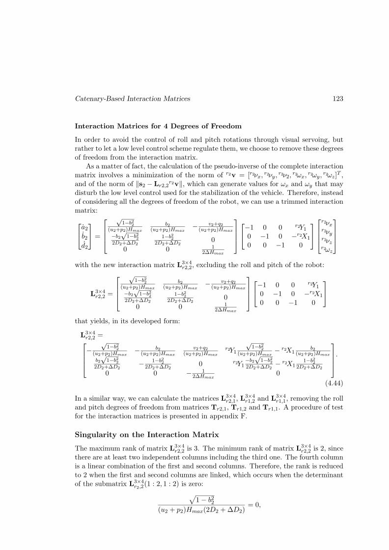
Catenary-Based Interaction Matrices 123
Interaction Matrices for 4 Degrees of Freedom
In order to avoid the control of roll and pitch rotations through visual servoing, butrather to let a low level control scheme regulate them, we choose to remove these degreesof freedom from the interaction matrix.
As a matter of fact, the calculation of the pseudo-inverse of the complete interactionmatrix involves a minimization of the norm of r2v = [r2νx,
r2νy,r2ν2,
r2ωx,r2ωy,
r2ωz]T ,
and of the norm of ‖s2 − Lr2,2r2v‖, which can generate values for ωx and ωy that may
disturb the low level control used for the stabilization of the vehicle. Therefore, insteadof considering all the degrees of freedom of the robot, we can use a trimmed interactionmatrix:
a2b2d2
=
√1−b2
2
(u2+p2)Hmax
b2(u2+p2)Hmax
− v2+q2(u2+p2)Hmax
−b2√
1−b22
2D2+∆D2
1−b22
2D2+∆D20
0 0 12∆Hmax
−1 0 0 r2Y10 −1 0 −r2X1
0 0 −1 0
r2νxr2νyr2νzr2ωz
with the new interaction matrix L3×4r2,2, excluding the roll and pitch of the robot:
L3×4r2,2 =
√1−b2
2
(u2+p2)Hmax
b2(u2+p2)Hmax
− v2+q2(u2+p2)Hmax
−b2√
1−b22
2D2+∆D2
1−b22
2D2+∆D20
0 0 12∆Hmax
−1 0 0 r2Y10 −1 0 −r2X1
0 0 −1 0
that yields, in its developed form:
L3×4r2,2 =−
√1−b2
2
(u2+p2)Hmax− b2
(u2+p2)Hmax
v2+q2(u2+p2)Hmax
r2Y1
√1−b2
2
(u2+p2)Hmax− r2X1
b2(u2+p2)Hmax
b2√
1−b22
2D2+∆D2− 1−b2
2
2D2+∆D20 r2Y1
−b2√
1−b22
2D2+∆D2− r2X1
1−b22
2D2+∆D2
0 0 − 12∆Hmax
0
.
(4.44)
In a similar way, we can calculate the matrices L3×4r2,1, L
3×4r1,2 and L3×4
r1,1, removing the rolland pitch degrees of freedom from matrices Tr2,1, Tr1,2 and Tr1,1. A procedure of testfor the interaction matrices is presented in appendix F.
Singularity on the Interaction Matrix
The maximum rank of matrix L3×4r2,2 is 3. The minimum rank of matrix L3×4
r2,2 is 2, sincethere are at least two independent columns including the third one. The fourth columnis a linear combination of the first and second columns. Therefore, the rank is reducedto 2 when the first and second columns are linked, which occurs when the determinantof the submatrix L3×4
r2,2(1 : 2, 1 : 2) is zero:
√1− b22
(u2 + p2)Hmax(2D2 +∆D2)= 0,

124 Tether Shape Control
which corresponds to
1− b2 = 0. (4.45)
The equation (4.45) represents the cases where b = sinα = ±1, thus α = ±90and the tether plane is perpendicular to the robot longitudinal plane. In such cases,the first column of the interaction matrix is zero. This produces a loss of control ofthe longitudinal velocity. As discussed in Section 3.4.3.2, these cases will be avoidedsince the tether is less visible (limited camera field of view) and it risks of becomingentangled with the robot.
Analyzing the matrix L3×4r2,2
we note that it can be singular due to infinite values, if:
2D2 +∆D2 = 0 (4.46)
u2 + p2 = 0 (4.47)
The singularity given in equation (4.46) corresponds to a tether whose span is zero(attachments points on the same vertical), which is not possible.
The equation (4.47) corresponds to a singularity that never occurs because u2+p2 6=0 and keeps a negative sign. If u2+p2 were to become zero, it would mean that the spanbetween the tether attachment points could be changed whatever the tether slackness,which is impossible (see equation (4.33)).
Another explanation can be given by looking at equation (4.33), and considering afixed ∆H2, which yields:
2D2 + ˙∆D2 = (u2 + p2)H2.
If we extend the catenary span, 2D2 +∆D2 increases, and the slackness H2 decreases,which means that 2D2 + ˙∆D2 is positive and H2 is negative. Therefore, (u2 + p2) < 0.Conversely, if we reduce the catenary span, 2D2+∆D2 decreases and the slackness H2
increases, which means that 2D2 + ˙∆D2 is negative and H2 is positive, also leading to(u2 + p2) < 0.

Follower Robot Control using Tether Visual Feedback 125
4.4 Follower Robot Control using Tether Visual Feedback
In this Section, we present the vision-based control scheme used to command the fol-lower robot motion in order to regulate the tether shape. As introduced in Chapter 2,the leader robot is free to explore its surroundings, while the follower robot main taskis to ensure, from its onboard camera feedback, that the tether cable does not hamperthe leader movements. Therefore, the follower must maintain the cable slack enoughnot to pull the leader. Moreover, it must keep a desired orientation between tetherand onboard camera in order to ensure that the tether is well visible in the image andthat its shape can be accurately estimated from the curve fitting algorithm presentedin Chapter 3. The tether attachment points difference of height must also be regulated,since it impacts the tether slackness and shape in the image.
Here, only the follower robot frontal camera is used in the visual servoing controlscheme (both leader and follower cameras will be used in Section 4.5). The featurevector to be regulated from the follower robot motion is defined as:
s2 =
a2b2d2
=
H2
Hmax
sinα2∆H2+∆Hmax
2∆Hmax
.
The error vector e2 between the current and the desired feature vector s∗2 is defined as:
e2 = s2 − s∗2. (4.48)
The error vector time derivative is therefore:
e2 = s2. (4.49)
As explained in the previous Section, the roll and pitch angles are assumed to befixed thanks to a low level control or to a mechanical self-stabilization. We use hence3 by 4 interaction matrices, removing the columns related to roll and pitch motions ofthe robot. For example, the interaction matrix L3×4
r2,2, given by the equation (4.44), is
a 3 by 4 matrix that links the variations of the feature vector s2 to the follower robotvelocities r2v3×4 = [νx, νy, νz, ωz]
T . In order to simplify the writing, we will note fromnow on:
Lr2,2 = L3×4r2,2
Lr1,2 = L3×4r2,2
Lr2,1 = L3×4r2,2
Lr1,1 = L3×4r2,2
r2v = r2v3×4
r1v = r1v3×4.
In the sequel, preliminary results with 2-D terrestrial robots are given. Then anumber of tether shape control schemes for 3-D underwater robots are tested in simu-lation. Two types of situations are addressed. First, the leader robot is stopped and the

126 Tether Shape Control
follower robot brings the tether from its initial to its desired shape. Second, the leaderrobot executes a predefined path and the follower robot must maintain the tether atits desired shape. The leader robot velocities may be considered or not in the followerrobot control law.
The simulations are carried out on Gazebo (Koenig and Howard, 2004). In thecase of underwater robots, the UUV (unmanned underwater vehicle) package (Manhaeset al., 2016) is used, as described in the previous Chapter. The robots are equipped withsimulated pressure sensors, frontal and rear cameras. The simulated tether is 1.50meterlong and 3millimeter thick. The maximum slackness is set at Hmax = 0.70meter. Themaximum attachment point difference of height is set at ∆Hmax = 0.50meter. Thecontrol loop runs at a rate of 30Hz.
4.4.1 Preliminary Results with Terrestrial Robots
In this Section we present a summary of our preliminary research results on tethershape control using terrestrial robots. More details are given in appendix E.
First, we introduce the work that was presented at the 2017 IEEE InternationalConference on Robotics and Automation (ICRA 2017), whose title is Catenary-based
Visual Servoing for Tethered Robots. This work addressed the use of catenary-model-based features to achieve visual servoing of an umbilical linking two terrestrialrobots.
Second, we introduce another work that compared catenary-based with image-based visual servoing controllers. More details are available in the article entitledTether Shape Control through Catenary-Model-Based Visual Servoing, inappendix E.
4.4.1.1 Catenary-Based Visual Servoing for Terrestrial Robots
The new visual servoing scheme introduced for catenary shaped deformable objects wastested on terrestrial robots to control the tether parametric shape by properly movingits fixation point.
The interaction matrix is a full 2×6 matrix (see equation (23) of the correspondingpaper in appendix E), assuming that the tether attachment points are at the sameheight. Only the features from the follower camera image view were taken into account.
The experimental system is composed of two terrestrial mobile robots of the samemotion capabilities linked with a slack rope.
One simulation and two real experiments were carried out in order to validate thecontrol law with two Turtlebots (Gerkey and Conley, 2011) with 2 DOF (translationvx and rotation wz). They were equipped with an onboard RGBD camera and linkedby a 1.4 meter long and 3 millimeter thick orange rope. The video frame rate was fixedto 10Hz. The same robot motion capabilities, rope length, thickness and maximum sagwere used in simulation and real experiments.

Follower Robot Control using Tether Visual Feedback 127
Simulation and Experimental Results One simulation and two real experimentsare presented in order to validate the control law. Two Turtlebots Gerkey and Conley(2011) with 2 DOF (translation νx and rotation ωz) are used as experimental robots.They are equipped with a Kinect device and linked by a 1.4 meter long and 3 millimeterthick orange rope (see Figure 4.6). The rope maximum sag is Hmax = 0.40m, corre-sponding to its attachment point’s height. The servoing algorithm runs in the followerrobot computer, which is equipped with a Intel Core i5-2410M @ 2.3 GHz processor.The video frame rate is fixed to 10Hz. The same robot motion capabilities, rope length,thickness and maximum sag are used in simulation and real experiments.
Figure 4.6: Experimental setup: two Turtlebots (Gerkey and Conley, 2011) simulate atether handling system for remotely operated robots. The leader robot freely exploresits surroundings while the follower robot is expected to maintain the tether slack enoughnot to hamper the leader movements
The objective of the simulation is that the follower robot moves the tether froma very slackened to a moderately tight shape. The tether orientation is controlled,passing from a large angle θ1 to a desired smaller angle. The initial and desired valuesof the feature vector are so = (0.9, 0.8) and s∗ = (0.5, 0.5), respectively. We assume thatthe robots can perfectly estimate the tether parameters, so the fitting process is notsimulated. Figure 4.7 presents the simulation results. As expected, both parametershave an exponential decay and converge to the desired value within 4 seconds for a gainλ = 0.75 and a sampling period of 0.1 seconds.
In the first experiment, the simulation initial conditions are repeated and the fol-lower robot moves the tether from an initial shape so = (0.9, 0.8) to a desired shapes∗ = (0.5, 0.5). We used the same gain as for simulation (λ = 0.75) and a fitting qualitythreshold Qmax = 1. Results are summarized in Figure 4.8.
In the second experiment (see Figure 4.9), the leader robot is freely displaced whilethe follower robot ensures that the rope keeps a desired shape s∗ = (0.7,−0.5). First,the leader robot moves forward, then turns left (24s). Next, it moves about 1.25meters forward (38s), makes a half-turn (50s) and moves about 1.25 meters forward
1for the Turtlebots, we note the orientation angle as θ, instead of α
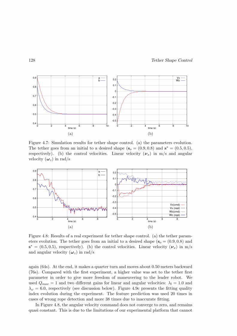
128 Tether Shape Control
0.4
0.5
0.6
0.7
0.8
0.9
0 2 4 6 8 10time (s)
ab
(a)
-0.5
-0.4
-0.3
-0.2
-0.1
0
0.1
0.2
0 2 4 6 8 10time (s)
VxWz
(b)
Figure 4.7: Simulation results for tether shape control. (a) the parameters evolution.The tether goes from an initial to a desired shape (so = (0.9, 0.8) and s∗ = (0.5, 0.5),respectively). (b) the control velocities. Linear velocity (νx) in m/s and angularvelocity (ωz) in rad/s
0.4
0.5
0.6
0.7
0.8
0.9
0 2 4 6 8time (s)
a
b
(a)
-0.5
-0.4
-0.3
-0.2
-0.1
0
0.1
0.2
0 2 4 6 8time (s)
Vx(cmd)
Vx (real)
Wz(cmd)
Wz (real)
(b)
Figure 4.8: Results of a real experiment for tether shape control. (a) the tether param-eters evolution. The tether goes from an initial to a desired shape (so = (0.9, 0.8) ands∗ = (0.5, 0.5), respectively). (b) the control velocities. Linear velocity (νx) in m/sand angular velocity (ωz) in rad/s
again (64s). At the end, it makes a quarter turn and moves about 0.50 meters backward(76s). Compared with the first experiment, a higher value was set to the tether firstparameter in order to give more freedom of maneuvering to the leader robot. Weused Qmax = 1 and two different gains for linear and angular velocities: λl = 1.0 andλω = 6.0, respectively (see discussion below). Figure 4.9c presents the fitting qualityindex evolution during the experiment. The feature prediction was used 20 times incases of wrong rope detection and more 38 times due to inaccurate fitting.
In Figure 4.8, the angular velocity command does not converge to zero, and remainsquasi constant. This is due to the limitations of our experimental platform that cannot
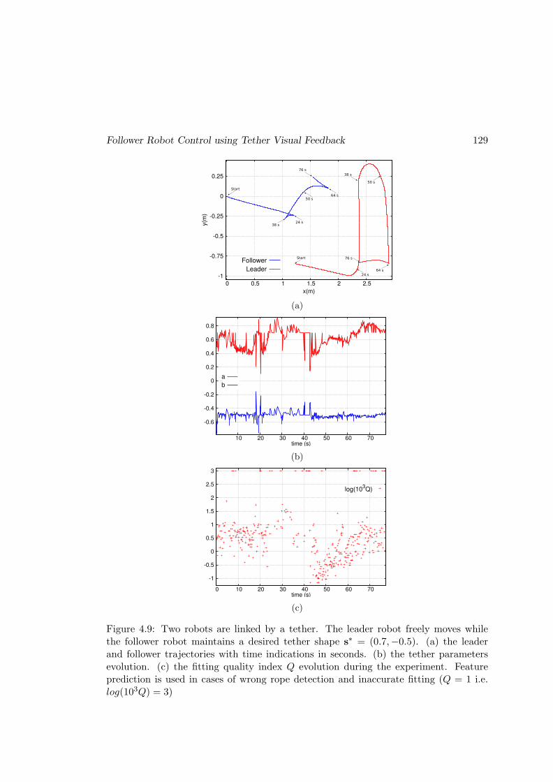
Follower Robot Control using Tether Visual Feedback 129
-1
-0.75
-0.5
-0.25
0
0.25
0 0.5 1 1.5 2 2.5
y(m
)
x(m)
Follower
Leader
24 s
24 s
38 s
38 s
50 s
50 s64 s
64 s
76 s
76 s
Start
Start
(a)
-0.6
-0.4
-0.2
0
0.2
0.4
0.6
0.8
10 20 30 40 50 60 70time (s)
a
b
(b)
-1
-0.5
0
0.5
1
1.5
2
2.5
3
0 10 20 30 40 50 60 70time (s)
log(103Q)
(c)
Figure 4.9: Two robots are linked by a tether. The leader robot freely moves whilethe follower robot maintains a desired tether shape s∗ = (0.7,−0.5). (a) the leaderand follower trajectories with time indications in seconds. (b) the tether parametersevolution. (c) the fitting quality index Q evolution during the experiment. Featureprediction is used in cases of wrong rope detection and inaccurate fitting (Q = 1 i.e.log(103Q) = 3)
130 Tether Shape Control
achieve a rotation velocity lower than 0.05 rad/s. In the second experiment, we selecteda higher gain for the angular velocity compared to the linear velocity gain in order toovercome this problem. As a future improvement, an integrator compensator to dealwith the low level control of the velocity can be added to the servoing loop.
Looking at Figure 4.8, we can note that the real experimentation curves are noisycompared with those obtained in simulation. This is mainly due to wrong rope detectionthat can affect the tether feature estimation. Another reason is the possible ropeoscillation during the robot motion, which can occur when the robot halts and restartsmotion. This could be taken into account by designing a dynamic controller that takesthe rope inertia into account. In addition, the rope can be tracked in the image by agradient-guided algorithm.
Despite the problem of nonholonomy, the control scheme was validated by simu-lation and by two series of real experiments. The comparison of simulation and realexperiments showed that the tether converged to their desired values, validating theproposed control law. More details about this work can be found in appendix E, wherethe paper Catenary-based Visual Servoing for Tethered Robots, presented atICRA 2017, is reproduced. These experiments constituted our first results obtainedwith catenary-based visual servoing of umbilicals. This work showed the feasibility ofthe catenary-based visual servoing proposed in the framework of this thesis.
4.4.1.2 Comparison of Catenary-Based Control with Image-Based Visual
Servoing
In a second series of studies, we compared the catenary-based controllers with standardimage-based visual servoing techniques. We considered some salient points such as thehighest and lowest tether points in the image, or we approximated the first portion ofthe tether with a line segment (see Figure 4.10). Such features were successfully used tocontrol a robot motion by regulating the shape of rigid objects in the image (Collewetand Chaumette, 2002; Cherubini et al., 2008). The tether shape evolution, velocitycommands and condition number of interaction matrices were studied in normal andlimit cases for two image-based controllers and both catenary-based controllers pro-posed:
• image points: coordinates of the tether highest and lowest points (pA and pB)detected in the image without taking into account that the points belong to acatenary projection (Espiau et al., 1992)
• image line segment : center, length and orientation of the segment pApB link-ing the highest and the lowest points of the tether detected in the image, withouttaking into account that the points belong to a catenary projection (Chaumetteet al., 1993)
• catenary parameters: two features s = [a b]T , related to tether slackness andorientation that parameterize the catenary curve to fit the tether 3D shape (Laran-jeira et al., 2017).

Follower Robot Control using Tether Visual Feedback 131
• catenary-projection lowest point: coordinates of the tether lowest point (pB)detected in the image, making the approximation that this point is the projectionof the 3D catenary lowest point .
xP0
(a)pA
pBp0x
(b)
x
pA
p0 pB
(c)
Figure 4.10: Image features used to manage the tether shape: its highest and lowestpoints in the image (pA and pB) and the line segment pApB in blue. (a) 3D simulatedscene where the tether 3D lowest point P0 is out of the follower’s camera field of view.(b) corresponding embedded view with p0 being the perspective projection of P0. (c)Another situation where P0 is inside the follower’s camera field of view
Simulation are performed using Gazebo Koenig and Howard (2004) to test thewhole control loop including computer vision algorithms. The setup is composed oftwo Turtlebots Gerkey and Conley (2011) linked by a 1 meter long and 3 mm thickorange rope that simulates the tether. The robots have 2 DOF (one translation andone rotation) and the follower is equipped with a camera that monitors an extremity ofthe rope. The maximum authorized rope sag is fixed to Hmax = 0.40m, correspondingto its attachment points height.
The rope is detected in the follower’s camera by a color segmentation algorithm,that is refined by morphological skeletonization. The segmented points are then usedto compute the visual servoing features.
Three simulations are carried out in order to compare the performances of vision-based tether shape controllers (see Figure 4.11). The objective is to study the controllers
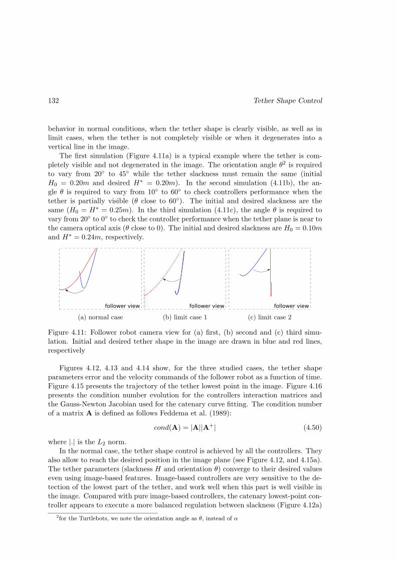
132 Tether Shape Control
behavior in normal conditions, when the tether shape is clearly visible, as well as inlimit cases, when the tether is not completely visible or when it degenerates into avertical line in the image.
The first simulation (Figure 4.11a) is a typical example where the tether is com-pletely visible and not degenerated in the image. The orientation angle θ2 is requiredto vary from 20 to 45 while the tether slackness must remain the same (initialH0 = 0.20m and desired H∗ = 0.20m). In the second simulation (4.11b), the an-gle θ is required to vary from 10 to 60 to check controllers performance when thetether is partially visible (θ close to 60). The initial and desired slackness are thesame (H0 = H∗ = 0.25m). In the third simulation (4.11c), the angle θ is required tovary from 20 to 0 to check the controller performance when the tether plane is near tothe camera optical axis (θ close to 0). The initial and desired slackness are H0 = 0.10mand H∗ = 0.24m, respectively.
follower view
(a) normal case
follower view
(b) limit case 1
follower view
(c) limit case 2
Figure 4.11: Follower robot camera view for (a) first, (b) second and (c) third simu-lation. Initial and desired tether shape in the image are drawn in blue and red lines,respectively
Figures 4.12, 4.13 and 4.14 show, for the three studied cases, the tether shapeparameters error and the velocity commands of the follower robot as a function of time.Figure 4.15 presents the trajectory of the tether lowest point in the image. Figure 4.16presents the condition number evolution for the controllers interaction matrices andthe Gauss-Newton Jacobian used for the catenary curve fitting. The condition numberof a matrix A is defined as follows Feddema et al. (1989):
cond(A) = |A||A+| (4.50)
where |.| is the L2 norm.In the normal case, the tether shape control is achieved by all the controllers. They
also allow to reach the desired position in the image plane (see Figure 4.12, and 4.15a).The tether parameters (slackness H and orientation θ) converge to their desired valueseven using image-based features. Image-based controllers are very sensitive to the de-tection of the lowest part of the tether, and work well when this part is well visible inthe image. Compared with pure image-based controllers, the catenary lowest-point con-troller appears to execute a more balanced regulation between slackness (Figure 4.12a)
2for the Turtlebots, we note the orientation angle as θ, instead of α

Follower Robot Control using Tether Visual Feedback 133
and orientation (Figure 4.12b). In the image plane, the resulting trajectory of the lowestpoint is more regular than pure image-based trajectories (Figure 4.15a). In addition,the catenary parameter controller is less sensitive to noisy tether detection whereas theother controllers are very dependent on the accurate detection of the lowest point inthe image.
0 5 10 15 20 25 30Time (s)
−0.02−0.010.00
0.01
0.02
0.03
0.04
0.05
Sla
ckn
ess
Err
or
(m)
Tether Slackness Error H −H∗
(a)
0 5 10 15 20 25 30Time (s)
−25
−20
−15
−10
−5
0A
ngle
Err
or
(deg)
Tether Angle Error θ − θ∗
(b)
0 5 10 15 20 25 30Time (s)
−0.010.00
0.01
0.02
0.03
0.04
0.05
0.06
0.07
0.08
Velo
city
(m/s
)
Linear Velocity Commands
(c)
0 5 10 15 20 25 30Time (s)
−0.25
−0.20
−0.15
−0.10
−0.05
0.00
Velo
city
(rad
/s)
Angular Velocity Commands
(d)
Figure 4.12: Normal case: error evolution for (a) tether slackness and (b) orientationas well as (c) linear and (d) angular command velocities. Tether initial and desiredshape are respectively: (H0 = 0.20m, θ0 = 20) and (H∗ = 0.20m, θ∗ = 45). Legendin Fig. 4.15d. All controllers use a gain λ = 1.0.

134 Tether Shape Control
In the first limit case, the tether desired shape is only achieved by the catenary pa-rameter controller (Figure 4.13). The other controllers cannot reach the desired tethershape leading to a residual offset of slackness (Figure 4.13a) and angle (Figure 4.13b).However, these controllers converge as expected in the image plane, while we observe adiscontinuity of the lowest point trajectory in the case of catenary-parameter controller(Figure 4.15b). This is not surprising since the catenary-parameter controller directlyregulates the tether 3D shape, and converges to the real lowest point that is outsidethe image.
0 10 20 30 40 50 60Time (s)
−0.02−0.010.00
0.01
0.02
0.03
0.04
0.05
Sla
ckn
ess
Err
or
(m)
Tether Slackness Error H −H∗
(a)
0 10 20 30 40 50 60Time (s)
−50
−40
−30
−20
−10
0
10
An
gle
Err
or
(deg)
Tether Angle Error θ − θ∗
(b)
0 10 20 30 40 50 60Time (s)
−0.010.00
0.01
0.02
0.03
0.04
0.05
0.06
0.07
0.08
Velo
city
(m/s
)
Linear Velocity Commands
(c)
0 10 20 30 40 50 60Time (s)
−0.25
−0.20
−0.15
−0.10
−0.05
0.00
Velo
city
(rad
/s)
Angular Velocity Commands
(d)
Figure 4.13: Limit case 1: error evolution for (a) tether slackness and (b) orientationas well as (c) linear and (d) angular command velocities. Tether initial and desiredshape are respectively: (H0 = 0.25m, θ0 = 10) and (H∗ = 0.25m, θ∗ = 60). Legendin Fig. 4.15d. All controllers use a gain λ = 1.0.
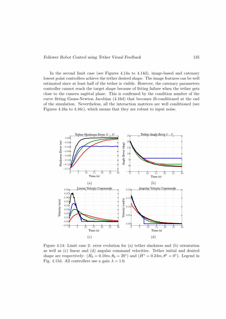
Follower Robot Control using Tether Visual Feedback 135
In the second limit case (see Figures 4.14a to 4.14d), image-based and catenarylowest point controllers achieve the tether desired shape. The image features can be wellestimated since at least half of the tether is visible. However, the catenary parameterscontroller cannot reach the target shape because of fitting failure when the tether getsclose to the camera sagittal plane. This is confirmed by the condition number of thecurve fitting Gauss-Newton Jacobian (4.16d) that becomes ill-conditioned at the endof the simulation. Nevertheless, all the interaction matrices are well conditioned (seeFigures 4.16a to 4.16c), which means that they are robust to input noise.
0 5 10 15 20 25 30Time (s)
−0.14−0.12−0.10−0.08−0.06−0.04−0.020.00
Sla
ckn
ess
Err
or
(m)
Tether Slackness Error H −H∗
(a)
0 5 10 15 20 25 30Time (s)
−5
0
5
10
15
20
25
An
gle
Err
or
(deg)
Tether Angle Error θ − θ∗
(b)
0 5 10 15 20 25 30Time (s)
−0.010.00
0.01
0.02
0.03
0.04
0.05
0.06
0.07
0.08
Velo
city
(m/s
)
Linear Velocity Commands
(c)
0 5 10 15 20 25 30Time (s)
0.00
0.05
0.10
0.15
0.20
Velo
city
(rad
/s)
Angular Velocity Commands
(d)
Figure 4.14: Limit case 2: error evolution for (a) tether slackness and (b) orientationas well as (c) linear and (d) angular command velocities. Tether initial and desiredshape are respectively: (H0 = 0.10m, θ0 = 20) and (H∗ = 0.24m, θ∗ = 0). Legend inFig. 4.15d. All controllers use a gain λ = 1.0.
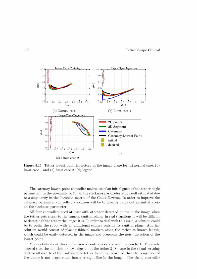
136 Tether Shape Control
−0.6 −0.5 −0.4 −0.3 −0.2 −0.1 0.0x(m)
−0.1
0.0
0.1
0.2
0.3
0.4
y(m
) ima
ge
bord
er
Image Plane Trajectory
(a) Normal case
−0.6 −0.5 −0.4 −0.3 −0.2 −0.1 0.0x(m)
−0.1
0.0
0.1
0.2
0.3
0.4
y(m
) ima
ge
bord
er
Image Plane Trajectory
(b) Limit case 1
−0.6 −0.5 −0.4 −0.3 −0.2 −0.1 0.0x(m)
−0.1
0.0
0.1
0.2
0.3
0.4
y(m
) ima
ge
bord
er
Image Plane Trajectory
(c) Limit case 2
2D points
2D Segment
Catenary
Catenary Lowest Point
initial
desired
(d)
Figure 4.15: Tether lowest point trajectory in the image plane for (a) normal case, (b)limit case 1 and (c) limit case 2. (d) legend
The catenary lowest-point controller makes use of an initial guess of the tether angleparameter. In the proximity of θ = 0, the slackness parameter is not well estimated dueto a singularity in the Jacobian matrix of the Gauss-Newton. In order to improve thecatenary parameter controller, a solution will be to directly carry out an initial guesson the slackness parameter.
All four controllers need at least 50% of tether detected points in the image whenthe tether gets closer to the camera sagittal plane. In real situations it will be difficultto detect half the tether the longer it is. In order to deal with this issue, a solution couldbe to equip the robot with an additional camera outside its sagittal plane. Anothersolution would consist of placing fiducial markers along the tether at known length,which could be easily detected in the image and overcome the noisy detection of thelowest point.
More details about this comparison of controllers are given in appendix E. The studyshowed that the additional knowledge about the tether 3-D shape in the visual servoingcontrol allowed to obtain satisfactory tether handling, provided that the projection ofthe tether is not degenerated into a straight line in the image. The visual controller

Follower Robot Control using Tether Visual Feedback 137
based on catenary parameters performed better in cases where the tether was partiallyout of the camera field of view. The visual control based on the lowest point couldbe useful near the degenerated cases when the lowest part of the catenary is visible.The standard Image-Based features failed to converge accurately in the case of partialvisibility of the tether in the image. Both catenary-based controllers could be combinedto design a more robust controller.
0 5 10 15 20 25 30Time (s)
0
2
4
6
8
10
12 Condition Number
(a)
0 10 20 30 40 50 60Time (s)
0
2
4
6
8
10
12 Condition Number
(b)
0 5 10 15 20 25 30Time (s)
0
2
4
6
8
10
12 Condition Number
(c)
0 10 20 30 40 50 60Time (s)
0
1
2
3
4
5
log10(cond(J))
Jacobian condition number
Normal case
Limit case 1
Limit case 2
(d)
Figure 4.16: Interaction matrices condition number evolution for (Fig. a) normal and(Figs. b and c). Legend in Fig. 4.15d. (d) condition number evolution for the curvefitting Gauss-Newton Jacobian during normal and limit cases
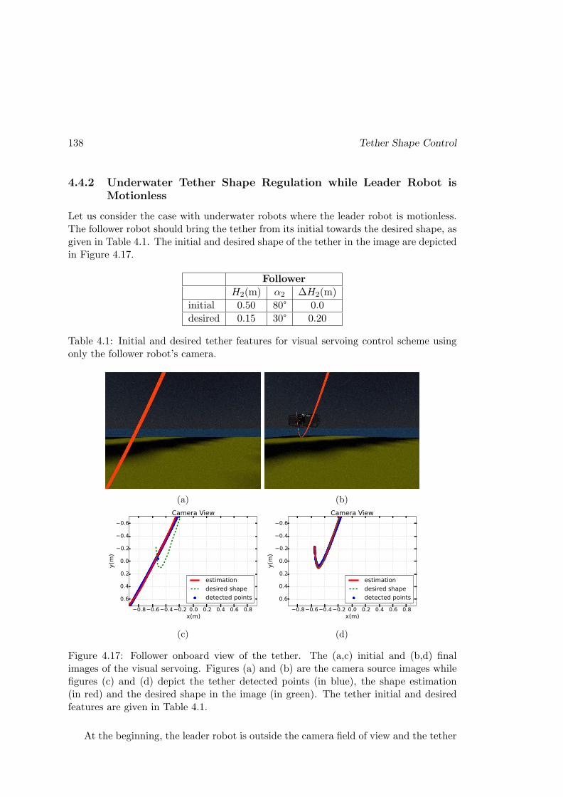
138 Tether Shape Control
4.4.2 Underwater Tether Shape Regulation while Leader Robot is
Motionless
Let us consider the case with underwater robots where the leader robot is motionless.The follower robot should bring the tether from its initial towards the desired shape, asgiven in Table 4.1. The initial and desired shape of the tether in the image are depictedin Figure 4.17.
Follower
H2(m) α2 ∆H2(m)
initial 0.50 80° 0.0
desired 0.15 30° 0.20
Table 4.1: Initial and desired tether features for visual servoing control scheme usingonly the follower robot’s camera.
(a) (b)
−0.8−0.6−0.4−0.2 0.0 0.2 0.4 0.6 0.8x(m)
−0.6
−0.4
−0.2
0.0
0.2
0.4
0.6
y(m
)
Camera View
estimationdesired shapedetected points
(c)
−0.8−0.6−0.4−0.2 0.0 0.2 0.4 0.6 0.8x(m)
−0.6
−0.4
−0.2
0.0
0.2
0.4
0.6
y(m
)
Camera View
estimationdesired shapedetected points
(d)
Figure 4.17: Follower onboard view of the tether. The (a,c) initial and (b,d) finalimages of the visual servoing. Figures (a) and (b) are the camera source images whilefigures (c) and (d) depict the tether detected points (in blue), the shape estimation(in red) and the desired shape in the image (in green). The tether initial and desiredfeatures are given in Table 4.1.
At the beginning, the leader robot is outside the camera field of view and the tether
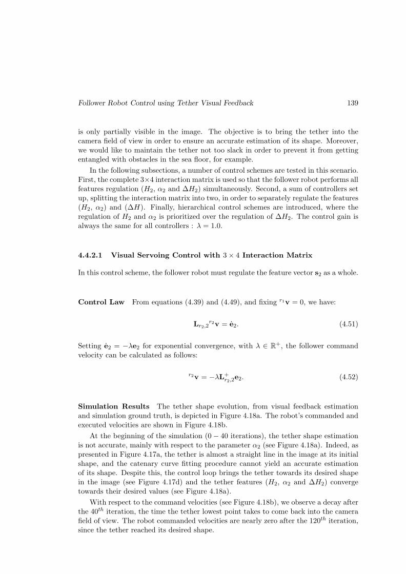
Follower Robot Control using Tether Visual Feedback 139
is only partially visible in the image. The objective is to bring the tether into thecamera field of view in order to ensure an accurate estimation of its shape. Moreover,we would like to maintain the tether not too slack in order to prevent it from gettingentangled with obstacles in the sea floor, for example.
In the following subsections, a number of control schemes are tested in this scenario.First, the complete 3×4 interaction matrix is used so that the follower robot performs allfeatures regulation (H2, α2 and ∆H2) simultaneously. Second, a sum of controllers setup, splitting the interaction matrix into two, in order to separately regulate the features(H2, α2) and (∆H). Finally, hierarchical control schemes are introduced, where theregulation of H2 and α2 is prioritized over the regulation of ∆H2. The control gain isalways the same for all controllers : λ = 1.0.
4.4.2.1 Visual Servoing Control with 3× 4 Interaction Matrix
In this control scheme, the follower robot must regulate the feature vector s2 as a whole.
Control Law From equations (4.39) and (4.49), and fixing r1v = 0, we have:
Lr2,2r2v = e2. (4.51)
Setting e2 = −λe2 for exponential convergence, with λ ∈ R+, the follower command
velocity can be calculated as follows:
r2v = −λL+r2,2
e2. (4.52)
Simulation Results The tether shape evolution, from visual feedback estimationand simulation ground truth, is depicted in Figure 4.18a. The robot’s commanded andexecuted velocities are shown in Figure 4.18b.
At the beginning of the simulation (0− 40 iterations), the tether shape estimationis not accurate, mainly with respect to the parameter α2 (see Figure 4.18a). Indeed, aspresented in Figure 4.17a, the tether is almost a straight line in the image at its initialshape, and the catenary curve fitting procedure cannot yield an accurate estimationof its shape. Despite this, the control loop brings the tether towards its desired shapein the image (see Figure 4.17d) and the tether features (H2, α2 and ∆H2) convergetowards their desired values (see Figure 4.18a).
With respect to the command velocities (see Figure 4.18b), we observe a decay afterthe 40th iteration, the time the tether lowest point takes to come back into the camerafield of view. The robot commanded velocities are nearly zero after the 120th iteration,since the tether reached its desired shape.
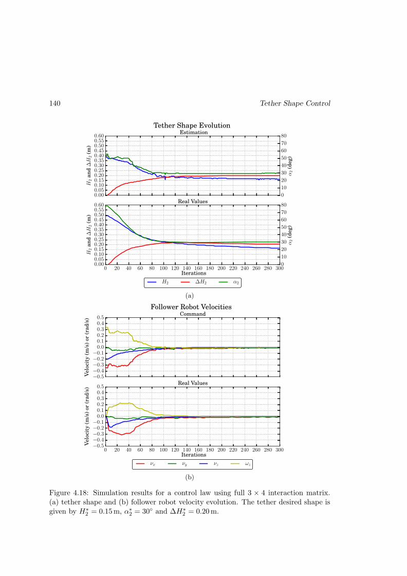
140 Tether Shape Control
0.000.050.100.150.200.250.300.350.400.450.500.550.60
H2
an
d∆H
2(m
)
Estimation
0 20 40 60 80 100 120 140 160 180 200 220 240 260 280 300
Iterations
0.000.050.100.150.200.250.300.350.400.450.500.550.60
H2
an
d∆H
2(m
)
Real Values
0
10
20
30
40
50
60
70
80
α2
(deg)
H2 ∆H2 α2
0
10
20
30
40
50
60
70
80
α2
(deg)
Tether Shape Evolution
(a)
−0.5−0.4−0.3−0.2−0.10.00.10.20.30.40.5
Velo
city
(m/s
)or
(ra
d/s
)
Command
0 20 40 60 80 100 120 140 160 180 200 220 240 260 280 300
Iterations
−0.5−0.4−0.3−0.2−0.10.00.10.20.30.40.5
Velo
city
(m/s
)or
(ra
d/s
)
Real Values
νx νy νz ωz
Follower Robot Velocities
(b)
Figure 4.18: Simulation results for a control law using full 3 × 4 interaction matrix.(a) tether shape and (b) follower robot velocity evolution. The tether desired shape isgiven by H∗
2 = 0.15m, α∗2 = 30 and ∆H∗
2 = 0.20m.

Follower Robot Control using Tether Visual Feedback 141
4.4.2.2 Sum of Controllers
We now introduce another control scheme, splitting the interaction matrix into two, inorder to separately regulate the features (H2, α2) and (∆H2). Thus, we ensure thatthe control of ∆H2 only generates vertical velocity commands (νz), whereas it mightalso generate forward velocity commands (νx) using the 3× 4 interaction matrix.
Control Law Let us note eH,α2 and e∆H
2 the error vectors related to the regulationof (H2, α2) and ∆H2, respectively:
eH,α2 =
[a2 − a∗2b2 − b∗2
]
and
e∆H2 =
[d2 − d∗2
].
Their interaction matrices are obtained splitting the matrix given in equation (4.44),as follows:
LH,αr2,2 =−
√1−b2
2
(u2+p2)Hmax− b2
(u2+p2)Hmax
v2+q2(u2+p2)Hmax
r2Y1
√1−b2
2
(u2+p2)Hmax− r2X1
b2(u2+p2)Hmax
b2√
1−b22
2D2+∆D2− 1−b2
2
2D2+∆D20 r2Y1
−b2√
1−b22
2D2+∆D2− r2X1
1−b22
2D2+∆D2
and
L∆Hr2,2 =
[0 0 − 1
2∆Hmax0].
Similarly to equation (4.52), we can calculate the follower robot control law as:
r2v = −λ1(LH,αr2,2
)+eH,α2 − λ2
(L∆Hr2,2
)+e∆H2 , (4.53)
where λ1, λ2 ∈ R+ are the control gains for the regulation of eH,α
2 and e∆H2 .
Simulation Results The same simulation presented in the previous subsection isnow performed using the sum controller. As a reminder, the tether initial and desiredshape are given in Table 4.1. The control gain is set to λ1 = λ2 = 1.0. The tether shapeevolution, from visual feedback estimation and simulation ground truth, is depicted inFigure 4.19a. The robot’s commands and executed velocities are shown in Figure 4.19b.
Analyzing Figure 4.19a, we observe that the tether reaches its desired shape within300 iterations. However, the feature ∆H2 takes more time to converge when comparedto the controller using the entire interaction matrix (see Figure 4.18a).
Such a control scheme may be interesting to ensure that the regulation of ∆H2 onlyimplies a vertical motion. Yet, since the first task also implies vertical motion, it canhappen that none of the tasks are fully regulated. In order to ensure tasks regulation,we have to set up a hierarchical control scheme.

142 Tether Shape Control
0.000.050.100.150.200.250.300.350.400.450.500.550.60
H2
an
d∆H
2(m
)
Estimation
0 20 40 60 80 100 120 140 160 180 200 220 240 260 280 300
Iterations
0.000.050.100.150.200.250.300.350.400.450.500.550.60
H2
an
d∆H
2(m
)
Real Values
0
10
20
30
40
50
60
70
80
α2
(deg)
H2 ∆H2 α2
0
10
20
30
40
50
60
70
80
α2
(deg)
Tether Shape Evolution
(a)
−0.5−0.4−0.3−0.2−0.10.00.10.20.30.40.5
Velo
city
(m/s
)or
(ra
d/s
)
Command
0 20 40 60 80 100 120 140 160 180 200 220 240 260 280 300
Iterations
−0.5−0.4−0.3−0.2−0.10.00.10.20.30.40.5
Velo
city
(m/s
)or
(ra
d/s
)
Real Values
νx νy νz ωz
Follower Robot Velocities
(b)
Figure 4.19: Simulation results for the sum of controllers. (a) tether shape and (b)follower robot velocity evolution. The tether desired shape is given by H∗
2 = 0.15m,α∗2 = 30 and ∆H∗
2 = 0.20m.

Follower Robot Control using Tether Visual Feedback 143
The interaction matrix presented in equation (4.44) already has nice decouplingproperties, which allows the features to be simultaneously regulated without disturbingeach other. As a result, we obtain a faster convergence of the tether features using theentire matrix instead of making the sum controllers. Let us look in the sequel theresults obtained with hierarchical control schemes.
4.4.2.3 Hierarchical Task Control
Let us now split the follower robot command into two tasks. The first task correspondsto the regulation of H2 and α2, The second task corresponds to the regulation of ∆H2.In order to ensure that the secondary task will not interfere the execution of the prioritytask, the redundancy formalism can be used (Mansard and Chaumette, 2007).
Control Law Let us note eH,α2 and e∆H
2 as the error vector of the priority andsecondary tasks, respectively:
eH,α2 =
[a2 − a∗2b2 − b∗2
]
and
e∆H2 =
[d2 − d∗2
].
Similarly to equation (4.52), we can calculate the follower robot control law as:
r2v = −λ(LH,αr2,2
)+eH,α2 +P1z, (4.54)
where
P1 = I−(LH,αr2,2
)+LH,αr2,2 (4.55)
is the orthogonal projection operator on the null space of LH,αr2,2, the interaction matrix
of the first task. The vector z is an arbitrary vector that can be used to apply thesecondary task. Thanks to the projector operator P1, the first task is ensured not tobe disturbed by the secondary command introduced by z.
We can now introduce the secondary task through:
z = −λ2(L∆Hr2,2
)+e∆H2
and rewriting equation (4.54) as:
r2v = −λ1(LH,αr2,2
)+eH,α2 − λ2P1
(L∆Hr2,2
)+e∆H2 , (4.56)
where λ1, λ2 ∈ R+ are the control gains for the first and second tasks, respectively.
The interaction matrices LH,αr2,2 and L∆H
r2,2 are obtained splitting the matrix given inequation (4.44), as made in subsection 4.4.2.2.
Actually, this control law can be seen as the application of the first task commandsand those of the second task that do not disturb the first task execution. The task

144 Tether Shape Control
hierarchy is respected. However, the second task execution is not optimal in the least-square sense.
An alternative to the control law given in equation (4.56) can be designed in orderto meet the requirements of optimal control.
Similarly to equation (4.51), the evolution of the second task error is given by:
e∆H2 = L∆H
r2,2r2v. (4.57)
Then, introducing equation (4.57) in (4.54) we obtain:
z =(L∆Hr2,2P1
)+[e∆H2 − L∆H
r2,2
(LH,αr2,2
)+eH,α2
], (4.58)
which can be finally introduced back in equation (4.54), yielding:
r2v =(LH,αr2,2
)+eH,α2 +P1
(L∆Hr2,2P1
)+[e∆H2 − L∆H
r2,2
(LH,αr2,2
)+eH,α2
], (4.59)
Since P1 is idempotent and Hermitian (it is a projection operator), equation (4.59) canbe rewritten as (Mansard and Chaumette, 2007):
r2v =(LH,αr2,2
)+eH,α2 +
(L∆Hr2,2
)+˙e∆H
2 , (4.60)
where L∆Hr2,2 = L∆H
r2,2P1 and ˙e∆H
2 = e∆H2 − L∆H
r2,2
(LH,αr2,2
)+eH,α2 . We can rewrite this
equation as:
r2v = −λ1(LH,αr2,2
)+eH,α2 − λ2
(L∆Hr2,2
)+e∆H2 , (4.61)
Let us present in the sequel the simulation results obtained from both control laws,given in equations (4.56) and (4.61)
Simulation Results The same simulation presented in the previous subsection isnow performed using the hierarchical control laws. As a reminder, the tether initialand desired shape were given in Table 4.1.
The simulation results for the hierarchical non-optimal controller (equation (4.56))are presented in Figure 4.20. The simulation results for the hierarchical optimal con-troller (equation (4.61)) are presented in Figure 4.21. The control gains are λ1 = λ2 =1.0 in both cases.

Follower Robot Control using Tether Visual Feedback 145
0.000.050.100.150.200.250.300.350.400.450.500.550.60
H2
an
d∆H
2(m
)
Estimation
0 20 40 60 80 100 120 140 160 180 200 220 240 260 280 300
Iterations
0.000.050.100.150.200.250.300.350.400.450.500.550.60
H2
an
d∆H
2(m
)
Real Values
0
10
20
30
40
50
60
70
80
α2
(deg)
H2 ∆H2 α2
0
10
20
30
40
50
60
70
80
α2
(deg)
Tether Shape Evolution
(a)
−0.5−0.4−0.3−0.2−0.10.00.10.20.30.40.5
Velo
city
(m/s
)or
(ra
d/s
)
Command
0 20 40 60 80 100 120 140 160 180 200 220 240 260 280 300
Iterations
−0.5−0.4−0.3−0.2−0.10.00.10.20.30.40.5
Velo
city
(m/s
)or
(ra
d/s
)
Real Values
νx νy νz ωz
Follower Robot Velocities
(b)
Figure 4.20: Simulation results for the hierarchical non-optimal control. (a) tethershape and (b) follower robot velocity evolution. The tether desired shape is given byH∗
2 = 0.15m, α∗2 = 30 and ∆H∗
2 = 0.20m.

146 Tether Shape Control
0.000.050.100.150.200.250.300.350.400.450.500.550.60
H2
an
d∆H
2(m
)
Estimation
0 20 40 60 80 100 120 140 160 180 200 220 240 260 280 300
Iterations
0.000.050.100.150.200.250.300.350.400.450.500.550.60
H2
an
d∆H
2(m
)
Real Values
0
10
20
30
40
50
60
70
80
α2
(deg)
H2 ∆H2 α2
0
10
20
30
40
50
60
70
80
α2
(deg)
Tether Shape Evolution
(a)
−0.5−0.4−0.3−0.2−0.10.00.10.20.30.40.5
Velo
city
(m/s
)or
(ra
d/s
)
Command
0 20 40 60 80 100 120 140 160 180 200 220 240 260 280 300
Iterations
−0.5−0.4−0.3−0.2−0.10.00.10.20.30.40.5
Velo
city
(m/s
)or
(ra
d/s
)
Real Values
νx νy νz ωz
Follower Robot Velocities
(b)
Figure 4.21: Simulation results for the hierarchical optimal control. a) tether shape and(b) follower robot velocity evolution. The tether desired shape is given by H∗
2 = 0.15m,α∗2 = 30 and ∆H∗
2 = 0.20m.

Follower Robot Control using Tether Visual Feedback 147
We clearly observe that using the hierarchical non-optimal controller, the secondarytask (regulation of ∆H) is not properly regulated at the beginning. The value of ∆Hovershoots its desired value by 0.13m around the 70th iteration (see Figure 4.20a).Using the hierarchical optimal controller, however, the secondary task can be betterexecuted and all the features converge towards their desired values within the 300iterations without overshoot (see Figure 4.21a). This behavior is expected (Mansardand Chaumette, 2007). In the non-optimal control, the second task commands arejust filtered by the projector operator, whereas, in the optimal control, the second taskcontrol law allows a more efficient distribution of the control efforts in the remainingdegrees of freedom of the robot. The difference on the velocity commands betweenthese two hierarchical control approaches is notable regarding the velocity componentνz (in blue) in Figures 4.20b and 4.21b. Using the optimal controller, the velocitycomponent νz has a lower magnitude, which represents an optimized command in termof control efforts.
4.4.2.4 Comparing Follower Robot Trajectories
The executed trajectories of the follower robot for each of the controllers above studiedis depicted in Figure 4.22.
−0.35−0.30−0.25−0.20−0.15−0.10−0.050.00
0.05
y(m
)
Top view
−0.7 −0.6 −0.5 −0.4 −0.3 −0.2 −0.1 0.0 0.1x(m)
−10.30−10.25−10.20−10.15−10.10−10.05−10.00−9.95
z(m
)
Side View
full mtx. h. nopt. h. opt. sum
Follower Robot Trajectories
Figure 4.22: Comparing the follower robot trajectories for the four controllers presentedin the previous subsections: full 3 × 4 interaction matrix controller (in red), sum ofcontrollers (in yellow), hierarchical non-optimal (in green) and hierarchical optimal (inblue) controllers. The robot starting position is marked by a black star.
The full interaction matrix and hierarchical optimal controllers generate similartrajectories. These trajectories go more directly towards the final position, when com-pared to the sum of controllers and the hierarchical non-optimal controller. The full
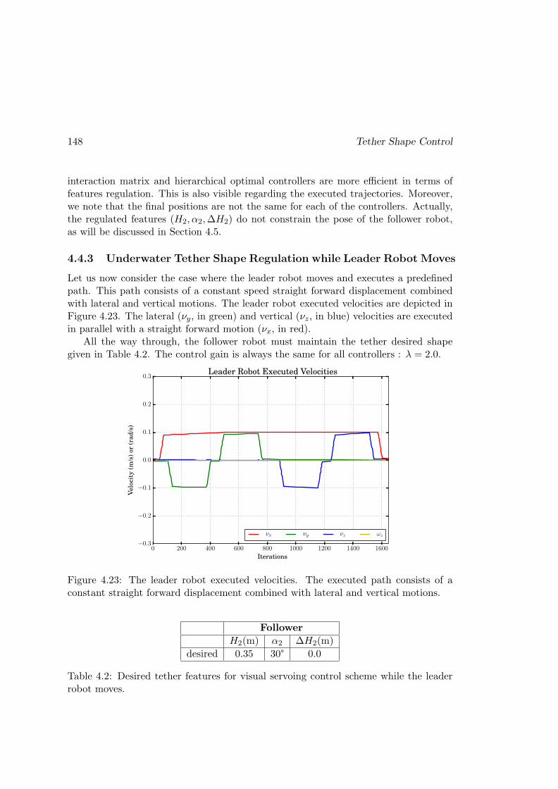
148 Tether Shape Control
interaction matrix and hierarchical optimal controllers are more efficient in terms offeatures regulation. This is also visible regarding the executed trajectories. Moreover,we note that the final positions are not the same for each of the controllers. Actually,the regulated features (H2, α2,∆H2) do not constrain the pose of the follower robot,as will be discussed in Section 4.5.
4.4.3 Underwater Tether Shape Regulation while Leader Robot Moves
Let us now consider the case where the leader robot moves and executes a predefinedpath. This path consists of a constant speed straight forward displacement combinedwith lateral and vertical motions. The leader robot executed velocities are depicted inFigure 4.23. The lateral (νy, in green) and vertical (νz, in blue) velocities are executedin parallel with a straight forward motion (νx, in red).
All the way through, the follower robot must maintain the tether desired shapegiven in Table 4.2. The control gain is always the same for all controllers : λ = 2.0.
0 200 400 600 800 1000 1200 1400 1600
Iterations
−0.3
−0.2
−0.1
0.0
0.1
0.2
0.3
Velo
city
(m/s
)or
(ra
d/s
)
Leader Robot Executed Velocities
νx νy νz ωz
Figure 4.23: The leader robot executed velocities. The executed path consists of aconstant straight forward displacement combined with lateral and vertical motions.
Follower
H2(m) α2 ∆H2(m)
desired 0.35 30° 0.0
Table 4.2: Desired tether features for visual servoing control scheme while the leaderrobot moves.
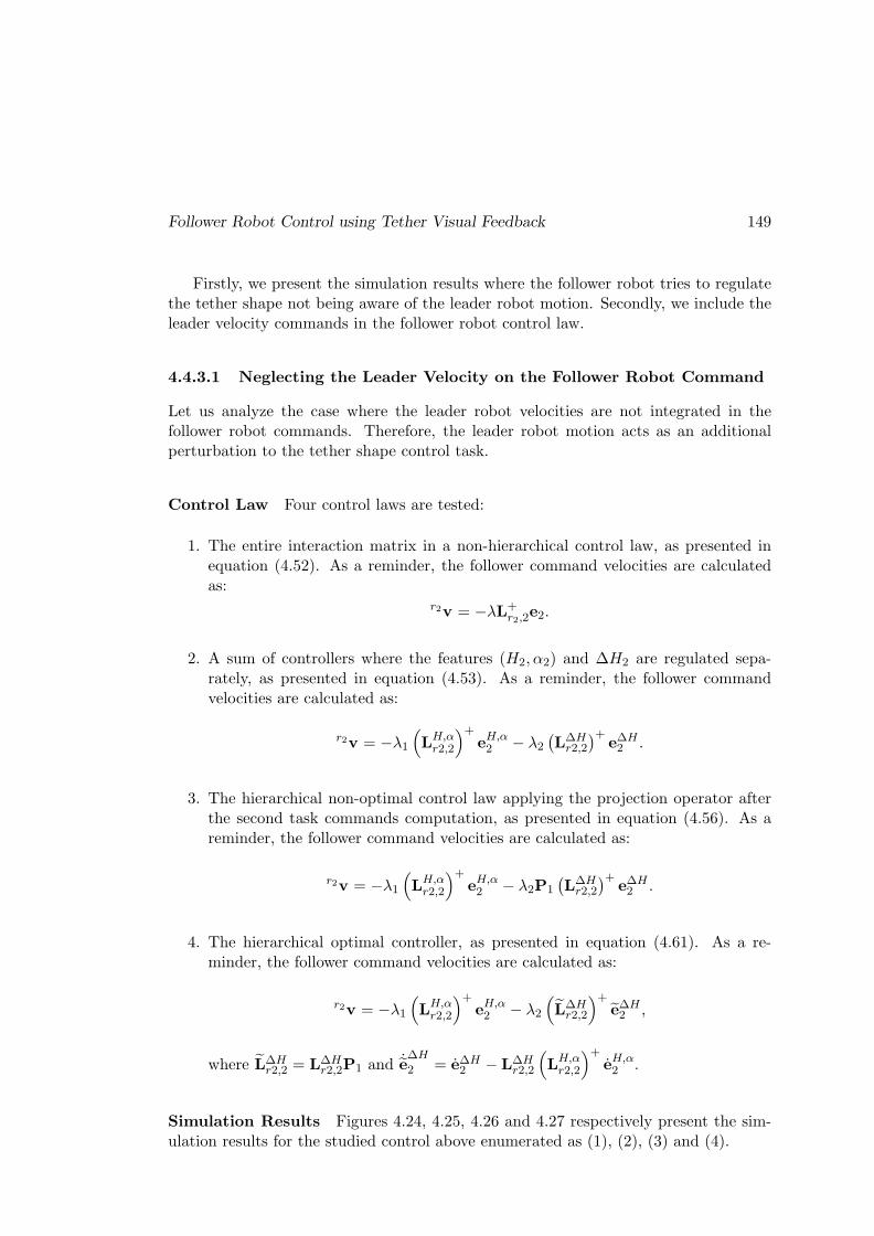
Follower Robot Control using Tether Visual Feedback 149
Firstly, we present the simulation results where the follower robot tries to regulatethe tether shape not being aware of the leader robot motion. Secondly, we include theleader velocity commands in the follower robot control law.
4.4.3.1 Neglecting the Leader Velocity on the Follower Robot Command
Let us analyze the case where the leader robot velocities are not integrated in thefollower robot commands. Therefore, the leader robot motion acts as an additionalperturbation to the tether shape control task.
Control Law Four control laws are tested:
1. The entire interaction matrix in a non-hierarchical control law, as presented inequation (4.52). As a reminder, the follower command velocities are calculatedas:
r2v = −λL+r2,2
e2.
2. A sum of controllers where the features (H2, α2) and ∆H2 are regulated sepa-rately, as presented in equation (4.53). As a reminder, the follower commandvelocities are calculated as:
r2v = −λ1(LH,αr2,2
)+eH,α2 − λ2
(L∆Hr2,2
)+e∆H2 .
3. The hierarchical non-optimal control law applying the projection operator afterthe second task commands computation, as presented in equation (4.56). As areminder, the follower command velocities are calculated as:
r2v = −λ1(LH,αr2,2
)+eH,α2 − λ2P1
(L∆Hr2,2
)+e∆H2 .
4. The hierarchical optimal controller, as presented in equation (4.61). As a re-minder, the follower command velocities are calculated as:
r2v = −λ1(LH,αr2,2
)+eH,α2 − λ2
(L∆Hr2,2
)+e∆H2 ,
where L∆Hr2,2 = L∆H
r2,2P1 and ˙e∆H
2 = e∆H2 − L∆H
r2,2
(LH,αr2,2
)+eH,α2 .
Simulation Results Figures 4.24, 4.25, 4.26 and 4.27 respectively present the sim-ulation results for the studied control above enumerated as (1), (2), (3) and (4).
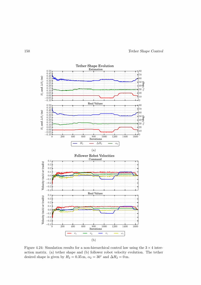
150 Tether Shape Control
−0.10−0.050.000.050.100.150.200.250.300.350.400.450.50
H2
an
d∆H
2(m
)
Estimation
0 200 400 600 800 1000 1200 1400 1600
Iterations
−0.10−0.050.000.050.100.150.200.250.300.350.400.450.50
H2
an
d∆H
2(m
)
Real Values
0
10
20
30
40
50
60
70
80
α2
(deg)
H2 ∆H2 α2
0
10
20
30
40
50
60
70
80
α2
(deg)
Tether Shape Evolution
(a)
−0.4−0.3−0.2−0.10.0
0.1
0.2
0.3
0.4
Velo
city
(m/s
)or
(ra
d/s
)
Command
0 200 400 600 800 1000 1200 1400 1600
Iterations
−0.4−0.3−0.2−0.10.0
0.1
0.2
0.3
0.4
Velo
city
(m/s
)or
(ra
d/s
)
Real Values
νx νy νz ωz
Follower Robot Velocities
(b)
Figure 4.24: Simulation results for a non-hierarchical control law using the 3× 4 inter-action matrix. (a) tether shape and (b) follower robot velocity evolution. The tetherdesired shape is given by H2 = 0.35m, α2 = 30 and ∆H2 = 0m.

Follower Robot Control using Tether Visual Feedback 151
−0.10−0.050.000.050.100.150.200.250.300.350.400.450.50
H2
an
d∆H
2(m
)
Estimation
0 200 400 600 800 1000 1200 1400 1600
Iterations
−0.10−0.050.000.050.100.150.200.250.300.350.400.450.50
H2
an
d∆H
2(m
)
Real Values
0
10
20
30
40
50
60
70
80
α2
(deg)
H2 ∆H2 α2
0
10
20
30
40
50
60
70
80
α2
(deg)
Tether Shape Evolution
(a)
−0.4−0.3−0.2−0.10.0
0.1
0.2
0.3
0.4
Velo
city
(m/s
)or
(ra
d/s
)
Command
0 200 400 600 800 1000 1200 1400 1600
Iterations
−0.4−0.3−0.2−0.10.0
0.1
0.2
0.3
0.4
Velo
city
(m/s
)or
(ra
d/s
)
Real Values
νx νy νz ωz
Follower Robot Velocities
(b)
Figure 4.25: Simulation results for the sum of controllers law with no task priority.(a) tether shape and (b) follower robot velocity evolution. The tether desired shape isgiven by H2 = 0.35m, α2 = 30 and ∆H2 = 0m.

152 Tether Shape Control
−0.10−0.050.000.050.100.150.200.250.300.350.400.450.50
H2
an
d∆H
2(m
)
Estimation
0 200 400 600 800 1000 1200 1400 1600
Iterations
−0.10−0.050.000.050.100.150.200.250.300.350.400.450.50
H2
an
d∆H
2(m
)
Real Values
0
10
20
30
40
50
60
70
80
α2
(deg)
H2 ∆H2 α2
0
10
20
30
40
50
60
70
80
α2
(deg)
Tether Shape Evolution
(a)
−0.4−0.3−0.2−0.10.0
0.1
0.2
0.3
0.4
Velo
city
(m/s
)or
(ra
d/s
)
Command
0 200 400 600 800 1000 1200 1400 1600
Iterations
−0.4−0.3−0.2−0.10.0
0.1
0.2
0.3
0.4
Velo
city
(m/s
)or
(ra
d/s
)
Real Values
νx νy νz ωz
Follower Robot Velocities
(b)
Figure 4.26: Simulation results for the hierarchical non-optimal controller. (a) tethershape and (b) follower robot velocity evolution. The tether desired shape is given byH2 = 0.35m, α2 = 30 and ∆H2 = 0m.

Follower Robot Control using Tether Visual Feedback 153
−0.10−0.050.000.050.100.150.200.250.300.350.400.450.50
H2
an
d∆H
2(m
)
Estimation
0 200 400 600 800 1000 1200 1400 1600
Iterations
−0.10−0.050.000.050.100.150.200.250.300.350.400.450.50
H2
an
d∆H
2(m
)
Real Values
0
10
20
30
40
50
60
70
80
α2
(deg)
H2 ∆H2 α2
0
10
20
30
40
50
60
70
80
α2
(deg)
Tether Shape Evolution
(a)
−0.4−0.3−0.2−0.10.0
0.1
0.2
0.3
0.4
Velo
city
(m/s
)or
(ra
d/s
)
Command
0 200 400 600 800 1000 1200 1400 1600
Iterations
−0.4−0.3−0.2−0.10.0
0.1
0.2
0.3
0.4
Velo
city
(m/s
)or
(ra
d/s
)
Real Values
νx νy νz ωz
Follower Robot Velocities
(b)
Figure 4.27: Simulation results for the hierarchical optimal controller. (a) tether shapeand (b) follower robot velocity evolution. The tether desired shape is given by H2 =0.35m, α2 = 30 and ∆H2 = 0m.
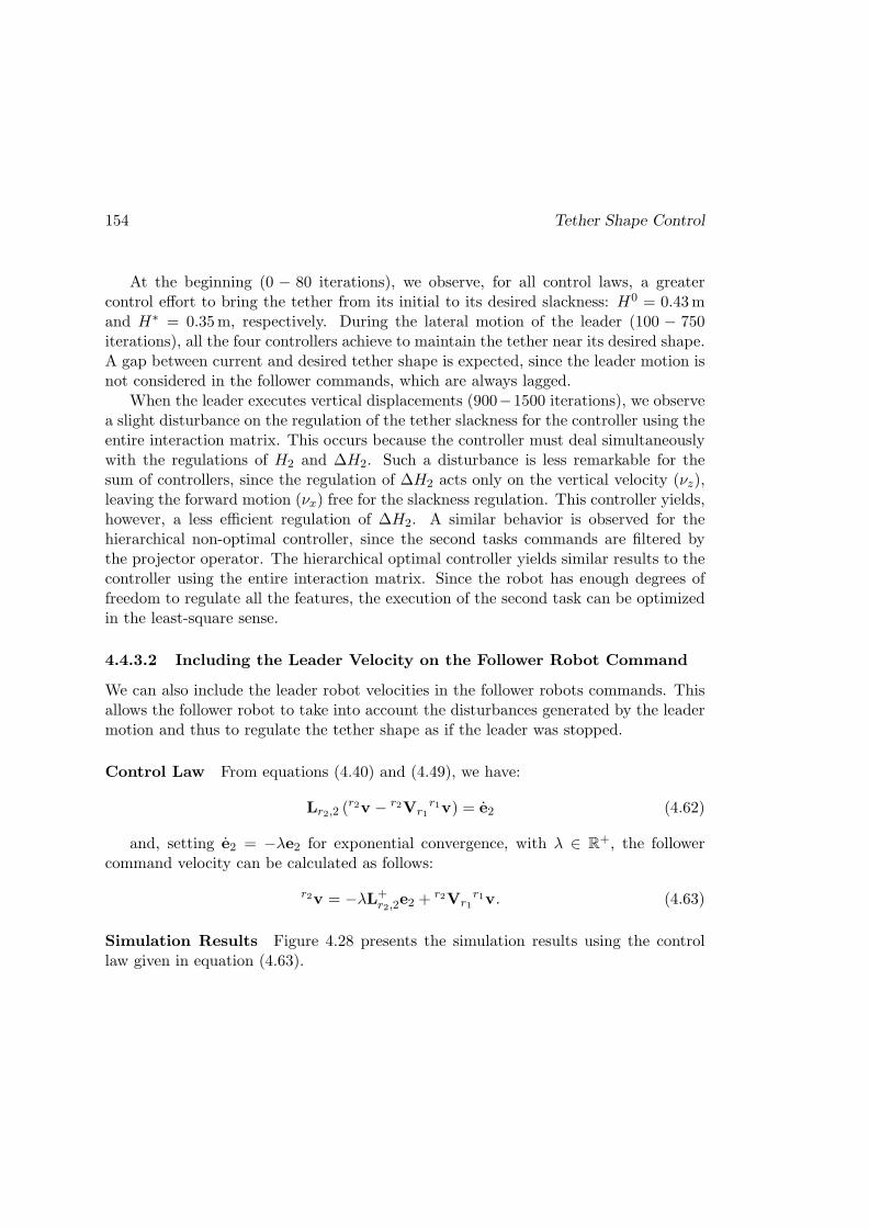
154 Tether Shape Control
At the beginning (0 − 80 iterations), we observe, for all control laws, a greatercontrol effort to bring the tether from its initial to its desired slackness: H0 = 0.43mand H∗ = 0.35m, respectively. During the lateral motion of the leader (100 − 750iterations), all the four controllers achieve to maintain the tether near its desired shape.A gap between current and desired tether shape is expected, since the leader motion isnot considered in the follower commands, which are always lagged.
When the leader executes vertical displacements (900−1500 iterations), we observea slight disturbance on the regulation of the tether slackness for the controller using theentire interaction matrix. This occurs because the controller must deal simultaneouslywith the regulations of H2 and ∆H2. Such a disturbance is less remarkable for thesum of controllers, since the regulation of ∆H2 acts only on the vertical velocity (νz),leaving the forward motion (νx) free for the slackness regulation. This controller yields,however, a less efficient regulation of ∆H2. A similar behavior is observed for thehierarchical non-optimal controller, since the second tasks commands are filtered bythe projector operator. The hierarchical optimal controller yields similar results to thecontroller using the entire interaction matrix. Since the robot has enough degrees offreedom to regulate all the features, the execution of the second task can be optimizedin the least-square sense.
4.4.3.2 Including the Leader Velocity on the Follower Robot Command
We can also include the leader robot velocities in the follower robots commands. Thisallows the follower robot to take into account the disturbances generated by the leadermotion and thus to regulate the tether shape as if the leader was stopped.
Control Law From equations (4.40) and (4.49), we have:
Lr2,2 (r2v − r2Vr1
r1v) = e2 (4.62)
and, setting e2 = −λe2 for exponential convergence, with λ ∈ R+, the follower
command velocity can be calculated as follows:
r2v = −λL+r2,2
e2 +r2Vr1
r1v. (4.63)
Simulation Results Figure 4.28 presents the simulation results using the controllaw given in equation (4.63).
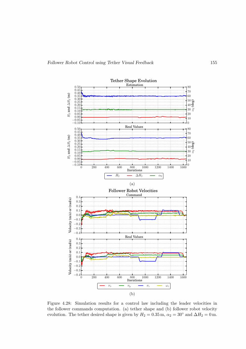
Follower Robot Control using Tether Visual Feedback 155
−0.10−0.050.000.050.100.150.200.250.300.350.400.450.50
H2
an
d∆H
2(m
)
Estimation
0 200 400 600 800 1000 1200 1400 1600
Iterations
−0.10−0.050.000.050.100.150.200.250.300.350.400.450.50
H2
an
d∆H
2(m
)
Real Values
0
10
20
30
40
50
60
70
80
α2
(deg)
H2 ∆H2 α2
0
10
20
30
40
50
60
70
80
α2
(deg)
Tether Shape Evolution
(a)
−0.4−0.3−0.2−0.10.0
0.1
0.2
0.3
0.4
Velo
city
(m/s
)or
(ra
d/s
)
Command
0 200 400 600 800 1000 1200 1400 1600
Iterations
−0.4−0.3−0.2−0.10.0
0.1
0.2
0.3
0.4
Velo
city
(m/s
)or
(ra
d/s
)
Real Values
νx νy νz ωz
Follower Robot Velocities
(b)
Figure 4.28: Simulation results for a control law including the leader velocities inthe follower commands computation. (a) tether shape and (b) follower robot velocityevolution. The tether desired shape is given by H2 = 0.35m, α2 = 30 and ∆H2 = 0m.

156 Tether Shape Control
Similarly to the previous control schemes, at the beginning of the simulation(0−80iterations), we observe a greater control effort of the follower robot to bring the tetherfrom its initial towards its desired slackness: H0
2 = 0.45m to H∗2 = 0.35m. For the
rest of the simulation, the tether is maintained near its desired shape. Some littleperturbations are observed in the change of direction of the robot leader, around the400th, 900th and 1200th iteration. The oscillations on the forward velocity command(νx) can be reduced through the use of a lower control gain, since the leader motion isincluded in the follower commands (we used λ = 2.0 in all simulations).
We note the follower robot executes a forward (νx) and lateral (νy) velocities duringa large part of the simulation (starting from 400th iteration until the end). This occursbecause the follower robot must keep its desired orientation with respect to the tether(regulate α2) while following the leader robot (regulate H2). Leader and follower robotsdo not have the same heading.
4.5 Follower Robot Control using Tether Visual Feedback
from Both Cameras - Underwater Case
The system we want to control has 4 degrees of freedom (DOF), as presented in Chap-ter 2 (see Figures 2.10 and 2.11):
1. the tether plane orientation with respect to the leader robot (α1);
2. the tether plane orientation with respect to the follower robot (α2);
3. the difference of height between the attachment points (∆H1 = −∆H2);
4. the distance between the attachment points (2D1 +∆D1 = 2D2 +∆D2), whichis actually a function of the tether slackness, as defined in equations (4.12) and(4.13).
The control schemes introduced in the previous Section do not allow us to control allthe DOF of the system, since the angle α1 is not regulated. Therefore, the relative posebetween leader and follower robot is not fully constrained, as presented in Figure 4.29.
Using only the follower robot camera, we achieve to control three tether features(H2, α2 and ∆H2) through the interaction matrix given in equation (4.44). The rankof this matrix is 3, which does not constrain all the degrees of freedom of the system.In order to constrain the relative pose between the robots, we use the leader camera toobtain additional information and regulate the angle α1.
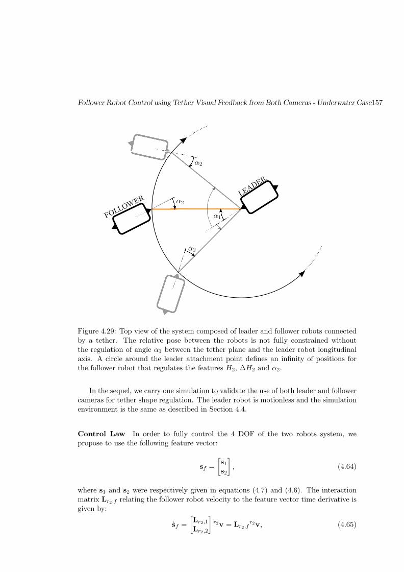
Follower Robot Control using Tether Visual Feedback from Both Cameras - Underwater Case157
α2
α1
α2
α2
FOLL
OWER
LEAD
ER
Figure 4.29: Top view of the system composed of leader and follower robots connectedby a tether. The relative pose between the robots is not fully constrained withoutthe regulation of angle α1 between the tether plane and the leader robot longitudinalaxis. A circle around the leader attachment point defines an infinity of positions forthe follower robot that regulates the features H2, ∆H2 and α2.
In the sequel, we carry one simulation to validate the use of both leader and followercameras for tether shape regulation. The leader robot is motionless and the simulationenvironment is the same as described in Section 4.4.
Control Law In order to fully control the 4 DOF of the two robots system, wepropose to use the following feature vector:
sf =
[s1s2
], (4.64)
where s1 and s2 were respectively given in equations (4.7) and (4.6). The interactionmatrix Lr2,f relating the follower robot velocity to the feature vector time derivative isgiven by:
sf =
[Lr2,1
Lr2,2
]r2v = Lr2,f
r2v, (4.65)

158 Tether Shape Control
with
Lr2,1 = −Lr1,1r1Vr2 =
−√
1−b21c21+b1s21
(u1+p1)Hmax−√
1−b21s21+b1c21
(u1+p1)Hmax− v1+q1
(u1+p1)Hmax−r2X2
√1−b2
1s21+b1c21
(u1+p1)Hmax
b1√
1−b21c21+(1−b2
1)s21
2D1+∆D1
b1√
1−b21s21−(1−b2
1)c21
2D1+∆D10 r2X2
b1√
1−b21s21−(1−b2
1)c21
2D1+∆D1
0 0 12∆Hmax
0
.
(4.66)
s21 = sin(α2 − α1) and c21 = cos(α2 − α1). The follower robot velocity commands arecalculated through:
r2v = −λL+r2,f
ef , (4.67)
where ef = sf − s∗f and s∗f is the desired feature vector.
Simulation Results The following simulation reproduces the same initial scenarioof the simulations presented in Section 4.4.2, where only the follower camera is used toregulate the tether shape while the leader robot remains stopped.
The initial tether features are given in Table 4.3. The initial and desired tethershape in the image are depicted in Figure 4.30. At the beginning, the tether is partiallyvisible in both leader and follower cameras.
The tether shape evolution, from visual feedback estimation and simulation groundtruth, is depicted in Figure 4.31a. The commanded and executed velocities of thefollower robot are shown in Figure 4.31b. The control gain is λ = 0.5.
Leader Follower
H1(m) α1 ∆H1(m) H2(m) α2 ∆H2(m)
initial 0.50 80° 0.0 0.50 80° 0.0
desired 0.35 30° −0.20 0.15 30° 0.20
Table 4.3: Initial and desired tether features.

Follower Robot Control using Tether Visual Feedback from Both Cameras - Underwater Case159
(a) (b)
−0.8−0.6−0.4−0.2 0.0 0.2 0.4 0.6 0.8x(m)
−0.6
−0.4
−0.2
0.0
0.2
0.4
0.6
y(m
)
Leader Camera
estimationdesired shapedetected points
(c)
−0.8−0.6−0.4−0.2 0.0 0.2 0.4 0.6 0.8x(m)
−0.6
−0.4
−0.2
0.0
0.2
0.4
0.6
y(m
)Leader Camera
estimationdesired shapedetected points
(d)
(e) (f)
−0.8−0.6−0.4−0.2 0.0 0.2 0.4 0.6 0.8x(m)
−0.6
−0.4
−0.2
0.0
0.2
0.4
0.6
y(m
)
Follower Camera
estimationdesired shapedetected points
(g)
−0.8−0.6−0.4−0.2 0.0 0.2 0.4 0.6 0.8x(m)
−0.6
−0.4
−0.2
0.0
0.2
0.4
0.6
y(m
)
Follower Camera
estimationdesired shapedetected points
(h)
Figure 4.30: Embedded image view of the tether from the (a,b,c,d) leader and (e,f,g,h)follower point of view. The (a,c,e,g) initial and (b,d,f,h) final images of the visualservoing. Figures (a,b,e,f) are the source images while figures (c,d,g,h) depict thetether detected points (in blue), the shape estimation (in red) and the desired shape inthe image (in green).
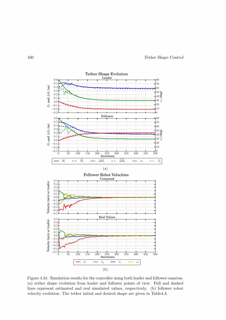
160 Tether Shape Control
−0.3−0.2−0.10.0
0.1
0.2
0.3
0.4
0.5
0.6
H1
an
d∆H
1(m
)
Leader
0 50 100 150 200 250 300 350 400 450 500
Iterations
−0.3−0.2−0.10.0
0.1
0.2
0.3
0.4
0.5
0.6
H2
an
d∆H
2(m
)
Follower
0
10
20
30
40
50
60
70
80
α2
(deg)
Hi Hi ∆Hi ∆H i αi αi
0
10
20
30
40
50
60
70
80
α1
(deg)
Tether Shape Evolution
(a)
−0.5−0.4−0.3−0.2−0.10.00.10.20.30.40.5
Velo
city
(m/s
)or
(ra
d/s
)
Command
0 50 100 150 200 250 300 350 400 450 500
Iterations
−0.5−0.4−0.3−0.2−0.10.00.10.20.30.40.5
Velo
city
(m/s
)or
(ra
d/s
)
Real Values
νx νy νz ωz
Follower Robot Velocities
(b)
Figure 4.31: Simulation results for the controller using both leader and follower cameras.(a) tether shape evolution from leader and follower points of view. Full and dashedlines represent estimated and real simulated values, respectively. (b) follower robotvelocity evolution. The tether initial and desired shape are given in Table4.3.

Discussion 161
Similar to the results obtained in Section 4.4.2, the tether shape estimation is notaccurate at the beginning of the simulation (0 − 80 iterations), as presented in Fig-ure 4.31a. Indeed, the tether is almost a straight line in the image at its initial shape(see Figure 4.30e), and the catenary curve fitting procedure cannot yield an accurateestimation of its shape. The curves of estimated and real values of the tether featuresmeet again after the 80th iteration, when the tether is completely visible in both images.
We note a greater oscillation of the estimated values of α2 when compared to theresults obtained in Section 4.4.2.1. This is caused by a greater lateral motion of thefollower robot. When only the follower’s camera is used to regulate the tether shape,the tether orientation is mainly regulated by a rotation (ωz) of the follower robot andthe lateral motion (νy) is almost zero (see Figure 4.18b). When using both cameras,however, the follower robot has to employ a greater lateral motion in order to regulatethe angle α1 simultaneously to α2. The lateral velocity νy causes a swinging motionof the tether plane, which is responsible for the oscillations on α1 and α2. Theseoscillations do not appear on the ground truth curve because the tether attachmentpoints do not oscillate.
Despite the initial shape estimation inaccuracies and the swinging motion of thecable, the control loop brings the tether towards its desired shape in the image (seeFigure 4.30h) and the tether features smoothly converge towards their desired values.The robot commanded velocities are nearly zero after the 300th iteration, since thetether reached its desired shape.
4.6 Discussion
The proposed tether shape control scheme has proved useful to properly manage thetether shape. Even in conditions of coarse tether shape estimation, such as cablepartial visibility, the controller achieves to bring the tether towards its desired positionin the image. The features converge to their desired values as required, with a smoothexponential decay of the error once the tether shape is well fitted in the image. It mayoccur that at the beginning, the tether is not well fitted due to a lack of tether detectedpoints in the image.
The controller has also proved to be robust to external perturbations, such as un-expected movements of the leader robot. This situation was tested in the case wherethe leader robot executes a path and the follower must ensure the tether remains atits desired shape. When the leader velocities are neglected by the follower, its com-mands are lagged, as expected, and the tether is maintained around its desired shape,within a small margin of error. When the leader velocities are included in the followercommands, the tether shape is maintained at its desired shape all along the path.
Four types of controllers were tested. First, the most straightforward approachwas implemented, using the entire interaction matrix to regulate all the catenary fea-tures simultaneously. This matrix showed to be efficient for the visual servoing controlscheme.
Second, a sum of controllers was tested and the features (H2, α2) and ∆H2 were
162 Tether Shape Control
separately regulated. Such a controller did not show good performances, in particu-lar, the regulation of ∆H2 introduced an overshoot generated by the vertical velocitycommands (νz). This is not surprising since both regulations combine their effects in aseparate way.
Third, a hierarchical non-optimal control was used for the regulation of (H2, α2) asa priority and then ∆H2 as a secondary task. This solution also showed an overshootfor ∆H2. Actually, the distribution of the secondary task commands were not optimalwith respect to the remaining degrees of freedom of the robot.
Forth, a hierarchical optimal control was tested. This controller optimized the exe-cution of the secondary task, carrying out the best of it without affecting the executionof the priority task. This controller achieved to regulate all the three features properlywithout overshoot. Convergence performances were observed to be comparable withthe controller using the full 3× 4 interaction matrix.
Finally, features from the onboard camera of the leader robot were added to thecontrol scheme. This allowed to regulate the angle α1 between the tether plane and theleader robot longitudinal axis. As a result, the relative position of both robots could befully constrained. The regulation of the features of both cameras and depth sensor wasachieved by stacking the corresponding interaction matrices: the one that regulates theleader features and the other that regulates the follower features. Satisfactory resultswere also obtained using both cameras, and all the features converged towards theirdesired values as required, with a smooth exponential decay of the error once the tetherwas well fitted in the image.
In the following, some perspectives of improvement of our catenary-based controlscheme are discussed.
Considering Roll and Pitch Disturbances The robots roll and pitch angles areassumed to be mechanically stabilized or regulated by a low level control law. Distur-bances on roll and pitch angles may occur when the robots are deployed in zones withstrong disturbances. As our ultimate goal is to deploy a chain of robots in the coastalzone, one of the first possible extensions to be implemented is to consider desired non-zero roll and pitch angles in the control schemes in order to take into account specificdiving movements, even though they are not controlled through visual servoing.
Investigate Other Visual Features We investigated the use of the catenary modelfor a hanging tether cable that links two robots. This model allowed us to parameterizethe tether shape accurately, using tether slackness and relative orientation with respectto the robots. Other parametric curves can be investigated. For example, parabolasand splines could be used to fit the tether shape and provide parameters to performvisual control of the tether shape. Recently, Fourier transform coefficients were used invision-based shape control of linear objects Zhu et al. (2018). This strategy could alsobe used for tether shape control.
Conclusions 163
Model-Based Dynamic Control Dynamic interactions between cable and robotscan also be modeled. The catenary model can provide information about the forcesexerted at its extremities. These could be used in a dynamic control scheme to preventthe robot motion from being disturbed by the cable weight and traction. Moreover, thehydrodynamic modeling of robots and cable can be made in order to achieve a moreprecise cable handling in water, taking into account its weight and dragging forces. Theswinging motion of the tether cable could also be considered.
4.7 Conclusions
In this Chapter we presented 3-D catenary-based visual servoing control schemes usedfor the shape regulation of a tether linking two robots, a leader and a follower. Thetether shape is regulated by the follower robot through the proper displacement of itsattachment point.
The tether shape is defined by three parameters: slackness H, orientation angleα and height difference between attachment points ∆H. These parameters are calledfeatures, whose values are estimated from sensory feedback data, namely the camerasand pressure sensors embedded on the robots. The pressure sensors give the differenceof height between the tether attachment whereas the cameras provide tether detectedpoints used to estimate its slackness and orientation through the curve fitting proceduredescribed in Chapter 3. The tether shape parameters are calculated in relation to therobots. Therefore, there are two slacknesses (H1 and H2), two orientations (α1 and α2),and two height differences (∆H1 and ∆H2), related to the leader and follower robots.These features are hence used by the control schemes we introduced to regulate thetether shape with respect to one or both robots simultaneously.
The control schemes proposed are proportional control laws based on the interactionmatrix relating the follower robot motion to the time derivative of the tether features.Three types of control schemes were tested in the regulation of the tether shape withrespect to the follower robot. All the control schemes have proved to properly managethe tether shape, even in conditions of coarse tether shape estimation, such as cablepartial visibility. Moreover, they demonstrated to be robust to external perturbations,such as unexpected movements of the leader robot.
First, the entire interaction matrix was used so that all the features were regulatedsimultaneously. All the features converged towards their desired values as required.
Second, a summing controller was tested and the features (H2, α2) and ∆H2 wereseparately regulated. As expected, such a controller did not outperform the controllerbased on the entire interaction matrix.
Third, two hierarchical control laws were tested for the regulation of (H2, α2) as apriority and then ∆H2 as a secondary task. The first one was a hierarchical non-optimalcontroller whose behavior tended to produce an overshoot of feature ∆H2, which wasalso observed with the summing controller. The other one was a hierarchical optimalcontroller that optimized the execution of the secondary task, carrying out the bestof it without affecting the execution of the priority task. All the features were thus

164 Tether Shape Control
properly regulated, with comparable convergence performances to the controller usingthe entire matrix.
The simultaneous regulation of the tether features with respect to both leader andfollower robots was also achieved with satisfactory results. The relative position of bothrobots could therefore be fully constrained.
The use of both leader and follower cameras opens interesting perspectives of futureworks, in the context of the study of high level navigation strategies. Hierarchicalcontrol schemes can be used to give priority to the regulation of the tether featureswith respect to the leader or follower robot, depending on the situation at hand.
Chapter 5
Conclusions
5.1 Summary
In this thesis we investigated the use of camera feedback for the shape control of atether linking two underwater robots, a leader and a follower. Both robots have thesame motion capabilities, and are assumed to remain in the horizontal, with roll andpitch angles autonomously regulated by a high frequency low level controller. Ourobjective was to prove the feasibility of a visual servoing control scheme that couldallow the follower robot to regulate the tether shape releasing the leader robot toexplore its surrounding, in autonomy or by teleoperation.
The tether linking the robots is modeled by a catenary. This model is useful toobtain shape parameters of the tether cable. Since our catenary model is symmetricwith respect to the attachment point frames, the catenary parameters are calculatedrelatively to each robot. These parameters, also called catenary features, are definedas: the difference of height between the attachment points, the tether slackness andorientation.
The robots are equipped with depth sensors and cameras positioned near the tetherattachment points. The height difference between the attachment points is calculatedfrom the depth sensors measurements, whereas the tether slacknesses and orientationsare estimated through an image fitting procedure based on the Gauss-Newton algo-rithm. Tether points are detected through color segmentation in the images providedby the embedded cameras feedback. The projection of the catenary model in the imageplane is thus fitted to the detected points, which yields the estimation of the tetherslackness and orientation.
The catenary curve fitting was validated in simulations and it showed to produceaccurate results on tether shape estimation. Residual filtering functions were addedto the fitting procedure in order to avoid singularities in the Gauss-Newton Jacobian,speed up its computation, and enhance the algorithm robustness to detection noise.Moreover, an initialization heuristic was introduced in order to obtain a starting pointcloser to the solution and hence avoid local minima.
The estimated catenary features are grouped in a feature vector, which must be
165
166 Conclusion
regulated in order to maintain the tether at a desired shape. The tether must be slackenough not to hamper the leader movements. Also, an adequate orientation betweenthe robots and the tether plane must be maintained so that the tether is kept inside thecamera field of view. This ensures an accurate shape estimation from camera feedback.
The tether shape is regulated by the follower robot motion, generating a properdisplacement of the tether attachment point. The relation between the follower robotmotion and the catenary feature time derivatives is given by an interaction matrix,which is the base of the visual servoing control scheme presented in this thesis. Ageneral formalism for the calculation of this interaction matrix was introduced, allowingthe regulation of the catenary features with respect to both leader and follower robots.
The catenary-based visual servoing control scheme was validated in simulations.A number of proportional control laws were tested, ranging from the use of one orboth robot’s cameras to the simultaneous or hierarchical regulation of features. Theproposed control scheme has proved to properly manage the tether shape, even inconditions of coarse shape estimation, such as cable partial visibility. Moreover, ithas been demonstrated to be robust to external perturbations, such as unexpectedmovements of the leader robot.
When compared to the control scheme regulating all the catenary features simul-taneously, the hierarchical control schemes also yielded satisfactory results, in terms ofrapidity, efficiency or robustness to external perturbations. Actually, the interactionmatrix we introduced proved to be efficient, since all the features were well trackedby the robot without disturbing each other. The hierarchical control schemes can beuseful in the implementation of high level navigation strategies, as will be discussed inthe following Section.
In short, the main contributions of this thesis can be enumerated as follows:
1. The real-time estimation of the tether shape through an image fitting procedurebased on the catenary model of the tether;
2. The achievement of tether shape regulation through an innovative catenary-basedvisual servoing control scheme;
3. The study of a number of control laws dedicated to tether shape regulation;
4. The relative positioning of two underwater robots linked by a tether from theirembedded cameras and depth sensors feedback.
The scientific publications, workshop participations and scientific popularizationactivities carried out in this thesis are listed in appendixG.
5.2 Perspectives
Looking forward for tether shape control, one interesting extension of this thesis is touse additional sensory information in order to provide reliable shape estimation for longtether cable lengths (with tens or hundreds of meters length). Cameras have a limited

Perspectives 167
range, and the tether cable remains visible only up to a few meters away. Moreover,operations in turbid water can make tether point detection difficult, compromising itsshape estimation from camera feedback.
As discussed in Chapter 3, additional sensors such as 3-D accelerometers can beadded to the tether ends in order to provide additional information about its shape (Mer-let, 2018b). These sensors could be useful to measure the departure angles of the tethercables, which can be used to calculate its slackness. Moreover, the accelerometers mayprovide information about the swinging motion of the tether cable, which was notconsidered in the control schemes proposed.
Even considering the case of large cables shape regulation, the cameras could yieldexploitable information about the cable orientation with respect to the robots. Theuse of both leader and follower cameras may also provide redundant information aboutthe tether slackness, which can be used together with accelerometers data in order toenhance the reliability of cable shape estimation.
The concept of catenary-based tether shape control for a pair of robots may alsobe extended for a chain composed of several underwater robots deployed by a surfacevessel. The visual servoing control scheme that we introduced could be used to regulatethe portion of tether cable connecting successive robots. Since the motion of one robothas an effect on the others, a high level control must be set up to avoid platooningeffect.
The navigation of the whole chain of robots is an interesting research theme to bedeveloped. The high level controller must manage the relative position between therobots depending on the situation at hand. If small cavities are to be crossed, therobots must be mostly aligned and the tether not too slack so as not to drag on thefloor. Otherwise, when exploring open sites, it would be better to have the robotsmore spaced laterally in order to have a wider perception of the environment. Thehierarchical control schemes can be used so that priority can be given to the orientationor slackness, depending on the situation.
Other geometric configurations than a chain of robots can be used. Triangular andsquared grids can be interesting formations to explore open sites and achieve a moredistributed perception of the environment.
Possible applications of this work include the exploration of coastal zones by smallunderwater tethered robots, called mini-ROVs. Small underwater robots are required tocarry out exploration missions of these zones due to the low depth. Alone, such robotscannot counterbalance the disturbance caused by tides and currents acting on the tethercable. Together, however, they can more efficiently control the tether shape. Moreover,the use of multiple robots connected by a tether yield a distributed perception of theunderwater environment for the human operator on the surface, which is interestingfor cartography purposes and synchronized data collection of the environment.
Catenary-based tether shape control can be also useful in the context of clutteredenvironments exploration, such as underwater caves and submerged mining sites. Insuch situations, the correct management of the tether shape is crucial for the successof the mission, preventing robots from being lost due to tether entanglement withobstacles.
168 Conclusion
In a broader sense, this thesis proved that the tether cable can be used for therelative positioning between robots, or between robot and a stationary base. This canbe used, for example, by a robot that anchors itself to the seabed relief or underwaterstructure in order to have its position stabilized for its mission execution. Anotherexample of application would be the relative positioning between a surface vessel anda scout robot.

Appendix A
Position and Orientation
Representation
In a 3-dimensional Euclidean space, noted E3, a coordinate reference frame is defined
as Fa(Pa, ia, ja,ka) and consists of an origin, denoted Pa, and a triad of mutuallyorthogonal basis vectors, denoted (ia, ja,ka), that are all fixed within a particular body(Siciliano and Khatib, 2016, chap. 1).
The position of a 3-D point, center of frame Fb, relative to another coordinate frameFa can be denoted by the 3× 1 vector
aPb =
aXbaYbaZb
. (A.1)
The components of this vector are the Cartesian coordinates of the center of Fb in theframe Fa, which are the projections the vector aPb onto the corresponding axes i, j,k.
The orientation of frame Fb relative to frame Fa can be denoted by expressing thebasis vectors (ib, jb,kb) in terms of the basis vectors (ia, ja,ka). This yields (
aib,a jb,
a kb),which when written together as a 3× 3 matrix is known as the rotation matrix
aRb =
ib · ia jb · ia kb · iaib · ja jb · ja kb · jaib · ka jb · ka kb · ka
, (A.2)
which is an special orthogonal matrix, such that aRTb = aR−1
b and det aRb = 1.An elementary rotation of Fb about the k axis of Fa through an angle θ is
aRb(k, θ) =
cos θ − sin θ 0sin θ cos θ 00 0 1
, (A.3)
while the same rotation around the j axis is
aRb(j, θ) =
cos θ sin θ 00 1 0
− sin θ cos θ 0
, (A.4)
169
170 Position and Orientation Representation
and around i axis is
aRb(i, θ) =
1 0 00 cos θ − sin θ
sin θ cos θ 0
. (A.5)
The Euler angle used to define the orientation of solid bodies in the space are notuniquely defined. Several formulations are proposed in the literature, among which wemainly distinguish roll-yaw-roll, roll-pitch-roll and roll-pitch-yaw. Any rotation matrixof E3 can be expressed in a form of a product of the three matrices as follows (Jaulin,2015):
bRa = aRb(k, θk)aRb(j, θj)
aRb(i, θi) (A.6)
Position vectors and rotation matrices can be combined together in an homogeneoustransformation in order to represent position and orientation in a compact notation.Any 3-D point vector iPa expressed relative to frame Fi can be expressed relative toFj if the position and orientation of Fi are known relative to the Fj :
jPa = jRiiPa +
jPi. (A.7)
This equation can be writtenjPa = jMi
iPa, (A.8)
wherejMi =
[jRi
jPi
0T 1
]
is the 4 × 4 homogeneous matrix that transforms vectors from coordinate frame Fi
to coordinate frame Fj , andjPa = [jPa 1]T and iPa = [iPa 1]T are homogeneous
representations of position vectors jPa and iPa. The homogeneous matrix iMj isinvertible and the inverse coordinates transformation from frame Fj to frame Fi isrepresented by:
jM−1i = iMj =
[jRT
i −jRTijPi
0T 1
].
The transformation between frames can be expressed as a composition of transforma-tions, such that:
kMi =kMj
jMi.

Appendix B
Expression of the catenary
parameter C
This appendix gives details about the calculation of the catenary parameter C as afunction of its slackness H, attachment point difference of height ∆H and cable totallength L.
The catenary shape of a hanging cable can be obtained from a set of three equations.The first two equations express that the tether extremities are points belonging to thecatenary. The third equation states that the total length of the cable is a knownconstant. These equations are given here above:
H =1
C[cosh(CD)− 1] (B.1)
H +∆H =1
C[cosh(C(D +∆D)− 1] (B.2)
L =1
C[sinh(C(D +∆D)) + sinh(CD)] , (B.3)
which can be rewritten as:
CH + 1 = cosh(CD) (B.4)
C(H +∆H) + 1 = cosh(C(D +∆D) (B.5)
CL = sinh(C(D +∆D)) + sinh(CD). (B.6)
We must eliminate D between the equations. Using the identity equation
cosh2(C(D +∆D))− sinh2(C(D +∆D)) = 1 (B.7)
with equations (B.5) and (B.6) leads to (this means that there can be a minus sign infront of sinh(C(D +∆D)) in Eq. (B.6)):
[C(H +∆H) + 1]2 − [CL− sinh(CD)]2 = 1, (B.8)
that can be developed to
[C(H +∆H) + 1]2 −[(CL)2 + sinh2(CD)− 2CL sinh(CD)
]= 1. (B.9)
171

172 Expression of the catenary parameter C
From equations (B.4) and (B.7) we have
sinh2(CD) = (CH + 1)2 − 1, (B.10)
that can be introduced in equation (B.9) yielding:
[(CH + 1) + C∆H)]2 − (CL)2 − (CH + 1)2 + 2CL sinh(CD) = 0. (B.11)
This equation can be further developed to:
(C∆H)2 + 2C∆H(CH + 1)− (CL)2 + 2CL sinh(CD) = 0 (B.12)
C(L2 −∆H2 − 2H∆H)− 2∆H = 2L sinh(CD). (B.13)
Taking the square of equation (B.13) leads to (this means that there can be a minussign in front of sinh(CD) in the equation above but C must remain positive):
[C(L2 −∆H2 − 2H∆H)− 2∆H
]2= 4L2
[(CH)2 + 2CH
]. (B.14)
This is a second order equation in C:
A.C2 +B.C + C = 0, (B.15)
with
A = (L2 −∆H2 − 2H∆H)2 − 4L2H2
= (L2 −∆H2)[L2 − (2H +∆H)2
](B.16)
B = −4∆H(L2 −∆H2 − 2H∆H)− 8HL2
= −4(L2 −∆H2)(2H +∆H) (B.17)
C = 4∆H2. (B.18)
The determinant ∆ is:
∆ = B2 − 4AC
= 64HL2(L2 −∆H2)(H +∆H). (B.19)
There exist solutions if ∆ > 0, i.e. if:
L > |∆H| (B.20)
H +∆H > 0 (B.21)
H is always positive because the attachment point P2 is always above the lowest pointP0 of the catenary. Therefore, if a solution exists, we necessarily have B < 0.
In this case the two solutions can be expressed as:
C1 =−B −
√∆
2A(B.22)
C2 =−B +
√∆
2A(B.23)
173
Since C > 0,
sign(C1C2) = sign(CA) = sign(A)
• ifA < 0, there is only one positive solution for C, which is C1 (√∆ =
√B − 4AC >
−B).
• if A > 0, there are two positive solutions C1 and C2 with C1 < C2. The catenarywith coefficient C2 is the tightest one (ch(C2X1) behaves like e
C2X1 whenX1 tendsto infinity, which increases much faster than eC1X1 as X1 increases.). Figures B.1and B.2 illustrate both solutions, the catenary C1 does not allow the lowest pointto belong to the umbilical, whereas the catenary C2 does.
If we want to have the tightest catenary as a solution, we must have A > 0, i.e.
L > 2H +∆H
since 2H +∆H > 0.
If ∆H = 0, we get:
C2 =−B +
√∆
2A(B.24)
=8L2H +
√64H2L4
2L2(L2 − 4H2)(B.25)
=16L2H
2L2(L2 − 4H2)(B.26)
=8H
L2 − 4H2(B.27)
If we replace L by 2R, we have:
C2 =8H
4R2 − 4H2=
2H
R2 −H2(B.28)
As a conclusion, the solution for C to have the catenary with the lowest pointbelonging to the umbilical is:
C =2(L2 −∆H2)(2H +∆H) + 4L
√H(L2 −∆H2)(H +∆H)
(L2 −∆H2) [L2 − (2H +∆H)2](B.29)
=2
L2 − (2H +∆H)2
(2H +∆H + 2L
√H
H +∆H
L2 −∆H2
)(B.30)
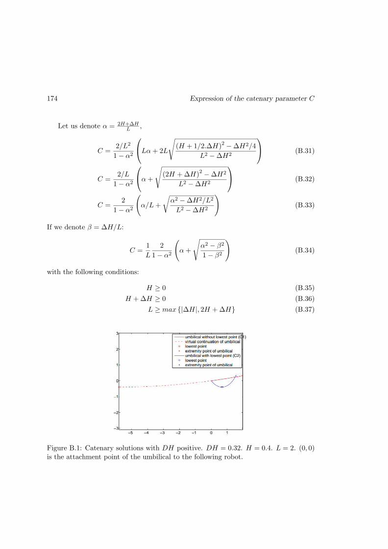
174 Expression of the catenary parameter C
Let us denote α = 2H+∆HL
,
C =2/L2
1− α2
Lα+ 2L
√(H + 1/2.∆H)2 −∆H2/4
L2 −∆H2
(B.31)
C =2/L
1− α2
α+
√(2H +∆H)2 −∆H2
L2 −∆H2
(B.32)
C =2
1− α2
(α/L+
√α2 −∆H2/L2
L2 −∆H2
)(B.33)
If we denote β = ∆H/L:
C =1
L
2
1− α2
(α+
√α2 − β21− β2
)(B.34)
with the following conditions:
H ≥ 0 (B.35)
H +∆H ≥ 0 (B.36)
L ≥ max |∆H|, 2H +∆H (B.37)
Figure B.1: Catenary solutions with DH positive. DH = 0.32. H = 0.4. L = 2. (0, 0)is the attachment point of the umbilical to the following robot.
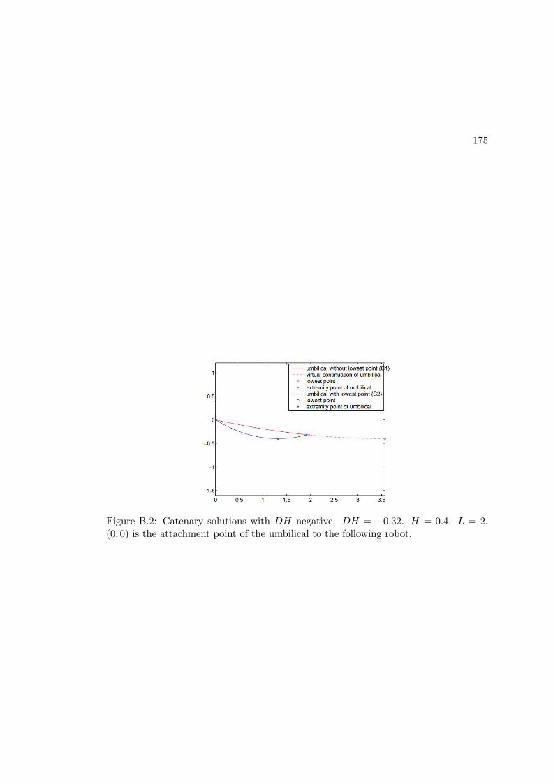
175
Figure B.2: Catenary solutions with DH negative. DH = −0.32. H = 0.4. L = 2.(0, 0) is the attachment point of the umbilical to the following robot.

176 Expression of the catenary parameter C
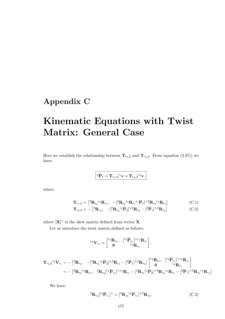
Appendix C
Kinematic Equations with Twist
Matrix: General Case
Here we establish the relationship between Tr1,2 and Tr2,2. From equation (2.87)) wehave:
˙2P1 = Tr1,2r1v +Tr2,2
r2v.
where
Tr1,2 =[2Rr2
r2Rr1 , −[2Rr2r2Rr1
r1P1]×2Rr2
r2Rr1
](C.1)
Tr2,2 = −[2Rr2 , −[2Rr2
r2P2]×2Rr2 − [2P1]
×2Rr2
](C.2)
where [X]× is the skew matrix defined from vector X.
Let us introduce the twist matrix defined as follows:
r2Vr1 =
[r2Rr1 , [r2Pr1 ]
×r2Rr1
0 r2Rr1
].
Tr2,2r2Vr1 = −
[2Rr2 , −[2Rr2
r2P2]×2Rr2 − [2P1]
×2Rr2
] [r2Rr1 , [r2Pr1 ]×r2Rr1
0 r2Rr1
]
= −[2Rr2
r2Rr1 ,2Rr2 [
r2Pr1 ]×r2Rr1 − [2Rr2
r2P2]×2Rr2
r2Rr1 − [2P1]×2Rr2
r2Rr1
]
We have:
2Rr2 [r2Pr1 ]
× = [2Rr2r2Pr1 ]
×2Rr2 , (C.3)
177

178 Kinematic Equations with Twist Matrix: General Case
This allows to apply the skew matrix in frame F2, instead of Fr2.
−Tr2,2r2Vr1 =
[2Rr2
r2Rr1 ,2Rr2 [
r2Pr1 ]×r2Rr1 − [2Rr2
r2P2]×2Rr2
r2Rr1 − [2P1]×2Rr2
r2Rr1
]
=[2Rr2
r2Rr1 , [2Rr2r2Pr1 ]
×2Rr2r2Rr1 − [2Rr2
r2P2]×2Rr2
r2Rr1 − [2P1]×2Rr2
r2Rr1
]
=[2Rr2
r2Rr1 ,[2Rr2
r2Pr1 ]× − [2Rr2
r2P2]× − [2P1]
× 2Rr2r2Rr1
]
=[2Rr2
r2Rr1 ,[2Rr2
r2Pr1 − 2Rr2r2P2 − 2P1
]× 2Rr2r2Rr1
]
=[2Rr2
r2Rr1 ,[2Rr2
r2Pr1 − 2Rr2r2P2 − 2Rr2
r2 (P2P1)]× 2Rr2
r2Rr1
]
=[2Rr2
r2Rr1 ,[2Rr2 r2 (Pr2Pr1 −Pr2P2 −P2P1)
]× 2Rr2r2Rr1
]
=[2Rr2
r2Rr1 ,[2Rr2
r2Rr1r1 (P1Pr1)
]× 2Rr2r2Rr1
]
Sincer1 (P1Pr1) = −r1P1,
we obtain:
−Tr2,2r2Vr1 =
[2Rr2
r2Rr1 , −[2Rr2
r2Rr1r1P1
]× 2Rr2r2Rr1
].
Finally,−Tr2,2
r2Vr1 = Tr1,2. (C.4)
Similarly,−Tr2,1
r2Vr1 = Tr1,1. (C.5)
Appendix D
Catenary Derivatives
The catenary projection equation was defined in equation (3.36) and is rewritten herebelow as a reminder:
y (s, xi) =1cZ
[−cosh (Cζ − CD)− 1
C+ aHmax +
cY2
],
where
ζ =cX2 − xicZ2
b+ x√1− b2
and
cZ =
√1− b2cX2 + bcZ2
b+√1− b2xi
.
The derivative of the catenary projection equation with respect to the parametersa = H
Hmaxand b = sinα was introduced by equations 3.45 and 3.46. They are rewritten
here below:
∂y(xi, s)
∂a=
1cZ
[−∂
1C
∂a[cosh (Cζ − CD)− 1]
− sinh (Cζ − CD)
C(A1 +A2 +A3) +Hmax
] (D.1)
and
∂y(s, xi)
∂b=− 1
C
∂ 1cZ
∂b[cosh (Cζ − CD)− 1− C (H + cY 2)]
− 1cZ
∂ζ
∂bsinh (Cζ − CD) .
(D.2)
In this appendix, we give the calculation details of these derivatives.
179
180 Catenary Derivatives
First, from equation D.1, the intermediate variables A1, A2 and A3 of are definedas:
A1 = ζ∂C
∂a(D.3)
A2 = −D∂C
∂a(D.4)
A3 = −C∂D
∂a. (D.5)
The catenary parameter C was defined in equation (2.17), which is presented againhere below as a reminder:
C = 2Cn
Cd
= 22H +∆H + 2L
√H H+∆H
L2−∆H2
L2 − (2H +∆H)2.
The partial derivative of C with respect to the a-parameter is:
∂C
∂a=∂C
∂H
dH
da(D.6)
∂C
∂H= 2
∂Cn
∂HCd − ∂Cd
∂HCn
C2d
(D.7)
∂Cn
∂H= 2 + L
2H +∆H√H(H +∆H)(L2 −∆H2)
(D.8)
∂Cd
∂H= −4(2H +∆H) , (D.9)
with dHda
= Hmax. The partial derivative of 1C
with respect to the a-parameter is:
∂ 1C
∂a=∂ 1C
∂H
dH
da(D.10)
∂ 1C
∂H=
∂Cd
∂HCn − ∂Cn
∂HCd
2C2n
. (D.11)
The partial derivative of D, the catenary half-span, with respect to the a-parameter is:
∂D
∂a=∂ 1C
∂aacosh(CH + 1) +
∂C∂aH + CHmax
C√
(CH)2 + 2CH(D.12)
Finally, the derivative given by equation (D.2) are calculated as follows:
∂ 1Z
∂b=
cX2 − cZ2xi√1− b2
(√1− b2 cX2 + b cZ2
)2 (D.13)
∂ζ
∂b= −
(cX2 − cZ2xi)(√
1− b2 − bxi)
√1− b2
(b+√1− b2xi
)2 . (D.14)
Appendix E
Preliminary Results with
Terrestrial Robots
In this appendix is resumed the preliminary work we made on tether shape controlusing terrestrial robots. Two articles are reproduced in the following pages.
First, the article we presented at the 2017 IEEE International Conference on Roboticsand Automation (ICRA 2017) is reproduced. The title of this paper is Catenary-
based Visual Servoing for Tethered Robots. It addressed the use of catenarymodel to achieve visual of an umbilical linking two terrestrial robots.
Second, the article Tether Shape Control through Catenary-Model-Based
Visual Servoing is reproduced. This paper makes a comparison between catenary-based and image-based visual servoing controllers.
181

Catenary-based Visual Servoing for Tethered Robots
Matheus Laranjeira 1, Claire Dune1 and Vincent Hugel1
Abstract— Tethers are used to supply power and transferdata for teleoperated robots. They are known to limit the robot’sworkspace and could have the effect of hampering its motion.What if we could take advantage of the tether? In this papera new visual servoing scheme for catenary shaped deformableobjects is introduced in order to control the tether parametricshape by properly moving its fixation point. In most of thevisual servoing approaches the target object is rigid and distantfrom the controlled robot. On the contrary, in this paper, theobject is deformable and attached to the robot, thus its 3Dshape changes while the robot is moving. The experimentalsystem is composed of two terrestrial mobile robots of the samemotion capabilities linked with a slack rope. Simulation and realexperiments validate the proposed control scheme for propertether handling.
I. INTRODUCTION
Tethered and umbilical systems are used to provide power,
communication and assistance to robots operating in severe
environments. Some planetary rovers are connected to a
remote station by a cable to secure the exploration of
unknown and steep terrains. Their motion can be controlled
thanks to cameras that can be mounted either on the rover [1]
or on the station [2]. Tethered systems are also designed for
underwater missions. The underwater tether is usually slack,
and links a remotely operated vehicle (ROV) to a ship on the
surface. Some research studies deal with solutions to prevent
the ROV from beeing disturbed by the tether due to ship
motion [3].
Long flexible sagging objects like tethers, cables, wires,
hoses can be modeled by splines [4] and catenaries [5], [6],
in the context of object transportation and aerial systems, or
by parabolas [7], in the case of cable-driven parallel robots.
These objects are subject to gravity and the geometrical
equation that matches their shape can be used to control
the motion of the load to be transferred from one location
to another.
Visual servoing [8], [9] controls a robot motion to regulate
some visual features that are usually extracted from rigid
objects that can be fixed or moving freely. First, geometrical
features such as points, line segments and circles were
investigated [10]. Then, 3D models were introduced for
known manufactured objects [11], [12], image moments to
deal with objects of natural shape [13], splines for shape
tracking [14] and algebraic curves for shape alignment [15].
Articulated objects were also considered [16]. Some recent
works focus on deformable object shape control where robots
push or pull the object to reach a desired configuration [17],
[18]. In the context of hose transportation, several robots
1 Cosmer Laboratory EA 7398, University of Toulon, France
Fig. 1: Experimental setup: two Turtlebots [19] simulate a
tether handling system for remotely operated robots. The
leader robot freely explores its surroundings while the fol-
lower robot is expected to maintain the tether slack enough
not to hamper the leader movements
were attached to a semi-rigid cable and a coordinate vi-
sual servoing control was introduced based on the cable
curvature derived from splines and GEDS (Geometrically
Exact Dynamic Splines) [4]. Unknown deformable objects
can be modeled thanks to their viscoelasticity properties [17]
or using virtual geometrical features such as image points,
distances and curvatures [18].
This paper deals with a novel visual servoing strategy
based on the deformable shape of a sagging tether that
links two terrestrial mobile robots of the same motion
capabilities. The objective is to free the leader robot from
tether management while the follower robot will be able to
position itself to ensure an average sag of the tether and
proper orientation with respect to it. The three points below
illustrate the contribution of this work:
• The tether is managed between two mobile robots
through a visual system embedded on the follower robot
that can extract visual information on the tether.
• The tether is modeled by a catenary shape whose
parameters are estimated thanks to a real time curve
fitting in the image. This allows to take into account
the deformation of the tether beyond pixels detected in
the image.
• An interaction matrix based on the estimated catenary
parameters is calculated and used for the motion control
of the follower robot with respect to the deformable
tether.
The paper is organized as follows: Section II presents the
tether modeling, Section III focuses on the visual servoing
strategy used for controlling the position of the follower
182

robot with respect to the tether. Section IV presents and dis-
cusses the experimental results. Finally, Section V concludes
the paper and gives directions for future work.
II. TETHER MODELING
A. Catenary-based geometrical modeling
The experimental setup is presented in Fig. 1. Two
terrestrial mobile robots of the same motion capabilities
simulate a tether handling system for remotely operated
robots. The leader robot freely explores its surroundings
while the follower robot is expected to maintain the tether
slack enough not to hamper the leader movements. Figure
2 defines the notations and reference frames used in the
remainder of the paper. Let Σr1 and Σr2 be two Cartesian
frames centered at the middle of the robots wheel axis with
X-axis pointing towards the front of the robot and a vertical
Z-axis. A camera is mounted on the follower robot to track
the tether shape. Let Σc be a Cartesian frame attached to the
camera’s optical center, with Z-axis being its optical axis
and Y -axis vertically set towards the ground. It is assumed
that the optical axis is aligned with the robot X-axis. A 3
millimeter orange rope that links the two robots simulates
the tether. Its attachment points are at the same height and
define the centers of the Cartesian frames Σ1 and Σ2, their
orientation being the same as the robot they are attached
to. The tether is modeled as a catenary, where R is its half-
length, D is the half-span between the attachment points and
H is the rope sag. Let Σ0 be a Cartesian frame attached to
the rope. Its center is the center of the rope and the X-axis
and Z-axis are in the rope plane.
The classic equation of a catenary, expressed in frame Σ0,
has the following form [20]:
Σ0 :
Y = 0
Z = 1C[cosh(Ct)− 1]
(1)
where C = 2·HR2−H2 . Expressing the same equation in Σ2
leads to:
Σ2 :
Y = tan θX
Z = 1C
[cosh
(C(
Ysin θ−D
))− 1]−H
(2)
where θ is the angle between the catenary plane and the
Σ2 X-axis. Finally, the same equation can be written in the
camera frame (Σc) as:
Σc :
Y = − 1
C[cosh (C (η −D))− 1] +H + Y2
Z = cot θ (−X +X2) + Z2
(3)
where η = −X+X2
sin θand (X2, Y2, Z2) are the coordinates of
Σ2 in frame Σc.
A 3-D point with coordinates P = (X,Y, Z) in the camera
frame is projected on the image plane as a 2-D point with
coordinates p = (x, y) through the equation:
xy1
=
1
Z
f 0 cx 00 f cy 00 0 1 0
XYZ1
(4)
a)
X0
Z0
b)
Fig. 2: Scheme of experimental setup. Two terrestrial mobile
robots with 2-DOF (rotation and translation) are linked by a
passive tether. (a) top view and (b) side view of the scene
where (cx, cy) are the coordinates of the principal point and
f is the focal length [21]. Therefore, using Eqs. (3) and (4)
we obtain the catenary projection on the image plane:
y =
η1
[− 1
C(cosh (C (η2 −D))− 1) + aHmax + Y2
](5)
where
η1 =b+√1− b2x√
1− b2X2 + bZ2
and η2 =X2 − Z2x
b+ x√1− b2
As variable shape parameters for the projected curve in the
image, we choose:
a =H
Hmax
(6)
and
b = sin θ (7)
with Hmax being the tether maximum acceptable sag (i.e. the
tether attachment point height). The parameters a and b are
respectively relative to the tether slackness and orientation
with respect to the follower robot. They range in the interval
[0, 1], and the sign of sin θ is discriminated by the side on
which the tether appears in the image. The tether is horizontal
when a = 0 and it reaches the ground when a = 1. When
b = 0 the tether belongs to the plane (Σ2, X2, Z2) and when
b = 1 it belongs to the plane (Σ2, Y2, Z2).
III. VISUAL SERVOING ALGORITHM
In this paper, the tether 3D shape is defined by the
following feature vector:
s = (a, b)
183
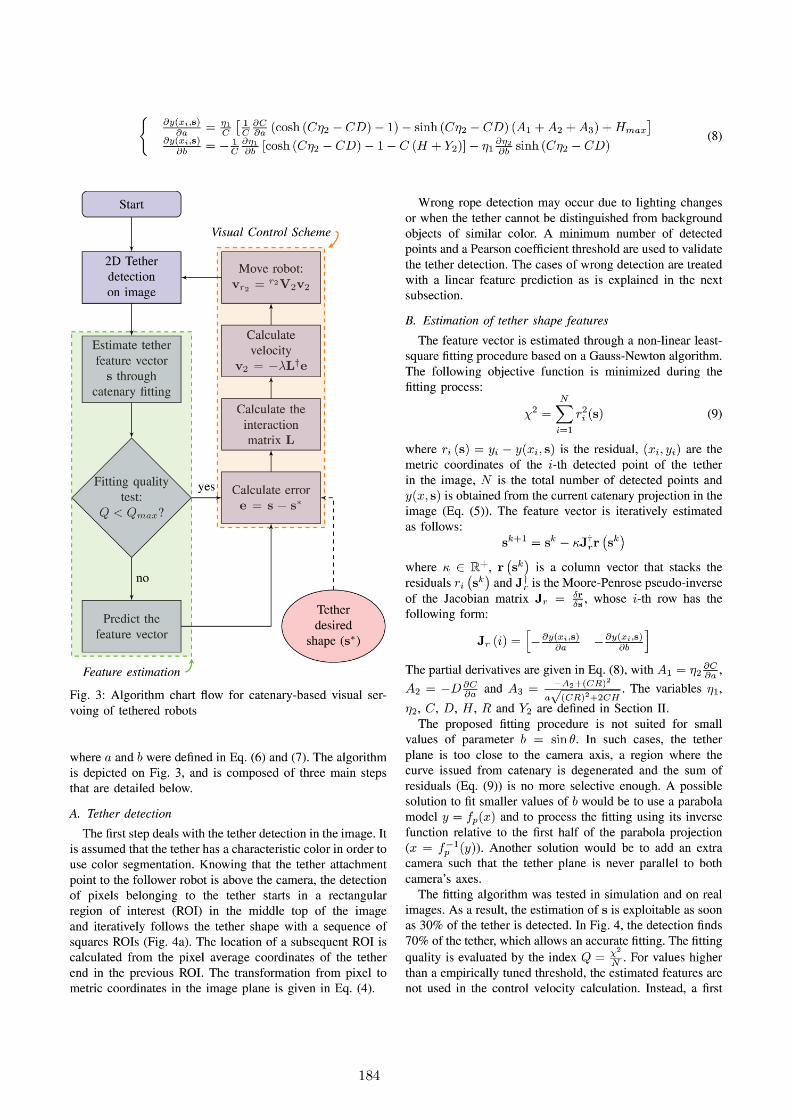

a)
-0.6 -0.4 -0.2 0 0.2 0.4 0.6
x(m)
-0.4
-0.3
-0.2
-0.1
0
0.1
0.2
0.3
0.4
y(m
)
Detected tether
Fitted
Desired
b)
Fig. 4: Catenary features estimation through a non-linear
least-squares fitting. (a) tether detection in the robot image
view. (b) tether fitting corresponding to the image view
above. The rope detected points are in blue, the fitted and
desired catenary curve are in red and green, respectively
order linearization of Eq. (11) is used to predict the feature
vector value, as follows:
s(t+ dt) = s(t) + L(t)v2(t) (10)
where dt is the sampling period, L is the catenary interaction
matrix and v2 = (v2, ω2) is the velocity vector of frame
Σ2 with linear velocity v2 and angular velocity ω2. In the
current implementation, the number of consecutive iterations
used for prediction is not limited.
C. Visual-based control scheme
The relation between the tether features time-derivative
and the attachment point Σ2 motion is given by the following
equation:
s = Lv2 (11)
The aim of visual-based control schemes is to minimize
the error e defined as
e = s− s∗ (12)
where s and s∗ are respectively the current and desired
feature vectors (see Fig. 4). In order to ensure an exponential
decay of the error, the following control law is designed [8]:
v2 = −λL†e (13)
where L† is the Moore-Penrose pseudo-inverse of L and
λ ∈ R+. The velocity of the follower robot is then obtained
through: vr2 = r2V2v2, where r2V2 is the twist transfor-
mation matrix from frame Σ2 to frame Σr2 .
We used a nonholonomic robot with 2 DOF to experimen-
tally validate our control scheme, as is explained in Section
IV. In such case, the conversion between vr2 and the pair of
control variables u = (vx, ωz) is achieved by the following
projection:
u =
[1 0 0 0 0 00 0 0 0 0 1
]vr2
D. Interaction matrix computation
The interaction matrix L is the tether deformation model.
It links the relative motion of the attached points to the
derivative of the tether parameters. Contrary to [18], the
object has a known parametric shape and this matrix is
analytically computed from the definition of s = (a,b).Let P0 = (X0, Y0, Z0) and P1 = (X1, Y1, Z1) be the
centers of frames Σ0 and Σ1, respectively. Evaluating and
differentiating Eq. (2) at P1, we get
H =
− C
C2[cosh (CD)− 1] + sinh (CD)
(CD
C+ D
)(14)
and differentiating the expression of C in Eq. (1) we have
C = KCH (15)
where KC =2(R2+H2)(R2−H2)2
. Then, from the definition of a in
Eq. (6) and replacing Eq. (15) in (14), we obtain
a =KH
Hmax
D (16)
where
KH =sinh (CD)
1 + KC
C2 [cosh (CD)− 1− CD sinh (CD)]
The relative motion of P1 in the reference frame Σ2, due
to the velocity of the follower robot v2 expressed in Σ2 is:
P1 = −v2 − ω2 × P1 (17)
Geometrically,
P0 =P1
2(18)
and
D =X0X0 + Y0Y0
D(19)
Thus, using Eqs. (17) and (18) in (19) we have:
D =1
2
− cos θ− sin θ
0Z1 sin θ−Z1 cos θ
Y1 cos θ −X1 sin θ
⊤
v2 (20)
185

0.00 2.001.00 3.000.50 1.50 2.50
0.00
−1.00
1.00
−1.50
−0.50
0.50
1.50
x(m)
y(m
)
Fig. 5: Multiple positions of the follower robot for the same
tether slackness and orientation: the problem only constrains
the tether shape and orientation w.r.t. the follower robot
Finally, using Eq. (20) in (16) and given that b = sin θ,
a =KH
2Hmax
−√1− b2−b0Z1b
−Z1
√1− b2
Y1√1− b2 −X1b
⊤
v2 (21)
Differentiating b = Y0
Dleads to:
b =Y0 − bD
D
From the expressions of Y0 and D in Eqs. (18) and (20)
respectively, we get:
b =1
2D
b√1− b2
−1 + b2
0Z1(1− b2)Z1b√1− b2
−Y1b√1− b2 −X1(1− b2)
⊤
v2 (22)
The complete interaction matrix (Eq. (23)) is composed
of the rows given in Eqs. (21) and (22) with one more
simplification: Z1 = 0 since the attachment points are at
the same height. The values of X1 and Y1 are geometrically
calculated from Eq. (2).
The rank of L is 2, which means that this control law only
commands two degrees of freedom of the follower robots,
i.e. the relative attached points distance and the follower
orientation with regards to the tether plane. Figure 5 shows
several follower positions for the same set of parameters
s = (a, b). Remaining degrees of freedom are thus available
for additional tasks, such as obstacle avoidance.
IV. EXPERIMENTAL RESULTS
A. Setup
One simulation and two real experiments are presented
in order to validate the control law. Two Turtlebots [19]
with 2 DOF (translation vx and rotation wz) are used as
experimental robots. They are equipped with a Kinect device
and linked by a 1.4 meter long and 3 millimeter thick orange
rope (Fig. 1). The rope maximum sag is Hmax = 0.40m,
corresponding to its attachment point’s height. The servoing
algorithm runs in the follower robot computer, which is
equipped with a Intel Core i5-2410M @ 2.3 GHz processor.
The video frame rate is fixed to 10Hz. The same robot motion
capabilities, rope length, thickness and maximum sag are
used in simulation and real experiments.
B. Simulation
The objective of the simulation is that the follower robot
moves the tether from a very slackened to a moderately tight
shape. The tether orientation is controlled, passing from a
large angle θ to a desired smaller angle. The initial and
desired values of the feature vector are so = (0.9, 0.8) and
s∗ = (0.5, 0.5), respectively. We assume that the robots can
perfectly estimate the tether parameters, so the fitting process
is not simulated. Figure 6 presents the simulation results. As
expected, both parameters have an exponential decay and
converge to the desired value within 4 seconds for a gain
λ = 0.75 and a sampling period of 0.1 seconds.
C. Real experiments
In the first experiment, the simulation initial conditions
are repeated and the follower robot moves the tether from
an initial shape so = (0.9, 0.8) to a desired shape s∗ =(0.5, 0.5). We used the same gain as for simulation (λ =0.75) and a fitting quality threshold Qmax = 1. Results are
summarized in Fig. 7.
In the second experiment (Fig. 8), the leader robot is freely
displaced while the follower robot ensures that the rope keeps
a desired shape s∗ = (0.7,−0.5). First, the leader robot
moves forward, then turns left (24s). Next, it moves about
1.25 meters forward (38s), makes a half-turn (50s) and moves
about 1.25 meters forward again (64s). At the end, it makes
a quarter turn and moves about 0.50 meters backward (76s).
Compared with the first experiment, a higher value was set
to the tether first parameter in order to give more freedom
of maneuvering to the leader robot. We used Qmax = 1and two different gains for linear and angular velocities:
λl = 1.0 and λω = 6.0, respectively (see discussion below).
Figure 8c presents the fitting quality index evolution during
the experiment. The feature prediction was used 20 times
in cases of wrong rope detection and more 38 times due to
inaccurate fitting.
In Fig. 7, the angular velocity command does not converge
to zero, and remains quasi constant. This is due to the
limitations of our experimental platform that cannot achieve
a rotation velocity lower than 0.05 rad/s. In the second
experiment, we selected a higher gain for the angular velocity
compared to the linear velocity gain in order to overcome
186

L =
[−KH
√1−b2
2Hmax− KHb
2Hmax0 0 0
KH(Y1
√1−b2−X1b)
2Hmax
b√1−b2
2D−1+b2
2D 0 0 0 −Y1b√1−b2+X1(1−b2)
2D
](23)
0.4
0.5
0.6
0.7
0.8
0.9
0 2 4 6 8 10time (s)
ab
a)
-0.5
-0.4
-0.3
-0.2
-0.1
0
0.1
0.2
0 2 4 6 8 10time (s)
VxWz
b)
Fig. 6: Simulation results for tether shape control. (a) the
parameters evolution. The tether goes from an initial to
a desired shape (so = (0.9, 0.8) and s∗ = (0.5, 0.5),respectively). (b) the control velocities. Linear velocity (vx)
in m/s and angular velocity (wz) in rad/s
this problem. As a future improvement, an integrator com-
pensator to deal with the low level control of the velocity
can be added to the servoing loop.
Looking at Fig. 7, we can note that the real experimen-
tation curves are noisy compared with those obtained in
simulation. This is mainly due to wrong rope detection that
can affect the tether feature estimation. Another reason is the
possible rope oscillation during the robot motion, which can
occur when the robot halts and restarts motion. This could
be taken into account by designing a dynamic controller that
takes the rope inertia into account. In addition, the rope can
be tracked in the image by a gradient-guided algorithm.
V. CONCLUSIONS AND PERSPECTIVES
This paper presents a new visual servoing control scheme
to manage a tether linking two terrestrial mobile robots. The
tether is modeled by a catenary and its shape parameters are
estimated by a non-linear least square fitting. A control law
0.4
0.5
0.6
0.7
0.8
0.9
0 2 4 6 8time (s)
a
b
a)
-0.5
-0.4
-0.3
-0.2
-0.1
0
0.1
0.2
0 2 4 6 8time (s)
Vx(cmd)
Vx (real)
Wz(cmd)
Wz (real)
b)
Fig. 7: Results of a real experiment for tether shape control.
(a) the tether parameters evolution. The tether goes from an
initial to a desired shape (so = (0.9, 0.8) and s∗ = (0.5, 0.5),respectively). (b) the control velocities. Linear velocity (vx)
in m/s and angular velocity (wz) in rad/s
that takes into account the tether deformation was introduced
in order to allow the robot to visually control the tether shape.
The control scheme is validated by simulation and by two
series of real experiments. The comparison of simulation and
real experiments shows that both curves converge, validating
the proposed control law. The vision-based tether shape
controller implemented here gives promising results.
Future work will address the extension of the visual
control scheme to multiple 6-D0F robots, and the use of
complementary sensors to increase visual feature detection
accuracy.
ACKNOWLEDGMENTS
This work was achieved thanks to specific funding
from the France PACA (Provence-Alpes-Cte-d’Azur) region,
and the French SUBSEATECH company, located in Mar-
seille, South-East of France (http://www.subsea-tech.com,
187

REFERENCES
[1] D. Tsai, I. A. D. Nesnas, and D. Zarzhitsky, “Autonomous vision-basedtethered-assisted rover docking,” in 2013 IEEE/RSJ International
Conference on Intelligent Robots and Systems, Nov 2013, pp. 2834–2841.
[2] J. Iqbal, S. Heikkila, and A. Halme, “Tether tracking and control ofrosa robotic rover,” in Control, Automation, Robotics and Vision, 2008.
ICARCV 2008. 10th International Conference on, Dec 2008, pp. 689–693.
[3] S. Prabhakar and B. Buckham, “Dynamics modeling and control ofa variable length remotely operated vehicle tether,” in Proceedings of
OCEANS 2005 MTS/IEEE, Sept 2005, pp. 1255–1262 Vol. 2.[4] Z. Echegoyen, I. Villaverde, R. Moreno, M. Graa,
and A. dAnjou, “Linked multi-component mobile robots:Modeling, simulation and control,” Robotics and Autonomous
Systems, vol. 58, no. 12, pp. 1292 – 1305, 2010,intelligent Robotics and Neuroscience. [Online]. Available:http://www.sciencedirect.com/science/article/pii/S0921889010001533
[5] J. Estevez and M. Grana, Robust Control Tuning by PSO of Aerial
Robots Hose Transportation. Cham: Springer International Pub-lishing, 2015, ch. Bioinspired Computation in Artificial Systems:International Work-Conference on the Interplay Between Natural andArtificial Computation, IWINAC 2015, Elche, Spain, June 1-5, 2015,Proceedings, Part II, pp. 291–300.
[6] T. Lee, “Geometric controls for a tethered quadrotor uav,” in 2015
54th IEEE Conference on Decision and Control (CDC), Dec 2015,pp. 2749–2754.
[7] T. Dallej, M. Gouttefarde, N. Andreff, R. Dahmouche, and P. Martinet,“Vision-based modeling and control of large-dimension cable-drivenparallel robots,” in 2012 IEEE/RSJ International Conference on Intel-
ligent Robots and Systems, Oct 2012, pp. 1581–1586.[8] F. Chaumette and S. Hutchinson, “Visual servo control. i. basic
approaches,” IEEE Robotics Automation Magazine, vol. 13, no. 4, pp.82–90, Dec 2006.
[9] ——, “Visual servo control. ii. advanced approaches [tutorial],” IEEE
Robotics Automation Magazine, vol. 14, no. 1, pp. 109–118, March2007.
[10] B. Espiau, F. Chaumette, and P. Rives, “A new approach to visualservoing in robotics,” IEEE Transactions on Robotics and Automation,vol. 8, no. 3, pp. 313–326, Jun 1992.
[11] A. Comport, E. Marchand, and F. Chaumette, “Robust model-basedtracking for robot vision,” in IEEE/RSJ Int. Conf. on Intelligent Robots
and Systems, IROS’04, vol. 1, Sendai, Japan, September 2004, pp.692–697.
[12] A. Petit, E. Marchand, and K. Kanani, “A robust model-based trackerfor space applications: combining edge and color information,” inIEEE/RSJ Int. Conf. on Intelligent Robots and Systems, IROS’2013,Tokyo, Japan, November 2013, pp. 3719–3724.
[13] O. Tahri and F. Chaumette, “Application of moment invariants to visualservoing,” in International Conference on Robotics and Automation,vol. 3, 2003, pp. 4276–4281.
[14] P. Li, F. Chaumette, and O. Tahri, “A shape tracking algorithm forvisual servoing,” in Proceedings of the 2005 IEEE International
Conference on Robotics and Automation, April 2005, pp. 2847–2852.[15] A. Y. Yazicioglu, B. Calli, and M. Unel, “Image based visual servoing
using algebraic curves applied to shape alignment,” in 2009 IEEE/RSJ
International Conference on Intelligent Robots and Systems, Oct 2009,pp. 5444–5449.
[16] A. Comport, E. Marchand, and F. Chaumette, “Kinematic sets for real-time robust articulated object tracking,” Image and Vision Computing,
IVC, vol. 25, no. 3, pp. 374–391, March 2007.[17] M. Higashimori, K. Yoshimoto, and M. Kaneko, “Active shaping of an
unknown rheological object based on deformation decomposition intoelasticity and plasticity,” in Robotics and Automation (ICRA), 2010
IEEE International Conference on, May 2010, pp. 5120–5126.[18] D. Navarro-Alarcon, Y.-h. Liu, J. G. Romero, and P. Li, “On the
visual deformation servoing of compliant objects: Uncalibrated controlmethods and experiments,” The International Journal of Robotics
Research, vol. 33, no. 11, pp. 1462–1480, 2014.[19] B. Gerkey and K. Conley, “Robot developer kits [ros topics],” IEEE
Robotics Automation Magazine, vol. 18, no. 3, pp. 16–16, Sept 2011.[20] J. Stewart, Calculus, 6th ed. Thomson Learning, 2007, ch. 7, p. 464.[21] R. I. Hartley and A. Zisserman, Multiple View Geometry in Computer
Vision, 2nd ed. Cambridge University Press, 2004, ch. 6, p. 155.
-1
-0.75
-0.5
-0.25
0
0.25
0 0.5 1 1.5 2 2.5
y(m
)
x(m)
Follower
Leader
24 s
24 s
38 s
38 s
50 s
50 s64 s
64 s
76 s
76 s
Start
Start
a)
-0.6
-0.4
-0.2
0
0.2
0.4
0.6
0.8
10 20 30 40 50 60 70time (s)
a
b
b)
-1
-0.5
0
0.5
1
1.5
2
2.5
3
0 10 20 30 40 50 60 70time (s)
log(103Q)
c)
Fig. 8: Two robots are linked by a tether. The leader robot
freely moves while the follower robot maintains a desired
tether shape s∗ = (0.7,−0.5). (a) the leader and follower
trajectories with time indications in seconds. (b) the tether
parameters evolution. (c) the fitting quality index Q evolution
during the experiment. Feature prediction is used in cases
of wrong rope detection and inaccurate fitting (Q = 1 i.e.
log(103Q) = 3)
188
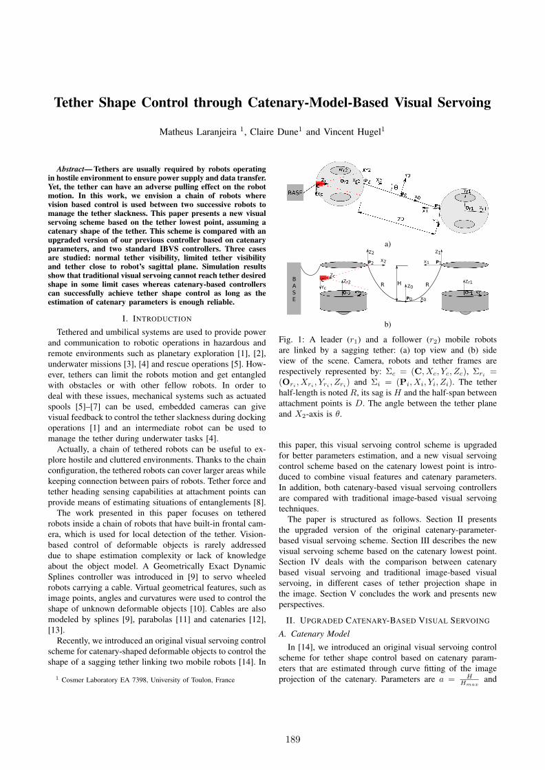
Tether Shape Control through Catenary-Model-Based Visual Servoing
Matheus Laranjeira 1, Claire Dune1 and Vincent Hugel1
Abstract— Tethers are usually required by robots operatingin hostile environment to ensure power supply and data transfer.Yet, the tether can have an adverse pulling effect on the robotmotion. In this work, we envision a chain of robots wherevision based control is used between two successive robots tomanage the tether slackness. This paper presents a new visualservoing scheme based on the tether lowest point, assuming acatenary shape of the tether. This scheme is compared with anupgraded version of our previous controller based on catenaryparameters, and two standard IBVS controllers. Three casesare studied: normal tether visibility, limited tether visibilityand tether close to robot’s sagittal plane. Simulation resultsshow that traditional visual servoing cannot reach tether desiredshape in some limit cases whereas catenary-based controllerscan successfully achieve tether shape control as long as theestimation of catenary parameters is enough reliable.
I. INTRODUCTION
Tethered and umbilical systems are used to provide power
and communication to robotic operations in hazardous and
remote environments such as planetary exploration [1], [2],
underwater missions [3], [4] and rescue operations [5]. How-
ever, tethers can limit the robots motion and get entangled
with obstacles or with other fellow robots. In order to
deal with these issues, mechanical systems such as actuated
spools [5]–[7] can be used, embedded cameras can give
visual feedback to control the tether slackness during docking
operations [1] and an intermediate robot can be used to
manage the tether during underwater tasks [4].
Actually, a chain of tethered robots can be useful to ex-
plore hostile and cluttered environments. Thanks to the chain
configuration, the tethered robots can cover larger areas while
keeping connection between pairs of robots. Tether force and
tether heading sensing capabilities at attachment points can
provide means of estimating situations of entanglements [8].
The work presented in this paper focuses on tethered
robots inside a chain of robots that have built-in frontal cam-
era, which is used for local detection of the tether. Vision-
based control of deformable objects is rarely addressed
due to shape estimation complexity or lack of knowledge
about the object model. A Geometrically Exact Dynamic
Splines controller was introduced in [9] to servo wheeled
robots carrying a cable. Virtual geometrical features, such as
image points, angles and curvatures were used to control the
shape of unknown deformable objects [10]. Cables are also
modeled by splines [9], parabolas [11] and catenaries [12],
[13].
Recently, we introduced an original visual servoing control
scheme for catenary-shaped deformable objects to control the
shape of a sagging tether linking two mobile robots [14]. In
1 Cosmer Laboratory EA 7398, University of Toulon, France
a)
X0
Z0HR R
X2
Z2 Z1
X1
Zr2 Zr1
Zc
Yc
C
P2
P0
P1
B
A
S
E
b)
Fig. 1: A leader (r1) and a follower (r2) mobile robots
are linked by a sagging tether: (a) top view and (b) side
view of the scene. Camera, robots and tether frames are
respectively represented by: Σc = (C, Xc, Yc, Zc), Σri =(Ori , Xri , Yri , Zri) and Σi = (Pi, Xi, Yi, Zi). The tether
half-length is noted R, its sag is H and the half-span between
attachment points is D. The angle between the tether plane
and X2-axis is θ.
this paper, this visual servoing control scheme is upgraded
for better parameters estimation, and a new visual servoing
control scheme based on the catenary lowest point is intro-
duced to combine visual features and catenary parameters.
In addition, both catenary-based visual servoing controllers
are compared with traditional image-based visual servoing
techniques.
The paper is structured as follows. Section II presents
the upgraded version of the original catenary-parameter-
based visual servoing scheme. Section III describes the new
visual servoing scheme based on the catenary lowest point.
Section IV deals with the comparison between catenary
based visual servoing and traditional image-based visual
servoing, in different cases of tether projection shape in
the image. Section V concludes the work and presents new
perspectives.
II. UPGRADED CATENARY-BASED VISUAL SERVOING
A. Catenary Model
In [14], we introduced an original visual servoing control
scheme for tether shape control based on catenary param-
eters that are estimated through curve fitting of the image
projection of the catenary. Parameters are a = HHmax
and
189
b = sin θ, respectively related to the tether slackness (H)
and to the tether orientation (θ) with respect to the follower
robot sagittal plane (Fig. 1). The tether maximum authorized
slackness is noted Hmax. The catenary 3D equation model-
ing the tether linking both robots is given by:
Σc :
Y = − 1
C[cosh (C (η −D))− 1] +H + cY2
Z = cot θ (−X + cX2) +cZ2
(1)
where C = 2·HR2−H2 , η = −X+X2
sin θand P2 = (cX2,
cY2,cZ2)
in frame Σc. The equation of the catenary projection on the
image plane is given by:
y = η1
[− 1
C(cosh (C (η2 −D))− 1) + aHmax + Y2
]
(2)
where η1 = b+√1−b2x√
1−b2cX2+bcZ2
and η2 =cX2−cZ2x
b+x√1−b2
. The
tether is supposed to be only subject to gravity, and that
its mass is negligible with respect to the robot’s mass.
Attachment points are at the same height.
The objective function of the curve fitting algorithm is
given by χ2 =∑N
i=1 r2i (s), where s = [a b]T , ri (s) =
yi−y(xi, s) is the residual, (xi, yi) are the metric coordinates
of the i-th detected point of the tether in the image, N is the
total number of detected points and y(x, s) is obtained from
the current catenary projection in the image (Eq. (2)). The
Gauss-Newton Jacobian used by the fitting algorithm is:
Jr (i) =[−∂y(xi,s)
∂a−∂y(xi,s)
∂b
](3)
The curve fitting algorithm used in this approach has the
advantage of only requiring 30% of tether visibility for
accurate shape estimation. However, this is a local approach
that can converge to a local minimum. In order to find a
global minimum, an initial guess can be estimated from the
position of the lowest point of the catenary.
B. Upgraded parameters estimation through initial guess
The initial guess for the catenary curve fitting algorithm
makes the following approximation: the lowest point pB
of the tether projection that is detected in the image is
approximated with the projection p0 = [x0, y0] of the tether
3D lowest point P0 (Fig. 2).
Evaluating Eq. (2) at p0 ≈ pB leads to
Σc :
D =cX2 − cZ2xB
sin θ + xB cos θ
H = yBcos θcX2 + sin θcZ2
sin θ + xB cos θ− cY2
(4a)
(4b)
The relation between D and H is obtained evaluating Eq. (1)
at P1, yielding:
H =1
C
[cosh(CD)− 1
](5)
In order to facilitate writing, let’s redefine Eq. (4) with:
D =G1
G3
and
H =G2
G3
where G1 = cX2 − cZ2xB , G2 =
yB
(cos θcX2 + sin θcZ2
)− cY2G3 and G3 =
sin θ + xB cos θ. Then, replacing Eq. (4) in (5) yields:
g(θ)=
2G22
R2G23 −G2
2
− cosh(
2G1G2
R2G23 −G2
2
)+ 1 (6)
The root of g(θ) yields an estimation of θ, and H is
obtained from Eq. (4b). This initial estimation of the catenary
parameters is then used by the curve fitting algorithm.
C. Visual Servoing Control
The aim of vision-based control schemes is to minimize an
error defined as e = s− s∗, where s and s∗ are respectively
the current and the desired visual feature vectors [15], [16].
In our control scheme, the feature vector s = [a b]T issued
from catenary parameters is regulated through the follower
robot motion using the following control law [14]:
vr2 = −λr2V2L+Ce (7)
where r2V2 is the twist transformation matrix from frame
Σ2 to Σr2 and λ ∈ R+. The interaction matrix LC is given
by Eq. (8), where KC =2(R2+H2)(R2−H2)
2 , 2P1 =(2X1,
2 Y1,2 Z1
)
in frame Σ2 is estimated thanks to the fitted catenary, and
KH =sinh
(CD
)
1 + KC
C2
[cosh
(CD
)− 1− CD sinh
(CD
)]
where C = 2HR2−H2
and D is given by Eq. (4a).
III. CATENARY LOWEST-POINT VISUAL SERVOING
The first version of the catenary-based controller uses
3D catenary parameters in the feature vector. We propose
to design a new controller driven by image features that
takes into account the catenary model of the tether. The idea
behind this new controller is to take advantage of the same
approximation that is used for the upgrade of the first version.
The image feature vector is therefore s = [xB yB ]T
, where
the coordinates (x0 y0) are approximated with (xB yB).The new interaction matrix LP that links the variation of
the feature vector s = [xB yB ]T
to the camera velocity is
calculated starting with the catenary model given by Eq. (1).
Let cP0 = (cX0,cY0,
cZ0),cP1 = (cX1,
cY1,cZ1) and
cP2 = (cX2,cY2,
cZ2) be respectively the catenary frame
center and the two attachment points in the follower camera
frame Σc. Differentiating the projection equation [17] at cP0
leads to:
Σc :
x0 =˙cX0 − x0 ˙cZ0
cZ0
y0 =˙cY0 − y0 ˙cZ0
cZ0
(9a)
(9b)
Then, differentiating Eq. (1) at cP0 and cP1 yields
˙cY0 = KHD (10)
190
Σ2 : LC =
−
KH
√1− b2
2Hmax− KHb
2Hmax0 0 0
KH
(
2Y1
√1− b2 − 2X1b
)
2Hmax
b√1− b2
2D
−1 + b2
2D0 0 0 −
2Y1b√1− b2 + 2X1(1− b2)
2D
(8)
The relative motion of cP1 in the reference frame Σc,
due to the camera velocity vc = (vc, wc) expressed in Σc is
given by˙cP1 = −vc − ωc ×c P1 (11)
Geometrically,
[˙cX0
˙cZ0
]T=
1
2
[˙cX1
˙cZ1
]T(12)
and using Eq. (11) leads to[
˙cX0
˙cZ0
]=
1
2
[−1 0 0 0 −cZ1
cY10 0 −1 −cY1
cX1 0
]vc (13)
From D2 = (cX0 − cX2)2 + (cZ0 − cZ2)
2,
˙D = − sin θ ˙cX0 + cos θ ˙cZ0 (14)
Using Eqs. (11) and (12) in Eq. (14),
˙D =
1
2
sin θ0
− cos θ
−cY1 cos θcZ1 sin θ − cX1 cos θ
−cY1 sin θ
T
vc (15)
Finally, replacing Eqs. (13), (15) and (10) in (9) and consid-
ering the approximation x0 ≈ xB and y0 ≈ yB leads to the
interaction matrix LP given by Eq. (17), where
cZ0 = cZ2 +D cos θcX0 = cX2 −D sin θcZ1 = cZ2 + 2D cos θ
Here it is assumed that the camera frame axes are parallel
with the axes of the tether attachment point frame. The
matrix is presented in frame Σ2 in order to be compared
to LC . The feature vector s = [xB yB ]T
is then regulated
through the following control law:
vr2 = −λr2V2L+Pe (16)
IV. COMPARISONS AND ANALYZES
Let us compare the catenary-based controllers with tra-
ditional image-based visual servoing techniques. We can
consider some salient points such as the highest and lowest
tether points in the image or approximate the first portion of
the tether with a line segment (see Fig. 2). Such features were
successfully used to control a robot motion by regulating
the shape of rigid objects in the image [18], [19]. The
tether shape evolution, velocity commands and condition
number of interaction matrices are studied in normal and
limit cases for two image-based controllers and the catenary-
based controllers:
• image points: coordinates of the tether highest and
lowest point (pA and pB) detected in the image without
taking into account that the points belong to a catenary
projection [20]
• image line segment : center, length and orientation of
the segment pApB linking the highest and the lowest
points of the tether detected in the image, without
taking into account that the points belong to a catenary
projection [21]
• catenary parameters: two features s = [a b]T , related
to the tether slackness and orientation that parameterize
the catenary curve fitting the tether 3D shape [14].
• catenary-projection lowest point: coordinates of the
tether lowest point (pB) detected in the image, making
the approximation that this point is the projection of the
3D catenary lowest point
xP0
a)pA
pBp0x
b)
x
pA
p0 pB
c)
Fig. 2: Image features used to manage the tether shape: its
highest and lowest point in the image (pA and pB) and the
line segment pApB in blue. (a) 3D simulated scene where
the tether 3D lowest point P0 is out of the follower’s camera
field of view. (b) corresponding embedded view with p0
being the perspective projection of P0. (c) Another situation
where P0 is inside the follower’s camera field of view
A. Simulation Setup
Simulation is performed using Gazebo [22] to test the
whole control loop including computer vision algorithms.
The setup is composed of two Turtlebots [23] linked by a
1 meter long and 3 mm thick orange rope that simulates
the tether. The robots have 2 DOF (one translation and one
191
Σ2 : LP =KH
2 cZ0
[xB
KH
1KH
0 0 0 (cZ1−cZ2)+xB(cX1−cX2)KH
yB
KH− cos θ − sin θ 0 0 0 −(cZ1 − cZ2) sin θ − (cX1 − cX2)
(cos θ − yB
KH
)]
(17)
rotation) and the follower is equipped with a camera that
monitors an extremity of the rope. The maximum authorized
rope sag is fixed to Hmax = 0.40m, corresponding to its
attachment points height.
The rope is detected in the follower’s camera by a color
segmentation algorithm, that is refined by morphological
skeletonization. The segmented points are then used to
compute the visual servoing features.
Three simulations are carried out in order to compare the
performances of vision-based tether shape controllers (see
Fig. 3). The objective is to study the controllers behavior in
normal conditions, when the tether shape is clearly visible,
as well as in limit cases, when the tether is not completely
visible or when it degenerates into a vertical line in the
image.
The first simulation (Fig. 3a) is a typical example where
the tether is completely visible and not degenerated in the
image. The angle θ is required to vary from 20 to 45
while the tether slackness must remain the same (initial H0 =0.20m and desired H∗ = 0.20m). In the second simulation
(Fig. 3b), the angle θ is required to vary from 10 to 60
to check controllers performance when the tether is partially
visible (θ close to 60). The initial and desired slackness
are the same (H0 = H∗ = 0.25m). In the third simulation
(Fig. 3c), the angle θ is required to vary from 20 to 0 to
check the controller performance when the tether plane is
near to the camera optical axis (θ close to 0). The initial
and desired slackness are H0 = 0.10m and H∗ = 0.24m,
respectively.
follower view
a) normal case
follower view
b) limit case 1
follower view
c) limit case 2
Fig. 3: Follower robot camera view for (a) first, (b) second
and (c) third simulation. Initial and desired tether shape in
the image are drawn in blue and red lines, respectively
B. Results Analysis
Figure 4 shows, for the three studied cases, the tether
shape parameters error and the velocity commands of the
follower robot as a function of time. Figure 5 presents the
trajectory of the tether lowest point in the image. Figure 6
presents the condition number evolution for the controllers
interaction matrices and the Gauss-Newton Jacobian used for
curve fitting (Eq. (3)). The condition number of a matrix A
is defined as follows [24]:
cond(A) = |A||A+| (18)
where |.| is the L2 norm.
In the normal case, the tether shape control is achieved
by all the controllers. They also allow to reach the desired
position in the image plane (see Figs. 4a to 4d and 5a). The
tether parameters (slackness H and orientation θ) converge
to their desired values even using image-based features.
Image-based controllers are very sensitive to the detection
of the lowest part of the tether, and work well when this
part is well visible in the image. Compared with pure
image-based controllers, the catenary lowest-point controller
appears to execute a more balanced regulation between slack-
ness (Fig. 4a) and orientation (Fig. 4b). In the image plane,
the resulting trajectory of the lowest point is more regular
than pure image-based trajectories (Fig. 5a). In addition, the
catenary parameter controller is less sensitive to noisy tether
detection whereas the other controllers are very dependent
on the accurate detection of the lowest point in the image.
In the first limit case, the tether desired shape is only
achieved by the catenary parameter controller (Figs. 4e
to 4h). The other controllers cannot reach the desired tether
shape leading to a residual offset of slackness (Fig. 4e)
and angle (Fig. 4f). However, these controllers converge as
expected in the image plane, while we observe a disconti-
nuity of the lowest point trajectory in the case of catenary-
parameter controller (Fig. 5b). This is not surprising since the
catenary-parameter controller directly regulates the tether 3D
shape, and converges to the real lowest point that is outside
the image.
In the second limit case (see Figs. 4i to 4l), image-
based and catenary lowest point controllers achieve the tether
desired shape. The image features can be well estimated
since at least half of the tether is visible. However, the
catenary parameters controller cannot reach the target shape
because of fitting failure when the tether gets close to the
camera sagittal plane. This is confirmed by the condition
number of the curve fitting Gauss-Newton Jacobian (Fig. 6d)
that becomes ill-conditioned at the end of the simulation.
Nevertheless, all the interaction matrices are well conditioned
(Figs. 6a to 6c), which means that they are robust to input
noise.
The catenary lowest-point controller makes use of an
initial guess of the tether angle parameter. In the proximity
of θ = 0, the slackness parameter is not well estimated,
since it is subjected to numerical drift resulting from small
denominator value in Eq. (4b). In order to improve the
catenary parameter controller, a solution will be to directly
carry out an initial guess on the slackness parameter.
All four controllers need at least 50% of tether detected
points in the image when the tether gets closer to the camera
sagittal plane. In real situations it will be difficult to detect
half the tether the longer it is. In order to deal with this issue,
192

a solution could be to equip the robot with an additional
camera outside its sagittal plane. Another solution would
consist of placing fiducial markers along the tether at known
length, which could be easily detected in the image and
overcome the noisy detection of the lowest point.
This work is a first step to the regulation of the tether
shape inside a chain of robots. In order to navigate in
narrow or cluttered environments, the relative position of two
successive robots will have to be fully constrained. In this
case, the distance between the two attachment points as well
as the two relative angles between the robots orientation and
the tether plane will have to be regulated. In the considered
scenario, the leader robot will be able to move freely while
the follower robot will be in charge of maintaining a desired
tether slackness. Catenary-based visual servoing will be
extended to fulfill this kind of scenario.
V. CONCLUSIONS AND PERSPECTIVES
This paper studied vision-based control strategies that can
be used to manage the shape of a sagging tether linking two
terrestrial robots. Four different visual controllers are tested
to regulate the tether shape. Two of them are pure image-
based while the other two are catenary-based controllers, one
that uses catenary parameters as features and another one that
uses image features taking advantage of the catenary model.
The study shows that the additional knowledge about the
tether 3D shape allows to obtain satisfactory tether handling.
Both catenary-based controllers could be combined to design
a more robust controller.
Future work will extend tether visual servoing control to
3D holonomic vehicles like underwater robots through the
management of vertical translation and pitch rotation. One
target application will be the displacement of a chain of
tethered robots inside a cluttered environment.
ACKNOWLEDGMENTS
This work was achieved thanks to specific funding from
the France PACA (Provence-Alpes-Cote-d’Azur) region,
and the French SUBSEATECH company, located in Mar-
seille, South-East of France (http://www.subsea-tech.com,
REFERENCES
[1] D. Tsai, I. A. D. Nesnas, and D. Zarzhitsky, “Autonomous vision-basedtethered-assisted rover docking,” in 2013 IEEE/RSJ International
Conference on Intelligent Robots and Systems, Nov 2013, pp. 2834–2841.
[2] J. Iqbal, S. Heikkila, and A. Halme, “Tether tracking and control ofrosa robotic rover,” in Control, Automation, Robotics and Vision, 2008.
ICARCV 2008. 10th International Conference on, Dec 2008, pp. 689–693.
[3] S. Prabhakar and B. Buckham, “Dynamics modeling and control ofa variable length remotely operated vehicle tether,” in Proceedings of
OCEANS 2005 MTS/IEEE, Sept 2005, pp. 1255–1262 Vol. 2.
[4] O. Khatib, X. Yeh, G. Brantner, B. Soe, B. Kim, S. Ganguly, H. Stuart,S. Wang, M. Cutkosky, A. Edsinger, P. Mullins, M. Barham, C. R.Voolstra, K. N. Salama, M. L’Hour, and V. Creuze, “Ocean one:A robotic avatar for oceanic discovery,” IEEE Robotics Automation
Magazine, vol. 23, no. 4, pp. 20–29, Dec 2016.
[5] D. P. Perrin, A. Kwon, and R. D. Howe, “A novel actuated tetherdesign for rescue robots using hydraulic transients,” in Robotics and
Automation, 2004. Proceedings. ICRA ’04. 2004 IEEE International
Conference on, vol. 4, April 2004, pp. 3482–3487 Vol.4.[6] P. McGarey, F. Pomerleau, and T. D. Barfoot, System Design of a
Tethered Robotic Explorer (TReX) for 3D Mapping of Steep Terrain
and Harsh Environments. Cham: Springer International Publishing,2016, pp. 267–281.
[7] M. Krishna, J. Bares, and E. Mutschler, “Tethering system design fordante ii,” in Proceedings of International Conference on Robotics and
Automation, vol. 2, Apr 1997, pp. 1100–1105 vol.2.[8] V. A. K. T. Rajan, A. Nagendran, A. Dehghani-Sanij, and R. C.
Richardson, “Tether monitoring for entanglement detection, disentan-glement and localisation of autonomous robots,” Robotica, vol. 34,no. 3, p. 527548, 2016.
[9] Z. Echegoyen, I. Villaverde, R. Moreno, M. Graa,and A. dAnjou, “Linked multi-component mobile robots:Modeling, simulation and control,” Robotics and Autonomous
Systems, vol. 58, no. 12, pp. 1292 – 1305, 2010,intelligent Robotics and Neuroscience. [Online]. Available:http://www.sciencedirect.com/science/article/pii/S0921889010001533
[10] D. Navarro-Alarcon, Y.-h. Liu, J. G. Romero, and P. Li, “On thevisual deformation servoing of compliant objects: Uncalibrated controlmethods and experiments,” The International Journal of Robotics
Research, vol. 33, no. 11, pp. 1462–1480, 2014.[11] T. Dallej, M. Gouttefarde, N. Andreff, R. Dahmouche, and P. Martinet,
“Vision-based modeling and control of large-dimension cable-drivenparallel robots,” in 2012 IEEE/RSJ International Conference on Intel-
ligent Robots and Systems, Oct 2012, pp. 1581–1586.[12] J. Estevez and M. Grana, Robust Control Tuning by PSO of Aerial
Robots Hose Transportation. Cham: Springer International Pub-lishing, 2015, ch. Bioinspired Computation in Artificial Systems:International Work-Conference on the Interplay Between Natural andArtificial Computation, IWINAC 2015, Elche, Spain, June 1-5, 2015,Proceedings, Part II, pp. 291–300.
[13] T. Lee, “Geometric controls for a tethered quadrotor uav,” in 2015
54th IEEE Conference on Decision and Control (CDC), Dec 2015,pp. 2749–2754.
[14] M. Laranjeira, C. Dune, and V. Hugel, “Catenary-based visual servoingfor tethered robots,” in 2017 IEEE International Conference on
Robotics and Automation (ICRA), May 2017, pp. 732–738.[15] F. Chaumette and S. Hutchinson, “Visual servo control. i. basic
approaches,” IEEE Robotics Automation Magazine, vol. 13, no. 4, pp.82–90, Dec 2006.
[16] ——, “Visual servo control. ii. advanced approaches [tutorial],” IEEE
Robotics Automation Magazine, vol. 14, no. 1, pp. 109–118, March2007.
[17] R. I. Hartley and A. Zisserman, Multiple View Geometry in Computer
Vision, 2nd ed. Cambridge University Press, 2004, ch. 6, p. 155.[18] C. Collewet and F. Chaumette, “Positioning a camera with respect
to planar objects of unknown shape by coupling 2-d visual servoingand 3-d estimations,” IEEE Transactions on Robotics and Automation,vol. 18, no. 3, pp. 322–333, Jun 2002.
[19] A. Cherubini, F. Chaumette, and G. Oriolo, “An image-based vi-sual servoing scheme for following paths with nonholonomic mobilerobots,” in 2008 10th International Conference on Control, Automa-
tion, Robotics and Vision, Dec 2008, pp. 108–113.[20] B. Espiau, F. Chaumette, and P. Rives, “A new approach to visual
servoing in robotics,” IEEE Transactions on Robotics and Automation,vol. 8, no. 3, pp. 313–326, Jun 1992.
[21] F. Chaumette, P. Rives, and B. Espiau, “Classification and realizationof the different vision-based tasks,” Visual servoing, vol. 7, pp. 199–228, 1993.
[22] N. Koenig and A. Howard, “Design and use paradigms for gazebo, anopen-source multi-robot simulator,” in 2004 IEEE/RSJ International
Conference on Intelligent Robots and Systems (IROS) (IEEE Cat.
No.04CH37566), vol. 3, Sept 2004, pp. 2149–2154 vol.3.[23] B. Gerkey and K. Conley, “Robot developer kits [ros topics],” IEEE
Robotics Automation Magazine, vol. 18, no. 3, pp. 16–16, Sept 2011.[24] J. T. Feddema, C. S. G. Lee, and O. R. Mitchell, “Automatic selection
of image features for visual servoing of a robot manipulator,” in Pro-
ceedings, 1989 International Conference on Robotics and Automation,May 1989, pp. 832–837 vol.2.
193
0 5 10 15 20 25 30Time (s)
−0.02−0.010.00
0.01
0.02
0.03
0.04
0.05
Sla
ckn
ess
Err
or
(m)
Tether Slackness Error H −H∗
a)
0 5 10 15 20 25 30Time (s)
−25
−20
−15
−10
−5
0
An
gle
Err
or
(deg)
Tether Angle Error θ − θ∗
b)
0 5 10 15 20 25 30Time (s)
−0.010.00
0.01
0.02
0.03
0.04
0.05
0.06
0.07
0.08
Velo
city
(m/s
)
Linear Velocity Commands
c)
0 5 10 15 20 25 30Time (s)
−0.25
−0.20
−0.15
−0.10
−0.05
0.00
Velo
city
(rad
/s)
Angular Velocity Commands
d)
0 10 20 30 40 50 60Time (s)
−0.02−0.010.00
0.01
0.02
0.03
0.04
0.05
Sla
ckn
ess
Err
or
(m)
Tether Slackness Error H −H∗
e)
0 10 20 30 40 50 60Time (s)
−50
−40
−30
−20
−10
0
10
An
gle
Err
or
(deg)
Tether Angle Error θ − θ∗
f)
0 10 20 30 40 50 60Time (s)
−0.010.00
0.01
0.02
0.03
0.04
0.05
0.06
0.07
0.08
Velo
city
(m/s
)
Linear Velocity Commands
g)
0 10 20 30 40 50 60Time (s)
−0.25
−0.20
−0.15
−0.10
−0.05
0.00
Velo
city
(rad
/s)
Angular Velocity Commands
h)
0 5 10 15 20 25 30Time (s)
−0.14−0.12−0.10−0.08−0.06−0.04−0.020.00
Sla
ckn
ess
Err
or
(m)
Tether Slackness Error H −H∗
i)
0 5 10 15 20 25 30Time (s)
−5
0
5
10
15
20
25
An
gle
Err
or
(deg)
Tether Angle Error θ − θ∗
j)
0 5 10 15 20 25 30Time (s)
−0.010.00
0.01
0.02
0.03
0.04
0.05
0.06
0.07
0.08V
elo
city
(m/s
)Linear Velocity Commands
k)
0 5 10 15 20 25 30Time (s)
0.00
0.05
0.10
0.15
0.20
Velo
city
(rad
/s)
Angular Velocity Commands
l)
Fig. 4: Error evolution for tether slackness and orientation as well as linear and angular command velocities for normal
case (Figs. a, b, c and d), limit case 1 (Figs. e, f, g and h) and limit case 2 (Figs. i, j, k and l). Tether initial
and desired shape are respectively: (H0 = 0.20m, θ0 = 20) and (H∗ = 0.20m, θ∗ = 45); (H0 = 0.25m, θ0 = 10) and
(H∗ = 0.25m, θ∗ = 60); (H0 = 0.10m, θ0 = 20) and (H∗ = 0.24m, θ∗ = 0). Legend in Fig. 5d. All controllers use a
gain λ = 1.0.
−0.6 −0.5 −0.4 −0.3 −0.2 −0.1 0.0x(m)
−0.1
0.0
0.1
0.2
0.3
0.4
y(m
) ima
ge
bord
er
Image Plane Trajectory
a) Normal case
−0.6 −0.5 −0.4 −0.3 −0.2 −0.1 0.0x(m)
−0.1
0.0
0.1
0.2
0.3
0.4
y(m
) ima
ge
bord
er
Image Plane Trajectory
b) Limit case 1
−0.6 −0.5 −0.4 −0.3 −0.2 −0.1 0.0x(m)
−0.1
0.0
0.1
0.2
0.3
0.4
y(m
) ima
ge
bord
er
Image Plane Trajectory
c) Limit case 2
2D points
2D Segment
Catenary
Catenary Lowest Point
initial
desired
d)
Fig. 5: Tether lowest point trajectory in the image plane for (a) normal case, (b) limit case 1 and (c) limit case 2. (d) legend
0 5 10 15 20 25 30Time (s)
0
2
4
6
8
10
12 Condition Number
a)
0 10 20 30 40 50 60Time (s)
0
2
4
6
8
10
12 Condition Number
b)
0 5 10 15 20 25 30Time (s)
0
2
4
6
8
10
12 Condition Number
c)
0 10 20 30 40 50 60Time (s)
0
1
2
3
4
5
log10(cond(J))
Jacobian condition number
Normal case
Limit case 1
Limit case 2
d)
Fig. 6: Interaction matrices condition number evolution for (Fig. a) normal and (Figs. b and c). Legend in Fig. 5d. (d)
condition number evolution for the curve fitting Gauss-Newton Jacobian during normal and limit cases
194
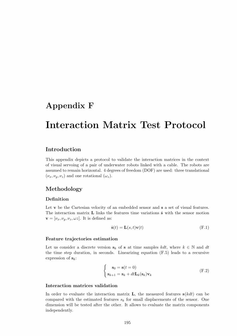
Appendix F
Interaction Matrix Test Protocol
Introduction
This appendix depicts a protocol to validate the interaction matrices in the contextof visual servoing of a pair of underwater robots linked with a cable. The robots areassumed to remain horizontal. 4 degrees of freedom (DOF) are used: three translational(νx, νy, νz) and one rotational (ωz).
Methodology
Definition
Let v be the Cartesian velocity of an embedded sensor and s a set of visual features.The interaction matrix L links the features time variations s with the sensor motionv = [νx, νy, νz, ωz]. It is defined as:
s(t) = L(s, t)v(t) (F.1)
Feature trajectories estimation
Let us consider a discrete version sk of s at time samples kdt, where k ∈ N and dtthe time step duration, in seconds. Linearizing equation (F.5) leads to a recursiveexpression of sk:
s0 = s(t = 0)
sk+1 = sk + dtLk(sk)vk
(F.2)
Interaction matrices validation
In order to evaluate the interaction matrix L, the measured features s(kdt) can becompared with the estimated features sk for small displacements of the sensor. Onedimension will be tested after the other. It allows to evaluate the matrix componentsindependently.
195
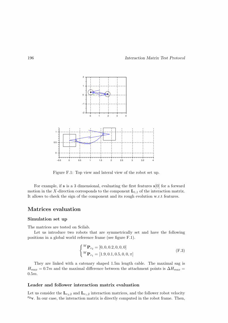
196 Interaction Matrix Test Protocol
0 2 41 3
0
−2
2
−1
1
0 2 41 3−0.5 0.5 1.5 2.5 3.5
0
1
0.5
Figure F.1: Top view and lateral view of the robot set up.
For example, if s is a 3 dimensional, evaluating the first features s[0] for a forwardmotion in the X-direction corresponds to the component L1,1 of the interaction matrix.It allows to check the sign of the component and its rough evolution w.r.t features.
Matrices evaluation
Simulation set up
The matrices are tested on Scilab.Let us introduce two robots that are symmetrically set and have the following
positions in a global world reference frame (see figure F.1).
WPr2 = [0, 0, 0.2, 0, 0, 0]WPr1 = [1.9, 0.1, 0.5, 0, 0, π]
(F.3)
They are linked with a catenary shaped 1.5m length cable. The maximal sag isHmax = 0.7m and the maximal difference between the attachment points is ∆Hmax =0.5m.
Leader and follower interaction matrix evaluation
Let us consider the Lr2,2 and Lr1,2 interaction matrices, and the follower robot velocityr2v. In our case, the interaction matrix is directly computed in the robot frame. Then,
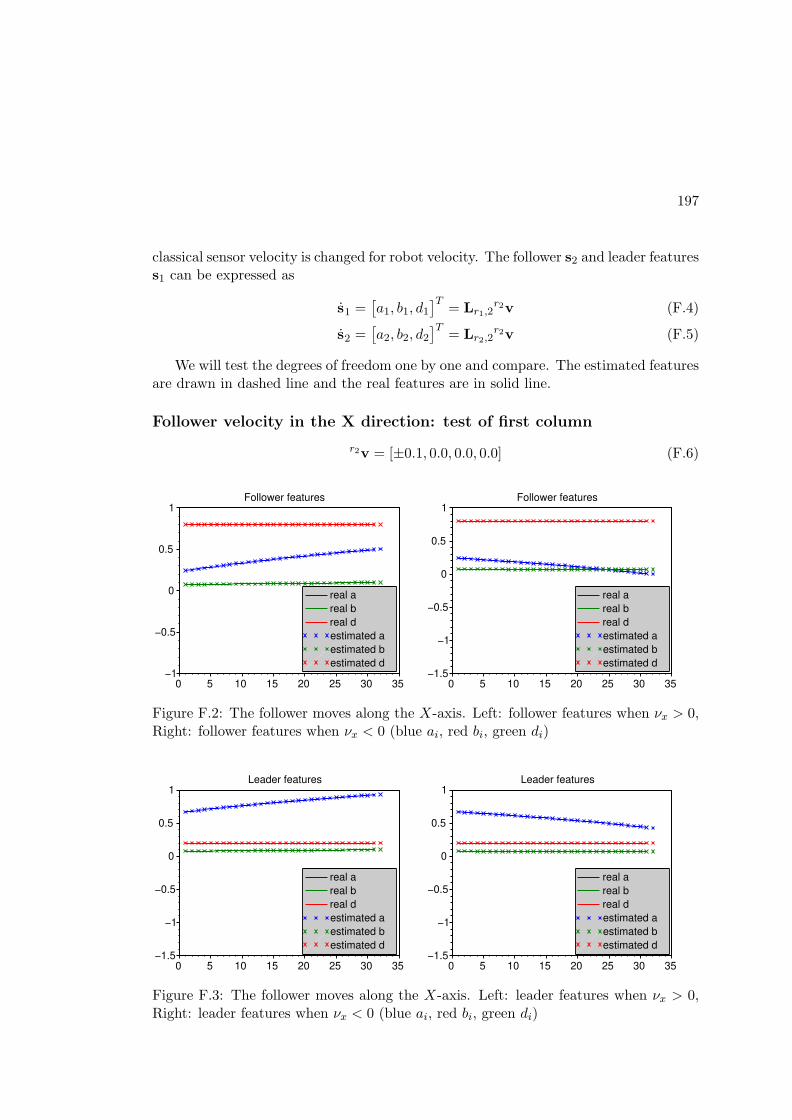
197
classical sensor velocity is changed for robot velocity. The follower s2 and leader featuress1 can be expressed as
s1 =[a1, b1, d1
]T= Lr1,2
r2v (F.4)
s2 =[a2, b2, d2
]T= Lr2,2
r2v (F.5)
We will test the degrees of freedom one by one and compare. The estimated featuresare drawn in dashed line and the real features are in solid line.
Follower velocity in the X direction: test of first column
r2v = [±0.1, 0.0, 0.0, 0.0] (F.6)
0 2010 305 15 25 35
0
−1
1
−0.5
0.5
real a
real b
real d
estimated a
estimated b
estimated d
Follower features
0 2010 305 15 25 35
0
−1
1
−1.5
−0.5
0.5
real a
real b
real d
estimated a
estimated b
estimated d
Follower features
Figure F.2: The follower moves along the X-axis. Left: follower features when νx > 0,Right: follower features when νx < 0 (blue ai, red bi, green di)
0 2010 305 15 25 35
0
−1
1
−1.5
−0.5
0.5
real a
real b
real d
estimated a
estimated b
estimated d
Leader features
0 2010 305 15 25 35
0
−1
1
−1.5
−0.5
0.5
real a
real b
real d
estimated a
estimated b
estimated d
Leader features
Figure F.3: The follower moves along the X-axis. Left: leader features when νx > 0,Right: leader features when νx < 0 (blue ai, red bi, green di)
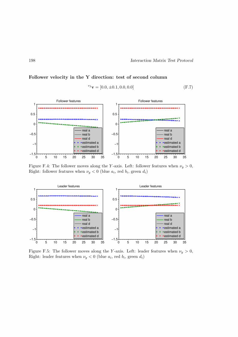
198 Interaction Matrix Test Protocol
Follower velocity in the Y direction: test of second column
r2v = [0.0,±0.1, 0.0, 0.0] (F.7)
0 2010 305 15 25 35
0
−1
1
−1.5
−0.5
0.5
real a
real b
real d
estimated a
estimated b
estimated d
Follower features
0 2010 305 15 25 35
0
−1
1
−1.5
−0.5
0.5
real a
real b
real d
estimated a
estimated b
estimated d
Follower features
Figure F.4: The follower moves along the Y -axis. Left: follower features when νy > 0,Right: follower features when νy < 0 (blue ai, red bi, green di)
0 2010 305 15 25 35
0
−1
1
−1.5
−0.5
0.5
real a
real b
real d
estimated a
estimated b
estimated d
Leader features
0 2010 305 15 25 35
0
−1
1
−1.5
−0.5
0.5
real a
real b
real d
estimated a
estimated b
estimated d
Leader features
Figure F.5: The follower moves along the Y -axis. Left: leader features when νy > 0,Right: leader features when νy < 0 (blue ai, red bi, green di)

199
Follower velocity along the Z-axis: test of third column
r2v = [0.0, 0.0,±0.1, 0.0] (F.8)
0 2010 305 15 25 35
0
−1
1
−1.5
−0.5
0.5
real a
real b
real d
estimated a
estimated b
estimated d
Follower features
0 2010 305 15 25 35
0
−1
1
−1.5
−0.5
0.5
1.5
real a
real b
real d
estimated a
estimated b
estimated d
Follower features
Figure F.6: The follower moves along the Z-axis. Left: follower features when νz > 0,Right: follower features when νz < 0 (blue ai, red bi, green di)
0 2010 305 15 25 35
0
−1
1
−1.5
−0.5
0.5
real a
real b
real d
estimated a
estimated b
estimated d
Leader features
0 2010 305 15 25 35
0
−1
1
−1.5
−0.5
0.5
real a
real b
real d
estimated a
estimated b
estimated d
Leader features
Figure F.7: The follower moves along the Z-axis. Left: leader features when νz > 0,Right: leader features when νz < 0 (blue ai, red bi, green di)
Follower velocity around the Z-axis: test of fourth column
r2v = [0.0, 0.0, 0.0,±0.1] (F.9)

200 Interaction Matrix Test Protocol
0 2010 305 15 25 35
0
−1
1
−1.5
−0.5
0.5
real a
real b
real d
estimated a
estimated b
estimated d
Follower features
0 2010 305 15 25 35
0
−1
1
−1.5
−0.5
0.5
real a
real b
real d
estimated a
estimated b
estimated d
Follower features
Figure F.8: The follower turns around the Z-axis. Left: follower features when ωz > 0.Right: follower features when ωz < 0. (blue ai, red bi, green di)
0 2010 305 15 25 35
0
−1
1
−1.5
−0.5
0.5
real a
real b
real d
estimated a
estimated b
estimated d
Leader features
0 2010 305 15 25 35
0
−1
1
−1.5
−0.5
0.5
real a
real b
real d
estimated a
estimated b
estimated d
Leader features
Figure F.9: The follower turns around the Z-axis. Left: leader features when ωz > 0.Right: leader features when ωz < 0. (blue ai, red bi, green di)
Conclusion
The estimated and real features are superimposed, which validates both matrices Lr1,2
and Lr2,2.

Appendix G
Scientific publications, Workshop
Participations and Scientific
Popularization Activities
International Conferences
1. M. Laranjeira, C. Dune and V. Hugel, Catenary-Based Visual Servoing for
Tethered Robots, In IEEE Int. Conf. on Robotics and Automation, ICRA’17,Pages. 732-738, Singapore, 2017.
2. M. Laranjeira, C. Dune and V. Hugel, Local Vision-Based Tether Control
for a Line of Underwater Robots, In Workshop on “New Horizons for Under-water Intervention Missions: from Current Technologies to Future Applications”at IROS 2018, Madrid, Spain, 2018.
3. M. Laranjeira, C. Dune and V. Hugel, Embedded Visual Detection and
Shape Identification of Underwater Umbilical for Vehicle Positioning,In MTS/IEEE OCEANS 2019. Accepted.
Others
1. M. Laranjeira, “Controle reference vision pour la robotique sous-marine”, 8esRencontres CARTT’16, Toulon, France, 2016.
2. M. Laranjeira, “La commande de robots interconnectes”, Fete de la science 2016a l’Universite de Toulon, Toulon, France, 2016.
3. M. Laranjeira, “Asservissement visuel pour objets deformables parametriques”,9es Rencontres CARTT’17, Toulon, France, 2017.
4. M. Laranjeira, “Etude comparative de controleurs references vision pour la com-mande coordonnee d’un ombilical”, Fete de la science 2017 a l’Universite deToulon, Toulon, France, 2017.
201

202Scientific publications, Workshop Participations and Scientific Popularization Activities
5. M. Laranjeira, “Asservissement visuel applique au controle de forme d’ombilicauxpour la robotique sous-marine”, Journee GT2 Robotique marine et sous-marine,Paris, France, 2017.

Appendix H
Resume en francais
Introduction
En robotique sous-marine, deux types de robots sont differencies par la presence oul’absence d’un ombilical les reliant a un navire de surface. On distingue ainsi les robotsautonomes, dits AUV (autonomous underwater vehicles) et les robots teleoperes, ditsROVs (Remotely Operated Vehicles). Les robots autonomes ont une grande libertede deplacement mais sont limites par leur autonomie et par l’intelligence embarquee.L’eau absorbant fortement les ondes, ils n’ont pas ou peu de moyen de communicationavec la surface durant leur immersion. Ils sont generalement dedies a des taches decartographie ou leur mission est d’effectuer un parcours predefini pour couvrir unezone. Les ROVs, quant a eux, sont privilegies dans des taches d’exploration ou demaintenance pour lesquelles un operateur en surface prend les decisions. Le cable sertde support au transfert des donnees, a haut debit. Il peut egalement transmettre del’energie et servir de support mecanique pour ramener le vehicule au navire de surface.Cependant, il limite la zone de deploiement et peut s’emmeler au fond ou s’accrochera des objets derivants, comme des filets.
La majorite des ROVs actuellement en service sont des engins de grande dimensionqui necessitent des systemes de mise a l’eau semblables a des grues (LARS, launchand recovery systems) et des navires de surfaces de grand tonnage, dont le cout defonctionnement est prohibitif. Le developpement d’engins de petite taille, de moindrecout et pouvant etre deployes par une ou deux personnes depuis une petite embarcationa un interet economique evident. Cependant, plus l’engin est petit, plus sa puissanceet son inertie sont faibles et plus les effets hydrodynamiques s’exercant sur le cableimpactent sa manoeuvrabilite. Le laboratoire COSMER et la societe Subseatech ontpropose d’aligner plusieurs petits ROVs afin de resoudre ce probleme. L’union desforces de propulsion des ROVs leur permet de lutter efficacement contre les forceshydrodynamiques et libere le ROV de tete, le leader, pour des taches d’exploration.
Nous appelons ce concept la cordee de robots (Fig. H.1). Les robots qui com-posent la cordee sont compacts, legers et avec une charge utile sensorielle limitee.Chaque robot joue le role d’actionneur et modifie la forme du cable en fonction dela situation. Notre strategie est d’eviter tout contact avec les obstacles pour limiter les
203

204 Resume en francais
emmelements. Si la profondeur est trop faible, il est preferable de maintenir l’ombilicalplus tendu afin d’eviter qu’il ne traıne sur le fond marin. Sinon, si l’environnement estplus large, l’ombilical peut etre plus lache afin de donner plus de liberte de mouvementaux robots.
10 m
0.70 m
Suiveur Leader
Focus de la these
2000 m
Figure H.1: Une chaıne de N robots relies compacts utilises pour explorer les eaux peuprofondes. La these porte sur le controle de la forme du cable entre les deux premiersrobots, a savoir le leader et son suiveur immediat. Les robots qui composent la chaınesont des mini-ROV legers equipes d’une camera frontale, d’une camera arriere, d’unecentrale inertielle et d’un profondimetre.
Dans le cadre de cette these, seuls les capteurs embarques sur les mini-ROVs sontutilises, soit principalement les cameras embarquees, et de maniere secondaire les pro-fondimetres et les centrales inertielles. Le cable n’est pas instrumente. Nous noussommes interesses plus particulierement a la premiere paire de robots, supposant quele comportement obtenu pourrait ensuite servir de controleur bas niveau entre deuxelements de la cordee et etre replique sur les autres paires de robots.
Les developpements realises dans le cadre de cette these visent a definir des strategiesde controle d’objets deformables par asservissement visuel, appliquees aux objets detype cable reliant deux robots sous-marins, un leader et un suiveur, en utilisant le re-tour des cameras embarquees. Les deux robots ont les memes capacites de mouvementet sont supposes rester a l’horizontale, les angles de roulis et de tangage etant regles defacon autonome par un controleur bas niveau haute frequence.
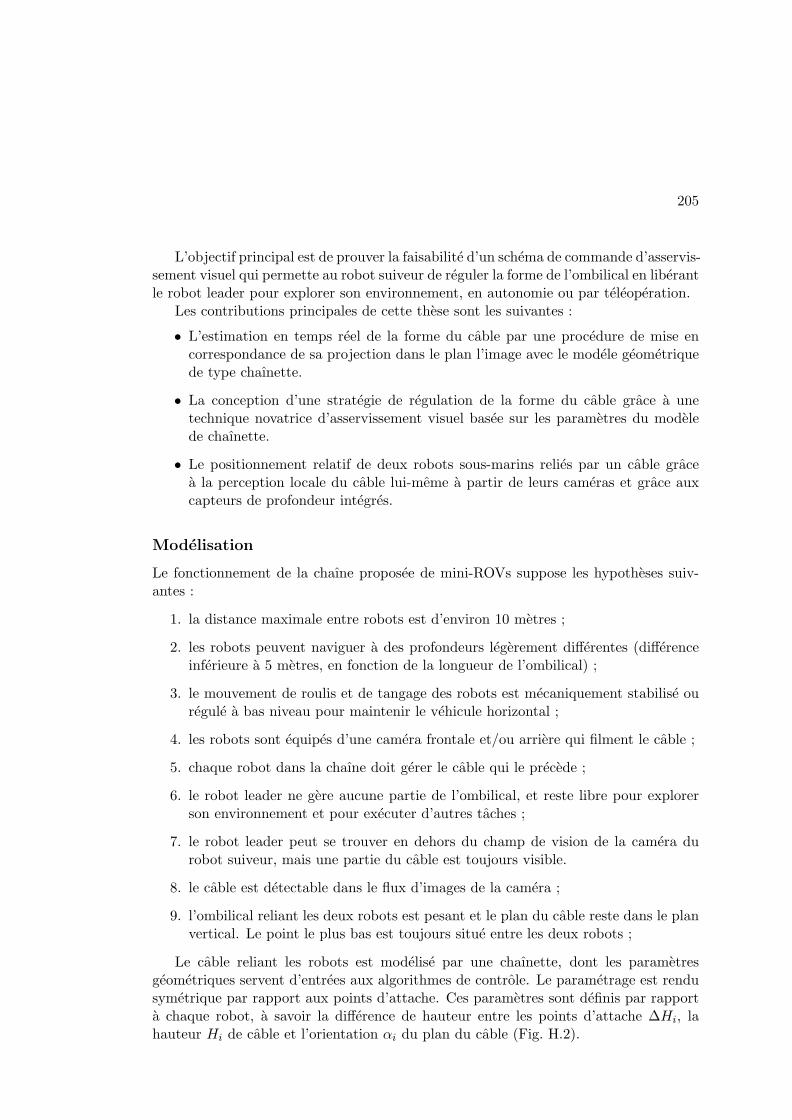
205
L’objectif principal est de prouver la faisabilite d’un schema de commande d’asservis-sement visuel qui permette au robot suiveur de reguler la forme de l’ombilical en liberantle robot leader pour explorer son environnement, en autonomie ou par teleoperation.
Les contributions principales de cette these sont les suivantes :
• L’estimation en temps reel de la forme du cable par une procedure de mise encorrespondance de sa projection dans le plan l’image avec le modele geometriquede type chaınette.
• La conception d’une strategie de regulation de la forme du cable grace a unetechnique novatrice d’asservissement visuel basee sur les parametres du modelede chaınette.
• Le positionnement relatif de deux robots sous-marins relies par un cable gracea la perception locale du cable lui-meme a partir de leurs cameras et grace auxcapteurs de profondeur integres.
Modelisation
Le fonctionnement de la chaıne proposee de mini-ROVs suppose les hypotheses suiv-antes :
1. la distance maximale entre robots est d’environ 10 metres ;
2. les robots peuvent naviguer a des profondeurs legerement differentes (differenceinferieure a 5 metres, en fonction de la longueur de l’ombilical) ;
3. le mouvement de roulis et de tangage des robots est mecaniquement stabilise ouregule a bas niveau pour maintenir le vehicule horizontal ;
4. les robots sont equipes d’une camera frontale et/ou arriere qui filment le cable ;
5. chaque robot dans la chaıne doit gerer le cable qui le precede ;
6. le robot leader ne gere aucune partie de l’ombilical, et reste libre pour explorerson environnement et pour executer d’autres taches ;
7. le robot leader peut se trouver en dehors du champ de vision de la camera durobot suiveur, mais une partie du cable est toujours visible.
8. le cable est detectable dans le flux d’images de la camera ;
9. l’ombilical reliant les deux robots est pesant et le plan du cable reste dans le planvertical. Le point le plus bas est toujours situe entre les deux robots ;
Le cable reliant les robots est modelise par une chaınette, dont les parametresgeometriques servent d’entrees aux algorithmes de controle. Le parametrage est rendusymetrique par rapport aux points d’attache. Ces parametres sont definis par rapporta chaque robot, a savoir la difference de hauteur entre les points d’attache ∆Hi, lahauteur Hi de cable et l’orientation αi du plan du cable (Fig. H.2).

206 Resume en francais
α1
Fr2
jr2ir2
Fr1
jr1
ir1
α2F2
j2i2
F0
j0
i0
F1
j1
i1
FW
jW
iW
(a)
FW
kW
iW
Fr2
kr2
ir2
F2 i2
k2 ∆H2
H2
F0
F1
k0
i0
k1
i1
Fr1
kr1
ir1
D2 D2 ∆D2
(b)
Figure H.2: (a) vue de dessus et (b) vue de cote de la premiere paire de robots com-posant la chaıne des robots. L’ombilical reliant les robots est modelise par une chaınettedont la hauteur est notee H2. La difference de hauteur entre les points d’attache ducote suiveur est ∆H2. La portee horizontale de chaınette correspondant a la hauteurH2 est notee D2 et ∆D2 est la portee supplementaire due a la difference de hauteur.Les angles d’orientation du cable par rapport a chaque repere de point d’attache sontnotes α1 et α2, respectivement pour les points d’attache du cable au robot de tete etau robot suiveur.
Perception proprioceptive du cable reliant deux robots sous-marins
Les robots sont equipes de capteurs de profondeur, et de cameras placees a proximitedes points d’attache du cable. La difference de hauteur entre les points de fixation estcalculee a partir des mesures prises par les capteurs de profondeur, tandis que la hauteuret l’orientation du cable sont estimees par une procedure de mise en correspondancedans le plan image basee sur l’algorithme de Gauss-Newton. Les points de la projec-tion du cable dans l’image sont detectes par segmentation couleur dans l’espace HSVpuis par l’application d’operateurs morphologiques : ouverture, fermeture et squeletti-sation. La projection du modele de chaınette dans le plan image est ainsi ajustee aux
207
points detectes, ce qui permet d’estimer les parametres correspondant a la hauteur eta l’orientation du cable.
Le schema general de l’algorithme de Gauss-Newton ameliore propose pour l’esti-mation des parametres de chaınette est presentee dans la figure H.3. Apres l’acquisitiond’une nouvelle image et la detection des points projetes dans l’image, l’estimation dela forme du cable passe par le calcul des residus qui representent la difference dansl’image entre les points detectes et la courbe a ajuster. Des fonctions de traitementdes residus ont ete ajoutees a la procedure d’ajustement afin d’eviter les problemesde calcul numerique dans la matrice Jacobienne de Gauss-Newton, afin d’accelerer soncalcul et d’ameliorer la robustesse de l’algorithme au bruit de detection. Elles sontdefinies suivant quatre etapes. L’etape 1 consiste a filtrer les residus en eliminant lespoints correspondants a des ecarts trop importants entre la courbe parametree et lacourbe formee par les points detectes. L’etape 2 effectue le sous-echantillonnage despoints 2-D de l’image afin de retenir un seul point par abscisse. L’etape 3 fait appela la methode des M-estimateurs afin de ponderer les ecarts et de favoriser les plusfaibles. L’etape 4 permet d’assurer que les parametres restent bien dans leur domainede definition.
detection des pointsdu cable
calcul des residus
suppressiondes residus non bornes
M-estimateurs
gestionsaturation
test critere d’arretnouvelle acquisitiond’image
Gauss-Newton
ameliore
sous-echantillonnagedes points 2-D
1.
2.
3.
4.
point de departs0 = [0.5, 0.5]T
vecteur de parametresestime s
iteration suivante
stop
heuristiqued’initialisation
ou
Figure H.3: Schema de l’algorithme de Gauss-Newton ameliore avec les quatre etapesnumerotees et l’heuristique d’initialisation.
De plus, une heuristique d’initialisation a ete introduite afin d’obtenir un pointde depart plus proche de la solution et ainsi eviter les minima locaux. L’heuristiqued’initialisation est definie en considerant que la projection dans l’image du point le plusbas de la chaınette 3D est approximee avec le point le plus bas detecte dans l’image.
L’ajustement des points detectes sur une courbe de type chaınette a ete valideen simulation et en situation reelle en bassin ; les resultats obtenus ont montre quel’estimation de la forme de l’ombilical etait suffisante pour notre application lorsqu’aumoins 30% des points de la projection du cable etaient detectes dans l’image.

208 Resume en francais
Controle de la forme du cable par asservissement visuel
Le schema global de commande du robot suiveur est decrit dans la figure H.4. La partieencadree en bleu designe le cœur des developpements effectues en terme d’asservissementvisuel sur les parametres du cable qui se deforme en fonction des mouvements des pointsd’attache sur le robot de tete et sur le robot suiveur (Fig. H.5).
estimationde la formedu cable
s∗
+
−
s
econtrole par
asservissementvisuel
controle PIDbas niveau
tangage/roulis
calcul despoussees
centraleinertielle
cameras
capteursde pression
r2v τcalcul descommandes
PWM
moteursPWM
100 Hz
20 Hz
20 Hz
ωx, ωy
φ∗,θ∗
φ, θ+
−
WPr,WΩr
Figure H.4: Schema global de controle par asservissement visuel base chaınette durobot sous-marin suiveur
.
La forme de l’ombilical est regulee par le mouvement du robot suiveur qui genere undeplacement adequat du point d’attache de l’ombilical. La figure H.5 decrit l’algorithmede controle par asservissement visuel qui consiste a calculer la vitesse que le robotsuiveur doit produire afin de conserver la forme desiree du cable dans l’image de sacamera embarquee. Les parametres estimes du modele de type chaınette sont regroupesdans un vecteur de parametres, appele s, qui doit etre regule afin de maintenir le cablea la forme desiree. Il doit etre suffisamment lache pour ne pas gener les mouvementsdu robot de tete. De plus, une orientation adequate entre chaque robot et le plan ducable doit etre maintenue afin de conserver une vue du cable a l’interieur du champde vision de la camera. Cela permet d’obtenir une estimation precise de la forme apartir du retour d’information de la camera. Cet algorithme passe par le calcul d’unematrice d’interaction 3D, qui traduit la relation entre le mouvement du robot suiveuret les derivees temporelles des parametres de la chaınette. Un formalisme generalpour le calcul de cette matrice d’interaction est propose, permettant la regulation desparametres du modele de type chaınette par rapport aux robots leader et suiveur. Ceformalisme decompose la matrice d’interaction en deux parties, une partie decrivant lacinematique du systeme, et une deuxieme partie decrivant le lien entre le mouvement
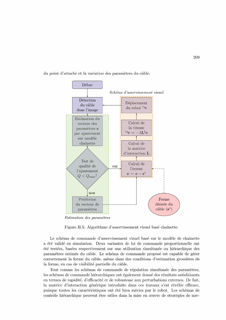
210 Resume en francais
igation de haut niveau au sein d’une cordee de robots sous-marins afin de donner lapriorite au placement d’un des robots par rapport au cable.
Perspectives
Dans la perspective du controle de la forme des cables, une extension interessante deces travaux de these est l’utilisation d’informations sensorielles supplementaires afin defournir une estimation fiable de la forme pour des cables longs (de plusieurs dizainesou centaines de metres de long). Les cameras ont une portee limitee et le cable restevisible jusqu’a quelques metres seulement. De plus, les operations en eau trouble peu-vent rendre difficile la detection des points du cable dans l’image, ce qui comprometl’estimation de sa forme a partir du retour visuel de la camera.
Des capteurs supplementaires, tels que des accelerometres mono ou tridimension-nels, peuvent etre ajoutes aux extremites du cable afin de fournir des informationssupplementaires sur sa forme. Ces capteurs pourraient etre utiles pour mesurer lesangles de depart du cable, et ainsi calculer la hauteur dans le cas d’un modele de typechaınette. De plus, les accelerometres peuvent fournir des informations sur le mouve-ment de balancement du cable, ce qui n’a pas ete pris en compte dans les schemas decommande proposes.
Meme dans le cas de la regulation de la forme de gros cables, les cameras pourraientfournir des informations exploitables sur l’orientation des cables par rapport aux robots.L’utilisation des cameras sur le robot de tete et le robot suiveur peut egalement fournirdes informations redondantes sur le relachement du cable, qui peuvent etre utiliseesavec les donnees des accelerometres afin d’ameliorer la fiabilite de l’estimation de laforme du cable.
Le concept de controle de la forme du cable par modele de chaınette entre deuxrobots peut egalement etre etendu a une chaıne composee de plusieurs robots sous-marins deployes par un navire de surface. Le schema de commande d’asservissementvisuel que nous avons introduit pourrait etre adapte a la regulation de l’ombilical reliantdeux robots consecutifs. Le mouvement d’un robot ayant un effet sur les autres, uncontrole de haut niveau doit etre mis en place pour eviter l’effet de platooning.
La navigation de toute la chaıne des robots est un theme de recherche prometteura developper. Le controleur de haut niveau doit gerer la position relative entre lesrobots en fonction de la situation. Si de petites cavites doivent etre traversees, lesrobots doivent etre le plus souvent alignes et l’ombilical pas trop lache pour ne pastraıner sur le sol. Sinon, lors de l’exploration de sites ouverts, il serait preferable queles robots soient plus espaces lateralement afin d’avoir une meilleure perception del’environnement. Les schemas de controle hierarchiques peuvent etre utilises pour quela priorite soit donnee a l’orientation ou au relachement, selon la situation.
Des configurations geometriques autres qu’une chaıne de robots peuvent etre utilisees.Des reseaux mailles de formation triangulaire ou carree peuvent etre utiles pour explorerdes sites ouverts et obtenir une perception plus distribuee de l’environnement.
Les applications possibles de ces travaux comprennent l’exploration des zones cotieres

211
par de petits robots sous-marins relies, appeles mini-ROV. De petits robots sous-marinssont necessaires pour effectuer des missions d’exploration de ces zones en raison de leurfaible profondeur. Seuls, ces robots ne peuvent pas contrebalancer les perturbationscausees par les marees et les courants agissant sur le cable. Ensemble, cependant,ils peuvent controler plus efficacement la forme de la laisse. De plus, l’utilisation deplusieurs robots relies par un cable permet une perception distribuee de l’environnementsous-marin pour l’operateur humain en surface, ce qui est utile pour la cartographie etla collecte synchronisee des donnees de l’environnement.
Le controle de la forme du cable base chaınette peut egalement etre employe dans lecontexte de l’exploration d’environnements encombres, tels que les grottes sous-marineset les sites miniers submerges. Dans de telles situations, la gestion correcte de la formedu cable est cruciale pour le succes de la mission, car elle permet d’eviter la perte desrobots suite a des accrochages avec les obstacles.
D’un point de vue general, les travaux presentes dans cette these ont prouve que lecable peut etre utilise pour le positionnement relatif entre les robots, ou entre un robotet une base fixe. Le concept peut etre mis a profit, par exemple, par un robot qui apour mission de s’ancrer au relief du fond marin ou a une structure sous-marine afin destabiliser sa position pour l’execution de sa mission. Un autre exemple d’applicationserait le positionnement relatif entre un navire de surface et un robot eclaireur.

212 Resume en francais

Bibliography
Abel, B. A. (1994). Underwater Vehicle tether management systems. In Proceedings ofOCEANS’94, volume 2, pages II/495–II/500 vol.2.
Aili, A. and Ekelund, E. (2016). Model-Based Design, Development and Control of anUnderwater Vehicle. Masters thesis, Linkoping University.
Allen, P. K., Timcenko, A., Yoshimi, B., and Michelman, P. (1993). Automated trackingand grasping of a moving object with a robotic hand-eye system. IEEE Transactionson Robotics and Automation, 9(2):152–165.
Antonelli, G., Fossen, T. I., and Yoerger, D. R. (2008). Underwater robotics. InSpringer Handbook of Robotics, pages 987–1008. Springer.
Bell, M. P. (2010). Flexible Object Manipulation. PhD thesis.
Bessa, W. M., Dutra, M. S., and Kreuzer, E. (2006). Thruster dynamics compensationfor the positioning of underwater robotic vehicles through a fuzzy sliding mode basedapproach. In ABCM Symposium Series in Mechatronics, volume 2, pages 605–612.
BlueRobotics (2019). T200 Thruster Characteristics. [Online; accessed 01-march-2019].
Bowen, A. D., Jakuba, M. V., Yoerger, D. R., Whitcomb, L. L., Kinsey, J. C., Mayer,L., and German, C. R. (2012). Nereid UI: A Light-Tethered Remotely OperatedVehicle for Under-Ice Telepresence. In OTC Arctic Technology Conference. OffshoreTechnology Conference.
Bretl, T. and McCarthy, Z. (2014). Quasi-static manipulation of a Kirchhoff elasticrod based on a geometric analysis of equilibrium configurations. The InternationalJournal of Robotics Research, 33(1):48–68.
Brignone, L., Raugel, E., Opderbecke, J., Rigaud, V., Piasco, R., and Ragot, S.(2015). First sea trials of HROV the new hybrid vehicle developed by IFREMER.In OCEANS 2015 - Genova, pages 1–7. ISSN:.
Brown, T., Stefanini, A., Georgiev, N., Sawoniewicz, J., and Nesnas, I. (2018). SeriesElastic Tether Management for Rappelling Rovers. In IROS: International Confer-ence on Intelligent Robots and Systems, pages 2893–2900, Madrid, Spain.
213
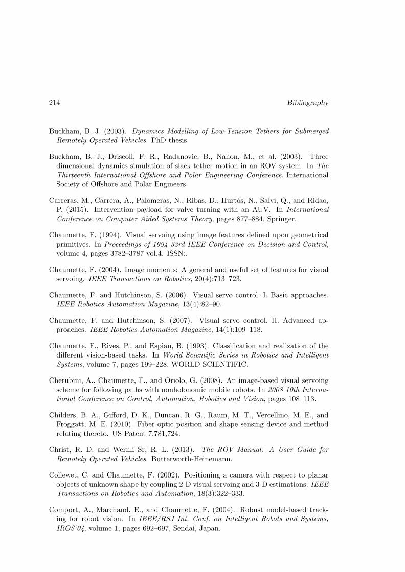
214 Bibliography
Buckham, B. J. (2003). Dynamics Modelling of Low-Tension Tethers for SubmergedRemotely Operated Vehicles. PhD thesis.
Buckham, B. J., Driscoll, F. R., Radanovic, B., Nahon, M., et al. (2003). Threedimensional dynamics simulation of slack tether motion in an ROV system. In TheThirteenth International Offshore and Polar Engineering Conference. InternationalSociety of Offshore and Polar Engineers.
Carreras, M., Carrera, A., Palomeras, N., Ribas, D., Hurtos, N., Salvi, Q., and Ridao,P. (2015). Intervention payload for valve turning with an AUV. In InternationalConference on Computer Aided Systems Theory, pages 877–884. Springer.
Chaumette, F. (1994). Visual servoing using image features defined upon geometricalprimitives. In Proceedings of 1994 33rd IEEE Conference on Decision and Control,volume 4, pages 3782–3787 vol.4. ISSN:.
Chaumette, F. (2004). Image moments: A general and useful set of features for visualservoing. IEEE Transactions on Robotics, 20(4):713–723.
Chaumette, F. and Hutchinson, S. (2006). Visual servo control. I. Basic approaches.IEEE Robotics Automation Magazine, 13(4):82–90.
Chaumette, F. and Hutchinson, S. (2007). Visual servo control. II. Advanced ap-proaches. IEEE Robotics Automation Magazine, 14(1):109–118.
Chaumette, F., Rives, P., and Espiau, B. (1993). Classification and realization of thedifferent vision-based tasks. In World Scientific Series in Robotics and IntelligentSystems, volume 7, pages 199–228. WORLD SCIENTIFIC.
Cherubini, A., Chaumette, F., and Oriolo, G. (2008). An image-based visual servoingscheme for following paths with nonholonomic mobile robots. In 2008 10th Interna-tional Conference on Control, Automation, Robotics and Vision, pages 108–113.
Childers, B. A., Gifford, D. K., Duncan, R. G., Raum, M. T., Vercellino, M. E., andFroggatt, M. E. (2010). Fiber optic position and shape sensing device and methodrelating thereto. US Patent 7,781,724.
Christ, R. D. and Wernli Sr, R. L. (2013). The ROV Manual: A User Guide forRemotely Operated Vehicles. Butterworth-Heinemann.
Collewet, C. and Chaumette, F. (2002). Positioning a camera with respect to planarobjects of unknown shape by coupling 2-D visual servoing and 3-D estimations. IEEETransactions on Robotics and Automation, 18(3):322–333.
Comport, A., Marchand, E., and Chaumette, F. (2004). Robust model-based track-ing for robot vision. In IEEE/RSJ Int. Conf. on Intelligent Robots and Systems,IROS’04, volume 1, pages 692–697, Sendai, Japan.
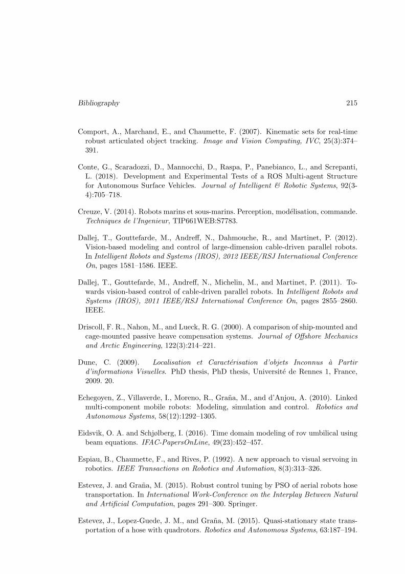
Bibliography 215
Comport, A., Marchand, E., and Chaumette, F. (2007). Kinematic sets for real-timerobust articulated object tracking. Image and Vision Computing, IVC, 25(3):374–391.
Conte, G., Scaradozzi, D., Mannocchi, D., Raspa, P., Panebianco, L., and Screpanti,L. (2018). Development and Experimental Tests of a ROS Multi-agent Structurefor Autonomous Surface Vehicles. Journal of Intelligent & Robotic Systems, 92(3-4):705–718.
Creuze, V. (2014). Robots marins et sous-marins. Perception, modelisation, commande.Techniques de l’Ingenieur, TIP661WEB:S7783.
Dallej, T., Gouttefarde, M., Andreff, N., Dahmouche, R., and Martinet, P. (2012).Vision-based modeling and control of large-dimension cable-driven parallel robots.In Intelligent Robots and Systems (IROS), 2012 IEEE/RSJ International ConferenceOn, pages 1581–1586. IEEE.
Dallej, T., Gouttefarde, M., Andreff, N., Michelin, M., and Martinet, P. (2011). To-wards vision-based control of cable-driven parallel robots. In Intelligent Robots andSystems (IROS), 2011 IEEE/RSJ International Conference On, pages 2855–2860.IEEE.
Driscoll, F. R., Nahon, M., and Lueck, R. G. (2000). A comparison of ship-mounted andcage-mounted passive heave compensation systems. Journal of Offshore Mechanicsand Arctic Engineering, 122(3):214–221.
Dune, C. (2009). Localisation et Caracterisation d’objets Inconnus a Partird’informations Visuelles. PhD thesis, PhD thesis, Universite de Rennes 1, France,2009. 20.
Echegoyen, Z., Villaverde, I., Moreno, R., Grana, M., and d’Anjou, A. (2010). Linkedmulti-component mobile robots: Modeling, simulation and control. Robotics andAutonomous Systems, 58(12):1292–1305.
Eidsvik, O. A. and Schjølberg, I. (2016). Time domain modeling of rov umbilical usingbeam equations. IFAC-PapersOnLine, 49(23):452–457.
Espiau, B., Chaumette, F., and Rives, P. (1992). A new approach to visual servoing inrobotics. IEEE Transactions on Robotics and Automation, 8(3):313–326.
Estevez, J. and Grana, M. (2015). Robust control tuning by PSO of aerial robots hosetransportation. In International Work-Conference on the Interplay Between Naturaland Artificial Computation, pages 291–300. Springer.
Estevez, J., Lopez-Guede, J. M., and Grana, M. (2015). Quasi-stationary state trans-portation of a hose with quadrotors. Robotics and Autonomous Systems, 63:187–194.
216 Bibliography
Feddema, J. T., Lee, C. G., and Mitchell, O. R. (1991). Weighted selection of imagefeatures for resolved rate visual feedback control. IEEE Transactions on Roboticsand Automation, 7(1):31–47.
Feddema, J. T., Lee, C. S. G., and Mitchell, O. R. (1989). Automatic selection of imagefeatures for visual servoing of a robot manipulator. In 1989 International Conferenceon Robotics and Automation Proceedings, pages 832–837 vol.2.
Feddema, J. T. and Mitchell, O. R. (1989). Vision-guided servoing with feature-basedtrajectory generation (for robots). IEEE Transactions on Robotics and Automation,5(5):691–700.
Fossen, T. I. (2011). Handbook of Marine Craft Hydrodynamics and Motion Control.John Wiley & Sons.
Fossen, T. I., Johansen, T. A., and Perez, T. (2009). A survey of control allocationmethods for underwater vehicles. In Underwater Vehicles. InTech.
Frank, J. E., Geiger, R., Kraige, D. R., and Murali, A. (2013). Smart tether system forunderwater navigation and cable shape measurement. US Patent 8,437,979.
Fukushima, E. F., Kitamura, N., and Hirose, S. (2000). A new flexible componentfor field robotic system. In Proceedings 2000 ICRA. Millennium Conference. IEEEInternational Conference on Robotics and Automation. Symposia Proceedings (Cat.No.00CH37065), volume 3, pages 2583–2588 vol.3.
Gennery, D. B. (1992). Visual tracking of known three-dimensional objects. Interna-tional Journal of Computer Vision, 7(3):243–270.
Gerkey, B. and Conley, K. (2011). Robot Developer Kits [ROS Topics]. IEEE RoboticsAutomation Magazine, 18(3):16–16.
Hashimoto, K. (1993). Visual Servoing, volume 7. World scientific.
Hawkes, G. S. and Jeffrey, D. C. (1987). Tether cable management apparatus andmethod for a remotely-operated underwater vehicle. US Patent 4,686,927.
Howell, C. T. (1992). Investigation of the Dynamics of Low-Tension Cables. PhDthesis, Woods Hole Oceanographic Institution MA.
Huber, P. (1981). Robust Statistics. Wiley Series in Probability and Statistics. Wiley.
Huntsberger, T. L., Trebi-Ollennu, A., Aghazarian, H., Schenker, P. S., Pirjanian, P.,and Nayar, H. D. (2004). Distributed control of multi-robot systems engaged intightly coupled tasks. Autonomous Robots, 17(1):79–92.
Huster, A., Bergstrom, H., Gosior, J., and White, D. (2009). Design and operationalperformance of a standalone passive heave compensation system for a work classROV. In OCEANS 2009, MTS/IEEE Biloxi-Marine Technology for Our Future:Global and Local Challenges, pages 1–8. IEEE.

Bibliography 217
Inzartsev, A. and Alexander Pavin (2009). AUV Application for Inspection of Under-water Communications. INTECH Open Access Publisher. OCLC: 884025486.
Iqbal, J., Heikkila, S., and Halme, A. (2008). Tether tracking and control of ROSArobotic rover. In Control, Automation, Robotics and Vision, 2008. ICARCV 2008.10th International Conference On, pages 689–693. IEEE.
Irvine, H. M. (1981). Cable Structures, volume 17. MIT press Cambridge, MA.
Jaulin, L. (2015). Mobile Robotics. Mobile Robotics.
Johnston, E. R., Beer, F., and Eisenberg, E. (2009). Vector Mechanics for Engineers:Statics and Dynamics. McGraw-Hill.
Katlein, C., Schiller, M., Belter, H. J., Coppolaro, V., Wenslandt, D., and Nicolaus,M. (2017). A New Remotely Operated Sensor Platform for Interdisciplinary Obser-vations under Sea Ice. Frontiers in Marine Science, 4:281.
Kervrann, C. and Heitz, F. (1998). A hierarchical Markov modeling approach forthe segmentation and tracking of deformable shapes. Graphical Models and ImageProcessing, 60(3):173–195.
Khatib, O., Yeh, X., Brantner, G., Soe, B., Kim, B., Ganguly, S., Stuart, H., Wang, S.,Cutkosky, M., Edsinger, A., et al. (2016). Ocean one: A robotic avatar for oceanicdiscovery. IEEE Robotics & Automation Magazine, 23(4):20–29.
Kiribayashi, S., Yakushigawa, K., and Nagatani, K. (2017). Position estimation oftethered micro unmanned aerial vehicle by observing the slack tether. In 2017 IEEEInternational Symposium on Safety, Security and Rescue Robotics (SSRR), pages159–165.
Klemas, V. V. (2015). Coastal and environmental remote sensing from unmanned aerialvehicles: An overview. Journal of Coastal Research, 31(5):1260–1267.
Koenig, N. and Howard, A. (2004). Design and use paradigms for Gazebo, an open-source multi-robot simulator. In 2004 IEEE/RSJ International Conference on In-telligent Robots and Systems (IROS) (IEEE Cat. No.04CH37566), volume 3, pages2149–2154 vol.3.
Krishna, M., Bares, J., and Mutschler, E. (1997). Tethering system design for DanteII. In Robotics and Automation, 1997. Proceedings., 1997 IEEE International Con-ference On, volume 2, pages 1100–1105. IEEE.
Krupinski, S., Desouche, R., Palomeras, N., Allibert, G., and Hua, M.-D. (2015). Pooltesting of AUV visual servoing for autonomous inspection. IFAC-PapersOnLine,48(2):274–280.

218 Bibliography
Laranjeira, M., Dune, C., and Hugel, V. (2017). Catenary-based visual servoing fortethered robots. In Robotics and Automation (ICRA), 2017 IEEE InternationalConference On, pages 732–738. IEEE.
Lee, T. (2015). Geometric controls for a tethered quadrotor UAV. In Decision andControl (CDC), 2015 IEEE 54th Annual Conference On, pages 2749–2754. IEEE.
L’Hour, M. and Creuze, V. (2016). French Archaeology’s Long March to the Deep - TheLune Project: Building the Underwater Archaeology of the Future. In ExperimentalRobotics, pages 911–927. Springer.
Lowe, D. G. (1992). Robust model-based motion tracking through the integration ofsearch and estimation. International Journal of Computer Vision, 8(2):113–122.
Ma, Y., Soatto, S., Kosecka, J., and Sastry, S. S. (2012). An Invitation to 3-d Vision:From Images to Geometric Models, volume 26. Springer Science & Business Media.
Mallapragada, V., Sarkar, N., and Podder, T. K. (2011). Toward a robot-assisted breastintervention system. IEEE/ASME Transactions on Mechatronics, 16(6):1011–1020.
Manhaes, M. M. M., Scherer, S. A., Voss, M., Douat, L. R., and Rauschenbach, T.(2016). UUV Simulator: A Gazebo-based package for underwater intervention andmulti-robot simulation. In OCEANS 2016 MTS/IEEE Monterey. IEEE.
Mansard, N. and Chaumette, F. (2007). Task Sequencing for High-Level Sensor-BasedControl. IEEE Transactions on Robotics, 23(1):60–72.
Marani, G., Choi, S. K., and Yuh, J. (2009). Underwater autonomous manipulationfor intervention missions AUVs. Ocean Engineering, 36(1):15–23.
Marchand, E., Bouthemy, P., Chaumette, F., and Moreau, V. (1999). Robust real-timevisual tracking using a 2D-3D model-based approach. In Computer Vision, 1999.The Proceedings of the Seventh IEEE International Conference On, volume 1, pages262–268. IEEE.
Marchand, E. and Chaumette, F. (2005). Feature tracking for visual servoing purposes.Robotics and Autonomous Systems, 52(1):53–70.
Marchand, E., Spindler, F., and Chaumette, F. (2005). ViSP for visual servoing: Ageneric software platform with a wide class of robot control skills. IEEE Roboticsand Automation Magazine, 12(4):40–52.
McGarey, P., MacTavish, K., Pomerleau, F., and Barfoot, T. D. (2016a). The lineleading the blind: Towards nonvisual localization and mapping for tethered mobilerobots. In Robotics and Automation (ICRA), 2016 IEEE International ConferenceOn, pages 4799–4806. IEEE.
Bibliography 219
McGarey, P., MacTavish, K., Pomerleau, F., and Barfoot, T. D. (2017). TSLAM:Tethered simultaneous localization and mapping for mobile robots. The InternationalJournal of Robotics Research, 36(12):1363–1386.
McGarey, P., Pomerleau, F., and Barfoot, T. D. (2016b). System design of a tetheredrobotic explorer (TReX) for 3D mapping of steep terrain and harsh environments.In Field and Service Robotics, pages 267–281. Springer.
McKerrow, P. J. and Ratner, D. (2007). The design of a tethered aerial robot. InProceedings 2007 IEEE International Conference on Robotics and Automation, pages355–360.
Merlet, J.-P. (2018a). Computing Cross-Sections of the Workspace of a Cable-DrivenParallel Robot with 6 Sagging Cables Having Limited Lengths. In InternationalSymposium on Advances in Robot Kinematics, pages 392–400. Springer.
Merlet, J.-P. (2018b). An Experimental Investigation of Extra Measurements for Solv-ing the Direct Kinematics of Cable-Driven Parallel Robots. In 2018 IEEE Interna-tional Conference on Robotics and Automation (ICRA), pages 6947–6952.
Merlet, J.-P. (2018c). Some properties of the Irvine cable model and their use forthe kinematic analysis of cable-driven parallel robots. In European Conference onMechanism Science, pages 409–416. Springer.
Milutinovic, M., Kranjcevic, N., and Deur, J. (2014). Multi-mass dynamic model of avariable-length tether used in a high altitude wind energy system. Energy conversionand management, 87:1141–1150.
Molchan, M. (2005). The role of micro-rovs in maritime safety and security. MolchanMarine Sciences, USA.
Murtra, A. C. and Tur, J. M. M. (2013). IMU and cable encoder data fusion for in-pipemobile robot localization. In TePRA, pages 1–6.
Navarro-Alarcon, D. and Liu, Y. (2018). Fourier-Based Shape Servoing: A New Feed-back Method to Actively Deform Soft Objects into Desired 2-D Image Contours.IEEE Transactions on Robotics, 34(1):272–279.
Navarro-Alarcon, D., Liu, Y., Romero, J. G., and Li, P. (2013a). Visually servoeddeformation control by robot manipulators. In 2013 IEEE International Conferenceon Robotics and Automation, pages 5259–5264.
Navarro-Alarcon, D., Liu, Y.-H., Romero, J. G., and Li, P. (2013b). Model-free vi-sually servoed deformation control of elastic objects by robot manipulators. IEEETransactions on Robotics, 29(6):1457–1468.
Navarro-Alarcon, D., Liu, Y.-h., Romero, J. G., and Li, P. (2014). On the visualdeformation servoing of compliant objects: Uncalibrated control methods and ex-periments , On the visual deformation servoing of compliant objects: Uncalibrated

220 Bibliography
control methods and experiments. The International Journal of Robotics Research,33(11):1462–1480.
Nayar, K. G., Sharqawy, M. H., Banchik, L. D., and V, J. H. L. (2016). Thermo-physical properties of seawater: A review and new correlations that include pressuredependence. Desalination, 390:1–24.
Nickels, K. and Hutchinson, S. (2001). Model-based tracking of complex articulatedobjects. IEEE Transactions on Robotics and Automation, 17(1):28–36.
Nicotra, M. M., Naldi, R., and Garone, E. (2017). Nonlinear control of a tethered UAV:The taut cable case. Automatica, 78:174–184.
Papanikolopoulos, N. P., Khosla, P. K., and Kanade, T. (1993). Visual tracking of amoving target by a camera mounted on a robot: A combination of control and vision.IEEE transactions on robotics and automation, 9(1):14–35.
Park, J.-Y., Jun, B.-h., Lee, P.-m., and Oh, J. (2009). Experiments on vision guideddocking of an autonomous underwater vehicle using one camera. Ocean Engineering,36(1):48–61.
Perrin, D. P., Kwon, A., and Howe, R. D. (2004). A novel actuated tether designfor rescue robots using hydraulic transients. In Robotics and Automation, 2004.Proceedings. ICRA’04. 2004 IEEE International Conference On, volume 4, pages3482–3487. IEEE.
Pettersson, A., Ohlsson, T., Davis, S., Gray, J., and Dodd, T. (2011). A hygienicallydesigned force gripper for flexible handling of variable and easily damaged naturalfood products. Innovative Food Science & Emerging Technologies, 12(3):344–351.
Prabhakar, S. and Buckham, B. (2005). Dynamics modeling and control of a vari-able length remotely operated vehicle tether. In OCEANS, 2005. Proceedings ofMTS/IEEE, pages 1255–1262. IEEE.
Prats, M., Palomeras, N., Ridao, P., and Sanz, P. J. (2012). Template Tracking andVisual Servoing for Alignment Tasks with Autonomous Underwater Vehicles. IFACProceedings Volumes, 45(27):256–261.
Pratt, K. S., Murphy, R. R., Burke, J. L., Craighead, J., Griffin, C., and Stover,S. (2008). Use of Tethered Small Unmanned Aerial System at Berkman Plaza IICollapse. In 2008 IEEE International Workshop on Safety, Security and RescueRobotics, pages 134–139.
Pressigout, M. (2006). Approches Hybrides Pour Le Suivi Temps-Reel d’objets Com-plexes Dans Des Sequences Videos. PhD thesis, Rennes 1.
Rajan, V. A. K. T., Nagendran, A., Dehghani-Sanij, A., and Richardson, R. C. (2016).Tether monitoring for entanglement detection, disentanglement and localisation ofautonomous robots. Robotica, 34(3):527–548.
Bibliography 221
Reverte, C. F., Thayer, S. M., Whittaker, W., Close, E. C., Slifko, A., Hudson, E., andVallapuzha, S. (2011). Autonomous inspector mobile platform. US Patent 8,024,066.
Ropars, B., Lasbouygues, A., Lapierre, L., and Andreu, D. (2015). Thruster’s dead-zones compensation for the actuation system of an underwater vehicle. In 2015European Control Conference (ECC), pages 741–746, Linz, Austria. IEEE.
Sahin, T. and Unel, M. (2004). Globally stabilized 3L curve fitting. In InternationalConference Image Analysis and Recognition, pages 495–502. Springer.
Salgado-Jimenez, T., Gonzalez-Lopez, J. L., Martinez-Soto, L. F., Olguin-Lopez, E.,Resendiz-Gonzalez, P. A., and Bandala-Sanchez, M. (2010). Deep water ROV designfor the Mexican oil industry. In OCEANS’10 IEEE SYDNEY, pages 1–6, Sydney,Australia. IEEE.
Shimono, S., Matsubara, O., Toyama, S., Nishizawa, U., Kato, S., and Arisumi,H. (2015). Development of underwater inspection system for dam inspection. InOCEANS 2015 - MTS/IEEE Washington, pages 1–6, Washington, DC. IEEE.
Shirai, Y. and Inoue, H. (1973). Guiding a robot by visual feedback in assemblingtasks. Pattern recognition, 5(2):99–106.
Short, A. D. and Woodroffe, C. D. (2009). The Coast of Australia. Cambridge Univer-sity Press.
Siciliano, B. and Khatib, O. (2016). Springer Handbook of Robotics. Springer.
Smolowitz, R. J., Patel, S. H., Haas, H. L., and Miller, S. A. (2015). Using a remotelyoperated vehicle (ROV) to observe loggerhead sea turtle (Caretta caretta) behavioron foraging grounds off the mid-Atlantic United States. Journal of ExperimentalMarine Biology and Ecology, 471:84–91.
Tahri, O. and Chaumette, F. (2003). Application of moment invariants to visual ser-voing. In International Conference on Robotics and Automation, volume 3, pages4276–4281.
Talke, K. A., de Oliveira, M., and Bewley, T. (2018). Catenary Tether Shape Analysisfor a UAV - USV Team. In IROS: International Conference on Intelligent Robotsand Systems, pages 7803–7809, Madrid, Spain.
Tognon, M. and Franchi, A. (2015). Control of motion and internal stresses for a chainof two underactuated aerial robots. In Control Conference (ECC), 2015 European,pages 1620–1625. IEEE.
Torabi, M., Hauser, K., Alterovitz, R., Duindam, V., and Goldberg, K. (2009). Guidingmedical needles using single-point tissue manipulation. In Robotics and Automation,2009. ICRA’09. IEEE International Conference On, pages 2705–2710. IEEE.
222 Bibliography
Triantafyllou, M. S. and Grosenbaugh, M. A. (1991). Robust control for underwatervehicle systems with time delays. IEEE Journal of Oceanic Engineering, 16(1):146–151.
Tsai, D., Nesnas, I. A., and Zarzhitsky, D. (2013). Autonomous vision-based tethered-assisted rover docking. In Intelligent Robots and Systems (IROS), 2013 IEEE/RSJInternational Conference On, pages 2834–2841. IEEE.
Tsai, R. (1987). A versatile camera calibration technique for high-accuracy 3D ma-chine vision metrology using off-the-shelf TV cameras and lenses. IEEE Journal onRobotics and Automation, 3(4):323–344.
van der Zwaan, S., Bernardino, A., and Santos-Victor, J. (2002). Visual station keepingfor floating robots in unstructured environments. Robotics and Autonomous Systems,39(3–4):145–155. Intelligent Robotic Systems - SIRS’2000.
Vishnu, T., Kumar, A., and Richardson, R. (2008). Tether monitoring techniquesfor environment monitoring, tether following and localization of autonomous mobilerobots. In Intelligent Robots and Systems, 2008. IROS 2008. IEEE/RSJ Interna-tional Conference On, pages 2109–2114.
Wakamatsu, H., Arai, E., and Hirai, S. (2006). Knotting/unknotting manipulation ofdeformable linear objects. The International Journal of Robotics Research, 25(4):371–395.
Wang, X. and Bhattacharya, S. (2018). A Topological Approach to Workspace andMotion Planning for a Cable-Controlled Robot in Cluttered Environments. IEEERobotics and Automation Letters, 3(3):2600–2607.
Wang, Z. and Hirai, S. (2011). Modeling and estimation of rheological properties of foodproducts for manufacturing simulations. Journal of food engineering, 102(2):136–144.
Weiss, L., Sanderson, A., and Neuman, C. (1987). Dynamic sensor-based control ofrobots with visual feedback. IEEE Journal on Robotics and Automation, 3(5):404–417.
Wernli, R. L. and Christ, R. D. (2009). Observation Class ROVs Come of Age. In SixthInternational Symposium on Underwater Technology Wuxi, China, April.
Wynn, R. B., Huvenne, V. A., Le Bas, T. P., Murton, B. J., Connelly, D. P., Bett,B. J., Ruhl, H. A., Morris, K. J., Peakall, J., Parsons, D. R., Sumner, E. J., Darby,S. E., Dorrell, R. M., and Hunt, J. E. (2014). Autonomous Underwater Vehicles(AUVs): Their past, present and future contributions to the advancement of marinegeoscience. Marine Geology, 352:451–468.
Yang, W., Zhang, Z., and Zhang, A. (2008). Research on an active heave compensationsystem for remotely operated vehicle. In Intelligent Computation Technology andAutomation (ICICTA), 2008 International Conference On, volume 2, pages 407–410.IEEE.
Bibliography 223
Yazicioglu, A. Y., Calli, B., and Unel, M. (2009). Image based visual servoing us-ing algebraic curves applied to shape alignment. In 2009 IEEE/RSJ InternationalConference on Intelligent Robots and Systems, pages 5444–5449.
Zhu, J., Navarro, B., Fraisse, P., Crosnier, A., and Cherubini, A. I. (2018). Dual-arm robotic manipulation of flexible cables. In IROS: International Conference onIntelligent Robots and Systems, Madrid, Spain.
Zikou, L., Papachristos, C., and Tzes, A. (2015). The power-over-tether system forpowering small UAVs: Tethering-line tension control synthesis. In Control and Au-tomation (MED), 2015 23th Mediterranean Conference On, pages 681–687. IEEE.

224 Bibliography

List of Figures
1 A chain of N small tethered robots used to explore shallow waters. . . . 9
1.1 Profile or cross-section of a typical wave-dominated beach showing thenear-shore zone, the surf zone, and finally the swash zone. Courtesyof Short and Woodroffe (2009). . . . . . . . . . . . . . . . . . . . . . . . 13
1.2 Some examples of French underwater robots. (a) the AUV A9 fromECA robotics. (b) the AUV glider Sea-Explorer from Alseamar. (c)Victor 6000, an Ifremer work-class ROV dedicated to scientific oceanresearch in deep waters. (d) the observation-class mini-ROV observerfrom Subseatech. . . . . . . . . . . . . . . . . . . . . . . . . . . . . . . 14
1.3 Some examples of tethers used by mini-ROVs. (a) the tether modelDLR-1P20-2C50 from Novasub for power supply and data transfer. (b)the Fathom tether from BlueRobotics that carries four pairs of 26 AWGwire for data exchange. (c) the µlinx 50 OM3 tether from OFS optics iscomposed of a multimode 50 µm optical fiber for data transfer. . . . . . 18
1.4 The maximum tether length for a given voltage V and a given cablecross-sectional area A. Extracted from Christ and Wernli Sr (2013). . . 19
1.5 Tether drag versus tether length. Extracted from Christ and Wernli Sr(2013). . . . . . . . . . . . . . . . . . . . . . . . . . . . . . . . . . . . . . 20
1.6 Main components for teleoperation in underwater robotics. A remotelyoperated vehicle (ROV), a tether management system (TMS) and alaunch and recovery system (LARS). Adapted from (Salgado-Jimenezet al., 2010). . . . . . . . . . . . . . . . . . . . . . . . . . . . . . . . . . 22
1.7 Two examples of a ROV operation with a negatively buoyant anchor toovercome the drag imposed by the umbilical: (a) a clump weight/depressorand (b) a cage used to protect the ROV against abrasions and deploy-ment damage while lowering and heaving the ROV. Both options canbe used with a tether management system (TMS) in order to reduce thedrag force the vehicle has to deal with. Courtesy of Christ and Wernli Sr(2013). . . . . . . . . . . . . . . . . . . . . . . . . . . . . . . . . . . . . . 23
1.8 Illustration of heave compensation. Courtesy of Christ and Wernli Sr(2013) . . . . . . . . . . . . . . . . . . . . . . . . . . . . . . . . . . . . . 24
225
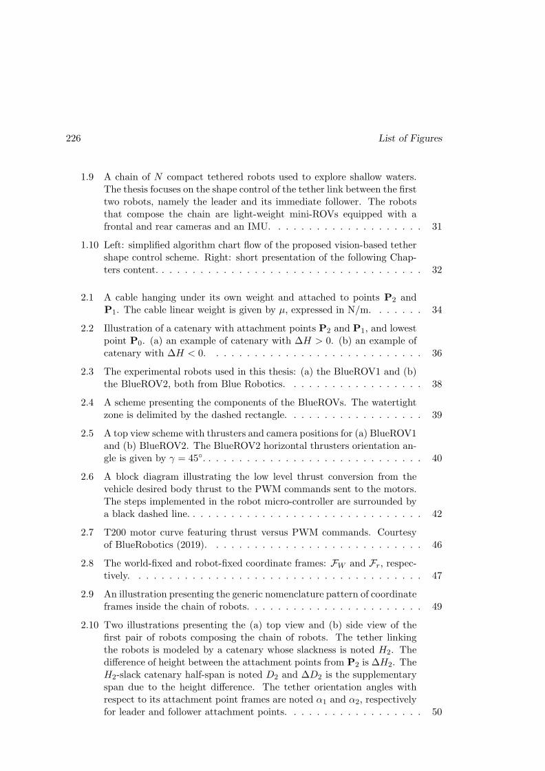
226 List of Figures
1.9 A chain of N compact tethered robots used to explore shallow waters.The thesis focuses on the shape control of the tether link between the firsttwo robots, namely the leader and its immediate follower. The robotsthat compose the chain are light-weight mini-ROVs equipped with afrontal and rear cameras and an IMU. . . . . . . . . . . . . . . . . . . . 31
1.10 Left: simplified algorithm chart flow of the proposed vision-based tethershape control scheme. Right: short presentation of the following Chap-ters content. . . . . . . . . . . . . . . . . . . . . . . . . . . . . . . . . . . 32
2.1 A cable hanging under its own weight and attached to points P2 andP1. The cable linear weight is given by µ, expressed in N/m. . . . . . . 34
2.2 Illustration of a catenary with attachment points P2 and P1, and lowestpoint P0. (a) an example of catenary with ∆H > 0. (b) an example ofcatenary with ∆H < 0. . . . . . . . . . . . . . . . . . . . . . . . . . . . 36
2.3 The experimental robots used in this thesis: (a) the BlueROV1 and (b)the BlueROV2, both from Blue Robotics. . . . . . . . . . . . . . . . . . 38
2.4 A scheme presenting the components of the BlueROVs. The watertightzone is delimited by the dashed rectangle. . . . . . . . . . . . . . . . . . 39
2.5 A top view scheme with thrusters and camera positions for (a) BlueROV1and (b) BlueROV2. The BlueROV2 horizontal thrusters orientation an-gle is given by γ = 45. . . . . . . . . . . . . . . . . . . . . . . . . . . . . 40
2.6 A block diagram illustrating the low level thrust conversion from thevehicle desired body thrust to the PWM commands sent to the motors.The steps implemented in the robot micro-controller are surrounded bya black dashed line. . . . . . . . . . . . . . . . . . . . . . . . . . . . . . . 42
2.7 T200 motor curve featuring thrust versus PWM commands. Courtesyof BlueRobotics (2019). . . . . . . . . . . . . . . . . . . . . . . . . . . . 46
2.8 The world-fixed and robot-fixed coordinate frames: FW and Fr, respec-tively. . . . . . . . . . . . . . . . . . . . . . . . . . . . . . . . . . . . . . 47
2.9 An illustration presenting the generic nomenclature pattern of coordinateframes inside the chain of robots. . . . . . . . . . . . . . . . . . . . . . . 49
2.10 Two illustrations presenting the (a) top view and (b) side view of thefirst pair of robots composing the chain of robots. The tether linkingthe robots is modeled by a catenary whose slackness is noted H2. Thedifference of height between the attachment points from P2 is ∆H2. TheH2-slack catenary half-span is noted D2 and ∆D2 is the supplementaryspan due to the height difference. The tether orientation angles withrespect to its attachment point frames are noted α1 and α2, respectivelyfor leader and follower attachment points. . . . . . . . . . . . . . . . . . 50

List of Figures 227
2.11 An illustration presenting the symmetry of the catenary features ac-cording to the reference frame chosen (F1 or F2). The catenary slack-ness are H1 = 0Z1 and H2 = 0Z2. The attachment points differ-ence of height is ∆H1 = 1Z2 and H2 = 2Z1. The catenary parame-ter C(H1,∆H1) = C(H2,∆H2) is invariant whatever the point Pi wechoose for the starting attachment point of the cable. Thanks to thesymmetry we have: ∆H1 = −∆H2, H1 = H2 +∆H2, H2 = H1 +∆H1,∆D1 = −∆D2, D1 = D2 + ∆D2, D2 = D1 + ∆D1. As a reminder:Hi > 0, Hi +∆Hi > 0, Di > 0 and Di +∆Di > 0. . . . . . . . . . . . . 51
3.1 Illustration of a pair of tethered robots where the field of view of thecameras is highlighted by red dashed lines. (a) top view and (b) side view. 58
3.2 Some examples of the mock tether images captured by the BlueROV1camera in different configurations. (a) the tether is completely visible.(b) the tether plane is aligned with the camera optical axis. (c) and(d) the tether is partially visible. The mock tether is made of a leadedcurtain wire wrapped by an orange cotton ribbon. . . . . . . . . . . . . 59
3.3 Frontal pinhole imaging model: the perspective projection of a 3-D pointPa on the image plane πi is the point pa. The camera center is noted Pc. 63
3.4 Transformation from pixels to meters coordinates. . . . . . . . . . . . . 63
3.5 Visible light spectrum for varying wavelengths. Extracted from shutha.org. 65
3.6 Hue representation. Courtesy of NYC Departement of Education. . . . . 66
3.7 Tether detection examples in both aerial (a,b,c) and underwater (d,e,f)experiments. The mode corresponding to the specific color of the tetheris selected by two thresholds in the hue histogram. The minimum andmaximum thresholds are displayed in green and red lines, respectively(b,e). The detected points are refined thanks to morphomathematicalclosing and skeletization (c,f). . . . . . . . . . . . . . . . . . . . . . . . . 66
3.8 Top view of a robot-tether system presenting the singularities on cate-nary shape estimation with respect to the tether orientation parameterb = sinα. (a) the tether is perpendicular to the robot longitudinal axis.(b) the tether plane is aligned with the segment PcP2 and the catenarycurve degenerates into a straight line in the image. The tether attach-ment point has an offset with respect to the camera axis (cX2 6= 0). (c)the specific case where cX2 = 0. . . . . . . . . . . . . . . . . . . . . . . . 73
3.9 Case of remote points and large residuals. (a) an illustration of residuals(black arrows) between tether detected points (in green) and the pro-jection of the catenary current estimation (in red). The tether lengthis L = 1.50m and the height difference between the attachment pointsis ∆H = 0. The tether shape is defined by the feature vector s =[0.6, 0.6] T , with Hmax = 0.70m. The red dashed line represents thecatenary points which are beyond the tether length (L = 1.50m). (b) atop view illustration of catenary remote points that become more andmore tight and vertical in the image plane as α→ α. . . . . . . . . . . 75
228 List of Figures
3.10 Chart flow of the improved Gauss-Newton algorithm. The four newfunctions added to the algorithm flow are numbered and highlighted bya pink background. . . . . . . . . . . . . . . . . . . . . . . . . . . . . . . 76
3.11 An example of tether points detection from simulated images. The sim-ulated tether is 1.50meter long, 3milimeter thick, with feature vectors = [0.6, 0.6]T , Hmax = 0.70meter and ∆H = 0meter. (a) the raw im-age obtained from follower robot camera. (b) the tether detected pointsobtained from image processing (described in Section 3.3) and used asinput data by the Gauss-Newton algorithm. . . . . . . . . . . . . . . . . 77
3.12 An example of unbounded residuals removal applied to tether pointsdepicted in Figure 3.11b. (a) the tether points are drawn in green, anexample of catenary shape estimation with s = [0.5, 0.5]T is drawn inred and some residuals are shown by black arrows. The red dashedline represents the catenary points that do not satisfy the boundingconditions and are therefore eliminated. (b) the selected points resultingfrom the unbounded residuals removal are drawn in blue. . . . . . . 78
3.13 An example of 2-D points subsampling applied to tether points thatwere already filtered by the unbounded residuals removal function, aspresented in Figure 3.12b. (a) the input points are drawn in blue andthe current catenary shape estimation (s = [0.5, 0.5]T ) is drawn in red.The unevenly tether points distribution is demonstrated by two zoomedregions. (b) the selected points resulting from the 2-D points subsam-pling are drawn in black. Only one tether point per abscissa is selected(the one with the smallest residual). . . . . . . . . . . . . . . . . . . . . 80
3.14 The hyperbolic tangent of the cost function of the catenary curve pre-sented in Figure 3.9, whose feature vector is s = [0.6, 0.6] T , the tethertotal length is L = 1.50m and ∆H = 0m. The hyperbolic tangentwas used to saturate the highest values of the cost function to 1. Thefunction minimum is marked by the red star at a = 0.6, b = 0.6. . . . . . 83
3.15 The hyperbolic tangent of the improved Gauss-Newton cost function ofthe catenary curve presented in Figure 3.9. The hyperbolic tangent wasused to saturate the highest values of the cost function to 1. The functionminimum at a = 0.6, b = 0.6, marked by the red star. . . . . . . . . . . 84
3.16 An illustration showing the difference between the projection of thetether 3D lowest point, p0 marked by a black cross, and the tetherlowest point detected in the image, pB marked by a red dot, is high-lighted. The observed tether is drawn in green and the catenary curvecorresponding to the initial guess is drawn by a red dashed line. (a) anembedded camera view where p0 is outside of the camera field of view.(b) another situation where p0 is inside camera field of view and pB ≈ p0. 85
3.17 The initial guess function g(b) given by equation (3.68) for a catenarywhose feature vector is [0.6, 0.6]T . The root of g(b) is searched in theinterval defined by the green vertical lines. . . . . . . . . . . . . . . . . . 91
List of Figures 229
3.18 Simulation results for the standard Gauss-Newton algorithm (GN). (a)the feature vector estimation error is represented in color scale. (b) thealgorithm exit status is depicted in color code. . . . . . . . . . . . . . . 94
3.19 Simulation results for the improved Gauss-Newton algorithm withoutinitial guess (IGN). (a) the feature vector estimation error is representedin color scale. (b) the algorithm exit status is depicted in color code. . . 95
3.20 Simulation results for the improved Gauss-Newton algorithm withoutinitial guess (IGN + IG). (a) the feature vector estimation error is rep-resented in color scale. (b) the algorithm exit status is depicted in colorcode. . . . . . . . . . . . . . . . . . . . . . . . . . . . . . . . . . . . . . . 96
3.21 The simulation of two BlueROV 1 linked by an orange sagging tether onGazebo. . . . . . . . . . . . . . . . . . . . . . . . . . . . . . . . . . . . . 97
3.22 The (a) source image and (b) tether detected points of study case 1.The tether shape is given by the feature vector s[0.40, 0.45]T , whichcorresponds to a slackness H = 0.28meter and orientation angle α = 27. 98
3.23 The descent of the GN algorithm marked by black dots. The startingpoint is at s0 = [0.5, 0.5]T and the solution is at s = [0.40, 0.45]T , markedby a red star. The cost function values are plotted in the backgroundusing the color scale depicted on the right. . . . . . . . . . . . . . . . . . 99
3.24 Comparison of the descent of IGN (white dots) and IGN + IG (blackdots) algorithms. The solution is at s = [0.40, 0.45]T , marked by a redstar. The cost function values are plotted in the background using thecolor scale depicted on the right. . . . . . . . . . . . . . . . . . . . . . . 99
3.25 Catenary curve fitting problem depicted in the image plane. The tetherdetected points are drawn in green dots, the tether catenary initial esti-mation is drawn by a red dashed line and the final estimation is drawnby a red full line. The tether shape estimation is achieved by the threemethods: (a) GN, (b) IGN and (c) IGN + IG algorithms. The initialguess of the tether shape is given by s0 = [0.38, 0.44]T . The solution isat s = [0.40, 0.45]T . . . . . . . . . . . . . . . . . . . . . . . . . . . . . . . 100
3.26 The (a) source image and (b) tether detected points of study case 2. Thetether shape is given by the feature vector s[0.4, 0.6]T , which correspondsto H = 0.28meter and α = 37. . . . . . . . . . . . . . . . . . . . . . . . 101
3.27 The descent of a standard Gauss-Newton algorithm marked by blackdots. The starting point is at s0 = [0.5, 0.5]T and the solution is ats = [0.4, 0.6]T , marked by a red star. The cost function values areplotted in the background using the color scale depicted on the right.The algorithm does not reach the solution. . . . . . . . . . . . . . . . . . 102
3.28 Comparison of the descent of the IGN (white dots) and IGN+IG (blackdots) algorithms. The solution is at s = [0.4, 0.6]T , marked by a red star.The cost function values are plotted in the background using the colorscale depicted on the right. The solution is only reached if an initialguess (s0 = [0.47, 0.57]T ) of the tether shape is given. . . . . . . . . . . 102

230 List of Figures
3.29 Catenary curve fitting problem depicted in the image plane for the threemethods studied: (a) GN, (b) IGN and (c) IGN+IG. The tether detectedpoints are drawn in green, the initial estimation is drawn by a red dashedline and the final estimation is drawn by a red full line. The correct tethershape estimation is only achieved by the improved Gauss-Newton withinitial guess (IGN+IG). . . . . . . . . . . . . . . . . . . . . . . . . . . . 103
3.30 Estimation and real values of the tether shape during the execution ofa path by the follower robot. (a) the fitting procedure is used duringthe whole path execution. (b) during the singularity crossing (around8 second), the fitting procedure is stopped and the previously estimatedvalues of the tether shape are maintained. . . . . . . . . . . . . . . . . . 105
4.1 Example of visual servo control on rigid and articulated objects. (a) anexperiment of positioning in front of a square extracted from Espiau et al.(1992). Detected feature points in large dots and their desired positionsare drawn in small white dots. (b) an example of an amorphous planarshape used to validate the use of image moments in visual servoing;extracted from Tahri and Chaumette (2003). (c) an example of shapealignment using a technique of contour fitting to estimate object featurepoints to be used in visual servoing (extracted from Yazicioglu et al.(2009)). The feature points trajectories are drawn in green and bluelines. (d) an example of visual servoing used to regulate the robot’spose with respect to a rigid object whose CAD model is known (fromComport et al. (2004)). (e) another similar example but applied toarticulated objects (from Comport et al. (2007)). . . . . . . . . . . . . . 111
4.2 Some examples of visual servoing on deformable objects. (a) shape con-trol of a sponge with current and desired shape feature drawn in red andgreen, respectively. Initial shape on the left-hand side and final shape onthe right-hand side. Extracted from Navarro-Alarcon et al. (2013b). (b)manipulation of an uterus model though visual feedback where the objectcontour is modeled by a truncated Fourier series. The desired contouris drawn in red and the figure was extracted from Navarro-Alarcon andLiu (2018). (c) the same technique of shape modeling through Fourierseries applied to 1-D objects. Image extracted from Zhu et al. (2018). . 114
4.3 Chart flow of the vision-based tether shape control scheme. Details aboutthe visual servoing control loop (blue frame) are given in Figure 4.4. . . 115
4.4 Algorithm chart flow for catenary-based visual servoing. . . . . . . . . . 116
4.5 Figure 3.1 is reproduced to remind the features definition. (a) top viewand (b) side view. . . . . . . . . . . . . . . . . . . . . . . . . . . . . . . 117
4.6 Experimental setup: two Turtlebots (Gerkey and Conley, 2011) simulatea tether handling system for remotely operated robots. The leader robotfreely explores its surroundings while the follower robot is expected tomaintain the tether slack enough not to hamper the leader movements . 127

List of Figures 231
4.7 Simulation results for tether shape control. (a) the parameters evolution.The tether goes from an initial to a desired shape (so = (0.9, 0.8) ands∗ = (0.5, 0.5), respectively). (b) the control velocities. Linear velocity(νx) in m/s and angular velocity (ωz) in rad/s . . . . . . . . . . . . . . 128
4.8 Results of a real experiment for tether shape control. (a) the tether pa-rameters evolution. The tether goes from an initial to a desired shape(so = (0.9, 0.8) and s∗ = (0.5, 0.5), respectively). (b) the control veloci-ties. Linear velocity (νx) in m/s and angular velocity (ωz) in rad/s . . 128
4.9 Two robots are linked by a tether. The leader robot freely moves whilethe follower robot maintains a desired tether shape s∗ = (0.7,−0.5). (a)the leader and follower trajectories with time indications in seconds. (b)the tether parameters evolution. (c) the fitting quality index Q evolutionduring the experiment. Feature prediction is used in cases of wrong ropedetection and inaccurate fitting (Q = 1 i.e. log(103Q) = 3) . . . . . . . . 129
4.10 Image features used to manage the tether shape: its highest and lowestpoints in the image (pA and pB) and the line segment pApB in blue.(a) 3D simulated scene where the tether 3D lowest point P0 is out of thefollower’s camera field of view. (b) corresponding embedded view withp0 being the perspective projection of P0. (c) Another situation whereP0 is inside the follower’s camera field of view . . . . . . . . . . . . . . . 131
4.11 Follower robot camera view for (a) first, (b) second and (c) third simu-lation. Initial and desired tether shape in the image are drawn in blueand red lines, respectively . . . . . . . . . . . . . . . . . . . . . . . . . . 132
4.12 Normal case: error evolution for (a) tether slackness and (b) orienta-tion as well as (c) linear and (d) angular command velocities. Tetherinitial and desired shape are respectively: (H0 = 0.20m, θ0 = 20) and(H∗ = 0.20m, θ∗ = 45). Legend in Fig. 4.15d. All controllers use a gainλ = 1.0. . . . . . . . . . . . . . . . . . . . . . . . . . . . . . . . . . . . . 133
4.13 Limit case 1: error evolution for (a) tether slackness and (b) orienta-tion as well as (c) linear and (d) angular command velocities. Tetherinitial and desired shape are respectively: (H0 = 0.25m, θ0 = 10) and(H∗ = 0.25m, θ∗ = 60). Legend in Fig. 4.15d. All controllers use a gainλ = 1.0. . . . . . . . . . . . . . . . . . . . . . . . . . . . . . . . . . . . . 134
4.14 Limit case 2: error evolution for (a) tether slackness and (b) orienta-tion as well as (c) linear and (d) angular command velocities. Tetherinitial and desired shape are respectively: (H0 = 0.10m, θ0 = 20) and(H∗ = 0.24m, θ∗ = 0). Legend in Fig. 4.15d. All controllers use a gainλ = 1.0. . . . . . . . . . . . . . . . . . . . . . . . . . . . . . . . . . . . . 135
4.15 Tether lowest point trajectory in the image plane for (a) normal case,(b) limit case 1 and (c) limit case 2. (d) legend . . . . . . . . . . . . . . 136
4.16 Interaction matrices condition number evolution for (Fig. a) normal and(Figs. b and c). Legend in Fig. 4.15d. (d) condition number evolutionfor the curve fitting Gauss-Newton Jacobian during normal and limit cases137

232 List of Figures
4.17 Follower onboard view of the tether. The (a,c) initial and (b,d) finalimages of the visual servoing. Figures (a) and (b) are the camera sourceimages while figures (c) and (d) depict the tether detected points (inblue), the shape estimation (in red) and the desired shape in the image(in green). The tether initial and desired features are given in Table 4.1. 138
4.18 Simulation results for a control law using full 3 × 4 interaction matrix.(a) tether shape and (b) follower robot velocity evolution. The tetherdesired shape is given by H∗
2 = 0.15m, α∗2 = 30 and ∆H∗
2 = 0.20m. . . 140
4.19 Simulation results for the sum of controllers. (a) tether shape and (b)follower robot velocity evolution. The tether desired shape is given byH∗
2 = 0.15m, α∗2 = 30 and ∆H∗
2 = 0.20m. . . . . . . . . . . . . . . . . 142
4.20 Simulation results for the hierarchical non-optimal control. (a) tethershape and (b) follower robot velocity evolution. The tether desired shapeis given by H∗
2 = 0.15m, α∗2 = 30 and ∆H∗
2 = 0.20m. . . . . . . . . . . 145
4.21 Simulation results for the hierarchical optimal control. a) tether shapeand (b) follower robot velocity evolution. The tether desired shape isgiven by H∗
2 = 0.15m, α∗2 = 30 and ∆H∗
2 = 0.20m. . . . . . . . . . . . 146
4.22 Comparing the follower robot trajectories for the four controllers pre-sented in the previous subsections: full 3 × 4 interaction matrix con-troller (in red), sum of controllers (in yellow), hierarchical non-optimal(in green) and hierarchical optimal (in blue) controllers. The robot start-ing position is marked by a black star. . . . . . . . . . . . . . . . . . . . 147
4.23 The leader robot executed velocities. The executed path consists of aconstant straight forward displacement combined with lateral and verti-cal motions. . . . . . . . . . . . . . . . . . . . . . . . . . . . . . . . . . . 148
4.24 Simulation results for a non-hierarchical control law using the 3 × 4interaction matrix. (a) tether shape and (b) follower robot velocity evo-lution. The tether desired shape is given by H2 = 0.35m, α2 = 30 and∆H2 = 0m. . . . . . . . . . . . . . . . . . . . . . . . . . . . . . . . . . . 150
4.25 Simulation results for the sum of controllers law with no task priority.(a) tether shape and (b) follower robot velocity evolution. The tetherdesired shape is given by H2 = 0.35m, α2 = 30 and ∆H2 = 0m. . . . . 151
4.26 Simulation results for the hierarchical non-optimal controller. (a) tethershape and (b) follower robot velocity evolution. The tether desired shapeis given by H2 = 0.35m, α2 = 30 and ∆H2 = 0m. . . . . . . . . . . . . 152
4.27 Simulation results for the hierarchical optimal controller. (a) tethershape and (b) follower robot velocity evolution. The tether desired shapeis given by H2 = 0.35m, α2 = 30 and ∆H2 = 0m. . . . . . . . . . . . . 153
4.28 Simulation results for a control law including the leader velocities in thefollower commands computation. (a) tether shape and (b) follower robotvelocity evolution. The tether desired shape is given by H2 = 0.35m,α2 = 30 and ∆H2 = 0m. . . . . . . . . . . . . . . . . . . . . . . . . . . 155

List of Figures 233
4.29 Top view of the system composed of leader and follower robots connectedby a tether. The relative pose between the robots is not fully constrainedwithout the regulation of angle α1 between the tether plane and theleader robot longitudinal axis. A circle around the leader attachmentpoint defines an infinity of positions for the follower robot that regulatesthe features H2, ∆H2 and α2. . . . . . . . . . . . . . . . . . . . . . . . . 157
4.30 Embedded image view of the tether from the (a,b,c,d) leader and (e,f,g,h)follower point of view. The (a,c,e,g) initial and (b,d,f,h) final images ofthe visual servoing. Figures (a,b,e,f) are the source images while figures(c,d,g,h) depict the tether detected points (in blue), the shape estimation(in red) and the desired shape in the image (in green). . . . . . . . . . . 159
4.31 Simulation results for the controller using both leader and follower cam-eras. (a) tether shape evolution from leader and follower points of view.Full and dashed lines represent estimated and real simulated values, re-spectively. (b) follower robot velocity evolution. The tether initial anddesired shape are given in Table4.3. . . . . . . . . . . . . . . . . . . . . . 160
B.1 Catenary solutions with DH positive. DH = 0.32. H = 0.4. L = 2.(0, 0) is the attachment point of the umbilical to the following robot. . . 174
B.2 Catenary solutions with DH negative. DH = −0.32. H = 0.4. L = 2.(0, 0) is the attachment point of the umbilical to the following robot. . . 175
F.1 Top view and lateral view of the robot set up. . . . . . . . . . . . . . . . 196
F.2 The follower moves along the X-axis. Left: follower features when νx >0, Right: follower features when νx < 0 (blue ai, red bi, green di) . . . . 197
F.3 The follower moves along the X-axis. Left: leader features when νx > 0,Right: leader features when νx < 0 (blue ai, red bi, green di) . . . . . . 197
F.4 The follower moves along the Y -axis. Left: follower features when νy > 0,Right: follower features when νy < 0 (blue ai, red bi, green di) . . . . . 198
F.5 The follower moves along the Y -axis. Left: leader features when νy > 0,Right: leader features when νy < 0 (blue ai, red bi, green di) . . . . . . 198
F.6 The follower moves along the Z-axis. Left: follower features when νz > 0,Right: follower features when νz < 0 (blue ai, red bi, green di) . . . . . 199
F.7 The follower moves along the Z-axis. Left: leader features when νz > 0,Right: leader features when νz < 0 (blue ai, red bi, green di) . . . . . . 199
F.8 The follower turns around the Z-axis. Left: follower features when ωz >0. Right: follower features when ωz < 0. (blue ai, red bi, green di) . . . 200
F.9 The follower turns around the Z-axis. Left: leader features when ωz > 0.Right: leader features when ωz < 0. (blue ai, red bi, green di) . . . . . . 200
234 List of Figures
H.1 Une chaıne de N robots relies compacts utilises pour explorer les eauxpeu profondes. La these porte sur le controle de la forme du cable entreles deux premiers robots, a savoir le leader et son suiveur immediat. Lesrobots qui composent la chaıne sont des mini-ROV legers equipes d’unecamera frontale, d’une camera arriere, d’une centrale inertielle et d’unprofondimetre. . . . . . . . . . . . . . . . . . . . . . . . . . . . . . . . . 204
H.2 (a) vue de dessus et (b) vue de cote de la premiere paire de robots com-posant la chaıne des robots. L’ombilical reliant les robots est modelisepar une chaınette dont la hauteur est notee H2. La difference de hauteurentre les points d’attache du cote suiveur est ∆H2. La portee horizon-tale de chaınette correspondant a la hauteur H2 est notee D2 et ∆D2
est la portee supplementaire due a la difference de hauteur. Les anglesd’orientation du cable par rapport a chaque repere de point d’attachesont notes α1 et α2, respectivement pour les points d’attache du cableau robot de tete et au robot suiveur. . . . . . . . . . . . . . . . . . . . . 206
H.3 Schema de l’algorithme de Gauss-Newton ameliore avec les quatre etapesnumerotees et l’heuristique d’initialisation. . . . . . . . . . . . . . . . . . 207
H.4 Schema global de controle par asservissement visuel base chaınette durobot sous-marin suiveur . . . . . . . . . . . . . . . . . . . . . . . . . . . 208
H.5 Algorithme d’asservissement visuel base chaınette. . . . . . . . . . . . . 209

Resume
Cette these porte sur le probleme du controle de la forme d’ombilicaux pour des robotssous-marins legers teleoperes (mini-ROVs), qui conviennent, grace a leur petite tailleet grande manoeuvrabilite, a l’exploration des eaux peu profondes et des espaces en-combres. La regulation de la forme de l’ombilical est cependant une tache difficile,car ces robots n’ont pas une puissance de propulsion suffisante pour contrebalancerles forces de traınee du cable. Pour faire face a ce probleme, nous avons introduit leconcept de Cordee de mini-ROVs, dans lequel plusieurs robots sont relies a l’ombilicalet peuvent, ensemble, contrebalancer les perturbations exterieures et controler la formedu cable.
Nous avons etudie l’utilisation des cameras embarquees pour reguler la forme d’uneportion de l’ombilical reliant deux robots successifs, un leader et un suiveur. Seul lerobot suiveur se chargera de la tache de regulation de la forme du cable. Le leaderest libere pour explorer ses alentours. L’ombilical est suppose etre legerement pesantet donc modelise par une chaınette. Les parametres de forme du cable sont estimesen temps reel par une procedure d’optimisation non-lineaire qui adapte le modele dechaınette aux points detectes dans les images des cameras. La regulation des parametresde forme est obtenue grace a une commande reliant le mouvement du robot a la vari-ation de la forme de l’ombilical. L’asservissement visuel propose s’est avere capablede controler correctement la forme du cable en simulations et experiences realisees enbasin.
Abstract
This thesis addresses the problem of tether shape control for small remotely operatedunderwater vehicles (mini-ROVs), which are suitable, thanks to their small size andhigh maneuverability, for the exploration of shallow waters and cluttered spaces. Themanagement of the tether is, however, a hard task, since these robots do not haveenough propulsion power to counterbalance the drag forces acting on the tether cable.In order to cope with this problem, we introduced the concept of a Chain of mini-ROVs, where several robots are linked to the tether cable and can, together, managethe external perturbations and control the shape of the cable.
We investigated the use of the embedded cameras to regulate the shape of a por-tion of tether linking two successive robots, a leader and a follower. Only the followerrobot deals with the tether shape regulation task. The leader is released to exploreits surroundings. The tether linking both robots is assumed to be negatively buoyantand is modeled by a catenary. The tether shape parameters are estimated in real-timeby a nonlinear optimization procedure that fits the catenary model to the tether de-tected points in the image. The shape parameter regulation is thus achieved through acatenary-based control scheme relating the robot motion with the tether shape varia-tion. The proposed visual servoing control scheme has proved to properly manage thetether shape in simulations and real experiments in pool.
Copyright © 2022 FDOKUMEN