Journal of Mechanical Science and Technology 26 (8) (2012) 2313~2323

www.springerlink.com/content/1738-494x DOI 10.1007/s12206-012-0610-5

Adaptive neural controller for visual servoing of robot manipulators with

camera-in-hand configuration† Jungmin Kim1, Naveen Kumar1,*, Vikas Panwar2, Jin-Hwan Borm1 and Jangbom Chai1

1Division of Mechanical Engineering, Ajou University, Suwon 443-749, Korea 2Department of Applied Mathematics, Defense Institute of Advanced Technology, Pune-411025, Maharashtra, India

(Manuscript Received August 9, 2010; Revised March 2, 2012; Accepted March 20, 2012)

----------------------------------------------------------------------------------------------------------------------------------------------------------------------------------------------------------------------------------------------------------------------------------------------

Abstract In this paper, an adaptive neural controller is proposed for visual servoing of robot manipulators with camera-in-hand configuration.

The controller is designed as a combination of a PI kinematic controller and feedforward neural network controller that computes the required torque signals to achieve the tracking. The visual information is provided using the camera mounted on the end-effector and the defined error between the actual image and desired image positions is fed to the PI controller that computes the joint velocity inputs needed to drive errors in the image plane to zero. Then the feedforward neural network controller is designed such that the robot's joint velocities converges to the given velocity inputs. The stability of combined PI kinematic and feedforward neural network computed torque is proved by Lyapunov theory. It is shown that the neural network can cope with the unknown nonlinearities through the adaptive learning process and requires no preliminary off learning. Simulation results are carried out for a three degrees of freedom microbot robot manipulator to evaluate the controller performance.

Keywords: Feedforward neural network; Kinematic control; Lyapunov stability; Visual servoing ---------------------------------------------------------------------------------------------------------------------------------------------------------------------------------------------------------------------------------------------------------------------------------------------- 1. Introduction

The visual servoing techniques present an attractive solution to motion control of autonomous manipulators evolving in unstructured environments. The robot motion control uses direct visual sensory information to achieve a desired relative position between the robot and a possibly moving object in the robot environment. While accomplishing visual servoing, the camera may either be statically located in the environment (fixed camera configuration) or it may be mounted on the end-effector of the manipulator (known as camera-in-hand con-figuration). With the former, camera fixed in the environment captures the images of both the robot and target object and the robot is moved in such a way that its end-effector reaches the desired target [1-2]. With the camera-in-hand configuration, the manipulator move in such a way that the projection of a static or moving object will be at a desired location in the im-age as captured by the camera [3-5]. The visual servoing sys-tems are also classified as Position Based Visual Servoing (PBVS) and Image Based Visual Servoing (IBVS) [6]. In this paper, we develop an IBVS system with camera-in-hand con-figuration. IBVS depends on the selection of features from the

image of the object and uses features directly in the visual sensory output without computing the object position and orientation. Feature based approach was proposed by Weiss et al. in Ref. [7]. Feddema et al. [8] proposed a scheme to gener-ate a trajectory in the image feature space. Papanikolopoulos et al. in Ref. [9] introduced sum of squared errors (SSD) opti-cal flow and presented many control algorithms e.g. propor-tional-integral (PI), pole assignment and linear quadratic Gaussian (LQG). Papanikolopoulos and Khosla also consid-ered an adaptive controller based on online estimation of the relative distance of the target and the camera obviating the need of off-line camera calibration [10]. Other adaptive con-trollers are addressed in Refs. [11-13]. In most of the above-cited works, the nonlinear robot dynamics is not taken in ac-count in the controller design and very few authors have con-sidered the issue of dynamic control. Nasisi and Carelli [14] considered the linearly parameterized model of robotic ma-nipulator and presented an adaptive controller to compensate for full robot dynamics. Zergeroglu et al. [15] considered the nonlinear tracking controllers with uncertain robot-camera parameters for planar robot manipulators. Liu et al. [16] pro-posed an adaptive controller for image based dynamic control of a robot manipulator using uncalibrated visual feedback from a fixed camera. Kim et al. [17] designed an image-based robust controller to compensate uncertainties with image

*Corresponding author. Tel.: +82 31 219 2939, Fax.: +82 31 219 1611 E-mail address: navindma@gmail.com

† Recommended by Associate Editor Cong Wang © KSME & Springer 2012

2314 J. Kim et al. / Journal of Mechanical Science and Technology 26 (8) (2012) 2313~2323

Jacobian and robot dynamics due to uncertain depth meas-urement and load variations. However these methods require the knowledge of complicated regression matrices and face difficulties in case of unmodeled disturbances. Garcia et al. [18] presented a new direct visual servoing system based on the transpose Jacobian matrix.

Recently, there has been increasing interest in the use of in-telligent control techniques e.g. artificial neural network. Due to their learning capabilities and inherent adaptiveness, ANN finds a good application in control design. The uses of appli-cation of neural networks learning robot dynamics are seen in Refs. [19-22]. Yet the use of neural network technologies with visual feedback is less addressed in literature e.g. Ref. [23]. Garcia-Rodriguez et al. [24] proposed an adaptive neural net-work controller for constrained image-based force-visual ser-voing for robot arms. Yu and Moreno-Armendariz [25] con-sidered the problem of visual servoing of planar robot manipu-lators in the presence of uncertainty associated with robot dynamics, camera system and Jacobian matrix by using neural networks. Zhao and Cheah [26] proposed a vision-based neu-ral network controller for robots with uncertain kinematics, dynamics and constraint surface.

In this paper, we use a feedforward neural network to com-pensate for the full robot dynamics that learns the robot dy-namics online and requires no preliminary off line learning. The controller is designed as a combination of a PI kinematic controller and feedforward neural network controller. The feedforward neural network computes the required torques to drive the robot manipulator to achieve desired tracking. The stability of combined PI kinematic and feedforward neural network computed torque is proved by Lyapunov theory.

The whole paper is organized as follows. In Section 2, the robot and camera models are considered. A review of feed-forward neural network is given in Section 3. The neural net-work based controller design is presented in Section 4. Nu-merical simulation results are included in Section 5. Section 6 gives concluding remarks.

2. Modeling of a robotic hand eye manipulator

2.1 Dynamic model

Based on the Euler-Lagrangian formulation, the motion equation of an n-link rigid robotic manipulator can be ex-pressed in joint space as

( ) ( , ) ( ) ( ) dM q q C q q q G q B q τ τ+ + + + = (1)

where q is the ( 1)n× joint variables vector, ( )M q is the inertia matrix, ( , )C q q is the coriolis and centrifugal matrix,

( )G q is the gravitational vector, ( )B q is the friction term, dτ denotes bounded unknown disturbances including unstruc-

tured and unmodeled dynamics as well, τ is the applied joint torque. The robot dynamics given in Eq. (1) has the following fundamental properties that have been exploited in the control-ler design.

Property 1. ( )M q is a symmetric positive definite matrix. Property 2. The matrix ( ) 2 ( , )M q C q q− is skew-symmetric.

2.2 Differential kinematics

The differential kinematics of a manipulator gives the rela-tionship between joint velocities q and the corresponding end-effector linear velocity wυ and angular velocity wω . This mapping is described by a (6 )n× matrix, termed as geometric Jacobian ( )gJ q which depends on the manipulator configura-tion.

0

( )pg

w Jq J q q

w Jυ

ω

⎡ ⎤ ⎡ ⎤= =⎢ ⎥ ⎢ ⎥

⎣ ⎦ ⎣ ⎦ (2)

where pJ is the (3 )n× matrix relative to the contribution of the joint velocities q to the end-effector linear velocity wυ and 0J is the (3 )n× matrix relative to the contribution of the joint velocities q to the end-effector angular velocity wω . If the end-effector position and orientation is expressed by regarding a minimal representation in the operational space, it is possible to compute the geometric Jacobian matrix through differentia-tion of the direct kinematics with respect to joint variables. The resulting Jacobian, termed analytical Jacobian ( )AJ q is related to the geometric Jacobian through

0

( ) ( )0 ( )g A

IJ q J q

T q⎡ ⎤

= ⎢ ⎥⎣ ⎦

(3)

where ( )T q is a transformation matrix that depends on the minimal parameters of the end-effector orientation.

2.3 Image plane modeling

Let a pinhole camera be mounted at the robot end-effector. The image of a 3D object, captured by the camera consists of a two-dimensional brightness pattern in the image plane that moves in the image plane as the object moves in the 3D space. Let the origin of the camera coordinate frame (end-effector frame) with respect to the robot coordinate frame be 3( )W W

C Cp p q R= ∈ . The orientation of the camera frame with respect to the robot frame is denoted as

( ) (3) .W WC CR R q SO= ∈ The presented control strategy is

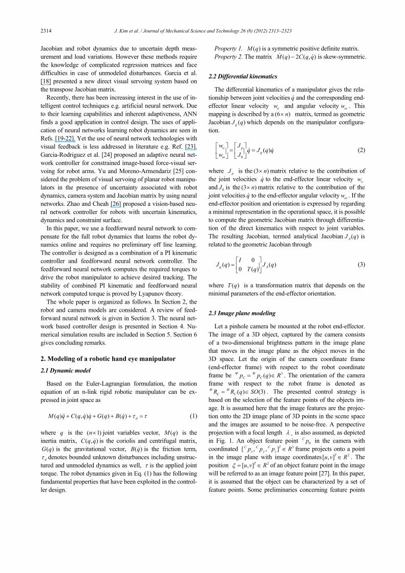
based on the selection of the feature points of the objects im-age. It is assumed here that the image features are the projec-tion onto the 2D image plane of 3D points in the scene space and the images are assumed to be noise-free. A perspective projection with a focal length λ ¸ is also assumed, as depicted in Fig. 1. An object feature point 0

C p in the camera with coordinated 3[ , , ]C C C T

x y zp p p R∈ frame projects onto a point in the image plane with image coordinates 2[ , ]Tu v R∈ . The position 2[ , ]Tu v Rξ = ∈ of an object feature point in the image will be referred to as an image feature point [27]. In this paper, it is assumed that the object can be characterized by a set of feature points. Some preliminaries concerning feature points

J. Kim et al. / Journal of Mechanical Science and Technology 26 (8) (2012) 2313~2323 2315

with moving objects are recalled below [14]. Let 3

0W p R∈ be the position of an object feature point ex-

pressed in robotic manipulator coordinate frame. Therefore, the relative position of this object feature located in the robot workspace, with respect to camera coordinate frame is [ , , ]C C C T

x y zp p p . According to the perspective projection the image feature point depends uniquely on the object feature position 0

W p and camera position and orientation, and is expressed as

C

xCC

yz

pupv p

αλξ⎡ ⎤⎡ ⎤

= = − ⎢ ⎥⎢ ⎥⎢ ⎥⎣ ⎦ ⎣ ⎦

(4)

where α is the scaling factor in pixels/m due to camera sampling and 0C

zp < . The time derivative yields

1 0.

0 1

Cx C

C xz C

yC Cz Cy

zCz

pp

pp

p pp

p

αλξ

⎡ ⎤− ⎡ ⎤⎢ ⎥

⎢ ⎥⎢ ⎥= − ⎢ ⎥⎢ ⎥⎢ ⎥⎢ ⎥− ⎣ ⎦⎢ ⎥⎣ ⎦

(5)

On the other hand, the position of the object feature point

with respect to the camera frame is given by

0( )[ ( )] .

Cx

C C W Wy W C

Cz

pp R q p p qp

⎡ ⎤⎢ ⎥ = −⎢ ⎥⎢ ⎥⎣ ⎦

(6)

Using general formula for velocity of a moving point in a

moving frame with respect to a fixed frame [28] and consider-ing a moving object, the time derivative of Eq. (6) can be ex-pressed in terms of the camera linear and angular velocities as [29]

0 0[ ( ( )) ( )]

Cx

C C W W W W Wy W C C C

Cz

pp R w p p q p vp

⎡ ⎤⎢ ⎥ = − × − + −⎢ ⎥⎢ ⎥⎣ ⎦

(7)

0

1 0 0 00 1 0 00 0 1 0

00

C C Cx z y

C C Cy z x

C C Cz y x

C WC WW C

WC WW C

p p pp p pp p p

R vR p

R w

⎡ ⎤ ⎡ ⎤− −⎢ ⎥ ⎢ ⎥= − −⎢ ⎥ ⎢ ⎥⎢ ⎥ ⎢ ⎥− −⎣ ⎦ ⎣ ⎦

⎡ ⎤ ⎡ ⎤+⎢ ⎥ ⎢ ⎥

⎣ ⎦ ⎣ ⎦

(8)

where W

Cv and WCw are the linear and angular velocity of

the camera with respect to the robot frame respectively. The movement of the feature point into the image plane as a func-tion of the object velocity and camera velocity is expressed by substituting Eq. (8) into Eq. (5) as

2 2

2 2

0

1 0

0 1

1 00

.0

0 1

C CC C Cx y Cx x z

yC C Cz z z

C C C CC Cz y x y Cx z

xC C Cz z z

Cx

CC Wz C WW C

WCC W CzW C y

Cz

p pp p p pp p p

p p p pp p pp p p

ppR v

R ppR w p

p

ξ

αλ

αλ

=

⎡ ⎤+− −⎢ ⎥⎢ ⎥− ⎢ ⎥+⎢ ⎥− − −⎢ ⎥⎣ ⎦

⎡ ⎤−⎢ ⎥

⎡ ⎤ ⎡ ⎤ ⎢ ⎥−⎢ ⎥ ⎢ ⎥ ⎢ ⎥⎣ ⎦ ⎣ ⎦ ⎢ ⎥−⎢ ⎥⎣ ⎦

(9) Finally, using Eqs. (2) and (3) we can expressξ in terms of

robot joint velocity q as

0 0 0( , , ) ( , )C C WzJ q p q J q p pξ ξ= + (10)

with

0 0

1 0( , ) .

0 1

Cx

CzC C

WC Cz y

Cz

pp

J q p Rp p

p

αλ

⎡ ⎤−⎢ ⎥

⎢ ⎥= − ⎢ ⎥⎢ ⎥−⎢ ⎥⎣ ⎦

(11)

3. Feedforward neural network

Mathematically, a two-layer feedforward neural network (Fig. 2) with n input units, m output units and N units in the hidden layer, is described by Eq. (12).

The output vector y is determined in terms of the input vector x by the formula

1 1

1,.....,N n

i ij jk k vj wij k

y w v x i mσ θ θ= =

⎡ ⎤⎛ ⎞= + + =⎢ ⎥⎜ ⎟⎝ ⎠⎣ ⎦

∑ ∑ (12)

where ( )σ ⋅ are the activation functions of the neurons of the hidden-layer. The inputs-to-hidden-layer interconnection weights are denoted by jkv and the hidden-layer-to-outputs interconnection weights by ijw . The bias weights are denoted

Fig. 1. Perspective projection.

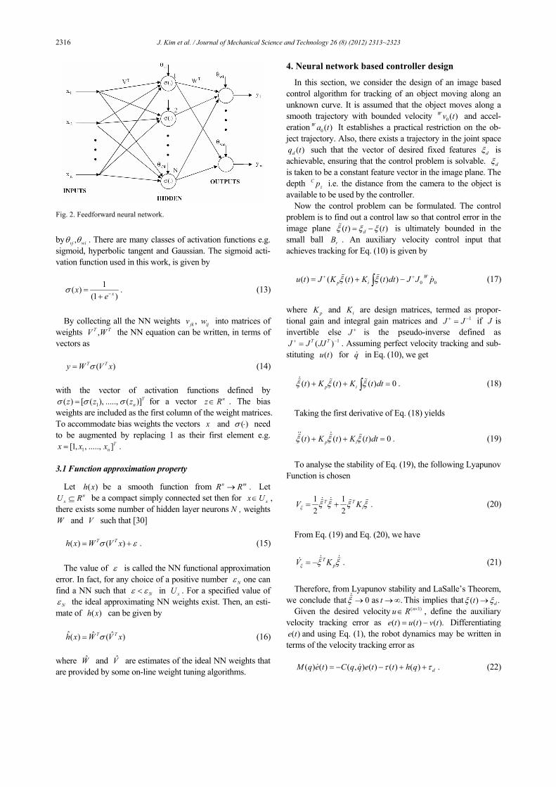
2316 J. Kim et al. / Journal of Mechanical Science and Technology 26 (8) (2012) 2313~2323

by ,vj wiθ θ . There are many classes of activation functions e.g. sigmoid, hyperbolic tangent and Gaussian. The sigmoid acti-vation function used in this work, is given by

1( ) .

(1 )xxe

σ −=+

(13)

By collecting all the NN weights ,jkv ijw into matrices of

weights ,T TV W the NN equation can be written, in terms of vectors as

( )T Ty W V xσ= (14)

with the vector of activation functions defined by

1( ) [ ( ), ....., ( )]Tnz z zσ σ σ= for a vector nz R∈ . The bias

weights are included as the first column of the weight matrices. To accommodate bias weights the vectors x and ( )σ ⋅ need to be augmented by replacing 1 as their first element e.g.

1[1, , ....., ] .Tnx x x=

3.1 Function approximation property

Let ( )h x be a smooth function from .n mR R→ Let n

xU R⊆ be a compact simply connected set then for xx U∈ , there exists some number of hidden layer neurons N , weights W and V such that [30]

( ) ( ) .T Th x W V xσ ε= + (15)

The value of ε is called the NN functional approximation

error. In fact, for any choice of a positive number Nε one can find a NN such that Nε ε< in xU . For a specified value of

Nε the ideal approximating NN weights exist. Then, an esti-mate of ( )h x can be given by

ˆ ˆ ˆ( ) ( )T Th x W V xσ= (16)

where W and V are estimates of the ideal NN weights that are provided by some on-line weight tuning algorithms.

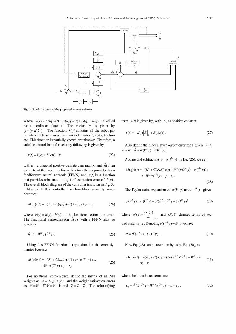
4. Neural network based controller design

In this section, we consider the design of an image based control algorithm for tracking of an object moving along an unknown curve. It is assumed that the object moves along a smooth trajectory with bounded velocity 0 ( )W v t and accel-eration 0 ( )W a t It establishes a practical restriction on the ob-ject trajectory. Also, there exists a trajectory in the joint space

( )dq t such that the vector of desired fixed features dξ is achievable, ensuring that the control problem is solvable. dξ is taken to be a constant feature vector in the image plane. The depth C

zp i.e. the distance from the camera to the object is available to be used by the controller.

Now the control problem can be formulated. The control problem is to find out a control law so that control error in the image plane ( ) ( )dt tξ ξ ξ= − is ultimately bounded in the small ball rB . An auxiliary velocity control input that achieves tracking for Eq. (10) is given by

0 0( ) ( ( ) ( ) ) Wp iu t J K t K t dt J J pξ ξ+ += + −∫ (17)

where pK and iK are design matrices, termed as propor-tional gain and integral gain matrices and 1J J+ −= if J is invertible else J + is the pseudo-inverse defined as

1( )T TJ J JJ+ −= . Assuming perfect velocity tracking and sub-stituting ( )u t for q in Eq. (10), we get

( ) ( ) ( ) 0 .p it K t K t dtξ ξ ξ+ + =∫ (18)

Taking the first derivative of Eq. (18) yields

( ) ( ) ( ) 0 .p it K t K t dtξ ξ ξ+ + = (19)

To analyse the stability of Eq. (19), the following Lyapunov

Function is chosen

1 1 .2 2

T TiV Kξ ξ ξ ξ ξ= + (20)

From Eq. (19) and Eq. (20), we have

.TpV Kξ ξ ξ= − (21)

Therefore, from Lyapunov stability and LaSalle’s Theorem,

we conclude that 0ξ → as .t →∞ This implies that ( ) .dtξ ξ→ Given the desired velocity ( 1)nu R ×∈ , define the auxiliary

velocity tracking error as ( ) ( ) ( ).e t u t v t= − Differentiating ( )e t and using Eq. (1), the robot dynamics may be written in

terms of the velocity tracking error as

( ) ( ) ( , ) ( ) ( ) ( ) .dM q e t C q q e t t h qτ τ= − − + + (22)

Fig. 2. Feedforward neural network.

J. Kim et al. / Journal of Mechanical Science and Technology 26 (8) (2012) 2313~2323 2317

where ( ) ( ) ( ) ( , ) ( ) ( ) ( )h y M q u t C q q u t G q B q= + + + is called robot nonlinear function. The vector y is given by

[ ]T T T Ty v u u= . The function ( )h y contains all the robot pa-rameters such as masses, moments of inertia, gravity, friction etc. This function is partially known or unknown. Therefore, a suitable control input for velocity following is given by

ˆ( ) ( ) ( )vt h q K e tτ γ= + − (23)

with vK a diagonal positive definite gain matrix, and ˆ( )h y an estimate of the robot nonlinear function that is provided by a feedforward neural network (FFNN) and ( )tγ is a function that provides robustness in light of estimation error of ( )h y . The overall block diagram of the controller is shown in Fig. 3.

Now, with this controller the closed-loop error dynamics becomes

( ) ( ) ( ( , )) ( ) ( )v dM q e t K C q q e t h q γ τ= − + + + + (24)

where ˆ( ) ( ) ( )h y h y h y= − is the functional estimation error. The functional approximation ˆ( )h y with a FFNN may be given as

ˆ ˆ( ) ( ).T Th y W V yσ= (25)

Using this FFNN functional approximation the error dy-

namics becomes

( ) ( ) ( ( , )) ( ) ( )ˆ( ) .

T Tv

T Td

M q e t K C q q e t W V y

W V y

σ ε

σ γ τ

= − + + +

− + + (26)

For notational convenience, define the matrix of all NN

weights as { , }Z diag W V≡ and the weight estimation errors as ˆ ˆ,W W W V V V= − = − and ˆZ Z Z= − . The robustifying

term ( )tγ is given by, with zK as positive constant

ˆ( ) ( ) ( ) .z MFt K Z Z e tγ = − + (27)

Also define the hidden layer output error for a given y as

ˆˆ ( ) ( ) .T TV y V yσ σ σ σ σ= − = − Adding and subtracting ˆ( )T TW V yσ in Eq. (26), we get

ˆ( ) ( ) ( ( , )) ( ) ( ( ) ( ))ˆ( ) .

T T Tv

T Td

M q e t K C q q e t W V y V y

W V y

σ σ

ε σ γ τ

= − + + − +

− + +

(28)

The Taylor series expansion of ( )TV yσ about ˆTV y gives

2ˆ ˆ( ) ( ) ( ) ( )T T T T TV y V y V y V y O V yσ σ σ ′= + + (29)

where ˆ

( )ˆ( )z z

d zzdzσσ

=

′ = and 2( )O z denotes terms of sec-

ond order in z . Denoting ˆ ˆ( )TV yσ σ′ ′= , we have

2ˆ ( ) ( ) .T TV y O V yσ σ ′= + (30) Now Eq. (28) can be rewritten by using Eq. (30), as

1

ˆ ˆ ˆ( ) ( ) ( ( , )) ( ) T T TvM q e t K C q q e t W V y W

wσ σ

γ′= − + + + +

+ (31)

where the disturbance terms are

2

1 ˆ ( ) .T T T Tdw W V y W O V yσ ε τ′= + + + (32)

Fig. 3. Block diagram of the proposed control scheme.

2318 J. Kim et al. / Journal of Mechanical Science and Technology 26 (8) (2012) 2313~2323

Finally, adding and subtracting ˆˆT TW V yσ ′ in Eq. (31), it is obtained

ˆ ˆ( ) ( ) ( ( , )) ( )

ˆˆ ˆ( ( )

T Tv

T T

M q e t K C q q e t W V y

W V y w

σ

σ σ γ

′= − + + +

′− + + (33)

where the modified disturbance terms are

2ˆ ( ) .T T T Tdw W V y W O V yσ ε τ′= + + +

The following bound on disturbance terms ( )w t can be

found with 0 1 2, ,c c c as positive constants [20]

0 1 2( ) ( ) .F F

w t c c Z c Z e t≤ + + (34)

4.1 Neural network weights update law

If with positive definite design parameters ,w vF G and 0κ > the adaptive neural network weight update law is

given by

ˆ ˆ ˆˆ ˆ

ˆ ˆ ˆˆ( ) .

T T Tw w w

Tv v

W F e F V ye F e W

V G y We G e V

σ σ κ

σ κ

′ ′= − −

′= − (35)

Then, the error state vector ( )e t and ,W V are uniformly

ultimately bounded (UUB) and the tracking error ( )e t can be made arbitrary small by increasing the control gains.

Proof: Let the function approximation property of FFNN

expressed by Eq. (15) hold with given accuracy Nε for all y in the compact set { : }y yU y y b= ≤ with 1y db k P> . Define

1 2{ : ( ) / }e y dU e e b k P k= ≤ − . Let (0) ee U∈ , then the function approximation property hold.

Consider the following Lyapunov function candidate

1 11 1 1( ) ( ) ( ) .2 2 2

T T Tw vL e M q e tr W F W tr V G V− −= + + (36)

The time derivative L of the Lyapunov function becomes

1 11( ) ( ) ( ) ( ) .2

T T T Tw vL e M q e e M q e tr W F W tr V G V− −= + + +

(37) Evaluating Eq. (37) along Eq. (33), we get

1

1

1 ˆ ˆ( , ) ( )2

ˆˆ ˆ( ( )) ( ) ( )

( ) .

T T T T T Tv

T T T T Tw

Tv

L e K e e C q q e e M q e e W V y

e W V y e w tr W F W

tr V G V

σ

σ σ γ −

−

′= − − + + +

′− + + + + (38)

From property 2, the matrix ( ) 2 ( , )M q C q q− is skew-

symmetric, hence

1 1( ) ( , ) ( ( ) 2 ( , )) 0 .2 2

T T Te M q e e C q q e e M q C q q e− = − =

Now Eq. (38) can be rewritten using adaptive learning rule

Eq. (35) together with ˆ ˆW W and V V= − = − ,

ˆ ˆˆ ˆ ˆ( ( ))ˆ ˆˆ ˆ( ) ( )

ˆ ˆˆ( )

T T T T T T Tv

T T T T T T T

T T T T

L e K e e W V y e W V y

e w tr W e W V y e W e W

tr V ye W V e V

σ σ σ

γ σ σ κ

σ κ

′ ′= − + + − +

′+ + − + + +

′− +

ˆ ˆˆ( ) (ˆ ˆ ˆ ˆ) (

ˆ ˆ ˆ )

T T T T T Tv

T T T T T T T T

T T T T T T

L e K e e w tr V ye W V e V

V ye W tr W e W V y e

W e W W e W V y e

γ σ κ

σ σ σ

κ σ σ

′= − + + + − + +

′ ′+ − + +

′+ −

ˆ ˆ( ) ( ) ( ) .T T T TvL e K e e w tr V e V tr W e Wγ κ κ= − + + + +

Taking norm on both sides, we get

22min ( ) ( )v MF F

L K e e w e e Z Z Zλ γ κ≤ − + + + −

2min 0 1 2

22

( ) ( )

ˆ( ) ( )

v F F

z F M MF F

L K e e c c Z c Z e

K Z Z e e Z Z Z

λ

κ

≤ − + + + −

+ + −

where min ( )vKλ is the minimum singular value of vK . The following identity is used in the derivation of the above ine-quality

2

22

ˆ( ) ( ( )) ,

.

T T

F F

MF FF FF

tr Z Z tr Z Z Z Z Z Z

Z Z Z Z Z Z

= − = −

≤ − ≤ −

Finally, choosing ZK such that 2ZK c> and using

ˆFF F

Z Z Z≤ + , the following expression is obtained

min 0 1{ ( ) ( )} .v MF F FL e K e c c Z Z Z Zλ κ≤ − − − + −

Thus, L is negative as long as the term in braces is posi-

tive. Defining 3 1 /Mc Z c κ= + and completing square terms, it is obtained

min 0 1

223 3

min 0

{ ( ) ( )}

( ) ( ) .2 4

v MF F F

v F

K e c c Z Z Z Z

c cK e Z c

λ κ

λ κ κ

− − + −

= + − − −

This is guaranteed positive as long as

either

23

0

min

4( ) e

v

c ce b

K

κ

λ

+> ≡ (39)

J. Kim et al. / Journal of Mechanical Science and Technology 26 (8) (2012) 2313~2323 2319

or 2

3 3 0 .2 4 ZF

c c cZ bκ

> + + ≡ (40)

Thus, L is negative outside a compact set. The form of

inequality shows that the control gain can be selected large enough so that 1 2( ) / .e y db b k P k< − Then, any trajectory

( )e t starting in eU ultimately lies within .eU Henceforth, according to Lyapunov theorem extension [20],

the uniform ultimate boundedness of ( )e t and F

Z is proved. Moreover, as evident from Eq. (39), the error ( )e t can be made small arbitrarily by increasing the control gain vK .

5. Simulation studies

The simulation has been performed for a three degrees of freedom microbot robot manipulator tracking an object point moving on an elliptical path as shown in Fig. 4. For explicit expression of mass matrix, coriollis and centripetal matrix, gravity terms and manipulator Jacobian, one can refer to Ref. [32]. The friction and unknown disturbances terms existing in the system are taken as

1 2( ) 5 sgn( ), 4cos(2 ), sin( ) cos(2 ),d dB q q q t t tτ τ= + = = +

3 2sin( ) .d tτ = To study the simulation results, we have considered the fol-

lowing three cases: Case 1: In this case we have used the adaptive controller. Case 2: In this case we have used the controller proposed

by Garcia et al. [18]. Case 3: In this case the proposed NN based controller has

been used. In all three cases same trajectories and same value of pa-

rameters have been used. To show the performance of all three cases Figs. 5-10 have been produced. For these figures, the following values of the parameters have been used:

1 2 3 1 2 3

2

5 , 4 , 2 , 2.5 ,

9.8 sec .

m kg m kg m kg L L L m

g m

= = = = = =

=

The camera parameters are set to be 1000 ,pixels mα = 0.01mλ = .

The gain parameters are taken as

Fig. 4. Virtual model of the robotic systems.

Fig. 5. Controller performance with adaptive controller (elliptic trajec-tory).

Fig. 6. Controller performance with adaptive controller (straight line trajectory).

Fig. 7. Controller performance with garcia et al. controller (elliptic trajectory).

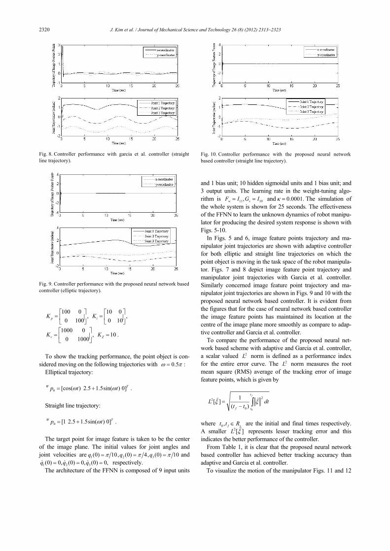
2320 J. Kim et al. / Journal of Mechanical Science and Technology 26 (8) (2012) 2313~2323

100 0 10 0, ,

0 100 0 10

1000 0, 10 .

0 1000

p i

v Z

K K

K K

⎡ ⎤ ⎡ ⎤= =⎢ ⎥ ⎢ ⎥⎣ ⎦ ⎣ ⎦⎡ ⎤

= =⎢ ⎥⎣ ⎦

To show the tracking performance, the point object is con-

sidered moving on the following trajectories with 0.5 :ω π= Elliptical trajectory:

0 [cos( ) 2.5 1.5sin( ) 0] .W Tp t tω ω= + Straight line trajectory:

0 [1 2.5 1.5sin( ) 0] .W Tp tω= + The target point for image feature is taken to be the center

of the image plane. The initial values for joint angles and joint velocities are 1 2 3(0) 10, (0) 4, (0) 10q q qπ π π= = = and

1 2 3(0) 0, (0) 0, (0) 0,q q q= = = respectively. The architecture of the FFNN is composed of 9 input units

and 1 bias unit; 10 hidden sigmoidal units and 1 bias unit; and 3 output units. The learning rate in the weight-tuning algo-rithm is 11 10,w vF I G I= = and 0.0001.κ = The simulation of the whole system is shown for 25 seconds. The effectiveness of the FFNN to learn the unknown dynamics of robot manipu-lator for producing the desired system response is shown with Figs. 5-10.

In Figs. 5 and 6, image feature points trajectory and ma-nipulator joint trajectories are shown with adaptive controller for both elliptic and straight line trajectories on which the point object is moving in the task space of the robot manipula-tor. Figs. 7 and 8 depict image feature point trajectory and manipulator joint trajectories with Garcia et al. controller. Similarly concerned image feature point trajectory and ma-nipulator joint trajectories are shown in Figs. 9 and 10 with the proposed neural network based controller. It is evident from the figures that for the case of neural network based controller the image feature points has maintained its location at the centre of the image plane more smoothly as compare to adap-tive controller and Garcia et al. controller.

To compare the performance of the proposed neural net-work based scheme with adaptive and Garcia et al. controller, a scalar valued 2L norm is defined as a performance index for the entire error curve. The 2L norm measures the root mean square (RMS) average of the tracking error of image feature points, which is given by

0

22

0

1[ ]( )

ft

f t

L dtt t

ξ ξ=− ∫

where 0 , ft t R+∈ are the initial and final times respectively. A smaller 2[ ]L ξ% represents lesser tracking error and this indicates the better performance of the controller.

From Table 1, it is clear that the proposed neural network based controller has achieved better tracking accuracy than adaptive and Garcia et al. controller.

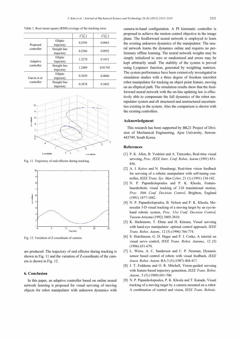
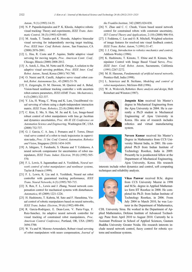
To visualize the motion of the manipulator Figs. 11 and 12

Fig. 8. Controller performance with garcia et al. controller (straight line trajectory).

Fig. 9. Controller performance with the proposed neural network basedcontroller (elliptic trajectory).

Fig. 10. Controller performance with the proposed neural network based controller (straight line trajectory).

J. Kim et al. / Journal of Mechanical Science and Technology 26 (8) (2012) 2313~2323 2321

are produced. The trajectory of end effector during tracking is shown in Fig. 11 and the variation of Z-coordinate of the cam-era is shown in Fig. 12.

6. Conclusion

In this paper, an adaptive controller based on online neural network learning is proposed for visual servoing of moving objects for robot manipulator with unknown dynamics with

camera-in-hand configuration. A PI kinematic controller is proposed to achieve the motion control objective in the image plane. The feedforward neural network is employed to learn the existing unknown dynamics of the manipulator. The neu-ral network learns the dynamics online and requires no pre-liminary offline learning. The neural network weights may be simply initialized to zero or randomized and errors may be kept arbitrarily small. The stability of the system is proved using Lyapunov function, generated by weighting matrices. The system performance have been extensively investigated in simulation studies with a three degree of freedom microbot robot manipulator for tracking an object point feature, moving on an elliptical path. The simulation results show that the feed-forward neural network with the on-line updating law is effec-tively able to compensate the full dynamics of the robot ma-nipulator system and all structured and unstructured uncertain-ties existing in the system. Also the comparison is shown with the existing controllers.

Acknowledgment

This research has been supported by BK21 Project of Divi-sion of Mechanical Engineering, Ajou University, Suwon-443749, South Korea.

References

[1] P. K. Allen, B. Yoshimi and A. Timcenko, Real-time visual servoing, Proc. IEEE Inter. Conf. Robot. Autom (1991) 851-856.

[2] A. J. Koivo and N. Houshangi, Real-time vision feedback for servoing of a robotic manipulator with self-tuning con-troller, IEEE Trans. Sys. Man Cyber, 21 (1) (1991) 134-142.

[3] N. P. Papanikolopoulos and P. K. Khosla, Feature-basedrobotic visual tracking of 3-D translational motion, Proc. 30th Conf. Decision Control, Brighton, England (1991) 1877-1882.

[4] N. P. Papanikolopoulos, B. Nelson and P. K. Khosla, Mo-nocular 3-D visual tracking of a moving target by an eye-in-hand robotic system, Proc. 31st Conf. Decision Control, Tucson-Arizona (1992) 3805-3810.

[5] K. Hashimoto, T. Ebine and H. Kimura, Visual servoing with hand-eye manipulator: optimal control approach, IEEE Trans. Robot. Autom., 12 (5) (1996) 766-774.

[6] S. Hutchinson, G. D. Hager and P. I. Corke, A tutorial on visual servo control, IEEE Trans. Robot. Automa., 12 (5) (1996) 651-670.

[7] L. Weiss, A. C. Sanderson and C. P. Neuman, Dynamic sensor based control of robots with visual feedback, IEEE Journ. Robot. Autom. RA-3 (5) (1987) 404-417.

[8] J. T. Feddema and O. R. Mitchell, Vision-guided servoing with feature-based trajectory generation, IEEE Trans. Robot. Autom., 5 (5) (1989) 691-700.

[9] N. P. Papanikolopoulos, P. K. Khosla and T. Kanade, Visual tracking of a moving target by a camera mounted on a robot: A combination of control and vision, IEEE Trans. Robotic.

Table 1. Root mean square (RMS) average of the tracking error.

21[ ]L ξ% 2

2[ ]L ξ% Elliptic

trajectory 0.2595 0.0963 Proposed controller Straight line

trajectory 0.2566 0.0952

Elliptic trajectory 1.2270 0.1631 Adaptive

controller Straight line trajectory 1.2489 0.01745

Elliptic trajectory 0.3929 0.4060 Garcia et al.

controller Straight line trajectory 0.3878 0.3842

Fig. 11. Trajectory of end-effector during tracking.

Fig. 12. Variation of Z-coordinate of camera.

2322 J. Kim et al. / Journal of Mechanical Science and Technology 26 (8) (2012) 2313~2323

Autom., 9 (1) (1993) 14-35. [10] N. P. Papanikolopoulos and P. K. Khosla, Adaptive robotic

visual tracking: Theory and experiments, IEEE Trans. Auto-matic Control, 38 (3) (1993) 429-445.

[11] M. Asada, T. Tanaka and K. Hosoda, Adaptive binocular visual servoing for independently moving target tracking, Proc. IEEE Inter. Conf. Robotic Autom., San Francisco, CA (2000) 2076-2081.

[12] L. Hsu, R. Costa and P. Aquino, Stable adaptive visual servoing for moving targets, Proc. American Contr. Conf., Chicago, Illinois (2000) 2008-2012.

[13] A. Astoli, L. Hsu, M. Netto and R. Ortega, A solution to the adaptive visual servoing problem, Proc. IEEE Inter. Conf. Robot. Autom., Seoul, Korea (2001) 743.748.

[14] O. Nasisi and R. Carelli, Adaptive servo visual robot con-trol, Robot. Autonomous Sys., 43 (2003) 51-78.

[15] E. Zergeroglu, D. M. Dawson, M. Queiroz and A. Behal, Vision-based nonlinear tracking controller s with uncertain robot-camera parameters, IEEE/ASME Trans. Mechatronics, 6 (3) (2001) 322-337.

[16] Y. Liu, H. Wang, C. Wang and K. Lam, Uncalibrated vis-ual servoing of robots using a depth-independent interaction matrix. IEEE Trans. Robotics, 22 (4) (2006) 804-817.

[17] C. Kim, E. Mo, S. Han, M. Jie and K. Lee, Image-based robust control of robot manipulators with Ima ge Jacobian and dynamics uncertainties, Proc. 4th IE EE Conference on Automation Science and Engineering, Washington DC, USA (2008) 732-737.

[18] G. J. Garcia, C. A. Jara, J. Pomares and F. Torres, Direct visal servo control of a robot to track trajectories in supervi-sion tasks, Proc. 11 Int. Conf. Control, Automation, Robotics and Vision, Singapore (2010) 1434-1439.

[19] A. Ishiguro, T. Furuhashi, S. Okuma and Y Uchikawa, A neural network compensator for uncertainties of robot ma-nipulators, IEEE Trans. Indust. Electron, 39 (6) (1992) 565-570.

[20] F. L. Lewis, S. Jagannathan and A. Yesildirek, Neural net-work control of robot manipulators and nonlinear systems, Taylor & Francis (1999).

[21] F. L. Lewis, K. Liu and A. Yesildirek, Neural net robot controller with guaranteed tracking performance, IEEE Trans. Neural Networks, 6 (3) (1995) 703-715.

[22] X. Ren, F. L., Lewis and J. Zhang, Neural network com-pensation control for mechanical systems with disturbances. Automatica, 45 (2009) 1221-1226.

[23] H. Hashimoto, T. Kubota, M. Sato and F. Harashima, Vis-ual control of robotic manipulators based on neural networks, IEEE Trans. Indust. Electron, 39 (6) (1992) 490-496.

[24] R. Garcia-Rodriguez, E. Dean-Leon, V. Parra-Vega, F. Ruiz-Sanchez, An adaptive neural network controller for visual tracking of constrained robot manipulators, Proc. American Control Conference, Portland, OR, USA (2005) 3694-3700.

[25] W. Yu and M. Moreno-Armendariz, Robust visual servoing of robot manipulators with neuro compensation, Journal of

the Franklin Institute, 342 (2005) 824-838. [26] Y. Zhao and C. C. Cheah, Vision based neural network

control for constrained robots with constraint uncertainty, IET Control Theory and Applications, 2 (10) (2008) 906-916.

[27] J. Feddema, C. Lee and O. R. Mitchell, Weighted selection of image features for resolved rate visual feedback control, IEEE Trans. Robot. Autom, 7 (1991) 31-47.

[28] J. J. Craig, Introduction to robotics mechanics and control, Addison-Wesley (1986).

[29] K. Hashimoto, T. Kimoto, T. Ebine and H. Kimura, Ma-nipulator Control with Image Based Visual Servo, Proc. IEEE Inter. Conf. Robot. Autom, Sacramento, California (1991) 2267-2272.

[30] M. H. Hassoun, Fundamentals of artificial neural networks. Prentice-Hall, India (1998).

[31] L. Sciavicco and B. Siciliano, Modeling and control of robot manipulators, McGraw-Hill (1996).

[32] W. A. Wolovich, Robotics: Basic analysis and design, Holt Reinehart and Winston (1987).

Jungmin Kim received his Master´s degree in Mechanical Engineering from the Ajou University in 2004. He is cur-rently a Ph.D student in Mechanical Engineering of Ajou University in Korea. His area of research includes robotics and virtual manufacturing system.

Naveen Kumar received his Master’s Degree in Mathematics from CCS Uni-versity Meerut India, in 2001. He com-pleted Ph.D from Indian Institute of Technology Roorkee, India in 2009. Presently he is postdoctoral fellow at the Department of Mechanical Engineering, Ajou University, Korea. His research

interests include robot dynamics and control, soft computing techniques and reliability analysis.

Vikas Panwar received B.Sc. degree from CCS University Meerut in 1998 and M.Sc. degree in Applied Mathemat-ics form IIT Roorkee in 2000. He com-pleted his Ph.D. from Indian Institute of Technology Roorkee, in 2006. From July 2004 to March 2010, he was Lec-turer in the Department of Mathematics,

CDL University Sirsa. He worked in the Department of Ap-plied Mathematics, Defense Institute of Advanced Technol-ogy Pune from April 2010 to August 2010. Currently he is Assistant Professor in School of Applied Sciences, Gautam Buddha University Greater Noida. His research interests in-clude neural network control, fuzzy control for robotic sys-tems and nonlinear systems.

J. Kim et al. / Journal of Mechanical Science and Technology 26 (8) (2012) 2313~2323 2323

Jin-Hwan Borm received his M.S. and Ph.D in Mechanical Engineering from the Ohio State University in 1985 and 1988 respectively. He is currently a pro-fessor in the Department of Mechanical Engineering of Ajou University in Korea. His area of research includes robotics and virtual manufacturing system.

Jangbom Chai received his Ph.D in Mechanical Engineering from Massa- chusetts Institute of Technology in 1993. He is currently a professor in the Department of Mechanical Engineering of Ajou University in Korea. His area of research includes dynamics and diagnostics.