Control, Models and Industrial Manipulators - DiVA Portal

Control, Models and Industrial Manipulators

Linköping studies in science and technology. Licentiate Thesis No. 1894

Erik Hedberg

Erik Hedberg

Control, Models and Industrial M

anipulators

2020

FACULTY OF SCIENCE AND ENGINEERING

Linköping studies in science and technology. Licentiate Thesis No. 1894, 2020 Department of Electrical Engineering

Linköping UniversitySE-581 83 Linköping, Sweden

www.liu.se

Linköping studies in science and technology. Licentiate ThesisNo. 1894

Control, Models andIndustrial Manipulators

Erik Hedberg

This is a Swedish Licentiate’s Thesis.

Swedish postgraduate education leads to a Doctor’s degree and/or a Licentiate’s degree.A Doctor’s Degree comprises 240 ECTS credits (4 years of full-time studies).

A Licentiate’s degree comprises 120 ECTS credits,of which at least 60 ECTS credits constitute a Licentiate’s thesis.

Linköping studies in science and technology. Licentiate ThesisNo. 1894


Erik Hedberg

[email protected]

Department of Electrical EngineeringLinköping UniversitySE-581 83 Linköping

Sweden

ISBN 978-91-7929-740-4 ISSN 0280-7971

Copyright © 2020 Erik Hedberg

Printed by LiU-Tryck, Linköping, Sweden 2020

Abstract

The two topics at the heart of this thesis are how to improve control of industrialmanipulators and how to reason about the role of models in automatic control.

On industrial manipulators, two case studies are presented. The first investigatesestimation with inertial sensors, and the second compares control by feedbacklinearization to control based on gain-scheduling.

The contributions on the second topic illustrate the close connection betweencontrol and estimation in different ways. A conceptual model of control is in-troduced, which can be used to emphasize the role of models as well as the hu-man aspect of control engineering. Some observations are made regarding block-diagram reformulations that illustrate the relation between models, control andinversion. Finally, a suggestion for how the internal model principle, internalmodel control, disturbance observers and Youla-Kučera parametrization can beintroduced in a unified way is presented.

v

Populärvetenskaplig sammanfattning

Arbetet bakom den här avhandlingen grundar sig i två huvudfrågor. Den förs-ta handlar om hur styrsystemen för industrirobotar kan förbättras. Den andrahandlar om hur man ska tänka kring modellers roll i reglering.

För att bygga en industrirobot med riktigt bra precision behövs både en bra meka-nisk konstruktion och ett bra styrsystem som kan reglera dess rörelser. Ett förbätt-rat styrssystem kan därför ge bättre precision, men också möjliggöra en lättareoch mindre kostsam mekanisk konstruktion utan att försämra precisionen.

Två aspekter på robotstyrning undersöks i den här avhandligen. Den första är såkallad skattning, att använda ytterligare sensorer för att få en bättre uppfattningom vad som händer med roboten. I det här fallet så kallade tröghetssensorer, sommäter acceleration och vinkelhastighet. Den andra handlar om reglering, om hurinformationen om robotens tillstånd ska användas för att korrigera dess rörelser.Här presenteras ett sätt att jämföra två olika metoder.

Reglerteknik beskrivs ibland som en vetenskap som handlar om att hantera infor-mation, och den hanteringen sker oftast i form av så kallade dynamiska modeller,matematiska samband som beskriver hur något förändras över tid.

En av de stora styrkorna med reglerteknik är att man kan använda mätningarfrån det styrda systemet för att minska behovet av på förhand framtagna model-ler. Det leder ibland till att den roll modeller spelar i reglering förbises. I den häravhandligen diskuteras olika exempel som kan användas för att belysa modell-konceptet i reglerteknik.

vii

Acknowledgments

This journey has been both sunshine and darkness, and I would like to thankthose who have contributed a bit of light along the way.

Martin Enqvist, for the support that kept me going, and for all the discussions.Johan Löfberg, for listening and for seeing what I see. Mikael Norrlöf, for alwaystaking the time to talk, and for the shared train rides. Svante Gunnarsson, foryour patience.

Stig Moberg and all the kind people at ABB Robotics, who welcomed me andtaught me so much about industrial robotics during lunches and fika breaks.

The fellow PhD students who made life at the division less lonely, both at workand outside of it. Your kindness and friendship have meant a great deal to me.

And of course my family and friends, for your love and support.

Linköping, November 2020Erik Hedberg

ix

Contents

1 Introduction 1

2 Industrial serial manipulators 32.1 Definition of industrial serial manipulator . . . . . . . . . . . . . . 32.2 The market for industrial robots . . . . . . . . . . . . . . . . . . . . 52.3 Anatomy of industrial serial manipulators . . . . . . . . . . . . . . 72.4 Desirable characteristics . . . . . . . . . . . . . . . . . . . . . . . . 10

3 Perspectives on control 133.1 Control as motivated action . . . . . . . . . . . . . . . . . . . . . . 143.2 Models and inversion . . . . . . . . . . . . . . . . . . . . . . . . . . 17

4 From internal model principle to Youla parametrization 234.1 Introduction . . . . . . . . . . . . . . . . . . . . . . . . . . . . . . . 234.2 Preliminaries . . . . . . . . . . . . . . . . . . . . . . . . . . . . . . . 244.3 Proposed procedure . . . . . . . . . . . . . . . . . . . . . . . . . . . 274.4 Pedagogical merits . . . . . . . . . . . . . . . . . . . . . . . . . . . . 324.5 Possible extensions . . . . . . . . . . . . . . . . . . . . . . . . . . . 33

5 Case study: Tool position estimation using inertial measurements 375.1 Introduction . . . . . . . . . . . . . . . . . . . . . . . . . . . . . . . 375.2 Related work . . . . . . . . . . . . . . . . . . . . . . . . . . . . . . . 385.3 System overview . . . . . . . . . . . . . . . . . . . . . . . . . . . . . 385.4 Estimation methods . . . . . . . . . . . . . . . . . . . . . . . . . . . 395.5 Trajectories . . . . . . . . . . . . . . . . . . . . . . . . . . . . . . . . 415.6 Experimental results . . . . . . . . . . . . . . . . . . . . . . . . . . 445.7 Discussion . . . . . . . . . . . . . . . . . . . . . . . . . . . . . . . . 455.8 Conclusions . . . . . . . . . . . . . . . . . . . . . . . . . . . . . . . 46

6 Case study: Feedback linearization compared to LQ-control 476.1 Introduction . . . . . . . . . . . . . . . . . . . . . . . . . . . . . . . 476.2 Simulation model . . . . . . . . . . . . . . . . . . . . . . . . . . . . 496.3 Control Design . . . . . . . . . . . . . . . . . . . . . . . . . . . . . . 50

xi

xii Contents

6.4 Experimental evaluation . . . . . . . . . . . . . . . . . . . . . . . . 546.5 Results . . . . . . . . . . . . . . . . . . . . . . . . . . . . . . . . . . 556.6 Discussion . . . . . . . . . . . . . . . . . . . . . . . . . . . . . . . . 556.7 Conclusions . . . . . . . . . . . . . . . . . . . . . . . . . . . . . . . 58

Bibliography 59

1Introduction

Good control systems are fundamental to high-performing industrial manipu-lators, and good models are fundamental to well-functioning control systems.These two observations motivate the work presented in this thesis.

Industrial manipulators

Chapter 2 gives a general overview of industrial manipulators. A case study on es-timation for industrial manipulators using inertial sensors is presented in Chap-ter 5, where a complementary filter and a Kalman filter are compared. Chap-ter 6 compares linear quadratic control design based on Jacobian linearizationand feedback linearization respectively.

Models and control

The great power of feedback is that one can do control without accurate a priorimodels of the controlled process. Because of this, the role of models in controlis sometimes downplayed. Chapter 3 tries to put the role of models in perspec-tive, and offers a discussion on the nature of control as well as some illuminatingblock diagram reformulations. Chapter 4 offers a suggestion for how the internalmodel principle, internal model control, disturbance observers and Youla-Kučeraparametrization can be taught in a unified way.

1

2Industrial serial manipulators

This chapter gives an introduction to industrial robots, in particular to so calledserial manipulators. First we introduce some terminology, followed by a briefoverview of the market for industrial robots and common applications. Then wediscuss how industrial serial manipulators (ISM) are commonly designed, andrelate this to what characteristics are desirable for an ISM.

2.1 Definition of industrial serial manipulator

The term robot is used to denote many things, from humanoid machines to pro-grammable industrial tools to computer programs.

In this thesis, robot is used in the sense given by ISO 8373 [2012], an interna-tional standard entitled Robots and robotic devices — Vocabulary. This standardis endorsed by the International Federation of Robotics (IFR), an industry associ-ation counting all major manufacturers of industrial robots as members.

The following definitions are taken from ISO 8373, with minor changes for read-ability. First the standard defines robot as a physical mechanism.

Robot — Actuated mechanism programmable in two or more axeswith a degree of autonomy, moving within its environment, to per-form intended tasks.

Then it introduces two main categories, industrial and service robots.1

1An alternative categorization, jokingly used by some industrial robot researchers, is industrialrobotics and spectacular robotics.

3

4 2 Industrial serial manipulators

Industrial robot — Automatically controlled, reprogrammable, mul-tipurpose manipulator, programmable in three or more axes, whichcan be either fixed in place or mobile for use in industrial automationapplications.

Service robot — Robot that performs useful tasks for humans or equip-ment, excluding industrial automation applications.

In the definition of industrial robot, we see that it is defined as a manipulator,which is also defined by the standard.

Manipulator — Machine in which the mechanism usually consists ofa series of segments, jointed or sliding relative to one another, for thepurpose of grasping and/or moving objects (pieces or tools) usuallyin several degrees of freedom.

It is worth noting that in their report World Robotics 2019 - Industrial Robotsthe IFR, which has been compiling statistics on the robot market for decades,lists several types of machines that would seemingly fit the above definition ofindustrial robot, but which the IFR does not consider as such for the purposes oftheir report, see IFR [2019].

Finally, most practitioners likely have little interest in an exact definition of whatis to be considered or not an industrial robot, and treat the question on a basis of"I know it when I see it"2.

2.1.1 Categorization of industrial robots

The IFR states that "In agreement with the robot suppliers, robots should be clas-sified only by mechanical structure as of 2004", and provides the following defi-nitions.

Articulated robot — A robot whose arm has at least three rotaryjoints.

Cartesian robot — Robot whose arm has three prismatic joints andwhose axes are correlated with a cartesian coordinate system.

SCARA3 robot — A robot, which has two parallel rotary joints to pro-vide compliance in a plane.

Parallel/Delta robot — A robot whose arms have concurrent pris-matic or rotary joints.

Cylindrical robot — A robot whose axes form a cylindrical coordinatesystem.

2A phrase popularized by the US Supreme Court in a case of trying to determine whether a givenmovie qualified as pornographic or not, see e.g. Gewirtz [1996].

3SCARA is sometimes read as Selectively Compliant Articulated Robot Arm, which would then beslightly inconsistent with the above definition of ’articulated’ robot.

2.2 The market for industrial robots 5

In this thesis we have chosen to use the term ’industrial serial manipulator’ as areasonable compromise between specificity and convenience. Let us define it asfollows.

Definition 2.1. Industrial serial manipulator (ISM)An industrial serial manipulator is an articulated industrial robot, consisting ofa series of rigid segments connected by actuated rotary joints.

2.2 The market for industrial robots

The IFR, as an interest organisation for manufacturers of robots, has as one of itsmain purposes to collect and compile statistical data from national associationsas well as individual member companies. The details in the following section arebased on the publicly available parts of the report by IFR [2019].

2.2.1 Customers and market size

The automotive sector has long been the largest adopter of industrial robots, al-though the electronics industry has almost caught up in recent years. This can beseen in Table 2.1, where IFRs categorization of robot installations in 2018 accord-ing to industry4 is roughly reproduced.

Table 2.1: Share of new robot installations in 2018.Industry Share

Automotive 30%Electronics 25%Metal and machinery 10%Plastic and chemical 5%Food 2%Others 10%Unspecified 18%

According to the aforementioned report, around 420 000 industrial robots wereinstalled during 2018, an increase of 6% compared to 2017. The number of newinstallations is reported to have grown on average 19% yearly between 2013 and2018.

Using an estimated average robot service life of 12 years5, the IFR calculates thatthere are currently 2.7 million industrial robots deployed worldwide, based on

4Based on the wonderfully named International Standard Industrial Classification of All EconomicActivities (ISIC), maintained by the Statistics Division of the United Nations (UNSD).

5Based on a study carried out in 2000 by the United Nations Economic Commission for Europetogether with the IFR.


previously reported installations. The report however also notes that there aresome indications that this service life estimate could be too conservative, andthat some tax authorities on the other hand calculate with a service life of fiveyears.

2.2.2 Common applications

The perhaps most common view of industrial robots among the public is as re-placement for human labor, but to a large degree they are also a replacement forother machines with a narrower range of applications. While industrial robotsmight require a larger initial investment, their multipurpose nature can allow forfaster and cheaper reconfiguration of production lines, or even enable manufac-turing of heterogeneous product models on a single production line.

Industrial robots are used for a wide variety of tasks, as exemplified by the de-tailed classification of applications used by the IFR, briefly summarized below:

• Handling and machine tending, such as palletizing, packaging, picking andplacing, metal casting, plastic moulding, inspection and testing.

• Welding and soldering, such as arc-, laser-, ultrasonic-, or plasma-welding.

• Dispensing, such as painting, sealing and coating.

• Processing, such as laser or water cutting, grinding, milling and polishing.

• Assembling and disassembling.

• Cleanroom use, for flat panel displays and semiconductors.

The flexibility to tackle such a wide variety of tasks comes not only from a ver-satile mechanical structure and exchangeable tools, but also from software thatmakes it easy for the customer to program the robot for various use cases.

2.2.3 Software

All major robot manufacturers offer software packages both for facilitating gen-eral deployment, programming and operation of robots and to provide special-ized functionality tailored to certain applications.

In addition to programming the motion of individual robots, it is also importantto provide software that support the design, visualization and simulation of en-tire production cells where robots and other machines work in synchronization.

Some examples of applications for which manufacturers offer specific softwarepackages are picking and placing of items on conveyor belts, spot welding, lasercutting, palletizing and painting.

2.3 Anatomy of industrial serial manipulators 7

2.3 Anatomy of industrial serial manipulators

As previously defined, a serial manipulator consists of a series of more or lessrigid segments, referred to as links, connected by rotary joints.

2.3.1 Joint configurations

The number of joints determine the degrees of freedom (DOF) of the manipulator,which in turn is an upper limit on the degrees of freedom with which the tool atthe end of the manipulator can be positioned.

Thus, six degrees of freedom are required to freely choose position and orienta-tion, collectively referred to as pose, of the tool, and therefore most ISMs featuresix joints. The point on the tool for which the position is specified is usuallycalled the tool center point (TCP). Some applications do not require full 6 DOFpositioning, e.g., when stacking products on a pallet it is often enough to onlycontrol position and orientation around the vertical axis.

The most common configuration of the first three joints is the so-called elbow-configuration, where the first joint rotates around the vertical axis and the twosubsequent joints have axes of rotation that are parallel to each other and to thehorizontal plane.

For 6-DOF manipulators, the last three joints are almost always in a so-calledspherical wrist configuration. This means that their axes of rotation always inter-sect in a common point, referred to as the wrist center point (WCP).

The main appeal of the spherical wrist configuration is that it simplifies the so-called inverse kinematics problem of finding joint angles corresponding to a de-sired TCP pose. One can first use the orientation to solve for the ’wrist angles’,and then the position to solve for the ’elbow angles’.

2.3.2 Physical characteristics

The size of the links, together with the placement of the joints, determines whichend-effector poses are attainable, and the set of such poses is called the robotworkspace. Often the (maximum) reach of the robot is used as a proxy for thesize of the workspace. Most industrial robots have a reach in the range of 0.5 to 4meters.

The maximum load that a robot model can lift while sustaining a given level ofperformance is often referred to as the (maximum) payload of that model. Mostmajor robot manufacturers offer models with payloads in the range of 3 to 600kg, with some offering maximum payloads as high as 1500 or even 2300 kg.

The links are most often constructed out of metal to make sure that the structureis as rigid as possible. In so-called collaborative robots, where safety dictatesthat the kinetic energy of the links be limited, plastic is often used to reduce theweight of the links.


Table 2.2: Range of maximum payload and reach for industrial serial manip-ulators, as listed online by manufacturers. Definitions of reach and payloadvary between manufacturers, so numbers should be considered as approxi-mate. Data collected from manufacturer websites during summer of 2020.

Manufacturer Payload [kg] Reach [m] Company origin

Fanuc 4 - 2300 0.55 - 4.7 JapanKawasaki 3 - 1500 0.5 - 4 JapanKUKA 2 - 1200 0.5 - 4 GermanyNachi 1 - 1000 0.35 - 4 JapanABB 0.5 - 800 0.48 - 4.2 SwedenYaskawa 0.5 - 800 0.35 - 4 JapanComau 3 - 650 0.63 - 3.7 ItalyHyundai 6 - 600 0.93 - 3.5 South KoreaStäubli 2.3 - 190 0.52 - 3.7 SwitzerlandPanasonic 4 - 22 1.1 - 2.7 JapanShibuara Machines 3 - 20 0.6 - 1.7 JapanYamaha 1 - 20 0.9 - 1.5 JapanUniversal Robotics 3 - 16 0.5 - 1.3 DenmarkDoosan 6 - 15 0.9 - 1.7 South KoreaOmron 4 - 14 0.65 - 1.3 JapanMitsubishi 3 - 12 0.5 - 1.4 JapanEpson 2.5 - 12 0.45 - 1.4 JapanDenso 0.5 - 12 0.43 - 1.3 Japan

There are a few industrial robot models where the links are partly manufacturedfrom carbon fiber to decrease weight while maintaining high stiffness. Carbonfiber is however less favourable in other respects such as cost and durability, lim-iting its success as a material for industrial robots.

Table 2.2 lists some manufacturers of industrial serial manipulators, and theavailable range of maximum payload and reach in the models presented on thecompany website. The companies that offer robots with payloads above 100 kgcan be considered prominent manufacturers of traditional industrial robots. Uni-versal Robotics is a well-known manufacturer of collaborative robots.

2.3.3 Actuation

Modern robots are practically always actuated by electric motors, and in generalthe control of the electrical current that generates the motor torque is fast enoughthat the motors can, for most purposes, be approximated as generating instanta-neous torque.

The most straightforward way of actuating all joints is to place a motor at eachjoint. However, keeping the mass and the amount of cabling at the outer linkslow is usually advantageous for performance. Therefore it is not uncommon to

2.3 Anatomy of industrial serial manipulators 9

supply mechanical power for subsequent joints by some transmission mechanismbuilt into a link.

In general, industrial robots use a geared transmission between motors the andsubsequent links, with gear ratios commonly in the double or triple digit region.Rarely are joints actuated with so-called direct drive, where one revolution of themotor is equal to one revolution of the actuated joint.

A higher gear ratio offers several advantages, most notably it allows for largertorques and better precision. The major drawback is that gearboxes invariably in-troduces additional flexibility into the manipulator, as well as friction and back-lash. For this reason good gearboxes, and good models of them, are crucial forhigh-performing manipulators.

2.3.4 Sensors

To estimate the position of the end-effector, most industrial robots use only mea-surements of the motor angles, which by virtue of the high gear ratio gives goodstatic precision but requires accurate gearbox models to estimate the dynamicbehaviour correctly. There are some commercial offerings that use additional sen-sors, such as a secondary encoder to directly measure the arm angle, i.e. the angleafter the gearbox, or an inertial measurement unit (IMU) to measure vibrationsand adjust the program to reduce them. In applications where the tool needs toapply pressure to a work object, force sensors are sometimes installed as a part ofthe tool.

For an academic robot researcher, additional sensors hold the promise of in-creased control performance. For an industrial robot designer, more sensors alsomean higher cost, additional design complexity and more components that canmalfunction.

2.3.5 Control cabinet

It is common to place part of the robot control system and power supply electron-ics in a separate cabinet. Such cabinets can often control several robots as well asother machines. One benefit of this separation is that placing the cabinet out ofreach from the robot assures it can be safely accessed.

2.3.6 Specializations

One example of adaptation for specific industry is the use of food-grade oil inrobots for use in food-processing, such that any leakage does not contaminatethe products. Another is robots for spray painting, which need to be carefullysealed so that paint does not enter sensitive parts of the robot as well as built sothat the risk of causing sparks that can ignite the aerosol paint is minimized.


2.4 Desirable characteristics

The wide variety of tasks for which robots are used require designers to considermany aspects of what it means for a robot model to perform well.

2.4.1 Motion performance

The most obvious criteria for a good industrial robot is that it should closelyfollow the movements we specify.

To get a feel for how such motion performance is measured, it is instructive tolook at the standard ISO 9283 [1998], Manipulating industrial robots — Perfor-mance criteria and related test methods, which specifies the following perfor-mance characteristics:

• Pose accuracy

• Pose repeatability

• Multi-directional pose accuracyvariation

• Distance accuracy

• Distance repeatability

• Position stabilization time

• Position overshoot

• Drift of pose characteristics

• Exchangeability

• Path accuracy

• Path repeatability

• Path accuracy on reorientation

• Cornering deviations

• Path velocity characteristics

• Minimum posing time

• Static compliance

• Weaving deviations

Accuracy means that the result is close to what is specified in the program, whilerepeatability means that the result is similar every time the programmed actionis performed, as illustrated in Figure 2.1.

Accuracy can be relative to a given TCP position or relative to the base of therobot, and by extension to the ’world frame’. The former can be referred to as rel-ative accuracy and the latter as absolute accuracy. Lack of accuracy can in someapplications easily be compensated with manual adjustment, while in others itis critical that the tool can be positioned accurately based solely on coordinatessupplied programmatically.

Repeatability is in general rather good with most industrial manipulators. Ina brief survey of online catalogues, manufacturers claim static repeatability be-tween 0.05 and 0.5 mm for most of their models. Static repeatability is mainly aproperty of the mechanical construction, and can hardly be improved by a con-trol system without additional sensors.

In contrast, good accuracy requires careful calibration and software compensa-tion. Measures of accuracy rarely seem to figure in advertising material, and

2.4 Desirable characteristics 11

(a) Low accuracy,good repeatability

(b) Better accuracy,worse repeatability

Figure 2.1: Some applications require good repeatability while other needhigh accuracy. If accuracy is measured in relation to another position of theend-effector we call it relative accuracy, if it is in relation to the robot basewe call it absolute accuracy.

many suppliers offer additional services or solutions for customers who requirehigh accuracy.

2.4.2 Other characteristics

Cost

The cost to purchase a manipulator is of course a crucial factor for commercialsuccess, it was for example reported as the biggest barrier to robot adoption ina survey of 85 companies across various industries, see McKinsey & Company[2019]. From an engineering perspective, the cost of manufacturing a manipula-tor is closely related to the quality of the control system, as good motion controlwill to some degree allow for a less expensive mechanical construction withoutloosing performance.

Ease of use

Configuring and programming robots can be quite time consuming, and ease ofuse is a characteristic that has a direct and non-negligible impact on the total costof installing and operating a robot.

Robustness

A good industrial robot design should be robust, in a broad sense of the word,to make it cost-efficient to manufacture and to allow users to obtain good perfor-mance without expert knowledge.

For example it should ideally be robust with regards to manufacturing tolerancesin the mechanical components, to wear in said components over time, to the wayit has been mounted, to additional cabling mounted on the links, to changes intemperature, to imperfect load information and to suboptimal tuning.


Finding a good balance between best case performance and robustness is an im-portant consideration, especially in designing the control system of the robot.

Safety

Safety is both important and difficult, but easily forgotten in an academic setting.When installing and operating robots, substantial effort is required to ensure thatthe risk of human injury is minimized.

Safety is primarily achieved by fencing off the robot cell and making sure thatthe robot stops whenever anyone enters the cell. But if the robot system itselfcan be made safer, the need for costly external safety measures and proceduresis reduced. This is one of the key selling points of so-called collaborative robots,or ’cobots’, which are meant to work alongside human workers without requiringextra safety measures.

3Perspectives on control

This chapter introduces a model of control which can be used to emphasize therole of models and the human aspect in control engineering, as well as someblock diagram reformulations that can be used to illustrate the relation betweenmodels, control and inversion.

Readers looking for an introduction to automatic control are well served by thetextbook Feedback Systems by Åström and Murray [2008], a modern text withemphasis on fundamental concepts, also freely available from the authors’ web-site. A more traditional as well as comprehensive, but equally solid and insight-ful, textbook is Control System Design by Goodwin et al. [2001]. The tutorialarticle Feedback for physicists by Bechhoefer [2005] offers a concise but rich in-troduction.

Figure 3.1: The word control can mean several things. At the heart of everycontrol loop are the beliefs and desires of the designer.

13

14 3 Perspectives on control

3.1 Control as motivated action

3.1.1 Definition

The following four definitions together form a simple model that gives a possibledefinition of "control" as an activity and the main characteristics of that activity.

Definition 3.1 (Control).Performing control means taking motivated action.

Definition 3.2 (Motivated action).An action is motivated if it is based on a desire, and on a belief of how the actionwill affect the fulfillment of the desire.1

Definition 3.3 (Desire).A desire is a combination of a model and a measure of similarity.

Definition 3.4 (Belief).A belief is a combination of a model and a degree of confidence.

Automatic control, which we might also call engineered control (or perhaps ar-tificial control, in keeping with the times), could then be defined as the art andscience of encoding beliefs and desires into a decision making mechanism.

This model, which we could call the desire-belief model, might seem too broador too toy-like to be of any use in an engineering context. I believe however that,thanks to its compactness, it can serve as a tool for highlighting two importantaspects of automatic control when discussing or teaching. And to quote Ljung[1999], our acceptance of models should be guided by "usefulness" rather than"truth".

First, with the choice of words it emphasizes the human component in control.Second, it emphasizes the role of models, especially the fact that models are usedto represent both what we want and what we think we know.

3.1.2 The human component

In the above definition, the words desire and belief are chosen because they havea decidedly human ring to them. The purpose of this is to emphasize the in-evitable human component in control engineering, a perspective that is easier tooverlook when using words with a more technical flavour, such as objective ormodel.

1This definition is taken more or less directly from the so called Humean theory of motivation,due originally to David Hume. See e.g. Smith [1987].

3.1 Control as motivated action 15

One can argue whether machines are capable of harbouring desires and beliefs,but as long as control is a human endeavour, human desire and belief will be aninevitable part of control.

Take for example the design of an industrial manipulator with automatic motioncontrol. No matter how ingenious the control design is, there will always existtrade-offs between different aspects of system performance. And to decide whatbalance best suits the customer’s desires requires an operator with an understand-ing both of the customer’s needs and of the industrial manipulator.

This example also an illustrates the multi-layered nature of control, where theoperator is part of a tuning process that controls the robot control system. Usingthe broad definition of control introduced previously, one can frame every auto-matic controller as being part of a larger control process, which is in turn partof an even larger process et cetera. The innermost processes might be well de-scribed by technical models, but as the perspective broadens a purely technicaldescription becomes less and less feasible.

In the above the definition of belief the human component is also illustrated bythe division into model and confidence. It emphasizes the fact that no matter howwell our models perform in experiment, in the end we have to use our judgmentto decide how confident we are in the model.

One could argue that our confidence in the model could be regarded as part ofthe model, perhaps quantified by some measure of probability. But by clearlyseparating the concept of a plant model, which might be probabilistic or not,and our confidence in it, the role of human judgment in automatic control ishighlighted.

Ultimately this can be related to a fundamental problem in philosophy of science,the problem of induction, described in e.g. Henderson [2020]. In short, how canwe be sure that the sun will rise tomorrow? Since we cannot formally prove thatit will, our certainty that it will indeed rise has to come in some part from humanjudgment, and not solely from formal reasoning.

The division of desire into model and similarity tries to capture the fact that itcan sometimes be quite straightforward to describe the result one would ideallylike to have, but more difficult to rank suboptimal results in order of desirabil-ity. This leads to situations where some degree of the desired behaviour can becaptured by formal specifications such as objective functions and mathematicalmodels, but where the final measure of desirability is expressed through the judg-ment of a skilled operator tuning the control system.

3.1.3 The dual role of models

The second benefit of using the proposed definition of control is that it empha-sizes the two-fold role of models; they express both what we believe about thesystem and how we would like it to behave2.

2And as Willems [2007] would phrase it, the behaviour is all there is.


These two roles and their interplay is efficiently illustrated by the verb "to expect".Consider the following sentence:

"I expect this to be done by tomorrow."

This can be interpreted as an estimate, an answer to the question when somethingwill be done. But it can equally be seen as a demand, as a command from someonewho wants something done by tomorrow.

Especially the latter interpretation is interesting from a control perspective, asupon further consideration it is not purely a demand. When a proficient managertells her subordinate "I expect you to finish by tomorrow", it is part demand andpart estimate; the statement expresses a belief that the employee is capable offinishing the task by tomorrow.

In an ideal case, we can represent these two roles by two separate structures, asdepicted in Figure 3.2. Here the first structure contains a model of our desire, andfeeds a suitable representation of it into the second structure, which contains ourbelief of how to choose the plant input in order to get the desired output, i.e. to"invert" the plant.

Pr P−1 P

Figure 3.2: In an ideal control scenario, we have a model of what we want,Pr , and an other model, P−1, of how to invert the plant P perfectly.

Note that in such an ideal scenario, if our desire for the system behaviour changes,we would only have to change parameters in the first structure to reflect this.However, such an ideal separation is rarely possible since it would require perfectinversion.

If we have to approximate the inversion, the choice of approximation will impactthe system behaviour. It should thus be chosen to reflect our desire as well asour belief. Since in practice all inverses of dynamical systems are approximate,this point is important to keep in mind when interpreting control schemes thatinvolve explicit plant models.

One example is the so called internal model control (IMC) scheme, depicted inFigure 3.3. At a first glance, it might look like there is a clear division of roles,where P represents our belief of how the plant functions while the parametersrepresenting our desired system behaviour would be in Q. But upon furtherconsideration it is not certain that a more accurate3 model P in this scheme willyield a more desirable behaviour for a given Q.

When a model is used to predict the plant behaviour, and the controller is fash-ioned to counteract all unexpected behaviour, the result is not only rejection of

3We have not touched upon the question of how to measure or rank the correctness of variousbeliefs, but arguably the measure of similarity used to compare actual behaviour to desired behaviourcan also be used to compare actual behaviour to predicted behaviour.

3.2 Models and inversion 17

Pr Q P

Pm

−

−

Figure 3.3: The so called internal model control scheme, here depicted withan explicit model for the reference signal.

exogenous disturbances but also an element of model following. The controller isin a sense trying to suppress the differences between how the plant and the modelrespond to inputs, whether this difference is a result of exogenous (unmodeled)disturbances or of incorrectly modeled plant dynamics.

Thus by using an incorrect model inside the feedback loop, the plant behaviourcan be shifted towards that of the model. If the model is used outside of thefeedback loop, as illustrated in Figure 3.4, there is model following in the senseof tracking the model output.

Emphasizing this dual role of models is also a question of emphasizing the role ofmodels in general. In feedforward control, where the controller does not receivemeasurements from the controlled process, it is clear that explicit models for theprocess are needed.

The role of models in feedback control is less obvious, and indeed one of themain benefits of feedback control is that it reduces the need for a priori models.Because of this, the role of models in feedback control is sometimes downplayed,with some researchers even labeling their methods as "model-free control", likeFliess and Join [2013]4.

One could take the view that the fundamental need for models is not reduced infeedback control, but rather that the burden is shifted from using a "synthetic"model to using the actual plant as a "real" model. This perspective is illustratedin the following section.

3.2 Models and inversion

In the previous discussion, the term model was used in a rather general sense.In automatic control terminology, a model is typically understood to mean a rep-resentation of the (causal) input-to-output relation, while a representation thatdescribes the (non-causal) relation output-to-input is referred to as an inversemodel. The former is sometimes referred to as a forward model for the sake ofclarity, while the later is sometimes just called an inverse.

It is often pointed out that the concept of inversion is at the heart of automatic

4Although they describe their method by stating that "the unknown ‘complex’ mathematicalmodel is replaced by an ultra-local model".


Model system

Given system

Compensator

−

⇐⇒

Model system Compensator Given system−

Figure 3.4: A "model following control system", at the top as depicted in thetextbook by Wolovich [1974], and at the bottom in a perhaps more familiar"feedforward form".

control, and that an approximate inverse can be obtained by using feedback froma forward model, see e.g. Chapter 2 in Goodwin et al. [2001].

3.2.1 Complementary filter interpretation of IMC

A corollary of this is that any standard error feedback control loop can be refor-mulated as feedforward control where a perfect model is used in the approximateinverse. This, together with a way of mixing the two formulations, is illustratedin Figure 3.5.

This "mixing" structure, a so called complementary filter, where the two blocksH and 1 − H sum to unity, becomes interesting when we consider the use of animperfect forward model P. In that case, which is illustrated in the top diagramof Figure 3.6, the complementary filter weights together a measured output fromthe true plant P and a predicted output from the model P.

This can be compared to the reformulation of a state-space observer as two trans-fer functions, one from the input to the estimate, T1, and one from the output tothe estimate, T2. The estimate is then unbiased in the sense that

C(T1 + T2P) = P, (3.1)

where C is the state-to-output mapping of the state space form of P. For detailssee e.g. Goodwin et al. [2001]. In this comparison, T2 would correspond to H andT1 to (1 − H)P.

More interesting to note however, is how straightforward it is to transform thiscomplementary filter scheme into an equivalent internal model control scheme,following the steps depicted in Figure 3.6. This offers an intuitive interpretation


Pr C P−

⇐⇒

Pr C

P

P−

⇐⇒

Pr C

1 − H P

P

H

−

Figure 3.5: These reformulations illustrate how a regular control loop canbe interpreted as inversion by means of feedback of a perfect model of theplant P, or as a mixture of both. Note that they do not require P to have anyparticular properties, such as for example linearity.

of the IMC-parameter Q as consisting of an approximate inverse F and a filter H ,that is

Q = FH, (3.2)

where H represents our trust in the measurements of the plant output comparedto the output predicted by our model. If H = 1 we only trust the measurements,and if H = 0 we only trust the model.

3.2.2 Complementary filter interpretation of error feedback

One can use the complementary filter idea for another, perhaps less insightful,but nonetheless interesting, reinterpretation of a standard error feedback loop.The idea is to factorize the controller into an approximate inverse and a filter,similar to how Q was interpreted in the previous section,

C = HP−1, (3.3)

and then use the filter part H to reinterpret the error fed to the controller as thedifference between the reference and the output of a complementary filter fusingthe plant output with the reference. This is illustrated in Figure 3.7.

The intuition is that H represents how much we trust the measured plant out-put compared to how strong our belief is that the plant will follow the reference


Pr C

1 − H P

P

H

−

⇐⇒

Pr C

P

P

P

H

− −

−

⇐⇒

Pr F P

P

H

−

−

⇐⇒

Pr F P

P

Q

−

−

Figure 3.6: Starting from the concept of using a complementary filter toweight together feedback from the real plant P and a model P, one can arriveat the familiar IMC structure. The last step requires additivity from theapproximate inverse F, which is present if C and P are linear.


without the intervention of feedback. The latter can be a reasonable belief forexample in the presence of additional feedforward control. Since the reformula-tion in Figure 3.7 already contains an approximate inverse, adding feedforwardrequires little modification, as illustrated by Figure 3.8.

3.2.3 Inversion of affine functions

When control is described as being about inversion, the prime example is in-version of so called transfer functions, which are used to describe linear time-invariant dynamical systems. For a linear transfer function, P, we have

Y = PU, (3.4)

and inversion comes in the form of a multiplicative inverse, P−1,

P−1Y = U, (3.5)

just like for any other linear function.

However, it is not often pointed out that when we model plants with exogenousdisturbances, we mostly model them as affine functions,

Y = PU + Pd, (3.6)

as illustrated in Figure 3.9.

Likewise, when we talk about controlling a plant modeled by an affine transferfunction, rarely do we explicitly mention inversion, opting instead to talk aboutcanceling of the disturbance. It might be worthwhile to sometimes use the word-ing that inverting an affine function,

P−1(Y − Pd ) = U, (3.7)

necessitates an additive inverse as well as a multiplicative one, as illustrated inFigure 3.10. This can serve as a good starting point for discussing how schemeswith forward or inverse models, such as the one depicted in Figure 3.6, can beadapted to affine plants.

This observation was inspired by the block diagram transformation tables pre-sented in the textbook by Oppelt [1964].


Pr C P−

C = HP−1

⇐⇒

Pr

1 − H

P−1

H

P−

Figure 3.7: Error feedback from a directly measured output can be reinter-preted as feedback from the output of a complementary filter which fusesthe reference and the measured output. This emphasizes the role of the con-troller as both a filter and as an inverse.

Pr 2

1 − H

P−1

H

P−

Figure 3.8: Adding feedforward to the scheme in Figure 3.7 is straighfor-ward since an approximate inverse P−1 is already present. At frequencieswhere we trust the feedforward more than the feedback, H should have asmall amplitude.

Pd

P

Figure 3.9: An affine transfer function.

Pd

P−1−

Figure 3.10: The inverse of an affine transfer function.

4From internal model principle to

Youla parametrization

This chapter introduces a line of reasoning that can be used as inspiration forteaching the Youla-Kučera parametrization (YKP), also known as Youla parametriza-tion. The chapter is a somewhat revised and extended1 version of a paper byHedberg et al. [2020] presented at the 21st IFAC World Congress.

4.1 Introduction

The Youla-Kučera parametrization of all stabilizing controllers for a given lineartime-invariant system is an important result in control theory and often appearsin courses on the subject. For stable plants, the YKP takes on a particularly simpleform, and it is therefore often first introduced to students in that setting.

For unstable plants, the formulations become more involved and the transitionfrom the stable case can be perceived as difficult to follow by some students. Espe-cially the multivariable case, where the concept of coprime matrix factorizationis an important tool, can pose difficulties.

The proposed line of reasoning, illustrated in Figure 4.1, takes as point of depar-ture the internal model principle (IMP), which can be a useful conceptual toolfor students when reasoning about control. Then two alternative controller struc-tures, both using a model of the plant, are introduced; internal model control(IMC) and disturbance observer (DOB). These two structures are used to intro-duce a more general structure, based on factorization, which provides a naturalbridge to the general formulation of the YKP.

1Most notably the addition of section 4.5.3, and some additions to sections 4.2.1, 4.4 and 4.5.2.

23

24 4 From internal model principle to Youla parametrization

Figure 4.1: The internal model principle (IMP) is used to introduce inter-nal model control (IMC) and disturbance observer (DOB). Comparing thesecontrol structures naturally leads to the concept of factorization, which is abridge to the general Youla-Kučera parametrization (YKP).

4.2 Preliminaries

4.2.1 The internal model principle

The internal model principle (IMP) is the idea that in order to control a systemand compensate for disturbances, the controller needs to have an understanding,i.e. an internal model, of how the system works and the nature of the distur-bances. Intuitively this seems like a reasonable proposition, and it is in accor-dance with our everyday experience as humans.

The concept has been formalized for multivariable linear systems by Francis andWonham [1975], and generalized to a setting of abstract automata by Wonham[1976].

An interesting paper by Conant and Ashby [1970] derives a general principleusing a broad concept of sets and mappings together with an argument based onentropy. The title of that paper, Every good regulator of a system must be a modelof that system, succinctly summarizes the internal model principle even thoughthe paper does not refer to it by that name. References to this paper seem to berare in control literature.

The internal model principle does not seem to figure prominently in textbookson automatic control. Åström and Murray [2008] for example mentions it inpassing when discussing observer-based state feedback, and Corriou [2004] callsit "a recommendation of general interest", briefly gives a frequency descriptionand references the work of Francis and Wonham [1975].

Of the surveyed textbooks, Goodwin et al. [2001] discusses the IMP the most.There, the internal model principle is discussed in relation to disturbance rejec-tion as well as reference tracking. It is brought up both for single input, singleoutput (SISO) systems in transfer function form and for multiple input, multi-ple output (MIMO) systems in state space form. In the latter case its relation todisturbance estimation is discussed. It is also mentioned in relation to achievingintegral action in LQ control.

In some literature, e.g. Åström and Wittenmark [1984], Maciejowski [1989],Chen [1999], Franklin et al. [2002], Dorf and Bishop [2008], the IMP is only used

4.2 Preliminaries 25

to refer to the principle that in order to compensate for a persistent disturbance,the controller needs to contain a model of the system generating the disturbance.

4.2.2 Internal model control

Internal model control (IMC) as introduced in Garcia and Morari [1982] refersto a particular control structure that uses an "internal model to predict the effectof the manipulated variables on the output". The book by Morari and Zafiriou[1989] is a widely cited reference, in which IMC is the basis for a robust controldesign procedure.

Brosilow and Tong [1978] introduces the same concept, under the name of in-ferential control, and focuses on the estimation aspect, making the connectionbetween the IMC and DOB ideas clear.

The main idea is that only the deviation from the predicted output, which can beinterpreteted as an output disturbance estimate dy , is fed back to the controller.

IMC is commonly presented with a block-diagram like the one in Figure 4.2, al-though García et al. [1989]2 observes that the two-degree-of-freedom (2-DOF)structure presented in Figure 4.3 is preferable. They also give a brief historicalsummary of how the concepts leading up to IMC control developed.

Horowitz [1963] discusses how 2-DOF structures are all equivalent, and amongthe examples we find the IMC structure under the name of model feedback (chap-ter 6, figure 6.1-1f). The book also offers the following illuminating quote on theequivalence of 2-DOF controllers:

"... it destroys the mystique of structure which seems to some to be of great impor-tance in feedback theory. The designer need not fear that, if he were only cleverenough, he could find some exotic structure with new and wonderful properties."

Frank [1974] gives a good account of how the ideas of model feedback evolved,and also provides an experimental design procedure (in section 2.7.1) that nicelyillustrates the relation between IMC and modeling.

There is a one-to-one correspondence between an error feedback controller C,shown in Figure 4.4, and an IMC controller Q such as in Figure 4.2, given by

C =Q

1 − PQ, Q =

1

C + PC. (4.1)

In case of a perfect model P = P, the transfer functions characterizing the closedloop system (the so-called Gang of Four, see e.g. Åström and Murray [2008])

2The title of that paper includes model predictive control, a term that has taken on a slightly dif-ferent meaning in modern control terminology. The process control oriented textbook Marlin [2000]uses it in the same sense as García et al. [1989] for IMC-like control.


Figure 4.2: IMC is often introduced using a 1-degree-of-freedom (1-DOF)structure.

Figure 4.3: García et al. [1989] advocates using a 2-DOF IMC structure. Thisstructure illustrates the interpretation of error feedback as feedforward com-bined with disturbance estimation and rejection.

takes on a particularly simple form,[yu

]=[PQ P(1 − PQ)Q 1 − PQ

] [rdu

], (4.2)

making them easy to analyze.

4.2.3 Disturbance observer

Another, less widespread, controller structure that also uses an internal model isthe disturbance observer structure (DOB), where an inverse model of the systemis used to estimate an input disturbance du and try to cancel that disturbance.The concept is illustrated in Figure 4.5, where the filter H should ideally be equalto 1, but has to have sufficient relative degree to ensure realizablility.

The term disturbance observer is introduced in Nakao et al. [1987], and Oboe[2018] gives a contemporary (and enthusiastic) introduction.

4.3 Proposed procedure 27

Figure 4.4: A common 1-DOF feedback controller structure.

Figure 4.5: The disturbance observer controller structure uses the model toestimate an input disturbance du , instead of an output disturbance dy likeIMC does.

4.2.4 The Youla-Kucera parametrization

The idea behind the Youla-Kučera parametrization (YKP) was presented indepen-dently in papers by Youla et al. [1976] and Kučera [1975]. It can be seen as adevelopment of the idea behind internal model control.

The YKP describes the set of all controllers that stabilize a given linear system,and parametrizes that set by a stable transfer function, often denoted Q. Thefact that the closed loop transfer functions become linear in Q makes the YKP apowerful tool for optimization-based synthesis of controllers.

4.3 Proposed procedure

In this section we present a suggestion for how the previously discussed topicscan be introduced to students.

4.3.1 Introduce the internal model principle

Introduce the idea that to control something, the controller needs knowledgeabout the process to be controlled. Appeal to everyday experience to show thatthis proposition is reasonable.

Mention that this intuitive principle can be formalized in different theoretical


Figure 4.6: Ideal IMC, where the estimated output disturbance is fedthrough an inverse of the model.

settings, one of which is linear time-invariant systems.

Note that in our field, system knowledge often takes the form of a mathematicalmodel. Add that the power of feedback control is that often a simple approxi-mation can suffice as model, in some cases as simple as knowing the sign of thesteady state gain.

4.3.2 Introduce IMC and DOB

Explain that one way of using a model in a controller, is to compare the actualsystem behaviour with the behaviour predicted by the model, and then usingonly the difference, i.e. the unexpected behaviour, to make an adjustment.

Introduce the IMC structure in Figure 4.3 as an example of the above, and men-tion that here all unexpected behaviour is in a sense interpreted as an outputdisturbance dy . Note that ideally, we would like to use a perfect model inverse,as in Figure 4.6, but that this is rarely possible.

Now, mention that it is also possible to regard all unexpected behaviour as aninput disturbance, and introduce the DOB structure in Figure 4.5 as an example.Note that we would ideally like to achieve the structure in Figure 4.7, but thatthis, again, is generally not possible.

4.3.3 Demonstrate equivalence between IMC and DOB

Note that the structure in Figure 4.5 can easily be turned into Figure 4.3 by first"sliding" the inverse model P−1 down through the summation junction and thenselecting H = QP.

4.3.4 Interpret in terms of factorization

Introduce Figure 4.8 as a way of describing both structures, and note that whenchanging between IMC and DOB, one invariant is that NM−1 = P, i.e. that N


Figure 4.7: Ideal DOB, where the estimated input disturbance is cancelleddirectly.

and M−1 is a factorization of P.

Remark that this might lead the curious mind to wonder if other interesting con-troller structures might be obtained by using different factorizations.

4.3.5 Introduce the polynomial factorization

Note that since we are dealing with a rational transfer function P = BA

, one natu-

ral choice to investigate would be to simply let N = B and M = A. Remark thatthis in fact gives us two stable transfer functions in the structure in Figure 4.9,since the polynomials by definition have no poles.

Admit that of course, polynomials are not proper transfer functions, and if wewould like to use the structure in Figure 4.8 for implementation we can insteadchoose a factorization

N = BC−1, M = AC−1 (4.3)

where C is a polynomial without roots in the right half plane and of sufficientdegree to make both N and M proper and thus realizable. Illustrate this by Fig-ure 4.10.

If suitable, show Table 4.1 to illustrate how a given IMC controller translates to

Table 4.1: Parameter choices to achieve equivalent controllers in differentformulations.

Structure Qv N M

IMC Q P 1DOB QP 1 P−1

PF QA−1 B AIPF QCA−1 BC−1 AC−1


Figure 4.8: A general 2-DOF IMC-like controller structure, similar to whatChen [1999] calls the controller-estimator or plant-input-output-feedbackstructure.

the DOB, the polynomial factorization (PF) and the implementable PF (IPF).

Figure 4.9: For a rational SISO system, factorization by the numerator anddenominator polynomials yields stable transfer functions.

4.3.6 Introduce the concept of YKP using IMC

Signal a change in perspective by clarifying that the previous discussion wasabout choosing controller structures based on the intuition of the IMP, but thatwe will now use the same structures to describe the set of all linear controllersthat stabilize a given system. To do this we consider the case when the model isperfect, P = P.

Derive, or simply introduce, the transfer functions (4.2) characterizing the closedloop system when using an IMC controller with a perfect model. Note that if P isstable, the "Gang of Four" (4.2) will be stable for any stable Q.

Note, or prove (e.g. Morari and Zafiriou [1989]), that not only does every stableQ give a stable closed loop system for a stable P, but every stabilizing feedbackcontroller C can be obtained by a stable Q and the expression (4.1).


Figure 4.10: To keep the factorized structure in implementation, a filterpolynomial C can be introduced to ensure properness, without restrictingdesign choices.

4.3.7 Extend to the unstable case

Return to the transfer functions (4.2) and note that if P is unstable, it is sufficientto find a stable Q that stabilizes the critical transfer functions

PQ, P(1 − PQ) (4.4)

to achieve internal stability for the closed loop system. Remark that we wouldlike a parametrization without such constraints on the parameter Q.

Demonstrate how this can be achieved by introducing

Q = Q0 + A2Q1. (4.5)

And writing the critical transfer functions (4.4) as

PQ0 + ABQ1, P(1 − PQ0) − B2Q1. (4.6)

Note that if Q0 is chosen to stabilize (4.4), we are free to choose any stable Q1,since B and A are stable by definition. Compare to homogeneous and particularsolutions of a differential equation.

Note, or prove (e.g. Morari and Zafiriou [1989]), that given a stabilizing Q0 allstabilizing controllers are then parametrized by the choice of a stable Q1.

4.3.8 Block-diagram representations and interpretations

Choose Q in the IMC controller as (4.5) and show, by inserting into Figure 4.9,that the corresponding controller can be described as in Figure 4.11, illustratingthat the YKP can be interpreted as two IMC-loops.

Now remark, or if suitable show, that the block diagram in Figure 4.11 can bysome deft manipulation be turned into the one depicted in Figure 4.12, thus il-lustrating another interpretation of the YKP as first applying an IMC-loop fordisturbance rejection and then applying an outer, stabilizing, feedback loop.

Since Figure 4.12 does not seem to be common in textbooks a few remarks are in


Figure 4.11: The general YKP can be interpreted as two IMC-loops, whereone is freely parametrized.

Figure 4.12: An alternative interpretation of the YKP is as an inner distur-bance rejection, or "model following", loop combined with an outer stabiliz-ing loop.

order. C is the feedback controller obtained from inserting Q0 into (4.1), and Q∗1and F∗ can be chosen as stable transfer functions of sufficient relative degree, butare not the same as Q1 and F in Figure 4.11. In deriving Figure 4.12 it is helpfulto observe that the stability of (4.6) implies that Q0 can always be factorized asQ0 = Q∗0A where Q∗0 is stable, and that (1 − Q0P) can be factorized in a similarmanner.

4.4 Pedagogical merits

The concepts introduced above are standard fare in control theory, and we do notpretend that our presentation of the material contains any novel interpretations.In a brief survey of textbooks we have however not found the same way of linkingthe concepts together.

4.5 Possible extensions 33

While we have not had the opportunity of trying this procedure in teaching, wewould like to highlight what we think are the pedagogical strengths:

a) We believe that exposing students to the idea of the IMP early, and stressingits generality, can aid them in developing a solid understanding of the close con-nection between modelling, estimation and control. The core of the IMP is quiteintuitive, and so the cost of including it in a course should be relatively low com-pared to the potential benefit.

b) Introducing the DOB structure alongside IMC can be a good opportunity toillustrate how block diagram manipulations reveal different interpretations ofthe same controller. It also illustrates how control can be regarded as estimationand compensation of disturbances.

c) When treating the YKP, it might be beneficial for student understanding tominimize the differences between the block diagrams used to illustrate the stableand the unstable case respectively. In this regard Figure 4.9 and Figure 4.12 couldbe advantageous compared to using Figure 4.2 together with e.g. Figure 4.13 orFigure 4.14.

d) Introducing factorization as a natural tool in the SISO case will likely facilitatean eventual transition to the use of coprime (transfer) matrix factorization for theMIMO case.

Figure 4.13: Åström and Murray [2008] uses a similar block-diagram to il-lustrate the general YKP. The transfer functions G0 and F−1

0 are obtainedfrom a coprime factorization of a stabilizing controller. C is a polynomialwith roots in the LHP.

4.5 Possible extensions

Finally we would like to note some illustrative examples that could, dependingon the type of course, fit well together with the proposed procedure.


Figure 4.14: Goodwin et al. [2001] illustrates the general YKP using thisstructure. The polynomials K and L constitute a polynomial factorizationof a stabilizing controller, and the roots of the polynomial E is part of theclosed-loop poles. Note that E can be eliminated from the block-diagram.

4.5.1 Derive the PID controller from DOB

Using the DOB structure in Figure 4.2 with a second order model,

P =1

s2 + as + b, (4.7)

and a first order low-pass filter,

H =1

1 + sT, (4.8)

it is straightforward to derive the equivalent error feedback controller,

C =s2 + as + b

sT=

sT

+aT

+bT s� Kp(1 +

1Ti s

+ Tds), (4.9)

from the structure in Figure 4.15. The result is a PID controller where the gainKp is inversely proportional to the time constant T of the filter H .

This example can serve as a good opportunity to elaborate on the fact that a sim-ple model can often be enough to achieve acceptable control performance, andthat this is one reason for the prevalence of PID control.

In the same spirit one can also mention that a first order low-pass filter is often agood place to start when investigating a signal processing problem.3

4.5.2 Discuss cascade control

The notion that IMC and DOB contain estimations of output/input disturbancescan be taken further by noting that every factorization N and M−1 of the systemcorresponds to viewing the system as composed of two subsystems in series, and

3To quote Glad and Ljung [2000]: The basic principle, as in all engineering work, is "to try simplethings first".

4.5 Possible extensions 35

Figure 4.15: A PID controller in disguise.

to interpreting the signal v in Figure 4.8 as the estimate of a disturbance enteringbetween these two subsystems.

If the system is indeed composed of two physical subsystems in series, and wehave access to a measurement of the intermediate signal, the IMC/DOB frame-work can easily incorporate this measurement, giving rise to a cascaded IMC con-trol structure, as illustrated in Figure 4.16. Further discussions of IMC in cascadestructures can be found in Semino and Brambilla [1996], however with a focuson parallel structures. Cesca and Marchetti [2005] examines tuning of series cas-cade IMC. A remark about series cascade IMC can also be found in the processcontrol textbook Bequette [2003] (section 10.5).

Fr u

P1

P1

Q1

P2y

P2

Q2

− −

Figure 4.16: IMC applied in a cascade structure.

4.5.3 Relate feedforward and IMC

While traditional discussions of feedback control might not emphasize the needfor models, discussions of feedforward control naturally concerns models andtheir inversion, and are therefore a good opportunity to also talk about internalmodel control.

A common scheme for feedforward, illustrated at the top of Figure 4.17, is to usea plant model P to predict the effect of the feedforward signal, and use this as areference for the feedback controller. This idea is closely related to the ideas be-hind IMC, and that relation can be nicely demonstrated using the block diagrammanipulations illustrated in Figure 4.17.


FP C P

F

−

⇐⇒

F P C P−

⇐⇒

F P Q P

P

−

−

⇐⇒

F

Q

P

P

−

−

Figure 4.17: A traditional feedforward scheme can be transformed into atwo degree of freedom IMC scheme by rewriting the feedback controller Cin its IMC form and performing some block diagram manipulation. Since Fis often chosen to approximate P−1 well, at least over the pass band of C, itis common to see the block FP replaced by unity in the topmost diagram.

5Case study: Tool position estimation

using inertial measurements

This chapter is a slightly revised version of the paper Hedberg et al. [2017], whichwas presented at the 20th IFAC World Congress. It compares two filtering ap-proaches for using inertial measurements to improve on purely kinematic posi-tion estimates.

5.1 Introduction

Industrial robot tool position control relies heavily on model-based feedforward,with a feedback loop based on motor angle measurements. When models are notaccurate enough additional measurements can be used to improve the accuracyof the tool position estimate. One possibility is to use inertial measurements, i.e.acceleration and angular velocity, of the tool. This work experimentally investi-gates how an Intertial Measurement Unit (IMU) mounted on the robot tool canimprove the estimates obtained from forward kinematics based on motor angles.

Position estimation based on inertial measurements is a well studied problem,and in this light, the contributions of this work are:

• The application to a 6-DOF industrial robot using highly accurate referencesensors, giving a qualitative feel for possible performance.

• Investigating the complementary filter (CF) for this kind of application,finding that it performs similarly to the more well-known Extended Kalmanfilter (EKF) and analysing the reasons behind this.

37

38 5 Case study: Tool position estimation using inertial measurements

Figure 5.1: To the left an ABB IRB4600 Industrial Robot and to the right aSensonor STIM300 IMU and test weight mounted on the robot.

5.2 Related work

For a general introduction to IMU-based estimation see for example Hol [2011].In the area of industrial robots, similar work has been carried out by Olofssonet al. [2016] and Chen and Tomizuka [2014]. The former is similar to the presentwork in scope; an EKF was compared to a Particle filter (PF) instead of a CF. In thelatter, a flexible-joint model of the robot is used, and joint-angles are estimatedusing individual KF:s.

The idea behind the CF was first introduced in a patent, Wirkler [1951], and thename was, to the authors’ best knowledge, introduced in Anderson and Fritze[1953]. The method has been well studied in the context of IMU-based estima-tion, especially attitude estimation. An introduction to the CF in that context isgiven in Jensen et al. [2013]. For an illuminating discussion of the relation be-tween complementary filtering and Kalman filtering see Brown [1972], also inthe context of intertial navigation. Regarding robotics there are examples of CFapplications in Roan et al. [2012], where it was applied to joint angle estimationon a humanoid robot, and Axehill et al. [2014], where it was applied to a parallelkinematic robot.

5.3 System overview

The experimental setup used in this work consists of an industrial robot with mo-tor angle measurements, an IMU mounted on the robot tool and a high-precisiontracking system for reference measurements. A more detailed presentation of thesetup is given by Norén [2014].

5.3.1 Industrial robot

The industrial robot used in the experiments is an IRB4600, shown in Figure 5.1.The robot is rated for a 45 kg payload, weighs around 420 kg and is roughly 2.4meters in upright position, see ABB [2016] for details.

5.4 Estimation methods 39

The robot is modelled using kinematics only, dynamic effects like friction or flex-ibilities are not modelled.

5.3.2 Inertial measurement unit

The sensor for measuring acceleration and angular velocity is a STIM300 IMU,which can be considered a high-end IMU, see Sensonor AS [2016] for specifica-tions. In Figure 5.1 the sensor is shown mounted on the robot. To be able to usethe sensor measurements and relate the measured acceleration and angular ve-locity to the robot motion it is necessary to estimate the position and orientationof the sensor relative to the robot. The first step is to compute the internal pa-rameters of the sensor, scaling and offset, and the orientation of the sensor withrespect to the robot. In the second step the position of the sensor is estimated bymoving the robot. For details see Norén [2014].

5.3.3 Sensor for evaluation purposes

An LTD840 laser tracker system from Leica Geosystems was used to obtain accu-rate position measurements for use as a reference. The system has an accuracy onthe order of 0.1 mm in the conditions under consideration, see Leica Geosystems[2016], and measurements are provided at 1 kHz sample rate. A limitation of thissystem is that it does not provide orientation measurements.

5.4 Estimation methods

5.4.1 Complementary filter

Complementary filtering is a way of approaching the problem of fusing measure-ments/estimates with different noise characteristics.

The idea of the CF is that in the absence of measurement noise the filter should bea perfect estimator. That is, there should be no dynamics between the true signaland the estimate, as those dynamics would distort the estimate even with perfectmeasurements. This is referred to as the complementary constraint. Other termsfound in literature are distortionless filtering and exact dynamic filtering, seeBrown and Hwang [1997]. It can also be viewed as a min-max approach, seeBrown [1972].

In the case where nothing is known about the statistical properties of the truesignal, i.e. the process noise completely dominates the measurement noise, anyoptimal estimate will satisfy the complementary constraint.

As such, a complementary filter is equivalent, as is any linear filter, to a Kalmanfilter derived under certain assumptions on the system. The principle behind thecomplementary filter is essentially the same as behind the so called error-state orindirect Kalman filter, see Brown [1972] and Maybeck [1979].


Having, by the choice of complementary filtering, assumed that the underlyingsignal is unpredictable the only remaining design parameters are the assump-tions on the relative spectral power densities of the measurement noise signals.

Let pFK be the forward kinematics position estimate and pIMU the position esti-mate obtained from integrating the IMU signals:

pFK = p + v

pIMU = p + w(5.1)

Here p is the true position and v and w are noise terms representing the errors inthe estimates. Then, in order to satisfy the complementary constraint, the finalestimate has to be of the following form, given in transfer function notation:

P(s) = G(s)PFK(s) + (1 − G(s))PIMU(s)

= P(s) + G(s)V (s) + (1 − G(s))W (s)(5.2)

Thus we see in equation (5.2) that the filter G(s) only affects the error terms, andwe want to choose G as to minimize the contribution of the error terms V (s) andW (s) to P(s).

When the noise terms have a low- and high-frequency character respectively, thetuning process reduces to choosing a cut-off frequency for the filter G(s) and anappropriate roll-off. Here, the low-frequency information is in the forward kine-matics as that estimate has no temporal drift, but fails to account for dynamiceffects such as link flexibility and friction. The IMU-measurements on the otherhand have a low-frequency bias drift, but captures rapid changes well.

Implementation and tuning of the complementary filter was done manually in amatter of hours, and resulted in choosing G(s) as a second-order low-pass filterwith a cut-off frequency of slightly less than 30 Hz.

The estimated states were tool position in world coordinate frame and tool orien-tation as a quaternion. The filtering was performed in two steps, first the orienta-tion estimate was updated and this update was then used to align the accelerationmeasurements with the world coordinate frame before integrating and updatingthe position estimate.

For simplicity, the same filter was used for all estimated states. A natural exten-sion would be to tune different filters for the position and orientation estimates.

5.4.2 Extended Kalman filter

The Kalman filter (KF) and its extension to non-linear systems in the form of theExtended Kalman filter (EKF) are well-known methods, see for example Gustafs-son [2012] for details.

5.5 Trajectories 41

The Kalman filter is an optimal solution to the linear filtering problem with Gaus-sian noise, in the sense that its estimates are unbiased with minimum variance.The Kalman filter approach relies on models of the system dynamics and has alarge number of design parameters compared to the complementary filter.

In the EKF, the algorithm used is basically the same as in the KF, but the nonlinearequations are linearized around the current state estimate at each timestep. In thenon-linear case the optimality of the KF is lost, but given "nice" non-linearities itis reasonable to expect the EKF to perform well.

Here, robot tool position is modelled by a constant acceleration model and toolorientation by a constant angular velocity model. The IMU is further modelled ashaving a separate bias for each axis and type of signal, giving the states of the EKFas position, velocity and acceleration of the tool in the world reference frame, ori-entation as a quaternion, angular velocity in the sensor frame and finally sensorbiases:

x =[p, v, a, q, ω, bacc, bgyr

](5.3)

Time update equations are straightforward given the constant-acceleration andconstant-velocity assumptions, see for example Gustafsson [2012]. The measure-ment equations can be written, with scaling factors from calibration omitted forsimplicity, as:

yp = p + e

yq = q + e

yacc = RIB(a + g) + bacc + e

ygyr = ω + bgyr + e

(5.4)

Where yp and yq are the forward kinematic estimates, yacc and ygyr the IMU-measurements, e represents measurement noise, RI

B a rotation from the worldframe to the IMU-frame and g gravity.

The EKF was tuned using a genetic algorithm for global optimization, which wasleft to run for a total period of several days. This resulted in a model with esti-mated process noise ten orders of magnitude larger than the estimated measure-ment noise.

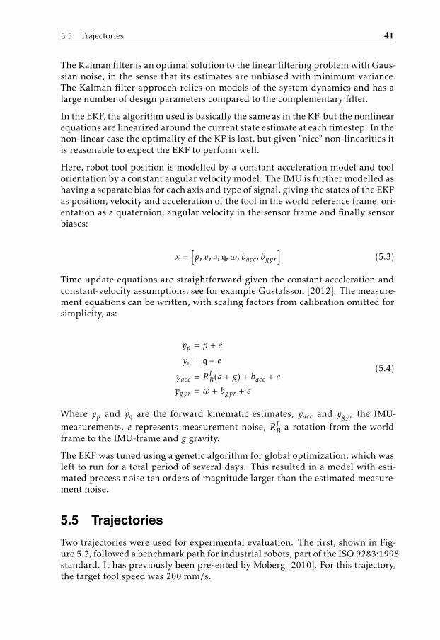
5.5 Trajectories

Two trajectories were used for experimental evaluation. The first, shown in Fig-ure 5.2, followed a benchmark path for industrial robots, part of the ISO 9283:1998standard. It has previously been presented by Moberg [2010]. For this trajectory,the target tool speed was 200 mm/s.


-50 0 50 100

X [mm]

-250

-200

-150

-100

-50

0

Y [

mm

]

Reference

CF

EKF

Figure 5.2: Estimates from the ISO trajectory. The trajectory is chosen to berepresentative of challenging industrial applications. The starting positionis marked with a circle, and the target tool speed was 200 mm/s.

5.5 Trajectories 43

60 80 100 120

X [mm]

-130

-120

-110

-100

-90

Y [m

m] Reference

CF

EKF

Figure 5.3: Details from the ISO-trajectory. Note that the travelled directionin the right part of the figure is downwards.

-30

30

-20Z [m

m]

30

-10

20

Y [mm]

0

20

X [mm]

1010

0 0

Reference

CF

EKF

Figure 5.4: Estimates from the cube trajectory, using a target tool speed of80 mm/s and high precision mode, i.e. stopping briefly at each corner.


Table 5.1: Root mean square error for the test trajectories and estimationmethods.

Trajectory CF EKF FKISO 0.95 mm 0.94 mm 1.44 mm

Cube 0.81 mm 0.93 mm 0.79 mm

5 5.5 6 6.5 7 7.5 8

t [s]

0

2

4

6

Err

or

[mm

]

CF

EKF

FK

Figure 5.5: Estimation error during a part of the ISO-trajectory. The twowide peaks after 5 s corresponds to the circle and the rapid succession ofpeaks corresponds to the series of 90◦ turns.

The second traced the edges of a cube with edge length of 30 mm, shown inFigure 5.4, where the target speed was 80 mm/s with brief stops in the corners.

In both trajectories the tool orientation was kept constant, as the laser trackingsystem requires line of sight and cannot measure orientation.

5.6 Experimental results

The performance of the estimation methods for the two test trajectories is sum-marized in Table 5.1, were it can be seen that the CF and the EKF provide similarresults in terms of root mean square error, with the CF performing slightly betteron the slower of the two trajectories.

The estimates are visualized in Figure 5.2 and Figure 5.4. A close-up of someinteresting features from the ISO trajectory is shown in Figure 5.3.

Characteristic parts of the time-error plots for the two trajectories are shown inFigure 5.5 and Figure 5.6 respectively.

5.7 Discussion 45

4.5 5 5.5 6 6.5 7 7.5

t [s]

0

1

2

3

Err

or

[mm

]

CF

EKF

FK

Figure 5.6: Estimation error during part of the cube trajectory, clearly show-ing the corners as the regions of a low error due to lower speed followed bya larger error due to change in direction.

5.7 Discussion

The difference in performance for the forward kinematics estimate, as shown inTable 5.1, between the two trajectories is notable. This is probably due to loweraccelerations in the cube trajectory, as the forward kinematics does not capturethe dynamic properties excited by acceleration, such as flexibilities in links andgearboxes. This can be supported by comparing the time-error plots and thetrajectories, where a clear connection is seen between acceleration and forwardkinematics error. E.g. the circle and the rapid succession of 90◦-turns in theISO trajectory can clearly be seen as error peaks for the forward kinematics inFigure 5.5.

The CF and the EKF estimates, using measurements of the acceleration, are notsensitive in the same way. It is, however, clear that several sections can be foundwhere the forward kinematics outperforms both filtering approaches, also in theISO trajectory, showing how IMU measurement noise is limiting the accuracy ofthe position estimates.

That the two filtering approaches perform similarly is not surprising given thelarge ratio between process and measurement noise that the EKF tuning resultedin, as such a ratio is essentially another way of stating the assumptions behindcomplementary filtering.

In retrospect it is also not surprising that these trajectories, containing parts withquite different characteristics, are not well described by a constant-accelerationmodel with stationary Gaussian process noise.

As the tool orientation could not be measured, it was kept constant during bothtrajectories, and nothing conclusive can be said regarding the accuracy of the


orientation estimates. However, since the orientation estimate is crucial for con-verting acceleration measurements from the sensor coordinate frame to the worldcoordinate frame, poor orientation estimates would most likely have had a largenegative impact on the position estimates.

5.8 Conclusions

By combining the motor angular measurements of an industrial robot with mea-surements from an IMU mounted on the robot tool, better estimates of the toolposition can be achieved compared to using only direct kinematics from motorangle measurements. The forward kinematics estimates deteriorate in parts ofthe trajectory containing large accelerations, and this is where the filtering ap-proaches offer an improvement.

Between the complementary filter and the extended Kalman filter there was nomajor difference in performance, the CF performed slightly better during theslower trajectory. This, as well as the large process noise obtained when tuningthe EKF, suggests that the statistical properties of the tracked signal are not welldescribed by the chosen motion models and the Gaussian distributions availablein the Kalman filtering framework.

When this is the case, using a CF might yield results comparable those of anEKF, while having both a less complex tuning process and lower computationalcomplexity.

6Case study: Feedback linearization

compared to LQ-control

This chapter is a slightly revised version of the paper by Hedberg et al. [2018],which was presented at the 12th IFAC Symposium on Robot Control. It comparestwo control schemes which are based on two different types of linearization, andintroduces a method for doing so in a fair way.

6.1 Introduction

A common scheme for control of industrial manipulators is model-based feed-forward combined with decentralized PID control of the motor angles. Thisscheme is relatively simple compared to the many well-known methods for cen-tralized control design offered in literature, but so far the potential benefits ofusing more complex controllers has not been convincing enough for widespreadindustrial adoption.

6.1.1 Motivation

Motor angles are often the only measurements available for feedback in indus-trial robots, mainly due to the cost of adding other types of sensors. This haslimited the attractiveness of methods that require additional measurements likearm angles or torque.

However, advances in technology and a constant demand for increased perfor-mance makes the use of additional sensors an increasingly viable option. Asfull-state feedback becomes more interesting for industrial applications so doesthe question of which full-state feedback design method is best suited for usein practice. To answer this question analysis, simulations and real-world experi-ments are needed.

47

48 6 Case study: Feedback linearization compared to LQ-control

The importance of feed-forward to achieve good tracking in robotic manipulatorsis well established. Therefore, disturbance rejection performance becomes themost important property when comparing different feedback controllers.

When comparing control methods, it is important that the comparison reflectsthe properties of the respective methods and not the way they were tuned. Tothat purpose, we introduces a way of choosing an LQ controller for a feedbacklinearized system such that the LQ loss function is equivalent, at a chosen operat-ing point, to that of an LQ controller designed for a Jacobian linearization in thesame operating point.

6.1.2 Related work

An overview of control methods for flexible joint robots, including feedback lin-earization, is provided in the survey paper by Spong [1990]. In a more recent sur-vey by Ozgoli and Taghirad [2006], the authors comment that although there hasbeen many theoretical results published since Spong [1990], adoption of thesemethods in practice is still scarce.

The benchmark model used in this chapter is introduced in Moberg et al. [2008].Another benchmark problem for control of flexible joint manipulators is intro-duced in Hoffmann et al. [2013], together with a controller derived using a linearparameter-varying (LPV) framework. The dissertation by Saupe [2013] is an ex-cellent investigation of LPV control applied to industrial manipulators.

In a recent work Kim and Croft [2017] introduce a control method based on singu-lar perturbation theory and compare it to feedback linearization in experimentson an industrial manipulator. The authors also make the observation that experi-mental results on feedback linearization are rarely reported in literature.

Brogliato et al. [1995] compares several non-linear control schemes for flexiblejoint manipulators, but do not include feedback linearization, and analyses themin a common theoretical framework to show structural similarities.

6.1.3 Contributions

Feedback linearization for flexible joint robots has been studied extensively froma theoretical point of view in the past, but there are to the authors’ best knowl-edge not many studies comparing it to other control methods in an industriallyrelevant control problem. This chapter

• introduces a method of designing LQ controllers for Feedback linearizationand Jacobian linearization to obtain similar performance in an operatingpoint, and

• compares the two controller types using an industrially relevant benchmarkmodel.

6.2 Simulation model 49

6.1.4 Outline

The benchmark model used for evaluation is introduced in Section 6.2. The con-trol design methods are described in Section 6.3 and Section 6.4 introduces theevaluation methodology. Thereafter the results are presented in Section 6.5 anddiscussed in Section 6.6.

6.2 Simulation model

The simulation model used in this chapter was first introduced in a benchmarkproblem by Moberg et al. [2008], and has been experimentally verified to wellrepresent the challenge of controlling a typical industrial robotic manipulator.In the benchmark problem, the task is to design a controller with robust perfor-mance using only motor angle feedback. Here, we instead study controllers withfull state feedback, which are expected to outperform methods that only use ac-tuator positions.

The benchmark model is a two-link flexible joint manipulator, illustrated in Fig-ure 6.1, and described by the equations

M1(qa)qa + C(qa, qa) + G(qa) + Dq + τ(qa, qm) = 0

M2qm − N−1τ(qa, qm) + ff ric(qm) = u

where q denotes angle, a arm, and m motor. The model features several realisticproperties such as

• non-linear motor friction ff ric,

• non-linear spring stiffness τ,

• time delays,

• quantization, and

• measurement noise.

50 kg

qa1

150 kg

TCP

qa2

Figure 6.1: Illustration of the robot model at arm configuration qa1, qa2 = 0,referred to as operating point 10 in the experimental evaluation. The toolcenter point (TCP) and link weights are also given.


The control input u represents motor torques, and is limited by |u1| ≤ 35 Nm,|u2| ≤ 20 Nm. The disturbances acting on the system are summarized in Table6.1.

Table 6.1: Disturbances

Type Description

Motor torques Frequency sweep from 15 to 0 Hz, 1 Nm.TCP force 0.5 s pulse of 500 N, varying direction.

In order to study full-state feedback the model introduced by Moberg et al. [2008]has been extended with measurements of motor velocity as well as arm-side angleand velocity.

6.3 Control Design

6.3.1 Model for control design

While it is possible to do Feedback linearization for more complex flexible-jointmodels, see De Luca [1988], we use a simplified model where linear damping andthe motor friction are neglected. This gives the model equations

qa = −M−11 (qa)(C(qa, qa) + G(qa) + τ(qa, qm))

qm = M−12 (N−1τ(qa, qm) + u).

(6.1)

The above simplifications are reasonable as the neglected terms contribute withdamping, and the approximation will thus be conservative in the sense that thereal system is better damped, see Khalil [2002]. Introduce the notation

P : x = f (x) + Bu, x =[qTa qTa qTm qTm

]T(6.2)

for the plant used for control design and its states.

Assumption 6.1. Furthermore, assume that f (x) includes gravity compensationsuch that all stationary joint configurations qa are equilibrium points for the sys-tem P.

6.3.2 LQ Control

Linear Quadratic (LQ) control is a well-known method for control of linear sys-tems, and is briefly introduced below. See e.g. Franklin et al. [2002] for furtherdetails. Given a controllable linear system and a quadratic loss function

V (x, u) =[xu

]T [Q N/2

N/2 R

] [xu

](6.3)

6.3 Control Design 51

a state feedback u = −Lx can always be found such that∞∫

0

V (x, u) dt (6.4)

is minimized, given that the penalty matrices Q, R, and N are chosen to ensurethat the loss function (6.3) is positive semi-definite. The cross term matrix N isseldom used in practice, as it is often hard to interpret intuitively.

6.3.3 Jacobian Linearization

In order to apply LQ design to the non-linear plant P, it is approximated by alinear plant Pδ. The approximation will be good in some neighbourhood of theequilibrium point x0, and the linear system can be written

Pδ : x = f ′x (x0)xδ + Bu, xδ = x − x0 (6.5)

where f ′x (x0) is the Jacobian matrix of f evaluated at x0. This is one of the mostfundamental methods of designing controllers for non-linear plants.

Now, introduce the following loss function

Vδ = xTδ Qxδ + uT Ru (6.6)

which will be used in designing an LQ controller

Kδ : u = −Lδxδ (6.7)

for the plant model Pδ.

Assumption 6.2. Restrict the choice of Q to only penalize the states qTa and qTa .This simplifies derivations and is reasonable from an application viewpoint, asend-effector movement depends directly on the arm angles.

6.3.4 Feedback Linearization

Some classes of non-linear systems can be turned into a linear system, withoutapproximation, by a non-linear state transform and feedback. This is called Feed-back linearization or sometimes Exact linearization (e.g. Kreutz [1989]) and canbe found in standard textbooks on non-linear control such as Khalil [2002]. Evenwhen it is not possible to render a system exactly linear, feedback may still renderit linear enough that linear control methods can be applied successfully.

For example, terms that have a damping effect, like friction, can often be left outof the linearizing feedback with good results, as described by e.g. Slotine and Li[1991].

The state transform for feedback linearization of P and the resulting states canbe written

y = T (x), y =[qTa qTa qTa q

(3)Ta

]T(6.8)


and can be derived by calculating the higher derivatives of qa, preferably with acomputer algebra system. The non-linear feedback

u = α(x) + β(x)v, (6.9)

where v is an artificial input, can then be derived by solving q(4)a (x, u) = v for u.

Using this feedback gives the closed loop

PF

: x = f (x) + B(α(x) + β(x)v), (6.10)

which is a linear system in the y-coordinates

PF

: y = AFy + B

Fv. (6.11)

Note that while Pδ is a linear approximation of P, the feedback linearized systemPF

is a linear plant with different dynamics. Also note that the arm angles andarm angular velocity states qa, qa are unchanged under the transformation,

x =[qTa qTa ∗ ∗

]T=⇒ T (x) =

[qTa qTa ∗ ∗

]T. (6.12)

The linear plant (6.11) can now be controlled using any control method for linearsystems.

However, due to the non-linear transformation, penalizing the magnitude of theartificial control inputs v does not translate directly to a penalty on the real con-trol signals u. This is one of the challenges of using feedback linearization inpractice.

6.3.5 Equivalent LQ Design

Let the deviation of y from a desired equilibrium point y0 = T (x0) be denoted yδ,and introduce the LQ controller

KF

: v = −LFyδ (6.13)

for use with the linearizing feedback (6.9). Use the feedback linearization vari-ables yδ and v to write the corresponding loss function as

VF(yδ, v) = yTδ QF

yδ + vT RFv + yTδ NF

v. (6.14)

Our interest now lies in choosing VF

so that the closed loop with KF

has equiva-lent performance to that of Kδ at the operating point x0. To that end, considerthat the loss function Vδ, given in (6.6), dictates the behaviour of the closed loopunder Kδ.

Proposition 6.3. The quadratic function VF

can be chosen to equal the secondorder Taylor expansion of Vδ at x0.

Proof: Consider the Taylor expansion of the feedback law (6.9) at the equilibrium

6.3 Control Design 53

point x0 given by

u = α(x) + β(x)v = α′x(x0)xδ + β(x0)v + O( ‖xδ‖2) (6.15)

where the O term uses the fact that

v = −LFyδ = −L

FT ′x(x0)xδ + O( ‖xδ‖2). (6.16)

Substitute (6.15) into Vδ given by (6.6) to obtain

Vδ = xTδ (Q + Q)xδ + vT Rv + xTδ Nv + O( ‖xδ‖3), (6.17)

where

Q = α′x(x0)T Rα′x(x0),

R = β(x0)T Rβ(x0),

N = 2α′x(x0)T Rβ(x0).

(6.18)

From (6.8) and Assumption 6.2 in Section 6.3.3 that Q only penalizes the statesqTa and qTa we have

xTδ Qxδ = yTδ Qyδ. (6.19)

For notational brevity introduce

H = (T ′x(x0))−1 =⇒ xδ = Hyδ + O( ‖xδ‖2) (6.20)

and substitute both (6.19) and (6.20) into (6.17) to obtain

Vδ = yTδ (Q + HT QH)yδ + vT Rv + yTδ HT Nv

+ O( ‖xδ‖3).(6.21)

Now, by comparing (6.21) with (6.14) it is clear that by using the weight matrices

QF

= Q + HT QH, RF

= R, NF

= HT N , (6.22)

the loss function VF

becomes a second order approximation of Vδ around theequilibrium point x0. �

Using the above choice of weight matrices, the controller KF

can be expectedto result in the same behaviour as Kδ for small deviations from x0, since thebehaviour of an LQ controller is entirely dictated by the choice of loss functionV , and the difference between the loss functions V

Fand Vδ vanishes at x0.

This approximative equivalence is of course only valid around the chosen equi-librium point, and deriving analytically what it means in terms of real worldperformance is difficult. Therefore we propose a simulated experimental evalua-tion.

6.3.6 Simplification of Equivalent LQ Design

One benefit of the method proposed in Section 6.3.5 is that it penalizes v in sucha way as to avoid large control inputs u, thus solving one of the challenges of


using feedback linearization. This benefit can also be obtained with the simplerchoice

QF

= Q, RF

= R, NF = 0, (6.23)

which disregards the contribution of α(x) to u in (6.9), and thus simplifies calcu-lations considerably.

In practice, the choice (6.23) was found to improve results compared to the choice(6.22), especially for large disturbances, and is therefore used in the followingexperimental evaluation.

6.4 Experimental evaluation

6.4.1 Implementation and simulation

The non-linear transform T (x) and related expressions α(x), β(x) and H(x0) werederived from the state equations (6.1) using computer algebra software. Thisprocess also generated functions for use in the simulation. The Jacobian matricesused in Pδ were obtained in the same manner.

Moberg et al. [2008] provides the benchmark models as a robot model written inC and a control system designed in Simulink. This was extended with additionalmeasurements and measurement noise.

6.4.2 Controller tuning

The weight matrices Q and R defining the loss function were chosen to be diago-nal, and suitable values were found through an extensive grid search over weightmatrices at different working points and noise levels.

Based on the grid search, two tunings, referred to as the high gain tuning (HG)and the low gain tuning (LG), were selected for further analysis.

6.4.3 Operating points

The system was evaluated at 18 different operating points, corresponding to thearm angles

qna =[

0−100◦ + n · 10◦

], n = 1...18. (6.24)

Note that in the coordinate system of the benchmark model, qa1 = 0 signifies thefirst link is standing upright, and qa2 = 0 that the second link is rotated 90◦ withrespect to the first link, as illustrated in Figure (6.1).

6.4.4 Performance measure

The benchmark problem introduced in Moberg et al. [2008] includes a perfor-mance measure chosen to describe desirable performance for an industrial ma-

6.5 Results 55

0 2 4 6 8 10 12 14 16 18

Operating point

20

40

60

80

100

120

140

160

Mean p

erf

orm

ance m

easure JL HG

FL HG

JL LG

FL LG

Figure 6.2: The performance measure obtained in different working points.Lower is better. Especially for the high gain tuning, the two controllerschemes have similar performance.

nipulator. The measure is a weighted sum of the maximum value of

• motor torque due to measurement noise,

• overall motor torque,

• tool position error due to external force disturbance,

• settling time after force disturbance, and

• tool position error due to motor disturbance.

All features are normalized with respect to a target performance. The tool po-sition errors and the settling time together make up 90% of the performancemeasure.

6.5 Results

The performance measure obtained from simulations in the different workingpoints is illustrated in Figure 6.2.

Representative examples of system responses to motor disturbances and externalforce disturbances are shown in Figure 6.3 and 6.4 respectively.

6.6 Discussion

6.6.1 Similarity

Tuning LQ controllers for Feedback linearization and Jacobian linearization re-spectively, the proposed method seems to give similar behaviour. Both in thesense that the two controller types achieve similar performance measures, asshown in Figure 6.2. But also in the sense that the system response to distur-bances is strikingly similar in many cases, as illustrated by Figures 6.3 and 6.4.


1 2 3 4 5 6 7 8 9

Time [s]

0

1

2

3

4

TC

P e

rror

[m]

10-4 Motor disturbance, operating point 1

JL

FL

1 2 3 4 5 6 7 8 9

Time [s]

0

0.5

1

1.5

TC

P e

rro

r [m

]


JL

FL

1 2 3 4 5 6 7 8 9

Time [s]

0

2

4

6

8

TC

P e

rror

[m]


JL

FL

Figure 6.3: Tool centre point (TCP) position error due to motor torque chirpdisturbance, using the high-gain configuration of the controllers. The twocontroller schemes show clear similarities.

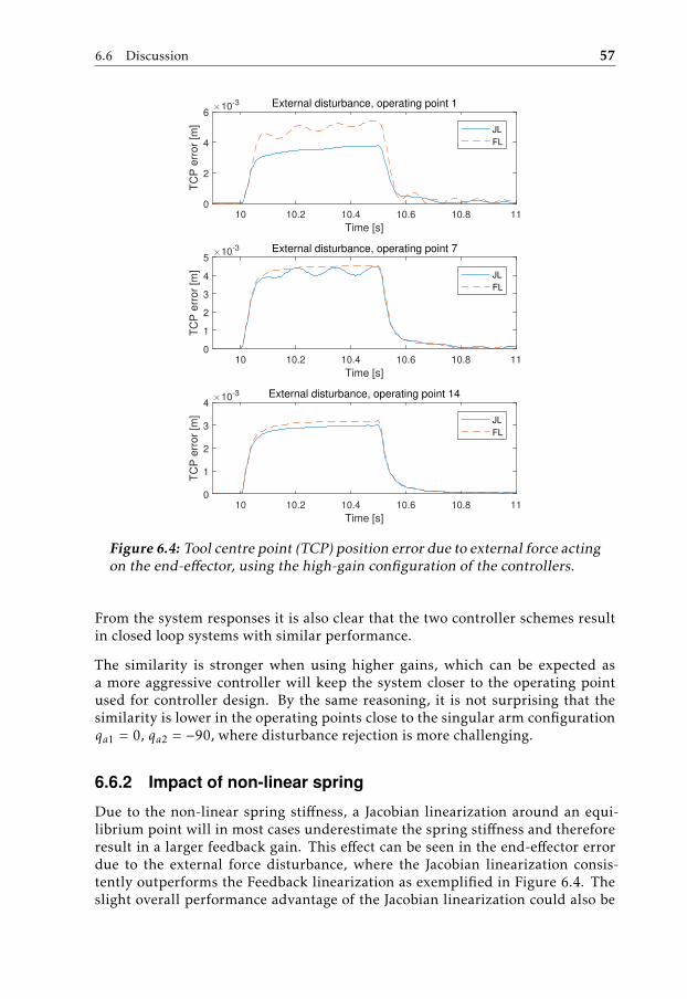
6.6 Discussion 57

10 10.2 10.4 10.6 10.8 11

Time [s]

0

2

4

6

TC

P e

rror

[m]

10-3 External disturbance, operating point 1

JL

FL

10 10.2 10.4 10.6 10.8 11

Time [s]

0

1

2

3

4

5

TC

P e

rror

[m]


JL

FL

10 10.2 10.4 10.6 10.8 11

Time [s]

0

1

2

3

4

TC

P e

rror

[m]


JL

FL

Figure 6.4: Tool centre point (TCP) position error due to external force actingon the end-effector, using the high-gain configuration of the controllers.

From the system responses it is also clear that the two controller schemes resultin closed loop systems with similar performance.

The similarity is stronger when using higher gains, which can be expected asa more aggressive controller will keep the system closer to the operating pointused for controller design. By the same reasoning, it is not surprising that thesimilarity is lower in the operating points close to the singular arm configurationqa1 = 0, qa2 = −90, where disturbance rejection is more challenging.

6.6.2 Impact of non-linear spring

Due to the non-linear spring stiffness, a Jacobian linearization around an equi-librium point will in most cases underestimate the spring stiffness and thereforeresult in a larger feedback gain. This effect can be seen in the end-effector errordue to the external force disturbance, where the Jacobian linearization consis-tently outperforms the Feedback linearization as exemplified in Figure 6.4. Theslight overall performance advantage of the Jacobian linearization could also be


due to this fact.

6.6.3 Considerations for control designers

From an engineering point of view, the Jacobian linearization scheme is signifi-cantly less demanding, both in implementation and in computational resources.The small differences in performance between the two schemes therefore sug-gest that for centralized disturbance rejection during trajectory tracking, a gainscheduling scheme based on Jacobian linearization might be a more efficient useof computational resources, which are in general a limiting factor on robot con-trollers.

The experimental evaluation also showed that quantization of arm-side measure-ments is a concern at the level of accuracy required in industrial manipulators.A 16-bit quantization of arm angles can give TCP errors on the order of 0.1 mmin the present model. This problem is less pronounced for motor side measure-ments, since the gear ratio of n = 200 means motor measurements translated toarm side gain log2(n) ≈ 7.6 bits of resolution.

6.7 Conclusions

Feedback linearization was compared to Jacobian linearization for disturbancerejection using an LQ controller. To that end, a method for equivalent controllertuning was introduced. Experiments on an industrially relevant benchmark modeldid not show any clear benefits of using Feedback linearization over Jacobian lin-earization.

Further studies are needed to compare the robustness properties of the two con-trol schemes. Robustness to model errors is important, but to use full state feed-back in practice, robustness to imperfect state estimates is crucial.

Bibliography

Robotics ABB. Datasheet IRB4600 Industrial Robot, 2016.

W. G. Anderson and E. H. Fritze. Instrument approach system steering computer.Proceedings of the IRE, 41(2):219–228, 1953.

Karl J. Åström and Richard M. Murray. Feedback Systems: An Introduction forScientists and Engineers. Princeton University Press, Princeton, 2008. ISBN978-0-691-13576-2.

Karl J. Åström and Björn Wittenmark. Computer Controlled Systems: Theoryand Design. Prentice-Hall Information and System Sciences Series. Prentice-Hall, Englewood Cliffs, N.J, 1984. ISBN 978-0-13-164319-2.

Johanna Wallén Axehill, Isolde Dressler, Svante Gunnarsson, Anders Roberts-son, and Mikael Norrlöf. Estimation-based ILC applied to a parallel kinematicrobot. Control Engineering Practice, 33:1–9, December 2014. ISSN 09670661.doi: 10.1016/j.conengprac.2014.08.008.

John Bechhoefer. Feedback for physicists: A tutorial essay on control. Reviews ofModern Physics, 77(3):783, 2005.

B. Wayne Bequette. Process Control: Modeling, Design, and Simulation. Prentice-Hall International Series in the Physical and Chemical Engineering Sciences.Prentice Hall PTR, Upper Saddle River, N.J, 2003. ISBN 978-0-13-353640-9.

Bernard Brogliato, Romeo Ortega, and Rogelio Lozano. Global tracking con-trollers for flexible-joint manipulators: A comparative study. Automatica, 31(7):941–956, 1995.

Coleman Brosilow and Martin Tong. Inferential control of processes: Part II. Thestructure and dynamics of inferential control systems. AIChE Journal, 24(3):492–500, 1978. ISSN 1547-5905. doi: 10.1002/aic.690240314.

R. G. Brown. Integrated Navigation Systems and Kalman Filtering: A Perspective.Navigation, 19(4):355–362, December 1972. ISSN 00281522. doi: 10.1002/j.2161-4296.1972.tb01706.x.

59

60 Bibliography

Robert Grover Brown and Patrick Y. C. Hwang. Introduction to Random Signalsand Applied Kalman Filtering: With MATLAB Exercises and Solutions. Wiley,New York, 3rd ed edition, 1997. ISBN 978-0-471-12839-7.

Mario R. Cesca and Jacinto L. Marchetti. IMC design of cascade control. InComputer Aided Chemical Engineering, volume 20, pages 1243–1248. Else-vier, 2005. ISBN 978-0-444-51987-0. doi: 10.1016/S1570-7946(05)80049-5.

Chi-Tsong Chen. Linear System Theory and Design. The Oxford Series in Elec-trical and Computer Engineering. Oxford University Press, New York, 3rd ededition, 1999. ISBN 978-0-19-511777-6 978-0-19-511778-3.

Wenjie Chen and Masayoshi Tomizuka. Direct Joint Space State Estimation inRobots With Multiple Elastic Joints. IEEE/ASME Transactions on Mechatron-ics, 19(2):697–706, April 2014. ISSN 1083-4435, 1941-014X. doi: 10.1109/TMECH.2013.2255308.

Roger C. Conant and W. Ross Ashby. Every good regulator of a system must bea model of that system. International Journal of Systems Science, 1(2):89–97,October 1970. ISSN 0020-7721. doi: 10.1080/00207727008920220.

Jean-Pierre Corriou. Process Control: Theory and Applications. Springer, Lon-don ; New York, 2004. ISBN 978-1-85233-776-6.

A. De Luca. Dynamic control of robots with joint elasticity. In 1988 IEEE Inter-national Conference on Robotics and Automation Proceedings, pages 152–158vol.1, April 1988. doi: 10.1109/ROBOT.1988.12040.

Richard C. Dorf and Robert H. Bishop. Modern Control Systems. Pear-son/Prentice Hall, Upper Saddle River, NJ, 11th ed edition, 2008. ISBN 978-0-13-227028-1.

Michel Fliess and Cédric Join. Model-free control. International Journal ofControl, 86(12):2228–2252, December 2013. ISSN 0020-7179. doi: 10.1080/00207179.2013.810345.

B. A. Francis and W. M. Wonham. The internal model principle for linear mul-tivariable regulators. Applied Mathematics and Optimization, 2(2):170–194,June 1975. ISSN 1432-0606. doi: 10.1007/BF01447855.

Paul M. Frank. Entwurf von Regelkreisen Mit Vorgeschriebenem Verhalten. Wis-senschaft Und Technik : Taschenausgaben. Braun, Karlsruhe, 1974. ISBN 978-3-7650-2016-2.

Gene F. Franklin, J. David Powell, and Abbas Emami-Naeini. Feedback Controlof Dynamic Systems. Prentice Hall, Upper Saddle River, NJ, 4th ed edition,2002. ISBN 978-0-13-032393-4.

Carlos E. Garcia and Manfred Morari. Internal model control. A unifying reviewand some new results. Industrial & Engineering Chemistry Process Designand Development, 21(2):308–323, April 1982. ISSN 0196-4305. doi: 10.1021/i200017a016.

Bibliography 61

Carlos E. García, David M. Prett, and Manfred Morari. Model predictive control:Theory and practice—A survey. Automatica, 25(3):335–348, May 1989. ISSN0005-1098. doi: 10.1016/0005-1098(89)90002-2.

Paul Gewirtz. On "I Know It When I See It". The Yale Law Journal, 105(4):1023,January 1996. ISSN 00440094. doi: 10.2307/797245.

Torkel Glad and Lennart Ljung. Control Theory. CRC Press, 2000. ISBN 978-1-4822-6816-4. doi: 10.1201/9781315274737.

Graham Clifford Goodwin, Stefan F. Graebe, and Mario E. Salgado. Control Sys-tem Design. Prentice Hall, Upper Saddle River, NJ, 2001. ISBN 978-0-13-958653-8.

Fredrik Gustafsson. Statistical Sensor Fusion. Studentlitteratur, Lund, 2012.ISBN 978-91-44-07732-1.

Erik Hedberg, Johan Norén, Mikael Norrlöf, and Svante Gunnarsson. IndustrialRobot Tool Position Estimation using Inertial Measurements in a Complemen-tary Filter and an EKF. 2017.

Erik Hedberg, Mikael Norrlöf, Stig Moberg, and Svante Gunnarsson. Comparingfeedback linearization and jacobian linearization for LQ control of an indus-trial manipulator. In Proccedings of the 12TH IFAC SYMPOSIUM ON ROBOTCONTROL, 2018.

Erik Hedberg, Johan Löfberg, and Anders Helmersson. A pedagogical path fromthe internal model principle to Youla-Kucera parametrization. In 21st IFACWorld Congress 2020, 2020.

Leah Henderson. The problem of induction. In Edward N. Zalta, editor, TheStanford Encyclopedia of Philosophy. Metaphysics Research Lab, Stanford Uni-versity, spring 2020 edition, 2020.

C. Hoffmann, S. M. Hashemi, H. S. Abbas, and H. Werner. Benchmark problem -Nonlinear control of a 3-DOF robotic manipulator. In 52nd IEEE Conferenceon Decision and Control, pages 5534–5539, December 2013. doi: 10.1109/CDC.2013.6760761.

Jeroen Hol. Sensor fusion and calibration of inertial sensors, vision, ultra-wideband and GPS. PhD thesis, Department of Electrical Engineering,Linköping University, Linköping, 2011.

Isaac M Horowitz. Synthesis of Feedback Systems. Academic Press, New York,1963.

IFR. World Robotics 2019 - Industrial Robots. Technical report, InternationalFederation of Robotics, Frankfurt am Main, Germany, 2019.

ISO 8373. Robots and robotic devices — Vocabulary. Standard ISO 8373:2012,International Organization for Standardization, Geneva, Switzerland, 2012.

62 Bibliography

ISO 9283. Manipulating industrial robots — Performance criteria and relatedtest methods. Standard ISO 9283:1998, International Organization for Stan-dardization, Geneva, Switzerland, 1998.

Austin Jensen, Cal Coopmans, and YangQuan Chen. Basics and guidelines ofcomplementary filters for small UAS navigation. In Unmanned Aircraft Sys-tems (ICUAS), 2013 International Conference On, pages 500–507. IEEE, 2013.

Hassan Khalil. Nonlinear Systems. Prentice Hall, January 2002. ISBN 978-0-13-122740-8.

J. Kim and E. A. Croft. Full-State Tracking Control for Flexible Joint RobotsWith Singular Perturbation Techniques. IEEE Transactions on Control SystemsTechnology, PP(99):1–11, 2017. ISSN 1063-6536. doi: 10.1109/TCST.2017.2756962.

Kenneth Kreutz. On manipulator control by exact linearization. IEEE Transac-tions on Automatic Control, 34(7):763–767, July 1989. ISSN 0018-9286. doi:10.1109/9.29408.

Vladimír Kučera. Stability of Discrete Linear Feedback Systems. IFAC Pro-ceedings Volumes, 8(1, Part 1):573–578, August 1975. ISSN 1474-6670. doi:10.1016/S1474-6670(17)67787-5.

Leica Geosystems. 2016.

Lennart Ljung. System Identification: Theory for the User. Prentice Hall Infor-mation and System Sciences Series. Prentice Hall PTR, Upper Saddle River, NJ,2nd ed edition, 1999. ISBN 978-0-13-656695-3.

Jan Marian Maciejowski. Multivariable Feedback Design. Electronic SystemsEngineering Series. Addison-Wesley, Wokingham, England ; Reading, Mass,1989. ISBN 978-0-201-18243-9.

Thomas E. Marlin. Process Control: Designing Processes and Control Systemsfor Dynamic Perfomance. McGraw-Hill, Boston, 2nd ed edition, 2000. ISBN978-0-07-039362-2.

Peter S. Maybeck. Stochastic Models, Estimation and Control. Number v. 141in Mathematics in Science and Engineering. Academic Press, New York, 1979.ISBN 978-0-12-480701-3.

McKinsey & Company. Industrial robotics: Insights into the sector’s futuregrowth dynamics. Technical report, 2019.

Stig Moberg. Modeling and Control of Flexible Manipulators. PhD Thesis,Linköping University, 2010.

Stig Moberg, Jonas Öhr, and Svante Gunnarsson. A Benchmark Problem for Ro-bust Control of a Multivariable Nonlinear Flexible Manipulator. IFAC Pro-ceedings Volumes, 41:1206–1211, 2008. ISSN 1474-6670. doi: 10.3182/20080706-5-KR-1001.00208.

Bibliography 63

Manfred Morari and Evanghelos Zafiriou. Robust Process Control. Prentice Hall,Englewood Cliffs, N.J, 1989. ISBN 978-0-13-782153-2.

M. Nakao, K. Ohnishi, and K. Miyachi. A Robust decentralized joint controlbased on interference estimation. In 1987 IEEE International Conference onRobotics and Automation Proceedings, volume 4, pages 326–331, March 1987.doi: 10.1109/ROBOT.1987.1087996.

Johan Norén. IMU-baserad skattning av verktygets position och orientering hosindustrirobot. 2014.

Roberto Oboe. How disturbance observer changed my life. In 2018 IEEE 15thInternational Workshop on Advanced Motion Control (AMC), pages 13–20,March 2018. doi: 10.1109/AMC.2019.8371055.

Björn Olofsson, Jacob Antonsson, Henk G. Kortier, Bo Bernhardsson, AndersRobertsson, and Rolf Johansson. Sensor Fusion for Robotic Workspace StateEstimation. IEEE/ASME Transactions on Mechatronics, 21(5):2236–2248, Oc-tober 2016. ISSN 1083-4435, 1941-014X. doi: 10.1109/TMECH.2015.2506041.

Winfried Oppelt. Kleines Handbuch technischer Regelvorgänge. Verlag Chemie,Berlin, 4., neubearb. u. erw. aufl edition, 1964.

S. Ozgoli and H. D. Taghirad. A Survey on the Control of Flexible Joint Robots.Asian Journal of Control, 8(4):1–15, December 2006.

Philip Roan, Nikhil Deshpande, Yizhou Wang, and Benjamin Pitzer. Manipu-lator state estimation with low cost accelerometers and gyroscopes. In 2012IEEE/RSJ International Conference on Intelligent Robots and Systems, pages4822–4827. IEEE, 2012.

Florian Saupe. Linear Parameter Varying Control Design for Industrial Manipu-lators. Ph.D. Thesis, Universität Hamburg-Harburg, 2013.

Daniele Semino and Alessandro Brambilla. An Efficient Structure for ParallelCascade Control. Industrial & Engineering Chemistry Research, 35(6):1845–1852, January 1996. ISSN 0888-5885, 1520-5045. doi: 10.1021/ie950710r.

Sensonor AS. Datasheet STIM300. 2016.

Jean-Jacques E. Slotine and Weiping Li. Applied nonlinear control. Prentice Hall,1991.

Michael Smith. The Humean Theory of Motivation. Mind, 96(381):36–61, 1987.ISSN 0026-4423.

Mark W. Spong. Control of flexible joint robots: A survey. Coordinated ScienceLaboratory Report no. UILU-ENG 90-2203, 1990.

Jan C. Willems. The Behavioral Approach to Open and Interconnected Systems.IEEE Control Systems, 27(6):46–99, December 2007. ISSN 1066-033X, 1941-000X. doi: 10.1109/MCS.2007.906923.

64 Bibliography

Walter H. Wirkler. Aircraft course stabilizing means, April 1951.

William A Wolovich. Linear Multivariable Systems. Springer Verlag, 1974. ISBN9781461263920.

W. M. Wonham. Towards an Abstract Internal Model Principle. IEEE Transac-tions on Systems, Man, and Cybernetics, SMC-6(11):735–740, November 1976.ISSN 0018-9472. doi: 10.1109/TSMC.1976.4309444.

D. Youla, H. Jabr, and J. Bongiorno. Modern Wiener-Hopf design of optimalcontrollers–Part II: The multivariable case. IEEE Transactions on AutomaticControl, 21(3):319–338, June 1976. ISSN 0018-9286, 1558-2523, 2334-3303.doi: 10.1109/TAC.1976.1101223.

Licentiate ThesesDivision of Automatic Control

Linköping UniversityP. Andersson: Adaptive Forgetting through Multiple Models and Adaptive Control of CarDynamics. Thesis No. 15, 1983.B. Wahlberg: On Model Simplification in System Identification. Thesis No. 47, 1985.A. Isaksson: Identification of Time Varying Systems and Applications of System Identifi-cation to Signal Processing. Thesis No. 75, 1986.G. Malmberg: A Study of Adaptive Control Missiles. Thesis No. 76, 1986.S. Gunnarsson: On the Mean Square Error of Transfer Function Estimates with Applica-tions to Control. Thesis No. 90, 1986.M. Viberg: On the Adaptive Array Problem. Thesis No. 117, 1987.

K. Ståhl: On the Frequency Domain Analysis of Nonlinear Systems. Thesis No. 137, 1988.A. Skeppstedt: Construction of Composite Models from Large Data-Sets. Thesis No. 149,1988.P. A. J. Nagy: MaMiS: A Programming Environment for Numeric/Symbolic Data Process-ing. Thesis No. 153, 1988.K. Forsman: Applications of Constructive Algebra to Control Problems. Thesis No. 231,1990.I. Klein: Planning for a Class of Sequential Control Problems. Thesis No. 234, 1990.F. Gustafsson: Optimal Segmentation of Linear Regression Parameters. Thesis No. 246,1990.H. Hjalmarsson: On Estimation of Model Quality in System Identification. Thesis No. 251,1990.S. Andersson: Sensor Array Processing; Application to Mobile Communication Systemsand Dimension Reduction. Thesis No. 255, 1990.K. Wang Chen: Observability and Invertibility of Nonlinear Systems: A Differential Alge-braic Approach. Thesis No. 282, 1991.J. Sjöberg: Regularization Issues in Neural Network Models of Dynamical Systems. ThesisNo. 366, 1993.P. Pucar: Segmentation of Laser Range Radar Images Using Hidden Markov Field Models.Thesis No. 403, 1993.H. Fortell: Volterra and Algebraic Approaches to the Zero Dynamics. Thesis No. 438,1994.T. McKelvey: On State-Space Models in System Identification. Thesis No. 447, 1994.T. Andersson: Concepts and Algorithms for Non-Linear System Identifiability. ThesisNo. 448, 1994.P. Lindskog: Algorithms and Tools for System Identification Using Prior Knowledge. The-sis No. 456, 1994.J. Plantin: Algebraic Methods for Verification and Control of Discrete Event DynamicSystems. Thesis No. 501, 1995.J. Gunnarsson: On Modeling of Discrete Event Dynamic Systems, Using Symbolic Alge-braic Methods. Thesis No. 502, 1995.A. Ericsson: Fast Power Control to Counteract Rayleigh Fading in Cellular Radio Systems.Thesis No. 527, 1995.M. Jirstrand: Algebraic Methods for Modeling and Design in Control. Thesis No. 540,1996.K. Edström: Simulation of Mode Switching Systems Using Switched Bond Graphs. ThesisNo. 586, 1996.

J. Palmqvist: On Integrity Monitoring of Integrated Navigation Systems. Thesis No. 600,1997.A. Stenman: Just-in-Time Models with Applications to Dynamical Systems. ThesisNo. 601, 1997.M. Andersson: Experimental Design and Updating of Finite Element Models. ThesisNo. 611, 1997.U. Forssell: Properties and Usage of Closed-Loop Identification Methods. Thesis No. 641,1997.M. Larsson: On Modeling and Diagnosis of Discrete Event Dynamic systems. ThesisNo. 648, 1997.N. Bergman: Bayesian Inference in Terrain Navigation. Thesis No. 649, 1997.V. Einarsson: On Verification of Switched Systems Using Abstractions. Thesis No. 705,1998.J. Blom, F. Gunnarsson: Power Control in Cellular Radio Systems. Thesis No. 706, 1998.P. Spångéus: Hybrid Control using LP and LMI methods – Some Applications. ThesisNo. 724, 1998.M. Norrlöf: On Analysis and Implementation of Iterative Learning Control. ThesisNo. 727, 1998.A. Hagenblad: Aspects of the Identification of Wiener Models. Thesis No. 793, 1999.

F. Tjärnström: Quality Estimation of Approximate Models. Thesis No. 810, 2000.C. Carlsson: Vehicle Size and Orientation Estimation Using Geometric Fitting. ThesisNo. 840, 2000.J. Löfberg: Linear Model Predictive Control: Stability and Robustness. Thesis No. 866,2001.O. Härkegård: Flight Control Design Using Backstepping. Thesis No. 875, 2001.J. Elbornsson: Equalization of Distortion in A/D Converters. Thesis No. 883, 2001.J. Roll: Robust Verification and Identification of Piecewise Affine Systems. Thesis No. 899,2001.I. Lind: Regressor Selection in System Identification using ANOVA. Thesis No. 921, 2001.

R. Karlsson: Simulation Based Methods for Target Tracking. Thesis No. 930, 2002.P.-J. Nordlund: Sequential Monte Carlo Filters and Integrated Navigation. Thesis No. 945,2002.M. Östring: Identification, Diagnosis, and Control of a Flexible Robot Arm. ThesisNo. 948, 2002.C. Olsson: Active Engine Vibration Isolation using Feedback Control. Thesis No. 968,2002.J. Jansson: Tracking and Decision Making for Automotive Collision Avoidance. ThesisNo. 965, 2002.N. Persson: Event Based Sampling with Application to Spectral Estimation. ThesisNo. 981, 2002.D. Lindgren: Subspace Selection Techniques for Classification Problems. Thesis No. 995,2002.E. Geijer Lundin: Uplink Load in CDMA Cellular Systems. Thesis No. 1045, 2003.

M. Enqvist: Some Results on Linear Models of Nonlinear Systems. Thesis No. 1046, 2003.

T. Schön: On Computational Methods for Nonlinear Estimation. Thesis No. 1047, 2003.F. Gunnarsson: On Modeling and Control of Network Queue Dynamics. Thesis No. 1048,2003.S. Björklund: A Survey and Comparison of Time-Delay Estimation Methods in LinearSystems. Thesis No. 1061, 2003.

M. Gerdin: Parameter Estimation in Linear Descriptor Systems. Thesis No. 1085, 2004.

A. Eidehall: An Automotive Lane Guidance System. Thesis No. 1122, 2004.E. Wernholt: On Multivariable and Nonlinear Identification of Industrial Robots. ThesisNo. 1131, 2004.J. Gillberg: Methods for Frequency Domain Estimation of Continuous-Time Models. The-sis No. 1133, 2004.G. Hendeby: Fundamental Estimation and Detection Limits in Linear Non-Gaussian Sys-tems. Thesis No. 1199, 2005.D. Axehill: Applications of Integer Quadratic Programming in Control and Communica-tion. Thesis No. 1218, 2005.J. Sjöberg: Some Results On Optimal Control for Nonlinear Descriptor Systems. ThesisNo. 1227, 2006.D. Törnqvist: Statistical Fault Detection with Applications to IMU Disturbances. ThesisNo. 1258, 2006.H. Tidefelt: Structural algorithms and perturbations in differential-algebraic equations.Thesis No. 1318, 2007.S. Moberg: On Modeling and Control of Flexible Manipulators. Thesis No. 1336, 2007.J. Wallén: On Kinematic Modelling and Iterative Learning Control of Industrial Robots.Thesis No. 1343, 2008.J. Harju Johansson: A Structure Utilizing Inexact Primal-Dual Interior-Point Method forAnalysis of Linear Differential Inclusions. Thesis No. 1367, 2008.J. D. Hol: Pose Estimation and Calibration Algorithms for Vision and Inertial Sensors.Thesis No. 1370, 2008.H. Ohlsson: Regression on Manifolds with Implications for System Identification. ThesisNo. 1382, 2008.D. Ankelhed: On low order controller synthesis using rational constraints. ThesisNo. 1398, 2009.P. Skoglar: Planning Methods for Aerial Exploration and Ground Target Tracking. ThesisNo. 1420, 2009.C. Lundquist: Automotive Sensor Fusion for Situation Awareness. Thesis No. 1422, 2009.C. Lyzell: Initialization Methods for System Identification. Thesis No. 1426, 2009.R. Falkeborn: Structure exploitation in semidefinite programming for control. ThesisNo. 1430, 2010.D. Petersson: Nonlinear Optimization Approaches toH2-Norm Based LPV Modelling andControl. Thesis No. 1453, 2010.Z. Sjanic: Navigation and SAR Auto-focusing in a Sensor Fusion Framework. ThesisNo. 1464, 2011.K. Granström: Loop detection and extended target tracking using laser data. ThesisNo. 1465, 2011.J. Callmer: Topics in Localization and Mapping. Thesis No. 1489, 2011.F. Lindsten: Rao-Blackwellised particle methods for inference and identification. ThesisNo. 1480, 2011.M. Skoglund: Visual Inertial Navigation and Calibration. Thesis No. 1500, 2011.

S. Khoshfetrat Pakazad: Topics in Robustness Analysis. Thesis No. 1512, 2011.

P. Axelsson: On Sensor Fusion Applied to Industrial Manipulators. Thesis No. 1511, 2011.A. Carvalho Bittencourt: On Modeling and Diagnosis of Friction and Wear in IndustrialRobots. Thesis No. 1516, 2012.P. Rosander: Averaging level control in the presence of frequent inlet flow upsets. ThesisNo. 1527, 2012.

N. Wahlström: Localization using Magnetometers and Light Sensors. Thesis No. 1581,2013.R. Larsson: System Identification of Flight Mechanical Characteristics. Thesis No. 1599,2013.Y. Jung: Estimation of Inverse Models Applied to Power Amplifier Predistortion. ThesisNo. 1605, 2013.M. Syldatk: On Calibration of Ground Sensor Networks. Thesis No. 1611, 2013.M. Roth: Kalman Filters for Nonlinear Systems and Heavy-Tailed Noise. Thesis No. 1613,2013.D. Simon: Model Predictive Control in Flight Control Design — Stability and ReferenceTracking. Thesis No. 1642, 2014.J. Dahlin: Sequential Monte Carlo for inference in nonlinear state space models. ThesisNo. 1652, 2014.M. Kok: Probabilistic modeling for positioning applications using inertial sensors. ThesisNo. 1656, 2014.J. Linder: Graybox Modelling of Ships Using Indirect Input Measurements. ThesisNo. 1681, 2014.G. Mathai: Direction of Arrival Estimation of Wideband Acoustic Wavefields in a PassiveSensing Environment. Thesis No. 1721, 2015.I. Nielsen: On Structure Exploiting Numerical Algorithms for Model Predictive Control.Thesis No. 1727, 2015.C. Veibäck: Tracking of Animals Using Airborne Cameras. Thesis No. 1761, 2016.N. Evestedt: Sampling Based Motion Planning for Heavy Duty Autonomous Vehicles. The-sis No. 1762, 2016.H. Nyqvist: On Pose Estimation in Room-Scaled Environments. Thesis No. 1765, 2016.Y. Zhao: Position Estimation in Uncertain Radio Environments and Trajectory Learning.Thesis No. 1772, 2017.P. Kasebzadeh: Parameter Estimation for Mobile Positioning Applications. ThesisNo. 1786, 2017.K. Radnosrati: On Timing-Based Localization in Cellular Radio Networks. ThesisNo. 1808, 2018.G. Lindmark: Methods and Algorithms for Control Input Placement in Complex Net-works. Thesis No. 1814, 2018.M. Lindfors: Frequency Tracking for Speed Estimation. Thesis No. 1815, 2018.

D. Ho: Some results on closed-loop identification of quadcopters. Thesis No. 1826, 2018.O. Ljungqvist: On motion planning and control for truck and trailer systems. ThesisNo. 1832, 2019.P. Boström-Rost: On Informative Path Planning for Tracking and Surveillance. ThesisNo. 1838, 2019.K. Bergman: On Motion Planning Using Numerical Optimal Control. Thesis No. 1843,2019.M. Klingspor: Low-rank optimization in system identification. Thesis No. 1855, 2019.A. Bergström: Timing-Based Localization using Multipath Information. Thesis No. 1867,2019.F. Ljungberg: Estimation of Nonlinear Greybox Models for Marine Applications. ThesisNo. 1880, 2020.


Linköping studies in science and technology. Licentiate Thesis No. 1894

Erik Hedberg

Erik Hedberg

Control, Models and Industrial M

anipulators

2020

FACULTY OF SCIENCE AND ENGINEERING

Linköping studies in science and technology. Licentiate Thesis No. 1894, 2020 Department of Electrical Engineering

Linköping UniversitySE-581 83 Linköping, Sweden

www.liu.se

Control, Models and Industrial Manipulators - DiVA Portal

Documents

Transcript of Control, Models and Industrial Manipulators - DiVA Portal