http://www.diva-portal.org

Postprint

This is the accepted version of a paper presented at International Symposium on PracticalAspects of Declarative Languages (PADL 2012).

Citation for the original published paper:

Broman, D., Nilsson, H. (2012)Node-Based Connection Semanticsfor Equation-Based Object-Oriented ModelingLanguagesIn: Proceedings of Fourteenth International Symposium on Practical Aspects ofDeclarative Languages (PADL 2012) (pp. 258-272).Lecture Notes in Computer Sciencehttps://doi.org/10.1007/978-3-642-27694-1_19

N.B. When citing this work, cite the original published paper.

Permanent link to this version:http://urn.kb.se/resolve?urn=urn:nbn:se:kth:diva-163771

Node-Based Connection Semantics for

Equation-Based Object-Oriented Modeling

Languages

David Broman1 and Henrik Nilsson2

1Department of Computer and Information Science, Linköping University, Swedendavid.broman@liu.se

1School of Computer Science, University of Nottingham, United Kingdomnhn@cs.nott.ac.uk

Abstract. Declarative, Equation-Based Object-Oriented (EOO) mod-eling languages, like Modelica, support modeling of physical systems bycomposition of reusable component models. An important applicationarea is modeling of cyber-physical systems. EOO languages typically fea-ture a connection construct allowing component models to be assembledinto systems much like physical components are. Different designs arepossible. This paper introduces, formalizes, and validates an approachbased on explicit nodes that expressly is designed to work for functionalEOO languages supporting higher-order modeling. The paper also con-siders Modelica-style connections and explains why that design does notwork for functional EOO languages, thus mapping out the design space.

Keywords: Declarative Languages, Modeling, and Simulation

1 Introduction

Equation-based Object-Oriented (EOO) languages is an emerging class of declar-ative Domain-Specific Languages (DSLs) for modeling the dynamic aspects ofsystems using (primarily) differential equations [6]. These languages are charac-terized by acausal modeling of individual objects in the domain(s) of interestand composition of such object models into a complete system model1. Acausalmodeling means there is no a priori assumption about the directionality of equa-tions (known vs. unknown variables). This greatly facilitates reuse and compo-sition [10], a crucial advantage for large models that can consist of thousands ofequations. Moreover, EOO languages are typically capable of expressing mod-els from arbitrary physical domains (e.g., mechanical, electrical, hydraulic) and

1 Some of these languages share typical traits of object-oriented programming lan-guages, such as a class system, but this is not essential: object-oriented here refersto the focus on composition of reusable models that have a direct correspondenceto objects in the physical world. Also, note that, unlike (imperative) object-orientedprogramming languages, EOO languages have no notion of mutable state.

This is the author prepared accepted version. © 2012 Springer. Published in:David Broman and Henrik Nilsson. Node-Based Connection Semantics for Equation-Based Object-Oriented Modeling Languages In Proceedings of Fourteenth International Symposium on Practical Aspects of Declarative Languages (PADL 2012), LNCS 7149, pages 258-272, Philadelphia, Pennsylvania, USA, 2012.https://link.springer.com/chapter/10.1007/978-3-642-27694-1_19The final publication is available at http://link.springer.com

of supporting hybrid modeling : modeling of both continuous-time and discrete-time aspects. State-of-the-art EOO languages include Modelica [11, 19], VHDL-AMS [15] and Verilog-AMS [1]. Taken together, the characteristics of EOO lan-guages make them particularly suitable for modeling Cyber-Physical Systems:complex systems that combine embedded computers and networks (the cyber)with physical processes [17]. Examples include cars, aircraft, and power plants.

Most EOO languages provide a mechanism to connect component modelstogether in a way that mimics how physical components may be interconnected.To obtain a purely mathematical model, these connections have to be translatedinto equations. This translation is the connection semantics. Unsurprisingly, theconnection semantics is grounded in physical reality, such as the conservationprinciples of various physical domains. Because these principles share a commonmathematical structure, it is possible to formulate the connection semantics ina domain-neutral way. To that end, two kinds of physical quantities are dis-tinguished: flow quantities and potential quantities. Connected flow quantitiesare translated into sum-to-zero equations, as a connection point itself does notprovide any capability of storing the flowing quantity, while connected poten-tial quantities are translated into equality constraints, as there can only be onepotential at a connection point. Modelica is one language taking this approach.

While state-of-the-art EOO languages like Modelica are highly successful,they do have acknowledged weaknesses, including limited support for structurallydynamic systems and limited meta-modeling capabilities per se [20, 26]. Theseand other considerations have led researchers to investigate a different approachto EOO language design that supports higher-order modeling. The common ideais to make models first class entities in the setting of a functional language andusing pure functions as the central abstraction mechanism [6, 14, 20].

Unfortunately, the connection semantics of Modelica-like languages is predi-cated on specific design aspects of such languages and does not readily carry overto a functional setting with first-class models. Moreover, at least the Modelicaconnection semantics is complex and has not been fully formalized, making itdifficult to understand it precisely (for end users as well as for implementors).

In this paper we propose an alternative approach to specifying the connectionsemantics based on explicit connection points, from now on nodes. The idea ofexplicit nodes is not new; for example, it is used in VHDL-AMS, Verilog-AMS,and other hardware description languages. The novel insight demonstrated inthis paper is how a node-based approach solves the problem of defining theconnection semantics in functional EOO languages. The resulting semantics isalso pleasingly clear. In more detail, our specific contributions are:

– We relate Modelica-style connection semantics (Section 2) and the node-based approach (Section 3), thus mapping out part of the design space, andwe explain why the former approach does not work in a functional setting.

– We formalize the semantics of the node-based approach (Section 4).– We describe and validate a prototype implementation of the node-based

approach in the Modeling Kernel Language (MKL) [6] (Section 5). (Notethat MKL is just a vehicle: the approach as such is language-independent.)

2 Modelica-Style Approach

This section gives an informal overview of Modelica-style connection semanticsand explains why this approach does not work in a functional setting. Our exam-ples are from the analog electrical domain. However, we re-iterate that connectionsemantics in this paper is domain-neutral unless stated otherwise [8].

2.1 Models and Equation Generation

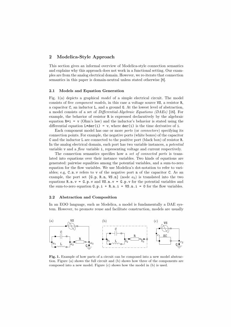
Fig. 1(a) depicts a graphical model of a simple electrical circuit. The modelconsists of five component models, in this case a voltage source VS, a resistor R,a capacitor C, an inductor L, and a ground G. At the lowest level of abstraction,a model consists of a set of Differential-Algebraic Equations (DAEs) [16]. Forexample, the behavior of resistor R is expressed declaratively by the algebraicequation R*i = v (Ohm’s law) and the inductor’s behavior is stated using thedifferential equation L*der(i) = v, where der(i) is the time derivative of i.

Each component model has one or more ports (or connectors) specifying itsconnection points. For example, the negative ports (white boxes) of the capacitorC and the inductor L are connected to the positive port (black box) of resistor R.In the analog electrical domain, each port has two variable instances, a potentialvariable v and a flow variable i, representing voltage and current respectively.

The connection semantics specifies how a set of connected ports is trans-lated into equations over their instance variables. Two kinds of equations aregenerated: pairwise equalities among the potential variables, and a sum-to-zeroequation for the flow variables. We use Modelica’s dot-notation to refer to vari-ables; e.g, C.n.v refers to v of the negative port n of the capacitor C. As anexample, the port set {G.p, R.n, VS.n} (node a3) is translated into the twoequations R.n.v = G.p.v and VS.n.v = G.p.v for the potential variables andthe sum-to-zero equation G.p.i + R.n.i + VS.n.i = 0 for the flow variables.

2.2 Abstraction and Composition

In an EOO language, such as Modelica, a model is fundamentally a DAE sys-tem. However, to promote reuse and facilitate construction, models are usually

R

C

L

VS

Ga3a2a1

R

C

L b2b1 b3

(a) (b)VS

Gc2

(c)

SCc1

Fig. 1. Example of how parts of a circuit can be composed into a new model abstrac-tion. Figure (a) shows the full circuit and (b) shows how three of the components arecomposed into a new model. Figure (c) shows how the model in (b) is used.

constructed hierarchically: related equations are grouped into models of physicalcomponents; such models can then be instantiated any number of times and fur-ther grouped into models of systems at progressively higher levels of abstraction.

For example, the model in Fig. 1(b) represents an abstraction of the compo-nents R, C, and L from Fig. 1(a). The dashed box represents the outside borderof the abstracted model. Fig. 1(c) shows another way to model the circuit in (a),this time as a composed model using the sub-circuit in (b) (named SC) as oneof the components. Hence, (a) and (c) model the exact same system, the onlydifference being that (c) introduces one more hierarchical level of abstraction.

The question is how to define connection semantics for composed modelswith several hierarchical levels of abstraction. In the Modelica-style, each port isconsidered either an outside or an inside port, depending on whether the currentviewpoint is inside or outside a model. For example, in Fig. 1(b), when generatingthe sum-to-zero equation for the connection b3, SC.n is considered an outside portand SC.R.n an inside port. The Modelica specification [19] states that outsideconnectors shall have a negative sign in sum-to-zero equations. The sum-to-zeroequation at node b3 is thus -SC.n.i + SC.R.n.i = 0. On the other hand, inmodel (c), port SC.n is considered an inside port, hence the resulting sum-to-zero equation for c2 is VS.n.i + SC.n.i + G.p.i = 0. Information about thehierarchical structure is thus exploited when generating the equations.

2.3 Problems in a Functional Setting

In the Modelica-style approach, models have ports that define instance variables.A port is a part of the model it belongs to, and as such, its position in a compo-sitional hierarchy becomes unambiguously determined; in particular, each portcan be classified as inside or outside with respect to a specific model context andthen treated accordingly for connection purposes.

In contrast, a functional EOO language uses function abstraction (or somevariant thereof) for expressing model abstractions, with “ports” becoming formalparameters. As a result, a port is no longer per se a part with an implied positionthat can inform the generation of sum-to-zero equations. We can attempt toovercome this by introducing connection nodes as an independent notion. Amodel abstraction is then seen as a function mapping nodes to equations. But anode is just a node, a value like any other, without any special relation to specificabstractions, meaning that the notions inside and outside become meaningless.For example, assume that the model SC is defined as a function with two formalparameters. A function call SC(c1,c2) results in the nodes c1 and c2 beingsubstituted into the function body of SC, yielding a collapsed hierarchy withoutany possibility to say whether a port is inside or outside.

Thus, the Modelica-style connection semantics does not carry over to a func-tional setting essentially because it is predicated on exploiting contextual in-formation alien to this setting. To address this, we develop in the following analternative approach that is suitable, based on nodes and branches (ElectricalEngineering terminology; here essentially a directed edge annotated with vari-ables) forming an explicit graph. Other possibilities are discussed in Sec. 6.3.

3 Node-Based Approach

This section informally describes the node-based approach to connection seman-tics. It has two phases: (1) Collapsing the hierarchical model structure into adirected graph of nodes, branches, and equations; (2) Translation of nodes andbranches into additional equations, yielding a pure system of equations; i.e.,the connection semantics proper. The approach is demonstrated using a smallresearch language called the Modeling Kernel Language (MKL) [6]: a typed func-tional language specifically designed for embedding equation-based DSLs. How-ever, note that the approach as such is language-independent.

3.1 Phase 1: Collapsing the Model Hierarchy

In an functional EOO-language, functions are used as the abstraction mecha-nism for describing composed models. For example, consider the following MKLmodel, which is the textual representation of Fig. 1(a):

def CircuitA () = {def a1,a2,a3:Electrical;SineVoltage (220,50,a1,a3);Capacitor (0.02,a1,a2);Inductor (0.1,a1,a2);Resistor (200,a2,a3);Ground(a3);

}

The model CircuitA is defined as a function without parameters. Three nodesa1, a2, and a3 of type Electrical are defined. The five component mod-els of the circuit are instantiated using function application; e.g., the applica-tion Capacitor(0.02,a1,a2) instantiates a capacitor of 0.02F. The connectiontopology is defined by supplying the electrical nodes to the components; e.g.,Capacitor is applied to nodes a1 and a2. Note how both parallel and serialconnections are expressed in this way (cf. Fig. 1(a)). The Capacitor model

def Capacitor(C:Real ,p:Electrical ,n:Electrical) = {def i:Current;def v:Voltage;Branch(i,v,p,n);C * der(v) = i;

}

has parameters C (capacitance) p (positive port), and n (negative port). Twounknown continuous-time signals i (current) and v (voltage) are defined insidethe body. The third line in the body instantiates a Branch with four elements.Conceptually, a branch is a path between two nodes through a component model.Branches are essential for the translational connection semantics because theycapture information necessary to generate correct signs in sum-to-zero equations.

Fig. 2 shows the resulting graph from evaluating the expression CircuitA().Filled black arrows represent the branches (labeled edges). The nodes a1, a2,

d1 d2 d3

iVC vVC

iC vC

iL vLiR vR

iG vG

vVC = 220 ⇤ sin(2 ⇤ ⇡ ⇤ 50 ⇤ time)

0.02 ⇤ der(vC) = iC

0.1 ⇤ der(iL) = vL200 ⇤ iR = vR

vG = 0

Fig. 2. The connection graph after collapsing the model hierarchy of CircuitA orCircuitC.

and a3 maps to d1, d2, and d3 respectively. The graph is directed where thearrow head represents the positive position (the third element of a branch-instantiation) and the tail the negative position (forth element). The unknownsfor a specific component are listed above each arrow. For example, iR is thecurrent flowing through the resistor branch and vR is the voltage drop across thebranch. The behavior equation for a specific component model is given belowthe arrow; e.g., Ohm’s law in the resistor case. The unfilled arrow represents areference branch (RefBranch) as used in the Ground model, for example:

def Ground(p:Electrical) = {def i:Current;def v:Voltage;RefBranch(i,v,p);v = 0;

}

Note that the RefBranch is only connected to one node. The intuition is thata reference branch makes the absolute values for a specific node accessible; i.e.,the absolute potential value in relation to a global implicit reference value. Theground model states that the potential in the ground node is zero (v = 0).

So far we have only used basic components, such as Resistor and Capacitor.We now consider a model where one of the components itself is a compositemodel. The following is an MKL model of the sub-circuit from Fig. 1(b):

def SubCircuit(p:Electrical ,n:Electrical) = {def b2:Electrical;Capacitor (0.02,p,b2);Inductor (0.1,p,b2);Resistor (200,b2,n);

}

The SubCircuit model is a function with two parameters p and n, both of typeElectrical. A minor difference compared with Fig. 1(b) is that only node b2is defined inside the model: because a user of SubCircuit will supply the nodesbetween which it is going to be connected via parameters p and n (nodes beingfirst-class), those nodes should not be defined inside SubCircuit. The model

def CircuitC(SC:TwoPin) = {def c1,c2:Electrical;SineVoltage (220,50,c1,c2);SC(c1,c2);Ground(c2);

}

is the MKL version of Fig. 1(c). It has one parameter SC of type TwoPin. Thisis an example where Higher-Order Acausal Models (HOAMs) [7] is used, i.e.,where a model is parametrized with another model. The type TwoPin,

type TwoPin = Electrical -> Electrical -> Equations

is defined as a curried function2 from nodes (type Electrical) to a systemof equations (type Equations). Because SubCircuit is of type TwoPin, theexpression CircuitC(SubCircuit) is well-typed and evaluating it results in aconnection graph. During evaluation, SC is replaced with SubCircuit, meaningSubCircuit gets applied to the nodes c1 and c2. Hence c1 and c2 are substi-tuted for the formal parameters p and n respectively. The resulting connectiongraph for CircuitC(SubCircuit) is the same as that for Fig. 1(a), up to re-naming of nodes. Thus, for CircuitA() the following holds: d1 = a1, d2 = a2,and d3 = a3, while for CircuitC(SubCircuit): d1 = c1, d2 = b2, and d3 = c2.

3.2 Phase 2: The Connection Semantics

In the second phase, we translate the connection graph into a set of equations.We describe this translation process by defining three translation rules.

In contrast to the Modelica semantics, ports do not define instance variables.Nodes are instead defined explicitly in the model (e.g., d1, d2, and d3 in Fig. 2),with each node corresponding to a set of connected ports in the Modelica ap-proach. Instead of enforcing the equality of all potential variables of a port setby generating equality constraints, we apply the following rule:

Rule 1 - Potential variables: Associate a distinct variable with eachnode in the system representing the potential in that node.

Three new distinct continuous-time variables vp1, vp2, and vp3 are thus associatedwith nodes d1, d2, and d3 respectively.

A sum-to-zero equation must be created for each node and the signs in theequation must be chosen appropriately. This is where the information capturedby branches comes into play. Consider the definition of Capacitor again. Thefirst argument to Branch is the flow variable representing the current i throughthe branch, the second argument the relative potential variable representing thevoltage v across the branch, the third argument the positive node p, and thefourth argument the negative node n. We can now define the second rule:2 All functions are curried in MKL even though the syntax of function definitions and

applications uses parentheses. This design choice was made to make the functionalstyle of programming more familiar to engineers used to the syntax of main-streamprogramming and modeling languages.

Rule 2 - Sum-to-zero equations: For each node n in the circuit, createa sum-to-zero equation, such that the flow variables for the branchesconnected to node n get a positive sign if the branch is pointing towardsthe node, and a negative sign if it is pointing away from the node. Forreference branches, the positive sign is always used.

Rule 2 results in the sum-to-zero equations iVC + iC + iL = 0, iR � iC � iL = 0,and iG � iR � iVC = 0 for nodes d1, d2, and d3 respectively.

The last translation rule defines the voltage across components:

Rule 3 - Branch equations: For each branch in the model, create anequation stating that the relative potential across a branch is equal tothe difference between the potential variable of the positive node and theone of the negative node. For a reference branch the relative potential isequal to the potential variable of the associated node.

Rule 3 results in one equation for each component; i.e., vVC = vp1 � vp3, vC =vp1 � vp2, vL = vp1 � vp2, vR = vp2 � vp3, and vG = vp3.

In the example, there are 13 variables in total: 10 variables originate fromthe potential and flow variables of each component, while 3 are generated fromthe nodes by rule 1. 5 behavior equations are explicitly stated for the model,3 further equations are generated by rule 2 (sum-to-zero), and 5 more by rule3. There are thus 13 equations and 13 variables: a necessary but not sufficientcondition for solving a set of independent equations.

We note the following invariants. First, for each node, rule 1 adds one variableand rule 2 adds one equation. Second, two variables are always defined for eachcomponent: one flow variable and one relative potential variable. There are alsoalways two equations for each component: one behavior equation defined in theoriginal component model, and one branch equation generated by rule 3.

These invariants make it clear that the balance between the number of vari-ables and equations is preserved under interconnection of correctly defined com-ponents. The approach is thus correct in that sense. However, the number ofgenerated equations is not minimal; for example, a sum-to-zero equation canalways be eliminated by using it to solve for one variable and substitute the re-sult into other equations. However, we are not concerned with such issues here asthat has to do with solving the equations, not with the semantics of connections.

4 Formalization of the Connection Semantics

In this section we formalize the node-based connection semantics. Note that theformalization is independent of MKL.

4.1 Notation and Syntax

Let N be a finite set of nodes and n 2 N denote a node element. Let V bea finite set of variables and v 2 V a variable. Let Bbin be the set of binary

branches and Bref be the set of unary reference branches. A binary branch isa quadruple (vf , vrp, n1, n2) 2 Bbin, where vf is a flow variable, vrp a relativepotential variable, n1 a first and n2 a second node connected to the branch. Areference branch is a triple (vf , vrp, n1) 2 Bref , where vf is the flow variable, vrpa relative potential variable, n1 a connected node. Let B = Bbin [ Bref be theset of all branches. The syntax of expressions e is given by the grammar rules

e ::= e + e | e - e | 0 | v

where + and - are the plus and minus operators, 0 the value zero, and v avariable. The syntax for an equation is e1 = e2, where e1 and e2 are expressions.Let E be a multiset of equations. A multiset is needed as equations could berepeated in a model3.

We use braces to denote sets and square brackets to denote multisets. Whenpattern matching on sets, the pattern A [ {a} matches a non-empty set with abeing bound to an arbitrary element of the set and A being bound to the restof the set, not including a.

We postulate an overloaded function vars that returns the set of variablesoccurring in a branch, an expression, or a (multi)set of branches or expressions.Similarly, we postulate an overloaded function nodes that returns the set ofnodes occurring in a branch or set of branches.

4.2 Semantics of Rules

Fig. 3 defines the connection semantics using (recursive) function definitions. Thefunctions are categorized according to the informal rules in previous section.

Rule 1 associates a new potential variable with each node. The functionpotvar returns a bijective function pv mapping each node to a correspondingpotential variable, distinct from any of the existing variables VBE .

Rule 2 describes the generation of the multiset of sum-to-zero equations. Therule defines one main function sumzeroeqns and one auxiliary function sumexpr.The function sumezeroeqns takes two arguments, where the first argument N isthe set of nodes and the second argument B the set of branches. For each n 2 N ,the function creates the corresponding sum-to-zero expression using set-buildernotation for multisets together with calling sumexpr. The first three cases ofsumexpr concern binary branches by matching on the quadruple (vf , vrp, n1, n2).Only branches directly connected to the node under consideration contribute tothe expression. The last two cases handle reference branches in the same manner.Note that a literal 0 is inserted at the end of the recursion. This zero could easilybe eliminated by introducing unary minus in the expression syntax. However,this would make the formalization less readable.

Rule 3 describes the generation of the multiset of relative potential equations.The rule defines a function brancheqns that takes two arguments. The first ar-gument pv is the mapping between nodes and potential variables (see Rule 1).3 We do not wish to eliminate redundant equations here, and we note that syntactic

equality on equations would not suffice for this purpose anyway.

The second argument B is the set of branches. Different equations are generateddepending on whether a branch is a binary branch or a reference branch.

The last function definition consem takes the set B of branches and multisetE of equations that already exists in the model (i.e, the behavior equations) asarguments. The function returns the final multiset of model equations; i.e., theinitial equations along with all generated equations.

A branch starting and ending at the same node is a bit of a special case. Therelative potential across such a branch is, of course, 0, and no special consid-eration is needed in rule 3 for the associated potential variable. However, sucha branch in itself imposes no constraints on the flow through it. Rule 2 thus

Rule 1 - Potential variables potvar(N,VBE)

potvar(N,VBE) = pv where pv : N ! VP is bijective, VP ✓ V, and VP \ VBE =;

Rule 2 - Sum-to-zero equations sumzeroeqns(N,B)

sumzeroeqns(N,B) = [ sumexpr(n,B) = 0 | n 2 N ]

sumexpr(n,B)

sumexpr(n, ;) = 0

sumexpr(n,B [ {b}) =

8>>>>>>>>>>>><

>>>>>>>>>>>>:

sumexpr(n,B) + vf if (vf , vrp, n1, n2) = b andn = n1 and n 6= n2

sumexpr(n,B) - vf if (vf , vrp, n1, n2) = b andn 6= n1 and n = n2

sumexpr(n,B) if (vf , vrp, n1, n2) = b and((n 6= n1 and n 6= n2) or(n = n1 and n = n2))

sumexpr(n,B) + vf if (vf , vrp, n1) = b and n = n1

sumexpr(n,B) if (vf , vrp, n1) = b and n 6= n1

Rule 3 - Branch equations brancheqns(pv , B)

brancheqns(pv , B) = [ eqn(b) | b 2 B ] where

eqn(b) =

⇢vrp = pv(n1) - pv(n2) if b = (vf , vrp, n1, n2)vrp = pv(n1) if b = (vf , vrp, n1)

Translational connection semantics consem(B,E)

consem(B,E) = E [ sumzeroeqns(N,B) [ brancheqns(pv , B) where

N = nodes(B)

VBE = vars(B) [ vars(E)

pv = potvar(N,VBE)

Fig. 3. Formalization of the node-based connection semantics.

carefully ignores any such branch, meaning that the associated flow variable willnot appear in any sum-to-zero equation. (Of course, it would usually appearin other equations, like component equations relating the relative potential andflow.)

5 Implementation and Evaluation

We have developed a prototype implementation of the node-base connectionsemantics as a functional EOO DSL in MKL. The prototype has three parts:

– Libraries for defining the elaboration semantics of a functional EOO DSLsupporting acausal modeling in the continuous-time domain. The connectionsemantics that is part of the elaboration semantics was implemented accord-ing to the formalization presented in this paper, with certain optimizationstogether with more efficient data structures.

– Libraries for defining reusable components (models of physical objects) with-in the analog electrical domain, the rotational mechanical domain, and au-tomatic control domain.

– Test models that use the modeling libraries.

The evaluation of the prototype so far was concerned with testing the correctnessof the node-based approach compared to Modelica’s approach. The selected testmodels were chosen according to the following criteria:

– Size of the model, where the largest model contained more than 1000 equa-tions after translation.

– Combination of and interaction between different physical domains, like elec-trical, mechanical, and control, to ensure domain-neutrality.

– Modeling abstraction and generation mechanisms, such as higher-order mod-els and recursively defined models.

The test procedure was as follows:

1. The model was created in Modelica using standard components in Modelicastandard library.

2. The same model was created by using components from MKL’s standardlibrary. This library has been modeled according to the Modelica library.

3. The Modelica model was simulated using Dymola 6 [9], a Modelica environ-ment. Data from the sensors was plotted and visualized.

4. The MKL model was translated into flat equations by the prototype imple-mentation following the connection semantics defined in this paper. Dymola6 was then used as a simulation backend to simulate and plot these flatequations. Using the same simulation backend for both the model expressedin Modelica and for the model expressed in MKL eliminates the risk of dif-ferences in the results due to differences in employed simulation methods.

5. The plotted results from the Modelica model and the MKL model werevisually compared.

In all cases the simulation result from the Modelica models were found to coincidewith the results from the corresponding MKL version of the model; i.e., theresults were the same. This confirms the described approach works as intended,in a functional setting, and is applicable for multi-physical modeling. Moreover,preliminary performance measurements of the translational semantics show thatthe approach can scale up to hundreds of thousands equations. Our approachhas not yet been evaluated for structurally dynamic systems, which we see asthe next step of future work.

6 Related Work

6.1 Modelica

The work most closely related to the node-based approach is the connection se-mantics for Modelica [11, 19]. As we saw (Sec. 2), Modelica lets the modeler spec-ify sets of interconnected component ports. Each such set corresponds to a nodeand is translated into connection equations by taking the context-dependent clas-sification of individual ports as being outside or inside into account. However,nodes are not an explicit notion. In contrast, to provide connection function-ality without relying on specific language design aspects (beyond the standardnotion of functions), nodes along with branches are made explicit notions in thenode-based approach and used to construct an explicit interconnection graphcontaining all necessary information for subsequent translation into connectionequations. This approach is thus a good fit for e.g. functional EOO languages asthe kind of contextual information used in Modelica is not available (Sec. 2.3).

Furic [12] proposes an alternative connection semantics for Modelica. Themain objective is to make models compose better and to support structural dy-namism. For example, in Modelica, missing or “duplicated” ground referencesin electrical models typically lead to under- and over-constrained systems ofequations respectively, and ideal switches might mean there is no one way of“grounding” the model that works for all structural configurations. Furic’s ap-proach is based on nodes, like our approach, but, following VHDL-AMS, it em-ploys relative potentials across branches between nodes, referred to as effort,while absolute potentials at nodes are of no concern, unlike in our approach andthe standard Modelica approach. The end result is an explicit representation ofthe model topology in the form of a graph, like in our case, which suggests that itmay be possible to adapt Furic’s approach to a functional setting. However, likefor VHDL-AMS, special source and sensor constructs are necessary to mediatebetween the “effort/flow world” and the “signal world”, e.g. to feed in externalstimuli or make observations. This is more direct in our setting. Furic’s work hasnot yet been formalized or thoroughly evaluated outside the electrical domain,but constitute another interesting node-based approach.

6.2 Hardware Description Languages

Hardware Description Languages, such as VHDL and Verilog, are primarily usedfor describing digital electrical circuits. However, there exist analog and mixed

signal (AMS) extensions to both these languages: VHDL-AMS [2] and Verilog-AMS [1] respectively. These variants allow modeling of continuous systems fromvarious physical domains. Both VHDL-AMS and Verilog-AMS have a node-basedconnection semantics, where nodes connect components together via ports. How-ever, in contrast to the work presented in this paper, neither language has aformally specified semantics for connections. The VHDL-AMS specification [15]describes the connection semantics informally as part of the elaboration phase ofthe language. Similarly, Verilog-AMS definition states that DAE equations aregenerated according to Kirchhoff’s laws, but does not specify how.

Lava [4] is a tool for specifying and verifying hardware circuits. It is em-bedded in Haskell and makes use of higher-order functions and combinators forcomposing circuits. Wired [3] is a relational language that is based on Lava, butalso models the layout of a circuit, including the wires. Both Lava and Wiredare used for describing digital circuits; the kind of connections discussed heregrounded in abstraction over phenomena from continuous physics is thus notrelevant. However, both employ a notion of explicit nodes for describing circuits.

SPICE [23] is a circuit simulation program originally developed at UC Berke-ley in the 1970s. Circuits are defined using netlists, a textual description whereelectrical components are connected together using nodes. SPICE uses a modi-fied nodal analysis method with special treatment for voltage sources to enablenumerical approximation. In contrast, our approach generates DAEs as out-put and relies on symbolic/numerical methods developed in the 1980s-1990s forsolving DAEs [18, 21, 22]. Also, SPICE is designed for analog circuit simulation,whereas our approach is based on ideas from Modelica and is domain-neutral.

6.3 Functional Acausal Languages

The Flow �-calculus [5] is a minimal EOO language developed by the first author.It is an extension of the �-calculus with primitives for generating flow equations.The approach to connections taken by the Flow �-calculus inspired the node-based approach presented here, but its semantics was more complex.

Functional Hybrid Modeling (FHM) [20] combines functional programmingand acausal modeling. It can be seen as a generalization of causal FunctionalReactive Programming (FRP) [25]. Hydra is a DSL within the FHM paradigmdeveloped by Giorgidze and Nilsson [14]. At present, the language is realized asan embedding in Haskell [24], with just-in-time compilation of simulation codefor speed. FHM supports highly structurally dynamic systems and it makes astrict distinction between time-invariant and time-varying entities, relegatingthe latter to secondary status. The central FHM modeling-specific abstractionis the signal relation. It is similar to model abstraction in MKL, but formallyparametrized on signals, time-varying values, not nodes.

Modelica-style connections are not applicable to FHM for the reasons out-lined in Sec. 2.3. Instead, a scheme is adopted with one connect-specificationper node enumerating all variables related by that node [13]. By assuming thatflow is always directed into a signal relation, the signs of the flow variables inthe generated sum-to-zero equations are always positive, independent of context.

Signal relation application then takes care of the necessary sign-reversal for flowquantities (what flows into one signal relation, flows out of another).

While this scheme is simple and quite effective, it does require connectionsto be expressed in a particular way. For example, and perhaps unexpectedly,connection by transitivity does not work. While static checks can be employedto catch mistakes, the node-based approach would be an interesting alternative.

7 Conclusions

We presented and formalized a new, node-based approach to specifying modelcomposition through connections in the context of equation-based, acausal lan-guages for modeling of physical systems. The main benefit compared to theconnect-based approach used in Modelica is that it does not assume much aboutthe language design. Thus it works well for, for example, functional EOO lan-guages, which, indeed, was the goal of the design. Additional advantages includeits simplicity and clarity, as evidenced by the formalization.

Acknowledgements

The authors would like to thank Peter Fritzson and John Capper for usefulcomments. The first author was funded by the ELLIIT project.

References

1. Accellera Organization. Verilog-AMS Language Reference Manual - Analog &Mixed-Signal Extensions to Verilog HDL Version 2.3.1, 2009.

2. P. J. Ashenden, G. D. Peterson, and D. A. Teegarden. The System Designer’s Guideto VHDL-AMS: Analog, Mixed-Signal, and Mixed-Technology Modeling. MorganKaufmann Publishers, USA, 2002.

3. E. Axelsson, K. Claessen, and M. Sheeran. Wired: Wire-Aware Circuit Design. InProceedings of 13th IFIP WG 10.5 Advanced Research Working Conference, volume3725 of LNCS, pages 5–19. Springer-Verlag, 2005.

4. P. Bjesse, K. Claessen, M. Sheeran, and S. Singh. Lava: hardware design in Haskell.In Proceedings of the third ACM SIGPLAN international conference on Functionalprogramming, pages 174–184, New York, USA, 1998. ACM Press.

5. D. Broman. Flow Lambda Calculus for Declarative Physical Connection Semantics.Technical Reports in Computer and Information Science No. 1, LiU ElectronicPress, 2007.

6. D. Broman. Meta-Languages and Semantics for Equation-Based Modeling and Sim-ulation. PhD thesis, Department of Computer and Information Science, LinköpingUniversity, Sweden, 2010.

7. D. Broman and P. Fritzson. Higher-Order Acausal Models. Simulation NewsEurope, 19(1):5–16, 2009.

8. F. E. Cellier. Continuous System Modeling. Springer-Verlag, New York, USA,1991.

9. Dassault Systems. Multi-Engineering Modeling and Simulation - Dymola - CATIA- Dassault Systemes. http://www.dymola.com [Last accessed: September 16, 2011].

10. H. Elmqvist, S. E. Mattsson, and M. Otter. Modelica - A Language for Physi-cal System Modeling, Visualization and Interaction. In Proceedings of the IEEEInternational Symposium on Computer Aided Control System Design, 1999.

11. P. Fritzson. Principles of Object-Oriented Modeling and Simulation with Modelica2.1. Wiley-IEEE Press, New York, USA, 2004.

12. S. Furic. Enforcing model composability in Modelica. In Proceedings of the 7thInternational Modelica Conference, pages 868–879, Como, Italy, 2009.

13. G. Giorgidze and H. Nilsson. Embedding a functional hybrid modelling language inHaskell. In Proceedings of the 20th International Symposium on the Implementationand Application of Functional Languages, 2008.

14. G. Giorgidze and H. Nilsson. Higher-Order Non-Causal Modelling and Simulationof Structurally Dynamic Systems. In Proceedings of the 7th International ModelicaConference, pages 208–218, Como, Italy, September 2009. LiU Electronic Press.

15. IEEE Std 1076.1-2007. IEEE Standard VHDL Analog and Mixed-Signal Exten-sions. IEEE Press, 2007.

16. P. Kunkel and V. Mehrmann. Differential-Algebraic Equations Analysis and Nu-merical Solution. European Mathematical Society, 2006.

17. E. A. Lee. CPS foundations. In Proceedings of the 47th Design Automation Con-ference, DAC ’10, pages 737–742, New York, USA, 2010. ACM Press.

18. S. E. Mattsson and G. Söderlind. Index reduction in differential-algebraic equationsusing dummy derivatives. SIAM Journal on Scientific Computing, 14(3):677–692,1993.

19. Modelica Association. Modelica - A Unified Object-Oriented Language for PhysicalSystems Modeling - Language Specification Version 3.2, 2010. Available from: http://www.modelica.org.

20. H. Nilsson, J. Peterson, and P. Hudak. Functional Hybrid Modeling. In PracticalAspects of Declarative Languages : 5th International Symposium, PADL 2003, vol-ume 2562 of LNCS, pages 376–390, New Orleans, Lousiana, USA, January 2003.Springer-Verlag.

21. C. C. Pantelides. The Consistent Initialization of Differential-Algebraic Systems.SIAM Journal on Scientific and Statistical Computing, 9(2):213–231, 1988.

22. L. R. Petzold. A Description of DASSL: A Differential/Algebraic System Solver.In IMACS Trans. on Scientific Comp., 10th IMACS World Congress on SystemsSimulation and Scientific Comp., Montreal, Canada, 1982.

23. T. L. Quarles, A. R. Newton, D. O. Pedersen, and A. Sangiovanni-Vincentelli.SPICE3 Version 3f3 User’s Manual. Technical report, Department of ElectricalEngineering and Computer Sciences, University of California, Berkeley, 1993.

24. Simon Peyton Jones. Haskell 98 Language and Libraries – The Revised Report.Cambridge University Press, 2003.

25. Z. Wan and P. Hudak. Functional reactive programming from first principles. InPLDI ’00: Proceedings of the ACM SIGPLAN 2000 conference on Programminglanguage design and implementation, pages 242–252, New York, USA, 2000. ACMPress.

26. D. Zimmer. Enhancing Modelica towards variable structure systems. In Proceedingsof the 1st International Workshop on Equation-Based Object-Oriented Languagesand Tools, pages 61–70, Berlin, Germany, 2007. LiU Electronic Press.