electrical, thermomechanical and reliability modeling of ...

ELECTRICAL, THERMOMECHANICAL AND RELIABILITY

MODELING OF ELECTRICALLY CONDUCTIVE ADHESIVES

A Dissertation Presented to

The Academic Faculty

by

Bin Su

In Partial Fulfillment of the Requirements for the Degree

Doctor of Philosophy in the School of Mechanical Engineering

Georgia Institute of Technology May 2006

ELECTRICAL, THERMOMECHANICAL AND RELIABILITY

MODELING OF ELECTRICALLY CONDUCTIVE ADHESIVES

Approved by: Dr. Jianmin Qu, Advisor School of Mechanical Engineering Georgia Institute of Technology

Dr. Suresh Sitaraman School of Mechanical Engineering Georgia Institute of Technology

Dr. Daniel Baldwin School of Mechanical Engineering Georgia Institute of Technology

Dr. C.P. Wong School of Material Science and Engineering Georgia Institute of Technology

Dr. Karl Jacob School of Polymer, Textile and Fiber Engineering Georgia Institute of Technology

Date Approved: November 28, 2005

iii

ACKNOWLEDGEMENTS

I would like to express my gratitude to my advisor, Dr. Jianmin Qu, for his

encouragement, advice, and research support throughout my Ph.D. study. Dr. Qu is a

tremendous mentor. His technical and editorial advice was essential to the completion of

this dissertation and has taught me innumerable lessons and insights on the workings of

academic research in general. I am grateful to have had the opportunity to work under his

guidance and direction.

My thanks also go to the members of my reading committee, Dr. Daniel Baldwin,

Dr. Karl Jacob, Dr. Suresh Sitaraman and Dr. C.P. Wong, for reading the draft of this

dissertation and providing many valuable comments that improved the contents of this

dissertation.

I am also grateful to my colleagues in Dr. Qu’s and Dr. Wong’s groups. In

particular, I would like to thank Min Pei, Yangyang Sun and Grace Yi Li for useful

discussions on the experiments in this thesis.

Last, but not least, I would like to thank my family for their understanding and

love during the past few years. Their support and encouragement were in the end what

made this dissertation possible.

To all of you, thank you.

iv

TABLE OF CONTENTS

Page

ACKNOWLEGDEMENTS vi

LIST OF TABLES ix

LIST OF FIGURES x

SUMMARY xv

CHAPTER

1 INTRODUCTION 1

1.1 Background 1

1.2 Research Objectives 2

1.3 Organization of Dissertation 3

2 LITERATURE REVIEW 6

2.1 Introduction to conductive adhesive technology 6

2.1.1 A brief overview of electronic packaging 6

2.1.2 Introduction to conductive adhesives 6

2.1.3 Types of conductive adhesives 7

2.1.4 Polymer binders and conductive fillers in conductive adhesives 8

2.2 Conduction mechanism in isotropic conductive adhesives 9

2.3 Fatigue behavior of conductive adhesives 11

2.4 Conductive adhesives under moisture condition 14

2.5 Conductive adhesives under impact 19

3 MEASUREMENT OF CONTACT RESISTANCE AND TUNNEL RESISTIVITY OF SILVER CONTACTS 21

3.1 Introduction 21

v

3.2 General Theory of Contact Resistance 22

3.2.1 Types of contact areas 22

3.2.2 Calculation of contact resistance 24

3.3 Measurement of contact resistance 26

3.3.1 Experimental setup 27

3.3.2 Material 30

3.4 Results and discussions 32

3.4.1 Contact resistance – contact force curve 32

3.4.2 Calculation of the contact area – Hertzian solution 34

3.4.3 Tunnel resistivity of silver contacts with different coatings 35

3.5 Conclusions 38

4 MODELING OF CONDUCTING NETWORK IN CONDUCTIVE ADHESIVES 40

4.1 Introduction 40

4.2 3-D microstructure models of conductive adhesives with spherical particles 42

4.3 Calculation of contact pressure and contact radius between two particles 48

4.3.1 Measurement of volume shrinkage of epoxy during the cure process 49

4.3.2 Finite element analysis of the contact between two spheres 52

4.4 Bulk resistance calculation 57

4.5 Simulation of the cure process 60

4.6 conclusions 62

5 EFFECT OF FILLER GEOMETRY ON THE CONDUCTION OF ISOTROPIC CONDUCTIVE ADHESIVES 65

5.1 Introduction 65

vi

5.2 Microstructure models of conductive adhesives 67

5.2.1 Models of conductive adhesives with spherical particles 67

5.2.2 Models of conductive adhesives with flakes 68

5.3 Contact and bulk resistance calculation 74

5.4 Introduction to design of experiments 76

5.5 Effects of geometric parameters of filler particles on the electrical conduction of conductive adhesives 81

5.5.1 Conductive adhesives with spherical particles of one size 82

5.5.2 Conductive adhesives with spherical particles having a normal size distribution 84

5.5.3 Conductive adhesives with spherical particles of two size classes, both having normal size distributions 87

5.5.4 Conductive adhesives with bendable flakes 90

5.5.5 Conductive adhesives with unbendable flakes 94

5.6 Discussions 98

5.7 Conclusions 104

6 FATIGUE BEHAVIOR OF CONDUCTIVE ADHESIVES 107

6.1 Introduction 107

6.2 Experimental procedure 108

6.2.1 Materials 108

6.2.2 Fatigue tests of conductive adhesives 110

6.2.3 Resistance measurement of conductive adhesive samples 117

6.2.4 Scanning electron microscopy 119

6.3 Results and discussions 120

6.3.1 Resistance change of conductive adhesive samples in fatigue tests121

6.3.2 Fatigue life models of conductive adhesives 126

vii

6.3.3 Influence of strain ratio on fatigue life of conductive adhesives 128

6.3.4 Influence of strain rate on the fatigue life of conductive adhesives131

6.3.5 Failure mechanism of conductive adhesives in fatigue tests 133

6.4 Conclusions 142

7 EFFECTS OF MOISTURE ON CONDUCTIVE ADHESIVES 145



7.2.1 Materials 146

7.2.2 Moisture conditioning of conductive adhesives 146

7.2.3 Moisture recovery of conductive adhesives 149

7.2.4 Resistance measurement of conductive adhesives 149

7.2.5 Fatigue test of conductive adhesives after moisture conditioning and recovery 151

7.3 Results and discussion 153

7.3.1 Moisture uptake of conductive adhesives 153

7.3.2 Resistance of conductive adhesives in moisture conditioning and after moisture recovery 158

7.3.3 Fatigue life of conductive adhesives after moisture conditioning 162

7.3.4 Fatigue life of conductive adhesives after moisture recovery 166

7.3.4 Failure mechanism of conductive adhesives in fatigue tests with moisture 169

7.4 Conclusions 172

8 CONDUCTIVE ADHESIVES UNDER DROP TESTS 175



8.2.1 Materials 176

viii

8.2.2 Test vehicle for drop tests 177

8.2.3 Drop tests 178

8.2.4 Shear modulus measurement 182

8.3 Results and discussion 184

8.3.1 Drop tests results 184

8.3.2 Shear modulus of conductive adhesives 187

8.3.3 Drop failure life model of conductive adhesives 188

8.3.4 Failure mechanism of conductive adhesives in drop tests 193

8.4 Conclusions 197

9 CONCLUSIONS 199

9.1 Summary and conclusions 199

9.2 Contributions of this research 202

9.3 Future work 205

REFERENCES 208

ix

LIST OF TABLES

Page

Table 1. Contact resistance - contact force curve fitting parameters for different coating materials on silver rods 33

Table 2. Factors and factor values for spherical particles having a normal size distribution 85

Table 3. Factors and factor values for spherical particles of two size classes, both having normal size distributions 88

Table 4. Factors and factor values of bendable flakes 91

Table 5. Summary of results of 2k factorial design for geometric parameters of conductive particles on the resistivity of conductive adhesives 98

Table 6. Maximum crosshead displacement and corresponding compressive/tensile strain of the conductive adhesive samples 114

Table 7. Crosshead speeds and corresponding strain rates 116

Table 8. Strain amplitudes and corresponding fatigue lives of conductive adhesive samples 126

Table 9. Strain ratios and corresponding fatigue lives of conductive adhesive samples129

Table 10. Strain rates and corresponding fatigue lives of conductive adhesive samples132

Table 11. Relative resistivity change of conductive adhesive samples after moisture recovery 160

Table 12. Fatigue life for conductive adhesives samples after moisture conditioning 163

Table 13. Fatigue life for conductive adhesives samples after moisture recovery 167

Table 14. Drop life of conductive adhesive joints in drop tests 187

Table 15. Max stress and strain energy in drop tests 190

x

LIST OF FIGURES

Page

Figure 1. Different types of contact area 23

Figure 2. Contact of two semi-infinite members 24

Figure 3. Experiment setup of contact resistance measurement between crossed silver rods 28

Figure 4. Relationship between contact force, contact resistance, contact pressure and tunnel resistivity 29

Figure 5. Wiring diagram of crossed rods contact resistance measurement 30

Figure 6. A typical measurement of contact resistance vs contact force for silver rods with un-cured epoxy coating 32

Figure 7. Fitted contact resistance - contact force curves of silver rods with different coatings 34

Figure 8. Tunnel resistivity vs contact pressure for silver rods with different coatings 36

Figure 9. Flow chart of the calculation of resistivity of conductive adhesives based on the microstructure model 42

Figure 10. Overlap vector of two overlapped spheres 45

Figure 11. Overlap vectors of three overlapped spheres 45

Figure 12. A completed microstructure model of a conductive adhesive block with spherical particles 48

Figure 13. Experiment setup for measurement of cure shrinkage of epoxy 51

Figure 14. Volume shrinkage of epoxy resin during cure under 150°C 52

Figure 15. The representative volume element for finite element analysis 53

Figure 16. Shear modulus of epoxy resin in 150°C isothermal cure 54

Figure 17. Poisson’s ratio of epoxy resin in 150°C isothermal cure 55

Figure 18. Young’s modulus of epoxy resin in 150°C isothermal cure 55

Figure 19. Contact pressure between two spherical particles in 150 °C isothermal cure 56

xi

Figure 20. Contact radius between two spherical particles in 150°C isothermal cure 57

Figure 21. Resistor network formed by contact resistances between conductive particles in a conductive adhesive 59

Figure 22. Bulk resistance calculation scheme of a conductive adhesive block 59

Figure 23. Sample of conductive adhesive strip 61

Figure 24. Conductive adhesive bulk resistivity change during cure 62

Figure 25. Parameters of a conductive flake in conductive adhesives 69

Figure 26. Projection of a flake in the x-y plane 69

Figure 27. Displacement vector of two overlapped flakes 70

Figure 28. An unbendable microstructure model of conductive adhesive with flake particles 72

Figure 29. The bending of a flake when contacting with another flake 73

Figure 30. Example main effect plot of a factor 78

Figure 31. Example interaction plot of two factors 79

Figure 32. Example Pareto chart of standardized effects of factors 81

Figure 33. Boxplot of resistivity of conductive adhesives when the particle radius changes 84

Figure 34. Pareto chart of the standardized effects of the mean and standard deviation of the particle radius 86

Figure 35. Main effect plot of the mean of the particle radius 87

Figure 36. Pareto chart of the standardized effects of the radius mean and radius standard deviation of particles of two size classes 89

Figure 37. Main effect plots of radius mean of bigger and smaller particles 90

Figure 38. Pareto chart of the standardized effects of maximum alignment angle, half length, and half width of bendable flakes 92

Figure 39. Main effect plots of the alignment angle and half length of bendable flakes 93

Figure 40. Interaction plot of the maximum alignment angle and half length of bendable flakes 94

xii

Figure 41. Pareto chart of the standardized effects of maximum alignment angle, half length, and half width of unbendable flakes 95

Figure 42. Main effect plot of the alignment angle and the half length of unbendable flakes 96

Figure 43. Interaction plot of the alignment angle and the half length of unbendable flakes 97

Figure 44. Comparison of resistivities of different models 102

Figure 45. Effective volume fractions of difference models 104

Figure 46. 3-D illustration of four-point beam bending test 110

Figure 47. Side view of four-point bending test 111

Figure 48. Fixture for the four-point push/pull beam bending test 112

Figure 49. Geometry of the bent beam 113

Figure 50. Upper crosshead displacement curve (crosshead speed: 10 mm/min, maximum cross head displacement: 10 mm) 115

Figure 51. Compressive/tensile strain of the upper beam surface vs displacement of the upper crosshead 116

Figure 52. The layout of the upper surface of the PCB beam 117

Figure 53. Stencil for application of conductive adhesives 119

Figure 54. The representative resistance change of a conductive adhesive sample during fatigue test (strain ratio = -1) 121

Figure 55. Resistance change of a conductive adhesive sample in one cycle of the fatigue test (strain ratio = -1) 122

Figure 56. Resistivity of a conductive adhesive sample in fatigue test 124

Figure 57. Fitted power law fatigue model with zero mean strain (R = 0) 128

Figure 58. The fatigue life of conductive adhesive samples under different strain ratios 130

Figure 59. Strain rates and corresponding fatigue lives of conductive adhesive samples with zero mean strain 132

Figure 60. Cross section of the conductive adhesive sample 133

xiii

Figure 61. Cross section of conductive adhesive samples before fatigue tests 134

Figure 62. Cross section of conductive adhesive samples after fatigue tests 135

Figure 63. A silver flake in a conductive adhesive sample before fatigue test 137

Figure 64. A silver flake in a conductive adhesive sample after fatigue test 137

Figure 65. Cross section of a conductive adhesive sample in fatigue test after 40 cycles (not failed), strain rate = 1.093 μ10-4 1/sec, strain amplitude = 0.0193, strain ratio = -1 139

Figure 66. Cross section of a conductive adhesive sample in fatigue test after 228 cycles (failed), strain rate = 1.093 μ10-4 1/sec, strain amplitude = 0.0193, strain ratio = -1 140

Figure 67. Positions of the pits due to the falling of silver flakes 141

Figure 68. Conductive adhesive sample on a glass slide 147

Figure 69. Gold-Coated copper pads for moisture conditioning 150

Figure 70. Flow chart of moisture-related tests of conductive adhesives 152

Figure 71. Weight percentage of the moisture uptake in conductive adhesive samples 154

Figure 72. Weight concentration percentage of the moisture uptake in epoxy resin samples 155

Figure 73. Weight concentration percentage of the moisture uptake of the epoxy resin in conductive adhesive samples 156

Figure 74. Moisture uptake of conductive adhesive and epoxy resin samples after full recovery 158

Figure 75. Resistivity change of conductive adhesive samples in moisture conditioning 160

Figure 76. Resistivity change of conductive adhesive samples in 85°C conditioning 161

Figure 77. Fatigue life of conductive adhesive samples after moisture conditioning 164

Figure 78. Relative fatigue life decrease due to moisture 165

Figure 79. Fitted power law model for conductive adhesives after moisture conditioning 166

Figure 80. Fatigue life of conductive adhesive samples after moisture recovery 167

xiv

Figure 81. Relative fatigue life decrease due to moisture conditioning and recovery 168

Figure 82. Fitted power law model for conductive adhesives after moisture conditioning and recovery 169

Figure 83. Cross section of a conductive adhesive sample with moisture after fatigue tests 170

Figure 84. A simple test vehicle for drop test 177

Figure 85. Dynatup 8250 impact apparatus 180

Figure 86. Lap shear specimen for shear modulus measurement 183

Figure 87. Acceleration of the test vehicle during drop test 185

Figure 88. Resistance of the conductive adhesive joints in drop test 186

Figure 89. Stress-strain curve for conductive adhesive lap shear joint 188

Figure 90. Inertia force applied on the conductive adhesive joint 189

Figure 91. Drop life data and fitted drop life model (logarithmic scale) 192

Figure 92. Drop life data and fitted drop life model 192

Figure 93. Crack location of conductive adhesive joints after drop tests 193

Figure 94. A conductive adhesive joint after drop test failure 194

Figure 95. The edge of the conductive adhesive joint after drop test failure 195

xv

SUMMARY

Isotropic electrically conductive adhesives are viewed as a replacement for

traditional tin-lead solders. Still, before conductive adhesives can be widely used, their

electrical conduction mechanism and reliability under harsh environmental conditions

need to be fully understood.

The first part of the dissertation focuses on understanding and modeling the

conduction mechanism of conductive adhesives. The research starts with an investigation

of the contact resistance between filler particles in conductive adhesives. The contact

resistance is measured between silver rods with different coating materials, and the

relationship between tunnel resistivity and contact pressure is obtained based on the

experimental results. Three dimensional microstructure models and resistor networks are

built to simulate electrical conduction in conductive adhesives. The bulk resistivity of

conductive adhesives is calculated from the computer-simulated model and is found to

agree well with experimental measurement. The effects of the geometric properties of

filler particles, such as size, shape and distribution, on electrical conductivity are studied

by the method of factorial design. Geometric parameters of the filler particles that have

significant impact on the overall electrical conductivity are identified for conductive

adhesives with spherical and flake particles.

The second part of the dissertation evaluates the reliability and investigates the

failure mechanism of conductive adhesives subjected to fatigue loading, moisture

conditioning and drop impacts. Fatigue tests are performed on conductive adhesive

samples. It is found that electrical conduction failure occurs prior to mechanical failure.

xvi

The experimental data show that electrical fatigue life can be described well by the power

law equation. The fatigue strain amplitude, strain ratio and strain rate all affect the

electrical fatigue life. The electrical failure of conductive adhesives in fatigue is due to

the impaired epoxy-silver interfacial adhesion. Moisture uptake in conductive adhesives

is measured after moisture conditioning and moisture recovery. The bulk resistivity is

found not to be affected by the moisture absorption, but the fatigue life of conductive

adhesives is significantly shortened after moisture conditioning and moisture recovery.

The moisture accelerates the debonding of silver flakes from epoxy resin, which results in

a reduced fatigue life. Drop tests are performed on test vehicles with conductive adhesive

joints. The electrical conduction failure happens at the same time as joint breakage. The

drop failure life is found to be correlated with the strain energy caused by the drop

impact, and a power law life model is proposed for drop tests. The fracture is found to be

interfacial between the conductive adhesive joints and components/substrates.

This research provides a comprehensive understanding of the conduction

mechanism of conductive adhesives. The computer-simulated modeling approach

presents a useful design tool for the conductive adhesive industry. The reliability tests

and proposed failure mechanisms are helpful to prevent failure of conductive adhesives in

electronic packages. Moreover, the fatigue and impact life models provide tools in

product design and failure prediction of conductive adhesives.

1

CHAPTER 1

INTRODUCTION

1.1 Background

Conductive adhesives offer a new kind of electrical connection between

components and printed circuit boards in the electronic packaging industry. PbSn solder

has been widely used in today’s electronic packaging industry. However, as a toxic

material, lead is currently in focus as an environmental problem. The soldering process is

being evaluated as environmental concerns have shifted to reducing the amount of lead in

the environment. Several legislative measures have been proposed to ban, tax or limit the

use of lead in solders. This threat has generated an industry-wide effort to identify lead

free alternatives [1]. Electrically conductive adhesives are seen as an environmentally

friendly alternative to lead bearing solders. Another major reason for the interest in

conductive adhesives is the requirement of increasing miniaturization and integration,

which leads to smaller passive components and more complex IC components [2].

Conductive adhesive material, on the other hand, has high resolution capability due to

smaller particle size than solder pastes, for which anisotropic conductive adhesives are

especially promising.

Conductive adhesives have already had some applications in the electronic

packaging industry but their use is still limited by reliability issues. Conductive adhesives

have been widely used in two areas: die attach adhesives have replaced many

metallurgical connections; and anisotropic conductive adhesive films are now the

dominant means for connecting flat panel displays [3]. However, conductive adhesives

do have limitations that need to be addressed before they will be considered for

widespread solder replacement. Some reliability issues are major obstacles that prevent

2

wide application of conductive adhesives. Such issues include deteriorated conduction

under fatigue, harsh environmental conditions, and impacts. To improve the performance

of conductive adhesives for electronic applications and to use them as a solder

replacement, fundamental studies are necessary to develop a better understanding of the

mechanisms underlying these reliability problems.

1.2 Research Objectives

This study is conducted to understand the behavior of conductive adhesives in

electronic packaging applications. The two objectives of the dissertation are listed below.

1. To understand and model the conducting mechanism of conductive adhesives;

2. To test and model the reliability behavior of conductive adhesives under harsh

environmental conditions.

The first objective is to investigate the electrical conduction mechanism of

conductive adhesives. There has been a general understanding that the electrical

conduction of conductive adhesives is obtained through the connection of conductive

fillers, when the volume fraction of the filler material is loaded over the percolation

threshold. However, there is no detailed understanding of the characteristics of the

electrical conduction between conductive particles. There has not been a microstructure

model to simulate the conduction of conductive adhesives. And how geometric

parameters of the conductive fillers affect the electrical conduction of conductive

adhesives is not clear. This research is conducted to try to solve these problems. This

study starts with the investigation of the contact resistance between silver particles. The

characteristic of contact resistance is studied and the tunnel resistivity of the tunnel film

is measured for silver contacts. A 3-D microstructure model is developed to calculate the

resistivity of conductive adhesives. Then based on the microstructure model, the effect of

geometric parameters of the conductive fillers is identified using the method of

experimental design.

3

The second objective is to understand the reliability behavior of conductive

adhesives under harsh environmental conditions by means of experiments. Tests are

performed under three conditions: fatigue loading, moisture conditioning, and drop

impact. In the limited literature [4-6] on the fatigue behavior of conductive adhesives, the

focus is on the mechanical adhesion strength. However, the conductive adhesive could

fail electronically well before any mechanical failure appears. In this study the electrical

resistance is monitored during the fatigue tests, and it is found that the failure criterion

should be based on conduction failure rather than mechanical failure. The fatigue life

model is proposed based on the test data. For the unstable resistance of conductive

adhesives in high-humidity environment, most studies are focused on the interface

resistance between the conductive adhesive joints and components/substrates [7-9]. This

study investigates the bulk resistivity change of the conductive adhesives under the effect

of moisture. The behavior of conductive adhesives under the combined attack of moisture

and fatigue is also studied. Few studies address the impact performance of conductive

adhesive. In this study custom-made test vehicles are drop-tested. The drop life model is

built by relating strain energy with the number of drops to failure. For tests in all three

conditions, both the mechanical and electrical failures are investigated and possible

failure mechanisms are proposed by the author.

1.3 Organization of Dissertation

This thesis is organized into nine chapters.

Chapter 1 gives brief background information related to this research. Objectives

and organization of the thesis are also presented.

Chapter 2 reviews literature covering several topics that are related to this

research work. The topics include conductive adhesives technology, conduction

mechanism of conductive adhesives, and behavior of conductive adhesives under fatigue,

moisture and impacts.

4

Chapters 3 through 8 are the core parts of this research, which can be roughly

divided into two parts. The first part is on the conduction mechanism of conductive

adhesives, including Chapters 3 to 5. The second part is from Chapter 6 to Chapter 8,

focusing on the reliability of conductive adhesives under fatigue, moisture and drop

testing.

Chapter 3 investigates the contact resistance between silver members. The

electrical conduction mechanism is discussed, and the contact resistance and tunnel

resistivity is measured between silver rods with different coating materials.

Chapter 4 gives a 3-D microstructure model of conductive adhesives. The cure

process of the conductive adhesive is simulated. The bulk resistivity is calculated based

on the model and the result is compared with experimental measurement.

Chapter 5 studies the effect of geometric parameters on the conduction of

conductive adhesives. Microstructure models are built for conductive adhesives with

spherical particles and flake particles. By factorial design, significant geometric

parameters are identified and optimized for the electrical conduction of conductive

adhesives.

Chapter 6 tests the conductive adhesive samples under compressive/tensile fatigue

loading. The fatigue life of conductive adhesives is fitted by the power law model. The

influences of strain ratio and strain rate are identified. The failure mechanism due to

fatigue loading is proposed.

Chapter 7 presents the effect of moisture on conductive adhesives. The resistance

of conductive adhesive samples is measured after moisture conditioning and moisture

recovery. Fatigue tests are also performed on the moisture-conditioned conductive

adhesive samples.

Chapter 8 is on the impact performance of conductive adhesive joints. Drop tests

are performed on a simple test vehicle. The maximum strain energy per unit bond area

5

caused by drop tests is calculated and related to the number of drops to failure. The

failure mechanism is discussed.

6

CHAPTER 2

LITERATURE REVIEW

2.1 Introduction to conductive adhesive technology

2.1.1 A brief overview of electronic packaging

Packaging of electronic circuits is the science and art of establishing

interconnection and a suitable operating environment for predominantly electrical circuits

to process or store information. The four main functions of packaging are [10]:

• Signal distribution, involving mainly topological and electromagnetic

consideration

• Power distribution, involving electromagnetic, structural and materials aspects

• Heat dissipation(Cooling), involving structural and materials consideration

• Mechanical, chemical and electromagnetic protection of components and

interconnections

Packaging technologies are evolving rapidly nowadays due to dramatic changes in

the electronics industry to meet the trends of high performance, low cost, and portability.

In general, packaging has evolved from dual-in-line, wire-bond, and through-hole in

printed wiring board technologies in the 1970s to ball array, chip scale, and surface

mount technologies in the 1990s. The number of discrete components has decreased

significantly, primarily due to advances in semiconductor technology.

2.1.2 Introduction to conductive adhesives

Conductive adhesives are composite materials consisting of solid conductive

fillers dispersed in a non-conductive polymer matrix. The polymer matrix, when cured,

provides the mechanical adhesion. The conductive fillers, when loaded over the

7

percolation threshold, form a network by connecting to each other in the polymer matrix

and thus provide the electrical connection. Nowadays, the large majority of integrated

circuits are mounted on printed circuit boards using SnPb soldering. However, the

demand for lead free materials is increasing year by year, and conductive adhesives are

seen as a promising replacement. Compared with traditional SnPb solders, conductive

adhesives have the following advantages[11-17]:

1) Lead-free and environment-friendly;

2) Lower curing temperature requirements than solder, thus preserving the

integrity of some temperature sensitive components;

3) Finer pitch capability due to small dimensions of metallic particles (up to

below 10μm) compared to SnPb grains (minimum 20μm);

4) Simpler processing capability since cleaning solvent is not required as for

solder;

5) Capability of bonding on non-solderable substrates, such as glass;

Although conductive adhesives have been proposed for electronic packaging for

many years[18], they have many limitations as well, such as low conductivity[15, 19],

poor impact performance[20], migration[21], and unstable contact resistance between

conductive adhesives and components[22-27].

2.1.3 Types of conductive adhesives

The two basic types of conductive adhesives used in electronic packaging are

isotropic conductive adhesives (ICA) and anisotropic conductive adhesives (ACA). ICAs

require a high loading of conductive adhesive fillers so that a continuous pathway for

electrons is produced. Typically, ICAs contain conductive filler concentrations between

20 and 35 vol. %, and are conductive in all directions. ACAs have uni-directional

conductivity, and they have lower loadings (typically 5% to 10% in volume) of

conductive fillers so that no electron pathway is provided within the X-Y plane. In a

8

sense, the ACA is an ICA with inadequate filler loading. ICAs are suitable for hybrid

applications and assembly of surface mount technology components[28], while the ACAs

are used to assemble very fine pitch components like LCDs[29-31] or non-leaded

components like flip chips[32-36]. One principal difference between ACA and ICA is

that ACA requires pressure during the joining process in order to make good contacts

with components/substrates [37].

2.1.4 Polymer binders and conductive fillers in conductive adhesives

Polymers are commonly classified as either thermoplastics – typically able to be

melted or softened with heat, or thermosets – which resist melting and cannot be re-

shaped. Adhesive binders can be of either type. Thermoplastic-based adhesives have the

important advantage of fast processing and easy rework. No chemical reactions occur

during application processing. Heat is applied to cause a change in physical state,

typically the transition from solid form to a flowable phase. Thermoset systems undergo

true chemical reactions which require from several minutes to hours. The cross-linked

thermosets are more likely to resist deformation and are much more mechanically stable,

compared with thermoplastics. Thermoset epoxies have been used since the early 1950s

and are by far the most common conductive adhesive binders [3].

Silver is the most commonly used conductive filler for isotropic conductive

adhesives because of its high electrical conductivity, chemical stability, and lower cost

compared to gold. Its most important feature is the high conductivity of the oxide.

Copper, which would appear to be the logical choice, produces oxides that become non-

conductive after exposure to heat and humidity. The other important attribute of silver is

that silver can be easily precipitated into a wide range of controllable sizes and shapes

[3]. Flake is the most commonly used shape of silver fillers [38].

The ability to resist oxidation allows nickel to be used as a somewhat stable

conductive filler. However, as a hard, poorly malleable metal, nickel cannot be easily

9

fabricated into flakes in an optimized geometry. Besides, conductive adhesives with

nickel fillers show both higher filler resistance and contact resistance than silver-filled

adhesives [39, 40].

A large number of metal-plated conductive particles have been described and

produced. Silver, nickel and gold plating on non-metals are the most common types of

filler product [3, 41]. Low–melting point metals have also been used as the coating

material of the filler particles, which provide metallurgical bonds among the conducting

particles as well as to the substrate and thus lead to enhanced electrical and mechanical

properties of the joints[42, 43]. Gallagher et al.[44] made conductive adhesives in which

the metallurgical connection between particles is formed by a transient liquid phase

sintering (TLPS).

In addition to the above-mentioned conductive fillers, other conductive fillers are

also used in special applications. For example, carbon nanotubes have been reported to be

used as the conductive fillers [45]. But these have not had a wide application yet.

2.2 Conduction mechanism in isotropic conductive adhesives

Since the electrical conduction of conductive adhesives is provided by the

network of conductive fillers, it is essential to understand the characteristics of the

contact resistance between filler particles. Electrical contact resistance is affected by

many factors, such as the oxidation layers on conductors[46, 47], the mechanical sliding

behavior[48], and arcing effects[49-52]. Contact resistance was first systematically

studied by Holm, who discussed stationary contacts, sliding contacts and electric

phenomena in switching contacts separately in his book. The contact resistance between

two conductors can be divided into two types: constriction resistance and tunneling

resistance [53]. The constriction resistance is a consequence of the current flow being

constricted through small conducting spots. It exists if the size of the conductors is

sufficiently large, say more than 20 times larger than the contact area. The tunnel

10

resistance is caused by conducting electrons penetrating thin contact films between the

contact components. The contact resistance depends on both material property constants

and geometric parameters of the contact area.

When the volume fraction of conductive fillers is above the percolation threshold,

denoted by Pc, the network of conductive fillers is formed throughout the conductive

adhesive. This is explained by the percolation theory[54-56]. The percolation threshold is

affected by particle size and shape, and some investigators incorporate shape factors and

packing density numbers in order to accurately reproduce the observed percolation

phenomenon. They have shown a critical volume fraction of 30–35%[57]. All of the

conductive adhesives have filler volume fractions above the percolation threshold to

ensure a good conductivity. Li and Morris[58, 59] built 2-D microstructure models to

simulate the percolation threshold in conductive adhesives. They also calculated the

resistance of conductive adhesives based on their models. However, their model has some

limitations since the particles are allowed to overlap and the contact resistance value

between particles is assumed.

Although the percolation theory guarantees that the conducting network is formed

with the volume fraction of conductive fillers above the percolation threshold, good

electrical conduction can only be formed after the epoxy is cured, and the final resistance

is dependent on the curing process. Experiments showed that the shrinkage of epoxy

during curing has a great effect on the formation of electrical conduction in conductive

adhesives. In other words, the intimate contact of conductive fillers is formed by the

stress induced by epoxy shrinkage[60, 61]. Klosterman et al.[62] measured the resistivity

of ICAs during cure and related it to the cure kinetics of the epoxy matrix. Based on the

observation that the resistivity decreased dramatically around a specific temperature with

ramp cure and over a narrow time range (<10 s) with isothermal cure, they suggested the

conduction development was accompanied by breakage and decomposition of the tarnish,

organic thin layers which cover the silver flake surface, and by the enlargement of the

11

contact area between silver flakes by thermal stress and shrinkage during the epoxy cure.

In thermoplastic ICA, drying (solvent evaporation) is found to be the step in which the

conductive paths are established [63].

2.3 Fatigue behavior of conductive adhesives

Although conductive adhesives have many advantages over SnPb solder, several

issues still need to be solved before they have wide application. Probably the most

significant one is the mechanical and electrical reliability of conductive adhesive joints.

The reliability of conductive adhesives under thermal stress fatigue is especially

critical[64-66]. When the environmental temperature varies, conductive adhesive joints

will be subjected to thermal stress caused by the CTE mismatch between components and

substrates. Since temperature change will be encountered for all electronic products, this

thermal stress is very likely to cause mechanical and electrical failure in adhesive joints.

The mechanical and electrical performance of conductive adhesive joints is found

to be dependent on the metal finish of the substrates [67, 68]. Gaynes et al. [13]

monitored the contact resistance during thermal cycling between conductive adhesive

joints and different platings: palladium alloy nickel, gold over nickel, nickel, and tin.

They observed that the performance of conductive adhesives on nickel and tin is

significantly inferior to that of conductive adhesives used on palladium alloy and gold.

Constable et al. [69] performed displacement-controlled shear fatigue tests on lap joints

with four isotropic conductive adhesives on four surface metallizations: Cu, Au, Pd, and

PdNi. The results suggested that choices of adhesive and metal surface finish are

interdependent and must be considered together with the application when considering

fatigue life. Nysaether et al. [70] studied conductive adhesive joints in flip chip on board

circuits; they found the resistance increases gradually with the number of thermal cycles,

and the lifetime of ICA joints is dependent on the bump type employed. Cross sections of

12

the cycled samples show that bump/ICA delamination is an important cause of joint

failure.

Stress ratio and load frequency have an effect on the fatigue life of conductive

adhesives. Gamatam et al. [4] tested adhesive joints of smooth stainless steel 304

adherents bonded with ECA. They found that the stress ratio had a strong effect on

fatigue life, and they assumed larger stress ratios resulted in larger crack opening and/or

crack tip displacement conditions. The fatigue life of the joint decreases considerably as

the frequency of the cyclic loading is decreased.

The fatigue life is also affected by the geometry of the structure to which the

adhesive is applied [4]. Mo et al. [71] found that the standoff height significantly

influences the maximum von Mises stress at the knee of the conductive adhesive joint

during thermal cycling.

Generally speaking, conductive adhesives show a higher compliance than SnPb

solder. This high compliance could give the conductive adhesives more resistance to

failure than solders. Constable et al. [69] observed strains after 1000 cycles to be in the

order of 10%, which is superior to solders. They deduced that silver particles must have

moved relative to one another since silver could not be strained so much without being

noticeable. Dudek et al. [72] and Mo et al. [73] showed that particles with intimate initial

contact tend to move relatively to each other based on their FE analysis results of curing

and thermal cycling process.

When debonding happens, it could be at the interface or in the adhesive.

Constable et al. [69] found in their experiments that debonded specimens had fatigue

failures that all occurred at the interface between adhesives and finishes. Kitazaki [74]

and Sancaktar et al. [75] showed that interfacial failures become the more likely mode of

failure in adhesive joints when the loading rate is increased. Gomatam et al. [76] found

the interfacial failure corresponds to high cyclic load and low load ratio, while the

cohesive failure corresponds to high load ratio and low cyclic load.

13

The viscoelastic nature of the organic matrix contributes to the increase in

resistivity [77, 78]. For highly compliant conductive adhesives, the joint resistivity

increased greatly with thermal cycling [79]. Dudek et al. [72] applied a simplified finite

element analysis in which they treated the epoxy matrix as a viscoelastic material. The

viscoelastic model gives decreased contacting pressure between fillers due to thermal

cycling.

One phenomenon to notice is that mechanical failure and electrical failure in

conductive adhesive joints do not happen at the same time. This is very different from

solder joints, in which 100% cracking is required to experience a small increase in

resistance. In conductive adhesives the joints can still maintain mechanical strength after

the electrical conductivity has deteriorated to an unusable value [69]. Keusseyan et al.

[79] also suggested that since the function of conductive adhesives include both

mechanical bonding and electrical connection, mechanical strength measurements alone

do not characterize the interconnection properties of conductive adhesives for surface

mount applications.

Researchers have proposed life prediction models for conductive adhesives, but

most of these models are developed with respect to mechanical failure. Constable et al.

[69] give a cycles-to-failure vs non-recoverable strain curve fit based on their

experiments. Gomatam et al. [5, 6] obtained S-N curves based on experiments, and they

changed the intercepts and slopes of the curves so that these curves can be used for

different environmental conditions and stress states.

Some researchers studied the cracking and fracture behavior of conductive

adhesives. Gupta et al. [80] studied isotropic conductive adhesives and obtained the

thermodynamic work of adhesion between the various epoxy-based adhesives and metal

adherents using both two liquid and three liquid probe methods. The bulk fracture

toughness is determined by measuring the specimen dimensions and the critical load at

fracture for specimens tested in a 3-point bending fixture. The interfacial fracture

14

toughness is determined by recording the crack length and the critical load required for

crack propagation by using a mixed-mode bending fixture. They found that the bulk

fracture toughness of most silver-filled adhesives studied is about same; the interfacial

fracture toughness is different and can be used for screening various die attach adhesives.

The surface energy of the adhesive appears to control the adhesive strength, as evidenced

by the correlation of interfacial fracture toughness versus intrinsic toughness of the

interface. Mo et al. [81] investigated the crack initiation and crack growth path in

conductive adhesives with scanning electron microscopy (SEM). They used a finite

element model to analyze thermal stresses inside the ICA joint and correlated observed

crack initiation with stress singularities. They found the fatigue life of the joint was

dominated by the propagation of the interfacial crack between the conductive adhesive

and the component. From the FEM analysis, the maximum von Mises stress occurs

around the knee of the joint. Vertical and horizontal interfacial cracks were observed to

initiate at the top and inner ends of the adhesive/component interface, respectively.

People have been trying to improve the electrical stability by changing the

formulation of conductive adhesives. Li et al. [76, 82, 83] introduced flexible molecules

into the epoxy resin formulation to accommodate the thermal stress. Some of the

formulations they studied exhibited acceptable contact resistance stability, and the

ECA/component joint interfaces remained intact through the thermal cycling tests.

Shimada et al. [40, 84] added low-melting point alloy as the conductive fillers in the hope

that the metallurgical connection formed by low-melting point alloy can give lower

contact resistance and more stable conductivity. Lu et al. [85] developed isotropic

conductive adhesives filled with low-melting-point alloy fillers.

2.4 Conductive adhesives under moisture condition

Both mechanical adhesion and electrical conduction will be degraded by moisture

invasion. Water can degrade adhesive properties through (i) depression of the Tg and

15

functioning as a plasticizer in the system, (ii) giving rise to swelling stresses in the

system, and (iii) giving rise to voids or promoting the catastrophic growth of voids

already present in the system. All three lead to degradation of mechanical properties [86-

88]. Li et al. [59] observed dramatic increase in electrical resistance and decrease in shear

strength after humidity exposure. Gomatam et al. [4] performed fatigue tests of

conductive adhesive joints after the joints were soaked in deionized water for 24 hours to

study the effect of high humidity, and they found the fatigue life is decreased at higher

humidity conditions in comparison to the normal test condition. In the tests of Dudek et

al. [72], the bulk resistance of conductive adhesives was found to be increased after

85°C/85%RH conditioning. They used a simplified finite element model to calculate the

contact pressure between conductive fillers. It was found that due to the small dimensions

of the joint, moisture diffuses rapidly to the inside of the adhesive joint. The moisture

swelling effects can then decrease the contact pressure between conductive fillers. Since

the contact pressure at the particle-to-particle interfaces prevents chemical degradation,

the process of lowering contact pressure seems to make the adhesive even more sensitive

to chemical degradation.

Plating finish is a very important consideration for adhesive applications when

moisture exists [89]; this could be due to various degrees of resistance to oxidization of

different plating materials. Gaynes et al. [13] measured the contact resistance of

conductive adhesive joints subjected to 85°C/80%RH conditioning, and found that a

palladium alloy surface provided an electrically superior joint compared to gold, tin, or

nickel. Liong et al. [90, 91] showed that Cu/OSP surface finish was most compatible with

the thermoplastic ICA in terms of contact resistance value. Jagt et al. [2] found that

conductive adhesive will give good and reliable electrical connections if used with AgPd

terminated components and Cu, Cu/Entek or Au metallization on the printed circuit

board. But with SnPb terminations the contact resistance might be unstable after climate

tests. The contact resistance on SnPb is due to a significant extent to surface oxidation,

16

which may happen during damp heat testing. They also proposed another possible cause

of resistance increase after damp heat testing, that is, Ag depletion in the adhesive, in

which Ag diffuses towards the SnPb layer. Klosterman et al. [62] found the bulk

resistivity of conductive adhesive joints decreased in the first 100 hour of exposure to

85°C/85%RH and did not change with humidity; however, the interfacial resistance

increased with the copper pads for some conductive adhesives. They assumed it was

caused by the oxidation of the copper pads due to moisture attack. Li et al. [58] observed

different degrees of oxidation of the PCB pad metallization due to moisture penetration

based on TEM analysis. Aluminum is known to be easily oxidized at room temperature

and moderate relative humidity, and this oxidization could lead to substantial increases in

interfacial resistance through the bond and ultimately to mechanical separation of the

bonded surfaces [92]. Light et al. [93] used a process that changes the nature of the

aluminum surface in a manner that greatly improves both the mechanical and electrical

stability on conductive adhesive-bonded assemblies under conditions of elevated

temperature and humidity.

De Vries et al. [94] first preconditioned with humidity and reflowed anisotropic

conductive films, then measured the contact resistance in 85°C/85%RH endurance tests.

They proposed that the moisture diffusion rate for the adhesives is larger than for the

flexible substrates. When this rate is too high, water vapor will accumulate during reflow

on the interface between flex material and adhesive. When the pressure exceeds a critical

value, delamination occurs. Therefore they suggest that the absorption and desorption of

moisture must be such that the adhesive absorbs little and the flexible substrate desorbs

fast. If not, a thermal shock as occurred during reflow will fatally damage the electrical

connections.

Resistance to moisture attack could be obtained by changing the conductive

adhesive formulation. Liong et al. [90, 91] used a kind of thermoplastic that is more

resistant to moisture than epoxy as the conductive adhesive matrix. However, the

17

adhesion strength was not satisfactory[63]. To improve the adhesion strength, they added

coupling agents and blended thermoplastic with epoxy, which again caused moisture

uptake increase. Lu et al. [8] used resin formulations consisting of epoxy and anhydrides

to formulate ICAs. This class of ICAs shows low moisture absorption. The contact

resistance of the ICAs on Sn and Sn/Pb decreases first and then increases slowly during

85°C/85%RH aging.

Corrosion of the conductive adhesives can result in either mechanical or electrical

failure. Corrosion can happen to the filler metal powder to increase the interconnection

resistivity with thermal cycling or humidity aging [79]. But most likely corrosion

happens at the interface of the conductive adhesive joints and component surfaces when

moisture exists, as described below.

Galvanic corrosion is believed to play a large role in the corrosion of conductive

adhesives. Lu et al. [7] measured the contact resistance of nickel-filled ICA on silver and

nickel wires after humidity conditioning, and found the nickel/silver combination gives

high contact resistance. The bulk resistance of silver and nickel-filled ICA is also higher

than nickel-filled or silver-filled ICA after humidity treatment. Therefore they concluded

that galvanic corrosion is the dominant mechanism for metal oxide formation and

unstable contact resistance between non-noble metal finished surface mount components.

They propose that when a non-noble metal contacts a noble metal under wet conditions,

moisture and oxygen diffuse into the interface and then the moisture condenses into

water. The accumulated water could dissolve some impurities from the resin and form an

electrolyte solution, and micro galvanic cells would then form at the interface. The less

noble metal acts as an anode and loses electrons. The noble metal acts as a cathode. As a

result, a layer of oxide is formed at the interface and the contact resistance increases

significantly after aging.

The surface finish to which conductive adhesives have contacts with plays a

significant role when corrosion happens. Liong et al. [91] observed Ni/Au surface finish

18

is most compatible with their thermoplastic-based ICA. Although the Cu surface finish

could have high adhesion capability, it has a higher corrosion potential than Au. As a

result, its contact resistance is not as stable as Ni/Au surface finish.

The formulation of a conductive adhesive can be changed to prevent corrosion

under moisture. Lu et al. [95-98] investigated the contact resistance behaviors of a class

of conductive adhesives that are based on anhydride-cured epoxy systems. Two corrosion

inhibitors were employed to stabilize the contact resistance. One of the corrosion

inhibitors is very effective to stabilize contact resistance of these ECAs on Sn/Pb, and the

corrosion inhibitor stabilizes contact resistance through adsorption on Sn/Pb surfaces.

They also used oxygen scavengers [98]; although these oxygen scavengers delayed the

contact resistance shift, they were not as effective as corrosion inhibitors.

Adding sacrificial metal in conductive adhesives is another way of minimizing

galvanic corrosion. Li et al. [59, 99] added two kind of aluminum alloy powders, as well

as aluminum, magnesium, and zinc powders as the sacrificial metals in conductive

adhesives. They tested the contact resistance between the ICA joints and different metal

finishes after 85°C/85%RH conditioning. Results showed that the addition of alloys

significantly suppressed the increase of the contact resistance on all tested metal surfaces.

The electrical potential of ECA, ECA with alloys and alloy powders was also measured,

and it was found that the order of reliability of contact resistance correlated with the order

of the corresponding electrode potential. They proposed that the galvanic corrosion is

governed by the difference in the potential of two dissimilar metals, and the larger the

difference is the faster the corrosion develops. Moon et al. [9] employed zinc, chromium,

and magnesium as the sacrificial anode in ICA, and studied the effect of particle sizes and

loading levels of sacrificial anode materials. They found that zinc and magnesium are

effective in controlling galvanic corrosion, resulting in stabilized contact resistance after

aging tests. But the load level of these metals needs to be controlled or else the stability

will be lost. Chromium and aluminum were not effective in suppressing corrosion

19

because of the strong tendency to self-passivate. The corrosion potential of the ICAs was

reduced by half with the addition of zinc and magnesium.

Kolyer[39] measured the shear strength and electrical resistance for different

conductive adhesive joints after exposure to salt spray for 1000 hours followed by 85°C

exposure for 1000 hours. He found that adhesive joints with gold plating and an epoxy

adhesive edge sealant had satisfactory performance. He also suggested that silver plating

of adherents, and many edge sealants are likely to function to prohibit corrosion.

Matienzo et al.[100] applied to the aluminum surface a material capable of bonding

chemically with the aluminum oxide and potentially bonding with the polymer binder in

the adhesive. This material acted as a corrosion inhibitor and the contact resistance

between conductive adhesive and aluminum was hereby stabilized.

2.5 Conductive adhesives under impact

Probably due to the high loading of metal fillers, the impact test is one of the most

severe tests for conductive adhesive joints [101, 102].

Mechanical energy can be dissipated into thermal energy in polymers because of

the viscoelastic nature of the polymer material [103]. Vona et al. [104] studied the

structure of the package and the performance of conductive adhesive joints, and they

determined that the key material property for improved impact resistance is the ability to

effectively dissipate mechanical energy. When the conductive adhesive joints are

subjected to impacts or vibrations, the internal friction created by segmental chain

motions results in heat buildup within the adhesive and subsequent absorption of the

vibrational energy. Therefore the impact strength of a material is closely related to its

damping property, the capability to dissipate energy. The damping property can be

represented by the loss factor, tan δ. Tong et al. [105] tried to improve impact

performance of conductive adhesives by increasing the loss factor and decreasing the

Young’s modulus at room temperature. They used polymers whose Tg is at or below

20

room temperature. Lu et al. [8, 98, 106] used rubber-modified epoxy resins and epoxide-

terminated polyurethane resins in the formulation of conductive adhesives and obtained

adhesive joints that passed all the drop tests. Xu et al.[107] also found that the loss factor

tan δ is an indicator of the adhesive’s ability to dissipate mechanical energy through heat.

They showed that the fracture energy tended to exhibit a logarithmic relationship with

loss factor, and the increased loss factor resulted in the improved impact performance.

Drop tests are usually adopted to study the effect of impact on conductive

adhesive joints [108]. A typical way to evaluate the impact performance of conductive

adhesive joints is dropping assemblies with adhesive joints from a certain height, with the

number of drops to detach the assembly being recorded [106]. The resistance of adhesive

joints can then be measured to check the integrity of the joints [109]. Xu et al. [107]

investigated the impact resistance using a novel falling wedge test. By dropping a wedge

to a double cantilever beam made of two PCBs which are connected by an adhesive layer,

the fracture energy was calculated for different kinds of conductive adhesives at different

temperatures. The authors suggested the falling wedge test is able to quantify the impact

resistance better than the drop test.

Rao et al. [110] performed a finite element analysis to estimate the natural

frequencies of a package assembled by conductive adhesives. Their experiments also

showed that conductive adhesives with high damping properties in the vibration

frequency range showed better impact performance.

21

CHAPTER 3

MEASUREMENT OF CONTACT RESISTANCE AND TUNNEL

RESISTIVITY OF SILVER CONTACTS

3.1 Introduction

One of the primary functions of conductive adhesives is providing electrical

conduction. Conductive adhesives are composed of conductive fillers and non-conductive

polymer matrix. The electrical conduction of conductive adhesives is provided by the

connections of filler particles. When the volume fraction of conductive particles is higher

than the percolation threshold, the conductive particles contact with each other and form

a network. It is this network that gives the path for electric current.

Between each pair of connected conductive particles a contact interface exists,

and this contact resistance on the contact interface affects the total conduction of the

conductive adhesive. In fact, since the bulk resistance of the conductive particles is

usually very small, especially when silver is chosen as the filler material, the contact

resistance is the major contributor of the resistance of conductive adhesives, Therefore it

is necessary to understand the conduction mechanism on the contact interface, and to

know how to calculate or measure the contact resistance between the conductive fillers.

Due to the low resistivity of silver and silver oxides as well as their stable

chemical properties, silver has been the most widely used filler material in conductive

adhesives. For example, almost all commercial conductive adhesives are made of silver

particles. For this reason, the following study of contact resistance is for silver contacts

only.

In this chapter, the general theory of contact resistance is reviewed. The contact

resistance consists of constriction resistance and tunnel resistance. The constriction

22

resistance can be calculated from the bulk resistivity of the contact material and the

radius of the contact area. The tunnel resistance is calculated from the tunnel resistivity of

the tunnel film divided by the area of the contact. The tunnel resistivity is related to the

contact pressure.

An experiment is designed to measure the contact resistance and to calculate the

tunnel resistivity between silver rods. The contact resistance is measured when the

contact pressure between the silver rods is changed, so that the tunnel resistivity – contact

pressure relationship can be obtained. The tunnel resistivity between silver rods is also

measured when different coatings are present on the silver surface. The measured tunnel

resistivity can be later used to calculate the contact resistance between silver particles in

conductive adhesives, or any other contacts between silver members in different

applications.

3.2 General Theory of Contact Resistance

Contact resistance exists on an electric contact. An electric contact means a

releasable junction between two conductors which is able to carry electric current. The

types of electric contacts include stationary contacts, sliding contacts and contacts with

arcing. Electric contacts are widely used in many applications. In Holm’s book [53], the

mechanism and calculation of electric contacts were studied systematically. The contacts

between silver particles in conductive adhesives are all stationary, hence the general

theory of stationary electric contacts is introduced in the following.

3.2.1 Types of contact areas

The contact area may consist of different parts. The apparent contact area, Aa, is

the area that seems to be in contact between two conductors. Not all of this contact area is

in true contact, although it looks to be true contact area by eye. The apparent contact area

is usually much larger than the true contact area. Another type of contact area is the load

23

bearing area, Ab, which is the true contact area. When two conductors are in contact, there

is always a load that presses the contact members together, and the load brings the

contact members to touch each other at some spot or small area. On this same spot or area

there exists pressure and the area is called the load bearing area, Ab. The load bearing area

Ab can again be divided into conducting area and insulating area. If the load bearing area

is covered by a relatively thick film, particularly thick tarnish films such as sulphide, the

area is completely insulating. If the load bearing area is metal-to-metal contact or covered

with sufficiently thin film, then the area is conducting and we call it the conducting area

Ac. An illustration of the different types of contact areas is shown in Figure 1.

Figure 1. Different types of contact area

The ratios between different contact areas are diversified. Quite often the apparent

contact area Aa is larger than the load bearing area Ab. Depending on the cleanness of the

surface of the contact members, the load bearing area Ab could be larger than or equal to

the conducting area Ac. In some cases it may happen that Aa = Ab = Ac, such as the two

cylinders placed crosswise in contact. This crossed cylinder contact will be used to

measure the contact resistance between silver rods in our experiment, and it will be

described in detail later.

apparent contact area Aa

insulating area

load bearing area Ab

conducting area Ac

24

3.2.2 Calculation of contact resistance

There are two types of resistance on the contact surface: constriction resistance

and tunnel resistance. The total contact resistance is the sum of the two types of

resistance.

The first type is constriction resistance. As we saw previously, not only is the load

bearing area Ab smaller than the apparent contact area Aa, but also only a fraction of it, Ac,

may be electrically conducting. When the conducting area is much smaller than the size

of the contact member, constriction resistance exists. Let’s consider a special contact

configuration. Assume there is a circular conducting area between two semi-infinite

contact members, and the diameter of the contact area is 2a. The model is shown in

Figure 2.

Figure 2. Contact of two semi-infinite members

The equipotential surfaces and current lines of flow are also shown in Figure 2. It

can be seen that the current lines of flow are bent to go through the small conducting

area. The bending of current lines causes an increase of resistance different than the case

2a

current lines of flow

equipotential surfaces

25

of a fully conducting, infinitely big contact surface. If the two contact members are made

of the same material and have a bulk resistivity of ρ, and the radius of the circular

conducting area is a, then the constriction resistance Rc is

2cR

aρ

= (3.1)

Although the above equation is used to calculate the restriction resistance between

two infinite bodies, it is also applicable when the size of the two contact members is

much larger than the contact area and when the distortion of current lines exists. For

example, if two metal cylinders are placed crosswise in contact, and the radius of the

cylinders is more than 20 times larger than that of the contact area, then Equation (3.1)

can be used to calculate the constriction resistance.

Another type of resistance on the contact surface is called tunnel resistance.

Electrons can penetrate thin contact films which would be insulating according to

classical physics. The contact film could be insulating contaminant, insulating oxide or

even air film. The process of electrons penetrating potential barriers is called the “tunnel

effect”. Tunnel resistance is a consequence of the tunnel effect, and it appears when a

contact surface is covered with very thin films, usually less than 50 Å thick [53]. The

tunnel resistance is affected by the property and area of the film on the contact surface. A

quantity σ, called tunnel resistivity, is defined to describe the resistivity of the thin film.

σ has the unit of Ωm2 or Ωcm2, meaning the resistance per m2 or cm2 of the film. If the

contact surface is circular with radius a, the tunnel resistance is defined as

2tRa

σπ

= (3.2)

The tunnel effect, and hence the tunnel resistivity, is extremely sensitive to the

thickness of the film. At the same time, the tunnel resistivity is also related to the

property of the film material. The calculation of tunnel resistivity is given by Holm as

[53]

26

22 2

210( , , )2 1

ABr

As e cmAB

σ σ ε−

= Φ = Ω+

(3.3)

where 5 7.27.32 10 ( )A s= ⋅ −Φ

and 6 101.265 10r

Bsε

−= ⋅ Φ − .

In Equation (3.3), s is the thickness of film, Φ is the work function for electrons to

enter from the contact member to the film material, and εr is the relative permittivity of

the film material. The units of s, and Φ are Å and eV, respectively. It can be seen from

Equation (3.3) that for a certain material with fixed work function Φ and relative

permittivity εr, the thickness of the film s affects the tunnel resistivity exponentially.

The total contact resistance on a contact interface is the sum of the constriction

resistance and tunnel resistance. If the contact area is circular with a radius a, the contact

resistance can be expressed as

22c tR R Ra a

ρ σπ

= + = + (3.4)

3.3 Measurement of contact resistance

In the above section the general theory of stationary contact resistance is

introduced. There are many contact interfaces between conductive particles in conductive

adhesives, and we hope that the contact resistance between the conductive particles can

be calculated using Equation (3.4).

The tunnel resistivity σ in Equation (3.4) needs to be measured. By looking at

Equation (3.4), in order for the contact resistance to be calculated two material property

constants need to be known. The first one is the bulk resistivity ρ of silver, which can be

easily found in a material handbook [111]. The second constant is the tunnel resistivity of

the film, σ. As we saw in last section, this tunnel resistivity σ depends on the film

thickness and the film material property. It seems very difficult to calculate the tunnel

resistivity σ using Equation (3.3). The reason is that even we if know the two material

27

constants of Φ and εr in Euqation (3.3), it is very hard to measure the film thickness s,

which is only tens of Å thick. Therefore the only feasible way to get the tunnel resistivity

of the silver contact is to measure the contact resistance by experiment and calculate the

tunnel resistivity σ from the contact resistance using Equation (3.4). Since the tunnel

resistivity is related to the contact pressure, an experiment was developed by the author to

measure the tunnel resistivity of silver contacts under different contact pressures, which

will be described next.

Since silver is the most widely used material for conductive particles in

conductive adhesives, only the contact resistance between silver members will be

calculated. Before the performing the experiments a thorough search of the literature had

been conducted. No available data was found for the tunnel resistivity of silver contact,

not to mention the tunnel resistivity data specifically for silver contacts in conductive

adhesives. Hence it is necessary that the measurement of tunnel resistivity be done as a

fundamental study of silver contacts. The measured data will be applicable to other kinds

of silver contacts.

3.3.1 Experimental setup

The contact resistance between silver rods is first measured, the contact resistance

– contact force relationship can then be transformed into the tunnel resistivity – contact

pressure relationship. The contact resistance between silver rods is measured by a

custom-made device. The two contact members are silver rods, and they are placed

crosswise in contact. The experiment setup is shown in Figure 3.

28

To voltimeterCurren

t lead

To volt

imete

r Current lead

Figure 3. Experiment setup of contact resistance measurement between crossed silver rods

As shown in Figure 3, the cross contact is formed by the top and bottom silver

rods. The top silver rod is fixed on an insulator stage that can move freely in the vertical

direction. The bottom silver rod is fixed on a block of insulator, and the insulator is

placed on a digital balance. Insulators are used here to prevent any disturbance of the

resistance measurement. Both the movable stage and the insulator block are grooved to

accommodate the silver rods, so that the silver rods will not roll when in contact. When

the top rod moves down, there will be a contact interface between the two crossed rods.

A digital balance is used to measure the contact force between the two silver rods.

The contact force is controlled by the displacement of the stage. By adjusting the

displacement of the moving stage, the contact force can be applied from 0 to 100 grams.

The stage moves down at a speed of 0.02 mm/min, or 0.33 µm/sec. The model of digital

balance is Mettler Toledo AB204-S, with the readability of 0.1 mg.

The contact force is changed so that the tunnel resistivity can be measured on the

contact interface under different contact pressures. As shown before in Equation (3.3),

the tunnel resistivity, and hence the tunnel resistance and contact resistance, is very

sensitive to the film thickness between the silver rods. The tunnel film can be

29

approximately seen as an elastic material: when the contact pressure is increased the

thickness of the film will become thinner, and the film thickness will increase with a

decreasing contact pressure. Hence the thickness of the film is related to the pressure on

the contact area. The contact pressure is related to the contact force between the two

silver rods. To measure the tunnel resistivity under different contact pressures, the contact

force between the two silver rods needs to be changed. The relationship between the

contact force, contact resistance, tunnel resistivity and contact pressure is shown in

Figure 4.

Contact pressure

Tunnel resistivity

Conact force

Contact resistance

Figure 4. Relationship between contact force, contact resistance, contact pressure and tunnel resistivity

To measure the contact resistance, the two silver rods are connected to a digital

multimeter. The wiring diagram is shown in Figure 5.

30

Figure 5. Wiring diagram of crossed rods contact resistance measurement

The wire connections to the silver rods are arranged so that the four-point

resistance measurement method can be used. When the stage is moved to change the

contact force, the thickness of the film on contact surface, the tunnel resistance and

contact resistance will also change. The change of the contact resistance is monitored by

the multimeter. The digital multimeter is Keithley 2001, with a resolution of 1 µΩ.

Both the multimeter and the digital balance are connected to computers so that

their readings can be recorded.

3.3.2 Material

The two rods are made of pure silver, and have a radius of 1.64 mm. The contact

resistance of bare silver-to-silver contact is measured.

The contact resistance is also measured with different coatings applied to the

silver rod surface. The reason is that in conductive adhesives the contact between silver

particles can be affected by different coating materials. Silver flakes are the most widely

used conductive fillers in conductive adhesives. In order to reduce the agglomeration of

silver flakes, stearic acid is often added into the conductive adhesive formulation [112].

The stearic acid is a long chain C-18 carboxylic acid. Experiments have shown that by

replacing the long-chain stearic acid with some short-chain acids the conductivity of

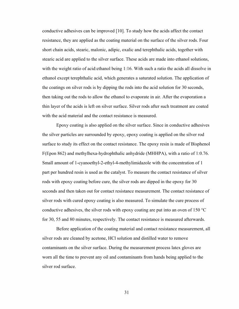
31

conductive adhesives can be improved [10]. To study how the acids affect the contact

resistance, they are applied as the coating material on the surface of the silver rods. Four

short chain acids, stearic, malonic, adipic, oxalic and terephthalic acids, together with

stearic acid are applied to the silver surface. These acids are made into ethanol solutions,

with the weight ratio of acid:ethanol being 1:16. With such a ratio the acids all dissolve in

ethanol except terephthalic acid, which generates a saturated solution. The application of

the coatings on silver rods is by dipping the rods into the acid solution for 30 seconds,

then taking out the rods to allow the ethanol to evaporate in air. After the evaporation a

thin layer of the acids is left on silver surface. Silver rods after such treatment are coated

with the acid material and the contact resistance is measured.

Epoxy coating is also applied on the silver surface. Since in conductive adhesives

the silver particles are surrounded by epoxy, epoxy coating is applied on the silver rod

surface to study its effect on the contact resistance. The epoxy resin is made of Bisphenol

F(Epon 862) and methylhexa-hydrophthalic anhydride (MHHPA), with a ratio of 1:0.76.

Small amount of 1-cyanoethyl-2-ethyl-4-methylimidazole with the concentration of 1

part per hundred resin is used as the catalyst. To measure the contact resistance of silver

rods with epoxy coating before cure, the silver rods are dipped in the epoxy for 30

seconds and then taken out for contact resistance measurement. The contact resistance of

silver rods with cured epoxy coating is also measured. To simulate the cure process of

conductive adhesives, the silver rods with epoxy coating are put into an oven of 150 °C

for 30, 55 and 80 minutes, respectively. The contact resistance is measured afterwards.

Before application of the coating material and contact resistance measurement, all

silver rods are cleaned by acetone, HCl solution and distilled water to remove

contaminants on the silver surface. During the measurement process latex gloves are

worn all the time to prevent any oil and contaminants from hands being applied to the

silver rod surface.

32

3.4 Results and discussions

Both the contact resistance and contact force are recorded by the computer when

contact happens between the two silver rods. The contact resistance – contact force curve

is plotted. We need to transform the contact resistance – contact force curve to tunnel

resistivity – contact pressure curve. This transformation is done by the calculation of the

radius of contact area, which can be approximated by Hertzian solution. The detailed

steps are described in the following.

3.4.1 Contact resistance – contact force curve

The contact resistance and contact force are recorded by the computer that is

connected to the multimeter and digital balance. A typical contact resistance – contact

force curve is shown in Figure 6.

It is seen that the contact resistance drops very fast when the contact force is

increased from zero. The curve can be well fitted by a power law

contact resistance (Ω) = c · (contact force (gram))d (3.5)

where c and d are two constant parameters, and can be fitted by least-square method

based on the experimental data.

0

0.002

0.004

0.006

0.008

0.01

0.012

0 20 40 60 80 100

contact force(gram)

cont

act r

esis

tanc

e(oh

m)

Figure 6. A typical measurement of contact resistance vs contact force for silver rods with un-cured epoxy coating

33

For each coating material the contact resistance – contact force curve is measured

3 times and the data are used to fit the power law relationship as shown in Equation (3.5).

The two constant parameters c and d are fitted by least-square method for each coating

material. A software package, Origin, is used to do this non-linear curve fit. The fitted

parameters c and d for each coating material are listed in Table 1. To measure how well the

curves are fitted, two quantities, the standard deviation of the residuals χ2/DoF and the

goodness of fit R2 are also listed in the table. Good curve fit is usually characterized with small

standard deviation of the residuals χ2/DoF and R2 close to 1. The two quantities in Table 1

show that the two parameters c and d are fitted reasonably well.

Table 1. Contact resistance - contact force curve fitting parameters for different coating

materials on silver rods

Clean silver, no coating

Stearic acid coating

Adipic acid coating

Malonic acid coating

Oxalic acid coating

Terephthalic acid coating

Epoxy coating, not cured

c 0.01316 0.04588 0.02406 0.0384 0.04292 0.00791 0.00946

d 0.4231 -0.63838 -0.76289 -0.69245 -0.88292 -0.66687 -0.5818

χ2/DoF 2.87e-6 2.72e-6 2.11e-7 3.45e-6 1.79e-6 8.18e-8 6.82e-7

R2 0.828 0.880 0.844 0.824 0.740 0.810 0.802

The fitted curves of contact resistance – contact force of silver with different coatings

are plotted in Figure 7 in logarithmic scale.

34

0

0.02

0.04

0.06

0.08

0.1

0.12

0.14

0.16

1 10 100

contact force (gram)

cont

act r

esis

tanc

e (o

hm)

stearicadipicoxalicterephthaliccleanmalonicuncured epoxy

Figure 7. Fitted contact resistance - contact force curves of silver rods with different coatings

The contact resistance of silver rods with epoxy coating cured under 150 °C for

30, 55 and 80 minutes are measured but not shown in Figure 7. The reason is that for

epoxy coatings with 55 and 80 minutes’ cure the silver rods appear to be insulated under

the contact force of 1- 100 grams. For 30 minutes’ cure the 3 contact resistance

measurements don not show a consistent pattern.

It can be clearly seen that the stearic acid shows the highest contact resistance among

all coatings. The bare silver-to-silver contact, uncured epoxy coating, and terephthalic acid

coating have the lowest resistance. The other three short-chain acids, namely the malonic,

oxalic and adipic acid, give contact resistances of intermediate value.

3.4.2 Calculation of the contact area – Hertzian solution

We have the measured contact resistance and contact force, but the contact

resistance – contact force relationship does not apply to other silver contacts because the

contact resistance is related to the contact radius of the silver rods in our experiment. The

radius of the contact area needs to be calculated in order to get the more general tunnel

35

resistivity – contact pressure relationship, which is independent from the size of the

contact area.

Since the two silver rods are identical in material and diameter, the contact area

between the two silver rods is circular. If seen as an elastic deformation, the radius of

contact area can be approximated by the Hertzian contact solution. The radius of the

contact area is given by Hertzian solution as [113]

12 36 (1 )

4Fra

Eν⎡ ⎤−

= ⎢ ⎥⎣ ⎦

(3.6)

where a is the radius of the contact area, F is the contact force, and r is the radius of the

silver rods. E and ν are the Young’s modulus and Poisson’s ratio of silver, which can be

found in a material handbook[111] to be 76,000 MPa and 0.39, respectively.

The contact force between the silver rods has been recorded by computer, hence

the contact radius can be calculated by using Equation (3.6) for different contact forces.

3.4.3 Tunnel resistivity of silver contacts with different coatings

Once the radius a of the contact area is calculated, the average contact pressure is

2

Fpaπ

= (3.7)

where F is the contact force and a is the radius of contact area.

The tunnel resistivity σ can be derived from Equation (3.4) as

2 ( )2

a Ra

ρσ π= − (3.8)

where R is the contact resistance, and ρ is the bulk resistivity of silver.

By using Equation (3.7) and (3.8), the measured contact resistance (R) – contact

force (F) curves can now be converted to tunnel resistivity (σ) – contact pressure (p)

curves. The tunnel resistivity (σ) – contact pressure (p) curves for different coating

materials are shown in Figure 8.

36

0

20

40

60

80

100

120

100 200 300 400 500 600

contact pressure (MPa)

tunn

el re

sist

ivity

(10^

-13

ohm

m^2

)

stearicadipicoxalicterephthaliccleanmalonicuncured epoxy

Figure 8. Tunnel resistivity vs contact pressure for silver rods with different coatings

For all coatings the tunnel resistivity goes down when contact pressure is

increased. This phenomenon can be explained by the theory of the tunnel effect. The

tunnel effect is the process of electrons penetrating thin contact films. As we recall, the

tunnel resistivity is a function of the thickness of the film s, the work function Φ which is

needed for the electron to emit from the metal to the film material, and the relative

permittivity εr of the film material. For a given coating material, the material property

parameters Φ and εr do not change with contact pressure, but the film thickness s

becomes smaller when the contact pressure is increased. The thinner film facilitates the

penetration of electrons and the tunnel resistivity is thus decreased with a smaller film

thickness s. The different slopes of the curves can be explained by the difference between

the modulus of the coating materials. Because the coating materials have different

modulus, the change of the coating thickness is different under the same amount of

contact pressure change, and consequently the slopes of the resistivity – contact pressure

curves are different for different coating materials.

37

The average contact pressure between spherical silver particles in conductive

adhesives after cure is approximately 167 MPa [9]. It can be seen from Figure 8 the

widely used stearic acid coating has the highest tunnel resistivity at this pressure, which

means that conductive adhesives with stearic acid have the highest resistivity.

At 167 MPa clean silver and silver with un-cured epoxy coating show much

smaller tunnel resistivity. The gap material between clean silver contacts is air, which can

also be easily compressed and driven out when the contact pressure is applied. The low

tunnel resistivity of uncured epoxy coating is because the epoxy before cure has the form

of fluid and can be easily squeezed out of the contact interface when a contact pressure is

applied. The residual epoxy is of such a small amount that it does not block the tunneling

electrons very much.

At the contact pressure of 167 MPa, malonic, oxalic, adipic and terephthalic acid

coatings all show smaller tunnel resistivities than the stearic acid. Terephthalic acid

coating shows the smallest tunnel resistivity. Malonic, oxalic, adipic and terephthalic are

dicarboxylic acids with shorter chain lengths than the stearic acid, and they tend to have

stronger affinity to silver than the C-18 stearic acid. It is very likely that these short chain

acids have a thinner film width s, and/or a smaller work function Φ than the C-18 stearic

acid. The penetration of the electrons is facilitated and the tunnel resistivity σ of these

acids coating is smaller than that of the stearic acid. Thus the replacement of the stearic

acid with short chain dicarboxylic acid in the epoxy could improve the conductive

property of conductive adhesives, as suggested in [114].

For silver with coatings of epoxy cured for 55 and 80 minutes under 150°C, the

epoxy has been fully cured under such curing conditions. The contact resistance is

infinitely large and there is no conduction through the contact interface. This can be

explained by the fact that the cured epoxy has a high elastic modulus and is not easy to

break or compress to a thin film to let the tunnel effect happen. Therefore epoxy coatings

cured for 55 and 80 minutes under 150°C appear to be totally insulating. It in another

38

way demonstrates the contacts between silver particles, and thus the conduction network

of the fillers in conductive adhesives must have been formed before the cure process. For

epoxy coating cured for 30 minutes, the epoxy is still in the process of cure. The tunnel

resistivity doesn’t show a consistent trend because some part of the epoxy film is cured

and some part is not, and the contact resistance is not stable on the contact interface.

The measured tunnel resistivity – contact pressure curves shown in Figure 8 are

data that is applicable for all silver contacts. The tunnel resistivity will be used in the next

chapter to calculate the contact resistance between silver particles in conductive

adhesives.

3.5 Conclusions

A tailor-made device was used to measure the contact resistance between silver

rods. By recording the contact resistance between silver rods under different contact

loads using computer, the contact load (R) – contact force (F) curve can be plotted. A

conversion is needed to get the tunnel resistivity (σ) – contact pressure (p) relationship.

Because both the contact resistance and contact force are related to the contact area, this

conversion is done by calculating the radius of the contact area using Hertzian contact

solution. The tunnel resistivity – contact pressure curves are plotted and it was found that

the tunnel resistivity decreases when the contact pressure is rising, which can be

explained by the tunnel film being compressed thinner under higher pressure. Apparently,

to get a low contact resistance a higher contact pressure is preferred.

The tunnel resistivity also depends on the property of the tunnel film material on

the contact surface. Since different acids are used in the manufacturing process of silver

flakes, the contact resistance of silver with different acids as the coating material was

measured, and their tunnel resistivities were calculated. Different acid coatings show

various tunnel resistivities. The C-18 stearic acid shows the highest resistivity. The short

chain dicarboxylic acids show smaller tunnel resistivities than the C-18 stearic acid.

39

Therefore the replacement of the stearic acid with dicarboxylic acids in conductive

adhesives could improve the conductivity of the conductive adhesives. Tunnel

resistivities of silver contact surface with epoxy coatings were also measured. The

uncured epoxy coating does not block the tunnel effect too much and a small contact

resistance was measured, but the cured epoxy coating is completely insulating due to its

high modulus and relatively large thickness. The fully cured epoxy coating gives an

infinitely large contact resistance between silver rods.

The measured tunnel resistivity (σ) – contact pressure (p) curves can be applied to

the calculation of contact resistance between silver particles in conductive adhesives, or

in other applications where silver-to-silver contact exists. In the next chapter, the

measured tunnel resistivity will be used to calculate the contact resistance between silver

particles, and furthermore on the calculation of the resistance of the filler network in

conductive adhesives.

40

CHAPTER 4

MODELING OF CONDUCTING NETWORK IN CONDUCTIVE

ADHESIVES

4.1 Introduction

In the previous chapter the contact resistance and tunnel resistivity were

measured. The measured resistivity can be used in this chapter to calculate the contact

resistance between silver particles.

In this chapter a simulation-based conductive adhesive model is built and the

resistivity of conductive adhesive is calculated based on the model. The cure process of

conductive adhesive is also simulated. The procedure is as follows: First the

microstructure model of conductive adhesives with spherical particles is constructed by

computer simulation, based on the given radius and volume fraction of the spherical

particles. Then the connections between particles are found out from the microstructure

model. The resistor network is obtained if every contact resistance is considered as a

resistor. By solving the resistor network the total resistance and bulk resistivity of

conductive adhesive is calculated.

The contact resistance between two particles is taken as the average contact

resistance and it is calculated before solving the resistor network. The contact resistance

is dependent on the contact area, bulk resistivity of silver and tunnel resistivity between

silver particles. The tunnel resistivity is dependent on the contact pressure. To get the

contact pressure and contact area, a finite element analysis on a representative volume

element is performed. The contact area and contact pressure is formed during the cure

process of the conductive adhesives. The epoxy of conductive adhesives is known to have

volume shrinkage during the cure process, and this volume shrinkage is measured by a

41

self-made device. The volume shrinkage of epoxy is applied as an eigenstrain to the

epoxy in the finite element model, and the contact pressure and contact area are obtained

from the finite element analysis. Based on the result of the finite element analysis, the

contact resistance between the two silver particles in the representative volume element is

computed, and this resistance value is taken as the average contact resistance value of all

particle contacts. The resistor network is solved next and the resistivity of the conductive

adhesive model is calculated.

The cure process of conductive adhesives is simulated. The detailed flow chart of

resistivity calculation in the cure process is shown in Figure 9. The resistivity of a

conductive adhesive sample during cure is measured in experiments and compared with

the resistivity calculated from our model. The two results show pretty good agreement,

which could be seen as a verification of our model.

42

Construction of microstructure

model

Identification of resistor network

Volume shrinkage

measurement

Finite element analysis

Calculation of contact area and contact

pressure

Contact resistance calculation

Calculation of bulk

resisatance

Calculation of bulk resistivity

Figure 9. Flow chart of the calculation of resistivity of conductive adhesives based on the microstructure model

4.2 3-D microstructure models of conductive adhesives with spherical particles

Electrically conductive adhesives are composites of polymeric matrix and

conductive fillers. The matrix is a dielectric material and provides mechanical adhesion;

the conductive fillers provide electrical conduction by connections between fillers. The

43

locations of the conductive fillers and how they are connected are important in

determining the electrical property, i.e., the electrical resistivity of the conductive

adhesives. In order to calculate the resistance of a conductive adhesive material, the

positions and inter-connections of the conductive fillers need to be known. A 3-D

microstructure model of conductive adhesives with spherical particles will be developed

in this section.

To describe the microstructure of a conductive adhesive, some information about

the conductive fillers has to be acquired first.

First the shape of the conductive fillers needs to be known. Apparently the shape

of conductive fillers determines the microstructure and connections of the fillers to some

extent. For conductive adhesives the electrical conduction is one of the primary functions,

therefore the shape of conductive fillers needs to be such that it can most facilitate the

electrical conduction. The shape of conductive fillers is also limited by ease of production

of the fillers. Flakes and spherical particles are two common shapes of conductive fillers,

which are low-cost, and easy to make. Between the two types, flakes have wider

applications as conductive fillers because of the better connectivity they provide over

spherical particles. However, the flakes have irregular forms and are hard to model. The

spherical particles, on the other hand, are easy to model because they are regular spheres

and only one parameter, the radius, is needed to describe their size.

The second parameter we need to know is the volume fraction of the conductive

fillers. As stated by the percolation theory, the volume fraction of the conductive fillers

has to be above the percolation threshold in order for the conductive adhesive to be

conductive. And indeed all conductive adhesive products have the volume fraction of

conductive fillers well above the percolation threshold. When building a microstructure

model of conductive adhesives the volume fraction of conductive fillers can be seen as

the known parameter.

44

For simplicity, in this chapter we only consider conductive adhesives with

spherical particles; and the three-dimensional microstructure model with uniform-sized

spherical particles will be built. All particles are assumed to be spheres and have the same

radius. If the radius of the spheres and the volume fraction of the conductive fillers are

given, to build the microstructure model we only need to determine the positions of the

conductive fillers, or, the coordinates (xi, yi, zi) of the centers of the particles in 3-D

space.

A very simple microstructure model is the Boolean model. Because the polymer

resin has high viscosity and the conductive fillers are completely blended with the resin,

the positions of conductive fillers can be seen as uniformly distributed in the resin, i.e.,

the density of the number of spheres per unit volume is the same everywhere in the

conductive adhesive. The easiest modeling method is to generate a set of uniform

randomly distributed coordinate values (xi, yi, zi) for all the centroids of the particles. This

kind of model is often called the Boolean model [115]. Simple as it is, it’s not a good

model because overlap is allowed and many of the spheres intersect with other ones. In

reality, the spheres are solid particles and they are not likely to overlap. A further

development based on the Boolean model is necessary [116].

The spheres that overlap in the Boolean model need to be separated. Imagine in

real conductive adhesives when two fillers are trying to overlap, a force is applied to the

two spheres when they are in contact and pushes them to keep them just in contact but

not to overlap. According to this idea, we can assume that a repulsion force is applied to

spheres that are overlapped, and this force makes the overlapped spheres to move a small

distance apart. The overlap vector can be introduced as follows. Suppose two spheres are

overlapped as shown in Figure 10. The overlap vector Vij of sphere i relative to sphere j is

defined as the minimum displacement vector needed for the sphere i to move, so that the

two spheres don’t overlap any more. If sphere i overlaps with several other spheres, the

net displacement vector of the center of sphere i is

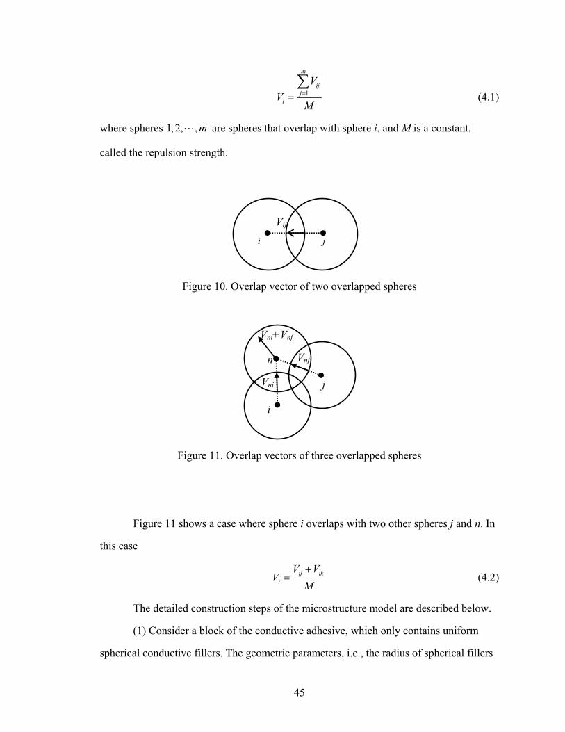
45

1

m

ijj

i

VV

M==

∑ (4.1)

where spheres 1,2, ,m are spheres that overlap with sphere i, and M is a constant,

called the repulsion strength.

Figure 10. Overlap vector of two overlapped spheres

Figure 11. Overlap vectors of three overlapped spheres

Figure 11 shows a case where sphere i overlaps with two other spheres j and n. In

this case

ij iki

V VV

M+

= (4.2)

The detailed construction steps of the microstructure model are described below.

(1) Consider a block of the conductive adhesive, which only contains uniform

spherical conductive fillers. The geometric parameters, i.e., the radius of spherical fillers

Vij

i j

j

i

n

Vni+Vnj

Vni

Vnj

46

r, the width w, length l and depth d of the conductive adhesive block, are given. If the

volume fraction of the conductive fillers cvf is also known, the number of spherical

particles in the conductive adhesive block can then be calculated by

3

34

vfwldcN

rπ= (4.3)

(2) Build a Boolean model. The coordinates of the centroid (xi, yi, zi) of each

sphere are generated from a uniform random number generator, and they satisfy

0 ix w< < , 0 iy l< < and 0 iz d< < to be located inside the conductive adhesive block.

The spheres are free to overlap.

(3) Analyze the particles one by one and find out each overlap in the Boolean

model. For each pair of overlapping spheres i and j, find the overlap vector Vij of sphere i

with respect to j. For every overlapping spherical particle i, calculate the net displacement

vector Vi by Equation (4.1).

(4) Move every overlapped particle i according to the net displacement vector Vi,

calculate the new locations of centers of all particles. Find out the maximum overlap

magnitude between all particles with new locations, denote it as τ.

(5) Compare τ with a pre-defined small number ε, which is the maximum

allowable overlap magnitude. If τ ε> , repeat (3) ∼ (5) until τ ε< is satisfied. If τ ε< ,

stop the iteration and the construction of the microstructure model is completed.

For the random number generation in step (2), a FORTRAN subroutine program

[117] was used. The program can generate different random numbers that are uniformly

distributed in the interval of [0, 1]. To get the coordinates of a sphere xi, yi and zi , simply

let

1 2 3, , i i ix r w y r l z r d= = = (4.4)

where r1, r2 and r3 are three random numbers, and w, l and d are the width, length and

depth of the conductive adhesive block. For each sphere the spatial coordinates are

47

generated from different random numbers r1, r2 and r3 so that all of the particle locations

are different.

There are two adjustable parameters in the iteration process. The first one is the

repulsion strength M in Equation (4.1), which controls the magnitude of the displacement

for each overlapped sphere to move in one iteration. A bigger repulsion strength M means

smaller displacements for the overlapped particles, resulting in a slower convergence

rate. But a too small M may move the spheres too much and cause even more spheres to

overlap after the iteration, and the final convergence will be difficult to reach. Therefore

an appropriate value of M needs to be selected in order to achieve a fast convergence rate.

In our study it was found that when M is set as 4.0 a good convergence rate can be

obtained. The second adjustable parameter is the maximum permissible overlap

magnitude ε. Since there is no absolute zero in a computer, overlaps that have smaller

magnitude than ε are not considered to be overlap. An overly large value of ε allows

very much overlap between spheres and makes the model not real; too small a value for ε

reduces the overlap between spheres but makes the model hard to converge. A balanced

value of 0.01r was chosen for ε in our model.

An example of the finished microstructure model for conductive adhesives with

spherical fillers is shown in Figure 12. In Figure 12 the dimensions of the block are

15μ15μ15 μm3, the sphere radius is 1 μm, the filler volume fraction cvf = 25%, M = 4.0

and ε = 0.01

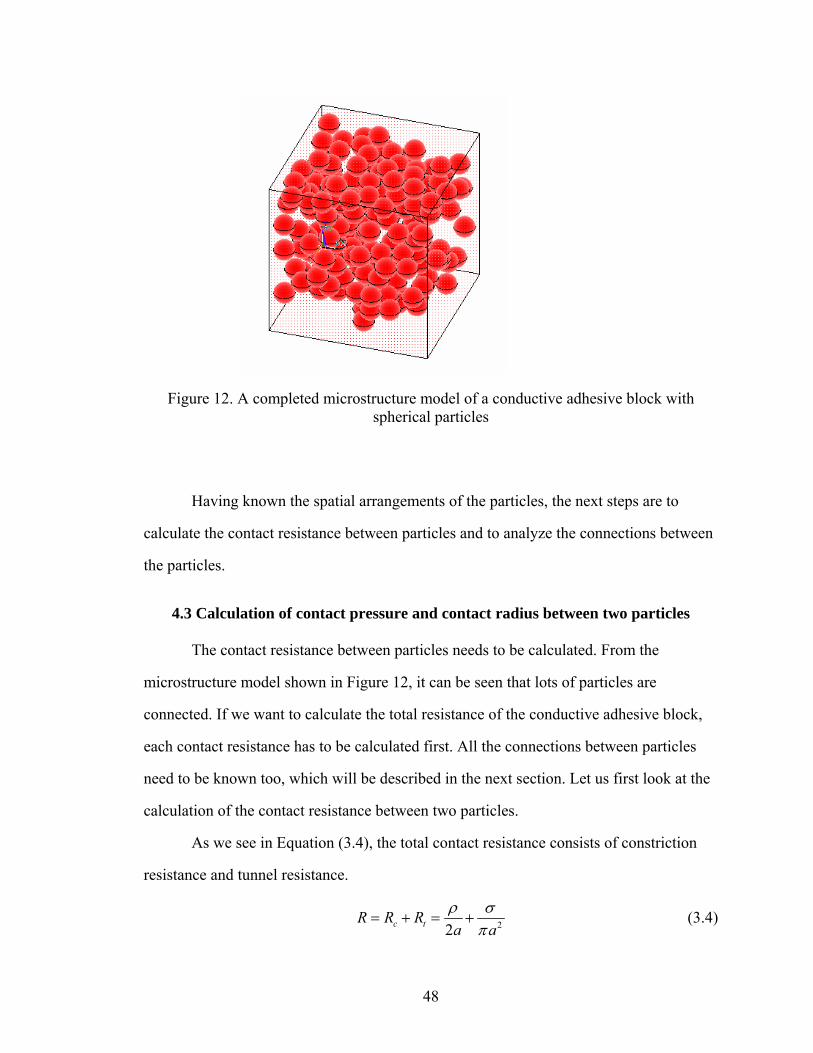
48

Figure 12. A completed microstructure model of a conductive adhesive block with spherical particles

Having known the spatial arrangements of the particles, the next steps are to

calculate the contact resistance between particles and to analyze the connections between

the particles.

4.3 Calculation of contact pressure and contact radius between two particles

The contact resistance between particles needs to be calculated. From the

microstructure model shown in Figure 12, it can be seen that lots of particles are

connected. If we want to calculate the total resistance of the conductive adhesive block,

each contact resistance has to be calculated first. All the connections between particles

need to be known too, which will be described in the next section. Let us first look at the

calculation of the contact resistance between two particles.

As we see in Equation (3.4), the total contact resistance consists of constriction

resistance and tunnel resistance.

22c tR R Ra a

ρ σπ

= + = + (3.4)

49

In order to apply Equation (3.4), three quantities need to be known: the contact

radius a, the bulk resistance ρ, and the tunnel resistivity σ. Suppose silver particles are

used as the conductive fillers, the bulk resistivity ρ of silver can be found in the material

handbook [111]. The tunnel resistivity σ has been measured in Chapter 3, but it depends

on the contact pressure. Therefore two parameters need to be determined: the contact

pressure p and the radius of the contact area a.

In conductive adhesives, the conductive fillers always have a volume fraction

above the percolation threshold. But even with a high volume fraction the conductive

adhesive is not conductive before it is cured. The conductive adhesive before cure is in

the form of paste and not conductive. During the cure process the volume of the polymer

resin shrinks and the modulus of the resin increases. The conductive fillers are pushed

together, and electrical conduction is built up. Only after the cure process do intimate

connections and contacts between particles form and the conductive adhesive becomes

conductive. It is the volume shrinkage and the modulus increase of the epoxy that push

the conductive fillers together to form a conducting network.

The cure process can be simulated by a finite element analysis on a representative

volume element of the conductive adhesive, and the contact pressure p and the radius of

the contact area a can be obtained from the finite element analysis. The resulting contact

pressure and radius can then be applied in Equation (3.4) to calculate the contact

resistance between two particles.

4.3.1 Measurement of volume shrinkage of epoxy during the cure process

In order to use finite element analysis to simulate the cure process, the volume

shrinkage of the epoxy has to be known. The following experiment is designed to

measure the volume shrinkage of epoxy during the cure process.

50

The volume shrinkage epoxy is obtained by measuring the buoyant force of the

epoxy in oil. The experiment is based on Archimedes’ principle, which says the buoyant

force on a submerged object is equal to the weight of the fluid displaced, or

B lF Vgρ= (4.5)

where FB is the buoyant force, ρl the density of liquid, V the volume of the object, and g

the acceleration of gravity.

Suppose we submerge the epoxy into oil and make two measurements of the

buoyant force, one at the beginning of the cure process and another in the cure process,

then

1 1B lF V gρ= (4.6)

2 2B lF V gρ= (4.7)

and the change of volume is

2 1 2 1

1 1 1 1

B B B

B B

V V F F FVV V F F

− − ΔΔ= = = (4.8)

The buoyant force is the difference of the weight of the epoxy in air and in oil. Let

0m g be the weight of the epoxy in air, 1m g the weight of epoxy in oil at the beginning of

cure and 2m g the weight of epoxy and in oil during the cure process, then we have

1 2

1 0 1

m mVV m m

−Δ=

− (4.9)

Thus the volume shrinkage of epoxy resin can be calculated if the weight of the

epoxy is measured in air before cure, in oil at the beginning of cure and during the cure

process by a high-resolution electronic balance. The experiment setup is shown in Figure

13.

51

resistance type temperature sensor

metal bar

thin string

mineral oil

epoxy resin

electronic balance

temperature controllerhot plate

TEFLON film

resistance type temperature sensor

metal bar

thin string

mineral oil

epoxy resin

electronic balance

temperature controllerhot plate

TEFLON film

Figure 13. Experiment setup for measurement of cure shrinkage of epoxy

A small amount of epoxy resin is placed on a very thin TEFLON film, and the

epoxy together with the film is immersed in a beaker filled with mineral oil. The epoxy

resin is made of Epon 862, hardener MHHPA and catalyst 2E4MZCN, with weight ratio

being 1 : 0.84 : 0.0184. The mineral oil in the beaker is heated by a hot plate to 150 °C. A

resistance type temperature sensor, together with an Omega temperature controller, is

used to monitor and control the temperature of the mineral oil. The epoxy resin and

TEFLON film are attached to a digital balance by a thin string, so that the weight of the

epoxy resin can be measured. The digital balance is Mettler Toledo AB204-S, with the

readability of 0.1 mg.

The volume shrinkage of the epoxy resin under 150°C is calculated according to

Equation (4.9) and displayed in Figure 14. Both the experimental data and the fitted line

are shown. The volume shrinkage can be seen as an eigenstrain, and it will be applied to

the epoxy resin in the finite element model to calculate the contact pressure and contact

radius between particles.

52

-0.08

-0.07

-0.06

-0.05

-0.04

-0.03

-0.02

-0.01

0

0 10 20 30 40

cure time (min)

volu

me

shrin

kage experiment data

fitted line

Figure 14. Volume shrinkage of epoxy resin during cure under 150°C

4.3.2 Finite element analysis of the contact between two spheres

The intimate contacts between silver particles are caused by the volume shrinkage

and modulus increase of the epoxy resin during cure, and the electrical conduction of

conductive adhesives is formed only after being cured. To find out the contact pressure

and contact radius between particles, the cure process is simulated by a finite element

analysis using ANSYS.

The finite element analysis is done on a representative volume element. Although

we already have the microstructure model, it can not be used in ANSYS as the

geometrical model. Because of the high geometric complexity of the microstructure

model, it is very hard to mesh either automatically or manually. Besides meshing, all the

contact analyses are nonlinear problems and will take a huge amount of time to converge.

To simplify the problem, we choose a representative volume element to do the analysis.

The axisymmetric model of this representative volume element is shown in Figure 15.

The two half circles are filler particles, and the surrounding material is epoxy. A very

small amount of epoxy between two the particles is taken out to ensure the two particles

53

will contact in the finite element analysis. This manual modification is small and will not

affect the finite element analysis results very much.

As can be seen, the element shown in Figure 15 is not the true representative

volume element. The reason is that in conductive adhesives not only two particles will

contact, very often multiple particles are in contact at the same time. Consequently the

contact pressure between a particular pair of spheres may be higher or lower than the

contact pressure we get from the representative volume element shown in Figure 15.

However, since there are an enormous amount of spheres and contact interfaces, some

contact pressure may be higher and some may be lower, the average contact pressure and

contact radius is assumed to be near that of our model.

Figure 15. The representative volume element for finite element analysis

The radius of the spheres is 1 μm, and the radius and the height of the epoxy are

1.30 μm and 4.59 μm, respectively. The volume fraction of the silver particles in the

finite element model is 27.7%, corresponding to same volume fraction of the conductive

adhesive microstructure model. The material of the particles is silver, and it is regarded as

54

elastic-perfect plastic material with Young’s modulus being 0.52 GPa and yield strength

0.05 GPa. The epoxy resin is modeled as an elastic material, with a changing Young’s

modulus in the cure process. The shear modulus of the epoxy resin under 150°C

isothermal cure is measured by a rheometer (TA Instruments AR-1000N) and shown in

Figure 16.

0

0.5

1

1.5

2

2.5

3

3.5

4

4.5

0 5 10 15 20 25 30 35

time (min)

shea

r mod

ulus

(MP

a)

experiment datafit line

Figure 16. Shear modulus of epoxy resin in 150°C isothermal cure

As can be seen from Figure 16, the shear modulus is mainly built up during the

first several minutes of cure. The change of the shear modulus can be fitted by a linearly

increasing line and a constant line. The Poisson’s ratio of the fully cured epoxy resin is

0.33 as specified by the manufacturer of Epon 862. If we assume the epoxy in liquid form

is incompressible and its Poisson’s ratio changes linearly in the cure process, the

Poisson’s ratio can be plotted as in Figure 17.

55

0

0.1

0.2

0.3

0.4

0.5

0.6

0 5 10 15 20 25 30 35time (min)

Poi

sson

's ra

tio

Figure 17. Poisson’s ratio of epoxy resin in 150°C isothermal cure

The Young’s modulus of the epoxy resin in cure can be calculated from the shear

modulus and Poisson’s ratio by

2(1 )E Gν= + (4.10)

where E is the Young’s modulus, G is the shear modulus, and ν is the Poisson’s ratio.

The Young’s modulus increases linearly at first, then stays at a constant value. It

is plotted in Figure 18.

0

2

4

6

8

10

12

0 5 10 15 20 25 30 35time (min)

You

ng's

mod

ulus

(MP

a)

Figure 18. Young’s modulus of epoxy resin in 150°C isothermal cure

56

The Poisson’s ratio and Young’s modulus of the epoxy resin in Figure 17 and

Figure 18 will be used in the finite element analysis.

The volume shrinkage of conductive adhesives during cure has been measured

experimentally as shown in Figure 14. By applying the volume shrinkage as an

eigenstrain to the epoxy resin in the finite element model, we can get the contact pressure

and contact radius between the two particles in the representative volume element. The

change of contact pressure and contact radius in 150°C isothermal cure is shown in

Figure 19 and Figure 20, respectively. Both the contact pressure and the contact radius

increase during the early stage of the cure process, then they approach a steady value in

the later stage of the cure process. The contact pressure and contact radius will be used to

calculate the contact resistance between particles in the next section.

0

0.04

0.08

0.12

0.16

0.2

0 5 10 15 20 25 30 35time (min)

cont

act p

ress

ure

(GP

a)

Figure 19. Contact pressure between two spherical particles in 150 °C isothermal cure

57

0

0.02

0.04

0.06

0.08

0.1

0 10 20 30time (min)

cont

act r

adiu

s ( μ

m)

Figure 20. Contact radius between two spherical particles in 150°C isothermal cure

4.4 Bulk resistance calculation

After the contact pressure and contact radius have been calculated, the contact

resistance between two particles can now be calculated by using Equation (3.4). The bulk

resistivity of silver ρ is 1.55μ10-6 Ωcm.[111]. The tunnel resistivity can be found

according to the tunnel resistivity curve of clean silver shown in Figure 8, based on the

contact pressure value obtained from the finite element analysis. The contact radius is

also known from the finite element analysis.

22c tR R Ra a

ρ σπ

= + = + (3.4)

The contact resistance between the two spheres in the representative volume

element is calculated, but it can also be taken as the average contact resistance between

each pair of connected particles in the conductive adhesive.

After the calculation of contact resistances between conductive fillers, the next

step is to compute the bulk resistance of a conductive adhesive.

The bulk resistance of conductive adhesives comes from the contact resistance

between particles. Because silver is an excellent conductor, the resistance of silver

58

particles is very small compared with the contact resistance between silver particles. The

major contributors of the bulk resistance of conductive adhesives are contact resistances

between silver particles, and all the contact resistances form a resistor network. The bulk

resistance of a conductive adhesive block is simply the total resistance of the resistor

network between the top and bottom surfaces.

In order to calculate the total resistance of the resistor network, all connections

between the particles need to be found first. Since we already have the microstructure

model and all the locations of the particles are known, the connections can be found by a

computer program. The two particles are assumed to be in contact and a resistor exists on

the contact interface when two adjacent spheres are very close or have a small overlap,

i.e.,

1 2r r ε+ < (4.11)

where r1 and r2 are the radii of the two spheres, and ε is the maximum allowable overlap.

The resistance value of the resistor is given by Equation (3.4). All the connections

between particles are found, and thus a resistor network is formed by all the contact

resistances between particles.

One example of the 3-D resistor network is shown in Figure 21, which is

corresponding to the microstructure model shown in Figure 12. Each point in Figure 21

represents the center of a particle. If two points are connected by a line, it means the two

particles are in contact. Each short line in the figure can be seen as a resistor, with a

resistance value of 0R , calculated by Equation (3.4). The isolate points represent particles

that are not connected to the resistor network, and they do not contribute to the electrical

conduction and the bulk resistance of the conductive adhesive.

59

Figure 21. Resistor network formed by contact resistances between conductive particles in a conductive adhesive

Figure 22. Bulk resistance calculation scheme of a conductive adhesive block

The scheme of bulk resistance calculation is shown in Figure 22. If we want to

calculate the resistance of the resistor network between the top and bottom faces of a

conductive adhesive block, the two faces are connected to two zero-resistance metal pads.

A conductive adhesvie

1 Amp

60

The two pads are connected with a current source, and the current source generates a

current of one ampere. Ohm’s law gives

URI

= (4.12)

If the top metal pad is set to have zero electric potential, the value of the voltage

U of the bottom pad is just the total resistance because the current being supplied is one

ampere. The voltage of the bottom panel can be solved by ANSYS’ static circuit analysis

module, and hence the total resistance of the resistor network is obtained.

4.5 Simulation of the cure process

To verify our model, the cure process is simulated in this section and the

resistivities calculated from our model and measured from experiment are compared.

An experiment was performed to measure the resistance of conductive adhesive

during cure. The conductive adhesive is made by blending silver spherical particles with

epoxy resin. The silver spherical particles are obtained from Ames Goldsmith Corp., and

they have an average radius of 1 μm. The epoxy resin consists of hisphenol-F (DGEBF)

Epon 862 from Hexion Specialty Chemicals, Inc., hardener methylhexa-hydrophthalic

anhydride (MHHPA) from Lindau Chemicals, Inc., and catalyst l-cyanoethyl-2-ethyl-4-

methylimidazole (2E4MZCN), from Shikoku Chemicals Corp. The weight ratio of

epoxy:hardener:catalyst is 1:0.84:0.0184. The weight ratio of silver and epoxy resin in

the conductive adhesive is 4:1. The conductive adhesive is applied to a printed circuit

board using a stainless-steel stencil. A piece of the conductive adhesive sample is shown

in Figure 23. The conductive adhesive sample is placed in a 150°C oven to be cured for

35 minutes. A multimeter is connected to the four copper lines on the circuit board to

constantly measure the resistance of the conductive adhesive strip, and the resistance

change of the conductive adhesive is recorded by a computer.

61

Figure 23. Sample of conductive adhesive strip

Although the resistance of conductive adhesive is measured, it can not be

compared with the resistance of our model because the size of the model is different from

the specimen. A reasonable comparison should be independent of specimen size, so the

resistivity is calculated and compared. The dimension of the conductive adhesive strip

between the copper pads is 10.16 mm μ 2.54 mm μ 0.1778 mm. The bulk resistivity of

the conductive adhesive can then be calculated using

RAL

ρ = (4.13)

where R and ρ are the resistance and resistivity of the conductive adhesive, A and L are

the cross section area and length of the conductive adhesive between the copper pads.

The resistance of the microstructure model of the conductive adhesive is also

calculated, as described in the previous sections. Similarly, the resistivity of the model is

calculated using Equation (4.13).

For each minute of the cure process the resistance of the conductive adhesive

sample is measured and resistivity calculated. The resistivity from the model is also

calculated at each time point. The comparison between the two is shown in Figure 24.

printed circuit board

conductive adhesive

copper trace

copper pad

62

0.0

0.1

0.2

0.3

0.4

0.5

0.6

0.7

0.8

0.9

1.0

0 5 10 15 20 25 30 35 40time (min)

resi

stiv

ity (o

hm c

m) from experiment

from model

Figure 24. Conductive adhesive bulk resistivity change during cure

The resistivity from the model matches pretty well with experimental data. At the

beginning of the cure process the resistivity is very high, meaning the electrical

conduction in the conductive adhesive has not been established yet. Both experiment and

model results show that the bulk resistivity drops fast in the first 5 minutes of the cure

process. This resistivity decrease is a result of the volume shrinkage and modulus

increase of the epoxy resin. The volume and modulus change of the epoxy resin cause the

contact radius and contact pressure to increase, and the contact resistance between

particles to decrease. The total resistance of the conductive adhesive, i.e. the resistor

network of contact resistances, is consequently reduced.

The resistivity approaches a steady value at the later stage of cure, indicating the

cure process gradually stops. The change of the resistivity shows good electrical

conduction of conductive adhesives can only be formed after the curing process.

4.6 conclusions

A 3-D micromechanics model was built to simulate the curing process and to

calculate the bulk resistivity of conductive adhesives with uniform spherical particles.

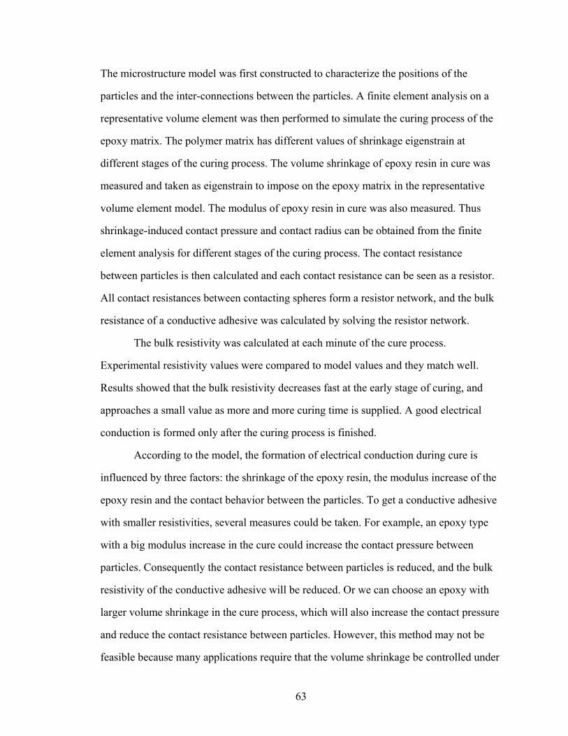
63

The microstructure model was first constructed to characterize the positions of the

particles and the inter-connections between the particles. A finite element analysis on a

representative volume element was then performed to simulate the curing process of the

epoxy matrix. The polymer matrix has different values of shrinkage eigenstrain at

different stages of the curing process. The volume shrinkage of epoxy resin in cure was

measured and taken as eigenstrain to impose on the epoxy matrix in the representative

volume element model. The modulus of epoxy resin in cure was also measured. Thus

shrinkage-induced contact pressure and contact radius can be obtained from the finite

element analysis for different stages of the curing process. The contact resistance

between particles is then calculated and each contact resistance can be seen as a resistor.

All contact resistances between contacting spheres form a resistor network, and the bulk

resistance of a conductive adhesive was calculated by solving the resistor network.

The bulk resistivity was calculated at each minute of the cure process.

Experimental resistivity values were compared to model values and they match well.

Results showed that the bulk resistivity decreases fast at the early stage of curing, and

approaches a small value as more and more curing time is supplied. A good electrical

conduction is formed only after the curing process is finished.

According to the model, the formation of electrical conduction during cure is

influenced by three factors: the shrinkage of the epoxy resin, the modulus increase of the

epoxy resin and the contact behavior between the particles. To get a conductive adhesive

with smaller resistivities, several measures could be taken. For example, an epoxy type

with a big modulus increase in the cure could increase the contact pressure between

particles. Consequently the contact resistance between particles is reduced, and the bulk

resistivity of the conductive adhesive will be reduced. Or we can choose an epoxy with

larger volume shrinkage in the cure process, which will also increase the contact pressure

and reduce the contact resistance between particles. However, this method may not be

feasible because many applications require that the volume shrinkage be controlled under

64

a certain level. Another way to reduce the resistivity of the conductive adhesives is to

remove materials that have big tunnel resistivities from the silver particle surface. For

example, using the short-chain dicarboxylic acids instead of the long-chain stearic acid in

the manufacturing process of flakes can reduce the tunnel resistivity and the bulk

resistivity of conductive adhesives, as shown in the last chapter.

The good match between the experiment and model shows the current modeling

approach is effective. The next chapter,a study of the effect of geometric parameters, will

be based on this approach.

65

CHAPTER 5

EFFECT OF FILLER GEOMETRY ON THE CONDUCTION OF

ISOTROPIC CONDUCTIVE ADHESIVES

5.1 Introduction

Since the conductive adhesive is proposed to replace solder in electronic

packaging, its conduction property, or resistivity, has been a significant concern.

Conductive adhesives with small resistivity are desired. People have been trying to make

conductive adhesive materials with good electrical conductivity by using different kinds

of filler materials, and by using particles with different shapes and sizes.

The geometric parameters of the particles such as shape, size and size distribution

certainly affect the resistivity of the conductive adhesive. To find out what the effects are,

the most natural way is to make conductive adhesive samples with particles of different

shape, size and size distribution, then cure the samples and measure their resistivity. But

if there are many configurations to be tried, many experiments will be involved and

significant time and effort will be required. Is it possible to study the effect of the

geometric parameters by running computer simulations instead of conducting real

experiments?

The answer is yes. The microstructure model described in the previous chapter is

effective in modeling the conductive adhesive. Once we have the microstructure model,

we can then find out the particle connections in the conductive adhesive and calculate the

resistivity of the conductive adhesive by solving the resistor network. In this chapter, the

microstructure models with different geometric parameters are built by computer

simulations. Then the resistivity is calculated and the effect of the geometric parameters

can be identified by looking at the value of the resistivity.

66

Conductive adhesives with both spherical and flake particles will be studied. The

microstructure model in the last chapter was for spherical particles, but some

modifications could be made to the model construction process so that conductive

adhesives with flake particles can also be modeled.

To analyze the effect of the geometric parameters, an experiment design method,

called the 2k factorial design, is used. The fist step is to identify all the geometric

parameters, or factors that are of interest. Then each of the parameters is set at two levels:

high and low. If there are k parameters or factors, totally there will be 2k combinations of

the parameters. For each combination, the resistivity of the models is calculated. The

factor values and the resistivity values are then taken to do the 2k factorial analysis. By

comparing the main effects and interaction effects of the parameters, the significant

factors can be determined. These are the factors that significantly affect the resistivity of

the conductive adhesive. Furthermore, the main effect plot and interaction plot will show

how the change of the factors can affect the resistivity of conductive adhesives.

Five conductive adhesive models are built and the effect of geometric parameters

of the conductive fillers in each model is studied. The five models are:

1. Conductive adhesives with uniform-sized spherical particles;

2. Conductive adhesives with spherical particles whose size follows a normal

distribution;

3. Conductive adhesives with spherical particles, whose size falls into two size

classes, with each following a normal size distribution;

4. Conductive adhesives with bendable flakes;

5. Conductive adhesives with unbendable flakes.

The approach to study the effect of particle geometric parameters by computer

simulation and factorial design is faster and more convenient than real experiments, and a

great amount of time and effort could be saved.

67

5.2 Microstructure models of conductive adhesives

The calculation of the bulk resistivity of conductive adhesives is based on the

calculation of the resistor network formed by all the contacts between conductive filler

particles. In order to get the resistor network, all connections between the particles need

to be found out first, and the connections are determined by the locations of the filler

particles. Therefore the microstructure model of conductive adhesives is important in

determining the conductive property.

Two types of microstructure models will be discussed in this chapter: models of

conductive adhesives with spherical particles as shown in the previous chapter, and

models of conductive adhesives with flake particles

5.2.1 Models of conductive adhesives with spherical particles

The simplest microstructure model is for conductive adhesives with uniform-sized

spherical particles. The construction steps are similar to those described in the previous

chapter. However, some modifications should be made if the size of the spheres has a

distribution. For example, if the radius of the spheres follows a normal distribution, with

the mean radius being μ and standard deviation σ, the radii of all spheres should be

generated in the following way. First, two random numbers r1 and r2 in the interval of [0,

1] are generated using a FORTRAN program [117], just as we did in last chapter. Then

the uniform distribution of the random number can be transformed into a normal

distribution by using [118]

1 1 2

2 1 2

2 ln cos(2 )

2 ln sin(2 )

x r r

x r r

π σ μ

π σ μ

⎡ ⎤= − +⎣ ⎦⎡ ⎤= − +⎣ ⎦

(5.1)

in which x1 and x2 are the two radii of spheres, and μ and σ are the mean of the radius

and standard deviation of the radius, respectively. Repeat using Equation (5.1) with

different random numbers r1 and r2, many different x1’s and x2’s can be generated. If we

68

put all the x1’s and x2’s together, they will be found to follow a normal distribution with

the mean being μ and the standard deviation being σ. Thus all the radii of the spherical

particles are obtained and they follow a normal distribution.

If there are two classes of spheres, and the radius of spheres in each class follows

a normal distribution, the generation of the radii is similar the above procedure. Equation

(5.1) will still be used, but with different values of (μ, σ) for each class of spheres.

It should be noticed that since the particles don’t have the same radius, the

calculation of the number of particles and analysis of overlap between particles will be

different from that used in Chapter 4. Slight modification will be needed.

5.2.2 Models of conductive adhesives with flakes

One other type of microstructure model is for conductive adhesives with flake

particles. Most commercial isotropic conductive adhesives contain silver flakes because

of the better conduction property they provide. The shape of silver flakes is irregular and

very hard to model exactly. To simplify the problem, the flakes are modeled using

rectangular blocks, with the thickness far less than the length and width of the conductive

adhesive block. Suppose there is a conductive adhesive sample that is conductive along

the y axis direction, the position and shape of a flake particle can be specified by 7

parameters, i.e., the x, y, and z coordinate of the center of the flake, the width 2w0, length

2l0 and thickness 2t0 of the flake, and the alignment angle α of the flake. The flakes in the

conductive adhesive will be aligned to a certain direction in the x-z plane after the

application process such as screen-printing. Hence one alignment angle α is assumed to

exist, which is the rotation angle with respect to axis z. A flake and its parameters are

shown in Figure 25. Because the thickness of the flake is much less than the other two

dimensions, if we look at the projection of the flake in the x-y plane, the flake can be

simplified as a line segment, shown in Figure 26.

69

Figure 25. Parameters of a conductive flake in conductive adhesives

Figure 26. Projection of a flake in the x-y plane

The construction of the microstructure model of flake particles is similar to that of

spherical particles, but with several differences. The first is that the flakes can not only

move but also rotate. If two flakes overlap, the two flakes need to be both moved and

rotated to stay clear of each other. The way of calculating the overlap vector is different.

Similar to the case of overlapped spherical particles, the overlap vector Vij of flake i

relative to flake j is defined as the minimum displacement vector needed for flake i to

move to be completely separate from flake j. For spherical particles, to check if two

spheres overlap only the distance between the centers of the two spheres needs to be

calculated. If the from-center-to-center distance is less the sum of the two radii, then the

two spheres overlap. To decide if two flakes overlap, we need to first look at the z

coordinate of the flakes. Denoting zi and zj as the z coordinates of the centers of flake i

02l

02w

02t

α x

z

y

02l α

x

y

70

and j, and w0 as the half width of the flake, only when the two intervals [ 0iz w− , 0iz w+ ]

and [ 0jz w− , 0jz w+ ] have intersection it is possible for the two flakes to overlap. If

[ 0iz w− , 0iz w+ ] and [ 0jz w− , 0jz w+ ] do overlap, the next step is to check if the

projections of the flakes in the x-y plane intersect. The two flakes intersect only when two

projected line segments intersect. Denote 1 2( , )i i as two end points of line segment i, and

1 2( , )j j as end points of line segment j. Denote d( 1,i j ) as the distance from point i1 to

line segment j, the magnitude of the overlap vector Vij is

1 2 1 2| | ( , ), ( , ), ( , ), ( , )ijV Minimum d i j d i j d j i d j i= (5.2)

An illustration of the overlap vector Vij of two overlapped flakes i and j is shown

in Figure 27.

Figure 27. Displacement vector of two overlapped flakes

If a flake is overlapping with many other flakes, the displacement vector of flake i

is calculated by

1

m

ijj

i

VV

M==

∑ (5.3)

where flakes 1,2, ,m are the flakes that overlap with flake i, and M is called the

repulsion strength. M is set as 4 in our study to speed up the convergence.

1i

2i

1j

2j

jα

iα

ijVx

y

71

In addition to the displacement vector, if flake i and flake j overlap, flake i needs

to be rotated by an angle to be separate from flake j. The rotation angle of flake i due to

overlap with flake j is

0

arcsin ijij

Vl

θ⎛ ⎞⎜ ⎟=⎜ ⎟⎝ ⎠

(5.4)

where l0 is the half length of flake i.

The rotation angle of flake i due to overlaps with other flakes is

1

m

ijj

i N

θθ ==

∑ (5.5)

where N is the rotational repulsion strength, which is similar to repulsion strength M. N is

set as 4 in our study.

The detailed construction steps of the conductive adhesive model with flake fillers

are as follows.

(1) Consider a block of the conductive adhesive that contains conductive flake

particles. The width, length and thickness of the flakes are 02w , 02l and 02t , respectively.

The dimensions of the conductive adhesive block are width w, length l and depth d. If the

volume fraction of the conductive fillers is given as vfc , then the number of flakes is

determined by

0 0 08

vfwldcN

w l t= (5.6)

(2) Build a Boolean model. The coordinate (xi, yi, zi) of the center of each flake is

generated from a uniform random number generator, and they satisfy 0 ix w< < ,

0 iy l< < and 0 iz d< < to be located in the conductive adhesive block. Suppose the

maximum alignment angle of the flakes is 0α , The alignment angle of each flake iα is

72

also randomly generated with the random number generator, with 0 0iα α α− < < . The

flakes are free to overlap in the Boolean model.

(3) Analyze the flakes for overlap one by one in the Boolean model. For each pair

of overlapping flakes i and j, find the overlap vector Vij and overlap angle ijθ of flake i

with respect to j. Then calculate the net displacement vector by Equation (5.3) and

rotation angle by Equation (5.5) for every overlapped flake i.

(4) Move every overlapped flake i by the net displacement vector Vi, and rotate it

by angle iθ . Calculate the new locations of all flakes. Find out the maximum overlap

magnitude of the newly displaced flakes, denote it as τ.

(5) Compare τ with a small number ε, which is the predetermined maximum

allowable overlap magnitude. If τ ε> , repeat (3) ~ (5) until τ ε< is satisfied. If τ ε< ,

stop the iteration and the construction of the microstructure model is completed. ε is set

as 00.02t in our study.

Figure 28 shows a finished microstructure model for conductive adhesive with

flakes.

Figure 28. An unbendable microstructure model of conductive adhesive with flake particles

73

The above model assumes that the flakes are rigid and don’t bend, and that there

is no deformation of the flakes. We call the above model the unbendable model. But

since the thickness of flakes is far less than the length and width, the flake may be bent

over easily when it contacts with other flakes. When flake bending happens, the contact

area between flakes becomes much larger than when no bending happens. However, this

bending behavior is complex and depends on the size, shape and location of the flakes,

and it is hard to tell how they are bent or how much length is bent. But we know the two

extreme cases of the flake deformation. One is the unbendable flake model, in which all

flakes do not deform and they can only have rigid body movements. The other one is the

bendable flake model, which is described as follows.

In the bendable flake model, if two flakes have overlap, we assume the shorter tip

of one of the two flakes is bent over as shown in Figure 29. The width of the contact area

is the bent section of one flake, and the length of the contact area is the overlap of the two

flakes along axis z direction. The bendable model can be built based upon the Boolean

model. First a Boolean model is built, in which the locations and alignment angles of

flakes are randomly generated, and the flakes are free to overlap. Then the overlaps of

flakes are analyzed by a computer program. If two flakes overlap, then one flake is

assumed to be bent like what is shown in Figure 29.

Figure 29. The bending of a flake when contacting with another flake

x

y

Contact area (bent tip)

z

74

The contact areas in the bendable flake model are bigger than the contact areas in

the unbendable flake model. Consequently the bendable flake model will have a lower

resistivity than the unbendable flake model. While both of the two models are not real,

the resistivities of the two models can be taken as the bounds of the true resistivity of

conductive adhesives with flakes: the resistivity calculated from the bendable flake model

can be taken as the lower bound of the true resistivity, and the resistivity from the

unbendable flake model as the upper bound.

Now that the microstructure models of conductive adhesives with spheres and

flakes have been built, the contact resistance between particles and the total resistance of

the conductive adhesive can be calculated next.

5.3 Contact and bulk resistance calculation

The contact resistance between spherical particles is still calculated by Equation

(3.4). For contact between silver spherical particles, the contact radius a is obtained from

the finite element analysis as shown in Chapter 4. The tunnel resistivity σ is measured in

Chapter 3 and is related to the contact pressure. The bulk resistivity of silver ρ is found in

the material handbook to be 1.55μ10-6 Ωcm [111].

22c tR R Ra a

ρ σπ

= + = + (3.4)

Some approximations are made for the contact area between flake particles. For

contacts between silver flakes, the contact areas are larger than those between spheres. It

is hard to calculate the real contact areas between flakes, therefore some assumptions are

made. The contact area between flakes is assumed to be rectangular. For contact area A1

between two bendable flakes, the length of A1 is the length of the bent tip of one flake as

shown in Figure 29, and the width of A1 is the overlap of two flakes in the z direction. For

unbendable flakes, we assume the width of the contact area A2 is of 2r0, and the length of

75

A2 is the overlap of two flakes in the z direction. In our study r0 is set as 1.4 μm, which is

the contact radius from the finite element analysis of the contact between two spheres

with the radius of 5 μm.

When calculating the contact resistance between flakes (including both bendable

and unbendable flakes), the calculation is slightly different than that of contact resistance

between spheres in the sense that no constriction resistance exists. As mentioned in

Chapter 3, the constriction resistance is caused by the current lines being distorted due to

the conducting area being decreased. If the contact area between particles is much smaller

than the size of the particle, then there exists a constriction on the contact interface. For

contacts between flakes, the conducting areas are fairly large compared to the size of the

flakes. Therefore, the constriction resistance between flakes is negligible and only tunnel

resistance exists. The contact resistance between two flakes is

tR RAσ

= = (5.7)

where Rt is the tunnel resistance, σ is the tunnel resistivity, and A is the contact area

between flakes.

Only the contact resistance between particles is considered, and the bulk

resistance of particles is neglected since it is much smaller than the contact resistance.

If the contact resistance calculated by Equation (3.4) or Equation (5.7) above is

taken as the average contact resistance between spheres or flakes, the total resistance of

the resistor network can then be calculated as we did in Chapter 4. Same procedure is

followed: first find out the connections between the particles, then build the resistor

network, and solve the total resistance of the resistor network by ANSYS’ electric circuit

analysis module. And again, to eliminate the effect of size, resistivity is calculated for

each conductive adhesive model.

76

5.4 Introduction to design of experiments

Up to now we have built the conductive adhesive models and calculated the

resistivity of these models. There are several geometric parameters of the conductive

particles that may affect the resistivity of the conductive adhesive. For example, if the

radius of spherical particles in conductive adhesives follows a normal distribution, there

are two parameters: the mean radius and standard deviation of the radius of particles. For

spherical particles of two classes of sizes with both following a normal distribution, there

are four parameters: the mean and standard deviation of bigger particle radius, and the

mean and standard deviation of smaller particle radius. Among these parameters, some

have bigger effects on the conduction of conductive adhesives, the others have smaller

effects. Our goal in this chapter is to study which parameters have the biggest effects on

and how they affect the resistivity of the conductive adhesive, and consequently how to

reduce the resistivity by choosing particles with the right geometric parameters.

The most intuitive approach is to vary each factor of interest in turn, and keep all

other factors that may influence the outcome resistivity at a fixed level. However, there is

a better method that has been widely used in the design of experiments – the factorial

experimental design. This method has some advantages over the “one factor at a time”

approach: it gives greater precision of estimating overall factor effects, enables

interactions between different factors to be explored, and allows the range of validity of

the conclusions to be extended by the insertion of additional factors [119]. Therefore

factorial design will be used in our study.

When experiments involve a study of the effects of two or more factors, factorial

designs are in general the most efficient for this type of experiments [120]. By a factorial

design we mean that all possible combinations of the levels of the factors are

investigated. For example, if there are a levels of factor A and b levels of factor B, then

there will be ab treatment combinations. One special case is that we have k factors and

each factor is at only two levels, such as “high” and “low” levels. A complete replicate of

77

such a design requires 2k observations and is called a 2k factorial design or a full factorial

design at two levels. In our study, whenever we build a microstructure model of

conductive adhesives and calculate its resistivity, the process can be seen as an

experiment and the resistivity can be seen as the experiment result. The resistivity is

dependent on the geometric parameters, and hence the geometric parameters are the

factors of the experiments. To apply the method of 2k factorial design, each geometric

parameter is set at a big value or “high” level, as well as at a small value or “low” level,

and the corresponding resistivity is calculated. At each combination of the geometric

parameters, 10 microstructure models will be built and corresponding resistivities

calculated. Since the random number generators are used in the construction of

microstructure models, these 10 models will be different even with same combination of

geometric parameter values. The replications of the calculations of resistivities will give a

more precise estimate of the resistivity for a certain combination of the geometric

parameters than just a single calculation with one model.

The effect of a factor is defined to be the change in response produced by a

change in the level of the factor, and is frequently called the main effect. Suppose we

want to measure the average effect of a geometric parameter or factor, A, on the

resistivity ρ of the conductive adhesive. The main effect of A is the difference between

the average ρ value of all experiments when factor A is at the high (+) level and average

ρ value of all experiments at the low (-) level of A. Notationally, A+ and A- are used to

represent the high and low levels of A, respectively, and ME(A) is the main effect of A.

The main effect of A is [121]

( ) ( ) ( )ME A A Aρ ρ= + − − (5.8)

where ( )Aρ + is the average of the ρ values obtained at A+ and ( )Aρ − is the ρ values

obtained at A-.

78

The main effect can be displayed graphically, which is referred to as a main

effects plot. The main effect plot graphs the averages of all the observations at each level

of the factor and connects them by a line. For two-level factors, the vertical height of the

line is the difference between the two averages, which is the main effect. The absolute

value of the vertical height determines the relative strength of a factor. The higher the

vertical height it is, the greater effect a factor has on the resistivity of the conductive

adhesive. An example of the main effect plot is shown in Figure 30. It can be seen in the

plot that when the value of the factor is changed from low to high level the result of the

experiment also increases.

factor level

Mea

n of

exp

erim

ent

resu

lt

highlow

47.0

46.5

46.0

45.5

45.0

44.5

44.0

Main Effects Plot

Figure 30. Example main effect plot of a factor

When there are two factors or more, interactions may exist between factors. The

interaction appears when the effect of one factor, say B, depends on the level of the other

factor, say A. Or in other words, the difference in response between the levels of one

factor is not the same at all levels of the other factors. Therefore when interaction is

79

significant it is not enough to look at main effect only; both the main effect and the

interaction effect need to be considered simultaneously to decide how one factor affects

the experiment result. The interaction effect is denoted by INT(A, B) and defined as [121]

1 1( , ) ( | ) ( | ) ( | ) ( | )2 2

INT A B B A B A A B A Bρ ρ ρ ρ= + − − = + − − (5.9)

where ( | )B Aρ + is the conditional main effect of B at the + level of A, and ( | )B Aρ + ,

( | )B Aρ − , ( | )A Bρ + and ( | )A Bρ − are similarly defined.

Interactions plots are useful for judging the presence of interaction. The

interaction plots of two factors are a couple of lines. Because the interaction is present

when the response at a factor level depends upon the levels of other factors, parallel lines

in an interaction plot indicate no interaction. The greater the departure of the lines from

the parallel state, the higher the degree of interaction. An example interaction plot is

shown in Figure 31. Since the two lines are not parallel there is an interaction between

the two factors.

B

Mea

n of

exp

erim

ents

200150

49

48

47

46

45

44

43

A2050

Interaction Plot of two factors

Figure 31. Example interaction plot of two factors

80

The main effect plot and interaction plot can show us how the change of factor

levels can change the result of experiments. But not all factors have the same magnitude

of effect on the experiment results. Some factors have bigger effects or more significance

on the experiment results than other factors. Very often the factors with significant effects

need to be found. For example, for conductive adhesives we hope to find out which

geometric parameters affect the resistivity of conductive adhesives the most, so that

selections could be made on the conductive particles to improve the conduction of

conductive adhesives.

Pareto charts can be used to identify those factors with the greatest effects on the

resistivity ρ. In the Pareto chart the effects of factors are first standardized and then

plotted in a decreasing order of the value of the effects. The process of the

standardization of the effects is as follows. First a linear regression is made with the

experimental results being taken as the response or dependent variable and factors taken

as independent variables. Then the coefficients and standard error of the coefficients of

the independent variables are calculated. The standardized effect is simply the coefficient

value divided by the standard error of the coefficients. The standard effects follow the t-

distribution.

The factors that have bigger standardized effects in the Pareto chart have more

effects on the experiment results. To separate factors with significant effects from those

with insignificant effects, a reference line is drawn. Factors with effects passing the

reference line are considered to have significant effects. The value of the reference line is

a critical t value, with the degree of freedom being (# of replications – 1)μ (2k), and a

significance level of 0.05. An example Pareto chart is shown in Figure 32. In this plot the

effects of factor A and B, as well as the interaction between A and B have significant

effect on the experiment result.

81

Term

Standardized Effect

ABC

AC

BC

C

AB

B

A

1614121086420

2.36

Factor NameA AB BC C

Pareto Chart of the Standardized Effects(Alpha = .05)

Figure 32. Example Pareto chart of standardized effects of factors

Based on the theory of percolation, the volume fraction of particles affects the

conductive property of conductive adhesives greatly. The effect of volume fraction is

much more than effects of geometric parameters. A small increase of the volume fraction

can greatly improve the conduction of the conductive adhesive. However, since in

conductive adhesives the increase of volume fraction is usually constricted to a certain

value due to the consideration of viscosity, and also because it is the effects of geometric

parameters that we want to investigate, in our study the volume fraction is set at a fixed

value above the percolation threshold. Thus the conduction of the conductive adhesive is

guaranteed, but the resistivity will not be affected by the particle volume fraction.

5.5 Effects of geometric parameters of filler particles on the electrical conduction of

conductive adhesives

Different conductive adhesive models are built, and the effects of geometric

parameters of filler particles are studied using 2k factorial design in this section. First the

geometric parameters are identified, and each parameter is set at high and low levels. For

each combination of the geometric parameters, 10 of the corresponding microstructure

82

models are constructed as described in the earlier sections of this chapter. The

replications of 10 models for one combination of geometric parameters would give a

more accurate estimate of the resistivity compared with only one replication per

combination. Since both the locations and sizes of particles are generated by random

number generators, all of the 10 microstructure models for one combination of geometric

parameters are different. The resistivity is then calculated for each microstructure model,

and the resistivity value together with the values of the geometric parameters are

recorded and used for the factorial analysis.

In each model, the size of the conductive adhesive block needs to be much larger

than the size of the particles to contain an adequate number of particles. This is to make

sure that the connection of particles and consequently the conduction of conductive

adhesives will not heavily depend on only a few of the filler particles. Also with the big

block dimensions the addition or subtraction of one particle will not affect the volume

fraction of the particles very much, thus a certain value of volume fraction can be

achieved in our microstructure model.

Different geometric parameters have different levels of effect on the resistivity of

conductive adhesives. Our first concern is to find out parameters with the biggest effects.

The Pareto charts are plotted to identify the significant parameters. Then for the

significant parameters, the main effect plots and interaction plots are shown to indicate

how the significant parameters affect the resistivity value.

All the factorial analysis and plots are done by the statistics software package

MINITAB version 14.

5.5.1 Conductive adhesives with spherical particles of one size

Conductive adhesives with spherical particles are studied first. We want to see

how the resistivity of conductive adhesives changes when the particle radius is varied.

Since all particles have the same radius, only one geometric parameter, the radius of the

83

particles, exists in this model. No factorial design needs to be used because factorial

design is only necessary when two or more factors exist. Therefore we simply vary the

value of the radius of particles, and calculate the resistivity of conductive adhesives

corresponding to each radius value.

The size of the conductive adhesive block is 100 100 100× × μm3. The volume

fraction of conductive particles is 30%, corresponding to a weight fraction of

approximately 80%. The radius of particles changes from 2 to 8 μm. For each value of

radius 10 simulations are conducted and the respective resistivities are calculated.

The boxplot of the results is shown in Figure 33. In the boxplot, the top of the box

is the third quartile value, the bottom of the box is the first quartile, and the horizontal

line segment in the box is the median value; outliers are shown as stars points. The

boxplot is helpful to show the data distribution, the central value and variability of the

data.

By looking at the median values of the resistivities, it can be seen that the

resistivity of the conductive adhesive is the smallest when the particle radius is at 2 μm.

When the particle radius increases the resistivity also increases. The resistivity is the

highest when particle radius is at 8 μm. The plot shows that for radius range of [2, 8] μm,

smaller radii generate smaller resistivities, or, better conductions of the conductive

adhesive. In other words, smaller particles are preferred if one wants to get a smaller

resistivity in this size range.

Looking at the height of the boxes, i.e. the difference between the first and third

quartile, we see different spreads of data at different values of radius. The spread of data

is the smallest when radius is at 2 μm. The data spreads more when particle radius is

increased. When the sphere radius is at 8 μm the spread is the biggest. To summarize

considering both the median value and the spread of data, a smaller resistivity is given by

a smaller particle radius.

84

radius(um)

resi

stiv

ity(1

0^-4

ohm

cm

)

8765432

140

120

100

80

60

40

20

0

Boxplot of resistivity(10^-4 ohm cm) vs radius(um)

Figure 33. Boxplot of resistivity of conductive adhesives when the particle radius

changes

5.5.2 Conductive adhesives with spherical particles having a normal size

distribution

Conductive adhesives with spherical particles are studied. The radius of the

particles follows a normal distribution, and the mean and standard deviation of the

particle radius are taken as the factors. The values of these two factors are changed, and

the effect of the change on the overall resistivity of the conductive adhesive is

investigated. Since there are two factors, the 2k factorial design is used here. The size of

the conductive adhesive block is 100×100×100 μm3. The volume fraction of conductive

particles is 30%. The two factors and the low and high values of the two factors are

shown in Table 2.

85

Table 2. Factors and factor values for spherical particles having a normal size distribution

For each combination of the factor values 10 microstructure models are

constructed and their corresponding resistivities are calculated. The factor values together

with the resistivity values are then used to perform the 2k factorial analysis. The main

effect plot and Pareto chart are plotted.

First we want to identify factors that have more significant effects than others.

This can be done by examination of the Pareto chart. The standardized effects of the two

factors are plotted in the Pareto chart as shown in Figure 34. Remember the factors that

pass the reference line are significant. It can be seen that the mean value of the particle

radius passes the reference line and has a significant effect on the resistivity of the

conductive adhesive. The other two terms, the standard deviation and the interaction

between the mean and standard deviation, don’t have significant effects. This means that

the change of the particle radius will influence the resistivity of conductive adhesives

greatly while changing the radius standard deviation will not change the resistivity too

much.

Factor A: mean

value of radius (μm)

Factor B: standard deviation

of mean radius (μm)

High level 8 0.2

Low level 3 1.0

86

Term

Standardized Effect

AB

B

A

2.52.01.51.00.50.0

2.028

Factor NameA radius(um)B radius sd(um)

Pareto Chart of the Standardized Effects(response is resistivity(10^-4ohm cm), Alpha = .05)

Figure 34. Pareto chart of the standardized effects of the mean and standard deviation of the particle radius

But how does the radius mean value change the resistivity of the conductive

adhesive? This question can be answered by the main effect plot of the radius mean,

which is the factor that has the most significant effect on the resistivity. The main effect

plot shown in Figure 35 tells that the resistivity of the conductive adhesive is lower when

the radius mean value is set at 3 μm than when set at 8 μm. This suggests that in order to

get a lower resistivity, the particles should be smaller for spherical particles with radius in

the range of 3 μm to 8 μm, and with standard deviation of radius in the range of 0.2 μm

to 1 μm.

87

radius(um)

Mea

n of

res

istiv

ity(1

0^-4

ohm

cm

)

83

50

45

40

35

30

Main Effects Plot (data means) for resistivity(10^-4ohm cm)

Figure 35. Main effect plot of the mean of the particle radius

5.5.3 Conductive adhesives with spherical particles of two size classes, both having

normal size distributions

In this section conductive adhesives with spherical particles are studied, but with

the particle size falling into two classes: bigger spheres and smaller spheres. This is to

study how the resistivity of conductive adhesives changes when mixing two sizes of

particles together as the conductive fillers. Particles in both size classes have normal

distributions, with different values of means and standard deviations.

There are five factors that could affect the resistivity of the conductive adhesive:

the mean and standard deviation of the radius of bigger spheres, the mean and standard

deviation of the radius of smaller spheres, and the volume fraction of bigger spheres. The

total volume fraction of the particles is constantly 30%. If the volume fraction of the

bigger spheres is increased, then the volume fraction of the smaller spheres is decreased.

But the sum of the two volume fractions is always kept at 30%.

The size of the conductive adhesive block is 100×100×100 μm3. The high and

low levels of each factor are listed in Table 3. These factors are set at high and low level

values, and for each combination of the factor values 10 microstructure models are built

88

and corresponding resistivities are calculated to study their effect on the resistivity of the

conductive adhesive. The factorial analysis is then performed.

Table 3. Factors and factor values for spherical particles of two size classes, both having normal size distributions

Factor A: mean of the

radius of bigger

spheres (μm)

Factor B: standard

deviation of the radius of

bigger spheres (μm)

Factor C: mean of the

radius of smaller

spheres (μm)

Factor D: standard

deviation of the radius of

smaller spheres (μm)

Factor E: volume

fraction of bigger spheres

High

level 8 1.3 4 0.6 20%

Low

level 4 0.6 2 0.3 10%

The Pareto chart of the standardized effects of the factors is shown in Figure 36.

The plot shows four effects are significant. The most significant one is the radius mean of

bigger particles. The next three are the interaction between the factors, which means the

interactions of the factors have significant effects on the resistivity. The fifth one is the

standard deviation of the radius mean of bigger particles, which doesn’t reach the

significance level but is very close to the reference line. The significant interactions

involve four and five factors. These interactions are not plottable, nor is it easy to control

the interactions by changing the particles’ size because too many factors are involved.

Therefore only the effects of the radius mean and radius standard deviation of bigger

particles will be discussed.

89

Term

Standardized Effect

CDACEACD

ECEAB

ABDBCEBEBCDEABC

ADECDEABE

ABCEBDEBCD

CD

AEACDEABDE

ADAC

BABCDBCDE

ABCDEA

6543210

1.968

Factor

radius2 std(um)E vf1

NameA radius1 mean(um)B radius1 std(um)C radius2 mean(um)D

Pareto Chart of the Standardized Effects(response is resistivity(10^-4 ohm cm), Alpha = .05, only 30 largest effects shown)

Figure 36. Pareto chart of the standardized effects of the radius mean and radius standard deviation of particles of two size classes

To see how the change of bigger particles’ radius affects the resistivity of the

conductive adhesive, main effect plots of the mean and standard deviation of the bigger

particle radius are drawn. The main effect plots in Figure 37 show that when the mean

radius of bigger particles is set at 4 μm the resistivity is smaller than when set at 8 μm.

When the radius standard deviation is at 0.6 μm the resistivity is smaller than at 1.3 μm.

The main effect plots tell that if a better conductive property is desired, smaller particles

that don’t have a wide range of variations need to be chosen.

90

Mea

n of

res

istiv

ity(1

0^-4

ohm

cm

)

84

3.1

3.02.9

2.82.7

2.62.5

2.42.32.2

1.30.6

radius1 mean(um) radius1 std(um)

Main Effects Plot (data means) for resistivity(10^-4ohm cm)

Figure 37. Main effect plots of radius mean of bigger and smaller particles

5.5.4 Conductive adhesives with bendable flakes

The conductive adhesive with bendable flake particles is studied in this section.

The conductive adhesive model with bendable flakes is described in previous sections.

There are three factors for the bendable flakes: the length of the flake, the width of the

flake and the maximum alignment angle with respect to axis z of the flake. All flakes are

assumed to have the same size. The thickness of the flakes is 0.25 μm. The size of the

conductive adhesive block is 40×40×40 μm3. The volume fraction of flakes is 30%.

The values of the flake length, width and the maximum alignment angle are

changed to study their effects on the resistivity of the conductive adhesive. The factors

together with their high and low level values are listed in Table 4.

91

Table 4. Factors and factor values of bendable flakes

Factor A: the

maximum

alignment

angle

Factor B: the

half length of

silver flakes

(μm)

Factor C: the

half width of

silver flakes

(μm)

High level π/4 (0.785) 10 5

Low level π/8 (0.393) 5 2.5

For each of the factor value combination, 10 microstructure models were built and

resistivities are calculated. Then the factorial analysis is performed. The Pareto chart in

Figure 38 shows that all of the parameter and their interactions are significant. However,

the maximum alignment angle and the length of flakes, together with the interaction

between the two factors, have the most significant effects on the resistivity of conductive

adhesives. Other effects are also significant, but far less than the first three effects.

Hence, only the factors of the maximum alignment angle and the half length of flakes

will be discussed.

92

Term

Standardized Effect

AC

ABC

C

BC

AB

B

A

76543210

1.993

Factor NameA alignment angleB half length(um)C half width(um)

Pareto Chart of the Standardized Effects(response is resistivity(10^-4 ohm cm), Alpha = .05)

Figure 38. Pareto chart of the standardized effects of maximum alignment angle, half

length, and half width of bendable flakes

To see how the maximum alignment angle and the half length affect the resistivity

of conductive adhesives, the main effect plots are drawn in Figure 39. The main effect

plots show that the resistivity can be reduced by increasing the maximum alignment

angle and the length of flakes. This can be explained intuitively: since we are calculating

the resistance between the top and bottom surfaces of the conductive adhesive block,

when the alignment angle is bigger the flakes are more aligned along the vertical

direction and have more chances to form connections in the vertical direction. And when

the flakes are longer, they are easier to contact with each other and the number of contact

interfaces in the conductive adhesive is reduced. As a result, the bulk resistivity of the

conductive adhesive is reduced.

By increasing the alignment angle and length of the flakes, the resistivity of the

conductive adhesive can be lowered. The alignment angle is introduced in the process of

the application of conductive adhesives, such as screen printing. To maintain a large

alignment angle, care such as control of the squeegee speed, angle and pressure should be

taken during the process of screen-printing the conductive adhesive paste. Choosing

93

longer flake particles is another way to improve the conduction of the conductive

adhesive.

Mea

n of

res

istiv

ity(1

0^-4

ohm

cm

)

0.7850.393

9

8

7

6

5

4

3

2

1

0105

alignment angle half length(um)

Main Effects Plot (data means) for resistivity(10^-4 ohm cm)

Figure 39. Main effect plots of the alignment angle and half length of bendable flakes

Since the effect of the interaction between the maximum alignment angle and the

length is also significant, the interaction plot is shown in Figure 40. The interaction

means that the effect of the maximum alignment angle also depends on the level of the

length of the flakes. The plot shows that when the maximum alignment angle is

/ 8π (0.393) the effect of the length is much bigger than when the alignment angle is at

/ 4π (0.785). This means that when the alignment angle is small, increasing the flake

length is more effective to reduce the resistivity of the conductive adhesive than when the

alignment angle is big. The resistivity of conductive adhesives with the maximum

alignment angle at / 4π is always lower than at / 8π , which is consistent with what we

saw in the main effect plots. When the alignment angle is at / 4π (0.785) and the half

length is at 10 μm we get the lowest resistivity.

94

half length(um)

Mea

n

105

18

16

14

12

10

8

6

4

2

0

alignmentangle0.3930.785

Interaction Plot (data means) for resistivity(10^-4 ohm cm)

Figure 40. Interaction plot of the maximum alignment angle and half length of bendable flakes

5.5.5 Conductive adhesives with unbendable flakes

The conductive adhesive with unbendable flake particles is studied. The factors

and factor values of the flakes are the same as those for bendable flakes, as shown in

Table 4. As described before, the difference between the model with bendable flakes and

that for unbendable flakes is that the contact area between bendable flakes is much larger

than the contact area between unbendable flakes, and consequently the contact resistance

between bendable flakes is much smaller.

The standardized effects of the factors are plotted in the Pareto to identify

significant factors, as shown in Figure 41. Similar to the bendable flakes model, three

effects are significant: the effect of the alignment angle, the length of the flake and the

interaction effect between the two factors; and of the three factors the alignment angle

has much more effect than the other two. All other effects are not past the reference line,

i.e., not significant to the resistivity of the conductive adhesive.

95

Term

Standardized Effect

BC

ABC

AC

C

B

AB

A

1086420

1.99

Factor NameA alignment angleB half length(um)C half width(um)

Pareto Chart of the Standardized Effects(response is resistivity(10^-4 ohm cm), Alpha = .05)

Figure 41. Pareto chart of the standardized effects of maximum alignment angle, half length, and half width of unbendable flakes

The main effect plot of the maximum alignment angle and half length is shown in

Figure 42. It shows that the resistivity is smaller when the maximum alignment angle of

the flake is at / 4π than at / 8π , which means the conduction of the conductive adhesive

is better when flakes are more tilted along the vertical direction. But unlike the previous

study of bendable flakes, longer flakes in the conductive adhesive do not always result a

lower resistivity. This can be seen later in the interaction plot. The main effect of the

flake length is much smaller than the main effect of the maximum alignment angle, while

for the bendable flakes the two main effects of the maximum alignment angle and the

length are approximately of the same magnitude. Therefore for the unbendable flakes

increasing the alignment angle of the flakes can reduce the resistivity of the conductive

adhesive more.

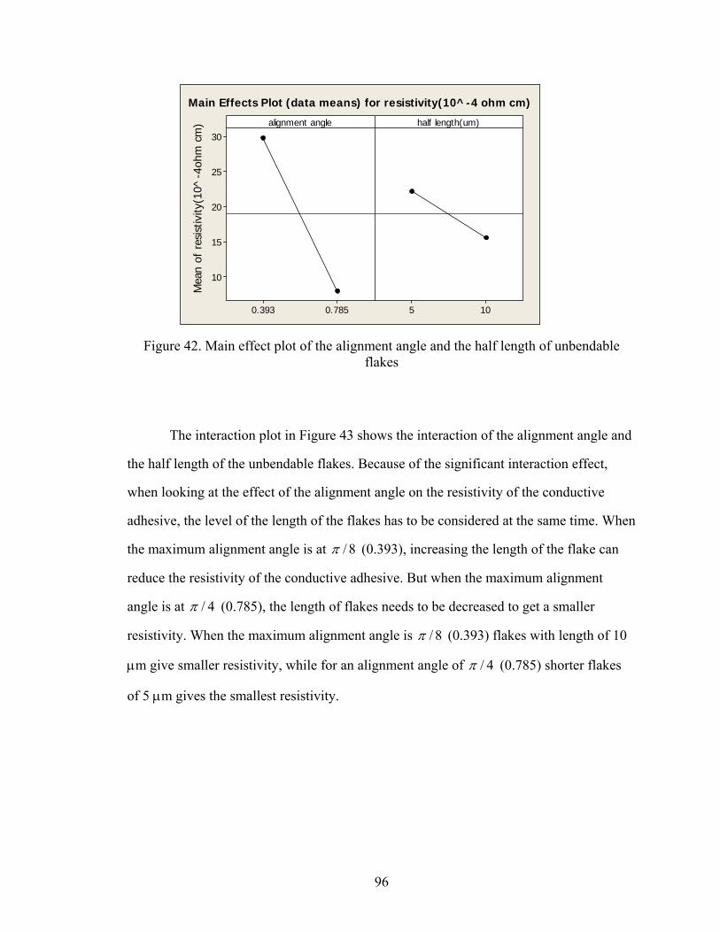
96

Mea

n of

res

istiv

ity(1

0^-4

ohm

cm

)

0.7850.393

30

25

20

15

10

105

alignment angle half length(um)

Main Effects Plot (data means) for resistivity(10^-4 ohm cm)

Figure 42. Main effect plot of the alignment angle and the half length of unbendable flakes

The interaction plot in Figure 43 shows the interaction of the alignment angle and

the half length of the unbendable flakes. Because of the significant interaction effect,

when looking at the effect of the alignment angle on the resistivity of the conductive

adhesive, the level of the length of the flakes has to be considered at the same time. When

the maximum alignment angle is at / 8π (0.393), increasing the length of the flake can

reduce the resistivity of the conductive adhesive. But when the maximum alignment

angle is at / 4π (0.785), the length of flakes needs to be decreased to get a smaller

resistivity. When the maximum alignment angle is / 8π (0.393) flakes with length of 10

μm give smaller resistivity, while for an alignment angle of / 4π (0.785) shorter flakes

of 5 μm gives the smallest resistivity.

97

half length(um)

Mea

n

105

40

35

30

25

20

15

10

5

alignmentangle0.3930.785

Interaction Plot (data means) for resistivity(10^-4 ohm cm)

Figure 43. Interaction plot of the alignment angle and the half length of unbendable flakes

The results of the factorial analysis of the four conductive adhesive models are

summarized in Table 5.

98

Table 5. Summary of results of 2k factorial design for geometric parameters of conductive particles on the resistivity of conductive adhesives

Models

Spherical particles

with normal

distribution

Spherical particles of

two sizes with normal

distributions

Bendable flakes

Unbendable flakes

Factors

Mean of radius,

standard deviation of

radius

Mean and standard deviation of bigger particles’ radius,

mean and standard deviation of smaller

particles’ radius

Flake length, width, and maximum

alignment angle

Flake length, width and maximum

alignment angle

Factor Mean radius Mean radius of bigger particles

Maximum alignment angle

Maximum alignment angle Most

significant factor level to get a

smaller resistivity

Low Low High High

factors N/A N/A Maximum

alignment angle and length

Maximum alignment angle

and length Factors with significant two-factor interaction

effect levels to get

a smaller resistivity

N/A N/A High and high High and low

5.6 Discussions

The method of factorial design is used to study the effect of parameters of the

conductive fillers on the resistivity of the conductive adhesives. It should be noted that

the conclusions drawn from this study hold true only for the specified range of values of

the factors. For factor values that go beyond the range new simulations and analyses

needs to be done.

The 2k factorial design only captures the linear dependency of the experiment

result on the parameters in the specified range. To see how the experimental result varies

with parameters over a wide range one needs to divide the wide domain into smaller

domains and make two-level factorial designs on each, so that the nonlinear trend can be

shown.

99

The radius mean value of spherical particles always has the most significant effect

on the resistivity, which means the size of spherical particles affects the conduction

property of conductive adhesives. By looking at the main effect plots of the radius of

spherical particles, we find that smaller spherical particles give better conduction for the

size range being studied. For both bendable and unbendable flakes, the alignment angle is

the most significant factor, and bigger alignment angles give smaller resistivities. For

bendable flake particles longer flakes gives lower resistivity, which is easy to understand

since longer flakes are easier to contact each other. But for unbendable flakes, longer

flakes don’t always result in smaller resistivity. This is because the effect of the length of

flakes on resistivity also depends on the value of the alignment angle, or in other words,

the interaction exists between the alignment angle and length of flakes.

The average resistivity of the conductive adhesive is plotted as a horizontal line in

all the main effect plots. Based on the main effect plots of Figure 39 and Figure 42, for

unbendable flakes the resistivity mean is 18.97×10-4 Ω cm, and for bendable flakes the

mean is 5.04×10-4 Ω cm. Obviously the resistivity of conductive adhesives with bendable

flakes is much smaller than with unbendable flakes. In the bendable flake model the

flakes are assumed to be very flexible to bend, while in the unbendable model the flakes

are assumed to be stiff. In reality the stiffness of the flakes should be in between these

two extreme cases. Therefore the bendable model provides the lower bound for the

resistivity value and the unbendable model provides the upper bound. The true resistivity

of conductive adhesives should be between 5.04×10-4 and 18.97×10-4 Ω cm, based on the

resistivity values from the two models. Some author gets the resistivity of between 4×10-4

and 10×10-4 Ω cm in experiments for conductive adhesives with flake particles [9], which

is not far from our result.

The resistivity comparison between conductive adhesives with flakes and

spherical particles can also be made. In our study, the average size of the filler particles is

100

around 5 μm and the volume fraction of particles is always kept at 30%. We can tell

which particle shape is better by looking at the average mean resistivity, which is

calculated by averaging all resistivities from simulations of all the factor combinations.

They are also plotted in the main effect plots as the horizontal lines. The average

resistivity for particles with normal distribution is 39.87×10-4Ω cm. The conductive

adhesives with spherical particles with one size show an average resistivity value of

33.8×10-4 Ω cm. If compared with the average resistivity of unbendable flakes, 18.97×10-

4 Ω cm, and bendable flakes, 5.04×10-4 Ω cm, apparently the flakes give better

conductive property than mono-sized spherical particles. However, the resistivity of

spherical particles with two sizes shows a value of 2.61×10-4 Ω cm, close to the bendable

flake model. Therefore the mix-up of particles of two sizes could greatly improve the

conduction of conductive adhesives. This can be explained intuitively: smaller particles

fill in the gaps between larger particles and more conduction paths are created. The fact

that most commercial conductive adhesives manufacturers use flakes instead of spherical

particles, and mix flakes of difference sizes to compound conductive adhesives indirectly

verifies our finding.

By adjusting the particle parameters a much lower average resistivity than the

overall average resistivity can be achieved. The mean resistivities are shown in Figure 44.

The lighter columns in the figure are the average of resistivities of all factor value

combinations; they correspond to the middle lines in the main effect plots. The darker

columns are calculated by taking the average of resistivities with the most significant

factor having been adjusted to levels that can produce smaller resistivities; they

correspond to the lowest point in the main effect plot of the most significant factor. The

average resistivity can be reduced greatly by adjusting the value of the most significant

factor. For bendable flakes, by setting the maximum alignment angle at / 4π the average

resistivity mean is as low as 0.21×10-4 Ω cm, a 96% drop from the overall average

101

resistivity of 5.04×10-4 Ω cm. For unbendable flakes, by setting the alignment angle at

/ 4π we can get an average resistivity of 6.78×10-4 Ω cm, a 64% drop from the overall

average resistivity of 18.97×10-4 Ω cm. For spherical particles, adjusting parameters also

gives lower resistivity, but the resistivity drop is not as much as with flake particles. For

spherical particles with uniform size, the average resistivity is 17.3×10-4 Ω cm by setting

the radius at 2 μm, a 49% drop from the overall average resistivity of 33.8×10-4 Ω cm.

For spherical particles with normal size distribution, the average resistivity is 30.74×10-

4 Ω cm by setting radius mean value at 3 μm, a 22.9% drop from the overall average

resistivity of 39.87×10-4 Ω cm. For spherical particles with two sizes, the average

resistivity of 2.21×10-4 Ω cm is obtained by setting the bigger particle radius mean at 4

μm, a 15% drop from the overall average resistivity of 2.61×10-4 Ω cm. The difference of

the resistivity between the overall average resistivity and the average resistivity with the

adjusted significant factor can be seen in Figure 44 by looking at the height difference

between the darker columns and the lighter columns. The plot shows that not only the

overall average resistivity of conductive adhesives with flakes is smaller than with

spherical particles, but also the resistivity of conductive adhesives with flakes can be

reduced more by adjusting the most significant factor. This again explains why most

commercial conductive adhesives use flakes as conductive fillers.

102

0

5

10

15

20

25

30

35

40

45

Sphericalparticles withuniform size

Sphericalparticles with

normaldistribution

Sphericalparticles of

two sizes withnormal

distributions

Bendableflakes

Unbendableflakes

resi

stiv

ity(1

0^-4

ohm

cm

)overall mean resistivitylowest mean resistivity

Figure 44. Comparison of resistivities of different models

The effective volume fraction of each conductive adhesive model can also be

calculated. In our study all of the conductive adhesives have a volume fraction of 30% for

the silver particles. However, not all of the particles contribute to the conduction of the

conductive adhesives. Only the particles that are part of the resistor network or the

electric conduction path act as conductors. Other particles that are not in the resistor

network could be seen as insulators because they don’t contribute the electrical

conduction of the conductive adhesive. Naturally we can introduce the concept of

effective volume fraction. The effective volume fraction is defined as the volume fraction

of the particles that contribute to the electrical conduction if conductive adhesives, it is

calculated by dividing the volume of the particles that are in the resistor network by the

total volume of the conductive adhesive. The effective volume fraction is an indication of

the number of the conduction paths formed by the particles in the conductive adhesive.

103

Figure 45 shows the average effective volume fractions of different conductive

adhesive models. The volume fraction of the filler particles is 30% for all conductive

adhesive models. The figure shows flake particles have effective volume fractions close

to 30%, which means almost all of the flakes contribute to the conduction of the

conductive adhesives. Spherical particles with one size and normal distribution have

effective volume fractions of 24%. For the model of spherical particles of two sizes with

normal distributions, the effective volume fraction is 23%. Clearly spherical particles

have lower effective volume fractions than flake particles, meaning the number of

conduction paths formed by spherical particles is less than by flakes. Since flakes have

higher effective volume fractions, almost all flakes contribute to the conduction and thus

more conduction paths are formed. For spherical particles many particles are isolated and

not as many conduction paths are formed. As a result, conductive adhesives with flakes

have better conduction than conductive adhesives with spherical particles. However,

spherical particles of two sizes with normal distributions have a small effective volume

fraction but still provide good conductive property. The reason could be the smaller

particles fill in the gap between bigger particles. These smaller particles contribute to the

effective volume fraction, but since they have small size they only add little to the

effective volume fraction. Therefore the total effective volume fraction of spherical

particles of two sizes is small while the conduction of the conductive adhesive is still

good.

104

0.2

0.22

0.24

0.26

0.28

0.3

0.32

Sphericalparticles

with uniformsize

Sphericalparticles

with normaldistribution

Sphericalparticles oftwo sizes

with normaldistributions

Bendableflakes

Unbendableflakes

effe

ctiv

e vo

lum

e fra

ctio

n

Figure 45. Effective volume fractions of difference models

5.7 Conclusions

The resistivity of conductive adhesives can be calculated through microstructure

models. The positions and sizes of the filler particles can be randomly generated by a

computer program, and models of conductive adhesives with both spherical particles and

flakes were studied. The resistivity of the conductive adhesive was calculated by solving

the resistor network formed by the filler particles. Since flakes have larger contact area

than spherical particles and have more conduction paths, the conduction of conductive

adhesive with flakes is better than with spherical particles.

The method of full factorial design of experiments was used to study the effects of

parameters of the particles. For each conductive model, the factors or geometric

parameters of the particles are identified first. Each of the factors is set to a high value

and a low level, and for each of the factor value combinations 10 models were built and

their resistivities calculated. The factor values together with the resistivity values were

then taken to perform the factorial analysis. The Pareto chart shows the factors that have

105

significant influence on the resistivity of the conductive adhesives. The main effect plot

and interaction plot of the factors show how to set the factors to get a lower resistivity.

For spherical particles the particle radius has the most significant effect on the resistivity,

for the radius range we studied. Smaller particles result in smaller resistivity. For flake

particles, the alignment angle of flakes has the most significant effect on the resistivity of

conductive adhesives. The length of flakes may also have a significant effect. If the

alignment angle and the length of flakes are adjusted, a smaller resistivity of the

conductive adhesive can be obtained. It was found that adjusting the geometric

parameters of the particles can change the resistivity greatly, especially for flake

particles.

The effective volume fraction of each conductive adhesive model is also

calculated. Flake particles have bigger effective volume fractions than spherical particles.

However, smaller effective volume fraction doesn’t always give bigger resistivity. For

example, spherical particles of two sizes have a small effective volume fraction but still

give a small resistivity, which means that mixing particles of two sizes could form the

conduction network in conductive adhesives more efficiently.

The conclusions drawn from the full factorial design are valid only for the data

range being studied. They should not be expanded to other ranges because these

conclusions may not hold for other data ranges. In order to study how the factors affect

the resistivities in other data ranges, new simulations and analyses should be done.

The 2k factorial experiment design and analysis is an efficient approach to study

the effect of geometric parameters on the conduction of conductive adhesives. Instead of

preparing conductive adhesive samples using different particles and measuring their

resistances, the effect of the geometric parameters can be analyzed by computer

simulations, which is more convenient and time-saving than actual experiments.

Some researchers have studied how the resistivity of conductive adhesives is

affected by adding nanoparticles by experiment [81] [122]. Although we are studying

106

micro-sized particles in this chapter, it is still possible to apply our approach to

investigate the effect of nanoparticles by modifying some parameters in our computer

simulation programs. However, it should be noted that if the particles are in nano size, the

bulk resistance of particles may not be negligible compared with the contact resistance

between particles. Caution should also be taken when building the microstructure model

if there is aggregation of the nanoparticles, because aggregated particles are different

from separate particles.

107

CHAPTER 6

FATIGUE BEHAVIOR OF CONDUCTIVE ADHESIVES

6.1 Introduction

In electronic packaging technologies such as surface mounting, the

interconnection joints connect the component and substrate and serve as the mechanical

as well as the electrical connection. The joints are required to accommodate any relative

displacement between the component and the board, such as the one induced by

temperature change. In fact, the thermal mismatch, which is a result from the action of

temperature changes on the different coefficients of expansion of the board and

component, is a major problem in electronic packaging. Another source of thermal

displacement is temperature gradients, which also lead to relative displacement between

components and substrates.

Very often the interconnection joints do not fail due to temperature extremes, but

fail under cyclic temperature changes. Cyclic temperature changes, which can be

encountered in conditions such as indoor/outdoor, summer/winter, etc., cause cyclic

displacements and finally can lead to thermal fatigue failures. The temperature change is

unlikely to be avoidable for most electronic packages. Therefore in order to gain long-

term reliability of the interconnection material, its fatigue behavior has to be studied and

be improved.

The fatigue behavior of PbSn solder has been investigated extensively; however

as another interconnection material the study of fatigue failure for conductive adhesives

is still inadequate. The fatigue behavior of conductive adhesives is very different from

that of metal solder. One reason is that the polymer matrix has different properties than

metal. Another reason is that conductive adhesives could fail in two ways: electrical or

108

mechanical, and one can happen before the other. This is different from solder, where

electrical failure is always accompanied by mechanical failure. Therefore the particular

fatigue behavior of conductive adhesive material has to be understood, especially when it

is seen as a replacement interconnection material to traditional PbSn solder.

In this chapter the fatigue behavior of conductive adhesives is studied through

mechanical fatigue tests. The conductive adhesive samples are applied on the surface of a

PCB beam. The four-point push/pull beam bending tests are conducted, so that the

compressive/tensile stress can be exerted on the conductive adhesive samples. By

bending the beam repetitively, cyclic uniaxial stress is applied on the conductive adhesive

samples. The resistances of the conductive adhesive samples are monitored during the

fatigue tests. A fatigue failure criterion is proposed in term of the resistivity increase,

which characterizes the decreased ability of conductive adhesive to pass electric current.

Based on the fatigue test data, a power law type fatigue model is used to relate the

number of cycles to failure with the compressive/tensile strain amplitude. The effect of

strain ratio on the fatigue life of conductive adhesives is studied by varying the

magnitude of the compressive and tensile strain. Tests are also performed to show the

effect of strain rates on the fatigue life of conductive adhesives. The microstructure of the

conductive adhesive samples is examined before and after fatigue tests to explore the

failure mechanism.

6.2 Experimental procedure

6.2.1 Materials

The fatigue behavior of a self-made conductive adhesive is studied, and it is

hoped that this investigation will shed some light on the general fatigue behavior of

conductive adhesives. The composition of a particular conductive adhesive may not be

the same as the one we used. Consequently there will be some difference between their

109

fatigue behaviors, which comes from the difference of the mechanical property of the

epoxy resin, the shape and size of the silver filler particles and the volume fraction of

silver and epoxy. However, when the property of epoxy resin, the geometry of the silver

flakes and the volume fraction of silver are not too far away from the ones in our

specimen, it is supposed that the fatigue behavior of the conductive adhesive will not

differ too much from the one used in our tests, and the fatigue failure mechanism of

conductive adhesives that will be discovered in this study will not lose its generality.

Moreover, the approach that is being adopted in this study can also be applied to

conductive adhesives of other types.

The conductive adhesive is made of thermoset epoxy resin and filler flakes. The

epoxy resin consists of hisphenol-F (DGEBF) Epon 862 from Hexion Specialty

Chemicals, Inc., hardener methylhexa-hydrophthalic anhydride (MHHPA) from Lindau

Chemicals, Inc., and catalyst l-cyanoethyl-2-ethyl-4-methylimidazole (2E4MZCN), from

Shikoku Chemicals Corp. The weight ratio of epoxy : hardener : catalyst is 1 : 0.84 :

0.0184. The silver flakes are SF 26LV, from Ferro Corporation. The average length of the

silver flakes is 10 μm. The weight ratio of silver and epoxy resin in the conductive

adhesive is 4 : 1, corresponding to an approximate volume fraction of silver of 30%.

After being added together, the epoxy resin and silver flakes are mildly blended with an

applicator stick for 5 minutes. Visual inspection is made to make sure the epoxy resin and

silver flakes are mixed thoroughly. The conductive adhesive after mixing is placed in a

freezer of -40°C to prevent any slow cure under room temperature. Before each use the

conductive adhesive sample bottle is taken out from the freezer and thawed under room

temperature for 30 minutes. During the thaw process the cap of the sample bottle is kept

closed to prevent moisture condensation on the conductive adhesive surface.

110

6.2.2 Fatigue tests of conductive adhesives

A four-point beam bending experiment is designed to load the conductive

adhesive with cycling tensile and compressive stress. An illustration of the experiment is

shown in Figure 46. In the four-point bending test the section of the beam between the

inner two fixtures is under pure bending with a constant bending moment. The

conductive samples are applied on the top surface of the beam, as shown in Figure 46 and

Figure 47. Since the thickness of the conductive adhesive is very thin compared with the

thickness of the beam, it is assumed that the conductive adhesive samples will have the

same strain as the top layer of the beam. In our test, four conductive adhesive samples are

applied between the two inner fixtures on the top surface of the beam. Because the

bending moment between the two inner fixtures is constant, these four conductive

samples will be subjected to the same magnitude of compressive/tensile strain.

Figure 46. 3-D illustration of four-point beam bending test

conductive adhesive

fixtures beam

111

Figure 47. Side view of four-point bending test

A special fixture is designed to conduct the four-point push/pull beam bending

test. The traditional four-point bending fixture is capable of pushing from one side only,

so that the beam can be bent in one direction. It can induce either tension or compression

on the top or bottom surface, but not both. However in the fatigue test it is desired that

the conductive adhesive samples can be both compressed and stretched. A special fixture

is designed as shown in Figure 48 to perform the push/pull bending test. One fixture set is

composed of two parts: the C (top) part and the T (bottom) part. Two fixture sets are

fastened on the crossheads of the load frame by screws. The gap opening between the C

part and T part is adjusted to be slightly bigger than the beam thickness to pass the PCB

beam, so that the vertical displacement of the beam is constrained. In the beam bending

test the outer two sets of fixtures are fastened on the lower crosshead of the load frame,

and the inner two sets are fastened on the upper crosshead. The lower crosshead of the

fixtures

conductive adhesive

beam

112

load frame together with the outter two fixture sets are fixed, and only the upper

crosshead and two inner fixtures are movable. When the inner two fixtures move down,

they exert a compressive stress on the upper surface of the beam, and when they move up

a tensile stress is exerted on the upper surface of the beam. Thus by controlling the

movement of the crosshead a continuously changing cycling stress will be applied to the

conductive adhesives samples. Furthermore, by varying the maximum upward and

downward displacement of the crosshead, the unsymmetrical loading with different

maximum tensile and compressive stress can be achieved.

Figure 48. Fixture for the four-point push/pull beam bending test

The strain of the top surface layer of the beam and the conductive adhesive

samples can be calculated based on the geometry of the bent beam, which is shown in

Figure 49. In the plot, ρ is the radius of the neutral plane of the bent beam, v is the

crosshead displacement, a0 is the length of the beam between the outer fixture and inner

113

fixture before bending, L0 is the length of the beam between the two outer fixtures before

bending, and θ1 and θ2 are two angles corresponding to two sections of the bent beam..

Figure 49. Geometry of the bent beam

The crosshead displacement v can be read from the computer connected to the

load frame. The two lengths a0 and L0 can be measured before the beam is bent. Having

known the three parameters v, a0 and L0, the radius ρ of the neutral plane of the bent

beam and the two angles θ1 and θ2 can be calculated by solving the following equations

2 1 2cos cos( )vρ θ ρ θ θ= + + (6.1)

[ ]

220

1 21 2

(1 cos( ))2sin

2 2

L ρ θ θθ θ

ρ

⎛ ⎞ + − +⎜ ⎟+ ⎝ ⎠= (6.2)

2 2

01sin2 2

a vθρ+

= (6.3)

After ρ is solved numerically from Equations (6.1) ~ (6.3), the strain ε of the top

layer of the beam and the conductive adhesive samples can be calculated by

114

2tερ

= (6.4)

where t is the thickness of the beam.

In our fatigue tests the beams are cut from copper cladded FR4 boards (printed

circuit boards), which are obtained from LPKF Laser & Electronics. The printed circuit

board is used for the reason of facilitating the resistance measurement of the conductive

adhesive samples, which will be discussed later. The beam has a length of 131 mm, width

19mm, and thickness 2.375 mm. Each beam is checked before and after the fatigue test to

make sure that the beam has not failed, because only in such case Equations (6.1) to (6.4)

are still valid. Before bending the distance between the two outer fixtures is 103.1 mm,

the distance between the two inner fixtures is 50.6 mm.

For a given value of the maximum displacement of the crosshead, the radius of

the neutral plane of the beam and the maximum compressive/tensile strain of the

conductive adhesive samples are calculated. Their values are listed in Table 6.

Table 6. Maximum crosshead displacement and corresponding compressive/tensile strain of the conductive adhesive samples

Maximum crosshead

displacement v (mm) 5.0 6.0 8.0 10.0 12.0

Radius of neutral plane of

the bent beam ρ (mm) 205.369 172.611 132.240 108.613 93.3361

Maximum compressive/tensile

strain ε of conductive adhesive

samples

0.005780 0.006877 0.008976 0.01093 0.01272

115

The fatigue test is displacement-controlled for the beam bending, and strain-

controlled for the conductive adhesive samples. The fatigue test is conducted in the

following manner. At the beginning of each cycle the crosshead is held still for 10

seconds. Then the upper crosshead moves down, which exerts a compressive strain on the

upper surface of the beam. After reaching the maximum downward displacement as

shown in Table 6, the upper crosshead moves up and loads the upper surface of the beam

with tensile stress. After reaching the maximum upward displacement, the crosshead

moves down to return to the zero displacement location. The displacement vs time plot of

the upper crosshead of the load frame is shown in Figure 50. The short horizontal line in

Figure 50 corresponds to the hold period at the beginning of each cycle.

-15

-10

-5

0

5

10

15

0 100 200 300 400 500 600

time (sec)

uppe

r cro

sshe

ad d

ispl

acem

ent (

mm

)

Figure 50. Upper crosshead displacement curve (crosshead speed: 10 mm/min, maximum cross head displacement: 10 mm)

116

The strain rates applied to the conductive adhesive samples can be varied by

adjusting the speed of the crosshead movement. The relationship between the

displacement of the crosshead and the compressive/tensile strain of the upper surface of

the beam is not strictly linear, but very close to a linear one. Figure 51 shows the

correlation between the two quantities. Therefore a constant speed of the crosshead will

result in an approximately constant strain rate for the conductive adhesive samples in the

fatigue test. The speed of the crosshead and its corresponding strain rate are shown in

Table 7.

0

0.002

0.004

0.006

0.008

0.01

0.012

0.014

0 2 4 6 8 10 12 14displacement of the upper crosshead (mm)

tens

ile/c

ompr

essi

ve s

train

of

the

uppe

r bea

m s

urfa

ce

Figure 51. Compressive/tensile strain of the upper beam surface vs displacement of the upper crosshead

Table 7. Crosshead speeds and corresponding strain rates

Speed of the crosshead (mm/min)6 8 10 15

Strain rate of the upper beam

surface (μ10-4 1/sec) 1.0930 1.4573 1.8217 2.7325

117

6.2.3 Resistance measurement of conductive adhesive samples

The resistance of the conductive adhesive samples is constantly under monitoring.

The two primary functions of the conductive adhesive are mechanical adhesion and

electrical conduction. In fatigue tests, the fatigue failure should be defined based not only

on the mechanical strength of the conductive adhesive but also on the electrical

conduction, whichever happens first. Hence the resistance of the conductive adhesive

samples are measured and monitored during the whole process of the fatigue test.

A custom-made printed circuit board is used as the beam to facilitate the

resistance measurement of the conductive adhesive samples. The layout of the upper

surface of the beam is shown in Figure 52. The FR4 board brought from vendor is

double-side copper cladded. To make the printed circuit board, the circuit layout is first

printed onto a Press-n-Peel Image Transfer Film obtained from Techniks Inc. The Press-

n-Peel film is pressed onto the copper surface of the FR4 board using a hot clothes iron.

After the Press-n-Peel film is peeled away, copper traces covered by the film are left on

the board. The board is then immersed in the Ferric Chloride solution. Since the copper

traces are covered with a film they remain on the board as shown in Figure 52, and other

areas of the copper are etched away.

Figure 52. The layout of the upper surface of the PCB beam

position of fixtures copper traces and pads conductive adhesive samples

Connected to multimeter

118

The copper traces are in pattern such that the resistance of the conductive

adhesive sample can be measured by the four-point measurement method. Four

conductive adhesive samples are applied to the upper surface of the beam between the

two inner fixtures. Because the section of the beam between the two inner fixtures is

subjected to a constant moment, the conductive adhesive samples all have the same

strain. The resistance change of the conductive adhesive will be studied based on the four

samples instead of just one sample to prevent any possible operation error or bias in a

single measurement.

Each conductive adhesive sample has four copper pad leads, which are soldered

with leads of a digital multimeter to measure its resistance. To measure the resistance of

all four conductive adhesive samples at the same time during the fatigue test, a scanner

card is used. The 16 leads (4 leads μ 4 samples) are connected to the scanner card, and

the scanner card is connected to the digital multimeter. Every time a “measure”

instruction is sent to the digital multimeter, the scanner card switches the inner relays and

the resistance of each conductive adhesive sample is measured one by one. The scanner

card is a 10-channel Model 2000-SCAN Scanner Card from Keithley. The digital

multimeter is Keithley Model 2001, with a resolution of 1 µΩ. The time interval between

each scan is 2 seconds, and after each scan all four resistance values are recorded into the

computer. The resistance measurement and the fatigue tests start at the same time, so that

the entire resistance change during the fatigue test can be captured.

The conductive adhesive is applied to the upper surface of the PCB beam by a

tailor-made stainless steel stencil. The stencil is shown in Figure 53. The thickness of the

stencil is 0.178 mm. The paste-form conductive adhesive is applied through the slots of

the stencil using a stainless steel squeegee. After the stencil is taken away, the PCB beam

and the conductive adhesive samples are put into a convection oven of 150°C to cure for

3 hours. The usual cure time for the conductive adhesive is 1 hour. The prolonged cure

119

time of 3 hours is to ensure that the conductive adhesive samples are all completely

cured. Then the conductive adhesive samples are cooled down in dry room temperature

for about 2 hours, after which the fatigue tests are performed. The size of the conductive

adhesive samples is measured before the fatigue test, with the average size of the

conductive adhesive sample being 2.5 mm wide, 7.6 mm long (the distance between the

copper pads on the PCB beam), and 0.170 mm thick. The size of the conductive samples

will be used later together with the resistance value to calculate its resistivity.

unit: mm

Figure 53. Stencil for application of conductive adhesives

6.2.4 Scanning electron microscopy

The scanning electron microscope is used to examine the microstructure change

of the conductive adhesive samples before and after fatigue tests.

The electrical conduction failure can be examined by microscopy pictures. Since

the conduction of conductive adhesives depends on the contacts between conductive

fillers, careful examination will be made to check the contacts between silver flakes. The

contact pressure between silver flakes is due to the cure shrinkage of the epoxy matrix,

only with good adhesion between the epoxy matrix and silver flakes the intimate contacts

between silver flakes can be maintained. Therefore the interface between the epoxy

matrix and the silver flakes will also be examined.

120

The microscopy pictures can also be used to check mechanical failure. In some

cases the mechanical failure can be observed by naked eye, such as the peeling off of the

conductive adhesive samples from the PCB beam, or the breakage of a conductive

adhesive sample. But sometimes the cracks are so small that they have to be checked by

microscope. With a magnification of over 10K under scanning electron microscopy, any

small damage in the conductive adhesive after fatigue tests will be found out.

Although the whole conductive adhesive material is a conductor, its epoxy resin is

not conducting and will cause charging effect when taking SEM pictures. To get a good-

quality image, the conductive adhesive samples are sputtered coated with a thin layer of

gold before taking SEM pictures. Images are taken of the cross sections of the conductive

adhesive samples before and after fatigue tests.

6.3 Results and discussions

The fatigue tests of conductive adhesive samples are conducted by the four-point

push/pull beam bending test. The resistance value of each conductive adhesive sample is

simultaneously recorded. It is found that the resistance value of the conductive adhesives

increases while more cycles are performed, but no mechanical damage is found. Clearly

the electrical conduction failure happens before any mechanical failure.

A failure criterion is proposed to define the failure of the conductive adhesive in

terms of electrical conduction. The fatigue life of the conductive adhesive is found to be

related with the strain range, and the relation can be fitted by the power law equation. The

fatigue life is also dependent on strain ratio and strain rate.

By the microscopy examination of the cross sections of the conductive adhesive

samples before and after fatigue tests, it is found that the interface between the epoxy

matrix and silver flakes is damaged by fatigue tests. Good contacts between silver flakes

are lost without the holding of the epoxy matrix, and the electrical conduction of

conductive adhesive is consequently deteriorated.

121

6.3.1 Resistance change of conductive adhesive samples in fatigue tests

The resistance of the conductive adhesive samples is constantly under

measurement after the fatigue test begins. It is found that the resistance of conductive

adhesive samples is significantly influenced by the compressive and tensile strain. The

resistance of a conductive adhesive sample measured during a fatigue test is shown in

Figure 54.

0.00

0.20

0.40

0.60

0.80

1.00

1.20

0 500 1000 1500 2000time (sec)

resi

stan

ce (o

hm)

Figure 54. The representative resistance change of a conductive adhesive sample during fatigue test (strain ratio = -1)

In Figure 54 the resistance of the conductive adhesive sample is plotted every 2

seconds. The spikes of the resistance values correspond to the time period in which the

conductive adhesive sample is subjected to tensile strain. The rising part of the spike is

due to the upward movement of the load frame crosshead, which applies an increasing

tensile strain on the conductive adhesive sample. When the tensile strain reaches the

maximum value, the resistance value also reaches the largest value, i.e., the top point of

122

the spike. Then the tensile strain is unloaded, and correspondingly the resistance value

decreases from the highest point. It can be seen that as the fatigue test goes on, the

highest resistance values, i.e., the height of the spikes, also increases.

0.00

0.10

0.20

0.30

0.40

0.50

0.60

450 550 650 750 850time (sec)

resi

stan

ce (o

hm)

Figure 55. Resistance change of a conductive adhesive sample in one cycle of the fatigue test (strain ratio = -1)

Figure 55 shows the resistance change in one fatigue cycle. From this plot the

resistance value change of the conductive adhesive sample when subjected to the tensile

stress and the compressive stress can be seen. The left and right circles in Figure 55

contain data points that have stable resistance values. These are the resistance values

corresponding to the beginning of each fatigue cycles, when the crosshead is hold still at

zero displacement position for 10 seconds. Because no strain is loaded on the conductive

adhesive sample, its resistance value is stable, as shown in the two circles of Figure 55.

The small discontinuity of the resistance curve, which is marked by the blue square in

Figure 55, is due to the strain being changed from compressive to tensile. The portion of

the curve between the square and the right circle is corresponding to the period when

123

tensile strain is exerted on the conductive adhesive sample, i.e., the spike in Figure 54.

The portion of the curve between the left circle and the square is corresponding to the

period of the fatigue test when compressive is applied to the conductive adhesive sample.

The effect of compressive strain and tensile strain on the resistance can be seen

from Figure 54 and Figure 55. Clearly the magnitude of the resistance decrease caused by

the compressive strain is much smaller than the resistance increase caused by the tensile

strain. The magnitudes of the compressive and tensile strains are the same, yet the

magnitudes of the resistance change they have caused are so different. This phenomenon

can be explained as follows. The conduction of the conductive adhesive is achieved

through the interconnections of the silver flakes, and the resistance of the conductive

adhesive is the total resistance of the resistor network formed by all the contact

resistances between flakes. As has been discussed in Chapter 3 and 4, when the contact

pressure is increased the contact resistance is decreased because of the enlargement of the

contact area and decrease of the tunnel resistivity. In the fatigue test, when the conductive

adhesive is subjected to tensile stress the contact pressures between the silver flakes are

reduced, the contact resistances between silver flakes are increased, and hence the total

resistance of the conductive adhesive is increased. When in compressive stress, the

contact pressures between silver flakes are enhanced, which reduces the contact

resistance between flakes and also the total resistance of the conductive adhesive. Before

the fatigue test the flakes are held together tight by the epoxy matrix due to volume

shrinkage of the epoxy matrix in the cure process, and contact pressure already exists on

the contact interfaces. When the conductive adhesive sample is loaded with compressive

stress in the fatigue test, the contact pressure can be increased but only to a limited extent.

Therefore the resistance decrease of the conductive adhesive sample is small. However,

when loaded with tensile stress, the contact pressures between the flakes are greatly

reduced and the contact resistances significantly increased. For this reason, the tensile

stress causes much larger magnitude of resistance increase of conductive adhesives than

124

the magnitude of the resistance decrease caused by the compressive stress in the fatigue

test.

The average of the resistance values measured during the first 10 seconds’ hold

time of each fatigue cycle is taken as the resistance value of the conductive adhesive

before that cycle. This resistance value increases as the number of fatigue cycles is

increased, which can be seen in Figure 55 by comparing the two resistance values in the

two circles. As more and more fatigue cycles are applied to the conductive adhesive

sample, its resistance value grows higher and higher. A typical resistivity change of a

conductive adhesive sample is shown in Figure 56, in which the resistivity is plotted

versus the number of cycles. The resistivity is calculated because the size effect of the

conductive adhesive sample can be eliminated. The resistivity is calculated by Equation

(4.13).

0

2

4

6

8

10

12

14

16

0 100 200 300 400 500 600 700# of cycles

resi

stiv

ity (1

0^-4

ohm

cm

)

Figure 56. Resistivity of a conductive adhesive sample in fatigue test

Conductive adhesive fails here

125

It can be seen that the resistivity of the conductive adhesive sample keeps

increasing as more and more fatigue cycles are performed. In order for conductive

adhesives to be usable as an interconnection material in electronic packaging, it is

proposed that the bulk resistivity should be less than 1μ10-3 Ωcm [1]. The average

resistivity of the conductive adhesive samples before fatigue tests is found to be around 5

μ10-4 Ωcm. Therefore the electrical conduction failure criterion of the conductive

adhesive samples in this study is defined as a 100% increase of the resistivity value. The

failure point of the conductive adhesive sample is shown in Figure 56.

No breakage of the conductive adhesive sample or debonding of the conductive

adhesive from the PCB beam is observed after the fatigue test, which means that the

electrical conduction failure happens well before the mechanical failure. Later

microscopy examination confirms this observation. Therefore the electrical conduction

failure criterion of 100% increase in resistivity should be considered instead of the

mechanical failure for conductive adhesives in fatigue. This electrical conduction failure

criterion will be applied to all conductive samples in our fatigue tests.

The electrical failure criterion can also be based on different magnitude of

resistivity increase. For example, the National Center for Manufacturing Sciences

(NCMS) Conductive Adhesives project has defined a requirement of less than 20% shift

in resistance after aging[1]. If the electrical failure criterion is set as 20% increase of

resistance, the electrical failure happens much earlier than the mechanical failure and

electrical failure criterion is even more appropriate than the mechanical failure criterion.

Although the strain amplitude, strain rates and strain ratio may be different from

sample to sample, a similar pattern of the resistance and resistivity change as shown in

Figure 54 to Figure 56 is observed in all conductive adhesive samples. For each

conductive adhesive sample, its resistivity change and the number of fatigue cycles are

recorded. These data will be used later to fit the fatigue life models.

126

6.3.2 Fatigue life models of conductive adhesives

A number of fatigue tests are conducted with different strain ranges being applied

to the conductive adhesive samples. The resistances of the conductive adhesive samples

are monitored throughout the fatigue test, and the number of cycles to failure (100%

increase of resistivity) is recorded. The strain amplitude and the corresponding fatigue

lives of four conductive adhesive samples are listed in Table 8. The strain rate of these

tests is 1.8217μ10-4 1/sec, and the maximum compressive and tensile strains are equal,

i.e., completely reversed strains are applied.

Table 8. Strain amplitudes and corresponding fatigue lives of conductive adhesive samples

Strain amplitude 0.006877 0.008976 0.01093 0.01272

2125 576 191 48

2312 662 228 40

1983 681 208 37

Fatigue lives of four

conductive adhesive samples

2123 671 231 35

Average fatigue life 2135.75 647.5 214.5 40

To utilize the experimental data, a fatigue life model for the electrical failure of

conductive adhesives is required. The Coffin-Manson model is probably the most popular

empirical fatigue life model, which has been successful on several common materials

including PbSn solder. The Coffin-Manson model assumes that the plastic strain causes

the fatigue damage in the material subjected to low cycle fatigue. Therefore the plastic

strain range of the material in fatigue test is used as the basis for life prediction.

127

For conductive adhesives, it is found that the fatigue life before electrical

conduction failure can be fitted by the power law model. The power law model can be

written as

(2 )2

cf fNε εΔ ′= (6.5)

where / 2εΔ is the strain amplitude, Nf is the number of cycles to failure, and fε ′ and c

are two constant parameters.

Although the forms are similar, Equation (6.5) has different meaning from that of

the Coffin-Manson equation. The Coffin-Manson equation considers the plastic

deformation where fatigue cracks begin, and it is often used on material that has local

yielding. For our fatigue tests, the failure is electrical conduction failure instead of

mechanical failure. This electrical conduction failure is caused by the debonding of silver

flakes from epoxy matrix, which will be shown later by microscopy examination. Hence

the damage caused by fatigue tests is on the interfacial adhesion rather on the epoxy

material. Hence by using the power law relationship of Equation (6.5) we are relating the

electrical fatigue life with the interfacial property of silver-epoxy by strain amplitudes

instead of with local plastic strain.

It is found that the fatigue life data in Table 8 can be well fitted by the power law

relationship in Equation (6.5) using the strain amplitude. The fitted strain amplitude – life

line is shown in Figure 57. The two parameters for the Coffin-Manson model are

0.1604

0.0273f

c

ε

= −

′ = (6.6)

128

0.001

0.01

0.1

10 100 1000 10000Nf: # of cycles to failure

Δε/

2: s

train

am

plitu

deexperiment datafitted line

Figure 57. Fitted power law fatigue model with zero mean strain (R = 0)

It can be seen from Figure 57 that when the strain amplitude is increased, the

fatigue life of the conductive adhesive sample is decreased. This is a fatigue behavior

similar to most PbSn solder materials.

6.3.3 Influence of strain ratio on fatigue life of conductive adhesives

To study the effect of tensile and compressive stress on the fatigue life of

conductive adhesives, different strain ratios are applied in the fatigue tests. The strain

ratio R is defined as the ratio between the minimum and the maximum strain

(compressive strain is defined as negative and tensile strain as positive):

min

max

R εε

= (6.7)

129

The strain ratio, its corresponding maximum compressive and tensile strain, and

the corresponding fatigue lives of four conductive adhesive samples are shown in Table

9. The strain rate of all the fatigue tests in Table 9 is 1.8217μ10-4 1/sec.

Table 9. Strain ratios and corresponding fatigue lives of conductive adhesive samples

Strain ratio R 0 -0.53 -1 -1.89 -∞

Maximum

compressive / tensile

strain

0 /

0.01093

-0.00578 /

0.01093

-0.01093 /

0.01093

-0.01093 /

0.00578

-0.01093

/ 0

754 403 191 806 >2000

681 343 228 775 >2000

703 419 208 766 >2000


conductive adhesive

samples (cycles) 727 370 231 754 >2000

Average fatigue life

(cycles) 716.25 383.75 214.5 775.25 >2000

The fatigue data of conductive adhesive samples under different strain ratios are

also shown in Figure 58. The conductive adhesive sample that is subjected to

compressive stress only does not fail even after 2000 cycles, hence it is not shown in

Figure 58.

130

-2

-1.8

-1.6

-1.4

-1.2

-1

-0.8

-0.6

-0.4

-0.2

0

0 200 400 600 800 1000Nf: # of cycles to failure

R: s

train

ratio

Figure 58. The fatigue life of conductive adhesive samples under different strain ratios

It can be seen that the strain ratio, or different combinations of the tensile and

compressive strain, has a significant effect on the fatigue life of conductive adhesives.

When the conductive adhesive sample is subjected to the compressive strain only, its

resistance does not increase significantly even after 2000 cycles. But when the

conductive adhesive sample is subjected to tensile strain only, it fails at around 716.5

cycles. All the other conductive adhesive failures also happen with the existence of

tensile strain. Therefore the tensile stress has to be present in order for the resistance of

conductive adhesive sample to increase.

Another way to see the effect of compressive and tensile strain is to look at how

the change of the compressive/tensile strain affects the fatigue life. The fatigue life of -

0.01093/0.01093 is about 214.5 cycles. After reducing the compressive strain and

changing the fatigue strain to -0.00578/0.01093, the fatigue life is increased to 383.75

0/0.01093

-0.00578/0.01093

-0.01093/0.01093

-0.01093/0.00578

131

cycles. But if the tensile strain is reduced and the specimen is tested with strain of -

0.01093/0.00578, the fatigue life can be improved to 775.25 cycles. Hence the tensile

strain does more damage to the conduction of conductive adhesive than the compressive

strain.

But the compressive strain also affects the fatigue life of conductive adhesives,

with the tensile strain of the same magnitude being present. The fatigue life of pure

tension (0/0.01093) is 716.5 cycles. When increasing the compressive strain to (- 0.00578

/ 0.01093) and (-0.01093/0.01093) the fatigue life decreases to 383.75 and 214.5 cycles.

Therefore the increase of the compressive stress will reduce the fatigue life of conductive

adhesive. The fully reversed stress gives the shortest fatigue life of conductive adhesives.

It should be noted that the fitted fatigue life model shown in Figure 57 and

Equation (6.6) is obtained based on fatigue test data with zero mean strain, i.e., with R =

0. Since strain ratio affects the fatigue life of conductive adhesives significantly, for

fatigue tests with strain ratio R ≠ 0 the two coefficients c and fε ′ in the power law model

Equation (6.5) will be different from those shown in Equation (6.6). To include the effect

of strain ratio in the fatigue life model, fatigue tests with different mean strain values

should be performed. Based on fatigue test data, a group of fatigue life models with

different values of coefficients c and fε ′ can be fitted and used to predict the life of

conductive adhesive joints subjected to fatigue loading with non-zero strain ratio.

6.3.4 Influence of strain rate on the fatigue life of conductive adhesives

Fatigue tests are also performed with different crosshead speeds to study the

effect of strain rate. The different strain rates tested are listed in Table 7. The fatigue lives

of conductive adhesive samples under different strain rates are listed in Table 10 and

plotted in Figure 59. The maximum compressive/tensile strain in these tests is 0.01093.

132

Table 10. Strain rates and corresponding fatigue lives of conductive adhesive samples

Strain rate (μ10-4 1/sec) 1.0930 1.4573 1.8217 2.7325

156 171 191 558

152 151 228 519

148 165 208 575



132 176 150 585

Average fatigue life 147 165.75 194.25 559.25

1.E-04

1.E-03

100 1000Nf: # of cycles to failure

stra

in ra

te (1

/sec

)

Figure 59. Strain rates and corresponding fatigue lives of conductive adhesive samples with zero mean strain

Figure 59 shows significant strain rate effect on the fatigue life of conductive

adhesives. Smaller strain rates fail the conductive adhesive with a fewer number of

cycles. When the strain rates is changed from 1.0930μ10-4 to 2.7325μ10-41/sec, the

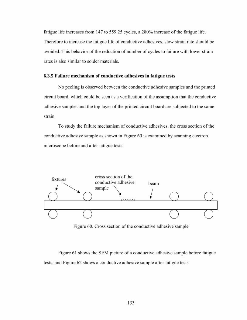
133

fatigue life increases from 147 to 559.25 cycles, a 280% increase of the fatigue life.

Therefore to increase the fatigue life of conductive adhesives, slow strain rate should be

avoided. This behavior of the reduction of number of cycles to failure with lower strain

rates is also similar to solder materials.

6.3.5 Failure mechanism of conductive adhesives in fatigue tests

No peeling is observed between the conductive adhesive samples and the printed

circuit board, which could be seen as a verification of the assumption that the conductive

adhesive samples and the top layer of the printed circuit board are subjected to the same

strain.

To study the failure mechanism of conductive adhesives, the cross section of the

conductive adhesive sample as shown in Figure 60 is examined by scanning electron

microscope before and after fatigue tests.

Figure 60. Cross section of the conductive adhesive sample

Figure 61 shows the SEM picture of a conductive adhesive sample before fatigue

tests, and Figure 62 shows a conductive adhesive sample after fatigue tests.

fixtures beam

cross section of the conductive adhesive sample

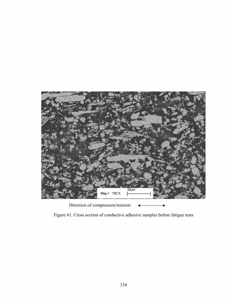
134

Figure 61. Cross section of conductive adhesive samples before fatigue tests

Direction of compression/tension:

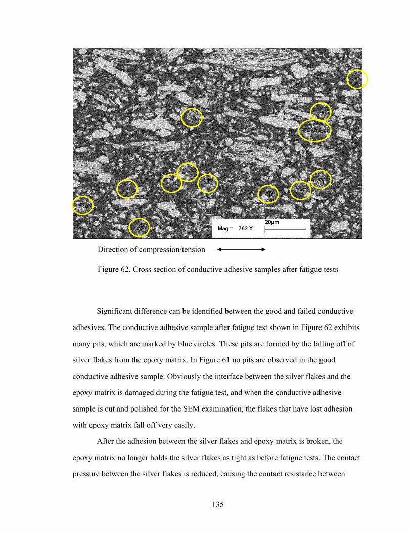
135

Figure 62. Cross section of conductive adhesive samples after fatigue tests

Significant difference can be identified between the good and failed conductive

adhesives. The conductive adhesive sample after fatigue test shown in Figure 62 exhibits

many pits, which are marked by blue circles. These pits are formed by the falling off of

silver flakes from the epoxy matrix. In Figure 61 no pits are observed in the good

conductive adhesive sample. Obviously the interface between the silver flakes and the

epoxy matrix is damaged during the fatigue test, and when the conductive adhesive

sample is cut and polished for the SEM examination, the flakes that have lost adhesion

with epoxy matrix fall off very easily.

After the adhesion between the silver flakes and epoxy matrix is broken, the

epoxy matrix no longer holds the silver flakes as tight as before fatigue tests. The contact

pressure between the silver flakes is reduced, causing the contact resistance between

Direction of compression/tension

136

silver flakes to increase. The total resistance of the conductive adhesives consequently is

increased. As more fatigue cycles are performed, more and more silver flakes lost

adhesion with the epoxy matrix. The number of interconnections between silver flakes is

reduced and the contact resistance between flakes becomes bigger. At a certain number of

fatigue cycles, the resistivity has increased to over two times the original resistivity value

before fatigue test, and the conductive adhesive is regarded as failed.

Since the electrical conduction failure is caused by the debonding of epoxy-silver

interface, the interfacial adhesion between epoxy and silver flakes is critical to the fatigue

life of conductive adhesives. Consequently, the fatigue life of conductive adhesives is

related to the interfacial crack growth between epoxy and silver flakes.

The interfacial debonding of the flakes from the epoxy matrix can be observed by

examining a single flake. Two silver flakes, one in a conductive adhesive sample before

fatigue test, another in a conductive adhesive sample after fatigue test, are shown in

Figure 63 and Figure 64. It can be seen from Figure 63 that the interface between the

silver flake and the epoxy matrix is not damaged, while the interface in Figure 64 has

been partially damaged. With more fatigue cycles, the crack between the flake and epoxy

matrix will propagate and finally cause a complete debonding of the silver flake. The

debonding of silver flakes could be due to the weak adhesion between the epoxy and

silver flakes, but the direct cause of the damage is fatigue tests.

137

Figure 63. A silver flake in a conductive adhesive sample before fatigue test

Figure 64. A silver flake in a conductive adhesive sample after fatigue test

138

It should be noted that no big cracks are found in the SEM images. Although there

are cracks and debonding between the epoxy matrix and the silver flakes, those are all

along the epoxy-silver interface. The fatigue test has not caused big cracks that go

through the conductive adhesive. Considering that there is also no breakage and peeling

off of conductive adhesive samples, the damage done to the conductive adhesive sample

by fatigue tests is mainly electrical. The electrical resistance has increased to an unusable

value well before major mechanical damage has developed. Therefore the fatigue should

be considered in terms of deterioration of electrical conduction rather than any

mechanical adhesion or breakage.

To observe the development of the debonding of silver flakes, two SEM pictures

are taken during the fatigue test and after fatigue test, as shown in Figure 65 and Figure

66. Figure 65 shows the flakes in the early stage of the fatigue test, and Figure 66 shows

the flakes after the fatigue test. By comparing these two images, it can be seen that in

Figure 65 the debonding between the flakes and the epoxy matrix is just beginning to

appear. Not only is the number fewer but also the size of the pits is smaller compared

with the SEM image after fatigue failure as shown in Figure 66. Because there are fewer

flakes that have been debonded from the epoxy during the fatigue test, the total resistance

during fatigue tests is smaller than the resistance after fatigue tests.

139

Figure 65. Cross section of a conductive adhesive sample in fatigue test after 40 cycles (not failed), strain rate = 1.093 μ10-4 1/sec, strain amplitude = 0.0193, strain ratio = -1


140

Figure 66. Cross section of a conductive adhesive sample in fatigue test after 228 cycles (failed), strain rate = 1.093 μ10-4 1/sec, strain amplitude = 0.0193, strain ratio = -1

Figure 67 shows another interesting finding: the positions of the pits are along the

direction that is 45° to the direction of compressive/tensile load. In fact this trend can also

be seen in Figure 62, Figure 65 and Figure 66. Since the fatigue load is uniaxial, the

maximum shear stress happens at the 45° direction to the direction of load. Many flakes

do not have enough interfacial adhesion with the epoxy matrix to resist the shear stress,

so they begin to debond and the pits are formed along the 45° direction. When a

sufficient number of flakes have been debonded from the epoxy matrix, the conduction of

the conductive adhesive is deteriorated.


141

Figure 67. Positions of the pits due to the falling of silver flakes

To verify the electrical failure mechanism of debonding is general and not

particular to the conductive adhesive samples used in our test, fatigue tests are also

performed on a commercial conductive adhesive material: Loctite 3889 from Henkel

Loctite Corporation. The microscopy examination of the cross section of the conductive

adhesive samples is made after electrical fatigue failure, and similar phenomenon of

debonding between silver flakes and epoxy matrix is observed. Therefore the epoxy-

silver debonding may be a common failure mechanism for conductive adhesives under

fatigue loading. The epoxy-silver interfacial adhesion is weakened by the cyclic loading,

and the electrical conduction of conductive adhesives is degraded as more fatigue cycles

are performed.


142

6.4 Conclusions

In this chapter, the fatigue behavior of conductive adhesives is studied by

conducting fatigue tests. Conductive adhesive samples are applied on the surface of PCB

beams, and cycling compressive/tensile strain is exerted on conductive adhesive samples

using four-point push/pull beam bending test. The resistance of conductive adhesive

samples is monitored and recorded during the fatigue testing process.

The resistances of the conductive samples increase significantly as more fatigue

cycles are performed. A failure criterion is proposed as conductive adhesive samples fail

electrically with a 100% increase of the original (before fatigue test) resistivity. Based on

this failure criterion, the electrical fatigue failure life of the conductive adhesive samples

can be quantified as the number of cycles to reach a 100% increase of resistivity.

The fatigue tests are strain-controlled by the displacement of the crosshead of the

load frame. The fatigue tests are conducted with different strain amplitudes. Test data are

then used to fit a fatigue model between the strain amplitude and number of cycles to

failure. The power law equation is used and found to fit the relation well. Similar to

solder, with higher strain amplitudes the fatigue life of conductive adhesives becomes

shorter.

The strain ratio has a significant effect on the fatigue life of conductive adhesives.

It is found that the tensile strain has a more detrimental effect on the electrical conduction

failure of the conductive adhesives. With compressive strain only, the conductive

adhesive samples exhibit no electrical fatigue failure or extremely long electrical fatigue

life. But with tensile strain being present, the conductive adhesive samples fail much

faster. Compressive strain has an effect on the fatigue life of a conductive adhesive when

tensile strain is present in the fatigue test: more compressive strain results in a shorter

fatigue life. The combination of a fully reversed tensile and compressive strain gives the

shortest electrical fatigue life of the conductive adhesives.

143

The effect of strain rate is investigated by varying the speed of the crosshead of

the load frame. It is found that the fatigue life of conductive adhesives is very sensitive to

the strain rate. Base on the test results, smaller strain rates result in shorter fatigue life of

conductive adhesives, a similar behavior to the solder material.

All the failures of conductive adhesives in our fatigue tests are electrical

conduction failure. No macroscopic breakage or crack is observed in the conductive

adhesive samples after fatigue tests. No big cracks in the epoxy matrix are observed by

scanning electron microscope either. Therefore the mechanical damage is very limited

even after the conductive adhesives have failed electrically. It is the electrical failure that

needs consideration when applying conductive adhesives in electronic packaging. This is

quite different from the failure of solder, in which mechanical failure is the major

concern.

The failure mechanism of conductive adhesives is found by scanning electron

microscopy examination. The SEM images of conductive adhesives after fatigue tests

show pits and cavitations left by the falling off of silver flakes. The interfacial adhesion

between silver flakes and the epoxy matrix is impaired by the fatigue test. With flakes

being partially debonded, the contact pressure and contact area between silver flakes are

reduced, which in turn increased the contact resistance between silver flakes. With severe

and complete debonding of silver flakes, the electrical conduction path is cut off. As the

result of the increase of the contact resistance between silver flakes, the total resistance is

increased and finally 100% resistivity increase is considered the failure of conductive

adhesives. The SEM images also show that the debonding of silver flakes appears mostly

along the 45° direction to the compressive/tensile load direction, where the maximum

shear stress exists.

More work is needed to predict the fatigue life of conductive adhesives in

electronic packaging. Our fatigue tests are performed with uniaxial tensile and

compressive loadings, and the fatigue life model is fitted using uniaxial strain. However,

144

in real applications the geometry of the conductive adhesive joints is different from our

conductive adhesive sample, which could be conductive adhesive posts, or filler joints.

The local strain inside a conductive adhesive joint is seldom uniaxial. To predict the

fatigue life of the conductive adhesive joints using our fatigue life model, some

conversion needs to be performed. A finite element analysis needs to be performed first

to determine the strain distribution in the conductive adhesive joint. Then the von Mises

equivalent strain can be calculated for a local point, and be applied in the fatigue life

model to predict the fatigue life of the conductive adhesive joint. If the stress

concentration is induced by the joint geometry, mechanical failure can happen before

electrical failure. Therefore both mechanical and electrical failures should be considered

for conductive adhesive joints with complex shapes. Another issue is that what we have

done in this study is mechanical fatigue testing. In electronic packaging the thermal

mismatch is the source of strain, and thermomechanical fatigue happens to the conductive

adhesive joints instead of mechanical failure only. The change of the material property,

especially the property change of the epoxy matrix under different temperatures, should

be considered when predicting the fatigue life of conductive adhesive joints. In summary,

the prediction of the fatigue life of conductive adhesive joints is not an easy task, and

more work needs to be done.

145

CHAPTER 7

EFFECTS OF MOISTURE ON CONDUCTIVE ADHESIVES

7.1 Introduction

Electronic packages may be exposed to a variety of environmental conditions

during their service life. Under some harsh environments the performance of conductive

adhesive joints may be deteriorated. Moisture/Water is one of the most commonly

encountered service environments that can affect the reliability of conductive adhesive

joints. The reason is that the conductive adhesive is an epoxy-based material, and epoxy

is known to be highly susceptible to moisture absorption. Moisture can lead to

undesirable changes in mechanical performance and electrical conduction of the

conductive adhesives. Therefore moisture must be considered a critical factor in

determining the long-term durability of the conductive adhesive joints.

In this chapter the effect of moisture on the electrical conduction of conductive

adhesives is studied. The conductive adhesive samples are moisture conditioned in the

85°C/85%RH humidity chamber and their weights are measured to determine the

moisture uptake. The resistance values of the conductive adhesive samples are measured

in the moisture conditioning process. The resistance change and the moisture uptake are

correlated, and it is found that the effect of moisture aging is not significant on the

resistance of conductive adhesives. Fatigue tests are also performed on conductive

adhesive samples after being moisture conditioned. After the fatigue tests it is found that

no major mechanical damage has been done, and the failure is still in terms of electrical

conduction. The electrical conduction of the conductive samples is found to be

deteriorating much faster in the fatigue test when moisture is present. After the moisture

conditioned conductive adhesive samples are fully baked in a 95°C convection oven,

146

fatigue tests are performed to study the recovery behavior from moisture uptake. The

fatigue life is found to be improved but still much less than conductive adhesive samples

without moisture conditioning. An accelerated failure mechanism of conductive adhesive

samples in fatigue tests with moisture is proposed.


7.2.1 Materials

A conductive adhesive material made by the author is used in tests to study the

effect of moisture. Both the ingredients and the preparation process of the conductive

adhesive are the same as those used in the fatigue test in the previous chapter. The reason

to use the same kind of conductive adhesive is to facilitate the comparison of the fatigue

lives of conductive adhesives with and without moisture. The fatigue life of conductive

adhesives without moisture has been obtained in last chapter. Similar fatigue tests will be

performed in this chapter on conductive adhesive samples after moisture conditioning.

Since the same conductive adhesive material is used in both tests, by comparing the

fatigue lives the effect of moisture can be identified.

7.2.2 Moisture conditioning of conductive adhesives

The conductive adhesive samples are put in the 85°C/85%RH humidity chamber

to be conditioned by moisture. The process of measuring the moisture uptake in

conductive adhesives is as follows. First the weight of a glass slide is measured as Wglass.

The conductive adhesive material is then applied on to the glass slide, as shown in Figure

68. Two adhesive tape strips are put on the glass slide, and a reservoir is formed between

the two adhesive tapes. The conductive adhesive is then deposited into the reservoir, and

its top surface is smoothed by a stainless steel squeegee. The glass slide is then put into a

convection oven of 150°C to cure the conductive adhesive for 3 hours, which ensures that

the conductive adhesive strip is totally cured. After the cure process, the conductive

147

adhesive sample is taken out of the 150°C oven and cooled down to dry room

temperature for about 1 hour. After it is fully cooled down, the adhesive tapes on the

glass slide are carefully removed and only the conductive adhesive sample is left. The

weight of the glass and the conductive adhesive sample is measured as W0. The weight of

the conductive adhesive strip can be calculated as W0 -Wglass. Then the glass slide with the

conductive adhesive strip is put into a humidity chamber of 85°C/85%RH to be

conditioned by moisture for about 210 hours. In the conditioning process the sample is

taken out periodically and weighed on a digital balance. Suppose the total weight of the

glass slide and the conductive adhesive is measured to be Wt at time t. Because the glass

slide does not absorb any moisture, the change of the weight Wt is only due to the

moisture absorption of the conductive adhesive sample. The weight concentration of

moisture C at time t in the conductive adhesive sample is simply

0

0

( ) t

glass

W WC tW W

−=

− (7.1)

Figure 68. Conductive adhesive sample on a glass slide

adhesive tapes

conductive adhesive

glass slide

148

The weight concentration of the moisture uptake C in the conductive adhesive

sample will be plotted versus time to show how the moisture uptake changes.

To eliminate any operation error that may appear in the measurement process,

three conductive adhesive samples instead of one were made, conditioned by moisture

and weighed by digital balance.

The size of the glass slide is 76.2 mm μ 25.4 mm. The conductive adhesive strips

after being fully cured have approximate dimensions of 76 mm μ 8 mm μ 0.6 mm. The

weight of the conductive adhesive samples is about 1.5 g. The weights of the conductive

adhesives don’t need to be precisely the same because what really matters is the relative

weight of the moisture uptake.

The humidity chamber is of model THJR, made by Tenney Environmental. The

condition of the chamber is set to 85°C/85%RH, with the tolerance of ≤0.1°C and

≤0.1%RH. The model of the digital balance is Mettler Toledo AB204-S. The readings

from the digital balance are always rounded to the nearest 0.1 mg.

The moisture uptake of the conductive adhesive is mainly attributed to the epoxy

matrix, and the silver flakes are not likely to absorb any moisture. Since there are a large

number of interfaces between the epoxy matrix and silver flakes in conductive adhesives,

it is good to know whether these interfaces affect the moisture uptake or not. Hence an

epoxy resin sample is also applied onto the glass slide and moisture conditioned under the

same condition as the conductive adhesive sample, and then the moisture uptake of the

epoxy resin is measured during the conditioning process. The difference between the

moisture uptake of the epoxy resin sample alone and the epoxy resin in conductive

adhesives is the moisture that is absorbed by the epoxy-silver interface. The moisture

uptake measurement process of the epoxy resin sample is the same as the conductive

adhesive sample. And similarly three epoxy resin samples are used to avoid any handling

error in the measurement process.

149

7.2.3 Moisture recovery of conductive adhesives

To evaluate the recoverability of the conductive adhesive and epoxy resin sample

from moisture uptake, the conductive adhesive and epoxy resin samples after moisture

conditioning are baked in a 95°C convection oven. The samples are taken out of the

convection oven every 12 – 24 hours and their weights are measured by the digital

balance. When the weights of the samples do not change after a period of 24 hours, it

means that the conductive adhesive or epoxy resin sample has been fully baked. The final

weights of the samples are recorded as Wrecovery. It is found that after about 144 hours

both the conductive adhesive samples and the epoxy resin samples are fully dried.

7.2.4 Resistance measurement of conductive adhesives

As mentioned before, electrical conduction is required for the conductive

adhesive to function properly as an interconnection material. Therefore the resistance of

conductive adhesive samples is measured during the moisture conditioning process.

To facilitate the resistance measurement, the conductive adhesive samples are

applied to the PCB by stainless steel stencil. The layout of the PCB circuits is the same as

shown in Figure 52. These conductive adhesive samples are put into the humidity

chamber together with epoxy resin samples for moisture uptake measurement. Whenever

the conductive adhesive and epoxy resin samples on glass slides are taken out of the

humidity chamber to weigh the moisture uptake, the conductive adhesive samples on

PCB are also taken out of the humidity chamber and to measure the resistance values. By

correlating the moisture uptake change and the resistance change, the effect of the

moisture uptake on the resistance of the conductive adhesive can be observed.

The resistance of conductive adhesives in 85°C condition is also measured.

Because the condition of the humidity chamber is set to 85°C/85%RH, the resistance can

be affected both by the 85°C temperature and the 85% relative humidity. To separate the

effects of 85% relative humidity and 85°C temperature, some conductive adhesive

150

samples are conditioned in the 85°C convection oven only and their resistance values are

measured during the conditioning process. The resistance values between the conductive

adhesive sample after 85°C/85%RH conditioning and 85°C conditioning will be

compared, and the difference will be purely due to moisture effect.

After moisture conditioning, the conductive adhesive samples on PCB are dried

up in the 95°C oven for 144 hours. To study the electrical conduction after moisture

recovery, the resistance of the conductive adhesive samples on PCB is measured after

they are fully dried in the 95°C convection oven.

Before the application of conductive adhesive samples, the copper pads that will

have contact with conductive adhesive samples on the PCB boards are all sputter coated

with a thin layer of gold, as shown in Figure 69. The reason is that it was found that the

contact resistance between the conductive adhesive and non-noble metal surface is

unstable under moisture conditioning due to galvanic corrosion[123]. Therefore the

copper pads are sputter gold-coated to prevent this corrosion, and the change of the

measured the resistance is hereby only due to the bulk resistance change of the

conductive adhesive samples.

Figure 69. Gold-Coated copper pads for moisture conditioning

copper pads and traces

conductive adhesive gold-coated copper pad

151

7.2.5 Fatigue test of conductive adhesives after moisture conditioning and recovery

Fatigue tests are performed on the conductive adhesive samples after moisture

conditioning and recovery. The same four-point push/pull beam bending test as in the

previous chapter is conducted. The conductive adhesive samples are stencil-printed onto

the surface of the PCB beam, and cyclic compressive/tensile strain is applied to the

conductive adhesive samples by the PCB beam bending. To study the effect of moisture,

before fatigue tests the PCB beam and the conductive adhesive samples are

preconditioned with moisture in the 85°C/85%RH humidity chamber for 168 hours. The

conductive adhesive samples after such moisture preconditioning are then taken to

conduct the fatigue test. During the fatigue tests, the resistance of these samples is

measured and recorded as described before. When the resistivity increase is over 100% of

the original value (before moisture conditioning), the conductive adhesive sample is

considered to have failed electrically. The number of cycles to failure is recorded and

compared with the fatigue life of conductive adhesives without moisture conditioning.

The fatigue tests are also performed after the moisture recovery of the conductive

adhesive samples. Before the fatigue tests, the conductive adhesive samples are first

preconditioned in the 85°C/85%RH humidity chamber for 168 hours, then fully dried in

the 95°C convection oven for 144 hours. Then the conductive samples on PCB beam is

taken out of the oven to conduct the fatigue test as described in the previous chapter. The

resistance change of the conductive adhesive samples in the fatigue test is recorded, and

the number of cycles to failure after moisture recovery is compared with the fatigue life

of conductive adhesives with and without moisture conditioning.

The flow chart of the moisture-related tests on conductive adhesives is shown in

Figure 70.

152

Fatigue test without moisture (performed in

Chapter 6)

Fatigue test after moisture conditioning

Resistance measurement after

moisture conditioning

Moisture uptake measurement after

moisture conditioning

Moisture recovery in 95°Cconvection oven

Moisture conditioning in 85°C/85%RH

humidity chamber

Fatigue test after moisture recovery

Resistance measurement after moisture recovery

Moisture uptake measurement after moisture recovery

Figure 70. Flow chart of moisture-related tests of conductive adhesives

153

7.3 Results and discussion

The moisture uptake of conductive adhesives is first presented to show the

amount of moisture that has been absorbed. The resistance measurements during moisture

conditioning are then correlated with the moisture uptake to study the effect of moisture.

Fatigue tests are performed on conductive adhesive samples after being moisture

conditioned in a humidity chamber and fully dried in a convection oven. The fatigue life

of the moisture-conditioned conductive adhesive samples is compared with conductive

adhesive samples without moisture. Finally the accelerating effect of moisture on the

failure of conductive adhesives in fatigue tests is discussed.

7.3.1 Moisture uptake of conductive adhesives

The weight of three conductive adhesive samples on glass slides is measured

before and during the process of moisture conditioning. The weight concentration

percentage of the moisture uptake in the conductive adhesives samples is calculated using

Equation (7.1). The weight percentage of the moisture uptake of the three conductive

adhesive samples is shown in Figure 71. It can be seen that the moisture uptake of the

three samples is very close. The conductive adhesive samples absorb moisture very fast

during the first 24 hours, then as time goes by the absorption rate is slows. After about

150 hours, the weight of the conductive adhesive samples does not increase any more,

suggesting that the moisture-saturated state in the conductive adhesive samples has been

reached.

154

0

0.1

0.2

0.3

0.4

0.5

0.6

0.00 50.00 100.00 150.00 200.00 250.00time (hour)

moi

stur

e up

take

(wt%

)sample 1sample 2sample 3

Figure 71. Weight percentage of the moisture uptake in conductive adhesive samples

The weight of the epoxy resin sample on glass is measured before and after

moisture conditioning in the 85°C/85%RH humidity chamber. The profile of the moisture

uptake percentage of epoxy resin at different times is shown in Figure 72. The weight

concentration percentage of moisture uptake in epoxy resin increases with time; the

moisture is absorbed fast at first, then the moisture uptake approaches a stable value of

1.7%.

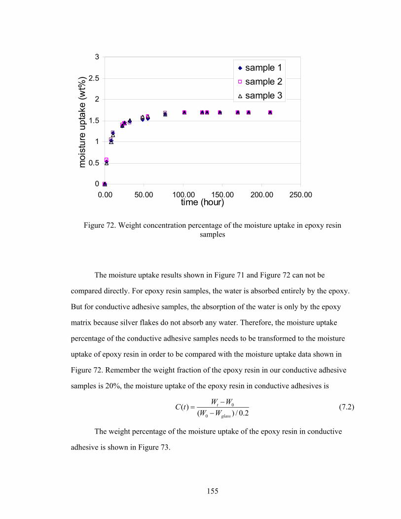
155

0

0.5

1

1.5

2

2.5

3

0.00 50.00 100.00 150.00 200.00 250.00time (hour)

moi

stur

e up

take

(wt%

)sample 1sample 2sample 3

Figure 72. Weight concentration percentage of the moisture uptake in epoxy resin samples

The moisture uptake results shown in Figure 71 and Figure 72 can not be

compared directly. For epoxy resin samples, the water is absorbed entirely by the epoxy.

But for conductive adhesive samples, the absorption of the water is only by the epoxy

matrix because silver flakes do not absorb any water. Therefore, the moisture uptake

percentage of the conductive adhesive samples needs to be transformed to the moisture

uptake of epoxy resin in order to be compared with the moisture uptake data shown in

Figure 72. Remember the weight fraction of the epoxy resin in our conductive adhesive

samples is 20%, the moisture uptake of the epoxy resin in conductive adhesives is

0

0

( )( ) / 0.2

t

glass

W WC tW W

−=

− (7.2)

The weight percentage of the moisture uptake of the epoxy resin in conductive

adhesive is shown in Figure 73.

156

0

0.5

1

1.5

2

2.5

3

0.00 50.00 100.00 150.00 200.00 250.00time (hour)

moi

stur

e up

take

(wt%

)

sample 1sample 2sample 3

Figure 73. Weight concentration percentage of the moisture uptake of the epoxy resin in

conductive adhesive samples The epoxy in conductive adhesives seems to absorb more moisture than the epoxy

sample alone. By comparing Figure 72 and Figure 73 it can be seen that the moisture

uptake of the epoxy resin in the conductive adhesive sample is 2.7%, which is more than

the moisture uptake value of 1.7% in the epoxy resin sample at saturation. This means

that with the same amount of epoxy resin, the epoxy resin in the conductive adhesive

absorbs more water than the epoxy resin alone. The reason lies in the interface between

the silver flakes and the epoxy matrix in the conductive adhesive. The water absorbed in

the epoxy matrix can be divided into free unbonded water and hydrogen-bonded water.

After the moisture is absorbed by the epoxy matrix, a large portion of the free water

molecules travels through and resides in the nanovoids and holes in the epoxy matrix.

There are also many micro-delaminations and pores associated with the epoxy-silver

interface because the interface between the silver flakes and epoxy resin in the

conductive adhesive is not perfect. These micro-delaminations and pores act just like the

157

nanovoids in the epoxy, providing residence for the free water molecules. Moreover,

when water travels to the epoxy-silver interface, the moisture-reacted metal surface can

form a weak, hydrated oxide surface. Both metal and oxides are relatively polar, and

water is absorbed onto the silver surface to become bonded water. Therefore the epoxy-

silver interface absorbs both free water and bonded water. As a result, the epoxy resin in

the conductive adhesive absorbs more water than the epoxy resin alone.

The amounts of time to reach saturation state are also different between epoxy

resin in conductive adhesives and epoxy resin alone. The epoxy alone needs about 100

hours to reach saturation, while for the epoxy in conductive adhesives it is after 150 hours

that the epoxy stops water absorption. For the moisture uptake of the epoxy alone, the

diffusion of the water can be approximated by the classical Fick’s second law, and the

moisture travels only inside the one-phase epoxy. But for the epoxy in conductive

adhesives, the silver flakes are diversely dispersed in the matrix. Since silver is not water-

absorbing, the diffusion of water has to bypass the silver flakes. The diffusion rate of

moisture is thus slowed down by the silver flakes in conductive adhesives, and

consequently the time to reach saturation is longer than is observed for the epoxy alone.

The moisture uptake percentage is also measured for the conductive adhesive

samples and epoxy resin samples after being fully dried in the 95°C convection oven for

144 hours. The data are plotted in Figure 74, in which the lighter columns are the weight

concentration percentage of the moisture uptake at the saturation stage, and the darker

columns are the moisture concentration after being baked. The plot shows that although

the samples are baked in the convection oven to a state where no more weight decrease

can be observed, the moisture absorbed in the moisture conditioning stage can not be

totally removed. This suggests that the water absorption in the epoxy matrix is an

irreversible process. The plot also shows that the epoxy in conductive adhesives recovers

less than the epoxy sample alone. Again the sorption of the moisture by the epoxy-silver

flake interface plays an important role. The interface between the epoxy and the silver

158

flakes not only absorbs water during the moisture conditioning, but also retains and reacts

with the water molecules. Therefore the weight gain after the baking process of the epoxy

resin in conductive adhesive is relatively larger than is observed for the epoxy sample

alone.

0.00

0.50

1.00

1.50

2.00

2.50

3.00

epoxy sample epoxy in conductive adheisves

moi

stur

e up

take

(wt%

)

saturation stateafter fully drying

Figure 74. Moisture uptake of conductive adhesive and epoxy resin samples after full recovery

7.3.2 Resistance of conductive adhesives in moisture conditioning and after moisture

recovery

The resistance of conductive adhesive samples is measured during the moisture

conditioning in the 85°C/85%RH humidity chamber. Their resistivity values are

159

calculated based on the measured resistance values. The relative change of the resistivity

is calculated by

Relative resistivity change 0

0

( )tρ ρρ

−= (7.3)

where ρ(t) is the resistivity of the conductive adhesive at time t, and ρ0 is the resistivity of

the conductive adhesive sample before the moisture conditioning.

The resistivity of conductive adhesive samples is found to be stable after moisture

conditioning. The relative resistivity change is plotted over moisture conditioning time

for four conductive adhesive samples as shown in Figure 75. It can be seen that for all

four conductive adhesive samples, the resistivity value varies with ≤4% of the original

resistivity value. There is no pattern that the resistivity increases due to moisture

conditioning. The variation of the resistivity is the “noise” in the process of resistance

measurement. The typical value of resistance for a conductive adhesive sample is 0.4 Ω,

4% of this value is 0.0016 Ω. The resistance of conductive adhesive samples is measured

by soldering four leads of a multimeter to the copper pads of the PCB as shown in Figure

69. Small Variations in the process of handling could cause the noise. Nevertheless, it is

clear that the resistivity of conductive adhesives does not change much after moisture

conditioning.

The conductive adhesive samples after moisture conditioning are then put into a

95°C convection oven and baked for 144 hours to recover from moisture uptake. The

resistance of the conductive adhesive samples after being fully dried is measured and the

relative resistivity change calculated for each sample, as shown in Table 11. The

resistivity values have not increased, but decreased slightly. The decrease is so small

(<3%) that the resistivity of the conductive adhesives can still be considered stable after

moisture recovery.

160

-50

-40

-30

-20

-10

0

10

20

30

40

50

0 50 100 150 200

time (hour)

rela

itive

resi

stiv

ity c

hang

e (%

) sample 1sample 2sample 3sample 4

Figure 75. Resistivity change of conductive adhesive samples in moisture conditioning

Table 11. Relative resistivity change of conductive adhesive samples after moisture recovery

Relative resistivity change after recovery

Sample 1 -1.44%

Sample 2 -2.75%

Sample 3 -2.11%

Sample 4 -2.17%

The resistivity value of conductive adhesive samples is also measured for

conductive adhesive samples conditioned in the 85°C convection oven, and the relative

resistivity change is calculated and plotted in Figure 76. Similar to Figure 75, the

161

resistivity change does not go beyond ≤4% of the original resistivity value. The

resistivity shows no apparent trend of significant change.

-50

-40

-30

-20

-10

0

10

20

30

40

50

0 50 100 150 200

time (hour)

rela

tive

resi

stiv

ity c

hang

e (%

) sample 1sample 2sample 3sample 4

Figure 76. Resistivity change of conductive adhesive samples in 85°C conditioning

Combining Figure 75, Table 11, and Figure 76, the resistivity of conductive

adhesives does not change either after 85°C conditioning or 85°C/85%RH moisture

conditioning, or after moisture recovery. After moisture conditioning, although the

moisture is absorbed by the epoxy matrix and by the interface between the epoxy matrix

and the silver flakes, the contacts between the silver flakes are not affected by the

moisture. This is because the intimate contacts between the connected silver flakes are

maintained by the contact pressure, and it is not easy for the moisture to penetrate to the

contact area between the silver flakes. Therefore the contact resistance of the contact

interface remains the same with moisture being present. After the moisture is baked away

in the recovery test, the contact interfaces are still intact from moisture. As a result the

162

total resistance of the network of silver flakes does not change and the resistivity of the

conductive adhesive samples remains the same as before moisture conditioning.

In our test the copper pads on the PCB are sputter coated with a thin layer of gold

to prevent contact resistance degradation between conductive adhesive samples and

copper pads, and the thickness of the gold layer is in order of nanometers. Because the

gold layer is coated directly onto copper pads, there could be diffusion between copper

and gold. However, in spite of the copper-gold diffusion, the measured resistance value

remains stable during the moisture conditioning process. Therefore both the contact

resistance between conductive adhesive samples and copper pads and the bulk resistance

of conductive adhesive samples are not affected by moisture, and the thin layer of gold

sputter coated on the copper pads is effective to reduce corrosion at the conductive

adhesive – copper pad interface under moisture condition.

7.3.3 Fatigue life of conductive adhesives after moisture conditioning

The above resistance measurement of conductive adhesive samples after moisture

conditioning is only done when no load is applied. However, in electronic packaging

temperature cycles can happen to the conductive adhesive joints after moisture invasion.

Thus the fatigue load caused by thermal expansion will be acting on the conductive

adhesive joints together with moisture. This section is to study the resistance change of

the conductive adhesive samples in fatigue tests when moisture is present.

The fatigue test is done by using the four-point push/pull beam bending test as

described in the previous chapter. The conductive adhesive samples after moisture

conditioning in 85°C/85%RH are tested in the fatigue test.

The resistance values of the conductive adhesive samples are monitored, and their

resistivity values are calculated. No mechanical failure in the conductive adhesive

samples is observed after the fatigue test, but their resistivities increase as more fatigue

cycles are conducted. Therefore the failure is still the electrical conduction failure, and

163

the failure criterion is specified as electrical failure happens when the resistivity value of

the conductive adhesive sample has a 100% increase. The fatigue life of conductive

adhesive samples after moisture conditioning in 85°C/85%RH humidity chamber for 168

hours is listed in Table 12. The fatigue tests are performed with a strain rate of

1.8217μ10-4 1/sec, and a fully reversed strain ratio R = -1.

Table 12. Fatigue life for conductive adhesives samples after moisture conditioning


1162 156 21 3

1271 167 25 3

1087 170 17 3



1072 155 19 3

Average fatigue life 1148 162 20.5 3

The fatigue life listed in Table 12 is also plotted in Figure 77. Also plotted in the

figure is the fatigue life of conductive adhesive samples without moisture. By comparing

the fatigue life between the two, clearly with moisture the fatigue load increases the

resistivity of conductive adhesives much faster than without moisture. Therefore the

fatigue life of conductive adhesives after moisture conditioning is significantly reduced

due to the effect of moisture.

164

0.006

0.007

0.008

0.009

0.01

0.011

0.012

0.013

0.014


Δε/

2: s

train

am

plitu

dewithout moistueafter moisture conditioning

Figure 77. Fatigue life of conductive adhesive samples after moisture conditioning

The relative decrease of fatigue life can be calculated based on the average fatigue

life after moisture conditioning and without moisture at each strain amplitude value. The

relative fatigue life decrease is calculated as

Relative fatigue life decrease f fm

f

N NN−

= (7.4)

where Nf is the fatigue life of conductive adhesives without moisture, and Nfm is the

fatigue life after moisture conditioning.

The relative fatigue life decrease is plotted in Figure 78. It can be seen that the

fatigue life is more decreased due to moisture when the strain amplitude is bigger. But

even at the small strain amplitude value of 0.0069, the fatigue life is decreased by 46.2%.

At the strain amplitude of 0.0127, the fatigue life is decreased by 92.5%. Therefore the

moisture accelerates the fatigue failure significantly.

165

010

2030

4050

6070

8090

100

0.0069 0.0090 0.0109 0.0127Δε/2: strain amplitude

rela

tive

fatig

ue li

fe d

ecre

ase

due

to m

oist

ure

(%)

Figure 78. Relative fatigue life decrease due to moisture

The fatigue life can also be fitted using the power law equation as in Equation

(6.5). The fitted power law equation and fatigue life data of the conductive adhesive

samples after moisture conditioning, together with the fatigue life data without moisture

obtained from last chapter, are shown in Figure 79. The two parameters in the power law

model for conductive adhesives after moisture conditioning are

0.1041

0.0158f

c

ε

= −

′ = (7.5)

166

-5

-4.9

-4.8

-4.7

-4.6

-4.5

-4.4

-4.3

0 2 4 6 8 10ln(2Nf)

ln( Δ

ε/2)

without moisturefit line: without moistureafter moisture conditioningfit line: after moisture conditioning

Figure 79. Fitted power law model for conductive adhesives after moisture conditioning

7.3.4 Fatigue life of conductive adhesives after moisture recovery

Fatigue tests are performed on conductive adhesive samples after moisture

conditioning and recovery. The samples are first moisture conditioned in 85°C/85%RH

humidity chamber for 168 hours, and then fully baked in the 95°C convection oven for

144 hours. The samples after such processing are then taken to perform the fatigue test,

and their resistance values are monitored during the fatigue test.

The number of cycles to failure for conductive adhesive samples after moisture

recovery is listed in Table 13 and shown in Figure 80. The fatigue test is performed at a

strain rate of 1.8217μ10-4 1/sec, and with a fully reversed strain ratio of R = -1. The

fatigue life data of conductive adhesives without moisture and after moisture

conditioning are also plotted in Figure 80 for comparison.

167

Table 13. Fatigue life for conductive adhesives samples after moisture recovery


1932 332 72 12

1765 350 79 10

1890 371 80 17



1840 369 91 15

Average fatigue life 1856.75 355.5 80.5 13.5

0.006

0.007

0.008

0.009

0.01

0.011

0.012

0.013

0.014


Δε/

2: s

train

am

plitu

de

without moistueafter moisture conditioningafter recovery

Figure 80. Fatigue life of conductive adhesive samples after moisture recovery

Based on Table 13 and Figure 80 it can be seen that the fatigue life of the

conductive adhesive samples is partly recovered. The fatigue life of the conductive

adhesive samples after recovery lies between the fatigue lives of samples with no

moisture and of samples with moisture conditioning.

168

The relative fatigue life decrease can also be calculated using Equation (7.4), with

replacing Nf,m, the average fatigue life of conductive adhesives after moisture

conditioning, with Nf,r , the average fatigue life after moisture recovery. The relative

fatigue life decrease due to moisture conditioning and recovery is shown in Figure 81.

The relative fatigue life decrease due to moisture conditioning is also plotted for

comparison. After fully drying, the fatigue life at each strain amplitude value is

improved. However, still the fatigue life is much shorter than conductive adhesives

without moisture conditioning. The small amount of moisture (1.06% weight, as shown

in Figure 74) that remained in the epoxy matrix and at the epoxy-silver interface after

moisture recovery can still reduce the fatigue life for as much as 66.25%.

01020304050

60708090

100

0.0069 0.0090 0.0109 0.0127Δε/2: strain amplitude

rela

tive

fatig

ue li

fe d

ecre

ase

due

to m

oist

ure

(%)

after moisture conditioningafter moisture recovery

Figure 81. Relative fatigue life decrease due to moisture conditioning and recovery

169

The fatigue life data of conductive adhesives after recovery is fitted using the

power law equation. The line of fit is shown in Figure 82 and the two parameters in the

power law equation for conductive adhesives after moisture recovery are

0.1274

0.0201f

c

ε

= −

′ = (7.6)

-5

-4.9

-4.8

-4.7

-4.6

-4.5

-4.4

-4.3

0 2 4 6 8 10ln(2Nf)

ln( Δ

ε/2)

without moisturefitted line: without moistureafter moisture conditioningfitted line: after moisture conditioningafter recoveryfitted line: after recovery

Figure 82. Fitted power law model for conductive adhesives after moisture conditioning and recovery

7.3.4 Failure mechanism of conductive adhesives in fatigue tests with moisture

The microstructure of conductive adhesive samples that have failed in fatigue

tests is examined with a scanning electron microscope. The cross sections (as shown in

Figure 60) of the samples are checked and SEM pictures are taken. Both the

microstructures of the failed conductive adhesive samples with moisture and after

moisture recovery are examined, and it is found that they are no different than the failed

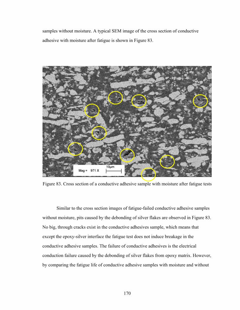
170

samples without moisture. A typical SEM image of the cross section of conductive

adhesive with moisture after fatigue is shown in Figure 83.

Figure 83. Cross section of a conductive adhesive sample with moisture after fatigue tests

Similar to the cross section images of fatigue-failed conductive adhesive samples

without moisture, pits caused by the debonding of silver flakes are observed in Figure 83.

No big, through cracks exist in the conductive adhesives sample, which means that

except the epoxy-silver interface the fatigue test does not induce breakage in the

conductive adhesive samples. The failure of conductive adhesives is the electrical

conduction failure caused by the debonding of silver flakes from epoxy matrix. However,

by comparing the fatigue life of conductive adhesive samples with moisture and without

171

moisture, it can be seen that the debonding process is much accelerated by the absorbed

water.

The moisture accelerates the debonding of the silver flakes in two ways: by

changing the mechanical property of the epoxy matrix, and by changing the interfacial

property between epoxy matrix and silver flakes.

The bulk property of epoxy matrix is affected by moisture. It has been shown that

in the saturated state, the elastic modulus of the epoxy decreases due to absorption of

moisture [124]. Because the change in the elastic modulus can alter the interfacial

fracture toughness between epoxy and silver considerably, moisture deteriorates the

epoxy-silver interfacial adhesion indirectly by decreasing the elastic modulus of the

epoxy resin. Therefore in the saturated state the flakes are easier to debond from the

epoxy matrix in fatigue test, which causes a faster degradation of the electrical

conduction and results in a shorter fatigue life.

Moisture can impair the epoxy-silver interfacial adhesion directly. Moisture acts

as a debonding agent through a combination of the following mechanisms: the moisture-

reacted metal surface can form a weak, hydrated oxide surface; moisture-assisted

chemical bond breakdown and moisture-related degradation or depolymerization [10].

Both metal and oxides are relatively polar. Water is preferentially absorbed onto the

oxide surface and creates a weak boundary layer at the metal-polymer interface that can

lead to adhesion problems. Hence the epoxy-silver adhesion is degraded.

With the detrimental effect of moisture on the mechanical property of epoxy

matrix and the epoxy-silver interface, the intimate contacts between silver flakes are

degraded faster and the fatigue life becomes shorter compared with the case where no

moisture is present. In the saturated state, both the two effects exist, and the fatigue life of

conductive adhesive samples is the shortest. After being fully dried, the majority of the

loss in elastic modulus of the epoxy matrix can be recovered by the removal of moisture.

Some permanent loss does occur, and the dominant mechanism responsible for the loss in

172

elastic modulus is plasticization due to moisture, which is a reversible process.

Nevertheless after drying up the recovery of elastic modulus consequently recovers part

of the epoxy-silver interfacial fracture toughness. Therefore upon fully drying the fatigue

life of the conductive adhesives is improved partly. However, still a large part of the

damage done by moisture to the epoxy-silver interface is not reversible, and the fatigue

life of conductive adhesive samples after drying up is still much less than the samples

with no moisture.

7.4 Conclusions

In this chapter the effect of moisture on the electrical conduction of conductive

adhesives is investigated. The conductive adhesive and epoxy resin samples are moisture

conditioned in an 85°C/85%RH humidity chamber, and the moisture uptake is measured

by examining the weight change during the conditioning process. It is found that both the

conductive adhesive samples and the epoxy resin samples absorb water and reach

saturated state after 168 hours of moisture conditioning process. By comparing the

weight percentage of the moisture absorbed by the epoxy resin in conductive adhesive

samples and the epoxy resin sample alone, it is found that the epoxy in conductive

adhesives absorbs more moisture. This is due to the epoxy-silver interface, which absorbs

both the free water and bonded water. However, the resistance of the conductive adhesive

samples does not change during and after the moisture conditioning in 85°C/85%RH

condition. The reason is that it is not easy for the moisture to diffuse into the contact

interfaces between silver flakes, which are held tightly by contact pressures.

Fatigue tests are performed to the conductive adhesive samples after moisture

conditioning. The resistance of the conductive samples is monitored during the fatigue

test. Electrical conduction failure still happens well before mechanical failure. The failure

of a conductive adhesive sample occurs when its resistivity increases by 100% of the

resistivity before fatigue tests. The fatigue life is found to be significantly reduced with

173

the presence of moisture. The relative decrease of the fatigue life ranges from 46.25% to

92.5% at a strain amplitude range of 0.0069 to 0.0127, compared with the fatigue life of

conductive adhesive samples without moisture. Fatigue tests are also performed on

conductive adhesive samples which are first moisture conditioned in an 85°C/85%RH

humidity chamber for 168 hours and then baked in a 95°C convection oven till fully

dried. It is discovered that the fatigue life is partly recovered. However, still the fatigue

life after moisture recovery is much less than that of the conductive adhesives without

moisture processing.

A failure mechanism is proposed for the failure of conductive adhesives in fatigue

tests with moisture being present. By examining the microstructure of conductive

adhesive samples, it is found that the debonding of silver flakes is the reason for the lost

electrical conduction. The moisture absorbed acts in two ways to accelerate the

debonding of the silver flakes: the degradation of the bulk elastic modulus of the epoxy

matrix and the of the adhesion between the epoxy matrix and the silver flakes. The two

effects both exist in the saturated state, and the fatigue life of conductive adhesives is

significantly decreased. After moisture recovery in the 95°C convection oven, a large part

of the elastic modulus is recovered and therefore the fatigue life of the conductive

adhesive samples is improved compared with the saturation state. However, since

interfacial adhesion of the epoxy-silver is irreversibly impaired by moisture, the fatigue

life after drying up is still much less than conductive adhesive samples without moisture

conditioning.

Although the electrical conduction of the conductive adhesive is not affected after

moisture aging, care must still be taken to avoid moisture being absorbed into conductive

adhesive joints. The reason is that in real electronic applications the temperature-induced

fatigue is often encountered. Whenever the two factors of fatigue and moisture act

together, the electrical reliability of the conductive adhesive joints is heavily impaired.

174

Therefore measures should be taken to prevent moisture absorption, such as using

hermetic packages.

175

CHAPTER 8

CONDUCTIVE ADHESIVES UNDER DROP TESTS

8.1 Introduction

Impact is often defined as a rapid transfer of energy to a mechanical system,

which could induce a significant change in the stress, velocity, acceleration or

displacement to the system. The increasing trend of electronic product miniaturization

has resulted in greater concern for impact reliability of electronic packaging for various

reasons. The miniaturized products tend to be more mobile and wearable and hence are

more at risk of accidental drop or impact when used. To support the product

miniaturization, the size of electronic packages is reduced through finer interconnections,

which are more vulnerable to drop impact. Moreover, polymeric based adhesive

interconnections are more vulnerable to drop impact.

In order to assess the damage of impact to the electronic packages, discover the

failure mechanism and find solutions to improve the package design, drop tests are

performed. In the drop test the measured maximum acceleration is often used as a

criterion of the impact resistance of a structure in microelectronic products.

Drop tests can be performed at different levels: the component level, the board

level and the product level. At the component level only a component with substrate is

dropped, and the failure of the interconnection material is studied. In board-level drop

tests, the printed circuit board is usually modeled as a beam or a plate, which is easy to be

bent by the stress induced during drop tests. The differential flexing between the PCB

and the components is often acting as the key failure driver. For drop tests at the product

level even more factors need to be considered. This is because not only the support of the

176

PCB is different than in board-level tests, but also because there could be clattering and

multiple impacts among the components inside the product.

In this chapter, the component level drop test is conducted on a simple test vehicle

composed of a copper resistor and a printed circuit board, which are bonded by a

conductive adhesive joint. The drop test condition is characterized by the maximum

acceleration experienced by the test vehicle, which can be adjusted by the drop height

and the felt material. The test vehicle is subjected to drops with various peak drop

accelerations and the number of drops to failure is recorded. A drop failure life model is

proposed based on the strain energy in the conductive adhesive joint induced by the drop

impact. The failure mechanism of the conductive joints in failure is discussed.


8.2.1 Materials

The formulation of the conductive adhesive used in the drop test is similar to

those used in the previous two tests. The only difference is that some spacer beads are

added into the conductive adhesive in order to maintain a constant bond line thickness

between the dummy resistor and the PCB board. The glass beads are GL-0275-B,

obtained from Mo-Sci Corporation. The average diameter of the glass beads is 75 μm, the

density of the spacer beads is 4.3 g/cm3. The ingredients of the conductive adhesive are

epoxy resin, silver flakes, and spacer beads. The weight ratio of silver flakes : epoxy resin

: spacer beads is 4 : 1 : 0.025. With this weight ratio, it is guaranteed that for every 1 mm2

of bonding area there exists at least 1.5 beads. Therefore for the whole bonding area there

will be enough spacer beads to make sure the thickness of the conductive adhesive is kept

relatively uniform.

177

8.2.2 Test vehicle for drop tests

A simple electronic package is designed to perform the drop test. This simple

package includes dummy resistors and printed circuit board, which are connected by the

conductive adhesive joint. The layout of the printed circuit board is shown in Figure 84.

The copper traces and pads are designed on the printed circuit board so that the four-point

resistance measurement method could be used. The four leads of a multimeter will be

soldered to the copper pads to measure the resistance of the two conductive adhesive

joints as shown in Figure 84. The two holes on the printed circuit board are used to fasten

the package on the impact tester.

Figure 84. A simple test vehicle for drop test

Copper blocks are used as dummy resistors, which are adhered to the copper pads

on the printed circuit board by conductive adhesive joints. The conductive adhesive

material is applied on the copper pads using a customized stencil. After the conductive

Unit: mm

connected to multimeter

copper block (dummy resistor)

conductive adhesive joint

drop direction

178

adhesive material is stencil-printed, the copper blocks are placed on the copper pads. The

printed circuit board and the copper blocks are then put into a 150°C convection oven for

3 hours to let the conductive adhesive joints be fully cured. In the curing process, a

weight of 50 grams is placed on each copper block. The weight will provide pressure on

the conductive adhesive joints to achieve better adhesion. After the conductive adhesive

joints are cured, the simple package is taken out of the 150°C convection oven and cooled

in room temperature for about 1 hour. Then drop tests are then performed on the test

vehicle.

The conductive adhesive joints after being cured have an average radius of 1.26

mm, and an average thickness of 101 μm.

The dummy resistors act as connectors between the conductive adhesive joints

and they will provide the inertia force in the drop test. Copper blocks are used to make

many of the dummy resistors. The copper blocks are cut from stock copper material using

diamond saw, and they are polished first by grit 800 sandpaper and then by grit 2400

sandpaper. The copper blocks after such processing have approximately the same size

and weight. The average weight of the copper block is 1.40 g. The average size of the

copper block is 9.8 mm μ 4.6 mm μ 3.5 mm.

Before the application of conductive adhesives, both the copper blocks and the

printed circuit board are cleaned by acetone, HCl solution and distilled water to remove

possible contaminants. And during the operation latex gloves are worn all the time to

prevent any contaminants from hands.

8.2.3 Drop tests

Drop tests are performed on a drop weight impact tester: Dynatup 8250 from

Instron, which is shown in Figure 85. The impact tester is originally for testing the impact

resistance of materials. The material under test is clamped in the sample holder, then the

tup together with a drop weight is dropped from a certain height along the two guide

179

rails. After being hit by the tup the material is examined for any damage due to impact.

The tup is connected to a load cell and computer data acquisition system, and a computer

program will calculate impact energy, energy absorbed by the material, tup velocity,

impact load maximum deflection of the tested material.

In our study, the tup of Dynatup 8250 impact tester is used as the drop test table.

Our test vehicle is mounted on the impact tester near the tup by two screws without

standoffs. The test vehicle and two screws weighs less than 8 g, which is very small

compared with 3674g, the total weight of the tup and drop weight. Therefore the

attachment of the test vehicle does not change the behavior of the tup. A big piece of steel

is placed at the location of the sample holder as the anvil. The tup tip is a half-inch

diameter hemispherical steel. To protect the tup tip from damage due to colliding with the

steel anvil, a nylon plate is added on top of the steel anvil as the felt material.

180

Figure 85. Dynatup 8250 impact apparatus

The test procedure is as follows. The tup and the drop weight are first raised to a

desired height by a hook. Then the hook is released to let the tup and weight fall down

along the two guide rails and hit the felt material. Upon impact, the load cell and data

acquisition system records all the impact-related data. There are two pneumatic rebound

brakes installed near the bottom of the guide rails. The pneumatic rebound brakes will be

fired to hold the drop weight and tup after impacts are finished, so that no more repeated

impacts will happen.

tup

sample holder

guide rail

181

Since the test vehicle is installed tightly by two screws at a place close to the tup,

the acceleration and velocity of the test vehicle is assumed to be the same as the tup.

Because the velocity and acceleration of the tup are all recorded by the data acquisition

system, these data are also known for the test vehicle and no more additional

accelerometer is needed on the test vehicle. Although this is a simplification and it is not

perfectly accurate due to some damping effect of the connection between the test vehicle

and the impact tester, it is still a good approximation because of the small size of the test

vehicle and its close distance to the tup.

In drop tests, the critical factor is the maximum value of the acceleration, which

can be adjusted by changing the falling height and the felt material.

It is assumed that the shear stress induced by the drop test is the most severe

scenario for the conductive adhesive joints. Therefore the test vehicle is mounted

vertically near the tup. The drop direction is shown in Figure 84.

As mentioned before the electrical conduction of the conductive adhesive joints is

a major concern, so the resistance of the adhesive joints is measured before and after the

drop test. The four copper pads are soldered with four leads of the multimeter as shown

in Figure 84 to measure the total resistance of the two conductive adhesive joints and the

resistance of the dummy resistor. Since the dummy resistor is made of copper block, its

bulk resistance (~ 10-5 Ω) is very small and negligible compared with the resistance of the

conductive adhesive joints (~ 4μ10-2 Ω). Hence any change of the resistance value in

drop tests will be due to the conductive adhesive joints.

Both mechanical failure and electrical conduction failure of the conductive

adhesive joints could happen in drop tests. The mechanical failure is considered as the

cracking or breakage of the conductive adhesive joints. The electrical failure criterion is

again specified as 100% increase of the original resistivity value of the conductive

adhesive joints. The integrity of the conductive adhesive joints are examined and the

182

resistance value checked after each drop, and whenever the mechanical or electrical

conduction failure happens the conductive adhesive joints are considered to have failed.

During the drop tests, it may happen that the conductive adhesive joint does not

fail after a single drop, but fails after a number of drops. The number of drops together

with the resistance value of the conductive adhesive joints is recorded.

8.2.4 Shear modulus measurement

The shear stress induced by the drop of the conductive adhesive sample is

considered to be the main driver of failure. It is desired that the strain energy can be

calculated and correlated to the number of drops to failure. The strain energy is calculated

from the shear modulus and shear stress. The shear stress can be calculated based on the

inertia force applied to the conductive adhesive joints by the copper block, which will be

discussed later. The shear modulus of the conductive adhesive joints is measured as

described below.

The lap shear specimen is used for the shear modulus measurement. The

specimen is shown in Figure 86. A conductive adhesive layer is used to bond two copper

bars. The same conductive adhesive material as applied in the drop test is used. The lap

shear is cured in 150°C convection oven for 3 hours before the lap shear test. The

dimension of the conductive adhesive joint after curing is 5.69 mm μ 4.88 mm μ 0. 101

mm.

183

Figure 86. Lap shear specimen for shear modulus measurement

To measure the shear modulus of the conductive adhesive joint, the shear stress

and shear strain need to be known. The lap shear specimen is tested on an EnduraTech

ScopeTester. The two ends of the lap shear specimen are clamped by the two fixtures of

the tester, which exerts a tensile force. The magnitude of the force is recorded by the

tester, which can be used to calculate the shear stress applied to the conductive adhesive

joint. The strain of the conductive adhesive joint is measured by the non-contact image

analysis method. Note that there are two marks on the lap shear specimen shown in

Figure 86. During the shear test a CCD camera is installed above the specimen to capture

images of the lap shear specimen. Because the two black marks have a high contrast to

the background color, the position of the two marks can be found by image analysis

software. The images are captured at each second of the test, and by comparing the length

between the two marks in each image the shear strain can be calculated. The shear strain

thus calculated is the total strain due to the deformation of the adhesive joint and the

copper bar. Since the shear modulus of copper is known, the shear strain due to the

copper bar can be calculated and subtracted from the total strain, and the strain in the

marks

conductive adhesive layer

force

force force

force

184

conductive adhesive joint is known. With both the shear stress and shear strain being

known, the shear modulus can be calculated.

8.3 Results and discussion

The drop test results are first presented. The acceleration experienced by the test

vehicle is assumed to be the same as the tup, and the acceleration curve is obtained from

the data acquisition system. The maximum acceleration is identified for drop tests with

different drop heights and felt material thicknesses, and for each acceleration level the

number of drops to failure is recorded. The shear modulus is obtained from the lap shear

specimen test. The shear modulus and the shear stress induced in the drop test by the

maximum acceleration are used to calculate the maximum strain energy per uni bond area

of the conductive adhesive joint. The number of drops and the maximum strain energy

per uni bond area are found to be correlated well by a power law model, which is similar

to the power law model in fatigue. At last the possible failure mechanism is proposed for

conductive adhesive joints in drop tests.

8.3.1 Drop tests results

Drop tests are performed on the test vehicle, with the integrity of the conductive

adhesive joints being checked and the resistance value being measured after each drop.

The acceleration of the test vehicle during the drop impact can be obtained from the data

acquisition system that is connected to the tup. A typical acceleration curve of the test

vehicle is shown in Figure 87. The shape of the acceleration curve is found to be near a

half sine shape.

The most critical factor in the drop test is the maximum acceleration [125],

corresponding to the instant at when the speed of the test vehicle is reduced to zero. This

maximum acceleration is the top point of the curve shown in Figure 87. The maximum

acceleration value can be adjusted by changing the drop height and the felt material. A

185

higher drop height will generate a faster initial speed for the tup to hit the felt material.

By making the felt material harder or thinner, the pulse duration (shown in Figure 87 as

the time span of the curve) can be made shorter. Thus by adjusting the drop height and

the nylon plate thickness, different maximum acceleration values can be achieved. In our

test, the height is in the range of 5 ~ 25 cm, and the pulse duration is in the range of 0.5 ~

1 ms, which generates an acceleration range of 1749 ~ 8113 m/s2.

0

500

1000

1500

2000

2500

3000

3500

4000

0.0 0.1 0.2 0.3 0.4 0.5 0.6 0.7time (ms)

acce

lera

tion

(m/s

^2)

Figure 87. Acceleration of the test vehicle during drop test

For each acceleration level, the resistance of the conductive adhesive joints is

measured. Figure 88 shows a typical resistance change as more drop tests are conducted.

It can be seen that the resistance value is almost constant during the first several drops.

Then suddenly the resistance value increases to an infinity value. Visual inspection of the

conductive adhesive joints suggests that there is no visible crack in the first drops. Even

after the 8th drop the dummy resistor is still bonded with the printed circuit board. But

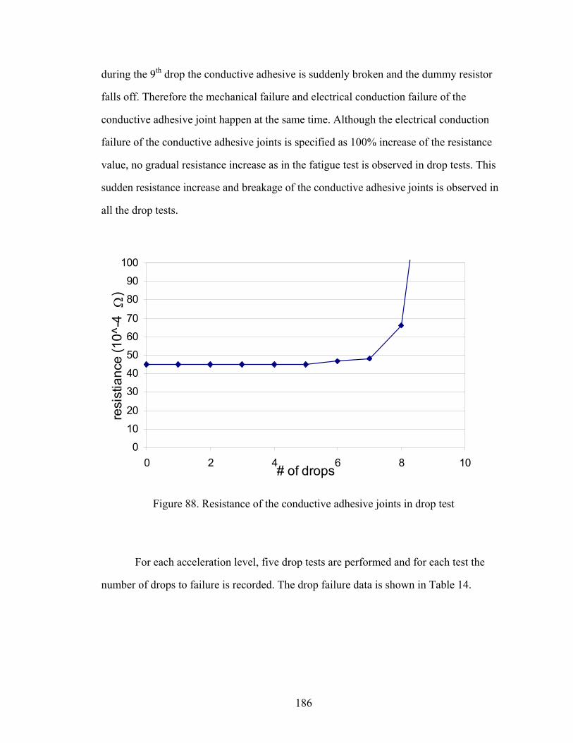
186

during the 9th drop the conductive adhesive is suddenly broken and the dummy resistor

falls off. Therefore the mechanical failure and electrical conduction failure of the

conductive adhesive joint happen at the same time. Although the electrical conduction

failure of the conductive adhesive joints is specified as 100% increase of the resistance

value, no gradual resistance increase as in the fatigue test is observed in drop tests. This

sudden resistance increase and breakage of the conductive adhesive joints is observed in

all the drop tests.

0

10

20

30

40

50

60

70

80

90

100

0 2 4 6 8 10# of drops

resi

stia

nce

(10^

-4 Ω

)

Figure 88. Resistance of the conductive adhesive joints in drop test

For each acceleration level, five drop tests are performed and for each test the

number of drops to failure is recorded. The drop failure data is shown in Table 14.

187

Table 14. Drop life of conductive adhesive joints in drop tests

Peak

acceleration

(m/s2)

# of drops to failure of five conductive adhesive

test vehicles

Average # of

drops to failure

1749.353 61 57 56 63 62 59.8

2211.624 35 42 43 37 39 39.2

2690.129 21 22 16 23 19 20.2

3461.325 19 16 15 16 17 16.6

3900.648 8 10 11 9 7 9

4699.318 6 5 6 4 7 5.6

6075.271 2 2 2 3 1 2

8113.097 1 1 1 2 1 1.2

8.3.2 Shear modulus of conductive adhesives

The shear modulus of the conductive adhesive joints is calculated from the shear

stress measured from the tester and the shear strain obtained from the image analysis. The

beginning portion of the measured shear strain and shear stress is plotted in Figure 89. It

can be seen that although there is some fluctuation of the data points, generally speaking

the stress-strain curve is linear. The shear modulus is just the slope of the curve shown in

Figure 89, which is calculated to be 1907 MPa. The shear strength of the conductive

adhesive is the stress just before the breakage of the adhesive joint, which is measured to

be 4.835 MPa. The shear modulus will be used to calculate the strain energy induced by

the drop test.

188

0

0.5

1

1.5

2

2.5

3

0.0E+00 4.0E-04 8.0E-04 1.2E-03 1.6E-03shear strain

shea

r stre

ss (M

Pa)

Figure 89. Stress-strain curve for conductive adhesive lap shear joint

8.3.3 Drop failure life model of conductive adhesives

A inertia force is applied to the conductive adhesive joints by the copper block in

the drop test. At the moment the tup hits the anvil, the speed of the tup and the printed

circuit board is quickly reduced from initial speed v0 to zero. However, the copper block

is still moving down with the falling speed v0. If the PCB is assumed to have the same

acceleration during the drop test as the tup, then the maximum inertia force F applied to

the conductive adhesive joint is simply

maxF ma= (8.1)

where m is the mass of the copper block (dummy resistor) and amax is the measured

maximum acceleration of the tup. The inertia force on the conductive adhesive joint is

shown in Figure 90.

189

F = ma

dummy resistorPCB

conductive adhesive joint

Figure 90. Inertia force applied on the conductive adhesive joint

The inertia force applies a shear stress on the conductive adhesive joint. Since the

maximum acceleration of the test vehicle/tup is already measured, the maximum shear

stress τmax can be calculated as

maxmax

maA

τ = (8.2)

where A is the total bonding area of the two conductive adhesive joints.

The maximum strain energy density during the drop test is

2max

12

UG

τ= (8.3)

where G is the shear modulus of the conductive adhesive.

The maximum strain energy density U in Equation (8.3) is the maximum strain

energy per unit volume of the conductive adhesive and has unit of J/m3. The maximum

strain energy density per unit bond area U0 can then be calculated as

2 2 2max max

0 22 2t m a tU Ut

G GAτ

= = = (8.4)

where t is the thickness of the conductive adhesive joint.

The maximum strain energy per unit bond area U0 is the amount of energy

required to debond a unit adhesion area, and it has a unit of J/m2. It is a quantity that can

be used to characterize the severity of the drop test. As can be seen from Equation (8.4),

the maximum strain energy per unit bond area U0 is dependent on the material shear

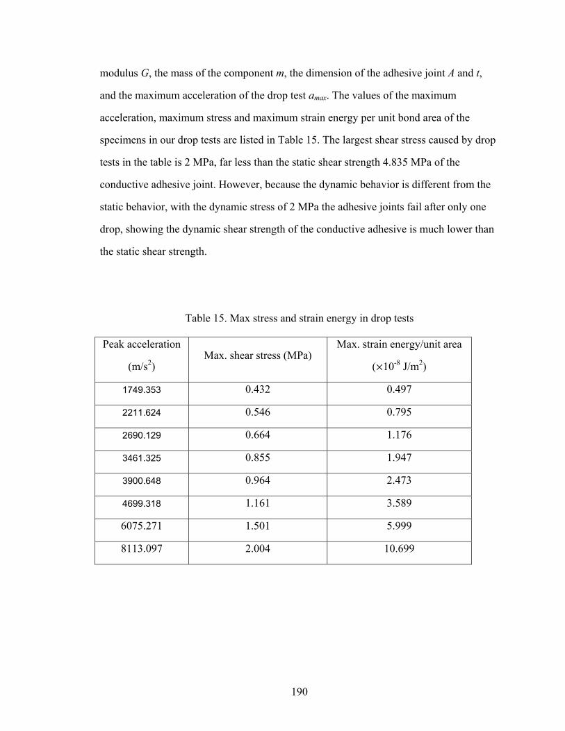
190

modulus G, the mass of the component m, the dimension of the adhesive joint A and t,

and the maximum acceleration of the drop test amax. The values of the maximum

acceleration, maximum stress and maximum strain energy per unit bond area of the

specimens in our drop tests are listed in Table 15. The largest shear stress caused by drop

tests in the table is 2 MPa, far less than the static shear strength 4.835 MPa of the

conductive adhesive joint. However, because the dynamic behavior is different from the

static behavior, with the dynamic stress of 2 MPa the adhesive joints fail after only one

drop, showing the dynamic shear strength of the conductive adhesive is much lower than

the static shear strength.

Table 15. Max stress and strain energy in drop tests

Peak acceleration

(m/s2) Max. shear stress (MPa)

Max. strain energy/unit area

(μ10-8 J/m2)

1749.353 0.432 0.497

2211.624 0.546 0.795

2690.129 0.664 1.176

3461.325 0.855 1.947

3900.648 0.964 2.473

4699.318 1.161 3.589

6075.271 1.501 5.999

8113.097 2.004 10.699

191

The maximum strain energy per unit bond area U0 can be correlated with the

average number of drops to failure Nf. It is found that the relationship between the two

quantities can be well fitted by a power law of

0 0 ( )fU U N β′= (8.5)

where 0U ′ and β are two constants. The values of the two constants in our drop life

model of the conductive adhesive joints are fitted to be

0

0.755

12.370U

β = −

′ = (8.6)

The drop life data and the fitted power law model are shown in Figure 91 in

logarithmic scale and in Figure 92 in normal scale. Clearly as the maximum strain energy

per unit area increases the drop life of the conductive adhesive is reduced significantly.

When U0 is above 10.7 μ 10-8 J/m2, the conductive adhesive joint will be failed by only

one drop. However, when U0 is 0.5 μ 10-8 J/m2 the drop life is about 60. And the drop life

increases exponentially when U0 is smaller than 0.5 μ 10-8 J/m2. Depending on the impact

reliability requirement for the specific electronic package, the critical maximum strain

energy per unit bond area can be defined. For example the value of 0.5 μ 10-8 J/m2 can be

used as the critical value. Conductive adhesive joints subjected to drops with maximum

strain energy per unit bond area less than this value can be considered safe. The concept

of the critical value of the maximum strain energy per unit bond area is similar to the

“endurance limit” in fatigue tests.

192

0

2

4

6

8

10

12

0 20 40 60 80Nf: # of drops to failure

U0:

max

stra

in e

nger

gy/u

nit

area

(10^

-8 J

/m^2

)experiment datafitted line

Figure 91. Drop life data and fitted drop life model (logarithmic scale)

0

1

10

100

1 10 100Nf: # of drops to failure

U0:

max

stra

in e

nger

gy/u

nit

area

(10^

-8 J

/m^2

) experiment datafitted line

Figure 92. Drop life data and fitted drop life model

193

8.3.4 Failure mechanism of conductive adhesives in drop tests

The failure of the conductive adhesive joints is found to happen suddenly. No

indicator of breakage is observed prior to the failure. For the fatigue test of conductive

adhesive samples, the electrical conduction failure is well ahead of the mechanical

failure. However, in drop tests the resistance of the conductive adhesive joints is stable

until the final drop, which leads to a completely open circuit. Hence the failure of the

conductive adhesive joints is instant, and the electrical conduction failure and mechanical

breakage happen at the same time, which is different from the fatigue failure.

As for the failure location, it is found that the breakage is on the interface between

the conductive adhesive joints and the copper surface of the printed circuit board. The

crack location is shown in Figure 93.

Figure 93. Crack location of conductive adhesive joints after drop tests

194

A microscope picture of a conductive adhesive joint after drop test failure is

shown in Figure 94. It can be seen that the failure face is at the interface between the

adhesive joint and the copper surface of the printed circuit board rather than cohesive

crack in the conductive adhesive layer.

An image of the edge of the conductive adhesive joint with a higher magnification

is shown in Figure 95. It shows that the crack surface is along the interface between the

silver flakes and the epoxy matrix. There is no crack penetrating the silver flakes. Instead,

the crack finds its way along the epoxy-silver interface until it reaches the adhesive-PCB

interface. The edge of the epoxy is sharp, and the crack surface in the epoxy is relatively

smooth, indicating the fracture is brittle and there is little plastic deformation involved.

This is because the fully cured epoxy resin under Tg is a brittle material that has very

limited energy-absorbing mechanisms. With the high strain rate load under impact

conditions, the tendency of the material to fail in a brittle mode is even more increased.

Figure 94. A conductive adhesive joint after drop test failure

drop direction

Conductive adhesive joint

copper resistor

195

Figure 95. The edge of the conductive adhesive joint after drop test failure

The foot of the conductive adhesive joint near the substrate or component is the

location where stress concentration exists. Therefore the micro-crack is first developed in

this area when the conductive adhesive joint is subjected to the high stress induced by the

dynamic loading. The interface between the epoxy and silver flakes is not perfect and

there are many micro-voids or pores at the interface, which means the energy required to

create a new crack surface along the interface is relatively small. Hence the crack travels

along the epoxy-flake interface until it reaches the conductive adhesive – substrate

interface. The crack then propagates along the interface quickly and the resistor falls off.

Since cracks in the conductive adhesive will increase their resistance, the

resistance of the conductive adhesive joint is an indicator of damage in the joints. It is

observed that the resistance of the conductive adhesive is stable until the last drop, hence

silver flake epoxy

196

it can be deduced that the big crack is formed only in the last drop and the propagation

speed is fast. In the previous drops although cracks may have developed, they are small

in size and can be closed after each drop. Hence the resistance shows a stable value until

the last drop, when the big crack opening appears.

The key factor governing the impact resistance of epoxy resin is its ability to

dissipate energy. One way to improve the impact performance of the adhesive joints is to

change the formula of conductive adhesives to improve its energy dissipation ability. In

polymer materials the mechanical energy is often turned into thermal energy, and

different ingredients can generate different energy dissipation abilities. For the epoxy

matrix composed of epoxy and hardener, the use of different hardeners produces changes

on the macromolecular network of the crosslinked epoxy systems and also on the

resulting macroscopic physical properties of epoxy-based materials. Hence the resin

ingredients can be modified to achieve a higher thermal diffusivity to diffuse the heat

generated under impact [126]. Some other researchers [105] designed conductive

adhesive materials with low Young’s modulus and high loss factor (tan δ) to improve the

ability to dissipate mechanical impact energy into thermal energy.

Since the crack propagates along the epoxy-silver and the adhesive-substrate

interface, another way to improve the impact performance is to increase the adhesion at

these interfaces. It should be noted that the interfacial adhesion is deteriorated badly

when moisture exists under static loading [124]. With dynamic loading such as in drop

tests, the adhesive-substrate adhesion can be even worse with the existence of moisture.

The geometry of the interconnection joints should be designed to avoid severe

stress concentration. Because the brittleness of the epoxy matrix suppresses plastic

yielding, the stress concentration is even more severe than when ductile material is used.

Higher stress concentration induces failure faster, therefore the geometry of the

conductive adhesive joints needs to be properly designed.

197

8.4 Conclusions

In this chapter the drop tests are conducted on a test vehicle, which consists of

copper resistor and printed circuit board that are bonded by conductive adhesive joints.

The acceleration curve of the test vehicle is obtained through an impact tester. Drop tests

are performed on the test vehicle with different peak accelerations and the number of

drops to failure is recorded. It is found that the electrical conduction and the mechanical

adhesion fail abruptly in the last drop. The shear modulus of the conductive adhesive

joint is measured by a lap shear specimen, so that for each drop test the maximum strain

energy per unit bond area induced by drop tests can be calculated. The relationship

between the number of drops to failure and the maximum strain energy per unit bond area

can be fitted by a power law model. The drop test is an effective approach to study the

impact performance of the conductive adhesive material.

By microscopy examination, the crack is found to develop from the foot of the

conductive adhesive joint, and then propagates to and along the adhesive-substrate

interface. The fracture is found to be a brittle type.

The improvement of the impact resistance of conductive adhesives can be made in

two ways. Since the crack propagates along the adhesive-substrate interface, one way to

improve the impact resistance is to increase the interfacial adhesion between the

conductive adhesive and substrates. Another way to improve the impact resistance is to

modify the properties of the conductive adhesive by changing the formulations so that the

mechanical energy can be more easily transferred to thermal energy by the epoxy.

The drop life model of the conductive adhesive joints is correlated with the

maximum strain energy induced by the drop impact using a power law equation.

However, the property of the conductive adhesive is not included in the model. To

incorporate the effect of material property such as damping into the drop life model, more

drop tests with different conductive adhesives are needed to be performed.

198

The drop test of the conductive adhesive joints at the component level is

conducted. To study the impact performance of conductive adhesive joints in real

packages, board level and product level drop tests needs to be performed. In the board

level test not only the inertia force but also the PCB bending acts as the major driver

causing drop failure. The combination of impact test and moisture effect is another topic

that deserves further investigation.

199

CHAPTER 9

CONCLUSIONS

9.1 Summary and conclusions

The motivation of this research lies in the many advantages of electrically

conductive adhesives over the traditional PbSn solders, including: (1) environmental

friendliness; (2) lower temperature processing; (3) finer pitch capability; (4) fewer

processing steps; (5) capability of bonding on on-solderable substrates. However, there

are several obstacles that need to be overcome in order for conductive adhesives to

replace solders. The main concern is the reliability of conductive adhesives under harsh

environmental conditions. It is with this background that this research is carried out.

The electrical conduction of conductive adhesives is achieved by the contacts

between silver particles. A tailor-made device is used to measure the contact resistance

between silver rods under different contact loads, and the tunnel resistivity – contact

pressure relationship is obtained. The tunnel resistivities of different coating materials are

measured and compared to find the coating material that gives the smallest contact

resistance. The contact resistance between silver particles can be calculated based on the

experimental results of tunnel resistivity. The measurement of the contact resistance and

tunnel resistivity provides the basis for calculating the resistivity of the conductive

adhesives from the computer-simulated microstructure model.

The computer-simulated microstructure models are proposed for modeling the

electrical conduction of conductive adhesives. It is found that the buildup of electrical

conduction of conductive adhesives in the cure process depends on the volume shrinkage

of epoxy resin, the modulus increase of epoxy resin, and the decrease of contact

resistance between filler particles. The resistivity of conductive adhesives is calculated

200

from the microstructure model and is found to agree well with the experimental

measurement, which means that the model is effective in simulating the conduction

mechanism of conductive adhesives.

Based on the computer-simulated microstructure model, the effect of geometric

parameters of filler particles on the electrical conductivity of conductive adhesives is

studied. The conduction of conductive adhesives depends on the shape, size, and size

distribution of the conductive fillers. By varying these geometric parameters and

calculating the bulk resistivity, the effects of the filler geometry and how the parameters

affect the electrical conduction of conductive adhesives can be identified. The method of

full factorial experimental design is used and the significant geometric parameters are

found out. The electrical conductivity of conductive adhesives can be accordingly

optimized.

The modeling approach not only provides an in-depth understanding of the

conduction mechanism in conductive adhesives, but also presents an effective way for

conductive adhesive manufacturers to design products with improved electrical

conductivity. The conductivity of the conductive adhesive can be optimized without real

experiments, and the effects of particle and epoxy parameters can be easily discovered by

computer simulations.

The reliability performance of conductive adhesives is evaluated by testing

conductive adhesive samples under fatigue loading, moisture conditioning, and drop

impacts. Fatigue tests show that the conductive adhesive fails electrically well before

mechanical failure occurs under cyclic loading. The strain amplitude, strain ratio, and

strain rate all have significant effects affecting the fatigue life of conductive adhesives.

The fatigue life is found to be fitted well by the power law model. By examination of the

cross section of the conductive adhesive samples, it is found that the electrical conduction

is deteriorated by the impaired epoxy-silver interfacial adhesion.

201

The moisture uptake is measured on conductive adhesive samples. Although the

conductive adhesives reach saturation after moisture conditioning, it is found that the

bulk resistivity does not change significantly by moisture uptake. Resistance

measurement after moisture recovery also shows stable bulk resistivity of conductive

adhesives. The stable bulk resistivity is because the contact interfaces between silver

flakes are not attacked by moisture diffusion. However, the fatigue test of conductive

adhesives after moisture conditioning and moisture recovery shows significantly

decreased electrical fatigue life. The reason is that the absorbed moisture reduces the

Young’s modulus of the epoxy matrix and degrades the fracture toughness of the epoxy-

silver interface, which accelerated the debonding of the silver flakes from the epoxy

resin. Still electrical conduction failure occurs much earlier than mechanical failure.

The drop impact test is found to be a good way to characterize the impact

resistance of conductive adhesive joints. A custom-made simple test vehicle is used in

drop tests. It is found that the mechanical failure and electrical failure of the conductive

adhesive joints occur at the same time. The crack originates at the foot of the conductive

adhesive joint, and propagates to the adhesive-substrate interface. The drop life can be

well correlated with the strain energy caused by the drop tests. A drop failure life model

is proposed using a power law model.

In all the reliability tests the electrical conduction failure happens before or

together with the mechanical failure. Therefore the electrical failure rather than the

mechanical failure should be considered for conductive adhesives, which is a different

failure behavior from solders. The interface property is critical in maintaining the

electrical conduction. In fatigue tests the failure is due to the weakened epoxy-silver

interfacial adhesion, in impact tests the failure is due to the brakeage of the conductive

adhesive joints is at the adhesive-component/substrate interface. Therefore the interfacial

adhesion has to be improved between the epoxy and silver flakes and between the epoxy

202

and components/substrates in order to get an improved reliability in fatigue and drop

tests.

9.2 Contributions of this research

This research has its contributions in two aspects: the understanding and modeling

of conduction mechanism in conductive adhesives; and the reliability evaluation and

failure mechanism investigation of conductive adhesives subjected to fatigue loading,

moisture conditioning and drop impacts.

The modeling of conduction mechanism in conductive adhesives consists of three

parts of work: the measurement of tunnel resistivity of silver contacts, the modeling of

conducting network in conductive adhesives, and the study of filler geometry effect on

the conduction of conductive adhesives.

Although it has long been known that the conduction of conductive adhesives is

achieved by the interconnections of the filler particles, no study has been proposed on

how to calculate the contact resistance between filler particles. This is partially due to the

fact that the tunnel resistivity of the tunnel film on the contact surface is not known. In

Chapter 3 the tunnel resistivity of silver contacts is measured by experiments. The contact

resistance between silver particles in conductive adhesives can then be calculated based

on the measured data. Different coating materials are also applied to study their effects on

the contact resistance and tunnel resistivity of silver contacts. To summarize, the key

contributions from Chapter 3 are

• Measured the tunnel resistivity of silver contacts with different coating materials

• Identified the effect of coating material on contact resistance and tunnel resistivity

• Obtained the tunnel resistivity – contact pressure relationship

Chapter 4 proposes an innovative approach to model the conducting network of

conductive particles based on the 3-D microstructure model of conductive adhesives.

This modeling approach considers factors such as the filler particle geometry, particle

203

location, interconnection of particles and contact resistance between particles. By this

modeling approach, the resistivity change of conductive adhesives in the cure process is

calculated and found to have good agreement with experimental data. The key

contributions of Chapter 4 are

• Proposed an effective new approach to calculate the conductivity/resistivity of

conductive adhesives based on the microstructure of filler particles

• Provided good understanding on the formation of electrical conduction of

conductive adhesives in the cure process

People have been trying to obtain good conduction of conductive adhesives by

changing the geometry of conductive fillers using the try-and-error method. In Chapter 5,

a method of factorial experimental design is adopted to study the effect of filler geometry

on the conduction of conductive adhesives based on the conducting network modeling

approach. Geometric parameters of spherical and flake particles that have significant

effects on the conductivity of conductive adhesives are identified, and optimization of the

filler geometry can be made to minimize the resistivity of conductive adhesives. Great

time and effort can be saved by using the experimental design and modeling approach

compared with the try-and-error method. The key contributions of Chapter 5 are

• Identified the effect of geometric parameters of filler particles on the conduction

of conductive adhesives by the method of factorial design

• Developed an approach to optimize filler geometry in conductive adhesives

• Provided a useful design tool for conductive adhesive manufacturers

The reliability evaluation of conductive adhesives is performed under three

conditions: fatigue loading, moisture conditioning and drop impact.

Most previous studies of conductive adhesive in fatigue tests are focused on the

mechanical adhesion. In our fatigue tests in Chapter 6, both mechanical and electrical

failure criterion are considered. It is found that the resistance of conductive adhesive

samples deteriorates rapidly as more fatigue cycles are performed, and electrical failure

204

may happen much earlier than mechanical failure. Therefore the electrical conduction

failure criterion should be considered instead of the mechanical adhesion failure.

Electrical fatigue life models are proposed based on the test data. The key contributions

of Chapter 6 are

• Discovered the electrical conduction behavior of conductive adhesives in fatigue

tests

• Discovered electrical conduction failure may occur much earlier than mechanical

failure for conductive adhesives

• Established electrical fatigue failure criterion of conductive adhesives

• Proposed new fatigue models of conductive adhesives based on the electrical

conduction failure

• Identified the electrical failure mechanism of conductive adhesives in fatigue tests

The previous study of moisture effect on conductive adhesives has been focused

on the interfacial property between the conductive adhesive and substrates/components.

In Chapter 7, the bulk property of conductive adhesive under moisture conditioning is

investigated. The resistance of conductive adhesives is measured after both moisture

conditioning and moisture recovery. Fatigue tests are also performed on conductive

adhesives after moisture conditioning. The key contributions of Chapter 7 are

• Measured the moisture uptake behavior of conductive adhesives in the moisture

conditioning process

• Identified the effect of moisture on bulk resistance of conductive adhesives

• Identified the effect of moisture on conductive adhesives under fatigue loading

• Discovered the failure mechanism of conductive adhesives under fatigue loading

when moisture is present

In present drop test standards, the test vehicle is tested under certain levels of

peak acceleration or simply certain levels of height. However, only peak accelerations or

205

drop heights are not enough to describe the severity of drop tests. In Chapter 8, a test

vehicle is designed to test conductive adhesive joints under drop tests and the strain

energy is calculated to characterize the severity of drop tests. The drop life models are

proposed for the life prediction of conductive adhesives based on the test result. The key

contributions of Chapter 8 are

• Related the severity of drop tests with strain energy

• Proposed drop life models which related the number of drops to failure with the

strain energy caused by drop impact

• Identified the failure mechanism of conductive adhesive joints under drop impact

9.3 Future work

The conductive adhesive samples used in the experiments are made by the author.

Although the conduction mechanism and failure mechanism discovered in the conductive

adhesives in this study have a certain generality, care should still be taken when

extrapolating the results to conductive adhesives with different formulations, especially

when the conductive adhesives have epoxy and filler particles with much different

properties. However, the modeling and testing approach used in this study is still

effective to study the conduction mechanism and failure mechanism for other conductive

adhesives.

Only mechanical fatigue tests are performed in this research. In real electronic

applications the loading is often due to thermal expansion, and thermomechanical fatigue

loadings rather than mechanical fatigue is the main fatigue failure driver. The property of

the epoxy matrix could change significantly due to temperature change. Hence it would

be necessary to study the fatigue behavior of conductive adhesives under the combined

effect of temperature and fatigue loading.

Only a simple shape of the conductive adhesive samples is considered in our

study, but the conductive adhesives in electronic packaging usually take more complex

206

forms such as posts or filler joints. Depending on the joint geometry, the strain and stress

in the joints could be very different from the simple uniaxial loading in our tests. For

example, stress concentration is raised significantly with an improper geometric design.

With the stress concentration, the mechanical failure may happen before the electrical

conduction failure. The stress and strain distribution in the conductive adhesive joints

could be complex, therefore the local critical point needs to be found out in order to use

the fatigue life model developed in our tests.

Copper finish is used in the drop impact tests. Since the adhesion of the adhesive-

component/substrate interface is critical in determining the impact resistance of

conductive adhesive joints, more tests should be conducted with different surface

finishes. It would also be helpful to understand the characteristic of the dynamic fracture

toughness between the conductive adhesive and different surface finishes of

components/substrates.

Only component level drop tests are conducted in this research. To determine the

reliability of conductive adhesive joints in electronic packages, board- and product-level

drop tests are needed. Other than the inertia force exerted on the conductive adhesive

joints in the component-level dropt tests, the bending of PCB and clattering between

adjacent boards could happen in board- and product-level drop tests. Hence more factors

need to be considered to evaluate the reliability of conductive adhesives in real drops of

electronic packages.

Another approach to study the fatigue and impact behavior of conductive

adhesives is to run finite element analysis. Many software packages are available for the

fatigue and dynamic impact simulation. The correlation of the finite element results and

the experimental results will help us to better understand the failure mechanism of

conductive adhesives under fatigue and drop tests, and provide a way to improve its

performance.

207

Finally, the performance of conductive adhesives under vibration tests has not

been addressed in this research. Though the loading caused by vibrations is also dynamic

like in drop tests, the failure of conductive adhesives due to vibrations is different than

that due to drop impacts, which deserves a separate topic of study.

208

REFERENCES

1. Zwolinski, M., et al., Electrically conductive adhesives for surface mount solder replacement. IEEE Transactions on Components, Packaging, and Manufacturing Technology Part C: Manufacturing, 1996. 19(4): p. 241-250.

2. Jagt, J.C., P.J.M. Beris, and G.F.C.M. Lijten, Electrically conductive adhesives: a prospective alternative for SMD soldering? IEEE Transactions on Components, Packaging, and Manufacturing Technology Part B: Advanced Packaging, 1995. 18(2): p. 292-298.

3. Liu, J., Conductive Adhesive for Electronics Packaging. 1999, Port Erin, Isle of Man, British Isles: Electrochemical Publications Ltd.

4. Gomatam, R. and E. Sancaktar. Behavior of electronically conductive filled adhesive joints under cyclic loading part 1: Experimental approach. in International Symposium and Exhibition on Advanced Packaging Materials Processes, Properties and Interfaces, Mar 11-14 2001. 2001. Braselton, GA.

5. Gomatam, R.R. and E. Sancaktar. Fatigue behavior of electronically conductive adhesive joints. in 2003 ASME International Mechanical Engineering Congress, Nov 15-21 2003. 2003. Washington, DC, United States: American Society of Mechanical Engineers.

6. Gomatam, R.R. and E. Sancaktar. Modeling Fatigue Behavior of Electronically Conductive Filled Adhesive Joints Under Cyclic Loading - A Novel Modeling Approach for Integrated Joint Life Prediction. in 2003 International Symposium on Microelectronics, Nov 18-20 2003. 2003. Boston, MA, United States: The International Society for Optical Engineering.

7. Lu, D., Q.K. Tong, and C.P. Wong, Mechanisms underlying the unstable contact resistance of conductive adhesives. IEEE Transactions on Electronics Packaging Manufacturing, 1999. 22(3): p. 228-232.

8. Lu, D. and C.P. Wong, High performance conductive adhesives. IEEE Transactions on Electronics Packaging Manufacturing, 1999. 22(4): p. 324-330.

209

9. Moon, K.-S., et al., Stabilizing contact resistance of isotropically conductive adhesives on various metal surfaces by incorporating sacrificial anode materials. Journal of Electronic Materials, 2004. 33(11): p. 1381-1388.

10. Tummala, R.R., Fundamentals of Microsystems Packaging. 2001, New York: McGraw-Hill.

11. Liu, J., Overview of advances in conductive adhesive joining technology for electronics applications. Materials Technology, 1995. 10(11-12): p. 247-252.

12. Liu, J.L., Z. Kristiansen, H. Khoo, C. Overview of conductive adhesive joining technology in electronics packaging applications. in Proceedings of the 3rd International Conference on Adhesive Joining and Coating Technology in Electronics Manufacturing. 1998.

13. Gaynes, M.A., et al., Evaluation of contact resistance for isotropic electrically conductive adhesives. IEEE Transactions on Components, Packaging, and Manufacturing Technology Part B: Advanced Packaging, 1995. 18(2): p. 299-304.

14. Keusseyan, R.L., J.L. Dilday, and B.S. Speck, Electric contact phenomena in conductive adhesive interconnections. International Journal of Microcircuits and Electronic Packaging, 1994. 17(3): p. 236-242.

15. Perichaud, M.G., et al. Industrial use of conductive adhesives for SMT assemblies. in Microelectronic Manufacturing Yield, Reliability, and Failure Analysis IV, Sep 23-24 1998. 1998. Santa Clara, CA, United States: The International Society for Optical Engineering.

16. Nguyen, G.P., et al. Electrical reliability of conductive adhesive for surface-mount applications. in Proceedings of the 1993 International Symposium on Microelectronics, Nov 9-11 1993. 1993. Dallas, TX, USA: Int Soc for Hybrid Microelectronics.

17. Connell, G., R.L.D. Zenner, and J.A. Gerber. Conductive adhesive flip-chip bonding for bumped and unbumped die. in Proceedings of the 1997 47th IEEE Electronic Components & Technology Conference, May 18-21 1997. 1997. San Jose, CA, USA: IEEE, Piscataway, NJ, USA.

18. Keister, F.Z., Evaluation of conductive adhesives for microelectronic applications. Electro-Technology, 1962. 69(1): p. 47-52.

210

19. Hvims, H.L., Conductive adhesives for SMT and potential applications. IEEE Transactions on Components, Packaging, and Manufacturing Technology Part B: Advanced Packaging, 1995. 18(2): p. 284-291.

20. Gilleo, K. Flip chip assembly with conductive adhesives. in 2000 HD International Conference on High-Density Interconnect and Systems Packaging, Apr 25-28 2000. 2002. Denver, CO, United States: The International Society for Optical Engineering.

21. Shirai, Y., M. Komagata, and K. Suzuki. Non-migration conductive adhesives. in First International IEEE Conference on Polymers and Adhesives in Microelectronics and Photonics: Incorporating POLY,PEP and Adhesives in Electronics (POLYTRONIC 2001), Oct 21-24 2001. 2001. Potsdam, Germany: Institute of Electrical and Electronics Engineers Inc.

22. Botter, H., R.B. Van Der Plas, and A. Arunjunai, Factors that influence the electrical contact resistance of isotropic conductive adhesive joints during climate chamber testing. International Journal of Microelectronic Packaging Materials and Technologies, 1998. 1(3): p. 177-185.

23. Nguyen, G., et al. Electrical reliability of conductive adhesive for surface mount applications. in Proceedings of the 1993 International Electronics Packaging Conference, Sep 12-15 1993. 1993. San Diego, CA, USA: Publ by IEPS, Wheaton, IL, USA.

24. Dreezen, G. and G. Luyckx, Lead free assembly : Conductive adhesives offer a real alternative. Global SMT and Packaging, 2003. 3(7): p. 15-18.

25. Kim, H.K. and F.G. Shi, Electrical reliability of electrically conductive adhesive joints: Dependence on curing condition and current density. Microelectronics Journal, 2001. 32(4): p. 315-321.

26. Kim, H.K., et al. Electrical reliability of conductive adhesive joints: Curing condition and current density dependence. in Process Control and Diagnostics, Sep 18-Sep 19 2000. 2000. Santa Clara, CA, USA: Society of Photo-Optical Instrumentation Engineers, Bellingham, WA, USA.

27. Small, D.J. Reliability considerations of electrically conductive adhesives. in NEPCON WEST '99, Feb 21-Feb 25 1999. 1999. Anaheim, CA, USA: Reed Exhibition Companies, Norwalk, CT, USA.

211

28. Cavasin, D., K. Brice-Heames, and A. Arab. Improvements in the reliability and manufacturability of an integrated RF power amplifier module system-in-package, via implementation of conductive epoxy adhesive for selected SMT components. in 53rd Electronic Components and Technology Conference 2003, May 27-30 2003. 2003. New Orleans LA, United States: Institute of Electrical and Electronics Engineers Inc.

29. Kristiansen, H. and J. Liu, Overview of conductive adhesive interconnection technologies for LCD's. IEEE Transactions on Components, Packaging, and Manufacturing Technology Part A, 1998. 21(2): p. 208-214.

30. Sea, T.Y., T.C. Tan, and E.K. Peh. Reflowable Anisotropic Conductive adhesives for flipchip packaging. in Proceedings of the 1997 1st Electronic Packaging Technology Conference, EPTC, Oct 8-10 1997. 1997. Singapore, Singapore: IEEE, Piscataway, NJ, USA.

31. Zenner, R.L.D., G. Connell, and J.A. Gerber. Adhesive and conductive adhesive flip chip bonding. in 1997 3rd International Symposium and Exhibition on Advanced Packaging Materilas Processes, Properties and Interfaces, Mar 9-12 1997. 1997. Braselton, GA, USA: IEEE, Piscataway, NJ, USA.

32. Perichaud, M.G., et al., Reliability evaluation of adhesive bonded SMT components in industrial applications. Microelectronics and Reliability, 2000. 40(7): p. 1227-1234.

33. Bolger, J.C. and J.M. Czarnowski, Area bonding conductive epoxy adhesives for low-cost grid array chip carriers. IEEE Transactions on Components, Packaging, and Manufacturing Technology Part C: Manufacturing, 1996. 19(3): p. 184-188.

34. Bolger, J.C., M. Reynolds, and J. Popielarczyk. Area bonding conductive (ABC) adhesives for flex circuit connection to LTCC/MCM substrates. in Proceedings of the 1995 45th Electronic Components & Technology Conference, May 21-24 1995. 1995. Las Vegas, NV, USA: IEEE, Piscataway, NJ, USA.

35. Czarnowski, J.M., et al. Evaluation of area bonding conductive adhesives for flip chip attach of area bonded die. in Proceedings of the 1996 IEEE/CPMT 19th International Electronics Manufacturing Technology Symposium, Oct 14-16 1996. 1996. Austin, TX, USA: IEEE, Piscataway, NJ, USA.

36. Ku, S.H., R.L. Rudman, and C.T. Murray. Development of anisotropic conductive adhesives for electronic interconnect applications. in 8th International Symposium

212

on Integrated Circuits, Devices and Systems, ISIC 99, Sep 8-10 1999. 1999. Singapore, Singapore: Nanyang Technological University.

37. Shiraishi, T., et al. A study of new compression type flip-chip bonding technique using conductive adhesive. in 2000 HD International Conference on High-Density Interconnect and Systems Packaging, Apr 25-28 2000. 2002. Denver, CO, United States: The International Society for Optical Engineering.

38. Lu, D., Q.K. Tong, and C.P. Wong, Study of lubricants on silver flakes for microelectronics conductive adhesives. IEEE Transactions on Components and Packaging Technologies, 1999. 22(3): p. 365-371.

39. Kolyer, J.M. Environmentally resistant, conductive adhesive bonds for radio frequency (RF) shielding. in Proceedings of the 1998 43rd International SAMPE Symposium and Exhibition. Part 1 (of 2), May 31-Jun 4 1998. 1998. Anaheim, CA, USA: SAMPE, Covina, CA, USA.

40. Shimada, Y., D. Lu, and C.P. Wong. Electrical characterizations and considerations of electrically conductive adhesives (ECAs). in International Symposium and Exibition on Materials Processes, Properties and Interfaces, Mar 6-Mar 8 2000. 2000. Braselton, USA: IEEE, Piscataway, NJ, USA.

41. Holloway, M., M. Konarski, and M. Ward. Accelerated aging of electrically conductive adhesives. in Proceedings of the NEPCON WEST'96. Part 2 (of 3), Feb 27-29 1996. 1996. Anaheim, CA, USA: Reed Exhibition Companies, Norwalk, CT, USA.

42. Kang, S.K. and S. Purushothaman, Development of conducting adhesive materials for microelectronic applications. Journal of Electronic Materials, 1999. 28(11): p. 1314-1318.

43. Kang, S.K., et al., Development of conductive adhesive materials for via fill applications. IEEE Transactions on Components and Packaging Technologies, 2001. 24(3): p. 431-435.

44. Gallagher, C., G. Matijasevic, and J.F. Maguire. Transient liquid phase sintering conductive adhesives as solder replacements. in Proceedings of the 1997 47th IEEE Electronic Components & Technology Conference, May 18-21 1997. 1997. San Jose, CA, USA: IEEE, Piscataway, NJ, USA.

213

45. Li, J., J.K. Lumpp, and E. Grulke. Carbon Nanotube Filled Conductive Adhesives. in 2003 International Symposium on Microelectronics, Nov 18-20 2003. 2003. Boston, MA, United States: The International Society for Optical Engineering.

46. Zhang, J.G., X.Y. Lin, and K. Sugimura. Characteristics & electric contact behavior of tarnished film covered on silver plated surface formed by indoor air exposure. in Proceedings of the 1996 42nd IEEE Holm Conference on Electrical Contacts Joint with the 18th International Conference on Electrical Contacts, Sep 16-20 1996. 1996. Chicago, IL, USA.

47. Aukland, N.R., et al., Contact resistance changes of silver, silver alloys, and gold plated silver coupons exposed to ozone. IEEE Transactions on Components and Packaging Technologies, 2000. 23(2): p. 317-322.

48. Hasegawa, M., T. Yamamoto, and K. Sawa, Significant increase of contact resistance of silver contacts by mechanical switching actions. IEEE Transactions on Components, Hybrids and Manufacturing Technology 37th Holm Conference on Electrical Contacts, Oct 7-9 1991, 1992. 15(2): p. 177-183.

49. Jemaa, N.B., et al., Erosion and contact resistance performance of materials for sliding contacts under arcing. IEEE Transactions on Components and Packaging Technologies, 2001. 24(3): p. 353-357.

50. Chen, Z.-K., H. Mizukoshi, and K. Sawa, Contact resistance characteristics of Ag material in breaking low-load DC arcs. IEEE Transactions on Components, Packaging, and Manufacturing Technology Part A, 1994. 17(1): p. 113-120.

51. Chen, Z.-K. and K. Sawa, Effect of oxide films and arc duration characteristics on Ag contact resistance behavior. IEEE Transactions on Components, Packaging, and Manufacturing Technology Part A, 1995. 18(2): p. 409-416.

52. Sone, H., H. Sugimoto, and T. Takagi. Measurement on contact resistance and surface profile of arcing AG contacts. in Proceedings of the 40th Holm Conference on Electrical Contacts, Oct 17-19 1994. 1994. Chicago, IL, USA: IEEE, Piscataway, NJ, USA.

53. Holm, R., Electric contacts, theory and application. 4th ed. 1967, New York: Springer-Verlag.

214

54. Shante, V.K.S. and S. Kirkpatrick, An introduction to percolation theory. Advances in Physics, 1971. 20(85): p. 325-57.

55. Kirkpatrick, S., Percolation and Conduction. Review of Modern Physics, 1973. 45(4): p. 574-588.

56. Springett, B.E., Conductivity of a system of metallic particles dispersed in an insulating medium. Journal of Applied Physics, 1973. 44(6): p. 2925-2926.

57. Turner, A.M.a.D.T., Influence of particle size on the electrical resistivity of compacted mixtures of polymeric and metallic powders. Journal of Applied Physics, 1971. 42(2): p. 614-618.

58. Li, L. and J.E. Morris, Electrical conduction models for isotropically conductive adhesives. Journal of Electronics Manufacturing, 1995. 5(4): p. 289-296.

59. Li, L., et al. Reliability and failure mechanism of isotropically conductive adhesives joints. in Proceedings of the 1995 45th Electronic Components & Technology Conference, May 21-24 1995. 1995. Las Vegas, NV, USA: IEEE, Piscataway, NJ, USA.

60. Lu, D., Q.K. Tong, and C.P. Wong, Conductivity mechanisms of isotropic conductive adhesives (ICAs). IEEE Transactions on Electronics Packaging Manufacturing, 1999. 22(3): p. 223-7.

61. Lu, D. and C.P. Wong, Effects of shrinkage on conductivity of isotropic conductive adhesives. International Journal of Adhesion and Adhesives, 2000. 20(3): p. 189-193.

62. Klosterman, D., L. Li, and J.E. Morris, Materials characterization, conduction development, and curing effects on reliability of isotropically conductive adhesives. IEEE Transactions on Components, Packaging, and Manufacturing Technology Part A, 1998. 21(1): p. 23-31.

63. Liong, S., C.P. Wong, and W.F. Burgoyne Jr. Adhesion improvement of thermoplastic isotropically conductive adhesive. in 52nd Electronic Components and Technology Conference, May 28-31 2002. 2002. San Diego, CA: Institute of Electrical and Electronics Engineers Inc.

215

64. O'Hara, W., C.-M. Cheng, and S.L. Smith. Cure processing effects of conductive adhesives as solder alternatives: Performance and reliability. in 2003 International Symposium on Microelectronics, Nov 18-20 2003. 2003. Boston, MA, United States: The International Society for Optical Engineering.

65. Rosner, B., J. Liu, and Z. Lai. Flip chip bonding using isotropically conductive adhesives. in 1996 IEEE 46th Electronic Components & Technology Conference, ECTC, May 28-31 1996. 1996. Orlando, FL, USA: IEEE, Piscataway, NJ, USA.

66. Rusanen, O. and J. Lenkkeri, Reliability issues of replacing solder with conductive adhesives in power modules. IEEE Transactions on Components, Packaging, and Manufacturing Technology Part B: Advanced Packaging, 1995. 18(2): p. 320-325.

67. Honore, J.P., H.D. Rubin, and M.K. Zierold. Reliability testing of conductive adhesives. in NEPCON West '92, Feb 23-27 1992. 1992. Anaheim, CA, USA: Publ by Cahner Exposition Group, Des Plaines, IL, USA.

68. Jagt, J.C., Reliability of electrically conductive adhesive joints for surface mount applications: A summary of the state of the art. IEEE Transactions on Components, Packaging, and Manufacturing Technology Part A, 1998. 21(2): p. 215-225.

69. Constable, J.H., et al., Continuous electrical resistance monitoring, pull strength, and fatigue life of isotropically conductive adhesive joints. IEEE Transactions on Components and Packaging Technologies, 1999. 22(2): p. 191-199.

70. Nysaether, J.B., Z. Lai, and J. Liu, Thermal cycling lifetime of flip chip on board circuits with solder bumps and isotropically conductive adhesive joints. IEEE Transactions on Advanced Packaging, 2000. 23(4): p. 743-749.

71. Mo, Z., et al., Thermal fatigue cracking of surface mount conductive adhesive joints. Soldering and Surface Mount Technology, 2004. 16(1): p. 48-52.

72. Dudek, R., et al., Reliability investigations on conductive adhesive joints with emphasis on the mechanics of the conduction mechanism. IEEE Transactions on Components and Packaging Technologies, 2000. 23(3): p. 462-469.

73. Mo, Z., et al., Electrical characterization of isotropic conductive adhesive under mechanical loading. Journal of Electronic Materials, 2002. 31(9): p. 916-920.

216

74. KITAZAKI, Y. and T. HATA, Surface- chemical criteria for the optimum adhesion- 2. 1971. 31(2): p. 193.

75. Sancaktar, E. and P. Zhang. Nonlinear viscoelastic modelling of the fiber-matrix interphase in composite materials. in 8th Biennial Conference on Failure Prevention and Reliability, Sep 17-21 1989. 1989. Montreal, Que, Can: Publ by ASME, New York, NY, USA.

76. Gomatam, R.R. and E. Sancaktar, Dynamic fatigue and failure behavior of silver-filled electronically conductive adhesive joints at ambient environmental conditions. Journal of Adhesion Science and Technology, 2004. 18(7): p. 731-750.

77. Gomatam, R.R. and E. Sancaktar, Fatigue and failure behavior of silver-filled electronically-conductive adhesive joints subjected to elevated temperatures. Journal of Adhesion Science and Technology, 2004. 18(8): p. 849-881.

78. Rafanelli, A.J. A methodology for evaluating the mechanical reliability of alternatives to tin-lead solder electronic interconnection systems (focus on electrically conductive adhesives). in 2001 ASME International Mechanical Engineering Congress and Exposition, Nov 11-16 2001. 2001. New York, NY, United States: American Society of Mechanical Engineers.

79. Keusseyan, R.L. and J.L. Dilday. Electric contact phenomena in conductive adhesive interconnections. in Proceedings of the 1993 International Symposium on Microelectronics, Nov 9-11 1993. 1993. Dallas, TX, USA: Int Soc for Hybrid Microelectronics.

80. Gupta, S., R.M. Hydro, and R.A. Pearson, Fracture behavior of isotropically conductive adhesives. IEEE Transactions on Components and Packaging Technologies, 1999. 22(2): p. 209-214.

81. Fan, L., et al. Electrical and thermal conductivities of polymer composites containing nano-sized particles. 2004. Las Vegas, NV, United States: Institute of Electrical and Electronics Engineers Inc., Piscataway, NJ 08855-1331, United States.

82. Li, H., et al. Reliability enhancement of electrically conductive adhesives in thermal shock environment. in 2004 Proceedings - 54th Electronic Components and Technology Conference, Jun 1-4 2004. 2004. Las Vegas, NV, United States: Institute of Electrical and Electronics Engineers Inc., Piscataway, NJ 08855-1331, United States.

217

83. Li, H., et al. Physical properties and thermocycling performance of electrically conductive adhesives (ECAs) modified by flexible molecules. in 2004 Proceedings - 9th International Symposium and Exhibition on Advanced Packaging Materials: Processes, Properties and Interfaces, Mar 24-26 2004. 2004. Atlanta, GA., United States: Institute of Electrical and Electronics Engineers Inc.

84. Shimada, Y., D. Lu, and C.P. Wong, Electrical characterizations of isotropic conductive adhesives (ICAs). Journal of Electronics Manufacturing, 2000. 10(2): p. 97-103.

85. Lu, D. and C.P. Wong, Isotropic conductive adhesives filled with low-melting-point alloy fillers. IEEE Transactions on Electronics Packaging Manufacturing, 2000. 23(3): p. 185-190.

86. Khoo, C.G.L. and J. Liu, Moisture sorption in some popular conductive adhesives. Circuit World, 1996. 22(4): p. 9-15.

87. Swanson, D.W. Qualification of high-purity, low-outgassing conductive adhesives for hybrid microcircuit assembly. in 3rd International SAMPE Electronics Conference: Electronic Materials and Processes, Jun 20-22 1989. 1989. Los Angeles, CA, USA: Publ by SAMPE, Covina, CA, USA.

88. Xu, S. and D.A. Dillard, Environmental aging effects on thermal and mechanical properties of electrically conductive adhesives. Journal of Adhesion, 2003. 79(7): p. 699-723.

89. Xu, S., D.A. Dillard, and J.G. Dillard, Environmental aging effects on the durability of electrically conductive adhesive joints. International Journal of Adhesion and Adhesives, 2003. 23(3): p. 235-280.

90. Liong, S. and C.P. Wong. An alternative to epoxy resin for application in isotropically conductive adhesive. in International Symposium and Exhibition on Advanced Packaging Materials Processes, Properties and Interfaces, Mar 11-14 2001. 2001. Braselton, GA.

91. Liong, S. and C.P. Wong. Development of thermoplastic isotropically conductive adhesive. in 51st Electronic Components and Technology Conference, May 29-Jun 1 2001. 2001. Orlando, FL: Institute of Electrical and Electronics Engineers Inc.

218

92. Kraus, H.S., PECULIAR BEHAVIOR OF ELECTRICALLY CONDUCTIVE ADHESIVES OF ALUMINUM SURFACES. SPE, Ont Sect, Reg Tech Conf, Plast Coat in Electr Appl, Mar 8-9 1976, 1976: p. 1-11.

93. Light, D.N., et al., Aluminum thick-metal-backed circuits: conductive adhesive technology. Proceedings of the 1996 IEEE 46th Electronic Components & Technology Conference, ECTC, May 28-31 1996, 1996: p. 588-598.

94. De Vries, J., Janssen, Esther, Humidity and Reflow Resistance of Flip Chip on Foil Assemblies With Conductive Adhesive Joints. IEEE Transactions on Components and Packaging Technologies, 2003. 26(3): p. 563-568.

95. Lu, D. and C.P. Wong, Study of contact resistance of conductive adhesives based on anhydride-cured epoxy systems. IEEE Transactions on Components and Packaging Technologies, 2000. 23(3): p. 440-446.

96. Lu, D., D. Wong, and C.P. Wong, Properties of conductive adhesives based on different curing agents. Journal of Electronics Manufacturing, 1999. 9(4): p. 241-248.

97. Lu, D., D. Wong, and C.P. Wong. Effects of curing agents on the properties of conductive adhesives. in International Symposium and Exibition on Materials Processes, Properties and Interfaces, Mar 6-Mar 8 2000. 2000. Braselton, USA: IEEE, Piscataway, NJ, USA.

98. Lu, D. and C.P. Wong, Development of conductive adhesives for solder replacement. IEEE Transactions on Components and Packaging Technologies, 2000. 23(4): p. 620-626.

99. Li, H., K.-S. Moon, and C.P. Wong. Effect of sacrificial anodic fillers on contact resistance stability of electrically conductive adhesives onto lead-free alloy surfaces. in 53rd Electronic Components and Technology Conference 2003, May 27-30 2003. 2003. New Orleans LA, United States: Institute of Electrical and Electronics Engineers Inc.

100. Matienzo, L.J., F.D. Egitto, and P.E. Logan, The use of silane coupling agents in the design of electrically stable interfaces of 6061 T6 aluminum alloy surfaces and epoxy-based electrically conductive adhesives. Journal of Materials Science, 2003. 38(24): p. 4831-4842.

219

101. Liu, J., L. Ljungkrona, and Z. Lai, Development of conductive adhesive joining for surface-mounting electronics manufacturing. IEEE Transactions on Components, Packaging, and Manufacturing Technology Part B: Advanced Packaging, 1995. 18(2): p. 313-319.

102. Harris, P.G., Conductive adhesives: a critical review of progress to date. Soldering & Surface Mount Technology, 1995(20): p. 4.

103. Rosen, S.L., Fundamental principles of polymeric materials. 2nd Edition ed. 1993, New York: John Wiley & Sons Inc.

104. Vona, S.A., Jr., et al., Surface mount conductive adhesives with superior impact resistance. Proceedings of the International Symposium and Exhibition on Advanced Packaging Materials Processes, Properties and Interfaces, 1998: p. 261-267.

105. Tong, Q.K., et al. Conductive adhesives with stable contact resistance and superior impact performance. in 1999 49th Electronic Components and Technology Conference (ECTC), Jun 1-Jun 4 1999. 1999. San Diego, CA, USA: IEEE, Piscataway, NJ, USA.

106. Lu, D., et al. Development of high performance surface mount conductive adhesives. in 50th Electronic Components and Technology Conference. 2000. Las Vegas, NV, USA: Institute of Electrical and Electronics Engineers Inc., Piscataway, NJ, USA.

107. Xu, S. and D.A. Dillard, Determining the Impact Resistance of Electrically Conductive Adhesives Using a Falling Wedge Test. IEEE Transactions on Components and Packaging Technologies, 2003. 26(3): p. 554-562.

108. Morris, J.E., et al. Reliability studies of an isotropic electrically conductive adhesive. in First International IEEE Conference on Polymers and Adhesives in Microelectronics and Photonics: Incorporating POLY,PEP and Adhesives in Electronics (POLYTRONIC 2001), Oct 21-24 2001. 2001. Potsdam, Germany: Institute of Electrical and Electronics Engineers Inc.

109. Lai, Z. and J. Liu, Anisotropically conductive adhesive flip-chip bonding on rigid and flexible printed circuit substrates. IEEE Transactions on Components, Packaging, and Manufacturing Technology Part B: Advanced Packaging, 1996. 19(3): p. 644-660.

220

110. Rao, Y., D. Lu, and C.P. Wong, A study of impact performance of conductive adhesives. International Journal of Adhesion and Adhesives, 2004. 24(5): p. 449-453.

111. Buch, A., Pure metals properties : a scientific-technical handbook. 1999, Materials Park, Ohio: ASM International.

112. Lu, D., C.P. Wong, and Q.K. Tong, A Fundamental study on silver flakes for conductive adhesives. Proceedings of the International Symposium and Exhibition on Advanced Packaging Materials Processes, Properties and Interfaces, 1998: p. 256-260.

113. Johnson, K.L., Contact Mechanics. 1987, Cambridge, UK: Cambridge University Press.

114. Li, Y., et al. Conductivity improvement of isotropic conductive adhesives with short-chain dicarboxylic acids. in 2004 Proceedings - 54th Electronic Components and Technology Conference, Jun 1-4 2004. 2004. Las Vegas, NV, United States: Institute of Electrical and Electronics Engineers Inc., Piscataway, NJ 08855-1331, United States.

115. Serra, J., Image Analysis and Mathematical Morphology. 1988, London: Academic Press.

116. Louis, P. and A.M. Gokhale, Computer simulation of spatial arrangement and connectivity of particles in three-dimensional microstructure: application to model electrical conductivity of polymer matrix composite. Acta Materialia, 1996. 44(4): p. 1519-1528.

117. Chandler, R. and P. Northrop, random number generation. http://www.homepages.ucl.ac.uk/~ucakarc/work/software/randgen.f, 2003.

118. Dodson, B. and D. Nolan, Reliability Engineering Handbook. 1999: Marcel Dekker Ltd.

119. Cox, D.R., planning Experiments. 1958: Wiley.

120. Montgomery, D.C., Design and Analysis of Experiments. 2nd Edition ed. 1984: Wiley.

221

121. Wu, C.F.J. and M. hamada, Experiments: Planning, Analysis, and Parameter Design Optimization. 2000: Wiley.

122. Ye, L., et al., Effect of Ag particle size on electrical conductivity of isotropically conductive adhesives. IEEE Transactions on Electronics Packaging Manufacturing, 1999. 22(4): p. 299-302.

123. Lu, D., C.P. Wong, and Q.K. Tong, Mechanisms underlying the unstable contact resistance of conductive adhesives. Proceedings of the 1999 49th Electronic Components and Technology Conference (ECTC), Jun 1-Jun 4 1999, 1999: p. 342-346.

124. Ferguson, T., Moisture and interfacial adhesion in microelectronic assemblie, in Mechanical Engineering. 2004, Georgia Institute of Technology: Atlanta.

125. JEDEC, JESD22-B104C. JEDEC Solid State Technology Association, 2004.

126. D'Almeida, J.R.M. and N. Cella, Analysis of the fracture behavior of epoxy resins under impact conditions. Journal of Applied Polymer Science, 2000. 77(11): p. 2486-2492.

electrical, thermomechanical and reliability modeling of ...

Documents

Transcript of electrical, thermomechanical and reliability modeling of ...