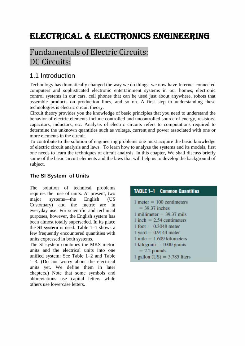
ELECTRICAL & ELECTRONICS ENGINEERING

Fundamentals of Electric Circuits: DC Circuits:

1.1 Introduction

Technology has dramatically changed the way we do things; we now have Internet-connected

computers and sophisticated electronic entertainment systems in our homes, electronic

control systems in our cars, cell phones that can be used just about anywhere, robots that

assemble products on production lines, and so on. A first step to understanding these

technologies is electric circuit theory.

Circuit theory provides you the knowledge of basic principles that you need to understand the

behavior of electric elements include controlled and uncontrolled source of energy, resistors,

capacitors, inductors, etc. Analysis of electric circuits refers to computations required to

determine the unknown quantities such as voltage, current and power associated with one or

more elements in the circuit.

To contribute to the solution of engineering problems one must acquire the basic knowledge

of electric circuit analysis and laws. To learn how to analyze the systems and its models, first

one needs to learn the techniques of circuit analysis. In this chapter, We shall discuss briefly

some of the basic circuit elements and the laws that will help us to develop the background of

subject.

The SI System of Units The solution of technical problems

requires the use of units. At present, two

major systems—the English (US

Customary) and the metric—are in

everyday use. For scientific and technical

purposes, however, the English system has

been almost totally superseded. In its place

the SI system is used. Table 1–1 shows a

few frequently encountered quantities with

units expressed in both systems.

The SI system combines the MKS metric

units and the electrical units into one

unified system: See Table 1–2 and Table

1–3. (Do not worry about the electrical

units yet. We define them in later

chapters.) Note that some symbols and

abbreviations use capital letters while

others use lowercase letters.

Power of Ten Notation Electrical values vary tremendously in size. In electronic systems, for example, voltages may

range from a few millionths of a volt to several thousand volts, while in power systems,

voltages of up to several hundred thousand are common. To handle this large range, the

power of ten notation (Table 1–5) is used—see Note.

To express a number in the power of ten notation, move the decimal point to where you want

it, then multiply the result by the power of ten needed to restore the number to its original

value. Thus, 247000 = 2.47×105 (The number 10 is called the base, and its power is called

the exponent.) An easy way to determine the exponent is to count the number of places (right

or left) that you moved the decimal point. Thus,

Similarly, the number 0.003 69 may be expressed as 3.69 ×10-3 as illustrated below.

Multiplication and Division Using Powers of Ten

To multiply numbers in power of ten notation, multiply their base numbers, then add their

exponents. Thus,

(1.2 × 103)(1.5 × 104) = (1.2)(1.5) × 10(3+4) = 1.8 × 107

For division, subtract the exponents in the denominator from those in the numerator. Thus,

N

OTES... NOTE: The complete range of powers of ten defined in the SI system includes twenty members. However, only those powers of common interest to us in circuit theory are shown in Table 1–5. PROBLEM

Convert the following numbers to power of ten notation, then perform the operation

indicated:

a. 276 × 0.009,

b. 98 200/20. Solution

a. 276 × 0.009 = (2.76 × 102)(9 × 10−3 ) = 24.8 × 10−1 = 2.48

b. 98 200/20 = ( 9.82 × 104) / (2 × 101) = 4.91 × 103

Addition and Subtraction Using Powers of Ten To add or subtract, first adjust all numbers to the same power of ten. It does not matter what

exponent you choose, as long as all are the same.

PROBLEM

Add 3.25 × 102 and 5 × 103

a. using 102 representation,

b. using 103 representation.

Solution

a. 5 × 10 3 = 50 × 102. Thus, 3.25 × 102 + 50 × 102 = 53.25 × 102.

b. 3.25 × 102 = 0.325 × 103. Thus, 0.325 × 103 + 5× 103 = 5.325× 103,

which is the same as 53.25 × 102

Powers Raising a number to a power is a form of multiplication (or division if the exponent

is negative). For example,

(2 × 103)2 =(2 × 103)(2 × 103) = 4 × 106

In general, (N × 10n)m = Nm × 10nm. In this notation, (2 × 103)2 = 22 ×103×2 = 4 × 106 as

before.

Integer fractional powers represent roots. Thus, 4 ½ =√4 = 2 and

271/3 = √273

= 3

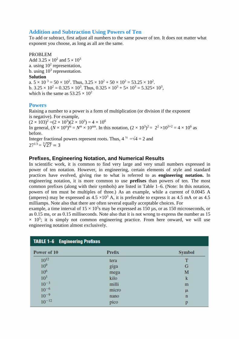
Prefixes, Engineering Notation, and Numerical Results In scientific work, it is common to find very large and very small numbers expressed in

power of ten notation. However, in engineering, certain elements of style and standard

practices have evolved, giving rise to what is referred to as engineering notation. In

engineering notation, it is more common to use prefixes than powers of ten. The most

common prefixes (along with their symbols) are listed in Table 1–6. (Note: In this notation,

powers of ten must be multiples of three.) As an example, while a current of 0.0045 A

(amperes) may be expressed as 4.5 ×103 A, it is preferable to express it as 4.5 mA or as 4.5

milliamps. Note also that there are often several equally acceptable choices. For

example, a time interval of 15 × 105s may be expressed as 150 µs, or as 150 microseconds, or

as 0.15 ms, or as 0.15 milliseconds. Note also that it is not wrong to express the number as 15

× 105; it is simply not common engineering practice. From here onward, we will use

engineering notation almost exclusively.

Circuit Diagrams Electrical and electronic circuits are constructed using components such as batteries,

switches, resistors, capacitors, transistors, and interconnecting wires. To represent these

circuits on paper, diagrams are used. In this book, we use three types: block diagrams,

schematic diagrams, and pictorials.

Block Diagrams

Block diagrams describe a circuit or system in simplified form. The overall problem is

broken into blocks, each representing a portion of the system or circuit. Blocks are labelled to

indicate what they do or what they contain, then interconnected to show their relationship to

each other. General signal flow is usually from left to right and top to bottom. Figure 1–5, for

example, represents an audio amplifier. Although you have not covered any of its circuits yet,

you should be able to follow the general idea quite easily—sound is picked up by the

microphone, converted to an electrical signal, amplified by a pair of amplifiers, then output to

the speaker, where it is converted back to sound. A power supply energizes the system. The

advantage of a block diagram is that it gives you the overall picture and helps you understand

the general nature of a problem. However, it does not provide detail.

FIGURE 1–5 An example block diagram. Pictured is a simplified representation of an audio amplification system.

Pictorial Diagrams

Pictorial diagrams provide detail. They help you visualize circuits and their operation by

showing components as they actually look physically. For example, the circuit of Figure 1–6

consists of a battery, a switch, and an electric lamp, all interconnected by wire. Operation is

easy to visualize—when the switch is closed, the battery causes current in the circuit, which

lights the lamp. The battery is referred to as the source and the lamp as the load.

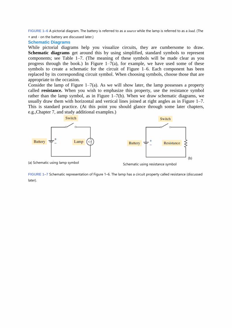
FIGURE 1–6 A pictorial diagram. The battery is referred to as a source while the lamp is referred to as a load. (The

+ and - on the battery are discussed later.)

Schematic Diagrams

While pictorial diagrams help you visualize circuits, they are cumbersome to draw.

Schematic diagrams get around this by using simplified, standard symbols to represent

components; see Table 1–7. (The meaning of these symbols will be made clear as you

progress through the book.) In Figure 1–7(a), for example, we have used some of these

symbols to create a schematic for the circuit of Figure 1–6. Each component has been

replaced by its corresponding circuit symbol. When choosing symbols, choose those that are

appropriate to the occasion.

Consider the lamp of Figure 1–7(a). As we will show later, the lamp possesses a property

called resistance. When you wish to emphasize this property, use the resistance symbol

rather than the lamp symbol, as in Figure 1–7(b). When we draw schematic diagrams, we

usually draw them with horizontal and vertical lines joined at right angles as in Figure 1–7.

This is standard practice. (At this point you should glance through some later chapters,

e.g.,Chapter 7, and study additional examples.)

(a) Schematic using lamp symbol

(b)

Schematic using resistance symbol

FIGURE 1–7 Schematic representation of Figure 1–6. The lamp has a circuit property called resistance (discussed

later).

2.1 VOLTAGE & CURRENT A basic electric circuit consisting of a source of electrical energy, a switch, a load, and

interconnecting wire is shown in Figure 2–1. When the switch is closed, current in the circuit causes the light to come on. This circuit is representative of many common circuits found in practice, including those of flashlights and automobile headlight systems. We will use it to helpdevelop an understanding of voltage and current.

FIGURE 2–1 A basic electric circuit.

Elementary atomic theory shows that the current in Figure 2–1 is actually a flow of charges. The cause of their movement is the “voltage” of the source. While in Figure 2–1 this source is a battery, in practice it may be any one of a number of practical sources, including generators, power supplies, solar cells, and so on. In this chapter we look at the basic ideas of voltage and current. We begin with a discussion of atomic theory. This leads us to free electrons and the idea of current as a movement of charge. The fundamental definitions of voltage and current are then developed. Following this, we look at a number of common voltage sources. The chapter concludes with a discussion of voltmeters and ammeters and the measurement of voltage and current in practice

2.2 Electrical Charge

Electrical charge is an intrinsic property of electrons and protons that manifests itself in the

form of forces—electrons repel other electrons but attract protons, while protons repel each

other but attract electrons. It was through studying these forces that scientists determined that

the charge on the electron is negative while that on the proton is positive.

“charge” can refer to the charge on an individual electron or to the charge associated with a

whole group of electrons.

In either case, this charge is denoted by the letter Q, and its unit of measurement in the SI

system is the coulomb. (The definition of the coulomb is considered in Section 2.2.) In

general, the charge Q associated with a group of electrons is equal to the product of the

number of electrons times the charge on each individual electron. Since charge manifests

itself in the form of forces, charge is defined in terms of these forces. This is discussed next.

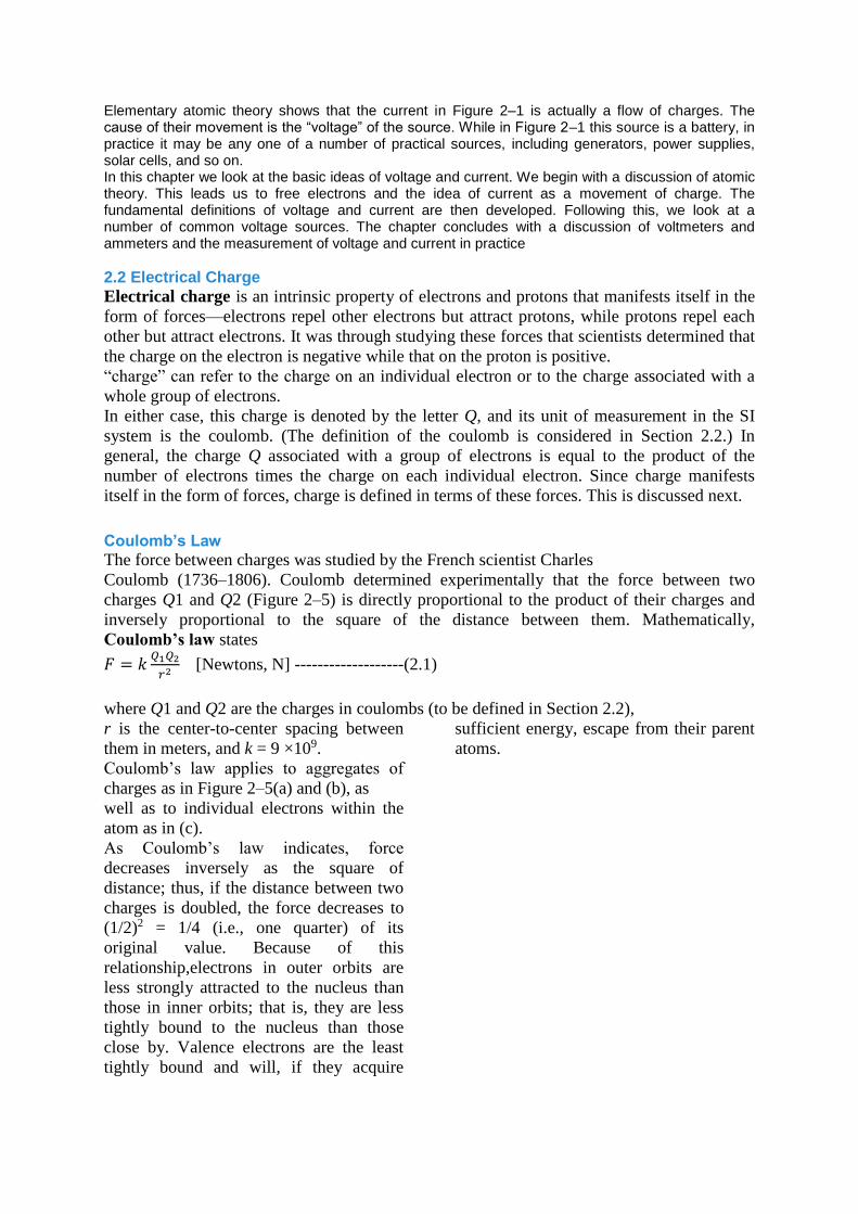
Coulomb’s Law

The force between charges was studied by the French scientist Charles

Coulomb (1736–1806). Coulomb determined experimentally that the force between two

charges Q1 and Q2 (Figure 2–5) is directly proportional to the product of their charges and

inversely proportional to the square of the distance between them. Mathematically,

Coulomb’s law states

𝐹 = 𝑘𝑄1𝑄2

𝑟2 [Newtons, N] -------------------(2.1)

where Q1 and Q2 are the charges in coulombs (to be defined in Section 2.2),

r is the center-to-center spacing between

them in meters, and k = 9 ×109.

Coulomb’s law applies to aggregates of

charges as in Figure 2–5(a) and (b), as

well as to individual electrons within the

atom as in (c).

As Coulomb’s law indicates, force

decreases inversely as the square of

distance; thus, if the distance between two

charges is doubled, the force decreases to

(1/2)2 = 1/4 (i.e., one quarter) of its

original value. Because of this

relationship,electrons in outer orbits are

less strongly attracted to the nucleus than

those in inner orbits; that is, they are less

tightly bound to the nucleus than those

close by. Valence electrons are the least

tightly bound and will, if they acquire

sufficient energy, escape from their parent

atoms.

FIGURE 2–5 Coulomb law forces

2.3 Voltage When charges are detached from one body

and transferred to another, a potential

difference or voltage results between them.

A familiar example is the voltage that

develops when you walk across a carpet.

Voltages in excess of ten thousand volts

can be created in this way. (We will define

the volt rigorously very shortly.) This

voltage is due entirely to the separation of

positive and negative charges, that is,

charges that have been pulled apart.

Figure 2–7 illustrates another example.

During electrical storms, electrons in

thunderclouds are stripped from their

parent atoms by the forces of turbulence

and carried to the bottom of the cloud,

leaving a deficiency of electrons (positive

charge) at the top and an excess (negative

charge) at the bottom. The force of

repulsion then drives electrons away

beneath the cloud, leaving the ground

positively charged. Hundreds of millions

of volts are created in this way. (This

is what causes the air to break down and a

lightning discharge to occur.)

FIGURE 2–7 Voltages created by separation

of charges in a thundercloud. The force

of repulsion drives electrons away beneath

the cloud, creating a voltage between the

cloud and earth as well. If voltage becomes

large enough, the air breaks down and a

lightning discharge occurs.

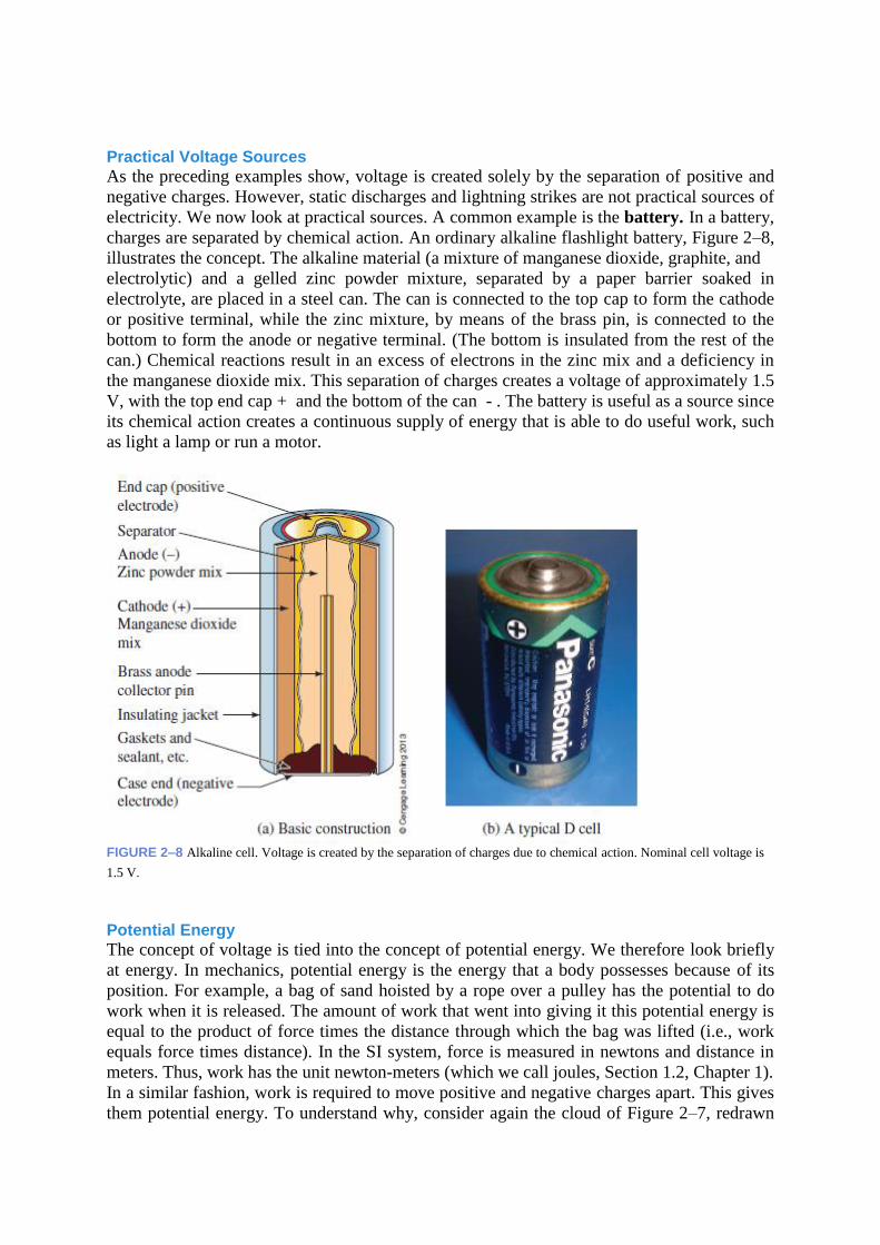
Practical Voltage Sources

As the preceding examples show, voltage is created solely by the separation of positive and

negative charges. However, static discharges and lightning strikes are not practical sources of

electricity. We now look at practical sources. A common example is the battery. In a battery,

charges are separated by chemical action. An ordinary alkaline flashlight battery, Figure 2–8,

illustrates the concept. The alkaline material (a mixture of manganese dioxide, graphite, and

electrolytic) and a gelled zinc powder mixture, separated by a paper barrier soaked in

electrolyte, are placed in a steel can. The can is connected to the top cap to form the cathode

or positive terminal, while the zinc mixture, by means of the brass pin, is connected to the

bottom to form the anode or negative terminal. (The bottom is insulated from the rest of the

can.) Chemical reactions result in an excess of electrons in the zinc mix and a deficiency in

the manganese dioxide mix. This separation of charges creates a voltage of approximately 1.5

V, with the top end cap + and the bottom of the can - . The battery is useful as a source since

its chemical action creates a continuous supply of energy that is able to do useful work, such

as light a lamp or run a motor.

FIGURE 2–8 Alkaline cell. Voltage is created by the separation of charges due to chemical action. Nominal cell voltage is

1.5 V.

Potential Energy

The concept of voltage is tied into the concept of potential energy. We therefore look briefly

at energy. In mechanics, potential energy is the energy that a body possesses because of its

position. For example, a bag of sand hoisted by a rope over a pulley has the potential to do

work when it is released. The amount of work that went into giving it this potential energy is

equal to the product of force times the distance through which the bag was lifted (i.e., work

equals force times distance). In the SI system, force is measured in newtons and distance in

meters. Thus, work has the unit newton-meters (which we call joules, Section 1.2, Chapter 1).

In a similar fashion, work is required to move positive and negative charges apart. This gives

them potential energy. To understand why, consider again the cloud of Figure 2–7, redrawn

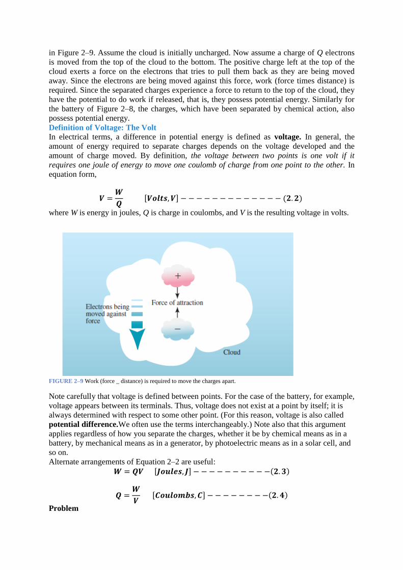
in Figure 2–9. Assume the cloud is initially uncharged. Now assume a charge of Q electrons

is moved from the top of the cloud to the bottom. The positive charge left at the top of the

cloud exerts a force on the electrons that tries to pull them back as they are being moved

away. Since the electrons are being moved against this force, work (force times distance) is

required. Since the separated charges experience a force to return to the top of the cloud, they

have the potential to do work if released, that is, they possess potential energy. Similarly for

the battery of Figure 2–8, the charges, which have been separated by chemical action, also

possess potential energy.

Definition of Voltage: The Volt

In electrical terms, a difference in potential energy is defined as voltage. In general, the

amount of energy required to separate charges depends on the voltage developed and the

amount of charge moved. By definition, the voltage between two points is one volt if it

requires one joule of energy to move one coulomb of charge from one point to the other. In

equation form,

𝑽 =𝑾

𝑸 [𝑽𝒐𝒍𝒕𝒔, 𝑽] − − − − − − − − − − − − − (𝟐. 𝟐)

where W is energy in joules, Q is charge in coulombs, and V is the resulting voltage in volts.

FIGURE 2–9 Work (force _ distance) is required to move the charges apart.

Note carefully that voltage is defined between points. For the case of the battery, for example,

voltage appears between its terminals. Thus, voltage does not exist at a point by itself; it is

always determined with respect to some other point. (For this reason, voltage is also called

potential difference.We often use the terms interchangeably.) Note also that this argument

applies regardless of how you separate the charges, whether it be by chemical means as in a

battery, by mechanical means as in a generator, by photoelectric means as in a solar cell, and

so on.

Alternate arrangements of Equation 2–2 are useful:

𝑾 = 𝑸𝑽 [𝑱𝒐𝒖𝒍𝒆𝒔, 𝑱] − − − − − − − − − −(𝟐. 𝟑)

𝑸 =𝑾

𝑽 [𝑪𝒐𝒖𝒍𝒐𝒎𝒃𝒔, 𝑪] − − − − − − − −(𝟐. 𝟒)

Problem

If it takes 35 J of energy to move a charge of 5 C from one point to another, what is the

voltage between the two points?

Solution

𝑉 = 𝑊

𝑄=

35𝐽

5𝐶= 7𝑉

Practice problems

1. The voltage between two points is 19 V. How much energy is required to move 67 _×1018

electrons from one point to the other?

2. The potential difference between two points is 140 mV. If 280 μJ of work are required to

move a charge Q from one point to the other, what is Q?

Answers

1. 204 J; 2. 2 mC

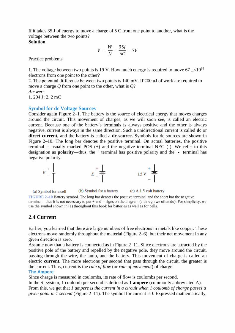
Symbol for dc Voltage Sources Consider again Figure 2–1. The battery is the source of electrical energy that moves charges

around the circuit. This movement of charges, as we will soon see, is called an electric

current. Because one of the battery’s terminals is always positive and the other is always

negative, current is always in the same direction. Such a unidirectional current is called dc or

direct current, and the battery is called a dc source. Symbols for dc sources are shown in

Figure 2–10. The long bar denotes the positive terminal. On actual batteries, the positive

terminal is usually marked POS (+) and the negative terminal NEG (-). We refer to this

designation as polarity—thus, the + terminal has positive polarity and the - terminal has

negative polarity.

FIGURE 2–10 Battery symbol. The long bar denotes the positive terminal and the short bar the negative

terminal—thus it is not necessary to put + and - signs on the diagram (although we often do). For simplicity, we

use the symbol shown in (a) throughout this book for batteries as well as for cells.

2.4 Current

Earlier, you learned that there are large numbers of free electrons in metals like copper. These

electrons move randomly throughout the material (Figure 2–6), but their net movement in any

given direction is zero.

Assume now that a battery is connected as in Figure 2–11. Since electrons are attracted by the

positive pole of the battery and repelled by the negative pole, they move around the circuit,

passing through the wire, the lamp, and the battery. This movement of charge is called an

electric current. The more electrons per second that pass through the circuit, the greater is

the current. Thus, current is the rate of flow (or rate of movement) of charge. The Ampere

Since charge is measured in coulombs, its rate of flow is coulombs per second.

In the SI system, 1 coulomb per second is defined as 1 ampere (commonly abbreviated A).

From this, we get that 1 ampere is the current in a circuit when 1 coulomb of charge passes a

given point in 1 second (Figure 2–11). The symbol for current is I. Expressed mathematically,

𝑰 =𝑸

𝒕 [ 𝒂𝒎𝒑𝒆𝒓𝒆𝒔, 𝑨] − − − − − − − −(𝟐. 𝟓)

where Q is the charge (in coulombs) and t is the time interval (in seconds) over which it is

measured. In Equation 2–5, it is important to note that t does not represent a discrete point in

time but is the interval of time during which the transfer of charge occurs. Alternate forms of

Equation 2–5 are

𝑸 = 𝑰𝒕 [ 𝑪𝒐𝒖𝒍𝒐𝒎𝒃𝒔, 𝑪] − − − − − − − −(𝟐. 𝟔)

And

𝒕 =𝑸

𝑰 [ 𝑺𝒆𝒄𝒐𝒏𝒅𝒔, 𝒔] − − − − − − − − − − − − − (𝟐. 𝟕)

Although Equation 2–5 is the theoretical definition of current, we never actually use it to

measure current. In practice, we use an instrument called an ammeter (Section 2.6). However,

it is an extremely important theoretical relationship that we will soon use to develop other

more practical relationships.

Problem

If 840 coulombs of charge pass through the imaginary plane of Figure 2–11 during a time

interval of 2 minutes, what is the current?

Solution Convert t to seconds. Thus,

𝐼 =𝑄

𝑡=

840𝐶

(2 × 60)𝑠= 7 𝐴

Practice problems

1. Between t =1 ms and t = 14 ms, 8 µC of charge pass through a wire. What is the current?

2. After the switch of Figure 2–1 is closed, current I = 4 A. How much charge passes through

the lamp between the time the switch is closed and the time that it is opened 3 minutes later?

Answers

1. 0.615 mA; 2. 720 C

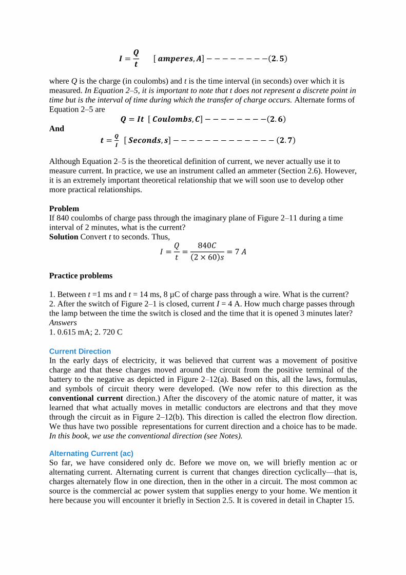
Current Direction

In the early days of electricity, it was believed that current was a movement of positive

charge and that these charges moved around the circuit from the positive terminal of the

battery to the negative as depicted in Figure 2–12(a). Based on this, all the laws, formulas,

and symbols of circuit theory were developed. (We now refer to this direction as the

conventional current direction.) After the discovery of the atomic nature of matter, it was

learned that what actually moves in metallic conductors are electrons and that they move

through the circuit as in Figure 2–12(b). This direction is called the electron flow direction.

We thus have two possible representations for current direction and a choice has to be made.

In this book, we use the conventional direction (see Notes). Alternating Current (ac)

So far, we have considered only dc. Before we move on, we will briefly mention ac or

alternating current. Alternating current is current that changes direction cyclically—that is,

charges alternately flow in one direction, then in the other in a circuit. The most common ac

source is the commercial ac power system that supplies energy to your home. We mention it

here because you will encounter it briefly in Section 2.5. It is covered in detail in Chapter 15.

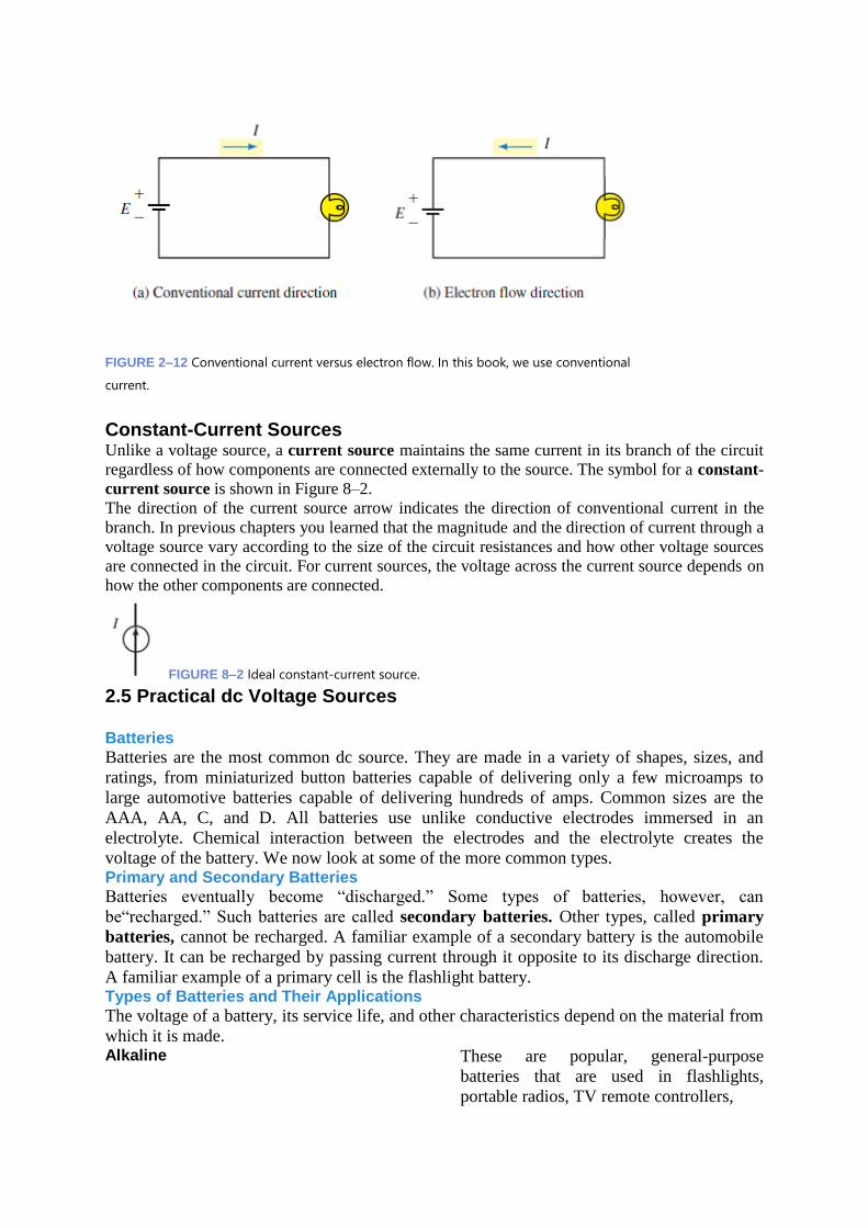
FIGURE 2–12 Conventional current versus electron flow. In this book, we use conventional

current.

Constant-Current Sources Unlike a voltage source, a current source maintains the same current in its branch of the circuit

regardless of how components are connected externally to the source. The symbol for a constant-

current source is shown in Figure 8–2.

The direction of the current source arrow indicates the direction of conventional current in the

branch. In previous chapters you learned that the magnitude and the direction of current through a

voltage source vary according to the size of the circuit resistances and how other voltage sources

are connected in the circuit. For current sources, the voltage across the current source depends on

how the other components are connected.

FIGURE 8–2 Ideal constant-current source.

2.5 Practical dc Voltage Sources Batteries

Batteries are the most common dc source. They are made in a variety of shapes, sizes, and

ratings, from miniaturized button batteries capable of delivering only a few microamps to

large automotive batteries capable of delivering hundreds of amps. Common sizes are the

AAA, AA, C, and D. All batteries use unlike conductive electrodes immersed in an

electrolyte. Chemical interaction between the electrodes and the electrolyte creates the

voltage of the battery. We now look at some of the more common types. Primary and Secondary Batteries

Batteries eventually become “discharged.” Some types of batteries, however, can

be“recharged.” Such batteries are called secondary batteries. Other types, called primary

batteries, cannot be recharged. A familiar example of a secondary battery is the automobile

battery. It can be recharged by passing current through it opposite to its discharge direction.

A familiar example of a primary cell is the flashlight battery. Types of Batteries and Their Applications

The voltage of a battery, its service life, and other characteristics depend on the material from

which it is made. Alkaline These are popular, general-purpose

batteries that are used in flashlights,

portable radios, TV remote controllers,

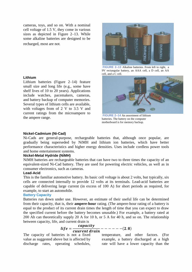
cameras, toys, and so on. With a nominal

cell voltage of 1.5 V, they come in various

sizes as depicted in Figure 2–13. While

some alkaline batteries are designed to be

recharged, most are not.

FIGURE 2–13 Alkaline batteries. From left to right, a

9V rectangular battery, an AAA cell, a D cell, an AA

cell, and a C cell. Lithium

Lithium batteries (Figure 2–14) feature

small size and long life (e.g., some have

shelf lives of 10 to 20 years). Applications

include watches, pacemakers, cameras,

and battery backup of computer memories.

Several types of lithium cells are available,

with voltages from of 2 V to 3.5 V and

current ratings from the microampere to

the ampere range.

FIGURE 2–14 An assortment of lithium

batteries. The battery on the computer

motherboard is for memory backup.

Nickel-Cadmium (Ni-Cad)

Ni-Cads are general-purpose, rechargeable batteries that, although once popular, are

gradually being superseded by NiMH and lithium ion batteries, which have better

performance characteristics and higher energy densities. Uses include cordless power tools

and home entertainment systems. Nickel-Metal Hydride (NiMH)

NiMH batteries are rechargeable batteries that can have two to three times the capacity of an

equivalent-sized Ni-Cad battery. They are used for powering electric vehicles, as well as in

consumer electronics, such as cameras. Lead-Acid

This is the familiar automotive battery. Its basic cell voltage is about 2 volts, but typically, six

cells are connected internally to provide 12 volts at its terminals. Lead-acid batteries are

capable of delivering large current (in excess of 100 A) for short periods as required, for

example, to start an automobile. Battery Capacity

Batteries run down under use. However, an estimate of their useful life can be determined

from their capacity, that is, their ampere-hour rating. (The ampere-hour rating of a battery is

equal to the product of its current drain times the length of time that you can expect to draw

the specified current before the battery becomes unusable.) For example, a battery rated at

200 Ah can theoretically supply 20 A for 10 h, or 5 A for 40 h, and so on. The relationship

between capacity, life, and current drain is

𝒍𝒊𝒇𝒆 =𝒄𝒂𝒑𝒂𝒄𝒊𝒕𝒚

𝒄𝒖𝒖𝒓𝒆𝒏𝒕 𝒅𝒓𝒂𝒊𝒏− − − − − −(𝟐. 𝟖)

The capacity of batteries is not a fixed

value as suggested above but is affected by

discharge rates, operating schedules,

temperature, and other factors. (For

example, a battery discharged at a high

rate will have a lower capacity than the

same battery discharged at a lower rate.)

At best, therefore, capacity is an estimate

of expected life under certain conditions.

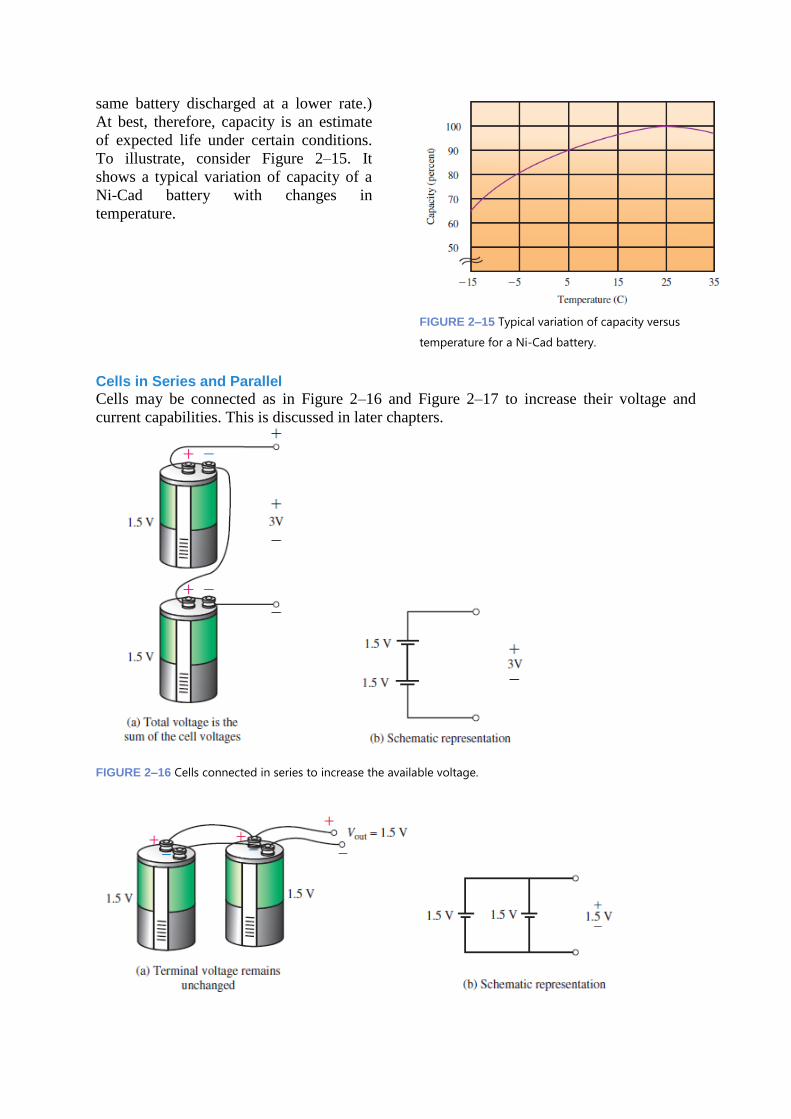
To illustrate, consider Figure 2–15. It

shows a typical variation of capacity of a

Ni-Cad battery with changes in

temperature.

FIGURE 2–15 Typical variation of capacity versus

temperature for a Ni-Cad battery.

Cells in Series and Parallel

Cells may be connected as in Figure 2–16 and Figure 2–17 to increase their voltage and

current capabilities. This is discussed in later chapters.

FIGURE 2–16 Cells connected in series to increase the available voltage.

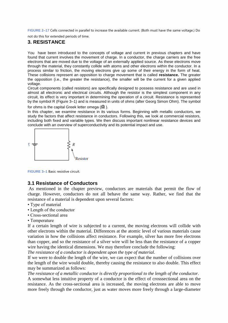
FIGURE 2–17 Cells connected in parallel to increase the available current. (Both must have the same voltage.) Do

not do this for extended periods of time.

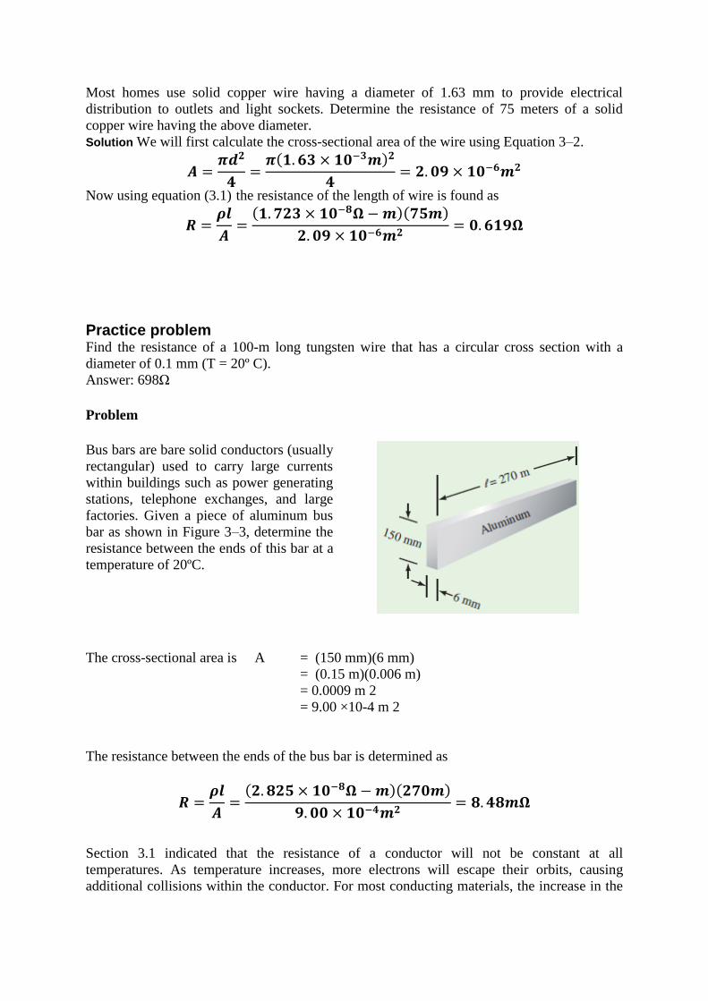
3. RESISTANCE You have been introduced to the concepts of voltage and current in previous chapters and have found that current involves the movement of charge. In a conductor, the charge carriers are the free electrons that are moved due to the voltage of an externally applied source. As these electrons move through the material, they constantly collide with atoms and other electrons within the conductor. In a process similar to friction, the moving electrons give up some of their energy in the form of heat. These collisions represent an opposition to charge movement that is called resistance. The greater the opposition (i.e., the greater the resistance), the smaller will be the current for a given applied voltage. Circuit components (called resistors) are specifically designed to possess resistance and are used in almost all electronic and electrical circuits. Although the resistor is the simplest component in any circuit, its effect is very important in determining the operation of a circuit. Resistance is represented by the symbol R (Figure 3–1) and is measured in units of ohms (after Georg Simon Ohm). The symbol

for ohms is the capital Greek letter omega (𝛀 ).

In this chapter, we examine resistance in its various forms. Beginning with metallic conductors, we study the factors that affect resistance in conductors. Following this, we look at commercial resistors, including both fixed and variable types. We then discuss important nonlinear resistance devices and conclude with an overview of superconductivity and its potential impact and use.

FIGURE 3–1 Basic resistive circuit.

3.1 Resistance of Conductors As mentioned in the chapter preview, conductors are materials that permit the flow of

charge. However, conductors do not all behave the same way. Rather, we find that the

resistance of a material is dependent upon several factors:

• Type of material

• Length of the conductor

• Cross-sectional area

• Temperature

If a certain length of wire is subjected to a current, the moving electrons will collide with

other electrons within the material. Differences at the atomic level of various materials cause

variation in how the collisions affect resistance. For example, silver has more free electrons

than copper, and so the resistance of a silver wire will be less than the resistance of a copper

wire having the identical dimensions. We may therefore conclude the following:

The resistance of a conductor is dependent upon the type of material.

If we were to double the length of the wire, we can expect that the number of collisions over

the length of the wire would double, thereby causing the resistance to also double. This effect

may be summarized as follows:

The resistance of a metallic conductor is directly proportional to the length of the conductor.

A somewhat less intuitive property of a conductor is the effect of crosssectional area on the

resistance. As the cross-sectional area is increased, the moving electrons are able to move

more freely through the conductor, just as water moves more freely through a large-diameter

pipe than a small-diameter pipe. If the cross-sectional area is doubled, the electrons would be

involved in half as many collisions over the length of the wire. We may summarize this effect

as follows:

The resistance of a metallic conductor is inversely proportional to the cross-sectional area of

the conductor.

The factors governing the resistance of a conductor at a given temperature may be

summarized mathematically as follows:

𝑹 =𝝆𝒍

𝑨 [𝒐𝒉𝒎𝒔, 𝛀] − − − −(𝟑. 𝟏)

where

𝝆 = _ resistivity, in ohm-meters (_-m)

𝒍 = length, in meters (m)

𝑨 =cross-sectional area, in square meters

(m2).

In the previous equation the lowercase

Greek letter rho (𝝆) is the constant of

proportionality and is called the resistivity

of the material. Resistivity is a physical

property of a material and is measured in

ohm-meters (𝛀 - m) in the SI system.

Table 3–1 lists the resistivities of various

materials at a temperature of 20º C. The

effects on resistance due to changes in

temperature will be examined in Section

3.4. Since most conductors are circular, as

shown in Figure 3–2, we may

determine the cross-sectional area from

either the radius or the diameter as

follows:

𝑨 = 𝝅𝒓𝟐 = 𝝅 (𝒅

𝟐)

𝟐

=𝝅𝒅𝟐

𝟒− −(𝟑. 𝟐)

FIGURE 3–2 Conductor with a circular cross section.

Problem

Most homes use solid copper wire having a diameter of 1.63 mm to provide electrical

distribution to outlets and light sockets. Determine the resistance of 75 meters of a solid

copper wire having the above diameter.

Solution We will first calculate the cross-sectional area of the wire using Equation 3–2.

𝑨 =𝝅𝒅𝟐

𝟒=

𝝅(𝟏. 𝟔𝟑 × 𝟏𝟎−𝟑𝒎)𝟐

𝟒= 𝟐. 𝟎𝟗 × 𝟏𝟎−𝟔𝒎𝟐

Now using equation (3.1) the resistance of the length of wire is found as

𝑹 =𝝆𝒍

𝑨=

(𝟏. 𝟕𝟐𝟑 × 𝟏𝟎−𝟖𝛀 − 𝒎)(𝟕𝟓𝒎)

𝟐. 𝟎𝟗 × 𝟏𝟎−𝟔𝒎𝟐= 𝟎. 𝟔𝟏𝟗𝛀

Practice problem Find the resistance of a 100-m long tungsten wire that has a circular cross section with a

diameter of 0.1 mm (T = 20º C).

Answer: 698Ω

Problem

Bus bars are bare solid conductors (usually

rectangular) used to carry large currents

within buildings such as power generating

stations, telephone exchanges, and large

factories. Given a piece of aluminum bus

bar as shown in Figure 3–3, determine the

resistance between the ends of this bar at a

temperature of 20ºC.

The cross-sectional area is A = (150 mm)(6 mm)

= (0.15 m)(0.006 m)

= 0.0009 m 2

= 9.00 ×10-4 m 2

The resistance between the ends of the bus bar is determined as

𝑹 =𝝆𝒍

𝑨=

(𝟐. 𝟖𝟐𝟓 × 𝟏𝟎−𝟖𝛀 − 𝒎)(𝟐𝟕𝟎𝒎)

𝟗. 𝟎𝟎 × 𝟏𝟎−𝟒𝒎𝟐= 𝟖. 𝟒𝟖𝒎𝛀

Section 3.1 indicated that the resistance of a conductor will not be constant at all

temperatures. As temperature increases, more electrons will escape their orbits, causing

additional collisions within the conductor. For most conducting materials, the increase in the

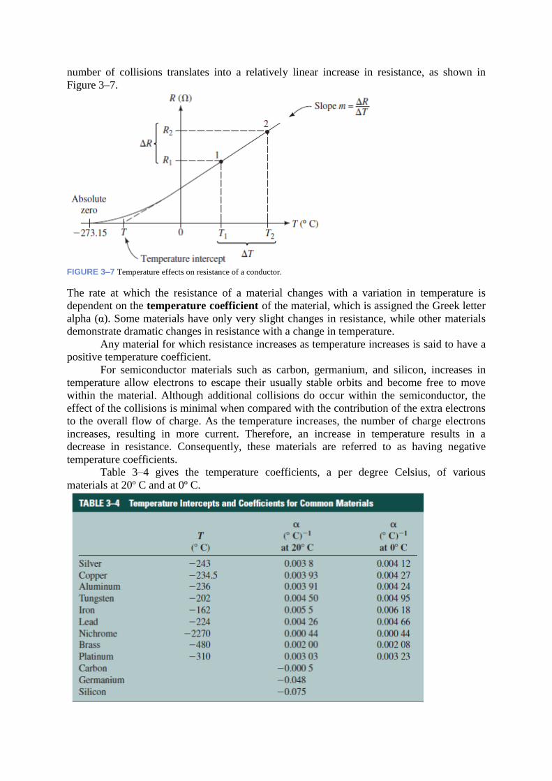
number of collisions translates into a relatively linear increase in resistance, as shown in

Figure 3–7.

FIGURE 3–7 Temperature effects on resistance of a conductor.

The rate at which the resistance of a material changes with a variation in temperature is

dependent on the temperature coefficient of the material, which is assigned the Greek letter

alpha (α). Some materials have only very slight changes in resistance, while other materials

demonstrate dramatic changes in resistance with a change in temperature.

Any material for which resistance increases as temperature increases is said to have a

positive temperature coefficient.

For semiconductor materials such as carbon, germanium, and silicon, increases in

temperature allow electrons to escape their usually stable orbits and become free to move

within the material. Although additional collisions do occur within the semiconductor, the

effect of the collisions is minimal when compared with the contribution of the extra electrons

to the overall flow of charge. As the temperature increases, the number of charge electrons

increases, resulting in more current. Therefore, an increase in temperature results in a

decrease in resistance. Consequently, these materials are referred to as having negative

temperature coefficients.

Table 3–4 gives the temperature coefficients, a per degree Celsius, of various

materials at 20º C and at 0º C.

If we consider that Figure 3–7 illustrates how the resistance of copper changes with

temperature, we observe an almost linear increase in resistance as the temperature increases.

Further, we see that as the temperature is decreased to absolute zero (T= - 273.15º C), the

resistance approaches zero.

In Figure 3–7, the point at which the linear portion of the line is extrapolated to cross the

abscissa (temperature axis) is referred to as the temperature intercept or the inferred absolute

temperature T of the material. By examining the straight-line portion of the graph, we see that

we have two similar triangles, one with the apex at point 1 and the other with the apex at

point 2. The following relationship applies for these similar triangles.

𝑹𝟐

𝑻𝟐 − 𝑻=

𝑹𝟏

𝑻𝟏 − 𝑻

This expression may be rewritten to solve for the resistance 𝑹𝟐 at any temperature 𝑻𝟐 as

follows:

𝑹𝟐 =(𝑻𝟐 − 𝑻)

(𝑻𝟏 − 𝑻)𝑹𝟏 − − − − − (𝟑. 𝟔)

An alternate method of determining the resistance 𝑹𝟐 of a conductor at a temperature 𝑻𝟐 is to

use the temperature coefficient a of the material. Examining Table 3–4, we see that the

temperature coefficient is not a constant for all temperatures, but rather is dependent upon the

temperature of the material. The temperature coefficient for any material is defined as

𝜶 =𝒎

𝑹𝟏

− − − − − − (𝟑. 𝟕)

The value of 𝜶 is typically given in chemical handbooks. In the preceding expression, 𝜶 is

measured in (º C)-1, R1 is the resistance in ohms at a temperature T1, and m is the slope of the

linear portion of the curve (m=Δ R / Δ T). It is left as an end-of-chapter problem for the

student to use Equations 3–6 and 3–7 to derive the following expression from Figure 3–6.

𝑹𝟐 = 𝑹𝟏[𝟏 + 𝜶𝟏(𝑻𝟐 − 𝑻𝟏)] − − − − − −(𝟑. 𝟖)

Problem-1 An aluminum wire has a resistance of 20Ω at room temperature (20º C). Calculate the

resistance of the same wire at temperatures of - 40º C, 100º C, and 200º C.

Solution From Table 3–4, we see that aluminum has a temperature intercept of –236º C.

At T = - 40º C:

The resistance at -40º C is determined using Equation 3–6.

𝑅−40℃ = [−40℃ − (−236℃)

20℃ − (−236℃)] 20Ω = (

196℃

256℃) 20Ω = 15.3Ω

At T= 100ºC,

𝑅100℃ = [−100℃ − (−236℃)

20℃ − (−236℃)] 20Ω = (

336℃

256℃) 20Ω = 26.3Ω

At T= 200ºC,

𝑅200℃ = [−200℃ − (−236℃)

20℃ − (−236℃)] 20Ω = (

436℃

256℃) 20Ω = 34.1Ω

This phenomenon indicates that the resistance of conductors changes quite

dramatically with changes in temperature. For this reason manufacturers generally

specify the range of temperatures over which a conductor may operate safely.

Problem - 2

Tungsten wire is used as filaments in incandescent light bulbs. Current in the wire causes the

wire to reach extremely high temperatures. Determine the temperature of the filament of a

100-W light bulb if the resistance at room temperature is measured to be 11.7 Ω and when the

light is on, the resistance is determined to be 144Ω.

Solution If we rewrite Equation 3–6, we are able to solve for the temperature T2 as follows:

𝑻𝟐 = (𝑻𝟏 − 𝑻)𝑹𝟐

𝑹𝟏

+ 𝑻

= [20℃ − (−202℃)]114Ω

11.7Ω+ (−202℃) = 2530℃.

3.5 Types of Resistors Virtually all electric and electronic circuits

involve the control of voltage and_or

current. The best way to provide such

control is by inserting appropriate values

of resistance into the circuit. Although

various types and sizes of resistors are

used in electrical and electronic

applications, all resistors fall into two main

categories: fixed resistors and variable

resistors. Fixed Resistors

As the name implies, fixed resistors are

resistors having resistance values that are

essentially constant. There are numerous

types of fixed resistors, ranging in size

from almost microscopic (as in integrated

circuits) to high-power resistors that are

capable of dissipating many watts of

power. Figure 3–8 illustrates the basic

structure of a molded carbon composition

resistor.

As shown in Figure 3–8, the molded

carbon composition resistor consists of a

carbon core mixed with an insulating filler.

The ratio of carbon to filler determines the

resistance value of the component: the

higher the proportion of carbon, the lower

the resistance. Metal leads are inserted into

the carbon core, and then the entire resistor

is encapsulated with an insulated coating.

Carbon omposition resistors are available

in resistances from less than 1Ω to 100

MΩ and typically have power ratings from

1⁄8 W to 2 W. Figure 3–9 shows various

sizes of resistors, with the larger resistors

being able to dissipate more power than

the smaller resistors.

Although carbon-core resistors have the

advantages of being inexpensive and easy

to produce, they tend to have wide

tolerances and are susceptible to large

changes in resistance due to temperature

variation. As shown in Figure 3–10, the

resistance of a carbon composition resistor

may change by as much as 5% when

temperature is changed by 100º C.

FIGURE 3–8 Structure of a molded carbon

composition resistor

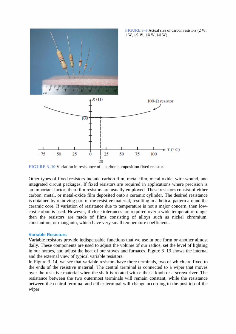
FIGURE 3–9 Actual size of carbon resistors (2 W,

1 W, 1⁄2 W, 1⁄4 W, 1⁄8 W).

FIGURE 3–10 Variation in resistance of a carbon composition fixed resistor.

Other types of fixed resistors include carbon film, metal film, metal oxide, wire-wound, and

integrated circuit packages. If fixed resistors are required in applications where precision is

an important factor, then film resistors are usually employed. These resistors consist of either

carbon, metal, or metal-oxide film deposited onto a ceramic cylinder. The desired resistance

is obtained by removing part of the resistive material, resulting in a helical pattern around the

ceramic core. If variation of resistance due to temperature is not a major concern, then low-

cost carbon is used. However, if close tolerances are required over a wide temperature range,

then the resistors are made of films consisting of alloys such as nickel chromium,

constantum, or manganin, which have very small temperature coefficients.

Variable Resistors

Variable resistors provide indispensable functions that we use in one form or another almost

daily. These components are used to adjust the volume of our radios, set the level of lighting

in our homes, and adjust the heat of our stoves and furnaces. Figure 3–13 shows the internal

and the external view of typical variable resistors.

In Figure 3–14, we see that variable resistors have three terminals, two of which are fixed to

the ends of the resistive material. The central terminal is connected to a wiper that moves

over the resistive material when the shaft is rotated with either a knob or a screwdriver. The

resistance between the two outermost terminals will remain constant, while the resistance

between the central terminal and either terminal will change according to the position of the

wiper.

(a) External view of variable resistors

FIGURE 3–13 Variable resistors.

(b) Internal view of variable resistor

FIGURE 3–14 (a) Variable

resistors

(b) Terminals of a variable

resistor

(c) Variable resistor used

as a potentiometer

If we examine the schematic of a variable resistor as shown in Figure 3–14(b), we see that the

following relationship must apply:

𝑅𝑎𝑐 = 𝑅𝑎𝑏 + 𝑅𝑏𝑐 − − − − − − − − − (3.9)

Variable resistors are used for two principal functions. Potentiometers, shown in Figure 3–

14(c), are used to adjust the amount of potential (voltage) provided to a circuit. Rheostats, the

connections and schematic of which are shown in Figure 3–15, are used to adjust the amount

of current within a circuit. Applications of potentiometers and rheostats will be covered in

later chapters.

(a) Connections of a rheostat (b) Symbol of a rheostat FIGURE 3–15

3.6 Color Coding of Resistors Large resistors such as the wire-wound resistors or the ceramic-encased power resistors have

their resistor values and tolerances printed on their cases. Smaller resistors, whether

constructed of a molded carbon composition or a metal film, may be too small to have their

values printed on the component. Instead, these smaller resistors are usually covered by an

epoxy or similar insulating coating over which several colored bands are printed radially as

shown in Figure 3–16.

The colored bands provide a quickly recognizable code for determining the value of

resistance, the tolerance (in percentage), and occasionally the expected reliability of the

resistor. The colored bands are always read from left to right, left being defined as the side of

the resistor with the band nearest to it. The first two bands represent the first and second

digits of the resistance value. The third band is called the multiplier band and represents the

number of zeros following the first two digits; it is usually given as a power of ten. The

fourth band indicates the tolerance of the resistor, and the fifth band (if present) is an

indication of the expected reliability of the component. The reliability is a statistical

indication of the expected number of components that will no longer have the indicated

resistance value after 1000 hours of use. For example, if a particular resistor has a reliability

of 1%, it is expected that after 1000 hours of use, no more than 1 resistor in 100 is likely to be

outside the specified range of resistance as indicated in the first four bands of the color codes.

Table 3–5 shows the colors of the various bands and the corresponding values.

FIGURE 3–16 Resistor color codes.

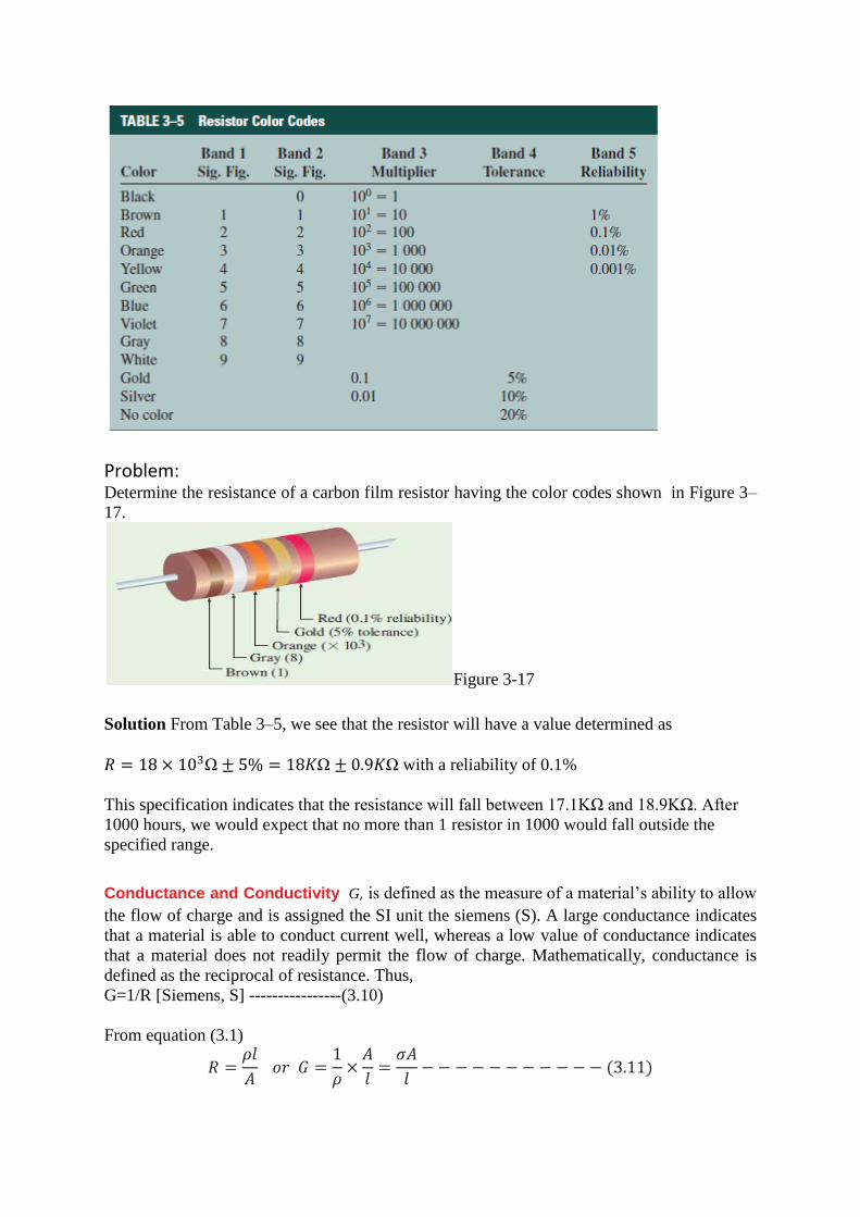
Problem: Determine the resistance of a carbon film resistor having the color codes shown in Figure 3–

17.

Figure 3-17

Solution From Table 3–5, we see that the resistor will have a value determined as

𝑅 = 18 × 103Ω ± 5% = 18𝐾Ω ± 0.9𝐾Ω with a reliability of 0.1%

This specification indicates that the resistance will fall between 17.1KΩ and 18.9KΩ. After

1000 hours, we would expect that no more than 1 resistor in 1000 would fall outside the

specified range.

Conductance and Conductivity G, is defined as the measure of a material’s ability to allow

the flow of charge and is assigned the SI unit the siemens (S). A large conductance indicates

that a material is able to conduct current well, whereas a low value of conductance indicates

that a material does not readily permit the flow of charge. Mathematically, conductance is

defined as the reciprocal of resistance. Thus,

G=1/R [Siemens, S] ----------------(3.10)

From equation (3.1)

𝑅 =𝜌𝑙

𝐴 𝑜𝑟 𝐺 =

1

𝜌×

𝐴

𝑙=

𝜎𝐴

𝑙− − − − − − − − − − − (3.11)

where σ is called the conductivity or specific conductance of a conductor. The unit of

conductance is siemens (S). Earlier, this unit was called mho.

It is seen from the above equation that the conductivity of a material is given by

𝜎 =𝐺𝑙

𝐴= 𝐺 𝑠𝑖𝑒𝑚𝑒𝑛𝑠 ×

𝑙𝑚𝑒𝑡𝑒𝑟

𝐴 𝑚𝑒𝑡𝑒𝑟2=

𝐺𝑙

𝐴 𝑆𝑖𝑒𝑚𝑒𝑛𝑠/𝑚𝑒𝑡𝑒𝑟

Hence, the unit of conductivity is siemens/metre (S/m).

Although the SI unit of conductance (siemens) is almost universally accepted, older books

and data sheets list conductance in the unit given as the mho (ohm spelled backward) and

having an upside-down omega,℧ , as the symbol. In such a case, the following relationship

holds:

1℧ = 1S ------------------(3.12)

POWER

If potential is multiplied by current 𝑑𝑞

𝑑𝑡, we have

𝑉 × 𝐼 =𝑑𝑊

𝑑𝑞×

𝑑𝑞

𝑑𝑡=

𝑑𝑊

𝑑𝑡= 𝑃

which gives rate of change of energy with time and is equal to power. The SI derived unit for

power (P) is watt expressed as Joule per sec.

ENERGY From the previous section we have

P =dW

dt

or dW = Pdt = VI dt or W = ∫ VI dt

and energy of a device is defined as the capacity of doing the work and its derived unit is

watts-sec.

OHM'S LAW

The relationship between voltage, resistance and current and the properties of resistance were investigated by the German physicist Georg Simon Ohm (1787–1854) using a circuit similar to that of Figure 3–1. Working with Volta’s recently developed battery and wires of different materials, lengths, and thicknesses, Ohm found that current depended on both voltage and resistance. For a fixed resistance, he found that doubling the voltage doubled the current, tripling the voltage tripled the current, and so on. Also, for a fixed voltage, Ohm found that the opposition to current was directly proportional to the length of the wire and inversely proportional to its cross-sectional area. From this, he was able to define the resistance of a wire and show that current was inversely proportional to this resistance; that is, when

he doubled the resistance, he found that the current decreased to half of its former value. These two results when combined form what is known as Ohm’s law.

Consider the circuit of Figure 4–1. Using a circuit similar in concept to this, Ohm determined

experimentally that current in a resistive circuit is directly proportional to its applied voltage

and inversely proportional to its resistance.

Fig. 4 – 1 (a) Experimental set-up (b) results.

A d.c. variable supply voltage is connected with positive terminal at point a and negative

terminal at ' b' as shown. As voltage is increased, the current recorded by the ammeter

increases. For every voltage value the current is recorded and the corresponding point is

plotted on the rectangular graph. With this a straight line graph passing through origin is

obtained in first quadrant. Next the terminals of the variable de supply are interchanged i.e. a

is connected to –ve polarity of de supply and b is connected to +ve polarity of de suply. Since

both the voltmeter and ammeter are moving coil, their individual connection should also be

interchanged so that meters can read up scale. This has been done to reverse the direction of

flow of current through the resister R. Again the voltage is varied and corresponding to each

voltage, current is recorded and the pairs of V and I are plotted in the third quadrant.

The experimental results indicate that there is a linear relationship between the current

and voltage both in the first and third quadrant. The slope of straight line is also same in both

the quadrants which shows that the potential difference across the terminals of the conductor

is proportional to the current passing through it i.e. 𝑽 ∝ 𝑰.

Also it is found that for a constant current in the conductor resistance should be

changed proportional to the potential difference i.e. 𝑉 ∝ 𝑅.

Combining the two proportionalities, we have

𝑉 ∝ 𝐼𝑅 𝑜𝑟 𝑉 = 𝑘𝐼𝑅

where k is a constant of proportionality. However, the units of voltage, current and

resistance are defined so that the value of k = 1. When the current is 1 amp, voltage 1 volt,

the resistance is 1 Ω.

𝑙 = 𝑘 . 1 . 1 Thus the equation becomes

𝑉 = 𝐼𝑅 The equation explains ohm's law which is stated as follows :

Physical condition (Temperature, Pressure etc.) of the conductor remaining constant,

the voltage across the terminals of a conductor is proportional to the current flowing through

it.

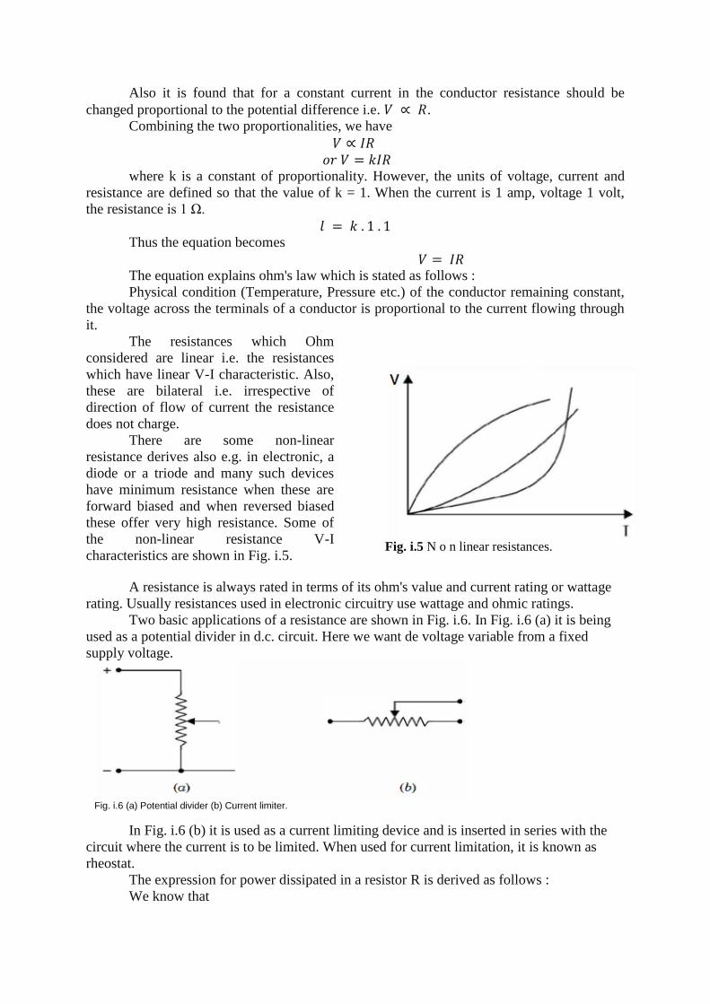
The resistances which Ohm

considered are linear i.e. the resistances

which have linear V-I characteristic. Also,

these are bilateral i.e. irrespective of

direction of flow of current the resistance

does not charge.

There are some non-linear

resistance derives also e.g. in electronic, a

diode or a triode and many such devices

have minimum resistance when these are

forward biased and when reversed biased

these offer very high resistance. Some of

the non-linear resistance V-I

characteristics are shown in Fig. i.5.

Fig. i.5 N o n linear resistances.

A resistance is always rated in terms of its ohm's value and current rating or wattage

rating. Usually resistances used in electronic circuitry use wattage and ohmic ratings.

Two basic applications of a resistance are shown in Fig. i.6. In Fig. i.6 (a) it is being

used as a potential divider in d.c. circuit. Here we want de voltage variable from a fixed

supply voltage.

Fig. i.6 (a) Potential divider (b) Current limiter.

In Fig. i.6 (b) it is used as a current limiting device and is inserted in series with the

circuit where the current is to be limited. When used for current limitation, it is known as

rheostat.

The expression for power dissipated in a resistor R is derived as follows :

We know that

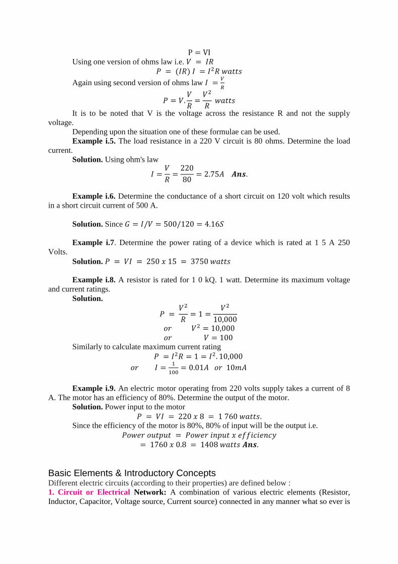
P = VI Using one version of ohms law i.e. 𝑉 = 𝐼𝑅

𝑃 = (𝐼𝑅) 𝐼 = 𝐼2𝑅 𝑤𝑎𝑡𝑡𝑠

Again using second version of ohms law 𝐼 =𝑉

𝑅

𝑃 = 𝑉.𝑉

𝑅=

𝑉2

𝑅 𝑤𝑎𝑡𝑡𝑠

It is to be noted that V is the voltage across the resistance R and not the supply

voltage.

Depending upon the situation one of these formulae can be used.

Example i.5. The load resistance in a 220 V circuit is 80 ohms. Determine the load

current.

Solution. Using ohm's law

𝐼 =𝑉

𝑅=

220

80= 2.75𝐴 𝑨𝒏𝒔.

Example i.6. Determine the conductance of a short circuit on 120 volt which results

in a short circuit current of 500 A.

Solution. Since 𝐺 = 𝐼/𝑉 = 500/120 = 4.16𝑆

Example i.7. Determine the power rating of a device which is rated at 1 5 A 250

Volts.

Solution. 𝑃 = 𝑉𝐼 = 250 𝑥 15 = 3750 𝑤𝑎𝑡𝑡𝑠

Example i.8. A resistor is rated for 1 0 kQ. 1 watt. Determine its maximum voltage

and current ratings.

Solution.

𝑃 = 𝑉2

𝑅= 1 =

𝑉2

10,000

𝑜𝑟 𝑉2 = 10,000 𝑜𝑟 𝑉 = 100

Similarly to calculate maximum current rating

𝑃 = 𝐼2𝑅 = 1 = 𝐼2. 10,000

𝑜𝑟 𝐼 =1

100= 0.01𝐴 𝑜𝑟 10𝑚𝐴

Example i.9. An electric motor operating from 220 volts supply takes a current of 8

A. The motor has an efficiency of 80%. Determine the output of the motor.

Solution. Power input to the motor

𝑃 = 𝑉𝐼 = 220 𝑥 8 = 1 760 𝑤𝑎𝑡𝑡𝑠. Since the efficiency of the motor is 80%, 80% of input will be the output i.e.

𝑃𝑜𝑤𝑒𝑟 𝑜𝑢𝑡𝑝𝑢𝑡 = 𝑃𝑜𝑤𝑒𝑟 𝑖𝑛𝑝𝑢𝑡 𝑥 𝑒𝑓𝑓𝑖𝑐𝑖𝑒𝑛𝑐𝑦 = 1760 𝑥 0.8 = 1408 𝑤𝑎𝑡𝑡𝑠 𝑨𝒏𝒔.

Basic Elements & Introductory Concepts Different electric circuits (according to their properties) are defined below :

1. Circuit or Electrical Network: A combination of various electric elements (Resistor,

Inductor, Capacitor, Voltage source, Current source) connected in any manner what so ever is

called an electrical network. We may classify circuit elements in two categories, passive and

active elements.

2. Parameters. The various elements of an electric circuit are called its parameters like

resistance, inductance and capacitance. These parameters may be lumped or distributed.

3. Liner Circuit. A linear circuit is one whose parameters are constant i.e. they do not

change with voltage or current.

4. Non-linear Circuit. It is that circuit whose parameters change with voltage or current.

5. Bilateral Circuit. A bilateral circuit is one whose properties or characteristics are the same

in either direction. The usual transmission line is bilateral, because it can be made to perform

its function equally well in either direction. Bilateral Element: Conduction of current in both directions in an element (example:

Resistance; Inductance; Capacitance) with same magnitude is termed as bilateral element.

6. Unilateral Circuit. It is that circuit whose properties or characteristics change with the

direction of its operation. A diode rectifier is a unilateral circuit, because it cannot perform

rectification in both directions.

Unilateral Element: Conduction of current in one direction is termed as unilateral (example:

Diode, Transistor) element.

7. Electric Network. A combination of various electric elements, connected in any manner

whatsoever, is called an electric network.

8. Passive Network is one which contains no source of e.m.f. in it. Passive Element: The element which receives energy (or absorbs energy) and then either

converts it into heat (R) or stored it in an electric (C) or magnetic (L ) field is called passive

element.

9. Active Network is one which contains one or more than one source of e.m.f.

Active Element: The elements that supply energy to the circuit is called active element. Examples

of active elements include voltage and current sources, generators, and electronic devices that

require power supplies. A transistor is an active circuit element, meaning that it can amplify

power of a signal. On the other hand, transformer is not an active element because it does not

amplify the power level and power remains same both in primary and secondary sides.

Transformer is an example of passive element. 10. Node is a junction in a circuit where two or more circuit elements are connected together.

11. Branch is that part of a network which lies between two junctions.

12. Loop. It is a close path in a circuit in which no element or node is encountered more than

once.

13. Mesh. It is a loop that contains no other loop within it. For example, the circuit of Fig. 2.1

(a) has even branches, six nodes, three loops and two meshes whereas the circuit of Fig. 2.1

(b) has four branches, two nodes, six loops and three meshes.

Fig. 2.1

Meaning of Response: An application of input signal to the system will produce an output signal,

the behavior of output signal with time is known as the response of the system.

4. SERIES CIRCUITS An electric circuit is the combination of any number of sources and loads connected in any

manner that allows charge to flow. The electric circuit may be simple, such as a circuit consisting

of a battery and a light bulb. Or the circuit may be very complex, such as the circuits contained

within a television set, microwave oven, or computer. However, no matter how complicated, each

circuit follows fairly simple rules in a predictable manner. Once these rules are understood, any

circuit may be analyzed to determine the operation under various conditions.

All electric circuits obtain their energy either from a direct current (dc) source or from an

alternating current (ac) source. In the next few chapters, we examine the operation of circuits

supplied by dc sources. Although ac circuits have fundamental differences when compared with

dc circuits, the laws, theorems, and rules that you learn in dc circuits apply directly to ac circuits

as well.

In the previous chapter, you were introduced to a simple dc circuit consisting of a single voltage

source (such as a chemical battery) and a single load resistance. The schematic representation of

such a simple circuit was covered in Chapter 4 and is shown again in Figure 5–1.

While the circuit of Figure 5–1 is useful in deriving some important concepts, very few practical

circuits are this simple. However, we will find that even the most complicated dc circuits can

generally be simplified to the circuit shown. We begin by examining the most simple connection,

the series connection.

In Figure 5–2, we have two resistors, R1 and R2, connected at a single point in what is said to be

a series connection. Two elements are said to be in series if they are connected at a single point

and if there are no other current-carrying connections at this point. A series circuit is constructed

by combining various elements in series, as shown in Figure 5–3. Current will leave the positive

terminal of the voltage source, move through the resistors, and return to the negative terminal of

the source. In the circuit of Figure 5–3, we see that the voltage source, E, is in series with R1, R1

is in series with R2, and R2 is in series with E. By examining this circuit, another important

characteristic of a series circuit becomes evident. In an analogy similar to water flowing in a pipe,

current entering an element must be the same as the current leaving the element. Now, since

current does not leave at any of the connections, we conclude that the following must be true:

The current is the same everywhere in a series circuit. While the preceding statement seems self-

evident, we will find that this will help to explain many of the other characteristics of a series

circuit.

4.1 Resistance in Series

When some conductors having resistances R1, R2 and R3 etc. are joined end-on-end as in Fig.

1.12, they are said to be connected in series. It can be proved that the equivalent resistance or

total resistance between points A and D is equal to the sum of the three individual resistances.

Being a series circuit, it should be remembered that (i) current is the same through all the three

conductors (ii) but voltage drop across each is different due to its different resistance and is given

by Ohm’s Law and (iii) sum of the three voltage drops is equal to the voltage applied across the

three conductors.There is a progressive fall in potential as we go from point A to D as shown in

Fig. 1.13.

V = V1 + V2 + V3 = IR1 + IR2 + IR3 —Ohm’s

Law

But V = IR

where R is the equivalent resistance of the series combination.

IR = IR1 + IR2 + IR3 or R = R1 + R2 + R3

Also 1

G=

1

G1+

1

G2+

1

G3

The power dissipated by each resistor is determined as

P1 = V1I =V1

2

R1

= I2R1

P2 = V2I =V2

2

R2

= I2R2

P3 = V3I =V3

2

R3

= I2R3

Hence,

P = P1 + P2 + P3

As seen from above, the main characteristics of a series circuit are :

1. same current flows through all parts of the circuit.

2. different resistors have their individual voltage drops.

3. voltage drops are additive.

4. applied voltage equals the sum of different voltage drops.

5. resistances are additive.

6. powers are additive.

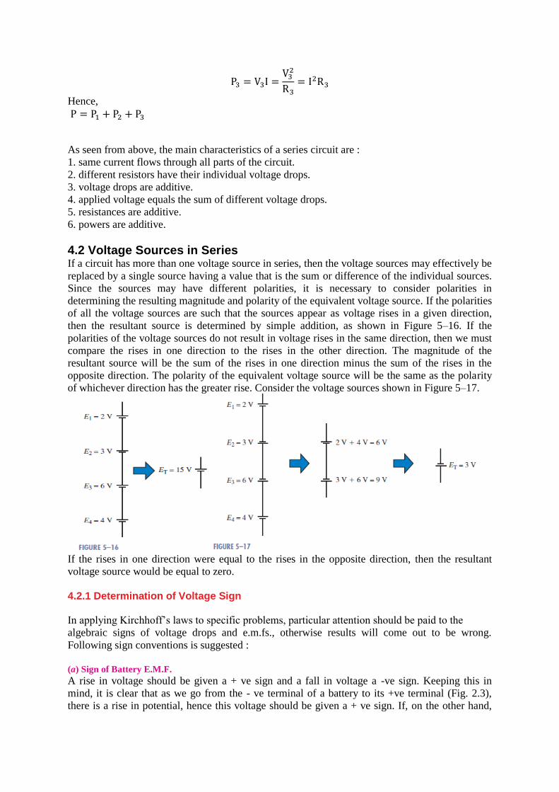
4.2 Voltage Sources in Series If a circuit has more than one voltage source in series, then the voltage sources may effectively be

replaced by a single source having a value that is the sum or difference of the individual sources.

Since the sources may have different polarities, it is necessary to consider polarities in

determining the resulting magnitude and polarity of the equivalent voltage source. If the polarities

of all the voltage sources are such that the sources appear as voltage rises in a given direction,

then the resultant source is determined by simple addition, as shown in Figure 5–16. If the

polarities of the voltage sources do not result in voltage rises in the same direction, then we must

compare the rises in one direction to the rises in the other direction. The magnitude of the

resultant source will be the sum of the rises in one direction minus the sum of the rises in the

opposite direction. The polarity of the equivalent voltage source will be the same as the polarity

of whichever direction has the greater rise. Consider the voltage sources shown in Figure 5–17.

If the rises in one direction were equal to the rises in the opposite direction, then the resultant

voltage source would be equal to zero.

4.2.1 Determination of Voltage Sign

In applying Kirchhoff’s laws to specific problems, particular attention should be paid to the

algebraic signs of voltage drops and e.m.fs., otherwise results will come out to be wrong.

Following sign conventions is suggested :

(a) Sign of Battery E.M.F.

A rise in voltage should be given a + ve sign and a fall in voltage a -ve sign. Keeping this in

mind, it is clear that as we go from the - ve terminal of a battery to its +ve terminal (Fig. 2.3),

there is a rise in potential, hence this voltage should be given a + ve sign. If, on the other hand,

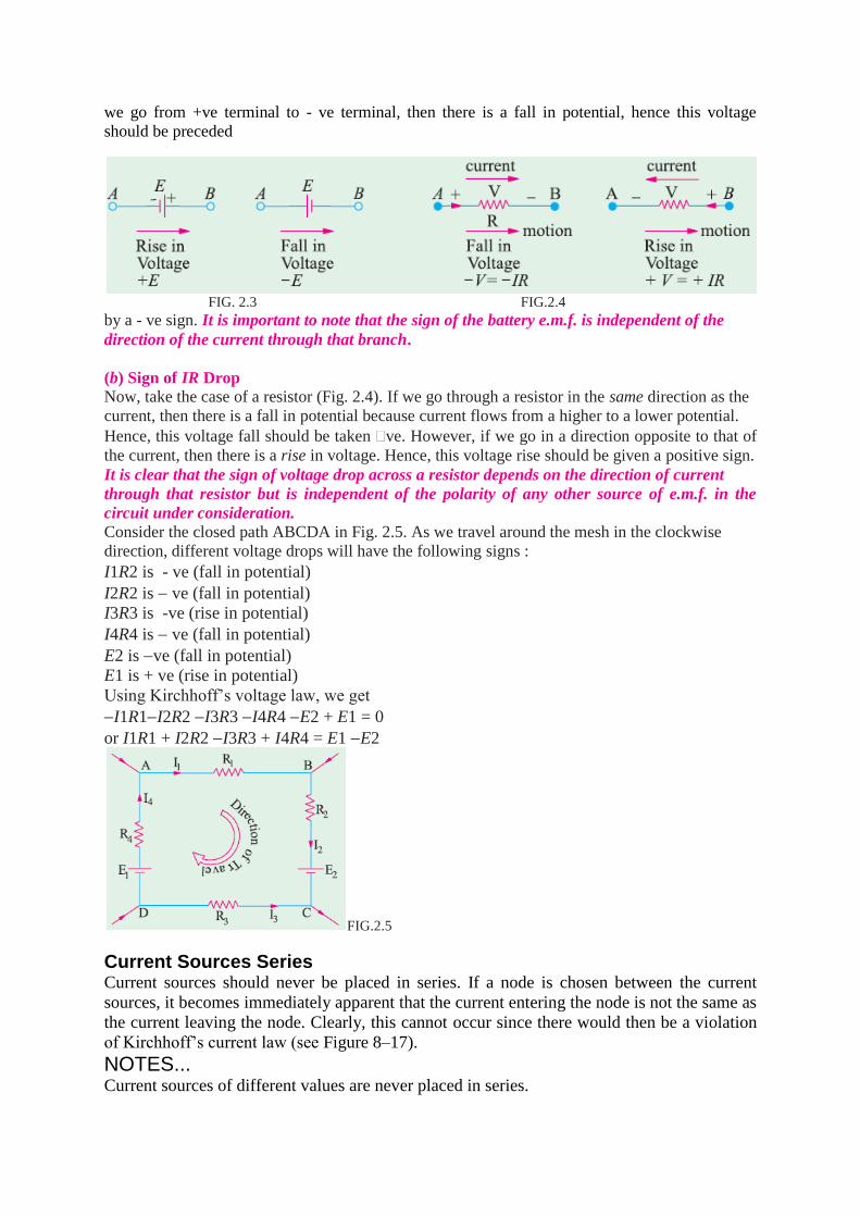
we go from +ve terminal to - ve terminal, then there is a fall in potential, hence this voltage

should be preceded

FIG. 2.3 FIG.2.4

by a - ve sign. It is important to note that the sign of the battery e.m.f. is independent of the

direction of the current through that branch.

(b) Sign of IR Drop

Now, take the case of a resistor (Fig. 2.4). If we go through a resistor in the same direction as the

current, then there is a fall in potential because current flows from a higher to a lower potential.

Hence, this voltage fall should be taken ve. However, if we go in a direction opposite to that of

the current, then there is a rise in voltage. Hence, this voltage rise should be given a positive sign.

It is clear that the sign of voltage drop across a resistor depends on the direction of current

through that resistor but is independent of the polarity of any other source of e.m.f. in the

circuit under consideration.

Consider the closed path ABCDA in Fig. 2.5. As we travel around the mesh in the clockwise

direction, different voltage drops will have the following signs :

I1R2 is -ve (fall in potential)

I2R2 is ve (fall in potential)

I3R3 is -ve (rise in potential)

I4R4 is ve (fall in potential)

E2 is ve (fall in potential)

E1 is + ve (rise in potential)

Using Kirchhoff’s voltage law, we get

I1R1I2R2 I3R3 I4R4 E2 + E1 = 0

or I1R1 + I2R2 I3R3 + I4R4 = E1 E2

FIG.2.5

Current Sources Series Current sources should never be placed in series. If a node is chosen between the current

sources, it becomes immediately apparent that the current entering the node is not the same as

the current leaving the node. Clearly, this cannot occur since there would then be a violation

of Kirchhoff’s current law (see Figure 8–17).

NOTES... Current sources of different values are never placed in series.

FIGURE 8–17

4.3 Kirchhoff’s Voltage Law Next to Ohm’s law, one of the most important laws of electricity is Kirchhoff’s

voltage law (KVL), which states the following:

The summation of voltage rises and voltage drops around a closed loop is equal to zero.

Symbolically, this may be stated as follows:

∑V = 0 for a closed loop (5–1)

In the preceding symbolic representation, the uppercase Greek letter sigma (∑) stands for

summation and V stands for voltage rises and drops. A closed loop is defined as any path that

originates at a point, travels around a circuit, and returns to the original point without

retracing any segments. An alternate way of stating Kirchhoff’s voltage law is as follows:

The summation of voltage rises is equal to the summation of voltage drops around a closed

loop.

∑Erises = ∑Vdrops for a closed loop (5–2)

If we consider the circuit of Figure 5–7, we may begin at point a in the lower left-hand

corner. By arbitrarily following the direction of the current, I, we move through the voltage

source, which represents a rise in potential from point a to point b. Next, in moving from

point b to point c, we pass through resistor R1, which presents a potential drop of V1.

Continuing through resistors R2 and R3, we have additional drops of V2 and V3, respectively.

By applying Kirchhoff’s voltage law around the closed loop, we arrive at the following

mathematical statement for the given circuit:

E - V1 - V2 - V3 = 0

Although we chose to follow the direction of current in writing Kirchhoff’s voltage law

equation, it would be just as correct to move around the circuit in the opposite direction. In

this case the equation would appear as follows:

V3 + V2+ V1 - E= 0

By simple manipulation, it is quite easy to show that the two equations are identical.

5.6 The Voltage Divider Rule The voltage dropped across any series resistor is proportional to the magnitude of the

resistor. The total voltage dropped across all resistors must equal the applied voltage

source(s) by Kirchhoff’s Voltage Law.

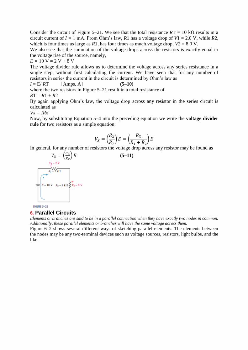
Consider the circuit of Figure 5–21. We see that the total resistance RT = 10 kΩ results in a

circuit current of I = 1 mA. From Ohm’s law, R1 has a voltage drop of V1 = 2.0 V, while R2,

which is four times as large as R1, has four times as much voltage drop, V2 = 8.0 V.

We also see that the summation of the voltage drops across the resistors is exactly equal to

the voltage rise of the source, namely,

E = 10 V = 2 V + 8 V

The voltage divider rule allows us to determine the voltage across any series resistance in a

single step, without first calculating the current. We have seen that for any number of

resistors in series the current in the circuit is determined by Ohm’s law as

I = E/ RT [Amps, A] (5–10)

where the two resistors in Figure 5–21 result in a total resistance of

RT = R1 + R2

By again applying Ohm’s law, the voltage drop across any resistor in the series circuit is

calculated as

Vx = IRx

Now, by substituting Equation 5–4 into the preceding equation we write the voltage divider

rule for two resistors as a simple equation:

𝑉𝑋 = (𝑅𝑋

𝑅𝑇) 𝐸 = (

𝑅𝑋

𝑅1 + 𝑅2) 𝐸

In general, for any number of resistors the voltage drop across any resistor may be found as

𝑉𝑋 = (𝑅𝑋

𝑅𝑇) 𝐸 (5–11)

6. Parallel Circuits Elements or branches are said to be in a parallel connection when they have exactly two nodes in common. Additionally, these parallel elements or branches will have the same voltage across them.

Figure 6–2 shows several different ways of sketching parallel elements. The elements between

the nodes may be any two-terminal devices such as voltage sources, resistors, light bulbs, and the

like.

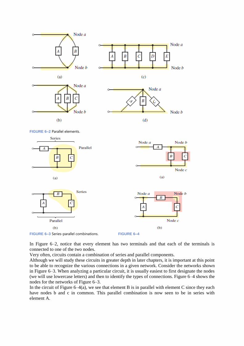
FIGURE 6–2 Parallel elements.

FIGURE 6–3 Series-parallel combinations. FIGURE 6–4

In Figure 6–2, notice that every element has two terminals and that each of the terminals is

connected to one of the two nodes.

Very often, circuits contain a combination of series and parallel components.

Although we will study these circuits in greater depth in later chapters, it is important at this point

to be able to recognize the various connections in a given network. Consider the networks shown

in Figure 6–3. When analyzing a particular circuit, it is usually easiest to first designate the nodes

(we will use lowercase letters) and then to identify the types of connections. Figure 6–4 shows the

nodes for the networks of Figure 6–3.

In the circuit of Figure 6–4(a), we see that element B is in parallel with element C since they each

have nodes b and c in common. This parallel combination is now seen to be in series with

element A.

In the circuit of Figure 6–4(b), element B is in series with element C since these elements have a

single common node: node b. The branch consisting of the series combination of elements B and

C is then determined to be in parallel with element A.

6.1 Resistances in Parallel

Three resistances, as joined in Fig. 1.15 are

said to be connected in parallel. In this case

(i) p.d. across all resistances is the same

(ii) current in each resistor is different and is

given by Ohm’s Law and

(iii) the total current is the sum of the three

separate currents.

𝐼 = 𝐼1 + 𝐼2 + 𝐼3 =𝑉

𝑅1

+𝑉

𝑅2

+𝑉

𝑅3

Now, 𝐼 =𝑉

𝑅 where V is the applied voltage

R = equivalent resistance of the parallel combination. 𝑉

𝑅=

𝑉

𝑅1

+𝑉

𝑅2

+𝑉

𝑅3

𝑜𝑟 1

𝑅=

1

𝑅1

+1

𝑅2

+1

𝑅3

Also, 𝐺 = 𝐺1 + 𝐺2 + 𝐺3

The main characteristics of a parallel circuit are :

1. same voltage acts across all parts of the circuit

2. different resistors have their individual current.

3. branch currents are additive.

4. conductances are additive.

5. powers are additive.

6.2 Voltage Sources in Parallel Voltage sources of different potentials should never be connected in parallel, since to do so

would contradict Kirchhoff’s voltage law. However, when two equal potential sources are

connected in parallel, each source will deliver half the required circuit current. For this reason

automobile batteries are sometimes connected in parallel to assist in starting a car with a “weak”

battery. Figure 6–22 illustrates this principle.

FIGURE 6–22 Voltage sources in parallel. FIGURE 6–23 Voltage sources of different

voltages must never be placed in parallel.

Figure 6–23 shows that if voltage sources of two different potentials are placed in parallel,

Kirchhoff’s voltage law will be violated around the closed loop. In practice, if voltage sources of

different potentials are placed in parallel, the resulting closed loop can have a very large current.

The current will occur even though there may not be a load connected across the sources.

Example 6–9 illustrates the large currents that can occur when two parallel batteries of different

potential are connected. 6.3. Assumed Direction of Current

In applying Kirchhoff’s laws to electrical networks, the question of assuming proper direction of

current usually arises. The direction of current flow may be assumed either clockwise or

anticlockwise.

If the assumed direction of current is not the actual direction, then on solving the quesiton, this

current will be found to have a minus sign. If the answer is positive, then assumed direction is the

same as actual direction (Example 2.10). However, the important point is that once a particular

direction has been assumed, the same should be used throughout the solution of the question.

Note. It should be noted that Kirchhoff’s laws are applicable both to d.c. and a.c. voltages and

currents. However, in the case of alternating currents and voltages, any e.m.f. of self-inductance

or that existing across a capacitor should be also taken into account (See Example 2.14).

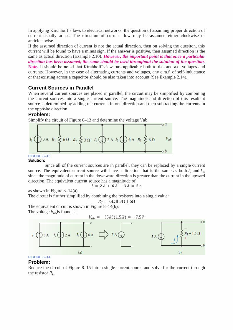
Current Sources in Parallel When several current sources are placed in parallel, the circuit may be simplified by combining

the current sources into a single current source. The magnitude and direction of this resultant

source is determined by adding the currents in one direction and then subtracting the currents in

the opposite direction.

Problem: Simplify the circuit of Figure 8–13 and determine the voltage Vab.

FIGURE 8–13

Solution:

Since all of the current sources are in parallel, they can be replaced by a single current

source. The equivalent current source will have a direction that is the same as both 𝐼2 and 𝐼3,

since the magnitude of current in the downward direction is greater than the current in the upward

direction. The equivalent current source has a magnitude of 𝐼 = 2 𝐴 + 6 𝐴 − 3 𝐴 = 5 𝐴

as shown in Figure 8–14(a).

The circuit is further simplified by combining the resistors into a single value:

𝑅𝑇 = 6Ω ∥ 3Ω ∥ 6Ω

The equivalent circuit is shown in Figure 8–14(b).

The voltage Vabis found as

𝑉𝑎𝑏 = −(5𝐴)(1.5Ω) = −7.5𝑉

FIGURE 8–14

Problem: Reduce the circuit of Figure 8–15 into a single current source and solve for the current through

the resistor 𝑅𝐿.

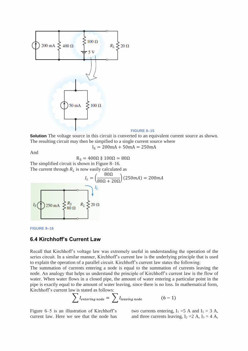
FIGURE 8–15

Solution The voltage source in this circuit is converted to an equivalent current source as shown.

The resulting circuit may then be simpified to a single current source where

IS = 200mA + 50mA = 250mA And

RS = 400Ω ∥ 100Ω = 80Ω The simplified circuit is shown in Figure 8–16.

The current through 𝑅𝐿 is now easily calculated as

𝐼𝐿 = (80Ω

80Ω + 20Ω) (250𝑚𝐴) = 200𝑚𝐴

FIGURE 8–16

6.4 Kirchhoff’s Current Law Recall that Kirchhoff’s voltage law was extremely useful in understanding the operation of the

series circuit. In a similar manner, Kirchhoff’s current law is the underlying principle that is used

to explain the operation of a parallel circuit. Kirchhoff’s current law states the following:

The summation of currents entering a node is equal to the summation of currents leaving the

node. An analogy that helps us understand the principle of Kirchhoff’s current law is the flow of

water. When water flows in a closed pipe, the amount of water entering a particular point in the

pipe is exactly equal to the amount of water leaving, since there is no loss. In mathematical form,

Kirchhoff’s current law is stated as follows:

∑ 𝐼𝑒𝑛𝑡𝑒𝑟𝑖𝑛𝑔 𝑛𝑜𝑑𝑒 = ∑ 𝐼𝑙𝑒𝑎𝑣𝑖𝑛𝑔 𝑛𝑜𝑑𝑒 (6 − 1)

Figure 6–5 is an illustration of Kirchhoff’s

current law. Here we see that the node has

two currents entering, I1 =5 A and I5 = 3 A,

and three currents leaving, I2 =2 A, I3 = 4 A,

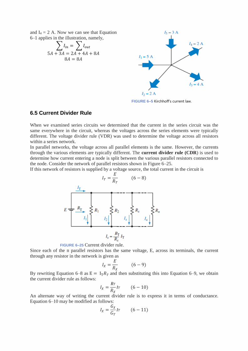
and I4 = 2 A. Now we can see that Equation

6–1 applies in the illustration, namely,

∑ 𝐼𝑖𝑛 = ∑ 𝐼𝑜𝑢𝑡

5𝐴 + 3𝐴 = 2𝐴 + 4𝐴 + 8𝐴

8𝐴 = 8𝐴

FIGURE 6–5 Kirchhoff’s current law.

6.5 Current Divider Rule When we examined series circuits we determined that the current in the series circuit was the

same everywhere in the circuit, whereas the voltages across the series elements were typically

different. The voltage divider rule (VDR) was used to determine the voltage across all resistors

within a series network.

In parallel networks, the voltage across all parallel elements is the same. However, the currents

through the various elements are typically different. The current divider rule (CDR) is used to

determine how current entering a node is split between the various parallel resistors connected to

the node. Consider the network of parallel resistors shown in Figure 6–25.

If this network of resistors is supplied by a voltage source, the total current in the circuit is

𝐼𝑇 =𝐸

𝑅𝑇

(6 − 8)

FIGURE 6–25 Current divider rule.

Since each of the n parallel resistors has the same voltage, E, across its terminals, the current

through any resistor in the network is given as

𝐼𝑋 =𝐸

𝑅𝑋

(6 − 9)

By rewriting Equation 6–8 as E = IT𝑅𝑇 and then substituting this into Equation 6–9, we obtain

the current divider rule as follows:

𝐼𝑋 =𝑅𝑇

𝑅𝑋

𝐼𝑇 (6 − 10)

An alternate way of writing the current divider rule is to express it in terms of conductance.

Equation 6–10 may be modified as follows:

𝐼𝑋 =𝐺𝑋

𝐺𝑇

𝐼𝑇 (6 − 11)

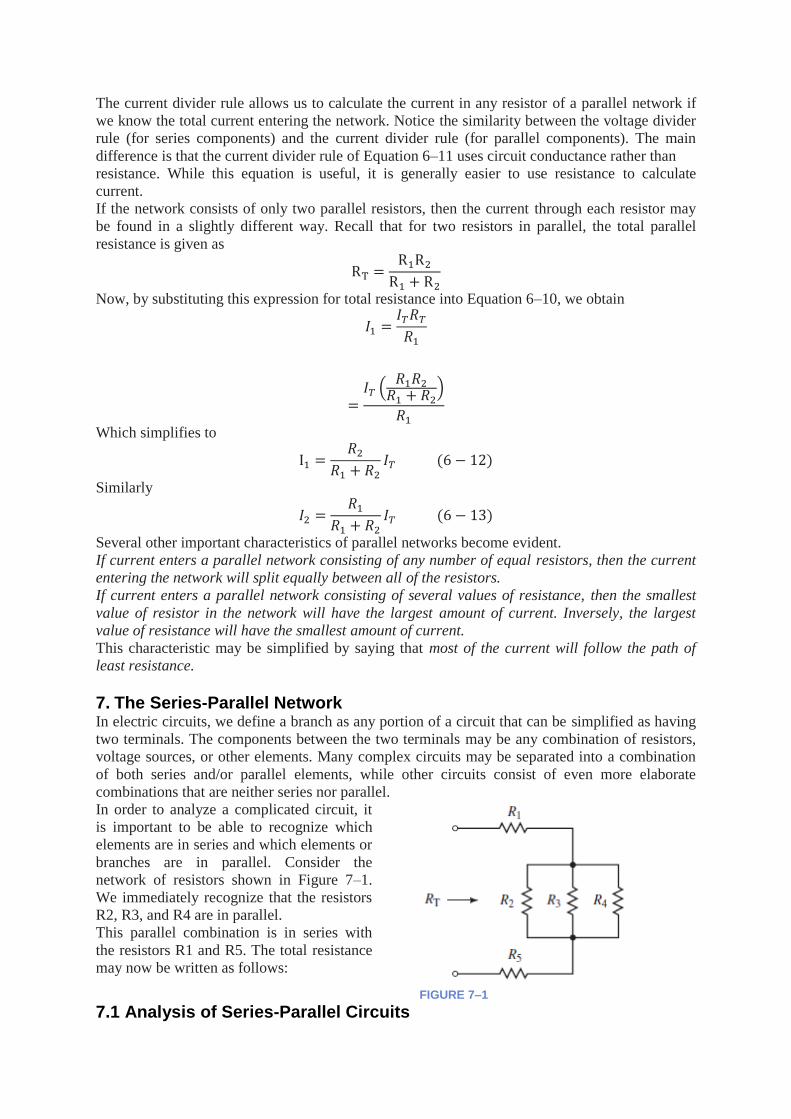
The current divider rule allows us to calculate the current in any resistor of a parallel network if

we know the total current entering the network. Notice the similarity between the voltage divider

rule (for series components) and the current divider rule (for parallel components). The main

difference is that the current divider rule of Equation 6–11 uses circuit conductance rather than

resistance. While this equation is useful, it is generally easier to use resistance to calculate

current.

If the network consists of only two parallel resistors, then the current through each resistor may

be found in a slightly different way. Recall that for two resistors in parallel, the total parallel

resistance is given as

RT =R1R2

R1 + R2

Now, by substituting this expression for total resistance into Equation 6–10, we obtain

𝐼1 =𝐼𝑇𝑅𝑇

𝑅1

=𝐼𝑇 (

𝑅1𝑅2

𝑅1 + 𝑅2)

𝑅1

Which simplifies to

I1 =𝑅2

𝑅1 + 𝑅2

𝐼𝑇 (6 − 12)

Similarly

𝐼2 =𝑅1

𝑅1 + 𝑅2

𝐼𝑇 (6 − 13)

Several other important characteristics of parallel networks become evident.

If current enters a parallel network consisting of any number of equal resistors, then the current

entering the network will split equally between all of the resistors.

If current enters a parallel network consisting of several values of resistance, then the smallest

value of resistor in the network will have the largest amount of current. Inversely, the largest

value of resistance will have the smallest amount of current.

This characteristic may be simplified by saying that most of the current will follow the path of

least resistance.

EXAMPLE

7. The Series-Parallel Network In electric circuits, we define a branch as any portion of a circuit that can be simplified as having

two terminals. The components between the two terminals may be any combination of resistors,

voltage sources, or other elements. Many complex circuits may be separated into a combination

of both series and/or parallel elements, while other circuits consist of even more elaborate

combinations that are neither series nor parallel.

In order to analyze a complicated circuit, it

is important to be able to recognize which

elements are in series and which elements or

branches are in parallel. Consider the

network of resistors shown in Figure 7–1.

We immediately recognize that the resistors

R2, R3, and R4 are in parallel.

This parallel combination is in series with

the resistors R1 and R5. The total resistance

may now be written as follows:

FIGURE 7–1

7.1 Analysis of Series-Parallel Circuits

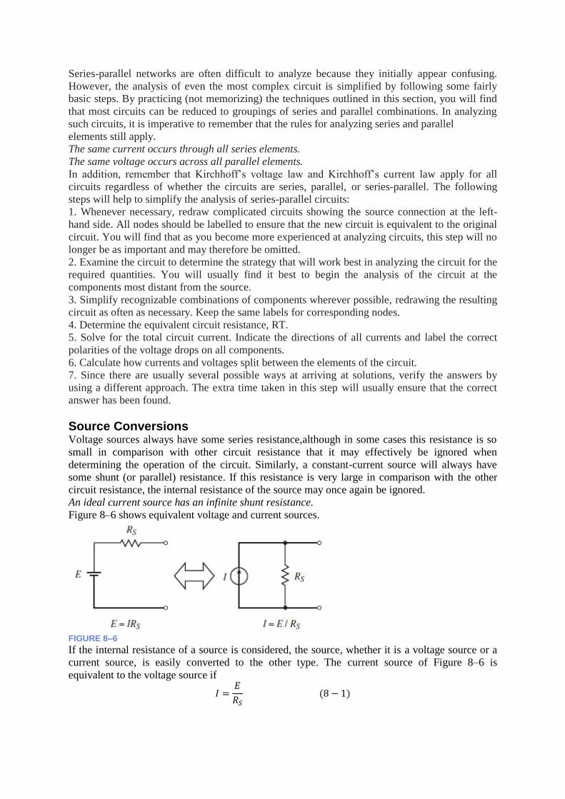
Series-parallel networks are often difficult to analyze because they initially appear confusing.

However, the analysis of even the most complex circuit is simplified by following some fairly

basic steps. By practicing (not memorizing) the techniques outlined in this section, you will find

that most circuits can be reduced to groupings of series and parallel combinations. In analyzing

such circuits, it is imperative to remember that the rules for analyzing series and parallel

elements still apply.

The same current occurs through all series elements.

The same voltage occurs across all parallel elements.

In addition, remember that Kirchhoff’s voltage law and Kirchhoff’s current law apply for all

circuits regardless of whether the circuits are series, parallel, or series-parallel. The following

steps will help to simplify the analysis of series-parallel circuits:

1. Whenever necessary, redraw complicated circuits showing the source connection at the left-

hand side. All nodes should be labelled to ensure that the new circuit is equivalent to the original

circuit. You will find that as you become more experienced at analyzing circuits, this step will no

longer be as important and may therefore be omitted.

2. Examine the circuit to determine the strategy that will work best in analyzing the circuit for the

required quantities. You will usually find it best to begin the analysis of the circuit at the

components most distant from the source.

3. Simplify recognizable combinations of components wherever possible, redrawing the resulting

circuit as often as necessary. Keep the same labels for corresponding nodes.

4. Determine the equivalent circuit resistance, RT.

5. Solve for the total circuit current. Indicate the directions of all currents and label the correct

polarities of the voltage drops on all components.

6. Calculate how currents and voltages split between the elements of the circuit.

7. Since there are usually several possible ways at arriving at solutions, verify the answers by

using a different approach. The extra time taken in this step will usually ensure that the correct

answer has been found.

Source Conversions Voltage sources always have some series resistance,although in some cases this resistance is so

small in comparison with other circuit resistance that it may effectively be ignored when

determining the operation of the circuit. Similarly, a constant-current source will always have

some shunt (or parallel) resistance. If this resistance is very large in comparison with the other

circuit resistance, the internal resistance of the source may once again be ignored.

An ideal current source has an infinite shunt resistance.

Figure 8–6 shows equivalent voltage and current sources.

FIGURE 8–6

If the internal resistance of a source is considered, the source, whether it is a voltage source or a

current source, is easily converted to the other type. The current source of Figure 8–6 is

equivalent to the voltage source if

𝐼 =𝐸

𝑅𝑆 (8 − 1)

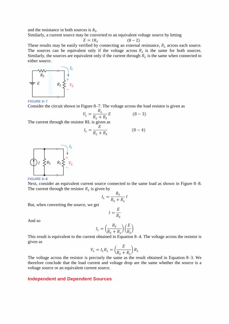
and the resistance in both sources is 𝑅𝑆.

Similarly, a current source may be converted to an equivalent voltage source by letting

𝐸 = 𝐼𝑅𝑆 (8 − 2)

These results may be easily verified by connecting an external resistance, 𝑅𝐿 across each source.

The sources can be equivalent only if the voltage across 𝑅𝐿 is the same for both sources.

Similarly, the sources are equivalent only if the current through 𝑅𝐿 is the same when connected to

either source.

FIGURE 8–7

Consider the circuit shown in Figure 8–7. The voltage across the load resistor is given as

𝑉𝐿 =𝑅𝐿

𝑅𝐿 + 𝑅𝑆

𝐸 (8 − 3)

The current through the resistor RL is given as

𝐼𝐿 =𝐸

𝑅𝐿 + 𝑅𝑆

(8 − 4)

FIGURE 8–8

Next, consider an equivalent current source connected to the same load as shown in Figure 8–8.

The current through the resistor 𝑅𝐿 is given by

𝐼𝐿 =𝑅𝑆

𝑅𝑆 + 𝑅𝐿

𝐼

But, when converting the source, we get

𝐼 =𝐸

𝑅𝑆

And so

𝐼𝐿 = (𝑅𝑆

𝑅𝑆 + 𝑅𝐿) (

𝐸

𝑅𝑆)

This result is equivalent to the current obtained in Equation 8–4. The voltage across the resistor is

given as

𝑉𝐿 = 𝐼𝐿𝑅𝐿 = (𝐸

𝑅𝑆 + 𝑅𝐿) 𝑅𝐿

The voltage across the resistor is precisely the same as the result obtained in Equation 8–3. We

therefore conclude that the load current and voltage drop are the same whether the source is a

voltage source or an equivalent current source.

Independent and Dependent Sources

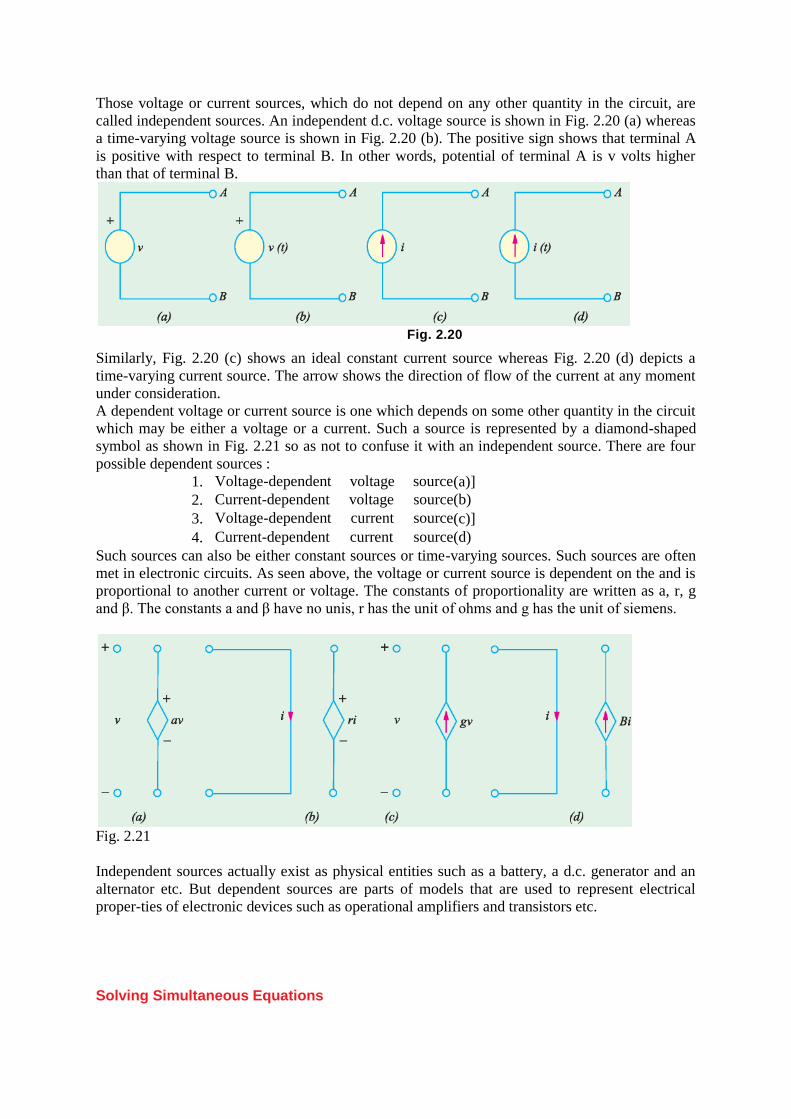
Those voltage or current sources, which do not depend on any other quantity in the circuit, are

called independent sources. An independent d.c. voltage source is shown in Fig. 2.20 (a) whereas

a time-varying voltage source is shown in Fig. 2.20 (b). The positive sign shows that terminal A

is positive with respect to terminal B. In other words, potential of terminal A is v volts higher

than that of terminal B.

Fig. 2.20

Similarly, Fig. 2.20 (c) shows an ideal constant current source whereas Fig. 2.20 (d) depicts a

time-varying current source. The arrow shows the direction of flow of the current at any moment

under consideration.

A dependent voltage or current source is one which depends on some other quantity in the circuit

which may be either a voltage or a current. Such a source is represented by a diamond-shaped

symbol as shown in Fig. 2.21 so as not to confuse it with an independent source. There are four

possible dependent sources :

1. Voltage-dependent voltage source

[Fig. 2.21 (a)]

2. Current-dependent voltage source

[Fig. 2.21

(b)

] 3. Voltage-dependent current source

[Fig. 2.21 (c)]

4. Current-dependent current source

[Fig. 2.21

(d)

] Such sources can also be either constant sources or time-varying sources. Such sources are often

met in electronic circuits. As seen above, the voltage or current source is dependent on the and is

proportional to another current or voltage. The constants of proportionality are written as a, r, g

and β. The constants a and β have no unis, r has the unit of ohms and g has the unit of siemens.

Fig. 2.21

Independent sources actually exist as physical entities such as a battery, a d.c. generator and an

alternator etc. But dependent sources are parts of models that are used to represent electrical

proper-ties of electronic devices such as operational amplifiers and transistors etc.

Solving Simultaneous Equations

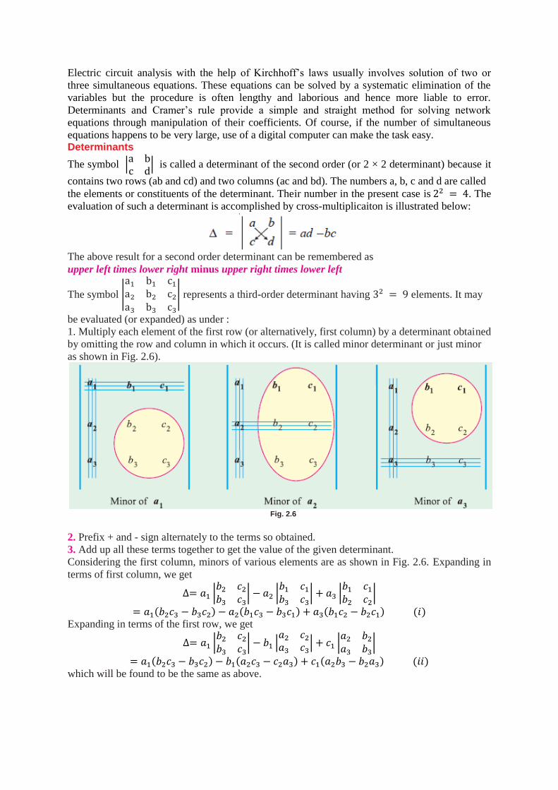
Electric circuit analysis with the help of Kirchhoff’s laws usually involves solution of two or

three simultaneous equations. These equations can be solved by a systematic elimination of the

variables but the procedure is often lengthy and laborious and hence more liable to error.

Determinants and Cramer’s rule provide a simple and straight method for solving network

equations through manipulation of their coefficients. Of course, if the number of simultaneous

equations happens to be very large, use of a digital computer can make the task easy. Determinants

The symbol |a bc d

| is called a determinant of the second order (or 2 × 2 determinant) because it

contains two rows (ab and cd) and two columns (ac and bd). The numbers a, b, c and d are called

the elements or constituents of the determinant. Their number in the present case is 22 = 4. The

evaluation of such a determinant is accomplished by cross-multiplicaiton is illustrated below:

The above result for a second order determinant can be remembered as

upper left times lower right minus upper right times lower left

The symbol |

a1 b1 c1

a2 b2 c2

a3 b3 c3

| represents a third-order determinant having 32 = 9 elements. It may

be evaluated (or expanded) as under :

1. Multiply each element of the first row (or alternatively, first column) by a determinant obtained

by omitting the row and column in which it occurs. (It is called minor determinant or just minor

as shown in Fig. 2.6).

Fig. 2.6

2. Prefix + and - sign alternately to the terms so obtained.

3. Add up all these terms together to get the value of the given determinant.

Considering the first column, minors of various elements are as shown in Fig. 2.6. Expanding in

terms of first column, we get

∆= 𝑎1 |𝑏2 𝑐2

𝑏3 𝑐3| − 𝑎2 |

𝑏1 𝑐1

𝑏3 𝑐3| + 𝑎3 |

𝑏1 𝑐1

𝑏2 𝑐2|

= 𝑎1(𝑏2𝑐3 − 𝑏3𝑐2) − 𝑎2(𝑏1𝑐3 − 𝑏3𝑐1) + 𝑎3(𝑏1𝑐2 − 𝑏2𝑐1) (𝑖) Expanding in terms of the first row, we get

∆= 𝑎1 |𝑏2 𝑐2

𝑏3 𝑐3| − 𝑏1 |

𝑎2 𝑐2

𝑎3 𝑐3| + 𝑐1 |

𝑎2 𝑏2

𝑎3 𝑏3|

= 𝑎1(𝑏2𝑐3 − 𝑏3𝑐2) − 𝑏1(𝑎2𝑐3 − 𝑐2𝑎3) + 𝑐1(𝑎2𝑏3 − 𝑏2𝑎3) (𝑖𝑖)

which will be found to be the same as above.

Example 2.1. Evaluate the determinant |7 −3 −4

−3 6 −2−4 −2 11

|

Solution. We will expand with the help of 1st column.

𝐷 = 7 |6 −2

−2 11| — 3 |

−3 −2−4 11

| + (−4) |−3 6−4 −2

|

= 7(66 − 4) + 3(−33 − 8) − 4(6 + 24) = 191 2.7. Solving Equations with Two Unknowns

Suppose the two given simultaneous equations are

ax + by = c

dx + ey = f

Here, the two unknown are x and y, a, b, d and e are coefficients of these unknowns whereas c

and

f are constants. The procedure for solving these equations by the method of determinants is as

follows

:

1. Write the two equations in the matrix form as [𝑎 𝑏𝑑 𝑒

] [𝑥𝑦] = [

𝑐𝑓]

2. The common determinant is given as ∆= |𝑎 𝑏𝑑 𝑒

| = 𝑎𝑒 − 𝑏𝑑

3. For finding the determinant for x, replace the coefficients of x in the original matrix by the

constants so that we get determinant ∆1 given by

∆1= |𝑐 𝑏𝑓 𝑒

| = 𝑐𝑒 − 𝑏𝑓

4. For finding the determinant for y, replace coefficients of y by the constants so that we get

∆2= |𝑎 𝑐𝑑 𝑓| = 𝑎𝑓 − 𝑐𝑑

5. Apply Cramer’s rule to get the value of x and y

𝑥 =∆1

∆=

𝑐𝑒 − 𝑏𝑓

𝑎𝑒 − 𝑏𝑑 𝑎𝑛𝑑 𝑦 =

∆2

∆=

𝑎𝑓 − 𝑐𝑑

𝑎𝑒 − 𝑏𝑑

Example 2.2. Solve the following two simultaneous equations by the method of determinants :

4𝑖1 − 3𝑖2 = 1 3𝑖1 − 5𝑖2 = 2

Solution. The matrix form of the equations is [4 −33 −5

] [𝑖1

𝑖2] = [

12

]

∆= |4 −33 −5

| = 4(−5)— 33 = −11

∆1= |1 −32 −5

| = 1(−5) − 2(−3) = 1

∆2= |4 13 2

| = (4 × 2) − (1 × 3) = 5

∴ 𝑖1 =∆1

∆= −

1

11 ; 𝑖2 =

∆2

∆= −

5

11

2.8. Solving Equations With Three Unknowns

Let the three simultaneous equations be as under :

ax by cz d

ex fy gz h

jx ky lz m

The above equations can be put in the matrix form as under :

[

𝑎 𝑏 𝑐𝑒 𝑓 𝑔𝑗 𝑘 𝑙

] [𝑥𝑦𝑧

] = [𝑑ℎ𝑚

]

The value of common determinant is given by

∆= |

𝑎 𝑏 𝑐𝑒 𝑓 𝑔𝑗 𝑘 𝑙

| = 𝑎(𝑓𝑙 − 𝑔𝑘) − 𝑏(𝑒𝑙 − 𝑗𝑔) + 𝑐(𝑒𝑘 − 𝑓𝑗)

The determinant for x can be found by replacing coefficients of x in the original matrix by the

constants.

∴ ∆1= |𝑑 𝑏 𝑐ℎ 𝑓 𝑔𝑚 𝑘 𝑙

| = 𝑑(𝑓𝑙 − 𝑔𝑘) − 𝑏(ℎ𝑙 − 𝑚𝑔) + 𝑐(ℎ𝑘 − 𝑓𝑚)

Similarly, determinant for y is given by replacing coefficients of y with the three constants.

∆2= |

𝑎 𝑑 𝑐𝑒 ℎ 𝑔𝑗 𝑚 𝑙

| = 𝑎(ℎ𝑙 − 𝑚𝑔) − 𝑑(𝑒𝑙 − 𝑗𝑔) + 𝑐(𝑒𝑚 − 𝑗ℎ)

In the same way, determinant for z is given by

∆3= |

𝑎 𝑏 𝑑𝑒 𝑓 ℎ𝑗 𝑘 𝑚

| = 𝑎(𝑓𝑚 − 𝑘ℎ) − 𝑏(𝑒𝑚 − 𝑗ℎ) + 𝑑(𝑒𝑘 − 𝑓𝑗)

As per Cramer’s rule

𝑥 =∆1

∆; 𝑦 =

∆2

∆; 𝑧 =

∆3

∆

Branch-Current Analysis Branch-current analysis allows us to directly calculate the current in each branch of a circuit.

Since the method involves the analysis of several simultaneous linear equations, you may find

that a review of determinants is in order.

When applying branch-current analysis, you will find the following technique useful.

1. Arbitrarily assign current directions to each branch in the network. If a particular branch

has a current source, then this step is not necessary since you already know the magnitude

and direction of the current in this branch.

2. Using the assigned currents, label the polarities of the voltage drops across all resistors in

the circuit.

3. Apply Kirchhoff’s voltage law around each of the closed loops. Write just enough

equations to include all branches in the loop equations. If a branch has only a current

source and no series resistance, it is not necessary to include it in the KVL equations.

4. Apply Kirchhoff’s current law at enough nodes to ensure that all branch currents have

been included. In the event that a branch has only a current source, it will need to be

included in this step.

5. Solve the resulting simultaneous linear equations.

PROBLEM

Find the current in each branch in the circuit of Figure 8–18.

FIGURE 8–18

Solution

Step 1: Assign currents as shown in Figure 8–18.

Step 2: Indicate the polarities of the voltage drops on all resistors in the circuit, using the assumed

current directions.

Step 3: Write the Kirchhoff voltage law equations.

Loop abcda: 6𝑉 − (2Ω)𝐼1 + (2Ω)𝐼2 − 4𝑉 = 0

Notice that the circuit still has one branch which has not been included in the KVL equations,

namely the branch cefd. This branch would be included if a loop equation for cefdc or for

abcefda were written. There is no reason for choosing one loop over another, since the overall

result will remain unchanged even though the intermediate steps will not give the same results.

Loop cefdc:

4V − (2Ω)I2 − (4Ω)I3 + 2V = 0 Now that all branches have been included in the loop equations, there is no need to write any

more. Although more loops exist, writing more loop equations would needlessly complicate the

calculations.

Step 4: Write the Kirchhoff current law equation(s). By applying KCL at node c, all branch currents in the network are included.Node c: I3 = I1 + I2 To simplify the solution of the simultaneous linear equations we write them as follows:

2I1 − 2I2 + 0I3 = 2 0I1 − 2I2 − 4I3 = −6

1I1 + 1I2 − 1I3 = 0

The principles of linear algebra allow us to solve for the determinant of the denominator as follows:

∆= |2 −2 00 −2 −41 1 −1

| = 2(2 + 4) − (−2)(0 + 4) + 0(0 + 2) = 20

Now, solving for the currents, we have the following:

𝐼1 =∆1

∆=

|2 −2 0

−6 −2 −40 1 −1

|

20=

2(2 + 4) + 2(6 + 0) + 020

=2420

= 1.2𝐴

Similarly,

𝐼2 =∆2

∆=

|2 2 00 −6 −41 0 −1

|

20=

2(6 + 0) − 2(0 + 4) + 020

=4

20= 0.2𝐴

And

𝐼3 =∆3

∆=

|2 −2 20 −2 −61 1 0

|

20=

2(0 + 6) + 2(0 + 6) + 2(0 + 2)20

=2820

= 1.4𝐴

PROBLEM

Find the currents in each branch of the circuit shown in Figure 8–19. Solve for

the voltage Vab.

FIGURE 8–19

Solution Notice that although Figure 8–19 has four currents, there are only three unknown

currents: I2, I3, and I4. The current I1 is given by the value of the constant-current source. In

order to solve this network we will need three linear equations. As before, the equations are

determined by Kirchhoff’s voltage and current laws.

Step 1: The currents are indicated in the given circuit.

Step 2: The polarities of the voltages across all resistors are shown.

Step 3: Kirchhoff’s voltage law is applied at the indicated loops:

Loop badb: −(2Ω)I2 + (3Ω)I3 − 8V = 0

Loop bacb: −(2Ω)I2 + (1Ω)I4 − 6V = 0

Step 4: Kirchhoff’s current law is applied as follows:

Node a: I2 + I3 + I4 = 5A

−2I2 + 3I3 + 0I4 = 8

−2I2 + 0I3 + 1I4 = 6

1I2 + 1I3 + 1I4 = 5

∴ ∆= |−2 3 0−2 0 11 1 1

| = −2(0 − 1) − 3(−2 − 1) + 0 = 11

Now solving for the currents, we have

I2 =

|8 3 06 0 15 1 1

|

11=

8(0 − 1) − 3(6 − 5) + 0

11= −

11

11= −1A

I3 =

|−2 8 0−2 6 11 5 1

|

11=

−2(6 − 5) − 8(−2 − 1) + 0

11=

22

11= 2A

I4 =

|−2 3 8−2 0 61 1 5

|

11=

−2(0 − 6) − 3(−10 − 6) + 8(−2 − 0)

11=

44

11= 4A

The current I2 is negative, which simply means that the actual direction of the current is opposite

to the chosen direction. Although the network may be further analyzed using the assumed current

directions, it is easier to understand the circuit operation by showing the actual current directions

as in Figure 8–20.

FIGURE 8–20

𝐼2= 1A

𝐼3 = 2A

𝐼4 = 4A

Using the actual direction for I2,Vab = +(2Ω)(1A) = 2V

8.5 Mesh (Loop) Analysis

In the previous section you used Kirchhoff’s laws to solve for the current in eachbranch of a

given network. While the methods used were relatively simple, branch-current analysis is

awkward to use because it generally involves solving several simultaneous linear equations. It is

not difficult to see that the number of equations may be prohibitively large even for a relatively

simple circuit.

A better approach and one that is used extensively in analyzing linear bilateral networks

is called mesh (or loop) analysis. While the technique is similar to branch-current analysis, the

number of simultaneous linear equations tends to be less. The principal difference between mesh

analysis and branchcurrent analysis is that we simply need to apply Kirchhoff’s voltage law

around closed loops without the need for applying Kirchhoff’s current law. The steps used in

solving a circuit using mesh analysis are as follows:

1. Arbitrarily assign a clockwise current to each interior closed loop in the network.

Although the assigned current may be in any direction, a clockwise direction is used to

make later work simpler.

2. Using the assigned loop currents, indicate the voltage polarities across all resistors in the

circuit. For a resistor that is common to two loops, the polarities of the voltage drop due

to each loop current should be indicated on the appropriate side of the component.

3. Applying Kirchhoff’s voltage law, write the loop equations for each loop in the network.

Do not forget that resistors that are common to two loops will have two voltage drops,

one due to each loop.

4. Solve the resultant simultaneous linear equations.

5. Branch currents are determined by algebraically combining the loop currents that are

common to the branch.

Example 2.1. Determine the current in all the branches of the network using loop analysis.

Fig. E2.1

Solution: Let the currents i1 and i2 be flowing in the two loops as shown. It is to be noted that

the direction of the currents is arbitrary. However, depending upon the values of i1 and i2 thus

obtained we can ascertain the direction. If they are coming out to be positive, the directions

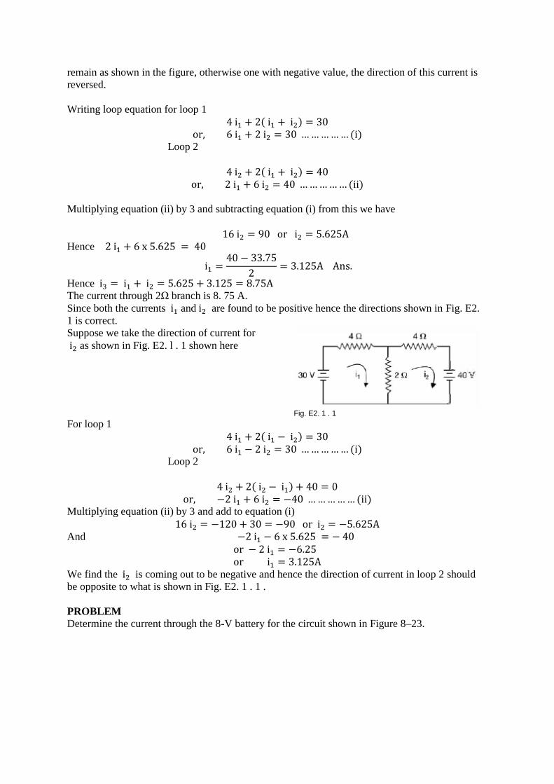
remain as shown in the figure, otherwise one with negative value, the direction of this current is

reversed.

Writing loop equation for loop 1

4 i1 + 2( i1 + i2) = 30

or, 6 i1 + 2 i2 = 30 … … … … … (i) Loop 2

4 i2 + 2( i1 + i2) = 40

or, 2 i1 + 6 i2 = 40 … … … … … (ii)

Multiplying equation (ii) by 3 and subtracting equation (i) from this we have

16 i2 = 90 or i2 = 5.625A

Hence 2 i1 + 6 x 5.625 = 40

i1 =40 − 33.75

2= 3.125A Ans.

Hence i3 = i1 + i2 = 5.625 + 3.125 = 8.75A

The current through 2Ω branch is 8. 75 A.

Since both the currents i1 and i2 are found to be positive hence the directions shown in Fig. E2.

1 is correct.

Suppose we take the direction of current for

i2 as shown in Fig. E2. l . 1 shown here

Fig. E2. 1 . 1

For loop 1

4 i1 + 2( i1 − i2) = 30

or, 6 i1 − 2 i2 = 30 … … … … … (i) Loop 2

4 i2 + 2( i2 − i1) + 40 = 0

or, −2 i1 + 6 i2 = −40 … … … … … (ii) Multiplying equation (ii) by 3 and add to equation (i)

16 i2 = −120 + 30 = −90 or i2 = −5.625A

And −2 i1 − 6 x 5.625 = − 40 or − 2 i1 = −6.25 or i1 = 3.125A

We find the i2 is coming out to be negative and hence the direction of current in loop 2 should

be opposite to what is shown in Fig. E2. 1 . 1 .

PROBLEM

Determine the current through the 8-V battery for the circuit shown in Figure 8–23.

FIGURE 8–23

Solution: Convert the current source into an

equivalent voltage source. The equivalent

circuit may now be analyzed by using the

loop currents shown in Figure 8–24.

FIGURE 8–24

LOOP1: − 10V − (2Ω)I1 − 3Ω(I1 − I2) − 8V = 0 or (5Ω)I1 − (3Ω)I2 = −18V

LOOP2: 8V − 3Ω( I2 − I1) − (1Ω)I2 − 6V = 0 or − (3Ω)I1 + (4Ω)I2 = 2V

Solving the equations using determinants, we have

∆= |5 −3

−3 4| = 11

∴ I1 =∆1

∆=

|−18 −3

2 4|

11 = −

66

11= −6A

& I2 = ∆2

∆=

|5 −18

−3 2|

11= −

44

11= −4A

If the assumed direction of current in the 8-V battery is taken to be I, then

I = I2 − I1 = −4 − (−6) = 2A

The direction of the resultant current is the same as I2(upward).

The circuit of Figure 8–23 may also be analyzed without converting the current source to a

voltage source. Although the approach is generally not used, the following example illustrates the

technique.

PROBLEM

FIGURE 8–25 Solution By inspection, we see that the loop current I1 = 5A. The mesh equations for the other

two loops are as follows:

LOOP 2: − 2Ω(I2 − I1) − 3Ω(I2 − I3) − 8V = 0 or (5Ω)I2 − (3Ω)I3 = −18V (∵ by putting the value of I1 = 5A)

LOOP 3: (1Ω)I3 − 6V + 8V − 3Ω(I3 − I2) = 0 or − (3Ω)I2 + (4Ω)I3 = 2V

By solving the equations

I2 = −6A ; I3 = −4A

The calculated values of the assumed reference currents allow us to determine the actual current

through the various resistors as follows:

IR1= I1 − I2 = −5A − (−6A) = 1A (downward)

IR2= I3 − I2 = −4A − (−6A) = 2A (upward)

I3 = −I34A (left) Format Approach for Mesh Analysis

A very simple technique may be used to write the mesh equations for any linear bilateral network.

When this format approach is used, the simultaneous linear equations for a network having n

independent loops will appear as follows:

R11I1 − R12I2 − R13I3 − ⋯ ⋯ ⋯ − R1nIn = E1

−R21I1 + R22I2 − R23I3 − ⋯ ⋯ ⋯ − R2nIn = E2

⋮ ⋮

−Rn1I1 − Rn2I2 − Rn3I3 − ⋯ ⋯ ⋯ + RnnIn = En

The terms R11, R22, R33, … . . , Rnnrepresent the total resistance in each loop and are found by

simply adding all the resistances in a particular loop. The remaining resistance terms are called

the mutual resistance terms. These resistances represent resistance which is shared between two

loops. For example, the mutual resistance R12 is the resistance in loop 1, which is located in the

branch between loop 1 and loop 2. If there is no resistance between two loops, this term will be

zero.

The terms containing R11, R22, R33, … . . , Rnnare positive, and all of the mutual resistance

terms are negative. This characteristic occurs because all currents are assumed to be clockwise.

If the linear equations are correctly written, you will find that the coefficients along the

principal diagonal ( R11, R22, R33, … . . , Rnn ) will be positive. All other coefficients will be

negative. Also, if the equations are correctly written, the terms will be symmetrical about the

principal diagonal—for example, R12 _ R21.

The terms E1, E2, E3, … … , En are the summation of the voltage rises in the direction of the

loop currents. If a voltage source appears in the branch shared by two loops, it will be included in

the calculation of the voltage rise for each loop.

The method used in applying the format approach of mesh analysis is as follows:

1. Convert current sources into equivalent voltage sources.

2. Assign clockwise currents to each independent closed loop in the network.

3. Write the simultaneous linear equations in the format outlined.

4. Solve the resulting simultaneous linear equations.

PROBLEM

Solve for the currents through R2 and R3 in the circuit of Figure 8–26.

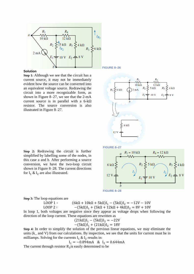
FIGURE 8–26 Solution

Step 1: Although we see that the circuit has a

current source, it may not be immediately

evident how the source can be converted into

an equivalent voltage source. Redrawing the

circuit into a more recognizable form, as

shown in Figure 8–27, we see that the 2-mA

current source is in parallel with a 6-kΩ

resistor. The source conversion is also

illustrated in Figure 8–27.

FIGURE 8–27

Step 2: Redrawing the circuit is further

simplified by labelling some of the nodes, in

this case a and b. After performing a source

conversion, we have the two-loop circuit

shown in Figure 8–28. The current directions

for I1 & I2 are also illustrated.

FIGURE 8–28

Step 3: The loop equations are

LOOP 1 ∶ (6kΩ + 10kΩ + 5kΩ)I1 − (5kΩ)I2 = −12V − 10V

LOOP 2 ∶ −(5kΩ)I1 + (5kΩ + 12kΩ + 4kΩ)I2 = 8V + 10V In loop 1, both voltages are negative since they appear as voltage drops when following the

direction of the loop current. These equations are rewritten as

(21kΩ)I1 − (5kΩ)I2 = −22V

−(5kΩ)I1 + (21kΩ)I2 = 18V Step 4: In order to simplify the solution of the previous linear equations, we may eliminate the

units (k_ and V) from our calculations. By inspection, we see that the units for current must be in

milliamps. Solving for the currents I1 & I2 results in:

I1 = −0.894mA & I2 = 0.644mA The current through resistor R2is easily determined to be

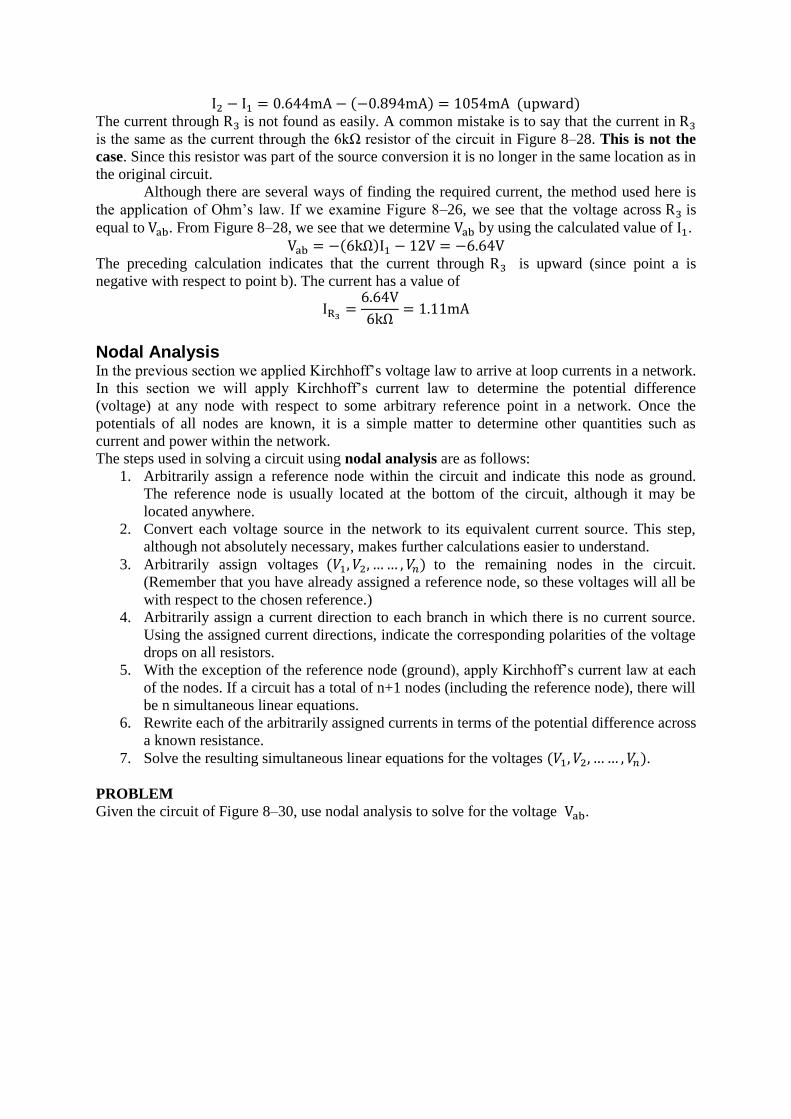
I2 − I1 = 0.644mA − (−0.894mA) = 1054mA (upward)

The current through R3 is not found as easily. A common mistake is to say that the current in R3

is the same as the current through the 6kΩ resistor of the circuit in Figure 8–28. This is not the

case. Since this resistor was part of the source conversion it is no longer in the same location as in

the original circuit.

Although there are several ways of finding the required current, the method used here is

the application of Ohm’s law. If we examine Figure 8–26, we see that the voltage across R3 is

equal to Vab. From Figure 8–28, we see that we determine Vab by using the calculated value of I1.

Vab = −(6kΩ)I1 − 12V = −6.64V

The preceding calculation indicates that the current through R3 is upward (since point a is

negative with respect to point b). The current has a value of

IR3=

6.64V

6kΩ= 1.11mA

Nodal Analysis In the previous section we applied Kirchhoff’s voltage law to arrive at loop currents in a network.

In this section we will apply Kirchhoff’s current law to determine the potential difference

(voltage) at any node with respect to some arbitrary reference point in a network. Once the

potentials of all nodes are known, it is a simple matter to determine other quantities such as

current and power within the network.

The steps used in solving a circuit using nodal analysis are as follows:

1. Arbitrarily assign a reference node within the circuit and indicate this node as ground.

The reference node is usually located at the bottom of the circuit, although it may be

located anywhere.

2. Convert each voltage source in the network to its equivalent current source. This step,

although not absolutely necessary, makes further calculations easier to understand.

3. Arbitrarily assign voltages (𝑉1, 𝑉2, … … , 𝑉𝑛) to the remaining nodes in the circuit.

(Remember that you have already assigned a reference node, so these voltages will all be

with respect to the chosen reference.)

4. Arbitrarily assign a current direction to each branch in which there is no current source.

Using the assigned current directions, indicate the corresponding polarities of the voltage

drops on all resistors.

5. With the exception of the reference node (ground), apply Kirchhoff’s current law at each

of the nodes. If a circuit has a total of n+1 nodes (including the reference node), there will

be n simultaneous linear equations.

6. Rewrite each of the arbitrarily assigned currents in terms of the potential difference across

a known resistance.

7. Solve the resulting simultaneous linear equations for the voltages (𝑉1, 𝑉2, … … , 𝑉𝑛).

PROBLEM

Given the circuit of Figure 8–30, use nodal analysis to solve for the voltage Vab.

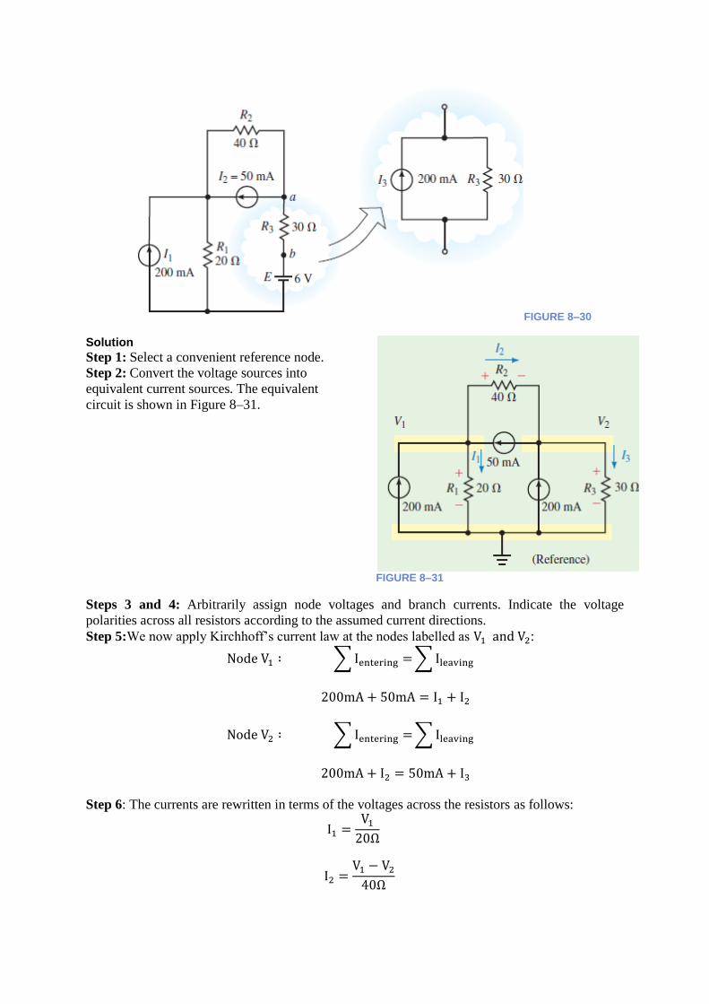
FIGURE 8–30

Solution

Step 1: Select a convenient reference node.

Step 2: Convert the voltage sources into

equivalent current sources. The equivalent

circuit is shown in Figure 8–31.

FIGURE 8–31

Steps 3 and 4: Arbitrarily assign node voltages and branch currents. Indicate the voltage

polarities across all resistors according to the assumed current directions.

Step 5:We now apply Kirchhoff’s current law at the nodes labelled as V1 and V2:

Node V1 ∶ ∑ Ientering = ∑ Ileaving

200mA + 50mA = I1 + I2

Node V2 ∶ ∑ Ientering = ∑ Ileaving

200mA + I2 = 50mA + I3

Step 6: The currents are rewritten in terms of the voltages across the resistors as follows:

I1 =V1

20Ω

I2 =V1 − V2

40Ω

I3 =V2

30Ω

The nodal equations become

200mA + 50mA =V1

20Ω+

V1 − V2

40Ω

200mA +V1 − V2

40Ω= 50mA +

V2

30Ω

Substituting the voltage expressions into the original nodal equations, we have the following

simultaneous linear equations:

(1

20Ω+

1

40Ω) V1 − (

1

40Ω) V2 = 0.25A

− (1

40Ω) V1 + (

1

30Ω+

1

40Ω) V2 = 0.15A

If we go back to the original circuit of Figure 8–30, we see that the voltage V2 is the same as the

voltage Va, namely

Va = 4.67V = 6V + Vab or Vab = 4.67V − 6V = −1.33V

PROBLEM

Determine the nodal voltages for the circuit shown in Figure 8–32.

FIGURE 8–32

Solution By following the steps outlined, the circuit may be redrawn as shown in Figure 8–33.

FIGURE 8–33

Applying Kirchhoff’s current law to the

nodes corresponding to V1 and V2, the

following nodal equations are obtained:

∑ Ientering = ∑ Ileaving

Node V1: I1 + I2 = 2A

Node V2: I3 + I4 = I2 + 3A

The currents may once again be written in terms of the voltages across the resistors:

I1 =V1

5Ω

I2 =V1 − V2

3Ω

I3 =V2

4Ω

I4 =V2

6Ω

The nodal equations become

Node V1 : V1

5Ω+

V1 − V2

3Ω= 2A

or (1

5Ω+

1

3Ω) V1 − (

1

3Ω) V2 = 2A

Node V2 : V2

4Ω+

V2

6Ω=

V1 − V2

3Ω+ 3A

or − (1

3Ω) V1 + (

1

4Ω+

1

6Ω+

1

3Ω) V2 = 3A

We may use any of the previously used methods to solve the simultaneous linear equations.

Consequently, the solutions for V1 and V2 are:

V1 = 8.65V and V2 = 7.85V Format Approach

A simple format approach may be used to write the nodal equations for any network having n + 1

nodes. Where one of these nodes is denoted as the reference node, there will be n simultaneous

linear equations, which will appear as follows:

G11V1 − G12V2 − G13V3 − ⋯ ⋯ ⋯ − G1nVn = I1

−G21V1 + G22V2 − G23V3 − ⋯ ⋯ ⋯ − G2nVn = I2

⋮ ⋮

−Gn1V1 − Gn2V2 − Gn3V3 − ⋯ ⋯ ⋯ + GnnVn = In

The coefficients (constants) G11, G22, G33, … . Gnn represent the summation of the

conductances attached to the particular node. The remaining coefficients are called the mutual

conductance terms. For example, the mutual conductance G23 is the conductance attached to

node V2, which is common to node V3. If there is no conductance that is common to two nodes,

then this term would be zero. Notice that the terms G11, G22, G33, … . Gnn are positive and that the

mutual conductance terms are negative. Further, if the equations are written correctly, then the

terms will be symmetrical about the principal diagonal— for example, G23 = G32.

The terms V1, V2, … … , Vn are the unknown node voltages. Each voltage represents the

potential difference between the node in question and the reference node.

The terms I1, I2, … … , In are the summation of current sources entering the node. If a

current source has a current such that it is leaving the node, then the current is simply assigned as

negative. If a particular current source is shared between two nodes, then this current must be

included in both nodal equations. The method used in applying the format approach of nodal

analysis is as follows:

1. Convert voltage sources into equivalent current sources.

2. Label the reference node as Label the remaining nodes as 𝑉1, 𝑉2, … … , 𝑉𝑛.

3. Write the linear equation for each node using the format outlined.

4. Solve the resulting simultaneous linear equations for 𝑉1, 𝑉2, … … , 𝑉𝑛.

The next examples illustrate how the format approach is used to solve circuit problems.

PROBLEM Determine the nodal voltages for the circuit shown in Figure 8–34.

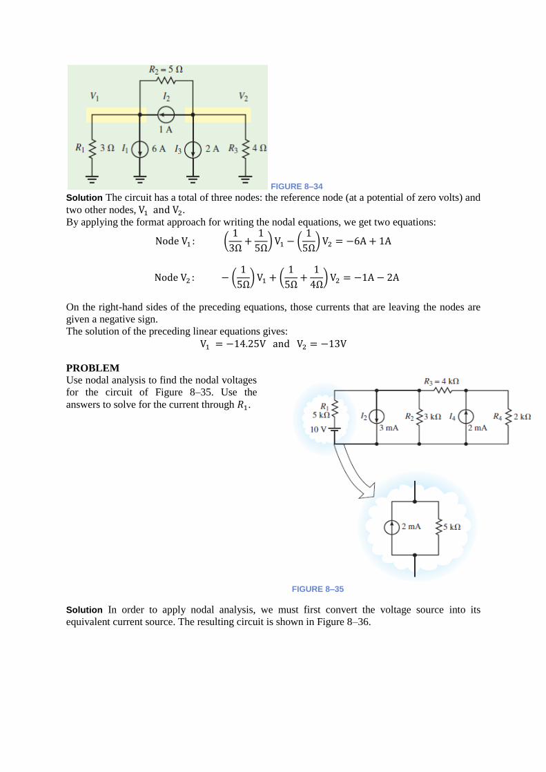
FIGURE 8–34

Solution The circuit has a total of three nodes: the reference node (at a potential of zero volts) and

two other nodes, V1 and V2.

By applying the format approach for writing the nodal equations, we get two equations:

Node V1 : (1

3Ω+

1

5Ω) V1 − (

1

5Ω) V2 = −6A + 1A

Node V2 : − (1

5Ω) V1 + (

1

5Ω+

1

4Ω) V2 = −1A − 2A

On the right-hand sides of the preceding equations, those currents that are leaving the nodes are

given a negative sign.

The solution of the preceding linear equations gives:

V1 = −14.25V and V2 = −13V

PROBLEM Use nodal analysis to find the nodal voltages

for the circuit of Figure 8–35. Use the

answers to solve for the current through 𝑅1.

FIGURE 8–35

Solution In order to apply nodal analysis, we must first convert the voltage source into its

equivalent current source. The resulting circuit is shown in Figure 8–36.

FIGURE 8–36 FIGURE 8–37

Labelling the nodes and writing the nodal equations, we obtain the following:

Node V1 : (1

5kΩ+

1

3kΩ+

1

4kΩ) V1 − (

1

4kΩ) V2 = 2mA − 3mA

Node V2 : − (1

4kΩ) V1 − (

1

4kΩ+

1

2kΩ) V2 = 2mA

Because it is inconvenient to use kilohms and milliamps throughout our calculations, we may

eliminate these units in our calculations. The solutions are as follows:

V1 = −0.476V and V2 = 2.51V

To determine the current through resistor𝑅1 = 5𝑘Ω, we first reassemble the circuit as it appeared

originally. Since the node voltage V1is the same in both circuits, we use it in determining the

desired current. The resistor may be isolated as shown in Figure 8–37.

The current is easily found as

𝐼 =10𝑉 − (−0.476𝑉)

5𝑘Ω= 2.10𝑚𝐴 (𝑢𝑝𝑤𝑎𝑟𝑑)

PROBLEM Example 2.39. Use Nodal analysis to determine the value of current i in the network of Fig. 2.73

We will apply KCL to the two nodes 1 and

2. Equating the incoming currents at node 1

to the outgoing currents, we have

6 =𝑉1 − 𝑉2

4+

𝑉1

8+ 3𝑖

Fig.2.73

As seen. i =V1

8 . Hence, the above equation becomes

6 =𝑉1 − 𝑉2

4+

𝑉1

8+ 3

𝑉1

8

0𝑟 3𝑉1 − 𝑉2 = 24 Similarly, applying KCL to node No. 2, we get

𝑉1 − 𝑉2

4+ 3𝑖 =

𝑉2

6

𝑜𝑟 𝑉1 − 𝑉2

4+ 3

𝑉1

8=

𝑉2

6

𝑜𝑟 3𝑉1 = 2𝑉2

From the above two equations, we get

𝑉1 = 16𝑉 𝑎𝑛𝑑 𝑖 =16

8= 2𝐴

Superposition Theorem The superposition theorem is a method that allows us to determine the current through or the

voltage across any resistor or branch in a network. The advantage of using this approach instead

of mesh analysis or nodal analysis is that it is not necessary to use determinants or matrix algebra

to analyze a given circuit. The theorem states the following:

In a linear network, if more than one number of sources (excitation) are acting, the

response in a certain branch can be obtained by superimposing algebraically the responses due

to various sources taking one excitation at a time and considering the remaining voltage sources

(ideal) short circuited or replaced by their equivalent internal impedances and current sources

(ideal) open circuited or replaced by their equivalent admittances.

NOTES... The superposition theorem does not apply to power, since power is not a linear quantity, but

rather is found as the square of either current or voltage.

PROBLEM Consider the circuit of Figure 9–1:

a. Determine the current in the load resistor,

RL. b. Verify that the superposition theorem does

not apply to power.

FIGURE 9–1

Solution

a. We first determine the current through RL due to the voltage source by removing the current

source and replacing in with an open circuit (zero amps) as shown in Figure 9–2.

FIGURE 9–2

The resulting current through RL is

determined from Ohm’s law as

IL(1) =20V

16Ω + 24Ω= 0.5A

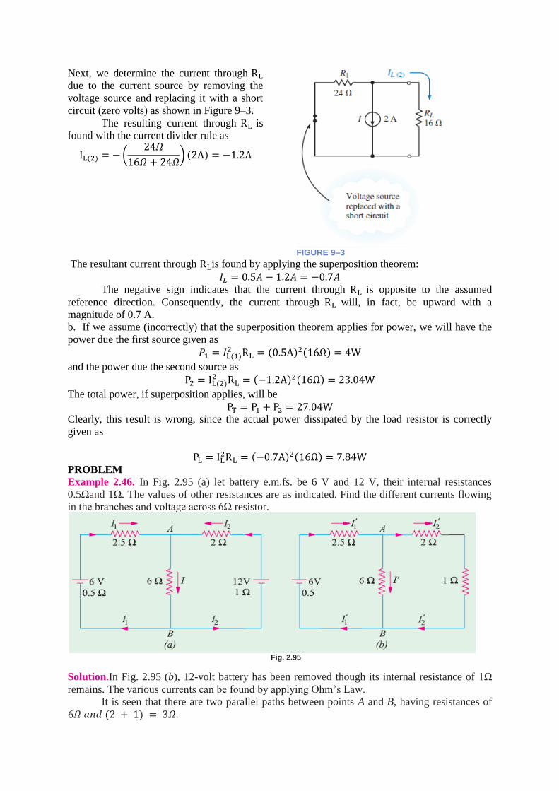
Next, we determine the current through RL

due to the current source by removing the

voltage source and replacing it with a short

circuit (zero volts) as shown in Figure 9–3.

The resulting current through RL is

found with the current divider rule as

IL(2) = − (24𝛺

16𝛺 + 24𝛺) (2A) = −1.2A

FIGURE 9–3

The resultant current through RLis found by applying the superposition theorem:

𝐼𝐿 = 0.5𝐴 − 1.2𝐴 = −0.7𝐴

The negative sign indicates that the current through RL is opposite to the assumed

reference direction. Consequently, the current through RL will, in fact, be upward with a

magnitude of 0.7 A.

b. If we assume (incorrectly) that the superposition theorem applies for power, we will have the

power due the first source given as

𝑃1 = 𝐼L(1)2 RL = (0.5A)2(16Ω) = 4W

and the power due the second source as

P2 = IL(2)2 RL = (−1.2A)2(16Ω) = 23.04W

The total power, if superposition applies, will be

PT = P1 + P2 = 27.04W Clearly, this result is wrong, since the actual power dissipated by the load resistor is correctly

given as

PL = IL2RL = (−0.7A)2(16Ω) = 7.84W

PROBLEM Example 2.46. In Fig. 2.95 (a) let battery e.m.fs. be 6 V and 12 V, their internal resistances

0.5Ωand 1Ω. The values of other resistances are as indicated. Find the different currents flowing

in the branches and voltage across 6Ω resistor.

Fig. 2.95

Solution.In Fig. 2.95 (b), 12-volt battery has been removed though its internal resistance of 1Ω

remains. The various currents can be found by applying Ohm’s Law.

It is seen that there are two parallel paths between points A and B, having resistances of

6𝛺 𝑎𝑛𝑑 (2 + 1) = 3𝛺.

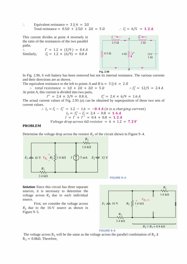
Equivalent resistance = 3 || 6 = 2𝛺 Total resistance = 0.5𝛺 + 2.5𝛺 + 2𝛺 = 5 𝛺 𝐼1

′ = 6/5 = 𝟏. 𝟐 𝑨.

This current divides at point A inversely in

the ratio of the resistances of the two parallel

paths.

∴ 𝐼′ = 1.2 × (3/9 ) = 0.4 𝐴

Similarly, 𝐼2′ = 1.2 × (6/9) = 0.8 𝐴

Fig. 2.96

In Fig. 2.96, 6 volt battery has been removed but not its internal resistance. The various currents

and their directions are as shown.

The equivalent resistance to the left to points A and B is = 3 || 6 = 2 𝛺

∴ 𝑡𝑜𝑡𝑎𝑙 𝑟𝑒𝑠𝑖𝑠𝑡𝑎𝑛𝑐𝑒 = 1𝛺 + 2𝛺 + 2𝛺 = 5 𝛺 ∴ 𝐼2′′ = 12/5 = 2.4 𝐴

At point A, this current is divided into two parts,

𝐼′′ = 2.4 × 3/9 = 0.8 𝐴, 𝐼1′′ = 2.4 × 6/9 = 1.6 𝐴

The actual current values of Fig. 2.95 (a) can be obtained by superposition of these two sets of

current values.

∴ 𝐼1 = 𝐼1′ − 𝐼1

′′ = 1.2 − 1.6 = −𝟎. 𝟒 𝑨 (𝑖𝑡 𝑖𝑠 𝑎 𝑐ℎ𝑎𝑟𝑔𝑖𝑛𝑔 𝑐𝑢𝑟𝑟𝑒𝑛𝑡) 𝐼2 = 𝐼2

′′ − 𝐼2′ = 2.4 − 0.8 = 𝟏. 𝟔 𝑨

𝐼 = 𝐼′ + 𝐼′ ′ = 0.4 + 0.8 = 𝟏. 𝟐 𝑨 𝑉𝑜𝑙𝑡𝑎𝑔𝑒 𝑑𝑟𝑜𝑝 𝑎𝑐𝑟𝑜𝑠𝑠 6𝛺 𝑟𝑒𝑠𝑖𝑠𝑡𝑜𝑟 = 6 × 1.2 = 𝟕. 𝟐 𝑽

PROBLEM

Determine the voltage drop across the resistor 𝑅2 of the circuit shown in Figure 9–4.

FIGURE 9–4

Solution Since this circuit has three separate

sources, it is necessary to determine the

voltage across 𝑅2 due to each individual

source.

First, we consider the voltage across

𝑅2 due to the 16-V source as shown in

Figure 9–5.

FIGURE 9–5

The voltage across R2 will be the same as the voltage across the parallel combination of R2 ∥R3 = 0.8kΩ. Therefore,

VR2(1) = − (0.8kΩ

0.8kΩ + 2.4kΩ) 16V = −4V

The negative sign in the preceding calculation simply indicates that the voltage across the

resistor due to the first source is opposite to the assumed reference polarity.

FIGURE 9–6 FIGURE 9–7

Next, we consider the current source. The resulting circuit is shown in Figure 9–6. From this

circuit, you can observe that the total resistance “seen” by the current source is

RT = R1 ∥ R2 ∥ R3 = 0.6kΩ

The resulting voltage across R2 is

VR2(2) = (0.6kΩ)(5mA) = 3V

Finally, the voltage due to the 32-V source is found by analyzing the circuit of Figure 9–7. The

voltage across R2is

VR2(3) = − (0.96kΩ

0.96kΩ + 1.6kΩ) 32V = 12V

By superposition, the resulting voltage is

VR2= VR2(1) + VR2(2) + VR2(3) = −4V + 3V + 12V = 11V

Thévenin’s Theorem In this section, we will apply one of the most important theorems of electric circuits. Thévenin’s

theorem allows even the most complicated circuit to be reduced to a single voltage source and a

single resistance.

Thévenin’s theorem is a circuit analysis technique that reduces any linear bilateral network to an

equivalent circuit having only one voltage source and one series resistor. The resulting two-

terminal circuit is equivalent to the original circuit when connected to any external branch or

component. In summary, Thévenin’s theorem is simplified as follows:

Any linear bilateral network may be reduced

to a simplified two-terminal circuit

consisting of a single voltage source in

series with a single resistor as shown in

Figure 9–9.

FIGURE 9–9

The following steps provide a technique that converts any circuit into its Thévenin equivalent:

1. Identify and remove the load from the circuit.

2. Label the resulting two terminals. We will label them as a and b, although any notation

may be used.

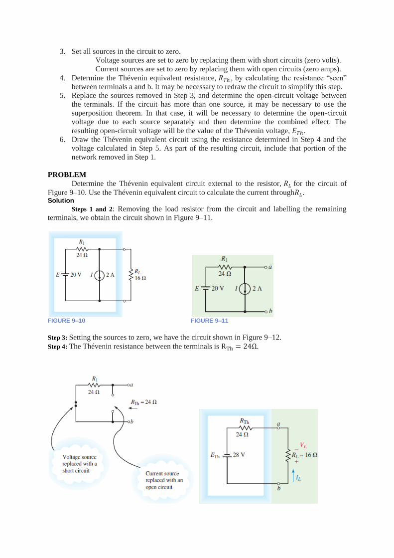
3. Set all sources in the circuit to zero.

Voltage sources are set to zero by replacing them with short circuits (zero volts).

Current sources are set to zero by replacing them with open circuits (zero amps).

4. Determine the Thévenin equivalent resistance, 𝑅𝑇ℎ, by calculating the resistance “seen”

between terminals a and b. It may be necessary to redraw the circuit to simplify this step.

5. Replace the sources removed in Step 3, and determine the open-circuit voltage between

the terminals. If the circuit has more than one source, it may be necessary to use the

superposition theorem. In that case, it will be necessary to determine the open-circuit

voltage due to each source separately and then determine the combined effect. The

resulting open-circuit voltage will be the value of the Thévenin voltage, 𝐸𝑇ℎ.

6. Draw the Thévenin equivalent circuit using the resistance determined in Step 4 and the

voltage calculated in Step 5. As part of the resulting circuit, include that portion of the

network removed in Step 1.

PROBLEM

Determine the Thévenin equivalent circuit external to the resistor, 𝑅𝐿 for the circuit of

Figure 9–10. Use the Thévenin equivalent circuit to calculate the current through𝑅𝐿. Solution

Steps 1 and 2: Removing the load resistor from the circuit and labelling the remaining

terminals, we obtain the circuit shown in Figure 9–11.

FIGURE 9–10 FIGURE 9–11

Step 3: Setting the sources to zero, we have the circuit shown in Figure 9–12.

Step 4: The Thévenin resistance between the terminals is RTh = 24Ω.

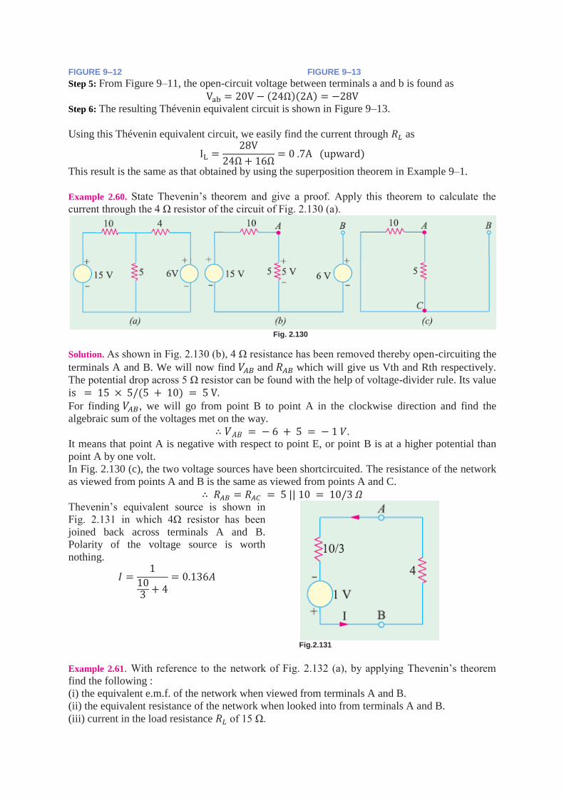
FIGURE 9–12 FIGURE 9–13

Step 5: From Figure 9–11, the open-circuit voltage between terminals a and b is found as

Vab = 20V − (24Ω)(2A) = −28V Step 6: The resulting Thévenin equivalent circuit is shown in Figure 9–13.

Using this Thévenin equivalent circuit, we easily find the current through 𝑅𝐿 as

IL =28V

24Ω + 16Ω= 0 .7A (upward)

This result is the same as that obtained by using the superposition theorem in Example 9–1.

Example 2.60. State Thevenin’s theorem and give a proof. Apply this theorem to calculate the

current through the 4 Ω resistor of the circuit of Fig. 2.130 (a).

Fig. 2.130

Solution. As shown in Fig. 2.130 (b), 4 Ω resistance has been removed thereby open-circuiting the

terminals A and B. We will now find 𝑉𝐴𝐵 and 𝑅𝐴𝐵 which will give us Vth and Rth respectively.

The potential drop across 5 Ω resistor can be found with the help of voltage-divider rule. Its value

is = 15 × 5/(5 + 10) = 5 V. For finding 𝑉𝐴𝐵, we will go from point B to point A in the clockwise direction and find the

algebraic sum of the voltages met on the way.

∴ 𝑉𝐴𝐵 = − 6 + 5 = − 1 𝑉. It means that point A is negative with respect to point E, or point B is at a higher potential than

point A by one volt.

In Fig. 2.130 (c), the two voltage sources have been shortcircuited. The resistance of the network

as viewed from points A and B is the same as viewed from points A and C.

∴ 𝑅𝐴𝐵 = 𝑅𝐴𝐶 = 5 || 10 = 10/3 𝛺 Thevenin’s equivalent source is shown in

Fig. 2.131 in which 4Ω resistor has been

joined back across terminals A and B.

Polarity of the voltage source is worth

nothing.

𝐼 =1

103 + 4

= 0.136𝐴

Fig.2.131

Example 2.61. With reference to the network of Fig. 2.132 (a), by applying Thevenin’s theorem

find the following :

(i) the equivalent e.m.f. of the network when viewed from terminals A and B.

(ii) the equivalent resistance of the network when looked into from terminals A and B.

(iii) current in the load resistance 𝑅𝐿 of 15 Ω.

Fig. 2.132

Solution. (i) Current in the network before load resistance is connected [Fig. 2.132 (a)]

=24𝑉

12 + 3 + 1 = 1.5 𝐴

∴ 𝑣𝑜𝑙𝑡𝑎𝑔𝑒 𝑎𝑐𝑟𝑜𝑠𝑠 𝑡𝑒𝑟𝑚𝑖𝑛𝑎𝑙𝑠 𝐴𝐵 = 𝑉𝑜𝑐 = 𝑉𝑡ℎ = 12 × 1.5 = 𝟏𝟖 𝑽 Hence, so far as terminals A and B are concerned, the network has an e.m.f. of 18 volt

(and not 24 V).

(ii) There are two parallel paths between points A and B. Imagine that battery of 24 V is removed

but not its internal resistance. Then, resistance of the circuit as looked into from point A and B is

[Fig. 2.132 (c)]

𝑅𝑖 = 𝑅𝑡ℎ = 12 ×4

12 + 4= 3 𝛺

(iii) When load resistance of 15 Ω is connected across the terminals, the network is reduced to

the structure shown in Fig. 2.132 (d).

𝐼 = 𝑉𝑡ℎ

𝑅𝑡ℎ + 𝑅𝐿

=18

15 + 3= 1𝐴

Example 2.65. Use Thevenin’s theorem to find the current in a resistance load connected between

the terminals A and B of the network shown in Fig. 2.138 (a) if the load is (a) 2 Ω (b) 1 Ω.

Solution. For finding open-circuit voltage 𝑉𝑜𝑐 𝑜𝑟 𝑉𝑡ℎ across terminals A and B, we must first

find current 𝐼2 flowing through branch CD. Using Maxwell’s loop current method, we have from

Fig. 2.131 (a).

−2𝐼1 − 4(𝐼1 − 𝐼2) + 8 = 0 𝑜𝑟 3𝐼1 − 2𝐼2 = 4

𝐴𝑙𝑠𝑜 − 2𝐼2 − 2𝐼2 − 4 − 4(𝐼2 − 𝐼1) = 0 𝑜𝑟 𝐼1 − 2𝐼2 = 1

From these two equations, we get 𝐼2 = 0.25 𝐴 As we go from point D to C, voltage rise = 4 + 2 × 0.25 = 4.5 𝑉 Hence, 𝑉𝐶𝐷 = 4.5 𝑜𝑟 𝑉𝐴𝐵 = 𝑉𝑡ℎ = 4.5 𝑉. Also, it may be noted that point A is positive with

respect to point B.

Fig. 2.138

In Fig. 2.138 (b), both batteries have been removed. By applying laws of series and parallel

combination of resistances, we get 𝑅𝑖 = 𝑅𝑡ℎ = 5/4 𝛺 = 1.25 𝛺. (i) When 𝑅𝐿 = 2 𝛺 ; 𝐼 = 4.5/(2 + 1.25) = 1.38 𝐴 (ii) When 𝑅𝐿 = 1 𝛺 ; 𝐼 = 4.5 (1 + 1.25) = 2.0 𝐴

Maximum Power Transfer Theorem In amplifiers and in most communication circuits such as radio receivers and transmitters, it is

often desired that the load receive the maximum amount of power from a source.

The maximum power transfer theorem states the following:

A load resistance will receive maximum power from a circuit when the resistance of the

load is exactly the same as the Thévenin resistance looking back at the circuit.

From Figure 9–45 we see that once the network has been simplified using Thévenin’s

theorem, maximum power will occur when

RL = RTH (9 − 3)

Proof:

Circuit current

𝐼𝐿 =ETH

RL+RTH

Power consumed by the load is

PL = 𝐼𝐿2RL =

ETH2 RL

(RL + RTH )2

− − − −(1)

For PLto be maximum, 𝑑PL

𝑑RL= 0

Differentiating equation (1), we have

𝑑PL

𝑑RL

= ETH2 [

1

(RL + RTH )2

+ RL (−2

(RL + RTH )3

)] = ETH2 [

1

(RL + RTH )2

−2RL

(RL + RTH )3

]

∴ 0 = ETH2 [

1

(RL + RTH )2

−2RL

(RL + RTH )3

]

or 2RL = RL + RTH or RL = RTH

FIGURE 9–45

Under maximum power conditions ( RL =RTH ), the preceding equations may be used

to determine the maximum power delivered

to the load and may therefore be written as

𝑃𝑚𝑎𝑥 =ETH

2

4RTH

=ETH

2

4RL

Example 2.115. In the network shown in Fig. 2.231 (a), find the value of RL such that maximum

possible power will be transferred to RL. Find also the value of the maximum power and the

power supplied by source under these conditions.

Solution. We will remove RL and find the equivalent Thevenin’s source for the circuit to

the left of terminals A and B. As seen from Fig. 2.231 (b) ETH equals the drop across the vertical

resistor of 3Ω because no current flows through 2 Ω and 1 Ω resistors.

Since 15 V drops across two series resistors of 3 Ω each, ETH = 15/2 = 7.5 𝑉. Thevenin’s resistance can be found by replacing 15 V source with a short-circuit.

As seen from Fig. 2.231 (b), RTH = 2 + (3 || 3) + 1 = 4.5 Ω. Maximum power transfer to the load will take place when RL = RTH = 4.5 Ω.

Fig. 2.231

Maximum power drawn by RL =ETH

2

4RL =

7.52

4× 4.5 = 3.125W.

Since same power in developed in Rth, power supplied by the source = 2 × 3.125 = 6.250 𝑊.

Report By: Dr. R.K.Das