Nonlinear viscoelastic wave propagation: an extension of Nearly Constant Attenuation (NCQ) models
Upload
khangminh22Category
view
0download
0
UNIVERSITY OF CALIFORNIA SAN DIEGO
Elastic and Thermal Wave Propagation based Techniques
for Structural Integrity Assessment
A dissertation submitted in partial satisfaction of the
requirements for the degree
Doctor of Philosophy in
Structural Engineering
by
Margherita Capriotti
Committee in charge:
Professor Francesco Lanza di Scalea, Chair
Professor Veronica Eliasson
Professor Hyonny Kim
Professor William Kuperman
Professor Thomas Liu
Professor Kenneth Loh
2019

Copyright
Margherita Capriotti, 2019
All rights reserved.

iii
The dissertation of Margherita Capriotti is approved, and it is
acceptable in quality and form for publication on microfilm and
electronically:
Chair
University of California San Diego
2019

iv
DEDICATION
to my parents,
who taught me love and freedom

v
EPIGRAPH
“ἐὰν μὴ ἔλπηται ανέλπιστον οὐκ ἐξευρήσει,
ανεξερεύνητον ἐὸν καὶ ἄπορον”
Ἡράκλειτος

vi
TABLE OF CONTENTS
SIGNATURE PAGE……………………………………………………………………………………………….…………iii
DEDICATION ................................................................................................................ iv
EPIGRAPH ....................................................................................................................... v
TABLE OF CONTENTS ................................................................................................ vi
LIST OF TABLES ........................................................................................................ viii
LIST OF FIGURES…………………………………………………………………………………………………………..…ix
ACKNOWLEDGEMENTS………………………………………………………………………………….………….xvi
VITA ............................................................................................................................... xx
ABSTRACT OF THE DISSERTATION ..................................................................... xxii
Chapter 1 Introduction ...................................................................................................... 1
1.1 Motivation ....................................................................................... 1
1.2 Approach ......................................................................................... 2
1.3 Outline of the dissertation ............................................................... 8
Chapter 2 Techniques of Elastic Wave Propagation .................................................... 11
2.1 Theory of Ultrasonic Guided Waves ............................................. 12
2.2 Analytical and Semi-analytical investigation ................................ 20
2.3 Global-Local model to predict scattering of guided elastic waves 30
2.3.1 Problem formulation ......................................................... 30
2.3.2 2D Case study: scattering of guided waves in skin-to-
stringer assembly of composite aircraft panels ................. 43
2.3.3 3D Case study: scattering of guided waves from internal
cracks in railroad tracks .................................................... 59
2.4 Application .................................................................................... 70
2.4.1 Test specimen and previous studies .................................. 70

vii
2.4.2 Nondestructive Inspection of Composite Aircraft Panels by
Ultrasonic Guided Waves and Statistical Processing ....... 81
2.4.3 Inspection of composite aerospace structures by extraction
of UGW transfer function ................................................. 94
Chapter 3 Techniques of Thermal Wave Propagation ................................................ 126
3.1 Background of Infrared Thermography: principles ................... 126
3.2 Theoretical Investigation ............................................................. 128
3.2.1 Theory of TW and Green’s function method.................. 128
3.2.2 Passive extraction of thermal Green’s function .............. 136
3.3 Numerical Investigation .............................................................. 140
3.3.1 Active thermal Green’s Function .................................... 140
3.3.2 Spatial discontinuity of Thermal Guided Waves ............ 144
3.4 Application: Composite Aerospace panels.................................. 149
Chapter 4 Comparison of UGW inspection of composite aerospace structures with UT
and CT datasets ............................................................................................................. 167
4.1 Introduction ................................................................................. 167
4.2 UGW features sensitivity to impact damage modes ................... 168
4.3 Correlation for quantitative damage characterization ................. 175
Chapter 5 Overall Conclusions and Future Recommendations ................................... 178
5.2 Elastic wave techniques .................................................................. 179
5.3 Thermal wave techniques ............................................................... 182
REFERENCES ............................................................................................................. 184
viii
LIST OF TABLES
Table 1 - Aluminum plate: Material properties ..................................................................................... 20
Table 2 - Composite plate: Layup .......................................................................................................... 22
Table 3 - Composite plate: Material properties ..................................................................................... 23
Table 4 - Composite plate: Equivalent material properties .................................................................... 23
Table 5 - Elastic properties for the CFRP lamina .................................................................................. 45
Table 6 - Rail AREMA 136 lbs Properties ............................................................................................ 61
Table 7 - Error of total energy: distance from boundary effect ............................................................. 69
Table 8 - Composite parts layup sequences ........................................................................................... 72
Table 9 - Contact technique features list. ............................................................................................... 86
Table 10 - Non-contact technique features list ...................................................................................... 90
Table 11- Layup and Lamina Elastic constants for the CFRP material. .............................................. 101

ix
LIST OF FIGURES
Figure 1 - Guided waves formation in plate .......................................................................................... 12
Figure 2 - Wave propagation and particle displacement in bulk isotropic medium. ............................. 13
Figure 3 - Displacement in anti-symmetric and symmetric modes........................................................ 19
Figure 4 - Analytical Dispersion curves for Aluminum plate in Table 1: (left) phase velocity, (right)
group velocity; anti-symmetric modes in red, symmetric modes in blue. ............................................. 20
Figure 5 - Local-Global reference system for multi-layered anisotropic plate. ..................................... 21
Figure 6 - Analytical Dispersion curves for Composite plate in Table 4Table 1: (left) phase velocity,
(right) group velocity; anti-symmetric modes in red, symmetric modes in blue. .................................. 23
Figure 7 - SAFE Dispersion curves for Aluminum plate: (top) phase velocity, (bottom) group velocity.
............................................................................................................................................................... 24
Figure 8 - In-plane (blue) and out-of-plane (red) displacements for modeshapes of A0 (left) and S0
(right) at 170 kHz for Aluminum plate. ................................................................................................. 25
Figure 9 - SAFE Dispersion curves for Composite plate in Table 2: (top) phase velocity, (bottom)
group velocity; (left) single laminate thickness, (right) double laminate thickness. ............................. 26
Figure 10 - In-plane (blue) and out-of-plane (red) displacements for modeshapes of A0 (left) and S0
(right) at 170 kHz for Composite plate. ................................................................................................. 27
Figure 11 - SAFE Dispersion curves for Composite plate (group velocity): comparison pristine (black)
and altered top surface layers (red). ....................................................................................................... 28
Figure 12 - In-plane (blue and black) and out-of-plane (red) displacements for modeshapes of A0 (left)
and S0 (right) modes for Composite plates: comparison pristine (solid) and altered surface layers
(dashed). ................................................................................................................................................. 29
Figure 13 - SAFE Dispersion curves for Composite plate (group velocity): comparison pristine (black)
and altered middle layers (red). ............................................................................................................. 29
Figure 14 - In-plane (blue and black) and Out-of-plane (red) displacements for modeshapes A0 (left)
and SH0 (right) modes for Composite plates: comparison pristine (solid) and altered middle layers
(dashed). ................................................................................................................................................. 30
Figure 15 - Geometrical representation of the scattering of an incident wave in a waveguide prismatic
structure in reflected and transmitted waves from a local region with geometrical and/or material
discontinuities. ....................................................................................................................................... 31
Figure 16 - Key steps of the Matlab GL code. ....................................................................................... 44
Figure 17 - Global-Local model of the composite skin-to-stringer assembly, with the four “defected”
configurations: delamination between skin and stringer (Defect 1), horizontal fracture in the stringer
heel (Defect 2), vertical fracture in the stringer cap (Defect 3), and delamination between 2nd and 3rd
laminae in the skin (Defect 4). ............................................................................................................... 45

x
Figure 18 - (left) Phase velocity dispersion curves and (right) group velocity dispersion curves for the
CFRP composite laminate (skin only) from the SAFE portion of the GL code. ................................... 47
Figure 19 - Skin laminate: (a) Transmission and reflection energy spectra and (b) cross-sectional
energy (Poynting vector) in the case of an m1 incident mode. (c) Transmission and reflection energy
spectra and (d) cross-sectional Poynting vector in the case of an m2 incident mode. ............................ 48
Figure 20 - Reflection and transmission energy spectra for (a) m1 incident mode and (b) m2 incident
mode in the skin-to-stringer pristine assembly. ..................................................................................... 50
Figure 21 - Scattering behaviour at specific frequencies (pristine skin-to-stringer assembly). (a)
Zoomed scattering spectra for the m1 incident mode with cross-sectional energy (Poynting vector) at
150 kHz (b) and at 200 kHz (c). Corresponding results for the m2 incident mode in (d), (e) and (f). . 51
Figure 22 - Defect 1 case (skin-stringer delamination). Wave transmission spectra for pristine, defect
and (defect-pristine) difference for (a) m1 incident - m1 transmitted; (b) m2 incident - m1 transmitted
(mode conversion); (c) m1 incident – m2 transmitted (mode conversion), and (d) m2 incident – m2
transmitted. ............................................................................................................................................ 53
Figure 23 - Defect 2 case (stringer heel crack). Wave transmission spectra for pristine, defect and
(defect-pristine) difference for (a) m1 incident - m1 transmitted; (b) m2 incident - m1 transmitted
(mode conversion); (c) m1 incident – m2 transmitted (mode conversion), and (d) m2 incident – m2
transmitted. ............................................................................................................................................ 54
Figure 24 - Defect 3 case (stringer cap crack). Wave transmission spectra for pristine, defect and
(defect-pristine) difference for (a) m1 incident - m1 transmitted; (b) m2 incident - m1 transmitted
(mode conversion); (c) m1 incident – m2 transmitted (mode conversion), and (d) m2 incident – m2
transmitted. ............................................................................................................................................ 56
Figure 25 - Defect 4 case (skin delamination). Wave transmission spectra for pristine, defect and
(defect-pristine) difference for (a) m1 incident - m1 transmitted; (b) m2 incident - m1 transmitted
(mode conversion); (c) m1 incident – m2 transmitted (mode conversion), and (d) m2 incident – m2
transmitted ............................................................................................................................................. 57
Figure 26 - Global-local model for 3D application on rail track. .......................................................... 61
Figure 27 - GL dispersion curves for railroad track: (left) phase velocity, (right) group velocity. ....... 62
Figure 28 - Mode 5: modeshapes side view for in-plane displacement (left), front-view for out-of-
plane displacement (right)...................................................................................................................... 62
Figure 29 - Mode 9: modeshapes side view for in-plane displacement (left), front-view for out-of-
plane displacement (right)...................................................................................................................... 63
Figure 30 - Reflection and transmission energy spectra for (left) m5 incident mode and (rigth) m8
incident mode in the pristine rail. .......................................................................................................... 63
Figure 31 - Reflection and transmission energy spectra for m5 incident mode in the defected head of
the rail by (a) 15%, (b) 50%, (c) 85% and (d) 100%. ............................................................................ 64
Figure 32 - Reflection and transmission energy spectra for m8 incident mode in the defected head of
the rail by (a) 15%, (b) 50%, (c) 85% and (d) 100%. ............................................................................ 65

xi
Figure 33 - Size of the Local region and element size study on mode 1 incident: (a) 10cm, (b) 20cm,
(c) 40cm. ................................................................................................................................................ 66
Figure 34 - Reflection/transmission energy spectra for m5 incident: study on number of max scattered
mode included in the analysis: (a) 20 modes, (b) 50 modes, (c) 100 modes, (d) 150 modes. ............... 68
Figure 35 - Reflection/transmission energy spectra for m2 (left) and m5 (right) incident on 100% H.A.
defect in a 20cm (top) vs a 40cm (bottom) rail. ..................................................................................... 69
Figure 36 - HEWABI project phase I: damage formation with 1D impact on panel (experimental
setup). ..................................................................................................................................................... 71
Figure 37 - 3D-printed hold-down mounts for transducers on outer skin .............................................. 73
Figure 38 - Different levels of disassembly for UGW tests: (a) full assembly with C-frame and shear
ties, (b) C-frame only removed, (c) C-frame and shear ties removed.................................................... 73
Figure 39 - Assembling/disassembling test results: (a) skin-only vs. entire assembly and (b) skin and
shear ties vs. entire assembly. ................................................................................................................ 74
Figure 40 - Conjoined panels by C-frame to study wave propagation in C-frame only: (left) outside
skin view, (right) inside skin view. ........................................................................................................ 75
Figure 41 - Conjoined panels tests result: (left) 50kHz, (right) 150kHz received waveform. ............... 75
Figure 42 - Angle tuning for mode selection in air-coupled transducer excitation/reception: (left)
orientation of the sensors, (right) phase velocity selection. ................................................................... 77
Figure 43 - Laser scanning test setup on composite panel: (left) fixed air-coupled receivers and
scanned region on specimen, (right) laser and optics used for excitation. ............................................. 77
Figure 44 - Time signal at node 1 for two air-coupled receivers (top and bottom): (a) aluminum plate
and (b) composite plate. ......................................................................................................................... 78
Figure 45 - FFT of signal at node 1 for A0 and S0 modes: (a) aluminum plate and (b) composite plate.
............................................................................................................................................................... 78
Figure 46 -2D FFT for experimental extraction of dispersion curves: (a) aluminum plate and (b)
composite plate. ..................................................................................................................................... 79
Figure 47 - Experimental dispersion curves (phase velocity): (a) aluminum plate and (b) composite
plate ........................................................................................................................................................ 79
Figure 48 – Data from experimental extraction of dispersion curves. Composite plate at node 1: (a)
gated time signal, (b) FFT of A0 mode, (c) time-frequency CWT, and (d) experimental dispersion
curve (group velocity) for A0 mode. ..................................................................................................... 80
Figure 49 - Test specimens: (a) Panel 1: five stringers, three C-frames panel with cracked skin and
cracked stringer; (b) Panel 2: four stringers, three C-frames panel with disbonded/detached stringer;
(c) Panel 3: three stringers, two C-frames panel with cracked skin, detached/cracked stringer and
disbonded stringer. ................................................................................................................................. 82
Figure 50 - (a) Schematic of the UGW approach for the aerospace panel inspection. (b) Differential
xii
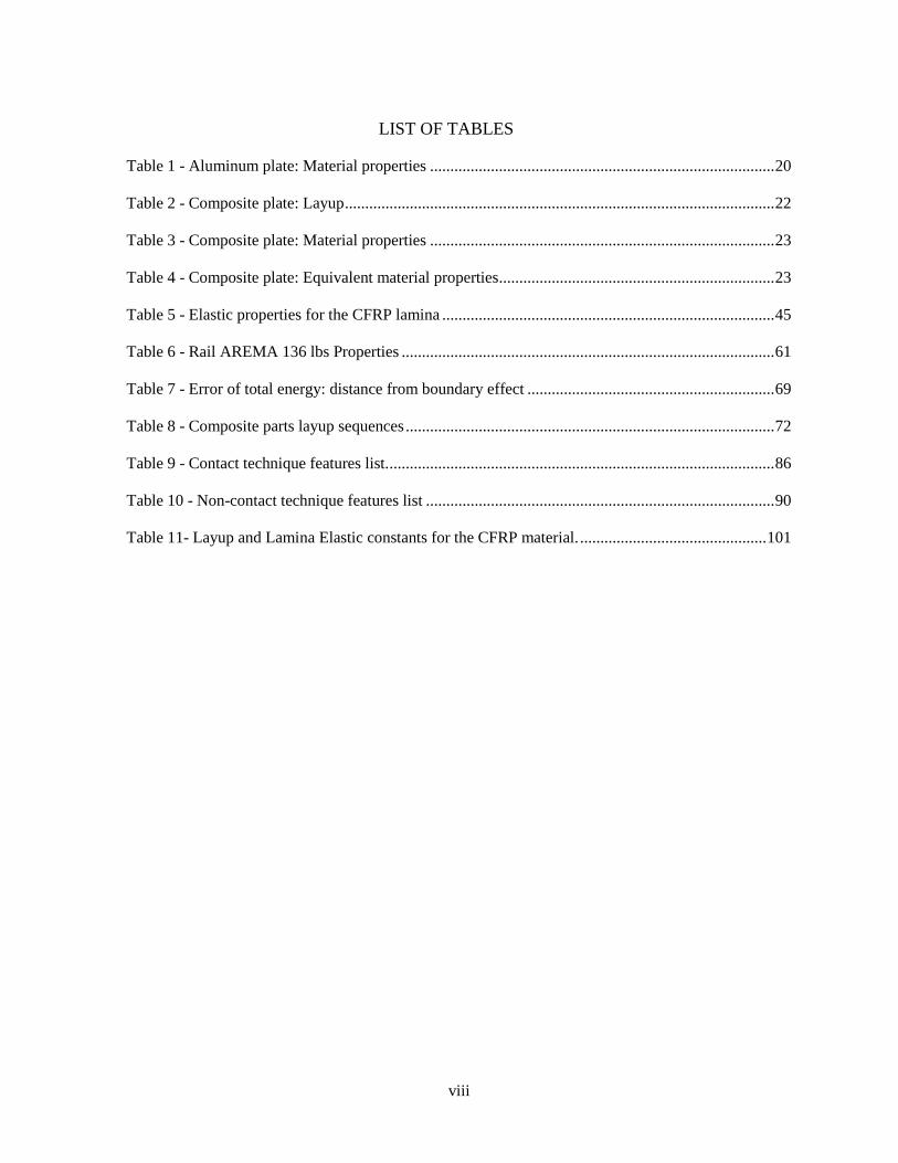
scheme for contact inspection. ............................................................................................................... 83
Figure 51 - FE model of a stiffened composite panel: (a) 3D view; (b) cross-sectional view showing
multi-mode wave propagation and acoustic inter-talk between the skin, stringer and shear ties. ......... 84
Figure 52 - Line scanning approach for (a) contact system and (b) non-contact system; cross-sectional
view (top drawings) and front view (bottom drawings). ....................................................................... 84
Figure 53 - Representative results from contact UGW scans: (a) Panel 1, (b) Panel 2. ........................ 87
Figure 54 - Amplitude Ratio from contact UGW scans: (a) Panel 1, (b) Panel 2 .................................. 88
Figure 55 - Non-contact air-coupled scanning prototype experimental setup on Panel 3. .................... 89
Figure 56 - Typical RF waveform measured by the air-coupled pitch-catch prototype from Panel 3. .. 89
Figure 57 - Representative results from noncontact (air-coupled) UGW scans of Panel 3: (a) skin
modes only; (b) skin modes plus stringer modes ................................................................................... 90
Figure 58 - Maximum Amplitude from non-contact UGW scans: Panel 3 ........................................... 91
Figure 59 - ROC curves for the contact NDE technique: cracked skin, disbonded stringer and detached
stringer defects (Panel 1 and Panel 2). ................................................................................................... 92
Figure 60 - ROC curves for the non-contact NDE technique (skin modes only): cracked skin, detached
stringer and disbonded stringer defects (Panel 3). ................................................................................. 92
Figure 61 - ROC curves for the non-contact NDE technique (skin and stringer modes): cracked skin,
detached stringer and disbonded stringer defects (Panel 3). .................................................................. 93
Figure 62 - Portable cart-scan set-up (left) with corresponding typical low SNR RF waveforms at
specific defective locations (right): cracked skin (top, red), detached/cracked stringer (center, black),
disbonded stringer (bottom, green), with respect to pristine location (blue). ........................................ 95
Figure 63 - Extraction of the structural transfer function between two points A and B by a single-
input-dual-output (SIDO) scheme. ......................................................................................................... 96
Figure 64 - Schematic of the SAFE method for modeling ultrasonic guided wave propagation in
laminated composites. ............................................................................................................................ 98
Figure 65 – Extraction of transfer function in composite laminate “skin”. ......................................... 101
Figure 66 – CFRP laminate skin: (a) response measured by receiver 1; (b) response measured by
receiver 2; (c) experimental transfer function in the frequency domain; (d) experimental transfer
function in the time domain; (e) comparison between experimental and numerical (SAFE) transfer
functions............................................................................................................................................... 103
Figure 67 – SAFE solutions for the CFRP laminate skin for 0 deg wave propagation direction: (a)
phase velocity dispersion curves; (b) group velocity dispersion curves; (c)-(e) cross-sectional
displacement profiles for modes S0, SH0 and A0 at 170 kHz. .............................................................. 105
Figure 68 – The CFRP stiffened panel “A” with defects. .................................................................... 106

xiii
Figure 69 - The CFRP stiffened panel “B” with defects...................................................................... 107
Figure 70 -The SIDO air-coupled scanning system for defect detection in the stiffened panels. ........ 109
Figure 71 - The SIDO hybrid impact/air-coupled scanning system for defect detection in the stiffened
panels. .................................................................................................................................................. 110
Figure 72 - Air-coupled system: (a), (b) raw waveforms received by the two receivers; (c)
reconstructed transfer function. ........................................................................................................... 111
Figure 73 - Hybrid impact/air-coupled system: (a), (b) raw waveforms received by the two receivers;
(c) reconstructed transfer function; (d) filtered transfer function (low frequency range); (e) filtered
transfer function (high frequency range). ............................................................................................ 113
Figure 74 - Effect of the stringer flange impact damage on the time-domain transfer functions: (a) air-
coupled system; (b) hybrid impact/air-coupled system (full bandwidth); (c) hybrid impact/air-coupled
system (low frequency range); (d) hybrid impact/air-coupled system (high frequency range). .......... 115
Figure 75 - Effect of the stringer cap impact damage on the time-domain transfer functions: (a) air-
coupled system; (b) hybrid impact/air-coupled system (full bandwidth); (c) hybrid impact/air-coupled
system (low frequency range); (d) hybrid impact/air-coupled system (high frequency range). .......... 117
Figure 76 - Damage Index traces from one scan through the stringer heel slit and the stringer cap slit
in panel A: (a) result from the air-coupled system; (b) result from the hybrid impact/air-coupled
system (full bandwidth); (c) result from the hybrid impact/air-coupled system (low frequencies vs.
high frequencies). ................................................................................................................................. 119
Figure 77 - Damage Index traces from one scan through the stringer flange impact in panel A: (a)
result from the air-coupled system; (b) result from the hybrid impact/air-coupled system (full
bandwidth); (c) result from the hybrid impact/air-coupled system (low frequencies vs. high
frequencies). ......................................................................................................................................... 121
Figure 78 - Damage Index traces from scans through the stringer cap impacts (30 J, 50 J and 70 J) in
panel B: (a) result from the air-coupled system; (b) result from the hybrid impact/air-coupled system
(full bandwidth); (c) result from the hybrid impact/air-coupled system (low frequencies vs. high
frequencies). ......................................................................................................................................... 123
Figure 79 - Planck's Law (left: linear scale; right: logarithmic scale): spectral radiant emission versus
wavelength ........................................................................................................................................... 127
Figure 80 - Green's function in space domain for different time instants: (left) diffusivity of PVC;
(right) diffusivity of Steel .................................................................................................................... 130
Figure 81 - Green's function in time domain for varying diffusivity values: (left) at x=2mm; (right) at
x=4mm ................................................................................................................................................. 130
Figure 82 - Heat propagation within a finite medium as a reflecting thermal wave ............................ 133
Figure 83 - Analytical frequency domain temperature distribution in finite medium: top surface (top),
bottom surface (bottom); at 1 Hz (left) and at 100 Hz (right). ............................................................. 134
Figure 84 - Analytical time domain temperature distribution in finite medium: top surface (left),
bottom surface (right), at y=0 and for varying distances x from the source x=0 ................................. 135
xiv
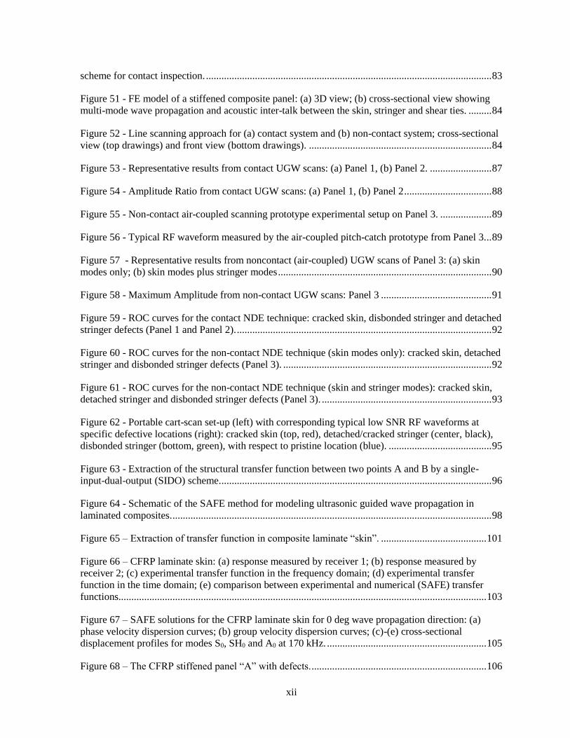
Figure 85 - Schematic of inverse scattering principle .......................................................................... 139
Figure 86 - Passive reconstruction of Green’s function: application to thermal waves. ...................... 139
Figure 87 - FEM Heat propagation in pristine Aluminum plate: geometry (left), heat wave propagation
as Temperature (right) ......................................................................................................................... 140
Figure 88 - FEM Heat propagation and defect interaction in Aluminum plate: geometry (left), heat
wave propagation as Heat flux (right) ................................................................................................. 141
Figure 89 - FEM temperature response: at source (left), at receivers on pristine side (center), at
receivers on defective side (right). ....................................................................................................... 142
Figure 90 - Cross-correlation of FEM temperature time histories: (top) between source and receivers
on pristine side, (bottom) between source and receivers on defective side. ........................................ 143
Figure 91 - Cross-correlation of FEM temperature time histories: (top to bottom) increasing distance
from source, between source and receivers on pristine side (blue), between source and receivers on
defective side (red). .............................................................................................................................. 143
Figure 92 - Cross-correlation of FEM temperature time histories: (left) peak value, (right) lag of peak,
for pairs of increasing distance from source, between source and receivers on pristine side (blue),
between source and receivers on defective side (red). ......................................................................... 144
Figure 93 - TGW in FEM pristine Aluminum plate ............................................................................ 145
Figure 94 - TGW in FEM Aluminum plate with slit ........................................................................... 146
Figure 95 - TGW in FEM Aluminum plate with corrosion ................................................................. 147
Figure 96 - FEM Slit in Aluminum plate, time histories along x: temperature (top left), spatial
derivative of temperature (top right), heat resultant (bottom left), heat x dir (bottom right) ............... 148
Figure 97 - FEM Corrosion in Aluminum plate, time histories along x: temperature (top left), spatial
derivative of temperature (top right), heat resultant (bottom left), heat x dir (bottom right) ............... 149
Figure 98 - TSR representative 1D plots (left, Shepard and Lhota, 2014): logarithmic Temperature
(top); 1st time derivative (center); 2nd time derivative (bottom); Scheme of specimen corresponding to
the TSR 1D plots (right). ..................................................................................................................... 152
Figure 99 - 3D Heat diffusion in a defective specimen: virtual heat source interpretation (Manohar,
2015) .................................................................................................................................................... 152
Figure 100 - Secondary cooling dependence on defect aspect ratio .................................................... 153
Figure 101 - Thermographic test on composite panels: skin side mode (left), stringer side mode (right)
............................................................................................................................................................. 155
Figure 102 - TSR Thermogrpahy test: Flange 90J impact. 1D plots (left); 2D maps (right) raw
Temperature (top), 1st derivative (center), 2nd derivative (bottom) at two time instants ...................... 158
Figure 103 - TSR Thermogrpahy test: Flange 90J impact, "stringer side". 1D plots (left); 2D maps
(right) raw Temperature (top left), 1st derivative early instant (bottom left), 1st derivative middle

xv
instant (top right), 1st derivative later instant (bottom right) ............................................................... 159
Figure 104 - TSR Thermogrpahy test: Flange 90J impact, "stringer side". 1D plots (left); 2D maps
(right) raw Temperature (top left), 2nd derivative early instant (bottom left), 2nd derivative middle
instant (top right), 2nd derivative later instant (bottom right) ............................................................. 160
Figure 105 - TSR Thermogrpahy test comparison: Flange 70J (left) vs 90J (right) impact, "stringer
side". 2D maps of 2nd derivative:early (top), middle (center), later (bottom) instants ....................... 161
Figure 106 - TSR Thermogrpahy test: Cap 50J impact, "stringer side". 1D plots (left); 2D maps (right)
raw Temperature (top left), 1st derivative early instant (bottom left), 1st derivative middle instant (top
right), 1st derivative later instant (bottom right) .................................................................................. 163
Figure 107 - TSR Thermogrpahy test: Cap 50J impact, "stringer side". 1D plots (left); 2D maps (right)
raw Temperature (top left), 2nd derivative early instant (bottom left), 2nd derivative middle instant
(top right), 2nd derivative later instant (bottom right) ......................................................................... 164
Figure 108 - TSR Thermogrpahy test comparison: Cap 30J (left) vs 50J (center) vs 70J (right) impact,
"stringer side". 2D maps of 2nd derivative:early (top), middle (center), later (bottom) instants......... 165
Figure 109 - Scheme of damaged panels: Panel A(left) and Panel B (right). ...................................... 169
Figure 110 - TF extracted from UGW scan inspection on Panel A with gated wavemodes: hybrid (left)
and non-contact (right) prototype. ....................................................................................................... 169
Figure 111 - Typical waveforms of pristine (blue) and defective (red) locations for flange damage
(left) and cap damage (right). ............................................................................................................... 170
Figure 112 - Phase based features versus location for 90J flange impacted stringer, hybrid prototype:
skewness (pink). From top left to bottom right: gate1, gate2, gate3, gate4, gate1+gate2, gate2+gate3,
gate3+gate4, entire signal. ................................................................................................................... 172
Figure 113 - Energy based features versus location for 90J flange impacted stringer, hybrid prototype:
RMS (red), area under FFT (yellow), maximum peak in FFT (green). From top left to bottom right:
gate1, gate2, gate3, gate4, gate1+gate2, gate2+gate3, gate3+gate4, entire signal. .............................. 172
Figure 114 - Energy based features extracted from 90J (left) and 70J (right) flange impacted stringer,
non-contact prototype. ......................................................................................................................... 173
Figure 115 - Energy based features versus location for cap impacted stringer, hybrid prototype: RMS
(red), area under FFT (yellow), maximum peak in FFT (green). From top left to bottom right: gate1,
gate2, gate3, gate4, gate1+gate2, gate2+gate3, gate3+gate4, entire signal. ........................................ 174
Figure 116 - Phase based features versus location for cap impacted stringer, hybrid prototype:
Skewness (pink). From top left to bottom right: gate1, gate2, gate3, gate4, gate1+gate2, gate2+gate3,
gate3+gate4, entire signal. ................................................................................................................... 174
Figure 118 - Correlation analyses between UGW extracted feature (red) and UT extracted feature: skin
damage (left), disbond (center) and undamaged flange (right). ........................................................... 176
Figure 117 - UT on 90J flange impact damage: extracted pixel count (left), time of flight segmented
map (right) versus location. Skin damage (red), disbond (green), flange damage (blue), undamaged
flange (white), undamaged skin (black). .............................................................................................. 176

xvi
ACKNOWLEDGEMENTS
I would like to profoundly acknowledge my advisor Prof. Lanza di Scalea, for the innumerable
opportunities he gave me, the trust in me and my work and the encouraging technical and personal
guidance. His enthusiasm for research, determination and honesty have always been fundamental and
will always be a reference point in my future.
I am truly grateful to Prof. Kim, who has always supported me and my research and has treated
me like one of his students. His positive attitude, technical expertise and wholesome person have been
of great endorsement to my research years.
Thanks to my Committee, who supported my research with enthusiasm and dedication. In
particular, thanks to Prof. Eliasson, who always gave a smile to my work, to Prof. Kuperman, for the
stimulating discussions and wise teachings, to Prof. Liu, for the inspiring lectures and availability, to
Prof. Loh, who advised me and made me feel as one of his students.
Most of my work is the result of the collaboration with Eric H. Kim, supporting each other
through struggles and successes. It has been a pleasure to work and grow with him, his patience,
kindness and resourceful expertise.
My gratitude goes to Antonino Spada, whose long-lasting collaboration was and is of extreme
importance to my research. His precise and expert knowledge together with his understanding and kind
persona supported me, even in the hardest moments.
A profound thank goes to the past and present members of the NDE/SHM Laboratory at UCSD:
I am happy to have worked with all of you and your technical and personal skills. Thank you to Stefano
Mariani, Thompson Nguyen, Xuan “Peter” Zhu, Simone Sternini (and the Uptown Funk times), Ranting
Cui and Diptojit Datta. A special thanks goes to Albert Liang, for his honest smile and invaluable
collaboration.
Thank you to the students of the Structural (and others) Deparment at UCSD: we supported and
encouraged each other’s work and goals, relying on scientific and human esteem. Thanks to Sumit
Gupta, Andrew Ellison, Ben Katko, Ernesto Criado Hidalgo, Francesco Fraternali.
xvii
I have been extremely lucky to meet many amazing women within UCSD: Negin Nazarian,
Sohini Manna, Niki Vazou, Ivana Escobar, Nathalì Cordero, Hanna Asefaw, Valeria Leone, Anya
Lefler, thank you for inspiring me and reminding me that it is not only possible but even better to be a
woman, scientist and human at the same time.
A special thanks goes to another Woman, Luciana Leone, whose sensitivity, strength and truth
I esteem and are beyond words: our bond is deeper and stronger than any fried parmigiana. Thank you
(& Giadina & Jonathan) for always cheering for me.
Thank you to my Tourmaline family, who encouraged me to be simply myself and enjoy it,
making my PhD years an intense and joyful adventure. Thank you to Marta “piuppazzachemmai”
Francesconi, Maria “La Mari” Ferraro, Amedeo Minichino, Mohammed Ghonima and Ryan Hanna,
who have always provided me with sincere advices, hugs and pushes, full of sweetness and spirit.
A sincere and full-of-love thank goes to my now SD family, who supported me in the toughest
moments with patience, understanding, enthusiasm and flavorful adventures: Andrei Pissarenko,
Lorenzo Casalino and Martina Audagnotto.
Thank you also to the Greek! friendship of “Kostas” Anagnostopoulos, “Dimo” Giamouridis,
Andreas Prodromou and George Koss; and to the curiously cynic one of Lorenzo Capriotti, Alessandra
Caselli, Matteo Marcozzi and Matteo Pellegri.
I would also like to acknowledge Jonathan Nussman, who, through “other sounds”, understood
me and helped me deeply, and Professor Bonazza, whose e-advice was key to this journey.
Thank you to my American families for always being ready to celebrate my achievements and
dreams: thank you to Zia Gail & Zio Sal, Diana, Laurie & Will, Christian & Olivia, David & Kathy,
Ken & Darlene, Zia Sharon, Mia & Anna, Mr. Yang. I am very happy to keep our crazy roots alive and
full of smiles.
A silently loud Thank You! goes to my closest friends, now far away, who never abandoned me
and constantly supported me with patience, determination and soul: Sara Spinozzi, Alessandro
Buonfigli, Irene Rossi, Mattia Bernetti, Roberto Savino.

xviii
All of my work is dedicated to and made possible by my parents, Patrizia and Giuseppe, who
taught me and have always given me unconditional love and unlimited freedom, understanding and
supporting the research, within and outside me.
Thank you to my sisters, Susanna and Annachiara, who are with me wherever I go as infinite
source and destination of pure love.
The greatest acknowledgement flies to Handa, whose gentle but firm love I never doubted of,
filling every aspect of my PhD research with soulful joy, novelty and curiosity.
I am deeply thankful and extremely enjoyed all the sweat, thoughts, silences, shouts, laughs and
tears we shared in these intense research years.
The research presented in Chapter 2 of this dissertation was supported by the Federal Aviation
Administration (FAA), under the Cooperative Agreement 12-C-AM-UCSD. I would like to thank
especially Dr. Larry Ilcewicz, who enthusiastically supported our research efforts and ideas.
The research presented in Chapter 3 was partially funded by the National Science Foundation
NSF, under the research grant CMMI-20140771.
Part of the research was also supported by the US Federal Railroad Administration under grant
FR-RRD-0027-11-01, with former program manager Mahmood Fateh and current program manager
Robert Wilson.
Chapter 2, Section 2.3, in full, has been submitted for publication of the material as it may
appear in International Journal of Solids and Structures 2019. Spada, Antonino; Capriotti, Margherita;
Lanza di Scalea, Francesco. The dissertation author was the second investigator and author of this
paper.
Chapter 2, Section 2.3.3, in full, is currently being prepared for submission for publication of
the material. Spada, Antonino; Capriotti, Margherita; Lanza di Scalea, Francesco. The dissertation
author was the second investigator and author of this material.
Chapter 2, Section 2.4.1, in part, is coauthored with Kim, Hyungsuk E. The dissertation author
was the primary author of this chapter.
xix
Chapter 2, Section 2.4.2, in full, is a reprint of the material as it appears in Materials Journals
2017. Capriotti, Margherita; Kim, Hyungsuk E.; Lanza di Scalea, Francesco; Kim, Hyonny. The
dissertation author was the primary investigator and author of this paper.
Chapter 2, Section 2.4.3, in full, has been submitted for publication of the material as it may
appear in Journal of Intelligent Material Systems and Structures 2019. Capriotti, Margherita; Lanza di
Scalea, Francesco. The dissertation author was the primary investigator and author of this paper.
Chapter 3, Section 3.4, in part, is currently being prepared for submission for publication of the
material. Capriotti, Margherita; Ellison, Andrew; Kim, Hyungsuk E.; Lanza di Scalea, Francesco; Kim,
Hyonny. The dissertation author was the primary investigator and author of this material.
Chapter 4, in full, is currently being prepared for submission for publication of the material.
Capriotti, Margherita; Ellison, Andrew; Kim, Hyungsuk E.; Lanza di Scalea, Francesco; Kim, Hyonny.
The dissertation author was the primary investigator and author of this material.

xx
VITA
2012 B. Sc. Mechanical Engineering, Università degli Studi di Parma, Italy
2014 M. Sc. Mechanical Engineering, Università degli Studi di Parma, Italy
2019 Ph. D. Structural Engineering, University of California San Diego
PUBLICATIONS
Spada, A., Capriotti, M., Lanza di Scalea, F., (in preparation). “Global-Local Model to predict
scattering of multiple and dispersive guided elastic waves: 3D application on railroad tracks”,
International Journal of Solids and Structures.
Capriotti, M., Ellison A., Kim H.E., Kim H., Lanza di Scalea, F., (in preparation). “Data Fusion and
Correlation of Ultrasonic guided waves inspection with other conventional NDE techniques for
composite aerospace structures”, Composite Structures.
Capriotti, M., Lanza di Scalea, F., (submitted). “Robust non-destructive inspection of composite
aerospace structures by extraction of ultrasonic guided-wave transfer function in single-input-dual-
output scanning systems”, Journal of Intelligent Material Systems and Structures.
Spada, A., Capriotti, M., Lanza di Scalea, F., (submitted). “Global-Local Model to predict scattering
of multiple and dispersive guided elastic waves in solids”, International Journal of Solids and
Structures.
Spada A., Capriotti M., Lanza di Scalea F., (2019). “Improved global-local model to predict guided-
wave scattering patterns from discontinuities in complex parts”, Proc.SPIE SMART STRUCTURES
AND MATERIALS + NONDESTRUCTIVE EVALUATION AND HEALTH MONITORING 2019,
vol. 10972.
Capriotti M., Cui R., Lanza di Scalea F., (2019). “Guided wave techniques for damage detection and
property characterization in composite aerospace structures”, Proc.SPIE SMART STRUCTURES
AND MATERIALS + NONDESTRUCTIVE EVALUATION AND HEALTH MONITORING 2019,
vol. 10972.
Lanza di Scalea F., Liang A., Sternini S., Capriotti M., Datta D., Zhu X., (2019). “Passive extraction
of Green’s function of solids and application to high-speed rail inspection”, Proc.SPIE SMART
STRUCTURES AND MATERIALS + NONDESTRUCTIVE EVALUATION AND HEALTH
MONITORING 2019, vol. 10970.
Lanza di Scalea, F., Zhu, X., Capriotti, M., Liang, A., Mariani, S., and Sternini, S., (2018). “Passive
Extraction of Dynamic Transfer Function from Arbitrary Ambient Excitations: Application to High
speed Rail Inspection from Wheel-generated Waves”, ASME Journal of Nondestructive Evaluation,
Diagnostics and Prognostics of Engineering Systems, 1(1), pp. 0110051- 01100512.
xxi
Capriotti M., Kim H. E., Lanza di Scalea F., Kim, H., (2017). “Non-Destructive Inspection of Impact
Damage in Composite Aircraft Panels by Ultrasonic Guided Waves and Statistical Processing”,
Materials Journal, Special Issue "Structural Health Monitoring for Aerospace Applications 2017",
10(6), 616; doi:10.3390/ma10060616.
Capriotti M., Cui R., Lanza di Scalea F., (2018). “Damage detection and visco-elastic property
characterization of composite aerospace panels using ultrasonic guided waves”, Proceedings of the
2018 Annual Conference of Experimental and Applied Mechanics, Mechanics of Composite, Hybrid
and Multifunctional Materials, vol.5.
Capriotti M., Kim H. E., Lanza di Scalea F., Kim, H., (2017). “Detection of major impact damage to
composite aerospace structures by ultrasonic guided waves and statistical signal processing”, X
International Conference on Structural Dynamics, EURODYN 2017.
Capriotti M., Sternini S., Lanza di Scalea F., (2017). “Passive Infrared Thermography for Defect
Detection and Imaging in Structures by Correlation of Diffuse Thermal Fields”. Society for
Experimental Mechanics, Annual Conference.
Capriotti M., Kim H. E., Lanza di Scalea F., Kim, H., (2017). “Development of an Ultrasonic
Nondestructive Inspection Method for Impact Damage Detection in Composite Aircraft Structures”,
Proc.SPIE SMART STRUCTURES AND MATERIALS + NONDESTRUCTIVE EVALUATION
AND HEALTH MONITORING 2017, vol.10169, doi: 10.1117/12.2258669
Capriotti M., Sternini S., Mariani S., Lanza di Scalea F., (2016). “Extraction of thermal Green’s
function using diffuse fields: a passive approach applied to thermography”, Proc.SPIE SMART
STRUCTURES AND MATERIALS + NONDESTRUCTIVE EVALUATION AND HEALTH
MONITORING 2016, vol. 9803, doi:10.1117/12.2218998

xxii
ABSTRACT OF THE DISSERTATION
Elastic and Thermal Wave Propagation based Techniques
for Structural Integrity Assessment
by
Margherita Capriotti
Doctor of Philosophy in Structural Engineering
University of California San Diego, 2019
Professor Francesco Lanza di Scalea, Chair
Non Destructive Evaluation (NDE) is a fundamental step in several phases of the lifespan
of structures. It aims at assessing the structure’s state of health to guarantee its proper functioning.
An added requirement of any NDE technique is to avoid any damage to the structure during the
actual test.
NDE of aircraft structures, in particular, is a crucial process to guarantee passenger safety
and ensure effective maintenance. Current visual inspection and lifespan estimation of aircraft are
not able to properly assess the health status of structures, especially when damage is present in the

xxiii
interior and is thus not visible. Composite aircrafts, in particular, are subjected to a wide variety
of damages that can develop in areas that are not directly accessible from the outside.
The main application of this research comes from the need for an NDE tool that can help
establishing the requirement for further inspections following a Ground-Service Equipment (GSE)
impact or similar event on a composite aircraft. A successful technique for this application must
be able to easily and rapidly inspect the structure, accessing it only from the outside, and detect
defects in a statistically reliable manner.
This dissertation studies the physics of propagation of elastic and thermal waves and their
interaction with material properties and discontinuities, combined to advanced signal processing,
for the purpose of damage detection and structural integrity assessment, with particular attention
to stiffened composite panels typical of modern commercial aircraft construction.
1
Chapter 1
Introduction
1.1 Motivation
Non Destructive Evaluation (NDE) is a fundamental step in several phases of the lifespan of
structures, that aims at assessing the structure’s health status and ensuring its quality. NDE includes a
variety of techniques, of different physical nature and levels of complexity of operation and interpretation
of the results, that all share the characteristic of not affecting the structure’s function. It is often employed
for damage detection and localization, but can extend to more quantitative outcomes, including property
characterization and residual strength estimation.
NDE of aircraft structures, in particular, is a crucial process to ensure passenger safety, industry
cost savings and technological advancements. Current visual inspection and lifespan estimation of aircraft
are not able to properly assess the health status of aircraft, especially when hidden damage is present in the
interior and can compromise the integrity of the overall assembly.
The vast majority of modern military and commercial aircrafts (e.g. B787, A380) is made of fiber-
reinforced composite materials, owing to their high strength-to-weight and stiffness-to-weight ratios
(Ashby, 1993). The complexities of the manufacturing process, for both the composite material itself and
the assembly, as well as the severity of external loads, in flight and during land operations, can develop a
2
number of structural defects that need to be detected and quantified through NDE techniques.
Composite aircraft, in particular, are subjected to a wide variety of damage that are very difficult
to avoid and visually detect. The formation and propagation of damage in such materials is still open to
further investigations and is unknown, especially if compared to metal. The Federal Aviation
Administration (FAA), together with other agencies and companies, are very interested in understanding
the causes and consequences of damages in aerospace structures and are currently devolving huge efforts
in trying to develop protocols for such materials (FAA Advisory Circular, 2009; CMH-17, 2017). Damages
have been categorized in 5 levels according to their severity and load carrying capacity (Ilcewitz, 2013),
with 5 being the most severe. High Energy Wide Area Blunt Impacts (HEWABI), due for example to
Ground Service Equipment (GSE) maneuvers, are very common during aircraft operation and can cause
major damages to the structure that are often not visible from the outside (Kim et al., 2014). Such impacts
are characterized by forces of large magnitudes and long time scales (DeFrancisci, 2013) and can severely
affect the structural integrity of key components (e.g. damage to stiffeners and C-frames), most of which
are internal, and thus challenging to access from a one-sided (external-only) NDE inspection.
1.2 Approach
Ultrasonic guided waves are an ideal candidate for this kind of inspection of composite aircraft
(Staszewsky et al., 2004).
“Guided” elastic waves are widely used to probe structural components with waveguide geometries
(plates, rod, pipes, etc..) in both NDE and Structural Health Monitoring (SHM) applications. Lamb waves,
for example, are specific guided waves in traction-free isotropic plates. Guided waves can maximize the
inspection range by exploiting the long propagation distances, while maintaining a sufficient sensitivity to
small structural anomalies (e.g. defects) owing to the relatively large frequencies (~ 100’s kHz for typical
plate-like structures). However, the propagation of guided waves is complicated by their multimode
character (several wave modes propagating simultaneously) and dispersive character (propagation velocity
3
is a function of frequency). Additional complications exist in the case of anisotropic layered components
(e.g. laminated composites) and/or built-up structures (e.g. stiffened panels) where the guided wave crosses
elements of varying thickness along its path.
Analytical solutions of guided wave propagation through multi-layered structures exist using well
known global matrix or transfer matrix methods (Rose, 2014). However, purely theoretical predictions
become quite challenging, or non-existent, in the presence of structural discontinuities such as defects.
Datta et al. (1988) used an approximated stiffness method to study guided dispersive propagation in
laminated anisotropic plates. Castaings et al. (2002) applied the modal decomposition method to analyze
scattering of an incident symmetric (axial) S0 or anti-symmetric (flexural) A0 Lamb mode by an internal
or an opening crack in isotropic plates, imposing velocity and stress continuity conditions at the crack
section. An improved analytical approach to predict Lamb waves scattering from a step geometrical
discontinuity considering a complex mode expansion with vector projection was recently proposed by
Giurgiutiu and co-workers (Podder and Giurgiutiu, 2016a, 2016b; Haider et al., 2018). These studies apply
to isotropic plates with thickness changes, presence of stiffeners, and horizontal cracks or disbonds. These
problems can be modelled by adjacent sub-regions with rectangular geometry (sub-plates).
Numerical methods can provide more flexibility to handle more complicated geometries and
defects. Guo and Cawley (1993), for example, applied the Finite Element (FE) method to investigate the
interaction of the S0 Lamb mode with delaminations at different interfaces in a composite laminate.
However, in order to maximize computational efficiency and maintaining accuracy at small wavelengths,
it is often not optimum to carry out an FE analysis for the entire domain. When the structural details and
anomalies are only a localized region of the entire “waveguide” panel, a hybrid Global-Local approach is
more appropriate. Hybrid methods couple the solution available analytically in the “global” region with
that available numerically (BEM or FEM) in the “local” region with the structural discontinuity. The
general hybrid method to predict elastic wave scattering based on a FE discretization of the local region
was utilized for axisymmetric inclusions in homogeneous isotropic media (Goetschel et al., 1982), other
axially-symmetric scattering problems (Rattanawangcharoen et al., 1997), isotropic plates with notches and

4
rivet-hole cracks (Chang and Mal, 1999; Mal and Chang, 2000; Zhou and Ichchou, 2011), defects in lap-
shear joints of isotropic plates (Chang and Mal, 1995), and isotropic plates with a normal transversely
isotropic weld (Al-Nassar et al., 1991). The problem of reflections of a fixed cracked edge was addressed
by Karunasena et al. (1995), while the scattering from a semi-infinite plate employing the BEM method for
the local part was studied by Galan and Abascal (2002), who later extended their BE-FE technique to plates
with inclusions, different cracks and materials (Galan and Abascal, 2005).
Other works focused on guided wave scattering in composite plates. The use of a hybrid FE local
discretization coupled with a boundary integral representation of the global part was investigated by Datta
et al. (1992) for the case of a uniaxial composite plate. Boundary integral formulations were utilized to
study scattering from interface cracks in a layered half-space and layered fiber—reinforced composites
(Karim and Kundu, 1988; Karim et al., 1989; Karim et al., 1992). FE local-global techniques were applied
to scattering in layered composite laminates with delaminations (Tian et al., 2004) and free edges (Dong
and Goetschel, 1982).
The vast majority of these previous works utilized theoretical solutions (mostly normal mode
expansion) to model the guided wave propagation in the global portion of the isotropic or composite plate.
However, such theoretical guided wave solutions are increasingly difficult to obtain for an anisotropic
composite laminate with a general number of layers. For this reason some of the authors of the present work
have recently exploited the numerical efficiency of the Semi-Analytical Finite Element method (SAFE)
(Hayashi et al., 2003; Bartoli et al. 2006; Marzani et al., 2008) to deal with the global portion of the GL
scattering problem in composite plates of arbitrary number of layers with delamination defects (Srivastava
and Lanza di Scalea, 2010). A similar use of SAFE in Global-Local scattering problems for layered
composites was shown later by Ahmad et al. (2013). The SAFE method only requires the FE discretization
of the cross-section of the laminate composite, and utilizes basic theoretical harmonic wave solutions in the
wave propagation direction. SAFE easily deals with the particular composite lay-up by simply rotating the
stiffness matrix of each layer in the wave propagation direction. In a Global-Local framework, the SAFE
global solutions are matched to the FE local solutions through continuity of displacements and tractions at
5
the local-global boundaries, as customary of hybrid approaches. Efficient wave propagation prediction, of
a variety of incoming/refracted UGW modes and for several geometrical built-ups and/or defect cases, can
be of great aid to the pre- and post- phases of experimental tests.
A number of studies have dealt with experimental tests of guided wave probing of components with
waveguide geometries, such as aircraft fuselage and wing panels (Raghavan and Cesnik, 2007; Croxford et
al., 2007; Staszewski et al., 2004; Rose, 2014; Giurgiutiu, 2015). Applications of ultrasonic guided waves
to detect structural damage in composites are numerous (e.g. Karim and Kundu, 1988; Kundu and Desai,
1989; Datta et al., 1988 and 1992; Guo and Cawley, 1993; Tian et al., 2004; Kessler et al., 2002; Lowe et
al., 2004; Matt et al., 2005; Banerjee et al., 2007; Ihn and Chang, 2008; Salas and Cesnik, 2009; Srivastava
and Lanza di Scalea, 2010; Sohn et al., 2011; Hudson et al., 2015; He and Yuan, 2015; Murat et al., 2016;
Ricci et al., 2016; Poddar and Giurgiutiu, 2016a and 2016b; Capriotti et al., 2017; Chong et al., 2017).
Generally, ultrasonic guided-wave test methods aim at detecting possible damage by identifying an
“anomalous” behavior of the structure as the ultrasonic energy travels from one point A to another point B.
Therefore, damage detection becomes an issue of extracting the structural “transfer function” between A
and B (HAB). In a practical test implementation, this transfer function is generally a frequency band-passed
version of the broadband acoustic Green’s function because it only applies to the useful frequency range
afforded by the ultrasonic transducers used to excite and detect the wave motion.
The extraction of the transfer function of the structure (i.e. without the effect of the excitation and
detection wave transduction paths) is essential to compare testing results to numerical or theoretical models
aimed at characterizing the damage that is being detected. The vast majority of guided-wave tests are
implemented in a “Single-Input-Single-Output” (SISO) mode, where an ultrasonic transmitter is used in
conjunction with a signal ultrasonic receiver. The extraction of the structure’s transfer function in this case
requires a deconvolution of the excitation from the reception - as well known since the 70’s in equivalent
electrical engineering applications (Roth, 1971). However, the precise excitation spectrum into the
structure is difficult to determine because it results from a convolution of the excitation signal, the
transmitting transducer frequency response, and the transducer-to-structure coupling frequency response
6
(which is generally unknown).
In addition, guided-wave inspection of structural components often requires some kind of scanning
of either the test part or the ultrasonic transducers to spatially map potential damage. Scanning can be most
efficiently performed by non-contact means of wave transduction (e.g. laser-based, air-coupled, water-
based). In these cases, extracting the pure transfer function of the structure without biases from the
excitation and detection response spectra is even more challenging because of the possible transduction
variations through the scan.
In light of the above requirements, a more robust guided-wave inspection test compared to the SISO
approach is to utilize a “dual-output” approach where the transfer function is extracted between two
receiving points. This is the approach used, for example, in “passive” structural monitoring utilizing
random excitations (e.g. operational loads on the structure), where it becomes essential to eliminate the
effects of the acoustic excitation source because generally uncontrolled (Farrar and James, 1997; Lobkis
and Weaver, 2001; Michaels and Michaels, 2005; Salvermoser et al., 2015; Snieder and Safak, 2006; Sabra
et al., 2007 and 2008; Duroux et al., 2010; Tippmann et al., 2015; Tippmann and Lanza di Scalea, 2015 and
2016; Lanza di Scalea et al., 2018a and 2018b). The “dual-output” approach has the best chance of
minimizing the effect of the energy transductions paths and isolating the true structural transfer function
that is the only metric affected by the presence of possible damage. It was recently shown in a couple of
different inspection scenarios (Snieder and Safak, 2006; Lanza di Scalea et al., 2018a and 2018b) how the
transfer function extraction in a dual-output approach is best conducted by performing a deconvolution
operation between the two receivers.
For remote inspection and 2D field imaging, NDE has relied also on InfraRed (IR) thermography.
A quite exhaustive review of the technique can be found in Shull (2002). IR Thermography allows for ease
and practicality in the experimental set-up and implementation, especially when large structures such as
aircrafts need to be inspected, and visualization of the results, providing a ready to use heat map of the
entire specimen, with no further need of interpretation. Especially when involving thin wide structures,
such as composite airplane fuselages or wings, IR thermography offers the possibility to inspect and image
7
subsurfaces, exploiting heat diffusion, detecting typical crucial damages as disbonds, delaminations and
cracks.
Theoretically, heat propagation has been studied for centuries. Cole and Beck et al., (2010)
thoroughly describe heat propagation in terms of Green’s Functions, relying on the fundamental theoretical
work by Morse & Feshback (1953) and Carslaw & Jaeger (1959). The interpretation of heat diffusion as
thermal waves has been investigated by numerous scientists (Marin, 2002; Marin et al., 2010, Ozisik and
Tzou, 1994). Mostly, Mandelis (Mandelis, 1995; Mandelis, 2013) and his co-workers (Nicolaideis et al.,
2000; Kaiplavil et al., 2012; Kaiplavil et al., 2014) think about the thermal field as the result of the
“propagation” of waves of fluctuating temperature, formulate the mathematical expression and apply it for
imaging in a variety of fields, according to specific signal processing techniques (Tabatabaei et al., 2009;
Tabatabaei et al., 2012).
While the passive GF retrieval by cross-correlation of diffuse fields has been fully demonstrated
(Lobkis and Weaver, 2001) and applied by numerous scientists in seismology, civil engineering (Snieder
and Safak, 2006), oceanography (Sabra et al., 2005) and SHM (Tippman et al., 2015; Lanza di Scalea et
al., 2018), as mentioned above, no experimental relevance has still been reported for thermal waves. Snieder
has extended the approach to other physics, including electromagnetics, optics and non-elastic fields, and
has generalized the formulation in terms of energy principles.
The exploitation of heat propagation and temperature evolution for inspection and imaging
translates into the IR thermography technique. Meola and Carlomagno in 2004 presented an exhaustive
review on the principles of IR thermogaphy and the recent advances in its main implementation techniques
(i.e. pulse thermography PT and lock in thermography). Servais et al. in 2008 used IR thermography for
the characterization of manufacturing and maintenance of aerospace composite discontinuities, relying on
on time and frequency methods. Ibarra-Castanedo et al. in 2007 and Lopez et al. in 2014 applied PT to
aerospace structures for a qualitative and quantitative assessment, exploiting and comparing three different
processing methods. In particular Flash Thermography processed according to the Thermal Signal
Reconstruction (TSR) method, proposed by Sheperd (2004), established an effective and more quantitative

8
approach of adopting IR thermography in NDE inspections. Shepard (2007) and his co-workers (Lhota,
2014; Frendberg, 2014; Oswald-Tranta, 2017), explain and discuss the method; many scientists and
applications adopted it, as in Roche et al., 2014. All of the above literature exploits temporal discontinuities
in the cooling evolution of temperature, after Lau et al in 1991 and Vavilov et al. in 1992 understood the
potential of the huge database offered by a video of 2D temperature maps, which constituted the recording
of the propagation of thermal waves.
Spatial discontinuities can also be exploited, in particular if spot or linear heat sources are applied:
Varis et al. (1995) discuss the evolution of heat in space in layered anisotropic carbon fiber composites,
Grinzato et al. (1998) apply it for NDE of frescoes, while Siakavellas et al. (2012) use line heating
thermography for the detection of cracks at fastener holes. The actual spatial deviation of thermal images
is proposed and used by Li et al. (2011) for crack imaging by laser-line and laser-spot thermography.
1.3 Outline of the dissertation
In this work, both elastic and thermal waves are discussed and investigated with the common
application to the NDE of composite structures used in modern commercial aircraft construction.
Chapter 2 describes elastic wave propagation.
In Section 2.1, the theory of ultrasonic guided waves introduces this propagation phenomenon and
NDE technique in aluminum and composite plates are reviewed.
In Section 2.2, a numerical approach (Global Local method) is presented. Predicting the scattering
behaviour of ultrasonic waves in the presence of specific structural defects is essential to (a) properly guide
the experimental implementation of an NDT/SHM test through proper selection of mode-frequency
combinations, and (b) provide quantitative, rather than qualitative information on a defect from knowledge
of the given defect’s scattering pattern. Such wave propagation predictions are very challenging in fuselage
and wing aircraft components that are anisotropic, multi-layered, and stiffened by built-up stringers.
Experiments using guided wave inspection of composite aerospace panels are presented in Section

9
2.3. This section describes a method that utilizes Ultrasonic Guided Waves (UGWs), non-contact
transducers and statistical processing to achieve the above-mentioned goals. The need for rapid inspection
of the structure points to UGWs as suitable candidates. The focus is on the detection of impact damage in
the aircraft (FAA, Composite aircraft structures, 2009), and on the development of a field-applicable
method. To do so, non-contact air-coupled ultrasonic transducers are employed in a scanning mode.
Section 2.4 discusses the “dual-output” approach of extracting the structural transfer function as
applied to a UGW test scenario, and implements this method in two scanning systems that are utilized for
damage detection in composite aircraft panels. This work is part of a larger research effort (Capriotti et al.,
2017) aimed at developing inspection systems for detecting impact-caused damage in parts representative
of commercial aircraft construction (e.g. B787 and A380). The work focuses on stiffened fuselage panels
consisting of a composite skin and co-cured composite stringers. Results are first shown for a composite
plate (skin-only) to compare the experimentally determined guided-wave transfer functions to that predicted
by a Semi-Analytical Finite Element (SAFE) method. The section then discusses the results of two scanning
systems utilizing the “dual-output” scheme, one based on a total air-coupled approach and the other one
based on a hybrid impact/air-coupled approach.
Chapter 3 describes thermal wave propagation.
In Section 3.1, the basic principles of IR thermography are explained.
This is followed by a theoretical investigation of heat diffusion in Section 3.2. The latter is
composed of a first introduction of heat propagation as thermal waves and its solution by the Green’s
function (GF) method. The formulation of temperature distribution in terms of GF solutions is exploited
for the theoretical derivation of thermal Green’s function retrieval, in a passive manner. Most of the
theoretical derivation for the thermal field in Section 3.2 relies on the analogies and differences between
the hyperbolic wave equation and parabolic heat diffusion equation and is derived from Snieder’s work on
the GF extraction for the diffusion equation (Snieder, 2006).
Section 3.3 presents numerical analyses of heat propagation in plates, for pristine and defective
10
cases. The simulations involve processing of temperature time histories for the retrieval of active thermal
Green’s functions, in time domain and spatial domain. In particular, the exploitation of the spatial domain
employs spot size and linear heat sources.
Lastly, the application of IR thermography to the NDE of composite aerospace structures and
damage detection is presented in Section 3.4. Flashed Thermography combined with the Thermographic
Signal Reconstruction (TSR) method, as proposed by Sheperd (2004), are employed on impacted composite
panels where different impact energies and types have generated damage on the flange and cap of the
stiffeners. The beneficial effect of the TSR processing on this experimental NDE approach is shown and
damage information can be inferred, besides detection only. The work relies also on the interpretation of
the defect as a virtual (or secondary) heat source, as observed by Manohar in his PhD thesis and related
works (Manohar et al., 2013).
Chapter 4 correlates UGWs measurements for quantitative damage characterization, gathering the
findings from elastic and thermal waves techniques. Section 4.1 motivates the work and describes the
datasets. In Section 4.2 features are extracted from the UGW measurements to understand their sensitivity
to specific damage modes. In Section 4.3, such features are correlated to ultrasonic C-scan, X-ray computed
tomography scan and IR thermography to detect and characterize specific damage modes.
In the last chapter (Chapter 5), the overall conclusions and future recommendations are provided.
11
Chapter 2
Techniques of Elastic Wave Propagation
The propagation of ultrasonic waves in a not infinite medium (semi-infinite or bounded) generates
a specific type of waves, named ultrasonic guided waves. The boundaries of the medium, as those given by
a half-space or a finite geometry, interact with the travelling wave so that boundary conditions can be
satisfied.
When ultrasonic longitudinal and shear waves propagate into waveguides as rods, tubes, thin plates
or multi-layered structures, they reflect back and forth inside the waveguide at certain angles, due to the
high mismatch in acoustic impedance at the boundaries, leading to interference phenomena (Figure 1). For
the particular incident angle and frequency chosen, the interference phenomena could be constructive,
destructive or intermediate.
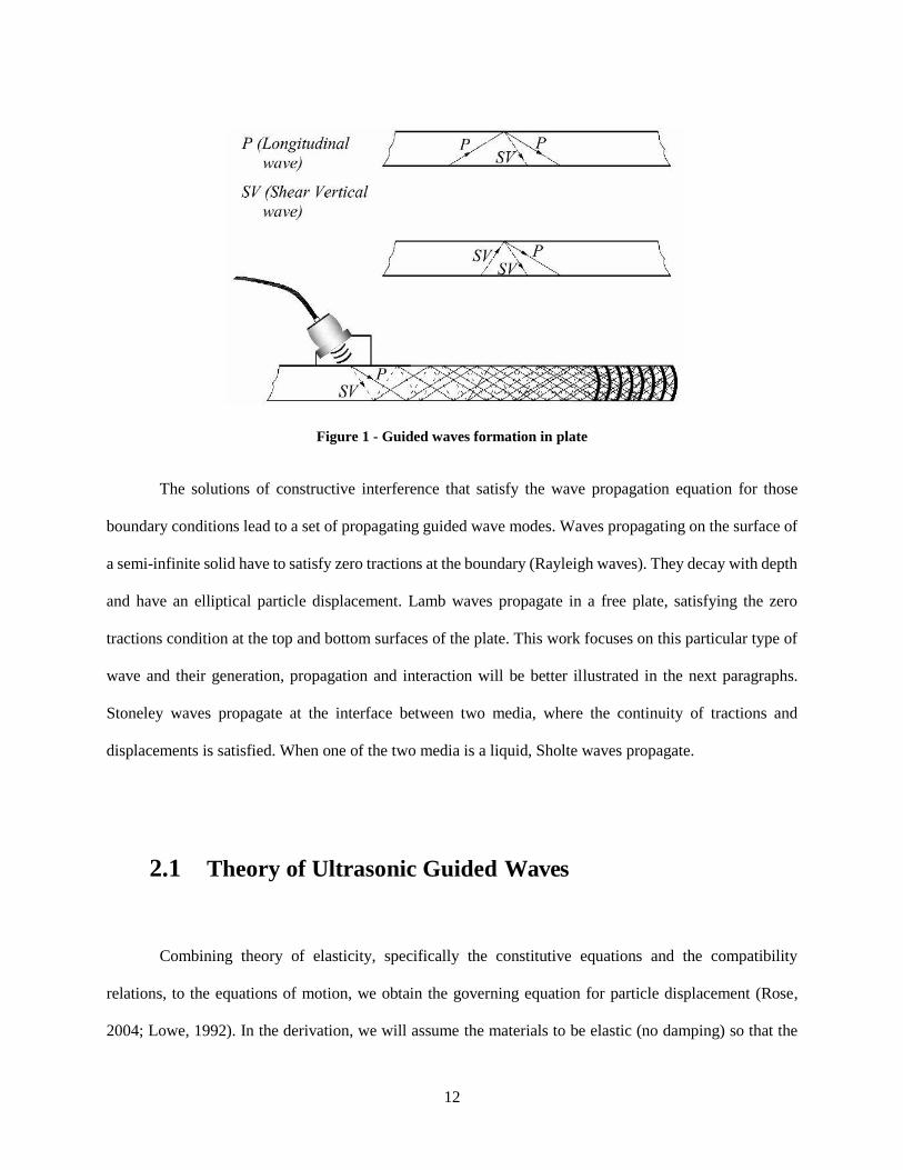
12
Figure 1 - Guided waves formation in plate
The solutions of constructive interference that satisfy the wave propagation equation for those
boundary conditions lead to a set of propagating guided wave modes. Waves propagating on the surface of
a semi-infinite solid have to satisfy zero tractions at the boundary (Rayleigh waves). They decay with depth
and have an elliptical particle displacement. Lamb waves propagate in a free plate, satisfying the zero
tractions condition at the top and bottom surfaces of the plate. This work focuses on this particular type of
wave and their generation, propagation and interaction will be better illustrated in the next paragraphs.
Stoneley waves propagate at the interface between two media, where the continuity of tractions and
displacements is satisfied. When one of the two media is a liquid, Sholte waves propagate.
2.1 Theory of Ultrasonic Guided Waves
Combining theory of elasticity, specifically the constitutive equations and the compatibility
relations, to the equations of motion, we obtain the governing equation for particle displacement (Rose,
2004; Lowe, 1992). In the derivation, we will assume the materials to be elastic (no damping) so that the
13
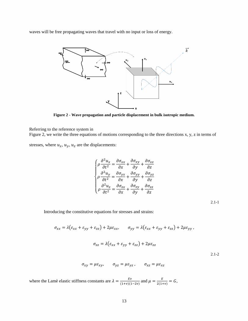
waves will be free propagating waves that travel with no input or loss of energy.
Figure 2 - Wave propagation and particle displacement in bulk isotropic medium.
Referring to the reference system in
Figure 2, we write the three equations of motions corresponding to the three directions x, y, z in terms of
stresses, where 𝑢𝑥, 𝑢𝑦, 𝑢𝑧 are the displacements:
{
𝜌
𝜕2𝑢𝑥𝜕𝑡2
=𝜕𝜎𝑥𝑥𝜕𝑥
+𝜕𝜎𝑥𝑦
𝜕𝑦+𝜕𝜎𝑥𝑧𝜕𝑧
𝜌𝜕2𝑢𝑦
𝜕𝑡2=𝜕𝜎𝑦𝑥
𝜕𝑥+𝜕𝜎𝑦𝑦
𝜕𝑦+𝜕𝜎𝑦𝑧
𝜕𝑧
𝜌𝜕2𝑢𝑧𝜕𝑡2
=𝜕𝜎𝑧𝑥𝜕𝑥
+𝜕𝜎𝑧𝑦
𝜕𝑦+𝜕𝜎𝑧𝑧𝜕𝑧
2.1-1
Introducing the constitutive equations for stresses and strains:
𝜎𝑥𝑥 = 𝜆(휀𝑥𝑥 + 휀𝑦𝑦 + 휀𝑧𝑧) + 2𝜇휀𝑥𝑥 , 𝜎𝑦𝑦 = 𝜆(휀𝑥𝑥 + 휀𝑦𝑦 + 휀𝑧𝑧) + 2𝜇휀𝑦𝑦 ,
𝜎𝑧𝑧 = 𝜆(휀𝑥𝑥 + 휀𝑦𝑦 + 휀𝑧𝑧) + 2𝜇휀𝑧𝑧
2.1-2
𝜎𝑥𝑦 = 𝜇휀𝑥𝑦, 𝜎𝑦𝑧 = 𝜇휀𝑦𝑧 , 𝜎𝑥𝑧 = 𝜇휀𝑥𝑧
where the Lamè elastic stiffness constants are 𝜆 =𝐸𝜈
(1+𝜈)(1−2𝜈) and 𝜇 =
𝐸
2(1+𝜈)= 𝐺,

14
and strain-displacements compatibility equations:
휀𝑥𝑥 =𝜕𝑢𝑥𝜕𝑥
, 휀𝑦𝑦 =𝜕𝑢𝑦
𝜕𝑦, 휀𝑧𝑧 =
𝜕𝑢𝑧𝜕𝑧
휀𝑥𝑦 =𝜕𝑢𝑥𝜕𝑦
+𝜕𝑢𝑦
𝜕𝑥, 휀𝑦𝑧 =
𝜕𝑢𝑦
𝜕𝑧+𝜕𝑢𝑥𝜕𝑦
, 휀𝑥𝑧 =𝜕𝑢𝑥𝜕𝑧
+𝜕𝑢𝑧𝜕𝑥
2.1-3
we obtain the equations of motion in 3D (eqs. 2.1-4) in terms of displacements, also known as the
governing wave equations:
{
𝜌
𝜕2𝑢𝑥𝜕𝑡2
= (𝜆 + 𝜇)𝜕
𝜕𝑥(𝜕𝑢𝑥𝜕𝑥
+𝜕𝑢𝑦
𝜕𝑦+𝜕𝑢𝑧𝜕𝑧) + 𝜇∇2𝑢𝑥
𝜌𝜕2𝑢𝑦
𝜕𝑡2= (𝜆 + 𝜇)
𝜕
𝜕𝑦(𝜕𝑢𝑥𝜕𝑥
+𝜕𝑢𝑦
𝜕𝑦+𝜕𝑢𝑧𝜕𝑧) + 𝜇∇2𝑢𝑦
𝜌𝜕2𝑢𝑧𝜕𝑡2
= (𝜆 + 𝜇)𝜕
𝜕𝑧(𝜕𝑢𝑥𝜕𝑥
+𝜕𝑢𝑦
𝜕𝑦+𝜕𝑢𝑧𝜕𝑧) + 𝜇∇2𝑢𝑧
2.1-4
For an isotropic medium, we can consider the x direction of wave propagation only. Assuming a
harmonic solution of the type:
𝒖 = (𝑢𝑥, 𝑢𝑦, 𝑢𝑧) = 𝐴𝑒𝑖(2𝜋𝒙𝜆−𝜔𝑡)
+ 𝐵𝑒𝑖(2𝜋𝒙𝜆+𝜔𝑡)
2.1-5
where the wavefront is an infinite plane perpendicular to the direction of wave propagation, and rewriting
it for the wavenumber 𝑘 =𝜔
𝑐 as:
𝒖 = (𝑢𝑥 , 𝑢𝑦, 𝑢𝑧) = 𝐴𝑒𝑖(𝒌𝒙−𝜔𝑡) + 𝐵𝑒𝑖(𝒌𝒙+𝜔𝑡)
2.1-6
we can recognize waves travelling in the positive x direction in the first term and in the negative direction
in the second term. The particle motion is a combination of the displacements in the three directions. Using
this solution in eq. (2.1-4), we can solve for two modes: a dilatational wave motion, where the particles
move parallel to the direction of wave propagation, with a speed dependent on both extensional and shear
behavior (longitudinal waves):

15
𝑐𝐿 =𝜔
𝑘= √
𝐸(1 − 𝜈)
𝜌(1 + 𝜈)(1 − 𝜈)
2.1-7
and a rotational motion, where the particles move perpendicular to the direction of wave propagation,
with a speed 𝑐𝑇 (shear waves):
𝑐𝑇 =𝜔
𝑘= √
𝐺
𝜌
2.1-8
To separate the fields in eqs. (2.1-4), we can use Helmoltz method, where we define the longitudinal
wave potential 𝐿 = ∇𝜙 and shear wave potential 𝑆 = ∇ x ψ. The total displacement field is given by the
superposition of the two potentials and the solution to the separated eqs. (2.1-9)
{
1
𝑐𝐿2 𝜕2𝜙
𝜕𝑡2= ∇2𝜙
1
𝑐𝑇2 𝜕2𝝍
𝜕𝑡2= ∇2𝝍
2.1-9
becomes:
𝜙 = 𝐴𝐿𝑒𝑖𝜔(
𝑵𝒙𝑐𝐿−𝑡)
= 𝐴𝐿𝑒𝑖(𝒌𝒙−𝜔𝑡)
𝝍 = 𝐴𝑆𝑒𝑖𝜔(
𝑵𝒙𝑐𝑇−𝑡)
= 𝐴𝑆𝑒𝑖(𝒌𝒙−𝜔𝑡)
2.1-10
where 𝒏 is the wave propagation direction vector, 𝐴𝐿 and 𝐴𝑆 are the complex amplitudes and 𝑐 =𝜔
|𝒌| is the
wave speed (Lowe, 1992).
Considering that the medium extends infinitely in the y direction, we can reduce the problem to a
2D infinite space (x-z), and simplify the derivation considering plane strain (𝜕
𝜕𝑦= 0) and in-plane motion
(𝑢𝑦 = 0). The displacements 𝑢𝑥 and 𝑢𝑧 can be found as:
16
𝒖 = ∇𝜙 = {𝑢𝑥 = 𝑛𝑥𝐴𝐿𝑒
𝑖𝜔(𝑁𝑥𝑥𝑐𝐿
+𝑁𝑧𝑧𝑐𝐿
−𝑡)
𝑢𝑧 = 𝑛𝑧𝐴𝐿𝑒𝑖𝜔(
𝑁𝑥𝑥𝑐𝐿
+𝑁𝑧𝑧𝑐𝐿
−𝑡)
2.1-11
for longitudinal waves and
𝒔 = ∇ x 𝛙 = {𝑢𝑥 = 𝑛𝑧𝐴𝑆𝑒
𝑖𝜔(𝑁𝑥𝑥𝑐𝑇
+𝑁𝑧𝑧𝑐𝑇
−𝑡)
𝑢𝑧 = 𝑛𝑥𝐴𝑆𝑒𝑖𝜔(
𝑁𝑥𝑥𝑐𝑇
+𝑁𝑧𝑧𝑐𝑇
−𝑡)
2.1-12
for shear waves.
Through the combination of these wave solutions to a set of boundary conditions for stress and
displacement, on the finite domain, as
𝑢(𝑥, 𝑦, 𝑧, 𝑡) = 𝑢0(𝑥, 𝑦, 𝑧, 𝑡)𝑡𝑖 = 𝜎𝑗𝑖𝑛𝑗
2.1-13
a relationship in terms of wave velocity versus frequency can be established (Rose, 2004). This so-called
dispersion relation governs the propagation of each guided wave mode in space and time and the
dependency of the wave phase velocity to frequency. The relationship between the incident angle and phase
velocity is expressed by the Snell’s Law, so that each waveguide has its unique set of dispersion curves.
Starting from the particular case of waves at the boundary between two semi-infinite half spaces,
for an incident longitudinal wave, the frequency of the incident shear wave and the two reflected
longitudinal and shear wave has to be the same. Together with Snell’s Law, where the wavenumber 𝑘𝑥 in
the x wave propagation direction has to be the same at the interface, the waves have to travel with the same
phase velocity 𝑐𝑝 =𝜔
𝑘𝑥.
The latter expresses a fundamental dependence of the frequency from the wavenumber and it
establishes that wave velocity is a function of frequency, hence wave distorsion must occur (Rose, 2004).
Also, the real solutions of k represent right and left propagating waves. While the individual harmonics

17
travel with different phase velocities 𝑐𝑝, the superimposed packet travels with the group velocity 𝑐𝑔. For
this group of waves to be maintained, the changes in phase for all the components should be the same,
leading to 𝑐𝑔 =𝑑𝜔
𝑑𝑘 and due to the dependence of the phase velocity on frequency, we also have that 𝑐𝑔 =
𝑐𝑝 + 𝑘𝑑𝑐𝑝
𝑑𝑘.
Many structures can be considered as waveguides themselves, naturally supporting the propagation
of guided waves, provided that the wavelengths are large enough compared to some key dimensions of the
waveguide. The energy of such waves is carried along the waveguide, with no leakage, as long as the
mismatch in acoustic impedance between the layers is significant.
For thin plates, the discussion seen about wave propagation at the interface of two media is extended to an
additional interface, where traction free conditions have to be satisfied at both interfaces constituting the
top and bottom of the plate. Moreover, the amplitudes of the displacements traveling out of such interfaces
have to equal zero, to satisfy conservation of energy (guided waves).
Relying again on the methods of potentials combined to a harmonic plane wave solution assumption of the
type of equations (2.1-10), which, for a plain strain case become:
𝜙 = 𝚽(𝒛)𝑒𝑖(𝑘𝑥−𝜔𝑡)
𝝍 = 𝚿(𝒛)𝑒𝑖(𝑘𝑥−𝜔𝑡)
2.1-14
It is possible to notice how they represent a solution of waves travelling along x (longitudinal
direction of the plate) and having a fixed distribution along z (transverse direction of the plate) as standing
waves. The displacements and stresses in terms of potentials are:
𝑢𝑥 = 𝑢 =𝜕𝜙
𝜕𝑥+𝜕𝜓
𝜕𝑧
𝑢𝑦 = 𝑣 = 0
𝑢𝑧 = 𝑤 =𝜕𝜙
𝜕𝑧+𝜕𝜓
𝜕𝑥

18
𝜎𝑧𝑥 = 𝜇 (𝜕𝑤
𝜕𝑥+𝜕𝑢
𝜕𝑧)
𝜎𝑧𝑧 = 𝜆 (𝜕𝑢
𝜕𝑥+𝜕𝑤
𝜕𝑧) + 2𝜇
𝜕𝑤
𝜕𝑧
2.1-15
Substituting equations (2.1-14) into the governing decoupled wave equations, we can solve as:
𝜙 = 𝚽(𝑧)𝑒𝑖(𝑘𝑥−𝜔𝑡) = [𝐴1 sin(𝑝𝑧) + 𝐴2cos (𝑝𝑧)]𝑒𝑖(𝑘𝑥−𝜔𝑡)
𝝍 = 𝚿(𝑧)𝑒𝑖(𝑘𝑥−𝜔𝑡) = [𝐵1 sin(𝑞𝑧) + 𝐵2cos (𝑞𝑧)]𝑒𝑖(𝑘𝑥−𝜔𝑡)
2.1-16
where 𝑝2 =𝜔2
𝑐𝐿2 − 𝑘
2 and 𝑞2 =𝜔2
𝑐𝑇2 − 𝑘
2.
We substitute these solutions into the displacements and stresses in equations (2.1-16) and
separate variables that are even or odd with respect to z=0 (Bartoli, 2007).
𝒖𝒙 = [(𝑨𝟐𝒊𝒌 𝒄𝒐𝒔(𝒑𝒛) + 𝑩𝟏𝒒 𝐜𝐨𝐬 (𝒒𝒛)) + (𝑨𝟏𝒊𝒌 𝒔𝒊𝒏(𝒑𝒛) − 𝑩𝟐𝒒 𝒔𝒊𝒏(𝒒𝒛))]𝒆𝒊(𝒌𝒙−𝝎𝒕)
𝒖𝒛 = [−(𝑨𝟐𝒑 𝒔𝒊𝒏(𝒑𝒛) + 𝑩𝟏𝒊𝒌 𝐬𝐢𝐧 (𝒒𝒛)) + (𝑨𝟏𝒑 𝒄𝒐𝒔(𝒑𝒛) − 𝑩𝟐𝒊𝒌 𝒄𝒐𝒔(𝒒𝒛))]𝒆𝒊(𝒌𝒙−𝝎𝒕)
2.1-17
In particular, thanks to the symmetry of the plate geometry, waves, whose displacement in the
propagation direction x is odd with respect to z=0, hence proportional to a sinusoidal function, constitute
the anti-symmetric modes (second terms of the above equations). Their in-plane particle displacement (𝑢 =
𝑢𝑥) is asymmetric and their out-of-plane displacement (𝑤 = 𝑢𝑧) is instead symmetric, as it will be shown
in Figure 8. For waves whose 𝑢𝑥 is even with respect to z=0, hence proportional to a cosinusoidal function
(first terms in the above equations), the in-plane particle displacement 𝑢 = 𝑢𝑥 is symmetric and their out-
of-plane displacement (𝑤 = 𝑢𝑧) is instead asymmetric, as shown in Figure 8. They constitute the symmetric
modes. The overall displacement generates a flexural behavior in the anti-symmetric mode and an
extensional one for the symmetric mode (see Figure 3).

19
Figure 3 - Displacement in anti-symmetric and symmetric modes
The amplitudes of potentials, displacements and stresses can be found imposing the traction-free
boundary conditions:
𝜎𝑧𝑥 = 𝜎𝑧𝑧 = 0 𝑎𝑡 𝑧 = ±𝑑
2= ±ℎ
2.1-18
where d is the thickness of the plate.
After some manipulations and substitutions into two homogenous equations, imposing the
determinant equal to zero to find a non-trivial solution to what is called the characteristic equation, we
obtain a transcendental equation for symmetric modes:
tan(𝑞ℎ)
tan(𝑝ℎ)= −
4𝑘2𝑝𝑞
(𝑞2 − 𝑘2)2
2.1-19
and for antisymmetric modes:
tan(𝑞ℎ)
tan(𝑝ℎ)= −
(𝑞2 − 𝑘2)2
4𝑘2𝑝𝑞
2.1-20
The solutions to the above equation can be found numerically for k, for a given ω, hence we
obtain the wave velocity for every <frequency*thickness> product.

20
2.2 Analytical and Semi-analytical investigation
For an isotropic Aluminum plate, whose properties are reported in Table 1, the solution of the
transcendental equations is shown in Figure 4: a root-finding algorithm searches for the wavenumber that
would verify the transcendental equation for given <frequency x thickness> values; the dispersion curves
are then computed in terms of phase and group velocities according to eqs.(2.1-19) and (2.1-20) for both
symmetric (blue) and anti-symmetric (red) modes.
Table 1 - Aluminum plate: Material properties
Property Name
Thickness
(mm)
Density
(kg/m3)
Ey
(GPa)
Gxy
(GPa)
ν CL
(m/s)
CT
(m/s)
Property Value 2.688 2700 72.08 26.96 0.3368 6370 3160
It is possible to notice the dispersive behavior of the propagating modes, especially for the first
anti-symmetric mode at low frequencies: the velocity changes rapidly causing higher frequencies to travel
faster than the lower ones, until reaching an asymptotic behavior.
To estimate dispersion curves analytically for a multi-layered plate, equivalent properties have to
be used. Each ply’s local stiffness modulus, shear modulus and Poisson ratio can be reduced into global
properties (Fung Y.C., 1965; Jones, 1999), thanks to the transformation below, with respect to the wave
Figure 4 - Analytical Dispersion curves for Aluminum plate in Table 1: (left) phase velocity, (right) group
velocity; anti-symmetric modes in red, symmetric modes in blue.
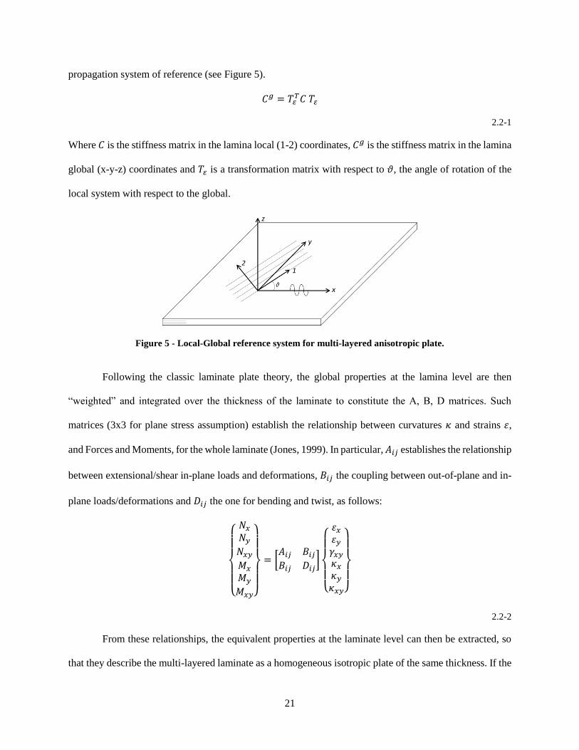
21
propagation system of reference (see Figure 5).
𝐶𝑔 = 𝑇𝜀 𝑇𝐶 𝑇𝜀
2.2-1
Where 𝐶 is the stiffness matrix in the lamina local (1-2) coordinates, 𝐶𝑔 is the stiffness matrix in the lamina
global (x-y-z) coordinates and 𝑇𝜀 is a transformation matrix with respect to 𝜗, the angle of rotation of the
local system with respect to the global.
Figure 5 - Local-Global reference system for multi-layered anisotropic plate.
Following the classic laminate plate theory, the global properties at the lamina level are then
“weighted” and integrated over the thickness of the laminate to constitute the A, B, D matrices. Such
matrices (3x3 for plane stress assumption) establish the relationship between curvatures 𝜅 and strains 휀,
and Forces and Moments, for the whole laminate (Jones, 1999). In particular, 𝐴𝑖𝑗 establishes the relationship
between extensional/shear in-plane loads and deformations, 𝐵𝑖𝑗 the coupling between out-of-plane and in-
plane loads/deformations and 𝐷𝑖𝑗 the one for bending and twist, as follows:
{
𝑁𝑥𝑁𝑦𝑁𝑥𝑦𝑀𝑥𝑀𝑦𝑀𝑥𝑦}
= [𝐴𝑖𝑗 𝐵𝑖𝑗𝐵𝑖𝑗 𝐷𝑖𝑗
]
{
휀𝑥휀𝑦𝛾𝑥𝑦𝜅𝑥𝜅𝑦𝜅𝑥𝑦}
2.2-2
From these relationships, the equivalent properties at the laminate level can then be extracted, so
that they describe the multi-layered laminate as a homogeneous isotropic plate of the same thickness. If the

22
plate in study is a fiber reinforced polymer, wave propagation phenomena due to fiber/matrix and ply-to-
ply interaction, anisotropy given by the fibers’ orientation and 3D effects are neglected. Moreover, the
reduction of anisotropic laminates to homogeneous isotropic plates doesn’t account for skewness and allows
decoupling between the Lamb modes and the SH0 mode, which is not true and can only be described by
other models (i.e. SAFE) and observed experimentally. As an example, the CFRP laminate with properties
described in Table 2 and Table 3 (old panel properties and layup) presents the dispersive behavior shown
in Figure 6, when reduced to an equivalent plate (Table 4). From the values corresponding to specific
elements in the ABD matrices, it is possible to predict coupling between stresses and strains in different
directions and planes:
𝐴𝑖𝑗 = [195.70 49.73 049.73 195.70 00 0 59.99
]; 𝐵𝑖𝑗 = [0]; 𝐷𝑖𝑗 = [140.98 20.28 6.3620.28 108.28 6.366.36 6.36 25.47
].
For example, being the laminate in analysis quasi-isotropic, it shows the same in-plane stiffness,
so that wave propagation along x or y direction should exhibit the same characteristics. Also, matrix B is
empty, so mode conversion from an A0 (dominated by out-of-plane displacement) into an S0 (dominated
by in-plane displacement) should be reduced. Lastly, being the coefficients 𝐴16 and 𝐴26 basically 0, very
little coupling should happen between SH0 and S0, and viceversa.
Table 2 - Composite plate: Layup
Material Name
Layup
(°)
Thickness
Ply (mm)
Density
(kg/m3)
Cytec X840/Z60 6k Weave Fabric 0 0.208 1600
Cytec X840/Z60 12k Tape [0/45/0/45/90/-45/0/45/90/-45]S 0.142 1600
Cytec X840/Z60 6k Weave Fabric 0 0.208 1600

23
Table 3 - Composite plate: Material properties
Material Name
E1
(GPa)
E2
(GPa)
E3
(GPa)
G12
(GPa)
G23
(GPa)
G13
(GPa)
ν12 ν23 ν13
Cytec X840/Z60
6k Weave Fabric
80 80 13.8 6.5 4.1 5.1 0.06 0.37 0.50
Cytec X840/Z60
12k Tape
168.2 10.3 10.3 7.0 3.7 7.0 0.27 0.54 0.27
Table 4 - Composite plate: Equivalent material properties
Property Name
Thickness
(mm)
Ex
(GPa)
Ey
(GPa)
Gxy
(GPa)
ν CL
(m/s)
CT
(m/s)
Property Value 2.688 48.895 48.895 16.023 0.254 6079 3165
Other methods can take into account the anisotropy of these materials. The analytical solution
presented above is a simplification and cannot fully capture the entire properties, especially in the transverse
plane xz. In fact, the classic laminate theory assumes the Euler Bernoulli theorem and plane stress (Jones,
1999), which is not correct for wave propagation in multi-layered anisotropic plates. In the case of multi-
layered plates, more advanced methods need to be employed to compute solutions (dispersion curves and
Figure 6 - Analytical Dispersion curves for Composite plate in Table 4Table 1: (left) phase velocity,
(right) group velocity; anti-symmetric modes in red, symmetric modes in blue.
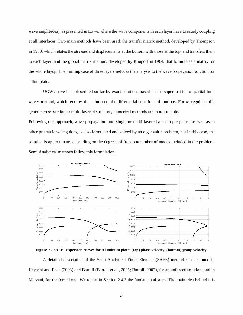
24
wave amplitudes), as presented in Lowe, where the wave components in each layer have to satisfy coupling
at all interfaces. Two main methods have been used: the transfer matrix method, developed by Thompson
in 1950, which relates the stresses and displacements at the bottom with those at the top, and transfers them
to each layer, and the global matrix method, developed by Knopoff in 1964, that formulates a matrix for
the whole layup. The limiting case of three layers reduces the analysis to the wave propagation solution for
a thin plate.
UGWs have been described so far by exact solutions based on the superposition of partial bulk
waves method, which requires the solution to the differential equations of motions. For waveguides of a
generic cross-section or multi-layered structure, numerical methods are more suitable.
Following this approach, wave propagation into single or multi-layered anisotropic plates, as well as in
other prismatic waveguides, is also formulated and solved by an eigenvalue problem, but in this case, the
solution is approximate, depending on the degrees of freedom/number of modes included in the problem.
Semi Analytical methods follow this formulation.
A detailed description of the Semi Analytical Finite Element (SAFE) method can be found in
Hayashi and Rose (2003) and Bartoli (Bartoli et al., 2005; Bartoli, 2007), for an unforced solution, and in
Marzani, for the forced one. We report in Section 2.4.3 the fundamental steps. The main idea behind this
Figure 7 - SAFE Dispersion curves for Aluminum plate: (top) phase velocity, (bottom) group velocity.
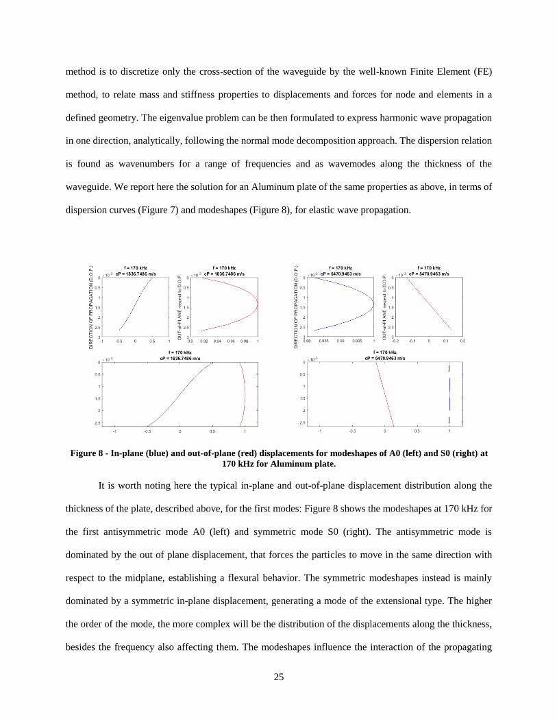
25
method is to discretize only the cross-section of the waveguide by the well-known Finite Element (FE)
method, to relate mass and stiffness properties to displacements and forces for node and elements in a
defined geometry. The eigenvalue problem can be then formulated to express harmonic wave propagation
in one direction, analytically, following the normal mode decomposition approach. The dispersion relation
is found as wavenumbers for a range of frequencies and as wavemodes along the thickness of the
waveguide. We report here the solution for an Aluminum plate of the same properties as above, in terms of
dispersion curves (Figure 7) and modeshapes (Figure 8), for elastic wave propagation.
It is worth noting here the typical in-plane and out-of-plane displacement distribution along the
thickness of the plate, described above, for the first modes: Figure 8 shows the modeshapes at 170 kHz for
the first antisymmetric mode A0 (left) and symmetric mode S0 (right). The antisymmetric mode is
dominated by the out of plane displacement, that forces the particles to move in the same direction with
respect to the midplane, establishing a flexural behavior. The symmetric modeshapes instead is mainly
dominated by a symmetric in-plane displacement, generating a mode of the extensional type. The higher
the order of the mode, the more complex will be the distribution of the displacements along the thickness,
besides the frequency also affecting them. The modeshapes influence the interaction of the propagating
Figure 8 - In-plane (blue) and out-of-plane (red) displacements for modeshapes of A0 (left) and S0 (right) at
170 kHz for Aluminum plate.

26
wave with the geometrical features of the plate (or waveguide in general), hence their particle motion can
be used to aim at specific interactions (i.e. surfaces or internal) and their excitation and reception has to be
maximized accounting for their distribution. These observations will be used along this work to design and
interpret experiments.
SAFE can accommodate anisotropic and multilayered plates and offers the advantage of easily
accessing the laminae stiffness properties to study guided wave propagation for a variety of cases.
Parametric studies and/or inversion with respect to the experimental data can be performed to solve
for laminate thickness, ply orientation and elastic constants, together with different wave propagation
directions and frequency ranges. The left plot in Figure 9 shows the dispersion curves obtained with SAFE
for the composite laminate in Table 2, along with its modeshapes in Figure 10, where we can observe the
distribution of the displacements along the thickness of the laminate.
Figure 9 - SAFE Dispersion curves for Composite plate in Table 2: (top) phase velocity, (bottom) group
velocity; (left) single laminate thickness, (right) double laminate thickness.

27
Figure 10 - In-plane (blue) and out-of-plane (red) displacements for modeshapes of A0 (left) and S0 (right) at
170 kHz for Composite plate.
The thickness of the plate affects the dispersion behavior, as it can be appreciated in Figure 9: the
right plots belong to the same laminate in the left, in terms of material properties and orientation of the
plies, but the specimen is now composed of two laminates, so that the thickness is twice the one in the left
plots. The modes “shift” to the left, appearing at lower frequencies. The shift of the cut-off frequencies of
modes can be used to infer plate thickness or the presence of defects/disbonds.
To be noted is also the presence of an additional mode type, the shear horizontal mode SH0: we are showing
it in here for completeness, since it is not correct to decouple the in-plane displacements (x and y directions)
due to the ply orientation and anisotropic behavior of the CFRP. Also, the skewness effect is neglected here
and in the experimental tests presented in the next sections, thanks to the quasi-isotropic layup of the
composite laminate in consideration and the observation of wave propagation in the direction corresponding
to one of the principle directions of material symmetry.
The modeshapes are shown in Figure 10 and maintain the same antisymmetric/symmetric properties of
those shown for an isotropic material (Aluminum). The discontinuity in the elastic properties along the
thickness, due to the different ply orientation, though, can be appreciated in the deviation of both in-plane
and out-of-plane displacements from low order polynomial trends.

28
An interesting study can be done when altering the stiffness properties at different plies and at different
locations along the thickness of the laminate. For example, Figure 11 and Figure 12 show the results for the
same CFRP laminate, when the stiffness matrix C is reduced to 5% at the first three top plies.
The reduction in the superficial stiffness manifests itself in the modeshape, where a discontinuity along the
displacement distribution appears for both in plane and out of plane displacements, when the structure is
excited by either the antisymmetric (left) or symmetric (right) mode.
Figure 11 - SAFE Dispersion curves for Composite plate (group velocity): comparison pristine
(black) and altered top surface layers (red).

29
The case of a 95% reduction in stiffness at the central plies is instead studied in Figure 13:
Figure 12 - In-plane (blue and black) and out-of-plane (red) displacements for modeshapes of A0 (left)
and S0 (right) modes for Composite plates: comparison pristine (solid) and altered surface layers
(dashed).
Figure 13 - SAFE Dispersion curves for Composite plate (group velocity): comparison pristine
(black) and altered middle layers (red).

30
The sensitivity of the wave propagation behavior to the lamina’s elastic properties can be
particularly observed in the modeshapes (Figure 14), where a strong discontinuity in the displacements
can be again noticed in correspondence of the plies with reduced stiffness. The SH0 mode in particular
excites this kind of defect, due to its shear in-plane nature, that couples very well with this “disbond-like”
case study.
These observations show the importance of wave propagation understanding and prediction and the
potential of Ultrasonic Guided Waves (UGWs) to inspect structures, infer structural changes and
quantitatively inform, beyond qualitative visual inspection.
2.3 Global-Local model to predict scattering of guided elastic
waves
2.3.1 Problem formulation
The present paper builds on the work by Srivastava and Lanza di Scalea (2010) to unify the global
(SAFE) -local (FE) formulation and implement it in a computationally efficient code able to solve extremely
Figure 14 - In-plane (blue and black) and Out-of-plane (red) displacements for modeshapes A0 (left) and SH0
(right) modes for Composite plates: comparison pristine (solid) and altered middle layers (dashed).
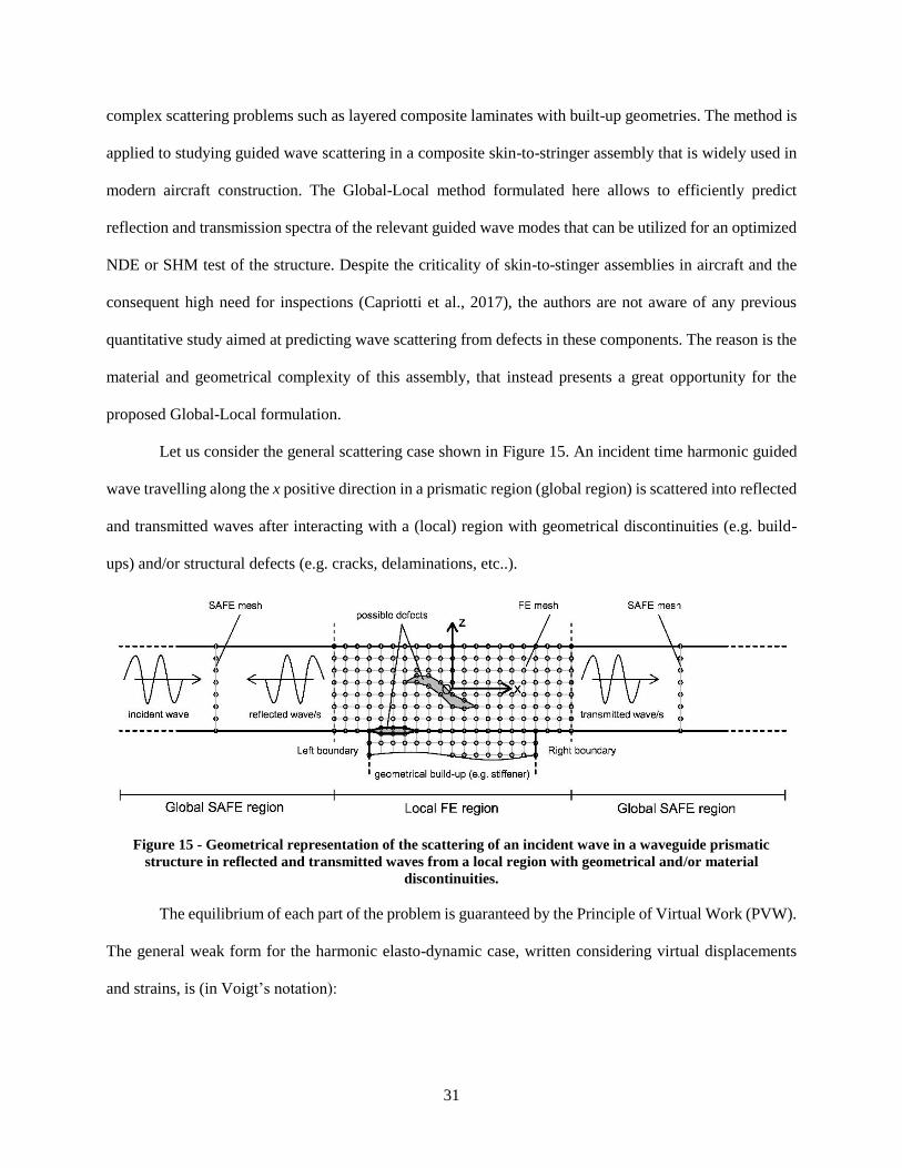
31
complex scattering problems such as layered composite laminates with built-up geometries. The method is
applied to studying guided wave scattering in a composite skin-to-stringer assembly that is widely used in
modern aircraft construction. The Global-Local method formulated here allows to efficiently predict
reflection and transmission spectra of the relevant guided wave modes that can be utilized for an optimized
NDE or SHM test of the structure. Despite the criticality of skin-to-stinger assemblies in aircraft and the
consequent high need for inspections (Capriotti et al., 2017), the authors are not aware of any previous
quantitative study aimed at predicting wave scattering from defects in these components. The reason is the
material and geometrical complexity of this assembly, that instead presents a great opportunity for the
proposed Global-Local formulation.
Let us consider the general scattering case shown in Figure 15. An incident time harmonic guided
wave travelling along the x positive direction in a prismatic region (global region) is scattered into reflected
and transmitted waves after interacting with a (local) region with geometrical discontinuities (e.g. build-
ups) and/or structural defects (e.g. cracks, delaminations, etc..).
Figure 15 - Geometrical representation of the scattering of an incident wave in a waveguide prismatic
structure in reflected and transmitted waves from a local region with geometrical and/or material
discontinuities.
The equilibrium of each part of the problem is guaranteed by the Principle of Virtual Work (PVW).
The general weak form for the harmonic elasto-dynamic case, written considering virtual displacements
and strains, is (in Voigt’s notation):

32
t
T T Td d d
ε σ u t u u (1)
where T
x y zu u u u , T
x y zt t t t , T
x y z yz xz xy ε , and
T
x y z yz xz xy σ are displacement, traction, strain and stress vectors respectively.
All these variables are space and time dependent. In Eq. (1) the bar above a letter stands for complex
conjugate, while u is the acceleration, ρ the density, Ω the volume of the medium and Γt the medium’s
loaded external surface. In this work, body forces and damping effects are neglected.
In order to model both reflections and transmissions, the entire domain Ω is subdivided into one
“local” region in the center and two “global” regions on either side. Figure 15 shows a plain strain case
(that is assumed in the application problem studied in this paper), where the cross-sectional SAFE
discretization of the global waveguide reduces to a 1D mesh along z, and a full FE mesh is instead used in
2D domain (x-z plane) for the local region. The extension of the concept to a general 3D case is trivial (2D
SAFE discretization in the global region and 3D FE discretization in the local region). The GL formulation
as written here applies to a general 3D case.
Let us imagine separating the local region from the global region at their left and right boundaries of
Figure 15. Since equilibrium must continue to hold, internal tractions arise at each boundary due to the
internal stress caused by the application of external actions. Using the PVW for each region, the traction
vector t in Eq. (1) consists of the internal tractions at the boundaries, which behave as new external forces.
The vector t could be evaluated as t σn , with n the unit vector normal to the Γt surface and σ the stress
second-order tensor. Alternatively, using Voigt notation:
T
nt L σ (2)
where
33
0 0
0 0
0 0
0
0
0
x
y
z
n
z y
z x
y x
n
n
n
n n
n n
n n
L (3)
with nx, ny, nz the direction cosines of the normal n. In what follows, a superscript ‘ ’ or ‘ g ’ is adopted to
identify quantities referring to the “local” region or the “global” region, respectively.
The local region is discretized by 2D or 3D finite elements. Accordingly, the approximate
displacement e
h
u at a point inside the local e-th element is obtained from the nodal values e
d through
the shape functions N using known FE concepts:
, , , , ,e e i t
h x y z t x y z e u N d (4)
where ω is the circular frequency.
The corresponding approximate strains and stresses are
e e
h h
ε Lu (5)
e e e
h h
σ C ε (6)
where L and eC are the compatibility and constitutive matrices respectively, with e
C a real matrix for
purely elastic cases, and a complex matrix for viscoelastic cases.
Including all the approximate variables in Eq. (1) and defining the vector U for the entire nodal local
displacements, the dynamic undamped equilibrium equations for the local region are obtained as:

34
2 K M U F , (7)
with K , M and F the classic FE stiffness matrix, mass matrix and force vector.
To interpolate the displacements of the global region, the same procedure is followed, but in a simplified
manner. The SAFE method adopts a harmonic exponential term, 𝑒𝑖(𝜉𝑥−𝜔𝑡), to describe analytically the
wave behaviour in the wave propagation direction, x, where ξ represents the wave number. By combining
the analytical solution along the wave propagation with an FE cross-sectional (y-z) discretization, the
approximate displacement g e
h
u within a single SAFE element of the global region can be written as:
g g g, , , ,i x te e
h x y z t y z e u N d (8)
with g ed the nodal displacements and g
N the shape functions of the global cross-sectional mesh.
Following the same steps discussed in Bartoli et al. (2006) or in Rose (2014), the expression of the
approximate strain vector in SAFE is derived as:
g g
1 2
i x te e
h i e
ε B B d (9)
where
1 , , 2andg g g
y y z z x B L N L N B L N (10)
are two compatibility matrices.
In Eq. (10) xL ,
yL and zL are particularized expressions of
nL given in Eq. (3) for a unit normal vector
aligned to the x, y or z axis respectively, while g
, yN and g
,zN are the derivatives of the global shape function

35
matrix with respect to the y or z coordinates. Approximate strains are then transformed into approximate
stresses by applying the constitutive laws
g g ge e e
h h
σ C ε (11)
with g eC the element constitutive matrix for the global region.
It is worth noting that in Eqs. (6) and (11) the constitutive matrices must refer to the (O, x, y, z)
reference system. Therefore, for anisotropic materials, any local stiffness matrix C (e.g. lamina in the
principal directions of material symmetry) needs to be transformed to the general (O, x, y, z) system C
according to
TC R CR (12)
with R the transformation matrix.
For the particular case of a laminated composite whose lamina is oriented at an angle with respect to the
x direction, the transformation matrix is:
2 2
2 2
2 2
0 0 0
0 0 0
0 0 1 0 0 0
0 0 0 0
0 0 0 0
2 2 0 0 0
m n mn
n m mn
m n
n m
mn mn m n
R (13)
with cosm and sinn .
With Eqs. (8)-(11) and (2) at hand, the PVW applied to the semi-infinite global region gives:
36
g 2 g g g K M U F (14)
where gU is the vector collecting the displacements of all the nodes of the global region mesh. Furthermore:
g
g g
1 2 1 21
el
e
nT e
ei i d
K B B C B B (15)
g
g g g
1
el
e
n Te
ed
M N N (16)
g
g g g g
1 21
el
et
n TT e
ne
i d
F N L C B B U (17)
are the stiffness matrix, mass matrix and force vector, respectively.
In Eqs. (15)-(17) 1
eln
e symbolizes the assembly operator, with
eln the total number of elements.
Referring again to the scattering case of Figure 15, it can be assumed that the nodal displacements
l Bq recorded at the left boundary is a combination of the incident wave and the reflected waves. The nodal
displacements r Bq at the right boundary, instead, are those of the transmitted waves. Hence:
,
.
l B incident reflected
r B transmitted
q q q
q q (18)
In the subject case of multimode guided waves, the incident, reflected and transmitted waves can be thought
of as the superimposition of a finite number NM of global cross-sectional mode shapes, each amplified by
a participation coefficient having the physical meaning of the amplitude of the single wave mode.

37
The incident mode can be modelled by imposed displacements or forces at the source. In the present
paper, a pure incident mode is generated by imposing the unique cross-sectional displacement shapes at the
relevant frequencies for the chosen mode. The evaluation of the unique mode shapes is performed by
solving an eigenproblem, that is shown in the next section. If the symbol Φ is used to represent the generic
mode shape, and the factor i te is omitted for simplicity, Eqs. (18) are explicitly rewritten as:
( )
1
Min s l B j l B
Ni d x i xj
l B in j
j
e A e
q Φ Φ (19)
( )
1
Mj r B
Ni xj
r B j
j
A e
q Φ (20)
where the superscript “+” represents a wave travelling in the right and the superscript “-” a wave travelling
in the left direction. Therefore: in
Φ and
in are mode shape and wavenumber of the incident wave (assumed
at unity amplitude); jA, ( )j
Φ and j
are amplitude, mode shape and wavenumber of the j-th reflected
mode; and jA, ( )j
Φ and j
amplitude, mode shape and wavenumber of the j-th transmitted mode. sd ,
l Bx and r Bx measure the distances of the source, left boundary and right boundary, respectively, from the
origin of the reference system that is set at the center of the local region (see Figure 15).
Eqs. (19) and (20) can be rewritten in a compact form:
in s l Bi d x
l B in e q Φ G D (21)
r B
q G D (22)
where
( )(1) (2) ( ) MNj
G Φ Φ Φ Φ (23)

38
1 2 M
T
j ND D D D D , (24)
with
j r Bi x
j jD A e (25)
j l Bi x
j jD A e . (26)
Eqs. (21) and (22) are entirely composed of known terms, except for the jA amplitudes. These equations
also guarantee the continuity of displacements between the global and the local regions. The evaluation of
jA is therefore performed in order to also guarantee the continuity of tractions at the left and the right
boundaries.
Let us recall the equilibrium Eq. (7) for the local region. A partition of Eq. (7) can be performed in order to
separate the contribution of the inner (I) and boundary (B) degrees of freedom, obtaining:
II IB I
BI BB BB
S S 0U
S S FU (27)
where
2 S K M , (28)
T
T T
B l B r B U q q , (29)
T
T T
B l B r B
F f f . (30)
In Eq. (30) l Bf and r Bf are the force vectors at the left and right boundaries. They are obtained as the
opposites of the consistent nodal force vectors at the same boundaries but considered as belonging to the
global regions.

39
From Eq. (17), for a unit normal vector n identifying the positive or negative directions of the x axis (
1 0T
n ), the consistent nodal force vectors for the two global regions are equal to:
g in s l Bi d x
l B in e F F F D (31)
g
r B
F F D (32)
where
( )(1) (2) ( ) MNj
F F F F F (33)
and
g
g g
1 21
el
etB
n TT e
in x in ine
i d
F N L C B B Φ , (34)
with
g
( ) g g ( )
1 21
el
etB
n Tj T e j
x je
i d
F N L C B B Φ . (35)
From Eqs. (31) and (32) l Bf and r Bf are obtained as:
g g,l B l B r B r B f F f F . (36)
A static condensation procedure applied to Eq. (27) leads to the following final equations:
* * in s li d xin in
BB BB e
BG 0 F 0 D Φ FS S
0 G 0 F D 0 0 (37)

40
where * 1
BB BB BI II IB
S S S S S is the condensed matrix of S.
Eq. (37) is solved to find D and D . Since the coefficient matrix is not square, the least squares method
should be applied. Once the D and D coefficients are known, the unknown jA and jA
reflected and
transmitted amplitudes can be finally determined.
As seen in the previous section, the GL method exploits the knowledge of at least NM mode shapes
of the guided waves. These are derived as the (unforced) solutions of the equilibrium Eqs. (14) for the
global region, which can be particularized as
2 2 g
1 2 3 Mi K K K M Φ 0 (38)
with M the number of total degrees of freedom for the global region mesh.
The stiffness matrices 1,2,3j j K are derived from Eq. (15) and explicitly given by Bartoli et al.
(2006). Eq. (38) constitutes a generalized eigenproblem in and . It is a common practice to reduce Eq.
(38) to a linear eigenproblem in by doubling the size of the problem:
2M
A B Q 0 (39)
where
ΦQ
Φ. A and B are known matrices for fixed values of the circular frequency . Their explicit
expression is:
2 g2 g
11
2 g
31 2
, Bi
K M 00 K MA
0 KK M K. (40)

41
The solution of Eq. (39) is given in terms of eigenvalues ξ and eigenvectors Q. While the eigenvectors are
complex, the eigenvalues can be pairs of real numbers (Re ) representing propagating waves in the ± x
directions, pairs of complex conjugate numbers (ImRe i ) representing evanescent waves decaying in
the ± x directions, or pairs of purely imaginary numbers (Imi ) representing non oscillating evanescent
waves in the ± x directions (Hayashi et al. 2003).
The corresponding mode shape Φ can be extracted as the upper part of vector Q, while the associated
attenuation, phase (pc ) and group (
gc ) velocities can be obtained as
Imatt (41)
p Rec (42)
2 3
g
2
2
T
L R
g T
L R
ic
Φ K K Φ
Φ M Φ (43)
with LΦ and
RΦ indicating the left and right mode shapes respectively.
The knowledge of the velocities for each 𝜉 − 𝜔 pair allows to build the dispersion curves. It is also
important for the purposes of this topic to “follow” a given wave mode at varying frequencies. In order to
do that, the results in this paper adopt the B-orthogonality wave mode sorting algorithm originally proposed
by Loveday and Long (2007). Since at the same frequency 𝜔, two eigenvectors r and s obtained from Eq.
(39) must respect the orthogonality condition with the B matrix, the same condition can be assumed for the
next frequency step , allowing to “follow” or “track” the mode during frequency sweeping
according to:
42
0
0
T
r s
if r s
if r s
Q BQ . (44)
The soundness of the proposed GL method can be validated by verifying the conservation of energy
between the incident mode and the scattered (reflected and transmitted) modes:
Refl
1
MNj j
in Transm
j
E E E
(45)
where inE , Refl
jE ,
jTransmE are the energy fluxes of the incident wave and of the j-th reflected and transmitted
waves, respectively.
The energy flux carried by the propagating mode j in the n direction over a unit period of time through
the cross-sectional area can be evaluated as:
j j
E d
P n , (46)
where
1Re
2
j j j
P σ u (47)
is the Poynting vector, with σ the stress tensor in matrix form notation and u the complex conjugate velocity
vector.
Substitution of Eq. (47) into Eq. (46) allows to rewrite Eq. (46) in Voigt notation as
1
Re2
Tj T
nE d
L σ u . (48)
43
By taking into account the harmonic time dependence of σ and u and considering the particular case of
waves travelling in the x direction, the energy term for the j-th mode becomes:
2
Re2
Tjj j jA
E i
F Φ (49)
where jΦ and j
F are the nodal displacements and correspondent consistent forces for mode j according
to the adopted FE discretization.
2.3.2 2D Case study: scattering of guided waves in skin-to-stringer
assembly of composite aircraft panels
The GL formulation described above was implemented in a Matlab© code. The code was designed to
calculate the response within a fixed frequency range of the incoming wave and for a fixed number of
frequency steps. The general numerical procedure is schematized in Figure 16.

44
Figure 16 - Key steps of the Matlab GL code.
The geometry of the case study is shown in Figure 17, and represents a scaled version of a skin-to-
stringer assembly found in commercial aircraft construction. This structure is being considered for
ultrasonic guided-wave inspection (Capriotti et al., 2017). Scattering results for typical incoming wave
modes were obtained for a “pristine” case and for four “damage” cases representing relevant defects in this
structure. These predictions can allow to best target the inspection to a particular defect and/or to
quantitatively relate a measured scattering behavior to a particular defect.
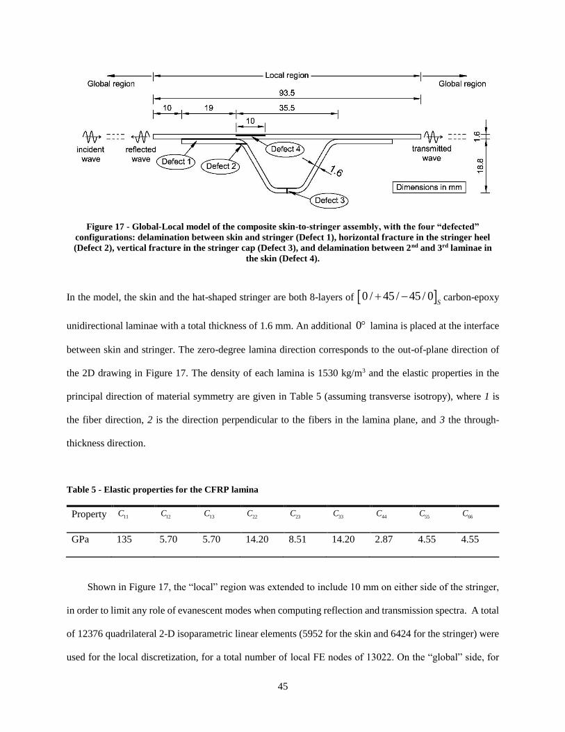
45
Figure 17 - Global-Local model of the composite skin-to-stringer assembly, with the four “defected”
configurations: delamination between skin and stringer (Defect 1), horizontal fracture in the stringer heel
(Defect 2), vertical fracture in the stringer cap (Defect 3), and delamination between 2nd and 3rd laminae in
the skin (Defect 4).
In the model, the skin and the hat-shaped stringer are both 8-layers of 0 / 45 / 45 / 0S
carbon-epoxy
unidirectional laminae with a total thickness of 1.6 mm. An additional 0 lamina is placed at the interface
between skin and stringer. The zero-degree lamina direction corresponds to the out-of-plane direction of
the 2D drawing in Figure 17. The density of each lamina is 1530 kg/m3 and the elastic properties in the
principal direction of material symmetry are given in Table 5 (assuming transverse isotropy), where 1 is
the fiber direction, 2 is the direction perpendicular to the fibers in the lamina plane, and 3 the through-
thickness direction.
Table 5 - Elastic properties for the CFRP lamina
Property 11C 12C
13C 22C
23C 33C
44C 55C
66C
GPa 135 5.70 5.70 14.20 8.51 14.20 2.87 4.55 4.55
Shown in Figure 17, the “local” region was extended to include 10 mm on either side of the stringer,
in order to limit any role of evanescent modes when computing reflection and transmission spectra. A total
of 12376 quadrilateral 2-D isoparametric linear elements (5952 for the skin and 6424 for the stringer) were
used for the local discretization, for a total number of local FE nodes of 13022. On the “global” side, for
46
computational consistency, two 1D isoparametric linear elements were used for each lamina, for a total of
16 elements and 17 nodes. Four Gauss points were used for the quadrature of the 2D elements, and 2 Gauss
points for the 1D elements. The maximum size of the elements was 0.26 mmL , in order to satisfy the
following customary meshing criterion:
T L (50)
where 2 /T Tc is the wavelength of transverse waves at frequency ω traveling at bulk shear velocity
Tc . With linear elements, values of 10 (Chang and Mal, 1995) or 20 (Bartoli et al., 2005; Galan
and Abascal, 2005) are customary. For the case of quadratic elements, a value of 4 was utilized. All
analyses were run using a Core i7 CPU with 64 GB of RAM, in the frequency range of DC-500 kHz, with
steps of 5 kHz. The incident wave source distance was 0.25 msd from the middle of the stringer (origin
of the reference system) on the left side of the drawing in Figure 17.
An initial validation of the accuracy of the proposed GL algorithm was conducted on a simpler
geometry of a pristine multi-layered composite plate corresponding to the skin only of Figure 17. This
analysis was done to check the generation of the dispersion curves and wave energy conservation in the
scattering process.
From the SAFE portion of the GL code, the results in terms of phase velocity and group velocity
dispersion curves in the DC-500 kHz frequency range are presented in Figure 18a and Figure 18b,
respectively. Four modes appear in this range, including three fundamental modes (m1, m2 and m3) and a
higher-order mode (m4) with cut-off frequency ~450 kHz. As expected, the curves are generally similar to
the Rayleigh-Lamb dispersion curves of isotropic plates, with m1 corresponding to the zero-order flexural
(A0) Lamb mode, m2 corresponding to the zero-order axial (S0) Lamb mode, m3 to the zero-order shear
horizontal (SH0) Lamb mode, and m4 to the first-order flexural (A1) Lamb mode.
For the remainder of the paper, the attention will be focused on the flexural and the axial modes since
they are the ones most commonly utilized in guided-wave testing of composite or metal plates.
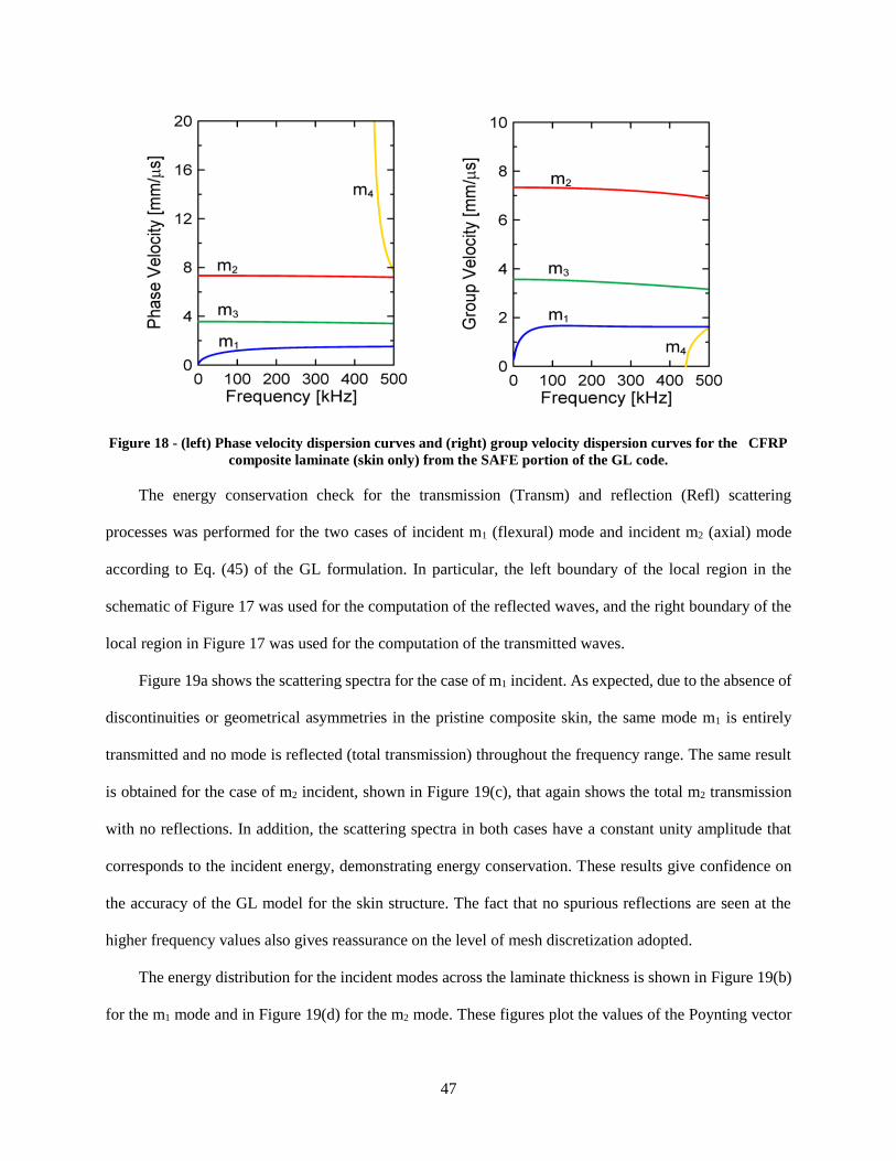
47
Figure 18 - (left) Phase velocity dispersion curves and (right) group velocity dispersion curves for the CFRP
composite laminate (skin only) from the SAFE portion of the GL code.
The energy conservation check for the transmission (Transm) and reflection (Refl) scattering
processes was performed for the two cases of incident m1 (flexural) mode and incident m2 (axial) mode
according to Eq. (45) of the GL formulation. In particular, the left boundary of the local region in the
schematic of Figure 17 was used for the computation of the reflected waves, and the right boundary of the
local region in Figure 17 was used for the computation of the transmitted waves.
Figure 19a shows the scattering spectra for the case of m1 incident. As expected, due to the absence of
discontinuities or geometrical asymmetries in the pristine composite skin, the same mode m1 is entirely
transmitted and no mode is reflected (total transmission) throughout the frequency range. The same result
is obtained for the case of m2 incident, shown in Figure 19(c), that again shows the total m2 transmission
with no reflections. In addition, the scattering spectra in both cases have a constant unity amplitude that
corresponds to the incident energy, demonstrating energy conservation. These results give confidence on
the accuracy of the GL model for the skin structure. The fact that no spurious reflections are seen at the
higher frequency values also gives reassurance on the level of mesh discretization adopted.
The energy distribution for the incident modes across the laminate thickness is shown in Figure 19(b)
for the m1 mode and in Figure 19(d) for the m2 mode. These figures plot the values of the Poynting vector
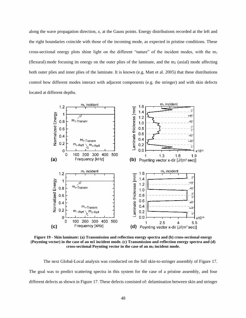
48
along the wave propagation direction, x, at the Gauss points. Energy distributions recorded at the left and
the right boundaries coincide with those of the incoming mode, as expected in pristine conditions. These
cross-sectional energy plots shine light on the different “nature” of the incident modes, with the m1
(flexural) mode focusing its energy on the outer plies of the laminate, and the m2 (axial) mode affecting
both outer plies and inner plies of the laminate. It is known (e.g. Matt et al. 2005) that these distributions
control how different modes interact with adjacent components (e.g. the stringer) and with skin defects
located at different depths.
Figure 19 - Skin laminate: (a) Transmission and reflection energy spectra and (b) cross-sectional energy
(Poynting vector) in the case of an m1 incident mode. (c) Transmission and reflection energy spectra and (d)
cross-sectional Poynting vector in the case of an m2 incident mode.
The next Global-Local analysis was conducted on the full skin-to-stringer assembly of Figure 17.
The goal was to predict scattering spectra in this system for the case of a pristine assembly, and four
different defects as shown in Figure 17. These defects consisted of: delamination between skin and stringer

49
(Defect 1), horizontal fracture in the stringer (Defect 2), vertical fracture in the stringer (Defect 3), and
delamination between 2nd and 3rd laminae in the skin (Defect 4). Defects 1, 2 and 3 were modelled by
removing some of the elements from the mesh; Defect 4 was modelled by doubling the nodes and physically
separating the elements between the second and third layer for the length specified in Figure 17.
The addition of the hat-shaped stringer to the skin laminate significantly increases the complexity of
the scattering problem. Key results from the GL model of the pristine assembly are shown in Figure 20 and
Figure 21 for the cases of incident m1 (flexural) mode and incident m2 (axial) mode.
Figure 20a shows the scattering spectra (reflections and transmission) in the DC-500 kHz frequency
range for an incident m1 mode. As for the skin-only results, the reflection spectra are computed at the left
boundary of the local region and the transmission spectra are computed at the right boundary of the local
region. As before, the total energy is computed adding up the transmitted and reflected energy for all the
modes, considering a unity incoming mode. Figure 20a shows a computed total energy spectrum flat and
close to 1, which satisfies conservation of energy to within very small numerical errors caused by the FE
discretization and the normal mode decomposition. The same figure also shows that, when m1 is incident,
the majority of the energy is transmitted through the skin-to-stringer assembly and reflected back into the
skin as the same mode m1, with very little mode conversion into m2. This is true at most frequencies, except
for specific frequencies such as 105 kHz, 200 kHz, 260-320 kHz and 450-470 kHz, where the mode-
converted m2 is transmitted through the overall structure more than m1. The lower frequency range (up to
200 kHz) is very sensitive to m1, reaching more than an 80% of transmission, with transmission peaks at ~
50 kHz and ~ 135 kHz. These values could therefore be ideal excitation frequencies for a pitch-catch
guided-wave inspection that uses m1 in transmission. Conversely, 90% of the m1 energy is reflected in the
high frequency range (~360-460 kHz) that can instead be considered for a pulse-echo guided-wave test
using reflection measurements. The spectra in Figure 20a also reveal interesting m1-m2 mode-conversion
bands, such as the m2 transmission in the ~ 260-320 kHz range and the m2 reflection around 200 kHz. The
mode conversion information can also be extremely useful in a practical guided-wave test. The higher-order

50
mode m4 appears with a very small contribution above its cut-off frequency of 450 kHz.
The corresponding case of an m2 incident mode is shown in Figure 20b. The spectra identify specific
frequency ranges for predominant transmission or reflection behaviour, as well as m2-m1 mode conversion
opportunities. For example, significant mode conversion into both transmitted m1 and reflected m1 occur in
the 150-350 kHz range, as well as at some other individual frequencies revealed by the energy peaks. The
plot also shows the small contribution of the higher-order mode m4 above 450 kHz.
Figure 20 - Reflection and transmission energy spectra for (a) m1 incident mode and (b) m2 incident mode in
the skin-to-stringer pristine assembly.
In order to shine additional light on these behaviours, Figure 21 shows results obtained when zooming
into the two salient frequency values of 150 kHz and 200 kHz. For an m1 incident mode, for example, the
spectra in Figure 21a shows that at 150 kHz most of the energy is transmitted as the same mode m1. This
result is best explained by the cross-sectional energy distribution (Poynting vector along x) shown in Figure
21b that confirms the same energy shapes at the left boundary and at the right boundary, i.e. little or no
disturbance to the nature of the m1 mode as it crosses through the stringer at this frequency. Conversely, at
a 200 kHz frequency, the spectra for the incident m1 mode in Figure 21a shows considerable (50%) mode
conversion into an m2. This different behaviour is again explained by the cross-sectional energy plots of
Figure 21c that show how the m1 cross-sectional shape at the left boundary changes into an m2 shape at the
(a) (b)
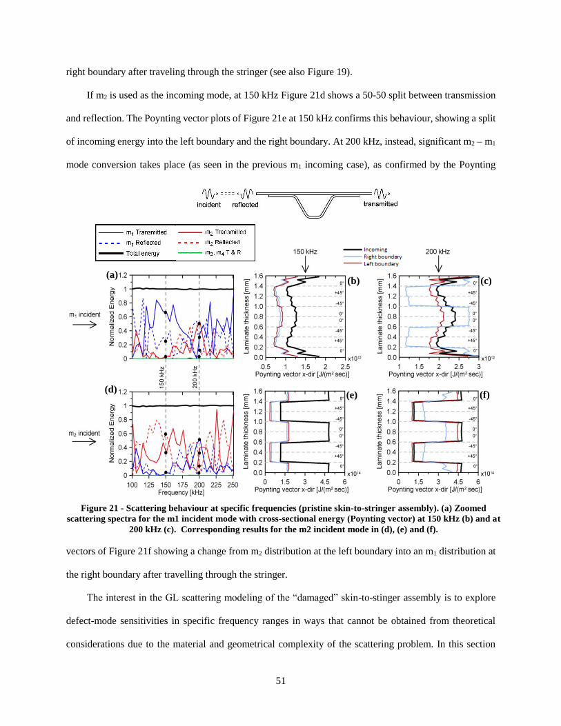
51
right boundary after traveling through the stringer (see also Figure 19).
If m2 is used as the incoming mode, at 150 kHz Figure 21d shows a 50-50 split between transmission
and reflection. The Poynting vector plots of Figure 21e at 150 kHz confirms this behaviour, showing a split
of incoming energy into the left boundary and the right boundary. At 200 kHz, instead, significant m2 – m1
mode conversion takes place (as seen in the previous m1 incoming case), as confirmed by the Poynting
vectors of Figure 21f showing a change from m2 distribution at the left boundary into an m1 distribution at
the right boundary after travelling through the stringer.
The interest in the GL scattering modeling of the “damaged” skin-to-stinger assembly is to explore
defect-mode sensitivities in specific frequency ranges in ways that cannot be obtained from theoretical
considerations due to the material and geometrical complexity of the scattering problem. In this section
(f)
(c) (b) (a)
(d) (e)
Figure 21 - Scattering behaviour at specific frequencies (pristine skin-to-stringer assembly). (a) Zoomed
scattering spectra for the m1 incident mode with cross-sectional energy (Poynting vector) at 150 kHz (b) and at
200 kHz (c). Corresponding results for the m2 incident mode in (d), (e) and (f).

52
scattering spectra from the GL method are shown for the various defects considered. For the sake of
compactness, the results are shown for the transmission behaviour only and considering possible mode
conversions. This is done in analogy with a pitch-catch guided-wave testing approach of the type
experimentally utilized for a similar structure by Capriotti et al. (2017). In order to better isolate the role of
each defect, the calculations are shown in terms of <defect - pristine> “difference” spectra. Negative values
in the difference spectra correspond to wave energy absorptions caused by the defect, whereas positive
values in the difference spectra correspond to enhanced wave transmission caused by the defect.
The results for Defect 1 (skin-to-stringer delamination) are shown in Figure 22. This delamination was
simulated by eliminating the transition lamina at the left side of the interface. If the flexural m1 is used as
the incoming mode (Figure 22a), frequencies in the 85-420 kHz range show a good sensitivity to this defect.
In particular, for example, significant m1 wave energy absorption (negative peaks in the difference
spectrum) can be expected at 160 kHz (70% absorption), 250 kHz and 350 kHz. Conversely, increased m1
energy transmission (as high as 70% increase) can be expected at 90 kHz and 290 kHz. The transmission
of the axial mode m2, Figure 20d, is also found quite sensitive to this defect. The figure for m2 transmission
shows significant absorption peaks (up to 90%) in the higher frequency range 250-450 kHz, and significant
transmission peaks (up to 85%) in the lower frequency range of 50-250 kHz. The stronger transmission at
certain frequencies can be intuitively explained by the fact that skin-stringer delamination eliminates wave
energy leakage into the stringer and thus confines the wave transmission to the skin only. The mode
conversion transmission spectra are also shown in Figure 20b and Figure 22c. These plots reveal specific
ranges of opportunity for detecting the damage through mode conversion, such as the 200-400 kHz range
where several absorption peaks are present. In an actual test, these mode-frequency ranges can be exploited
to optimally detect this kind of defect.
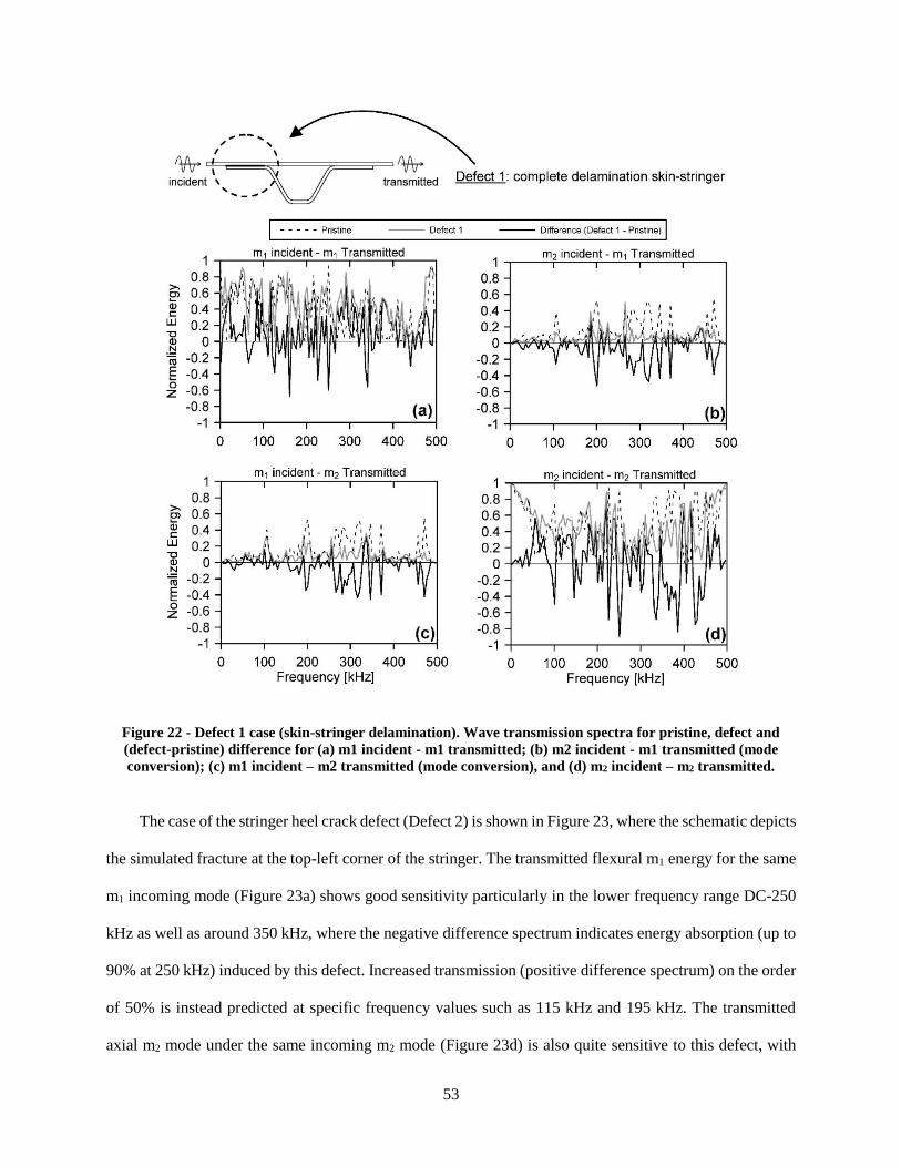
53
Figure 22 - Defect 1 case (skin-stringer delamination). Wave transmission spectra for pristine, defect and
(defect-pristine) difference for (a) m1 incident - m1 transmitted; (b) m2 incident - m1 transmitted (mode
conversion); (c) m1 incident – m2 transmitted (mode conversion), and (d) m2 incident – m2 transmitted.
The case of the stringer heel crack defect (Defect 2) is shown in Figure 23, where the schematic depicts
the simulated fracture at the top-left corner of the stringer. The transmitted flexural m1 energy for the same
m1 incoming mode (Figure 23a) shows good sensitivity particularly in the lower frequency range DC-250
kHz as well as around 350 kHz, where the negative difference spectrum indicates energy absorption (up to
90% at 250 kHz) induced by this defect. Increased transmission (positive difference spectrum) on the order
of 50% is instead predicted at specific frequency values such as 115 kHz and 195 kHz. The transmitted
axial m2 mode under the same incoming m2 mode (Figure 23d) is also quite sensitive to this defect, with

54
wave energy absorption as high as 90% in the 350 – 450 kHz range, and increased transmissions up to 50%
in other frequency ranges. The mode conversion spectra of m2 incident-m1 transmitted (Figure 23b) and m1
incident-m2 transmitted (Figure 23c) generally show less sensitivity to this defect than the same-mode
spectra, with maximum ~40% energy absorption in the 200 – 350 kHz range.
Figure 23 - Defect 2 case (stringer heel crack). Wave transmission spectra for pristine, defect and (defect-
pristine) difference for (a) m1 incident - m1 transmitted; (b) m2 incident - m1 transmitted (mode conversion);
(c) m1 incident – m2 transmitted (mode conversion), and (d) m2 incident – m2 transmitted.
The case of the stringer cap crack (Defect 3) is shown in Figure 24. The transmission spectra are
similar to those obtained for the Defect 2 case: the flexural m1 - m1 combination (Figure 24a) is most
sensitive in the low frequency range DC-200 kHz, while the axial m2 – m2 combination (Figure 24d) is
55
mostly sensitive in the higher frequency range of 250-450 kHz. In these ranges, both combinations show
significant energy absorption (as high as ~ 90%) caused by the defect. The mode-converted spectra of m2
– m1 (Figure 24b) and m1 – m2 (Figure 24c) for Defect 3 are also similar to those of Defect 2, with smaller
sensitivity compared to the same-mode spectra. One notable difference between the two stringer damage
cases is the same-mode transmission spectrum around 250 kHz, where the stringer heel crack Defect 2
causes 90% absorption for the m1 - m1 combination (Figure 23a) that does not occur for the stringer cap
crack Defect 3 (Figure 24a); the opposite occurs for the m2 – m2 combination at 250 kHz, where the stringer
cap crack Defect 3 produces 90% absorption (Figure 24d) that is much reduced for the stringer heel crack
Defect 2 (Figure 23d). These kinds of considerations can help selecting specific mode-frequency
combinations and/or interpreting results of guided-wave measurements in these structures.

56
Figure 24 - Defect 3 case (stringer cap crack). Wave transmission spectra for pristine, defect and (defect-
pristine) difference for (a) m1 incident - m1 transmitted; (b) m2 incident - m1 transmitted (mode conversion);
(c) m1 incident – m2 transmitted (mode conversion), and (d) m2 incident – m2 transmitted.
The last defect that was considered is the skin delamination (Defect 4), that was inserted between the
2nd and the 3rd layer of the composite skin laminate as schematized in Figure 25. In this case, a very sensitive
combination is the same mode flexural m1 - m1 (Figure 25a), with significant energy absorption throughout
the entire frequency range and absorption peaks of 70% at 80 kHz and 210 kHz. Interestingly, the axial m2
– m2 combination (Figure 25d) is only sensitive to this delamination in the high frequency range above 400
kHz, with a peak 80% absorption at 425 kHz. This result is expected by the rule of thumb consideration of
ultrasonic testing where higher frequencies are more sensitive due to the smaller wavelength-to-defect size

57
ratios. However, the full GL analysis presented here reveals a much more complete picture of mode
sensitivities, with specific “sensitive” mode-frequency combinations also at the lower frequencies (e.g. in
the aforementioned m1 - m1 combination). Since the skin delamination breaks the geometrical symmetry of
the skin, it creates some m2 – m1 and m1 – m2 mode conversions, shown in Figure 25b and Figure 25c,
particularly in the 250-350 kHz range. The mode conversions in this frequency range could also be utilized
to detect this kind of defect in an actual inspection test.
Figure 25 - Defect 4 case (skin delamination). Wave transmission spectra for pristine, defect and (defect-
pristine) difference for (a) m1 incident - m1 transmitted; (b) m2 incident - m1 transmitted (mode conversion);
(c) m1 incident – m2 transmitted (mode conversion), and (d) m2 incident – m2 transmitted
This work has addressed the problem of scattering of multimode and dispersive elastic waves

58
propagating in waveguide geometries. Among other applications, this topic is of great interest to ultrasonic
guided-wave NDT or SHM of structural components where defects are detected by recording transmission
or reflection scattering of a generated incoming wave mode. Predictions of these scattering patterns for a
given defect can allow to select optimum mode-frequency combinations for the incoming mode, and/or to
identify the type of defect being detected by a specific scattering observation.
For general cases that are complex in terms of either geometry or material properties (or both), this
problem requires a numerical solution. A unified Global – Local (GL) approach has been presented here,
exploiting the computational efficiency of the Semi-Analytical Finite Element (SAFE) technique for a
cross-sectional discretization of the “global” portion, coupled with a full Finite Element discretization of
the “local” portion containing the scatterer. Compared to previous GL studies, this contribution adds: (a) a
general and consistent formulation for the evaluation of the nodal tractions at the global-local boundaries;
(b) the implementation of a robust mode tracking control, based on B-orthogonality, for the automatic
selection of incoming and scattered modes; (c) the possibility to model a wide frequency range also
including higher-order modes; (d) the automatic inclusion of an energy balance check in the results; and (e)
the unification of SAFE and FE in a stand-alone numerical Matlab code that is readily extendable to more
general cases (e.g. independent treatment of the two global regions, explicitly given theoretical formulation
such as consistent nodal forces at the boundaries, or extension to 3D cases).
The proposed GL algorithm was applied to a composite skin-to-stringer assembly typical of
commercial aircraft construction. Various relevant defects were modelled, and scattering spectra were
obtained for guided-wave frequencies as high as 500 kHz under incoming flexural (A0-type) or axial (S0-
type) modes that are typically employed as excitations in guided-wave testing of these components. The
results reveal quite interesting transmission spectra, same-mode or mode-converted, that are peculiar to
each of the defects considered. These predictions can be extremely useful to guide and interpret guided-
wave inspection tests conducted on these components.
The results shown for the skin-to-stringer case study only apply to the specific geometry and material
properties considered. However, the cross-sectional mode shapes mostly control the partition of energy
59
between the incoming mode and the scattered modes. Consequently, some scalability of the results to
components of different thicknesses can be qualitatively predicted on the basis of the well-known
invariance of the guided-wave cross-sectional mode shapes with the <frequency × thickness> product (Rose
2014). In other words, for the same mode shape to be generated, frequency and thickness must be inversely
proportional. As a result, for example, specific frequency values of interest in the scattering spectra
predicted for a given thickness of the skin could be scaled to a different skin thickness, provided that the
<frequency × thickness> product is the same.
The section has considered elastic waves with no viscoelastic damping. Damping could be included
by considering complex stiffness matrices in the analysis resulting in complex wavenumbers as discussed,
for example, by Bartoli et al. (2006). The inclusion of damping would affect the predicted scattering spectra
mostly in amplitude, with presumably small shifts in peak frequency positions since those are mostly
controlled by cross-sectional mode shapes (that should not change significantly with damping).
2.3.3 3D Case study: scattering of guided waves from internal cracks in
railroad tracks
Although the GL formulation presented applies to a general 3D case, the case study considered in the
previous section was a 2D (plain strain) analysis that is quite applicable to a scanning-type guided-wave
system of the type utilized by Capriotti et al. (2017). An extension to a 3D scattering case for internal flaws
in railroad tracks using this algorithm has also been studied by the authors and is presented below.
Even though, railroad tracks are usually inspected by ultrasonic bulk waves, they can be considered
as waveguides themselves, since their own geometry supports the propagation of elastic guided waves. The
scattering in this structure is of particular interest to the authors both from a theoretical point of view, as an
extension of the GL method to a 3D case, and for a practical use to aid the work described in (Lanza di
Scalea et al., 2018). The extension of the GL method to the 3D case requires the use of 3D elements in the

60
FE local region and of 2D elements in the SAFE global region; also, the assumption of plain strain is
removed. Wave propagation in the x-direction only is still considered.
The geometry of the 3D case study is shown in Figure 26, and represents a real size version of a 136
lbs track, as the one found in regular railways. Scattering results for typical incoming wave modes were
obtained for a “pristine” case and for four “damage” cases representing different percentages of damage in
the rail head, in presence of a transverse defect (as similarly done in Bartoli et al., 2005), one of the most
relevant cause of failure of this structure, due to fatigue. The material properties and dimensions of the rail
are described in Table 6. The defect is modeled as a missing slice of the head of the rail, perpendicular to
the wave propagation direction, where a column of element has been removed for 15%, 50%, 85% or 100%
of the cross-section in the head.
A total of 22884 wedge 3-D isoparametric linear elements, arranged in 81 columns, were used for the
local discretization, for a total number of local FE nodes of 13022. On the “global” side, for computational
consistency, 284 triangular linear elements were used to discretize the cross-section for a total of 182 nodes.
Six Gauss points were used for the quadrature of the 3D elements, and three Gauss points for the 2D
elements. The maximum size of the elements was L=0.25 mm, in order to satisfy the meshing criterion:
LT (1)
where T is the wavelength of transverse waves Due to computational limitation in the RAM, a value of
𝛽 = 20 satisfies the meshing criterion up to 33 kHz, while a 𝛽 = 10 is satisfied up to 66 kHz. The
performance degrades as frequencies increase and will be better discussed in the following paragraphs. All
analyses were run using the same Core i7 CPU with 64 GB of RAM, in the frequency range of DC-200
kHz, with steps of 1 kHz, to capture the highly populated dispersion behavior of this kind of waveguide.
The incident wave source distance was 𝑑𝑠 = 1 m from the center of the geometry (origin of the reference
system) on the left side.
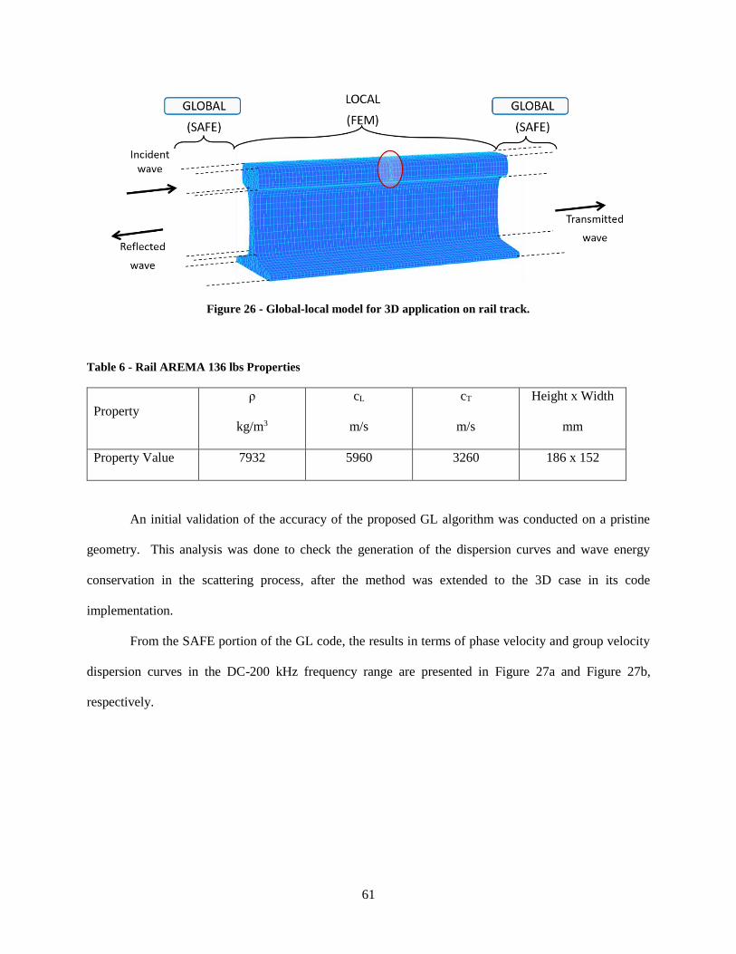
61
Figure 26 - Global-local model for 3D application on rail track.
Table 6 - Rail AREMA 136 lbs Properties
Property
ρ
kg/m3
cL
m/s
cT
m/s
Height x Width
mm
Property Value 7932 5960 3260 186 x 152
An initial validation of the accuracy of the proposed GL algorithm was conducted on a pristine
geometry. This analysis was done to check the generation of the dispersion curves and wave energy
conservation in the scattering process, after the method was extended to the 3D case in its code
implementation.
From the SAFE portion of the GL code, the results in terms of phase velocity and group velocity
dispersion curves in the DC-200 kHz frequency range are presented in Figure 27a and Figure 27b,
respectively.

62
Figure 27 - GL dispersion curves for railroad track: (left) phase velocity, (right) group velocity.
A large number of modes populate the dispersion curve in this case (e.g. 10 modes in the first 10 kHz
only), due to the size of the waveguide and its complex cross-section.
Figure 28 - Mode 5: modeshapes side view for in-plane displacement (left), front-view for out-of-plane
displacement (right).
(a) (b)
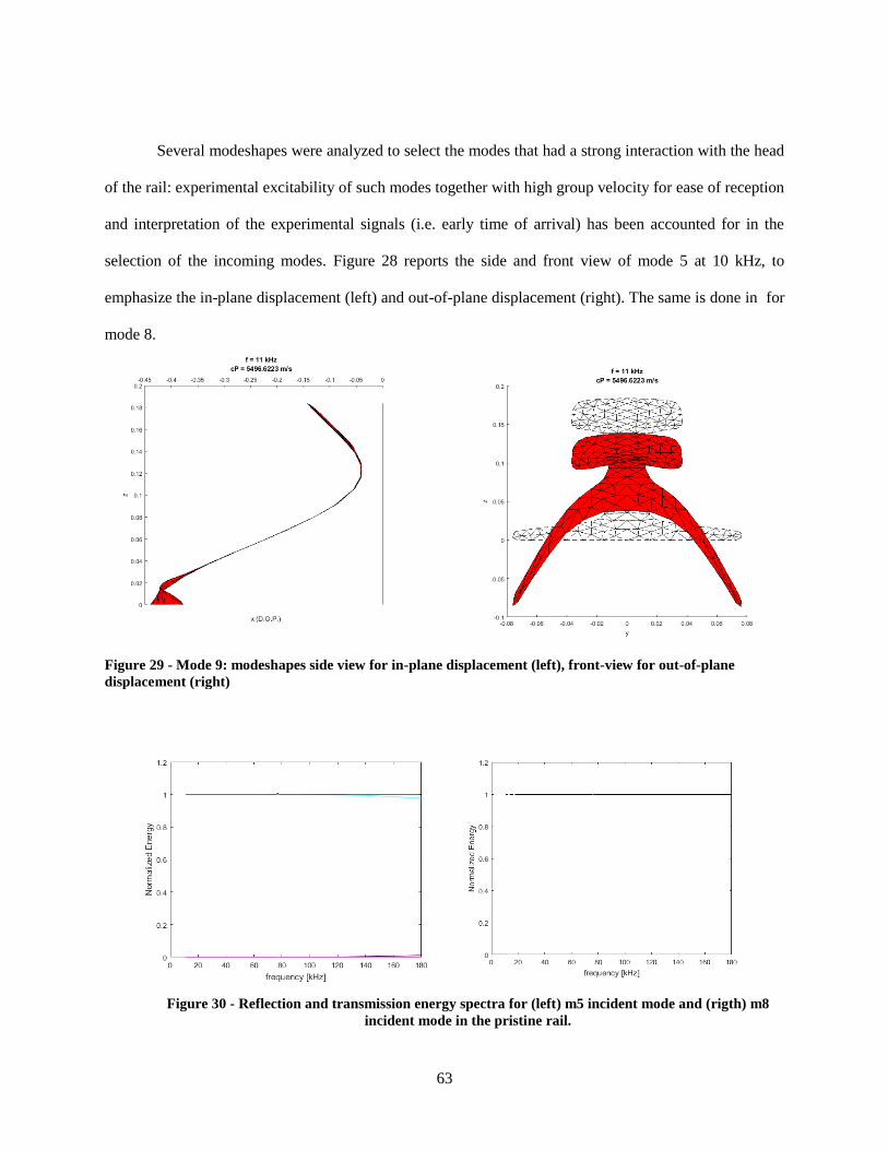
63
Several modeshapes were analyzed to select the modes that had a strong interaction with the head
of the rail: experimental excitability of such modes together with high group velocity for ease of reception
and interpretation of the experimental signals (i.e. early time of arrival) has been accounted for in the
selection of the incoming modes. Figure 28 reports the side and front view of mode 5 at 10 kHz, to
emphasize the in-plane displacement (left) and out-of-plane displacement (right). The same is done in for
mode 8.
Figure 30 - Reflection and transmission energy spectra for (left) m5 incident mode and (rigth) m8
incident mode in the pristine rail.
Figure 29 - Mode 9: modeshapes side view for in-plane displacement (left), front-view for out-of-plane
displacement (right)

64
Figure 30 shows the Normalized Energy for a pristine rail, when mode 5 (left) or mode 8 (right)
are incident in the range 10-180 kHz. Both plots validate the 3D GL method, showing conservation of
energy for the entire frequency range, when the pristine rail is analyzed. A slight mode conversion takes
place above 130 kHz when mode 5 is incident.
Figure 31 shows the same mode 5 interacting with a transverse defect in the rail, of an increasing
percentage.
It is clear how the discontinuity creates mode conversion, reducing the transmitted energy: the
larger the defect size (15% to 50%), the stronger the mode conversion (30% to 75% of the total energy),
and the lower the frequency at which mode conversion occurs (50 kHz to 20 kHz). The latter phenomena
can be explained by the physical interaction and hence alteration of waves of increasing wavelength with
Figure 31 - Reflection and transmission energy spectra for m5 incident mode in the defected head
of the rail by (a) 15%, (b) 50%, (c) 85% and (d) 100%.
(d)
(a)
(c)
(b)

65
larger defects. Moreover, when the defect involves 85% and more of the rail head, most of the wave is
reflected back (dashed lines). At 50 kHz, mode 5 couples with mode 29 in particular, where up to 60% of
the latter is reflected back when the whole head of the rail is damaged. This effect could be exploited for
example when using a pulse-echo approach in an experimental set-up to detect and characterize the
percentage of defected rail. It also highlights how, for frequencies higher than 160 kHz, the conservation
of energy is not respected, with an effect that is clearer as the defect size increases. This is related with the
leakage of energy absorption from modes included in the analysis towards modes that are not.
When exciting the structure with mode 8 (Figure 32), the inspecting wave starts interacting with
Figure 32 - Reflection and transmission energy spectra for m8 incident mode in the defected head of
the rail by (a) 15%, (b) 50%, (c) 85% and (d) 100%.
(a)
(c)
(b)
(d)
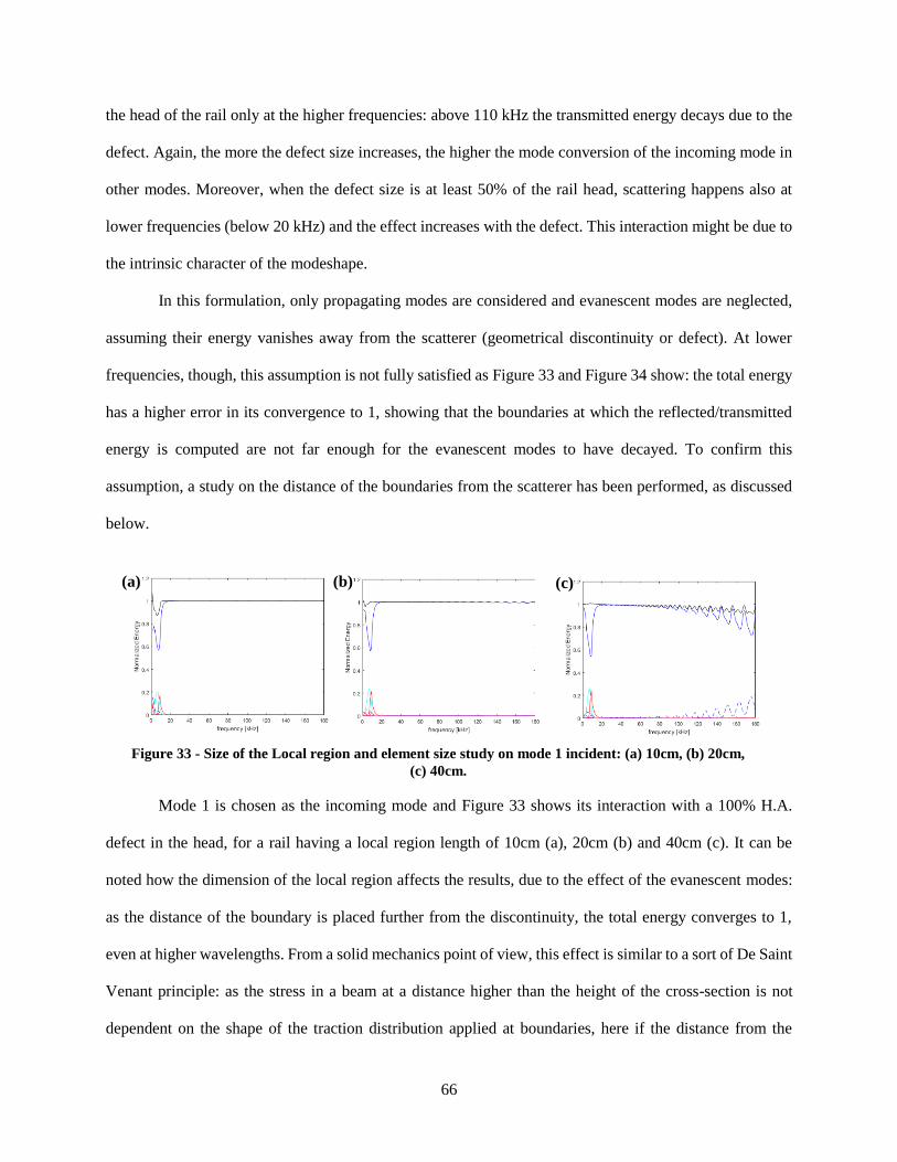
66
the head of the rail only at the higher frequencies: above 110 kHz the transmitted energy decays due to the
defect. Again, the more the defect size increases, the higher the mode conversion of the incoming mode in
other modes. Moreover, when the defect size is at least 50% of the rail head, scattering happens also at
lower frequencies (below 20 kHz) and the effect increases with the defect. This interaction might be due to
the intrinsic character of the modeshape.
In this formulation, only propagating modes are considered and evanescent modes are neglected,
assuming their energy vanishes away from the scatterer (geometrical discontinuity or defect). At lower
frequencies, though, this assumption is not fully satisfied as Figure 33 and Figure 34 show: the total energy
has a higher error in its convergence to 1, showing that the boundaries at which the reflected/transmitted
energy is computed are not far enough for the evanescent modes to have decayed. To confirm this
assumption, a study on the distance of the boundaries from the scatterer has been performed, as discussed
below.
Mode 1 is chosen as the incoming mode and Figure 33 shows its interaction with a 100% H.A.
defect in the head, for a rail having a local region length of 10cm (a), 20cm (b) and 40cm (c). It can be
noted how the dimension of the local region affects the results, due to the effect of the evanescent modes:
as the distance of the boundary is placed further from the discontinuity, the total energy converges to 1,
even at higher wavelengths. From a solid mechanics point of view, this effect is similar to a sort of De Saint
Venant principle: as the stress in a beam at a distance higher than the height of the cross-section is not
dependent on the shape of the traction distribution applied at boundaries, here if the distance from the
Figure 33 - Size of the Local region and element size study on mode 1 incident: (a) 10cm, (b) 20cm,
(c) 40cm.
(a) (b) (c)

67
boundary is smaller than the height of the cross-section, energy is not conserved.
In the same analysis, it is evident how the meshing refinement affects the performance of the
method. Due to computational limitations, the size of the elements used to discretize the geometry is
augmented as the distance to be modeled increases, namely dx=1.25mm for the 10cm case, dx=2.5mm for
the 20cm case, dx=5mm for the 40cm case. Depending on the phase velocity of the mode, the criterion is
not satisfied above a certain frequency, and convergence errors become larger as the frequency increases.
A trade-off between the element size and the dimension of the local problem needs to be found to optimize
the results and computational expense. In addition, scalability can be exploited for isotropic and symmetric
cases, exploiting the dispersion relationship between phase velocity and <frequency x thickness> product,
so that a real sized problem, very computationally expensive, can be scaled down to a smaller and faster
study.
Finally, the number of scattered modes to be included in the analysis was investigated. Particularly
for large and complex waveguides as railroad tracks, the number of modes populating the dispersion curves
is very high, hence the dimension of the problem is quite big, both in terms of theoretical complexity and
computational effort. A condition on the inclusion of the maximum number of scattered modes can be
imposed, as long as the error in the total energy remains within an acceptable threshold (i.e. less than 10%).
Figure 34 shows the improvement in the total energy result as the number of modes is increased, for an
incoming mode 5 on the 100% defect case.
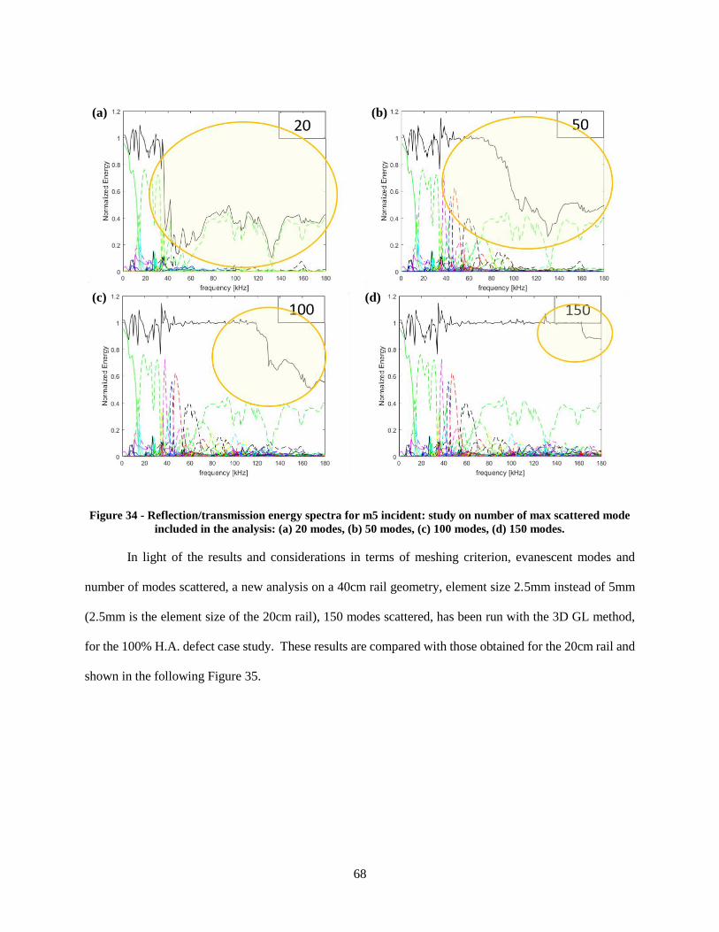
68
Figure 34 - Reflection/transmission energy spectra for m5 incident: study on number of max scattered mode
included in the analysis: (a) 20 modes, (b) 50 modes, (c) 100 modes, (d) 150 modes.
In light of the results and considerations in terms of meshing criterion, evanescent modes and
number of modes scattered, a new analysis on a 40cm rail geometry, element size 2.5mm instead of 5mm
(2.5mm is the element size of the 20cm rail), 150 modes scattered, has been run with the 3D GL method,
for the 100% H.A. defect case study. These results are compared with those obtained for the 20cm rail and
shown in the following Figure 35.
(d)
(a)
(c)
(b)

69
For both modes, it can be noticed how the distance damage-boundaries affects the result,
confirming the influence of the evanescent modes to achieve conservation of energy. The error with respect
to a total normalized energy converging to 1 reduces as the distance from the boundaries increases and
exceeds twice the cross-section of the waveguide (see Table 7).
Table 7 - Error of total energy: distance from boundary effect
Size Local
Region (cm)
Error (%)
Mode 1 Mode 2 Mode 3 Mode 4
20 12.8 7.2 11.9 23.6
40 2.4 1.4 4.0 11.4
Figure 35 - Reflection/transmission energy spectra for m2 (left) and m5 (right) incident on 100% H.A.
defect in a 20cm (top) vs a 40cm (bottom) rail.
70
In this work, the 136lbs rail track and transverse defect have been studied only, but the proposed
GL method can be extended to any waveguide geometry and type of defect.
In addition, the homogeneous solution presented here can be extended to the forced solution, where
a spatial and temporal distribution of forces can more closely simulate a real test scenario. The
implementation of such solution requires a precise frequency step and frequency range to satisfy sampling
criteria and to provide a minimum time range to observe wave propagation for the modeled distance. The
author is currently running a variety of cases for both isotropic and anisotropic materials, 2D and 3D
problems, to extract a time-domain response representing the structural behavior of the specimen with and
without defects, given certain loading set-ups.
2.4 Application
The theoretical and numerical studies performed in the previous sections provide insights in
ultrasonic guided wave propagation and enables experimental tests and NDE inspections on composite
panels. Three major sets of composite panels were fabricated in the Advanced Composite Laboratory at
UCSD for the High Energy Wide Area Blunt Impact (HEWABI) project, followed by the NDE HEWABI
project and a later NASA project. Details on the specimens fabrication and impact damage formation are
provided in Section 2.4.1. UGWs were chosen as the NDE technique to inspect the damaged panels. An
inspection prototype was developed, as shown in Section 2.4.2, after some preliminary investigations,
described in the section below.
2.4.1 Test specimen and previous studies
In the first place, composite panels from a previous FAA HEWABI project (De Francisci, 2013)
developed many major internal damage modes of interest from impact tests. These previously tested
composite panels made ideal test specimens for damage-detection studies in the NDE project because they
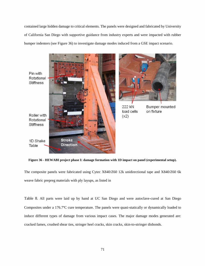
71
contained large hidden damage to critical elements. The panels were designed and fabricated by University
of California San Diego with supportive guidance from industry experts and were impacted with rubber
bumper indenters (see Figure 36) to investigate damage modes induced from a GSE impact scenario.
Figure 36 - HEWABI project phase I: damage formation with 1D impact on panel (experimental setup).
The composite panels were fabricated using Cytec X840/Z60 12k unidirectional tape and X840/Z60 6k
weave fabric prepreg materials with ply layups, as listed in
Table 8. All parts were laid up by hand at UC San Diego and were autoclave-cured at San Diego
Composites under a 176.7ºC cure temperature. The panels were quasi-statically or dynamically loaded to
induce different types of damage from various impact cases. The major damage modes generated are:
cracked fames, crushed shear ties, stringer heel cracks, skin cracks, skin-to-stringer disbonds.

72
Table 8 - Composite parts layup sequences
Part Layup Thickness (mm) Material
Skin [0/[0/45/90/-45]2S/0]* 2.7 Tape
Stringer [[0/45/-45/90/45/-45/0]S/0]** 2.4 Tape
Shear Tie [45/0]3S 2.9 Fabric
C-frame [45/0]3S*** 2.9 Fabric
* First and last 0° plies are woven fabric
** Last 0° ply is woven fabric
*** Two additional 0° fabric were added to both sides of flange
Skin and stiffening internal components have their own unique wave path and share a common
wave path only at the mechanically fastened region every 12 inches, where the shear-ties, bolted to the skin,
connect the C-frames to the whole assembly, as shown in Figure 38a. Although wave propagation through
each individual internal component was studied, differentiating between stiffened internal structure wave
transmission versus skin wave transmission remained challenging. The complex assembly and depth of the
internal components affects the wave propagation scattering pattern and travel through multiple wave paths.
It is very important to understand how much of the wave transmitted/received through the skin penetrates
the internal components and is affected by it. Therefore, various levels of assembly and aspects of joining
were further investigated to establish their influence on UGW transmission.
The tests performed on the panel, with subcomponent parts assembled and disassembled, helped to
understand wave energy leakage into the internal structural components versus transmission within the skin
only. UGW tests were performed first on the full assembly (skin with C-frame bolt joined by shear ties),
then again after removal of the C-frame, and, finally, after the removal of the shear ties (see Figure 38).
The transducers were consistently fixed in place throughout these assembly and disassembly procedures,
using a 3D-printed hold-down mount, as seen in Figure 37, to avoid variations in amplitude due to coupling
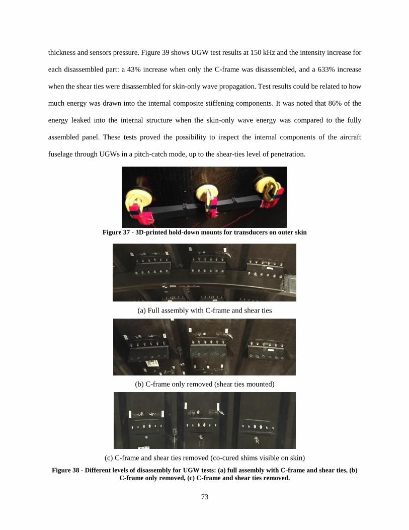
73
thickness and sensors pressure. Figure 39 shows UGW test results at 150 kHz and the intensity increase for
each disassembled part: a 43% increase when only the C-frame was disassembled, and a 633% increase
when the shear ties were disassembled for skin-only wave propagation. Test results could be related to how
much energy was drawn into the internal composite stiffening components. It was noted that 86% of the
energy leaked into the internal structure when the skin-only wave energy was compared to the fully
assembled panel. These tests proved the possibility to inspect the internal components of the aircraft
fuselage through UGWs in a pitch-catch mode, up to the shear-ties level of penetration.
Figure 37 - 3D-printed hold-down mounts for transducers on outer skin
(a) Full assembly with C-frame and shear ties
(b) C-frame only removed (shear ties mounted)
(c) C-frame and shear ties removed (co-cured shims visible on skin)
Figure 38 - Different levels of disassembly for UGW tests: (a) full assembly with C-frame and shear ties, (b)
C-frame only removed, (c) C-frame and shear ties removed.
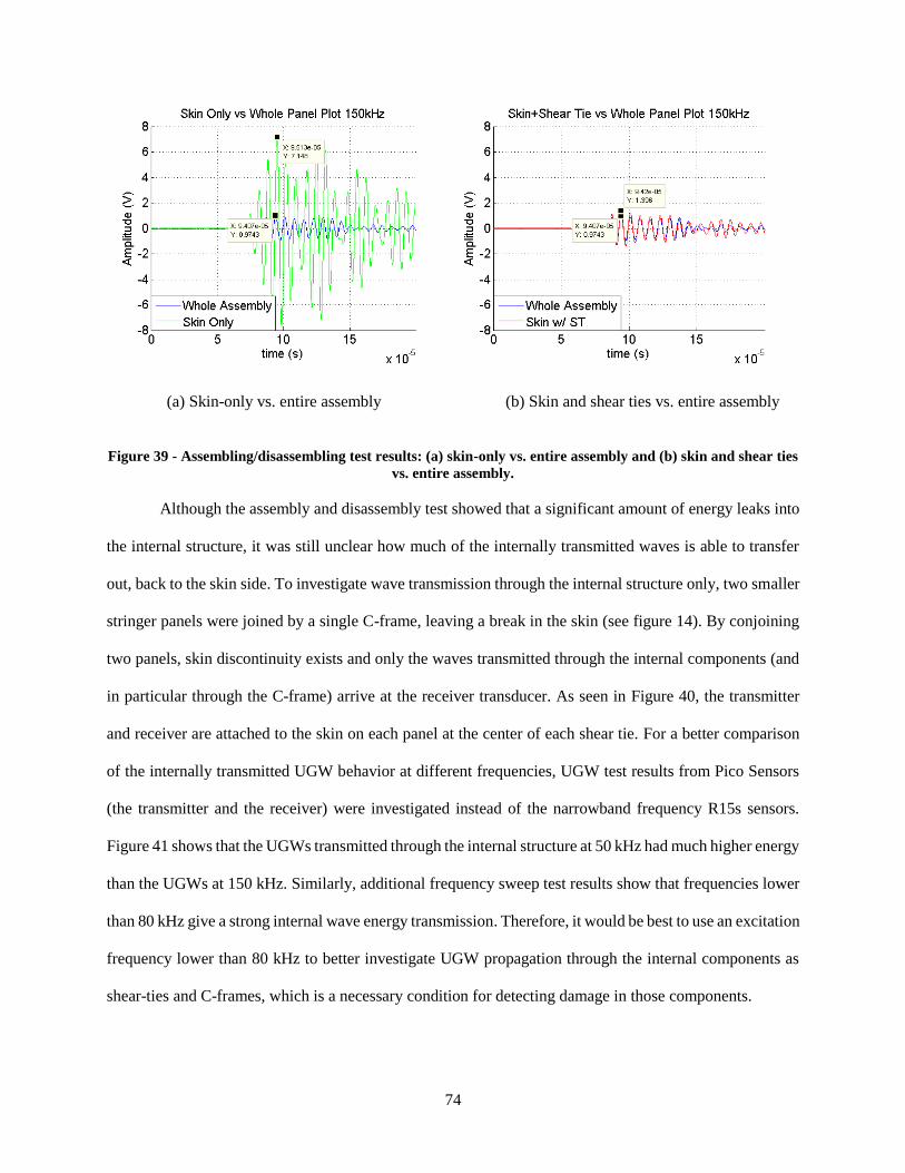
74
(a) Skin-only vs. entire assembly (b) Skin and shear ties vs. entire assembly
Figure 39 - Assembling/disassembling test results: (a) skin-only vs. entire assembly and (b) skin and shear ties
vs. entire assembly.
Although the assembly and disassembly test showed that a significant amount of energy leaks into
the internal structure, it was still unclear how much of the internally transmitted waves is able to transfer
out, back to the skin side. To investigate wave transmission through the internal structure only, two smaller
stringer panels were joined by a single C-frame, leaving a break in the skin (see figure 14). By conjoining
two panels, skin discontinuity exists and only the waves transmitted through the internal components (and
in particular through the C-frame) arrive at the receiver transducer. As seen in Figure 40, the transmitter
and receiver are attached to the skin on each panel at the center of each shear tie. For a better comparison
of the internally transmitted UGW behavior at different frequencies, UGW test results from Pico Sensors
(the transmitter and the receiver) were investigated instead of the narrowband frequency R15s sensors.
Figure 41 shows that the UGWs transmitted through the internal structure at 50 kHz had much higher energy
than the UGWs at 150 kHz. Similarly, additional frequency sweep test results show that frequencies lower
than 80 kHz give a strong internal wave energy transmission. Therefore, it would be best to use an excitation
frequency lower than 80 kHz to better investigate UGW propagation through the internal components as
shear-ties and C-frames, which is a necessary condition for detecting damage in those components.

75
Figure 40 - Conjoined panels by C-frame to study wave propagation in C-frame only: (left) outside skin view,
(right) inside skin view.
Figure 41 - Conjoined panels tests result: (left) 50kHz, (right) 150kHz received waveform.
The use of UGWs and the analysis employed in the development of the technique rely on the wave
propagation as it is determined by the given material, geometry, assembly, and finally health condition of
the specimen. The characterization of the wave-propagation properties becomes important to understand
and better exploit the feature changes, and validate the assumption made to perform the experimental tests.
As discussed in the previous section, the analytical solution cannot account for the wave propagation
Break in Skin
Excitation Reception
Wave Path Through Frame
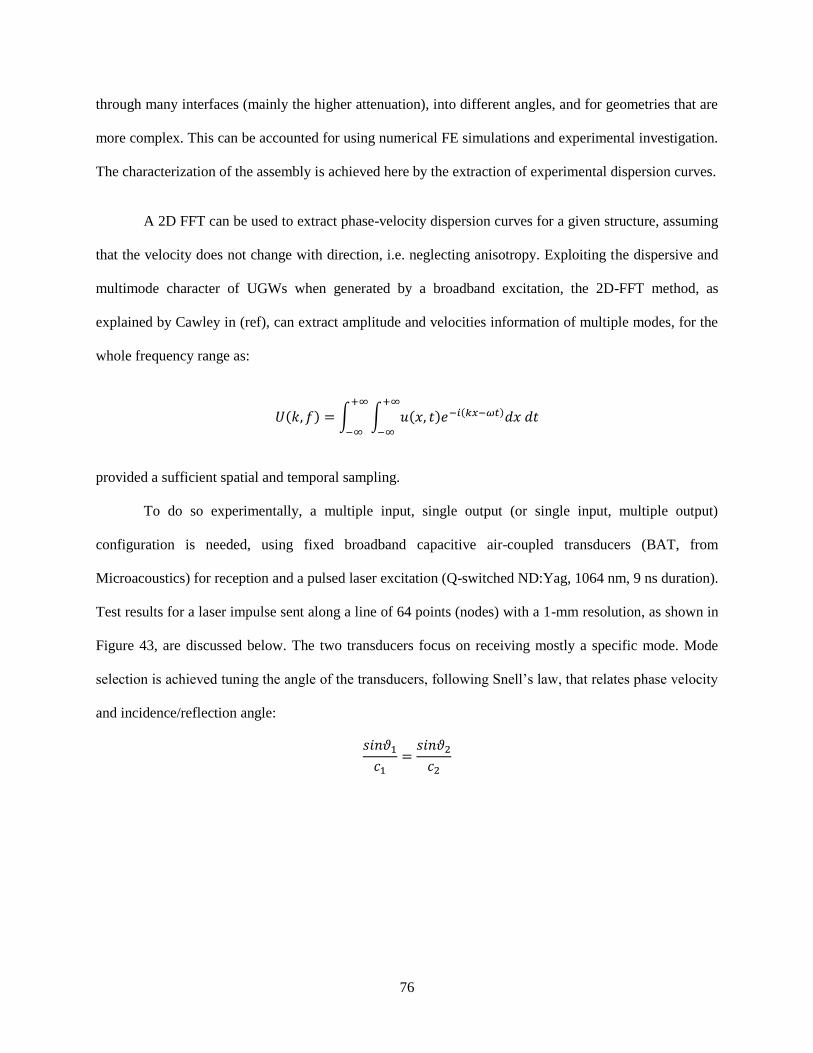
76
through many interfaces (mainly the higher attenuation), into different angles, and for geometries that are
more complex. This can be accounted for using numerical FE simulations and experimental investigation.
The characterization of the assembly is achieved here by the extraction of experimental dispersion curves.
A 2D FFT can be used to extract phase-velocity dispersion curves for a given structure, assuming
that the velocity does not change with direction, i.e. neglecting anisotropy. Exploiting the dispersive and
multimode character of UGWs when generated by a broadband excitation, the 2D-FFT method, as
explained by Cawley in (ref), can extract amplitude and velocities information of multiple modes, for the
whole frequency range as:
𝑈(𝑘, 𝑓) = ∫ ∫ 𝑢(𝑥, 𝑡)𝑒−𝑖(𝑘𝑥−𝜔𝑡)𝑑𝑥 𝑑𝑡+∞
−∞
+∞
−∞
provided a sufficient spatial and temporal sampling.
To do so experimentally, a multiple input, single output (or single input, multiple output)
configuration is needed, using fixed broadband capacitive air-coupled transducers (BAT, from
Microacoustics) for reception and a pulsed laser excitation (Q-switched ND:Yag, 1064 nm, 9 ns duration).
Test results for a laser impulse sent along a line of 64 points (nodes) with a 1-mm resolution, as shown in
Figure 43, are discussed below. The two transducers focus on receiving mostly a specific mode. Mode
selection is achieved tuning the angle of the transducers, following Snell’s law, that relates phase velocity
and incidence/reflection angle:
𝑠𝑖𝑛𝜗1𝑐1
=𝑠𝑖𝑛𝜗2𝑐2
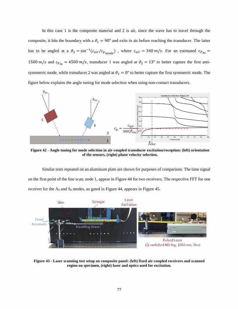
77
In this case 1 is the composite material and 2 is air, since the wave has to travel through the
composite, it hits the boundary with a 𝜗1 = 90° and exits in air before reaching the transducer. The latter
has to be angled at a 𝜗2 = sin−1(𝑐𝑎𝑖𝑟/𝑐𝑝𝑚𝑜𝑑𝑒
) , where 𝑐𝑎𝑖𝑟 = 340 𝑚/𝑠. For an estimated 𝑐𝑃𝐴0 =
1500 𝑚/𝑠 and 𝑐𝑃𝑆0 = 4500 𝑚/𝑠, transducer 1 was angled at 𝜗2 = 13° to better capture the first anti-
symmetric mode, while transducer 2 was angled at 𝜗2 = 0° to better capture the first symmetric mode. The
figure below explains the angle tuning for mode selection when using non-contact transducers.
Similar tests repeated on an aluminum plate are shown for purposes of comparison. The time signal
on the first point of the line scan, node 1, appear in Figure 44 for two receivers. The respective FFT for one
receiver for the A0 and S0 modes, as gated in Figure 44, appears in Figure 45.
Figure 43 - Laser scanning test setup on composite panel: (left) fixed air-coupled receivers and scanned
region on specimen, (right) laser and optics used for excitation.
1
2
Figure 42 - Angle tuning for mode selection in air-coupled transducer excitation/reception: (left) orientation
of the sensors, (right) phase velocity selection.
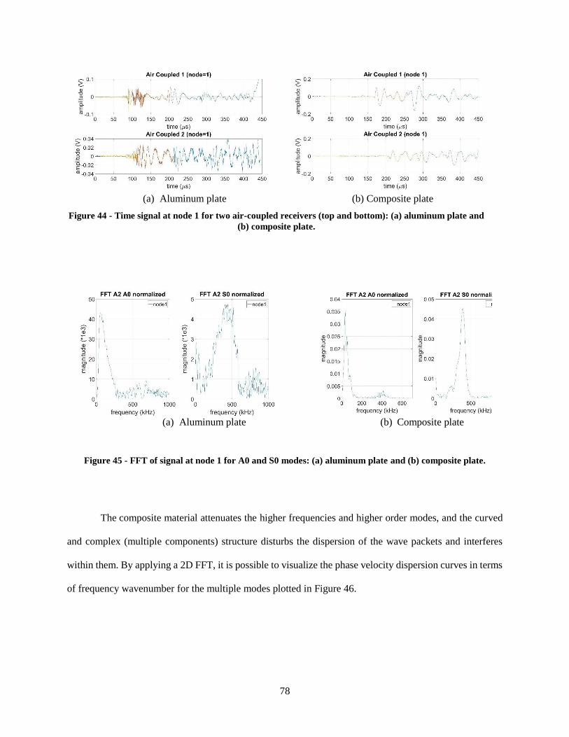
78
(a) Aluminum plate (b) Composite plate
(b)
(a) Aluminum plate (b) Composite plate
The composite material attenuates the higher frequencies and higher order modes, and the curved
and complex (multiple components) structure disturbs the dispersion of the wave packets and interferes
within them. By applying a 2D FFT, it is possible to visualize the phase velocity dispersion curves in terms
of frequency wavenumber for the multiple modes plotted in Figure 46.
Figure 44 - Time signal at node 1 for two air-coupled receivers (top and bottom): (a) aluminum plate and
(b) composite plate.
Figure 45 - FFT of signal at node 1 for A0 and S0 modes: (a) aluminum plate and (b) composite plate.
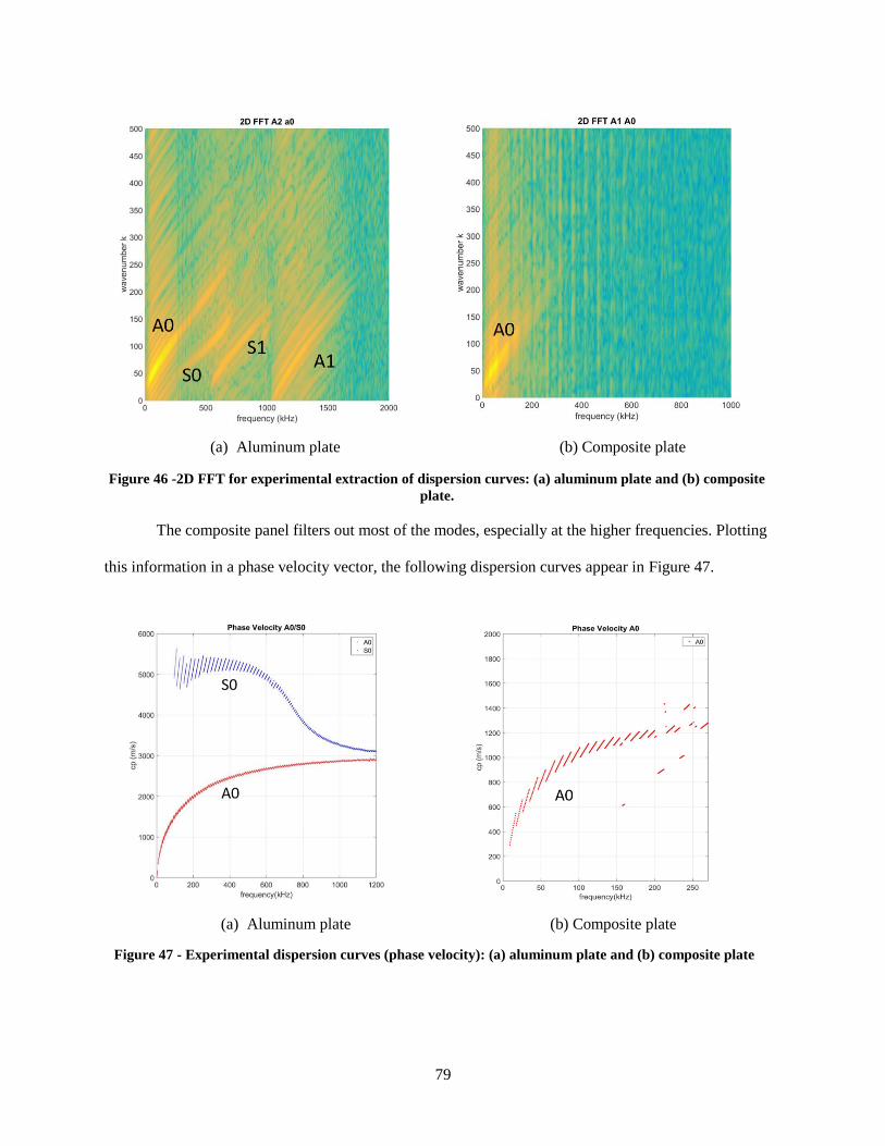
79
(a) Aluminum plate (b) Composite plate
(b)
The composite panel filters out most of the modes, especially at the higher frequencies. Plotting
this information in a phase velocity vector, the following dispersion curves appear in Figure 47.
(a) Aluminum plate (b) Composite plate
Figure 46 -2D FFT for experimental extraction of dispersion curves: (a) aluminum plate and (b) composite
plate.
Figure 47 - Experimental dispersion curves (phase velocity): (a) aluminum plate and (b) composite plate
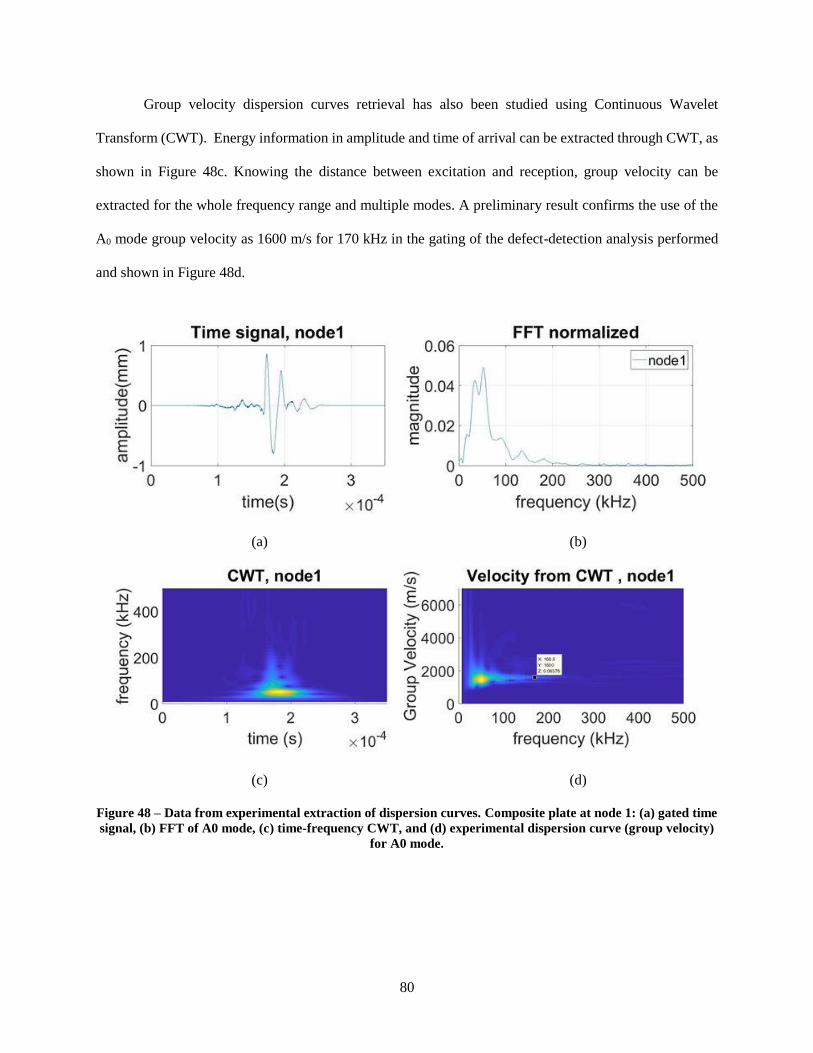
80
Group velocity dispersion curves retrieval has also been studied using Continuous Wavelet
Transform (CWT). Energy information in amplitude and time of arrival can be extracted through CWT, as
shown in Figure 48c. Knowing the distance between excitation and reception, group velocity can be
extracted for the whole frequency range and multiple modes. A preliminary result confirms the use of the
A0 mode group velocity as 1600 m/s for 170 kHz in the gating of the defect-detection analysis performed
and shown in Figure 48d.
(a) (b)
(c) (d)
Figure 48 – Data from experimental extraction of dispersion curves. Composite plate at node 1: (a) gated time
signal, (b) FFT of A0 mode, (c) time-frequency CWT, and (d) experimental dispersion curve (group velocity)
for A0 mode.
81
2.4.2 Nondestructive Inspection of Composite Aircraft Panels by
Ultrasonic Guided Waves and Statistical Processing
The same carbon/epoxy composite panels representative of commercial aircraft construction (e.g.
wide-body fuselage), manufactured and tested at UCSD from a previous FAA sponsored HEWABI project,
(De Francisci, 2013) were used to develop and test the NDE technique. The panels were designed and
manufactured following industry procedures and dedicated fabrication processes to achieve comparable
aerospace characteristics and quality. While the test specimens varied in size, they were manufactured with
the same material and overall structural design. Each test panel (Figure 49) was composed of a curved skin,
stiffened by co-cured stringers along longitudinal direction, and by C-frames (bolted to the skin by shear-
ties) along the radial direction. The lay-up of the skin was as in Table 8. All parts were cured via the
autoclave process.
These panels were subjected to wide area blunt impacts by using a rubber impactor driven by a one
degree of freedom actuator table to simulate a GSE in-service contact and resulting damage formation.
Different damage types and severities at various locations were generated and surveyed by visual inspection
and hand-held ultrasonic scanning. Detected damage included, from the outside skin into the C-frames: skin
cracks, stringer-skin disbonds or detachments, stringer cracks, shear tie cracks, and C-frame cracks. Some
of these are highlighted in Figure 49.

82
The nature of the structure suggested the use of UGW: the ultrasonic waves can travel inside the
different components of the assembly that behave as natural waveguides. Moreover, the complexity of the
panels, in terms of size, curvature, material and number of interfaces and travelling paths, require wide area
coverage and low attenuation, properties that can be satisfied by UGW. The schematic below (Figure 50(a))
shows the adopted inspection approach: the excitation is sent from the outside skin, the wave penetrates
Figure 49 - Test specimens: (a) Panel 1: five stringers, three C-frames panel with cracked skin and cracked
stringer; (b) Panel 2: four stringers, three C-frames panel with disbonded/detached stringer; (c) Panel 3:
three stringers, two C-frames panel with cracked skin, detached/cracked stringer and disbonded stringer.
(c)
(b) (a)

83
into the stringers and shear ties, travels into the C-frames and, after interacting with defects if present, can
be collected again from receivers placed on the outer skin.
(a) (b)
Numerical Finite Element studies of UGW propagation in this kind of stiffened panel were
previously conducted in Nucera et al. (2015), in the context of real-time impact force identification. Those
simulations also supported the idea of exploiting the multiple wave modes simultaneously present in this
structure. Figure 51 shows some results from FE simulations conducted using the procedure detailed in
Nucera et al. (2015), where it is possible to notice the presence of the two fundamental modes (anti-
symmetric A0 and symmetric S0) and their propagation into the different components. The specific
excitation used in this figure was an impulsive force of duration of 0.1 μs, and therefore generating a usable
frequency bandwidth up to 10 kHz. These kinds of simulations aided the time gating of the various wave
modes measured in the experimental tests that are discussed in the next sections.
Figure 50 - (a) Schematic of the UGW approach for the aerospace panel inspection. (b) Differential
scheme for contact inspection.
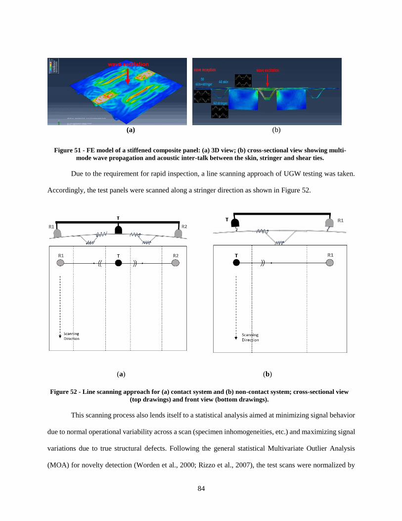
84
(a) (b)
Due to the requirement for rapid inspection, a line scanning approach of UGW testing was taken.
Accordingly, the test panels were scanned along a stringer direction as shown in Figure 52.
(a)
(b)
This scanning process also lends itself to a statistical analysis aimed at minimizing signal behavior
due to normal operational variability across a scan (specimen inhomogeneities, etc.) and maximizing signal
variations due to true structural defects. Following the general statistical Multivariate Outlier Analysis
(MOA) for novelty detection (Worden et al., 2000; Rizzo et al., 2007), the test scans were normalized by
Figure 51 - FE model of a stiffened composite panel: (a) 3D view; (b) cross-sectional view showing multi-
mode wave propagation and acoustic inter-talk between the skin, stringer and shear ties.
Figure 52 - Line scanning approach for (a) contact system and (b) non-contact system; cross-sectional view
(top drawings) and front view (bottom drawings).
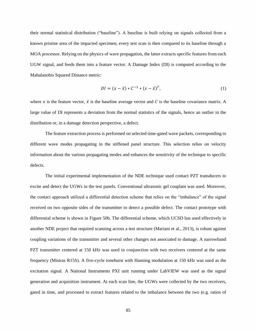
85
their normal statistical distribution (“baseline”). A baseline is built relying on signals collected from a
known pristine area of the impacted specimen; every test scan is then compared to its baseline through a
MOA processor. Relying on the physics of wave propagation, the latter extracts specific features from each
UGW signal, and feeds them into a feature vector. A Damage Index (DI) is computed according to the
Mahalanobis Squared Distance metric:
𝐷𝐼 = (𝑥 − �̅�) ∗ 𝐶−1 ∗ (𝑥 − �̅�)𝑇, (1)
where 𝑥 is the feature vector, �̅� is the baseline average vector and 𝐶 is the baseline covariance matrix. A
large value of DI represents a deviation from the normal statistics of the signals, hence an outlier in the
distribution or, in a damage detection perspective, a defect.
The feature extraction process is performed on selected time-gated wave packets, corresponding to
different wave modes propagating in the stiffened panel structure. This selection relies on velocity
information about the various propagating modes and enhances the sensitivity of the technique to specific
defects.
The initial experimental implementation of the NDE technique used contact PZT transducers to
excite and detect the UGWs in the test panels. Conventional ultrasonic gel couplant was used. Moreover,
the contact approach utilized a differential detection scheme that relies on the “imbalance” of the signal
received on two opposite sides of the transmitter to detect a possible defect. The contact prototype with
differential scheme is shown in Figure 50b. The differential scheme, which UCSD has used effectively in
another NDE project that required scanning across a test structure (Mariani et al., 2013), is robust against
coupling variations of the transmitter and several other changes not associated to damage. A narrowband
PZT transmitter centered at 150 kHz was used in conjunction with two receivers centered at the same
frequency (Mistras R15S). A five-cycle toneburst with Hanning modulation at 150 kHz was used as the
excitation signal. A National Instruments PXI unit running under LabVIEW was used as the signal
generation and acquisition instrument. At each scan line, the UGWs were collected by the two receivers,
gated in time, and processed to extract features related to the imbalance between the two (e.g. ratios of

86
amplitudes). The specific features used are listed in Table 9 (𝑥1/2 refers to the signal from receiver 1 and
2, respectively).
Table 9 - Contact technique features list.
Feature # Feature Name Feature Extraction
1 RMS Ratio 𝑅𝑀𝑆(𝑥1)
𝑅𝑀𝑆(𝑥2)
2 Maximum Value Ratio 𝑀𝑎𝑥(𝑀𝑎𝑥|𝑥1|
𝑀𝑎𝑥|𝑥2|,𝑀𝑎𝑥|𝑥2|
𝑀𝑎𝑥|𝑥1|)
3 Area under Packet Ratio 𝐴𝑟𝑒𝑎(𝑥1)
𝐴𝑟𝑒𝑎(𝑥2)
4 Peak to Peak Normalized Difference |𝑃𝑝𝑘(𝑥1) − 𝑃𝑝𝑘(𝑥2)|
√𝑃𝑝𝑘(𝑥1) ∗ 𝑃𝑝𝑘(𝑥2)
5 Area under FFT Normalized Difference |𝐴𝑟𝑒𝑎𝐹𝐹𝑇(𝑥1) − 𝐴𝑟𝑒𝑎𝐹𝐹𝑇(𝑥2)|
√𝐴𝑟𝑒𝑎𝐹𝐹𝑇(𝑥1) ∗ 𝐴𝑟𝑒𝑎𝐹𝐹𝑇(𝑥2)
6
Maximum Value Cross-Correlation
Normalized Difference
max(𝑥𝑐𝑜𝑟𝑟(𝑥1, 𝑥2))
√max(𝑥𝑐𝑜𝑟𝑟(𝑥1)) ∗ max(𝑥𝑐𝑜𝑟𝑟(𝑥2))
7 Variance Normalized Difference |𝑉𝑎𝑟(𝑥1) − 𝑉𝑎𝑟(𝑥2)|
√𝑉𝑎𝑟(𝑥1) ∗ 𝑉𝑎𝑟(𝑥2)
8 RMS Normalized Difference |𝑅𝑀𝑆(𝑥1) − 𝑅𝑀𝑆(𝑥2)|
√𝑅𝑀𝑆(𝑥1) ∗ 𝑅𝑀𝑆(𝑥2)
These features were then fed into the feature vector and used to compute the DI metric according to
eq. (1). The scan resolution across the damaged areas was approximately 1 cm.
Representative results are shown in Figure 53(a) and (b) for Panel 1 and Panel 2, respectively. The
vertical lines represent known positions of defects from the prior visual surveys and ultrasonic scans. It can
be noticed how the DI increases noticeably in known damaged areas, with very low noise levels, owing to
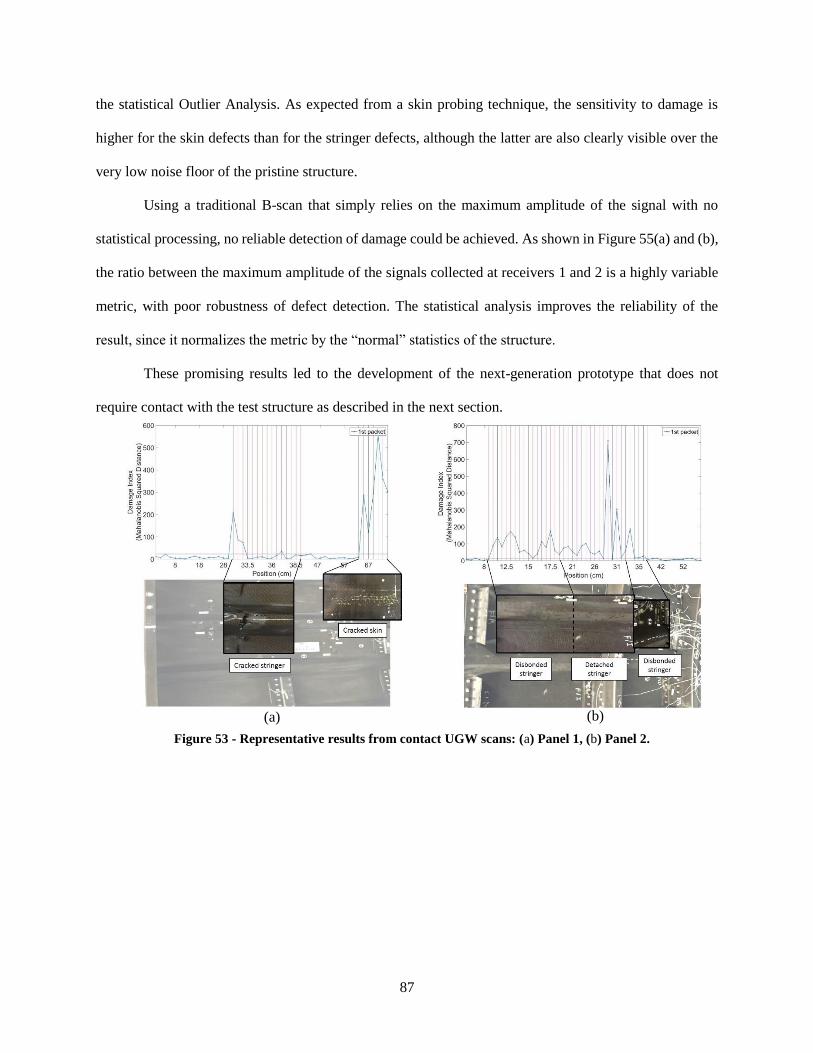
87
the statistical Outlier Analysis. As expected from a skin probing technique, the sensitivity to damage is
higher for the skin defects than for the stringer defects, although the latter are also clearly visible over the
very low noise floor of the pristine structure.
Using a traditional B-scan that simply relies on the maximum amplitude of the signal with no
statistical processing, no reliable detection of damage could be achieved. As shown in Figure 55(a) and (b),
the ratio between the maximum amplitude of the signals collected at receivers 1 and 2 is a highly variable
metric, with poor robustness of defect detection. The statistical analysis improves the reliability of the
result, since it normalizes the metric by the “normal” statistics of the structure.
These promising results led to the development of the next-generation prototype that does not
require contact with the test structure as described in the next section.
Figure 53 - Representative results from contact UGW scans: (a) Panel 1, (b) Panel 2.
(a) (b)

88
To ease the applicability of a rapid scanning technique for an actual field application, a non-contact
version of the UGW system was designed, constructed and tested, which omits the need of couplant
application per scan. Shown in Figure 55, the non-contact scanning prototype consists of a cylindrically
focused air-coupled transmitter (Ultran NCG200-S50-C76-EP-X) (right-hand side in Figure 55) and an
unfocused air-coupled receiver (Ultran NCG200-S19) operated in a pitch-catch mode. The transducers
(both narrowband with a central frequency of 170 kHz) are mounted on a moving cart that allows the rapid
and consistent scanning of the test structure. The stability of the non-contact coupling removes the need for
the differential approach such that a simple pitch-catch test scheme is appropriate. The transducers are also
oriented at angles that maximize the transduction of the dominant flexural mode in the panel’s skin (Rose,
2004; Tuzzeo et al., 2007). Both transducers are piezocomposite devices that minimize the acoustic
impedance mismatch with air for maximum ultrasonic signal transmission and reception. The excitation
signal is a five-cycle toneburst with Hanning modulation centered at 170 kHz. The same NI PXI unit used
in the contact setup was used for signal excitation and acquisition.
Figure 54 - Amplitude Ratio from contact UGW scans: (a) Panel 1, (b) Panel 2
(a) (b)
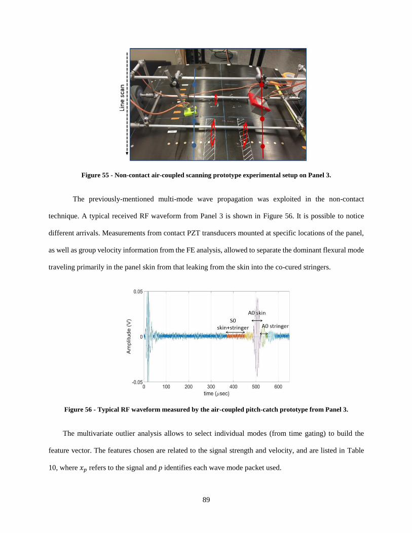
89
Figure 55 - Non-contact air-coupled scanning prototype experimental setup on Panel 3.
The previously-mentioned multi-mode wave propagation was exploited in the non-contact
technique. A typical received RF waveform from Panel 3 is shown in Figure 56. It is possible to notice
different arrivals. Measurements from contact PZT transducers mounted at specific locations of the panel,
as well as group velocity information from the FE analysis, allowed to separate the dominant flexural mode
traveling primarily in the panel skin from that leaking from the skin into the co-cured stringers.
Figure 56 - Typical RF waveform measured by the air-coupled pitch-catch prototype from Panel 3.
The multivariate outlier analysis allows to select individual modes (from time gating) to build the
feature vector. The features chosen are related to the signal strength and velocity, and are listed in Table
10, where 𝑥𝑝 refers to the signal and p identifies each wave mode packet used.

90
Table 10 - Non-contact technique features list
Feature # Feature Name Feature Extraction
1 Maximum Value 𝑀𝑎𝑥|𝑥𝑝|
2 Index of Maximum Value 𝐼𝑛𝑑(𝑀𝑎𝑥|𝑥𝑝|)
3 Variance 𝑉𝑎𝑟(𝑥𝑝)
4 Kurtosis 𝐾𝑢𝑟𝑡(𝑥𝑝)
The figure below presents the DI trace obtained from the line scan of test panel 3 and using (a) only
skin modes, and (b) skin and stringer modes. It can be noticed how adding the stringer modes results into
an enhanced defect detection sensitivity, especially for the stringer defects.
(a) (b)
Again, the B-scan for the maximum amplitude value is reported in Figure 58, to show the benefit of
the statistical analysis.
Figure 57 - Representative results from noncontact (air-coupled) UGW scans of Panel 3: (a) skin
modes only; (b) skin modes plus stringer modes

91
Figure 58 - Maximum Amplitude from non-contact UGW scans: Panel 3
In order to properly assess the performance of the tests, Receiver Operating Characteristic (ROC)
curves were computed (Mariani S., PhD Thesis 2007). These plots compare the Probability of Detection
(POD) to the Probability of False Alarm (PFA) for different threshold levels applied to the DI traces.
ROC curves were computed for each defect type at varying DI thresholds: a curve located in the upper
left corner of the plot indicates a good defection performance (high POD and low PFA). The Area Under
the Curve (AUC) is a metric that summarizes this goodness in performance. The dashed straight line
represents the 50-50 guess.
Figure 59 shows the ROC curves for the contact NDE prototype on Test Panel 1 and Test Panel 2 for
the disbonded stringer, the detached stringer and the cracked skin types of defects. Each symbol in the
curves represents a threshold level applied to the DI traces from the line scans. These results indicate, for
example, that the cracked skin defect can be detected with an 86% POD and 0% PFA or, alternatively, with
a 100% POD and 26% PFA. Similarly, the disbonded stringer defect can be detected with a 94% POD and
0% PFA or, alternatively, with a 100% POD and 29% PFA. A somewhat worse performance was found for

92
the detached stringer defect, where an 80% POD affords a 0% PFA (and a 100% POD results into a 47%
PFA).
Figure 59 - ROC curves for the contact NDE technique: cracked skin, disbonded stringer and detached
stringer defects (Panel 1 and Panel 2).
Figure 60 and Figure 61 show the ROC curves for the non-contact NDE technique applied to Test
Panel 3. Figure 60 shows the results obtained using the skin modes only. The detection performance is
excellent, especially considering the non-contact nature of the coupling. The best detection performance
was found for the cracked skin and the disbonded stringer defect (e.g. 100% POD with less than 10% PFA),
with somewhat worse performance for the detached/cracked stringer defect (e.g. 100% POD with 25%
PFA, or 70% POD with 0% PFA).
Figure 60 - ROC curves for the non-contact NDE technique (skin modes only): cracked skin, detached
stringer and disbonded stringer defects (Panel 3).
In Figure 61, the stringer modes are added to the skin modes in the feature vector. This combination
results in a perfect detection performance for all defects considered, i.e. a 100% POD with 0% PFA. The

93
reason for this improvement is that the acoustic cross-talk between skin and stringer is such that modes
primarily propagating into one of the two components are sensitive to defects in the other component, in
addition to defects in the same component.
Figure 61 - ROC curves for the non-contact NDE technique (skin and stringer modes): cracked skin,
detached stringer and disbonded stringer defects (Panel 3).
This section summarizes a rapid NDE technique for the detection of structural defects in composite
aircraft structures subjected to Ground Service Equipment (GSE) impacts. The approach taken utilizes the
waveguide geometry of the structure by means of ultrasonic guided waves. Two laboratory prototypes for
line scanning have been developed, one using contact PZT transducers with a differential approach, and
one using non-contact (air-coupled) transducers in a pitch-catch approach. The inspection utilizes a
statistical outlier analysis that compensates each measurement for the normal (baseline) variation during a
scan, thereby increasing the POD (true detections) and decreasing the PFA (false positive). Tests conducted
on previously impacted test panels representative of commercial aircraft construction indicated an excellent
detection performance (in terms of POD vs. PFA tradeoffs) for skin and stringer defects. A perfect detection
for these defects was actually obtained by the non-contact system once both skin wave modes and stringer
wave modes were combined in the statistical feature vector.
The prototypes discussed here are early-stage laboratory systems that do not include automatic data
processing of the scan. Ongoing work is aimed at adding a tachometer to track the position of the inspection
head, and implementing automatic signal processing to generate the scan output in quasi-real time.

94
The defects tested in this study were limited to the panel skin and stringers. Defects located in the
deeper structure, specifically shear ties and C-frames, were not targeted because the frequencies used were
found too high to penetrate these regions. Ongoing work is aimed at testing lower UGW frequencies in an
effort to penetrate into the C-frames to provide comprehensive coverage of the structure.
2.4.3 Inspection of composite aerospace structures by extraction of
UGW transfer function
To increase the level of damage/structural characterization, as explained in the introduction, and to
reduce the equipment bulkiness, towards portability and automation for in situ inspection, the UGW NDE
technique moved to a new design and more advanced approach.
The motivation to an improved scanning and signal processing can be well understood observing Figure
62, where three defected condition of the panel show very low SNR, when using a linear (less powerful)
amplifier:

95
Figure 62 - Portable cart-scan set-up (left) with corresponding typical low SNR RF waveforms at specific
defective locations (right): cracked skin (top, red), detached/cracked stringer (center, black), disbonded
stringer (bottom, green), with respect to pristine location (blue).
It can be noticed how the quality of the signal degraded and the wavemodes are less clear. Also,
the data obtained in Figure 62 are the result of an averaging processing where 100 averages per scan have
been used.
To better investigate and isolate wave propagation in the stiffening structure skin-to-stringer and
its interaction with different damage modes, a third set of composite panels was fabricated at UCSD under
a NASA project.
The theory of the dual-output extraction of the transfer function is illustrated below. The problem
at hand is schematized in the block diagram of Figure 63. The first goal is to isolate the transfer function
of the waveguide structure between two points A and B, HAB. The second goal is to associate any changes

96
in the extracted HAB to the presence of structural damage between A and B. The technique shown in Figure
63 uses one transmitter of ultrasonic guided waves (e.g. an air-coupled transmitter or an impactor in a
scanning system) in combination with two receivers positioned at points A and B (e.g. a pair of air-coupled
receivers) – hence a single-input-dual-output (SIDO) scheme.
Figure 63 - Extraction of the structural transfer function between two points A and B by a single-input-dual-
output (SIDO) scheme.
The formulation is more easily presented in the frequency domain. By using the convolution theorem and
assuming linearity, the signal measured by receiver 1 can be written as:
1 1 1( ) ( ) ( ) ( ) ( ) ( ) ( )SAM f S f T f TS f H f SR f R f (1)
In eq. (1), S(f) is the input signal, T(f) is the transmitting transducer frequency response, TS(f) is the
transducer-to-structure coupling frequency response, HSA(f) is the structure transfer function between
source and point A, SR1(f) is the structure-to-receiver 1 coupling response, and R1(f) is the receiver 1
frequency response.

97
Similarly, the signal measured by receiver 2 can be written as:
2 2 2( ) ( ) ( ) ( ) ( ) ( ) ( ) ( )SA ABM f S f T f TS f H f H f SR f R f (2)
where HAB(f) is the desired structure transfer function between A and B, SR2(f) is the structure-to-receiver
2 coupling response, and R2(f) is the receiver 2 frequency response.
The deconvolution operation between the two receivers leads to:
2 2 2
1 1 1
( ) ( ) ( )( )
( ) ( ) ( )AB
M f SR f R fDeconv H f
M f SR f R f (3)
If the two receivers are the same device (e.g. two air-coupled receivers), their frequency response and
structure-to-transducer coupling can be reasonably assumed equal, hence: R1(f)= R2(f) and SR1(f)= SR2(f).
In this case,
2
1
( )( )
( )AB
M fDeconv H f
M f (4)
The time-domain transfer function can be simply computed from the frequency domain by an inverse
Fourier Transform operation:
( ) ( )eAB ABH t H f df
(5)
Hence the deconvolution operation between the two receivers can isolate the desired structure transfer
function without the influence of spurious factors, primarily the excitation signal that can be highly variable
(e.g. an impactor) and could lead to false positive indications of damage.
If the response of the two receivers is different, the deconvolution operation of eq. (3) can still be
an effective structural monitoring metric because it leads to a scaled version of the pure HAB where the scale
factor does not change during the scanning process. Hence any changes in this metric can be reasonably
attributed to changes in the structure (e.g. damage) between A and B.
In an effort to validate the transfer function extraction by the above SIDO scheme, the paper
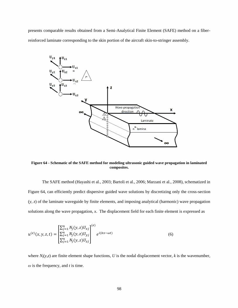
98
presents comparable results obtained from a Semi-Analytical Finite Element (SAFE) method on a fiber-
reinforced laminate corresponding to the skin portion of the aircraft skin-to-stringer assembly.
Figure 64 - Schematic of the SAFE method for modeling ultrasonic guided wave propagation in laminated
composites.
The SAFE method (Hayashi et al., 2003; Bartoli et al., 2006; Marzani et al., 2008), schematized in
Figure 64, can efficiently predict dispersive guided wave solutions by discretizing only the cross-section
(y, z) of the laminate waveguide by finite elements, and imposing analytical (harmonic) wave propagation
solutions along the wave propagation, x. The displacement field for each finite element is expressed as
𝑢(𝑒)(𝑥, 𝑦, 𝑧, 𝑡) = [
∑ 𝑁𝑗(𝑦, 𝑧)𝑈𝑥𝑗𝑛𝑗=1
∑ 𝑁𝑗(𝑦, 𝑧)𝑈𝑦𝑗𝑛𝑗=1
∑ 𝑁𝑗(𝑦, 𝑧)𝑈𝑧𝑗𝑛𝑗=1
]
(𝑒)
𝑒𝑖(𝑘𝑥−𝜔𝑡) (6)
where Nj(y,z) are finite element shape functions, U is the nodal displacement vector, k is the wavenumber,
ω is the frequency, and t is time.
99
In the case of a multilayered composite laminate, the local lamina stiffness matrix C can be rotated
onto the global (x, y, z) reference system of the laminate using the following transformation relation (Bartoli
et al., 2006):
11 2C R C R
(7)
The global stiffness matrix Cθ is then assembled to describe the entire laminate.
Using energy balance from Hamilton’s principle, the SAFE formulation leads to the following
eigenvalue problem for an M-degree of freedom system:
2
0A B QM
k (8)
where the matrices A and B contain mass and stiffness terms and the vector T[ ]Q U Uk contains the
nodal displacements (Hayashi et al., 2003).
The eigenproblem of eq. (7) can be solved by finding the eigenvalues km (m-th mode wavenumber)
and the eigenvectors Um (m-th mode cross-sectional mode shapes) for each frequency ω. Considering
propagative modes only, the phase velocity dispersion curves for the waveguide are then calculated as
cph(ω) = ω/ k, and the group velocity as cgr(ω) = ω / k following well known relations (Rose, 2014).
These eigensolutions represent the unforced vibrating modes of the waveguide. From these, a
transfer function for the structure can be calculated by computing the “forced” solution of the waveguide,
i.e. the waveguide’s response at point xR to a given forcing excitation at point xS. The forced response can
be calculated from SAFE in a normal mode expansion sense by summing the contributions of the unforced
modes, each weighted by a “participation factor” that represents the degree of similarity between the
excitation shape and the mode shape (Hayashi et al., 2003). Using the notation by (Marzani et al., 2008),
the forced response in the frequency domain can be written as:

100
( )
1
( )U U F U m R S
mM Tik x xm m
R L Rm m
kx i e
D
(9)
where Q B QT
m mm L RD , m is the individual mode, M is the total number of forward propagating modes,
the subscripts L and R represent left and right eigenvectors, the superscript T is transpose, and the vector
F contains the applied nodal forces in frequency (Fourier coefficients). Eq. (9) is solved at each frequency
value (Fourier series expansion). The forced response can be converted to the time domain by the following
inverse Fourier Transform:
( , ) ( , )eU UR Rx t x f df
(10)
For purposes of comparison with the experimental transfer function, the SAFE predicted response
is computed by considering a forcing function signal that best matches the frequency content of the
experimental signals. For example, for a (narrowband) air-coupled transducer excitation, the model uses a
Hanning modulated toneburst forcing function with a similar frequency bandwidth; for a (broadband)
hammer impact excitation, the model uses an impulse-type forcing function.
This section presents a comparison between experimental and predicted transfer functions for
guided waves propagating in a Carbon-Fiber-Reinforced Composite (CFRP) laminate representative of the
skin of a B787 aircraft fuselage panel. The laminate was a 30 cm × 30 cm plate, composed of 16 plies,
each with a thickness of 0.164 mm, with a quasi-isotropic and symmetric layup [45/-45/0/45/90/-45/0/90]s.
Material’s constants from the manufacturer (unidirectional prepreg tape) are shown in Table 11.
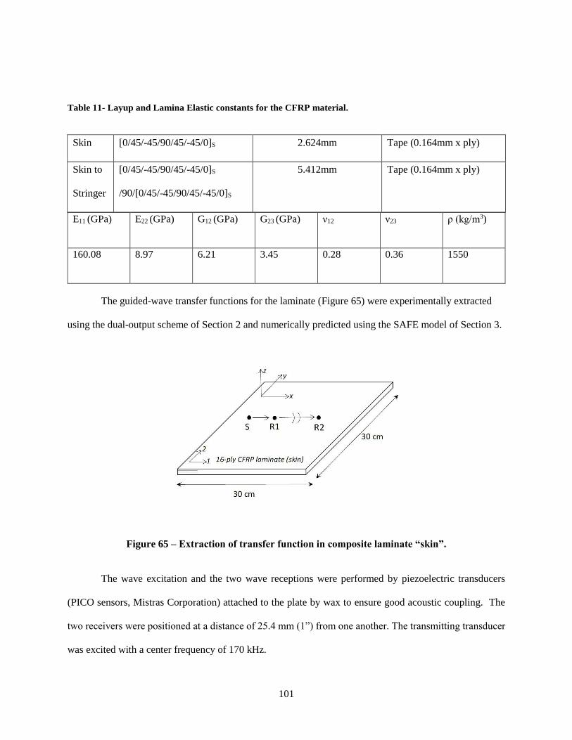
101
Table 11- Layup and Lamina Elastic constants for the CFRP material.
Skin [0/45/-45/90/45/-45/0]S 2.624mm Tape (0.164mm x ply)
Skin to
Stringer
[0/45/-45/90/45/-45/0]S
/90/[0/45/-45/90/45/-45/0]S
5.412mm Tape (0.164mm x ply)
E11 (GPa) E22 (GPa) G12 (GPa) G23 (GPa) ν12 ν23 ρ (kg/m3)
160.08 8.97 6.21 3.45 0.28 0.36 1550
The guided-wave transfer functions for the laminate (Figure 65) were experimentally extracted
using the dual-output scheme of Section 2 and numerically predicted using the SAFE model of Section 3.
Figure 65 – Extraction of transfer function in composite laminate “skin”.
The wave excitation and the two wave receptions were performed by piezoelectric transducers
(PICO sensors, Mistras Corporation) attached to the plate by wax to ensure good acoustic coupling. The
two receivers were positioned at a distance of 25.4 mm (1”) from one another. The transmitting transducer
was excited with a center frequency of 170 kHz.

102
The experimental transfer function was extracted by first time-gating the responses from the two
receivers to eliminate wave reflections from the plate’s boundaries (Figure 66(a) and (b)). After
transforming to the frequency domain, the deconvolution operation between the receivers was performed
according to eq. (4), followed by a band-pass filtering in the 50 kHz – 270 kHz range that contained the
signal energy from the measurements - Figure 66(c). An inverse Fourier Transform lead to the time-domain
experimental transfer function that is shown in Figure 66(d). The final trace in Figure 66(d) shows a clear
wave packet arriving at around 20 sec. This corresponds to a flexural guided wave mode for the composite
laminate that would be produced by an excitation located at R1 and detected by a receiver located at R2 in
Fig. 3, and is exactly the type of result that was expected by the dual-output deconvolution operation in this
case. If a structural defect were to be present between R1 and R2, this trace would be affected due to wave
scattering at the discontinuity.
The corresponding transfer function predicted by the SAFE model for this case is also shown in
Figure 66(e) and overlapped to the experimental trace. Amplitudes are scaled to 1 since attenuation effects
were not considered in the numerical analysis. The match is quite favorable, in terms of both arrival times
and overall shape of the wave packet. This result confirms the applicability of the deconvolution operation
between the two receivers to extract the structure’s transfer function.

103
Figure 66 – CFRP laminate skin: (a) response measured by receiver 1; (b) response measured by receiver 2;
(c) experimental transfer function in the frequency domain; (d) experimental transfer function in the time
domain; (e) comparison between experimental and numerical (SAFE) transfer functions.

104
To calculate the predicted response, the SAFE model was run for the given laminate lay-up using
the properties in Table 11 and rotating the stiffness matrix of each ply according to eq. (7). The wave
propagation direction was along the fibers in the top ply of the laminate. The FE cross-sectional
discretization used quadratic mono-dimensional elements with 2 elements per ply, 3 nodes per element and
three degrees of freedom per node. The analysis started with the computation of the unforced guided-wave
modes of the laminate as the solutions of the eigenproblem in eq. (8). Figure 67 shows the results of the
unforced solutions from SAFE in terms of phase velocity dispersion curves –Figure 67(a), group velocity
dispersion curves – Figure 67(b), and cross-sectional displacement mode shapes at 170 kHz for the three
fundamental wave modes of axial (S0) – Figure 67(c), flexural (A0) – Figure 67(e), and shear horizontal
(SH0) – Figure 67(d). Some of the profiles show the typical “jumpy” behavior that is due to the different
ply orientations. For the computation of the transfer function shown in Figure 66(e), eq. (10) was employed
at the two receiver positions R1 and R2 using a forcing function at S consisting of an out-of-plane force
(direction z) applied to the top node of the cross-section as a toneburst of 50 -270 kHz, consistently with
the experimental bandwidth.
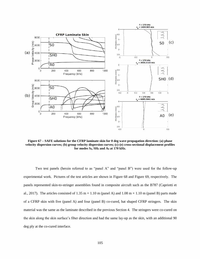
105
Figure 67 – SAFE solutions for the CFRP laminate skin for 0 deg wave propagation direction: (a) phase
velocity dispersion curves; (b) group velocity dispersion curves; (c)-(e) cross-sectional displacement profiles
for modes S0, SH0 and A0 at 170 kHz.
Two test panels (herein referred to as “panel A” and “panel B”) were used for the follow-up
experimental work. Pictures of the test articles are shown in Figure 68 and Figure 69, respectively. The
panels represented skin-to-stringer assemblies found in composite aircraft such as the B787 (Capriotti et
al., 2017). The articles consisted of 1.35 m × 1.10 m (panel A) and 1.08 m × 1.10 m (panel B) parts made
of a CFRP skin with five (panel A) and four (panel B) co-cured, hat shaped CFRP stringers. The skin
material was the same as the laminate described in the previous Section 4. The stringers were co-cured on
the skin along the skin surface’s fiber direction and had the same lay-up as the skin, with an additional 90
deg ply at the co-cured interface.

106
The two panels contained a series of defects that were of interest to this study. Shown in Figure
68, panel A contained two slits (one on the stringer cap and the other one on the stringer heel), and an
impact damage site on the stringer flange (at impact energy of ~80 J). Shown in Figure 69, panel B contained
three impact damage sites on the stringer cap (at impact energies of ~30 J, ~50 J and ~70 J, respectively).
The interest was to develop an expedite method to detect these defects that are representative of common
impact-caused structural damage found in these structures. A requirement of the method was to access the
panels on the skin side, since access to the interior aircraft structure is generally not allowed in a practical
inspection at an airport depot.
Figure 68 – The CFRP stiffened panel “A” with defects.

107
Figure 69 - The CFRP stiffened panel “B” with defects.
The experimental approach chosen for this task was to exploit the guided-wave transfer function
across each stringer as the metric to detect the damage of interest. According to the SIDO scheme discussed
above, this required two receivers placed on either side of the stringer, in combination with a wave
transmitter. The deconvolution operation, filtered in the useful frequency band of the waves, yielded time-
domain transfer functions characterizing the wave path between the two receivers.
Damage sensitive features were extracted from the transfer function traces and processed by an
Outlier Analysis (OA) (Barnett and Lewis, 1994; Worden et al., 2000). The waveforms were gated
according to expected time of arrival of the main flexural “skin” mode, but also including an earlier higher-
order flexural mode due to the flanges, axial modes propagating into the skin and later flexural and/or
converted modes propagating into the stringer. The gate window also avoided reflections from the outer
boundaries of the panels and from adjacent stringers’ flanges. A multivariate OA was used, where a

108
Damage Index was computed from the Mahalanobis Squared Distance (MSD) operation, where the transfer
function at each scanned position along the panel was compared to the mean and the covariance of a set of
transfer functions from known pristine areas of the panel (baseline). Root Mean Square (related to the
signal magnitude or strength) and Skewness (related to the signal shape or phase distribution) were
computed from the gated time-domain transfer functions and combined into the Feature Vector for the
computation of the MSD discordancy metric (Damage Index). These features are among those previously
used in ultrasonic guided-wave testing studies (e.g. Rizzo et al., 2007).
The tests were implemented in a line scanning mode to generate the Damage Index trace along the
stringer (similarly to an ultrasonic B-scan display). A high Damage Index corresponded to points where
the transfer function was a statistical outlier relative to the pristine region, hence indicative of a defect
location.
Two scanning systems were designed for this purpose. The first system (“air-coupled system”,
Figure 70) was based on air-coupled ultrasonic excitation and detection and operated in a relatively high
and narrow frequency bandwidth of 110 – 210 kHz. This frequency was expected to be sensitive to damage
affecting primarily the skin and the skin-to-stringer interface, such as the stringer flange impact damage.
The transmitter was a cylindrically-focused, 50 mm x 50 mm, piezocomposite air-coupled transducer
(NCG200-S50-C76-EP-X from Ultran Corporation) with a center frequency 200 kHz. The two receivers
were unfocused piezocomposite air-coupled transducers (NCG200-S19 also from Ultran Corporation) with
a center frequency of 200 kHz.
The second system (hybrid “impact/air-coupled system”, Figure 71) replaced the air-coupled
excitation with a custom impactor to lower and broaden the frequency bandwidth to 40 – 275 kHz. The
lower frequency was expected to better penetrate the stringers for detection of the stringer cap impact
damage. The impactor was a specially built, ultralight CFRP laminated strip with an aluminum tip with a
proven performance of a DC-350 kHz frequency range. Since the deconvolution operation is independent
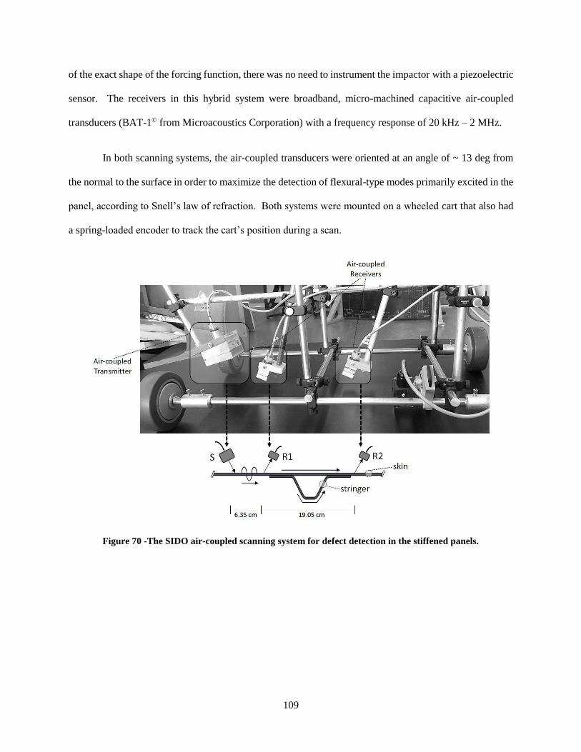
109
of the exact shape of the forcing function, there was no need to instrument the impactor with a piezoelectric
sensor. The receivers in this hybrid system were broadband, micro-machined capacitive air-coupled
transducers (BAT-1© from Microacoustics Corporation) with a frequency response of 20 kHz – 2 MHz.
In both scanning systems, the air-coupled transducers were oriented at an angle of ~ 13 deg from
the normal to the surface in order to maximize the detection of flexural-type modes primarily excited in the
panel, according to Snell’s law of refraction. Both systems were mounted on a wheeled cart that also had
a spring-loaded encoder to track the cart’s position during a scan.
Figure 70 -The SIDO air-coupled scanning system for defect detection in the stiffened panels.

110
Figure 71 - The SIDO hybrid impact/air-coupled scanning system for defect detection in the stiffened panels.
Typical waveforms recorded in the air-coupled system by the two receivers under air-coupled
excitation across the stringer of one of the test panels are shown in Figure 72(a) and (b). The signals are
characterized by a main A0 skin mode, according to the time of arrival and the nature of the test set up,
followed by reflections from the edges of the panel and from the skin-to-stringer overlap. Notice the large
attenuation affecting the signal at receiver 2 due to the significant wave leakage and scattering as it travels
across the skin-to-stringer assembly. The transfer function extracted from these measurements, shown in
Figure 72(c), has a much improved signal-to-noise ratio with clearer waveform features in terms of both
magnitudes and arrival times. This transfer function is less dependent on transduction responses and
highlights the coherent contributions between the two receivers. As such, the full transfer function allows
to detect other modes arriving prior to and after the dominant skin flexural mode, caused by the complex
wave path across the assembly.
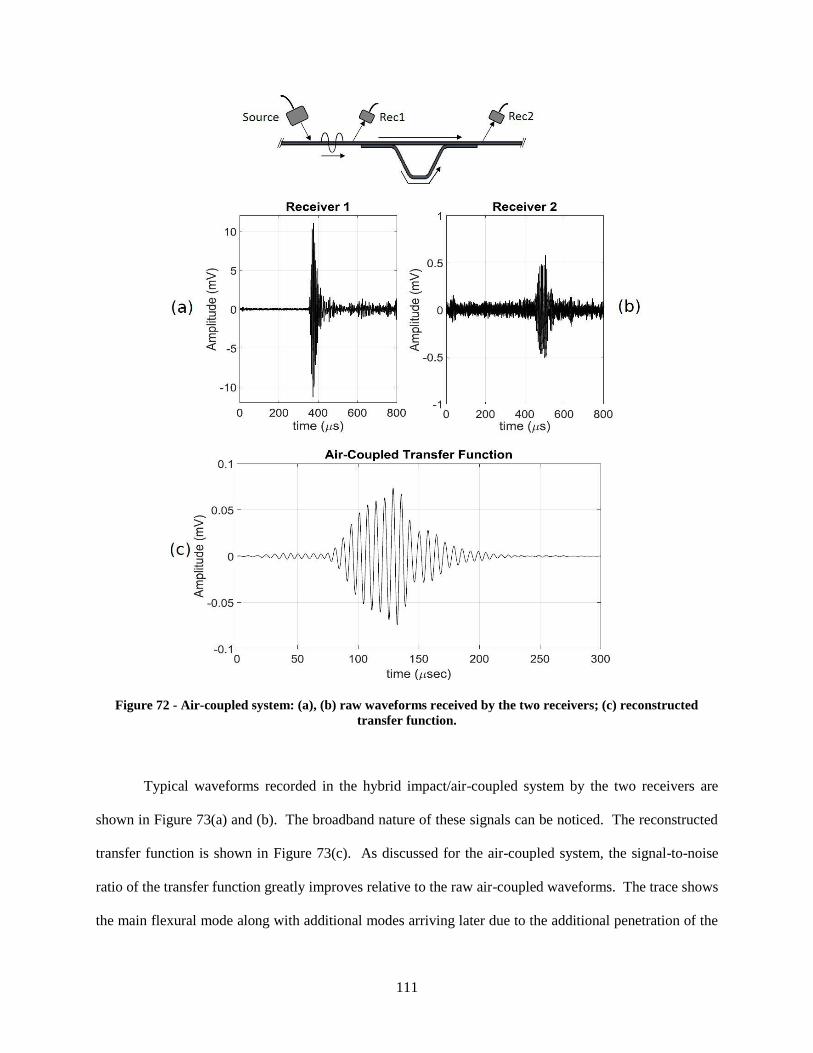
111
Figure 72 - Air-coupled system: (a), (b) raw waveforms received by the two receivers; (c) reconstructed
transfer function.
Typical waveforms recorded in the hybrid impact/air-coupled system by the two receivers are
shown in Figure 73(a) and (b). The broadband nature of these signals can be noticed. The reconstructed
transfer function is shown in Figure 73(c). As discussed for the air-coupled system, the signal-to-noise
ratio of the transfer function greatly improves relative to the raw air-coupled waveforms. The trace shows
the main flexural mode along with additional modes arriving later due to the additional penetration of the

112
wave energy into the stringer. The various modes can be identified more clearly than in the raw waveforms.
Figure 73(d) and (e) shows the filtered versions of the transfer function in the bands of 1-115 kHz and 115-
275 kHz, respectively. Again, wave arrivals and shapes are very clear in the transfer function results.

113
Figure 73 - Hybrid impact/air-coupled system: (a), (b) raw waveforms received by the two receivers; (c)
reconstructed transfer function; (d) filtered transfer function (low frequency range); (e) filtered transfer
function (high frequency range).

114
The next two figures show the effect of damage on the time-domain transfer function of the two
systems. Figure 74 includes representative results from the stringer flange impact damage in panel A. The
main effect of this type of damage is an attenuation and phase shift of the transfer function signatures. This
is seen in both the air-coupled transfer function of Figure 74(a), and the hybrid transfer function of Figure
74(b). This result can be explained by the increased scattering experienced by the guided wave as it travels
through the damaged portions of the skin-to-stinger overlap that was impacted. The fact that the attenuation
is as evident in the air-coupled trace of Figure 74(a) as in the impact/air-coupled trace of Figure 74(b)
suggests that this type of damage affects directly the skin, either by damage extending through the skin or
by damage at the skin-to-stringer overlap region. The results for the high-frequency band and the low-
frequency band of the hybrid system confirm this observation. The transfer function attenuation is more
evident in the high-frequency range of Figure 74(d) compared to the low-frequency range of Figure 74(c),
as the low frequency range has a higher propensity to penetrate from the skin into the stringer.
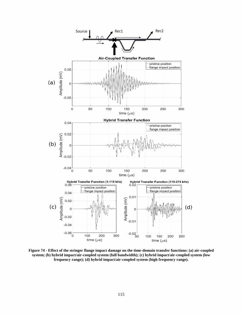
115
Figure 74 - Effect of the stringer flange impact damage on the time-domain transfer functions: (a) air-coupled
system; (b) hybrid impact/air-coupled system (full bandwidth); (c) hybrid impact/air-coupled system (low
frequency range); (d) hybrid impact/air-coupled system (high frequency range).
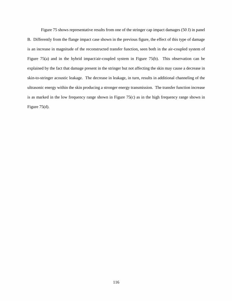
116
Figure 75 shows representative results from one of the stringer cap impact damages (50 J) in panel
B. Differently from the flange impact case shown in the previous figure, the effect of this type of damage
is an increase in magnitude of the reconstructed transfer function, seen both in the air-coupled system of
Figure 75(a) and in the hybrid impact/air-coupled system in Figure 75(b). This observation can be
explained by the fact that damage present in the stringer but not affecting the skin may cause a decrease in
skin-to-stringer acoustic leakage. The decrease in leakage, in turn, results in additional channeling of the
ultrasonic energy within the skin producing a stronger energy transmission. The transfer function increase
is as marked in the low frequency range shown in Figure 75(c) as in the high frequency range shown in
Figure 75(d).

117
Figure 75 - Effect of the stringer cap impact damage on the time-domain transfer functions: (a) air-coupled
system; (b) hybrid impact/air-coupled system (full bandwidth); (c) hybrid impact/air-coupled system (low
frequency range); (d) hybrid impact/air-coupled system (high frequency range).
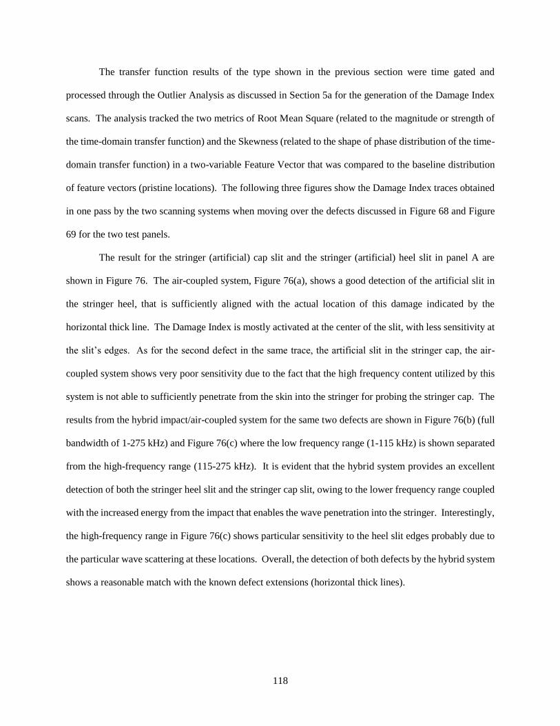
118
The transfer function results of the type shown in the previous section were time gated and
processed through the Outlier Analysis as discussed in Section 5a for the generation of the Damage Index
scans. The analysis tracked the two metrics of Root Mean Square (related to the magnitude or strength of
the time-domain transfer function) and the Skewness (related to the shape of phase distribution of the time-
domain transfer function) in a two-variable Feature Vector that was compared to the baseline distribution
of feature vectors (pristine locations). The following three figures show the Damage Index traces obtained
in one pass by the two scanning systems when moving over the defects discussed in Figure 68 and Figure
69 for the two test panels.
The result for the stringer (artificial) cap slit and the stringer (artificial) heel slit in panel A are
shown in Figure 76. The air-coupled system, Figure 76(a), shows a good detection of the artificial slit in
the stringer heel, that is sufficiently aligned with the actual location of this damage indicated by the
horizontal thick line. The Damage Index is mostly activated at the center of the slit, with less sensitivity at
the slit’s edges. As for the second defect in the same trace, the artificial slit in the stringer cap, the air-
coupled system shows very poor sensitivity due to the fact that the high frequency content utilized by this
system is not able to sufficiently penetrate from the skin into the stringer for probing the stringer cap. The
results from the hybrid impact/air-coupled system for the same two defects are shown in Figure 76(b) (full
bandwidth of 1-275 kHz) and Figure 76(c) where the low frequency range (1-115 kHz) is shown separated
from the high-frequency range (115-275 kHz). It is evident that the hybrid system provides an excellent
detection of both the stringer heel slit and the stringer cap slit, owing to the lower frequency range coupled
with the increased energy from the impact that enables the wave penetration into the stringer. Interestingly,
the high-frequency range in Figure 76(c) shows particular sensitivity to the heel slit edges probably due to
the particular wave scattering at these locations. Overall, the detection of both defects by the hybrid system
shows a reasonable match with the known defect extensions (horizontal thick lines).

119
Figure 76 - Damage Index traces from one scan through the stringer heel slit and the stringer cap slit in panel
A: (a) result from the air-coupled system; (b) result from the hybrid impact/air-coupled system (full
bandwidth); (c) result from the hybrid impact/air-coupled system (low frequencies vs. high frequencies).

120
The scan results over the flange impact defect of panel A are shown in Figure 77. Figure 77(a)
shows a very good detection of the impacted flange by the air-coupled system, with maximum sensitivity
at the center of the suspected damage (as reported by an ultrasonic A-scan). Hence it is confirmed that the
high-frequency range of the air-coupled system is sufficiently sensitive to the overlap between the skin and
the stringer that is likely affected by the flange impact. Very good detection of this damage is also shown
by the hybrid system in Figure 77(b) (full bandwidth) and Figure 77(c) where the low frequency range and
the high frequency range are separated. In particular, the high frequency range seems to be mostly sensitive
to the center of the damage, whereas the low frequency range is also activated by the wave absorption in
the wider delaminated area around the impact location.
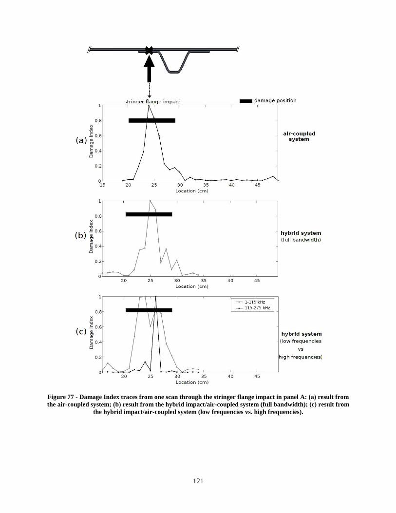
121
Figure 77 - Damage Index traces from one scan through the stringer flange impact in panel A: (a) result from
the air-coupled system; (b) result from the hybrid impact/air-coupled system (full bandwidth); (c) result from
the hybrid impact/air-coupled system (low frequencies vs. high frequencies).
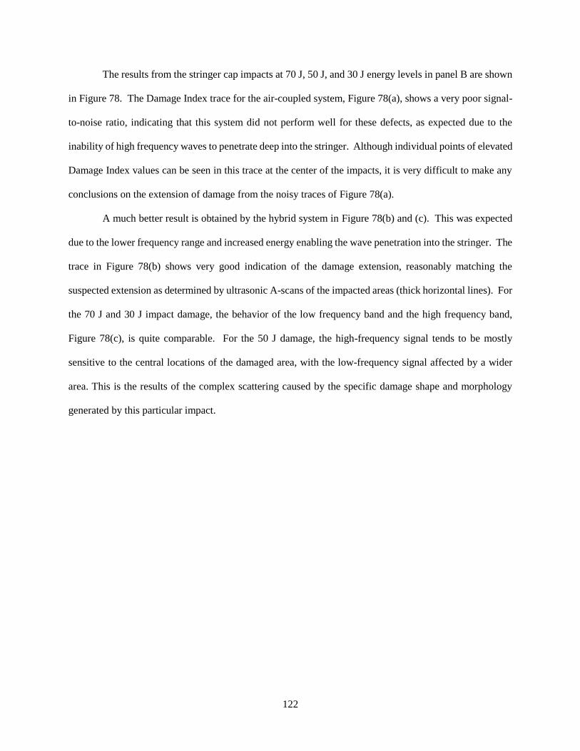
122
The results from the stringer cap impacts at 70 J, 50 J, and 30 J energy levels in panel B are shown
in Figure 78. The Damage Index trace for the air-coupled system, Figure 78(a), shows a very poor signal-
to-noise ratio, indicating that this system did not perform well for these defects, as expected due to the
inability of high frequency waves to penetrate deep into the stringer. Although individual points of elevated
Damage Index values can be seen in this trace at the center of the impacts, it is very difficult to make any
conclusions on the extension of damage from the noisy traces of Figure 78(a).
A much better result is obtained by the hybrid system in Figure 78(b) and (c). This was expected
due to the lower frequency range and increased energy enabling the wave penetration into the stringer. The
trace in Figure 78(b) shows very good indication of the damage extension, reasonably matching the
suspected extension as determined by ultrasonic A-scans of the impacted areas (thick horizontal lines). For
the 70 J and 30 J impact damage, the behavior of the low frequency band and the high frequency band,
Figure 78(c), is quite comparable. For the 50 J damage, the high-frequency signal tends to be mostly
sensitive to the central locations of the damaged area, with the low-frequency signal affected by a wider
area. This is the results of the complex scattering caused by the specific damage shape and morphology
generated by this particular impact.
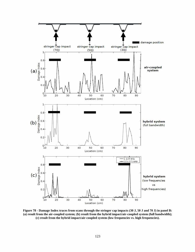
123
Figure 78 - Damage Index traces from scans through the stringer cap impacts (30 J, 50 J and 70 J) in panel B:
(a) result from the air-coupled system; (b) result from the hybrid impact/air-coupled system (full bandwidth);
(c) result from the hybrid impact/air-coupled system (low frequencies vs. high frequencies).

124
Concluding, a transfer function approach for ultrasonic guided-wave testing is presented for
damage detection purposes. The method is based on a single-input-dual-output (SIDO) scheme that
minimizes the effects of the transducers’ response and the transducers-to-structure coupling effects
compared to a traditional single-input-single-output (SISO) guided-wave testing. For example, the SIDO
method enables the use of excitation sources with unknown spectra (e.g. non-instrumented impactors). By
utilizing a deconvolution operation, the SIDO approach additionally brings out the coherent wave paths
between the two receivers and minimizes the incoherent contributions. These performances are particularly
relevant to scanning systems where the acoustic transduction can be variable.
This method, combined with a statistical Outlier Analysis, was utilized to design two scanning
systems applied to the rapid inspection of representative composite aircraft panels subjected to various
types of impact-caused damage. The two systems explore, respectively, the narrow/high frequency range
(~110-210 kHz) offered by non-contact air-coupled piezocomposite transducers and the broad/low
frequency range (~ 40-270 kHz) offered by the combination of an ultralight impactor and air-coupled
capacitive transducers. The results show how stringer flange impacts affect the skin and the skin-to-stringer
interface, generally producing a decrease in wave transmission strength that is detectable by the high
frequency wave content excited by both the air-coupled system and the hybrid system. Stringer cap impacts,
instead, generally produce an increase in wave transmission strength (through decreased acoustic leakage)
that mostly affects the low frequency and high magnitude wave content that are excited by the hybrid
system.

125
ACKNOWLEDGEMENTS
Chapter 2, Section 2.3, in full, has been submitted for publication of the material as it may
appear in International Journal of Solids and Structures 2019. Spada, Antonino; Capriotti,
Margherita; Lanza di Scalea, Francesco. The dissertation author was the second investigator and
author of this paper.
Chapter 2, Section 2.3.3, in full, is currently being prepared for submission for publication
of the material. Spada, Antonino; Capriotti, Margherita; Lanza di Scalea, Francesco. The
dissertation author was the second investigator and author of this material.
Chapter 2, Section 2.4.1, in part, is coauthored with Kim, Hyungsuk E. The dissertation
author was the primary author of this chapter.
Chapter 2, Section 2.4.2, in full, is a reprint of the material as it appears in Materials
Journals 2017. Capriotti, Margherita; Kim, Hyungsuk E.; Lanza di Scalea, Francesco; Kim,
Hyonny. The dissertation author was the primary investigator and author of this paper.
Chapter 2, Section 2.4.3, in full, has been submitted for publication of the material as it
may appear in Journal of Intelligent Material Systems and Structures 2019. Capriotti, Margherita;
Lanza di Scalea, Francesco. The dissertation author was the primary investigator and author of
this paper.

126
Chapter 3
Techniques of Thermal Wave Propagation
3.1 Background of Infrared Thermography: principles
Infrared Thermography is one of the most common NDE techniques for the inspection of the
subsurface of structures in several applications. The possibility to cover a wide area and to simply interpret
and visualize the results makes it very powerful and easy to apply. Moreover, the technique is non-contact
and allows in-situ inspection, avoiding the need to disassemble the structure for dedicated testing. It is
usually operated in an active manner, where an external heat source (usually consisting in powerful light
sources, emitted in a very short time period) “excites” the thermal field in the specimen and temperature
differences can be appreciated, both spatially and temporally. Both theory and applications will be shown.
The drawback of the need of an external heat source could be overcome with passive thermography,
avoiding additional costs and set-up effort, preserving the thermal status of the specimens and offering
additional resolution and imaging enhancement. Moreover, the nature of the technique itself supports this
alternative approach, since the output of a common thermographic test (thermal image) constitutes a huge
temperature database of the specimen. This latter approach will be illustrated theoretically.
IR thermography evolved from photothermal radiometry (PTR), where an IR detector monitors the
surface temperature variation in the sample, measured as a change in the infrared emission according to
Stefan-Boltzmann’s law:
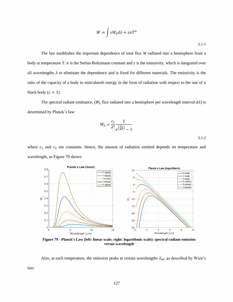
127
𝑊 = ∫휀𝑊𝜆𝑑𝜆 = 휀𝜎𝑇4
3.1-1
The law establishes the important dependence of total flux W radiated into a hemisphere from a
body at temperature T. 𝜎 is the Stefan-Boltzmann constant and 휀 is the emissivity, which is integrated over
all wavelengths 𝜆 to eliminate the dependence and is fixed for different materials. The emissivity is the
ratio of the capacity of a body to emit/absorb energy in the form of radiation with respect to the one of a
black body (휀 = 1).
The spectral radiant emittance, (𝑊𝜆 flux radiated into a hemisphere per wavelength interval 𝑑𝜆) is
determined by Planck’s law:
𝑊𝜆 =𝑐1𝜆5
1
𝑒(𝑐2𝜆𝑇)− 1
3.1-2
where 𝑐1 and 𝑐2 are constants. Hence, the amount of radiation emitted depends on temperature and
wavelength, as Figure 79 shows:
Also, at each temperature, the emission peaks at certain wavelengths 𝜆𝑚, as described by Wien’s
law:
Figure 79 - Planck's Law (left: linear scale; right: logarithmic scale): spectral radiant emission
versus wavelength
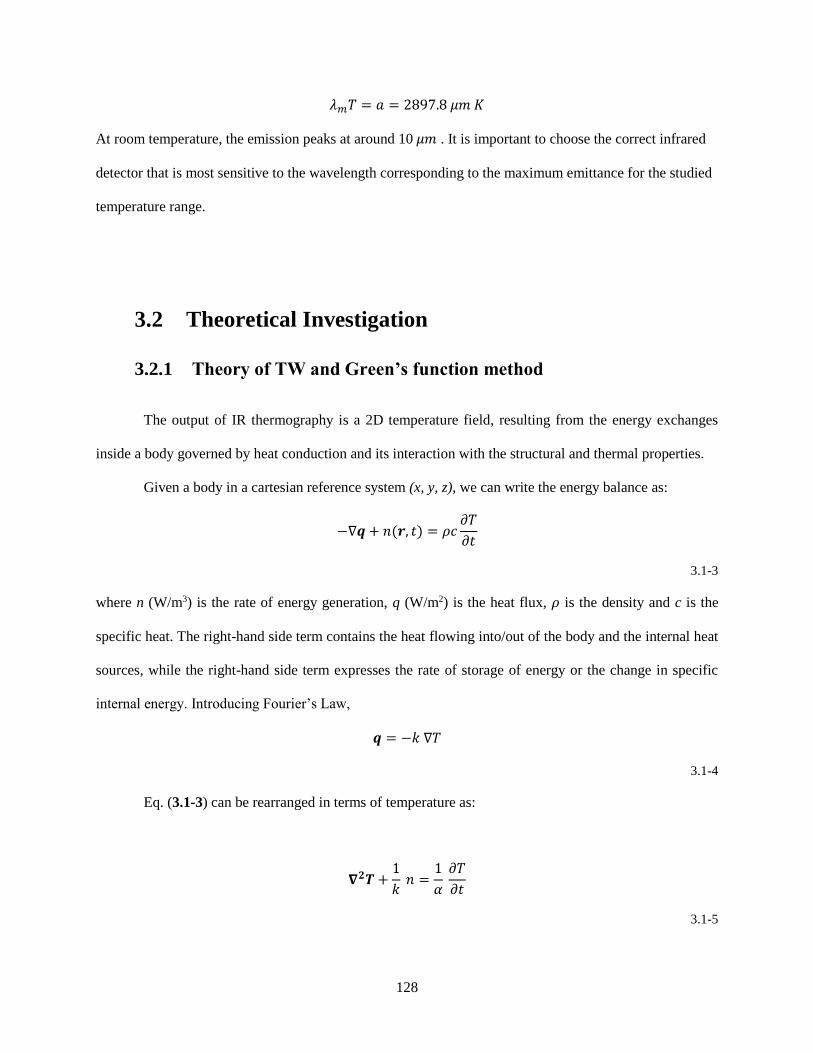
128
𝜆𝑚𝑇 = 𝑎 = 2897.8 𝜇𝑚 𝐾
At room temperature, the emission peaks at around 10 𝜇𝑚 . It is important to choose the correct infrared
detector that is most sensitive to the wavelength corresponding to the maximum emittance for the studied
temperature range.
3.2 Theoretical Investigation
3.2.1 Theory of TW and Green’s function method
The output of IR thermography is a 2D temperature field, resulting from the energy exchanges
inside a body governed by heat conduction and its interaction with the structural and thermal properties.
Given a body in a cartesian reference system (x, y, z), we can write the energy balance as:
−∇𝒒 + 𝑛(𝒓, 𝑡) = 𝜌𝑐𝜕𝑇
𝜕𝑡
3.1-3
where n (W/m3) is the rate of energy generation, q (W/m2) is the heat flux, 𝜌 is the density and c is the
specific heat. The right-hand side term contains the heat flowing into/out of the body and the internal heat
sources, while the right-hand side term expresses the rate of storage of energy or the change in specific
internal energy. Introducing Fourier’s Law,
𝒒 = −𝑘 ∇𝑇
3.1-4
Eq. (3.1-3) can be rearranged in terms of temperature as:
𝛁𝟐𝑻 +1
𝑘 𝑛 =
1
𝛼 𝜕𝑇
𝜕𝑡
3.1-5

129
Where the material dependence of the temperature distribution is expressed by the diffusivity 𝛼 =𝑘
𝜌𝑐=
[𝑚2
𝑠]. Eq. (3.1-5) is the governing heat diffusion equation.
The same result can be achieved starting from a more generalized heat wave equation:
𝜵2𝑻 +1
𝑘�̅�(𝒓, 𝑡) =
1
𝛼
𝜕𝑻
𝜕𝑡+1
𝑠2𝜕2𝑻
𝜕𝑡2
3.1-6
where �̅�(𝑟, 𝑡) = 𝑛(𝑟, 𝑡) +𝛼
𝑠2𝜕𝑛(𝑟,𝑡)
𝜕𝑡 and s is the thermal wave speed. For speeds that are very high (in metals
s=105 m/s) and thermal time constants 𝜏𝑐 =𝑅2
𝛼 very small (in metals, 𝜏𝑐 =10-14 s), but larger than the
material’s relaxation time 𝜏 (Ozisik et al., 1994; Marin, 2010), the above equation can be simplified to a
Fourier type heat conduction, expressed by eq.(3.1-5). To be noticed, the neglection of the propagating term
in eq. (3.1-6) makes heat propagation a parabolic diffusion equation. Although the scientific community is
divided on this controversial definition, we will refer to this kind of propagation as thermal wave (TW).
The solution to eq. (3.1-5) can be found in terms of Green’s function. This method is very useful
when dealing with analogies with propagating fields and when defects or inhomogeneities can be viewed
as secondary sources (Cole et al., 2010). The formal definition of Green’s function has itself very powerful
consequences in manipulating wave fields and interpreting them. The Green’s function is the solution to an
auxiliary equation:
𝛻2𝒈+1
𝛼𝛿(𝒓 − 𝒓0)𝛿(𝑡 − 𝜏) =
1
𝛼
𝜕𝒈
𝜕𝑡
3.1-7
for an excitation of the delta Dirac type in time and space and homogenous initial and boundary conditions.
It is the transfer function of the path between the source and any space coordinate and it is here reported in
1-D as:

130
𝑔( 𝑥, 𝑡 ∣∣ 𝜉, 𝜏 ) =1
√4𝜋𝛼(𝑡 − 𝜏)𝑒−(𝑥−𝜉)2
4𝛼(𝑡−𝜏)
3.1-8
The GF itself contains the structural and material information needed to characterize the specimen.
In an NDE perspective, any alteration to the Green’s function of a path can represent the presence of a
defect: Figure 80 shows the spatial effect of the alteration of diffusivity in the 1D GF, for various instants
of time.
Figure 81 shows the Green’s function evolution in time, as evaluated at two different locations,
2mm and 4mm from the source respectively: the trend changes due to diffusivity, where a highly diffusive
material as Gold (𝛼 = 127 mm2/s) dissipates heat much faster than PVC (𝛼 = 0.08 mm2/s).
Figure 80 - Green's function in space domain for different time instants: (left) diffusivity of PVC; (right)
diffusivity of Steel
Figure 81 - Green's function in time domain for varying diffusivity values: (left) at x=2mm; (right) at
x=4mm

131
The retrieval of the GF in a thermal field could be used for defect detection and material
characterization.
Transforming the equation of heat diffusion in the frequency domain, it becomes:
𝜵2𝑻(𝒓,𝝎) −1
𝑘𝑁(𝒓, 𝜔) = 𝜎2𝑇(𝒓, 𝜔)
3.1-9
where 𝜎(𝜔) = √𝑖𝜔
𝛼= (1 + 𝑖)√
𝜔
2𝛼 is a type of a wavenumber. To be noted, 𝜎(𝜔) is the complex
counterpart of a real wavenumber, using the analogy with the elastic wave equation (Mandelis, 1995). It
contains a material dependency as the inverse relationship with diffusivity, and expresses a dispersive
relationship, between time and space (or frequency and wavenumber) governed by an analogous velocity
term (diffusivity).
The TW solution in terms of Green’s function is:
𝑇(𝑟, 𝜔) = (𝛼
𝑘)∭ 𝑄(𝑟0, 𝜔)𝐺(𝑟|𝑟0; 𝜔)𝑑𝑉0
𝑉0
+ 𝛼∮ [𝐺(𝑟|𝑟0𝑠; 𝜔)𝛻0𝑇(𝑟0
𝑠, 𝜔) − 𝑇(𝑟0𝑠, 𝜔)𝛻0𝐺(𝑟|𝑟0
𝑠; 𝜔)]𝑑𝑆0𝑆0
3.1-10
it can be expressed as the result of two contributions: the transfer function of a certain path convoluted with
a source 𝑄(𝑟0, 𝜔) or the temperature distribution due to initial temperature boundary conditions. We can
think about 𝐺 as the building block for more complex solutions, where the source is arbitrary and the initial
and boundary conditions are inhomogeneous.
Exploiting the concepts above and following Mandelis (2013), the first case study is a simple plate,
considered as a semi-infinite and then finite medium.
In the first case, the Green’s function associated to the homogeneous problem is:

132
𝐺(𝑅|𝑅′;𝜔) =1
4𝜋𝛼(𝑒−𝜎𝑅
𝑅+𝑒−𝜎𝑅′
𝑅′)
3.1-11
where R’=|𝑟 − 𝑟′0|is the source location. The problem is formulated as 3D heat diffusion, where Neumann
adiabatic boundary conditions are applied. The heat source is simulated as a Gaussian Laser beam, of width
W, with time harmonic flux, and it is imposed as an initial boundary condition as:
𝑘𝛻0𝑇(𝑟𝑜𝑠, 𝜔) =
𝐹02(1 + 𝑒𝑖𝜔𝑡)𝑒
−𝑥2+𝑦2
𝑊2
3.1-12
so that the resulting thermal wave field is:
𝑇(𝑥, 𝑦, 𝑧; 𝜔) =𝐹02𝑘𝑒−(𝑥2+𝑦2)𝑊2 (∫
𝑒−𝜎√𝜌2+𝑧2−(
𝜌𝑊)2
√𝜌2 + 𝑧2 𝐼0 (
2𝜌
𝑊2√𝑥2 + 𝑦2)𝜌𝑑𝜌
∞
0
)
3.1-13
When reducing the source to a very focused beam located in (𝑥0𝑠, 𝑦0
𝑠), on top of the plate (z=0), the
TW simplifies to:
𝑇(𝑥, 𝑦, 𝑧; 𝜔) =𝛼𝐹02𝑘
𝐺(𝑥, 𝑦, 𝑧|𝑥0𝑠, 𝑦0
𝑠, 0; 𝜔) = (𝐹04𝜋𝑘
)𝑒−𝜎√(𝑥−𝑥0)
2+(𝑦−𝑦0)2+𝑧2
√(𝑥 − 𝑥0𝑠)2 + (𝑦 − 𝑦0
𝑠)2 + 𝑧2
3.1-14
When considering the plate as a medium bounded by two infinite parallel planes at z=0 and z=L,
where L is the thickness of the plate, we can schematize the problem as follows (see Figure 82):
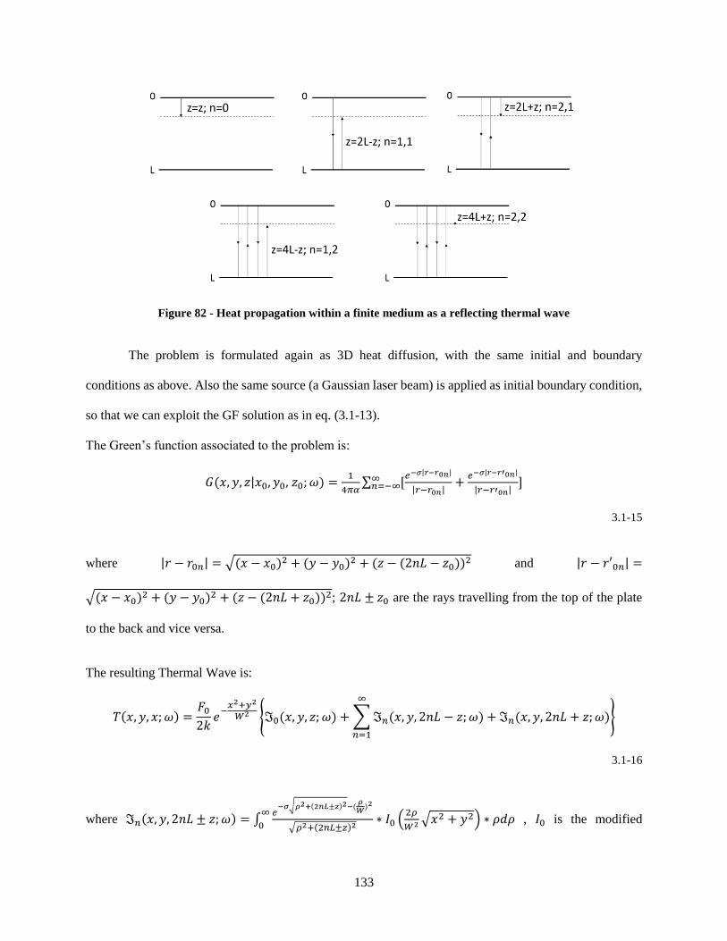
133
Figure 82 - Heat propagation within a finite medium as a reflecting thermal wave
The problem is formulated again as 3D heat diffusion, with the same initial and boundary
conditions as above. Also the same source (a Gaussian laser beam) is applied as initial boundary condition,
so that we can exploit the GF solution as in eq. (3.1-13).
The Green’s function associated to the problem is:
𝐺(𝑥, 𝑦, 𝑧|𝑥0, 𝑦0, 𝑧0; 𝜔) =1
4𝜋𝛼∑ [
𝑒−𝜎|𝑟−𝑟0𝑛|
|𝑟−𝑟0𝑛|+𝑒−𝜎|𝑟−𝑟′0𝑛|
|𝑟−𝑟′0𝑛|]∞
𝑛=−∞
3.1-15
where |𝑟 − 𝑟0𝑛| = √(𝑥 − 𝑥0)2 + (𝑦 − 𝑦0)
2 + (𝑧 − (2𝑛𝐿 − 𝑧0))2 and |𝑟 − 𝑟′0𝑛| =
√(𝑥 − 𝑥0)2 + (𝑦 − 𝑦0)
2 + (𝑧 − (2𝑛𝐿 + 𝑧0))2; 2𝑛𝐿 ± 𝑧0 are the rays travelling from the top of the plate
to the back and vice versa.
The resulting Thermal Wave is:
𝑇(𝑥, 𝑦, 𝑥; 𝜔) =𝐹02𝑘𝑒−𝑥2+𝑦2
𝑊2 {ℑ0(𝑥, 𝑦, 𝑧; 𝜔) +∑ℑ𝑛(𝑥, 𝑦, 2𝑛𝐿 − 𝑧;𝜔) + ℑ𝑛(𝑥, 𝑦, 2𝑛𝐿 + 𝑧;𝜔)
∞
𝑛=1
}
3.1-16
where ℑ𝑛(𝑥, 𝑦, 2𝑛𝐿 ± 𝑧;𝜔) = ∫𝑒−𝜎√𝜌2+(2𝑛𝐿±𝑧)2−(
𝜌𝑊)2
√𝜌2+(2𝑛𝐿±𝑧)2
∞
0∗ 𝐼0 (
2𝜌
𝑊2√𝑥2 + 𝑦2) ∗ 𝜌𝑑𝜌 , 𝐼0 is the modified

134
Bessel function of 1st kind and order 0 and 𝜌 = √(𝑥 − 𝑥0)2 + (𝑦 − 𝑦0)
2.
Heat propagation is treated as a thermal wave bouncing back and forth off the surfaces of the plate,
treated as half-spaces, so that the resulting thermal field is the sum of all the contributions given by the
reflections within the thickness of the plate. This interpretation is valid for thin structures and has been
implemented in Matlab for an Aluminum plate of 10mm x 10mm x 6mm, n=4 backwall reflections. It can
be noticed how the Temperature diffuses from the location of the source outwards and through the depth
(Figure 83). Also, the different frequency components of the field behave differently, showing a higher
diffusion for higher frequencies.
Figure 83 - Analytical frequency domain temperature distribution in finite medium: top surface (top), bottom
surface (bottom); at 1 Hz (left) and at 100 Hz (right).

135
The time domain solution is found inverting the frequency domain solution: due to computational
limitations the thermal field evolution is observed up to 1s (Figure 84). Errors show up in the front surface
due to time discretization issues.
The above analytical formulation offered insights on heat propagation interpreted as a thermal
diffusing wave and has been used in both passive and active IR thermographic approaches. The semi-
infinite medium problem can be related to cases where the diffusion is observed in the depth dimension
and/or the diffusion has not yet reached the backwall, since the thickness is greater than the one needed to
provide “reflections”. The plate as bounded by two surfaces is used when visualizing heat propagation as
thermal guided waves and/or when the presence of a defective surface acts as a reflector within the thickness
of the plate. The results provide hints on the possibility of performing material characterization and defect
detection, if a thermal GF is retrieved. Numerical simulations, using a commercial software, have been
implemented to model cases with more complex geometries, materials (i.e. inhomogeneous thermal
properties, defects, …) and to observe heat diffusion in longer time scales.
Moreover, the above-mentioned TW field solutions of heat propagation can be used for a passive
Figure 84 - Analytical time domain temperature distribution in finite medium: top surface (left), bottom surface
(right), at y=0 and for varying distances x from the source x=0
136
approach of IR thermography. The theoretical feasibility of passive Green’s function extraction in thermal
fields is here discussed.
3.2.2 Passive extraction of thermal Green’s function
Cross-correlation of diffuse fields to retrieve GFs has been demonstrated for elastic, dissipative and
electromagnetic waves (Snieder et al., 2009; Snieder et al., 2007; Lobkis and Weaver, 2001; Kuperman,
2008) and widely used in many applications as seismology (Snieder, 2004; Waapenar et al., 2006; Sabra et
al., 2005), oceanography (Sabra et al., 2005) and structural health monitoring (Tippman et al., 2015; Sabra
et al., 2008; Lanza di Scalea et al., 2018a). This is possible because the time-averaged cross-correlation
operation suppresses the incoherent part of the response between the two points, and builds up the coherent
part which corresponds to the ballistic and antiballistic response (Green’s function) between the two
receiving points. The approach relies on the fluctuation-dissipation theorem, as discussed by Callen and
Welton in 1951 and by Callen and Greene in 1952. This fundamental energy theorem states that a
thermodynamic system in equilibrium is related to macroscopic irreversible processes in the same way as
generalized fluctuating forces relate to a characterizing dissipative parameter, intrinsic of the system itself:
⟨𝜉2⟩ = −2k
𝜋∫
𝜎𝑠(𝜔)𝑑𝜔
𝜔2
∞
−∞
3.1-17
where 𝜉2is the mean spectral density of the spontaneous fluctuations, 𝜎𝑠 is the conductance and k is a
constant.
This means that the random fluctuations in a system, acquired passively, contain information about
the system within the dissipative parameter, that, if extracted, could be then imaged and/or used for NDE
or characterization.
The retrieval of the latter could be achieved in terms of GF extraction. For the diffusion equation,
following (Snieder, 2006), we can write:
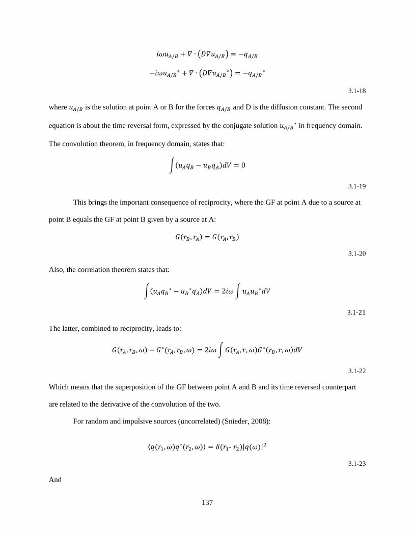
137
𝑖𝜔𝑢𝐴/𝐵 + 𝛻 ∙ (𝐷𝛻𝑢𝐴/𝐵) = −𝑞𝐴/𝐵
−𝑖𝜔𝑢𝐴/𝐵∗ + 𝛻 ∙ (𝐷𝛻𝑢𝐴/𝐵
∗) = −𝑞𝐴/𝐵∗
3.1-18
where 𝑢𝐴/𝐵 is the solution at point A or B for the forces 𝑞𝐴/𝐵 and D is the diffusion constant. The second
equation is about the time reversal form, expressed by the conjugate solution 𝑢𝐴/𝐵∗ in frequency domain.
The convolution theorem, in frequency domain, states that:
∫(𝑢𝐴𝑞𝐵 − 𝑢𝐵𝑞𝐴)𝑑𝑉 = 0
3.1-19
This brings the important consequence of reciprocity, where the GF at point A due to a source at
point B equals the GF at point B given by a source at A:
𝐺(𝑟𝐵, 𝑟𝐴) = 𝐺(𝑟𝐴, 𝑟𝐵)
3.1-20
Also, the correlation theorem states that:
∫(𝑢𝐴𝑞𝐵∗ − 𝑢𝐵
∗𝑞𝐴)𝑑𝑉 = 2𝑖𝜔∫𝑢𝐴𝑢𝐵∗𝑑𝑉
3.1-21
The latter, combined to reciprocity, leads to:
𝐺(𝑟𝐴, 𝑟𝐵, 𝜔) − 𝐺∗(𝑟𝐴, 𝑟𝐵, 𝜔) = 2𝑖𝜔∫𝐺(𝑟𝐴, 𝑟, 𝜔)𝐺
∗(𝑟𝐵, 𝑟, 𝜔)𝑑𝑉
3.1-22
Which means that the superposition of the GF between point A and B and its time reversed counterpart
are related to the derivative of the convolution of the two.
For random and impulsive sources (uncorrelated) (Snieder, 2008):
⟨𝑞(𝑟1, 𝜔)𝑞∗(𝑟2, 𝜔)⟩ = 𝛿(𝑟1- 𝑟2)|𝑞(𝜔)|
2
3.1-23
And

138
𝑢(𝑟) = ∫𝐺(𝑟, 𝑟0)𝑞(𝑟0)𝑑𝑉0
3.1-24
Using these equations into the previously obtained eq. (3.1-22), we have:
𝐺(𝑟𝐴, 𝑟𝐵, 𝜔) − 𝐺∗(𝑟𝐴, 𝑟𝐵, 𝜔)|𝑞(𝜔)|
2 = 2𝑖𝜔 ⟨𝑢𝐴(𝑟𝐴, 𝜔)𝑢𝐵∗ (𝑟𝐵, 𝜔)⟩
3.1-25
and
𝐺(𝑟𝐴, 𝑟𝐵, 𝑡) − 𝐺(𝑟𝐴, 𝑟𝐵, −𝑡) ∗ 𝐶𝑞 = −2𝑑
𝑑𝑡⟨𝑢𝐴(𝑟𝐴, 𝑡)𝑢𝐵(𝑟𝐵, 𝑡)⟩
3.1-26
in frequency and time domain, respectively. Equations (3.1-25) and (3.1-26) state that the GF solution
between point A and B, multiplied by the power spectrum of the sources, is proportional to the time
derivative of the frequency domain convolution (or time domain cross-correlation) of the fields at point A
and B. The thermal Green’s Function between two locations can be reconstructed by the cross-correlation
of random thermal field fluctuations, recorded at those two locations.
Particular attention has to be placed on the temporal and spatial averaging of the recorded signals
and cross-correlated results. Also, the diffusive state of the field needs to be such that it allows for the
coherent paths only to emerge from the cross-correlations and any other random path to be averaged out.
The inverse scattering theorem has also been investigated from a theoretical point of view and
understood in a thermal and defect detection perspective. Interpreting the defect as a scatterer, the
superposition of the direct and backscattered fields is related to the auto-correlation of the field at the source:
𝐺(𝒓0, 𝒓0) − 𝐺∗(𝒓0, 𝒓0) =
1
|𝑆(𝜔)|2⟨|𝑢(𝒓0, 𝒓0)|
2⟩
3.1-27
A schematic of the concept is represented below and has been observed in simulations:
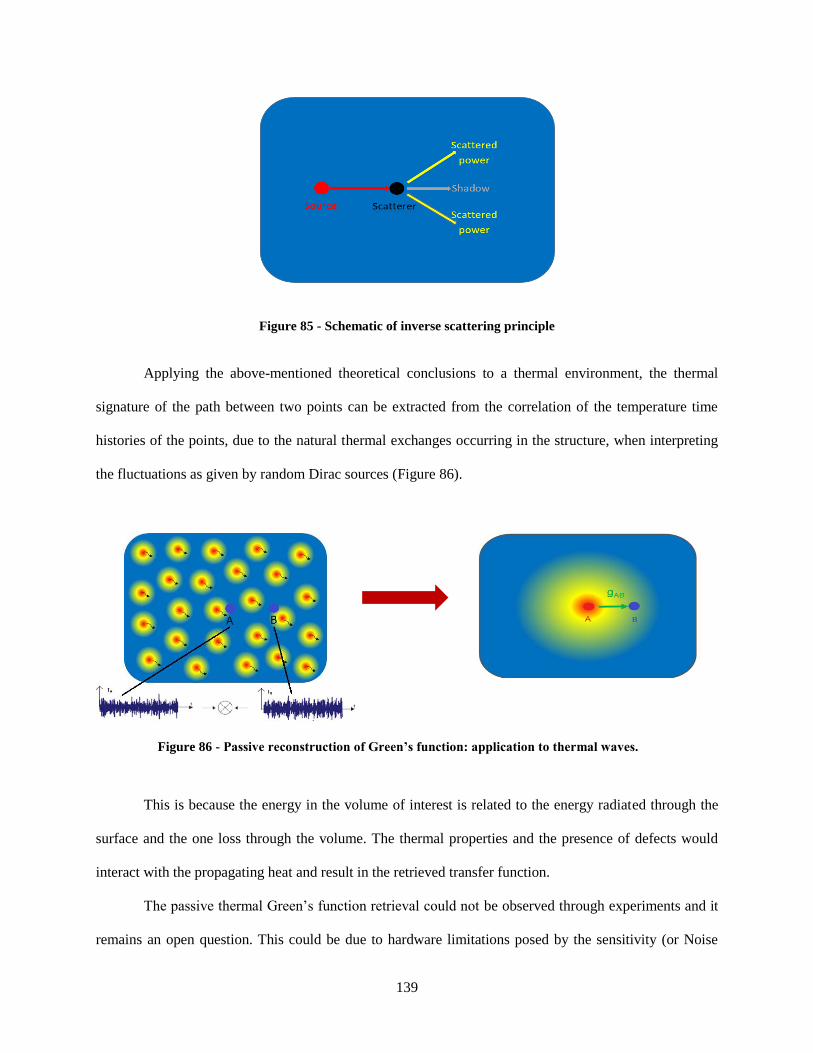
139
Figure 85 - Schematic of inverse scattering principle
Applying the above-mentioned theoretical conclusions to a thermal environment, the thermal
signature of the path between two points can be extracted from the correlation of the temperature time
histories of the points, due to the natural thermal exchanges occurring in the structure, when interpreting
the fluctuations as given by random Dirac sources (Figure 86).
This is because the energy in the volume of interest is related to the energy radiated through the
surface and the one loss through the volume. The thermal properties and the presence of defects would
interact with the propagating heat and result in the retrieved transfer function.
The passive thermal Green’s function retrieval could not be observed through experiments and it
remains an open question. This could be due to hardware limitations posed by the sensitivity (or Noise
Figure 86 - Passive reconstruction of Green’s function: application to thermal waves.

140
Equivalent Temperature Difference, NETD) of current IR thermocameras. Another reason could be the
necessity of stronger diffused sources, that could not be observed/reproduced in a laboratory environment.
Whether the thermal vibrations of atoms are able to generate thermal transients at the macroscopic level to
be reconstructed passively, remains an interesting aspect to be further investigated.
3.3 Numerical Investigation
3.3.1 Active thermal Green’s Function
Finite element simulations have been performed to understand the conductive heat transfer into plate-
like specimens. An Aluminum plate of 2mm thickness has been modeled in LS-Dyna. An impulsive heat
source excites the thermal field and heat propagation is observed in Figure 87, mapping temperature.
Figure 87 - FEM Heat propagation in pristine Aluminum plate: geometry (left), heat wave propagation
as Temperature (right)
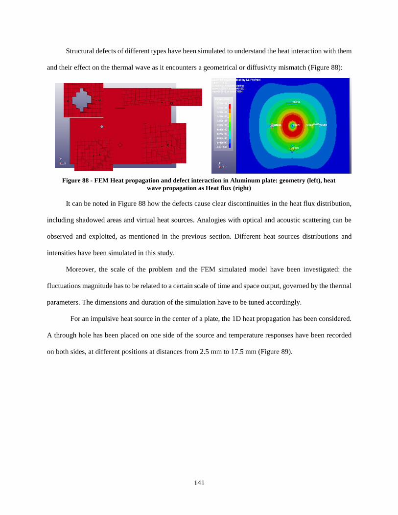
141
Structural defects of different types have been simulated to understand the heat interaction with them
and their effect on the thermal wave as it encounters a geometrical or diffusivity mismatch (Figure 88):
It can be noted in Figure 88 how the defects cause clear discontinuities in the heat flux distribution,
including shadowed areas and virtual heat sources. Analogies with optical and acoustic scattering can be
observed and exploited, as mentioned in the previous section. Different heat sources distributions and
intensities have been simulated in this study.
Moreover, the scale of the problem and the FEM simulated model have been investigated: the
fluctuations magnitude has to be related to a certain scale of time and space output, governed by the thermal
parameters. The dimensions and duration of the simulation have to be tuned accordingly.
For an impulsive heat source in the center of a plate, the 1D heat propagation has been considered.
A through hole has been placed on one side of the source and temperature responses have been recorded
on both sides, at different positions at distances from 2.5 mm to 17.5 mm (Figure 89).
Figure 88 - FEM Heat propagation and defect interaction in Aluminum plate: geometry (left), heat
wave propagation as Heat flux (right)

142
Figure 89 - FEM temperature response: at source (left), at receivers on pristine side (center), at receivers on
defective side (right).
The temperature distribution is affected by the presence of the defect according to the inverse
scattering principle: the receivers before the defect keep a higher temperature at later times of propagation
since the heat is blocked by the hole and is “reflecting” back; the receivers after the defect have a lower
temperature since the hole “shadows” the heat.
Cross-correlations have been performed to retrieve the thermal Green’s function between the heat
source and the recording nodes (Figure 90 and Figure 91).
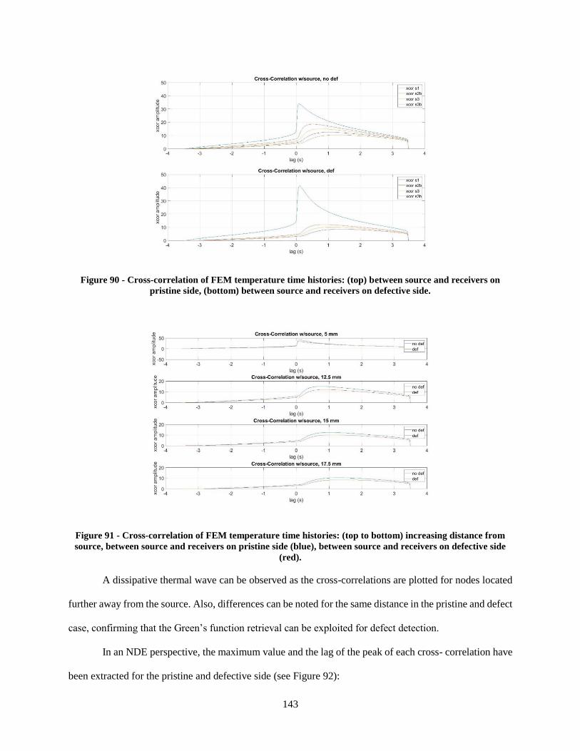
143
Figure 90 - Cross-correlation of FEM temperature time histories: (top) between source and receivers on
pristine side, (bottom) between source and receivers on defective side.
Figure 91 - Cross-correlation of FEM temperature time histories: (top to bottom) increasing distance from
source, between source and receivers on pristine side (blue), between source and receivers on defective side
(red).
A dissipative thermal wave can be observed as the cross-correlations are plotted for nodes located
further away from the source. Also, differences can be noted for the same distance in the pristine and defect
case, confirming that the Green’s function retrieval can be exploited for defect detection.
In an NDE perspective, the maximum value and the lag of the peak of each cross- correlation have
been extracted for the pristine and defective side (see Figure 92):
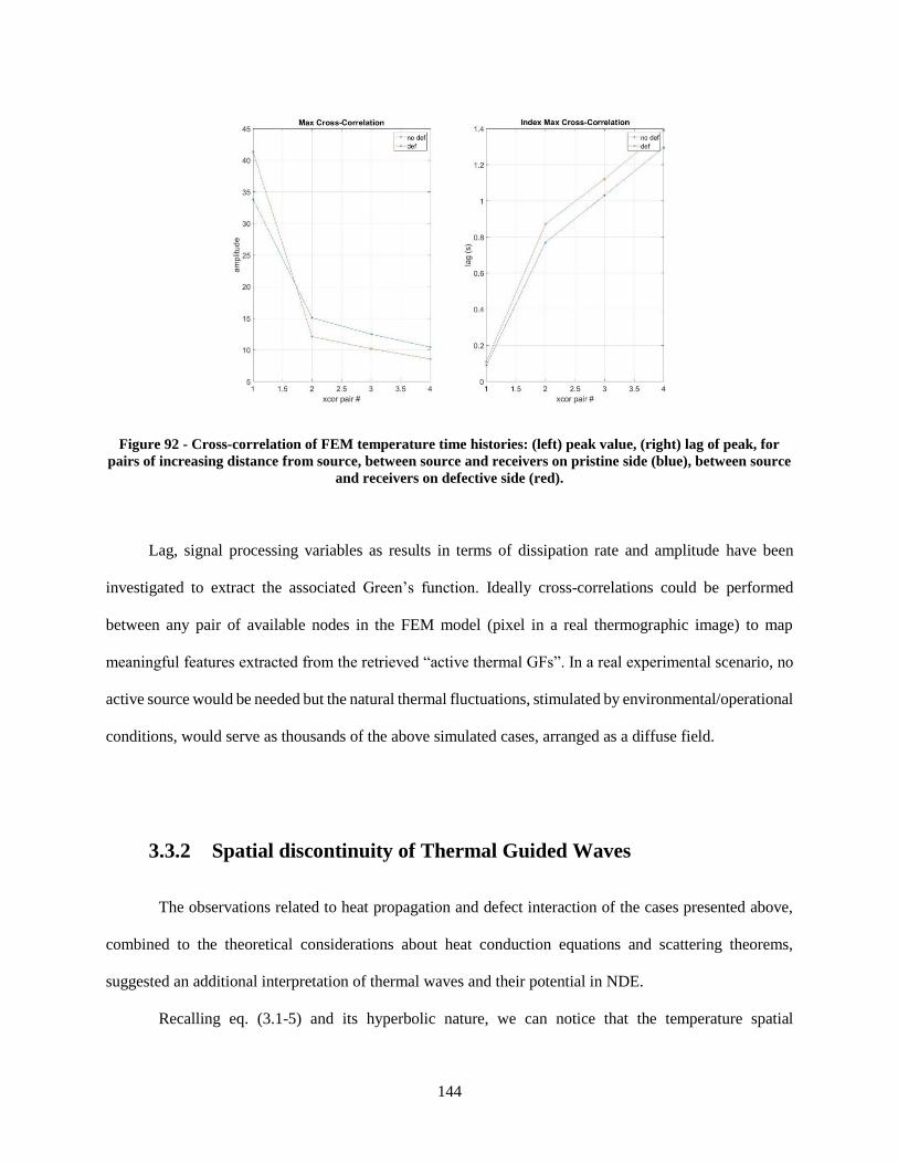
144
Figure 92 - Cross-correlation of FEM temperature time histories: (left) peak value, (right) lag of peak, for
pairs of increasing distance from source, between source and receivers on pristine side (blue), between source
and receivers on defective side (red).
Lag, signal processing variables as results in terms of dissipation rate and amplitude have been
investigated to extract the associated Green’s function. Ideally cross-correlations could be performed
between any pair of available nodes in the FEM model (pixel in a real thermographic image) to map
meaningful features extracted from the retrieved “active thermal GFs”. In a real experimental scenario, no
active source would be needed but the natural thermal fluctuations, stimulated by environmental/operational
conditions, would serve as thousands of the above simulated cases, arranged as a diffuse field.
3.3.2 Spatial discontinuity of Thermal Guided Waves
The observations related to heat propagation and defect interaction of the cases presented above,
combined to the theoretical considerations about heat conduction equations and scattering theorems,
suggested an additional interpretation of thermal waves and their potential in NDE.
Recalling eq. (3.1-5) and its hyperbolic nature, we can notice that the temperature spatial
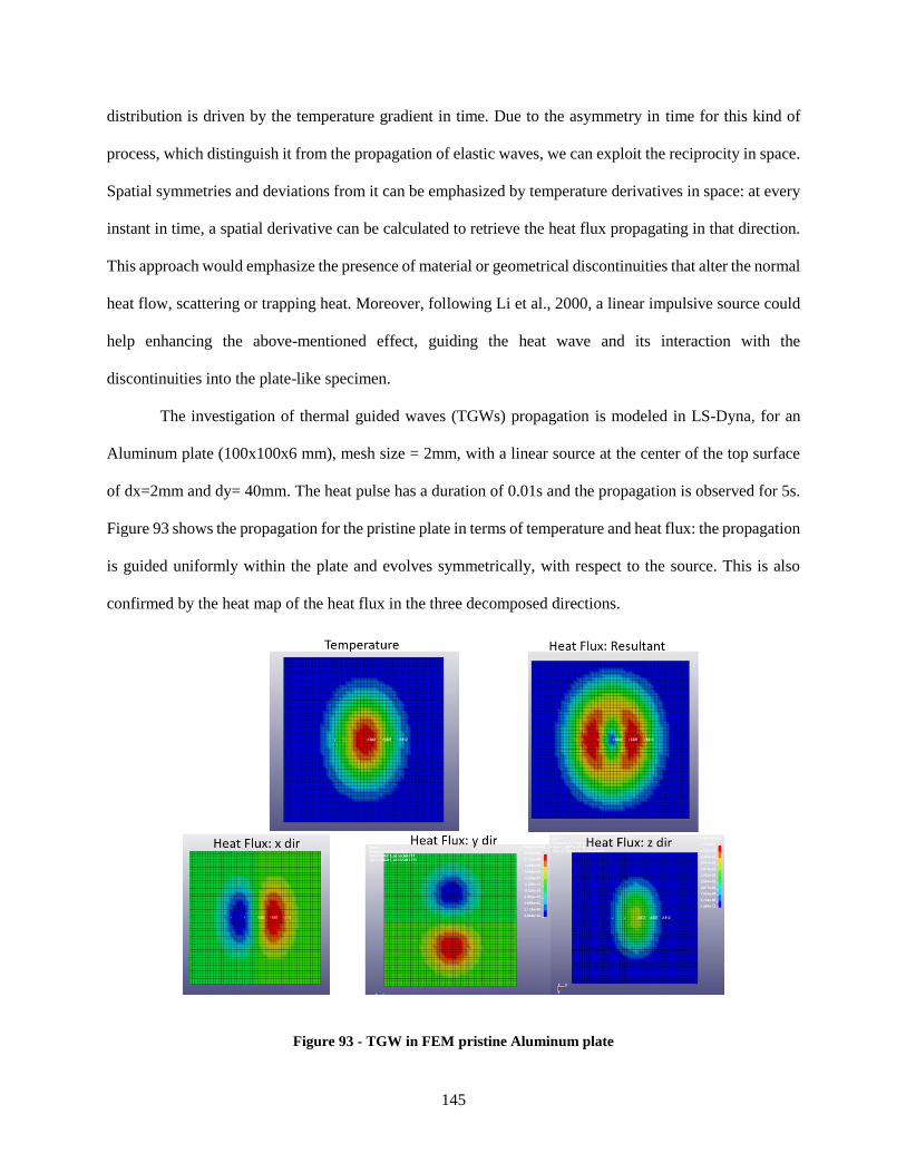
145
distribution is driven by the temperature gradient in time. Due to the asymmetry in time for this kind of
process, which distinguish it from the propagation of elastic waves, we can exploit the reciprocity in space.
Spatial symmetries and deviations from it can be emphasized by temperature derivatives in space: at every
instant in time, a spatial derivative can be calculated to retrieve the heat flux propagating in that direction.
This approach would emphasize the presence of material or geometrical discontinuities that alter the normal
heat flow, scattering or trapping heat. Moreover, following Li et al., 2000, a linear impulsive source could
help enhancing the above-mentioned effect, guiding the heat wave and its interaction with the
discontinuities into the plate-like specimen.
The investigation of thermal guided waves (TGWs) propagation is modeled in LS-Dyna, for an
Aluminum plate (100x100x6 mm), mesh size = 2mm, with a linear source at the center of the top surface
of dx=2mm and dy= 40mm. The heat pulse has a duration of 0.01s and the propagation is observed for 5s.
Figure 93 shows the propagation for the pristine plate in terms of temperature and heat flux: the propagation
is guided uniformly within the plate and evolves symmetrically, with respect to the source. This is also
confirmed by the heat map of the heat flux in the three decomposed directions.
Figure 93 - TGW in FEM pristine Aluminum plate

146
When introducing defects in the plate as a slit (2x10x2 mm) to simulate a crack, or a reduction in
thickness (8x8x4 mm), to simulate corrosion, the diffusion is affected and symmetry is broken. The effect
is noticeable in the temperature maps, but is much stronger in the heat flux, where the defect scatters heat
and acts as a secondary heat source.
Figure 94 - TGW in FEM Aluminum plate with slit

147
Figure 95 - TGW in FEM Aluminum plate with corrosion
Both defects shadow heat in the x direction and slow the symmetrical evolution of heat in the later
portion of the plate. Heat is trapped within the defect leading to local effects in all directions (Figure 94 and
Figure 95).
Temperature and heat flux time histories have been extracted every mm along the x direction, at
the top surface of the plate: the solid lines represent the pristine area of the plate on the left side of the
source, while the dashed ones represent the defective side. The blue and yellow curves represent an early
instant, while the red and purple curves a later one. Monitoring temperature along a horizontal line on the
surface of the plate, the primary and secondary scatterings lead to a slight increase before and slight decrease
after the defect (Figure 96 and Figure 97 top left). This effect is slightly noticeable in the temperature plots
but is well emphasized in the heat flux, dominated by the heat flux in the x direction, due to the nature of
the linear source.
In a real application, one could only measure temperature and both the defect detection and imaging
performance would be reduced by the very low contrast. Using Fourier’s law:
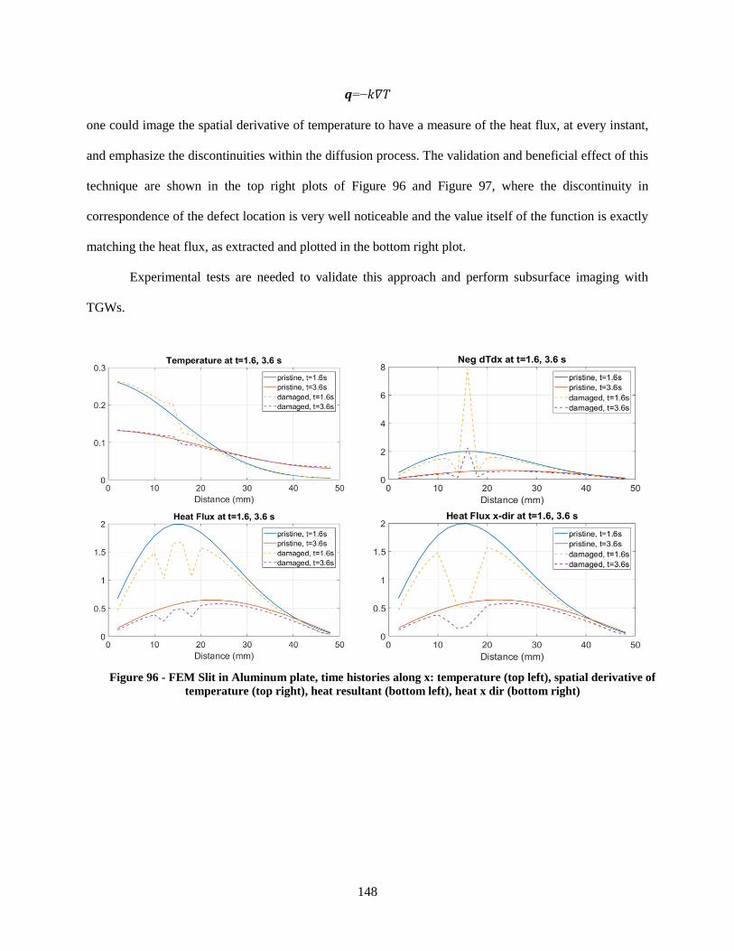
148
𝒒=−𝑘𝛻𝑇
one could image the spatial derivative of temperature to have a measure of the heat flux, at every instant,
and emphasize the discontinuities within the diffusion process. The validation and beneficial effect of this
technique are shown in the top right plots of Figure 96 and Figure 97, where the discontinuity in
correspondence of the defect location is very well noticeable and the value itself of the function is exactly
matching the heat flux, as extracted and plotted in the bottom right plot.
Experimental tests are needed to validate this approach and perform subsurface imaging with
TGWs.
Figure 96 - FEM Slit in Aluminum plate, time histories along x: temperature (top left), spatial derivative of
temperature (top right), heat resultant (bottom left), heat x dir (bottom right)

149
Figure 97 - FEM Corrosion in Aluminum plate, time histories along x: temperature (top left), spatial
derivative of temperature (top right), heat resultant (bottom left), heat x dir (bottom right)
3.4 Application: Composite Aerospace panels
Although many techniques and applications are available, as well reviewed by Meola, Carlomagno
2003, especially after exploiting the available temperature-time histories (Vavilov, 1992), in the literature,
IR thermography has been widely used for aerospace inspection, because, beside the above-mentioned
advantages, the thin character of aircrafts makes them great candidates for this technique. Baleagas et al.
(1987) applied pulsed PTR to CFRP, Favro et al. (1992) proposed a real time thermal wave tomographic
method in graphite-epoxy structural components subjected to impact damage and more recently
Usamentiaga et al. (2013) proposed the automatic detection of such damage in thin CFRP composites.
Servais et al. (2008) used it to inspect aerospace composite discontinuities for the characterization of their
manufacturing and maintenance using phase information, after several works in the same field. Ibarra-

150
Castanedo et al. (2007) reviewed the assessment of aerospace structures by pulsed thermography, used in
combination of different processing approaches.
Among the reviewed methods, exploiting the wave nature of heat propagation, as heat diffusing in
3D into the structure and reflecting from the backwall and/or defects, we use the Thermal Signal
Reconstruction (TSR) technique, as developed by Shepard (2004), to perform NDE on the same composite
panels, used in the Elastic waves section. The TSR relies on the two following equations:
∆𝑇(𝑡) =𝑄
𝑒√𝜋𝑡
3.4-1
∆𝑇(𝑡) =𝑄
𝑒√𝜋𝑡(1 + 2∑𝑒−
(𝑛𝐿)2
𝛼𝑡
∞
𝑛=1
)
3.4-2
for a semi-infinite and finite medium respectively, which are basically the time domain version of equations
(3.1-14 and 3.1-16), where ∆𝑇 is the temperature evolution in time, normalized by the initial temperature
and e is the effusivity (𝑒 = √𝑘𝜌𝑐). Visualizing the temperature distribution in a logarithmic scale, it is
possible to simplify the time-temperature relation and to appreciate the effect of the geometry in the
propagation. From eq. (3.4-1), we can write:
ln(∆𝑇(𝑡)) = ln(𝐾) −1
2ln (𝑡)
3.4-3
here K is a constant.
It can be noticed how the logarithm of temperature decays linearly with time. For a finite medium
(i.e. a plate), we account for the multiple reflection within the surfaces: the decay decreases with time, as
the number of reflections within the plate increases. Figure 98top shows the trends for the semi-infinite
(green), finite plate (black). Rearranging the terms to solve for the temperature, the above equations
become:

151
T(t) = exp (𝑎0 + 𝑎1 ln(𝑡) + …+ 𝑎𝑛 ln(𝑡)𝑛)
3.4-4
Hence, the temperature evolution in time can be expressed by a polynomial function. This
simplifies the temperature-time relationship both in the theoretical and in the experimental scenario. In fact,
the large amount of data, which constitutes one of the disadvantages of thermography, can now be reduced
to a simpler function, where only n+1 constants need to be stored. Moreover, the polynomial can be better
exploited mathematically, due to its smooth trend. The time derivative allows to appreciate the deviation
from a “regular” cooling history, showing the presence of defects within the depth of the plate (Figure 98
left, center). A positive slope represents the reflection from a wall and the arrival of the maximum provides
information on the depth of the latter, since temperature plateaus (i.e. maximum temperature increase after
cooling, since heat cannot be created).
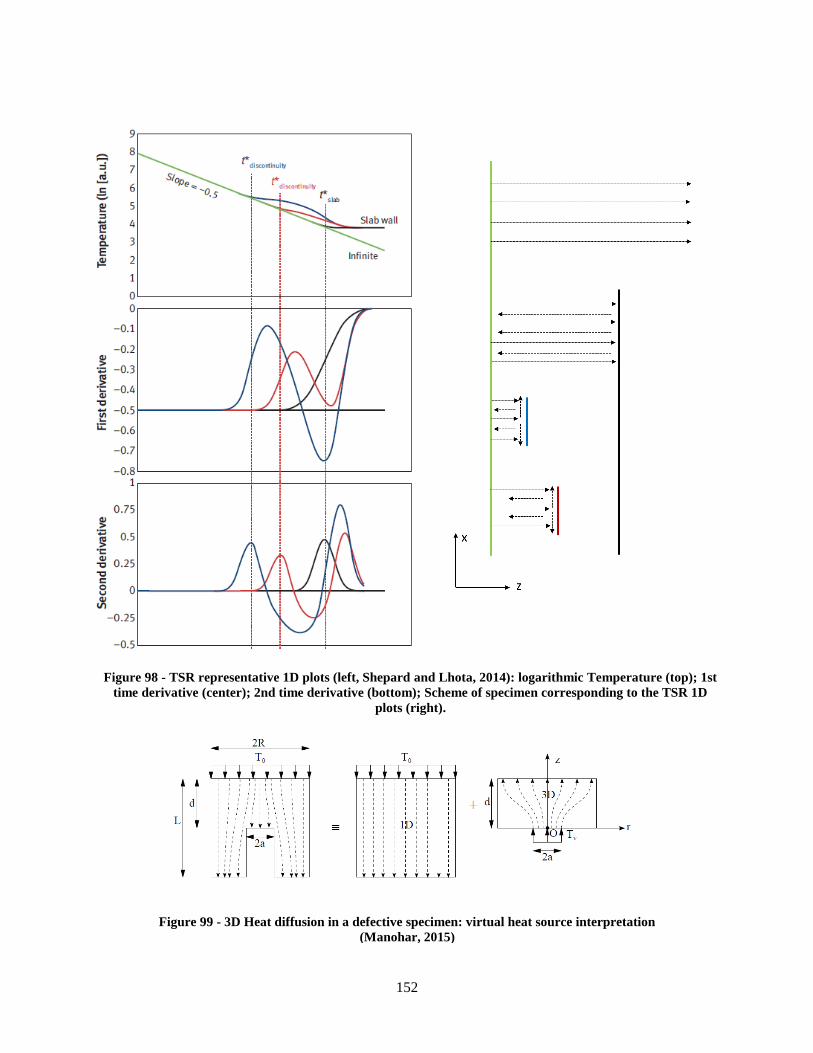
152
Figure 99 - 3D Heat diffusion in a defective specimen: virtual heat source interpretation
(Manohar, 2015)
Figure 98 - TSR representative 1D plots (left, Shepard and Lhota, 2014): logarithmic Temperature (top); 1st
time derivative (center); 2nd time derivative (bottom); Scheme of specimen corresponding to the TSR 1D
plots (right).

153
As discussed in Manohar (2013; Manohar et al., 2015) and in the previous theoretical section, the
temperature evolution in a defective portion of a specimen can be viewed as the summation of two
contributions: a diffusion of heat through the depth and reflections, and consequent decrease in cooling,
after hitting a discontinuity.
This latter scattering effect, as pictured in Figure 99, can also be seen as if the defect traps heat
above its reflective surface and becomes a secondary heat source itself, initiating a secondary 3D diffusion
process. The more localized and “discontinuous” the defect, the more the “trap and release” effect is
evident. To capture this phenomenon, and enhance defect detection and visualization, a second time
derivative can be performed on the polynomial. The change in the rate of cooling is here emphasized: the
maximum represents the flex point in the cooling, hence the reflection from the discontinuity, while the
minimum represents the later highest cooling, hence the 3D diffusion due to the localized defect (Figure
99bottom). To be noted, the absence of defects within the medium should be demonstrated by a positive
second derivative, since no secondary cooling should occur. The time of arrival of the maximum of the
second derivative (also known as saturation or break time) is related to the depth L of the reflective wall
and diffusivity as:
𝑡𝑠𝑎𝑡 =𝐿2
𝜋𝛼
Figure 100 - Secondary cooling dependence on defect aspect ratio

154
The defect type itself influences the secondary cooling effect, hence the second derivative, both in
magnitude and time of positive and negative peak arrival (Shepherd, Frendberg, 2014). Different
consideration on the defect aspect ratio, defined as diameter/depth of the defect must be done to interpret
the results correctly.
Figure 100 reports three different cases of variations in defect in-plane size (diameter, in-plane
extension), depth (distance from the front surface) and thickness (transverse discontinuity size). The first
case (Figure 100 left) compares two defects at the same depth but with different in-plane extensions: the
red defect will have a stronger and longer secondary cooling, since the lateral diffusion will take longer to
dissipate. The second case (Figure 100 center) considers the depth of the defect: the closer to the primary
heat source, the greater the amount of heat to be reflected and hence diffused as a secondary source. A
minimum aspect ratio is needed, above which detection can be performed. In the third case, a more
“localized” defect is compared to a thin one, as an insert or delamination (Figure 100 right): the greater
discontinuity in the thickness direction, the greater the mismatch in diffusivity, hence the stronger the trap
and release effect. Flat inserts, disbonds and delaminations are harder to detect with respect to flat bottom
holes, inclusions and cracking.
The combination of the TSR and the virtual heat source will be applied in this work to detect and study
defects in aerospace panels.
The same composite panels (
Table 8), manufactured under the NASA project described in the previous chapter and impacted
with different energy levels on the stringer cap and flange, have been tested for an independent IR
thermography damage survey.
Two flash lamps (detail flash lamps) provided the excitation and a FLIR A320 Thermocamera
(320x240, 30 Hz) recorded the temperature evolution for 120s, including the time of excitation, to capture
the entire cooling transient, in a “reflection mode”.
The results are presented as 2D maps, at specific time instants, optimized according to 1D time
plots. The three 1D time plots (temperature, 1st derivative, 2nd derivative) use the TSR method, implemented
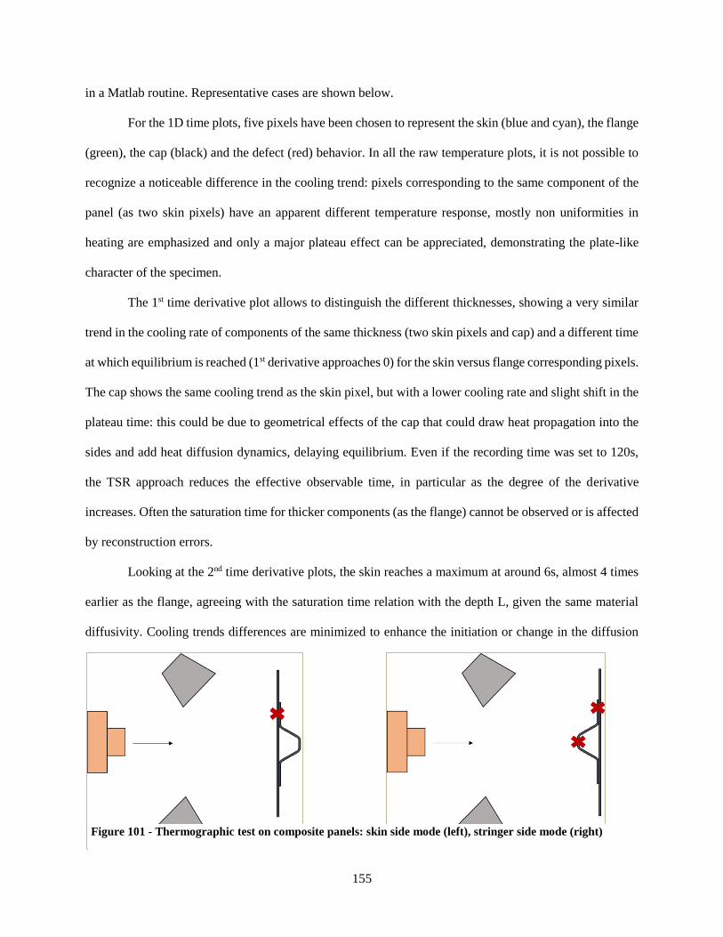
155
in a Matlab routine. Representative cases are shown below.
For the 1D time plots, five pixels have been chosen to represent the skin (blue and cyan), the flange
(green), the cap (black) and the defect (red) behavior. In all the raw temperature plots, it is not possible to
recognize a noticeable difference in the cooling trend: pixels corresponding to the same component of the
panel (as two skin pixels) have an apparent different temperature response, mostly non uniformities in
heating are emphasized and only a major plateau effect can be appreciated, demonstrating the plate-like
character of the specimen.
The 1st time derivative plot allows to distinguish the different thicknesses, showing a very similar
trend in the cooling rate of components of the same thickness (two skin pixels and cap) and a different time
at which equilibrium is reached (1st derivative approaches 0) for the skin versus flange corresponding pixels.
The cap shows the same cooling trend as the skin pixel, but with a lower cooling rate and slight shift in the
plateau time: this could be due to geometrical effects of the cap that could draw heat propagation into the
sides and add heat diffusion dynamics, delaying equilibrium. Even if the recording time was set to 120s,
the TSR approach reduces the effective observable time, in particular as the degree of the derivative
increases. Often the saturation time for thicker components (as the flange) cannot be observed or is affected
by reconstruction errors.
Looking at the 2nd time derivative plots, the skin reaches a maximum at around 6s, almost 4 times
earlier as the flange, agreeing with the saturation time relation with the depth L, given the same material
diffusivity. Cooling trends differences are minimized to enhance the initiation or change in the diffusion
Figure 101 - Thermographic test on composite panels: skin side mode (left), stringer side mode (right)

156
events only. Defects can be appreciated as they show a unique signature, usually different from the other
components, while being closer to the flange (for the flange impacts) since they are mainly affecting the
latter.
Figure 102 shows a 90J impacted flange specimen, when inspected from the “skin side”: the top
2D plot shows the raw temperature, where only heat non uniformities in the excitation and surface
emissivity differences can be noticed. In the 1st derivative 2D (central) plot, the flange shows as a darker
region with respect to the skin, due to its more negative cooling rate driven by the doubled thickness. A
skirt shaped damage can be recognized within the flange, with a larger edge on the exterior flange side,
since the delamination involves the whole flange to skin bond, but extends more in-plane as it moves further
away from the stiffener. The 2nd derivative 2D plot (bottom) reduces the differences in the diffusion process
(uniform plot) and is shown at two instants: the earlier one enhances the localized skin defect while the
later shows again the skirt shaped delamination and the increased severity further away from the stiffener.
Another test has been performed on the same flange impacted specimen, when inspecting the
“stringer side” (Figure 103 and Figure 104): although such modality would not take place in an in-situ
inspection, it can still be performed for NDE to have a full field subsurface defect map and to infer
additional insights on defect formation.
The 1st derivative 2D plot, at early instants, still shows the geometrical features of the stringer,
because of the different scattering from the edges and non-perpendicular surfaces; the different cooling
trend can be already observed at the damage location. Flange and skin show different behavior as time
evolves and the skirt shaped damage emerges, with the higher severity cooling dynamics around the impact
location, due to the “stair” delamination mode. The 2nd derivative 2D plots enhance thickness differences
(uniform skin-thick vs flange-thick components) and emphasize the 3D “trap and release” effect due to the
localized secondary diffusion process. The top of the cap itself manifests a second cooling, due to the
geometrical confinement of heat (Figure 104 top right) and the defect extending to the flange can be clearly
located. Moreover, closer to the hat, the defect shows an opposite simultaneous trend, maybe due to the
evolution of the delamination in multiple plies of different orientation. At later instants, the opposite trend

157
is instead observed for locations closer to the hat with respect to further away from it: the trap and release
effect occurs within the damage, probably due to the different levels (number and depth) of the plies
involvement (“stair mode”). Both the 1st and 2nd derivatives show a high severity damage on the stringer
flange that was not emerging in the “skin mode” inspection: the damage shows clear and localized,
involving different plies within the flange, the disbond at the 16th ply emerges later, since it is deeper in the
specimen and shows wider at the edges, merging with the skin.
As for a comparison of the severity of the damage due to a different impact energy, the 2nd
derivative plots from the “stringer-side” inspection are reported (Figure 105). Slightly different instants
have been chosen, as differences peak at slightly different times. The 70J case shows a less localized
damaged, less plies involvement and smaller in-plane extent. The delamination is more contained within
the flange itself and stays more superficial.

158
Fig
ure
10
2 -
TS
R T
her
mo
grp
ah
y t
est:
Fla
ng
e 90
J i
mp
act
. 1
D p
lots
(le
ft);
2D
ma
ps
(rig
ht)
raw
Tem
per
atu
re (
top
), 1
st d
eriv
ati
ve
(cen
ter)
, 2
nd d
eriv
ati
ve
(bo
tto
m)
at
two
tim
e in
sta
nts

159
Fig
ure
10
3 -
TS
R T
her
mo
grp
ah
y t
est:
Fla
ng
e 90
J i
mp
act
, "
stri
ng
er s
ide"
. 1
D p
lots
(le
ft);
2D
ma
ps
(rig
ht)
ra
w T
emp
era
ture
(to
p
left
), 1
st d
eriv
ati
ve
earl
y i
nst
an
t (b
ott
om
lef
t),
1st
der
iva
tiv
e m
idd
le i
nst
an
t (t
op
rig
ht)
, 1
st d
eriv
ati
ve
late
r i
nst
an
t (b
ott
om
rig
ht)
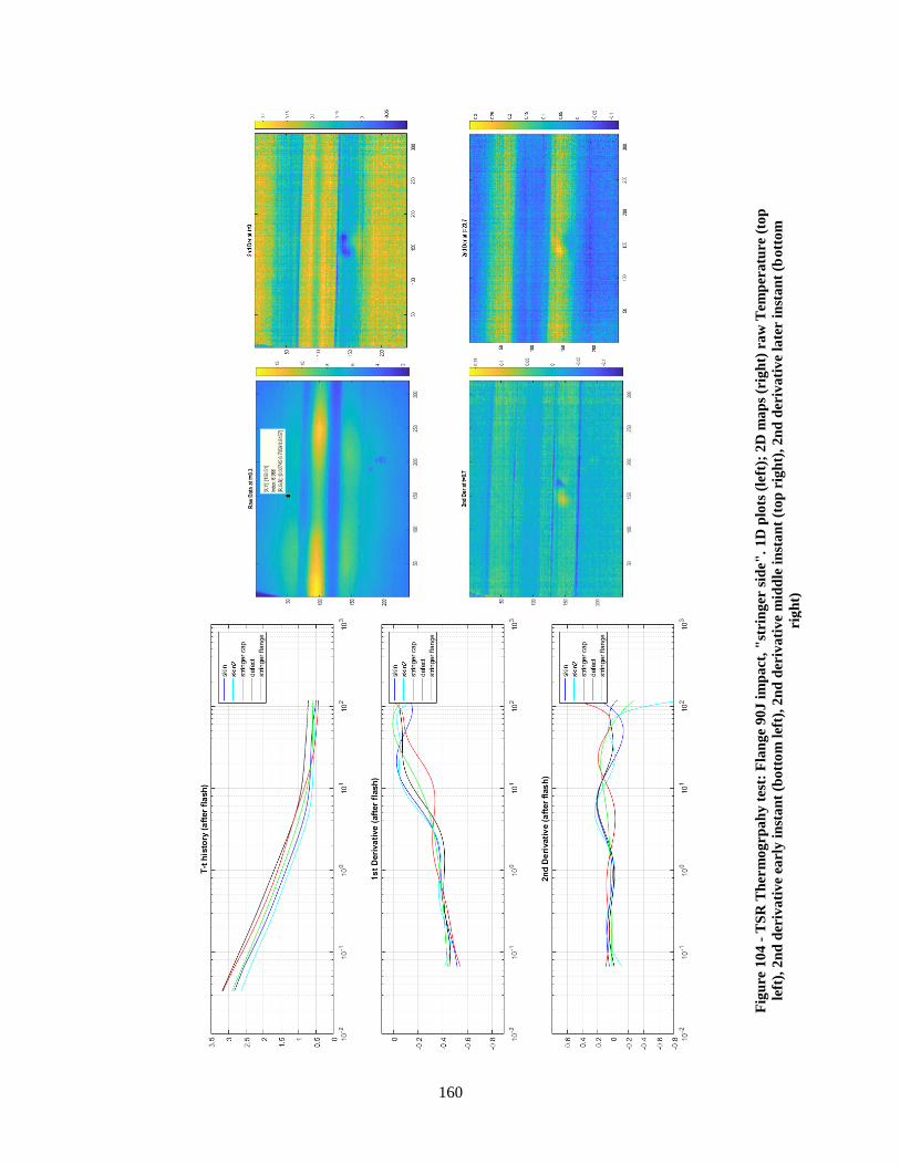
160
Fig
ure
10
4 -
TS
R T
her
mo
grp
ah
y t
est:
Fla
ng
e 90
J i
mp
act
, "
stri
ng
er s
ide"
. 1
D p
lots
(le
ft);
2D
ma
ps
(rig
ht)
ra
w T
emp
era
ture
(to
p
left
), 2
nd
der
iva
tiv
e ea
rly
in
sta
nt
(bo
tto
m l
eft)
, 2
nd
der
iva
tiv
e m
idd
le i
nst
an
t (t
op
rig
ht)
, 2
nd
der
iva
tiv
e la
ter
inst
an
t (b
ott
om
rig
ht)
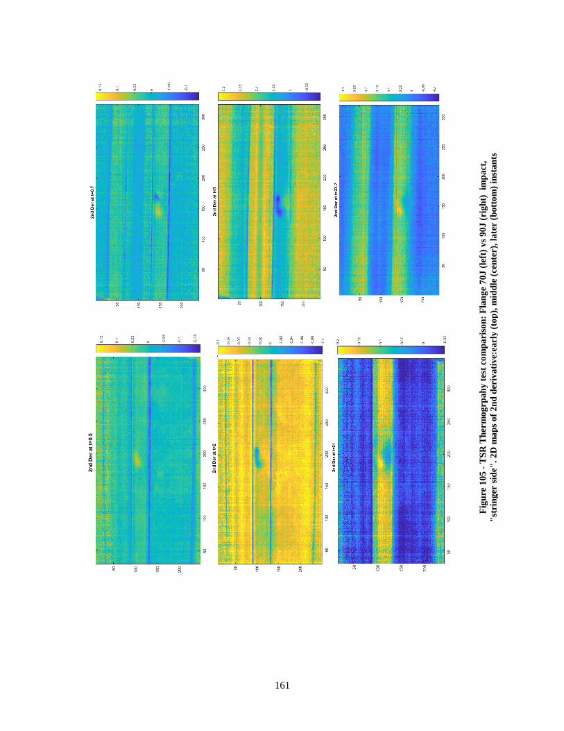
161
Fig
ure
10
5 -
TS
R T
her
mo
grp
ah
y t
est
com
pa
riso
n:
Fla
ng
e 7
0J
(le
ft)
vs
90
J (
rig
ht)
im
pa
ct,
"st
rin
ger
sid
e"
. 2
D m
ap
s o
f 2
nd
der
iva
tiv
e:ea
rly
(to
p),
mid
dle
(ce
nte
r),
late
r (
bo
tto
m)
inst
an
ts
162
Figure 106 and Figure 107 report the IR thermographic tests performed on the cap impacts, from
the “stringer-side” inspection mode. As the 2D plots show, the TSR approach eliminates both the
irregularities in the heat excitation and the surface emissivity (e.g. marks from the UT A-scan and writings).
The 1st derivative allows the detection of the damage on the top of the stringer hat and the visualization of
a superficial central type of defect and a deeper and wider delamination type of defect. The delamination
on the top of the hat extends along the longitudinal dimension of the stringer, starting from a thinner central
area, corresponding to the impact location. It looks like the laminate propagated the damage to the sides,
opening up plies into multiple delaminations. The 2nd derivative 2D plots confirm this damage formation
assumption, especially in the later instants, where a cross-shaped damage, involving multiple and deeper
layers emerges very well. The earlier instants emphasize the more superficial damage and the diagonally
opposite secondary cooling trend, suggesting a stair case damage mode progression, due to the lay-up.
The comparison among the 30J, 50J and 70J cap impact damages is shown in Figure 108. The 2nd
derivative 2D maps enhance the defect initiation and progression thanks to the trap and release effect of
this very localized damaged. The trend of the impact is exactly the same, demonstrating the same kind of
defect, but the severity increases with the impact energy. In particular, the damage extends more along the
cap and on the sides and local cracking increases (middle and bottom plots). At a very early time, the virtual
heat source effect is very strong and it increases with the severity of the damage: the diagonal asymmetry
confirms the augmented cracking and staircase damage progression.

163
Fig
ure
10
6 -
TS
R T
her
mo
grp
ah
y t
est:
Ca
p 5
0J
im
pa
ct,
"st
rin
ger
sid
e".
1D
plo
ts (
left
); 2
D m
ap
s (r
igh
t) r
aw
Tem
per
atu
re (
top
lef
t),
1st
der
iva
tiv
e ea
rly
in
sta
nt
(bott
om
lef
t),
1st
der
iva
tiv
e m
idd
le i
nst
an
t (t
op
rig
ht)
, 1
st d
eriv
ati
ve
late
r i
nst
an
t (b
ott
om
rig
ht)

164
Fig
ure
10
7 -
TS
R T
her
mo
grp
ah
y t
est:
Ca
p 5
0J
im
pa
ct,
"st
rin
ger
sid
e".
1D
plo
ts (
left
); 2
D m
ap
s (r
igh
t) r
aw
Tem
per
atu
re (
top
lef
t),
2n
d
der
iva
tiv
e ea
rly
in
sta
nt
(bott
om
lef
t),
2n
d d
eriv
ati
ve
mid
dle
in
sta
nt
(to
p r
igh
t),
2n
d d
eriv
ati
ve
late
r i
nst
an
t (b
ott
om
rig
ht)

165
Fig
ure
10
8 -
TS
R T
her
mo
grp
ah
y t
est
com
pa
riso
n:
Ca
p 3
0J
(le
ft)
vs
50
J (
cen
ter)
vs
70J
(ri
gh
t)
imp
act
, "
stri
ng
er s
ide"
. 2
D m
ap
s o
f
2n
d d
eriv
ati
ve:
earl
y (
top
), m
idd
le (
cen
ter)
, la
ter (
bo
tto
m)
inst
an
ts

166
ACKNOWLEDGEMENTS
Chapter 3, Section 3.4, in part, is currently being prepared for submission for publication
of the material. Capriotti, Margherita; Ellison, Andrew; Kim, Hyungsuk E.; Lanza di Scalea,
Francesco; Kim, Hyonny. The dissertation author was the primary investigator and author of this
material.
167
Chapter 4
Comparison of UGW inspection of
composite aerospace structures with UT
and CT datasets
4.1 Introduction
The characterization of damage in structures is often a tradeoff between the complexity of the
inspection set-up and the depth of penetration/resolution/sensitivity of the technique. The choice of the
NDE approach to be employed is usually the result of a balance between several factors as difficulty
and time of inspection, cost, accessibility, portability, performance and safety. Moreover, the desired
level of inspection itself needs to be considered (i.e. damage detection only, damage localization,
damage characterization, imaging, microscopic imaging). Hence, the different NDE techniques do not
have to be exclusive, but can be employed at different stages and integrated to validate assumptions and
offer additional information about the status of the specimen and/or damage.
UGWs inspection embodies advantageous traits offering simplicity of implementation and
interpretation, wide-area coverage, low-cost together with a high probability of detection and acceptable
resolution, in particular for the inspection of large aerospace structures. Moreover, the development of
UGW techniques may be able to characterize not only the presence of damage but also distinguish the
type and severity of the latter, while maintaining rapid deployment.

168
To this end, a comparative study of multiple levels of NDE fidelity has been conducted on
impacted composite panels. The developed SIDO UGW scanning prototypes, both in their non-contact
and hybrid approaches, have been compared to submerged C-scan ultrasonic testing (UT), X-ray
Computed Tomography (CT) and IR Thermography. Specifically, the comparison may allow enhanced
interpretation of the UGW results as: the distinction between cap versus flange impact damage, the
detection of skin damage versus disbond as separate damage modes (for the flange impact type) and the
detection of the severity of the delaminations (for the cap impact type). Also, the enabled interpretation
of specific waveform features and their relation to specific damage types could be used to enhance
and/or tailor the damage detection performance (i.e. improved feature extraction/selection to input in a
MOA) and to improve the design of the tests (i.e. excitation/reception mode, most sensitive frequency-
mode combination, scan resolution, scan penetration, etc. ).
In particular, the UGWs results is being compared to the UT inspection for the Flange type
damage and with the CT scans for the Cap type damage. The conclusions drawn for both damage types
can be also compared to the discussion presented in Section 3.4 about the thermographic inspection.
4.2 UGW features sensitivity to impact damage modes
The same SIDO UGW prototype, presented in Section 2.3.4, was used to scan Panel A and
Panel B, with the flange and cap type impact damages, respectively, in their entirety, to better simulate
a real inspection scenario. UT and CT inspection have been performed in a later stage, after the panels
were cut into single stringers. A more detailed scheme of the impacted panels is shown in Figure 109.

169
The collected waveforms have been gathered and organized in a database, according to their
location along the longitudinal dimension of the stringer and centered around the impact location, so
that they could be later compared with the other techniques. The waveforms have been gated as follows
(Figure 110), prior feature extraction, for the hybrid (left) and non-contact (right) extracted transfer
function:
Figure 110 - TF extracted from UGW scan inspection on Panel A with gated wavemodes: hybrid (left) and
non-contact (right) prototype.
Ca
p I
mp
act
30
J
Cap
Im
pact
50J
C
ap
Im
pact
70J
F
lan
ge Im
pact
70J
Cap
Slit
Hee
l
Slit
Fla
nge Im
pa
ct
90J
Figure 109 - Scheme of damaged panels: Panel A(left) and Panel B (right).

170
The main A0 skin mode dominates the signal in both configurations and is plotted in red. The
later portion of the signal, highlighted in yellow, contains higher order modes, either interacting with
the flanges and travelling into the stringer. The coda of the signal, in purple, contains reflections from
the boundaries and other stringers. The earlier mode, in blue, in the hybrid configuration could be the
A1 mode, mostly due to the double thickness of the flanges.
From such waveforms and for each mode (or combination of modes), energy-based features
(namely RMS, maximum value of the FFT, area under the FFT) and phase-based features (namely time
of arrival of the maximum peak, dominant frequency, skewness) have been extracted, to capture the
main differences caused by the wave interacting with the defects. Figure 111 (left) reports a
representative transfer function waveform from a pristine location, in blue, versus a flange impacted
one, in red. Figure 111 (right) is instead representative of a cap impact location. It can be noticed how
the flange impact damage absorbs energy, mostly in the early modes, related to the skin and flange; for
the cap impact instead, less energy penetrates the stringer, due to the presence of defects in the cap, and
contributes to an amplitude increase (with respect to a pristine condition) in both the flange and skin
anti-symmetric modes.
We report below the results for a representative case of flange impact, on Panel A, stringer 3:
Figure 113, Figure 112, Figure 114, Figure 115 and Figure 116 plot the normalized features versus the
location along the stringers in each plot. Each plot belongs to features extracted for different gates and
combination of gates, from the earlier to the later modes within the waveform. The energy features have
Figure 111 - Typical waveforms of pristine (blue) and defective (red) locations for flange damage
(left) and cap damage (right).

171
been plotted together since they qualitatively capture the same trend in the signal (red for RMS, green
for the peak of FFT and yellow for the area under the FFT), while the skewness has been selected as the
most representative phase-related feature (pink).
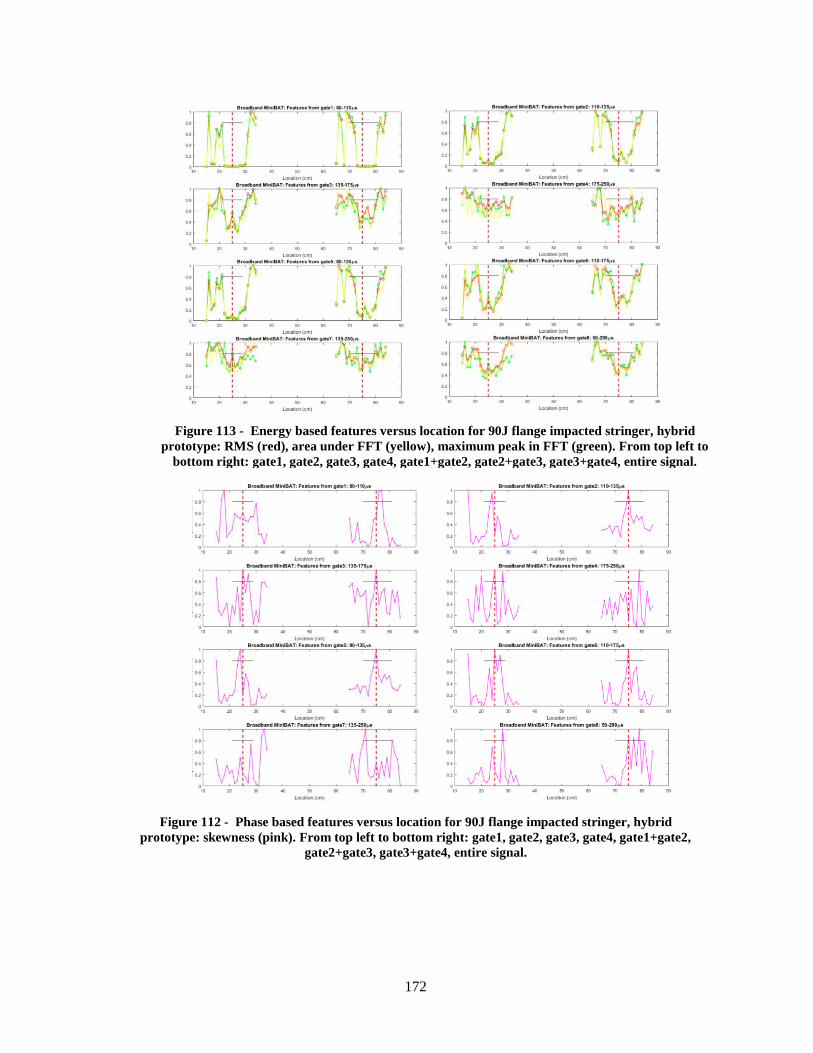
172
Figure 113 - Energy based features versus location for 90J flange impacted stringer, hybrid
prototype: RMS (red), area under FFT (yellow), maximum peak in FFT (green). From top left to
bottom right: gate1, gate2, gate3, gate4, gate1+gate2, gate2+gate3, gate3+gate4, entire signal.
Figure 112 - Phase based features versus location for 90J flange impacted stringer, hybrid
prototype: skewness (pink). From top left to bottom right: gate1, gate2, gate3, gate4, gate1+gate2,
gate2+gate3, gate3+gate4, entire signal.

173
The energy-related plot confirm absorption for the entire extension of the damage, in particular
for the first two modes (Figure 113). The third gate is also showing the same trend but with less
sensitivity. The skewness instead peaks in correspondence of the center of the damage (Figure 112): the
dispersion of the guided wave is mostly affected in the earlier modes and where the defect is highly
altering the overall thickness of the specimen. Moreover, the severity of damage can be inferred from a
quantitative analysis of the features. Figure 114 shows the results from the non-contact scanning
prototype: the left plot reports the 90J flange impact, where up to 60-80% of the energy of the
dominating wavemode is absorbed. For the 70J flange impact, on the right, the energy is absorbed up to
50-70%.
For the cap impact on Panel B, stringer 3, hybrid scanning prototype, again the first wavemodes
capture the presence of the damage, the A0 in particular, being the most highly penetrating mode. In
this damage type though, the energy transmission is enhanced by the defect, with respect to the pristine
condition (Figure 115).
The skewness is less robust in detecting the center of the impact (Figure 116): this could be due
to the dispersion effect being less accentuated when the defect is deeper in the structure or when this
kind of damage does not really cause a thickness change within the skin and flange, hence is not
dramatically affecting the velocity of the wave and the presence of early higher order modes.
The above considerations, both in the energy and dispersion content, can help distinguish the
damage type.
Figure 114 - Energy based features extracted from 90J (left) and 70J (right) flange
impacted stringer, non-contact prototype.

174
Figure 115 - Energy based features versus location for cap impacted stringer, hybrid prototype:
RMS (red), area under FFT (yellow), maximum peak in FFT (green). From top left to bottom right:
gate1, gate2, gate3, gate4, gate1+gate2, gate2+gate3, gate3+gate4, entire signal.
Figure 116 - Phase based features versus location for cap impacted stringer, hybrid prototype:
Skewness (pink). From top left to bottom right: gate1, gate2, gate3, gate4, gate1+gate2,
gate2+gate3, gate3+gate4, entire signal.

175
4.3 Correlation for quantitative damage characterization
To quantitatively capture and differentiate damage severity, type and mode (skin damage versus
disbond versus crack/delamination dominated mode) and move beyond damage detection with UGWs,
a correlation analysis has been implemented. The damaged locations have been inspected with higher
resolution techniques that provided the “ground truth” of the defect, in terms of depth, lateral extension,
number and level of plies involved. This information has been quantified at every cm, to be compared
to the UGW scans. The flange type damages have been compared with the UT scans, where four damage
modes have been identified (Figure 118): skin damage (red), disbond (green), flange (blue) and
undamaged (white).
A normalized cross-correlation has been performed and the maximum value within 3cm around
the impact center is extracted for all the features and wavemodes, to capture their sensitivity to specific
damage modes. A positive correlation of the feature with the defect mode establishes an enhanced
transmission, while a negative correlation shows absorption due to the defect; vice versa with respect to
the undamaged mode. Also, the lag value can be used to provide information about misalignment in the
cart inspection, skewness of the wave propagation and/or beam spreading effects.

176
For the sake of brevity, representative results are shown in Figure 117, for the 90J flange impact,
reporting the highest correlations extracted for each damage mode:
The skin damage correlates best with the skewness, extracted from the sixth gate. This confirms
the effect of the change in thickness and most superficial skin alteration to the dispersion of the wave.
The disbond is best captured by the RMS of the entire waveform: the damage affects multiple modes
and components, and confirms the absorption cause by the disbond since the correlation is negative. The
area under the FFT for the central and later part of the signal correlates up to 0.97 with the undamaged
shape. This means that the extension of the damage manifests itself in the waveform, both in the energy
and frequency content, and can be captured and estimated. Moreover, the feature extracted from most
of the gates correlate negatively with the disbond, while they correlate positively with the undamaged,
confirming the energy absorption behavior.
Figure 118 - UT on 90J flange impact damage: extracted pixel count (left), time of flight segmented map
(right) versus location. Skin damage (red), disbond (green), flange damage (blue), undamaged flange
(white), undamaged skin (black).
S3F1
Figure 117 - Correlation analyses between UGW extracted feature (red) and UT extracted feature: skin
damage (left), disbond (center) and undamaged flange (right).
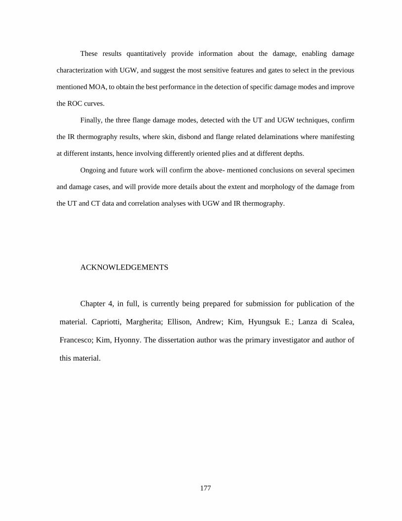
177
These results quantitatively provide information about the damage, enabling damage
characterization with UGW, and suggest the most sensitive features and gates to select in the previous
mentioned MOA, to obtain the best performance in the detection of specific damage modes and improve
the ROC curves.
Finally, the three flange damage modes, detected with the UT and UGW techniques, confirm
the IR thermography results, where skin, disbond and flange related delaminations where manifesting
at different instants, hence involving differently oriented plies and at different depths.
Ongoing and future work will confirm the above- mentioned conclusions on several specimen
and damage cases, and will provide more details about the extent and morphology of the damage from
the UT and CT data and correlation analyses with UGW and IR thermography.
ACKNOWLEDGEMENTS
Chapter 4, in full, is currently being prepared for submission for publication of the
material. Capriotti, Margherita; Ellison, Andrew; Kim, Hyungsuk E.; Lanza di Scalea,
Francesco; Kim, Hyonny. The dissertation author was the primary investigator and author of
this material.

178
Chapter 5
Overall Conclusions and Future
Recommendations
In this dissertation, two major NDE techniques have been discussed: elastic ultrasonic waves,
particularly ultrasonic guided waves (UGWs), and Infrared Thermography, where heat diffusion is used
in its interpretation as thermal waves. Both UGWs and IR Thermography have been applied to large
composite aerospace panels representative of modern commercial aircraft construction.
The theoretical investigation of the techniques provided a better understanding of the effect of
material properties and geometry on the wave propagation and enabled wave manipulation and
exploitation of specific features, depending on the wave interaction with the structural defects of interest
in stiffened composite aircraft panels.
The numerical analyses aimed at the modeling of relevant case studies, as plate-like geometries
and multi-layered materials, in a pristine and defective status. The numerical results provided an
accurate and efficient tool to aid the design of experimental inspection strategy, as well as to interpret
the recorded data.
Different experimental set-ups have been experimentally tested and iterated on representative
aircraft composite panels in the laboratory.
179
5.2 Elastic wave techniques
This dissertation has addressed the problem of scattering of multimode and dispersive elastic
UGWs. Among other applications, this topic is of great interest to ultrasonic guided-wave NDT or SHM
of structural components where defects are detected by recording transmission or reflection scattering
of a generated incoming wave mode. Predictions of these scattering patterns for a given defect can allow
to select optimum mode-frequency combinations for the incoming mode, and/or to identify the type of
defect being detected by a specific scattering observation.
For general cases that are complex in terms of either geometry or material properties (or both),
this problem requires a numerical solution.
A unified Global – Local (GL) approach has been presented here, exploiting the computational
efficiency of the Semi-Analytical Finite Element (SAFE) technique for a cross-sectional discretization
of the “global” portion, coupled with a full Finite Element discretization of the “local” portion
containing the scatterer. Compared to previous GL studies, this contribution adds: (a) a general and
consistent formulation for the evaluation of the nodal tractions at the global-local boundaries; (b) the
implementation of a robust mode tracking control, based on B-orthogonality, for the automatic selection
of incoming and scattered modes; (c) the possibility to model a wide frequency range also including
higher-order modes; (d) the automatic inclusion of an energy balance check in the results; and (e) the
unification of SAFE and FE in a stand-alone numerical Matlab code that is readily extendable to more
general cases (e.g. independent treatment of the two global regions, explicitly given theoretical
formulation such as consistent nodal forces at the boundaries, or extension to 3D cases).
The proposed GL algorithm was applied to a composite skin-to-stringer assembly typical of
commercial aircraft construction. Various relevant defects were modelled, and scattering spectra were
obtained for guided-wave frequencies as high as 500 kHz under incoming flexural (A0-type) or axial
(S0-type) modes that are typically employed as excitations in guided-wave testing of these components.
The results reveal quite interesting transmission spectra, same-mode or mode converted, that are

180
peculiar to each of the defects considered. These predictions can be extremely useful to guide and
interpret guided-wave inspection tests conducted on these components. The case study considered was
a 2D (plain strain) analysis that is quite applicable to a scanning-type guided-wave system of the type
utilized by Capriotti et al. (2017). An extension to a 3D scattering case for internal flaws in railroad
tracks using this algorithm has also been studied by the authors. High group velocity and excitable
modes were chosen as incoming modes to probe a pristine and defective model of track. Results have
been presented in terms of energy scattered from transverse head defects of different sizes. Mesh
refinement, local region length and number of modes included in the analysis have also been considered.
The results shown for the skin-to-stringer case study and railroad tracks only apply to the
specific geometry and material properties considered. However, the cross-sectional mode shapes mostly
control the partition of energy between the incoming mode and the scattered modes. Consequently, some
scalability of the results to components of different thicknesses can be qualitatively predicted on the
basis of the well-known invariance of the guided-wave cross-sectional mode shapes with the <frequency
× thickness> product (Rose 2014). In other words, for the same mode shape to be generated, frequency
and thickness must be inversely proportional. As a result, for example, specific frequency values of
interest in the scattering spectra predicted for a given thickness of the skin could be scaled to a different
skin thickness, provided that the <frequency × thickness> product is the same. The model has considered
elastic waves with no viscoelastic damping. Damping could be included by considering complex
stiffness matrices in the analysis resulting in complex wavenumbers as discussed, for example, by
Bartoli et al. (2006). A forced solution, that includes the reproduction of typical experimental excitation
and reception set-ups (distances, narrow/broadband signals, area of influence of the sensor) and time-
domain responses has also been implemented and is currently being studied for a variety of geometries,
damage types and applications.
This research proposes a rapid NDE technique for the detection of structural defects in
composite aircraft structures subjected to ground service equipment (GSE) impacts. The approach taken
utilizes the waveguide geometry of the structure by means of ultrasonic guided waves. Two laboratory
181
prototypes for line scanning were developed, one using contact PZT transducers with a differential
approach and one using non-contact (air-coupled) transducers in a pitch–catch approach. The inspection
utilizes a statistical outlier analysis that compensates each measurement for the normal (baseline)
variation during a scan, thereby increasing the POD (true detections) and decreasing the PFA (false
positive). Tests conducted on previously impacted test panels representative of commercial aircraft
construction indicated an excellent detection performance (in terms of POD vs. PFA tradeoffs) for skin
and stringer defects. A perfect detection for these defects was actually obtained by the non-contact
system once both skin wave modes and stringer wave modes were combined in the statistical feature
vector.
The defects tested in this study were limited to the panel skin and stringers. Defects located in
the deeper structure, specifically shear ties and C-frames, were not targeted, because the frequencies
used were found to be too high to penetrate these regions. Ongoing work is aimed at testing lower UGW
frequencies in an effort to penetrate into the C-frames to provide comprehensive coverage of the
structure.
A transfer function approach for ultrasonic guided-wave testing is also presented for damage
detection purposes. The method is based on a single-input-dual-output (SIDO) scheme that minimizes
the effects of the transducers’ response and the transducers-to-structure coupling effects compared to a
traditional single-input-single-output (SISO) guided-wave testing. For example, the SIDO method
enables the use of excitation sources with unknown spectra (e.g. non-instrumented impactors). By
utilizing a deconvolution operation, the SIDO approach additionally brings out the coherent wave paths
between the two receivers and minimizes the incoherent contributions. These performances are
particularly relevant to scanning systems where the acoustic transduction can be variable.
This method, combined with a statistical Outlier Analysis, was utilized to design two scanning
systems applied to the rapid inspection of representative composite aircraft panels subjected to various
types of impact-caused damage. The two systems explore, respectively, the narrow/high frequency
range (~110-210 kHz) offered by non-contact air-coupled piezocomposite transducers and the
182
broad/low frequency range (~ 40-270 kHz) offered by the combination of an ultralight impactor and air-
coupled capacitive transducers. The results show how stringer flange impacts affect the skin and the
skin-to-stringer interface, generally producing a decrease in wave transmission strength that is
detectable by the high frequency wave content excited by both the air-coupled system and the hybrid
system. Stringer cap impacts, instead, generally produce an increase in wave transmission strength
(through decreased acoustic leakage) that mostly affects the low frequency and high magnitude wave
content that are excited by the hybrid system.
The prototypes discussed here are early-stage laboratory systems that do not include automatic
data processing of the scan. Ongoing work is aimed at adding an encoder to track the position of the
inspection head, implementing automatic signal processing to generate the scan output in quasi-real time
and automating the mini impactor excitation modality for the hybrid prototype.
Follow-up work should be devoted to more detailed analyses on the ultrasonic wave interaction
with each of these defects. For the impact locations, this will require knowledge of the precise extent
and morphology of the damage that will be obtained from X-ray computed tomography and/or ultrasonic
C-scan of the test panels. This future study will also refine the selection of damage-sensitive features
and of the time gates imposed on the reconstructed transfer function for the Outlier Analysis scans.
5.3 Thermal wave techniques
Heat propagation as a diffusion phenomenon has been investigated in terms of thermal wave
propagation. The solution proposed here is the formulation of the thermal field (Temperature) by the
use of Green’s functions. The method has been chosen to exploit the analogies and dissimilarities with
travelling elastic waves, so as to visualize the defects as secondary heat sources and to manipulate the
equations in frequency domain, using convolution and correlation theorems, similarly to what done with
elastic waves

183
The passive retrieval of a thermal Green’s function by cross-correlation of diffuse fields has
been demonstrated theoretically. Although the feasibility is supported by the theoretical formulation and
the experimental availability of a large database of temperature time histories, output by infrared 2D
detectors, hardware limitations prevented the extraction of a thermal transfer function. The validity of
the theoretical idea also needs to be further investigated in terms of scale, specifically distances between
the Green’s function path, magnitude of the temperature fluctuations, time duration of the diffusion and
frequency of the oscillations. Enormous differences arise when observing heat diffusion at the
macroscale, as the thermal field recorded by a thermocamera, and at the nanoscale, where atomic
vibrations and interactions govern the heat transport.
Such limitations, also characterized by the lack of time invariance in the diffusion process,
suggested the exploitation of spatial symmetries. Numerical studies have been performed on plate-like
structures for metals of different diffusivities. The interaction of heat with the defects and the alteration
of the heat flow has been captured with the use of spatial derivatives. The method enhances the detection
of discontinuities and can be interpreted as the visualization of the heat trapped/shadowed by the defect.
The implementation of such method in time could also provide the extraction of a heat propagation
speed, related to the diffusivity, offering quantitative structural characterization by IR thermographic
measurements, and could be experimentally applied following the grid method (Grediac et al., 2016).
Further numerical and experimental studies have been started in this direction.
Finally, the Thermographic Signal Reconstruction (TSR) method combined to the virtual heat
source concept have been applied to composite aerospace structures, with different damage type. The
technique allowed the elimination of surface emissivity and heating non-uniformities and enhanced the
detection and distinction of skin damage, disbond, flange and cap damage. The time derivatives enable
quantitative defect detection, in terms of depth, type and orientation of the involved plies. This
information is being currently validated through the comparison with UT and CT scans.
184
REFERENCES
Ahmad, Z. A. B., Vivar-Perez, J. M., Gabbert, U., 2013. Semi-analytical finite element method for
modeling of lamb wave propagation. CEAS Aeronautical Journal, 4(1), 21-33.
Alleyne, D.; Cawley, P., 1992. The interaction of Lamb waves with defects. IEEE Trans. Ultrason.
Ferroelectr. Freq. Control, 39, 381–397.
Alleyne, D.N. and Cawley, P., 1990, December. A 2-dimensional Fourier transform method for the
quantitative measurement of Lamb modes. In Ultrasonics Symposium, 1990. Proceedings., IEEE
1990 (pp. 1143-1146). IEEE.
Almond, D.P. and Lau, S.K., 1994. Defect sizing by transient thermography. I. An analytical treatment.
Journal of Physics D: Applied Physics, 27(5), p.1063.
Al-Nassar, Y. N., Datta, S. K., Shah, A. H., 1991. Scattering of Lamb waves by a normal rectangular
strip weldment. Ultrasonics, 29(2), 125-132.
Ashby, M.F. and Cebon, D., 1993. Materials selection in mechanical design. Le Journal de Physique
IV, 3(C7), pp.C7-1.
Baleagas, D., Deom, A., Boscher, D., Gardette, G., 1987. NDT of carbon-epoxy composites by a pulsed
photothermal method and transposition to stimulated infrared thermography. Qualite Revue Pratique de
Controle Industriel, No. 147, pp. 58–63.
Banerjee S, Ricci F, Monaco E, Lecce L and Mal AK (2007) Autonomous impact damage monitoring
in stiffened composite panel. Journal of Intelligent Material Systems and Structures 18(6): 623-633.
Barnett V and Lewis T (1994) Outliers in Statistical Data. New York, Wiley.
Bartoli, I., Lanza di Scalea, F., Fateh, M., Viola, E., 2005. Modeling guided wave propagation with
application to the long range defect detection in railroad tracks. NDT&E International, 38, 325-334.
Bartoli, I., Marzani, A., di Scalea, F. L., Viola, E., 2006. Modeling wave propagation in damped
waveguides of arbitrary cross-section. Journal of Sound and Vibration, 295(3-5), 685-707.
Bartoli, I., 2007. Structural health monitoring by ultrasonic guided waves. PhD dissertation, UC San
Diego, CA, USA.
Broggini, F. and Snieder, R., 2012. Connection of scattering principles: A visual and mathematical tour.
European Journal of Physics, 33(3), p.593.
Callen, H.B. and Welton, T.A., 1951. Irreversibility and generalized noise. Physical Review, 83(1), p.34.
Callen, H.B. and Greene, R.F., 1952. On a theorem of irreversible thermodynamics. Physical Review,
86(5), p.702.
Caprino, G., 1983. On the prediction of residual strength for notched laminates. Journal of Materials
Science, 18(8), pp.2269-2273.
Capriotti, M., Kim, H. E., Lanza di Scalea, F., Kim, H., 2017. Non-Destructive inspection of impact
185
damage in composite aircraft panels by ultrasonic guided waves and statistical
processing. Materials, 10(6), 1-12.
Carslaw, H.S. and Jaeger, J.C., 1959. Conduction of heat in solids. Oxford: Clarendon Press, 1959, 2nd
ed.
Castaings, M., Le Clezio, E., Hosten, B., 2002. Modal decomposition method for modeling the
interaction of Lamb waves with cracks. The Journal of the Acoustical Society of America, 112(6), 2567-
2582.
Cawley P., The rapid non-destructive inspection of large composite structures. Composites 1994,
Volume 25, 351-357.
Chang, Z., Mal, A. K., 1995. A global-local method for wave propagation across a lap joint. ASME
Applied Mechanics Division Publications AMD, 204, 1-1.
Chang, Z., Mal, A.,1999. Scattering of Lamb waves from a rivet hole with edge cracks. Mechanics of
materials, 31(3), 197-204.
Chong SY, Victor JJ and Todd MD (2017) Full-field ultrasonic inspection for a composite sandwich
plate skin-core debonding detection using laser-based ultrasonics. In: Health Monitoring of Structural
and Biological Systems 2017, Portland, US, 10170, 1017007. International Society for Optics and
Photonics.
Cole, K.D., Beck, J.V., Haji-Sheikh, A. and Litkouhi, B., 2010. Heat conduction using Green’s
functions. Taylor & Francis.
Croxford A, Wilcox P, Drinkwater B and Konstandtinidis G (2007) Strategies for guided-wave
structural health monitoring. In: Proceedings of the Royal Society of London A: Mathematical, Physical
and Engineering Sciences, 463(2087), 2961-2981. The Royal Society.
Datta, S. K., Ju, T. H., Shah, A. H., 1992. Scattering of an impact wave by a crack in a composite
plate. Journal of Applied Mechanics, 59(3), 596-603.
Datta, S. K., Shah, A. H., Bratton, R. L., Chakraborty, T., 1988. Wave propagation in laminated
composite plates. The Journal of the Acoustical Society of America, 83(6), 2020-2026.
DeFrancisci, G.K., 2013. High Energy Wide Area Blunt Impact on Composite Aircraft Structures. Ph.D.
Dissertation, Advanced Composites and Aerospace Laboratory, University of California, San Diego,
CA, USA.
di Scalea, F.L. and McNamara, J., 2004. Measuring high-frequency wave propagation in railroad tracks
by joint time–frequency analysis. Journal of Sound and Vibration, 273(3), pp.637-651.
di Scalea, F.L., Bonomo, M. and Tuzzeo, D., 2001. Ultrasonic guided wave inspection of bonded lap
joints: noncontact method and photoelastic visualization. Research in Nondestructive Evaluation, 13(3),
pp.153-171.
Dong, S.B., Goetschel, D.B., 1982. Edge effects in laminated composite plates. Journal of Applied
Mechanics, 49, 129-135.
Duroux A, Sabra KG, Ayers J and Ruzzene M (2010) Extracting guided waves from cross-correlations
of elastic diffuse fields: Applications to remote structural health monitoring. Journal of the Acoustical

186
Society of America, 127(1), 204–215.
Farrar CR and James GH (1997) System identification from ambient vibration measurements on a
bridge. Journal of Sound and Vibration, 205(1), 1–18.
Favro, L.D., Han, X., Ouyang, Z., Sun, G., Sui, H. and Thomas, R.L., 2000. Infrared imaging of defects
heated by a sonic pulse. Review of scientific instruments, 71(6), pp.2418-2421.
Favro, L.D., Jin, H.J., Wang, Y.X., Ahmed, T., Wang, X., Kuo, P.K. and Thomas, R.L., 1992. IR thermal
wave tomographic studies of structural composites. In Review of Progress in Quantitative
Nondestructive Evaluation (pp. 447-451). Springer, Boston, MA.
Federal Aviation Administration, Composite Aircraft Structure, Advisory Circular, 2009, No: 20-
107(B).
Galán, J. M., Abascal, R., 2002. Numerical simulation of Lamb wave scattering in semi‐ infinite
plates. International Journal for Numerical Methods in Engineering, 53(5), 1145-1173.
Galán, J. M., Abascal, R., 2005. Boundary element solution for the bidimensional scattering of guided
waves in laminated plates. Computers & structures, 83(10-11), 740-757.
Gershenson, M., US Secretary of Navy, 2000. Synthetic aperture processing for diffusion-equation-
based target detection. U.S. Patent 6,147,636.
Gholizadeh S., A review of non-destructive testing methods of composite materials, Procedia Structural
Integrity, 2016, Volume 1, 50-57.
Giurgiutiu V (2015) Structural Health Monitoring of Aerospace Composites, Elsevier Science.
Giurgiutiu V., Piezoelectric wafer active sensors for structural health monitoring of composites
structures using tuned guided waves. Journal of Engineering Materials and Technology 2011, Volume
133, 0410121-0410126.
Giurgiutiu V., Soutis C., Enhanced composites integrity through structural health monitoring, Applied
Composite Materials 2012, Volume 19, 813-829.
Goetschel, D. B., Dong, S. B., Muki, R., 1982. A global local finite element analysis of axisymmetric
scattering of elastic waves. Journal of Applied Mechanics, 49(4), 816-820.
Grediac, M., Sur, F., & Blaysat, B. (2016). The Grid Method for In‐ plane Displacement and Strain
Measurement: A Review and Analysis. Strain, 52(3), 205-243.
Grinzato, E., Bison, P.G., Bressan, C. and Mazzoldi, A., 1998. NDE of frescoes by infrared
thermography and lateral heating. In Eurotherm Seminar (Vol. 60, pp. 64-67).
Guo, N., Cawley, P., 1993. The interaction of Lamb waves with delaminations in composite
laminates. The Journal of the Acoustical Society of America, 94(4), 2240-2246.
Haider, M. F., Bhuiyan, M. Y., Poddar, B., Lin, B., Giurgiutiu, V., 2018. Analytical and experimental
investigation of the interaction of Lamb waves in a stiffened aluminum plate with a horizontal crack at
the root of the stiffener. Journal of Sound and Vibration, 431, 212-225.

187
Hayashi, T., Song, W. J., Rose, J. L., 2003. Guided wave dispersion curves for a bar with an arbitrary
cross-section, a rod and rail example. Ultrasonics, 41(3), 175-183.
He J., Yuan FG (2015) Damage identification for composite structures using a cross-correlation
reverse-time migration technique. Structural Health Monitoring, 14(6), 558-570.
Hudson T, Hou T, Grimsley B and Yuan FG (2015) Detection of CFRP composite manufacturing
defects using a guided wave approach, NASA report NF1676L-19900.
Ibarra-Castanedo, C., Genest, M., Servais, P., Maldague, X.P. and Bendada, A., 2007. Qualitative and
quantitative assessment of aerospace structures by pulsed thermography. Nondestructive Testing and
Evaluation, 22(2-3), pp.199-215.
Ihn JB and Chang FK (2008) Pitch-catch Active Sensing Methods in Structural Health Monitoring for
Aircraft Structures. Structural Health Monitoring, 7(1), 15-19.
Ilcewicz L., 2010. FAA Composite Safety Administration and Certification Initiatives. JAMS
Conference.
Ilcewicz L., High Energy Wide Area Blunt Impact (HEWABI) as related to Safety and Certification.
Composite Transport DT & Maintenance Workshop, September, 2015, Quebec, CA.
Jones, R.M., 2014. Mechanics of composite materials. CRC press.
Kaiplavil, S. and Mandelis, A., 2011. Highly depth-resolved chirped pulse photothermal radar for bone
diagnostics. Review of Scientific Instruments, 82(7), p.074906.
Kaiplavil, S. and Mandelis, A., 2012, February. Bone-demineralization diagnosis in a bone-tissue-skin
matrix using the pulsed-chirped photothermal radar. In Photonic Therapeutics and Diagnostics VIII
(Vol. 8207, p. 82076L). International Society for Optics and Photonics.
Kaiplavil, S. and Mandelis, A., 2014. Truncated-correlation photothermal coherence tomography:
“crisp” imaging breaking through the diffusion resolution and depth barriers,”. Nature Photon.
Karim, M. R., Awal, M. A., Kundu, T., 1992. Elastic wave scattering by cracks and inclusions in plates:
in-plane case. International Journal of Solids and Structures, 29(19), 2355-2367.
Karim, M. R., Kundu, T., 1988. Transient surface response of layered isotropic and anisotropic half-
spaces with interface cracks: SH case. International Journal of Fracture, 37, 245-262.
Karim, M. R., Kundu, T., Desai, C. S., 1989. Detection of delamination cracks in layered fiber-
reinforced composite plates. Journal of Pressure Vessel Technology, 3,165-171.
Karunasena, W. M., Liew, K. M., Kitipornchai, S., 1995. Hybrid analysis of Lamb wave reflection by
a crack at the fixed edge of a composite plate. Computer methods in applied mechanics and
engineering, 125(1-4), 221-233.
Kessler SK., Spearing S.M., Soutis C., Damage detection in composite materials using Lamb wave
method. Smart Materials and Structures 2002, Volume 11, 269-278.
Kim H., DeFrancisci G.K., Chen Z.M., Ground Vehicle Blunt Impact Damage Formation to Composite
Aircraft Structures, Advanced Composite Materials 2014, Volume 23, 53-71.
188
Kuperman W., 2008. Correlation of randomly excited diffusive fields., notes.
Kuperman W., 2016. Diffusor Matrices, notes.
Lanza di Scalea F, Sternini S and Liang AY (2018b) Robust passive reconstruction of dynamic
transfer function in dual-output systems. Journal of the Acoustical Society of America, 143(2), 1019-
1028.
Lanza di Scalea F, Zhu X, Capriotti M, Liang AY, Mariani S and Sternini S (2018a) Passive
extraction of dynamic transfer function from arbitrary ambient excitations: Application to high-speed
rail inspection from wheel generated waves. Journal of Nondestructive Evaluation Diagnostics
Prognosis Engineering Systems, 1(1), 011005.
Lau, S.K., Almond, D.P. and Milne, J.M., 1991. A quantitative analysis of pulsed video thermography.
Ndt & E International, 24(4), pp.195-202.
Li, T., Almond, D. P., Rees, D. A. S. (2011). Crack imaging by scanning laser-line thermography and
laser-spot thermography. Measurement Science and Technology, 22(3), 035701.
Lobkis, O.I., Weaver, R.L., 2001. On the emergence of the Green’s function in the correlations of a
diffuse field. The Journal of the Acoustical Society of America, 110(6), pp.3011-3017.
Lopez, F., Ibarra-Castanedo, C., Maldague, X. and Nicolau, V.D., 2014. Pulsed thermography signal
processing techniques based on the 1D solution of the heat equation applied to the inspection of
laminated composites. Materials Evaluation, 72(1).
Loveday, P. W., Long, C. S., 2007. Time domain simulation of piezoelectric excitation of guided waves
in rails using waveguide finite elements. Sensors and Smart Structures Technologies for Civil,
Mechanical, and Aerospace Systems, 6529, 65290.
Lowe M. J. S. 1992. Plate waves for the NDT of diffusion bonded Titanium. PhD Thesis, Imperial
College, London.
Lowe MJS, Neau G and Deschamps M (2004) Properties of guided waves in composite plates, and
implications for NDE. In: AIP Conference Proceedings, Review of Quantitative Nondestructive
Evaluation Vol. 23, (ed DO Thompson and DE Chimenti), 700(1), 214–221, AIP.
Mal A., Ricci F., Samajder H., Baid H., NDE of Composite Structures using Ultrasonic Guided Waves,
Health Monitoring of Structural and Biological Systems, Proc. of SPIE 2013, Volume 8695.
Mal, A., Chang, Z., 2000. A semi‐ numerical method for elastic wave scattering
calculations. Geophysical Journal International, 143(2), 328-334.
Mandelis A., Thermophotonic radar and thermal coherence tomographies. In Proc. VIIth International
Workshop on Advances in Signal Processing for Non Destructive Evaluation of Materials
(ASPNDE) (pp. 3-4).
Mandelis, A., 2013. Diffusion-wave fields: mathematical methods and Green functions. Springer
Science & Business Media.

189
Manohar A., 2012. Quantitative nondestructive testing using infrared thermography. PhD Thesis. UC
San Diego.
Mariani S., Nguyen T., Phillips R., Kijanka P., Lanza di Scalea F., Staszewski W., Fateh, M., Carr, G.,
Non-Contact Air-Coupled Ultrasonic Guided Wave Inspection of Rails. Structural Health Monitoring
International Journal, Special Issue on Noncontact Measurement Technologies 2014, Vol.12, 539-548.
Mariani, S., 2015 Non-Contact Ultrasonic Guided Wave Inspection of Rails: Next Generation
Approach. Ph.D. Dissertation, NDE & SHM Laboratory, University of California, San Diego, CA, USA.
Marín, E., 2010. Characteristic dimensions for heat transfer. Latin-American Journal of Physics
Education, 4(1), pp.56-60.
Marín, E., Marín-Antuña, J. and Díaz-Arencibia, P., 2002. On the wave treatment of the conduction of
heat in photothermal experiments with solids. European journal of physics, 23(5), p.523.
Marzani, A., 2008. Time–transient response for ultrasonic guided waves propagating in damped
cylinders. International Journal of Solids and Structures, 45(25-26), pp.6347-6368.
Marzani, A., Viola, E., Bartoli, I., Lanza di Scalea, F., Rizzo, P., 2008. A Semi-analytical Finite Element
Formulation for modeling stress wave propagation in axisymmetric damped waveguides. Journal of
Sound and Vibration, 318(3), 488-505.
Matt, H., Bartoli, I., Lanza di Scalea, F., 2005. Ultrasonic guided wave monitoring of composite wing
skin-to-spar bonded joints in aerospace structures. Journal of the Acoustical Society of America, 118(4),
2240-2252.
Meola, C., Carlomagno, G.M., 2004. Recent advances in the use of infrared thermography.
Measurement science and technology, 15(9), p.R27.
Michaels JE and Michaels TE (2005) Detection of structural damage from the local temporal
coherence of diffuse ultrasonic signals. IEEE Transactions on Ultrasonics, Ferroelectrics and
Frequency Control, 52(10), 1769–1782.
Morse, P.M. and Feshbach, H., 1954. Methods of theoretical physics. American Journal of Physics,
22(6), pp.410-413.
Morse, P.M. and Feshbach, H., 2010. Methods of theoretical physics, Vol. II.
Murat B, Khalili P and Fromme P (2016) Scattering of guided waves at delaminations in composite
plates. Journal of the Acoustical Society of America, 139(6), 3044-3052.
Nicolaides, L. and Mandelis, A., 2000. Novel dental dynamic depth profilometric imaging using
simultaneous frequency-domain infrared photothermal radiometry and laser luminescence. Journal of
biomedical optics, 5(1), pp.31-40.
Nucera, C., White, S., Chen, Z.M., Kim, H. and Lanza di Scalea, F., 2015. Impact monitoring in stiffened
composite aerospace panels by wave propagation. Structural Health Monitoring, 14(6), pp.547-557.
Oswald-Tranta, B. and Shepard, S.M., 2013, May. Comparison of pulse phase and thermographic signal
reconstruction processing methods. In Thermosense: Thermal Infrared Applications XXXV (Vol. 8705,
p. 87050S). International Society for Optics and Photonics.

190
Ozisik, M.N. and Tzou, D.Y., 1994. On the wave theory in heat conduction. Journal of Heat Transfer,
116(3), pp.526-535.
Pickering, S.G. and Almond, D.P., 2007. An evaluation of the performance of an uncooled
microbolometer array infrared camera for transient thermography NDE. Nondestructive Testing and
Evaluation, 22(2-3), pp.63-70.
Poddar, B. and Giurgiutiu, V., 2016a. Complex modes expansion with vector projection using power
flow to simulate Lamb waves scattering from horizontal cracks and disbonds. The Journal of the
Acoustical Society of America, 140(3), 2123-2133.
Poddar, B. and Giurgiutiu, V., 2016b. Scattering of Lamb waves from a discontinuity: an improved
analytical approach. Wave Motion, 65, 79-91.
Raghavan A and Cesnik CE (2007) Review of guided-wave structural health monitoring. The Shock and
Vibration Digest, 39, 91-114.
Rattanawangcharoen, N., Zhuang, W., Shah, A. H., Datta, S. K., 1997. Axisymmetric guided waves in
jointed laminated cylinders. ASCE Journal of Engineering Mechanics, 123(10), 1020-1026.
Ricci, F., Monaco, E., Maio, L., Boffa, N.D. and Mal, A.K., 2016. Guided waves in a stiffened
composite laminate with a delamination. Structural Health Monitoring, 15(3), pp.351-358.
Riegert G., Pfleiderer K., Gerhard H., Solodov I. and Busse G., Modern methods of NDT for inspection
of aerospace structures., ECNDT, Berlin, Germany, 2006.
Rizzo P, Sorrivi E, Lanza di Scalea F and Viola E (2007) Wavelet-based Outlier Analysis for Guided
Wave Structural Monitoring: Application to Multi-wire Strands. Journal of Sound and Vibration,
307(1-2), 52-68.
Roche, J.M., Leroy, F.H. and Balageas, D.L., 2014. Images of thermographic signal reconstruction
coefficients: a simple way for rapid and efficient detection of discontinuities. Materials evaluation,
72(1).
Rose, J.L., 2004. Ultrasonic Waves in Solid Media; Cambridge University Press: Cambridge, UK.
Roth PR (1971) Effective measurements using digital signal analysis. IEEE Spectrum, 8(4), 62–70.
Sabra, K.G., Roux, P. and Kuperman, W.A., 2005. Emergence rate of the time-domain Green’s
function from the ambient noise cross-correlation function. The Journal of the Acoustical Society of
America, 118(6), pp.3524-3531.
Sabra, K.G., Gerstoft, P., Roux, P., Kuperman, W.A. and Fehler, M.C., 2005. Extracting time‐domain Green's function estimates from ambient seismic noise. Geophysical Research Letters, 32(3).
Sabra KG, Srivastava A, Lanza di Scalea F, Bartoli I, Rizzo P and Conti S (2008) Structural health
monitoring by extraction of coherent guided waves from diffuse fields. Journal of the Acoustical
Society of America, 123(1), EL8–EL13.
Sabra KG, Winkel ES, Bourgoyne DA, Elbing BR, Ceccio SL, Perlin M and Dowling DR (2007)
Using cross correlations of turbulent flow induced ambient vibrations to estimate the structural
impulse response. Application to structural health monitoring. Journal of the Acoustical Society of
America, 121(4), 1987–1995.

191
Salas K and Cesnik CE (2009) Guided wave structural health monitoring using CLoVER transducers
in composite materials. Smart Materials and Structures, 19(1), 015014.
Salvermoser J, Hadziioannou C and Stahler SC (2015) Structural monitoring of a highway bridge
using passive noise recordings from street traffic. Journal of the Acoustical Society of America,
138(6), 3864–3872.
Schnars U., Heinrich R., Applications of NDT Methods on Composite Structures in Aerospace Industry,
Conference on damage in composite materials, Stuttgart, Germany, 2006, pp. 1-8.
Servais, P., Gerlach, N., Habermehl, J., Ibarra-Castanedo, C. and Maldague, X., 2008. Characterization
of manufacturing and maintenance of aerospace composite discontinuities using infrared thermography.
Materials Evaluation, 66(9).
Shepard, S. and Frendberg, M., 2014. Thermographic detection and characterization of flaws in
composite materials. Materials Evaluation, 72(7).
Shepard, S. and Lhota, J.R., 2014. Thermography: More Than a Pretty Picture. Materials Evaluation,
72(1).
Shepard, S.M., 2007, October. Flash thermography of aerospace composites. In IV Conferencia
Panamericana de END Buenos Aires (Vol. 7).
Shepard, S.M., Thermal Wave Imaging Inc, 2004. System for generating thermographic images using
thermographic signal reconstruction. U.S. Patent 6,751,342.
Siakavellas N., 2012. Detection of radial cracks at fastener holes by either eddy current or line heating
stimulated thermography. Emerging Technologies in Non Destructive Testing, 483-488.
Snieder, R., 2004. Extracting the Green’s function from the correlation of coda waves: A derivation
based on stationary phase. Physical Review E, 69(4), p.046610.
Snieder, R. and Safak, E., 2006. Extracting the building response using seismic interferometry: Theory
and application to the Millikan Library in Pasadena, California. Bulletin of the Seismological Society of
America, 96(2), pp.586-598.
Snieder, R., 2006. Retrieving the Green’s function of the diffusion equation from the response to a
random forcing. Physical Review E, 74(4), p.046620.
Snieder, R., 2007. Extracting the Green’s function of attenuating heterogeneous acoustic media from
uncorrelated waves. The Journal of the Acoustical Society of America, 121(5), pp.2637-2643.
Snieder, R., Sánchez-Sesma, F.J. and Wapenaar, K., 2009. Field fluctuations, imaging with
backscattered waves, a generalized energy theorem, and the optical theorem. SIAM Journal on Imaging
Sciences, 2(2), pp.763-776.
Snieder, R., Slob, E. and Wapenaar, K., 2010. Lagrangian Green's function extraction, with applications
to potential fields, diffusion and acoustic waves. New Journal of Physics, 12(6), p.063013.
Snieder, R., Wapenaar, K. and Wegler, U., 2007. Unified Green’s function retrieval by cross-correlation;
connection with energy principles. Physical Review E, 75(3), p.036103.

192
Sohn H, Dutta D, Yang J, Park H, Desimio M, Olson S and Swenson E (2011) Delamination detection
in composites through guided wave field image processing. Composites Science and technology,
71(9), 1250-1256.
Srivastava, A. and Lanza di Scalea, F., 2010. Quantitative structural health monitoring by ultrasonic
guided waves. ASCE Journal of Engineering Mechanics, 136(8), 937-944.
Staszewski, W., Boller, C., Tomlinson, G. R., 2004. Health monitoring of aerospace structures: smart
sensor technologies and signal processing. John Wiley & Sons.
Tabatabaei, N. and Mandelis, A., 2009. Thermal-wave radar: A novel subsurface imaging modality with
extended depth-resolution dynamic range. Review of Scientific Instruments, 80(3), p.034902.
Tabatabaei, N. and Mandelis, A., 2011. Thermal coherence tomography using match filter binary phase
coded diffusion waves. Physical review letters, 107(16), p.165901.
Tabatabaei, N., Mandelis, A. and Amaechi, B.T., 2011. Thermophotonic radar imaging: An emissivity-
normalized modality with advantages over phase lock-in thermography. Applied Physics Letters,
98(16), p.163706.
Tang, B., & Henneke, E. G. I. I. (1989). Lamb-wave monitoring of axial stiffness reduction of laminated
composite plates. Mater. Eval., 47(8), 928-934.
Tian J, Gabbert U, Berger H and Su X (2004) Lamb wave interaction with delaminations in CFRP
laminates. Computers Materials & Continua, 1(4), 327-336.
Tippmann JD and Lanza di Scalea F (2015) Passive-only damage detection by reciprocity of Green’s
functions reconstructed from diffuse acoustic fields with application to wind turbine blades. Journal of
Intelligent Material Systems and Structures, 26(10), 1251–1258.
Tippmann JD and Lanza di Scalea F (2016) Passive-only defect detection and imaging in composites
using diffuse fields. In: Mechanics of Composite and Multi-functional Materials, Volume 7, 67-72.
Springer, Cham.
Tippmann JD, Zhu X and Lanza di Scalea F (2015) Application of damage detection methods using
passive reconstruction of impulse response functions. Philos. Trans. R. Soc. A, 373(2035), 20140070.
Tretout H., David D., Thevenot F., Review of advanced NDT methods for composites aerospace
structures, Proc. Int. Symp. On Advanced Materials for Lightweight Structures, Noordwijk., The
Netherlands, 1994, pp.624-634.
Tuzzeo D., Lanza di Scalea F., Noncontact air-coupled guided wave ultrasonics for detection of thinning
defects in aluminum plates. Journal of Research in Nondestructive Evaluation 2001, Volume 13, 61-
77.
Usamentiaga, R., Venegas, P., Guerediaga, J., Vega, L. and López, I., 2013. Automatic detection of
impact damage in carbon fiber composites using active thermography. Infrared Physics & Technology,
58, pp.36-46.
Varis, J., Rantala, J. and Hartikainen, J., 1994. A numerical study on the effects of line heating in layered
anisotropic carbon fiber composites. Research in Nondestructive Evaluation, 6(2), pp.69-83.

193
Vavilov, V., 1992, July. Thermal non destructive testing: short history and state-of-art. In QIRT (Vol.
92, pp. 1992-028).
Vavilov, V.P. and Maldague, X.P., 1992, April. Dynamic thermal tomography: new promise in the IR
thermography of solids. In Thermosense XIV: An Intl Conf on Thermal Sensing and Imaging Diagnostic
Applications (Vol. 1682, pp. 194-207). International Society for Optics and Photonics.
Wapenaar, K. and Fokkema, J., 2006. Green’s function representations for seismic interferometry.
Geophysics, 71(4), pp.SI33-SI46.
Wang L., Yuan F.G., Group Velocity and characteristic wave curves of Lamb waves in composites:
Modeling and experiments. Composites Science and Technology 2007, Volume 67, 1370-1384.
Worden K, Pierce SG, Manson G, Philp WR, Staszewski W and Culshaw B (2000) Detection of
defects in composite plates using Lamb waves and novelty detection. International Journal of System
Science, 31(11), 1397–1409.
Worden, K., Manson, G. and Fieller, N.R., 2000. Damage detection using outlier analysis. Journal of
Sound and Vibration, 229(3), pp.647-667.
Zhou, W. J., Ichchou, M. N., 2011. Wave scattering by local defect in structural waveguide through
wave finite element method. Structural Health Monitoring, 10(4), 335-349.
Copyright © 2022 FDOKUMEN