High Frequency Elastic Wave Emission Caused by a Single ...
204
DOCTORAL THESIS High Frequency Elastic Wave Emission Caused by a Single Elastohydrodynamically Lubricated Contact Fundamental sources and Principles Stephan Schnabel Machine Elements
-
Upload
khangminh22 -
Category
Documents
-
view
2 -
download
0
Transcript of High Frequency Elastic Wave Emission Caused by a Single ...

DOCTORA L T H E S I S
Department of Engineering Sciences and MathematicsDivision of Machine Elements High Frequency Elastic Wave Emission
Caused by a Single Elastohydrodynamically Lubricated Contact
Fundamental sources and Principles
Stephan Schnabel
ISSN 1402-1544ISBN 978-91-7583-686-7 (print)ISBN 978-91-7583-687-4 (pdf)
Luleå University of Technology 2016
Stephan Schnabel High Frequency E
lastic Wave E
mission C
aused by a Single Elastohydrodynam
ically Lubricated Contact
Machine Elements


HIGH FREQUENCY ELASTIC WAVE EMISSIONCAUSED BY A SINGLE ELASTOHYDRODYNAMICALLY
LUBRICATED CONTACT– FUNDAMENTAL SOURCES AND PRINCIPLES –
STEPHAN SCHNABEL
Luleå University of TechnologyDepartment of Mathematics, Applied Physics and Mechanical Engineering,
Division of Machine Elements

Printed by Luleå University of Technology, Graphic Production 2016
ISSN 1402-1544 ISBN 978-91-7583-686-7 (print)ISBN 978-91-7583-687-4 (pdf)
Luleå 2016
www.ltu.se
Cover figure: Picture of a ball bounce on a lubricated plate
Title page figure: Picture of ball samples used in this Thesis
HIGH FREQUENCY ELASTIC WAVE EMISSIONS CAUSED BY ASINGLE ELASTOHYDRODYNAMICALLY LUBRICATED CONTACT
– FUNDAMENTAL SOURCES AND PRINCIPLES–
Copyright c© Stephan Schnabel (2016).
This document is available at
http://www.ltu.se
The document may be freely distributed in its original form including the cur-rent author’s name. None of the content may be changed or excluded withoutpermissions from the author.
ISSN: XXXX-xxxx
This document was typeset in LATEX 2ε

Preface
The work presented in this doctoral thesis was carried out at Luleå Universityof Technology at the Division of Machine Elements, as a part of the SKF - Uni-versity Technology Centre. I would like to thank both SKF and VINNOVA forthe financial support of this project. I would also like to thank all SKF employ-ees at SKF-ERC in Nieuwegein, the Netherlands, SKF-CMC in Livingston,Scotland and SKF-CMC in Luleå, Sweden, that have contributed to the projectthrough fruitful discussions and shared knowledge. I would like to thank FlorinTatar (SKF-ERC, Netherlands), Allan Thomson (SKF-CMC, Livingston) andPer-Erik Larsson (SKF-CMC, Luleå) for their help and hospitality. Further Iwould like to express my gratitude to my supervisors Associate-Professor PärMarklund and Professor Roland Larsson for guidance, which was far abovetheir duties, throughout this work and for the discussions which inspired me inmy research. I would also like to thank Pär especially for support during thefirst months in a new culture and an unknown system.Further, I would like to thank LKAB, SKF-CMC Luleå and Bosch-RexrothSweden for their support during the beginning of my doctoral study until thelicentiate thesis. Especially I would like to mention Jari Leinonen, Per-ErikLarsson, Daniel Nilsson and Bengt Liljedahl.Furthermore, I am thankful for the great work environment in both the Divisionof Machine Elements and the SKF-University Technology Centre. Thanks toall for a fantastic and inspiring work environment. It is a pleasure to work withall of you. I would also like to thank the Division of Solid Mechanics, for theirhelp with experimental setups and for providing computational time on theircluster. Thereby I would like to give special credit to Stefan Golling and JanGranström.I want as well to mention both my friends in Luleå and in Germany for theirsupport. Without my friends here in Luleå I would never have found the rightbalance between work and recovering spare time, which gave me the powerand strength for my studies. Also big thanks to all of my friends back home in
i
Germany, which kept in contact even though it has been more than five yearssince I left the country. Keeping the friendship even though more than 2500 kmseparate us meant a lot to me. The list would be too long to list everyone, sotherefore I will just mention Michi, Robert, Bene and Oli, representative of allof them.Finally I would like to thank my family and relatives, who supported my stepto move to Sweden and were the anchor in my life even though I live in anothercountry.Ich möchte mich bei Ihnen für die uneingeschränkte Liebe und Unterstützungbedanken. Vorallem möchte ich meine Eltern, meinen Bruder und meinenOpa erwähnen, die am meisten entbehrt haben. Und abschliessend möchte ichmeinen leider viel zu früh verstorbenen Großeltern und Verwandten Gedenken,die diesen Augenblick leider nur noch in Gedanken beiwohnen.
"Dank’schön"

Abstract
Elastohydrodynamically lubricated (EHL) contacts are fundamental for sev-eral rotating machine elements. For example gears, rolling element bearingsand lubricated chain drives work due to the principle of EHL. All of these ma-chine elements require maintenance and, as condition based maintenance hasincreased in industry, the need for monitoring techniques has also increased. Inorder to avoid incorrect condition indications, since the 60’s researchers haveimproved signal processing of existing monitoring tools and developed newtechniques as a complement to these existing tools. In the past two decadesacoustic emission has been identified as a new complementary tool for mon-itoring of rolling element bearings and investigated intensively by several re-search groups. However, most of the investigations were carried out at lowrotational speeds. Furthermore, most of the investigations used simple signalprocessing methods like activation counts (AC) or trend analysis of the rootmean square signal (RMS). One reason for using simple experimental con-ditions and signal processing methods is the complexity of a rolling elementbearing itself. A rolling element bearing consists of several EHL contacts andeach contact has different operational conditions (film thickness, slide to rollratio, contact pressure, entrainment speed). The measured signal is the summa-tion of all EHL contacts. This complexity is one reason why the high frequencyemissions of an EHL contact are still not fully understood. Therefore, an in-vestigation of the acoustic emission of a single EHL contact was here carriedout within the framework of a PhD project.In this thesis simplified experiments were used to represent either a single EHLcontact or elements of an EHL contact. Both acoustic emissions of tensile testsand ball impacts on a solid plate were studied and analyzed with respect totheir significance for EHL contacts. For all investigations carried out in thisthesis an absolute calibration method developed by McLaskey and Glaser wasused. This calibration method was validated for boundary restricted systems,where a good agreement for zero frequencies was found, however, unsatisfying
iii

agreement was discovered for resonances of a boundary restricted system. Theinvestigation found elastic waves in boundary restricted systems consist of twofundamental types. Zero frequencies will be enhanced for cases were excita-tion source and elastic wave are independent, while an interaction of sourceand elastic wave results in a pure resonance problem.Furthermore, the time dependency of acoustic emission signals was investi-gated. As mentioned previously most existing investigations are carried outat low and constant rotational speed. The dependency of acoustic emissionsignals and speed is reported in literature as well as difficulties with acousticemission measurements at elevated rotational speeds. By using ball impactswith different ball sizes and tensile tests with different displacement speeds thetime dependency was analyzed with respect to excitation time (contact time ofball impact) and event frequency (amount of dislocation movement and planeslip movements in a certain time frame). Thereby an indirect quadratic pro-portionality between acoustic emission amplitude and contact time was found.This proportional relationship is also valid for RMS signals with short averag-ing windows if system damping is low. For event frequency and RMS signalsthe results of the tensile tests suggest a direct proportional relationship.Furthermore, Hertzian and EHL contact impacts were studied and compared.Thereby it was observed that the overall amplitude of the signal increases forEHL contacts in comparison to Hertzian contacts. In addition the third zerofrequency disappears, which is most likely due to cavitation effects. Further-more, the results show a shift of the first and second zero frequency towardshigher frequencies, which is caused by the localised deformation of EHL con-tacts as a result of the solidification of the lubricant. This behaviour of zerofrequencies was in line with simulation results. However, the agreement be-tween simulation and measurement for the location of zero frequencies and thesignal amplitude was not satisfying. This mismatch was most likely caused bythe assumption of the global contact force acting at a single point, causing aperfect elastic deformation in the simulation. Additionally, for the findings re-garding zero frequencies, a change in the excitation of resonances above thefirst zero frequency in boundary restricted systems was also found, comparingHertzian and EHL impacts.Finally, full scale tests on a complete rolling element bearing were carried outduring the PhD project to validate findings of the single contact experiments.Magnetite contaminated rolling element bearings and their acoustic emissionsignals were investigated with respect to the use of sulfur additives, contam-ination and rotational speed. These tests were executed at varying speed forsingle measurements and constant speed for continuous measurement record-

ing. The results of the full scale tests showed good agreement with previousresults of the component tests, such as bouncing ball and tensile tests. Tran-sient forces are the main source of signals for well lubricated rolling elementbearings or bearings at high rotational speed, while acoustic emission signalsof contaminated bearings at low rotational speed were dominated by plasticdeformation signals. Furthermore, it was found that sulfur additives reducethe plastic deformation signal by up to 70% in comparison to contaminatedbearings lubricated with plain grease.

Contents
Preface i
Abstract iii
Nomenclature xv
I Comprehensive Summary 1
1 Introduction 31.1 Tribology . . . . . . . . . . . . . . . . . . . . . . . . . . . . 31.2 Condition monitoring . . . . . . . . . . . . . . . . . . . . . . 5
2 Acoustic emission of single EHL contact 72.1 EHL . . . . . . . . . . . . . . . . . . . . . . . . . . . . . . . 72.2 Acoustic emission . . . . . . . . . . . . . . . . . . . . . . . . 132.3 Research gap and objectives . . . . . . . . . . . . . . . . . . 17
3 Theory and definition 193.1 Definition of elastic waves . . . . . . . . . . . . . . . . . . . 193.2 Sources of elastic waves in an EHL contact . . . . . . . . . . 203.3 Green’s function approach . . . . . . . . . . . . . . . . . . . 223.4 Definition of specimen declaration . . . . . . . . . . . . . . . 23
4 Absolute calibration 25
5 Component tests 295.1 Bouncing ball . . . . . . . . . . . . . . . . . . . . . . . . . . 295.2 Tensile tests . . . . . . . . . . . . . . . . . . . . . . . . . . . 33
vii

6 Simulation of elastic waves 376.1 Infinite plate . . . . . . . . . . . . . . . . . . . . . . . . . . . 386.2 Boundary restricted system . . . . . . . . . . . . . . . . . . . 39
7 Transient forces 417.1 Infinite plate . . . . . . . . . . . . . . . . . . . . . . . . . . . 417.2 Boundary restricted systems . . . . . . . . . . . . . . . . . . 44
7.2.1 Independent source and elastic wave . . . . . . . . . . 457.2.2 Interacting source and elastic wave . . . . . . . . . . 47
7.3 Signal amplitude . . . . . . . . . . . . . . . . . . . . . . . . 49
8 Plastic deformation 53
9 Conclusions 59
10 Future work 63
II Appended Papers 65
A Hertzian contact 67A.1 Introduction . . . . . . . . . . . . . . . . . . . . . . . . . . . 70A.2 Experimental setup . . . . . . . . . . . . . . . . . . . . . . . 71A.3 Green’s function approach . . . . . . . . . . . . . . . . . . . 74A.4 Calibration . . . . . . . . . . . . . . . . . . . . . . . . . . . 76A.5 Simulation . . . . . . . . . . . . . . . . . . . . . . . . . . . . 77A.6 Zero frequencies . . . . . . . . . . . . . . . . . . . . . . . . 78A.7 Results and discussion . . . . . . . . . . . . . . . . . . . . . 79
A.7.1 Evaluation of absolute calibration for boundary restrictedsystems . . . . . . . . . . . . . . . . . . . . . . . . . 79
A.7.2 Hertzian contacts in boundary restricted systems . . . 83A.8 Conclusions . . . . . . . . . . . . . . . . . . . . . . . . . . . 87A.9 Acknowledgments . . . . . . . . . . . . . . . . . . . . . . . 89
B Single EHL contact 91B.1 Introduction . . . . . . . . . . . . . . . . . . . . . . . . . . . 94B.2 Experimental Setup . . . . . . . . . . . . . . . . . . . . . . . 95
B.2.1 Infinite plate . . . . . . . . . . . . . . . . . . . . . . 95B.2.2 Boundary restricted systems . . . . . . . . . . . . . . 97
B.3 Theory for Simulation . . . . . . . . . . . . . . . . . . . . . . 98

B.4 Results and discussion . . . . . . . . . . . . . . . . . . . . . 101B.4.1 Infinite plate . . . . . . . . . . . . . . . . . . . . . . 101B.4.2 Boundary restricted system . . . . . . . . . . . . . . . 106
B.5 Summary . . . . . . . . . . . . . . . . . . . . . . . . . . . . 107B.6 Acknowledgments . . . . . . . . . . . . . . . . . . . . . . . 109
C Time dependency 111C.1 Introduction . . . . . . . . . . . . . . . . . . . . . . . . . . . 114C.2 Background . . . . . . . . . . . . . . . . . . . . . . . . . . . 115
C.2.1 Hertzian impacts for variation of pulse duration time . 116C.2.2 Tensile tests as a variation of the event frequency . . . 116
C.3 Experimental Setup . . . . . . . . . . . . . . . . . . . . . . . 117C.3.1 Hertzian impact setup . . . . . . . . . . . . . . . . . 118C.3.2 Tensile tests setup . . . . . . . . . . . . . . . . . . . 119
C.4 Results . . . . . . . . . . . . . . . . . . . . . . . . . . . . . . 121C.4.1 Hetzian impact . . . . . . . . . . . . . . . . . . . . . 121C.4.2 Tensile tests . . . . . . . . . . . . . . . . . . . . . . . 125
C.5 Discussion . . . . . . . . . . . . . . . . . . . . . . . . . . . . 129C.6 Conclusions . . . . . . . . . . . . . . . . . . . . . . . . . . . 130C.7 Acknowledgments . . . . . . . . . . . . . . . . . . . . . . . 130
D Short term effect of Fe3O4 particles 131D.1 Introduction . . . . . . . . . . . . . . . . . . . . . . . . . . . 134D.2 Experimental setup . . . . . . . . . . . . . . . . . . . . . . . 135
D.2.1 Rolling bearing test rig . . . . . . . . . . . . . . . . . 135D.2.2 Test setup . . . . . . . . . . . . . . . . . . . . . . . . 137
D.3 Results . . . . . . . . . . . . . . . . . . . . . . . . . . . . . . 138D.3.1 Test duration of 24 hours . . . . . . . . . . . . . . . . 139D.3.2 Test duration of 168 hours . . . . . . . . . . . . . . . 141
D.4 Discussion . . . . . . . . . . . . . . . . . . . . . . . . . . . . 145D.5 Conclusions . . . . . . . . . . . . . . . . . . . . . . . . . . . 146D.6 Acknowledgments . . . . . . . . . . . . . . . . . . . . . . . 146
E Plastic deformation in bearings 149E.1 Introduction . . . . . . . . . . . . . . . . . . . . . . . . . . . 152E.2 Experimental setup . . . . . . . . . . . . . . . . . . . . . . . 153
E.2.1 Tensile tests . . . . . . . . . . . . . . . . . . . . . . . 154E.2.2 Full scale bearing test . . . . . . . . . . . . . . . . . . 155
E.3 Results and discussion . . . . . . . . . . . . . . . . . . . . . 157

E.3.1 Acoustic emission signals from plastic deformation intensile tests . . . . . . . . . . . . . . . . . . . . . . . 157
E.3.2 Acoustic emission signals of plastic deformation inrolling element bearings . . . . . . . . . . . . . . . . 159
E.4 Conclusions . . . . . . . . . . . . . . . . . . . . . . . . . . . 165E.5 Acknowledgments . . . . . . . . . . . . . . . . . . . . . . . 165
Bibliography 167

Appended Papers
[A] S. Schnabel, S. Golling, P. Marklund and R. Larsson"Absolute measurement of elastic waves excited by Hertzian contactin boundary restricted systems"Submitted to Tribology LettersThe article includes an evaluation of an absolute calibration method forboundary restricted systems. It also investigates elastic waves excitedby a Hertzian impact and compares them to a Green’s function approachsimulated signal. The experimental work and the post processing wascarried out by Stephan Schnabel. He developed the experimental scheme,experimental setup and wrote the article. Stefan Golling developed in co-operation with Stephan Schnabel the FEM simulation to obtain Green’sfunction. Both Pär Marklund and Roland Larsson were involved in dis-cussions regarding the experimental setup and the results.
[B] S. Schnabel, P. Marklund and R. Larsson"Elastic waves of a single EHL contact"Submitted to Tribology LettersIn this work both experimental and numerical results of elastic wavesexcited by a single EHL contact are presented. Furthermore, these re-sults are compared to the Hertzian reference case. Stephan Schnabelhas contributed through development of the experimental scheme/setup,execution of experimental work, result analysis and through writing thearticle. Both Pär Marklund and Roland Larsson were involved in the dis-cussions regarding the experimental setup and the results. Furthermore,the initial idea of complementary LDV measurements was proposed byP. Marklund.
xi

[C] S. Schnabel, S. Golling, P. Marklund and R. Larsson"The influence of contact time and event frequency on acoustic emis-sion"Submitted to Proceedings of the Institution of Mechanical Engineers,Part J: Journal of Engineering TribologyWork in this article includes acoustic emission measurements of ten-sile tests and bouncing ball setups, which were analyzed with respectto contact time and event frequency. Signal analysis, bouncing ball ex-periments and article writing was done by Stephan Schnabel, while ten-sile tests were a collaboration between Stephan Schnabel and StefanGolling. Both Pär Marklund and Roland Larsson were involved in thediscussions regarding the experimental setup and the results.
[D] S. Schnabel, P. Marklund and R. Larsson"Study of the short term effects of Fe3O4 particles in rolling elementbearings"Published in Proceedings of the Institution of Mechanical Engineers,Part J: Journal of Engineering Tribology, 2014, vol.228(10), pp. 1063-1070In this work the effect of iron oxide contaminants on the performanceof rolling element bearings was investigated. Further the influence ofextreme pressure additives on contaminated contacts was studied. Theexperimental scheme and work was performed by Stephan Schnabel,who also wrote the article. Both Pär Marklund and Roland Larsson wereinvolved in the discussions regarding the results. Pär Marklund also tookpart in the development of the experimental scheme.
[E] S. Schnabel, P. Marklund, R. Larsson and S. Golling"The detection of plastic deformation in rolling element bearings byacoustic emission"To be submittedThe article provides results of both full scale bearing tests and singlesource tests such as tensile test and bouncing ball setup. The singlesource tests are used to explain the results of the full scale test. StephanSchnabel planned and carried out all experimental work. Furthermore,he was the responsible person for signal analysis and article writing. Ste-fan Golling supported the tensile tests experimental work as a machineoperator. Both Pär Marklund and Roland Larsson were involved in thediscussions regarding the experimental setup and the results.

Additional publications notincluded in the thesis
[1] S. Schnabel, P. Marklund, I. Minami and R. Larsson."Monitoring of running-in of an EHL contact using contact impedance"Tribology Letters, 2016; vol.63(3), p.1-10
[2] S. Martin-del-Campo, F. Sandin, S. Schnabel, P. Marklundand J. Delsing"Exploratory analysis of acoustic emission in steel using dictionarylearning"IEEE International Ultrasonics Symposium, 2016, Tours/France
xiii


Nomenclature
δ1,δ2 Material factor of ball (1), plate/disc (2) [Pa−1]
∆ f Spectrum resolution [Hz]
Λ EHL film parameter [−]
ν1,ν2 Possion’s ratio of ball (1), plate/disc (2) [−]
ω Frequency [Hz]
ρ1,ρ2 Density of ball (1), plate/disc (2) [ kgm3 ]
τ Time, impact base [s]
ξ Position of impact [−]
ai Amplitude value at frequency i [−]
b Width of elliptical contact area [m]
cp Speed of elastic pressure wave [ ms ]
cp1,cp2 Speed of elastic pressure wave inlubricant layer (2) and solid plate (1) [ m
s ]
DO Diameter of outer raceway [m]
E1,E2 Elastic modulus of ball (1), plate/disc (2) [Pa]
fE End value of measured frequency range [Hz]
f j Force in direction j [N]
famp Maximum force measured during calibration test [N]
xv
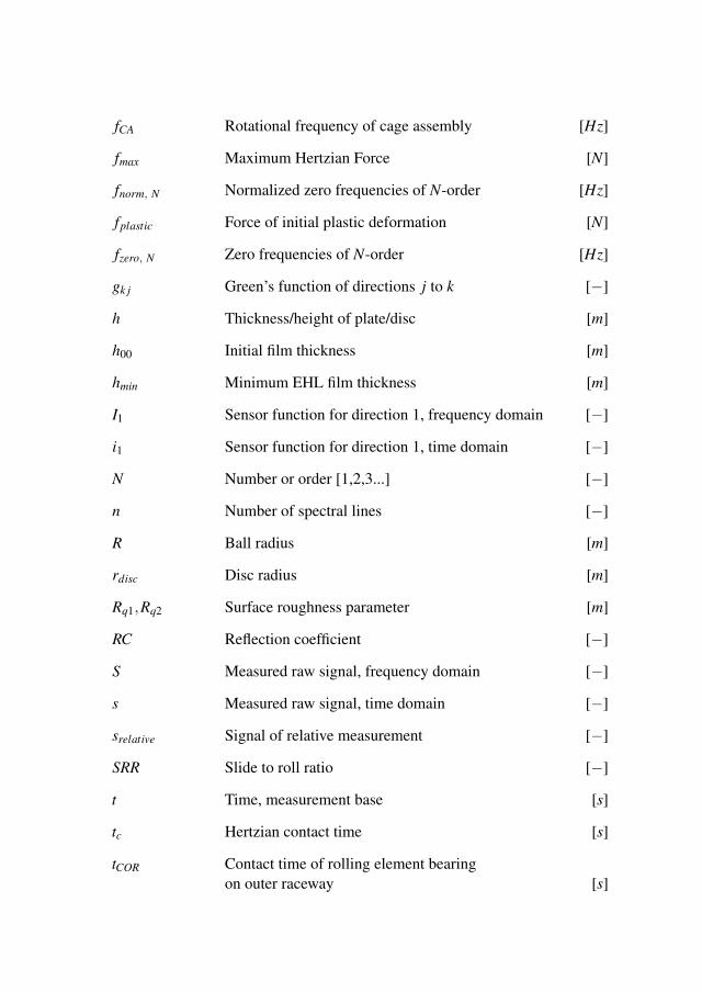
fCA Rotational frequency of cage assembly [Hz]
fmax Maximum Hertzian Force [N]
fnorm, N Normalized zero frequencies of N-order [Hz]
fplastic Force of initial plastic deformation [N]
fzero, N Zero frequencies of N-order [Hz]
gk j Green’s function of directions j to k [−]
h Thickness/height of plate/disc [m]
h00 Initial film thickness [m]
hmin Minimum EHL film thickness [m]
I1 Sensor function for direction 1, frequency domain [−]
i1 Sensor function for direction 1, time domain [−]
N Number or order [1,2,3...] [−]
n Number of spectral lines [−]
R Ball radius [m]
rdisc Disc radius [m]
Rq1,Rq2 Surface roughness parameter [m]
RC Reflection coefficient [−]
S Measured raw signal, frequency domain [−]
s Measured raw signal, time domain [−]
srelative Signal of relative measurement [−]
SRR Slide to roll ratio [−]
t Time, measurement base [s]
tc Hertzian contact time [s]
tCOR Contact time of rolling element bearingon outer raceway [s]

tre f lection,H Reflection time across plate/disc height/thickness [s]
tre f lection,R Reflection time across disc radius [s]
trise Rise time of step function [s]
T REND Trend value of WinCon system [−]
Ue Entrainment speed [ ms ]
Uk Displacement in direction k, frequency domain [−]
uk Displacement in direction k, time domain [−]
UEHL Vertical maximum displacement of an EHL contact [m]
UHertz Vertical maximum displacement of a Hertzian contact [m]
UHI AE RMS value of Hertzian impact tests [V ]
UREB Estimated AE RMS value of rolling element bearing [V ]
Us1,Us2 Speed of surfaces, ball (1), disc (2) [ ms ]
v0 Impact velocity [ ms ]
x Position of sensor [−]
Z1,Z2 Acoustic Impedance of solid plate (1),lubricant layer/air (2) [ Ns
m3 ]
Chemical Abbreviation
Fe2O3 Hematite
Fe3O4 Magnetite
FeO Iron oxide
FeS Ferrous sulfide
FeSO4 Ferrous sulfate
O2 Oxygen
R Carbon-hydrogen chain

S Sulfur
ZDDP Zinc dialkyl dithiophosphate
Acronyms
AC Activation counts
ACC Accelerometer
AE Acoustic emission
BB Bouncing ball
BonD Ball on disc
EHL Elastohydrodynamic lubrication
FB Four ball
FEM Finite element method
LDV Laser Doppler vibrometer
RePD Reciprocating pin on disc
RMS Root mean square
RoPD Rotational pin on disc
SKF Rolling element bearing manufacturer
SRR Slide to roll ratio
TD Twin disc

Part I
Comprehensive Summary
1


Chapter 1
Introduction
This Thesis mainly deals with research in two fields - tribology and conditionmonitoring. Both research fields are interdisciplinary and important for sus-tainable societies. The environmental program of the United Nations (UNEP)has pointed out the importance of efficient use of product life cycle and energyefficiency for a green economy [1]. Furthermore, the UNEP has included thesetwo requirements in their Agenda 2030 [2]. Thereby, the United Nations haveindirectly pointed out the importance of research fields such as tribology andcondition monitoring. Both research fields are essential to improve energy effi-ciency and to minimize waste of product life. However, despite the importanceof these research fields for future sustainable societies, they are on the wholeonly known to experts rather than the general public. Therefore, both researchfields will be introduced in this chapter. Fundamental theory used in this thesis,such as acoustic emission (AE) and elastohydrodynamically lubricated (EHL)contacts, will be mentioned in this chapter. However, a detailed introductionto these terms and the related research fields will be given in Chapter 2.
1.1 Tribology
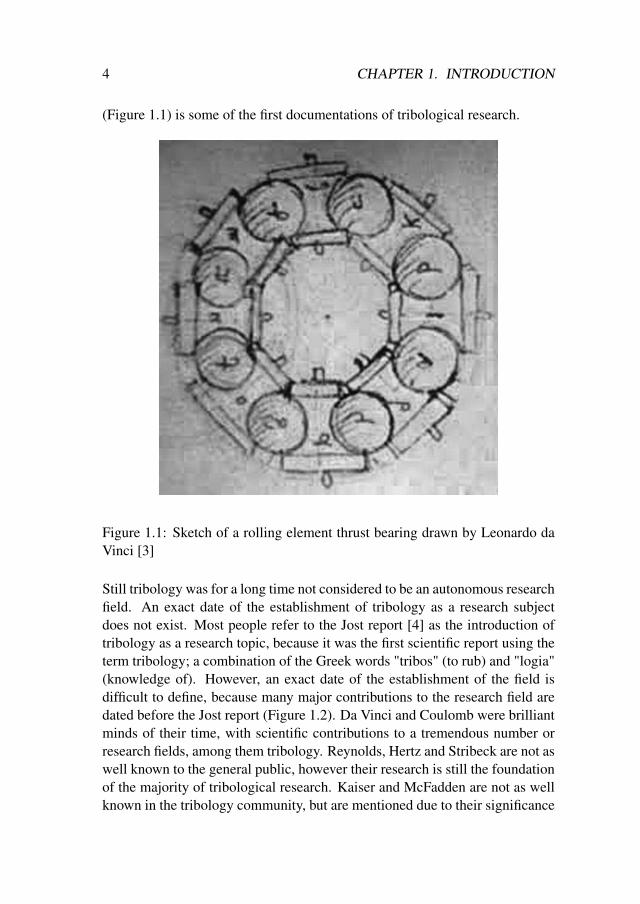
The problems caused by tribological systems, such as wear, lubrication, fatigueand friction, have challenged mankind since the beginning of their existence.Some of the most important inventions in human history are solutions to tri-bological problems. The invention of the wheel reduced friction tremendouslyand the invention of oil lubrication reduced both friction and wear of slidingsurfaces. Even famous inventors such as Leonardo da Vinci dedicated time tosolving tribological problems. His drawing of a rolling element thrust bearing
3
4 CHAPTER 1. INTRODUCTION
(Figure 1.1) is some of the first documentations of tribological research.
Figure 1.1: Sketch of a rolling element thrust bearing drawn by Leonardo daVinci [3]
Still tribology was for a long time not considered to be an autonomous researchfield. An exact date of the establishment of tribology as a research subjectdoes not exist. Most people refer to the Jost report [4] as the introduction oftribology as a research topic, because it was the first scientific report using theterm tribology; a combination of the Greek words "tribos" (to rub) and "logia"(knowledge of). However, an exact date of the establishment of the field isdifficult to define, because many major contributions to the research field aredated before the Jost report (Figure 1.2). Da Vinci and Coulomb were brilliantminds of their time, with scientific contributions to a tremendous number orresearch fields, among them tribology. Reynolds, Hertz and Stribeck are not aswell known to the general public, however their research is still the foundationof the majority of tribological research. Kaiser and McFadden are not as wellknown in the tribology community, but are mentioned due to their significance

1.2. CONDITION MONITORING 5
regarding the research topic of this thesis. While Kaiser was the first recordingacoustical waves of materials during deformation processes, McFadden con-tributed by introducing FFT based vibration analysis, which is still the mostcommon type of condition monitoring of machine elements.As hard as it is to date the establishment of tribology as a research topic, thedefinition of tribology is easy:
"Tribology is the study of interacting surfaces in relative motion."
Figure 1.2: Timeline of the research field tribology (Reynolds [5], Hertz [6],Stribeck [7], Kaiser [8], Jost [4] and McFadden & Smith [9, 10])
As industrialization has progressed, the demand on life cycle efficiency and en-ergy efficiency has increased. This increasing demand is met through researchin the field of tribology and nowadays, tribology is an established researchtopic with several branches, among them biotribology, automotive tribology,high temperature tribology, tribo-chemistry and elastohydrodynamic lubrica-tion. This thesis focus on the last mentioned branch, elastohydrodynamic lu-brication (EHL). Everybody has been dependent on EHL contacts, but only afew are aware of them. EHL contacts are crucial for the function of bicycles,cars, trains, pumps and wind turbines, among many other things. EHL is thebasis for many machine parts, such as rolling element bearings, gears and camfollowers.
1.2 Condition monitoring
Condition monitoring can be defined according to ISO 17359 as: "observationof parameters for evaluation of the performance of an application" [11]. Thisgeneral definition includes almost everything, even a fire guard in the stoneage, fits the definition. However, the standard is a good basis for deriving more

6 CHAPTER 1. INTRODUCTION
specified definitions, such as SKF, a leading rolling element bearing manufac-turer, did. SKF defined condition monitoring as [12]: "Condition monitoringis the process of determining the condition of machinery while in operation."SKFs definition is limited to on-line monitoring, where parameters are recordedand assessed during operation. Beside on-line monitoring, off-line monitoringalso exists. A well known example of off-line monitoring are structural checksof aeroplanes. However, there is a trend in industry to replace off-line moni-toring with on-line monitoring.Both A. van Beek and Tedric A. Harris [13] point out the importance of con-dition monitoring for future efficiency. Harris and Kotzalas [13] even state:"Maintenance is considered the largest controllable cost in modern industry."Further, they claim condition monitoring is the only tool able to cut thesecosts. However, Harris and Kotzalas [13] also mention that additional re-search is necessary to prove the reliability of monitoring techniques and ac-curacy of prognostic models. More specific in terms of this thesis, Mba andRao [14] claim acoustic emission will be, among others, one of the importanttools for condition monitoring in future applications. However, they also pointout that additional research is required before the "intelligent information ofacoustic emission signals" [14] can be processed without loss of information.Niknam et al. [15] even see condition monitoring already today as superior incomparison to statistical based failure prognosis.Condition monitoring in the research field of tribology is used to evaluateperformance of a tribological system or to detect the occurrence of a defect.Thereby parameters such as load, frictional force/coefficient, temperature, vi-bration, acoustic emission, contact impedance and oil film thickness, amongstother things are observed. The huge amount of tribologically interesting pa-rameters, shows that condition monitoring is an important part of tribologyresearch and is expected to be even more important in the future.This thesis will show that huge contributions to knowledge on the relationshipsbetween tribological contact conditions and measured parameters have alreadybeen made. However, there is still the need for further breakthroughs.

Chapter 2
Acoustic emission of a singleelastohydrodynamic contact
This PhD work started with the idea of investigating acoustic emission (AE)signals of a single elastohydrodynamically lubricated (EHL) contact. Limitingthe system to a single EHL contact enables a more detailed study of AE sig-nals in comparison to full machine elements such as rolling element bearingsand gears. However, even an EHL contact is a complex system, which willbe explained in this chapter. Additionally, difficulties and breakthroughs ininterpretations of AE signals are presented in this chapter.
2.1 Elastohydrodynamically lubricated contacts
Elastohydrodynamically lubricated (EHL) contacts occur in rolling elementbearings, gears and cam followers, among others. EHL contacts are non-conformal lubricated contacts with surfaces in relative motion. In an idealcase the surfaces are separated by a thin layer of lubricant. Pressures in this lu-bricant film can reach, within normal operating conditions, up to 2.5 GPa, andin certain cases even 3.0 GPa as Harris and Kotzalas point out [13]. Withinfatigue research these typical pressures are exceeded and the contact is over-loaded with up to 8.0 GPa to accelerate tests. At these high pressures thelubricant solidifies and surfaces deform elastically as illustrated in Figure 2.1.As shown in Figure 2.1, the elastic deformation reduces at the outlet of thecontact and this causes a pressure spike. This pressure spike was first observedby Petrusevich [16]. The film of an EHL contact was first measured by Goharand Cameron [17] using a interferometric method presented by Kirk [18].
7

8 CHAPTER 2. ACOUSTIC EMISSION OF SINGLE EHL CONTACT
Figure 2.1: Schematic drawing of an EHL contact
Ideally both surfaces are separated by a lubricant film in an EHL contact. How-ever, a decrease of entrainment speed, a decrease of viscosity or an increasein load can cause the elasto-hydrodynamic film to collapse. A measure for thedegree of film separation is the film thickness parameter Λ:
Λ =hmin√
Rq21 +Rq2
2
(2.1)
Based on this film parameter Λ different lubrication regimes can be distin-guished [19, 20].
EHL Λ>3 In the elastohydrodynamic lubrication regimeboth surface are fully separated by a fluid film,which solidifies in the contact. The total load thecontact is exposed to is thereby carried by the lu-bricant film.
Mixed 1≤ Λ≤ 3 In the mixed lubrication regime, both lubricantfilm and asperities carry the load. The ratio ofload carried between asperities and film dependson the degree of separation.
Boundary Λ<1 In the boundary lubrication regime all load is car-ried by the asperities of the surfaces in contact.
However, the boundaries of these lubrication regimes are not as distinct as the

2.1. EHL 9
classification of the film thickness parameter suggests. The boundaries of thedifferent regimes are calculated based on the combined surfaces roughness ofboth surfaces. However, the surface roughness is reduced within the contactdue to elastic deformation. A smoothening of the surface roughness by elas-tic deformation is one of the critics of this distinct classification of lubricationregimes [21]. Another aspect which questions the separation based on only sur-face roughness is the effect of roughness structure on pressure built up and filmformation, such as shown by Choo et al. [22] and Guegan et al. [23]. Both in-vestigations showed that structures such as grinding grooves from manufactur-ing processes affect the speed at which the EHL regime is entered. Boundariesbetween different lubrication regimes are hard to determine, which can be seenby monitoring the coefficient of friction across all lubrication regimes. Theseobserved coefficients of friction can be plotted in a Stribeck curve, named afterRichard Stribeck who first published this curve in a journal [7]. Figure 2.2ashows a schematic drawing of such a Stribeck curve. This schematic illustra-tion is also divided into lubrication regimes. However, the smooth coefficientof friction curve indicates that there are smooth transitions between lubricationregimes, rather than distinct boundaries, based on Λ.Another parameter which has an influence on EHL contact conditions is theslide-to-roll ratio (SRR) (2.2). Friction curves such as shown in Figure 2.2a,are based on a constant SRR. However, investigations have shown a signifi-cant influence of SRR on friction and film formation [25]. As a solution onemight add a third axis to extend the Stribeck curve, which is known as frictionmapping [24] (Figure 2.2b).
SRR =Us1−Us2
Ue(2.2)
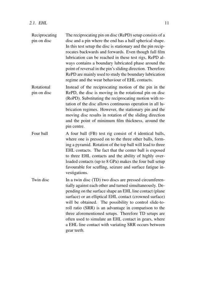
Stribeck curves (Figure 2.2a), friction mapping (Figure 2.2b) [24], investiga-tions on film formation [26, 27] or EHL contact behaviour [28] are usuallycarried out in component test rigs, rather than on machine elements such asgears, bearings or cam followers. Different component test rigs were devel-oped in the past, to investigate EHL contacts in detail.

10 CHAPTER 2. ACOUSTIC EMISSION OF SINGLE EHL CONTACT
(a) Stribeck curve
(b) Friction map [24]
Figure 2.2: Schematic illustration of a Stribeck-curve and the different lubri-cation regimes
2.1. EHL 11
Reciprocatingpin on disc
The reciprocating pin on disc (RePD) setup consists of adisc and a pin where the end has a half spherical shape.In this test setup the disc is stationary and the pin recip-rocates backwards and forwards. Even though full filmlubrication can be reached in these test rigs, RePD al-ways contains a boundary lubricated phase around thepoint of reversal in the pin’s sliding direction. ThereforeRePD are mainly used to study the boundary lubricationregime and the wear behaviour of EHL contacts.
Rotationalpin on disc
Instead of the reciprocating motion of the pin in theRePD, the disc is moving in the rotational pin on disc(RoPD). Substituting the reciprocating motion with ro-tation of the disc allows continuous operation in all lu-brication regimes. However, the stationary pin and themoving disc results in rotation of the sliding directionand the point of minimum film thickness, around thepin centre.
Four ball A four ball (FB) test rig consist of 4 identical balls,where one is pressed on to the three other balls, form-ing a pyramid. Rotation of the top ball will lead to threeEHL contacts. The fact that the center ball is exposedto three EHL contacts and the ability of highly over-loaded contacts (up to 8 GPa) makes the four ball setupfavourable for scuffing, seizure and surface fatigue in-vestigations.
Twin disc In a twin disc (TD) two discs are pressed circumferen-tially against each other and turned simultaneously. De-pending on the surface shape an EHL line contact (planesurface) or an elliptical EHL contact (crowned surface)will be obtained. The possibility to control slide-to-roll ratio (SRR) is an advantage in comparison to thethree aforementioned setups. Therefore TD setups areoften used to simulate an EHL contact in gears, wherea EHL line contact with variating SRR occurs betweengear teeth.

12 CHAPTER 2. ACOUSTIC EMISSION OF SINGLE EHL CONTACT
Ball on disc In a ball on disc (BonD) setup, SRR is, (as in the TDsetup) controllable. The maximum contact pressureis comparable to the BonD and TD setup (around 2-3 GPa). However, instead of a line contact, a circularEHL contact is obtained. Additionally this setup allowsinterferometric film thickness measurements if a sap-phire disc is used. Due to this capability BonD setupsare frequently used in rheological EHL investigationsand as a tool for evaluation of numerical studies.
Bouncing ball A bouncing ball (BB) is probably the simplest setup. Aball is simply dropped onto a lubricated plate/disc andthis creates a circular EHL contact. An advantage ofsuch a setup is the absence of secondary machine parts,such as support bearings, electric motors, or force ac-tuators, which eliminates disturbances caused by theseparts. However, the BB setup does not allow for a con-tinuous study of an EHL contact and is limited to ashort time of impact. In the most common setup theplate is horizontal and the EHL impact is studied withpure rolling conditions. However, by tilting the plateeven sliding can be introduced to the BB setup. Moredetailed explanations can be found in Chapter 5, Sec-tion 5.1.
Except for the four ball setup, all mentioned setups enable the study of a singleEHL contact and are therefore of interest for this investigation.Besides a tremendous amount of experimental investigations on EHL contacts,using the aforementioned component test rigs, several theoretical studies onEHL contacts have been carried out. The basis of all theoretical investigationsis Reynolds thin film approximation [5] which enables numerical examina-tion of the pressure within the EHL film. One of the most comprehensivestudies was the investigation of an elliptical EHL contact by Hamrock andDowson [29]. They used a variety of different loads, rotational speeds andmaterial properties and mapped the behaviour of elastohydrodynamically lu-bricated point contacts. The investigations of Lubrecht et al. [30] and Ven-ner [31], introducing multigrid and multilevel approaches to increase com-putational speed, can be seen as the start of computational tribology. Manyresearchers adapted their approach, among them Larsson and Höglund [32].They published a study on an EHL impact, providing theoretical support to

2.2. ACOUSTIC EMISSION 13
bouncing ball experiments.As computational power increased the finite element method (FEM) was in-creasingly applied to solve EHL contact problems. One of the first FEM stud-ies, providing a solution capable of solving realistic contact pressures of up to4 GPa, was carried out by Houpert and Hamrock [33]. More recently Hab-chi et al. [34] presented a FEM based approach for solving EHL problems ofboth line and point contacts.
2.2 Acoustic emission
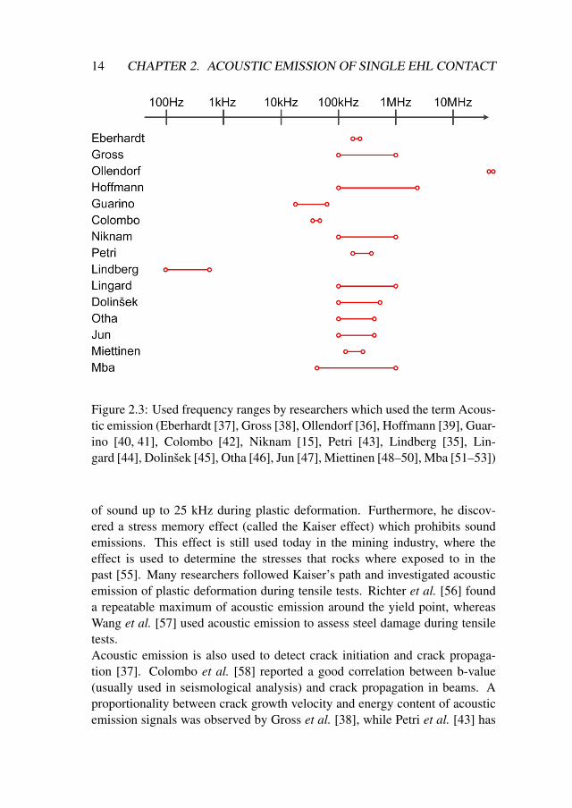
Acoustic emission is a term which refers to monitoring of high frequencies of asystem. However, different researchers define the term differently, particularlyin respect to the monitored frequency. In Figure 2.3 the frequencies used bydifferent researchers in combination with the phrase "acoustic emission" arevisualised. Figure 2.3 shows that a majority of researchers use a frequencyrange between a 20 kHz and a couple of MHz. However, there are exceptions.Lindberg et al. [35] studied the acoustic emission of disc brakes. Lindberget al. [35] represents automotive industry applications, where the term acous-tic emission refers to the noise drivers are exposed to. In these applications nofrequencies higher than 21 kHz are measured. Ollendorf and Schneider [36]are situated at the other end of the frequency range. They have used lasermeasurements at up to 70 MHz to evaluate coating films and also used theterm acoustic emission. However, recently these high frequencies are referredto as optical acoustic emission instead.To standardize the term acoustic emission, the American Society for Test-ing and Materials has introduced the following definition (ASTM E1316):"...waves generated by the rapid release of energy from localized sources withina material...". It was the first definition of acoustic emission and is basedon the needs of non destructive testing. However, the definition does notfit for the purposes of condition monitoring of machine elements. There-fore Niknam et al. [15] defined acoustic emission differently: "AE signalsare caused by crack growth, plastic deformation, friction, corrosion, leak anddefect growth such as fatigue that appear as high-frequency AE events in therange from 20 kHz to 1 MHz."Even long before AE was defined researchers already dedicated their work tothese emissions of elastic waves, without knowing the term acoustic emission.Kaiser [8, 54] investigated already in the 50’s the sound emission from differ-ent materials during tensile and Brinell tests. He found a significant emission
14 CHAPTER 2. ACOUSTIC EMISSION OF SINGLE EHL CONTACT
Figure 2.3: Used frequency ranges by researchers which used the term Acous-tic emission (Eberhardt [37], Gross [38], Ollendorf [36], Hoffmann [39], Guar-ino [40, 41], Colombo [42], Niknam [15], Petri [43], Lindberg [35], Lin-gard [44], Dolinšek [45], Otha [46], Jun [47], Miettinen [48–50], Mba [51–53])
of sound up to 25 kHz during plastic deformation. Furthermore, he discov-ered a stress memory effect (called the Kaiser effect) which prohibits soundemissions. This effect is still used today in the mining industry, where theeffect is used to determine the stresses that rocks where exposed to in thepast [55]. Many researchers followed Kaiser’s path and investigated acousticemission of plastic deformation during tensile tests. Richter et al. [56] founda repeatable maximum of acoustic emission around the yield point, whereasWang et al. [57] used acoustic emission to assess steel damage during tensiletests.Acoustic emission is also used to detect crack initiation and crack propaga-tion [37]. Colombo et al. [58] reported a good correlation between b-value(usually used in seismological analysis) and crack propagation in beams. Aproportionality between crack growth velocity and energy content of acousticemission signals was observed by Gross et al. [38], while Petri et al. [43] has

2.2. ACOUSTIC EMISSION 15
proved that micro fracturing processes follow a power law statistical behaviour.Pure ductile fracture processes were investigated by Gerberich et al. [59]. Theyfound huge differences in acoustic emission magnitudes comparing tensionand compression fractures. Furthermore, they found huge differences in AEmagnitude between different heat treatments and thereby different micro struc-tures.Inspired by the results on acoustic emission of plastic deformation and crackpropagation, researchers started to investigate condition monitoring possibili-ties of different structures. The research group of Carpinteri used AE to mon-itor historical buildings and bridges [60]. Thereby they found similarities be-tween AE events and damage progress. Niar and Cai [61] state in their review,that accumulative AE measurements are a promising method for monitoringsteel and concrete bridges. However, they also admit practical challengeswhich need to be addressed. Another application where acoustic emission isused to monitor the structure are coatings and coating evaluations. Bull [62]has distinguished the four failure modes for brittle and ductile coatings re-spectively by comparing acoustic emission time signal patterns. Ollendorf andSchneider [36] were able to measure the E-modulus of an adhesion film, whichis sensitive to micro cracks.Chemistry is another field which has shown increased interest in acoustic emis-sion. Sawada et al. [63] has shown that both a phase separation and a phasetransition can be monitored by acoustic emission. The phase transition fromliquid to solid was clearly detected by AE, whereas the melting process wasnot that distinctly detectable. Sawada investigated three different substances(water, sodium thiosulfate and methoxybenzylidene-4n-butylaniline) and con-cludes that the sharp increase in AE activity is caused by crystal formation.Another use of acoustic emission as a chemical monitoring tool was shown byBelchamber et al. [64]. In their publication they prove the linear dependencybetween acoustic emission and the hydration of silica gel. Furthermore, it wasshown by Betteridge et al. [65] that exothermic reactions can be monitored byAE. Even electro-chemical processes can be monitored by acoustic emission asCrowther et al. [66] showed. Hydrogen gas bubble formation of the electroly-sis cell at the cathode was detected and correlated to both the acoustic emissionand the electrical potential of the electrolysis cell. The experiment showed aclear correlation between gas bubble formation and the acoustic power.In machine elements investigations have proved the capability of acoustic emis-sion to detect dents, contamination and lubrication changes. To seed dents or adefect is a common way to evaluate detectability of faults in machine elements.In the 80’s McFadden and Smith [67] used scratches on the inner raceway’s of a

16 CHAPTER 2. ACOUSTIC EMISSION OF SINGLE EHL CONTACT
rolling element bearing and were able to detect the defect at a rotational speedof up to 850 rpm. Later Morhain and Mba [68] have shown that even up to4000 rpm seeded faults can be detected by acoustic emission. Choudhury andTandon [69] were able to detect seeded scratches on a rolling element bearing.The propagation of such defects (scratches and dents) was studied by Elfor-jani and Mba [53]. They observed correlation between AE bursts in the timedomain and the defect size. In another investigation Elforjani and Mba [70]generated defects by overloading instead of introducing them prior to the test.They used a plane disc for a thrust bearing to increase contact pressure andobserved natural pitting defects, which were detected by acoustic emission.Additionally, the same correlation between AE burst duration and defect sizewas observed.Particle contamination of rolling element bearings is another well investigateddefect monitored with acoustic emission monitoring. Miettinen and Patani-itty [71] were able to use acoustic emission for detection of contamination inslowly rotating bearings (0.5 to 5 rpm). Later this approach was expandedby Miettinen and Andersson [48] who were able to relate activation counts(AC) of AE signals to the contaminant concentration, the particle size and thetype of particle. While Miettinen used AC in his investigations, Jamaludin andMba [72] used stress waves. Both methods showed a distinct difference be-tween contaminated and uncontaminated bearings.Beside the various investigations on failure detection, some investigations usenon-faulty bearings, where correlations between acoustic emission and the lu-brication were found. Niknam et al. found statistically significant differencesin AE signals between lubricated and dry rolling element bearings, regardlessof load or rotational speed. A change in AC of AE was observed by Mietti-nen et al. [49] for different greases. They correlated different grease thickenerto AC levels. Additionally they concluded higher viscosity of the base oil leadto more AC due to starvation phenomena. However, Otha et al. [46] observeda decrease of RMS value of acoustic emission signals with increased base oilviscosity. Hamel et al. [52] correlated film thickness parameter Λ and acousticemission signals in a gear. They changed viscosity by changing the tempera-ture of the oil and observed a reduction of RMS value of the acoustic emissionsignal for increased film thickness (Λ).

2.3. RESEARCH GAP AND OBJECTIVES 17
2.3 Research gap and objectives
Knowledge about acoustic emission and its use for condition monitoring hasincreased tremendously over the past decades, due to excellent research effortsin the past. In many investigations researchers have shown the ability of AEto monitor and detect failures in machine elements. A small outline of thisresearch was presented in the previous section (Section 2.2). Still the use ofacoustic emission as a monitoring tool in industry is rare. While in laboratorysetups all critical parameters, such as load, degree of contamination, failuresize, temperature and lubricant properties, can be either controlled or mon-itored, these parameters are often unknown in industrial applications. Thislack of information leads to challenges for AE signal interpretation. Com-mon analysis methods used for acoustic emission signals include among oth-ers RMS (root mean square) [46, 52, 73], amplitudes [70, 72] and activationcounts [48, 49, 71]. These signal processing methods have the huge advan-tage of a maximized data reduction. Such a data reduction might have beenhistorically necessary. However, today the need for data reduction is not asurgent anymore and therefore, the drawback of information loss by using theseprocessing methods has increased in importance. Processing the AE data in asmart way, requires knowledge of which information is of interest. Hence, agood understanding of the cause of AE signals in an EHL contact is required.However, this understanding of these causes and the process from generationto detection of the AE signals in EHL contacts still has many deficits. For ex-ample several investigations [49,73–75] have reported a significant increase ofAE activity with increased rotational speeds, without further explanation. Fur-thermore, McFadden and Smith [67] earlier pointed out problems with failuredetection at elevated rotational speed. Investigations on full sampled acousticemission signals of single EHL contacts are rare. Elforjani and Mba [53, 70]have published some of the rare investigations including full sampled acous-tic emission signals and were able to find a correlation between raceway faultsand AE bursts in the time domain. However, by using a rolling element bearingincluding raceway faults, they studied a complex and severe case (faulty bear-ing). Studies on acoustic emission of single EHL contacts do exist. Therebyball on disc setups [76,77], twin disc setups [78] and Pin/ball on cylinder setups(similar to pin on disc) [79] were used. However, even these studies focusedon rather severe contact conditions, such as wear under high pressure and puresliding. Therefore, a need for a study focusing on acoustic emission of a singleEHL contact operating in normal bearing conditions without faults was iden-tified. Based on this need, the identified research gap, the PhD work focused

18 CHAPTER 2. ACOUSTIC EMISSION OF SINGLE EHL CONTACT
on fulfilling these needs and the following, rather general, research questionswere formulated:
I. What are the sources of acoustic emission signals of EHL contacts?
II. How is an acoustic emission signal of a single EHL contact dependent onthe contact properties?
III. Can acoustic emission signals of single EHL contacts be simulated?
IV. How are acoustic emission signals of component setups related to acous-tic emission signals of complete machine elements, such as rolling ele-ment bearings?

Chapter 3
Theory and definition
This chapter includes the definitions and hypotheses that the thesis is basedon. The author’s own definition for acoustic emission is introduced, to avoidany confusion about the term. Furthermore, hypotheses on possible sources ofAE in EHL contacts are presented. These hypotheses were the foundation ofall experiment work carried out in this thesis. Finally the concept of Green’sfunction is introduced, which is the base of all simulations within the frame ofthis work.
3.1 Definition of elastic waves
As mentioned in Section 2.2, different definitions of acoustic emission ex-ist, which are based on the source of acoustic emission. However, this thesishas the objective to determine the source, which leads to uncertainties aboutthe term acoustic emission. Instead of source based, the definition should bebased on the obtained signal. Signals in this thesis are measured with eitheran AE-transducer or a laser-Doppler-vibrometer. Both methods measure themovement of the surface over time. Even though the AE-transducer mea-sures acceleration and the Laser-Doppler-vibrometer measures velocity, bothare physically coupled to a surface movement. Because the measurement prin-ciple of the acoustic emission signal is the only certainty in this investigation, itwill be the basis for definition of acoustic emission as regards this thesis work.Therefore, the term acoustic emission will be defined for the entire thesis as:
Acoustic emission is an elastic wave causing an oscillating dis-placement of a point of measurement at the surface over time witha frequency higher than 20 kHz.
19
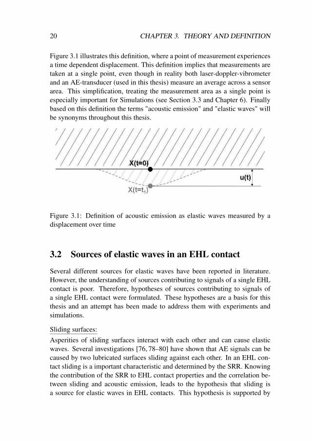
20 CHAPTER 3. THEORY AND DEFINITION
Figure 3.1 illustrates this definition, where a point of measurement experiencesa time dependent displacement. This definition implies that measurements aretaken at a single point, even though in reality both laser-doppler-vibrometerand an AE-transducer (used in this thesis) measure an average across a sensorarea. This simplification, treating the measurement area as a single point isespecially important for Simulations (see Section 3.3 and Chapter 6). Finallybased on this definition the terms "acoustic emission" and "elastic waves" willbe synonyms throughout this thesis.
Figure 3.1: Definition of acoustic emission as elastic waves measured by adisplacement over time
3.2 Sources of elastic waves in an EHL contact
Several different sources for elastic waves have been reported in literature.However, the understanding of sources contributing to signals of a single EHLcontact is poor. Therefore, hypotheses of sources contributing to signals ofa single EHL contact were formulated. These hypotheses are a basis for thisthesis and an attempt has been made to address them with experiments andsimulations.
Sliding surfaces:Asperities of sliding surfaces interact with each other and can cause elasticwaves. Several investigations [76, 78–80] have shown that AE signals can becaused by two lubricated surfaces sliding against each other. In an EHL con-tact sliding is a important characteristic and determined by the SRR. Knowingthe contribution of the SRR to EHL contact properties and the correlation be-tween sliding and acoustic emission, leads to the hypothesis that sliding isa source for elastic waves in EHL contacts. This hypothesis is supported by

3.2. SOURCES OF ELASTIC WAVES IN AN EHL CONTACT 21
Löhr et al. [78]. They found a correlation between SRR and AE signal strengthin a twin disc application. However, one should consider that all investigationsmentioned are conducted in the mixed and boundary lubrication regime.Even though sliding is expected to contribute to AE signals of EHL contacts,this thesis will focus on EHL contacts in pure rolling, which eliminates slidingas a source for AE signals. This limitation is necessary due to the time frameof this thesis. Still during experimental design and evaluation of full bearingtests one needs to be aware of this possible source.
Transient force:Transient forces are known to cause elastic waves. A force acting on a spe-cific point and varying over time, causes elastic deformation on the surfaceand initiates an elastic wave. This is known as a transient force signal. In 1958Sherwood [81] has shown the correlation in a theoretical approach based on asemi-infinite solid space. Later Glaser et al. [82] observed these elastic wavesin an experimental approach. That transient forces cause elastic waves is afact, the question remains whether they occur in EHL contacts or not. McLas-key and Glaser [83] measured and calculated elastic waves caused by transientforces of a Hertzian contact using a bouncing ball experiment setup. The samesetup was used by Larsson and Höglund [32] to investigate an EHL contacttheoretically. Thereby they observed only small differences comparing dry(Hertzian) and lubricated (EHL) impact forces. Furthermore, Sunnersjö [84]has shown how geometrical imperfections caused by manufacturing processesin combination with transient forces of rolling element bearings affect vibra-tion patterns. Therefore it is assumed transient forces are a significant sourceof acoustic emission signals in EHL contacts.
Plastic deformation:Plastic deformations causing rapid movements at the grain boundaries causeelastic waves. However, plastic deformation is a phenomena which is usuallynot associated with rolling element bearings or EHL contacts. However, evenwell functioning EHL contacts are exposed to plastic deformation of the sub-surface region due to residual stresses [85] (Fatigue process). Furthermore,plastic deformation can occur locally in asperities during running-in. Finally,plastic deformation can be caused by unfavourable operating conditions, suchas particle contamination. Since plastic deformation can occur and several in-vestigations [56,57,86] have correlated plastic deformation and acoustic emis-sion, it is considered to be a possible source for AE signals of EHL contacts.
22 CHAPTER 3. THEORY AND DEFINITION
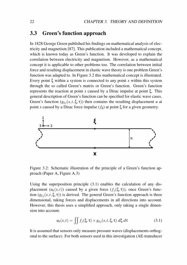
3.3 Green’s function approach
In 1828 George Green published his findings on mathematical analysis of elec-tricity and magnetism [87]. This publication included a mathematical concept,which is known today as Green’s function. It was developed to explain thecorrelation between electricity and magnetism. However, as a mathematicalconcept it is applicable to other problems too. The correlation between initialforce and resulting displacement in elastic wave theory is one problem Green’sfunction was adapted to. In Figure 3.2 this mathematical concept is illustrated.Every point ξ within a system is connected to any point x within this systemthrough the so called Green’s matrix or Green’s function. Green’s functionrepresents the reaction at point x caused by a Dirac impulse at point ξ. Thisgeneral description of Green’s function can be specified for elastic wave cases.Green’s function (gk j(x, t,ξ,τ)) then contains the resulting displacement u atpoint x caused by a Dirac force impulse ( fδ) at point ξ for a given geometry.
Figure 3.2: Schematic illustration of the principle of a Green’s function ap-proach (Paper A, Figure A.3)
Using the superposition principle (3.1) enables the calculation of any dis-placement (uk(x, t)) caused by a given force ( f j(ξ,τ)), once Green’s func-tion (gk j(x, t,ξ,τ)) is derived. The general Green’s function approach is threedimensional, taking forces and displacements in all directions into account.However, this thesis uses a simplified approach, only taking a single dimen-sion into account.
uk(x, t) =x
f j(ξ,τ)×gk j(x, t,ξ,τ) dξ dτ (3.1)
It is assumed that sensors only measure pressure waves (displacements orthog-onal to the surface). For both sensors used in this investigation (AE-transducer

3.4. DEFINITION OF SPECIMEN DECLARATION 23
and Laser-Doppler vibrometer) the maximum sensitivity is for waves orthog-onal to the surface and declines with any angle less than 90◦. Further it isassumed that all forces act orthogonal to the surface. Based on these two as-sumptions equation (3.1) can be simplified to equation (3.2). Both variablesfor dimensions (k, j) will be set to k = j = 1, using the definitions of directionsshown in Figure 3.2. Additionally, the double integral simplifies for a singledimension to a convolution.
u1(x, t) = f1(ξ,τ)∗g11(x, t,ξ,τ) (3.2)
3.4 Definition of specimen declaration
In this thesis a specific declaration for specimens used in the bouncing ballsetup was used. This declaration is consistent throughout the thesis and ex-plained in Figure 3.3. The first two letters indicate the shape, which is in chaseof this thesis always a ball (RB, rolling element ball). The following numbersrepresent the diameter in mm and the last three characters indicate the toler-ance of the specimen. The tolerance term follows the standard ISO3290 andincludes tolerances for average diameter variation, maximum diameter varia-tion, deviation from spherical form and surface roughness.
Figure 3.3: Explanation of specimen declaration used in this Thesis

Chapter 4
Absolute calibration
AE-transducers are piezoelectric accelerometers, which do not record the ac-tual acceleration of a point, but record the acceleration of a measurement pointmodulated with a sensor specific sensor function i1(t). When AE-transducersare used for relative measurements this modulation does not influence theresults, because the sensor function will be cancelled out as shown in equa-tion (4.1).
srelative(x, t1, t2) =u1(x, t1)∗ i1(t)u1(x, t2)∗ i1(t)
=u1(x, t1)u1(x, t2)
(4.1)
However, the sensor function needs to be determined in case AE-transducersare used for absolute measurements. Equation (4.2) shows that the sensor func-tion i1(t) is the link between the actual measured signal s(x, t) and the physicalcause of the signal, the displacement (u1(x, t)) at point x.
s(x, t) = u1(x, t)∗ i1(t) (4.2)
Therefore, the extraction of the sensor function through absolute calibrationenables the correlation of single measurements to physical causes. Being ableto correlate single signals and physical events is elementary for identifyingsources of the signal and thereby sources of AE signals in single EHL con-tacts.For extraction of the sensor function a calibration experiment is needed, whereboth sensor signal s(x, t) and the actual physical measure (in this case the dis-placement u1(x, t)) can be obtained. The displacement (u1(x, t)) can be simu-lated or measured. Jacobs and Woolsey [88] presented an absolute calibrationmethod based on reference measurements executed with Laser interferometry,
25

26 CHAPTER 4. ABSOLUTE CALIBRATION
while McLaskey and Glaser [89] presented a method based on simulated ref-erence signals. The method based on simulated reference signals was used forcalibrations in this thesis.As a calibration experiment a glass caliper burst was used, due to the goodexcitation of high frequencies [90]. Figure 4.1 shows the experimental setup.Thereby, a calibration plate with the dimensions 1.0x0.5x0.051m was used toavoid reflections within the measurement time in horizontal direction. The AE-transducer was placed underneath the calibration plate and a glass caliper tubeon top of the calibration plate. Both sensor and glass caliper tube were verti-cally aligned. A cylindrical probe was positioned on top of the glass calipertube with a 90◦ longitudinal shift. Then the probe was pressed against theglass caliper tube, decreasing distance between cylindrical probe and calibra-tion plate until the glass caliper tube burst.
Figure 4.1: Schematic drawing of the calibration setup with a glass caliperburst as a source
The recorded signal of this experiment corresponds to s(x, t) and is illustratedin Figure 4.2-c. The displacement (u1(x, t)) was calculated based on equa-tion (3.2) presented in Section 3.3. The corresponding Green’s function wasobtained by using Hsu’s script [91], a simulation code allowing the calcula-tion of Green’s function for plates which are infinite in two dimensions (Fig-ure 4.2-a). The force of the glass caliper burst was calculated according to the

27
following equation:
f (τ) =famp
2× (1− cos(πτ/trise)), 0≤ |τ| ≤ trise
f (τ) = 0 , τ < 0 (4.3)
f (τ) = famp , τ > trise
A rise time of 200 ns assumed as suggested by McLaskey and Glaser [89]. Theforce the cylindrical probe was exposed to was recorded during the calibrationexperiment. Assuming the maximum recorded force corresponds to the forceat which the glass caliper tube burst, the value for famp in equation (4.3) isfound. With both force function and Green’s function (Figure 4.2-a) obtained,the theoretical displacement was calculated according to equation (3.2). Trans-forming this result for the displacement into the frequency domain results in atheoretical spectra of a caliper burst, shown in Figure 4.2-b.
(a) Green’s function (b) Spectra caliper burst
(c) Uncompensated spectra Sensor (d) Transfer function of sensor
Figure 4.2: Illustration of simulated, measured and calculated signals for cali-bration
The recorded signal of the calibration experiment is also transformed into the

28 CHAPTER 4. ABSOLUTE CALIBRATION
frequency domain, as shown in Figure 4.2-c. The transformation to the fre-quency domain enables the calculation of the sensor function by simple divi-sion (4.5), instead of the convolution in the time domain (4.2).
S(x,ω) =U1(x,ω)I1(ω) (4.4)
I1(ω) = S(x,ω)/U1(x,ω) (4.5)
The result of this division in the frequency domain, the transfer function of thesensor I1(ω), is shown in Figure 4.2-d.To evaluate the transfer function of the sensor, McLaskey and Glaser’s [83]experiments on Hertzian impacts were repeated. Steel balls of different sizeswere dropped from different heights onto the calibration plate. Figure 4.3shows spectra of one of these experiments (steel ball �1.5 mm dropped from250 mm). While the uncompensated spectra (blue) mismatches the simulatedspectra (green), the spectra after compensation by the transfer function ofthe sensor (red) correlates to a much better degree with the simulated spec-tra (green). Furthermore, the obtained results agree with the published resultsby McLaskey and Glaser [83]. Therefore the calibration was seen as success-ful.
Figure 4.3: Ilustration of calculated, uncompensated and compensated spectraof signals from the evaluation test
It should be noted that all spectra of accelerometer signals shown in the re-mainder of this thesis are compensated by the transfer function of the sensorobtained by the calibration method detailed here.

Chapter 5
Component tests
Component tests are used to study a phenomena, such as an EHL contact,individually in a controlled environment. In Section 2.1 several component testsetups for investigations of EHL contacts were mentioned. In this section thechoice of a bouncing ball setup over all other possible setups will be justified.An explanation will be given of how the component test chosen relates to realapplications containing EHL contacts. Thereby the component tests will becompared to rolling element bearings. Additionally the correlation with tensiletests and rolling element bearings will be explained.
5.1 Bouncing ball
In this thesis work, the bouncing ball setup was chosen over many other EHLcomponent test setups (Section 2.1). The most important reason for choosinga bouncing ball setup was the possibility to measure a pure signal of a singleEHL contact. More complex setups such as ball on disc or twin disc, mayenable more variability and may be closer to EHL contacts existing in applica-tions like rolling element bearings, however, more complex test setups includesecondary acoustic emission signals. Bearings, gearboxes and belt drives ofthese test rigs emit acoustic emissions of their own. Even though attenuationof these elastic waves will minimize the contribution to the overall measuredsignal, acoustic emission of these support components will still affect the mea-surement. Whereas the bouncing ball setup allows the measurement of a pureacoustic emission signal of a single EHL contact.Drawbacks of the bouncing ball setup are that slide-to-roll ratio (SRR) andfilm thickness are hard to control. Instead of forced SRR such as in a ball on
29

30 CHAPTER 5. COMPONENT TESTS
disc setup, the SRR in a bouncing ball setup is dependent on contact prop-erties. The SRR can be controlled by the angle of impact of the ball. Theimpact angle in combination with the coefficient of friction (dependent on filmthickness and lubricant properties, among other things) leads to a certain SRR.Furthermore, the absolute calibration shown in Chapter 4 is only valid for animpact orthogonal to the surface. Therefore, the bouncing ball setup was onlyused with horizontal plates and orthogonal impacts, which corresponds to purerolling (SRR=0).The film thickness in a bouncing ball setup is dependent on the impact velocity(v0). However, the impact velocity depends on the thickness of the lubricantlayer on the disc, which dampens the balls velocity before impact. Thereforelubricant layers should be prepared with a initial thickness thick enough toprovide fully flooded conditions of the contact, but not any thicker. The opti-mum initial film thickness is equal to the expected maximum film thickness.However, in practice it is hard to prepare lubrication layers thin enough (lessthan 10 µm) not to affect impact velocity. Furthermore, to provide an evendistributed lubricant layer of similar initial film thickness throughout an ex-periment series is difficult. Therefore, dry impacts, so called Hertzian impact,where always executed as reference measurements, in order to know the con-tribution of the film preparation to the experimental error.A bouncing ball setup enables measurement of a single EHL contact undera short time period, contrary to a measurement on a rolling element bearing,where several EHL contacts are emitting elastic waves continuously. This dif-ference can be clearly seen by comparing two 25 µs long recordings of anAE-transducer from a bouncing ball experiment and a rolling element bearing(Figure 5.1). While in a bouncing ball setup a single impulse and its atten-uation can be studied (Figure 5.1-a), several impulses are contributing to acontinuous signal in a rolling element bearing (Figure 5.1-b).Despite this difference the bouncing ball setup and rolling element bearing arestill similar, as Figure 5.2 shows. In both, the rolling EHL contact (rollingelement bearing) and the EHL impact (bouncing ball setup), the surfaces areseparated by a solidified lubricant layer. However, while the deformation of theEHL impact is point symmetrical, the rolling EHL contact is axially symmetri-cal along the centerline in rolling direction. The maximum deformation (uEHL)is difficult to compare, because they depend on different variables. Whilethe maximum deformation of the EHL impact depends on lubricant proper-ties and impact velocity, the maximum deformation of the rolling EHL contactdepends on lubricant properties, entrainment speed and load. The Hertzianreference case, however, can be compared to the EHL impact. Larsson and

5.1. BOUNCING BALL 31
(a) Bouncing ball (b) Rolling element bearing
Figure 5.1: Comparison of signals obtained in a bouncing ball setup and in afull bearing test
Höglund [32] observed that the maximum deformation of an EHL impact anda Hertzian impact of balls dropped from the same height is almost identical.Only a minimal higher maximum deformation was observed for EHL impactsin their theoretical study. However, the bigger contact area of a Hertzian im-pact in comparison to an EHL impact leads to a bigger maximum force forHertzian impacts. Larsson and Höglund [32] observed as well a longer contacttime for EHL impacts in comparison to Hertzian impacts. However, the dif-ference was just determined qualitatively. For a Hertzian impact, the contacttime can be calculated analytically based on equation (5.1), while an exact de-termination of the contact time for an EHL impact is not possible. The contacttime of a Hertzian impact is defined as the time where the force does not equalzero, which corresponds to the surfaces in contact. In an EHL impact there isalready a nonzero force as the ball penetrates the lubricant layer, resulting in asignificantly longer contact time.
tc = 4.53(4ρ1π(δ1 +δ2)/3)2/5R1v−1/50 (5.1)
where δi =1−ν2
i
πEi
Furthermore, the larger contact area of a Hertzian impact in comparison to anEHL impact leads to higher contact pressures for EHL impacts, even thoughthe maximum impact force of Hertzian impacts is larger than for EHL im-pacts. This contact pressure of an EHL impact is comparable with the contact

32 CHAPTER 5. COMPONENT TESTS
Figu
re 5
.2: I
llust
ratio
n of
sim
ulat
ed, m
easu
red
and
calc
ulat
ed si
gnal
s for
cal
ibra
tion

5.2. TENSILE TESTS 33
pressure of a rolling EHL contact, while the forces of an EHL impact and arolling EHL contact are usually not compared. Rolling EHL contacts are typi-cally solved as a stationary problem with contact load as an input variable forsimulations. Therefore, any integration over parts of the contact will be depen-dent on the discretization of the simulation. Still, Figure 5.2 show similaritiesof the shape of the force comparing an EHL impact and a rolling EHL contact.However, a better comparison is made by using contact pressures. For bothEHL impact and rolling EHL contact the contact pressure is expected to besimilar, when contact pressure across the rolling EHL contact is compared tocontact pressure over time for EHL impacts.In summary it can be stated that despite the different experimental setups anddeformation processes, the force and contact pressure functions of a Hertzianimpact, EHL impact and rolling EHL contact show similarities and thereforeelastic waves caused by transient forces should be similar too.
5.2 Tensile tests
EHL contacts in standard operating conditions are working in elastic condi-tions and should not be exposed to plastic deformation. However, on a localscale asperity deformations can even occur in a well functioning EHL contact.Particles entering the contact is another scenario where plastic deformationmight be introduced to EHL contacts. Particles will increase the contact pres-sure locally, which can lead to plastic deformation.Plastic deformation is known to cause acoustic emission and is part of the def-inition of acoustic emission according to the ASTM E1316 [92]. To studyacoustic emission of plastically deforming structures individually and with ashigh signal to noise ratio as possible, tensile tests were chosen. Tensile testsare among the standard material tests with the most severe plastic deformationand therefore provide a good signal strength. Furthermore, acoustic emissionsof tensile tests are a well researched phenomena, providing references for testevaluation. However, most of the investigations focus on crack initiation andpropagation (red zone in Figure 5.3). It is also the regime where acoustic emis-sions reach a maximum level of activity. EHL contacts operate in the elasticregion, which is marked green in Figure 5.3. In the elastic region there is noacoustic emission. As shown in Figure 5.3, during elastic deformation (greenzone) only background noise is measured. However, around the yield pointa local maximum of the acoustic emission signal occurs. The plastic regionaround the yield point (yellow zone in Figure 5.3) corresponds to plastic re-

34 CHAPTER 5. COMPONENT TESTS
Figure 5.3: Example of an acoustic emission measurement during a tensiletest, with different zones highlighted
gions which might occur in an EHL contact on an asperity level or caused byparticles. Therefore, a study of acoustic emission signals of tensile tests aroundthe yield point are of interest with regards to plastic deformation caused byEHL contacts.For this PhD-thesis, tensile tests were conducted with two different geome-tries. One standard tensile test geometry (Figure 5.4, Geometry I) which willbe referred to as geometry I throughout the thesis. The second tensile sam-ple (Figure 5.4, Geometry II) has a more restricted deformation zone and isreferred to as geometry II.

5.2. TENSILE TESTS 35
Figure 5.4: Schematic drawings of the geometries used in the tensile tests andthe sensor position


Chapter 6
Simulation of elastic waves
Within the frame of this PhD thesis simulations of elastic waves were per-formed. However, these simulations only represent signals of transient forces.Sources such as sliding and plastic deformation are not considered in thesesimulations.As mentioned in Section 3.3, all simulations presented in this thesis are basedon a Green’s function approach in a simplified form (Equation (3.2)). Usingthis simplified approach both Green’s function and the force function are re-duced to a one dimensional vector and are independent of each other. Theforce function for Hertzian impacts is analytically calculated according to thefollowing equation:
f (τ) = fmax sin(πτ/tc)3/2 , 0≤ τ≤ tcf (τ) = 0 , τ < 0 (6.1)
f (τ) = 0 , τ > tc
where tc is calculated according to equation (5.1), presented in Section 5.1 andfmax is calculated according to the following equation:
fmax = 1.917ρ3/51 (δ1 +δ2)
−2/5R21v6/5
0 (6.2)
where δi =1−ν2
i
πEi
While the force function for Hertzian impacts was calculated analytically, anumerical simulation by Larsson and Höglund [32] was used to calculate theforce functions for EHL impacts.
37

38 CHAPTER 6. SIMULATION OF ELASTIC WAVES
6.1 Simulation of elastic waves in an infinite plate
Plates where only reflections in the vertical direction are considered and bothhorizontal directions are considered infinite will be called infinite plates in thisthesis. By only taking reflections in one dimension into account, calculationof Green’s function is simplified and allows the use of a standard (NBSIR 85-3234) [91]. This standard is a script to determine Green’s function for onerestricted and two infinite dimensions, using generalized ray theory. By con-volution of a force function and the results of the simulated Green’s function,acoustic emission signals for both Hertzian and EHL impacts were obtained.Figure 6.1 shows spectra of a simulated Hertzian (Blue solid line) and EHL im-
Figure 6.1: Simulation of spectra caused by Hertzian and EHL impacts on aninfinite plate (Paper B, Figure B.5)
pact (red dashed line). The Hertzian case was previously presented by McLas-key and Glaser [83]. In their study they also presented the location of the localminima, called zero frequencies ( fZero, N):
fZero, N =N +0.75
tc(6.3)
where N is the order of the zero frequency (N=1,2,3,...). This dependency ofthe local minina of the spectra on the contact time is characteristic for Hert-zian impacts. However, for EHL impacts the definition of the contact timeis not that simple as shown in Section 5.1. Therefore EHL impacts will becompared to Hertzian impacts in this study, which act as reference cases. The

6.2. BOUNDARY RESTRICTED SYSTEM 39
spectra of the EHL impact shows a smaller amplitude and a shift of the zerofrequencies towards lower values in comparison to the spectra of the Hertzianimpact. These differences are caused by the force functions, because for bothsimulations, Green’s function is identical. The lower amplitude is caused bya lower maximum force of the EHL impact in comparison to the Hertzian im-pact, while the frequency shift is caused by the increased time duration of theforce function of the EHL impact.
6.2 Simulation of elastic waves in a boundary restrictedsystem
Systems where all reflections are accounted for will be called boundary re-stricted systems throughout this thesis. Taking reflections in all dimensionsinto account, instead of only vertical reflections, increases the complexity ofthe calculation of Green’s function. Hsu’s script [91] used for the infinite platecase is no longer valid. Instead a finite element method simulation was carriedout to calculate Green’s function. An element length of 50 µm and a time stepof 10 ns was used. Simulating discs with a diameter of 103.8 mm and differ-ent heights resulted in an enormous amount of finite elements. Therefore, anLS DYNA solver for rotational symmetry was used, which led to a significantreduction in elements. However, this simplification limited the simulation toimpacts and measurements along the centre line only.As was the case for the infinite plate, impacts in boundary restricted systemswere only simulated where the initial force and the resulting elastic wave areindependent of each other. In Figure 6.2 simulated spectra of signals of bothHertzian and EHL impacts in boundary restricted systems are shown. The re-sults are similar to the infinite plate case (Figure 6.1), because the force func-tions are identical. Only Green’s function differs between the infinite platecase and the boundary restricted case. Both cases (Figure 6.1 and Figure 6.2)show a decrease of the amplitude and a shift of the zero frequencies for theEHL impact in comparison to the Hertzian impact. However, zero frequen-cies are harder to identify in the boundary restricted systems, especially forEHL impacts. This is a direct result of the reflection in horizontal directions,which are taken into account. These reflections enhance resonances and maskthe pressure wave, whereas in the infinite plate case the simulated signal onlycontains the pure pressure wave signal.The information about these resonances is embedded in the Green’s function.Simulating a ball impact with an extremely small diameter (�1 µm) and nor-
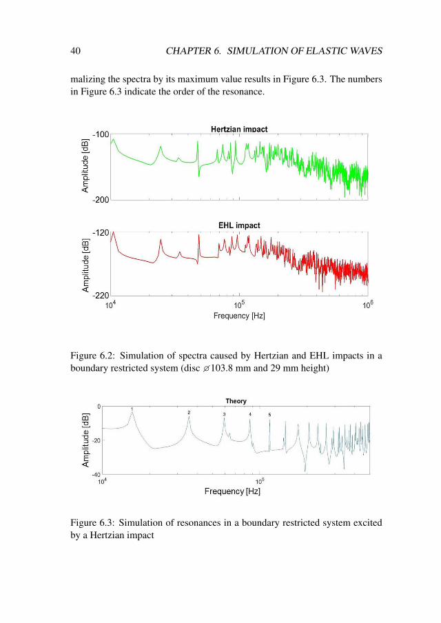
40 CHAPTER 6. SIMULATION OF ELASTIC WAVES
malizing the spectra by its maximum value results in Figure 6.3. The numbersin Figure 6.3 indicate the order of the resonance.
Figure 6.2: Simulation of spectra caused by Hertzian and EHL impacts in aboundary restricted system (disc �103.8 mm and 29 mm height)
Figure 6.3: Simulation of resonances in a boundary restricted system excitedby a Hertzian impact

Chapter 7
Elastic waves caused bytransient forces
Investigations conducted within the frame of this thesis showed that transientforces are the dominating source of AE in well functioning pure rolling(SRR=0) EHL contacts. Therefore, it is important to know the impact of con-tact conditions on frequency content and signal parameters such as amplitudeand RMS. In this chapter especially the contact time is analyzed as a contactcondition. Thereby, results are shown ranging from reflection free measure-ments in two dimensions to measurements with reflections in all three dimen-sion and interacting source and elastic waves. Results in this chapter are basedon measurements of bouncing ball setups and a full scale bearing test.
7.1 Ball impacts on an infinite plate
Ball impacts on an infinite plate were performed on the same calibration plateused for experiments in Chapter 4. Within the measurement time reflectionsdid not need to be considered, because horizontal reflections did neither havethe time to reflect back to the point of wave initiation (impact point) nor did thehorizontal reflections have the time to reflect back to the measurement point.Therefore, the experimental setup fullfilled the definition of a infinite plate pre-sented in Chapter 6.In Figure 7.1 and Figure 7.2 spectra of AE signals of both a Hertzian and anEHL impact are shown. The measured spectra are compared to the simula-tions presented in Chapter 6. For the Hertzian impact (Figure 7.1) a goodagreement of the zero frequencies between simulation (blue dashed line) and
41

42 CHAPTER 7. TRANSIENT FORCES
Figure 7.1: Simulated and measured spectra of a Hertzian impact on an infiniteplate (Paper B, Figure B.6)
measurement (yellow solid line) was observed. Even the amplitudes of bothspectra are similar, however, a slight overestimation of the amplitude by thesimulation was observed. Contrary to the Hertzian impact, the simulation forthe EHL impact (red dashed line) underestimated the amplitude of the spectra(Figure 7.2) of EHL impacts (green solid line). Furthermore, the zero frequen-cies do not agree when comparing simulation and measurement. The simula-tion suggests a frequency shift towards lower frequencies in comparison to theHertzian impact, while measurement show a shift towards higher frequenciesin comparison to the Hertzian impact. However, the overall suggested shapeof the spectra and the shape of the measured spectra show similarities, withdistinct zero frequencies of first and second order, while the third order cannot be identified due to additional excitation of frequencies from 0.5 MHz to1 MHz. This excitation could be caused by cavitation. Cavitation was foundto be able to excite these frequencies [93] and occurs once the ball reboundsfrom the plate.For simulations of both Hertzian impact and EHL impact it is assumed that thetotal contact force acts at a single point, at which the force initiates a perfectelastic deformation. The results suggest that this assumption is valid for theHertzian case, while for the EHL case this assumption needs to be reconsid-ered. A possible explanation for the poorer agreement between simulation andmeasurement of the EHL impact in comparison to the Hertzian impact couldbe the solidification of the lubricant. As shown in Figure 5.2 in Section 5.1,

7.1. INFINITE PLATE 43
Figure 7.2: Simulated and measured spectra of an EHL impact on an infiniteplate (Paper B, Figure B.7)
the lubricant layer has a huge influence on the deformation behaviour of bothball and plate, due to the solidification of the lubricant layer. Larsson andHöglund [32] showed that the total contact force of an EHL impact is smallerand the contact duration is longer than for a dry impact. However, they alsoshowed that the deformation at the centre point of an EHL impact is slightlylarger than for a Hertzian impact and they showed that the contact pressure atthe centre is significantly larger for EHL impacts in comparison to Hertzianimpacts. These findings imply that EHL impacts are more localized phenom-ena than Hertzian impacts. Using the total force to initiate the elastic wavesin the simulations might not be the best approach, considering this localizedconcentration of pressure and deformation at the centre point of EHL impacts,because ultimately the deformation of the surface causes the elastic wave, notthe force.Figure 7.3 shows that the shift of zero frequencies towards higher values incomparison to the Hertzian reference cases is observed in more than just a sin-gle measurement. This frequency shift is consistent throughout all measure-ments. Each marker in Figure 7.3 represent the average of 8 measurements,while the error bars indicate the standard deviation. The normalized frequencyrepresents the zero frequency multiplied by the contact time of the Hertzianreference case. It is clearly shown that all EHL impacts are located at highernormalized frequencies in comparison to the corresponding Hertzian referencecase. Furthermore, the standard deviation is bigger for the EHL cases and in-

44 CHAPTER 7. TRANSIENT FORCES
Figure 7.3: Normalized zero frequencies of Hertzian and EHL impacts on aninfinite plate (Paper B, Figure B.8)
creases with decreasing drop height. This increase in standard deviation couldbe caused by the preparation of the lubricant layer. While in the Hertzian casethe surface only needed to be clean, a thin and even lubrication layer had to beprepared for EHL impacts. Differences in initial film thickness of this layer,which was hard to control, had a direct impact on the measurements by vis-cous damping of the ball. The huge standard deviation for EHL impacts meanthat no significant difference in zero frequencies could be observed betweenthe two lubricants with different viscosities.
7.2 Ball impacts on boundary restricted system
For elastic waves in the boundary restricted system (discs of �103.8mm) twodifferent cases were observed using the bouncing ball setup. In the first casethe initiating force and the resulting elastic wave are independent and the zerofrequencies are amplified in the same way as impacts on the infinite plate (Sec-

7.2. BOUNDARY RESTRICTED SYSTEMS 45
tion 7.1). If the reflections reflect back to the point of impact before the ballrebounds, the elastic waves and the initiating force interfere with each other. Inthis second case the elastic wave and initiating force are not independent anylonger and no zero frequencies are amplified. Instead, results show that reso-nances are excited once the elastic wave and force interact with each other.
7.2.1 Independent source and elastic wave
This thesis, refers to experimental cases as independent when reflections donot reach back to the point of impact, before the ball rebounds. Results ofsuch independent bouncing ball experiments in boundary restricted systemsshow that AE signals behave in a similar way to the infinite plate case. InFigure 7.4 measurement (red dashed line) and simulation (green solid line) ofa Hertzian impact on a disc with 29 mm thickness is shown. Both simulation
Figure 7.4: Spectra of a Hertzian impact on a disc with�103.8 mm and 29 mmheight (Paper A, Figure A.7b)
and measurement show zero frequencies located at the expected positions, asseen for the infinite plate case. However, the zero frequencies can not be asclearly identified in the boundary restricted systems. While in the infinite platecase (Figure 7.1 and Figure 7.2) these local minima called zero frequenciesare clear without any doubt, the zero frequencies of an impact in a boundaryrestricted system are indistinct due to the noisy spectra caused by the reflec-

46 CHAPTER 7. TRANSIENT FORCES
tions. A moving average of the spectra (blue solid line - Figure 7.4) reduces thenoisiness and allows localization of the zero frequencies. However, the identi-fication of these minima is inaccurate in comparison to the infinite plate case.For EHL impacts the zero frequencies are so indistinct that an identificationwas not possible. Therefore only Hertzian impacts are shown for the boundaryrestricted systems.
Figure 7.5: Normalized zero frequencies of Hertzian impacts in boundary re-stricted systems (Paper A, Figure A.8)
In Figure 7.5 normalized zero frequencies of all bouncing ball experimentswith independent elastic waves and sources are plotted. Each marker repre-sents the average of 8 impacts. The difficulties of identification of the zerofrequencies can be as well seen by the large standard deviations (error bars)in Figure 7.5. Equivalent Hertzian impacts on infinite plates (hollow markersin Figure 7.3) show a significantly smaller standard deviation. However, iden-tification is still possible. Comparing the normalized zero frequencies of firstand second order impacts on boundary restricted systems (Figure 7.5) and oninfinite plates (Figure 7.3) shows identical positions of 1.75 for first and 2.75for second order zero frequencies. Therefore, the identified zero frequencies
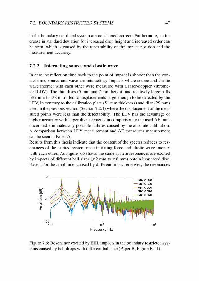
7.2. BOUNDARY RESTRICTED SYSTEMS 47
in the boundary restricted system are considered correct. Furthermore, an in-crease in standard deviation for increased drop height and increased order canbe seen, which is caused by the repeatability of the impact position and themeasurement accuracy.
7.2.2 Interacting source and elastic wave
In case the reflection time back to the point of impact is shorter than the con-tact time, source and wave are interacting. Impacts where source and elasticwave interact with each other were measured with a laser-doppler vibrome-ter (LDV). The thin discs (5 mm and 7 mm height) and relatively large balls(�2 mm to �8 mm), led to displacements large enough to be detected by theLDV, in contrary to the calibration plate (51 mm thickness) and disc (29 mm)used in the previous section (Section 7.2.1) where the displacement of the mea-sured points were less than the detectability. The LDV has the advantage ofhigher accuracy with larger displacements in comparison to the used AE tran-ducer and eliminates any possible failures caused by the absolute calibration.A comparison between LDV measurement and AE-transducer measurementcan be seen in Paper A.Results from this thesis indicate that the content of the spectra reduces to res-onances of the excited system once initiating force and elastic wave interactwith each other. As Figure 7.6 shows the same system resonances are excitedby impacts of different ball sizes (�2 mm to �8 mm) onto a lubricated disc.Except for the amplitude, caused by different impact energies, the resonances
Figure 7.6: Resonance excited by EHL impacts in the boundary restricted sys-tems caused by ball drops with different ball size (Paper B, Figure B.11)

48 CHAPTER 7. TRANSIENT FORCES
are identical. The same behaviour was observed by changing impact energythrough a change of impact velocity (drop height), while changing the system(disc) obviously influenced the resonances.Even though the spectra consisted exclusively of resonances, which limited in-formation about the EHL impact, the contact time still influenced the spectra.In Figure 7.7 normalized spectra of Hertzian impacts (blue dashed line) andEHL impacts (red solid line) are shown. For both cases it can be seen thatthe amplitude of higher order resonances drops faster with increased ball sizeand thereby increased contact time. The black dashed vertical lines in Fig-ure 7.7 indicate the theoretical position of the zero frequency of the first order( fzero, 1). Even though the spectra do not contain zero frequencies, the theoret-ical position of fzero, 1 agrees with a 20dB cut off. Amplitudes of resonancesat frequencies lower than fzero, 1 show a decrease of 0dB to 20dB in compar-ison to the maximum amplitude, while amplitudes at frequencies higher thanfzero, 1 decreased more than 20dB. Therefore, spectra of impacts where sourceand wave interact still contain information about the contact time.
Figure 7.7: Comparison of normalized spectra of EHL and Hertzian impactsexciting resonances (measured by LDV) (Paper B, Figure B.12)
Further information on the resonance behaviour and the agreement between
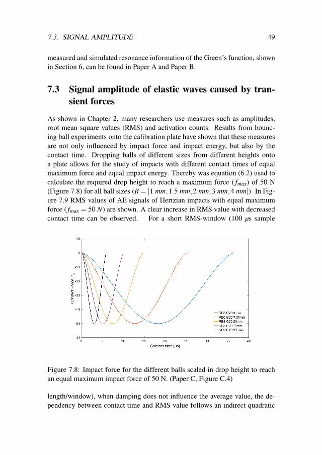
7.3. SIGNAL AMPLITUDE 49
measured and simulated resonance information of the Green’s function, shownin Section 6, can be found in Paper A and Paper B.
7.3 Signal amplitude of elastic waves caused by tran-sient forces
As shown in Chapter 2, many researchers use measures such as amplitudes,root mean square values (RMS) and activation counts. Results from bounc-ing ball experiments onto the calibration plate have shown that these measuresare not only influenced by impact force and impact energy, but also by thecontact time. Dropping balls of different sizes from different heights ontoa plate allows for the study of impacts with different contact times of equalmaximum force and equal impact energy. Thereby was equation (6.2) used tocalculate the required drop height to reach a maximum force ( fmax) of 50 N(Figure 7.8) for all ball sizes (R = [1 mm,1.5 mm,2 mm,3 mm,4 mm]). In Fig-ure 7.9 RMS values of AE signals of Hertzian impacts with equal maximumforce ( fmax = 50 N) are shown. A clear increase in RMS value with decreasedcontact time can be observed. For a short RMS-window (100 µs sample
Figure 7.8: Impact force for the different balls scaled in drop height to reachan equal maximum impact force of 50 N. (Paper C, Figure C.4)
length/window), when damping does not influence the average value, the de-pendency between contact time and RMS value follows an indirect quadratic

50 CHAPTER 7. TRANSIENT FORCES
Figure 7.9: Dependency of RMS values of acoustic emission signals causedby transient forces on contact time (measured by LDV) (Paper C, Figure C.9)
proportional tendency. The same dependency is valid for correlation of contacttime and amplitude values of acoustic emission signals (Paper C, Figure C.8).Scaling the drop height to give equal maximum impact force leads to smalldifferences in impact energy. However, repetitions of the experiments withequal impact energies instead of equal maximum impact force showed similarresults (more detailed results can be found in Paper C).The experiments with the bouncing ball setup suggest that the speed dependentacoustic emission signal of rolling element bearings is caused by a change ofcontact time with changed rotational speed. Defining the contact time of arolling element bearing (tCOR) based on the elliptical contact length in rollingdirection (b), raceway diameter of the outer ring (Do) and frequency of cage as-sembly rotation ( fCA) enables the comparison of the bouncing ball experimentsand rolling element bearing tests at different speeds.
tCOR =b
fCA ∗DO ∗π(7.1)
UREB =t2c
t2COR∗UHI (7.2)
Using Equation (7.2), the results of the Hertzian impacts shown in Figure 7.9

7.3. SIGNAL AMPLITUDE 51
were scaled to estimate RMS values of AE signals of a spherical rolling el-ement bearing (SKF 22220 E) at different rotational speeds and a constantload of 10 kN. These estimated RMS values are shown in Figure 7.10 (trian-gular markers). Considering that the estimated RMS values are based on asingle Hertzian impact and are compared to measured RMS values of a spheri-cal rolling element bearing (circular markers in Figure 7.10) with several EHLcontacts, the agreement of the RMS values is good. In particular the agreementof estimated and measured RMS values over increased rotational speed showsgood agreement. The deviation at speeds from 1 rpm to 30 rpm is caused bythe background noise of the measurement and therefore this deviation is notunexpected.
Figure 7.10: RMS values of elastic waves caused by transient forces in a rollingelement bearing (Paper E, Figure E.7)


Chapter 8
Elastic waves excited by plasticdeformation
In Section 5.2 it was mentioned that acoustic emission signals around the yieldpoint are of interest, when tensile tests are analyzed with respect to plasticdeformation in rolling element bearings. The signal strength (amplitudes andRMS values) of acoustic emission signals around the yield point is dependenton several parameters. Results have shown that both the cross sectional areaof the tensile sample and the hardness of the tensile sample influence ampli-tude and RMS values of AE signals. The two different geometries used in thisthesis (Figure 5.4) showed an increase of amplitude with increasing cross sec-tional area. The increase in AE signal amplitude is most probably caused byan increased plastically deformed volume. However, for tensile tests the plas-tically deformed volume is difficult to determine, which is the reason tensiletests refer to the cross section of maximum tensile stress.Results of tensile tests with ferrite and bainite samples of identical geometryindicate clearly an increase of AE signal amplitude with increased hardness.This difference in amplitude for bainite and ferrite samples can be seen in Fig-ure E.3 in Paper E. Both the dependency on hardness and on deformed volumeare in line with the conclusions of Miettinen and Andersson [48], which foundincreased AE activity in contaminated rolling element bearings with increasedparticle concentration (deformed volume) and increased particle hardness.Additionally, results showed a dependency of AE amplitude and RMS valuefor increased displacement speed. Tensile tests with 7 different displacementspeeds (the speed the hydraulic cylinders extend the tensile sample) were car-ried out. As Figure 8.1 shows, a linear dependency between displacement
53

54 CHAPTER 8. PLASTIC DEFORMATION
Figure 8.1: Dependency of RMS values of acoustic emission signals (causedby plastic deformation during tensile tests) on extension speed (Paper E, Fig-ure E.4)
speed and RMS value was found. During a tensile test a certain plastic defor-mation is induced in the sample. Increasing the displacement speed (within therange used in this thesis) should not have any effect on the plastic deformation.Therefore, it can be assumed that an increase of displacement speed increasesthe amount of plastic events during a given time interval, which leads to a sum-mation and the linear dependency.This linear dependency of AE signal amplitude on displacement speed is es-pecially interesting, considering the quadratic dependency of AE signal am-plitude of transient force signals presented in Section 7.3. The combinationof these two dependencies might be the cause for problems of detection ofparticle contamination in rolling element bearings at elevated speed (see Chap-ter 2). While at elevated rotational speeds the AE signals of plastic deformationcaused by particle contamination are masked by transient force AE signals, theAE signals of plastic deformation get more dominant with decreased rotationalspeed. An experiment with a spherical rolling element bearing lubricated withcontaminated and uncontaminated grease supports this hypothesis.The results (Figure 8.2) show no significant difference between AE signals ofcontaminated and uncontaminated bearings at elevated rotational speed, whichsupports the theory that AE signals contain mainly transient force signals. De-
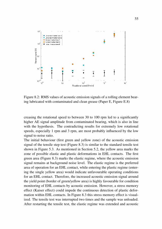
55
Figure 8.2: RMS values of acoustic emission signals of a rolling element bear-ing lubricated with contaminated and clean grease (Paper E, Figure E.8)
creasing the rotational speed to between 30 to 100 rpm led to a significantlyhigher AE signal amplitude from contaminated bearing, which is also in linewith the hypothesis. The contradicting results for extremely low rotationalspeeds, especially 1 rpm and 3 rpm, are most probably influenced by the lowsignal to noise ratio.The initial behaviour (first green and yellow zone) of the acoustic emissionsignal of the tensile step test (Figure 8.3) is similar to the standard tensile testshown in Figure 5.3. As mentioned in Section 5.2, the yellow area marks thezone of possible elastic and plastic deformations in EHL contacts. The firstgreen area (Figure 8.3) marks the elastic regime, where the acoustic emissionsignal remains at background noise level. The elastic regime is the preferredarea of operation for an EHL contact, while entering the plastic regime (enter-ing the single yellow area) would indicate unfavourable operating conditionsfor an EHL contact. Therefore, the increased acoustic emission signal aroundthe yield point (border of green/yellow area) is highly favourable for conditionmonitoring of EHL contacts by acoustic emission. However, a stress memoryeffect (Kaiser effect) could impede the continuous detection of plastic defor-mation within EHL contacts. In Figure 8.3 this stress memory effect is visual-ized. The tensile test was interrupted two times and the sample was unloaded.After restarting the tensile test, the elastic regime was extended and acoustic

56 CHAPTER 8. PLASTIC DEFORMATION
emission was not detected even though the force exceeded the initial force ofplastic deformation, fplastic. These extended elastic regimes (indicated by thesecond and third green area) imply that acoustic emission can only be recordedonce plastic deformation occurs that is more severe than any of the previouslyoccurring plastic deformations within the material.
Figure 8.3: Acoustic emission signal obtained from a tensile step test, whichvisualises the Kaiser effect
For condition monitoring purposes of EHL contacts, the Kaiser effect is adrawback. However, in long term testing of rolling element bearings with con-taminated grease no influence of the Kaiser effect was observed. In Figure 8.4RMS values of acoustic emission recordings of rolling element bearings oper-ated for 168 hours are shown. The results show that acoustic emission signalsof contaminated bearings (Figure 8.4-c,d) continue throughout the test dura-tion with larger AE signals than uncontaminated bearings (Figure 8.4-a,b). Ifthe Kaiser effect would contribute to the acoustic emission signal, the AE sig-nals of contaminated bearings would decrease towards the level of AE signalsof uncontaminated bearings, which is clearly not the case. A possible expla-nation could be the random distribution of particles within a rolling element
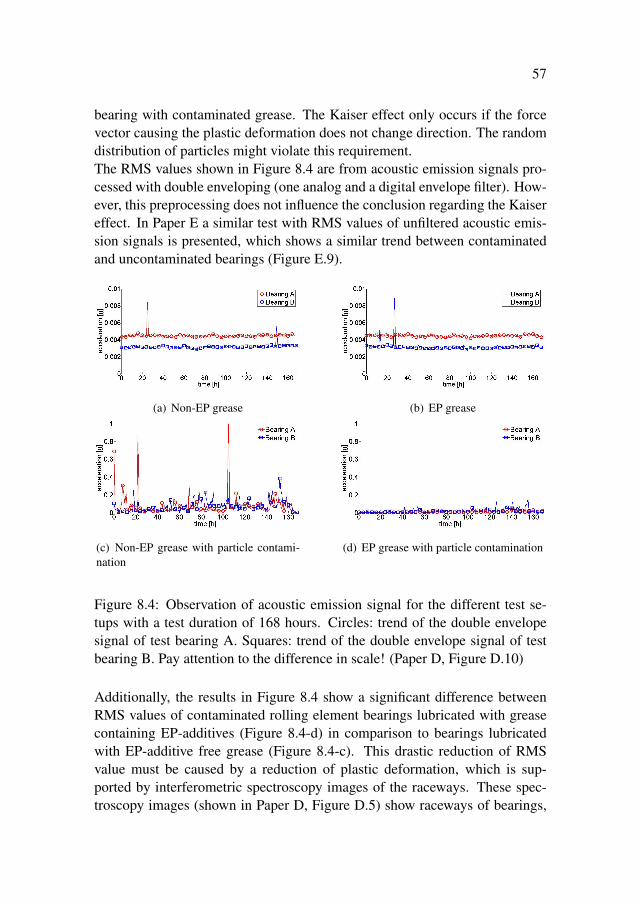
57
bearing with contaminated grease. The Kaiser effect only occurs if the forcevector causing the plastic deformation does not change direction. The randomdistribution of particles might violate this requirement.The RMS values shown in Figure 8.4 are from acoustic emission signals pro-cessed with double enveloping (one analog and a digital envelope filter). How-ever, this preprocessing does not influence the conclusion regarding the Kaisereffect. In Paper E a similar test with RMS values of unfiltered acoustic emis-sion signals is presented, which shows a similar trend between contaminatedand uncontaminated bearings (Figure E.9).
(a) Non-EP grease (b) EP grease
(c) Non-EP grease with particle contami-nation
(d) EP grease with particle contamination
Figure 8.4: Observation of acoustic emission signal for the different test se-tups with a test duration of 168 hours. Circles: trend of the double envelopesignal of test bearing A. Squares: trend of the double envelope signal of testbearing B. Pay attention to the difference in scale! (Paper D, Figure D.10)
Additionally, the results in Figure 8.4 show a significant difference betweenRMS values of contaminated rolling element bearings lubricated with greasecontaining EP-additives (Figure 8.4-d) in comparison to bearings lubricatedwith EP-additive free grease (Figure 8.4-c). This drastic reduction of RMSvalue must be caused by a reduction of plastic deformation, which is sup-ported by interferometric spectroscopy images of the raceways. These spec-troscopy images (shown in Paper D, Figure D.5) show raceways of bearings,

58 CHAPTER 8. PLASTIC DEFORMATION
where bearings lubricated with the EP-additive free grease are to a higher de-gree plasticly deformed in comparison to raceways of bearings lubricated withEP-additive grease. An explanation could be provided by a chemical reaction(Equation (8.2) and Equationn (8.1)) between the particles (magnetite oxide)and the sulfur based EP-additive. The resulting FeSO4 and FeS are both softerthan the initial magnetite oxide particles (Fe3O4), which explains the reductionin plastic deformation to the raceways.
2 Fe3O4 +4 S−−R+O2 −→ 2 FeSO4 +2 FeS+2 FeO+4 R (8.1)
Fe3O4 +3 S−−R+2 O2 −→ 2 FeSO4 +FeS+3 R (8.2)
Furthermore, the resulting compounds (FeSO4 and FeS) are used as solid lu-bricants in journal bearings [94]. Yuan-Dong et al. [94] used these compoundsto reduce wear and protect the sliding surfaces, which is in line with the resultsobtained.

Chapter 9
Conclusions
The conclusions of this PhD work can be divided into two parts, based on thefirst research question: "What are the sources of acoustic emission signalsin EHL contacts?". During this thesis work two possible sources (transientforce and plastic deformation) were evaluated and found to be contributors toacoustic emission signals from EHL contacts. However, this does not excludethe possibility of additional sources of AE signals from EHL contacts, such asfrom sliding.Transient forces as a source of acoustic emission in EHL contacts was a majorpart of this thesis and the following conclusions regarding transient forces canbe drawn, based on research questions two to four.
How is an acoustic emission signal of a single EHL contact dependenton the contact properties?
• Contact time was found to be the most important single contactproperty influencing AE signals caused by transient forces in EHLcontacts.
• The contact time determines the location of zero frequencies, wherefirst and second orders exist for single EHL contacts and are lo-cated at higher frequencies in comparison to Hertzian referencecases. Zero frequencies were found in both infinite plate and bound-ary restricted system setups. However, in boundary restricted sys-tems the detection is highly hindered by reflections.
• Once initiating force and elastic wave do interact with each other,zero frequencies are no longer detectable and resonances are en-hanced instead.
59

60 CHAPTER 9. CONCLUSIONS
• A quadratic dependency between contact time and AE amplitudeswas observed. Additionally it was found that amplitudes of elasticwave signals of EHL contacts are higher than the amplitudes ofHertzian reference cases, which is most probably caused by thedifference in surface deformation.
Can acoustic emission signals of single EHL contacts be simulated?
• Elastic waves caused by transient forces in EHL contacts can besimulated. It was found that a Green’s function approach predictsthe shape of the spectra of an AE signal caused by a single EHLcontact correctly. However, the position of zero frequencies andthe amplitude are not well predicted, which indicates that forcebased simulations of elastic waves are not ideal for EHL contacts.
How are acoustic emission signals of component setups related to acous-tic emission signals of complete machine elements, such as rolling el-ement bearings?
• Comparing full bearing test with bouncing ball experiments showedthat transient forces are the main source of elastic waves in rollingelement bearings at elevated rotational speeds.
• Both bearing tests and bouncing ball tests showed a similar quadraticrelation between amplitude and contact time/rotational speed re-spectively.
Beside transient forces, plastic deformation was investigated as a possiblesource of acoustic emission signals from EHL contacts. Thereby, the study ledto the following conclusions regarding plastic deformation as a source, basedon research question two and four.
How is an acoustic emission signal of a single EHL contact dependenton the contact properties?
• As for transient force signals, time dependency was found to bean important factor for AE signals caused by plastic deformations.However instead of the quadratic dependency, such as for transientforce signals, a linear dependency between AE signal amplitudeand event frequency was found.

61
• Experiments indicated that hardness and deformed volume also in-fluence the AE signal amplitude. However, these dependenciesshould be studied in more detail before conclusions on the exactinfluence of these properties can be drawn.
How are acoustic emission signals of component setups related to acous-tic emission signals of complete machine elements, such as rolling el-ement bearings?
• AE signals caused by plastic deformations do not exist or are maskedby transient force signals in rolling element bearings operating innormal conditions.
• AE signals caused by plastic deformations can be detected in se-vere operating conditions, such as particle contamination, and fol-low the same linear trend with regards to event frequency as tensiletests.
Additionally, interesting results on the contribution from plastic deformationand transient force to the overall acoustic emission signal of EHL contactswere observed:
• Plastic deformation in rolling element bearings can only be detected byacoustic emission signals in combination with traditional signal process-ing techniques (RMS and AC among others) at low rotational speeds,where transient force signals are smaller than signals caused by plasticdeformation of the raceways. Otherwise signals caused by plastic defor-mations are masked by signals caused by transient forces.
All conclusions are based on experiments executed in a controlled laboratoryenvironment, which needs to be considered before adapting results to industrialapplications. Signal to noise ratios in industrial applications are most proba-bly worse than in the experiments performed here. Therefore, signals mightdeviate and condition monitoring through acoustic emission might be a morecomplex task.


Chapter 10
Future work
This Thesis has to some extent answered the research questions (Section 2.3)on sources and contact properties contributing to acoustic emission signals insingle EHL contacts. However, there is still scientific work left before theresearch questions are answered completely. This required scientific work islisted in this chapter. Additionally, academic research is pointed out, which isnecessary to be able to implement findings of this research to rolling elementbearings or other EHL based machine elements.To improve understanding of elastic waves excited by single EHL contactseven further, the following future work is suggested:
• Experiments have shown that the relatively large sensor area violates thepoint assumption and increases measurement inaccuracy. Repetition ofparts of the experiments with an improved sensor system would revealthe contribution of the large sensor area to the error margin, especiallyin the boundary restricted system.
• Simulations of elastic waves based on force as an initiating source showedsome weaknesses. It would be interesting to investigate if substitution offorce with pressure or surface deformation will improve the agreementbetween measurement and simulation.
• This thesis focused on transient force and plastic deformation as sourcesof elastic waves. However, investigations have shown that sliding sur-faces can cause elastic waves too. To introduce slide to roll ratio to abouncing ball setup, experiments can be repeated with tilted plates. Al-ternatively, pure sliding of EHL contacts in ball on disc or twin discsetups could be studied.
63

64 CHAPTER 10. FUTURE WORK
Improving the understanding of elastic waves caused by single EHL contactsis important. However, it is as important to adapt this understanding to appli-cations such as rolling element bearings or whole machines. Therefore, furtherfuture work is suggested:
• Results have shown that acoustic emission caused by plastic deforma-tion from particle contamination can be detected at low speed, while atelevated rotational speeds transient force signals dominate. The severityof the plastic deformation determines, therefore, the maximum speed,where plastic deformation is detectable. Therefore, it is necessary to in-vestigate how particle size, particle concentration and particle hardnessinfluence the maximum rotational speed where plastic deformation isstill detectable.
• Sources of elastic waves, such as plastic deformation, sliding and tran-sient forces usually occur simultaneously in EHL contacts. Therefore,it is necessary to study the interaction of these different sources in acontrolled environment before the results are adapted to rolling elementbearings. Investigations in a ball on disc setup might be a good choicefor this intermediate step.
• Results have shown that in most of the rolling element bearing appli-cations spectra of acoustic emission signals only display resonances,which makes spectral analysis for failure detection difficult. Therefore,future work regarding time signal analysis is suggested. First attempts incombination with dictionary learning [95] have shown promising resultsand should be studied further.

Part II
Appended Papers
65


Paper A
Hertzian contacts in boundaryrestricted systems
67


69
Submitted to Tribology Letters
Absolute measurement of elastic waves excited byHertzian contacts in boundary restricted systems
S. Schnabel1,3, S. Golling2, P. Marklund1,3, R. Larsson1,3
1)Luleå University of Technology, SKF-University Technology centre2)Luleå University of Technology, Division of Solid Mechanics,
3)Luleå University of Technology, Division of Machine Elements,SE-97187 Luleå, Sweden
Abstract In most applied monitoring investigations using acoustic emission,measurements are carried out relatively, even though that limits the use of theextracted information. The authors believe acoustic emission monitoring canbe improved by instead using absolute measurements. However, knowledgeabout absolute measurement in boundary restricted systems is limited. Thisarticle evaluates a method for absolute calibration of acoustic emission traduc-ers and evaluate its performance in a boundary restricted system.Absolute measured signals of Hertzian contact excited elastic waves in bound-ary restricted systems were studied with respect to contact time and excita-tion energy. Good agreement is shown between measured and calculated sig-nals. For contact times short enough to avoid interaction between elastic wavesand initiating forces the signals contain both resonances and zero frequencies,whereas for longer contact times the signals exclusively contained resonances.For both cases a Green’s function model and measured signals showed goodagreement.
Keywords: Hertz contact, elastic waves, Acoustic Emission, Green’s function,boundary restricted system, condition monitoring

70 PAPER A. HERTZIAN CONTACT
A.1 Introduction
Acoustic emissions (AE), or as well called high frequency emissions, haveover the past decade become increasingly popular in the application of nonde-structive testing and condition monitoring. This technique has been proven inthe separation of failure modes [62], the monitoring of wear [45,96], the spec-ification of contaminated systems [48, 97] and to differentiate lubricants [50]and lubrication regimes [52]. However, most of the investigations use simplesignal processing methods such as root mean square (RMS) [52,97] and activa-tion counts (AC) [48,50,62,96]. All these investigations use relative measure-ment methods and signals are acquired using piezoelectric transducers, whichlimits investigations without further calibration to measure relatively. This useof relative measurement methods also limits the extraction of information ofthe acoustic wave.The authors hypothesize that condition monitoring techniques could be im-proved by improving processing of the signal. A fuller understanding of therelation between the source of the wave and the actual measured signal wouldimprove the processing of the signal. Absolute measurement would thereforebe required so that the relation between the signal and the wave source couldbe ascertained. Both McLaskey [89] and Jacobs [88] have presented methodsfor absolute calibration of piezoelectric transducers. However, there are noevaluations of the validity of the methods which are independent of the sys-tem. McLaskeys method for absolute calibration of piezoelectric transducersis used.The method is evaluated for boundary restricted systems using a Laser-Doppler vibrometer (LDV) and Green’s function based on an FEM simulationas a comparison. The term "boundary restricted systems" is used for systemswhere reflections of all dimensions are taken into account (in this investiga-tion disc samples), whereas systems which are boundary free in one or twodimension are not included in this definition (calibration plate - reflection isonly considered in one dimension).An absolute measurement is required to improve condition monitoring capa-bility of high frequency emissions. However, a better understanding of the re-lation between source and signal is as well an essential knowledge for improv-ing condition monitoring by acoustic emission. Several researchers have suc-cessfully connected source and signal for high frequency emissions. McLas-key [83] has for example related a signal of a piezoelectric transducer to theactual force function by using a Green’s function approach. Kundu [98] haspresented a mathematical method to locate Hertzian impacts by minimizing er-ror functions. The impact of cracks on wave propagation in plates was studied

A.2. EXPERIMENTAL SETUP 71
by Liu [99] with FEM based on a Green’s function for transfer of the initialsource. Glaser [82] was able to calculate the wave propagation in an isotropichalf space with a viscoelastic propagator and compared it to actual measure-ments. All these investigations have used either thin plates in order to minimizethe problem to two dimensions or have used huge geometries in comparison tothe measurement time to avoid reflections. In both cases the boundary restric-tions are simplified. However, in industrial applications boundary restrictionsoften comprise a great part of contribution to the measured signal.Other researchers have taken boundary restrictions into account by usingsmaller geometries with limited sizes, were reflection could not be neglected,but have focused on linking physical properties to the measured signal ratherthan the actual source. Han [100], for example, related the yield stress intensile tests with wave forms, while Niknam [15] related AE signals with astatistical approach to lubrication conditions. However, in these investigationsabsolute measurement is not used nor do they relate signal and source directlyto each other.Investigations with boundary restricted systems which relate wave source andsignal are rare. One of the few that do is an investigation about crack prop-agation in brittle amorphous materials, where Gross [38] links the spectra ofthe excitation to the speed of the crack propagation. However, investigationsof Hertzian contact excited, boundary restricted systems, could not be found,even though such systems are fundamental for condition monitoring of rollingelement bearings. Understanding the relation between AE source and AE sig-nals in a rolling element bearing would enable new opportunities for improvedsignal processing. This article therefore describes a experimental analysis ofHertzian contacts in boundary restricted systems and compares the results toprevious investigations without boundary restrictions.
A.2 Experimental setup
Steel balls (SKF) with diameters from �1.5mm to �10mm were used asHertzian excitation for all experiments. The balls were dropped from differentheights onto different plates (Table A.1). Impact positions were identical forall experiments so as to obtain repeatable measurements. To achieve as iden-tical impact positions as possible a hemispherical magnetic holder was devel-oped (Figure A.1). With a magnetic force just enough to overcome gravitythe ball samples were self aligning by positioning at lowest potential energy,right centered beneath the half sphere. Any redirection problem due to residual

72 PAPER A. HERTZIAN CONTACT
Figure A.1: Schematic of the experimental setup. a) accelerometer setup, b)LDV setup
magnetism was minimized due to the minimization of contact area. This re-peatability is visualized in Figure A.2. It shows repeated drops onto a pressuresensitive paper from various heights. The spread of contact points increaseswith increasing drop height. However, the results demonstrate an acceptablerepeatability, especially considering that the ball penetrates the 0.1mm thickpressure sensitive paper.
Figure A.2: Drop tests for evaluation of repeatability with pressure sensitivepaper. a) 350mm drop height b) 250mm drop height c) 150mm drop height
Another adjustment of the test setup was the position of sensors (LDV andaccelerometer respectively) relative to the position of the impact. Using aGreen’s function approach it is important to have impact point and sensor pointvertically aligned to each other (according to Figure A.3, points ξ and x). Toachieve this setup the laser was aligned vertically by aligning the reflection of
A.2. EXPERIMENTAL SETUP 73
a water bath. If the laser was reflected back to its source by the water surface,the laser hit the water surface at a 90 degree angle and was thereby verticallyaligned. Once the laser was vertically aligned the magnetic holder was cen-tered to the laser. Thereby was the effect used that the reflection right back tothe laser source is maximized, when the laser hit the center point of the sphere.
Table A.1: Test setup
Disc samples Ball samples Drop heights
[mm]
Aluminum 7075 5mm RB1.5 G20 100mmAluminum 7075 7mm RB2 G20 150mmSteel 2511 5mm RB3 G20 250mmSteel 2511 7mm RB4 G20 350mmSteel 2511 29mm RB6 G20
RB8 G20RB10 G20
As shown in Figure A.1 the various samples (discs) are clamped between tworubber o-ring seals. In this investigation five different discs were used and ex-cited by different Hertzian impacts as shown in Table A.1. The discs samplesonly differ in material and thickness. Both diameter (�103.8mm) and a 30◦
chamfer on one side were identical for all samples. Several combinations ofdisc and ball samples were tested and measured with both the laser-doppler vi-brometer and the piezoelectric accelerometer. Each measurement was repeatedeight times. All samples and test equipment, except pre- amplifier and acqui-sition computer, were mounted on an optical table to minimize disturbances ofthe surrounding.Accelerometer measurements were executed with the same broadband flat-response sensor (Physical acoustics WSα) used with the calibration measure-ments. As a pre-amplifier a Physical Acoustic 2/4/6C was used with an in-built bandpass filter of 100 kHz - 1200 kHz. The sensor was attached usingbeeswax. Thereby beeswax was both the attachment and the couplant. Asmall portion was heated to 75◦C. Then the sensor was pressed with deadweights onto the discs, while waiting until both disc and couplant reachedroom temperature again. Beeswax was chosen following tests with variousmethods for the attachments prior to the investigation. Additionally severalother researchers have in previous tests used beeswax as a couplant for acous-

74 PAPER A. HERTZIAN CONTACT
tic measurements [101] [102].The laser measurement was executed with a device called OFV056 from Poly-tec. The OFV056 is a laboratory type laser-doppler vibrometer which uses ared laser. In this investigation a sensitivity of 1.25 mm/s was used in com-bination with a measurement range of 1Hz to 1MHz. The laser head wasused in combination with a matching controller and pre-amplifier box (PolytecOFV3001S). As shown in Figure A.1 it was necessary to redirect the laser byan optical mirror (Thorlabs PF20-03-P01).The signals of both the LDV and the accelerometer are stored with a 14-bitdigitizer PCI-card (GaGe OSC-432-007). A Sample rate of 10 MS/s was usedand in total 10000 samples per signal were recorded, which resulted in a mea-surement time of 1ms. However, limited to a measurement time of 100µs. Allsignals were triggered on a positive flank with a pretrigger storage of 1µs.
A.3 Green’s function approach
Both the calibration and simulation are based on a Green’s function approach,where a single function describes the time dependent relation between twophysical measures at two points within the system boundaries. Usually, theGreen’s function g is a matrix which describes the relationship between points(x, ξ) for given directions (k, j) at specific times (t, τ):
uk(x, t) =x
f j(ξ,τ)×gk j(x, t,ξ,τ) dξ dτ (A.1)
However, in this paper a simplified case is used, such as that which McLaskeyand Glaser suggest [83]. It is assumed that the major contribution is the pres-sure wave through the material and therefore the simplified Greens function isonly dependent on a single direction. As shown in Figure A.3 the two points ofinterest are only separated in direction 1 by the distance h. For all other direc-tions the distance between x and ξ is zero. All exciting forces f are assumedto be perpendicular to the plate and forces therefore only act along direction1. The same applies for the displacement u. If these assumptions are madeGreen’s function may be simplified according to equation (A.2) as shown byMcLaskey and Glaser [83]:
u1(x, t) = f1(ξ,τ)∗g11(x, t,ξ,τ) (A.2)
Equation (A.2) allows determination of the displacement (u1(x, t)) in the per-pendicular direction to the plate at the sensor position, by convolution of

A.3. GREEN’S FUNCTION APPROACH 75
Green’s function (g11(x, t,ξ,τ)) and given force functions ( f1(ξ,τ)). The Green’s
Figure A.3: Schematic for declaration of experimental setup
function approach presented in this report requires independence between forcefunction and Green’s function. Therefore calculations are only valid for con-tact times (tc) shorter than any reflection time back to the point of force ini-tiation (ξ). This is especially important for the boundary restricted systems(in this investigation small discs) and reflection times are therefore defined asfollowing:
tre f lection H = 2hcp
(A.3)
tre f lection R = 2rdisc
cp(A.4)
where tre f lection H and tre f lection R are reflection times across the disc and radialrespectively. The variables h and rdisc are height and radius of the disc and cp
is the speed of the pressure wave in the given material.The Green’s function approach as used in this investigation is based on twopoint assumptions: One assumption is that the global force of a Hertzian elas-tic contact model as shown in equation (A.8) act on a single point (in thisinvestigation ξ). This assumption requires a small contact area and a deforma-tion that is as homogeneous as possible across the contact area. The secondpoint assumption used in this investigation is that calculated displacements ofa single point (in this investigation x) represent measured acoustic waves bya sensor with a finite contact area. This assumption requires a ratio betweensensor diameter and distance of the measurement point (x) to source point (ξ)as small as possible.

76 PAPER A. HERTZIAN CONTACT
A.4 Calibration
McLaskey’s and Glaser’s [89] method was used for calibration of the accelerom-eter. As a calibration system a steel plate (Toolox40) with dimensions of1 x 0.5 x 0.051m was used. The huge dimensions of the steel plate were nec-essary in order avoid reflections from the side walls during the measurementtime of 100µs. Being able to neglect reflections allowed the use of Hsu’s [91]script for calculating Green’s function, which uses only material properties andthe thickness of the plate as input parameters. The source for the wave was aglass capillary tube (D=�1,4mm and d=�1mm) which was compressed un-til it burst on the surface of the plate. A glass capillary burst was chosen asa source because of its good excitation of high frequencies due to the rapidrelease of force [90] and that the following equation may be used:
f (τ) =famp
2× (1− cos(πτ/trise)), 0≤ |τ| ≤ trise
f (τ) = 0 , τ < 0 (A.5)
f (τ) = famp , τ > trise
The calibration was carried out in a tensile test machine, where the steel platewas positioned under a steel cylinder and pressed against it with the glass cap-illary in between. With a speed of 0.01mm/s the plate was elevated towards thesteel cylinder and the force on the glass capillary as a result increased succes-sively. During the whole calibration the force on the steel cylinder, and therebythe force on the glass capillary, was measured continuously with a sample rateof 50 Samples/s. With the force measurement, the force, at which the glasscapillary burst, was identified by the force maximum. This force maximumwas the input value for famp of equation (A.5). The released elastic wave wasmeasured with an accelerometer (Physical acoustics WSα), which was posi-tioned centered to the source underneath the steel plate (positions comparableto x in Figure A.3). By transforming the measured accelerometer signal s(x, t)and the calculated theoretical displacement u1(x, t) to the frequency plane thesensor function is calculated by simple division:
s(x, t) = u1(x, t)∗ i1(t) (A.6)
I1(ω) = S(x,ω)/U1(x,ω) (A.7)
Directions of force and displacement as well as relative positions of sourceand measurement point were kept constant for all experiments. The extractedsensor function was therefore valid for all measured accelerometer signals.

A.5. SIMULATION 77
A.5 Simulation
A simulation was carried out to be compared with experimental findings.Thereby the spectra of the displacement U1(x,ω) was studied. First u1(x, t)was calculated by convolution of f1(ξ,τ) and g11(x, t,ξ,τ) (equation (A.2)).For the force function an equation based on Hertz elastic contact mechanicsderived by Reed [103] was used:
f (τ) = fmax sin(πτ/tc)3/2 , 0≤ τ≤ tcf (τ) = 0 , τ < 0 and τ > tc (A.8)
Maximum force ( fmax) and contact time (tc) are calculated based on geometri-cal and physical properties according to the following equations:
fmax = 1.917ρ3/51 (δ1 +δ2)
−2/5R21v6/5
0 (A.9)
tc = 4.53(4ρ1π(δ1 +δ2)/3)2/5R1v−1/50 (A.10)
where δi =1−ν2
i
πEi
The indexes in Equation (A.9) and (A.10) refer to the ball (index 1) and thedisc (index 2), while index 0 refers to the velocity at the time 0 (initial impactvelocity v0).Knowing materials and geometrical properties of the samples allows the calcu-lation of an analytical solution for the force function. However, a solution forGreen’s function (g11(x, t,ξ,τ)) of the used samples where reflections could notbe neglected was neither solvable analytically nor by the Hsu’s [91] script usedfor calibration. Therefore a Finite element method (FEM) analysis was carriedout to generate Green’s functions for disc samples used in this investigation.The FEM analysis was based on an LS DYNA solver for rotational symme-try. The element size of the rectangular elements was 50µm. Time steps areusually connected to element size and material properties in LS DYNA, whichresults in 3.6ns for steel and 3.7ns for aluminum. However, in this investiga-tion a storage interval of 10ns was used to artificially increase the time stepand thereby to homogenize the time step for all samples.Figure A.4 shows a schematic drawing of the FEM model with the red sym-metry axis on the left side. The three yellow marked nodes on the top (markedwith F) of the disc in Figure A.4 represent the nodes for the force initiation.The nodes were exposed to a step force with a rise time of 100ns. The threenodes form a circular area with a radius of 100µm, where the maximum force

78 PAPER A. HERTZIAN CONTACT
Figure A.4: Schematic drawing of the FEM model with the symmetry axis andnodes for loading (F), response extraction (M) and constrain (B)
applied is 1N over this circular area. Usually Green’s function approaches aretransfer functions between two points. However, to obtain convergence, theFEM model uses three points for the force initiation. The stored output of themodel is the displacement in y-direction of a single node on the lower side ofthe disc positioned on the symmetry axis (Yellow node marked with M, Fig-ure A.4). A boundary constrain was introduced to take the fixation of the discsinto account. A single node with a distance to the symmetry axis equivalentto the radius of the rubber seals was tied in the y- and the z-direction (Yellownode marked with B, Figure A.4). By taking the derivative of the FEM-result(displacement in y-direction of node M), Green’s function for specific sampleswere obtained. In combination with the equation for the force function (A.8), itenabled the calculation of the spectra for various Hertzian impacts. However,simulated results were only valid as long as the force and elastic wave do notinteract (tc < tre f lection H , tre f lection R).
A.6 Zero frequencies
Zero frequencies according to McLaskey [83] are calculated by using equa-tion (A.11). McLaskey and Glaser [83] have shown acoustic waves excitedby a Hertzian contact have local minima in the signal spectra (Figure A.5 -fzero,1, fzero,2, fzero,3) which they call zero frequencies. These zero frequenciesare determined by the contact time (tc) and have different orders

A.7. RESULTS AND DISCUSSION 79
(N = [1,2,3,4, ...]) which are in theory infinite.
fzero,N =N +0.75
tc(A.11)
However, in practice measurement of zero frequencies at higher orders aredifficult due to higher damping of higher frequencies. This study thereforealso focuses, as do McLaskey and Glaser [83], on zero frequencies up to thethird order.
A.7 Results and discussion
Results are divided in two sections. After repeating earlier results [83] to con-firm that the calibration, by McLaskey’s and Glaser’s [89] method, was correctexecuted, the calibration method was evaluated for boundary restricted sys-tems. Thereby measured spectra of acoustic waves in disc samples were com-pared to FEM simulated spectra and LDV measured spectra. In the secondsection results on the behavior of Hertzian excited elastic waves in boundaryrestricted systems will be shown. For cases were source and wave interactwith each other LDV measured spectra are presented and analyzed. In the caseof independent source and wave, accelerometer measured spectra are shown,analyzed and compared to FEM simulations with respect to zero frequencies.
A.7.1 Evaluation of absolute calibration for boundary restrictedsystems
As mentioned in section A.4 a calibration method by McLaskey [89] was usedto extract the sensor function I1(ω). To confirm that the calibration was exe-cuted correctly, McLaskey’s experiment with Hertzian contacts was repeated.Figure A.5 shows the results to be repeated and Figure A.6 shows the repeatedexperiment for control of the calibration. The theoretical signal (green) is cal-culated with Hsu’s script and equations (A.2), (A.8), (A.9) and (A.10). InFigure A.6a a clear difference between the measured raw-signal and the calcu-lated theoretical signal can be seen. However after compensating for the sensorfunction I1(ω), the measured accelerometer signal (red) and the theoretical sig-nal (green) show a good agreement (Figure A.6b) between 20kHz and 1.2MHz.Even the zero frequencies ( fzero,n) of the theoretical signal and the measuredaccelerometer signal match each other. Comparing to McLaskeys experimentsthe zero frequencies are positioned at similar positions considering plate ma-terial and ball sample. Both the overall agreement and the agreement of the

80 PAPER A. HERTZIAN CONTACT
Figure A.5: Schematic replication of results obtained by McLaskey [83]
zero frequencies (Figure A.6b) indicate a successful calibration and extrac-tion of the sensor function and are in line with the earlier result of McLaskey(Figure A.5). The difference in zero frequencies between the two results iscaused by different plate materials (aluminum vs. steel) and ball sizes (1mmvs. 1.5mm) which results in different contact times tc. Therefore the differenceis expected and does not affect the conclusion of a successful calibration.The extracted and controlled sensor function was then used for compensa-tion of accelerometer signals recorded from Hertzian excitations in boundaryrestricted systems. These compensated signals were then compared to FEM-simulation and LDV measured signals. For cases where source and wave donot interact with each other, the FEM simulated signal was used as a refer-ence, while LDV measured signals were the reference for cases where sourceand wave do interact. The use of two different references was necessary, be-cause for thick discs the displacement was too small to be detected by the LDVand the interaction of wave and source in thin discs could not be managed bythe FEM simulation. Figure A.7a shows both the LDV measured and compen-sated accelerometer measured signal of a Hertzian impact (�8mm Ball) on a5mm thick aluminum disc. Geometrical dimensions lead to multiple reflec-tions (tre f lection H =1.575µs and tre f lection R =16.346µs) within the disc in alldirections during the contact time of 31.96µs. Therefore excitation force and

A.7. RESULTS AND DISCUSSION 81
(a) raw signal
(b) calibrated signal
Figure A.6: Calibration evaluation
82 PAPER A. HERTZIAN CONTACT
(a) comparison of LDV measurement and accelerometer signal
(b) comparison of theoretical signal and accelerometer signal
Figure A.7: Calibrated accelerometer measurements on boundary restrictedsystems

A.7. RESULTS AND DISCUSSION 83
resulting wave are interacting with each other. As a result the Hertzian impactexcites resonances of the plate rather than enhancing zero frequencies. Forthis case the calibration method shows weaknesses (Figure A.7a). While theLDV measured signal (purple) clearly shows the excitation of the resonances,the compensated accelerometer signal represents these resonances only poorly.Even though the signals show some similarities, the compensated accelerom-eter signal would not be enough to identify the resonances on its own. Apossible explanation for the weak agreement, beside the calibration, can be thesensor itself. In comparison to the calibration plate, the sensor does changethe system for the small discs by adding additional weight. The sensor ratheris large (�19mm) and therefore violates the point assumption of the Green’sfunction approach.The absolute calibration seems more promising in boundary restricted sys-tems if the exciting force and wave reflections do not interact with each other(Figure A.7b). For measurements shown in Figure A.7b a ball of the size of�1,5mm was dropped onto a steel plate with a thickness of 29mm. By reduc-ing the ball size and increasing the thickness, contact time was reduced (5.1µs)and reflection times were increased (tre f lection H =9.831µs andtre f lection R =17.59µs). In this case both excitation of the resonances and en-hancing of zero frequencies was expected according to the calculated theo-retical signal (green). Comparing the calculated signal and the compensatedaccelerometer signal (red) a good agreement of the zero frequencies can beobserved. However, the excited resonances indicated by the theoretical signalare not clearly represented by the compensated accelerometer signal.Sensor function compensated accelerometer signals are capable of identifyingzero frequencies in boundary restricted systems. However, the method in com-bination with the used equipment is not able to identify the excited resonances,even though theory would suggest otherwise. Possible explanations could beas mentioned a violation of the point assumption. While the assumption is de-cent for the Hertzian contact, the used sensor head with a diameter of 20mmviolates this assumption. Another explanation could be nonlinearities in thesensor function. The calibration method assumes the sensor function (I1(ω))to be linear for a given frequency across the excitation amplitude, which mightnot be the case.
A.7.2 Hertzian contacts in boundary restricted systems
For boundary restricted systems a finite element model was for this investiga-tion developed to replace Hsu’s script which did not take any reflections into

84 PAPER A. HERTZIAN CONTACT
account. In combination with the Green’s function approach, this model is alsoonly valid for excitations which do not interact with the excited elastic wave.Comparing the calculated spectra (green solid line) in Figure A.7b with thecompensated accelerometer signal (red dashed line), shows that both are ableto identify the zero frequencies. Zero frequencies according to McLaskey [83]were calculated (A.11) and are indicated with the dashed vertical lines. Bothcalculated and measured signals match the zero frequencies to a good degree.
Figure A.8: Normalized frequencies of the first three zero frequencies for dif-ferent balls and drop heights on a boundary restricted system (steel plate 29mmthickness and �103.8mm)
By normalization of the zero frequencies over the contact time (tc) experimentswith different ball sizes and drop heights are comparable. Figure A.8 shows avisualization of normalized zero frequencies of several combinations of dropheight and ball size. Each marker represents the mean value of eight measure-ments and the error bars represents the standard deviation of the eight measure-ments. The results show that the identification of zero frequencies is clearlypossible in boundary restricted systems. However, the failure margin increases

A.7. RESULTS AND DISCUSSION 85
(a) drop height
(b) ball size
Figure A.9: Comparison of LDV measurements of different impact energiesand contact times on a Steel 2511 plate of 5mm thickness by changing dropheight and ball size.

86 PAPER A. HERTZIAN CONTACT
in comparison with the case of an infinite plate [83].The failure margin showsa clear increasing trend with increased ball size. The reason for the increase ismost probably the increase of contact time. For balls with a diameter of 3mmthe contact time (tc) is almost as long as the reflection time (tre f lection H). Thecontact time increases as well with a decrease in drop height. However, theresults show a decreased failure margin. This is most likely caused by the in-creased spread of the impacts from increased heights as shown in Figure A.2.By decreasing the reflection time (tc > tre f lection H) by decreasing plate thick-ness, zero frequencies could neither be detected by measurements nor by theFEM model based Green’s functions approach. As the results indicate, elas-tic wave responses in a boundary restricted system turn into a pure resonanceproblem once the contact time exceeds the reflection times. As Figure A.9shows neither a change in drop height nor a change in ball size has an effecton the excited resonances. However, a change in contact time by changing ballsize does change the cut off as Figure A.10 indicates. Thereby matches thefirst zero frequency fzero,1 (indicated as a dotted line in Figure A.10) to a gooddegree matches a -20dB cut off.
Figure A.10: Spectra of signals with normalized amplitude for different ballsizes
Even though the Green’s function approach is not valid for cases where ini-tiating force and elastic wave interact, it still provides information about the

A.8. CONCLUSIONS 87
Figure A.11: Comparison of resonances calculated and measured
location of the resonances. In Figure A.11 both the normalized spectra of analuminum plate 5mm obtained by calculation and by measurement are shown.The theoretical location and the measured location of the resonances are notidentical, but show good agreement. Comparing calculated and measured res-onances one to five (as indicated in Figure A.11) for different plates and ballsizes (�8 to �3) results in Figure A.12. Except for resonance one the agree-ment between calculated location and measured location is good consideringthe simplicity of the FEM model and the accuracy of the experiments. Thelarger deviation for the location of the first resonance can be partly explainedby the larger percentage difference between spectral lines at low frequenciesand the short time obtained by calculation and by measurement of 1 ms.
A.8 Conclusions
After evaluating calibration based on Green’s functions it can be concludedthat the approach is also valid for boundary restricted systems with respectto zero frequencies. The calibration is however, not accurate enough to de-tect resonances. This might be explained by violation of the assumptions ofthe Green’s function approach by the sensor system or by a summation of

88 PAPER A. HERTZIAN CONTACT
Figure A.12: Degree of agreement between resonances calculated and mea-sured by the LDV
measurement inaccuracy. The evaluation is, however, promising enough to in-vestigate more accurate sensor systems which violate the assumptions of theGreen’s function approach to a lesser degree.The investigation shows a clear difference between excitation times shorterthan reflection times and excitation times longer than reflection times. In casesof independence of elastic waves and excitation force, the spectra containsboth zero frequencies and resonances. Thereby the zero frequencies followReed’s [103] contact model, as suggested by McLaskey [83]. However if elas-tic wave and excitation force do interact, zero frequencies are not detectableanymore and the measured spectra exclusively contains resonances. Eventhough zero frequencies are not detectable in this case, the first zero frequencydoes affect the spectral signal by determining the -20dB cut-off frequency. Ad-ditionally it was shown that the Green’s function approach does provide partialinformation about the resonance location and is in line with measurements.

A.9. ACKNOWLEDGMENTS 89
A.9 Acknowledgments
The authors would like to acknowledge the financial support of SKF and VIN-NOVA (Grant number: Smarta-maskiner, 2013-5575), as well as the helpfuldiscussions with SKF-researchers, among them especially Dr. Florin Tatar,SKF-ERC, Netherlands.


Paper B
Elastic waves of a single EHLcontact
91


93
Submitted to Tribology Letters
Elastic waves of a single elastohydrodynamicallylubricated contact
S. Schnabel1,2, P. Marklund1,2, R. Larsson1,2
1)Luleå University of Technology, SKF-University Technology centre2)Luleå University of Technology, Division of Machine Elements,
SE-97187 Luleå, Sweden
Abstract Elastic waves are widely used for condition monitoring of rolling el-ement bearings through vibration or acoustic emission measurements. Whilevibration signals are understood to a high degree due to many scientific investi-gations as well as a long history of usage in the field, acoustic emission signalsof rolling element bearings are poorly understood. Therefore, this investigationpresents simulation studies and measurements of a single elasto-hydrodynamiclubricated (EHL) contact. In this investigation the EHL contact is a ball bounc-ing on a lubricated plate. The simulation based on Green’s function and themeasurements based on a accelerometer to some extent agree. A shift of zerofrequencies towards higher frequencies when compared to Hertzian referencemeasurements was determined for an infinite plate setup. Taking boundary re-strictions into account elastic waves of a Hertzian contact and an EHL contactonly differ by a damping of higher resonances which is most likely caused bythe EHL film.
Keywords: EHL contact, EHL, Hertz contact, elastic waves, Acoustic Emis-sion, Green’s function, ball impact, bouncing ball

94 PAPER B. SINGLE EHL CONTACT
B.1 Introduction
Acoustic emission (AE) has been shown in several studies to be a viable methodfor condition monitoring of rolling element bearings. Signals from contami-nated bearings were in these studies successfully correlated to type [48, 96],size [48,96,104] and concentration [48,96] of particle contamination. In addi-tion the type of lubricant [49,71,97] and the lubrication abstinence [15] in bothcontaminated and uncontaminated cases were correlated with signals moni-tored by acoustic emission transducers. Artificial implemented dents [73] onthe outer ring and failure growth [70] was another operating condition withwhich AE was correlated. In 20214 Hamel et.al. [52] determined the relationbetween acoustic emission signals and the lubrication regime. However, re-gardless of the application of acoustic emission in scientific studies it is still ararely used method of condition monitoring in industrial applications. The sig-nal to noise ratio (SNR) is one factor. Special test rigs which limit the amountof noise from other machinery parts are employed in all the experiments in thestudies. Most of them in addition operate in severe conditions which improvesthe SNR. In industrial applications, however, it is more difficult to observethe phenomena presented in the investigations mentioned. For these reasonsit is important to improve signal processing of acoustic emission raw data andin addition, there is a need for the origin of acoustic emission in an elasto-hydrodynamic lubricated (EHL) contact to be understood.One way of improving understanding of the origin of acoustic emission in anEHL contact is to break the rolling element bearing down into the componentlevel. One of these investigations on a component level was carried out by Rah-man et al. [105]. This study focused on the correlation of acoustic emissionsignal and contact fatigue in a twin disc setup. A pure sliding EHL contact andits acoustic emission was studied by Wang et al. [106] in a ball on disc appara-tus. There are, however, few investigations on a component level. The difficul-ties of the complex nature of an EHL contact itself remain. This complexity ofan EHL contact is also a reason for fundamental research in acoustic emissionto focus on fundamental sources such as transient forces [83] or cavitation [93]which both occur in an EHL contact. However, studying fundamental sourcesis just a first step towards the study of full EHL contacts. Therefore, this articleinvestigates EHL contacts based on the investigations mentioned into transientforce and cavitation. In this investigation a special case of EHL contact, witha bouncing ball on a lubricated plate, is examined. This EHL contact was cho-sen because transient forces and cavitation can be expected, while sliding as asource of acoustic emission is minimized, due to a pure squeeze contact.

B.2. EXPERIMENTAL SETUP 95
B.2 Experimental Setup
All experiments were carried out at room temperature and in a laboratory envi-ronment. Acoustic emission signals were sampled with a 14-bit digitizer PCI-card of GaGe (product number OSC-432-007). Sample rate and total samplelength were set to 10MSamples/s and 10.000 Samples respectively. Addition-ally, to the sample length a pretrigger of 10 Samples was used which equiva-lents to 1µs. This short pre-trigger coud be used due to the low noise level andthe low trigger threshold. This threshold was -3% of the measurement rangewhich was±10V. Signals were triggered on a negative flank. As a comparison,the background noise during experiments was between ±1% and ±2% of themeasurement range.To study an elasto hydrodynamic lubricated contact, a thin layer of lubricantwas applied onto the plates or discs. In theory the layer should be as thickas the maximum film thickness of the EHL contact to avoid viscous damp-ing of the ball impact. In practice the lubricant layer was applied as thinly aspossible, so that viscous damping effects were minimized. In this way 0.5mlof lubricant was applied at the position of the ball impact and smeared outacross an area of 50mm x 50mm. This lubricant layer was then covered with anon-cellulose based paper, absorbing the majority of the lubricant film. Afterremoving the paper, the film was exposed for 10 minutes to a low and steadyair flow, which distributed the lubrication layer evenly and caused possible airbubbles to burst. This procedure was identical for all applied lubricant films inthis investigation.
B.2.1 Infinite plate
Figure B.1 shows a schematic drawing of the experimental setup of tests on aplate that is considered to have infinite length and breadth. The plate used hasthe dimensions of 1x0.5x0.051m and can be considered infinite for a measure-ment duration of 84µs because reflections in horizontal directions are not rele-vant. The shortest horizontal reflection time (based on width 0.5m) is 84.75µswhich means the elastic wave does not return to the point of measurementwithin the recorded time. Hence the plate can be considered infinite and bound-aries do not need to be considered in the horizontal direction. However, acrossthe plate (0.051m) reflection times are shorter and therefore boundaries needto be considered in the vertical direction. Therefore, the plate was boundaryrestricted in one dimension and infinite in the two horizontal dimensions. Dueto the two boundary free dimensions the plate is considered to be an infinite

96 PAPER B. SINGLE EHL CONTACT
plate throughout the article.The plate was, during the experiments, resting on two rubbercylinders (�10mm) placed on each end of the 1m side (Figure B.1). The AEsensor was mounted centered underneath the plate and was vertically alignedwith a magnetic holder. In this way the ball impact occurred centered onthe sensor position only separated vertically by the plate thickness (epicentralsetup). To improve the accuracy of the impact position the magnetic holderwas shaped as a sphere to obtain automatic alignment based on gravity.
Figure B.1: Schematic drawing of experimental setup for tests on plate con-sidered to be infinite
Acoustic emission signals were recorded by a broadband flat-response trans-ducer (WSα) from Physical Acoustics in combination with a preamplifier(Physical Acoustic 2/4/6C). In addition to the amplifying circuit the amplifierhad an inbuilt bandpass filter with corner frequencies of 100kHz and 1.2MHz.In all experiments presented in this article the AE sensor was attached withbeeswax to the specimens. Thereby a small amount of beeswax was appliedonto the plate and heated to 75◦C, followed by pressing the AE sensor withdead weight onto the plate. Before starting the tests a temperature measure-ment made certain that the plate was cooled to below 25◦C. All signals of the

B.2. EXPERIMENTAL SETUP 97
acoustic emission sensor presented in this investigation were compensated forthe sensor function. This sensor function was obtained by a glass caliper burstexperiment as suggested by McLaskey and Glaser [89] as a method for abso-lute calibration.
Table B.1: Test setup for infinite plate case
Ball samples Ball radius drop heights
RB1.5 G20 0.75mm 350mmRB2 G20 1.0mm 250mmRB3 G20 1.5mm 150mmRB4 G20 2.0mm
For experiments with the infinite plate setup four different steel balls were usedand each ball was dropped from three different heights (Table B.1). Each com-bination (ball size and height) was repeated 8 times for the lubricated experi-ments. Hertzian reference measurements under dry conditions were repeated4 times for each combination.
B.2.2 Boundary restricted systems
Tests for boundary restricted systems were executed on disc samples with adiameter of 103.8mm. The disc samples only differed in height (Table B.2).Due to the dimensions of the disc reflection cannot be neglected and bound-aries of all dimensions need to be considered. Therefore the term boundaryrestricted system will be used for all experiments with discs. The balls werefor the boundary restricted cases dropped from three different heights onto thediscs. As previously shown [107] there are in boundary restricted systems twomajor cases; One where the exciting source and elastic wave are independent,and one where both interact with each other. The latter case (interaction be-tween source and wave) is studied in this article for an EHL contact. Thelaser doppler vibrometer (LDV) used for acoustic emission measurement inthe boundary restricted system is the Polytec OFV056. The Polytec OFV056was used in combination with a control and preamplifying unit of the samemanufacturer (Polytec OFV3001S). As shown in figure B.2 the laser had tobe redirected, which was done by an optical mirror (Thorlabs PF20-03-P01).The sensitivity setting was chosen to be 1.25 mm/s, which resulted in a fre-quency range of 1Hz to 1MHz of the LDV system. As for the infinite platesetup, the measurement point and impact point were vertically aligned to mea-

98 PAPER B. SINGLE EHL CONTACT
Figure B.2: Schematic drawing of the experimental setup for tests on boundaryrestricted systems
sure an epicentral impact. The magnetic holder and sampling card were alsoidentical in both measurement setups. However, the setups differ in terms ofpositioning of the plates and discs respectively. While the plate was resting onrubber cylinders (Figure B.1), the discs needed to be clamped in between tworubber seals (Figure B.2), because the net weight of the discs was not enoughto prohibit movement during impacts. The dimension of the rubber seals was� 100mm and the thickness was � 2.5mm. For the boundary restricted sys-tems both EHL contact and reference measurements with Hertzian contactswere repeated 8 times for each combination (ball size, disc height and dropheight).
B.3 Theory for Simulation
Signals presented in this investigation are simulated based on a Green’s func-tion approach (B.1), where force function ( f j(ξ,τ)) and Green’sfunction (gk j(x, t,ξ,τ)) are convoluted with each other to obtain a time sig-

B.3. THEORY FOR SIMULATION 99
Table B.2: Test setup for boundary restricted case
Ball samples Ball radius drop heights disc heights
RB2 G20 1.0mm 350mm 5mmRB3 G20 1.5mm 250mm 7mmRB4 G20 2.0mm 150mmRB6 G20 3.0mmRB8 G20 4.0mm
nal for the displacement (uk(x, t)). Variables x, t,ξ and τ represent thereby theposition of the sensor, the time scale of the sensor signal, the position of theimpact and the time scale of the impact respectively. Indexes indicate the di-rection of the force, displacement and Green’s function.
uk(x, t) = f j(ξ,τ)∗gk j(x, t,ξ,τ) (B.1)
As Figure B.3 shows index 1 refers to the direction perpendicular to the plate.It is assumed for the entire article that displacements (uk(x, t)) and all initiat-ing forces ( f j(ξ,τ)) are perpendicular to the plate, which results in k = j = 1for indexes of equation (B.1). Green’s function for an infinite plate was cal-
Figure B.3: Schematic drawing for declaration of experimental setup
culated numerically by using Hsu’s script [91], which is valid for the infiniteplate setup and a measurement time of 84µs. The force function, however, wascalculated either numerically or analytically for EHL impacts and Hertzianimpacts respectively. Forces of EHL impacts are calculated by using a numer-ical EHL solver of Larsson and Höglund [32] which is based on a multigrid
100 PAPER B. SINGLE EHL CONTACT
f (τ) = fmax sin(π(τ− t f ilm)
tc)3/2 , t f ilm ≤ τ≤ (tc + t f ilm)
f (τ) = 0 , τ < t f ilm (B.2)
f (τ) = 0 , τ > (tc + t f ilm)
-multilevel solution [31]. The script requires an initial film thickness (h00) asan input parameter. This initial film thickness needs to be minimal to minimizeviscous damping of the ball by the lubricant film. However, the film thicknessneeds to be at least as thick as the maximum film thickness of the EHL contact.After empirical trials, the factor for the initial film thickness (h00) was set to10µm and was identical for all simulations in this investigation.In the case of Hertzian impacts a modified version of Reed’s [103] elastic con-tact model was employed (Equation (B.2)). Maximum force ( fmax) and contacttime (tc) are calculated according to the following equations:
fmax = 1.917ρ3/51 (δ1 +δ2)
−2/5R21v6/5
0 (B.3)
tc = 4.53(4ρ1π(δ1 +δ2)/3)2/5R1v−1/50 (B.4)
where δi =1−ν2
i
πEi
and indexes 1 and 2 refer to ball and plate respectively, while the film offsettime (t f ilm) is the time required to pass an initial film:
t f ilm =h00
v0(B.5)
While the ball needs to pass the initial film thickness in the EHL model, Reed’soriginal equation does not take that into account and starts from t = 0. To syn-chronize both force functions with respect to the initial metal to metal contact,Reeds force function was shifted. This shift was done by implementing anadditional variable, the film offset time (t f ilm).
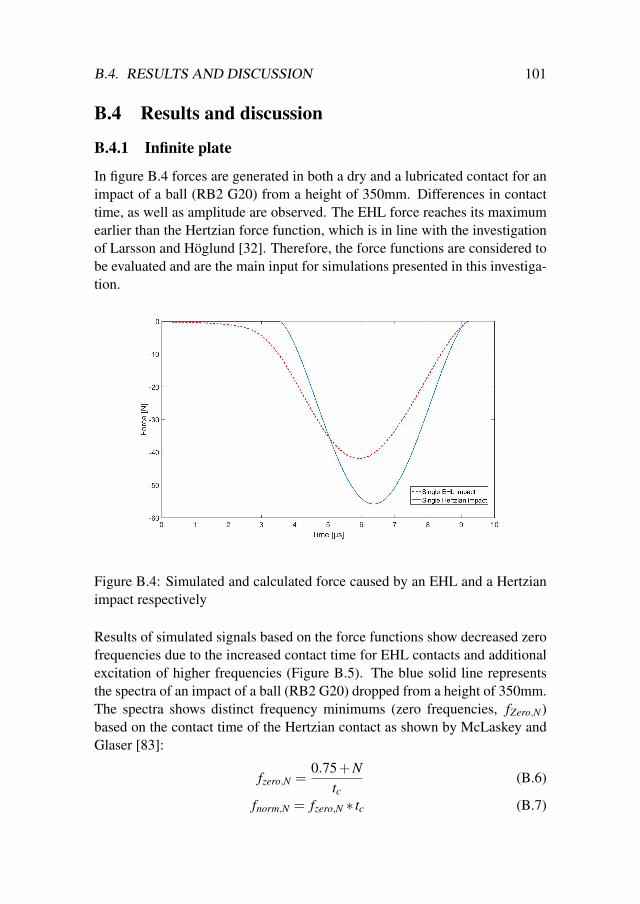
B.4. RESULTS AND DISCUSSION 101
B.4 Results and discussion
B.4.1 Infinite plate
In figure B.4 forces are generated in both a dry and a lubricated contact for animpact of a ball (RB2 G20) from a height of 350mm. Differences in contacttime, as well as amplitude are observed. The EHL force reaches its maximumearlier than the Hertzian force function, which is in line with the investigationof Larsson and Höglund [32]. Therefore, the force functions are considered tobe evaluated and are the main input for simulations presented in this investiga-tion.
Figure B.4: Simulated and calculated force caused by an EHL and a Hertzianimpact respectively
Results of simulated signals based on the force functions show decreased zerofrequencies due to the increased contact time for EHL contacts and additionalexcitation of higher frequencies (Figure B.5). The blue solid line representsthe spectra of an impact of a ball (RB2 G20) dropped from a height of 350mm.The spectra shows distinct frequency minimums (zero frequencies, fZero,N)based on the contact time of the Hertzian contact as shown by McLaskey andGlaser [83]:
fzero,N =0.75+N
tc(B.6)
fnorm,N = fzero,N ∗ tc (B.7)

102 PAPER B. SINGLE EHL CONTACT
The red dashed line shows the spectra of the simulated EHL impact. Com-
Figure B.5: Simulated spectra of signals of Hertzian and EHL impacts with aball (RB2 G20) dropped from 350mm height
paring the spectra to the Hertzian impact shows zero frequencies shift to-wards lower frequencies. Using equation (B.7) gives in indication of expectedpositions of frequency minimums. While Hertzian zero frequencies agreewith McLaskey’s and Glaser’s [83] suggested positions ( fnorm,N = [1.75, 2.75,3.75]), zero frequencies for EHL impacts shift according to the simulation to1.61 and 2.53. The third zero frequency cannot be identified, which can be acause of cavitation. As Zong et al. [93] demonstrate cavitation excites highfrequencies, which would be in line with covering zero frequencies such as inthis case for third order and higher orders.Figure B.6 shows the comparison of simulation (blue dashed line) and mea-sured (yellow solid line) signals for a Hertzian impact. As an earlier inves-tigation [83] showed, agreement is good and could be replicated for this in-vestigation. This demonstrates that Hertzian measurement is a good referencemeasurement. A slight overestimation of the simulated signal can be seen,which is especially interesting if compared to Figure B.7 (Comparison of EHLimpacts). For EHL impacts the simulation (red dashed line) underestimatesthe measured signal (green solid line). The overestimation in the Hertzian caseis known [83], but the underestimation in the EHL case was not previouslyknown. This overestimation become even more contradictory when the lubri-cant layer is taken into account. Instead of having an interface of steel and air,

B.4. RESULTS AND DISCUSSION 103
Figure B.6: Comparison of simulated and measured spectra of Hertzian im-pacts with a ball (RB2 G20) dropped from 350mm height
Figure B.7: Comparison of simulated and measured spectra of EHL impactswith a ball (RB2 G20) dropped from 350mm height
the interface on the upper part of the plate consists of steel and lubricant. Thisaffects the reflection coefficient (B.8), which decreases due to an increase ofdensity (ρ2 increases). A change of reflection coefficient was ot taking intoaccount by using Hsu’s script [91] for Green’s function. One explanation for

104 PAPER B. SINGLE EHL CONTACT
the increase in the amplitude even though the reflection coefficient decreased,could be the improved transmission of the exciting force. As couplants areused to improve transmission to the sensor, the lubricant could act as a cou-plant to improve transmission of the initial excitation.
RC =Z2−Z1
Z2 +Z1=
cp2ρ2− cp1ρ1
cp2ρ2 + cp1ρ1(B.8)
Furthermore, it can be seen in figure B.7 that the effect of covering third andhigher order zero frequencies (possibly due to cavitation) predicted by the sim-ulation is also observed for measured signals. The position of the zero frequen-
Figure B.8: Zero frequencies of first and second order, normalized to the Hert-zian reference contact time for different drop heights and ball sizes.
cies, however, do differ between simulated and measured signals. Instead of ashift towards lower frequencies, as suggested by the simulation, zero frequen-cies of an EHL impact shift towards higher frequencies when compared to theHertzian reference impact. This is even more apparent in figure B.8 where nor-malized zero frequencies for all test conditions of the infinite plate are shown.
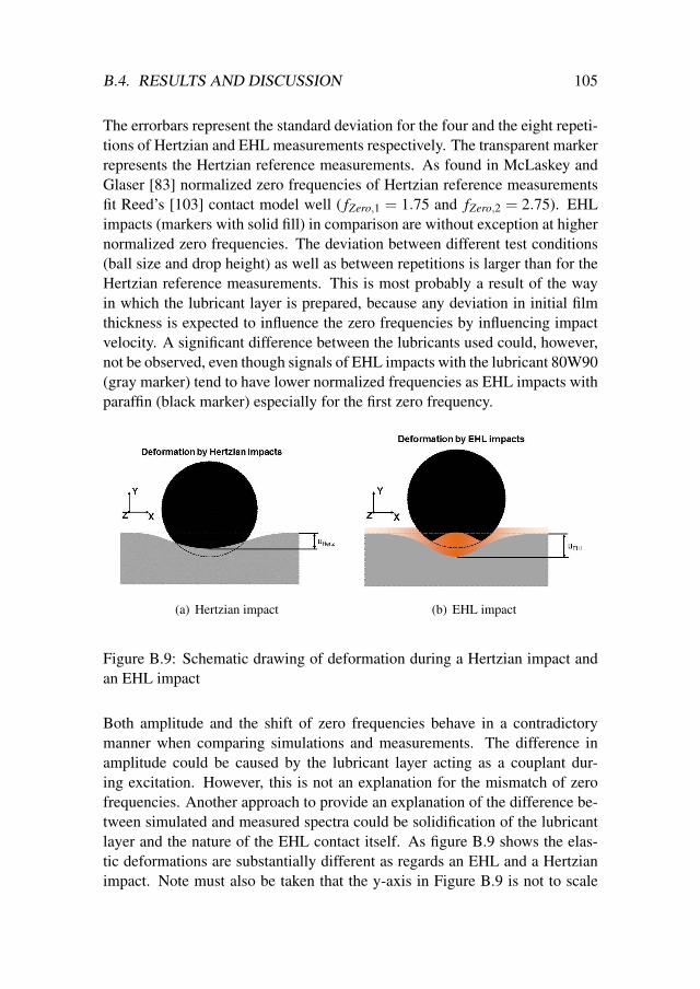
B.4. RESULTS AND DISCUSSION 105
The errorbars represent the standard deviation for the four and the eight repeti-tions of Hertzian and EHL measurements respectively. The transparent markerrepresents the Hertzian reference measurements. As found in McLaskey andGlaser [83] normalized zero frequencies of Hertzian reference measurementsfit Reed’s [103] contact model well ( fZero,1 = 1.75 and fZero,2 = 2.75). EHLimpacts (markers with solid fill) in comparison are without exception at highernormalized zero frequencies. The deviation between different test conditions(ball size and drop height) as well as between repetitions is larger than for theHertzian reference measurements. This is most probably a result of the wayin which the lubricant layer is prepared, because any deviation in initial filmthickness is expected to influence the zero frequencies by influencing impactvelocity. A significant difference between the lubricants used could, however,not be observed, even though signals of EHL impacts with the lubricant 80W90(gray marker) tend to have lower normalized frequencies as EHL impacts withparaffin (black marker) especially for the first zero frequency.
(a) Hertzian impact (b) EHL impact
Figure B.9: Schematic drawing of deformation during a Hertzian impact andan EHL impact
Both amplitude and the shift of zero frequencies behave in a contradictorymanner when comparing simulations and measurements. The difference inamplitude could be caused by the lubricant layer acting as a couplant dur-ing excitation. However, this is not an explanation for the mismatch of zerofrequencies. Another approach to provide an explanation of the difference be-tween simulated and measured spectra could be solidification of the lubricantlayer and the nature of the EHL contact itself. As figure B.9 shows the elas-tic deformations are substantially different as regards an EHL and a Hertzianimpact. Note must also be taken that the y-axis in Figure B.9 is not to scale

106 PAPER B. SINGLE EHL CONTACT
and deformations therefore are highly emphasized, in order to show basic dif-ferences with and without lubricant. While the Hertzian impact (Figure B.9-a)results in a uniform deformation of both plate and ball, the EHL impact (Fig-ure B.9-b) results in a deformation that is more localized due to the partlysolidified lubricant (indicated by the color scheme). Furthermore, the maxi-mum deformation is larger in the EHL case compared to Hertzian impact forthe center position, as was previously observed by Larsson and Höglund [32].Simulations in this investigation are based on a point assumption. A globalforce function is applied at a single point assuming the contact area is so smallthat it can be considered to be a single point. However, this assumption alsoimplies that deformations within the contact area are uniform so that the globalforce function may be used, which might be true for the Hertzian impact, butis definitely violated by the EHL impact. The difference on a local scale couldbe the cause of both amplitude (Higher maximum deformation for EHL im-pacts) and frequency shift (localized faster deformation changes). A possiblesolution for future investigations could be to use the Green’s function approachto transfer deformations within the system instead of global forces coupled todeformations by fully elastic models.
B.4.2 Boundary restricted system
Figure B.10: Comparison of resonances in the boundary restricted system forHertzian and EHL impacts of a ball (RB4 G20) dropped from 350mm height
A previously study [107] showed that an elastic wave excited by Hertzian con-tacts in boundary restricted systems reduces to a resonance problem once wave

B.5. SUMMARY 107
Figure B.11: Comparison of resonances in the boundary restricted system EHLimpacts with different ball sizes dropped from 350mm height
and source interact. As figure B.10 shows the difference in excitation force be-tween EHL impact and Hertz impact does not influence the measured signal.With both excitations identical resonances are triggered and the spectra are al-most identical, except for an additional spike in between resonances for theHertzian excitation.A change in impact energy by changing ball size only influenced the ampli-tudes (figure B.11) of the resonances, which is also in line with previous Hert-zian investigations [107]. However, a change in ball size does influence theresonance cut off, due to the change of contact time. For Hertzian impact the-20dB cut off and the first zero frequency agree to a high extent [107]. In thecase of EHL impacts it was found that resonance cut offs occur much earlier.As figure B.12 shows the Hertzian contact (blue dashed line) excites to a higherdegree higher resonances in comparison with an EHL contact (red solid line).A reason for the earlier cut off could be the damping of the EHL film whencompared with the dry Hertzian impact.
B.5 Summary
In this study a simulated spectrum, based on a Green’s function approach,and excited by an EHL contact is presented. The simulated spectrum partlyshowed good agreement with measured elastic waves. The overall shape ofthe spectrum and a covering of zero frequencies of higher order (3rd order and

108 PAPER B. SINGLE EHL CONTACT
Figure B.12: comparison of normalized spectra of signals excited by Hertzianand EHL impacts
higher), most probably due to cavitation, was observed on both measured andsimulated spectra. However, the zero frequencies of simulation and measure-ment do not match. This could be caused by the point assumption used inthe Green’s function approach. It is, therefore, suggested that in future inves-tigations of EHL contacts a Green’s function approach based on deformationrather than on global force be used. The measured normalized zero frequencieswere found to be higher for EHL excited elastic waves than for those excitedby a Hertzian contact. A significant differentiation of normalized zero fre-quencies due to different lubricants could not be observed, due to relative largedeviations between repetitions, but the lubricant with higher viscosity tendedto have lower normalized first zero frequencies. Additionally, it was observedthat boundary restricted systems excited by EHL impacts resulted in the sameresonance behavior as for Hertzian excited systems. The only observed differ-ence was a damping of resonances at higher frequencies, which is most likelycaused by the lubrication film.

B.6. ACKNOWLEDGMENTS 109
B.6 Acknowledgments
The authors would like to acknowledge the financial support of SKF and VIN-NOVA (Grant number: Smarta-maskiner, 2013-5575), as well as the helpfuldiscussions with SKF-researchers, among them especially Dr. Florin Tatar,SKF-ERC, Netherlands.


Paper C
Contact time andevent frequency
111


113
Submitted to Proceedings of the Institution of Mechanical Engineers,Part J: Journal of Engineering Tribology
The influence of contact time and event frequency onacoustic emission signals
S. Schnabel1,3, S. Golling2, P. Marklund1,3, R. Larsson1,3
1)Luleå University of Technology, SKF-University Technology centre2)Luleå University of Technology, Division of Solid Mechanics,
3)Luleå University of Technology, Division of Machine Elements,SE-97187 Luleå, Sweden
Abstract Studies of acoustic emission of rotating machine elements is oftenperformed under constant speed. There are few investigations on speed andcontact time dependency of acoustic emission signals, even tough some in-vestigations have reported difficulties at elevated rotational speeds. Simplifiedexperiments are, therefore, presented in this article to increase understandingof time dependency of acoustic emission signals. Hertzian impacts and tensiletests are used to study contact time, the time duration of an event and off-set time, the time between events, accordingly event frequency. The resultsof these model experiments indicate an indirect quadratic proportionality ofacoustic emission amplitudes and contact time (umax ∝ 1/(t2
c )), as well as aproportional relation between root mean square (RMS) and event frequency(RMS ∝ fevent ∝ 1/to f f set). The relationship between contact time and RMS ofacoustic emission signals is strongly dependent on the damping of the system.
Keywords: Hertz contact, Elastic waves, Acoustic Emission, RMS, Activationcounts, condition monitoring, Rolling element bearing

114 PAPER C. TIME DEPENDENCY
C.1 Introduction
Acoustic emission is today a frequently used monitoring tool for research intribology and is also used in some industrial applications as a complement tovibration analysis. For laboratory tests researchers have linked acoustic emis-sion successfully to particle contamination [48, 71], lubrication regime [52],lubricant [46, 49], failure size [73] and failure propagation [53]. Thereby re-searchers have proven acoustic emission is capable both of monitoring operat-ing conditions and of detecting failures in rolling element bearings. However,there is a huge discrepancy between reported laboratory scale tests and re-ported field tests. While many researchers provide laboratory results, no fieldtest for acoustic emission measurements could be found in the field of tribol-ogy. Other fields have reported field tests, but all of them are static cases, likethe crack propagations on steel bridges [108] or health monitoring of bendingwind turbine blades [109]. Furthermore, all mentioned laboratory investiga-tions [46,48,49,52,53,70–73] use single speed test setups, where they monitorbearings at a certain speed at a time. Additionally many researchers focus onslow rotating applications [53, 70–72], whereas investigations on high speedapplications, such as Feng et al. [110], are rare.McFadden and Smith [67] reported difficulties of failure detection with acous-tic emission measurements in combination with elevated speeds. In combina-tion with the huge amount of investigations focusing on low speeds, the re-ported difficulties of McFadden and Smith [67] indicates a speed dependencyof acoustic emissions of rolling element bearings that is not fully understood.Rolling element bearings in industrial applications are often exposed to speedvariations and start stop cycles, which makes it important to understand thespeed dependency of acoustic emission signals. The few investigations thatinclude speed variation in their experimental setup use either a different tribo-logical system such as journal bearings [80] or have another focus than speeddependency in their analysis [111]. Therefore an initial investigation was car-ried out, which addresses the problem of speed dependency of acoustic emis-sion signals.Instead of using a full rolling element bearing setup up to investigate the de-pendency of rotational speed, this study investigates experiments that are evenfurther simplified such as ball bounces and tensile tests. The ball bouncing testsetup is simplified to study changes of contact time. Contact time in a rollingelement bearing is the time the rolling element needs to pass the width of itsown contact area. The tensile test with varied speeds is intended to representgiven acoustic emission events where occurrence frequency is speed depen-

C.2. BACKGROUND 115
dent. Examples of such events with speed dependent occurrence can be overrolling of contaminants (for a given concentration) or asperity interaction be-tween either rolling element and raceway or rolling element and cage.When it comes to acoustic emission as a monitoring tool measures like RMS(root mean square) [46, 52, 73], amplitudes [70, 72] and activationcounts (AC) [48, 49, 71] are often used. Therefore, this article focuses on thetime dependency of RMS values and amplitude values of acoustic emissionsignals. The fundamental results obtained from these simplified experimentsmay be considered as a basis for future investigations on more complex sys-tems such as rolling element bearings.
C.2 Background
According to ASTM standard [92] acoustic emission is the phenomena of tran-sient elastic waves caused by rapid releases of energy. Based on this definitionit is assumed in this study that all acoustic emission signals can be describedas a series of force pulses as shown in figure C.1, where the pulses can varyin amplitude ( fmax) and duration (tc). The time between different pulses willbe defined as offset time (to f f set). The use of such a simple model for acoustic
Figure C.1: Schematic drawing of acoustic emission events based on theASTM definition for acoustic emission
sources reduces time dependent variables to pulse duration time (tc) and eventfrequency ( fevent = (to f f set)
−1). The investigation of one variable at a time willlead to an increased understanding of principles for the time dependency of

116 PAPER C. TIME DEPENDENCY
acoustic emission signals.
C.2.1 Hertzian impacts for variation of pulse duration time
In order to investigate the influence of (tc) a herztian impact was chosen. Suchan elastic impact of a ball on a solid plate causes a force pulse (Figure C.2)which is variable in duration time and amplitude by varying impact velocity(v0) and ball radius (R). Based on Reed’s [103] model for fully elastic im-pacts (C.1), both amplitude (C.2) and duration time (C.3) of the force pulsecan be calculated.
f (t) =− fmax sin(πt/tc)3/2 , 0≤ t ≤ tcf (t) = 0 , t < 0 and t > tc (C.1)
fmax = 1.917ρ3/51 (δ1 +δ2)
−2/5R21v6/5
0 (C.2)
tc = 4.53(4ρ1π(δ1 +δ2)/3)2/5R1v−1/50 (C.3)
where δi =1−ν2
i
πEi
Reed’s contact model is based on material properties such as elastic modu-lus (Ei), Poisson’s ratio(νi) and density (ρi), where the indexes (i) refer toball (i = 1) and plate (i = 2). By using steel balls and a steel plate, impact ve-locity (v0) and ball radius (R) are the remaining variables to control amplitudeand contact time.
C.2.2 Tensile tests as a variation of the event frequency
Richter et al. [56] have reported increased and repeatable acoustic emissionactivity around the yielding point. The main mechanism of plasticity at thatpoint is plane slip movement as stated by Taylor [112]. Plane slip in crystalstructures or metals is according to Taylor [112] a rapid and digital phenom-ena due to the equilibriums in the crystal structure. The force to overcomeequilibrium state is calculated for plane slip according to the Peach-Koehlerequation [113] for movement of dislocations. At the grain boundaries dislo-cations introduce stress, which results in either micro fracture or plastic graindeformation [114]. For both cases the duration time, the transition from oneequilibrium to another, is much shorter than the time interval between two sam-ples of acoustic emission measurements. It is, therefore, in this investigation

C.3. EXPERIMENTAL SETUP 117
Figure C.2: Force pulse of a single Hertzian contact calculated according toReed’s model for elastic impacts
assumed that excitation forces in the tensile test are delta impulses of differ-ent amplitudes. Both force amplitude and direction of these delta impulses aredependent on the Burgers vector and thereby on the crystal’s structure and ori-entations of the grains. However, it is assumed that the global elastic wave isindependent of grain orientation and the dislocation’s position within a tensiletest sample due to the stochastic nature of grain orientation and dislocation’spositions. Based on these assumptions different speeds in tensile tests willinfluence the offset time without influencing excitations due to the slip phe-nomena mentioned above, which means change in speed will be proportionalto the event frequency (vtensile ∝ fevent).
C.3 Experimental Setup
For all tests an accelerometer (WSal pha) from Physical Acoustics was used.The sensor was in both test setups attached by beeswax to the test sample.Beeswax thereby acted both as a glue and a couplant. First the beeswaxwas applied to the test samples and after heating it to 75◦C the sensor waspressed onto the sample. When both couplant and sample had cooled down toroom temperature the tests were started. The sensor signal was amplified by apreamplifier (Physical Acoustic 2/4/6C) and digitally stored with a 14-bit PCI-digitizer (GaGe OSC-432-007). The measured signal was bandpass filtered by

118 PAPER C. TIME DEPENDENCY
the preamplifier (100kHz to 1.2MHz).
C.3.1 Hertzian impact setup
Figure C.3 shows the schematic setup for Hertzian impact experiments. Thesensor was attached to a steel plate (Toolox 40) with the dimensionsof 1.0x0.5x0.51m and excited by Hertzian impact through ball drops. Ballswere dropped using a spherical magnetic holder. The spherical shape of themagnetic holder allowed a drop of the balls, which hit the plate verticallyaligned to the sensor position, with minimal spin and perfect free fall. Theplate was resting on two supporting rubber line contacts.
Figure C.3: Schematic drawing of the setup for experiments on Hertzian im-pacts
Size and corresponding drop height are shown in Table C.1. Size and dropheight were matched based on equation C.2 and C.3 to have a constant forceamplitude of -50N, so that the impulses only varied by contact time (Fig-ure C.4). Each test was repeated 8 times and signals were recorded for 6mswith a pretrigger of 50µs. The recorded signal was stored with a sample rate

C.3. EXPERIMENTAL SETUP 119
Table C.1: Test setup
test-no. Ball samples Ball radius drop heights
1 RB2 G20 1.0mm 295mm2 RB3 G20 1.5mm 76mm3 RB4 G20 2.0mm 29mm4 RB6 G20 3.0mm 7.55mm5 RB8 G20 4.0mm 3mm
of 10 Msamples/s and amplified by 40dB.
Figure C.4: Calculated impact forces for different tests configurations (Ta-ble C.1) based on Reed’s model for elastic impacts.
C.3.2 Tensile tests setup
For the tensile test ferrite steel samples were used, due its single phase andbeneficial structure as explained in Section C.2.2 The dimension of the samplesare shown in Figure C.5 and is valid for all tensile test samples used in thisinvestigation. Two-thirds of the broad end parts of the samples were clampedby hydraulic activated grips in the tensile tester, which consisted of a hydraulictest frame for tension and compression from the supplier Dartec combined

120 PAPER C. TIME DEPENDENCY
with a control unit of Instron. The used tensile tester has a maximum capacityof 250kN.The tensile tests were carried out at six different speeds (0.03mm/s, 0.07mm/s,0.1mm/s, 0.3mm/s, 0.7mm/s and 1.0mm/s). The range was thereby limited bythe control circuit of the tensile test machine, which was not able to maintain aconstant speed above 1.0mm/s. The lower range of the test speed was limitedby the acoustic emission measurement. For speeds lower than 0.03mm/s thetests would have been longer than the maximum storage time. The used speedrange required to reduce the sample rate to 5 Msamples/s to limit the maximumstorage time to 132s, due to the capacity of the internal storage (2GB) of thedigitizer card.
Figure C.5: Schematic drawing of the dimensions of the tensile test specimensand the sensor position. Dimensions are in mm.
During the tensile tests, applied force, cylinder position of the tensile tester,extension of the test sample and acoustic emission were recorded. All signalswere triggered by a TTL signal in order to synchronize them. Both force andextension were recorded with a sample frequency of 50Hz. The measurementof the actual extension was processed to obtain a measure in percent, based onthe initial length of the extensiometer (50mm). Force measurements were usedwithout further treatment of the data.The acoustic emission sensor was as for the Hertzian impact tests attached withbeeswax and the sensor position can be seen in Figure C.5.

C.4. RESULTS 121
C.4 Results
Results of this investigation are divided in two sections. In Section C.4.1 re-sults of the acoustic waves excited by ball impacts are presented. Both am-plitude and RMS values of signals were analyzed with respect to the contacttime. The results of tensile tests are presented in Section C.4.2, where ampli-tudes and RMS values were analyzed with respect to displacement speed ofthe tensile tests.
C.4.1 Hetzian impact
As shown in Figure C.6, signals obtained by Hertzian impacts were excitationswith extremely low damping, due to the test setup and the size of the excitedplate. These signals were rectified by post processing of the data and short-ened to 1ms of measurement plus the pretrigger signal of 50µs (Figure C.7).
Figure C.6: Raw acoustic emission signal obtained from a Hertzian impact
The given geometry leads to theoretical reflection times of 88µs and 171µsfor length and depth respectively, which is the cause of the modulation of thesignals as shown in Figure C.7. There are both peak to peak intervals and min-imum to minimum intervals which are multiples of the reflection time. Thesepost processed signals were then analyzed with respect to the contact time(tc) (C.3) of the Hertzian excitation of the ball bounces.Figure C.8 shows the 10 highest values of the post processed signals (Fig-ure C.7) for all Hertzian excitations. As mentioned in section C.1 all Hertzian

122 PAPER C. TIME DEPENDENCY
Figure C.7: Rectified signal of the acoustic emission sensor
Figure C.8: Peak values of acoustic emission signals with respect to contacttime for impacts with equal force
impacts were repeated 8 times. The error bars represent the deviations foreach maximum value and excitation within these eight repetitions. Figure C.8
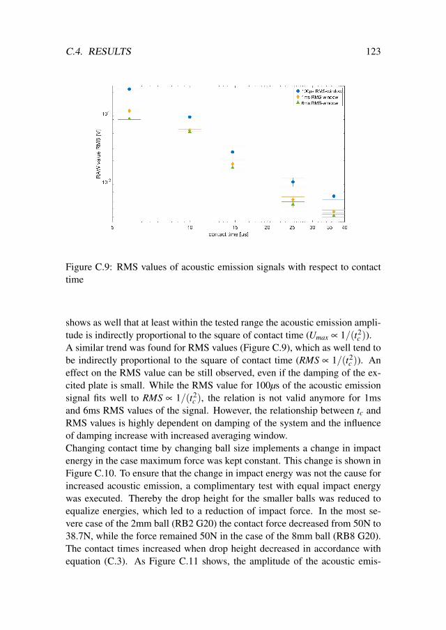
C.4. RESULTS 123
Figure C.9: RMS values of acoustic emission signals with respect to contacttime
shows as well that at least within the tested range the acoustic emission ampli-tude is indirectly proportional to the square of contact time (Umax ∝ 1/(t2
c )).A similar trend was found for RMS values (Figure C.9), which as well tend tobe indirectly proportional to the square of contact time (RMS ∝ 1/(t2
c )). Aneffect on the RMS value can be still observed, even if the damping of the ex-cited plate is small. While the RMS value for 100µs of the acoustic emissionsignal fits well to RMS ∝ 1/(t2
c ), the relation is not valid anymore for 1msand 6ms RMS values of the signal. However, the relationship between tc andRMS values is highly dependent on damping of the system and the influenceof damping increase with increased averaging window.Changing contact time by changing ball size implements a change in impactenergy in the case maximum force was kept constant. This change is shown inFigure C.10. To ensure that the change in impact energy was not the cause forincreased acoustic emission, a complimentary test with equal impact energywas executed. Thereby the drop height for the smaller balls was reduced toequalize energies, which led to a reduction of impact force. In the most se-vere case of the 2mm ball (RB2 G20) the contact force decreased from 50N to38.7N, while the force remained 50N in the case of the 8mm ball (RB8 G20).The contact times increased when drop height decreased in accordance withequation (C.3). As Figure C.11 shows, the amplitude of the acoustic emis-

124 PAPER C. TIME DEPENDENCY
Figure C.10: Impact energy for the tests executed with various ball size andwith an equal force
Figure C.11: Peak values of acoustic emission signals with respect to contacttime for impacts with equal impact energy
sion signal, even for equal impact energies, is strongly dependent on contacttime. However, the inclination of the slope in the double logarithmic scale is

C.4. RESULTS 125
smaller when compared to the tests with equal force (Figure C.8). This af-fects the dependency between contact time and acoustic emission amplitude(Umax ∝ 1/(t2
c )→ Umax ∝ 1/(t1.9c )), but a strong dependency of contact time
and amplitude of the acoustic emission signal is still shown.
C.4.2 Tensile tests
Figure C.12: Force and acoustic emission of a whole tensile test (results shownare executed with a speed of 0.7mm/s)
A representative result for force and acoustic emission measurement of thetensile tests (speed 0.7mm/s in this case) is shown in figure C.12. These re-sults are in line with the observations of Richter et al. [56] of increased activityof acoustic emission at the yielding point. The increased acoustic emissionactivity after an initial elastic phase with lower AE activity is even more pro-nounced in Figure C.13 where parts from crack initiation and propagation wereexcluded by zooming in at the initial part of an AE signal of a tensile test, tofocus only on the elastic plastic regime.To analyze the signal with respect to speed around the yielding point, bothforce and acoustic emission measurements were converted to displacementbased signals. As Figure C.15 shows that force measurement (Figure C.15a)
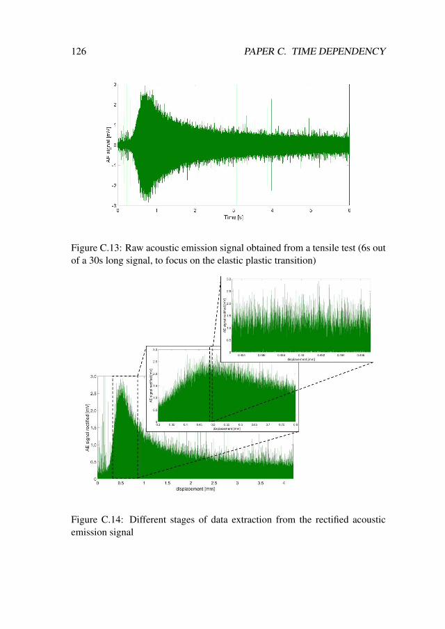
126 PAPER C. TIME DEPENDENCY
Figure C.13: Raw acoustic emission signal obtained from a tensile test (6s outof a 30s long signal, to focus on the elastic plastic transition)
Figure C.14: Different stages of data extraction from the rectified acousticemission signal
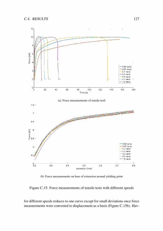
C.4. RESULTS 127
(a) Force measurements of tensile testl
(b) Force measurements on base of extension around yielding point
Figure C.15: Force measurements of tensile tests with different speeds
for different speeds reduces to one curve except for small deviations once forcemeasurements were converted to displacement as a basis (Figure C.15b). Hav-

128 PAPER C. TIME DEPENDENCY
ing assured equal force for all experiments only speed is left as a cause forchanges of the acoustic emission signal.At first acoustic emission signals were rectified by post processing identical tothe processing of signals of the Hertzian impact (Figure C.14). Converting sig-nals to a displacement basis through simple multiplication of the time step andthe speed of the test sample then followed. The signals were reduced to signalsaround the yielding point, after transforming signals from a time step basis toa displacement basis. In cases of this study the data was reduced to signalsbetween 0.3mm and 0.8mm displacement (Figure C.14), which correspondedto the region around the yield point. In Figure C.16 signals are rectified forall the tested speeds presented. Even without further analysis a clear speeddependency on the acoustic emission signals of the executed tensile tests canbe seen.
Figure C.16: Rectified acoustic emission signal around the yielding point
To extract more detailed information about the speed dependency, the point ofmaximum amplitude was extracted for every curve. In order to avoid maximafrom local spikes, a moving average with a window of 0.05mm displacementwas used. This extracted point for every test was used to extract RMS valuesat the Maximum (dmax) itself and at a PreMaximum point (dmax− 0.1mm), aswell as at a PostMaximum point (dmax +0.1mm). The window size of the ex-tracted RMS values respresents in all cases 20ms. These extracted RMS valuesare shown in Figure C.17. The error bars represent therefore, the variation inspeed within the analyzed signal (0.3mm to 0.8mm displacement) and error

C.5. DISCUSSION 129
bars for a certain test speed are equal therefore. The figure shows as well thatthe speed dependency for the tensile test is linear. In combination with thetheoretical background presented in Section 2 (vtensile ∝ fevent), these resultssuggest a linear dependency between the RMS value of the acoustic emissionsignal and the event frequency (RMS ∝ fevent ∝ 1/to f f set).
Figure C.17: Rectified acoustic emission signal around the yielding point
C.5 Discussion
The following dependencies are indicated by the results:
• RMS ∝ fevent ∝ 1/to f f set
• umax ∝ 1/t2c (for constant force)
• RMS ∝ 1/t2c (for constant force and low level of damping)
These dependencies are require systems with low level of damping and a shortaveraging window of the RMS signal. The dependencies hold true even whenmeasurement inaccuracies and repeatability of the results are taken into ac-count. However, further validation with additional sensors and experimentalsetups are suggested to investigate influence of sensor, sensor mounting andsystem damping on the speed dependency of acoustic emission.

130 PAPER C. TIME DEPENDENCY
Furthermore, this investigation is based on simplified experiments, which leadsto the matter of transferability. In the case of a rolling element bearing, resultscannot be transfered directly without further investigation, because of the com-plexity of the elasto-hydrodynamic lubricated (EHL) contact. High frequencyemissions in an EHL contact can have several causes, such as stress waves oftransient forces, elastic-plastic deformations on a micro scale or asperity inter-action of the two surfaces. These sources may change both event frequency andcontact time not just with a change of rotational speed, but most likely as wellwith changes of Slide-to-roll ratio, load and film thickness among other vari-ables. The results of this investigation can not therefore, be adapted to complexsystems like rolling element bearings straight away. The results should insteadbe seen as a basis for investigations on more complex systems.
C.6 Conclusions
It is concluded that the article has shown changes in contact time and event fre-quency have two different impacts on both amplitude and RMS values. Whileboth amplitude and RMS value increases quadratically with a reduction ofcontact time, the RMS value increases linearly with an increase of event fre-quency. Furthermore it is concluded that simplified experiments have provento be a good supplement for full bearing tests in an early stage of investigation.
C.7 Acknowledgments
The authors would like to acknowledge the financial support of SKF and VIN-NOVA, as well as the helpful discussions with SKF-researchers, among themespecially Dr. Florin Tatar, SKF-ERC, Netherlands.

Paper D
Short term effect of Fe3O4particles
131


133
Published by Proceedings of the Institution of Mechanical Engineers,Part J: Journal of Engineering Tribology
Study of the short term effect of Fe3O4 particles in rollingelement bearings
Observation of vibration, friction and change of surface topography ofcontaminated angular contact ball bearings
S. Schnabel, P. Marklund, R. Larsson
Luleå University of Technology, Division of Machine Elements,SE-97187 Luleå, Sweden
Abstract The harsh environment rolling element bearings are exposed to iniron mining industries is replicated in a laboratory scale in this work. Bearings(SKF 7204BEP) were tested both with and without magnetite oxide (Fe3O4)contamination. In order to study the interaction between contaminants andextreme pressure (EP) additives the rolling element bearings were lubricatedwith two different greases. A grease without EP and a grease containing sulfurbased EP additives were used. Further the effect of the contamination-additiveinteraction on rolling bearing performance and monitoring signals (vibrationand acoustic emission) was investigated. The obtained results indicate an ad-vantage of EP additive in case of the investigated operating conditions. More indetail the use of EP additives decreased wear, surface roughness, vibration andacoustic emission for both test durations of 24 and 168 hours. The decreaseof the acoustic emissions and the surface roughness parameter Rq in case ofthe tests with a duration of 168h as high as 70 % and 60 % respectively usingEP additives in comparison with the plain grease were observed. The majorcause for this reduction seems to be the interaction between contaminants andEP additives.
Keywords: Rolling element bearing, condition monitoring, contaminants, ex-treme pressure (EP) additives
134 PAPER D. SHORT TERM EFFECT OF FE3O4 PARTICLES
D.1 Introduction
Rolling element bearings located in the production lines of mining industriesare mainly affected by the contamination of iron ore particles. This contami-nation leads to a significant shortening of the bearing life and decrease therebythe productivity due to standstills. Even the use of advanced sealing and lu-brication systems can not prevent the significant decrease of the life of rollingbearings working in the mining environment.Third body abrasive wear due to contamination is a common failure sourceof rolling element bearings [115]. As a result, many researchers have inves-tigated the effect of contamination on rolling element bearing performance,bearing life time and the detection of debris. In these investigations differenttypes of contaminants were used. The most common used contaminant is sil-ica [48, 96, 116–118], but diamonds [115] and iron oxides [48, 96] were alsoused.While Sayles and Ioannides [119, 120] as well as Gabelli et al. [121] investi-gated the influence of debris on fatigue life of rolling element bearings and itsstatistical calculation, did other authors focus on the performance of the EHLcontact itself. The wear behavior of EHL contacts and the particle movementwere studied by Dwyer-Joyce et al. [115]. The same research team character-ized the probability of particles entering the contact with the result that wearincreases with increased particles size due to the higher probability that par-ticle enter the EHL contact [122]. A more industrial focused summary onrolling bearing performance with contaminated lubricants was carried out byWennehorst and Poll [123].Vibration and acoustic emission are common tools to monitor contaminatedbearings. Both Maru et al. [118] and Tandon et al. [96] have investigatedthe effect of particle size and concentration on rolling element bearings, us-ing either oil and vibration [118] or grease and acoustic emission [96] fortheir test setups. The wear behavior of contaminated bearings were studiedby Kahlman et. al. [117] and Akagaki et. al. [104] using both vibration andsurface imaging techniques. Another investigation using vibration as a moni-toring tool was carried out by Hariharan and Srinivasan [116]. They showedthe interaction of the root mean square (RMS) of the vibration signal and therotational speed of the bearing at different concentrations of contamination.But the type of particles has also an influence on the signals of the monitor-ing tools, like Miettinen and Andersson, [48] have shown. In their work theypresented the activity of the acoustic emission signal for steel, iron, FexOy andquartz particles.

D.2. EXPERIMENTAL SETUP 135
Even though iron oxides were used in previous studies [48, 96], they focusedmore on the detection of the contaminants rather than the influence on therolling element bearing. Further, do the previous investigations not take theeffect of additives into account. Some studies [48, 124] use different base oilsin order to examine the effect of base oil properties on a contaminated contact.However knowledge about the effect and mechanisms of additives on contam-inated systems is missing. Therefore this work was carried out to study theshort term effect of contamination on surface topography of raceways, vibra-tion and acoustic emission signals with respect to the type of lubricant.
D.2 Experimental setup
The test samples were prepared in a laboratory environment and the all testsetups were executed at room temperature.
D.2.1 Rolling bearing test rig
The investigation was carried out in an in-house built rolling bearing test rig(Figures D.1 and D.2). The principle of the rig is based on a free moving bear-ing carrier (pos. 4 in Figure D.1) to be able to measure the sum of the frictiontorque from both test bearings (pos. 2 in Figure D.1). The tested bearings areloaded with an axial load by a spring shown in Figure D.2-a. Thereby is themaximum adjustable axial load 2.5 kN.
1: support bearing2: test bearing3: rack4: free moving bearing carrier
Figure D.1: Schematics of the Rolling bearing test rig used for this investiga-tion.

136 PAPER D. SHORT TERM EFFECT OF FE3O4 PARTICLES
The test rig is capable to run with a rotational speed between 100 rpm and2500 rpm, due to a variable frequency drive. The measured variables were incase of the 24 hour tests friction torque and vibrations of the test bearings. Forthe tests with a duration of one week the rig was additionally equipped withacoustic emission sensors. The Friction torque is measured by a force sen-sor connected to a torque arm (Figure D.2-b). A commercial vibration systemcalled WindCon is used to investigate vibrations from the tested bearings [125].The accelerometer (SKF-607M69) was placed in the center of the test bearingcarrier in order to measure vibrations from both test bearings (Figure D.2). Inorder to get as close to the contacts as possible, the acoustic emission sen-sors (CMSS786M) were mounted above each of the tested angular contact ballbearings. The measured frequency ranges are 0-10 kHz for the vibration and0.1-0.5 MHz for the acoustic emission. Both signals where measured with asample storage rate of 0.625Hz. however, the sample rate of the measurementwas 2.56 kHz for the vibration signals and 1.28 MHz for the acoustic emissionsignals. The hardware of the sensors create an envelope signal of the measuredacoustic emission, due to the amount of data, which is otherwise not process-able by the WindCon system.During this investigation mainly the trend analysis function of the WindConsystem was used. The trend value (D.1) in this case is the quadratic meanvalue across the frequency spectrum for one measured sample.
T REND =1n
√√√√ fE
∑i=0
a2i , with n =
fE
∆ f(D.1)
where T REND is the trend value, fE is the end value of the measured fre-quency range, ∆ f is the discretization of the frequency range and ai is theamplitude at a certain frequency. The discretization of the system for the pre-sented results is 1 Hz. The Trend values were calculated for both the vibration,the acoustic emission and their envelope signals respectively. The presentedtrend value diagrams are based on the envelope of the vibration signal and thedouble envelope of the acoustic emission signal. The 40 trend values duringa period of one minute are compared with each other and the highest valueis stored. These stored values within the test duration represent the trend ofvibration and acoustic emission level respectively.

D.2. EXPERIMENTAL SETUP 137
Figure D.2: Image of the free moving bearing carrier. a) top view, b) side view.
D.2.2 Test setup
Eight different test setups were used in the investigation (Table D.1), wherebyfour test setups (test-no 1 to 4) acted as reference samples without contamina-tion. Standard angular contact ball bearings (SKF 7204BEP) were used in all
Table D.1: Test setup
test-no. lubricant type contami-
nation (wt)
number of
samples
test duration
[h]
1 SL12-602 0% 2 242 1 1683 SL12-603 0% 2 244 1 1685 SL12-602 9.1% 4 246 2 1687 SL12-603 9.1% 4 248 2 168
tests and for each sample one pair of bearings was tested. Before the test thebearings were cleaned by an ultrasonic cleaning in heptane as a solvent andthen lubricated with 3 g of grease. The reference samples were lubricated withuncontaminated grease and the samples of test 5 to 8 were lubricated with a

138 PAPER D. SHORT TERM EFFECT OF FE3O4 PARTICLES
mixture of 3 g grease and 0,3 g magnetite particles (Fe3O4). The size distribu-tion of the contaminant is shown in Figure D.3. The contaminated grease wasmixed in a beaker before it was applied to the bearings.
Figure D.3: Size distribution of the magnetite particles used as contaminants.
The greases SL12-602 and SL12-603 were used as lubricants. SL12-602 (non-EP grease) is a grease with a lithium thickener and a mineral base oil. Antiox-idants are the only additives in the grease. SL12-603 (EP grease) is based onthe grease SL12-602, but contains in addition a sulfur based extreme pressureadditive added to the base oil of the grease.The prepared bearing samples were tested during 24 hours and 168 hours re-spectively. For both cases the bearings were tested at a rotational speed of180rpm and by applying a axial load of 2 kN, which results in a life timeL10h of 147,000 hours. During all tests the friction torque was measured inorder to calculate the coefficient of friction and the vibration trend was mon-itored. In addition to the vibration trend, the trend of the acoustic emissionsignal was monitored for tests with a duration of 168 h. After the test dura-tions of 24 h and 168 h the tested bearings were disassembled and cleaned byultrasonic cleaning in a solvent (heptane) and the surface topography of theraceways was measured. For this measurements a 3D optical interferometryspectroscope (WYKO NT1100) was used.
D.3 Results
All results showed good repeatability and the results of the different test dura-tion are in line with each other. Patterns for surface measurement and trends in

D.3. RESULTS 139
both vibration and acoustic emission measurements are consistent through outthe whole investigation.
D.3.1 Test duration of 24 hours
From a coefficient of friction (COF) point of view, the tests did not indicateany advantage of EP additives. Figure D.4 shows the coefficient of frictionover the test duration of 24 hours. Addition of contaminants as well as EP-additives lead to an increase of COF in comparison to the reference sample.
Figure D.4: Average coefficient of friction over the test duration of 24 hoursfor the used test setups.
The measurements of the surface topography (Figure D.5) on the other handshowed a clear difference between EP and non-EP grease. Analyzing the sur-face features of the images of the raceways (Figure D.5) indicates similaritiesbetween four of the pictures. The image marked with a) is a new bearing, whilethe images b) and c) show tested bearing raceways of the non-EP grease andEP grease references without contamination. In all these samples the grindinggrooves of the manufacturing process are still visible. The grinding groovesstill remain in the sample with EP grease and a 10% particle contamination(Figure D.5-e). However the grinding grooves are not visible for the contami-

140 PAPER D. SHORT TERM EFFECT OF FE3O4 PARTICLES
nated sample without EP-additives, as shown in Figure D.5-d.
Figure D.5: Images of the surface measurements with interferometric spec-troscopy after a test duration of 24 hours. a) unused bearing, b) bearing withnon-EP grease, c) bearing with EP grease, d) contaminated bearing with non-EP grease, e) contaminated bearing with EP grease
Further enable the images (Figure D.5) of the surface topography a analysis ofthe surface roughness . For all uncontaminated tests (Figure D.5-a,b,c) the sur-face roughness parameter Rq is within a range of 100 nm to 130 nm. But forboth contaminated tests (Figure D.5-d,e) the surface roughness has increasedsignificantly. However the increase for tests using EP grease (Figure D.5-e) ismuch lower than for the non-EP grease tests (Figure D.5-d). While the surfaceroughness parameter Rq of non-EP grease samples increase to about 500 nm,the EP grease samples had a end value of about 300 nm. Further are pittingdents only visible for images of the contaminated non-EP grease samples (Fig-ure D.5-d).The vibration signals shown in Figure D.6 are the trend (D.1) of envelope sig-nals with different frequency ranges. Beside test setup 5 (non-EP grease withcontamination) all tests show a constant vibration trend signal. The vibrationtrends of the tests with non-EP grease and contamination are increasing duringthe 24 hours of testing. The end value increases to as much as three times theinitial value, while for all other test-setups (test-no. 1,3,7 of Table D.1) the endvalue does not differ significantly in comparison to the initial one.

D.3. RESULTS 141
(a) Non-EP grease (b) EP grease
(c) Non-EP grease with particle contami-nation
(d) EP grease with particle contamination
Figure D.6: Observation of vibration signal for the different test setups. Yel-low: trend of an envelope signal with a range of 10 Hz-1 kHz. Blue: trend ofan envelope signal with a range of 10 Hz-100 Hz. Observe the difference inscale!
D.3.2 Test duration of 168 hours
The friction behavior (Figure D.7) follows the exact same pattern as the 24hour tests (Figure D.4), where both addition of EP additives and contamina-tion increases the coefficient of friction. The values for COF are decreasingin all cases during a running in period, followed by a period were the COFstabilizes on a certain level. Further does the COF, as expected, fluctuate moreby adding contaminants. Another observation is that the systems without EPadditives and with contamination (Figure D.7-C) have a prolonged running inperiod in comparison to the other test setups.As expected, the surface roughness did not change significantly for the un-contaminated test setups. In comparison to the unused reference sample, witha surface roughness of Rq=100 nm (Figure D.8-a), the surface roughness pa-rameter Rq of the uncontaminated non-EP grease sample (Rq=150 nm, Fig-ure D.8-b) and the EP-grease sample (Rq=115 nm, Figure D.8-c) increasedonly slightly. For the contaminated cases the elevated wear rate seen in the 24hour tests maintained through the 168 hour tests and resulted in even roughersurfaces as seen after the 24 hour tests. Not just the surface roughness increaseduring the 168 hours tests, but also the deviation of the measured surfaceparameters increased for the contaminated samples. The surface roughnessparameter Rq varied from 800 nm to 1000 nm in case of the non-EP grease

142 PAPER D. SHORT TERM EFFECT OF FE3O4 PARTICLES
Figure D.7: Average coefficient of friction over over the test duration of 168hours for the used test setups.
Figure D.8: Images of the surface measurements with interferometric spec-troscopy after a test duration of 168 hours. a) unused bearing, b) bearing withnon-EP grease, c) bearing with EP grease, d) contaminated bearing with non-EP grease, e) contaminated bearing with EP grease

D.3. RESULTS 143
(Figure D.8-d). While Rq for EP-grease samples were measured in between300 nm and 500 nm (Figure D.8-e).
(a) Non-EP grease (b) EP grease
(c) Non-EP grease with particle contami-nation
(d) EP grease with particle contamination
Figure D.9: Observation of vibration signal for the different test setups withan test duration of 168 hours. Red: trend of an envelope signal with a range of10 Hz-100 Hz. Observe the difference in scale!
Comparing the vibration signals from the 24 hour tests and the 168 hour tests(Figures D.6 and D.9) some differences are observed, but the overall patternseems to be maintained throughout both tests. As for the 24 hour tests, the 168hour tests have low constant vibration levels for uncontaminated samples (Fig-ure D.9-a,b) and accelerated vibration levels for the samples contaminated withiron oxide (Figure D.9-c,d). Thereby is in general the vibration level lowerfor samples with EP grease (Figure D.9-d) in comparison to the samples withnon-EP grease (Figure D.9-c). However the increasing trend seen from theprevious 24 hour tests (Figure D.6-c) was not observed for the 168 hour tests(Figure D.9-c).The detection of acoustic emission was only used for the samples with an testduration of 168 hours. But the results of the acoustic emission (Figure D.10)substantiate both the previous mentioned vibration responses of the tests andthe observed differences between uncontaminated and contaminated as well asthe differences between the two types of greases. Especially the difference of

144 PAPER D. SHORT TERM EFFECT OF FE3O4 PARTICLES
(a) Non-EP grease (b) EP grease
(c) Non-EP grease with particle contami-nation
(d) EP grease with particle contamination
Figure D.10: Observation of acoustic emission signal for the different testsetups with an test duration of 168 hours. Circles: trend of the double envelopesignal of test bearing A. Squares: trend of the double envelope signal of testbearing B. Observe the difference in scale!
the acoustic emission between non-EP grease (Figure D.10-c) and EP greaseis even more distinct in compare to the vibration responses. The differences intrend values of the double envelope of the acoustic emission signal of the testsetups no. 6 and no. 8 (Table D.1) were as high as 70%.Ploting the mean values of vibration and acoustic emission signals allows a di-rect comparison of the different test setups (Figure D.11). For all measures thereference samples for non-EP grease and EP grease do not show a significantdifference. Further are all reference measures several factors lower than thecontaminated samples. The clearest difference was observed for the acousticemission signals of the contaminated bearings used during the 168 hour tests.Also the average of the vibration signals of the contaminated tests for both the24 and the 168 hours show a significant difference. However the difference isnot as extreme for the vibration signals in comparison to the acoustic emissionsignals.

D.4. DISCUSSION 145
Figure D.11: Comparison of the average values for vibration and acousticemission between the different test setups
D.4 Discussion
All eight setups with contaminated rolling element bearings simulate the harshenvironment in the iron mining industry and show a difference in vibrationtrend and surface topography already after the relatively short test durationof respectively 24 hours and 168 hours. The observed advantage of EP ad-ditives could have several reasons. The most obvious would be a reactionof the additive with the bearing surfaces in order to form sacrificing layers.The theory would explain the differences in both acoustic emission and vi-bration responses of different test samples as well as the difference in surfaceroughness. But this would not explain the results of the surface topographyimages shown in Figure D.5. The missing grinding grooves of samples withnon-EP grease and contaminations (Figure D.5-d) compared to the other testsamples could be a indication of higher wear rate,which is contradictory to thetheory of sacrificing layers. This difference in wear rate between test setupno. 5 and 7 (Table D.1) could be a result of a possible chemical reactions (D.2)and (D.3) of the sulfur based EP-additive with the contaminants itself.
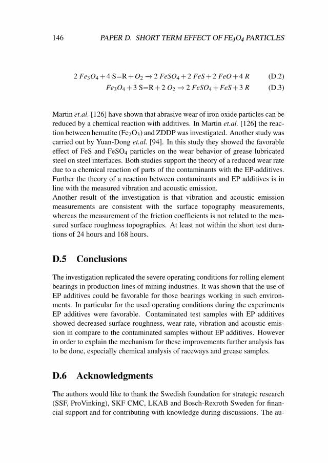
146 PAPER D. SHORT TERM EFFECT OF FE3O4 PARTICLES
2 Fe3O4 +4 S−−R+O2 −→ 2 FeSO4 +2 FeS+2 FeO+4 R (D.2)
Fe3O4 +3 S−−R+2 O2 −→ 2 FeSO4 +FeS+3 R (D.3)
Martin et.al. [126] have shown that abrasive wear of iron oxide particles can bereduced by a chemical reaction with additives. In Martin et.al. [126] the reac-tion between hematite (Fe2O3) and ZDDP was investigated. Another study wascarried out by Yuan-Dong et.al. [94]. In this study they showed the favorableeffect of FeS and FeSO4 particles on the wear behavior of grease lubricatedsteel on steel interfaces. Both studies support the theory of a reduced wear ratedue to a chemical reaction of parts of the contaminants with the EP-additives.Further the theory of a reaction between contaminants and EP additives is inline with the measured vibration and acoustic emission.Another result of the investigation is that vibration and acoustic emissionmeasurements are consistent with the surface topography measurements,whereas the measurement of the friction coefficients is not related to the mea-sured surface roughness topographies. At least not within the short test dura-tions of 24 hours and 168 hours.
D.5 Conclusions
The investigation replicated the severe operating conditions for rolling elementbearings in production lines of mining industries. It was shown that the use ofEP additives could be favorable for those bearings working in such environ-ments. In particular for the used operating conditions during the experimentsEP additives were favorable. Contaminated test samples with EP additivesshowed decreased surface roughness, wear rate, vibration and acoustic emis-sion in compare to the contaminated samples without EP additives. Howeverin order to explain the mechanism for these improvements further analysis hasto be done, especially chemical analysis of raceways and grease samples.
D.6 Acknowledgments
The authors would like to thank the Swedish foundation for strategic research(SSF, ProVinking), SKF CMC, LKAB and Bosch-Rexroth Sweden for finan-cial support and for contributing with knowledge during discussions. The au-

D.6. ACKNOWLEDGMENTS 147
thors would also like to acknowledge Statoil Fuel and Retail for providing boththe grease samples and know-how of grease lubrication.

Paper E
Plastic deformation in rollingelement bearings
149


151
To be Submitted
The Detection of Plastic Deformation in Rolling ElementBearings by Acoustic Emission
S. Schnabel1,2, P. Marklund1,2, R. Larsson1,2, S. Golling3
1)Luleå University of Technology, SKF-University Technology centre2)Luleå University of Technology, Division of Machine Elements,
3)Luleå University of Technology, Division of Solid Mechanics,SE-97187 Luleå, Sweden
Abstract The detection of plastic deformation caused by particle contami-nation in rolling element bearings using acoustic emission is reliable at lowspeeds as shown in several studies. However, there are no studies at greaterspeeds of the detection of plastic deformation by acoustic emission in rollingelement bearings. The acoustic emission signals of rolling element bearingshave, however, been shown to be dominated by transient force signals whichare elastic waves caused by transient forces acting at the raceway surface. Thisis especially the case at elevated speeds. This study therefore aims to fill thisgap and investigates the contribution of signals caused by plastic deformationsand transient force signals to the overall acoustic emission signal is investi-gated in this study. The results of the test showed a dominance of transientforce signals at elevated speeds, which masks signals caused by plastic de-formation and prohibits the detection of particle contamination. However, theexponential dependency of rotational speed on transient force signals changedthe ratio between the plastic deformation signal and the transient force signalover a wide range within the tested speed which went from 1rpm to 3000rpmin a rolling element bearing setup. With decreasing speed the contribution oftransient force signals to the overall measured acoustic emission signal de-creased and eventually the contamination was detectable. The influence of astress memory effect, the so called Kaiser effect, on the detection of plasticdeformation in rolling element bearings was studied. However, an influenceon detection, due to the Kaiser effect, of plastic deformation caused by particlecontamination was not observed.
Keywords: Rolling element bearing, acoustic emission, elastic waves, tensiletest, plastic deformation, transient force, contamination, RMS

152 PAPER E. PLASTIC DEFORMATION IN BEARINGS
E.1 Introduction
According to the ASTM standard [92], acoustic emission is defined as:
"...Rapid release of energy, due to stresses within a material..."
This definition is defined by the field on nondestructive testing and limitsacoustic emission to applications where plastic stresses occur. This definitionapplies to severe operating conditions in the case of a rolling element bearing.Particle contamination is one such severe condition where plastic deforma-tion in rolling element bearings can occur. Particle contamination also occursin several investigations of acoustic emissions (AE) in rolling element bear-ings [48, 71, 72, 96]. Changes in acoustic emission signals based on particlesize [48, 96], degree of contamination [71, 96] and type of particle [48] havebeen reported. However, in a well functioning rolling element bearing plasticstresses are at a minimum and tend to be negligible. However, acoustic emis-sion signals in well lubricated and well operating rolling element bearings havebeen recorded in several studies [52, 72, 111]. These signals are not caused byplastic stresses and are most likely caused by transient forces: This source ofacoustic emission signals has been studied in model experiments such as thatwith a bouncing ball [83], a glass caliper burst [90], or a pencil lead burstsetup [127]. However, there are few studies on acoustic emissions caused bytransient forces in rolling element bearings. Furthermore, reported acousticemission signals caused by transient force [83, 90, 127] exceed the signal am-plitudes reported by studies using plastic deformation as a source [128–130]by several magnitudes. Therefore, signals caused by plastic deformations onlywere compared. Once plastic deformation reaches a level where cracks areinitiated, signals may exceed the signals caused by transient forces. However,plastic deformations severe enough to cause cracks are not relevant for rollingelement bearings. However, researchers were able to detect mild plastic defor-mation caused by particle contamination in rolling element bearing tests.The authors hypothesize that detectability of plastic deformation in rolling ele-ment bearings is influenced by the dependency of acoustic emission signals onexcitation time [127]. Based on the authors’ hypothesis, plastic deformationwill be detectable if excitation times get long enough so amplitudes of signalsgenerated by plastic deformation exceed amplitudes of signals caused by tran-sient forces. In this investigation both simplified test setups and full bearingtests are shown and analyzed with respect to the authors’ initial hypothesis.Furthermore, the existence of the Kaiser effect [8, 54] in full bearings test se-tups is investigated. The Kaiser effect is a stress memory effect named after

E.2. EXPERIMENTAL SETUP 153
Josef Kaiser who discovered that acoustic emission signals caused by plasticdeformation occur only during the initial deformation. According to Kaiserno acoustic emission can be observed on a deformed sample unless the initialdeformation force is exceeded, which causes further plastic deformation.
E.2 Experimental setup
In this investigation two different test setups were used to study acoustic emis-sion signals caused by plastic deformation. First, pure plastic deformation sig-nals were studied in a tensile test, to understand influences of material hardnessand extension speed (occurrence frequency of plastic events) on the acousticemission signal. The results of this simplified plastic deformation test wereused to interpret acoustic emission signals of a second test setup, a full bearingtest. In the full bearing test, rolling element bearings lubricated with clean andcontaminated grease were studied. Assuming that acoustic emission signalsare caused by transient forces in well functioning rolling element bearings, theAE signals of contaminated bearings were compared to the tensile test signaland the clean bearing test signal, to identify the contribution of plastic de-formation to the overall measured acoustic emission signal of contaminatedrolling element bearings. A comparison of tensile tests and full bearings testswas also made with regards to detectability of the stress memory effect, calledthe Kaiser effect. In both tensile tests and full bearing tests, this stress memoryeffect can prohibit acoustic signals of plastic deformation, which could influ-ence detectability of contamination in bearings.For both the tensile tests and the bearing tests an acoustic emission transducer(WSα) from Physical Acoustics was used. Signals were amplified by an am-plifier (2/4/6C) from the same supplier and recorded by a 14-bit PCI-digitizer(GaGe OSC-432-007). Furthermore, the signal was bandpass filtered (100 kHz- 1200 kHz). The sample rate was chosen to be 5 Msamples/s for the tensiletest and 10 Msamples/s for the bearing tests. In case of the tensile test thesample rate had to be reduced, due to the recording time being longer than 30seconds and the maximum storage capacity of the digitizer card. The sensorwas mounted with beeswax on to the outer ring and the tensile test samples re-spectively. Beeswax was thereby applied onto the surface and heated to 75◦Cbefore the sensor head was pressed onto the surface. The tests started afterboth the beeswax and the surface had reached room temperature.

154 PAPER E. PLASTIC DEFORMATION IN BEARINGS
E.2.1 Tensile tests
The tensile tests were executed with two different samples. One sample wasa pure ferrite sheet, while the second sheet metal consisted almost exclusivelyof bainite. The sheets had a thickness of 1.3 mm and were shaped according tothe schematic drawing shown in Figure E.1. The dimensions of the diminutionof the sample were crucial, because they not only determine the point of crackinitiation, but also, together with the sheet thickness, determine the deformedvolume of the test sample. Other dimensions of the sheet did not matter for thetest and are therefore not shown in Figure E.1 nor controlled prior to the ten-sile tests. Figure E.1 also shows the position of the acoustic emission sensor,which was identical for all tests.
Figure E.1: Schematic drawing of the tensile test sample including dimensionsand sensor position
For the tensile tests a hydraulic test frame (Dartec) was used and controlledby a unit supplied by Instron. During tests the samples were clamped witha hydraulic grip at both ends and were extended with an extension speed of0.03 mm/s to 1.0 mm/s, while a load cell recorded the load with a samplefrequency of 50 Hz. To synchronize both load and the acoustic emission mea-surement, both recording starts were triggered by a TTL signal of the Instroncontrol unit. For the standard tests the samples were torn apart with constantextension speed until the sample was broken. The procedure for the Kaisereffect test, however, was more complex. In the Kaiser effect test the samplewas loaded beyond the yield point, where plastic deformation occurs. This

E.2. EXPERIMENTAL SETUP 155
was followed by a rapid unloading until the sample was load free. Thereaftera second loading cycle was initiated, where the sample was loaded beyond theprevious applied load. After a second unloading, the sample was loaded untilfailure.
E.2.2 Full scale bearing test
The full scale experiments were executed on a test rig for large bearings devel-oped by SKF. In Figure E.2a a schematic drawing of the main shaft assembly
(a) Schematic drawing side view
(b) Schematic drawing frontview
(c) Photo test bearingfront view
(d) Photo test bearing top view
Figure E.2: Schematic drawing of the main shaft assembly, actuator installa-tion and image of the test bearing used in this investigation

156 PAPER E. PLASTIC DEFORMATION IN BEARINGS
is shown. As support bearings two spherical roller bearings (SKF 22212-E),mounted in a SKF SNL 212 housing, were used. The test bearing used in thisinvestigation was a double row spherical roller bearing (SKF 22220-E). Thistest bearing was mounted in a bearing holder, which was held in place by aspring assembly (Figure E.2). However, before the bearing holder and outerring were clamped by the spring assembly, load was applied through a hy-draulic jack in combination with a lever system (Figure E.2b). Throughout alltest the test bearing was loaded with 10 kN. The setup with a bearing holderclamped by a spring assembly, secured almost pure radial loading and a ben-eficial measurement condition by low acoustic coupling to the surroundings.The test rig is driven by an electric servo motor (MXSV145-28-5-24-3I-A6)in combination with a frequency converter (Parker Compax3). The motor wasconnected to the main shaft by a rubber coupling, which reduced elastic waveemission of the motor to the main shaft assembly.In the bearing test rig two different test procedures were performed. One testwith variable speed, where the speed was increased from 1 rpm to 3000 rpm af-ter an initial run in at 3000 rpm for 15 min. Acoustic emission measurementswere carried out at eight rotational speeds (1, 3, 10, 30, 100, 300, 1000 and3000 rpm) after 5 min additional run-in at each rotational speed. The acousticemission measurements were manually triggered after 5 minutes. Three AEmeasurements of 1 second length were recorded with 30 seconds in betweenat each speed. This test procedure was repeated for both the clean and the con-taminated bearing case.The second test procedure performed in the bearing test rig was a continuousrun for 30 hours at constant speed (180 rpm) for both clean and contaminatedbearings. Similar to the first procedure were 3 AE measurements of 1 secondlength recorded at a time. For both test procedures the bearing was grease lu-bricated; in the clean case with SKF LGWM 2/0.4 grease, while in the contam-inated case the test bearing was lubricated with a mixture of SKF LGWM 2/0.4grease (90.9%) and magnetite (Fe3O4) particles (9.1%). The exact distributionof particle size and the mixing procedure are identical to those in an earlierinvestigation [97] made by the authors. The acoustic emission transducer wasfor all bearing tests placed at the sidewall of the outer ring above the loadedzone.

E.3. RESULTS AND DISCUSSION 157
E.3 Results and discussion
This section is divided in two subsections. One where pure plastic deformationsignals generated by tensile tests are presented and analyzed. In a second part,the contribution of plastic deformation signals to the total acoustic emissionsignal is analyzed based on full bearing tests with plain and with contaminatedgrease.
E.3.1 Acoustic emission signals from plastic deformation in tensiletests
Acoustic emission signals and load measurements of two standard tensile testsare shown in Figure E.3. Figure E.3a presents the results of a tensile test withferrite, while Figure E.3b shows results of a test with a bainite sample. Forboth samples the acoustic emission signal shows an increased amplitude afterpassing the yield stress. However, this increase in amplitude is shown moreclearly in the case of the ferrite sample (Figure E.3a). Another similarity for
(a) Ferrite (b) Bainite
Figure E.3: Acoustic emission measurements of a tensile test (be aware of thedifferent scales)
both samples is the rapid increase in amplitude during crack initiation andpropagation. However, for rolling element bearings the signal behavior aroundthe yield stress is of interest. Before reaching the yield stress (linear force), thetensile test is in the elastic regime. According to Kaiser [54] acoustic emis-sion does not exist for elastic deformation. The measurements, however, showa low amount of acoustic emission for the bainite case, while the ferrite casehas no acoustic emission during elastic deformation and is, therefore, in linewith Kaiser [54]. The reason for acoustic emission in the elastic regime in thebainite case might be residual stresses from the hardening process. By passing

158 PAPER E. PLASTIC DEFORMATION IN BEARINGS
the yield stress (once force is not longer linear) the plastic regime is enteredand acoustic emission should be emitted [54]. For both sample types AE wasdetected in the plastic regime. Furthermore, a local maximum was observedshortly after passing the yield stress. The most significant difference betweenthe ferrite and the bainite sample is the absolute value of the amplitude aroundthe yield point. While the acoustic emission amplitude of the ferrite samplereaches 0.6 mV, the amplitude reaches almost 10 mV with the bainite sample.This indicates that acoustic emission signals caused by plastic deformation in-crease in amplitude with increasing hardness of the deformed material.The number of plastic events within a given time interval (event frequencyfevent) has additionally been shown to have a huge impact on acoustic emis-sion amplitudes [131]. For this previous investigation [131] identical ferritesamples were used and the extension speed of the tensile test was varied. Fig-ure E.4 shows how AE RMS values obtained in tensile tests increase withincreased extension speed. The AE RMS values represent, in Figure E.4, theroot mean square of a window of 20 ms around the local maximum after pass-ing the yield stress. During all tensile tests, regardless extension speed, sim-ilar plastic deformations are performed, in case identical tensile samples areused. Increasing the extension speed implies an increase in event frequencyand more plastic events within a given time interval. Finally, the increase inplastic events within a given time interval will add up to an increase in acousticemission amplitude and RMS value [131].
Figure E.4: RMS values of acoustic emission signals around the yield pointfor different speeds of a ferrite sample.
The Kaiser effect is clearly shown in Figure E.5, where acoustic emission sig-nals of both ferrite and bainite samples are recorded during tensile tests withtwo load releases. Acoustic emission signals (blue curve Figure E.5) reduced

E.3. RESULTS AND DISCUSSION 159
to background noise level as the load (red curve Figure E.5) is released and re-mains at background noise level until the previous maximum applied load wasexceeded. This stress memory effect is valid for different geometries and ma-terials as shown by J. Kaiser [8,54]. However, while the Kaiser effect is clearlydetectable in simplified plastic deformation tests, such as Brinell tests [54] andtensile tests (Figure E.5), its effect on the detectability of contamination inrolling element bearings is unclear.
(a) Ferrite (b) Bainite
Figure E.5: Acoustic emission measurements of a tensile test with step wiseloading and unloading of the sample
E.3.2 Acoustic emission signals of plastic deformation in rollingelement bearings
Figure E.6 shows, acoustic emission signals in both time and frequency do-main of bearings at 100 rpm, the speed with the clearest difference in RMSvalue. The most obvious difference between a contaminated and an uncon-taminated bearing is the amplitude in the time domain causing the differencein RMS value shown in this study (Figure E.8 at 100rpm). The AE signal inthe time domain for the contaminated bearing is in line with investigations byMiettinen and Andersson [48]. Considering the particle type (Fe3O4) and par-ticle concentration (9.1% wt) a continuous signal with elevated amplitude wasexpected [48]. Additionally, the time domain of AE signals of contaminatedbearings shows pulsations which were not detected in the case of uncontami-nated bearings. Some of Miettinen’s and Andersson’s measurements showedthese pulsations in their study too. However, they did not give any cause orexplanation. The relatively long duration (10 ms - 30 ms) of these pulses indi-cate a global cause, such as particle agglomeration, rather than differences inthe plastic deformation process over time. Therefore, this phenomenon does

160 PAPER E. PLASTIC DEFORMATION IN BEARINGS
not influence this current study and is not addressed in detail.
Figure E.6: Time signal and spectra of acoustic emission measurements of acontaminated and an uncontaminated bearing at 100 rpm and 10 kN load.
Spectra shown in Figure E.6 are sensor function compensated by McLaskey’sand Glaser’s method [89] for absolute calibration. Comparing spectra of AEsignals of contaminated and uncontaminated bearings shows, beside an in-crease in amplitude, no clear differences. However, previously the tensile testsindicated that plastic deformation excites frequencies evenly. Therefore, simi-lar spectra for contaminated and uncontaminated bearings are to be expected.Furthermore, resonances and bearing frequencies are not visible in the spectrashown, because they are below the measurement range (100 kHz to 1 MHz).In summary, the only, though clear, difference in AE signals between con-taminated and uncontaminated bearings is the amplitude, which explains theuse of measures, such as amplitude, activation counts and mean values, inprevious investigations regarding acoustic emission and particle contamina-tion [48, 96, 104]. These studies were, however, carried out at a constant andrelatively low speed, to avoid interaction between the AE signals caused byplastic deformation and AE signals caused by transient forces. While plasticdeformation caused by tensile tests is easily detected and analyzed by acous-

E.3. RESULTS AND DISCUSSION 161
tic emission, the detection and analysis of plastic deformation through AE inrolling element bearings is impeded by AE signals resulting from transientforces. AE signals resulting from transient forces in a bouncing ball applica-tion had been previously studied [131]. AE amplitudes were found to be highlydependent on contact time (tc). The term "contact time" in a bouncing ballsetup refers to the time the ball is in contact with the plate. For rolling elementbearings, however, the term contact time is not commonly used. Therefore, therolling element bearing contact time (tCOR) in this study is defined as the time arolling element requires to pass the contact width of its own contact area in thedirection of rolling. Equation (E.1) describes this definition mathematically:
tCOR =b
fCA ∗DO ∗π(E.1)
where tCOR is the contact time on the outer ring, b is the width of the ellipticalcontact area along the rolling direction, fCA is the rotational frequency of thecage assembly and DO is the diameter of the outer raceway. This mathematicalexpression (E.1) was used to estimate the RMS value of a rolling element bear-ing used in this study (SKF 22220 E). Thereby, the elliptical contact width (b)was calculated for a Hertzian contact based on the geometrical measures of thebearing. Using RMS value results of the previous study with a bouncing ballsetup [131], the RMS values for the rolling element bearing were estimated byscaling based on contact time, using the following equation:
UREB =t2c
t2COR∗UHI (E.2)
where UREB is the estimated RMS value of the rolling element bearing, UHI
is the RMS value of previous Hertzian impact tests [131] and tc is the contacttime of these Hertzian ball impacts of the previous investigation [131].These estimated RMS values (UREB) are shown in Figure E.7 (red trianglemarker). The trend of the estimated RMS values shows good agreement withRMS values recorded from full scale bearing tests with clean grease (circularmarkers - Figure E.7). The slight underestimation of estimated RMS valuescompared with measured RMS values was expected due to several reasons.One reason is the use of Hertzian dry impacts as a reference. A previous studyhas shown an increase in amplitude of AE signals for an EHL impact com-pared with a Hertzian impact [132]. The second reason is the slide-to-rollratio of the rolling element bearing. While the Hertzian impact, which wasthe reference case, is solely a compression problem, sliding is introduced inthe full bearing test, which may contribute to the acoustic emission signal.

162 PAPER E. PLASTIC DEFORMATION IN BEARINGS
Figure E.7: RMS values of acoustic emission measurements obtained froma full bearing test compared to calculated values from bouncing ball experi-ments [131]. Error bars represent the standard deviation.
Furthermore, several EHL contacts contribute to the acoustic emission signalin the bearing test, while the reference signal was based on a single Hertziancontact. The difference between calculated and measured RMS values below100rpm (Figure E.7) is due to measurement limitations. The black markerin Figure E.7 represents measurements of background noise and explains whyRMS values below 100rpm do not decrease any further, even though the calcu-lation suggests a decrease. In summary, estimated and measured values showgood agreement considering that they represent a single non-sliding Hertziancontact (estimated values) and a group of EHL contacts with various slide-to-roll ratio (measured values).The results shown so far in this study give an indication for acoustic emissionsignals of contaminated bearings. Comparison of the amplitude levels of thetensile tests (Figure E.3) and the measurement of the background noise duringrolling element bearing tests with plain grease (Figure E.7, diamond markers)shows that the plastic deformation signals are of the same magnitude as thebackground noise. Additionally, the speed dependency of AE signals causedby plastic deformation (Figure E.4) suggests that plastic deformation signalsexceed the background noise level with increased rotational speed. However,the AE signals caused by transient forces increase to the power of two with the

E.3. RESULTS AND DISCUSSION 163
rotational speed (Figure E.7, circular markers). Hence, the highest probabilityof detection of plastic deformation caused by particle contamination in rollingelement bearings should be at the highest speed where the transient force isstill at background noise level. In the case of the bearing used for this investi-gation, the rotational speed with the highest probability of detection would be30 rpm (Figure E.7).
Figure E.8: RMS values of acoustic emission measurements obtained froma full bearing test with particle contaminated and uncontaminated bearings.Error bars represent the standard deviation.
A comparison between the measurements of uncontaminated rolling elementbearings (circular marker in Figure E.8) and the contaminated rolling ele-ment bearings(quadratic marker in Figure E.8) shows the biggest differenceat 100 rpm rotational speed, instead of 30 rpm as suggested by the previousresults. Still, the previous results of bouncing ball and tensile tests provided agood estimate. Furthermore, figure E.8 supports the hypothesis of detectabilityof plastic deformation in rolling element bearings, once contact times becomelong enough. So at an elevated speed, the acoustic emission signal caused bytransient forces becomes dominant and covers signals caused by contamina-tion (in the case of this experiment from 300 rpm to 3000 rpm). However, asrotational speed decreases the contribution of the transient force to the overallacoustic emission signal decreases. As a result RMS values of contaminatedbearings (quadratic marker in Figure E.8) are higher in amplitude when com-

164 PAPER E. PLASTIC DEFORMATION IN BEARINGS
Figure E.9: RMS values of acoustic emission measurements obtained from afull bearing test with constant speed (180rpm) over 30h. Error bars representthe standard deviation.
pared to RMS values of rolling element bearings lubricated with clean greasefor a rotational speed at or below 100 rpm. Exceptions are the measurementpoints at 1 and 3 rpm. However, it must be taken into account that the minimumrecommended rotational speed is 10rpm for the bearing used in this investiga-tion. Additionally, RMS values at speeds of 1 and 3 rpm are almost at the levelof the background noise. Therefore, the accuracy of measurement decreases atthese speeds. If the results at 1 and 3 rpm are excluded, the relation betweenAE signals of contaminated and uncontaminated bearings at different speedsbehaves according to the initial hypothesis and is in line with previous resultsof tensile tests and bouncing ball experiments [131].Tensile tests have shown the detectability of plastic deformation in rolling el-ement bearings could be impeded by the Kaiser effect. However, during a testduration of 30h the acoustic emission signal of a contaminated rolling elementbearing varies only minimally (quadratic markers Figure E.9). With a stablelevel of the RMS signal throughout the entire test duration results suggest theKaiser effect does not affect acoustic emission measurements caused by plas-tic deformation of contaminated bearings. In the case of an influence throughthis stress memory effect, RMS values of contaminated bearings would haveapproached the reference measurement of a clean bearing (circular markers

E.4. CONCLUSIONS 165
Figure E.9), which it clearly did not. A possible explanation could be the ran-dom distribution of the contaminants. The Kaiser effect is based on plasticdeformation that is caused by a force vector that acts at the same point and inthe same direction. The random distribution of contaminants most probablyviolates this condition and prohibits influence of the Kaiser effect in contami-nated rolling element bearings.
E.4 Conclusions
This study shows that detectability of plastic deformation in rolling elementbearings caused by particle contamination depends on the ratio between sig-nals caused by plastic deformation and transient force signals. It is concludedthat transient force signals dominate the acoustic emission signal of a rollingelement bearing at elevated rotational speed and this prohibits the detectionof particle contamination. However, as rotational speed decreases, the con-tribution of transient force signals decrease. Eventually the contribution oftransient force signals are so weak that plastic deformation can be detected.The transient force signals show similarities to estimates based on bouncingball experiments. These similarities could provide a prediction of the acous-tic emission signal caused by the transient force and it is recommended thatfurther studies be conducted. A good prediction of the AE signals was ob-tained from the initial tensile tests. The results indicate that full scale bearingtests could be understood better by using component tests, studying isolatedphenomena, such as plastic deformation or transient forces. Finally, it is con-cluded that the Kaiser effect does not influence detection of plastic deformationcaused by particle contamination.
E.5 Acknowledgments
The authors would like to acknowledge the financial support of SKF and VIN-NOVA, as well as the helpful discussions with SKF-researchers, among themespecially Dr. Florin Tatar, SKF-ERC, Netherlands.

Bibliography
[1] N. Sabha, S. Fulai, I. Kempf, P. Kumar, L. Noronha, S. Stone, andP. Sukhdev. Uncovering pathways towards an inclusive green econ-omy. Summery report, United Nations Environment Programme UNEP,2015.
[2] UNEP/EA.1/INF/18 Protocol of United Nations Environment Assem-bly, Second session Nairobi. Delivering on the environmental di-mension of the 2030 agenda for sustainable development U a conceptnote. Technical report, United Nations Environment Programme UNEP,2015.
[3] Italian Tribology Association. Associazione italiana di tribologia,http://www.aitrib.it/, dec 2013.
[4] H.P. Jost. Lubrication (tribology) education and research. Technicalreport, Department of education and science, HMSO London, 1966.
[5] O. Reynolds. On the theory of lubrication and its application to mrbeuchamp tower’s experiments, including an experimental determina-tion of the viscosity of olive oil. Philosophical Transactions of the RoyalSociety, vol.177:pp.157–234, 1886.
[6] R. H. Hertz. Über die berührung elastischer körper. Gesammelte Werke,Vol.1, 1895.
[7] R. Stribeck. Die wesentlichen eigenschaften der gleit- und rollen-lager. Zeitschrift des Verbands deutscher Ingenieure VDI, 46:1341–1348,1432–1438, 1902.
[8] J. Kaiser. Erkenntnisse und folgerungen aus der messung vongeräuschen bei zugbeanspruchung von metallischen werkstoffen.Archiv für das Eisenhüttenwesen, 1953.
167

168 BIBLIOGRAPHY
[9] P.D. McFadden and J.D. Smith. Model for the vibration produced by asingle point defect in a rolling element bearing. Journal of Sound andVibration, 96(1):69–82, 1984.
[10] P.D. McFadden and J.D. Smith. The vibration produced by multiplepoint defects in a rolling element bearing. Journal of Sound and Vibra-tion, 98(2):263–273, 1985.
[11] Iso 17359:2011 condition monitoring and diagnostics of machines –general guidelines.
[12] SKF webpage. Condition monitoring, Juli 2016.
[13] Tedric A. Harris and Michael N. Kotzalas. Rolling bearing analysis :essential concepts of bearing technology. CRC/Taylor & Francis, BocaRaton, Fla., 5. ed. edition, 2007.
[14] D. Mba and R.B.K.N. Rao. Development of acoustic emission tech-nology for condition monitoring and diagnosis of rotating machines;bearings, pumps, gearboxes, engines and rotating structures. The Shockand vibration Digest, 38(1):pp.3–16, 2006.
[15] Seyed Ali Niknam, Victor Songmene, and Y. H. Joe Au. The use ofacoustic emission information to distinguish between dry and lubricatedrolling element bearings in low-speed rotating machines. InternationalJournal of Advanced Manufacturing Technology, 69(9-12):2679–2689,DEC 2013.
[16] A. Petrusevich. Fundamental conclusions from the contact-hydrodynamic theory of lubrication. IZV. Akademic Nauk. SSSR (ONT),2:209ff, 1951.
[17] R. Gohar and A. Cameron. Optical measurement of oil film thicknessunder elasto-hydrodynamic lubrication. Nature, 200:pp.458–459, Nov1963.
[18] M.T. Kirk. Hydrodynamic lubrication of perspex. Nature, 194:pp.965–966, June 1962.
[19] Tedric A. Harris and Michael N. Kotzalas. Rolling bearing analysis :advanced concepts of bearing technology. CRC/Taylor & Francis, BocaRaton, Fla., 5. ed. edition, 2007.

BIBLIOGRAPHY 169
[20] B. Hamrock. Fundamentals of fluid film lubrication. McGraw-Hill,1994.
[21] P. Cann, E. Ioannides, B. Jacobson, and A.A. Lubrecht. The lambdaratio a critical re examination. Wear, 175:pp.177–188, 1994.
[22] Dr. Jian Wen Choo, Dr. Andrew V. Olver, Prof. Hugh A. Spikes (STLEmember), Dr. Marie-Laure Dumont, and Prof. Eustathios Ioan-nides (STLE member). The influence of longitudinal roughness in thin-film, mixed elastohydrodynamic lubrication. Tribology Transactions,49(2):248–259, 2006.
[23] Johan Guegan, Amir Kadiric, and Hugh Spikes. A study of the lubri-cation of ehl point contact in the presence of longitudinal roughness.Tribology Letters, 59(1):1–18, 2015.
[24] M. Björling, R. Larsson, P. Marklund, and E. Kassfeldt. Elastohy-drodynamic lubrication friction mapping - the influence of lubricant,roughness, speed, and slide-to-roll ratio. Proceedings of the Institu-tion of Mechanical Engineers, Part J: Journal of Engineering Tribology,225(7):671–681, 2011.
[25] C.H. Venner and A.A. Lubrecht. Numerical analysis of the influenceof waviness on the film thickness of a circular ehl contact. Journal ofTribology, 118(1):153–161, 1996.
[26] A.D. Chapkov, S. Bair, P. Cann, and A.A. Lubrecht. Film thickness inpoint contacts under generalized newtonian ehl conditions: Numericaland experimental analysis. Tribology International, 40(10-12 SPEC.ISS.):1474–1478, 2007.
[27] Lavern D Wedeven, D Evans, and Alastair Cameron. Optical analysis ofball bearing starvation. Journal of Lubrication Technology, 93(3):349–361, 1971.
[28] B.-R. Höhn, K. Michaelis, and O. Kreil. Influence of surface roughnesson pressure distribution and film thickness in ehl-contacts. TribologyInternational, 39(12):1719–1725, 2006.
[29] B. Hamrock and D. Dowson. Isothermal elastohydrodynamic lubrica-tion of point contacts: Part 1 - theoretical formulation. Journal of Tri-bology, 98(2):pp.223–228, 1976.

170 BIBLIOGRAPHY
[30] A. Lubrecht, W.E. Ten Napel, and R. Bosma. Multigrid, an alter-native method for calculating film thickness and pressure profiles inelastohydrodynamically lubricated line contacts. Journal of Tribology,108(4):pp.551–556, 1986.
[31] C.H. Venner. Multilevel solution of the EHL line and point contact prob-lems. Phd-thesis, University of Twente, ISBN 90-9003974-0, 1991.
[32] Roland Larsson and Erik Höglund. Numerical simulation of a ballimpacting and rebounding a lubricated surface. Journal of Tribology,117(1):94–102, 1995.
[33] L.G. Houpert and B. Hamrock. Fast approach for calculating filmthickness and pressures in elastohydrodynamically lubricated contactsat high loads. Journal of Tribology, 108(3):pp.411–419, 1986.
[34] W. Habchi, D. Eyheramendy, P. Vergne, and G. Morales-Espejel. A full-system approach of the elastohydrodynamic line/point contact problem.Journal of Tribology, 130(2), 2008.
[35] E. Lindberg, N.-E. HÃurlin, and P. GÃuransson. An experimental studyof interior vehicle roughness noise from disc brake systems. AppliedAcoustics, 74(3):396–406, 2013.
[36] H. Ollendorf and D. Schneider. A comparative study of adhesion testmethods for hard coatings. Surface and Coatings Technology, 113(1-2):86–102, 1999.
[37] E. Eberhardt, B. Stimpson, and D. Stead. Effects of grain size on theinitiation and propagation thresholds of stress-induced brittle fractures.Rock Mechanics and Rock Engineering, 32(2):81–99, 1999.
[38] S.P. Gross, J. Fineberg, M. Marder, W.D. McCormick, and H.L. Swin-ney. Acoustic emission from rapidly moving cracks. Physical ReviewLetters, 71(19):3162–3165, NOV 8 1993.
[39] M.J. Hoffmann, M. Hammer, A. Endriss, and D.C. Lupascu. Correlationbetween microstructure, strain behavior, and acoustic emission of softpzt ceramics. Acta Materialia, 49(7):1301–1310, 2001.
[40] A. Guarino, A. Garcimartan, and S. Ciliberto. An experimental test ofthe critical behaviour of fracture precursors. European Physical JournalB, 6(1):13–24, 1998.

BIBLIOGRAPHY 171
[41] J. Guarino and R. Hamilton. Stethoscope-based detection of detorquedbolts using impact-induced acoustic emissions. volume 22, 2015.
[42] S. Colombo, M.C. Forde, I.G. Main, and M. Shigeishi. Predictingthe ultimate bending capacity of concrete beams from the "relaxationratio" analysis of ae signals. Construction and Building Materials,19(10):746–754, 2005.
[43] A. Petri, G. Paparo, A. Vespignani, A. Alippi, and M. Costantini. Ex-perimental evidence for critical dynamics in microfracturing processes.Physical Review Letters, 73(25):3423–3426, 1994.
[44] S. Lingard and K.K. Ng. An investigation of acoustic emission in slidingfriction and wear of metals. Wear, 130(2):367–379, 1989.
[45] S Dolinsek and J Kopac. Acoustic emission signals for tool wear iden-tification. WEAR, 225(1):295–303, APR 1999. 12th International Con-ference on Wear of Materials, ATLANTA, GA, APR 25-29, 1999.
[46] Hiroyuki Ohta, Shinya Hayashi, Soichiro Kato, and Yutaka Igarashi. Ef-fects of Grease Types on Vibration and Acoustic Emission of DefectiveLinear-Guideway Type Recirculating Ball Bearings. Journal of Tribol-ogy - Transactions of the ASME, 133(2), APR 2011.
[47] M.B.G. Jun, K. Bourne, R.E. DeVor, and S.G. Kapoor. Estimation of ef-fective error parameters in high-speed micro-endmilling. InternationalJournal of Machine Tools and Manufacture, 47(9):1449–1454, 2007.
[48] J. Miettinen and P. Andersson. Acoustic emission of rolling bear-ings lubricated with contaminated grease. Tribology International,33(11):777–787, 2000.
[49] J. Miettinen, P. Andersson, and V. Wikström. Analysis of grease lu-brication of a ball bearing using acoustic emission measurement. Pro-ceedings of the Institution of Mechanical Engineers, Part J: Journal ofEngineering Tribology, 215(6):535–544, 2001.
[50] J. Miettinen and P. Pataniitty. Operation monitoring of grease lubri-cated rolling bearings by acoustic emission measurements. Interna-tional Journal of COMADEM, 7(2):2–11, 2004.
[51] D. Mba. The use of acoustic emission for estimation of bearing defectsize. Journal of Failure Analysis and Prevention, 8(2):188–192, 2008.

172 BIBLIOGRAPHY
[52] Mhmod Hamel, Abdulmajid Addali, and David Mba. Monitoringoil film regimes with acoustic emission. Proceedings of the Institu-tion of Mechanical engineers PartJ: Journal of Engineering Tribology,228(2):223–231, FEB 2014.
[53] M. Elforjani and D. Mba. Natural mechanical degradation measure-ments in slow speed bearings. Engineering Failure Analysis, 16(1):521–532, JAN 2009.
[54] J. Kaiser. Untersuchungen über das Auftreten von Geräuschen beimZugversuch. PhD thesis, TU München, 1950.
[55] A. Lavrov. The kaiser effect in rocks: Principles and stress estimationtechniques. International Journal of Rock Mechanics and Mining Sci-ences, 40(2):151–171, 2003.
[56] H Richter, J Bohmert, and HW Viehrig. The use of acoustic emissionto determine characteristic dynamic strength and toughness propertiesof steel. Nuclear Engineering and Design, 188(2):241–254, APR 1999.11th European Conference on Fracture (ECF11), POITIERS, FRANCE,1997.
[57] H. W. Wang, H. M. Yu, H. Q. Xiao, Z. Y. Han, and H. Y. Luo. Steeldamage based on acoustic emission. Materials Research Innovations,19(5):288–291, MAY 2015.
[58] S. Colombo, I.G. Main, and M.C. Forde. Assessing damage of rein-forced concrete beam using "b-value" analysis of acoustic emission sig-nals. Journal of Materials in Civil Engineering, 15(3):280–286, 2003.
[59] W.W. Gerberich, M. Stout, K. Jatavallabhula, and D. Atteridge. Acous-tic emission interpretation of ductile fracture processes. InternationalJournal of Fracture, 15(6):pp.491–514, Dec 1979.
[60] A. Carpinteri, G. Lacidogna, and N. Pugno. Structural damage diag-nosis and life-time assessment by acoustic emission monitoring. Engi-neering Fracture Mechanics, 74(1-2):273–289, 2007.
[61] A. Nair and C.S. Cai. Acoustic emission monitoring of bridges: Reviewand case studies. Engineering Structures, 32(6):1704–1714, 2010.
[62] SJ Bull. Failure modes in scratch adhesion testing. Surface & CoatingsTechnology, 50(1):25–32, DEC 16 1991. 18th International Conf onMetallurgical coatings and thin films, San Diego, CA, APR 22-26, 1991.

BIBLIOGRAPHY 173
[63] T. Sawada, Y. Gohshi, A. Chikako, and K. Furuya. Acoustic emis-sion from phase transition of some chemicals. Analytical Chemistry,57:pp.1743–1745, 1985.
[64] R.M. Belchamber, D. Betteridge, M.P. Collins, T. Lilley, C.Z. Mar-czewski, and A.P. Wade. Quantitative study of acoustic emission froma model chemical process. Analytical Chemistry, 58:pp.1873–1877,1986.
[65] D. Betteridge, M.T. Joshlin, and T. Lilley. Acoustic emissions fromsome chemical reactions. Analytical Chemistry, 53:pp.1064–1073,1981.
[66] T.G. Crowther, A.P. Wade, P.D. Wentzell, and R. gopal. Characteriza-tion of acoustic emission from an electrolysis cell. Analytica ChimicaActa, 254:pp.223–234, 1991.
[67] PD McFadden, P.Fadden and JD Smith. Acoustic emission transducersfor the vibration monitoring of bearings as low speeds. Proceedings ofthe Institution of Mechanical engineers PartC: Journal of MechanicalEngineering Science, 198(8):127–130, 1984.
[68] A. Morhain and D. Mba. Bearing defect diagnosis and acoustic emis-sion. Proceedings of the Institution of Mechanical Engineers, Part J:Journal of Engineering Tribology, 217(4):257–272, 2003.
[69] A. Choudhury and N. Tandon. Application of acoustic emission tech-nique for the detection of defects in rolling element bearings. TribologyInternational, 33(1):39–45, 2000.
[70] M. Elforjani and D. Mba. Accelerated natural fault diagnosis in slowspeed bearings with Acoustic Emission. Engineering Fracture Mechan-ics, 77(1):112–127, JAN 2010.
[71] J Miettinen and P Pataniitty. Acoustic emission in monitoring extremelyslowly rotating rolling bearing. In McIntyre, J and Sleeman, D, editor,COMADEM ‘99, Proceedings, pages 289–297, 1999. 12th InternationalCongress on Condition Monitoring and Diagnostic Engineering Man-agement, UNIV Sunderland, Sunderland, England, JUL 07-09, 1999.
[72] N. Jamaludin and D. Mba. Condition monitoring of slow-speed rollingelement bearings using stress waves. Proceedings of the Institution of

174 BIBLIOGRAPHY
Mechanical Engineers, Part E: Journal of Process Mechanical Engi-neering, 215(4):245–271, 2001.
[73] Yongyong He, Xinming Zhang, and Michael I. Friswell. Defect Diagno-sis for Rolling Element Bearings Using Acoustic Emission. Journal ofVibration and Acoustics-Transactions of the ASME, 131(6), DEC 2009.
[74] C.K. Tan and D. Mba. Correlation between acoustic emission activityand asperity contact during meshing of spur gears under partial elasto-hydrodynamic lubrication. Tribology Letters, 20(1):63–67, 2005.
[75] T. Toutountzakis and D Mba. Acoustic emission activity during geardefect diagnosis. Non-Destructive Testing and evaluation International,7:pp.471–477, 2003.
[76] L. Wang, R. Wood, and J. Sun. Acoustic emissions from oil lubricatedmetal on metal sliding contacts. Insight: Non-Destructive Testing andCondition Monitoring, 50(9):506–511, 2008.
[77] A. Piatkowska and T. Piatkowski. Measurement and analysis of acous-tic emission in the tribological system ball-on-disc. Diagnostyka, nr4(44):43–48, 2007.
[78] M. Löhr, J. Bohse, and U. Effner. Schallemission beiwäzbeanspruchung. Tribologie und Schmierungstechnik, 50(2):5–7, 2003.
[79] H.S. Benabdallah and D.A. Aguilar. Acoustic emission and its relation-ship with friction and wear for sliding contact. Tribology Transactions,51(6):738–747, 2008.
[80] B.-H. Rho, D.-G. Kim, and K.-W. Kim. Effects of design parameters onthe noise of rotor-bearing systems. Tribology International, 37(8):599–605, 2004.
[81] JWC Sherwood. Elastic wave propagation in a semi-infinite solidmedium. Proceedings of the Physical Society, 71(2):207, 1958.
[82] SD Glaser, GG Weiss, and LR Johnson. Body waves recorded inside anelastic half-space by an embedded, wideband velocity sensor. Journalof the Acoustical Society of America, 104(3, 1):1404–1412, SEP 1998.

BIBLIOGRAPHY 175
[83] Gregory C. McLaskey and Steven D. Glaser. Hertzian impact: Exper-imental study of the force pulse and resulting stress waves. Journal ofthe Acoustical Society of America, 128(3):1087–1096, SEP 2010.
[84] C.S. Sunnersjö. Rolling bearing vibrations-the effects of geometricalimperfections and wear. Journal of Sound and Vibration, 98(4):455–474, 1985.
[85] A. Warhadpande, F. Sadeghi, R.D. Evans, and M.N. Kotzalas. Influ-ence of plasticity-induced residual stresses on rolling contact fatigue.Tribology Transactions, 55(4):422–437, 2012.
[86] Gongtian Shen, Lifei Li, Zheng Zhang, and Zhanwen Wu. AcousticEmission Behavior of Titanium During Tensile Deformation. In Shen, Gand Wu, Z and Zhang, J, editor, Advances in Acoustic Emission Technol-ogy, volume 158 of Springer Proceedings in Physics, pages 235–243.Chinese Soc Non Destruct Testing; China Special Equipment Inspect &Res Inst, 2015. 2nd World Conference on Acoustic Emission (WCAE),Shanghai, PEOPLES R CHINA, OCT 30-NOV 02, 2013.
[87] George Green. An essay on the application of mathematical analysis tothe theories of electricity and magnetism. author published, 1828.
[88] L. Jacobs and C. Woolsey. Transfer functions for acoutic-emissiontransducers using Laser interferometry. Journal of the Acoustical So-ciety of America, 94(6):3506–3508, DEC 1993.
[89] Gregory C. McLaskey and Steven D. Glaser. Acoustic Emission SensorCalibration for Absolute Source Measurements. Jounral of Nondestruc-tive Evaluation, 31(2):157–168, JUN 2012.
[90] F. Breckenridge, C. Tscheigg, and M. Greenspan. Acoustic emission:Some applications of lamb’s problem. J. Acoust. Soc. Am., 57:626–631,1975.
[91] N. Hsu. Dynamic green’s functions of an infinite plate - a computerprogram. Technical Report No. NBSIR 85-3234, National Bureau ofStandards, Center of Manufacturing Engineering, Gaithersburg, 1985.
[92] ASTM E1316: Standard Terminology for Nondestructive examinations.
[93] P Zhong, HL Tong, FH Cocks, MS Pearle, and GM Preminger. Tran-sient cavitation and acoustic emission produced by different laserlithotripters. Journal of Endourology, 12(4):371–378, AUG 1998.

176 BIBLIOGRAPHY
[94] L. Yuan-Dong, W. Cheng-Biao, Y. Jing-Jing, and L. Jia-Jun. The effectof fes solid lubricant on the tribological properties of bearing steel undergrease lubrication. Tribology Transactions, 53(5):667–677, 2010.
[95] S. Martin-del Campo, F. Sandin, S. Schnabel, P. Marklund, and J. Dels-ing. Exploratory analysis of acoustic emission in steel using dictonarylearning. In IEEE International Ultrasonics Symposium, Tours/France,2016.
[96] N. Tandon, K.M. Ramakrishna, and G.S. Yadava. Condition monitoringof electric motor ball bearings for the detection of grease contaminants.Tribology International, 40(1):29–36, 2007.
[97] S. Schnabel, P. Marklund, and R. Larsson. Study of the short-term effectof Fe3O4 particles in rolling element bearings: Observation of vibra-tion, friction and change of surface topography of contaminated angularcontact ball bearings. Proceedings of the Institution of Mechanical engi-neers PartJ: Journal of Engineering Tribology, 228(10, SI):1063–1070,OCT 2014.
[98] Tribikram Kundu, Samik Das, and Kumar V. Jata. Point of impact pre-diction in isotropic and anisotropic plates from the acoustic emissiondata. Journal of the Acoustical Society of America, 122(4):2057–2066,OCT 2007.
[99] S.W. Liu and S.K. Datta. Scattering of ultrasonic wave by cracks ina plate. Journal of Applied Mechanics - Transactions of the ASME,60(2):352–357, JUN 1993. 1st Joint meeting of the American Soc. ofcivil engineers and the American Soc. of Mechanical engineers, SES,Charlottesville, VA, JUN 06-09, 1993.
[100] Zhiyuan Han, Hongyun Luo, and Hongwei Wang. Effects of strainrate and notch on acoustic emission during the tensile deformation ofa discontinuous yielding material. Materials Science and Engineer-ing A - Structural materials, properties, microstructure and processing,528(13-14):4372–4380, MAY 24 2011.
[101] Paul A. Johnson, Heather Savage, Matt Knuth, Joan Gomberg, andChris Marone. Effects of acoustic waves on stick-slip in granular mediaand implications for earthquakes. NATURE, 451(7174):57–U5, JAN 32008.
BIBLIOGRAPHY 177
[102] O Derakhshan, J Hougthon, R. Jones, and P. March. Cavitation moni-toring of hydroturbines with RMS acoutic emission. In Acoustic emis-sion: Current practice and future directions, volume 1077 of AmericanSociety for testing and materials special technical publication, pages305–315. Amer. Soc. Nondestruct. testing, IEEE, 1991. Symp on Worldmeeting on Acoustic Emission, Charlotte, NC, MAR 20-23, 1989.
[103] J. Reed. Energy losses due to elastic wave propagation during an elasticimpact. Journal of Physics D: Appl. Phys., 18:2329–2337, 1985.
[104] T. Akagaki, M. Nakamura, T. Monzen, and M. Kawabata. Analysis ofthe behaviour of rolling bearings in contaminated oil using some condi-tion monitoring techniques. Proceedings of the Institution of Mechan-ical Engineers, Part J: Journal of Engineering Tribology, 220(5):447–453, 2006.
[105] Ziaur Rahman, Hiroaki Ohba, Takeo Yoshioka, and Takashi Ya-mamoto. Incipient damage detection and its propagation monitoringof rolling contact fatigue by acoustic emission. Tribology International,42(6):807–815, JUN 2009.
[106] L. Wang, R. Wood, and J. Sun. Acoustic emissions from oil lubricatedmetal on metal sliding contacts. INSIGHT, 50(9):506–511, SEP 2008.
[107] S. Schnabel, S. Golling, P. Marklund, and R. Larsson. Absolute mea-surement of elastic waves excited by hertzian contacts in boundary re-stricted systems. Tribology Letter, To be submitted.
[108] J. Yu, P. Ziehl, B. Zrate, and J. Caicedo. Prediction of fatigue crackgrowth in steel bridge components using acoustic emission. Journal ofConstructional Steel Research, 67(8):1254–1260, 2011.
[109] M.J. Blanch and A.G. Dutton. Acoustic emission monitoring of fieldtests of an operating wind turbine. Key Engineering Materials, 245-246:475–480, 2003.
[110] Y. Feng, S. Thanagasundram, and F.S. Schlindwein. Discrete wavelet-based thresholding study on acoustic emission signals to detect bearingdefect on a rotating machine. volume 1, pages 511–518, 2006.
[111] Juan Luis Ferrando Chacon, Estefania Artigao Andicoberry, VassiliosKappatos, Georgios Asfis, Tat-Hean Gan, and Wamadeva Balachan-

178 BIBLIOGRAPHY
dran. Shaft angular misalignment detection using acoustic emission.Applied Acoustics, 85:12–22, NOV 2014.
[112] G.I. Taylor. The mechanism of plastic deformation of crystals. part1: Theoretical. Proceedings of the Royal Society of London. Se-ries A Containing Papers of a Mathematical and Physical Character,145(855):362–387, 1934.
[113] M. Peach and J.S. Koehler. The forces exerted on dislocations and thestress fields produced by them. Physical Review, 80(3):436–439, 1950.
[114] Richard W. Hertzberg. Deformation and fracture mechanics of engi-neering materials. Wiley, New York, 4. ed. edition, 1996.
[115] R.S. Dwyer-Joyce, R.S. Sayles, and E. Ioannides. An investigationinto the mechanisms of closed three-body abrasive wear. Wear, 175(1-2):133–142, 1994.
[116] V. Hariharan and P.S.S. Srinivasan. Condition monitoring studies on ballbearings considering solid contaminants in the lubricant. Proceedings ofthe Institution of Mechanical Engineers, Part C: Journal of MechanicalEngineering Science, 224(8):1727–1748, 2010.
[117] L. Kahlman and I.M. Hutchings. Effect of particulate contaminationin grease-lubricated hybrid rolling bearings. Tribology Transactions,42(4):842–850, 1999.
[118] M.M. Maru, R.S. Castillo, and L.R. Padovese. Study of solid contami-nation in ball bearings through vibration and wear analyses. TribologyInternational, 40(3):433–440, 2007.
[119] R.S. Sayles and E. Ioannides. Debris damage in rolling bearings and itseffects on fatigue life. Journal of Tribology, 110(1):26–31, 1988.
[120] E. Ioannides. Contamination and the skf new life theory for rollingbearings. Spokesman (National Lubricating Grease Institute), 54(9Dec.):14–19, 1990.
[121] A. Gabelli, G.E. Morales-Espejel, and E. Ioannides. Particle damage inhertzian contacts and life ratings of rolling bearings. Tribology Trans-actions, 51(4):428–445, 2008.
BIBLIOGRAPHY 179
[122] R.S. Dwyer-Joyce. Predicting the abrasive wear of ball bearings bylubricant debris. Wear, 233-235:692–701, 1999.
[123] B. Wennehorst and G. Poll. Influence of lubricant contaminants on theservice life and working properties of roller bearings. Tribologie undSchmierungstechnik, 54(5):11–17, 2007.
[124] T. Sada and T. Mikami. Effect of lubricant film thickness on ball bearinglife under contaminated lubrication (part 1): Life tests for ball bearingsin contaminated oil. Japanese Journal of Tribology, 49(6):631–639,2004.
[125] Official homepage for the system WindCon ofSKF. http://www.skf.com/group/industry-solutions/wind-energy/applications/ main-shaft/geared/windcon.html, Nov 2013.
[126] J.M. Martin, T. Onodera, C. Minfray, F. Dassenoy, and A. Miyamoto.The origin of anti-wear chemistry of zddp. Faraday Discussions,156:311–323, 2012.
[127] M.R. Gorman. Plate wave acoustic emission. Journal of the AcousticalSociety of America, 90(1):358–364, JUL 1991.
[128] Alena Spielmannova, Michal Landa, Anna Machova, Petr Hausild, andPavel Lejcek. Influence of crack orientation on the ductile-brittle be-havior in Fe-3 wt.% Si single crystals. Materials Characterization,58(10):892–900, Oct 2007.
[129] E.N. Landis. Micro-macro fracture relationships and acoustic emissionsin concrete. Construction and Building Materials, 13(1-2):65–72, Feb-Mar 1999.
[130] Timothy D. Burchell and Don Erdman. The shear fracture toughness,K-IIc, of graphite. Carbon, 98:267–279, Mar 2016.
[131] S. Schnabel, S. Golling, P. Marklund, and R. Larsson. The influence ofcontact time and event frequency on acoustic emission signals. Submit-ted to Part J, 2016.
[132] S. Schnabel, P. Marklund, and R. Larsson. Elastic waves of a singleelasto-hydrodynamic contact. submitted to Tribology Letters, 2016.